A&A 490, 589–600 (2008)DOI: 10.1051/0004-6361:200810410c© ESO 2008

Astronomy&

Astrophysics

VIMOS-VLT integral field kinematics of the giant low surfacebrightness galaxy ESO 323-G064�

L. Coccato1, R. A. Swaters2, V. C. Rubin3, S. D’Odorico4, and S. S. McGaugh2

1 Max-Plank-Institut für Extraterrestrische Physik, Giessenbachstraβe, 85741 Garching bei München, Germanye-mail: lcoccato@mpe.mpg.de

2 Department of Astronomy, University of Maryland, College Park, MD 20742-2421, USA3 Carnegie Institution of Washington, 5241 Broad Branch Road NW, Washington, DC 20015, USA4 European Southern Observatory, Karl-Schwarzschild-Straβe 2, 85748 Garching bei München, Germany

Received 17 June 2008 / Accepted 12 September 2008

ABSTRACT

Aims. We have studied the bulge and the disk kinematics of the giant low surface brightness galaxy ESO 323-G064 in order toinvestigate its dynamical properties and the radial mass profile of the dark matter (DM) halo.Methods. We observed the galaxy with integral field spectroscopy (VLT/VIMOS, in IFU configuration), measured the positions ofthe ionized gas by fitting Gaussian functions to the [O III] λλ4959, 5007 and Hβ emission lines, and fit stellar templates to the galaxyspectra to determine velocity and velocity dispersions. We modeled the stellar kinematics in the bulge with spherical isotropic Jeansmodels and explored the implications of self consistent and dark matter scenarios for NFW and pseudo isothermal halos.Results. In the bulge-dominated region, r < 5′′, the emission lines show multi-peaked profiles. The disk dominated region of thegalaxy, 13′′ < r < 30′′, exhibits regular rotation, with a flat rotation curve that reaches 248± 6 km s−1. From this we estimate the totalbarionic mass to be Mbar ∼ 1.9 × 1011 M� and the total DM halo mass to be MDM ∼ 4.8 × 1012 M�. The stellar velocity and velocitydispersion have been measured only in the innermost ≈5′′ of the bulge, and reveal a regular rotation with an observed amplitude of140 km s−1 and a central dispersion of σ = 180 km s−1. Our simple Jeans modeling shows that dark matter is needed in the central 5′′to explain the kinematics of the bulge, for which we estimate a mass of ≈(7 ± 3) × 1010 M�. However, we are not able to disentangledifferent DM scenarios. The computed central mass density of the bulge of ESO 323-G064 resembles the central mass density ofsome high surface brightness galaxies, rather than that of low surface brightness galaxies.

Key words. galaxies: kinematics and dynamics – galaxies: spirals – galaxies: individual: ESO 323-G064

1. Introduction

Galaxy properties define a continuum, in size, luminosity, mass,and surface brightness. Low surface brightness (LSB) galaxieshave significantly extended the range in surface brightness overwhich galaxies can be studied, and thus they have received agreat deal of attention in studies of dark matter (e.g. Pfennigeret al. 1994; de Blok & McGaugh 1997; McGaugh et al. 2001;Swaters et al. 2000, 2003; Kuzio de Naray et al. 2008), stellarcontent (e.g. de Blok et al. 1995; Bothun et al. 1997; Boissieret al. 2008) and gas content (e.g. O’Neil & Schinnerer 2003;Pizzella et al. 2008b). Because of their unique properties, LSBgalaxies also play a significant role in our understanding of theuniverse. Their distribution in the field and in galaxy clusterswill help us to understand the bright and dark matter distributionin the local neighborhood and in the universe; their number anddensity distribution may be relevant to the study of damped Ly-αabsorption seen against quasars (e.g. Jimenez et al. 1999; O’Neil2002). Like high surface brightness galaxies, LSB galaxies alsospan a range in properties, such as size, mass, and bulge size.For example, Bothun et al. (1990) discovered a class of giantLSB galaxies, and Beijersbergen et al. (1999) studied a sampleof bulge-dominated LSB galaxies. To date, very little is known

� Based on observations carried out at the European SouthernObservatory (ESO 075.B-0695).

of the properties of giant-sized or bulge-dominated LSB galax-ies even though they can enhance our understanding of galaxyformation and evolution by providing an opportunity to sam-ple galaxies in a hitherto almost unexplored regime of galaxyproperties. Several scenarios have been proposed to explain theirformation: density peak in voids (Hoffman et al. 1992), bar insta-bility (Noguchi 2001; Mayer & Wadsley 2004), or secular evo-lution from ring galaxies (Mapelli et al. 2008).

To fill the gap between regular and giant LSBs, Swaters,Rubin, & McGaugh (SRM in preparation) have recently com-pleted a study of the kinematics of a sample of bulge domi-nated LSB galaxies. Their aim is to study the dark matter prop-erties and to determine whether bulge-dominated LSB galaxiesare dark matter dominated like other LSB galaxies (de Blok &McGaugh 1997; Swaters et al. 2003).

In this paper we show additional results obtained for the gi-ant LSB galaxy ESO 323-G064, selected from the SRM project.ESO 323-G064 has an heliocentric velocity of 14 830 km s−1 ata distance of 194 Mpc (assuming H0 = 75 km s−1 Mpc−1 anda galactocentric correction of −278 km s−1). On its digital skysurvey and 2MASS images, ESO 323-G064 has a bright, com-pact bulge, surrounded by a low surface brightness disk. There issome evidence of a weak bar component. The long slit spectra ofESO 323-G064 obtained (SRM, in preparation) with the 6.5 mBaade Telescope at LCO, show strong, double-peaked emission

Article published by EDP Sciences

590 L. Coccato et al.: 2D kinematics of the giant LSB galaxy ESO 323-G064

from Hα, [N II], [SII], [OI] in the nuclear region. The large ex-tent (47 kpc) of the Hα and the large peak-to-peak rotation veloc-ity of 445 km s−1 (on the plane of the sky) mark ESO 323-G064as a likely giant LSB.

In order to determine the kinematics of the stars in the bulge-dominated region, and to compare these motions with those ofthe gas in both the nucleus and at larger radii, we decided toobtain two dimensional data using an integral field unit. Thiswill give a better picture of the complex gaseous kinematicsespecially the double peaked emission revealed by the longslit data. Optical two-dimensional observations in LSB galax-ies have been obtained in the past (i.e. Swaters et al. 2003;Kuzio de Naray et al. 2006, 2008; Pizzella et al. 2008b) but,so far, never for the stellar component of a giant LSB.

The paper is organized as follow: in Sect. 2 we present theintegral field observations and discuss the data reduction pro-cess; in Sects. 3 and 4 we present the kinematical results for theionized gas and stellar components respectevely; in Sect. 5 wepresent the Jeans model to the stellar kinematics and in Sect. 6we discuss the results.

2. Observations and data reduction

The integral-field spectroscopic observations were carried outin service mode with the Very Large Telescope (VLT) at theEuropean Southern Observatory (ESO) in Paranal (Chile) fromJune to August 2005 during dark time. The Unit Telescope3 (Melipal) was equipped with the Visible Multi ObjectSpectrograph (VIMOS) in the Integral Field Unit (IFU) config-uration. The seeing, measured by the ESO Differential ImageMeteo Monitor, was generally below 0.′′7 except for observationson July 1st during which the seeing was around 1.′′5 (one 30 minexposure) and observations on 4th August in which the seeingwas between 0.′′7 and 1.′′0 (one 30 min exposure).

The observations were organized into 8 exposures of 30 mineach, divided into two different pointings with an offset of25 arcsec. Each telescope pointing has a field of view of 27 ×27 arcsec2 and it is recordered on a 4 CCD mosaic. We hereafterrefer to the 4 CCDs as quadrants, and we refer to the 2 observedfields as field A and field B. Quadrants # 1,2,3 and 4 cover theNE,SE,SW and NW portions of the field of view respectively.Field A (4×30 min exposures, with a few pixel dithering) coversthe NW side of the galaxy, while Field B (4 × 30 min exposureswith a few pixel dithering) covers the SE side of the galaxy. Thefield of view of the four VIMOS quadrants was projected onto amicro lens array. This was coupled to optical fibers which wererearranged on a linear set of micro lenses to produce an entrancepseudo-slit to the spectrograph. The pseudo-slit was 0.′′95 wideand generated a total of 1600 spectra covering the field of viewwith a spatial resolution of 0.′′67 per fiber. Each quadrant wasequipped with the HR-blue resolution grism (4120–6210 Å) anda thinned, back-illuminated EEV44 CCD with 2048× 4096 pix-els of 15 × 15 μm2. The spectral resolution measured on the skyemission lines is λ/Δλ ≈ 1700; σinstr ≈ 75 km s−1.

Together with every exposure a set of night calibration spec-tra were taken: one comparison spectrum (Neon plus Argon) forthe wavelength calibration and 3 quartz lamp exposures for theflat field correction and fibers identification.

For each VIMOS quadrant all the spectra were traced, iden-tified, bias subtracted, flat field corrected, corrected for rel-ative fiber transmission, and wavelength calibrated using the

routines of the ESO Recipe EXecution pipeline (ESOrex)1.Cosmic rays and bad pixels were identified and cleaned usingstandard MIDAS1 routines. We checked that the wavelength re-binning was done properly by measuring the difference betweenthe measured and predicted wavelength for the brightest night-sky emission lines in the observed spectral ranges (Osterbrocket al. 1996). The resulting accuracy in the wavelength calibrationis better than 5 km s−1. The intensity of the night-sky emissionlines was used to correct for the different relative transmissionof the VIMOS quadrants. The processed spectra were organizedin a data cube using the tabulated correspondence between eachfiber and its position in the field of view. From the single expo-sures of every observed field we built a single data cube. Thespectra were co-added after correcting for the position offset.The offset was determined by comparing the position of the in-tensity peaks of the two reconstructed images obtained by col-lapsing the data cubes along the wavelength direction. The accu-racy of the offset is ±0.5 pixel (�0.′′33). This slight deteriorationof the spatial resolution does not affect the results.

Finally, we co-added the two available data cubes (field Aand field B) by using the intensity peaks of the flux maps asa reference for the alignment. In this way we produced a singledata cube to be analyzed in order to derive the surface brightnessand two dimensional field kinematics.

In Fig. 1 we show the two reconstructed images of both theobserved fields, obtained by collapsing the data cube along thedirection of dispersion.

2.1. Sky subtraction

The sky subtraction is a critical step in the data analysis (es-pecially for stellar kinematics) because 1) the galaxy absorptionlines are weak and 2) some weak sky emission lines overlap withthe galaxy emission lines.

The automatic ESOrex pipeline evaluated and corrected thespectra for the different efficiency of the fibers and the 4 de-tectors. But in order to avoid possible problems due to a poorcorrection of the efficiency difference for the four quadrants, wedecided to evaluate the sky contribution for every quadrant sepa-rately. This choice is supported by the fact that the useful signalfor the stellar kinematics is contained entirely in one quadrant(quadrant #3 for field A observations and quadrant #4 for field Bobservations, respectively).

For each quadrant we identified the spectra in which thegalaxy’s contribution is negligible and we computed the median.Finally we subtracted the median sky spectrum from every sin-gle spectrum of the quadrant.

3. Gaseous kinematics

ESO 323-G064 presents very bright emission lines in the nu-cleus together with fainter emission lines located at larger radii.

The gas kinematics are measured by fitting to each spectruma background level and several Gaussian components. The num-ber of components is chosen depending on which and how manyemission lines are visible at the considered spectrum. No con-straints are applied to the fitting parameters: velocities, velocitydispersions and intensities are independent.

To determine the kinematics, we used a non-linear least-squares minimization algorithm based on the robust Levenberg-Marquardt method implemented by Moré et al. (1980). The

1 ESOrex and MIDAS are developed and maintained by the EuropeanSouthern Observatory.

L. Coccato et al.: 2D kinematics of the giant LSB galaxy ESO 323-G064 591

Fig. 1. Left panel: R-band image of ESO 323-G064 from the ESO-Uppsala Galaxy surface photometry catalog (ESO-LV, Lauberts 1982). Northis top, east is left. Right panel: reconstructed image of ESO 323-G064 from combination of 8 exposures. Scale and orientation are as in the leftpanel.

Fig. 2. A) Rotation curve of ESO 323-G064 from Hβ emission, formed from the two dimensional velocity field of the disk (open diamonds).Filled circles are the stellar rotation circular velocity curve after correction for asymmetric drift (see Sect. 5.4.1). B) Velocity field of Hβ emissionat large nuclear distance. C) Velocity dispersion field of Hβ emission at large nuclear distance. In both panels B) and C), galaxy central contoursare shown, the field of view is 46′′ × 46′′ , North is at top, East at left.

actual computation has been done using the MPFIT procedureimplemented by C. B. Markwardt under the IDL environment2.

3.1. Ionized gas at large radii

Faint Hβ emission is detected at 15′′ ≤ r ≤ 35′′. At this distancefrom the center, the gas is associated with the disk component.It reaches �15 050 km s−1 on the NE side and �14 500 km s−1

on the SW side. The intrinsic velocity dispersion ranges between30 and 50 km s−1 showing that this gaseous component is quitecold (see Fig. 2).

To derive a rotation curve from the two-dimensional velocityfield of the gaseous disk, we divided the gaseous disk in concen-tric rings, with the same inclination (i) and the same orientation

2 The updated version of this code is available onhttp://cow.physics.wisc.edu/∼craigm/idl/idl.html

on the sky (PA). Each ring is constructed in order to contain thesame numbers (20) of data points, with velocities vn and positionangles φn

3. We also assume the gas is moving in circular mo-tion, therefore the velocity VM(R) in the Mth bin centered at R ismeasured by fitting the following function to the N = 20 pointswithin the bin:

V(φ,R) = VM(R) × cos(φ + PA) × sin(i) + Vsys. (1)

The best fit results in a systemic velocity of Vsys = 14 830 ±12 km s−1, a position angle on the sky of PA = 38 ± 3 (slightlydifferent from the 32 degrees derived on the ESO-LV R-band andB-band images, an inclination of i = 61.5 ± 0.9 (consistent with

3 φn are measured counterclockwise starting from the galaxy majoraxis.

592 L. Coccato et al.: 2D kinematics of the giant LSB galaxy ESO 323-G064

the 60 degrees from ESO-LV images4.) and a center consistentwithin a pixel with the photometric center of the bulge. At everybin position the IDL fitting procedure gives the amplitude of ro-tation VM(R) and its error. We show in the left panel of Fig. 2 thederived rotation curve of ESO 323-G064. The rotation curve isrelatively constant with radius. The average rotation value (tak-ing into account the incliation) is 248±6 km s−1. The result doesnot change if we hold the position angle constant at PA = 32 asderived from ESO-LV images.

Since the velocity dispersion of the ionized gas is quite small,we can approximate the measured velocity rotation with the cir-cular velocity VC. This allows us to estimate the total baryonicmass of the galaxy, from the baryonic Tully Fisher relation, asdescribed in McGaugh (2005):

Mbar = 50 · V4C = (1.9 ± 0.2) × 1011 M�. (2)

In addition, we can also make a rough estimate of the total massMDM of the dark matter halo through the relation:

MDM = 2.52 × 1012( VC

200

)3

= (4.8 ± 0.4) × 1012 M�. (3)

To derive the formula, we followed the prescriptions by Bryan& Norman (1998) and Bullock et al. (2001) using ΩΛ = 0.7,Ωm = 0.3, h = 0.7, Δc = 105.4 and z ≈ 0.05. The error estimatesfor Mbar and MDM are simply given by the error propagation inEqs. (2) and (3).

3.2. Ionized gas in nuclear region

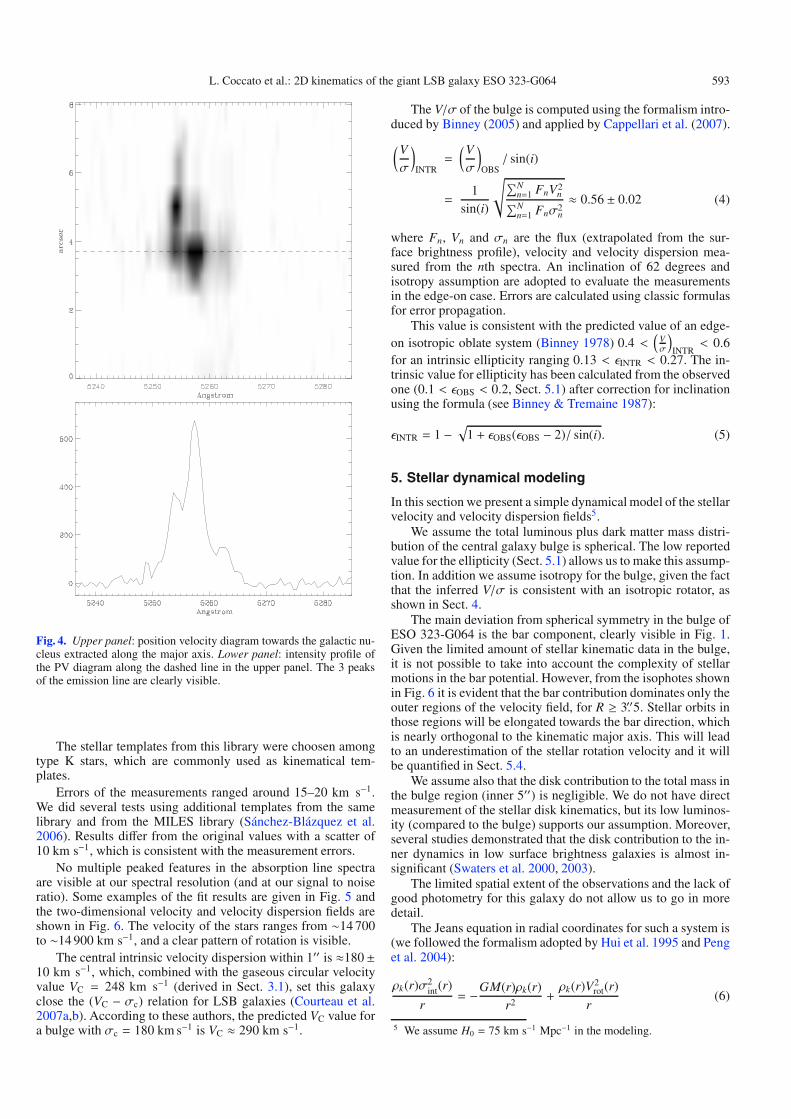
Hβ, [O III] λ4959 and [O III] λ5007 bright emission lines arevisible in the nuclear regions within r < 5′′. Interestingly, atsome locations these emission lines are triple peaked (see Figs. 3and 4). This complexity is probably generated by three barelyresolved emission-line regions located close to the center but atdifferent azimuthal angles.

In order to have kinematical informations for all the 3 re-gions, we fitted each of the the galaxy emission lines with threeindependent Gaussian functions, and the results (velocity, veloc-ity dispersion and intensity) were compiled separately.

The velocity field of the three components do not show a reg-ular rotation. Their averaged radial velocities are approximately14539 ± 38, 14726 ± 31, and 14992 ± 26 km s−1. These valueswere inferred from the [O III] velocity field (mean value between[O III] λ4959 and [O III] λ5007) because it is not affected by stel-lar absorption as is the Hβ emission line. The velocity dispersionin each of the 3 regions is between 50 and 100 km s−1.

The measured FWHM of the 3 regions is about 1.′′7, which isvery similar to the one of the foreground star (≈1.′′3). The max-imum distance measured between the centroids of the 3 regionsis 1.′′0.

We can exclude that the observed multi-peak line profile isan artifact caused by the data reduction because:

1. The sky lines observed in each quadrant (either in the rawspectra or in the final reduced data cube) are not multipeaked. This eliminates instrumental effects (e.g., a shift ofthe instrument during the exposure) or pipeline errors (e.g.,a shift in the dispersion direction during the data cube com-bining) as a source of the triple-peaked profiles.

4 Images from scanned plates can be downloaded fromhttp://www.astro-wise.org/portal/aw_datasources.shtml.

Fig. 3. Examples of [O III] emission line profiles, in which the 3 peaksare visible. Hβ emission line has been omitted in this plot because it isvery faint with respect to the [O III]. The blue, green and red lines rep-resent the fits to the first, second and third emitting regions respectively.

2. The three peaks in the galaxy emission line are present be-fore and after the sky subtraction and they are present alsoin the raw spectra. Moreover, the few sky lines which areoverlap with the galaxy emission lines are very weak.

3. The three peaks are visible in all the galaxy emission linesand the ratio between the intensities of the componentsis (almost) the same if measured in Hβ, [O III] λ4959 or[O III] λ5007.

4. The peaks are visible also if we consider only the exposurewith the best seeing condition.

4. Stellar kinematics

The stellar kinematics have been measured by means ofthe Penalized Pixel-Fitting (ppxf) method by Cappellari &Emsellem (2004). We chose a library of stellar templates fromValdes et al. (2004) provided together with the ppfx tools. Thesespectra have a spectral range of 4780–5460 Å and spectral res-olution of 1.0 Å at 5100 Å (σ ∼ 22 km s−1, which had beendeteriorated in order to match the instrumental one).

L. Coccato et al.: 2D kinematics of the giant LSB galaxy ESO 323-G064 593

Fig. 4. Upper panel: position velocity diagram towards the galactic nu-cleus extracted along the major axis. Lower panel: intensity profile ofthe PV diagram along the dashed line in the upper panel. The 3 peaksof the emission line are clearly visible.

The stellar templates from this library were choosen amongtype K stars, which are commonly used as kinematical tem-plates.

Errors of the measurements ranged around 15–20 km s−1.We did several tests using additional templates from the samelibrary and from the MILES library (Sánchez-Blázquez et al.2006). Results differ from the original values with a scatter of10 km s−1, which is consistent with the measurement errors.

No multiple peaked features in the absorption line spectraare visible at our spectral resolution (and at our signal to noiseratio). Some examples of the fit results are given in Fig. 5 andthe two-dimensional velocity and velocity dispersion fields areshown in Fig. 6. The velocity of the stars ranges from ∼14 700to ∼14 900 km s−1, and a clear pattern of rotation is visible.

The central intrinsic velocity dispersion within 1′′ is ≈180±10 km s−1, which, combined with the gaseous circular velocityvalue VC = 248 km s−1 (derived in Sect. 3.1), set this galaxyclose the (VC − σc) relation for LSB galaxies (Courteau et al.2007a,b). According to these authors, the predicted VC value fora bulge with σc = 180 km s−1 is VC ≈ 290 km s−1.

The V/σ of the bulge is computed using the formalism intro-duced by Binney (2005) and applied by Cappellari et al. (2007).(Vσ

)INTR

=

(Vσ

)OBS/ sin(i)

=1

sin(i)

√∑Nn=1 FnV2

n∑Nn=1 Fnσ2

n

≈ 0.56 ± 0.02 (4)

where Fn, Vn and σn are the flux (extrapolated from the sur-face brightness profile), velocity and velocity dispersion mea-sured from the nth spectra. An inclination of 62 degrees andisotropy assumption are adopted to evaluate the measurementsin the edge-on case. Errors are calculated using classic formulasfor error propagation.

This value is consistent with the predicted value of an edge-on isotropic oblate system (Binney 1978) 0.4 <

(Vσ

)INTR

< 0.6for an intrinsic ellipticity ranging 0.13 < εINTR < 0.27. The in-trinsic value for ellipticity has been calculated from the observedone (0.1 < εOBS < 0.2, Sect. 5.1) after correction for inclinationusing the formula (see Binney & Tremaine 1987):

εINTR = 1 − √1 + εOBS(εOBS − 2)/ sin(i). (5)

5. Stellar dynamical modeling

In this section we present a simple dynamical model of the stellarvelocity and velocity dispersion fields5.

We assume the total luminous plus dark matter mass distri-bution of the central galaxy bulge is spherical. The low reportedvalue for the ellipticity (Sect. 5.1) allows us to make this assump-tion. In addition we assume isotropy for the bulge, given the factthat the inferred V/σ is consistent with an isotropic rotator, asshown in Sect. 4.

The main deviation from spherical symmetry in the bulge ofESO 323-G064 is the bar component, clearly visible in Fig. 1.Given the limited amount of stellar kinematic data in the bulge,it is not possible to take into account the complexity of stellarmotions in the bar potential. However, from the isophotes shownin Fig. 6 it is evident that the bar contribution dominates only theouter regions of the velocity field, for R ≥ 3.′′5. Stellar orbits inthose regions will be elongated towards the bar direction, whichis nearly orthogonal to the kinematic major axis. This will leadto an underestimation of the stellar rotation velocity and it willbe quantified in Sect. 5.4.

We assume also that the disk contribution to the total mass inthe bulge region (inner 5′′) is negligible. We do not have directmeasurement of the stellar disk kinematics, but its low luminos-ity (compared to the bulge) supports our assumption. Moreover,several studies demonstrated that the disk contribution to the in-ner dynamics in low surface brightness galaxies is almost in-significant (Swaters et al. 2000, 2003).

The limited spatial extent of the observations and the lack ofgood photometry for this galaxy do not allow us to go in moredetail.

The Jeans equation in radial coordinates for such a system is(we followed the formalism adopted by Hui et al. 1995 and Penget al. 2004):

ρk(r)σ2int(r)

r= −GM(r)ρk(r)

r2+ρk(r)V2

rot(r)

r(6)

5 We assume H0 = 75 km s−1 Mpc−1 in the modeling.

594 L. Coccato et al.: 2D kinematics of the giant LSB galaxy ESO 323-G064

Fig. 5. Examples of the stellar kinematics fit quality. Black is the galaxy spectrum, while red (green) represents the portion of the stellar templatewhich was included (excluded) from the fit.

which, when solved for the intrinsic velocity dispersion σint, is:

σ2int(r) =

1ρk(r)

∫ ∞

rρk(x)

GM(x) − xV2rot(x)

x2dx (7)

where ρk is the mass density radial profile for the tracer of thepotential (i.e. the stars), Vrot is the intrinsic rotation curve of thestellar component, M is the total mass of the galaxy and G is thegravitational constant.

The velocity dispersion projected on the sky is:

σ2(R) = V2LOS(R) − Vs(R)2 (8)

where Vs is the projected rotation curve of the stars (seeSect. 5.2) and VLOS is the line-of-sight second velocity moment,projected into the sky, given by:

V2LOS(R) =

2RΣ(R)

∫ ∞

R

(σ2

int(r) + V2rot(r)

R2

r2

)ρk(r)r√r2 − R2

dr. (9)

5.1. Density of the kinematical tracer

There are no good CCD images of ESO 323-G064 available inthe literature. The better available photometry is from the ESO-LV catalog6. We performed a bulge/disk decomposition usinggalfit (Peng et al. 2002), adopting a de Vaucouleurs law forthe bulge and an exponential law for the disk. We derived an

6 See Sect. 3.1 for the images source.

effective radius Re = 0.′′67 and an average ellipticity of 0.3 forthe bulge, position angle PA = 32 and inclination i = 60 for thedisk. With the ESO-LV images we confirmed also that the stellardisk of ESO 323-G064 is in the LSB regime. Its surface bright-ness in the B-band ranges from ∼23.3 mag arcsec−2 at the centerto ∼26.5 mag arcsec−2 at 35′′. Even though the ESO-LV imageshave been useful to get an estimate of the surface brightness,they had insufficient signal-to-noise and spatial resolution to getreliable values of the bulge parameters. We therefore used ourVIMOS observations, collapsing the observed data cube alongthe dispersion direction and deriving a surface brightness pro-file from the resulting image. We fit a de Vaucouleurs law tothis profile and derived an effective radius Re = 0.′′9 (see Fig. 7)and a ellipticity ranging from 0.1 to 0.2, not too far from theadopted spherical approximation. Although the signal-to-noiseratio of the VIMOS observations is low, the advantage is thatthe VIMOS spatial resolution (0.′′67/pixel) is higher than that ofthe ESO-LV images (1.′′35/pixel). This makes us more confidentof bulge parameter values based on VIMOS observations thanvalues based on ESO-LV images.

The de Vaucouleurs profile resembles the Hernquist (1990)mass model in which the intrinsic density distribution is givenby:

ρk(r) =MLa2π

1

r (r + a)3(10)

where ML is the total luminous mass and a = Re/1.8153.

L. Coccato et al.: 2D kinematics of the giant LSB galaxy ESO 323-G064 595

Fig. 6. Stellar radial velocity and velocity dispersion fields, with thebulge central isophotes shown. The field of view is 14′′ × 14′′, Northis up, East is left.

The projection on the sky of Eq. (10) is given by:

Σ(R) = 2∫ ∞

R

ρk(r)r√r2 − R2

dr. (11)

Equations (10) and (11) will be used in Eq. (9) to determine thevelocity moments for the mass calculation.

Fig. 7. Dots: surface brightness profile obtained by collapsing thedata cube along dispersion direction. Continuous line: de Vaucouleursfit to the measured surface brightness, with Re = 0.′′9 and μe =−16.8 mag arcsec−2 (arbitrary zero point). The innermost point was notincluded in the fit, since it is affected by the seeing.

5.2. Intrinsic and projected rotation curve

Because of the limited spatial extent and resolution of the obser-vations, a “bidimensional” approach to the Jeans equation can-not be reliably carried out. We therefore decided to average az-imuthally and then bin radially the bidimensional velocity andvelocity dispersion fields. To do that, we divided them in N ra-dial bins7 (after several tests, it turned out that 1.′′5 per bin is anoptimal value) and for each radial bin at a given position rN we:

– calculated the velocity V(rN) by fitting the function v′(φ) =V(rN) × cos(φ + PA) + Vsys to all the velocity data pointswithin the Nth bin. φ is the angle measured in the galaxyequatorial plane, PA is the galaxy position angle on the sky8

and Vsys = 14 825 km s−1 is the adopted systemic velocity;– calculated the velocity dispersion σN(rN) by averaging all

the velocity dispersion data points within the Nth bin. Inthis computation, we took into account also the value of thevelocity gradient along the resolution element (1.′′5) and re-moved it from the velocity dispersion.

In Eq. (7), the quantity Vrot is the intrinsic stellar rotation curve.It can be parametrized with the expression:

Vrot(r) =v∞r√r2 + r2

h

(12)

where v∞ is its asymptotic value for the velocity and rh is a scaleparameter. The adopted function was chosen in order to properlymatch the observed velocity curve with the minimum number offree parameters. This expression has been used for example alsoin the spherical PNe system of Centaurus A (Hui et al. 1995;Peng et al. 2004).

The observed rotation curve is obtained projecting Eq. (12)on to the sky (Binney & Tremaine 1987):

Vs(R) =2RΣ(R)

∫ ∞

R

ρk(r)Vrot(r)√r2 − R2

dr. (13)

7 Bins have an elliptical shape with 〈ε〉 = 0.15 in order to take intoaccount the bulge ellipticity we observed.8 We fixed the position angle to the value PA = 38 derived in Sect. 3.1.We tested this assumption leaving PA free to vary in the fit and we foundthe value to be consistent with 38◦.

596 L. Coccato et al.: 2D kinematics of the giant LSB galaxy ESO 323-G064

Equations (12) and (13) will be used in Eqs. (8) and (9) to com-pute the velocity moments.

5.3. Radial mass profile

The radial distribution of the total mass M(r) of the galaxy bulgeis given by the sum of the luminous and dark matter contents9.The contribution Mk of the luminous component is obtained byintegrating Eq. (10) in the volume. It leads to:

Mk(r) =MLr2

(r + a)2· (14)

Together with the self consistent case, in which the total massof the galaxy is given only by the contribution of the stars, weexplored also two different scenarios for the dark matter content:Navarro et al. (1997, NFW hereafter), and the pseudo isothermalhalos.

Their mass density distribution are:

ρNFW(r) =ρs

r/rs (r/rs + 1)2(15)

ρisot(r) =ρ0

1 + (r/r0)2(16)

where rs, ρs, r0 and ρ0 are scale parameters.The corresponding mass distributions are given by the vol-

ume integration of Eqs. (15) and (16). We obtain:

MNFW(r) = 4πρsr3s

[ln (1 + r/rs) − r/rs

1 + r/rs

](17)

Misot(r) = 4πρ0r30 [r/r0 − arctan (r/r0)] . (18)

In the dark matter scenarios, the total mass M(r) is given byadding to Mk one of the contributions expressed in Eqs. (17)or (18).

5.4. Model results

We fit Eqs. (8) and (13) separately to the velocity V(rN) andvelocity dispersion σ(rN) data points (see Sect. 5.2). The actualfit computation was done using the MPFIT algorithm, as done inSect. 3.

One could add constraints to the halo parameter by includingthe disk Hβ rotation curve and the disk surface brightness profileinto the fit. However, given the large uncertainties on the diskphotometric profiles, we decided to focus our mass model onlyto the bulge regions. For completeness, we present the models inwhich the disk data are used in Appendix A.

The fit results are shown in Fig. 8 and are listed in Table 1.Fig. 8 shows the best fit model results (solid line) together withthe observed radial profiles of velocity and velocity dispersionderived in Sect. 5.2. The last observed point of the rotation curveis below the best fit rotation curve, possibly the result of thebar influence on the stellar kinematics for R ≥ 3.′′5 as discussedin Sect. 5. Assuming this deviation is entirely due to the bar, arough estimate of its effect on our results can be obtained from afit of the velocity curve without taking into account the last ve-locity measurement. This is shown as the gray line in the upperpanel of Fig. 8. The maximum difference between the two rota-tion curves (within 4.′′5) is ≈14%. Mass scales as the square of

9 In Sect. 5 we assumed that the disk contribution to the bulge massand dynamics is neglegible.

Fig. 8. Upper panel: stellar measured velocity curve of the bulge (filledcircles, see Sect. 5.2) and the best fit model from Eq. (13). The blackline represents the best rotation curve model, while the gray line repre-sents the best rotation curve model excluding the last data point fromthe fit. Lower panel: measured radial velocity dispersion (filled circles,see Sect. 5.2) compared to the NFW (solid line), the pseudo isothermal(dashed line) and the self consistent (dotted line) best fit models.

Table 1. Bulge parameters from the best fit model. Values are convertedassuming D = 194 Mpc on the right column.

Parameter Value

Rotation curve:

v∞ 174 ± 26 [km s−1]

rh 1.6 ± 0.8 [arcsec] (1.5 ± 0.8 [kpc])

Self consistent χ̃2 = 3.6

ML 6.6+1.9−1.4 [1010 M�]

NFW: χ̃2 = 0.8

ML 2.33.5−2.5+ [1010 M�]

log10 ρs 10.1+0.2−0.2 [log10 (M�/“3)] (ρs = 15+9

−5 [M� pc−3])

rs 0.7+0.2−0.2 [arcsec] (0.67 ± 0.19 [kpc])

Isothermal: χ̃2 = 1.5

ML 4.5+3−2 [1010 M�]

log10 ρ0 9.6+0.2−0.4 [log10 (M�/“3)] (ρ0 = 5+2

−1 [M� pc−3])

r0 0.4+0.1−0.1 [arcsec] (0.38 ± 0.09 [kpc] )

the velocity, therefore we would expect a maximal underestima-tion of the total bulge mass of ΔM/M = 2ΔV/V = 28%, whichless than a factor of 1.3.

From Fig. 8 we can see that the self consistent model pro-vides a poor fit to the data, compared to the dark matter sce-narios. The bulge kinematics are therefore better explained, un-der our assumptions, with the presence of DM, although we arenot able to disentangle between NFW and pseudo isothermalmodels.

L. Coccato et al.: 2D kinematics of the giant LSB galaxy ESO 323-G064 597

Fig. 9. χ2 confidence levels for the NFW dark matter halo model. The crosses represent the location of the best fit in the parameter space (χ̃2 = 0.8).

Fig. 10. χ2 confidence levels for the pseudo isothermal dark matter halo model. The crosses represent the location of the best fit in the parameterspace (χ̃2 = 1.5).

The reduced χ2 of both dark matter models is close to 1,while the self consistent case gives a value of 3.6. In Figs. 9and 10 we show the 1σ, 2σ and 3σ χ2 confidence levels in theparameter space. Those plots were produced by scaling the mea-sured χ2 value to the ideal one χ2 = N − M = 3 (N = 6 isthe number of data points, M = 3 is the number of free param-eters) and taking the expected Δχ2 variations for 3 parameters(i.e. 3.53, 8.02 and 14.2; Press et al. 1992, Chap. 15.6).

The total mass of the bulge (calculated using Eqs. (17) and(18) for r = 5′′) is (7.4 ± 3.2) × 1010 M� and (7.1 ± 3.6) ×1010 M� according to the NWF and pseudo isothermal scenarios,respectively, while the ratio of the dark matter content to the totalmass is about 0.55 and 0.42, at that radius. In the no dark matterscenario the bulge mass is (6.5±1.6)×1010 M�. The total fractionof dark matter in the bulge, as a function of the radius, is shownin Fig. 11.

Errors of the bulge mass are computed by applying errorpropagation formulas to Eqs. (14), (17) and (18).

5.4.1. Mass density radial profile

From the measured stellar rotation curve and the radial veloc-ity dispersion profiles (i.e. data points in Fig. 8) we derived themass density profiles and compared them with the best modelpredictions.

First we calculated the circular velocity VC using the asym-metric drift correction (assuming isotropy):

V2C(rN) − v2(rN) = −σ2(rN)

∂ ln(ν)∂ ln(rN)

· (19)

If we insert the observed bulge r1/4 radial profile for the lightdistribution ν of the kinematic tracer we obtain:

V2C(rN) = v2(rN) + 1.92σ2(rN)

(rN

Re

)1/4

· (20)

Stellar mean circular velocity obtained with the asymmetric driftcorrection is Vc = 243 ± 6 km s−1 which is consistent with theone measured from the gas in the disk regions (248± 6 km s−1).

Finally we calculated the mass density as done in de Bloket al. (2001) assuming a spherical mass distribution:

ρ(rN) =1

4πG

⎡⎢⎢⎢⎢⎣V2C

r2N

+ 2VC

rN

(∂VC

∂R

)R=rN

⎤⎥⎥⎥⎥⎦ · (21)

We did not fit these calculated mass density values because theydo not contain more information than the observed V and σthemselves. Moreover, our direct fit to the observed quantitiesdoes not depend on the assumption adopted in the mass densitycalculation. We show in Fig. 12 the comparison between the de-rived ρ and the prediction by the NFW and pseudo isothermaldark matter halo models.

598 L. Coccato et al.: 2D kinematics of the giant LSB galaxy ESO 323-G064

Fig. 11. Fraction of dark matter mass compared to total mass, as a func-tion of radial distance, for the inner 5′′ of ESO 323-G064. NFW (solidline); pseudo isothermal (dashed line).

Fig. 12. Filled circles: mass density values derived from the observedvelocity and velocity dispersion (Eq. (21)) compared to the best fit NFW(continuous line), pseudo isothermal (dashed line) and self consistent(dotted line) model predictions.

6. Discussion and conclusions

We presented the two-dimensional velocity and velocity disper-sion fields for the gaseous and stellar components of the LSBgalaxy ESO 323-G064. The gas emission lines show a verybright and complex structure within the central 5′′, character-ized by 3 peaks, which we interpret as due to the presence of 3spatially unresolved emitting regions. At radii out to 30′′, in theregion dominated by the galaxy disk, a weak Hβ emission is de-tected showing a regular velocity field with a maximal amplitudeof 248 ± 6 km s−1.

The stellar absorption lines are detectable only in the veryinnermost regions of the bulge. The stellar kinematics shows aregular rotation with an amplitude of ±140 km s−1 and a centralvelocity dispersion of ≈180 km s−1. The intrinsic (V/σ)INTR ratiofor the bulge is 0.56±0.02, which is consistent with an isotropicrotator in the 0.1 < εOBS < 0.2 observed ellipticity range, con-sidering an inclination of 62 degres. These values of V/σ andε place the bulge of ESO 323-G064 among fast rotator bulges(Cappellari et al. 2006). The value of V/σ is considerably smallwhen compared to the average value determined from the sam-ple of 6 bulge dominated LSB galaxies of Pizzella et al. 2008(〈V/σ〉 > 1).

The circular velocity, 248 ± 6 km s−1 measured from thegaseous disk, places ESO 323-G064 in good agreement with thelocation of LSB galaxies in the VC − σc plane (Courteau et al.2007a,b). On the other hand, this value is lower then the value of320 km s−1predicted by Pizzella et al. (2005).

The intrinsic bulge ellipticity value for ESO 323-G064(εINTR = 0.20±0.07) is consistent with the mean value of bulgesof the high surface brightness disk galaxies 〈εHSB〉 = 0.15 (as de-termined by Méndez-Abreu et al. 2008) while it is lower than the

average value for bulge dominated LSB galaxies 〈εLSB〉 = 0.45(as found by Pizzella et al. 2008a in a small sample of 6 bulgedominated LSB).

The amplitude of the gaseous rotation curve (248±6 km s−1)leads to an estimate of the total baryonic mass in the galaxy ofMbar = (1.9± 0.2)× 1011 M� using the empirical baryonic TullyFisher, as done in McGaugh (2005). Moreover, under the hy-pothesis of a ΛCDM universe (see Sect. 3.1 for details on theassumed parameters), we estimate the total mass for the darkmatter halo MDM ∼ 5 × 1012 M�.

We produce spherical isotropic Jeans models for the stel-lar kinematics in the bulge, exploring the self consistent, NFWand pseudo isothermal scenarios. Even though the data are tobe taken with some caveats (due to the lack of good photometry,limited spatial extension and resolution of the stellar kinematics)with this simple analysis we show that dark matter scenarios fitthe data better than the self consistent model. The derived totalbulge mass is (7±3)×1010 M� but we are not able to disentanglebetween the two different dark matter models.

The derived central bulge mass density (see Table 1) isρ = 15+9

−5 [M� pc−3] in the NFW scenario, and ρ = 5+2−1 [M� pc−3]

in the pseudo isothermal scenario. Typical values of central massdensity range from few 10−3 M� pc−3 to few 10−2 M� pc−3 forregular low surface brightness (see for example Kuzio de Narayet al. 2006; de Blok et al. 2001) and giant low surface bright-ness galaxies (Pickering et al. 1997). On the contrary, a muchwider range of values is measured for regular galaxies, from few10−3 M� pc−3 to several 103 M� pc−3 (i.e. Salucci & Borriello2001; Noordermeer et al. 2007). Therefore, in this picture, thebulge of ESO 323-G064 resembles more the central mass den-sity of regular bulges than those measured in low surface bright-ness galaxies. This is consistent also with the fact that bulgesof giant LSB galaxies are photometrically similar to those ofregular high surface brigthtness galaxies (McGaugh et al. 1995;Beijersbergen et al. 1999).

Acknowledgements. The authors wish to thank the referee A. Bosma for usefulsuggestions which improved the paper content and the discussion.

Appendix A: Constraining the halo parameterswith disk Hβ velocity curve and surface brightness

The Hβ velocity curve measured in the disk between 10′′ < R <30′′ (Sect. 3.1) and the disk surface photometry from the ESO-LV images can be used to constrain the dark halo parameters,under the assumption that the measured Hβ velocity curve is agood representation of the galaxy circular velocity.

A.1. Circular velocity for the disk and the halo

The circular velocity predicted for a pseudo isothermal halo is:

Visot(r) = VH

√1 − r0

rarctan

(rr0

)(22)

where VH =√

(4πGρ0r20) and ρ0, r0 are the halo parameters de-

fined in Sect. 5.3.The circular velocity predicted for a NFW halo is (Navarro

et al. 1997):

VNFW(r) = V200

[1x× ln(1 + cx) − cx/(1 + cx)

ln(1 + c) + c/(1 + c)

]1/2

· (23)

L. Coccato et al.: 2D kinematics of the giant LSB galaxy ESO 323-G064 599

Table 2. Galfit best fit parameters.

R-band B-bandBulge:Mtot 16.23 ± 0.5 mag 17.75 ± 0.5 magRe 0.65 ± 1 arcsec 0.55 ± arcsecb/a 0.71 ± 0.3 0.71 ± 0.3PA 13 ± 20 deg -72 ± 20 deg

Disk:Mtot 14.11 ± 0.5 mag 15.81 ± 0.5 magμ0 21.2 ± 0.4 mag 23.3 ± 0.4 magh 12.4 ± 1 arcsec 13.6 ± 2 arcsecb/a(∗) 0.53 ± 0.3 0.52 ± 0.3PA 33 ± 5 deg 32 ± 6 deg

Note: (∗) A disk axial ratio b/a = 0.53 corresponds toan inclination i = 60◦ , assuming an intrinsic disk axialratio of q0 = 0.18 (Guthrie 1992).

In Eq. (23) c is the concentration parameter, related to the densityparameter ρs (used in our fit procedure) and the critical densityρcritic = 3H2/(8πG) (H = 75 is the adopted value for the Hubbleconstant) with the following equation:

ρs/ρcritic =2003

cln(1 + c) − c/(1 + c)

· (24)

The parameter V200 in Eq. (23) is the circular velocity at r200 =rsc (rs is the halo scale parameter used in our fit procedure) andit is defined as:

V200 =

(GM200

r200

)1/2

(25)

where

M200 = 2004π3× ρcriticr3

200. (26)

Together with the halo circular velocities defined by Eqs. (22)and (23) we have to add the contribution given by the stellardisk (the bulge contribution is negligible at this radial range).Assuming an exponential disk with central mass surface den-sity M0 and scale length h, the predicted circular velocity is(Freeman 1970):

Vdisk(r)=

√4πGM0

r2

4h

[I0

( x2h

)K0

( x2h

)− I1

( x2h

)K1

( x2h

)](27)

where In and Kn are modified Bessel functions of the first andsecond kind.

To obtain the mass surface density M0 and the disk scaleparameter we retrieved ESO-LV images of ESO 323-G064 inthe B and R bands and performed a photometric decompositionwith galfit (Peng et al. 2002).

The result of the galfit decomposition are listed in Table 2.From the total disk magnitude in R and B band we compute acolor of (B − R)disk = 1.70 ± 0.5. Using the prescription by Bell& de Jong (2001) we can compute the mass-to-light ratio of thedisk in the R band (M/L)disk = 4.81 ± 0.77. The computationmade use of the relation between color and mass-to-light ratiofor different models as listed in Table 3 of Bell & de Jong (2001).We use the relation in the R because the scatter between differentmodels is smaller.

From the central disk surface brightness μ0 = 21.2 ±0.3 mag arcsec−2 measured from the galfit decomposition inthe R-band, assuming a distance of D = 194 Mpc, an extinc-tion of AR = 0.231 mag (from the NED database) the disk

Fig. 13. Model results obtained including the disk data. Upper panel:stellar velocity dispersion (filled circles, see Sect. 5.2) compared to theNFW (solid line), the pseudo isothermal (dashed line) and the self con-sistent (dotted line) best fit models. Lower Panel: measured circular ve-locity (open circles, from the Hβ rotation curve derived in Sect. 3.1)compared to the NFW (solid line), the pseudo isothermal (dashed line)and the self consistent (dotted line) best fit models.

mass-to-light ratio (M/L)disk = 4.81 ± 0.77 we calculate thecentral mass surface density M0 = (491 ± 201) M� pc−2 =(4.3 ± 1.8) × 108 M� arcsec−2.

Therefore, we can compute the total circular velocity VC byadding the contribution of the light (Eq. (27)) to the contributionof the halo (Eqs. (22) or (23) depending on the adopted sce-nario).

A.2. Mass model using stellar and gaseous kinematics

We have also performed the mass model fit as described inSect. 5 using the constraints from the Hβ circular velocity. Asin the previous case we fit first the empirical bulge stellar rota-tion curve (to obtain r∞ and rh, Eq. (12)) and then we fit simul-taneously the stellar velocity dispersion (i.e the filled circles inFig. 8) and the Hβ circular velocity (i.e the open diamonds inFig. 2) data.

Fit results are shown in Fig. 13 and the best fit parameters arelisted in Table 3. The results are similar to those in Table 1. Withthe additional constraints from the disk, both pseudo isothermaland NFW scenario give a reasonable fit to the data and it is notpossible, given the errors, to say which is the best one.

The formal errors given by the fit algorithm are slightly lowerthan the ones listed in Table 1, because of the addition of datapoints in the fit. However, the fit errors do not include the uncer-tainties from the disk photometry and the errors in the relationbetween mass-to-light ratio and disk (B − R) color.

Errors in disk central surface brightness and in the mass-to-light ratio translate into an error of ΔM0/M0 ∼ 41% on the masscentral surface density, which is an error of ∼20% on the diskvelocity curve (Vdisk ∝ √M0). However, the fact that the twodifferent fit approaches lead to similar results is reassuring.

600 L. Coccato et al.: 2D kinematics of the giant LSB galaxy ESO 323-G064

Table 3. Best fit parameters from the simultaneous fit of the stellar ve-locity dispersion and the Hβ rotation curve. Values are converted as-suming D = 194 Mpc on the right column.

Parameter Value

Rotation curve:

v∞ 174 ± 26 [km s−1]

rh 1.6 ± 0.8 [arcsec] (1.5 ± 0.8 [kpc])

Self consistent χ̃2 = 3.6

ML 6.6+1.9−1.4 [1010 M�]

NFW: χ̃2 = 0.9

ML 0.541.0−0.4+ [1010 M�]

log10 ρs 10.0+0.2−0.2 [log10 (M�/“3)] (ρs = 13+8

−5 [M� pc−3])

rs 0.85+0.14−0.15 [arcsec] (0.80 ± 0.18 [kpc])

Isothermal: χ̃2 = 1.4

ML 3.5+3−2 [1010 M�]

log10 ρ0 9.6+0.2−0.4 [log10 (M�/“3)] (ρ0 = 5+2

−1 [M� pc−3])

r0 0.39+0.08−0.09 [arcsec] (0.37 ± 0.08 [kpc] )

Deep photometric observations and an accurate determina-tion of the mass-to-light ratio are highly desirable to better con-strain the mass distribution in ESO 323-G064.

References

Beijersbergen, M., de Blok, W. J. G., & van der Hulst, J. M. 1999, A&A, 351,903

Bell, E. F., & de Jong, R. S. 2001, ApJ, 550, 212Binney, J. 1978, MNRAS, 183, 501Binney, J. 2005, MNRAS, 363, 937Binney, J., & Tremaine, S. 1987, Galactic dynamics (Princeton, NJ: Princeton

University Press), 747Boissier, S., Gil de Paz, A., Boselli, A., et al. 2008, ArXiv e-prints, 803Bothun, G., Impey, C., & McGaugh, S. 1997, PASP, 109, 745Bothun, G. D., Schombert, J. M., Impey, C. D., & Schneider, S. E. 1990, ApJ,

360, 427Bryan, G. L., & Norman, M. L. 1998, ApJ, 495, 80Bullock, J. S., Kolatt, T. S., Sigad, Y., et al. 2001, MNRAS, 321, 559Cappellari, M., & Emsellem, E. 2004, PASP, 116, 138Cappellari, M., Bacon, R., Bureau, M., et al. 2006, MNRAS, 366, 1126Cappellari, M., Emsellem, E., Bacon, R., et al. 2007, MNRAS, 379, 418

Courteau, S., McDonald, M., & Widrow, L. M. 2007a, [arXiv:0709.3682]Courteau, S., McDonald, M., Widrow, L. M., & Holtzman, J. 2007b, ApJ, 655,

L21de Blok, W. J. G., & McGaugh, S. S. 1997, MNRAS, 290, 533de Blok, W. J. G., van der Hulst, J. M., & Bothun, G. D. 1995, MNRAS, 274,

235de Blok, W. J. G., McGaugh, S. S., Bosma, A., & Rubin, V. C. 2001, ApJ, 552,

L23Freeman, K. C. 1970, ApJ, 160, 811Guthrie, B. N. G. 1992, A&AS, 93, 255Hernquist, L. 1990, ApJ, 356, 359Hoffman, Y., Silk, J., & Wyse, R. F. G. 1992, ApJ, 388, L13Hui, X., Ford, H. C., Freeman, K. C., & Dopita, M. A. 1995, ApJ, 449, 592Jimenez, R., Bowen, D. V., & Matteucci, F. 1999, ApJ, 514, L83Kuzio de Naray, R., McGaugh, S. S., de Blok, W. J. G., & Bosma, A. 2006,

ApJS, 165, 461Kuzio de Naray, R., McGaugh, S. S., & de Blok, W. J. G. 2008, ApJ, 676, 920Lauberts, A. 1982, ESO/Uppsala survey of the ESO(B) atlas (Garching:

European Southern Observatory (ESO))Mapelli, M., Moore, B., Ripamonti, E., et al. 2008, MNRAS, 383, 1223Mayer, L., & Wadsley, J. 2004, MNRAS, 347, 277McGaugh, S. S. 2005, ApJ, 632, 859McGaugh, S. S., Schombert, J. M., & Bothun, G. D. 1995, AJ, 109, 2019McGaugh, S. S., Rubin, V. C., & de Blok, W. J. G. 2001, AJ, 122, 2381Méndez-Abreu, J., Aguerri, J. A. L., Corsini, E. M., & Simonneau, E. 2008,

A&A, 478, 353Moré, J. J., Garbow, B. S., & Hillstrom, K. E. 1980, User Guide for

MINPACK-1 (Argonne Nat. Lab. Rep. ANL-80-74; Argonne: ArgonneNational Laboratory)

Navarro, J. F., Frenk, C. S., & White, S. D. M. 1997, ApJ, 490, 493Noguchi, M. 2001, MNRAS, 328, 353Noordermeer, E., van der Hulst, J. M., Sancisi, R., Swaters, R. S., & van Albada,

T. S. 2007, MNRAS, 376, 1513O’Neil, K. 2002, in Extragalactic Gas at Low Redshift, ed. J. S. Mulchaey, &

J. Stocke, ASP Conf. Ser., 254, 202O’Neil, K., & Schinnerer, E. 2003, ApJ, 588, L81Osterbrock, D. E., Fulbright, J. P., Martel, A. R., et al. 1996, PASP, 108, 277Peng, C. Y., Ho, L. C., Impey, C. D., & Rix, H.-W. 2002, AJ, 124, 266Peng, E. W., Ford, H. C., & Freeman, K. C. 2004, ApJ, 602, 685Pfenniger, D., Combes, F., & Martinet, L. 1994, A&A, 285, 79Pickering, T. E., Impey, C. D., van Gorkom, J. H., & Bothun, G. D. 1997, AJ,

114, 1858Pizzella, A., Corsini, E. M., Dalla Bontà, E., et al. 2005, ApJ, 631, 785Pizzella, A., Corsini, E. M., Sarzi, M., et al. 2008a, MNRAS, 387, 1099Pizzella, A., Tamburro, D., Corsini, E. M., & Bertola, F. 2008b, A&A, 482, 53Press, W. H., Teukolsky, S. A., Vetterling, W. T., & Flannery, B. P.

1992, Numerical recipes in FORTRAN. The art of scientific computing(Cambridge: University Press), 2nd edn.

Salucci, P., & Borriello, A. 2001, in Dark Matter in Astro- and Particle Physics,ed. H. V. Klapdor-Kleingrothaus, 12

Sánchez-Blázquez, P., Peletier, R. F., Jiménez-Vicente, J., et al. 2006, MNRAS,371, 703

Swaters, R. A., Madore, B. F., & Trewhella, M. 2000, ApJ, 531, L107Swaters, R. A., Verheijen, M. A. W., Bershady, M. A., & Andersen, D. R. 2003,

ApJ, 587, L19Valdes, F., Gupta, R., Rose, J. A., Singh, H. P., & Bell, D. J. 2004, ApJS, 152,

251