View Selection Using Randomized SearchPanos Kalnis Nikos Mamoulis Dimitris Papadias

Abstract

An important issue in data warehouse development is the selection of a set of views to materialize in order to

accelerate OLAP queries, given certain space and maintenance time constraints. Existing methods provide good

results but their high execution cost limits their applicability for large problems. In this paper, we explore the

application of randomized, local search algorithms to the view selection problem. The efficiency of the proposed

techniques is evaluated using synthetic datasets, which cover a wide range of data and query distributions. The

results show that randomized search methods provide near-optimal solutions in limited time, being robust to data and

query skew. Furthermore, they can be easily adapted for various versions of the problem, including the simultaneous

existence of size and time constraints, and view selection in dynamic environments. The proposed heuristics scale

well with the problem size, and are therefore particularly useful for real life warehouses, which need to be analyzed

by numerous business perspectives.

Keywords: View selection, OLAP, Data warehouse

2

1. INTRODUCTION

A data warehouse stores large amounts of consolidated, historical data and is especially designed to support business

decision queries. The process of interactively using the warehouse to answer such queries is referred to as On-line

Analytical Processing (OLAP). Users are mainly interested in summary information of a measure as a function of

some business perspectives (dimensions). Consider, as an example, a warehouse that consolidates information about

company sales. For each sale event, dimensional information which may be interesting for data analysis, is the

product sold, the customer and its shipping date. In practice, the number of dimensions can be large. Given the

amount of information in the warehouse, it is very time consuming to answer aggregate queries directly from the base

tables. A common technique to accelerate OLAP is to precalculate some aggregations and store them as materialized

views. The aim is to select a set of views for materialization, such that the query cost is minimized, while meeting the

space and/or maintenance cost constraints which are provided by the administrator. [6, 10, 11] describe greedy

algorithms for the view selection problem. In [4] an extension of these algorithms is proposed, to select both views

and indices on them. [2] employ a method which identifies the relevant views, for a given workload. [22] use a

simple and fast algorithm for selecting views in configurations with special properties. [26] study the minimization of

both query execution and view maintenance costs, under the constraint that all queries should be answered from the

selected views. Finally, [18] propose the dynamic materialization and maintenance of query results considering both

space and time constraints.

The above methods are effective when the number of views is relatively small but they do not scale well with

dimensionality. The complexity of the greedy methods does not allow their application for numerous dimensions. In

our implementation, the algorithm of [11] ran for over six hours in order to select a set of views that fit in 1% of the

data cube space for a flat fact table with 14 dimensions. We also observed that the sorting method [22] does not

perform well for arbitrary view sizes and query workloads. In this paper we propose the application of randomized

search heuristics, namely Iterative Improvement and Simulated Annealing, which select fast a sub-optimal set of

views. These methods are traditionally used to solve hard combinatorial optimization problems, where systematic

search algorithms are unacceptably slow. Although they cannot guaranty theoretical bounds for their results, they

have been proven very efficient for some classes of optimization problems. In the database literature they have

successfully been applied to the optimization of large join queries [24, 12].

3

Our contribution includes:

(i) the adaptation of randomized search methods for the view selection problem. We propose transformation rules

that help the algorithms move through the search space of valid view selections, in order to identify sets of views

that minimize the query cost.

(ii) the comparison of the methods with existing systematic alternatives. We experimentally show that randomized

search provides solutions very close to the optimal bounded algorithm by [11], while requiring significantly less

time to converge.

(iii) their application to several different problem variations, including existence of both size and update time

constraints and dynamic view selection. The robustness of randomized search to all variations is evaluated

through extensive experimentation. The proposed heuristics achieve near-optimal solutions within limited time

and scale well with the problem size. Therefore, they are applicable to large, real life problems.

The rest of the paper is organized as follows. Section 2 provides background on the view selection problem and

describes existing methods for solving it. Randomized search algorithms are described in section 3, while section 4

illustrates their application for view selection under the size and update time constraints. Section 5 contains an

extensive experimental evaluation of the proposed methods and section 6 concludes the paper.

2. BACKGROUND

For the rest of the paper we will assume that the multi-dimensional data are mapped on a relational database using a

star schema [16]. Let D1, D2, …, Dn be the dimensions of the database, such as Product, Customer and Time. Let M

be the measure of interest; Sales for example. Each Di table stores details about the dimension, while M is stored in a

fact table F. A tuple in F contains the measure plus pointers to the dimension tables.

There are O(2n) possible group-by queries for a data warehouse with n dimensional attributes. A detailed group-

by query can be used to answer more abstract aggregations. Harinarayan et. al. [11] introduced the search lattice L,

which is a directed graph whose nodes represent group-by queries and edges express the interdependencies among

group-bys. There is a path from node ui to node uj, if ui can be used to answer uj.

Materializing and maintaining all views in the lattice is impossible in typical warehouses because of two

reasons:

4

(i) the required space for storing all views is huge even for today’s rapid decrease of value/megabyte of secondary

storage. In typical enterprise warehouses the number of views are in the order of thousands and a significant

percentage of them is expected to be as large as the fact table.

(ii) the update window is typically small in comparison to the time required to update all views. Even if the disk

space is infinite, it is impossible to maintain all views within an acceptable time period.

Therefore, selecting which views to materialize, given certain space and maintenance cost constraints and the

expected query workload, is an important problem.

We assume that query q is best evaluated from view v, if the set of attributes appearing in the query are the grouping

attributes of the view. In some cases, however, queries that involve selections on some attributes might be evaluated

better from a view with a finer granularity if the appropriate indexes existed on it. Although complicated cost models

that consider these factors are possible, here we adopt the linear cost model used in previous studies [11, 2, 22]. In

the sequel, we sometimes use the term view v to denote the corresponding query q that is best evaluated by v.

Let L be the set of views in the data cube lattice, and M (M ⊆ L) be the set of materialized views. Each view v ∈

L has the following three values associated with it: the query frequency fv, the update frequency gv and the reading

cost rv. According to the linear cost model, the cost of answering a query q (which corresponds to view v) is

analogous to the size of v, if v is materialized, or to the size of the smallest ancestor of v that has been materialized.

For simplicity, we consider that the cost of reading a materialized view v is equal to the number of tuples in it, i.e., rv

denotes both the reading cost and the size of v. The storage cost of M is:

( ) ∑∈

=Mv

vrMS (1)

Let u(v,M) be the update cost of a view v when the set of materialized views is M. Then, the cost of updating M is:

( ) ( )∑∈

⋅=Mv

v M,vugMU(2)

Let q(v,M) be the cost of answering query v when M is materialized. The total cost of answering queries is:

( ) ( )∑∈

⋅=Lv

v MvqfMQ , (3)

The view selection problem is defined as follows: Find a set M, (M ⊆ L), such that Q(M) is minimum provided that

S(M)≤Smax or U(M)≤Umax, where Smax is the maximum space that can be allocated for materialized views and Umax the

5

maximum update window allowed. Because a data cube of d dimensions has 2d views andd22 candidate viewsets,

algorithms that exhaustively search the space of possible view combinations are unacceptably slow, even for a small

number of dimensions. As a result, several algorithms that find a sub-optimal viewset have been proposed.

2.1 View selection under the Space Constraint

Most studies on view selection consider only the space constraint, assuming either that Smax is very tight in

comparison to Umax, or that S(M) is linearly related to U(M). A greedy algorithm which constructs M incrementally

was proposed in [11] (we call it GSC for greedy under the space constraint). Starting from an empty set (initially

M=∅), the view with the maximum benefit per unit space b(v,M) is selected. The benefit of adding a view v to a set

of materialized views M is the total cost of answering queries using M minus the cost using M∪{v}, normalized to

the size of v:

vr

vMQMQMvb

}){()(),(

∪−= (4)

After adding v to M the algorithm updates q(v′,M), for each view v′∈L affected by the change. GSC continues

picking views until the space limit is reached. [11] prove that the viewset found by this algorithm has benefit at least

63% of the optimal. Typically, the result is very close to the optimal. The complexity of GSC is O(k⋅n2), where k is

the number of selected views and n is the total number of views. Because n grows exponentially with the

dimensionality, the algorithm is unacceptably slow for large numbers of dimensions. A theoritical study on the view

selection problem and on GSC in particular, can be found in [17].

Another heuristic, called pick by size (PBS) [22], picks views in increasing size until the space limit is reached.

If the queries are not uniformly distributed, the sorting key is the size of the view divided by the number of queries

that are best evaluated by it. PBS selects the same set of views as GSC in O(n⋅logn) provided that the lattice is size

restricted, i.e., the size of each view is at least k+1 times larger than the size of its largest child (where k is the

number of its children). For non-uniform query distributions, the weighted view sizes have to follow the same rule. If

this rule does not apply, the method cannot give a quality guarantee for the picked selection.

6

2.2 View selection under the Maintenance Cost Constraint

As the ratio of price/capacity of secondary storage media is constantly dropping, the maintenance cost (i.e. the

update time) constraint becomes the limiting factor in the view selection problem [6, 18]. Although the space

constraint seems similar to the maintenance cost constraint, they have a significant difference. The space occupied by

a set of views always increases when a new view is inserted, while the maintenance cost does not; it is possible for

the update time of a set of views to decrease after the addition of a new one. To illustrate this consider the lattice of

Figure 1, where v1, v3, and v4 are materialized, i.e. M={v1, v3, v4}. Assume that the query and update frequencies for

all views are equal and that 10% of each view is updated incrementally from the changes of its smallest ancestor

[20]. For simplicity, in this example the maintenance cost is considered equal to the cost of reading the changes from

a parent view (i.e. we exclude the cost of merging the changes). The total space occupied by the views is S(M) =

1020, and the total update time is U(M) = 3⋅100 = 300, since each view is updated from the changes of v1, which are

10% of its size. If v2 is added to M, the total space occupied by the views increases, i.e. S(M) becomes 1120.

However, the maintenance cost of M decreases, i.e. U(M) = 100+100+10+10 = 220, because v3, v4 can be updated by

reading the changes of v2.

v1

v2

v3 v4

(1000)

(100)

(10) (10)

Figure 1: Example of view maintenance

This non-monotonic nature of maintenance cost increases the complexity of view selection algorithms. [6] propose a

greedy algorithm which, like GSC, is guaranteed to give a solution within (1-1/e)=63% of the optimal one. The

solution is built incrementally; each step considers all possible “inverted trees” (i.e. combinations of nodes that form

trees when the direction of edges is reversed) in the lattice and the inverted tree with the largest benefit is added to

the set M. The complexity of a step is in the worst case exponential to the number of nodes in the lattice, rendering

the algorithm inapplicable for realistic problems where the number of views is in the order of thousands.

Until now we have discussed the static view selection problem; the views are selected once when the warehouse

is set up and are materialized. Normally, the administrator monitors the workload of the system and might choose to

recalibrate it by selecting a new set of views, if the query pattern has changed significantly. The recalibration process

7

is expensive and pays off only if it is performed after a long period of time. Another alternative is proposed by [18].

In order to track the changes in query patterns, they employ a dynamic system called Dynamat, which considers both

the size and maintenance cost constraints. Dynamat uses a pool (i.e. a kind of disk cache) that stores “fragments”,

which are aggregate query results in a finer granularity than views (they may include selection ranges on some

dimensions). The pool is initially empty. During the on-line phase, when a query arrives, the system checks whether

there is a related materialized fragment in the pool. In this case, the fragment is used to answer the query, otherwise

the base tables are accessed and the result is stored as a new fragment in the pool. If the pool gets full (space

constraint) a fragment is chosen for replacement or the new results are not materialized depending on a benefit

metric. During the update window, Dynamat must discard a number of fragments so that the remaining ones can be

updated within the available time. In the sequel, we call this problem dynamic view selection.

All the semantics that apply to views also apply to fragments differentiating only on the granularity. Therefore

we can assume without lost of generality that Dynamat has materialized a set of views L. The objective at the update

phase, is to keep a set M⊆L of views such that U(M)≤Umax and Q(M) is minimized. Dynamat initially discards all

fragments whose maintenance cost is larger than the update window. A greedy algorithm then evicts fragments of

low benefit, until the constraint is satisfied. The remaining fragments are updated and the system goes on-line. [6]

argue that simple greedy methods like the above can produce arbitrary bad results.

For the rest of the paper, we will assume that views are updated incrementally [7, 20, 1, 5, 14]. We will also

consider that the sources provide the set of updates (usually a log file) and the aggregate functions are self-

maintainable [20]. We apply these assumptions to simulate realistic update windows, although the proposed

algorithms do not depend on them.

3. RANDOMIZED ALGORITHMS

As mentioned in the previous paragraph, existing view selection algorithms that provide guarantee of their results

independently of the lattice properties [11, 10, 6] are inapplicable to high dimensional problems, where the number

of views is large. A similar problem appears in query optimization at operational databases. If a relational query

consists of a limited number of join clauses, application of systematic algorithms, like dynamic programming, which

find the optimal ordering of joins is efficient. As the number of joins increases, however, the running time of

systematic methods grows exponentially, rendering exhaustive optimization inapplicable. Motivated by this fact, a

8

number of approaches [24, 12, 8] use fast randomized search heuristics, that estimate sub-optimal execution plans for

large relational queries. In practice, however, the demand for query optimization using randomized search is limited,

since queries that involve more than 10 joins are seldom posed. On the other hand, in OLAP applications it is

common to have 10-15 dimensions, resulting to 210-215 views, and randomized search for sub-optimal viewsets

becomes the only practical optimization method.

The search space of an optimization problem can be thought of as an undirected graph, where nodes correspond

to candidate solutions. Each node (also called state) has a cost assigned to it and the aim of the optimization process

is to find the one with the minimum cost. At the view selection problem each state corresponds to a set of views

which meet the space or time constraint. An edge of the graph defines a move (or transition) from one state to

another after applying a simple transformation. The move is called downhill if the destination state has a lower cost

than the starting one. In the opposite case it is called uphill. A state from which no moves are downhill is called local

minimum. The local minimum with the minimum cost is called global minimum. The graph should be connected, i.e.,

there should be at least one path of transitions between any two states. Randomized algorithms start from a random

initial state and apply sequences of transformations trying to detect the global minimum.

A simple, yet efficient hill climbing heuristic is iterative improvement (II) [21, 24]. Starting from a random

initial state (called seed), II performs random series of moves and accepts only downhill ones, until a local minimum

is detected. This process is repeated until a time limit is reached, each time with a different seed. Since the number of

neighbors of a state may be large and the algorithm needs to retain its randomness, a state is conventionally

considered as local minimum if a long sequence of consecutive uphill moves is attempted from it.

Simulated annealing (SA) [15] follows a procedure similar to II, but it also accepts uphill moves with some

probability. This probability is gradually decreased with time and finally the algorithm accepts only downhill moves

leading to a good local minimum. The intuition behind accepting uphill moves is led by the fact that some local

minima may be close to each other, separated by a small number of uphill moves. If only downhill moves were

accepted (as in II) the algorithm would stop at the first local minimum visited, missing a subsequent (and possibly

better) one. In order to comply with the initial version of SA, we use the same terminology. The initial temperature

T0 corresponds to an initial (usually high) probability of accepting an uphill move. The algorithm tries a number of

moves (inner iterations) for each temperature value T, which gradually decreases, allowing SA to accept uphill

moves less frequently. When the temperature is small enough, the probability of accepting an uphill move converges

9

to zero and SA behaves like II. The system is then said to be frozen and the algorithm terminates. In our problem, we

set the probability to accept an uphill move to e-∆C/T, where ∆C is the cost difference between the new and the

previous state. The number of inner iterations for a value of T is typically proportional to the size of the problem.

Another alternative is random sampling (RA). Given a time limit, RA selects states randomly and returns the

state with the minimum cost from those visited. In general, sampling is efficient when the local minima are not much

worse than a random state. [8] illustrate that for relational query optimization sampling converges to an acceptable

solution faster than II and SA. This shows that RA can be a useful approach when very limited time is given for

searching, e.g. enough for verifying the cost of only a small number of states.

In most problems, II and SA find better solutions than RA when they are given enough time to search. Typically,

II converges faster than SA to a good solution, but the quality of the final solution of SA is better. II works well if

there are many “deep” local minima, the quality of which does not differ much, whereas SA is better when the cost

difference between local minima can be large and they are close to each other. In the latter case a hybrid method,

two-phase optimization (2PO) [12], which combines II and SA can be more efficient than both algorithms. This

method uses II to quickly locate an area where many local minima exist, and then applies SA with a small initial

temperature to search for the global minimum in this area. Thus, 2PO avoids unnecessary large uphill moves at the

early stages of SA and the non-acceptance of uphill moves in II.

4. RANDOMIZED SEARCH FOR VIEW SELECTION

As discussed in the previous section, the efficiency of randomized search is determined by three factors [13]: (i) the

number of local minima (ii) the depth of local minima, i.e. how fast they can be reached, and (iii) the variance of

their quality, i.e. how much they differ from the global minimum. Furthermore, the choice of transformation rules

and the methods that estimate the cost of a random state and update this cost after a transition have a significant

impact on performance. In this section we discuss the application of randomized search algorithms to the view

selection problem.

4.1 View Selection Under the Space Constraint

The search space in this problem is the total number of view combinations that meet the space constraint.

Enumerating all states is intractable, since exhaustive search is required. In order to generate random states we

10

incrementally select views until the constraint is violated. Views larger than the available space are not considered at

all by the algorithms.

The problem of straightforwardly applying II and SA is the fact that there is no seamless way of defining

transitions in the search space. For example let s be a state (a set of views) with size |s|. A possible transition from s

to some other state s′ would be to replace one view v ∈ s with some v′ ∉ s. If |s|-rv+rv′ exceeds the space constraint,

the new state s′ is not valid, i.e. it is not within the search space. Practically, it is impossible to define the valid

transitions individually for each state. For the current problem, we use the following transitions:

1. Pick an unselected view and add it to the existing selection. If the space constraint is violated, randomly remove

selected views until a valid state is reached.

2. Remove a selected view and “fill” the rest of the space with views picked randomly.

selected views

sorted views

v1 v2 v3 v4 v5 v7v6 v8 v9 v10 v11 v12 v13 v14

...

v15

v7 v11 v2 v13 v5

bound

2 2 2 3 3 3 3 4 4 4 5 5 7 9

3 5 372 2

Smax = 22

Figure 2: Fast moves using a sorted array

Move 1 may lead to a state with more empty space than the previous one, but the transition can still be downhill.

However, after removing a view (move 2) the available space may be small, making the selection of replacing views

that do not violate the space constraint difficult. In order to avoid redundant checks in this case we order the views

with respect to their sizes. This makes move 2 more flexible, as it can now pick random views to fill the dead space

only from the fraction of views that fit in. As an example, consider a set M of selected views and an array of sorted

views, as shown in Figure 2. If v5 is removed, the empty space becomes 5. We can now pick a random vi, among the

12 first views (this bound can be quickly found using binary search). Because the removed or some other already

selected view can be in this range, we attempt a number of tries (as many as the number of valid views for selection -

in this case 12) until a free view is found (e.g. v3). The bound is then updated (e.g. 7) according to the newly

available space (e.g. 3) and the selection process is continued until the space limit is reached or selection fails after a

number of tries. Alternatively, the array of sorted views can be updated dynamically after a pick or a removal from

11

M, in order to ensure only valid picks. However, in our implementation we have found that the cost of dynamically

updating the sorted array does not pay off.

During a transition, several views may be inserted or deleted from M. The implication of this is that each state has

numerous neighbors and that two states in the search space are connected with a relatively short path. Using the

above set of moves, the algorithms can easily escape from areas of low benefit. The trade-off is that some parts of the

space are not extensively searched and good local minima may be missed. We also experimented with “smoother”

transitions that take into account the structure of the lattice (e.g., swaps between adjacent views in the lattice) but the

quality of the solutions was worse.

4.2 View Selection Under the Maintenance Cost Constraint

At view selection under the maintenance cost constraint, the non-monotonic nature of U(M) limits the variety of

moves that can be practically applied. The maintenance cost of a view depends on the views that are already

materialized, in contrast to its size, which is constant. If a set of views V is added in a set M of existing views and the

maintenance cost is violated, this does not mean that a superset of V also violates the constraint. Therefore, a state

can theoretically have a large number of downhill neighbors, which cannot be easily defined. In order to restrict the

number of neighbors of a state, we chose to implement the following simple moves:

1. Pick an unselected view and add it to the existing selection.

2. Replace a selected view with an unselected one.

3. Remove a selected view.

RA uses only move 1. II does not use move 3, since it cannot be downhill. For SA and 2PO, however, move 3 makes

sense, since uphill moves may be accepted. All legal moves for each algorithm have the same probability of being

applied.

In our implementation if one of the above moves leads to a violation of the maintenance cost constraint, it is

rejected. We have experimented with versions of the algorithms that accept invalid states hoping that a subsequent

move could lead to a valid state with lower total query cost. Nevertheless the results were not promising; the

algorithms usually got trapped in invalid states and spent most of the time trying to satisfy the maintenance cost

constraint rather than minimizing the query cost.

12

Local search algorithms can be easily extended to capture view selection under both space and maintenance cost

constraints. A move is accepted only if it leads to a state where both constraints are satisfied. In addition, as we show

in the experimental evaluation, the method can be applied for the dynamic view selection problem.

4.3 Incremental Cost Update After a Transition

In order for adjacent states to be efficiently evaluated, the cost difference after a move should be computed

incrementally. To meet this requirement, for each view v in the lattice we need to maintain the following information:

(i) the cost q(v,M) of answering a query that corresponds to this view, and (ii) the ancestor view A(v,M) used to

answer queries that correspond to v. Initially the set of selected views is empty and A(v,M) = NULL, q(v,M) = |DW|

for each v, denoting that queries that correspond to v are answered directly from the warehouse base tables.

When vm is selected for materialization, information about the other views is updated by a procedure (Figure 3)

that visits the descendants of vm and updates information to those that may benefit from it. This recursive function

initially takes as parameters the triple ({vm}, vm, ∆C = 0). If view v is not benefited by vm, then the descendants of v

need not be checked. Otherwise, the benefit of using vm may propagate to the lower lattice level. In order to avoid

testing a node twice, the lattice is traced level by level, in a breadth first search manner. The benefit (cost reduction)

of adding vm is accumulated in ∆C during the updates and used by the randomized algorithms.

function update_addition(ViewSet V, View vm, int ∆C) {nextV := ∅; subV := ∅;for each v ∈ V /* for each potentially affected node at this lattice level */

if (q(v,M) > rm) { /* if the cost of answering queries using vm is smaller than the current cost */A(v,M) := vm; /* update v’s ancestor used to answer queries */∆C += fv⋅(q(v, M) - rm); /* accumulate benefit of materializing vm */q(v,M) := rm; /* update v’s qcost */add all children of v to nextV; /* they should be checked at the next level */

}else add all children of v to subV; /* they should not be checked at the next level */

nextV := nextV - subV; /* remove from consideration children of non-benefited views */if nextV ≠ ∅ then update_addition(nextV, vm, ∆C); /* update the affected nodes at the lower lattice level */

}

Figure 3: update_addition function

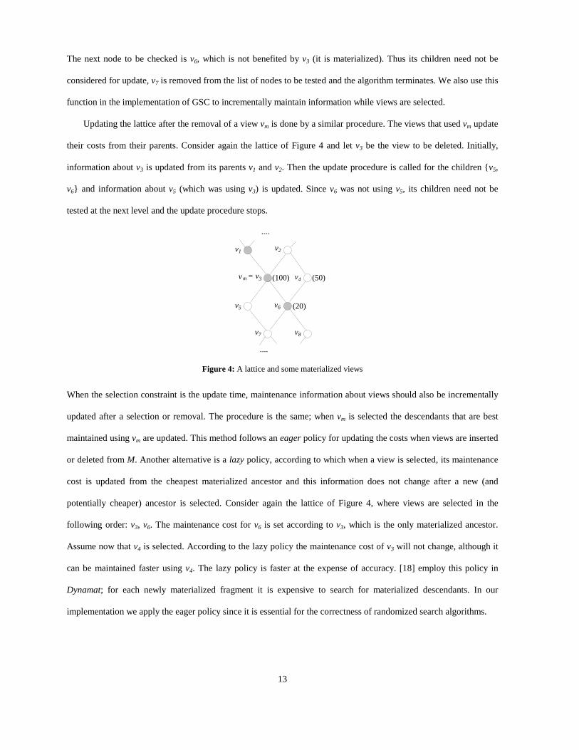
As an example of incremental cost update after the selection of a view, consider the part of the lattice depicted in

Figure 4 and let vm=v3. Assume that v1 and v6 were selected before the addition of v3. First q(v3,M) and A(v3,M) are

updated, and update_addition is recursively called for its children v5, v6. Assuming that v5 is benefited by v3, its cost

parameters are updated and its child v7 is added to the list of nodes to be tested at the subsequent call of the function.

13

The next node to be checked is v6, which is not benefited by v3 (it is materialized). Thus its children need not be

considered for update, v7 is removed from the list of nodes to be tested and the algorithm terminates. We also use this

function in the implementation of GSC to incrementally maintain information while views are selected.

Updating the lattice after the removal of a view vm is done by a similar procedure. The views that used vm update

their costs from their parents. Consider again the lattice of Figure 4 and let v3 be the view to be deleted. Initially,

information about v3 is updated from its parents v1 and v2. Then the update procedure is called for the children {v5,

v6} and information about v5 (which was using v3) is updated. Since v6 was not using v5, its children need not be

tested at the next level and the update procedure stops.

v1 v2

v3 v4

v5 v6

v7 v8

....

....

vm = (100) (50)

(20)

Figure 4: A lattice and some materialized views

When the selection constraint is the update time, maintenance information about views should also be incrementally

updated after a selection or removal. The procedure is the same; when vm is selected the descendants that are best

maintained using vm are updated. This method follows an eager policy for updating the costs when views are inserted

or deleted from M. Another alternative is a lazy policy, according to which when a view is selected, its maintenance

cost is updated from the cheapest materialized ancestor and this information does not change after a new (and

potentially cheaper) ancestor is selected. Consider again the lattice of Figure 4, where views are selected in the

following order: v3, v6. The maintenance cost for v6 is set according to v3, which is the only materialized ancestor.

Assume now that v4 is selected. According to the lazy policy the maintenance cost of v3 will not change, although it

can be maintained faster using v4. The lazy policy is faster at the expense of accuracy. [18] employ this policy in

Dynamat; for each newly materialized fragment it is expensive to search for materialized descendants. In our

implementation we apply the eager policy since it is essential for the correctness of randomized search algorithms.

14

4.4 Parameters and execution cost analysis

An advantage of randomized search algorithms is that they can be tuned in order to achieve a trade-off between

execution cost and quality of solutions. In small problems, for instance, II and SA can be adjusted to try a large

number of transitions from each state in order to extensively search the area around it. In large problems this number

may be reduced in order to search a larger portion of the state space. On the other hand, greedy algorithms do not

have this property since their execution cost is predetermined by the problem size. In our implementation we used

the following parameters for II, SA and 2PO:

• II: II accepts a local minimum after 4⋅d consecutive uphill moves, where d is the dimensionality. We do not use

a number proportional to the number of views n, in order to prevent the explosion of the cost of II with the

dimensionality.

• SA: The initial temperature of SA is set to ∆Cinit/cinit, where ∆Cinit is the cost difference between an empty

selection and the random initial state, and cinit the number of views in the random initial state. The temperature

reduction rate is set to 0.9. SA is considered to reach the freezing condition when T < 1 and during the last 4

consecutive stages of SA the best solution found so far has not changed. Each stage of SA performs n/10

iterations, where n is the number of views.

• 2PO: II is executed until it finds 5 local minima, and the deepest of them is taken as seed. SA is applied from

this state with an initial temperature two orders of magnitude smaller than ∆CII/cII, where ∆CII is the cost

difference between an empty selection and the seed, and cII the number of views in the seed.

The parameters were experimentally tuned to take the above values. The tuning is not presented here due to space

constraints. Other studies that utilize randomized search (e.g. [12]) have also determined the parameter values after

tuning, since adjustment based on theoretical analysis is not possible for most hard combinatorial optimization

problems. However, we can provide an analysis of the execution cost when the above parameters are used for a

lattice of n views. The cost of an inner iteration of II depends on how deep is the local minimum. After a downhill

move is made, the algorithm may attempt O(d) = O(logn) moves before the next downhill. The update cost for each

incremental move (either uphill or downhill) is O(n), since a large fraction of nodes from the lattice (in the worst

case the whole lattice) may have to be visited. Therefore the worst case cost of an inner iteration of II is O(h⋅n⋅logn),

where h is the depth of a local minimum.

15

The cost of SA depends on the number t of outer iterations (temperature reductions), the number of inner

iterations and the cost of propagating the changes of a move. The two latter factors are in the order of O(n). The

number of temperature reductions t depends on the initial temperature T0. Recall that T0 is defined as the average

benefit per selected view in the initial state of SA. The number of views that may benefit from a selected view is

O(n) and thus we can bound T0 by O(n). The number of temperature reductions is logarithmic to this number since

T0⋅(reduction rate)t = freezing temperature, and the freezing temperature and reduction rate are constants. Therefore

the overall running cost of SA is bounded by O(n2⋅logn). The cost of 2PO is also bounded by O(n2⋅logn), since the

ratio between the initial temperature of the algorithms is theoretically constant, and the initial runs of II are expected

to be less expensive than the second phase of 2PO. As we will see in the experimental section, however, the

execution cost rate between SA and 2PO is not constant, at least for the tested cases.

5. EXPERIMENTAL EVALUATION

We ran experiments over a synthetic dataset that models transactions of a shipping company. The warehouse has 15

dimensions and its schema is a subset of the TPC-R database schema [25]. In experiments involving d≤15

dimensions, the warehouse was projected to the first d dimensions. In order to test the performance of view selection

algorithms under various conditions, we generated four versions of the warehouse. The sizes of the views for each

version of the lattice are presented in Table 1. The first lattice models warehouses with uniform data distribution,

where there is complete independence between the values for each combination of dimensions. The second and third

lattices model situations with a small dependency between dimensions, rendering some difference between the sizes

of views that belong to different lattice levels. The fourth lattice was generated as follows. Each view is given a code,

the 1’s in the binary representation of which denote the grouping dimensions. For instance, consider a 3D lattice in

the order {P, C, T}. The bottom view is encoded with 0 (binary 000), the top view with 7 (binary 111) and the view

{P, T} with 5 (binary 101). The sizes of the views in the lattice are computed level by level, starting from the bottom

view, which has size 1. The size of view v with code c is then defined as:

size(v) = min(c2, Product of sizes of children(v) in the lattice)

The resulting sizes of the views formulate a skewed lattice with the views at the bottom right area having very small

sizes and the views at the top left area having large sizes.

16

We also generated four different query distributions (Table 2) to simulate various warehouse workloads. The

uniform query workload simulates cases where all views in the lattice have equal probability to be queried. The

second distribution models cases where views involving half of the dimensions have greater probability to be

retrieved. The rationale behind this model is driven from the statistical fact that typical queries involve few

dimensions. For example, aggregate queries of the TPC-R benchmark typically involve 3-5 dimensional attributes

from more than 15 candidates. The third distribution favors some dimensions, e.g. most queries in the TPC-R

benchmark involve the ShipDate attribute. The last distribution was generated in a reverse way than c_skewed was

generated; the query weight for a view was the reciprocal of its size in c_skewed. c_skewed and q_skewed were

generated to simulate situations where the selection of specific views is favored, which is in general a disadvantage

for the local search algorithms. The update cost of each view was set to 10% of the reading cost of the materialized

ancestor with the smallest size. All experiments were run on a UltraSparc2 workstation (200 MHz) with 256MB of

main memory.

c_analytic_1 The fact table has 50 million tuples. The size of each view was estimated using the analytical algorithm in

[23].

c_analytic_09 The same as c_analytic_1, but the size of each view was set at most 90% of the size of its smallest parent.

c_analytic_08 The same as c_analytic_1, but the size of each view was set at most 80% of the size of its smallest parent.

c_skewed The views which are at the upper left part of the lattice have higher probability to have larger rv than those

which are on the lower right part of the lattice.

Table 1: Distribution of view sizes

q_uniform All views in the lattice have the same query frequency.

q_gaussian Views from certain lattice levels have higher probability to be queried. The frequency distribution between

lattice levels is normal (Gaussian) with µ=l/2 where l is the number of levels in the lattice, and σ=1.

q_gausszipf The same as q_gaussian but the views at the same level have different query frequencies following a zipf

distribution with θ=1 [9].

q_skewed Skewed distribution. The views which are at the lower right part of the lattice have higher probability to

have larger query frequency than those which are on the upper left part (opposite than c_skewed).

Table 2: Distribution of query frequencies

17

5.1 Experiments with the space constraint

In the first set of experiments we consider only the space constraint. In all experiments Smax was set to 1% of the data

cube size. We have implemented three systematic algorithms; GSC, PBS, and EX, an algorithm that exhaustively

searches the space of view combinations. EX works in a branch and bound manner in order to avoid unnecessary

checks; if a set of views violates the space constraint, then none of its supersets is evaluated. We also implemented

the four randomized algorithms using the set of moves and parameters described in section 4.

Figure 5a illustrates the average execution time of systematic algorithms as a function of the number of

dimensions d, over all combinations of lattices and query distributions. There were no great differences in the

running cost of a specific algorithm between cases with the same dimensionality, since cost is mainly determined by

dimensionality for all algorithms. The complexity of GSC is O(k⋅n2), where k is the number of selected views. For

the tested lattices, we observed that k grows linearly with n (this also holds in the experiments of [22]), thus the cost

of GSC is O(n3) and the algorithm becomes very expensive for d≥12. EX cannot be applied for more than 6

dimensions. Interestingly, GSC found the same result as EX, i.e. the optimal solution, in all combinations of lattices

and query distributions from d=3 to 6. The running time of PBS is significantly lower and the algorithm can be

applied even for a large number of dimensions. Nevertheless as we show later, in general it does not always select

good viewsets.

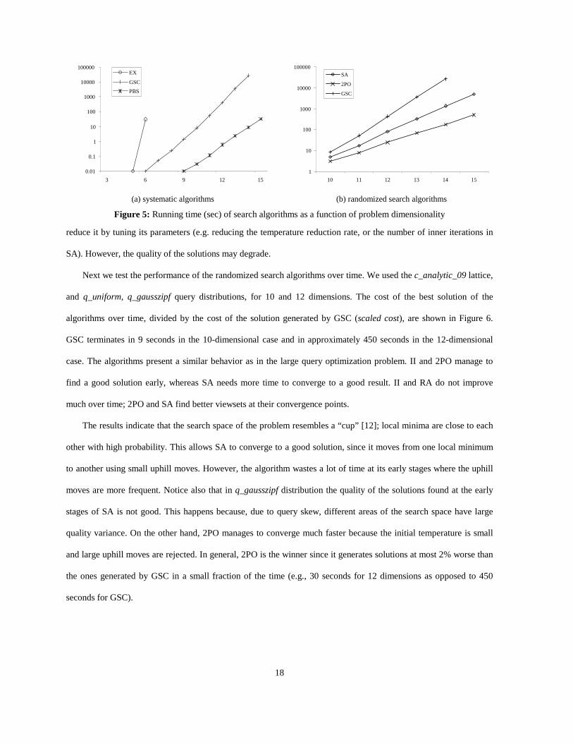
Figure 5b compares the cost of GSC with that of SA and 2PO as a function of the dimensionality. Randomized

search was applied for more than 9 dimensions, because for smaller lattices the cost of GSC is trivial. The point

where SA and 2PO converge determines the running time of the algorithms, and therefore their applicability to the

view selection problem. As expected both algorithms are faster than GSC due to their lower complexity O(n2⋅logn).

Since n=2d the difference explodes with d. Interestingly, the running time of 2PO grows with a smaller rate than SA

although the number of outer loops in both cases is O(logn). A similar situation was also observed in [12], where the

cost ratio between SA and 2PO increases with the number of relations in large tree join queries. This can be

explained by the fact that 2PO starts with a local minimum and the probability of a move to make large changes in

the lattice after an update is very small, resulting in sub-linear update cost. For d=15 2PO runs three orders of

magnitude faster than GSC, providing, as we will see later, results very close to it. Although the execution cost of

randomized search increases with dimensionality (due to the exponential growth of the lattice), it is possible to

18

reduce it by tuning its parameters (e.g. reducing the temperature reduction rate, or the number of inner iterations in

SA). However, the quality of the solutions may degrade.

Next we test the performance of the randomized search algorithms over time. We used the c_analytic_09 lattice,

and q_uniform, q_gausszipf query distributions, for 10 and 12 dimensions. The cost of the best solution of the

algorithms over time, divided by the cost of the solution generated by GSC (scaled cost), are shown in Figure 6.

GSC terminates in 9 seconds in the 10-dimensional case and in approximately 450 seconds in the 12-dimensional

case. The algorithms present a similar behavior as in the large query optimization problem. II and 2PO manage to

find a good solution early, whereas SA needs more time to converge to a good result. II and RA do not improve

much over time; 2PO and SA find better viewsets at their convergence points.

The results indicate that the search space of the problem resembles a “cup” [12]; local minima are close to each

other with high probability. This allows SA to converge to a good solution, since it moves from one local minimum

to another using small uphill moves. However, the algorithm wastes a lot of time at its early stages where the uphill

moves are more frequent. Notice also that in q_gausszipf distribution the quality of the solutions found at the early

stages of SA is not good. This happens because, due to query skew, different areas of the search space have large

quality variance. On the other hand, 2PO manages to converge much faster because the initial temperature is small

and large uphill moves are rejected. In general, 2PO is the winner since it generates solutions at most 2% worse than

the ones generated by GSC in a small fraction of the time (e.g., 30 seconds for 12 dimensions as opposed to 450

seconds for GSC).

0.01

0.1

1

10

100

1000

10000

100000

3 6 9 12 15

EX

GSC

PBS

1

10

100

1000

10000

100000

10 11 12 13 14 15

SA

2PO

GSC

(a) systematic algorithms (b) randomized search algorithms

Figure 5: Running time (sec) of search algorithms as a function of problem dimensionality

19

In the next experiment we test how the quality of the solutions scales with dimensionality. All algorithms were

left to run until the point where SA converges (except for 2PO which terminates earlier). Figure 7 shows the costs of

the solutions of the randomized algorithms scaled to the cost of GSC’s solution for various problem dimensions.

Two combinations of view sizes and queries distributions were tested. In the first combination (c_analytic_09, q-

_uniform) the difference of all algorithms is small and even RA is acceptable. This implies that independently of the

dimensionality, there are numerous good solutions; the local minima are relatively shallow and random solutions do

not differ much from the best one.

On the other hand, for the skewed combination (c_skewed, q_skewed) the local minima are deeper and they are

at different levels, thus (i) RA provides solutions up to 60% worse than the other methods, (ii) the difference

between II and the best randomized methods is not trivial. SA and 2PO in both cases find results with quality very

close to the ones produced by GSC; 2PO is preferable because it converges much faster. The most important

observation, however, is the fact that the quality ratio of II, SA and 2PO over GSC is almost stable with

dimensionality, indicating that the methods are expected to produce good results at higher dimensions.

q_uniform q_gausszipf

d=10

RA

II

SA

2PO

0.99

1

1.01

1.02

1.03

1.04

1.05

1.06

1 2 3 4 5 61

1.02

1.04

1.06

1.08

1.1

1.12

1 2 3 4 5 6

d=12

RA

II

SA

2PO

1

1.01

1.02

1.03

1.04

1.05

1.06

1.07

1.08

1.09

10 20 30 40 50 60 70 801

1.05

1.1

1.15

1.2

1.25

1.3

1.35

10 20 30 40 50 60 70 80

Figure 6: Scaled cost of the best solution found by the algorithms over time (sec).

20

RA II SA 2PO

1

1.01

1.02

1.03

1.04

1.05

1.06

1.07

1.08

1.09

1.1

10 11 12 13 141

1.1

1.2

1.3

1.4

1.5

1.6

1.7

10 11 12 13 14

(a) c_analytic_09 - q_uniform (b) c_skewed - q_skewed

Figure 7: Scaled costs of the randomized algorithms as a function of dimensionality

Since PBS is the fastest systematic algorithm, in the last experiment we test the quality of PBS solutions in

comparison to GSC and try to identify the cases, where PBS can be applied. Tables 3 and 4 summarize the scaled

quality of PBS and 2PO respectively over GSC for various lattice and query distribution parameters, when d=10.

The tables show that PBS is good only for c_analytic_1, which is size restricted. In other cases it produces solutions

worse than RA. Especially for the skewed lattice the quality of the solutions is very bad. On the other hand 2PO is

robust to all lattices and query distributions. The quality of its solutions is extremely close to those of GSC

(sometimes better). The worst case (5%) arises at the skewed lattice, where the global minimum is slightly deeper

than the local minimum detected.

PBS/GSC c_analytic_1 c_analytic_09 c_analytic_08 c_skewed

q_uniform 1 1.1599 1.3346 2.0843

q_gaussian 1.0189 1.2239 1.5642 2.4582

q_gausszipf 1.0199 1.228 1.6205 2.6136

q_skewed 1 1.1849 1.3892 2.9861

Table 3: Relative quality of solutions produced by PBS

2PO/GSC c_analytic_1 c_analytic_09 c_analytic_08 c_skewed

q_uniform 1.0013 0.9994 1.0091 1.0397

q_gaussian 1.0050 0.9983 1.0115 1.0583

q_gausszipf 1.0016 1.0140 1.0111 1.0449

q_skewed 1 1.0023 0.9993 1.0204

Table 4: Relative quality of solutions produced by 2PO

21

5.2 Experiments with the maintenance cost constraint

When the update time constraint is considered, there is no greedy algorithm that can be used for benchmarking (like

GSC), since the algorithm of [6] is too expensive for more than 6 dimensions. Thus, we scale the cost of randomized

search methods by dividing it by the total query cost when all views are materialized. This implies that in some cases

although the scaled cost is greater than 1, the selection can still be optimal given the maintenance cost constraint.

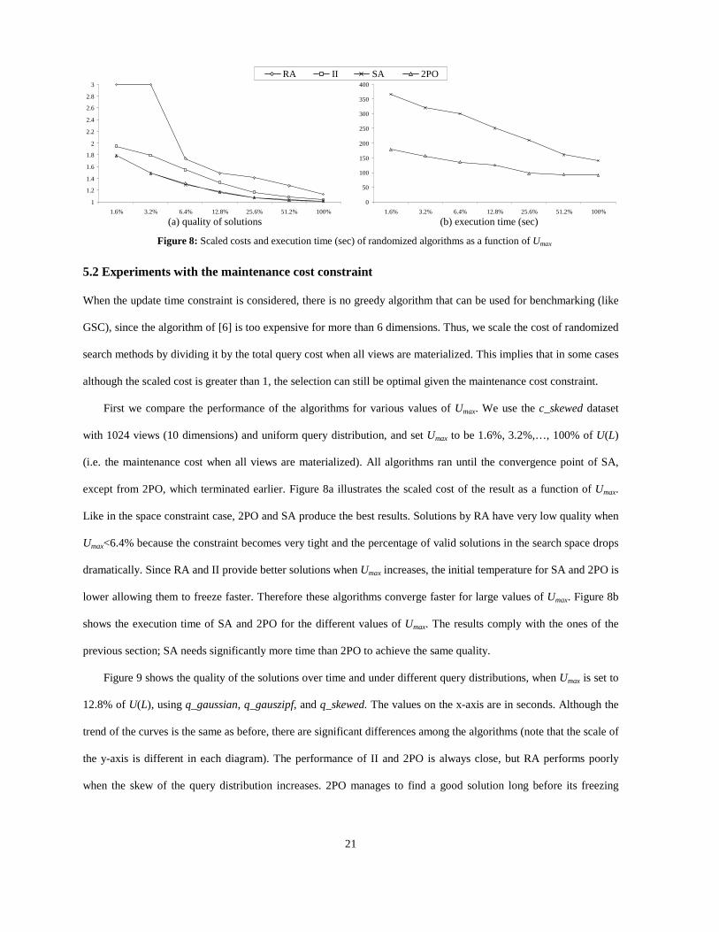
First we compare the performance of the algorithms for various values of Umax. We use the c_skewed dataset

with 1024 views (10 dimensions) and uniform query distribution, and set Umax to be 1.6%, 3.2%,…, 100% of U(L)

(i.e. the maintenance cost when all views are materialized). All algorithms ran until the convergence point of SA,

except from 2PO, which terminated earlier. Figure 8a illustrates the scaled cost of the result as a function of Umax.

Like in the space constraint case, 2PO and SA produce the best results. Solutions by RA have very low quality when

Umax<6.4% because the constraint becomes very tight and the percentage of valid solutions in the search space drops

dramatically. Since RA and II provide better solutions when Umax increases, the initial temperature for SA and 2PO is

lower allowing them to freeze faster. Therefore these algorithms converge faster for large values of Umax. Figure 8b

shows the execution time of SA and 2PO for the different values of Umax. The results comply with the ones of the

previous section; SA needs significantly more time than 2PO to achieve the same quality.

Figure 9 shows the quality of the solutions over time and under different query distributions, when Umax is set to

12.8% of U(L), using q_gaussian, q_gauszipf, and q_skewed. The values on the x-axis are in seconds. Although the

trend of the curves is the same as before, there are significant differences among the algorithms (note that the scale of

the y-axis is different in each diagram). The performance of II and 2PO is always close, but RA performs poorly

when the skew of the query distribution increases. 2PO manages to find a good solution long before its freezing

RA II 2POSA

1

1.2

1.4

1.6

1.8

2

2.2

2.4

2.6

2.8

3

1.6% 3.2% 6.4% 12.8% 25.6% 51.2% 100%

0

50

100

150

200

250

300

350

400

1.6% 3.2% 6.4% 12.8% 25.6% 51.2% 100%

(a) quality of solutions (b) execution time (sec)

Figure 8: Scaled costs and execution time (sec) of randomized algorithms as a function of Umax

22

point. The most beneficial views are gathered in a specific part of the lattice and RA fails to identify a good set since

it picks the views using uniform sampling. The same fact also affects SA. Nevertheless, SA can still identify a high

quality solution provided that it has enough time to converge.

In the next experiment we study how well the algorithms scale with the problem size. We used the c_skewed

distribution for the view sizes, uniform distribution for the queries and we set Umax=12.8%. In order to simulate

situations where there is a limited time for optimization, each algorithm was terminated after 120 sec. (even if it did

not converge). The size of the problem varied from 256 to 8192 views corresponding to 8-13 dimensions of a

complete lattice. The quality of solutions is shown in Figure 10. Observe that the order in the algorithms’

performance is preserved until 10 dimensions. For larger problems SA is ineffective since it does not have enough

time to freeze. Although 2PO doesn’t converge either (for instance, it has time to perform only one inner loop for

d=13), it still manages to find good solutions even for big problem sizes.

1

1.2

1.4

1.6

1.8

2

2.2

2.4

8 9 10 11 12 13

RA

II

SA

2PO

Figure 10: Scaled costs of solutions as a function of dimensionality (constant execution time)

5.3 Experiments with other cases

In this section we apply randomized search to solve two more view selection problems. First, we consider the case

where both space and update time constraints exist. Next we apply randomized search in the context of dynamic view

RA II 2POSA

1

1.2

1.4

1.6

1.8

2

2.2

2.4

4 8 16 32 64 128 2561

1.5

2

2.5

3

3.5

4

4.5

4 8 16 32 64 128 2561

11

21

31

41

51

4 8 16 32 64 128 256

(a) q_gaussian (b) q_gauszipf (c) q_skewed

Figure 9: Convergence time (sec) for different query distributions (c_skewed dataset)

23

selection [18]; we assume that a set of views that violate Umax has been materialized and the goal is to find the

optimal subset to maintain. In both experiments we used c_skewed, q_uniform and a pool of 1024 views.

In order to compare the algorithms in the presence of both constraints, we varied Smax between 1% and 12% of

S(L) (i.e. the size of the whole data cube) and set Umax to 51.2% of U(L). The algorithms were allowed to run until

the point where SA converges. The set of moves is the same as for the update time constraint including checks for

violations of the space constraint as discussed in section 4.2. The quality of solutions generated by the algorithms,

scaled to the quality of selecting the whole lattice, is shown in Figure 11. Observe that there is no difference in the

relative performance of the algorithms when both constraints are used; SA and 2PO find the best solutions, but SA

needs much more time to converge. An interesting point to notice is the region of values where each constraint is

restrictive. For Smax≤8% the quality of the solutions produced by all algorithms improves when Smax increases, since

there is space available for more views to be selected. On the other hand, when Smax>8% the performance of all

algorithms stabilizes because Smax stops being the restrictive constraint and Umax becomes the significant factor.

In the next experiment, we apply 2PO for the dynamic view maintenance problem and compare it with the

greedy algorithm of Dynamat, using the eager policy for both algorithms. Umax was set to 1.6%, 3.2%,… 100% of

U(L). Figure 12a shows the quality of the solutions for each value of Umax while Figure 12b shows the corresponding

running time. When there is enough time to update all views (Umax = 100% U(L)), the greedy algorithm performs a

trivial check and outputs the optimal solution (all views), otherwise 2PO is the obvious winner, since it finds better

solutions in less time. Note that if the lazy policy was used, the absolute running time would be lower, but the trend

would be the same.

1

1.05

1.1

1.15

1.2

1.25

1.3

1.35

1.4

1.45

1.5

1% 2% 4% 6% 8% 10% 12%

RA

II

SA

2PO

Figure 11: Scaled cost of the results as a function of available space when both constraints are considered

24

1

1.5

2

2.5

3

3.5

1.6% 3.2% 6.4% 12.8% 25.6% 51.2% 100%

2PO

greedy

0

50

100

150

200

250

300

350

1.6% 3.2% 6.4% 12.8% 25.6% 51.2% 100%

2PO

greedy

(a) scaled cost of solutions (b) execution time

Figure 12: Comparison of 2PO with the greedy algorithm of Dynamat

6. CONCLUSIONS

In this paper we have studied the application of randomized search heuristics to the view selection problem in data

warehouses. Four progressively more efficient algorithms, namely Random Sampling, Iterative Improvement,

Simulated Annealing and Two-Phase Optimization were adapted to find a sub-optimal set of views that minimizes

querying cost, and meets the space or maintenance constraints of the warehouse. The constraints define an irregular

search space of possible view combinations, which complicates the application of the search algorithms. In order to

overcome this difficulty we define two sets of transitions, one for each type of constraint.

In general, the search space may change significantly depending on the nature of the dataset and the query skew.

In skewed environments the difference between two solutions is very large and so is the performance variance among

the algorithms. The quality of the solutions produced by SA and 2PO (given enough time to search) is always better

than the ones produced by RA and II. For non-skewed settings the difference is not significant, indicating that the

latter algorithms may also be utilized when SA and 2PO do not manage to converge within the time allocated for

view selection. 2PO achieves the best performance in all tested cases because it converges fast to a good local

minimum.

For the case where only the space constraint is considered, we compared randomized search with a greedy

algorithm (GSC), which finds near-optimal solutions but its execution cost is cubic to the number of views and with

PBS, which is faster but requires certain restrictions on the lattice. The quality of the results of PBS was not good for

lattices that are not size restricted. Although the sizes of views may follow the restriction rule of [22] in many

warehouses, the weighted sizes with respect to the query workload can be arbitrary. 2PO managed to find solutions

25

extremely close to GSC (and sometimes better), in three orders of magnitude less time for a 15-dimensional

warehouse. As the execution cost gap between randomized search and GSC increases with dimensionality,

randomized search becomes the only viable solution to the view selection problem.

When the limiting factor is maintenance cost, the applicability of systematic algorithms is more restricted and

randomized search becomes essential even for a small number of dimensions. As the update window increases the

efficiency of randomized search also increases, because it is easier to move in the space of valid selections. The

results are very promising; when the update window is not trivial, the solution found by 2PO is close to the lower

bound (i.e. the querying cost when all views are materialized). Randomized search was also applied considering both

constraints and for a dynamic view selection problem, where it was proved more efficient than greedy methods in

terms of both selection quality and running time.

Summarizing, randomized search algorithms have significant advantages over existing methods for view

selection, since (i) they are applicable to high-dimensional problems. (ii) their parameters can be tuned to adjust the

trade-off between quality of solutions and execution time; in this way larger problems can be solved. (iii) they can be

easily adapted to solve several versions of the view selection problem. In the future we plan to explore the

application of randomized search to other problems like index selection [4] and view maintenance [19].

REFERENCES

[1] S. Agarwal, R. Agrawal, P.M. Deshpande, A. Gupta, J.F. Naughton, R. Ramakrishnan, S. Sarawagi, “On the

Computation of Multidimensional Aggregates”, in: Proc. VLDB, 1996.

[2] E. Baralis, S. Paraboschi, E. Teniente, “Materialized view selection in a multidimensional database”, in: Proc.

VLDB, 1997.

[3] J. Gray, A. Bosworth, A. Layman, and H. Pirahesh, “Data cube: a relational aggregation operator generalizing

group-by, cross-tabs and subtotals”, in: Proc. Int'l Conf. on Data Engineering, 1996.

[4] H. Gupta, V. Harinarayan, A. Rajaraman, J.D. Ullman, “Index Selection for OLAP”, in: Proc. Int'l Conf. on

Data Engineering, 1997.

[5] T. Griffin, L. Libkin, “Incremental Maintenance of Views with Dublicates”, in: Proc. ACM SIGMOD, 1995.

26

[6] H. Gupta, I.S. Mumick, “Selection of Views to Materialize Under a Maintenance-Time Constraint”, in: Proc.

Int'l Conf. on Database Theory, 1999.

[7] A. Gupta, I.S. Mumick, V.S. Subrahmanian, “Maintaining Views Incrementally”, in: Proc. ACM SIGMOD,

1993.

[8] C. Galindo-Legaria, A. Pellenkoft, M. Kersten, “Fast, Randomized Join-Order Selection - Why Use

Transformations?”, in: Proc: VLDB, 1994.

[9] J. Gray, P. Sundaresan, S. Englert, K. Baclawski, P.J. Weinberger, “Quickly Generating Billion Record

Synthetic Databases”, in: Proc. ACM SIGMOD, 1994.

[10] H. Gupta, “Selection of Views to Materialize in a Data Warehouse”, in: Proc. Int'l Conf. on Database Theory,

1997.

[11] V. Harinarayan, A. Rajaraman, and J.D. Ullman, “Implementing Data Cubes Efficiently”, in: Proc. ACM

SIGMOD, 1996.

[12] Y. Ioannidis, Y.C. Kang, “Randomized Algorithms for Optimizing Large Join Queries”, in: Proc. ACM

SIGMOD, 1990.

[13] Y. Ioannidis, Y.C. Kang, “Left-deep vs. Bushy Trees: An Analysis of Strategy Spaces and its Implications for

Query Optimization”, in: Proc. ACM SIGMOD, 1991.

[14] H. Jagadish, I. Mumick, A.Silberschatz, “View Maintenance Issues in the Chronicle Data Model”, in: Proc.

ACM PODS, 1995.

[15] S. Kirkpatrick, C. Gelat, M. Vecchi, “Optimization by Simulated Annealing”. Science, 220, (1983), 671-680.

[16] R. Kimball, “The Data Warehouse Toolkit”. John Wiley, 1996.

[17] H. Karloff, M.Michail, “On the complexity of the view selection problem”, in: Proc. ACM PODS, 1999.

[18] Y. Kotidis, N. Roussopoulos, “DynaMat: A Dynamic View Management System for Data Warehouses”, in:

Proc. ACM SIGMOD, 1999.

[19] W. Labio, R. Yerneni, H. Garcia-Molina, “Shrinking the Warehouse Update Window”, in: Proc. ACM

SIGMOD, 1999.

27

[20] I.S. Mumick, D. Quass, B.S. Mumick, “Maintenance of data cubes and summary tables in a warehouse”, in:

Proc. ACM SIGMOD, 1997.

[21] S. Nahar, S. Sahni, E. Shragowitz, “Simulated Annealing and Combinatorial Optimization”, in: Proc. 23rd

Design Automation Conference, pp. 293-299, 1986.

[22] A. Shukla, P.M. Deshpande, J.F. Naughton, “Materialized View Selection for Multidimensional Datasets”, in:

Proc. VLDB, 1998.

[23] A. Shukla, P.M. Deshpande, J.F. Naughton, and K. Ramasamy, “Storage Estimation for Multidimensional

Aggregates in the Presence of Hierarchies”, in: Proc. VLDB, 1996.

[24] A. Swami, A. Gupta, “Optimization of Large Join Queries”, in: Proc. ACM SIGMOD, 1988.

[25] Transaction Processing Performance Council, TPC Benchmark R (Decision Support), Rev. 1.0.1,

http://www.tpc.org/, 1993 - 1998

[26] D. Theodoratos, T.K. Sellis, “Data Warehouse Configuration”, in: Proc. VLDB, 1997