Viability of commercial depth sensors for the REX medical ...
137
Copyright is owned by the Author of the thesis. Permission is given for a copy to be downloaded by an individual for the purpose of research and private study only. The thesis may not be reproduced elsewhere without the permission of the Author.
-
Upload
khangminh22 -
Category
Documents
-
view
0 -
download
0
Transcript of Viability of commercial depth sensors for the REX medical ...

Copyright is owned by the Author of the thesis. Permission is given for a copy to be downloaded by an individual for the purpose of research and private study only. The thesis may not be reproduced elsewhere without the permission of the Author.

Viability of Commercial
Depth Sensors for the
REX Medical Exoskeleton
A thesis presented in partial fulfilment of the requirements for the degree of
Master of Engineering
in
Mechatronics
at Massey University, Albany,
New Zealand
by
MANU F. LANGE
2016

The author declares that this is his own work, except where due acknowledgement has been given.
The thesis is submitted in fulfilment of the requirements of a Masters in Engineering at Massey
University, New Zealand.
Manu Lange
ii

Abstract
Closing the feedback loop of machine control has been a known method for gaining stability.
Medical exoskeletons are no exception to this phenomenon. It is proposed that through machine
vision, their stability control can be enhanced in a commercially viable manner. Using machines
to enhance human’s capabilities has been a concept tried since the 19th century, with a range of
successful demonstrations since then such as the REX platform. In parallel, machine vision has
progressed similarly, and while applications that could be considered to be synonymous have been
researched, using computer vision for traversability analysis in medical exoskeletons still leaves a
lot of questions unanswered. These works attempt to understand better this field, in particular,
the commercial viability of machine vision system’s ability to enhance medical exoskeletons.
The key method to determine this will be through implementation. A system is designed that
considers the constraints of working with a commercial product, demonstrating integration into
an existing system without significant alterations. It shows using a stereo vision system to gather
depth information from the surroundings and amalgamate these. The amalgamation process
relies on tracking movement to provide accurate transforms between time-frames in the three-
dimensional world. Visual odometry and ground plane detection is employed to achieve this,
enabling the creation of digital elevation maps, to efficiently capture and present information
about the surroundings. Further simplification of this information is accomplished by creating
traversability maps; that directly relate the terrain to whether the REX device can safely navigate
that location. Ultimately a link is formed between the REX device and these maps, and that
enables user movement commands to be intercepted. Once intercepted, a binary decision is
computed whether that movement will traverse safe terrain. If however the command is deemed
unsafe (for example stepping backwards off a ledge), this will not be permitted, hence increasing
patient safety. Results suggest that this end-to-end demonstration is capable of improving patient
safety; however, plenty of future work and considerations are discussed. The underlying data
quality provided by the stereo sensor is questioned, and the limitations of macro vs. micro
applicability to the REX are identified. That is; the works presented are capable of working on a
macro level, but in their current state lack the finer detail to improve patient safety when operating
a REX medical exoskeleton considerably.
iii
Acknowledgements
I would like to thank the following parties:
My Friends & Family for their continued support and lenience, without whom this would not
have been half as enjoyable.
Associate Professor Johan Potgieter for his supervision, advice and confidence in my self-
management by demonstrating a hands-off approach.
Massey University for their continued support and funding to perform this research in the form
of scholarships.
Ken & Elizabeth Powell for their generous bursary that helped fund the advancement of tech-
nology as was their intention.
Callaghan Innovation for enabling the co-operation of Massey University and REX Bionics
through their partnership research and development grant. This greatly helped fund the
research and has helped build a relationship between the two entities.
REX Bionics for their full support and enthusiasm in this research. Without them truly none of
this would have been possible. Their supportive staff continually demonstrated kindness
and genuine interest in where this could lead, while always offering a helping hand.

Contents
Abstract . . . . . . . . . . . . . . . . . . . . . . . . . . . . . . . . . . . . . . . . . . . iii
Acknowledgements . . . . . . . . . . . . . . . . . . . . . . . . . . . . . . . . . . . . iv
Contents . . . . . . . . . . . . . . . . . . . . . . . . . . . . . . . . . . . . . . . . . . v
List of Figures . . . . . . . . . . . . . . . . . . . . . . . . . . . . . . . . . . . . . . . viii
List of Tables . . . . . . . . . . . . . . . . . . . . . . . . . . . . . . . . . . . . . . . . x
1 Introduction . . . . . . . . . . . . . . . . . . . . . . . . . . . . . . . . . . . . . . 1
2 Literature Review . . . . . . . . . . . . . . . . . . . . . . . . . . . . . . . . . . . 42.1 Robotic Exoskeletons . . . . . . . . . . . . . . . . . . . . . . . . . . . . . . . 4
2.1.1 Exoskeletons in Medical Applications . . . . . . . . . . . . . . . . . . 5
2.2 Machine Learning . . . . . . . . . . . . . . . . . . . . . . . . . . . . . . . . . 7
2.2.1 Machine Learning in Medical Exoskeletons . . . . . . . . . . . . . . . 8
2.3 Machine Vision . . . . . . . . . . . . . . . . . . . . . . . . . . . . . . . . . . 8
2.3.1 Stereo Vision . . . . . . . . . . . . . . . . . . . . . . . . . . . . . . . 9
2.3.2 Light Scanning . . . . . . . . . . . . . . . . . . . . . . . . . . . . . . 13
2.3.3 Machine Vision in Mobile Robotics . . . . . . . . . . . . . . . . . . . 16
2.4 Conclusion of Findings . . . . . . . . . . . . . . . . . . . . . . . . . . . . . . 19
3 Depth Vision and its Applicability to REX . . . . . . . . . . . . . . . . . . . . . . 203.1 Co-existing with the REX . . . . . . . . . . . . . . . . . . . . . . . . . . . . . 21
3.2 Hardware and Software Technology Selection . . . . . . . . . . . . . . . . . . 22
3.2.1 Vision Hardware Selection for the REX . . . . . . . . . . . . . . . . . 22
3.2.2 Depth Vision Software . . . . . . . . . . . . . . . . . . . . . . . . . . 27
3.2.3 Processing Hardware Centred on Depth Vision . . . . . . . . . . . . . 29
3.2.4 Decision Validation and Testing . . . . . . . . . . . . . . . . . . . . . 30
4 Extracting Raw Data . . . . . . . . . . . . . . . . . . . . . . . . . . . . . . . . . 32
v

CONTENTS
4.1 Camera Calibration . . . . . . . . . . . . . . . . . . . . . . . . . . . . . . . . 32
4.2 Reading Depth . . . . . . . . . . . . . . . . . . . . . . . . . . . . . . . . . . 33
4.3 Coordinate Systems and Ground Planes . . . . . . . . . . . . . . . . . . . . . 37
4.3.1 Aligning with the Ground Plane . . . . . . . . . . . . . . . . . . . . . 38
4.4 Camera Motion and Odometry . . . . . . . . . . . . . . . . . . . . . . . . . . 40
4.4.1 Odometry Fusion . . . . . . . . . . . . . . . . . . . . . . . . . . . . . 43
4.5 Combining Solutions . . . . . . . . . . . . . . . . . . . . . . . . . . . . . . . 43
5 Implementing with Robot Operating System . . . . . . . . . . . . . . . . . . . . 445.1 Filesystem Management . . . . . . . . . . . . . . . . . . . . . . . . . . . . . 44
5.2 Computation Graph . . . . . . . . . . . . . . . . . . . . . . . . . . . . . . . . 45
5.3 The Community . . . . . . . . . . . . . . . . . . . . . . . . . . . . . . . . . . 47
5.4 Robot Operating System (ROS) and the REX . . . . . . . . . . . . . . . . . . 47
6 Elevation Maps . . . . . . . . . . . . . . . . . . . . . . . . . . . . . . . . . . . . . 516.1 Working with Point Clouds Efficiently . . . . . . . . . . . . . . . . . . . . . . 51
6.1.1 Octrees . . . . . . . . . . . . . . . . . . . . . . . . . . . . . . . . . . 52
6.1.2 Gridmapping . . . . . . . . . . . . . . . . . . . . . . . . . . . . . . . 53
6.2 Simultaneous Localization and Mapping . . . . . . . . . . . . . . . . . . . . . 54
7 Traversability Maps . . . . . . . . . . . . . . . . . . . . . . . . . . . . . . . . . . 587.1 Traversing with the REX . . . . . . . . . . . . . . . . . . . . . . . . . . . . . 58
7.1.1 Traversability Filters . . . . . . . . . . . . . . . . . . . . . . . . . . . 59
7.1.2 Combining Traversability Layers . . . . . . . . . . . . . . . . . . . . 63
7.2 Interfacing with the REX . . . . . . . . . . . . . . . . . . . . . . . . . . . . . 63
8 Dataset Generation . . . . . . . . . . . . . . . . . . . . . . . . . . . . . . . . . . 66
9 Results . . . . . . . . . . . . . . . . . . . . . . . . . . . . . . . . . . . . . . . . . 699.1 Traversability Mapping . . . . . . . . . . . . . . . . . . . . . . . . . . . . . . 69
9.2 Laser Data Set . . . . . . . . . . . . . . . . . . . . . . . . . . . . . . . . . . . 75
9.3 Interfacing with the REX . . . . . . . . . . . . . . . . . . . . . . . . . . . . . 81
10 Discussion and Conclusion . . . . . . . . . . . . . . . . . . . . . . . . . . . . . . 8410.1 Discussion . . . . . . . . . . . . . . . . . . . . . . . . . . . . . . . . . . . . . 84
10.2 Conclusion . . . . . . . . . . . . . . . . . . . . . . . . . . . . . . . . . . . . 88
Bibliography . . . . . . . . . . . . . . . . . . . . . . . . . . . . . . . . . . . . . . . . 91
Appendices . . . . . . . . . . . . . . . . . . . . . . . . . . . . . . . . . . . . . . . . . 102I ZED Datasheet . . . . . . . . . . . . . . . . . . . . . . . . . . . . . . . . . . 103
vi

CONTENTS
II DUO MLX Datasheet . . . . . . . . . . . . . . . . . . . . . . . . . . . . . . . 106
III Jetson TX1 Datasheet . . . . . . . . . . . . . . . . . . . . . . . . . . . . . . . 109
IV REX Exoskeleton Datasheet . . . . . . . . . . . . . . . . . . . . . . . . . . . 111
V Additional Results . . . . . . . . . . . . . . . . . . . . . . . . . . . . . . . . 113
VI Source Code . . . . . . . . . . . . . . . . . . . . . . . . . . . . . . . . . . . . 114
vii

List of Figures
2.1 Medical Exoskeletons . . . . . . . . . . . . . . . . . . . . . . . . . . . . . . . 6
2.2 Stereo Matching Process . . . . . . . . . . . . . . . . . . . . . . . . . . . . . 10
2.3 Epipolar Geometry . . . . . . . . . . . . . . . . . . . . . . . . . . . . . . . . 11
2.4 Cost Aggregation Windows . . . . . . . . . . . . . . . . . . . . . . . . . . . . 12
2.5 Time of Flight camera principles . . . . . . . . . . . . . . . . . . . . . . . . . 14
2.6 Principles of Structured Light . . . . . . . . . . . . . . . . . . . . . . . . . . . 15
2.7 Humanoid Robot Terrain Mapping . . . . . . . . . . . . . . . . . . . . . . . . 19
3.1 Depth Sensor trade-offs . . . . . . . . . . . . . . . . . . . . . . . . . . . . . . 24
3.2 URG-04LX-UG01 Laser Scanner . . . . . . . . . . . . . . . . . . . . . . . . 24
3.3 Commercial Time of Flight Cameras . . . . . . . . . . . . . . . . . . . . . . . 25
3.4 ZED & Duo Stereo Cameras . . . . . . . . . . . . . . . . . . . . . . . . . . . 26
3.5 Jetson TX1 Module . . . . . . . . . . . . . . . . . . . . . . . . . . . . . . . . 30
4.1 Stereo Calibration Sample . . . . . . . . . . . . . . . . . . . . . . . . . . . . 33
4.2 Duo Dashboard GUI . . . . . . . . . . . . . . . . . . . . . . . . . . . . . . . 34
4.3 Duo OpenCV Calibration Flowchart . . . . . . . . . . . . . . . . . . . . . . . 35
4.4 Comparing Stereo Re-projections . . . . . . . . . . . . . . . . . . . . . . . . . 35
4.5 ZED Depth Explorer GUI . . . . . . . . . . . . . . . . . . . . . . . . . . . . . 36
4.6 Coordinates Frames in use . . . . . . . . . . . . . . . . . . . . . . . . . . . . 38
4.7 Ground Calibration Process . . . . . . . . . . . . . . . . . . . . . . . . . . . . 39
5.1 ROS Pipeline Demonstration . . . . . . . . . . . . . . . . . . . . . . . . . . . 45
5.2 REX Model in ROS . . . . . . . . . . . . . . . . . . . . . . . . . . . . . . . . 48
5.3 Complete ROS Graphs of the system . . . . . . . . . . . . . . . . . . . . . . . 49
5.3 Complete ROS Graphs of the system . . . . . . . . . . . . . . . . . . . . . . . 50
6.1 Octree Representation . . . . . . . . . . . . . . . . . . . . . . . . . . . . . . . 52
6.2 Elevation Mapping output . . . . . . . . . . . . . . . . . . . . . . . . . . . . 57
7.1 Traversability Map Sample . . . . . . . . . . . . . . . . . . . . . . . . . . . . 63
7.2 REX-LINK Flowchart . . . . . . . . . . . . . . . . . . . . . . . . . . . . . . 64
viii

LIST OF FIGURES
8.1 Laser Dataset Point Clouds . . . . . . . . . . . . . . . . . . . . . . . . . . . . 68
9.1 Flat Terrain Results . . . . . . . . . . . . . . . . . . . . . . . . . . . . . . . . 69
9.2 Flat Terrain Analysis . . . . . . . . . . . . . . . . . . . . . . . . . . . . . . . 70
9.3 Door Terrain Results . . . . . . . . . . . . . . . . . . . . . . . . . . . . . . . 71
9.4 Door Terrain Analysis . . . . . . . . . . . . . . . . . . . . . . . . . . . . . . . 71
9.5 Demo Stairs Terrain Results . . . . . . . . . . . . . . . . . . . . . . . . . . . 72
9.6 Demo Stairs Terrain Analysis . . . . . . . . . . . . . . . . . . . . . . . . . . . 72
9.7 Large Flight of Stairs Terrain Results . . . . . . . . . . . . . . . . . . . . . . . 73
9.8 Large Flight of Stairs Terrain Analysis . . . . . . . . . . . . . . . . . . . . . . 73
9.9 Complex Stairs Terrain Results . . . . . . . . . . . . . . . . . . . . . . . . . . 74
9.10 Flat Area Laser Comparison . . . . . . . . . . . . . . . . . . . . . . . . . . . 76
9.11 Production Stairs Laser Comparison (a) . . . . . . . . . . . . . . . . . . . . . 77
9.12 Production Stairs Laser Comparison (b) . . . . . . . . . . . . . . . . . . . . . 77
9.13 Harsh Environment Laser Comparison . . . . . . . . . . . . . . . . . . . . . . 79
9.14 Ground Truth Traversability Map . . . . . . . . . . . . . . . . . . . . . . . . . 80
9.15 REX-Link Interface Overview . . . . . . . . . . . . . . . . . . . . . . . . . . 81
9.16 REX-Link Interface Demonstration . . . . . . . . . . . . . . . . . . . . . . . 82
ix

List of Tables
2.1 Geometry Detection Methods Survey . . . . . . . . . . . . . . . . . . . . . . . 16
3.1 Depth Camera Hardware Summary . . . . . . . . . . . . . . . . . . . . . . . . 23
4.1 Camera Absolute Axial Error at Different Ranges . . . . . . . . . . . . . . . . 37
8.1 Faro Focus3D Accuracy . . . . . . . . . . . . . . . . . . . . . . . . . . . . . . 66
8.2 Laser Datasets . . . . . . . . . . . . . . . . . . . . . . . . . . . . . . . . . . . 67
x

Chapter 1
Introduction
Rex Bionics is a New Zealand based, garage graduate company that has changed the level of
interaction possible between technology and humankind. Beginning with the desire to re-enable
humans who could no longer use their lower limbs, from the home garage to production facility,
the business has grown together human and machine in a unique manner. Their core product, the
REX, is the first self-supported medical exoskeleton to be commercially available. Being self-
supported was a major focus of the team, not only because this would give a marketing advantage
over similar medical exoskeletons; but because of the wish to allow patients to interact with their
environment while standing. Rather than having to support one’s self with crutches, patients are
free to go about their usual activities, interact with others and complete tasks. However while this
feature thoughtfully placed Rex Bionics exoskeleton apart from other products, it also reduced
the stability of the platform when navigating uneven terrain. Fundamentally this was a control
limitation, as mechanically the device could navigate the sloped terrain. Assuming the control
methods maintained a stable centre of mass over the grounded foot, which had roll and pitch
rotational freedom, the device could stand. The issue, however, was that although attempted, no
closed-loop control solution had been developed to stabilise the device.
With an apparent abundance of sensory technology and portable processing power being available
to consumers, there seemed an obvious solution: close the loop. Machine vision can capture
significant amounts of data about the environment and with advances in processing technology,
infer relevant information to base decisions on. Advances in sensor technology have allowed
cameras to perceive depth as humans do, adding yet another dimension of information available
for decision-making.
Machine vision and humanoid robotics is not an uncharted topic, with the likes of Humanoid
Robots Lab (HRL) doing significant work, along with other laboratories around the world. These
groups to date focus however on robotics not inhabited by humans. The benefits of combining
1

CHAPTER 1. INTRODUCTION
these two technologies still lie largely untested. This research focuses on this novel application of
existing technologies in a commercial setting.
The question of why this should be attempted can easily be approached from various directions;
however, the predominant considerations are patient safety and empowerment. At the core of
REX’s focus is re-enabling patients; and to be able to do this effectively, users must feel confident.
Confidence can be enhanced by demonstrating that the latest technology helps ensure patient
safety by reducing fall rates, letting the user focus on the therapy process rather than their safety.
Additionally, advancing the sensory ability of the REX will lead to allowing advanced terrain
navigation, reducing restrictions on where patients may go and what they may do with the REX,
thus empowering them to be less dependent.
Research has indicated that terrain navigation and classification of a humanoid robot is possible,
and has identified key considerations when implementing such a system, however, this has not
been translated into a commercial product. Identifying the benefits such systems can offer a user
are important in determining if the technology is worth pursuing commercially. Considering the
availability of depth sensing technology, the integration into consumer products is still largely
untapped, arguably due to difficulties with sensors in uncontrolled environments. In pursuing
this application, issues faced when commercialising depth technology are identified and potential
solutions implemented.
Avoiding rediscovering known findings required an extensive literature review to be carried out.
This highlighted how researchers in approached and answered similar hypothesis, but also needed
to be continuously translated to apply to the REX. The following key challenges were approached
to respond to the hypothesis that machine vision could extend medical exoskeleton’s ability to
traverse terrain:
1. Technology Selection – Literature review quickly identified that research outcomes would
be significantly shaped by the technology employed, making this an important choice.
Each sensor category offered its strengths and weaknesses, as did software and processing
hardware. These choices are critically reviewed, and the decisions made are supported by
knowledge identified by fellow researchers.
2. Relating Data and Time – Observing all necessary information in a single instance would
limit the usefulness of the information. Instead, linking information observed at different
times and from different vantage points extended the ability to capture information. Adding
this temporal dimension, however, required knowledge of precise transforms between
frames, so the information could be merged in a common frame of reference.
3. Extendible Framework – Avoiding reworking significant challenges, choosing a frame-
work that provided solutions to these was essential. For software, this meant choosing an
2

CHAPTER 1. INTRODUCTION
operating system and a set of libraries and applications that implemented standard features
required for a machine vision robotics system.
4. Simplifying Information – While the insight gained by depth-cameras was crucial for
this research; they also produce large amounts of data. Managing, understanding and
working with raw point clouds was excessive, and so this was reduced, without losing
vital information such as elevation. It was possible to reduce complexity significantly but
maintain the basic underlying relevant information.
5. Determing Traversability – The definition of traversable is relative to with what one
wishes to traverse the terrain. To this extent, the simplified representation of the immediate
surroundings is assessed for traversability by the REX. Interfacing this information directly
to the REX when moving then closes the loop and signifies a key milestone in this research.
These challenges are all faced with applicability to the REX kept steadily in focus, ensuring that
the results presented are representative of what could be commercially achieved on the platform.
At times this presents a severe limitation, but one that is necessary to determine the commercial
viability of machine vision systems with medical exoskeletons.
By overcoming these challenges, this work describes the path to combining the fields of machine
vision and medical exoskeletons, something which has previously not been attempted. This
work will significantly help the REX move to a dynamic movement model capable of traversing
unknown terrain safely and extending the use-cases of the device.
3
Chapter 2
Literature Review
2.1 Robotic Exoskeletons
Exoskeletons, as first defined in the field of anatomy, mean “the protective or supporting structure
covering the outside of the body of many animals” [HarperCollins Publishers, 2016]. With
inspiration from the animal kingdom (in particular insects), there have been attempts at advancing
humans ability with such devices. Passive devices such as the one detailed in this article [Agrawal
et al., 2006], focus on removing the passive load on gravity on joints for medical examination.
However, since the first conception of a ‘powered exoskeleton’ by Nicholas Yagn in [Yagn, 1890],
a branch of human assistive devices of powered exoskeletal nature has emerged. Early attempts
such as the Hardiman, arguably the earliest true powered exoskeleton suit, developed by General
Electric in the 1960s had extensive limitations such as those detailed in the final project report
[Fick and Makinson, 1971]. These restrictions mostly led to these projects being discontinued and
only now in the 21st century have technology advancements allowed commercial opportunities to
arise. This has seen development in three fundamental areas of robotic exoskeletons categories
[Pons, 2008]:
Empowering Increasing the strength capabilities of humans has been one of the original mo-
tivators of exoskeleton robotics. Originally coined extenders [Kazerooni, 1990], these
often operate by mimicking the human intent (or motion) but will removing load from
the operator. Not necessarily restrained to encompassing a human, remotely teleoperated
designs also fall under this category.
Orthotic With medical technologies increasing, a large sector of exoskeletons attempt to restore
lost human functionality. Devices in this category will often attempt to re-enable humans
after they have lost the use of their limbs by retraining their body on how to operate
4

CHAPTER 2. LITERATURE REVIEW
correctly. To achieve this, these devices often attempt to integrate as closely to the human
body as capable, often employing neurological links.
Prosthetic Unique applications of robotic limbs are possible when the patient has lost the
original limb. In these cases, one is not restrained by working around the original limb, but
can completely replace it with a mechanical (or bio-mechanical) device. A large market
exists for enabling re-integration of amputees into society by re-enabling them to function
independently. Prosthetics have existed for a long time, however, advances robotics have
allowed them to become intelligent in nature.
2.1.1 Exoskeletons in Medical Applications
With the medical industry becoming increasingly intertwined with information technology
[Thompson and Brailer, 2004, Meara et al., 2004], medical devices are being developed globally
to more increasingly reliant on technology. From specialised robotic surgery [Lanfranco et al.,
2004] to health information standards for collaborative public health analysis such as those
developed by the USA’s Department of Health & Human Services, the implementations are vast.
To keep this review of current technologies focused, it will only focus on exoskeletons employed
by the medical sector, specifically robotic/assistive platforms. This is the market that Rex Bionics
operate within. In recent years suits such as the Robotic EXoskeleton (REX) platform, the
ReWalk, Hybrid Assistive Limb (HAL), EKSO, and many more have all been targeted at medical
use. The ReWalk (image 2.7a) was the first commercially available device (within the US) that
enables patients with loss of lower limb control to stand, walk and climb stairs. The device
requires the patient use crutches to support themselves and so needs them to have a healthy
and operational upper body. Rex Bionics differentiated themselves from this, by developing a
self-supporting device (image 2.7b) that does not require crutches for operation, and yet can still
perform the same actions; the REX. The Phoenix from SuitX (image 2.1e) differentiates itself by
being a modular light weight device (only 12.25 kg), but does again require crutches for operation.
It achieves this by only having two actuators, at the hip, allowing the other joints to move freely.
Esko or eLEGS again employs crutches and stems out of Berkeley Bionics, is slightly heavier
(roughly 20 kg), and can provide adaptive amounts of assistance per side. The HAL (image 2.1d)
stems from Cyberdyne, a Japanese company, and is heavily employed in medical facilities there1. The device features a cybernetic control system that can determine user intent purely from
electrical signals from the body. Approaching the solution differently, this stationary Lokomat
(image 2.1f) device is produced by Swiss company Hocoma. Employing a treadmill design in
combination with a precision controlled exoskeleton for the lower body it can effectively re-train
1http://www.theaustralian.com.au/news/world/robots-to-the-rescue-as-an-aging-japan-looks-for-help/story-
e6frg6so-1226494698495
5

CHAPTER 2. LITERATURE REVIEW
(a) ReWalk 6.0
(b) Esko
(c) REX
(d) HAL
(e) Phoenix
(f) Lokomat
Figure 2.1: Medical Exoskeletons – A (non-complete) collection of medical exoskeletons availablecommercially. Images sources: [Rewalk, 2012, Ekso Bionics Holdings, 2015, REX, 2014, CYBERDYNE,2014, US Bionics, 2016, Hocoma, 2016]
6

CHAPTER 2. LITERATURE REVIEW
movement gaits. Proven to improve walking speed in clinical trials [Hidler et al., 2009], this
device is employed in many medical facilities.
2.2 Machine Learning
Machine Learning is a term that, although defined in a simple manner, is often used with ad
understanding of what it entails. It has emerged with the recent explosion of the ‘total digital
universe’ [Gantz and Reinsel, 2012]. Whilst still fundamentally bound by T. Mitchell’s ()
definition: “A computer program is said to learn from experience E with respect to some class of
tasks T and performance measure P, if its performance at tasks in T, as measured by P, improves
with experience E”, its boundaries are vague. It is closely related to statistics and data mining.
Fundamentally there are three fields that machine learning can be split into supervised learning,
unsupervised learning and reinforcement learning [Murphy, 2012]. These three areas however
sometimes have vague boundaries, and implementations can be hard to classify.
Supervised learning is the process of taking one or more sets of input-output pairs and developing
a map from inputs to outputs. This is the form of machine learning most used in practical situations
[Murphy, 2012]. Supervised learning can be closely linked to optimisation and classification
(and their subfields) problems. A typical example of its real world implementation is email spam
filtering. One major drawback of supervised learning is the creation of these input-output pairs.
They often require experts to spend much time manually classifying data.
Unsupervised learning focuses on explorative knowledge acquisition. Unlike supervised learning,
it does not have input-output pairs to learn from. In fact, the nature and existence of the outputs
are generally unknown. This feature of not having to know the outputs first in a training set
makes unsupervised learning arguably more powerful. It enables computers to perform knowledge
discovery in unknown areas. An example of its immense use was demonstrated in when the digital
content provider Netflix created a competition with a 1M United States Dollars (USD) prize2.
The competition required a system to predict user’s interests better based on their ratings. The
prize was claimed in by a team of researchers who implemented many machine learning models
to achieve this result. Another example is demonstrated by Hofmann et al., where the authors
develop and prove the use of Probabilistic Latent Semantic Analysis (PLSA) to automatically
index documents based on content [Hofmann, 2001]. As it is becoming increasingly difficult to
generate a dataset for every possible answer, reliance on these methods which are proven to work
is rising.
Reinforcement learning, like unsupervised learning, is not given input-output pairs to learn
2http://www.netflixprize.com/
7

CHAPTER 2. LITERATURE REVIEW
from. However, in contrast to unsupervised learning, it is generally implemented in a continuous
learning loop. That is, it will have a measure of performance, and attempt to achieve better on
every iteration, even during runtime. A typical example of this is the pole balancing problem
that has been the test case of many reinforcement learning publications [Michie, 1968, Schaal,
1997, Si and Wang, 2001]. Si et al. even extend this challenge to a triple inverted pendulum
balancing challenge, demonstrating their algorithm. In this regard, similar to unsupervised
learning, reinforcement learning is heavily implemented where it is impossible or inconceivable
to generate large data sets with answers.
2.2.1 Machine Learning in Medical Exoskeletons
Examples of machine learning in medicine are becoming more frequent, especially in data
analysis, where there are often significant amounts of variables [Cleophas et al., 2013]. While
Cleophas et al.’s book provides an extensive range of examples and applications of machine
learning applied to medicine in general, there are far fewer examples when looking at exoskeletons.
A recent survey on model learning for robot control [Nguyen-Tuong and Peters, 2011] highlights
the importance of embracing machine learning to enable automatic control model generation for
the future of autonomy. They review case studies of machine learning applied and point out what
it achieved well. Looking at a particular example, teleoperated control of a humanoid robot was
successfully generalised using a combination of neural networks and particle swarm optimisation
(both core to machine learning) [Stanton et al., 2012]. The authors demonstrate that it is possible
to build a framework that does not explicitly understand the kinematic models of the robot but can
quickly determine control signals that generate desired outputs. Brain Machine Interface (BMI) is
another interesting area of research, where it was recently demonstrated that a BMI could control
a REX medical exoskeleton by employing machine learning to decode Electroencephalogram
(EEG) signals [Contreras-Vidal and Grossman, 2013, Kilicarslan et al., 2013]. Similarly He et al
investigate using EEG and Electromyography (EMG) to develop a BMI functional with NASA’s
X1 exoskeleton suit [He et al., 2014]. It is evident when looking at these recent advances that
there will be plenty more scope for research in this area over the coming years.
2.3 Machine Vision
Machine vision, closely related to machine learning, is an incredibly complex field of research, in
part because we do not yet understand human’s vision and perception [Szeliski, 2010]. Vision is
a primary input to human’s decision-making process when interacting with the world. Likewise,
vision is quickly becoming a fundamental input for the decision-making processes of computer
programs. Research in machine vision attempts to model the environment in a visual sense using
8

CHAPTER 2. LITERATURE REVIEW
complex mathematical algorithms and models. However, unlike humans who easy grasp the
concepts of vision, dimensions, occlusion, context, and other such intricacies, these prove to be
fundamental challenges for computers. This challenge stems from the inverse nature of computer
vision; that being the process of attempting to recover information from incomplete observations,
often employing forward based models (physics) [Szeliski, 2010]. This fact and the importance
of the potential possibilities has led to recent research in this field growing significantly [Hamzah
and Ibrahim, 2015]. As a result of this, reviewing current literature and developing a summary of
current state of technology itself could be the topic of a thesis. To contain the scope, only a few
specific technologies will be reviewed in detail.
2.3.1 Stereo Vision
As with animals and humans with binocular vision, programs have been enabled in a similar
manner, allowing stereopsis. Usually featuring two digital cameras separated by a horizontal
distance, systems employ complex matching algorithms to extract a depth map. The entire
process begins with camera selection and placement. The key parameters for camera placement
are interaxial separation and convergence angle.
Interaxial separation refers to the distance between two camera sensors. This plays a great role
in the depth perception. Greater interaxial separation increases depth perception but decreases
the minimum distance objects can be perceived at. On the flip side, smaller separation reduces
depth perception but allows for successful matching at close distances. While this parameter is
more important when the media will be viewed by humans, since wrong values can cause viewing
discomfort, it also plays a role in the matching algorithms ability to function. The convergence
angle again plays a role in the distances the vision system will be effective at. However, due to
computational implementations and consistent overall performance, cameras are mostly aligned
parallel. The reason for this is detailed in the image rectification process.
Rectification of pairwise captured images is an important step in the process of stereo vision.
Since no two cameras (lenses and sensors) will produce identical digital images, for matching
purposes, it is important that they be as noise free as possible. Also, images are rectified to be on
a common plane and have parallel epipolar lines. The process of rectification usually begins with
calibration training of the system. Here calibration images used to extract key parameters, learn
lens distortions and transformation matrices required for computational simplification. Typically,
this can be expressed in 12 parameters as Ch = AWh [Memon and Khan, 2001]. Here Ch
represent the camera coordinates, Wh are the world homogeneous coordinates and A is a vector
of the 12 unknown parameters. In general, there are three approaches to determining these
parameters: linear, nonlinear and two-step methods [Memon and Khan, 2001]. Linear methods
are computationally very fast as they assume a very simplistic pinhole camera model. This does,
9

CHAPTER 2. LITERATURE REVIEW
however, limit the models to not correcting for distortion effects, which are significant in lower
standard products. Contrary to this, non-linear methods, can account for these lens distortions.
However, due to its iterative nature, the initial parameter guess is important to ensure convergence.
In two-step methods, some parameters are found directly, while others are iteratively discovered.
Various novel techniques have been introduced with the advancements of machine learning
[Memon and Khan, 2001]. An example of this is a calibration procedure that uses Artificial
Neural Network (ANN)s to perform the correction. Intrinsic to the nature of ANN however, this
method does not reveal the underlying parameters, but rather operates as a black box.
Once rectified, the images pass through a framework of algorithms to generate a disparity map.
This is generally accepted to be a four-stage process as detailed in the figure 2.2 [Hamzah and
Ibrahim, 2015]. Each stage can consist of a multitude of algorithms that process the images
Figure 2.2: Stereo Matching Process – The general process of stereo matching can be broken into fourstages [Hamzah and Ibrahim, 2015].
individually or combined. As a combined process these can be classified as a local or global
approach. This classification stems from the computational approach used when calculating
disparity. If the calculation at a given point depends only on values surrounding it within a given
window, this is classified as local. Examples of these approaches have been explored in papers
such as [Tuytelaars and Van Gool, 2000, Gerrits and Bekaert, 2006, Zhang et al., 2009]. Opposing
this, a global approach will attempt to calculate the disparity map as to minimise some global error
or energy function. This function will penalise data that differ from the target, and also penalise
noisy data. This two-termed approach ensures that data is both valid and noise free, however,
is computationally expensive [Hamzah and Ibrahim, 2015]. This stems from the fact that they
normally skip the second stage, cost aggregation, and work with all the pixel data. As with many
statistical processes, the first stage in this process is matching cost computation. Matching cost
computation is able to evaluate how well a pixel on one image matches a pixel on the other image.
This can be defined as determining the parallax values of each point in two images [Brown et al.,
2003]. Since this is a fundamental task to complete for every single combination of pixels, this is
often constrained to reduce computational complexity. For example, given a 640 p× 480 p image,
over 94 billion comparisons would have to be made if every pixel of one image were compared
to every pixel of the other image. This large search field can be quickly reduced. Given the
rectification process is correctly calibrated, the data will be constrained to be epipolar in geometric
properties. Once constrained, matching points must lie on the epipolar lines e, as detailed in 2.3.
This reduces the search space from the entire data set to only the horizontal line (for horizontally
separated cameras) currently being computed [Song et al., 2014]. With this reduced sample set,
10

CHAPTER 2. LITERATURE REVIEW
Figure 2.3: Epipolar Geometry – An example of epipolar lines applied to stereo vision. For a point at anydepth from camera C1, lying on epipolar line E1, the same point will appear somewhere along line E2
from perspective C2 given the images are rectified to align epipolar lines. Image reproduced from [Lazaroset al., 2008]
pixel-based techniques again become viable. Early pixel based approaches featured Absolute
Difference (AD), Squared Differences (SD) and variations of these. Other than pixel-based
approaches, area or window-based methods will analyse multiple pixel sub-groups. These are
capable of offering higher quality data as each matching process is essentially averaged, making it
more resilient to noise. Common implementations for window based algorithms include the Sum
of Squared Differences (SSD), Sum of Absolute Differences (SAD), Normalised Correlations
(NCC), Rank Transforms (RT) and Census Transforms (CT) [Lazaros et al., 2008]. The region
considered is commonly referred to as support or aggregation window and is flexible in shape,
that is it can be various shapes that may or may not change during run-time. Since in essence,
this approach is an averaging process, it features common pitfalls. The assumption that pixels
within the support region have similar disparity values is not always true. For example, pixels
near depth discontinuities or edges may be vastly different. Hence appropriate parameters must be
selected to ensure useful output. An interesting branch of algorithms, Feature Based Techniques,
exists, however, is plagued by lower accuracy. Since these only focus on features extracted from
the images and try to match these, they only generate sparse disparity maps. They are however
computationally very efficient as they have a significantly smaller sample sizes [Liu et al., 2014].
Details of these individual approaches are outside of the scope of this thesis as it is intended to
acquire a product that outputs the disparity map computed.
The next stage of cost aggregation attempts to reduce uncertainties. Since pixel-wise matching cost
computation is insufficient for precise matching, a support region is again employed to improve
matching accuracy. Similarly, this support region is of flexible nature. Many research efforts
have advanced this field (list from [Hamzah and Ibrahim, 2015] page 11), and so the original
11

CHAPTER 2. LITERATURE REVIEW
Fixed Window (FW) approach is used less often [Hamzah and Ibrahim, 2015]. A summary of
the basic approaches can be seen in figure 2.4. The authors of [Fang et al., 2012] performed a
Figure 2.4: Cost Aggregation Windows – Examples of windows to use in the process of stereo matching.(a) is a simplistic 5x5 window, (b) adaptive window, (c) uses a window with adaptive eights, (d) showspossible adaptive window results. Image reproduced from [Hamzah and Ibrahim, 2015]
study comparing the use of these techniques and concluded that Adaptive Support Weight (ASW)
was most advantageous to use. Essentially it is similar to an Adaptive Window (AW) approach
with a flexible window shape, since the weightings of each neighbour are variable. Where other
approaches fail to maintain object boundaries (since they are smoothed out), ASW assigns weights
based on pixel disparity correlation to the target pixel, resulting in well-maintained edges.
Disparity selection begins to collate all the possibilities accumulated above. A local winner takes
all Winner Takes All (WTA) algorithm chooses the disparity with the minimum associated cost.
This is a simple argmin function that iterates the discrete possibilities of disparity values. This is
a fairly concise and straightforward step that is well defined. A few alternatives such as Markov
Random Field (MRF) do exist, but WTA is the most commonly used approach [Hamzah and
Ibrahim, 2015]
Refinement of the now populated disparity map now takes place. Here the disparity map is noise
filtered (again), and special cases such as occlusion are handled. Hamzah and Ibrahim identify
12
CHAPTER 2. LITERATURE REVIEW
that this step usually consists of two core parts; regularisation and interpolation. Regularisation
is a simple pre-filter that removes inconsistent disparity estimations; primarily points that are
considerably different to neighbouring values. Interpolation on the other-hand attempts to fill in
disparity values that are missing due to occlusion or unsuitable matching. Amongst attempts used
are Gaussian filters and median edge filters such as those extended by Michael et al. [Michael
et al., 2013]. These will fill in sections of the disparity map by making probabilistic guesses,
primarily based on neighbouring disparity values.
A desired result of this four-step process is a smooth and accurate disparity map that can directly
(with known camera parameters) be re-projected to a three-dimensional point cloud. The wide
array of choices on how to progress from two cameras to a point cloud make this a non-trivial
task to implement, especially because there often exists no clear best approach.
2.3.2 Light Scanning
Light Scanning depth vision systems employ active sensing to determine the topology of a scene.
Fundamentally they differ in the sense that in most systems stereo vision is passive; that is it
does not emit any radiation (including visible light) itself, it is a passive sensor. Light scanning
systems however actively scan the field of view with an emitted signal, determining depth by
tracking how that signal interacts with the environment. This field can be further divided into two
subcategories as detailed below.
Time of Flight Cameras
Understanding the speed of a radiated wave combined with precise timing, in theory, allows
measurements of distances following the same principles of bats with sound waves [Kleinschmidt
and Magori, 1985]. However due to the high speed of light waves, 1mm corresponds to 6.6 ps in
measuring accuracy required, which obviously presents a technological challenge. A solution to
this is described in patent [Shyy, 1993], employing Digitally Programmable Delay Generators
(DPDG) to very accurately measure time delays using principal properties of resistive-capacitive
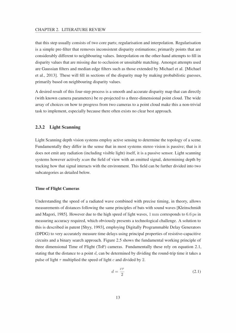
circuits and a binary search approach. Figure 2.5 shows the fundamental working principle of
three dimensional Time of Flight (ToF) cameras. Fundamentally these rely on equation 2.1,
stating that the distance to a point d, can be determined by dividing the round-trip time it takes a
pulse of light τ multiplied the speed of light c and divided by 2.
d =cτ
2(2.1)
13

CHAPTER 2. LITERATURE REVIEW
Figure 2.5: Time of Flight camera principles – This figure depicts the working principles of a three-dimensional depth sensing camera employing time of flight technology. Differences in phases are measuredwith regards to the reference sending wave, then using known properties of light speed the distance traveledcan be deduced. Figure source: [Lange and Seitz, 2001].
This allowed for very accurate, sub-millimetre distance measurements and is still employed in
modern geo-surveying laser scanners. These devices, however, are only able to sample a single
point per operation, and while modern devices use mirrors to scan a three-dimensional scene
quickly, this is still challenging to implement in moving robotics and can be very costly. To
overcome this limitation, systems capable of simultaneous three-dimensional sensing have been
developed, employing smart modulation techniques to distinguish data points with an array of
sensors [Lange, 2000], such as depicted in figure 2.5. By carefully measuring the phase-shift of a
reflected signal these sensors are able to instantaneously sample an image, similar to a traditional
imaging chip. The Kinect sensors(both versions) are excellent examples and are amongst the
most employed in robotics and research with many articles published referencing them [Hsu,
2011, El-laithy et al., 2012, Zhang, 2012, Fankhauser et al., 2015, Maykol Pinto et al., 2015, Yang
et al., 2015] (it is infeasible to reference them all here). These sensors, however, rely heavily on
accurately distinguishing their signal from ambient noise. With the most commonly employed
wavelength being infra-red (invisible and harmless to the human eye at low powers), sunlight is a
large source of noise, providing many challenges in using such systems outdoors [Fankhauser
et al., 2015].
Structured Light cameras
Essentially a version of stereoscopic vision, Structured Light (SL) cameras usually employ a
virtual second perspective in the means of a projected known pattern (or structure) of light (visible
or invisible to the human eye) onto the scene. Triangulation is used to determine the distances of
pixels with information gathered by a binary search approach. Using the trigonometric equation
14

CHAPTER 2. LITERATURE REVIEW
2.2, it is possible to calculate the camera to point distance R using the angles θ and α which can
be determined from the matched pixel locations within an image, and the baseline B.
R = Bsin(θ)
sin(α+ θ)(2.2)
Various coded patterns are projected onto the scene and imaged from a camera in a different
perspective. The offset caused by perspective in these patterns is compared and allows for back
depth perception to the object with the known distance between the sensor and projector and
the perceived pixel offset of the pattern [Posdamer and Altschuler, 1982]. These principles are
demonstrated in figure 2.6, with a simple projector-camera set-up. Advances in SL have been
(a) Structure projection (b) Triangulation calculation
Figure 2.6: Principles of Structured Light – This figure demonstrates the principles of generating depthfrom structured light. a shows how a pattern is projected onto and distorted by an object. b then shows thetrigonometry used to determined the object height Z based on the difference distance d given that B isknown. Original figures sourced from [Geng, 2011].
demonstrated in various pattern encodings and processing techniques that can allow for very
accurate scene reconstructions. Accuracy is commonly proportional to scene sampling volume,
such that a system sampling a 6 cm× 12 cm× 16 cm volume has an accuracy of less than 100 μm
[Hall-Holt and Rusinkiewicz, 2001], whilst a system scanning an area of 0.23m has an accuracy
of 450 μm [Gernat et al., 2008]. These systems tend to be considerably processing intensive,
with the author of second example ([Gernat et al., 2008]) stating it took hundreds of hours of
post processing in addition to a full day of collection to build the model. Many modern systems
exist that employ structured light for scene capturing and achieve some of the highest accuracies.
However, due to the above-discussed limitations, often either the sensor or the scene must remain
static. [Hall-Holt and Rusinkiewicz, 2001] demonstrate this with the aforementioned sensor,
which is capable of capturing depth information at 60Hz, but requiring the sensor to remain
stationary while the object in the scene could be rotated.
15

CHAPTER 2. LITERATURE REVIEW
2.3.3 Machine Vision in Mobile Robotics
Applications of machine vision are vast and readily accepted in many major industries [Szeliski,
2010]. In academia, it is a heavily researched and documented topic with many books ([Szeliski,
2010]) providing detailed summaries of algorithms and approaches. While much research and
technology are focused on the manufacturing automation industry (as this is a major market),
for mobile robotics the implementations are still not as densely distributed. However with such
breadth in the types of technology and how to apply them, it was important to review what
approaches were being perused, specifically to mobile robot geometry detection. Table 2.1 tries
Table 2.1: Geometry Detection Methods Survey – A non-extensive survey of literature focused on planeand stair detection, with key details extracted and summarised.
Author Year Summary Approach RGB/2D/3Da Frame/SLAMb Comments
Maohai 2014Fast stair metric
extraction
Stereo, RGB
feature detection,
V-Disparity
RGB & 2DNon-
temporal
Trained RGB Classifier, then focuses on ROI with
V-Disparity to detect planes, extract height and tread.
Bumblebee stereo Camera.
Delmerico 2013Detect stairs
semantically
Kinect, 2D/3D
Edge Detection2D Temporal
Uses 2D/3D combination. 2D edges, 3D points ex-
tracted. Extracts edges every frame, but ’detects’
stairs of a registered point cloud over time
Lee 2012Wearable Staircase
Stereo
Haar Features,
Ground plane
segmentation
RGB & 2D
& 3DTemporal
Uses RGB to detect stairs, many false positives, fil-
ters with RANSAC ground plane from stereo and
temporal consistency
Osswald 2011Humanoid Stair
Climbing
Lidar, Scanline
Grouping2D
Non-
temporal
Uses 2D LIDAR over angles with scan line group-
ing. Here lines are found in multiple 2D scans, then
grouped in 3D, creating a plane.
Holz 2011Fast Plane
Segmentation
RGB-D, 3D
Normals, Cluster
Segmentation
3DNon-
temporal
Uses RGB-D, Computes normals, clusters and seg-
ments based on these. 30Hz
Ben-Tzvi 2010 Plane SegmentationLidar, 2D Edge
Detection2D Temporal
Uses a 2D LIDAR over angles to make 3D. Then
makes depth contour maps, edge detection, segmen-
tation of planes
Oniga 2010 Road DetectionStereo, DEM,
Expected Density2D
Non-
temporal
Uses disparity to DEM, then performs various algo-
rithms. Works in 2D and 3D mix. Expected Density
difference is a very interesting approach.
Hesch 2010 Descending stairs2D, Texture,
Optical Flow, LinesRGB
Non-
temporal
Uses RGB only to find descending stairs, doesn’t
extract info.
Hernandez 2010RGB stairs
vanishing point
2D, Vanishing
Point, Directional
Filter, Lines
RGBNon-
temporal
Uses RGB, very fast, high detection, no extracted
detail.
Gutmann 2008Environment Map
Perception
Stereo, Planar
Segmentation,
Scanline Grouping
2D BothUses plane segmentation to semantically label data
and store SLAM.
Michel 2007GPU RGB
Humanoid Stairs
Canny Edge, GPU,
Model ProjectionRGB
Non-
temporal
Uses RGB edges to detect stairs. Fed a lot of assump-
tions. Fits CAD model of stairs to locate them
a Denotes methods employed during processing, not necessarily capturing of data. RGB denotes color information only, 2D denotes depth / disparity
images, 3D denotes point clouds.b This describes the time variance of the process. Systems that consider a temporal dimension are said to operate in a time-variant manner and include time
as a dimension.
to demonstrate a non-exhaustive list of literature that would be relevant towards this research. It
demonstrates the amount of design choice faced when implementing machine vision (in particular
geometrical shape detection) into robotics.
Maohai et al. demonstrate an efficient and fast staircase detection process that combined traditional
Red Green Blue (RGB) with depth map disparity analysis to achieve promising results [Maohai
et al., 2014]. First using a two-dimensional classifier employing a 29-layer cascade involving
16

CHAPTER 2. LITERATURE REVIEW
655 Haar-like features, the system is able to quickly detect the presence of a staircase with high
confidence (in a test set of 311 negative test images, they had zero false positives). Their use of v-
disparity then enables them to reduce the three-dimensional plane extraction to a computationally
efficient two-dimensional problem capable of extracting three-dimensional features with an
accuracy of 2mm for close planes.
[Delmerico et al., 2013] demonstrate a different approach, working purely with the depth/disparity
information from a Kinect camera. They perform staircase edge detection by specifically looking
for discontinuities in the depth data, indicating abrupt geometry changes. Points representing
these edges are then used in a three-dimensional manner to fit a plane within a bounding box.
This represents the step dimensions with its pitch relative to the ground and the step width. This
detection algorithm is capable of operating at 20Hz, with accuracies of 3◦ in pitch (roughly 2 cm
in step height), however this is performed in post processing and not during collection.
[Lee et al., 2012] employ temporal consistency to their stair detection process, an idea that enforces
consistency over time in the data collected. For general detection, they too used Haar-like features
with cascade classifiers and v-disparity. Running their detection process in post-processing on
data gathered from a wearable stereo camera showed promising speeds, but takes advantage of a
large and powerful processing machine.
[Osswald et al., 2011a, Osswald et al., 2011b, Maier et al., 2012, Maier et al., 2013, Hornung et al.,
2014, Karkowski and Bennewitz, 2016] and their HRL published a lot of research on the topic
of relevance, with their humanoid stair climbing being of particular interest. In [Osswald et al.,
2011b], the group demonstrate a functional application of laser scanner based staircase traversal
for a humanoid robot. Their research, however, does point out the restrictions of employing laser
scanners requiring the robot to stand still every two steps and tilt its head to gather a new set of
points to analyse. Navigation of complex stair terrain is achieved with the humanoid robot, with
their approaches detecting stairs 7 cm in height with a model error of 0.42 cm.
[Holz et al., 2011] demonstrates a more general focus; plane detection in point clouds. Employing
methods to compute surface normals quickly, they perform fast plane segmentation with rates
of up to 30Hz. An interesting feature they employ is cleaning the point cloud once planes have
been detected by pulling points towards the plane average that probably belong to that plane.
While Holz et al. used an Red Green Blue Depth (RGB-D) camera, [Ben-Tzvi et al., 2010]
perform plane segmentation on a mobile tracked robot using a pitch actuated laser range finder,
similar to the process of [Osswald et al., 2011a]. Instead of plane fitting, the author uses depth
map contours to determine and extract them.
[Oniga and Nedevschi, 2010a, Oniga and Nedevschi, 2010b] introduce more concepts to the
solution through the use of Digital Elevation Map (DEM)s in their road detection research. A
17

CHAPTER 2. LITERATURE REVIEW
DEM significantly reduces the size of a three-dimensional data set by reducing measurements to
one vertical reading per configurable area. The authors also employ techniques to increase the
density of data in their DEMs taking into account the re-projection angles of the camera viewing
the scene. A particularly interesting method employed by the authors is generating a density
map, that measures the three-dimensional points per DEM cell. Areas of high density are likely
obstacles because multiple readings in the same x− y space indicate a vertical obstacle relative
to the camera (such as a wall).
Many of the articles mentioned above focus on ascending stairs, however, [Hesch et al., 2010]
concentrate on detecting descending stairwells and labelling them. Without any depth cameras,
the authors implement a method that tracks optical flow between frames. Then using this temporal
attribute they detect abrupt changes in flow indicating a descending stairwell. They demonstrate
this functioning on a tracked robot which first determined the presence of a stairwell and then
proceeds to navigate down it.
Reviewing earlier publications, there are more that chose to simply use RGB without depth
information, due to computational requirements. [Hernandez and Kang-Hyun, 2010] demon-
strates using such technology and vanishing point analysis to locate stairs effectively in outdoor
environments. Not being restricted by the infra-red limitations of depth cameras, their methods
successfully detect outdoor stairs with an acceptable false positive rate very quickly (0.08 s). They
demonstrate this working with a broad range of stairs, lighting and angles, proving its robustness
purely with RGB cameras.
Using a combination of these ideas, [Gutmann et al., 2008] (who later co-authors with HRL, no
doubt contributing some of these ideas), demonstrates an impressive solution on a humanoid robot
(QRIO). Running on limited processing their approach uses a tri-stereo camera to generate DEM
and then intelligently semantically label this with relation to the robot’s abilities. Demonstrating
this, they show the robot navigating a complex scene, littered with obstacles, stairs, and even a
tunnel that have to be navigated as seen in figure 2.7. Of interest in particular was that the robot
could distinguish that it would have to enter a different movement mode (crawling) in order to
traverse under the table (tunnel).
[Michel et al., 2007] demonstrate using a simple RGB camera, but employ the Graphics Processing
Unit (GPU) to improve speed, which also makes their methods more robust to noise from camera
shake commonly an issue on bipedal robots. They demonstrate climbing stairs with their large
bipedal HRP-2 robot, proving the capability of their methods.
18

CHAPTER 2. LITERATURE REVIEW
(a) Obstacle course with Nao robot (b) Generated terrain map and path
Figure 2.7: Humanoid Robot Terrain Mapping – An example of a humanoid robot (Nao) navigatingterrain and semantically labelling them. Images directly sourced from [Gutmann et al., 2008]
Machine Vision in Exoskeletons
While technically a lot of the above is relevant to exoskeleton robotics, it is still of interest
to review specific examples of such applications, of which there are only a few. Advances in
BMI were demonstrated using a combination of EEG, eye-tracking, and RGB-D cameras to
interface a human with an exoskeleton upper limb [Frisoli et al., 2012]. Here the authors use
a Kinect camera to detect objects for interaction in front of the patient, then track the patient’s
gaze to detect which object they wish to interact with, and finally, await the correct brain activity
indicating that the patient wishes to carry out interaction. They successfully demonstrated this
with a L-Exos, an exoskeleton for an arm that helps guide patients limbs when they can no longer
control them [Frisoli et al., 2005]. A different approach is presented that uses machine vision
with standard RGB images to determine user intent from facial expressions and control an upper
body exoskeleton [Baklouti et al., 2008]. Although their results seem inconclusive, their approach
is novel and further strengthens the argument of how broad machine vision applications are.
2.4 Conclusion of Findings
With such a vast array of technology and applications, it is difficult to assert that something has
not been explored previously; however, no direct applications of machine vision for path planning
have been demonstrated on an exoskeleton that were published at the time of writing. Identifying
this unexplored application, and a large amount of research undergone with mobile robotic path
planning (especially humanoid) it seemed worthwhile exploring the potential of implementing
a machine vision guidance system on a (medical) exoskeleton. End-user applications, such as
rehabilitation, will benefit from the increased control such research will lead too.
19

Chapter 3
Depth Vision and its Applicability toREX
The use of machine vision to extend the ability of devices in both the consumer and manufacturing
sector are growing steadily1. It has been used in many manufacturing environments to aid
automation and is also making in roads into the consumer goods sector with depth enabled
devices such as Google’s Project Tango2. For many of these applications, machine vision provides
a straightforward and semi-universal approach to closing a control feedback loop. The sheer
amount of applicability and diversity of machine vision as a process monitoring and quality
control tool, has lead to many systems and products being redesigned with industry in mind.
Instead of tactile sensors on a conveyor belt, now an imaging system can verify not only part
count on a production line but also perform a variety of quality control checks. In fact, companies
such as Point Grey specialise in providing finely tuned machine vision sensors for applications
ranging from industrial automation to medical to security geographic information systems. Being
a tightly intertwined discipline of mechatronics, machine vision relies just as much on software
as it does on the hardware. Smart, efficient software is critical to making sense of the abundant
data transmitted by the hardware, and add value. Many commercial and non-commercial tools
have been developed that aid in the post-processing of data gathered by machine vision systems,
for example, Matrox or OpenCV. As a result, the industries ’learning curve’ to applying these
tools has been simplified greatly since its conception.
1Search result hit counts for papers published containing machine vision and applications show a steady growth
over time2An initiative to introduce depth vision to mobile phones by integrating compatibility into Android and developing
standard hardware for phone manufacturers to use. http://get.google.com/tango/
20

CHAPTER 3. DEPTH VISION AND ITS APPLICABILITY TO REX
3.1 Co-existing with the REX
The focus of this research was not to develop just another vision system, but one functional with
medical exoskeletons, more specifically the REX platform. As shown in figure 2.7b, the REX
device is a bipedal medical device, capable of supporting a human in the standing position that
can no longer do so themselves. It is roughly 1.3m in height (adjustable per patient), 0.645m
in width and 0.66m in depth, and weighs around 50 kg with battery. Patients must be between
1.42m to 1.93m in height and between 40 kg to 100 kg in weight to use the device. Mechanically
the device is powered by 10 actuators over 6 joints. Powered by a battery the device can move
forward at a speed of 0.0347m/ sec, and can do so for 1 h straight. Primarily the device is used
by clinicians to help humans recover the use, or maintain the health of their lower body after an
accident or disease which prevents them from doing so themselves.
In order develop a compatible vision system, right from the beginning, certain aspects had to be
considered when making decisions. They are:
1. Functionality
(a) Able to detect the immediate surroundings geometrically
(b) Function in real-time, with speeds relative to REX’s speeds
(c) Detect ground plane level shifts, such as curb-ways
(d) Extending the above, detect stairways and extract important metrics
(e) Not negatively impact the REX’s performance
2. Aesthetics
(a) Small enough to integrate without causing obstructions
(b) Ability to function from a aesthetically pleasing location
3. User Interaction
(a) Be safe to use, unable to cause harm to occupant, whilst
(b) Presenting useful information to non-technical end-users and
(c) Give choices that are easy to understand
Whilst some of these items do not need any expansion, such as item ground-plane detection (1c),
some items such as patient safety (3a) caused a lot of discussion throughout the research. Being in
the medical industry places a lot of pressure and restrictions upon devices developed, something
21

CHAPTER 3. DEPTH VISION AND ITS APPLICABILITY TO REX
that is not inherently apparent. For the team developing the REX, patient safety (3a) is often a
major influence. It is for example why the device walks as it does, with an inhuman gait, so that
at any instant if power is cut, the device is able to stand stable. This also becomes a consideration
when programming such a device, where failure modes become less apparent. To adhere to these
strict regulations to which the device is qualified, any additions must also do so, or not tamper
with those in place. By considering the two systems disconnected, that is the REX platform does
not process any of the vision information and vice versa, and placing human decision-making
at the boundary of interaction, this issue can be mitigated. By not allowing the vision system to
make any actions, it is adhering to patient safety (3a) by placing it in the patients’ own hands.
3.2 Hardware and Software Technology Selection
Depth vision, as a subfield of machine vision, also looks to follow the same path of development.
Split across three main core technologies; stereo, time of flight, structured light, there is, however,
no universal approach to implementing and applying depth vision. The usage restrictions and
sub-variables of each core technology only expands the already complex choice of suitable
hardware for a machine vision task. Inverse to this, the selection of depth sensors available is
severely dwarfed by that of two-dimensional cameras. This selection is further dissected into
research and commercial categories, of which very few fall into the latter. Three-dimensional
processing software is also an important aspect and is discussed below.
3.2.1 Vision Hardware Selection for the REX
Unlike two-dimensional systems, the choices when looking for three-dimensional sensors is very
restricted. Arguably as a result of the infancy of applications within large industries, there simply
has not been enough demand for three-dimensional vision. This fact is evident when scoping
a potential device for use within a commercial product such as the REX platform. Table 3.1
presents a summary of depth sensors. While not an exhaustive list, this represents the majority of
sensors currently3 available to an end-user. To provide a comparison, a two-dimensional depth
sensing scanner has been included. Prices are included to relate back to commercial viability.
Note that cameras such as the Kinect v2 or the R200 are successors of older generation models not
included in the table. The application very much dictates the camera choice, at least in the sense
of core technology. As identified in the literature review, the different technologies behave very
differently circumstantially. Figure 3.1 shows three key performance metrics for depth cameras
that are often considered to match the application. There yet exists no universal technology that
3List sourced in Q1 2016
22

CHAPTER 3. DEPTH VISION AND ITS APPLICABILITY TO REX
Table 3.1: Depth Camera Hardware Summary – A non-exhaustive list of depth sensing technologycommercially available
Camera Supplier Price (USD) Technology Resolution (px)
ZED StereoLabs $449 Stereo Vision 1920x1080
R200 Intel $99 Combination 640x480
Duo MLX Duo3D Division $695 Stereo Vision 752x480
R12 Raytrix Stereo Array 3 MP
Structure Sensor Occipital $379 Structured Light 640x480
SentisToF - M100 Bluetechnix $830 ToF 160x120
Kinect v2 Microsoft $200 ToF 512x424
URG-04LX-UG01 Hokuyo $1,140 Laser 2D 0.36 deg
is able to perform in all metrics equally, although the MC3D claims this [Matsuda et al., 2015].
As the state-of-the-art is advanced, these axes extend and so it is also unlikely that a universal
solution will ever exist, making the task of selecting a suitable sensor a constant one. Review of
recent literature[Matsuda et al., 2015, Gupta et al., 2013, Taguchi et al., 2012, Fankhauser et al.,
2015] focused on characterising depth cameras reveals roughly where each technology lies on
this graph.
Time of flight systems that employ laser scanning are very accurate. However, the slow sampling
rate and high cost (while not included on this graph, still relevant) limit the applications they are
of use in. Laser scanner systems are very light independent due to their unique signal encoded
into a powerful laser beam, making them very reliable and accurate. However since laser scanners
operate on a points-per-second sampling rate, they are generally slow to sample a full three-
dimensional field of view. Well suited for the manufacturing industry, they perform their best
when mounted in a fixed location and scanning only a few preset points, such as dimensions
of a part on a conveyor belt. On a moving platform, such as the REX, laser scanners rely on
accurate localisation and or inertial measurement units to correct for the origin movement of
the sensor relative to its static surroundings, adding complexity to the system. Laser scanners
in themselves are already incredibly complex, and this is reflected in their pricing. The URG-
04LX-UG01 (shown in table 3.1 and figure 3.2) is an example of a budget sensor, capable only of
sampling a single two-dimensional plane, and yet is still the most expensive sensor on the table.
This demonstrates the enormous cost involved with the complex mechanical optics of a laser
scanner based system, with highly accurate land survey scanners costing closer to 50,000 USD4. Size and weight are more attributes laser scanners do not traditionally excel in. These were
important factors to consider for the REX platform, being a consumer device, where aesthetics are
often more important than functionality. When considering a sensor for the REX platform, laser
scanners had to be dismissed from consideration, due to many of the reasons explained before.
4Faro Focus 3D X 330 Scanner
23

CHAPTER 3. DEPTH VISION AND ITS APPLICABILITY TO REX
x, acqusition speed
y, resolution
z, light resilience
Single-shot, eg Kinect
Laser Scanning
Gray Codes
Stereo Vision example
ToF, eg Kinect v2
Figure 3.1: Depth Sensor trade-offs – A visual representation of the compromises faced when choosinga depth sensor. Here the [x, y, z] axis represent the acquisition speed, resolution, and light resilienceof the technologies respectively. Some examples are labelled based off the publishings of Matsuda et al.[Matsuda et al., 2015]. The Stereo vision example purely shows that while not the best at any, stereo isconfigurable, and can hence achieve a balance.
Figure 3.2: URG-04LX-UG01 Laser Scanner – An entry level laser scanner seen in many roboticsresearch applications due to its small size and relatively low cost. Image source: [Unknown, 2016]
Modern time of flight systems employing phase patterns projected in infra-red to sample an entire
frame at once have overcome the sampling rate issue but cannot maintain the accuracy and light
independence of laser scanners. These sensors display their strength under controlled lighting,
where they can produce low noise, high frame-rate reconstructions of the three-dimensional world.
Playing less of a role in the industrial scene, these sensors are emerging in the consumer sector.
Their low price point is arguably the major driver behind this and makes this sensor category
perfect for consideration for the REX platform. Conversely, the reduced performance in certain
lighting scenarios challenges suitability for the REX platform. As explained in the review of
24

CHAPTER 3. DEPTH VISION AND ITS APPLICABILITY TO REX
this technology (section 2.3.2), their dependence on active infra-red as a signal medium deeply
affects their performance under sunlight. The closed loop feedback depth system is arguably most
important outdoors, where the terrain encountered is less human-made and hence less predictable.
In this category, there were two key choices: Kinect v2 and the SentisToF M100. From Microsoft,
the Kinect v2 is arguably one of the most mainstream depth sensors on the market, after its
predecessor the Kinect v1. An example of a scene recorded with the Kinect v2 comparison to
other sensors in figure 4.4d. While this sensor produces very low noise data at great ranges and
accuracy, unfortunately as with the laser scanners, aesthetics take prescient over functionality. It
is the largest of the cameras considered, and requires a large external power adapter due to its high
consumption. Designed for use in the home-entertainment sector, size and manoeuvrability did
not play a large role in the design of the camera. For these reasons the Kinect v2 was disregarded
from selection. The SentisToF M100 camera is an impressive, small form factor time of flight
camera, shown in figure 3.3b. Measuring 50mm× 55mm× 36mm this sensor was well suited
(a) Kinect v2 (b) Sentis ToF M100
Figure 3.3: Commercial Time of Flight Cameras – A sample of two commercially available time-of-flightbased cameras. Bluetechnix’s small time of flight sensor, the Sentis ToF M100, and the Kinect v2 fromMicrosoft, which is a very commonly used research camera. Image Sources: [Microsoft, 2014, Bluetechnix,2016]
for the REX dimensionally. With a sensor frame size of 160 px× 120 px, the camera lacks high
resolution but still has enough to be of use at short to medium range. Although the SentisToF
M100 is a contender for the REX platform, due to its higher cost and reliance on active infra-red
illumination, this camera was not acquired for development.
Structured light was the core technology relied upon by the original Kinect sensor. Characteristics
of structured light sensors are well understood by the research community through extensive
characterisation[Zanuttigh et al., 2016]. Often used for ground truth measurements, in very
well controlled environments, this depth sensing technology is capable of very accurate scene
reconstructions. However to achieve such accuracy, many restrictions have to be enforced;
otherwise, performance suffers severely. Again relying heavily on active infra-red illumination,
and sometimes even visible light illumination, the scene lighting must be consistently controlled.
25

CHAPTER 3. DEPTH VISION AND ITS APPLICABILITY TO REX
Some commercially available sensors exist for a more general purpose use, similar to the Kinect
v1, however, their data was often rather noisy in outdoor environments. For the most part, this
disqualified these sensors from consideration for the REX platform. The Structure sensor from
Occipital is a small consumer based sensor, but lacks the accuracy to be considered here. Covered
later, the Intel R200 partially relies on structured light to sense depth, and a sample of its output
can be seen in figure 4.4c.
Unlike the previous technologies, stereo vision is usually considered a passive sensor, being
that it does not emit any signals of its own. Uncoupling the sensor from a dependence on
light signals of its own, reduces the overpowering effect of the sun in outdoor environments,
making stereo vision systems well suited here. Commercial stereo vision systems are not
the most common, however, due to their customisation requirements. It is hard for a single
product to capture the market, such as the Kinect did, rather end users choose two or more
two-dimensional cameras and construct their own stereo system. This places stereo vision outside
of reach for many companies who lack the internal expertise to do so. The ZED, a depth camera
(a) ZED (b) DUO MLX
Figure 3.4: ZED & Duo Stereo Cameras – Images of the two stereo cameras considered in this research.Image Sources: [Stereolabs, 2016, Code Laboratories, 2016]
from Stereolabs, aims at bridging this gap and is depicted in figure 3.4a. With a baseline of
120mm, the camera is able to detect disparities across a large range from 0.7m to 20m. The
minimum range of 0.7m is not ideal for REX platform, limiting it’s close proximity collision
detection. As explained in section 2.3.1, to maintain accuracy at large ranges, each camera on
the ZED is capable of capturing 2208 px× 1242 px. While obviously increasing accuracy, the
extra computational requirement (with roughly nine times more data points over a traditional
640 px× 480 px image) needs to be considered. A comparative sample of the ZED’s output
can also be seen in figure 4.4b. The baseline forces the ZED to be longer in one dimension,
resulting in a size of 175mm× 30mm× 33mm, which is still acceptable for integrating on the
REX platform. Requiring only a single USB3 interface cable made the ZED additionally easy to
integrate wherever required upon the platform. Another stereo camera acquired for testing was
26

CHAPTER 3. DEPTH VISION AND ITS APPLICABILITY TO REX
the DUO MLX from Code Laboratories (shown in figure 3.4b). This stereo camera uses active
infrared to help in low-light environments, however, comes at the cost of it being more susceptible
to noise introduced by sunlight. It is however sized at only 52mm× 25mm× 13mm, making
it very easy to potentially have multiple cameras (front and rear-facing) on the REX platform.
A baseline of 30mm combined with a sensor frame resolution of 752 px× 480 px give it an
effective range of 0.25m to 2.5m. Besides this sensor uses global shutters capable of frame rates
as high as 360Hz (at a lower resolution), making it very well suited for visual odometry ( a topic
covered later), especially combined with its internal six degrees of freedom inertial measurement
unit included. Like with the ZED, the DUO MLX does not require an external power source other
than the USB2 cable for communications.
While these three core technologies define most depth sensors, there exist a few sensors that do
not easily fit into these categories. Intel’s R200 is such a sensor, combining both infra-red based
structured light with passive stereo to generate it’s depth maps this presents a novel approach.
While this sensor performs a lot better in uncontrolled environments than previous sensors,
especially given its small form factor of only 130mm× 20mm× 7mm, it was not chosen for
integration with the REX platform at this time point. It could however easily be considered at a
later time point. Another such combination of technologies is the research device codenamed
MC3D, developed at Northwestern University Evanston, Illinois. How this device overcomes
some of the challenges facing conventional depth cameras is detailed in their article, however as
it is not available for purchase and not easy to reconstruct, it too was not employed in the scope
of this research [Matsuda et al., 2015].
3.2.2 Depth Vision Software
As with most forms of sensors, it is simply not enough to gather the data with hardware. Software
to make sense of the data streams arguably become even more crucial with depth vision systems,
due to the sheer quantity of information contained. As a quick example of this, images are
often 24 bits per pixel, 8 bits per colour channel. In addition to this, depth data contains x-y-z
co-ordinates usually stored as double precision floating points, an extra bits per pixel/point. Not
only is there a far larger quantity of data, but it is also harder to display and communicate for
human interaction and analysis, being that most human interface devices operate on a three-
dimensional principal. This fundamental limitation in how we interact with technology is a key
focus of many researchers, but no widely accepted commercial method exists for interacting with
three-dimensional data natively. For this reason and the purpose of automation, it is important
that the implementation developed can analyse the depth information directly and only present
the end-user with simple choices. However, just as with depth vision hardware, software capable
of working with depth data is far from being as refined and developed as that designed to operate
27
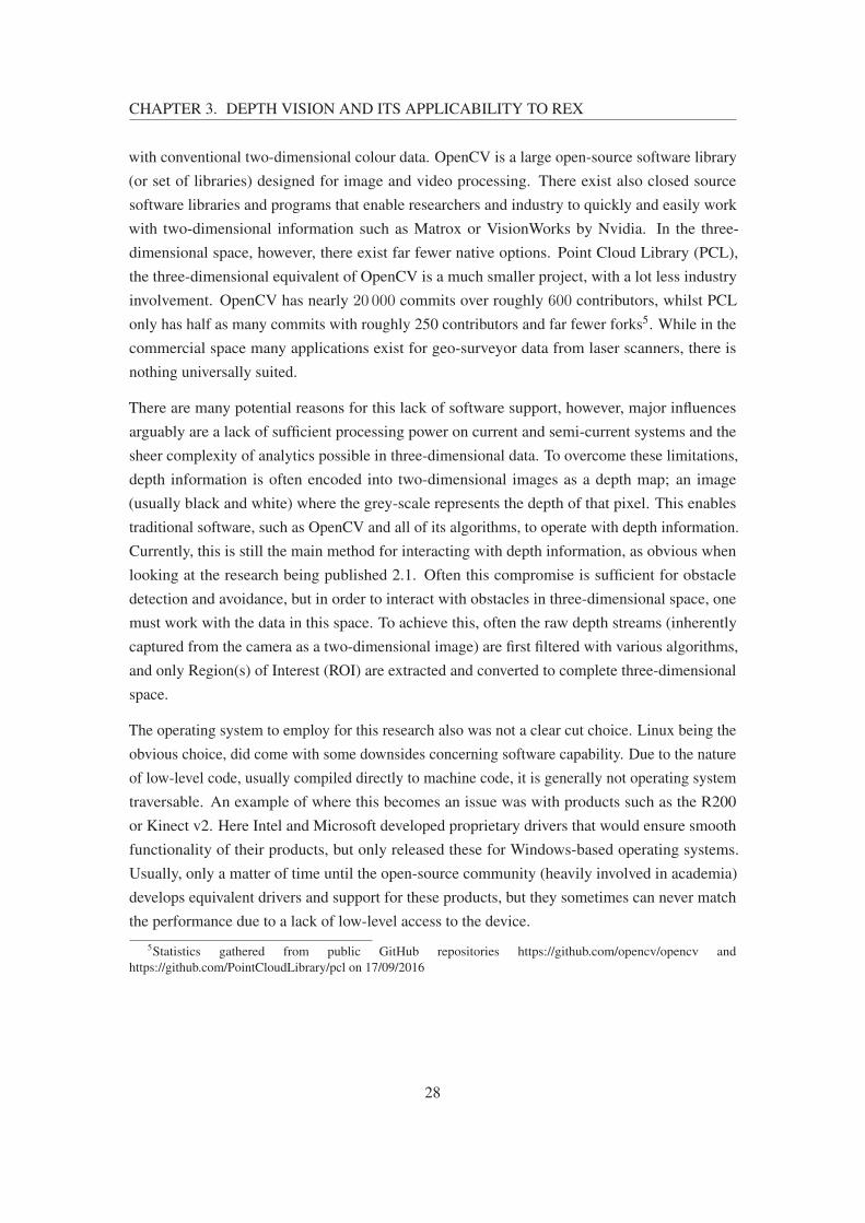
CHAPTER 3. DEPTH VISION AND ITS APPLICABILITY TO REX
with conventional two-dimensional colour data. OpenCV is a large open-source software library
(or set of libraries) designed for image and video processing. There exist also closed source
software libraries and programs that enable researchers and industry to quickly and easily work
with two-dimensional information such as Matrox or VisionWorks by Nvidia. In the three-
dimensional space, however, there exist far fewer native options. Point Cloud Library (PCL),
the three-dimensional equivalent of OpenCV is a much smaller project, with a lot less industry
involvement. OpenCV has nearly 20 000 commits over roughly 600 contributors, whilst PCL
only has half as many commits with roughly 250 contributors and far fewer forks5. While in the
commercial space many applications exist for geo-surveyor data from laser scanners, there is
nothing universally suited.
There are many potential reasons for this lack of software support, however, major influences
arguably are a lack of sufficient processing power on current and semi-current systems and the
sheer complexity of analytics possible in three-dimensional data. To overcome these limitations,
depth information is often encoded into two-dimensional images as a depth map; an image
(usually black and white) where the grey-scale represents the depth of that pixel. This enables
traditional software, such as OpenCV and all of its algorithms, to operate with depth information.
Currently, this is still the main method for interacting with depth information, as obvious when
looking at the research being published 2.1. Often this compromise is sufficient for obstacle
detection and avoidance, but in order to interact with obstacles in three-dimensional space, one
must work with the data in this space. To achieve this, often the raw depth streams (inherently
captured from the camera as a two-dimensional image) are first filtered with various algorithms,
and only Region(s) of Interest (ROI) are extracted and converted to complete three-dimensional
space.
The operating system to employ for this research also was not a clear cut choice. Linux being the
obvious choice, did come with some downsides concerning software capability. Due to the nature
of low-level code, usually compiled directly to machine code, it is generally not operating system
traversable. An example of where this becomes an issue was with products such as the R200
or Kinect v2. Here Intel and Microsoft developed proprietary drivers that would ensure smooth
functionality of their products, but only released these for Windows-based operating systems.
Usually, only a matter of time until the open-source community (heavily involved in academia)
develops equivalent drivers and support for these products, but they sometimes can never match
the performance due to a lack of low-level access to the device.
5Statistics gathered from public GitHub repositories https://github.com/opencv/opencv and
https://github.com/PointCloudLibrary/pcl on 17/09/2016
28

CHAPTER 3. DEPTH VISION AND ITS APPLICABILITY TO REX
3.2.3 Processing Hardware Centred on Depth Vision
Less crucial than finding the right camera or algorithms, the hardware to perform the calculations
on is often overlooked in a research domain. Often their processing power consumption and
availability are not as restricted as on a commercial robotic platform. Modern processing has
enabled ever lower power devices to exist, but when it comes to working with masses of data,
these devices often choke. The REX platform contains a lithium-ion power source, mainly
used to drive the actuators, which would also power any processing hardware. Being a mobile
consumer product a continuous consideration for them is end-user battery life, and any additional
drain shortens this. Space for the processing unit to reside is also very limited on the REX.
Especially with the aim of investigating integration with the REX platform, it was critical that
any work developed, would function with these resource restraints. Space, power and processing
requirements pointed towards requiring a Single Board PC (SBC) rather than a modular computing
solution. System on Chip (SoC) solutions have also considered, but are these are often targeted at
higher volume products that can afford the overhead of PCB design around a SoC. There are many
contenders in the space of SBC, especially aided by the maker revolution, where the hobbyist
market has become large enough to interest manufacturers of these boards. This has resulted in
many reasonably priced, well documented and supported, powerful SBC such as the Raspberry Pi.
The Raspberry Pi 3 features a 1.2GHz quad-core 64-bit ARMv8 Central Processing Unit (CPU)
and 1GB of Random Access Memory (RAM). They also contain all the peripherals and Input
/ Output (IO) required for quick development and simple integration, such as network, display,
Human interface device (HID), and storage. Other devices such as the ODROID or BeagleBoard
offer similar performance and all for a similar price of roughly 30USD to 60USD. Those devices
are all based on the Advanced Reduced Instruction Set Computing (RISC) Machine (ARM)
architecture, imposing cross-compatibility restrictions for software. Luckily ARM is becoming
more mainstream, mostly in response to the mobile phone and tablet market, meaning much
software has either been ported or re-written to be compatible. Most, but not all, parts of OpenCV
and PCL are compilable on ARM systems, meaning this was not a limiting factor for decision
making. Often however when combining non-mainstream devices (such as depth cameras), with
non-mainstream architecture, device drivers are not developed or lack functionality, making this a
more significant concern. In these cases SBC units such as the Osprey from VersaLogic provide
an alternative. While usually costing more, these boards use Intel’s range of Atom processors,
again providing a different compatibility set.
Stereo matching algorithms, in particular, must perform thousands of operations to calculate
the disparity of each pixel, and these can easily be implemented in parallel. This fact opens
up a new type of SBC or SoC; namely one that implements massively parallel processing,
usually by employing a GPU. Largely motivated by academic research into accelerating machine
vision[Fung and Mann, 2005], many common algorithms are being implemented using GPU
29

CHAPTER 3. DEPTH VISION AND ITS APPLICABILITY TO REX
architecture, meaning some of OpenCV’s and PCL’s functionality can be executed on the GPU
already. Machine learning has also played a role in this domain, further spurring integration of
GPUs into embedded devices. Nvidia is a company that has been especially focused on this
domain, with the automotive industry being a massive incentive for them. The Tegra series of
SoCs from Nvidia are specifically targeted at this market, and already found in many auto-mobiles.
Aimed at the industry of automated robotics and employing the Tegra core, the Jetson series were
a perfect potential solution for this research. Being a complete SBC with an ARM CPU coupled
to a powerful Tegra GPU and featuring a wide variety of IOs this board had it all. The latest
Figure 3.5: Jetson TX1 Module – Nvidia’s SBC, the Jetson TX1, aimed at the automotive industry. On theright a brief summary of specifications. Sources: [Nvidia, 2016]
revision, the Jetson TX1 (depicted in figure 3.5), was chosen due to its powerful combination
of processors, whilst costing 500USD for a development kit, and less for the actual SBC. Also
worth mentioning, the Software Development Kit (SDK) available for the Jetson TX1 makes
developing machine vision applications a quick process. To make efficient use of the GPU core, a
full Linux based image with appropriate drivers is maintained by Nvidia. Combining this with its
footprint of only 50mm× 87mm and typically under 12W of power consumption under max
load, this was the ideal choice.
3.2.4 Decision Validation and Testing
With sufficient understanding of the available technology in relation to vision hardware, software,
and processing hardware, conclusions were met and the suiting equipment was acquired. The
following items purchased:
1. ZED stereo high-resolution camera
2. DUO MLX stereo infra-red camera
30

CHAPTER 3. DEPTH VISION AND ITS APPLICABILITY TO REX
3. Nvidia Jetson TX1 embedded GPU SBC
4. Day hire of Faro S120 Laser scanner
Once the equipment arrived some initial classification and testing was done to establish what
working with them would entail. This will determine the ease-of-use of the products, involving
setting up the software environments for the cameras to produce data, and for the Jetson TX1 to
boot and be operational. First the cameras were tested with a Windows operating system, but then
quickly migrated to the Jetson TX1 as this was crucial for further development.
31

Chapter 4
Extracting Raw Data
To start characterising the sensors, a fair comparison of data quality was an obvious first step.
This proved to reveal a lot about using the cameras that was not apparent from their respective
datasheets. Being commercial cameras sold with software development kits and support, these
products were advertised as functional out of the box. The extent of this functionality had to be
tested.
4.1 Camera Calibration
Stereo calibration is a critical task to stereo vision, and much academic work has gone into
developing these techniques. Both cameras support fairly standard calibration, and store this
data on the camera, while also being factory calibrated. Initial testing of ranges however quickly
showed that the Duo MLX was consistently misjudging depth, pointing towards a calibration
error. After contacting Code Laboratories, it was discovered that in fact the calibration process
employed and supported for the Duo MLX was not adept at handling wide angle lenses, which
were fitted. After pointing out this flaw to the Code Laboratories team, much time was spent
trying to re-calibrate the device using a generic OpenCV approach rather than the provided
package. OpenCV includes a library that is focused around performing these tasks, calib3d,
which helped a lot in speeding up the process. Eventually, a suitable calibration was able to be
conducted, and figure 4.1 shows the gathering of samples. These correlated circular patterns are
used to calculate camera intrinsic and extrinsic properties such as principal points, focal lengths,
distortion and projection matrices.
The calibration preloaded onto the ZED was of acceptable accuracy, and it did not require re-
calibration. It is worth noting that while putting more time into calibration can guarantee more
32

CHAPTER 4. EXTRACTING RAW DATA
Figure 4.1: Stereo Calibration Sample – An OpenCV based calibration program for the DUO MLX withfish-eye lenses
accurate results, the purpose of this research was to use consumer products and developing/refining
calibration techniques was outside of the scope of this work.
4.2 Reading Depth
Since both cameras came with SDKs, it was necessary to familiarise with how these functioned,
and how to extract depth data from the devices. Also because it was intended to let the camera
manufacturers device driver do the depth calculations and not use a common open source solution,
the accuracy of these also needed to be tested. Within Windows, it was simple to install the
relevant SDK, connect the camera and launch their viewing application to view a depth stream
(for example figure 4.2). A flat board with checker patterns affixed (to give the board texture and
to measure lateral error) was used and the Duo MLX was placed at distances of 300mm and
600mm distance from the board. The dashboard for interacting with the Duo MLX and viewing
the depth stream (shown in figure 4.2) exposes many options for fine tuning both the camera and
the process of generating depth. It was not feasible to measure the effect of each setting on the
depth error since one would have had to check for cross-correlation and there would have been
hundreds of combinations. Before adjusting the calibration as explained above, the depth values
were consistently short of the actual distance. At 300mm, over 23 samples gathered, the mean
distance recorded was 255mm, giving an axial error of 45mm. Laterally the checker patterns
measured 50.0mm, but the camera mean over the same samples was 46.6mm, giving an error
of 3.4mm. Repeated at 600mm, the axial error rose considerably to 142mm, and the lateral
error rose to 7.7mm. It quickly became apparent that the camera was not functioning properly, as
33

CHAPTER 4. EXTRACTING RAW DATA
Figure 4.2: Duo Dashboard GUI – Shows the user interface for operating the DUO MLX Camera. Theupper images are the raw infra-red filtered images, while the lower section shows a coloured depth map.On the right are options to customise the data output generation parameters.
these errors grew proportional to distance as if the answers were being scaled incorrectly, which
lead to the before mentioned investigation of calibration methods revealing the fish-eye lens issue.
The challenge of getting valid depth information out of the Duo MLX did not, however, stop
at calibration. It is important here to note the chronological order of events. The Duo MLX
was received first, then testing revealed calibration errors. Much time passed with no solution, a
calibration program was developed using OpenCV, however, this could not update the calibration
stored on the camera (due to propriety access). The Flowchart shown in figure 4.3 demonstrates
the process used to accomplish this. Hence the included Duo software library responsible for
generating depth could not be used. Meanwhile, Code Laboratories had been made aware of the
problem, but not provided a solution. To not completely stall progress, a depth calculation program
was developed, again relying on OpenCV’s libraries. This was a lengthy and cumbersome process,
and roughly as it was completed, Code Laboratories released an updated firmware and SDK
that addressed the issues faced. Due to all these issues and to reduce the overhead and learning
curve required to use the Duo MLX, a middle-layer was developed that made using the camera
more ’plug and play’ compatible2. The software library also allowed image rectification using
OpenCV as opposed to Duo’s closed source methods. This combined the OpenCV calibration
work shown in figure 4.3, with an easier interface to working with the Duo. It also enabled users
to perform the rectification with OpenCV’s open-source libraries as opposed to Duo’s. This was
2Available at https://github.com/nznobody/duo_wrapper, however, development has ceased
34

CHAPTER 4. EXTRACTING RAW DATA
Figure 4.3: Duo OpenCV Calibration Flowchart – By using the features of OpenCV, a calibration programwas developed 1 that follows this process to calculate the parameters required to un-distort the images.This prepares them for stereo matching algorithms.
an important feature to enable because the Duo libraries, whilst supporting multi-threading, did
not support using the GPU to perform the rectification or disparity calculations. Being able to
carry out these tasks on the GPU made a tremendous difference (roughly a 20 times performance
boost in image rectification, demonstrated with the afore mentioned wrapper software) in system
resources available to the user, and was the whole intention behind purchasing the Jetson TX1.
Now reading depth values with relative accuracy (as seen in table 4.1), a large discrepancy still
existed in re-projecting the depth values to x and y co-ordinates (seen in table 4.1). This is a
(a) Duo MLX (b) ZED (c) Realsense R200 (d) Kinect v2
Figure 4.4: Comparing Stereo Re-projections – Re-projected point clouds from each camera of the samebox and same view point
process that carefully depends on the calibration of the camera, indicating that there were still
fundamental issues with the device. Figure 4.4a helps demonstrate why even though the distances
may read correct, an accurate re-projection is critical to re-creating a scene that is of use once
the viewpoint is rotated. The challenges faced calibrating and re-projecting with the Duo began
to consume too much time, and so development focus was shifted to the ZED. This frustrating
experience is an indication of what working with fringe technology can be like.
Unlike the software included with the Duo, ZED’s depth viewer was rather simplistic concerning
settings. Figure 4.5 depicts the interface supplied. It did not expose the core settings associated
with stereo disparity calculations such as WindowSize or PreFilterCap. There are three
35

CHAPTER 4. EXTRACTING RAW DATA
Figure 4.5: ZED Depth Explorer GUI – Shows the user interface for operating the ZED Camera. Theupper left shows raw colour images, lower left shows grey-scale depth-map and on the right a rotatablepoint cloud projection.
main view-panels; side-by-side raw video, depth video, and a manipulatable point cloud viewer.
The Graphical User Interface (GUI) allows for exports of any of the data formats (image, depth,
point cloud). Configurable settings are resolution and frame-rate of the camera, and a quality
or performance mode for the depth generation, and a confidence threshold. The confidence
threshold in particular was an important setting that changed the output considerably. As detailed
in the literature review (section 2.3.1), quality of a match is an important measure of confidence.
However, this results in flat non-unique planes scoring low confidence measures, such that if
the data were filtered to exclude low-confidence values, the ground would often be excluded.
Tuning this detail is detailed in depth when ground plane extraction is discussed, since it affected
this the most. Switching to the ZED required the Jetson TX1 to be set up, because unlike the
Duo, the ZED did not have an option for CPU disparity calculations and required a discrete GPU.
Since stereo calculations have to be performed on every pixel individually, this vast quantity
would bottleneck on a CPU. On the Jetson TX1 the ZED is able to display a depth stream at
1080p resolution in real time, whilst mostly processing on the GPU. Table 4.1 demonstrates
the minimum operational range of the ZED. Under 1000mm, the ZED struggles to capture
the disparity, because the large baseline results in very different views of the object. However,
over this range the ZED quickly gains accuracy and is able to re-project depth information into
meaningful point clouds as seen in figure 4.4b.
36

CHAPTER 4. EXTRACTING RAW DATA
Table 4.1: Camera Absolute Axial Error at Different Ranges – A brief comparison of camera performancein comparable scenarios
Duo Zed R200a
Distance
(mm)
Abs Axial
Error (mm)
Std. Dev.
(mm)
Abs Axial
Error (mm)
Std. Dev.
(mm)
Abs Axial
Error (mm)
Std. Dev.
(mm)
500 285b
600 5 10.5
800 45 15
1000 11 15 18 12.5 45 4
1500 45 27 18 24.7 26 14.5
2000 155 32 6 10
The cameras were placed looking at a white board with a textured pattern applied. Depth samples of the board were
extracted, mean and the standard deviation was calculated. The absolute axial error is the difference between expected
distance and actual, not to be mistaken for axial noise, which is the variability in data representing a flat plane. The board
angle and perpendicularity was calibrated with a Hokuyo laser scanner. This data is only supposed to represent the relative
performance of the cameras.a The R200 is only included here as a brief comparison of a differing technology typeb Since this was below the minimum range of the ZED, the data was barely recognizable as a plane, and a estimated figure
was extracted by hand. Purely included to demonstrate the ZED’s range limitations.
4.3 Coordinate Systems and Ground Planes
Information is arduous to comprehend without a relative measure and context. With depth
information, one of the most important aspects to consider is the coordinate frame being used.
For depth data re-projected to a point cloud, a three-dimensional Cartesian coordinate system is
employed. If such a system is employed, any position in three-dimensional space can be uniquely
identified by the signed distance to three mutually perpendicular planes (or equivalent)[Korn
and Korn, 2000]. An important point of consideration is the origin point where all three planes
cross, as this is the zero point, and how they are aligned relative to the world. The Duo and ZED
both follow the right-handed rule3 for defining their axis in a Cartesian manner. They do not,
however, follow the same orientation; with the Duo having negative z aligned perpendicularly
in front of the camera, positive x to the right and positive y upwards. The ZED, on the other
hand, has positive z aligned perpendicularly in front of the camera positive x to the right and
positive y downwards. To enable consistency and compatibility, when extracting point clouds
from these cameras, these coordinate frames were transformed to align with those set out by
the ROS Enhancement Proposal (REP)1034. This states that relative to the object x should face
forward, y to the left and z upwards. Equally as important as the camera’s location in Cartesian
space, is the camera’s orientation, defining its rotational alignment. Rotations in three dimensions
contain much ambiguity unless properly defined. Whilst defining them here is outside of the
3Assigning axis based on the direction your right thumb, index and middle finger point when mutually perpendicu-
larly aligned4Sourced from http://www.ros.org/reps/rep-0103.html
37

CHAPTER 4. EXTRACTING RAW DATA
scope, it will be noted that the most commonly applied method in this work are using quaternions5
4.3.1 Aligning with the Ground Plane
With the data in a known coordinate frame, the next step was to place this frame relative to
something larger. Given the purpose of navigating surrounding terrain, it was important to extract
the height of this terrain, in particular, relative to the ground plane. The camera had to be mounted
in a location that allowed its perspective to produce useful information. Since the ZED performed
better at ranges above one meter, this had to be considerably high off the ground, preferably with
a not too steep and not too shallow angle relative to the ground. Working with the REX platform,
this meant the most likely location for mounting was the around the hip height at an angle of
roughly 45◦ downwards. As the REX is a moving robotic platform and has its own tolerances,
this angle cannot be assumed to be constant and valid for the ground plane. To accurately map the
height of surrounding terrain it was critical to properly determine the camera’s angle to the ground
plane, otherwise as the camera moved away from the origin, the ground plane would appear to
shift vertically. It became apparent that this angle calibration process would be an important step
to address whilst building elevation maps with the depth data. During testing, the camera was
mounted on a tripod at a similar height and angle as it would be on the REX. In the early stages,
the camera coordinate frame was was defined at a set hight and pitch rotation as described in
figure 4.6 by h and θ.
x
yz
ph
x′
y′ z′
θ
Figure 4.6: Coordinates Frames in use – Camera coordinate frame (x’-y’-z’) is defined relative to theground coordinate frame (z-y-z). The camera (denoted by grey cube) can be thought of at height h, facingalong y’. y’ is rotated from p through angle θ, which represents a pitch rotation.
Statically transforming the camera frame to the ground plane frame like this however quickly
revealed its limitations. Careful attention had to be given to ensure rotation in the yaw and roll
5Originally defined by W. Hamilton in the 19th century, the theory behind quaternions is covered in this
book[Kuipers, 1999] and the mathematics involved in transforming these to and from various other notations, including
Euler angles, is covered in this article[Diebel, 2006]
38

CHAPTER 4. EXTRACTING RAW DATA
axis was 0◦, otherwise, the ground plane would appear to shift as described above. This was
practically impossible to achieve in the test environment, let alone once mounted on the REX,
giving rise to the requirement for a dynamic ground plane calibration process.
Determining the ground plane in computer vision is a common challenge and has had significant
research efforts [Vaz and Ventura, 2015, Lin et al., 2010, Zhao et al., 2007, Pears and Liang, 2001].
Being a special case of generalised plane detection, relevant research in this area such as [Schnabel
et al., 2007] who describe using Random Sample Consensus (RANSAC) algorithms for generic
shape detection or [Yang and Forstner, 2010] who apply this directly to plane detection in point
cloud data on stairs. Following the methods described (in particular [Vaz and Ventura, 2015]),
Figure 4.7: Ground Calibration Process – Flow graph of the calibration process run at start-up thatcalibrates the ZED depth camera to the ground and the REX
figure 4.7 depicts the operational flow implemented in a ROS node named rex ground calib.
Details of working with ROS are described in chapter 5, and will not be detailed here. The
operational flow begins on launch and waits for new incoming point cloud messages from the
camera. These messages are timestamped and contain the name of the coordinate frame they are
represented in. Once received PCL’s RANSAC fitting algorithm is used to find the largest plane
within the point cloud, outputting the coefficients describing the plane as ax+ by + cz + d = 0.
Understanding this equation represents a normal vector �n(a, b, c) to the plane, at a distance d
from the origin gives rise to a method of transforming into the planes coordinate frame. Then
a vector �h(a′, b′, c′) is determined where a′ = −d× a, b′ = −d× b, c′ = −d× c (given �n is a
unit vector) that begins at the origin of the camera coordinate frame and takes the shortest path to
the plane (is perpendicular to the plane). Next, we must calculate the rotation that transforms �h
to align with the −z axis of the camera coordinate frame. Using quaternions this is a matter of
using vector cross products to determine the axis of rotation and vector dot products to determine
39

CHAPTER 4. EXTRACTING RAW DATA
the angle between the two vectors.
q = cosθ
2+ i sin
θ
2vx + j sin
θ
2vy + k sin
θ
2vz (4.1)
Equation 4.1 demonstrates how quaternion q can be defined given a vector �v(x, y, z) and angle
θ. To provide a better calibration, multiple quaternions are gathered over multiple input point
cloud samples. Once a sufficient sample size is acquired, it is required to average these, a process
defined by Markley[Markley et al., 2007]. Markley’s approach is simplified based on a method
employed in the game engine sector 6. Since the transform of coordinate frames depends on both
orientation and translation, the length of �h samples is averaged and taken as the z axis offset. With
the transform between the ground plane frame and the camera frame fully defined, it is published
via ROS’s framework. This allows all future point clouds published in the camera frame to be
translated to the ground plane frame. To adhere to ROS’s notation guidelines the ground plane
frame is called the odom frame. Additionally, as the framework was already in place, this node
published the offset between the ZED Camera and the root of the REX exoskeleton. This was
configurable via ROS parameters encase the mounting point of the ZED changed.
4.4 Camera Motion and Odometry
Two approaches exist in computer vision; time-invariant and time-variant processes. In general, a
process is time-invariant if it is outcomes do not explicitly depend on time, that is at any given
moment a set input will produce an identical output. Mathematically speaking y(t) = x(t) is
time-invariant whilst y(t) = x(t) + x(t − 1) is time-variant. The meaning behind this in the
context of computer vision is that of systems that operate frame by frame, or those that consider
previous frames (the past) as well. To give a contextual example may be that of a visual collision
avoidance system that analyses input from a camera and determines if a collision is likely. A
time-invariant system would look at a single frame, and attempt to determine if the object is too
close or on a collision course. A time-variant system, however, would try to track that object
over a series of frames, allowing it to extract more detail about the object such as it’s velocity
vector. Another way of describing a time variant system is one that has a temporal dimension to
consider. A survey of literature focused on plane and stair detection was conducted to understand
these merits, presented in table 2.1. Although not an extensive survey, it provides an insight to
approaches being pursued. There is no clear ’correct’ solution, and both have their merits worth
considering, which is supported by the diversity presented in this table.
Understanding the objectives helped determine that a system employed by the REX platform
would benefit from considering the time dimension, that is being time-variant or temporal in
6http://wiki.unity3d.com/index.php/Averaging_Quaternions_and_Vectors
40

CHAPTER 4. EXTRACTING RAW DATA
functionality. To understand this, consider the task of navigating a passage sideways, such as
the REX passing through a door frame. Constructing a system that can close the feedback loop
and advise if the next motion is safe can consider two options: install enough cameras that a
continuous 360◦ image can be reconstructed of the REX’s surroundings or store the information
seen on approach, then track relative movement once rotated sideways. Remembering that there
is no ’correct’ method, it again comes down to weighing the merits of each and deciding based
on these. Relating these merits back to the design considerations defined in chapter 3 provides
reasoning to the decision process. For example, it becomes apparent that multiple cameras could
be aesthetically unappealing and also demand too much processing power. For the REX platform,
a temporal solution would be required to meet the objectives adequately whilst also adopting the
design considerations.
Knowing that the system would consider information from the past, determined that a system
tracking the motion of the camera would be required. Information from the past can only be
considered in the current frame, if a transform, t) is known that relates the two frames and places
them relatively in all considered dimensions (t = [x, y, z, i, j, k, w, t] where x, y, z are positional
transforms, i, j, k, w rotational and t a time transform). Tracking the transformation in time is a
trivial task, within a given accuracy the computers clock can achieve this. However relating the
two frame’s transformations in three-dimensional space is non-trivial, and is the topic of much
research, especially in machine vision (refer to table). Two key approaches exist to this task:
absolute and relative tracking. Examples of absolute positioning such as Global Positiong System
(GPS) or cellular triangulation are relative in the sense that they place the target relative to some
other object, but are considered to be absolute as they do not relate the current position to the
previous one. Relative tracking technologies, such as an Inertial Measurement Unit (IMU), on
the other-hand, are temporal systems that track changes in position over time and can determine
position by integrating these temporal changes. Whilst many modern mobile platforms employ
GPS, this was not an option for the REX; GPS doesn’t function well indoors and is only accurate
to 5m. The Duo camera included a 6 axis IMU, however, the issue with integrating motion data
to gain position is that over time error accumulates and so the position is said to drift. Visual
odometry has proved its worth in the recent years, being employed successfully on the Mars
exploration rovers[Maimone et al., 2007]. Such a system is both time-variant and time-invariant,
in that the movement calculated depends on data in the past, but most modern systems will
generate identical absolute positions when presented with an identical scene. Visual odometry, in
essence, tracks the apparent motion of key features within successive images through optical flow
and assumes they are for the most part stationary, giving rise to the fact the camera has moved.
Modern implementations also employ a form of loop-closure, where key features are tracked in a
database and when seen again, the system knows it has returned to a previous location, removing
drift effect over large loops. Visual odometry systems will still produce drift over large distances
that do not feature loop closures, such as a straight line, due to calibration and approximation
41

CHAPTER 4. EXTRACTING RAW DATA
errors causing scaling errors.
Initially, visual odometry was attempted with the Duo camera, because it had global shutter
sensors. The issues with using rolling shutters for visual odometry are explained in these
articles[Li et al., 2013, Lovegrove et al., 2013], whilst also solutions are offered. However, since
a global shutter stereo camera was already available, its use was investigated with various visual
odometry implementations: RTABMap[Labbe and Michaud, 2014], ORB-SLAM[Mur-Artal et al.,
2015], and LSD-SLAM[Engel et al., 2014]. These researchers all made their implementations
open-source with the majority of code hosted on GitHub. Compiling these and building a
functional pipeline on the Jetson TX1 was a pretty straight forward task. While the original
code was not necessarily compatible with the ARM platform, most were presented as CMake
projects. CMake is a cross-platform open-source collection of tools for building code natively7.
This made it easy to adjust compilation options and update certain snippets to add compatibility.
ORB-SLAM functioned best, with a real-time solution possible, even though the GPU was
un-utilised. Had development carried on with these packages, an extension would have been to
port compatible sections of the algorithm onto the GPU to free up the CPU. Again, the issues of
incorrect image rectification caused the Duo to lose accuracy in motion, rendering it of no use.
Conveniently around this time-frame an update to the SDK for the ZED added built-in visual
odometry. Being implemented within their closed-source driver, the workings of this could
not be investigated, but it functioned well. An interesting trade-off was discovered here; the
visual odometry system functioned better when the camera was operating at a higher frame-rate
and resolution. It can be speculated that Code Laboratories employ a method similar to those
published, which rely heavily on feature tracking within RGB images. So the larger the resolution,
the easier it is to track unique features. Also, the faster the frame-rate, the lower the approximation
errors of integrating are due to approximating the motion between frames to be linear. However
re-projecting the images to point-clouds at a high frame-rate and resolution consumed the majority
of resources and so a trade-off had to be made. Since their ROS compatible driver was open-source8, it was possible to extend this framework. This gave way to developing a flexible framework
that in essence operated at two separate frame-rates, grabbing the raw images and performing
visual odometry at a high rate, whilst then down-sampling and publishing the point clouds at a
lower rate. A few minor improvements and bug fixes were made as part of this work and pulled
into the main source tree, but the main functionality was not integrated due to time constraints.
7https://cmake.org/8https://github.com/stereolabs/zed-ros-wrapper
42

CHAPTER 4. EXTRACTING RAW DATA
4.4.1 Odometry Fusion
Visual odometry functions well with a motion that is effectively linear between samples (frames
grabbed). This is not the case for erratic motion, with fast accelerations (such as changes in
trajectory) on the Jetson TX1, because with limited processing power the sampling rate was
15Hz. IMUs, on the other hand, can easily operate at a much higher rate with lower processing
requirements. The Duo’s IMU can operate at 100Hz, reducing the integration error component
introduced when estimating pose and orientation, however as mentioned they are susceptible
to drift. Recent research[Leutenegger et al., 2015] on tightly integrating visual odometry with
that of an IMU has proven to reduce error build up. The article identifies that the combination
of information rich pictures with accurate short term estimations of an IMU complement each
other very effectively. Combining the two is not a simple task of averaging, since as previously
mentioned, they are fundamentally different. With visual odometry generally reporting absolute
positions, and IMU reporting velocity information, these data formats are not directly compatible.
One approach is to differentiate the visual odometry readings into velocities, combine both in the
velocity domain (by considering sensor covariances to do a weighted average), then re-integrate
the combined result to a position. Due to time constraints, this topic was abandoned, and sensor
fusion was never implemented but the open-source implementation of[Leutenegger et al., 2015]
is hosted on GitHub9.
4.5 Combining Solutions
Having sufficiently explored the depth producing capabilities of the two cameras, development
had to move forwards. A ROS framework was developed and tested that reliably produced point
clouds in the camera frame, but also provided a transform to a fixed odom frame. The ZED stereo
camera provided both the point clouds and the transform between frames by tracking motion with
visual odometry. Allowing flexible mounting, a calibration routine would ensure the information
was aligned with the ground plane.
9https://github.com/ethz-asl/okvis
43
Chapter 5
Implementing with Robot OperatingSystem
The beauty in open-source methodology is it allows an individual to work with and contribute
to a project much larger than themselves. ROS is an example of such a project, originating out
of Stanford University, but becoming a large worldwide collaboration of work. Fundamentally
ROS consists of software that implements best practice for robotics applications. Adopted by
Willow Garage in 2007, it has been developed to provide a universal approach to implementing
robotic applications. Although other similar frameworks exist, such as YARP1, ROS has a large
active community distributed across many universities and industry alike. Often when developing
a system from the ground up, one is faced with recreating common systems to support the actual
task at hand, especially in software. ROS’s core task is to reduce this duplication of work, and
instead enable an advanced configurable system to be used by many. Since this research would
cover many areas of robotics and require them to work efficiently together on something referred
to as a pipeline, ROS was an obvious key development tool. ROS Consists of three core features
as described in the subsequent sections.
5.1 Filesystem Management
ROS considerably simplifies the distribution of software packages by defining a set of standards
that must be adhered to for compilation. This allows users to download and compile distributed
works on their local machine with little difficulty, providing they have a standard ROS setup.
1Yet Another Robot Platform, http://www.yarp.it/
44

CHAPTER 5. IMPLEMENTING WITH ROBOT OPERATING SYSTEM
Valid ROS packages must contain formatted package manifests2, which are used to compile
the source, if required (some packages do not require compilation as they are descriptive only).
Following the methodology of Linux, most common ROS packages can be simply installed via
the package management system, e.g. apt-get install ros-kinetic-PACKAGE. A
non-exhaustive list of available packages is maintained 3, the source code for these and others is
most commonly hosted on GitHub. As a build system ROS supports rosbuild or the catkin
systems, both of which employ the cmake build system described earlier. These manage a
workspace on the development machine and ensure project dependencies are met across ROS
packages when compiling, by feeding information to the cmake system. For example building
an entire set of packages being developed within a workspace requires calling catkin build
from within the workspace, all changed packages (and their dependencies) will be checked for
changes and rebuilt if any are found. Utilising this ability, software development in this area was
split into two workspaces: core ws and rex ws. The first contained mostly dependencies that
required little or no editing from the source code provided, while the latter contained projects
written for this research and forks of open source software that were adapted to be compatible.
While not strictly speaking a ROS standard, all works developed were version controlled utilising
GitHub and are selectively publicly available: https://github.com/nznobody (some
content was kept private due to commercial sensitivity).
5.2 Computation Graph
At its core ROS contains a messaging framework, providing a standard, extensible method for
processes to exchange information. When developing larger systems, these pipelines inevitably
become non-linear, that is information does not simply flow from one end to the other. It becomes
complex to manage the flow and synchronisation of information within a single machine or across
a distributed architecture. The publisher/subscriber paradigm of message handling in computer
code is a well-established practice for managing this complexity. First we must explain nodes in
Figure 5.1: ROS Pipeline Demonstration – A simple ROS pipeline example: keyboard commands fromone node control the turtle in another
2As with many ROS standards, they are defined in REPs. The package manifest is defined here: http://www.ros.org/reps/rep-0127.html
3http://www.ros.org/browse/list.php
45

CHAPTER 5. IMPLEMENTING WITH ROBOT OPERATING SYSTEM
the context of ROS: In essence, they are processes that perform a task. These could be compiled
code or a script, but they all integrate the ROS client library native to them, for example, roscpp
with C++ code. A master node is responsible for acting as a central register and lookup to enable
inter-node communication, commonly referred to as ros core. Contained within this master,
is a parameter server that simplifies the process of configuring pipelines, allowing a central
storage of parameters by lookup name. Understanding these principles, the need for inter-node
messaging can easily be demonstrated, as depicted in figure 5.1, showing a nodegraph exported
from ROS’s rqt graph. It demonstrates the flow of information (keyboard commands) from
node teleop turtle to node turtlesim via the message topic /turtle1/cmd vel,
resulting in turtle movement (shown on the right). This simple example is the building block of
much more complex systems ranging many nodes with hundreds of message topics potentially
across distributed locations and networks. As messages are a reactive system, the ROS concept of
services are proactive, in that an action or response can be instigated when requested by a node.
True to the universal solution nature, both messages and services are completely customisable
by creating definition files. A large selection of standard messages and services does exist that
should be considered to promote a universally compatible system.
ROS provides an extensive collection of tools for analysing, debugging and logging development,
such as the node graphs generated in figure 5.1. Some of the key programs and their features are:
roscore The core process, known as the master. All nodes must be able to communicate with the
master as it manages topic registration and variable storage.
rosrun Is used to launch nodes in the correct environment and attempt to establish contact with
the master.
roslaunch A customisable approach to rosrun. Reads a description file and can from this launch
many nodes with pre-set settings, names and outputs.
rviz The primary method for displaying any visual output, such as images, point clouds, maps or
pose information. Can also be used to publish messages that interact with this data.
rosnode A method for getting information about running nodes and optionally terminating nodes.
rostopic Can query and list all topics, displaying their content, bandwidth and frequency. Can
also publish messages.
rqt gui A GUI for a collection of utilities such as the above. Can be used to inspect the node
graphs, message topography, transform frames and pretty much any aspect of an operating
ROS system.
rosbag A utility for recording and playing back messages. Can record all or a subset of published
messages and at a later time play them back, at varying speeds and with pausing. An
46

CHAPTER 5. IMPLEMENTING WITH ROBOT OPERATING SYSTEM
incredibly useful tool.
The above list is far from being exhaustive, and there are many user created tools that help
development. Functional detail will not be described in this text, as it is already well documented
and not feasible to summarise effectively.
5.3 The Community
Perhaps the most important aspect of ROS, is the sharing of knowledge about a common platform.
Because it is used by many developers, there is a very lively and active community built around
the software, willing to help. This is an invaluable resource that can make an apparently steep
learning curve relatively easy to master. The community maintains the large list of packages
mentioned afore, but also takes part in active peer helping via their questions and answers site
http://answers.ros.org/. Peer reviewing of issues and solving them was a substantial
assistance in the implementation of this research. The ROSWiki is also very well maintained and
documents a lot of the packages available with examples and tutorials. Continuous improvement
of the core functionality is seen through releases of new distributions, and there is a fundamental
revision to ROS2 in the works 4.
5.4 ROS and the REX
A part of integrating the REX into the ROS pipeline was to create a model of the REX for
visualisation and potentially collision detection at a later stage. Within ROS there exist multiple
avenues for creating models, ranging from simple static shapes to detailed dynamic models
imported from 3D files. Originally a part of ROS, Gazebo 5 is focused on simulating robotics. It
is able to test algorithms and configurations in simulated environments quickly. However this is
what it focuses on, and for that reason, it was decided not to employ Gazebo, as it was too focused
on simulations and not working with real environments. Instead the native ROS framework,
xacro6, was used to build and simulate a dynamic model. Xacro defines a XML macro language,
and enables more complex native urdf 7 to be written with ease. Urdf is the basis of most ROS
models and can be natively displayed in rviz. A simplified model of the REX was created, based
of maximum collision bounding rectangles and is shown in figure 5.2. This was created from the
code attached in appendix source code listing 3. Consisting of a hip bounding shape, an upper
4Still in early development, but publicly open-sourced at https://github.com/ros25http://gazebosim.org/6http://wiki.ros.org/xacro7http://wiki.ros.org/urdf
47

CHAPTER 5. IMPLEMENTING WITH ROBOT OPERATING SYSTEM
Figure 5.2: REX Model in ROS – Model of REX robot made with ROS’s xacro framework and dynamicallysimulated with an application written to mimic real movement maps.
leg section, a lower leg section and a foot per side this model is also able to simulate the joints
between these parts as demonstrated in the right-hand image. Within ROS it is standard to get
sensor information that would be able to determine joint angles and update the model. While
theoretically possible, the interface to extract this information in the desired form from the REX
would have been very cumbersome to implement because the REX only reports actuator lengths,
not direct joint angles. Instead, a ROS node was written that could publish the expected joint
angles for a specific movement map, simulating this sensory feedback loop. The angles were
extracted from the V-REX (virtual REX movement simulator) and stored in configuration files that
could be loaded by the joint state simulating node; rex model. This compromise was acceptable
for immediate testing as the actual angles did not differ much from the simulated ones, however
ultimately to manage dynamic terrain (not yet possible with the REX in general), a proper closed
loop feedback system would be needed.
The completed ROS pipeline graph involves 16 nodes that intercommunicate with messages and
services. Shown in figure 5.3a, this clearly demonstrates the modularity of working with ROS.
Since frame transforms play a vital part in relating all these nodes, figure 5.3b shows the entire
transform tree of the pipeline. A sample ROS program is also included in the appendices (code
listing 1 and 2 in appendix VI) that demonstrates the basic functionality of such a program. It is
the rex interface program, that was responsible for interfacing the REX with the mapping
solutions.
48

CHAPTER 5. IMPLEMENTING WITH ROBOT OPERATING SYSTEM
(a) ROS Node Graph
Figure 5.3: Complete ROS Graphs of the system – System overview of both the nodes and transformsused in the final implementation of this research
49

CHAPTER 5. IMPLEMENTING WITH ROBOT OPERATING SYSTEM
(b) ROS Transform frame graph
Figure 5.3: Complete ROS Graphs of the system – System overview of both the nodes and transformsused in the final implementation of this research
50

Chapter 6
Elevation Maps
When faced with masses of information, it is key to reduce this to a more useful summary. This
was a challenge confronted with the point clouds received from the cameras because there was
simply too much data to work with the raw clouds in real time. To navigate this issue, key
concepts were combined from the papers reviewed (table 2.1). Many of these researchers operated
with two-dimensional data such as depth images, however as earlier discussed it was decided to
operate in three-dimensional space for this research. A lot could still be learned and assimilated
from their workings, to enable efficient and effective processing of the point clouds.
6.1 Working with Point Clouds Efficiently
Oniga used a method of converting their disparity maps to DEMs, allowing a change of perspective
when analysing a two-dimensional image[Oniga and Nedevschi, 2010a, Oniga and Nedevschi,
2010b]. The value in this approach when operating in 3 dimensions is from reducing memory
management complexity for storing point clouds. First, one must understand the storage of
point clouds in memory, of which there are two main implementations (at least within PCL):
organised and unorganised. The difference stems from the method of capture; with point clouds
from cameras that perform re-projection producing organised point clouds, and other sources
generally producing un-organised clouds. In memory, organised point clouds are stored as
a two-dimensional array of points p = [x, y, z] and in unorganised these are a single long
one-dimensional array of points. When re-projecting from a two-dimensional disparity image,
neighbouring points are naturally also spatially close, so storing them close in memory has
advantages. Algorithms that operate on neighbourhoods of points (such as normal calculations1),
1http://pointclouds.org/documentation/tutorials/normal_estimation_using_integral_images.php
51

CHAPTER 6. ELEVATION MAPS
use this storage technique to speed up the search process for neighbouring points, with the priori
that they will be located close in memory. In an unorganised point cloud, this can be a lengthy
operation as the algorithm must search the entire memory array because there is no guarantee that
they are allocated by spatial proximity. This knowledge was used when performing the RANSAC
plane detection in section 4.3.1 on an organised point cloud with PCL. Location lookups are still
inefficient in both memory structures because the memory location does not directly map to a
point’s spatial location, making processes such as collision detection slow.
6.1.1 Octrees
Octrees are a memory organisation technique (not just for point clouds) that help address this,
enabling quicker processing of spatial algorithms. Conceptualised in 1980 by Meagher, this
process of memory organisation recursively subdivides memory organisation into octant sectors,
gaining granularity at each level. Figure 6.1 visually explains the recursive nature. It can be
Figure 6.1: Octree Representation – Visual representation of octree memory and spatial layout. Source:[WhiteTimberwolf, 2010].
seen that if one wishes to query a particular spatial location, there is a fixed lookup length,
regardless of location that is purely dependent on granularity (resolution) desired. There exist
several well-developed libraries for working with octrees both within PCL and as standalone2.
Similar research into humanoid robot navigation using machine vision successfully used an
implementation of octrees to manage their point clouds[Maier et al., 2012]. Octrees, however,
express an important limitation: they must be spatially of a pre-defined finite size, which directly
relates to the memory space required to achieve a certain accuracy. For confined application, this
is no issue, but the REX is a platform that must move with its user, and the operational confines
2OctoMap is an example: https://octomap.github.io/
52

CHAPTER 6. ELEVATION MAPS
are not known in advance. Presented with this knowledge a potential workaround would be to
rebuild the tree when the robot approaches an edge of the current extents, but this can be a very
costly process and is non-ideal.
6.1.2 Gridmapping
An alternate method to octrees is to reduce the complexity of the point cloud to a 2.5 dimensional
level. Fankhauser et al. perform significant work in building a framework that operates efficiently
in this domain[Fankhauser and Hutter, 2016]. While octree representation of point clouds
maintains full three-dimensional compatibility, this work limits each [x, y] location to only
have a single z height. It can be imagined as a stack of images, where each pixel location
represents an [x, y] spatial location, and the value of the pixel stores a parameter about that
location. Their implementation, named Grid Map, is made available open source at https:
//github.com/ethz-asl/grid_map and was of great use to this research. Each grid
map layer can store a type of information and is organised in memory so that a predefined sized
grid map can move without requiring a complete rebuild. To achieve this, the point cloud is
compartmentalised into a grid of a chosen resolution, with the method of resolving duplicate
points within one grid cell being user defined. Because elevation information is critical for
navigation, it becomes evident that when merging points that co-exist in one [x, y] cell (such as
points vertically up a wall section) they should be merged into the highest point, as this represents
the height of an obstacle in that location. Storing these in a two-dimensional memory array makes
looking up a particular location trivial, and finding neighbouring values equally efficient. Limiting
each two-dimensional location to a single value, might appear to be working in two-dimensional
space, but allowing grids to be stacked, allows for multiple values separated by key for each
location. For example, one grid map could store the maximum elevation detected whilst another
could store the minimum, allowing a pseudo three-dimensional appearance. Extending upon this
idea Fankhauser et al. implement an efficient method for map relocating, allowing the boundaries
to be relocated, without reallocating the underlying data. This functionality makes it perfect for
working with mobile robots that need to navigate terrain in an unconfined space. One is able
to define a relatively small map around the robot origin, that moves with the robot as it does,
representing just enough information to be computationally efficient but effectively describe
the immediate surroundings for navigation. A grid size of 25mm (or sometimes 50mm for
performance) was chosen with a map size of 6m× 6m and the robot located in the middle,
giving 3m of obstacle detection in each direction. When the robot pose is updated via the visual
odometry pipeline described in section 4.4, the map boundaries maintain a 3m offset from the
new location. Information no longer within the boundaries is forgotten and new area contained is
filled with data from the camera if available or set to unknown if not.
53

CHAPTER 6. ELEVATION MAPS
6.2 Simultaneous Localization and Mapping
Simultaneous Localisation and Mapping (SLAM) is a key concept to enabling effective use of
depth vision. As discussed in section 4.4, data will need to be gathered over time and be stored
to enable an effective system. Conveniently grid maps are well suited to this and Fankhauser et
al. provide a framework (called elevation mapping) built around ROS and grid map capable of
efficiently performing this[Fankhauser et al., 2014]. In SLAM there are a few important concepts
to consider that Fankhauser et al. address. Defining the transforms between frames is one of
these, as described in section 4.4, whilst another is that of fusing consecutive point clouds into
one, where information overlaps. Here the authors introduce a concept of fusing overlapping
information based on the variances of each data point (the old and the new). To understand this
key feature we must examine their algorithm for performing these updates:
h+ =σ2ph
− + σ2−h p
σ2p + σ2−
h
, σ2+h =
σ2−h σ2
p
σ2−h + σ2
p
(6.1)
In this equation new height measurements (p, σ2p) are fused with the existing estimation (h, σ2
h),
where − superscripts denote values prior to the update and + denotes post update. More
mathematical insight is given in the original article, but it is important to understand that the
variance (σ2) plays a significant role in the weighting of new readings in this implementation of a
Kalman filter. The author employed a pre-filter to handle data points that are significantly different
based on the Mahalanobis distance [Mahalanobis, 1936]. This pre-filter selects whether the h and
p should be merged as described in equation 6.1 or ignored whilst increasing the variance by a
pre-defined amount. Aimed at helping handle cells which have multi-height readings, such as
walls, or cells that have outliers and moving objects, this effectively delays the merging of values
that are too different until enough cycles have passed that the variance has grown to consider the
new outlier.
The use of variance proved to be non-trivial when implementing this with a stereo depth camera
since working models defining this property had not been implemented. For the Kinect and
Kinect v2 articles[Fankhauser et al., 2015, Nguyen et al., 2012] have in-depth explored the sensor
variance and defined a mathematical model that is capable of describing it. The open-source
code supporting this work [Fankhauser et al., 2014] included sensor pre-processors that were
configurable to match the sensor employed. These preprocessors existed for the following sensor
models:
Perfect This model was for ground truth data, setting the height variance to 0.
Laser Estimates normal and lateral variances in sensor frame and transforms them to a single
height variance. The normal noise is based on an experimental constant whilst the lateral
54

CHAPTER 6. ELEVATION MAPS
noise is a linear equation with experimental constants multiplied by distance. Based on the
workings detailed in [Pomerleau et al., 2012].
Kinect Also estimates normal and lateral variances first in the sensor frame and then transforms
them to a single height variance. Uses experimental constants in linear equations for both
factors. Taken from [Nguyen et al., 2012].
Stereo There existed a stereo model based on the workings of Hannes Keller of ETH Zurich, but
these were never published and cannot be found on the public domain. To this extent his
algorithm has been extracted from the code and reproduced in equations 6.2 and 6.3 for
normal σ2n and lateral variance σ2
l :
σ2n =
(D
d2
)2 ((P5d+ P2)
√(P3d+ P4 − j)2 + (R− i)2 + P1
)(6.2)
σ2l = (Ll)2 (6.3)
where P1−5 are constants related to re-projection, D is the depth to disparity factor, d is
the disparity (reverse calculated from point’s z value), i and j are the row a column the
original point was re-projected from in the disparity image, R is the amount of rows in
the original image, L is the lateral noise factor and l is the distance of the original point
from the sensor (calculated from vector length of point). Without the original material,
it is hard to decipher the original intent of equation 6.2. It is possible to speculate that
(σ2n) is proportional to the initial pixel distance from the image centre (The square-root
component in eq. 6.2), since these depend on row and column information. This comes
as no surprise as many articles dating back to the conception days of stereo re-projection
have identified the error caused by quantisation [Freundlich et al., 2015, Rodriguez and
Aggarwal, 1990, Solina, 1985, Mcvey and Lee, 1982], which is related to pixel-position on
the sensor.
Experimenting with these preprocessors and the ZED camera revealed that they had little to no
effect or undesirable effects. However using the perfect filter also had the undesired effect of
not correctly updating scene changes, such as a person walking through the field of view. This
would leave artefacts on the map that would not be resolved in a reasonable period of time. In an
attempt to improve the data merging, the following sensor models were added:
Simplified Stereo Because the exact nature of parameters P1−5 could not be determined in 6.2,
that sensor pre-processor could not be employed (attempting to empirically determine them
proved unsuccessful). A simplified model was created that closely bound the variance to l,
the distance of the point from the sensor, as this seemed to be a predominant factor in most
literature. Based of derivations performed by [Rodriguez and Aggarwal, 1990], it is stated
55
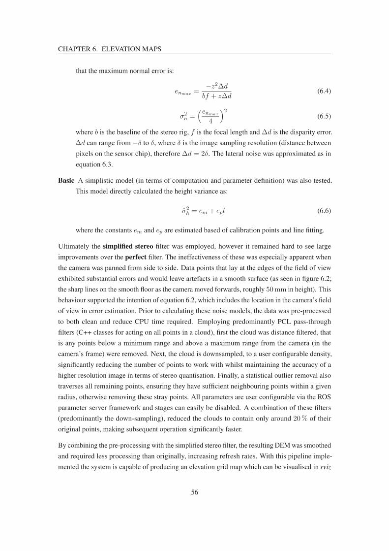
CHAPTER 6. ELEVATION MAPS
that the maximum normal error is:
enmax =−z2Δd
bf + zΔd(6.4)
σ2n =
(enmax
4
)2(6.5)
where b is the baseline of the stereo rig, f is the focal length and Δd is the disparity error.
Δd can range from −δ to δ, where δ is the image sampling resolution (distance between
pixels on the sensor chip), therefore Δd = 2δ. The lateral noise was approximated as in
equation 6.3.
Basic A simplistic model (in terms of computation and parameter definition) was also tested.
This model directly calculated the height variance as:
σ2h = em + epl (6.6)
where the constants em and ep are estimated based of calibration points and line fitting.
Ultimately the simplified stereo filter was employed, however it remained hard to see large
improvements over the perfect filter. The ineffectiveness of these was especially apparent when
the camera was panned from side to side. Data points that lay at the edges of the field of view
exhibited substantial errors and would leave artefacts in a smooth surface (as seen in figure 6.2;
the sharp lines on the smooth floor as the camera moved forwards, roughly 50mm in height). This
behaviour supported the intention of equation 6.2, which includes the location in the camera’s field
of view in error estimation. Prior to calculating these noise models, the data was pre-processed
to both clean and reduce CPU time required. Employing predominantly PCL pass-through
filters (C++ classes for acting on all points in a cloud), first the cloud was distance filtered, that
is any points below a minimum range and above a maximum range from the camera (in the
camera’s frame) were removed. Next, the cloud is downsampled, to a user configurable density,
significantly reducing the number of points to work with whilst maintaining the accuracy of a
higher resolution image in terms of stereo quantisation. Finally, a statistical outlier removal also
traverses all remaining points, ensuring they have sufficient neighbouring points within a given
radius, otherwise removing these stray points. All parameters are user configurable via the ROS
parameter server framework and stages can easily be disabled. A combination of these filters
(predominantly the down-sampling), reduced the clouds to contain only around 20% of their
original points, making subsequent operation significantly faster.
By combining the pre-processing with the simplified stereo filter, the resulting DEM was smoothed
and required less processing than originally, increasing refresh rates. With this pipeline imple-
mented the system is capable of producing an elevation grid map which can be visualised in rviz
56

CHAPTER 6. ELEVATION MAPS
as a point cloud (or surface) as demonstrated in figure 6.2.
Figure 6.2: Elevation Mapping output – Demonstrating the elevation mapping pipeline output. The imagein the top left is that seen by the camera, whilst the main image is a 3 dimensional reconstruction of this.The co-ordinate frames demonstrate the map origin (odom), the robot’s origin (initial frame), and thecurrent location (zed tracked frame).
57

Chapter 7
Traversability Maps
With consistent elevation information extracted from the camera’s depth clouds, it was possible to
begin analysing what this information could reveal for the REX platform. As discussed in section
3.1, where the design considerations of a device that would benefit the REX are investigated;
masses of elevation information would be of no benefit to the end user. For the platform at hand,
the main concern is traversability: is it safe and possible to take a step in the desired direction? To
address this, mobile robotic systems often create traversability maps based on a variety of sensory
information [Pradeep et al., 2010, Fankhauser et al., 2014, Karkowski and Bennewitz, 2016].
These maps can then be used directly to query a certain movement or a series of movements that
when combined form a path between points.
7.1 Traversing with the REX
Since traversable is relative to the vehicle trying to navigate the terrain it was unlikely to find
a solution that would generate accurate maps for the REX. However as we were working with
the ROS platform, there existed a lot of open source solutions that would easily be adjusted to
suit, saving a considerable amount of time. Again a member of ETH Zurich had provided their
solution to traversability mapping open source on GitHub 1, with its functionality explained
in [Wermelinger et al., 2016]. Their framework was forked into a local application named
rex traversability and adapted for the REX platform. Written by the same research group as the
grid mapping project, these elevation maps were directly compatible. The first customisation was
the footprint of the robot, as this understandably greatly effects the map output. REX’s footprint
here is described as a rectangular polygon, 200mm× 400mm in size, however, a simplified
circular model is also provided with a radius of 300mm. Testing indicated that this model might
1https://github.com/ethz-asl/traversability_estimation
58

CHAPTER 7. TRAVERSABILITY MAPS
need extending later on as whilst the feet occupied only the size give, the upper robot occupied
more, especially when swaying during movement. One could not, however, increase the actual
footprint, as this would prevent the robot from determining stairs as traversable.
7.1.1 Traversability Filters
In order to determine traversability, we must investigate what makes terrain un-traversable.
Heavily dependent on drive system configuration, this has no universal solution, however there
are a few standard terrain metrics that most systems depend on. Wermelinger et al. address this
in a universal manner, by implementing a filter based system with configurable parameters that
produce a standard uniform traversability metric. These filters can be configured depending on the
vehicle, as that their outputs are scaled relative to what is and is not acceptable for that platform.
Utilising the systems developed for ROS to filter data in an efficient manner, the following filters
process DEMs and can be stacked to form a chain of filters:
Step For humanoid robots there exists a height limit that is considered as traversable, usually
higher than on a wheeled or tracked robot, due to the kinematics of the limb joints. This
filter was crucial for the desired research outcome of investigating stair climbing on
medical exoskeletons. Mathematically the filter attempts to determine the maximum height
difference between cells, but filters these values as to provide some resilience against noise.
In essence the filter iterates through every cell twice, using some defined parameters, to
determine first the maximum height difference in an area, and then if enough cells qualify
as step-cells in the vicinity. This approach ensurse that a singular noisy height reading does
not result in non-traversable terrain and is detailed in pseudo algorithm 1.
Slope Similar to the the step height, slope tolerances depend a lot on the platform navigating the
terrain. The REX ankle joint is capable of pitch and roll rotations however the platform as
a whole must always remain stable encase of power loss. The slope the feet are placed at
plays a large role in stability, since in general the device should not be operated on slopes
larger than a few degrees. Here the traversability is simply computed from a comparison of
the normal angle at that cell against a configurable critical slope value as shown in pseudo
algorithm 2.
Surface Normals Used not directly to observe traversability, but instead for many other filters,
this property uses a search radius to estimate the average surface normal within the area.
The mathematics behind this involve plane fitting and is performed by solving for a set of
eigenvectors and eigenvalues, as shown in pseudo algorithm 3.
Roughness In order to maintain traction and a stable footing the surface must also be relatively
flat. To judge this, a roughness filter will classify the elevation map based on the unevenness
59

CHAPTER 7. TRAVERSABILITY MAPS
of the surface. Again this filter employs surface normals to estimate an average plane, and
then computes the distance between this plane to every point within a search radius. This
distance is root-mean-squared and used as an indicator or roughness as explained in pseudo
algorithm 4
Algorithm 1 Step Filter
Require: critStep � Critical step height parameter
Require: critCount � Critical cell count parameter
Require: r1, r2 � 1st and 2nd search radius
1: procedure UPDATE(GridMap M ) � First cycle
2: for each Cell c ∈M do3: minHeight← 04: maxHeight← 05: for each Cell d within radius r1 of c do6: if d.height > maxHeight then7: maxHeight← d.height8: else if d.height < minHeight then9: minHeight← d.height
10: end for each11: c.step← maxHeight−minHeight12: end for each13: for each Cell c ∈M do � Second cycle
14: maxStep← 015: nCritical← 016: for each Cell d within radius r2 of c do17: if d.step > maxStep then18: maxStep← d.step
19: if d.step > critStep then20: nCritical ++
21: end for each22: maxStep← argMin(maxStep, nCritical
critCountmaxStep)23: if maxStep < critStep then24: c.traversability ← 1− maxStep
critStep25: else26: c.traversability ← 0
27: end for each
60

CHAPTER 7. TRAVERSABILITY MAPS
Algorithm 2 Slope Filter
Require: critSlope � Critical slope angle
1: procedure UPDATE(GridMap M )
2: for each Cell c ∈M do3: slope← acos(c.surface normal z)4: if slope < critSlope then5: c.traversability ← 1− slope
critSlope6: else7: c.traversability ← 0
8: end for each
Algorithm 3 Surface Normals Filter
Require: r1 � Radius of normal sample
Require: � �covM is the covariance matrix
Require: � The solveEigen function solves for eigenvector (V T ) and values (V )1: procedure UPDATE(GridMap M )
2: for each Cell c ∈M do3: nCount← 04: �p [ ]5: for each Cell d within radius r1 of c do6: �p.pushback(d. �point)7: nCount← nCount+ 18: end for each9: �m← average(�p)
10: �NN [ ]11: for each Cell d within radius r1 of c do12: �NN.pushback(d. �point− �m)13: end for each14: �covM ← �NN · �NN
ᵀ
15: solveEigen
⎛⎝covM = V
⎡⎣ λ1
. . .λd
⎤⎦V T
⎞⎠
16: smallV alue←∞17: smallIndex← 018: nCount← 019: for each EigenValue v within V do20: if v < smallvalue then21: smallV alue← v22: smallIndex← nCount
23: nCount← nCount+ 124: end for each25: c. �normal← V T [smallIndex]26: end for each
61

CHAPTER 7. TRAVERSABILITY MAPS
Algorithm 4 Roughness Filter
Require: critRough � Critical roughness quantity
Require: r1 � Radius of roughness sample
1: procedure UPDATE(GridMap M )
2: for each Cell c ∈M do3: nCount← 04: �p [ ]5: for each Cell d within radius r1 of c do6: �p.pushback(d. �point)7: nCount← nCount+ 18: end for each9: �m← average(�p)
10: planeParam← �m • c. �normal11: sum← 012: for each Cell d within radius r1 of c do13: sum← sum+
(�m • d. �normal − planeParam
)2
14: end for each15: roughness =
√sum
nCount−1
16: if roughness < critRough then17: c.traversability ← 1− roughness
critRough18: else19: c.traversability ← 0
20: end for each
62

CHAPTER 7. TRAVERSABILITY MAPS
7.1.2 Combining Traversability Layers
With a lot of information now at hand as an output of the filters, this needs to be amalgamated to
a simplistic model that can be referred to by other parts of the system. A weighted summation
E
B
A
D
C
Figure 7.1: Traversability Map Sample – This demonstration traversability map shows what the combinedoutputs of the individual filters may produce. Worth noting in this image are the smooth footpaths (E), therougher grass terrain (A), and the non traversable stair edges (D) and bushes (C). Slopes are also lightlydetected (B).
was used to combine the layers into one traversability map, as shown in figure 7.1. This allowed
differing importance to be placed on the individual layers depending on the situation, or as it may
be the noise levels. For example when operating with the REX, often the weighting of the slope
filter was significantly reduced. This was due to the surface normal filter not considering a large
enough area (was computationally too expensive) during fitting, rendering it susceptible to noise
caused by disconnects in the map. By reducing the weighting of the slope filter, small noise bands
where not enough to stop traversing, however, consistent sloped terrain still was detected.
7.2 Interfacing with the REX
Demonstrating this technology functioning with the REX platform was always a key milestone
for this research. To investigate the applicability of this research to medical exoskeletons and the
REX in particular, a working interface had to be demonstrated. It was identified early on that it
would not be possible to directly integrate the vision pipeline to the Master Control Unit (MCU)
63

CHAPTER 7. TRAVERSABILITY MAPS
of the REX for regulatory reasons, so an alternative route had to be explored. The obvious choice
of interface with the MCU was via REX-LINK, a proprietary Application Programming Interface
(API) that exposes various levels of control over the robotic device. Predominantly exposed via a
Bluetooth connection with the device, this API is used predominantly by physicians to monitor
the device, ensuring patients are being placed into the poses they require. Since the REX a highly
regulated medical device, advanced access to REX-LINK is carefully controlled, but can allow
authorised individuals to remote control authorised devices. This ability presented a solution to
demonstrate an end-to-end solution demonstrating functionality with the REX as detailed in figure
7.2. Employing C#, an interface program was written (as it contained a proprietary API, this
Figure 7.2: REX-LINK Flowchart – This demonstrates the flow of operations when interfacing with theREX platform. A continuous stream of three-dimensional points is gathered from the ZED, processed andintegrated into the stored maps. When the user issues a command on the REX (via the joystick) this isintercepted, and sent to the Jetson via Bluetooth and REX-LINK. The stored database of maps is thenqueried if the desired movement is considered traversable, and a yes / no decision is made. If consideredtraversable, an acknowledgement sound is played, and the REX moves as normal. If not, a tone indicatingthat it is not considered safe to move in that direction is played and no movement occurs.
could not be made public) that connected to the REX Platform via REX-LINK with authorisation
to remote control the device. The program would monitor the user input joystick, and if moved,
intercept the command for processing. Due to software compatibilities of the REX-LINK API,
this program had to run on a Windows operating system, providing an extra layer of complexity
not detailed in figure 7.2. In practice a Windows laptop was used to connect to and intercept user
64

CHAPTER 7. TRAVERSABILITY MAPS
input from the REX, which then in turn (via TCP\IP WebSocket, employing rosbridge suite2)
communicated with the Jetson TX1 (Linux), forwarding the query via a ROS service call. The
Jetson would then respond a status of either: traversable, non-traversable or error. If software
running on the laptop received a positive response, it would play an acknowledgement tune on
the actual REX and then after a suitable delay, begin the movement. Otherwise a tone would
be emitted, alerting the user that this movement was deemed not possible. This entire process
was typically able to be executed in less than 100ms, effectively happening seamlessly behind
the scenes to the user (initial first query could take up to 1000ms establishing the connection).
Physically the camera was mounted to the left armrest of the REX with a custom mount and 3D
printed bracket. The angle of the mount could be altered to test different configurations. Usually,
an angle of 30◦ to 35◦ was employed (below the horizon). Functionality wise this demonstrated
the machine vision interface successfully implemented on the REX medical exoskeleton and
directly interacting with the device, concluding the implementation requirements of the research.
2http://wiki.ros.org/rosbridge_suite
65

Chapter 8
Dataset Generation
In order to validate the results of this research in a more quantitative manner, it was determined a
ground-truth dataset should be created, and this was included in the budget (section 3.2.4). As the
primary focus of this work was to investigate machine vision for traversability analysis, geometric
accuracy was an important metric. Researchers often will compare their work to the ground-truth,
something that is known to be as close to reality as possible (within a small margin of error). This
would create a benchmark to compare result accuracy, and a ground truth for error calculations to
optimise algorithms. With the technology available in depth sensing moving quickly, this would
also indicate what may be possible in this field sensors improve to be on par with current laser
scanning technology.
For depth perception often laser scanners are employed to develop these accurate maps due to
their consistently small error. The datasets described here were created with a Faro Focus3D S120
laser scanner, which is a very accurate surveying scanner capable of up to 120m scanning range.
Characteristics of the device (especially ranging error) are shown in table 8.1. Point sampling flat
Table 8.1: Faro Focus3D Accuracy – Measurement accuracy of Faro Focus3D laserscanner series, including the S120 unit that was used. Error is given as ranging errora
Surface
Reflectivity10m
10m - noise
compressedb 25m25m - noise
compressed
90% refl. 0.6mm 0.3mm 0.95mm 0.5mm10% refl. 1.2mm 0.6mm 2.2mm 1.1mm
a Ranging noise is defined as a standard deviation of values about the best-fit
plane for measurementb A noise-compression algorithm may be activated to average points in sets of 4
or 16, thereby compressing raw data noise by a factor of 2 or 4
terrain surfaces in the data gathered indicate that these values are reasonable, although there is
66

CHAPTER 8. DATASET GENERATION
additional error introduced in the multi-scan registration process. However this combined error
is still negligible in comparison to the sensors and SLAM implementations being tested, and so
serves as a valid comparison.
Since geometric terrain navigation was the focus of this research, a diverse set of environments
would be required to validate the methods employed on the REX. These should include reference
areas such as flat floors but also doorways, different types of stairs, curbs, and more. Key
Locations were chosen around Albany, Auckland, New Zealand that would be convenient to
return to. These consist of a household setting, an industrial environment (including office space)
and public outdoor environments around Massey University Albany. Notable features of each
Table 8.2: Laser Datasets – A summary table of the laser datasets generated as part of this research, size and notable featurescontained.
Label Project Name Size (m) Points (millions) Notable Features
A HOME Ballymore 15x14x7 72 Household, Doorways, Curved Stairs
B MASSEY AVKellDrive 75x40 127 Outdoors, Roadside curbs, Public Park
C MASSEY AVStairs 7x7x7 47 Complex Angled Staircase
D MASSEY EPCourtyard 01 58x76 93 Outdoors, Slopes, Varied Steps, Varied Terrain
E MASSEY EPCourtyard 02 24x17 31 Outdoors, Large Stairs
F MASSEY EPCourtyard 03 85x66 77 Grass, Stairs, Ledges
G MASSEY EPCourtyard 04 9x8 28 Single, Stairs
H REX Complete 39x35 125 Large Internal Area
I REX DemoStairs 12x12 42 Standard Stairs, Standard Ramp
J REX Office 4x4 7 Desks
K REX ProductionStairs 12x4x7 38 Large flight of stairs
L REX Reception 11x8x6 63 Complex Stairs, Glass railings
M REX SteepStairs 9x5 46 Steep Stairs, No kickboards
set are labelled for convenience in table 8.2. Each of the scenes is then down-sampled to 1mm,
cleaned 1, exported and photographed, converted to a DEM (resolution of 25mm), and also
exported. The outputs of this process are shown in figure 8.1 for each scene.
In order to promote comparison, the point-clouds generated by this are publicly available2 to
download and work with in common file formats (PCL compatible). This process has allowed the
generation of a ground-truth standard that research outputs can be compared to for validation.
1Via CloudCompare’s statistical outlier removal with parameters of 7 points and 4.0 standard deviations2Due to the large size they are hosted at todo. Certain sections have been removed due to commercial sensitivity.
67

CHAPTER 8. DATASET GENERATION
(a) Household in Auckland (b) Albany Kell Drive & Park (c) Massey AV Stairs
(d) Massey Courtyard 01 (e) Massey Courtyard 02 (f) Massey Courtyard 03
(g) Massey Courtyard 04 (h) Rex Warehouse (i) Rex Demonstration Stairs
(j) Rex Production Stairs (k) Rex Reception (l) Rex Steep Stairs
Figure 8.1: Laser Dataset Point Clouds – Point clouds of each dataset generated for this research. NormalRGB points and DEM coloured points are superimposed to help perceive height. One sample set (RexOffice) is not shown here for formatting reasons.
68

Chapter 9
Results
9.1 Traversability Mapping
Combining the hardware and software development of implementing a vision system on the
REX exoskeleton, this chapter details the results achieved and attempts to qualitatively and
quantitatively assess them. Testing the system as a whole was a process that had to be developed
and progressed various stages. The most basic system that demonstrated outputting traversability
maps was with the ZED camera mounted on a trolley with the Jetson TX1, a screen, keyboard,
mouse and Uninterupted Power Supply (UPS). With this setup and ROS’s recording ability, it
was possible to gather the following results demonstrating the system’s initial capability. Figure
(a) Camera Scene(b) Trolley Map (c) REX Mounted Map
Figure 9.1: Flat Terrain Results – Elevation and traversability maps for a flat open area (seen in a). In bthe movement (depicted by the red arrows) was on the trolley, whilst in c it was with the camera attachedto the REX
9.1 shows the most simple terrain: a clear flat area with items around the edges. From left to
right are depicted the colour image of the scene as captured by the camera, the output maps when
employing a trolley for movement, and the outputs of using a REX for movement. Focusing
first on image 9.1b, it is possible to identify the flat floor, the boxes along the left-hand side, and
the two obstacles straight ahead protruding from the wall line. There are a few small spots that
69

CHAPTER 9. RESULTS
show up as black (non-traversable). These are false negatives in the interpretation of the terrain
and are in fact flat floor, due to noise in the stereo data. Often the segment lines in the concrete
pads (seen in image 9.1a) are enough of a lighting and reflectivity difference to result in elevation
noise. Under normal operation, the traversability map is kept smaller, to reduce processing power
required and increase overall refresh-rates. The concrete poured floor is relatively flat (Confirmed
in laser dataset), revealing the wavy nature of stereo vision by the range of colours representing
the core floor section. Image 9.1c depicts the same scene and roughly the same start and end
positions, but the camera was mounted to the REX platform for movement. The REX’s movement
maps are very linear with sharp transitions, resulting in non-smooth trajectories. These can be
visualised by the red arrows and when compared to 9.1b, the difference is clear. This non-linear
motion is difficult for the ZED to track, given the computing resources it has access too, resulting
in inaccuracies for the pose estimation of the robot, and consequently, the merging of grid map
messages. In the elevation, and consequently the traversability, maps this manifests itself as
jagged edges. These are e specially apparent in the peripheral vision areas as seen along the
right edge in image 9.1c. Figure 9.2 further investigates the difference between smooth motion
(a) Camera Scene (b) Trolley Map (c) REX Mounted Map
Figure 9.2: Flat Terrain Analysis – Focusing on the difference between data generated with a REX movingthe camera as opposed to a trolley image a shows the jagged edges and labels their height. Histogramsb and c show the spread of points representing the ground plane form the trolley data and the REX datarespectively. Note the larger spread in c.
and abrupt motion by comparing the spread of points representing the floor plane when trolley
mounted (image 9.2b) and REX mounted (image 9.2c). Individual edge height differences are
also annotated in image 9.2a, ranging from 0.030m to 0.078m, with the larger difference being
at the edges. Mainly triggering the slope filter, this causes the traversability map to be fairly noisy
and filled with horizontal lines. The key features (the floor, the boxes on the right, the back wall,
and the obstacles protruding) are still clearly present, and so the challenge of differentiating them
is discussed later.
Figure 9.3 features a doorway straight ahead of the camera, with the door standing ajar. This
introduces the interesting feature of considerable lighting change (visible in 9.3a, it is considerably
darker through the door and is artificial lighting as opposed to natural lighting), and also a tracking
challenge when forced to track with a narrow field of view for feature tracking. Image 9.3b again
shows the smooth movement maps generated using a trolley to approach the doorway with only
70
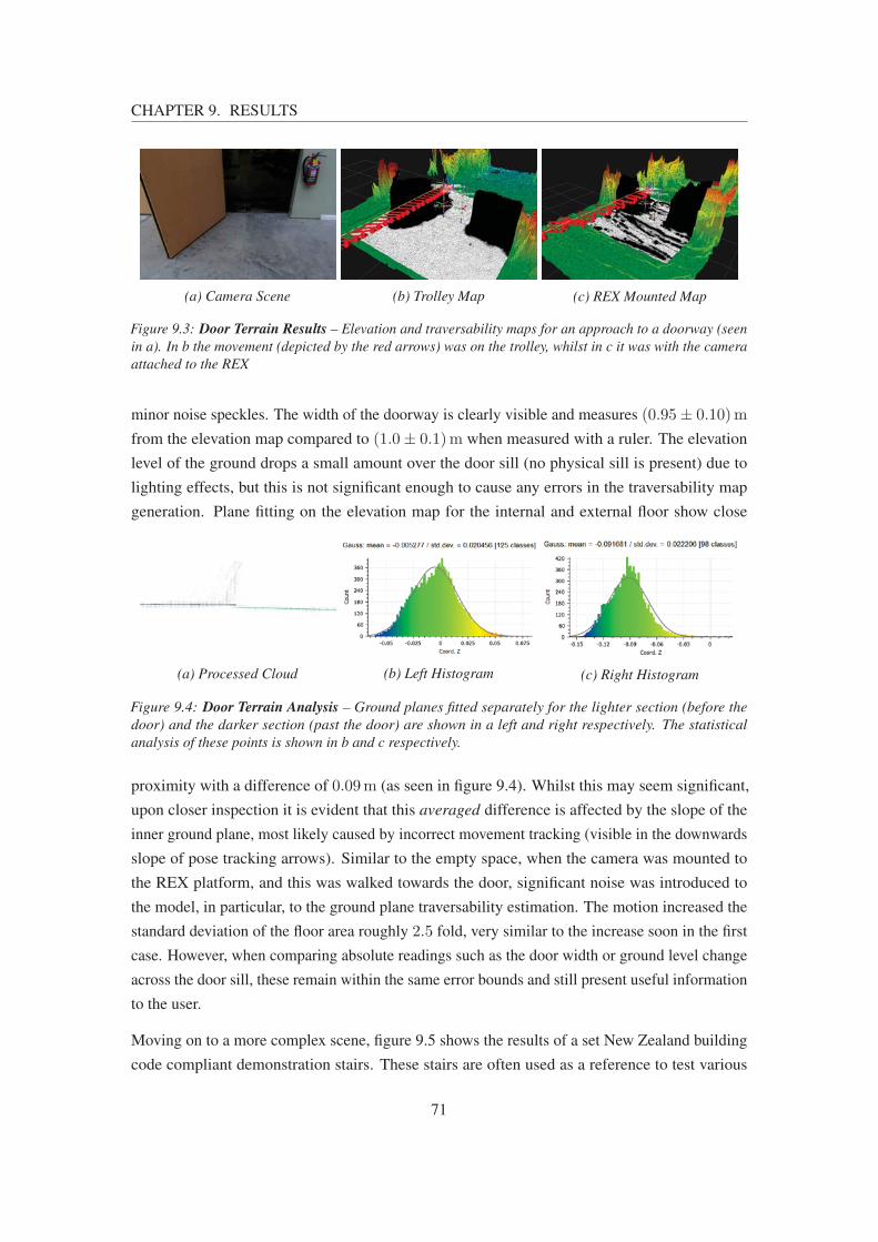
CHAPTER 9. RESULTS
(a) Camera Scene (b) Trolley Map (c) REX Mounted Map
Figure 9.3: Door Terrain Results – Elevation and traversability maps for an approach to a doorway (seenin a). In b the movement (depicted by the red arrows) was on the trolley, whilst in c it was with the cameraattached to the REX
minor noise speckles. The width of the doorway is clearly visible and measures (0.95± 0.10)m
from the elevation map compared to (1.0± 0.1)m when measured with a ruler. The elevation
level of the ground drops a small amount over the door sill (no physical sill is present) due to
lighting effects, but this is not significant enough to cause any errors in the traversability map
generation. Plane fitting on the elevation map for the internal and external floor show close
(a) Processed Cloud (b) Left Histogram (c) Right Histogram
Figure 9.4: Door Terrain Analysis – Ground planes fitted separately for the lighter section (before thedoor) and the darker section (past the door) are shown in a left and right respectively. The statisticalanalysis of these points is shown in b and c respectively.
proximity with a difference of 0.09m (as seen in figure 9.4). Whilst this may seem significant,
upon closer inspection it is evident that this averaged difference is affected by the slope of the
inner ground plane, most likely caused by incorrect movement tracking (visible in the downwards
slope of pose tracking arrows). Similar to the empty space, when the camera was mounted to
the REX platform, and this was walked towards the door, significant noise was introduced to
the model, in particular, to the ground plane traversability estimation. The motion increased the
standard deviation of the floor area roughly 2.5 fold, very similar to the increase soon in the first
case. However, when comparing absolute readings such as the door width or ground level change
across the door sill, these remain within the same error bounds and still present useful information
to the user.
Moving on to a more complex scene, figure 9.5 shows the results of a set New Zealand building
code compliant demonstration stairs. These stairs are often used as a reference to test various
71

CHAPTER 9. RESULTS
(a) Camera Scene (b) Trolley Map (c) REX Mounted Map
Figure 9.5: Demo Stairs Terrain Results – Elevation and traversability maps of a demonstration set ofstairs compliant to New Zealand’s building code (seen in a). In b the movement (depicted by the redarrows) was on the trolley, whilst in c it was with the camera attached to the REX
features of the REX and so using them for the vision system was obvious. There are three steps,
and four railings with a wide space in the middle for the REX to use, whilst assistants can ensure
patient safety from outside sections. The traversability filter output can be appreciated here,
clearly showing the three steps in image 9.5b as consistent black bars. With sufficient tuning
of the parameters detailed in equation 1 the bands became narrow enough to allow stepping
in-between them. The steps are further investigated in figure 9.6, which highlights them in
(a) Coloured Stair Cloud (b) Histogram of trolley (c) Histogram with REX (d) Histogram with laser
Figure 9.6: Demo Stairs Terrain Analysis – Showing the individual stairs hand picked in image a. Thehistogram shows the four peaks from left to right of the floor, 1st and 2nd steps and the the top platform.Histogram b is from the trolley dataset whilst c was with the ZED mounted on the REX. For comparisonthe histogram from the laser dataset is shown in d, with perfect peaks.
height-mapped colour. Each step measured (0.15± 0.05)m in height, compared to 0.18m in
reality. The sharpness of the peaks in the histogram 9.6b demonstrate precision of the data points
whilst the distance between peaks shows their accuracy (should measure 0.18m), as demonstrated
with 9.6d. Comparing 9.6b and 9.6c shows the impact of mounting the ZED on the REX platform.
The four peaks are still visible, however clearly less defined in 9.6c, reinforced by the reduced
clarity in traversability estimation shown in image 9.5c. The distance between peaks is still not
accurate, but has similar precision at (0.14± 0.05)m.
Although fully building code compliant, the demonstration stairs are aesthetically not like a
normal set of stairs. Figure 9.7 challenges the pipelines ability to track multi-story traversability
across large flights of stairs. Totalling 20 stairs, divided by a mid platform these represent a normal
set of straight stairs with well-defined front edges and naturally lit by ambient sunlight. With the
72

CHAPTER 9. RESULTS
(a) Scene (b) REX Mounted Map (c) Hand Guided Map
Figure 9.7: Large Flight of Stairs Terrain Results – Mapping a large flight of stairs with a centre platformas shown in a. Approaching the stairs with the camera mounted to the REX is shown in image b and sinceneither the trolley, nor the REX were capable of traversing the stairs, it was carried up by hand in image c.
understanding that the trolley gives smoother results, it was decided to demonstrate this no longer,
but rather attempt to test the tracking ability when climbing the entire flight of stairs. Image
9.7b first demonstrates the approach with the REX, still showing traversable bands matching the
frequency of stairs, albeit rather narrow. Image 9.7c then demonstrates the same stairs traversed
on foot carrying the ZED camera in a relatively consistent stance. Trials revealed that this had to
be higher than when mounted to the REX; otherwise the camera struggled to accurately track
movement and re-project point clouds due to the operational minimum distance limit and the
approaching climbing stairs. This resulted in the camera being held at roughly 1.8m height angled
downwards. With many stairs detected it was possible to analyse the precision and accuracy
(a) REX Histogram
(b) Hand Histogram
110
130
150
170
190
210
0
5
10
15
Height [mm]
Fre
qu
ency
(c) Step Height Histogram
Figure 9.8: Large Flight of Stairs Terrain Analysis – First we compare the step separation (indicated bypeaks in height value histograms) between the maps generated with a REX (a) and when hand-held (b).Then the peak separation of all are analysed in chart c.
73

CHAPTER 9. RESULTS
of the detection process in more detail. Figure 9.8 does this by extracting and comparing the
height histograms of both REX mounted data and hand-held data, and then both combined. With
histogram 9.8c in mind it is possible to determine that the system consistently under-estimates
step height (an average of (0.170± 0.004)m). In terms of accuracy the gathered samples had a
standard deviation of 0.024m. The system also correctly identified the mid-platform as a suitable
traversable area. Tread depth was compared (in a similar manner, using histogram peaks), with the
hand-held map averaging (0.275± 0.025)m in depth and (0.285± 0.005)m in the laser scan.
At 1.25m wide, the previous set of stairs is wider than normal, making detection with the ZED
easier. To contrast this a standard set of stairs with a width of 1.10m was tested.
(a) Scene (b) REX Elevation Maps
Ground
1st Step
2nd Step
Platform
Wall
(c) Pointcloud Side View
Figure 9.9: Complex Stairs Terrain Results – Traversability of some more complex stairs featuring variedlighting, glass and a right angle, as depicted in a. The elevation map here is less definitive as shown infigure c, resulting in a less clearly defined traversability map (shown in b). The annotations show howlittle height is present in the 1st step.
These stairs also featured a number of other complexities such as; clear glass sides, carpet texture
and direct sunlight streaks (all visible in 9.9a). It is therefore not surprising that the definition of
the elevation (and consequently traversability) maps was reduced as shown in image 9.9b, which
was generated with the ZED mounted to the REX platform. It is very heard to distinguish the
first step (shown in image 9.9c), because it is nearly level with the ground plane, and so it is
not detected as a step on the traversability maps. Adding to the factors making detection hard,
these stairs are also only 0.165m tall with the first step measuring only 0.155m in height. The
pipeline did pick up well on the traversable areas in the ground plane, clearly marking the internal
rock-garden and reception desk as non-traversable.
Tied into all the results, the sensors ability to perform under sunlight, whilst not quantitatively,
was understood qualitatively through repeat exposure to such environments. In general, these
results indicate that on a macro scale the results are accurate, but calculating traversability from
elevation still requires refinement.
74

CHAPTER 9. RESULTS
9.2 Laser Data Set
A common practice when proposing research results is to compare them to a standard. With
limited prior work with machine vision traversability mapping on medical exoskeletons available,
research outputs are here compared to a ground-truth dataset generated with a laser scanner as
described in chapter 8. With the focus of traversability mapping being primary, two comparisons
will be made to evaluate performance:
Gridmap Comparison Select areas will be mapped using the methods described in the preceding
chapters, and the resulting gridmaps will be saved as point clouds (each cell as one point
with the appropriate height). A relevant matching area of the laser point cloud is processed
with the identical pipeline, and the resulting gridmaps are also converted back to point
clouds. The two gridmaps in point cloud form are then aligned, first roughly manually,
then using regression to optimise the match. Differences between the two clouds are then
computed using two approaches; Direct Cloud to Cloud (C2C) and Multiscale Model to
Model Cloud Comparison (M3C2)[Lague et al., 2013]. Whilst similar both algorithms
have their advantages as described by Lague et al., so both are presented here.
Traversability Comparison The above exported elevation maps are processed through the
traversability mapping node. The resulting map is exported in two formats; an image
(greyscale) for displaying, where white is traversable and black is non-traversable, and
each pixel is one unit of the map. The other export is a point cloud, where each point
corresponds to a traversability cell (storing [x, y] information), and the point height (z)
stores the traversability of the cell. A height of 0 defines non-traversable, and a height of
1.0 defines fully traversable. In this form, it was possible to employ the same comparisons
as above (C2C and M3C2) between the two outputs for visual analysis. Figures 9.10 and
9.12 explain how this works in practice and how to interpret the results.
Having established a standard practice for comparing results, processing could begin, which took
a significant amount of time, even on a workstation computer, as some of the clouds had over 100
million points. Figure 8.1 and table 8.2 provide a summary of the datasets.
Starting with a simple flat area comparison, figures 9.10b and 9.10c demonstrate the differences
in technologies as explained in the caption. This clearly helps confirm some of the results
demonstrated in the previous section, especially regarding the discontinuities introduced by the
rough movement of the REX. It also begins to investigate the effect of intense direct sunlight on
the sensor.
Looking at a more complex example, we again analyse the double set of stairs (as in section 9.1),
this time comparing the traversability maps generated. Figure 9.11 shows both the DEMs and
75
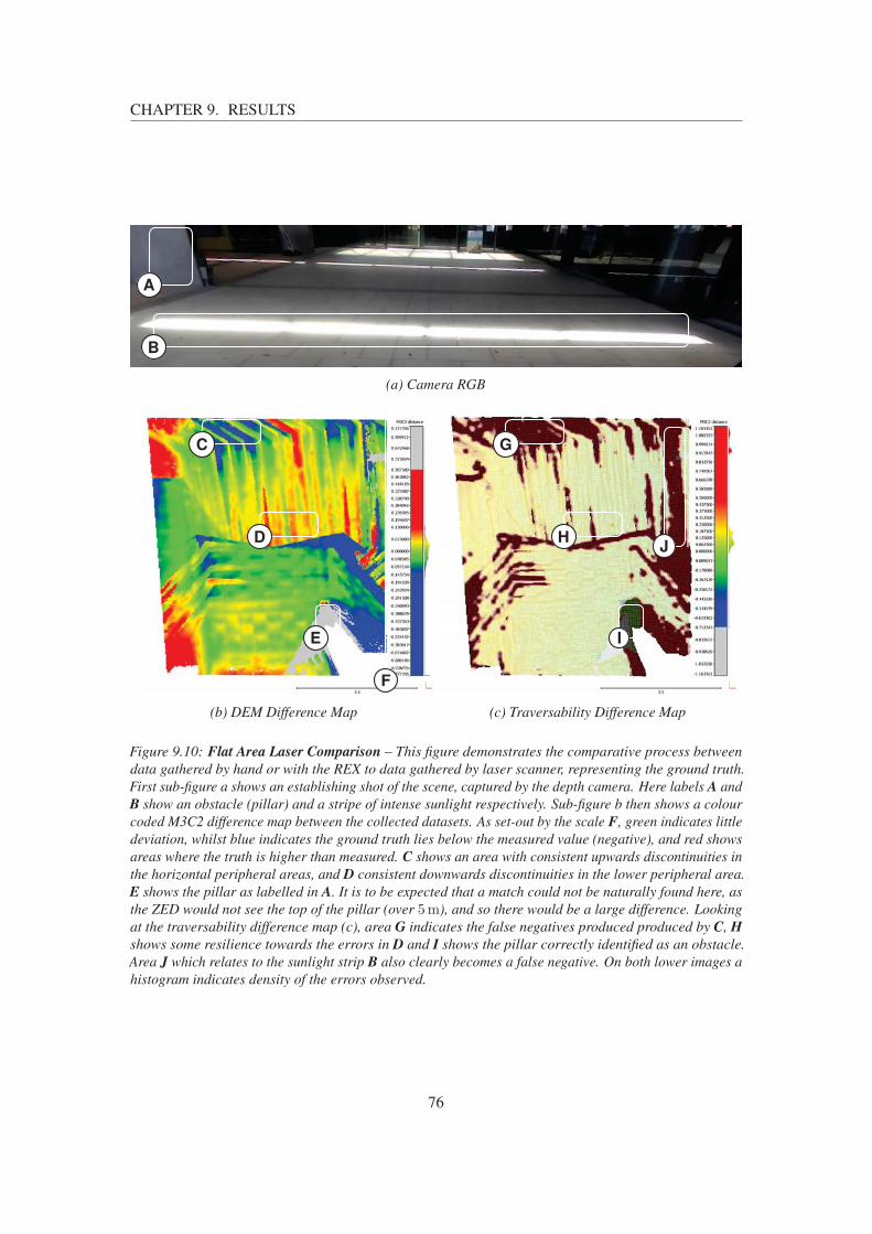
CHAPTER 9. RESULTS
A
B
(a) Camera RGB
C
D
E
F
(b) DEM Difference Map
G
H
I
J
(c) Traversability Difference Map
Figure 9.10: Flat Area Laser Comparison – This figure demonstrates the comparative process betweendata gathered by hand or with the REX to data gathered by laser scanner, representing the ground truth.First sub-figure a shows an establishing shot of the scene, captured by the depth camera. Here labels A andB show an obstacle (pillar) and a stripe of intense sunlight respectively. Sub-figure b then shows a colourcoded M3C2 difference map between the collected datasets. As set-out by the scale F, green indicates littledeviation, whilst blue indicates the ground truth lies below the measured value (negative), and red showsareas where the truth is higher than measured. C shows an area with consistent upwards discontinuities inthe horizontal peripheral areas, and D consistent downwards discontinuities in the lower peripheral area.E shows the pillar as labelled in A. It is to be expected that a match could not be naturally found here, asthe ZED would not see the top of the pillar (over 5m), and so there would be a large difference. Lookingat the traversability difference map (c), area G indicates the false negatives produced produced by C, Hshows some resilience towards the errors in D and I shows the pillar correctly identified as an obstacle.Area J which relates to the sunlight strip B also clearly becomes a false negative. On both lower images ahistogram indicates density of the errors observed.
76

CHAPTER 9. RESULTS
(a) Laser DEM (b) Hand DEM (c) Laser Traversability (d) Hand Traversability
Figure 9.11: Production Stairs Laser Comparison (a) – Detailed difference analysis of the doublestaircase dataset. Left clouds a and b show the coloured elevation maps generated using the laser scannerand ZED respectively. Right figures then show the traversability maps from a top down perspective,showing clear similarities.
the traversability map side by side for a visual comparison. Using this information figure 9.12
then analyses the differences as described, using M3C2 pointcloud comparison. As annotated it
identifies areas that matched well, and areas that did not, either false positives (areas noted as
traversable, that are in truth not), or false negatives (areas that are noted as not-traversable but
in fact are). The results here clearly show that the camera is able to perform fairly well under
these conditions in mapping the environment, and whilst the DEMs do not directly match, the
A
BC
D
E
Figure 9.12: Production Stairs Laser Comparison (b) – An area correctly (in both the laser data and ZEDdata) identified as non-traversable, indicated by green and black (A), Correctly identified as traversable,shown with green and white (B), area falsely classified as not traversable shown with red and black (C),and an area falsely classified as traversable shown with blue and white (D). Areas where camera shakecause disconnects are clearly visible as in (E).
77

CHAPTER 9. RESULTS
traversability outcomes are very similar.
Direct sunlight and harsh texture conditions proved challenging for the methods put in place.
Figure 9.13 demonstrates a lot of challenging features within one scene, and reports on how the
methods perform. Looking down a set of stairs is of particular interest to the REX, since it must
approach them backwards. These results (albeit in harsh lighting) show that whilst the overall
height and slope of the stairs, and the horizon are correctly identified (figure 9.13b), because the
camera detects them only as a smooth slope, the traversability maps are wrong. The effect of
bright sunlit scenes mixed directly with shaded areas is also demonstrated.
To demonstrate the capability of the traversability mapping, a ground truth map is directly
processed and analysed. Figure 9.14 shows the main courtyard at Massey University (Albany,
New Zealand) processed with the same methods as the core results. The acquisition of this data
is explained in section 8. It is shown here primarily to discuss the future potential of this work,
when sensors are improved to produce similar levels of data on mobile moving platforms.
Comparing results from the REX platform (and also hand-held) highlights the important areas
where the sensors cause false results. Many scenes were scanned and then also traversed with the
REX that are not presented in this section, but included in the additional content.
78

CHAPTER 9. RESULTS
A
B
C
(a) Camera RGB
D
EF
(b) DEM Difference Map
H
I
(c) Traversability Difference Map
Figure 9.13: Harsh Environment Laser Comparison – Demonstrates a very harsh environment in termsof lighting and geometry for the ZED camera. With a harsh lighting difference across A, the cameracannot simple adjust exposure to suit either and it must compromise. This places obstacles in the darksuch as the side rails (B). Downwards stairs are also challenging to detect due to the horizon visible inC. The elevation map is fairly accurate, with 50% of points lying within 5mm of the ground truth, and90% within 14mm. D shows how little effect the harsh lighting conditions have on the ZED in a real usecase scenario. E demonstrates how the horizon was correctly detected (with minimal erroneous pixels),whilst F shows the continued inaccuracies in the horizontal peripheal vision, failing to properly detect thedark obstacles labelled in B. Figure c however identifies the requirement for tuning of the traversabilityparameters to match lighting conditions. Area I identifies how most stairs were not correctly detected, andH shows large false negative areas.
79

CHAPTER 9. RESULTS
C
A
B
D
(a) Laser DEM
C
A
B
D
E
(b) Laser Traversability
Figure 9.14: Ground Truth Traversability Map – Showing the results when the same methods are appliedto clean ground truth data. Figure a shows the height coloured DEM with a scale one the right. Left (b)shows the processed traversability. A shows a ramp clearly on both maps, with the flat mid section beingdetected (the slope critical value parameter remained unchanged, but could be reduced to make this moreapparent). The non-standard geometry around point B is converted to clearly separated surfaces. Theoccasional noise is present, as shown in area C, where a flat surface as a non traversable cell labelled.Stairs are also clearly labelled D. Surface roughness is detectable in these results where all the grasssurfaces (such as E) are a slightly darker shade. This feature was completely un-utilised on the REX dueto significant false negative traversability results from noisy data.
80

CHAPTER 9. RESULTS
9.3 Interfacing with the REX
Whilst sections 9.1 and 9.2 present the algorithm’s results by analysing the data outputs, this
section considers the complete integration with the REX as described in section 7.2. Working
around the limitations set by a commercial environment, it was still possible to implement and
demonstrate simple integration with the REX. Figure 9.15 left to right shows the camera mounted
(a) REX Mounted ZED (b) Complete system in action (c) Backend Footstep Query
Figure 9.15: REX-Link Interface Overview – Demonstrating a complete end to end application of themethods developed, the ZED is mounted to the left armrest of the REX (a), the device is then operated by aperson (b), and when a movement command is issued, the traversability map is first queried, preventingthe movement if deemed non-traversable (c). The green square indicated the area the REX would inhabit ifthe requested command would be allowed, however clearly being in occupied terrain, in this case it wouldbe intercepted and stopped.
below the left-hand armrest of the REX, the REX in operation with the camera and Jetson
TX1 onboard, and a movement request that would stop the REX as it is on the blocked terrain.
Although the Jetson TX1 could easily have been powered by the REX battery, it was deemed
inappropriate to modify the device purely for the demonstration, leaving an extension cord to
power the PC.
To demonstrate the capabilities of this interface, a demonstration scene is traversed, collision with
an obstacle is avoided, and the REX is inhibited from reversing into an obstacle. To capture this,
figure 9.16 shows the entire process, with the video frames overlaid, and the individual interface
moments also captured. In the 3rd position, the forwards command from the user is intercepted
and stopped, as it is deemed unsafe, instead playing a warning tone. The 4th position shows
the methods ability to prevent collision with obstacles not directly visible to the camera at that
moment. Here the table is still remembered in memory, and by tracking the motion of the robot
81

CHAPTER 9. RESULTS
2nd 1st3rd
4th
(a) Interface Demonstration Lapse
(b) Interface outputs 1st pose (c) Interface outputs 2nd pose
(d) Interface outputs 3rd pose (e) Interface outputs 4th pose
Figure 9.16: REX-Link Interface Demonstration – Taking extracts from a video, figure a shows themovements made during demonstrating the REX-Link interface with a table obstacle. 1st the occupantgets into the REX, the initial gridmap, traversability map and camera output (from the ZED) are shown infigure b. Then the occupant issues commands via the joystick, which are then relayed to the Jetson TX1 viabluetooth. Shown as a green square (seen in figure c) the footprint queries determine if the movement iscarried out. In then 2nd position this is clearly possible and so the robot carries of forwards until it reachesthe 3rd position. Figure d shows the table clearly detected as a non-traversable edge. It does determine thatthe table top itself is flat and traversable, however the footstep query determines that it cannot reach this.From this position the user takes a couple steps backwards, and circumnavigates the table, proceeding toapproach it backwards. This will be possible until in the 4th position, where as shown in figure e, memoryof the tables presence stops the REX.
82

CHAPTER 9. RESULTS
visually, it is predicted when the table is directly behind the robot, intercepting and stopping
movement in that direction.
This entire process and another demonstration are visible as videos in the digital media supplied
with this document or on-line1. These are played at five times speed and demonstrate interception
of movements that would cause a collision, both in-front and behind the REX. They show both a
camera recording of the entire scene, as well as all the interface outputs (gridmaps, traversability
maps and ZED camera stream), providing full oversight of the actions happening.
It was successfully demonstrated that the careful design decisions taken whilst developing the
methods made implementation on an actual REX possible. Multiple scenarios are tested, and the
platform has been extended to have loop closing feedback from the surrounding environment that
it can act upon. This is done in a safe manner, where it will only intercept and inhibit commands
it deems unsafe, and will never autonomously issue movement commands not first issues by the
user.
1https://goo.gl/kfQoKu
83

Chapter 10
Discussion and Conclusion
Determining and understanding the significance of these results for REX platform is an important
aspect of this work. Having investigated a wide range of scenarios, it is attempted to summarise
the strengths and weaknesses of the applied methods. It also provides an opportunity to review
the original focus of commercial integration. This will naturally lead into discussing the direction
of potential future work in this field of research and extensions to the methods employed.
10.1 Discussion
Analysing the scenarios presented in section 9.1, the extent to which this system can provide
useful information is qualitatively questioned. Whilst the system is capable of detecting flat terrain
and walls when stationary, and even when smoothly moved (such as on a trolley), the fact that
a significant amount of noise is introduced when mounted to a walking REX is an issue (figure
9.1). Analysing the causes of this suggests a solution; that improved visual odometry paired with
accurate, high-speed, inertial tracking would significantly improve the results. This stems from
reviewing the recorded sessions and noting that the movement tracking features large discrete
steps, rather than smooth movements. Since the temporal combining of point clouds depends
on an accurate transform between time-frames (described in chapter 6), the result of delayed or
inaccurate transforms will be discontinuities in alignment. With results being published of highly
accurate, fast moving visual odometry [Bloesch et al., 2015, Leutenegger et al., 2015], this is
not a significant hindrance, and should easily be overcome with time. The authors demonstrate
it accurately tracking movement aboard a roller-coaster ride with extreme accelerations, and
yet still providing accurate positional estimations1. Another deficiency of using purely pose
information from the ZED camera was that it is provided with no measure of confidence, which
1https://www.youtube.com/watch?v=9RaenslCedA
84

CHAPTER 10. DISCUSSION AND CONCLUSION
meant that this could not be considered further down the pipeline. Hence whilst the grid mapping
code base implements including pose uncertainty when merging with past data, this could not
be used due to the lack of this information. Visual odometry often relies on tracking features
in successive frames to place in them a three-dimensional space. Many algorithms are capable
of storing the key-points, and over time build a database of consistent point-features to improve
tracking. This functionality was not implemented, as testing was constantly being carried out
in new locations, but for a device permanently located in a home or clinic, this could further
help improve tracking. Having access to fast and accurate positional information with measures
of confidence will significantly reduce the discontinuities, with results trending towards those
gathered on the trolley.
A new stereo sensor filter was added to the grid mapping code-base as described in chapter 6.
This helped improve the temporal combining of data frames, however still has a lot of extension
potential. Calculating point variance as described in the algorithms did not seem to be sufficient
in managing noise introduced by the stereo camera, especially in the peripheral vision areas.
Figure 9.10 demonstrates this, showing significant errors in traversability mapping in the outer
areas. Negative effects were most prominent when reversing or pivoting. In these scenarios, data
from extreme edges can end up rotated to lie directly at the foot of the REX and be too close
to be updated (due to ZED’s minimum range), resulting in significant errors directly interfering
with movement. Incorporating a confidence measure into the stereo filter would further help
assign useful error probability information to points. Stereo confidence measures each have their
own merits, as discussed by Hu and Mordohai, and it is important to use a fitting model [Hu
and Mordohai, 2012]. By extending the implemented filter to capture these probabilities and
employing them as weights when merging points that inhabit the same DEM cell, the map would
progressively become smoother as surfaces average out.
By improving the above-discussed points the quality of information gathered can be improved;
however, it will be challenging to adjust the scale of error from macro to micro fundamentally.
Shown in figure 9.3, the proposed system functions well at detecting macro objects in relation to
the REX (such as doorways), but cannot detect micro objects that affect the REX. An obstacle
only a few mm in height, if placed in the right location, can cause instability of the REX
platform resulting in the device tipping over. Discussed in chapter 6, quantisation error of stereo
matching produces errors larger than this in many scenarios. Recalling the equation defining
stereo quantisation error (eq. 6.4), factors of influence in reducing this under user control are
the baseline and focal-length (defined in pixel units, effectively including resolution into the
equation)2. Changing these parameters to effect accuracy is investigated by Gallup et al., who
develop a fixed error stereo sensor; that is a sensor with identical quantisation error at all operable
2This stereo vision calculator helps demonstrate this fact: https://nerian.com/support/resources/calculator/
85

CHAPTER 10. DISCUSSION AND CONCLUSION
ranges [Gallup et al., 2008]. The authors acknowledge that baseline cannot be arbitrarily increased
as near-field perception is lost, but recognise that increasing the resolution requires it to grow
proportionally to zmax4 (where zmax is the furthermost detectable object). Employing this type
of technology, the stereo error can be improved; however, it will be challenging reduce the error
significantly, allowing detection of micro obstacles that pose a danger to the REX’s stability.
Parameter optimisation and adaptation was a large issue when progressing methods and collecting
results in varied scenarios. Across all the ROS nodes employed when operating, there are over
100 configurable parameters that contribute to the results produced. Although not all have major
effects, minor changes compound to changes in results that are not understood. Key parameters
to do with the ZED’s SDK regarding frame-rate, resolution, depth matching quality and tracking
are still poorly understood, often trial and error was used to adjust these values. Stemming from
the large potential for covariance between parameters, it was not within the scope of this research
to determine these relations. It is feasible to employ advances in machine learning and controlled
reinforcement learning to address this issue. Using ground truth (such as laser based traversability)
maps is a commonly employed technique in machine optimisation and is directly applicable in
this situation. Additionally, the inclusion of ambient lighting levels (via a light sensor) could
help adjust parameters to match, maintaining optimum results when transitioning from indoors to
outdoors. Literature shows that evolutionary algorithms can be effectively employed, providing
the constraints are well understood[Back and Schwefel, 1993].
Relating to technology compromise, the results indicate that a combination of sensors, utilising
each’s strengths, could further improve reliability. Stereo-depth sensor’s ability to still function
in sunlight was a key factor in choosing the technology, and in this regard, it has proven that it
can perform; even in bright sunlight (figure 9.13 and more in the additional content). Combining
sensory inputs to improve accuracy is not a novel approach. Maier et al. employ such a tactic in
their article, using a Computer Aided Design (CAD) scene to represent the static information of
the map (walls, stairs, structural), and a RGB-D camera to add dynamic objects and obstacles to
the map [Maier et al., 2012]. From a commercial standpoint, using CAD to map the environment
REX will inhabit is not directly feasible, but employing a laser scanner, such as that used in
chapter 8, is a potential. Effectively creating mm accurate maps of the static environment (such as
those shown in figure 9.14), semantic labelling of this could allow significant data noise reduction,
such as disregarding points detected below the surface or within walls. With REX’s price-point in
consideration, this is a feasible solution to allowing patients more freedom and diverse movements
when using the device within a shared location such as a physiotherapy clinic. ToF cameras have
only been shown in this research for comparative purposes; it is, however, clear that there exist
opportunities for these to function alongside stereo vision. Recent ToF sensors developed3 are
small enough that they could provide targeted feedback. For example, these could be mounted
3Such as pmd’s 19k-S3 – http://www.pmdtec.com/html/pdf/pmdPhotonICs_19k_S3.pdf
86
CHAPTER 10. DISCUSSION AND CONCLUSION
in the foot or on the ankle of the device to provide highly accurate surface maps (since these
operate at less than 1% error in accuracy). As with the laser mapping, employing ToF would
not replace stereo, but rather extend it. Determining step height and depth was investigated and
results show that while steps are consistently detected (figures 9.7, and 9.12), it is still difficult to
extract the correct step height (figure 9.8c). Analysing the results, the key issue is that the steps
are not detected as flat parallel platforms, but rather smoothed slopes, making feature extraction
difficult. It could be investigated if a two-dimensional laser scanner mounted so that it could scan
vertically could augment these methods sufficiently to resolve this ambiguity.
When collecting results, a key issue was alignment with the ground plane. The methods developed
in section 4.3.1 enabled case-by-case alignment (critical to the dynamic start position of the
REX), but did present challenges when operating in harsh environments. Often result recordings
had to be discarded because the ground-plane alignment would be wrong, causing the DEMs
to be completely erroneous (since the process assumes the positive z-axis is perpendicular to
the ground). Investigating the causes of this revealed that excessive sunlight would cause the
first 10 s to 30 s of depth data to be significantly warped due to over exposure whilst the camera
adjusted. Although an interim fix of simply delaying the single-shot ground alignment process
when operating outdoors (giving the camera time to adjust) sufficed, it did raise awareness that a
constantly updating alignment process would be advantageous. It would, however, have to be
determined when the floor was sufficiently visible, as a stable result relied on this.
Map update rates of less than 1Hz caused additional complications visible in the results. The
Jetson TX1 was employed to generate the results presented, and an effort was maintained to keep
this real-time in nature; however there was much room for improvements. Investigating these
revealed that the hardware was not being utilised to its full potential, often leaving the GPU and
sometimes even individual CPU cores unloaded. Reason for this was the reliance on platform
independent code, such as grid mapping, which was not designed to be multi-threaded in nature
necessarily, or utilise the GPU. In fact only ZED’s SDK made use of the GPU resources, even
though all processes that deal with point-clouds (or derivations thereof, such as DEMs) are well
suited for the kind of hardware parallelization offered by GPUs. Future improvements in this
research would have to investigate implementing core processing steps within the GPU to achieve
greater update rates, potentially also reducing the discontinuity that has been a primary source of
erroneous results.
Employing ROS has been a significant advantage in bringing together the many aspects of
implementing a depth vision system (illustrated in figure 5.3a), and whilst introducing some
overhead to the system, this was an acceptable compromise. An example of what ROS enabled can
be seen when looking at the results in section 9.3, demonstrating an end-to-end implementation
of the systems with a human operated REX. As the REX Link interface is only compatible with
Windows operating systems, ROS’s messaging structure and core framework allowed a quick
87

CHAPTER 10. DISCUSSION AND CONCLUSION
solution (less than a day development time) to a cross-platform communication issue complex in
nature. Extending on this, inserting additional building blocks becomes a modular process, for
example integrating depth information from an additional ToF sensor would be a trivial matter.
Throughout all parts of this work, patient safety was always considered highly important. REX
Bionics carefully considers all design choices it must make as their medical class devices must be
safe to operate and incapable of causing harm. The implications of this have become apparent
during this research, especially regarding software safety. To determine software as medically safe
is an incredibly difficult task, and as identified early on, would be far outside of the scope of this
research. It is, however, likely that a framework such as ROS would never be directly considered
medically safe, due to it’s extensively large code-base. This introduces a certain challenge, to
which the most obvious solution is to separate the two core components as demonstrated in the
results. Posing implications for future development, however, this leaves to question if it could
ever be considered safe for a framework, such as the one presented, to autonomously control a
device inhabited by a human being. Discussions around this often identify that this strenuous
restriction of systems can hold back technology from reaching patients that desperately require
and want it.
10.2 Conclusion
Since the late 19th century, humans have attempted to extend their capabilities by literally
surrounding themselves with technology in the form of an exoskeleton. This Technology has
rapidly advanced, consistently extending the capability of these devices and broadening the
outreach of their applications. Medical exoskeletons are becoming mainstream with multiple
companies pursuing the technology, each adding their improvements, jointly advancing the state-
of-the-art. REX Bionics is a company heavily involved in medical exoskeleton development
and uniquely offer the only non-crutch assisted platform, primarily targeted for physiotherapy
of patients unable to control their lower body. As they do not rely on four points of ground
contact (crutches), terrain navigation and understanding is vital to the stable and safe operation
of their devices. Analysing their current technology, it was identified that this could potentially
be advanced by applying machine vision practices to their unique application case to help close
the machine control loop. Reviewing literature on the matter indicated that research on such an
application had not yet been pursued and that the benefits for such a device were yet unknown.
Considering what research had been conducted, especially in the areas of machine vision applied
to mobile robotics, an extensive review of the literature was conducted, forming an educated
foundation of knowledge on which to build. The core challenge would be developing a system
compatible with the REX platform that was not only viable in a theoretical manner but provided
an easy path to commercial viability both regarding technology and benefit to the customer.
88

CHAPTER 10. DISCUSSION AND CONCLUSION
Removing constraints that held other research within a theoretical academic domain would be a
core challenge of this work. From a hardware perspective, this was addressed by choosing to work
with a commercially available depth camera (the ZED), reducing the time-to-market. Initially,
two stereo vision systems were trialled, but the ZED proved to suit the purpose better. One
constraint that often was faced with similar work was that ToF or structured light cameras, whilst
being generally more accurate, had limited to no functionality outdoors. Stereo vision (whilst
introducing its own challenges) removed this constraint. Pairing the ZED with a Jetson TX1
embedded computing module presented consumer-grade hardware that could easily be integrated
into the REX platform, should this research prove beneficial. Choosing to develop with ROS
as a core component enabled this research to quickly and efficiently bring togeather multiple
aspects and processes. By breaking tasks down to have smaller and precise goals, a pipeline
of these was easily constructed, individually joined by the ROS framework to tackle a greater
complex task. A major challenge identified in this work was the lack of a clear path to employing
machine vision to such an application. Extracting useful information required the development
of high-level drivers that would work with the ZED to provide calibration and alignment of the
data provided relative to the REX platform. Ground plane detection and visual odometry allowed
the system to track the movement of the platform in three-dimensional space with respect to
time, which was fundamental to building up a map of the surroundings. Filters were developed
that focused on removing the noise produced by stereo-vision devices before this was integrated
into temporal DEMs of the environment. Based heavily on the working of the ASL-ETHZ4
group, this data was processed and analysed for traversability by the REX platform. Representing
the surrounding terrain as a map of traversable to non-traversable (values between 1.0 and 0.0
respectively), allowed for the device to quickly determine whether a specific movement was
potentially unsafe. To tie everything together, methods of testing the frameworks developed on
an actual REX were put in place. This involved interfacing with the REX platform, intercepting
user commands, querying the traversability maps, and either allowing or denying the movement
request.
Evaluating the ability of the developed methods to correctly sense, map, and label terrain, in
a manner the was directly integrated to the REX was demonstrated through various results.
Building in complexity, differing aspects of performance were presented; from flat floor detection
to complex stairways in mixed lighting and obscured terrain. These results highlighted the
systems general capability to correctly identify terrain, although do show significant challenges
introduced by the jerky movement of the REX platform. Stairs are detected with reasonable
accuracy and relevant information such as step height and pitch is proved to be contained in the
maps. Results are directly compared to a ground-truth data set gathered with a laser scanner.
These assess the operability outdoors in mixed lighting and direct sunlight, where (although
4http://www.asl.ethz.ch/
89

CHAPTER 10. DISCUSSION AND CONCLUSION
degraded) useful results are still produced. Also, these provide a good quantitative measure
of inaccuracy in the terrain traversability estimation process. Summarising these results, their
usefulness is demonstrated by showing them in use with a REX device.
Questioning the validity of these results and revisiting the initial question, commercial viability
of a machine vision system for medical exoskeletons, a critical discussion identifies that key
areas require further investigation before this can be answered. Whilst this work and the results
demonstrate an interaction between the two fields that does extend the ability of the device, the
constraints and conditions of operating are still too confined. Additionally, end-user engagement
and benefit are not directly assessed, leaving the commercial cost-benefit question largely open.
Potential directions that can solve the key issues identified in these works, such as sensor
inaccuracy or motion-tracking, are suggested. Ultimately the knowledge base about applying
machine vision to medical exoskeletons has been extended with a practical application that
identifies some of the key challenges that still need to be overcome to provide a commercially
viable solution that enhances the user experience.
90

Bibliography
[Agrawal et al., 2006] Agrawal, S. K., Banala, S. K., Fattah, A., Scholz, J. P., Krishnamoorthy,
V., and Hsu, W.-L. (2006). A gravity balancing passive exoskeleton for the human leg. In
Robotics: Science and Systems.
[Baklouti et al., 2008] Baklouti, M., Bruin, M., Guitteny, V., and Monacelli, E. (2008). A human-
machine interface for assistive exoskeleton based on face analysis. In 2008 2nd IEEE RAS &
EMBS International Conference on Biomedical Robotics and Biomechatronics, pages 913–918.
[Back and Schwefel, 1993] Back, T. and Schwefel, H.-P. (1993). An overview of evolutionary
algorithms for parameter optimization. Evolutionary computation, 1(1):1–23.
[Ben-Tzvi et al., 2010] Ben-Tzvi, P., Charifa, S., and Shick, M. (2010). Extraction of 3D im-
ages using pitch-actuated 2D laser range finder for robotic vision. In Robotic and Sensors
Environments (ROSE), 2010 IEEE International Workshop on, pages 1–6. IEEE.
[Bloesch et al., 2015] Bloesch, M., Omari, S., Hutter, M., and Siegwart, R. (2015). Robust
visual inertial odometry using a direct EKF-based approach. In Intelligent Robots and Systems
(IROS), 2015 IEEE/RSJ International Conference on, pages 298–304. IEEE.
[Bluetechnix, 2016] Bluetechnix (2016). Sentis tof - m100 camera. https://support.
bluetechnix.at/mediawiki/images/7/71/Sentis-ToF-M100_Pers_
Lense_W300.png. Accessed: 2016-11-18.
[Brown et al., 2003] Brown, M. Z., Burschka, D., and Hager, G. D. (2003). Advances in compu-
tational stereo. 25(8):993–1008.
[Cleophas et al., 2013] Cleophas, T. J., Zwinderman, A. H., and Cleophas-Allers, H. I. (2013).
Machine learning in medicine. Springer.
[Code Laboratories, 2016] Code Laboratories (2016). Duo mlx stereo camera. https://
duo3d.com/public/media/products/web_00-4.png. Accessed: 2016-11-14.
91

BIBLIOGRAPHY
[Contreras-Vidal and Grossman, 2013] Contreras-Vidal, J. L. and Grossman, R. G. (2013). Neu-
rorex: A clinical neural interface roadmap for eeg-based brain machine interfaces to a lower
body robotic exoskeleton. In 2013 35th Annual International Conference of the IEEE Engi-
neering in Medicine and Biology Society (EMBC), pages 1579–1582. IEEE.
[CYBERDYNE, 2014] CYBERDYNE, I. (2014). Hal exoskeleton. https://
robotonomics.files.wordpress.com/2014/04/cyberdine.png. Accessed:
2016-11-13.
[Delmerico et al., 2013] Delmerico, J., Baran, D., David, P., Ryde, J., and Corso, J. J. (2013).
Ascending stairway modeling from dense depth imagery for traversability analysis. In Robotics
and Automation (ICRA), 2013 IEEE International Conference on, pages 2283–2290. IEEE.
Basically a gold mine for references. Will need to do a lot of reading.
[Diebel, 2006] Diebel, J. (2006). Representing attitude: Euler angles, unit quaternions, and
rotation vectors. Matrix, 58(15-16):1–35.
[Ekso Bionics Holdings, 2015] Ekso Bionics Holdings, I. (2015). Esko exoskele-
ton. http://exoskeletonreport.com/wp-content/uploads/2015/03/
Ekso_Exoskeleton.jpg. Accessed: 2016-11-13.
[El-laithy et al., 2012] El-laithy, R. A., Huang, J., and Yeh, M. (2012). Study on the use of
microsoft kinect for robotics applications. In Position Location and Navigation Symposium
(PLANS), 2012 IEEE/ION, pages 1280–1288. IEEE.
[Engel et al., 2014] Engel, J., Schops, T., and Cremers, D. (2014). Lsd-slam: Large-scale direct
monocular slam. In European Conference on Computer Vision, pages 834–849. Springer.
[Fang et al., 2012] Fang, J., Varbanescu, A. L., Shen, J., Sips, H., Saygili, G., and Van
Der Maaten, L. (2012). Accelerating cost aggregation for real-time stereo matching. In
Parallel and Distributed Systems (ICPADS), 2012 IEEE 18th International Conference on,
pages 472–481. IEEE.
[Fankhauser et al., 2014] Fankhauser, P., Bloesch, M., Gehring, C., Hutter, M., and Siegwart,
R. (2014). Robot-centric elevation mapping with uncertainty estimates. In International
Conference on Climbing and Walking Robots (CLAWAR), Poznan, Poland, pages 433–440.
[Fankhauser et al., 2015] Fankhauser, P., Bloesch, M., Rodriguez, D., Kaestner, R., Hutter, M.,
and Siegwart, R. (2015). Kinect v2 for mobile robot navigation: Evaluation and modeling. In
Advanced Robotics (ICAR), 2015 International Conference on, pages 388–394. IEEE.
92
BIBLIOGRAPHY
[Fankhauser and Hutter, 2016] Fankhauser, P. and Hutter, M. (2016). A universal grid map
library: Implementation and use case for rough terrain navigation. In Robot Operating System
(ROS), pages 99–120. Springer.
[Fick and Makinson, 1971] Fick, B. and Makinson, J. (1971). Hardiman i prototype for machine
augmentation of human strength and endurance: Final report.
[Freundlich et al., 2015] Freundlich, C., Zavlanos, M., and Mordohai, P. (2015). Exact bias
correction and covariance estimation for stereo vision. In 2015 IEEE Conference on Computer
Vision and Pattern Recognition (CVPR), pages 3296–3304.
[Frisoli et al., 2012] Frisoli, A., Loconsole, C., Leonardis, D., Banno, F., Barsotti, M., Chisari,
C., and Bergamasco, M. (2012). A new gaze-bci-driven control of an upper limb exoskeleton
for rehabilitation in real-world tasks. IEEE Transactions on Systems, Man, and Cybernetics,
Part C (Applications and Reviews), 42(6):1169–1179.
[Frisoli et al., 2005] Frisoli, A., Rocchi, F., Marcheschi, S., Dettori, A., Salsedo, F., and Berga-
masco, M. (2005). A new force-feedback arm exoskeleton for haptic interaction in virtual
environments. In First Joint Eurohaptics Conference and Symposium on Haptic Interfaces for
Virtual Environment and Teleoperator Systems. World Haptics Conference, pages 195–201.
IEEE.
[Fung and Mann, 2005] Fung, J. and Mann, S. (2005). Openvidia: parallel GPU computer
vision. In Proceedings of the 13th annual ACM international conference on Multimedia, pages
849–852. ACM.
[Gallup et al., 2008] Gallup, D., Frahm, J.-M., Mordohai, P., and Pollefeys, M. (2008). Variable
baseline/resolution stereo. In Computer Vision and Pattern Recognition, 2008. CVPR 2008.
IEEE Conference on, pages 1–8. IEEE.
[Gantz and Reinsel, 2012] Gantz, J. and Reinsel, D. (2012). The digital universe in 2020: Big
data, bigger digital shadows, and biggest growth in the far east. IDC iView: IDC Analyze the
future, 2007:1–16.
[Geng, 2011] Geng, J. (2011). Structured-light 3d surface imaging: a tutorial. Advances in
Optics and Photonics, 3(2):128–160.
[Gernat et al., 2008] Gernat, T., McPherron, S., Dibble, H., and Hublin, J. (2008). An application
of structured light scanning to documenting excavated surfaces and in situ finds: examples
from the middle paleolithic sites of jonzac and roc de marsal, france. In Layers of Perception:
Proceedings of the 35th International Conference on Computer Applications and Quantitative
Methods in Archaeology, volume 10, pages 51–57. Kolloquien zur Vor-und Fruhgeschichte.
93

BIBLIOGRAPHY
[Gerrits and Bekaert, 2006] Gerrits, M. and Bekaert, P. (2006). Local stereo matching with
segmentation-based outlier rejection. In The 3rd Canadian Conference on Computer and
Robot Vision (CRV’06), pages 66–66. IEEE.
[Gupta et al., 2013] Gupta, M., Yin, Q., and Nayar, S. K. (2013). Structured light in sunlight. In
Proceedings of the IEEE International Conference on Computer Vision, pages 545–552.
[Gutmann et al., 2008] Gutmann, J.-S., Fukuchi, M., and Fujita, M. (2008). 3D perception and
environment map generation for humanoid robot navigation. 27(10):1117–1134.
[Hall-Holt and Rusinkiewicz, 2001] Hall-Holt, O. and Rusinkiewicz, S. (2001). Stripe boundary
codes for real-time structured-light range scanning of moving objects. In Computer Vision,
2001. ICCV 2001. Proceedings. Eighth IEEE International Conference on, volume 2, pages
359–366. IEEE.
[Hamzah and Ibrahim, 2015] Hamzah, R. A. and Ibrahim, H. (2015). Literature survey on stereo
vision disparity map algorithms.
[HarperCollins Publishers, 2016] HarperCollins Publishers, editor (2016). Collins English Dic-
tionary - Complete & Unabridged 10th Edition. HarperCollins.
[He et al., 2014] He, Y., Nathan, K., Venkatakrishnan, A., Rovekamp, R., Beck, C., Ozdemir, R.,
Francisco, G. E., and Contreras-Vidal, J. L. (2014). An integrated neuro-robotic interface for
stroke rehabilitation using the nasa x1 powered lower limb exoskeleton. In 2014 36th Annual
International Conference of the IEEE Engineering in Medicine and Biology Society, pages
3985–3988.
[Hernandez and Kang-Hyun, 2010] Hernandez, D. C. and Kang-Hyun, J. (2010). Outdoor stair-
way segmentation using vertical vanishing point and directional filter. In Strategic Technology
(IFOST), 2010 International Forum on, pages 82–86.
[Hesch et al., 2010] Hesch, J. A., Mariottini, G. L., and Roumeliotis, S. I. (2010). Descending-
stair detection, approach, and traversal with an autonomous tracked vehicle. In Intelligent
Robots and Systems (IROS), 2010 IEEE/RSJ International Conference on, pages 5525–5531.
Going down stairs.
[Hidler et al., 2009] Hidler, J., Nichols, D., Pelliccio, M., Brady, K., Campbell, D. D., Kahn, J. H.,
and Hornby, T. G. (2009). Multicenter randomized clinical trial evaluating the effectiveness of
the lokomat in subacute stroke. Neurorehabilitation and neural repair, 23(1):5–13.
[Hocoma, 2016] Hocoma (2016). Lokomat rehab device. https://www.hocoma.com/
fileadmin/user/Bilder/LokomatNanos/L6-LN-group_Hocoma_1603_
5369.jpg. Accessed: 2016-11-13.
94
BIBLIOGRAPHY
[Hofmann, 2001] Hofmann, T. (2001). Unsupervised learning by probabilistic latent semantic
analysis. Machine learning, 42(1-2):177–196.
[Holz et al., 2011] Holz, D., Holzer, S., Rusu, R. B., and Behnke, S. (2011). Real-time plane
segmentation using rgb-d cameras. In RoboCup 2011: robot soccer world cup XV, pages
306–317. Springer.
[Hornung et al., 2014] Hornung, A., Oßwald, S., Maier, D., and Bennewitz, M. (2014).
Monte Carlo localization for humanoid robot navigation in complex indoor environments.
11(02):1441002.
[Hsu, 2011] Hsu, H.-m. J. (2011). The potential of kinect in education. 1(5):365.
[Hu and Mordohai, 2012] Hu, X. and Mordohai, P. (2012). A quantitative evaluation of con-
fidence measures for stereo vision. IEEE Transactions on Pattern Analysis and Machine
Intelligence, 34(11):2121–2133.
[Karkowski and Bennewitz, 2016] Karkowski, P. and Bennewitz, M. (2016). Real-time footstep
planning using a geometric approach. In 2016 IEEE International Conference on Robotics
and Automation (ICRA), pages 1782–1787. IEEE.
[Kazerooni, 1990] Kazerooni, H. (1990). Human-robot interaction via the transfer of power and
information signals. IEEE Transactions on Systems, Man, and Cybernetics, 20(2):450–463.
[Kilicarslan et al., 2013] Kilicarslan, A., Prasad, S., Grossman, R. G., and Contreras-Vidal,
J. L. (2013). High accuracy decoding of user intentions using EEG to control a lower-body
exoskeleton. In Engineering in Medicine and Biology Society (EMBC), 2013 35th Annual
International Conference of the IEEE, pages 5606–5609. Used with REX.
[Kleinschmidt and Magori, 1985] Kleinschmidt, P. and Magori, V. (1985). Ultrasonic robotic-
sensors for exact short range distance measurement and object identification. In IEEE 1985
Ultrasonics Symposium, pages 457–462.
[Korn and Korn, 2000] Korn, G. A. and Korn, T. M. (2000). Mathematical handbook for scien-
tists and engineers: Definitions, theorems, and formulas for reference and review. Courier
Corporation.
[Kuipers, 1999] Kuipers, J. B. (1999). Quaternions and rotation sequences, volume 66. Princeton
university press Princeton.
[Labbe and Michaud, 2014] Labbe, M. and Michaud, F. (2014). Online global loop closure
detection for large-scale multi-session graph-based slam. In 2014 IEEE/RSJ International
Conference on Intelligent Robots and Systems, pages 2661–2666. IEEE.
95

BIBLIOGRAPHY
[Lague et al., 2013] Lague, D., Brodu, N., and Leroux, J. (2013). Accurate 3d comparison of
complex topography with terrestrial laser scanner: Application to the rangitikei canyon (nz).
ISPRS Journal of Photogrammetry and Remote Sensing, 82:10–26.
[Lanfranco et al., 2004] Lanfranco, A. R., Castellanos, A. E., Desai, J. P., and Meyers, W. C.
(2004). Robotic surgery: A current perspective. 239(1):14–21. 14685095[pmid] 0000658-
200401000-00003[PII] Ann Surg.
[Lange, 2000] Lange, R. (2000). 3d time-of-flight distance measurement with custom solid-state
image sensors in cmos/ccd-technology. Diss., Department of Electrical Engineering and
Computer Science, University of Siegen.
[Lange and Seitz, 2001] Lange, R. and Seitz, P. (2001). Solid-state time-of-flight range camera.
37(3):390–397.
[Lazaros et al., 2008] Lazaros, N., Sirakoulis, G. C., and Gasteratos, A. (2008). Review of stereo
vision algorithms: from software to hardware. 2(4):435–462.
[Lee et al., 2012] Lee, Y. H., Leung, T.-S., and Medioni, G. (2012). Real-time staircase detection
from a wearable stereo system. In Pattern Recognition (ICPR), 2012 21st International
Conference On, pages 3770–3773. IEEE.
[Leutenegger et al., 2015] Leutenegger, S., Lynen, S., Bosse, M., Siegwart, R., and Furgale,
P. (2015). Keyframe-based visual–inertial odometry using nonlinear optimization. The
International Journal of Robotics Research, 34(3):314–334.
[Li et al., 2013] Li, M., Kim, B. H., and Mourikis, A. I. (2013). Real-time motion tracking on
a cellphone using inertial sensing and a rolling-shutter camera. In Robotics and Automation
(ICRA), 2013 IEEE International Conference on, pages 4712–4719. IEEE.
[Lin et al., 2010] Lin, C.-H., Jiang, S.-Y., Pu, Y.-J., and Song, K.-T. (2010). Robust ground plane
detection for obstacle avoidance of mobile robots using a monocular camera. In Intelligent
Robots and Systems (IROS), 2010 IEEE/RSJ International Conference on, pages 3706–3711.
IEEE.
[Liu et al., 2014] Liu, J., Sang, X., Jia, C., Guo, N., Liu, Y., and Shi, G. (2014). Efficient stereo
matching algorithm with edge-detecting. In SPIE/COS Photonics Asia, pages 927335–927335–
7. International Society for Optics and Photonics. feature based cost function.
[Lovegrove et al., 2013] Lovegrove, S., Patron-Perez, A., and Sibley, G. (2013). Spline fusion:
A continuous-time representation for visual-inertial fusion with application to rolling shutter
cameras. In BMVC.
96

BIBLIOGRAPHY
[Mahalanobis, 1936] Mahalanobis, P. C. (1936). On the generalized distance in statistics. Pro-
ceedings of the National Institute of Sciences (Calcutta), 2:49–55.
[Maier et al., 2012] Maier, D., Hornung, A., and Bennewitz, M. (2012). Real-time navigation
in 3d environments based on depth camera data. In 2012 12th IEEE-RAS International
Conference on Humanoid Robots (Humanoids 2012), pages 692–697. IEEE.
[Maier et al., 2013] Maier, D., Lutz, C., and Bennewitz, M. (2013). Integrated perception,
mapping, and footstep planning for humanoid navigation among 3D obstacles. In Intelligent
Robots and Systems (IROS), 2013 IEEE/RSJ International Conference on, pages 2658–2664.
IEEE.
[Maimone et al., 2007] Maimone, M., Cheng, Y., and Matthies, L. (2007). Two years of visual
odometry on the mars exploration rovers. Journal of Field Robotics, 24(3):169–186.
[Maohai et al., 2014] Maohai, L., Han, W., Lining, S., and Zesu, C. (2014). A robust vision-based
method for staircase detection and localization. 15(2):173–194.
[Markley et al., 2007] Markley, F. L., Cheng, Y., Crassidis, J. L., and Oshman, Y. (2007). Aver-
aging quaternions. Journal of Guidance, Control, and Dynamics, 30(4):1193–1197.
[Matsuda et al., 2015] Matsuda, N., Cossairt, O., and Gupta, M. (2015). Mc3d: Motion contrast
3d scanning. In Computational Photography (ICCP), 2015 IEEE International Conference on,
pages 1–10. IEEE.
[Maykol Pinto et al., 2015] Maykol Pinto, A., Costa, P., Moreira, A. P., Rocha, L. F., Veiga, G.,
and Moreira, E. (2015). Evaluation of depth sensors for robotic applications. In Autonomous
Robot Systems and Competitions (ICARSC), 2015 IEEE International Conference on, pages
139–143.
[Mcvey and Lee, 1982] Mcvey, E. S. and Lee, J. W. (1982). Some accuracy and resolution
aspects of computer vision distance measurements. IEEE Transactions on Pattern Analysis
and Machine Intelligence, PAMI-4(6):646–649.
[Meara et al., 2004] Meara, E., White, C., and Cutler, D. M. (2004). Trends in medical spending
by age, 1963–2000. 23(4):176–183.
[Memon and Khan, 2001] Memon, Q. and Khan, S. (2001). Camera calibration and three-
dimensional world reconstruction of stereo-vision using neural networks. 32(9):1155–1159.
[Michael et al., 2013] Michael, M., Salmen, J., Stallkamp, J., and Schlipsing, M. (2013). Real-
time stereo vision: Optimizing semi-global matching. In Intelligent Vehicles Symposium (IV),
2013 IEEE, pages 1197–1202. IEEE.
97
BIBLIOGRAPHY
[Michel et al., 2007] Michel, P., Chestnutt, J., Kagami, S., Nishiwaki, K., Kuffner, J., and Kanade,
T. (2007). GPU-accelerated real-time 3D tracking for humanoid locomotion and stair climbing.
In Intelligent Robots and Systems, 2007. IROS 2007. IEEE/RSJ International Conference on,
pages 463–469. IEEE.
[Michie, 1968] Michie, D. (1968). Memo functions and machine learning. Nature, 218(5136):19–
22.
[Microsoft, 2014] Microsoft (2014). Kinect v2 for windows camera. https:
//kinectsen.wikispaces.com/file/view/kinectv2.jpg/532072280/
472x264/kinectv2.jpg. Accessed: 2016-11-18.
[Mur-Artal et al., 2015] Mur-Artal, R., Montiel, J., and Tardos, J. D. (2015). Orb-slam: a
versatile and accurate monocular slam system. IEEE Transactions on Robotics, 31(5):1147–
1163.
[Murphy, 2012] Murphy, K. P. (2012). Machine learning: a probabilistic perspective. MIT
press.
[Nguyen et al., 2012] Nguyen, C. V., Izadi, S., and Lovell, D. (2012). Modeling kinect sensor
noise for improved 3d reconstruction and tracking. In 2012 Second International Conference
on 3D Imaging, Modeling, Processing, Visualization & Transmission, pages 524–530. IEEE.
[Nguyen-Tuong and Peters, 2011] Nguyen-Tuong, D. and Peters, J. (2011). Model learning for
robot control: a survey. Cognitive processing, 12(4):319–340.
[Nvidia, 2016] Nvidia (2016). Jetson tx1 module and specifications. http:
//images.anandtech.com/doci/9779/Jetson_TX1_Press_Deck_
Final-page-006.jpg. Accessed: 2016-11-14.
[Oniga and Nedevschi, 2010a] Oniga, F. and Nedevschi, S. (2010a). Polynomial curb detection
based on dense stereovision for driving assistance. In Intelligent Transportation Systems
(ITSC), 2010 13th International IEEE Conference on, pages 1110–1115. IEEE.
[Oniga and Nedevschi, 2010b] Oniga, F. and Nedevschi, S. (2010b). Processing dense stereo
data using elevation maps: Road surface, traffic isle, and obstacle detection. 59(3):1172–1182.
[Osswald et al., 2011a] Osswald, S., Gorog, A., Hornung, A., and Bennewitz, M. (2011a). Au-
tonomous climbing of spiral staircases with humanoids. In Intelligent Robots and Systems
(IROS), 2011 IEEE/RSJ International Conference on, pages 4844–4849. IEEE.
[Osswald et al., 2011b] Osswald, S., Gutmann, J. S., Hornung, A., and Bennewitz, M. (2011b).
From 3D point clouds to climbing stairs: A comparison of plane segmentation approaches for
98

BIBLIOGRAPHY
humanoids. In Humanoid Robots (Humanoids), 2011 11th IEEE-RAS International Conference
on, pages 93–98.
[Pears and Liang, 2001] Pears, N. and Liang, B. (2001). Ground plane segmentation for mobile
robot visual navigation. In Intelligent Robots and Systems, 2001. Proceedings. 2001 IEEE/RSJ
International Conference on, volume 3, pages 1513–1518. IEEE.
[Pomerleau et al., 2012] Pomerleau, F., Breitenmoser, A., Liu, M., Colas, F., and Siegwart, R.
(2012). Noise characterization of depth sensors for surface inspections. In Applied Robotics
for the Power Industry (CARPI), 2012 2nd International Conference on, pages 16–21. IEEE.
[Pons, 2008] Pons, J. L. (2008). Wearable robots: biomechatronic exoskeletons.
[Posdamer and Altschuler, 1982] Posdamer, J. L. and Altschuler, M. D. (1982). Surface measure-
ment by space-encoded projected beam systems. Computer Graphics and Image Processing,
18(1):1–17.
[Pradeep et al., 2010] Pradeep, V., Medioni, G., and Weiland, J. (2010). Robot vision for the
visually impaired. In 2010 IEEE Computer Society Conference on Computer Vision and
Pattern Recognition-Workshops, pages 15–22. IEEE.
[Rewalk, 2012] Rewalk (2012). Rewalk 6.0 exoskeleton. http://rewalk.com/
wp-content/uploads/2015/05/radi-k-rehacare-2012-2.jpg. Accessed:
2016-11-13.
[REX, 2014] REX, B. (2014). Rex medical exoskeleton. http://werob2014.org/
images/exo_rexbionics.jpg. Accessed: 2016-11-13.
[Rodriguez and Aggarwal, 1990] Rodriguez, J. J. and Aggarwal, J. K. (1990). Stochastic analysis
of stereo quantization error. IEEE Transactions on Pattern Analysis and Machine Intelligence,
12(5):467–470.
[Schaal, 1997] Schaal, S. (1997). Learning from demonstration. Advances in neural information
processing systems, pages 1040–1046.
[Schnabel et al., 2007] Schnabel, R., Wahl, R., and Klein, R. (2007). Efficient ransac for point-
cloud shape detection. In Computer graphics forum, volume 26, pages 214–226. Wiley Online
Library.
[Shyy, 1993] Shyy, Y.-H. (1993). Laser range finder. Google Patents.
[Si and Wang, 2001] Si, J. and Wang, Y.-T. (2001). Online learning control by association and
reinforcement. IEEE Transactions on Neural Networks, 12(2):264–276.
[Solina, 1985] Solina, F. (1985). Errors in stereo due to quantization.
99
BIBLIOGRAPHY
[Song et al., 2014] Song, T., Tang, B., Zhao, M., and Deng, L. (2014). An accurate 3-D fire
location method based on sub-pixel edge detection and non-parametric stereo matching.
50:160–171.
[Stanton et al., 2012] Stanton, C., Bogdanovych, A., and Ratanasena, E. (2012). Teleoperation of
a humanoid robot using full-body motion capture, example movements, and machine learning.
In Proc. Australasian Conference on Robotics and Automation.
[Stereolabs, 2016] Stereolabs (2016). Zed stereo camera. https://www.stereolabs.
com/img/product/ZED_product_main.jpg. Accessed: 2016-11-14.
[Szeliski, 2010] Szeliski, R. (2010). Computer vision: algorithms and applications. Springer
Science & Business Media.
[Taguchi et al., 2012] Taguchi, Y., Agrawal, A., and Tuzel, O. (2012). Motion-aware structured
light using spatio-temporal decodable patterns. In European Conference on Computer Vision,
pages 832–845. Springer.
[Thompson and Brailer, 2004] Thompson, T. G. and Brailer, D. J. (2004). The decade of health
information technology: delivering consumer-centric and information-rich health care.
[Tuytelaars and Van Gool, 2000] Tuytelaars, T. and Van Gool, L. J. (2000). Wide baseline stereo
matching based on local, affinely invariant regions. In BMVC, volume 1, page 4.
[Unknown, 2016] Unknown (2016). Urg-04lx-ug01 laser scanner. https://www.vstone.
co.jp/robotshop/images/URG-04LX-UG01_01.jpg. Accessed: 2016-11-18.
[US Bionics, 2016] US Bionics, I. (2016). Phoenix exoskeleton. http://geekologie.
com/2016/02/06/phoenix-exoskeleton.jpg. Accessed: 2016-11-13.
[Vaz and Ventura, 2015] Vaz, M. and Ventura, R. (2015). Real-time ground-plane based mobile
localization using depth camera in real scenarios. 80(3-4):525–536.
[Wermelinger et al., 2016] Wermelinger, M., Diethelm, R., Krusi, P. A., Siegwart, R., and Hutter,
M. (2016). Navigation Planning for Legged Robots in Challenging Terrain. PhD thesis.
[WhiteTimberwolf, 2010] WhiteTimberwolf (2010). Schematic drawing of an octree, a data
structure of computer science.
[Yagn, 1890] Yagn, N. (1890). Apparatus for facilitating walking. Google Patents.
[Yang et al., 2015] Yang, L., Zhang, L., Dong, H., Alelaiwi, A., and El Saddik, A. (2015).
Evaluating and improving the depth accuracy of kinect for windows v2. 15(8):4275–4285.
100

BIBLIOGRAPHY
[Yang and Forstner, 2010] Yang, M. Y. and Forstner, W. (2010). Plane detection in point cloud
data. In Proceedings of the 2nd int conf on machine control guidance, Bonn, volume 1, pages
95–104.
[Zanuttigh et al., 2016] Zanuttigh, P., Marin, G., Dal Mutto, C., Dominio, F., Minto, L., and
Cortelazzo, G. M. (2016). Operating principles of structured light depth cameras. In Time-of-
Flight and Structured Light Depth Cameras, pages 43–79. Springer. noise.
[Zhang et al., 2009] Zhang, K., Lu, J., and Lafruit, G. (2009). Cross-based local stereo matching
using orthogonal integral images. IEEE Transactions on Circuits and Systems for Video
Technology, 19(7):1073–1079.
[Zhang, 2012] Zhang, Z. (2012). Microsoft kinect sensor and its effect. 19(2):4–10.
[Zhao et al., 2007] Zhao, J., Katupitiya, J., and Ward, J. (2007). Global correlation based ground
plane estimation using v-disparity image. In Proceedings 2007 IEEE International Conference
on Robotics and Automation, pages 529–534. IEEE.
101

Appendices
102

Dimensions
Features High-Resolution and High Frame-rate 3D Video Capture
Depth Perception indoors and outdoors at up to 20m
6-DOF Positional Tracking
Large-scale 3D Mapping using ZEDfu
Video Video Mode Frames per second Output Resolution (side by side)
2.2K 15 4416x1242
1080p 30 3840x1080
720p 60 2560x720
WVGA 100 1344x376
Depth Depth Resolution
Same as selected video resolution
Depth Range
Depth Format
32-bits
Stereo Baseline
TECH SPECS
Appendix I
I ZED Datasheet
103

0.7 - 20 m (2.3 to 65 ft) 120 mm (4.7")
Motion 6-axis Pose Accuracy
Position: +/- 1mmOrientation: 0.1°
Frequency
Up to 100Hz
Technology
Real-time depth-based visual odometry and SLAM
Lens Wide-angle all-glass dual lens with reduced distortion
Field of View: 110° (D) max.
ƒ/2.0 aperture
Sensors Sensor Resolution
4M pixels per sensor with large 2-micron pixels
Sensor Size
1/3” backside illumination sensors with high low-light sensitivity
Camera Controls
Adjust Resolution, Frame-rate, Exposure,Brightness, Contrast, Saturation,Gamma, Sharpness and White Balance
Sensor Format
Native 16:9 Format for a greater horizontal field of view
Shutter Sync
Electronic Synchronized Rolling Shutter
ISP Sync
Synchronized Auto Exposure
Connectivity Connector
USB 3.0 port with 1.5m integrated cable
Power
Power via USB5V / 380mA
Mounting Options
Mount the camera to the ZED mini tripodor use its 1/4"-20 UNC thread mount
Operating Temperature
0°C to +45°C (32°F to 113°F)
Size and Weight Dimensions
175 x 30 x 33 mm (6.89 x 1.18 x 1.3’’)
Weight
159 g (0.35 lb)
Compatible OS
Appendix I
104

Windows 7, 8, 10 Linux
Third-party Support
SDK SystemRequirements
Dual-core 2,3GHz or faster processor
4 GB RAM or more
Nvidia GPU with compute capability > 2.0
In The Box ZED Stereo camera
Mini Tripod stand
USB Drive with Drivers and SDK
Documentation
Order your ZED today
Start building exciting new applications that recognize and understandyour environment.
Order Now
Appendix I
105

DUO MLX Product Brief v1.1 duo3d.com
Embeddable stereo imaging for high performance 3D sensing.
DUO MLX
Code Laboratories introduces a new series of machine vision
cameras, utilizing low latency and low noise CMOS sensors and
hardware synchronization. With a wide range of accessories and
customizable illumination, lens, mounts and more the DUO offers
a unique and powerful solution for researchers and integrators.
Using high-speed USB 2.0 bus protocol and offering a fully
programmable illumination array, digitization and processing of
monochrome video signals, these cameras are designed for real-
time uncompressed stereo video streaming and digital still image
acquisition while maintaining resolution and high frame rates.
DUO mini lx
solution. Featuring an ultra-compact design and low level sensor
access in an extremely lightweight solution (only 12.5 grams).
The ultra small form factor provides more versatility in space
restricted applications.
With a standard USB 2.0 interface, Micro USB connector and
modular components to allow for use in real-time/high demand
applications. The camera supports a standard M8 Lens Mount
The software provides thorough documentation and low level
access to sensor data making it easy to integrate into existing
and embedded systems. With a robust C API and SDK examples,
common languages/frameworks such as C/C++, C#, Python and
more are supported.
usage and is highly optimized for real-time scenarios. Target
areas of application are machine vision, human computer
interaction, automotive, robotics, microscopy inspection, military,
Solution Overview
Appendix II
II DUO MLX Datasheet
106
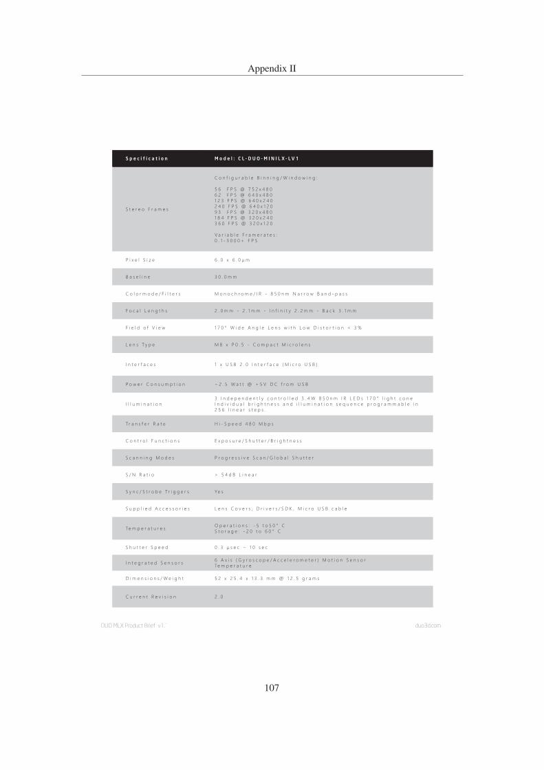
DUO MLX Product Brief v1.1 duo3d.com
S p e c i f i c a t i o n M o d e l : C L - D U O - M I N I L X - L V 1
S t e r e o F r a m e s
C o n f i g u r a b l e B i n n i n g / W i n d o w i n g :
5 6 F P S @ 7 5 2 x 4 8 06 2 F P S @ 6 4 0 x 4 8 01 2 3 F P S @ 6 4 0 x 2 4 02 4 0 F P S @ 6 4 0 x 1 2 09 3 F P S @ 3 2 0 x 4 8 01 8 4 F P S @ 3 2 0 x 2 4 03 6 0 F P S @ 3 2 0 x 1 2 0
V a r i a b l e F r a m e r a t e s :0 . 1 - 3 0 0 0 + F P S
P i x e l S i z e
B a s e l i n e 3 0 . 0 m m
C o l o r m o d e / F i l t e r s M o n o c h r o m e / I R - 8 5 0 n m N a r r o w B a n d - p a s s
F o c a l L e n g t h s 2 . 0 m m - 2 . 1 m m - I n f i n i t y 2 . 2 m m - B a c k 3 . 1 m m
F i e l d o f V i e w 1 7 0 ° W i d e A n g l e L e n s w i t h L o w D i s t o r t i o n < 3 %
L e n s T y p e M 8 x P 0 . 5 - C o m p a c t M i c r o l e n s
I n t e r f a c e s 1 x U S B 2 . 0 I n t e r f a c e ( M i c r o U S B )
P o w e r C o n s u m p t i o n ~ 2 . 5 W a t t @ + 5 V D C f r o m U S B
I l l u m i n a t i o n3 I n d e p e n d e n t l y c o n t r o l l e d 3 . 4 W 8 5 0 n m I R L E D s 1 7 0 ° l i g h t c o n eI n d i v i d u a l b r i g h t n e s s a n d i l l u m i n a t i o n s e q u e n c e p r o g r a m m a b l e i n 2 5 6 l i n e a r s t e p s .
T r a n s f e r R a t e H i - S p e e d 4 8 0 M b p s
C o n t r o l F u n c t i o n s E x p o s u r e / S h u t t e r / B r i g h t n e s s
S c a n n i n g M o d e s P r o g r e s s i v e S c a n / G l o b a l S h u t t e r
S / N R a t i o > 5 4 d B L i n e a r
S y n c / S t r o b e T r i g g e r s Ye s
S u p p l i e d A c c e s s o r i e s L e n s C o v e r s , D r i v e r s / S D K , M i c r o U S B c a b l e
Te m p e r a t u r e s O p e r a t i o n s : - 5 t o 5 0 ° CS t o r a g e : - 2 0 t o 6 0 ° C
S h u t t e r S p e e d
I n t e g r a t e d S e n s o r s 6 A x i s ( G y r o s c o p e / A c c e l e r o m e t e r ) M o t i o n S e n s o rTe m p e r a t u r e
D i m e n s i o n s / W e i g h t 5 2 x 2 5 . 4 x 1 3 . 3 m m @ 1 2 . 5 g r a m s
C u r r e n t R e v i s i o n 2 . 0
Appendix II
107

DUO MLX Product Brief v1.1 duo3d.com
Sensor Access & Control
The DUO API provides low level access and
control of the device and related sensors.
Whether running in standalone or in an
array the API allows for precise manipulation
of common parameters such as acquisition
rates and illumination methods. This is a
requirement for developing fully custom
machine vision applications.
Applications & Algorithms The DUO SDK provides high level
applications and algorithms for working
with modern stereo vision systems. With
applications ranging from standard matching
examples, dense 3D reconstruction, hand
and face tracking and more we aim to give
developers a head start by providing highly
optimized production quality solutions.
[email protected] create vision™Code Laboratories, Inc.Las Vegas, Nevada - USA
© Copyright 2014 Code Laboratories, Inc.. All rights reserved. DUO3D™ and its associated logo are trademarks of CL Inc. and are the subject of trademark applications or registrations in various countries around the world. All other trademarks are the property of their respective owners. All CL Inc. products and services are subject to continuous development. We reserve the right to alter
Requirements
Phone: 1-800-282-5031
Software Overview
30.02mm
13.30mm
25.40mm
52.02mm
Appendix II
108

Unleash Your Potential with the Jetson TX1 Development Kit
The Tech Specs
The Jetson TX1 Developer Kit is a full-featured development platform for visual computing designed to get you up and running fast. It comes pre-flashedwith a Linux environment, includes support for many common APIs, and is supported by NVIDIA’s complete development tool chain. The board alsoexposes a variety of standard hardware interfaces, enabling a highly flexible and extensible platform. This makes it ideal for all your applications requiringhigh computational performance in a low-power envelope.
What's in the DevKit?
You will receive the Jetson TX1 Developer Board, AC adapter with power cord, a USB Micro B to USB A adapter, a copy of the Quick Start Guide, SafetyGuide, and two Antennas for Wi-Fi.
JETSON TX1 MODULE
NVIDIA Maxwell™ GPU with 256 NVIDIA® CUDA® CoresQuad-core ARM® Cortex®-A57 MPCore Processor4 GB LPDDR4 Memory16 GB eMMC 5.1 Flash Storage10/100/1000BASE-T Ethernet
JETSON CAMERA MODULE
5 MP Fixed Focus MIPI CSI Camera
BUTTONS
Power On/OffResetForce RecoveryUser-Defined
I/O
Appendix III
III Jetson TX1 Datasheet
109

USB 3.0 Type AUSB 2.0 Micro AB (supports recovery and host mode)HDMIM.2 Key EPCI-E x4Gigabit EthernetFull-Size SDSATA Data and PowerGPIOs, I2C, I2S, SPI*TTL UART with Flow ControlDisplay Expansion Header*Camera Expansion Header*
*I/O expansion headers: refer to product documentation for header specification.
POWER OPTIONS
External 19V AC adapter
The following items are recommended, but not included:
HDMI Display and Cable (Type A)Keyboard and MouseJTAG DebuggerTTL to RS232 UART
Select Your Country Austria (http://www.nvidia.de/object/jetson-tx1-dev-kit-de.html)
Belgium (http://www.nvidia.fr/object/jetson-tx1-dev-kit-fr.html)
Canada (http://www.nvidia.com/object/jetson-tx1-dev-kit.html)
Czech Republic (http://www.nvidia.co.uk/object/jetson-tx1-dev-kit-uk.html)
Denmark (http://www.nvidia.co.uk/object/jetson-tx1-dev-kit-uk.html)
Finland (http://www.nvidia.co.uk/object/jetson-tx1-dev-kit-uk.html)
France (http://www.nvidia.fr/object/jetson-tx1-dev-kit-fr.html)
Germany (http://www.nvidia.de/object/jetson-tx1-dev-kit-de.html)
Ireland (http://www.nvidia.co.uk/object/jetson-tx1-dev-kit-uk.html)
Israel (http://www.nvidia.co.uk/object/jetson-tx1-dev-kit-il.html)
Italy (http://www.nvidia.it/object/jetson-tx1-dev-kit-it.html)
Japan (http://www.nvidia.co.jp/object/jetson-tx1-dev-kit-jp.html)
South Korea (http://www.nvidia.co.kr/object/jetson-tx1-dev-kit-kr.html)
Luxembourg (http://www.nvidia.fr/object/jetson-tx1-dev-kit-fr.html)
Netherlands (http://www.nvidia.co.uk/object/jetson-tx1-dev-kit-uk.html)
Norway (http://www.nvidia.co.uk/object/jetson-tx1-dev-kit-uk.html)
Poland (http://www.nvidia.pl/object/jetson-tx1-dev-kit-pl.html)
Portugal (http://www.nvidia.es/object/jetson-tx1-dev-kit-es.html)
Appendix III
110

Appendix IV
IV REX Exoskeleton Datasheet
111

Appendix IV
112

Appendix V
V Additional Results
Included in the bonus content package are results not published here. These are sorted by location
and often include processed point cloud exports alongside traversability mapping images.
113

Appendix VI
VI Source Code
Listing 1: ROS Interface Program C++ Header
1 // ========================================================================
2 // Rex ROS Sample Core Node
3 // Copyright(C) {2016} {Manu Lange}
4 //
5 // This program is free software : you can redistribute it and / or modify
6 // it under the terms of the GNU General Public License as published by
7 // the Free Software Foundation, either version 3 of the License, or
8 // (at your option) any later version.
9 //
10 // This program is distributed in the hope that it will be useful,
11 // but WITHOUT ANY WARRANTY; without even the implied warranty of
12 // MERCHANTABILITY or FITNESS FOR A PARTICULAR PURPOSE.See the
13 // GNU General Public License for more details.
14 //
15 // You should have received a copy of the GNU General Public License
16 // along with this program.If not, see < http ://www.gnu.org/licenses/>.
17 // ========================================================================
18 #pragma once
19
20 #include <r o s / r o s . h>
21 #include < s t d s r v s / Empty . h>
22 #include < t f 2 r o s / t r a n s f o r m l i s t e n e r . h>
23 #include <t f 2 g e o m e t r y m s g s / t f 2 g e o m e t r y m s g s . h>
24 #include < t f 2 / c o n v e r t . h>
25 #include < t f 2 e i g e n / t f 2 e i g e n . h>
26 #include <v e c t o r>
27 #include <geomet ry msgs / TransformStamped . h>
28 #include <geomet ry msgs / Twis t . h>
29 #include <geomet ry msgs / PolygonStamped . h>
30 #include <v i s u a l i z a t i o n m s g s / Marker . h>
31 #include <geomet ry msgs / PoseStamped . h>
32 #include < r e x i n t e r f a c e / s t e p Q u e r y . h>
33 #include < t r a v e r s a b i l i t y m s g s / C h e c k F o o t p r i n t P a t h . h>
34 #include < t r a v e r s a b i l i t y m s g s / F o o t p r i n t P a t h . h>
35 #include < t r a v e r s a b i l i t y m s g s / T r a v e r s a b i l i t y R e s u l t . h>
36
37 class R e x I n t e r f a c e
38 {39 public :
40 R e x I n t e r f a c e ( r o s : : NodeHandle& nodeHandle ) ;
41 ˜ R e x I n t e r f a c e ( ) ;
42
43 /*!
114

Appendix VI
44 * Attempts to take a step in the given direction.
45 * @param request the ROS service request.
46 * @param response the ROS service response.
47 * @return true if successful.
48 */
49 bool s t e p ( r e x i n t e r f a c e : : s t e p Q u e r y : : R e q u es t& r e q u e s t , r e x i n t e r f a c e : :
s t e p Q u e r y : : Response& r e s p o n s e ) ;
50
51 /*!
52 * Reads in all the parameters from the parameter server.
53 * @return true if successful.
54 */
55 bool r e a d P a r a m t e r s ( ) ;
56
57 /*!
58 * Callback for a movement goal message. Well check if footstep is
possible at goal.
59 * @return true if successful.
60 */
61 void s t e p Q u e r y C a l l b a c k (const geomet ry msgs : : Po s e S t a m p e d C o n s t P t r&
message ) ;
62
63 void v i s u a l i s e (const geomet ry msgs : : Pose f o o t p r i n t ) ;
64
65 private :
66 r o s : : NodeHandle& nodeHand le ;
67 r o s : : P u b l i s h e r m a r k e r P u b l i s h e r ;
68 r o s : : S u b s c r i b e r s t e p Q u e r y P o s e S u b s c r i b e r ;
69 r o s : : S e r v i c e S e r v e r s t e p F o r w a r d S e r v i c e ;
70 r o s : : S e r v i c e S e r v e r s t e p S e r v i c e ;
71 r o s : : S e r v i c e C l i e n t f o o t p r i n t C h e c k e r S u b s c r i b e r ;
72 t f 2 r o s : : B u f f e r t f B u f f e r ;
73 t f 2 r o s : : T r a n s f o r m L i s t e n e r t f L i s t e n e r ;
74
75 //! Vertices of the footprint polygon in base frame.
76 s t d : : v e c t o r<geomet ry msgs : : Po in t32> f o o t p r i n t P o i n t s ;
77
78 //parameters
79 s t d : : s t r i n g f o o t p r i n t S e r v i c e N a m e ;
80 s t d : : s t r i n g f o o t p r i n t F r a m e ;
81 double s t e p F o r w a r d D i s t a n c e ;
82 double s t e p B a c k w a r d D i s t a n c e ;
83 double s t e p S i d e w a y s D i s t a n c e ;
84 double f o o t p r i n t R a d i u s ;
85 double s a f e T r a v e r s e ;
86
87 /// <summary>Joystick sectors</summary>
115

Appendix VI
88 enum E J o y s t i c k S e c t o r : int
89 {90 NO POSITION = 0 ,
91 INSIDE N ,
92 INSIDE NE ,
93 INSIDE E ,
94 INSIDE SE ,
95 INSIDE S ,
96 INSIDE SW ,
97 INSIDE W ,
98 INSIDE NW ,
99 OUTSIDE N ,
100 OUTSIDE NNE ,
101 OUTSIDE NE ,
102 OUTSIDE ENE ,
103 OUTSIDE E ,
104 OUTSIDE ESE ,
105 OUTSIDE SE ,
106 OUTSIDE SSE ,
107 OUTSIDE S ,
108 OUTSIDE SSW ,
109 OUTSIDE SW ,
110 OUTSIDE WSW,
111 OUTSIDE W ,
112 OUTSIDE WNW,
113 OUTSIDE NW,
114 OUTSIDE NNW,
115 } ;
116
117 enum Resu l tCode : int
118 {119 OK = 0 ,
120 NOT TRAVERSABLE,
121 ERROR = −1,
122 } ;
123 } ;
Listing 2: ROS Interface Program C++ Source
1 // ========================================================================
2 // Rex ROS Sample Core Node
3 // Copyright(C) {2016} {Manu Lange}
4 //
5 // This program is free software : you can redistribute it and / or modify
6 // it under the terms of the GNU General Public License as published by
7 // the Free Software Foundation, either version 3 of the License, or
8 // (at your option) any later version.
116

Appendix VI
9 //
10 // This program is distributed in the hope that it will be useful,
11 // but WITHOUT ANY WARRANTY; without even the implied warranty of
12 // MERCHANTABILITY or FITNESS FOR A PARTICULAR PURPOSE.See the
13 // GNU General Public License for more details.
14 //
15 // You should have received a copy of the GNU General Public License
16 // along with this program.If not, see < http ://www.gnu.org/licenses/>.
17 // ========================================================================
18
19 #include <i o s t r e a m>
20 #include <p c l / common / common headers . h>
21 #include <Eigen / Core>
22
23
24 #include "../include/rex_interface/rex_interface.hpp"
25
26
27
28 R e x I n t e r f a c e : : R e x I n t e r f a c e ( r o s : : NodeHandle& nodeHandle )
29 : nodeHandle ( nodeHandle ) ,
30 t f L i s t e n e r ( t f B u f f e r )
31 {32 r e a d P a r a m t e r s ( ) ;
33
34 //Load publishers
35 m a r k e r P u b l i s h e r = nodeHandle . a d v e r t i s e <v i s u a l i z a t i o n m s g s : : Marker>("
visualization_marker" , 0 ) ;
36
37 //Load service handlers
38 s t e p F o r w a r d S e r v i c e = nodeHandle . a d v e r t i s e S e r v i c e ("step_forward" , &
R e x I n t e r f a c e : : s t epForward , this ) ;
39 s t e p S e r v i c e = nodeHandle . a d v e r t i s e S e r v i c e ("step" , &R e x I n t e r f a c e : : s t e p ,
this ) ;
40
41 //Subscribe to services
42 f o o t p r i n t C h e c k e r S u b s c r i b e r = nodeHandle . s e r v i c e C l i e n t <
t r a v e r s a b i l i t y m s g s : : C h e c k F o o t p r i n t P a t h >( f o o t p r i n t S e r v i c e N a m e ) ;
43
44 //Subscribe to messages
45 s t e p Q u e r y P o s e S u b s c r i b e r = nodeHandle . s u b s c r i b e ("/move_base_simple/goal
" , 1 , &R e x I n t e r f a c e : : s t e p Q u e r y C a l l b a c k , this ) ;
46
47 }48
49 R e x I n t e r f a c e : : ˜ R e x I n t e r f a c e ( )
50 {
117

Appendix VI
51 nodeHandle . shutdown ( ) ;
52 }53
54 bool R e x I n t e r f a c e : : s t e p ( r e x i n t e r f a c e : : s t e p Q u e r y : : Reques t& r e q u e s t ,
r e x i n t e r f a c e : : s t e p Q u e r y : : Response& r e s p o n s e )
55 {56 //Establish local variables
57 t r a v e r s a b i l i t y m s g s : : C h e c k F o o t p r i n t P a t h f o o t p r i n t S e r v i c e ;
58 t r a v e r s a b i l i t y m s g s : : F o o t p r i n t P a t h f o o t p r i n t P a t h ;
59 geomet ry msgs : : Pose f o o t p r i n t ;
60 r e s p o n s e . r e s u l t C o d e = Resu l tCode : : ERROR; //default to error
61
62 geomet ry msgs : : TransformStamped t r a n s f o r m S t a m p e d ;
63 //Get transform to map
64 try {65 t r a n s f o r m S t a m p e d = t f B u f f e r . l o o k u p T r a n s f o r m ("map" ,
66 "base_link" ,
67 r o s : : Time ( 0 ) , r o s : : D u r a t i o n ( 1 . 0 ) ) ;
68 }69 catch ( t f 2 : : T r a n s f o r m E x c e p t i o n &ex ) {70 ROS WARN("%s" , ex . what ( ) ) ;
71 return false ;
72 }73
74 //tf2::Vector3 footPosition;
75 E igen : : Vec to r3d f o o t P o s i t i o n ;
76
77 //Check if the direction queried is handled. This should become generic
eventually..
78 f o o t P o s i t i o n . z ( ) = 0 . 0 ; //Default z height
79 f o o t p r i n t . o r i e n t a t i o n . x = f o o t p r i n t . o r i e n t a t i o n . y = f o o t p r i n t .
o r i e n t a t i o n . z = f o o t p r i n t . o r i e n t a t i o n .w = 0 . 0 ; //Default
orientation
80 switch ( r e q u e s t . d i r e c t i o n )
81 {82 case OUTSIDE N :
83 f o o t P o s i t i o n . x ( ) = s t e p F o r w a r d D i s t a n c e ;
84 f o o t P o s i t i o n . y ( ) = 0 . 0 ;
85 break ;
86 case OUTSIDE E :
87 f o o t P o s i t i o n . x ( ) = 0 . 0 ;
88 f o o t P o s i t i o n . y ( ) = −s t e p S i d e w a y s D i s t a n c e ;
89 break ;
90 case OUTSIDE S :
91 f o o t P o s i t i o n . x ( ) = −s t e p B a c k w a r d D i s t a n c e ;
92 f o o t P o s i t i o n . y ( ) = 0 . 0 ;
93 break ;
118

Appendix VI
94 case OUTSIDE W :
95 f o o t P o s i t i o n . x ( ) = 0 . 0 ;
96 f o o t P o s i t i o n . y ( ) = s t e p S i d e w a y s D i s t a n c e ;
97 break ;
98 default :
99 return false ; //Unhandled case, return an error.
100 }101
102 //Transform frames
103 Eigen : : A f f i n e 3 d eigenTF = t f 2 : : t r a n s f o r m T o E i g e n ( t r a n s f o r m S t a m p e d ) ;
104 Eigen : : A f f i n e 3 f e i g e n T F f = eigenTF . c a s t<float>() ; //need flaot form
for PCL helper
105 f o o t P o s i t i o n = eigenTF∗ f o o t P o s i t i o n ;
106 float r o l l , p i t c h , yaw ;
107 p c l : : g e t E u l e r A n g l e s ( e igenTFf , r o l l , p i t c h , yaw ) ;
108 //ROS_INFO("Roll: %f, Pitch: %f, Yaw: %f", roll,pitch,yaw);
109 float yawTOw = ( 1 . 5 7 0 7 9 6 / yaw ) ; //For some reason the quarternion uses
a scale of 2.0 per pi radians... Maybe it uses 2 * vector length,
which I set to 1.0?
110 //bug may be the normalisation of quart. Testing
111 Eigen : : Q u a t e r n i o n<double> t e s t i n g ;
112 t f 2 : : Q u a t e r n i o n normalQuat ;
113 normalQuat . setRPY ( 0 . 0 , 0 . 0 , yaw ) ;
114 normalQuat . n o r m a l i z e ( ) ;
115 //Set rotation
116 f o o t p r i n t . o r i e n t a t i o n . x = normalQuat . x ( ) ;
117 f o o t p r i n t . o r i e n t a t i o n . y = normalQuat . y ( ) ;
118 f o o t p r i n t . o r i e n t a t i o n . z = normalQuat . z ( ) ;
119 f o o t p r i n t . o r i e n t a t i o n .w = normalQuat .w( ) ;
120
121 //load footprints into service message
122 f o o t p r i n t . p o s i t i o n . x = f o o t P o s i t i o n . x ( ) ;
123 f o o t p r i n t . p o s i t i o n . y = f o o t P o s i t i o n . y ( ) ;
124 f o o t p r i n t . p o s i t i o n . z = 0 . 0 ; //footPosition.z(); //Testing force 0
125 f o o t p r i n t P a t h . p o s e s . h e a d e r . f r a m e i d = f o o t p r i n t F r a m e ; //Test using /
map instead of footprintFrame_
126 f o o t p r i n t P a t h . p o s e s . h e a d e r . s tamp = r o s : : Time : : now ( ) ;
127 f o o t p r i n t P a t h . p o s e s . p o s e s . p u s h b a c k ( f o o t p r i n t ) ;
128
129 //Using polygon
130 f o o t p r i n t P a t h . r a d i u s = 0 . 0 ; //Testing polygons
131 f o o t p r i n t P a t h . f o o t p r i n t . h e a d e r = f o o t p r i n t P a t h . p o s e s . h e a d e r ;
132
133 for ( s i z e t i = 0 ; i < f o o t p r i n t P o i n t s . s i z e ( ) ; i ++)
134 {135 f o o t p r i n t P a t h . f o o t p r i n t . po lygon . p o i n t s . p u s h b a c k ( f o o t p r i n t P o i n t s [ i ] )
;
119

Appendix VI
136 }137
138 //copy into service request
139 f o o t p r i n t S e r v i c e . r e q u e s t . p a t h . p u s h b a c k ( f o o t p r i n t P a t h ) ;
140
141 ROS INFO ("Debugging: %f, %f, %f || %f, %f, %f, %f || %s" ,
142 f o o t p r i n t P a t h . p o s e s . p o s e s . f r o n t ( ) . p o s i t i o n . x ,
143 f o o t p r i n t P a t h . p o s e s . p o s e s . f r o n t ( ) . p o s i t i o n . y ,
144 f o o t p r i n t P a t h . p o s e s . p o s e s . f r o n t ( ) . p o s i t i o n . z ,
145 f o o t p r i n t P a t h . p o s e s . p o s e s . f r o n t ( ) . o r i e n t a t i o n . x ,
146 f o o t p r i n t P a t h . p o s e s . p o s e s . f r o n t ( ) . o r i e n t a t i o n . y ,
147 f o o t p r i n t P a t h . p o s e s . p o s e s . f r o n t ( ) . o r i e n t a t i o n . z ,
148 f o o t p r i n t P a t h . p o s e s . p o s e s . f r o n t ( ) . o r i e n t a t i o n . w,
149 f o o t p r i n t P a t h . p o s e s . h e a d e r . f r a m e i d . c s t r ( ) ) ;
150
151 //call service
152 f o o t p r i n t C h e c k e r S u b s c r i b e r . w a i t F o r E x i s t e n c e ( ) ; //wait for it
153 ROS DEBUG("Calling footprint checker service" ) ;
154 f o o t p r i n t C h e c k e r S u b s c r i b e r . c a l l ( f o o t p r i n t S e r v i c e ) ;
155
156 //Testing Visualisation
157 v i s u a l i s e ( f o o t p r i n t ) ;
158
159 double r e s u l t = 0 . 0 ;
160 r e s u l t = f o o t p r i n t S e r v i c e . r e s p o n s e . r e s u l t . f r o n t ( ) . t r a v e r s a b i l i t y ;
161 ROS INFO ("Traversibility: %f" , r e s u l t ) ;
162
163 if ( r e s u l t >= s a f e T r a v e r s e ) //Todo: Figure out why sometimes it
returns values around 0.95 when some cells are ’unseen’
164 r e s p o n s e . r e s u l t C o d e = Resu l tCode : : OK;
165 else
166 r e s p o n s e . r e s u l t C o d e = Resu l tCode : : NOT TRAVERSABLE;
167
168 //Todo: Figure out how to handle unmapped terrain properly...? Maybe the
isSafe flag on footpath response?
169
170 return true ;
171 }172
173 bool R e x I n t e r f a c e : : r e a d P a r a m t e r s ( )
174 {175 //Added footprint for query
176 // Read footprint polygon.
177 XmlRpc : : XmlRpcValue f o o t p r i n t ;
178 if ( nodeHandle . ge tParam ("footprint/footprint_polygon" , f o o t p r i n t ) ) {179 if ( f o o t p r i n t . s i z e ( ) < 3) {180 ROS WARN("Footprint polygon must consist of at least 3 points.
120

Appendix VI
Only %i points found." , f o o t p r i n t . s i z e ( ) ) ;
181 f o o t p r i n t P o i n t s . c l e a r ( ) ;
182 }183 else {184 geomet ry msgs : : P o i n t 3 2 p t ;
185 p t . z = 0 . 0 ;
186 for (int i = 0 ; i < f o o t p r i n t . s i z e ( ) ; i ++) {187 p t . x = (double ) f o o t p r i n t [ i ] [ 0 ] ;
188 p t . y = (double ) f o o t p r i n t [ i ] [ 1 ] ;
189 f o o t p r i n t P o i n t s . p u s h b a c k ( p t ) ;
190 }191 }192 }193 else {194 ROS WARN("Traversability Map: No footprint polygon defined." ) ;
195 }196
197 nodeHandle . param ("footprintServiceName" , f o o t p r i n t S e r v i c e N a m e , s t d : :
s t r i n g ("/rex_traversibility/check_footprint_path" ) ) ;
198 nodeHandle . param ("footprintFrame" , f o o t p r i n t F r a m e , s t d : : s t r i n g ("
base_link" ) ) ;
199 nodeHandle . param ("stepForwardDistance" , s t e p F o r w a r d D i s t a n c e , 0 . 4 0 ) ;
200 nodeHandle . param ("stepBackwardDistance" , s t e p B a c k w a r d D i s t a n c e , 0 . 2 5 ) ;
201 nodeHandle . param ("stepSidwaysDistance" , s t e p S i d e w a y s D i s t a n c e , 0 . 1 0 ) ;
202 nodeHandle . param ("footprintRadius" , f o o t p r i n t R a d i u s , 0 . 1 5 ) ;
203 nodeHandle . param ("safeTraverse" , s a f e T r a v e r s e , 0 . 8 0 ) ;
204 return true ;
205 }206
207 void R e x I n t e r f a c e : : s t e p Q u e r y C a l l b a c k (const geomet ry msgs : :
P o s e S t a m p e d C o n s t P t r& message )
208 {209 t r a v e r s a b i l i t y m s g s : : C h e c k F o o t p r i n t P a t h f o o t p r i n t S e r v i c e ;
210 t r a v e r s a b i l i t y m s g s : : F o o t p r i n t P a t h f o o t p r i n t P a t h ;
211 geomet ry msgs : : Pose f o o t p r i n t ;
212
213 //Copy pose information into footprint message
214 f o o t p r i n t . p o s i t i o n . x = message−>pose . p o s i t i o n . x ;
215 f o o t p r i n t . p o s i t i o n . y = message−>pose . p o s i t i o n . y ;
216 f o o t p r i n t . p o s i t i o n . z = message−>pose . p o s i t i o n . z ;
217
218 f o o t p r i n t . o r i e n t a t i o n . x = message−>pose . o r i e n t a t i o n . x ;
219 f o o t p r i n t . o r i e n t a t i o n . y = message−>pose . o r i e n t a t i o n . y ;
220 f o o t p r i n t . o r i e n t a t i o n . z = message−>pose . o r i e n t a t i o n . z ;
221 f o o t p r i n t . o r i e n t a t i o n .w = message−>pose . o r i e n t a t i o n .w;
222
223 //load footprints into service message
121

Appendix VI
224 f o o t p r i n t P a t h . p o s e s . h e a d e r . f r a m e i d = f o o t p r i n t F r a m e ; //This should
be changed...
225 f o o t p r i n t P a t h . p o s e s . h e a d e r . s tamp = r o s : : Time : : now ( ) ;
226 f o o t p r i n t P a t h . p o s e s . p o s e s . p u s h b a c k ( f o o t p r i n t ) ;
227
228
229 //assign radius, this could later be a polygon
230 f o o t p r i n t P a t h . r a d i u s = 0 . 0 ; //Testing polygons
231 f o o t p r i n t P a t h . f o o t p r i n t . h e a d e r = f o o t p r i n t P a t h . p o s e s . h e a d e r ;
232
233 for ( s i z e t i = 0 ; i < f o o t p r i n t P o i n t s . s i z e ( ) ; i ++)
234 {235 f o o t p r i n t P a t h . f o o t p r i n t . po lygon . p o i n t s . p u s h b a c k ( f o o t p r i n t P o i n t s [ i ] )
;
236 }237
238 //copy into service request
239 f o o t p r i n t S e r v i c e . r e q u e s t . p a t h . p u s h b a c k ( f o o t p r i n t P a t h ) ;
240
241 ROS INFO ("Debugging: %f, %f, %f || %f, %f, %f, %f || %s" ,
242 f o o t p r i n t P a t h . p o s e s . p o s e s . f r o n t ( ) . p o s i t i o n . x ,
243 f o o t p r i n t P a t h . p o s e s . p o s e s . f r o n t ( ) . p o s i t i o n . y ,
244 f o o t p r i n t P a t h . p o s e s . p o s e s . f r o n t ( ) . p o s i t i o n . z ,
245 f o o t p r i n t P a t h . p o s e s . p o s e s . f r o n t ( ) . o r i e n t a t i o n . x ,
246 f o o t p r i n t P a t h . p o s e s . p o s e s . f r o n t ( ) . o r i e n t a t i o n . y ,
247 f o o t p r i n t P a t h . p o s e s . p o s e s . f r o n t ( ) . o r i e n t a t i o n . z ,
248 f o o t p r i n t P a t h . p o s e s . p o s e s . f r o n t ( ) . o r i e n t a t i o n . w,
249 f o o t p r i n t P a t h . p o s e s . h e a d e r . f r a m e i d . c s t r ( ) ) ;
250
251 //call service
252 f o o t p r i n t C h e c k e r S u b s c r i b e r . w a i t F o r E x i s t e n c e ( ) ; //wait for it
253 ROS DEBUG("Calling footprint checker service" ) ;
254 f o o t p r i n t C h e c k e r S u b s c r i b e r . c a l l ( f o o t p r i n t S e r v i c e ) ;
255
256 //Testing Visualisation
257 v i s u a l i s e ( f o o t p r i n t ) ;
258
259 double t e s t = 0 . 0 ;
260 t e s t = f o o t p r i n t S e r v i c e . r e s p o n s e . r e s u l t . f r o n t ( ) . t r a v e r s a b i l i t y ;
261 ROS INFO ("Traversibility: %f" , f o o t p r i n t S e r v i c e . r e s p o n s e . r e s u l t . f r o n t ( ) .
t r a v e r s a b i l i t y ) ;
262
263 }264
265
266 void R e x I n t e r f a c e : : v i s u a l i s e (const geomet ry msgs : : Pose f o o t p r i n t )
267 {
122

Appendix VI
268 //Testing Visualisation
269 v i s u a l i z a t i o n m s g s : : Marker marker ;
270 marker . h e a d e r . f r a m e i d = "map" ;
271 marker . h e a d e r . s tamp = r o s : : Time ( ) ;
272 marker . ns = "rex_interface" ;
273 marker . i d = 0 ;
274 marker . t y p e = v i s u a l i z a t i o n m s g s : : Marker : : LINE STRIP ;
275 marker . a c t i o n = v i s u a l i z a t i o n m s g s : : Marker : :ADD;
276 marker . pose . p o s i t i o n . x = f o o t p r i n t . p o s i t i o n . x ;
277 marker . pose . p o s i t i o n . y = f o o t p r i n t . p o s i t i o n . y ;
278 marker . pose . p o s i t i o n . z = f o o t p r i n t . p o s i t i o n . z ;
279 marker . pose . o r i e n t a t i o n . x = f o o t p r i n t . o r i e n t a t i o n . x ;
280 marker . pose . o r i e n t a t i o n . y = f o o t p r i n t . o r i e n t a t i o n . y ;
281 marker . pose . o r i e n t a t i o n . z = f o o t p r i n t . o r i e n t a t i o n . z ;
282 marker . pose . o r i e n t a t i o n .w = f o o t p r i n t . o r i e n t a t i o n .w;
283
284 for ( s i z e t i = 0 ; i < f o o t p r i n t P o i n t s . s i z e ( ) ; i ++)
285 {286 geomet ry msgs : : P o i n t t e s t 2 ;
287 t e s t 2 . x = f o o t p r i n t P o i n t s [ i ] . x ;
288 t e s t 2 . y = f o o t p r i n t P o i n t s [ i ] . y ;
289 t e s t 2 . z = f o o t p r i n t P o i n t s [ i ] . z ;
290 marker . p o i n t s . p u s h b a c k ( t e s t 2 ) ;
291 }292 marker . s c a l e . x = 0 . 0 5 ;
293 marker . s c a l e . y = 1 . 0 ;
294 marker . s c a l e . z = 1 . 0 ;
295 marker . c o l o r . a = 0 . 7 5 ; // Don’t forget to set the alpha!
296 marker . c o l o r . r = 0 . 0 ;
297 marker . c o l o r . g = 1 . 0 ;
298 marker . c o l o r . b = 0 . 0 ;
299 m a r k e r P u b l i s h e r . p u b l i s h ( marker ) ;
300 }
Listing 3: ROS Xacro model code
1 <?xml version="1.0"?>
2 <robot xmlns:xacro="http://www.ros.org/wiki/xacro" name="rex_collision">
3 <xacro:property name="robotName" value="rex"/>
4 <xacro:property name="pelvisWidth" value="0.470"/>
5 <xacro:property name="upperLegDepth" value="0.15"/>
6 <xacro:property name="upperLegWidth" value="0.15"/>
7 <xacro:property name="upperLegHeight" value="0.43"/>
8 <xacro:property name="lowerLegDepth" value="0.15"/>
9 <xacro:property name="lowerLegWidth" value="0.15"/>
10 <xacro:property name="lowerLegHeight" value="0.416"/>
11 <xacro:property name="footDepth" value="0.366"/>
123

Appendix VI
12 <xacro:property name="footWidth" value="0.190"/>
13 <xacro:property name="footHeight" value="0.144"/>
14 <xacro:property name="footBackToAnkle" value="0.126"/>
15 <xacro:property name="footInsideToAnkle" value="0.150"/>
16
17 <!--NOTE: Floor to base_link distance = ${ref_foot}-footHeight-->
18
19 <xacro:macro name="default_inertial" params="mass">
20 <inertial>
21 <mass value="${mass}"/>
22 <inertia ixx="1.0" ixy="0.0" ixz="0.0" iyy="1.0" iyz="0.0" izz="1.0"
/>
23 </inertial>
24 </xacro:macro>
25
26 <xacro:macro name="upperleg" params="prefix reflect">
27 <link name="${prefix}_upperleg">
28 <visual>
29 <geometry>
30 <box size="${upperLegDepth} ${upperLegWidth} ${upperLegHeight}"/>
31 </geometry>
32 <origin xyz="0 0 -${upperLegHeight/2}" rpy="0 0 0"/>
33 <material name="white">
34 <color rgba="1 1 1 1"/>
35 </material>
36 </visual>
37 <!--This is currently more of a place holder and not used...-->
38 <xacro:default_inertial mass="10"/>
39 </link>
40 <joint name="pelvis_to_${prefix}_upperleg" type="revolute">
41 <axis xyz="0 1 0"/>
42 <parent link="${robotName}_base_link"/>
43 <child link="${prefix}_upperleg"/>
44 <origin xyz="0 ${reflect*pelvisWidth/2} 0"/>
45 <limit effort="1000.0" lower="-${pi/4}" upper="${pi/4}" velocity="10"
/>
46 </joint>
47 </xacro:macro>
48
49 <xacro:macro name="lowerleg" params="prefix reflect">
50 <link name="${prefix}_lowerleg">
51 <visual>
52 <geometry>
53 <box size="${lowerLegDepth} ${lowerLegWidth} ${lowerLegHeight}"/>
54 </geometry>
55 <origin xyz="0 0 -${lowerLegHeight/2}" rpy="0 0 0"/>
56 <material name="white">
124

Appendix VI
57 <color rgba="1 1 1 1"/>
58 </material>
59 </visual>
60 <!--This is currently more of a place holder and not used...-->
61 <xacro:default_inertial mass="10"/>
62 </link>
63 <joint name="${prefix}_upperleg_to_${prefix}_lowerleg" type="revolute">
64 <axis xyz="0 1 0"/>
65 <parent link="${prefix}_upperleg"/>
66 <child link="${prefix}_lowerleg"/>
67 <origin xyz="0 0 -${upperLegHeight}"/>
68 <limit effort="1000.0" lower="-${pi/4}" upper="${pi/4}" velocity="10"
/>
69 </joint>
70 </xacro:macro>
71
72 <xacro:macro name="foot" params="prefix reflect">
73 <link name="${prefix}_foot">
74 <visual>
75 <geometry>
76 <box size="${footDepth} ${footWidth} ${footHeight}"/>
77 </geometry>
78 <origin xyz="${footDepth/2-footBackToAnkle} ${reflect*(footWidth/2-
footInsideToAnkle)} -${footHeight/2}" rpy="0 0 0"/>
79 <material name="white">
80 <color rgba="1 1 1 1"/>
81 </material>
82 </visual>
83 <!--This is currently more of a place holder and not used...-->
84 <xacro:default_inertial mass="10"/>
85 </link>
86 <joint name="${prefix}_lowerleg_to_${prefix}_foot" type="revolute">
87 <axis xyz="0 1 0"/>
88 <parent link="${prefix}_lowerleg"/>
89 <child link="${prefix}_foot"/>
90 <origin xyz="0 0 -${lowerLegHeight}"/>
91 <limit effort="1000.0" lower="-${pi/4}" upper="${pi/4}" velocity="10"
/>
92 </joint>
93 </xacro:macro>
94
95 <link name="${robotName}_base_link">
96 <visual>
97 <geometry>
98 <box size="0.10 0.411 0.332"/>
99 </geometry>
100 <origin rpy="0 0 0" xyz="-0.160 0 -0.008"/>
125

Appendix VI
101 <material name="black">
102 <color rgba="0 0 0 1"/>
103 </material>
104 </visual>
105 <visual>
106 <geometry>
107 <box size="0.230 0.060 0.180"/>
108 </geometry>
109 <origin rpy="0 0 0" xyz="-0.07 ${pelvisWidth/2} 0.040"/>
110 <material name="white">
111 <color rgba="0 0 0 1"/>
112 </material>
113 </visual>
114 <visual>
115 <geometry>
116 <box size="0.230 0.060 0.180"/>
117 </geometry>
118 <origin rpy="0 0 0" xyz="-0.07 -${pelvisWidth/2} 0.040"/>
119 <material name="white">
120 <color rgba="0 0 0 1"/>
121 </material>
122 </visual>
123 </link>
124
125 <xacro:upperleg prefix="right" reflect="-1"/>
126 <xacro:upperleg prefix="left" reflect="1"/>
127 <xacro:lowerleg prefix="right" reflect="-1"/>
128 <xacro:lowerleg prefix="left" reflect="1"/>
129 <xacro:foot prefix="right" reflect="-1"/>
130 <xacro:foot prefix="left" reflect="1"/>
131 </robot>
126