1

Version 1.1

User Guide

2

Table of Contents Introduction ................................................................................................................................ 4

Setup .................................................................................................................................. 6

1.A) City Context .................................................................................................................... 6

1.B) Cost Data ........................................................................................................................ 7

1.C) Emission Factors ............................................................................................................ 7

1.D) Advanced User Options .................................................................................................. 8

INVENTORY ....................................................................................................................... 9

2.A) Base Year Inventory........................................................................................................ 9

I. Base Year Charts ............................................................................................................. 9

II. Base Year Tables ..........................................................................................................10

2.B) Growth Factors ..............................................................................................................10

I. Activity Growth Factors ...................................................................................................10

II. Building Inventory Growth Factors .................................................................................12

2.C) Projections .....................................................................................................................12

I. Sector Projections ...........................................................................................................12

II. Inventory Projections ......................................................................................................12

2.D) Targets ..........................................................................................................................13

I. Target Type Selection .....................................................................................................13

II. Target Level ...................................................................................................................14

III. Target Setting Resources..............................................................................................14

BENCHMARKING .............................................................................................................16

3.A) City Comparison ............................................................................................................16

3.B) Indicator Summary .........................................................................................................17

ACTIONS ..........................................................................................................................18

4.A) Action Selection .............................................................................................................18

I. Overview .........................................................................................................................18

II. Sector Selection .............................................................................................................18

III. City Authority .................................................................................................................19

IV. Assessment ..................................................................................................................21

V. Action Selection .............................................................................................................22

4.B) Action Development .......................................................................................................22

4.C) Financial Metrics ............................................................................................................46

3

I. Abatement Cost Curve ....................................................................................................46

II. Financial Performance Chart ..........................................................................................47

III. Financial Performance Table ........................................................................................48

4.D) Co-benefits ....................................................................................................................48

I. Co-benefits Matrix ...........................................................................................................48

II. Co-benefits Description ..................................................................................................49

RESULTS .........................................................................................................................50

5.A) Aggregate Results .........................................................................................................50

I. Emissions Performance ..................................................................................................50

II. Energy Performance ......................................................................................................51

5.B) Sector Results................................................................................................................51

I. Emissions Performance ..................................................................................................51

II. Energy Performance ......................................................................................................52

5.C) Action Summary ............................................................................................................53

5.D) Scenario Comparison ....................................................................................................53

I. Scenario Selection ..........................................................................................................53

II. Scenario Results ............................................................................................................54

III. Scenario Charts ............................................................................................................54

IV. Scenario Tables ............................................................................................................55

4

INTRODUCTION

Welcome to CURB: Climate Action for Urban Sustainability. This toolkit is designed to help guide

cities through the process of planning and implementing a range of interventions to reduce energy use, save money, and cut local greenhouse gas (GHG) emissions. The technology and policy interventions covered by CURB can also help deliver important local quality of life benefits, including improved air quality, local economic development and job creation

CURB was developed through collaboration between the World Bank Group, the C40 Cities network, and AECOM Technology Corporation. Each institution is actively engaged in supporting climate, energy, and sustainability planning efforts at the local scale in cities around the world. CURB is intended to allow planners to assess the implications of different policy and technology interventions.

CURB’s flexible and modular design responds to local realities, recognizing that impacts germane to one city (e.g. energy or emission impacts, cost savings, etc.) may be valued differently by others. CURB therefore presents information in different ways so users can select the information most relevant to their work.

The calculations made by the CURB tool are based on modeling approaches or assumptions developed by world-class engineers, economists, and planners. Their accuracy is linked to the quality of the data used in the tool, however, which is why CURB consistently asks the user to provide locally relevant information. Because data gaps are a common problem in cities, CURB does provide city, national or regional proxy data that the user can rely on if local information is unavailable or considered unreliable.

This User Guide explains the purpose and approach used in each of the six modules contained in the Toolkit. This Guide also explains what types of information are required to run each module, and what type of output is ultimately generated to support local planning and decision-making.

If any section of this user guide is unclear, please feel free to offer suggestions on how it can be improved by contacting the development team.

CURB contains a total of six modules with the following features:

Setup is where the user can enter basic data about the overall situation in a city and sectoral

profiles. This information is then used repeatedly throughout the Tool to help make different calculations.

Inventory converts the information provided in the Setup module into estimates of which sectors

create the greatest energy demand and GHG emissions and how the situation may change over time. It is in this module that the user also has the option to set future reduction performance targets against which progress can be measured.

Benchmarking allows users to compare their cities with other cities across a range of key

performance indicators in each sector.

Action is the heart of the tool. This module allows the user to select which sectors she would like

to focus on, and then to rate the city’s authority to take action in each sector. This information is then quickly translated into a rapid assessment of the maximum impact potential and implementation feasibility of every intervention included in CURB. This module is intended to help users decide which interventions are worthy of further exploration. Users then determine whether

5

each intervention will be included or excluded in the overall plan. Detailed cost and impact assessments are calculated based on information provided about the anticipated deployment level of each intervention. At any time, users may go back and change the options selected, either to drop or add interventions or to change the anticipated deployment rate that will ultimately be achieved.

Results shows the combined impact of selected interventions on urban GHG emissions, local

energy demand, and spending levels. This module also demonstrates how successful the particular scenario will be at delivering the city’s emission or energy demand reduction targets.

In the Introduction sub-module tabs, users can learn about the tool’s purpose, identify CURB

partners, and ensure that the tool is displayed in an optimal manner for their computer settings.

CURB is a Microsoft Excel-based tool designed for Excel 2010 and later versions.

6

SETUP

Setup is where the user can enter basic data about the city that will be used in other modules.

All user entry fields are highlighted in blue.

To the extent possible, the user should seek to enter locally specific data to improve the accuracy of the

results. At the same time, CURB recognizes that data is not always readily available. The tool thus

provides the option to select default values that draw on proxy data already built into CURB. These

estimates are linked to data from a similar city, country or larger geographic region where the user is

located. The user can see the proxy values that are assumed by clicking on the gray button to the right

as shown below. Ideally, the default option will only be used in cases where there is no or only partial city-

specific data available.

If the user opts to rely on certain proxy data, he can move onto the next question. If the user selects the

option to provide local data, lines will appear for the user to provide city-specific information.

If partial data is available, the user can enter the available data. Proxy data will be used for the remaining

data points. The underlying data assumptions can be changed in Advanced Setup which will be outlined

in Advanced Setup (1.C).

1.A) City Context

City Context asks the user to set baseline and target years for emissions and to provide information about the city’s climate, population, and employment. It also asks for basic inputs, including:

Residential and commercial buildings

Municipal buildings and public lighting

Grid-supplied energy profile

Solid waste generation levels, composition, and management practices

Wastewater generation and management

Water conveyance system design

Transportation patterns

7

For cities that have already completed a comprehensive energy study or GHG emissions inventory, many

of the data points required in this section will already have been collected. If the city has conducted an

emissions inventory that was developed in accordance with the Global Protocol on Community Scale

Greenhouse Gas Emissions (GPC), and the city has reported this information using the official template

developed by the C40 and World Resources Institute, then this information can be easily entered into

CURB. Please note that in subsequent versions of CURB, the official GPC template will be able to be

uploaded directly into CURB. When entering data manually, users should ensure that any information

submitted as part of their GHG inventory is consistent with city data entered throughout the rest of City

Context.

Where available, the far right column marked "source" provides space to add any additional comments,

such as noting if a particular data point is from a year other than the Baseline Year. Please also indicate

in this column if the answer was provided in units other than those suggested in the "Units" column. In

subsequent versions, CURB will adapt calculations accordingly. Some of the blue cells provide dropdown

menus to select different options. Selecting the cell will display the dropdown arrow to choose from

different options.

1.B) Cost Data

This section asks the user to enter various inputs on the cost of energy in the target city and provides

proxy data for each region if data is unavailable. To the extent that the user is able to provide locally-

specific data, CURB will better model the costs and savings of various interventions as they contribute to

changes in energy use over time.

Each data point is sorted by sector (e.g. residential, commercial) and fuel type (e.g. electricity, natural

gas). The user is also asked to enter estimates of how these costs will change over time, providing a

separate cost input for the Baseline Year and Target Years selected in City Context (1.A).

1.C) Emission Factors

The emissions page allows the user to specify different emission factors for the target city. CURB allows

the user to select from three options: select national emission factors, obtained from the IEA database;

8

enter city specific emission factors to be applied to all sectors; or enter city and sector specific emission

factors.

Selecting any these options will display a set of cells, similar to previous sections, which will allow the

user to enter the information for the specified option.

1.D) Advanced User Options

Advanced data allows the user to change the technical assumptions underlying the Building Energy, Electricity Generation, Solid Waste, Wastewater, and Transport models. These include information such as estimates of how much energy is consumed by different energy technologies (in different settings); emission “factors” used to convert energy data into GHG emissions; etc. Due to the advanced nature of this option, it is not recommended that users change these default estimates. If this action is desired, however, please contact the CURB team for information on how to access this data.

9

INVENTORY

Inventory takes the information provided by the user in the Setup module and visualizes emissions sources and how they will change over time. It is in this module that users have the option to set an emissions or energy use reduction target against which progress can be measured.

2.A) Base Year Inventory

I. Base Year Charts

The Base Year Chart tab provides a graphical representation of emissions in each sector in the baseline

year that was selected in City Context (1.A).

The toggle at the bottom right of the chart allows users to switch between viewing this information in

terms of emissions (tonnes of carbon dioxide equivalent: tCO2e) or energy (MWh).

Note that if a user chooses to view information by energy rather than emissions, the user will not be able

to see as many sectors; results are confined to Building and Facility Energy, Manufacturing and

Construction Energy, Energy Industries, Agriculture and Other Energy, and Transport. Other sectors like

Solid Waste, Wastewater, Industrial Processes and Product Use, and Land, Forestry and Land Use are

omitted here because they do not involve energy use. For instance, any energy use from solid waste

trucks would be included in Transport, while energy use in industry would be covered under

Manufacturing and Construction Energy.

Categorization of sectors in this section is consistent with GPC methodology. For more information, see

Global Protocol for Community-Scale Greenhouse Gas Emission Inventories.

10

II. Base Year Tables

This tab shows the same information as in Base Year Charts, but in tabular format and with additional

detail. It goes beyond aggregate emissions in each sector to give a detailed breakdown of energy use

and emissions for each fuel type and end use. In other words, this tab provides a full emissions inventory.

If the user entered inventory information in City Context (1.A), that information is seen here. If the user did

not enter inventory data, these values are modeled from the other inputs provided in the Setup module. If

there are any values that seem inaccurate, users have the option to override them with their own data.

The GPC inventory is broken down to three levels of detail:

Scope 1: Direct emissions from sources within the defined boundary

Scope 2: Energy-related indirect emissions from the use of grid-supplied electricity, heating,

and/or cooling

Scope 3: All other indirect emissions

More detailed information on the scopes can be found in the GPC guidance.

2.B) Growth Factors

This section allows users to set growth factors for each sector’s energy use and for building stock in the

target city. The information entered here will allow CURB to take the Baseline Inventory and project

energy use and emissions until the final Target Year in the form of a “business as usual” scenario. The

results of these projections are available in the next section, Projections (2.C).

I. Activity Growth Factors

Activity growth refers to changes in energy use and emissions in different sectors over time, from the

Baseline Year to the Target Year selected in the Setup. A growth factor defines the rate of anticipated

growth in each sector over a specific time period.

11

There are three options for entering activity growth factors.

Option 1: Accept population growth as a proxy for activity growth. This assumes that growth in

energy use and emissions across all sectors will be proportionate to citywide population growth.

Population data is drawn from the United Nations Department of Economic and Social Affairs

Population Division and their report World Urbanization Prospects: The 2014 Revision.

Option 2: Use data from the International Energy Agency (IEA). The IEA’s Energy Technology

Perspectives study (2014) creates three different scenarios to show how energy use at the

national and regional level might change over time given various economic development and

technology assumptions. CURB takes the IEA’s “business as usual” scenario for likely changes in

energy and emissions and scales it to the city level.

Both of the above options use proxy data to get a sense of how energy use and emissions in the

target city might change over time. The option to use IEA data is likely more accurate than the

population data, yet it is important to remember that neither option is based on local data specific

to the target city.

Option 3: Enter city-specific growth rates. Using this option is likely to provide the most accurate

estimate of how energy use and emissions will change over time, yet it is also the most

demanding for the user. The user is asked to enter growth factors for each fuel type by end use,

across multiple time periods. In most cities this data will not be readily available. If data is

available, however, the CURB developers recommend copying IEA data, then overriding any

pieces of information for which there are city-specific numbers.

12

II. Building Inventory Growth Factors

Like section I, Activity Growth Factor, this section also asks for a series of growth factors, but this time for

building stock. The numbers entered here will help to improve the accuracy of interventions related to

private buildings. If the user is not interested in pursuing interventions related to private buildings, this

section can be disregarded.

The tool asks the user to enter two numbers for residential and commercial buildings: the percentage of

existing buildings that will be redeveloped, and the anticipated growth rate of new buildings. The user is

asked to supply these estimates for three time periods between the Baseline Year and Target Year for

each interim target set.

2.C) Projections

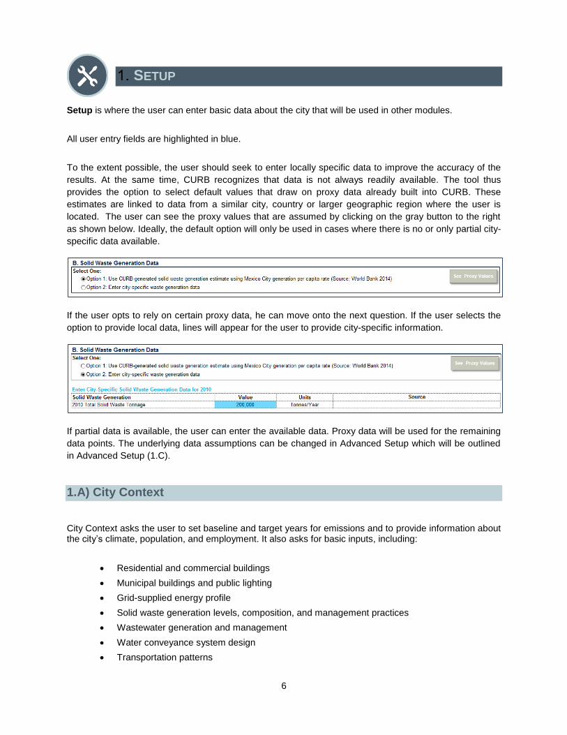
I. Sector Projections

The results of sections 2.A and 2.B are displayed here. On this screen the user can view aggregate

emissions or energy use in each sector and how they are likely to change over time, based on the growth

factors entered in 2.B. Like in section 2.A above, the user can toggle back and forth between viewing

energy and emissions using the buttons at the bottom right of the graph.

II. Inventory Projections

Here the user can see a more detailed version of forward projections in tabular format, with emissions

and energy use broken down by fuel type and end use.

13

2.D) Targets

This section helps the user to set a citywide target to reduce either greenhouse gas (GHG) emissions or

energy use.

Once the target is set, subsequent modules will guide the user through the process of selecting and

customizing different interventions to reduce energy use and emissions in the target city.

In the Results module (5), users can see how far chosen interventions take their city towards achieving

the city’s target. Note that it is possible to make changes to the target at any point in the tool.

I. Target Type Selection

There are three main steps in this section, with further guidance on each provided in Target Setting

Resources (III).

The first step asks the user to select whether to set the target in terms of emissions or energy reductions.

The relative merits of each are described in more detail in Target Setting Resources (III). It should be

14

noted that when setting an emissions reduction target, the user will still be able to see the impact of

various interventions in terms of energy use—and vice versa.

The second step asks the user to select what specific type of energy or emissions target he would like to

select. There are three main options in CURB: base year goal, base year intensity goal, and baseline

scenario goal. Some types of targets may be more appropriate than others for the target city. More

information is provided on each in Target Setting Resources (III).

The final step asks whether the user would like to set interim targets in addition to longer-term energy or

emissions reduction goal. More information is available in Target Setting Resources (III).

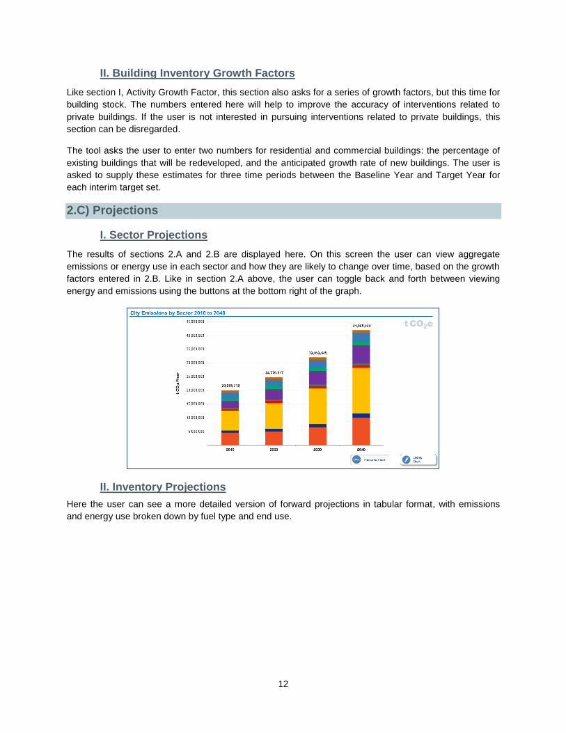
II. Target Level

Once he has selected the type of target to set, the next page allows the user to choose how much to

reduce energy use and emissions and by when. As a general rule, targets should be ambitious yet

achievable.

Research by C40 Cities and Arup has identified 228 cities across the world that have set emissions

reduction targets, most of which are set for 2020 or 2050. These targets vary in the level of ambition from

less than 20% all the way to 100% reductions in GHG emissions.

III. Target Setting Resources

This section provides the user with detailed information and guidance on how to approach selecting the

target type (Section I) and target level (Section II). A brief overview is provided below; please refer to the

CURB Excel tool for more detail.

To set targets, the user must choose between options in 3 areas:

1. Emissions vs. energy target: The user may choose to set their targets in terms of emissions or

energy use.

a. Emissions is a commonly used benchmark, and more than 200 cities around the world

have set greenhouse gas reduction targets to help guide local climate action. Further, an

emissions target covers interventions in all sectors.

15

b. Energy reduction may be appropriate for cities focused primarily on energy reduction

goals. However, not all interventions may lead to energy reduction, such as those in Solid

Waste and Water and Wastewater.

2. Target type: This step determines the reference point upon which targets are calibrated.

a. A base year goal calculates each final and interim target as a relative quantity to the base

year. Because base year information is known, this target type grants a degree of

certainty and few additional data requirements.

b. A base year intensity goal refers to targets relative to a ratio in the base year, such as

emissions as a proportion of population. This method may be advantageous for cities

experiencing large economic or population growth, but provides less certainty due to the

introduction of an additional projected variable.

c. A baseline scenario goal sets targets relative to projected emissions in a “business as

usual” scenario. This target type is suitable for cities in which emissions are expected to

increase significantly over time if no actions are taken.

3. Interim targets: Users may choose to set interim targets for the intervening years between the

base year and the long term target. Interim targets help to track progress over time, but requires

user inputs for those intervening years.

16

BENCHMARKING

Benchmarking allows users to compare their cities with other cities across a range of sector-specific

indicators relevant to energy use, service delivery levels, or GHG emissions.

3.A) City Comparison

CURB allows the user to compare the target city’s performance to other cities around the world in the

Benchmarking module. CURB currently includes 23 different Key Performance Indicators (KPIs) across

six sectors. Data from other cities was obtained from a variety of datasets. To the maximum extent

possible, the CURB team has relied on data sets that are updated on a regular basis, to ensure CURB

stays as current as possible.

To assess the target city’s performance, select a Sector by clicking the logo on the left. The Key

Performance Indicators available for that sector will then appear in the middle of the screen. Select one of

these KPI’s and the bar chart on the right will change, displaying a city-by-city comparison of the selected

KPI. In the bar chart, the target city will be highlighted in yellow, with other cities represented in light blue.

In general, the best-performing cities are those closer to the right side of each graph.

By default, the target city is compared to all other cities for which data was available. To narrow the list of

cities to which the target city is compared, select one of the “Benchmark Comparison Filters”, which

include:

“Region” -- this filter compares the target city with others in the same geographic region.

17

“Development” -- this filter compares the target city with others at a similar level of socio-

economic development, as measured by the Human Development Index (HDI) rating.

“Climate” – this filter compares the target city with others in a similar climatic zone.

While the Region and Development filters may be of general interest to the target city, the Climate filter is

designed primarily for use in two specific KPIs: “Building GHG emissions per capita” in Private Building

Energy and “Public building energy consumption” in Municipal Building Energy. This is because climate

type is a strong driver of energy demand and associated emissions in buildings, since heating and cooling

loads vary widely across regions with different climates. For instance, all other things being equal, a city

with hot summers and cold winters is likely to have much higher energy use in its buildings sector than a

city with a more temperate climate.

When selecting a filter, click on the filter and then re-click on the KPI of interest to update the chart.

At the bottom of the screen, the user can see the information from the bar graph in tabular format, with

precise values, the year the data is from, and the source of the data.

3.B) Indicator Summary

The 23 KPIs referenced within CURB are listed below. Please refer to the CURB Excel tool for more

information on each of the KPIs, including definitions of each and data sources.

Sector KPI

Private Building Energy Building GHG emissions per capita

% population with electrical service

Municipal Building Energy and Public Lighting Public building energy consumption

Average streetlight energy use

Electricity Generation Grid emissions factor

% of energy derived from renewables

Solid Waste Solid waste GHG emissions per capita

Solid waste generated per capita

% of population with solid waste collection

% of solid waste recycled

% of solid waste biologically treated

Water and Wastewater Wastewater GHG emissions per capita

Water GHG emissions per capita

% of city’s wastewater that is untreated

% of population with wastewater collection

% of population with access to improved water

Transportation Transport GHG emissions per capita

Private automobiles per capita

% trips in personal automobiles

% trips via public transit

% trips via non-motorized modes

Overall Total GHG emissions per capita

Electricity use per capita

18

ACTIONS

Actions is the heart of the tool. It allows users to select which sectors they would like to focus on and rate

the target city’s authority to take action in each sector. Estimates of feasibility, cost, and emissions

reduction potential allow users to quickly compare potential actions and make a preliminary selection of

actions that seem most suitable for the city. Users then have the chance to customize each of the chosen

actions and see how each contributes to the overall emissions reduction target. After customizing

interventions, users will be able to view more detailed information on costs and co-benefits. At any time,

the user may go back and change the options selected, either to drop or add more as desired.

4.A) Action Selection

I. Overview

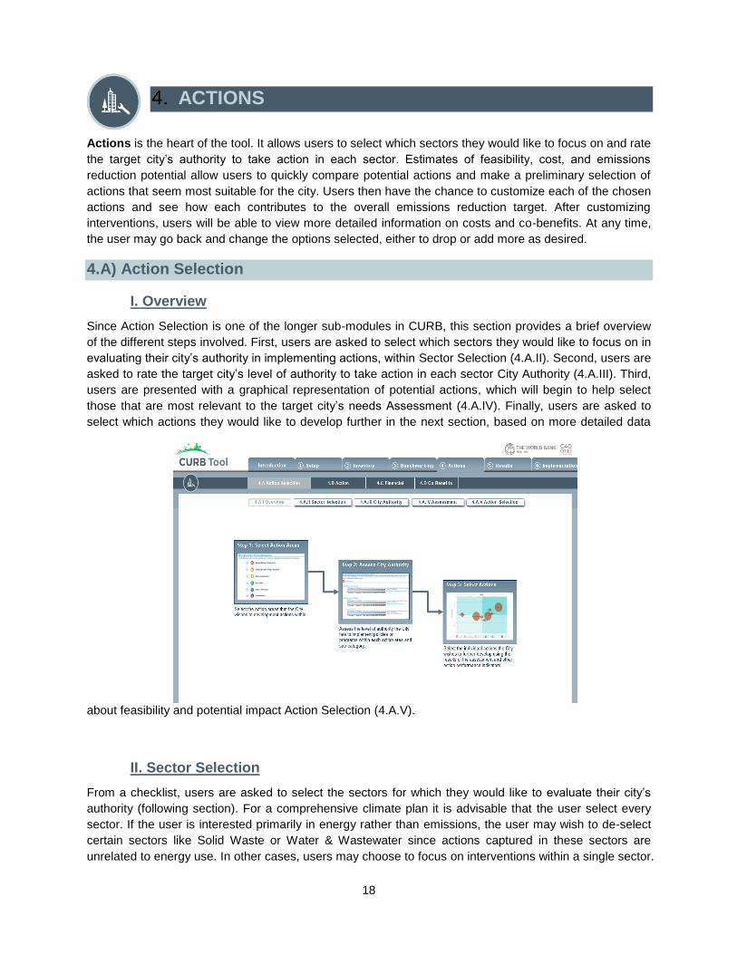
Since Action Selection is one of the longer sub-modules in CURB, this section provides a brief overview

of the different steps involved. First, users are asked to select which sectors they would like to focus on in

evaluating their city’s authority in implementing actions, within Sector Selection (4.A.II). Second, users are

asked to rate the target city’s level of authority to take action in each sector City Authority (4.A.III). Third,

users are presented with a graphical representation of potential actions, which will begin to help select

those that are most relevant to the target city’s needs Assessment (4.A.IV). Finally, users are asked to

select which actions they would like to develop further in the next section, based on more detailed data

about feasibility and potential impact Action Selection (4.A.V).

II. Sector Selection

From a checklist, users are asked to select the sectors for which they would like to evaluate their city’s

authority (following section). For a comprehensive climate plan it is advisable that the user select every

sector. If the user is interested primarily in energy rather than emissions, the user may wish to de-select

certain sectors like Solid Waste or Water & Wastewater since actions captured in these sectors are

unrelated to energy use. In other cases, users may choose to focus on interventions within a single sector.

19

Please note that users are able to return to this screen at any point to change their selection by adding or

dropping sectors.

III. City Authority

This section asks the user to assess what authority the local government has to take action in each sector

and sub-sector. This is important because the degree of authority a city has in a particular area will

necessarily reflect the feasibility of any given action. Users are only asked to evaluate city authority for

those sectors selected in the previous section.

Authority is measured across three different parameters:

(i) Own/Operate: the degree of ownership the city exercises over the particular

asset/function/service in question. For instance, a city which owns/operates the local public

20

transport system is likely to have a stronger ability to take action in that area than a city that has

limited or no influence over operations.

(ii) Policies, Regulations, and Enforcement: the degree to which a city is able to set and enforce

policy in each sector. For instance, a local government that is able to set and enforce policy over

private buildings will have a greater capacity to act than one which lacks the authority to set policy

in that sector, or which can set policy but has limited power in terms of enforcement.

(iii) Control Budget: the degree to which the city controls the budget for the asset/function/service in

question. For instance, a local government that controls the budget for public street lighting is

likely in a better position to take action in that sector than one in which the local government has

no budgetary control.

It is important that the user select the appropriate degree of authority the target city has over each sector

by moving every slider, since this will help determine the feasibility of each intervention as displayed in

the following two sections (Assessment (4.A.IV) and Action Selection (4.A.V)).

The following tables are designed to help determine how to set each slider. Note that in the case of

private buildings, it is only possible to determine the city’s authority in terms of policies, regulations and

enforcement, since it is assumed the city authority does not by definition own or control the budget of

private assets.

Table 1: Own/Operates

Slider position Definition

Low or No Influence Does not own or operate asset/service

Influences Policy Can influence operations

Enforces But No Policy Manages procurement of operator

Policy But No Enforcement Partially owns or operates asset/service

Policy and Enforcement Owns or operates asset/service

Table 2: Policies, Regulations, Enforcement

Slider position Definition

Low or No Influence Has no influence over policies/regulation or enforcement

Influences Policy Can influence policies/regulation or enforcement

Enforces But No Policy Enforces, BUT can’t set policies/regulation

Policy But No Enforcement Sets policies/regulation, BUT does not enforce

Policy and Enforcement Sets AND enforces policies/regulations

Table 3: Control Budget

Slider position Definition

Low or No Influence Has no influence over budget for asset/function

Influences Budget Has influence over budget for asset/function

Controls Budget Controls influence over budget for asset/function

21

IV. Assessment

The series of charts in this section will give a preliminary sense of which actions the user may wish to

develop further in Action Development (4.B) by presenting the user with rough estimates of the relative

cost, feasibility and maximum emissions impact of different interventions in each sector.

The ease of implementation is shown on the horizontal axis, with results influenced in part by the

authority sliders the user was asked to set in the previous section City Authority (4.A.III) and in part by the

technical feasibility of each action. Actions further to the left are deemed more difficult than those to the

right.

The relative cost of each action is shown on the vertical axis. Actions further toward the bottom are more

costly to implement, while those above the line are expected to result in net savings.

The size of the bubble represents the relative size of emissions abatement potential for each action

category.

Actions in the top right quadrant are likely to be less difficult to implement in the target city and also

achieve cost savings—either to the city itself or to other stakeholders, depending on the sector. By

contrast, actions in the bottom left are likely to be more difficult to implement and come at a higher cost.

Below the table are buttons that allow users to switch between sectors. The table at the bottom of the

page gives more detail about the potential savings and emissions reductions, and also allows the user to

select or deselect action categories.

It is important to note that the calculations here are based on the maximum cost/savings and emissions

impact potential that would be achieved assuming 100% penetration of each intervention (e.g. upgrading

all streetlights, or efficiency improvements in all buildings) rather than the likely level of deployment in the

target city. As such, they should only be taken as rough estimates indicative of the actions that are likely

to yield the best outcomes for the city.

22

It may be helpful to switch back to these charts when it comes to selecting actions to develop further in

the next section Action Selection (4.A.V).

V. Action Selection

This section summarizes the inputs from this module in a single table, which allows comparison of

different actions in order to decide which actions the user would like to develop further in Action (4.B)

Development. The last column on the right recommends high opportunity actions based on user inputs in

previous sections. Note that the user can return to this summary page at any point during the action

design process.

City Authority summarizes the results of the sliders changed in City Authority (4.A.III). Green circles

indicate a higher degree of authority in that sector, orange/yellow circles indicate medium authority, and

red circles indicate limited authority. Black circles indicate not applicable.

Technical Difficulty gives an overall sense of how difficult each intervention is from a technical perspective,

unrelated to the target city’s capacity. Similar to above, green circles indicate a lower degree of technical

difficulty, orange/yellow circles indicate medium technical difficulty, and red circles indicate a higher

degree of technical difficulty.

Similarly, the green indicates savings in the Savings column and the more dollar signs there are, the

greater the savings. The following two columns are related to the emissions abatement potential.

The user should review the provided information and select interventions that the city wishes to pursue.

4.B) Action Development

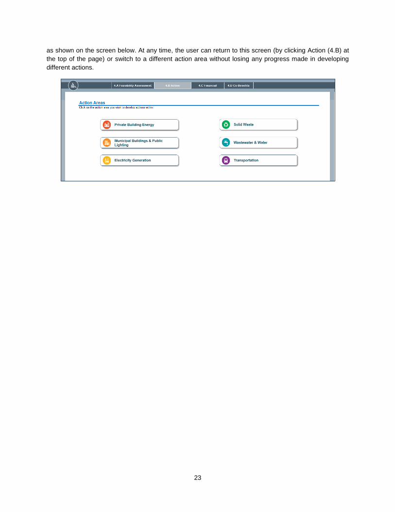
Now that the user has considered which actions to pursue further, this section allows the user to

customize each individual action for the target city. The user begins by clicking on a sector to start with,

23

as shown on the screen below. At any time, the user can return to this screen (by clicking Action (4.B) at

the top of the page) or switch to a different action area without losing any progress made in developing

different actions.

24

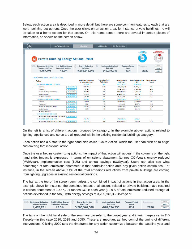
Below, each action area is described in more detail, but there are some common features to each that are

worth pointing out upfront. Once the user clicks on an action area, for instance private buildings, he will

be taken to a home screen for that sector. On this home screen there are several important pieces of

information, as shown on the screen below.

On the left is a list of different actions, grouped by category. In the example above, actions related to

lighting, appliances and so on are all grouped within the existing residential buildings category.

Each action has a button to the right hand side called “Go to Action” which the user can click on to begin

customizing that individual action.

Once the user begins customizing actions, the impact of that action will appear in the columns on the right

hand side. Impact is expressed in terms of emissions abatement (tonnes CO2/year), energy reduced

(kWh/year), implementation cost ($US) and annual savings ($US/year). Users can also see what

percentage of total emissions abatement in that particular action area any given action contributes. For

instance, in the screen above, 14% of the total emissions reductions from private buildings are coming

from lighting upgrades in existing residential buildings.

The bar at the top of the screen summarizes the combined impact of actions in that action area. In the

example above for instance, the combined impact of all actions related to private buildings have resulted

in carbon abatement of 1,457,701 tonnes CO2/e each year (13.9% of total emissions reduced through all

actions developed in the tool), with energy savings of 3,205,948,356 kWh/year.

The tabs on the right hand side of the summary bar refer to the target year and interim targets set in 2.D

Targets—in this case 2020, 2035 and 2050. These are important as they control the timing of different

interventions. Clicking 2020 sets the timeframe for any action customized between the baseline year and

25

2020. Clicking 2035 sets the timeframe for any action customized between 2020 and 2035. Clicking 2050

sets the timeframe for any action customized between 2035 and 2050. This allows staggering of different

interventions across time. For instance, the user may wish to pursue energy efficiency upgrades in

existing buildings between now and 2020, while focusing on new buildings post 2020. Users may wish to

pursue some actions in all years until the target; others may be shorter term and begin or end in one of

the interim targets.

Please note that the emissions impacts of any action selected in one time frame (e.g. 2020) are only

accounted for within that time period; to realize benefits across multiple time frames, the action should be

selected for each interim target year.

The dials in the upper right corner show progress towards the emissions reduction target set earlier in the

tool (if one was set). The dial on the left shows overall progress towards the target through all actions in

all sectors that have been customized so far. The dial on the right shows the emissions reductions

achieved for a given action area—in this case private buildings.

Once the user begins entering specific actions within each sector, there is an additional feature to

consider across all actions. For each action, the user can select whether it is a local action or a

national/region action and what year the action should be implemented in. This information helps the user

make a more realistic plan for the city by staggering actions as appropriate for local circumstances.

Additionally, this information provides insights into cash flows for each action as well as the impact from

local versus national/regional actions.

PRIVATE BUILDING ENERGY

Actions related to private buildings can be split broadly into demand side and supply side interventions. Demand side interventions involve energy efficiency (plus some fuel switching),

while supply side interventions include distributed renewables and district energy. All actions can be applied to residential buildings, commercial buildings, or both. Residential buildings are divided into low, low-middle, high-middle, and high-income buildings. Commercial buildings are divided into retail, office, hospital and hotel spaces. For energy efficiency and fuel switching measures, the user can choose to apply actions to both existing buildings (i.e. retrofit) and new buildings (i.e. new construction). As with other sectors, the user can specify a time period in which the action is to be implemented by using the buttons in the top right hand corner.

26

The following is a brief summary list of the actions in the private buildings sector: Energy Efficiency in Existing Buildings Residential Energy Efficiency and Fuel Switching Upgrades Includes separate actions for lighting, appliances & electronics, space heating and cooling, water heating, and cooking across different income cohorts (low, low-middle, high-middle, and high income buildings). Actions involving heating and cooling allow for fuel switching in addition to efficiency upgrades. Commercial Energy Efficiency and Fuel Switching Upgrades Includes separate actions for lighting, appliances & electronics, space heating and cooling, water heating, and building envelope for different commercial building types including retail, office, hospital and hotel spaces. Actions involving heating and cooling allow for fuel switching in addition to efficiency upgrades. Energy Efficiency in New Buildings Note that actions related to new buildings (lighting, appliances & electronics, space heating and cooling, water heating, and building envelope upgrades) have been consolidated under a single “Go to Action” tab. This is to reflect the nature of the different policy or implementation options that are frequently used to target new construction. In contrast to energy efficiency retrofits, which may often focus on a specific technology or end-use (e.g. boiler upgrades, building envelope upgrades), things like building codes for new construction typically require minimum compliance across a range of different end-uses. As such, interventions have been grouped into a single action tab. Energy Efficient Residential Construction Includes actions for lighting, appliances & electronics, space heating and cooling, water heating, and the building envelope for different income cohorts (low, low-middle, high-middle, and high income buildings). Actions involving heating and cooling allow for fuel switching in addition to efficiency upgrades. Energy Efficient Commercial Construction Includes actions for lighting, appliances & electronics, space heating and cooling, water heating, and the building envelope for different commercial building types including retail, office, hospital, and hotel spaces. Actions involving heating and cooling allow for fuel switching in addition to efficiency upgrades. Distributed Renewables in Existing Buildings Residential PV Allows user to select the average system size (kWh/m2) and the percentage of buildings the intervention will target, with separate inputs for different income cohorts. Commercial PV Allows user to select the average system size (kWh/m2) and the percentage of buildings the intervention will target, with separate inputs for different types of commercial building. District Energy in Existing Buildings District Energy For district heating, the action allows the user to determine the efficiency of the boilers, whether cogeneration is to be used, and the fuel. For district cooling, the user can select the chiller efficiency. The user can then decide what percentage of different types of residential and commercial buildings to which heating and/or cooling systems should be applied. In each case, clicking on the “Go to Action” button will take the user to a similar screen:

27

The page above shows the lighting efficiency action for residential buildings. Within the action are a number of different options: energy saving light bulbs for internal spaces, energy saving light bulbs for common and exterior areas, and lighting controls for common and exterior areas. Each of these separate actions has a slider to the right hand side that controls the “saturation” level of each action, i.e. what percentage of the building stock will the actions target? There are different sets of sliders for different income groups: low income residential housing, low-middle income, high-middle income and high income residential housing. This allows for flexibility in customizing actions. For instance, a user may wish to pursue upgrades to indoor lighting that target only low income households (e.g. 80% of low income households, determined by the saturation level slider) rather than all income groups, or vice versa. On moving the sliders, users can immediately see changes reflected in the summary bar at the top. This shows emissions reductions, energy reductions, costs and savings for this specific intervention (i.e. residential lighting efficiency for existing buildings, in this case). The bar charts on the right hand side show the impact of each different action on energy demand. There is a separate chart for each income group. The vertical axis shows energy demand in kWh per square meter. The horizontal axis has four different bars showing energy demand before/after action has been taken for both flats and houses. The first bar on the left shows the base case energy demand for flats/apartments, with the bar immediately to the right indicating improved case energy demand. The third bar from the left indicates the base case energy demand for houses, while the bar to the far right shows demand in the improved case. The base case bars represent energy demand for that building type (in this case low income residential housing) before any actions were taken. The improved case bars show decreased energy demand accounting for all actions taken in private buildings that target residential units for that income group. The charts are dynamic, such that they immediately reflect changes in energy use resulting from moving the saturation rate sliders. Each color represents a different source of energy use: purple for heating, blue for cooling, light grey for fan energy, green for appliances and electronics, yellow for lighting, orange for hot water, red for cooking and dark grey for other. The “Reset Page to Zero” button above the sliders will reset the saturation rate for all actions on this page to 0%.

28

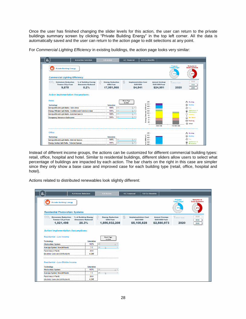
Once the user has finished changing the slider levels for this action, the user can return to the private buildings summary screen by clicking “Private Building Energy” in the top left corner. All the data is automatically saved and the user can return to the action page to edit selections at any point. For Commercial Lighting Efficiency in existing buildings, the action page looks very similar:

Instead of different income groups, the actions can be customized for different commercial building types: retail, office, hospital and hotel. Similar to residential buildings, different sliders allow users to select what percentage of buildings are impacted by each action. The bar charts on the right in this case are simpler since they only show a base case and improved case for each building type (retail, office, hospital and hotel). Actions related to distributed renewables look slightly different:

29

In addition to selecting a saturation level that determines what percentage of each building type the action will target, the user can also choose the size of the average solar system in kW/unit, where unit refers to an individual building. Moving this slider will change the total panel area required and the amount of electricity generated per unit. The action page for commercial buildings is very similar. The final action page in the private buildings sector is for district energy:

MUNICIPAL BUILDINGS AND PUBLIC LIGHTING

There are three types of actions in Municipal Buildings and Public Lighting: 1) Energy Efficiency and Fuel Switching, 2) Public Lighting Energy, and 3) Municipal Distributed Renewable Energy.

Energy Efficiency and Fuel Switching

30

Municipal Building actions related to energy efficiency and fuel switching are very similar to the Private Building Energy actions and essentially a subset of those. For Municipal Office Building Lighting Efficiency and Municipal Office Building Envelope Energy Efficiency, the user can choose what percent of buildings they want to apply the specified technologies to by adjusting the sliders associated with each technology.

For Municipal Office Building Heating and Cooling System Efficiency and Fuel Switching, the user can

choose to change the fuel associated with high efficiency condensing boilers by selecting the appropriate

fuel through the dropdown menu next to it. The user can also change what percent of buildings they want

to apply the specified technologies to by adjusting the associated sliders to the right of each technology.

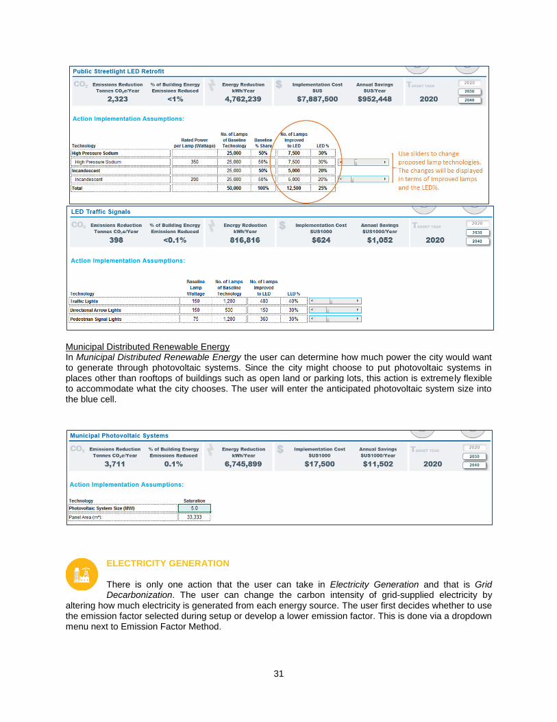
Public Lighting Energy The Public Lighting Energy action allows the user to change what percentage of streetlights and traffic lights are using various lighting technologies.

31

Municipal Distributed Renewable Energy In Municipal Distributed Renewable Energy the user can determine how much power the city would want to generate through photovoltaic systems. Since the city might choose to put photovoltaic systems in places other than rooftops of buildings such as open land or parking lots, this action is extremely flexible to accommodate what the city chooses. The user will enter the anticipated photovoltaic system size into the blue cell.

ELECTRICITY GENERATION

There is only one action that the user can take in Electricity Generation and that is Grid Decarbonization. The user can change the carbon intensity of grid-supplied electricity by

altering how much electricity is generated from each energy source. The user first decides whether to use the emission factor selected during setup or develop a lower emission factor. This is done via a dropdown menu next to Emission Factor Method.

32

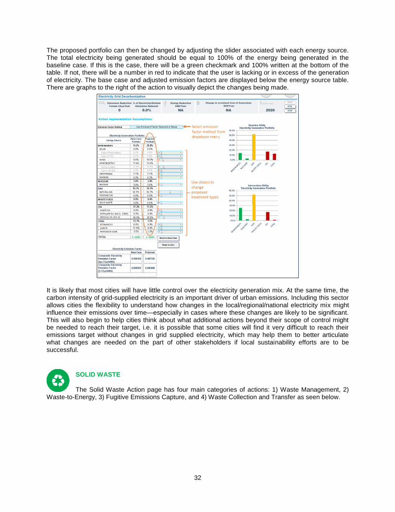
The proposed portfolio can then be changed by adjusting the slider associated with each energy source. The total electricity being generated should be equal to 100% of the energy being generated in the baseline case. If this is the case, there will be a green checkmark and 100% written at the bottom of the table. If not, there will be a number in red to indicate that the user is lacking or in excess of the generation of electricity. The base case and adjusted emission factors are displayed below the energy source table. There are graphs to the right of the action to visually depict the changes being made.

It is likely that most cities will have little control over the electricity generation mix. At the same time, the carbon intensity of grid-supplied electricity is an important driver of urban emissions. Including this sector allows cities the flexibility to understand how changes in the local/regional/national electricity mix might influence their emissions over time—especially in cases where these changes are likely to be significant. This will also begin to help cities think about what additional actions beyond their scope of control might be needed to reach their target, i.e. it is possible that some cities will find it very difficult to reach their emissions target without changes in grid supplied electricity, which may help them to better articulate what changes are needed on the part of other stakeholders if local sustainability efforts are to be successful.

SOLID WASTE

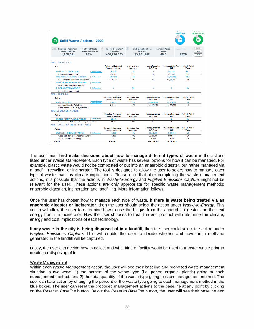
The Solid Waste Action page has four main categories of actions: 1) Waste Management, 2) Waste-to-Energy, 3) Fugitive Emissions Capture, and 4) Waste Collection and Transfer as seen below.

33

The user must first make decisions about how to manage different types of waste in the actions listed under Waste Management. Each type of waste has several options for how it can be managed. For example, plastic waste would not be composted or put into an anaerobic digester, but rather managed via a landfill, recycling, or incinerator. The tool is designed to allow the user to select how to manage each type of waste that has climate implications. Please note that after completing the waste management actions, it is possible that the actions in Waste-to-Energy and Fugitive Emissions Capture might not be relevant for the user. These actions are only appropriate for specific waste management methods: anaerobic digestion, incineration and landfilling. More information follows.

Once the user has chosen how to manage each type of waste, if there is waste being treated via an anaerobic digester or incinerator, then the user should select the action under Waste-to-Energy. This action will allow the user to determine how to use the biogas from the anaerobic digester and the heat energy from the incinerator. How the user chooses to treat the end product will determine the climate, energy and cost implications of each technology. If any waste in the city is being disposed of in a landfill, then the user could select the action under Fugitive Emissions Capture. This will enable the user to decide whether and how much methane generated in the landfill will be captured. Lastly, the user can decide how to collect and what kind of facility would be used to transfer waste prior to treating or disposing of it. Waste Management Within each Waste Management action, the user will see their baseline and proposed waste management situation in two ways: 1) the percent of the waste type (i.e. paper, organic, plastic) going to each management method, and 2) the total quantity of the waste type going to each management method. The user can take action by changing the percent of the waste type going to each management method in the blue boxes. The user can reset the proposed management actions to the baseline at any point by clicking on the Reset to Baseline button. Below the Reset to Baseline button, the user will see their baseline and

34

proposed waste management situation in terms of quantity of waste (thousands of tonnes). These quantities will automatically adjust as the user changes the percent of waste being moved.

Once the user has gone through all of the waste types that the city would like to improve management of, he should click on the Solid Waste button at the top left corner of the screen to return to the main Solid Waste Action page. At this time, if the user has chosen to manage some waste with either anaerobic digestion or incineration, he should select the Waste-to-Energy action. If not, and the user has chosen to manage some waste via a landfill, then he should select the Enhanced Landfill Methane Recovery action. If the user has not chosen any of these methods to manage the city’s waste then he can proceed to another sector.

Waste to Energy

The Waste-to-Energy actions allow the user to determine how the end product (i.e. biogas, heat energy) of the waste-to-energy technology will be utilized. If the city already has an anaerobic digester and incinerator, the user can enter what the city currently does with the biogas and/or heat energy in the left column of the blue cells under Baseline Split. For example, if the city currently manages some waste via anaerobic digestion, the user can enter how much of the anaerobic digester biogas is flared, used to generate electricity, used for thermal energy and/or used for co-generation (both thermal and electricity). Otherwise, the user can directly enter in the proposed split of how the biogas and/or heat energy will be used in the right column of the blue cells. How the biogas and/or heat energy is used will determine the emissions impact of the anaerobic digester and/or incinerator.

35

Fugitive Emissions Capture If the city manages some waste at a landfill, the user should select the Enhanced Landfill Methane Recovery action. In this action, the user can decide how much of the methane generated in the landfill the city will be able to capture. The user will input the anticipated recovery into the blue cell and immediately see the emissions abatement that will result by each waste type.

Waste Collection and Transfer Energy

In Waste Collection and Transfer the user can enter information about the current vehicle fleet that collects waste as well as information about energy currently consumed at any transfer stations, if the baseline information provided is incorrect. Then the user can determine emissions, energy and financial implications of anticipated changes in fuel and quantity consumed for both the vehicle fleet and transfer station.

36

Return to the main Solid Waste Actions page to see the summary of emissions, energy, and financial implications of the solid waste actions.

WATER AND WASTEWATER

The Wastewater and Water Action page has three main categories of actions: 1) Wastewater Treatment Switching and Optimization, 2) Wastewater Biogas-to-Energy, and 3) Water Conveyance Energy Improvements as seen below.

37

In Wastewater Treatment Switching and Optimization, the user can change their current wastewater treatment methods and/or improve their current treatment methods. In Wastewater Biogas-to-Energy, the user can determine how to use any biogas being generated through anaerobic digestion. How the user chooses to treat the end product will determine the climate, energy and cost implications of each technology. Water Conveyance Energy Improvements allows the user to change the pump efficiency for water conveyance, increase the number of improved water conveyance pumps in the city and improve distribution water loss. Wastewater Treatment Switching and Optimization In the first action, Wastewater Treatment Type Switching, the user will see their baseline and proposed wastewater treatment types. The user can take action by changing the percent of wastewater being treated by each treatment type. The user can do this by using the slider to the right of each treatment type to adjust the percent of wastewater being sent to that treatment type. The two graphs on the right side of the screen show how the proposed distribution of wastewater treatment types compares to the baseline in a visual format. The user should ensure that the total amount of wastewater that is being managed does not exceed 100% of the original wastewater quantity. To do so, the user can see below the table if there is a green checkmark with a corresponding text of 100% indicating that all of the wastewater is being managed or if there is a red number that is less than or greater than 100. The user can reset the proposed management actions to the baseline at any point by clicking on the Reset to Baseline button.

38

The user can also choose to improve the treatment technologies beyond the baseline through the rest of the actions in Wastewater Treatment Switching and Optimization. In Latrine Improvements, the user can change the level of sediment being removed from latrines by adjusting the slider to set the proposed level. If the baseline assumption is inaccurate, this can be changed by clicking on the “Change Baseline” link above the baseline sediment removal level.

39

For Anaerobic Treatment Lagoon Improvements and Facultative Treatment Lagoon Improvements, the user can change the percentage of lagoons with surface aerators by adjusting the slider. If the baseline percentage of lagoons with aerators is incorrect, it can be changed through the “Change Baseline” link above the baseline assumption. Note that aerators are only applied to lagoons without biogas capture systems.

For Activated Sludge Treatment Plant Improvements, the user can choose the level of nitrogen removal as well as the percentage of plants with denitrification technology. There are three options that can be chosen from a dropdown menu for the proposed level of nitrogen removal: 1) Basic (50% removal), 2) Advanced (80% removal), or 3) Limit of Technology (3 mg/L). The proposed percentage of plants with denitrification technology can be adjusted through the slider and any baseline assumptions can be changed through the “Change Baseline” link.

For Direct Discharge Improvements, the user can select a new pre-treatment technology to increase BOD removal efficiency and that what portion of flow the new technology should apply to. The options for pre-treatment technology are 1) coarse screens or 0% removal, 2) fine screens or 5% removal, or 3) primary settling or 30% removal.

40

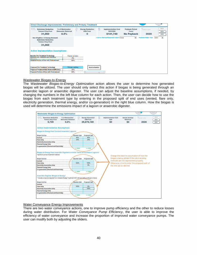
Wastewater Biogas-to-Energy The Wastewater Biogas-to-Energy Optimization action allows the user to determine how generated biogas will be utilized. The user should only select this action if biogas is being generated through an anaerobic lagoon or anaerobic digester. The user can adjust the baseline assumptions, if needed, by changing the numbers in the left blue column for each action. Then, the user can decide how to use the biogas from each treatment type by entering in the proposed split of end uses (vented, flare only, electricity generation, thermal energy, and/or co-generation) in the right blue column. How the biogas is used will determine the emissions impact of a lagoon or anaerobic digester.

Water Conveyance Energy Improvements There are two water conveyance actions, one to improve pump efficiency and the other to reduce losses during water distribution. For Water Conveyance Pump Efficiency, the user is able to improve the efficiency of water conveyance and increase the proportion of improved water conveyance pumps. The user can modify both by adjusting the sliders.

41

42

In Water Delivery Loss Reduction, if the user anticipates any improvements in water distribution losses then the slider can be adjusted accordingly.

Return to the main Wastewater and Water main action page to see the summary of emissions, energy, and financial implications of the solid waste actions.

TRANSPORTATION The transportation scenario planning builds upon the Avoid-Shift-Improve1 strategy framework that is commonly used in cities to calculate the emission and energy effects of different types of

transportation actions. This framework categorizes actions as one of the following:

• Avoid/Reduce: addresses the need to improve the transportation system by a reduction in length of trips or number of daily trips

• Shift/Maintain: aims to improve efficiency by promoting modal shift from high energy consuming modes (i.e. Auto) to public transportation or non-motorized options.

• Improve: focuses on vehicle fuel efficiency, low carbon fuels and energy carriers

The following is a brief summary list of the actions in the transport sector: Low Carbon Urban Design This module allows the user to specify the reduction in future total trips or trip distance that come as a product of efficient and compact urban design, and transit oriented development. Passenger Mode Shift CURB allows the user to specify the modal shift expectations for the future of the following modes: private automobiles, motorcycle, taxis, moto-taxis, micro/minibus, standard bus and BRT, subway, light rail, commuter rail and ferryboats Vehicle Fuel Switch This action allows the user to change the fuel usage (motor gasoline, diesel/gas oil, biodiesel, biogasoline, ethanol, compressed natural gas, liquefied petroleum gas, hydrogen and electricity) of different vehicle types (passenger automobiles, light and medium-duty trucks, motorcycle, taxis, moto-taxis, micro/minibus, standard bus and BRT, subway, light rail, commuter rail and ferryboats). External Transportation Model

This module will allow the user to input from other scenario planning or transportation planning models.

Once entering the transportation sector, the user will find a summary of all sector actions:

1 Dalkman, H. Branningan, C. Leferve, B. and Enriquez, A. Urban Transport and Climate Change. Deutsche Gesellschaft für Internationale GIZ

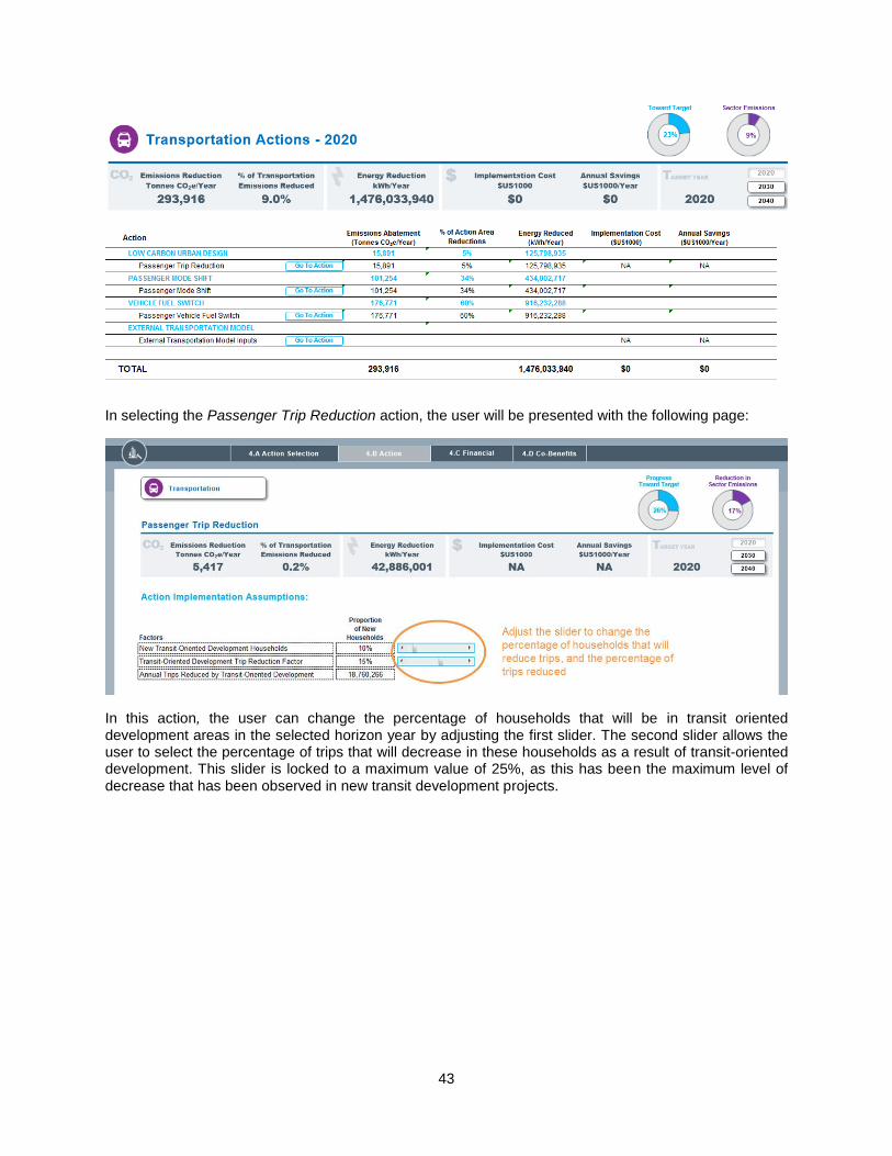
43

In selecting the Passenger Trip Reduction action, the user will be presented with the following page:

In this action, the user can change the percentage of households that will be in transit oriented development areas in the selected horizon year by adjusting the first slider. The second slider allows the user to select the percentage of trips that will decrease in these households as a result of transit-oriented development. This slider is locked to a maximum value of 25%, as this has been the maximum level of decrease that has been observed in new transit development projects.

44

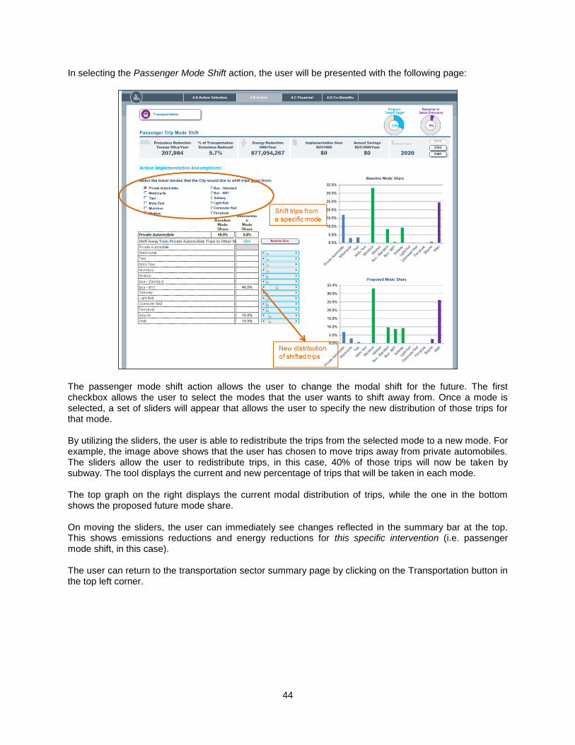
In selecting the Passenger Mode Shift action, the user will be presented with the following page:

The passenger mode shift action allows the user to change the modal shift for the future. The first checkbox allows the user to select the modes that the user wants to shift away from. Once a mode is selected, a set of sliders will appear that allows the user to specify the new distribution of those trips for that mode. By utilizing the sliders, the user is able to redistribute the trips from the selected mode to a new mode. For example, the image above shows that the user has chosen to move trips away from private automobiles. The sliders allow the user to redistribute trips, in this case, 40% of those trips will now be taken by subway. The tool displays the current and new percentage of trips that will be taken in each mode. The top graph on the right displays the current modal distribution of trips, while the one in the bottom shows the proposed future mode share. On moving the sliders, the user can immediately see changes reflected in the summary bar at the top. This shows emissions reductions and energy reductions for this specific intervention (i.e. passenger mode shift, in this case). The user can return to the transportation sector summary page by clicking on the Transportation button in the top left corner.

45

From there the user can select the Vehicle Fuel Switch action, which will lead to the following page:

Similar to the previous action, the Passenger Vehicle Fuel Switch action allows the user to change the fuel used by vehicles and follows the same logic. The first checkbox allows the user to select the vehicles for which the future fuel use will change. Once a vehicle type is selected, a set of sliders will appear that allows the user to specify the new fuel usage for that vehicle type. The user will propose a new fuel for that specific vehicle type. A new set of sliders will appear for each of the vehicle types selected. By utilizing the sliders, the user will be able to redistribute the fuel usage from the selected vehicle type to a new usage mix. For example, the image above shows that the user has chosen to change the fuel usage of private automobiles. The sliders allow the user select a new fuel mix for these vehicles. The total mix of fuels must equal 100%; the total sum at the bottom of the page will highlight green when it is correct. The top graph on the right displays the current vehicle fuel distribution, while the one in the bottom shows the proposed fuel distribution.

46

The final transportation action, External Transportation Model Inputs, enables users to utilize the outcomes of more complex behavioral models within CURB. Inputs within this action replace any other actions within the Transportation module.

The action allows the user to input the following:

Emissions Reduction in 2020 (CO2/Year)

Energy Reduction in 2020 (kWh/Year)

Trip Reduction in 2020 (Trips/Year)

Reduction in Vehicle Kilometers Traveled in 2020 (VKT/Year)

NPV of Implementation Cost 2010 to 2020 ($US1000)

NPV of Cost Savings 2010 to 2020 ($US1000/Year) These results will then be used to compare the sector outcomes with the other sectors’ emission reductions, energy impact and costs.

4.C) Financial Metrics

I. Abatement Cost Curve

This section provides a chart of the emission abatement cost curve for each of the selected actions. Each

action is indicated by a rectangle:

The width of the rectangle (on the horizontal axis) shows the reduction potential of the action

The height of the rectangle indicates the cost of the action

Actions with positive costs are above the zero line

Actions below the zero line are expected to result in savings (or negative costs)

47

The legend below the cost curve allows the user to select and deselect the actions included in the

abatement curve and provides detailed information.

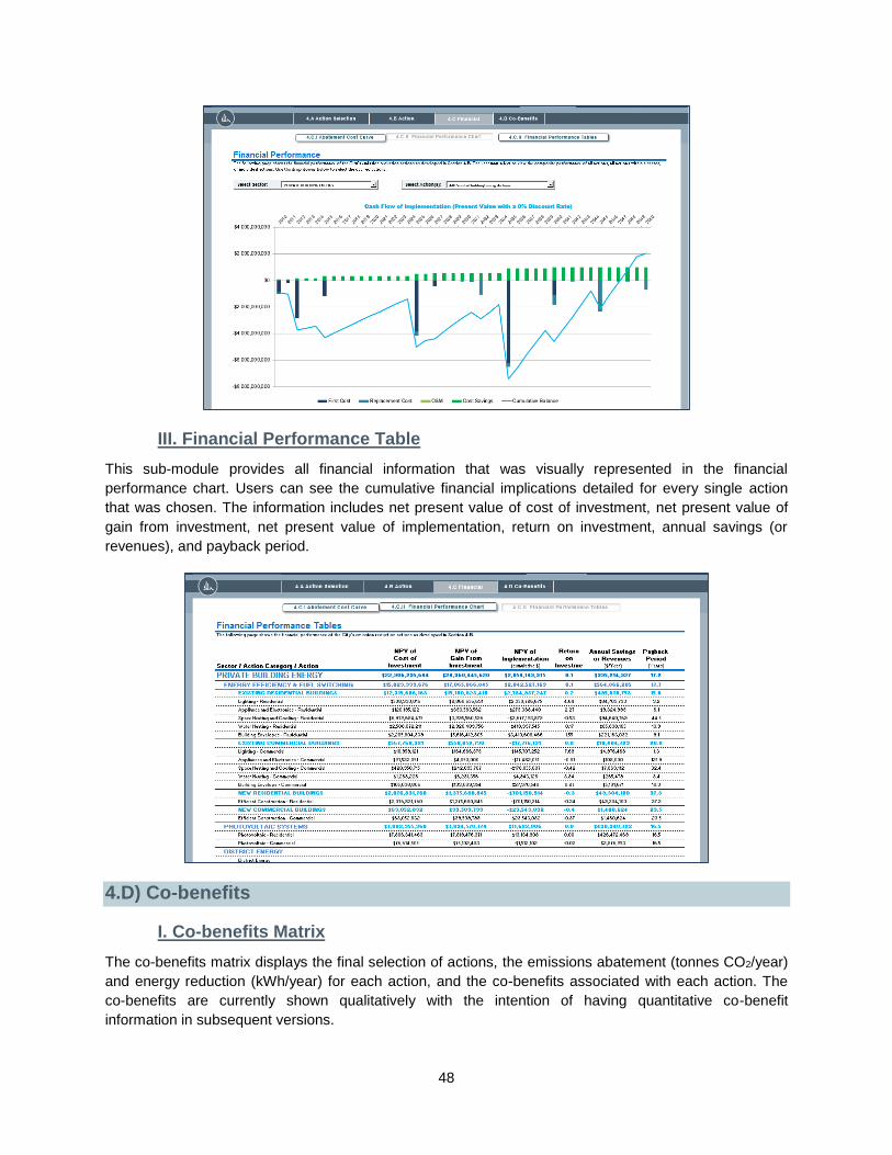
II. Financial Performance Chart

The present value of annual cash flow of implementation can be seen for each action until the final target

year. The charts provided in this sub-module will allow the city to begin understanding how costs/savings

will vary over time and determine the proper sequencing of actions for their specific circumstances.

Information on first cost, replacement cost, operations and maintenance, cost savings, and cumulative

balance are all included so that the user can visually understand the financial implications of a specific

action.

The user can select which sector (or all) they would like to see the cash flow of implementation for in the

first dropdown and then choose the specific action (or all actions) of interest in the second dropdown. The

chart is then updated accordingly. Below the chart, the user can see more detailed information via a table

that provides the cumulative amounts for the action or sector.

48

III. Financial Performance Table

This sub-module provides all financial information that was visually represented in the financial

performance chart. Users can see the cumulative financial implications detailed for every single action

that was chosen. The information includes net present value of cost of investment, net present value of

gain from investment, net present value of implementation, return on investment, annual savings (or

revenues), and payback period.

4.D) Co-benefits

I. Co-benefits Matrix

The co-benefits matrix displays the final selection of actions, the emissions abatement (tonnes CO2/year)

and energy reduction (kWh/year) for each action, and the co-benefits associated with each action. The

co-benefits are currently shown qualitatively with the intention of having quantitative co-benefit

information in subsequent versions.

49

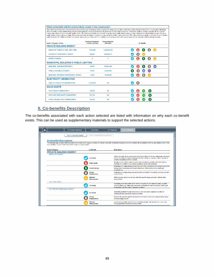
II. Co-benefits Description

The co-benefits associated with each action selected are listed with information on why each co-benefit

exists. This can be used as supplementary materials to support the selected actions.

50

RESULTS

Results demonstrates the combined and individual impact of chosen actions on urban emissions, energy and costs. Here the user can see how actions add up to reach the city’s emissions target, understand the financial implications, and view the emissions and energy impacts. If desired, the user can go back to adjust or select additional actions.

5.A) Aggregate Results

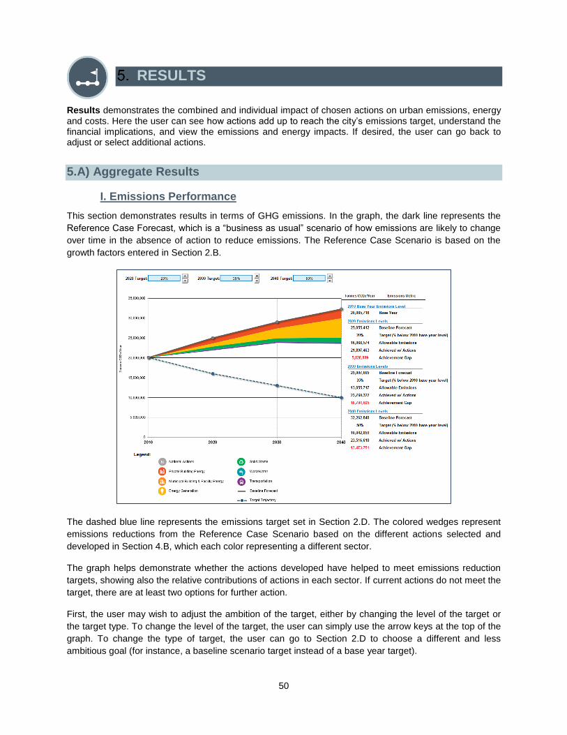
I. Emissions Performance

This section demonstrates results in terms of GHG emissions. In the graph, the dark line represents the

Reference Case Forecast, which is a “business as usual” scenario of how emissions are likely to change

over time in the absence of action to reduce emissions. The Reference Case Scenario is based on the

growth factors entered in Section 2.B.

The dashed blue line represents the emissions target set in Section 2.D. The colored wedges represent

emissions reductions from the Reference Case Scenario based on the different actions selected and

developed in Section 4.B, which each color representing a different sector.

The graph helps demonstrate whether the actions developed have helped to meet emissions reduction

targets, showing also the relative contributions of actions in each sector. If current actions do not meet the

target, there are at least two options for further action.

First, the user may wish to adjust the ambition of the target, either by changing the level of the target or

the target type. To change the level of the target, the user can simply use the arrow keys at the top of the

graph. To change the type of target, the user can go to Section 2.D to choose a different and less

ambitious goal (for instance, a baseline scenario target instead of a base year target).

51

The second option is to return to the Action module and select more or different actions, or else increase

the ambition of actions already selected, for instance by increasing the penetration rate. Note that it is

generally better to pick actions that are achievable if target and results are to be realistic.

The table on the right gives a more detailed breakdown of the information displayed in the graph. For

each target year, the user can see emissions quantities for the Reference Case, the target set, the

reductions achieved with interventions, and any potential gap between the target and delivered reductions.

II. Energy Performance

This section demonstrates results in terms of energy performance. Information is presented in the same

format as Emissions Performance (5.A.I) above, only with progress shown towards the energy reduction

rather than emissions goal.

5.B) Sector Results

I. Emissions Performance

The graph in this section shows the same results as in 5.A.I, but with more emphasis on the relative

contributions of each sector to emissions reductions, including those attributed to national actions. This

graph is shown as a waterfall so that users can quickly see which sectors are contributing the most to

emissions reduction.

52

The user can select whether to view the waterfall graph in terms of sectors as seen in the screenshot

above or in terms of national actions versus local actions by sector. The latter chart enables the city to

quickly understand what sectors they have more control over and what they can contribute to emissions

and energy use reduction.

II. Energy Performance

This section demonstrates results in terms of energy performance. Information is presented in the same

format as Emissions Performance (5.B.I) above, only with progress shown towards energy reduction

rather than emissions goal.

53

5.C) Action Summary

The table in this sub-modules shows the emissions reduced/year, % of total emissions reduction, energy

reduced/year, implementation cost, and annual savings for every action in order to compare the results

side-by-side rather than view these results individually or sectorally in the Action module. Users can

return to the sub-module 4.B. Action at any time to alter actions.

5.D) Scenario Comparison

In the Scenario Comparison sub-module, users can save up to three scenarios, which are a

comprehensive suite of actions, and then see how they compare when deciding the city’s final set of

actions. The sub-module provides information on how the scenarios compare to their targets, how they

compare to each other by sectoral and overall emissions, and how they compare in terms of emissions,

energy and costs. The scenarios that are saved are static and cannot be changed. The current scenario

can always be adjusted based on lessons learned from previous scenarios.

I. Scenario Selection

This action allows the user to name and save the current scenario in order to go back and build a new

scenario. In Add a Scenario, users can select whether they wish to save the current scenario as Scenario

1, 2 or 3, name the scenario, and save it. As scenarios are developed, if the user wishes to remove any

previous scenario and add the newly developed one, the user can scroll below to Remove a Scenario and

select the scenario to be removed before pushing the associated button.

54

II. Scenario Results

In the graph, users can see the emissions trajectory for all 3 saved scenarios, the current scenario and

the baseline projections. Users can compare these results to any of the targets set by selecting the

scenario with the desired targets. Users can select the scenario in a dropdown to the right of the chart.

III. Scenario Charts

Users can select which metrics to compare for a given horizon year across the scenarios and whether

they want to compare by sector or overall. Users can compare across emissions reduction, energy

savings, and cost performance of the scenarios.

55

IV. Scenario Tables

This table provides the same information as in the Scenario Charts and more detailed information. It

allows users to compare between all scenarios and actions taken. The user can select the metric

(emissions reduction, energy savings, or cost performance), horizon year, and the level of detail desired.

At any point, a user can revisit the current scenario to make adjustments as needed based on the

comparisons.