Verification of a simplified car-following theory
10
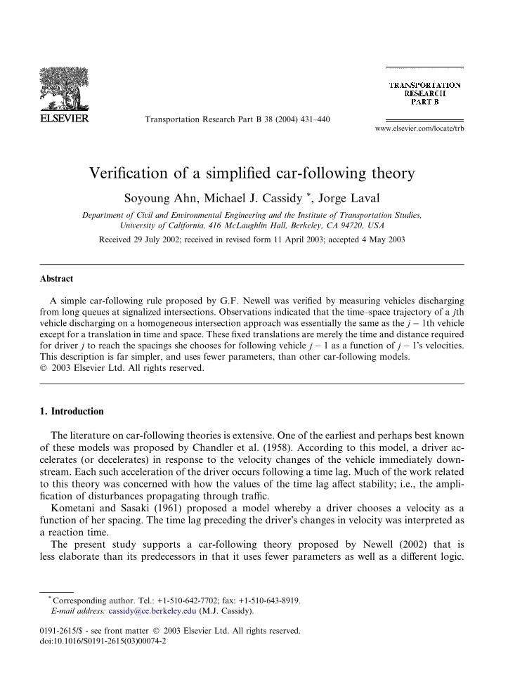
Verification of a simplified car-following theory Soyoung Ahn, Michael J. Cassidy * , Jorge Laval Department of Civil and Environmental Engineering and the Institute of Transportation Studies, University of California, 416 McLaughlin Hall, Berkeley, CA 94720, USA Received 29 July 2002; received in revised form 11 April 2003; accepted 4 May 2003 Abstract A simple car-following rule proposed by G.F. Newell was verified by measuring vehicles discharging from long queues at signalized intersections. Observations indicated that the time–space trajectory of a jth vehicle discharging on a homogeneous intersection approach was essentially the same as the j 1th vehicle except for a translation in time and space. These fixed translations are merely the time and distance required for driver j to reach the spacings she chooses for following vehicle j 1 as a function of j 1Õs velocities. This description is far simpler, and uses fewer parameters, than other car-following models. Ó 2003 Elsevier Ltd. All rights reserved. 1. Introduction The literature on car-following theories is extensive. One of the earliest and perhaps best known of these models was proposed by Chandler et al. (1958). According to this model, a driver ac- celerates (or decelerates) in response to the velocity changes of the vehicle immediately down- stream. Each such acceleration of the driver occurs following a time lag. Much of the work related to this theory was concerned with how the values of the time lag affect stability; i.e., the ampli- fication of disturbances propagating through traffic. Kometani and Sasaki (1961) proposed a model whereby a driver chooses a velocity as a function of her spacing. The time lag preceding the driverÕs changes in velocity was interpreted as a reaction time. The present study supports a car-following theory proposed by Newell (2002) that is less elaborate than its predecessors in that it uses fewer parameters as well as a different logic. Transportation Research Part B 38 (2004) 431–440 www.elsevier.com/locate/trb * Corresponding author. Tel.: +1-510-642-7702; fax: +1-510-643-8919. E-mail address: [email protected] (M.J. Cassidy). 0191-2615/$ - see front matter Ó 2003 Elsevier Ltd. All rights reserved. doi:10.1016/S0191-2615(03)00074-2
-
Upload
independent -
Category
Documents
-
view
1 -
download
0
Transcript of Verification of a simplified car-following theory
Transportation Research Part B 38 (2004) 431–440www.elsevier.com/locate/trb
Verification of a simplified car-following theory
Soyoung Ahn, Michael J. Cassidy *, Jorge Laval
Department of Civil and Environmental Engineering and the Institute of Transportation Studies,
University of California, 416 McLaughlin Hall, Berkeley, CA 94720, USA
Received 29 July 2002; received in revised form 11 April 2003; accepted 4 May 2003
Abstract
A simple car-following rule proposed by G.F. Newell was verified by measuring vehicles discharging
from long queues at signalized intersections. Observations indicated that the time–space trajectory of a jthvehicle discharging on a homogeneous intersection approach was essentially the same as the j� 1th vehicle
except for a translation in time and space. These fixed translations are merely the time and distance required
for driver j to reach the spacings she chooses for following vehicle j� 1 as a function of j� 1�s velocities.This description is far simpler, and uses fewer parameters, than other car-following models.
� 2003 Elsevier Ltd. All rights reserved.
1. Introduction
The literature on car-following theories is extensive. One of the earliest and perhaps best knownof these models was proposed by Chandler et al. (1958). According to this model, a driver ac-celerates (or decelerates) in response to the velocity changes of the vehicle immediately down-stream. Each such acceleration of the driver occurs following a time lag. Much of the work relatedto this theory was concerned with how the values of the time lag affect stability; i.e., the ampli-fication of disturbances propagating through traffic.
Kometani and Sasaki (1961) proposed a model whereby a driver chooses a velocity as afunction of her spacing. The time lag preceding the driver�s changes in velocity was interpreted asa reaction time.
The present study supports a car-following theory proposed by Newell (2002) that isless elaborate than its predecessors in that it uses fewer parameters as well as a different logic.
* Corresponding author. Tel.: +1-510-642-7702; fax: +1-510-643-8919.
E-mail address: [email protected] (M.J. Cassidy).
0191-2615/$ - see front matter � 2003 Elsevier Ltd. All rights reserved.
doi:10.1016/S0191-2615(03)00074-2
432 S. Ahn et al. / Transportation Research Part B 38 (2004) 431–440
According to this simple theory, a driver selects her preferred spacings for given velocities in suchway(s) that a vehicle�s trajectory looks like that of its leader, but with a translation in time andspace. Disturbances therefore neither amplify nor decay. Rather, they propagate as waves throughtraffic at an average speed independent of the vehicle velocity. Furthermore, drivers do not choosevelocities as a function of spacings following some reaction time(s). Instead, a driver adopts thevelocity of her leader once she has reached the spacing she chooses for that velocity.
The logic behind Newell�s simplified model is described more completely in the followingsection. Our methods of extracting and analyzing traffic data followed directly from this logic, asdescribed in Section 3. Namely, we recorded on video the motions of queued vehicles as theydischarged into signalized intersections during initial periods of the green. From these videos, wemeasured vehicle trajectories. The temporal and spatial translations between consecutive trajec-tories were found to come from a common joint probability distribution, just as described inNewell�s theory. The statistical tests used for this verification, along with the outcomes of thesetests, are described in Section 4. Certain implications of our findings are noted in the conclusions.Some limitations of Newell�s theory and areas of future work are discussed there as well.
2. Background
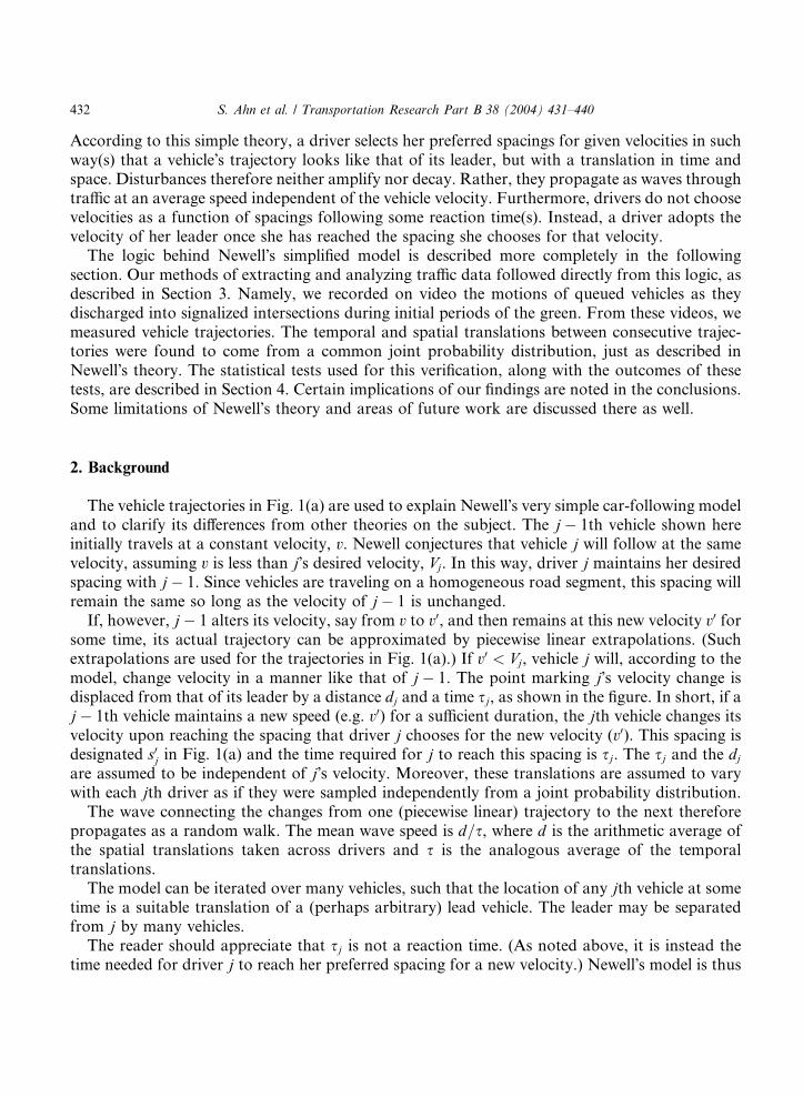
The vehicle trajectories in Fig. 1(a) are used to explain Newell�s very simple car-following modeland to clarify its differences from other theories on the subject. The j� 1th vehicle shown hereinitially travels at a constant velocity, v. Newell conjectures that vehicle j will follow at the samevelocity, assuming v is less than j�s desired velocity, Vj. In this way, driver j maintains her desiredspacing with j� 1. Since vehicles are traveling on a homogeneous road segment, this spacing willremain the same so long as the velocity of j� 1 is unchanged.
If, however, j� 1 alters its velocity, say from v to v0, and then remains at this new velocity v0 forsome time, its actual trajectory can be approximated by piecewise linear extrapolations. (Suchextrapolations are used for the trajectories in Fig. 1(a).) If v0 < Vj, vehicle j will, according to themodel, change velocity in a manner like that of j� 1. The point marking j�s velocity change isdisplaced from that of its leader by a distance dj and a time sj, as shown in the figure. In short, if aj� 1th vehicle maintains a new speed (e.g. v0) for a sufficient duration, the jth vehicle changes itsvelocity upon reaching the spacing that driver j chooses for the new velocity (v0). This spacing isdesignated s0j in Fig. 1(a) and the time required for j to reach this spacing is sj. The sj and the djare assumed to be independent of j�s velocity. Moreover, these translations are assumed to varywith each jth driver as if they were sampled independently from a joint probability distribution.
The wave connecting the changes from one (piecewise linear) trajectory to the next thereforepropagates as a random walk. The mean wave speed is d=s, where d is the arithmetic average ofthe spatial translations taken across drivers and s is the analogous average of the temporaltranslations.
The model can be iterated over many vehicles, such that the location of any jth vehicle at sometime is a suitable translation of a (perhaps arbitrary) lead vehicle. The leader may be separatedfrom j by many vehicles.
The reader should appreciate that sj is not a reaction time. (As noted above, it is instead thetime needed for driver j to reach her preferred spacing for a new velocity.) Newell�s model is thus
τj
velocity
spac
ing,
s j
Vj
dj
(b)
sj
dj
τj
s ,j
vehicle j-1
vehicle j
v
v
time
dist
ance
(a)
density
flow
Average Desired Velocity
d / τ
1/d
1/τ
(c)
,
Fig. 1. (a) Piecewise linear vehicle trajectories (adopted from Newell, 2002), (b) relation between velocity and spacing
for an individual driver (adopted from Newell, 2002), (c) density-flow curve for Newell�s theory.
S. Ahn et al. / Transportation Research Part B 38 (2004) 431–440 433
based upon drivers� preferred following distances for given velocities in a way that distinguishes itfrom most other car-following theories. It follows that each driver adopts her own relation be-tween velocity and spacing and, as shown in Fig. 1(b), this relation is linear with slope sj.
1
Finally, Newell transformed his car-following model into a macroscopic one for describingaverage driver behavior. In this way, he established a connection between his theory and fluidmodels. This simple transformation leads to a linear relation between queued flows and densities,as shown in Fig. 1(c). 2 This form indicates that in queued traffic, flow is a linear decreasing
1 That the slope of each j�s spacing–speed relation is sj follows from the trajectories in Fig. 1(a) showing that j�sspacing, sj, equals dj þ v � sj.
2 That the macroscopic relation between queued densities and flows is linear follows from the previous discussion, but
the reader can refer to Newell (2002) for the simple analytical derivation.
434 S. Ahn et al. / Transportation Research Part B 38 (2004) 431–440
function of density and the relation depends upon d and s. The average wave speed, d=s, is in-dependent of vehicle velocities.
3. Data and study scope
The methods used in this study to verify Newell�s car-following theory followed from the logicjust described. We measured the trajectories of vehicles as they discharged from long queues onhomogeneous approaches to signalized intersections. The methods used for collecting the neededmeasurements are described below.
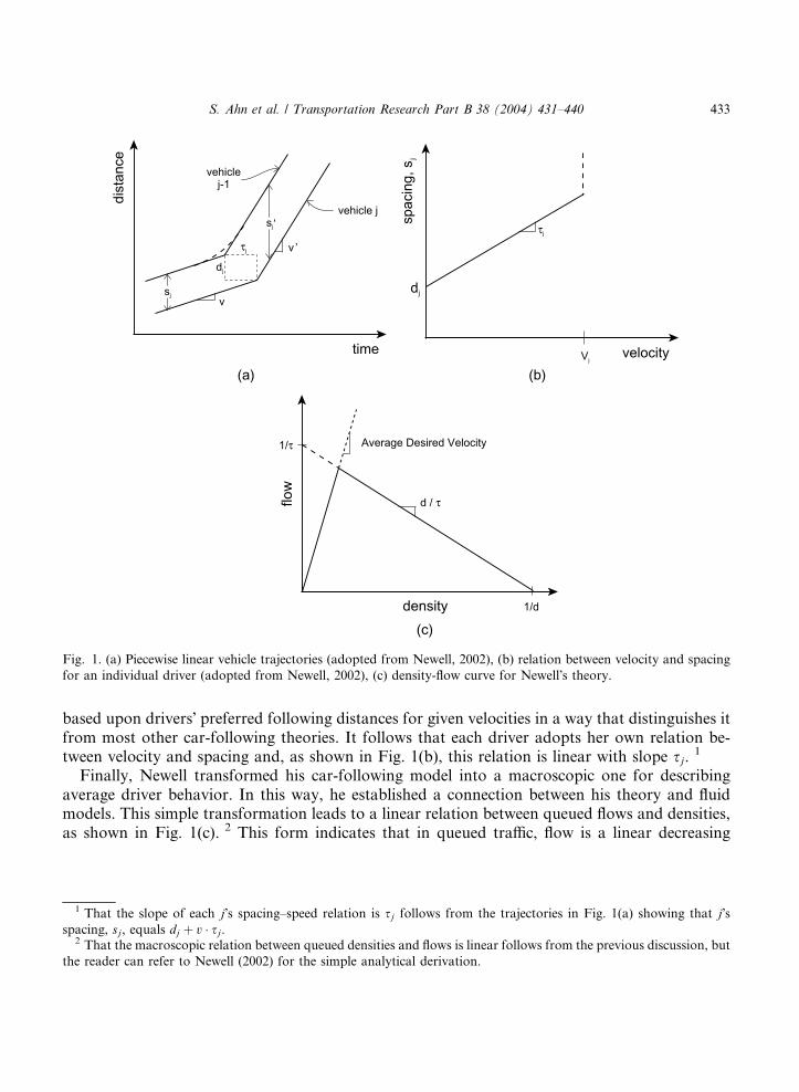
The data were obtained by video-taping traffic on the arterial approaches to two signalizedintersections, both located in Oakland, California. These are illustrated in Figs. 2(a) and (b). Thisdata collection took place during afternoon rush periods in 2001 and videos were taken ofmultiple travel lanes at each of the two intersections, as annotated in the figures. The queues ineach of these lanes grew to include 10 vehicles or more in virtually every cycle captured in ourvideos. To record these long queues in their entirety, the videos were taken from top floors of tallbuildings nearby.
N
W. McArthur Blvd.
(How
e St.)
curb lane
center lane
median lane
Vantage point
Lanes from which datawere extracted
(a)
(W. Grand Ave.)
Harrison St.
curb lane
center lane
median lane
turning lane
(b)
N
Vantage point
Lanes from which datawere extracted
Fig. 2. (a) McArthur site, (b) Harrison site.
S. Ahn et al. / Transportation Research Part B 38 (2004) 431–440 435
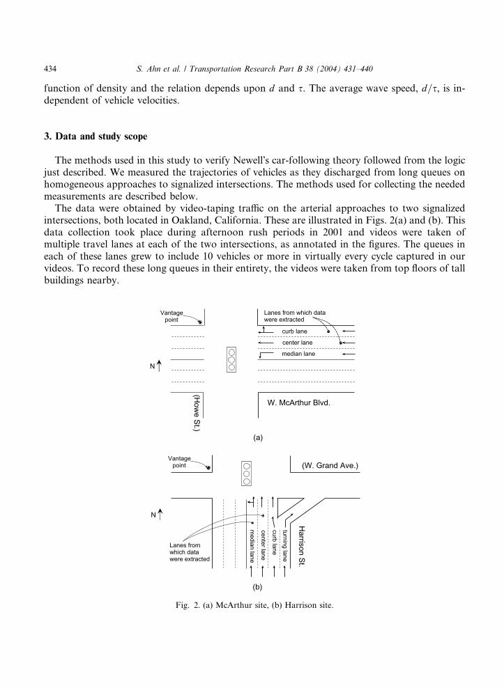
The trajectories for many of these discharging vehicles were constructed by measuring (fromvideo) the times each passed fixed reference points along the intersection approaches. Thesereference points were separated by short distances of 3–6 m (10–20 ft) and each vehicle�s passagetimes were plotted in the time–space plane. A polynomial trend line was then fit to each set of suchpoints corresponding to a unique vehicle. The order of a polynomial curve was determined on acase by case basis, depending upon the pattern of measured points that mapped the vehicle�smotion.
Identical velocities were mapped from one trajectory to the next; (the reader will note that theslopes of a smoothed trajectory are the instantaneous velocities estimated for that vehicle). Themappings were performed for a sample of the velocities displayed by the trajectories. These werethe vehicle velocities just above 0 km/h and at 6.5 km/h, 13 km/h, and 19.5 km/h (4 mph, 8 mphand 12 mph), as shown in Fig. 3. The waves signaling vehicles to adopt these velocities are shownin the figure as heavy dashed lines. The slope of any such line is the wave�s speed. Notably, thetemporal and spatial translations that traced the propagation if these waves (sj and dj for eachvehicle j) were found to have come from a common joint probability distribution, as per Newell�ssimple theory.
But trajectories were not constructed for all the discharging vehicles observed on video. Thus,measurements were not usually taken of each trajectory�s temporal and spatial translations along
0
6.5 km/h
13 km/h
19.5 km/h
Vehicle 1
Vehicle 2
Vehicle 3
Last vehicle in cycle m, n
wavespeed
T(n )
D(n )
time
distance
Intersection
Stop bar
Fig. 3. Construction of piecewise trajectories and the waves they reveal.
436 S. Ahn et al. / Transportation Research Part B 38 (2004) 431–440
wave paths. Instead, most of the observations were collected in a more aggregate fashion, asdescribed below. This greatly simplified the task of data extraction and it provided for an effectiveway of validating Newell�s model.
For each lane, and for each signal cycle, trajectories were constructed for the vehicles in queueas they discharged into the intersection. The first one or two vehicles were usually disregarded inour analysis; since the camera did not view traffic far downstream of the intersection, the first oneor two trajectories of each cycle could not be constructed over sufficiently large intervals of timeand space.
For each cycle m, the number of queued vehicles in a given lane, nm, was noted. We thenmeasured the T ðnmÞ and DðnmÞ, the total time and distance covered by a wave propagatingthrough a queue, as illustrated in Fig. 3. These T ðnmÞ and DðnmÞ were separately measured foreach of the four waves described by the trajectories.
According to Newell�s theory, the [T ðnmÞ;DðnmÞ] is a bivariate process with independent in-crements. This assumption of independence was verified by measuring the sj and dj for variousvehicle j after we constructed the trajectories for each and every vehicle discharging from a sampleof the queues captured in our videos.
Thus, the [T ðnmÞ;DðnmÞ] can be described by a bivariate normal distribution with mean andcovariance matrix proportional to nm, i.e.,
½T ðnmÞ;DðnmÞ� � BVN ½s�
� nm; d � nm�;r2s rds
rsd r2d
� �� nm
�ð1Þ
Since the nm varied with m, samples taken in each cycle were not identically distributed. The fiveparameters in Eq. (1) (s, d, r2
s , r2d and rsd) were therefore obtained using maximum likelihood
estimation. These parameters were separately estimated for each of the four wave types in a givenlane. They were then jointly estimated again from the [T ðnmÞ;DðnmÞ] measured for all (four) wavesin a lane.
These estimates were next used in a likelihood ratio test. The outcome indicated that a commonbivariate normal distribution can be used for describing [T ðnmÞ;DðnmÞ] for any of the four waves ina given lane. The test thus confirmed Newell�s hypothesis that [sj; dj] vary as if they were sampledindependently from some joint probability distribution.
It is notable that our validation methods used trajectories that were, in reality, continuallyaccelerating; i.e., most vehicles videoed in the discharging queues did not actually maintain a fixedvelocity for an extended period. That our tests nonetheless support Newell�s theory attests to therobust nature of his simple model. These tests are described in the following section.
4. Verifying the theory
The presentations in this section show that the [sj; dj] in each lane came from a common jointdistribution. To this end, we first verified the assumption underlying Eq. (1); i.e., that the[T ðnmÞ;DðnmÞ] has independent increments. This was done by constructing the trajectories for allof the discharging vehicles from a sample of the queues. The temporal and spatial translationsbetween consecutive trajectories were then measured along the waves.
2
4
6
8
10
12
2 4 6 8 10 12-1
0
1
2
3
-1 0 1 2 3
-1
0
1
2
3
-1 0 1 2 3 2
4
6
8
10
12
2 4 6 8 10 12
(a) (b)
(c) (d)
d (m
)j+
1
d (m)j
d (m
)j+
1
d (m)j
τ (s
ec)
j+1
τj (sec)
τ (s
ec)
j+1
τj (sec)
Fig. 4. (a) sj vs sjþ1; curb lane of McArthur site; wave marking vehicle velocity of 6.5 km/h, (b) dj vs djþ1; curb lane of
McArthur site; wave marking vehicle velocity of 6.5 km/h, (c) sj vs sjþ1; median lane of Harrison site; wave marking
vehicle velocity of 13 km/h, (d) dj vs djþ1; median lane of Harrison site; wave marking vehicle velocity of 13 km/h.
S. Ahn et al. / Transportation Research Part B 38 (2004) 431–440 437
Some typical examples of these samples are presented as lag-one scatter-plots in Fig. 4(a)–(d).The samples in each plot were taken from a single lane for one of the four different wave types; aslabeled in the figure. Each plot displays the measured spatial or temporal translation for a jthvehicle vs that translation observed for its neighbor jþ 1. In every case, the pattern of data scatterreveals no trends or correlations. The [sj; dj] can therefore be taken as independent across drivers.
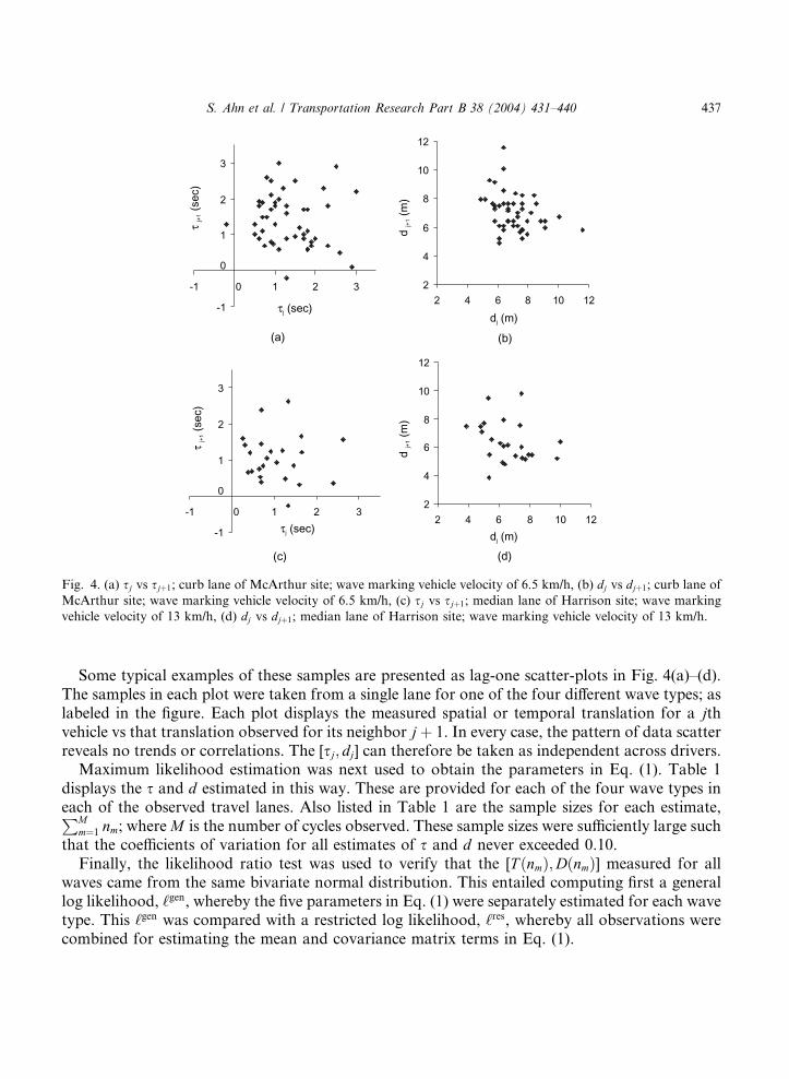
Maximum likelihood estimation was next used to obtain the parameters in Eq. (1). Table 1displays the s and d estimated in this way. These are provided for each of the four wave types ineach of the observed travel lanes. Also listed in Table 1 are the sample sizes for each estimate,PM
m¼1 nm; whereM is the number of cycles observed. These sample sizes were sufficiently large suchthat the coefficients of variation for all estimates of s and d never exceeded 0.10.
Finally, the likelihood ratio test was used to verify that the [T ðnmÞ;DðnmÞ] measured for allwaves came from the same bivariate normal distribution. This entailed computing first a generallog likelihood, ‘gen, whereby the five parameters in Eq. (1) were separately estimated for each wavetype. This ‘gen was compared with a restricted log likelihood, ‘res, whereby all observations werecombined for estimating the mean and covariance matrix terms in Eq. (1).
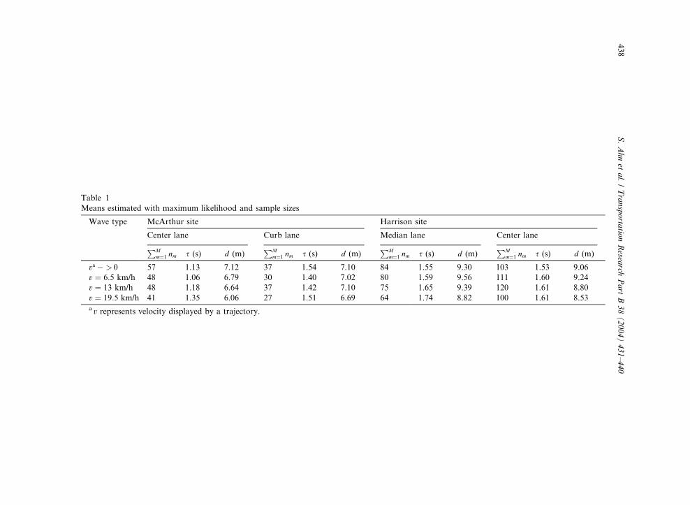
Table 1
Means estimated with maximum likelihood and sample sizes
Wave type McArthur site Harrison site
Center lane Curb lane Median lane Center lane
PMm¼1 nm s (s) d (m)
PMm¼1 nm s (s) d (m)
PMm¼1 nm s (s) d (m)
PMm¼1 nm s (s) d (m)
va � > 0 57 1.13 7.12 37 1.54 7.10 84 1.55 9.30 103 1.53 9.06
v ¼ 6:5 km/h 48 1.06 6.79 30 1.40 7.02 80 1.59 9.56 111 1.60 9.24
v ¼ 13 km/h 48 1.18 6.64 37 1.42 7.10 75 1.65 9.39 120 1.61 8.80
v ¼ 19:5 km/h 41 1.35 6.06 27 1.51 6.69 64 1.74 8.82 100 1.61 8.53a v represents velocity displayed by a trajectory.
438
S.Ahnet
al./Transporta
tionResea
rchPart
B38(2004)431–440
χ152
Harrison siteMcArthur site
23.0
16.2
22.8
11.8
CenterLane
CurbLane
CenterLane
MedianLane
0
10
20
30
40
50
α=0.05
25
Fig. 5. Results of ratio tests showing [T ðnmÞ;DðnmÞ] is independent of vehicle velocity.
S. Ahn et al. / Transportation Research Part B 38 (2004) 431–440 439
The log likelihood ratio, 2� ð‘gen � ‘resÞ, has a Chi-Square distribution, in this case with degreeof freedom 15; (15 is the number of parameters lost in the restricted model). The log likelihoodratios obtained for each travel lane are shown in Fig. 5. In each instance, these are smaller than 25,the Chi-Square critical value at the 0.05 significance level.
The general and restricted models are therefore identical in a statistical sense; i.e., their dif-ferences are insignificant. This means that the same bivariate normal distribution can be used todescribe the [T ðnmÞ;DðnmÞ] for each of our four wave types; i.e., the distribution is independent ofvehicle velocity. It follows that each jth driver�s [sj; dj] came from some common joint probabilitydistribution, as per Newell�s simple theory.
5. Conclusions
As platoons accelerate on homogeneous highways, a jth vehicle evidently follows the sametrajectory as the j� 1th vehicle except for a translation in time and space. For the data observed inthe present work, the translations [sj; dj] varied as if drawn independently from a joint distribution.The finding supports Newell�s simplified car-following theory. This, in turn, supports the macro-scopic traffic theory of Lighthill and Whitham (1955) with a triangular shaped density-flow curve.
Our finding does indicate that the congested branch of the density-flow curve is linear in form,at least for the low vehicle velocities observed here. Wave speed was thus the same for differentvalues of flow or density within the ranges observed. In contrast to what is described by non-lineardensity-flow curves, we observed that accelerating vehicles did not create waves that fannedoutward.
It is notable that the effects created by non-linear density-flow curves were not even observed atvehicle velocities very close to zero. We cannot verify, however, that non-linear effects do not arise
440 S. Ahn et al. / Transportation Research Part B 38 (2004) 431–440
in queued traffic when vehicle velocities approach desired velocities. These conditions were outsidethe range of what was studied here since many vehicles in the discharging queues did not reachsuch high velocities while on the homogeneous approaches to the intersections.
Of further note, Newell�s theory is particularly susceptible to vehicle lane-changing maneuvers(i.e., over-taking), as these interrupt car following. Lane changing seldom arose in the presentstudy (and the cycles in which we observed lane-change maneuvers were excluded from our an-alyses). But Mauch and Cassidy (2002) demonstrate that Newell�s theory fails for the case ofqueued freeway traffic when heavy lane-changing takes place. It would seem that improvements intraffic flow theories will come by incorporating lane-changing effects.
Improved traffic theories should also result by better understanding the influences of geometricinhomogeneities on driver behavior. Of course, Newell�s simplified theory is not expected to holdat inhomogeneities and we have even observed an instance of this. In addition to the measure-ments already described in this manuscript, we examined discharging queues in the curb lane fornorthbound traffic at the Harrison intersection; see Fig. 2(b). As shown in the figure, the lane hasan inhomogeneity. Namely, its width reduces upstream of the intersection. Not surprisingly, ouranalyses of the data indicated that car-following in that lane was not described as per Newell�stheory.
Trajectories in this curb lane are currently being studied to obtain insights into car-followingbehavior at the inhomogeneity. One cannot model driver behavior at inhomogeneities withoutfirst understanding what actually occurs.
Finally, the present work did not explicitly verify that a jth driver tends to maintain the same[sj; dj] over her trip,
3 even though this driver attribute is also part of Newell�s theory. But findingsreported from earlier research can now be used as evidence that this attribute actually occurs.
Previous work by Cassidy and Windover (1998), for example, has shown that individual drivershave their own ‘‘personalities’’ (i.e., different drivers choose different spacings for a given velocity)and that drivers tend to remember their personalities. In light of the present findings reportedhere, this earlier finding can be taken as support for Newell�s contention that a [sj; dj] is main-tained by each driver j.
References
Cassidy, M.J., Windover, J.R., 1998. Driver memory: motorist selection and retention of individualized headways in
highway traffic. Transpn Res. 32A, 129–137.
Chandler, R.E., Herman, R., Montroll, E.W., 1958. Traffic dynamics: studies in car following. Oper. Res. 6, 165–184.
Kometani, E., Sasaki, T., 1961. Dynamic behavior of traffic with a nonlinear spacing. In: Herman, R. (Ed.), Theory of
Traffic Flow. Elsevier, Amsterdam, pp. 105–119.
Lighthill, M.J., Whitham, G.B., 1955. I Flood movement in long rivers. II A theory of traffic flow on long crowded
roads. On kinematic waves in highway traffic. Proc. Roy. Soc. (London) A229, 281–345.
Mauch, M., Cassidy, M.J., 2002. Freeway traffic oscillations: observations and predictions. In: Tailor, M.A.P. (Ed.),
Traffic and Transportation Theory in the 21st century. Elsevier, New York, pp. 653–673.
Newell, G.F., 2002. A simplified car-following theory: a lower order model. Transport. Res. 36B, 195–205.
3 For each jth trajectory, we sampled only four different vehicle velocities and therefore obtained only four joint
observations of [sj; dj]. This would be too small a sample from which to draw conclusions.