vector bundles and gauge theory uw math 865 – spring 2022

VECTOR BUNDLES AND GAUGE THEORYUW MATH 865 – SPRING 2022

ALEX WALDRON

Contents

Part I. Topological classification of vector bundles 2

1. Definition, first examples, bundle morphisms (1/25) 2

2. Motivating questions, bundle operations (1/27) 6

3. Quotients, metrics, splitting (2/1) 11

4. Pullbacks, homotopy theorem (2/3) 16

5. Structure group, orientation (2/8) 20

6. Clutching construction, quaternionic line bundles (2/8-10) 23

7. Universal vector bundles, characteristic classes (2/15) 29

8. Classification of vector bundles in low dimension, transversality (2/17) 33

9. Principal bundles, reduction of structure group (2/22) 40

10. Correspondence with vector bundles, universal G-bundles (2/24) 46

Part II. Connections, curvature, Chern-Weil Theory 50

11. Connections (3/1) 50

12. Curvature (3/3) 54

13. Flatness and curvature (3/8) 59

14. Chern-Weil forms (3/10) 61

15. Structure group for connections, Gauss-Bonnet, higher Chern classes (3/22) 66

16. Whitney product formula, Pontryagin and Euler classes (3/24) 71

Part III. The Yang-Mills functional 77

17. Definition and first properties (3/24-29) 77

18. Maxwell’s equations and the magnetic monopole (3/29-31) 82

19. Yang-Mills connections and minimizers in 2D (3/31) 85

20. Instantons in 4D (4/5) 87

21. Uhlenbeck’s Theorem: warm-up I (4/5-7) 91

22. Uhlenbeck’s Theorem: warm-up II, statement, key estimate (4/7-12) 97

23. Uhlenbeck’s Theorem: proof, statement of Compactness Theorem (4/12-14) 100

Part IV. Holomorphic bundles 106

24. Definition and first examples (4/19) 106

25. ∂-operator, Chern connection, integrability (4/21) 110

Date: July 1, 2022.

2 ALEX WALDRON

26. Action of the complexified gauge group (4/26) 116

27. Holomorphic splitting, stability, Narasimhan-Seshadri Theorem (4/28-5/3) 121

28. Donaldson’s proof, I (4/28-5/3) 125

29. Donaldson’s proof, II (5/5) 129

Part I. Topological classification of vector bundles

1. Definition, first examples, bundle morphisms (1/25)

1.1. The definition. Let π ∶ E ↠ X be a surjective map between topological spaces. (A

map will always be assumed to be continuous.)1

Given an open set U ⊂X, a section of π over U is a map s ∶ U → E such that

π s = 1U .

Equivalently, s must satisfy

s(x) ∈ Ex = π−1(x)for each x ∈ U. In case U =X, s is called a global section.

We write2

Γ(U,E) = sections of π over U.These sets obviously fit together to form a sheaf over X, although we do not plan to use this

fact in the short term.

Fix a base field K = R or C. Many of the results will also apply for K = H, but some care

may be required.

Definition 1.1. We say that π ∶ E →X is a vector bundle over K of rank r ∈ N if:

(1) Each fiber Ex is endowed with operations + and ⋅ giving the structure of a vector space

over K of dimension r, and these operations are continuous in the subspace topology on

Ex ⊂ E.(2) For each x0 ∈ X, there exists an open neighborhood U ∋ x0 and a local frame of

sections eαrα=1 over U, such that the map

U ×Kr → π−1(U) ⊂ E(x, a1, . . . , ar)↦ a1e1(x) +⋯ + anen(x)

is a homeomorphism.

1.2. Terminology. E = “total space,” X = “base space,” (U,eα) = “local trivialization.”Vector bundle of rank 1 = “line bundle” (Note: real and complex line bundles have very

different properties.)

Given s ∶ V → E and U ⊂ V, the restriction of s is given by the composition

s∣U ∶ U Vs→ E.

1Thanks to Connor Simpson for providing the latex draft of these notes after each class!2As of now, Γ refers only to the space of continuous sections. For smooth or holomorphic bundles, it will

denote the space of smooth or holomorphic sections.

VECTOR BUNDLES AND GAUGE THEORY UW MATH 865 – SPRING 2022 3

If eα is a local frame for E over U, the local components of of s,

sα ∶ U ∩ V →K, α = 1, . . . , r,

are defined by the rule

s∣U∩V =∑α

sαeα.

These are defined by the composition

sα ∶ U ∩ Vs∣U∩VÐ→ π−1(U ∩ V ) ∼Ð→ (U ∩ V ) ×Kr αÐ→K,

where the second arrow is the inverse of the homeomorphism defined by the frame eα,according to item (2) of Definition 1.1. Hence, the local components are always continuous.

Lastly, given a complex vector bundle E of rank r, there is a canonical real vector bundle of

rank 2r obtained by restricting the scalar field to R ⊂ C. This is referred to as the underlying

real bundle. We shall sometimes abuse notation and refer to the underlying real bundle by

the same letter E.

1.3. Examples.

Kr =X ×Kr, the trivial bundle of rank r.

E = [0,1] × R/ ∼, where (0, v) ∼ (1,−v) for all v ∈ R. The base space is X = S1 =[0,1] /(0 ∼ 1), with the obvious projection. This is the Mobius bundle. A local

trivialization exists over any proper subset of S1, but no global trivialization exists

(exercise).

The tangent bundle TS2, defined by

π ∶ TS2 = (x, v) ∈ S2 ×R3 ∣ x ⋅ v = 0→ S2,

with the subspace topology from S2 ×R3.

Given x0 ∈ S2, a local frame near x0 can be defined as follows. Choose x1, x2 ∈ R3

such that x0, x1, x2 form an orthonormal basis. Let

e1(x) = x × x1, e2(x) = x × x2.

Then these form a local frame on the open hemisphere U = x ∈ S2 ∣ x ⋅ x0 > 0.Note that TS2 can also be made into a C-line bundle by the rule

i ⋅ (x, v) = (x,x × v)

This operation satisfies i ⋅ i = −1, so gives a well-defined scalar multiplication by C(this is called an almost-complex structure).

1.4. Bundle morphisms. In what follows we shall often refer to a “vector bundle,” with

the fixed base field K understood.

Definition 1.2. Given two vector bundles E and F overX, a bundle morphism σ ∶ E → F

is a map such that the diagram

Eσ

//

F

X

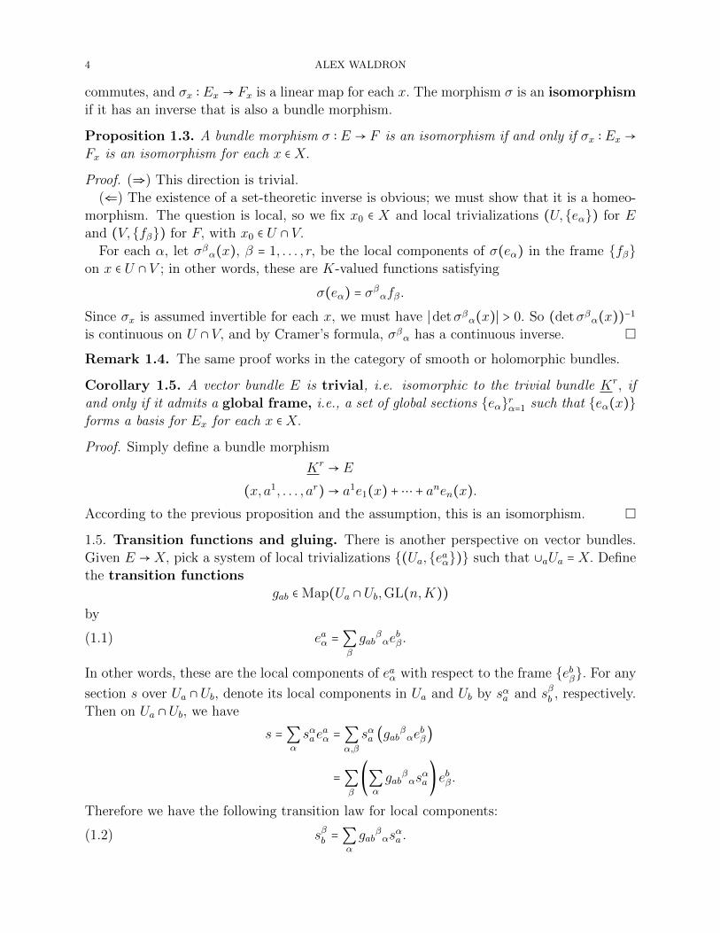
4 ALEX WALDRON

commutes, and σx ∶ Ex → Fx is a linear map for each x. The morphism σ is an isomorphism

if it has an inverse that is also a bundle morphism.

Proposition 1.3. A bundle morphism σ ∶ E → F is an isomorphism if and only if σx ∶ Ex →Fx is an isomorphism for each x ∈X.

Proof. (⇒) This direction is trivial.

(⇐) The existence of a set-theoretic inverse is obvious; we must show that it is a homeo-

morphism. The question is local, so we fix x0 ∈ X and local trivializations (U,eα) for Eand (V,fβ) for F, with x0 ∈ U ∩ V.

For each α, let σβα(x), β = 1, . . . , r, be the local components of σ(eα) in the frame fβon x ∈ U ∩ V ; in other words, these are K-valued functions satisfying

σ(eα) = σβαfβ.Since σx is assumed invertible for each x, we must have ∣detσβα(x)∣ > 0. So (detσβα(x))−1is continuous on U ∩ V, and by Cramer’s formula, σβα has a continuous inverse.

Remark 1.4. The same proof works in the category of smooth or holomorphic bundles.

Corollary 1.5. A vector bundle E is trivial, i.e. isomorphic to the trivial bundle Kr, if

and only if it admits a global frame, i.e., a set of global sections eαrα=1 such that eα(x)forms a basis for Ex for each x ∈X.

Proof. Simply define a bundle morphism

Kr → E

(x, a1, . . . , ar)→ a1e1(x) +⋯ + anen(x).According to the previous proposition and the assumption, this is an isomorphism.

1.5. Transition functions and gluing. There is another perspective on vector bundles.

Given E →X, pick a system of local trivializations (Ua,eaα) such that ∪aUa =X. Definethe transition functions

gab ∈Map(Ua ∩Ub,GL(n,K))by

(1.1) eaα =∑β

gabβαe

bβ.

In other words, these are the local components of eaα with respect to the frame ebβ. For anysection s over Ua ∩Ub, denote its local components in Ua and Ub by sαa and sβb , respectively.

Then on Ua ∩Ub, we have

s =∑α

sαaeaα =∑

α,β

sαa (gabβαebβ)

=∑β

(∑α

gabβαs

αa) ebβ.

Therefore we have the following transition law for local components:

(1.2) sβb =∑α

gabβαs

αa .


Now, given three charts Ua, Ub, and Uc, it is clear from the definition that these transition

functions must satisfy

gaa = 1gac = gbc ⋅ gab

(1.3)

on Ua ∩Ub ∩Uc. Here, ⋅ denotes matrix multiplication in GL(n,K). The rule (1.3) is known

as the cocycle condition.

Conversely, given the data of an open cover Ua and any collection of GL(n,K)-valuedfunctions gab on Ua ∩ Ub, for each a and b, we can construct a vector bundle as follows.

Consider the disjoint union of trivial bundles

(1.4) E0 =∐a

Ua ×Kr

and form the relation

(x, v) ∈ Ua ×Kr ∼ (x, gab ⋅ v) ∈ Ub ×Kr

for each a, b. The cocycle condition (1.3) precisely implies that this is an equivalence relation.

In particular, we may let

E = E0/ ∼,

which has a well-defined projection map to X with fiber Kn. In this way, such gluing data

gives rise to a vector bundle over X; the construction is clearly inverse to choosing local

frames to form transition functions for a given bundle E.

The notion of isomorphism is very concrete from the perspective of transition functions:

Proposition 1.6. Two bundles are isomorphic if and only if, after passing to a common

refinement Ua, their transition functions are related by

(1.5) fab = τagabτ−1b

for a collection of GL(r,K)-valued functions τa on Ua.

Proof. Exercise in the definitions.

Remark 1.7. For the case of line bundles (r = 1), we have GL(r,K) = K×, so the transi-

tion functions and changes-of-frame are just nonvanishing K-valued functions. The cocycle

condition (1.3) just says that gab is a sheaf cocycle, for the sheaf C 0(K×) of nonvanishingcontinuous K-valued functions on X, viewed as a sheaf of abelian groups under multiplica-

tion. The isomorphism condition (1.5) just says that two cocycles differ by a coboundary.

Proposition 1.6 can therefore be rephrased as follows in terms of sheaf cohomology:

Corollary 1.8. The set of isomorphism classes of line bundles over X is in natural bijection

with the sheaf cohomology group H1(X,C 0(K×)).

A cohomological approach is also possible for higher-rank bundles (in a much more com-

plicated way, called “obstruction theory”), but the homotopy approach that we will take is

more powerful (and more standard).

6 ALEX WALDRON

1.6. Exercises.

1. Prove that the Mobius bundle is nontrivial.

2. Prove that TS2 ⊕R is trivial. (See below for definition of direct sum ⊕.)3. Prove Proposition 1.6.

2. Motivating questions, bundle operations (1/27)

2.1. Two more examples.

1. The best-known example of a vector bundle is the following. Suppose that X = Mhappens to be an n-dimensional smooth manifold with a coordinate atlas (Ua,xiani=1.The tangent bundle TM of M is the vector bundle with transition functions

gabji =

∂xjb∂xia

.

These are derived from the coordinate frames of M, best written symbolically as

eai =∂

∂xia,

whence the transition functions above are just the Jacobians of the transition maps

between the coordinate charts. The cocycle condition follows from the chain rule.

Since the transition functions are smooth GL(n,R)-valued functions on open sets of

M, TM is called a smooth vector bundle.3

2. If M happens to be a complex manifold of complex dimension n, with a holomorphic

coordinate atlas (Ua,ziani=1), we may form the holomorphic tangent bundle

T 1,0M using the transition functions

∂zjb∂zia

.

This is a rank n C-vector bundle. Since the transition functions are holomorphic

GL(n,C)-valued functions, we call this is a holomorphic vector bundle.4

2.2. Motivating questions. Here are some big motivating questions for the class. The first

one is much too big and we will not get to discuss it this semester, although the techniques

that we’ll introduce turn out to have much to say about it.

Question 1. Which topological manifolds admit smooth structures?

3Equivalently, we can define a smooth vector bundle by going through Definition 1.1 and requiring all

objects to be smooth manifolds and all projections, sections, etc., to be smooth.4Equivalently, we can define a holomorphic vector bundle by going back through Definition 1.1 and

requiring all objects to be complex manifolds and all projections, sections, etc., to be holomorphic...we will

do this later.

We will also show that the underlying real vector bundle of T 1,0M, as a rank 2n real vector bundle, is

canonically isomorphic to TM, the tangent bundle of the underlying 2n-dimensional smooth manifold.


Note: a topological manifold is a space that’s locally homeomorphic to Rn, i.e., possesses a

coordinate atlas with continuous transition maps. Such an atlas is called a smooth structure

on M if the transition maps are C∞. (Note: transition maps are between coordinate charts

on a manifold. Transition functions are between local frames in a vector bundle.)

Answer. n ≤ 2, all (we can write them down).

n = 3, all (E. Moise, ’50s).

n ≥ 4, most no. In particular:

n ≥ 5, only finitely many distinct smooth structures per topological manifold.

n = 4, still possible that infinitely many non-diffeomorphic smooth structures exist on

every smooth 4-manifold, as is already known for R4 and certain closed 4-manifolds.

Smale, Milnor, Freedman, Donaldson, not to mention many non-Fields-medalists...

The first question that we plan to say something about is in some sense a “linearization”

of the above question.

Question 2. Suppose that X =M is a smooth manifold, and E →M is a topological vector

bundle (see Definition 1.1) overM. Can E be given the structure of a smooth vector bundle?

Equivalently: do there exist continuous changes-of-frame τa on a coordinate atlas Uasuch that the new transition functions τagabτ−1b are smooth?

Answer. Yes. We should know how to prove this in not too long.

Question 3. Suppose that M is a complex manifold and E →M is a smooth (or indeed a

topological) complex vector bundle over M. Can E be given the structure of a holomorphic

vector bundle?

Equivalently: do there exist smooth changes-of-frame τa on a coordinate atlas Ua suchthat the new transition functions τagabτ−1b are holomorphic?

Answer. dimCM = 1, yes.dimCM ≥ 2, yes, if and only if E carries a connection whose curvature is of type (1,1). We

will define these objects in due course.

Question 4. Suppose that M is a compact Kahler manifold and E → M is a holomor-

phic vector bundle. Can E be given the structure of a flat bundle, compatible with the

holomorphic structure?

Equivalently: do there exist holomorphic changes-of-frame τa on a coordinate atlas Uasuch that the new transition functions τagabτ−1b are constant?

Answer. dimCM = 1, yes, if and only if the first Chern class vanishes and E is stable in

Mumford’s sense. This is the Narasimhan-Seshadri Theorem. We will define both Chern

classes and stability in due course.

dimCM ≥ 2, there is an optimal generalization called the Donaldson-Uhlenbeck-Yau Theorem

which we may get to discuss at the end (for the case dimCM = 2).

8 ALEX WALDRON

2.3. Goal of Part I. Before trying to make progress on Questions 2-4 above, we have to

address the following more basic problem.

Definition 2.1. Given a subgroup G ⊂ GL(n,K), we say that a vector bundle has structure

group G if all of its transition functions take values in G.

A priori, any real vector bundle has structure group GL(n,R), and any complex vector

bundle has structure group GL(n,C), but one often wants to restrict things further.5

Note that having structure group G is just a pointwise condition on the transition func-

tions, so more mundane than the above questions about smooth and holomorphic structures.

The goal of Part I is to give a method to classify all vector bundles with structure group

G over a given base space X. We will describe a general answer to this question in terms of

homotopy theory, and also show how to extract useful answers in the cases we’re interested

in.

2.4. Bundle operations. We’ll now continue developing the bundle formalism.

We have the following Meta-Theorem. Any6 functorial operation on the category of

vector spaces gives rise to one on the category of vector bundles.

2.4.1. Direct sum. The direct sum of two bundles has total space equal to the fiber product

E ⊕ F = E ×X F = (v,w) ∈ E × F ∣ πE(v) = πF (w).

The fiber is Ex⊕Fx, and the trivializations are the obvious ones. To check that it is actually

a vector bundle, it is easiest to just write down the transition functions. If g is a transition

function for E and f is a transition function for F, then the transition function for E ⊕F is

g ⊕ f,

i.e., the induced map on Ex ⊕ Fx for each x. By functoriality of ⊕ on vector spaces, this

preserves the identity and compositions, therefore it preserves the cocycle conditions (1.3).

2.4.2. Other operations. Here is a table with all the operations we discussed, together with

the transition functions:Operation Transition function

E ⊕ F g ⊕ fE ⊗K F g ⊗K f

E∗ = HomK(E,K) (gT )−1EndKE = E ⊗K E∗ g ⊗ (gT )−1

ΛkE k × k minors of g

detE det g

E g.

Note: For a complex bundle E, E is the same underlying real bundle but with a new complex

scalar multiplication, defined by

λ ⋅E v ∶= λ ⋅E v.5There is a formalism (that of principal bundles) to make the structure group something more intrinsic,

i.e., not just about transition functions with respect to a certain frame. We will introduce this when needed.6This is only true up to a point, as we will discuss below.


2.4.3. Dual frames and Einstein summation. One aspect here requires further explanation.

Given a frame eα for E, we usually work in the dual frame eα for E∗, which is uniquely

defined by the rule

eβ(eα) = δβα.

Given sections s = ∑α sαeα of E and t = ∑β tβeβ of E∗, we have

t(s) =∑β

tβeβ(∑

α

sαeα)

=∑α,β

sαtβeβ(eα)

=∑β,α

sαtβδβα

=∑α

sαtα.

The Einstein summation convention says that when pairing sections of E and its dual

bundle E∗, using the dual frame, we can omit the ∑α and just write

t(s) = sαtα.

So, when used properly, the convention should always be about summing the local compo-

nents of a section of a bundle (up index) and its dual bundle (down index) in the dual frame.

The mathematical content of the convention is that this is an a priori well-defined scalar.

Of course, it is common to abuse the notation, for instance to omit the Σα when writing

s = sαeα to define the local components themselves. But one should be aware that when

used properly, the Einstein convention has mathematical content.

Example 2.2. In the special case thatM is a smooth manifold of dimension n and E = TM,

and we are working in a coordinate chart xini=1, the tangent bundle has a distinguished

coordinate frame

ei =∂

∂xi

as described above in §2.1. The dual frame of the cotangent bundle E∗ = T ∗M is written as:

ei = dxi,

and satisfies

dxi ( ∂

∂xj) = δij.

Ordinarily,we will use the Latin indices i, j, k, ℓ, only for a coordinate frame/coframe

of the tangent bundle. So, Greek indices refer to an arbitrary frame for a vector bundle

E, but Latin indices refer to a specific type of frame for the bundles TM and T ∗M over a

smooth manifold.7

7The letters a, b, c that we have attached to coordinate charts above are labels, not indices. Eventually

we will omit these labels completely...an abuse of notation that is critical to our ability to do differential

geometry.

10 ALEX WALDRON

2.4.4. Endomorphisms. Following this convention, given a frame for E, we also have a nat-

ural frame for the endomorphism bundle

EndKE = HomK(E,E) = E ⊗K E∗

given by

eβ ⊗ eα.So a section of the endomorphism bundle

σ =∑α,β

σβαeβ ⊗ eα

acts on a section s = ∑γ sγeγ of E by

σ(s) =⎛⎝∑α,β

σβαeβ ⊗ eα⎞⎠(∑γ

sγeγ)

= ∑α,β,γ

σβαsγδαγeβ

=∑α,β

(σβαsα)eβ.

Using Einstein summation, we can just write

(σ(s))β = σβαsα.

So we wind up with the usual matrix multiplication rule.

We shall use similar notations on all tensor products between bundles and their duals, so

that we can always pair an up and a down index of the same bundle.

2.5. Subbundles. A subbundle E ⊂ F is by definition a subset that has the structure of

a vector bundle over X in the subspace topology. We have the following:

Lemma 2.3. For an injective bundle morphism φ ∶ E → F, the image φ(E) ⊂ F is a

subbundle, and φ ∶ E → φ(E) is an isomorphism.

Proof. It suffices to show that the map φ ∶ E → φ(E) is a homeomorphism, where φ(E) ⊂ Fis given the subspace topology.

Since the question is local, we may let x0 ∈X and choose a coordinate neighborhood U on

which we identify

E∣U ≅ U ×Kn.

Let vα = φx0(eα) ∈Kn, for α = 1, . . . , k. By assumption, these are linearly independent, so we

may complete them to a basis

v1, . . . , vk, vk+1, . . . vn

for Kn. Let V = ⟨vk+1, . . . , vn⟩ ⊂Kn. Then we may define a bundle morphism over U by

φ⊕ 1 ∶ E∣U ⊕ V → F ∣U(s, v)↦ φ(s) + v.

By assumption, this is an isomorphism on the fiber Ex0 . By the usual argument (see proof of

Proposition 1.3), this implies that it is a bundle isomorphism over a neighborhood W ∋ x0.


The map φ over W is obtained by restricting this isomorphism to two subspaces that are in

bijection; therefore, φ is also a homeomorphism over W. Since x0 ∈ X was arbitrary, we are

done.

2.6. Exercises.

1. Check that the transition functions of E∗ with respect to dual frames are given by

(gT )−1.2. Convince yourself that

Λk(E ⊕ F ) ≅ ⊕i+j=kΛiE ⊗ΛjF.

3. Show that the direct sum or tensor product of two copies of the Mobius bundle is

trivial.

4. Show that for any line bundle, L⊗L∗ is canonically isomorphic to the trivial bundle.

(Hint: write down an obvious morphism to the trivial line bundle.)

3. Quotients, metrics, splitting (2/1)

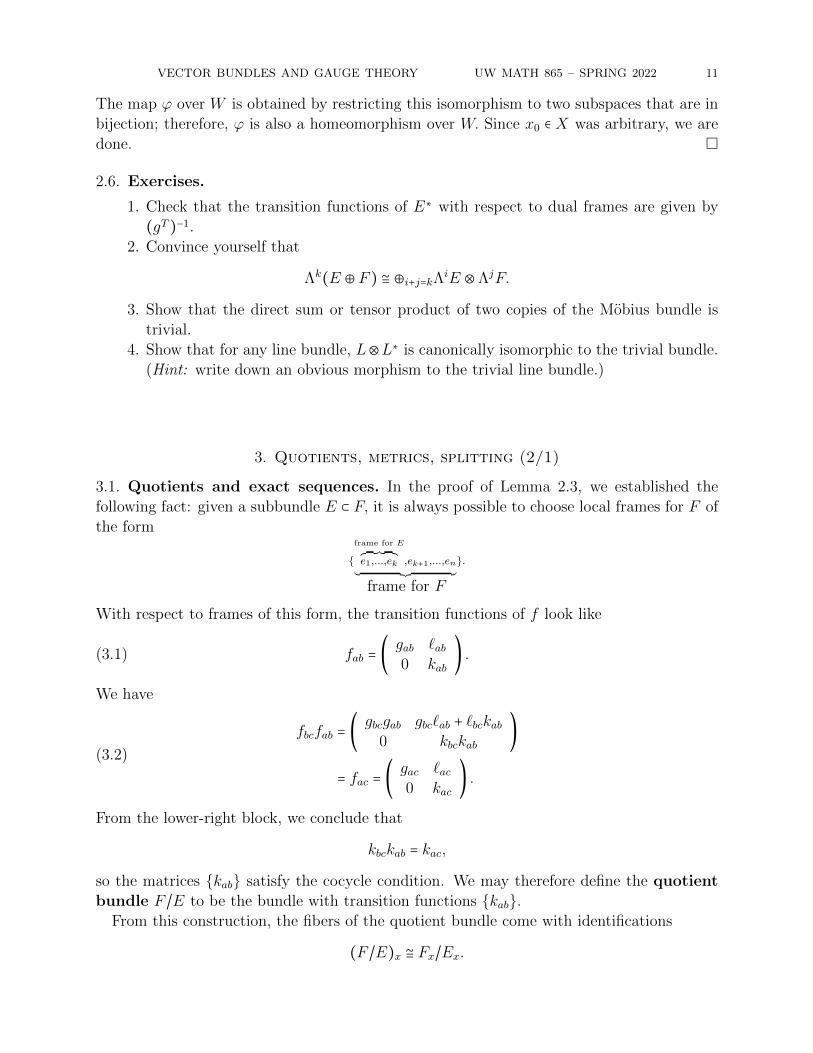
3.1. Quotients and exact sequences. In the proof of Lemma 2.3, we established the

following fact: given a subbundle E ⊂ F, it is always possible to choose local frames for F of

the form

frame for E

³ ¹¹¹¹¹¹¹¹·¹¹¹¹¹¹¹¹¹µe1,...,ek ,ek+1,...,en´ ¹¹¹¹¹¹¹¹¹¹¹¹¹¹¹¹¹¹¹¹¹¹¹¹¹¹¹¹¹¹¹¹¹¹¹¹¹¹¹¹¹¹¹¹¹¹¸ ¹¹¹¹¹¹¹¹¹¹¹¹¹¹¹¹¹¹¹¹¹¹¹¹¹¹¹¹¹¹¹¹¹¹¹¹¹¹¹¹¹¹¹¹¹¹¶

.

frame for F

With respect to frames of this form, the transition functions of f look like

(3.1) fab = (gab ℓab0 kab

) .

We have

fbcfab = (gbcgab gbcℓab + ℓbckab0 kbckab

)

= fac = (gac ℓac0 kac

) .(3.2)

From the lower-right block, we conclude that

kbckab = kac,

so the matrices kab satisfy the cocycle condition. We may therefore define the quotient

bundle F /E to be the bundle with transition functions kab.From this construction, the fibers of the quotient bundle come with identifications

(F /E)x ≅ Fx/Ex.

12 ALEX WALDRON

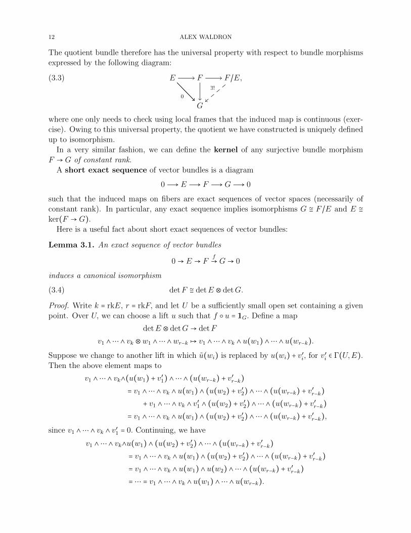
The quotient bundle therefore has the universal property with respect to bundle morphisms

expressed by the following diagram:

(3.3) E //

0

F

// F /E,∃!

||

G

where one only needs to check using local frames that the induced map is continuous (exer-

cise). Owing to this universal property, the quotient we have constructed is uniquely defined

up to isomorphism.

In a very similar fashion, we can define the kernel of any surjective bundle morphism

F → G of constant rank.

A short exact sequence of vector bundles is a diagram

0Ð→ E Ð→ F Ð→ GÐ→ 0

such that the induced maps on fibers are exact sequences of vector spaces (necessarily of

constant rank). In particular, any exact sequence implies isomorphisms G ≅ F /E and E ≅ker(F → G).

Here is a useful fact about short exact sequences of vector bundles:

Lemma 3.1. An exact sequence of vector bundles

0→ E → Ff→ G→ 0

induces a canonical isomorphism

(3.4) detF ≅ detE ⊗ detG.

Proof. Write k = rkE, r = rkF, and let U be a sufficiently small open set containing a given

point. Over U, we can choose a lift u such that f u = 1G. Define a map

detE ⊗ detG→ detF

v1 ∧⋯ ∧ vk ⊗w1 ∧⋯ ∧wr−k ↦ v1 ∧⋯ ∧ vk ∧ u(w1) ∧⋯ ∧ u(wr−k).

Suppose we change to another lift in which u(wi) is replaced by u(wi) + v′i, for v′i ∈ Γ(U,E).Then the above element maps to

v1 ∧⋯ ∧ vk∧(u(w1) + v′1) ∧⋯ ∧ (u(wr−k) + v′r−k)= v1 ∧⋯ ∧ vk ∧ u(w1) ∧ (u(w2) + v′2) ∧⋯ ∧ (u(wr−k) + v′r−k)+ v1 ∧⋯ ∧ vk ∧ v′1 ∧ (u(w2) + v′2) ∧⋯ ∧ (u(wr−k) + v′r−k)

= v1 ∧⋯ ∧ vk ∧ u(w1) ∧ (u(w2) + v′2) ∧⋯ ∧ (u(wr−k) + v′r−k),

since v1 ∧⋯ ∧ vk ∧ v′1 = 0. Continuing, we have

v1 ∧⋯ ∧ vk∧u(w1) ∧ (u(w2) + v′2) ∧⋯ ∧ (u(wr−k) + v′r−k)= v1 ∧⋯ ∧ vk ∧ u(w1) ∧ (u(w2) + v′2) ∧⋯ ∧ (u(wr−k) + v′r−k)= v1 ∧⋯ ∧ vk ∧ u(w1) ∧ u(w2) ∧⋯ ∧ (u(wr−k) + v′r−k)= ⋯ = v1 ∧⋯ ∧ vk ∧ u(w1) ∧⋯ ∧ u(wr−k).


Hence, the map is independent of the choice of local lift, so gives a globally well-defined

bundle morphism. Since it is clearly a local isomorphism, it is a global isomorphism (3.4).

Alternatively, one can obtain the isomorphism at the level of transition functions, directly

from (3.1).

3.2. The tautological bundle over CP1. Recall

CP1 = complex lines through the origin in C2= [u, v] ∈ C2 ∖ (0,0)/ [u, v] ∼ [λu,λv]∀λ ∈ C×.

(3.5)

This is covered by the two coordinate charts

U0 = [1, z] ∣ z ∈ C, U1 = [w,1] ∣ w ∈ C.

The tautological bundle over CP1 is the subbundle of C2 = CP2 ×C2 defined by

O(−1) = ([u, v] , (a, b)) ∣ av − bu = 0.

The fiber over x = [u, v] is the plane

O(−1)x = (a, b) ∈ x = (λu,λv) ∣ λ ∈ C.

We define the hyperplane bundle O(1) over CP1 by the exact sequence

(3.6) 0→ O(−1)→ C2 → O(1)→ 0.

(In other words, we define O(1) = C2/O(−1) for the above inclusion.) According to Lemma

3.1, we have an isomorphism

O(−1)⊗O(1) ≅ Λ2C2 ≅ C.

Tensoring with O(−1)∗, and using the fact O(−1)∗ ⊗O(−1) ≅ C (Exercise 2.6.4), we obtain

O(1) ≅ C⊗O(1) ≅ O(−1)∗ ⊗O(−1)⊗O(1) ≅ O(−1)∗ ⊗C ≅ O(−1)∗.(3.7)

We obtain

O(1) = O(−1)∗,

which is an alternate definition.

An equivalent way of describing this isomorphism is to fix a nondegenerate skew-symmetric

C-bilinear form on C2, for instance

ω = (0 −11 0

) .

For any subbundle L ⊂ C2 (indeed over any base), this sets up an isomorphism

L∼→ (C2/L )∗

v ↦ ω(v, ⋅).(3.8)

14 ALEX WALDRON

3.3. Metrics and splitting of exact sequences.

Definition 3.2. A metric ⟨⋅, ⋅⟩ on a vector bundle E is a continuously varying inner product

on the fibers. For K = R, this means a real inner product

K = R ∶ ⟨v,w⟩x = ⟨w, v⟩x ∈ R,and forK = C, this means a Hermitian inner product. We take a convention that a Hermitian

inner product is complex-linear in the second coordinate, so we have

K = C ∶ ⟨λv,w⟩ = ⟨w,λv⟩ = λ ⟨w, v⟩ = λ⟨w, v⟩ = λ ⟨v,w⟩ ∈ C.More precisely, a real inner product is a global section of E∗ ⊗R E∗, and a Hermitian inner

product is a global section of E∗ ⊗C E∗.

Proposition 3.3. Every vector bundle over a paracompact base space carries a metric.

Note: A topological space is called paracompact if it is Hausdorff and every open cover

has a locally finite subcover. By an argument involving Urysohn’s Lemma, this is equivalent

to the statement that every open cover admits partitions of unity!

Proof. We abuse notation somewhat.

Given a system of local trivializations Ua, choose a subordinate partition of unity ρa.Let δaαβ be the Euclidean inner product in the trivialization Uα. Then ρaδaαβ (no sum) is a

well-defined global section of E∗ ⊗E∗. Let⟨⋅, ⋅⟩ =∑

a

ρaδaαβ.

On each fiber Ex, this is a convex linear combination of inner products, so is itself an inner

product.

Corollary 3.4. In the category of (topological) vector bundles, every exact sequence splits.

Proof. Let E ⊂ F be a subbundle, and choose a metric on F. Define G = E⊥ ⊂ F. Thisis locally the kernel of a surjective map from F to Kn−k, so is a subbundle, and clearly

E ⊕G = F, whence G ≅ F /E.

Corollary 3.5. For any complex bundle, we have E ≅ E∗.

Proof. The isomorphism is given by v ↦ ⟨⋅, v⟩ , which is complex-conjugate-linear as a map

from E, hence linear as a map from E.

Corollary 3.6. Any real vector bundle admits a reduction of structure group to O(n). Anycomplex vector bundle admits a reduction of structure group to U(n). The reductions are

unique up to isomorphism of O(n) (or U(n))-bundles.

Proof. Choose a metric onE.Given any local frame eα, the Gram-Schmidt process uniquely

reduces eα to an orthonormal frame:

e1, e2 . . . , en e1, e2, e3, . . . , en e1, e2, e3, e4, . . . , en ⋯ e1, e2, e3, . . . , en.

(3.9)


This amounts to right-multiplying by an upper-triangular matrix with positive real entries

on the diagonal. Letting gβα be a transition function between two such orthonormal frames

eα and fα, we have

δαβ = ⟨eα, eβ⟩

= ⟨gγαfγ, gδβfδ⟩= gγαgδβ ⟨fγ, fδ⟩= gγαgδβδγδ.

(3.10)

In other words, we have

1 = gTg,

so g belongs to U(n), as claimed.

The uniqueness part requires a bit more thought. It should amount to Gram-Schmidt again

plus the fact that the group of upper-triangular matrices with positive diagonals intersects

U(n) in the identity.

3.4. The category of vector bundles. Here we summarize some of the good and bad

properties of the category of vector bundles over X.

1. The tensor product ⊗ is an exact functor, because the same is true for vector spaces.

(For general modules, ⊗ or only right-exact.)

2. Exact sequences split. This is not true holomorphically, though.

3. The global sections functor

Γ(⋅) = Γ(X, ⋅)

is exact. Left-exactness is true for sheaves generally. On topological/smooth bun-

dles, it is also right-exact, because exact sequences split. Again, this is not true for

holomorphic bundles.

4. There is a natural map

Γ(E) × Γ(F )→ Γ(E ⊗ F ),

but this may not be surjective. This is actually a key feature of the subject because

it allows you to “generate” new sections by tensoring with powers of a certain kind

of line bundle.

5. The category of vector bundles is not an abelian category, because kernels and cok-

ernels only exist (as vector bundles) for morphisms of constant rank. In the complex-

analytic or algebraic setting, the category of coherent sheaves is the smallest abelian

category that contains vector bundles, which is a very manageable sub-category of

the sheaves of OX-modules. In the smooth category (i.e. the category of sheaves of

C∞X -modules), quotients are not necessarily finitely generated modules, so what you

get is a big mess as far as I know.

16 ALEX WALDRON

3.5. Exercises.

1. Check that the map in the “∃!” arrow in the universal property of the quotient (3.3)

is a bundle morphism.

2. Define the tautological bundle ORP1(−1) over RP1 in a similar way as for CP1. Check

that ORP1(−1) is the Mobius bundle. (Here we identify RP1 with S1 by the map

[cos θsin θ]↦ (cos 2θ

sin 2θ) .)

3. Check that Γ(⋅) is exact on the category of vector bundles over X. (I.e. topological

or smooth vector bundles).

4. Give an example of a real line bundle L such that the natural map

Γ(L) × Γ(L)→ Γ(L2)

is not surjective.

4. Pullbacks, homotopy theorem (2/3)

4.1. Pullbacks and bundle maps. The last bundle operation we’ll discuss is of funda-

mental importance.

Definition 4.1. Suppose that E → Y is a vector bundle and f ∶ X → Y is any map. We

may form the pullback f∗E as follows: the total space is the fiber product

f∗E = E ×Y X = (v, x) ∣ π(v) = f(x),

and addition is defined by the same rule as on E. If (U,eα) is a local trivialization for E,

then

(f−1(U),eα f)

is a local trivialization for f∗E, as one can check; the transition functions of f∗E are obtained

by precomposing the transition functions of E with f.

The pullback has the following obvious properties:

1. 1∗E = E2. g∗f∗E ≅ (f g)∗E3. f∗(E ⊕ F ) ≅ f∗E ⊕ f∗F4. f∗(E ⊗ F ) ≅ f∗E ⊗ f∗F.

These properties can be summarized by saying that pullback by f ∶X → Y induces a natural

transformation from the category of vector bundles on Y to vector bundles on X.

The definition of pullback comes in tandem with the following one.

Definition 4.2. Suppose that E′ → X and E → Y are vector bundles of the same rank, r.

A map φ ∶ E′ → E is called a bundle map if it carries each vector space E′x isomorphically

onto some Ey.


In particular, a bundle map induces a continuous function φ0 ∶ X → Y by sending x ∈ Xto πE(φ(Ex)). In other words, we have the following diagram:

E′φ//

E

Xφ0// Y

IMPORTANT WARNING: A bundle morphism is not always a bundle map, because

the latter is required to be an isomorphism on fibers. However, note that in the case X = Yand φ0 = 1, a bundle map is exactly a bundle isomorphism.

The concepts of pullback and bundle map turn out to be completely equivalent.

Lemma 4.3. Suppose that φ ∶ E′ → E is any bundle map. Then we have a canonical

isomorphism

E′ ≅ φ∗0E.

Proof. The existence of a map E′ → φ∗0E follows from the universal property of the fiber

product:

E′

##

!!

φ

φ∗0E//

E

Xφ0// Y.

This is clearly a bundle morphism, and has maximal rank since φ does, so is an isomorphism.

4.2. Examples.

1. The pullback by a constant map f ∶X → y0 ∈ Y is a trivial bundle X ×Ey0 .2. Given a subspace S ⊂ X and ι ∶ S → X the inclusion map, the pullback of a bundle

E is simply the restriction

ι∗E = E∣S ,

which has total space π−1(S) and trivializations obtained by intersecting open sets

of X with S.

3. Let p ∶M → N be any covering map between smooth manifolds, i.e., the differential

dpx ∶ TxM → Tp(x)N is an isomorphism for each x. (The fibers are discrete.) Then dp

is a bundle map, so according to the Lemma, we have

p∗TN ≅ TM.

4. Let p ∶ Sn → RPn be the projection map, whose fibers consist of pairs of antipodal

points. By the previous item, we have an isomorphism p∗TRPn ≅ TSn. Meanwhile,

the pullback p∗ORPn(−1) is isomorphic to the trivial bundle over Sn (exercise).

18 ALEX WALDRON

5. Let π ∶ E → X be the projection map for a vector bundle. We can restrict this map

to the open set E ∖ 0, where 0 is the zero section, and consider the pullback

π∗E → E ∖ 0.The resulting vector bundle has a “tautological” section, given by

(x, v)↦ (v, (x, v)).In fact this is a nonvanishing global section, so spans a trivial 1-dimensional subbundle

of π∗E. Iterating the construction, one can eventually trivialize the pullback of E

completely.8

4.3. The Homotopy Theorem. What makes the pullback construction so important is

the following property.

Theorem 4.4. Suppose that f0, f1 ∶X → Y are homotopic. Then for any bundle E → Y,

f∗0E ≅ f∗1E.

Recall that two maps f0, f1 are homotopic if there exists ft ∶X×[0,1]→ Y such that ft=0 = f0and ft=1 = f1. Given such ft, we can pull back E → Y to obtain a bundle

f∗t E →X × [0,1]for which f∗t E∣X×0 ≅ f∗0E and f∗t E∣X×1 ≅ f∗1E (since restriction is a form of pullback, and

pullbacks are transitive). Theorem 4.4 therefore follows directly from:

Theorem 4.5 (Homotopy Theorem). Suppose E → X × [0,1] is any vector bundle over a

paracompact space X, and write Et = E∣X×t . ThenE0 ≅ E1.

We will prove the special case that X is compact (and Hausdorff). For a slick proof in the

paracompact case, see Hatcher VBKT, Theorem 1.6.

Lemma 4.6. Let E and F be vector bundles over X × [0,1] , with X compact, and suppose

that Et ≅ Ft. Then there exists ε > 0 such that

E∣X×(t−ε,t+ε) ≅ F ∣X×(t−ε,t+ε) .

Proof. A morphism E → F is equivalent to a section of Hom(E,F ) = F ⊗ E∗. This is an

isomorphism if and only if the determinant of the local component matrix with respect to

any local frames at any point.

By assumption, we have a section σ0 of Hom(Et, Ft) = Hom(E,F )∣X×t . We can choose

a finite (since X is compact) open cover of X, Ua, with the property that both E and F

are trivial over Ua × (t − εa, t + εa), for each a. (This is because products form a subbasis

for the topology on X × [0,1] .)8This construction is usually applied not to E ∖ 0 but to its quotient under scalar multiplication, the

projectivization P(E). This is a fiber bundle with fiber P(Ex) and structure group PGL(n,K). Rather than

a nonvanishing section, one obtains a tautological subbundle of the pullback. After finitely many iterations,

one obtains a decomposition of E into a direct sum of line bundles. This is known as the splitting principle,

and is an important trick in Bott and Tu’s book for example.


Now, since E and F are trivial over Ua × (t− εa, t+ εa), σ0∣Uaextends trivially to a section

σa0 ∈ Γ(Ua × (t − εa, t + εa),Hom(E,F )).

Let ρa be a partition of unity subordinate to Ua. Then the sections

ρaσa0 ∈ Γ(X × (t − εa, t + εa),Hom(E,F ))

are well-defined and continuous.

Let ε0 =mina εa > 0. We may form the sum

σ =∑a

ρaσa0 ∈ Γ(X × (t − ε0, t + ε0),Hom(E,F )).

Since ρaσa∣Ua×t = ρaσ, we have

σ∣X×t =∑a

ρaσa0 ∣X×t =∑

a

ρaσ0 = σ0.

Therefore σ restricts to the isomorphism σ on X × t. By the usual argument, the local

determinants are nonvanishing in a neighborhood of X ×t, and σ is an isomorphism. Since

X is compact, we may take this neighborhood of the form X ×(t−ε, t+ε) for some ε > 0.

Proof of Theorem 4.5. Let pt ∶X × [0,1]→X × t be the projection map. Define F t = p∗tE.By definition, we have

Et ≅ (F t)t .By the lemma, for each t ∈ [0,1] , there exists εt > 0 such that

E∣X×t−εt,t+εt ≅ Ft∣X×(t−εt,t+εt) .

But clearly (F t)s are all isomorphic to Et, so we conclude that

Es ≅ Etfor all t − εt ≤ s ≤ t + εt.

Now, choose a finite cover of [0,1] by open intervals of the form (t − εt, t + εt). Choose a

finite set of times

0 = t0, t1, t2, . . . , tN = 1such that [ti, ti+1] is contained in one of these intervals, for each i. We then have

E0 = Et0 ≅ Et1 ≅ Et2 ≅ ⋯ ≅ EtN = E1,

as desired.

We write Vectn,K(X) for the set of isomorphism classes of vector bundles of rank n over

K.

Corollary 4.7. A homotopy equivalence f ∶X → Y induces a natural bijection

f∗ ∶ Vectn,K(Y )∼→ Vectn,K(X).

Proof. Let g be a homotopy inverse to f , so f g ∼ 1 ∼ g f. Then

(f g)∗ = g∗f∗ = 1∗ = 1

by Property 1 following Definition 4.1. Similarly, f∗g∗ = 1, so f∗ is a bijection.

20 ALEX WALDRON

Corollary 4.8. Any bundle E over a contractible space X is trivial.

Proof. Let ft ∶ X × [0,1] → X be the contracting map, with f1 = 1 and f0(X) = x0 ∈ X. Bythe homotopy theorem, we have

f∗1E = E ≅ f∗0E =X ×Ex0by Example 4.2.1.

4.4. Exercises.

1. Justify the statement in Example 4.2.4.: the pullback of the tautological bundle

ORPn(−1)→ RPn by the projection map p ∶ Sn → RPn is trivial.

2. Modify the proof of the Homotopy Theorem to show that in fact E ≅ p∗0E0 over

X × [0,1] .3. Read the proof of the paracompact case of the Homotopy Theorem in Hatcher VBKT,

Theorem 1.6; or try to devise a proof without looking it up.

5. Structure group, orientation (2/8)

5.1. Determinant bundles and reduction to SO(n) and SU(n). Fix a group G ⊂GL(n,K), and recall that E is said to have structure group G if all its transition func-

tions take values pointwise in G. We say that two bundles with structure group G are

G-isomorphic (often just isomorphic) if there exists an isomorphism such that the τain (1.5) also take values in G.9

For any subgroup H ⊂ G, note that any H-bundle is in particular a G-bundle. Given

a G-bundle E, we say that the structure group of E can be reduced to H if there is an

H-bundle E′ such that E′ ≅ E as G-bundles. This is equivalent to choosing a new collection

of G-equivalent local frames for E such that the transition functions with respect to these

frames belong to H.

Recall from the proof of Corollary 3.6 that choosing a metric on E has the effect of

reducing the structure group of any rank r line bundle to O(r), in the real case, or U(r), inthe complex case. In geometry, it’s equally important to fix an orientation (when possible)

as well as a metric on a given manifold. This is a question of choosing a volume form, i.e.,

a section of the top exterior power of the cotangent bundle. The same notion is important

for general vector bundles, and so we make the following

Definition 5.1. A real vector bundle is called orientable if detE has a nonvanishing global

section, or equivalently, is a trivial line bundle. (The equivalence follows from Corollary 1.5.)

We now want to give an equivalent formulation in terms of reduction of structure groups.

The relevant group is SO(n), which we reintroduce; for future use, we’ll also calculate its

0’th and 1st homotopy groups.

9We will at some point introduce the intrinsic definition of G-bundles, where the definition of isomorphism

can be made without reference to local frames.


Recall that SO(n) ⊂ O(n) is the subgroup with determinant +1, which is an index-2

subgroup. We have SO(1) ≅ ⟨e⟩ , and there is fibration

(5.1) SO(n)→ SO(n + 1)→ Sn

for each n, so it follows by induction that SO(n) is connected for all n. Therefore O(n) hastwo connected components.

We have SO(2) ≅ U(1) ≅ S1, so π1(SO(2)) ≅ Z. To compute the fundamental groups of

SO(3) and higher, recall that

(5.2) SU(2) = (z −ww z

) ∣ z,w ∈ C, ∣z∣2 + ∣w∣2 = 1 .

Clearly SU(2) ≅ S3 ⊂ C2. Now, the adjoint action of SU(2) on its Lie algebra, the real

3-dimensional space of skew-Hermitian 2 × 2 complex matrices, is an isometric action with

stabilizer ±1. This can be checked explicitly from the definition (5.2) (exercise). The action

therefore sets up a fibration

Z2 → SU(2)→ SO(3).The long exact sequence of this fibration implies that π1(SO(3)) ≅ π0(Z2) ≅ Z2. Then, the

fibration (5.1) implies that π1(SO(n)) ≅ Z2 for all n ≥ 3. To summarize, we have

π1(SO(n)) ≅⎧⎪⎪⎨⎪⎪⎩

Z n = 2Z2 n ≥ 3.

The relevance of SO(n) here is as follows.

Proposition 5.2. A real vector bundle is orientable iff its structure group reduces to SO(n).

Proof. For the (⇐) direction, given E with structure group SO(n), the transition functions

of detE are by definition equal to one. Hence detE is a trivial bundle.

For the (⇒) direction, suppose given both a nonvanishing section V of detE and a metric

h on E. By choosing orthonormal frames as in Corollary 3.6, we can reduce the structure

group of E to O(n). The metric h also induces a metric on detE, and we let

V = V

∣V ∣hto obtain a volume form of norm one. Now, reorder each local frame (if necessary) so that

V = e1 ∧ ⋯ ∧ er. Then for a transition function g between two such local frames eα and e′α,

we have

(5.3) V = e1 ∧⋯ ∧ er = (det g) e′1 ∧⋯ ∧ e′r = det g V .

So V = det g V , and det g = 1, so g takes values in SO(n).

Next, we discuss the complex case. The unitary groups each fit into a fibration

(5.4) U(n)→ U(n + 1)→ S2n+1.

Since U(1) ≅ S1, we have π0(U(1)) = 0 and π1(U(1)) = Z, and the long exact sequence of a

fibration gives

(5.5) π0(U(n)) = ⟨e⟩ , π1(U(n)) = Z

22 ALEX WALDRON

for all n ≥ 1. Since U(n) is connected, we must have U(n) ⊂ SO(2n). Therefore:

Corollary 5.3. The underlying real bundle of any complex vector bundle is orientable.

Recall that SU(n) ⊂ U(n) is the subgroup with complex determinant one. So we have a

fibration

(5.6) SU(n)→ U(n) det→ U(1).This fibration / exact sequence of groups has a section:

U(1)→ U(n)

eiθ ↦⎛⎜⎝

eiθ 0 ⋯0 1 ⋯⋮ ⋮ ⋱

⎞⎟⎠.

From this we learn that topologically, U(n) ≅ SU(n) × U(1) (although as groups it is a

semidirect product), so SU(n) is connected and simply connected for all n.

Proposition 5.4. For a complex vector bundle E of rank r, the complex determinant bundle

detCE = ΛrE is trivial iff the structure group reduces to SU(n).

Proof. The (⇐) direction is the same as in Proposition 1.6. For the (⇒) direction, we can

as above reduce to U(n) and choose a complex volume form V of norm one. Now, in each

local frame, we have V = f(x)e1 ∧ ⋯ ∧ er, where f(x) is complex-valued of norm one. Just

replace e1 by e1/f(x). By the same argument as in (5.3), we conclude that the transition

functions have complex determinant one, so belong to SU(n).10

5.2. Some more remarks. We should point out the most famous feature of these homotopy

groups. Notice that from the exact sequences of the fibrations (5.1) and (5.4), it follows that

πi(O(n)) ≅ πi(O(n + 1)) for n > i + 1and

πi(U(n)) ≅ πi(U(n + 1)) for n > i/2.For each i, we can therefore define the stable homotopy groups

πsi (O(n)) = limn→∞

πi(O(n)),

and

πsi (U(n)) = limn→∞

πi(U(n)).Bott discovered that these are periodic in i, with period 8 and 2, respectively. In particular,

for U(n), the formula (5.5) describes all the stable homotopy groups for even and odd i.

Bott periodicity was originally proved by applying Morse theory to the loop spaces of

these Lie groups, but can also be arrived at via K-theory of real or complex vector bundles,

which involves only the tools we’re developing in this part of the course. For a lucid account

of this glorious story, I recommend Bott’s article The periodicity theorem for the classical

groups and some of its applications (1970). Details of the K-theory proof of the periodicity

theorem appear in the books by Atiyah and Hatcher listed in the references.

10Thanks to Anuk for pointing out that a previous version of this argument was stupid.


The Morse theory ideology behind Bott’s original proof also fed back into the theory of

vector bundles through Atiyah and Bott’s paper The Yang-Mills equations on a Riemann

surface (1983) and in the development of Floer theory, still perhaps the hottest research

area in geometry/topology. Another recommended survey article by Bott, touching on these

developments, is Morse Theory Indomitable (1988).

5.3. Exercises.

1. Check the above claim that SU(2) acting by conjugation on its Lie algebra of 2 × 2skew-Hermitian matrices sets up an isomorphism

SU(2)/ ⟨±1⟩ ∼→ SO(3).

(Hint: To begin with, how does the U(1)-subgroup

(eiθ 0

0 e−iθ) ∣ θ ∈ S1

act on (i 0

0 −i)? How does it act on the subspace

(0 −ww 0

) ∣ w ∈ C?)

2. Justify the cancellation property used in the two proofs above: if s is a nonvanishing

section of a line bundle and s = f ⋅ s for a function f, then f ≡ 1.

6. Clutching construction, quaternionic line bundles (2/8-10)

6.1. The clutching construction. We are now in a position to classify vector bundles

with a given structure group over the n-sphere.

The classification rests on the following construction. The sphere Sn is a union of two

closed hemispheres Sn± , both of which are homeomorphic to disks centered at the north and

south poles, p±. Their boundaries coincide in an equatorial sphere of one lower dimension:

∂Sn± = ±Sn−1.

We also have

Nε(Sn+) ∩Nε(Sn−) = Nε(Sn−1),

where Nε means open ε-neighborhood. Since Nε(Sn±) deformation retracts onto Sn± , preserv-

ing Sn−1, it is completely equivalent to construct bundles using the closed cover Sn = Sn+ ∪Sn−instead of the open cover Sn = Nε(Sn+) ∪Nε(Sn−).Given any map g ∶ Sn−1 → G, we can simply construct the bundle with transition function

g between Sn+ and Sn− . We refer to this bundle as Eg. This is referred to as the clutching

construction.

24 ALEX WALDRON

Examples 6.1. 1. The Mobius bundle over S1 is associated to the clutching function

g ∶ S0 → O(1) ≅ S0 ⊂ R×

±1↦ ±1.(6.1)

2. Consider the tangent bundle TS2 → S2. Drawing the frames coming down/up from

the north/south pole to the equator, one can see that

(e+1

e+2) = (cos 2θ − sin 2θ

sin 2θ cos 2θ)(e

−1

e−2) .

This matrix is g+−, in the convention (1.1), and corresponds to rotation by 2θ when

acting on R2 in the usual way.

3. For the tautological bundle O(−1)→ CP1 ≅ S2, we have two frames:

[1, z]↦ (1, z) ∈ C2

over U0, and

[w,1]↦ (w,1) ∈ C2

over U1. On U0 ∩U1, we have w = z−1, and

(1, z) = z(z−1,1) = z(w,1).

So our clutching function is

z = eiθ ∶ S1 → U(1) ≅ S1.

Let’s now find the transition function of the underlying real rank 2 bundle. We have

e+1 = (1, z), e+2 = i(1, z), e−1 = (w,1), e−2 = i(w,1).

So, since z = cos θ + i sin θ, our transition function goes:

e+1 = (1, z) = z(w,1) = cos θe−1 + sin θe−2

e+2 = i(1, z) = iz(w,1) = − sin θe−1 + cos θe−2 .

Therefore, the transition matrix g+− corresponds to rotation by −θ on R2.

4. We define the bundle O(n)→ S2 ≅ CP1 to be the complex line bundle with clutching

function z−n. For n ∈ Z, we conclude:

(6.2) O(n) ≅ O(1)⊗n.

From the previous example, we find:

(6.3) TS2 ≅ O(2).

Here is the main result about this construction. We write [Sk,G] for the set of unbased

homotopy classes of maps Sk → G. (Note that this is a surjective image of the based homotopy

group πk(G) if G is connected, and they are the same if G is simply connected.)


Theorem 6.2. Every bundle over Sn arises from the clutching construction. If [g0] = [g1] ∈[Sn−1,G] , then Eg0 and Eg1 are isomorphic over Sn. Conversely, assuming G is connected,

if Ef ≅ Eg for two functions f, g ∶ Sn−1 → G, then [f] = [g] ∈ [Sn−1,G] .In summary, we have

[Sn−1,G] ≅ G-bundles over Sn/G-isomorphism

assuming G is connected; if not, we have a surjective map.

Proof. For the first statement, given any bundle E → Sn, according to Corollary 4.8, the

restrictions to the contractible sets Sn± are trivial. Therefore E can be trivialized over these

two sets, with a transition function g ∶ Sn−1 → G. Hence E ≅ Eg.For the homotopic ⇒ isomorphic direction, we prove the case G = GL(r,K) and leave

the case of general G as an exercise. Let gt ∶ Sn−1 × [0,1] → GL(r,K) be the homotopy

between g0 and g1. Consider the two sets Sn+ × [0,1] and Sn− × [0,1] , which cover Sn × [0,1]and intersect along Sn−1 × [0,1] . We can use gt as a clutching function over Sn−1 × [0,1] , toobtain a bundle

E → Sn × [0,1]for which E∣Sn×i ≅ Egi , for i = 0,1. By the homotopy theorem, we must have

Eg0 ≅ Eg1 ,

as claimed.

For the isomorphic ⇒ homotopic direction, let E,F → Sn. Given trivializations of E and

F over Sn± , we have transition functions g ∶ Sn−1 → G for E and f ∶ Sn−1 → G for F.

Suppose τ ∶ E → F is an isomorphism over Sn, and write

τ± = τ ∣Sn±

for the G-valued functions giving the isomorphism. These are related by

f ⋅ τ+ = τ− ⋅ g

on Sn−1, or

(τ−)−1 ⋅ f ⋅ τ+ = g.We have Sn−1 = ∂Sn+ = ∂Dn. Then we can simply write

τ+tx = τ+∣Sn−1t

,

where Sn−1t is the sphere at angle tπ/2 from the north pole, p+. We have

τ+tx =⎧⎪⎪⎨⎪⎪⎩

τ+ t = 1τ+(p+) t = 0

.

In particular, τ+ ∼ τ(p+) is homotopic to a constant map. We therefore have

g = (τ−)−1fτ+ ∼ (τ−(p−))−1 fτ+(p+).

Since G is connected by assumption, we further have

τ±(p±) ∼ 1.

26 ALEX WALDRON

Therefore

g ∼ (τ−(p−))−1 fτ+(p+) ∼ f,as desired.

Corollary 6.3. Every complex line bundle over S2 is isomorphic to O(n), for some n, and

these are non-isomorphic for distinct n. Hence,

Vect1,C(S2) ≅ Z.

Proof. By Corollary 3.6, any complex line bundle has a reduction of structure group to

U(1) ≅ S1, which is connected. By the previous theorem, we have

Vect1,C(S2) ≅ [S1,U(1)] ≅ Z.

Corollary 6.4 (Hairy ball theorem). The tangent bundle of S2 has no nonvanishing global

sections.

Proof. We saw in Example 6.1 above that TS2 ≅ O(2) as a complex line bundle. By the

previous corollary, this is nontrivial, so cannot have a nonvanishing global section.

Corollary 6.5. Every real line bundle over Sn, n ≥ 2, is trivial. Every complex line bundle

over Sn, n ≥ 3, is trivial.

Proof. This is because πi(Sk) = 0 for k = 0 and i ≥ 1, or for k = 1 and i ≥ 2.

Corollary 6.6. Under the clutching construction, the set of isomorphism classes of SU(2)-bundles over S4 corresponds to Z.

Proof. By the discussion in the previous subsection, we have SU(2) ≅ S3, so π3(SU(2)) ≅Z.

Corollary 6.7. Vect2,C(S4) ≅ Z.

Proof. Let E → S4 be a rank 2 complex vector bundle. We know from Corollary 6.5 that

detE is trivial, so the structure group reduces to SU(2). The result follows by the previous

corollary.

This can also be proved by calculating π3(U(2)) directly from the fibration (5.6).

6.2. SU(2)-bundles and quaternionic line bundles. We saw above that there is a Z’sworth of SU(2)-bundles over S4. It is worth describing a generator of these, for future use.

First, we should discuss SU(2)-bundles generally, which is best done using the quaternions.

Recall that H is the 4D real associative algebra generated by

qi, i = 0,1,2,3

where11

q0 = 1, q2i = −1 for i = 1,2,3, and q1q2q3 = 1.11These quaternions are given in terms of Hamilton’s quaternions by q1 = −i, q2 = −j, q3 = −k. We use this

convention in order that the standard action of SU(2) will be given by quaternion multiplication on the left.


The quaternions act on themselves both by left- and by right-multiplication, and it turns

out that these actions together give all of EndR4. This is part of why the quaternions are so

useful.

For a quaternion

x = x0q0 + x1q1 + x2q2 + x3q3,

we have the conjugation map

x = x0q0 − x1q1 − x2q2 − x3q3,

which satisfies xy = yx. A quaternion has real and imaginary parts

Rex = 1

2(x + x), Imx = 1

2(x − x).

We have a standard quaternionic inner product

(6.4) ⟨x, y⟩ = xy ∈ H

whose real part corresponds to the standard inner product on R4. In particular, for x as

above, we have

(6.5) ∣x∣2 = xx =4

∑i=0(xi)2 = xx.

The inverse of a nonzero quaternion is therefore given by

x−1 = x

∣x∣2.

This makes H into a normed associative division algebra (one of only three).

We also want to think about H as a complex vector space. For this, choose the complex

structure on H given by right-multiplication by q1:

ix = x ⋅ q1.

With this complex structure, we get to make the standard identification of H ≅ R4 with C2 ∶

C2 ∼→ H

(x0 + ix1x2 + ix3)↦ q0(x0 + x1q1) + q2(x2 + x3q1).

(6.6)

Since it is an associative algebra, the action of H by left-multiplication on H automatically

commutes with the complex structure. Moreover, the action by unit-norm quaternions pre-

serves the norm ∣ ⋅ ∣ (exercise). Therefore, left-multiplication by the unit quaternions S3 ⊂ Hautomatically belongs to the group U(2) = GL(2,C) ∩ O(4). Since this is a 3-dimensional

subgroup, it must be SU(2). More explicitly, one can check (exercise) that the left-action in

28 ALEX WALDRON

the above basis on C2 is given by:

q1 ⋅ − = (i 0

0 −i)

q2 ⋅ − = (0 −11 0

)

q3 ⋅ − = (0 i

i 0) .

(6.7)

In particular, our identification agrees with (5.2).

Conversely, SU(2) is exactly the subgroup of O(4) (or of SL(4,R)) consisting of elements

that commute with the right-action of H on itself.12 The right-action also gives a copy of

SU(2), so there is a map

SU(2) × SU(2)→ SO(4)

whose kernel is ±(1,1). Hence, the LHS is the universal cover of the SO(4), also known as

Spin(4) ∶SU(2) × SU(2) = Spin(4).

Proposition 6.8. Every complex rank 2 bundle with structure group SU(2) determines a

quaternionic line bundle, and vice-versa.13

Proof. (⇒) Since SU(2) commutes with the right-action of H on H ≅ C2 in any local triviliza-

tion (using the above identification), this gives a globally well-defined scalar multiplication

by H (on the right).

(⇐) To reduce the structure group, choose a global quaternionic metric generalizing (6.4),

i.e., a map

⟨⋅, ⋅⟩ ∶ E ×E → H

which is right-H-linear in the second entry and satisfies14

⟨v,w⟩ = ⟨w, v⟩ .

This can be done as in the real and complex cases. One can use the same Gram-Schmidt

procedure to make the frames quaternionically orthonormal. Then the transition functions

will preserve the real part of the inner product and commute with the right H-action, so

belong to SU(2).15

12On a quaternionic vector space of dimension n, this group is called Sp(n), or sometimes called the

compact symplectic group. So we have the exceptional isomorphism SU(2) ≅ Sp(1). Take care not to confuse

Spin(n), the connected double cover of SO(n) for n ≥ 3, with Sp(n).13We shall always take quaternionic vector spaces to have a scalar multiplication by H on the right.14Maybe this can be stated in terms of quaternionic tensor products of quaternionic line bundles with

their bars, but I don’t want to go there.15More generally, this argument lets you reduce the structure group of a rank-n quaternionic vector bundle

to Sp(n).


Example 6.9. Let

HP1 = quaternionic lines through the origin in H2= [u, v] ∈ H2 ∖ (0,0)/ [u, v] ∼ [uλ, vλ]∀λ ∈ H×.

(6.8)

This is covered by the two coordinate charts

U0 = [1, z] ∣ z ∈ H, U1 = [w,1] ∣ w ∈ H.

As with the complex numbers, it follows that

HP1 ≅ S4.

The tautological bundle over HP1 is the subbundle of H2 = HP1 ×H2 defined by

OHP1(−1) = ([u, v] , (a, b)) ∣ (a, b) ∈ [u, v].

The fiber over [u, v] is the plane

(uλ, vλ) ∣ λ ∈ H.

As in Example 6.1.3., one can compute the transition function

g+−(x) = x ⋅ −

for x ∈ S3 ≅ SU(2). So under the clutching construction, this bundle corresponds to 1 ∈π3(SU(2)) ≅ Z.

6.3. Exercises.

1. Give a proof of the (homotopic⇒ isomorphic) direction in Theorem 6.2 for general G.

(Hint: you can do it directly from (1.5) without referencing the homotopy theorem.)

2. Prove that every complex line bundle over S1 is trivial.

3. Prove that every real vector bundle of rank 2 over Sn, n ≥ 3, is trivial.4. Show that O(2) ⊕ C ≅ O(1) ⊕ O(1) over S2. (For a short argument, see Hatcher

VBKT, Example 1.13.)

5. Show that the action of right- or left-multiplication by unit-norm quaternions pre-

serves the norm (6.5).

6. Check (6.7).

7. Universal vector bundles, characteristic classes (2/15)

Definition 7.1. A rank r vector bundle Er → Y over K is said to be universal if every

rank r vector bundle E → X is the pullback E = f∗Er by some map f ∶ X → Y , unique up

to homotopy.

If it exists, a universal bundle is unique up to homotopy equivalence: suppose that E′r → Y ′

is another universal bundle. Then E′r = f∗Er for some f ∶ Y ′ → Y and Er = g∗E′r for some

g ∶ Y → Y ′. Hence, g∗f∗Er = Er, so g∗f∗ ∼ 1 by uniqueness, and f∗g∗ ∼ 1 by symmetrical

argument.

The space Y (up to homotopy equivalence) is called the classifying space for Vectr,K .

30 ALEX WALDRON

7.1. Projective spaces. Let K = R,C or H, and let KPn be the projective space of lines

in Kn+1. KPn is covered by charts

Ui = [X0 ∶ ⋯ ∶Xn] ∶X i ≠ 0 ≅→Kn, [X0 ∶ ⋯ ∶Xn]↦ (X0/X i, . . . , X i/X i, . . . ,Xn/X i).

There are inclusions

KPn KPn+1, [X0 ∶ ⋯ ∶Xn]↦ [X0 ∶ ⋯ ∶Xn ∶ 0].

This direct limit of this system is KP∞, where S ⊂ KP∞ is closed if and only if S ∩KPn is

closed for all n.

The tautological bundle of KPn is

OKPn(−1) = (x, v) ∈KPn ×Kn+1 ∶ v ∈ x.

If we think of Kn+1 as a sub-bundle of Kn+2, then we obtain inclusions OKPn(−1) OKPn+1(−1). The direct limit of this system is OKP∞(−1) ⊂K∞X .Note: K∞ is the infinite direct sum, consisting of tuples where all but finitely many entries

are zero. This is not the same thing as Hilbert space!

By reading Hatcher’s Algebraic Topology, or knowing that cup product is dual to intersec-

tion product, one gets

Proposition 7.2. For n ≤∞, one has:

H∗(RPn,Z2) ≅ Z2[x]/xn+1, where degx = 1 H∗(CPn,Z) ≅ Z[x]/xn+1, where degx = 2 H∗(HPn,Z) ≅ Z[x]/xn+1, where degx = 4.

The inclusions KPn →KPn+1 induce the obvious maps on cohomology. Taking the inverse

limit yields

H∗(KP∞,R) ≅ R[x],

where R = Z2 when K = R and R = Z otherwise.

Let k = dimRK. The unit sphere bundle inside

O(−1)Kn+1 →KPn

is

Sk−1 → Sk(n+1)−1 →KPn.

Letting n→∞, we obtain

Sk−1 → S∞ →KP∞.

Since S∞ is contractible, the LES for homotopy groups implies

πi(KP∞) ≅ πi−1(Sk−1).

Specializing K, we obtain

K = R then RP∞ ≅K(Z2,1) K = C then CP∞ ≅K(Z,2).


7.2. Grassmannians. Let K = R or C. The Grassmannian of r-planes in Kn is

Gr,n = r-planes in Kn.

To topologize this set, fix a metric on Kn and embed Gr,n via

Gr,n →Kn2

X ↦ πX ∈ End(Kn) ≅Kn ⊗ (Kn)∗ ≅Kn2

,

where πX is the orthogonal projection onto X. The Grassmannian inherits the subspace

topology.

The Grassmannian is covered by (nr) charts, corresponding to the r × r minors of an r × nprojection matrix πX . Each chart is diffeomorphic to Kr(n−r) because r(n−r) is the number

of free entries in the row-reduced echelon form of r × n matrix of rank r.

There are inclusions Gr,n → Gr,n+1, with limit Gr = r-planes in K∞. The tautological

bundle on Gr is

Er = (x, v) ∶ v ∈ x ⊂K∞.An interesting fact that we may prove later:

if K = R, then H∗(Gr) ≅ Z2[x1, . . . , xr] with degxi = i and if K = C, then H∗(Gr) ≅ Z[x1, . . . , xr] with degxi = 2i.

7.3. Tautological bundles on Grassmannians are universal.

Theorem 7.3. Er → Gr is universal for rank r bundles on paracompact bases when K = R,C(or K = H and r = 1.)

Lemma 7.4. Let X be a paracompact space. Bundle maps

E Er

X Gr

are equivalent to injective morphisms

E K∞X

X.

Proof. Define the map tautologically and check continuity locally.

Proof of Theorem 7.3. Choose a locally finite cover Ua on which E is trivialized. Let ρabe a partition of unity subordinate to the cover. Since the cover is trivializing, there are

bundle maps φa ∶ E∣Ua → Ua ×Kr →Kr.

Since suppρa ⊂ Ua, we obtain a map ρaφa ∶ E →Kr, which is an injective bundle morphism

on supp (ρa). Defineφ =⊕

aρaφa ∶ E →⊕

a(Kr) =K∞

32 ALEX WALDRON

(wlog, Ua is countable). This morphism is injective, so by Lemma 7.4, we obtain a bundle

map

E Er

X Gr.f

To finish, we check this is unique up to homotopy. Suppose f, g ∶X → Gr are such that

f∗Er ≅ E ≅ g∗Er.

We must show that f ∼ g. Equivalently, given φ,ψ ∶ E → K∞X injective, we must show that

φ and ψ are homotopic through injective morphisms.

Define a homotopy from α0 = 1 to

α1(x1, x2, . . .) = (x1,0, x2,0, x3,0, . . .)

by

αt ∶K∞ →K∞, (x1, x2, . . .)↦ (x1, (1 − t)x2, (1 − t)x3 + tx2,⋯).Similarly, define βt such that β0 = 1 and

β1(x1, x2, . . .) = (0, x1,0, x2,0, . . .).

The homotopy

Ft = (1 − t)α1 φ + tβ1 ψis injective for all t. This gives us

φ = α0 φ ∼ α1 φ = F0 ∼ F1 = β1 ψ ∼ β0 ψ = ψ.

7.4. Characteristic classes.

Definition 7.5. A characteristic class for rank r vector bundles is a natural transforma-

tion

c ∶ Vectr,K(−)→H∗(−,R),for some ring R.

In other words, for all bundles E → X, we obtain a class c(E) ∈ H∗(X,R), which must

satisfy

(7.1) c(f∗E) = f∗(c(E))

for all f ∶ Z →X.

Lemma 7.6. Characteristic classes c correspond bijectively to cohomology classes c ∈H∗(Gr).

Proof. (→) Given a characteristic class c, define c = c(Er).(←) Given c ∈H∗(Gr), define

c(E) = f∗E c,


where fE ∶ X → Gr is a classifying map for E. Since classifying maps are unique up to

homotopy, c(E) is well-defined. This is functorial because given a map g ∶ Z →X, we obtain

a diagram

g∗E E Er

Z X Gr.g f

Since f g is covered by a bundle map, it is a classifying map for g∗E. This gives us

c(g∗E) = (f g)∗E = g∗f∗E = g∗c(E)).

So c(−) satisfies (7.1) and is indeed a characteristic class.

Definition 7.7. Let L be a line bundle (r = 1) over K = R,C, or H. Notice that G1 =KP∞.So by (7.2), we have the following characteristic classes:

K = R, w1(L) corresponding to x ∈ Z2[x] ≅ H∗(RP∞,Z2), with degx = 1, is the first

Stiefel-Whitney class.

K = C, c1(L) corresponding to x ∈ Z[x] ≅ H∗(CP∞,Z), with degx = 2, is the first

Chern class.

Note: by convention, we choose the generator x such that c1(O(−1)) = −x. K = H, p1(L) corresponding to x ∈ Z[x] ≅ H∗(HP∞,Z), with degx = 4, is the first

Pontryagin class.16

7.5. Exercises.

1. Think through the proof of Lemma 7.4.

2. * Think about the infinite quaternionic Grassmannian for r > 1. Is it a classifying

space for bundles over H of rank r > 1?3. * Try to develop the theory of infinite-rank bundles, either modeled on K∞ or on

Hilbert space. Can you make a universal bundle?

4. * Read about K-theory and the classifying spaces BO and BU.

8. Classification of vector bundles in low dimension, transversality (2/17)

8.1. All topological bundles on a smooth manifold are smooth. Let’s finally get

Question 1 from Section 2.2 out of the way.

Theorem 8.1. Let M be a smooth manifold and E →M a vector bundle. Then there exists

a unique smooth bundle E′ →M such that E ≅top E′.

Proof. Let f ∶M → Gr = limn→∞Gr,n be the classifying map of E. By cellular approximation,

there is a cellular map

f1 ∶M → Gr,N

16Warning: the characteristic class p1(L) that we have just defined for an SU(2)-bundle is actually ± 12

times the ordinary Pontryagin class of the underlying real vector bundle.

34 ALEX WALDRON

(for some large N) with f1 ∼ f . The restriction

Er∣Gr,N→ Gr,N

is smooth by construction. By smooth approximation, there is f2 ∼ f1 such that

f2 ∶M → Gr,N

is a smooth map. Now take

E′ = f∗2Er∣Gr,N≅ E.

Theorem 8.2. If two smooth bundles are topologically isomorphic, then they are smoothly

isomorphic.

Proof. This follows by uniqueness in the last construction. Alternatively, one can simply take

the continuous section of Hom(E,E′) = E′ ⊗E∗ giving the isomorphism and approximate it

by a smooth section.

8.2. Classification of line bundles. Recall the first examples of characteristic classes given

in Definition 7.7 above. In the case of line bundles (r = 1) over R or C, these classes actuallytell us everything that’s going on.

Theorem 8.3. Real and complex line bundles are classified up to isomorphism by w1 and

c1, respectively.

Proof. We have

real line bundles on X ≅ [X,RP∞]≅ [X,K(Z2,1)]≅H1(X,Z2).

The same proof works for complex bundles, replacing RP∞ with CP∞ =K(Z,2).

Another proof of Theorem 8.3 for Chern classes. The SES of groups

0→ Z 2πi⋅→ Cexp(⋅)→ C∗ → 0

gives rise to a short exact sequence of sheaves

0→ Z→ C0X(C)→ (C0

X(C))× → 0.

The LES of this sequence is

⋯→H1(C0X(C))→H1(C0

X(C)×)c′1→H2(X,Z)→H2(C0

X(C))→ ⋯.As X is paracompact, C0

X(C) is a fine sheaf; therefore

H1(C0X(C)) =H2(C0

X(C)) = 0and c′1 is an isomorphism. The LES in cohomology is functorial under pullback of sheaves,

so c′1 is a characteristic class.

Since the pullback on cohomology induced by CP1 → CP∞ is an isomorphism in degree

2, to show that c1 = c′1 it suffices to check that c′1(OCP1(−1)) = −[CP1]. This is surprisingly

annoying. We will check this later when we have the best definition of Chern classes.


Another important fact about w1 and c1 is:

Lemma 8.4. Let L,L′ be K-line bundles.

If K = R, then w1(L⊗R L′) = w1(L) +w1(L′). If K = C, then c1(L⊗C L′) = c1(L) + c1(L′).

Proof. We do the complex case; the real case is the same.

The classifying map for OCP1(n) is

CP1 z↦z−n→ CP1 CP∞.

We know this based on clutching functions. This is a degree −n map, so the pullback of the

generator of H∗(CP1) is −n[CP1]. This shows that

c1(O(1)⊗n) = c1(O(n)) = nc1(O(1)),

which gives us the desired statement for line bundles over CP1. This also gives the statement

for the bundles O(n) over CP∞.Here is how you can get the general statement (which I admit I completely failed to prove

in class). Consider the map

h ∶ CP∞ ×CP∞ → CP∞

([z1, z2, . . .] , [w1,w2, . . .])↦ [z1,w1, z2,w2, . . .] .(8.1)

Consider the line bundle

L−1 = h∗O(−1).One can check (exercise) that

(8.2) L−1 ≅ π∗1O(−1)⊗ π∗2O(−1).

By Kunneth, the cohomology ring is given by

H∗ (CP∞ ×CP∞) ≅ Z [x, y] .

Let

ι1 ∶ CP∞ → CP∞ × x0 ⊂ CP∞ ×CP∞

be the inclusion of the first factor. Since h ι1 = 1, we have

ι∗1c1(L−1) = c1(O(−1)) = −x.

Similarly,

ι∗2c1(L−1) = −y.We therefore have

c1 (L−1) = −x − y.Now, given two bundles L and L′ over a space X, with classifying maps f and g, respectively,

we may take

f × g ∶X → CP∞ ×CP∞.Then (8.2) gives

(f × g)∗ (L−1) ≅ L⊗L′.

36 ALEX WALDRON

So

c1(L⊗L′) = (f × g)∗(−x − y)= − (f∗(x) + g∗(y))= c1(L) + c1(L′),

as desired.

Note: You can also prove the fact for Chern classes by thinking about the map c′1 defined

above using the exponential exact sequence, which involves taking a log...this is what changes

multiplication (tensor product) into addition.

Another note: we will later give a different definition of Chern classes for which this fact

becomes patently obvious.

8.3. First Stiefel-Whitney and Chern class of higher-rank bundles.

Definition 8.5. If E is a real (resp. complex) vector bundle then the first Steifel-Whitney

class (resp. Chern) class of E is defined by

w1(E) ∶= w1(detRE)

or, respectively,

c1(E) = c1(detCE).Since determinant clearly commutes with pullback, these are automatically characteristic

classes!

Corollary 8.6. A real vector bundle is orientable iff w1 = 0. A complex vector bundle reduces

to SU(n) if and only if c1 = 0.

Proof. Immediate from Definition 5.1, Proposition 5.4, and Theorem 8.3.

Proposition 8.7. For r ≥ 1, w1(E ⊕ F ) = w1(E) +w1(F ) and c1(E ⊕ F ) = c1(E) + c1(F ).

Proof. If k = rkE and ℓ = rk(F ), then ⋀k+ℓ(E ⊕ F ) = ⋀kE ⊗ ⋀ℓF . We’re done by Lemma

8.4.

One can define the higher Stiefel-Whitney and Chern classes now if one knows the co-

homology of the Grassmannian (see e.g. Milnor and Stasheff, §6). However, they are not

so easy to work with from that perspective. Also, one usually goes the other way, getting

the cup product structure on the Grassmannian using the properties of characteristic classes

(see Milnor and Stasheff, §7).Our approach will be to get an explicit construction of the higher Chern classes over

smooth manifolds, then to get their properties from the construction. (For Stiefel-Whitney,

I’m not sure one can avoid some nasty algebraic topology.)

8.4. Transversality. This section develops a key notion in differential topology that is also

very handy for dealing with higher-rank vector bundles.

Definition 8.8. Let f ∶ M → N and g ∶ Q → N be maps of smooth manifolds. We say f

and g are transverse and write

f ∩∣ g


if for all x ∈ N such that there exist p ∈M and q ∈ Q with f(p) = x = g(q), we have

Imdfp + Imdgq = TxN.

On the LHS, we mean the span of two subspaces, not necessarily a direct sum.

Example 8.9. If f(M) ∩ g(Q) = ∅, then they f ∩∣ g by definition. For instance, two skew

lines in R3 are transverse. On the other hand, two lines in R3 that meet at a point are not

transverse.

Lemma 8.10. If f ∩∣ g and both are embeddings, then f(M)∩g(Q) is an embedded subman-

ifold of N of codimension

codim(M) + codim(N).

In particular, if

codim(M) + codim(N) > dim(Q),

i.e.

dim(M) + dim(N) < dim(Q),

and f ∩∣ g, then f(M) ∩ g(Q) = ∅.

Proof. The first statement follows from the implicit function theorem.

For the second statement, assume that x ∈ N is a transverse intersection point. Then

ImTpM + ImTqN = TxN. But the sum of the dimensions of the spaces on the LHS is less

than the dimension of the space on the RHS, so this is absurd.

Definition 8.11. A section s ∶M → E of a vector bundle vanishes transversely if s ∩∣ 0,

where 0 is the zero section of E.

Theorem 8.12. Every smooth vector bundle has a section that vanishes transversely.

Low-brow proof of Theorem 8.12 a la Milnor-Stasheff pages 210–214. Pick non-vanishing sec-

tions on trivializing opens, and carefully combine them one-by-one using Sard’s Theorem.

We shall also give a high-brow proof, which requires establishing two lemmas.

Lemma 8.13. Suppose that F →M and π ∶ G→ N are vector bundles and we have a bundle

map f ′ ∶ F → G and another space Q with g′ ∶ Q→ G and g ∶ Q→ N, such that the following

diagram commutes:

F G

M N Q.

f ′

π

f

g

g′

If f ′ ∩∣ g′ then f ∩∣ g.

Proof. Diagram chase using fact that π is a submersion (exercise).

Lemma 8.14. If E →M is smooth, then there exists F →M such that E ⊕ F is trivial.

38 ALEX WALDRON

Proof. If M is compact, then by the argument used in the proof of Theorem 7.3, you can

inject E into KN , with N finite (since the cover is finite). Then let F be the orthogonal

complement of E in KN .

For M non-compact, one can use the Whitney embedding theorem to get the statement

for a finite N. See Bredon, Topology and geometry, p. 97.

High-brow proof of Theorem 8.12. Let M0→ E be the zero section. By Lemma 8.14, there is

F →M such that E ⊕ F ≅KN =M ×KN . We have a diagram

F E ⊕ F M ×KN KN

M E M,

f ′

h

π

∼

0s′

s′′

s

where f ′ is a bundle map. Here, we choose s, s′, and s′′ as follows.

Let h be the composition of the top row. By Sard’s Theorem, we may let z be a regular

value of h. Let

s′′ ∶ y ↦ (y, z).Then let s′ and s are defined to make the diagram commute.

We claim that f ′ ∩∣ s′. Identify E⊕F ≅M ×KN by the middle map in the top row, which

gives

Ty(E ⊕ F ) ≅ TxM ⊕KN ,

for each y ∈ E ⊕ F with π(y) = x. Suppose v ∈ Fx with f ′(v) = (x, z) ∈M ×KN . Then

Tf ′(v)(E ⊕ F ) ≅ TxM ⊕ TzKN .

The image of df ′v spans the second factor TzKN ≅ KN because z is chosen to be a regular

regular value of h. We have ds′′ = (1,0) by construction, so ds′′ spans TxM. Therefore, the

two together span Tf ′(v)(E ⊕ F ). We conclude that f ′ ∩∣ s′.By Lemma 8.13, we can conclude that 0 ∩∣ s, so s vanishes transversely.

Remark 8.15. A slight generalization of the previous argument shows that for any map f

from a manifold X to the total space E (in place of the zero section), there exists a section of

E transverse to f.We can then get the following statement: given any immersed submanifold

X ⊂ N and map f ∶ M → N, there exists an immersed submanifold X ′ close to X that is

transverse to f. This follows by letting E be the normal bundle of X and using the tubular

neighborhood theorem.

Among other things, this result is the basis for “intersection theory:” see Griffiths and

Harris, §0.4.

8.5. Vector bundles on manifolds of dimension ≤ 4.

Theorem 8.16. Every complex vector bundle E of rank r on M2 or M3 splits as

L⊕Cr−1

for a complex line bundle L.


Proof. Let d = dimM = 2 or 3.

If r = 1, there is nothing to show.

Suppose r ≥ 2. By the last theorem, we may choose a transversely vanishing section s of

E. The image of the zero section and of s both have dimension d, whereas dimE = d + 2r.But

d + d < d + 2r,since r ≥ 2 and d ≤ 3. By Lemma 8.10, we conclude that s ∩ 0 = ∅. Hence, s spans a trivial

subbundle of E. This gives E ≅ E′ ⊕C.If rankE′ ≥ 2, we may choose a nonvanishing section of E′, giving another trivial factor.

Continuing, we obtain the desired splitting.

Corollary 8.17. The first Chern class classifies complex vector bundles of any rank on M2

or M3.

Proof. By the previous Theorem, we in fact have

detE ≅ L

for the line bundle L appearing in the splitting. So the result follows from the corresponding

result for line bundles.

Theorem 8.18. If M is a compact oriented 4-manifold, then the first Pontrjagin class gives

an isomorphism

p1 ∶ SU(2) bundles on M→H4(M) ≅ Z.

Proof. Recall that SU(2)-bundles are the same as quaterionic line bundles, so they are clas-

sified by HP∞. Let f ∶M → HP∞ be the classifying map of such a bundle.

The cell structure of HP∞ has a single cell in each dimension divisible by 4; consequently,

the subcomplex HP1 ≅ S4. By cellular approximation, f ∼ g for some g ∶ M → HP1 = S4.

By a theorem of Hopf, for any compact oriented n-manifold N , there is an isomorphism

[N,Sn] ≅→ Z by [f]↦ deg(f), so p1 is an isomorphism.

Remark 8.19. For a proof of the Hopf Theorem and its generalization to dim(M) > n =dimSn via framed cobordism theory (based mainly on the transversality theorem discussed

in the previous subsection), see Milnor’s classic short text Topology from the differentiable

viewpoint.

Corollary 8.20. SU(n)-bundles over a 4-manifold M all split as

E = E′ ⊕Cr−2,

where E′ is an SU(2)-bundle. In particular, if the M is orientable, SU(n)-bundles are

classified by a single integer.

Proof. Exercise.

Remark 8.21. By Theorem 8.18,

SU(2)-bundles on S7 ≅ π6(S3) ≅ Z12.

40 ALEX WALDRON

However, the first Pontriyagin class of a bundle on S7 is zero, simply because H4(S7) = 0;hence, p1 doesn’t classify SU(2)-bundles on S7. This shows that characteristic classes, while a

handy device in low dimensions/ranks, in general do not classify bundles up to isomorphism.

8.6. Exercises.

1. Check that L−1 ≅ π∗1O(−1)⊗ π∗2O(−1), where L−1 = h∗O(−1) for the map defined by

(8.1).

2. For a complex vector bundle E, prove that c1(E∗) = −c1(E).3. Prove Lemma 8.13.

4. Prove Corollary 8.20.

9. Principal bundles, reduction of structure group (2/22)

9.1. Definition and examples. Principal bundles give a way to make the structure group

intrinsic, rather than something tied to a collection of local frames.

Definition 9.1. Let G be a Lie group. A principal bundle with structure group G, also

called a (principal) G-bundle, is a space P with a continuous, free, right G-action such that

the projection map

π ∶ P →X = P /Gis locally trivial; that is, for all x ∈X there is U ∋ x open and a G-equivariant homemorphism

φ such that

U ×G π−1(U)

U

φ

commutes.

Examples 9.2.

Trivial bundle X ×G with the action of G on itself by right-multiplication.

Let P = S1, X = S1 and π ∶ P → X, z ↦ z2. This is a principal Z2-bundle. The

action of Z2 on S1 is negation, which acts transitively on each fiber ±z. This is theboundary of the Mobius strip.

If G is a Lie subgroup of a group K, then K→ K/G (right coset space) is a principal

G-bundle.

(Hopf fibration) Recall that U(1) ≅ S1, SU(2) ≅ S3 and that S1 acts on S3 ⊂ C2 by

multiplication. Ths quotient is SU(2)/U(1) = CP1 ≅ S2. So we obtain a principal

bundle P = S3 → CP1 with structure group U(1), which identical with the Hopf

fibration

S1 → S3 → S2.

Alternatively, this can be viewed as the unit circle bundle in C→ O(−1)→ CP1, since

O(−1) ∖ 0 ≅ C2 ∖ (0,0).


(Unit circle bundle inside any complex line bundle) To generalize the previous exam-

ple, let L be a complex line bundle (with a hermitian metric), and let P ⊂ L be the

unit circle bundle. The action of unit complex scalars U(1) on L preserves P, and

acts freely and transitively on each fiber

Px ≅ S1 ⊂ Lx ≅ C.

It is obvious that the local trivializations of L give rise to local trivializations of P,

so this is a principal U(1)-bundle. (Generalized Hopf fibration) In particular, for L = O(−1)→ CPn, we have

U(1) ≅ S1 P = S2n+1 Cn+1 ∖ (0,0)

C O(−1) CPn

so we obtain a principal bundle with structure group U(1), whose total space is

actually the sphere S2n+1.

(Unit SU(2)-bundle inside a quaternionic line bundle) By similarly considering the

unit sphere bundle inside a quaternionic line bundle, with the global right-action of

unit quaternionic scalars (SU(2) ⊂ H∗), we obtain a principal SU(2)-bundle. (Quaternionic Hopf fibration) For example, for the tautological bundle over HPn, wehave

S3 S4n+3

H OHPn(−1) HPn

The first of these is sometimes called the quaternionic Hopf fibration

S3 → S7 → S4.

This actually gives a generator of Z ⊂ π7(S4). (Covering spaces) For an example of a completely different flavor, let p ∶ X → X be

any covering map of a path-connected space. Let

G = Deck transformations = π1(X)/p∗π1(X)

with the discrete topology. Then p ∶ X → X is a principal G-bundle. Notice that

the identification of the fibers with G is non-canonical: if we change the basepoint,

then it changes. So this demonstrates the idea that the fiber of a principal bundle is

homeomorphic to G, due to having a free, transitive G-action, but not in a canonical

way. (This is called a “G-torsor” in fancy language.)

Definition 9.3. A principal bundle π ∶ P → X is called smooth if π is a submersion and

the G-action is smooth.

Theorem 9.4. Every free, proper, smooth G-action on a smooth manifold P gives a smooth

principal bundle P → P /G.

42 ALEX WALDRON

Proof sketch. The Quotient Manifold Theorem (Lee, Smooth manifolds, Chapter 21) implies

that π is a submersion. Hence, we have a local section s ∶ U → P by the implicit function

theorem, yielding a trivialization

U ×G→ P ∣U(x, g)↦ s(x) ⋅ g.

Note: if G is compact, then any continuous action is proper. The previous theorem says

that any free action by a compact Lie group on a smooth manifold gives a principal bundle.

So we are dealing with a very general concept!

9.2. Transition functions, bundle maps, and isomorphisms.

Lemma 9.5. A right G-equivariant map φ ∶ G → G is given by left-multiplication by some

g0 ∈ G.

Proof. If g0 = φ(e), then φ(g) = φ(eg) = φ(e)g = g0g.

Proposition 9.6. The transition functions of P are left-multiplication by G-valued functions

gab(x) satisfying gbcgab = gac and gaa = e.

Proof. The transition map

φ−1b φa ∶ Ua ∩Ub ×G→ Ua ∩Ub ×G.

is G-equivariant on each fiber over Ua ∩ Ub, so by Lemma 9.5, it is of the form (x, g) ↦(x, gab(x) ⋅g). The remainder of the statement is immediate from the cocycle conditions.

Definition 9.7. A bundle map φ ∶ P → Q is a right G-equivariant map.

Note that φ automatically preserves fibers, and by Lemma 9.5, is given by left-multiplication

in the trivializations.

Proposition 9.8. A principal bundle P is trivial over U ⊂ X if and only if there exists a

section s ∶ U → P .

Proof. Given a section s ∶ U → P ∣U , we obtain a homeomorphism U ×G → P ∣U by (x, g) ↦s(x) ⋅ g.

Definition 9.9. A bundle isomorphism is a bundle map over X; that is, a bundle map

P → Q such that

P Q

X

commutes.


9.3. Bundle operations. Some of our old bundle operations still work:

Pullback: the same, and the correspondence between pullback and bundle maps still

holds

Product: if P → X is a G-bundle and Q → X is an H-bundle, then P ×X Q is a

G ×H-bundle over X, analogous to direct sum of vector bundles.

We also have a new kind of product for principal bundles, which is what makes them so

useful.

Definition 9.10. Let F be a topological space, and suppose G acts on F on the left; that

is, there is a map

ρ ∶ G→ Homeo(F )such that the evaluation map

G × F → F

(x, y)↦ ρ(x) ⋅ y

is continuous. The associated (fiber) bundle (with fiber F ) is

P ×ρ F = (P × F )/ ∼,(p, f) ∼ (p ⋅ g, ρ(g−1) ⋅ f).

Note that this is no longer necessarily a principal bundle, just a fiber bundle, i.e. a (locally

trivial) fibration with fiber F.

Often, when the action ρ ∶ G → Aut(F ) is obvious (such as ρ ∶ U(1) → C∗ C = F ), wewill simply write

P ×G Finstead of P ×ρ F, which is standard notation.

Lemma 9.11. Suppose that P = U ×G is a trivial principal bundle. Then the map

(U ×G) ×ρ F∼→ U × F

[(x, g), f]↦ (x, ρ(g) ⋅ f)

is an isomorphism.

Proof. It’s well-defined because

[(x, g ⋅ h), ρ(h−1)f]↦ (x, ρ(gh)ρ(h−1) ⋅ f) = (x, ρ(g) ⋅ f),

and the inverse is (x, f)↦ [(x, e), f].

Immediately from the lemma, we have:

Corollary 9.12. P ×ρ F is a fiber bundle with fiber F and transition functions ρ(gab).

Example 9.13. Suppose F = V is a finite-dimensional vector space and ρ ∶ G→ GLK(V ) isa K-linear representation. Then P ×ρ V is a vector bundle over K of rank r = dimK V .

For instance, if P is the principal U(1)-bundle given as the unit circle bundle inside a line

bundle, L (per Example 9.2), then we have a natural isomorphism P ×U(1)C ≅ L. (Exercise)

44 ALEX WALDRON

Definition 9.14. The bundle of gauge transformations of P is

GP = P ×ρ G,

where ρ(g) ⋅ h = ghg−1 (the adjoint action).

The gauge group is a fiber bundle with fiber G. However, it is not naturally a principal

G-bundle. One good reason why not is that GP always has a section, so that would make it

always trivial. Note however that for abelian structure groups, GP is always globally trivial

(since the adjoint action is trivial).

Proposition 9.15. We have

Γ(U,GP ) = bundle isomophisms of P over U.

Proof. Exercise.

Definition 9.16. Let g = Lie(G) and ρ ∶ G→ Aut(g) the adjoint rep. Then

gP = P ×ρ g

is the bundle of infinitesimal gauge transformations of P .

The infinitesimal gauge transformations form a vector bundle (cf. Example 9.13). The

exponential map g → G is equivariant (i.e. an intertwiner) for the adjoint actions of G. It

therefore gives rise to a global exponential map

exp ∶ gP → GP

which is a homeomorphism between a neighborhood of the zero section and a neighborhood

of the identity section. The map exp also works on spaces of sections.

Remark 9.17 (Vector bundles are enough). It is a fact that any compact Lie group has

a faithful representation ρ ∶ G AutC(V ). Since ρ is injective, the transition functions of

the vector bundle P ×ρ V encode those of P . Hence, if you don’t like principal bundles and

only care about compact structure groups, you are free to just study complex vector bundles

(with structure group G, in the sense of §5.1) without any loss of generality.

9.4. Extension and reduction of structure group.

Definition 9.18. Let H < G be a subgroup.

If Q is an H-bundle, then QG = Q ×H G is the extension of Q to G.

If P is a G-bundle, then an H-bundle Q is a reduction of P to H if there is an

isomorphism QG → P .

Notice that every principal G-bundle has in particular an action by H < G. We make the

following observation:

Lemma 9.19. G-isomorphisms QG → P are equivalent to H-equivariant maps Q → P over

X (i.e. sending Qx into Px for all x ∈X).

Proof. (→) Take the composition Q QG → P.


(←) Suppose P → X is a G-bundle and Q → X an H-bundle and that φ ∶ Q → P is an

H-equivariant map over X. Then φ factors as

Q QG P

X

φ

φ1 φ2

where

φ1 ∶ Q→ QG, x↦ [x, e]φ2 ∶ QG → P, [x, g]↦ φ(x) ⋅ g.

The latter map is well-defined because

[xh,h−1g]↦ φ(xh) ⋅ h−1g = φ(x) ⋅ hh−1g = φ(x)g

for h ∈H.

Proposition 9.20. Let P be a G-bundle. Reductions of P to H are equivalent to (in par-

ticular, in bijection with) sections of P ×G G/H.

Proof. First observe that we have an isomorphism

P ×G G/H → P /H[p, g]↦ (p ⋅ g) ⋅H.

(9.1)

The result comes from the diagram:

Q P P /H ≅ P ×G G/H

Xs

Given a reduction of structure group Q, s comes from the composition of the top row,

which descends to X (because the orbits of H on Q are clearly sent to points in P /H).

Given a section s ∶X → P ×GG/H, we can set Q = s∗P, where P is regarded as an H-bundle

over P /H.

9.5. Exercises.

1. Prove Proposition 9.15.

2. Let P be the (trivial) U(1)-bundle over S1. Give an example of two reductions to

Z2 = ±1 ⊂ U(1) that are not isomorphic as Z2-bundles.

3. Check that the transition functions of an associated bundle are given by ρ(gab),where gab are the transition functions of P, as stated in Corollary 9.12.

4. (From Example 9.13) Let L be a complex line bundle with a Hermitian metric,

and P the unit sphere bundle viewed as a principal U(1)-bundle. Write down an

isomorphism P ×U(1) C ≅ L.5. Use the equivalence statement in Proposition 9.20 to give proofs of Propositions 5.2

and 5.4.

46 ALEX WALDRON

10. Correspondence with vector bundles, universal G-bundles (2/24)

10.1. Correspondence between principal G-bundles and vector bundles. We pre-

viously defined a vector bundle with structure group G in terms of transition functions.

Principal G-bundles give us a nicer way to rephrase this.

Example 10.1. If L is a complex line bundle with a Hermitian metric, then the unit sphere

bundle is a principal U(1)-bundle P . On the other hand, P ×U(1) C ≅ L (here, we write

P ×U(1) C to denote P ×ρ C where ρ ∶ U(1)→ C∗ is the standard representation).

Definition 10.2. Given E → X a real (resp. complex) vector bundle with a (Hermitian)

metric, the principal frame bundle Fr(E) is the principal O(r)-bundle (resp. U(r)-bundle) with fiber

Fr(E)x = (v1, . . . , vr) ∈ Ex orthonormal ⊂ E⊕rxover x ∈X. An element aβα ∈ O(r) (resp. U(r)) acts on the right by

aβα ∶ (vα)↦ (vβaβα).

Proposition 10.3. Let E →X be a K-vector bundle of rank r.

If K = R, then Fr(E) ×O(r) Rr ≅ E. If K = C, then Fr(E) ×U(r) Cr ≅ E.

Proof. The isomorphism is

[(vα), (aα)]↦∑α

vαaα.

This is almost manifestly well-defined, and an isomorphism.

Suppose that E is a vector bundle with structure group G. Concretely, this means that

all fibers of E are isomorphic to a vector space V and there is a map ρ ∶ G → GL(V ) suchthat the transition maps lie in the image. Since ρ(G) is a subgroup of GLK(V ) ⊂ V ⊗V ∗, itis stable under the right action ρ(h) ⋅ g ∶= ρ(h)ρ(g).Definition 10.4. Let E → X be a vector bundle with structure group G, V a fiber of

E, and ρ ∶ G → GLK(V ) as above. The frame bundle of E is the principal G-bundle

FrG(E) ⊂ E ⊗ V ∗ with fiber

FrG(E)x = ρ(G) ⊂ Ex ⊗ V ∗ ≅ V ⊗ V ∗

and G-action by right-multiplication (i.e., acting trivially on Ex and on V ∗ by the dual

representation).

Proposition 10.5. FrG(E) ×G V ≅ E

Proof. Exercise in the definitions.

10.2. Homotopy classification of principal bundles. Previously, we classified vector

bundles using maps to Grassmannians. We’ll now do the same for principal bundles. The

classifying space for principal G-bundles is called BG, and the universal principal G-bundle

is called EG→ BG.


Theorem 10.6 (Homotopy theorem for principal bundles). If P → X × [0,1] is a principal

G-bundle on paracompact base X, then P ≅ π∗1P , where π1 ∶X × [0,1]→X × 1.

Proof. Choose a countable cover Ua of X such that P ∣Ua×[0,1] is trivial for each a (exercise,

sketched in class). Let ρa be a locally finite partition of unity for Ua. Let

λa(x) =ρa(x)

maxb(ρb(x)).

For each x ∈X, we evidently have maxa λa(x) = 1.Let

ra ∶X × [0,1]→X × [0,1], (x, t)↦ (x,max(t, λa(x)).Since

ra∣X∖Ua×[0,1] = 1,ra lifts to a bundle map ra ∶ P → P defined by

ra∣X∖Ua×[0,1] = 1

on U ca, and on Ua as the composition

P ∣Ua×[0,1] ≅ Ua × [0,1] ×G(ra,1)→ Ua × [0,1] ×G ≅ P ∣Ua×[0,1].

Now, consider the infinite composition

r = ⋯ r3 r2 r1(sensical because the partition of unity is locally finite, so only finitely many ri’s act by the

identity on any point). This is covered by

r = ⋯ r3 r2 r1.

But since maxa λa(x) = 1 for any x, r factors as

X × 1

X × [0,1] X × [0,1]r

so r is the desired bundle map covering the projection X × [0,1]→X × 1.

Corollary 10.7. If f0 ∼ f1, then f∗0P ≅ f∗1P .

Definition 10.8. EG→ BG is called universal for G-bundles if for every G-bundle P →X,

there exists a bundle map P → EG, which is unique up to homotopy of G-equivariant maps

(i.e. bundle maps).17

By the same argument as for universal vector bundles, BG is automatically unique up to

homotopy equivalence.

Theorem 10.9. A G-bundle Q → Y is universal iff the total space Q is contractible (as a

space without G-action).

17My definition of the universal G-bundle during class was slightly too weak. In fact, my argument for

the (→) direction of Theorem 10.9 was incorrect without this stronger definition.

48 ALEX WALDRON

Proof sketch. See tom Dieck’s Algebraic topology, Theorem 14.4.12, for a short, complete,

and immoral, proof. See Steenrod, Theorem 19.4, for a proof of a bit weaker statement.

(→) To see that Q is weakly contractible; that is, πi(Q) = 0, let φ ∶ Sn → Q. We obtain a

bundle map φ ∶ Sn ×G→ Q by (x, g)↦ φ(x) ⋅ g. Meanwhile, we can also make a bundle map

by fixing q0 ∈ Q and letting φ0 ∶ Sn ×G → Q by (x, g) ↦ q0 ⋅ g. Since Q is universal, φ ∼ φ0

through bundle maps φt ∶ (Sn ×G) × [0,1]→ Q with φ1 = φ and φ0 = φ0.

Now, the restriction of φt to Sn × e × [0,1]→ Q gives a homotopy contracting φ.

(←) Suppose that Q is contractible. Given a CW complex X and a bundle P → X, we

obtain a map P → Q using the fact that P is trivial on every cell, as follows. Suppose

that the map has been constructed up to the n-skeleton of X. Let Bn+1 be an n-cell with

boundary Sn. We obtain the diagonal dashed arrow below because Q is contractible, which

we can then lift to P ∣Bn+1 ≅ Bn+1 ×G by multiplication, as usual.

P ∣Sn P ∣Bn+1 Q

Sn Bn+1 X.

This shows how to lift the bundle map to the n + 1-skeleton, and it continues in the same

way.

Corollary 10.10. BG is connected, and we have πi+1(BG) = πi(G), for all i ≥ 0.

Proof. This follows from the long exact homotopy sequence of the fibration

G→ EG→ BG

and the fact that πi(EG) = 0 for all i.

Corollary 10.11. Given a subgroup H < G, the total space of EG is also the total space of

EH.

Proof. We have

EG

BH = EG/H BG = EG/G.Since EG is contractible, the principal bundle at left must be EH → BH !

Example 10.12. Consider Z2 < U(1) < SU(2). We have

S∞ = EZ2 = EU(1) = ESU(2)

RP∞ = BZ2 CP∞ = BU(1) HP∞ = BSU(2)Here, because S∞ is contractible, we know that it is the universal bundle for each of these

groups, so we get the identities in the bottom row. (These also follow simply because we


have demonstrated a canonical equivalence between each of the three types of line bundle

and the corresponding type of principal bundle.)

Theorem 10.13 (Milnor). For any topological group G, EG → BG exists. And if G is a

Lie group, then BG has the homotopy type of a CW complex.

Proof idea. In the previous example, we can write S∞ ⊂ C∞ as

S∞ = (z1t1, z2t2, . . . , ) ∶ ti ∈ [0,1], zi ∈ U(1),∑ t2i = 1,where all but finitely many ti’s must be zero, and for ti = 0, all zi’s are considered the same.

Generalizing this, Milnor builds a space called the infinite join of G with itself:

EG = G ∗G ∗G ∗⋯

= ((g1, t1), (g2, t2), . . .) ∶ gi ∈ G, ti ∈ [0,1],∑ t2i = 1 .One can let G act here on the right, which is clearly a free action. See tom Dieck, §14.4, forthe proof that this guy is universal (and contractible, which he uses to prove that actually

any EG must be contractible).

Example 10.14.

ESO(n) BSO(n) = Gn(R∞)

EO(n) BO(n) = Gn(R∞).

= /Z2

Here, BSO(n) has to be there by the previous argument. In fact, it is the connected double

cover of BO(n), which must exist because π1(BO(n)) = π0(O(n)) = Z2. More explicitly, this

is just the Grassmannian of oriented n-planes, which you could show classifies SO(n)-bundlesby carrying out the same proof as for O(n)-bundles while keeping track of orientation. So

in the end, I don’t have any neat consequences of Milnor’s theorem to show you. (Except

maybe that EG is always strongly contractible, which perhaps you really can’t prove without

constructing it.)

10.3. Exercises.

1. Think through the proof of Proposition 10.5.

2. Justify the first sentence in the proof of Theorem 10.6 (as sketched during class).

Note: the fact that you can choose a countable collection of trivializations is proven

in the Appendix to Ch. 1 of Hatcher’s VBKT.

3. * Find a neat consequence of Milnor’s Theorem 10.13, the existence of classifying

spaces.

50 ALEX WALDRON

Part II. Connections, curvature, Chern-Weil Theory

11. Connections (3/1)

11.1. The definition. A connection, A, on a smooth vector bundle E → M assigns to

each piecewise smooth path γ ∶ [a, b]→M and w ∈ Eγ(a) a piecewise smooth lift

γAw = γw ∶ [a, b]→ E

such that

γw(a) = wand

πE γw = γ.This assignment must satisfy:

(1) If γ ∶ [a, b]→M and η ∶ [b, c]→M , with γ(b) = η(b), then

γ ⋆ η = γ ⋆ η.

(2) The map

Eγ(a) → Eγ(b)

w ↦ γw(b)

is K-linear.

(3) The derivative γ′w(a) ∈ TwE is a linear function of γ′(a) ∈ Tπ(w)M .18

Remark 11.1. If one drops (2), then this definition makes sense on a general smooth

fiber bundle (this is called an “Ehresmann connection”). In fact, one just has to choose a

“horizontal distribution” consisting of the subbundle of TE given at w ∈ E by

γ′w(0) ∣ γ(0) = πE(w).

11.2. Terminology.

The linear map

TAγ,a,b ∶ Eγ(a) → Eγ(b)

w ↦ γw(b)

is called the parallel transport operator along γ.

Let

Ωx = γ ∶ [0,1]→M ∣ γ(0) = γ(1) = xbe the space of loops based at x. The group

TAγ,0,1 ∣ γ ∈ Ωx ⊂ GLK(Ex)

is called the holonomy group of A at x. It can be shown using (3) above that this

is indeed a group (exercise).

18This is really two statements: that γ′w(a) depends only on the initial tangent vector to the path γ, and

that it does so in a linear fashion.


The restricted holonomy group at x is given by

Tγ,0,1 ∣ γ ∈ Ωx is contractible.

A connection is called flat if the restricted holonomy groups are trivial.

Given a section s of E along γ, the covariant derivative of s along γ is defined by

∇As(γ(t))dt

∶= limh→0

⎛⎝s(γ(t + h)) − TAγ,t,t+h(s(γ(t)))

h

⎞⎠∈ Eγ(t).

Note that this is again a section of E along γ.

Proposition 11.2. The covariant derivative along γ satisfies the Leibniz rule:

∇A(λs)dt

= dλdt⋅ s + λ ⋅ ∇As

dt

for λ ∈ C∞ and s ∈ Γ(E).

Proof. By (1), it suffices to check for t = 0 ∶

∇A(λ ⋅ s)dt

∣t=0= limt→0

1

t(λ(γ(t)) ⋅ s(γ(t)) − TAγ,0,t(λ(γ(0)) ⋅ s(γ(0))))

= limt→0

1

t

⎛⎝[λ(γ(t)) ⋅ s(γ(t)) − λ(γ(0)) ⋅ s(γ(t))] + λ(γ(0)) ⋅ [s(γ(t)) − TAγ,0,t(s(γ(0)))]

⎞⎠

= dλdt∣t=0s(γ(0)) + λ(γ(0))∇As

dt∣t=0.

Definition 11.3. A covariant derivative (without any paths!) is a map

∇ ∶ Γ(E)→ Γ(T ∗M ⊗E)

which is linear with respect to multiplication by constants, and satisfies the Leibniz rule

∇(λ ⋅ s) = dλ⊗ s + λ ⋅ ∇s,

for scalar functions λ ∈ C∞(M) and sections s ∈ Γ(E).If v is a tangent vector at x ∈M, we can pair with ∇(s) ∈ T ∗M ⊗E to obtain an element

∇v(s) ∶= (∇s)(v) ∈ Ex.

This is thought of as the “covariant derivative in the v direction.” Similarly, for a vector

field X and s ∈ Γ(E), we obtain another section of E denoted by

∇Xs ∶= (∇s)(X).

Note that just by definition, we have

(11.1) ∇λXs = λ∇Xs

for any λ ∈ C∞.

52 ALEX WALDRON

11.3. Connections and covariant derivatives are the same thing. Given a connection,

A, we can define a covariant derivative

∇A ∶ Γ(E)→ Hom(TM,E) ≅ T ∗M ⊗E

s↦ (v ∈ TxM ↦∇As(γ(t))

dt∣t=0∈ Ex)

where γ ∶ [0,1]→M is any path with γ′(0) = v. By (3), this is independent of the path, and

we already showed that it satisfies Leibniz rule.

Conversely, given any covariant derivative ∇, we obtain a connection by defining the lift

γw(t) to satisfy

(11.2) ∇γ′(t)γw(t) = 0, γw(0) = w.

We can sum up the two-way correspondence just by saying that a section s(γ(t)) is covari-antly constant along γ(t) if and only if

s(γ(t)) = γs(0)(t).

In the subsection that follows, we will use local coordinates to check that the prescription

(11.2) indeed defines a unique connection. One can already check (exercise) that such a

connection would have to satisfy (1-3) above.

11.4. Local coordinate description. Let A be a connection and τ = eα be a local frame

for E. The “connection form” of A with respect to τ is a matrix of 1-forms defined by

∇Aeβ = (Aτ)αβeα.

Given local coordinates xi on M, we can further write

(Aτ)αβ = (Aτ)αiβdxi

where (Aτ)αiβ are functions. In this notation,

∇A, ∂∂xi

eβ = (Aτ)αiβeα.

Often, we will abusively omit τ from the RHS and A from the LHS.

For a section

s = sαeαin this local frame, we have

∇ ∂∂xi

s = (dsα ⊗ eα) (∂

∂xi) + sα∇ ∂

∂xieα

= (∂sα

∂xi+Aαiβsβ) eα.

(11.3)

(Here I pulled a quick switcharoo between α and β in the second term.) Because of the

formula (11.3), one defines

∇isα ∶= (∇ ∂

∂xis)α = ∂s

α

∂xi+Aαiβsβ,

which is a perfectly good notation, as long as you don’t confuse ∇isα with an actual derivative

of the individual function sα.


The rule (11.2) now reads:

∇γ′(t)γ(t) = 0

= dγj

dt∇ ∂

∂xjγα(t)

= dγj

dt(∂γ

α

∂xj+Aαjβγβ) .

Here we have used the linearity (11.1). Applying the chain rule to the first term, we obtain

simply

(11.4)dγα

dt= −dγ

j

dtAαjβγ

β.

This is a linear ODE system for γα, so a unique solution exists over the entire interval

[a, b] for any choice of initial data γ(a) = w. Hence, we can indeed use this rule to define a

connection.

Note: If one substitutes γ(t) = γ′(t) ∈ Tγ(t)M in the previous equation, we recover the geo-

desic equation...which after all just says that the derivative of the path should be covariantly

constant along itself.

Remark 11.4. Do not fear abuse of notation. All abuse of notation in differential geometry

is just suppression of labels.

11.5. Examples.

If E =X ×Kr is the trivial bundle, then the product connection is defined by

γw(t) = (γ(t),w).

Any collection of nr2 functions

Aαiβ ∣ i = 1, . . . , n and α,β = 1, . . . , r

defines a connection on the trivial bundle. Hence, locally (and indeed globally, as

we’ll show), every smooth vector bundle has a vast supply of connections.

The Mobius bundle has a flat connection given by “keeping a vector the same length.”

Going once around the band negates your vector. Precisely, this is defined by A = 0on U0 and A = 0 on U1, but this is not a product connection because the Mobius

bundle is not a trivial bundle.

Let g be a (pseudo-)Riemannian metric on TM . The Levi-Civita connection is

defined by

Γkij =1

2gkℓ (∂igℓj + ∂jgℓi − ∂ℓgij)

in each coordinate chart. This is the unique torsion-free and metric-compatible con-

nection on TM. Here, “metric-compatible” means

X(g(Y,Z)) = g(∇XY,Z) + g(Y,∇XZ).

“Torsion-free” means

∇XY −∇YX = [X,Y ],

54 ALEX WALDRON

which only makes sense on the tangent bundle. The point is that the above formula

shows that a torsion-free metric-compatible connection exists locally, but since it’s

unique, it’s well-defined globally. This is special to metrics on the tangent bundle; a

metric on a general vector bundle does not come with a preferred connection (unless

the bundle is holomorphic, in which case this is a theorem of Chern that we will

prove).

11.6. Exercises.

1. Check that the connection defined by (11.2) satisfies (1-3) in the definition of a

connection, if it exists.

2. Show that the holonomy group is a group.

3. Show that given a connection A on E, one can define a pullback connection f∗A on

f∗E in an obvious way.

4. Remind yourself how to derive the formula for the Levi-Civita connection, and in

so-doing, prove that it exists and is unique.

12. Curvature (3/3)

12.1. Transformation of connections. Let E →M be a vector bundle with a connection

A. Choose coordinates xi on M and frames eα and e′α with

eα = σβαe′β.

The connection “matrices” Aαiβ are defined by

∇ieβ = Aαiβeα.

Changing to the frame e′α, the left-hand side is

∇ieβ = ∇i(σβαe′β)= ∂iσβαeβ + σβα∇ie′β= (∂iσγα + σβα(A′)γiβ)e

′γ.

The right-hand side is

Aαiβeα = Aαiβσγαe′γ.Comparing coefficients of e′γ, and using the notation of ordinary matrix multiplication, we

see that

∂iσ +A′iσ = σAiÔ⇒ A′i = σAiσ−1 − ∂iσσ−1.(12.1)

We will henceforth refer to (12.1) as the transformation rule for connections.

From the parable of the transformation rule is derived the moral:

A connection is not a tensor.


However, a difference of connections is a tensor (in particular, a section of T ∗M ⊗End(E))because

σ(A −B) = σ(A) − σ(B) = σAσ−1 − ∂iσσ−1 − σBσ−1 + ∂iσσ−1 = σ(A −B)σ−1.

Consequently, the space of all connections on E, denoted by

AE,

is an affine space modeled on the vector space

Γ(T ∗M ⊗EndE).

In particular, if A and B are connections, then λA + (1 − λ)B is a connection for 0 ≤ λ ≤ 1(exercise).

Proposition 12.1. Every vector bundle carries a connection; indeed, a Γ(T ∗M ⊗ EndE)’sworth of them.

Proof. Choose Ua a trivializing cover and a partition of unity ρa. Then E∣Ua ≅ Ua ×Kr,

so we have the product connection Aa on Ua. Now let

A =∑ρaAa.

Near any point, this is a convex linear combination of connections, so it is a connection

globally.

Recall that the bundle of gauge transformations of E is the fiber bundle

GE ⊂ End(E)

whose fiber at each point consists of invertible endomorphisms. Sections of GE correspond

to bundle automorphisms of E. If σ ∈ Γ(GE) and A is a connection, we can pull back (or

push forward) by the isomorphism σ in an obvious way; in fact, the rule is just

σ(A) = σAσ−1 − dσσ−1,

exactly as for local changes of frame. Two connections should be considered isomorphic if

they are equal after acting by a global gauge transformation.

At the broadest level, the field of differential geometry called “gauge theory” studies the

space of isomorphism classes (moduli space) of connections modulo gauge on bundles over

smooth manifolds. This space is just the quotient

BE ∶= AE/Γ(GE).

In fact, AE is an infinite-dimensional vector space and Γ(GE) is an infinite-dimensional Lie

group, so this is a very well-behaved quotient. In particular, away from fixed points (which

actually correspond to reducible connections), it is easy to make BE into a Banach (indeed,

a Hilbert) manifold.

Given how time is flying, we probably won’t get to say too much more about the global

shape of the space BE...one can read chapters 4-5 of Donaldson and Kronheiemer, or for an

easier reference, the book by Freed and Uhlenbeck.

56 ALEX WALDRON

Remark 12.2. Physicists have other opinions and would call the study of BE “classical

gauge theory.” Differential geometers would prefer not to call this “gauge theory” at all

because it is only the study of vector bundles and connections modulo isomorphism, which

is the most natural thing in the world.

12.2. Curvature: Intuitive definition. We’ve now defined connections and seen that

vector bundles have tons of them. But many of these are isomorphic, and we want to be

able to tell them apart (or in particular, tell which ones are trivial). So, as with any moduli

problem, we need to extract an invariant to see what’s going on.

Suppose we have a connection A on E →M . Fix local coordinates xi around p ∈M so

that p is the origin of the chart, and fix two indices i, j. Let γs,t be the loop at p that is a

coordinate rectangle of width s and height t, oriented counter-clockwise. We will compute

TAγs,t for small s and t.

Choose a gauge (=frame) eα such that, in coordinates, eα(0) = 0. For any x in the chart,

let [0, x] be the line segment from the origin to x, and let

γx ∶ [0,1]→ [0, x]

be a radial (in coordinates) path from 0 to x.

Let eα(x) = TAγx(eα(0)). This gives a smooth frame with (∇ieα)(0) = 0 for all α and

(∇ieα)(0, . . . , xi, . . . ,0) = 0.

Then Aαiβ are smooth functions (since defined by varying the parameters of an ODE) and

satisfy Aαiβ(0) = 0 and Aαiβ(0, . . . , xi, . . . ,0) = 0. The Taylor expansion of Ai at 0 in the

xi, xj-plane reads

Ai = 0 + s∂iAi + t∂jAi +O(2)= t∂jAi(0) +O(2).

Similarly, we have

Aj = s∂iAj(0) +O(2).Now,

Tγs,t = Tγ4 Tγ3 Tγ2 Tγ1 .Since Tγ1 and Tγ4 are both along radial rays in our coordinates, we have Tγ1 = 1 = Tγ4 . Forthe other ones, it’s easy to see from the above Taylor expansions and the ODE (11.4) that

we must have:19

Tγ2 = 1 − ts∂iAj(0) +O(3)Tγ3 = 1 + st∂jAi(0) +O(3).

Composing all of these, we obtain

(12.2) Tγs,t = 1 − st(∂iAj(0) − ∂jAi(0)) +O(3)

The coefficient of −st is the curvature, Fij(0), at the origin.

19In class I actually had the signs wrong here. It should be −, because the ODE for parallel transport has

−A on the RHS.


12.3. Curvature: Lame definition. The curvature of X,Y ∈ Γ(TM) is the operator on

Γ(E) defined by

(12.3) F (X,Y ) = ∇X∇Y −∇Y∇X −∇[X,Y ].

One can check directly using the Leibniz rule (exercise) that F (X,Y ) is C∞-bilinear in Xand Y, as well as C∞-linear over Γ(E). It therefore defines a section of the vector bundle

Ω2 ⊗ EndE. Hence, we have the well-known fact that although connections themselves are

not tensors, their curvatures are.

Note: this also follows by considering the intuitive definition in the last subsection more

carefully; or by following the slick definition of curvature that we will give in the next

subsection.

Let’s get a formula for the components of the tensor we’ve just defined, which will also

allow us to compare explicitly with the definition in the previous subsection.

Convention. For ω ∈ Ωk, and given local coordinates xi on M, we define its tensor

components ωi1⋯ik by the rule:

ω = 1

k!ωi1⋯ikdx

i1 ∧⋯ ∧ dxik ,

where ω is assumed to be alternating. This also works for forms tensored with any bundle.

In particular, for the curvature tensor, the components Fij are defined by

F = 1

2Fijdx

i ∧ dxj,

or, also choosing a frame for E, by

F = 1

2Fij

αβdx

i ∧ dxj ⊗ eα ⊗ eβ.

Proposition 12.3. We have

Fijαβ = ∂iAαjβ − ∂jAαiβ +AαiγA

γjβ −A

αjγA

γiβ.

Proof. Applying the formula (12.3) to the commuting vector fields ∂∂xi

and ∂∂xj, and to the

section eβ of E, we have

F ( ∂∂xi

,∂

∂xj) eβ = Fijαβeα

= (∇ ∂

∂xi∇ ∂

∂xj−∇ ∂

∂xj∇ ∂

∂xi) eβ

= ∇ ∂

∂xi(Aαjβeα) −∇ ∂

∂xj(Aαiβeα)

= ( ∂∂xi

Aαjβ) eα +Aαjβ∇ ∂

∂xieα − (

∂

∂xjAαiβ) eα −Aαiβ∇ ∂

∂xjeα

= (∂iAαjβ − ∂jAαiβ)eα + (AαjβAγiα −AαiβA

γjα)eγ

= (∂iAαjβ − ∂jAαiβ +AαiγAγjβ −A

αjγA

γiβ)eα,

(12.4)

where we have exchanged α and γ in the second term.

Note: Plugging in 0 in radial gauge, we see that the formula of the proposition agrees with

the coefficient of −st in (12.2).

58 ALEX WALDRON

12.4. Curvature: Better definition. We first consider: how does a connection interact

with bundle operations? Suppose A is a connection on E.

Duals: Let eα be the dual frame on E∗ to a given frame on E, and let t = tαeα be

a section of E∗. Then we define a connection (also called A) on E∗ by

∇At = dtα ⊗ eα −Aαβtαeβ.

Given any section s of E, this satisfies

(12.5) d(t(s)) = (∇At)(s) + t(∇As).

(Exercise.)

Tensor product: let A and B be connections on E and F . These induce a “coupled”

connection on E ⊗ F by the prescription:

∇ ∂

∂xi(sαβeα ⊗ fβ) = (∂isαβ +Aαiγsγβ +B

βiγs

αγ)eα ⊗ fβ.

One can check (exercise) that this is a well-defined connection.

Letting F = E∗ in the previous item, we have EndE = E ⊗ E∗. There is a natural

map

Tr ∶ E ⊗E∗ →K

gotten by letting a section and the dual eat each other. This is known as the trace

map, for reasons which one can check in local coordinates (exercise). Then the

coupled connection ∇ defined in the previous item also satisfies the Leibniz rule:

∂iTr(s⊗ t) = Tr(∇is⊗ t + s⊗∇it).

We have the notation

Ωk(E) ∶= Ωk ⊗E,

where one thinks of this as the bundle of k-forms “valued” in E. Define the covariant

exterior derivative

DA ∶ Ωk(E) = Ωk ⊗E 1⊗∇A→ Ωk ⊗ T ∗M ⊗E ∧→ Ωk+1 ⊗E = Ωk+1(E).(12.6)

In coordinates, if

s = sαeα ⊗ dxi1 ∧⋯ ∧ dxik ∈ Γ(Ωk(E)),

we have

(12.7) DA(s) = (∇isα)eα ⊗ dxi ∧ dxi1 ∧⋯ ∧ dxik .

Definition 12.4. The curvature operator is given by

FA =D2A ∶ E = Ω0(E)→ Ω2(E).


12.5. Exercises.

1. Show that a convex linear combination of connections is again a connection.

2. Check that the definition (12.3) gives a tensor.

3. Check explicitly that parallel transporting a basis of TpM radially yields a smooth

frame in a neighborhood of p, as used in the calculation of holonomy along around

γs,t.

4. Check the well-definedness and stated properties for connections on duals, tensors,

and End’s.

5. Prove the following general commutation formula, for T a general tensor, i.e., a

section of E⊗k ⊗ (E∗)⊗ℓ ∶

[∇ ∂

∂xi,∇ ∂

∂xj]Tαβ⋯δ⋯ = FijαγT γβ⋯δ⋯ + FijβγTαγ⋯δ⋯ +⋯

− FijγδTαβ⋯γ⋯ −⋯.

13. Flatness and curvature (3/8)

Let A be a connection. Recall that if eα and e′α are local frames with eα = σβαe′β, thenthe transformation law says that after change of frame, A is

σAσ−1 − dσ ⋅ σ−1.

If we also choose coordinates xi on M , we can further write

A = Aαiβ dxi ⊗ eα ⊗ eβ.

If yj(xi) is a change of coordinates and A′ the coordinate-changed connection form, then

(A′)αjβeα = ∇ ∂

∂yjeβ = ∇( ∂xi

∂yj∂

∂xi)eβ =

∂xi

∂yj∇ ∂

∂xieβ =

∂xi

∂yjAαiβeα.

Hence

A′j =∂xi

∂yjAi,

just like for an ordinary 1-form. So although the “connection form” A is not a tensor overall,

it does transform like a tensor with respect to the cotangent bundle factor (i.e. the “Latin”

index).

Recall that curvature was defined to be

F = 1

2Fij

αβ dx

i ∧ dxj ⊗ eα ⊗ eβ ∈ Ω2(EndE),

where in a local frame / using matrix multiplication, we can write

(13.1) Fij = ∂iAj − ∂jAi + [Ai,Aj] .

Theorem 13.1. FA ≡ 0 if and only if A is flat, i.e., there exist local frames in which the

connection forms vanish identically.

60 ALEX WALDRON

Proof. Supposing that FA ≡ 0, we must construct a local frame in which A ≡ 0.Choose coordinates xi on M , centered at p ∈ M , and let eα be a frame obtained by

parallel transport from eα(0) along radial rays in the chart. Choose a 2-plane through the

origin in the chart, and let r and θ be polar coordinates on the plane. Over this plane, the

connection form is

A = Aαrβ dr ⊗ eβ ⊗ eα +Aαθβ dθ ⊗ eβ ⊗ eα.Since the eα’s were constructed by radial parallel transport, if r = xi ∂

∂xiis the radial vector

field, then

∇reα(x) ≡ 0.Consequently, Ar ≡ 0 in this frame. Moreover, the coefficients of curvature are

Frθ = ∂rAθ − ∂θAr + [Ar,Aθ]= ∂rAθ,

since Ar ≡ 0 hence also ∂θAr ≡ 0. Since FA ≡ 0 by assumption, we obtain

∂rAθ ≡ 0.

But since ∂∂θ → 0 as r → 0, we have Aθ → 0 as r → 0. (This follows since the frame is smooth,

and connections do in fact transform as tensors in the tangent-vector variable, as discussed

above.) Hence Aθ ≡ 0 as well.

Since the 2-plane through the origin was arbitrary, we conclude that A ≡ 0 in the radial

frame.

Corollary 13.2. Assume M is connected. Vector bundles E → M with flat connections,

up to isomorphism, are in one to one correspondence with representations of π1(M), up to

conjugation.

Proof idea. Fix x0 ∈M . Given a flat connection A, we obtain a representation by

π1(M,x0)→ GLK(Ex0)[γ]↦ TAγ .

It’s an exercise to check that this is well-defined, i.e., independent of the homotopy class of

the loop. Then it’s obvious that acting by an isomorphism of the bundle just conjugates by

the action of this isomorphism on Ex0 .

Conversely, given a representation, one lifts the action of the group of deck transformation

to the trivial bundle over M (the universal cover) using this representation. The quotient

by this action gives the required flat bundle on M.

These operations are inverses, so we have a one-to-one correspondence.

Recall our better definition of curvature (Definition 12.4), which was based on the defini-

tion of the covariant exterior derivative

DA ∶ Ωk(E)→ Ωk+1(E)ω = s⊗ dxi1 ∧⋯ ∧ dxik ↦ ∇is⊗ dxi1 ∧⋯ ∧ dxik

= (∂is +Ai ⋅ s)⊗ dxi1 ∧⋯ ∧ dxik .


As abusively as usual, we’ll henceforth write

dω ∶= ∂is⊗ dxi1 ∧⋯ ∧ dxik

A ∧ ω ∶= Ai ⋅ s⊗ dxi1 ∧⋯ ∧ dxik ,

so the above formula becomes simply

DAω = dω +A ∧ ω.

For a section s of E, we now compute

D2As =DA(ds +A ⋅ s)= d(ds +As) +A ∧ (ds +As)= d2s + dA ⋅ s −A ∧ ds +A ∧ ds +A ∧A ⋅ s= (dA +A ∧A) ⋅ s.

(13.2)

This formula shows that the “curvature operator” of Definition 12.4 is in fact just multipli-

cation by the EndE-valued 2-form

(13.3) FA = dA +A ∧A.

This is Cartan’s formula for FA. In particular, FA is a manifestly well-defined C∞-linear

operator on s, as one sees direction from the formula (13.2).

Unwinding the local coordinate definition, one can see that (13.1) and (13.3) refer to the

same object (exercise).

13.1. Exercises.

1. Fill in the details in the proof of Corollary 13.2.

2. Make sure you can see that the formulae (13.1) and (13.3) are the same.

3. Let A be a connection on E, with curvature FA. Let A also define a connection on

E∗ by the rule (12.4). For t a section of E∗, show that

D2At = −t ⋅ FA.

14. Chern-Weil forms (3/10)

14.1. Reality check: curvature is a tensor in our notation. Let E be a vector bundle,

A a connection, and fix a local frame τ = eα. As explained above, we often suppress the

frame label and just write A = Aτ .Cartan’s formula (13.3) reads

FA = dA +A ∧A.The wedge product in this expression is the following canonical bundle morphism:

Ωk(EndE)⊗Ωℓ(EndE)→ Ωk+ℓ(EndE)(14.1)

(ωαβ)⊗ (ηγδ)↦ ωαγ ∧ ηγδ.(14.2)

62 ALEX WALDRON

Let’s check (for the third time) that FA transforms as a tensor for a change of frame σ = σαβ.Let

A′ = Aσ(τ) = σAτσ−1 − dσσ−1.

Now,

FA′ = dA′ +A′ ∧A′ = d(σAσ−1 − dσσ−1) + (σAσ−1 − dσσ−1) ∧ (σAσ−1 − dσ σ−1)= dσ ∧Aσ−1 + σdAσ−1 − σA ∧ (−σ−1dσσ−1)− d2σ σ−1 + dσ ∧ (−σ−1dσ σ−1)+ σAσ−1 ∧ σAσ−1 − dσσ−1 ∧ σAσ−1

− σAσ−1 ∧ dσσ−1 + dσσ−1 ∧ dσσ−1.

Note that dσσ−1 ∧ σAσ−1 = dσ ∧Aσ−1, so we can cancel 3 pairs of terms and are left with:

σdAσ−1 + σA ∧Aσ−1 = σ(dA +A ∧A)σ−1 = σFAσ−1.

14.2. Identities for curvature. Above, we defined the covariant exterior derivative

DA ∶ Ωk(E)→ Ωk+1(E)α ↦ dα +A ∧ α.

Replacing E by EndE, we have

DA ∶ Ωk(EndE)→ Ωk+1(EndE),

given by

(DAω)αβ = (dω)αβ +Aαγ ∧ ωγβ −Aγβ ∧ ωαγ.

This just reexpresses the definition of DA, using the connection induced by A on tensors and

duals (see §12.4). Using the above ∧ operation on EndE-valued forms, we can rewrite this

as:

(14.3) DAω = dω +A ∧ ω + (−1)k+1ω ∧A.

Proposition 14.1. The operator DA on EndE obeys the following identities:

(1) DA(ω ∧ η) =DAω ∧ η + (−1)kω ∧DAη, where ω ∈ Ωk(EndE) and η ∈ Ωℓ(EndE).(2) dTrω ∧ η = Tr(DAω ∧ η + (−1)kω ∧DAη)(3) dTrω ∧ η ∧ µ = Tr(DAω ∧ η ∧ µ + (−1)kω ∧DAη ∧ µ + (−1)k+ℓω ∧ η ∧DAµ), where ω,

η, and µ are k-, ℓ-, and m- forms, respectively. Similar identities hold for general

wedge products.

(4) D2Aω = FA ∧ ω + (−1)k+1ω ∧ FA.

Proof. Exercises. You can either do these directly using the formula (14.3), or by using either

of the definitions (12.6) or (12.7) and properties of ∇A.

Theorem 14.2 (“Second” Bianchi identity).

DAFA = 0.


Proof 1 of Theorem 14.2.

DAFA = d(dA +A ∧A) +A ∧ (dA +A ∧A) − (dA +A ∧A) ∧A.= d2A + dA ∧A −A ∧ dA +A ∧ dA +A ∧A ∧A − dA ∧A −A ∧A ∧A = 0.

Proof 2 of Theorem 14.2. In different notation, we have

DAFA = ∇ ∂

∂xi(12F ( ∂

∂xj,∂

∂xk))dxi ∧ dxj ∧ dxk

= 1

12

⎛⎜⎜⎜⎝

∇ ∂

∂xiF ( ∂

∂xj,∂

∂xk) +∇ ∂

∂xjF ( ∂

∂xi,∂

∂xk) +∇ ∂

∂xkF ( ∂

∂xi,∂

∂xj)

−∇ ∂

∂xiF ( ∂

∂xk,∂

∂xj) −∇ ∂

∂xjF ( ∂

∂xk,∂

∂xi) −∇ ∂

∂xkF ( ∂

∂xj,∂

∂xi)

⎞⎟⎟⎟⎠dxi ∧ dxj ∧ dxk,

where we have used the antisymmetry of dxi ∧ dxj ∧ dxk. (We could also have arrived at this

expression directly from (12.6).) Since coordinate vector fields commute, the expression in

parentheses is equal to

[∇ ∂

∂xi, [∇ ∂

∂xj,∇ ∂

∂xk]] + [∇ ∂

∂xj, [∇ ∂

∂xk,∇ ∂

∂xi]] + [∇ ∂

∂xk, [∇ ∂

∂xi,∇ ∂

∂xj]] .

But according to the Jacobi identity, which holds for any triple of linear operators, this must

vanish.

Remark 14.3. The so-called “first” Bianchi identity Rijkℓ +Rikℓj +Riℓjk = 0 only applies to

the Riemann curvature tensor (i.e. the curvature of the Levi-Civita connection associated to

a metric on TM), and does not even make sense for a connection on a general vector bundle.

For this reason, when discussing general vector bundles and connections, it’s not ambiguous

to simply call Theorem 14.2 the “Bianchi identity.”

Lemma 14.4. If a ∈ Ω1(EndE), then

FA+a = FA +DAa + a ∧ a.

In particular, if At is a family of connections, then

d

dtFAt =DAt (

dAtdt) .

Proof. We calculate

FA+a = d(A + a) + (A + a) ∧ (A + a) = dA + da +A ∧A +A ∧ a + a ∧A + a ∧ a= FA +DAa + a ∧ a.

Here we have used (14.3), with k = 1.The second identity is the infinitesimal version of the first.

64 ALEX WALDRON

14.3. Chern-Weil forms.

Theorem 14.5 (Chern-Weil). For each p ∈ N, the 2p-form

TrK(p times

³¹¹¹¹¹¹¹¹¹¹¹¹¹¹¹¹¹¹¹¹¹¹¹¹¹¹¹¹·¹¹¹¹¹¹¹¹¹¹¹¹¹¹¹¹¹¹¹¹¹¹¹¹¹¹¹¹µFA ∧⋯ ∧ FA)

is closed, and its cohomology class is independent of the connection A on E.

Proof. Applying the Leibniz rule (3) of Proposition 14.1, we have

dTr(FA ∧⋯ ∧ FA) = Tr(DAFA ∧⋯ ∧ FA) +Tr(FA ∧DAFA ∧⋯ ∧ FA) +⋯.

By Theorem 14.2, each term vanishes.

Next, let A and B be connections on E, and put

a = B −A ∈ Ω1(EndE).

Let At ∶= A + ta. Thend

dtTr(FAt ∧⋯ ∧ FAt) = Tr(FAt ∧ FAt ∧⋯ ∧ FAt + FAT

∧ FAT∧⋯ ∧ FAt) +⋯)

= Tr(DAa ∧ FAt ∧⋯ ∧ FAt + FAt ∧DAa ∧⋯ ∧ FAt +⋯)= pTr(DAa ∧ FAt ∧⋯ ∧ FAt)= pdTr(a ∧ FAt ∧⋯FAt),

where we have used the cyclic property of the trace, the Leibniz rule (3), and the Bianchi

identity. Since A0 = A and A1 = B, we obtain

TrFB ∧⋯ ∧ FB −Tr(FA ∧⋯ ∧ FA) = ∫1

0d(pTr(a ∧ FAt ∧⋯ ∧ FAt))dt

= d [∫1

0pTr(a ∧ FAt ∧⋯FAt)dt] .

This shows that

[TrFA ∧⋯ ∧ FA] = [Tr(FB ∧⋯ ∧ FB)] ∈H2p(M),as claimed.

Corollary 14.6. [Tr(FA ∧⋯ ∧ FA)] ∈H2p(M) defines a characteristic class.

Proof. By the previous Theorem, this expression is a well-defined function of the bundle E

up to isomorphism. We need only check that it behaves properly under pullback. This is

true because f∗FA = Ff∗A, which is clear from (13.3), so

f∗Tr(FA ∧⋯ ∧ FA) = Tr(Ff∗A ∧⋯ ∧ Ff∗A).

Definition/Lemma 14.7. Let E be a vector bundle over C. The first Chern class is given

by

c1(E) = [i

2πTrCFA] ∈H2(M).

This agrees with Definition 7.7/8.5 of c1.


Proof. It suffices to check that c1(O(−1) → CP1) = −x (exercise: think about why this is

sufficient). Here, x is the generator of H2(CP1,Z) ≅ Z that pairs to one with the fundamental

class.

Let U0 = (z, τ0) and U1 = (w, τ1), with the frames τ0, τ1 given in Example 6.1.3. above.

We have z = 1w on the overlap. We showed that τ0 = zτ1, so the transition function is just

σ = σ01(z) = z.

Let

Aτ0 = dzz

1 + ∣z∣2on U0, and

Aτ1 = − dww

1 + ∣w∣2on U1.

Claim. This gives a well-defined connection on O(−1)→ CP1.

Proof of claim.

σAτ0σ−1 − dσ σ−1 = zAτ0z−1 − dz z−1

= Aτ0 − dz z−1

= dzz ( 1

1 + ∣z∣2− 1

∣z∣2)

= dzz(∣z∣2 − (1 + ∣z∣2))

∣z∣2(1 + ∣z∣2)

= − dzz

∣z∣2(1 + ∣z∣2)

= − 1

w2

dw∣w∣2w(1 + 1/∣w∣2)

= − dww

1 + ∣w∣2= Aτ1 .

Now, we compute the curvature in the U0 chart:

FA∣U0= d (Aτ0) +Aτ0 ∧Aτ0

´¹¹¹¹¹¹¹¹¹¹¹¹¹¹¹¹¸¹¹¹¹¹¹¹¹¹¹¹¹¹¹¹¹¶0

= −dz ∧ dz1 + ∣z∣2

+ dzz ∧ (dzz + zdz)(1 + ∣z∣2)2

= dz ∧ dz(1 + ∣z∣2)2

(−(1 + ∣z∣2) + ∣z∣2)

= − dz ∧ dz(1 + ∣z∣2)2

.

Here, Aτ0 ∧Aτ0 = 0 since this is a C-valued 1-form.

66 ALEX WALDRON

Now, dz ∧ dz = −2idx ∧ dy, so

(c1(O(−1)), [CP1]) = i

2π ∫C=U0

2idx ∧ dy(1 + ∣z∣2)2

= − 1π ∫

2π

0∫∞

0

r dr dθ

(1 + r2)2

= −2ππ ∫

∞

0

r dr

(1 + r2)2

= −∫∞

0

du

(1 + u)2

= −(− 1

1 + u∣∞

0) = −1.

14.4. Exercises.

1. Prove Proposition 14.1.

2. Think about why it suffices to check (c1(O(−1)), [CP1]) = −1 in the above Defini-

tion/Lemma.

3. Let gE = Ω0(EndE). Given u ∈ Γ(gE), let σt = exp(tu) ∈ Γ(GE). Show that

d

dt(σ−t(A))∣

t=0=DAu.

Here, σt(A) is the transformed connection by the usual rule (12.1).

4. Let A,B be connections and put a = B −A. Prove the following identity:

Tr (FB ∧ FB − FA ∧ FA) = dTr(DAa ∧ a +2

3a ∧ a ∧ a) .

The form inside the d on the RHS is called the (relative) Chern-Simons form.

15. Structure group for connections, Gauss-Bonnet, higher Chern classes

(3/22)

Recall: if eα is a frame, then a connection A is on sufficiently small opens U given by

A = Aαiβdxi ⊗ eα ⊗ eβ ∈ Γ(U,Ω1(EndE)),

but these local representatives do not glue to a global section. The curvature operator is

locally

FA = dA +A ∧A = dA +1

2[Ai,Aj]dxi ∧ dxj ∈ Ω2(EndE),

and these do glue to an honest global section of Ω2(EndE). We proved earlier that FA ≡ 0iff A

loc≡ 0.


15.1. Structure group for connections and metric compatibility. Suppose that E

has structure group G ⊂ GL(r,K). G acts on g = Lie(G) ⊂ M r×r(K) via the adjoint

representation, so g ⊂ Kr ⊗ (Kr)∗ is G-invariant. Hence, there is a well-defined subbundle

gE ⊂ EndE = E ⊗E∗ given by

(gE)x = g ⊂ EndEx.Equivalently, letting P = FrG(E) be the principal G-frame bundle (per §10.4), we just have

gE = gP = P ×Ad g.

Definition 15.1. A connection on E has structure group G iff in each local frame, the

connection forms belong to Ω1(g). In particular, the curvature FA will be a genuine section

of Ω2(gE).Examples 15.2.

Let G = GL(n,C) ⊂ GL(2n,R), then g = gl(n,C) = Mn×n(C), so Ai is a complex-

linear matrix.

Let G = O(n) ⊂ GL(n,R), so

g = o(n) = skew-symmetric matrices.

An O(n)-structure is equivalent to a metric h on E. Then A has structure group

O(n) iff Aαiβ is skew-symmetric in α ↔ β. Equivalently, ∇A must be compatible

with h; that is,

d ⟨s, t⟩ = ⟨∇As, t⟩ + ⟨s,∇At⟩ .To see the equivalence, let eα be an orthonormal frame (i.e. hαβ = δαβ) and let

s = sαeα and t = tαeα be sections. Then

∂i ⟨s, t⟩ = ∂i(sαtα) = (∂isα)tα + sα(∂itα) + (Aαiβsβtα −Aαiβsβtα)

= (∂isα)tα + sα(∂itα) +Aαiβsβtα + sβAβiαt

α

= (∇isα)tα + sα(∇itα)= ⟨∇is, t⟩ + ⟨s,∇it⟩ .

Let G = U(n) ⊂ GL(n,C) and E is rank n over C. Equivalently, E has an Hermitian

metric h = ⟨⋅, ⋅⟩. Then A has structure group U(n) iff locally

Ai ∈ u(n) = A† = −A.

This is again equivalent to the compatibility (Leibniz) rule:

d ⟨s, t⟩ = ⟨∇As, t⟩ + ⟨s,∇At⟩ .

For G = SU(n), we have

g = su(n) = A† = −A,TrCA = 0.

Let G = SU(2), which we view as the unit sphere inside the quaternions H. (See §6.2.)Then E is a G-bundle iff it is an H-line bundle with metric. We have

g = su(2) = ImH = ⟨q1, q2, q3⟩ ≅ R3.

68 ALEX WALDRON

One can see by examining the formula (6.7) that these indeed span the algebra of

traceless skew-hermitian 2× 2 matrices. Hence, the connection matrices of a connec-

tion with structure group SU(2) are ImH-valued 1-forms.

15.2. Properties of the first Chern class, revisited. Recall from last time that

[TrK(∧pFA)] ∈H2p(M)

defines a characteristic class. Briefly, this is because

(1) DAFA = 0 by Bianchi, which, together with the Leibniz rule, implies that the above

is closed.

(2) For a family At of connections, we have

d

dtFAt =DAt (

∂

∂tAt) .

Combined with the Leibniz rule and Bianchi identity, this gives us

d

dtTr∧pFAt = pTr(

d

dtFAt ∧⋯ ∧ FAt)

= pTr((DAt

d

dtAt) ∧⋯ ∧ FAt)

= d(pTr( ddtAt ∧ FAt ∧⋯ ∧ FAt)) .

Hence, writing schematically, we have

d

dt[Tr∧pFAt] = 0 ∈H2p(M),

which is to say, the cohomology class is constant along the path. Applying this to

the straight line path between two connections, we have the independence.

(3) Since f∗FA = Ff∗A, we have the required functoriality under pullback.

Example 15.3. For K = C, we have c1(E) = i2π [TrCFA]. Indeed, we checked last time that

c1(OCP1(−1)) = −[CP1]∗ = −x.

Proposition 15.4. For complex line bundles E and F, we have:

(1) c1(E∗) = −c1(E)(2) c1(E ⊕ F ) = c1(E) + c1(F )(3) c1(E ⊗ F ) = c1(E)rk(F ) + rk(E)c1(F ).

Proof. We went through great pains to prove special cases of this in Lemma 8.4 and Propo-

sition 8.7 above; now each follows just by letting A induce a connection according to the

rules in §12.4, as follows.(1) A induces a connection on E∗ by “−AT” locally. The curvature of A on E∗ is given

by −F TA (see Exercise 13.13.).

(2) Let A be a connection on E and B a connection on F . Then “A ⊕ B” defines a

connection on E ⊕ F , and FA⊕B = FA ⊕ FB.(3) A⊗B = A⊗ 1E + 1F ⊗B and FA⊗B = FA ⊗ 1F + 1E ⊗ FB.


15.3. First Chern class of surfaces.

Definition 15.5. Let Σ be an oriented 2-manifold. Since Σ is oriented, TΣ has structure

group GL+(2,R). We can always reduce to the orthogonal group, so we can reduce to SO(2),which is equal to U(1). Hence, TΣ reduces (uniquely up to isomorphism) to structure group

U(1), and we write

c1(Σ) ∶= c1(TΣ).

The definition makes sense more generally for any almost-complex manifold (i.e. a manifold

whose tangent bundle is endowed with the structure of a complex vector bundle).

Example 15.6.

c1(CP1) = c1(O(2)) = 2 (i.e. (c1(O(2)), [CP1]) = 2). c1(T 2) = 0 because the torus is parallelizable, i.e., has trivial tangent bundle.

Definition 15.7. Let h be a Riemannian metric on TΣ, where Σ is a surface. We can

define an almost-complex structure I on TΣ which rotates each tangent plane 90 degrees

counterclockwise. Let Γh be the Levi-Civita connection of h, which commutes with I, so

can be viewed as a connection on the complex line bundle TX. Its curvature is a 1× 1 skew-

hermitian-matrix-valued 2-form, i.e. a purely imaginary 2-form. Hence we may define the

Gauss curvature Kh ∈ C∞(X,R) by the prescription

iTrCFΓh=Kh dVh.

Theorem 15.8 (Gauss-Bonnet). Let Σg be a compact orientable surface of genus g and h

any Riemannian metric on Σg. Then

c1(Σg) =1

2π ∫Kh dVh = χ(Σg) = 2 − 2g.

Proof. The first and third equalities are by definition; the middle equality remains.

We already know that the middle equality is true when g = 0,1 by the previous examples,

so we may proceed by induction. As c1(Σg) is independent of the metric h, we can deform h

as we wish without changing the integral of the Gauss curvature. Hence, we can decompose

Σg+1 (in a C1,1 fashion) as: Σg, minus two round hemispheres, plus half a torus, yielding

“Σg+1 = Σg −Σ0 +1

2Σ1.”

A gorgeous picture was drawn in class. Hence,

∫Σg+1

KhdVh = ∫Σg

KhdVh − ∫Σ0

KhdVh + 0 = χ(Σg) − χ(Σ0) = χ(Σg) − 2 = 2 − 2(g + 1).

By induction, we are done.

15.4. General method to construct characteristic classes of G-bundles. Let P (X)be an AdG-invariant polynomial on g; that is, an element of

(⊕k≥0

Symk g∗)AdG

.

70 ALEX WALDRON

Example 15.9. Let G = GL(r,C), so g = gl(r,C) consists of all r × r complex matrices,

which we write as X = (Xαβ). A polynomial on g is just a polynomial in the variables Xα

β.

The following are Ad-invariant:

TrC(X) =Xαα ∈ g∗ = Hom(g,C). By the “cyclic property of the trace,” we have

TrY XY −1 = TrXY −1Y = TrX,

so this is indeed Ad-invariant.

TrC(Xk) =Xα1α2X

α2α3⋯Xαk

α1 ∈ Hom(Symk g,C). detC(X) = ∑σ∈Sn

sgn(σ)X1σ(1)X

2σ(2)⋯Xn

σ(n). This satisfies

detY XY −1 = detX,

as you may know.

In particular, given any Lie subgroup H ⊂ GL(n,C), these each restrict to AdH-invariant

polynomials on h ⊂ gl(n,C). However, smaller algebras may have additional invariant poly-

nomials.

Let P (X) be an AdG-invariant polynomial and A a connection on E with structure group

G. We can evaluate P on the curvature tensor, to obtain a section

P (FA) ∈ Ω∗,even(M).

This requires some explanation. In a local frame, the curvature is just a g-valued 2-form.

Since 2-forms commute under the wedge product (indeed, Ω∗,even is a commutative algebra),

it makes sense to plug a collection of 2-forms into a multivariate polynomial. Furthermore,

P (FA) is globally well-defined, because

P (σ ⋅ FA ⋅ σ−1) = P (FA)

by Ad-invariance.

Example 15.10. For P (X) = Tr(Xk), we have

P (FA) = Tr(FA ∧⋯ ∧ FA).

This is just the expression that we studied in the last section, which we showed yields a well-

defined characteristic class. In fact this is true for any invariant polynomial: for a general

proof, see Milnor and Stasheff, “Fundamental Lemma” on p. 296.

Definition 15.11. Given any complex vector bundle E of rank r over a smooth manifold

M, the Chern classes ck(E) ∈H2k(M), for k = 0, . . . , r, are defined by the prescription

[det(1 + i

2πFA)] =

r

∑k=0

ck(E).

Here, we are letting P (X) = det (1 + i2πX) , which is an Ad-invariant polynomial on gl(r,C),

and evaluating on FA as discussed above. The brackets on the LHS mean that we are taking

cohomology classes. We will discuss this formula more next time.


15.5. Exercises.

1. Justify the item in Example 15.2 stating that a connection on a complex line bundle

is compatible with a Hermitian metric if and only if its connection forms are skew-

Hermitian (i.e. it has structure group u(n)).2. Make sure you can unpack the notation used in the proof of Proposition 15.4.

3. Check that the Gauss curvature of Definition 15.7 agrees with the usual definition

(i.e. the sectional curvature in dimension two).

16. Whitney product formula, Pontryagin and Euler classes (3/24)

16.1. Invariant polynomials, again. Last time we saw that to construct a characteristic

class for G-bundles, we should take

P (X) ∈⊕k≥0(Symk g∗)AdG

an AdG-invariant polynomial on g = Lie(G).Example 16.1. Let G = GL(n,C), so g = gl(n,C). Write X = (Xα

β) ∈ gl(n,C). We

previously saw that determinant, trace, and power symmetric polynomials are all AdG-

invariant. The elementary symmetric polynomials σi, defined by

(16.1) det(1 + tX) =n

∑k=0

tkσk(X),

are another important example. If X is the diagonal matrix with diagonal entries λ1, . . . , λn,

then

σ0(X) = 1σ1(X) =∑

i

λi

σ2(X) =∑i<jλiλj

⋮σk(X) = ∑

i1<i2<⋯<ikλi1⋯λik .

Lemma 16.2. Let K = R or C. An AdG-invariant polynomial P (X) on gl(n,K) is equal

to a symmetric polynomial in the eigenvalues of X.

Proof. Any matrix with distinct eigenvalues is diagonalizable over C, so diagonalizable ma-

trices are dense in gl(n). Hence, P is determined by its values on diagonalizable matrices,

and must be a polynomial in the eigenvalues of X. Since P is invariant under Sn ⊂ GL(n),acting on the subset of diagonal matrices, it must be symmetric in the eigenvalues.

Lemma 16.3. If K = R or C, then the elementary symmetric polynomials (resp. power

symmetric polynomials) are algebraically independent generators for the ring of symmetric

72 ALEX WALDRON

polynomials over K. Equivalently, any symmetric polynomial can be written uniquely as a

polynomial in the elementary symmetric polynomials (resp. power symmetric polynomials).

Proof. This is covered in undergrad algebra. You can also prove it first for power functions,

which is easier, then use Newton’s Identities.

Corollary 16.4. The elementary symmetric polynomials are expressible as polynomials in

the power symmetric polynomials, and vice-versa.

Example 16.5.

σ1(X) = λ1 +⋯ + λn = TrX = p1(X) σ2(X) = ∑i<j λiλj = 1

2((∑i λi)

2 −∑i λ2i ) = 12(p1(X)2 − p2(X)).

16.2. The Chern-Weil homomorphism. Given any Lie subgroup G ⊂ GL(n,C) with

Lie algebra g ⊂ gl(n,C), let P (X) be an AdG-invariant polynomial on g and let A be a

connection on a vector bundle E with structure group G. We can evaluate

P (FA) ∈ Ω∗,even(M)

as follows. Locally,

F = Fαβeα ⊗ eβ

with Fαβ ∈ Ω2, a complex-valued 2-form, so

P (FA) = P (Fαβ).

This makes sense because even forms commute. Moreover, the form is independent of the

frame because P is AdG-invariant and FA transforms as a tensor for AdG.

Lemma 16.6. P (FA) is closed and independent of A on E, so cP (E) = [P (FA)] defines a

characteristic class for G-bundles.

Proof. This is called the “Fundamental Lemma” in Milnor-Stasheff, Appendix C. For the

case G = GL(n,C), we can argue as follows. Last time we proved that pk(X) = Tr(Xk) is Ad-invariant, hence [pk(FA)] defines a characteristic class. Since power symmetric polynomials

generate all symmetric polynomials, it follows that all symmetric polynomials on gl(n,C)give characteristic classes.

Recall that characteristic classes for G-bundles are equivalent to cohomology classes in

H∗(BG). Hence, we can define the Chern-Weil homomorphism

(Sym g∗)AdG →H∗,even(BG,C)P ↦ cP (EG).

Theorem 16.7 (Chern). For a semisimple structure group G, the Chern-Weil homomor-

phism is an isomorphism.

We will not discuss the proof except in the case G = GL(n,C), where this will follow from

Theorem 16.12 below.


16.3. Chern classes, again. For k = 0, . . . , r = rkC(E), the k’th Chern class of a complex

bundle is given by

ck(E) ∶= [σk (i

2πFA)] ∈H2k(M).

By the construction (16.1) of the elementary symmetric polynomials, this is equivalent to

Definition 15.11 from last class.

Example 16.8. Recall from Example 16.5 that σ2(X) = 12(p1(X)2 − p2(X)). Hence

c2(E) =1

2( i2π)2

[(TrFA)2 −Tr(FA ∧ FA)] =1

8π2[TrFA ∧ FA] +

1

2c1(E)2.

Expressions for c3, c4, . . . in terms of the Tr(FA∧⋯∧FA) can be determined in similar fashion,

just by calculating with symmetric polynomials!

Definition 16.9. The total Chern class is given by

c(E) ∶=r

∑k=0

ck(E) = [det(1 +i

2πFA)] .

Theorem 16.10 (Whitney product formula). For a direct sum of two complex vector bundles

E and F, the total Chern class is given by

c(E ⊕ F ) = c(E) c(F ).

Proof. By definition, we have

det(1E⊕F +i

2π(FA ⊕ FB)) = det(

1E + i2πFA 0

0 1F + i2πFB

)

= det(1E +i

2πFA)det(1F +

i

2πFB)

= c(E)c(F ).

Example 16.11. Over CPn, we have:

c(O(1)⊕O(−1)) = (1 + x)(1 − x) = 1 − x2 =⎧⎪⎪⎨⎪⎪⎩

1, for n = 11 − x2, for n ≥ 2.

For n = 1, this must be true: we have the exact sequence (3.6) above, which splits by

Corollary 3.4, so the bundle is trivial. On the other hand, since x2 ≠ 0 ∈ H4(CPn) for n ≥ 2,this bundle is not trivial (even topologically).

Another result worth mentioning here is the following:

Theorem 16.12. The integral cohomology ring of the complex infinite Grassmannian is a

polynomial algebra freely generated by the Chern classes of the universal bundle:

H∗(Gr,Z) =H∗(BGL(n,C),Z) ≅ Z[σ1(Er), . . . , σr(Er)].

In particular, the Chern classes give all characteristic classes of GL(n,C)-bundles.

74 ALEX WALDRON

Proof. See Milnor and Stasheff, Theorem 14.5. The fact that the generators are algebraically

independent follows from the rank-one case by an argument based on the Whitney product

formula. To see that these generate the whole ring, one observes that Gr has exactly as

many Schubert cells in each dimension as there are polynomials of the same degree in these

generators.

16.4. A word about other structure groups.

16.4.1. The orthogonal group. For G = O(r), we can define the Pontryagin classes, pk(E) ∈H4k(M), by

[det(1 + 1

2πFA)] =

⌊r/4⌋

∑k=0

pk(E).

Note that for the above expression to make sense, we should have [σ2k+1(FA)] = 0 for each

k. This is in fact the case: for instance, for k = 1, since FA is a skew-symmetric real matrix,

we have TrRFA = 0. To see the vanishing in general, note that the Pontryagin classes can be

given in terms of Chern classes by the formula

pk/2(E) = (−i)kck(E ⊗R C),

which follows directly from the definition. Since E ⊗R C ≅ E ⊗R C, it follows from the

definition of Chern classes that c2k+1(E ⊗R C) = 0 (exercise).

16.4.2. The special orthogonal group. Let G = SO(r), with r even. Then g is again the

subspace of skew-symmetric matrices. Up to conjugation, an element of g will be block

diagonal with 2 × 2 blocks of the form

( 0 λi−λi 0

) .

The Pfaffian

Pf(X) =∏i

λi

is a degree r/2 polynomial which clearly satisfies

(16.2) Pf(X)2 = detX.

Since SO(r) acts on the subspace of block-diagonal matrices of the above form by permuting

the blocks while changing the signs of an even number of them, the product is well-defined

and Ad-invariant. For a given r, an expression for Pf(X) in terms of the matrix entries Xαβ

can be found directly from (16.2).

The Euler class is defined by

e(E) = [Pf(FA)] ∈Hr(M).

Since U(r/2) ⊂ SO(r), the Euler class of a complex bundle is well-defined, and equal to none

other than the top Chern class:

(16.3) e(E) = cr(E).

In the topological approach to characteristic classes (see Milnor-Stasheff), one first defines

the Euler class of an oriented bundle using the Thom isomorphism, and later defines the


Chern classes by downwards induction from (16.3). The Euler class/top Chern class also has

a simple interpretation in terms of the vanishing locus of a transverse section: see Griffiths

and Harris.

The reason for the terminology is the following:

Theorem 16.13 (Chern-Gauss-Bonnet). For a compact, smooth, orientable manifold, M,

we have

∫Me(TM) = χ(M).

Proof. See Milnor and Stasheff, Corollary 11.2 and Appendix C, p. 331.

Note that ifM is an almost-complex manifold, then the Euler class of the tangent bundle is

nothing but cn(M) = e(TM), so this generalizes classical Gauss-Bonnet from last class. Also

note that the result is only interesting if dimM is even; otherwise χ(M) = 0, by Poincare

duality, and ∫M e(TM) = 0, either by definition or by Milnor and Stasheff, Property 9.4.

16.5. Moral. The above theorem says that the Euler characteristic can be determined by

integrating certain universal expressions in the Riemann curvature tensor. On the other

hand, the topology of the manifold imposes restrictions on the curvature of any possible

metric. This interplay between curvature and topology is a central theme in differential

geometry (including gauge theory).

For us, the main takeway is something more mundane:

Corollary of Chern-Weil theory. If any Chern class of a complex vector bundle is

nonzero, then it cannot admit a flat connection.

Similarly, if any Pontryagin class of a real bundle is nonzero, then it cannot admit a flat

connection.

If the Euler class of an orientable real bundle with metric is nonzero, then it cannot admit

a metric-compatible flat connection.20

For this reason, we need to quantify the total amount of curvature that connections on a

given bundle can carry; this is the role of the Yang-Mills functional.

16.6. Exercises.

1. Recall from Exercise 6.3.4. that

O(2)⊕O ≅C∞ O(1)⊕O(1)

over CP1. Show that this fails over CPn for n ≥ 2.2. Show that c2k+1(E ⊗R C) = 0, for each k.3. For a 4 × 4 skew-symmetric real matrix, X, find a polynomial formula for Pf(X) in

terms of its matrix coefficients.

4. Suppose that E is a complex vector bundle, and let ER be the underlying real bundle.

Show that ER⊗RC ≅ E⊕E. Use this to determine a formula for the Pontryagin classes

of ER in terms of the Chern classes of E. (See Milnor-Stasheff, Corollary 15.5, for

such a formula.)

20Interestingly, this result fails when one removes “metric-compatible” from the statement: see the end

of Appendix C in Milnor and Stasheff.

76 ALEX WALDRON

5. Show that the Euler class of a complex bundle is equal to the top Chern class. (Hint:

this follows from the identity detRX = ∣detCX ∣2, where one views X ∈ gl(n,C) ⊂gl(2n,R). See my complex manifolds notes, Theorem 3.1.5, for a careful proof.)


Part III. The Yang-Mills functional

17. Definition and first properties (3/24-29)

17.1. The definition. Let g be a metric on TM and h a metric on E → M, a real vector

bundle with structure group O(n) (as defined by h). Suppose that φi is an orthonormal

frame for T ∗M . By convention, we let g induce the metric on Ωk(M) in which

φi1 ∧⋯ ∧ φiki1<⋯<ikis an orthonormal frame. Given a metric-compatible connection, A, the pointwise norm of

the curvature tensor is

∣FA∣2 =

RRRRRRRRRRRRRRRR

∑i<jα,β

Fijαβdx

i ∧ dxj ⊗ eα ⊗ eβRRRRRRRRRRRRRRRR

2

= ∑i<j,k<ℓα,β,γ,δ

FijαβFkℓ

δγg

ikgjℓhαδhβγ,

where gij (resp. hαβ) is the inverse matrix of gij (resp. hαβ).

Definition 17.1. The Yang-Mills functional is given by

YM(A) = 1

2 ∫M∣FA∣2dVg.

This expression is manifestly invariant under orthogonal gauge transformations. Conse-

quently, it descends to a function on the moduli space of (metric-compatible) connections

modulo gauge:

YM ∶BE = AE/GE → R≥0.We had previously stated that classical gauge theory is the study of the space of connections

modulo gauge. This wasn’t quite precise: it is the study of the Yang-Mills functional on the

space of metric-compatible connections modulo gauge.

17.2. Yang-Mills connections. Recall that if E →M is a real vector bundle, then

flat connections on E/gauge ≅ reps of π1(M)/conjugacy.

This is a nice, finite-dimensional variety inside the giant, mysterious infinite-dimensional

space BE. So it would be very convenient if we could just restrict our attention to flat

connections. However, we saw last time that any vector bundle with ci(E) ≠ 0, for some i,

cannot carry a flat connection.

We can nonetheless look for connections with the “least amount” of curvature, i.e., mini-

mizers for the Yang-Mills functional E ∶B → R≥0. This will be our goal.

The first step is to compute the first variation of YM. Let

At = A + ta, a ∈ Ω1(gE).

If M is compact (so integrals are finite and integration by parts works) then

d

dtYM(At)∣

t=0= 1

2 ∫Md

dt⟨FAt , FAt⟩ ∣

t=0dV

= ∫M⟨ ddtFAt , FAt⟩ ∣

t=0dV

78 ALEX WALDRON

= ∫M⟨DAt

d

dtAt, FAt⟩ dV

= ∫M⟨DAa,FA⟩ dV

= ∫M⟨a,D∗AFA⟩ dV.

Here,

D∗A ∶ Ω2(gE)→ Ω1(gE)is the formal adjoint of DA. We will see below in Definition/Lemma 17.4 that this is a

concrete differential operator.

Definition 17.2. A is called a Yang-Mills connection, i.e., a critical point of the Yang-

Mills functional, if and only if

D∗AFA = 0.The remainder of this section is devoted to writing down this PDE explicitly.

17.2.1. The formal adjoint. Let φi be an orthonormal frame. The Hodge ∗-operator

∗ ∶ Ωk → Ωn−k

is the unique linear operator such that

∗(φi1 ∧⋯ ∧ φik) = ±φik+1 ∧⋯φin ,

where the ± and ik+1, . . . , in are determined by the requirement

±φi1 ∧⋯ ∧ φik ∧ φik+1 ∧⋯φin = dVol.

This operator is characterized by the following property: if α and β are real-valued k-forms,

then we have

⟨α,β⟩dVol = α ∧ ∗β.We define

∗ ∶ Ωk(E)→ Ωn−k(E)by extending linearly; in other words, we let ∗ act on the form component without touching

the bundle component.

Lemma 17.3. ∗2 = (−1)k(n−k) on k-forms.

Proof. Exercise.

Consider the special case of Ωk(gE). Here, as always, we are assuming that the structure

group is O(n) or a Lie subgroup, so elements of g are skew-symmetric matrices. Let eαbe an orthonormal frame for E and u, v ∈ Γ(gE). The local components are given by

u = uαβeα ⊗ eβ, v = vαβeα ⊗ eβ,

where we go back to using the Einstein convention. By skew-symmetry, we have

⟨u, v⟩ = uαβvαβ = −uαβvβα = −Tr(u ⋅ v).


A k-form ω ∈ Ωk(EndE) has components

ω = ωαβeα ⊗ eβ =1

k!ωi1⋯ik

αβ dx

i1 ∧⋯ ∧ dxik ⊗ eα ⊗ eβ.

Recall that the wedge product between endomorphism-valued forms was defined in (14.1) by

ω ∧ η = (ωαγ ∧ ηγβ)eα ⊗ eβ.

For ω, η ∈ Ωk(gE) ⊂ Ωk(EndE), we have

⟨ω, η⟩dVol = ⟨ωαβ, ηαβ⟩dVol = ωαβ ∧ ∗ηαβ= −ωαβ ∧ ∗ηβα= −Trω ∧ ∗η.

(17.1)

Definition/Lemma 17.4. The formal adjoint D∗A ∶ Ωk(gE)→ Ωk−1(gE) is given by

D∗A = (−1)1+n(k+1) ∗DA∗

and satisfies

∫M⟨DAµ,ω⟩dV = ∫

M⟨µ,D∗Aω⟩dV,

for compactly supported forms µ ∈ Ωk−1(gE) and ω ∈ Ωk(gE).

Proof. We have

dTr(µ ∧ ∗ω) = Tr(DAµ ∧ ∗ω) + (−1)k−1Tr(µ ∧DA ∗ ω).

Integrating both sides gives

0 = ∫ Tr(DAµ ∧ ∗ω) + (−1)k−1Tr(µ ∧DA ∗ ω).

Moving over the left-hand term, we have

−∫ Tr(DAµ,ω) = ∫ ⟨DAµ,ω⟩ dV = (−1)k−1∫ Tr(µ ∧DA ∗ ω)

= (−1)k ∫ ⟨µ,∗−1DA ∗ ω⟩ dV

= (−1)k+(n−k+1)(k−1)∫ ⟨µ,∗DA ∗ ω⟩ dV,

by Lemma 17.3, since DA ∗ ω is an n − k + 1-form. Note that

k + (n − k + 1)(k + 1) ≡ 1 + (n − k + 2)(k + 1) ≡ 1 + n(k + 1) + k(k + 1) ≡ 1 + n(k + 1) mod 2,

so this gives the desired formula.

The Yang-Mills equation says that D∗AFA = 0. By the Definition/Lemma and Exercise

17.3, this means

0 = ± ∗DA ∗ FA.But ±∗ is an isomorphism, so this is equivalent to

DA ∗ FA = 0.

The Bianchi identity tells us DAFA = 0. Put together, the two equations

DA ∗ FA = 0, DAFA = 0

80 ALEX WALDRON

just state that FA is a harmonic 2-form (with respect to A and the chosen metrics on

the bundle and base manifold). So the equation is very natural from a geometric/analytic

perspective, once we have the right framework within which to state it.

17.2.2. Another expression for the formal adjoint. We’ll rewrite the Yang-Mills equation in

a different and simpler-looking form.

Recall that the covariant exterior derivative was originally defined by the composition

DA ∶ Ωk(gE) T ∗M ⊗Ωk(gE) Ωk+1(gE).∇A ∧

If we choose a section of ∧ ∶ T ∗M ⊗ Ωk(gE) → Ωk+1(gE), for instance by identifying both

with subspaces of the full tensor product T ∗M⊗k, then the adjoint should just be given by

the restriction

D∗A = ∇∗A∣Ωk(gE)⊂(T ∗M)⊗k

.

This identification can be a bit confusing when metrics are involved, so we shall instead

make the following explicit calculation.

Recall our convention that we always take the tensor components of a k-form to be alter-

nating; so we have

ω = ∑i1<⋯<ik

ωi1,...,ikdxi1 ∧⋯ ∧ dxik = 1

k!ωi1...ikdx

i1 ∧⋯ ∧ dxik ,

where the indices in the rightmost term run over all values of i1, . . . , ik according to the

usual Einstein summation convention. Choose geodesic coordinates at a point p ∈M, so that

gij(p) = δij. We have the following expression for the inner product between two k-forms at

p ∶

(17.2) ⟨ω, η⟩ = ∑i1<⋯<ik

⟨ωi1⋯ik , ηi1⋯ik⟩ =1

k!⟨ωi1⋯ik , ηi1⋯ik⟩ ,

where we abuse the Einstein summation convention on the RHS. Given a (k − 1)-form

µ = 1

(k − 1)!µi1⋯ikdx

i1 ∧⋯ ∧ dxik ,

we have

DAµ =1

(k − 1)!∇i1µi2⋯ikdxi1 ∧⋯ ∧ dxik

= 1

k!(∇i1µi2⋯ik −∇i2µi1i3⋯ik −⋯ −∇ikµi2⋯i1)dxi1 ∧⋯ ∧ dxik ,

(17.3)

where we have used the fact that dxi1 ∧⋯ ∧ dxik is alternating in i1, . . . , ik. The coefficients

are now alternating, so these are the genuine components of the k-form DAµ. By (17.2), we

have

⟨DAµ,ω⟩ =1

k!⟨∇i1µi2⋯ik −∇i2µi1i3⋯ik −⋯ −∇ikµi2⋯i1 , ωi1⋯ik⟩

= kk!⟨∇i1µi2⋯in , ωi1⋯ik⟩ =

1

(k − 1)!⟨∇i1µi2⋯in , ωi1⋯ik⟩ ,


since ωi1⋯ik is alternating. Reverse-engineeering the Leibniz rule, we have

⟨DAµ,ω⟩ =1

(k − 1)!(∇i1 ⟨µi2⋯ik , ωi1i2⋯ik⟩ − ⟨µi2⋯ik ,∇i1ωi1⋯ik⟩)

= div(something) − 1

(k − 1)!⟨µi2⋯ik ,∇i1ωi1⋯ik⟩ .

Note that the divergence term vanishes after integration, and by (17.2), the second term is

just the inner product between (k−1)-forms. So we obtain another expression for the formal

adjoint:

(17.4) (D∗Aω)i2⋯ik = −∇iωii2⋯ik = −gij∇iωji2⋯ik .

Using this expression, the Yang-Mills equation is just:

(17.5) ∇iFik = 0.

While this expression looks simpler than that of Definition 17.4, we are using the Levi-Civita

connection to differentiate cotangent-bundle indices. Also note that in this calculation, we

have implicitly applied “Ricci’s Lemma” several times; this says that ∇igjk = 0 for the

Levi-Civita connection (exercise), so one can always pass the metric through a covariant

derivative.

Remark 17.5 (Raising and lowering indices). Here is a remark for those of you who never

took a first course in general relativity (or a second course in differential geometry). As we

know, a metric g on E induces an isomorphism

E → E∗

s↦ ⟨−, s⟩g .

The coordinate expression for the image is obtained by “lowering indices,” as follows. In a

local frame, write

gαβ = ⟨eα, eβ⟩

for the components of the metric tensor (a section of E∗ ⊗E∗), and

gαβ

for the inverse matrix of gαβ, which gives a section of E ⊗E. Given a section s = sαeα of E,

we can “lower the index” of s by setting

sα ∶= gαβsβ.

This gives us a section sαeα of E∗, where eα is the dual frame of eα. This is the image

of s under the above isomorphism.

We can also “raise the index” back as follows:

gαβsβ = gαβ(gβγsγ) = δαγsγ = sα.

Since raising the index on sα gives us back the original components sα, the notation is

well-defined.

82 ALEX WALDRON

17.3. Exercises.

1. Prove Lemma 17.3.

2. Show that the coefficients in the last line of (17.3) are indeed alternating.

3. Prove “Ricci’s Lemma,” which states that ∇igjk = 0 for the Levi-Civita connection.

(Hint: this just amounts to the statement that ∇ is metric-compatible.)

4. Use “Ricci’s Lemma” to justify the calculations leading to (17.4), which were based

on assuming gij = δij.5. Write out the full Yang-Mills equation as a PDE in local components / coordinates,

involving gij, Aαiβ, and (if necessary) Γkij. Check that the expression obtained using

Definition 17.4 agrees with that of (17.5).

18. Maxwell’s equations and the magnetic monopole (3/29-31)

Example 18.1. Let G = U(1), so g = iR. A connection on M = R3 may be written

A = i(A1dx1 +A2dx

2 +A3dx3).

The 3-vector A = (A1,A2,A3) is called the vector potential by physicists.

The curvature of A is

F = dA = i(∂1A2 − ∂2A1)dx1 ∧ dx2 + i(∂1A3 − ∂3A1)dx1 ∧ dx3 + i(∂2A3 − ∂3A2)dx2 ∧ dx3.

Define B = (B1,B2,B3) by

(Fij) = i⎛⎜⎝

0 B2 −B3

−B2 0 B1

B3 −B1 0

⎞⎟⎠,

or in classical notation,

B = ∇× A.

This explains why the letter F is used for the curvature of a connection: it stands for

“field-strength tensor.”

We have

∗F = i (B1dx1 +B2dx

2 +B3dx3) .

The Yang-Mills equation reads:

d ∗ F = 0 ⇐⇒ ∇ × B = 0.

The Bianchi identity reads:

dF = 0 ⇐⇒ ∇ ⋅ B = 0.

Together, these are just Maxwell’s equations with electric field E ≡ 0.Note that “gauge invariance” is just the familiar statement from electromagnetism that

B is unchanged by sending A to A + du.


Example 18.2. Consider a connection over R3,1 given by

A = i (ρdt +A1dx1 +A2dx

2 +A3dx3) .

Here, ρ is the so-called “electric potential,” and A is the vector potential as above. Define

E and B by

(Fij) = i

⎛⎜⎜⎜⎜⎝

0 E1 E2 E3

−E1 0 B2 −B3

−E2 −B2 0 B1

−E3 B3 −B1 0

⎞⎟⎟⎟⎟⎠

.

In other words, E = ∇ρ and B = ∇×A. Calculating out the Yang-Mills equations and Bianchi

identity in Minkowski signature, one finds the four Maxwell equations, coming in pairs:

∇× B = ∂E∂t

∇ ⋅ E = 0⇐⇒ d ∗ F = 0

∇× E = −∂B∂t

∇ ⋅ B = 0⇐⇒ dF = 0.

Remark 18.3 (The Dirac equation). Let A be a connection and ψ be a spinor field on R3,1,

which is given by a complex 4-vector. According to Dirac, ψ should describe the wavefunction

of an electron in the electromagnetic field A, subject to the Dirac equation

i /∇A ψ =mψ.

Here m is the mass and

i /∇A ψ = iγµ ⋅ (∂µ +Aµ)ψ,where γµ are the four 4 × 4 “Dirac matrices.” Notice that A appears here as part of the

equation, unlike in Maxwell’s equations. Dirac was the first to posit that A might have a

physical meaning, rather than just being a convenient mathematical device, as was thought

classically.

Example 18.4 (Dirac’s magnetic monopole). Over R3 ∖ 0, let

E ≡ 0, B = qrr3.

This represents a magnetic monopole of charge q; notice that the field strength goes as 1/r2,exactly as for an electric monopole. Viewing B as a 1-form, we have

−i ∗ F = B = qxidxi

r3= −qd(1

r) ,

which is closed. We also have

−idF = d ∗B = qd ∗ d(1r) = −∆(1

r) = 0,

so this is a solution of Maxwell’s equations.

84 ALEX WALDRON

Is F the curvature of a connection A on R3 ∖ 0? Dirac was motivated to ask this question

(in his own language) just based on trying to write down his equation in the presence of a

magnetic monopole, in a consistent way. This was the beginning of gauge theory, in 1931.

Let θ, ϕ be spherical coordinates, where ϕ measures rotation around the z-axis and θ

measures angle from the z-axis. We have

F = i ∗B = iq sin θ dθ ∧ dϕ.

Set

U0 =M ∖ (0,0, z) ∶ z ≤ 0U1 =M ∖ (0,0, z) ∶ z ≥ 0.

On U0, set

A0 = q(1 − cos θ)dϕ,which extends smoothly across the positive z-axis. On U1, set

A1 = −q(1 + cos θ)dϕ,

which extends across the negative z-axis. It’s clear that dAi = F on Ui.

To have this define a connection, we need

A0 −A1 = σ−1dσ = d logσ

for some U(1)-valued function σ on U0 ∩U1. We have

A0 −A1 = 2iq dϕ = d(2iqϕ),

so we must have

logσ = 2iqϕ + i(constant)⇒ σ = ce2iqϕ.This is a well-defined function on U0 ∩U1 if and only if

2q ∈ Z.

So this is a necessary and sufficient condition for the monopole with charge q to be the

curvature of a connection on a U(1)-bundle.Dirac reached the same conclusion by considering his equation for two wavefunctions on U0

and U1, which needed to be related by a well-defined phase factor σ over U0∩U1. (Recall from

quantum mechanics that two wavefunctions that differ only by a phase factor are supposed

to represent the same physical state—this is how physicists think of gauge invariance.) He

concluded that the charge of a magnetic monopole must be quantized, if such a thing exists.

Really, he had just discovered the first Chern class.

Example 18.5. Define a connection on O(k)→ CP1 ≅ S2 by

A0 = ik Im(z dz)1 + ∣z∣2

on U0

and

A1 = −ik Im(wdw)1 + ∣w∣2

on U1.


This is just a u(1) version of the connection we considered during the proof of Lemma 14.7

above. Carrying over the proof there (exercise), we can calculate the curvature

FA = ik dz ∧ dz(1 + ∣z∣2)2

= −ikdVS2 ,

where dVS2 is the volume form of S2 in stereographic coordinates (a.k.a. the Fubini-Study

form). Hence, ∗S2FA = −ik, and d∗S2 FA = 0, so this is a solution of the Yang-Mills equation

on S2. In fact, the pullback of A by the radial projection R3 ∖ 0 → S2 is just the Dirac

monopole, with k = ±2q.

18.1. Exercises.

1. Do the calculations to show that the Yang-Mills equations for a U(1)-bundle over

R3,1 are equivalent to the full Maxwell’s equations. (Note: you have to be slightly

careful with the Hodge star operator in Minkowski signature.)

2. Calculate the curvature of the connection in Example 18.5.

3. Show that the Dirac monopole is the pullback of the connection of Example 18.5 by

the projection R3 ∖ 0→ S2.

19. Yang-Mills connections and minimizers in 2D (3/31)

Let M = Σ be a compact, oriented, connected, 2-dimensional Riemannian manifold.

Definition 19.1. For a complex bundle E → Σ, we define

deg(E) = ∫Σc1(E) ∈ Z.

Given E → Σ, with connection A, we have FA ∈ Ω2(gE), so ∗FA ∈ Ω0(gE) = Γ(gE). Since∗FA is a zero-form, the Yang-Mills equation DA ∗ FA = 0 in fact implies

∇A ∗ FA = 0.

Hence, ∗FA is covariantly constant, as is FA = ∗FA dV. We conclude that the curvature of

any Yang-Mills connection over a Riemann surface must be covariantly constant.

Given x ∈ Σ, let V = Ex. Since ∗FA is skew-adjoint, it has a complete set of eigenvectors

with eigenvalues iλk, where λk ∈ R, with multiplicity rk. Let Vk be the iλk-eigenspace.

We can decompose V = ⊕k Vk, and ∗FA = ⊕k iλk1Vk . But ∗F is covariantly constant, so

the eigenvalues are also covariantly constant and the eigenspaces are preserved by parallel

transportation. Consequently, the Vk’s at each point form a subbundle Ek ⊂ E, and we have

E =⊕k

Ek,

with

F =⊕k

iλk1Ek⊗ dV.

Also note that

deg(Ek) =i

2π ∫TrF ∣Ek

= −λkrk2π

Vol(Σ),

86 ALEX WALDRON

so the values of λk are determined by the degree and rank of Ek. This proves the first

statement of the following theorem.

Theorem 19.2. Assume Vol(Σ) = 1. Given E → Σ, any Yang-Mills connection A splits E

into ⊕kEk, where

FA =⊕k

2π deg(Ek)i rk(Ek)

1Ek⊗ dV.

Moreover, A minimizes YM if and only if k = 1 and

FA =2π deg(E)i rk(E)

1E ⊗ dV.

Remark 19.3. The quantitydeg(E)rk(E)

=∶ µ(E)

is called the slope of E.

A connection A whose curvature solves (19.2) is called projectively flat.

Proof of “moreover”. Recall that ∗F is an r×r matrix, and ∣F ∣2 = ∣∗F ∣2. For any matrix X,

∣X ∣2 =XαβX

αβ ≥

1

n(TrX)2.

This is from Cauchy-Schwarz:

TrX =Xαα =Xα

βδαβ = ⟨X,1⟩ ≤ ∣X ∣

√n.

Hence(TrX)2

n≤ ∣X ∣2.

Also according to Cauchy-Schwarz, equality holds iff X is a constant times 1. The value of

this constant is fixed by the first part of the Theorem.

As a corollary of the proof, we have:

Corollary 19.4. For any connection A on E → Σ, where VolΣ = 1, we have

YM(A) ≥ 4π2deg(E)2rk(E)

,

with equality if and only if A is projectively flat.

Example 19.5. Suppose rk(E) = 1. Pick A0 any connection on E → Σ. We have

FA0+a = FA0 +DA0a + a ∧ a = FA0 + da,because a ∧ a = 0 and the endomorphism bundle of a rank 1 bundle is trivial.

We shall choose a to be of the form

a = ∗dffor f ∈ C∞(Σ). Then

∗(FA0+a) = ∗FA0 + ∗d ∗ df = ∗FA0 −∆f.We claim that there exists f such that

(19.1) ∆f = ∗FA0 + 2πidegE.


This is because

∫ ∗FA0dV = ∫ FA0 = −2πidegE Ô⇒ ∫ (∗FA0 + 2πidegE) dV = 0.

Hence, the RHS of (19.1) has average zero. Since Σ is a compact manifold, this is necessary

and sufficient to solve (19.1).

Taking f to be the solution of (19.1), we get

FA0+a = FA0 + ∗∆f = FA0 − (FA0 + 2πidegE) =2π

ideg(E).

Hence, minimizers exist on line bundles over Riemann surfaces.

Example 19.6. Recall that all higher-rank complex bundles over Σ split topologically as

E = L⊕Cr−1.

Take A on L as in the previous example. Then A⊕ (product connection) is Yang-Mills, but

not a minimizer.

Example 19.7. Since O(1) ⊕ O(−1) ≅C∞ C2 → CP1, this bundle carries both a (trivial)

minimizer, and a non-minimizing Yang-Mills connection given by the direct sum of two of

the connections from Example 18.5 with opposite charges.

In general, a minimizer does exist for any bundle over a compact Riemann surface. This

can be shown using Uhlenbeck’s theorem (which also works in dimension 3), relying on heavy

analysis, or directly using principal bundle formalism, as in Atiyah-Bott, §6. However, this

is all much too trivial, since really we are just looking for a modified type of flat connection.

The Yang-Mills equation on a Riemann surface is only interesting when you consider the

interplay with holomorphic structures, as we’ll do later.

19.1. Exercises.

1. * Suppose that A is a non-minimizing Yang-Mills connection over Σ, i.e., a connection

whose curvature is a direct sum of at least two factors with different slopes. Can you

write down a path of connections starting from A that decreases the Yang-Mills

functional?

2. * Read Atiyah-Bott, §6.

20. Instantons in 4D (4/5)

20.1. Instantons. Suppose thatM =M4 is oriented with metric g. The Hodge star operator

⋆ ∶ Ω2(M)→ Ω2(M)

now acts on 2-forms, with ∗2 = (−1)2(4−2) = 1. We further have

⟨α,∗β⟩dV = α ∧ β = β ∧ α = ⟨β,∗α⟩dV = ⟨∗α,β⟩dV

so ∗ is self-adjoint. Since ∗2 = 1, the eigenvalues of ∗ are ±1, and we obtain an orthogonal

decomposition

Ω2 = Ω2+ ⊕Ω2−,

88 ALEX WALDRON

where Ω2± denotes the ±1 eigenspace of ∗.Let R4 have coordinates x0, . . . , x3. Observe that

∗(dx0 ∧ dx1) = dx2 ∧ dx3.

We have the following explicit frames for Ω2+,

dx0 ∧ dx1 + dx2 ∧ dx3, dx0 ∧ dx2 − dx1 ∧ dx3, dx0 ∧ dx3 + dx1 ∧ dx2,

and for Ω2−,

dx0 ∧ dx1 − dx2 ∧ dx3, dx0 ∧ dx2 + dx1 ∧ dx3, dx0 ∧ dx3 − dx1 ∧ dx2.

Definition 20.1. A connection on E → M4 is called an instanton if FA ∈ Ω2+(gE) or

FA ∈ Ω2−(gE). The former are called self-dual and the latter are called anti-self-dual.

Proposition 20.2. Instantons are Yang-Mills.

Proof. DA ∗ FA = ±DAFA = 0 by Bianchi identity.

We can decompose FA into self-dual and anti-self-dual parts as follows:

FA = F +A + F −A =1

2(FA + ∗FA) +

1

2(FA − ∗FA).

Notice that FA = F −A iff F +A = 0 iff

FA + ∗FA = 0.This “anti-self-duality equation” is a first-order PDE in A, whereas the general Yang-Mills

equation is a 2nd-order PDE in A. So we say that the ASD equation is a “first-order reduc-

tion” of the Yang-Mills equation.

Recall (perhaps from Example 19.6) that not all Yang-Mills connections are minimizers

of YM. Nevertheless, we have:

Proposition 20.3. Instantons are minimizers of YM on a compact 4-manifold. Specifically,

for connections with structure group SU(r), we have

(20.1) YM(A) ≥ 4π2∫Mc2(E),

with equality iff A is anti-self-dual.

Proof. Recall that for ξ ∈ su(r) ⊂ u(r) ⊂ so(2r), we have

−Tr ξ2 = ∣ξ∣2.

Let FA = F +A + F −A. Then

Tr(FA ∧ FA) = TrF +A ∧ F +A + F −A ∧ F −A= − ⟨F +A,∗F +A⟩dV − ⟨F −A,∗F −A⟩dV= (−∣F +A ∣2 + ∣F −A ∣2)dV.

On the other hand, since F +A and F −A are orthogonal, we have

∣FA∣2 = ∣F +A ∣2 + ∣F −A ∣2.


Adding 2∣F +A ∣2dV to the first formula, we obtain the RHS of the second formula; so

∣FA∣2dV = Tr(FA ∧ FA) + 2∣F +A ∣2dV.

Integrating yields

YM(A) = 1

2 ∫∣FA∣2dV =

1

2 ∫Tr(FA ∧ FA) + ∫ ∣F +A ∣2 dV.

By Example 16.8, on an SU(r)-bundle, the RHS is

4π2 ⟨c2(E),M⟩ + ∫ ∣F +A ∣2.

This implies (20.1), with equality iff F +A ≡ 0.

20.2. Extended example: the standard instanton. Recall the following from Section

§6.2. Hamilton’s quaternions H are a 4-dimensional real algebra generated by q0, qi for

i = 1,2,3, subject to the relations

q0 = 1q2i = −1, i = 1,2,3

q1q2q3 = 1.

For a = aiqi ∈ H, the norm is given by

∣a∣2 = aa = aa =∑ ∣ai∣2 ∈ R.

The real and imaginary parts of a are

Re(a) = a + a2

and Im(a) = a − a2∈ R ⋅ q1, q2, q3 ≅ R3 ⊂ H ≅ R4.

The unit sphere S3 ⊂ H forms a group isomorphic to SU(2). (You can see the isomorphism

by letting the unit sphere act on H by left-multiplication.) The exponential map identifies

the imaginary quaternions ImH with the Lie algebra su(2).We define an H-valued function on H ≅ R4 by:

x = xiqi.

The following is an H-valued 1-form on R4 ∶

dx = qidxi.

Consider the H-valued 2-form

dx ∧ dx = (q0dx0 + q1dx1 +⋯) ∧ (q0dx0 − q1dx1 −⋯).

Here we are combining wedge product with quaternion multiplication, as we always do for

matrix-valued (or algebra-valued) forms. Expanding yields

dx0 ∧ dx1(−2q1) + dx0 ∧ dx2(−2q2) + dx0 ∧ dx3(−2q3)− [q1, q2]dx1 ∧ dx2 − [q1, q3]dx1 ∧ dx3 − [q2, q3]dx2 ∧ dx3

= −2(q1(dx0 ∧ dx1 − dx2 ∧ dx3) + q2(dx0 ∧ dx2 + dx1 ∧ dx3) + q3(dx0 ∧ dx3 − dx1 ∧ dx2)).

90 ALEX WALDRON

Comparing with the standard basis of anti-self-dual 2-forms above, we see that dx ∧ dx ∈Ω2−(ImH) is an ImH-valued anti-self-dual 2-form. Similarly, one can show that dx ∧ dx ∈Ω2+(ImH) is a self-dual 2-form (exercise).

Define a connection on R4 by

A(x) = Im(xdx)1 + ∣x∣2

.

We have

dA = Im [dx ∧ dx1 + ∣x∣2

+ xd(1 + ∣x∣2)−1 ∧ dx] .

Simplifying the second term yields

(20.2) xd(1 + ∣x∣2)−1 ∧ dx = −x(dxx + x dx) ∧ dx(1 + ∣x∣2)2

= −1(1 + ∣x∣2)2

[xdx ∧ xdx + ∣x∣2dx ∧ dx] .

Also

A ∧A = Im(xdx ∧ xdx(1 + ∣x∣2)2

) ,

since for α ∈ Ω1(H), Im(α ∧ α) = Im(α) ∧ Im(α) (exercise). Assembling the parts of FA, we

see that A ∧A cancels with the second term in (20.2). We obtain:

FA = dA +A ∧A =1

(1 + ∣x∣2)2Im(dx ∧ dx) = dx ∧ dx

(1 + ∣x∣2)2.

(In the last equality we have removed the Im because dx∧dx is already purely imaginary, as

we computed above.) Hence, A is an anti-self-dual connection! It is called the standard in-

stanton, or the Belyavin-Polyakov-Schwarz-Tyupkin (BPST) instanton, after the physicists

who discovered it in 1975.

This is a finite-energy Yang-Mills connection on R4. Dimension 4 is the only dimension

for which Euclidean space can carry one.21 In fact, this also can only work for nonabelian

structure group. So the BPST instanton is truly a remarkable beast.

Let’s now think about the second Chern class of this guy. We have

TrCFA ∧ FA =Tr

(1 + ∣x∣2)4(−2)2 (q21(−2dV ) + q22(−2dV ) + q23(−2dV ))

= 1

(1 + ∣x∣2)4(−2)43 = 48

(1 + ∣x∣2)4dV.

In polar coordinates, dV = r3dr ∧ dVS3 ; since the volume of S3 is 2π2, integrating gives

∫R4

TrCFA ∧ FA = 96π2∫∞

0

r3 dr

(1 + r2)4.

Substitute x = r2 and dx = 2r dr to get

48π2∫∞

0

(1 + x − 1)dx(1 + x)4

= 48π2 (∫∞

0

1

(1 + x)3dx − ∫

∞

0

1

(1 − x)4dx) = 8π2.

Comparing this result with Example 16.8 suggests that A extends to a connection on an

SU(2)-bundle E → S4 with c2(E) = 1.21Note that the U(1)-connection we wrote down in Example 18.5 was Yang-Mills on S2, but not on R2.

In dimension four, the equations are conformally invariant, so our guy is actually ASD on both S4 and R4.


This is true! Applying the gauge transformation σ(x) = x∣x∣ on R4 ∖ 0, we can obtain

a connection form that is smooth in the variable y = x−1 (exercise). In fact, it is a general

theorem of Uhlenbeck that any finite-energy Yang-Mills connection on R4 extends to S4. We

don’t have time to discuss this result, unfortunately.

20.3. Further discussion. By applying translations and scaling to the standard instanton,

we can write down a 5-dimensional family of instantons:

Aλ,x0(x) =Im((x − x0)dx)λ2 + ∣x − x0∣2

.

(Exercise: show that these are instantons.) If you visualize, the parameter x0 translates A

around, and the λ scales A, making it more or less concentrated.

This story goes much, much further. It is a hard fact that the moduli space of instantons

with c2 = 1 on S4 is homeomorphic to an open 5-ball, so this is all of them. The family can

be compactified by adding in the S4 on the boundary, and note that this is just our M. For

more on this story, see Atiyah’s book (about writing down all the instantons on S4) and/or

Donaldson & Kronheimer’s book (about extracting invariants from compactified instanton

moduli spaces on general 4-manifolds).

20.4. Exercises.

1. Show that dx ∧ dx is an ImH-valued self-dual 2-form on R4.

2. Prove that for α ∈ Ω1(H), Im(α ∧ α) = Im(α) ∧ Im(α).3. Show that the standard instanton extends to a smooth connection on S4.

4. Show that the 5-dimensional family above consists of instantons.

21. Uhlenbeck’s Theorem: warm-up I (4/5-7)

Recall from §13 that a connection A satisfies FA ≡ 0 if and only if there local exist frames

τ such that Aτ ≡ 0. We proved this just by choosing a “radial gauge,” in which Aτr ≡ 0, anddeducing that Aτ ≡ 0 if the curvature vanishes.

Uhlenbeck asked: suppose FA is “small” (or maybe just bounded). Can you choose gauges

such that Aτ is “small” (or bounded)? The answer is yes, in a very precise sense. The

technique for showing this is called “Coulomb gauge fixing;” one tries to choose τ such that

(1) d∗Aτ = 0(2) Aτ is “as small as FA.”

As we’ll see, in the right setup, the second item follows from the first, and is also used to

prove it.

21.1. Warm-up I: abelian case. Let M be compact and G = U(1), so gE = iR. Let d be

the product connection on the trivial bundle, and write

∇A = d + a

92 ALEX WALDRON

where a ∈ Ω1M(iR). Let

σ = exp(χ)with χ ∈ iR. By our transformation law,

σ(A) = a − dσσ−1 = a − dχ.

The curvature is

FA = da.What is Coulomb gauge here? To make condition (1) hold, we need

d∗σ(A) = d∗a − d∗dχ = d∗a −∆χ = 0,

or equivalently,

∆χ = d∗a.This is solvable because

∫ (d∗a)dV = ∫ ad(dV ) = 0.

(This is the same fact we used above to construct Yang-Mills connections on line bundles over

Riemann surfaces.) So a Coulomb gauge exists, establishing the first desideratum above.

Next, we note that the operator

d⊕ d∗ ∶ Ω1 → Ω2 ⊕Ω0

is an example of an elliptic operator. We have

∣∣da∣∣2L2 + ∣∣d∗a∣∣2L2 = ∫ (∣da∣2 + ∣d∗a∣2)dV

= ∫ (⟨da, da⟩ + ⟨d∗a, d∗a⟩)dV

= ∫ (⟨d∗da + dd∗a, a⟩)dV

= ∫ ⟨∆Hodgea, a⟩dV.

The Bochner-Weitzenbock formula says

∆Hodge = ∇∗∇+ 0’th order terms,

where ∇ is the Levi-Civita connection. Applying this yields

∫ ⟨∆Hodgea, a⟩dV = ∫ ⟨∇∗∇a + (0’th order)a, a⟩dV ≥ ∫ ∣∇a∣2dV −C ∫ ∣a∣2 dV.

Rearranging, we get

∫ ∣a∣2 + ∫ ∣∇a∣2 ≤ C (∫ ∣da∣2 + ∫ ∣d∗a∣2 + ∫ ∣a∣2) ,

or in other words

(21.1) ∣∣a∣∣L21≤ C (∣∣da∣∣ + ∣∣d∗a∣∣ + ∣∣a∣∣) ,

where ∣∣⋅∣∣ = ∣∣⋅∣∣L2 and ∥a∥L21is equal by definition to the LHS of (21.1). This is the simplest

example of an elliptic estimate.


Claim. Since

H1(M) = ker (d⊕ d∗∣Ω1) = 0,

we may drop the ∥a∥ term from the RHS (at the price of possibly increasing the constant),

to obtain

(21.2) ∣∣a∣∣L21≤ C (∣∣da∣∣ + ∣∣d∗a∣∣) .

Proof of claim. This follows from a well-known Rellich-plus-contradiction argument, which

we now give.

Note that it is sufficient to show that

∣∣a∣∣ ≤ C (∣∣da∣∣ + ∣∣d∗a∣∣) .

Assume that this fails for all constants C, and let an be a form for which the estimate fails

with C = n. We may renormalize so that ∥an∥ = 1. Then we have

1 = ∣∣an∣∣L2 ≥ n (∣∣dan∣∣ + ∣∣d∗an∣∣) .

Rearranging, we obtain

∣∣dan∣∣ + ∣∣d∗an∣∣ ≤1

n.

Clearly, from (21.1), the norms ∥an∥L21are uniformly bounded. Hence, by Banach-Alaoglu,

we may take a weakly convergent subsequence

an b

in L21. By Fatou’s Lemma (lower-semicontinuity of norms under weak limits), we have

∣∣db∣∣ + ∣∣d∗b∣∣ ≤ lim infn→∞

∣∣dan∣∣ + ∣∣d∗an∣∣ ≤ limn→∞

1

n= 0.

But by Rellich, we have an → b strongly in L2, so

∥b∥L2 = limn→∞∥an∥L2 = lim

n→∞1 = 1.

Hence, b is a unit-norm element with db = 0 = d∗b. This contradicts the assumption that

ker (d⊕ d∗∣Ω1) = 0.We conclude that with a large-enough constant, the desired estimate holds.

If we’re in Coulomb gauge, where d∗a = 0, then (21.2) reduces to

∣∣a∣∣L21≤ C ∣∣FA∣∣ ,

which is the second desideratum above.

94 ALEX WALDRON

21.2. Sobolev spaces. We’ll now begin setting up the machinery to prove the existence of

Coulomb gauges for nonabelian structure groups.

Let f be a function on a compact Riemannian n-manifold M . The Sobolev norm of f is

(21.3) ∣∣f ∣∣Lpk∶=

k

∑i=0(∫

M∣∇(i)f ∣pdV )

1/p.

The Sobolev space, also denoted Lpk, is the completion of C∞ with respect to the Lpk norm.

Theorem 21.1 (Sobolev inequalies/embedding). We have the following compact embeddings

of Banach spaces.

(1) Lpq Lnpn−p for p < n. In other words, the following Sobolev inequality holds:

∣∣f ∣∣L

npn−p≤ C ∣∣f ∣∣Lp

1.

(2) More generally, Lpk Lqℓ if

k − np≥ ℓ − n

qand k > ℓ.

(3) Lpk C0 if k − np > 0.

Example 21.2.

For n ≤ 4, we get L21 L4.

If n < 4, then L22 C0, but this fails for n = 4.

Generally, Lp2 C0 for p > n2 .

Lemma 21.3 (Sobolev multiplication I). For p ≥ n2 , multiplication of functions gives a

smooth map of Banach spaces

Lp1 ×Lp1 → Lp

(f, g)↦ fg.

Proof sketch. If p ≥ n2 , then

Lp1 Lnpn−p L2p.

We have

∣∣fg∣∣Lp = (∫ fpgp)1/p≤ (∫ f 2p)

1/2p(∫ g2p)

1/2p≤ C (∣∣f ∣∣Lp

1∣∣g∣∣Lp

1)

where the first inequality is by Holder. Proving continuity/smoothness involves bounding

polynomials in f and g using arguments similar to those above (exercise).

Lemma 21.4 (Sobolev multiplication II). For p > n2 , multiplication

Lp1 ×Lp2 → Lp1

is continuous (indeed, smooth).

Proof. Since 2 − np > 0,

Lp2 C0.

We have

∣∣∇(fg)∣∣Lp = ∣∣∇f ⋅ g∣∣Lp + ∣∣f ⋅ ∇g∣∣Lp .


Now,

∣∣∇f ⋅ g∣∣Lp ≤ ∣∣∇f ∣∣Lp ∣∣g∣∣C0 ≤ ∣∣∇f ∣∣Lp ∣∣g∣∣Lp2≤ ∣∣f ∣∣Lp ∣∣g∣∣Lp

1.

By the previous multiplication theorem,

∣∣f ⋅ ∇g∣∣Lp ≤ C (∣∣f ∣∣Lp1∣∣∇g∣∣Lp

1) ≤ C ∣∣f ∣∣Lp

1∣∣g∣∣Lp

2.

Overall, we obtain

∣∣∇(f ⋅ g)∣∣Lp ≤ C(∣∣f ∣∣Lp1∣∣g∣∣Lp

2).

Continuity follows by similar manipulations with the Leibniz rule.

Lemma 21.5 (Sobolev multiplication III). If p > n2 then multiplication

Lp2 ×Lp2 → Lp2

is continuous.

Proof. Exercise.

Remark 21.6. Note that Sobolev multiplication III implies that Lp2 is a Banach algebra,

for p > n/2. These are very special objects.

21.3. Sobolev sections, connections, and gauge transformations. Fix a smooth ref-

erence connection ∇ref on E →M , coupled to ∇LC when necessary. We can define Sobolev

norms of differential forms and sections by the same rule (21.3), with ∇ref in place of ∇. We

obtain Sobolev spaces again as the completion of the space of smooth sections with respect

to the norm. We will use an obvious notation in which, for example, the Sobolev space of

Lpk global adjoint-bundle-valued 1-forms will be denoted by

Lpk (Ω1 (gE)) .

Note that a different choice of (smooth) reference connection would give a uniformly equiv-

alent norm; so the topology of the Sobolev space is independent of the reference connection,

and any estimates will depend on it only up to a constant.

Each of the above multiplication theorems applies to the natural operations that we know

on these objects (wedge, tensor product, contraction, etc.). This follows just by remark-

ing that these sections belong to the appropriate Sobolev spaces if and only if their local

components do.

Now, in order to do gauge fixing for nonabelian structure groups, we also need Sobolev

spaces of connections and gauge transformations. For any connection, we shall abuse notation

by writing

∇A = ∇ref +A,with A ∈ Ω1(gE). This uniquely determines the global 1-form A in terms of the corresponding

connection. We define the Sobolev norm of a connection to be the Sobolev norm of the

corresponding 1-form.

Recall that we view the bundle of gauge transformations GE ⊂ EndE as a subbundle of

the endomorphism bundle. Hence, gauge transformations are in particular sections of EndE,

and we may define the Sobolev norm of a gauge transformation to be its norm as a section

of EndE.

96 ALEX WALDRON

Definition 21.7. Write A pk for the space of Lpk Sobolev connections and G p

k+1 for the space

of Lpk+1 Sobolev gauge transformations, with the latter viewed as a subset of Lpk+1(EndE).Remark 21.8. If σ ∈ G p

k+1 with p > n2 and k ≥ 1, then detσ = 1 and ∣σ∣ =

√r, even after

we take Sobolev completions. This is a crucial fact, requiring us to work with a compact

structure group. The analysis below fails utterly for noncompact structure groups.

It is a remarkable fact that gauge theory “works” in the Sobolev setting.

Theorem 21.9.

(1) For p ≥ n/2,

A p1 → Lp(Ω2(gE))A↦ FA

is continuous (smooth).

(2) For p > n/2, G p2 forms a Banach Lie group with Lie algebra Lp2(gE).

(3) For p > n/2, the gauge action

G p2 ×A p

1 → A p1

(σ,A)↦ σ(A)

is continuous (smooth).

Proof. (1) We have

FA = Fref +DrefA +A ∧A.ButDrefA ∈ Lp, and by Sobolev multiplication I, A∧A ∈ Lp. So this map is continuous.

(2) The group property follows by the Sobolev multiplication Theorem III. Furthermore,

since Lp2(EndE) is a Banach algebra, the exponential map is well-defined and smooth.

Since σ takes values in G ⊂ O(r), we have detσ = 1 and ∣σ∣ =√r, as remarked above.

It follows from Cramer’s rule and Sobolev multiplication III that the map σ ↦ σ−1 is

continuous.

(3) We have

(21.4) σ(A) = σAσ−1 −Drefσ σ−1.

Since σ ∈ Lp2, A ∈ Lp1, and σ

−1 ∈ Lp2 by (2), the first term is in L1p by Sobolev multi-

plication II. We also have Drefσ ∈ Lp1 by definition, so the second term also lives in

Lp1.

21.4. Exercises.

1. Convince yourself that the multiplication maps in the Sobolev embedding lemmas

are smooth, as maps between Banach spaces.

2. Prove Sobolev multiplication III. (Hint: imitate the proof of II.)

3. Prove (21.4).


22. Uhlenbeck’s Theorem: warm-up II, statement, key estimate (4/7-12)

22.1. Warm-up II: Slice Theorem. We’ll construct a relative Coulomb gauge: if A

and B are connections on E, then we want to transform B so that

(22.1) D∗A(σ(B) −A) = 0.

The motivation is as follows. Consider a family of gauge transformations

σt = exp(−tχ), χ ∈ gE.

By Exercise 14.4.3., we haved

dtσt(A) =DAχ.

Hence, the image of

DA ∶ gE → Ω1(gE)is that of the infinitesimal gauge action at A. Notice that

Ker(D∗A) = (ImDA)⊥

because

∫ ⟨α,DAχ⟩ = ∫ ⟨D∗Aα,χ⟩ .

Hence, the space of connections in relative Coulomb gauge is an orthogonal “slice” of the

gauge action. Slices are what give you coordinate charts on a quotient (in this case, the

moduli space B = A /G ), so the following theorem is important in Donaldson theory.

Theorem 22.1 (Slice Theorem). Assume p > n/2. For all B sufficiently close to A in Lp1, a

relative Coulomb gauge σ ∈ G p2 , satisfying (22.1), exists.

Proof. Write B = A + a, so

σ(B) = σ (A + a)σ−1 −Drefσ σ−1

= σaσ−1 − (Drefσ +Aσ − σA)σ−1 +AÔ⇒ σ(B) −A = σaσ−1 − (DAσ)σ−1

(recall that we define the 1-forms A and B by DA =Dref+A and DB =Dref+B, respectively).Define a map

N ∶ A p1 × G p

2 → Lp(ImD∗A)(a, σ)↦D∗A(−DAσ σ

−1 + σaσ−1).

By Theorem 21.9, N is a smooth nonlinear map of Banach spaces.

Write σ = exp(χ) for χ ∈ Lp2(gE). Then the linearization of N at (0,0) is given by

L(a,χ) = −D∗ADAχ +D∗Aa.

As in the linear case,

D∗ADA ∶ Lp2(gE)→ Lp(ImD∗A)is onto because D∗ADA is a (formally) self-adjoint elliptic operator.

98 ALEX WALDRON

(More precisely: since D∗ADA is self-adjoint elliptic, its image is closed and its cokernel is

equal to its kernel. In other words, D∗ADAχ = α is solvable if and only if α ⊥ KerD∗ADA. But

KerD∗ADA = KerDA, due to integration by parts. Hence, as above,

α =D∗Aβ ⊥ KerDA = KerD∗ADA,

so we’re done.)

By the implicit function theorem, there exists ε > 0 such that for all ∣∣a∣∣Lp1< ε, there exists

χ ∈ Lp2 with N(a, eχ) = 0. Then σ = exp(χ) is the desired gauge.

Note: This proof gives no useful control on ε (hence is just a warm-up); we want to get

Coulomb gauge just assuming ∣∣FA∣∣ is small.

22.2. Uhlenbeck’s Theorem. Let d = Dref be the product connection on Rn = M × Rr,

where M is an n-dimensional compact manifold with H1(M) = 0. For each ε > 0, let

A p1,ε ∶= A ∈ A

p1 on Rr ∶ ∥FA∥Ln/2 ≤ ε .

Let Aε ⊂ A p1,ε be the path component of d inside A p

1,ε. I.e., Aε is the set of connections

with small curvature in Ln/2 that are connected to the trivial connection by a path of such

connections.

Theorem 22.2 (“Uhlenbeck’s Theorem22”). Assume n2 < p < n and H1(M) = 0. For ε > 0

sufficiently small (depending on M,r), the following hold: for all A ∈ Aε there exists σ ∈ G p2

such that

(1) d∗σ(A) = 0(2) ∣∣σ(A)∣∣Lq

1≤ C ∣∣FA∣∣Lq for all n/2 ≤ q ≤ p.

The proof is contained in the next subsection. We will use the “method of continuity:”

given a path At from A0 = d to A1 = A, with At ∈ A p1,ε for each t ∈ [0,1] , we will show that

t ∈ [0,1] ∶ At satisfies (1) and (2)

is both open and closed. The particular framework of the proof is not as important as the

following a priori estimate, on which it depends crucially.

Lemma 22.3 (Key estimate). There exists η > 0 and N > 0 (depending only on M,r, and

p) such that if

d∗A = 0and

∣∣A∣∣Ln < η,then

∣∣A∣∣Lq1≤ N ∣∣FA∣∣Lq

for all n2 ≤ q ≤ p.22Uhlenbeck proved the result not on a compact manifold but on a ball with Neumann boundary condi-

tions; this is a “lazy” version of her result, which is sufficient for our purposes. The textbook “Uhlenbeck

Compactness” by Wehrheim contains a full exposition of the original version of Uhlenbeck’s Theorem.


Proof. We have the following elliptic estimate:

∣∣A∣∣Lq1≤ C1(∣∣dA∣∣Lq + ∣∣d∗A∣∣Lq + ∣∣A∣∣Lq).

We proved the q = 2 case yesterday; see Donaldson and Kronheimer, Appendix A.V (and

references therein), for the general case. By the same argument as for q = 2, under the

assumption H1(M) = 0, we can drop the ∣∣A∣∣Lq term from the RHS:

(22.2) ∣∣A∣∣Lq1≤ C1 (∣∣dA∣∣Lq + ∣∣d∗A∣∣Lq) .

We first prove a special case where the numbers are simpler, then do the general case.

The case n = 4, q = 2. Here we have the Sobolev inequality

∥A∥L4 ≤ C2∥A∥L21.

Combining this with the above elliptic estimate, we obtain

∣∣A∣∣L4 ≤ C1C2 (∣∣dA∣∣ + ∣∣d∗A∣∣)≤ C1C2 ∣∣dA∣∣ ,

by the Coulomb gauge condition. Here as always we write ∣∣⋅∣∣ = ∣∣⋅∣∣L2 .

Recall that FA = dA+A∧A. We estimate the quadratic term in the curvature, as follows:

∣∣A ∧A∣∣L2 ≤ ∣∣A∣∣2L4 ≤ ∣∣A∣∣L4 (C1C2 ∣∣dA∣∣)≤ C1C2η ∣∣dA∣∣ .

Since dA = FA−A∧A, we may rewrite the elliptic estimate above using the triangle inequality:

∣∣A∣∣L21≤ C1 ∣∣dA∣∣ ≤ C1(∣∣FA∣∣ + ∣∣A ∧A∣∣) ≤ C1 ∣∣FA∣∣ +C1C2η ∣∣A∣∣ .

We now assume that

(22.3) η ≤ 1

2C1C2

.

Then we may rearrange the last inequality, to obtain

1

2∣∣A∣∣L2

1≤ (1 −C1C2η) ∣∣A∣∣L2

1≤ C1 ∣∣FA∣∣ .

In summary,

∣∣A∣∣L21≤ 2C1 ∣∣FA∣∣ .

Hence, for η as in (22.3), the desired inequality holds with N = 2C1.

The general case. We shall let q = p, since the proof is the same for q in the stated

range. We have

∣∣A ∧A∣∣Lp ≤ ∣∣A∣∣2L2p

Since p < n, we have the Sobolev inequality23

∣∣A∣∣Lp′ ≤ C ∣∣A∣∣Lp1,

23We will now follow the standard convention of using the same letter C for the constant in each estimate,

where C is allowed to increase as the text goes along. To make things kosher, one would just go through the

text in order and put a label on each C. Hence, as before, our abuse of notation is no more than suppression

of labels.

100 ALEX WALDRON

where

(22.4) 1 − np= − n

p′.

We also have the interpolation inequality (really just Holder’s inequality)

∣∣A∣∣L2p ≤ ∣∣A∣∣1/2Lp′ ∣∣A∣∣

1/2Lp′′ ,

where p′′ is determined by1

2p= 1

2p′+ 1

2p′′.

Multiplying both sides by 2n and substituting (22.4) above, we haven

p= np− 1 + n

p′′.

This simplifies to

p′′ = n.Combining the Sobolev and interpolation inequalities above, we obtain

(22.5) ∣∣A ∧A∣∣Lp ≤ ∣∣A∣∣2L2p ≤ ∣∣A∣∣Ln ∣∣A∣∣Lp′ ≤ C ∣∣A∣∣Ln ∣∣A∣∣Lp1.

Applying the Coulomb gauge condition in the elliptic estimate (22.2), we have

∣∣A∣∣Lp1≤ C ∣∣dA∣∣Lp ≤ C(∣∣FA∣∣Lp + ∣∣A ∧A∣∣Lp)

≤ C(∣∣FA∣∣Lp + ∣∣A∣∣Ln ∣∣A∣∣Lp1)

≤ C(∣∣FA∣∣Lp + η ∣∣A∣∣Lp1).

As long as η ≤ 12C , we can absorb the rightmost term (as above) to obtain the desired

estimate.

22.3. Exercises.

1. Show that B is in relative Coulomb gauge with respect to A if and only if A is in

relative Coulomb gauge with respect to B.

23. Uhlenbeck’s Theorem: proof, statement of Compactness Theorem

(4/12-14)

We’re now in a position to prove Theorem 22.2.

Given A ∈ Aε, let At ∈ A p1,ε be a path with A0 = 0 and A1 = A. Let S ⊂ [0,1] be the set of

t for which there exists σ ∈ G p2 such that

(U1) d∗σ(At) = 0and

(U2) ∣∣σ(At)∣∣Lq1≤ N ∣∣FA∣∣Lq

for n/2 ≤ q ≤ p, where N is the constant of the Key Estimate above. Note that 0 ∈ S, sinceA0 is the product connection, which satisfies (U1-U2) trivially. Hence S is nonempty. Since

[0,1] is connected, it suffices to show that S is both open and closed.


Openness. Fix t0 ∈ S and let σ0 be the gauge transformation such that (U1-U2) hold for

B = σ0(At0).First of all, note that the Sobolev conjugate of n/2 is

(n2)∗= n(n/2)n − n/2

= n.

This gives us

∣∣B∣∣Ln ≤ C ∣∣B∣∣Ln/21≤ CN ∣∣FB ∣∣Ln/2 ≤ CNε.

Hence, as long as we assume

ε < η

CN,

we have

(U3) ∣∣B∣∣Ln < η.

Now, given a further gauge transformation σ = exp(χ), we have

d∗(σ(B + bt)) = d∗(exp(χ)(B + bt) exp(−χ) − d exp(χ) exp(−χ).

As before, the linearization is

d∗(−DBχ + bt).

Claim. With B as above, d∗DB is surjective onto (Kerd)⊥ = Imd∗ ⊂ gE.

Proof of claim. 24 Using the formula (17.4) for the adjoint and the Coulomb gauge condition,

we may write

d∗DBχ = d∗dχ + d∗ [B,χ]= d∗dχ + [d∗B,χ] − [B.dχ]= d∗dχ − [B.dχ] .

(Exercise: check this manipulation carefully.) Using the triangle inequality and the same

Holder inequality as in (22.5) above, we obtain

∥d∗DBχ∥Lp ≥ ∥d∗dχ∥Lp − ∥B∥Ln∥dχ∥Lp′ .

Now, since ddχ = 0, our elliptic estimate (22.2) reads

C∥d∗dχ∥Lp ≥ ∥dχ∥Lp′1.

The Sobolev inequality gives

C∥dχ∥Lp1≥ ∥dχ∥Lp′ .

Combining these with (U3), we obtain

∥d∗DBχ∥Lp ≥ 1

C∥dχ∥Lp

1−C∥B∥Ln∥dχ∥Lp

1

≥ ( 1C−Cε) ∥dχ∥Lp

1.

After possibly taking ε smaller, this implies the claim. 24Omitted during class.

102 ALEX WALDRON

Now, write σ0(At) = B + bt, so bt is a path in Ω1(gE) with bt0 = 0. By the implicit function

theorem, for t sufficiently close to t0, there is a smooth family χt ∈ gE, with χt0 = 0, suchthat

d∗(exp(χt)(B + bt)) = 0.Letting σt = exp(χt) ⋅ σ0, we have

d∗σt(At) = 0,which is (U1).

It remains to establish (U2) for t in a neighborhood of t0. But (U2) implies (U3), which

is an open condition; so for t sufficiently close to t0, we still have

∣∣σt(At)∣∣Ln < η.

By the Key Estimate, we therefore have

∣∣σt(At)∣∣Lq1≤ N ∣∣FAt ∣∣Lq

for n/2 ≤ q ≤ p. This establishes (U2), completing the proof that S is open.

Closedness. Suppose that ti ∈ S and ti → t∞ ∈ [0,1]. We need to prove that t∞ ∈ S.Our setup provides Ai ∶= Ati → At∞ =∶ A∞ ∈ A

p1 , for which there are σi such that

(23.1) A′i ∶= σi(Ai) = σiAiσ−1i − dσi σ−1i .

satisfy (U1) and (U2). Both of these conditions are intuitively “closed conditions”: (U1) is

an equation, and both sides of (U2) are continuous functions of the connection. So if we

were able to extract strong limits of σi ∈ G p2 and A′i ∈ A p

1 , then we’d be done. In fact, we’ll

only be able to extract weak limits, but this will be sufficient.

We define the weak topology based on the inclusions

G p2 ⊂ L

p2(EndE)

and the identification

A p1 ≅ L

p1(Ω1(gE)),

which (as above) is based on fixing a product connection d =Dref as our reference connection.

Note that Lpk is a reflexive Banach space with dual Lp

p−1−k , so the weak topology is defined by

integration of the section and its derivatives against Lp

p−1 sections.

Since each A′i satisfies (U2) by assumption, this sequence is bounded in Lp1. Hence, by the

Banach-Alaoglu Theorem, we may assume that A′i A′∞ in L1p after passing to a subsequence.

We will now construct a gauge transformation σ∞ ∈ G p2 such that σ∞(A∞) = A′∞. The

technique for doing this is called “bootstrapping.”

We first multiply (23.1) by σi, to obtain

(23.2) dσi = σiAi −A′iσi.

Since σi ∈ L∞ and Ai,A′i ∈ Lp1 ⊂ Lp

′, we have

supi∣∣dσi∣∣Lp′ <∞.

Hence, again passing to a subsequence (if necessary), we may assume σi σ∞ in Lp′

1 .


Now, differentiating gives

∇dσi = ∇σiAi + σi ⋅ ∇Ai −∇A′iσi −A′i∇(σi)−1.

We have uniform bounds on ∇σi ∈ Lp′, Ai ∈ Lp

′, σi ∈ L∞, ∇Ai ∈ Lp, ∇A′i ∈ Lp, A′i ∈ Lp

′, and

∇(σi)−1 ∈ Lp′. Note that

p′ = np

n − p> np

n/2= 2p,

so multiplication

Lp′ ×Lp′ → Lp

is continuous. Putting these all together, we have

supi∣∣∇dσi∣∣Lp <∞,

i.e., σi is bounded in Lp2. After again passing to a subsequence, we may assume that σi σ∞weakly in Lp2. This completes our “bootstrap.”

We will now argue that the equation

(23.3) dσ∞ = σ∞A∞ −A′∞σ∞holds. We know that all the terms belong to Lp1, based on Theorem 21.9, but it remains to

check that (23.2) implies (23.3) under weak convergence σi σ∞, Ai A∞, and A′i A′∞.

Since σi converge weakly in Lp2, dσi dσ∞ weakly in Lp1, which takes care of the LHS. Since

Ai converges weakly in Lp1, the product σiAi converges weakly to σ∞A∞ in Lp1; this can be

checked using a standard trick and the definition of weak convergence based on integration

against functions in Lp−1p (exercise). Similarly, A′iσi converges weakly to A∞σ∞. Hence, each

term of (23.2) converges Lp1-weakly to the corresponding term in (23.3); since weak limits

are unique, we conclude that (23.3) holds, as desired. It follows that σ∞(A∞) = A′∞.Finally, we must show that σ∞(A∞) satisfies (U1-U2). Since d∗ is continuous from Lp1 → Lp,

the equation (U1) is preserved under weak limits. For (U2), we argue as follows. By Fatou’s

Lemma (i.e. lower-semicontinuity of the norm under a weak limit), we have

∥σ∞(A∞)∥Lp1= ∥A′∞∥Lp

1≤ lim inf

i→∞∥σi(Ai)∥Lp

1.

From (U2), we have

lim infi→∞

∥σi(Ai)∥Lp1≤ C lim inf

i→∞∥FAi∥Lp .

But since Ai → A∞ strongly, we have

lim infi→∞

∥FAi∥Lp = lim

i→∞∥FAi∥Lp = ∥FA∞∥Lp .

And, in view of the gauge equivalence (23.3), we know that

∣FA∞ ∣ = ∣σ∞FA∞σ−1∞ ∣ = ∣Fσ∞(A∞)∣

almost-everywhere. Hence

∥FA∞∥Lp = ∥Fσ∞(A∞)∥Lp .

Combining these observations, we obtain (U2) for σ∞(A∞). This shows that S is closed,

completing the proof.

104 ALEX WALDRON

Corollary 23.1. Fix n/2 < p < n. Let A be a connection over the unit ball B1 ⊂ Rn with

∣∣FA∣∣Ln/2 < ε0.

Then there exists a gauge transformation σ such that

∣∣σ(A)∣∣Lq1(B1/2) ≤ C ∣∣FA∣∣Lq(B1)

for n/2 ≤ q ≤ p

Proof. Choose a smooth map φ ∶ Sn → B1 such that the upper hemisphere Sn+ is mapped

diffeomorphically onto B3/4 ⊂ B1. Let D = φ−1(B1/2) ∩ Sn+ .Given a connection A on B1, form the pullback φ∗A on Sn. Since φ is a smooth map from

a compact space, ∣dφ∣ is bounded, so

∣Fφ∗A(x)∣ = ∣φ∗FA(x)∣ ≤ C ∣FA(φ(x))∣.

We now obtain

∣∣Fφ∗A∣∣Ln/2(Sn) ≤ C ∣∣FA∣∣Ln/2(B1) .

For ε0 sufficiently small,

∣∣Fφ∗A∣∣Ln/2(Sn) ≤ Cε0 ≤ ε,where ε is the constant from Uhlenbeck’s theorem. If σ′ is a Coulomb gauge on Sn, then

σ = (φ∣−1D )∗σ′

is the desired gauge on B1/2.

It remains to show that φ∗A ∈ Aε, the connected component of d in A p1,ε. Consider the

map

ψt ∶ B1 → Bt ⊂ B1

x↦ tx

for 0 ≤ t ≤ 1. We have

ψ∗tA = tA(t ⋅ x)ψ∗0A = 0ψ∗1A = A

and

Fψ∗tA(x) = ψ∗t FA(x) = t2(dA(tx) + (A ∧A)(tx)) = t2FA(tx).

Also,

∣∣Fψ∗tA∣∣n/2Ln/2 = ∫

B1

∣t2FA(tx)∣n/2 dV

= ∫B1

∣FA(tx)∣ntn dV

= ∫Bt

∣FA(x)∣n dV

= ∣∣FA∣∣n/2Ln/2(Bt)

≤ ∣∣FA∣∣n/2Ln/2(B1)< ε0.


This allows us to apply Uhlenbeck’s theorem to φ∗ψ∗tAt.

Note that Holder’s inequality gives us

∣∣FA∣∣Ln/2(Br) ≤ r1−n/4 ∣∣FA∣∣L2(Br) ≤ 2r

1−n/4YM(A).

Hence, if n ≤ 4, the Yang-Mills energy controls the Ln/2 norm of the curvature, with an

improvement on small balls for n < 4. This observation leads to:

Theorem 23.2 (Uhlenbeck’s compactness theorem, low-dimensional version). If M is a

closed manifold of dimension n ≤ 3, then any sequence of connections Ai ⊂ A p1 , n/2 < p < n,

with uniformly bounded Yang-Mills energy, has a weakly convergent subsequence modulo

gauge, which converges strongly in A q1 for any q < p.

Proof sketch. Pick neighborhoods on which to apply Uhlenbeck’s Theorem. You can bound

how small they have to be using the uniform bound on energy. Construct a good gauge on

each neighborhood using the corollary, then patch them together. (This is nontrivial, but

we don’t have time to discuss it.)

23.1. Exercises.

1. Read the proof of the surjectivity claim in the openness part of the proof, and make

sure you believe the calculation.

2. Prove that if fi f in Lp2 and gi g in Lp1, where p > n/2, thenfigi fg

in Lp1. (Hint: use the trick figi−fg = (fi−f)gi−f(gi−g) together with the definition

of weak convergence by integration.)

3. Make sure you’re convinced by the ending of the closedness proof.

106 ALEX WALDRON

Part IV. Holomorphic bundles

24. Definition and first examples (4/19)

I’ll assume that you’ve seen this material and go fast. If not, you can look at my complex

manifolds notes.

24.1. The definition. Let M be a complex manifold with dimCM = n. This means that

we have coordinate charts zi ⊂ Cn on M with underlying real charts

x1, y1, . . . , xn, yn ⊂ R2n

with zi = xi +√−1yi. For wi ⊂ Cn any other complex chart, the transition map zi(wj) is

required to be holomorphic.

The complex Jacobian of a transition map is the n×n complex matrix-valued function

( ∂zi

∂wj)ij

.

Here we use the standard notations

dzi = dxi +√−1dyi ∂

∂zi= 1

2( ∂∂xi−√−1 ∂

∂yi)

dzi = dxi −√−1dyi ∂

∂zi= 1

2( ∂∂xi+√−1 ∂

∂yi) .

If we think of the complex Jacobian as a 2n× 2n matrix over R, then it agrees with the real

Jacobian. (This is true if and only if a map is holomorphic.)

Let π ∶ E →M be a smooth complex vector bundle of (complex) rank r.

Definition 24.1. A holomorphic structure E on E is a complex manifold structure on

the total space E such that π ∶ E → M is a holomorphic submersion. In particular, E has

local holomorphic frames; that is, frames (in the usual sense) that consist of holomorphic

sections

fµ ∶M → Erµ=1.Equivalently, for any local holomorphic section s ∶ U ⊂ M → E, there are holomorphic

functions sµ, µ = 1, . . . , r, such that

s = sµfµ.The transition functions are defined as usual: if faµ and f bν are frames, then gabνµ are

defined by

faµ = gabνµf bν .Now gabνµ are holomorphic functions satisfying the cocycle conditions. Conversely, given any

collection gabµν of holomorphic matrix-valued functions satisfying the cocycle conditions,

there exists a unique holomorphic vector bundle with these transition functions. This is

shown exactly as in the continuous case. Consequently,

holomorphic vb’s on M of rank r/isomorphism ≅H1(M,GL (r,C)),

where GL (r,C) is the sheaf of holomorphic GL(r,C)-valued functions.


In the rank 1 case, this is actually a useful description:

Pic(M) ∶= holomorphic line bundles/isomorphism ≅H1(M,O∗M).

The holomorphic exponential sequence is the short exact sequence of sheaves

0→ Z 2πi⋅Ð→ OM

exp(⋅)Ð→ O∗M → 0.

Note that this is indeed an exact sequence, since in the sheaf category one only requires

surjectivity on stalks (exercise). The associated long exact sequence has a segment

⋯→H1(M,Z)→H1(M,OM)→H1(M,O∗M) = Pic(M)c1→H2(M,Z)→ ⋯.

Hence, we should think of Pic(M) as having discrete part, coming from H2(M,Z) and a

continuous part coming from H1(M,OM). If M is a Riemann surface of genus g, then

H1(M,OM) ≅ Cg,H1(M,Z) ≅ Z2g, H2(M,Z) ≅ Z, and H2(M,OM) = 0, so

Pic(M) ≅ Cg/Z2g ⊕Z.

Here the embedding of Z2g in Cg need not be the standard one.

“All” bundle operations work in the holomorphic category (barring conjugation, of course).

However, there are a few major differences:

Exact sequences do not always split.

The Homotopy Theorem fails (you should expect this because Pic has a continuous

part).

The space of global sections of a holomorphic bundle is a finite-dimensional complex

vector space (provided M is compact).

24.2. Examples.

1. O(k)→ CPn.2. The holomorphic tangent bundle T 1,0M of any complex manifold M . This has

transition functions ∂zi∂wj . As a real bundle, it is isomorphic to the tangent bundle of

the smooth manifoldM. (One can see this either by defining a canonical isomorphism

between real and holomorphic tangent vectors at a point, or by remarking that the

underlying real matrix of the holomorphic Jacobian agrees with the real Jacobian.

For either point of view, see my complex manifolds notes).

3. The holomorphic cotangent bundle (or rather its sheaf of sections) is sometimes

denoted by

ΩM = Γhol(T ∗M).This is the bundle/sheaf of holomorphic 1-forms on M.

4. The canonical (line) bundle KM ∶= ∧nΩM .

5. Consider the rank-2 bundle O(1) ⊕ O(−1) → CP1. This has a holomorphic section

vanishing at an isolated point. Meanwhile, there is an exact sequence

0→ O(−1)→ C2 → O(1)→ 0.

However, C2 has no section vanishing at an isolated point. Therefore

C2 /≅ O(−1)⊕O(1)

108 ALEX WALDRON

holomorphically; this is an example of a non-split exact sequence of holomorphic

bundles.

24.3. Line bundles associated to divisors. Let M = Σ be a compact Riemann surface,

i.e. a compact complex manifold of complex dimension one.

Fix p ∈ Σ and let U1 ∋ p be a coordinate chart with

U1 ≅D1 = z ∶ ∣z∣ < 1 ⊂ C.

Let

U0 = Σ ∖ p.

The point bundle O(p) is by definition the holomorphic vector bundle with transition

function

g10 = z−1

on U0 ∩U1 ≅D1 ∖ 0.Let s1 = z on U1 and s0 = 1 of U1. This defines a global holomorphic section, s, of O(p),

because

s0 = 1 = z−1z = g10s1.

Note that s vanishes transversely at p.

IMPORTANT WARNING. The notation O(p), with p ∈ Σ a point, should not be con-

fused with O(k), with k ∈ Z an integer. The former is a point bundle over an arbitrary

Riemann surface, whereas the latter is a power of the hyperplane bundle over CPn. It is ofcourse true that for Σ = CP1 and any point p, O(p) ≅ O(1) (exercise).

Claim. deg(O(p)) = 1

First proof of claim. Let N,S be the north and south poles of CP1. We have OCP1(N) ≅OCP1(1). A classifying map for O(p) → Σ is obtained by sending D1/2 ⊂ U1 to CP1 ∖ Shomeomorphically, and crushing Σ∖U1 to S. Based on the transition functions, this is clearly

covered by a bundle map O(p)→ O(1). Since this is a degree 1 map, we get the result.

Second proof of claim. Choose a smooth cutoff function φ on Σ with

φ =⎧⎪⎪⎨⎪⎪⎩

0 on D1/2 ⊂ U1

1 on Σ ∖D3/4 ⊂ U0.

Define a connection on O(p) as follows:

On U1: A1 = −φdz z−1

On U0: A0 = (1 − φ)dz z−1.

The corresponding curvature form is

FA = −d(φd log z).


Since FA∣Σ∖D3/4= d2 log z ≡ 0, we have

deg(O(p)) = i

2π ∫MFA

= − i

2π ∫U1

d(φd log z)

= −i2π ∫S1

d log z

= − i

2π2πi = 1.

(24.1)

(Exercise: why doesn’t this calculation violate Stokes’s Theorem?)

We note that this is an example of the general fact that the degree of a holomorphic bundle

is given by the number of zeroes minus the number of poles (counted with multiplicity) of a

meromorphic section.

Definition 24.2. A divisor on Σ is a formal Z-linear combination of points of Σ. Given a

divisor

D =∑i

nipi −∑j

mjqj,

where ni,mj > 0, setO(D) ∶=⊗

i

O(pi)⊗ni ⊗⊗j

(O(qj)⊗mi)∗.

It follows from the additive property of the first Chern class (Lemma 8.4) and the above

claim for point bundles that

degO(D) =∑ni −∑mj.

Alternatively, we can define O(D) by transition functions, as above: let Ui ∋ pi be dis-

joint small balls, U0 = Σ ∖ pi, and take gi0 = z−ni . We have the following well-known

correspondence:

(24.2) Global holomorphic sections of O(D) ≅

⎧⎪⎪⎪⎪⎨⎪⎪⎪⎪⎩

Global meromorphic functions on Σ

with poles of order ≤ ni at piand zeroes of order ≥mi at qi

⎫⎪⎪⎪⎪⎬⎪⎪⎪⎪⎭

.

In our setup, the correspondence is simply gotten by taking a global section s to its local

component s0 on the chart U0 = Σ ∖ (pi ∪ qi).As an application, we can show the following:

Claim. If Σ is compact with genus ≥ 1, then O(p) /≅ O(q) for p ≠ q.

Proof of claim.

Hom(O(q),O(p)) ≅ O(p)⊗O(q)∗ ≅ O(p − q).A nonzero section of the RHS is a meromorphic function with a single simple pole—equivalently,

a non-constant, degree 1 map Σ→ CP1. Since degree 1 holomorphic maps are invertible, this

cannot exist.

110 ALEX WALDRON

Note that by contrast, we must have

O(p) ≅C∞ O(q)

for any p, q, if Σ is connected, since a complex line bundle is determined up to smooth

isomorphism by its degree (Theorem 8.3).

24.4. Exercises.

1. Prove that the holomorphic exponential sequence is an exact sequence of sheaves.

2. Show that for any point p ∈ CP1, we have O(p) ≅ O(1).3. Explain why the calculation in (24.1) does not violate Stokes’s Theorem.

4. If you are not already familiar, check the details of the correspondence (24.2).

5. Try to cook up an explicit smooth isomorphism between O(p) and O(q) for p, q ∈ Σconnected.

25. ∂-operator, Chern connection, integrability (4/21)

25.1. ∂-operators on bundles. Recall that on a complex manifold, C-valued differential

forms split as:

Ωk ⊗C = ⊕p+q=k

Ωp,q,

where

Ωp,q = ⟨dzi1 ∧⋯ ∧ dzip ∧ dzj1 ∧⋯ ∧ dzjq⟩ .If f is a C-valued function, then

df = ∂f + ∂f = ∂f∂zi

dzi + ∂f∂zj

dzj.

We extend ∂ and ∂ to forms as follows. If

ω = 1

p!q!ωi1⋯ipj1⋯jqdz

i1 ∧⋯dzip ∧ dzj1 ∧⋯ ∧ dzjq

then

∂ω ∶= 1

p!q!

∂ωi1⋯ipj1⋯jq∂zi

dzi ∧ dzi1 ∧⋯dzip ∧ dzj1 ∧⋯ ∧ zjq

and ∂ω is similar. As for functions,

dω = ∂ω + ∂ω ∈ Ωp+1,q ⊕Ωp,q+1.

The Leibniz rule holds:

(25.1) ∂(α ∧ β) = ∂α ∧ β + (−1)∣α∣α ∧ ∂β.

Moreover,

0 = d2 = (∂ + ∂)2 = ∂2 + ∂∂ + ∂∂ + ∂2.Examining the types of the LHS, we see that

(25.2) ∂2 = 0 = ∂2.


and

(25.3) ∂∂ = −∂∂.

Definition 25.1. Let E be a complex vector bundle on a complex manifold M . A ∂-

operator on E is a first-order differential operator

∂ ∶ Ωp,q(E)→ Ωp,q+1(E)

satisfying the Leibniz rule (25.1), as well as

∂2 = 0.

Recall that a holomorphic structure E on E is given by local holomorphic frames fµsuch that transition functions, defined by

faµ = gabνµf bν ,

are all holomorphic.

Lemma 25.2. For any holomorphic bundle E , the ∂-operator on M extends uniquely to a

∂-operator on E, denoted ∂E , such that

∂Es = 0

for all holomorphic sections s ∈ Γ(E).

Proof. Choose any local holomorphic frame fµ. Given ω = ωµ ⊗ fµ ∈ Ωp,q(E), define

∂E(ωµ ⊗ fµ) ∶= ∂ωµ ⊗ fµ.

For s = sµfµ a holomorphic section, we have

∂E(sµfµ) = ∂sµ ⊗ fµ = 0

because all the sµ’s are holomorphic. So this satisfies the requirement, as long as it is well-

defined. To show that ∂E is well-defined, suppose f ′ν = gµνfµ is another holomorphic frame,

and compute:

∂E(ων ⊗ f ′ν) = ∂E(ων ⊗ gµνfµ)= ∂E(gµνων ⊗ fµ)= (∂(gµν) ∧ ων + gµν ∂ων)⊗ fµ= ∂ων ⊗ gµνfµ= ∂ων ⊗ f ′ν .

So our definition would have been the same in a different holomorphic frame.

112 ALEX WALDRON

25.2. Hermitian bundles and the Chern connection. Recall that a Hermitian metric

⟨, ⟩ on E is a smooth C-valued bilinear form on the fibers, satisfying

⟨λs, t⟩ = λ ⟨s, t⟩⟨s, λt⟩ = λ ⟨s, t⟩

⟨t, s⟩ = ⟨s, t⟩.Definition 25.3. A Hermitian vector bundle is a holomorphic vector bundle with a

Hermitian metric. A connection A on a Hermitian vector bundle is compatible with the

Hermitian(/holomorphic) structure if

(1) A is unitary. Equivalently, A is compatible with the metric, meaning

X ⟨s, t⟩ = ⟨(DAs)(X), t⟩ + ⟨s, (DAt)(X)⟩for any vector field X.

(2) ∂A ∶= π0,1 DA = ∂E .

Lemma 25.4. Every Hermitian vector bundle has a unique compatible connection, called

the Chern connection.

Proof 1. Let eα be a local unitary frame for E. Define a ∈ Ω0,1(End(E)) by∂Eeα = aβαeβ

and let

A = −a∗ + a.Recall from the third item in Example 15.2 that a connection is unitary if and only if its

connection matrix in a unitary frame is skew-hermitian. Note that

A∗ = −a + a∗ = −A,so our connection is indeed unitary. Moreover, by definition, we have

D0,1A eα = aβαeβ = ∂Eeα.

It’s also clearly unique, so well-defined globally.

Proof 2. Let fµ be a local holomorphic frame for E .25 The metric tensor is the section of

E∗ ⊗E∗ with local components

Hµν ∶= ⟨fµ, fν⟩ .Observe that

Hµν =Hνµ.

Let Hνµ be the inverse matrix of Hµν , satisfying

HκµHµν = δκν .We want to find A such that D0,1

A fµ = 0. This is true iff A0,1 = 0 in this (holomorphic) frame,

so we must have A = A1,0. Letting DAfµ = Aνµfν , the compatibility condition reads:

dHµν = ⟨Aκµfκ, fν⟩ + ⟨fµ,Aκνfκ⟩ = AκµHκν +HµκAκν .

25Since we are making a different choice of frame, the connection form A in Proof 2 will be different from

the connection form A in Proof 1.


Consequently, A must satisfy

∂Hµν =HµκAκν

∂Hµν = AκµHκν .

Multiplying by the inverse matrix in the first equation, we have

Hκµ∂Hµν = Aκν .

If we take this as our definition, then we can compute

AκµHκν =Hκλ∂HλµHκν

=Hλκ∂HµλHκν

= ∂Hµλδλν

= ∂Hµν .

So our choice also solves the second equation.

Proposition 25.5 (Corollary of Proof 2 above). Writing H = (Hµν) for the metric and A

for the connection form in a local holomorphic frame, we have the following local formula

for the Chern connection

A =H−1∂H = A1,0

and its curvature

FA = ∂A.

In particular, the curvature of A is of type (1,1).

Proof. The formula for the connection was derived in Proof 2 of the previous Lemma. For

the curvature, we have

FA = dA +A ∧A = ∂A + ∂A +A ∧A= −H−1∂HH−1 ∧ ∂H +H−1∂2H + ∂A +H−1∂H ∧H−1∂H= ∂A ∈ Ω1,1(EndE).

Remark 25.6. We can obtain an even nicer local formula for the trace of the curvature:

TrFA = ∂TrH−1∂H = ∂∂ log detH.

This formula is important in complex geometry.

25.3. Integrability. We showed above that any Hermitian vector bundle (i.e. a holomor-

phic bundle with metric) comes with a ∂-operator and a unitary connection for which this

∂-operator is just ∂A =D0,1A .

Conversely, we have the following answer to Question 3 in §2.2 above.

114 ALEX WALDRON

Theorem 25.7. Any ∂-operator on a complex bundle E, per Definition 25.1, gives rise to

a holomorphic structure E on E.

Equivalently, any unitary connection A on E with curvature FA ∈ Ω1,1(EndE) defines a

holomorphic structure on E. (In particular, if n = 1, then Ω0,2 = 0 = Ω2,0, so any unitary

connection will do.)

Note: The statements are equivalent because FA = D2A is of type (1,1) if and only if the

(0,2) part of FA,(D0,1

A )2 ∶ Ω0,0(E)→ Ω0,2(E),

vanishes, i.e., D0,1A = ∂A defines a ∂-operator. In this case, since A is unitary, the (2,0) part

must also vanish.

Proof. We’ll prove the result for n = 1 andM = Σ a Riemann surface. The higher-dimensional

case requires only a bit more thought.

Choose a metric ⟨, ⟩ on E and let A be the Chern connection for the given ∂-operator on

E, which is then just ∂A. Given x0 ∈ Σ, we must construct a frame fµ near x0 such that

∂Afµ = 0. (Exercise: use the Leibniz rule to show that the transition functions gµν between

these local frames must be holomorphic.)

Start with any unitary frame eα near x0, and let

∂Aeα = aβαdz ⊗ eβ,

where aβα ∈ C∞C . We want to construct a new frame

fµ = gβµeβ,

with gβµ(z) invertible, such that

0 = ∂Afµ = (∂gβµ∂z+ aβαgαµ)dz ⊗ eβ.

Equivalently, in matrix notation,

∂g

∂z+ a ⋅ g = 0.(∗)

We now make several reductions. First of all, because we’re only looking for a local frame,

it suffices to solve (∗) over a small disk Dr ∋ x0 for some r > 0. If we pull back along the map

D1 →Dr

z ↦ r ⋅ z

then

∂

∂z 1

r

∂

∂za(z) a(r ⋅ z)

so (∗) becomes1

r

∂g

∂z+ a(rz)g = 0


or equivalently∂g

∂z+ ra(rz)g = 0.

Moreover, since we are only interested in solving (∗) in a neighborhood, we can choose φ a

smooth cutoff with φ∣Dr/2 ≡ 1, suppφ ⊂Dr, and replace a by φ ⋅a. In this way, after rescaling,

we are free to assume that

suppa ⊂D1

and

supC∣a∣ < η,

with η > 0 arbitrarily small.

We now recall the Cauchy kernel. Given θ(z) a compactly supported (matrix-valued)

function on C, the function

(Lθ)(z) = 1

2πi ∫Cθ(w)w − z

dw ∧ dw

satisfies∂

∂z(Lθ(z)) = θ(z).

(Exercise: prove this or see Lemma 1.6.3 of AW’s notes on complex manifolds.) In addition,

supposing that supp θ ⊂D1, we have the following estimate:

∣Lθ(z)∣ ≤ sup ∣θ∣2π ∫

D1

1

∣w∣dVw =

sup ∣θ∣2π

⋅ 2π∫1

0

1

rrdr = sup ∣θ∣.

To solve (∗), we can take g = 1 + h, so g solves (∗) if and only if h solves

∂h

∂z= −a(1 + h).

Defining the integral operator

T (h) = L(−a(1 + h)),this last equation is equivalent to the fixed-point equation

T (h) = h.

Since a is supported in the unit disk, the above estimate on L gives

supC∣T (h1) − T (h2)∣ = sup

C∣L(−a(1 + h1 − (1 + h2)))∣

≤ sup ∣a(h2 − h1)∣≤ η sup ∣h2 − h1∣.

Hence, for η < 1, T gives a contraction mapping

L∞(C)→ L∞(C).

By the Contraction Mapping Theorem, there exists a unique h such that g = 1+h solves (∗).Also, since ∣T (h)∣ = ∣h∣ ≤ η(1 + ∣h∣) (by the above calculation), assuming that η < 1

2 , ∣h∣ < 1and g is invertible. Lastly, if follows by bootstrapping from the fixed-point equation that h

is actually smooth.

The case n > 1 is proved by induction: see pp. 52-53 of Donaldson-Kronheimer.

116 ALEX WALDRON

25.4. Exercises.

1. Use the Leibniz rule to show that ∂2A = 0 then for local frames fµ,f ′ν with ∂Afµ =0 = ∂Af ′ν , the transition functions gµν must be holomorphic.

2. Prove the formula for the Cauchy Kernel (or see Lemma 1.6.3 of my complex mani-

folds notes).

3. Show that for any holomorphic section s of a holomorphic line bundle with metric,

we have the local formula ∂∂ log ∣s∣2h = ∂∂ logh, where h is the local component of the

metric in a holomorphic frame.

4. Use the formula of Remark 25.6 and the previous exercise to show that the degree

of the divisor of zeroes of a (nontrivial) holomorphic section of a line bundle on a

Riemann surface is equal to the degree. Conclude that a holomorphic bundle with

negative degree can have no nontrivial holomorphic sections.

26. Action of the complexified gauge group (4/26)

26.1. Isomorphism of holomorphic structures. Recall that if E → Σ is a bundle over a

Riemann surface, then a holomorphic structure E on E is equivalent to an operator ∂E such

that ∂Es = 0 for all s ∈ Γ(E) holomorphic, the Leibniz rule holds, and ∂2E = 0.Fix a Hermitian metric ⟨, ⟩ on E. Given a holomorphic structure ∂E on E, theChern connection is the unique unitary

connection A such that

∂E = ∂A ∶ Ω0(E) DA→ Ω1(E)π0,1→ Ω0,1(E).

Given a unitary connection A on E, ∂A =∶ ∂E defines a holomorphic structure on

E (by Theorem 25.7); for this item we want to be on a Riemann surface to avoid

requiring ∂2A = 0.In this way, we have a complete equivalence between holomorphic structures and unitary

connections on a fixed smooth bundle with metric over a Riemann surface. The goal will be

to use this equivalence to describe the set of isomorphism classes of holomorphic structures

on E.

Definition 26.1. Let E and F be two holomorphic structures on the same underlying

smooth complex bundle E. We say that E and F are isomorphic, and write E ≅ F , ifthere is an automorphism g ∈ AutC(E) such that for each holomorphic section s ∈ Γ(E),g(s) ∈ Γ(F).

Equivalently,

(26.1) ∂Fg(s) = g∂E(s)

for general sections s, or

∂F = g ∂E g−1

= ∂E − ∂Eg g−1.(26.2)


We introduce the notation

G C = AutC(E) ⊂ E ⊗C E∗.

This discussion has shown that two holomorphic structures are isomorphic if and only if they

belong to the same orbit under the G C-action given by (26.2).

26.1.1. Transforming Chern connections. Fix a Hermitian metric on E. Suppose that the

Chern connections of E and F are A and B, respectively. Then

∂F = ∂B = ∂A −∂Ag ⋅ g−1´¹¹¹¹¹¹¹¹¹¹¹¹¹¹¹¹¹¹¸¹¹¹¹¹¹¹¹¹¹¹¹¹¹¹¹¹¹¹¶

=∶a

.

From Proof 1 of Lemma 25.4 (existence of the Chern connection), we must have

∂B = ∂A − a∗ = ∂A + (∂Ag ⋅ g−1)∗.

Note that this does not agree with the usual transformation rule for connections; unless g ∈ Gis unitary, in which case we have:

(∂Ag ⋅ g−1)∗ = (g−1)∗∂A(g∗) = g∂Ag−1 = −gg−1∂Agg−1 = −∂Ag g−1,

and the action is just the ordinary action of the gauge group. Hence, the action of G C on

Chern connections is an extension of the action of G by gauge transformations! This yields

a powerful analogy:

G G finite dimensional compact Lie group

G C Gc the complexification of G

G c A Gc V with V a finite-dimensional complex representation.

isom. classes of holomorphic structures Gc-orbits.

26.2. Invariant theory. Given a complex Lie group acting linearly on a vector space,

Gc V, it is a classical problem to describe the space of orbits.

Example 26.2. Let G = U(1) ⊂ C∗ = Gc. This acts on V = C2 by

λ ⋅ (zw) = ( λz

λ−1w).

The orbits of this action on V ∖ 0 can be listed as follows:

(z,w) ∣ zw = c ≠ 0(z,0)(0,w).

The second two orbits are problematic because

(λz,0) ∩ (0, λ−1w) ≠ ∅.

This means (analytically) that the quotient will not be Hausdorff and (algebraically) that

you can’t separate these two orbits with a holomorphic function.

Definition 26.3. A nonzero orbit Gc ⋅ x is semistable if Gc ⋅ x /∋ 0.

118 ALEX WALDRON

In the above example, the first set of orbits are semistable (indeed stable, meaning the

stabilizer of a point is discrete), and the second two are unstable. In Mumford’s geometric

invariant theory, the GIT quotient of V is given by

V //Gc“∶=”V ss/Gc,

where the “” are because we also need to identify (strictly) semistable orbits whose orbit

closures intersect. A fundamental theorem in GIT states that this gives us an algebraic

variety. In the above example, the GIT quotient is C∗, just coming from the constant c in

the first set of orbits; after projectivization, this is just a single point.

The task is then to understanding the properties (for instance, the topology) of V //Gc.

There is a powerful approach to this problem via differential (in particular, symplectic)

geometry, which is easiest to illustrate with the same example as above.

Example 26.4 (Example 26.2, continued). Note that V = C2 has a symplectic form

i

2(dz ∧ dz + dw ∧ dw).

The action of U(1) on V preserves this form. There exists a moment map

µ ∶ V → Lie(U(1)) = iR,

satisfying

⟨dµx(−), ξ⟩ = ω(Lxξ,−),where

Lxξ ∶=d

dt∣t=0

exp(tξ)x.

Here, up to constants, the moment map is given by

µ(zw) = i(∣z∣2 − ∣w∣2).

Notice (by inspection) that each stable orbit contains a zero of µ, unique up to the action

of U(1). This points to the following general result:

Theorem 26.5 (Kempf-Ness). Assume that Gc acts on V as above, and the action of G ⊂ Gc

is unitary. Then, the Gc-orbit of x ∈ V is semistable if and only if Gc ⋅ x ∩ µ−1(0) ≠ ∅.

This theorem is basically trivial in the U(1) case, but it is quite nontrivial (and interesting)

in the general case. It has the following corollary:

Corollary 26.6. There is a homeomorphism

V //Gc ≅ µ−1(0)/G.

The quotient on the RHS is that of a much smaller set of points by a much smaller (indeed,

a compact) group, so is potentially much easier to understand.

26.3. Running with the analogy. To complete the analogy, we need substitutes for the

symplectic form, moment map, stability, etc.


26.3.1. Symplectic form, complex structure, and metric. Recall that

TAAE ≅ Ω1(gE),

with A corresponding to a plus a reference connection. Define

ω(a, b) ∶= −∫ΣTr(a ∧ b).

Since Tr is symmetric and ∧ is alternating on 1-forms, we have

ω(a, b) = ∫ΣTr(b ∧ a) = −ω(b, a),

so this is alternating as desired. It’s easy to see that ω is nondegenerate, and it’s also closed

for tautological reasons.

Next, we define the (almost)-complex structure

J ∶ a↦ ∗a.

We have

J2 = ∗2 = (−1)1(2−1) = −1.We then get a metric for free:

(a, b) ∶= ω(a, Jb) = −∫ Tra ∧ ∗b

= ∫ ⟨a, b⟩dV.

26.3.2. Moment map.

Definition/Lemma 26.7. A moment map for the action of GE on AE is given by

µ(A) ∶= ∗FA.

Proof. We need to check that

⟨dµ(A)(a), ξ⟩ = ω(LAξ, a)

for all a ∈ TAAE and ξ ∈ gE.We have

dµ(A)(a) = d

dt∣t=0∗ FA+ta = ∗DAa.

Also recall from Exercise 14.4.3. that the infinitesimal gauge action is given by

d

dt∣t=0(exp(−tξ))(A) =DAξ = LAξ.

Hence,

⟨dµ(A)(a), ξ⟩ = ∫Σ⟨∗DAa, ξ⟩ dV = ∫

ΣTr(ξ ⋅DAa)dV

= −∫ΣTr(DAξ ∧ a)dV = ω(LAξ, a).

120 ALEX WALDRON

Note that zeroes of the moment map correspond to flat connections. Also note that the

central elements of gE (for the adjoint action of GE) are precisely the constant multiples

of i1E. You can always add a constant central element to the moment map. So in fact we

should look for elements with ∗F = i ⋅ const ⋅ 1E, i.e. projectively flat connections, since flat

connections can’t exist unless c1(E) = 0. The constant is in turn determined by the the first

Chern class, as we know from Theorem 19.2.

So, the analogy with invariant theory dictates that we should look for a projectively flat

connection in each isomorphism class of holomorphic structures. This is exactly what we’re

set up to do!

Note that there’s one last/crucial part of the analogy that we have not yet touched, which

is the question of stability. This only enters for higher-rank bundles, as we’ll discuss next

time. As for the rank 1 case, we have the following refinement of Example 19.5 above.

Theorem 26.8 (Rank 1 case). Let L be a complex line bundle over Σ with a unitary con-

nection A, and assume that Vol(Σ) = 1. There exists a complexified gauge transformation

g ∈ G C such that

∗Fg(A) =2π

ideg(L).

In particular, any Hermitian (holomorphic) line bundle has a compatible projectively flat

connection.

Note: Here, as above, g(A) denotes the Chern connection of g ∂A g−1.

Proof. We have

∂g(A) = ∂A − ∂Ag g−1

∂g(A) = ∂A + (∂Agg−1)∗.

Note that g is a section of EndC(L) ≅ C, since L is a line bundle, and A induces the product

connection; so we may write ∂A = ∂ and ∂A = ∂. Taking g = exp(h), we obtain

∂g(A) = ∂A − ∂h∂g(A) = ∂A + (∂h)∗ = ∂A + ∂(h∗).

So

Fg(A) = dA + d(−∂h + ∂(h∗)) = FA − 2∂∂Re(h) Ô⇒ ∗Fg(A) = ∗FA + 4i∆Re(h).

Here we have used (25.2-25.3). Then

∗Fg(A) + 2πideg(L) = ∗FA + 2πideg(L) + 4i∆Re(h) = 0

is solvable, by Chern-Weil, as in Example 19.5.

Remark 26.9. An analogous result holds for (1,1) connections on line bundles over gen-

eral compact Kahler manifolds, and follows from the ∂∂-lemma; see Griffiths and Harris,

Proposition on p. 148.


26.4. Exercises.

1. Check the equivalent definition (26.1).

2. Show that the gauge transformation g constructed in Theorem 26.8 is unique up to

an action of R × G , where G is the unitary gauge group.

27. Holomorphic splitting, stability, Narasimhan-Seshadri Theorem

(4/28-5/3)

27.1. Plan of attack, main difficulty. Let E → Σ be holomorphic of rank r ≥ 1. Our

strategy for finding a compatible projectively flat connection will be:

(1) Fix A0 with ∂A0 = ∂E .(2) Choose gi ∈ G C such that gi(A0) minimizes the Yang-Mills functional.

(3) Try to extract a limit B, which should be a Yang-Mills connection.

(4) See if F , the holomorphic structure defined by ∂B, defines a holomorphic structure

isomorphic to E .All of these will be relatively easy with the tools we have, except for the final step. Must

F be isomorphic to E? The kind of problem you might worry about is: E is not split, but Fis. We can give the following explicit example.

Example 27.1 (From 5/3 class). Let Σ = CP1.We work in the usual charts (U0, z), (U1,w),with z = w−1. We use the usual holomorphic frames for O(k), related by τ1 = z−kτ0.Let E be the underlying smooth bundle of O(−1)⊕O(1) → CP1. Define a ∂-operator on

E by

∂A = (∂O(−1) a

0 ∂O(1)) ,

where

a ∈ Ω0,1(Hom(O(1),O(−1)) = Ω0,1(O(−2))

is defined on (U0, τ0) by

a0(z) =dz

(1 + ∣z∣2)2

and on (U1, τ1) by

a1(w) = z2a0(z) =−dw

w2(1 + ∣w∣−1)2w−2 = −dw

(1 + ∣w∣2)2.

We claim that

s =⎧⎪⎪⎨⎪⎪⎩

( −z1+∣z∣2 ,1) , on (U0, τ0)( −11+∣w∣2 ,w) , on (U1, τ1)

is a well-defined, non-vanishing, holomorphic section with respect to ∂A, i.e., ∂As = 0. Thisis easy to check (exercise).

122 ALEX WALDRON

Since s is non-vanishing, the holomorphic structure defined by ∂A is not isomorphic to

O(−1)⊕O(1). In fact, it’s easy to write down a second, linearly independent section (exer-

cise), which shows that the holomorphic structure defined by ∂A is isomorphic to C2. Hence,

we have just written down the non-split extension26

0→ O(−1)→ C2 → O(1)→ 0.

Now, let

gt = (1 0

0 t) ,

so that

∂gt(A0) = gt ∂A g−1t = gt (∂O(−1) t−1a

0 t−1∂O(1))

= (∂O(−1) t−1a

0 ∂O(1)) .

By definition, the isomorphism classes [∂gt(A)] = [∂A] are the same. However,

limt→∞

∂gt(A) = (∂O(−1) 0

0 ∂O(1)) ,

which is the split holomorphic structure on E. Hence, the limit of this 1-parameter family

of ∂-operators exists, but is not isomorphic to the rest of the family.

Note, however, that this exact pathology would not actually occur in our argument, be-

cause O(−1)⊕O(1) is not flat, while C2 is, so we’d zoom right past the former in minimizing

the Yang-Mills functional. This reflects the fact that C2 is semistable, per the definition that

we’re about to give.

Remark 27.2. This setting is more subtle than finite-dimensional GIT, because there,

stable orbits are by definition closed. Here, none of the orbits are closed, because every

vector bundle over a Riemann surface has at least some proper subbundles.

27.2. Stability. The following condition will turn out to be the right one. Recall that the

slope of E (or E) is given by

µ(E) = µ(E) = degE

rk(E).

Definition/Lemma 27.3 (Mumford-Takemoto). A holomorphic vector bundle E → Σ is

said to be stable if for all proper holomorphic subbundles S ⊂ E ,

µ(S) < µ(E)

or equivalently,

µ(E/S) > µ(E).We say that E is semistable if the same statement holds with ≤ replacing < .

26There is a general theory of extensions of sheaves/bundles which you can read about in many places,

for instance Donaldson-Kronheimer §10.2.1. The thing to keep in mind is that two extensions can be non-

isomorphic, as extensions, even while the bundles in question are isomorphic. This is the case here with the

family gt(A) for t ≠ 0.


Proof of equivalence. Since all exact sequences split topologically, by Proposition 15.4, we

have

µ(E) = deg(E)rk(E)

= deg(S) + deg(E/S)rk(S) + rk(E/S)

.

For b, d > 0, it is trivial to see thata

b< cd

if and only ifa

b< a + cb + d

< cd.

This yields the desired equivalence.

Examples 27.4 (Some non-explicit examples; see Ch. 4 of Algebraic surfaces and holomor-

phic vector bundles by Friedman).

1. g = 0: the Theorem of Grothendieck states that all holomorphic bundles on CP1

split holomorphically. Hence, by the lemma, the only stable bundles are line bundles

(exercise). However, there are many semistable bundles, for instance C2 (exercise).27

2. g = 1: Atiyah (1956) proved that all rank 2 bundles on an elliptic curve are extensions

of line bundles. In particular, given p ∈ Σ, you can obtain a stable rank 2 bundle as

the unique non-split extension of O(p) by O. Since p is arbitrary, and you can always

tensor a stable bundle with a line bundle, this gives lots of examples of rank-2 stable

bundles on elliptic curves.

3. g ≥ 2: given any line bundle L→ Σ with degL = −1, there does exist a stable degree-0

extension

0→ L→ V → L−1 → 0.

See Friedman for a proof.

4. It is a theorem of Lubke that TCPn is stable. See the book of Okonek-Schneider-

Spindler for much more on the subject. A theorem of Mehta and Ramanathan states

that the restriction of a stable bundle to a generic curve in a sufficiently high power

of an ample class is again stable. So, for a generic complete-intersection curve in

CPn, the restriction of TCPn is stable.

5. Flat unitary bundles have constant transition functions, so are automatically holo-

morphic. Recall that flat bundles of rank r are the same as representations of π1(Σ)in U(r), and it’s not hard to show that these exist (exercise). The irreducible repre-

sentations turn out to give stable bundles; this is the “if” direction of the big theorem

that we’re about to state.

Theorem 27.5 (Narasimhan-Seshadri, 1965; new proof by Donaldson, 1982). Let Σ be a

compact Riemann surface with unit volume. An indecomposable Hermitian bundle E → Σ

(i.e. a holomorphic bundle with metric ⟨, ⟩) is stable if and only if there exists a complexified

gauge transformation g ∈ G CE such that the isomorphic holomorphic structure on E defined

by

g ∂E g−1

27Notice that degO(−1) = −1, so this was not a destabilizing subbundle of C2 in the above example.

124 ALEX WALDRON

admits a compatible unitary connection A which is projectively flat, i.e., satisfies

∗FA =2πµ(E)

i1E.

Moreover, g is unique up to the action of G ⊂ G C.

We’ll prove this theorem in the next two sections.

Notice that for the case c1 = 0, the theorem states that all stable bundles are (holomorphi-

cally) isomorphic to flat unitary bundles. Hence, the last example above is in fact the only

example. This answers Question 4 in §2.2 above.

Also note that the theorem partly explains why algebraic geometers do not go to very

great lengths to construct explicit examples of stable bundles on curves; we know exactly

what they are. The task that has occupied many of them since 1965, however, is to describe

the topology of this moduli space.

27.3. Curvature of holomorphic subbundles and quotients. We’ll run through some

material from Griffiths and Harris that’s crucial to Donaldson’s proof.

Suppose that

0→ S → E → U → 0

is a SES of holomorphic vector bundles. Give E a metric ⟨, ⟩ and compatible unitary con-

nection A such that ∂A = ∂E .Smoothly, we can choose local unitary frames for E of the form

e1, . . . , es, es+1, . . . , erwhere e1, . . . , es is a frame for S and es+1, . . . , er is a frame for U ≅ S⊥. (The last

isomorphism is only smooth, not holomorphic.) If we think of A as a matrix of 1-forms, then

A = (AS β

−β∗ AU) ,

where

β = πSDA(es+1, . . . , er)is the second fundamental form of A. We have

∂E = ∂A∣S = ∂Sbecause S ⊂ E is holomorphic, and

∂U = πU ∂E .We have

0 = πS⊥ ∂A(e1, . . . , es) = (−β∗)0,1,so β = β0,1 is a matrix of (0,1)-forms. Globally,

β ∈ Ω0,1(S ⊗U∗) and β∗ ∈ Ω1,0(U ⊗ S∗).If we use this to compute curvature, we obtain

FA = dA +A ∧A

= ( dAS dβ

−dβ∗ dAU) + ( AS ∧AS − β ∧ β∗ AS ∧ β + β ∧AU

−β∗ ∧AS −AU ∧ β∗ −β∗ ∧ β +AU ∧AU)


= (FAS− β ∧ β∗ DS⊗U∗β

−DU⊗S∗β∗ FAU− β∗ ∧ β) .

On a Riemann surface,

β = βzdz and β∗ = (βz)∗dz,and

i(−β ∧ β∗) = −iβzβ∗z dz ∧ dz = 2βzβ∗z dVol.Consequently,

iFA∣S= FAS

− iβ ∧ β∗ ≥ iFAS

in the sense that the LHS is more positive (as a Hermitian matrix) relative to dVol than the

RHS. This goes under the slogan:

curvature decreases in holomorphic subbundles.

Similarly, we have

iFA∣U= FAU

− iβ∗ ∧ β ≤ iFAU,

which is to say:

curvature increases in holomorphic quotients.

Remark 27.6. There is a general notion of positivity for Hermitian vector bundles on

complex manifolds, called “Griffiths positivity.” The line bundle case is well-known if you’ve

studied the Kodaira embedding theorem: over a Riemann surface, it’s just saying that if

you go around a counterclockwise loop at a point, then the holonomy on the fiber also goes

counterclockwise.

27.4. Exercises.

1. Verify the claims in Example 27.1.

2. Show that a stable bundle is indecomposable, i.e., cannot be holomorphically iso-

morphic to a direct sum of proper subbundles.

3. Show that C2 → CP1 is semistable.

4. Write down an irreducible representation of π1(Σ), for Σ compact of genus g ≥ 2, intoSU(2). Also prove that for g = 1, any representation is reducible.

28. Donaldson’s proof, I (4/28-5/3)

We’re now in a position to give Donaldson’s proof (1982) of Theorem 27.5.

For the sake of simplicity, we will restrict our attention to the case rk(E) = 2 and deg(E) =0. Stability in this case means that for all holomorphic sub-line-bundles S ⊂ E , deg(S) < 0,or equivalently, deg(E/S) > 0. The equation to solve becomes ∗FA = 0, or FA = 0, so we are

just looking for a flat connection compatible with the holomorphic structure.

Let A0 be the Chern connection of (E , ⟨⋅, ⋅⟩). Choose gi ∈ G C such that

Ai ∶= gi(A0)

126 ALEX WALDRON

is a minimizing sequence of the Yang-Mills energy over g ∈ G C. Explicitly, this means

YM(Ai)→ infg∈G CYM(g(A0)).

By Uhlenbeck’s theorem, there exist σi ∈ G such that, after passing to a subsequence, we

obtain weak L21 convergence

(28.1) σi(Ai) B,

and

YM(B) ≤ infg∈G CYM(g(A0)).

(Exercise: justify the use of Uhlenbeck’s theorem here.) We replace gi by σigi, so that (28.1)

becomes

Ai B.

Two questions now remain:

(1) Does ∂B define a holomorphic structure isomorphic to that of ∂A0?

(2) Is B projectively flat?

Let E and F be the holomorphic structures of ∂A and ∂B, respectively. We need to compare

them. This will be based on the following extremely cute observation.

Claim. A complexified gauge transformation g ∈ G C ⊂ Ω0,0(E ⊗ E∗) is holomorphic, as a

map

E → F ,if and only if

∂B⊗A0g = 0.

Proof of claim. Let s be a holomorphic section of E , equivalently,

∂As = 0loc= ∂s +A ⋅ s.

Locally, we have

∂B(g(s)) = ∂g ⋅ s + g ⋅ ∂s +B ⋅ g ⋅ s − g ⋅A ⋅ s + g ⋅A ⋅ s= (∂g +B ⋅ g − g ⋅A) ⋅ s + g ⋅(∂s +A ⋅ s)

´¹¹¹¹¹¹¹¹¹¹¹¹¹¹¹¹¹¹¹¹¹¹¹¹¹¸¹¹¹¹¹¹¹¹¹¹¹¹¹¹¹¹¹¹¹¹¹¹¹¹¹¶0

= ∂B⊗A(g) ⋅ s.

Hence, the LHS vanishes for all s if and only if ∂B⊗A(g) = 0.

Lemma 28.1 (Key analytic lemma). There exists a nonzero holomorphic map

E α→ F .

Proof. Assume the contrary. Then

ker(∂B⊗A0) = 0.

The operator ∂B⊗A0 is elliptic, so we have the strong elliptic estimate

∣∣g∣∣L21≤ C ∣∣∂B⊗A0g∣∣ .


(Compare with (21.2), for the operator d⊕ d∗.) Since we’re in dimension less than four, we

also have the Sobolev inequality

∣∣g∣∣L4 ≤ C ∣∣g∣∣L21.

We also know:

Ai B weakly in L21, so Ai → B strongly in L4

∂B⊗A0 − ∂Ai⊗A0 = (B −Ai)0,1 ∣∣∂B⊗A0g − ∂Ai⊗A0g∣∣ ≤ ∣∣B −A∣∣L4 ∣∣g∣∣L4 by Holder.

Assembling the pieces, we have

∣∣g∣∣L4 ≤ C ∣∣∂B⊗A0g∣∣ ≤ C ∣∣∂Ai⊗A0g + (∂B⊗A0 − ∂Ai⊗A0)g∣∣

≤ C (∣∣∂Ai⊗A0g∣∣ + ∣∣B −Ai∣∣L4 ∣∣g∣∣L4) .Rearranging, we have

(1 −C ∣∣B −Ai∣∣L4) ∣∣g∣∣L4 ≤ C ∣∣∂Ai⊗A0g∣∣ .Choosing i sufficiently large, we may assume

∣∣B −Ai∣∣L4 <1

2C.

This gives us

∣∣g∣∣L4 ≤ C ∣∣∂Ai⊗A0g∣∣ .We now apply this estimate with g = gi, to obtain

∣∣gi∣∣L4 ≤ C ∣∣∂Ai⊗A0gi∣∣ = 0,

since gi is holomorphic between ∂A0 and ∂Ai= ∂gi(A0), so gi = 0.

But gi ∈ G C, which contains only invertible sections, so this is absurd.

It remains to show that if E is stable, then α is an isomorphism. There are two cases:

(1) Suppose α has full rank somewhere on E . Then

∧2α ∶ ∧2E → ∧2F

is not identically zero. But

deg∧2E = deg E = degE = 0 = degF = deg∧2F ,

where the first and last equalities are by definition. So

deg(Hom(∧2E ,∧2F)) = deg(F) − deg(E) = 0.

By Exercise 25.44., the holomorphic section ∧2α vanishes nowhere, so α has full rank

everywhere. This completes the proof in the first case, leaving only:

(2) Suppose that α has full rank nowhere. Let P = ker(α) (i.e. the sheaf kernel), which

a moment’s thought shows to be a sub-line-bundle (exercise). We therefore have a

short exact sequence

(28.2) 0→ P → E → Q→ 0,

where Q ∶= E/P. Since deg E = 0, we have

degQ = d > 0

128 ALEX WALDRON

by stability, and

degP = −d < 0,

since deg E = 0 by assumption.

Claim. There is a sub-line-bundleM ⊂ F such that degM ≥ d.

Proof of claim. We have

0 P E Q 0

F M0 ∶= Im(α).

α ≅

As it stands, M0 is a subsheaf of F , which is a subbundle where rk(α) = 1. Let

z1, . . . , zn ⊂ Σ be the set of points where rk(α) = 0. Near zi, we have

α(z) = (α11(z) α12(z)α21(z) α22(z)

) = (z − zi)ki (α11(z) α12(z)α21(z) α22(z)

) .

where αij(zi) ≠ 0 for some i, j. Hence, α defines a map

M ∶=M0 ⊗⊗i

O(kizi)α→ F .

By construction, rank(α) = 1 everywhere, so M ⊂ F is a subbundle. Also by con-

struction, we have

degM = degM0 +∑i

ki ≥ d.

We now have, in addition to (28.2), the short exact sequence of holomorphic vector

bundles

(28.3) 0→M→ F → N → 0,

where degM ≥ d and degN ≤ −d. These two sequences will be used next time to

prove two lemmas, both based on §27.3, which will complete the proof.

28.1. Exercises.

1. Justify the use of Uhlenbeck’s compactness theorem to extract a weak L21 limit from

a minimizing sequence of YM over a Riemann surface.

2. Show that P = kerα is a sub-line-bundle of E in the situation above.


29. Donaldson’s proof, II (5/5)

Lemma 29.1. In the case that α has full rank nowhere, we have

YM(B) ≥ 4π2d2.

Proof. Recall our second exact sequence:

0→M→ F → N → 0.

In a unitary frame,

B = (BM β

−β∗ BN)

so

FB = (FBM − β ∧ β∗ Dβ

−Dβ∗ FBN − β∗ ∧ β.)

Let f(z) ∶= i ∗ FβM . Then

∫ ∣FBM − β ∧ β∗∣2 = ∫ ∣i ∗ FBM − i ∗ (β ∧ β∗)∣2dVol

= ∫ ∣f(z) + ∣β∣2∣2dVol

≥ (∫ (f(z) + ∣β∣2)dVol)2

= (2πd + ∫ ∣β∣2dVol)2

≥ 4π2d2.

Similarly,

∫ ∣FBN − β∗ ∧ β∣2dVol ≥ 4π2d2.

Hence,

YM(B) = 1

2 ∫∣FB ∣2dVol ≥

1

2(4π2d2 + 4π2d2) = 4π2d2.

Lemma 29.2. In the case that α has full rank nowhere, there exists g ∈ G C such that

YM(g(A0)) < 4π2d2.

To prove Lemma 29.2, we need a tiny bit of Hodge theory.

Proposition 29.3 (Kahler identities on a Riemann surface).

(1) On Ω0,1, ∂∗A = −i ∗ ∂A.(2) On Ω1,0, ∂∗A = i ∗ ∂A.

Proof. Let α ∈ Ω0,0 and

β = βzdz ∈ Ω0,1.

These forms pair as follows:

⟨α,β⟩ = αβzdz.

130 ALEX WALDRON

Hence,

d ⟨α,β⟩ = (Dzα)βzdz ∧ dz + αDzβzdz ∧ dz

= (Dzαβz + αDzβz)dz ∧ dz

We can reexpress the terms above:

⟨∂Aα,β⟩ = ⟨Dzαdz, βzdz⟩ = 2Dzαβz

i

2∂Aβ =

i

2Dzβzdz ∧ dz =DzβzdVol Ô⇒ ∗

i

2∂Aβ =Dzβz.

Consequently,

d ⟨α,β⟩ = −12(⟨∂Aα,β⟩ + ⟨α, i ∗ ∂Aβ⟩)dz ∧ dz.

Integrating yields the claimed adjoint relation (1). We leave (2) as an exercise.

Proof of Lemma 29.2. Recall our first exact sequence

0→ P → E → Q→ 0.

Regard E = P ⊕ Q as smooth bundles. We first act by a block-diagonal complex gauge

transformation

g = (gP 0

0 gQ)

such that g(A0)P and g(A0)Q are both projectively flat. This is possible by Theorem 26.8.

Set A = g(A0), which takes the form

A = (AP β

−β∗ AQ)

where

FAP= 2πdiω

FAQ= −2πdiω.

Here, ω is the Kahler from (volume form). Moreover, note that β /≡ 0 because E does not

split holomorphically, by assumption.

The curvature is now given by

FA = (2πidω − β ∧ β∗ DAβ

−DAβ∗ −2πidω − β∗ ∧ β) .

Next, we act by

g = (1 −α0 1

) .

This has the effect

∂A ∂A − (0 ∂Aα

0 0)

β β − ∂Aα.


By Hodge theory for ∂A, ∂Aβ = 0 implies that there exists an α such that

∂∗A(β + ∂Aα) = 0.

We make make a further replacemeent

β β + ∂Aα.

But by the last Proposition (Kahler identities), we have

∂Aβ = 0 = ∂∗β = −i ∗ ∂Aβ,

so

DAβ = ∂Aβ + ∂Aβ = 0.Hence, the off-diagonal blocks of the curvature now also vanish.

Finally, let

gt = (t 0

0 1)

and put At = gt(At). As in Example 27.1, this has the effect of replacing β with tβ. We

therefore have

FAt = (2πidω − t2β ∧ β∗ 0

0 −2πiω − t2β∗ ∧ β) .

We obtain

iFAt = (−2πd + t2∣β∣2 0

0 2πd − t2∣β∣2)ω

and

YM(FAt) = ∫ ∣2πd − t2∣β∣2∣2dVol < 4π2d2

for small t.

Corollary 29.4. The map α is an isomorphism.

Proof. Otherwise, the two lemmas contradict one-another.

A few points remain:

FB = 0 Uniqueness

Flat Ô⇒ (semi)stable.

Since it’s the last day of class, we’d better content ourselves with the first item.

Since E ≅ F is stable, the only endomorphisms of E are scalar multiples of the identity

(exercise). Equivalently,

⟨1⟩ = kerDB ∣EndE = kerD∗BDB ∣EndE.

Since

∫ TrFB = degE = 0 = ∫ ⟨1,∗FB⟩dVol,

there is a nonzero Hermitian matrix h satisfying

D∗BDBh = −i ∗ FB.

132 ALEX WALDRON

Let gt = exp(th) and Bt = gt(B). Computing as in the proof of the rank-1 case (Theorem

26.8), the first variation is

δtBt = ∂Bh − ∂Bh.Observe that

∗dz = idz∗dz = −idz,

so

∗DBh = ∗(∂Bh + ∂Bh) = i(∂B − ∂B)h.Multiplying by i, we obtain

δtBt = i ∗DBh.

Recall our formula for the first variation of the Yang-Mills functional:

δtYM(Bt) = ∫ ⟨δtBt,D∗BFB⟩dVol.

Since D∗B = − ∗DB∗ and ∗ is an isometry, this gives

δtYM(Bt) = −∫ ⟨iDBh,DB ∗ F ⟩dVol

= −∫ ⟨iD∗BDBh,∗FB⟩dVol

= −∫ ⟨∗FB,∗FB⟩dVol

= − ∣∣FB ∣∣2 .But B is a minimizer, so

0 ≤ δtYM(Bt) = −∥FB∥2.Therefore B is flat!

Remark 29.5. In general dimension, one replaces ∗F with ΛωF, where Λω is the adjoint of

the Lefschetz operator. This gives the Hermitian Yang-Mills equation:

ΛωF + 2πiµ(E)1E = 0.

Theorem 29.6 (Donaldson-Uhlenbeck-Yau). An indecomposable holomorphic bundle on a

compact Kahler manifold is stable if and only if it admits a Hermitian Yang-Mills connection.

In complex dimension two/real dimension four, and for a bundle with degE = 0, it turns outthat you’re Hermitian Yang-Mills (ΛωF = 0 = F 0,2 = F 2,0) if and only if you’re an instanton

(F +A = 0). For this reason, the DUY theorem plays a fundamental role in Donaldson theory.

In higher dimensions, it has yet to achieve its full potential.

29.1. Exercises.

1. Prove Proposition 29.3(2).

2. Prove that a stable bundle is simple, i.e., has no automorphisms other than constant

multiples of the identity. (Hint: try the usual Schur’s lemma argument.)

vector bundles and gauge theory uw math 865 – spring 2022

Documents

Transcript of vector bundles and gauge theory uw math 865 – spring 2022