VCE Mathematical Methods Units 3&4 Volume 1: Topic Tests

VCE Mathematical Methods Units 3&4Volume 1: Topic Tests

FIRST EDITION

(VCE Study Design 2017 − 2021)

Solutions available as a digital download:

http://www.decodeguides.com.au

Tim Koussas

Trevor Batty

Dr Will Hoang

Dr Nathaniel Lizak

Dr Thushan Hettige

Editors: Will Swedosh and Daniel Levy

2

ISBN 978-1-922445-12-4First published in 2020, by:Decode Publishing Pty LtdABN 16 640 806 686PO Box 1007Ashwood, VIC 3147E-mail: [email protected]

A note about copyingWe get it. We were there ourselves no more than a few years ago. It’s tough being a VCE student. You wantto do the best you can, and to do so you need to have the best materials. Everyone else seems to have all theresources that you don’t have. You can’t afford to buy them all, and you don’t want to put that pressure onyour parents to buy more books for you, when they already work hard enough to send you to school. If youhave friends who cannot afford this book but would benefit from its contents, nothing we can do will stop youfrom letting them copy it without paying for it, and we are honestly happy that they are going to benefit fromthis wonderful resource.

But if you can afford it, we ask that you kindly spare a thought for the people who wrote this book. We’restudents who took considerable time and effort, some to the detriment of other commitments, to collate our wis-dom and expertise in these subjects and provide them in an easily-accessible book form. Please be considerateof the talented authors who wrote this book, and do the right thing.

Legal jargonCopyright © Decode Publishing Pty Ltd 2020All rights reserved.With the exception of that which is permitted by the Australian Copyright Act of 1968, no part of this book maybe reproduced, stored in a retrieval system, or transmitted in any form or by any means, electronic, mechanicalor otherwise, without prior written permission.

2

3

Preface: How to use this book

The purpose of the decode: VCE Study Guides is to provide practice questions for specific VCE subjects(in this case, Mathematical Methods Units 3&4), and also to provide comprehensive solutions to each ofthese questions. This book contains only the questions themselves, which have been written to match thestyle of questions you will get in the official end-of-year VCAA exams (VCAA, the Victorian Curriculum andAssessment Authority, is the organisation responsible for writing and marking final VCE exams, among otherthings). The solutions manual, freely available for download at www.decodeguides.com/solutions, containsmarking schemes for each question, as well as model solutions (indicating how each question may be answeredin an exam for full marks) and detailed solutions.

The bulk of what the authors have actually written is contained in the detailed solutions section of thesolutions manual, where we cover all thought processes used in answering each of the questions in this book.We believe this to be what separates us from the rest of the market, as most of the VCE practice material youwill come across will only come with model solutions, and sometimes not even that!

The overall structure of this book can be seen in the table of contents on page 5. We have topic testsin four areas, which are based on the four areas of study listed in the VCAA study design for Methods 3&4.These four areas are “functions and graphs”, “algebra”, “calculus”, and “probability and statistics”.

Our topic tests are intended to serve as something like “practice SACs” (SACs are the tests taken atyour school that contribute to your final subject marks). Naturally, since different schools will have differentSACs, we can’t exactly predict the content of your SACs. We have opted for sticking close to the style of theend-of-year exams in these tests, while focusing on one area of study at a time (with some minor exceptions).

As with the areas themselves, our tests in each area will build on knowledge from the previous areas.Occasionally, some of our tests will also require knowledge that is, strictly speaking, from later areas ofstudy. Specifically, some of our tests in the “functions and graphs” area will use some of the knowledge from“algebra”. This is because teachers and textbooks will often blend the first two areas of study, as they tend to gohand-in-hand in terms of teaching. Also, some of our “algebra” tests will use some basic calculus knowledge;namely, the use of differentiation in finding stationary points of polynomials, as well as the equations of linestangent to curves. This amount of calculus knowledge is covered in Units 1&2, and for this reason your SACshave a high chance of including some basic calculus before you formally start learning calculus in Units 3&4.

We mention these discrepancies as a disclaimer to the fact that our tests in each area cover only thecontent listed in the corresponding area in the VCAA study design. Ultimately, though, all of our tests arewithin the scope of the study design, and contain content that is very likely to appear in SACs correspondingto the relevant area of study.

As for the actual structure of the tests, we have written each test in the same format as a VCAA exam,but with half the number of marks. The VCAA end-of-year exam formats for Methods are as follows:

• Examination 1: Contains 40 marks’ worth of short-answer questions and is to be completed in one hourusing only the provided formula sheet (and a device for writing on paper). Contributes 22% to your finalmark for Methods.

• Examination 2: Contains 20 multiple-choice questions (1 mark each) and 60 marks’ worth of extended-response questions, and is to be completed in two hours using a CAS calculator and a bound reference,as well as the provided formula sheet. Contributes 44% to your final mark for Methods.

As such, our tech-free tests each contain 20 marks’ worth of short-answer questions, and are intended to becompleted in half an hour using only the formula sheet provided at the end of this book (which is the same asVCAA’s formula sheet). Similarly, our tech-active tests contain 10 multiple-choice questions and 30 marks’worth of extended-response questions, and are intended to be completed in one hour using a calculator and abound reference (and the formula sheet if you wish). More details are given on the front cover of each test.

The second part of this book is easier to describe: it consists of three sets of practice exams. Each setconsists of a practice Examination 1 and a practice Examination 2, and these have exactly the same format asthe VCAA exams.

Whether you stick to the constraints suggested for each test is up to you, since the book doesn’t come withpocket-sized test supervisors. Without adequate practice, though, the VCAA exams can be brutal, especially

3

4

the second one. Attempting to complete the tests and practice exams in the suggested amount of time, and onlywith the allowed references, will most likely help you work on your own techniques for answering questionsquickly. That said, if you don’t get everything done in time, it’s vital that you go back and learn as much fromyour mistakes as you can; any of the top students in each year can attest to this. Apart from explaining howto do every single question in this book, our detailed solutions suggest a lot of time-management techniques,such as techniques for using calculators efficiently, as well as common tricks or formulas that can be used tosave time.

A strategy that may be effective is to complete the first of each pair of tests at a leisurely pace, checkyour answers, read the detailed solutions, and then do the second test of the pair under timed conditions. Ifyou aren’t confident in a particular area, then this would be more effective than trying to do the test withoutknowing any of the content (although it might be better to learn the content from textbooks first, just so youhave two whole tests that you can do under timed conditions).

The fact that the final examinations are worth a whopping 66% of your final score makes practice undertimed conditions invaluable (not to mention that most of your Methods SACs are likely to also be held undertimed conditions, and these contribute the remaining 34%). You should therefore save at least two pairs of ourpractice examinations for when you are ready to complete them under timed conditions.

If you have time during your exam preparation, you should do any of the questions in our topic tests thatyou didn’t get around to completing during the year, and also read some of the detailed solutions for these tests,as we’ve scattered a lot of exam advice throughout the book (not just in the solutions to the practice exams).

This edition of the decode: VCE Study Guide for Methods is written for the VCAA study design that wasimplemented in 2016. If you’re reading this within a few years of 2016, you will not have many past VCAAexams from the current study design to work with. In this case, these official past VCAA exams (which arefreely available on the VCAA website) will be precious commodities, and should be saved until the last fewweeks before your actual exams.

Before attempting relevant past exams, it’s worth having a look at the exams from the previous studydesign (effective in 2006-2015), since a vast majority of the questions will still be relevant. If you’re not surewhether something is relevant, you should check with the study design. In fact, it’s a good idea to go over thestudy design for its own sake, and most of the top students will do this. There may be small things that yourteachers miss, so it’s a good way to make sure that you’ve covered everything.

The VCAA exams based on the current study design are by far the best practice material for the subject,although we have done our best to create practice exams in the same style. Apart from updating our material inthis edition to suit the current study design, we have rewritten major sections of both the question book and thesolutions manual in order to more closely match VCAA’s style and format. We’ve also hopefully caught anyerrors that stuck around, and hopefully not created any new ones, but if you find any then feel free to email usat [email protected], and we will update the solutions manual to include any errors thatyou may have found. Comments and suggestions are also appreciated! We don’t claim that every single one ofour solutions is the absolute best way to explain a given topic, but we have certainly done our best. Therefore,even a comment such as “the solution to question X is confusing because it doesn’t explain Y” is extremelyhelpful to us in improving the quality of the guide.

There will be plenty more for us to say in the solutions manual, but for now, we wish you the best of luckwith your studies.

– Tim Koussas

4

5

TABLE OF CONTENTS

Functions and graphsTechnology-free test 1 7Technology-free test 2 13Technology-active test 1 19Technology-active test 2 31AlgebraTechnology-free test 1 47Technology-free test 2 53Technology-active test 1 59Technology-active test 2 69CalculusTechnology-free test 1 79Technology-free test 2 85Technology-active test 1 93Technology-active test 2 107Probability and statisticsTechnology-free test 1 121Technology-free test 2 127Technology-active test 1 133Technology-active test 2 143

AppendixAuthor biographies 154Official exam formula sheet 155

5

6

This page has intentionally been left blank.

6

STUDENT NUMBER

Letter

MATHEMATICAL METHODS

Functions and graphsTechnology-free test 1

Day Date

Reading time:*.** to *.** (10 minutes)Writing time:*.** to *.** (30 minutes)

Structure of testNumber of

questions

Number of questions

to be answered

Number of

marks

5 5 20

Allowed materials• Pens, pencils, highlighters, erasers, sharpeners and rulers.

Materials supplied• The two-page formula sheet at the end of this book may be used.

© Decode Publishing Pty Ltd 2020

DECODE: VCE MATHEMATICAL METHODS 8

InstructionsAnswer all questions in the spaces provided.In all questions where a numerical answer is required, an exact value must be given, unlessotherwise specified.In questions where more than one mark is available, appropriate working must be shown.Unless otherwise indicated, the diagrams in this book are not drawn to scale.

Question 1 (5 marks)Consider the function 5 : R→ R, where 5 (G) = G2 − G − 2.

a. Solve the equation 5 (G) = 0 for G ∈ R. 2 marks

b. On the set of axes below, sketch the graph of the function 5 .

Label any turning points with their coordinates. 2 marks

G

H

$ 1 2 3 4−4 −3 −2 −1

1

2

3

4

−3

−2

−1

Volume 3Solutions ManualScan QR code™ to open!

8(QR code not available in sample)

9 DECODE: VCE MATHEMATICAL METHODS

c. Hence, find the set of values of G ∈ R for which 5 (G) > 0. 1 mark

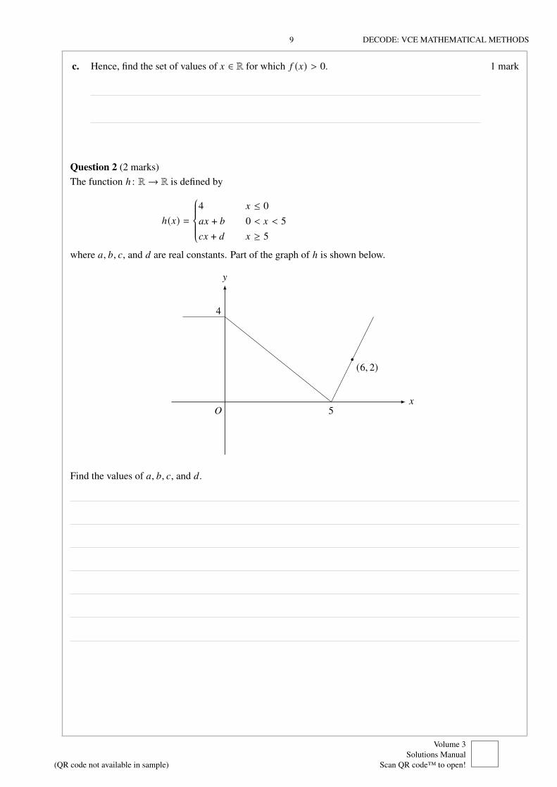
Question 2 (2 marks)The function ℎ : R→ R is defined by

ℎ(G) =

4 G ≤ 00G + 1 0 < G < 52G + 3 G ≥ 5

where 0, 1, 2, and 3 are real constants. Part of the graph of ℎ is shown below.

G

H

$

4

5

(6, 2)

Find the values of 0, 1, 2, and 3.

(QR code not available in sample)9

Volume 3Solutions Manual

Scan QR code™ to open!


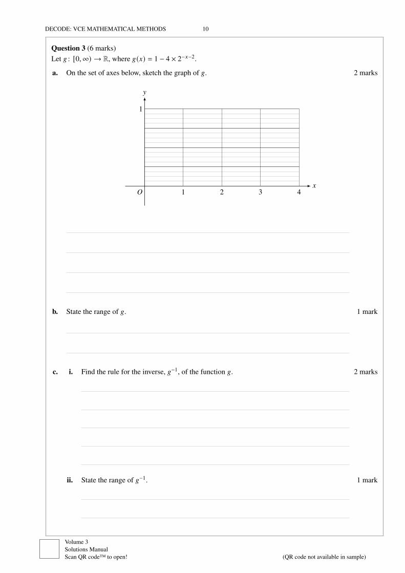
Question 3 (6 marks)Let 6 : [0,∞) → R, where 6(G) = 1 − 4 × 2−G−2.

a. On the set of axes below, sketch the graph of 6. 2 marks

G

H

$ 1 2 3 4

1

b. State the range of 6. 1 mark

c. i. Find the rule for the inverse, 6−1, of the function 6. 2 marks

ii. State the range of 6−1. 1 mark



11 DECODE: VCE MATHEMATICAL METHODS

Question 4 (4 marks)

The function 5 has rule 5 (G) = tan(6G − c

2

)and is defined over its maximal domain.

a. Find the period of 5 . 1 mark

b. The line G = 0 is a vertical asymptote of the graph of 5 , where 0 ∈[0,c

2

].

Find the possible value(s) of 0. 3 marks

(QR code not available in sample)11

Volume 3Solutions Manual

Scan QR code™ to open!


Question 5 (3 marks)The transformation ) : R2 → R2 is defined by

)

( [G

H

] )=

[1 00 3

] [G

H

]+

[1−1

].

The image of the curve H = 3G2 + 1 under the transformation ) has equation H = 0G2 + 1G + 2.Find the values of 0, 1, and 2.

END OF TEST

Download the solutions manual at www.decodeguides.com.au or scan the below QR code!



STUDENT NUMBER

Letter



Day Date



questions

Number of questions

to be answered

Number of

marks

5 5 20




STUDENT NUMBER

Letter


Functions and graphsTechnology-active test 1

Reading time: 15 minutesWriting time: 1 hour

Structure of testSection Number of

questions

Number of questions

to be answered

Number of

marks

A 10 10 10B 2 2 30

Total 40

Allowed materials• Pens, pencils, highlighters, erasers, sharpeners, rulers, a protractor, set squares, aids for curve

sketching, one bound reference, one approved technology (calculator or software) and, ifdesired, one scientific calculator. Calculator memory DOES NOT need to be cleared. Forapproved computer-based CAS, full functionality may be used.



STUDENT NUMBER

Letter


Functions and graphsTechnology-active test 2



questions

Number of questions

to be answered

Number of

marks

A 10 10 10B 3 3 30

Total 40





STUDENT NUMBER

Letter


AlgebraTechnology-free test 1

Day Date



questions

Number of questions

to be answered

Number of

marks

5 5 20




STUDENT NUMBER

Letter


AlgebraTechnology-free test 2

Day Date



questions

Number of questions

to be answered

Number of

marks

5 5 20




STUDENT NUMBER

Letter


AlgebraTechnology-active test 1



questions

Number of questions

to be answered

Number of

marks

A 10 10 10B 3 3 30

Total 40





STUDENT NUMBER

Letter


AlgebraTechnology-active test 2



questions

Number of questions

to be answered

Number of

marks

A 10 10 10B 2 2 30

Total 40





STUDENT NUMBER

Letter


CalculusTechnology-free test 1

Day Date



questions

Number of questions

to be answered

Number of

marks

4 4 20




STUDENT NUMBER

Letter


CalculusTechnology-free test 2

Day Date



questions

Number of questions

to be answered

Number of

marks

4 4 20




STUDENT NUMBER

Letter


CalculusTechnology-active test 1



questions

Number of questions

to be answered

Number of

marks

A 10 10 10B 2 2 30

Total 40





STUDENT NUMBER

Letter


CalculusTechnology-active test 2



questions

Number of questions

to be answered

Number of

marks

A 10 10 10B 3 3 30

Total 40





STUDENT NUMBER

Letter


Probability and statisticsTechnology-free test 1

Day Date



questions

Number of questions

to be answered

Number of

marks

5 5 20




STUDENT NUMBER

Letter


Probability and statisticsTechnology-free test 2

Day Date



questions

Number of questions

to be answered

Number of

marks

4 4 20




STUDENT NUMBER

Letter


Probability and statisticsTechnology-active test 1



questions

Number of questions

to be answered

Number of

marks

A 10 10 10B 2 2 30

Total 40





STUDENT NUMBER

Letter


Probability and statisticsTechnology-active test 2



questions

Number of questions

to be answered

Number of

marks

A 10 10 10B 2 2 30

Total 40





154

Author biographies

Tim Koussas, the lead author of this study guide, achieved an impressive trifecta of study scores of 50, 48 and47 in Mathematical Methods, Further Mathematics and Specialist Mathematics when he graduated from ParadeCollege in 2011. He also received a Premier’s Award in Mathematical Methods for placing among the top 5students in the state. He has since completed a Bachelor of Science at La Trobe University, graduating withfirst class honours as dux of his cohort. Tim is currently completing a PhD in the field of Pure Mathematics atLa Trobe University.

Trevor Batty graduated dux of Copperfield College in 2011, achieving a study score of 45 raw in MathematicalMethods. He has since completed a double Bachelor of Aerospace Engineering and Science at Monash Uni-versity, maintaining an outstanding high distinction average. During his undergraduate years, Trevor has beenan influential member of the Monash University Unmanned Aerial System team, writing avionics software toauto-pilot the team’s competition entry in the UAV challenge.

Dr Will Hoang graduated from Melbourne Grammar School in 2011, achieving an ATAR of 99.90. Whilestill in year 11, he achieved a perfect 50 in Mathematical Methods and received a Premier’s Award in thesubject for placing among the top 5 students in the state. Will has since completed a Bachelor of Biomedicine(Chancellor’s Scholars Program) and a Doctor of Medicine (MD) at the University of Melbourne, and is nowa practicing doctor.

Dr Nathaniel Lizak graduated dux of Bialik College in 2011 with an ATAR of 99.90, which included a perfect50 and a Premier’s Award in Specialist Mathematics. In that same year, Nathaniel also achieved the impressivefeat of scoring the top mark in the University of Melbourne Extension Program for Mathematics (which allowsVCE students to undertake university-level mathematics studies). Nathaniel has completed a Bachelor ofMedicine and Bachelor of Surgery at Monash University, achieving first-class honours, and is now a practisingdoctor. As an undergraduate student, Nathaniel has made an impressive achievement, being published in amedical journal for original research into multiple sclerosis.

Dr Thushan Hettige graduated dux of Scotch College in 2011 with an ATAR of 99.95, scoring 5 perfect50s (one of which included Mathematical Methods) and Premier’s Awards in Chemistry, Biology, EnglishLanguage and Mathematical Methods. This means that Thushan was in the top 5 students in the state for fourof the subjects he studied. Thushan also won the silver medal at the International Chemistry Olympiad inTurkey. His achievements earned him the Australian Students’ Prize for 2011, which is awarded to the top500 students from across the country. Thushan has since racked up extensive tutoring experience, both at VCElevel and in mentoring MBBS students in earlier year levels. He has completed his Bachelor of Medicine andBachelor of Surgery with honours, and is now a practising doctor.

William Swedosh scored a perfect 50 in Mathematical Methods in his graduating year of 2007 at McKinnonSecondary College. He has since completed a double Bachelor of Engineering and Science with an averagescore of 94% across his mathematics units. William now works for the CSIRO, modelling the physics ofbushfires.

154

VCE Mathematical Methods Units 3&4Volume 2: Trial Examinations

FIRST EDITION


Solutions available as a digital download:

http://www.decodeguides.com.au

Tim Koussas

Trevor Batty

Dr Will Hoang

Dr Nathaniel Lizak

Dr Thushan Hettige


2

ISBN 978-1-922445-13-1First published in 2020, by:Decode Publishing Pty LtdABN 16 640 806 686PO Box 1007Ashwood, VIC 3147E-mail: [email protected]




2

3

Preface: How to use this book

The purpose of the decode: VCE Study Guides is to provide practice questions for specific VCE subjects(in this case, Mathematical Methods Units 3&4), and also to provide comprehensive solutions to each ofthese questions. This book contains only the questions themselves, which have been written to match thestyle of questions you will get in the official end-of-year VCAA exams (VCAA, the Victorian Curriculum andAssessment Authority, is the organisation responsible for writing and marking final VCE exams, among otherthings). The solutions manual, freely available for download at www.decodeguides.com.au, contains markingschemes for each question, as well as model solutions (indicating how each question may be answered in anexam for full marks) and detailed solutions. This publication is sold as two separate volumes; the other volumecan be purchased separately at retailers or on our website www.decodeguides.com.au. This preface will explainhow to use these two volumes together.

The bulk of what the authors have actually written is contained in the detailed solutions section of thesolutions manual, where we cover all thought processes used in answering each of the questions in this book.We believe this to be what separates us from the rest of the market, as most of the VCE practice material youwill come across will only come with model solutions, and sometimes not even that!

The overall structure of this second volume can be seen in the table of contents on page 5.Describing Volume 1 (which, again, is purchased separately), we have topic tests in four areas, which

are based on the four areas of study listed in the VCAA study design for Methods 3&4. These four areas are“functions and graphs”, “algebra”, “calculus”, and “probability and statistics”.

Our topic tests are intended to serve as something like “practice SACs” (SACs are the tests taken atyour school that contribute to your final subject marks). Naturally, since different schools will have differentSACs, we can’t exactly predict the content of your SACs. We have opted for sticking close to the style of theend-of-year exams in these tests, while focusing on one area of study at a time (with some minor exceptions).

As with the areas themselves, our tests in each area will build on knowledge from the previous areas.Occasionally, some of our tests will also require knowledge that is, strictly speaking, from later areas ofstudy. Specifically, some of our tests in the “functions and graphs” area will use some of the knowledge from“algebra”. This is because teachers and textbooks will often blend the first two areas of study, as they tend to gohand-in-hand in terms of teaching. Also, some of our “algebra” tests will use some basic calculus knowledge;namely, the use of differentiation in finding stationary points of polynomials, as well as the equations of linestangent to curves. This amount of calculus knowledge is covered in Units 1&2, and for this reason your SACshave a high chance of including some basic calculus before you formally start learning calculus in Units 3&4.

We mention these discrepancies as a disclaimer to the fact that our tests in each area cover only thecontent listed in the corresponding area in the VCAA study design. Ultimately, though, all of our tests arewithin the scope of the study design, and contain content that is very likely to appear in SACs correspondingto the relevant area of study.

As for the actual structure of the tests, we have written each test in the same format as a VCAA exam,but with half the number of marks. The VCAA end-of-year exam formats for Methods are as follows:

• Examination 1: Contains 40 marks’ worth of short-answer questions and is to be completed in one hourusing only the provided formula sheet (and a device for writing on paper). Contributes 22% to your finalmark for Methods.

• Examination 2: Contains 20 multiple-choice questions (1 mark each) and 60 marks’ worth of extended-response questions, and is to be completed in two hours using a CAS calculator and a bound reference,as well as the provided formula sheet. Contributes 44% to your final mark for Methods.

As such, our tech-free tests each contain 20 marks’ worth of short-answer questions, and are intended to becompleted in half an hour using only the formula sheet provided at the end of this book (which is the same asVCAA’s formula sheet). Similarly, our tech-active tests contain 10 multiple-choice questions and 30 marks’worth of extended-response questions, and are intended to be completed in one hour using a calculator and abound reference (and the formula sheet if you wish). More details are given on the front cover of each test.

Volume 2 (which you are holding in your hands right now) is easier to describe: this consists of three setsof practice exams. Each set consists of a practice Examination 1 and a practice Examination 2, and these haveexactly the same format as the VCAA exams.

3

4

Whether you stick to the constraints suggested for each test is up to you, since the book doesn’t come withpocket-sized test supervisors. Without adequate practice, though, the VCAA exams can be brutal, especiallythe second one. Attempting to complete the tests and practice exams in the suggested amount of time, and onlywith the allowed references, will most likely help you work on your own techniques for answering questionsquickly. That said, if you don’t get everything done in time, it’s vital that you go back and learn as much fromyour mistakes as you can; any of the top students in each year can attest to this. Apart from explaining howto do every single question in this book, our detailed solutions suggest a lot of time-management techniques,such as techniques for using calculators efficiently, as well as common tricks or formulas that can be used tosave time.

A strategy that may be effective is to complete the first of each pair of tests at a leisurely pace, checkyour answers, read the detailed solutions, and then do the second test of the pair under timed conditions. Ifyou aren’t confident in a particular area, then this would be more effective than trying to do the test withoutknowing any of the content (although it might be better to learn the content from textbooks first, just so youhave two whole tests that you can do under timed conditions).

The fact that the final examinations are worth a whopping 66% of your final score makes practice undertimed conditions invaluable (not to mention that most of your Methods SACs are likely to also be held undertimed conditions, and these contribute the remaining 34%). You should therefore save at least two pairs of ourpractice examinations for when you are ready to complete them under timed conditions.

If you have time during your exam preparation, you should do any of the questions in our topic tests thatyou didn’t get around to completing during the year, and also read some of the detailed solutions for these tests,as we’ve scattered a lot of exam advice throughout the book (not just in the solutions to the practice exams).

This edition of the decode: VCE Study Guide for Methods is written for the VCAA study design that wasimplemented in 2016. If you’re reading this within a few years of 2016, you will not have many past VCAAexams from the current study design to work with. In this case, these official past VCAA exams (which arefreely available on the VCAA website) will be precious commodities, and should be saved until the last fewweeks before your actual exams.

Before attempting relevant past exams, it’s worth having a look at the exams from the previous studydesign (effective in 2006-2015), since a vast majority of the questions will still be relevant. If you’re not surewhether something is relevant, you should check with the study design. In fact, it’s a good idea to go over thestudy design for its own sake, and most of the top students will do this. There may be small things that yourteachers miss, so it’s a good way to make sure that you’ve covered everything.

The VCAA exams based on the current study design are by far the best practice material for the subject,although we have done our best to create practice exams in the same style. Apart from updating our material inthis edition to suit the current study design, we have rewritten major sections of both the question book and thesolutions manual in order to more closely match VCAA’s style and format. We’ve also hopefully caught anyerrors that stuck around, and hopefully not created any new ones, but if you find any then feel free to email usat [email protected], and we will update the solutions manual to include any errors thatyou may have found. Comments and suggestions are also appreciated! We don’t claim that every single one ofour solutions is the absolute best way to explain a given topic, but we have certainly done our best. Therefore,even a comment such as “the solution to question X is confusing because it doesn’t explain Y” is extremelyhelpful to us in improving the quality of the guide.

There will be plenty more for us to say in the solutions manual, but for now, we wish you the best of luckwith your studies.

– Tim Koussas

4

5

TABLE OF CONTENTS

Set 1Written examination 1 7Written examination 2 19Set 2Written examination 1 43Written examination 2 53Set 3Written examination 1 71Written examination 2 83

AppendixAuthor biographies 105Official exam formula sheet 106

5

6

This page has intentionally been left blank.

6

STUDENT NUMBER

Letter


Set 1Written examination 1


Structure of examinationNumber of

questions

Number of questions

to be answered

Number of

marks

9 9 40

• Students are permitted to bring into the examination room: pens, pencils, highlighters,erasers, sharpeners and rulers.

• Students are NOT permitted to bring into the examination room: any technology (calculatorsor software), notes of any kind, blank sheets of paper and/or correction fluid/tape.


Students are NOT permitted to bring mobile phones and/or any other unauthorisedelectronic devices into the examination room.


STUDENT NUMBER

Letter



Reading time: 15 minutesWriting time: 2 hours

Structure of examinationSection Number of

questions

Number of questions

to be answered

Number of

marks

A 20 20 20B 4 4 60

Total 80

• Students are permitted to bring into the examination room: pens, pencils, highlighters,erasers, sharpeners, rulers, a protractor, set squares, aids for curve sketching, one boundreference, one approved technology (calculator or software) and, if desired, one scientificcalculator. Calculator memory DOES NOT need to be cleared. For approved computer-based CAS, full functionality may be used.

• Students are NOT permitted to bring into the examination room: blank sheets of paperand/or correction fluid/tape.




STUDENT NUMBER

Letter





questions

Number of questions

to be answered

Number of

marks

10 10 40






STUDENT NUMBER

Letter





questions

Number of questions

to be answered

Number of

marks

A 20 20 20B 4 4 60

Total 80






STUDENT NUMBER

Letter





questions

Number of questions

to be answered

Number of

marks

10 10 40






STUDENT NUMBER

Letter





questions

Number of questions

to be answered

Number of

marks

A 20 20 20B 4 4 60

Total 80






Copyright © Decode Publishing Pty Ltd 2020

All rights reserved.

With the exception of that which is permitted by the Australian Copyright Act of 1968, no part of this bookmay be reproduced, stored in a retrieval system, or transmitted in any form or by any means, electronic,

mechanical or otherwise, without prior written permission.

A note about copying

This complimentary eBook is provided to you as a free digital download on our website, available to theowner of any of our study guides. This is to make it as easy as possible for our students who have Volumes 1

and 2 of this publication to access this solution manual, without breaking their backs. If all three volumeswere printed in a single book, it would be over 700 pages and weigh 1 kg and neither your back, your

schoolbag nor the trees would be particularly happy.

Whilst obviously we would prefer that you do not do this, for our authors’ sake, there is nothing that we cando to physically stop you from distributing this eBook, for free, to anyone who you think may benefit fromwhat we believe is a wonderful resource; we obviously encourage (conflict of interest alert!) that anyone

holding this eBook purchase Volumes 1 and 2 to gain the most benefit by scanning the above QR code. Theonly thing we do ask is not to use any part of this book for commercial reasons, especially given the trust wehave placed in you by publishing this online. That would be very poor form, and illegal. On another note, we

really hope you find this publication valuable. Our authors have worked extremely hard to develop thisresource for you.

1

VCE Mathematical Methods Units 3&4Volume 3: Solution Manual

FIRST EDITION


Volume 1 (Trial SACs) and Volume 2 (Trial Examinations) can be purchased at retailers or on ourwebsite, the link of which is below; alternatively, scan the above QR code.

www.decodeguides.com.au

Note: This solution manual can only be used in conjunction with volumes 1 and 2, which canbe purchased as described above.

Tim Koussas

Trevor Batty

Dr Will Hoang

Dr Nathaniel Lizak

Dr Thushan Hettige


First published in 2020, by:Decode Publishing Pty LtdABN 16 640 806 686PO Box 1007Ashwood, VIC 3147E-mail: [email protected]




3

TABLE OF CONTENTS

Section 1: Model Solutions and Marking Schemes

Volume 1: Topic Tests


Volume 2: Trial Examinations

Trial examination set 1Written examination 1 58Written examination 2 63Trial examination set 2Written examination 1 69Written examination 2 75Trial examination set 3Written examination 1 80Written examination 2 86

4

Section 2: Detailed Solutions

Volume 1: Topic Tests


Volume 2: Trial Examinations

Trial examination set 1Written examination 1 318Written examination 2 327Trial examination set 2Written examination 1 348Written examination 2 355Trial examination set 3Written examination 1 376Written examination 2 381

5

Section 1:Model Solutions and Marking Schemes


Model solutions and marking scheme

Click to jump: 1a, 1b, 1c, 2, 3a, 3b, 3ci, 3cii, 4a, 4b, 5.

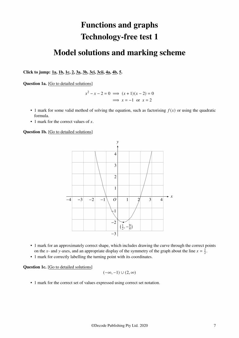
Question 1a. [Go to detailed solutions]

G2 − G − 2 = 0 =⇒ (G + 1) (G − 2) = 0=⇒ G = −1 or G = 2

• 1 mark for some valid method of solving the equation, such as factorising 5 (G) or using the quadraticformula.

• 1 mark for the correct values of G.

Question 1b. [Go to detailed solutions]

G

H

$

( 12 ,−

94)

1 2 3 4−4 −3 −2 −1

1

2

3

4

−3

−2

−1

• 1 mark for an approximately correct shape, which includes drawing the curve through the correct pointson the G- and H-axes, and an appropriate display of the symmetry of the graph about the line G = 1

2 .• 1 mark for correctly labelling the turning point with its coordinates.

Question 1c. [Go to detailed solutions](−∞,−1) ∪ (2,∞)

• 1 mark for the correct set of values expressed using correct set notation.

©Decode Publishing Pty Ltd. 2020 7

Question 2 [Go to detailed solutions]

0 =0 − 45 − 0

= −45

1 = 4

2 =2 − 06 − 5

= 2

ℎ(5) = 0 =⇒ 2 · 5 + 3 = 0 =⇒ 3 = −10

• 1 mark for using appropriate methods to calculate 0, 2, and 3, such as calculating gradients or usingsimultaneous equations.

• 1 mark for the correct values of 0, 1, 2, and 3.

Question 3a. [Go to detailed solutions]

G

H

$ 1 2 3 4

1

• 1 mark for an approximately correct shape.• 1 mark for drawing the curve with the correct H-coordinates on each of the vertical lines; that is, the

graph should pass through (0, 0),(1, 1

2),(2, 3

4),(3, 7

8), and

(4, 15

16). Slight deviations from these points

are acceptable. These points do not need to be labelled.

Question 3b. [Go to detailed solutions][0, 1)

• 1 mark for the correct range.

8 ©Decode Publishing Pty Ltd. 2020

Question 3ci. [Go to detailed solutions]

Simplifying 6(G):6(G) = 1 − 22 · 2−G−2 = 1 − 2−G .

Let H = 6−1(G). Then

6(H) = G =⇒ 1 − 2−H = G

=⇒ 2−H = 1 − G

=⇒ −H = log2(1 − G)=⇒ H = − log2(1 − G)=⇒ 6−1(G) = − log2(1 − G)

• 1 mark for a valid method for finding inverse functions, such as using the identity 6(6−1(G)) = G orsolving the equation 6(H) = G for H. In the latter case, writing something along the lines of “For inverse,swap G and H” or “Let H = 6−1(G)” is required.

• 1 mark for a correct expression for 6−1(G).

Question 3cii. [Go to detailed solutions][0,∞)

• 1 mark for the correct range.

Question 4a. [Go to detailed solutions]c

6

• 1 mark for the correct period.

Question 4b. [Go to detailed solutions]

A solution to cos(60 − c

2

)= 0 is given by 60 − c

2=

c

2, so 0 =

c

6is one solution. Using the period from part

a.,0 =

c

6− c

6,

c

6,

c

6+ c

6,

c

6+ 2c

6= 0,

c

6,c

3,c

2

• 1 mark for attempting to solve cos(60 − c

2)= 0, or an equivalent equation, for 0.

• 1 mark for using an appropriate method to generate all solutions to the equation, such as using a formulafor the general solution or using periodicity.

• 1 mark for the correct values of 0.

Question 5 [Go to detailed solutions]

)

( [G

H

] )=

[G + 1

3H − 1

]so ) sends H = 3G2 + 1 to H = 3(3(G − 1)2 + 1) − 1. Since

3(3(G − 1)2 + 1) − 1 = 9(G − 1)2 + 2 = 9G2 − 18G + 9 + 2 = 9G2 − 18G + 11,

we have0 = 9, 1 = −18, 2 = 11.

• 1 mark for an appropriate method for applying ) to the given curve to find the transformed curve, suchas decomposing ) into simple transformations and applying them in the correct order, defining newcoordinate variables and then using algebra, or simply reading off the transformations from the matrices.

• 1 mark for obtaining a correct equation for the transformed curve at some stage, even if not in the correctform; for example, writing down H = 3(3(G − 1)2 + 1) − 1.

• 1 mark for the correct values of 0, 1, and 2.



Detailed solutions

Click to jump: 1a, 1b, 1c, 2, 3a, 3b, 3ci, 3cii, 4a, 4b, 5.

Question 1a. [Go to model solutions]

The importance of solving quadratic equations in this course cannot be overstated. For this reason, I will givea very lengthy discussion on the topic of quadratic equations, which will hopefully put to rest any uncertaintiesyou may have in this area. The working to the actual question begins here if you want to skip ahead.

Being able to solve a quadratic equation is an assumed skill from the first two units of Mathematical Methods,but it’s never too late to learn how to solve them, unless perhaps your exam starts 10 minutes from now. Youwill need to solve a quadratic equation or two on the actual VCAA tech-free exam, and since this exam usuallyconsists of about 9-12 questions, a reasonable percentage of the exam marks will be accessible if you cansolve quadratic equations. That being said, there’s more to it than just being able to solve an explicit quadraticequation that’s given to you; sometimes you need to recognise a quadratic equation that’s “hidden” (we willhave examples of this in later questions), and then solve it.

Regardless of how they might show up in exams, the first thing to worry about is knowing the precise defini-tion of a quadratic equation. The emphasis on precise mathematical definitions is actually very poor in VCEmathematics compared to what (I think) it should be; there are even some past exam questions whose correct-ness depends on which one of several definitions is used. These are more general comments, and they don’tnecessarily relate to quadratic equations in particular, but I really do want to get these ideas across. There isa lot to be gained from knowing exactly what you’re dealing with, which is why we don’t walk across darkrooms when we can just turn on a light.

With that out of the way, here is the definition. A real1 quadratic equation is an equation that can be written inthe form

0G2 + 1G + 2 = 0,

where 0, 1, 2 ∈ R are constants2, 0 ≠ 0, and G is a real variable. The constants 0, 1, and 2 are also called thecoefficients of the equation 0G2 + 1G + 2 = 0. The reason 0 = 0 is excluded is that in this case, the equationreduces to the linear equation 1G + 2 = 0.

It is common to refer to the equation 0G2 + 1G + 2 = 0 as a “quadratic equation in G”. This is usually done tospecify the variable in which the equation is quadratic. An example is the equation G4 + 2G2 + 1 = 0, which isa quadratic equation in G2, as G4 + 2G2 + 1 = (G2)2 + 2(G2) + 1. It is confusing to only refer to G4 + 2G2 + 1 = 0as a quadratic equation, as it is not a quadratic equation in G, but the less-obvious variable G2. (It is, however,a quartic equation in G.) This line of thinking is the basis of some of the more difficult questions involvingquadratics, but for now we will return to focus on the basic solution processes.

We are first going to explore the factorisation method for solving quadratics – which you are likely to havelearned before, but perhaps have never considered the topic in this level of detail. We will then discuss a morecomprehensive method for solving quadratics, which is the quadratic formula.

1There are versions of the quadratic equation that use complex numbers rather than just real numbers. Complex numbers are dealtwith in Specialist Mathematics, but not in Mathematical Methods.

2Note that we use the symbol R to denote the set of real numbers. VCAA tends to use a plain unbolded ', which is a questionablechoice.


In brief, the factorisation method is:

• write 0G2 + 1G + 2 as a product of two expressions that are linear in G;

• apply the null factor law3 to obtain two (possibly identical) linear equations in G;

• solve these linear equations individually.

The hardest part of this method is the factorisation itself, since it’s relatively easy to solve the equation 0G2 +1G + 2 = 0 once the expression 0G2 + 1G + 2 is factorised. Consider, for example, the quadratic equation5G2 + 3G − 2 = 0, which can be written as (5G − 2) (G + 1) = 0. The null factor law implies that either 5G − 2 = 0or G + 1 = 0. We then individually solve these equations, obtaining G = 2

5 and G = −1 respectively, which givesus the two solutions to the original equation 5G2 + 3G − 2 = 0. In symbols,

5G2 + 3G − 2 = 0 =⇒ (5G − 2) (G + 1) = 0 =⇒ 5G − 2 = 0 or G + 1 = 0 =⇒ G =25

or G = −1,

which is not much work at all.Having given a small refresher on why factorisation is useful, we should now think about how to obtain afactorised expression in the first place. An important thing to note is that this method won’t always work, inthat you won’t always get nice factored expressions such as (5G − 2) (G + 1) that don’t involve any complicatedirrational numbers.To illustrate this point, consider the pleasant-looking equation G2 − 4G + 2 = 0, which has solutions G = 2 +

√2

and G = 2 −√

2 (never mind why for the moment). To see how this relates to the factored form, the expressionG2 − 4G + 2 factorises to

(G − 2 −

√2) (G − 2 +

√2). The process of finding factors by inspection won’t be able

to find relatively complicated factors like these, so an attempt to factorise G2 − 4G + 2 the usual way won’t getyou anywhere.Apart from not having nice solutions, it’s also possible for a quadratic equation to have no solutions at all, suchas the equation G2 +2G +2 = 0. This can be written as (G +1)2 = −1, which has no real solutions, since (G +1)2

is never negative. As such, the expression G2 + 2G + 2 can’t be factorised in any way using only real numbers.Now, how do we look for simple factors, and how do we know when to give up? We will start with a simplifiedversion of the quadratic equation, G2 + 1G + 2 = 0. We want to write G2 + 1G + 2 in the form (G + ℎ) (G + :); thatis, we want to find ℎ and : such that

G2 + 1G + 2 = (G + ℎ) (G + :).

This is done by expanding (G + ℎ) (G + :), which makes it easier to compare it to G2 + 1G + 2. Expanding(G + ℎ) (G + :), we get

(G + ℎ) (G + :) = G2 + ℎG + :G + ℎ: = G2 + (ℎ + :)G + ℎ:.

Rephrasing the problem, we want to find ℎ and : such that

G2 + (ℎ + :)G + ℎ: = G2 + 1G + 2.

By comparing these expressions, we see that we require ℎ + : = 1 and ℎ: = 2. In other words, to be able towrite G2 + 1G + 2 in the form (G + ℎ) (G + :), we need to find two numbers that add up to 1 and multiply to give2.We still need to address the more general case of factoring 0G2 + 1G + 2, but we will give an example of thissimpler case first. Consider the expression G2 − 3G − 10. To write this in the form (G + ℎ) (G + :), we need tofind ℎ and : such that ℎ + : = −3 and ℎ: = −10.Now, we’ve come to an important point in the factorisation method, which is how we go about finding ℎ and: . Generally, we will only try to find integer solutions, and if we find that there are no integer solutions, weproceed to using the quadratic formula.In a sense, factorisation could theoretically work every time (that solutions exist) if you just keep trying num-bers, but it is ridiculous to attempt this knowing how complicated some solutions can be. Imagine how long itmight take to see that G2 − 4G + 2 factorises to

(G − 2 −

√2) (G − 2 +

√2)

just by trying values of ℎ and : .

3The null factor law is: for real numbers 0, 1, if 01 = 0, then 0 = 0 or 1 = 0. Intuitively, this says that multiplying two non-zeroreal numbers can never give 0 as a result.


Now, even if we restrict ourselves to looking for integer solutions to ℎ + : = −3, there are still infinitely manyoptions for ℎ and :; that is, there are infinitely many pairs of integers that add to −3. For this reason, we firstconsider ℎ: = −10, which only has finitely many integer solutions (because −10 only has finitely many integerdivisors). This will generally be the case when trying to factorise G2 + 1G + 2; there are only finitely many waysto write an integer 2 as a product of two integers.The possible ways of writing 10 as a product of two positive integers are 1 × 10 and 2 × 5, disregarding theorder in which the factors are written. We want two integers that multiply to −10, so we can extend this byadding negative signs in: the options are (−1) × 10, 1 × (−10), (−2) × 5, and 2 × (−5).The next step is to see if any of these pairs add up to −3 – recall that we want numbers that multiply to −10and add to −3. The pair 2,−5 has these two properties, so we can choose ℎ = 2, : = −5, and hence obtain thefactorisation G2 − 3G − 10 = (G + 2) (G − 5). Of course I chose an example where this method would work, butif none of the four pairs we found added up to −3, it would then be best to use the quadratic formula.Now, how do we factorise the more general expression 0G2 + 1G + 2? As we’ve already alluded to, there’s nopoint in trying to factorise this expression unless 0, 1, and 2 are integers, since if they aren’t then the quadraticformula is likely to be more time-efficient. If 0, 1, and 2 are at least rational, then the equation 0G2 + 1G + 2 = 0can be modified to have integer coefficients. For example, the equation 1

3G2 + 2G + 4 = 0 can be multiplied by

3 to give G2 + 6G + 12 = 0, which has the same solutions but is easier to work with.It’s worth mentioning that, if you can take 0 out as a common (integer) factor, then it will probably make lifeeasier. An example is the quadratic expression 3G2 + 6G + 3. Here we can take out 3 as a common factor toobtain the expression 3

(G2 + 2G + 1

). This reduces the situation to the one we’ve already discussed, which is

factorising an expression of the form G2 + 1G + 2. Even if 0 doesn’t come out as a common factor, the threecoefficients 0, 1, and 2 might have some smaller common factor other than 1 (such as in 4G2 + 6G + 2), andtaking out this factor will still help, since it makes the coefficients smaller and thus reduces the number ofpossible factors to try.After making as many simplifications as possible and still arriving at an equation of the form 0G2 + 1G + 2 = 0(with 0 ≠ 1), we attempt to factorise 0G2 + 1G + 2 in the form (<G + ℎ) (=G + :). As before, we expand this andrelate our unknowns ℎ, : , <, and = to 0, 1, and 2. We have

0G2 + 1G + 2 = (<G + ℎ) (=G + :) = <=G2 + =ℎG + <:G + ℎ: = <=G2 + (=ℎ + <:)G + ℎ:.

As you can probably tell, having the 0 in the equation 0G2 + 1G + 2 = 0 complicates matters quite a bit, whichis why efforts should be made to get rid of it or at least make it smaller. Still, there are some similar features tothe method of solving the simplified version G2 + 1G + 2 = 0. For starters, we can see that <= = 0 and ℎ: = 2,so that we end up having only finitely many (integer) options for ℎ, : , <, and =.What makes this harder is having to try two pairs of integers at once, which usually means we end up withmany more possibilities that need to be tried; for each choice of ℎ, : , <, and = such that <= = 0 and ℎ: = 2,we need to check that =ℎ+<: = 1. Depending on how many factors 0 and 2 have, it may still be more efficientto go straight to using the quadratic formula.An example is probably in order. We will solve the equation 4G2 − 30G + 14 = 0 by factorisation. First, divideby 2 to get 2G2 − 15G + 7 = 0. Both 2 and 7 are prime numbers, so we only have a few possible factorisationsof each number. The number 2 can be written as 1 × 2 or (−1) × (−2), and similarly 7 can be written as 1 × 7or (−1) × (−7).Now, here the order in which we choose ℎ and : (or < and =) matters, since interchanging ℎ and : in (<G +ℎ) (=G + :) can result in a genuinely different expression. However, we can swap ℎ and : if we also swap <

and =, because this amounts to writing the two linear factors in the opposite order.Before trying out possibilities, the following observations will always come in handy while factorising. First,note that you can always make the coefficient of G2 positive, because you can multiply the equation 0G2+1G+2 =

0 by −1. Recall that to have 0G2 + 1G + 2 = (<G + ℎ) (=G + :) we at least need <= = 0, so if we ensure that 0 ispositive we can also ensure that < and = have the same sign. Finally, because of the fact that

(<G + ℎ) (=G + :) = (−<G − ℎ) (−=G − :),

we can ensure that < and = are both positive. For instance, if we tried < = −1 and = = −2, we could just aswell try < = 1 and = = 2 if we also swap the signs of ℎ and : , because (<G + ℎ) (=G + :) turns out the sameeither way.


In this scenario, we can assume that < = 1 and = = 2, because the only way to write 2 as a product of twopositive integers is 1 × 2 (disregarding order, as usual). Why not < = 2 and = = 1? Because the order of thefactors in (<G + ℎ) (=G + :) doesn’t matter. Thus, we effectively end up with only one possibility for < and =,so we just need to try different possibilities for ℎ and : .Another fortunate feature of this quadratic equation is that the coefficient of G (namely −15) is negative. Thisis useful because the requirement that =ℎ + <: = −15 implies that ℎ, : , <, and = can’t all be positive. We’vealready chosen < and = to be positive, so we just need to test ℎ and : with ℎ: = 7, where ℎ and : aren’t bothpositive. This leaves just two possibilities, ℎ = −1 and : = −7, or ℎ = −7 and : = −1. You won’t always beable to make this simplification, but it’s definitely worth looking out for.A common way of testing out possibilities is to write ℎ, : , <, and = in a square like so:

= :

< ℎ

The case < = 1, = = 2, ℎ = −7 and : = −1 would be written as

2 −7

1 −1

This actually avoids having to introduce new pronumerals such as ℎ, : , <, and =, since you can jump straightto writing down squares like these once you know what equation you want to solve (2G2 − 15G + 7 = 0 inthe present case). Thinking up factors of 2 and 7 can be done in your head, as well as simplifications suchas the fact that the left-hand column is effectively the only thing you can write down. Because this is really atrial-and-error process, though, you may need to keep rubbing out parts of the diagram if there isn’t enoughspace on the exam or test paper to keep drawing new squares.How does this diagram get us anywhere, though? Each row can be thought of as a possible factor of 2G2 −15G + 7. The above corresponds to testing the factors G − 1 (from the top row) and 2G − 7 (from the bottomrow). The way of testing that you have the right factors is to calculate =ℎ +<: , which is made easy by writingthe four numbers in a square. It amounts to multiplying the diagonallly opposite numbers with each other andthen adding the two products.

2 −7

1 −12 · (−1) + 1 · (−7) = −9

Due to this way of calculating =ℎ + <: , this particular way of finding factors is often referred to as the “crossmethod”.Here we end up with =ℎ + <: = −9, but we want =ℎ + <: = −15, so we need to make another guess. We rubout −1 and −7 and then write them in the opposite order.

2 −1

1 −72 · (−7) + 1 · (−1) = −15

Success! Now we read off the factors from the square:

2 −1

1 −7

(2G − 1)×

(1G − 7)


Hence, we have 2G2−15G+7 = (G−7) (2G−1). The original equation 4G2−30G+14 = 0 is therefore equivalentto the equation 2(G − 7) (2G − 1) = 0, which has solutions G = 7 and G = 1

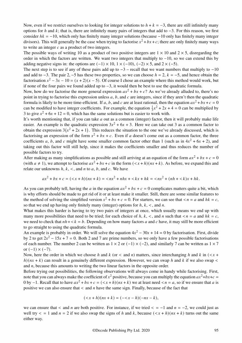
2 .To give another example, we will solve −7G2 + 6G + 16 = 0. Making the coefficient of G2 positive, we multiplyby −1 to give 7G2 − 6G − 16 = 0. The coefficients have no common factor other than 1, so, like in the lastexample, we proceed to looking for a factorisation of the form (G + ℎ) (7G + :) (since 7 is prime, we onlyreally have one choice for the coefficients of G in the linear factors, given the observations made in the previousexample). We can start writing down a square of numbers.

7

1

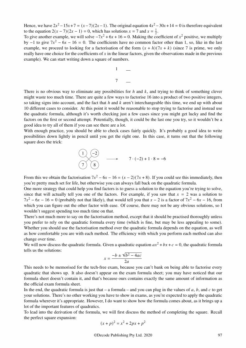
There is no obvious way to eliminate any possibilities for ℎ and : , and trying to think of something clevermight waste too much time. There are quite a few ways to factorise 16 into a product of two positive integers,so taking signs into account, and the fact that ℎ and : aren’t interchangeable this time, we end up with about10 different cases to consider. At this point it would be reasonable to stop trying to factorise and instead usethe quadratic formula, although it’s worth checking just a few cases since you might get lucky and find thefactors on the first or second attempt. Potentially, though, it could be the last one you try, so it wouldn’t be agood idea to try all of them if you can see there are a lot.With enough practice, you should be able to check cases fairly quickly. It’s probably a good idea to writepossibilities down lightly in pencil until you get the right one. In this case, it turns out that the followingsquare does the trick:

7 8

1 −27 · (−2) + 1 · 8 = −6

From this we obtain the factorisation 7G2 − 6G − 16 = (G − 2) (7G + 8). If you could see this immediately, thenyou’re pretty much set for life, but otherwise you can always fall back on the quadratic formula.One more strategy that could help you find factors is to guess a solution to the equation you’re trying to solve,since that will actually tell you one of the factors. For example, if you saw that G = 2 was a solution to7G2 − 6G − 16 = 0 (probably not that likely), that would tell you that G − 2 is a factor of 7G2 − 6G − 16, fromwhich you can figure out the other factor with ease. Of course, there may not be any obvious solutions, so Iwouldn’t suggest spending too much time on that.There’s not much more to say on the factorisation method, except that it should be practised thoroughly unlessyou prefer to rely on the quadratic formula every time (which is fine, but may be less appealing to some).Whether you should use the factorisation method over the quadratic formula depends on the equation, as wellas how comfortable you are with each method. The efficiency with which you perform each method can alsochange over time.We will now discuss the quadratic formula. Given a quadratic equation 0G2 + 1G + 2 = 0, the quadratic formulatells us the solutions:

G =−1 ±

√12 − 40220

This needs to be memorised for the tech-free exam, because you can’t bank on being able to factorise everyquadratic that shows up. It also doesn’t appear on the exam formula sheet; you may have noticed that ourformula sheet doesn’t contain it, and that’s because ours contains exactly the same amount of information asthe official exam formula sheet.In the end, the quadratic formula is just that – a formula – and you can plug in the values of 0, 1, and 2 to getyour solutions. There’s no other working you have to show in exams, as you’re expected to apply the quadraticformula wherever it’s appropriate. However, I do want to show how the formula comes about, as it brings up alot of the important features of quadratics.To lead into the derivation of the formula, we will first discuss the method of completing the square. Recallthe perfect square expansion:

(G + ?)2 = G2 + 2?G + ?2


This can sometimes be used backwards to factorise quadratic espressions. Not all quadratics are perfectsquares, but fortunately it is easy to tell if a quadratic G2 + 1G + 2 is a perfect square. We want

G2 + 1G + 2 = (G + ?)2 = G2 + 2?G + ?2,

and this gives us a way to find a relationship between 1 and 2 that can be used as a test. From the aboveequalities, we have 1 = 2? and 2 = ?2, which allows us to relate 1 and 2 as follows: given 1, we can halve itand then square it to obtain 2. To show this symbolically,(

1

2

) 2=

(2?2

) 2= ?2 = 2,

so the quadratic G2 + 1G + 2 is a perfect square precisely when

2 =

(1

2

) 2.

I wouldn’t suggest memorising this, because there’s an easier way to derive it that we will see later. But fornow, let’s try this out on G2 + 4G + 4, where 1 = 2 = 4. We have(

1

2

) 2=

(42

) 2= 22 = 4 = 2,

and hence G2 + 4G + 4 is a perfect square and can therefore be written in the form (G + ?)2. Finding ? is easygiven that we’ve already shown that 1 = 2?. This says that ? is half of 1, so ? = 2 in this case. Hence,

G2 + 4G + 4 = (G + 2)2,

as you can check by expansion.Now, the coefficient of G2 could always be something other than 1, but you can still apply the above test bytaking out the coefficient of G2 as a common factor. Consider for example the quadratic 4G2 + 4G + 1, whichcan be written as

4G2 + 4G + 1 = 4(G2 + G + 1

4

).

You can then apply the test 2 =(12) 2 to the quadratic G2 + G + 1

4 . Here it turns out that the equation 2 =(12) 2

holds, and so we can write

4G2 + 4G + 1 = 4(G2 + G + 1

4

)= 4

(G + 1

2

) 2,

which, for the sake of interest, can be simplified as

4(G + 1

2

) 2=

(2(G + 1

2

) ) 2= (2G + 1)2.

Although not every quadratic is a perfect square, it is still possible to write a quadratic expression in theturning-point form 0(G + ℎ)2 + : , which is as close to a perfect square expression as you can get. This way ofexpressing a quadratic is arguably the most useful in terms of solving 0(G + ℎ)2 + : = 0 as well as sketchingthe curve H = 0(G + ℎ)2 + : . This is how easy it is to solve the equation 0(G + ℎ)2 + : = 0 for G:

0(G + ℎ)2 + : = 0 =⇒ (G + ℎ)2 = − :

0=⇒ G + ℎ = ±

√− :

0=⇒ G = −ℎ ±

√− :

0

There is a problem in that − :0

will be negative if 0 and : have the same sign, which implies that we can’ttake its square roots, but on the bright side, this observation makes it easy to tell when a quadratic equation(with the quadratic written in turning-point form) has no solutions: we require either that : = 0, or that 0 and: have opposite sign. For example, the equation −2(G + 1)2 + 5 = 0 will have solutions, while the equation2(G − 2)2 + 1 = 0 has no solutions.


As for how the turning-point form helps to sketch the graph, first observe the transformations required to obtainthe curve H = 0(G+ℎ)2+ : from the curve H = G2 (doing this is desirable because the shape of H = G2 is familiarand relatively easy to understand). We can get to H = 0(G + ℎ)2 + : from H = G2 as follows:

H = G2 → H = 0G2 → H = 0(G + ℎ)2 → H = 0(G + ℎ)2 + :

Hence, dilating4 by a factor of 0 parallel to the H-axis, translating by −ℎ units in the G-direction, and translatingby : units in the H-direction (in that order) sends the curve H = G2 to the curve H = 0(G + ℎ)2 + : .

H = G2 H = 0G2 H = 0(G + ℎ)2

−ℎ

H = 0(G + ℎ)2 + :

−ℎ

:

In applying these three basic transformations, what happens to the turning point of H = G2? It starts out at(0, 0). Dilating doesn’t move the origin anywhere. Translating by −ℎ horizontally sends (0, 0) to (−ℎ, 0),and translating by : vertically sends (−ℎ, 0) to (−ℎ, :), so the overall process sends (0, 0) to (−ℎ, :). Theturning point of H = 0(G + ℎ)2 + : is therefore located at (−ℎ, :). If you aren’t particularly comfortable withtransformations and can’t see how this works, then I suggest reading the detailed solution to question 5 of thistest (which begins here), where we cover transformations in depth.Incidentally, the sign of 0 tells us whether the turning point is a maximum or a minumum. That is, it willbe a minimum if 0 is positive and a maximum if 0 is negative. This is solely due to the first transformationmultiplying the H-coordinates by 0, because translations don’t change the nature of stationary points. If 0 > 0then H = 0G2 will still have a minimum. If 0 < 0, going from H = G2 to H = 0G2 will reflect the curve in theG-axis as well as dilating vertically, which turns the minimum into a maximum.

H = G2 H = 0G2, 0 < 0

Using the two examples from earlier, the turning point of H = −2(G + 1)2 + 5 is a maximum and the turningpoint of H = 2(G − 2)2 + 1 is a minimum.Since the curve H = 0(G + ℎ)2 + : has its turning point at (−ℎ, :), we can see that it is easy to find the turningpoint of a quadratic curve when expressed in turning-point form – hence the name. Using our two examplesagain, the curve H = −2(G + 1)2 + 5 has its turning point at (−1, 5), and the curve H = 2(G − 2)2 + 1 has itsturning point at (2, 1).This is all well and good, but we still need to know how to find the turning-point form of a quadratic 0G2+1G+2.Unlike the factorisation method we’ve discussed, this involves no trial and error. First, we write

0G2 + 1G + 2 = 0

(G2 + 1

0G

)+ 2.

Here we’ve just taken 0 out as a common (real-number) factor of 0G2 and 1G, for reasons that will hopefullybecome clear. Let’s concentrate on the part inside the brackets, which is

G2 + 1

0G.

We know the form of a perfect square: G2 + 2?G + ?2. As we’ve discussed, this tells us what the constant termshould look like in terms of the coefficient of G. Taking 1

0, halving it, and then squaring it, we get

(120

) 2= 12

402 ;hence, the following is a perfect square:

G2 + 1

0G + 12

402

4To be precise, if 0 < 0 then we are really dilating by −0 and then reflecting in the G-axis.


Now, you might be thinking that we can’t just add whatever we want. But we can if we also subtract it. Thatis,

G2 + 1

0G = G2 + 1

0G + 12

402 − 12

402 .

We’ve just added and subtracted the same number, but remarkably this gets us most of the way there! Thereason is that G2 + 1

0G + 12

402 is a perfect square, as we’ve already mentioned, and so

G2 + 1

0G = G2 + 1

0G + 12

402 − 12

402 =

(G + 1

20

) 2− 12

402 .

We can now replace G2 + 10G in the expression 0

(G2 + 1

0G)+ 2 and get

0

(G2 + 1

0G

)+ 2 = 0

( (G + 1

20

) 2− 12

402

)+ 2.

We’re almost there; we just need to do a small amount of algebra.

0

( (G + 1

20

) 2− 12

402

)+ 2 = 0

(G + 1

20

) 2− 0 · 12

402 + 2

= 0

(G + 1

20

) 2+ 2 − 12

40.

Hence, we’ve shown that

0G2 + 1G + 2 = 0

(G + 1

20

) 2+ 2 − 12

40.

This indeed has the form 0(G + ℎ)2 + : , with ℎ = 120 and : = 2 − 12

40 .In practice, if you want to convert a quadratic to turning-point form, then it’s best to remember the generalprocedure rather than the formula 0G2 + 1G + 2 = 0

(G + 1

20) 2 + 2 − 12

40 . There’s nothing stopping you frommemorising it, but it would be more productive to use your brain space on other things, like the quadraticformula. Remembering the general procedure might even help you memorise the formula. We will demonstratethe general procedure on the expression 4G2 + 4G + 2. First write

4G2 + 4G + 2 = 4(G2 + G) + 2,

then add and subtract the appropriate constant inside the bracket, which in this case is 14 =

( 12) 2 (the square of

half of the coefficient of G in G2 + G, which is 1). Following this by some algebra, we arrive at the turning-pointform without too much effort.

4(G2 + G) + 2 = 4(G2 + G + 1

4− 1

4

)+ 2

= 4(G2 + G + 1

4

)− 1 + 2

= 4(G + 1

2

) 2+ 1.

Now that we can write any quadratic expression in turning-point form, we can derive the quadratic formulawithout much more effort. Remember that the quadratic formula just gives the solutions to the equation0G2 + 1G + 2 = 0, when they exist. The way to derive the quadratic formula, then, is to solve the equation0G2 + 1G + 2 = 0 algebraically. Expressing 0G2 + 1G + 2 in turning-point form was most of the work – we’ve


already seen how to solve quadratic equations using the turning-point form, so we just need to repeat thisprocess.

0G2 + 1G + 2 = 0 =⇒ 0

(G + 1

20

) 2+ 2 − 12

40= 0

=⇒ 0

(G + 1

20

) 2=

12

40− 2 =

12 − 40240

=⇒(G + 1

20

) 2=

12 − 402402 .

If the right-hand side of the last equation is negative, there will be no solutions. Otherwise, we can proceed tosolve:

0G2 + 1G + 2 = 0 =⇒(G + 1

20

) 2=

12 − 402402

=⇒ G + 1

20= ±

√12 − 402

402

=⇒ G = − 1

20±√12 − 402

20

=⇒ G =−1 ±

√12 − 40220

.

This is the quadratic formula, so we are done. There is more to be said, however. The quantity 12 − 402appearing under the square root sign plays an important role in deciding the number of solutions to the equation0G2+1G+2 = 0. Due to this, the number 12−402 is referred to as the discriminant of the equation 0G2+1G+2 = 0.To explain this in more detail, recall that 0G2 + 1G + 2 = 0 is equivalent to(

G + 1

20

) 2=

12 − 402402 .

Noting that 402 is positive, we see that the sign of the right-hand side is the same sign as the discriminant12 − 402, which appears as the numerator. If 12 − 402 < 0, then the equation 0G2 + 1G + 2 = 0 has no solutions.If 12 − 402 = 0, then there is one solution:(

G + 1

20

) 2= 0 =⇒ G = − 1

20.

This can also be obtained from the quadratic formula. Finally, if 12 − 402 > 0, then√12 − 402 is non-zero,

leading to two solutions to the equation 0G2 + 1G + 2 = 0 as given by the quadratic formula.Another useful feature of the discriminant is that it enables us to tell if a quadratic 0G2 + 1G + 2 can be writtenas a perfect square 0(G + ℎ)2. To see this, consider the turning-point form as found before:

0G2 + 1G + 2 = 0

(G + 1

20

) 2+ 2 − 12

40

For 0G2 + 1G + 2 to be a perfect square, then, we require that

2 − 12

40= 0 =⇒ 12

40= 2 =⇒ 12 = 402 =⇒ 12 − 402 = 0.

That is, the 0G2 + 1G + 2 is a perfect square exactly when 12 − 402 = 0, in which case

0G2 + 1G + 2 = 0

(G + 1

20

) 2.


How does this relate to 2 =(12) 2 from earlier? In that situation we had 0 = 1, so 12 − 402 = 0 becomes

12 − 42 = 0, and you can show with a small amount of manipulation that this is the same as 2 =(12) 2.

As a final example before giving solutions to the actual question, we’ll demonstrate the use of the formula tosolve the equation 16G2 + 6G − 7 = 0. We have 0 = 16, 1 = 6, and 2 = −7, so

G =−6 ±

√62 − 4 · 16 · (−7)

2 · 16.

This is about as tricky as the arithmetic can possibly get in a tech-free Methods exam (and this is actually anequation from a past exam). Multiplying out 4 · 16 · 7 is a little difficult, more so in a high-stakes exam. Butyou actually don’t need to work out what it is; there are smarter ways to go about it. Let’s concentrate on thepart under the square root sign (the discriminant):

62 − 4 · 16 · (−7) = 36 + 4 · 16 · 7 = 4 · (9 + 16 · 7)

That’s a little better. Since 6 is even, 62 is divisible by 4, so 4 comes out as a common factor due to the 402term. We’ve reduced the problem to working out 9 + 16 · 7, which turns out to be equal to 121. Having brokenthings down a little, we can calculate the solutions:

G =−6 ±

√62 − 4 · 16 · (−7)

2 · 16

=−6 ±

√4 · (9 + 16 · 7)2 · 16

=−6 ±

√4 · 121

2 · 16

=−6 ± 2 · 11

2 · 16

=−3 ± 11

16

=−1416

,816

= −78,

12

The overall point of this example is that you don’t actually have to compute every product you see, since itmight be easier to cancel things out first. You still can, of course, but you should choose methods that minimisethe chances of you making arithmetic errors, for obvious reasons.Now, to the actual question, which is to solve the equation G2 − G − 2 = 0. We will solve this in three ways:factorisation, completing the square, and using the quadratic formula.To factorise, we look for two integers that multiply to −2 and add to −1, and it’s pretty easy to see that 1 and−2 do the job, so we can write G2 − G − 2 = (G + 1) (G − 2). Hence, the solutions to the equation G2 − G − 2 = 0are G = −1 and G = 2. This is an example where factorisation is definitely the quickest method, and can evenbe completed in reading time in your head.To complete the square, we take the coefficient of G (which is −1), halve it, then square it, to obtain 1

4 . We thenadd and subtract the resulting number and then factor the perfect square.

G2 − G − 2 = G2 − G + 14− 1

4− 2 =

(G − 1

2

) 2− 1

4− 2 =

(G − 1

2

) 2− 9

4.

Solving G2 − G − 2 = 0 for G, we use the turning-point form.(G − 1

2

) 2− 9

4= 0 =⇒

(G − 1

2

) 2=

94

=⇒ G − 12= ±3

2=⇒ G =

12± 3

2


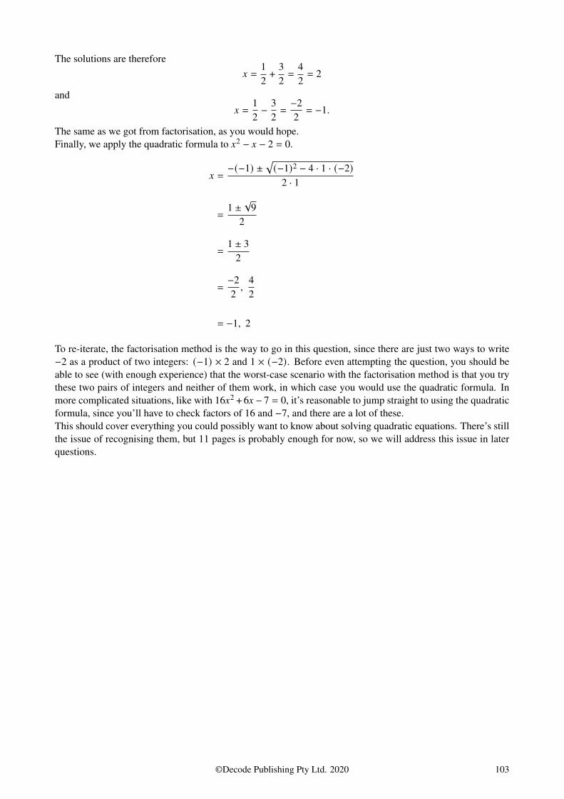
The solutions are thereforeG =

12+ 3

2=

42= 2

andG =

12− 3

2=−22

= −1.

The same as we got from factorisation, as you would hope.Finally, we apply the quadratic formula to G2 − G − 2 = 0.

G =−(−1) ±

√(−1)2 − 4 · 1 · (−2)

2 · 1

=1 ±

√9

2

=1 ± 3

2

=−22,

42

= −1, 2

To re-iterate, the factorisation method is the way to go in this question, since there are just two ways to write−2 as a product of two integers: (−1) × 2 and 1 × (−2). Before even attempting the question, you should beable to see (with enough experience) that the worst-case scenario with the factorisation method is that you trythese two pairs of integers and neither of them work, in which case you would use the quadratic formula. Inmore complicated situations, like with 16G2 + 6G − 7 = 0, it’s reasonable to jump straight to using the quadraticformula, since you’ll have to check factors of 16 and −7, and there are a lot of these.This should cover everything you could possibly want to know about solving quadratic equations. There’s stillthe issue of recognising them, but 11 pages is probably enough for now, so we will address this issue in laterquestions.


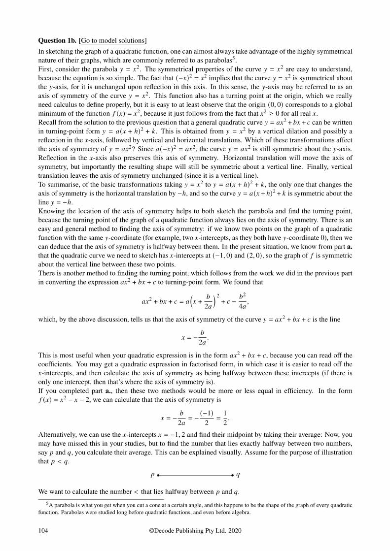
Question 1b. [Go to model solutions]

In sketching the graph of a quadratic function, one can almost always take advantage of the highly symmetricalnature of their graphs, which are commonly referred to as parabolas5.First, consider the parabola H = G2. The symmetrical properties of the curve H = G2 are easy to understand,because the equation is so simple. The fact that (−G)2 = G2 implies that the curve H = G2 is symmetrical aboutthe H-axis, for it is unchanged upon reflection in this axis. In this sense, the H-axis may be referred to as anaxis of symmetry of the curve H = G2. This function also has a turning point at the origin, which we reallyneed calculus to define properly, but it is easy to at least observe that the origin (0, 0) corresponds to a globalminimum of the function 5 (G) = G2, because it just follows from the fact that G2 ≥ 0 for all real G.Recall from the solution to the previous question that a general quadratic curve H = 0G2 + 1G + 2 can be writtenin turning-point form H = 0(G + ℎ)2 + : . This is obtained from H = G2 by a vertical dilation and possibly areflection in the G-axis, followed by vertical and horizontal translations. Which of these transformations affectthe axis of symmetry of H = 0G2? Since 0(−G)2 = 0G2, the curve H = 0G2 is still symmetric about the H-axis.Reflection in the G-axis also preserves this axis of symmetry. Horizontal translation will move the axis ofsymmetry, but importantly the resulting shape will still be symmetric about a vertical line. Finally, verticaltranslation leaves the axis of symmetry unchanged (since it is a vertical line).To summarise, of the basic transformations taking H = G2 to H = 0(G + ℎ)2 + : , the only one that changes theaxis of symmetry is the horizontal translation by −ℎ, and so the curve H = 0(G + ℎ)2 + : is symmetric about theline H = −ℎ.Knowing the location of the axis of symmetry helps to both sketch the parabola and find the turning point,because the turning point of the graph of a quadratic function always lies on the axis of symmetry. There is aneasy and general method to finding the axis of symmetry: if we know two points on the graph of a quadraticfunction with the same H-coordinate (for example, two G-intercepts, as they both have H-coordinate 0), then wecan deduce that the axis of symmetry is halfway between them. In the present situation, we know from part a.that the quadratic curve we need to sketch has G-intercepts at (−1, 0) and (2, 0), so the graph of 5 is symmetricabout the vertical line between these two points.There is another method to finding the turning point, which follows from the work we did in the previous partin converting the expression 0G2 + 1G + 2 to turning-point form. We found that

0G2 + 1G + 2 = 0

(G + 1

20

) 2+ 2 − 12

40,

which, by the above discussion, tells us that the axis of symmetry of the curve H = 0G2 + 1G + 2 is the line

G = − 1

20.

This is most useful when your quadratic expression is in the form 0G2 + 1G + 2, because you can read off thecoefficients. You may get a quadratic expression in factorised form, in which case it is easier to read off theG-intercepts, and then calculate the axis of symmetry as being halfway between these intercepts (if there isonly one intercept, then that’s where the axis of symmetry is).If you completed part a., then these two methods would be more or less equal in efficiency. In the form5 (G) = G2 − G − 2, we can calculate that the axis of symmetry is

G = − 1

20= − (−1)

2=

12.

Alternatively, we can use the G-intercepts G = −1, 2 and find their midpoint by taking their average: Now, youmay have missed this in your studies, but to find the number that lies exactly halfway between two numbers,say ? and @, you calculate their average. This can be explained visually. Assume for the purpose of illustrationthat ? < @.

? @

We want to calculate the number < that lies halfway between ? and @.

5A parabola is what you get when you cut a cone at a certain angle, and this happens to be the shape of the graph of every quadraticfunction. Parabolas were studied long before quadratic functions, and even before algebra.


? @<

Notice that the distance between ? and < is < − ?, while the distance between @ and < is @ − <.

? @<

< − ? @ − <

Since < is halfway between ? and @, these two distances are equal; that is, < − ? = @ − <. Solving thisequation for <, we get

< − ? = @ − < =⇒ 2< = ? + @ =⇒ < =? + @

2,

which is the average of ? and @. We can use the to calculate the midpoint of the G-intercepts G = −1, 2, whichis

−1 + 22

=12.

We’ve calculate in two different ways that the graph of 5 has the line G = 12 as its axis of symmetry. The

turning point of the graph lies on this line, so we can use this G-value to find the H-coordinate of the turningpoint:

5

(12

)=

14− 1

2− 2 = −9

4

Hence, the turning point occurs at( 1

2 ,−94). This is a good thing to mark on the provided axes before attempting

to draw the curve itself. We know the G-intercepts, so we can mark these in too.

G

H

$

( 12 ,−

94)

1 2 3 4−4 −3 −2 −1

1

2

3

4

−3

−2

−1

Drawing a nice, symmetric, and smooth curve can be tough, especially when you’re under pressure. For thisreason, you should try to calculate as many points as possible without wasting too much time. There is somebalance to be struck, because you want to get the curve right the first time, but you don’t want to be calculatingcoordinates for ten minutes.Once you’ve calculated the coordinates that are absolutely required for marks, you can look for some low-hanging fruit. In this case (and most others), the H-intercept is easy to calculate: 5 (0) = −2. Using symmetryabout the line G = 1

2 , we also have 5 (1) = −2 (which can also be calculated directly without difficulty). Wecan mark these points on the grid. Labelling them isn’t required, so it would waste precious time to do so.


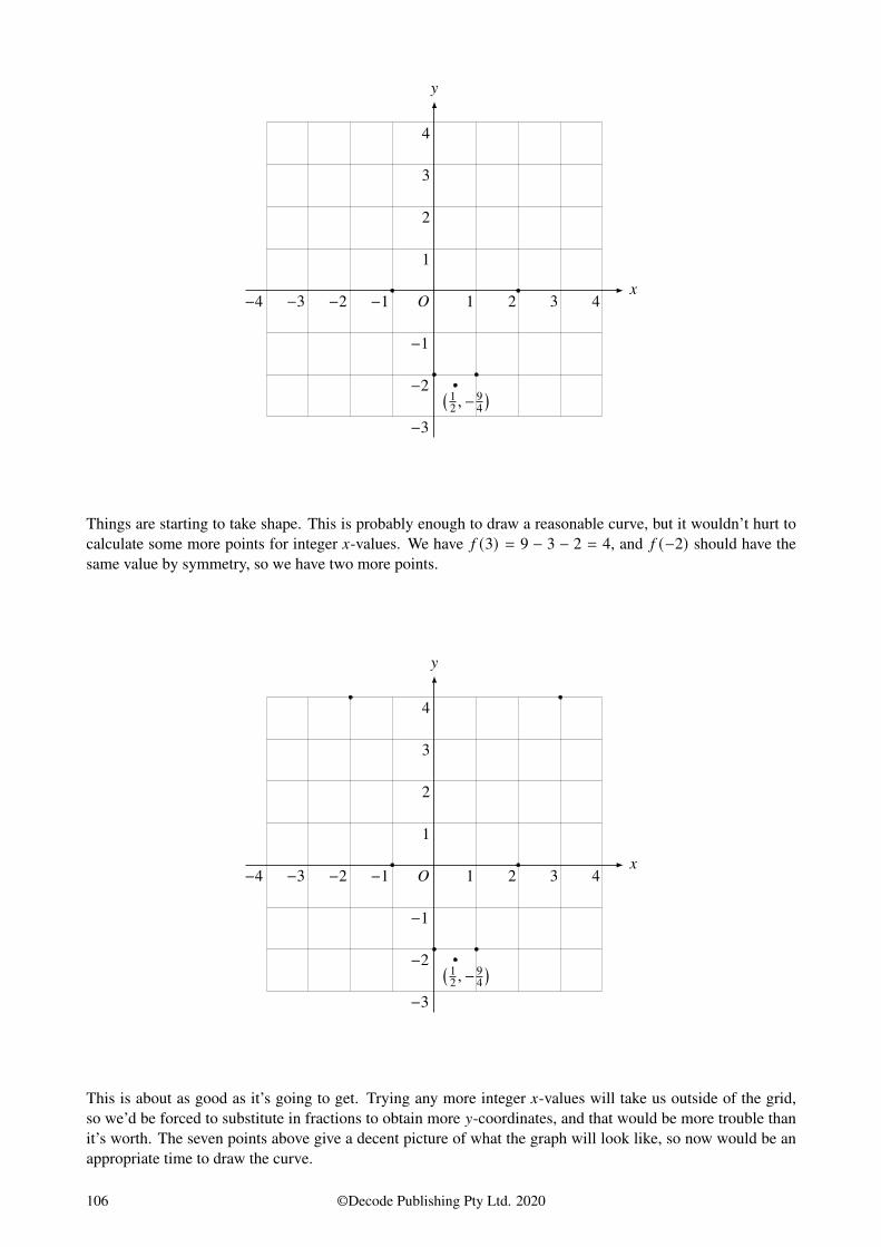
G

H

$

( 12 ,−

94)

1 2 3 4−4 −3 −2 −1

1

2

3

4

−3

−2

−1

Things are starting to take shape. This is probably enough to draw a reasonable curve, but it wouldn’t hurt tocalculate some more points for integer G-values. We have 5 (3) = 9 − 3 − 2 = 4, and 5 (−2) should have thesame value by symmetry, so we have two more points.

G

H

$

( 12 ,−

94)

1 2 3 4−4 −3 −2 −1

1

2

3

4

−3

−2

−1

This is about as good as it’s going to get. Trying any more integer G-values will take us outside of the grid,so we’d be forced to substitute in fractions to obtain more H-coordinates, and that would be more trouble thanit’s worth. The seven points above give a decent picture of what the graph will look like, so now would be anappropriate time to draw the curve.


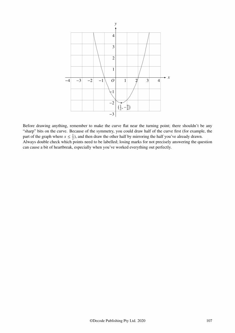
G

H

$

( 12 ,−

94)

1 2 3 4−4 −3 −2 −1

1

2

3

4

−3

−2

−1

Before drawing anything, remember to make the curve flat near the turning point; there shouldn’t be any“sharp” bits on the curve. Because of the symmetry, you could draw half of the curve first (for example, thepart of the graph where G ≤ 1

2 ), and then draw the other half by mirroring the half you’ve already drawn.Always double check which points need to be labelled; losing marks for not precisely answering the questioncan cause a bit of heartbreak, especially when you’ve worked everything out perfectly.


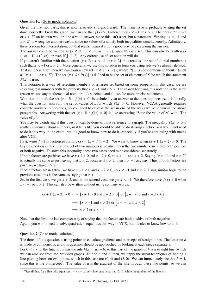
Question 1c. [Go to model solutions]

Given the first two parts, this is now relatively straightforward. The main issue is probably writing the setdown correctly. From the graph, we can see that 5 (G) > 0 when either G < −1 or G > 2. The phrase “G < −1or G > 2” on its own wouldn’t be a valid answer, since this isn’t a set, but a statement. Writing “G < −1 andG > 2” is wrong for another reason, since no values of G satisfy both inequalities simultaneously. Admittedly,there is room for interpretation, but that really means it’s not a good way of expressing the answer.The answer could be written as {G ∈ R : G < −1 or G > 2}, since this is a set. This can also be written as(−∞,−1) ∪ (2,∞), or even R\[−1, 2]. Any correct use of set notation will do.If you aren’t familiar with the notation {G ∈ R : G < −1 or G > 2}, it is read as “the set of all real numbers Gsuch that G < −1 or G > 2”. More generally, we use this notation to form sets using sets we’ve already defined.That is, if ( is a set, then we can form a new set {G ∈ ( : %(G)}, where %(G) is some statement about G (suchas “G < −1 or G > 2”). The set {G ∈ ( : %(G)} is defined to be the set of elements of ( for which the statement%(G) is true.This notation is a way of selecting members of a larger set based on some property; in this case, we areselecting real numbers with the property that G < −1 and G > 2. The reason for using this notation is the samereason we use any mathematical notation: it’s succinct, and allows for more precise statements.With that in mind, the set {G ∈ R : 5 (G) > 0} is technically an answer to the question, because it is literallywhat the question asks for: the set of values of G for which 5 (G) > 0. However, VCAA generally requiresconcrete answers to questions, so you need to express the set in one of the ways we’ve shown in the aboveparagraphs. Answering with the set {G ∈ R : 5 (G) > 0} is like answering “State the value of ?” with “Thevalue of ?”.You may be wondering if this question can be done without reference to a graph. The inequality 5 (G) > 0 isreally a statement about numbers, so it feels like you should be able to do it using algebra. You would not needto do it this way in the exam, but it’s good to know how to do it, especially if you’re continuing with mathsafter VCE.First, write 5 (G) in factorised form, 5 (G) = (G + 1) (G − 2). We want to know when (G + 1) (G − 2) > 0. Thekey observation is this: if a product of two numbers is positive, then the two numbers are either both positiveor both negative. To solve this inequality, these two cases need to be considered separately.If both factors are positive, we have G + 1 > 0 and G − 2 > 0, so G > −1 and G > 2. Saying “G > −1 and G > 2”is actually the same as just saying that G > 2, because if G > 2, then G > −1 anyway. Thus, if both factors arepositive, we have G > 2.If both factors are negative, we have G + 1 < 0 and G − 2 < 0, so G < −1 and G < 2. Using similar logic to theprevious case, this is the same as saying that G < −1.So, in the first case, we get G > 2, and in the second case, we get G < −1. We therefore have 5 (G) > 0 whenG < −1 or G > 2. This can also be written without using so many words:

(G + 1) (G − 2) > 0 =⇒(G + 1 > 0 and G − 2 > 0

)or

(G + 1 < 0 and G − 2 < 0

)=⇒

(G > −1 and G > 2

)or

(G < −1 and G < 2

)=⇒ G > 2 or G < −1

Note that the first line is a compact way of saying that the factors are both positive or both negative.Again, you won’t need to solve quadratic inequalities this way in VCE, but it’s nice to know how to do it.

Question 2 [Go to model solutions]

The thrust of this question is using points to calculate gradients and intercepts of straight lines. The function ℎ

is made of components, and this question should be approached by looking at each piece separately.For 0 < G < 5, the function ℎ has the rule ℎ(G) = 0G + 1, so this part of the graph of ℎ is a straight line (whichwe can also see from the provided graph). To find 0 and 1, then, we apply the usual techniques of finding aline passing between two points, which in this case are (0, 4) and (5, 0). We can immediately see that 1 = 4,since this is the H-intercept6. The value of 0 is the gradient of the line through these two points, so we can

6Recall that, for a line with equation H = <G + 2, the H-intercept occurs at (0, 2), while the gradient of the line is <.


use the standard “rise over run” formula. The gradient of the line passing through the two points (G1, H1) and(G2, H2) (when G1 ≠ G2) is

H2 − H1G2 − G1

,

so to calculate 0, we use the points (0, 4) and (5, 0), giving

0 =0 − 45 − 0

= −45.

The same formula can be used with the points (5, 0) and (6, 2) to find that 2 = 2. Finding 3 is only slightlyless straightforward, but if we know 2 it’s not too bad. We can see that ℎ(5) = 0 from the given graph, so if weuse the actual rule for ℎ, we get ℎ(5) = 52 + 3 = 0. Knowing the value of 2, we get 3 = −52 = −10.

This is more of a revision question than an exam-style question, but you will need to know straight lines prettywell, since many of the more complicated questions are based on this knowledge.


This is a bit of a trick question, since the expression for 6(G) isn’t given in the simplest form possible. It’scommon for VCAA to test manipulation of powers of small numbers. Here, you need to spot that rewriting 4as 22 will allow you to combine powers and simplify the expression for 6(G); that is,

6(G) = 1 − 22 · 2−G−2 = 1 − 22−G−2 = 1 − 2−G .

(Here we used the index law 0G0H = 0G+H to combine powers.) This is a less cumbersome expression, andit’s easier to see what the graph will look like. Of course, you’re not required to simplify it to get marks, butit will make your life easier, considering the lack of calculator access. The 2−G term will become arbitrarilysmall with increasing G, so the graph of 6 will approach the line H = 1. With the set of axes we are given, youwould hope that 6(G) never exceeds 1, and this is so: the quantity 2−G is always positive, so 6(G) = 1 − 2−Gwill always be less than 1. The graph of 6 must therefore approach the line H = 1 from below. Another thingto note is that, since 2−G gets smaller as G increases, the value of 6(G) will increase with increasing G.

This should give some idea of what the graph of 6 looks like, but still doesn’t really help you nail down theexact shape. An obvious thing to do is find the H-intercept. Using the simplified expression for 6(G), we have6(0) = 1 − 20 = 1 − 1 = 0, so the graph of 6 passes through the origin. The simplified expression found abovemakes it much easier to calculate 6(G) for any given G-value, and once again we are reaping the benefits offinding it. The vertical lines on the grid occur at integer G-values, so finding the corresponding H-values wouldhelp quite a bit in drawing the graph.

We have

6(1) = 1 − 2−1 = 1 − 12, 6(2) = 1 − 1

4, 6(3) = 1 − 1

8, 6(4) = 1 − 1

16.

Here we used another index law: 0−G = 10G .

As we mentioned in the first question, you don’t need to fully simplify these values unless they’re explicitlyrequired as an answer to a question. The reason for doing this isn’t that simplifying the fractions is too difficult;it’s more that leaving the values as they are above gives you more of a feel for what’s going on. It’s also niceand easy to work with in this situation; the value of 6(1) is 1/2 of a unit from the top line, the value of 6(2)is 1/4 of a unit from the top line, and so on. These points should be marked in before you start drawing thecurve, as it makes the task much easier and allows for more precision on your part. Adding in extra key pointsto your free-hand graphs in exams will ensure you never lose marks for graph shape in these questions (if donecorrectly).


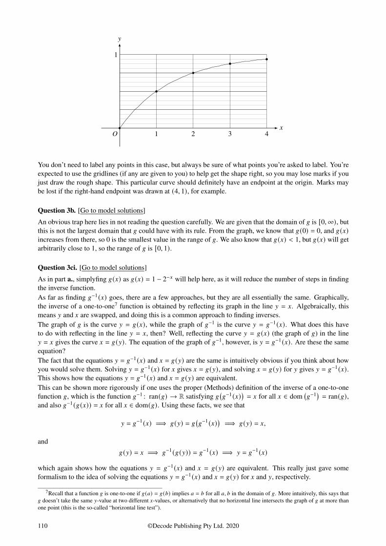
G

H

$ 1 2 3 4

1

You don’t need to label any points in this case, but always be sure of what points you’re asked to label. You’reexpected to use the gridlines (if any are given to you) to help get the shape right, so you may lose marks if youjust draw the rough shape. This particular curve should definitely have an endpoint at the origin. Marks maybe lost if the right-hand endpoint was drawn at (4, 1), for example.


An obvious trap here lies in not reading the question carefully. We are given that the domain of 6 is [0,∞), butthis is not the largest domain that 6 could have with its rule. From the graph, we know that 6(0) = 0, and 6(G)increases from there, so 0 is the smallest value in the range of 6. We also know that 6(G) < 1, but 6(G) will getarbitrarily close to 1, so the range of 6 is [0, 1).

Question 3ci. [Go to model solutions]

As in part a., simplyfing 6(G) as 6(G) = 1 − 2−G will help here, as it will reduce the number of steps in findingthe inverse function.As far as finding 6−1(G) goes, there are a few approaches, but they are all essentially the same. Graphically,the inverse of a one-to-one7 function is obtained by reflecting its graph in the line H = G. Algebraically, thismeans H and G are swapped, and doing this is a common approach to finding inverses.The graph of 6 is the curve H = 6(G), while the graph of 6−1 is the curve H = 6−1(G). What does this haveto do with reflecting in the line H = G, then? Well, reflecting the curve H = 6(G) (the graph of 6) in the lineH = G gives the curve G = 6(H). The equation of the graph of 6−1, however, is H = 6−1(G). Are these the sameequation?The fact that the equations H = 6−1(G) and G = 6(H) are the same is intuitively obvious if you think about howyou would solve them. Solving H = 6−1(G) for G gives G = 6(H), and solving G = 6(H) for H gives H = 6−1(G).This shows how the equations H = 6−1(G) and G = 6(H) are equivalent.This can be shown more rigorously if one uses the proper (Methods) definition of the inverse of a one-to-onefunction 6, which is the function 6−1 : ran(6) → R satisfying 6

(6−1(G)

)= G for all G ∈ dom

(6−1) = ran(6),

and also 6−1(6(G)) = G for all G ∈ dom(6). Using these facts, we see that

H = 6−1(G) =⇒ 6(H) = 6(6−1(G)

)=⇒ 6(H) = G,

and

6(H) = G =⇒ 6−1(6(H)) = 6−1(G) =⇒ H = 6−1(G)

which again shows how the equations H = 6−1(G) and G = 6(H) are equivalent. This really just gave someformalism to the idea of solving the equations H = 6−1(G) and G = 6(H) for G and H, respectively.

7Recall that a function 6 is one-to-one if 6(0) = 6(1) implies 0 = 1 for all 0, 1 in the domain of 6. More intuitively, this says that6 doesn’t take the same H-value at two different G-values, or alternatively that no horizontal line intersects the graph of 6 at more thanone point (this is the so-called “horizontal line test”).


To find 6−1(G), we let H = 6−1(G). This implies that 6(H) = G, so we solve this equation for H.

6(H) = G =⇒ 1 − 2−H = G

=⇒ 2−H = 1 − G

=⇒ −H = log2(1 − G)=⇒ H = − log2(1 − G)=⇒ 6−1(G) = − log2(1 − G)

The idea behind this approach is that we know what 6 is already, so it can be applied to H. In case you missed it,in going from the second line to the third, we used the fundamental relationship between exponential functionsand logarithms, which is that, for 0 > 1 and H > 0, we have

0G = H ⇐⇒ G = log0 (H)

In other words, the equations 0G = H and G = log0 (H) are logically equivalent, so you can use them to convertbetween exponential functions and logarithms. In more detail, solving 0G = H for G gives G = log0 (H), whilesolving G = log0 (H) for H gives 0G = H. This may resemble the discussion of how the equations H = 6−1(G)and G = 6(H) are equivalent, and that is because log0 (G) is the inverse of the function 0G , which is actually thedefinition of log0 (G).These questions (where you find the inverse of a given function) will always involve manipulation of powerfunctions, exponential functions, or logarithms (inverses of circular functions are not part of the Methodscourse), so you can prepare pretty well for them.

Question 3cii. [Go to model solutions]

This is a straightforward test on the relationship between the domain and range of an invertible function andthe domain and range of its inverse. In effect, the domain and range of a function are swapped when you invertthe function. This can be understood graphically; the G- and H-values are swapped in going from the graph ofa function to the graph of its inverse, as we showed in the previous part.Based on this observation, the range of 6−1 is the domain of 6, which is [0,∞); this is given to you explicitlyas the domain of 6. Again, it would be easy to miss this and assume 6 is defined everywhere, which wouldimply that the range of 6−1 is all of R (but it isn’t).


The period of a function 5 is the smallest positive number ? such that 5 (G+ ?) = 5 (G) for all G in the domain of5 , if such a number exists. The period of 5 is then the smallest (non-zero) amount by which you can translatethe graph of 5 horizontally and end up with exactly the same curve. Given a function 5 , it is useful to knowwhat simple transformations of 5 will affect the period of 5 , since in Methods you will only be asked to findthe period of a function obtained as a simple transformation of sin, cos, or tan. In the following, it will beuseful to think of 5 as one of these three functions.Before getting started, click here and have a read if you aren’t particularly comfortable with transformations,since most of what follows will be based on transformations.Suppose that 6(G) = 0 5 (G), where 0 ≠ 0. Then 6 must have the same period as 5 ; the values of 5 havebeen uniformly scaled (with an order reversal if 0 < 0), so the cyclic pattern will remain the same. Thinkof this graphically; vertical scaling or reflecting in the G-axis will not affect the period. Similarly, if 6(G) =

5 (G) + 1, then 6 will have the same period as 5 , since this just moves the graph of 5 vertically. Thus, applyingtransformations in the H-direction of the graph of 5 will not affect its period.What about translating in the G-direction? If 6(G) = 5 (G + 2), then 6 still has the same period as 5 . If youchange the position of the hands of an analogue clock, it will still repeat every 12 hours.For reflecting in the H-axis, we consider 6(G) = 5 (−G). Again, the period of 6 is the same as 5 . If a clock runsbackwards at its normal speed, it will still repeat every 12 hours.All that’s left is dilation in the G-direction, and this is the only thing that affects the period. The graph of 5 willrepeat itself every ? units in the G-direction, so if we dilate the graph of 5 by a factor of 0 in the G-direction(where 0 > 0), it will repeat itself every 0? units; that is, the new period is 0?.


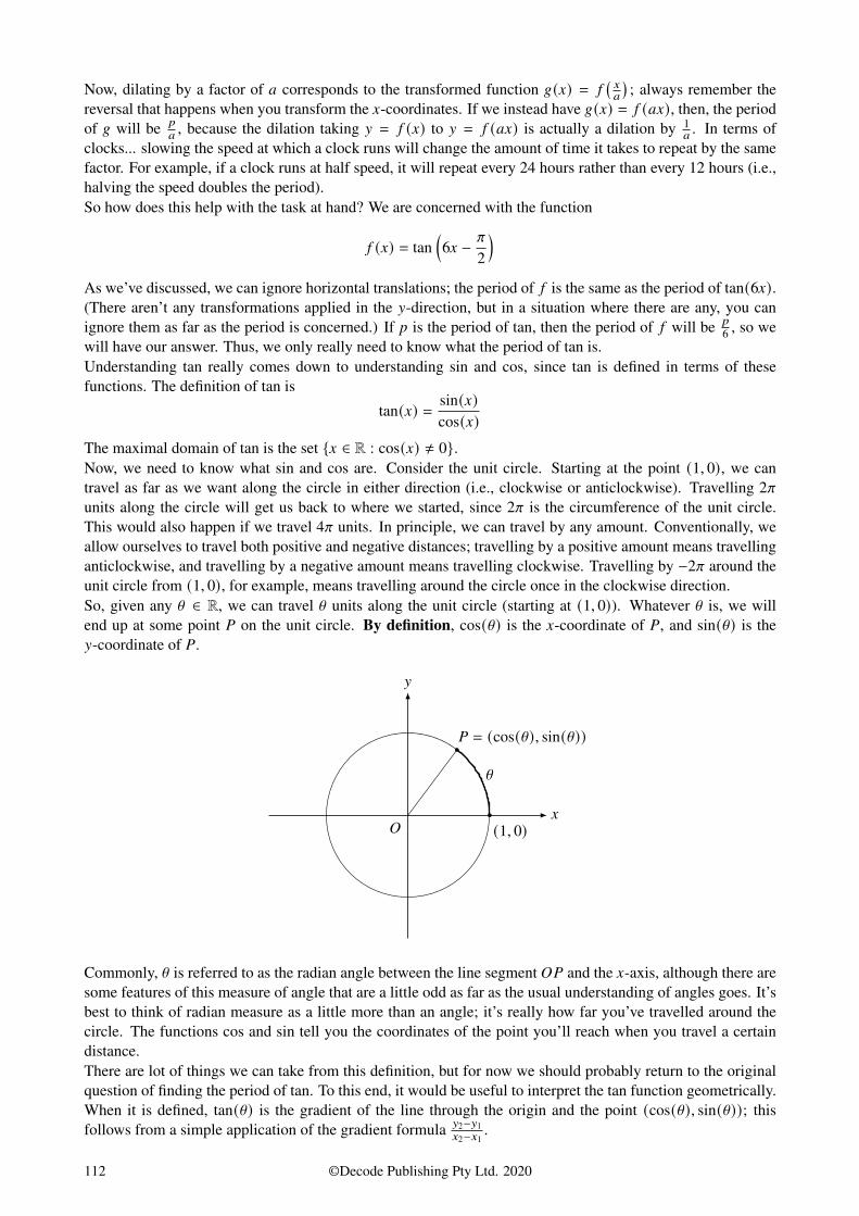
Now, dilating by a factor of 0 corresponds to the transformed function 6(G) = 5(G0

); always remember the

reversal that happens when you transform the G-coordinates. If we instead have 6(G) = 5 (0G), then, the periodof 6 will be ?

0, because the dilation taking H = 5 (G) to H = 5 (0G) is actually a dilation by 1

0. In terms of

clocks... slowing the speed at which a clock runs will change the amount of time it takes to repeat by the samefactor. For example, if a clock runs at half speed, it will repeat every 24 hours rather than every 12 hours (i.e.,halving the speed doubles the period).So how does this help with the task at hand? We are concerned with the function

5 (G) = tan(6G − c

2

)As we’ve discussed, we can ignore horizontal translations; the period of 5 is the same as the period of tan(6G).(There aren’t any transformations applied in the H-direction, but in a situation where there are any, you canignore them as far as the period is concerned.) If ? is the period of tan, then the period of 5 will be ?

6 , so wewill have our answer. Thus, we only really need to know what the period of tan is.Understanding tan really comes down to understanding sin and cos, since tan is defined in terms of thesefunctions. The definition of tan is

tan(G) = sin(G)cos(G)

The maximal domain of tan is the set {G ∈ R : cos(G) ≠ 0}.Now, we need to know what sin and cos are. Consider the unit circle. Starting at the point (1, 0), we cantravel as far as we want along the circle in either direction (i.e., clockwise or anticlockwise). Travelling 2cunits along the circle will get us back to where we started, since 2c is the circumference of the unit circle.This would also happen if we travel 4c units. In principle, we can travel by any amount. Conventionally, weallow ourselves to travel both positive and negative distances; travelling by a positive amount means travellinganticlockwise, and travelling by a negative amount means travelling clockwise. Travelling by −2c around theunit circle from (1, 0), for example, means travelling around the circle once in the clockwise direction.So, given any \ ∈ R, we can travel \ units along the unit circle (starting at (1, 0)). Whatever \ is, we willend up at some point % on the unit circle. By definition, cos(\) is the G-coordinate of %, and sin(\) is theH-coordinate of %.

G

H

$

% = (cos(\), sin(\))

(1, 0)

\

Commonly, \ is referred to as the radian angle between the line segment $% and the G-axis, although there aresome features of this measure of angle that are a little odd as far as the usual understanding of angles goes. It’sbest to think of radian measure as a little more than an angle; it’s really how far you’ve travelled around thecircle. The functions cos and sin tell you the coordinates of the point you’ll reach when you travel a certaindistance.There are lot of things we can take from this definition, but for now we should probably return to the originalquestion of finding the period of tan. To this end, it would be useful to interpret the tan function geometrically.When it is defined, tan(\) is the gradient of the line through the origin and the point (cos(\), sin(\)); thisfollows from a simple application of the gradient formula H2−H1

G2−G1.


G

H

$

(cos(\), sin(\))

(1, 0)

\

H = tan(\) · G

If you travel around the circle by a further c units (and no less!), you’ll end up on the other side of the circle(remember that the circumference of the unit circle is c), but the line through the origin and the point you reachwill be exactly the same. In particular, it will have the same gradient.

G

H

$

(cos(\ + c), sin(\ + c))

(1, 0)

\

H = tan(\ + c) · G

The two gradients are equal, so tan(\) = tan(\ + c). From this simple observation, we can see that the periodof tan is c; hence, the period of 5 is c

6 . More generally, the period of a function of the form 5 (G) = tan(0G),with 0 > 0, is c

0.


Here, we will assume some knowledge of the graph of tan. It’s good to see how the graph connects with thegeometric interpretation above. As \ increases from 0 to c

2 , the gradient of the line through (cos(\), sin(\))and the origin will tend towards infinity. Since tan(\) is the gradient of this line, we see this behaviour in thegraph of tan.The graph of tan will have vertical asymptotes at every value of \ such that the line through (cos(\), sin(\))and the origin is vertical. This happens when the point (cos(\), sin(\)) is either at the very top or the verybottom of the unit circle; for example, when \ = c

2 . Another asymptote is reached whenever \ increases ordecreases by c.The point is that we can find asymptotes by using the period, provided we know where one asymptote is. Wecan do this for any simple transformation of the tan function, such as the function in this question. Unlike theperiod, the location of asymptotes will usually be affected by horizontal translations, but the distance betweenthe asymptotes remains the same. The distance between adjacent asymptotes of tan is the same as its period,and this is true of any simple transformations of tan.To algebraically find the location of an asymptote of a transformed tan function, it’s best not to work with ∞or −∞ as if it were a number; avoid writing things like “Let 5 (G) = ∞”. Apart from the fact that it probably


won’t help, it’s nonsensical in a couple of ways. The asymptotes of H = tan(G) occur when cos(G) = 0, so thisis really the equation you want to solve. In this case, we have

5 (G) = tan(6G − c

2

)=

sin(6G − c

2)

cos(6G − c

2)

We know G = 0 is an asymptote of the graph of 5 , so we solve cos(60− c

2)= 0 to find 0. Since cos

(c2)= 0, a

possible solution is 60 − c2 = c

2 ; solving this for 0 gives 0 = c6 . We can find the locations of other asymptotes

by adding and subtracting the period of 5 . We are asked for 0 within the interval[0, c

2]

, so there are onlyfinitely many values of 0; a general solution is not required (general solutions have never been required intech-free exams, at least in the last 11 years).Going backwards from 0 = c

6 , subtracting the period of 5 (which is also c6 ) gives 0, and subtracting any more

will take us out of the required interval. If we add the period, we get 0 = c6 + c

6 = c3 , and adding once more

gives 0 = c3 + c

6 = c2 , which brings us to the other end of the interval. The possible values of 0 are

0 = 0,c

6,c

3,c

2

Question 5 [Go to model solutions]

This is probably a good place to carefully cover the theory behind transformations of the plane in order toaddress any subtleties you might have missed. The solutions to the actual question, if you want to skip ahead,start here.This area is often taught poorly, but it is genuinely hard to teach, mainly due to fact that the Methods courselacks a lot of important concepts that would make it easier to explain. We won’t introduce concepts outside ofthe course, though, so we’ll explain transformations using only Methods knowledge.First, we’ll define dilations. For 0 > 0, a dilation by a factor of 0 in the G-direction (also called a dilation by afactor of 0 from the H-axis) is the function8 ) : R2 → R2 defined by ) (G, H) = (0G, H). Essentially, ) multipliesthe G-coordinate of every point in the plane by 0. (I’m going to use the symbol ) many times, so you’ll haveto keep track of what ) is at any given time.)

G

H

$ 1

)

G

H

$ 0

Similarly, a dilation by a factor of 0 in the H-direction (or a dilation by a factor of 0 from the G-axis) is definedas the function ) (G, H) = (G, 0H). Geometrically, this is a vertical stretching rather than a horizontal stretching.It is usually of interest (in this course) to know how dilations affect the graphs of functions. Let 5 : � → R,where � is some subset of R. The graph of 5 is the set of points (G, H) such that H = 5 (G). Under a dilation,these points may be mapped to new points, which will result in a new curve.To carefully verify results about transformations, it is useful to think of a function ) : R2 → R2 as sending apoint (G, H) to a new point (G ′, H′). Giving names to the coordinates of the new point gives you more to workwith (in a helpful way, as we will see).

8You may be used to thinking of a function as having subsets of R as its domain and range, but a function can map between anytwo sets. The notation ) : R2 → R2 shows up in Methods exams but not in a big way.


G

H

$

)

(G, H)

(G ′, H′)

Let’s consider again a dilation by a factor of 0 in the G-direction, which is the function ) (G, H) = (0G, H). Thepoint (G, H) gets sent to the point (0G, H), so we let (G ′, H′) = (0G, H).To understand what happens to the graph of 5 , we ask: if (G, H) satisfies the equation H = 5 (G), what equationdoes the point (G ′, H′) satisfy? This is a slightly ill-defined problem, but the aim is to get an equation kind oflike H = 5 (G).We defined (G ′, H′) = (0G, H), so we have a relationship between the new and old coordinates. More specifi-cally, we have G ′ = 0G and H′ = H. Rearranging the former gives G = G′

0; there is not much we can do with the

latter.Since H = H′ and G = G′

0, the equation H = 5 (G) is the same as the equation H′ = 5

(G′

0

). This says that the curve

H = 5 (G) gets mapped to the curve H = 5(G0

). The reason we can change the variable names back to normal is

always tricky to explain, but it really comes down to the fact that the graph of a function is technically a set ofpoints, not an equation. The graph of 5 is really the set

{(G, H) : H = 5 (G)}

As we have seen, under ) , this set becomes{(G ′, H′) : H′ = 5

( G ′0

) }Since this is a set, it doesn’t really matter what you called the variables, so it is the same as the set{

(G, H) : H = 5

( G0

) }.

This can be done even more carefully and convincingly by using more sophisticated set-theoretic notions, butthis would take us outside of the course. In a nutshell, dilating by a factor of 0 in the G-direction sends thecurve H = 5 (G) to the curve H = 5

(G0

). This is all you really need to know, but it’s good to know why dilating

in the G-direction has this effect.We can apply the same approach to see what happens when we dilate in the H-direction via the function) (G, H) = (G, 0H). Again, we write (G ′, H′) for the new coordinates, so G ′ = G and H′ = 0H, the latter beingequivalent to H =

H′

0. By replacing old variables with the new ones, the equation H = 5 (G) is equivalent to

H′

0= 5 (G ′), which in turn is equivalent to H′ = 0 5 (G ′). The equation of the new curve is therefore H = 0 5 (G).

Hopefully you can see the differences between the two types of dilations – particularly, why one involvesdivision by 0 and the other doesn’t. The answer is basically that both involve division by 0, but we generallyrearrange equations to express things in terms of H.In hindsight, we could have allowed 0 < 0, since it causes no problems with the algebra9, but it’s a little trickierto interpret this geometrically. For this reason, we usually look at the specific case 0 = −1.The function ) (G, H) = (−G, H) takes the negative of each G-coordinate – the points (G, H) and (−G, H) areswapped by ) , so the entire plane is reflected in the H-axis.

9The case 0 = 0 does cause some problems, particularly in transforming graphs, since we divided by 0. The correspondingtransformations are perfectly sensible – they just act a little extremely, namely by squashing the entire plane onto an axis. This type oftransformation won’t come up in VCE.


G

H

$

(1, 1)(−1, 1)

(1,−1)(−1,−1)

Similarly, the function ) (G, H) = (G,−H) swaps the points (G, H) and (G,−H), reflecting the plane in the G-axis.We’ve actually already worked out what these transformations do to the curve H = 5 (G); simply substitute0 = −1 into what we’ve already obtained. The reflection ) (G, H) = (−G, H) sends H = 5 (G) to H = 5

(G−1

); i.e.,

H = 5 (−G). The reflection ) (G, H) = (G,−H) sends the curve H = 5 (G) to H = − 5 (G).So, for 0 < 0, we can more easily describe the transformation ) (G, H) = (0G, H) as follows. First, notethat 0 = −1, where 1 is a positive number (well, 1 = −0, to be precise). This means ) (G, H) = (−1G, H),so the G-values are dilated by 1, and the plane is also reflected in the H-axis (the order in which these twotransformations are carried out doesn’t matter, just because the order in which you multiply G by −1 and 1

doesn’t matter, because you end up with −1G either way).Decomposing ) in this way is good for interpreting ) geometrically, but it complicates the algebra. We couldsimply say that ) multiplies the G-coordinate of every point by 0 (whether 0 is positive or negative), but thisgives a little less intuition for what is happening10. In describing transformations in words, VCAA expectsgeometric words like “dilation” and “reflection” rather than “multiplication”.Since we can dilate along both coordinate axes separately, we can try to do both at once. Let 0, 1 ∈ R, let)1(G, H) = (0G, H), and let )2(G, H) = (G, 1H). These types of transformations have already been discussed, butwe need to give them different names in order to combine them. We can define a new transformation ) by) (G, H) = )1()2(G, H)); this is one transformation followed by another, resulting in a new transformation. Wecalculate a more explicit rule for ) :

) (G, H) = )1()2(G, H)) = )1(G, 1H) = (0G, 1H).

We get the same thing if we perform )1 and )2 in the other order, which hopefully makes sense geometrically– multiplying the G-coordinates doesn’t affect the H-coordinates, so it doesn’t matter if you multiply the H-coordinates before or after the G-coordinates. Basically, we can do them both at once, which is what ) does.We defined ) as the function “do )2, then do )1”, so we can almost immediately say what ) does to the curveH = 5 (G). Applying )2, we get the curve H = 5

(G0), and applying )1 to this curve gives H = 1 5

(G0), so ) sends

the curve H = 5 (G) to the curve H = 1 5(G0).

The function ) (G, H) = (0G, 1H) encapsulates all dilations and reflections; by choosing appropriate values of 0and 1, you can perform any sequence of dilations and reflections by using the single transformation ) .Let’s see how this works with an example. Consider the sequence of transformations:

• Reflection in the G-axis

• Dilation by a factor of 2 from the G-axis

• Reflection in the H-axis

• Dilation by a factor of 3 from the H-axis


10This is a common trade-off in mathematics; concepts can be described more compactly at the cost of an intuitive understanding.This problem can be tackled by trying to understand each concept in a number of different ways.


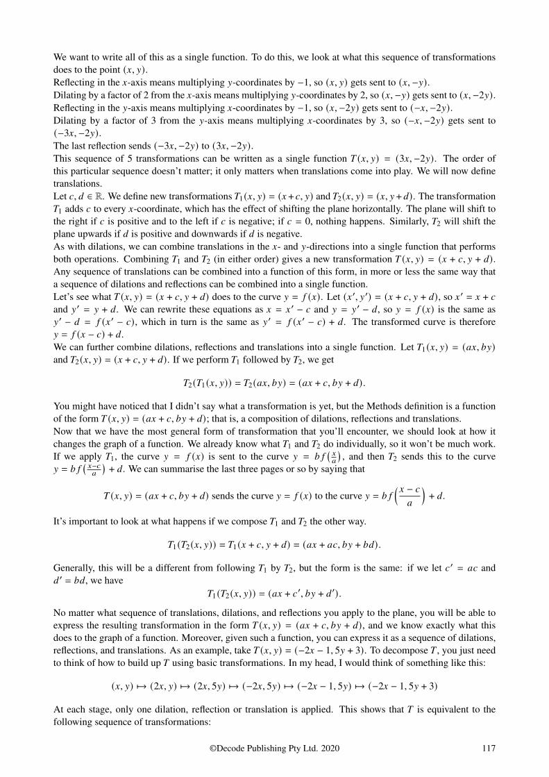
We want to write all of this as a single function. To do this, we look at what this sequence of transformationsdoes to the point (G, H).Reflecting in the G-axis means multiplying H-coordinates by −1, so (G, H) gets sent to (G,−H).Dilating by a factor of 2 from the G-axis means multiplying H-coordinates by 2, so (G,−H) gets sent to (G,−2H).Reflecting in the H-axis means multiplying G-coordinates by −1, so (G,−2H) gets sent to (−G,−2H).Dilating by a factor of 3 from the H-axis means multiplying G-coordinates by 3, so (−G,−2H) gets sent to(−3G,−2H).The last reflection sends (−3G,−2H) to (3G,−2H).This sequence of 5 transformations can be written as a single function ) (G, H) = (3G,−2H). The order ofthis particular sequence doesn’t matter; it only matters when translations come into play. We will now definetranslations.Let 2, 3 ∈ R. We define new transformations )1(G, H) = (G + 2, H) and )2(G, H) = (G, H + 3). The transformation)1 adds 2 to every G-coordinate, which has the effect of shifting the plane horizontally. The plane will shift tothe right if 2 is positive and to the left if 2 is negative; if 2 = 0, nothing happens. Similarly, )2 will shift theplane upwards if 3 is positive and downwards if 3 is negative.As with dilations, we can combine translations in the G- and H-directions into a single function that performsboth operations. Combining )1 and )2 (in either order) gives a new transformation ) (G, H) = (G + 2, H + 3).Any sequence of translations can be combined into a function of this form, in more or less the same way thata sequence of dilations and reflections can be combined into a single function.Let’s see what ) (G, H) = (G + 2, H + 3) does to the curve H = 5 (G). Let (G ′, H′) = (G + 2, H + 3), so G ′ = G + 2

and H′ = H + 3. We can rewrite these equations as G = G ′ − 2 and H = H′ − 3, so H = 5 (G) is the same asH′ − 3 = 5 (G ′ − 2), which in turn is the same as H′ = 5 (G ′ − 2) + 3. The transformed curve is thereforeH = 5 (G − 2) + 3.We can further combine dilations, reflections and translations into a single function. Let )1(G, H) = (0G, 1H)and )2(G, H) = (G + 2, H + 3). If we perform )1 followed by )2, we get

)2()1(G, H)) = )2(0G, 1H) = (0G + 2, 1H + 3).

You might have noticed that I didn’t say what a transformation is yet, but the Methods definition is a functionof the form ) (G, H) = (0G + 2, 1H + 3); that is, a composition of dilations, reflections and translations.Now that we have the most general form of transformation that you’ll encounter, we should look at how itchanges the graph of a function. We already know what )1 and )2 do individually, so it won’t be much work.If we apply )1, the curve H = 5 (G) is sent to the curve H = 1 5

(G0

), and then )2 sends this to the curve

H = 1 5(G−20

)+ 3. We can summarise the last three pages or so by saying that

) (G, H) = (0G + 2, 1H + 3) sends the curve H = 5 (G) to the curve H = 1 5

( G − 2

0

)+ 3.

It’s important to look at what happens if we compose )1 and )2 the other way.

)1()2(G, H)) = )1(G + 2, H + 3) = (0G + 02, 1H + 13).

Generally, this will be a different from following )1 by )2, but the form is the same: if we let 2′ = 02 and3 ′ = 13, we have

)1()2(G, H)) = (0G + 2′, 1H + 3 ′).

No matter what sequence of translations, dilations, and reflections you apply to the plane, you will be able toexpress the resulting transformation in the form ) (G, H) = (0G + 2, 1H + 3), and we know exactly what thisdoes to the graph of a function. Moreover, given such a function, you can express it as a sequence of dilations,reflections, and translations. As an example, take ) (G, H) = (−2G − 1, 5H + 3). To decompose ) , you just needto think of how to build up ) using basic transformations. In my head, I would think of something like this:

(G, H) ↦→ (2G, H) ↦→ (2G, 5H) ↦→ (−2G, 5H) ↦→ (−2G − 1, 5H) ↦→ (−2G − 1, 5H + 3)

At each stage, only one dilation, reflection or translation is applied. This shows that ) is equivalent to thefollowing sequence of transformations:


• Dilation by a factor of 2 from the H-axis

• Dilation by a factor of 5 from the G-axis


• Translation by 1 unit in the negative direction of the G-axis (i.e., to the left)

• Translation by 3 units in the positive direction of the H-axis (i.e., upwards)

If you are given such a list, you can find the resulting transformation by applying each transformation in thelist to the point (G, H). We can apply the above list of transformations to the point (G, H):

(G, H) ↦→ (2G, H) ↦→ (2G, 5H) ↦→ (−2G, 5H) ↦→ (−2G − 1, 5H) ↦→ (−2G − 1, 5H + 3)

This gives back the original function ) (G, H) = (−2G − 1, 5H + 3). So a transformation can be written either asa function ) (G, H) = (0G + 2, 1H + 3) or as a list of dilations, reflections, and translations. If you prefer workingwith one form, you should learn how to go from the form you don’t like to the form you do like, since they canbe given to you in either form. It’s also possible that you will be asked to write a transformation in a certainform, but this is not very common. To be on the safe side, you should be comfortable with converting a list toa function and vice versa.I haven’t yet addressed matrix notation, but it’s really just another way of writing out the function ) (G, H) =

(0G + 2, 1H + 3). A point (G, H) can alternatively be written in matrix form as[G

H

]Of course, the information that it carries is the same, but now it’s vertical. So far so good. Now, if we have afunction ) (G, H) = (0G + 2, 1H + 3), we can write the pairs as matrices:

)

( [G

H

] )=

[0G + 2

1H + 3

]Again, the pairs have just been written vertically. The next part uses some matrix multiplication and addition.Observe that [

0 00 1

] [G

H

]+

[2

3

]=

[0G

1H

]+

[2

3

]=

[0G + 2

1H + 3

]= )

( [G

H

] )So, finally, we have

)

( [G

H

] )=

[0 00 1

] [G

H

]+

[2

3

]In this course, transformations will usually be written in matrix form, rather than the form ) (G, H) = (0G +2, 1H + 3). You may be wondering whether there is an advantage of writing ) in matrix form, since it is a lotless compact than the alternative. As far as this course is concerned, there is actually no advantage whatsoever,and I find VCAA’s choice to put it in the course a little confusing. It’s just something you’ll have to cope with.That’s not to say matrices aren’t useful – quite the opposite is true – it’s just that you don’t really need to usethem for transformations as simple as these.We now have enough theory to be able to answer the original question (as well as every question about trans-formations). We are given

)

( [G

H

] )=

[1 00 3

] [G

H

]+

[1−1

]and we want to see how this transforms the curve H = 3G2 + 1. This isn’t exactly how the question is phrased,but that is really what it’s asking. It’s asked in a way that forces you to write the answer in a certain form (thisreally just makes it easier to mark).First, we can rewrite ) more compactly as ) (G, H) = (G + 1, 3H − 1). We now apply the result

) (G, H) = (0G + 2, 1H + 3) sends the curve H = 5 (G) to the curve H = 1 5

( G − 2

0

)+ 3,


In this specific case, we have 0 = 1, 1 = 3, 2 = 1, 3 = −1, and 5 (G) = 3G2 + 1, so we get

) (G, H) = (G + 1, 3H − 1) sends the curve H = 3G2 + 1 to the curve H = 3(3(G − 1)2 + 1) − 1.

All that’s left is to simplify the right-hand side of H = 3(3(G − 1)2 + 1) − 1.

H = 3(3(G − 1)2 + 1) − 1= 9(G − 1)2 + 3 − 1= 9(G2 − 2G + 1) + 2= 9G2 − 18G + 9 + 2= 9G2 − 18G + 11.

This is the form required by the question; you just need to finish up by saying what 0, 1, and 2 are11. In termsof writing out the answer, be sure to refer to the model solutions.

11These aren’t the same 0, 1, 2 that appear in the equation H = 1 5(G−20

)+ 3. You should use different names if you want to write

out the general equation in your answer, but you don’t really need to write out the general equation.


VCE Mathematical Methods Units 3&4 Volume 1: Topic Tests

Documents

Transcript of VCE Mathematical Methods Units 3&4 Volume 1: Topic Tests