Vascular plant species richness along elevation gradient of the Karnali river valley, Nepal...

Received: 16th Jan-2014 Revised: 26th March-2014 Accepted: 27th March-2014 Research article

VASCULAR PLANT SPECIES RICHNESS ALONG ELEVATION GRADIENT OF THE KARNALI RIVER VALLEY, NEPAL HIMALAYA

Prakash Bhattaraia*, Kuber Prasad Bhattab, Rita Chhetric and Ram Prasad Chaudharya,d

a. Central Department of Botany, Tribhuvan University, Kathmandu, Nepal. b. Bhaktapur Multiple Campus, Tribhuvan University, Bhaktapur, Nepal. c. National Herbarium and Plant Laboratories (KATH), Lalitpur, Nepal.

d. Research Centre for Applied Science and Technology, Tribhuvan University, Kathmandu, Nepal Corresponding author e mail: [email protected]

Phone: +977 1 4331322 Fax: +977 1 5010759

ABSTRACT: In the present study, primarily we aim to check the prediction of species richness pattern with elevation gradient and compare the empirical study with regional pattern and regressed it with different environmental parameter as well. The sampling method was designed to include all the habitat types and vegetation. Latitude, longitude, altitude, and aspect were recorded for each plot. The total vascular plants along with the life forms were regressed against the altitude. The regression was also done between species richness and different environmental parameters. A Generalized Linear Model (GLM) with a quasi-poisson error of distribution was used to elucidate the pattern of species richness. A total of 199 vascular plant species were recorded of which 145 species were herbs, 21 trees and 33 shrubs. Species richness of total vascular plants and all life forms showed a unimodal pattern with altitude. An empirical study coincides with the regional study forming a peak at mid altitude but no plateau was observed in our study. Despite the pattern, regional studies showed a mid altitude peak at 1500 m asl but our study had a peak at an altitude of 3500 m asl. This study clearly shows the differences in pattern of species richness between the regional scale and local scale which is due to the differences in sampling strategy and data gathering methods.

Keywords: Species richness elevation gradient, Generalized linear model, Unimodal, Ecotone

INTRODUCTION

The mountain forests in Himalaya are ideal sites for the comparative study of vegetation zonation in humid monsoonal climates because of their essentially continuous extension of mountain topography from tropical to alpine regions. The Himalayan mountain range exhibits the largest elevation gradient in the world and a very wide range of climatic zone [1], from ca. 60 m. asl at the Gangetic plains (Terai in south Nepal) to the Himalayan peaks above 8000 m. asl. Variation in species diversity along elevation gradients and available soil moisture shows the similar pattern as latitudinal variations [2, 3]. The Mountains are therefore considered as the place having several ecotones between different habitat types under steep climatic gradients. This large environmental variation within a small geographic area makes elevation gradients ideal for investigating patterns in species richness [4]. In general, species richness is lower at higher altitudes [5], just as the number of species decreases progressively in cooler climates as one moves from tropical to polar region. Study of species richness with elevation has been known for over a century and found a different trend with elevation [6, 7, 8].

International Journal of Plant, Animal and Environmental Sciences Page: 114 Available online at www.ijpaes.com

Bhattarai et al Copyrights@2014 IJPAES ISSN 2231-4490

Rahbek [9, 10], review of literature on species richness and elevation gradients, found that about 50% studies show a hump trend in species richness with a maximum species at mid-elevation, another 25% show a monotonic decline in species richness from low elevation to high elevation and remaining shows nearly constant from the lowlands to mid-elevation and strong decline further i.e. diversity plateau at low elevations. With increasing elevation [11, 12, 13, 14, 15] have found a decreasing trend in species richness, whereas others have found a hump shaped relationship between species richness and elevation [9, 16, 17, 18, 19, 20, 21]. More recent studies show maximum species richness at middle elevations for vascular plants [17, 19, 22, 23], pteridophytes [24, 25] however, the monotonic decline in species richness as the elevation increase is also found [9,10, 15, 26, 27, 28, 29].

To describe variation in vascular plant richness and species composition along altitudinal gradients in different climates and vegetation types, different approach have been postulated like number of species with lower and upper distribution limits i.e. species turnover [27, 30] , mid domain effect [19], similarity or dissimilarity indices (12, 27, 31, 32], ordination and classification techniques [31, 32, 33, 34, 35]. The formation of the highland systems provided wide ranges of environmental templates along altitudinal gradients for species to shift up and down during past climate changes [36]. Concerning the mechanisms explaining altitudinal gradients of richness, there were a number of factors considered to be important for elevational clines of richness [8]. Some of these may include climatic factors mainly rainfall and temperature, area effect, and increased isolation with elevation [37]. In regard to climatic factors, mainly temperature and rainfall, temperature decreases with increasing altitude while rainfall increases non-linearly with altitude in the tropics and hence produce a double complex gradient and affect the abundance, diversity and richness of species along the mid altitudinal gradient [37]. Topographic and other environmental heterogeneity gains more importance in explaining the variation in species richness at landscape scales [38]. Topographic heterogeneity owing to the effect of slope, aspect and altitude affects the distribution of individual plants and communities by indirectly regulating the distribution of moisture, nutrients and through the influence of micro-climatic and hydrological processes in the site [39]. Various researches have been carried out in Nepal Himalaya to show a relationship between species and elevation at both regional and local sale. A peak for interpolated species richness of flowering plants is found between 1500 and 2500 m and a plateau occurs between 3000 and 4000 m [19] whereas a maximum richness for endemic species is observed between 3800 and 4200 m [23]. A general unimodal pattern of species richness for different life from groups along Nepalese Himalaya elevation gradient have been elucidated by different researchers, see [40] for liverworts and mosses; [41] for lichens; [42] for orchids; [43] for medicinal plants and [44] for ferns. This generality of pattern could be the result of uniformity in data generation as most of the data have been compiled by interpolation. Interpolation underestimates species richness at the extremes and produces a spurious mid-elevation peak as it assumes the presence of species between the extremes [19]. Interpolation also violates control over sampling area and intensity, and may increase the spurious effects of spatial autocorrelation [25].

The hump-shaped pattern is the most common for different life-forms and among different areas particularly when considered at regional scales. However, the peak of the species richness curve does not coincide when species richness is modulated at local scales [20, 44] and for different life-forms [24, 40, 41]. These differences in richness patterns may be because of differences in sampling strategies and standardisation of sampling plots [8, 20]. The ongoing debate about differences in diversity patterns is largely related to the lack of consensus about the protocol to study diversity patterns, namely scale effects [8, 9, 19, 20, 21]. That is why different scales and sampling intensity has been invoked to explain the range of richness patterns observed in the Nepalese Himalaya [19, 20, 44]. As a result, any understanding of these patterns clearly requires consistency in sampling strategy within the Nepalese Himalaya.

The empirical study on species density and elevation from the eastern Nepal shows a unimodal pattern for understory plants and trees [20] while a high elevation plateau in richness was found in central Nepal [45]. [44] used empirical data for vascular plants from eastern Nepal between 100 and 1500 m and found a hump shape pattern for all spermatophytes, shrubs and trees, while, woody climbers and ferns showed a positive monotonic trend with elevation. Climbers, herbaceous climbers, all herbaceous plants and grasses have no significant relationship with elevation [44]. Therefore, in this study, we aim to check i) the general liaison pattern between elevation and species richness of flowering plants at the local scale, ii) the pattern of species richness for all the functional groups along elevation to make a comparison with the obtained general patterns for total vascular plants and iii) the comparison between the observed pattern with regional model.



MATERIALS AND METHODS

Study Area

Humla district is situated in the north western corner of Nepal. The district belongs to the Karnali region, stretches between 29° 35' N to 30° 70' N latitudes and 81° 18' E to 82° 10' E longitudes, and spans an area of 5,655 km2. The terrain of Humla is rugged with elevations ranging from 1,220 to 7,336 m. asl. The sampling area ranges from an altitude between 2800 m. asl to 4400 m. asl. The north latitude range between 29° 57.994' N to 30° 05.022' N where as the longitude between 81° 57.102' E to 82° 02.633' E. (Fig 1.).

Fig.1. Location map of the study area; (A) location of the Humla district within the country and Hindukush Himalayan range (B) parts of the districts comprising study sites (C) sampling site (dots) within the study

site(29°57.994' N to 30°05.022' N and 81° 57.102' E to 82° 02.633' E; 2800 m. asl to 4400 m. asl)

International Journal of Plant, Animal and Environmental Sciences Page: 116

Available online at www.ijpaes.com


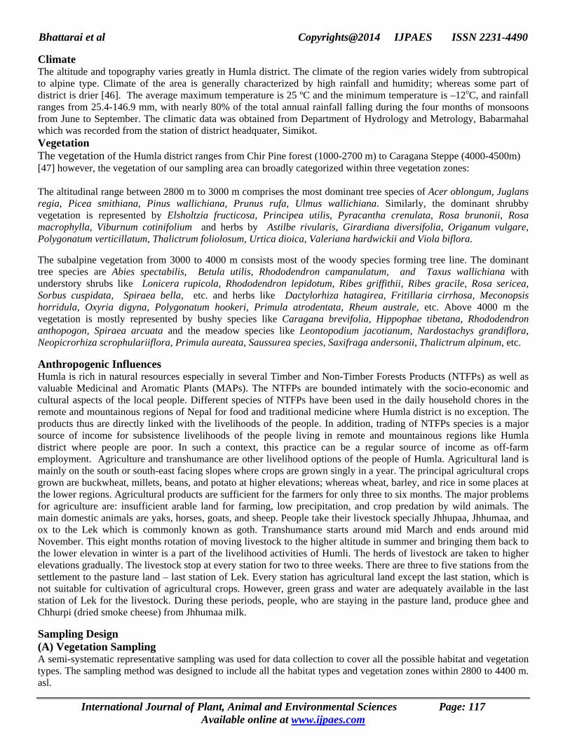
Climate The altitude and topography varies greatly in Humla district. The climate of the region varies widely from subtropical to alpine type. Climate of the area is generally characterized by high rainfall and humidity; whereas some part of district is drier [46]. The average maximum temperature is 25 ºC and the minimum temperature is –12oC, and rainfall ranges from 25.4-146.9 mm, with nearly 80% of the total annual rainfall falling during the four months of monsoons from June to September. The climatic data was obtained from Department of Hydrology and Metrology, Babarmahal which was recorded from the station of district headquater, Simikot. Vegetation The vegetation of the Humla district ranges from Chir Pine forest (1000-2700 m) to Caragana Steppe (4000-4500m) [47] however, the vegetation of our sampling area can broadly categorized within three vegetation zones: The altitudinal range between 2800 m to 3000 m comprises the most dominant tree species of Acer oblongum, Juglans regia, Picea smithiana, Pinus wallichiana, Prunus rufa, Ulmus wallichiana. Similarly, the dominant shrubby vegetation is represented by Elsholtzia fructicosa, Principea utilis, Pyracantha crenulata, Rosa brunonii, Rosa macrophylla, Viburnum cotinifolium and herbs by Astilbe rivularis, Girardiana diversifolia, Origanum vulgare, Polygonatum verticillatum, Thalictrum foliolosum, Urtica dioica, Valeriana hardwickii and Viola biflora.

The subalpine vegetation from 3000 to 4000 m consists most of the woody species forming tree line. The dominant tree species are Abies spectabilis, Betula utilis, Rhododendron campanulatum, and Taxus wallichiana with understory shrubs like Lonicera rupicola, Rhododendron lepidotum, Ribes griffithii, Ribes gracile, Rosa sericea, Sorbus cuspidata, Spiraea bella, etc. and herbs like Dactylorhiza hatagirea, Fritillaria cirrhosa, Meconopsis horridula, Oxyria digyna, Polygonatum hookeri, Primula atrodentata, Rheum australe, etc. Above 4000 m the vegetation is mostly represented by bushy species like Caragana brevifolia, Hippophae tibetana, Rhododendron anthopogon, Spiraea arcuata and the meadow species like Leontopodium jacotianum, Nardostachys grandiflora, Neopicrorhiza scrophulariiflora, Primula aureata, Saussurea species, Saxifraga andersonii, Thalictrum alpinum, etc.

Anthropogenic Influences Humla is rich in natural resources especially in several Timber and Non-Timber Forests Products (NTFPs) as well as valuable Medicinal and Aromatic Plants (MAPs). The NTFPs are bounded intimately with the socio-economic and cultural aspects of the local people. Different species of NTFPs have been used in the daily household chores in the remote and mountainous regions of Nepal for food and traditional medicine where Humla district is no exception. The products thus are directly linked with the livelihoods of the people. In addition, trading of NTFPs species is a major source of income for subsistence livelihoods of the people living in remote and mountainous regions like Humla district where people are poor. In such a context, this practice can be a regular source of income as off-farm employment. Agriculture and transhumance are other livelihood options of the people of Humla. Agricultural land is mainly on the south or south-east facing slopes where crops are grown singly in a year. The principal agricultural crops grown are buckwheat, millets, beans, and potato at higher elevations; whereas wheat, barley, and rice in some places at the lower regions. Agricultural products are sufficient for the farmers for only three to six months. The major problems for agriculture are: insufficient arable land for farming, low precipitation, and crop predation by wild animals. The main domestic animals are yaks, horses, goats, and sheep. People take their livestock specially Jhhupaa, Jhhumaa, and ox to the Lek which is commonly known as goth. Transhumance starts around mid March and ends around mid November. This eight months rotation of moving livestock to the higher altitude in summer and bringing them back to the lower elevation in winter is a part of the livelihood activities of Humli. The herds of livestock are taken to higher elevations gradually. The livestock stop at every station for two to three weeks. There are three to five stations from the settlement to the pasture land – last station of Lek. Every station has agricultural land except the last station, which is not suitable for cultivation of agricultural crops. However, green grass and water are adequately available in the last station of Lek for the livestock. During these periods, people, who are staying in the pasture land, produce ghee and Chhurpi (dried smoke cheese) from Jhhumaa milk.

Sampling Design (A) Vegetation Sampling A semi-systematic representative sampling was used for data collection to cover all the possible habitat and vegetation types. The sampling method was designed to include all the habitat types and vegetation zones within 2800 to 4400 m. asl.



Five plots in each elevation band of 100 m (a total of 80 plots) were laid randomly. Each plot was divided into four sub-plots of size 5 × 5 m and species presence were recorded for each subplot separately. The first plot was laid by observing the tallest tree in the altitudinal range in the forest while in open shrub and grass land the plot was laid randomly by altitude observation. The distance between two plots was not less than 20 m (walking distance) to avoid the clustering of the plots. To avoid biasness the direction of next plot from the earlier one was determined by lottery.

(B) Sampling for Environmental Variables Longitude, latitude, and elevation of each sample plot were recorded by global positioning system (GPS, eTrex Garmin) and elevation was cross-checked with a standardized altimeter. Slope and aspect of each plot were recorded by a clinometer compass. Soil moisture and pH of each sub-plot were recorded by using a gauge (Soil pH and moisture Tester; Model DM 15) with a default scale of 1 to 8 for both parameters.

Dung deposition and location of the plot from goat-sheds were combined to evaluate the grazing gradient. Grazing was graded on a zero to four scale starting from zero for no sign of grazing and four for the plot where dung were present in all subplots. Plots very near to goat-sheds were assigned level four and farthest as level one and zero for no goat-shed within the territory. The average value of both was considered in the analysis. The rock cover was estimated by visual observation. The average of three people’s estimation was used for analysis. The numerical value of zero to four was given, where one was given if the exposed surface area consists about 25% of rock of the total 10 x 10 m plot whereas four was given if whole exposed surface area was covered by rocks. Specimen Collection and Identification The study was conducted in the month of May-June. Prior to detail sampling of plots, the sampling site was selected by KSLCI team. Most of the plant species were identified in the field at the time of data collection using the floristic literatures [48, 49]. Experts from the Central Department of Botany were helpful in the field for plant identification. Species that could not be identified in the field were collected, tagged, made dry and brought to Central Department of Botany for further identification. Digital photographs of live plant species were taken in the field and the photo number and tag number were noted. The unidentified specimens were identified by comparing the specimens with relevant specimens deposited at Tribhuvan University Central Herbarium (TUCH) and National Herbarium and Plant Laboratories (KATH). Experts from the Central Department of Botany and KATH were consulted for identifying species along with the photographs. Tag number and photo number were used for correct naming of species. [50] was followed for the nomenclature. Some of the species identified to the genus level were also incorporated in the analysis. Voucher specimens are housed at TUCH. Numerical Analysis Regression The total number of species encountered within a sample plot with an area of 100m2 is regarded as species richness in our study. Number of species were treated as the response variables and regressed against altitude. Flowering plants were further categorised into different life-forms and were also used to evaluate their richness patterns [44]. A Generalised Linear Model [51, 52] was used to elucidate the pattern of species richness along the altitudinal gradient. A log linear model with a Poisson error distribution was used for the analysis due to the count nature of the response variables. A quasi- Poison error distribution with F- test was used to handle the over dispersion of the deviance [53]. The significance of each model was tested against the null model as well as with each other up to the third-order polynomials. Forward selection of model was done. R version 2.10.1 was used for regression analyses and graphical representation. RESULTS

A total of 199 vascular plant species were recorded during the sampling, of which 188 are the angiosperms (belonging to 55 families and 128 genera), 7 are the gymnosperms (4 families and 7 genera), and 4 are the pteridophytes (4 families and 4 genera). Among the total vascular plants, 145 species were herbs, 21 species were trees, and 33 species were shrubs. The angiosperm flora is dominated by dicotyledons (165 species) over the monocotyledons (23 species).

Overall Species Richness Pattern for Vascular Plants

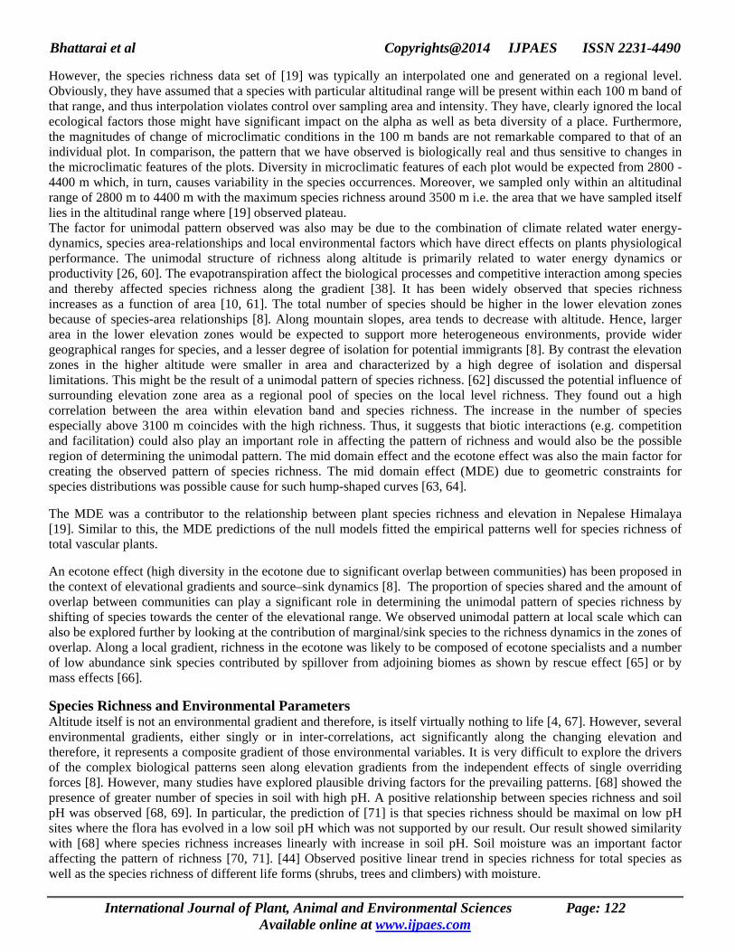
Regression analysis (GLM) revealed a unimodal relationship between overall species richness and altitude with a peak around 3500 m (Figure 2 a, Table 1.).



Here, the number of all types of species declined substantially towards the two extremes of the elevation gradient while more species were found to be accumulated at the mid-altitude (around 3500 m) forming a hump shaped pattern. The highest species richness of vascular plants was encountered at an altitude of 3455 m represented by 77 species whereas the lowest species richness was encountered at an altitude of 4362 m represented by only 17 plant species.

Species Richness Pattern of Different Functional Groups

The same analysis for the different plant functional groups revealed the almost consistent patterns of species richness to those for the overall plant species richness. The pattern was common for herbs, shrubs and trees (Figure 2b, 2c and 2d respectively, Table 1). All these three groups, the herbs, shrubs and trees species revealed a unimodal pattern of richness with a peak at an altitude of about 3500-3600 m, 3500 m and 3400 m, respectively. The shrubs and trees species showed the richness plateau at an altitude between 3300 m- 3800 m and 3200 m – 3700 m respectively.

Table 1. Summary of generalized linear model used to describe the relationship between species richness and altitude. Regression statistics for species richness: GLM model are significant over 1st & 2nd order (Altitude is

Predictor).

Response variables Model Polynomial

order

Res degree of freedom

Residual deviance DF Deviance F value Pr (>F)

Total vascular plants

Null 0 79 354.34 GLM 1 78 331.48 1 22.854 5.4158 0.05 GLM 2 77 71.34 2 2 283 150.51 0.001

Herbs Null 0 79 263.46 GLM 1 78 253.24 1 10.229 3.1544 0.1 GLM 2 77 54.615 2 208.85 143.84 0.001

Shrubs Null 0 79 96.321 GLM 1 78 89.471 1 6.8499 5.7039 0.05 GLM 2 77 53.900 2 42.42 30.332 0.001

Trees Null 0 79 91.584 GLM 1 78 74.987 1 16.561 20.686 0.001 GLM 2 77 50.089 2 41.459 35.721 0.001



Figure 2. Species richness of: a) total vascular plants, b) herbs, c) shrubs and d) trees with altitude. The line was fitted by generalized linear model.

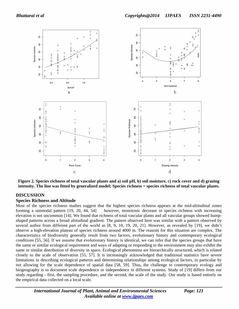
Species Richness Pattern and Environmental Parameters Species richness of vascular plants was also regressed separately with each of the recorded environmental parameters (soil pH, soil moisture, rock cover, and grazing intensity). A linear increase in the number of species was observed with the- increasing gradient of pH (i.e. acidic to alkaline soil) (Figure 3a, Table 2) as well as increasing grazing intensity (low to high grazing) (Figure 3d, Table 2).

Table 2. Summary of generalized linear model used to describe the relationship between species richness and environmental parameters. Regression statistics for species richness against environmental parameters: GLM

model are significant over 2nd order; pH = soil pH, Moisture = soil moisture.

Response variables Model Polynomial

order

Res degree of freedom

Residual deviance DF Deviance F value Pr (>F)

pH Null 0 79 354.34 GLM 1 78 184.37 1 169.97 73.192 0.001 GLM 2 77 183.93 2 170.41 36.282 ns*

Moisture Null 0 79 354.34 GLM 1 78 322.97 1 31.37 7.7088 0.001 GLM 2 77 255.33 2 99.006 15.185 0.001

Rock cover

Null 0 79 354.34 GLM 1 78 227.88 1 76.46 21.485 0.001 GLM 2 77 266.01 2 80.839 11.323 ns*

Grazing intensity

Null 0 79 354.34 GLM 1 78 336.37 1 17.696 4.1522 0.05 GLM 2 77 329.35 2 24.986 2.9334 ns*

The maximum species richness was encountered in the sample plots with the soil pH 7.5 and with high grazing intensity (i.e. at grazing scale of 4). Additionally, the vascular plant species richness decreases linearly with increasing rock cover (Figure 3c, Table 2). However, a unique ‘hump back-shaped’ pattern of species richness was observed with the soil moisture gradient (Figure 3b, Table 2). Here, lesser number of species was observed at the mid-moisture gradient, whereas interestingly, species richness was increased towards the extremes of the gradient forming a hump back-shape curve



Figure 2. Species richness of total vascular plants and a) soil pH, b) soil moisture, c) rock cover and d) grazing intensity. The line was fitted by generalized model; Species richness = species richness of total vascular plants.

DISCUSSION Species Richness and Altitude Most of the species richness studies suggest that the highest species richness appears at the mid-altitudinal zones forming a unimodal pattern [19, 20, 44, 54] however, monotonic decrease in species richness with increasing elevation is not uncommon [14]. We found that richness of total vascular plants and all vascular groups showed hump-shaped patterns across a broad altitudinal gradient. The pattern observed here was similar with a pattern observed by several author from different part of the world as [8, 9, 10, 19, 20, 21]. However, as revealed by [19], we didn’t observe a high-elevation plateau of species richness around 4000 m. The reasons for this situation are complex. The characteristics of biodiversity generally result from two factors, evolutionary history and contemporary ecological conditions [55, 56]. If we assume that evolutionary history is identical, we can infer that the species groups that have the same or similar ecological requirement and ways of adapting or responding to the environment may also exhibit the same or similar distribution of diversity in space. Ecological phenomena are hierarchically structured, which is related closely to the scale of observation [55, 57]. It is increasingly acknowledged that traditional statistics have severe limitations in describing ecological patterns and determining relationships among ecological factors, in particular by not allowing for the scale dependence of spatial data [58, 59]. Thus, the challenge to contemporary ecology and biogeography is to document scale dependence or independence in different systems. Study of [19] differs from our study regarding - first, the sampling procedure, and the second, the scale of the study. Our study is based entirely on the empirical data collected on a local scale.



However, the species richness data set of [19] was typically an interpolated one and generated on a regional level. Obviously, they have assumed that a species with particular altitudinal range will be present within each 100 m band of that range, and thus interpolation violates control over sampling area and intensity. They have, clearly ignored the local ecological factors those might have significant impact on the alpha as well as beta diversity of a place. Furthermore, the magnitudes of change of microclimatic conditions in the 100 m bands are not remarkable compared to that of an individual plot. In comparison, the pattern that we have observed is biologically real and thus sensitive to changes in the microclimatic features of the plots. Diversity in microclimatic features of each plot would be expected from 2800 - 4400 m which, in turn, causes variability in the species occurrences. Moreover, we sampled only within an altitudinal range of 2800 m to 4400 m with the maximum species richness around 3500 m i.e. the area that we have sampled itself lies in the altitudinal range where [19] observed plateau. The factor for unimodal pattern observed was also may be due to the combination of climate related water energy-dynamics, species area-relationships and local environmental factors which have direct effects on plants physiological performance. The unimodal structure of richness along altitude is primarily related to water energy dynamics or productivity [26, 60]. The evapotranspiration affect the biological processes and competitive interaction among species and thereby affected species richness along the gradient [38]. It has been widely observed that species richness increases as a function of area [10, 61]. The total number of species should be higher in the lower elevation zones because of species-area relationships [8]. Along mountain slopes, area tends to decrease with altitude. Hence, larger area in the lower elevation zones would be expected to support more heterogeneous environments, provide wider geographical ranges for species, and a lesser degree of isolation for potential immigrants [8]. By contrast the elevation zones in the higher altitude were smaller in area and characterized by a high degree of isolation and dispersal limitations. This might be the result of a unimodal pattern of species richness. [62] discussed the potential influence of surrounding elevation zone area as a regional pool of species on the local level richness. They found out a high correlation between the area within elevation band and species richness. The increase in the number of species especially above 3100 m coincides with the high richness. Thus, it suggests that biotic interactions (e.g. competition and facilitation) could also play an important role in affecting the pattern of richness and would also be the possible region of determining the unimodal pattern. The mid domain effect and the ecotone effect was also the main factor for creating the observed pattern of species richness. The mid domain effect (MDE) due to geometric constraints for species distributions was possible cause for such hump-shaped curves [63, 64].

The MDE was a contributor to the relationship between plant species richness and elevation in Nepalese Himalaya [19]. Similar to this, the MDE predictions of the null models fitted the empirical patterns well for species richness of total vascular plants.

An ecotone effect (high diversity in the ecotone due to significant overlap between communities) has been proposed in the context of elevational gradients and source–sink dynamics [8]. The proportion of species shared and the amount of overlap between communities can play a significant role in determining the unimodal pattern of species richness by shifting of species towards the center of the elevational range. We observed unimodal pattern at local scale which can also be explored further by looking at the contribution of marginal/sink species to the richness dynamics in the zones of overlap. Along a local gradient, richness in the ecotone was likely to be composed of ecotone specialists and a number of low abundance sink species contributed by spillover from adjoining biomes as shown by rescue effect [65] or by mass effects [66].

Species Richness and Environmental Parameters Altitude itself is not an environmental gradient and therefore, is itself virtually nothing to life [4, 67]. However, several environmental gradients, either singly or in inter-correlations, act significantly along the changing elevation and therefore, it represents a composite gradient of those environmental variables. It is very difficult to explore the drivers of the complex biological patterns seen along elevation gradients from the independent effects of single overriding forces [8]. However, many studies have explored plausible driving factors for the prevailing patterns. [68] showed the presence of greater number of species in soil with high pH. A positive relationship between species richness and soil pH was observed [68, 69]. In particular, the prediction of [71] is that species richness should be maximal on low pH sites where the flora has evolved in a low soil pH which was not supported by our result. Our result showed similarity with [68] where species richness increases linearly with increase in soil pH. Soil moisture was an important factor affecting the pattern of richness [70, 71]. [44] Observed positive linear trend in species richness for total species as well as the species richness of different life forms (shrubs, trees and climbers) with moisture.



By contrast, we did not find the pattern as shown by them and got the hump back-shaped when species richness was regressed against moisture. Soil under the dense Abies-Betula forest (that lies along the tree line ecotone) of subalpine vegetation zone of Nepal Himalaya is often characterized by the high organic carbon, high moisture, and low pH [72]. Irrespective of the high soil moisture and humidity in such habitat, the dark canopy of the forest that checks the penetration of light to the ground layer, in combination with the relatively lower (acidic) soil pH, limits the undergrowth of many herbaceous species. The general consensus of species richness should peak at moderate grazing [8, 21] but our finding did not match with this and observed the gradual increase in richness pattern with grazing. The anomalous pattern with previous finding may be due to the fact that the cattle spend more time in grazing area and thus help to make the soil more nutritive. Despite that the cattle also contributed significantly in seed dispersal [45] of plant species forming more species at the region. The rock cover was also used to show the species richness pattern. We observed the linear decrease of species number with increase in rock cover. This probably was because in such plot the land was barren, less nutritive, and with low soil moisture. Besides that the area (soil cover) also obviously decreased with an increase in the rock cover. Therefore, the species, except for some of the mosses and lichens, did not have enough suitable space to spread and colonize.

CONCLUSIONS The species richness of total vascular plants and all life forms have a unimodal relationship with altitude at local scale which follows the same pattern as seen at regional scale. Species richness is affected by multiple factors acting individually or in combinations. Several factors, such as climate related water energy-dynamics, species area relationships, and local environmental factors may work in concert to produce such observed patterns. In addition, altitude represents composite gradient of several environmental variables which at times are inter-correlated. A number of other environmental variables play a dominant role to explain the pattern of richness at the local scale. At the local scale, topographic and habitat heterogeneity as well as soil properties capture the patterns of species richness along elevation gradients. ACKNOWLEDGEMENT We would extend our sincere gratitude to Kailash Sacred Landscape Conservation Initiative Nepal Project funded by International Centre for Integrated Mountain Development (ICIMOD) for supporting this study. We are grateful to Mr. Raj K Gautam, Mr. Mandhata Acharya, and Mr. Mahesh Limbu for their encouragement, interactions, suggestions, continuous help and good company during field work. We wish to thank Mr. Jimin Lama, local assistant, for his help in the field work. Mr. Janardan Mainali is acknowledged for his help in preparation of GIS map of the study area.

REFERENCES

[1] Dobremez JF 1976. Le Ne´pal, e´cologie et bioge´ographie. Centre National de la Recherche Scientifique, Paris. [2] Simpson GG 1964. Species density of North America mammals. Systematic Zoology 13: 57-73. [3] Cook RE 1969. Variation in species density of North American birds. Systematic Zoology 18: 63–84. [4] Körner C 2000. Why are there global gradients in species richness? Mountains might hold the answer. Trends in

Ecology & Evolution 15: 513–514. [5] Ohlemuller R, Wilson JB 2000. Vascular plant species richness along latitudinal and altitudinal gradients: a

contribution from New Zealand temperate rain forests. Ecology letters 3: 262-266. [6] Wallace AR 1878. Tropical nature and other essays. Macmillan, New York. [7] Pianka ER (1966) Latitudinal gradients in species diversity, a review of concepts. American Naturalist 100: 33–46. [8] Lomolino MV 2001. Elevation gradients of species-richness, historical and prospective views. Global Ecology and

Biogeography 10: 3-13. [9] Rahbek C 1995. The elevational gradient of species richness, a uniform pattern? Ecography 18: 200-205. [10] Rahbek C 1997. The relationship among area, elevation, and regional species richness in Neotropical birds.

American Naturalist 149: 875–902. [11] Yoda K 1967. A preliminary survey of the forest vegetation of eastern Nepal. Journal of Art and Science. Chiba

University National Science series 5: 99-140. [12] Hamilton AC 1975. A quantitative analysis of altitudinal zonation in Uganda forests. Vegetatio 30: 99-106.



[13] Gentry AH 1988. Changes in plant community diversity and floristic composition on climate and geographical

gradients. Annals of the Missouri Botanical Garden 75: 1-34. [14] Stevens GC 1992. The elevational gradient in altitudinal range, an extension of Rapoport’s latitudinal rule to

altitude. American Naturalist 140: 893–911. [15] Fosaa AM 2004. Biodiversity patterns of vascular plant species in mountain vegetation in the Faroe

Islands.Diversity & Distribution 10: 217–223. [16] Whittaker RH, Niering WA 1975. Vegetation of the Santa Catalina Mountains, Arizona. V. Biomass production

and diversity along the elevational gradient. Ecology 56: 771-790. [17] Lieberman DM, Lieberman RP, Hartshorn GS 1996. Tropical forest structure and composition on a large – scale

altitude gradient in Costa Rica. Journal of Ecology 84:137-152. [18] Odland A, Birks HJB 1999. The altitudinal gradient of vascular plant species richness in Aurland, western

Norway. Ecography 22: 548-566. [19] Grytnes JA, Vetaas OR 2002. Species richness and altitude, a comparison between simulation models and

interpolated plant species richness along the Himalayan altitudinal gradient, Nepal. American Naturalist 159: 294-304.

[20] Carpenter C 2005. The environmental control of plant species density on a Himalayan elevation gradient. Journal of Biogeography 32: 999–1018.

[21] Nogues-Bravo D, Araujo MD, Romdal T, Rahbek C 2009. Scale effects and human impact on the elevational species richness gradients. Nature 453: 216-210.

[22] Austrhein G 2002. Plant diversity patterns in semi-natural grasslands along an elevational gradient in Southern Norway. Plant Ecology 161: 193-205.

[23] Vetaas OR, Grytnes JA 2002. Distribution of vascular plant species richness and endemic richness along the Himalayan elevation gradient in Nepal. Global Ecology and Biogeography 11: 291-301.

[24] Bhattarai KR, Vetaas OR, Grytnes JA 2004a. Fern species richness along a Central Himalayan elevational gradient, Nepal. Journal of Biogeography 31: 389–400.

[25] Kluge J, Kessler M, Dunn RR 2006. What drives elevational patterns of diversity? A test of geometric constraints,climate and species pool effects for pteridophytes on an elevational gradient in Costa Rica. Global Ecology and Biogeography 15: 358-371.

[26] Rahbek C 2005. The role of spatial scale and the perception of large-scale species richness patterns. Ecology Letters 8: 224-239.

[27] Vazquez GJA, Givnish TJ 1998. Altitudinal gradients in tropical forest composition, structure, and diversity in the Sierra de Manantlan. Journal of Ecology 86: 999-1020.

[28] Grytnes JA 2003. Species-richness patterns of vascular plants along seven altitudinal transects in Norway. Ecography 26: 291-300.

[29] Nagy L, Grabherr G, Korner C, Thompson DBA 2003. Alpine biodiversity in space and time: a synthesis. In:

Nagy L, Grabherr G, Korner C, Thompson DBA (Eds.) Alpine biodiversity in Europe. Sprigner-Verlag: Berlin. pp 453- 464.

[30] van Steenis CGGJ 1984. Floristic altitudinal zones in Malesia. Botanical Journal of the Linnean Society 89: 289-292.

[31] Baruch Z 1984. Ordination and classification of vegetation along an altitudinal gradient in the Venezuelan paramos. Vegetatio 55: 115- 126.

[32] Kirkpatrick JB, Brown MJ 1987. The nature of the transition from sedgeland to alpine vegetation in southwest Tasmania, I. Altitudinal vegetation change on four mountains. Journal of Biogeography 14: 539-549.

[33] Druitt DG, Enright NJ, Ogden J 1990. Altitudinal zonation in the mountain forests of Mt Hauhungatahi, North Island, New Zealand. Journal of Biogeography 17: 205-220.

[34] Kitayama K 1992. An altitudinal transect study of the vegetation on Mount Kinabalu. Borneo. Vegetatio 102:149-171.

[35] Boyce RL 1998. Fuzzy set ordination along an elevation gradient on a mountain in Vermont, USA. Journal of Vegetation Science 9: 191-200.

[36] Bobe R 2006. The evolution of arid ecosystems in eastern Africa. Journal of Arid Environments 66: 564-584. [37] Brown JH, Lomolino MV 1998. Biogeography. 2nd ed. Sinauer Associates, Incl. publishers. Sunderlands MA.



[38] O'Brien EM, Field R, Whittaker RJ 2000. Climatic gradients in woody plant (tree and shrub) diversity: water-

energy dynamics, residual variation, and topography. Oikos 89: 588-600. [39] Parker KC, Bendix J 1996. Landscape scale geomorphic influences on vegetation patterns on four environments.

Physical Geography 17: 113-141. [40] Grau O, Grytnes JA, Birks HJB 2007. A comparison of elevational species richness patterns of bryophytes with

other plant groups in Nepal, Central Himalaya. Journal of Biogeography 34: 1907-1915. [41] Baniya CB, Solhoy T, Gauslaa Y, Palmer MW 2010. The elevation gradient of lichen species richness in Nepal.

The Lichenologist 42: 83-96. [42] Acharya KP, Vetaas OR, Birks HJB 2011. Orchid species richness along Himalayan elevational gradients. Journal

of Biogeography 38: 1821-1833. [43] Rokaya MB, Münzbergova Z, Shrestha MR, Timsina B 2012. Distribution Patterns of Medicinal Plants along an

Elevational Gradient in Central Himalaya, Nepal. Journal of Mountain Science 9: 201-213. [44] Bhattarai KR, Vetaas OR 2003. Variation in plant species richness of different lifeforms along a subtropical

elevation gradient in the Himalayas, east Nepal. Global Ecology and Biogeography 12: 327–340. [45] Panthi M, Chaudhary RP, Vetaas OR 2007. Plant species richness and composition in a trans-Himalayan inner

valley of Manang district, central Nepal. Himalayan Journal of Sciences 4: 57-64. [46] Zomer R, Oli KP 2011. Kailash Sacred Landscape Conservation Initiative (KSLCI), Feasibility Assessment

Report, Kathmandu: ICIMOD. [47] Stainton JDA 1972. Forest of Nepal. John Murray & Co., London. [48] Polunin O, Stainton A 1984. Flowers of the Himalaya. Oxford University Press, New Delhi. [49] Stainton A 1988. Flowers of the Himalaya: A supplement. Oxford University Press, NewDehli. [50] Press JR, Shrestha KK, Sutton DA 2000. Annotated Checklist of the Flowering Plants of Nepal. The Natural

History Museum, London. [51] McCullagh P, Nelder JA 1989. Generalized linear models, 2nd edn. Chapman & Hall, London. [52] Dobson AJ 1990. An introduction to generalized linear models. Chapman & Hall, London. [53] Crawley MJ 2007. The R book. John Wiley and Sons, Ltd. [54] Oommen MA, Shanker K 2005. Elevational species richmess patterns emerge from multiple local mechanisms in

Himalayan woody plants. Ecology 86: (11), 3039-3047. [55] Whittaker RJ, Willis KJ, Field R 2001. Scale and species richness: towards a general, hierarchical theory of

species diversity. Journal of Biogeography 28: 453-470 [56] Ricklefs RE 2004. A comprehensive framework for global patterns in biodiversity. Ecology Letters 7: 1-15. [57] Meentemeyer V 1989. Geographical perspectives of space, time and scale. Landscape Ecology 3: 163-173. [58] Legendre P, Fortin M J 1989. Spatial pattern and ecological analysis. Vegetatio 80: 107–138. [59] Legendre P 1993. Spatial autocorrelation: Trouble or new paradigm? Ecology 74: 1659-1673. [60] O'Brien EM 1998. Water-energy dynamics, climate, and prediction of woody plant species richness: an interim

general model. Journal of Biogeography 25: 379-398. [61] He F, Legendre P, LaFrankie JV 1996. Spatial pattern of diversity in a tropical rain forest in Malaysia. Journal of

Biogeography 23: 57–74. [62] Romdal TS, Grytnes JA 2007. An indirect area effect on elevational species richness patterns. Ecography 30: 440-

448. [63] Colwell RK, Lees DC 2000. The mid-domain effect: geometric constraints on the geography of species richness.

Trends in Ecology and Evolution 15:70–76. [64] Colwell RK, Rahbek C, Gotelli NJ 2004. The middomain effect and species richness patterns: what have we

learned so far? American Naturalist 163:E1–E23. [65] Brown JH, Kodric-Brown A 1977. Turnover rates in insular biogeography: effect of immigration on extinction.

Ecology 58: 445-449. [66] Shmida A, Wilson MV 1985. Biological determinants of species diversity. Journal of Biogeography 12: 1-20. [67] Brown JH (2001) Mammals on mountainsides: elevational patterns of diversity. Global Ecology and

Biogeography 10:101-109. [68] Grime JP 1979. The humped-back model: a response to Oksanen. Journal of Ecology 85: 97-98. [69] Partel M 2002. Local plant diversity patterns and evolutionary history at the regional scale. Ecology 83: 2361-

2366.



[70] Peet RK 1978. Forest vegetation of the Colorado Front Range: pattern of species diversity. Vegetatio 37: 65-78. [71] de Lafontaine G, Houle G 2007. Species richness along a production gradient: a multivariate approach. American

Journal of Botany 94: 79-88. [72] Bhatta, KP 2009. Responses of Himalayan Subalpine Plant Species to Selected Environmental Variables in

Langtang National Park, Nepal. Dissertation submitted for partial fulfillment of Regional Master’s degree in Biodiversity and Environment Management under Tribhuvan University, Nepal and University of Bergen, Norway.


Vascular plant species richness along elevation gradient of the Karnali river valley, Nepal...

Documents

Transcript of Vascular plant species richness along elevation gradient of the Karnali river valley, Nepal...