Journal of Atmospheric and Solar-Terrestrial Physics 73 (2011) 388–399

Contents lists available at ScienceDirect

Journal of Atmospheric and Solar-Terrestrial Physics

1364-68

doi:10.1

n Corr

E-m

journal homepage: www.elsevier.com/locate/jastp

Variations in climate parameters at time intervals from hundreds to tens ofmillions of years in the past and its relation to solar activity

O.M. Raspopov a,n, V.A. Dergachev b, M.G. Ogurtsov b,c, T. Kolstrom d, H. Jungner e, P.B. Dmitriev b

a SPbF IZMIRAN, Muchnoi per. 2, St. Petersburg 191023, Russiab Ioffe Physico-Technical Institute, St. Petersburg, Russiac Central Astronomical Observatory at Pulkovo, Russiad Mekrijarvi Research Station, Yliopistontie 4, 82900 Ilomantsi, University of Joensuu, Finlande Radiocarbon Dating Laboratory, University of Helsinki, Finland

a r t i c l e i n f o

Article history:

Accepted 8 February 2010Unique palaeoclimatic data with annual time resolution as tree ring widths and annual varve deposits

are analyzed in order to reveal periodicities in climatic processes at tens to hundreds of million years

Available online 17 February 2010

Keywords:

Climate change

Solar activity

Tree rings

Varve

26/$ - see front matter & 2010 Elsevier Ltd. A

016/j.jastp.2010.02.012

esponding author: Tel.: 7 812 310 52 32; fax

ail address: oleg@or6074.spb.edu (O.M. Raspo

a b s t r a c t

ago. The climatic periodicities thus found are compared with the solar and climatic periodicities

observed at present.

& 2010 Elsevier Ltd. All rights reserved.

1. Introduction

At present a large body of palaeoclimatic data with annualtime resolution is available. As a rule, these data relate to the timeinterval of the last 10–15 thousand years. At the start of the 20thcentury the founder of dendrochronology A.E. Douglas discoveredthat there was a �11-year cyclicity in radial tree ring growth, andhe attributed this periodicity to the climatic effect of the 11-yearsolar cycle (Schwabe cycle) (Douglass, 1919; 1926; 1936). In lateryears he and other researchers analyzed dendro-chronologicaland other palaeoclimatic materials with layered structure (varves,aerosol densities in Greenland and Antarctic ice cap layers, etc.)and revealed indications of climatic variations corresponding tofundamental solar activity cycles: 22–23 years (Hale cycle),80–100 years (Gleissberg cycle), �200 years (Suess-deVries cycle)and �2300–2400 years (Hallstattzeit cycle) (Ol’, 1969; Shiyatov,1975; Sonett and Suess, 1984; Pudovkin and Lubchich, 1989;Dergachev and Chistyakov, 1993; Dergachev, 1996; Cook et al.,1997; Hoyt and Schatten, 1997, Cini Castagnoli et al., 1998; Whiteet al., 2000; Roig et al., 2001; Raspopov et al., 2001; Vasiliev andDergachev, 2002; Ogurtsov et al., 2002a, 2002b; Schimmelmannet al., 2003; Prasad et al., 2004; Raspopov et al., 2004; Vasilievet al., 2004; Wiles et al., 2004; Raspopov et al., 2005; Shao et al.,2005; Dergachev, 2006, 2007; Raspopov et al., 2008). Note thatperiodicities of around 30 and 17–18 years rather often can beobserved in climatic oscillations as well. The former is referred to

ll rights reserved.

: 7 812 310 50 35.

pov).

as the Bruckner cyclic. The 17–18-year periodicity can beattributed to the effect of cyclicity in lunar tides (lunar Saroscycle – 18.6 years) (Currie, 1993; Cook et al., 1997; Hoyt andSchatten, 1997). On the other hand, both periodicities are close tocombination of the frequencies of the solar Gleissberg and Halecycles (Raspopov et al., 2001).

Thus, climatic variations can be a useful indicator of theexistence of solar activity periodicities. This climatic indicator canbe used to estimate solar forcing during time intervals for whichother methods are inapplicable. Direct measurements of variationin solar activity (sunspot observations) cover only an interval ofabout the last 400 years, and cosmogenic 14C and 10Be isotopeswidely used for estimation of solar activity in the past have a half-life period of 5730 and about 1.5 million years. For this reason,they cannot be used to analyze variations in solar activity duringthe time intervals of millions of years in the past. Indirectinformation on cyclicities in solar activity during those timeintervals can be obtained from analysis of climatic variations.

The aim of this work was to analyze unique palaeoclimaticdata with time resolution from one to several years for the timeinterval from 250 to 12 million years in the past. These data areannual variations in varve thicknesses (about 250 million yearsold) from West Texas (USA) (Dean, 2000), ring width variations offossil cypress (�68–70 million years old) found in a coal mine inthe Province of Alberta (Canada) (http://www.technology.gov.ab.ca/en/student_projects_265.cfm), and variations in ring width ofthe fossil Douglas fir (about 12 million years old) exhibited at theNational Museum of Natural History in Washington (USA). In ourstudy all three types of palaeoclimatic data were subjected tospectral and wavelet analysis with the aim of revealing climatic

O.M. Raspopov et al. / Journal of Atmospheric and Solar-Terrestrial Physics 73 (2011) 388–399 389

periodicities in the past. The data obtained were compared withpresent-day solar and climatic periodicities.

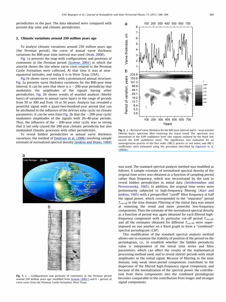
Fig. 2. a – Record of varve thickness for the 800-year interval and b – local wavelet

(Morlet basis) spectrum after removing the linear trend. The spectrum was

normalized to the 0.99 confidence level (the regions outlined by the black line

exceed the 0.99 confidence level). The significance was evaluated for an

autoregression process of the first order (AR(1) process or red noise) and AR(1)

2. Climatic variations around 250 million years ago

To analyze climatic variations around 250 million years ago(the Permian period), the curve of annual varve thicknessvariations for 800-year time interval was used (Dean, 2000).

Fig. 1a presents the map with configurations and positions ofcontinents in the Permian period (Scotese, 2001) in which theasterisk shows the site where varve cores related to the PermianCastle Formation were collected. At that time it was at near-equatorial latitudes, and today it is in West Texas (USA).

Fig.1b shows varve cores with a pronounced annual structure.Fig. 2a presents varve thickness variations for the 800-year timeinterval. It can be seen that there is a �200-year periodicity thatmodulates the amplitudes of the signals having otherperiodicities. Fig. 2b shows results of wavelet analysis (Morletbasis) of variations in annual varve layers in the range of periodsfrom 50 to 300 and from 10 to 50 years. Analysis has revealed apowerful signal with a quasi-two-hundred-year period that canbe attributed to the influence of the deVries solar cyclic on climateparameters. It can be seen from Fig. 2b that the �200-year cyclicmodulates amplitudes of the signals with 20–40-year periods.Thus, the influence of the �200-year solar cyclic was so strongthat it not only caused the 200-year climatic periodicity but alsomodulated climatic processes with other periodicities.

To reveal hidden periodicities in annual varve thicknessvariations, the method of Dmitriev et al. (2006) involving sampleestimate of normalized spectral density (Jenkins and Watts, 1969)

coefficients were estimated using the procedure described by Ogurtsov et al.

(2002b).

Fig. 1. a – Configurations and positions of continents in the Permian period

around 250 million years ago (modified from Scotese (2001)) and b – picture of

varve cores from the Permian Castle Formation, West Texas.

was used. The standard spectral analysis method was modified asfollows. A sample estimate of normalized spectral density of theoriginal time series was obtained as a function of sampling periodrather than frequency, which was necessitated by the task toreveal hidden periodicities in initial data (Serebrennikov andPervozvansky, 1965). In addition, the original time series werepreliminarily subjected to high-frequency filtering (Alari andJenkins, 1965) with a prespecified ‘‘cutoff’’ filter frequency at halfthe signal power, which corresponded to the ‘‘separator’’ periodTcut-off in the time domain. Filtering of the initial data was aimedat removing the trend and more powerful low-frequencycomponents. Then the estimate of the normalized spectral densityas a function of period was again obtained for each filtered high-frequency component with its particular cut-off period Tcut-off,and all the estimates obtained for different Tcut-off were super-imposed on one another on a fixed graph to form a ‘‘combined’’spectral periodogram (CSP).

This modification of the standard spectral analysis methodallows one to examine the stability of position of the period on theperiodogram, i.e., to establish whether the hidden periodicityvalue is independent of the initial time series and filterparameters, which can affect the results of the mathematicalprocessing method used, and to reveal shorter periods with smallamplitudes in the initial signal. Because of filtering in the timedomain, only weak short-period components contribute to thedispersion of the filtered high-frequency signal component, andbecause of the normalization of the spectral power the contribu-tion from these components into the combined periodogrambecomes comparable to the contribution from longer and strongersignal components.

O.M. Raspopov et al. / Journal of Atmospheric and Solar-Terrestrial Physics 73 (2011) 388–399390

Normalized spectral densities were plotted not only for theinitial data but also for their high-frequency components filteredwith different Tcut-off. Therefore, the reliability of maximum peakmagnitudes calculated for each normalized spectral density of thefiltered components on the assumption that its values are randomnoise with a normal distribution typically exceeding the sig-nificance level of 4–7s, which is also valid for analysis of annualvarve thickness variability.

The periodograms of annual varve thickness variations arepresented in Fig. 3. It can be seen that climatic oscillations exhibitpronounced periodicities similar to those observed in modernclimate. In addition to the �200-year periodicity, solar forcingcan be responsible for the climate oscillations with the 96-year(Gleissberg cycle), 26-year (Hale cycle), and 12-year (Schwabecycle) periods. The 18-year period can be attributed to the lunarcyclicity (Saros cycle). The oscillations of about 46 years observedalso in modern climate can be the second harmonic of theGleissberg cycle. The 36-year cyclicity has an analog in modernclimate: it is referred to as the Bruckner cycle. Raspopov et al.(2001) put forward the hypothesis that the Bruckner cyclicity isalso due to solar forcing: this periodicity is close to the combinedfrequency of the Gleissberg and Hale cyclicities. The data onmodulation of 20–40-year oscillations by the �200-year solarcyclicity speak in favor of this supposition.

Fig. 3. Periodogram of variations in varve thickness. a – Periodogram of variations in va

Tcut-off=7, 19, 31, 53, 79, 113, 173 years (the upper panel) and separate filtered high-fr

from the top). The horizontal lines show mean value and significance levels from 1s t

values are random noise with normal distribution. b – Sample estimate of normalized s

high-frequency components with Tcut-off=7, 19, 31, 53, 79, 113, 173 years (the upper p

7 years (the second-forth panels from the top). The horizontal lines show mean value an

assumption that these values are random noise with normal distribution.

3. Climatic variations around 68–70 million years ago

Analysis of climatic variations 68–70 million years ago is basedon the data on ring width variations of a fossil cypress that grewat the territory of the Province of Alberta in Canada (http://www.technology.gov.ab.ca/en/student_projects_265.cfm). The cypress(Fig. 4a) was found in a coal mine several kilometers from theBattle River power station in the eastern part of the Province ofAlberta (531N, 1141W). The cypress is dated back to the lateCretaceous period (68–70 million years ago) the climate of whichwas considerably warmer than the modern one. In particular,this is supported by the fact that cypresses of this type today grow21–231 more to the south – in Florida and Southern California(USA). Continent configurations and positions in the lateCretaceous period are shown in Fig. 4b. The Province of Albertawas at that time in a coastal region with a mild and wet climate inthe tree growth region. This is evidenced by the diameter of thetree shown in Fig. 4a.

Fig. 5a shows variations in cypress ring width. A record of 380rings was obtained by A. Cook (http://www.technology.gov.ab.ca/en/student_projects_265.cfm). Attention should be paid to anunusual feature in the radial tree growth. While the ring width ofconifers typically decreases as the tree becomes older, thesituation with the initial cypress growth time interval is

rve thickness for the initial data and their filtered high-frequency components with

equency components with Tcut-off=173, 79, and 19 years (the second-forth panels

o 5s for periodogram value of filtered components by the assumption that these

pectral density of variations in varve thickness for the initial data and their filtered

anel) and separate filtered high-frequency components with Tcut-off=113, 53, and

d significance levels from 1s to 5s for periodogram value of filtered components by

Fig. 4. a – Photo of the fossil cypress (68–70 million years old) [http://vishnu.glg.nau.edu/rcb/Late_Cret/ipg/] and b – configurations and positions of continents during the

late Cretaceous period (modified from Scotese (2001)). The asterisk shows the growth site of the cypress.

O.M. Raspopov et al. / Journal of Atmospheric and Solar-Terrestrial Physics 73 (2011) 388–399 391

opposite: the average ring width increases, which points to asharp improvement in growth conditions for the tree during thefirst approximately 80–100 years, and only after this the ringwidth decreases. The unusual behavior of long-term changes inthe cypress ring width can be understood if we consider, as anexample, long-term changes in radial growth of Scots pine innorthern Sweden in the last 1500 years (Grudd, 2008). Fig. 6shows a generalized picture of long-term tree-ring widthvariations from the first year of tree growth for more than 600trees. It can be seen from Fig. 6 that a tree ring increase occursonly during the first few years, and then the pine ring widthrather sharply decreases (during the first 50–70 years). As evidentfrom Fig.5a, the cypress ring widths exhibit an opposite behavior,i.e., they increase during 80–100 years. This may imply thatclimatic changes were favorable for tree growth during the initialtime interval of cypress growth.

The record shown in Fig. 5a was subjected to wavelet analysis(Morlet basis) (Fig.5b), analysis of hidden periodicities by themethod developed by Dmitriev et al. (2006) (Fig. 7), and also

filtering in the ranges of periods 8–10 years, 18–22 years, and28–32 years (Fig. 8). Wavelet analysis revealed that the tree ringwidth record contained periodicities with periods 8–10, 20–22,60, and 100–120 years. The 20–22-year and 100–120-year periodsare close to the solar Gleissberg and Hale cycles (Fig. 5b). Detailedanalysis of the solar activity for the last 300 years has shown thatthe solar Gleissberg cyclicity can be separated into 60–80 and100–130-year periodicities (Ogurtsov et al., 2002a). It is likely thatthe situation in the past was similar.

The 8–10-year periodicity can be related to the solar Schwabecycle. However, to state that it is a direct manifestation of theSchwabe periodicity it must be supposed that the solar activitylevel was high during a long time. In this case the 11-year cyclecould reduce to �8–10 years.

Fig. 7 presents the periodogram obtained by the method ofDmitriev et al. (2006). As can be seen from the graph, in additionto the periodicities mentioned above, the spectrum includes aperiodicity of about 30 years (Bruckner cycle) and also apronounced quasi-two hundred year periodicity. The latter

Fig. 5. a – Cypress ring width record (thin line) and 45-year moving average (thick line) and b – local wavelet (Morlet basis) spectrum of cypress ring width index. The

spectrum was normalized to the 0.99 confidence level (the regions outlined by the black line exceed the 0.99 confidence level). The significance was evaluated for an

autoregression process of the first order (AR(1) process or red noise) and AR(1) coefficients were estimated using the procedure described by Ogurtsov et al. (2002b).

Fig. 6. Tree-ring width regional growth curve for Northern Fennoscandia based on

620 Scots pines (Pinus sylvestris L.) covering the period AD 500–2004; 2–45-year

moving average cypress ring width record (modified from Grudd, 2008).

O.M. Raspopov et al. / Journal of Atmospheric and Solar-Terrestrial Physics 73 (2011) 388–399392

periodicity, which is likely to be associated with the solar Suess-deVries cyclicity, is also traced in Fig. 8b–d, where dendroseriesfiltered data in the ranges of periods revealed in the periodogram(8–10, 18–22, and 28–32 years) (Fig. 7) are given. In all filteringfrequency ranges, modulation of signal amplitudes with a �200-year period is detected. This suggests that climatic variations inthe ranges of periods of about 8–10 years, 18–22 and 28–32 yearsalso experienced the effect of solar activity. Note that a similarphenomenon was revealed in analysis of climatic variations in thetime interval around 250 million years ago (Fig. 2).

Fig. 7. Periodogram of the variations in cypress ring width for the initial data and

their filtered high-frequency components with Tcut-off=7, 17, 31, 53, 83, 127, 179

years (the upper panel) and separate filtered high-frequency components for the

initial time4 series and with Tcut-off=83 and 17 years (the second-forth panels from

the top). The horizontal lines show mean value and significance levels from 1s to

5s for periodogram value of filtered components by assumption that these values

are random noise with a normal distribution.

4. Climatic variations around 12 million years ago

The National Museum of Natural History in Washington (USA)exhibits a cut of a fossil tree – Douglas fir. The age of the sample isdated back to 12 million years (the Middle Miocene epoch –16–11 million years ago). The fossil tree was found in Washingtonstate, USA (471N, 1201W). Configurations and positions ofcontinents in the Middle Miocene epoch were similar to thepresent-day ones (Fig. 9a). However, there was a connection

Fig. 8. a – Cypress ring width record; b, c, d (respectively) – results of filtering of the cypress ring width record in the ranges of 8–10, 18–22, and 28–32-year periods.

Fig. 9. a – Configurations and positions of continents in the Middle Miocene (modified from Scotese (2001)) and b – the section of the fossil Douglas fir (12 million years of

age).

O.M. Raspopov et al. / Journal of Atmospheric and Solar-Terrestrial Physics 73 (2011) 388–399 393

between South and North America. North America and Eurasiawere not separated (in the Pacific region). Thus, the structureof oceanic currents was different from the present-day one,which affected internal atmospheric processes. According tomeasurements of the 18O/16O ratio in bottom sediments and

biological materials, the temperature in the Middle Mioceneepoch was 2–3 1C higher than in modern times (Crowly andNorth, 1991). At the latitudes of Washington state (north-west ofUSA), where the fossil tree was found, vegetation growth couldhave been more intense than in present days.

Fig. 10. a – Douglas fir ring width record and b – local wavelet (Morlet basis) spectrum of Douglas fir ring width. The spectrum was normalized to the 0.99 confidence level

(the regions outlined by the black line exceed the 0.99 confidence level). The significance was evaluated for an autoregression process of the first order (AR(1) process or

red noise) and AR(1) coefficients were estimated using the procedure described by Ogurtsov et al. (2002b).

Fig. 11. Periodogram of variations in Douglas fir ring width for the initial data and their filtered high-frequency components with Tcut-off=7, 13, 19, 29, 79, 37, 61 years (the

upper panel) and separate filtered high-frequency components with Tcut-off=29, 19, and 13 years (the second-forth panels from the top). The horizontal lines show mean

value and significance levels from 1s to 5s for periodogram value of filtered components by assumption that these values are random noise with a normal distribution.

O.M. Raspopov et al. / Journal of Atmospheric and Solar-Terrestrial Physics 73 (2011) 388–399394

O.M. Raspopov et al. / Journal of Atmospheric and Solar-Terrestrial Physics 73 (2011) 388–399 395

Fig. 9b shows a section of the fossil Douglas fir exhibited in theMuseum in Washington (photograph made by O.M. Raspopov).Annual tree rings are pronounced in the cut, and about 150 ringscould be measured from the tree centre to the edge. Variations inthe Douglas fir ring width are shown in Fig. 10a. Attention shouldalso be paid here, like in the case of fossil cypress, to an unusualfeature in the radial tree growth. At the beginning of the treegrowth the average ring width increases, which points to animprovement in growth conditions during approximately 50years, and only after that the ring width begins to decrease. Inapproximately 50 years the radial growth stabilizes. This againpoints to climate change and improvement in tree growthconditions. The smoothed curve of radial tree growth variationsshown in Fig. 10a covers the time interval of �100–120 yearscharacterizing a possible climatic periodicity. It may correspondto the Gleissberg cyclicity of solar activity.

The curve of variations in the Douglas fir ring width wassubjected to wavelet and spectral analysis. Result of waveletanalysis (Morlet basis) is presented in Fig. 10b, and results ofspectral analysis by the method of Dmitriev et al. (2006) areshown in Fig. 11. Both types of analyses have revealedperiodicities of about 31–34, 17, 9–12, and 4 years. Note thatthe spectral analysis based on the Fourier technique also revealedthese periodicities.

Thus, it can be stated that the time interval around 12 millionyears ago was characterized by the Bruckner cyclicity (�31–34years), lunar cyclicity (�17 years), and also periodicities corre-sponding to the solar Schwabe (�11 years) and possibly also theGleissberg (�100 years) cycles.

5. Discussion

Analysis of climatic periodicities for the time intervals tens andhundreds of million years ago show that these periodicitiescorrespond to modern solar periodicities in spite of differentclimatic conditions and configurations and positions of continentsof our planet around 12, 68–70, and 250 million years ago. Theclimate was 2–3 1C warmer than the modern one 12 million yearsago, 5–6 1C warmer in the late Cretaceous period (68–70 millionyears ago), and 2 1C warmer in the Permian period (250 millionyears ago) (Crowly and North, 1991). Since continental configura-tions and positions during the time intervals consideredwere markedly different from each other, atmospheric and oceaniccirculations were essentially different, and thus climatic condi-

Fig. 12. Wavelet analysis of solar activity variations (D

tions at the Earth’s surface were also different. The existence of thesame periodicities during all the time periods discussed can,therefore, be attributed to an external influence, i.e., solar forcing.

Special attention should be paid to the �200-year periodicityrevealed in the spectrum of cypress ring width variations(�68–70 million years ago) (Fig. 7) and also in several frequencyranges in filtered data of the cypress ring width record (Fig. 8).Periodicities with shorter periods were amplitude-modulated bythe �200-year period. A similar amplitude modulation of periodsof tens of years was also revealed in analysis of varve thicknessrecord from 250 million years ago. The spectrum of varvethickness variations contains basic solar periodicities, which arealso typical of the modern time, i.e., �200, �90, �60, and �26years. In addition, the Bruckner cyclicity of �36 years and 18-yearperiodicity was found.

Note that amplitude modulation of shorter solar activityperiodicities by longer ones occurs in the Holocene as well.Vasiliev et al. (2000) has shown that in the time interval of the last8000 years the �200-year solar activity variation (Suess-deVriescycle) (D14C) is modulated by the 2300–2400-year solar periodi-city (Hallstattzeit cycle).

Thus, modulation of periodicities with shorter periods bylonger-period periodicities is a characteristic feature of solaractivity. Therefore, it can be supposed that the �200-yearamplitude modulation of climatic periodicities 250 and 68–70million years ago was due to solar forcing.

68–70 million years ago the North American continent wasseparated by the ocean into western and eastern parts (Fig. 4b),which had to exert a considerable influence on atmospheric andoceanic circulations. Nevertheless, the periodicity of climaticprocesses corresponds to solar activity periodicities. Wavelet andspectral analyses revealed periodicities of �110 years, �65 years,and �9 years. In addition, filtration of the data revealed aperiodicity of around 200 years (Fig. 8). The patterns ofdevelopment of �100 and �65-year oscillations are very similarto the patterns of solar activity variations in the last 300 years.Results of wavelet analysis of variations in solar activity (D14C) forthe last 300 years are given in Fig. 12 [Ogurtsov et al., 2002a]. Itcan be seen from Fig. 12 that there are two areas of variations,around 50–65 years and 110 years, like 68–70 million years ago(Fig. 5b). This suggests that these climatic variations in theCretaceous period were also due to solar forcing. Note that inmodern time (around 1775) the Schwabe cycle decreased to9 years (Fig. 12). Therefore, the 9-year periodicity revealed fromthe cypress record can also be associated with solar activity.

14C) in the modern epoch (Ogurtsov et al., 2002a).

O.M. Raspopov et al. / Journal of Atmospheric and Solar-Terrestrial Physics 73 (2011) 388–399396

12 million years ago continental configurations and positionswere almost identical to the present-day ones. The spectra ofdecadal climatic oscillations around 12 million years ago (Douglasfir record) also bear resemblance to the spectra of present-dayclimatic oscillations. They exhibited 9–12-year oscillations thatcan be interpreted as the effect of the 11-year solar cycle, and alsothe Bruckner (31–34 years) and 17–18-year cyclicity. The lattercan be interpreted as the effect of lunar tidal variations. Theaveraged curve of radial Douglas fir growth variations demon-strates a climatic periodicity of �100–120 years (Fig. 10a).Therefore, it can be supposed that at that time climateexperienced a strong influence of a secular solar cycle (Gleissbergcycle).

As noted above, the periodicities revealed from Permian varve-and tree-ring width-records of a fossil cypress and a Douglas firare similar to the climatic periodicities observed at present. Anexample supporting this statement is the similarity the TRWrecord of living and subfossil (50,000 BP) Fitzroya cupresoides fromsouthern Chile (Fig. 13) (Roig et al. 2001). Note that 50,000 yearsago the continental configuration was identical to the modernsituation. As seen from Fig. 13, the spectra are very similar: thepeaks at 87–94, 47–51, 35, 23.6, and 17.8 years in living trees

Fig. 13. Spectral characteristics of subfossil (a), living (b) and South American conifer F

subfossil and modern chronologies (c) (modified from Roig et al.(2001)). The thick line c

years.

have analogs in the sub fossil chronology ( peaks at 87–94, 45.5,31.5, 24.1, and 17.8 years). In addition, the sub fossil chronologyhas a pronounced quasi two hundred year peak (153–245 years).Cross correlation of the record also revealed a peak at 11.8 years.Note that similar periodicities are observed themselves indifferent combinations in the chronologies with ages of millionsof years analyzed in this paper (Figs. 3, 7 and 11). In addition tothe peaks that can be attributed to solar forcing, the spectraexhibit a periodicity of 17–18 years. This periodicity is typicallyinterpreted as the effect of the 18.6-year lunar tidal cycle (Currie,1993; Cook et al., 1997; Hoyt and Schatten, 1997). The physicalorigin of this effect is unclear, but it can be supposed that tidalprocesses affect long-term changes in atmospheric circulation,which in its turn affects climatic processes. The 17–18-yearclimatic periodicity is observed in modern times not only in thedata for South America presented in Fig. 13. This periodicity ischaracteristic of the drought rhythm in the USA (Currie, 1993;Cook et al., 1997). It has also been revealed for the Kola Peninsula(Raspopov et al., 2001) and Finland (Ogurtsov et al., 2008). Thefact that the 17–18-year periodicity is observed in regions ofthe Earth far away from each other suggests that it has a globalorigin.

itzroya Cupressoides from southern Chile, and cross spectral relationships between

orresponds to the 95% confidence level. The numbers at the peaks show periods in

O.M. Raspopov et al. / Journal of Atmospheric and Solar-Terrestrial Physics 73 (2011) 388–399 397

Another hypothesis on the nature of the 17–18-year climaticperiodicity was put forward by Raspopov et al. (2001). Experi-mental data and result from simulation indicate that thetemperature response to solar activity variations has a regionalcharacter (Waple et al., 2002; Raspopov et al., 2007,2008). Thismeans that the atmosphere–ocean system responds nonlinearlyto the global solar signal. If several periodic signals affect such anonlinear system, the system response can occur not only atfrequencies of the affecting signals but also at combinations oftheir frequencies (Burroughs, 1992). The first combination of thesolar Gleissberg (80–90 years) and Hale (22–23 years) cycles leadsto periods of about 17 and 30 years. Thus, the 17–18-year cycleand also the Bruckner climatic cycle may be interpreted asgenerated by a combination of frequencies of solar cycles in the

Fig. 14. Map showing the regions where climatic variations with

Fig. 15. a – Solar activity variations (D14C) for the last 1000 years, b – summer temper

Sarbaev (1998), c and d – results of filtering of the curves of solar activity variations and

and e and f – results of wavelet analysis of the curves of solar activity variations and su

atmosphere–ocean system. It is important to emphasize that thebasic statement of this hypothesis, i.e., a nonlinear response of theatmosphere–ocean system to global external forcing, is applicableto any continental configuration.

Note that the �200-year climatic oscillations in the modernepoch (the last 1000–2000 years) have been revealed not only inSouth America, as mentioned above, but also in many terrestrialarchives in different regions of the Earth, i.e., in summer andannual temperature records, records of precipitation, records ofaerosol concentrations in Greenland and Antarctic ice, in glacieradvances and retreats, in lake and sea sediments, etc. (Sonett andSuess, 1984; Peterson et al., 1991; Anderson, 1992, 1993; Cooket al., 1996; Zolitschka, 1996; Dean, 1997; Cini Castagnoli et al.,1998; Qin et al., 1999; Hong et al., 2000; Hodell et al., 2001;

a period of about 200 years are observed in modern times.

ature variations in Tien Shan for the same time interval from Mukhamedshin and

summer temperature variations in Tien Shan in the range of periods 180–230 years

mmer temperature variations in Tien Shan in the range of periods 100–300 years.

O.M. Raspopov et al. / Journal of Atmospheric and Solar-Terrestrial Physics 73 (2011) 388–399398

Nyberg et al., 2001, Yang et al., 2002; Esper et al., 2003; Fleitmanet al., 2003; Haeberli and Holzhauser, 2003; Hu et al., 2003;Schimmelmann et al., 2003; Soon and Yaskell, 2003; Wiles et al.,2004; Wang et al., 2005; Shao et al., 2005; Raspopov et al., 2007,2008). The regions where �200-year climatic oscillations wereobserved are shown in Fig. 14. It is evident that these oscillationswere detected in Europe, North and South America, Asia,Tasmania, and Arctic and Antarctica, i.e., all over the world.Sonett and Suess (1984) were the first to reveal the �200-yearclimatic cyclicity in their analysis of variations in bristlecone pinering width. This cyclicity can be attributed to the effect of thequasi-two-hundred-year solar cycle observed in 14C production.A good correlation between the climatic and solar variationsconsidered can be demonstrated by taking variations in summertemperatures in Central Asia (Tien Shan Mountains) as anexample. Fig. 15a and b shows variations in 14C concentrationfrom Stuiver et al. (1998) and variations in summer temperaturesin Tadjikistan (39.51N, 70.71E) derived from analysis of variationsin tree-ring width of Juniperus turkestanica (Mukhamedshin andSarbaev, 1988) for the last millennium. The curves were subjectedto filtering in the range of periods 180–230 years and waveletanalysis in the range of periods 100–300 years (Raspopov et al.,2007, 2008). Results of analysis are given in Fig. 15c–f. Fig. 15clearly shows that the dynamics of solar and climatic periodicitiesin the range of periods considered is similar. The correlationcoefficient between the filtered curves in Fig. 15e,d was estimatedto be 0.94. Our analysis of 200-year climatic oscillations inmodern times and also data of other researchers referred to abovesuggest that these climatic oscillations can be attributed to solarforcing.

The results obtained in our study for climatic variationsmillions of years ago indicate, in our opinion, that the �200-year solar cycle exerted a strong influence on climate parametersat those time intervals as well.

6. Conclusions

We found that the most intense climatic oscillations in thepast (tens and hundreds of millions of years ago) had quasi-twohundred year and quasi-secular periodicities. These climaticoscillations are most likely due to the influence of the Suess-deVries and Gleissberg solar cycles on climatic processes, becausethe climatic response to these solar cycles are observedirrespective of considerable changes in configurations and posi-tions of continents and, hence, internal processes in the atmo-sphere–ocean system.

Climatic variations can be a peculiar indicator of solar activityperiodicities. Analysis of palaeoclimatic data has revealed thattheir spectra exhibit cyclicities similar to the present-day solarperiodicities. Thus, it can be supposed that analysis of climaticperiodicities in the time intervals from tens to hundred millionyears ago gives information on variations in solar activity thatcannot be obtained by other methods.

It should be emphasized that palaeoclimatic records exhibitedthe Bruckner (around 30 years) and the 17–18-year periodicitiesirrespective of the climatic conditions at the Earth’s surface. In ouropinion, this indicates that these periodicities were associatedwith the influence of external factors on the atmosphere–oceansystem rather than with processes in within this system. Apossible source of the 17–18-year oscillations is lunar forcing(Currie, 1993; Cook et al., 1997). Another explanation for thegeneration of these cycles, and also of the Bruckner cycle, is thatthey are the combinations of the Gleissberg (80–90 years) andHale (22–23 years) cycles (Raspopov et al., 2001).

Acknowledgements

The authors wish to thank L.A. Batkova for her help in dataprocessing. The work was supported by The Program of BasicResearch of Presidium of RAS no. 16 )Environment under theConditions of Changing Climate*.

M.G. Ogurtsov is thankful to the program of an exchangebetween the Russian and Finnish Academies (project no. 16),program ‘‘Solar Activity and Physical Processes in the Sun–EarthSystem’’ of Presidium of the Russian Academy of Sciences, andRFBR Grant nos. 06-02-16268, 06-04-48792, and 07-02-00379 forfinancial support.

References

Alari, A.S., Jenkins, G.M., 1965. An example of digital filtering. Journal of the RoyalStatistical Society, Series C (Applied Statistics) 14 (1), 70–74.

Anderson, R.Y., 1992. Possible connection between surface wind, solar activity andthe Earth’s magnetic field. Nature 358, 51–53.

Anderson, R.Y., 1993. The varve chronometer in Elk Lake record of climaticvariability and evidence for solar-geomagnetic-14C-climate connection. In: In:Bradbury, J.P., Dean, W.E. (Eds.), Elk Lake, Minnesota: Evidence for RapidClimate Change in the North-Central United States, 276. Geological Society ofAmerica, pp. 45–68 Special Paper.

Burroughs, W.L., 1992. Weather Cycles. Real or Imaginary. Cambridge UniversityPress 207p.

Cini Castagnoli, G., Bonito, G., Della Monica, P., Procopio, S., Taricco, C., 1998. Onthe solar origin of the 200y Suess wiggles. Evidence from thermoluminescencein sea sediments. II Nuovo Cimento 21 (2), 237–241.

Cook, E.R., Meko, D.M., Stockton, C.W., 1997. A new assessment of possible solarand lunar forcing of the bidecadal drought rhythm in the western UnitedStates. Journal of Climate 10, 1343–1356.

Cook, E.R., Buckley, B., D’Arrigo, R.D., 1996. Inter-decadal climate oscillations in theTasmanian sector of the Southern Hemisphere: evidence from tree rings overthe past three millennia. In: Jones, P.D., Dradly, R.S., Jouzel, J. (Eds.), ClimateVariations and Forcing Mechanisms of the Last 2000 Years, vol. 41. Springer,NATO ASI Series I: Global Environmental Change, Berlin, pp. 141–160.

Crowly, T.J., North, G.R., 1991. Paleoclimatology. Oxford University Press, NewYork 349p.

Currie, R.G., 1993. Lunar–solar 18.6- and solar 10–11-year signals in USA airtemperature record. International Journal of Climatology 13, 31–50.

Dean, W.E., 1997. Rates, timing, and cyclicity of Holocene eolian activity in north-central United States: evidence from varved lake sediments. Geology 25,331–334.

Dean, W.E., 2000. The Sun and climate. In: USGS Fact Sheet, FS-095-00, pp. 1–5.Dergachev, V.A., Chistyakov, V.F., 1993. 210- and 2400-year solar cycles and

climate change, Solar Cycle. Physico-Technical Institute, Saint-Petersburgpp. 112–130 (in Russian).

Dergachev, V.A., 1996. Cosmogenic radiocarbon concentration in the Earth’satmosphere and solar activity during the last milennia. Geomagnetism andAeronomy 36 (2), 49–60.

Dergachev, V.A., 2006. Solar forcing of climate. Bulletin of Russian Academy ofSciences: Physics 70 (10), 1544–1548.

Dergachev, V.A., Kartavykh, Yu.Yu., Ogurtsov, M.G., Raspopov, O.M., 2007.Dendroindication of solar forcing of climate in the last milennium. Bulletinof Russian Academy of Sciences: Geography No. 3, 107–114.

Dmitriev, P.B., Kudryavtsev, I.V., Lazukov, V.P., Matveev, G.A., Savchenko, M.I.,Skorodumov, D.V., Charikov, Yu.E., 2006. Solar flares registered by the ‘‘IRIS’’spectrometer onboard the Coronas-F satellite: peculiarities of the X-rayemission. Solar System Research 40 (2), 142–152.

Douglass, A.E., 1919. Climatic Cycles and Tree-Growth: A Study of the AnnualRings of Trees in Relation to Climate and Solar Activity. Carnegie Inst,Washington V. 1. 127 p. 1928. V.2. 166 p. 1936.V.3, 171 p.

Esper, J., Shiyatov, S.G., Mazepa, V.S., Wilson, R.J.S., Graybill, D.A., Funkhouser, G.,2003. Temperature-sensitive Tien Shan tree ring chronologies show multi-centennial growth trends. Climate Dynamics 21, 699–706.

Fleitman, D., Burns, S.J., Mudelsee, M., Neff, U., Kramers, J., Mangini, A., Matter, A.,2003. Holocene forcing of the Indian monsoon recorded in a stalagmite fromSouthern Oman. Science 300, 1737–1739.

Grudd, H., 2008. Tornetrask tree-ring width and densityAD 500–2004: a test ofclimate sensitivity and a new 1500-year reconstruction of north Fennoscan-dian summers. Climate Dynamics 31, 843–857.

Haeberli, W., Holzhauser, H., 2003. Alpine glacier mass changes during the pasttwo millennia. PAGES News 1, 13–15.

Hodell, D.A., Brenner, M., Curtis, J.H., Guilderson, T., 2001. Solar forcing of droughtfrequency in the Maya lowlands. Science 292, 1367–1370.

Hong, Y.T., Jiang, H.B., Liu, T.S., Zhou, L.P., Beer, J., Li, H.D., Leng, X.T., Hong, B., Qin,X.G., 2000. Response of climate to solar forcing recorded in a 6000-year d18Otime-series of Chinese peat cellulose. The Holocene 10 (1), 1–7.

Hoyt, D.V., Schatten, R.H., 1997. The Role of the Sun in Climate Change. OxfordUniversity Press, New York 279p.

O.M. Raspopov et al. / Journal of Atmospheric and Solar-Terrestrial Physics 73 (2011) 388–399 399

Hu, F.S., Kaufman, D., Yoneji, Su., Nelson, D., Shemesh, A., Huang, Y., Tian, J., Bond,G., Clegg, B., Broun, T., 2003. Cyclic variation and solar forcing of Holoceneclimate in the Alaskan Subarctic. Science 301, 1890–1893.

Jenkins, G.M., Watts, D.G., 1969. Spectral Analysis and its Application. Holden-Day,San Francisco, Cambridge, London, Amsterdam 525p.

Mukhamedshin, R.D., Sarhaev, S.K., 1988. Champion of Longevity. Kaynar, Alma-Ata (in Russian).

Nyberg, J., Kuijpers, A., Malmgren, B.A., Kundzendorf, H., 2001. Late Holocenechanges in precipitation and hydrography recorded in marine sediments fromthe northern Caribbean Sea. Quaternary Research 56, 87–102.

Ogurtsov, M.G., Kocharov, G.E., Lindholm, M., Merilainen, J., Eronen, M.,Nagovitsyn, Yu.A., 2002a. Evidence of solar variations in tree-ring-basedclimate reconstruction. Solar Physics 205, 403–417.

Ogurtsov, M.G., Nagovitsyn, Yu.A., Kocharov, G.E., Jungner, H., 2002b. Long-periodcycles of Sun’s activity recorded in direct solar data and proxies. Solar Physics211 (1), 371–394.

Ogurtsov, M.G., Raspopov, O.M., Helama, S., Oinonen, M., Lindholm, M., Jungner, H.,Merilainen, J., 2008. Climatic variability along a north–south transectof Finland over the last 500 years: signature of solar influence or internalclimate oscillations? Geografiska Annaler, Series A, Physical Geography 90 (2),141–150.

Ol’, A.I., 1969. 22-year cycle of solar activity in climate. In: Reports AANII 289.Leningrad. Hydrometeoizdat, pp. 116–120.

Peterson, L.C., Overpeck, J.T., Kipp, N.G., Imbrie, I., 1991. A high resolution LateQuarternary upwelling record from the anoxic Cariaco Basin, Venezuela.Paleooceanography 6 (1), 99–119.

Pudovkin, M.I., Lubchich, A.A., 1989. Manifistation of solar and magnetic activitycycles in the air temperature variations in Leningrad. Geomagnetism andAeronomy 29 (3), 359–363.

Prasad, S., Vos, H., Negendank, J.F.W., Waldmann, N., Goldstein, S., Stein, M., 2004.Evidence from Lake Lisan of solar influence on decadal-to centennial-scaleclimate variability variability during marine oxygen isotope state 2. Geology32 (7), 581–584.

Qin, X., Tan, M., Liu, T., Wang, X., Li, T., Lu, J., 1999. Spectral analysis of a 1000-yearstalagmite lamina-thickness record from Shihua Cavern, Beijing, China, and itsclimatic significance. The Holocene 9 (6), 689–694.

Raspopov, O.M., Shumilov, O.I., Kasatkina, E.A., Turunen, J., Lindholm, M., Kolstrom,T., 2001. Nonlinear character of solar forcing of climatic processes. Geomag-netism and Aeronomy 41 (4), 407–412.

Raspopov, O.M., Dergachev, V.A., Kolstrom, T., 2004. Periodicity of climateconditions and solar variability derived from dendrochronological and otherpalaeo climatic data in high latitudes. Palaeogeography, Palaeoclimatology,Palaeoecology 208, 127–139.

Raspopov, O.M., Dergachev, V.A., Kolstrom, T., 2005. Variations in cosmic rays andclimate change in high latitudes in the last 500 years. Bulletin of RussianAcademy of Sciences: Physics 69 (6), 893–895.

Raspopov, O.M., Dergachev, V.A., Kuzmin, A.V., Kozyreva, O.V., Ogurtsov, M.G.,Kolstrom, T., Lopatin, E., 2007. Regional troposopheric responses to long-termsolar activity variations. Advances in Space Research 40, 1167–1172.

Raspopov, O.M., Dergachev, V.A., Esper, J., Kozyreva, O.V., Frank, D., Ogurtsov, M.G.,Kolstrom, T., Shao, X., 2008. The influence of the de Vries (�200-year)solar cycle on climate variability: result from the Central Asian Mountains andtheir global link. Palaeogeography, Palaeoclimatology, Palaeoecology 259,6–10.

Roig, F.A., Le-Quesne, C., Boninsegna, J.A., Briffa, K.R., Lara, A., Grudd, H., Jones, Ph.,Villagran, G., 2001. Climate variability 50,000 years ago in mid-latitude Chileas reconstructed from tree rings. Nature 410, 567–570.

Schimmelmann, A., Lange, C.B., Meggers, B.J., 2003. Palaeoclimatic and archae-ological evidence for a �200-yr recurrence of floods and droughts linkingCalifornia, Masamerica and South America over past 2000 years. The Holocene13 (5), 763–788.

Scotese, C.R., 2001. Atlas of Earth History. PALEOMAP Project, Arlington, Texas 52 p.Serebrennikov, M.G., Pervozvansky, A.A., 1965. Revealing Hidden Periodicities.

Nauka, Moscow 244p. (in Russian).Shao, X., Liang, E., Huang, L., Wang, L., 2005. A 1437-year precipitation history from

Qilian juniper in the northeastern Qinghai-Tibetan Plateau. PAGES News 13(2), 14–15.

Shiyatov, S.G., 1975. Secular cycle in variations of larch growth index (Larixsibirica) at the polar timberline, Biological Fundamentals of Dendrochronol-ogy. Vilnus-Leningrad, pp. 47–53, (in Russian).

Sonett, C.P., Suess, H.E., 1984. Correlation of bristlecone pine ring width withatmospheric carbon-14 variations: climate–sun relation. Nature 308,141–143.

Soon, W.W., Yaskell, S.H., 2003. The Maunder Minimum and the Variable Sun–Earth Connection. World Scientific Publishing Co. Pte. Ltd, Singapore.

Stuiver, M., Reimer, P.J., Braziunas, T.F., 1998. High-precision radiocarbon agecalibration for terrestrial and marine samples. Radiocarbon 40 (3), 1127–1152.

Vasiliev, S.S., Dergachev, V.A., 2002. The �2400-year cycle in atmosphericradiocarbon concentration: bispectrum of 14C data over the last 8000 years.Annales Geophysicae 20, 115–120.

Vasiliev, C.C., Dergachev, V.A., Raspopov, O.M., 2004. Reconstruction of Greenlandtemperature for the last milennium, solar activity and North-Atlanticoscillations. Geomagnetism and Aeronomy 44 (1), 123–228.

Vasiliev, S.S., Dergachev, V.A., Raspopov, O.M., 2000. Sources of long-termvariations in radiocarbon concentration in the Earth’s atmosphere. Geomag-netism and Aeronomy 39 (6), 749–757.

Wang, Y., Cheng, H., Edwards, R.L., He, Y., Kong, X., An, Z., Wu, J., Kelly, M.J.,Dykoski, C.A., Li, X., 2005. The Holocene Asian monsoon: links to solar changesand North Atlantic climate. Science 308, 854–857.

Waple, F.M., Mann, M.E., Bradly, R.S., 2002. Long-term pattern of solar irradiationforcing in model experiments and proxy based surface temperature recon-struction. Climate Dynamics 18, 563–778.

White, W.B., Dettinger, M.D., Cayan, D.R., 2000. Global average upper oceantemperature response to changing solar irradiance: existing the internaldecadal mode. In: Proceedings of the 1st Solar and Space weatherEuroconference, ‘‘The solar Cycle and Terrestrial Climate’’, Santa Cruz deTenerife, Tenerife, Spain, 25–29 September 2000, ESA SP-463.

Wiles, G.C., D’Arrigo, R.D., Villalba, R., Calkin, P.E., Barclay, D.J., 2004. Century-scalesolar variability and Alaskan temperature change over past millennium.Geophysical Research Letters 31, L15203, doi:10.1029/204gl1020050.

Yang, B., Braeuning, A., Johnson, K.R., Yafeng, S., 2002. General characteristics oftemperature variation in China during the last two millennia. GeophysicalResearch Letters 29, 1324–1327.

Zolitschka, B., 1996. High resolution lacustrine sediments and their potential forpalaeoclimatic reconstruction. In: Jones, P.D., Bradly, R.S., Jouzel, J. (Eds.),Climate Variations and Forcing Mechanism of the Last 2000 years. NATO ASISeries, vol. 141. Springer-Verlag, Berlin, Heidelberg, pp. 454–478.