Variational modeling and assembly constraints in tolerance analysis of rigid part assemblies: planar...

ORIGINAL ARTICLE

Variational modeling and assembly constraints in toleranceanalysis of rigid part assemblies: planar and cylindricalfeatures

Pasquale Franciosa & Salvatore Gerbino &

Stanislao Patalano

Received: 15 June 2009 /Accepted: 23 October 2009 /Published online: 8 December 2009# Springer-Verlag London Limited 2009

Abstract In this paper, a general methodology to dotolerance analysis of rigid assemblies is proposed. Firstly,tolerance specification sets, according to GD&T or ISOspecifications, are translated into variational features byusing 4×4 homogenous transformation matrices. In partic-ular, planar and cylindrical features are considered. Then,once all variational features are modeled, assembly con-straints among parts are introduced. To solve assemblyconstraints, an assembly transformation matrix is evaluated.By using point, line, and plane entities and their combina-tions, kinematic joints are modeled. A numerical procedureis proposed to solve fully and over-constrained assemblies.The best-fit alignment among variational mating features isperformed by using optimization algorithms. The proposedmethod for tolerance analysis of rigid part assembliesallows to simulate different assembly sequences. Finally,in order to show the effectiveness of the proposedmethodology, three case studies are described and analyzed.

Keywords Tolerance analysis . Feature modeling .

Variational features . Assembly constraints . Assemblysimulation . GD&T/ISO specifications

1 Introduction

Assembly design and analysis are quite important inproduct development and in many application fields suchas kinematics and dynamics, assembly sequence generation,and assembly-based design [1].

The assembly model is obtained by specifying assemblyjoints and solving for the specified assembly constraints tofind out the relative positions of parts [2–4].

Several methods have been proposed related to theassembly constraint problem. The modified Newton–Raph-son method and the Levenberg–Marquardt method allow tosolve for non-linear assembly equations in a simultaneousway by using iterative algorithms. Other approaches arebased on algebraic procedures, in which each assemblyconstraint is subdivided into a sequence of rotation andtranslation operations by using a reduction of degrees offreedom (DoFs) [5, 6].

Specific commercial software, such as Working Model®and Adams®, provides a joint mating method that uses jointmating constraints to define relations between componentsand solve for constraint equations [7]. Nowadays, themodern CAD systems integrate “motion-based solver” toperform the assembly motion analysis, mainly based on anassembly constraint solver.

All these methods are based on themain hypothesis of idealrigid parts. Part deformation and part-to-part contacts may betaken into account into FEM-based approaches. The mechan-ical contact problem of a deformable assembly is typicallyperformed by means of the Lagrange multiplier method orpenalty method [8]. Generally speaking, the non-linearcontact problem is solved in an iterative way.

In the tolerance analysis field, the evaluation ofgeometric feature variations, for given assembly constraintsets, is of interest. Over the years, researchers haveaddressed their attention on numerical procedures tosimulate the behavior and final deviations of real assembled

P. Franciosa : S. PatalanoUniversity of Naples Federico II,Naples, Italy

P. Franciosae-mail: [email protected]

S. Patalanoe-mail: [email protected]

S. Gerbino (*)University of Molise, School of Engineering,Termoli (CB), Italye-mail: [email protected]

Int J Adv Manuf Technol (2010) 49:239–251DOI 10.1007/s00170-009-2400-5

parts. Typically, in the field of rigid part assemblies, onlysmall rotational and translational displacements of featuresbeing assembled are considered. When parts exhibit a wideflexible behavior (such as sheet-metal parts, which arewidely used in automotive and aeronautic applications), theircompliant ability should be considered. To do it, several andvalid methodologies, mainly based on FEM approach, havebeen proposed and implemented into computer aidedtolerancing (CAT) tools, such as TAA® by DassaultSystemes, 3DCS-FEA® by Dimensional Systems Inc.,VisVSA-FEA® by UGS Co., or Statistical Variation Analysisand Finite Element Analysis (SVA-FEA) proposed in [9].

In many industrial contents, the rigid body approach isstill widely adopted even for compliant assemblies. Manycommercial tools—see for example VisVSA® (by UGSCo.), eM-TolMate® (by UGS Co.), CETOL 6σ® (bySigmetrix LLC.), 3DCS® (by Dimensional Systems Inc.),Mechanical Advantage® (by Cognition Co.), and Sig-mund® (by Varatech Co.)—are available nowadays to dotolerance analysis of rigid part assemblies. These CATpackages allow to do both worst-case and statisticalanalyses. Most of such CAT packages are based on MonteCarlo simulations. There is also a small number ofkinematics-based commercial tools (such as CETOL 6σ),which use a kinematic loop-based approach [10].

Nevertheless, there are several weaknesses and limitstoday when operating with CAT systems. First of all, alimit is the non-neglecting difference in the results reachedthrough different CAT systems, operating on the sameassembly. Then, a critical aspect is the contrast betweenthe richness of ISO or ANSI tolerance specifications andthe limitedness of the available sets of tolerances that havebeen implemented in some commercial CAT systems [11].

Methodologies proposed in literature to accomplishtolerance analysis of rigid parts may be distinguished intoone-dimensional tolerance charts, parametric tolerance anal-ysis, vector loop (or kinematic)-based tolerance analysis,and tolerance domain analysis, as suggested in [12], where awide survey of the current computer-based methodsavailable to capture tolerance zones, according to ISO orANSI specifications, is presented. A wide overview onmathematical model to construct geometric tolerance zone isalso in [13].

An interesting approach to do tolerance analysis isproposed in [1, 14]. Here, 4×4 homogeneous matrices areused to model small translational and rotational deviationsof assembly features. Multivariate joint probability densityfunctions and direct Monte Carlo simulations are used toperform tolerance analysis of assemblies. This methodallows to parameterize the whole assembly as a set ofvariational features. However, it does not provide anefficient procedure to model the effective contact amongassembly features and closed chains.

In [15, 16], the “Tolerance-Map” (T-Map) model ispresented. T-map is a hypothetical euclidean space, whosesize and shape reflect all variational possibilities for afeature. A similar approach is proposed in [17, 18] wherethe Minkowski sum operator is used to combine domains ofvariations related to each tolerance specification. Then, thecombined domain is compared with the functional domain,which envelops all assembly configurations.

[19] proposed an interesting approach combining twowell-known models: the Jacobian matrix model, based onthe infinitesimal modeling of open kinematic chains inrobotics, and the tolerance zone representation model, usingsmall displacement torsors to establish the extreme limitswithin which points and surfaces can vary.

A systematic approach was proposed in [20] introducingtopological and technological related surface (TTRS)theory. The authors defined seven canonical shape typesas basis to defining tolerances and part location schemes. Inthis way, any desired feature can be constructed from theseshapes, giving it well-defined mathematical properties.

Moving from TTRS theory [20], in the actual work, amethodology, called statistical variation analysis for toler-ancing (SVA-TOL), to simulate variational mechanicalassemblies of rigid parts is presented, including the detaileddescription of the assembly conditions among matingfeatures.

The general SVA-TOL workflow can be summarized asfollows. Nominal assembly geometry is imported from aCAD system. Then, tolerance specifications are modeledfor each part being assembled, according to ISO or ANSIspecifications [21–24], and assembly constraints are intro-duced among assembly features. Each constraint equation isconsidered as a combination of point, line, and planeentities. The focus is on the analysis of alignmentconstraints. A numerical solution, based on iterativealgorithms, for the assembly constraint problem is provid-ed. This procedure gives the “best” fit configuration amongassembly features.

The paper is arranged as follows: in Section 2, the SVA-TOL methodology is summarized; Section 3 describes theproposed methodology to model variational features; inSection 4, assembly constraints among variational featuresare introduced; three case studies are described inSections 5; finally, Section 6 draws the conclusions.

2 Methodology overview

During assembly phase, variations propagate part-to-part.This propagation is strictly related to the constraint state ofthe assembly. Mechanical assemblies may be classified intounder-, fully, and over-constrained. In the first case, theassembly is a mechanism with some DoF; fully constrained

240 Int J Adv Manuf Technol (2010) 49:239–251

are those assemblies with the 3-2-1 location assemblyscheme; instead, in the third case, the location schemeis 3-2-(NOC+1), where “NOC” is the number of over-constraints. Typically, additional constraints cause parts todeform. This is especially true for sheet-metal parts, widelyused into mechanical and aerospace applications. Thepresent paper focuses on fully and over-constrainedassemblies.

The general SVA-TOL workflow is based on two mainsteps. In the first step, variational features are modeled;then, assembly constraints among variational features areintroduced in the second step. The first step is based on thework proposed in [25]. More details and enhancement arehere adopted and described.

Starting from the nominal assembly geometry, importedfrom a CAD system, tolerance specifications are modeledfor each part being assembled, according to ISO or ANSIrules. In particular, in the proposed model tolerance,specifications are modeled for planar and cylindricalsurfaces. By using 4×4 homogenous transformation matri-ces, each variational feature is parameterized into a localereference frame, attached to the feature, using the geomet-rical parameters of the same feature. Variational transfor-mation matrices are then introduced to consider smalltranslational and rotational displacements. These displace-ments are dependent among them. The envelope of allsmall displacement parameters is described through ahyper-polyhedron, which is—generally speaking—a do-main of the Rn parametric space and represents all sourcesof variation. Given this domain, variational features cannow be generated. To do it, a Monte Carlo simulation ishere adopted.

Once variational features have been defined, assemblyconstraints among mating parts are introduced. By usingpoint, line, and plane entities and their combinations,kinematic joints are modeled. A numerical procedure isproposed to solve fully and over-constrained assemblies.The proposed assembly model allows to take into accountdifferent assembly sequences. The best-fit alignment amongmating features is performed by using iterative optimizationalgorithms.

3 Variational feature modeling

3.1 Hypotheses

The proposed variational feature methodology, for rigidpart assemblies, is based on the following hypotheses:

& Any feature preserves its original shape, so planar facesremain always planar, cylindrical faces remain alwayscylindrical.

& Small displacements are assumed, that is in accordancewith the tolerance specification phase in which smalldeviations are usually considered.

Thus, an ideal feature can be associated to the real one.The associated ideal feature can be generated as a leastsquares solution. In this paper, the associated feature isdirectly obtained from the CAD model.

3.2 Feature modeling

The 4×4 transformation matrix approach is a well-knownmethodology, used in several engineering fields, such asrobotics or assembly design.

The 4×4 homogeneous matrices are used to completelydefine the location of a part or a feature, with respect to aglobal reference frame. For instance, the homogeneousmatrix, from the frame Ωi to Ω0 one, can be expressed as inEq. 1, where {Δ}={Δ1, Δ2, Δ3} is the position vector,while [R] is the 3×3 rotation matrix. These matrices canmodel tolerance specifications, with respect to ISO or ANSIstandards.

M½ �Ωi!Ω0¼

R11 R12 R13 Δ1

R21 R22 R23 Δ2

R31 R32 R33 Δ3

0 0 0 1

26664

37775 ¼ R½ � Δf g

0f gT 1

" #ð1Þ

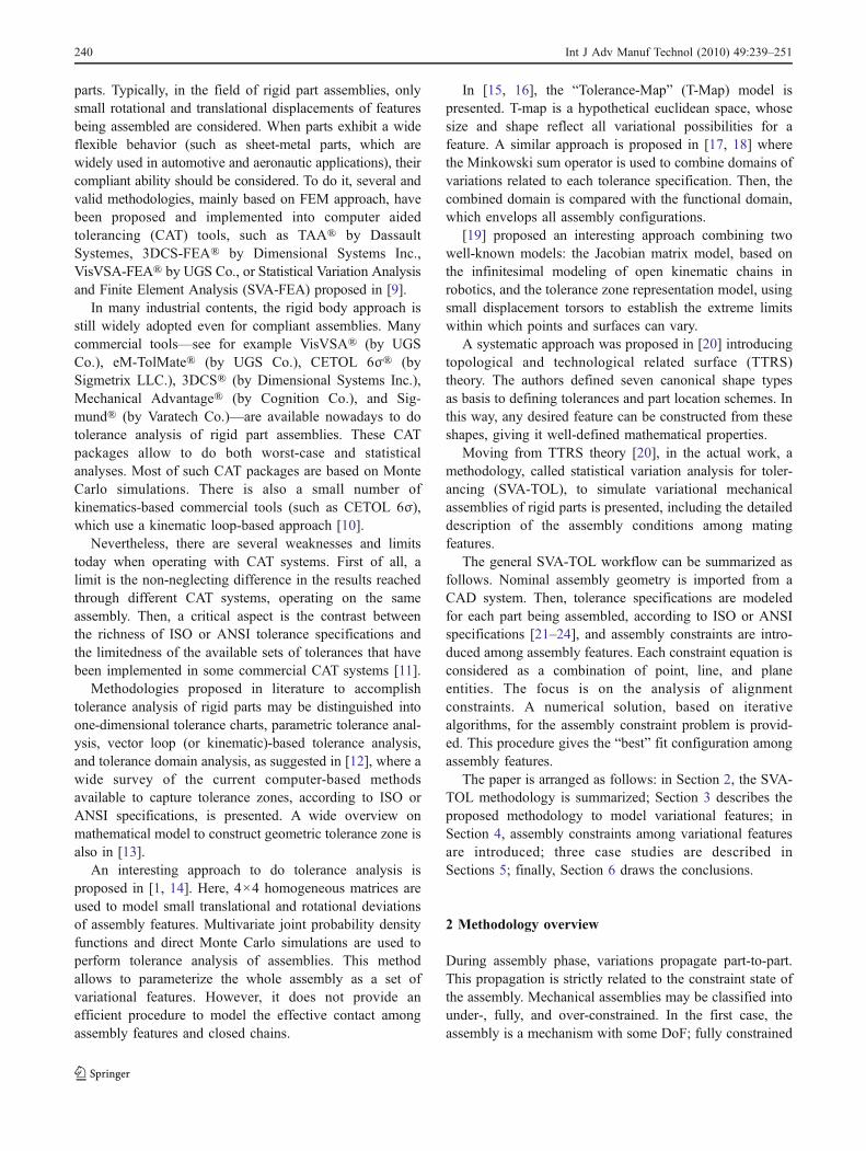
Starting from TTRS theory, a matrix variational modelhas been here developed. As shown in Fig. 1, three mainfeatures have been introduced:

& Nominal feature: as described in Section 3.1, thenominal feature is coincident with the associated

Nominal Feature

Actual Feature

Derived Feature

Ω 0

Ω i

Ω j

Ω ai Ω aj

Ωai

dj

ζ

ζ

Fig. 1 Feature modeling. A coordinate reference frame is attached toeach feature

Int J Adv Manuf Technol (2010) 49:239–251 241

feature, and it is imported directly from the CADmodel.

& Actual feature: it is the “perturbed” feature, according totolerance deviations.

& Derived feature: it is the one derived from the actualdatum feature (“A” in Fig. 1), with respect to thespecified tolerance (“&” in Fig. 1). “&” is any relatedtolerance, such as location, orientation, profile, andrunout tolerances.

Each elementary feature is parameterized by means of:

& Geometric parameters: radius and height of a cylinder,width and length of a plane, and so on;

& Variational parameters: small displacements due tosmall deviations between the actual and the derivedfeature; these parameters depend on the local referenceframe attached to the feature; and,

& Datum constraints: the derived feature is constrained tothe datum features, if assigned.

The general matrix variational model can be expressedas in Eq. 2 (see Fig. 1):

M½ �Ωaj;Ω0¼ M½ �Ωj!Ω0

� M½ �Ωaj!Ωj�

� MD½ ��1Ωj!Ωi

� M½ �Ωai!Ωi� MD½ �Ωj!Ωi

�

� M½ ��1Ωj!Ω0

ð2Þ

MD½ �Ωj!Ωi¼ M½ ��1

Ωi!Ω0� M½ �Ωj!Ω0

ð3Þ

M½ �Ωaj!Ωj¼

1 �gF bF ΔxF

gF 1 �aF ΔyF

�bF aF 1 ΔzF

0 0 0 1

2666664

3777775

ð4Þ

Equation 2 represents, in the global reference Ω0, thetransformation of any point belonging to the actual featureΩaj and initially defined in Ω0 itself (only nominal CADgeometries are known). MD½ �Ωj!Ωi

is the datum link matrix,and it is defined by Eq. 3; “j” is the actual feature, while “i”is the actual datum feature; M½ �Ωai!Ωi

is the variation matrixof the datum feature, which imposes the same relativeorientation, as in the nominal model, between the datumand the derived feature Ωai

dj; finally, M½ �Ωaj!Ωjis the

variation matrix of the analyzed feature.Feature variational parameters are counted in the

variation matrix (Eq. 4), where {ΔF}={ΔxF, ΔyF, ΔzF}and {ΘF}={αF, βF, γF} are small displacements and smallrotations vectors, respectively. Therefore, Eq. 2 allows to

transform the “j” feature into the global assembly frame,Ω0, according to tolerance specifications and datumassignment. This procedure has to be iterated for anyfeature of any part being assembled. In this way, theassembly is modeled as a set of parameterized variationalfeatures. Feature variational parameters are dependentamong them [14]. In fact, if all parameters are at theirmaximum value, a portion of the feature would be outsidethe geometrical tolerance zone. Therefore, for each toler-ance zone, variational parameter constraints must bederived. Generally speaking, variational parameter con-straints may be calculated by evaluating the small displace-ment, DPi , of the ith point, Pi, belonging to the analyzedfeature. To do it, one can write:

DPi ¼ M½ �Ωaj!Ωj� Pi � Pi ¼ ΔF þ

1 �gF bFgF 1 �aF

�bF aF 1

24

35

� Pi � Pi ¼ ΔF þ ΘF ^ Pi

ð5Þ

Variational parameter constraints should be derived for anyfeature, as proposed in the TTRS classification. In thepresent work, two particular cases are considered: planarand cylindrical features.

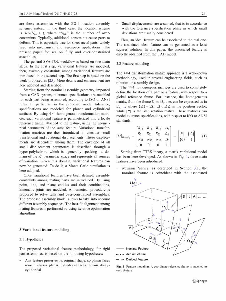
A planar feature is parameterized through a vector, Np, apoint, Pp, the length, Ap, and the width, Bp (Fig. 2a). Then,the mathematical representation of a planar feature becomes:

Plane : Pi � Pp

� � � Np ¼ 0 ð6Þwhere Pi is any point belonging to the planar surface.

In general, planar features may have no rectangularboundary. The relative bounding rectangle is here calculat-ed for any planar feature. The bounding rectangle of agiven planar geometry is the smallest rectangle whichcompletely includes that geometry. The principal compo-nent analysis is here used to calculate this rectangle, byevaluating eigenvectors of the statistical covariance matrix,related to the vertices of the planar feature [28].

Thus, in the following, each planar feature will beassumed as a rectangular planar feature. The local coordi-nate frame is oriented along the edges of the rectangle andis located into its area centroid (see Fig. 2a). Then, forplanar features, translational and rotational small displace-ment parameters become {ΔF}={ΔxF, 0, 0} and {ΘF}={0,βF, γF}, respectively.

Thus, after writing Eq. 5 for the four vertices of therectangular planar geometry, variational parameter con-straints are:

� T

2� ΔxF � gF � AP=2� bF � BP=2 � T

2ð7Þ

Inequalities (Eq. 7) assure that any point belonging to theplanar surface is inside the specified tolerance zone, T,supposed symmetrical.


A cylindrical feature is defined by a vector, Nc, and apoint, Pc (to specify the cylindrical feature's axis) and theheight, Lc (Fig. 2b). The parametric representation is:

Axis : PiðtÞ ¼ Pc þ t � Nc ð8Þwhere “t” is the axis parameter, which represents any pointbelonging to the cylindrical feature's axis. Here, the localframe has the local x-axis directed along the cylinder axisand is located on the middle of the same axis.

For cylindrical surfaces, translational and rotationalsmall displacement parameters become {ΔF}={0, ΔyF,ΔzF} and {ΘF}={0, βF, γF}, respectively. In this case,Eq. 5 has to be written for the two end points of thecylindrical feature's axis. Then, one can write:

ffiffiffiffiffiffiffiffiffiffiffiffiffiffiffiffiffiffiffiffiffiffiffiffiffiffiffiffiffiffiffiffiffiffiffiffiffiffiffiffiffiffiffiffiffiffiffiffiffiffiffiffiffiffiffiffiffiffiffiffiffiffiffiffiffiffiffiffiffiffiffiffiffiffiffiffiΔyF � g � Lc=2� �2 þ ΔzF � b � Lc=2ð Þ2

q� T

2ð9Þ

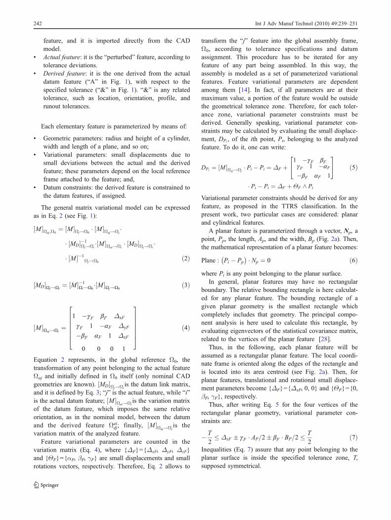
A graphical representation of Eqs. 7 and 9 may beaccomplished by means of hyper-polyhedrons.

Hyper-polyhedrons envelop all variational feature con-figurations, according to tolerance specifications andgeometrical parameters.

For example, Fig. 3a and b show, in the variationalparameter space, the hyper-polyhedrons for planar andcylindrical features, respectively.

Once all features have been parameterized, the assemblycan be made up by defining constraints among parts. In thiscontest, the assembly modeling is accomplished into twomain steps. In the first one, a DoFs analysis is performed.In the second step, assembly constraints among parts areintroduced, accordingly.

Next section gives details of the proposed methodologyto model and simulate assembly constraints among varia-tional features.

4 Assembly constraint modeling

4.1 Hypotheses and methods

In general, during assembly operations, an object part (OP)has to be moved to satisfy constraints of target parts (TP).

The relative location of the object part, with respect tothe target, in the small displacement hypothesis, isrepresented by a 4×4 transformation matrix, as in Eq. 10,where M½ �ΩOP!ΩTP

is the assembly transformation matrix,while [RA] and {ΔA} are the rotational matrix and thetranslational vector, respectively.

M½ �ΩOP!ΩTP¼

1 �gA bA ΔxA

gA 1 �aA ΔyA

�bA aA 1 ΔzA

0 0 0 1

266666664

377777775¼ RA½ � ΔAf g

0f g 1

24

35

ð10ÞThis matrix is initially unknown and depends on the six

rigid small motion parameters (three rotations and threetranslations).

The DoFs allowed for each joint are assumed invariants,and then they are not considered into the assembly

ΔxFa b

βF YF

ΔzF

βF YF

Fig. 3 a Parameter space for planar tolerance zone. b Parameter spacefor cylindrical tolerance zone. ΔyF=0

Tolerance Zone Derived Plane

y z x

BP AP

Pi

T

PP

NP

Tolerance Zone Derived Axis

y

z

x

Lc

T

Pi

Pc Nc

a

b

Fig. 2 a Planar tolerance zone. b Cylindrical tolerance zone


simulation. This is made by DoFs analysis which allows todetermine the number of DoFs removed by the assemblyconstraints. “Reduction constraint” method [6] or Screwtheory [26, 27] may be adopted, but in the presentapproach, this is still a manual operation.

Each constraint may be considered as combination ofelementary geometry entities, (points, lines, and planes) asproposed in TTRS theory.

4.2 Assembly constraint modeling

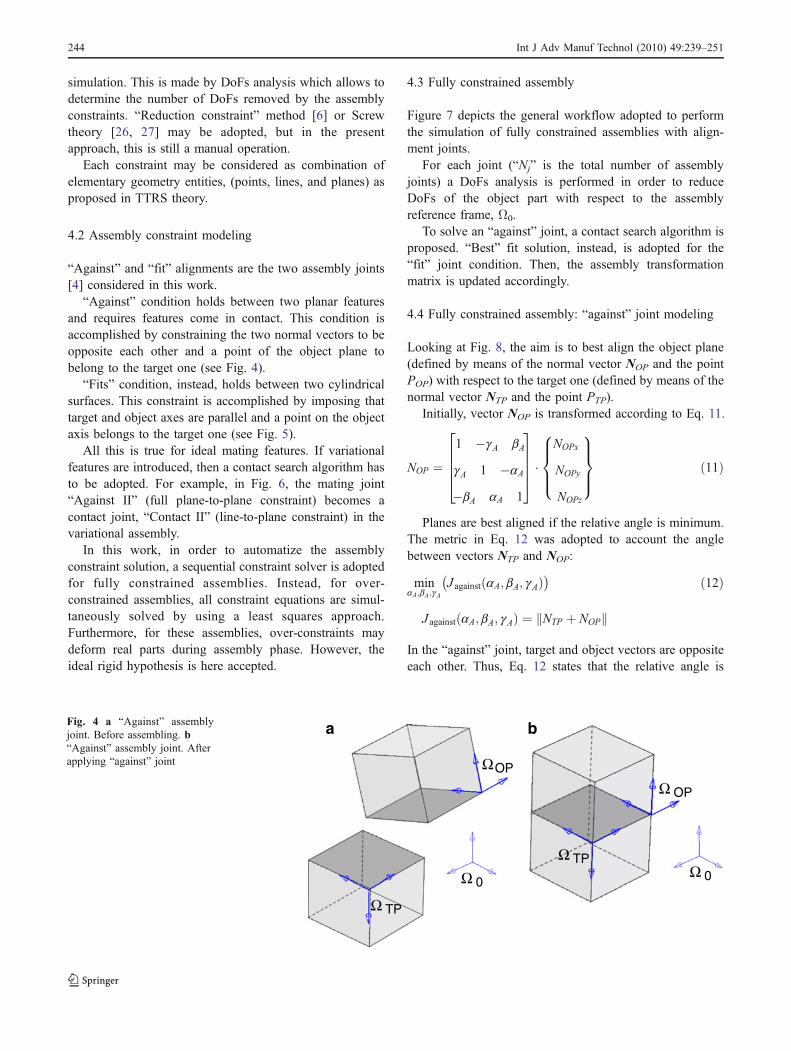
“Against” and “fit” alignments are the two assembly joints[4] considered in this work.

“Against” condition holds between two planar featuresand requires features come in contact. This condition isaccomplished by constraining the two normal vectors to beopposite each other and a point of the object plane tobelong to the target one (see Fig. 4).

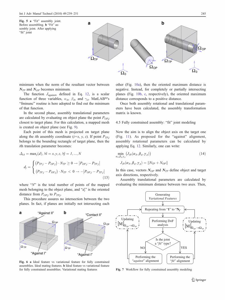
“Fits” condition, instead, holds between two cylindricalsurfaces. This constraint is accomplished by imposing thattarget and object axes are parallel and a point on the objectaxis belongs to the target one (see Fig. 5).

All this is true for ideal mating features. If variationalfeatures are introduced, then a contact search algorithm hasto be adopted. For example, in Fig. 6, the mating joint“Against II” (full plane-to-plane constraint) becomes acontact joint, “Contact II” (line-to-plane constraint) in thevariational assembly.

In this work, in order to automatize the assemblyconstraint solution, a sequential constraint solver is adoptedfor fully constrained assemblies. Instead, for over-constrained assemblies, all constraint equations are simul-taneously solved by using a least squares approach.Furthermore, for these assemblies, over-constraints maydeform real parts during assembly phase. However, theideal rigid hypothesis is here accepted.

4.3 Fully constrained assembly

Figure 7 depicts the general workflow adopted to performthe simulation of fully constrained assemblies with align-ment joints.

For each joint (“Nj” is the total number of assemblyjoints) a DoFs analysis is performed in order to reduceDoFs of the object part with respect to the assemblyreference frame, Ω0.

To solve an “against” joint, a contact search algorithm isproposed. “Best” fit solution, instead, is adopted for the“fit” joint condition. Then, the assembly transformationmatrix is updated accordingly.

4.4 Fully constrained assembly: “against” joint modeling

Looking at Fig. 8, the aim is to best align the object plane(defined by means of the normal vector NOP and the pointPOP) with respect to the target one (defined by means of thenormal vector NTP and the point PTP).

Initially, vector NOP is transformed according to Eq. 11.

NOP ¼1 �gA bA

gA 1 �aA

�bA aA 1

26664

37775 �

NOPx

NOPy

NOPz

8>><>>:

9>>=>>;

ð11Þ

Planes are best aligned if the relative angle is minimum.The metric in Eq. 12 was adopted to account the anglebetween vectors NTP and NOP:

minaA;bA;gA

J against aA; bA; gAð Þ� �

J against aA; bA; gAð Þ ¼ NTP þ NOPk k

ð12Þ

In the “against” joint, target and object vectors are oppositeeach other. Thus, Eq. 12 states that the relative angle is

Ω TP

ΩOP

Ω 0 Ω TP

Ω OP

Ω 0

baFig. 4 a “Against” assemblyjoint. Before assembling. b“Against” assembly joint. Afterapplying “against” joint


minimum when the norm of the resultant vector betweenNTP and NOP becomes minimum.

The function Jagainst, defined in Eq. 12, is a scalarfunction of three variables, αA, βA, and γA. MatLAB®'s“fminunc” routine is here adopted to find out the minimumof that function.

In the second phase, assembly translational parametersare calculated by evaluating on object plane the point POP,j

closest to target plane. For this calculation, a mapped meshis created on object plane (see Fig. 9).

Each point of this mesh is projected on target planealong the ith assembly coordinate (i=x, y, z). If point PTP,j

belongs to the bounding rectangle of target plane, then theith translation parameter becomes:

ΔiA ¼ maxjðdÞ;∀i ¼ x; y; z;∀j ¼ 1; :::;N

dj ¼PTP;j � POP;j

� � � NTP � 0 ! POP;j � PTP;j

�� PTP;j � POP;j

� � � NTP < 0 ! � POP;j � PTP;j

�� 8<:

ð13Þwhere “N” is the total number of points of the mappedmesh belonging to the object plane, and “dj” is the orienteddistance from POP,j to PTP,j.

This procedure assures no intersection between the twoplanes. In fact, if planes are initially not intersecting each

other (Fig. 10a), then the oriented maximum distance isnegative. Instead, for completely or partially intersectingplanes (Fig. 10b, c, respectively), the oriented maximumdistance corresponds to a positive distance.

Once both assembly rotational and translational param-eters have been calculated, the assembly transformationmatrix is known.

4.5 Fully constrained assembly: “fit” joint modeling

Now the aim is to align the object axis on the target one(Fig. 11). As proposed for the “against” alignment,assembly rotational parameters can be calculated byapplying Eq. 12. Similarly, one can write:

minaA;bA;gA

J fit aA; bA; gAð Þ� �

J fit aA; bA; gAð Þ ¼ NTP þ NOPk k

ð14Þ

In this case, vectors NOP and NTP define object and targetaxis directions, respectively.

Assembly translational parameters are calculated byevaluating the minimum distance between two axes. Then,

Ω TP

Ω OP

“Against I”

“Against II”

Ω TP

Ω OP

“Against I”

“Contact II”

Fig. 6 a Ideal feature vs variational feature for fully constrainedassemblies. Ideal mating features. b Ideal feature vs variational featurefor fully constrained assemblies. Variational mating features

Performing the “fit” alignment

NO YES

Is the joint a “fit” type?

Generating Variational Features

Repeating from “1” to “Nj”

Performing DoFanalysis

Performing the “against” alignment

Updating

[ ]TPOPΩM

Updating

[ ]TPOP

M →Ω

Ω →Ω

Fig. 7 Workflow for fully constrained assembly modeling

ΩTP

ΩOP

Ω0

ΩTP

ΩOP

Ω0

a bFig. 5 a “Fit” assembly joint.Before assembling. b “Fit” as-sembly joint. After applying“fit” joint


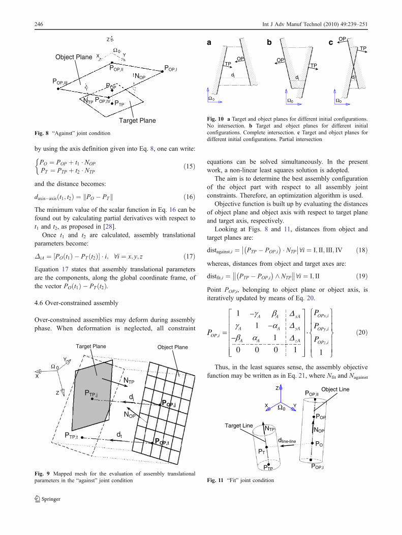
by using the axis definition given into Eq. 8, one can write:

PO ¼ POP þ t1 � NOP

PT ¼ PTP þ t2 � NTP

�ð15Þ

and the distance becomes:

daxis�axis t1; t2ð Þ ¼ PO � PTk k ð16ÞThe minimum value of the scalar function in Eq. 16 can befound out by calculating partial derivatives with respect tot1 and t2, as proposed in [28].

Once t1 and t2 are calculated, assembly translationalparameters become:

ΔiA ¼ PO t1ð Þ � PT t2ð Þ½ � � i; ∀i ¼ x; y; z ð17ÞEquation 17 states that assembly translational parametersare the components, along the global coordinate frame, ofthe vector PO t1ð Þ � PT t2ð Þ.

4.6 Over-constrained assembly

Over-constrained assemblies may deform during assemblyphase. When deformation is neglected, all constraint

equations can be solved simultaneously. In the presentwork, a non-linear least squares solution is adopted.

The aim is to determine the best assembly configurationof the object part with respect to all assembly jointconstraints. Therefore, an optimization algorithm is used.

Objective function is built up by evaluating the distancesof object plane and object axis with respect to target planeand target axis, respectively.

Looking at Figs. 8 and 11, distances from object andtarget planes are:

distagainst;i ¼ PTP � POP;i

� � � NTP

�� ∀i ¼ I; II; III; IV ð18Þwhereas, distances from object and target axes are:

distfit;i ¼ PTP � POP;i

� � ^ NTP

�� ∀i ¼ I; II ð19ÞPoint POP,i, belonging to object plane or object axis, isiteratively updated by means of Eq. 20.

ð20Þ

Thus, in the least squares sense, the assembly objectivefunction may be written as in Eq. 21, where Nfit and Nagainst

Ω 0

Z

X

Y

PTP,j

PTP,t

POP,j

POP,t

Target Plane Object Plane

dt

NTP

NOP

dj

Fig. 9 Mapped mesh for the evaluation of assembly translationalparameters in the “against” joint condition

Ω 0

NOP

NTP

POP

PTP

Z

X Y

POP,IPOP,II

POP,III

POP,IV

Object Plane

Target Plane

Fig. 8 “Against” joint condition

Ω 0

TP OP

dj

Ω0

TP OP

dj

Ω0

TP

OP

dj

a b c

Fig. 10 a Target and object planes for different initial configurations.No intersection. b Target and object planes for different initialconfigurations. Complete intersection. c Target and object planes fordifferent initial configurations. Partial intersection

Ω0 POP

Z

X Y

NTP NOP

PO PT

PTP

dline-line

Target Line

Object Line

POP,I

POP,II

Fig. 11 “Fit” joint condition


are the number of “fit” and “against” joint conditions,respectively.

J over aA; bA; gA;ΔxA;ΔyA;ΔzA

� �

¼X2�N fit

i¼1

dist2fit;i þX4�N against

j¼1

dist2against;j ð21Þ

Equation 21 takes into account simultaneously all smallmotion parameters. This function can be minimized byusing any non-linear least squares routine, such as theMatLAB®'s “lsqnonlin”.

5 Case studies

In this section, three case studies are analyzed. In the firststudy, the proposed method to solve fully constrainedassemblies has been tested on a two-part assembly. In thesecond application, an over-constrained assembly is solvedby using the proposed least squares approach. Finally, inthe last application, an industrial device is analyzed, takinginto account geometric dimensioning and tolerancing(GD&T) tolerance specifications. All numerical simulationshave been performed in MatLAB® environment.

5.1 Fully constrained assembly

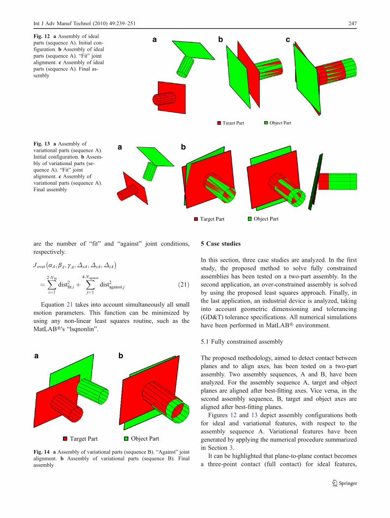
The proposed methodology, aimed to detect contact betweenplanes and to align axes, has been tested on a two-partassembly. Two assembly sequences, A and B, have beenanalyzed. For the assembly sequence A, target and objectplanes are aligned after best-fitting axes. Vice versa, in thesecond assembly sequence, B, target and object axes arealigned after best-fitting planes.

Figures 12 and 13 depict assembly configurations bothfor ideal and variational features, with respect to theassembly sequence A. Variational features have beengenerated by applying the numerical procedure summarizedin Section 3.

It can be highlighted that plane-to-plane contact becomesa three-point contact (full contact) for ideal features,

Target Part Object Part

a b

Fig. 14 a Assembly of variational parts (sequence B). “Against” jointalignment. b Assembly of variational parts (sequence B). Finalassembly


a b cFig. 12 a Assembly of idealparts (sequence A). Initial con-figuration. b Assembly of idealparts (sequence A). “Fit” jointalignment. c Assembly of idealparts (sequence A). Final as-sembly


a bFig. 13 a Assembly ofvariational parts (sequence A).Initial configuration. b Assem-bly of variational parts (se-quence A). “Fit” jointalignment. c Assembly ofvariational parts (sequence A).Final assembly


whereas it degenerates into a two-point contact (partialcontact) for variational features. Moreover, after “fit” jointalignment, variational planes are partially intersecting (seeFig. 13). Only by introducing “against” joint, right-contactbetween mating planes is assured.

What happens for the assembly sequence B is depictedinto Fig. 14 (only for variational features). In this case,“against” joint assures a full contact between mating planes.Then, “fit” joint tries to best align the two axes. However,the cylindrical features intersect each other. The proposedmodel does not consider contact between cylindricalfeatures, but allows to best fit the related axes. Therefore,for more realistic results, flexibility of mating parts shouldbe introduced into the model.

5.2 Over-constrained assembly

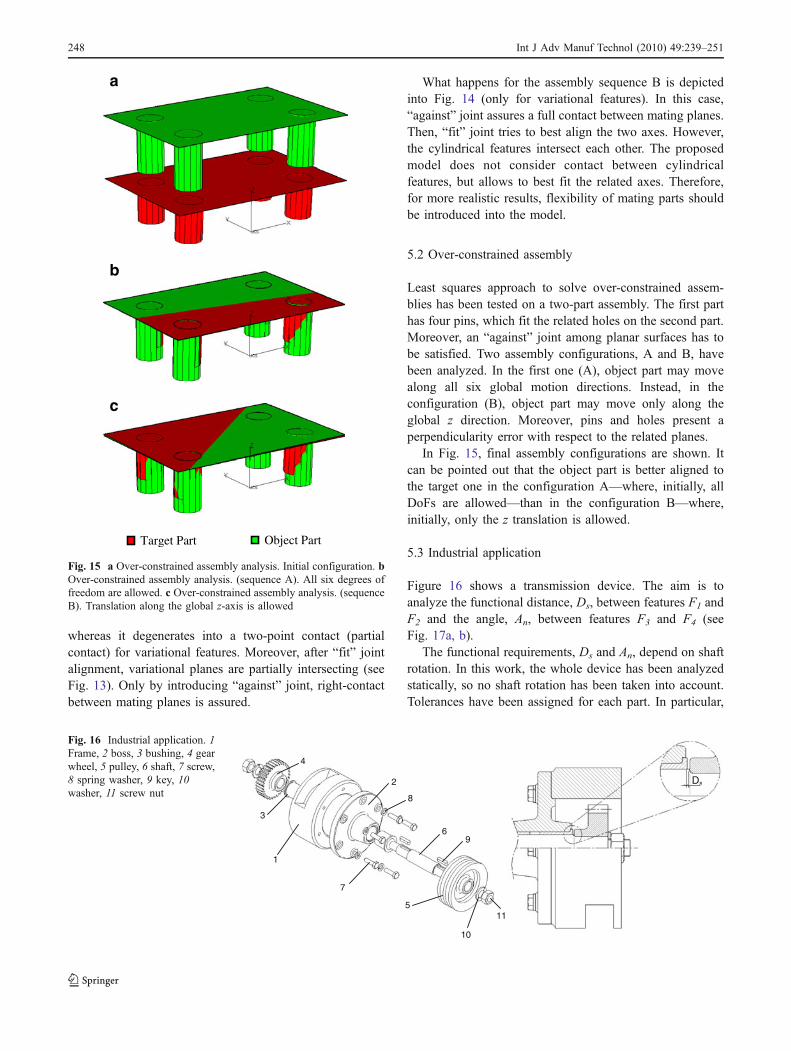
Least squares approach to solve over-constrained assem-blies has been tested on a two-part assembly. The first parthas four pins, which fit the related holes on the second part.Moreover, an “against” joint among planar surfaces has tobe satisfied. Two assembly configurations, A and B, havebeen analyzed. In the first one (A), object part may movealong all six global motion directions. Instead, in theconfiguration (B), object part may move only along theglobal z direction. Moreover, pins and holes present aperpendicularity error with respect to the related planes.

In Fig. 15, final assembly configurations are shown. Itcan be pointed out that the object part is better aligned tothe target one in the configuration A—where, initially, allDoFs are allowed—than in the configuration B—where,initially, only the z translation is allowed.

5.3 Industrial application

Figure 16 shows a transmission device. The aim is toanalyze the functional distance, Ds, between features F1 andF2 and the angle, An, between features F3 and F4 (seeFig. 17a, b).

The functional requirements, Ds and An, depend on shaftrotation. In this work, the whole device has been analyzedstatically, so no shaft rotation has been taken into account.Tolerances have been assigned for each part. In particular,


a

b

c

Fig. 15 a Over-constrained assembly analysis. Initial configuration. bOver-constrained assembly analysis. (sequence A). All six degrees offreedom are allowed. c Over-constrained assembly analysis. (sequenceB). Translation along the global z-axis is allowed

1

2

3

4

5

6

7

8

10

11

9

Ds

Fig. 16 Industrial application. 1Frame, 2 boss, 3 bushing, 4 gearwheel, 5 pulley, 6 shaft, 7 screw,8 spring washer, 9 key, 10washer, 11 screw nut


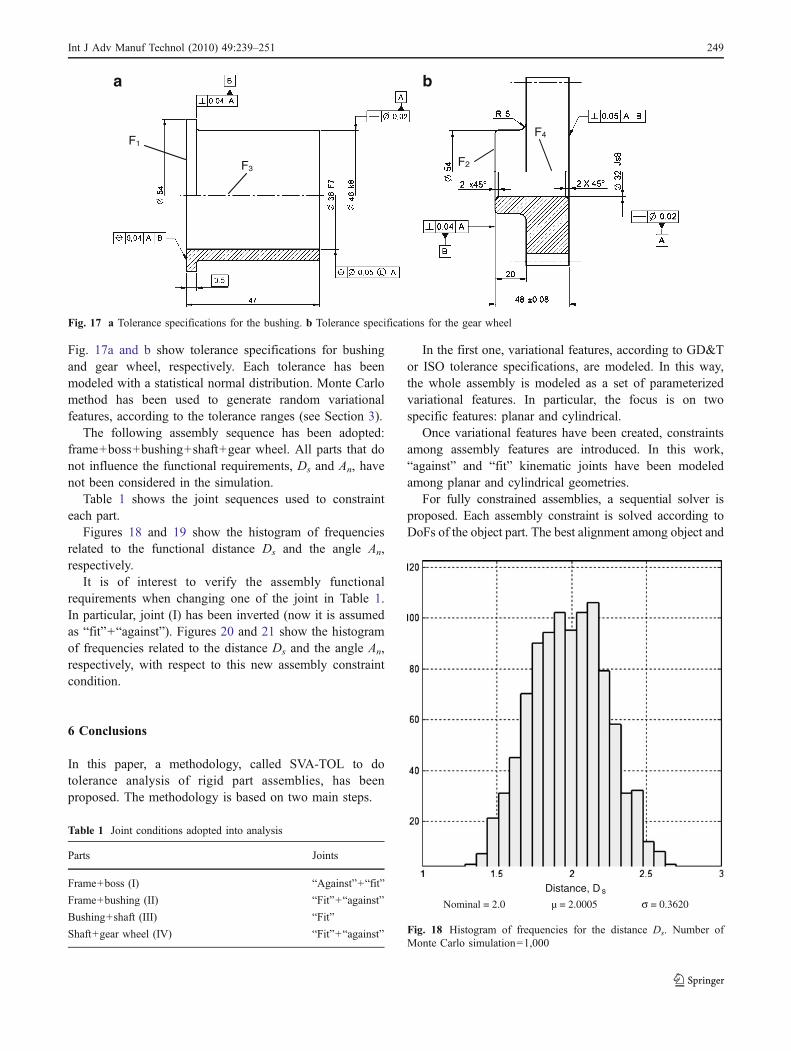
Fig. 17a and b show tolerance specifications for bushingand gear wheel, respectively. Each tolerance has beenmodeled with a statistical normal distribution. Monte Carlomethod has been used to generate random variationalfeatures, according to the tolerance ranges (see Section 3).

The following assembly sequence has been adopted:frame+boss+bushing+shaft+gear wheel. All parts that donot influence the functional requirements, Ds and An, havenot been considered in the simulation.

Table 1 shows the joint sequences used to constrainteach part.

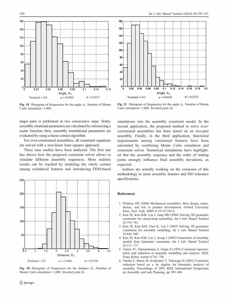
Figures 18 and 19 show the histogram of frequenciesrelated to the functional distance Ds and the angle An,respectively.

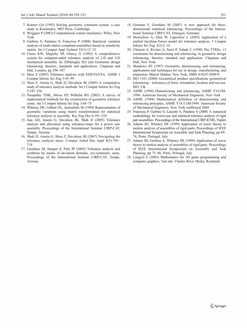
It is of interest to verify the assembly functionalrequirements when changing one of the joint in Table 1.In particular, joint (I) has been inverted (now it is assumedas “fit”+“against”). Figures 20 and 21 show the histogramof frequencies related to the distance Ds and the angle An,respectively, with respect to this new assembly constraintcondition.

6 Conclusions

In this paper, a methodology, called SVA-TOL to dotolerance analysis of rigid part assemblies, has beenproposed. The methodology is based on two main steps.

In the first one, variational features, according to GD&Tor ISO tolerance specifications, are modeled. In this way,the whole assembly is modeled as a set of parameterizedvariational features. In particular, the focus is on twospecific features: planar and cylindrical.

Once variational features have been created, constraintsamong assembly features are introduced. In this work,“against” and “fit” kinematic joints have been modeledamong planar and cylindrical geometries.

For fully constrained assemblies, a sequential solver isproposed. Each assembly constraint is solved according toDoFs of the object part. The best alignment among object and

F1

F3 F2

F4

a b

Fig. 17 a Tolerance specifications for the bushing. b Tolerance specifications for the gear wheel

Distance, D s

Nominal = 2.0 µ = 2.0005 σ = 0.3620

Fig. 18 Histogram of frequencies for the distance Ds. Number ofMonte Carlo simulation=1,000

Table 1 Joint conditions adopted into analysis

Parts Joints

Frame+boss (I) “Against”+“fit”

Frame+bushing (II) “Fit”+“against”

Bushing+shaft (III) “Fit”

Shaft+gear wheel (IV) “Fit”+“against”


target parts is performed in two consecutive steps: firstly,assembly rotational parameters are calculated byminimizing ascalar function; then, assembly translational parameters areevaluated by using a linear contact algorithm.

For over-constrained assemblies, all constraint equationsare solved with a non-linear least squares approach.

Three case studies have been analyzed. The first onehas shown how the proposed constraint solver allows tosimulate different assembly sequences. More realisticresults can be reached by modeling the whole contactamong cylindrical features and introducing FEM-based

simulations into the assembly constraint model. In thesecond application, the proposed method to solve over-constrained assemblies has been tested on an two-partassembly. Finally, in the third application, functionalrequirements among variational features have beencalculated by combining Monte Carlo simulation andconstraint solver. Numerical simulations have highlight-ed that the assembly sequence and the order of matingjoints strongly influence final assembly deviations, asexpected.

Authors are actually working on the extension of thismethodology to more assembly features and ISO tolerancespecifications.

References

1. Whitney DE (2004) Mechanical assemblies, their design, manu-facture, and role in product development. Oxford UniversityPress, New York. ISBN 0-19-515782-6

2. Kim JS, Kim KM, Lee J, Jung HB (2004) Solving 3D geometricconstraints for closed-loop assemblies. Int J Adv Manuf Technol23:755–761

3. Kim JS, Kim KM, Choi K, Lee J (2005) Solving 3D geometricconstraints for assembly modelling. Int J Adv Manuf Technol16:843–849

4. Kim JS, Kim KM, Lee J, Jeong J (2005) Generation of assemblymodels from kinematic constraints. Int J Adv Manuf Technol26:131–137

5. Turner JU, Subramaniam S, Gupta S (1992) Constraint represen-tation and reduction in assembly modelling and analysis. IEEETrans Robot Autom 8:741–750

6. Tanaka F, Murai M, Kishinami T, Tokunaga H (2001) Constraintreduction based on a lie algebra for kinematic analysis ofassembly. Proceedings of 2001 IEEE International Symposiumon Assembly and task Planning, pp 399–404

Distance, D s

Nominal = 2.0 µ = 2.3666 σ = 0.5158

Fig. 20 Histogram of frequencies for the distance Ds. Number ofMonte Carlo simulation=1,000. Inverted joint (I)

Angle, A n

Nominal = 0.0 µ = 0.0404 σ = 0.0217

Fig. 19 Histogram of frequencies for the angle An. Number of MonteCarlo simulation=1,000

Fig. 21 Histogram of frequencies for the angle An. Number of MonteCarlo simulation=1,000. Inverted joint (I)


7. Kramer GA (1992) Solving geometric constraint system: a casestudy in Kinematics. MIT Press, Cambridge

8. Wriggers P (2002) Computational contact mechanics. Wiley, NewYork

9. Gerbino S, Patalano S, Franciosa P (2008) Statistical variationanalysis of multi-station compliant assemblies based on sensitivitymatrix. Int J Comput Appl Technol 33(1):12–23

10. Chase KW, Magleby SP, Glancy G (1995) A comprehensivesystem for computer-aided tolerance analysis of 2-D and 3-Dmechanical assembly. In: ElMaraghy HA (ed) Geometric designtolerancing: theories, standards and applications. Chapman andHall, London, pp 294–307

11. Shen Z (2003) Tolerance analysis with EDS/VisVSA. ASME JComput Inform Sci Eng 5:95–99

12. Shen Z, Ameta G, Shah JJ, Davidson JK (2005) A comparativestudy of tolerance analysis methods. Int J Comput Inform Sci Eng5:247–256

13. Pasupathy TMK, Morse EP, Wilhelm RG (2003) A survey ofmathematical methods for the construction of geometric tolerancezones. Int J Comput Inform Sci Eng 3:64–75

14. Whitney DE, Gilbert OL, Jastrzebski M (1994) Representation ofgeometric variations using matrix transformation for statisticaltolerance analysis in assembly. Res Eng Des 6:191–210

15. Jian AD, Ameta G, Davidson JK, Shah JJ (2005) Toleranceanalysis and allocation using tolerance-maps for a power sawassembly. Proceedings of the International Seminar CIRP-CAT,Tempe, Arizona

16. Shah JJ, Ameta G, Shen Z, Davidson JK (2007) Navigating thetolerance analysis maze. Comput Aided Des Appl 4(5):705–718

17. Giordano M, Samper S, Petit JP (2005) Tolerance analysis andsynthesis by means of deviation domains, axi-symmetric cases.Proceedings of the International Seminar CIRP-CAT, Tempe,Arizona

18. Germain F, Giordano M (2007) A new approach for three-dimensional statistical tolerancing. Proceedings of the Interna-tional Seminar CIRP-CAT, Erlangen, Germany

19. Desrochers A, Ghie W, Laperrière L (2003) Application of aunified Jacobian-Torsor model for tolerance analysis. J ComputInform Sci Eng 3(2):2–14

20. Clément A, Rivière A, Serré P, Valade C (1998) The TTRSs: 13constraints for dimensioning and tolerancing, in geometric designtolerancing: theories, standard and application. Chapman andHall, New York

21. Meadows JD (1997) Geometric dimensioning and tolerancing,applications and techniques for use in design, manufacturing, andinspection. Marcel Dekker, New York. ISBN 0-8247-9309-9

22. ISO 1101 (2004) Geometrical product specifications geometricaltolerancing—tolerances of form, orientation, location and run-out.ISO, UK

23. ASME (1994) Dimensioning and tolerancing, ASME Y14.5M-1994. American Society of Mechanical Engineers, New York

24. ASME (1994) Mathematical definition of dimensioning andtolerancing principles, ASME Y14.5.1M-1994. American Societyof Mechanical Engineers, New York reaffirmed 2004

25. Franciosa P, Gerbino S, Lanzotti A, Patalano S (2008) A numericalmethodology for worst-case and statistical tolerance analysis of rigidpart assemblies. Proceedings of the International CIRP-ICME, Naples

26. Adams JD, Whitney DE (1999) Application of screw theory tomotion analysis of assemblies of rigid parts, Proceedings of IEEEInternational Symposium on Assembly and Task Planning, pp 69–74, Porto, Portugal, July

27. Adams JD, Gerbino S, Whitney DE (1999) Application of screwtheory to motion analysis of assemblies of rigid parts. Proceedingsof IEEE International Symposium on Assembly and TaskPlanning, pp 75–80, Porto, Portugal, July

28. Lengyel E (2003) Mathematics for 3D game programming andcomputer graphics, 2nd edn. Charles River Media, Rockland


Variational modeling and assembly constraints in tolerance analysis of rigid part assemblies: planar...

Documents

Transcript of Variational modeling and assembly constraints in tolerance analysis of rigid part assemblies: planar...