Variable neighborhood search for the economic lot sizing

problem with product returns and recovery

Angelo Sifaleras∗

Department of Applied Informatics, School of Information Sciences, University of

Macedonia, 156 Egnatia Str., Thessaloniki 54636, Greece

Ioannis Konstantaras

Department of Business Administration, School of Business Administration, University

of Macedonia, 156 Egnatia Str., Thessaloniki 54636, Greece

Nenad Mladenovic

LAMIH, University of Valenciennes, France

Abstract

The economic lot sizing problem with product returns and recovery is animportant problem that appears in reverse logistics, and has recently beenproved to be NP-hard. In this paper, we suggest a Variable NeighborhoodSearch (VNS) metaheuristic algorithm for solving this problem. It is the firsttime that such an approach has been used for this problem in the literature.Our research contributions are threefold: first, we propose two novel VNSvariants to tackle this problem efficiently. Second, we present several newneighborhoods for this combinatorial optimization problem, and an efficientlocal search method for exploring them. The computational results, obtainedon a recent set of benchmark problems with 6480 instances, demonstrate thatour approach outperforms the state-of-the-art heuristic methods from theliterature, and that it achieved an average optimality gap equal to 0.283%within average 8.3 seconds. Third, we also present a new benchmark set withthe largest instances in the literature. We demonstrate the robustness of the

∗Corresponding author. Tel: +302310 891884, Fax: +302310 891881Email addresses: sifalera@uom.gr (Angelo Sifaleras), ikonst@uom.gr (Ioannis

Konstantaras), nenad.mladenovic@univ-valenciennes.fr (Nenad Mladenovic)

Preprint submitted to International Journal of Production Economics October 27, 2014

proposed VNS approach in this new benchmark set compared with Gurobioptimizer.

Keywords: Inventory, Variable Neighborhood Search, MathematicalProgramming, Lot Sizing, Remanufacturing2010 MSC: 90B05, 90C59, 65K05, 90-08

1. Introduction

Reverse logistics stands for all operations related to the return of productsand materials. It is a process of planning, implementing, and controllingthe efficient, cost effective flow of raw materials, in-process inventory, fin-ished products and related information from the point of consumption to thepoint of origin for the purpose of recovery value or proper disposal. Reusingproduct, or material returns have gained considerable attention in industryand academia because of economical, environmental and legislative reasons.Balancing economic development with environmental protection is a key chal-lenge to sustain manufacturing companies. Conventional manufacturing isunsustainable because of its significant adverse environmental impacts. Re-manufacturing can help companies to achieve sustainable manufacturing bysaving costs via reductions in consumption of natural resources. Remanufac-turing can also help reduce environment burden by decreasing landfill wastesand reclaim resources and energy already consumed in the original manufac-turing of the products. Besides the environmental benefits, remanufacturingalso provides economic incentives to companies by selling the remanufacturedproducts and extending the life cycles of the products [13].

Remanufacturing transforms used products into like new ones. After dis-assembly, sorting and cleaning, modules and parts are extensively inspectedand problematic parts are repaired, or if not possible, replaced by new parts[16]. These operations allow a considerable amount of value incorporated inthe used product to be regained. Remanufactured products have usually thesame quality as the new products and are sold for the same price, but theyare less costly. The significance of remanufacturing is that it would allowmanufacturers to respond to environmental and legislative pressure by en-abling them to meet waste legislation while maintaining high productivity forhigh-quality, lower-cost products with less landing filling and consumptionof raw materials and energy [19].

Inventory management and control is one of the key decision making areas

2

while managing product returns and remanufacturing. A scientific literaturereview of the existing quantitative models on inventory control with prod-uct returns and remanufacturing can be found in the recent work of Akcali& Cetinkaya [1]. The Dynamic or Economic Lot Sizing Problem (DLSP orELSP) is one of the most extensively researched topics in inventory controlliterature. ELSP considers a warehouse or retailer facing a dynamic anddeterministic demand for a single item over a finite horizon [40]. A lot ofresearch has been done on dynamic lot sizing since late 1950s after the sem-inal paper [40]. For a general review of the economic lot sizing problem,readers may refer to [6, 7]. The ELSP with remanufacturing options (EL-SRP) is an extension of the classical Wagner Whitin model. The additionalfeature is that in each period known quantities of used products enter thesystem. These returns can be remanufactured to satisfy demand besides reg-ular manufacturing. This means that there are two types of inventory: theinventory of returns and the inventory of serviceables, where a serviceableis either a newly manufactured item or a remanufactured returned item. InELSR problem, the traditional trade-off between set-up and holding costs isextended with remanufacturing set-up cost and holding cost for returns.

Many different variants of the ELSR problem, described above, have beenstudied. Richter & Sombrutzki [28] extended the classical Wagner-Whitinmodel by introducing remanufacturing process. They assumed that the dy-namic demand could be satisfied from two sources: newly produced items,and the used ones, returned to the system, stored and remanufactured. Theypresented a dynamic programming algorithm to determine the periods inwhich products are manufactured and remanufactured. Richter & Weber [29]introduced a reverse Wagner-Whitin model with variable manufacturing andremanufacturing costs. They also investigated the behaviour of the systemwith a disposal option. Golany et al. [14] studied a variant of ELSRP withdeterministic demand and return setting in the presence of disposal optionsand provided a polynomial solution algorithm. Yang et al. [44] extended thework by Golany et al. [14] on the concave cost functions. Based on a specialstructure of the extreme-point optimal solutions for the minimum concavecost problem, they developed a polynomial-time heuristic algorithm. Beltran& Krass [5] studied the case where demand can be satisfied by new itemsand unprocessed returned items, and the returned items can also be disposed.They proposed some useful properties of the optimal solution (manufactur-ing and disposal decisions) which led to a dynamic programming algorithm.Pineyro & Viera [23] proposed and evaluated a set of inventory policies de-

3

signed for the ELSRP under the assumption that remanufacturing the useditems is more suitable than disposing them and producing new items. Te-unter et al. [36] presented two variants of the basic dynamic lot sizing modelwith product returns. In the first model variant, it is assumed that there is ajoint set up cost for manufacturing and remanufacturing when the same pro-duction line is used for both processes, and the second model variant assumedseparate set up costs for manufacturing and remanufacturing when separateproduction lines are used. For these two models, several heuristic algorithmswere proposed and compared with the computational performance of modi-fied versions of three well-known heuristics, namely Silver-Meal (SM), LeastUnit Cost, and Part Period Balancing. Teunter et al. [38] later advancedthe study of the ELSRP by developing fast but simple heuristics that canprovide near-optimal solutions. Schulz [30] proposed a generalization of theSilver-Meal based heuristic introduced by Teunter et al. [36] for the separateset up cost setting by using known results of the static lot sizing problem.

Recently, Nenes et al. [22] studied some inventory control policies forinspection and remanufacturing and proposed alternative policies when bothdemand of new products and returns of used products are stochastic; Helm-rich et al. [27] added some valid inequalities to the original formulation ofthe ELSRP to improve its formulation, and also presented reformulationsbased on the shortest path problem for the ELSR problem. Also, Pineyroand Viera [24] extended the ELSR problem for the case where substitutionis allowed for remanufactured items.

Tang & Teunter [35] studied the multi product dynamic lot sizing problemfor a hybrid production line with manufacturing new products and reman-ufacturing the returned products. They considered one manufacturing andone remanufacturing lot for each product during a common cycle time andformulated a Mixed Integer Linear Programming (MILP) problem to find anexact solution. The multi-product dynamic lot sizing problem with two pro-duction sources, manufacturing and remanufacturing, for which operationsare performed on separate dedicated lines was studied in [37]. The authorsproposed a mixed integer programming model to solve the problem for afixed cycle time, which can be combined with a cycle time search to find anoptimal solution. In [45], the multi-product ELSRP was further analyzed,extending the scheduling policy from the common cycle to a basic periodpolicy. They relaxed the constraint of one manufacturing lot and one reman-ufacturing lot for each product during a common cycle time studied in [35],and they proposed an algorithm to solve their model.

4

Recently, both trajectory-based and population-based metaheuristics wereused to tackle the ELSR problem. Pineyro and Viera [23] suggested a TabuSearch procedure for solving the problem tackled, even with a more generalcost structure and final disposing of returns. Li et al. [18] also developeda Tabu Search (TS) algorithm based on an alternative mixed-integer linearprogramming formulation. The TS algorithm solves the problem of severalsmall linear sub-problems of the original model. Moustaki et al. [21] studiedthe behavior of Particle Swarm Optimization (PSO) algorithm on the ELSRproblem. The most suitable variants of the algorithm were identified, and thenecessary modifications in the formulation of the corresponding optimizationproblem were provided. The performance of the above two metaheuristicalgorithms were compared with the Silver-Meal based heuristics, proposedby Schulz [30], in each of the above papers, and showed that the proposedalgorithms can be considered as a promising alternative for solving ELSRproblem. In a very recent paper [4], the authors proved that the ELSR prob-lem is NP-hard, and they constructed a heuristic method that uses dynamicprogramming and the Wagner-Whitin algorithm to solve the problem.

In this work, we propose two novel variants of the Variable NeighborhoodSearch (VNS) algorithm to find the optimal solution for the ELSR problem,and also we assess their performance first on the test suite used by Schulz[30], and second on a new benchmark set with more than four times largerinstances. The proposed VNS approach is also compared with the estab-lished SM-based variants from [30] and other metaheuristics optimizationalgorithms. Although VNS has also been applied to other inventory prob-lems [2, 3, 41, 42, 43], this is the first time that it is used for this particularproblem.

1.1. Research contributions

The research contributions of this paper are as follows:

• Two novel VNS schemes are proposed for the first time and tested forthis combinatorial optimization ELSR problem. The methodologicalcontribution is based on the fact that the proposed VNS approachesuse new strategies for the local search and also for the shaking phase.• Several new neighborhoods for this combinatorial optimization problem

are presented and an efficient local search method for exploring themis described.

5

• The computational results obtained on an established set of bench-mark problems with 6480 instances show that our VNS metaheuristicalgorithm outperforms the state-of-the-art heuristic methods from theliterature, and that it is able to achieve an average optimality gap equalto 0.283% within average 8.3 seconds.• Our approach does not depend on any other, commercial or not, solver

for either computing a starting solution or an intermediate compu-tation. Thus, it is a self-contained solver without any link to othercallable library API.• The proposed VNS solver is quite fast and requires only 8.3 and 30

seconds to solve all the instances of this set of 6480 benchmark problemson average and maximum case, respectively.• A new benchmark set with the currently largest instances (52 periods)

in the literature have been developed and is made publicly available.Computational results obtained on this new data set prove the robust-ness of the proposed VNS approach.

1.2. Outline

The rest of the paper is organized as follows: Section 2 provides the basicformulation of the problem. In Section 4, the neighborhood structures thatare used in our VNS approach are analytically described. The proposedVNS metaheuristic algorithm is described in Section 3, where we also discussthe necessary adaptation of the VNS framework in order to fit the specificproblem requirements. Section 5 exposes the obtained results, and the paperconcludes with Section 6.

2. Model formulation

The problem discussed in this paper is to satisfy the demand of items ineach period at the lowest possible total cost. The demand is given for afinite planning horizon and is assumed to be not stationary. It can be sat-isfied by both manufactured new items and remanufactured returned ones(both known as “serviceables”). Also, the number of returns is known for allperiods and assumed to be not stationary. The returns can be completelyremanufactured and sold as the new ones. The problem studied in our paperconsists of the dynamic lot sizing model with both remanufacturing and man-ufacturing setup costs, as it was introduced by [36] and studied by [30]. Thelot sizing problem under separate manufacturing and remanufacturing set up

6

costs is suitable for situations where there are separate production lines, onefor manufacturing and one for remanufacturing. The aim is to determine thenumber of remanufactured and manufactured items per period in order tominimize the sum of set up costs of the manufacturing and remanufacturingprocesses and holding costs for returns and serviceables under various oper-ational constraints. Before presenting the formulation of the ELSR problem,we first introduce some notations:

t: time period, t = 1, 2, . . . , T .

D(t): demand for time period t.

R(t): number of returned items in period t that can be completely remanu-factured and sold as new.

hM : holding cost for the serviceable items per unit time.

hR: holding cost for the recoverable items per unit time.

zM(t): binary decision variable denoting the initiation of a manufacturing lotin period t.

zR(t): binary decision variable denoting the initiation of a remanufacturinglot in period t.

xM(t): number of manufactured items in period t.

xR(t): number of items that are eventually remanufactured in period t.

kM : manufacturing setup cost.

kR: remanufacturing setup cost.

yM(t): inventory level of serviceable items in period t.

yR(t): inventory level of items that can be remanufactured in period t.

The ELSR problem can be modeled as a MILP problem as follows [30]:

minC =T∑t=1

(kRzR(t) + kMzM(t) + hRyR(t) + hMyM(t)) , (1)

where:

zR(t) =

{1, if xR(t) > 0,

0, otherwise,zM(t) =

{1, if xM(t) > 0,

0, otherwise,(2)

are binary decision variables denoting the initiation of a remanufacturing ormanufacturing lot, respectively. Naturally, the model is accompanied by anumber of constraints [30]:

7

yR(t) = yR(t− 1) +R(t)− xR(t),yM(t) = yM(t− 1) + xR(t) + xM(t)−D(t),∀ t = 1, 2, . . . , T.

(3)

xR(t) ≤MzR(t),xM(t) ≤MzM(t),∀ t = 1, 2, . . . , T.

(4)

yR(0) = yM(0) = 0,zR(t), zM(t) ∈ {0, 1},yR(t), yM(t), xR(t), xM(t) ≥ 0,∀ t = 1, 2, . . . , T.

(5)

The constraints defined in Eq. (3) are the inventory balance equationswhich compute the inventory of returns and serviceables, respectively. Equa-tion (4) ensures that a fixed setup cost is incurred when remanufacturing ormanufacturing takes place, respectively. The parameter M is a sufficientlylarge number; [30] suggests the use of the total demand during the planninghorizon. Finally, Eq. (5) ensures that the inventories are initially empty, setsthe indicator variables and prevents negative (re)manufacturing or inventory.

Some interesting properties of the considered model have been identifiedin [36] such as that there is a possibility of attaining optimal solutions thatdo not adhere to the zero–inventory property. Since the ELSR problem isNP-hard, the need for efficient metaheuristic algorithms is visible.

3. Novel VNS schemes for solving ELSRP

VNS is a metaheuristic based on a systematic change of the neighborhoodstructures within a search introduced by Mladenovic and Hansen [20]. Themain idea of this trajectory-based method is to improve the incumbent solu-tion by examining solutions belonging to different neighborhoods (intensifi-cation or local search part), and sometimes letting, temporarily, the objectivefunction to deteriorate in order to escape from locally optimal solutions (di-versification or shaking part). VNS has already been successfully used forsolving various combinatorial and global optimization problems [9, 15, 34, 39].

In this paper we suggest two VNS variants with new strategies for thelocal search and also for the shaking phase, and describe their correspondingreasoning. The first one, since the cardinality of the proposed neighborhoods

8

is the same, is based on computation of the total number of local search im-provements per neighborhood. This way, the most frequently used “moves”/ neighborhoods are considered first. Thus, we suggest ordering neighbor-hoods based on the success of local search improvements per neighborhood,computed by using extensive preliminary testing, and use it in local searchphase of VNS. Such a local search and VNS obtained, we call Ordered Vari-able Neighborhood Descent (OVND) and Ordered General VNS (OGVNS),respectively. Furthermore, we also suggest a new strategy that is based onrandom choice of all the neighborhoods in shaking phase of OGVNS. Thesecond one is based on random choice of neighborhoods in VND phase andshaking phase of General VNS. Thus, the second VNS variant uses Ran-domised VND as a local search and new Shaking and will be called Ran-domised GVNS (RGVNS). More precisely, RGVNS takes only five randomlychosen neighborhoods in each local search step and shaking phase.

Similarly to the majority of the metaheuristic implementations in theliterature, both schemes of our VNS approach for the solution of ELSRPconsist of several parts. Firstly, a heuristic initialization method is applied inorder to provide us with a starting solution. Afterwards, the VND heuristic isapplied to improve our starting solution. The last part of our VNS approachis the shaking or perturbation phase.

3.1. Constructive Heuristic

Li et al. [18] in order to find an initial solution to the ELSRP for theirblock-chain based tabu search algorithm used the commercial CPLEX solverto solve a Linear Problem (LP). However, in cases where the solution of thatLP did not result in integer-valued variables, they again applied CPLEX tosolve an Integer Problem (IP). In this work, we have implemented a quitesimple constructive heuristic where the total demand is fulfilled by a single lot(without remanufacturing units) in the first period. Although this proposedinitialization method cannot guarantee a quality starting solution, it is verysimple, runs in O(T ), and moreover it does not depend on other solvers oroptimization software packages [32]. Discussion on the quality of the startingsolutions over all test instances, produced by the proposed heuristic initial-ization method is made later in Section 5.6. Also, Baki et al. [4] recentlyproposed a heuristic construction method based on dynamic programming.In contrast to such sophisticated initialization methods, we implemented aquite simple constructive heuristic where the total demand is fulfilled by a

9

single lot (without remanufacturing units) in the first period. This initial-ization method is quite similar to the starting solution method proposed byPineyro and Viera [24] of zero-remanufacturing.

Algorithm 1 Heuristic initialization method1: procedure Heuristic Start(T,R,D, xR, xM , yR, yM , zR, zM )2: xR, zR, xM , zM , yR, yM ← 03: yR(1)← R(1)4: for i = 2, T do5: yR(i)← yR(i− 1) + R(i)6: yM (T + 1− i)← yM (T + 2− i) + D(T + 2− i)7: end for8: xM (1)← yM (1) + D(1)9: zM (1)← 1

10: end procedure

In the pseudocode (Heuristic Start) of the proposed heuristic initial-ization method, please note that, the expressions in line 2 use whole arrayoperations as in Fortran. Thus, by xR = 0, we denote that xR(t) = 0,∀t ∈ 1 . . . T .

3.2. VND algorithm

The number of different neighborhoods, and their corresponding order in theVariable Neighborhood Descent (VND) and shaking procedures are very im-portant factors for the efficiency of any VNS-based methodology, and thusthey consist well-studied issues of VNS. For example, Li et al. [18] reportfour different neighborhoods using one-shift, two-shift, exchange, and crosstwo-shift operators in their paper [18]. Following their notation, a neigh-borhood N(σ) is a set of neighboring solutions in the solution space thatis formally defined as N(σ) = {solution σ′ obtained by applying one / ormore change(s) to σ}. VND constitutes a deterministic algorithm aiming tointensify the local search in the neighborhoods described in Section 4, via asystematic neighborhood change. As previously mentioned, the two proposedVNS schemes have quite different strategies for local search. Regarding theOGVNS variant, based on extensive testing of different combinations (de-scribed later in Subsection 5.6), the following order of neighborhoods wasdecided to be used in our experiments: [N4, N15, N1, N2, N10, N19, N12,N8, N5, N18, N16, N7, N17, N14, N13, N3, N6, N11, N9]. Thus, the steepestdescent heuristic is used for kmax = |N | = 19 neighborhood structures (Nk,where k = 1, . . . , kmax).

10

Algorithm 2 VND1: procedure VND(T,R,D, hR, hM , kR, kM , σ, kmax)2: repeat3: improvement← 04: for k ← 1, kmax do5: for t← 1, T do6: Find the best neighbor σ′ of σ (σ′ ∈ Nk(σ))7: if the obtained solution σ′ is better than σ then8: Set σ ← σ′

9: Set improvement← 110: end if11: end for12: end for13: until improvement == 014: end procedure

On the other hand, the RGVNS variant takes kmax = 5 neighborhoods inrandom order out of the 19 in each VND step. The VND algorithm sequen-tially searches each neighbor for each period, with only a few exceptions (e.g.,N1 and N2 cannot be applied for t = 1). The pseudo-code of the proposedVND algorithm (VND) is as follows:

3.3. Randomized shaking phase of VNS

Each metaheuristic method has an intensification and a diversification method.In both OGVNS and RGVNS variants, the VND algorithm and the shakingphase constitute the intensification and diversification methods, respectively.Once the VND is not able to further improve the current best (incumbent)solution by local search, the randomized shaking phase starts in order to ex-plore larger neighborhoods (OGVNS and RGVNS consider kmax = 19 and 5neighborhoods in the shaking, respectively). The randomized shaking phaseis based on a shuffle to the order of neighborhoods, in order to get a new com-plete random solution. Roughly speaking, the aim of the shaking phase is toescape from locally optimal solutions, and thus it allows us to evaluate unex-plored areas of the feasible region. More specifically, the randomized shakingphase contributes in an uncontrolled expanding of the search to unexploredregions in the solution space. Both variants of the proposed VNS approachexplore valleys surrounding a local optimum, until a stopping condition issatisfied (i.e., a maximum computing time in our case).

We have implemented a shaking phase which can be described as largeneighborhood search. The fact that we shake k consecutive neighborhoods

11

one-after-the-other from the beginning to the end, permits us to explorefar apart valleys containing near-optimal solutions. The pseudo-code of theproposed VNS algorithm (VNS) is as follows:

Algorithm 3 VNS1: procedure VNS(T,R,D, hR, hM , kR, kM , σ, kmax)2: Apply the Heuristic Start method3: while time < max time do4: Apply the VND method5: Shake k consecutive Nk (k ∈ 1 . . . kmax) one-after-the-other6: Apply the Knuth Shuffle method and generate a random Nk order7: end while8: end procedure

In order to generate a random permutation of the initial order of neigh-borhoods (i.e., in line 6 of the VNS pseudo-code), we apply the Knuth Shuffle

method. The latter method for generating a random permutation of a finiteset was originally published by Fisher & Yates in [12], later designed for com-puter use by Durstenfeld in [10], and analytically described in the well-knownbook by Knuth [17]. The time complexity of the Knuth shuffle method (orFisher-Yates shuffle method) is O(T ) (for the ELSRP with T periods). Sincethe Knuth shuffle method requires a random number generator, we have useda portable random generator based on the book by Press et al. [25]. Thisway the proposed solver is independent of the compiler used each time, (i.e.,the pseudo-random generator implemented by Intel Fortran, gfortran, etc.).

4. Neighborhood structures for solving ELSRP

4.1. Neighborhood structures

The neighborhood structures used are not nested, (i.e., each one does notnecessarily contain the previous) as happens usually in the case of VNSimplementations for other optimization problems (i.e., 2-opt, 3-opt for theTraveling Salesman Problem (TSP)). For some optimization problems manynon-nested neighborhood structures may be designed, and then the ques-tion of their order is essential for the final success of the method. Roughlyspeaking, one way is to make their order in non-decreasing order of theircardinality, another is to make random order and the third one is in usingmemory. Puchinger & Raidl reported 10-20 MILP-based neighborhoods for

12

the multidimensional knapsack problem [26], and also proposed to considerthe faster to search (or smaller) neighborhoods first.

Although several authors in the literature suggest that a small number ofneighborhoods (i.e., |N | = 3 or 4) is sufficient, we have followed a differentapproach, which helped us to develop an efficient VND. In this paper, 19 dif-ferent neighborhoods have been applied for adapting the VNS methodologyto the ELSRP. The reason for having so many different neighborhoods is dueto the fact that each neighborhood corresponds to a combination of different“moves”. Such moves are either increment or reduction in the values of thevarious decision variables (i.e., xM , xR, yM , yR). These different moves areappropriately combined in order to balance any change in the Eqs. 3. Thisway, we are able to visit neighboring solutions without any feasibility viola-tions. A description of the neighborhoods follows:

N1(σ) = {σ′ | σ′ is obtained by shifting the set-up for manufacturingzM(t) in one period from 0 to 1, by reducing only some yM variables and aprevious xM(i) variable, for some t = 1, 2, . . . , T , and i < t},

N2(σ) = {σ′ | σ′ is obtained by shifting the set-up for manufacturingzM(t) in one period from 1 to 0, by increasing only some yM variables and aprevious xM(i) variable, for some t = 1, 2, . . . , T , and i < t},

N3(σ) = {σ′ | σ′ is obtained by shifting the set-up for remanufacturingzR(t) in one period from 0 to 1, by strictly reducing some yR variables andincreasing some yM variables, for some t = 1, 2, . . . , T},

N4(σ) = {σ′ | σ′ is obtained by shifting the set-up for remanufacturingzR(t) in one period from 0 to 1, by strictly reducing some yR, yM , and xMvariables, for some t = 1, 2, . . . , T},

N5(σ) = {σ′ | σ′ is obtained in case that when both the set-up for manu-facturing zM(t) and remanufacturing zR(t) in one period exists, we shift theset-up for remanufacturing zR(t) in that period from 1 to 0 by increasingsome yR variables, for some t = 1, 2, . . . , T},

N6(σ) = {σ′ | σ′ is obtained in case where both the set-up for manufac-turing zM(t) and remanufacturing zR(t) in one period exists, and we shiftthe set-up for manufacturing zM(t) in that period from 1 to 0 by increasingsome yR variables, for some t = 1, 2, . . . , T},

13

N7(σ) = {σ′ | σ′ is obtained by shifting the set-up for manufacturingzM(t) in one period from 1 to 0 (or reduce only that xM(t) variable) andshift the set-up for remanufacturing zR(t) in that period from 0 to 1 (or in-crease only that xR(t) variable), by strictly reducing some yR variables andmay also shift the set-up for manufacturing zM(t) in another period from 0to 1, for some t = 1, 2, . . . , T},

N8(σ) = {σ′ | σ′ is obtained by shifting the set-up for remanufacturingzR(t) in one period from 1 to 0, and shifting the set-up for manufacturingzM(t) in that period from 0 to 1 (or increase only that xM(t) variable), bystrictly increasing some yR variables, for some t = 1, 2, . . . , T},

N9(σ) = {σ′ | σ′ is obtained by shifting the set-up for remanufacturingzR(t) in one period from 1 to 0 and shifting the set-up for manufacturingzM(t) in that period from 0 to 1 (or increase only that xM(t) variable), bystrictly reducing some yR variables and increasing some yM variables, forsome t = 1, 2, . . . , T},

N10(σ) = {σ′ | σ′ is obtained in case where between two periods withzM values equal to 1, we reduce as much as possible some yM variables (andperhaps shift the set-up for manufacturing zM(t) in one period from 1 to 0)and increase some xM variables, for some t = 1, 2, . . . , T},

N11(σ) = {σ′ | σ′ is obtained in case where the set-up for manufactur-ing zM(t) and remanufacturing zR(t) in one period exists, then between twoperiods with zR values equal to 1, we reduce as much as possible some yRvariables (and perhaps shift the set-up for manufacturing zM(t) in anotherperiod from 0 to 1), for some t = 1, 2, . . . , T},

N12(σ) = {σ′ | σ′ is obtained by shifting the set-up for remanufacturingzR(t) in one period from 1 to 0, by strictly increasing some yM , yR variables,and one xM variable, for some t = 1, 2, . . . , T},

N13(σ) = {σ′ | σ′ is obtained by shifting the set-up for remanufacturingzR(t) in one period from 1 to 0 (or reduce only that xR variable) and shiftingthe set-up for manufacturing zM(t) in that period from 0 to 1 (or increaseonly that xM variable), by strictly reducing some yM and yR variables, forsome t = 1, 2, . . . , T},

14

N14(σ) = {σ′ | σ′ is obtained by shifting the set-up for remanufacturingzR(t) in one period from 1 to 0, by strictly reducing some yM and yR vari-ables, for some t = 1, 2, . . . , T},

N15(σ) = {σ′ | σ′ is obtained by shifting the set-up for remanufactur-ing zR(t) in one period from 1 to 0 (or reduce only that xR variable), bystrictly increasing some yR variables and reducing some yM variables, forsome t = 1, 2, . . . , T},

N16(σ) = {σ′ | σ′ is obtained by shifting the set-up for manufacturingzM(t) in one period from 1 to 0 (or reduce only that xM variable) and shift-ing the set-up for manufacturing zM(t) in another period from 0 to 1 (orincrease only that xM variable), by strictly reducing some yM variables, forsome t = 1, 2, . . . , T },

N17(σ) = {σ′ | σ′ is obtained by reducing some yM variables (and per-haps shifting the set-up for manufacturing zM(t) in one period from 1 to 0)and shifting the set-up for remanufacturing zR(t) in one period from 0 to1 (or increase that xR variable), by reducing some yR variables, for somet = 1, 2, . . . , T},

N18(σ) = {σ′ | σ′ is obtained by reducing some yR variables, by shiftingthe set-up for remanufacturing zR(t) in one period from 0 to 1 and increasingsome yM variables, for some t = 1, 2, . . . , T},

N19(σ) = {σ′ | σ′ is obtained in case where between two periods withzR values equal to 1, we reduce as much as possible some yR variables (andperhaps shift the set-up for remanufacturing zR(t) in one of these two periodfrom 1 to 0) and increase one xM variable}.

Maintaining feasibility. The routines that implement these neighborhoodshave been designed to return only feasible solutions (σ′), in case it is pos-sible. Otherwise, no change is made in the current solution (σ) for thatspecific period t. However, in order to verify that our VNS implementationis always working with feasible solutions, we have also developed an auxiliaryroutine check feasibility that checks the feasibility in O(T ) time. Thisway, all the intermediate solutions so as the final solution, are guaranteed tobe feasible.

15

4.2. Illustrative example

Assume the following small example with T = 3 periods, in Table 1.

Table 1: Small example (T = 3) data.

T = 3 hR = 0.2 kR = 200hM = 1 kM = 2000

t D R1 130 632 160 703 200 40

By solving this small example with Gurobi, an optimal solution equalto 2453.2 can be found. The initial solution computed by the constructiveheuristic of Subsection 3.1 follows in the upper part of Table 2.

Table 2: Incumbent & optimal solutions found by the constructive heuristic and a neigh-boring solution in N4, respectively.

xR zR xM zM yR yM0 0 490 1 63 360

Incumbent solution 0 0 0 0 133 2000 0 0 0 173 00 0 317 1 63 187

Optimal solution 0 0 0 0 133 27173 1 0 0 0 0

The above incumbent solution has an objective value equal to 2633.8with a mean absolute percentage error equal to 7.36%. By applying theproposed VND algorithm, an optimal solution can be reached if we searchfor t = 3 in the neighborhood N4, (for t = 1 or 2 although we find feasibleneighboring solutions, their corresponding objective values are worse thanthe current incumbent solution). Thus, the computation of the neighboringsolution in N4 for t = 3, is as follows: i) First, the value of the xR(3) variableis increased from 0 to 173 (equal to yR(3)) and the corresponding binarydecision variable zR(3) variable is shifted from 0 to 1. ii) Second, in order tobalance the equations 3, we decrease the yR(3) variable from 173 to 0, andiii) The variables yM(2), yM(1), and xM(1) are reduced from 200, 360, and

16

490 to 27, 187, and 317 respectively. Thus, Equations 3 are balanced again.The optimal solution found by searching for t = 3 in N4 is presented in thelower part of Table 2.

5. Numerical testing

This Section presents comparative computational results of both proposedVNS variants regarding different benchmark sets. Subsection 5.4 shows theresults of an extensive computational study of the VNS method, using thewell-known set of benchmark problems (6480 instances with T = 12 peri-ods) proposed by Schulz in [30], and compared with state-of-the-art heuristicmethods. Subsection 5.5 describes a new benchmark set (with T = 52 peri-ods), and demonstrate the robustness of the VNS approach, using large-scaleinstances compared with Gurobi optimizer. It is noteworthy that, currently,no other benchmark set for the ELSRP includes such a large number of 108instances with this problem dimension (52 periods) in the literature.

The results of these two computational studies have shown that thefirst variant (OGVNS algorithm) performs better than the second variant(RGVNS algorithm) in the benchmark set by Schulz [30]. It appears thatthe OGVNS variant computed approximately 2.5 times lower mean absolutepercentage error (0.283%) compared to the RGVNS variant (0.712%) withkmax = 5 neighborhoods. Also, the RGVNS variant with kmax = 6 neighbor-hoods achieved an error equal to (0.769%). This difference can be attributedto the fact that the local search step of the OGVNS variant is more effi-cient for small instances since it is based on kmax = 19 instead of kmax = 5neighborhoods. However, this situation changes in the computational studyregarding the new large-scale instances. More specifically, it appears thatthe RGVNS variant performs slightly better than the OGVNS variant. Thisdifference can be attributed to the fact that the instances are more than fourtimes larger, and the randomized local search step with kmax = 5 performsquicker and better than the extensive ordered local search step with kmax =19 neighborhoods. Due to these reasons, the following Subsections 5.4 and5.5 describe the efficiency and effectiveness of the OGVNS and the RGVNSvariant, respectively.

5.1. Computing environment

We ran the experiments on a computer running Ubuntu Linux 14.04 64Bitwith an Intel Core i7 4770K CPU at 3.5 GHz with 8 MB L3 cache and

17

32 GB DDR3 1600MHz main memory. Both VNS implementations wereimplemented in Fortran and compiled, using the Intel Fortran 64 compiler XEv.14.0.1.106 with the –fast option (on Linux it is equivalent to the collectionof options: –ipo, –O3, –no-prec-div, –static, and –xHost).

5.2. Stopping condition

Two stopping conditions were used in the proposed VNS approach. First,our VNS metaheuristic algorithm stops if an (known) optimal solution hasbeen computed. Second, we stop our VNS metaheuristic algorithm in 30seconds. This time limit was carefully selected due to two reasons. First,this is a common time limit in the metaheuristics literature and acceptablefrom a computational point of view. Second, the paper by Schulz [30] didnot report analytic computation times whereas the paper by Moustaki etal. [21] and Li et al. [18] reported high worst-case time limits equal to 180seconds and 430.98 seconds, respectively. However, all the instances of thebenchmark set of Schulz [30] were solved by our OGVNS algorithm withinaverage only 8.3 seconds.

5.3. Test instances by Schulz [30]

Our OGVNS algorithm was applied on exactly the same set of benchmarkproblems proposed by Schulz in [30], which is an extended version of the setof benchmark problems suggested in [36]. This set of test instances has beensolved by CPLEX 11 in order to find their optimal solutions. Specifically, itconsists of a full factorial study of several ELSRP instances with a commonplanning horizon of T = 12 time periods. Each of the setup and the holdingcosts kR, kM , and hR, hM , respectively, takes three different values. Thereturns and demands are drawn from normal distributions with both smalland large deviations. The mean of the returns’ distribution assumes alsothree different values (return ratios). The exact configuration of the testproblems is reported in Table 3.For each specific combination of parameter values, 20 different probleminstances were produced in [30]. The specific test suite was selected in ourstudy because it contained a large number of 6480 different problem in-stances. Also, it facilitated comparisons with the results reported in [30]for the adapted SM algorithm and its enhanced versions, and the resultsreported in [21] for the PSO implementation adapted to the ELSRP.

The obtained statistics were compared with the corresponding values re-ported in the thorough analysis of Schulz [30] for four versions of the adapted

18

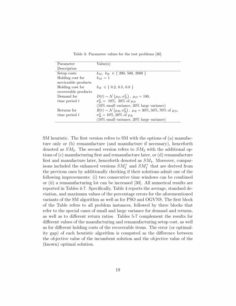
Table 3: Parameter values for the test problems [30].

Parameter Value(s)DescriptionSetup costs kM , kR ∈ { 200, 500, 2000 }Holding cost for hM = 1serviceable productsHolding cost for hR ∈ { 0.2, 0.5, 0.8 }recoverable productsDemand for D(t) ∼ N

(µD, σ

2D

), µD = 100,

time period t σ2D = 10%, 20% of µD

(10% small variance, 20% large variance)Returns for R(t) ∼ N

(µR, σ

2R

), µR = 30%, 50%, 70% of µD,

time period t σ2R = 10%, 20% of µR

(10% small variance, 20% large variance)

SM heuristic. The first version refers to SM with the options of (a) manufac-ture only or (b) remanufacture (and manufacture if necessary), henceforthdenoted as SM2. The second version refers to SM2 with the additional op-tions of (c) manufacturing first and remanufacture later, or (d) remanufacturefirst and manufacture later, henceforth denoted as SM4. Moreover, compar-isons included the enhanced versions SM+

2 and SM+4 that are derived from

the previous ones by additionally checking if their solutions admit one of thefollowing improvements: (i) two consecutive time windows can be combinedor (ii) a remanufacturing lot can be increased [30]. All numerical results arereported in Tables 4-7. Specifically, Table 4 reports the average, standard de-viation, and maximum values of the percentage errors for the aforementionedvariants of the SM algorithm as well as for PSO and OGVNS. The first blockof the Table refers to all problem instances, followed by three blocks thatrefer to the special cases of small and large variance for demand and returns,as well as to different return ratios. Tables 5-7 complement the results fordifferent values of the manufacturing and remanufacturing setup cost, as wellas for different holding costs of the recoverable items. The error (or optimal-ity gap) of each heuristic algorithm is computed as the difference betweenthe objective value of the incumbent solution and the objective value of the(known) optimal solution.

19

5.4. Experimental results on Schulz [30] benchmarks (T = 12)

As it is shown in Tables 4-7, the proposed OGVNS approach outperforms thestate-of-the-art heuristic methods (i.e., SM2, SM4, SM

+2 , SM4

+, and PSO)from the literature and was able to find 75.8% of the optimal solutions andachieve an average cost error equal to 0.283% in a few seconds.

Table 4: Percentage cost error for all instances as well as for dif-ferent variance of demand, returns, and return ratios.

Algorithm Avg. (%) Std. (%) Max. (%)All Instances SM2 7.5 7.9 49.2

SM4 6.1 7.6 47.3SM+

2 6.9 7.9 49.2SM4

+ 2.2 2.9 24.3PSO 4.3 4.5 49.8

OGVNS 0.3 0.8 8.9Demand Small SM2 7.2 7.9 43.6

Variance SM4 6.0 7.6 47.3SM+

2 6.6 7.9 43.5SM4

+ 2.1 2.8 18.9PSO 4.4 4.6 49.8

OGVNS 0.3 0.7 8.9Large SM2 7.8 8.0 49.2Variance SM4 6.1 7.5 43.9

SM+2 7.2 8.0 49.2

SM4+ 2.4 3.0 24.3

PSO 4.1 4.5 48.3OGVNS 0.3 0.8 6.2

Returns Small SM2 7.3 7.8 47.2Variance SM4 6.1 7.6 47.3

SM+2 6.8 7.8 47.2

SM4+ 2.2 2.9 21.1

PSO 4.3 4.6 46.7OGVNS 0.3 0.8 6.2

Large SM2 7.7 8.0 49.2Variance SM4 6.1 7.5 46.3

SM+2 7.1 8.0 49.2

SM4+ 2.3 2.9 24.3

PSO 4.2 4.5 49.8OGVNS 0.3 0.7 8.9

Return Ratio 30% SM2 5.5 5.5 31.3SM4 3.7 4.5 28.5SM+

2 4.9 5.4 31.3SM4

+ 1.2 1.8 12.1

20

Table 4: Percentage cost error for all instances as well as for dif-ferent variance of demand, returns, and return ratios.

Algorithm Avg. (%) Std. (%) Max. (%)PSO 3.5 3.1 45.5

OGVNS 0.2 0.6 5.650% SM2 8.5 9.4 40.1

SM4 7.3 8.2 41.8SM+

2 8.0 9.3 39.8SM4

+ 2.3 2.7 16.2PSO 4.1 4.0 34.0

OGVNS 0.3 0.7 6.070% SM2 8.4 8.0 49.2

SM4 7.2 8.7 47.3SM+

2 8.0 8.0 49.2SM4

+ 3.3 3.5 24.3PSO 5.1 5.9 49.8

OGVNS 0.5 1.1 7.9

Table 5: Percentage cost error for different levels of manufacturingsetup cost.

Algorithm Avg. (%) Std. (%) Max. (%)KM = 200 SM2 4.3 4.5 20.2

SM4 3.4 3.6 17.6SM+

2 3.5 4.0 20.2SM4

+ 2.3 2.6 13.5PSO 4.0 3.1 45.5OGVNS 0.4 0.8 6.0

KM = 500 SM2 5.4 5.2 25.1SM4 3.9 3.9 19.3SM+

2 4.8 4.9 23.7SM4

+ 2.1 2.5 12.8PSO 4.5 4.1 27.5OGVNS 0.3 0.8 8.9

KM = 2000 SM2 12.8 9.9 49.2SM4 10.9 10.4 47.3SM+

2 12.6 9.9 49.2SM4

+ 2.3 3.4 24.3PSO 4.4 5.9 49.8OGVNS 0.1 0.4 5.2

21

Table 6: Percentage cost error for different levels of remanufactur-ing setup cost.

Algorithm Avg. (%) Std. (%) Max. (%)KR = 200 SM2 10.9 9.1 49.2

SM4 6.6 7.8 40.2SM+

2 10.0 9.4 49.2SM4

+ 1.9 2.1 11.8PSO 5.7 5.5 49.8OGVNS 0.5 1.0 8.9

KR = 500 SM2 7.9 6.6 34.7SM4 8.1 8.2 47.3SM+

2 7.3 6.6 34.7SM4

+ 3.4 3.2 19.1PSO 3.8 4.1 37.4OGVNS 0.3 0.7 6.0

KR = 2000 SM2 3.7 6.0 29.4SM4 3.5 5.7 25.7SM+

2 3.6 5.9 29.4SM4

+ 1.4 2.9 24.3PSO 3.3 3.5 45.5OGVNS 0.1 0.3 3.1

Our findings in Tables 5 and 6 show that the mean absolute percentageerror of the solutions was inversely proportional to the manufacturing & re-manufacturing cost values. The same findings have also been verified in therecent work by Li et al. in [18], regarding their block-chain based tabu searchalgorithm for the ELSRP. One possible justification of this pattern is the factthat the manufacturing / re-manufacturing decision seems appealing as therespective setup costs become smaller; and thus more interesting combina-tions occur that needs to be examined. In other case, if the manufacturing/ re-manufacturing cost values become higher, then it is prohibitive eitherto manufacture or re-manufacture and, therefore, keeping a stock of prod-ucts in the inventory is the only viable way (that leads to fewer interestingcombinations to check).

Table 7: Percentage cost error for different levels of holding cost.

Algorithm Avg. (%) Std. (%) Maximum (%)hR = 0.2 SM2 5.9 8.0 42.9

SM4 5.3 8.0 47.3SM+

2 5.8 8.0 42.9SM4

+ 1.7 2.5 21.1

22

Table 7: Percentage cost error for different levels of holding cost.

Algorithm Avg. (%) Std. (%) Maximum (%)PSO 4.5 5.2 49.8OGVNS 0.2 0.7 6.2

hR = 0.5 SM2 7.5 7.7 49.2SM4 6.5 7.6 42.4SM+

2 7.0 7.7 49.2SM4

+ 2.3 3.0 24.3PSO 4.3 4.5 45.5OGVNS 0.3 0.7 5.9

hR = 0.8 SM2 9.1 7.7 44.4SM4 6.3 7.0 40.3SM+

2 8.1 7.8 44.4SM4

+ 2.8 3.0 20.6PSO 4.0 3.9 42.9OGVNS 0.3 0.8 8.9

The performance of each aforementioned method is measured by the per-centage error, which is defined as the percentage gap between the optimalsolution (zopt) and the best solution found by our OGVNS algorithm (zbest).The mean absolute percentage error per each problem instance is computedas 100× (zbest − zopt)/zopt. The same way of computing the percentage errorwas used in the studies by Schulz [30] and Moustaki et al. [21]. Therefore, afair comparison between these five approaches (i.e., SM2, SM4, SM

+2 , SM4

+,and PSO) is guaranteed. However, it would not be correct to compare theproposed OGVNS algorithm with the recent work by Li et al. [18], sincethe authors used a different way of computing the mean absolute percent-age error (i.e., 100 × (zbest − zopt)/zbest ), as it is reported in their paper.Regardless of this difference, Li et al. [18] report in their paper that theirblock-chain tabu search algorithm achieved an average cost error equal to0.00082% (using this different way of computing the error) on the same setof benchmark problems. On the other hand, our current implementationachieves an average cost error equal to 0.283% on the same set of benchmarkproblems. However, it should be noted that our proposed implementationhas two distinct benefits. First, it does not depend on any other, commercialor not, integer programming solver (such for example as CPLEX which isrequired in their implementation). For example, in case of larger problems(e.g., T = 52 periods), even the CPLEX solver might require a large amountof computational time to provide only a starting solution. Second, our pro-posed OGVNS approach is considerably faster. The average and maximum

23

computational time for each test instance is only 8.3 and 30 seconds respec-tively, whereas the block-chain based tabu search algorithm presented in [18]require 53.4 and 490.4 seconds on average and maximum case, respectively,as it is depicted in Table 8. In case that the same time-limit of 490.4 secondswas also used by our solver instead of 30 seconds then, even lower averageoptimality gap would have been found. However, the special focus was toprovide not only optimal or near-optimal solutions for the ELSRP but alsoto achieve low computational times, too.

Table 8: Computational times of TS-DLRR [18] and OGVNS.

Computational timesAlgorithm Avg. (sec.) Max. (sec.)

All instances TS-DLRR 53.68 490.38OGVNS 8.30 30.00

Demand Small variance TS-DLRR 58.68 490.38OGVNS 8.00 30.00

Large variance TS-DLRR 48.69 484.33OGVNS 7.60 30.00

Returns Small variance TS-DLRR 54.48 490.38OGVNS 8.30 30.00

Large variance TS-DLRR 52.80 484.33OGVNS 8.00 30.00

Return ratio 30% TS-DLRR 56.51 490.38OGVNS 7.50 30.00

50% TS-DLRR 51.75 475.93OGVNS 8.00 30.00

70% TS-DLRR 52.80 484.33OGVNS 9.10 30.00

kM 200 TS-DLRR 54.79 484.33OGVNS 11.90 30.00

500 TS-DLRR 65.12 490.38OGVNS 8.80 30.00

2000 TS-DLRR 41.14 413.68OGVNS 3.90 30.00

kR 200 TS-DLRR 65.38 478.91OGVNS 12.20 30.00

500 TS-DLRR 61.65 490.38OGVNS 09.20 30.00

2000 TS-DLRR 34.02 484.33OGVNS 3.30 30.00

hR 0.2 TS-DLRR 49.50 475.93OGVNS 7.20 30.00

0.5 TS-DLRR 55.18 484.33

24

Table 8: Computational times of TS-DLRR [18] and OGVNS.

Computational timesAlgorithm Avg. (sec.) Max. (sec.)OGVNS 8.50 30.00

0.8 TS-DLRR 56.37 490.38OGVNS 8.90 30.00

5.5. Experimental results on larger instances (T = 52)

Although the proposed VNS approach outperforms other metaheuristic ap-proaches in the well-known benchmark set by Schulz [30], we demonstratethe robustness by additional computational experiments with even larger in-stances. Thus, we have developed a new full factorial study with a commonplanning horizon T of 52 periods for each instance. This new proposed bench-mark was designed with the same parameter values as in Schulz [30], but itfeatures significantly more difficult instances that are more than four timeslarger. In this new set of benchmark problems, both setup cost parameterskR and kM can be equal to 200, 500, and 2000. Additionally, the holdingcost hM for the serviceable items per unit time is set to one, and the holdingcost hR for the recoverable items per unit time can be equal to 0.2, 0.5, and0.8. Moreover, the customer demands D follow a normal distribution witha mean of 100 units per period, and the amounts of returned products Rfollow a normal distribution with a mean of 30, 50, and 70 units per period.Furthermore, the coefficient of variation in the normal distributions was setto 10% (small variance) and 20% (large variance).

For each setting of the return and demand values, four instances wererandomly drawn. Thus, totally 34 × 22 × 4 = 108 different instances werecreated. Efforts were made to solve each one of them using the latest versionof the state-of-the-art Gurobi optimizer v5.6.2 within a reasonable amount oftime set to 1 hour and tolerance set to 10−4. However, due to the increasedcomputational difficulty, the Gurobi optimizer solved only 54 instances tooptimality. Regarding the remaining instances, the Gurobi optimizer hasonly computed an upper bound of the optimal objective value. Therefore,the proposed RGVNS implementation is compared using all the instanceswith either optimal solutions or only suboptimal. Our RGVNS variant iscompared against Gurobi in order to present the mean optimality error as inthe previous Subsection 5.4 and the differences in CPU time.

It is noteworthy that this new benchmark set is more difficult and largerthan those that have ever been used in the literature, for the ELSR problem.

25

Also, it is the largest one with a realistic planning horizon of 52 weeks peryear. Apart from the Schulz data set, other smaller data sets include the dataset by Li et al. [18] with only 10 instances with dimension T = 50, solved tooptimality. This new benchmark set is publicly available from the authorsweb site: http://users.uom.gr/~sifalera/benchmarks.html. Interestedreaders may find all the 108 instances, with either the optimal solutions foundby Gurobi in the 54 instances or the currently best known solutions for theremaining 54 instances. Regular updates will be made, once new optimalsolutions or new best feasible solutions are found, in the future.

As it is shown in Figure 1, the RGVNS variant achieves an average costerror equal to 2.44% (note that, the optimal values are denoted with boldfont). However, this performance was achieved using only 30 seconds in av-erage, compared to 2450.55 seconds that was required by Gurobi. Totally,the Gurobi solver required 81.69 times more computational time for reachingthese (either optimal or suboptimal) solutions. Nevertheless, the proposedRGVNS approach computed a feasible solution for all the remaining 54 in-stances, whereas it was not possible for the Gurobi optimizer to compute theoptimal solution.

26

No

Guro

bi5.6.2

Randomized

VNS

zB

est

CPU

(secs)

zV

NS

CPU

(secs)

Error(%

)1

8698.8

3600.00

8895.2

30

2.26

28781.8

3600.00

9185.4

30

4.60

38541.6

3187.88

8793.8

30

2.95

48943.8

3600.00

9391.2

30

5.00

59717.0

3600.00

9853.0

30

1.40

69962.5

3600.00

10240.5

30

2.79

79598.0

3600.00

9955.0

30

3.72

89803.5

3600.00

10327.0

30

5.34

910266.2

1095.08

10573.8

30

3.00

10

10812.8

3600.00

11184.8

30

3.44

11

10290.8

3600.00

10445.4

30

1.50

12

10745.6

3600.00

11027.0

30

2.62

13

13201.0

3600.00

13568.0

30

2.78

14

12131.4

3600.00

12387.4

30

2.11

15

13018.4

3600.00

13403.6

30

2.96

16

11853.2

3600.00

12230.6

30

3.18

17

14236.5

3600.00

14429.5

30

1.36

18

13151.0

3600.00

13660.0

30

3.87

19

13902.0

3600.00

14278.5

30

2.71

20

13495.5

3600.00

13725.0

30

1.70

21

14842.4

3600.00

15063.6

30

1.49

22

14122.2

3600.00

14595.4

30

3.35

23

14561.2

3600.00

14854.4

30

2.01

24

13865.9

3600.00

14428.2

30

4.06

25

25657.2

1254.05

26068.2

30

1.60

26

21247.4

3327.17

22016.8

30

3.62

27

24364.4

403.35

24988.2

30

2.56

28

20329.0

2009.03

20479.4

30

0.74

29

26561.0

574.85

26888.0

30

1.23

30

22332.5

840.33

22851.5

30

2.32

31

26625.5

685.63

27326.0

30

2.63

32

23229.5

508.37

23945.5

30

3.08

33

27872.6

724.77

28482.2

30

2.19

34

24116.8

335.65

25426.0

30

5.43

35

26762.4

293.72

27823.6

30

3.97

36

24065.2

334.73

24785.8

30

2.99

37

10622.2

2181.19

10937.4

30

2.97

38

12011.0

3550.75

12266.8

30

2.13

39

10652.2

199.03

10867.0

30

2.02

40

11741.6

3600.00

12088.6

30

2.96

41

12249.5

3600.00

12585.0

30

2.74

42

13845.0

3600.00

13998.5

30

1.11

43

12309.0

569.93

12616.0

30

2.49

44

13627.0

3600.00

13895.0

30

1.97

45

13348.0

3600.00

13584.4

30

1.77

46

15030.8

3422.24

15543.4

30

3.41

47

13635.6

688.26

13979.0

30

2.52

48

15051.8

3600.00

15788.2

30

4.89

49

15625.4

3600.00

15982.8

30

2.29

50

15447.8

3600.00

15984.8

30

3.48

51

14997.8

3600.00

15409.6

30

2.75

52

15176.6

3600.00

15494.0

30

2.09

53

16782.0

3600.00

17172.0

30

2.32

54

17102.5

3600.00

17757.0

30

3.83

No

Guro

bi5.6.2

Randomized

VNS

zB

est

CPU

(secs)

zV

NS

CPU

(secs)

Error(%

)55

16591.4

3600.00

17149.5

30

3.36

56

17217.9

3600.00

17544.0

30

1.89

57

18047.5

3600.00

18215.6

30

0.93

58

18780.2

3600.00

19158.4

30

2.01

59

17742.8

3600.00

18337.2

30

3.35

60

18646.5

3600.00

19212.6

30

3.04

61

27623.8

3200.40

28428.2

30

2.91

62

24892.6

2689.20

25562.4

30

2.69

63

26587.4

1496.08

28083.0

30

5.63

64

24252.4

936.57

24596.2

30

1.42

65

29328.5

2200.10

30033.0

30

2.40

66

26961.5

3600.00

27544.0

30

2.16

67

28484.0

713.44

29139.0

30

2.30

68

27019.0

2115.69

28116.0

30

4.06

69

30515.4

1149.58

31117.4

30

1.97

70

28758.4

3600.00

30014.6

30

4.37

71

29864.6

658.30

30497.4

30

2.12

72

28195.1

3600.00

30267.6

30

7.35

73

14443.4

3.47

14835.4

30

2.71

74

18364.0

145.99

18517.4

30

0.84

75

14954.0

7.75

15007.0

30

0.35

76

17857.8

29.37

17979.2

30

0.68

77

18546.0

10.78

18903.5

30

1.93

78

23069.5

119.99

23266.5

30

0.85

79

18657.5

10.29

18821.0

30

0.88

80

23329.0

33.39

23449.5

30

0.52

81

20999.8

18.80

21431.8

30

2.06

82

26519.6

46.33

27048.6

30

1.99

83

21114.4

9.71

21649.4

30

2.53

84

26162.8

12.50

27142.6

30

3.75

85

19646.0

1423.74

19834.8

30

0.96

86

22567.6

1134.49

23128.6

30

2.49

87

19880.4

2107.85

19963.6

30

0.42

88

22483.8

427.87

22646.6

30

0.72

89

23013.5

3600.00

23190.0

30

0.77

90

27076.0

3600.00

27632.0

30

2.05

91

22706.5

775.33

23090.5

30

1.69

92

26754.0

3600.00

26793.0

30

0.15

93

25890.8

3600.00

26118.8

30

0.88

94

30229.2

3600.00

30669.6

30

1.46

95

26188.8

2839.44

26935.8

30

2.85

96

29504.4

2795.49

30231.2

30

2.46

97

32952.4

2250.36

33512.0

30

1.70

98

33332.2

3600.00

33940.0

30

1.82

99

33072.4

2309.81

33586.2

30

1.55

100

33115.0

2936.20

33539.2

30

1.28

101

36285.9

3600.00

36581.0

30

0.81

102

37205.5

3600.00

38265.5

30

2.85

103

36173.5

3128.83

37194.0

30

2.82

104

36817.0

3253.05

37861.5

30

2.84

105

38728.0

3600.00

39020.2

30

0.75

106

40310.4

3600.00

41261.8

30

2.36

107

38611.2

3600.00

39281.0

30

1.73

108

39826.1

3083.32

40932.4

30

2.78

Avg.

2450.55

30

2.44

Fig

ure

1:

Res

ult

son

larg

erin

stan

ces

(T=

52).

27

5.6. Discussion

In Table 11, we report the evolution of the optimality gap, (i.e., percentagedminimum error, average error, and maximum error) after each phase of theOGVNS algorithm regarding the set of benchmarks by Schulz [30]. As wecan see, the heuristic start that was employed reached an average error of135.9%. Although this initialization method did not contribute a qualitystarting solution, it was rapid and thus it permitted us to vastly improveit during the next phase. The VND algorithm is afterward applied to thatstarting solution, reducing the average error to 8.4%. Last, using the shakingprocedure based on a complete random order of neighborhoods, an averageerror of 0.283% is reached.

Table 11: Percentage cost error after each OGVNS phase.

Min. (%) Avg. (%) Max. (%)Heuristic start 13.7 135.9 385.3VND 0.0 8.4 50.9Shaking phase 0.0 0.3 8.9

Although a single significant improvement is sometimes more effectivethan several minor improvements, we decided to count the number of im-provements caused by each neighborhood structure instead of the magnitudeof the improvements per neighborhood structure. This way, the most oftenused neighborhood structures were placed first in the order of the VND al-gorithm, in order to accelerate the search. As it was shown, neighborhoodsN15, N4, N2, and N1 contributed the most in the VND method with 29.5%,26.0%, 12.1%, and 11.1%, respectively. This information resulted after anextensive preliminary testing of the proposed OGVNS algorithm on all in-stances. Afterward, the neighborhoods were sorted according to the numberof their local search improvements. This order was finally used by the OVNDalgorithm on all instances. An equally interesting option would be to test adifferent order based on the magnitude of the improvements per neighbor-hood structure instead of the numbers of improvements.

6. Conclusions and future work

In this paper we have addressed the economic lot sizing problem with prod-uct returns and recovery in reverse logistics. We have proposed two novel

28

VNS metaheuristic algorithms that employ new strategies for both the localsearch step and the shaking process. Our VNS approach tackles the NP-hard ELSR problem efficiently and outperforms the state-of-the-art heuristicmethods from the literature (SM variants and PSO). We presented severalnew neighborhoods for this combinatorial optimization problem and an ef-ficient local search method for exploring them. Finally, we also described anew simple heuristic initialization method for this problem. Based on exten-sive numerical testing, using a recent large set of benchmark problems with6480 instances, our approach was able to achieve an average optimality gapequal to 0.283% within average 8.3 seconds. Finally, a new benchmark setwith the currently largest instances (52 periods) in the literature has beendeveloped and made publicly available. The results got by using this latterset showed that the proposed VNS approach is quite efficient in solving largeproblems with a small optimality gap.

A subject for a future work is the adaptation of OGVNS to multi-productdynamic lot sizing problems in closed-loop supply chain [33], and other com-bined problems of inventory and network optimization [31]. Furthermore, itwould be interesting to develop a parallel implementation of our proposedmetaheuristic OGVNS algorithm (e.g., [8, 11]).

Acknowledgement

The authors would like to express their deep appreciation to Dr. T. Schulzfor providing the complete test set that was used in the experimental partof the paper. Also, the work by the third author was conducted at Na-tional Research University Higher School of Economics and supported by RSgrant 14-41-00039. Finally, the authors gratefully acknowledge the helpfulsuggestions of two anonymous reviewers.

References

[1] E. Akcali, S. Cetinkaya, Quantitative models for inventory and pro-duction planning in closed-loop supply chains, International Journal ofProduction Research 49 (2011) 2373–2407.

[2] B. Almada-Lobo, R.J. James, Neighbourhood search meta-heuristicsfor capacitated lot-sizing with sequence-dependent setups, InternationalJournal of Production Research 48 (2010) 861–878.

29

[3] B. Almada-Lobo, J.F. Oliveira, M.A. Carravilla, Production planningand scheduling in the glass container industry: A VNS approach, Inter-national Journal of Production Economics 114 (2008) 363–375.

[4] M.F. Baki, B.A. Chaouch, W. Abdul-Kader, A heuristic solution pro-cedure for the dynamic lot sizing problem with remanufacturing andproduct recovery, Computers & Operations Research 43 (2014) 225–236.

[5] J. Beltran, D. Krass, Dynamic lots sizing with returning items and dis-posals, IIE Transactions 34 (2002) 437–448.

[6] N. Brahimi, S. Dauzere-Peres, Single item lot sizing problems, EuropeanJournal of Operational Research 168 (2006) 1–16.

[7] L. Buschkuhl, F. Sahling, S. Helber, H. Tempelmeier, Dynamic capac-itated lot-sizing problems: a classification and review of solution ap-proaches, OR Spectrum 32 (2010) 231–261.

[8] T. Davidovic, T.G. Crainic, MPI parallelization of variable neighbor-hood search, Electronic Notes in Discrete Mathematics 39 (2012) 241–248.

[9] A. Divsalar, P. Vansteenwegen, D. Cattrysse, A variable neighborhoodsearch method for the orienteering problem with hotel selection, Inter-national Journal of Production Economics 145 (2013) 150–160.

[10] R. Durstenfeld, Algorithm 235: Random permutation, Communicationsof the ACM 7 (1964) 420.

[11] M. Eskandarpour, S.H. Zegordi, E. Nikbakhsh, A parallel variable neigh-borhood search for the multi-objective sustainable post-sales network de-sign problem, International Journal of Production Economics 145 (2013)117–131.

[12] R. Fisher, F. Yates, Example 12, Statistical Tables, London (1938).

[13] R. Geyer, L.N. Van Wassenhove, A. Atasu, The economics of reman-ufacturing under limited component durability and finite product lifecycles, Management Science 53 (2007) 88–100.

[14] B. Golany, J. Yang, G. Yu, Economic lot–sizing with remanufacturingoptions, IIE Transactions 33 (2001) 995–1003.

30

[15] S. Hanafi, J. Lazic, N. Mladenovic, C. Wilbaut, I. Crevits, New vari-able neighbourhood search based 0-1 mip heuristics, Yugoslav Journalof Operations Research - (2014) –. (to appear).

[16] W.L. Ijomah, A model-based definition of the generic remanufacturingbusiness process (2002).

[17] D.E. Knuth, The Art of Computer Programming, Vol. 2: SeminumericalAlgorithms, volume 2, Addison-Wesley, 1969.

[18] X. Li, F. Baki, P. Tian, B.A. Chaouch, A robust block-chain basedtabu search algorithm for the dynamic lot sizing problem with productreturns and remanufacturing, Omega 42 (2014) 75–87.

[19] R.T. Lund, Remanufacturing, Technology Review 87 (1984) 19–23.

[20] N. Mladenovic, P. Hansen, Variable neighborhood search, Computers &Operations Research 24 (1997) 1097–1100.

[21] E. Moustaki, K.E. Parsopoulos, I. Konstantaras, K. Skouri, I. Ganas,A first study of particle swarm optimization on the dynamic lot sizingproblem with product returns, in: Proceedings of the XI Balkan Con-ference on Operational Research (BALCOR 2013), Belgrade-Zlatibor,Serbia, 2013, pp. 348–356.

[22] G. Nenes, S. Panagiotidou, R. Dekker, Inventory control policies forinspection and remanufacturing of returns: A case study, InternationalJournal of Production Economics 125 (2010) 300–312.

[23] P. Pineyro, O. Viera, Inventory policies for the economic lot–sizing prob-lem with remanufacturing and final disposal options, Journal of Indus-trial and Management Optimization 5 (2009) 217–238.

[24] P. Pineyro, O. Viera, The economic lot-sizing problem with remanufac-turing and one-way substitution, International Journal of ProductionEconomics 124 (2010) 482–488.

[25] W.H. Press, S.A. Teukolsky, W.T. Vetterling, B.P. Flannery, Numericalrecipes in Fortran 77: The art of scientific computing, volume 1, 2 ed.,Cambridge University Press, 1992.

31

[26] J. Puchinger, G. Raidl, Bringing order into the neighborhoods: re-laxation guided variable neighborhood search, Journal of Heuristics 14(2008) 457–472.

[27] M.J. Retel Helmrich, R. Jans, W. van den Heuvel, A.P. Wagelmans,Economic lot-sizing with remanufacturing: complexity and efficient for-mulations, IIE Transactions 46 (2014) 67–86.

[28] K. Richter, M. Sombrutzki, Remanufacturing planning for the reversewagner/whitin models, European Journal of Operational Research 121(2000) 304–315.

[29] K. Richter, J. Weber, The reverse wagner/whitin model with variablemanufacturing and remanufacturing cost, International Journal of Pro-duction Economics 71 (2001) 447–456.

[30] T. Schulz, A new silver–meal based heuristic for the single–item dynamiclot sizing problem with returns and remanufacturing, International Jour-nal of Production Research 49 (2011) 2519–2533.

[31] A. Sifaleras, Minimum cost network flows: Problems, algorithms, andsoftware, Yugoslav Journal of Operations Research 23 (2013) 3–17.

[32] A. Sifaleras, Classification of network optimization software packages,in: M. Khosrow-Pour (Ed.), Encyclopedia of Information Science andTechnology, 3rd ed., IGI Global, Hershey, PA, 2015, pp. 7054–7062.

[33] A. Sifaleras, I. Konstantaras, General variable neighborhood searchfor the multi-product dynamic lot sizing problem in closed-loop sup-ply chain, in: 3rd International Conference on Variable NeighborhoodSearch (VNS’14), Djerba, Tunisia, 2014.

[34] A. Sifaleras, D. Urosevic, N. Mladenovic, Preface: EURO Mini Confer-ence (MEC XXVIII) on Variable Neighborhood Search, Electronic Notesin Discrete Mathematics 39 (2012) 1–4.

[35] O. Tang, R.H. Teunter, Economic lot scheduling problem with returns,Production and Operations Management 15 (2006) 488–497.

[36] R.H. Teunter, Z.P. Bayindir, W. Van den Heuvel, Dynamic lot sizingwith product returns and remanufacturing, International Journal of Pro-duction Research 44 (2006) 4377–4400.

32

[37] R.H. Teunter, K. Kaparis, O. Tang, Multi–product economic lot schedul-ing problem with separate production lines for manufacturing and re-manufacturing, European Journal of Operational Research 191 (2008)1241–1253.

[38] R.H. Teunter, O. Tang, K. Kaparis, Heuristics for the economic lotscheduling problem with returns, International Journal of ProductionEconomics 118 (2009) 323–330.

[39] D. Urosevic, Variable neighborhood search for maximum diverse group-ing problem, Yugoslav Journal of Operations Research 24 (2014) 21–33.

[40] H.M. Wagner, T.M. Whitin, Dynamic version of the economic lot sizemodel, Management Science 5 (1958) 88–96.

[41] Y. Xiao, I. Kaku, Q. Zhao, R. Zhang, A reduced variable neighbor-hood search algorithm for uncapacitated multilevel lot-sizing problems,European Journal of Operational Research 214 (2011) 223–231.

[42] Y. Xiao, I. Kaku, Q. Zhao, R. Zhang, A variable neighborhood searchbased approach for uncapacitated multilevel lot-sizing problems, Com-puters and Industrial Engineering 60 (2011) 218–227.

[43] Y. Xiao, R. Zhang, Q. Zhao, I. Kaku, Y. Xu, A variable neighborhoodsearch with an effective local search for uncapacitated multilevel lot-sizing problems, European Journal of Operational Research 235 (2014)102–114.

[44] J. Yang, B. Golany, G. Yu, A concave–cost production planning problemwith remanufacturing options, Naval Research Logistics 52 (2005) 443–458.

[45] S. Zanoni, A. Segerstedt, O. Tang, Multiproduct economic lot schedulingproblem with manufacturing and remanufacturing using a basic periodpolicy, Computers & Industrial Engineering 62 (2012) 1025–1033.

33