Variable cirrus shading during CSIP IOP 5. I: Effects on the initiation of convection

QUARTERLY JOURNAL OF THE ROYAL METEOROLOGICAL SOCIETYQ. J. R. Meteorol. Soc. 133: 1643–1660 (2007)Published online in Wiley InterScience(www.interscience.wiley.com) DOI: 10.1002/qj.124

Variable cirrus shading during CSIP IOP 5. I: Effects on theinitiation of convection

J. H. Marsham,a* C. J. Morcrette,b K. A. Browning,b A. M. Blyth,a D. J. Parker,a

U. Corsmeier,c N. Kalthoffc and M. Kohlerc

a University of Leeds, UKb University of Reading, UK

c Universitat/Forschungszentrum Karlsruhe, Germany

ABSTRACT: Observations from the Convective Storm Initiation Project (CSIP) show that on 29 June 2005 (IntensiveObservation Period 5) cirrus patches left over from previous thunderstorms reduced surface sensible and latent heat fluxesin the CSIP area. Large-eddy model (LEM) simulations, using moving positive surface-flux anomalies, show that we expectthe observed moving gaps in the cirrus cover to significantly aid convective initiation. In these simulations, the timing ofthe CI is largely determined by the amount of heat added to the boundary layer, but weak convergence at the rear edge ofthe moving anomalies is also significant.

Meteosat and rain-radar data are combined to determine the position of convective initiation for all 25 trackable showersin the CSIP area. The results are consistent with the LEM simulations, with showers initiating at the rear edge of gaps, atthe leading edge of the anvil, or in clear skies, in all but one of the cases. The initiation occurs in relatively clear skies inall but two of the cases, with the exceptions probably linked to orographic effects.

For numerical weather prediction, the case highlights the importance of predicting and assimilating cloud cover. Theresults show that in the absence of stronger forcings, weak forcings, such as from the observed cirrus shading, candetermine the precise location and timing of convective initiation. In such cases, since the effects of shading by cirrusanvils from previous convective storms are relatively unpredictable, this is expected to limit the predictability of theconvective initiation. Copyright 2007 Royal Meteorological Society

KEY WORDS cloud shading; nonclassical mesoscale circulation; flux inhomogeneity; convective inhibition

Received 11 December 2006; Revised 24 May 2007; Accepted 31 May 2007

1. Introduction

Predicting the precise location and timing of convectivestorms remains a major challenge for numerical weather-prediction (NWP) models. Although the new generationof non-hydrostatic models, which use grid spacings of theorder of one kilometre, can sometimes give reasonablepredictions of such storms (e.g. Golding et al., 2005),they cannot consistently forecast them (Clark and Lean,2006). The Convective Storm Initiation Project (CSIP)(Browning et al., 2006a), which took place in the summerof 2005 in southern England, aims to improve ourunderstanding of the mechanisms that initiate convectivestorms in the mid-latitude maritime climate of the UK.This understanding can then be used to understand thelikely sources of error in high-resolution NWP forecasts,and so improve NWP.

This paper explores the effects of moving cirrus anvilson the convective initiation (CI) observed on 29 June2005, during CSIP Intensive Observation Period (IOP) 5.

* Correspondence to: J. H. Marsham, Institute for Atmospheric Sci-ence, School of Earth and Environment, University of Leeds, Leeds,LS2 9JT, UK. E-mail: [email protected]

These anvils were generated by storms over France, andthen advected over the UK. A number of the showers thatdeveloped during IOP 5 did so within the area of southernEngland where numerous instruments were deployed aspart of CSIP (Browning et al., 2006a). A subjectiveexamination of the location of the first appearance ofthese showers, made during the course of nowcastingfor CSIP, suggested that the presence of cirrus shieldsmay have been influencing the locations of CI (Browninget al., 2006b), despite the cirrus moving at approximately15 ms−1.

It is well known that mesoscale spatial variations influxes can induce circulations, such as the sea breezesthat frequently affect CI in the UK (Bennett et al., 2006).In general, variations in cloud cover, or other parameterssuch as soil wetness or vegetation, can also induce suchcirculations (called ‘nonclassical mesoscale circulations’by Segal and Arritt (1992)).

Segal et al. (1986) described idealized two-dimensionalsimulations of circulations driven by variable cloudcover. The contrast between an extensive clear area(about 80 km across) and an extensive cloudy area wasshown to induce a circulation comparable to a sea breeze,when the clouds reduced solar fluxes by 60%. They

Copyright 2007 Royal Meteorological Society

1644 J. H. MARSHAM ET AL.

noted that even two hours of partial cloud cover canlead to the generation of a circulation that may be ofmeteorological significance; but all model runs were per-formed with slower-moving cloud-cover variations thanwere observed in CSIP IOP 5 (1.7 ms−1 compared withapproximately 15 ms−1).

Cases of cloud shading affecting CI had been observedpreviously. Bailey et al. (1981) showed that the con-trast between two extensive areas of cloudy and clearsky (about 300 km across) appears to have generateda mesoscale circulation, which initiated storms; andMcNider et al. (1984) showed that a mesoscale circula-tion driven by cloud-cover variations was responsible forthe initiation of a line of thunderstorms in Texas. How-ever, both these cases involved more extensive areas ofslower-moving cloud cover than were observed duringCSIP IOP 5. Roebber et al. (2002) described a case fromOklahoma and Kansas (USA), where a cirrus shield wasimportant in limiting the development of convection andreducing the competition between storms. Their resultsalso suggested that gaps in the moving cirrus cover (diam-eters of 50 km or more, with speeds of approximately50 km/h) could be linked to the initiation of convection.However, this effect on CI was not evaluated statistically,and the relative contributions of boundary-layer warmingand convergence induced by the gaps were not evaluated.

Section 2 of this paper briefly describes CSIP IOP 5.Section 3 quantifies the observed effects of the cir-rus cover on the surface fluxes. Idealized modelling,described in Section 4, is then used to investigate whateffects we expect such moving surface-flux anomalies tohave on CI. The observed locations of the CI relative tothe cirrus clouds are then discussed in Section 5, in thecontext of these modelling results.

The observed effects of the cirrus shading on theboundary layer are discussed in the second part ofthis study (Marsham et al., 2007). There, we showthat the boundary layer was approximately 0.8 g kg−1

drier under thick cirrus, and that this cirrus led to theformation of a stable internal layer at the surface, fewerwarm moist updraughts, and in some places a decreasedboundary-layer height. These effects on the boundarylayer are expected to have inhibited CI, thus supportingthe conclusions of this paper.

2. Synoptic situation and overview of convectiveinitiation in the CSIP area

A mature cyclone was present over the British Isles on 29June 2005 (Figure 1). The CSIP area, in southern Eng-land, was behind (south of) the occluded front associatedwith this cyclone. Thunderstorms over northwest Franceat 06:00 UTC generated long-lived cirrus anvils. Afterthe demise of these storms, the orphaned anvils wereadvected across the Channel, reaching the CSIP area ataround 09:00 UTC. From around 10:30 UTC onwards,convective showers initiated over southern England andquickly developed into a series of thunderstorms. Thesestorms merged to form a band of heavy precipitationextending east–west across Britain (Figure 2). As aresult of this heavy rain, some flash-flooding occurred inOxfordshire (approximately 100 km north of Chilbolton).

Figure 3 shows the orphaned cirrus anvils. Theseappear as blue areas in the satellite images, since theyare cold and reflect solar radiation relatively well. Therain-radar data show that no precipitation from theseanvils reached the surface. Convective clouds, whichappear as unevenly-coloured yellow regions, were also

Figure 1. Met Office analysis of mean sea-level pressure at 12:00 UTC on 29 June 2005 (CSIP IOP 5).

Copyright 2007 Royal Meteorological Society Q. J. R. Meteorol. Soc. 133: 1643–1660 (2007)DOI: 10.1002/qj

CIRRUS SHADING DURING CSIP IOP 5. I: INITIATION OF CONVECTION 1645

observed. Some of these produced significant precipita-tion, as shown by the rain-radar data. Figure 3 shows acumulonimbus appearing to form approximately 20 kmnortheast of Chilbolton on the edge of a roughly-circular gap (diameter about 25 km) at 12:00 UTC. By13:00 UTC there were two significant showers in thisgap, which had grown in size and been advected north-wards.

3. Observed effects of the cirrus cover on surfacefluxes

Figure 4 shows the radiative effects of the cirrus anvilsat Chilbolton, where solar and surface fluxes were mea-sured. Surface heat fluxes (Figure 4(a)) were measuredby eddy correlation (Andreas et al., 2005; Kalthoff et al.,2006). Figure 4(b) shows visible-wavelength top-of-

Figure 2. Radar rain rates at 15:00 UTC on 29 June 2005 (CSIP IOP 5). The Chilbolton radar is at the centre of the range rings, shown at 25 kmintervals. Part of the line of storms approximately 100 km north of Chilbolton developed from showers that initiated near Chilbolton, which are

the subject of this study.

Figure 3. Left: false-colour Meteosat images. Visible top-of-atmosphere reflectance is shown in red and green, and 11 µm brightness temperatureis shown in blue, so that cirrus appears blue and cumulus yellow. Positions of surface-flux observations are indicated by white crosses (withBath west of Chilbolton). Right: rain-radar data (the colour scale is the same as in Figure 2). Both Meteosat and radar plots are shown at 12:00and 13:00 UTC, and range rings are centred on the Chilbolton radar and shown at 25 km intervals. The apparent difference between the satellite

and radar positions of the easternmost storm at 13:00 UTC is due to parallax.



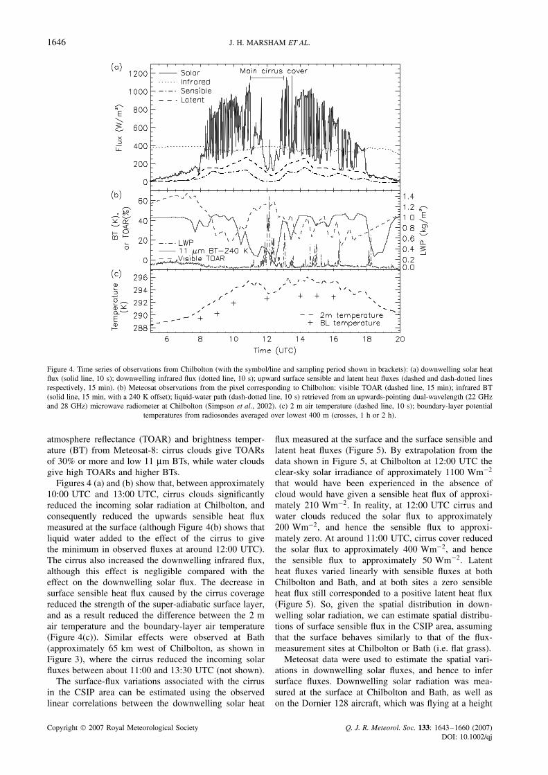
Figure 4. Time series of observations from Chilbolton (with the symbol/line and sampling period shown in brackets): (a) downwelling solar heatflux (solid line, 10 s); downwelling infrared flux (dotted line, 10 s); upward surface sensible and latent heat fluxes (dashed and dash-dotted linesrespectively, 15 min). (b) Meteosat observations from the pixel corresponding to Chilbolton: visible TOAR (dashed line, 15 min); infrared BT(solid line, 15 min, with a 240 K offset); liquid-water path (dash-dotted line, 10 s) retrieved from an upwards-pointing dual-wavelength (22 GHzand 28 GHz) microwave radiometer at Chilbolton (Simpson et al., 2002). (c) 2 m air temperature (dashed line, 10 s); boundary-layer potential

temperatures from radiosondes averaged over lowest 400 m (crosses, 1 h or 2 h).

atmosphere reflectance (TOAR) and brightness temper-ature (BT) from Meteosat-8: cirrus clouds give TOARsof 30% or more and low 11 µm BTs, while water cloudsgive high TOARs and higher BTs.

Figures 4 (a) and (b) show that, between approximately10:00 UTC and 13:00 UTC, cirrus clouds significantlyreduced the incoming solar radiation at Chilbolton, andconsequently reduced the upwards sensible heat fluxmeasured at the surface (although Figure 4(b) shows thatliquid water added to the effect of the cirrus to givethe minimum in observed fluxes at around 12:00 UTC).The cirrus also increased the downwelling infrared flux,although this effect is negligible compared with theeffect on the downwelling solar flux. The decrease insurface sensible heat flux caused by the cirrus coveragereduced the strength of the super-adiabatic surface layer,and as a result reduced the difference between the 2 mair temperature and the boundary-layer air temperature(Figure 4(c)). Similar effects were observed at Bath(approximately 65 km west of Chilbolton, as shown inFigure 3), where the cirrus reduced the incoming solarfluxes between about 11:00 and 13:30 UTC (not shown).

The surface-flux variations associated with the cirrusin the CSIP area can be estimated using the observedlinear correlations between the downwelling solar heat

flux measured at the surface and the surface sensible andlatent heat fluxes (Figure 5). By extrapolation from thedata shown in Figure 5, at Chilbolton at 12:00 UTC theclear-sky solar irradiance of approximately 1100 Wm−2

that would have been experienced in the absence ofcloud would have given a sensible heat flux of approxi-mately 210 Wm−2. In reality, at 12:00 UTC cirrus andwater clouds reduced the solar flux to approximately200 Wm−2, and hence the sensible flux to approxi-mately zero. At around 11:00 UTC, cirrus cover reducedthe solar flux to approximately 400 Wm−2, and hencethe sensible flux to approximately 50 Wm−2. Latentheat fluxes varied linearly with sensible fluxes at bothChilbolton and Bath, and at both sites a zero sensibleheat flux still corresponded to a positive latent heat flux(Figure 5). So, given the spatial distribution in down-welling solar radiation, we can estimate spatial distribu-tions of surface sensible flux in the CSIP area, assumingthat the surface behaves similarly to that of the flux-measurement sites at Chilbolton or Bath (i.e. flat grass).

Meteosat data were used to estimate the spatial vari-ations in downwelling solar fluxes, and hence to infersurface fluxes. Downwelling solar radiation was mea-sured at the surface at Chilbolton and Bath, as well ason the Dornier 128 aircraft, which was flying at a height



Figure 5. Observed surface and solar fluxes at (a) Chilbolton and (b) Bath, from 10:00 to 14:00 UTC. Solid lines show least-squares fits to datafrom the named site. Dashed lines show fits to data from the other site.

of about 500 m from 09:00 to 12:38 UTC. The expectedclear-sky downwelling solar flux was calculated at hourlyintervals using the observed profile and the Fu–Liou radi-ation code (Fu and Liou, 1992, 1993), and these data werethen interpolated to give a value for each observationtime.

Figure 6 shows the correlations between the solartransmission (i.e. the observed downwelling solar radi-ation divided by the calculated clear-sky value) and theMeteosat data, for the visible TOARs and the 11 µm BTs.(Observed errors in the geolocation of the Meteosat datawere corrected, and a parallax correction was applied toall pixels (Johnson et al., 1994), using a cloud-top heightof 6 km. This height was derived from vertical scans bythe high-power radars at Chilbolton. The Meteosat pixelused was then shifted by up to one pixel north or southto give the best correlations, to allow for uncertainties inthese two corrections.) The linear fits calculated for thetwo sites were similar, except where an outlying obser-vation with a high TOAR gave a shallower gradient forthe Bath data.

Figure 7 shows surface sensible heat fluxes calcu-lated from Meteosat data, using the linear fits betweenMeteosat data and solar transmission (Figure 6), andbetween surface sensible heat flux and downwellingsolar radiation (Figure 5), observed at Chilbolton. TheChilbolton site was chosen, rather than Bath, because theprecipitating storms studied were nearer to Chilbolton.These estimated fluxes are valid only over land andfor surfaces similar to those where the eddy-correlationfluxes were obtained (i.e. over flat grass). The fluxesare also only valid for cloud conditions similar to thoseobserved. Thus, although Figures 7 (a) and (b) showbroadly similar patterns, they do show significantly dif-ferent fluxes in some areas. Both show extensive areasoutside the cirrus coverage (Figure 3) with surface sen-sible fluxes of approximately 200 Wm−2, values of0–50 Wm−2 under the cirrus, and gaps in the cirrus coverwith fluxes of about 150 Wm−2. However, significantdifferences between Figures 7 (a) and (b) do occur, forexample 100 km north of Chilbolton, in an area affected

by low stratiform cloud, and 75 km west-southwest ofChilbolton, in an area with widespread shallow cumulus.These occur because the correlations between Meteosatobservations and solar transmission were derived largelyfor cirrus cover. However, coverage of low stratiformcloud was very limited in the area of interest during thehours preceding CI, and we show in Section 4.5 that theeffects on modelled CI of neglecting the shading from,and radiative heating of, developing cumulus are rela-tively small.

It is of interest to compare the magnitude of thevariations in surface fluxes induced by the moving cirrusanvils with typical effects of land-use variations onsurface fluxes. In southern England, apart from land/seaeffects, the largest land-use effects are from urban versusrural areas. Urban areas are expected to increase daytimesurface sensible fluxes by up to a factor of two anddecrease latent heat fluxes by a factor of between oneand six (Thielen et al., 2000). There are, however, nomajor urban areas in the CSIP area (the largest urbanareas have diameters of approximately 15 km). Variationsin vegetation are likely to have effects of up to onlya factor of 2.5 (Segal and Arritt, 1992), and vegetationvariations in southern England also tend to occur on smallspatial scales, so have limited potential for significantdevelopment of mesoscale circulations. In addition, urbanareas and vegetation areas essentially alter only theBowen ratio, which does not alter the flux of equivalentpotential temperature (Betts et al., 1996), while gaps inthe cirrus shading increase both sensible and latent fluxes,and so increase the equivalent-potential-temperature flux.However, variations in Bowen ratio, due to variationsin surface properties, can result in differences in thedependence of the total surface heat flux (sensible pluslatent) on boundary-layer cloud cover. This effect hasbeen neglected; but, as discussed above, the vegetationcover of southern England is relatively uniform.

In conclusion, the magnitudes of the cloud-inducedvariations in fluxes in this case are probably greater thanany urban or vegetation effects. However, in contrastwith land-use variations, the observed cloud-induced



Figure 6. Plots of estimated transmission of solar radiation and Meteosat visible TOAR (a, c, e) and 11 µm BT (b, d, f). Surface data fromChilbolton (a, b) and Bath (c, d) are shown, as well as data from the Dornier 128 aircraft (e, f). For surface data (a, b, c, d), transmission ismean transmission over 200 s (visible) and 600 s (infrared) (i.e. the time taken for a cloud moving at 5 ms−1 to traverse a Meteosat pixel of1 km or 3 km). Error bars show the standard deviation in the Meteosat observations over 3 × 3 pixels, and the standard deviation in the solartransmission over 400 s (visible) and 1200 s (infrared) (10 s-resolution data from Chilbolton and 10 min-resolution data from Bath). For aircraftdata (e, f), transmission is mean transmission over 10 s (visible) and 30 s (infrared) (i.e. approximately the time taken for the aircraft to traverse

a Meteosat pixel of 1 km or 3 km). Straight-line fits are for Chilbolton (solid line), Bath (dashed line), and the aircraft data (dotted line).

variations are moving relative to the surface, and so theeffects are short-lived for a given area. The effects of thismotion are investigated in the next section.

4. Modelling the effects of moving surface-fluxanomalies

Despite the significant approximations in the estimationof effects of the cirrus cloud on the surface fluxes(Figure 7), the estimated fluxes are sufficiently precisefor setting up idealized modelling studies, using theMet Office large-eddy model (LEM) (Gray et al., 2001;e.g. Grabowski et al., 2006). These modelling studies testthe sensitivity of modelled CI to flux variations of similarmagnitudes to those observed during CSIP IOP 5.

The various model runs used are summarized inTable I. Runs using moving positive surface-flux anoma-lies (POS2D and POS3D) were used to investigate the role ofgaps in the cirrus cover in CI. Runs using a moving neg-ative surface-flux anomaly (NEG2D) were used to investi-gate the development of convection along the outer edgesof the cirrus anvil. Finally, runs with a radiative-transferscheme coupled to the LEM (FULLRADN) were used toinvestigate the effects of neglecting the shading by con-vective clouds and the radiative heating of those clouds.

4.1. Method

Simulations using version 2.3 of the LEM were usedto simulate the effects of moving surface-flux anoma-lies. The LEM is a non-hydrostatic model that can berun in one, two or three dimensions. Although the LEMcan be used with a three-phase microphysics scheme,



Figure 7. Estimated surface sensible heat flux at 12:00 UTC, calculated using the observed correlation between solar and sensible fluxes (Figure 5),and the mean correlation between solar transmission and (a) Meteosat visible TOAR and (b) Meteosat 11 µm BT (Figure 6). These fluxes were

derived using surface-flux observations from two locations, and so errors are large in some areas; fluxes are not valid over the sea.

Table I. Summary of sets of model runs used in this paper.

Name Domain size Unperturbed fluxes(sensible & latent, Wm−2)

M D

(km)v

(ms−1)

POS2D 500 km 60 & 180 2 to 5 2 to 50 0 to 15POS3D 500 km by 3 × D 60 & 180 5 30 10 and 15NEG2D 500 km 240 & 480 0.25 to 0.5 100 0 to 15FULLRADN 500 km f (solar): see Figure 5 0.5 30 10

only cloud-water and rain (a Kessler rain scheme)were included, since the process of CI that was beinginvestigated occurred before the ice-phase processeswere significant (the melting level was at approximately3000 m, about 1400 m above the level of free convec-tion). The model domain was 20 km deep, and Rayleighdamping was applied above 13 km. For two-dimensionalsimulations, we used horizontal grid spacings of 200 mand vertical grid spacings of 50–100 m in the bound-ary layer and 100 m up to heights of approximately5000 m, with progressively larger vertical grid spacingsabove 5000 m. Horizontal grid spacings of 1 km wereused in three-dimensional simulations (POS3D), becauseof computational constraints, and vertical grid spacingswere identical to those used in two-dimensional simula-tions. Periodic lateral boundary conditions were used inall simulations.

The model was initialized with the radiosondesounding, shown in Figure 8, made from Reading at11:15 UTC. Reading, approximately 50 km northeast ofChilbolton, was the closest site to the initiation of thedeeper cells observed northeast of Chilbolton between12:00 and 13:00 UTC. For two-dimensional simulations,the model domain was aligned with the observed wind atthe level of the cirrus clouds. This gave boundary-layerwinds of up to 5 ms−1 (Figure 8(b)).

In all runs, it was assumed that the only effect of thecirrus was to modify the downwelling solar radiation atthe surface, and hence the surface fluxes; this is justified,because vertical scans by the Chilbolton radars showthat the cirrus did not extend much below 5 km andfalling ice could not reach convective storms initiating ataround 1600 m (the level of free convection). Radiativeheating of the cloud and atmosphere, as well as shadingof the surface by the developing convection, were alsoneglected in most simulations (POS2D, POS3D and NEG2D).These last assumptions were tested in a third set ofsimulations (FULLRADN), which used a radiative-transferscheme coupled to the LEM.

For runs used to investigate the role of gaps in thecirrus cover in CI (POS2D and POS3D), uniform sensibleand latent fluxes of 60 Wm−2 and 180 Wm−2 respec-tively were applied at the surface in the model, except inthe moving flux anomaly, where fluxes were multipliedby a factor M . This positive flux anomaly representedthe effect of a gap in the cirrus cover. The width of theflux anomaly, D, was varied between 2 km and 50 km.This range of scales encompasses the 25 km size ofthe gap observed northeast of Chilbolton at 12:00 UTC(Figure 3). The speed of the anomaly was varied betweenzero and 15 ms−1; the speed of travel of the anvil wastracked by Meteosat (this is consistent with radiosonde



Figure 8. 11:15 UTC radiosonde profile from Reading, one of the nearest radiosonde sites to the early shower-initiation events: (a) tephigram;(b) wind velocities. In the legend, ‘2D wind’ refers to the wind profile used in two-dimensional LEM simulations (this is the wind velocity in

the direction of the wind velocity at the cirrus altitude).

wind data, which showed wind speeds of approximately15 ms−1 at the cirrus altitude of approximately 7 km, or400 hPa). The factor M was varied between 2 and 5.In the two-dimensional simulations, a large domain of500 km was used. Thus, an anomaly of width 50 kmmoving at 15 ms−1 did not reach the far end of thedomain in a 7 h simulation. In three-dimensional sim-ulations (POS3D), the domain width was three times theanomaly diameter D (in the dimension perpendicular tothe cirrus steering velocity), and again 500 km long.

To investigate the development of cumulus along theouter edges of the overall cirrus anvil (NEG2D), uniformsensible and latent fluxes of 240 Wm−2 and 480 Wm−2

respectively were applied at the surface in the model,except in the moving flux anomaly where fluxes werereduced by a factor M . The diameter of the cold anomalywas fixed at 100 km, approximately the diameter of theanvil shown in Figure 3, and its speed again variedbetween zero and 15 ms−1. The model domain was600 km long. Thus, these experiments were very similarto the positive-anomaly runs, except that in this case thepositive area (i.e. the area not affected by the negativeanomaly) was wide (500 km), whereas the warm area inthe runs with a positive anomaly was narrow (2–50 km).

For the third set of runs (FULLRADN), used to testthe assumption that shading by convective clouds andradiative heating of convective clouds could be neglected,a constant top-of-atmosphere downwelling solar flux wasused, calculated for 12:00 UTC at Chilbolton on 29 June2005. This downwelling flux was halved, except in a30 km gap moving at 10 ms−1, which represented thegap in the cirrus cloud cover. The surface fluxes were

specified to depend on the downwelling solar radiationat the surface, using the linear correlation shown forChilbolton in Figure 5, allowing shading by convectiveclouds to be accounted for. The four-stream radiationmodel, with six solar and twelve infrared bands, of (Fuand Liou, 1992, 1993) was used, with an independentpixel approximation.

4.2. Scale analysis

With spatially-uniform and time-invariant surface fluxes,the time taken for cloud top to reach a particular heightbetween 1100 m and 3000 m was found to be, to a goodapproximation, inversely proportional to the surface flux(not shown). So, with a surface flux F , the time taken inthe absence of a flux anomaly is

t = Q

F, (1)

where Q is the amount of heat required per unit area. Amoving surface-flux anomaly, with diameter D and speedv, increasing surface fluxes by a factor M , will affect anypoint for a time less than or equal to D/v. Therefore, Ifheat is not mixed horizontally, the time taken for thecloud top to reach a particular height will be reduced by(M − 1)D/v, if this time depends only on the maximumamount of heat added to the boundary layer at any point.

The situation is not one-dimensional, though. Figure 9shows a schematic of the heat added to the bound-ary layer, if the heat is not mixed horizontally, at timet > D/v. Using this simple model, we expect the pres-sure perturbation �p induced by the flux anomaly to



be proportional to Q2 − Q1 (Figure 9). Thus, using theBoussinesq approximation, the maximum pressure gradi-ent induced, dp/dx, is approximated by

�p

�x≈ g

CpT

Q2 − Q1

D, (2)

where g is the acceleration due to gravity, Cp is thespecific heat capacity of the air, and T is the meantemperature in the boundary layer. Substituting for Q1

and Q2 (Figure 9) gives:

�p

�x≈ g

CpT

(M − 1)F

v. (3)

These expressions are equally valid for a positiveor a negative anomaly, and the pressure gradient isindependent of the anomaly diameter D. From themomentum equation, using

�u ≈ 1

ρ�t

�p

�x, (4)

(where ρ is the air density and �u is the velocityperturbation in time �t), and

�t = D

v,

Equation (3) gives:

�u

�x≈ g

ρCpT

(M − 1)F

v2 . (5)

Hence, from continuity and convergence in two dimen-sions,

dw

dz= −du

dx,

we get:w

H≈ g

ρCpT

(M − 1)F

v2 , (6)

where w is the vertical velocity and H the depth ofthe boundary layer. We expect this convergence to be

D

Totalheatadded

MFFFF Ft=0

D

Anomaly speed, v

Wind

Distance

Model cross section at t > D/v

t=t

Q2

Q1

Q1=tFQ2=(t+(M–1)D/v)F

Figure 9. Schematic of the model set-up for the POS2D and POS3D runs,with a positive flux anomaly (diameter D, speed v) at time t > D/v.The initial anomaly position is shown in grey, and the final positionin black. A quantity of heat Q1 has been added to columns unaffectedby the flux anomaly, while for columns over which the whole anomaly

has moved, this is increased to Q2.

increased for a circular anomaly in three dimensions,using

dw

dz= −du

dx− dv

dy,

in the three-dimensional case.This uplift will lift any lid at the top of the boundary

layer, reducing the convective inhibition (CIN):

CIN = 1

z0

∫R�T dz, (7)

where �T is the difference in density temperaturebetween the parcel and its surroundings, R is the gasconstant for dry air, and z0 is the scale height of theatmosphere. Assuming that the convergence leads toadiabatic uplift of air at the top of the boundary layer,this gives:

dCIN

dt= R

z0

(p0

p

)− RCp

∫w

dθv

dzdz, (8)

where dθ/dz is the dry adiabatic lapse rate, and where wehave assumed that pressure is constant over the regionof CIN. Over the time (D/v) for which the anomalyincreases the surface fluxes at a point, this will reducethe CIN by approximately

�CIN ≈(

p0

p

)− RCp RgH 2

z0ρCpT

dθv

dz

(M − 1)FD

v3 . (9)

Thus, with a flux of MF over the anomaly, and aconstant pressure p0, the time taken for CI is reduced by

�t ≈ RgH 3

z0CpT

dθv

dz

(M − 1)D

Mv3 , (10)

if the whole boundary-layer depth has to be heated toovercome the CIN.

Figure 10 shows another schematic of the heat addedto the boundary layer, this time with t < D/v, againassuming that heat does not mix horizontally. In this casethe maximum pressure gradient induced is given by:

�p

�x≈ g

CpT

Q2 − Q1

tv, (11)

or:�p

�x≈ g

CpT

(M − 1)F

v. (12)

Using Equation (4), and

�x = v�t,

we obtain:�u

�x≈ g

ρCpT

(M − 1)F

v2 . (13)



Totalheatadded

Anomaly speed, v

Distance

Model cross section at t < D/v

MF

t=0

tv tv

FF F

Wind

t=t

Q2

Q1

Q1=MtFQ2=tF

Figure 10. As Figure 9, but for t < D/v and for a negative fluxanomaly (NEG2D).

This is the same expression as Equation (5), for t >

D/v, and again it is valid for positive or negative fluxanomalies.

4.3. Modelled effects of moving positive surface-fluxanomalies

All runs described in this section are two-dimensionalexcept where stated otherwise. In runs using small(2–50 km-width) positive flux anomalies (i.e. POS2D andPOS3D in Table I), the modelled cloud-top height tendedto remain at approximately 1 km for some time, andthen grew rapidly through the level of free convectionat 1600 m to approximately 4 km.

For cases where the time taken for the cloud-top toreach a particular height (the ‘onset time’) is greater than

the transit time (D/v), if the one-dimensional argumentpresented in Section 4.2 holds, then the data shown inFigure 11 should follow straight lines (as indicated by thediagonal dashed lines). The data in Figure 11 are closeto straight lines, but with slightly steeper gradients thanthe 1 : 1 dashed lines shown. This shows that it is largelythe quantity of heat added to any point that determineswhen the cloud top reaches a particular height (the one-dimensional assumption), but the convergence producedby the moving anomalies also significantly aids the devel-opment of the convection. The data shown in Figures11 (b) and (c) are further from the dashed straight linesshown than the data shown in Figure 11(a). This showsthat convergence effects are more significant for the timetaken for the cloud top to reach 1600 m or 3000 m than1100 m. The level of free convection is approximately1600 m, so Figure 11(b) shows the timing of CI. Thereis a discontinuity in the data shown in Figure 11(b), withCI approximately 1 h faster for (M − 1)D/v > 0.7. Thisdoes not seem to correspond to any threshold in the quan-tities D, D/v, M and so on, but suggests that there isa threshold in (M − 1)D/v for the anomalies to inducesufficient convergence to affect the modelled CI.

As (Petch, 2006) leads us to expect, increasing thegrid spacing from 200 m to 1 km in the Met Office LEMincreases the time taken for the cloud top to reach itslevel of free convection (Figures 11 (b) and (d)). Petch

Figure 11. Time taken for cloud-top height to reach (a) 1100 m, (b, d) 1600 m and (c) 3000 m (‘onset time’), plotted against (M − 1)D/v (theeffect of the positive flux anomaly expected from a one-dimensional argument, Section 4.2), for multiple model runs. Panels (a, b, c) show resultsfrom two-dimensional runs with 200 m grid spacings. Panel (d) shows results from two- and three-dimensional runs with 1 km grid spacings.Dashed diagonal lines show the results expected from the one-dimensional argument (Section 4.2), with the dashed diagonal line in (d) the sameas that shown in (b). Symbols indicate the magnitude of the flux anomaly. Data within a square are for v = 15 ms−1 and varying D; otherwisedata are for D = 30 km and varying v. Large diamonds indicate where the transit time (D/v) is greater than the onset time. Dotted vertical

lines demarcate the estimated range of observed (M − 1)D/v.



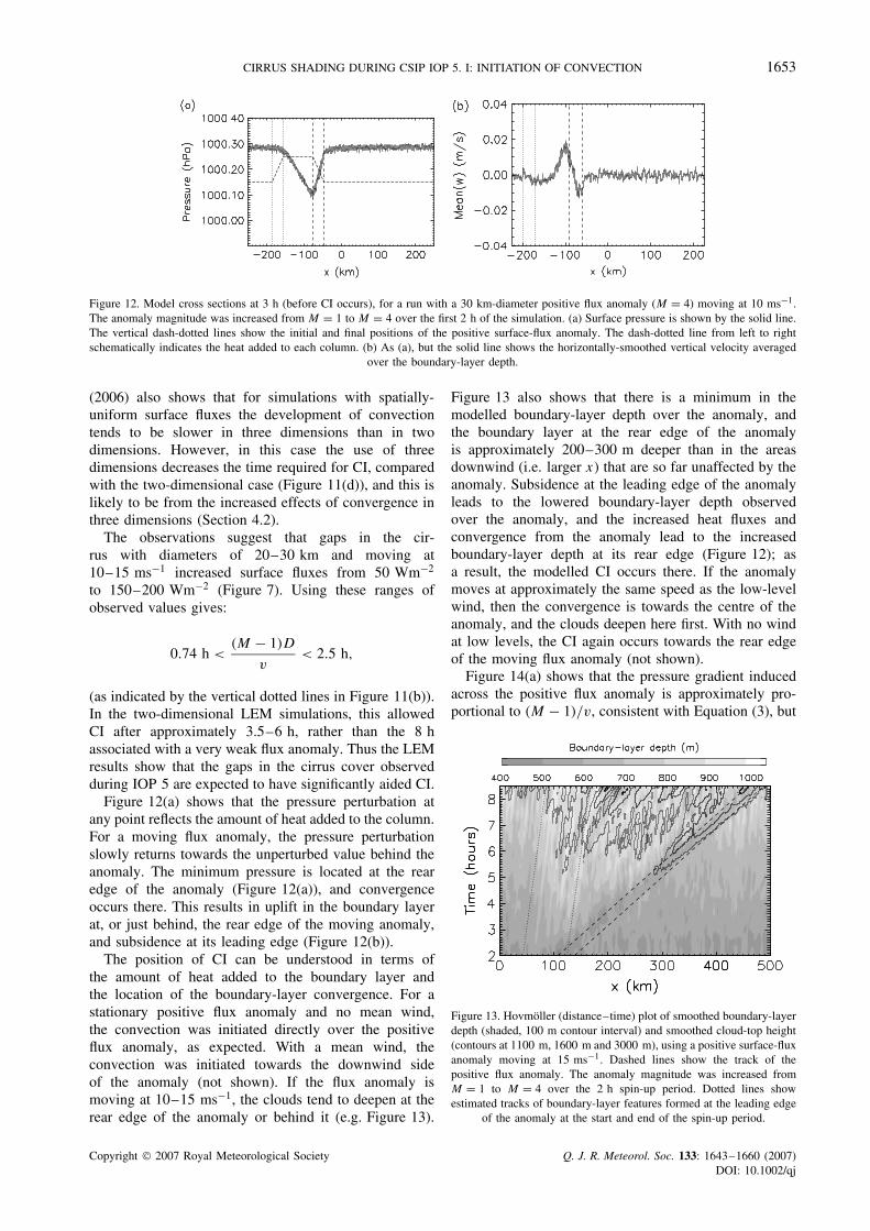
Figure 12. Model cross sections at 3 h (before CI occurs), for a run with a 30 km-diameter positive flux anomaly (M = 4) moving at 10 ms−1.The anomaly magnitude was increased from M = 1 to M = 4 over the first 2 h of the simulation. (a) Surface pressure is shown by the solid line.The vertical dash-dotted lines show the initial and final positions of the positive surface-flux anomaly. The dash-dotted line from left to rightschematically indicates the heat added to each column. (b) As (a), but the solid line shows the horizontally-smoothed vertical velocity averaged

over the boundary-layer depth.

(2006) also shows that for simulations with spatially-uniform surface fluxes the development of convectiontends to be slower in three dimensions than in twodimensions. However, in this case the use of threedimensions decreases the time required for CI, comparedwith the two-dimensional case (Figure 11(d)), and this islikely to be from the increased effects of convergence inthree dimensions (Section 4.2).

The observations suggest that gaps in the cir-rus with diameters of 20–30 km and moving at10–15 ms−1 increased surface fluxes from 50 Wm−2

to 150–200 Wm−2 (Figure 7). Using these ranges ofobserved values gives:

0.74 h <(M − 1)D

v< 2.5 h,

(as indicated by the vertical dotted lines in Figure 11(b)).In the two-dimensional LEM simulations, this allowedCI after approximately 3.5–6 h, rather than the 8 hassociated with a very weak flux anomaly. Thus the LEMresults show that the gaps in the cirrus cover observedduring IOP 5 are expected to have significantly aided CI.

Figure 12(a) shows that the pressure perturbation atany point reflects the amount of heat added to the column.For a moving flux anomaly, the pressure perturbationslowly returns towards the unperturbed value behind theanomaly. The minimum pressure is located at the rearedge of the anomaly (Figure 12(a)), and convergenceoccurs there. This results in uplift in the boundary layerat, or just behind, the rear edge of the moving anomaly,and subsidence at its leading edge (Figure 12(b)).

The position of CI can be understood in terms ofthe amount of heat added to the boundary layer andthe location of the boundary-layer convergence. For astationary positive flux anomaly and no mean wind,the convection was initiated directly over the positiveflux anomaly, as expected. With a mean wind, theconvection was initiated towards the downwind sideof the anomaly (not shown). If the flux anomaly ismoving at 10–15 ms−1, the clouds tend to deepen at therear edge of the anomaly or behind it (e.g. Figure 13).

Figure 13 also shows that there is a minimum in themodelled boundary-layer depth over the anomaly, andthe boundary layer at the rear edge of the anomalyis approximately 200–300 m deeper than in the areasdownwind (i.e. larger x) that are so far unaffected by theanomaly. Subsidence at the leading edge of the anomalyleads to the lowered boundary-layer depth observedover the anomaly, and the increased heat fluxes andconvergence from the anomaly lead to the increasedboundary-layer depth at its rear edge (Figure 12); asa result, the modelled CI occurs there. If the anomalymoves at approximately the same speed as the low-levelwind, then the convergence is towards the centre of theanomaly, and the clouds deepen here first. With no windat low levels, the CI again occurs towards the rear edgeof the moving flux anomaly (not shown).

Figure 14(a) shows that the pressure gradient inducedacross the positive flux anomaly is approximately pro-portional to (M − 1)/v, consistent with Equation (3), but

Figure 13. Hovmoller (distance–time) plot of smoothed boundary-layerdepth (shaded, 100 m contour interval) and smoothed cloud-top height(contours at 1100 m, 1600 m and 3000 m), using a positive surface-fluxanomaly moving at 15 ms−1. Dashed lines show the track of thepositive flux anomaly. The anomaly magnitude was increased fromM = 1 to M = 4 over the 2 h spin-up period. Dotted lines showestimated tracks of boundary-layer features formed at the leading edge

of the anomaly at the start and end of the spin-up period.



Figure 14. Modelled (a) pressure gradient as a function of (M − 1)/v (Equation (3)), and (b) maximum vertical velocity integrated over theboundary-layer depth (smoothed over 2 km) as a function of (M − 1)/v2 (Equation (6)) at 4 h, for runs with no saturation.

the values are approximately three-quarters of those pre-dicted. Figure 14(b) shows the maximum vertical windin the boundary layer at the rear edge of the positiveflux anomaly, which is proportional to (M − 1)/v2, con-sistent with Equation (6), but with values approximatelyone-third of those predicted. Considering the idealizednature of the arguments used to derive the theoreticalvalues, these differences between the modelled and pre-dicted quantities shown in Figure 14 are not surprising.

Figure 15 shows the difference between the modelresults and the linear fit shown in Figure 11, as a func-tion of (M − 1)D/Mv3 (Equation (10)), representing theimpact on CIN. The results correlate to some extent, pro-viding some support for the effects of the convergence-driven uplift outlined in Section 4.2. Again, the scatterand the differences in the absolute values are certainlynot surprising, given the idealized nature of the scalingarguments involved. The relationship is not as good asthat between the deviation and (M − 1)D/v, however(Figure 11(b)); thus this deviation depends more on theextra heat added to any column by the flux anomaly thanon the estimated impact on CIN (Equation (10)). Thisshows that although the theory outlined in Section 4.2predicts the pressure gradients and uplift well, the effectson CIN and CI are more complex.

Figure 15. Deviation of data shown in Figure 11(b) from thestraight-line fit, as a function of (M − 1)D/Mv3 (compare with Equa-

tion (10)).

4.4. Modelled effects of moving negative surface-fluxanomalies

A wide (100 km-diameter) moving negative flux anomalywas applied to represent the effects of the overall cirrusanvil (NEG2D runs, Table I), rather than the positiveanomalies used to represent the gaps in Section 4.3. Thesesimulations are essentially similar to those describedin (Segal et al., 1986), except that the speed of thecloudy region is much larger here (up to 15 ms−1

compared with 1.7 ms−1). Results from (Segal et al.,1986) suggest that convergence and uplift should begenerated at the edges of the cold anomaly, and thatthis uplift should be maintained or enhanced at theleading edge of the anomaly, but reduced on its trailingedge.

Two sets of simulations were performed. The firstincluded no saturation, so vertical velocities were due todry convection influenced by the moving cold anomaly.This allowed the effects of the cold anomaly, onceit had moved far from its starting position, to beunderstood without the added complexities of moistconvection. In the second, warm phase, microphysicswere included. This resulted in clouds forming whilethe position of the cold anomaly overlapped its initialposition.

Figure 16 shows that without saturation in the modelthe moving cold anomaly suppressed convection in itspath, as expected, but there is uplift just inside itsleading edge and subsidence at its trailing edge. Thisuplift is reduced when the anomaly speed is increased(Figure 16(b)), and the uplift and corresponding horizon-tal pressure gradients are again predicted reasonably wellby the theory described in Section 4.1 (not shown).

With saturation included in the model, clouds form anddeepen in the region of maximum heating, i.e. ahead ofand behind the track of the cold anomaly (Figure 17).Figure 17(a) shows that with a mean wind, which allowsclouds to move more ‘in phase’ with the anomaly, deeperconvection persists in the region of convergence alongthe leading edge of the anomaly. Clouds are suppressedin the subsidence at the trailing edge of the movinganomaly, with or without the mean wind in the model(Figure 17).



Figure 16. Vertical velocity w, averaged over the boundary-layer depth after 4 h (so that t > D/v), in model runs without saturation and liquidwater. The thin and thick lines shows data smoothed over 4 km and 40 km, respectively. Results are from a dry run (i.e. with no saturation),so clouds do not affect the velocities. The observed wind was used. Dotted (dashed) lines give the starting (final) position of the cold anomaly,

which is moving at 15 ms−1. Anomaly speeds of (a) 10 ms−1 and (b) 15 ms−1 were used.

Figure 17. Hovmoller (distance–time) plots of modelled LWP using a cold anomaly, moving at 15 ms−1, using (a) observed wind and (b) nowind. Contours are at 0.01 kg m−2 (dotted lines), 0.1 kg m−2 (thin solid lines) and 1.0 kg m−2 (thick solid lines). Dashed lines show the path

of the moving cold anomaly.

Overall, the suppression of convection by the coldanomaly is clear, and the results predict enhancementof convection at the leading edge of the cirrus anvilsduring CSIP IOP 5 and subsidence at their trailing edge.This suggests that the cumulus convection observed atthe leading edge of the anvil (Section 5) may have beenenhanced by circulations induced by the cirrus-cloudshading.

4.5. Results from simulations using a radiative-transfermodel

Here we test the assumptions used so far: that the effectsof shading by convective clouds and radiative heatingof convective clouds can be neglected. Figure 18 showsa space–time diagram of cloud-top height from modelruns (FULLRADN in Table I) neglecting and includingthese effects. It can be seen that the convection isfairly insensitive to allowing the convective clouds tointeract with the downwelling radiation. With and withoutthe fully-coupled radiation, convection develops alongthe rear (upwind) edge of the positive flux anomalyand behind the anomaly (Figure 18). This justifies theassumption, used in Sections 4.3 and 4.4, that the effectsof the cirrus clouds can be represented by movingsurface-flux anomalies.

The shading by developing convective clouds reducedthe surface sensible heat fluxes by around 20 Wm−2.However, radiative heating of those clouds to someextent compensated for the reduction in surface fluxes byincreasing the column-integrated radiative heating ratesby up to 10 Wm−2. These values are small comparedwith the magnitude of the effects of the solar fluxanomaly itself, which in these runs increases surface-sensible-heat fluxes from approximately 40 Wm−2 to125 Wm−2. As a result, a run allowing for shading byconvective clouds and radiative heating of those cloudsgives very similar CI to a run neglecting both effects(Figure 18).

5. Analysis of observed convective initiation in theCSIP area

Section 2 shows the kind of observational data thatled Browning et al. (2006a) to hypothesize that variableshadowing by moving cirrus anvils may have affectedCI during CSIP IOP 5. Modelling results discussed inSection 4 show that this is indeed to be expected. Inthis section, we examine the observational data in detail,to see whether these findings are fully substantiated.In fact, the observed fields of cirrus cloud cover andconvective development were complex, and so the results,



Figure 18. Hovmoller (distance–time) plots of smoothed cloud-top heights above 1600 m, (a) without radiative heating of clouds or shading byconvective clouds, and (b) with fully-coupled radiation. The diagonal dashed lines show the path of the moving positive solar flux anomaly,

which increased the modelled downwelling solar flux by a factor of two.

while supporting the hypothesis, are not in themselvesdefinitive.

Tracking the observed precipitation and the corre-sponding cumulus convection, using the rain-radar net-work and Meteosat data respectively, allowed the loca-tions of convective initiation and development to bedetermined and compared with the cirrus cloud cover.The starting point of this analysis was to determine thetrajectories of all precipitation echoes forming withinthe CSIP area (a 200 km-by-200 km square centred onChilbolton) that could be tracked for at least two framesof the 15 min data from the radar network. Those echoesthat formed on the outer edge of pre-existing showers,which are likely to have been due to secondary initiation,were excluded from the analysis. A total of 25 showerswere tracked in this way.

The high-resolution visible data from Meteosat werethen used to track the specific convective clouds asso-ciated with these 25 showers. A parallax correction wasapplied to the Meteosat data (Johnson et al., 1994). Thisassumed a cloud-top height of 5 km, since radiosondedata collected in the CSIP area showed that, providedthe lid at around 900 hPa could be overcome, con-vection from the surface could rise to a height ofaround 550 hPa (approximately 5 km). This was alsoobserved in the LEM simulations. Figure 19 shows thatthere is good agreement between the location of theradar and satellite tracks (black and grey lines, respec-tively), except that convective clouds were normallyvisible before precipitation was detected. This showsthat the parallax correction used is sufficiently accu-rate for the purpose intended, i.e. determining the loca-tion of the convective clouds with respect to the cirrusclouds.

The 11 µm BT from Meteosat was used to definemasks (shown as grey in Figure 19), which approxi-mately described the locations of the cirrus cloud at thetimes of CI. Observations of the cirrus cloud made bythe 3 GHz radar at Chilbolton indicated that the baseof the cirrus was located between 5.5 km and 6.5 km.Radiosonde data showed that the temperature at 6 kmwas around 250 K, so a BT threshold of 250 K was used

to define the area covered by the cirrus clouds. This sim-ple threshold used to define the cirrus mask is fairly crude(for example, it does not take account of thin cirrus thatappears warmer than this threshold), but it is useful asa means of classifying the location of initiation of theshowers in terms of whether they occur under cloudyor clear sky. In addition, the 250 K threshold used wasthe maximum BT for which the cirrus shading had cleareffects on the water-vapour mixing ratio observed at mid-levels in the boundary layer (Marsham et al., 2007, figure8).

Determining the location of CI for the clouds thatdeveloped into showers was not always easy, becauseof obscuration by cirrus for certain periods of time, andso the procedure is explained in some detail. For eachof the 25 showers, the times of first precipitation echo(FPE) and first satellite cloud were determined fromthe radar network and Meteosat high-resolution visibledata. The observed propagation speeds and directions ofthe rain showers and cumulus clouds (when detected)were then used to estimate a series of locations for thedeveloping convection in the hour preceding FPE, in casethis convection was hidden by cirrus cover during thistime. This was not a problem after 13:15 UTC, since afterthis time all showers initiated in clear skies, so Figure 19is limited to showing these tracks for showers that formedbefore this time. If one of these back-trajectory locationshad been under the cirrus, then there would have beenthe possibility that cumulus clouds formed earlier thancould be detected and were hidden by the cirrus; but thiswas never observed to occur. Consequently, for showersfor which clouds were detectable in the satellite data,the time of first observed convective cloud was taken asthe time of CI. In some cases, however, there were nowell-defined clouds in the visible imagery that could beassociated with the radar tracks. For these cases, the timeof CI was assumed to be the most recent time when theback-trajectory was under clear sky (showers 4, 12, 13and 19, with assumed CI 30–45 min before FPE). If thisnever occurred (showers 11 and 17), then initiation musthave occurred under the cirrus, and the time of CI wastaken as 30 min before FPE (since 32 min was the meantime difference between FPE and observed CI).



-100 -80 -60 -40 -20 0 20 40 60 80 100-100

-80

-60

-40

-20

0

20

40

60

80

1001100 1115

11451130

Distance (km)

-100 -80 -60 -40 -20 0 20 40 60 80 100

Distance (km)

-100 -80 -60 -40 -20 0 20 40 60 80 100

Distance (km)

-100 -80 -60 -40 -20 0 20 40 60 80 100

Distance (km)

Dis

tanc

e (k

m)

-100

-80

-60

-40

-20

0

20

40

60

80

100

Dis

tanc

e (k

m)

-100

-80

-60

-40

-20

0

20

40

60

80

100

Dis

tanc

e (k

m)

-100

-80

-60

-40

-20

0

20

40

60

80

100

Dis

tanc

e (k

m)

16

4

9

13

1

(a)

(c) (d)

(b)

Figure 19. Position of the cirrus mask (grey shading) when CI was estimated to have occurred. The tracks of the showers initiating at that timeare plotted using grey triangles and black lines (radar-derived). The tracks of the convective clouds (when seen by Meteosat) are plotted usingblack circles and grey lines. Inferred locations from CI until a shower was observed are shown by asterisks. The coastline is shown by a blackline. Numbers are used to identify each shower. Initiation was observed to occur in clear skies after 13:15 UTC, and so these times are not

shown (showers 21 to 25). The figure is continued overleaf.

The above analysis showed 2 out of the 25 showersinitiating under the cirrus rather than in clear skies. Themean fraction of sky occupied by the cirrus mask at thetimes of CI was 14%, so a purely random set of CIs wouldhave had 3.5 ± 1.7 of the 25 showers initiating under thecirrus (1.7 is the standard deviation of the binomial dis-tribution). The observed value of 2 out of 25 is thereforeapproximately one standard deviation below the mean.Repeating this analysis, but excluding showers formingafter 13:15 UTC (since these formed in clear skies) givesan observed value of 2 out of 25 showers, and an expectedvalue of 2.9 ± 1.6 for randomly-distributed showers.These results only allow limited confidence in rejectingthe null hypothesis that the cirrus cover did not affect thespatial distribution of the initiation of convection.

Closer inspection of Figure 19 shows that there appearto be four main sub-regions of CI: first, at the leadingedge of the anvil (showers 3, 4, 8, 10, 12, 13 and 16);

secondly, within or at the rear edge of the gap in thecirrus that was situated east of Chilbolton at 12:00 UTC(showers 17, 18, 19 and 20); thirdly, in clear skies behindthe trailing edge of the cirrus anvil (showers 2, 5, 6, 7,14, 15 and 21); and finally, in clear skies far from thecirrus (showers 1 and 9, as well as showers 22, 23, 24 and25, which are not shown but initiated in clear skies after13:15 UTC). If showers 4, 12, 13 and 19 are assumed toinitiate 30 min before FPE, rather than at their last clear-sky location, these categorizations are unchanged. Thispattern of behaviour, with observed CI occurring closeto the rear edge of gaps, at the leading edge of the cirrusanvil and in clear skies, is consistent with the modellingstudies described in Section 4, which show convergenceat the leading edge of the anvil and at the rear edgeof gaps. Shower 11 is the only clear exception to thispattern, since it initiates under the cirrus anvil (shower17 initiates under the cirrus, but at the rear edge of a gap).



2

3

8

10

12

20

1417

18

11

15

19

5

67

-100 -80 -60 -40 -20 0 20 40 60 80 100-100

-80

-60

-40

-20

20

0

40

60

80

1001200 1230

13001245

Distance (km)

-100 -80 -60 -40 -20 0 20 40 60 80 100

Distance (km)

-100 -80 -60 -40 -20 0 20 40 60 80 100

Distance (km)

-100 -80 -60 -40 -20 0 20 40 60 80 100

Distance (km)

Dis

tanc

e (k

m)

(e)

-100

-80

-60

-40

-20

20

0

40

60

80

100

Dis

tanc

e (k

m)

(f)

-100

-80

-60

-40

-20

20

0

40

60

80

100

Dis

tanc

e (k

m)

(g)

-100

-80

-60

-40

-20

20

0

40

60

80

100

Dis

tanc

e (k

m)

(h)

Figure 19. (Continued).

Finally, it is also interesting to note that 6 out of the25 observed CI locations were within 5 km of the edgeof the cirrus mask. If showers were randomly located,we would expect this to be 1.9 ± 1.3 out of 25 (onaverage, 7.6% of the region was within 5 km of theedge of the mask). Again, repeating this analysis for onlyshowers forming before 13:15 UTC gives an observedvalue of 6 showers, and an expected value of 1.6 ±1.2 for randomly-distributed showers. These observedvalues are significantly larger than those expected from arandom distribution of showers, strongly supporting thehypothesis that convergence at the edge of the cirrus anvilaffected CI.

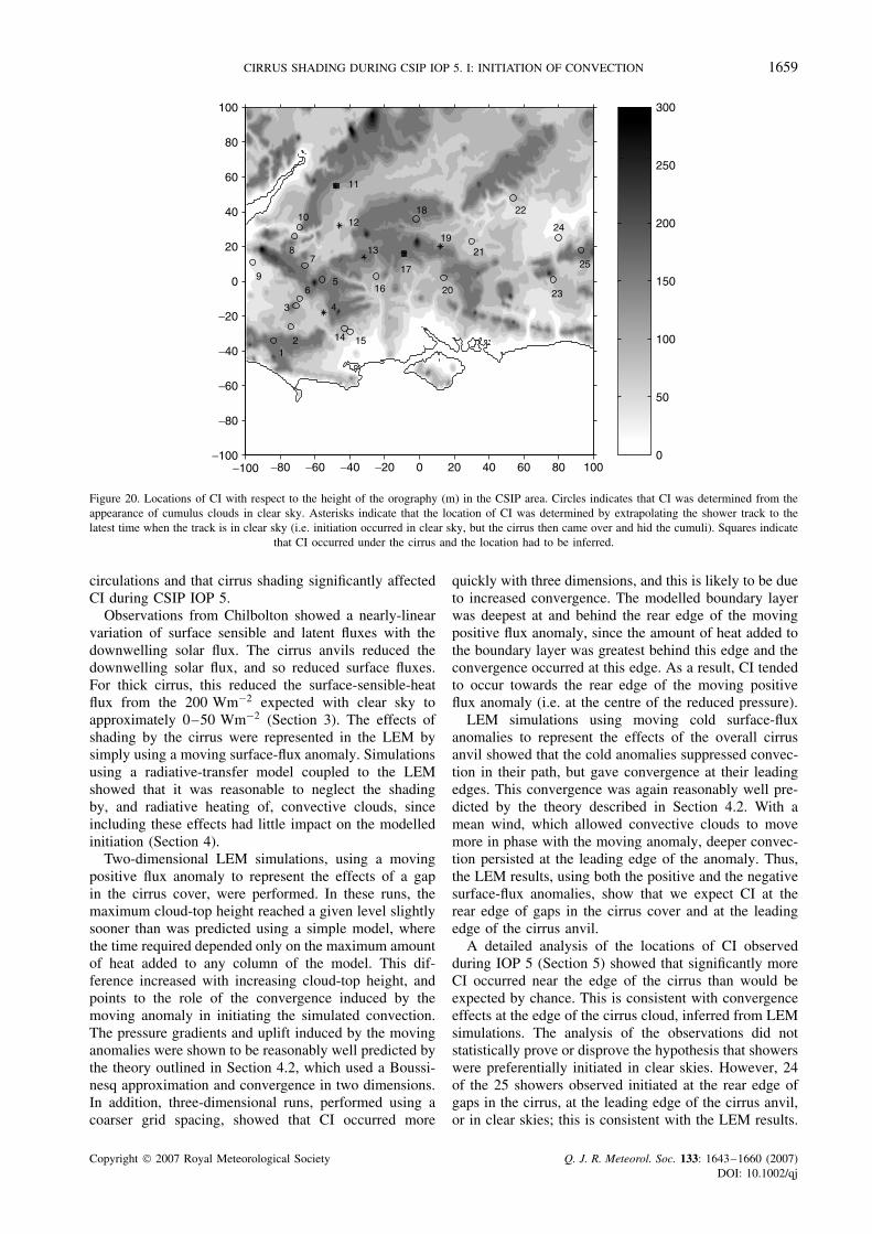
Figure 20 shows inferred locations of CI in relation tothe orography of the CSIP area. It is clear that showersinitiated further south, where the hills also extendedfurther south, suggesting that orographic effects werealso significant. Figure 20 also shows that the showersthat were inferred to have initiated under the cirrus (11and 17) formed on the south-facing (windward) slopes ofhills, suggesting that orographic effects may have beensignificant in these cases.

6. Conclusions

The results described lead us to believe that shading fromcirrus anvils had significant effects on CI during CSIPIOP 5. In LEM simulations, based on observations fromIOP 5, cirrus shading suppressed CI, and the rear edge ofgaps in the cirrus cover and the leading edge of the cirrusanvil were preferred locations for initiation, because ofthe convergence there. Observations of CI from rain-radarand Meteosat satellite data support the hypothesis thatthe leading edge of the anvil, the rear edge of gaps inthe cirrus and clear-sky regions were preferred locationsfor initiation. These results are consistent with (Roebberet al., 2002), but for CSIP IOP 5 the effects of the cirrusshading on surface fluxes have been quantified, LEMsimulations have been used to examine the mechanisms,and the observed distribution of initiation events has beenevaluated statistically. In addition, the effects of the cirrusshading on the boundary layer, described in (Marshamet al., 2007), provide further support for the hypothesesthat variations in cirrus cloud cover led to mesoscale



−100 −80 −60 −40 −20 0 20 40 60 80 100−100

−80

−60

−40

−20

0

20

40

60

80

100

12

3

56

78

9

10

11

12

13

14 15

16

17

18

19

20

21

22

23

24

25

0

50

100

150

200

250

300

4

Figure 20. Locations of CI with respect to the height of the orography (m) in the CSIP area. Circles indicates that CI was determined from theappearance of cumulus clouds in clear sky. Asterisks indicate that the location of CI was determined by extrapolating the shower track to thelatest time when the track is in clear sky (i.e. initiation occurred in clear sky, but the cirrus then came over and hid the cumuli). Squares indicate

that CI occurred under the cirrus and the location had to be inferred.

circulations and that cirrus shading significantly affectedCI during CSIP IOP 5.

Observations from Chilbolton showed a nearly-linearvariation of surface sensible and latent fluxes with thedownwelling solar flux. The cirrus anvils reduced thedownwelling solar flux, and so reduced surface fluxes.For thick cirrus, this reduced the surface-sensible-heatflux from the 200 Wm−2 expected with clear sky toapproximately 0–50 Wm−2 (Section 3). The effects ofshading by the cirrus were represented in the LEM bysimply using a moving surface-flux anomaly. Simulationsusing a radiative-transfer model coupled to the LEMshowed that it was reasonable to neglect the shadingby, and radiative heating of, convective clouds, sinceincluding these effects had little impact on the modelledinitiation (Section 4).

Two-dimensional LEM simulations, using a movingpositive flux anomaly to represent the effects of a gapin the cirrus cover, were performed. In these runs, themaximum cloud-top height reached a given level slightlysooner than was predicted using a simple model, wherethe time required depended only on the maximum amountof heat added to any column of the model. This dif-ference increased with increasing cloud-top height, andpoints to the role of the convergence induced by themoving anomaly in initiating the simulated convection.The pressure gradients and uplift induced by the movinganomalies were shown to be reasonably well predicted bythe theory outlined in Section 4.2, which used a Boussi-nesq approximation and convergence in two dimensions.In addition, three-dimensional runs, performed using acoarser grid spacing, showed that CI occurred more

quickly with three dimensions, and this is likely to be dueto increased convergence. The modelled boundary layerwas deepest at and behind the rear edge of the movingpositive flux anomaly, since the amount of heat added tothe boundary layer was greatest behind this edge and theconvergence occurred at this edge. As a result, CI tendedto occur towards the rear edge of the moving positiveflux anomaly (i.e. at the centre of the reduced pressure).

LEM simulations using moving cold surface-fluxanomalies to represent the effects of the overall cirrusanvil showed that the cold anomalies suppressed convec-tion in their path, but gave convergence at their leadingedges. This convergence was again reasonably well pre-dicted by the theory described in Section 4.2. With amean wind, which allowed convective clouds to movemore in phase with the moving anomaly, deeper convec-tion persisted at the leading edge of the anomaly. Thus,the LEM results, using both the positive and the negativesurface-flux anomalies, show that we expect CI at therear edge of gaps in the cirrus cover and at the leadingedge of the cirrus anvil.

A detailed analysis of the locations of CI observedduring IOP 5 (Section 5) showed that significantly moreCI occurred near the edge of the cirrus than would beexpected by chance. This is consistent with convergenceeffects at the edge of the cirrus cloud, inferred from LEMsimulations. The analysis of the observations did notstatistically prove or disprove the hypothesis that showerswere preferentially initiated in clear skies. However, 24of the 25 showers observed initiated at the rear edge ofgaps in the cirrus, at the leading edge of the cirrus anvil,or in clear skies; this is consistent with the LEM results.



Of the 25 showers, 23 initiated in relatively clear skies,rather than under the cirrus. In both cases, the exceptionsinitiated over the south-facing slopes of significant hills,suggesting that in these cases orographic effects weresignificant. In addition, the observed CI occurred furthersouth to the west of Chilbolton, where hills also extendfurther south, suggesting that the CI may have been moregenerally affected by the orography.

In summary, this CSIP case shows that for forecastingconvective storms using NWP models it is importantto predict or assimilate cloud cover and account forits effects on solar and surface fluxes. At the stageof boundary-layer warming when the CIN has becomesmall, very small perturbations can determine preciselywhere and when CI will occur (e.g. Morcrette et al.,2006; Marsham and Parker, 2006). In such cases, evensmall gaps in cloud cover, of approximately 30 kmdiameter, can significantly affect CI, despite movingrelative to the surface. NWP models cannot be expectedto predict the detailed evolution of upper-level cloudsat long lead times, especially for highly inhomogeneousanvils from earlier convective storms. This provides asignificant limitation on the predictability of CI in caseswhere such subtle forcings are significant.

Acknowledgements

We would like to thank EUMETSAT for the Meteosatdata used in this paper, and the Met Office for theNimrod rain-rate images and the surface-pressure analysischart used. Observations from Chilbolton were courtesyof the Chilbolton Facility for Atmospheric and RadioResearch (CFARR) at the CCLRC-Chilbolton Obser-vatory, distributed via the NERC British AtmosphericData Centre (BADC). We would also like to thank allthose involved in the CSIP field campaigns, and the twoanonymous reviewers whose comments have improvedthe clarity of this paper. This project was funded bythe Natural Environment Research Council (NERC):NER/O/S/2002/00971.

References

Andreas EL, Jordan RE, Makshtas AP. 2005. Parameterizing turbulentexchange over sea ice: the ice station Weddell results. Boundary-Layer Meteorol. 114: 439–460.

Bailey MJ, Carpenter LR, Lowther LR, Passant CW. 1981. A mesoscaleforecast for 14 August 1975 – the Hampstead storm. Meteorol. Mag.110: 147–161.

Bennett LJ, Browning KA, Blyth AM, Parker DJ, Clark PA. 2006.A review of the initiation of precipitating convection in the UnitedKingdom. Q. J. R. Meteorol. Soc. 132: 1001–1020.

Betts AK, Ball JH, Beljaars ACM, Miller MJ, Viterbo PA. 1996.The land surface–atmosphere interaction: A review based onobservational and global modeling perspectives. J. Geophys. Res.101: 7209–7225.

Browning K, Blyth A, Clark P, Corsmeier U, Morcrette C, Agnew J,Bamber D, Barthlott C, Bennett L, Beswick K, Bitter M, Bozier K,Brooks B, Collier C, Cook C, Davies F, Deny B, Engelhardt M,Feuerle T, Forbes R, Gaffard C, Gray M, Hankers R, Hewison T,Huckle R, Kalthoff N, Khodayar S, Kohler M, Kraut S, Kunz M,Ladd D, Lenfant J, Marsham J, McGregor J, Nicol J, Norton E,Parker D, Perry F, Ramatschi M, Ricketts H, Roberts N, Russell

A, Schulz H, Slack E, Vaughan G, Waight J, Watson R, Webb A,Wieser A, Zink K. 2006a. The Convective Storm Initiation Project.Bull. Am. Meteorol. Soc. (to appear).

Browning K, Morcrette C, Blyth A, Bennett L, Clark P, Corsmeier U,Agnew J, Barkwith A, Barthlott C, Behrendt A, Bennett A, BeswickK, Bozier K, Brooks B, Chalmers N, Collier C, Cook C, DacreH, Davies F, Davies L, Davies O, Deny B, Devine G, Dixon M,Engelhardt M, Fitch A, Forbes R, Gaffard C, Gallagher M, GoddardJ, Gray M, Hewison T, Huckle R, Illingworth A, Kalthoff N, KeeleyS, Khodayar S, Kilburn C, Kohler M, Kottmeier C, Kraut S, LaddD, Lean H, Lenfant J, Marsham J, McGregor J, Mobbs S, Nicol J,Norton E, Parker D, Perry F, Ramatschi M, Richardson A, RickettsH, Roberts N, Russell A, Slack E, Vaughan G, Watson R, Webb A,Weckwerth T, Wieser A, Wilson J, Wrench C, Wulfmeyer V, ZinkK. 2006b. ‘A summary of the Convective Storm Initiation ProjectIntensive Observation Periods’. Met Office Forecasting ResearchTechnical Report: 474/JCMM Report 153.

Clark P, Lean H. 2006. ‘An overview of high resolution UMperformance for CSIP cases’. Met Office Forecasting ResearchTechnical Report: 478/JCMM Report 155.

Fu Q, Liou KN. 1992. On the correlated k-distribution method forradiative transfer in nonhomogeneous atmospheres. J. Atmos. Sci.49(22): 2139–2156.

Fu Q, Liou KN. 1993. Parameterization of the radiative properties ofcirrus clouds. J. Atmos. Sci. 50(13): 2008–2025.

Golding B, Clark P, May B. 2005. Boscastle flood: Meteorologicalanalysis of the conditions leading to the flooding on 16 August 2004.Weather 60(8): 230–235.

Grabowski WW, Bechtold P, Cheng A, Forbes R, Hailliwell C,Khairoutdinov M, Lang S, Nasuno T, Petch J, Tao WK, Wong R,Wu X, Xu KM. 2006. Daytime convective development over land:A model intercomparison based on LBA observations. Q. J. R.Meteorol. Soc. 132: 317–344.

Gray MEB, Petch J, Derbyshire SH, Brown AR, Lock AP, Swann HA.2001. ‘Version 2.3 of the Met. Office large eddy model’. Met Office(APR) Turbulence and Diffusion Rep. 276. Met Office, Exeter, UK.

Johnson DB, Flament P, Bernstein RL. 1994. High-resolution satelliteimagery for mesoscale meteorological studies. Bull. Am. Meteorol.Soc. 75: 5–33.

Kalthoff N, Fiebig-Wittmaack M, Meißner C, Kohler M, Uriarte M,Bischoff-Gauß I, Gonzales E. 2006. The energy balance, evapo-transpiration and nocturnal dew deposition of an arid valley in theAndes. J. Arid Environ. 65: 420–443.

Marsham JH, Parker DJ. 2006. Secondary initiation of multiple bandsof cumulonimbus over southern Britain. II: Dynamics of secondaryinitiation. Q. J. R. Meteorol. Soc. 132: 1053–1072.

Marsham JH, Blyth AM, Parker DJ, Beswick K, Browning KA,Corsmeier U, Kalthoff N, Khodayar S, Morcertte CJ, Norton EG.2007. Variable cirrus shading during CSIP IOP 5. II: Effects on theconvective boundary layer. Q. J. R. Meteorol. Soc. 133: 1661–1675.

McNider RT, Jedlovec JD, Wilson GS. 1984. Data analysis andmodel simulation of the initiation of convection on April 24, 1982.Pp. 543–549 in Tenth Conf. on Weather Forecasting and Analysis,Tampa. American Meteorological Society.

Morcrette CJ, Browning KA, Blyth AM, Bozier KE, Clark PA, LaddD, Norton EG, Pavelin E. 2006. Secondary initiation of multiplebands of cumulonimbus over southern Britain. I: An observationalcase-study. Q. J. R. Meteorol. Soc. 132: 1021–1051.

Petch JC. 2006. Sensitivity studies of developing convection in a cloud-resolving model. Q. J. R. Meteorol. Soc. 132: 345–358.

Roebber PJ, Scultz DM, Romero R. 2002. Synoptic regulation of the 3May 1999 tornado outbreak. Weather and Forecasting 17: 399–429.

Segal M, Arritt RW. 1992. Nonclassical mesoscale circulations causedby surface sensible heat-flux gradients. Bull. Am. Meteorol. Soc.73(10): 1593–1604.

Segal M, Purdom JFW, Song JL, Pielke RA, Mahrer Y. 1986.Evaluation of cloud shading effects on the generation andmodification of mesoscale circulations. Mon. Weather Rev. 114:1201–1212.

Simpson PM, Brand EC, Wrench CL. 2002. ‘Microwave radiometermeasurements at Chilbolton – liquid water path algorithm develop-ment and accuracy’. EU FP5-CloudNET Project Report.

Thielen J, Wobrock W, Gadian A, Mestayer PG, Creutin JD. 2000.The possible influence of urban surfaces on rainfall development:a sensitivity study in 2D in the meso-γ -scale. Atmos. Res. 54(1):15–39.


Variable cirrus shading during CSIP IOP 5. I: Effects on the initiation of convection

Documents

Transcript of Variable cirrus shading during CSIP IOP 5. I: Effects on the initiation of convection