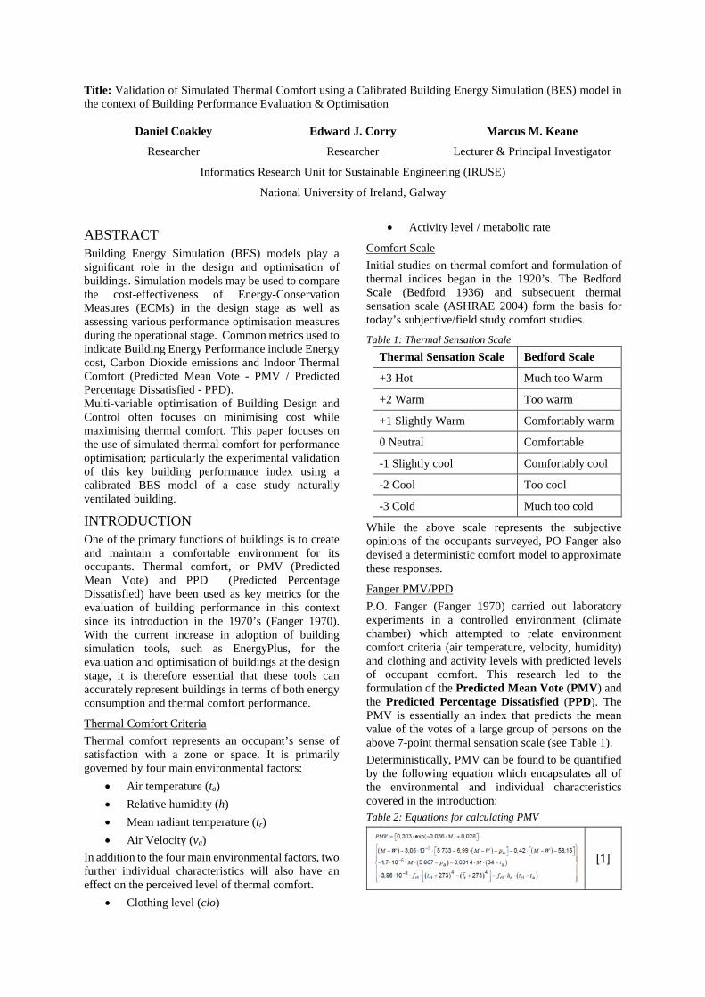
Title: Validation of Simulated Thermal Comfort using a Calibrated Building Energy Simulation (BES) model in the context of Building Performance Evaluation & Optimisation

Daniel Coakley

Researcher

Edward J. Corry

Researcher

Marcus M. Keane

Lecturer & Principal Investigator

Informatics Research Unit for Sustainable Engineering (IRUSE)

National University of Ireland, Galway

ABSTRACT Building Energy Simulation (BES) models play a significant role in the design and optimisation of buildings. Simulation models may be used to compare the cost-effectiveness of Energy-Conservation Measures (ECMs) in the design stage as well as assessing various performance optimisation measures during the operational stage. Common metrics used to indicate Building Energy Performance include Energy cost, Carbon Dioxide emissions and Indoor Thermal Comfort (Predicted Mean Vote - PMV / Predicted Percentage Dissatisfied - PPD). Multi-variable optimisation of Building Design and Control often focuses on minimising cost while maximising thermal comfort. This paper focuses on the use of simulated thermal comfort for performance optimisation; particularly the experimental validation of this key building performance index using a calibrated BES model of a case study naturally ventilated building.

INTRODUCTION One of the primary functions of buildings is to create and maintain a comfortable environment for its occupants. Thermal comfort, or PMV (Predicted Mean Vote) and PPD (Predicted Percentage Dissatisfied) have been used as key metrics for the evaluation of building performance in this context since its introduction in the 1970’s (Fanger 1970). With the current increase in adoption of building simulation tools, such as EnergyPlus, for the evaluation and optimisation of buildings at the design stage, it is therefore essential that these tools can accurately represent buildings in terms of both energy consumption and thermal comfort performance.

Thermal Comfort Criteria Thermal comfort represents an occupant’s sense of satisfaction with a zone or space. It is primarily governed by four main environmental factors:

• Air temperature (ta) • Relative humidity (h) • Mean radiant temperature (tr) • Air Velocity (va)

In addition to the four main environmental factors, two further individual characteristics will also have an effect on the perceived level of thermal comfort.

• Clothing level (clo)

• Activity level / metabolic rate

Comfort Scale Initial studies on thermal comfort and formulation of thermal indices began in the 1920’s. The Bedford Scale (Bedford 1936) and subsequent thermal sensation scale (ASHRAE 2004) form the basis for today’s subjective/field study comfort studies.

Table 1: Thermal Sensation Scale Thermal Sensation Scale Bedford Scale

+3 Hot Much too Warm

+2 Warm Too warm

+1 Slightly Warm Comfortably warm

0 Neutral Comfortable

-1 Slightly cool Comfortably cool

-2 Cool Too cool

-3 Cold Much too cold

While the above scale represents the subjective opinions of the occupants surveyed, PO Fanger also devised a deterministic comfort model to approximate these responses.

Fanger PMV/PPD P.O. Fanger (Fanger 1970) carried out laboratory experiments in a controlled environment (climate chamber) which attempted to relate environment comfort criteria (air temperature, velocity, humidity) and clothing and activity levels with predicted levels of occupant comfort. This research led to the formulation of the Predicted Mean Vote (PMV) and the Predicted Percentage Dissatisfied (PPD). The PMV is essentially an index that predicts the mean value of the votes of a large group of persons on the above 7-point thermal sensation scale (see Table 1). Deterministically, PMV can be found to be quantified by the following equation which encapsulates all of the environmental and individual characteristics covered in the introduction: Table 2: Equations for calculating PMV

[1]

[2]

[3]

Where; M = metabolic rate (W/m2);

W = effective mechanical power (W/m2);

Icl = clothing insulation (m2 ⋅ K/W);

fcl = clothing surface area factor;

ta = air temperature (°C);

tr = mean radiant temperature (°C);

var = the relative air velocity (m/s);

pa = water vapour partial pressure (Pa);

hc = convective heat transfer coefficient [W/(m2⋅K)];

tcl = clothing surface temperature (°C)

clo = clothing units, 1 clo = 0.155m2.oC/W. Since PMV predicts the mean of the comfort votes from a large group, another useful measure is the percentage of the total that will be dissatisfied with the thermal environment. (i.e. those that would vote >2 or <-2 on the thermal sensation scale.

PPD = 100−95⋅exp (−0.03353⋅PMV4−0.2179.PMV2)

Figure 1: PPD versus PMV

Figure 2: PPD versus Temperature (with Clothing)

CASE STUDY Our chosen case study is an 80-seater computer lab in a large engineering building. Located on campus at the

National University of Ireland, Galway, this provided the most suitable demonstrator in terms of access and data availability. In addition, previous assessments had revealed that computer labs in general had relatively highly levels of occupant dissatisfaction in terms of thermal comfort. The study was carried out during peak operating hours on 13/03/2012 (14:00-18:00)

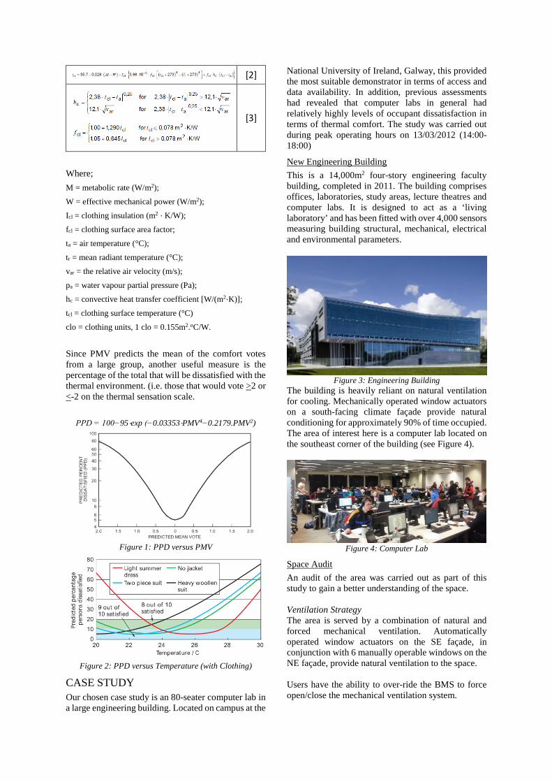
New Engineering Building This is a 14,000m2 four-story engineering faculty building, completed in 2011. The building comprises offices, laboratories, study areas, lecture theatres and computer labs. It is designed to act as a ‘living laboratory’ and has been fitted with over 4,000 sensors measuring building structural, mechanical, electrical and environmental parameters.

Figure 3: Engineering Building The building is heavily reliant on natural ventilation for cooling. Mechanically operated window actuators on a south-facing climate façade provide natural conditioning for approximately 90% of time occupied. The area of interest here is a computer lab located on the southeast corner of the building (see Figure 4).

Figure 4: Computer Lab

Space Audit An audit of the area was carried out as part of this study to gain a better understanding of the space. Ventilation Strategy The area is served by a combination of natural and forced mechanical ventilation. Automatically operated window actuators on the SE façade, in conjunction with 6 manually operable windows on the NE façade, provide natural ventilation to the space. Users have the ability to over-ride the BMS to force open/close the mechanical ventilation system.

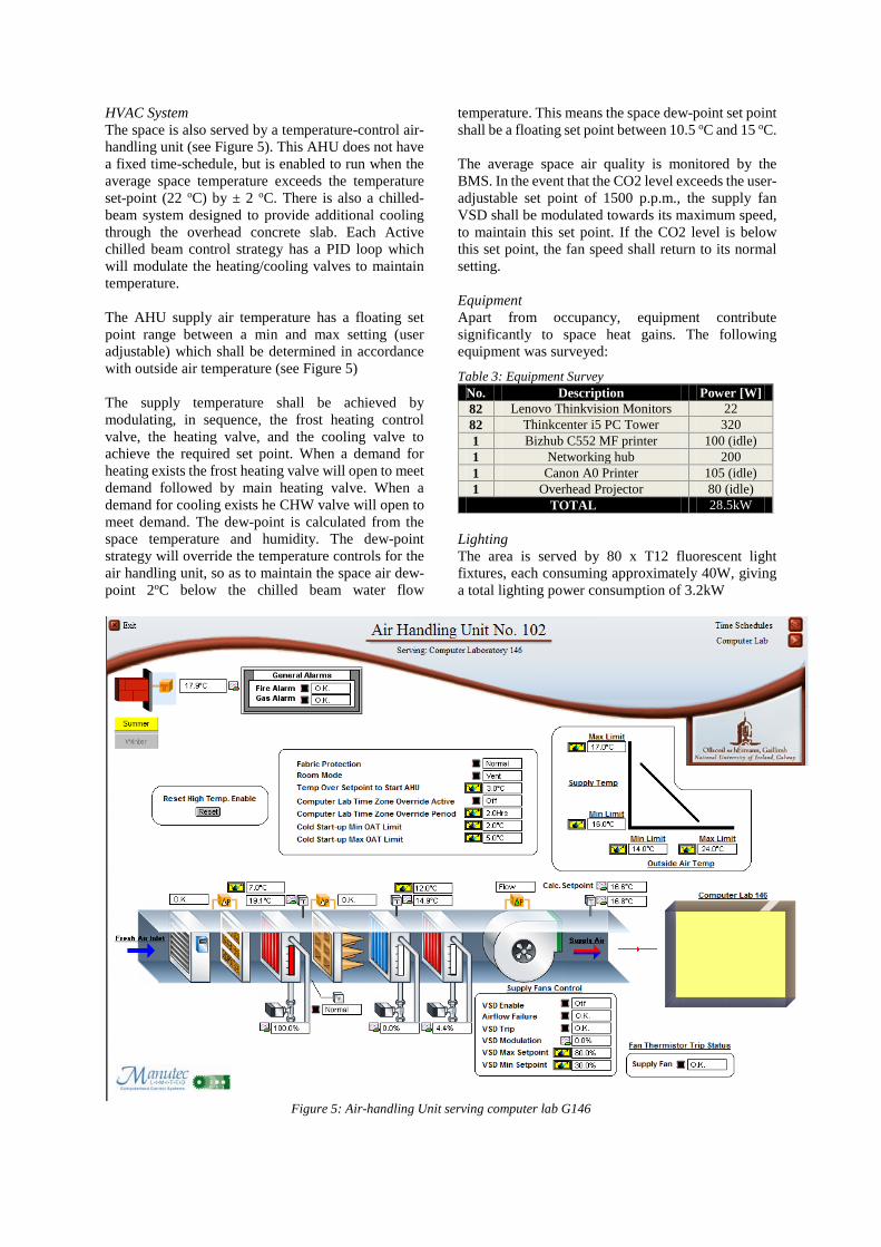
HVAC System The space is also served by a temperature-control air-handling unit (see Figure 5). This AHU does not have a fixed time-schedule, but is enabled to run when the average space temperature exceeds the temperature set-point (22 oC) by ± 2 oC. There is also a chilled-beam system designed to provide additional cooling through the overhead concrete slab. Each Active chilled beam control strategy has a PID loop which will modulate the heating/cooling valves to maintain temperature. The AHU supply air temperature has a floating set point range between a min and max setting (user adjustable) which shall be determined in accordance with outside air temperature (see Figure 5) The supply temperature shall be achieved by modulating, in sequence, the frost heating control valve, the heating valve, and the cooling valve to achieve the required set point. When a demand for heating exists the frost heating valve will open to meet demand followed by main heating valve. When a demand for cooling exists he CHW valve will open to meet demand. The dew-point is calculated from the space temperature and humidity. The dew-point strategy will override the temperature controls for the air handling unit, so as to maintain the space air dew-point 2oC below the chilled beam water flow

temperature. This means the space dew-point set point shall be a floating set point between 10.5 oC and 15 oC. The average space air quality is monitored by the BMS. In the event that the CO2 level exceeds the user-adjustable set point of 1500 p.p.m., the supply fan VSD shall be modulated towards its maximum speed, to maintain this set point. If the CO2 level is below this set point, the fan speed shall return to its normal setting. Equipment Apart from occupancy, equipment contribute significantly to space heat gains. The following equipment was surveyed:

Table 3: Equipment Survey No. Description Power [W] 82 Lenovo Thinkvision Monitors 22 82 Thinkcenter i5 PC Tower 320 1 Bizhub C552 MF printer 100 (idle) 1 Networking hub 200 1 Canon A0 Printer 105 (idle) 1 Overhead Projector 80 (idle)

TOTAL 28.5kW Lighting The area is served by 80 x T12 fluorescent light fixtures, each consuming approximately 40W, giving a total lighting power consumption of 3.2kW

Figure 5: Air-handling Unit serving computer lab G146

METHODOLOGY The following section will be broken down into three main sections:

1. Measurement-based PMV 2. Survey-based PMV 3. Simulation-based PMV

1. Measurement-based PMV In order to validate simulation outputs, a quantitative assessment of each simulated zone was carried out. This study was conducted using a combination of thermal comfort metering equipment, handheld Temp/RH meters and building management system (BMS) instrumentation. The following section describes how each measurement was taken and presents a summary of the findings. Table 8 presents a summary of the overall results.

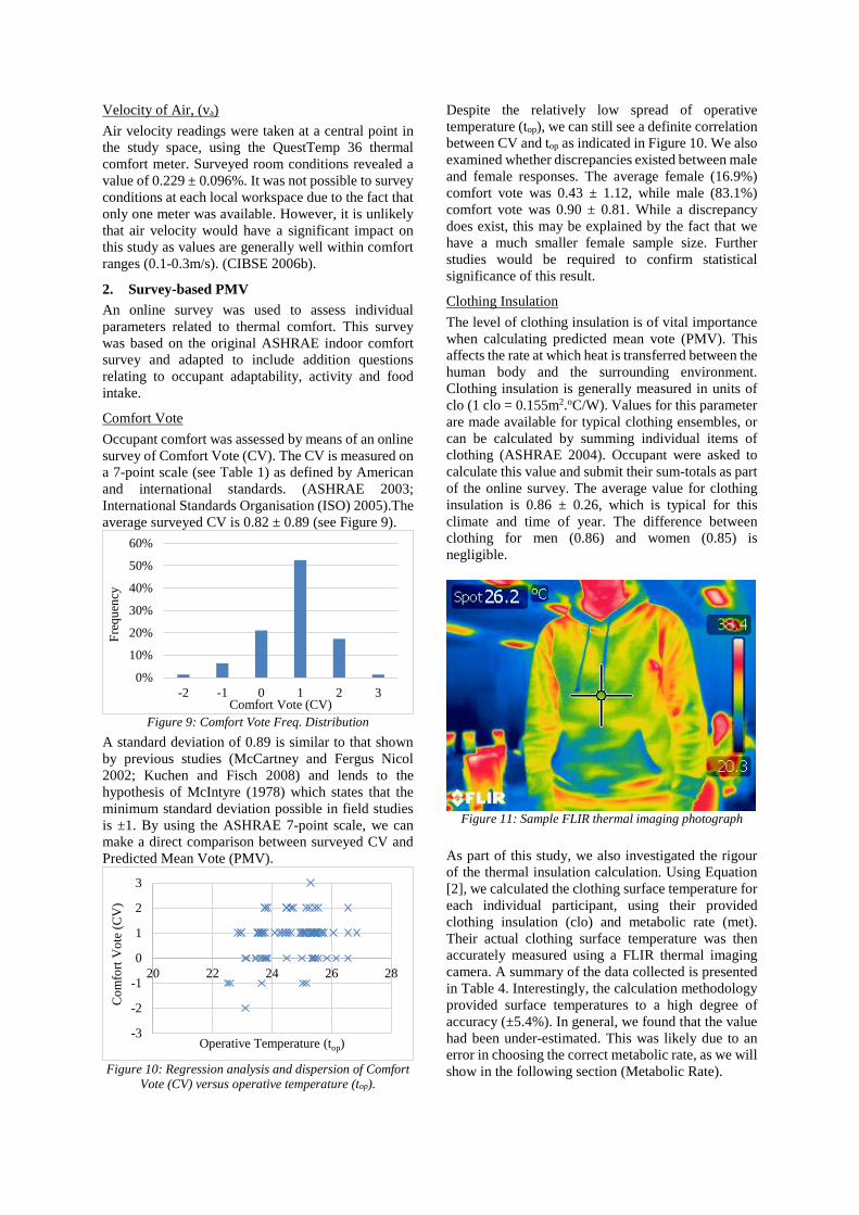
Weather Data It has been shown that perceptions of thermal comfort are dependent not only on indoor micro-climate, but also on outside meteorological parameters (Auliciems 1969). In addition, detailed weather data is required to accurately model building operation. For this purpose, a weather station was installed on campus measuring:

• Dry-bulb temperature (± 0.5˚C); • Relative humidity (± 2%); • Barometric pressure (± 50Pa); • Wind speed [±0.1ms-1 (0.3 – 10ms-1); ± 1% (

10 - 55ms-1); ± 2% (> 55ms-1)]; • Wind speed -3s gust [(±0.1ms-1 (0.3 – 10ms-

1); ± 1% ( 10 - 55ms-1); ± 2% (> 55ms-1)]; • Wind direction [± 2% (>5ms-1)]; • Global solar irradiance (<5%); • Diffuse solar radiation (<15%); • Barometric pressure (± 50Pa);

Figure 6: Outdoor Dry-bulb temperature, 2012

Galway has a typical maritime temperate climate, with average temperatures ranging from 5.9 °C (43 °F) in January to around 15.9 °C (61 °F) in July.

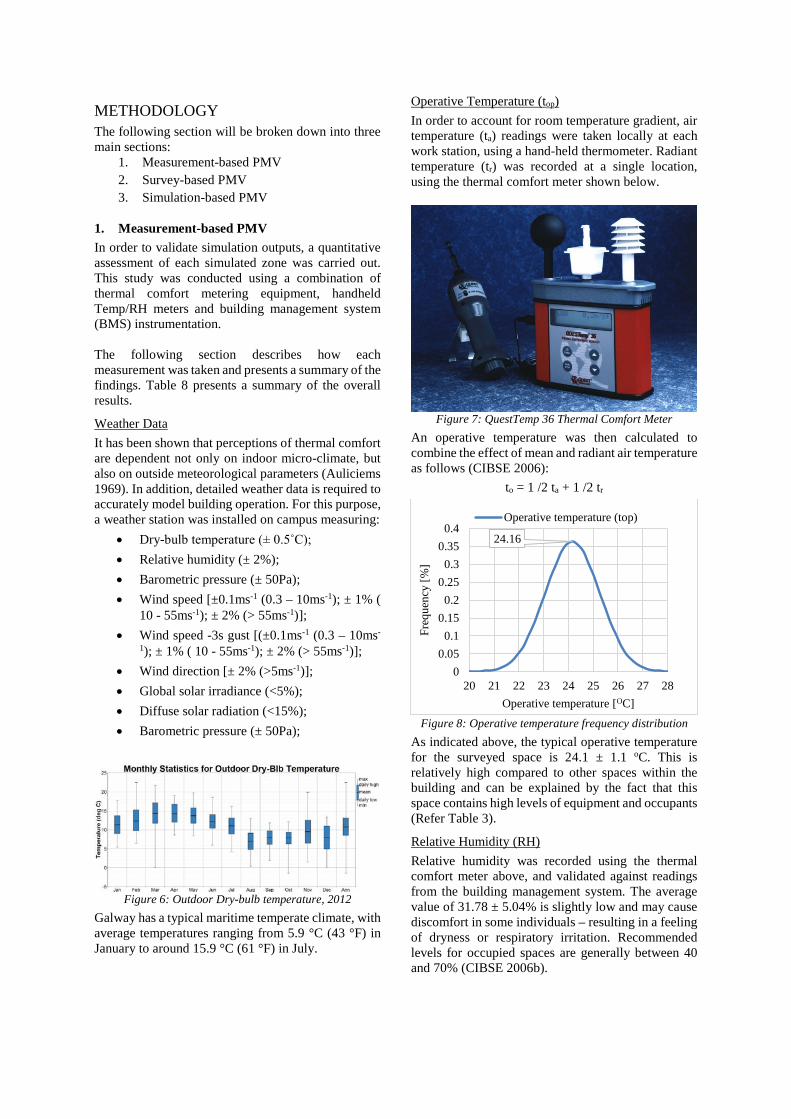
Operative Temperature (top) In order to account for room temperature gradient, air temperature (ta) readings were taken locally at each work station, using a hand-held thermometer. Radiant temperature (tr) was recorded at a single location, using the thermal comfort meter shown below.

Figure 7: QuestTemp 36 Thermal Comfort Meter

An operative temperature was then calculated to combine the effect of mean and radiant air temperature as follows (CIBSE 2006):

to = 1 /2 ta + 1 /2 tr

Figure 8: Operative temperature frequency distribution

As indicated above, the typical operative temperature for the surveyed space is 24.1 ± 1.1 oC. This is relatively high compared to other spaces within the building and can be explained by the fact that this space contains high levels of equipment and occupants (Refer Table 3).

Relative Humidity (RH) Relative humidity was recorded using the thermal comfort meter above, and validated against readings from the building management system. The average value of 31.78 ± 5.04% is slightly low and may cause discomfort in some individuals – resulting in a feeling of dryness or respiratory irritation. Recommended levels for occupied spaces are generally between 40 and 70% (CIBSE 2006b).

24.16

00.050.1

0.150.2

0.250.3

0.350.4

20 21 22 23 24 25 26 27 28

Freq

uenc

y[%

]

Operative temperature [OC]

Operative temperature (top)

Velocity of Air, (va) Air velocity readings were taken at a central point in the study space, using the QuestTemp 36 thermal comfort meter. Surveyed room conditions revealed a value of 0.229 ± 0.096%. It was not possible to survey conditions at each local workspace due to the fact that only one meter was available. However, it is unlikely that air velocity would have a significant impact on this study as values are generally well within comfort ranges (0.1-0.3m/s). (CIBSE 2006b).

2. Survey-based PMV An online survey was used to assess individual parameters related to thermal comfort. This survey was based on the original ASHRAE indoor comfort survey and adapted to include addition questions relating to occupant adaptability, activity and food intake.

Comfort Vote Occupant comfort was assessed by means of an online survey of Comfort Vote (CV). The CV is measured on a 7-point scale (see Table 1) as defined by American and international standards. (ASHRAE 2003; International Standards Organisation (ISO) 2005).The average surveyed CV is 0.82 ± 0.89 (see Figure 9).

Figure 9: Comfort Vote Freq. Distribution

A standard deviation of 0.89 is similar to that shown by previous studies (McCartney and Fergus Nicol 2002; Kuchen and Fisch 2008) and lends to the hypothesis of McIntyre (1978) which states that the minimum standard deviation possible in field studies is ±1. By using the ASHRAE 7-point scale, we can make a direct comparison between surveyed CV and Predicted Mean Vote (PMV).

Figure 10: Regression analysis and dispersion of Comfort

Vote (CV) versus operative temperature (top).

Despite the relatively low spread of operative temperature (top), we can still see a definite correlation between CV and top as indicated in Figure 10. We also examined whether discrepancies existed between male and female responses. The average female (16.9%) comfort vote was 0.43 ± 1.12, while male (83.1%) comfort vote was 0.90 ± 0.81. While a discrepancy does exist, this may be explained by the fact that we have a much smaller female sample size. Further studies would be required to confirm statistical significance of this result.

Clothing Insulation The level of clothing insulation is of vital importance when calculating predicted mean vote (PMV). This affects the rate at which heat is transferred between the human body and the surrounding environment. Clothing insulation is generally measured in units of clo (1 clo = 0.155m2.oC/W). Values for this parameter are made available for typical clothing ensembles, or can be calculated by summing individual items of clothing (ASHRAE 2004). Occupant were asked to calculate this value and submit their sum-totals as part of the online survey. The average value for clothing insulation is 0.86 ± 0.26, which is typical for this climate and time of year. The difference between clothing for men (0.86) and women (0.85) is negligible.

Figure 11: Sample FLIR thermal imaging photograph

As part of this study, we also investigated the rigour of the thermal insulation calculation. Using Equation [2], we calculated the clothing surface temperature for each individual participant, using their provided clothing insulation (clo) and metabolic rate (met). Their actual clothing surface temperature was then accurately measured using a FLIR thermal imaging camera. A summary of the data collected is presented in Table 4. Interestingly, the calculation methodology provided surface temperatures to a high degree of accuracy (±5.4%). In general, we found that the value had been under-estimated. This was likely due to an error in choosing the correct metabolic rate, as we will show in the following section (Metabolic Rate).

0%

10%

20%

30%

40%

50%

60%

-2 -1 0 1 2 3

Freq

uenc

y

Comfort Vote (CV)

-3

-2

-1

0

1

2

3

20 22 24 26 28

Com

fort

Vot

e (C

V)

Operative Temperature (top)

Table 4: Summary of clothing insulation and measured clothing surface temperatures

clo Value No. CV Tcl,meas Tcl,calc Error <0.5 12 0.67 30.517 29.45 4.56%

0.5-0.6 16 0.56 30.544 29.05 5.05% 0.6-0.7 22 0.77 29.609 28.77 5.11% 0.7-0.8 48 0.77 29.115 28.41 4.80% 0.8-0.9 50 0.84 28.904 28.06 6.42% 0.9-1 22 0.82 29.073 28.21 4.25% 1-1.1 19 1.00 28.763 27.52 4.78%

1.1-1.2 9 1.11 27.456 27.30 7.21% 1.2-1.3 6 1.00 28.467 27.34 5.92% 1.3-1.4 7 0.86 27.414 26.98 6.27% 1.4-1.5 2 1.00 29.950 26.81 10.41%

>1.5 6 1.00 26.617 26.85 5.32% Total 219 0.82 29.062 28.19 5.39%

Food Intake The intake of food has been shown to cause an increase in metabolic rate (i.e. the rate at which the human body generates heat) by up to 15% immediately after consumption (Fanger 1970). Therefore, participants were asked whether they had consumed and food/drink within the past hour. They were also asked to provide details where possible. We found that almost 75% of those surveyed had consumed food/drink within the past hour (see Table 5). There is a definite discrepancy between those who did not consume any food/drink (0.71) and those that did (0.83-0.96), in particular those that consumed a hot drink. The difference can be accounted for by the increase in metabolic rate instigated by the intake of food and drink, as well as the increased sense of warmth accompanied by the consumption of hot drinks such as tea or coffee.

Table 5: Food intake summary Food Intake No. Percent PMV None of these 55 25.11% 0.71 Cold Drink Combos 93 42.47% 0.83 Hot Drink Combos 25 11.42% 0.96 Meal Combos 46 21.00% 0.87 Grand Total 219 100.00% 0.82

Metabolic Rate / Activity level The metabolic rate (met) defines the rate at which the human body produce heat through internal processing of calories from food. It is a product primarily of activity and food intake as well as, to a lesser degree, age and fitness level (Schofield 1985; Gillooly et al. 2001).

Table 6: Metabolic Rates Metabolic Rate % Total Met Std. Dev. Female 16.79% 1.095 0.100 Male 83.21% 1.103 0.165

Total 100.00% 1.101 0.156

Metabolic rate was surveyed by asking participants to find the corresponding value for their particular activity by using standardised tables provided (ASHRAE 2004). Average recorded metabolic rate was 1.1 ±0.156, corresponding generally to sedentary, seated office activity. However, this may be an underestimation when considering a laboratory environment where students are returning from other lectures and other areas of the campus. In addition, food intake is not accounted for in these figures. As discussed in the previous section, food intake can increase metabolic rate by up to 15% immediately after consumption.

Adaptations Humans cannot be assumed to be passive observers when considering thermal comfort. Each individual has the freedom to make adaptations to their personal attire and local environment to increase thermal comfort (Baker and Standeven 1996). However, with the increasing shift towards further automation in buildings, humans are given less control over their environment. A sense of control and ability to interact with one’s environment is generally assumed to have a positive influence on user satisfaction (Kuchen and Fisch 2008). In this study, users had little opportunity to interact with their overall environment. Instead, in order to have any impact on their personal sense of thermal comfort, personal adaptations were required. This was demonstrated in the significant number of participants (~39%) who removed one or more items of clothing (Refer Table 7):

Table 7: Clothing Adaptations

Clothing No. Percent ‘clo’ CV Std. Dev.

Added 1 0.5% 2.00 -1.00 No change 132 60.3% 0.88 0.72 0.86 Removed 86 39.3% 0.80 1.00 0.89 Total 219 100.0% 0.86 0.82 0.89

3. Simulation-based PMV Discussion of the model development process is outside of the scope of this paper. However, two previously published papers (Coakley, Raftery, and Molloy 2012; Coakley et al. 2011) describe the model development and calibration process in detail. To summarise, the overall process may be broken down into five main steps:

1. Data gathering / building audit. 2. Evidence-based BES model development. 3. Bounded grid search 4. Refined grid search (optional) 5. Uncertainty analysis

A single zone model for the computer lab, adapted from a whole-building BIM, is used for the purpose of this study.

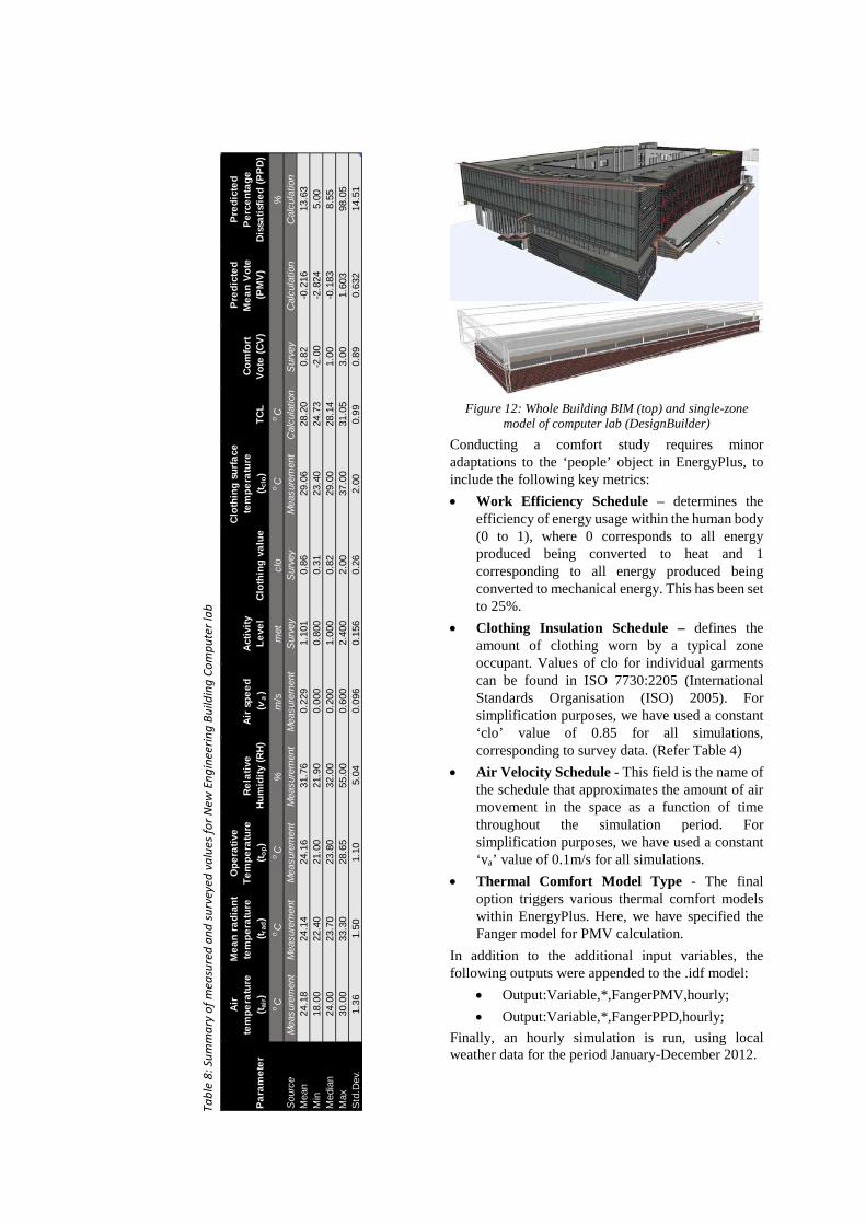
Figure 12: Whole Building BIM (top) and single-zone

model of computer lab (DesignBuilder) Conducting a comfort study requires minor adaptations to the ‘people’ object in EnergyPlus, to include the following key metrics: • Work Efficiency Schedule – determines the

efficiency of energy usage within the human body (0 to 1), where 0 corresponds to all energy produced being converted to heat and 1 corresponding to all energy produced being converted to mechanical energy. This has been set to 25%.

• Clothing Insulation Schedule – defines the amount of clothing worn by a typical zone occupant. Values of clo for individual garments can be found in ISO 7730:2205 (International Standards Organisation (ISO) 2005). For simplification purposes, we have used a constant ‘clo’ value of 0.85 for all simulations, corresponding to survey data. (Refer Table 4)

• Air Velocity Schedule - This field is the name of the schedule that approximates the amount of air movement in the space as a function of time throughout the simulation period. For simplification purposes, we have used a constant ‘va’ value of 0.1m/s for all simulations.

• Thermal Comfort Model Type - The final option triggers various thermal comfort models within EnergyPlus. Here, we have specified the Fanger model for PMV calculation.

In addition to the additional input variables, the following outputs were appended to the .idf model:

• Output:Variable,*,FangerPMV,hourly; • Output:Variable,*,FangerPPD,hourly;

Finally, an hourly simulation is run, using local weather data for the period January-December 2012.

Tabl

e 8:

Sum

mar

y of

mea

sure

d an

d su

rvey

ed v

alue

s for

New

Eng

inee

ring

Build

ing

Com

pute

r lab

Para

met

er

Air

tem

pera

ture

(t a

ir)

Mea

n ra

dian

t te

mpe

ratu

re

(t rad

)

Ope

rativ

e Te

mpe

ratu

re

(t op)

Rela

tive

Hum

idity

(RH)

Air s

peed

(va)

Activ

ity

Leve

lCl

othi

ng v

alue

Clot

hing

sur

face

te

mpe

ratu

re

(t clo

)TC

LCo

mfo

rt Vo

te (C

V)

Pred

icte

d M

ean

Vote

(P

MV)

Pred

icte

d Pe

rcen

tage

Di

ssat

isfie

d (P

PD)

oC

oC

oC

%m

/sm

etcl

ooC

oC

%S

ourc

eM

easu

rem

ent

Mea

sure

men

tM

easu

rem

ent

Mea

sure

men

tM

easu

rem

ent

Sur

vey

Sur

vey

Mea

sure

men

tC

alcu

latio

nS

urve

yC

alcu

latio

nC

alcu

latio

nM

ean

24.1

824

.14

24.1

631

.76

0.22

91.

101

0.86

29.0

628

.20

0.82

-0.2

1613

.63

Min

18.0

022

.40

21.0

021

.90

0.00

00.

800

0.31

23.4

024

.73

-2.0

0-2

.824

5.00

Med

ian

24.0

023

.70

23.8

032

.00

0.20

01.

000

0.82

29.0

028

.14

1.00

-0.1

838.

55M

ax30

.00

33.3

028

.65

55.0

00.

600

2.40

02.

0037

.00

31.0

53.

001.

603

98.0

5S

td.D

ev.

1.36

1.50

1.10

5.04

0.09

60.

156

0.26

2.00

0.99

0.89

0.63

214

.51

RESULTS A yearly simulation of the computer lab, using the data gathered during the space audit and thermal comfort survey, yielded the following results (Table 9):

Predicted Mean Vote (PMV) In respect of simulated predicted mean vote, we find that the simulation yields a relative consistent yearly PMV, with an average value of 1.043 ±0.08. This compares favourably with the thermal comfort survey conducted above which yielded an average PMV of 0.82 ±0.89. Of course, a smaller standard deviation is present as we are only simulating single average values for PMV as opposed to an actual random sample of comfort votes, as was the case in the field study.

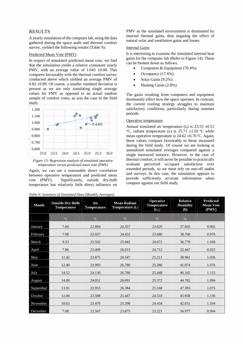
Figure 13: Regression analysis of simulated operative

temperature versus predicted mean vote (PMV) Again, we can see a reasonable direct correlation between operative temperature and predicted mean vote (PMV). Significantly, outside dry-bulb temperature has relatively little direct influence on

PMV as the simulated environment is dominated by internal thermal gains, thus negating the effect of natural solar and ventilation gains and losses.

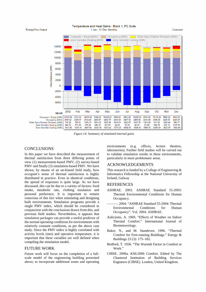
Internal Gains It is interesting to examine the simulated internal heat gains for the computer lab (Refer to Figure 14). These can be broken down as follows.

• Computers & Equipment (70.4%) • Occupancy (17.6%) • Solar Gains (9.2%) • Heating Gains (2.8%)

The gains resulting from computers and equipment dominantly effect how the space operates. In contrast, the current cooling strategy struggles to maintain satisfactory conditions, particularly during summer periods.

Operative temperature Annual simulated air temperature (ta) is 23.53 ±0.51 oC, radiant temperature (tr) is 25.71 ±1.02 oC while mean operative temperature is 24.62 ±0.76 oC. Again, these values compare favourably to those measured during the field study. Of course we are looking at annualised simulated averages compared against a single measured instance. However, in the case of thermal comfort, it will never be possible to practically evaluate perceived occupant satisfaction over extended periods, so we must rely on one-off audits and surveys. In this case, the simulation appears to provide sufficiently accurate information when compare against our field study.

Table 9: Summary of Simulated Data (Monthly Averages)

Month Outside Dry-Bulb Temperature

Air Temperature

Mean Radiant Temperature (tr)

Operative Temperature

(top)

Relative Humidity

(h)

Predicted Mean Vote

(PMV)

°C °C °C °C %

January 7.84 22.884 24.357 23.620 37.845 0.965

February 7.98 22.927 24.432 23.680 38.760 0.979

March 9.53 23.502 25.842 24.672 36.779 1.109

April 7.86 23.409 26.015 24.712 32.447 0.925

May 11.42 23.875 26.547 25.211 38.961 1.036

June 12.40 23.993 26.780 25.386 41.074 1.076

July 14.52 24.130 26.766 25.448 46.165 1.115

August 14.08 24.052 26.691 25.372 44.782 1.094

September 13.91 23.953 26.384 25.168 47.393 1.075

October 12.06 23.588 25.447 24.518 45.958 1.136

November 10.63 23.470 25.398 24.434 42.051 1.104

December 7.08 22.567 23.875 23.221 36.977 0.904

R² = 0.4345

0.600

0.700

0.800

0.900

1.000

1.100

1.200

23.0 23.5 24.0 24.5 25.0 25.5 26.0

CONCLUSIONS In this paper we have described the measurement of thermal satisfaction from three differing points of view (1) measurement-based PMV, (2) survey-based PMV and finally (3) simulation-based PMV. We have shown, by means of an un-biased field study, how occupant’s sense of thermal satisfaction is highly distributed in practice. Even in identical conditions, the spread of responses is quite large. As we have discussed, this can be due to a variety of factors: food intake, metabolic rate, clothing insulation and personal preference. It is important to remain conscious of this fact when simulating and designing built environments. Simulation programs provide a single PMV index, which should be considered in conjunction with the conclusions drawn from this, and previous field studies. Nevertheless, it appears that simulation packages can provide a useful predictor of the normal operating conditions for environments with relatively constant conditions, as per the above case study. Since the PMV index is highly correlated with activity levels (met) and operative temperature, it is important that these variables are well defined when compiling the simulation model.

FUTURE WORK Future work will focus on the completion of a full-scale model of the engineering building presented above, to incorporate additional zones and operating

environments (e.g. offices, lecture theatres, laboratories). Further field studies will be carried out to validate simulation results in these environments, particularly in more problematic areas.

ACKNOWLEDGEMENTS This research is funded by a College of Engineering & Informatics Fellowship at the National University of Ireland, Galway

REFERENCES ASHRAE. 2003. ASHRAE Standard 55-2003:

Thermal Environmental Conditions for Human Occupancy.

———. 2004. “ASHRAE Standard 55-2004: Thermal Environmental Conditions for Human Occupancy”. Vol. 2004. ASHRAE.

Auliciems, A. 1969. “Effects of Weather on Indoor Thermal Comfort.” International Journal of Biometeorology.

Baker, N., and M. Standeven. 1996. “Thermal Comfort for Free-running Buildings.” Energy & Buildings 23 (3): 175–182.

Bedford, T. 1936. “The Warmth Factor in Comfort at Work.”

CIBSE. 2006a. KS6:2006 Comfort. Edited by The Chartered Institution of Building Services Engineers (CIBSE). London, United Kingdom.

Figure 14: Summary of simulated internal gains

———. 2006b. CIBSE Guide A: Environmental Design. Edited by The Chartered Institution of Building Services Engineers (CIBSE). 7th Ed. London, United Kingdom.

Coakley, Daniel, Paul Raftery, and Padraig Molloy. 2012. “Calibration of Whole Building Energy Simulation Models: Detailed Case Study of a Naturally Ventilated Building Using Hourly Measured Data.” In Building Simulation and Optimization, 57–64. Loughborough, UK: ISBN: 978-1-897911-42-6.

Coakley, Daniel, Paul Raftery, Padraig Molloy, and Gearoid White. 2011. “Calibration of a Detailed BES Model to Measured Data Using an Evidence-Based Analytical Optimisation Approach.” In Proceedings of the 12th International IBPSA Conference. Sydney, Australia.

Fanger, P. O. 1970. Thermal Comfort. Danish Press. Gillooly, J F, J H Brown, G B West, V M Savage, and

E L Charnov. 2001. “Effects of Size and Temperature on Metabolic Rate.” Science (New York, N.Y.) 293 (5538) (September 21): 2248–51.

International Standards Organisation (ISO). 2005. “ISO 7730:2005 Ergonomics of the Thermal Environment — Analytical Determination and Interpretation of Thermal Comfort Using Calculation of the PMV and PPD Indices and Local Thermal Comfort Criteria.”

Kuchen, E., and M.N. Fisch. 2008. “Spot Monitoring: Thermal Comfort Evaluation in 25 Office Buildings in Winter.” Building and Environment In Press,.

McCartney, Kathryn J, and J Fergus Nicol. 2002. “Developing an Adaptive Control Algorithm for Europe.” Energy and Buildings 34 (6) (July): 623–635.

McIntyre, DA. 1978. “Three Approaches to Thermal Comfort.” ASHRAE Transactions.

Schofield, WN. 1985. “Predicting Basal Metabolic Rate, New Standards and Review of Previous Work.” Human Nutrition. Clinical Nutrition.