This is an electronic reprint of the original article.This reprint may differ from the original in pagination and typographic detail.

Powered by TCPDF (www.tcpdf.org)

This material is protected by copyright and other intellectual property rights, and duplication or sale of all or part of any of the repository collections is not permitted, except that material may be duplicated by you for your research use or educational purposes in electronic or print form. You must obtain permission for any other use. Electronic or print copies may not be offered, whether for sale or otherwise to anyone who is not an authorised user.

Kurkela, Matti; Maksimainen, Mikko; Julin, Arttu; Rantanen, Toni; Virtanen, Juho-Pekka;Hyyppä, Juha; Vaaja, Matti Tapio; Hyyppä, HannuUtilizing a Terrestrial Laser Scanner for 3D Luminance Measurement of Indoor Environments

Published in:Journal of Imaging

DOI:10.3390/jimaging7050085

Published: 01/05/2021

Document VersionPublisher's PDF, also known as Version of record

Published under the following license:CC BY

Please cite the original version:Kurkela, M., Maksimainen, M., Julin, A., Rantanen, T., Virtanen, J-P., Hyyppä, J., Vaaja, M. T., & Hyyppä, H.(2021). Utilizing a Terrestrial Laser Scanner for 3D Luminance Measurement of Indoor Environments. Journal ofImaging, 7(5), [85]. https://doi.org/10.3390/jimaging7050085

Journal of

Imaging

Article

Utilizing a Terrestrial Laser Scanner for 3D LuminanceMeasurement of Indoor Environments

Matti Kurkela 1,* , Mikko Maksimainen 1 , Arttu Julin 1 , Toni Rantanen 1 , Juho-Pekka Virtanen 1,2 ,Juha Hyyppä 2 , Matti Tapio Vaaja 1 and Hannu Hyyppä 1,2

�����������������

Citation: Kurkela, M.; Maksimainen,

M.; Julin, A.; Rantanen, T.; Virtanen,

J.-P.; Hyyppä, J.; Vaaja, M.T.; Hyyppä,

H. Utilizing a Terrestrial Laser

Scanner for 3D Luminance

Measurement of Indoor

Environments. J. Imaging 2021, 7, 85.

https://doi.org/10.3390/

jimaging7050085

Academic Editors: Rémi Cozot,

Olivier Le Meur and

Christophe Renaud

Received: 26 March 2021

Accepted: 4 May 2021

Published: 10 May 2021

Publisher’s Note: MDPI stays neutral

with regard to jurisdictional claims in

published maps and institutional affil-

iations.

Copyright: © 2021 by the authors.

Licensee MDPI, Basel, Switzerland.

This article is an open access article

distributed under the terms and

conditions of the Creative Commons

Attribution (CC BY) license (https://

creativecommons.org/licenses/by/

4.0/).

1 Department of Built Environment, School of Engineering, Aalto University, FI-00076 Aalto, Finland;mikko.maksimainen@aalto.fi (M.M.); arttu.julin@aalto.fi (A.J.); toni.rantanen@aalto.fi (T.R.);juho-pekka.virtanen@aalto.fi (J.-P.V.); matti.t.vaaja@aalto.fi (M.T.V.); hannu.hyyppa@aalto.fi (H.H.)

2 Finnish Geospatial Research Institute FGI, Geodeetinrinne 2, FI-02430 Masala, Finland; juha.hyyppa@nls.fi* Correspondence: matti.kurkela@aalto.fi

Abstract: We aim to present a method to measure 3D luminance point clouds by applying theintegrated high dynamic range (HDR) panoramic camera system of a terrestrial laser scanning(TLS) instrument for performing luminance measurements simultaneously with laser scanning. Wepresent the luminance calibration of a laser scanner and assess the accuracy, color measurementproperties, and dynamic range of luminance measurement achieved in the laboratory environment.In addition, we demonstrate the 3D luminance measuring process through a case study with aluminance-calibrated laser scanner. The presented method can be utilized directly as the luminancedata source. A terrestrial laser scanner can be prepared, characterized, and calibrated to apply it tothe simultaneous measurement of both geometry and luminance. We discuss the state and limitationsof contemporary TLS technology for luminance measuring.

Keywords: luminance measurement; lighting distribution; 360◦; HDR imaging; 3D; terrestriallaser scanning

1. Introduction

Laser scanning is a commonly applied 3D measuring technology for indoor measure-ment. Laser scanning is based on measuring 3D coordinates from an environment using alaser beam. As a result, a 3D point cloud is formed from a dense set of 3D measurements.Most contemporary laser scanners also contain one or more integrated cameras that areused to capture a panoramic image used for point colorization. The R (red), G (green),and B (blue) values of the captured image are projected onto the point cloud to obtaincoloring for points. In addition to visualization, the color information has been applied forregistration [1] and segmentation [2]. However, the point cloud colorization quality varies,depending on the selected terrestrial laser scanning (TLS) instrument [3].

In the past, terrestrial laser scanning has been widely applied in archaeology [4],cultural heritage [5], forestry [6], industry [7], geology [8], surveying [9], and constructionengineering [10]. Today, terrestrial laser scanners are also a commonly used instrumentin the architecture, engineering, construction, owner, operator (AECOO) industry. In TLS,one path of development is automating the processing of raw measurement into moresophisticated 3D models [11–13]. Another path of development is the integration of paralleldata and sensors in laser scanning [14,15].

Two-dimensional luminance photometry is commonly applied to measure indoorsurface luminances [16,17]. Luminance is the measure of light reflected or emitted froman area, commonly measured in candelas per square meter (cd·m−2). In lighting design,luminance distribution is an important aspect, as it affects the security, well-being, visualcomfort [18], and aesthetics of the indoor environment. The luminance distribution isusually measured via imaging luminance photometry, where a calibrated digital camera is

J. Imaging 2021, 7, 85. https://doi.org/10.3390/jimaging7050085 https://www.mdpi.com/journal/jimaging

J. Imaging 2021, 7, 85 2 of 24

used to obtain an absolute luminance value for each pixel. Imaging luminance photometryhas been applied in the assessment of light pollution [19,20]. High dynamic range (HDR)imaging is a key technology in imaging luminance photometry [21]. In HDR imaging,a set of images with different exposure times is combined to extend the dynamic rangeof a single exposure. This technique has been applied in architecture [22]. Moreover,the HDR technique is under constant development, for example by being applied to 360◦

imaging [23] and by improved image fusion algorithms [24]. As a technology, imagingluminance photometry via HDR imaging has become well-established. However, an innateproblem in measurement relying on individual images is the loss of 3D data in measuring.

Via photogrammetric 3D reconstruction, 2D luminance images can also be utilizedfor obtaining a 3D luminance measuring of a measured indoor environment [25]. Still,photogrammetry can perform poorly when measuring the 3D geometry of smooth, mono-colored, and uniform surfaces [26]. Luminance measurement applications require accurateradiometric data, and the use of 3D luminance measuring in design would be beneficial notonly for lighting designers but also for architects [27]. However, indoor 3D luminance mea-surements made with a terrestrial laser scanner have not been extensively studied. Existingresearch has shown that luminance maps obtained via imaging luminance photometrycan be combined with TLS [28] and MLS point clouds [29,30]. As stated, contemporaryTLS instruments commonly contain imaging sensors for point cloud colorization. As thesensors are increasingly applicable for HDR imaging [3], the utilization of such HDRimaging-capable TLS instruments for producing a 3D point cloud with luminance informa-tion is a topical development issue. While the use of TLS for lighting design via luminancemeasuring has been suggested in earlier research [27,28], a solution employing the TLSimages for luminance measuring is missing, since Rodrique et al. [27] utilized a separateimaging luminance photometer and they did not register the luminance values into a 3Dluminance point cloud. Instead, they assessed the geometry and luminance measuring asseparate entities. Vaaja et al. [28] manually combined images obtained with a conventionalsingle-lens reflex camera into a point cloud produced by TLS. However, in this case, the im-ages did not cover the full 360◦, and the data integration relied on manual methodology,limiting the efficiency.

In this study, we aim to present a method to measure 3D luminance point clouds.We apply the integrated high dynamic range (HDR) panoramic camera system of a TLSinstrument for 3D HDR luminance measurements simultaneously with laser scanning.We present a method for utilizing the images captured with a TLS instrument as the lu-minance data source (Table 1). Firstly, we present the luminance calibration of a laserscanner, and we assess the accuracy, color measurement properties, and dynamic range ofluminance measurement achieved in a laboratory environment. Secondly, we demonstratethe 3D luminance measuring process through a case study with a luminance-calibratedlaser scanner. We analyze the results and discuss the effect of scanning angles on lumi-nance measurements. In addition, we explore future research directions in 3D luminancemeasuring. The novelty of our study is that the method covers the 360◦ 3D luminancemeasurements and increases the level of automation in the data integration. In addition,the luminance point cloud data is enriched with the angle between the surface normal andthe measurement direction.

J. Imaging 2021, 7, 85 3 of 24

Table 1. Measurements and results performed in the study and their sections.

Laboratory measurements

Method:

Reference color target measurements:(Section 2.2 Luminance calibration of a ter-restrial laser scanner; Section 2.3 Luminancedata processing)

Results:

Luminance calibration factor for TLS:(Section 3.1 Reference color target measure-ments; Section 3.2 Luminance measurementcomparison and Appendix A.1 Color target)

Field measurementsMethod:

TLS data of the study area: (Section 2.4 Casestudy) and the luminance calibration factorfrom laboratory measurements

Results: Absolute luminance point clouds: (Section 3.3Case study and Appendix A.2 Sample areas)

2. Materials and Methods2.1. Terrestrial Laser Scanner

For terrestrial laser scanning, we used a time-of-flight scanner Leica RTC360 (HexagonAB, Stockholm, Sweden) [31,32]. According to the manufacturer, the scanning field of viewis 360◦ horizontal and 300◦ vertical, and the measured 3D point accuracy is 1.9 mm at 10 m.The scanner has three 4000 × 3000 pixel image sensors mounted to the scanner body (seeFigure 1). Together, the sensors cover a vertical view of 300◦. These sensors are used tocreate a panoramic image of 20,480 × 10,240 pixels with 5-bracket HDR imaging. The entireequirectangular panoramic image consists of 12 adjacent vertical images. The total scantime is 4 min 21 s, including HDR imaging with a scan resolution setting of 3.0 mm at 10 m.

Figure 1. Time-of-flight scanner Leica RTC360.

In the RTC360, HDR imaging is performed with a fixed exposure without any priorexposure measurements [3]. The imaging system of the RTC360 can therefore be calibrated

J. Imaging 2021, 7, 85 4 of 24

to interpret the absolute luminance values of the measured environment. Furthermore,the panoramic image can be exported for editing as an EXR file without losing the highdynamic range of the images and registered into the point cloud without losing the dynamicinformation. These attributes make the Leica RTC360 a usable measurement device forluminance-calibrated terrestrial laser scanning.

2.2. Luminance Calibration of a Terrestrial Laser Scanner2.2.1. Reference Color Target

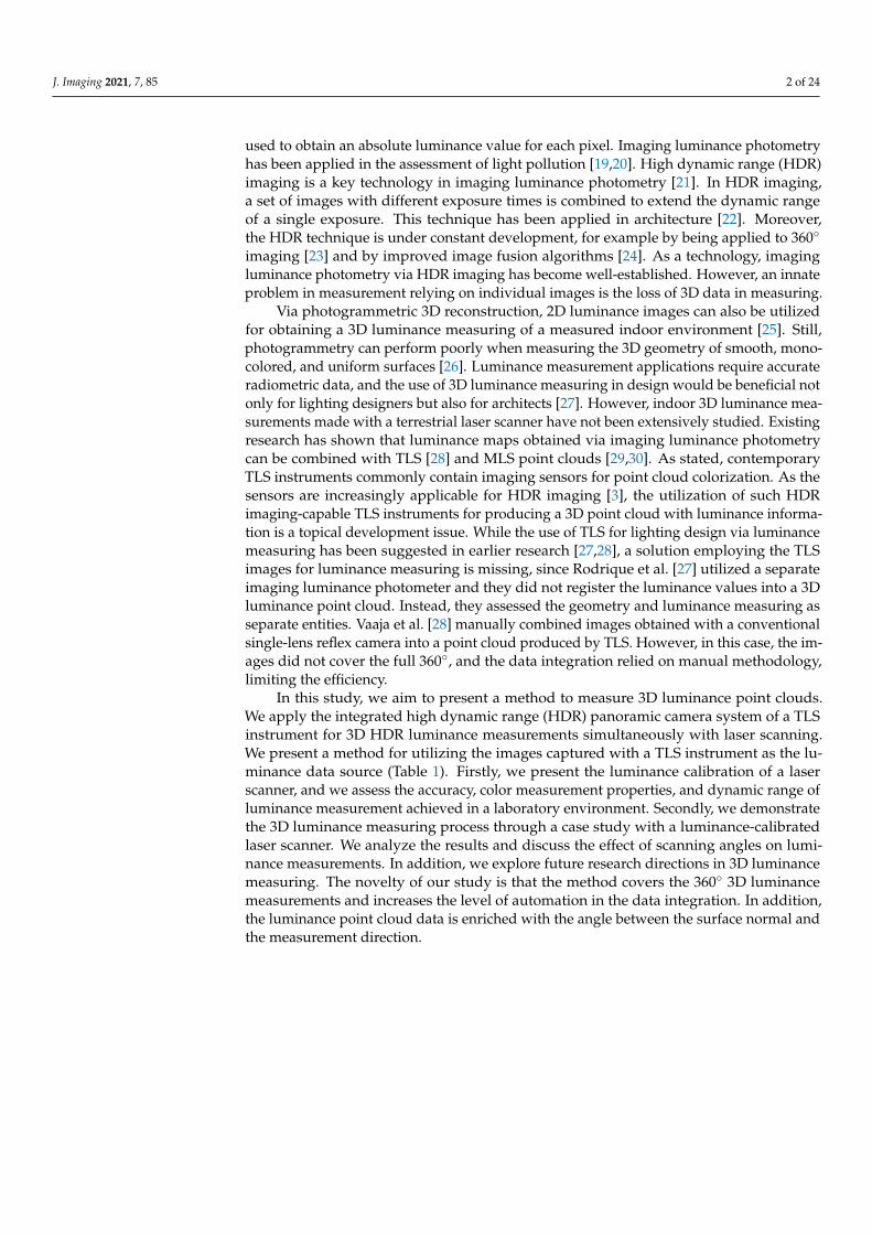
A standardized color target, the X-Rite ColorChecker Classic chart (Grand Rapids, MI,USA) [33], was attached to the wall. The ColorChecker Classic chart is used in photographyfor creating camera profiles and correcting white balance and color. The chart is designedfor color management in a variety of lighting conditions. Figure 2 shows the chart of 24different colored patches with measured colorimetric reference data provided by X-Rite.The size of the ColorChecker Classic was 21.59 × 27.94 cm. In the X-Rite documents,the patches were labeled in a different order. Table 2 lists colorimetric reference data forthe ColorChecker Classic manufactured after November 2014. The values were reported asCIE L*a*b* data.

Table 2. The colorimetric reference data for the ColorChecker Classic chart provided by X-Rite. X-RiteNo. is the patch name used by X-Rite; L is the luminance value; a and b are color coordinates.

Patch No. X-Rite No. L a b

1 A4 95.19 −1.03 2.932 B4 81.29 −0.57 0.443 C4 66.89 −0.75 −0.064 D4 50.76 −0.13 0.145 E4 35.63 −0.46 −0.486 F4 20.64 0.07 −0.467 A3 28.37 15.42 −49.88 B3 54.38 −39.72 32.279 C3 42.43 51.05 28.62

10 D3 81.8 2.67 80.4111 E3 50.63 51.28 −14.1212 F3 49.57 −29.71 −28.3213 A2 62.73 35.83 56.514 B2 39.43 10.75 −45.1715 C2 50.57 48.64 16.6716 D2 30.1 22.54 −20.8717 E2 71.77 −24.13 58.1918 F2 71.51 18.24 67.3719 A1 37.54 14.37 14.9220 B1 64.66 19.27 17.521 C1 49.32 −3.82 −22.5422 D1 43.46 −12.74 22.7223 E1 54.94 9.61 −24.7924 F1 70.48 −32.26 −0.37

J. Imaging 2021, 7, 85 5 of 24

1919 2020 2121 2222 2323 2424

1313 1414 1515 1616 1717 1818

77 88 99 1010 1111 1212

1 22 33 44 55 66

Figure 2. The measured target X-Rite ColorChecker Classic and the patch numbers used in this study.

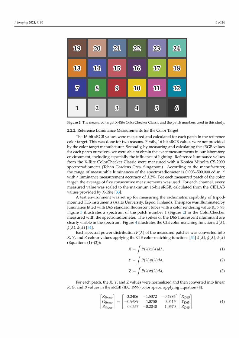
2.2.2. Reference Luminance Measurements for the Color Target

The 16-bit sRGB values were measured and calculated for each patch in the referencecolor target. This was done for two reasons. Firstly, 16-bit sRGB values were not providedby the color target manufacturer. Secondly, by measuring and calculating the sRGB valuesfor each patch ourselves, we were able to obtain the exact measurements in our laboratoryenvironment, including especially the influence of lighting. Reference luminance valuesfrom the X-Rite ColorChecker Classic were measured with a Konica Minolta CS-2000spectroradiometer (Teban Gardens Cres, Singapore). According to the manufacturer,the range of measurable luminances of the spectroradiometer is 0.003–500,000 cd·m−2

with a luminance measurement accuracy of ±2%. For each measured patch of the colortarget, the average of five consecutive measurements was used. For each channel, everymeasured value was scaled to the maximum 16-bit sRGB, calculated from the CIELABvalues provided by X-Rite [33].

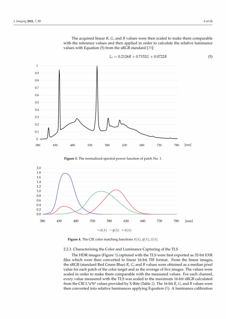
A test environment was set up for measuring the radiometric capability of tripod-mounted TLS instruments (Aalto University, Espoo, Finland). The space was illuminated byluminaires fitted with D65 standard fluorescent tubes with a color rendering value Ra > 93.Figure 3 illustrates a spectrum of the patch number 1 (Figure 2) in the ColorCheckermeasured with the spectroradiometer. The spikes of the D65 fluorescent illuminant areclearly visible in the spectrum. Figure 4 illustrates the CIE color matching functions x(λ),y(λ), z(λ) [34].

Each spectral power distribution P(λ) of the measured patches was converted intoX, Y, and Z colour values applying the CIE color-matching functions [34] x(λ), y(λ), z(λ)(Equations (1)–(3)):

X =∫

P(λ)x(λ)dλ, (1)

Y =∫

P(λ)y(λ)dλ, (2)

Z =∫

P(λ)z(λ)dλ, (3)

For each patch, the X, Y, and Z values were normalized and then converted into linearR, G, and B values in the sRGB (IEC 1999) color space, applying Equation (4):Rlinear

GlinearBlinear

=

3.2406 −1.5372 −0.4986−0.9689 1.8758 0.0415

0.0557 −0.2040 1.0570

XD65YD65ZD65

(4)

J. Imaging 2021, 7, 85 6 of 24

The acquired linear R, G, and B values were then scaled to make them comparablewith the reference values and then applied in order to calculate the relative luminancevalues with Equation (5) from the sRGB standard [35]:

Lr = 0.2126R + 0.7152G + 0.0722B (5)

0

0.1

0.2

0.3

0.4

0.5

0.6

0.7

0.8

0.9

1

[nm]380 430 480 530 580 630 680 730 780

Figure 3. The normalized spectral power function of patch No. 1.

0.00.20.40.60.81.01.21.41.61.82.0

[nm]380 430 480 530 580 630 680 730 780

Figure 4. The CIE color matching functions x(λ), y(λ), z(λ).

2.2.3. Characterizing the Color and Luminance Capturing of the TLS

The HDR images (Figure 5) captured with the TLS were first exported as 32-bit EXRfiles which were then converted to linear 16-bit TIF format. From the linear images,the sRGB (standard Red Green Blue) R, G, and B values were obtained as a median pixelvalue for each patch of the color target and as the average of five images. The values werescaled in order to make them comparable with the measured values. For each channel,every value measured with the TLS was scaled to the maximum 16-bit sRGB calculatedfrom the CIE L*a*b* values provided by X-Rite (Table 2). The 16-bit R, G, and B values werethen converted into relative luminances applying Equation (5). A luminance calibration

J. Imaging 2021, 7, 85 7 of 24

factor was obtained by comparing the relative luminance measured with the TLS to theabsolute luminance measured with the spectroradiometer.

Figure 5. The color target cropped from the panoramic image captured with the TLS instrument.

2.3. Luminance Data Processing

As in Section 2.2.3, the HDR images were exported as 32-bit EXR files from the TLSmeasurement data, and the 32-bit EXR files were converted to 16-bit TIF files, applyingPython 3.6.9 with libraries OpenEXR (1.3.2) (San Francisco, CA, USA), Numpy (1.16.6)(Cambridge, MA, USA), and OpenCV-Python (4.2.0.32) (Willow Garage, Menlo Park, CA,USA). Relative luminance values were calculated for each pixel in the 16-bit TIF filesapplying Equation (5), and the 16-bit relative monochromatic luminance values were codedover the three 8-bit RGB channels of a respective pixel and a new image was saved as an8-bit TIF [25]. Hence, the new 8-bit relative luminance TIF image contains a wider dynamicrange than a regular 8-bit RGB image, as all three channels carry the relative luminancedata. The coded 8-bit file format allowed further processing of data in software that doesnot support a wider dynamic range, e.g., 16-bit data. The 8-bit TIF images were projectedand registered as the R, G, and B values in the point cloud. Point by point, the R, G, and Bvalues were converted back to relative luminance values. Finally, the luminance calibrationfactor (see Section 2.2.3) was applied to interpret the relative luminance values as absoluteluminance values, and the absolute luminance value was registered to each point in thepoint cloud. Figure 6 illustrates the luminance point cloud generating process.

Data acquisition (image & 3D points)

Point cloud preprocessing (filtering & registering)

Luminance image processing

Relative luminance point cloudsReplacing original images with relative luminance images

Absolute luminance point clouds

Point cloud

Figure 6. The workflow for creating data for indoor 3D luminance maps.

J. Imaging 2021, 7, 85 8 of 24

2.4. Case Study2.4.1. Study Area

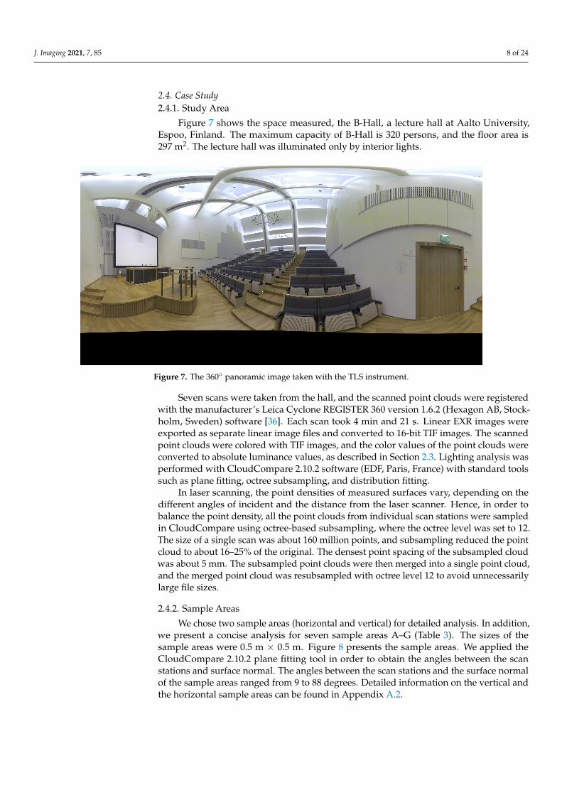
Figure 7 shows the space measured, the B-Hall, a lecture hall at Aalto University,Espoo, Finland. The maximum capacity of B-Hall is 320 persons, and the floor area is297 m2. The lecture hall was illuminated only by interior lights.

Figure 7. The 360◦ panoramic image taken with the TLS instrument.

Seven scans were taken from the hall, and the scanned point clouds were registeredwith the manufacturer’s Leica Cyclone REGISTER 360 version 1.6.2 (Hexagon AB, Stock-holm, Sweden) software [36]. Each scan took 4 min and 21 s. Linear EXR images wereexported as separate linear image files and converted to 16-bit TIF images. The scannedpoint clouds were colored with TIF images, and the color values of the point clouds wereconverted to absolute luminance values, as described in Section 2.3. Lighting analysis wasperformed with CloudCompare 2.10.2 software (EDF, Paris, France) with standard toolssuch as plane fitting, octree subsampling, and distribution fitting.

In laser scanning, the point densities of measured surfaces vary, depending on thedifferent angles of incident and the distance from the laser scanner. Hence, in order tobalance the point density, all the point clouds from individual scan stations were sampledin CloudCompare using octree-based subsampling, where the octree level was set to 12.The size of a single scan was about 160 million points, and subsampling reduced the pointcloud to about 16–25% of the original. The densest point spacing of the subsampled cloudwas about 5 mm. The subsampled point clouds were then merged into a single point cloud,and the merged point cloud was resubsampled with octree level 12 to avoid unnecessarilylarge file sizes.

2.4.2. Sample Areas

We chose two sample areas (horizontal and vertical) for detailed analysis. In addition,we present a concise analysis for seven sample areas A–G (Table 3). The sizes of thesample areas were 0.5 m × 0.5 m. Figure 8 presents the sample areas. We applied theCloudCompare 2.10.2 plane fitting tool in order to obtain the angles between the scanstations and surface normal. The angles between the scan stations and the surface normalof the sample areas ranged from 9 to 88 degrees. Detailed information on the vertical andthe horizontal sample areas can be found in Appendix A.2.

J. Imaging 2021, 7, 85 9 of 24

A

BC

D

E

F

G

Figure 8. The intensity image from scanning station 6 shows the locations of the sample areas for luminance measurements.The green areas represent the sample areas A–G. The red area represents the vertical sample area. The yellow area representsthe horizontal sample area. White points represent the 6 different scanning locations with the seventh scanning locationbeing the observer of the image.

Table 3. The sample areas.

Sample Area Material

A wooden doorB painted woodC painted concrete wallD painted vertical slatted timberE painted vertical slatted timberF painted horizontal slatted timberG painted concrete wall

Vertical textile-covered acoustic boardHorizontal wooden table

3. Results3.1. Reference Color Target Measurements

Table 4 presents the reference sRGB values measured from the X-Rite ColorCheckerClassic with the spectroradiometer. The measured spectral power distributions wereconverted into sRGB values applying Equations (1)–(4).

J. Imaging 2021, 7, 85 10 of 24

Table 4. The sRGB values (16-bit) of the X-Rite ColorChecker Classic board, calculated from thespectra measured with the spectroradiometer, and scaled to match the X-Rite nominal values.

Patch No. R G B

1 62,782 62,269 56,7512 41,236 41,525 38,8953 25,391 25,701 23,9934 13,472 13,375 12,3705 6498 6633 62856 2699 2606 24147 2660 3735 20,1038 4945 20,983 42849 29,753 3094 2760

10 57,323 40,884 28511 35,392 6377 20,27312 −447 16,836 24,88813 50,372 14,128 188814 4941 7354 26,86115 38,649 6226 801616 7631 3249 959317 24,366 36,005 298118 53,556 26,190 132819 12,565 6284 406020 38,994 20,567 14,32121 8588 13,919 22,31322 7652 11,057 351423 16,275 14,978 28,12924 9578 36,325 26,761

3.2. Luminance Measurement Comparison

Table 5 presents the laser scanner luminance measurements compared to the spec-troradiometer luminance measurements. Only the lowest row of grayscale patches (1–6)were used for luminance calibration (see Figure 1). The 16-bit values were calculated intorelative luminance values, applying Equation (5). The laser scanner absolute luminancemeasurements were derived using a simple linear regression with the spectroradiometervalues. We assume that the sensor noise increases the low-end luminance values capturedby the camera of the laser scanner. Hence, an improved iteration of the laser scannerabsolute luminance values was derived by reducing the original 16-bit value by the abso-lute difference in the smallest compared luminance value (18.2 cd·m−2 − 13.9 cd·m−2 =4.3 cd·m−2) multiplied by the calibration factor (146.3) obtained with the linear regression.

Table 5. The laser scanner luminance measurements compared to a spectroradiometer. The table shows the differences andrelative differences between the reference luminance measured with a spectroradiometer and the luminance measured witha TLS. The luminance measured with a TLS was calculated by linear regression and by linear regression and noise removal.

Patch No. A B C Diff. (A,C) Relative Diff. (A,C) D Diff. (A,D) Relative Diff. (A,D)

1 329.8 48,753.6 333.2 3.4 1.0% 330.8 1.0 0.3%2 219.6 32,784.2 224.1 4.4 2.0% 221.0 1.4 0.6%3 135.8 20,786.2 142.1 6.3 4.7% 138.5 2.8 2.0%4 70.9 11,449.6 78.3 7.4 10.4% 74.4 3.5 4.9%5 35.0 6165.6 42.1 7.1 20.4% 38.1 3.0 8.7%6 13.9 2665.2 18.2 4.3 31.1% 14.0 0.1 0.7%

A: Spectroradiometer value in cd·m−2. B: Laser scanner 16-bit value, average of five scans. C: Laser scanner luminance value in cd·m−2,obtained by linear regression. D: Laser scanner luminance value in cd·m−2, obtained by linear regression and noise removal.

J. Imaging 2021, 7, 85 11 of 24

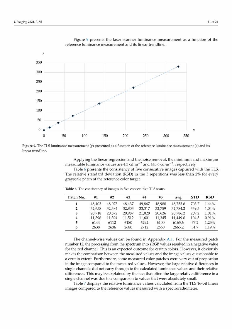
Figure 9 presents the laser scanner luminance measurement as a function of thereference luminance measurement and its linear trendline.

0

50

100

150

200

250

300

350

0 50 350300250200150100x

y

Figure 9. The TLS luminance measurement (y) presented as a function of the reference luminance measurement (x) and itslinear trendline.

Applying the linear regression and the noise removal, the minimum and maximummeasurable luminance values are 4.3 cd·m−2 and 443.6 cd·m−2, respectively.

Table 6 presents the consistency of five consecutive images captured with the TLS.The relative standard deviation (RSD) in the 5 repetitions was less than 2% for everygrayscale patch of the reference color target.

Table 6. The consistency of images in five consecutive TLS scans.

Patch No. #1 #2 #3 #4 #5 avg STD RSD

1 48,403 48,073 48,437 49,867 48,988 48,753.6 703.7 1.44%2 32,658 32,384 32,803 33,317 32,759 32,784.2 339.5 1.04%3 20,718 20,572 20,987 21,028 20,626 20,786.2 209.2 1.01%4 11,396 11,394 11,512 11,601 11,345 11,449.6 104.5 0.91%5 6144 6112 6180 6292 6100 6165.6 77.2 1.25%6 2638 2636 2680 2712 2660 2665.2 31.7 1.19%

The channel-wise values can be found in Appendix A.1. For the measured patchnumber 12, the processing from the spectrum into sRGB values resulted in a negative valuefor the red channel. This is an expected outcome for certain colors. However, it obviouslymakes the comparison between the measured values and the image values questionable toa certain extent. Furthermore, some measured color patches were very out of proportionin the image compared to the measured values. However, the large relative differences insingle channels did not carry through to the calculated luminance values and their relativedifferences. This may be explained by the fact that often the large relative difference in asingle channel was due to a comparison to values that were absolutely small.

Table 7 displays the relative luminance values calculated from the TLS 16-bit linearimages compared to the reference values measured with a spectroradiometer.

J. Imaging 2021, 7, 85 12 of 24

Table 7. The relative luminance values calculated from the TLS 16-bit linear images compared todifferent sets of reference values. The table presents the values ordered according to the referencecolor target (Figure 2).

TLS 16-Bit Linear Images Compared to the ReferenceValues Measured with a Spectroradiometer

Relative luminance values calculated fromthe TLS 16-bit linear images8418.6 24,482.7 15,137.8 10,691.0 17,647.0 31,555.7

19,673.6 10,007.0 13,167.5 5486.0 30,092.9 26,973.77559.0 18,091.8 37,820.5 37,820.5 13,644.1 17,318.7

61,969.5 41,645.5 14,543.5 14,543.5 7838.0 3379.1

Linear spectroradiometer values calculatedand scaled from the measured spectra7458.4 24,033.5 13,392.0 9788.6 16,203.3 29,948.3

20,950.0 8249.2 13,248.4 4638.9 31,146.1 30,213.04688.5 16,367.8 8737.3 41,447.7 13,549. 13,742.7

61,979.3 41,273.9 25,512.0 13,322.6 6578.9 2611.9

Relative difference between the values measuredwith a TLS and a spectroradiometer12.9% 1.9% 13.0% 9.2% 8.9% 5.4%6.1% 21.3% 0.6% 18.3% 3.4% 10.7%61.2% 10.5% 7.2% 8.8% 0.7% 26.0%0.0% 0.9% 3.5% 9.2% 19.1% 29.4%

Average: 12.0 %

Table 8 presents the adjusted absolute luminance values for each patch in the colortarget measured with the TLS compared to the reference luminance values measured withthe spectroradiometer. Figure 10 presents the 3D luminance point cloud of the referencecolor target.

353.1

266.5

179.8

93.1

6.4

cd·m−2

Figure 10. Luminances of the measured color target X-Rite ColorChecker Classic. The patches in thelowest row of patches (1–6) are the grayscale patches used for luminance calibration.

J. Imaging 2021, 7, 85 13 of 24

Table 8. The adjusted TLS luminance measurements compared to the reference values measuredwith a spectroradiometer. The table presents the values ordered according to the reference colortarget (Figure 2).

TLS Luminance Measurements Compared to the Reference Values Measuredwith a Spectroradiometer

Absolute adjusted luminance values measured with a TLS41.1 127.9 77.7 53.4 91.3 166.4

101.7 50.1 66.7 25.4 158.1 141.136.8 93.4 46.2 199.6 69.5 89.6

330.9 221.0 138.4 74.3 38.1 14.0

Absolute adjusted luminance values measured with a spectroradiometer39.7 127.8 71.4 52.0 86.4 159.4

111.3 44.1 70.5 24.7 165.5 160.525.1 87.0 46.4 220.2 72.2 73.3

329.8 219.6 135.8 70.9 35.0 13.9

Absolute difference1.5 0.1 6.4 1.4 5.0 7.19.6 6.0 3.7 0.7 7.4 19.4

11.7 6.4 0.3 20.6 2.7 16.31.1 1.3 2.7 3.4 3.1 0.1

Average: 5.7

Relative difference3.7% 0.1% 8.9% 2.7% 5.8% 4.4%8.6% 13.7% 5.3% 2.8% 4.5% 12.1%

46.7% 7.4% 0.6% 9.3% 3.7% 22.3%0.3% 0.6% 2.0% 4.9% 8.8% 0.4%

Average: 7.5 %

3.3. Case Study3.3.1. The Case Study of a Luminance Measurements

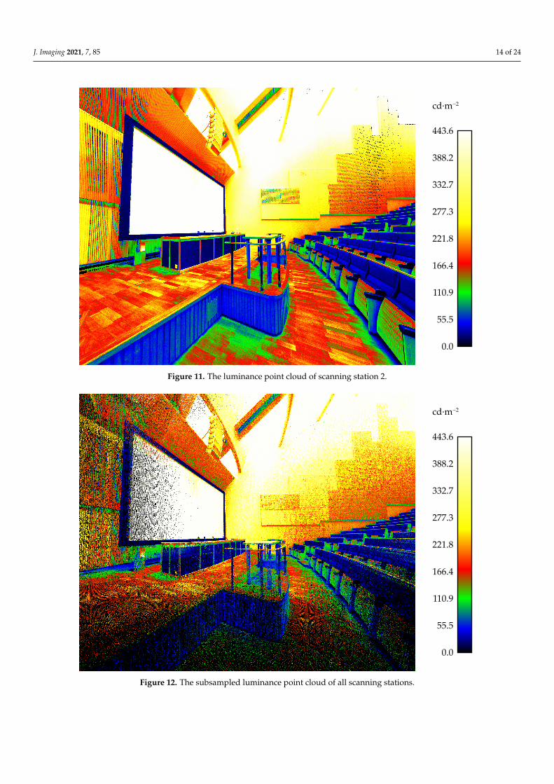
The chosen test site was measured with a luminance-calibrated TLS. Figure 11 showsthe luminance measurement obtained a single scan station projected onto 3D points, whileFigure 12 illustrates seven merged luminance measurements subsampled to the octree level12 as described in Section 2.3. The range of measured luminances was 0–443.6 cd·m−2.In the measured space, the measurement range covers most of the measurable surfaces.However, the luminance of the light sources and the surfaces around them were too highto be measured with the TLS used in this study.

J. Imaging 2021, 7, 85 14 of 24

443.6

388.2

332.7

277.3

221.8

166.4

110.9

55.5

0.0

cd·m−2

Figure 11. The luminance point cloud of scanning station 2.

443.6

388.2

332.7

277.3

221.8

166.4

110.9

55.5

0.0

cd·m−2

Figure 12. The subsampled luminance point cloud of all scanning stations.

J. Imaging 2021, 7, 85 15 of 24

3.3.2. Sample Area Analysis of 3D Luminance Measurements

Figure 13 illustrates the point clouds and their corresponding merged histograms forthe vertical and horizontal sample areas (see Figure 8). Illustrations of each laser scan andtheir merged point clouds and corresponding histograms for both sample areas can befound in Appendix A.2.

cd·m−2

(a) (b)

(d)(c)

cd·m−2

Figure 13. The point cloud (a) and its corresponding histogram (b) for the vertical sample area, and the point cloud (c) andits corresponding histogram (d) for the horizontal sample area.

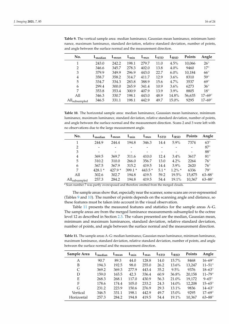
Tables 9 and 10 present the measured features and statistics for the vertical sample areaand the horizontal sample area, respectively. The values presented are the median, Gaus-sian mean, minimum and maximum luminances, standard deviation, relative standarddeviation, number of points, and angle between the surface normal and the measure-ment direction.

J. Imaging 2021, 7, 85 16 of 24

Table 9. The vertical sample area: median luminance, Gaussian mean luminance, minimum lumi-nance, maximum luminance, standard deviation, relative standard deviation, number of points,and angle between the surface normal and the measurement direction.

No. Lmedian Lmean Lmin Lmax LSTD LRSD Points Angle

1 243.0 242.2 198.1 279.7 11.0 4.5% 10,066 26◦

2 346.6 345.7 278.3 402.0 13.8 4.0% 9460 17◦

3 379.9 349.9 296.9 443.0 22.7 6.0% 10,184 66◦

4 358.7 358.2 314.7 411.7 12.9 3.6% 8310 59◦

5 334.7 334.3 283.8 388.9 15.6 4.7% 3537 69◦

6 299.4 300.0 265.9 341.4 10.9 3.6% 6273 36◦

7 353.8 353.4 300.9 407.9 13.9 3.9% 8805 18◦

All 346.3 330.7 198.1 443.0 48.9 14.8% 56,635 17–69◦

Allsubsampled 346.5 331.1 198.1 442.9 49.7 15.0% 9295 17–69◦

Table 10. The horizontal sample area: median luminance, Gaussian mean luminance, minimumluminance, maximum luminance, standard deviation, relative standard deviation, number of points,and angle between the surface normal and the measurement direction. Scans 2 and 3 were left withno observations due to the large measurement angle.

No. Lmedian Lmean Lmin Lmax LSTD LRSD Points Angle

1 244.9 244.4 194.8 346.3 14.4 5.9% 7374 63◦

2 - - - - - - - 87◦

3 - - - - - - - 88◦

4 369.5 369.7 311.6 410.0 12.4 3.4% 3617 81◦

5 310.2 310.0 266.0 356.7 13.0 4.2% 2264 76◦

6 367.5 367.9 315.2 419.5 14.4 3.9% 2620 76◦

7 428.1 * 427.9 * 399.1 * 443.5 * 5.1 * 1.2% * 6336 79◦

All 302.6 302.7 194.8 419.5 59.2 19.5% 15,875 63–88◦

Allsubsampled 257.3 284.2 194.8 419.5 54.4 19.1% 10,367 63–88◦

* Scan number 7 was partly overexposed and therefore omitted from the merged clouds.

The sample areas show that, especially near the scanner, some scans are over-represented(Tables 9 and 10). The number of points depends on the scanning angle and distance, sothese features must be taken into account in the visual observation.

Table 11 presents the measured features and statistics for the sample areas A–G.The sample areas are from the merged luminance measurements subsampled to the octreelevel 12 as described in Section 2.3. The values presented are the median, Gaussian mean,minimum and maximum luminances, standard deviation, relative standard deviation,number of points, and angle between the surface normal and the measurement direction.

Table 11. The sample areas A–G: median luminance, Gaussian mean luminance, minimum luminance,maximum luminance, standard deviation, relative standard deviation, number of points, and anglebetween the surface normal and the measurement direction.

Sample Area Lmedian Lmean Lmin Lmax LSTD LRSD Points Angle

A 90.7 89.3 44.0 128.8 14.0 15.7% 8468 16–69◦

B 194.3 192.5 98.0 255.0 26.2 13.6% 13,247 11–51◦

C 369.2 369.3 277.9 443.4 35.2 9.5% 9376 18–63◦

D 159.0 165.5 42.3 336.4 60.9 36.8% 20,158 11–79◦

E 268.3 268.1 117.0 430.9 56.3 21.0% 19,172 9–65◦

F 178.6 174.4 105.0 233.2 24.3 14.0% 12,208 15–65◦

G 231.2 223.9 150.6 276.9 29.3 13.1% 9836 14–63◦

Vertical 346.5 331.1 198.1 442.9 49.7 15.0% 9295 17–69◦

Horizontal 257.3 284.2 194.8 419.5 54.4 19.1% 10,367 63–88◦

J. Imaging 2021, 7, 85 17 of 24

4. Discussion and Conclusions4.1. Laboratory Measurements

We characterized the color and luminance measurement quality of a terrestrial laserscanner and we presented a workflow where an HDR image captured by a TLS instrumentwas converted into absolute luminance values. Compared to the reference, the TLS capturedluminance values with an average absolute difference of 2.0 cd·m−2 and an averagerelative difference of 2.9% for the grayscale patches (No. 1–6). For all patches, the averageabsolute difference and average relative differences were 5.7 cd·m−2 and 7.5%, respectively.The relative difference between the TLS measurement and the reference measurementwas notable for certain patches such as blue (46.7%) and cyan (22.3%). This indicates thatcertain heavily weighted spectra translate suboptimally into luminance values when usingstandard sRGB conversion factors. However, as we can characterize the channel-wisevalues for each patch in the X-Rite ColorChecker, we would be able to obtain conversionfactors that would be more optimal for the camera in the TLS than the sRGB conversionfactors. Optimized factors could possibly decrease the difference between the luminancevalues measured with the TLS and the reference values for the weighted spectra.

4.2. Field Measurements

We explored the possibilities of simultaneous laser scanning and luminance imagingthrough a case study. Thus, the level of automation increased in comparison with theprevious luminance data and TLS point cloud integration, and the luminance data integrityand usability improved.

The dynamic range needed for luminance measurement depends on the application.The widest dynamic range is required when measuring nighttime outdoor environments,for example, road lighting. In order to measure the lowest end of mesopic luminanceson the road surface to the glaring light source, a measurement range of 0.01 cd·m−2 toapproximately 100,000 cd·m−2 would be needed. This is a little more than 23 f-stops.The system used in this study had an effective dynamic range of 4.3–443.6 cd·m−2 or abit less than 9 f-stops. This dynamic range is almost sufficient to measure the luminancedistribution of the surfaces in an indoor space but nowhere near wide enough for roadlighting measurements. Moreover, it is a technologically difficult task to extend the dynamicrange towards the low luminance levels. The sensors would have to be more sensitive yethave a better signal-to-noise ratio. Another solution is to apply HDR imaging with longerexposure times, which obviously makes measuring slower or less convenient.

For indoor applications, however, HDR imaging could be applied by adding imagescaptured with shorter exposure times. This way, the dynamic range of a TLS could beextended to be sufficient for indoor measurement from the low-end surface luminances(1 cd·m−2) to the glaring light sources (100,000 cd·m−2). This upward extension of thedynamic range would enable the measurements needed when calculating the unified glarerating (UGR). Furthermore, it would be possible to measure the luminance of the lightsources if the dynamic range of HDR imaging is wide enough.

To determine the location of the measuring device, terrestrial laser scanning allowsthe measurement angle to be defined for each measured point. The point can be assigneda location, color value, absolute luminance value, intensity, point normal, and anglebetween point normal and surface normal. This information can be used in the future todetermine the properties of the scanned object, such as reflectivity and gloss. The anglebetween the scan station and the measured surface normal was not verified by any othermethod in this study. We considered the collected point cloud data accurate enough forangle measurement.

4.3. Limitations of TLS as a Luminance Photometer

Usually, a TLS instrument captures a panoramic image as a composite of severaladjacent images that are overlapped and blended together. The technique is often calledimage stitching. The quality of the stitching is difficult to quantify, and we did not assess

J. Imaging 2021, 7, 85 18 of 24

the inaccuracies of image stitching. However, the TLS instrument (Leica RTC360) could bemore suitable if the uncertainty of the panoramic image stitching process was known andthere was a possibility to maintain the bit depth of the measurement in the RGB-registeredpoint clouds. As for now, registering the raw imaging bit depth into the point cloudrequires manual effort.

Different TLS instruments employ various imaging sensor installations, such as com-pletely separate camera systems operated from atop of the TLS instrument (e.g., Riegl [37]),integrated imaging sensors utilizing the same rotating mirror as the laser ranging sensor,or sets of cameras mounted in the instrument’s chassis, as in the applied Leica RTC360 scan-ner [3]. The realization of the imaging system affects the quality of produced panoramicimages, e.g., through differences in parallax.

Contemporary TLS instruments are capable of obtaining rather high point densitiesand measurement speeds. For example, for the instrument applied in our work, the man-ufacturer reports a measuring speed of 2 million points per second and a point spacingof 3 mm at 10 m [31]. As a result, a single point cloud obtained with this instrument maycontain up to approx. 200 million points [38]. A mapping campaign in a complex indoorenvironment may therefore well exceed a billion points. These data amounts present atechnical challenge and require suitable storage systems to be applied in processing and dis-tribution. Understandably, point cloud storage [39], distribution [40], and application [41]have become topical development tasks.

For assessing the color measurement of the TLS instrument, the 24 patch X-RiteColorChecker Classic was applied. In order to improve the color measurement assessment,a color chart with 99 patches could be used as defined in ANSI/IES Method for EvaluatingLight Source Color Rendition TM-30-20 [42].

4.4. Future Research Directions

In future studies, a method for determining the reflectivity of a surface can be de-veloped as the locations of the measurements and the locations and luminances of thelight sources are known. However, this method does not completely solve the reflectiv-ity measurement. For more reliable reflectivity measurement, the light distribution ofthe light sources and the integration of light within the measurement space also need tobe determined.

Simultaneous geometry and luminance measuring executed with a TLS can be appliedin lighting design and lighting retrofitting. A 3D mesh model can be created from themeasured point cloud. The mesh model can be converted into a CAD 3D model, which canbe imported into lighting design software such as DIALux or Relux.

Since the scanner alone is not yet comparable in terms of image quality, the bestresult is obtained by combining terrestrial laser scanning and photogrammetry. As of yet,a TLS cannot replace conventional imaging luminance photometry in terms of luminancemeasurement. However, the TLS-based luminance measurement does not fall far behind.When the measurable luminance range is widened, the TLS luminance measurementwould perform at a similar level as conventional imaging luminance photometry forindoor measurements and outdoor daytime measurements. Furthermore, both of theserequired improvements have been solved as individual technologies, but the advancementshave not yet been implemented in a TLS. Hence, we are only a few steps away fromluminance measurements being obtained as a side product of geometry measurementor vice versa. In TLS luminance measurement, the luminance data is registered intothe measured geometry. This is a feature that is completely unobtainable using onlyconventional imaging luminance photometry.

As TLS point clouds capture the surrounding environment from all directions, theirstudy requires different user interfaces than those used for navigating 2D image datasets. 3D point clouds can of course be studied on conventional displays, either with freelynavigable 3D environments or—akin to panoramic images—by fixing the viewpoint andjumping from one measuring position to another. In complex indoor environments, im-

J. Imaging 2021, 7, 85 19 of 24

mersive display devices, such as virtual reality head-mounted displays, offer a potentiallymore intuitive alternative for navigating complex virtual 3D environments. By leveraginggame-engine technology, laser scanning point clouds can be brought into VR [43]. Adaptingthe point cloud visualization to the study of luminance data represents an obvious task forfuture development.

Author Contributions: Conceptualization, M.K., M.M., and A.J.; methodology, M.K., M.M., and A.J.;validation, M.K., M.M., T.R., and J.-P.V.; formal analysis, M.K. and M.M.; investigation, M.K., M.M.,and T.R.; resources, H.H. and M.T.V.; writing—original draft preparation, M.K., M.M., A.J., T.R.,J.-P.V.; writing—review and editing, M.K., M.M., A.J., T.R., J.-P.V., J.H., M.T.V., and H.H.; visualization,M.K., M.M., and T.R.; project administration H.H. and M.T.V.; funding acquisition, M.T.V., J.-P.V.,J.H., and H.H. All authors have read and agreed to the published version of the manuscript.

Funding: The Strategic Research Council of the Academy of Finland is acknowledged for financialsupport for the project “Competence Based Growth Through Integrated Disruptive Technologies of3D Digitalization, Robotics, Geospatial Information and Image Processing/Computing—Point CloudEcosystem (No. 293389, 314312)”. Additionally, this study has been done under the Academy ofFinland Flagship Ecosystem “UNITE” (projects 337656 and VN/3482/2021), the Academy of Finlandproject Profi5 “Autonomous systems” (No. 326246), the European Social Fund (S21997) and the Cityof Helsinki Innovation Fund project “Helsinki Smart Digital Twin 2025”.

Institutional Review Board Statement: Not applicable.

Informed Consent Statement: Not applicable.

Data Availability Statement: The data presented in this study are openly available in Zenodo at10.5281/zenodo.4743890, reference number [44].

Conflicts of Interest: The authors declare no conflict of interest.

Appendix A. Measurement Details

Appendix A.1. Color Target

Tables A1 and A2 show the 16-bit values for each R, G, and B channel measuredwith the TLS and the spectroradiometer respectively. Values are linear and scaled to becomparable. Table A3 presents the relative differences between the measurements.

Table A1. Linear TLS measurement scaled to be comparable with the X-Rite color target values foreach channel R, G, and B.

Linear TLS Measurements

R10,692.7 30,952.0 13,659.6 10,150.2 18,788.2 23,719.430,721.9 9517.4 24,409.8 75,61.3 27,007.0 35,455.96262.7 13,528.1 18,500.5 43,229.6 23,587.9 12,114.562,099.9 41,784.1 26,448.1 14,719.9 7959.9 3515.6

G7979.8 23,218.5 14,811.0 11,299.7 16,310.0 33,972.417,776.4 8586.8 10,183.6 4419.7 33,092.5 26,607.66721.2 20,359.0 7095.9 39,333.0 10,118.4 17,906.862,077.7 41,613.9 26,379.5 14,525.8 7776.2 3321.9

B6069.3 17,956.2 22,728.0 6253.3 27,530.8 30,691.45933.8 25,516.7 9621.1 9938.7 9466.1 5623.919,675.9 9071.1 4934.5 6909.8 19,288.6 26,818.160,513.9 41,550.7 26,353.4 14,199.2 8091.1 3544.0

J. Imaging 2021, 7, 85 20 of 24

Table A2. Linear spectroradiometer measurement scaled to be comparable with the X-Rite colortarget values for each channel R, G, and B.

Linear Spectroradiometer Measurements

R12,564.9 38,994.4 8588.3 7652.1 16,275.1 9578.050,372.5 4940.8 38,649.1 7630.9 24,366.3 53,555.92660.2 4944.7 29,753.2 57,323.2 35,391.7 −446.762,781.8 41,236.4 25,391.0 13,471.6 6497.8 2699.1

G6283.6 20,566.6 13,919.4 11,057.2 14,978.0 36,325.314,128.2 7353.7 6226.0 3249.3 36,004.7 26,190.23735.4 20,983.3 3093.5 40,883.9 6377.4 16,835.562,268.6 41,525.3 25,701.3 13,374.6 6632.7 2605.9

B4059.6 14,321.4 22,313.1 3513.8 28,129.3 26,760.91888.1 26,861.4 80,16.2 9593.0 2980.7 1327.720,103.2 4284.2 2760.3 285.3 20,272.9 24,888.556,751.4 38,894.6 23,993.5 12,369.5 6284.7 2413.8

Table A3. The absolute values of relative differences between the linear TLS and spectroradiometermeasurements for each channel R, G, and B.

The Relative Differences

R14.9% 20.6% 59.0% 32.6% 15.4% 147.6%39.0% 92.6% 36.8% 0.9% 10.8% 33.8%135.4% 173.6% 37.8% 24.6% 33.4% 2811.9%1.1% 1.3% 4.2% 9.3% 22.5% 30.2%

average: 76.4%G27.0% 12.9% 6.4% 2.2% 8.9% 6.5%25.8% 16.8% 63.6% 36.0% 8.1% 1.6%79.9% 3.0% 129.4% 3.8% 58.7% 6.4%0.3% 0.2% 2.6% 8.6% 17.2% 27.5%

average: 23.1%B49.5% 25.4% 1.9% 78.0% 2.1% 14.7%214.3% 5.0% 20.0% 3.6% 217.6% 323.6%2.1% 111.7% 78.8% 2322.1% 4.9% 7.8%6.6% 6.8% 9.8% 14.8% 28.7% 46.8%

average: 149.9%

Appendix A.2. Sample Areas

Tables A4 and A5 show the luminance values of each sample area for each scan as wellas illustrations of each laser scan and its merged point clouds and corresponding histogramfor both of the samples. The deviations observed between the different scans were causedby different viewing angles and possible changes in luminance between the different scans.

J. Imaging 2021, 7, 85 21 of 24

Table A4. The vertical sample area: included scans (single scan stations “1–7”, merged scans “All”, and the merged scansubsampled with octree level 12), sample area visualization, histogram of luminances, number of points, and angle betweenthe surface normal and the measurement direction.

No. Sample Area Histogram Points Angle

1 10,066 26◦

2 9460 17◦

3 10,184 66◦

4 8310 59◦

5 3537 69◦

6 6273 36◦

7 8805 18◦

All 56,635 17–69◦

Allsubsampled 9295 17–69◦

J. Imaging 2021, 7, 85 22 of 24

Table A5. The horizontal sample area: included scans (single scan stations “1–7”, merged scans “All”, and merged scansubsampled with octree level 12), sample area visualization, histogram of luminances, the number of points, and the anglebetween the surface normal and the measurement direction. Scans 2 and 3 were left with no observations due to the largemeasurement angle. Scan number 7 was partly overexposed and therefore omitted from the merged clouds.

No. Sample area Histogram Points Angle

1 7374 63◦2 - - - 87◦3 - - - 88◦

4 3617 81◦

5 2264 76◦

6 2620 76◦

7 6336 79◦

All 15,875 63–88◦

Allsubsampled 10,367 63–88◦

References1. Park, J.; Zhou, Q.Y.; Koltun, V. Colored Point Cloud Registration Revisited. In Proceedings of the IEEE International Conference

on Computer Vision (ICCV), Venice, Italy, 22–29 October 2017.2. Zhan, Q.; Liang, Y.; Xiao, Y. Color-based segmentation of point clouds. Laser Scanning 2009, 38, 155–161.3. Julin, A.; Kurkela, M.; Rantanen, T.; Virtanen, J.P.; Maksimainen, M.; Kukko, A.; Kaartinen, H.; Vaaja, M.T.; Hyyppä, J.; Hyyppä,

H. Evaluating the Quality of TLS Point Cloud Colorization. Remote Sens. 2020, 12, 2748. [CrossRef]

J. Imaging 2021, 7, 85 23 of 24

4. Lerma, J.L.; Navarro, S.; Cabrelles, M.; Villaverde, V. Terrestrial laser scanning and close range photogrammetry for 3Darchaeological documentation: The Upper Palaeolithic Cave of Parpalló as a case study. J. Archaeol. Sci. 2010, 37, 499–507.[CrossRef]

5. Guarnieri, A.; Remondino, F.; Vettore, A. Digital photogrammetry and TLS data fusion applied to Cultural Heritage 3D modeling.Int. Arch. Photogramm. Remote Sens. Spat. Inf. Sci. 2006, 36, 1–6.

6. Bienert, A.; Scheller, S.; Keane, E.; Mullooly, G.; Mohan, F. Application of terrestrial laser scanners for the determination of forestinventory parameters. Int. Arch. Photogramm. Remote Sens. Spat. Inf. Sci. 2006, 36, 1–5.

7. Sternberg, H.; Kersten, T.P. Comparison of terrestrial laser scanning systems in industrial as-built-documentation applications.Opt. 3D Meas. Tech. VIII 2007, 1, 389–397.

8. Buckley, S.J.; Howell, J.; Enge, H.; Kurz, T. Terrestrial laser scanning in geology: Data acquisition, processing and accuracyconsiderations. J. Geol. Soc. 2008, 165, 625–638. [CrossRef]

9. Pinkerton, M. Terrestrial laser scanning for mainstream land surveying. Surv. Q. 2011, 300, 7.10. Yuan, L.; Guo, J.; Wang, Q. Automatic classification of common building materials from 3D terrestrial laser scan data. Autom.

Constr. 2020, 110, 103017. [CrossRef]11. Sirmacek, B.; Lindenbergh, R. Active Shapes for Automatic 3D Modeling of Buildings. J. Imaging 2015, 1, 156–179. [CrossRef]12. Antón, D.; Medjdoub, B.; Shrahily, R.; Moyano, J. Accuracy evaluation of the semi-automatic 3D modeling for historical building

information models. Int. J. Archit. Herit. 2018, 12, 790–805.13. Yang, L.; Cheng, J.C.; Wang, Q. Semi-automated generation of parametric BIM for steel structures based on terrestrial laser

scanning data. Autom. Constr. 2020, 112, 103037. [CrossRef]14. Stenz, U.; Hartmann, J.; Paffenholz, J.A.; Neumann, I. A Framework Based on Reference Data with Superordinate Accuracy for

the Quality Analysis of Terrestrial Laser Scanning-Based Multi-Sensor-Systems. Sensors 2017, 17, 1886. [CrossRef]15. Ma, J.; Niu, X.; Liu, X.; Wang, Y.; Wen, T.; Zhang, J. Thermal Infrared Imagery Integrated with Terrestrial Laser Scanning and

Particle Tracking Velocimetry for Characterization of Landslide Model Failure. Sensors 2020, 20, 219. [CrossRef] [PubMed]16. Hiscocks, P.D.; Eng, P. Measuring luminance with a digital camera. Syscomp Electron. Des. Ltd. 2011, 686, 1–25.17. Wolska, A.; Sawicki, D. Practical application of HDRI for discomfort glare assessment at indoor workplaces. Measurement 2020,

151, 107179. [CrossRef]18. Chiou, Y.S.; Saputro, S.; Sari, D.P. Visual Comfort in Modern University Classrooms. Sustainability 2020, 12, 3930. [CrossRef]19. Jechow, A.; Kyba, C.C.; Hölker, F. Beyond All-Sky: Assessing Ecological Light Pollution Using Multi-Spectral Full-Sphere Fisheye

Lens Imaging. J. Imaging 2019, 5, 46. [CrossRef]20. Wallner, S. Usage of Vertical Fisheye-Images to Quantify Urban Light Pollution on Small Scales and the Impact of LED Conversion.

J. Imaging 2019, 5, 86. [CrossRef]21. Inanici, M.; Galvin, J. Evaluation of High Dynamic Range Photography as a Luminance Mapping Technique; OSTI: Oak Ridge, TN, USA,

2004, pp. 1–28. [CrossRef]22. Cauwerts, C.; Piderit, M.B. Application of High-Dynamic Range Imaging Techniques in Architecture: A Step toward High-Quality

Daylit Interiors? J. Imaging 2018, 4, 19. [CrossRef]23. Hirai, K.; Osawa, N.; Hori, M.; Horiuchi, T.; Tominaga, S. High-Dynamic-Range Spectral Imaging System for Omnidirectional

Scene Capture. J. Imaging 2018, 4, 53. [CrossRef]24. Merianos, I.; Mitianoudis, N. Multiple-Exposure Image Fusion for HDR Image Synthesis Using Learned Analysis Transformations.

J. Imaging 2019, 5, 32. [CrossRef]25. Kurkela, M.; Maksimainen, M.; Julin, A.; Virtanen, J.P.; Männistö, I.; Vaaja, M.T.; Hyyppä, H. Applying photogrammetry to

reconstruct 3D luminance point clouds of indoor environments. Archit. Eng. Des. Manag. 2020, 1–17.26. Lehtola, V.V.; Kurkela, M.; Hyyppä, H. Automated image-based reconstruction of building interiors–A case study. Photogramm. J.

Finl. 2014, 24, 1–13. [CrossRef]27. Rodrigue, M.; Demers, C.M.H.; Parsaee, M. Lighting in the third dimension: Laser scanning as an architectural survey and

representation method. Intell. Build. Int. 2020, 1–17.28. Vaaja, M.T.; Kurkela, M.; Virtanen, J.P.; Maksimainen, M.; Hyyppä, H.; Hyyppä, J.; Tetri, E. Luminance-Corrected 3D Point

Clouds for Road and Street Environments. Remote Sens. 2015, 7, 11389–11402. [CrossRef]29. Vaaja, M.T.; Kurkela, M.; Maksimainen, M.; Virtanen, J.P.; Kukko, A.; Lehtola, V.V.; Hyyppä, J.; Hyyppä, H. Mobile mapping of

night-time road environment lighting conditions. Photogramm. J. Finl. 2018, 26, 1–17. [CrossRef]30. Maksimainen, M.; Vaaja, M.T.; Kurkela, M.; Virtanen, J.P.; Julin, A.; Jaalama, K.; Hyyppä, H. Nighttime Mobile Laser Scanning

and 3D Luminance Measurement: Verifying the Outcome of Roadside Tree Pruning with Mobile Measurement of the RoadEnvironment. ISPRS Int. J. Geo-Inf. 2020, 9, 455. [CrossRef]

31. Leica RTC360 3D Laser Scanner | Leica Geosystems. Available online: https://leica-geosystems.com/products/laser-scanners/scanners/leica-rtc360 (accessed on 24 March 2021).

32. Biasion, A.; Moerwald, T.; Walser, B.; Walsh, G. A new approach to the Terrestrial Laser Scanner workflow: The RTC360 solution.In FIG Working Week 2019: Geospatial Information for a Smarter Life and Environmental Resilience; FIG: Hanoi, Vietnam, 2019.

33. X-Rite. New Color Specifications for ColorChecker SG and Classic Charts—X-Rite (2016). Available online: https://zenodo.org/record/3245895#.YJiptqExVPY (accessed on 24 March 2021).

34. Smith, T.; Guild, J. The C.I.E. colorimetric standards and their use. Trans. Opt. Soc. 1931, 33, 73–134. [CrossRef]

J. Imaging 2021, 7, 85 24 of 24

35. International Electrotechnical Commission. Multimedia Systems and Equipment-Colour Measurement and Management—Part2-1: Colour Management-Default RGB Colour Space-sRGB. IEC 61966-2-1. 1999. Available online: https://webstore.iec.ch/publication/6169 (accessed on 24 March 2021).

36. Leica Cyclone REGISTER 360 | Leica Geosystems. Available online: https://leica-geosystems.com/products/laser-scanners/software/leica-cyclone/leica-cyclone-register-360 (accessed on 24 March 2021).

37. RIEGL-Produktdetail. Available online: http://www.riegl.com/nc/products/terrestrial-scanning/produktdetail/product/scanner/48/ (accessed on 24 March 2021).

38. White Paper: Leica RTC360 Image Resolution | Leica Geosystems. Available online: https://leica-geosystems.com/products/laser-scanners/scanners/rtc360-image-resolution-white-paper (accessed on 24 March 2021).

39. Van Oosterom, P.; Martinez-Rubi, O.; Ivanova, M.; Horhammer, M.; Geringer, D.; Ravada, S.; Tijssen, T.; Kodde, M.; Gonçalves, R.Massive point cloud data management: Design, implementation and execution of a point cloud benchmark. Comput. Graph. 2015,49, 92–125. [CrossRef]

40. El-Mahgary, S.; Virtanen, J.P.; Hyyppä, H. A Simple Semantic-Based Data Storage Layout for Querying Point Clouds. ISPRS Int.J. Geo-Inf. 2020, 9, 72. [CrossRef]

41. Kulawiak, M.; Kulawiak, M.; Lubniewski, Z. Integration, Processing and Dissemination of LiDAR Data in a 3D Web-GIS. ISPRSInt. J. Geo-Inf. 2019, 8, 144. [CrossRef]

42. David, A.; Fini, P.T.; Houser, K.W.; Ohno, Y.; Royer, M.P.; Smet, K.A.G.; Wei, M.; Whitehead, L. Development of the IES methodfor evaluating the color rendition of light sources. Opt. Express 2015, 23, 15888–15906. [CrossRef]

43. Virtanen, J.P.; Daniel, S.; Turppa, T.; Zhu, L.; Julin, A.; Hyyppä, H.; Hyyppä, J. Interactive dense point clouds in a game engine.ISPRS J. Photogramm. Remote Sens. 2020, 163, 375–389. [CrossRef]

44. Kurkela, M.; Maksimainen, M.; Julin, A.; Rantanen, T.; Virtanen, J.P. B-Hall Sample Areas for Lighting Analysis (Version 1.0.0).Zenodo. Available online: https://zenodo.org/record/4743890#.YJkVAdwRWhc (accessed on 24 March 2021).