Using Science to Improve the BLM WILD HORSE AND BURRO ...
451
Using Science to Improve the BLM WILD HORSE AND BURRO PROGRAM A WAY FORWARD
-
Upload
khangminh22 -
Category
Documents
-
view
0 -
download
0
Transcript of Using Science to Improve the BLM WILD HORSE AND BURRO ...

NATIO
NA
L RESEARC
H C
OU
NC
ILTH
E NATIO
NA
L AC
AD
EMIES PRESS
Usin
g Sc
ienc
e to
Impr
ov
e th
e BL
M W
ild H
or
se an
d B
ur
ro
Pr
og
ra
m
Using Science to Improve theBLM Wild Horse and
Burro ProgramA WAY FORWARD

PREPUBLICATION COPY
Using Science to Improve the BLM Wild Horse and Burro Program
A Way Forward
Committee to Review the Bureau of Land Management
Wild Horse and Burro Management Program
Board on Agriculture and Natural Resources Division on Earth and Life Studies

PREPUBLICATION COPY
THE NATIONAL ACADEMIES PRESS 500 Fifth Street, NW Washington, DC 20001 NOTICE: The project that is the subject of this report was approved by the Governing Board of the National Research Council, whose members are drawn from the councils of the National Academy of Sciences, the National Academy of Engineering, and the Institute of Medicine. The members of the committee responsible for the report were chosen for their special competences and with regard for appropriate balance. This study was supported by Contract Ll1PC00058 between the National Academy of Sciences and the Bureau of Land Management. Any opinions, findings, conclusions, or recommendations expressed in this publication are those of the author(s) and do not necessarily reflect the views of the organizations or agencies that provided support for the project. Library of Congress Cataloging-in-Publication Data or International Standard Book Number 0-309-0XXXX-X Library of Congress Catalog Card Number 97-XXXXX [Availability from program office as desired.] Additional copies of this report are available for sale from the National Academies Press, 500 Fifth Street, NW, Keck 360, Washington, DC 20001; (800) 624-6242 or (202) 334-3313; http://www.nap.edu/ . Cover: Design by Michael Dudzik. Horse photo courtesy of the Bureau of Land Management. Burro photo courtesy of Michael Gallagher. Back cover photo courtesy of the Bureau of Land Management. Copyright 2013 by the National Academy of Sciences. All rights reserved. Printed in the United States of America

PREPUBLICATION COPY
The National Academy of Sciences is a private, nonprofit, self-perpetuating society of distinguished scholars engaged in scientific and engineering research, dedicated to the furtherance of science and technology and to their use for the general welfare. Upon the authority of the charter granted to it by the Congress in 1863, the Academy has a mandate that requires it to advise the federal government on scientific and technical matters. Dr. Ralph J. Cicerone is president of the National Academy of Sciences.
The National Academy of Engineering was established in 1964, under the charter of the National Academy of Sciences, as a parallel organization of outstanding engineers. It is autonomous in its administration and in the selection of its members, sharing with the National Academy of Sciences the responsibility for advising the federal government. The National Academy of Engineering also sponsors engineering programs aimed at meeting national needs, encourages education and research, and recognizes the superior achievements of engineers. Dr. Charles M. Vest is president of the National Academy of Engineering.
The Institute of Medicine was established in 1970 by the National Academy of Sciences to secure the services of eminent members of appropriate professions in the examination of policy matters pertaining to the health of the public. The Institute acts under the responsibility given to the National Academy of Sciences by its congressional charter to be an adviser to the federal government and, upon its own initiative, to identify issues of medical care, research, and education. Dr. Harvey V. Fineberg is president of the Institute of Medicine.
The National Research Council was organized by the National Academy of Sciences in 1916 to associate the broad community of science and technology with the Academy’s purposes of furthering knowledge and advising the federal government. Functioning in accordance with general policies determined by the Academy, the Council has become the principal operating agency of both the National Academy of Sciences and the National Academy of Engineering in providing services to the government, the public, and the scientific and engineering communities. The Council is administered jointly by both Academies and the Institute of Medicine. Dr. Ralph J. Cicerone and Dr. Charles M. Vest are chair and vice chair, respectively, of the National Research Council.
www.national-academies.org
.

PREPUBLICATION COPY
PREPUBLICATION COPY v
COMMITTEE TO REVIEW THE BUREAU OF LAND MANAGEMENT
WILD HORSE AND BURRO MANAGEMENT PROGRAM
GUY H. PALMER, Chair, IOM,1 Washington State University, Pullman CHERYL S. ASA, St. Louis Zoo, St. Louis, Missouri ERIK A. BEEVER, U.S. Geological Survey, Bozeman, Montana MICHAEL B. COUGHENOUR, Colorado State University, Fort Collins LORI S. EGGERT, University of Missouri, Columbia ROBERT GARROTT, Montana State University, Bozeman LYNN HUNTSINGER, University of California, Berkeley LINDA E. KALOF, Michigan State University, East Lansing PAUL R. KRAUSMAN, University of Montana, Missoula MADAN K. OLI, University of Florida, Gainesville STEVEN PETERSEN, Brigham Young University, Provo, Utah DAVID M. POWELL, Wildlife Conservation Society, Bronx Zoo, New York City DANIEL I. RUBENSTEIN, Princeton University, Princeton, New Jersey DAVID S. THAIN, University of Nevada, Reno (retired)
Staff KARA N. LANEY, Study Director JANET M. MULLIGAN, Senior Program Associate for Research KATHLEEN REIMER, Senior Program Assistant ROBIN A. SCHOEN, Director, Board on Agriculture and Natural Resources NORMAN GROSSBLAT, Senior Editor
1Institute of Medicine
PREPUBLICATION COPY
vi
BOARD ON AGRICULTURE AND NATURAL RESOURCES
NORMAN R. SCOTT, Chair, NAE,1 Cornell University, Ithaca, New York (Emeritus) PEGGY F. BARLETT, Emory University, Atlanta, Georgia SUSAN CAPALBO, Oregon State University, Corvallis GAIL CZARNECKI-MAULDEN, Nestle Purina PetCare, St. Louis, Missouri HAROLD L. BERGMAN, University of Wyoming, Laramie RICHARD A. DIXON, NAS,2 University of North Texas, Denton GEBISA EJETA, Purdue University, West Lafayette, Indiana ROBERT B. GOLDBERG, University of California, Los Angeles FRED GOULD, NAS,2 North Carolina State University, Raleigh GARY F. HARTNELL, Monsanto Company, St. Louis, Missouri GENE HUGOSON, University of Minnesota, St. Paul MOLLY M. JAHN, University of Wisconsin, Madison JAMES W. JONES, NAE,1 University of Florida, Gainesville ROBBIN S. JOHNSON, Cargill Foundation, Wayzata, Minnesota A.G. KAWAMURA, Solutions from the Land, Washington, DC STEPHEN S. KELLEY, North Carolina State University, Raleigh JULIA L. KORNEGAY, North Carolina State University, Raleigh PHILIP E. NELSON, Purdue University, West Lafayette, Indiana (Emeritus) CHARLES W. RICE, Kansas State University, Manhattan JIM E. RIVIERE, IOM,3 Kansas State University, Manhattan ROGER A. SEDJO, Resources for the Future, Washington, DC KATHLEEN SEGERSON, University of Connecticut, Storrs MERCEDES VAZQUEZ-AÑON, Novus International, Inc., St. Charles, Missouri Staff
ROBIN A. SCHOEN, Director CAMILLA YANDOC ABLES, Program Officer KARA N. LANEY, Program Officer JANET M. MULLIGAN, Senior Program Associate for Research KATHLEEN REIMER, Senior Program Assistant EVONNE P.Y. TANG, Senior Program Officer PEGGY TSAI, Program Officer 1National Academy of Engineering 2National Academy of Sciences 3Institute of Medicine
PREPUBLICATION COPY vii
Preface
千里之行,始于足下
Lao-tzu, The Way of Lao-tzu
The above quotation has been translated most commonly as “A journey of a thousand miles begins with a single step” and, alternatively, as “Even the longest journey must begin where you stand.” In both interpretations, there is relevance to moving forward to improve management of free-ranging horses and burros on public lands in the western United States. Although there is a broad spectrum of public opinion regarding how horses should be managed on the land, there is also common ground as to the goal of sustaining healthy equid populations managed on healthy rangeland. In light of the charge to our committee and in the course of our public engagement, it is clear that the status quo of continually removing free-ranging horses and then maintaining them in long-term holding facilities, with no foreseeable end in sight, is both economically unsustainable and discordant with public expectations. It is equally evident that the consequences of simply letting horse populations, which increase at a mean annual rate approaching 20 percent, expand to the level of “self-limitation”—bringing suffering and death due to disease, dehydration, and starvation accompanied by degradation of the land—are also unacceptable. Those facts define the point from which we must begin the journey. However, it also provides a direction for the next steps: how can the natality be effectively managed so as to ensure that genetically viable, physically and behaviorally healthy equid populations are maintained on the land while preserving the ecosystem itself?
The committee has endeavored to examine the full array of options to meet that goal by reviewing prior National Research Council reports on the Wild Horse and Burro Program, studying existing data and current program procedures used by the Bureau of Land Management, and inviting experts to present evidence related to equid behavior, genetics, and reproduction as well as management approaches. Importantly, the committee did not limit itself to free-ranging horses and burros in the western United States but incorporated knowledge derived from the study of equid populations as diverse as donkeys in Sicily, zebras in Africa, and horses on Assateague Island and other barrier islands of the eastern United States. In a similar vein, the committee included studies of diverse ecosystems in which multiple species overlap, such as Yellowstone and the Serengeti, and lessons learned in resolution of environmental issues in which different sectors of the public held views that once seemed irreconcilable. The committee

PREPUBLICATION COPY
viii
took seriously the public’s valuation of free-ranging horses and burros on public lands, the importance of promoting a healthy multiple-use ecosystem, and the economic consequences of simply continuing the status quo. On behalf of the committee, I want to express my appreciation to each and every person who took the time, effort, and expense of providing public comment and to those who shared their “citizen science” data with the committee.
A study of this magnitude requires a tremendous commitment from the committee members. All have sacrificed evenings, weekends, and vacations—without financial compensation—in this commitment and in their desire to bring the best possible science to bear on a challenging issue. Individually and collectively, they brought a wealth of experience and knowledge and engaged in vigorous intellectual debate to meet the challenge. On behalf of the committee, I express our thanks and appreciation to the study director, Kara Laney; to Robin Schoen, director of the Board on Agriculture and Natural Resources; to Janet Mulligan, senior program associate for research; and to Kati Reimer, senior program assistant. Without their planning, organization, and editing expertise, this report would not have been possible. I also want to recognize the valuable contributions of Dr. Irwin Liu, who provided expertise on equid fertility.
Science alone, even the best science, cannot resolve the divergent viewpoints on how best to manage free-ranging horses and burros on public lands. Evidence-based science can, however, center debate about management options on the basis of confidence in the data, predictable outcomes of specific options, and understanding of both what is known and where uncertainty remains. I am confident that this study provides a centerpoint and hope that it will serve as a guide for the first step in the journey toward ensuring that genetically viable, physically and behaviorally healthy equid populations can be maintained while preserving a thriving, balanced ecosystem on public lands. Guy Hughes Palmer Chair, Committee to Review the Bureau of Land Management Wild Horse and Burro Management Program

PREPUBLICATION COPY ix
Acknowledgments
This report is the product of the cooperation and contribution of many people. The
members of the committee thank all the speakers who provided briefings to the committee (Appendix C contains a list of presentations to the committee). Members also wish to express gratitude to Dr. Irwin Liu, University of California, Davis, for his time and input.
This report has been reviewed in draft form by persons chosen for their diverse perspectives and technical expertise in accordance with procedures approved by the National Research Council’s Report Review Committee. The purpose of this independent review is to provide candid and critical comments that will assist the institution in making its published report as sound as possible and to ensure that the report meets institutional standards of objectivity, evidence, and responsiveness to the study charge. The review comments and draft manuscript remain confidential to protect the integrity of the deliberative process. We wish to thank the following for their review of this report:
Barry Ball, Gluck Equine Research Center, University of Kentucky David Berman, Ozecological Pty Ltd Elissa Z. Cameron, University of Tasmania C. Rex Cleary, Bureau of Land Management (retired) Leonard Jolley, U.S. Department of Agriculture, Natural Resources Conservation Service (retired) Robin C. Lohnes, American Horse Protection Association Robin K. McGuire, Lettis Consultants International, Inc. John McLain, Resource Concepts Inc. Colleen O’Brien, Australian Brumby Alliance Greg Olsen, GHO Ventures, LLC Oliver A. Ryder, San Diego Zoo Institute for Conservation Research Donald B. Siniff, University of Minnesota (Emeritus) Thomas Webler, Social and Environmental Research Institute Gary C. White, Colorado State University (Emeritus)
Although the reviewers listed above have provided many constructive comments and
suggestions, they were not asked to endorse the conclusions or recommendations, nor did they see the final draft of the report before its release. The review of this report was overseen by coordinator, Dr. Stephen W. Barthold, University of California, Davis, appointed by the Division on Earth and Life Studies, and monitor, Dr. May R. Berenbaum, University of Illinois, Urbana-Champaign, appointed by the NRC’s Report Review Committee. The coordinator and monitor

PREPUBLICATION COPY
x
were responsible for making certain that an independent examination of this report was carried out in accordance with institutional procedures and that all review comments were carefully considered. Responsibility for the final content of this report rests entirely with the author committee and the institution.

xi
PREPUBLICATION COPY
Contents
SUMMARY ....................................................................................................................................1
1 FREE-RANGING HORSES AND BURROS IN THE WESTERN
UNITED STATES ..........................................................................................................15 Committee Charge and Approach, 18 Bounds of the Study, 23 Status of Free-Ranging Horses and Burros Under Bureau of Land Management
Jurisdiction, 25 Organization of the Report, 32 References, 33
2 ESTIMATING POPULATION SIZE AND GROWTH RATES ...................................37
Estimating the Size of Free-Ranging Equid Populations, 38 Equid Population Growth Rates, 58 Conclusions, 63 References, 67
3 POPULATION PROCESSES............................................................................................73
Density-Dependent Factors, 74 Density-Independent Population Controls, 82 Effects of Predation, 84 Consequences and Indicators of Self-Limitation, 87 Management Factors, 94 Conclusions, 98 References, 100
4 METHODS AND EFFECTS OF FERTILITY MANAGEMENT ...............................109
Equine Social Behavior and Social Structure, 110

PREPUBLICATION COPY
xii
Reproduction in Domestic Horses and Donkeys, 111 Potential Methods of Fertility Control in Free-Ranging Horses and Burros, 112 Adjustment of Sex Ratio to Limit Reproductive Rates, 113 Female-Directed Methods of Fertility Control, 114 Male-Directed Methods of Fertility Control, 140 Additional Factors in Evaluating Methods of Fertility Control, 146 Identifying the Most Promising Fertility-Control Methods, 147 Conclusions, 152 References, 154
5 GENETIC DIVERSITY IN FREE-RANGING HORSE AND BURRO
POPULATIONS ...........................................................................................................167 The Concept and Components of Genetic Diversity, 167 Research on Genetic Diversity in Free-Ranging Populations Since 1980, 168 The Relevance of Genetic Diversity to Long-Term Population Health, 169 Is There an Optimal Level of Genetic Diversity in a Managed Herd or Population?, 174 Management Actions to Achieve Optimal Genetic Diversity, 186 Conclusions, 192 References, 194
6 POPULATION MODELS AND EVALUATION OF MODELS .................................201
Utility of Population Models, 201 Population Models Applied to Horses and Burros, 202 Population-Modeling Framework Used by the Bureau of Land Management, 205 The Wild Horse Management System Model, 209 Alternative Modeling Approaches, 210 Conclusions, 214 References, 217
7 ESTABLISHING AND ADJUSTING APPROPRIATE MANAGEMENT LEVELS ........................................................................................................................223
The History of Appropriate Management Levels, 224 Evaluation of the Handbook Approach, 227 Establishing and Validating Appropriate Management Levels: Science and Perceptions, 241 Conclusions, 257
References, 261 8 SOCIAL CONSIDERATIONS IN MANAGING FREE-RANGING HORSES AND BURROS ..............................................................................................................271
Disparate Values Related to Free-Ranging Horses and Burros, 272 The Case for Public Participation, 275 Opportunities for the Bureau of Land Management to Engage the Public, 289 Conclusions, 292
References, 293

PREPUBLICATION COPY xiii
9 A WAY FORWARD .........................................................................................................301 The Problem with “Business as Usual”, 301 The Toolbox, 302 A New Approach, 305
References, 307 APPENDIXES A Biographical Sketches, 309 B Previous National Research Council Reports on Free-Ranging Horses and Burros, 313 C Presentations to the Committee, 321 D Questions and Requests from the Committee, 323 E Herd Management Areas, 327 F Pairwise Values of Genetic Distance (Fst), 345

PREPUBLICATION COPY
xiv

1 PREPUBLICATION COPY
Summary
Since 1971, the Bureau of Land Management (BLM) of the U.S. Department of the Interior has been responsible for managing the majority of free-ranging horses and burros on arid federal public lands in the western United States. In the Wild Free-Roaming Horses and Burros Act of 1971 (92 P.L. 195), the U.S. Congress charged BLM with the “protection, management, and control of wild free-roaming horses and burros on public lands.” However, the agency is also tasked with managing the land for multiple uses. Public lands provide habitat for horses and burros, but they are also used for recreation, mining, forestry, grazing for livestock, and habitat for wild ungulates and other species. Therefore, although the act stipulated that free-ranging horses and burros were “an integral part of the natural system of the public lands,” it limited their range to “their known territorial limits” in 1971. The land was to be “devoted principally but not exclusively to their welfare in keeping with the multiple-use management concept of public lands.” Horses and burros were to be managed at “the minimal feasible level.” In addition, management was to “achieve and maintain a thriving natural ecological balance on the public lands,” protect wildlife habitat, and prevent range deterioration.
The goal of managing free-ranging horses and burros to achieve the vaguely defined thriving natural ecological balance within the multiple-use mandate for public lands has challenged BLM’s Wild Horse and Burro Program since its inception. When BLM commissioned the National Research Council to conduct a study of the program in 2011, budget costs for managing the animals were mounting. To sustain healthy populations on healthy rangeland and to maintain a thriving natural ecological balance, BLM attempts to manage herds within population-size ranges that it deems appropriate management levels (AMLs) for designated regions known as Herd Management Areas (HMAs). However, because there are human-created barriers to dispersal and movement and no substantial predator pressure, maintaining a herd within an AML requires removing animals in roundups, also known as gathers. Adoption demand does not balance the number of animals removed, and there is no political support for culling unadopted animals. Therefore, BLM pays for animals removed from the range to live in long-term holding pastures for the remainder of their lives. At the time the committee’s report was prepared, long-term holding costs consumed about half the Wild Horse and Burro Program’s budget.
BLM is subject to ardent criticism from various stakeholders regarding its approach to management of free-ranging equids. Some parties express concern that the health of the range and the condition of other species that inhabit the land are adversely affected by populations of

2 BLM WILD HORSE AND BURRO PROGRAM
PREPUBLICATION COPY
horses and burros that often exceed AMLs. Other members of the public think that horses and burros are unfairly restricted and are concerned that AMLs are too low to maintain genetically healthy herds and that horses and burros are confined to too little public land. They are also concerned about the stress placed on animals during gathers and in holding facilities.
To improve the sustainability and public acceptance of the program, BLM asked the National Research Council Committee to Review the Bureau of Land Management Wild Horse and Burro Program to build on previous Research Council reports on the program and to provide BLM with a scientific evaluation of the program’s pressing challenges (Box S-1).
BOX S-1 Statement of Task
At the request of the Bureau of Land Management (BLM), the National Research Council (NRC)
will conduct an independent, technical evaluation of the science, methodology, and technical decision-making approaches of the Wild Horse and Burro Management Program. In evaluating the program, the study will build on findings of three prior reports prepared by the NRC in 1980, 1982, and 1991 and summarize additional, relevant research completed since the three earlier reports were prepared. Relying on information about the program provided by BLM and on field data collected by BLM and others, the analysis will address the following key scientific challenges and questions:
1. Estimates of the wild horse and burro populations: Given available information and methods, how
accurately can wild horse and burro populations on BLM land designed for wild horse and burro use be estimated? What are the most accurate methods to estimate wild horse and burro herd numbers and what is the margin of error in those methods? Are there better techniques than BLM currently uses to estimate population numbers? For example, could genetics or remote sensing using unmanned aircraft be used to estimate wild horse and burro population size and distribution?
2. Population modeling: Evaluate the strengths and limitations of models for predicting impacts on wild
horse populations given various stochastic factors and management alternatives. What types of decisions are most appropriately supported using the WinEquus model? Are there additional models BLM should consider for future uses?
3. Genetic diversity in wild horse and burro herds: What does information available on wild horse and
burro herds’ genetic diversity indicate about long-term herd health, from a biological and genetic perspective? Is there an optimal level of genetic diversity within a herd to manage for? What management actions can be undertaken to achieve an optimal level of genetic diversity if it is too low?
4. Annual rates of wild horse and burro population growth: Evaluate estimates of the annual rates of
increase in wild horse and burro herds, including factors affecting the accuracy of and uncertainty related to the estimates. Is there compensatory reproduction as a result of population-size control (e.g., fertility control or removal from herd management areas)? Would wild horse and burro populations self-limit if they were not controlled, and if so, what indicators (rangeland condition, animal condition, health, etc.) would be present at the point of self-limitation?
5. Predator impact on wild horse and burro population growth: Evaluate information relative to the
abundance of predators and their impact on wild horse and burro populations. Although predator management is the responsibility of the U.S. Fish and Wildlife Service or State wildlife agencies and given the constraints in existing federal law, is there evidence that predators alone could effectively control wild horse and burro population size on BLM land designed for wild horse and burro use?
6. Population control: What scientific factors should be considered when making population control
decisions (roundups, fertility control, sterilization of either males or females, sex ratio adjustments to favor males and other population control measures) relative to the effectiveness of control approach, herd health, genetic diversity, social behavior, and animal well-being?

SUMMARY 3
PREPUBLICATION COPY
7. Fertility control of wild horses: Evaluate information related to the effectiveness of fertility control
methods to prevent pregnancies and reduce herd populations. 8. Managing a portion of a population as non-reproducing: What scientific and technical factors should
BLM consider when managing for wild horse and burro herds with a reproducing and nonreproducing population of animals (i.e., a portion of the population is a breeding population and the remainder is nonreproducing males or females)? When managing a herd with reproducing and nonreproducing animals, which options should be considered: geldings, vasectomized males, ovariectomized mares, or other interventions? Is there credible evidence to indicate that geldings or vasectomized stallions in a herd would be effective in decreasing annual population growth rates, or are there other methods BLM should consider for managing stallions in a herd that would be effective in tangibly suppressing population growth?
9. Appropriate Management Level (AML) establishment or adjustment: Evaluate BLM’s approach to
establishing or adjusting AML as described in the 4700-1 Wild Horses and Burros Management Handbook. Based upon scientific and technical considerations, are there other approaches to establishing or adjusting AML BLM should consider? How might BLM improve its ability to validate AML?
10. Societal considerations: What are some options available to BLM to address the widely divergent and
conflicting perspectives about wild horse and burro management and to consider stakeholder concerns while using the best available science to protect land and animal health?
11. Additional Research Needs: Identify research needs and opportunities related to the topics listed
above. What research should be the highest priority for BLM to fill information and data gaps, reduce uncertainty, and improve decision-making and management?
KEY FINDINGS FINDING: Management of free-ranging horses and burros is not based on rigorous population-monitoring procedures.
At the time of the committee’s review, most HMAs did not use inventory methods or statistical tools common to modern wildlife management. Survey methods used to obtain sequential counts of populations on HMAs were often inconsistent and poorly documented and did not quantify uncertainty related to estimates. The committee concluded that many methodological flaws identified in previous reviews of the program have persisted.
However, improvements in population monitoring have been implemented in recent years, and the committee supports these efforts. Aggregating neighboring HMAs, on which free movement of horses or burros is known or likely, into HMA complexes to coordinate population surveys, removals, and other management actions can improve data quality and interpretation and enhance population management (Figure S-1). The committee commends the partnership between BLM and the U.S. Geological Survey to develop rigorous, practical, and cost-effective survey methods that account for imperfect detection of animals. The committee strongly encourages continuing this collaborative research effort to develop a suite of survey methods effective for the variety of landscapes occupied by free-ranging equids. Transferring this

4 BLM WILD HORSE AND BURRO PROGRAM
PREPUBLICATION COPY
knowledge to managers responsible for monitoring populations is essential if the reforms are to be institutionalized.
BLM should develop protocols for how frequently surveys are to be conducted and ensure that the resources are available to field personnel to maintain a standardized survey schedule. Consideration should be given to identifying sentinel populations in a subset of HMAs that represent the diverse ecological settings throughout western rangelands. Detailed, annual demographic studies of sentinel populations could be used to improve assessment of population dynamics and responses to changes in animal density, management interventions, seasonal weather, and climate. Record-keeping needs to be substantially improved; the committee recommends the development of a uniform relational database that is accessible to and used by all field offices for recording all pertinent population survey data.
FIGURE S-1 Herd Management Areas managed together or with Wild Horse (or Burro) Territories as complexes. NOTE: Blank Herd Management Areas are not managed as part of a complex. DATA SOURCE: Mapping data and complex information provided by the Bureau of Land Management.

SUMMARY 5
PREPUBLICATION COPY
FINDING: On the basis of the information provided to the committee, the statistics on the national population size cannot be considered scientifically rigorous.
The links between the statistics on the national population size and actual population surveys, which are the foundational data of all estimates, are obscure. The procedures used for developing annual HMA population-size estimates from counts are not standardized and often not documented. Therefore, it seems that the national statistics are the product of hundreds of subjective, probably independent, judgments and assumptions by range managers and administrators about the proportion of animals counted during surveys, population growth rates, effects of management interventions, and potential animal movements between HMAs.
Development and use of a uniform and centralized relational database, which captures all inventory and removal data generated at the level of the field offices and animal processing and holding facilities, to generate annual program-wide statistics would provide a clear connection between the data collected and the reported statistics. The committee also suggests that the survey data at the HMA level and procedures used to modify the survey data to generate population estimates be made readily available to the public to improve transparency and public trust in the management program.
In the committee’s judgment, the reported annual population statistics are probably underestimates of the actual number of equids on the range inasmuch as most of the individual HMA population estimates are based on the assumption that all animals are detected and counted in population surveys. A large body of scientific literature on techniques for inventorying horses and other large mammals clearly refutes that assumption and suggests that the proportion of animals missed on surveys ranges from 10 to 50 percent. An earlier National Research Council committee and the Government Accountability Office also concluded that reported statistics were underestimates. FINDING: Horse populations are growing at 15-20 percent a year.
The committee concluded that the age-structure data of horses removed from the range can provide a reasonable assessment of the general growth rate of the free-ranging horse populations in the western United States. The population growth-rate index derived from those data is generally consistent with the herd-specific population growth rates reported in the literature. On the basis of the published literature and the additional management data reviewed by the committee, the committee concluded that most free-ranging horse populations managed by BLM are probably growing at 15-20 percent a year. FINDING: Management practices are facilitating high horse population growth rates.
Free-ranging horse populations are growing at high rates because their numbers are held below levels affected by food limitation and density dependence. In population ecology, density dependence refers to the influence of density on such population processes as population growth, age-specific survival, and natality. Effects of increased population density are manifested through such changes as reductions in pregnancy, fecundity, percentage of females lactating, young-to-female ratios, and survival rates. Regularly removing horses holds population levels below food-limited carrying capacity. Thus, population growth rate could be increased by removals through compensatory population growth from decreased competition for forage. As a

6 BLM WILD HORSE AND BURRO PROGRAM
PREPUBLICATION COPY
result, the number of animals processed through holding facilities is probably increased by management.
FINDING: The primary way that equid populations self-limit is through increased competition for forage at higher densities, which results in smaller quantities of forage available per animal, poorer body condition, and decreased natality and survival.
Density dependence, due to food limitation, will reduce population growth rates in equids and other large herbivores through reduced fecundity and survival. Case studies show that animal responses to density dependence will include increased numbers of animals that are in poor body condition and are dying from starvation.
Rangeland health is also affected by density dependence. Equids invariably affect vegetation abundance and composition. Reduced vegetation cover, shifts in species composition, and increased erosion rates often occur on rangelands occupied by equids. However, no case study has reported that the changed vegetation cannot persist over a long period of time or that complete loss of vegetation cover is an inevitable outcome. The results are consistent with theoretical predictions that when a herbivore population is introduced, vegetation cover will initially change and productivity will often be reduced by herbivory. In some environments, however, moderate levels of herbivory have little adverse effect or even have favorable effects on plant production. Vegetation production may decline, but it may stabilize at a lower level as herbivore populations come into quasiequilibrium with the altered vegetation. Whether such a system can persist over the long term is unknown. FINDING: Predation will not typically control population growth rates of free-ranging horses. A large predator, when abundant, can influence the dynamics of free-ranging ungulates. However, the potential for predators to affect free-ranging horse populations is limited by the absence of abundance of such predators as mountain lions and wolves on HMAs. Mountain lions are ambush predators and require habitats that have broken topography and tree cover, whereas equids favor habitats that have more extensive viewsheds. Wolves are capable of chasing prey across open, flat topography and have substantial effects on a few horse populations on other continents and certain areas in Canada. Despite evidence that wolves prey on equids elsewhere, the committee was unable to identify any examples of wolf predation on free-ranging equids in the United States. The distribution of wolves in the western United States has been severely reduced by humans, and few habitats of free-ranging horses were occupied by wolves at the time the report was prepared; in addition, there had been little study of the overlap between burros and predators. FINDING: The most promising fertility-control methods for application to free-ranging horses or burros are porcine zona pellucida (PZP) vaccines, GonaCon™ vaccine, and chemical vasectomy.
The criteria most important in selecting promising fertility-control methods for free-ranging equids are the delivery method, availability, efficacy, duration of effect, and potential physiological and behavioral side effects. Considering those criteria, the methods judged most

SUMMARY 7
PREPUBLICATION COPY
promising are PZP and GonaCon vaccination of females and chemical vasectomy in males. Each method has advantages and disadvantages (Table S-1). Of the PZP vaccines, PZP-22 and SpayVac® seem most appropriate and practical because of their longer duration of effect. GonaCon can be used and has been tested in males, and its effects are similar to those of chemical castration. Preserving natural behaviors is important, so GonaCon seems more appropriate for use in females in that some research has suggested that female sexual behavior continues. However, further studies on behavioral effects of this product are needed. Chemical vasectomy is promising as an alternative to or in combination with treating females. The effects of surgical vasectomy, and presumably of chemical vasectomy, on sexual behavior closely parallel those of the PZP vaccines and possibly of GonaCon.
No method that does not affect physiology or behavior has been developed. The most appropriate comparison in assessing the effects of any fertility-control method is with gathering. That is, to what extent does the prospective method affect health, herd structure, and the expression of natural behaviors compared with the effects of gathering? The selected methods are considered the most promising because they have the fewest and least serious effects on those parameters. Their application requires handling the animals (gathering), but this process is no more disruptive than the current method for controlling numbers and does not entail the further disruption of removal and relocation to long-term holding facilities. Considering all the current options, these three methods, either alone or in combination, offer the most acceptable alternative for managing population numbers.

8 BLM WILD HORSE AND BURRO PROGRAM
PREPUBLICATION COPY
TABLE S-1 Advantages and Disadvantages of the Most Promising Fertility-Control Methods
Method Advantages Disadvantages
PZP-22 and SpayVac®a
Research and application in both captive and free-ranging horses
Capture needed for hand injection of PZP-22
Allows estrous cycles to continue so natural behaviors are maintained
Extended breeding season requires males to defend females longer
High efficacy With repeated use, return to fertility becomes less predictable
Can be administered during pregnancy or lactation
Out-of-season births are possible
Chemical Vasectomy
Simpler than surgical vasectomy Requires handling and light anesthesia
Permanent Permanent
No side effects expected Only surgical vasectomy has been studied in horses, so side effects of the chemical agent are unknown
Normal male behaviors maintained Extended breeding season requires males to defend females longer and may result in late-season foals if remaining fertile males mate
Should have high efficacy Only surgical vasectomy has been studied in horses, so efficacy rate is unknown
GonaCon™ for Females
Capture may be needed for hand injection of initial vaccine and any boosters
Effective for multiple years Lower efficacy than PZP-vaccine products, especially after first year
Sexual behavior exhibited Sexual behavior may not be cyclic, inasmuch as ovulation appears to be blocked
Social behaviors not affected in the single field study
Should not be administered during early pregnancy because abortion could occur
Few data on horses aPZP-22 and SpayVac® are formulated for longer efficacy and require further documentation of continued efficacy and of rate of unexpected effects.

SUMMARY 9
PREPUBLICATION COPY
FINDING: Management of equids as a metapopulation is necessary for the long-term genetic health of horses and burros at the HMA or HMA-complex level. The committee reviewed the results of genetic studies of 102 horse HMAs that were based on samples collected during 2000-2012 and found that the reported levels in genetic diversity for most populations were similar to those in healthy mammalian populations, although that could change in time. Little is known about the genetic health of burros; the few studies that have been conducted reported low genetic diversity compared with that in domestic donkeys. Management actions to achieve optimal genetic diversity may involve intensive management of individual animals in HMAs, translocations of free-ranging horses and burros among HMAs or holding areas to effect genetic restoration, or some combination of these. The committee recommends routine monitoring at all gathers and the collection and analysis of a sufficient number of samples to detect losses of diversity. The committee also recommends that BLM consider at least some animals on different HMAs as a single population and use the principles of metapopulation theory to direct management activities that attain and maintain the level of genetic diversity needed for continued survival, reproduction, and adaptation to changing environmental conditions. Although there is no minimum viable population size above which a population can be considered forever viable, studies suggest that thousands of animals will be needed for long-term viability and maintenance of genetic diversity. Few HMAs are large enough to buffer the effects of genetic drift and herd sizes must be maintained at prescribed AMLs, so managing HMAs as a metapopulation will reduce the rate of reduction of genetic diversity over the long term. Movement of individual animals among HMAs to maintain genetic diversity will need to be guided by genetic, demographic, behavioral, and logistical factors.
FINDING: Phenotypic data have not been recorded and integrated into genetic management of free-ranging populations. Recording the occurrence of diseases and clinical signs and the ages and sexes of the affected animals would allow BLM to monitor the distribution and prevalence of genetic conditions that have direct effects on population health.
Ten or 11 conditions in horses are known to be caused by genetic mutations. Some are not lethal, so it is possible for the mutations to increase in frequency in HMAs, especially if inbreeding occurs. Few conditions present clinical signs that would be unambiguous and readily discernible during a gather. However, because many of the conditions can be diagnosed via genetic screening of blood or hair samples, surveillance of the genetic mutations underlying them is possible in HMAs. Screening samples from gathered horses could generate frequencies of the alleles involved in the disorders, and the frequencies could be monitored during later gathers to determine whether a particular HMA has a higher occurrence of a given mutation that might affect the fitness of the herd. Although there are no known clinical issues in burros, the committee recommends that BLM routinely monitor and record any morphological anomalies in burros that may indicate the deleterious effects of inbreeding.

10 BLM WILD HORSE AND BURRO PROGRAM
PREPUBLICATION COPY
FINDING: Input parameters used in the WinEquus model are not transparent, and it is unclear whether or how results are used in management decisions.
BLM includes results of WinEquus population modeling in its gather plans and environmental assessments of horse HMAs. WinEquus uses an individual-based approach (each animal is tracked individually as opposed to the use of aggregated age-sex or life-stage classes) to simulate population dynamics and management of free-ranging horses in the framework of age-structured and sex-structured population models. Given appropriate data, it can incorporate the effects of environmental and demographic stochasticities, density dependence, and management actions and can simulate population dynamics for up to 20 years. There are no similar modeling studies of burros.
The committee found that, given appropriate data, WinEquus can adequately simulate horse population dynamics under alternative management actions (no treatment, removal, female fertility control, and the combination of removal and fertility control). However, the WinEquus results depend heavily on values of input parameters and on the WinEquus options selected by the user when setting up the simulations. Values of input parameters and data used to estimate the values were rarely provided, and the WinEquus options selected often were not described. Most gather plans and environmental assessments simply copied and pasted WinEquus output and gave no explanation or interpretation of the results. Those results cannot be adequately interpreted without knowledge of the input parameter values and WinEquus options selected by the user.
It appeared that one of the default datasets was used to model population dynamics of most or all HMAs or HMA complexes. It is therefore not surprising that most plans and assessments arrived at identical conclusions regarding the potential effects of the management alternatives considered.
The majority of gather plans conveyed nothing about whether or how results of population modeling were used to make management decisions, so the committee could not determine with certitude whether or how BLM uses WinEquus results. Specifically, it was difficult to determine whether results were used to make management decisions or were offered as justification for management decisions that were made independently of modeling results. Furthermore, in the absence of at least some site-specific data and relevant information regarding input parameters and WinEquus options, model results would be difficult for a critical reader to accept as pertinent and meaningful. A clear description of input parameters, including those needed for various management alternatives, and a detailed description of various WinEquus options selected by the user would help the general public to determine the reliability of WinEquus modeling results. In addition, a clear explanation of whether or how results of population modeling were used would improve transparency with the public.
FINDING: A more comprehensive model or suite of models could help BLM to address and adapt to challenges related to management of horses and burros on the range, management of animals in holding facilities, and program costs.
The adequacy of a population model depends on how (and for what purpose) BLM plans to use it, characteristics and processes included in it, management alternatives to be simulated, and availability of data to assign values to parameters of the model. If BLM plans to use a population model for short-term horse population projection and to evaluate potential effects of

SUMMARY 11
PREPUBLICATION COPY
such management alternatives as female fertility control, removal, or a combination of the two, WinEquus is probably sufficient.
However, a suitable modeling framework could inform short-term and long-term management plans. Such a framework would simulate life history, social behavior, mating system, genetics, forage limitation, use of habitat, climate variation, and effects of alternative management actions throughout horse or burro life spans. The usefulness of the information obtained from population modeling is directly related to the reliability of the data used to assign values to parameters and depends on how adequately the model structure reflects life history of the study organisms and whether and to what extent deterministic, stochastic, and management actions that affect the study population are considered. The committee recognizes that HMA managers often do not have adequate input information to estimate model parameter values for most HMAs. Therefore, efforts should be made to ensure that future modeling exercises use data from the target HMA or HMA complex or a sentinel population that closely resembles the target population being modeled.
A comprehensive modeling study that evaluates the population dynamics of horses or burros in the western rangelands and in short-term and long-term holding facilities and the costs and consequences of management alternatives, including those not yet available to BLM, would help in evaluating whether and to what extent stated management objectives are achievable under current or projected funding situations. Such a study could help to identify the most effective or cost-effective management options to achieve the objectives or the achievable goals given available funding and policy constraints.
FINDING: The Wild Horses and Burros Management Handbook lacks the specificity necessary to guide managers adequately in establishing and adjusting appropriate management levels.
The Wild Horses and Burros Management Handbook, issued by BLM in 2010, provides some degree of consistency in goals, forage allocation, and general habitat considerations and should help to improve consistency in how AMLs are set. However, it does not provide detail related to monitoring and assessment methods. The resulting flexibility allows managers to decide what specific approaches fit local environmental conditions and administrative capacity but makes it difficult to review the program’s on-the-ground methods. The handbook would be more informative if it provided guidelines on how to conduct various kinds of assessments, even if there were various appropriate methods available, or referenced appropriate sources, linking them to particular settings or situations. The handbook lacks clear protocols for evaluating habitat components other than forage availability. Without clear protocols specific enough to ensure repeatability, the monitoring organization cannot determine whether observed change is due to changes in condition or to changes in methods. Protocols should also include establishment of controls when the goal is to distinguish treatment or management effects from other causes of change.
FINDING: The handbook does not clarify the vague legal definitions related to implementing and assessing management strategies for free-ranging equids.
Managing equid populations as free-ranging with the minimal management called for in the legislation entails conceptual challenges associated with defining what constitutes land

12 BLM WILD HORSE AND BURRO PROGRAM
PREPUBLICATION COPY
deterioration or health, thriving natural ecological balance, and rangeland condition. For example, the concept of a thriving natural ecological balance does not provide guidance for determining how to allocate forage and other resources among multiple uses, which ecosystem components should be included and monitored in the “balance,” or how to decide when a system is out of “balance.” It brings up arguments over whether such a balance exists in nature or is even possible. Furthermore, it is easily conflated with the forage allocation process, which is a policy decision. Similarly, rangeland health and setting of land health standards may be seen as a problem of developing specific ecological measurements and standards or as a matter of arriving at a consensus about how rangelands should be maintained. Without precise definitions, those concepts are uninformed by science and open to multiple interpretations. The handbook does not provide assistance in dealing with this dilemma.
An alternative approach for setting AMLs would address the challenge of defining terms used as management criteria, including appropriate, thriving, natural, in balance, healthy, and deteriorated. The approach would involve the development of a conceptual model for ecosystem functioning relative to management objectives and of indicators to measure the degree of departure from a scientifically informed conceptual model of an “appropriately” functioning free-ranging equid ecosystem.
FINDING: How AMLs are established, monitored, and adjusted is not transparent to stakeholders, supported by scientific information, or amenable to adaptation with new information and environmental and social change.
AMLs are a focal point of controversy between BLM and the public. It is therefore necessary to develop and maintain standards for transparency, quality, and equity in AML establishment, adjustment, and monitoring. Research suggests that transparency is an important contributor to the development of trust between agencies and stakeholders. The public should be able to understand the methods used and how they are implemented and should be able to access the data used to make decisions. Transparency will also encourage high quality in data acquisition and use. Data and methods used to inform decisions must be scientifically defensible. Resources are allocated to horses or burros in a context of contending uses for BLM lands, all of which have some standing in the agency’s charge for multiple-use management.
Environmental variability and change, changes in social values, and the discovery of new information require that AMLs be adaptable. Adaptive management, an iterative decision-making process, can incorporate development of management objectives, actions to address these objectives, monitoring of results, and repeated adaptation of management to achieve desired results. A key tenet of adaptive management is treating management actions as testable hypotheses. Maximizing long-term knowledge of the system and thereby improving management hinge on several fundamental tenets of research and monitoring design, including the use of controls and replication and controlling for variability over time. Uncertainty should be explicitly incorporated into estimated measures (such as herd size or utilization rate on an HMA). The committee concludes that the above principles could be more thoroughly integrated into the Wild Horse and Burro Program to increase the defensibility and scientific validity of management actions.

SUMMARY 13
PREPUBLICATION COPY
FINDING: Resolving conflicts with polarized values and opinions regarding land management rests on the principles of transparency and community-based public participation and engagement in decision-making. Decisions of scientific content will have greater support if they are reached through collaborative, broadly based, integrated, and iterative analytic-deliberative processes that involve both the agency and the public.
There are several well-developed processes for encouraging public participation in public-lands decision-making and management. To reduce conflict and improve the transparency and quality of decisions, the committee suggests using the analytic-deliberative approach to public participation. Participatory decision-making processes foster the development of a shared understanding of the ecosystem, an appreciation for others’ viewpoints, and the development of good working relationships. Thus, BLM should engage with the public in ways that allow public input to influence agency decisions, develop an iterative process between public deliberation and scientific discovery, and codesign the participatory process with representatives of the public. Finding ways to involve citizens in data-gathering or other scientific practices may help to build relationships and understanding. Because there are also concerns about horses and burros among the national—not just the local and regional—public, it would be appropriate for BLM to support research that uses survey methods that go beyond opinion polls to capture tradeoffs in public concerns to improve understanding of perceptions, values, and preferences regarding horse and burro management, as was recommended by the National Research Council in 1980 and 1982. FINDING: Tools already exist for BLM to use in addressing challenges faced by its Wild Horse and Burro Program.
The continuation of “business-as-usual” practices will be expensive and unproductive for BLM. Because compelling evidence exists that there are more horses on public rangelands than reported at the national level and that horse population growth rates are high, unmanaged populations would probably double in about 4 years. If populations were not actively managed for even a short time, the abundance of horses on public rangelands would increase until animals became food-limited. Food-limited horse populations would affect forage and water resources for all other animals on shared rangelands and potentially conflict with the multiple-use policy of public rangelands and the legislative mandate to maintain a thriving natural ecological balance. Fertility-control agents have been pursued to enhance efficacy of population management, with the potential to reduce population growth rates and hence the number of animals added to the national population each year. The potential effects of fertility control, however, are limited by the number and proportion of animals that must be effectively treated with contraceptive agents. The committee’s conclusions that there are considerably more horses and possibly burros on public lands than reported and that population growth rates are high suggest that the effects of fertility intervention, although potentially substantial, may not completely alleviate the challenges BLM faces in the future in effectively managing the nation’s free-ranging equid populations, given legislative and budgetary constraints.
However, the tools already exist for BLM to address many challenges. Given the nature of the situation, a satisfactory resolution will take time, resources, and dedication to a combination of strategies underpinned by science. In the short term, intensive management of free-ranging horses and burros would be expensive, but addressing the problem immediately

14 BLM WILD HORSE AND BURRO PROGRAM
PREPUBLICATION COPY
with a long-term view is probably a more affordable and satisfactory answer than continuing to remove animals to long-term holding facilities. Investing in science-based management approaches would not solve the problem instantly, but it could lead the Wild Horse and Burro Program to a more financially sustainable path that manages healthy horses and burros with greater public confidence.

15 PREPUBLICATION COPY
1
Free-Ranging Horses and Burros in the Western United States
Since 1971, the Bureau of Land Management (BLM) of the U.S. Department of the Interior has been responsible for managing the majority of free-ranging horses and burros on arid federal public lands in the western United States. In the Wild Free-Roaming Horses and Burros Act of 1971 (92 P.L. 195), the U.S. Congress charged BLM1 with the “protection, management, and control of wild free-roaming horses and burros on public lands.” BLM was charged to protect the equids because, the legislation noted, “wild free-roaming horses and burros are living symbols of the historic and pioneer spirit of the West . . . and [they] are fast disappearing from the American scene.” In the mid-20th century, horse and burro populations were affected by competing uses for the land, including livestock grazing, and by roundups, from which the animals were often sold for slaughter (GAO, 1990). The protection provided in the 1971 legislation built on the “Wild Horse Annie Act” (86 P.L. 234), passed in 1959, which prohibited the use of motorized vehicles, including aircraft, to hunt free-ranging horses and outlawed the poisoning of watering holes on public lands.
The agency was also tasked with managing and controlling the population because of the multiple uses of public lands. Public lands provide habitat to horses and burros, but they are also used for recreation, mining, forestry, grazing for livestock, and habitat for wildlife, including mule deer, pronghorn, and bighorn sheep. Therefore, although the act stipulated that free-ranging horses and burros were “an integral part of the natural system of the public lands” and were to be managed “as components of the public lands,” it limited their range by definition to “their known territorial limits” in 1971. Such public lands were to be “devoted principally but not exclusively to [horse and burro] welfare in keeping with the multiple-use management concept of public lands.” In addition, horses and burros were to be managed at “the minimal feasible level.” Management should “achieve and maintain a thriving natural ecological balance on the public lands,” protect wildlife habitat, and prevent range deterioration.
The goal of protecting free-ranging horses and burros while managing and controlling them to achieve a vaguely defined thriving natural ecological balance within the multiple-use mandate for public lands has challenged BLM’s Wild Horse and Burro Program since its
1The Wild Free-Roaming Horses and Burros Act of 1971 also pertains to free-ranging horses and burros found on public lands administered by the U.S. Forest Service. This report focuses on animals managed by BLM, which is responsible for over 90 percent of the equid population on public lands in the western United States (GAO, 2008).

16 BLM WILD HORSE AND BURRO PROGRAM
PREPUBLICATION COPY
inception. Amendments to the Wild Free-Roaming Horses and Burros Act have not diminished the difficulty. BLM is to monitor the population size to determine where there is an excess of horses and burros; such a situation is to be identified when “a thriving natural ecological balance and multiple-use relationship” is threatened (92 P.L. 195 as amended by the Public Rangelands Improvement Act of 1978, 95 P.L. 514). It is BLM’s responsibility to determine when that relationship is under threat and to remove animals to achieve balance. The legislation allows the destruction of old, sick, or lame animals. Excess animals removed from the range may be adopted. Those for which there is no adoption demand are to be “destroyed in the most humane and cost efficient manner possible”; however, the destruction of healthy, unadopted free-ranging horses and burros has been restricted either by a moratorium instituted by the director of BLM or by the annual Congressional appropriations bill for the Department of the Interior in most years. Free-ranging horses and burros have successfully sustained populations in North America for over 300 years, and no large predator widely overlaps with their territory. Since 1989, adoptions have seldom exceeded the number of animals removed from the range; in the 2000s, the discrepancy neared a 2:1 ratio of animals removed to animals adopted (GAO, 2008). Thus, BLM’s effort to control horse and burro numbers by removing animals from the range has led to the stockpiling of “excess” horses and burros in holding facilities (Figures 1-1 and 1-2). In fiscal year 2012, more than 45,000 animals were in holding facilities, and their maintenance consumed almost 60 percent of the Wild Horse and Burro Program’s budget (BLM, 2012a).
With holding costs in 2010 projected to nearly double those in 2004 (Bolstad, 2011), the U.S. Senate Committee on Appropriations in 2009 instructed BLM to “prepare and publish a new comprehensive long-term plan and policy for management of wild horses and burros” (U.S. Congress, Senate, 2009). BLM responded with a proposed strategy designed around seven topics. With respect to science and research, one method for improving the use of science in its management of horses and burros was to “commission the [National Academy of Sciences] to review earlier reports and make recommendations on how the BLM should proceed in light of the latest scientific research” (BLM, 2011a).

FREE-RANGING HORSES AND BURROS 17
PREPUBLICATION COPY
FIGURE 1-1 Horse population reported by the Bureau of Land Management (BLM), horses removed from the range, and horses in holding facilities, 1996-2012 (for years available). DATA SOURCE: Horse population data from BLM (1996, 1997, 1998, 1999, 2000, 2001, 2002, 2003, 2005a, 2005b, 2006a, 2007a, 2008a, 2009a, 2010, 2011b, 2012b); horse removal data provided by BLM; holding-facilities data from BLM (2004, 2006b, 2007b, 2008b, 2009b, 2011c, 2012c).

18 BLM WILD HORSE AND BURRO PROGRAM
PREPUBLICATION COPY
FIGURE 1-2 Burro population reported by the Bureau of Land Management (BLM), burros removed from the range, and burros in short-term holding facilities, 1996-2012 (for years available). NOTE: There are no long-term holding facilities for burros. DATA SOURCE: Burro population data from BLM (1996, 1997, 1998, 1999, 2000, 2001, 2002, 2003, 2005a, 2005b, 2006a, 2007a, 2008a, 2009a, 2010, 2011b, 2012b); burro removal data provided by BLM; holding-facilities data from BLM (2004, 2006b, 2007b, 2008b, 2009b, 2011c, 2012c).
COMMITTEE CHARGE AND APPROACH
The committee formed by the National Research Council of the National Academy of Sciences in response to BLM’s request was given a long statement of task that required a variety of expertise (Box 1-1). The charge called on the Committee to Review the Bureau of Land Management Wild Horse and Burro Management Program to investigate the annual rates of growth in the animal populations, the implications of genetic diversity for their long-term health, and how they interact with the environment. It also asked the committee to assess the effects of management actions, such as treating animals with contraceptives or removing animals from the range, and to evaluate BLM’s tools for measuring the effects. Agency methods for determining the number of animals living on the range and the number of animals appropriate for the range were also to be examined. Finally, the committee was tasked to identify options that could address stakeholder concerns making use of the best available science.

FREE-RANGING HORSES AND BURROS 19
PREPUBLICATION COPY
To accomplish the committee’s comprehensive charge, members were appointed on the basis of their scientific research and experience with the questions involved in the statement of task. Experts were selected from the fields of behavioral ecology, conservation biology, genetics, natural-resources management and range ecology, population ecology, reproductive physiology, sociology, veterinary medicine, and wildlife ecology. (The committee members’ biographies are in Appendix A.) The committee also retained a consultant who had expertise in equine reproduction. The committee’s study was the first examination of BLM’s Wild Horse and Burro Program by the National Research Council in over 20 years. The National Research Council had published three reports on free-ranging horses and burros under BLM’s jurisdiction. The first two reports, Wild and Free-Roaming Horses and Burros: Current Knowledge and Recommended Research, Phase I Final Report (1980) and Wild and Free-Roaming Horses and Burros: Final Report (1982), completed the first and third phases of a three-phase study mandated by Congress in the Public Rangelands Improvement Act of 1978 (95 P.L. 514).2 Those reports were the product of one study committee, the Committee on Wild and Free-Roaming Horses and Burros, which was convened from 1979 to 1982. The third report, Wild Horse Populations: Field Studies in Genetics and Fertility (1991), was undertaken by a separate committee, the Committee on Wild Horse and Burro Research, in accordance with congressional appropriations in fiscal year 1985 to fund another study. The Committee to Review the Bureau of Land Management Wild Horse and Burro Management Program was asked to build on the findings in those three reports. Appendix B contains a summary of findings of the earlier studies that overlap with the statement of task for the Committee to Review the Bureau of Land Management Wild Horse and Burro Management Program.
2The second phase of the study consisted of research projects recommended by the committee in its first
report.

20 BLM WILD HORSE AND BURRO PROGRAM
PREPUBLICATION COPY
BOX 1-1
Statement of Task
At the request of the Bureau of Land Management (BLM), the National Research Council (NRC)
will conduct an independent, technical evaluation of the science, methodology, and technical decision-making approaches of the Wild Horse and Burro Management Program. In evaluating the program, the study will build on findings of three prior reports prepared by the NRC in 1980, 1982, and 1991 and summarize additional, relevant research completed since the three earlier reports were prepared. Relying on information about the program provided by BLM and on field data collected by BLM and others, the analysis will address the following key scientific challenges and questions:
1. Estimates of the wild horse and burro populations: Given available information and methods, how
accurately can wild horse and burro populations on BLM land designed for wild horse and burro use be estimated? What are the most accurate methods to estimate wild horse and burro herd numbers and what is the margin of error in those methods? Are there better techniques than BLM currently uses to estimate population numbers? For example, could genetics or remote sensing using unmanned aircraft be used to estimate wild horse and burro population size and distribution?
2. Population modeling: Evaluate the strengths and limitations of models for predicting impacts on wild
horse populations given various stochastic factors and management alternatives. What types of decisions are most appropriately supported using the WinEquus model? Are there additional models BLM should consider for future uses?
3. Genetic diversity in wild horse and burro herds: What does information available on wild horse and
burro herds’ genetic diversity indicate about long-term herd health, from a biological and genetic perspective? Is there an optimal level of genetic diversity within a herd to manage for? What management actions can be undertaken to achieve an optimal level of genetic diversity if it is too low?
4. Annual rates of wild horse and burro population growth: Evaluate estimates of the annual rates of
increase in wild horse and burro herds, including factors affecting the accuracy of and uncertainty related to the estimates. Is there compensatory reproduction as a result of population-size control (e.g., fertility control or removal from herd management areas)? Would wild horse and burro populations self-limit if they were not controlled, and if so, what indicators (rangeland condition, animal condition, health, etc.) would be present at the point of self-limitation?
5. Predator impact on wild horse and burro population growth: Evaluate information relative to the
abundance of predators and their impact on wild horse and burro populations. Although predator management is the responsibility of the U.S. Fish and Wildlife Service or State wildlife agencies and given the constraints in existing federal law, is there evidence that predators alone could effectively control wild horse and burro population size on BLM land designed for wild horse and burro use?
6. Population control: What scientific factors should be considered when making population control
decisions (roundups, fertility control, sterilization of either males or females, sex ratio adjustments to favor males and other population control measures) relative to the effectiveness of control approach, herd health, genetic diversity, social behavior, and animal well-being?
7. Fertility control of wild horses: Evaluate information related to the effectiveness of fertility control
methods to prevent pregnancies and reduce herd populations. 8. Managing a portion of a population as non-reproducing:3 What scientific and technical factors should
BLM consider when managing for wild horse and burro herds with a reproducing and nonreproducing
3A mare is a mature female horse. A stallion is a mature male horse. A gelding is a castrated male horse.

FREE-RANGING HORSES AND BURROS 21
PREPUBLICATION COPY
population of animals (i.e., a portion of the population is a breeding population and the remainder is nonreproducing males or females)? When managing a herd with reproducing and nonreproducing animals, which options should be considered: geldings, vasectomized males, ovariectomized mares, or other interventions? Is there credible evidence to indicate that geldings or vasectomized stallions in a herd would be effective in decreasing annual population growth rates, or are there other methods BLM should consider for managing stallions in a herd that would be effective in tangibly suppressing population growth?
9. Appropriate Management Level (AML) establishment or adjustment: Evaluate BLM’s approach to
establishing or adjusting AML as described in the 4700-1 Wild Horses and Burros Management Handbook. Based upon scientific and technical considerations, are there other approaches to establishing or adjusting AML BLM should consider? How might BLM improve its ability to validate AML?
10. Societal considerations: What are some options available to BLM to address the widely divergent and
conflicting perspectives about wild horse and burro management and to consider stakeholder concerns while using the best available science to protect land and animal health?
11. Additional Research Needs: Identify research needs and opportunities related to the topics listed
above. What research should be the highest priority for BLM to fill information and data gaps, reduce uncertainty, and improve decision-making and management?
Six information-gathering meetings took place during the study process (Appendix C). In addition to a presentation from BLM, the committee heard from experts in fertility control, predation, behavioral ecology, and genetics of free-ranging horses and burros. It also received presentations of research on free-ranging horses and burros by the U.S. Geological Survey and the U.S. Fish and Wildlife Service, on the use of adaptive management to address natural-resources issues, on tools for communicating science effectively, and on methods for engaging the public in assessment and decision-making on scientific issues. The committee heard from many interested parties at four public-comment sessions and received numerous written submissions on research and stakeholder concerns related to free-ranging horses and burros and to BLM’s management of the animals (Box 1-2).

22 BLM WILD HORSE AND BURRO PROGRAM
PREPUBLICATION COPY
BOX 1-2
Divergent Opinions on Appropriate Management of Free-Ranging Horses and Burros
The management of free-ranging horses and burros on public lands is a long-standing source of contention among stakeholder groups. During the course of its review, the committee heard from BLM and from many interested parties about the struggle of managing horses and burros in accordance with a thriving natural ecological balance and the multiple-use mandate. The intent of the Wild Free-Roaming Horses and Burros Act was interpreted differently by various stakeholders, and many critiques of BLM’s implementation of the law were offered. In a presentation to the committee, BLM outlined its mandate under the current law. Among the law’s stipulations are that animals are to be managed on land on which they were found in 1971, the land is to be managed for multiple uses, and excess animals are to be removed immediately if appropriate management levels are exceeded.
Some parties who participated in public-comment sessions expressed concern that rangeland health was adversely affected because the population of horses and burros often exceeded appropriate management levels. This perspective considered competition between equids and wildlife to be detrimental to wildlife. It was also pointed out that livestock, which have grazing rights on public lands, do not remain on the land all year, unlike horses.
Other participants in the public sessions of committee meetings communicated that horses and burros were unfairly limited in their range and in their numbers. From that point of view, appropriate management levels were too low to maintain genetically healthy herds, and horses and burros were restricted to too few acres of public land. For example, the number of acres on which livestock are allowed is much greater than that of the Herd Management Areas (the land allocated to horses and burros). Many participants asserted that the horse is a reintroduced wildlife species and fills a niche in its ecosystem. Concern was also expressed about the stress placed on animals during gathers (roundups) and in holding. There were many requests for BLM to provide more robust and transparent evidence to support its management decisions.
Most commenters agreed that the operation of the program was excessively expensive and that management could be improved to reduce costs and increase the welfare of all animals on the range. The committee based its findings and conclusions on a number of sources. In addition to the information gathered at its meetings, committee members examined peer-reviewed scientific literature on free-ranging horses and burros, particularly literature published since the previous National Research Council reports were completed. The committee analyzed data on free-ranging horse and burro populations and genetics that it received from BLM and from E. Gus Cothran of Texas A&M University, respectively, in response to submitted inquiries (Appendix D). It also synthesized responses from BLM, Stephen Jenkins, and Charles de Seve regarding population modeling and from BLM on establishing herd population levels. When it was relevant, the committee also consulted gray and unpublished literature to inform its analysis.
The committee did not limit itself to research and data on free-ranging horses and burros in the western United States. It also consulted studies on free-ranging horses and burros on the barrier islands off the East Coast of the United States, particularly the herds on Assateague Island and Shackleford Banks.4 Those populations are not under BLM management and are not subject to the Wild Free-Roaming Horses and Burros Act of 1971, but results of research on the herds,
4Several free-ranging horse and burro herds are resident on barrier islands off the East Coast of the United States and Canada. The herds on Assateague Island (Maryland) and Shackleford Banks (North Carolina) are managed by the U.S. Department of the Interior’s National Park Service (NPS). There are free-ranging equid populations in the United States that are not under the jurisdiction of BLM. Some are managed by other federal agencies, such as NPS and the U.S. Fish and Wildlife Service; Indian reservations, state agencies, and local entities are also responsible for some herds.

FREE-RANGING HORSES AND BURROS 23
PREPUBLICATION COPY
which in many cases have been studied much more often and thoroughly than BLM herds, were relevant to the conclusions drawn by the committee. Germane studies of the biology, physiology, and behavioral ecology of domestic horses and burros, Przewalski’s horses (wild horses native to central Asia), free-ranging horse and burro populations in other countries, native equid species on other continents, and free-ranging ungulates in the United States and elsewhere were also assessed (Box 1-3).
BOX 1-3
Describing Horses and Burros Under Different Management Regimes
In the literature that the committee reviewed, there were many nuances regarding the management regimes of horse and burro populations and other animals. To clarify the differences, the committee defines the terms that are used in the report here. Free-Ranging. Although the 1971 legislation calls horses and burros in the western United States free-roaming, the committee chose to use the term free-ranging to reflect the purposeful and spatially adaptive uses of the rangelands that the horses and burros inhabit. Such populations are allowed to use spatially extensive habitats in ways that increase access to forage, improve their physiological condition, and increase the probability of their own and their population’s viability. (In many of the contraceptive studies reviewed by the committee, treatments were applied to free-ranging horses that had been gathered from the range and held captive for study.) Semi–Free-Ranging. The committee uses this term to refer to populations of horses and burros that are confined to limited areas, for example, in fenced reserves or protected areas that are nevertheless expansive enough for the animals to move freely over larger areas than typical farms or ranches. Domestic. For the purposes of the report, domestic describes an animal that is kept by humans, typically as a companion animal or as livestock. This is different from definitions based on presumed inherited effects of domestication in ancestral blood lines. The report terminology distinguishes between domestic donkeys and free-ranging burros.
BOUNDS OF THE STUDY
The committee’s statement of task was extensive but did not encompass all issues and challenges pertaining to the Wild Horse and Burro Program. The committee’s tasks pertained to management issues related to horses and burros on the range. It was not asked to examine BLM procedures and actions related to gathers—the roundups that BLM conducts to administer such management actions as adjusting sex ratios on the range, treating animals with contraceptives, and removing animals from the range. The committee’s tasks did not include investigation of the effects of gathers on the welfare of gathered horses and burros. The welfare of animals in holding facilities or of animals that leave the program through adoption or sale was also not part of the study’s charge. A critique of the legal framework under which the horses and burros are managed (including the number of acres on which BLM manages the animals), an examination of BLM’s legal authority to use euthanasia, and specific recommendations for program budget allocations were similarly not within the scope of the study. The committee was not tasked with examining issues within BLM that may affect how the Wild Horse and Burro Program functions. One example is related to livestock grazing. The agency’s multiple-use mandate includes administering grazing allotments on public lands to private owners of livestock. Whether livestock or equids do or should receive preferential

24 BLM WILD HORSE AND BURRO PROGRAM
PREPUBLICATION COPY
treatment by BLM when rangeland is allocated or when the number of animals on the range is adjusted to keep rangelands healthy was not within the study’s scope. Another example is BLM’s internal organizational structure. The committee was not asked to examine how the organizational hierarchy of national, state, and field offices and the responsibilities of and working relationships between these levels pertain to BLM’s effectiveness in managing horses and burros. In addition, as became evident from public comments at information-gathering sessions and submitted written comments, the statement of task did not include questions that are of concern to many stakeholders. The study did not investigate such topics as the relevance of the evolutionary origin of the horse species in North America and the logistical and economic feasibility of establishing ecosanctuaries for horses and burros. The study did not examine the procedures that BLM uses to gather horses and burros, so it did not explore whether alternative methods of gathering equids could be used. Furthermore, the report does not comment on whether the number of free-ranging horses and burros deemed appropriate by BLM or the area of range available to equids should be increased or decreased. As a committee established under the auspices of the National Research Council, the Committee to Review the Bureau of Land Management Wild Horse and Burro Management Program was constituted to answer science-based questions. Although the answers to science-based questions inform policy decisions, it is the role of decision-makers to weigh the values associated with the possible outcomes of management actions. National Research Council committees are also not constituted to be bodies of legal review or critique. Therefore, many of the questions alluded to above were not within the prerogative of the committee. Horses and burros removed from the range by culling or by gathering and moving them to long-term holding are not managed on the range and thus were not within the committee’s statement of task. The report’s findings on the effects of population control on herd health, genetic diversity, and social behavior (Chapters 4 and 5) would apply to horses and burros remaining on the range if a herd were culled; in contrast, policy decisions to cull on or near the range or to remove animals to long-term holding facilities permanently to control animal populations are value judgments. Similarly, the answers to questions related to the numbers of animals of any species on the range are determined by the public’s values, both economic and emotional, concerning not only equids but livestock, wildlife, rangeland conditions, and other natural resources. Science can inform what effects different combinations of species and population levels may have on the range, but science cannot say what decisions should be made. Acts of Congress are policy decisions. The committee recognized that a complicated legal framework affects how free-ranging horses and burros are managed and that the complexity of the framework may create an impediment to effective management. However, it is the role of members of Congress, as representatives of their constituents, to promulgate or amend laws. In the report, the committee commented only by way of description on the legal framework under which horses and burros are managed.
Because of the existing legal framework that protected horses and burros at the time of the study, the committee did not investigate whether the horse should be considered a reintroduced species because of its evolution in North America. Previous National Research Council reports (NRC, 1980, 1982) examined the question and reported that the dearth of information regarding changes in the horse, Equus caballus, since domestication, which occurred after the species crossed the land bridge into Eurasia, and changes in the environment and the

FREE-RANGING HORSES AND BURROS 25
PREPUBLICATION COPY
complex of species in North America since the Pleistocene epoch,5 when E. caballus inhabited the continent, made the designation of the horse as a reintroduced species difficult to assess. Discoveries about the evolutionary and genetic history of the horse have been made since those reports (see Weinstock et al., 2005), but uncertainty remains regarding the degree of similarity or change in the morphology and behavior between modern horses and ancestral horses from Pleistocene North America. In the context of the committee’s study, free-ranging horses and burros under BLM management, whether or not they are considered a species reintroduced into North America, are protected by the Wild Free-Roaming Horses and Burros Act and therefore have the protection stipulated in the law, that is, to their known territorial limits as of 1971.
Regarding evaluations of gather techniques, the effects of gathers on horses and burros, and the condition of animals placed in long-term holding facilities, such a study would be better conducted by a committee specifically constituted with the expertise to assess animal welfare. The treatment of animals during gathers and in holding facilities has been studied by the Government Accountability Office (2008) and by a task force of the American Association of Equine Practitioners (2011). Investigating the circumstances of animals that leave the program through sale or adoption is more appropriate for a body that has auditing authority. The committee was not asked to assess the viability of ecosanctuaries, so such expertise was not included in the committee’s makeup.
Though the committee did not address the aforementioned issues directly, it recognized that increasing costs of gathering animals and holding them indefinitely drove Congress to ask BLM to develop a long-term plan for managing free-ranging horses and burros. The committee was also aware that concerns for animals gathered and placed in holding or released from the program through adoption or sale cause much of the stakeholder frustration with the Wild Horse and Burro Program. In fulfilling its statement of task, which sets forth how BLM can use science to improve management of animals on the range, the committee had the goal in this report to provide BLM with tools that could help the agency to decrease the use of and spending on contentious practices and to manage healthy populations on the range.
STATUS OF FREE-RANGING HORSES AND BURROS UNDER BUREAU OF LAND MANAGEMENT JURISDICTION
At the time the committee conducted its review, BLM reported that 31,453 horses and 5,841 burros were on the range (BLM, 2012b). The animals live on Herd Management Areas (HMAs),6 rangeland that they inhabited in 1971 and that BLM has found to have adequate forage, water, cover, and space to support them. In 2012, there were 179 HMAs, 171 of which contained equids. Figure 1-3 shows HMAs designated by BLM for use by horses, burros, or both. Recognizing that the proximity of some HMAs to one another allows animals to move from one HMA to another, BLM began to manage some groups of HMAs as complexes, or larger units, in the late 2000s. In 2012, 93 HMAs were parts of complexes (Figure 1-4).
HMAs are in 10 states; almost half the 179 are in Nevada (Table 1-1). BLM reported in 2012 that almost 60 percent of the free-ranging horse population was in Nevada, followed by Wyoming and Utah, at 11 and 10 percent, respectively. Over 50 percent of the burros on the range were in Arizona and 25 percent were in Nevada (Figure 1-5). 5The Pleistocene epoch ended 11,700 years before the present.
6U.S. Forest Service herd areas are referred to as Wild Horse (or Burro) Territories.

26 BLM WILD HORSE AND BURRO PROGRAM
PREPUBLICATION COPY
FIGURE 1-3 Herd Management Areas (HMAs) in 2012. NOTE: The HMAs are categorized by the species that the Bureau of Land Management (BLM) manages in an area. Burros may live in some HMAs that are managed only for horses and vice versa. HMAs discussed often in the report are circled on the map. DATA SOURCE: Mapping data provided by BLM. Species data from BLM (2012b).

FREE-RANGING HORSES AND BURROS 27
PREPUBLICATION COPY
FIGURE 1-4 Herd Management Areas (HMAs) managed together or with Wild Horse or Burro Territories as complexes. NOTE: Blank HMAs are not managed as part of a complex. The complex codes in the legend correspond to the following HMAs:

28 BLM WILD HORSE AND BURRO PROGRAM
PREPUBLICATION COPY
CA1 Buckhorn, Coppersmith CA2 Round Mountain (managed by the U.S. Forest Service with the Devil’s Garden Plateau Wild Horse Territory) CA3 Fort Sage (California), Fort Sage (Nevada) CA4 High Rock, Nut Mountain, Wall Canyon, Bitner, Fox Hog ID1 Black Mountain, Hard Trigger ID2 Four Mile (Idaho), Sand Basin NM1 Carracas Mesa (managed by the U.S. Forest Service) NV1 Stone, Cabin, Saulsbury, Hot Creek, Reveille (managed by the Bureau of Land Management with Monitor Wild Horse Territory) NV2 Pancake, Sand Springs West (managed by the Bureau of Land Management with Monte Cristo Wild Horse Territory) NV3 Johnnie, Red Rocks, Wheeler Pass (managed by the Bureau of Land Management with Spring Mountain Wild Horse Territory) NV4 Fish Lake Valley (managed by the Bureau of Land Management with U.S. Forest Service Wild Horse Territory) NV5 Triple B, Maverick-Medicine (managed by the Bureau of Land Management with Cherry Springs Wild Horse Territory) NV6 Antelope, Antelope Valley, Goshute, Spruce-Pequop NV7 Owyhee, Little Owyhee, Little Humboldt, Rock Creek, Snowstorm Mountain NV8 Blue Wing Mountains, Seven Troughs, Lava Beds, Nightengale Mountains, Kamma Mountains, Shawave Mountains NV9 Diamond, Diamond Hills North, Diamond Hills South NV10 Callaghan, Rocky Hills, Bald Mountain NV11 Buffalo Hills, Fox-Lake Range NV12 Seven Mile, Fish Creek, Little Fish Lake, North Monitor (managed with Butler Basin and Little Fish Lake Wild Horse Territories) NV13 Roberts Mountain, Whistler Mountain NV14 Montgomery Pass (managed by the U.S. Forest Service) NV15 Hickison Summit (managed by the U.S. Forest Service with the Hickison Wild Burro Territory) NV16 Calico Mountains, Black Rock East, Black Rock West, Granite Range, Warm Springs Canyon OR1 Coyote Lake, Alvord Tule Springs, Sand Springs, Sheepshead/Heath Creek OR2 Kiger, Riddle Mountain OR 3 Murderer’s Creek (managed by the U.S. Forest Service with Murderer’s Creek Wild Horse Territory) UT1 Choke Cherry (Utah), Mt. Elinor (Utah), Eagle (Nevada) UT2 Bible Springs, Four Mile (Utah), Tilly Creek UT3 North Hills (managed by the Bureau of Land Management with the North Hills Wild Horse Territory) WY1 Adobe Town, Salt Wells Creek WY2 Divide Basin, Lost Creek, Stewart Creek, Antelope Hills, Green Mountain, Crooks Mountain WY3 Dishpan Butte, Muskrat Basin, Conant Creek, Rock Creek Mountain WY4 White Mountain, Little Colorado DATA SOURCE: Mapping data and complex information provided by the Bureau of Land Management.

FREE-RANGING HORSES AND BURROS 29
PREPUBLICATION COPY
TABLE 1-1 Herd Management Areas, by State, 2012
State Number of Herd Management Areas
Number of Herd Management Areas with Free-Ranging
Equids Arizona 7 7 California 21 19 Colorado 4 4 Idaho 6 6 Montana 1 1 Nevada 85 79 New Mexico 2 2 Oregon 18 18 Utah 19 19 Wyoming 16 16 Total 179 171
SOURCE: Bureau of Land Management (2012b).

30 BLM WILD HORSE AND BURRO PROGRAM
PREPUBLICATION COPY
FIGURE 1-5 Number of equids reported by the Bureau of Land Management (BLM) for each Herd Management Area in 2012. DATA SOURCE: Mapping data provided by BLM. Population data from BLM (2012b).

FREE-RANGING HORSES AND BURROS 31
PREPUBLICATION COPY
As required by the Wild Free-Roaming Horses and Burros Act (as amended), BLM sets an appropriate management level (AML) for each HMA, the numeric population range at which the agency has determined a herd can be maintained in healthy condition without adversely affecting a thriving natural ecological balance. When establishing an AML, BLM must also consider other federal acts pertaining to public lands, including the Federal Land Policy and Management Act of 1976 (94 P.L. 579), the Wilderness Act of 1964 (88 P.L. 577), the National Historic Preservation Act of 1966 (89 P.L. 665), the Clean Water Act of 1972 (92 P.L. 500), the Endangered Species Act of 1973 (93 P.L. 205), and the Forest and Rangeland Renewable Resources Planning Act of 1974 (93 P.L. 378). The requirements of these acts as they pertain to free-ranging horse and burro management are discussed in Chapter 7 (see “The History of Appropriate Management Levels”). Table 1-2 shows the upper bounds of AMLs and the estimated population of each species in each state. Often, when populations exceed the upper bound of AML, BLM conducts a gather. After a gather, a healthy animal may be released back to the range, released back to the range after being gelded or treated with a contraceptive, or removed to a short-term holding facility. Animals removed from the range may be put up for adoption.7 An animal that is not adopted is ultimately moved to a long-term holding facility, where it remains. In 2010, BLM removed 9,042 animals from the range (BLM, email communication, December 11, 2011). As of September 2012, it held 14,238 animals in short-term holding facilities and 33,623 in long-term holding facilities (BLM, 2012c). TABLE 1-2 Upper Limits of Appropriate Management Levels and Population Estimates of Horses and Burros by State, 2012
State Appropriate Management Levels
Population Estimates
Horse Burro Horse Burro Arizona 240 1,436 502 3,194 California 1,585 478 1,965 939 Colorado 812 0 967 0 Idaho 617 0 640 0 Montana 120 0 170 0 Nevada 11,964 814 18,425 1,456 New Mexico 83 0 108 0 Oregon 2,690 25 2,093 35 Utah 1,786 170 3,040 217 Wyoming 3,725 0 3,543 0 Total 23,622 2,923 31,453 5,841
SOURCE: Bureau of Land Management (2012b).
7At times during the lifetime of the law, BLM has had the authority to sell animals without limitation.
During 2005-2010, it sold roughly 650 animals a year (Bolstad, 2011). At the time the study was conducted, BLM had authority to sell animals, although legislation to remove the authority had been proposed.

32 BLM WILD HORSE AND BURRO PROGRAM
PREPUBLICATION COPY
ORGANIZATION OF THE REPORT
Because a thorough review of the literature on horse and burro biology was conducted in the 1980 National Research Council report, this report begins with questions pertinent to the statement of task. Information from the 1980 report on the social organization of free-ranging horses and burros is summarized briefly in Box 1-4, and equid life history is explained further in later chapters. Although burros are discussed in this report, the management of horses is featured more comprehensively as more studies have been conducted on free-ranging horses than on burros. Also, at the time this report was published, BLM estimated that it managed over 30,000 horses and fewer than 6,000 burros on the range. Thus, the committee inferred that managing horses was the more pressing issue for BLM and that its review should devote more attention to horses than to burros.
BOX 1-4
Social Organization of Free-Ranging Equids
Equids organize themselves socially in a variety of forms. Two dominant forms are harem organization and territorial organization. A harem, also known as a band, consists of a dominant stallion, subordinate adult males and females, and offspring. The group is strongly bonded, although bands are not entirely stable. Typically, adults in the group are not close genetic relatives. Movement among bands is not uncommon; it often occurs when a stallion is displaced, when a stallion defeats a competitor for a mare, or when females reach maturity. Harem organization is common in free-ranging horses; an average band size is five animals. Occasionally, bands come together to form temporary aggregations or herds. In territorial organization, a male typically defends a territory and mates with females that enter the area. The mother-offspring relationship is the only stable bond. Burros typically display this form of social organization. Temporary groups of bachelor males exist in both organization patterns. Successful management of horses and burros requires knowing how many animals live on the range. BLM often receives criticism about the validity of the reported number of animals and therefore asked the committee to review its methods for estimating the size of the population of free-ranging horses and burros under its jurisdiction. The committee was also charged with evaluating the estimated population growth rate that BLM uses, another issue that is highly contentious between some stakeholders and BLM. Chapter 2 analyzes data provided to the committee by BLM and reviews the literature on population survey techniques to address this task. Population processes, such as population growth and self-limitation, affect population size. They can be influenced by the density of a population or by independent factors, such as climate or, in the case of free-ranging horses and burros, management decisions. Chapter 3 examines how density-dependent and density-independent factors and management actions may affect the population processes of free-ranging horses and burros. Changes in the size of a population due to density, climate, predation, and management actions are specifically studied.
BLM has used the contraceptive porcine zona pellucida in mares since 2004, but it has been administered to so few animals that it has had no effect on population size. Since the earlier National Research Council reports were published (NRC, 1980, 1982, 1991), considerable progress has been made in developing and testing fertility control for wild animal populations, both free-ranging and captive. Chapter 4 investigates the fertility-control options for mares and stallions that are available to BLM. The on-the-range feasibility and efficacy of each method is
FREE-RANGING HORSES AND BURROS 33
PREPUBLICATION COPY
assessed, and the effect of potential widespread application of these methods on population processes is evaluated. Chapter 5 summarizes the research on genetic diversity in free-ranging horse and burro populations in the western United States. Much work has been conducted since the earlier National Research Council reports were published, and genetic-testing capabilities have advanced. The chapter examines the relevance of genetic diversity to long-term herd health of ungulates in general and of free-ranging horses and burros in particular. It presents methods for maintaining healthy levels of genetic diversity. It also reviews the science on the minimum population size needed for viability and explores the different ways in which free-ranging horse and burro populations could be managed for genetic diversity, for example: In terms of genetics, should a population be defined as the animals on an HMA, the animals on an HMA complex, or the entire population of free-ranging horses or burros?
Anticipating the effects of a management action can help decision-makers to select the most efficient and productive course of action when managing animal populations. Chapter 6 reviews population models that are or could be used by BLM to project the effects of management actions (such as removals from the range, contraceptive treatments, and changes in the sex ratio) on the population dynamics of a herd or a larger population. The components necessary for a modeling framework that would comprehensively address the Wild Horse and Burro Program’s challenges are detailed. The Wild Free-Roaming Horses and Burros Act charges BLM with establishing AMLs and managing populations to protect and restore a thriving natural ecological balance of all wildlife species, particularly endangered species, and to protect rangelands from deterioration. The agency must also consider the capacity of an area to support equids in a healthy condition and the multiple-use objective of BLM management when determining AMLs. In Chapter 7, the committee examines the process that BLM has designed for establishing and adjusting AMLs, as published in its Wild Horses and Burros Management Handbook in June 2010. The chapter also reviews alternative approaches that BLM might use to set and validate AMLs. As alluded to in Box 1-2, there are strong and often divergent stakeholder opinions regarding the management of horses and burros, and BLM has often been criticized for its procedures by parties holding conflicting opinions and values. Chapter 8 explores ways in which BLM can use participatory approaches to find greater convergence on management objectives and actions that use the best science available. The issue of the horse as native to North America is also addressed in the chapter. Chapter 9 uses the report’s findings to suggest a sustainable path forward for the Wild Horse and Burro Program built on scientific research.
REFERENCES
AAEP (American Association of Equine Practitioners). 2011. BLM Task Force Report. Lexington, KY: AAEP.
BLM (Bureau of Land Management). 1996. Public Land Statistics 1996. Available online at http://www.gpo.gov/fdsys/search/pagedetails.action?granuleId=&packageId=GPO-DOI-BLM-PUBLAND-1996/. Accessed November 8, 2012.

34 BLM WILD HORSE AND BURRO PROGRAM
PREPUBLICATION COPY
BLM (Bureau of Land Management). 1997. Public Land Statistics 1997. Available online at http://www.blm.gov/public_land_statistics/pls97/index.html/. Accessed November 8, 2012.
BLM (Bureau of Land Management). 1998. Public Land Statistics 1998. Available online at http://www.blm.gov/public_land_statistics/pls98/index.html/. Accessed November 8, 2012.
BLM (Bureau of Land Management). 1999. Public Land Statistics 1999. Available online at http://www.blm.gov/public_land_statistics/pls99/welc99.html/. Accessed November 8, 2012.
BLM (Bureau of Land Management). 2000. Public Land Statistics 2000. Available online at http://www.blm.gov/public_land_statistics/pls00/index.html/. Accessed November 8, 2012.
BLM (Bureau of Land Management). 2001. Public Land Statistics 2001. Available online at http://www.blm.gov/public_land_statistics/pls01/pls01.pdf/. Accessed November 8, 2012.
BLM (Bureau of Land Management). 2002. Public Land Statistics 2002. Available online at http://www.blm.gov/public_land_statistics/pls02/pls02.pdf/. Accessed November 8, 2012.
BLM (Bureau of Land Management). 2003. Public Land Statistics 2003. Available online at http://www.blm.gov/public_land_statistics/pls03/pls03.pdf/. Accessed November 8, 2012.
BLM (Bureau of Land Management). 2004. Minutes of the National Wild Horse and Burro Advisory Board Meeting, August 9-10, Reno, NV.
BLM (Bureau of Land Management). 2005a. Herd Area Statistics. Available online at http://www.blm.gov/pgdata/etc/medialib/blm/wo/Planning_and_Renewable_Resources/wild_horses_and_burros/statistics_and_maps/fy_2005_ha_hma_final.Par.92184.File.dat/2005%20HA%20HMA%20stats%20all%20states%20final.pdf/. Accessed November 8, 2012.
BLM (Bureau of Land Management). 2005b. Public Land Statistics 2004. Available online at http://www.blm.gov/public_land_statistics/pls04/pls04.pdf/. Accessed November 8, 2012.
BLM (Bureau of Land Management). 2006a. Herd Area Statistics. Available online at http://www.blm.gov/pgdata/etc/medialib/blm/wo/Planning_and_Renewable_Resources/wild_horses_and_burros/statistics_and_maps/fy_2006_ha_hma_final.Par.68237.File.dat/2006%20HAHMAstats.pdf/. Accessed November 8, 2012.
BLM (Bureau of Land Management). 2006b. Minutes of the National Wild Horse and Burro Advisory Board Meeting, December 11, Las Vegas, NV.
BLM (Bureau of Land Management). 2007a. Herd Area Statistics. Available online at http://www.blm.gov/pgdata/etc/medialib/blm/wo/Planning_and_Renewable_Resources/wild_horses_and_burros/statistics_and_maps/fy_2007_ha_hma_final.Par.88940.File.dat/2007%20HAHMA%20all%20states%20final%20_all.pdf/. Accessed November 8, 2012.
BLM (Bureau of Land Management). 2007b. Minutes of the National Wild Horse and Burro Advisory Board Meeting, November 5, Portland, OR.
BLM (Bureau of Land Management). 2008a. Herd Area Statistics. Available online at http://www.blm.gov/pgdata/etc/medialib/blm/wo/Planning_and_Renewable_Resources/w

FREE-RANGING HORSES AND BURROS 35
PREPUBLICATION COPY
ild_horses_and_burros/statistics_and_maps/fy_08_ha_hma_final.Par.13820.File.dat/HAHMA2008statsnoAMLedited[1].pdf/. Accessed November 8, 2012.
BLM (Bureau of Land Management). 2008b. Minutes of the National Wild Horse and Burro Advisory Board Meeting, November 17, Reno, NV.
BLM (Bureau of Land Management). 2009a. Herd Area Statistics. Available online at http://www.blm.gov/pgdata/etc/medialib/blm/wo/Planning_and_Renewable_Resources/wild_horses_and_burros/statistics_and_maps/fy_2009_ha_hma_final.Par.6745.File.dat/2009HAHMA2009statsnoAMFinalLaphalist.pdf/. Accessed November 8, 2012.
BLM (Bureau of Land Management). 2009b. Minutes of the National Wild Horse and Burro Advisory Board Meeting, September 28, Washington, DC.
BLM (Bureau of Land Management). 2010. Herd Area Statistics. Available online at http://www.blm.gov/pgdata/etc/medialib/blm/wo/Planning_and_Renewable_Resources/w
ild_horses_and_burros/statistics_and_maps.Par.73957.File.dat/HAHMAstats2010Post.pdf/. Accessed November 8, 2012.
BLM (Bureau of Land Management). 2011a. Proposed Strategy: Details of the BLM’s Proposed Strategy for Future Management of American’s Wild Horses and Burros. Washington, DC: U.S. Department of the Interior.
BLM (Bureau of Land Management). 2011b. Herd Area Statistics. Available online at http://www.blm.gov/pgdata/etc/medialib/blm/wo/Planning_and_Renewable_Resources/wild_horses_and_burros/statistics_and_maps.Par.67883.File.dat/HAHMA_stats2011.pdf/. Accessed November 8, 2012.
BLM (Bureau of Land Management). 2011c. Minutes of the National Wild Horse and Burro Advisory Board Meeting, October 13-14, Arlington, VA.
BLM (Bureau of Land Management). 2012a. Minutes of the National Wild Horse and Burro Advisory Board Meeting, April 23-24, Reno, NV.
BLM (Bureau of Land Management). 2012b. Herd Area Statistics. Available online at http://www.blm.gov/pgdata/etc/medialib/blm/wo/Planning_and_Renewable_Resources/wild_horses_and_burros/statistics_and_maps.Par.13260.File.dat/HAHMAstats2012Final.pdf/. Accessed November 8, 2012.
BLM (Bureau of Land Management). 2012c. National Wild Horse and Burro Advisory Board information for National Wild Horse and Burro Advisory Board meeting, October 29-30, Salt Lake City, UT.
Bolstad, D. 2011. Wild Horse and Burro Program. Presentation to the National Academy of Sciences’ Committee to Review the Bureau of Land Management Wild Horse and Burro Management Program, October 27, Reno, NV.
GAO (U.S. Government Accountability Office). 1990. Rangeland Management: Improvements Needed in Federal Wild Horse Program. Washington, DC: U.S. Government Accountability Office.
GAO (U.S. Government Accountability Office). 2008. Effective Long-term Options Needed to Manage Unadoptable Wild Horses. Washington, DC: U.S. Government Accountability Office.
NRC (National Research Council). 1980. Wild and Free-Roaming Horses and Burros: Current Knowledge and Recommended Research. Phase I Report. Washington, DC: National Academy Press.
NRC (National Research Council). 1982. Wild and Free-Roaming Horses and Burros. Final Report. Washington, DC: National Academy Press.

36 BLM WILD HORSE AND BURRO PROGRAM
PREPUBLICATION COPY
NRC (National Research Council). 1991. Wild Horse Populations: Field Studies in Genetic and Fertility. Washington, DC: National Academy Press.
U.S. Congress, Senate. 2009. Senate report 111-38 to accompany H.R. 2996, the Department of the Interior, Environment, and Related Agencies Appropriations Bill, 2010. 111th Congress, 1st session, p. 11.
Weinstock, J., E. Willerslev, A. Sher, W. Tong, S.Y.W. Ho, D. Rubenstein, J. Storer, J. Burns, L. Martin, C. Bravi, A. Prieto, D. Froese, E. Scott, L. Xulong, and A. Cooper. 2005. Evolution, systematics, and phylogeography of pleistocene horses in the new world: A molecular perspective. PLoS Biology 3:1373-1379.

37 PREPUBLICATION COPY
2
Estimating Population Size and Growth Rates
Understanding the number and distribution of free-ranging horses and burros on their range is explicitly part of the mandate to the Bureau of Land Management (BLM) in the Wild Free-Roaming Horses and Burros Act of 1971 (92 P.L. 195). That act, as amended by the Public Rangelands Improvement Act of 1978 (95 P.L. 514), states that BLM “shall maintain a current inventory of wild free-roaming horses and burros on given areas of the public lands” to, in part, “make determinations as to whether and where an overpopulation exists and whether action should be taken to remove excess animals.”1 Thus, nearly all the management actions that BLM takes on Herd Management Areas (HMAs) are predicated on the population-size estimates of equids on the range. Population estimates aid in allocation and management of forage and habitat and underlie the establishment of appropriate management levels (AMLs). In addition, data on changing horse and burro abundance provide information that can be used to estimate population growth rates; aid in accruing knowledge to understand population and evolutionary processes (Chapters 3 and 5); assess the effectiveness of such management actions as removals, sex-age class manipulations, and contraceptive treatments to reduce population growth rates (Chapter 4); provide important information for assigning values to parameters of population models (Chapter 6); determine whether AMLs are being maintained and meeting their objectives (Chapters 5 and 7); and inform all those who have an interest in free-ranging horses and burros (Chapter 8). This chapter responds to the BLM request for a review of free-ranging horse and burro population estimates, techniques to improve those estimates, and population growth rates.
In fiscal year 2011, BLM spent about $641,250 to estimate the abundance of horses and burros on HMAs; that is about 1 percent of the Wild Horse and Burro Program’s annual budget (BLM, 2011). However, maintaining a current, accurate, and robust inventory of horses and burros living on land under its jurisdiction has been a continuing struggle for BLM. Because accurate estimates of free-ranging horse and burro populations are the foundation of scientifically based management of these animals, third parties have paid considerable attention
1“Excess animals” are ones that “must be removed from an area in order to preserve and maintain a thriving natural ecological balance and multiple-use relationship in that area” (95 P.L. 514). Chapter 7 discusses the concept of thriving natural ecological balance and the multiple-use mandate of the act.

38 BLM WILD HORSE AND BURRO PROGRAM
PREPUBLICATION COPY
to assessments of BLM’s methods for inventorying horses and burros over the history of the program (NRC, 1980, 1982; GAO, 1990, 2008). The committee received unfavorable comments during the study process from many members of the public regarding BLM’s reports of equid population estimates and assumed or reported population growth rates. This chapter focuses initially on estimation of free-ranging horse and burro populations. It first distinguishes the difference between counting animals and estimating population size and discusses why this methodological distinction is important for management and transparency. It then reviews several classes of population-survey methods and their strengths, weaknesses, and applicability to free-ranging horses and burros. The section that follows evaluates information available on the methods used by BLM to inventory equid populations and report the results to the public and Congress when this study was conducted. Recent initiatives to improve BLM’s inventory procedures are then described with recommendations for strengthening the scientific validity and accuracy of the inventory program and enhancing communication of these important statistics to stakeholders. The second topic addressed in the chapter deals with population growth rates. A number of data sources that provide insight into growth rates of horse and burro populations are reviewed, and the results critiqued and synthesized. The chapter ends with a summary of the committee’s conclusions regarding BLM’s horse and burro inventory and reporting procedures and an assessment of typical population growth rates realized on western rangelands. The conclusions are then interpreted in the context of the challenges faced in managing free-ranging equid populations in the future.
ESTIMATING THE SIZE OF FREE-RANGING EQUID POPULATIONS
Since the inception of the Wild Horse and Burro Program, BLM’s population inventory program has involved attempting to survey completely the fixed areas occupied by free-ranging equids, known as HMAs, and to count all the animals detected. Those inventory surveys are commonly referred to as censuses in BLM reports; however, a census involves the perfect enumeration of every animal that occupies a given area of interest; that is, every animal is detected and counted. That is ideal, but counting free-ranging animal populations is an imperfect exercise. Topography, the extent of survey areas, vegetation structure, weather, animal behavior and coat color, the size of areas used by individual animals, the performance of aircraft used by observers, the skill and condition of observers, sun angle, cloud cover, and wind speed are some of the major factors that can influence the detectability of animals, which in turn affects the accuracy, efficiency, and effectiveness of survey methods (MacKenzie et al., 2006). For any given set of survey conditions, those factors can result in observers’ failure to detect animals that are present in a survey area or their unknowing detection and counting of the same animals on multiple occasions. Although animals can be missed or double-counted during the same survey, a large body of scientific literature on techniques for inventorying large mammals has demonstrated that failure to detect animals is overwhelmingly more common (Caughley, 1974a; Pollock and Kendall, 1987; Samuel et al., 1987). The first studies of probabilities of detection of free-ranging horses on western rangelands reported that in typical surveys only 7 percent of horses were undetected in flat, treeless terrain, but 50-60 percent were undetected in more rugged terrain with tree cover (Frei et al., 1979; Siniff et al., 1982). More recent studies of inventory techniques have reaffirmed those conclusions (Walter and Hone, 2003; Laake et al., 2008;

ESTIMATING POPULATION SIZE 39
PREPUBLICATION COPY
Lubow and Ransom, 2009; Ransom, 2012a). Overcounting horses has only been reported for a relatively high-density population in New Zealand where the systematic flight pattern of the helicopter, with closely spaced flight lines and routinely low altitude above ground, resulted in bands of horses unknowingly being counted several times (Linklater and Cameron, 2002).
Thus, the animal counts (the total number of animals tallied in a given survey) derived from BLM’s typical inventory procedures do not reflect the true number of animals in an HMA but instead represent what is more appropriately termed a population estimate, that is, an approximation of the true population that is based on the data collected (the count). The counts themselves represent the minimum number of animals occupying the HMA, but how closely the counts approximate the true number of animals occupying a given HMA depends on the proportion of the animals that are undetected and thus are not counted. For example, if a BLM aerial survey counted 180 horses on an HMA and 90 percent of the animals were detected, the count was a reasonably accurate population estimate in that the true number of horses occupying the HMA was 200. However, if only 50 percent of the animals were detected, the count would represent a poor population estimate in that the true population size was actually 360 horses. There is a large body of methodological and statistical literature on the development and testing of techniques for obtaining accurate and precise estimates of animal abundance (Seber, 1982; Pollock et al., 1990; Lancia et al., 1996; Nichols and Conroy, 1996; Krebs, 1999; Williams et al., 2001; Mills, 2007; Conroy and Carrol, 2009). It provides insights on how to detect and count animals better, procedures for estimating detection probability, and techniques for “adjusting” or statistically extrapolating count data collected in various ways to produce more accurate population estimates and measures of the precision of estimates.
Population Survey and Detection Methods
Scientifically robust surveying techniques are essential for obtaining accurate estimates of the abundance of free-ranging horses and burros that are necessary for successful management of herds on BLM-managed rangelands. As detailed above, horses and burros are imperfectly detected for a number of reasons, but ground-based assessments, aerial surveys, remote-sensing imagery, genetic techniques, or some combination of these can be effective for locating animals and estimating the size of a population of equids in a target domain, such as an HMA or an HMA complex. This section reviews selected survey methods that were supported by scientific research and in use as of late 2012. It also describes methods that may have potential for detecting free-ranging equids in a logistically and fiscally feasible manner. Ground-Based and Aerial Survey Methods To prevent undercounting or double counting of free-ranging ungulates, especially in heterogeneous or topographically complex landscapes, several techniques have been developed that allow explicit quantification of sampling uncertainty and detectability of animals. The following methods have been applied effectively to estimate detectability and uncertainty in estimating the abundance of free-ranging horses and burros. Strip and Line Transects. A target domain is sampled by traveling along lines that are often placed systematically across relatively homogeneous landscapes and, in more heterogeneous landscapes, may be distributed in more complex arrangements to ensure adequate coverage (Caughley, 1974a; Buckland and Turnock, 1992). The lines, known as transects, are typically

40 BLM WILD HORSE AND BURRO PROGRAM
PREPUBLICATION COPY
traveled by aircraft that carry one or more observers to record animals detected. In strip-transect surveys, the observer constrains recording of animals to a relatively narrow width of the transect to try to fulfill the assumption that all animals in the transect are detected. The resulting data are used to estimate a density of animals in the areas covered by the strip transects, and this density is extrapolated to the entire area that was sampled to obtain an estimate of the number of animals in the sampled area (Burnham et al., 1980; Marsh and Sinclair, 1989). In line-transect surveys, observers record all animals spotted while they traverse the transect, typically using distance sampling (Buckland et al., 2004, 2005), in which all groups of animals detected are recorded with their perpendicular distance from the transect. Such data aggregated across many transects are then used to estimate a detection probability function, which assumes that all groups of animals on the transect line are perfectly detected, and detectability declines for groups of animals at increasing distances from the transect line. The primary advantage of this technique for free-ranging horses is that distance sampling can accommodate large spatial areas of high topographic and vegetative heterogeneity (J. Ransom, National Park Service, personal communication, August 10, 2012), and detection probability is explicitly modeled and estimated. Assumptions of the approach are that lines are placed randomly with respect to the distribution of the objects (such as equids) sampled, that equids do not move because of the aircraft (that is, they are detected at their initial locations), that perpendicular distances from the transect line to each equid group are measured accurately, and that detections are statistically independent events. U.S. Geological Survey biologists were as yet unable to find a distance-measuring device that worked satisfactorily, but they were developing such a tool (J. Ransom, National Park Service, personal communication, August 10, 2012). Ransom et al. (2012) used distance sampling and minimally trained local observers in Mongolia to estimate the abundance of wild asses (Equus hemionus). Mark-Recapture and Mark-Resight. In mark-recapture studies, animals are uniquely marked (or identified individually on the basis of unique markings or characteristics) and later recaptured (either physically or with visual recapture methods) so that a detection history of each marked animal can be compiled. Population size can be estimated by applying open-population or closed-population mark-recapture models to detection-history data (Schwarz and Arnason, 1996; Williams et al., 2001). Software packages, such as Program MARK (White and Burnham, 1999), provide a flexible framework for implementing closed-population and open-population models in estimating abundance and related parameters.
Whereas conventional capture-recapture methods for estimating population size (e.g., Otis et al., 1978; Williams et al., 2001) generally require animals to be uniquely marked in such a way that a detection history for each marked animal can be compiled, more recent mark-resight approaches can also incorporate sightings of unmarked animals into the estimation framework (McClintock and White, 2009). Mark-resight efforts can often be less expensive and less invasive (Minta and Mangel, 1989; McClintock and White, 2007) than traditional mark-recapture methods (Otis et al., 1978). In particular, animals need to be captured only one time (capture is often the most hazardous, stressful, and expensive aspect of these estimation techniques); after initial marking periods, additional data can be collected with sighting surveys, which do not necessitate physical capture of animals and thus are less invasive (McClintock et al., 2009). However, mark-resight methods assume that animals are sampled and resighted in a closed population (that is, no immigration, emigration, births, or deaths occur) and that the

ESTIMATING POPULATION SIZE 41
PREPUBLICATION COPY
number of marked animals available for resighting is known exactly or can be reliably estimated (McClintock et al., 2009). Those assumptions can be approximated by conducting sighting surveys soon after the initial marking (to ensure a closed population), by using radio collars with mortality sensors on all captured animals (McClintock and White, 2007), or by using other mark-resight models that do not require that the number of marked animals be exactly known (Arnason et al.,1991; McClintock et al., 2009). McClintock et al. (2009) provided an estimation framework that addresses both constraints by using Poisson-log (PNE) and zero-truncated Poisson logit-normal (ZPNE) mixed-effects models. Various versions of mark-resight models are available in the freeware Program MARK (White and Burnham, 1999). Mark-resight techniques using natural distinguishing characteristics of horses have been used in Australia and New Zealand (Linklater and Cameron, 2002; Dawson and Miller, 2008), and Lubow and Ransom (2009) used a photograph-based form of mark-resight methods for enumerating free-ranging horses in the western United States by identifying each group of horses (via such markings as blaze, socks, and coat color) and determining how many groups were resighted on later flights. Transects should be widely spaced so that an HMA can be completely covered multiple times with differently oriented transects (Lubow and Ransom, 2009). Lubow and Ransom (2009) reported that the advantages of the photographic mark-resight technique for free-ranging horses are that it can be performed with only one observer, it does not matter if horses are displaced by the aircraft or if a group is encountered repeatedly on the same survey, the technique works in areas with tree cover and complex terrain, and most covariate data are captured in each photograph, so the need to write them down is eliminated. Lubow and Ransom (2009) suggested that the method is likely to produce negatively biased (but quantified) estimates of abundance, and bias probably would increase as the visibility of the horses decreases (for example, more complex topography or more tree cover). Lubow and Ransom noted that it might take several visits to obtain reliable estimates; validation of photographic mark-resight data suggested that it would take six or more occasions in areas that have complex topography and heavy tree cover. According to data collected by Lubow and Ransom (2009) at McCullough Peaks, Little Owyhee, and Pryor Mountain HMAs, the approach provided consistent and reliable estimates of total horse numbers (within 3-9 percent of exact counts). The limitations are that helicopters (which are more expensive to use than fixed-wing aircraft) are usually needed to observe markings in photographs, a high-resolution digital camera with an image-stabilized lens must be used, and it may be difficult to separate horses that have similar coat colors or that are in HMAs that have large numbers of animals (J. Ransom, National Park Service, personal communication, August 10, 2012). This method will probably perform poorly for burros (J. Ransom, National Park Service, personal communication, August 10, 2012). Simultaneous-Double Count. Two observers independently record the number of animals seen from a given location at the same time. Records are compared to inform population estimates by assessing how many animals or groups of animals are detected by both observers and how many are detected by only one observer or the other (Caughley, 1974a; Ransom, 2012b). The technique can also be used in combination with distance sampling (Kissling and Garton, 2006). It is assumed that observers do not communicate during the observations, that observations are recorded honestly (i.e., it is not a competition), and that transects traveled are uniform, are predetermined, and cover the entire area of interest. The advantages of this method for free-ranging horses are that it provides an estimate of abundance with quantified error and does not

42 BLM WILD HORSE AND BURRO PROGRAM
PREPUBLICATION COPY
require any special equipment. The limitation is that, even with two observers, it is unlikely that it will be sufficient to overcome large biases due to high landscape heterogeneity. Pre-Gather and Post-Gather Counts. The number of animals captured or removed from the land is used to inform population estimates. This technique can be used when a count has been conducted and is followed soon thereafter by a gather, in which a relatively large proportion of the horses are removed and the quantity is known. Another count is conducted soon after the gather. The difference between the two counts can be used to estimate the detection probability (Eberhardt, 1982).
All the methods except removals or captures can be conducted from the ground or from
the air. In ground-based surveys, observers might traverse transects on foot, in vehicles, on horseback, or a combination of the three. Ground-based observers may be in prepositioned, stationary blinds to count animals with the mark-resight or double-observation methods. Cameras can be used to photograph animals at places of common congregation, such as watering holes (Cao et al., 2012; Petersen et al., 2012), and animals can be identified in a series of photographs over time by their markings; this procedure is typically used in a mark-resight analytical framework. Given the sizes of HMAs and their varied topography, it is usually practical and cost-effective to conduct surveys of horses and burros from the air. Helicopters and fixed-wing aircraft are the two aerial survey platforms typically used. In some cases, fixed-wing aerial surveys, which are less expensive than helicopter surveys, are adequate to locate and count animals, especially in areas dominated by sagebrush or other low-growing vegetation. In areas that have higher canopy and cover, however, helicopters may be needed for slower and more careful searching patterns. In aerial surveys, survey methods may be combined. For example, more than one observer may count animals as an aircraft follows a transect pattern by using distance sampling. Transect patterns can also be flown more than once during a survey to increase accuracy of population estimation, assuming that animals do not move substantially relative to flight paths between surveys.
Similarly, the Wild Horse Identification Management System (Osborn, 2004) was established in the Pryor Mountains to enumerate free-ranging horses by using unique coat-color markings and morphological characteristics in photographs. Lubow and Ransom (2009) used this approach in three HMAs (whose horse populations were of known size and were each smaller than 400) that were monitored weekly. Before correcting for detection probability, population size was biased (undercounted) by as much as 32 percent, but estimates accounting for heterogeneity of sighting probability (detection probability) were within 3-29 percent of the true number of animals known to be occupying the areas at the time of the surveys (Lubow and Ransom, 2009). The authors considered the cost of the more accurate models that quantified uncertainty in population-size estimates to be comparable with the costs of raw counts typically used by BLM (Lubow and Ransom, 2009), although the post-processing staff time required can be greater for this technique (Ransom, 2012b). Remote-Sensing Methods
Remote-sensing technology can be used effectively to locate and count free-ranging horses and burros with a wide variety of sensors on satellites or manned and unmanned aircraft. The sensors can obtain high-resolution images at user-defined times and locations and can

ESTIMATING POPULATION SIZE 43
PREPUBLICATION COPY
capture surface-reflectance characteristics at various spatial resolutions. Manned and unmanned aircraft can also take high-resolution videography that can be used to count horses and assess condition. New technology, including videography that detects movement patterns and measures speed of travel, can sense features with tremendous detail and accuracy. These methods will continue to be developed and improved and will allow even higher-resolution information with decreased costs. The development of remote-sensing technology to be used with unmanned (drone) aircraft also reduces the risk associated with flying planes and helicopters.
High-resolution remote-sensing imagery can be used to observe unique coat patterns and to detect identifying marks or scars for horse identification. Aerial images taken from manned and unmanned aircraft can produce images with centimeter-level resolution. In addition to color or color-infrared imagery, forward-looking infrared (FLIR) cameras can detect body heat from more than one-fourth of a mile above the ground (Millette et al., 2011). Those cameras have the potential to distinguish horses from the surrounding environment and provide an accurate method for counting animals. Quickbird and Ikonos are satellite sensors that acquire data with resolution of 0.5 to 1 m. These midlevel resolution sensors may be effective for detecting horses and for monitoring change in population densities. Higher-resolution satellite images have been developed and in time will be more readily available.
There are limitations that should be considered when selecting the appropriate remote-sensing platform with respect to estimating populations of free-ranging horses and burros (Millette et al., 2011). First, the spatial resolution of the data must be fine enough to detect individual animals (especially when animals are moving or in a herd) and reduce misidentification with other animal species. Insufficient resolution can be a problem with many satellite-based sensors. Second, data acquisition may be untimely because some technologies rely on orbiting satellites that pass over a given landscape only at intervals of a few days to a few weeks. Third, many remote-sensing technologies are expensive. Fourth, some cameras have too small a field of view and may need to pan back and forth (such as FLIR and handheld cameras). Fifth, the detectability of animals may depend on weather, time of day, vegetation composition and structure, or local topography in a survey area, and quantification of detection probability can be difficult. For example, radiant heat from the Earth’s surface (in particular during the daytime) can camouflage the heat produced from a horse or burro when FLIR sensors are used. Sixth, weather patterns, particularly cloud cover, can preclude data collection with many remote-sensing technologies and can add risk to aircraft operators. Finally, current Federal Aviation Administration restrictions limit the use of unmanned aerial vehicles. Genetic Techniques
A number of studies have used molecular markers to identify animals in noninvasively collected samples to estimate population size. That approach is particularly effective for populations in which individuals are difficult to detect because of vegetative cover or elusive behavior. Traditionally, such populations were surveyed with indirect methods, or indexes, such as sign counts (e.g., feces and tracks), which were corrected for estimates of the rates at which the signs are deposited and decay. In many cases, however, those estimates have relatively large confidence intervals, which limit their usefulness in managing or monitoring populations (Barnes, 2002). For such populations, multilocus genotypes derived from noninvasively collected samples (e.g., feces, hair, and scent marks) have been used as genetic tags for individuals. With a capture-mark-recapture design, populations have been surveyed and the resulting data have been analyzed to estimate population sizes. Genetic tags have advantages

44 BLM WILD HORSE AND BURRO PROGRAM
PREPUBLICATION COPY
over traditional tagging systems in that animals retain their genotypes throughout their lives (thus, tags cannot be lost), and there is no reason to believe that a noninvasively assigned tag will affect the ability to resample the animal (the animals cannot become trap-happy or trap-shy). For dangerous or difficult-to-observe species—such as bears (Woods et al., 1999; Sawaya et al., 2012), mountain lions (Ernest et al., 2000), tigers (Sugimoto et al., 2012), wolves (Stenglein et al., 2010), coyotes (Kohn et al., 1999), and mountain gorillas (Guschanski et al., 2009)—genetic surveys have provided information about not only population sizes but sex ratios, levels of genetic diversity, and relatedness.
Although to the committee’s knowledge the genetic-tag method has not been used for free-ranging horses, the necessary preliminary work to develop methods of preserving and genotyping DNA from horse dung has been done. There was no need to estimate population size for the Assateague Island National Seashore herd because individual horses are carefully monitored by park management, but the National Park Service sought information about relatedness among individuals to assess and inform its management regime. In a collaborative study with scientists at the Smithsonian Institution, methods of preserving horse dung were tested, and a representative set of microsatellite loci was optimized (Eggert et al., 2010). Potential disadvantages of this method include the time needed for genotyping and data analysis and the difficulties that may be encountered in finding a laboratory willing to conduct the work at a reasonable cost.
Herd Management Area Survey Information Requested and Received by the Committee
The committee initially requested the most recent 12 years of records (2000-2011) on all HMAs so that it could evaluate the methods and procedures used by BLM to estimate sizes of free-ranging horse and burro populations at the time of its study. Because BLM publishes annual national statistics on the numbers of horses and burros on western public rangelands, the committee assumed that requested records would include an estimate of the population of each HMA for each year. Actual surveys of the number of animals occupying a given HMA are usually not conducted annually (BLM, 2010), so the committee expected only a subset of years for each HMA to include records of actual animals counted on the basis of some survey procedure and estimates for the intervening years to be based on previous inventories. For years when counts were conducted, the committee requested the approximate date of the count, the survey platform used (e.g., ground, fixed-wing aircraft, helicopter), and whether the inventory covered the entire HMA or used some sort of sampling regimen whereby a portion of the HMA was surveyed and the results were extrapolated to obtain a population estimate for the entire HMA.
Previous research on techniques for surveying free-ranging horses and burros (Frei et al., 1979; Siniff et al., 1982; Walter and Hone, 2003; Laake et al., 2008; Lubow and Ransom, 2009) and many other large mammal species (Caughley, 1974a; Pollock and Kendall, 1987; Samuel et al., 1987) has demonstrated that not all animals are detected on surveys. Thus, survey results require the estimation of detection probability and adjustment of the number of animals counted to account for the proportion of animals that were undetected. The committee also asked whether the number of animals counted was adjusted to produce the population estimate for a given year. The committee was informed that populations in years in which no counts were conducted were estimated by multiplying the previous year’s population estimate by some assumed population

ESTIMATING POPULATION SIZE 45
PREPUBLICATION COPY
growth rate until another count was conducted (Box 2-1; BLM, personal communication, December 2011). If the HMA had experienced a gather and removal of horses in the intervening year, the number of animals removed was incorporated into the later year’s population estimate. Thus, for years in which no count was performed for the HMA, the committee requested that BLM report the growth rate that was applied to obtain the population estimate with the removal data provided in a separate master database.

46 BLM WILD HORSE AND BURRO PROGRAM
PREPUBLICATION COPY
BOX 2-1
Converting Counts to Population Estimates
BLM biologists obtain counts of free-ranging horses and burros to inform management decisions and to monitor equid populations. Counts can be reported directly as a “population estimate” of the animals occupying a given area, or they may be altered on the basis of other information in an attempt to make the estimate more accurate. Research has consistently shown that not all animals are detected and counted when biologists conduct surveys to count them, whether from the ground or with the use of aircraft. If an estimate of the percentage of animals detected is available, the count can be adjusted by that value to obtain an estimate that is a more accurate reflection of the number of animals in the population. For example, if 80 percent of the horses in an area are assumed to have been detected and counted in an aerial survey, this value can be converted into a proportion (0.80) and the count divided by the proportion to obtain a population estimate. The appropriate calculations for the 2 years depicted in Figure 2-1 in which counts were conducted would be
Year Count
Estimated Proportion of
Animals Detected Calculation Population Estimate
2001 422 0.80 422/0.80 528 2004 722 0.80 722/0.80 903
If a count is not conducted in a given year but a population estimate is still needed, an estimate can be obtained by multiplying the previous year’s population estimate by an estimate of the growth rate of the population. For example, if the horse population is assumed to be growing by 20 percent a year, this value can be converted into a λ value (finite population multiplier) of 1.20 and multiplied by the previous year’s population estimate to project the size of the population in the following year when a count was not conducted. The appropriate calculations for the 2 years depicted in Figure 2-1 in which a count was not conducted would be
Year
Previous Year’s Population Estimate
Estimated Population
Growth Rate (λ) Calculation Projected
Population Size 2002 528 1.20 (528)(1.20) 634 2003 634 1.20 (634)(1.20) 761
If a detection probability or growth rate is used to adjust counts without empirically measuring either quantity, the values may simply be assumptions or “best guesses,” and the adjusted counts would be reported as population estimates with no associated measure of precision. The accuracy of such estimates depends on how closely the assumed detection probability and growth rate reflect the truth, which is probably unknown. There are, however, statistical procedures for obtaining quantitatively rigorous estimates of detection probability, population size, and growth rate on the basis of data, and there are measures of precision of each estimate. When values derived from such rigorous methods are used to adjust counts to obtain a population estimate, the precision of the population estimate can also be determined. Measures of precision are extremely valuable in interpreting estimates of population size and

ESTIMATING POPULATION SIZE 47
PREPUBLICATION COPY
growth rate. A common way to convey precision of a population parameter (population size or growth rate) is to report a 90-percent confidence interval (CI) for the parameter such that there would be 90-percent probability that the real value of the parameter lies within the interval (Williams et al., 2001). For example, one population estimation method (method 1) may provide a population-size estimate of 700 horses with an associated 90-percent CI of 680–720 horses. A second method (method 2) may yield the same population-size estimate of 700 horses, with an associated 90-percent CI of 500–900 horses. In that hypothetical example, the estimate of population size obtained with method 1 is said to be more precise than that obtained with method 2 because method 1 provides a relatively narrow CI. Whenever possible, a population estimation method that provides a more precise estimate is desirable in that one can have more confidence that the population estimate is a better approximation of the true number of animals occupying the survey area than a less precise estimate. FIGURE 2-1 An example of how periodic counts of free-ranging horses on an individual Herd Management Area could be converted to estimates of population size by applying estimates of detection probabilities and the annual growth rate of the population. NOTE: In this fictitious example, aerial counts conducted in 2001 and 2004 were used to obtain population estimates on the basis of estimates of (or assumptions about) the detection probability (proportion of horses detected on the surveys) and the growth rate of the horse population. The example assumes no horse removals during the 4-year period. If a removal had occurred, the number of horses removed would be subtracted for the appropriate year to obtain the next year’s population estimate.

48 BLM WILD HORSE AND BURRO PROGRAM
PREPUBLICATION COPY
The committee was informed by the national Wild Horse and Burro Program office that the HMA-specific data requested were not aggregated into a central database but were dispersed among the BLM field offices. It was suggested that a more manageable request for BLM personnel would be that the committee receive a sample of HMA data from a maximum of 40 HMAs. BLM provided a list of the 179 HMAs distributed among 10 western states, with associated data on AML and the current population estimate for each HMA, to aid the committee in selecting a sample of HMAs. The committee excluded HMAs for which the AML was zero, current population estimates were zero, or where reported numbers reflected a mix of burros and horses. To increase the uniformity of the data, HMAs that had burros (and no horses) were not included. The remaining 142 HMAs contained only horses and were ordered by the current population estimate, ranging from 5 to 1,355 (Figure 2-2; Appendix E, Table E-2). Of the 142 HMAs, the committee excluded the ones that had estimated populations of 50 or fewer, because the small populations represent less than 3 percent of the horses on western rangelands. From the remaining HMA list, every third one was then selected to obtain a sample distributed evenly over the range of population sizes that occur on BLM-administered lands. That process resulted in a sample of 36 HMAs. The committee subjectively added four other HMAs that had been included in earlier research on population dynamics of free-ranging horses in the western United States (Eberhardt et al., 1982; Garrott et al., 1991a), and that brought the sample to 40 HMAs (Table 2-1; Appendix E, Table E-3). The committee received the data that it requested on all 40 HMAs. The assessment of methods used by BLM to obtain field counts of horses and estimates of population size is based information on the 40 HMAs provided to the committee by BLM. The committee sought to provide a synthetic overview of the horse inventory methods used by BLM; nonetheless, it recognized that its assessment, summarized in the following, may not accurately reflect how horses are counted or population sizes estimated on every HMA. TABLE 2-1 Distribution of 142 Herd Management Areas (HMAs) among Western States That Contained Only Horses and were Actively Managed by the Bureau of Land Management and Distribution of the Sample of 40 HMAs Used by the Committee to Evaluate Wild Horse and Burro Program Methods for Surveying Horse Abundance and Estimating Population Sizes
State
Number of HMAs Available
Number of HMAs in Sample
Arizona 1 0 California 15 2 Colorado 4 3 Idaho 6 1 Montana 1 1 New Mexico 2 0 Nevada 63 21 Oregon 17 6 Utah 17 2 Wyoming 16 4 Total 142 40

ESTIMATING POPULATION SIZE 49
PREPUBLICATION COPY
FIGURE 2-2 Distribution of 142 Herd Management Areas (HMAs) that contained free-ranging horse populations of various herd sizes. NOTE: Population estimates were based on survey records available as of February 2011. DATA SOURCE: Based on information provided to the committee by the Bureau of Land Management in December 2011.
Assessment of Horse-Count Data for the Sample of Herd Management Areas
The frequency with which surveys were conducted to count horses in each HMA in the sample was highly variable. Among the 40 HMAs surveyed, four reported counting horses no more than once a decade, nine counted horses an average of every 3-4 years, five counted horses an average of 2 of every 3 years, 17 about every other year, and five every year. In HMAs in which horses were not counted every year, there was no discernible pattern in the interval between counts. Information on the methods used for each reported count was frequently unreported (Tables 2-2 to 2-4).
Assuming that the reported data on the 40 sampled HMAs generally represent the procedures routinely used by BLM to enumerate horses on all HMAs, the committee made several generalizations about counts on all HMAs.2 Most counts are obtained with aerial surveys in which an entire area is surveyed in an effort to obtain a complete count of the horses occupying an HMA with no attempt to apply sampling methods or to estimate the proportion of
2The data supplied by BLM for all 40 HMAs can be retrieved from the study’s public access file. To obtain the information, contact the National Research Council’s Public Access Records Office at [email protected].

50 BLM WILD HORSE AND BURRO PROGRAM
PREPUBLICATION COPY
animals that were undetected. A helicopter was the preferred aircraft, although fixed-wing aircraft were also frequently used. Some surveys were conducted from the ground on foot, in vehicles, on horseback, or with a combination of the three. Ground-based surveys appeared to be performed primarily in states that had relatively few HMAs and in which the total number of horses on an HMA was low (under 150). It was also common for reported counts to be attributed to gather operations. Explanations were not provided for the individual gather-based counts, but the committee’s best understanding of such counts was that a gather operation was conducted on an HMA for the purpose of removing horses from the rangeland. The gathers were assumed to have captured all horses on an HMA, and the reported count represented the number of captured horses that were released back onto the rangelands. Although survey methods used for some HMAs in the sample that the committee examined appeared to be consistent with respect to time of year and survey platform, the timing of surveys on many of the reviewed HMAs were inconsistent; they were often distributed over 6-9 months of the year, and this led the committee to conclude that such practices are common. It was also relatively common in the sample of HMAs that the committee examined for survey methods to differ from count to count on a given HMA—some counts were performed from helicopters, others from fixed-wing aircraft, and others from gathers.
It was difficult for the committee to understand the rationale for the timing and distribution of counts for the sample of HMAs, but it did detect what appeared to be a pattern related to timing of gathers and horse removals (provided to the committee in separate files by the national office). A common pattern observed in the HMA records was a report of a complete count followed by a variable period of years in which no counts were performed and then a report of another count immediately before a major gather and horse removal. On some occasions, a follow-up count was reported immediately after a removal. On the basis of recommendations of the National Research Council Committee on Wild and Free-Roaming Horses and Burros (NRC, 1982), BLM-published procedures for surveying and counting free-ranging horses (BLM, 2010), correspondence with Wild Horse and Burro Program administrators, and a review of a sample of HMA environmental assessment documents prepared for horse removals, the committee interpreted that pattern as reflecting a need to have a recent count of horses on an HMA before a removal. Thus, the committee speculates that after a period of no counts, when a population was assumed to have increased, expertise of the local manager indicated that the horse population needed to be reduced, and a count was conducted to determine whether the population was over the AML. If the count was sufficiently higher than the established upper bound of the AML, an environmental assessment was prepared, and a gather and removal occurred. Post-removal counts were often recorded as gather counts; this suggests that the gather was assumed to have captured all horses on the HMA and that the count reflected the number of horses that were released back onto the HMA. Alternatively the post-removal counts may have reflected a combination of the number of horses released and some estimate of the number on the HMA that remained uncaptured. It was unclear from the data that the committee received which of those assumptions was made by BLM managers for individual records.

ESTIMATING POPULATION SIZE 51
PREPUBLICATION COPY
TABLE 2-2 Example of Horse Inventory Data on Little Book Cliffs Wild Horse Range in Colorado, Showing Routine and Methodologically Consistent Annual Surveys
Year
Annual Population Estimate
Population Count
Date of Count
Type of Craft
Percentage of Area
Inventoried Method
Adjustment of Count
2000 153 153 August Vehicle/horse All Visual None 2001 169 169 August Vehicle/Horse All Visual None 2002 195 195 August Vehicle/Horse All Visual None 2003 154 154 August Vehicle/Horse All Visual None 2004 178 178 August Vehicle/Horse All Visual None 2005 132 132 August Vehicle/Horse All Visual None 2006 144 144 August Vehicle/Horse All Visual None 2007 165 165 August Vehicle/Horse All Visual None 2008 122 122 August Vehicle/Horse All Visual None 2009 133 133 August Vehicle/Horse All Visual None 2010 138 138 August Vehicle/Horse All Visual None 2011 142 142 August Vehicle/Horse All Visual None
NOTE: The number of horses counted in complete surveys of the HMA is the same number reported for population estimates; thus, it is assumed that all animals were detected during the surveys. SOURCE: Survey response from the Bureau of Land Management, February 2012.

52 BLM WILD HORSE AND BURRO PROGRAM
PREPUBLICATION COPY
TABLE 2-3 Example of Horse Inventory Data on Reveille Herd Management Area in Nevada, Showing Irregular and Inconsistent Survey Methods
Year
Annual Population Estimate
Population Count
Date of Count Type of Craft
Percentage of Area
Inventoried Method Adjustment
of Count 2000 164 190 November Helicopter 100 Grid None 2001 187 2002 96 2003 111 9 December 23 Fixed-wing
airplane 70 Grid None
2004 61 61 October 15 Helicopter 100 Grid None 2005 71 2006 135 119 January 6 Helicopter 100 Grid None 2007 57 79 January 7 Helicopter 100 Grid None 2008 66 2009 77 213 September 9 Helicopter 100 Grid None 2010 213 231 February 10 Helicopter 100 Grid None 2011 91
NOTE: These data provide an example of the difficulty of understanding how annual population estimates were derived from the survey count data. SOURCE: Survey response from the Bureau of Land Management, March 2012.

ESTIMATING POPULATION SIZE 53
PREPUBLICATION COPY
TABLE 2-4 Example of Horse Inventory Data on Desatoya Herd Management Area in Nevada, Showing Irregular and Inconsistent Survey Methods and Incomplete Records
Year
Annual Population Estimate
Population Count
Date of Count
Type of Craft
Percentage of Area
Inventoried Method
Adjustment
of Count 2000 304 August Jet Ranger 100% Direct 2001 294 December 1 80% Direct 2002 2003 2004 February 4 2005 2006 2007 238 April 7 Jet Ranger 100% Direct 2008 2009 2010 434 April 10 Jet Ranger 100% Direct 2011 543 July 11 Jet Ranger 100% Direct
NOTE: These data provide an example of the difficulty of understanding how annual population estimates were derived from the survey count data. SOURCE: Survey response from the Bureau of Land Management, March 2012.

54 BLM WILD HORSE AND BURRO PROGRAM
PREPUBLICATION COPY
Relationship Between Direct Counts of Horses and Reported Herd Management Area Population Estimates
All annual population estimates for the 2000-2011 period requested were provided for 24 of the sample of 40 HMAs; no estimates provided for five HMAs, and estimates for the other 11 were incomplete (generally, less than 50 percent of the estimates were provided). No reported population estimates included associated measures of precision. The committee assumed that all population estimates were derived in some fashion from survey count data (as described and illustrated in Figure 2-1), and the description of the process used to develop annual population estimates provided by the national Wild Horse and Burro Program office supports this assumption.
When the data [annual HMA population estimates] are updated for any given year the starting point is the previous year’s population estimate. These data are updated based on the following: 1) removals (gathers) that have been conducted since February 28th of the previous year, 2) new population surveys (census) that have been conducted since February 28th of the previous year and 3) when no population surveys were conducted in the previous year, the previous year’s data are increased to account for the year’s foals based on historical experience regarding annual population increase typical of that HMA (normally about 20% if a gather/removal had not been conducted). When no population survey has been conducted consideration is also given to the estimated effects of any fertility control vaccines that have been previously administered. (BLM, email communication, May 2, 2012) As mentioned, most population estimates reported in years when counts were conducted
for the 40 sampled HMAs simply reported the number of animals counted without adjustment for the proportion of undetected animals or measures of precision. In the few instances in which a population estimate for a given year was higher than a count in the same year, there was little notation to indicate that the difference was due to application of a detection probability adjustment. In cases in which it seemed plausible that that occurred, the committee calculated the assumed detection probability by dividing the annual count by the population estimate; the resulting values of assumed detection probability generally ranged from 0.7 to 0.9. However, there were substantial records for the sampled HMAs of reported population estimates that were considerably smaller than the counts in those years when there were no records of horses being removed. There were also instances in which population estimates were much higher than reported counts but with no explanation for the differences.
The methods used to estimate population sizes in years in which no counts were conducted were seldom noted in the records provided to the committee. When records clearly stated that an assumed population growth rate was applied to the previous year’s population estimate, an annual growth rate of 20 percent was generally used. As with detection probability, when it seemed plausible that a population growth rate was used to project population estimates for years in which no counts were conducted, the committee calculated the assumed growth rate by dividing the second year’s annual population estimate by the previous year’s annual population estimate to obtain an estimate of λ, that is, the population growth rate. The resulting values (reported as percent growth) were variable, generally ranging from 3 to 38 percent; values

ESTIMATING POPULATION SIZE 55
PREPUBLICATION COPY
of 15 to 25 percent were most common. A substantial proportion of the population estimates reported for years in which no counts or gathers were conducted, however, diverged enough from the estimates reported both immediately before and after that without further explanations the committee could not understand how such values were obtained. One plausible explanation for at least some of those cases is that horses were freely moving on and off HMAs.
Relationship Between Direct Counts of Horses and National Population Estimates
National statistics that provide estimates of the total number of free-ranging horses and burros on public rangelands are published annually in BLM reports and on the Wild Horse and Burro Program website. Those are important statistics because they are interpreted by various public constituencies to gauge the success of the program’s management, are used in formal government reviews of the program (NRC, 1980, 1982; GAO, 2008; OIG, 2010), and are foundational data for planning and budgetary documents, such as BLM’s Proposed Strategy: Details of the BLM’s Proposed Strategy for Future Management of America’s Wild Horses and Burros (BLM, 2011). The procedure used to generate the annual state and national estimates was described to the committee as follows.
Each year shortly after February 28th, field offices submit updated estimates for each HMA to the National Program Office. These field submissions are compiled into one national report that lists new estimates for each HMA and that is organized by state. (BLM, email communication, May 2, 2012)
Given the incompleteness of the counts and population estimates that the committee received for the sample of 40 HMAs, which came from the field offices, it was not clear how the national statistics could be calculated. Therefore, the committee requested the series of HMA estimates that were reported to the national office from the field offices and used in generating the state and national estimates for the most recent 5-10 years. In response to its request, the committee was pointed to the national HMA-specific estimates for fiscal years 2005-2011 that were posted on the program’s website.3 The committee also received files with earlier national HMA estimates from fiscal years 2000-2004. However, the corresponding information that the national office received from the field offices to generate the published estimates was not provided to the committee. The committee was informed that that information was discarded after the annual national statistics were published (BLM, personal communication, May 2012). Thus, the committee received no documentation linking the national statistics to information reported from the field offices. It was not clear whether the information from the field offices was modified by some procedure at the national office before publication on the program’s website, but various correspondence with personnel at the national office suggested that some changes were made. That impression was reinforced when the committee compared the national HMA-specific population estimates with those reported by the field offices for the sample data on 40 HMAs provided to the committee. The committee found that a substantial proportion of the HMA estimates published by the national office did not correspond to the ones the committee received
3Available online at http://www.blm.gov/wo/st/en/prog/whbprogram/herd_management/Data.html/. Accessed November 20, 2012.

56 BLM WILD HORSE AND BURRO PROGRAM
PREPUBLICATION COPY
from the field offices; discrepancies ranged from modest to many hundreds of animals. In addition, all HMAs in the reported national statistics had a population estimate for all years, whereas a substantial proportion of the HMA records that the committee received from the field offices had no population estimates reported for some of the years.
Evaluation of Current Methods for Enumerating Free-Ranging Horse Populations
The sample of HMA records made available to the committee and examined with the evaluation of the national population statistics indicates that robust inventory procedures were adhered to on few HMAs during the most recent decade of population monitoring. The committee identified five primary weaknesses in inventory procedures: inconsistent methods, likely movement of horses among HMAs, little or no effort to quantify detection probability and apply corrections accordingly, no attempt to quantify precision of abundance estimates, and inadequate record keeping and database management. It is reasonable to expect that different survey techniques may be optimal in inventorying animals depending on attributes of individual HMAs, such as the size of the equid population and of the area, accessibility, distinctiveness of individual horses, ruggedness of topography, and presence of tree cover. Once a survey method is determined for an HMA or HMA complex, however, it should be used consistently so that variation in the number of animals counted from one survey to the next can be reasonably attributed to population changes and is not confounded by the use of different techniques. The most prevalent problems that the committee identified in that regard were inconsistency in the timing of surveys and in the survey platform used (fixed-wing, helicopter, ground-based, or gathers). Movement of horses across HMA boundaries can seriously confound interpretation of changes in the numbers of animals counted from one survey to the next. Although there appear to be few data on this issue, field personnel recognize it as a common problem, and relatively large changes in the numbers of animals counted in consecutive surveys may be reasonably attributed to movement of animals on and off HMAs. It was not clear to the committee whether data on spatial distribution of animals are routinely collected during inventory surveys. Information on where animals are observed can provide important insights into habitat use and resource selection by free-ranging equids, which in turn would contribute to a better understanding of competition with livestock and wildlife and assist in decisions on forage allocation and other issues related to rangeland health (see Chapter 7).
It is also well documented that the types of survey methods used for counting free-ranging horses and burros are imperfect in that various proportions of animals will not be detected in any given survey and detection probability can vary over time and space. Evidence clearly indicates that, under some conditions that are common for rangelands occupied by free-ranging horses and burros, the proportion of animals missed can be substantial. Thus, the routine reporting of the uncorrected counts as population estimates results in inventory numbers that are systematically biased low. Finally, the apparent difficulty of meeting data requests from the committee, the incompleteness of many of the records provided to the committee, and the lack of data supporting the national population statistics indicate deficiencies in the routine documentation of survey efforts and results and in database management. Many of the same issues were also identified by the National Research Council Committee on Wild and Free-Roaming Horses and Burros, which reviewed similar records near the start of the Wild Horse and Burro Program over 30 years ago (NRC, 1980, 1982).

ESTIMATING POPULATION SIZE 57
PREPUBLICATION COPY
Initiatives to Improve Methods for Enumerating Free-Ranging Horse Populations
At the time this report was written, BLM had initiated a number of actions aimed at improving the rigor, reliability, and utility of the procedures used to estimate the abundance of free-ranging horses and burros. First, in its Wild Horses and Burros Management Handbook (BLM, 2010), BLM provided guidelines for survey techniques used to enumerate free-ranging horses and burros, stating
· The target interval for conducting population surveys is every 2 years, as
recommended by the National Research Council Committee on Wild and Free-Roaming Horses and Burros (NRC, 1982).
· Techniques that provide sightability and detection corrections are to be used. · Survey methods and timing are to be consistent. · All details of each survey are to be recorded and permanently on file. · Survey data are to be entered into a centralized database (the Wild Horse and
Burro Program System).
The committee readily endorses those guidelines. Adherence to them will greatly improve the utility of equid population estimates.
Second, in response to the widely held perception that free movement of animals among adjacent HMAs confounds inventory procedures and reduces the ability to interpret counts, managers have subjectively assessed their knowledge of equid movements among adjoining HMAs and aggregated 93 of 179 HMAs into HMA “complexes.” Each complex is composed of two to six areas managed for equids; many HMAs are managed with adjacent U.S. Forest Service Wild Horse (or Burro) Territories. The goal is to coordinate surveys, gathers, removals, and other management actions among HMAs within a designated complex and thus to manage all horses in a complex as a single biological population (BLM, 2010). The committee thinks that that procedural change has the potential to improve interpretation of counts substantially, although the degree of improvement hinges critically on how often and how many animals move across HMA boundaries. Conducting aerial inventories over large areas, however, has its own set of challenges. The committee had no knowledge of implementation at the field level with respect to the coordination of population surveys and management actions (removals) among HMAs within designated complexes.
Third, for over a decade, scientists from the U.S. Geological Survey (USGS) Fort Collins Science Center have conducted research and provided scientific support to the Wild Horse and Burro Program. In 2004, an Aerial Survey Work Plan was developed and field research was implemented to develop and test improved techniques for inventorying free-ranging horses from both helicopter and fixed-wing survey platforms. Several methods were evaluated including various mark-resight techniques, distance sampling (transects), and sightability models. The research reaffirmed that substantial proportions of horses are not detected in aerial surveys and that detection is poorer in more rugged and tree-covered terrain than in flatter, more open landscapes (Lubow and Ransom, 2009). Several of the mark-resight techniques evaluated were successful in accounting for varied detection probability and for providing estimates close to the known number of horses in the experimental populations. Less successful techniques that were

58 BLM WILD HORSE AND BURRO PROGRAM
PREPUBLICATION COPY
evaluated included distance sampling, forward-looking infrared technology, and remote sensing. In addition, GPS mapping technologies were incorporated into all aerial survey procedures and provided data on animal distributions and patterns of resource selection. At the time this report was written, the USGS team had trained eight BLM personnel in the new survey methods, and they had started to conduct rigorous surveys on 35 HMAs in seven states. In August 2012, BLM hired a national aerial-survey coordinator to continue to implement reforms in the inventorying procedures (BLM, 2012).
The committee encourages BLM to continue such collaboration and reform of its procedures. Those actions and adherence to the survey guidelines in the 2010 handbook will improve the accuracy and defensibility of its population estimates. More robust and transparent data may also improve its relationship with stakeholders (see Chapters 7 and 8).
EQUID POPULATION GROWTH RATES
The change in abundance of a population over some period is generally known as a growth rate. Understanding growth rates is important for efficient and effective management of free-ranging equid populations. Knowing population growth rates gives managers the ability to project how quickly populations will increase and when management actions (such as removals or fertility treatments) need to be applied. They are also key information for determining the magnitude of fertility treatments needed to reduce population growth rate to some desired level and, after treatment, to evaluate whether the intervention had the expected effect. Growth-rate estimates are used to estimate the size of populations in years in which counts will not be conducted (Figure 2-1), as estimates are needed for inventory, management, and planning purposes.
Like populations of most other terrestrial mammals in North America, free-ranging horse population dynamics have a seasonal cycle in which animals are added to the population by births during a relatively short interval in the spring and animals are removed from the population through deaths (and management removals) throughout the year. The natural interval for estimating population growth rates is the year. Each species has an inherent maximum population growth rate that is dictated by its life-history characteristics, including how often animals can reproduce, the number of young produced per reproductive event, the age at which animals become reproductively mature, and the death rates for the various age classes of animals.
There was essentially no knowledge of free-ranging horse population dynamics and growth rates when the populations received federal protection in 1971. During the decade that followed, federal land-management agencies, primarily BLM and the U.S. Forest Service, began to inventory horse and burro populations, and a number of studies of horse demography were undertaken. Scientific demographic investigations of free-ranging horses, however, were limited to three 1- to 2-year studies of western herds (Feist and McCullough, 1975; Nelson, 1979; Boyd, 1980), two studies of herds on barrier islands on the Atlantic coast (Welsh, 1975; Keiper, 1979), and a study of ponies in Britain (Tyler, 1972). A review of the studies by the National Research Council Committee on Wild and Free-Roaming Horses and Burros (NRC, 1980) and novel analyses conducted by that committee revealed ambiguities. The committee noted that the 16- to 22-percent annual growth-rate estimates derived from direct counts conducted by management agencies were notably higher (by up to 10 percent) than estimates obtained with population

ESTIMATING POPULATION SIZE 59
PREPUBLICATION COPY
models (Conley, 1979; Wolfe, 1980; NRC, 1980, 1982) that used the best available survival and fecundity data on domestic horses and from the few studies of free-ranging horse populations. A good understanding of demographic processes can contribute substantially to the effectiveness of programs designed to manage wildlife populations; the 1980 National Research Council report recommended additional research on demography, and considerable progress has been made on horses. There have been a few studies of feral burro demography in Australia (Freeland and Choquenot, 1990; Choquenot, 1990, 1991), but little is known about the demography of free-ranging burros in the western United States. Because key aspects of burro life-history characteristics and their ecological niche differ from those of horses, this committee recommends separate studies on burro population growth rates.
Population Growth Rate Estimates Based on Counts
The most direct method for estimating growth rate of a population is to obtain counts or population estimates over multiple years. If the population is growing at a relatively constant rate over the period for which counts or estimates of abundance are available, the abundance values, when log-transformed, will be approximately linear. Linear-regression techniques can be used to fit a line to the data, and the estimated slope of the line provides an estimate of the instantaneous growth rate of the population, denoted by r (Caughley, 1977; Eberhardt, 1987). The procedure also provides an estimate of the precision of r. The slope estimate can be back-transformed (exponentiated) to obtain the finite population growth rate, denoted by λ. The λ value is also referred to as the population multiplier in that one can multiply a population estimate (or count) in a given year by λ to obtain an estimate of the number of animals in the population a year later (see Box 2-1 for an example). When λ is 1, the population is stable or unchanging; when λ is over 1.0, the population is increasing; and when λ is under 1.0 the population is decreasing. Thus, a λ of 1.03 indicates that a population is growing by 3 percent a year, and a λ of 1.20 indicates that a population is growing by 20 percent a year. For consistency in reporting growth rates, the committee used the convention used in BLM documents: reporting growth rates as annual percentages.
A number of studies have used log-linear regression of time series of counts of free-ranging horse populations in the western United States to estimate annual growth rates. The National Research Council Committee on Wild and Free-Roaming Horses and Burros (NRC, 1980) calculated a weighted mean of 16 percent for aerial count data on 25 HMAs in five states. Wolfe (1980) used count data on 12 HMAs in six states and calculated values ranging from 8 to 30 percent and an unweighted mean of 22 percent but in a later publication suggested a typical growth rate of 15 percent for western U.S. herds (Wolfe, 1986). Counts of two Oregon horse herds were used by Eberhardt et al. (1982) to estimate growth rates ranging from 20 to 22 percent. Similarly, Garrott et al. (1991a) estimated growth rates ranging from 15 to 27 percent with a mean of 21 percent for 12 HMAs in four states. Since those studies were published, a number of additional analytical methods have been developed to estimate population growth rates, and associated measures of precision, on the basis of a time series of counts or abundance estimates that can provide enhanced insight into population processes (Dennis et al., 1991, 2006; Humbert et al., 2009). The techniques would be useful in future studies of Wild Horse and Burro Program inventory data.
The Pryor Mountain herd in Montana is perhaps the most well-studied free-ranging horse population in the western United States. The herd’s size (100-200) and the small and traversable

60 BLM WILD HORSE AND BURRO PROGRAM
PREPUBLICATION COPY
geography of the HMA have been conducive to a number of estimates of this population’s growth rate over the last 3 decades. Nearly all animals have been individually identified in the population because of unique color and marking patterns and have been closely monitored each year, so reproduction, mortality, and total number of horses on the range have been known with considerable certainty, and this allows each annual growth increment to be approximated relatively precisely. Under those special conditions, it is reasonable to estimate an annual λ by dividing the count obtained in a given year by the count obtained in the preceding year. Estimating annual growth rates from counts conducted in two consecutive years is not reliable for most free-ranging equid populations because variation in the proportion of animals detected from one count to the next and movement of animals between adjacent HMAs can dramatically bias λ estimates either upward or downward. Those problems are not prevalent in the small, isolated, and intensively studied Pryor Mountain herd, in which annual estimates from consecutive counts can be considered reliable.
Garrott and Taylor (1990) reported an average annual growth rate of about 18 percent in 1977-1986 in the Pryor Mountain herd, and a similar growth rate was reported by Singer et al. (2000) in 1992-1997. More recently, Roelle et al. (2010) reported a temporary decline in the herd’s annual growth rate to about 11 percent. The lower growth rate was attributed at least partly to lower foal survival due to mountain lion predation and possibly the effects of contraceptive treatment of a modest number of mares, but growth had returned to higher rates near the end of their studies (2005-2007) coincident with hunters harvesting several mountain lions from the range. Similar individual-based studies of horse demography conducted in a number of populations occupying barrier islands along the Atlantic coast have documented annual growth rates of 4.3 percent in the Cumberland Island, Georgia, population (Goodloe et al., 2000), about 10 percent in the Assateague Island, Maryland, population (Keiper and Houpt, 1984), and 16 percent in the Shackleford Banks, North Carolina, population (Wood et al., 1987).
Population Growth Rate Estimates Based on Models
A more indirect method for investigating population growth rates of free-ranging horse populations is the construction of population models that use age-specific estimates of horse survival and fecundity rates obtained from field studies. Model-based approaches provide asymptotic or long-term population growth rate estimates that are based on input parameters as opposed to the abundance-based approaches discussed in the previous section that provide estimates of realized growth rates. Such exercises were initially conducted about 3 decades ago when little demographic information was available to provide a basis for assigning values to parameters in such models (Conley, 1979; Wolfe, 1980; NRC, 1980, 1982). During the decade after those studies, additional information on survival and reproductive rates was published (Seal and Plotka, 1983; Keiper and Houpt, 1984; Berger, 1986; Siniff et al., 1986; Wolfe et al., 1989; Garrott and Taylor, 1990; Garrott, 1991a; Garrott et al., 1991a). Garrott et al. (1991b) used insights from those studies to parameterize the Lotka/Cole equation with a variety of age-specific fecundity and survival schedules to model western free-ranging horse population growth rates. The modeling exercise yielded growth-rate estimates of 11-27 percent. Later published studies have provided additional estimates of the range of survival and fecundity rates in specific free-ranging and fenced-in horse populations on western U.S. rangelands (Greger and Romney, 1999; Turner and Morrison, 2001; Roelle et al., 2010) and Atlantic barrier islands (Goodloe et al.,

ESTIMATING POPULATION SIZE 61
PREPUBLICATION COPY
2000) and herds in France (Monard et al., 1997; Cameron et al., 2000), New Zealand (Linklater et al., 2004), Argentina (Scorolli and Lopez Cazorla, 2010), and Australia (Dawson and Hone, 2012). Those studies generally reported survival and fecundity rates within the ranges of those used in earlier population modeling efforts.
When capture-recapture data collected on individually marked horses are available, Pradel’s temporal symmetry models can also be used to estimate realized population growth rate (Pradel, 1996; Williams et al., 2001). That approach allows the estimation of other useful demographic parameters (such as apparent survival and recruitment rates) and the modeling of these parameters as functions of covariates. However, application of the approach requires that horses be individually marked and recaptured (physically or visually) in such a way that the capture history of each animal can be compiled. BLM does not regularly mark horses, and the effort required to describe and catalog unique identifiable natural markings of individual horses in most situations is not practical. Data on several intensively studied horse populations on Atlantic barrier islands and in the western United States are being collected and can be used in those types of models (Goodloe et al., 2000; Turner and Kirkpatrick, 2002; Lubow and Ransom, 2009; Roelle et al., 2010).
Population Growth Rate Estimates Based on Horse Age-Structure Data
Another source of data that was available to the committee to help in gaining insight into the average growth rates of free-ranging horse populations was the age structure of the horses captured and removed from western rangelands. Those data are routinely collected on all horses captured and removed during management gathers; irruption and wear of teeth are used to estimate the age of each horse removed from public rangelands as it was processed before transfer to adoption or holding facilities. The age structure of a population is the result of many interacting population processes, and this complicates interpretation of age-ratio data on individual populations (Caughley, 1974b). However, as discussed earlier in this chapter, analysis of inventory data on free-ranging horse populations and population modeling approaches provided relatively consistent results with respect to the average growth rate of horses on western rangelands. Thus, it is reasonable to use the aggregate age-structure data on horses captured and removed from the rangelands, which are collected independently of the inventory data, in an attempt to corroborate horse population growth rates derived from inventory data.
The committee had access to age data on 167,927 horses captured and removed during 1989-2011; the number of animals captured and removed each year varied from 2,468 to 11,416.4 A reasonable index of the average growth rate of horses on western rangelands can be calculated by dividing the number of young-of-the-year horses (that is, horses less than 1 year old) by the total number of horses 1 year of age and older in a captured and removed sample and multiplying the result by 100 to obtain a percentage. The committee used a 5-year moving average with the 1989-2011 dataset of ages of captured and removed horses when calculating the index to have a large sample of captured and removed horses that would be characteristic of the diverse ecological settings of western rangelands and to reduce variation due to the particular subset of horse populations gathered in any given year. The growth rate index generally was 20-
4The data supplied by BLM for the removed animals can be retrieved from the study’s public access file. To obtain the information, contact the National Research Council’s Public Access Records Office at [email protected].

62 BLM WILD HORSE AND BURRO PROGRAM
PREPUBLICATION COPY
25 percent with some indication of a modest increase during the 1990s; but during the most recent decade, the growth rate index was relatively stable or perhaps experienced a slight decline (Figure 2-3).
FIGURE 2-3 An index of population growth rate of free-ranging horses based on data on ages of 167,927 horses captured and removed from western rangelands in the United States to manage their abundance. NOTE: Age-structure data were available for 1989-2011; the number of horses captured and removed each year ranged from 2,468 to 11,416. The index was calculated by dividing the number of young-of-the-year horses by the total number of horses 1 year of age and older in a sample of horses captured and removed from rangelands and then multiplying the result by 100 to obtain a percentage. A 5-year moving average was used to calculate a growth rate index; the annual values plotted in the graph were derived from the age data from a given year, the 2 preceding years, and the 2 following years.
The age-structure data would need to have come from horses captured and removed
immediately before the birth pulse for the index to reflect realized growth rates of the free-ranging horse populations accurately and thus to account for all deaths of horses over the year after the birth pulse. Gathers, however, occurred throughout the year and were most concentrated in August-February. The index therefore probably overestimates growth rates to some extent. It is difficult to estimate the magnitude of the bias, but, on the basis of the available literature on timing and extent of mortality of horses, the committee believes that the bias is modest.
The index also assumes that the age distributions of horses captured and removed from rangelands were representative of the age structure of the free-ranging populations. A bias could have been introduced into the age-structure data of captured and removed horses if managers tended to remove the youngest horses, which were more easily adopted, and to return older, less adoptable horses to the rangelands. Such a practice, if widespread, would inflate the index and suggest that population growth rates were higher than what were actually realized. The
0
5
10
15
20
25
30In
dex
Pop.
Gro
wth
Rat
e (%
)
suzanneroy
Highlight
suzanneroy
Sticky Note
Does this corrlate at all with removals?
suzanneroy
Highlight
suzanneroy
Highlight

ESTIMATING POPULATION SIZE 63
PREPUBLICATION COPY
committee had no way to evaluate such a potential bias directly. It did, however, review preliminary environmental assessments of a sample of recent HMA gather plans to gain some insight into the potential bias in the age-structure data. Age-selective removals were nearly always considered in the gather plans that the committee reviewed, but the preferred (proposed) actions often did not involve age-selective removals. The committee also noted that in a number of the environmental assessments that presented the history of gathers, usually no captured horses were returned to the rangelands. For gathers in which some captured horses were released, the number of horses returned to the rangeland generally constituted a small proportion of the total number of animals captured. In addition, diverse reasons for the selection of horses to be released were stated, including considerations of conformation, coat color and marking patterns, and the release of mares that were treated with a contraceptive vaccine. It was also stated that horses were selected for release to “maintain a diverse age structure.” Thus, the committee found little evidence to suggest an overt and consistent bias in the age structure of horses that were removed from rangelands and concluded that the age-structure data can provide a reasonable assessment of the general growth rate of the free-ranging horse populations on public rangelands in the western United States.
The committee concludes that the population growth rate index derived from the age structure of captured and removed horses is generally consistent with the herd-specific population growth rates reported in the literature. That suggests that a mean annual population growth rate in the free-ranging western horse population approaching 20 percent is a reasonable approximation.
CONCLUSIONS
From its review of the information provided by BLM on population-survey methods, approaches to data collection and population estimation, and records on horse removals and the committee’s review of the relevant literature on estimating ungulate populations and population growth rate, the committee draws the following conclusions.
Estimating the Size of Free-Ranging Equid Populations
Management of the nation’s free-ranging horses and burros should be based on rigorous population monitoring procedures that are consistently applied by all BLM field offices. The methods reviewed by the committee for monitoring animal numbers on a small subset of HMAs may be adequate, but all reviews of the procedures routinely used by BLM to survey free-ranging horses and burros since the inception of the Wild Horse and Burro Program have identified substantial methodological flaws. On the basis of the information that was reviewed, the committee concluded that many of the shortcomings identified in previous reviews have persisted. At the time that the committee completed its review, inventory methods and statistical tools common to modern wildlife management were used to count horses on only a few HMAs. In addition, survey methods used to obtain sequential counts of horse populations on an HMA were often inconsistent and generally poorly documented.
Initiatives to improve population monitoring have, however, been implemented in recent years. Aggregating neighboring HMAs on which free movement of horses is known or likely into HMA complexes for the purposes of coordinating population surveys, removals, and other
suzanneroy
Highlight
suzanneroy
Highlight

64 BLM WILD HORSE AND BURRO PROGRAM
PREPUBLICATION COPY
management actions is an important step that can improve data quality and interpretation and enhance population management. The committee commends the partnership between BLM and USGS to develop rigorous, practical, and cost-effective survey methods that account for imperfect detection of animals. The committee strongly encourages BLM to continue that collaborative research effort to identify and refine a suite of survey methods that are effective for the varied landscapes occupied by horses and burros. Transferring the resulting knowledge to those in the field offices responsible for routine monitoring of populations is essential if the reforms are to be institutionalized.
Once more rigorous survey methods are adopted, they need to be standardized and consistently used, as dictated in the Wild Horses and Burros Management Handbook (BLM, 2010). The committee reaffirms the recommendations of a previous National Research Council committee that annual population surveys are not required to adequately monitor and manage free-ranging horse and burro populations. BLM, however, should develop protocols for how frequently surveys are to be conducted and ensure that the resources are available to field personnel to maintain a standardized survey schedule. Consideration should also be given to identifying a subset of HMAs that typify the diverse ecological settings throughout western rangelands that can be used as sentinel populations in which detailed demographic studies are conducted annually to assess population dynamics and responses to changes in animal density, to management interventions, and to variation in seasonal weather and potential trends in climate. Record-keeping needs to be substantially improved; the committee recommends that the Wild Horse and Burro Program develop a uniform relational database—that is accessible to and used by all field offices—for recording all pertinent population survey data.
On the basis of the information provided to the committee, it cannot consider the national statistics scientifically rigorous. The data used in the national statistics are the HMA counts that the committee assumes are converted to population estimates for each year in which counts are conducted, and the counts are extrapolated to produce population estimates in later years in which counts are not conducted (Figure 2-1). The procedures used for developing annual HMA population estimates from counts are not standardized and often are not documented, but it seems clear that the national statistics are the product of many hundreds of subjective and probably independent judgments and assumptions by range managers and administrators about the proportions of horses counted in surveys, population growth rates, effects of management interventions, and potential animal movements between HMAs. Perhaps most important, the links between the national statistics and actual population-size surveys, which are the foundational data of all estimates (whether derived at the field-office or national level), are obscure. Thus, the procedures and processes used by the Wild Horse and Burro Program to generate the national statistics impart a large measure of uncertainty in the numbers and their interpretation. Development of a uniform and centralized relational database that captures all inventory and removal data generated at the level of the field offices and animal processing and holding facilities and that is used by the national office to generate annual program-wide statistics would provide a clear connection between the data collected and the reported statistics. The committee also suggests that the survey data at the level of the HMA and any procedures used to modify the survey data to generate population estimates be made readily available to the public to improve the transparency of and public trust in the management program (see Chapters 7 and 8).

ESTIMATING POPULATION SIZE 65
PREPUBLICATION COPY
In addition to the methodological shortcomings of BLM’s current animal inventory and data-management procedures, it is the committee’s judgment that the reported annual population statistics are probably substantial underestimates of the actual number of horses occupying public lands inasmuch as most of the individual HMA population estimates are based on the assumption that all animals are detected and counted in population surveys—that is, perfect detection. A large body of scientific literature focused on inventory techniques for horses and many other large mammals clearly refutes that assumption and shows estimates of the proportion of animals missed on surveys ranging from 10 to 50 percent depending on terrain ruggedness and tree cover (Caughley, 1974a; Siniff et al., 1982; Pollock and Kendall, 1987; Garrott et al. 1991a; Walter and Hone, 2003; Lubow and Ransom, 2009). The committee has little knowledge of the distribution of HMAs with respect to terrain roughness and tree cover, but a reasonable approximation of the average proportion of horses undetected in surveys throughout western rangelands may be 0.20 to 0.30. If those proportions are applied to the 2012 population estimate of 31,453, the national statistic would need to be adjusted to 39,316–44,933. The conclusion by this committee that there are considerably more horses on public rangelands in the western United States than reported in the Wild Horse and Burro Program national statistics was also reached by an earlier National Research Council committee (NRC 1980, 1982) and by the Government Accountability Office (2008).
Population Growth Rates
The earlier National Research Council committee questioned claims of population growth rates in free-ranging horses on western rangelands exceeding 5-10 percent (NRC, 1980), but adequate studies conducted since then have clearly demonstrated that growth rates approaching 20 percent or even higher are realized in many horse populations. That conclusion is corroborated by studies of survival and fecundity rates and reinforced by population models that integrated these estimates to project growth rates. It is more difficult to estimate the typical or average population growth rate in western horse populations inasmuch as such an assessment would require estimating growth rates in an adequate representative sample drawn from all horse populations managed by BLM. Although the literature provides a relatively large number of growth-rate estimates, the studied populations constitute a sample of convenience in that they were selected simply because data for estimating growth rates were available or there was specific scientific or management interest in particular populations. Those studies collectively demonstrate that growth rates vary substantially from one population to another and may also vary from one period to another in the same population.
The age-structure data on animals removed from the range probably provide the most representative sample in that the data were collected over several decades, involved multiple management gathers from a large proportion of HMAs, and involved large numbers of animals. Those data also provided a relatively consistent estimate of the proportion of young-of-the-year animals in free-ranging populations that is consistent with the generally high growth rates documented for individual herds that were based on direct counts. It is also to be expected that most free-ranging horse population growth rates are close to the biological potential for the species, given the general management policy of periodically removing relatively large proportions of populations to meet AML goals, which, in turn, were established at least partially to ensure that horses were not routinely food-limited (see Chapters 3 and 7). On the basis of the
suzanneroy
Highlight

66 BLM WILD HORSE AND BURRO PROGRAM
PREPUBLICATION COPY
published literature and the additional management data reviewed by the committee, the committee concludes that it is likely that most free-ranging horse populations on public rangelands in the western United States are growing at an annual rate of 15-20 percent.
Consequences for Management
The committee’s conclusions that there are substantially more horses on public rangelands than reported and that horse populations generally are experiencing high population growth rates have important consequences for management. Population growth rates of 20 percent a year would result in populations doubling in about 4 years and tripling in about 6 years. Thus, if populations were not actively managed for even short periods, the abundance of horses on public rangelands would rapidly increase until animals became resource-limited (see Chapter 3). Resource-limited horse populations would affect forage and water resources for many other animals that share the rangelands with them and potentially conflict with the legislative mandate that BLM maintain a thriving natural ecological balance. They would also increase the possibility of conflict with the multiple-use policy of public rangelands (see Chapter 7). Thus, BLM should diligently monitor and manage free-ranging horse populations to meet the numerous congressional mandates in the Wild Free-Roaming Horse and Burro Act of 1971 and the Public Rangelands Improvement Act of 1978.
The larger the population of horses on public lands and the higher the growth rate of the populations, the larger the increment of new animals each year. BLM has been removing an average of about 8,000 horses from rangelands each year for the last decade in an effort to control horse populations and meet its legal obligations. Removing such a large number of horses each year has substantially exceeded the capacity of BLM to place horses into private ownership; a result is that many tens of thousands of unwanted horses are maintained in long-term holding facilities until they die. Despite the aggressive program to remove horses from public rangelands, BLM’s population-management program has not been able to reduce the free-ranging horse population to the targeted AML. For 2012, the maximum AML for horses was 23,622 (the maximum AML for burros was 2,923).
Additional management interventions in the form of various fertility-control agents have been pursued to enhance the efficacy of population management. The emerging technologies have the potential to reduce population growth rates and hence the increment of animals added to the national population each year (see Chapter 4); this might substantially increase the opportunity for the removal program to attain management goals. The potential impact of fertility control, however, is limited by the number and proportion of animals that must be effectively treated with the contraceptive agents, and it is likely to affect the genetic makeup of populations unless carefully monitored (see Chapter 5). All modeling studies exploring the potential impacts of contraceptive treatments on horse population growth rates have demonstrated that the higher the intrinsic growth rate of the population, the higher the proportion of horses that must be treated to reduce population growth rates to a prescribed level (Garrott, 1991b; Garrott and Siniff, 1992; Garrott et al., 1992; Coughenour, 1999, 2000, 2002; Gross, 2000; Bartholow, 2007; Ballou et al., 2008). Thus, the potential implementation of broad-scale fertility-control management to aid in curbing population growth rates will be confronted by the challenge of treating the large number of horses that will probably be required to have
suzanneroy
Highlight
suzanneroy
Highlight
suzanneroy
Highlight
suzanneroy
Highlight
suzanneroy
Highlight
suzanneroy
Highlight

ESTIMATING POPULATION SIZE 67
PREPUBLICATION COPY
appreciable affects on horse population demography. Studies specific to burro population demography will be necessary to tailor similar management actions to that species.
REFERENCES
Arnason, A.N., C.J. Schwarz, and J.M. Gerrard. 1991. Estimating closed population size and number of marked animals from sighting data. Journal of Wildlife Management 55:716-730.
Ballou, J.D., K. Traylor-Holzer, A.A. Turner, A.F. Malo, D. Powell, J. Maldonado, and L. Eggert. 2008. Simulation model for contraceptive management of the Assateague Island feral horse population using individual-based data. Wildlife Research 35:502-512.
Bartholow, J.M. 2007. Economic benefit of fertility control in wild horse populations. Journal of Wildlife Management 71:2811-2819.
Barnes, R.F.W. 2002. The problem of precision and trend detection posed by small elephant populations in West Africa. African Journal of Ecology 40:179-185.
Berger, J. 1986. Wild Horses of the Great Basin: Social Competition and Population Size. Chicago: University Chicago Press.
BLM (Bureau of Land Management). 2010. Wild Horses and Burros Management Handbook, H-4700-1. Washington, DC: U.S. Department of the Interior.
BLM (Bureau of Land Management). 2011. Proposed Strategy: Details of the BLM’s Proposed Strategy for Future Management of American’s Wild Horses and Burros. Washington, DC: U.S. Department of the Interior.
BLM (Bureau of Land Management). 2012. National Wild Horse and Burro Advisory Board information for National Wild Horse and Burro Advisory Board meeting, October 29-30, Salt Lake City, UT.
Boyd, L.E. 1980. Natality and foal survivorship of feral horses in Wyoming’s Red Desert. Ph.D. dissertation. University of Wyoming, Laramie.
Buckland, S.T. and B.J. Turnock. 1992. A robust line transect method. Biometrics 48:901-909. Buckland, S.T., D.R. Anderson, K.P. Burnham, J.L. Laake, D.L. Borchers, and L. Thomas, eds.
2004. Advanced Distance Sampling: Estimating Abundance of Biological Populations. New York: Oxford University Press.
Buckland, S.T., D.R. Anderson, K.P. Burnham, and J.L. Laake. 2005. Distance sampling. Encyclopedia of Biostatistics.
Burnham, K.P., D.R. Anderson, and J.L. Laake. 1980. Estimation of density from line transect sampling of biological populations. Wildlife Monographs 72:1-202.
Cameron, E.Z., W.L. Linklater, K.J. Stafford, and E.O. Minot. 2000. Aging and improving reproductive success in horses: Declining residual reproductive value or just older and wiser? Behavioral Ecology and Sociobiology 47:243–249.
Cao, Q., M. Songer, Y.J. Zhang, D.F. Hu, D.I. Rubenstein, and P. Leimgruber. 2012. Resource use and limitations for released Przewalski’s horses at Kalamaili Nature Reserve, Xinjiang, China. Presentation at the International Wild Equid Conference. September 18-22, Vienna, Austria.
Caughley, G. 1974a. Bias in aerial survey. Journal of Wildlife Management 38:921-933. Caughley, G. 1974b. Interpretation of age ratios. Journal of Wildlife Management 38:557-562. Caughley, G. 1977. Analysis of vertebrate populations. New York: Wiley-Interscience.
suzanneroy
Highlight

68 BLM WILD HORSE AND BURRO PROGRAM
PREPUBLICATION COPY
Choquenot, D. 1990. Rate of increase for populations of feral donkeys in northern Australia. Journal of Mammalogy 71:151-155.
Choquenot, D. 1991. Density-dependent growth, body condition, and demography in feral donkeys: Testing the food hypothesis. Ecology 72:805-813.
Conley, W. 1979. The potential for increase in horse and ass populations: A theoretical analysis. Paper presented at Symposium on Ecology and Behavior of Feral Equids. September 6-8, Laramie, WY.
Conroy, M.J. and J.P. Carroll. 2009. Capture–mark–recapture studies for estimating abundance and density. Pp. 135-159 in Quantitative Conservation of Vertebrates. Oxford: Wiley-Blackwell.
Coughenour, M.B. 1999. Ecosystem Modeling of the Pryor Mountain Wild Horse Range. Final Report to U.S. Geological Survey Biological Resources Division, U.S. National Park Service, and U.S. Bureau of Land Management. Fort Collins, CO: Natural Resource Ecology Laboratory.
Coughenour, M.B. 2000. Ecosystem modeling of the Pryor Mountain Wild Horse Range: Executive summary. Pp. 125-131 in Managers’ Summary - Ecological Studies of the Pryor Mountain Wild Horse Range, 1992-1997, F.J. Singer and K.A. Schoenecker, compilers. Fort Collins, CO: U.S. Geological Survey.
Coughenour, M.B. 2002. Ecosystem modeling in support of the conservation of wild equids: The example of the Pryor Mountain Wild Horse Range. Pp. 154-162 in Equids: Zebras, Asses and Horses: Status Survey and Conservation Action Plan, P.D. Moehlman, ed. Gland, Switzerland: IUCN.
Dawson, M.J. and C. Miller. 2008. Aerial mark-recapture estimates of wild horses using natural markings. Wildlife Research 35:365-370.
Dawson, M.J. and J. Hone. 2012. Demography and dynamics of three wild horse populations in the Australian Alps. Austral Ecology 37:97-109.
Dennis, B., P.L. Munholland, and J.M. Scott. 1991. Estimation of growth and extinction parameters for endangered species. Ecological Monographs 61:115-143.
Dennis, B., J.M. Ponciano, S.R. Lele, M.L. Taper, and D.F. Staples. 2006. Estimating density dependence, process noise, and observation error. Ecological Monographs 76:323-341.
Eberhardt, L.L. 1982. Calibrating an index by using removal data. Journal of Wildlife Management 46:734-740.
Eberhardt, L.L. 1987. Population projections from simple models. Journal of Applied Ecology 24:103-118.
Eberhardt, L.L., A.K. Majorowicz, and J.A. Wilcox. 1982. Apparent rates of increase for two feral horse herds. Journal of Wildlife Management 46:367-374.
Eggert, L.S., D.M. Powell, J.D. Ballou, A.F. Malo, A. Turner, J. Kumer, C. Zimmerman, R.C. Fleischer, and J.E. Maldonado. 2010. Pedigrees and the study of the wild horse population of Assateague Island National Seashore. Journal of Wildlife Management 74:963-973.
Ernest, H.B., M.C.T. Penedo, B.P. May, S.M. Syvanen, and W.M. Boyce. 2000. Molecular tracking of mountain lions in the Yosemite Valley region in California: Genetic analysis using microsatellites and faecal DNA. Molecular Ecology 9:433-441.
Freeland, W.J. and D. Choquenot. 1990. Determinants of herbivore carrying capacity: Plants, nutrients and Equus asinus in northern Australia. Ecology 71:589-597.

ESTIMATING POPULATION SIZE 69
PREPUBLICATION COPY
Feist, J.D., and D. McCullough. 1975. Reproduction in feral horses. Reproduction and Fertility (Suppl.) 23:13-18.
Frei, M., J. Peterson, and I. Hall. 1979. Aerial census of wild horses in western Utah. Journal of Range Management 32:8-11.
GAO (U.S. General Accounting Office). 1990. Rangeland Management: Improvements Needed in Federal Wild Horse Program. Washington, DC: U.S. Government Accountability Office.
GAO (U.S. Government Accountability Office). 2008. Effective Long-Term Options Needed to Manage Unadoptable Wild Horses. Washington, DC: U.S. Government Accountability Office.
Garrott, R.A. 1991a. Sex ratios and differential survival of feral horses. Journal of Animal Ecology 60:929-936.
Garrott, R.A. 1991b. Feral horse fertility control: Potential and limitations. Wildlife Society Bulletin 19:52-58.
Garrott, R.A. and D.B. Siniff. 1992. Limitations of male-oriented contraception for controlling feral horse populations. Journal of Wildlife Management 56:456-464.
Garrott, R.A. and L. Taylor. 1990. Dynamics of a feral horse population in Montana. Journal of Wildlife Management 54:603-612.
Garrott, R.A., D.B. Siniff, and L.L. Eberhardt. 1991a. Growth rates of feral horse populations. Journal of Wildlife Management 55:641-648.
Garrott, R.A., T.C. Eagle, and E.D. Plotka. 1991b. Age-specific reproduction in feral horses. Canadian Journal of Zoology 69:738-743.
Garrott, R.A., D.B. Siniff, J.R. Tester, T.C. Eagle, and E.D. Plotka. 1992. A comparison of contraceptive technologies for feral horse management. Wildlife Society Bulletin 20:318-326.
Goodloe, R.B., R.J. Warren, D.A. Osborn, and C. Hall. 2000. Population characteristics of feral horses on Cumberland Island, Georgia and their management implications. Journal of Wildlife Management 64:114-121.
Greger, P.D. and E.M. Romney. 1999. High foal mortality limits growth of a desert feral horse population in Nevada. Western North American Naturalist 59:374-379.
Gross, J.E. 2000. A dynamic simulation model for evaluating effects of removal and contraception on genetic variation and demography of Pryor Mountain wild horses. Biological Conservation 96:319-330.
Guschanski, K., L. Vigilant, A. McNeilage, M. Gray, E. Kagoda, and M.M. Robbins. 2009. Counting elusive animals: Comparing field and genetic census of the entire mountain gorilla population of Bwindi Impenetrable National Park, Uganda. Biological Conservation 142:290-300.
Humbert, J., L.S. Mills, J.S. Horne, and B. Dennis. 2009. A better way to estimate population trends. Oikos 118:1940-1946.
Keiper, R.R. 1979. Population Dynamics of Feral Ponies. Pp. 175-183 in Symposium on the Ecology and Behavior of Wild and Feral Equids. September 6-8, Laramie, WY.
Keiper, R. and K. Houpt. 1984. Reproduction in feral horses: An eight year study. American Journal of Veterinary Research 45:991-995.
Kissling, M.L. and E.O. Garton. 2006. Estimating detection probability and density from point-count surveys: A combination of distance and double-observer sampling. Auk 123:735-752.

70 BLM WILD HORSE AND BURRO PROGRAM
PREPUBLICATION COPY
Kohn, M.H., E.C. York, D.A. Kamradt, G. Haught, R.M. Sauvajot, and R.K. Wayne. 1999. Estimating population size by genotyping faeces. Proceedings of the Royal Society of London 266:657-663.
Krebs, C.J. 1999. Ecological Methodology. New York: Addison-Welsey. Laake, J., M.J. Dawson, and J. Hone. 2008. Visibility bias in aerial survey: Mark-recapture, line
transect or both? Wildlife Research 35:299-309. Lancia, R.A., J.D. Nichols, and K.H. Pollock. 1996. Estimating the number of animals in wildlife
populations. Pp. 215-253 in Research and Management Techniques for Wildlife and Habitat, T.A. Bookhout, ed. Bethesda, MD: The Wildlife Society.
Linklater, W.L. and E.Z. Cameron. 2002. Escape behaviour of feral horses during a helicopter count. Wildlife Research 29:221-224.
Linklater, W.L., E.Z. Cameron, E.O. Minot, and K.J. Stafford. 2004. Feral horse demography and population growth in the Kaimanawa Ranges, New Zealand. Wildlife Research 31:119-128.
Lubow, B.C. and J.I. Ransom. 2009. Validating aerial survey photographic mark-recapture for naturally marked feral horses. Journal of Wildlife Management 73:1420-1429.
MacKenzie, D.I., J.D. Nichols, J.A. Royle, K.H. Pollock, L.L. Bailey, and J.E. Hines. 2006. Occupancy Estimation and Modeling: Inferring Patterns and Dynamics of Species Occurrence. Burlington, MA: Academic Press.
Marsh, H. and D.F. Sinclair. 1989. Correcting for visibility bias in strip transect aerial surveys of aquatic fauna. Journal of Wildlife Management 53:1017-1024.
McClintock, B.T. and G.C. White. 2007. Bighorn sheep abundance following a suspected pneumonia epidemic in Rocky Mountain National Park. Journal of Wildlife Management 71:183-189.
McClintock, B.T. and G.C. White. 2009. A less field-intensive robust design for estimating demographic parameters with mark-resight data. Ecology 90:313-320.
McClintock, B.T., G.C. White, M.F. Antolin, and D.W. Tripp. 2009. Estimating abundance using mark-resight when sampling is with replacement or the number of marked individuals is unknown. Biometrics 65:237-246.
Millette, T.L., D. Slaymaker, E. Marcano, C. Alexander, and L. Richardson. 2011. AIMS-THERMAL – A thermal and high resolution color camera system integrated with GIS for aerial moose and deer census in northeastern Vermont. Alces 47:27-37.
Mills, L.S. 2007. Conservation of Wildlife Populations. Oxford: Blackwell. Minta, S. and M. Mangel. 1989. A simple population estimate based on simulation for capture-
recapture and capture-resight data. Ecology 70:1738-1751. Monard, A.M., P. Duncan, H. Fritz, and C. Feh. 1997. Variations in the birth sex ratio and
neonatal mortality in a natural herd of horses. Behavioral Ecology and Sociobiology 41:243-249.
NRC (National Research Council). 1980. Wild and Free-Roaming Horses and Burros: Current Knowledge and Recommended Research. Phase I Report. Washington, DC: National Academy Press.
NRC (National Research Council). 1982. Wild and Free-Roaming Horses and Burros: Current Knowledge and Recommended Research. Final Report. Washington, DC: National Academy Press.

ESTIMATING POPULATION SIZE 71
PREPUBLICATION COPY
Nelson, K.J. 1979. On the question of male-limited population growth in feral horses (Equus caballus). M.S. thesis. New Mexico State University.
Nichols, J.D. and M.J. Conroy. 1996. Techniques for estimating abundance and species richness. Pp. 177-192 in Measuring and Monitoring Biological Diversity: Standard Methods for Mammals, D.E. Wilson, F.R. Cole, J.D. Nichols, R.Rudran, and M.S. Foster, eds. Washington, DC: Smithsonian Institution Press.
Osborn, R.G. 2004. WHIMS User’s Manual. Fort Collins, CO: U.S. Geological Survey. OIG (Office of Inspector General). 2010. Bureau of Land Management Wild Horse and Burro
Program. Report no. C-IS-BLM-0018-2010. Washington, DC: U.S. Department of the Interior.
Otis, D.L., K.P. Burnham, G.C. White, and D.R. Anderson. 1978. Statistical inference from capture data on closed animal populations. Wildlife Monographs 62:3-135.
Petersen, S.L., C.A. Carr, G.H. Collins, P.A. Clark, D.E. Johnson, C. Boyd, K. Davies, and A.J. Gooch. 2012. Free-roaming horse distribution and habitat use patterns within riparian and upland areas in western North America. Presentation at the International Wild Equid Conference. September 18-22, Vienna, Austria.
Pollock, K.H. and W.L. Kendall. 1987. Visibility bias in aerial surveys: A review of estimation procedures. Journal of Wildlife Management 51:502-510.
Pollock, K.H., J.D. Nichols, C. Brownie, and J.E. Hines. 1990. Statistical inference for capture-recapture experiments. Wildlife Monographs 107:1-97.
Pradel, R. 1996. Utilization of capture-mark-recapture for the study of recruitment and population growth rate. Biometrics 52:703-709.
Ransom, J.I. 2012a. Detection probability in aerial surveys of feral horses. Journal of Wildlife Management 76:299-307.
Ransom, J.I. 2012b. USGS Research on Wild Horses and Burros. Presentation to the National Academy of Sciences’ Committee to Review the Bureau of Land Management Wild Horse and Burro Management Program, January 27, Spokane, WA.
Ransom, J.I., P. Kaczensky, B.C. Lubow, O. Ganbaatar, and N. Altansukh. 2012. A collaborative approach for estimating terrestrial wildlife abundance. Biological Conservation 153:219-226.
Roelle, J.E., F.J. Singer, L.C. Zeigenfuss, J.I. Ransom, L. Coates-Markle, and K.A. Schoenecker. 2010. Demography of the Pryor Mountain Wild Horses, 1993-2007. U.S. Geological Survey Scientific Investigations Report 2010-5125. Reston, VA: U.S. Geological Survey.
Schwarz, C.J. and A.N. Arnason. 1996. A general methodology for the analysis of capture-recapture experiments in open populations. Biometrics 52:860-873.
Samuel, M.D., E.O. Garton, M.W. Schlegal, and R.G. Carson. 1987. Visibility bias during aerial surveys of elk in north-central Idaho. Journal of Wildlife Management 51:622-630.
Sawaya, M.A., J.B. Stetz, A.P. Clevenger, M.L. Gibeau, and S.T. Kalinowski. 2012. Estimating grizzly and black bear population abundance and trend in Banff National Park using noninvasive genetic sampling. PLoSOne 7(5):e34777.
Scorolli, A.L. and A.C. Lopez Cazorla. 2010. Demography of feral horses (Equus caballus): A long-term study in Tornquist Park, Argentina. Wildlife Research 37:207-214.
Seal, U.S. and E.D. Plotka. 1983. Age-specific pregnancy rates in feral horses. Journal of Wildlife Management 47:422-429.
Seber, G.A.F. 1982. The Estimation of Animal Abundance and Related Parameters. New York: Macmillan.

72 BLM WILD HORSE AND BURRO PROGRAM
PREPUBLICATION COPY
Singer, F.J., L. Zeigenfuss, L. Coates-Markle, and F. Schwieger. 2000. A demographic analysis, group dynamics, and genetic effective number in the Pryor Mountain wild horse population, 1992-1997. Pp. 73-89 in Managers’ Summary - Ecological Studies of the Pryor Mountain Wild Horse Range, 1992-1997, F.J. Singer and K.A. Schoenecker, compilers. Fort Collins, CO: U.S. Geological Survey.
Siniff, D.B., J.R. Tester, R.D. Cook, and G.L. McMahon. 1982. Census Methods for Wild Horses and Burros: Final Report. Minneapolis: University of Minnesota.
Siniff, D.B., J.R. Tester, and G.L. McMahon. 1986. Foaling rates and survival of feral horses in western Nevada. Journal of Range Management 39:296-297.
Stenglein, J.L., L.P. Waits, D.E. Ausband, P. Zager, and C.M. Mack. 2010. Efficient, noninvasive genetic sampling for monitoring reintroduced wolves. Journal of Wildlife Management 74:1050-1058.
Sugimoto, T., J. Nagata, V.V. Aramilev, and D.R. McCullough. 2012. Population size estimation of Amur tigers in Russian Far East using noninvasive genetic samples. Journal of Mammalogy 93:93-101.
Turner, J.W. and J.F. Kirkpatrick. 2002. Effects of immunocontraception on population, longevity and body condition in wild mares (Equus caballus). Reproduction, Supplement 60:187-195.
Turner, J.W. and M.L. Morrison. 2001. Influence of predation by mountain lions on numbers and survivorship of a feral horse population. The Southwestern Naturalist 46:183-190.
Tyler, S.J. 1972. The behavior and social organization of the New Forest ponies. Animal Behavior Monographs 5:85-196.
Walter, M.J. and J. Hone. 2003. A comparison of 3 aerial survey techniques to estimate wild horse abundance in the Australian Alps. Wildlife Society Bulletin 31:1138-1149.
Welsh, D.A. 1975. Population, behavioral and grazing ecology of the horse of Sable Island, Nova Scotia. Ph.D. dissertation. Dalhousie University, Halifax, Canada.
White, G.C. and K.P. Burnham. 1999. Program MARK: Survival estimation from populations of marked animals. Bird Study 46 Supplement:120-138.
Williams, B.K., J.D. Nichols, and M.J. Conroy. 2001. Analysis and Management of Animal Populations. San Diego: Academic Press.
Wolfe, M.L. 1980. Feral horse demography: A preliminary report. Journal of Range Management 33:354-360.
Wolfe, M.L. 1986. Population dynamics of feral horses in the western North America. Journal of Equine Veterinary Science 6:231-235.
Wolfe, M.L., L.C. Ellis, and R. MacMullen. 1989. Reproductive rates of feral horses and burros. Journal of Wildlife Management 53:916-924.
Wood, G.W., M.T. Mengak, and M. Murphy. 1987. Ecological importance of feral ungulates at Shackleford Banks, North Carolina. American Midland Naturalist 118:236-244.
Woods, J.G., D. Paetkau, D. Lewis, B.N. McLennan, M. Proctor, and C. Strobeck. 1999. Genetic tagging of free-ranging black and brown bears. Wildlife Society Bulletin 27:616–627.

73 PREPUBLICATION COPY
3
Population Processes
The Bureau of Land Management (BLM) asked the committee to address the following questions as part of the discussion of potential rates of horse and burro population growth: Would free-ranging horse and burro populations self-limit if they were not controlled? If so, what indicators (such as rangeland condition, animal condition, and health) would be present at the point of self-limitation? To address those questions, it is necessary to review the factors that limit population growth in an unmanaged population1 and that determine free-ranging horse and burro population growth and dynamics aside from management removals. Population growth and self-limitation are population processes in the sense that they involve a suite of underlying functions that lead to the result. The underlying functions include changes in natality and survival in response to environmental variables that affect forage availability, such as weather and population density. The committee was also asked to assess whether there is compensatory reproduction as a result of population size control, such as fertility control or removal from Herd Management Areas (HMAs). Compensatory reproduction is defined as an increase in reproduction as a direct or indirect consequence of management reductions, including removals and contraception. Indirect responses could include increased fertility, foal survival, or adult survival due to reduced competition for forage.
For self-limitation to occur, it is necessary for population processes to respond to population density (Figure 3-1). That is, population processes—such as population growth rates, age-specific survival rates, natality, and age of bearing first offspring (primiparity)—must be density-dependent. As density increases, population growth rate decreases because of increased competition for resources. Population processes are also altered by density-independent factors, particularly climatic conditions and variations. Natality and mortality can be affected by climatic conditions through direct effects on animals. Climatic conditions also affect resource abundance, for example, through effects on forage production. Population size can be reduced by predation, and predator abundance is affected by prey abundance. Population growth can also be affected by dispersal, immigration and emigration, and management factors, such as removal of animals from the range and contraception. This chapter examines the changes in population processes of
1Unmanaged populations of horses and burros are not domestic animals, and they are not fed or given veterinary care. Their numbers are not controlled by removals or contraception.

74 BLM WILD HORSE AND BURRO PROGRAM
PREPUBLICATION COPY
free-ranging equids due to density-dependent, density-independent, predation, and management factors.
FIGURE 3-1 Population processes, including density-independent and density-dependent controls.
DENSITY-DEPENDENT FACTORS
It is a general principle of ecology that populations do not continue to grow indefinitely, but the mechanisms of reduction in growth as densities increase are not always well understood (Flux, 2001). Mechanisms may include competition for resources among members of the same species at high densities (Ginzburg, 1986; Berryman, 2003), complex social behaviors (Wynne-Edwards, 1965), and combinations of physiological responses to social cues (Wolff, 1997).
Density dependence can be seen most easily by examining the S-shaped curve of population size changing over time described by the logistic equation
dN/dt = rN([K - N]/K), where dN/dt is the instantaneous rate of change in N, N is the size of the population (number of individuals), r is the intrinsic rate of natural increase, and K is the carrying capacity, that is, the maximum population size that the environment can support as affected by resource abundance. The discrete form of the equation defines the population increment over an interval of time, such as a year, and is expressed as
Nt + 1 = Nt + R(Nt[K - Nt]/K),

POPULATION PROCESSES 75
PREPUBLICATION COPY
where Nt + 1 is the population size in the next year or generation, Nt is the population size in the current year or generation, R is the maximum rate of increase per year or generation, and K is the carrying capacity. The annual or generational increment can be defined as
∆N = Nt + 1 - Nt.
Early in the growth process there is a period in which population grows without limitation because the difference between Nt and K is so large that the density-dependent term ([K - Nt]/K) produces little constraint on ∆N (Figure 3-2A). At the inflection point (point α in Figure 3-2A), ∆N (point β in Figure 3-2A) is maximized, but as Nt approaches K, growth slows; it even becomes negative if Nt is greater than K.
The population trajectory represented by the logistic equation, as portrayed in Figure 3-2A, assumes that R and K do not vary over time. If, however, environmental variation is great and harsh conditions periodically reduce R or K independently of density, the importance of density dependence diminishes. If such variations are great enough, the population will rarely experience density dependence. Population sizes that are strongly affected by such density-independent factors show sawtooth-like increases and decreases and do not come to a steady equilibrium with resources. Density independence is explained further below.
Carrying capacity is a concept that has multiple definitions that depend on the situation. For populations of unmanaged large herbivores, carrying capacity is determined by resource availability, primarily food, so it is sometimes called the food-limited or ecological carrying capacity. Food-limited carrying capacity (K in the logistic model) can be determined empirically by letting a population grow until it comes into quasiequilibrium with the resource base. That idea of carrying capacity is different from the idea of carrying capacity discussed in Chapter 7, in which forage supplies are estimated and combined with an appropriate forage utilization level to set an appropriate management level (AML) in an attempt to preserve a thriving natural ecological balance. That is not to say that a population at or near K cannot result in a thriving natural ecological balance. However, the value of K will most likely be higher than the carrying capacity set in the AML process. Similarly, food-limited carrying capacity will be higher than the stocking rate that maximizes animal or vegetation productivity, which Caughley (1979) referred to as economic carrying capacity. For example, the maximum rate of animal production would be attained at Point α in Figure 3-2B, which might be the objective if animals were being produced for sale or for hunting.
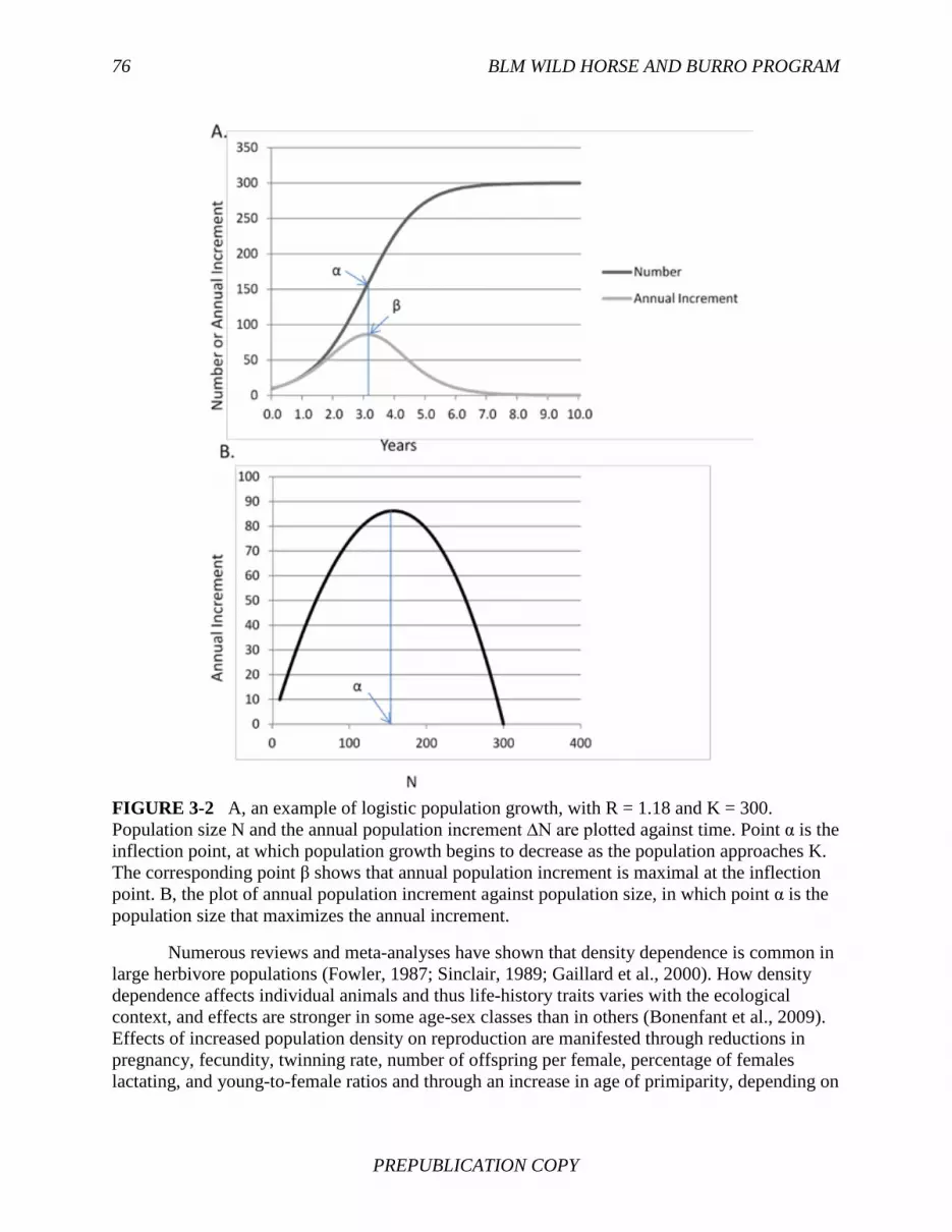
76 BLM WILD HORSE AND BURRO PROGRAM
PREPUBLICATION COPY
FIGURE 3-2 A, an example of logistic population growth, with R = 1.18 and K = 300. Population size N and the annual population increment ∆N are plotted against time. Point α is the inflection point, at which population growth begins to decrease as the population approaches K. The corresponding point β shows that annual population increment is maximal at the inflection point. B, the plot of annual population increment against population size, in which point α is the population size that maximizes the annual increment.
Numerous reviews and meta-analyses have shown that density dependence is common in large herbivore populations (Fowler, 1987; Sinclair, 1989; Gaillard et al., 2000). How density dependence affects individual animals and thus life-history traits varies with the ecological context, and effects are stronger in some age-sex classes than in others (Bonenfant et al., 2009). Effects of increased population density on reproduction are manifested through reductions in pregnancy, fecundity, twinning rate, number of offspring per female, percentage of females lactating, and young-to-female ratios and through an increase in age of primiparity, depending on

POPULATION PROCESSES 77
PREPUBLICATION COPY
the species, population, and environmental context. Survival rate responses to population density are common, but they vary among ungulate populations.
Effects of Density on Population Processes
Several studies of density dependence have included or focused exclusively on equids. In Kruger National Park, South Africa, adult and juvenile zebra survival rates were adversely affected by density and favorably affected by rainfall (Owen-Smith et al., 2005). Similarly, zebra population dynamics in Kenya were best explained by a model of rainfall-mediated density dependence (Georgiadis et al., 2003) that involved fecundity and survival. An unmanaged horse population in Argentina exhibited density-dependent responses. Reduced fecundity was the primary response to increased density. Adult female survival was also reduced at higher densities, but to a lesser degree (Scorolli and Lopez Cazorla, 2010). In a feral donkey population in Australia, fecundity was high and not related to density; however, ages of males at sexual maturity and juvenile mortality increased at higher densities (Freeland and Choquenot, 1990; Choquenot, 1991; also noted in Bonenfant et al., 2009). Pregnancy rates declined at higher densities in horses in the eastern United States (Kirkpatrick and Turner, 1991). In Nevada, it was not uncommon for 2-year-old mares to foal, in contrast to earlier evidence indicating foaling did not begin until the age of 3 (Berger, 1986; Garrott et al., 1991). Garrott et al. (1991) argued that age at first reproduction is more likely to be earlier when forage is more abundant and when competition for forage is reduced. Jenkins (2000) analyzed data from the Granite Range and Pryor Mountain horse herds and reported evidence that population growth rate decreased with increasing population. Roelle et al. (2010) confirmed those findings in the Pryor Mountain horse herd. Thus, density dependence appears to take a variety of forms in equids. Responses to density are often age-specific. Gaillard et al. (1998) reviewed evidence related to the conceptual model proposed by Eberhardt (1977) in which density effects on population vital rates (e.g., birth and death rates) would occur first in juvenile survival, then in age at first reproduction, then in reproductive rates of prime-aged (most highly reproductive) adults, and finally in adult survival. They noted that Fowler’s (1987) review supported Eberhardt’s model. The Gaillard et al. review provided further support of the model and reported that survival of prime-aged adults is relatively invariant whereas juvenile survival varies considerably from year to year. They reported that the pattern of high, stable adult survival and variable juvenile survival is observed in a wide variety of environments regardless of whether mortality is density-dependent or density-independent. They noted that higher annual variation in juvenile survival as compared to adult survival can arise from multiple causes including increased vulnerability to predation, drought, harsh winters, and factors causing low birth weights and early growth rates. In an unmanaged horse population in Argentina that was approaching carrying capacity, fecundity was affected by density and rainfall, but adult, juvenile, and foal survival rates were not (Scorolli and Lopez Cazorla, 2010). Although juvenile survival varies more than adult survival, population growth rate is highly sensitive to variations in adult survival, less sensitive to changes in juvenile survival, and moderately sensitive to changes in fecundity (Gaillard et al., 2000).

78 BLM WILD HORSE AND BURRO PROGRAM
PREPUBLICATION COPY
Possible Effects of Domestication
It is possible that domestication has selected for forms of density dependence that are different from those in undomesticated populations. Flux (2001) proposed that the tendency to self-regulate differs between feral and “wild-type” populations. It is believed that domestication of European rabbits by monks for over 600 years has led to feral populations that have been observed at densities of up to 200/ha in Australia and New Zealand (Thompson and King, 1994), whereas “wild” species seldom reach 4/ha. However, it is also likely that introduced rabbit populations in those locations are less affected by predation and disease. Other feral species also reach higher densities than their closest “wild” relatives, such as goats, pigs, cats, and domestic pigeons. Many of those species have been implicated in severely detrimental effects on habitats and native species (Flux, 2001).
Genetic history may contribute to the reproductive response of free-ranging equids to resource scarcity. A population of unmanaged horses in the Camargue (France) declined in body condition because of scarce resources, and this led to reduced foal and mare survival without a concurrent decline in fecundity (Grange et al., 2009). The authors pointed out that that pattern is different from the one in wild, nonferal ungulate populations, in which fecundity decreases well before adult survival as resources become more limiting. Other domesticated species, such as cattle, have shown the same pattern as the Camargue horses. The authors argued that domestication has selected for reproduction over survival even when resources are scarce. As a result, feral populations are more likely to oscillate strongly, and the tradeoff of decreased adult survival may make them more vulnerable to harsh environmental conditions.
Nutritional and Physiological Mechanisms
Fowler’s (1987) review indicated that food shortage is the primary factor in density dependence. The mechanisms through which food limitation affects population vital rates are most likely effects of poor nutrition, energy balance, and body condition on reproductive processes and survival rates (e.g., Gaidet and Gaillard, 2008). Poor nutritional status may also impair animal feeding and predator avoidance and increase susceptibility to adverse weather. Feral donkey populations in Australia were regulated by food-limited juvenile mortality, which in turn was related to the nutritional status of lactating females (Choquenot, 1991). In an unmanaged population of horses in the Australian Alps, population growth rate declined as numbers increased because of decreased fecundity and decreased adult and juvenile survival (Dawson and Hone, 2012). Those response variables were related to body condition and available food, and mean body condition correlated positively with forage biomass. In the Pryor Mountains, foal survival rate was positively related to precipitation, and this suggests a link to forage production and availability mediated through the condition of the mares (Roelle et al., 2010). The authors cited several other studies, including Garrott and Taylor’s (1990) study of the horse populations in the Pryor Mountains, whose results suggested that forage availability can affect mare condition and thus foaling rates. In addition to the total quantity of food, the quantity of high-quality food items may be diminished when populations are near carrying capacity. When an Australian donkey population reached carrying capacity, females ingested a diet of low nutritional value, whereas those in a population below carrying capacity were able to ingest a nutrient-rich diet (Freeland and

POPULATION PROCESSES 79
PREPUBLICATION COPY
Choquenot, 1990). Low diet quality resulted in low levels of stored nutrients in the females, which impaired their ability to raise offspring. When resources are scarce, females are induced into anestrus as a result of poor body condition (Ginsberg, 1989). Birth sex ratios may be affected because mares in poorer condition have more female foals (Cameron et al., 1999). The effect of body condition on sex ratio probably occurs at conception. The age at first reproduction and reproductive rates of 2- to 4-year-old horses are affected by competition for forage, which reduces the amount of forage per individual and thus increases the time needed for individuals to attain sexual maturity (Garrott and Taylor, 1990). Saltz et al. (2006) reported that rainfall during the year before conception and drought conditions during gestation were important determinants of reproductive success in Asiatic wild ass. They focused on rainfall before conception because females in poor condition would not go into estrus. To summarize, the causal pathways underlying density dependence begin with population size (Figure 3-3). Climatic conditions and spatial accessibility determine the availability of forage for herbivores. Population size affects the amount of forage available per animal: as population size increases, forage per animal declines; this results in reduced forage intake and reduced body condition, which affect survival rates and natality.
FIGURE 3-3 Nutrition-based mechanisms underlying density dependence and density independence.
Behavioral Mechanisms
There are two fundamental mechanisms of behavior-mediated density dependence: increased dispersal at high densities and changes in social interactions that affect reproduction.
The role of dispersal in density dependence remains uncertain because there have been few studies (Bonenfant et al., 2009). Duncan (1992) found no evidence of a social mechanism

80 BLM WILD HORSE AND BURRO PROGRAM
PREPUBLICATION COPY
that regulates equid populations below levels determined by their food resources. However, others have found that increased social stress at high density may contribute to density dependence (Linklater et al., 2004). Tatin et al. (2009) found that reduced space can slow the growth of a population of a Przewalski’s horse herd before forage becomes limiting. They suggested that reproduction decreased as a result of mare dispersals to avoid incest (Monard and Duncan, 1996).
Where populations are spatially unbounded, dispersal can forestall density-dependent control as long as there are places where populations are small and individuals in crowded locations can disperse (Owen-Smith, 1983; Pulliam, 1988). Such source-sink population complexes where emigration keeps densities low will be common where environmental forces—ranging from physical factors, such as climate, to biological factors involving predators—operate over large areas. But where there are boundaries to dispersal, as on natural islands or habitat islands created by human landscape change, densities can increase to a point at which feedback from crowding lowers fecundity and adult and juvenile survival.
Crowding changes behavior in many ways among horses and burros. In Nevada, high equid densities were associated with increased incidences of confusion, separation, and desertion of foals by mares at water points in the dry season (Boyd, 1979). Berger (1983a) reported that social instability, specifically high rates of turnover among harem males, adversely affect female reproductive success and patterns of age-specific fecundity. He also indicated that increased levels of sexual harassment can lower female body condition and disrupt normal endocrine function. By virtue of their hindgut fermentation system, equids can subsist on low-quality vegetation, and they typically compete by maximizing intake relative to other animals (Rubenstein, 1994). However, when densities increase, individual agonistic interactions increase, and this reduces time available foraging and thus competitive ability. Equid females rely on male protection to increase time spent in feeding, and this increases the likelihood that foals will survive to the age of independence (Rubenstein, 1986). Thus, any interference that impinges on a female’s ability to forage can lower body condition and reduce fecundity and survival. Moreover, because band stability increases a female’s long-term reproductive success (Rubenstein and Nuñez, 2009), disturbance that leads to more rapid turnover in the tenure of harem males or increased competition among females that leads to female movements among groups will alter important demographic vital rates.
Including Density Dependence in Models
Density dependence has been considered in a number of models of ungulate population dynamics. The trajectory of an unmanaged population of horses in Argentina was successfully modeled by fitting a simple logistic equation with a best-fit intrinsic rate of increase and carrying capacity (Scorolli and Lopez Cazorla, 2010). Georgiadis et al. (2003) developed a model of zebra populations that included density dependence in the form of a ratio of rainfall (as a surrogate of food availability) to density. The inclusion of that density-dependent term improved model accuracy despite the large fraction of variation that was explained by rainfall alone. Rubenstein (2010) modeled Grevy’s and plains zebra populations. Density dependence was solely through age at first reproduction, inasmuch as population growth rate is very sensitive to the number of 3-year-olds reproducing. Overall fecundity was linked to annual rainfall. Density dependence was statistically significant in models of four horse populations (Eberhardt and Breiwick, 2012): Equus ferus caballus in Argentina (Scorolli and Lopez Cazorla, 2010), the

POPULATION PROCESSES 81
PREPUBLICATION COPY
Camargue (Grange et al. 2009), and Oregon (Eberhardt et al., 1982) and Equus ferus przewalskii in a fenced area in France (Tatin et al., 2009).
Density dependence in the population dynamics of Serengeti wildebeest was modeled by Mduma et al. (1999). Density dependence was most strongly exerted through adult mortality, and the primary cause of death was undernutrition. Thus, mortality was modeled as a function of food per capita, and food supply was modeled as a function of rainfall. The model predicted a period of population growth following a period when population size was reduced below food-limited carrying capacity by rinderpest.2 Projected population dynamics varied within a wide range as a result of rainfall and food-supply variation, but the projected population nevertheless reached maximal levels because of density-dependent feedback.
Lubow et al. (2002) fitted a series of alternative population projection models to population data on elk in Rocky Mountain National Park. Logistic regression was used to estimate recruitment (the number of individuals added to a population through births) and survival rates of calves and survival rates of each sex and age segment as functions of population size and seasonal temperatures and precipitations. Because of the effects of population density in the models, populations stabilized at some upper limit, which the authors identified as the carrying capacity. The primary mechanism of density feedback was a nearly linear decline in calf recruitment followed by sharply declining calf survival.
An approach to the modeling of time-varying carrying capacity for Yellowstone elk populations was based on temporal variations in food availability (Wallace et al., 1995, 2004; Coughenour and Singer, 1996a). Food availability was affected by spatial heterogeneity, spatial overlap of elk, and spatially variable food availability. The latter was affected by the distributions of snow depth across the landscape throughout winter, which was affected by snowfall and temperature, which in turn were related to elevation. The effect of snow depth on forage-intake rate was explicitly represented. An energy-balance model was used to derive temporal changes in elk body condition (fat reserves) on the basis of the balance of energy intake and expenditure. Mean body condition was used to determine the fraction of animals in a normally distributed population that would die because of extremely low body condition—an approach originally developed by Hobbs (1989).
A similar idea was extended into actual population-dynamics modeling. A metaphysiological modeling approach was developed to represent the effects of energy storage on population dynamics (Getz and Owen-Smith, 1999; Owen-Smith, 2002a,b). Because animals and plants can store energy in body tissues, they have a reserve for use in times of food shortage. The approach links animal energy reserves to population dynamics; the reserves alter population dynamics, for example, through an increase in mortality when there are food shortages in the environment.
In an ecosystem modeling approach (Coughenour, 1992, 1999, 2000, 2002; Weisberg et al., 2006), the energy balance of the herbivore population is simulated as an outcome of forage intake and energy expenditure. The energy balance determines storage (fat) reserves, a measure of body condition. Condition in turn affects survival and fecundity. Forage intake depends on forage-biomass density, which establishes a link between population dynamics and forage. This type of model is explained in greater detail in Chapter 6.
Some equid population modelers have avoided considering density dependence and food-limited carrying capacity because populations are limited by other factors. Saltz and Rubenstein (1995) modeled Asiatic wild ass populations with a Leslie matrix, but because the populations
2An often fatal viral disease that affects even-toed ungulates.

82 BLM WILD HORSE AND BURRO PROGRAM
PREPUBLICATION COPY
were so small relative to the expansive area available, it was unlikely that density dependence was important, so it was not included in the model. Although the WinEquus model that is used by BLM has the capability to consider K (carrying capacity), it is rarely invoked in most BLM applications of the model because populations are always held below food-limited capacity by management removals (see Chapter 6). Gross (2000) ignored food limitations and carrying capacity in his individual-based model of the Pryor Mountain herd. He presumed that horse populations will be managed below food-limited carrying capacity and therefore not allowed to self-regulate. Linklater et al. (2004) also did not attempt to consider density dependence in their model, although it was useful for estimating population growth rates below carrying capacity.
The assumption that most BLM-managed populations are below food-limited carrying capacity and thus unaffected by density dependence appears to be reasonable given that management has heretofore aimed to ensure the prevention of rangeland deterioration, largely interpreted as preventing overuse of the forage and habitat (see Chapter 7). However, an outcome of this situation is that few data or modeling studies have provided information on outcomes of density dependence in horse or burro populations on lands under the purview of BLM. Although density dependence has not been a concern in BLM-managed HMAs and models, it will be necessary to include it in any model that addresses the question posed to the committee regarding self-limitation.
DENSITY-INDEPENDENT POPULATION CONTROLS
Large herbivore population dynamics are generally influenced by a combination of stochastic environmental variation and population density (Saether, 1997). Unmanaged or minimally managed populations should be expected to fluctuate about some mean tendency in quasiequilibrium, and the degree of fluctuation will depend on the degree of climatic variability. The dynamics of more intensively managed populations can also be expected to vary in response to density-independent factors, inasmuch as density-independent effects are in play irrespective of whether populations are managed to levels below which density dependence takes effect.
Density independence is often incorporated into predictive models of equid population dynamics. Saltz et al. (2006) applied a Leslie matrix model with demographic and environmental stochasticity to an Asiatic wild ass population in Israel. Annual precipitation during the year before conception, drought conditions during gestation, and population size determined reproductive success. They reported that increased rainfall variability in global climate-change scenarios increased extinction probability by a factor of nearly 10. The widely used WinEquus population model (see Chapter 6) incorporates density independence as stochastic variation in recruitment and survival. At the other end of the model-complexity spectrum, the ecosystem modeling approach described in Chapter 6 represents density independence by simulating climatically driven variations in forage production and effects of snow cover on forage availability.
Effects of Climatic Variability
Variable precipitation and winter weather conditions can have marked effects on horse and burro population dynamics. Precipitation affects equids indirectly through its effect on total forage biomass production and the length of time that forage remains green and more highly

POPULATION PROCESSES 83
PREPUBLICATION COPY
nutritious (Figure 3-3). Winter weather can act directly on horses and burros through thermal stress, but more often it acts indirectly as snow cover affects forage availability.
A stage-structured model of an elk population in Yellowstone that included calf, cow, and bull elk classes modeled recruitment and mortality of each class by using the best equations determined from forward, stepwise multiple regression analyses and using precipitation amounts and elk number as the independent variables (Coughenour and Singer, 1996b). Winter precipitation was a surrogate for snow cover and later forage availability. The model revealed that expected population trajectories should exhibit wide variation in response to this density-independent regulation. Although a population equilibrium could be predicted and could be interpreted as one measure of food-limited carrying capacity, there was considerable variation above and below the equilibrium value. A series of mild winters, for example, could result in population sizes above mean K, and the converse would be true in a series of severe winters.
Precipitation appears to have a substantial influence on equid populations. Berger (1986) could find little evidence of density dependence in his data on the Granite Range HMA and suggested that responses to weather variations were overriding and confounding. Roelle et al. (2010) reported that foal survival rate in the Pryor Mountain Wild Horse Range was positively related to precipitation, probably because of the effects of variable forage production on mare condition. They noted that other investigators had suggested that forage availability can affect foaling rates in this manner (Green and Green, 1977; Nelson, 1978; Berger, 1986; Siniff et al., 1986, Garrott and Taylor, 1990). Horse populations in Australia possibly increased by a factor of 4 during good rainfall years in the 1970s (Berman, 1991), and dry conditions and more intense management reduced the population by 70 to 80 percent in the central part of the country. A 10- to 20-percent birth rate is probably realistic in poor years, and a 25- to 30-percent birth rate in good years (Berman, 1991). Joubert (1974) observed lower recruitment rates in a zebra population in dry years and a large dieoff during a drought. Owen-Smith et al. (2005) reported that juvenile survival was sensitive to rainfall variability in most of 10 African ungulate species, and there was no evidence of density dependence. Rainfall also affected adult survival in several declining species.
Density-independent mortality was documented by Berger (1983b) in the Granite Range of Nevada. Two horse groups perished as a result of severe winter snowstorms. High-altitude, snow-induced mortality may be common. He concluded that unpredictably heavy snow accumulation is a principal mortality agent in the Granite Range, as it may be elsewhere in the Great Basin. Berger (1983b) referred to the winter of 1977, when an estimated 300 horses (50 percent of the population) died in the Buffalo Hills near the Granite Range. Berger (1986) reported a pattern of low mortality in most years but markedly higher mortality in occasional years of bad weather. In Wyoming’s Red Desert, abortions and still-births after a severe winter reduced natality by one-third (Boyd, 1979).
Reduction in Equilibrial Tendencies by Density Independence
In climatically variable environments, the importance of density-independent population dynamics increases. The implication of strong density independence is that in climatically variable environments herbivore populations should not be expected to reach a steady state in which population density is in stable equilibrium with forage production. Climatic variations include severe winters and droughts. When the coefficient of variation of annual rainfall, and presumably food availability, exceeds 30 percent, population size is less likely to be determined

84 BLM WILD HORSE AND BURRO PROGRAM
PREPUBLICATION COPY
by mean food-limited carrying capacity (Caughley, 1987; see also the section “Understanding Ecosystem Dynamics” in Chapter 7). Saether (1997) also theorized that lags in the responses of populations to environmental variations, in the absence of predation, will make a stable equilibrium between ungulates and their food resources unlikely. As a result, horse populations may not necessarily decline rapidly during moderate droughts despite reductions in plant growth, and the grazing pressure, expressed as a percentage offtake, may periodically increase above average values.
Ellis and Swift (1988) proposed that plant-herbivore systems in climatically variable environments are unlikely to be equilibrial and that traditional concepts of food-limited carrying capacity have relatively little value in predicting herbivore population sizes and dynamics in such environments. They proposed that a herbivore population in an environment subject to periodic droughts is periodically reduced to a low level independently of density. The population then recovers slowly until the next drought causes another reduction. As a result, the population is kept below food-limited carrying capacity—it is unable to use available food resources fully because of low density. That idea was supported by a model of zebra population dynamics (Georgiadis et al., 2003) that provided realistic predictions for 2 decades (Georgiadis et al., 2007). The model captured the fundamental mechanism of rapid population decline during dry periods and slow increase during wet periods. The greater the variability in rainfall, the greater the proportion of time that the population spends below carrying capacity.
The Ellis and Swift (1988) study generated controversy: some interpreted it to suggest that plant-herbivore systems would be generally nonequilibrial and herbivore populations would naturally be held below food-limited carrying capacity and thus below sizes that would cause overgrazing and degradation. The conclusions of Ellis and Swift, however, were limited to environments that had a high degree of climatic variability, and the implication was that such systems have nonequilibrial tendencies, not that they are absolutely nonequilibrial. Illius and O’Connor (1999, 2000) showed that herbivore populations in drought-prone environments would be “disequilibrial,” still in quasiequilibrium with critical food supplies during dry periods. Thus, plant resources should appear to be lightly used during wet periods, and on the average a small fraction of plant growth should be used. Illius and O’Connor recognized the importance of key resource areas on the landscape, such as natural dry-season grazing reserves that define the dry-season bottlenecks and thus limit herbivore populations to a particular density. Density dependence therefore exists, but it is temporally variable inasmuch as food-limited carrying capacity varies with precipitation and, in seasonally cold environments, with snow cover.
EFFECTS OF PREDATION
Predators prey on wild equids; predation on onagers and zebras has been reported in Asia (Solomatin, 1973) and Africa (Kruuk, 1972; Schaller, 1972), respectively. In Africa, predation may limit some zebra populations (Sinclair and Norton-Griffiths, 1982; Mills et al., 1995). Zebras and other ungulates were not limited by food in Namibia but most likely by predation or disease (Gasaway et al., 1996). Zebra maintained excellent body condition during dry seasons and after droughts. Recruitment rates continued to be high, corresponding to those of a growing population. Such recruitment rates could be balanced only by high rates of yearling and adult mortality, which would presumably be caused by predation or disease. Predation was suspected of being a major population control in a collection of ungulate populations in Kruger National

POPULATION PROCESSES 85
PREPUBLICATION COPY
Park (Owen-Smith et al., 2005). Adult zebra survival was strongly related to increasing density, but the steepness of the response indicated that it was strongly affected by prey-switching by lions in response to decreased availability of alternative prey species. Mills et al. (1995) reported that zebra populations in Kruger were influenced by predation but to a smaller extent than wildebeest or buffalo. However, rainfall was the primary determinant of zebra population dynamics. In Serengeti National Park, Tanzania, zebra populations have remained roughly constant for decades, despite large changes in wildebeest and other bovid numbers caused by a rinderpest epidemic (Sinclair and Norton-Griffiths, 1982; Grange et al., 2004). Very low first-year survival limits the zebra population in the Serengeti, according to Grange et al. (2004), who found evidence that rates of predation on zebras were high and hypothesized that predation potentially holds the population in a “predator pit.” The principal predators, lion and spotted hyena, feed mainly on adult zebra, so it was not clear what the main sources of foal mortality were. Using data from 23 near-natural ecosystems in Africa, Grange and Duncan (2006) reported that zebra abundance relative to that of bovids is lower in ecosystems that have high lion densities and that zebra abundance is not as affected by forage abundance as bovid abundance; this suggests that zebras are more sensitive to predation than are bovids. Rubenstein (2010) reported that 73 percent of lion dung samples contained Grevy’s zebra and 53 percent contained plains zebra hair. One wildlife conservancy had high rates of lion predation on zebra. Wolves are quite capable of preying on equids. In southern Europe, equids constituted 6.2 percent of wolf diets (range, 0-24 percent) (Meriggi and Lovari, 1996). In Abruzzo National Park, Italy, horses constituted 70 percent of wolf diets; however, unguarded horses are commonly hobbled in that area to prevent long-range movements (Patalano and Lovari, 1993, cited in Meriggi and Lovari, 1996). In northwestern Spain, a population of free-ranging ponies is heavily preyed on by wolves (Lagos and Barcena, 2012). Foal survival rate was very low (0.41), and 76 percent of foal carcasses found were killed by wolves. Van Duyne et al. (2009) reported that wild Przewalski’s horse foals were killed by wolves in Hustai National Park, Mongolia, and cautioned that predation could influence translocation efforts. However, those horses are sufficiently vigilant to survive and reproduce, so perhaps they have not lost essential skills (King and Gurnell, 2012). Wolves in a multiprey system have been reported to prey on feral horses in Alberta, Canada. Webb (2009) reported that one of 36 kills by wolves included a feral horse. Webb (2009) located 192 ungulates that had been killed by wolves in 11 packs from 2003 to 2006. Some 7 percent were feral horses, and they made up 12 percent of the total biomass consumed (0.01 ± 0.02 feral horse/pack/day). Despite evidence that wolves prey on equids elsewhere, the committee was unable to identify any examples of wolf predation on free-ranging equids in the United States. Most predation on free-ranging equids in North America has been attributed to mountain lions. That has been reported by Robinette et al. (1959) and Ashman et al. (1983). Berger (1983c) cited an unpublished report of 21 cases of mountain lion predation on free-ranging horses in the Great Basin; those deaths spanned more than 20 years and had negligible effects on population growth. Feral (but not free-ranging) horses constituted 11 percent of mountain lion diets in Alberta (Knopff and Boyce, 2009). Horses constituted 10-13 percent of adult male lion diets, but female lion diets were almost devoid of horses (Knopff et al., 2010). Overall, mountain lion predation on free-ranging equids in North America is, with few exceptions, considered uncommon (Berger, 1986). One of the exceptions is the free-ranging horse population on the central California-Nevada border. Turner et al. (1992) examined foal survival rates in the area (the Montgomery

86 BLM WILD HORSE AND BURRO PROGRAM
PREPUBLICATION COPY
Pass Wild Horse Territory managed by the U.S. Forest Service) because there was a ban on mountain lion hunting in California and low hunting pressure in Nevada that led to a high density of mountain lions. The study was conducted from May 1986 to July 1991 by examining the horse and mountain lion populations and documenting deaths of horses. The average annual cohort of foals over the 5 years was 32. The annual survival rates were calculated for foals (0.27), yearlings (0.95), and adults (0.96). From 1987 to 1990, 48 foals were lost; 58 percent were located as carcasses and 82 percent of those were killed by mountain lions. The authors concluded that mountain lion predation had a substantial effect on the demography of that free-ranging horse population. The study was continued, and Turner and Morrison (2001) used 11 years of data (1987-1997) to examine again the influence of mountain lions on the horse population in Montgomery Pass Wild Horse Territory. Their results supported the earlier work of Turner et al. (1992): mountain lions were responsible for the deaths of 45 percent of the foals that were born. Mountain lion predation was also hypothesized as a major factor in limiting horse population growth in an area of southern Nevada where they use high-elevation forested habitats in summer (Greger and Romney, 1999). Those habitats are excellent for mountain lions because of their broken topography.
By and large, research that has addressed the question of predation on free-ranging equids in North America has been limited to anecdotal observations and a few published papers, but at the time of the committee’s review, studies at the University of Nevada, Reno, that should provide more quantitative data were under way. The work in several mountain ranges of western Nevada was examining predation by mountain lions in multiprey systems in which free-ranging horses had various densities. Diet data were being obtained by using information from GPS-collared mountain lions to investigate predation events; more than 700 predation events had been investigated as of June 2012. Ten of 13 collared mountain lions that had access to free-ranging horses regularly consumed horses as prey. Horses were documented to have been consumed as prey by collared mountain lions in eight mountain ranges throughout the study area in western Nevada (Virginia, Pah Rah, Fox, Lake, Wassuk, and Excelsior ranges and Virginia and Smoke Creek Mountains). Preliminary data suggest that in that study area, where free-ranging horses are available as prey, more than 50 percent of the diet of collared mountain lions is made up of horses when diet data on individual mountain lions are pooled. Preliminary results suggest that mountain lions in that multiprey system are generalists at the population level but that some diet specialization occurs at the individual level: some lions select for deer where horses are more abundant, and some select for horses to the near exclusion of other prey items where mule deer, bighorn sheep, and domestic animals are present. There is also some evidence that the magnitude of predation on horses by mountain lions may be related to the density of free-ranging horses, greater predation on horses occurring where densities of horses are higher (Andreasen, 2012). The potential for mountain lions to affect the sizes of populations of free-ranging horses in North America is limited by the fact that most HMAs are in areas that have few mountain lions. The ranges of mountain lions tend to be concentrated in forested areas and at higher elevations (Kertson et al., 2011) and in areas that have mountainous or otherwise broken topography with limited viewsheds. In contrast, many horse populations favor habitats that have more extensive viewsheds. Mountain lions are ambush predators and require habitats that provide opportunities for stalking or finding prey without being seen. Other predators, such as wolves are more cursorial—capable of pursuing prey across open habitats. That a large predator, when abundant, can substantially influence the dynamics of free-ranging horses is not surprising inasmuch as black bears (Zager and Beecham, 2006), mountain

POPULATION PROCESSES 87
PREPUBLICATION COPY
lions (Wehausen, 1996), and other predators (Ballard et al., 2001; Boertje et al., 2010) have exerted strong influences on ungulate populations. However, the influence of predation on horses in the western United States is considerably limited by a lack of habitat overlap both with mountain lions and with wolves. Another constraint is that among free-ranging horse populations, foals are the usual prey, and predation on adults has rarely been documented until the recent studies in Nevada. Population size is not affected as much by foal survival as it is by adult survival (Eberhardt et al., 1982), and foal survival is strongly affected by other variables (such as weather).
CONSEQUENCES AND INDICATORS OF SELF-LIMITATION
If a population of herbivores were to self-limit, effects on the ecosystem would be expected. This section reviews the theory, expectations, and case-study examples of free-ranging horses in self-limiting circumstances.
Theory
Riney (1964) and Caughley (1970, 1976) proposed that, on introduction of a large herbivore into an ecosystem not previously occupied, there would be an initial irruption of the population that would lead to a decline in vegetation conditions, which would in turn lead to a decline in the herbivore population and allow partial vegetation recovery (Figure 3-4). The herbivore-vegetation system would then reach a new equilibrium between plant productivity and herbivore population density in which vegetation productivity and cover may be less than that in a system that does not have herbivores or in a system that is managed for maximal herbivore productivity. The resulting plant-herbivore system may be less productive, have less standing herbaceous biomass, and have a different plant species composition, but it may nevertheless be functional and sustainable. That conceptual model assumes that the vegetation-soil system has the capacity to persist in some form through and beyond the initial period after an introduction, in which it has been heavily used and reduced in function. It also assumes that surviving vegetation components would be adapted to withstand recurrent herbivory and would increase in relative abundance to form a plant community that is more adapted to withstand herbivory. As noted in Chapter 7, under some conditions, productivity of herbivory-adapted plant species may not be reduced by herbivory.

88 BLM WILD HORSE AND BURRO PROGRAM
PREPUBLICATION COPY
FIGURE 3-4 Large-herbivore population trajectory after an introduction. Herbivory causes a decline in plant production and thus in K. Here, K in the underlying logistic model declines linearly from 300 to 200 individuals from year 7 to year 10, and this results in a decline in herbivore population size.
General Expectations
There is no doubt that large herbivores have numerous effects on their environments that result from grazing, browsing, trampling, and behavioral and competitive interactions with other species (see Chapter 7). When the population is food-limited and population growth rate decreases to zero, the forage resource base will most likely be heavily grazed. Horses and burros have the ability to graze plants down to the ground. They can kill plants through uprooting and trampling, create areas of low vegetation cover, and change plant species composition to favor less desirable or exotic species. At some point, reduced vegetation cover can lead to accelerated soil erosion and decreased vegetation productivity and rangeland health (NRC, 1994; Pellant et al., 2005). If resulting feedbacks to equid population growth are ineffective or if they have been disrupted by human activities, rangeland ecosystems can be pushed across thresholds into degraded states from which recovery is difficult or impossible (see Chapter 7).
Grazing pressures can be expected to be spatially heterogeneous. In expansive habitats, it is simplistic to think of a mean grazing pressure uniformly distributed across the landscape; a variety of factors affect animal distributions beside forage. It is more realistic to expect that some areas will be heavily, perhaps “excessively,” grazed while other areas are little used and may serve as refugia for plant species that are more sensitive to grazing by large herbivores. The heavily used, disturbed areas are, however, also refugia for disturbance-adapted plant species. One example is the existence of increased levels of disturbance near water sources. Such areas have sometimes been referred to as sacrifice areas because they are an inevitable outcome of the presence of large herbivores, their requirements for water, and the fact that water is distributed at point locations.
It can be expected—on the basis of logic, experience, and modeling studies cited above—that because horses or burros left to “self-limit” will be food-limited, they will also have poorer body condition on the average. If animals are in poorer condition, mortality will be greater,

POPULATION PROCESSES 89
PREPUBLICATION COPY
particularly in times of food shortage resulting from drought or severe winter weather. Indeed, when population growth rate is zero, mortality must balance natality. Whether that is acceptable to managers or the public is beyond the purview of the committee, but it is a biological reality.
It is difficult to generalize about whether these are natural and expected outcomes in unmanaged large-herbivore or, more specifically, free-ranging equid ecosystems. On the basis of evidence presented above, many large-herbivore populations are regulated through food limitation as a natural process. The evidence reviewed above also indicates that predation is a factor in some large-herbivore populations and some equid populations. Most horse and burro populations in North America appear to be little affected by predation because predators are absent or present at low densities, possibly because they have been extirpated or simply because habitats are not suitable for them. The degree of naturalness is also affected by other human activities, such as restrictions on dispersal and other movements, the presence of livestock, and water development.
Case Studies
The only way to know the consequences of self-limitation for the vegetation, horses and burros, and the ecosystem is to observe the consequences where self-limitation has been allowed to occur. As pointed out above, there are few cases in which free-ranging horse populations have not been managed and have been left to self-regulate and in which simultaneous scientific studies of the vegetation and of the equids have been carried out. But there are probably many cases in North America in which equid populations have gone unmanaged, or have been minimally managed, for a number of years. In some cases, the equids have been studied but their effects on habitats have not (e.g., Berger, 1986). In other cases, the equids and their effects on landscapes have not been studied. Some unmanaged populations on tribal lands have received little or no scientific study.3
The responses of equids to a situation of self-limitation have been discussed above with regard to density dependence. As noted, density dependence results from food limitation, a decline in animal nutritional condition, and consequent decreased recruitment and survival rates. Many examples of equid ecosystems around the world were given. Chapter 7 reviews the numerous effects that horses have on their habitats and on other species and examines the concepts of thriving natural ecological balance and AMLs. Horses will have some effects on their habitats at the point of food limitation, and these could be pronounced. On the basis of studies of systems that have high densities of horses, although not necessarily at the point of food limitation, reasonably well-informed hypotheses can be developed about the expected state of vegetation and other species when the equid population reaches the point of self-limitation. However, whether such a system can be self-sustaining (or perhaps even “thriving”) over the long term cannot be known without experimentation.
New Zealand
Free-ranging horses in New Zealand are derived from animals introduced from various sources in the 19th and 20th centuries (Rogers, 1991). They once ranged over much of the central North Island but have diminished since the 1950s. The only remaining population survives in the Kaimanawa Mountains because of restricted public access on military lands. The
3For example, Yakama Nation in Washington, available online: http://www.ynwildlife.org/.

90 BLM WILD HORSE AND BURRO PROGRAM
PREPUBLICATION COPY
Kaimanawa unmanaged population was continuing to increase and had not reached food limitation as of 1990 (Rogers, 1991). However, in the southern portion of the area, horses were expanding their ranges in response to increased density. The most important habitats for horses included wide basins with areas of volcanic ash supporting tall red tussock and short hard tussock grasslands. Grazing by domestic sheep, cattle, and horses and burning since the 1890s converted tall red tussock to short tussock grasslands.
A 20-m x 20-m grazing exclosure in degraded short tussock grassland resulted in changed plant species composition. The dominant intertussock grass species increased while 12 low-stature species and total species diversity decreased as the hard tussock species increased in stature and shaded them. Adventive (introduced) species also expanded. It is notable that the tall red tussock grass decreased. The exclosure also showed that grazing was not reducing the recruitment of hard tussock. Thus, cessation of horse grazing did not restore the original red tussock species, so the vegetation might have been converted to an “alternate stable state” as explained in the section “Understanding Ecosystem Dynamics” in Chapter 7. Furthermore, cessation of grazing resulted in adverse changes in species composition toward the adventive species, and this indicates that a moderate level of grazing would maintain the more desirable hard tussock grassland physiognomy (appearance) and species composition.
Vegetation responses to horses varied from north to south. In the north, where horse numbers were low, in the most prevalent habitats, red tussock appeared to be slowly recovering from the degradation resulting from early European livestock. In some habitats in the north, particularly mesic sites, horse grazing continued to have substantial adverse effects on biodiversity. In contrast, in the south, the landscape was more resilient to horse grazing because of the changes in species composition that had resulted from prior European livestock grazing. Thus, it might be concluded that exposure to grazing in the south had changed the plant community to one that is more resilient, and thus adapted, to further grazing by free-ranging horses. Moreover, the persistence of the hard tussock physiognomy (appearance) depends on continued moderate grazing.
Balancing free-ranging horses with the conservation of biodiversity across the landscape depends on the recognition of spatial heterogeneity between the north and south. In the south, Rogers (1991) concluded that horse preserves could be recognized where their numbers could be manipulated for the benefit of the horses and indigenous landscapes. In the north, however, he concluded that horse grazing compromises nature conservation values, so their numbers may have to be controlled.
It should be noted that no mammalian herbivores were present in New Zealand before the introduction of domesticated livestock by European settlers. Consequently, the responses of vegetation in New Zealand to introduced mammalian herbivores could differ from responses of vegetation that has coevolved with mammalian herbivores. Central Australia
Berman (1991) studied populations of feral horses in central Australia. Aerial surveys in 1981 and 1984 indicated that there were about 206,000 animals. Populations may have quadrupled during a period of good rains in the 1970s, but drier conditions, decreased rangeland availability, and management more recently have reduced the population by 70-80 percent. That suggests that horse populations increased and then decreased in response to forage availability; horses might have been above food-limited carrying capacity in dry conditions. Berman observed that variations in vegetation, wildlife, and soil erosion corresponded with changes in

POPULATION PROCESSES 91
PREPUBLICATION COPY
grazing intensity. High densities were associated with denudation, low densities of kangaroos, water holes with horse carcasses, and increased gully erosion. Horse and cattle dung density and gully erosion decreased with distance from water while plant cover and kangaroo dung increased with distance from water. Feral horses were able to affect almost all rangeland areas in central Australia because they are able to walk up to 50 km from water and traverse hills, which are barriers to cattle. Berman noted that many examples of soil erosion exist in parts of central Australia; although these have often been attributed to overgrazing by horses and cattle, it is difficult to prove that horses and cattle cause a substantial amount of erosion because erosion also takes place without them in these environments. Horse and cattle diets and habitats overlap, so it was not possible to differentiate vegetation and soil responses that were due to horses rather than cattle.
Argentina
In the Pampean grasslands of Ernesto Tornquist Provincial Park, Argentina, an unmanaged population of horses increased according to a logistic curve and was beginning to show signs of density dependence, as noted above (Scorolli and Lopez Cazorla, 2010). Although density had no effects on survival, it affected fecundity. The authors hypothesized that fecundity was reduced at higher densities because of reduced pregnancy in mares that had low body condition. De Villalobos and Zalba (2010) and de Villalobos et al. (2011) reported that the horses reduced herbaceous cover and facilitated establishment of an invasive pine species. They suggested that grazing had caused reduced plant diversity and species evenness and altered the composition of communities. Other native and exotic ungulate species had declined as a result of competition with the horses. Shackleford Banks
Shackleford Banks, a barrier island off the coast of North Carolina, supports a population of free-ranging horses that has experienced increases and decreases in population numbers in response to changes in carrying capacity resulting from management practices. Before the National Park Service (NPS) acquired the island and incorporated it into the Cape Lookout National Seashore, free-ranging horses shared the island with domestic livestock, including cattle, sheep, and goats (Rubenstein, 1981). After NPS removed all domestic stock from the island in the late 1980s, free-ranging horse numbers more than doubled from a competitively determined, food-limited carrying capacity of 104 animals to a new level, without competition from livestock, slightly over 220. That provided an opportunity to witness changes in behavior and vital rates when density-dependent effects were removed and reappeared as the population expanded. At first, body-condition scores increased from 3.5 to over 4 (on a 1-5 scale, with a score of 1 representing a horse in poor condition) as food previously consumed by livestock was now being eaten by horses. Fecundity also increased slightly, the interbirth interval declined from about 3 years to slightly more than 2 years and mortality in adult and juvenile males and females dropped 15 percent (Rubenstein and Dobson, 1996). However, as the population reached the new carrying capacity, those patterns reversed, and vital rates returned to their previous equilibrium levels.
Observable declines in body condition and increases in mortality, especially after hurricanes and winter storms, prompted the development of a plan for population control (Rubenstein and Dobson, 1996). As the population climbed to its new peak of 225 animals, rates of aggression increased among males and normally peaceful females, the variety of social

92 BLM WILD HORSE AND BURRO PROGRAM
PREPUBLICATION COPY
systems changed as territorial harems gave way to harems that had large overlapping ranges, and many harems became populated by more than one male. Although those changes helped to mediate some of the consequences of crowding while the population was in transition, in the end a new carrying capacity was reached and was accompanied by changes in behavior and vital rates. One of the biggest changes was a reduction in the stability of the harem. Pressure from increasing numbers of bachelor and harem males lowered female feeding rates, increased the percentage of females that changed groups each year from just under 11 percent to just over 25 percent, and increased the skew in reproductive success (a nonequitable distribution of reproduction among individuals) of males and females. Once NPS started managing the population to cycle around 125, average body condition and vital rates improved and the reproductive skew of both sexes was reduced, and this improved the genetic health of the population (Rubenstein and Nuñez, 2009).
Horses on Shackleford Banks decreased the abundance of Spartina grasses (Wood et al., 1987; Hay and Wells, 1991). Grazed habitats had less vegetation, a higher diversity of foraging birds, higher densities of crabs, and lower species richness of fishes (Levin et al., 2002). Horses altered habitats indirectly in many ways. Oostervaardersplassen, the Netherlands
In the Oostvaardersplassen Reserve in the Netherlands, Heck cattle, red deer, and Konik horses have been left unmanaged since the 1980s and have reached high densities (Vulink, 2001). It is a relatively moist ecosystem, having been reclaimed from the sea and having high annual precipitation. The management objective is to allow natural processes to operate to the greatest extent possible although the reserve is fenced. The management is informed by an appreciation of the natural, expected, and even desirable effects of large herbivores on other components of the ecosystem and the possibility of natural regulation through density dependence. Herbivores were originally introduced to keep the vegetation in a more open state because there was considerable woody encroachment. The herbivore species are close analogues of the native herbivores that would have been present hundreds of years ago. Large predators are absent. The Konik horses have shown a higher intrinsic rate of population increase than Heck cattle (Vulink, 2001) and have outnumbered the cattle, which apparently are regulated by food shortage in winter. If current trends continue, the horses and red deer will probably outcompete the cattle and displace them (ICMO2, 2010).
Because the reserve is small and most of it is easily visible to the public, animals that die of starvation or old age can be seen, and this leads to dilemmas with respect to the ethical treatment of animals (ICMO, 2006; ICMO2, 2010). Large dieoffs during severe winters are periodic. On ethical grounds, animals that are suffering and dying are culled (shot) to prevent further suffering. That is also justified as a replacement for predators and as a moral responsibility of humans because of the creation of artificial barriers to movements out of the reserve (fences).
The following responses have been observed
· The number of animals culled in response to weather conditions is highly variable.
· The number of animals culled has increased over the last decade because populations have reached ecological (food-limited) carrying capacity.
· The average body condition of animals has declined over the last decade.

POPULATION PROCESSES 93
PREPUBLICATION COPY
· Mortality has increased with annual variability in mortality. Mortality is expected to balance recruitment in the near future.
· Plant productivity and the number of animals that the area can support will possibly decline somewhat because of depletion of soil nutrients.
· Grazing promotes short swards and prevents woody regeneration. · Grazing increases plant diversity on the small scale but not the large scale.
(ICMO2, 2010) Pryor Mountain Wild Horse Range A population of horses descended from Andalusian Spanish mustangs has inhabited the Pryor Mountains possibly since the 1700s (BLM, 1984). The earliest record of their presence is a photograph of a roundup of 101 horses in 1910. Although the horses have inhabited the Pryor Mountains since then, they were never counted until 1970. Horse traps were built by ranchers in the 1930s and 1940s, but the numbers removed were never recorded. When BLM announced plans to remove the horses in 1964, they appeared to be in good shape despite the condition of the range. Local ranchers commented that the range was not overgrazed, that horse birth rates were low, and that the horses were in no worse condition than they were 50 years before (Ryden, 1990). Notably, considerable numbers of domestic livestock were permitted to use the range from 1907 to 1930. Half as many livestock units were permitted after 1930. In 1970, when a census of the horses occurred, there were 270 horses (Feist and McCullough, 1975). Horse reductions began with roundups in 1971 and 1973 and reduced the herd to 120-130. The horses have since been managed through removals to about 85-120. Most recently, the U.S. Department of Agriculture’s Natural Resources Conservation Service carried out an assessment (Ricketts et al., 2004), which recommended an AML of 45-142 and noted the following
· Over the last half-century, the conditions of the horse range were described as very poor to fair in a number of BLM assessments.
· The condition of the range is getting worse on the basis of low proportions of preferred plant species and evidence of soil erosion.
· In 2004, the health of the rangeland at six sites was rated at 2.0-3.75 (average, 2.75) on a scale of 0-5. A score of 4 or more is considered healthy relative to the historical potential climax vegetation. A score of 2.5 or less is considered unhealthy and to have a strong possibility of nonrecovery in the absence of external energy inputs (such as mechanical seeding). (Ricketts et al., 2004)
Apparently, although horses have been managed since 1973 at much lower numbers than were present initially and despite reductions in livestock numbers in the 1930s, unhealthy range conditions have persisted. However, Singer et al. (2000) noted that former managers who visited the range in 1997 remarked on an overall improvement in plant condition. In an ecosystem modeling assessment (see Chapter 7) of the Pryor Mountain Wild Horse Range, it was possible to examine vegetation and animal responses to various horse densities, including the number present in 1970 (Coughenour, 1999, 2000, 2002). It was also possible to determine food-limited carrying capacity by letting the model run with no horse removals until it came into quasiequilibrium with vegetation productivity. With horse numbers held constant at 270, the model simulated markedly reduced herbaceous biomass compared with what happened with no horses. Forb biomass proportion increased while grass proportion decreased. Root

94 BLM WILD HORSE AND BURRO PROGRAM
PREPUBLICATION COPY
biomass was also decreased. In the simulation in which horse populations were allowed to grow freely, plant responses were not much different from those with the number fixed at 270.
Grazing was predicted to be heterogeneously distributed. When 1971-1996 observed horse numbers (87-250 horses; mean, 157) were used, 40-70 percent of the landscape was predicted to be lightly grazed, 5-20 percent grazed less than 80 percent, and 5-15 percent grazed to 50- to 80-percent offtake. The model predicted that with historical horse densities, some parts of the landscape would experience substantial decreases in herbaceous biomass. With no culling, the fraction of the landscape that would be heavily grazed would increase markedly. The model simulated that horse numbers would initially increase to over 300, level off, plunge dramatically in response to a drought, and then gradually increase and level off at a mean of 270, the food-limited carrying capacity. In both the fixed number and the freely varying simulations, horse body condition declined to low levels, particularly in dry years or years with severe winters. In separate simulations comparing horse body conditions with no culling versus actual densities in 1970-1995, horse body condition was markedly lower with no culling. At food-limited carrying capacity, plant cover would be lower than what exists on the range, and the fraction of the landscape receiving extremely heavy use would increase (see Chapter 7). In the heavily used areas, herbaceous cover would be reduced to less than 20 percent of potential, and soil erosion rates in those areas would probably also be higher. Horses would be in poorer body condition, and horse mortality would be higher.
MANAGEMENT FACTORS
Management itself alters horse and burro population growth rates through a variety of mechanisms aside from the simple direct effects of removals or reduced fertility due to contraception. The indirect effects of management are considerable. One likely response is compensatory population growth as a result of reductions in numbers. Horse and burro populations are seldom limited by density because they are kept below food-limited carrying capacity through removals and to some extent through treatment with the contraceptive porcine zona pellucida (PZP; discussed in Chapter 4). Indeed, AMLs are usually set in such a way that considerable forage material is uneaten; this is the very purpose of the allowable use level (see Chapter 7). That leaves horses and burros in a position for compensatory population growth because they are below food-limited carrying capacity. If there were no intervention, herds would reach food-limited carrying capacity, body condition would decline, natality and survival rates would decline, and more animals would die of starvation. Removals are likely to keep the population at a size that maximizes population growth rate (see Figure 3-2B), which in turn maximizes the number of animals that must be removed and processed through holding facilities. Management may also alter population growth by affecting dispersal, particularly through fencing but also by permitting conflicting land uses that alter habitats for horses and burros. Impaired dispersal would decrease population growth because of increased competition for forage. Water provision, in contrast, could increase population growth rate by increasing the area of habitat that has water and thus total available forage. Horses in arid Australia were reported to range as far as 50 km from water (Berman, 1991), but maximum distances would probably be considerably less in rugged topography or where there are other impediments to movement.
suzanneroy
Highlight
suzanneroy
Highlight
suzanneroy
Highlight
suzanneroy
Highlight

POPULATION PROCESSES 95
PREPUBLICATION COPY
Compensatory Reproduction
Compensatory reproduction in response to gathers is likely in any population that exhibits density dependence. To the extent that a population is being regulated by food supply, decreased density will provide more forage per individual, increasing body condition, reproduction, and survival and thus population growth rate. Choquenot (1991), in a study of feral donkeys in Australia, reported that population growth was regulated by food-related juvenile mortality. Dawson and Hone (2012) advised that compensatory responses in survival, fecundity, and age at first reproduction in the population should be considered in any management program. In particular, they were referring to the fact that their data showed that survival and fecundity were increased and age at first reproduction decreased at lower densities, so it is likely that reductions in density due to culling will have the same effect.
The response of population growth rate to increased density must be known in order to predict the degree of compensatory growth that can be expected at a given population density. If the population size is above the theoretical inflection point of the logistic growth trajectory (point α in Figure 3-2A), reductions will increase the annual population growth increment. However, if the population size is below the theoretical inflection point, reductions will decrease the annual growth increment. Various models of density dependence, as discussed above, could be used to predict the degree of compensatory growth resulting from animal removals in relation to the population size and the rate of removal.
Gathering has also been shown to have varied indirect effects on reproductive success. In Idaho and Wyoming, foaling success rates were higher among gathered horses than among horses that were not gathered (Hansen and Mosley, 2000). Foaling success rates in Idaho were 29 percent, 31 percent, and 43 percent for mares not gathered, mares gathered and adopted, and mares gathered but released, respectively. In Wyoming, foaling success rates were 29 percent, 42 percent, and 48 percent in those groups. There were no statistically significant differences among groups, however, most likely because samples were small in relation to high variance. Effects of gathers on body condition, lactation status, and pregnancy were not reported. It is important to note that such results, if real, would most likely be attributable to forage limitation and lower body condition among ungathered than among gathered mares. In contrast, in another study, foaling was lower among gathered horses. Pregnant mares that were gathered and removed had substantially lower reproductive success than ungathered mares at one site, and gathered and released mares had less reproductive success than ungathered mares at a second site (Ashley and Holcombe, 2001). The authors speculated that that was a result of loss of fetuses due to the stress of being gathered and handled for a long period. Animals that were removed were transported 246 km to a holding facility, where they were held for 21 days before adoption. A number of miscarriages were observed at the holding facility.
Kirkpatrick and Turner (1991) compared a population managed with annual foal removals on Chincoteague Island, Virginia, with an unmanaged population on Assateague Island, Maryland. Management-level applications of PZP did not begin on Assateague Island until 1994, after the 1989 study (Turner and Kirkpatrick, 2002.) They hypothesized that there would be greater fetal losses in the unmanaged population because of the concurrent physiological stresses of lactation and pregnancy (weaning rarely occurs before 1 year and it commonly occurs at 2 years). They estimated pregnancy and foaling rates of 40 free-ranging mares on Assateague Island and 48 managed mares on Chincoteague Island and found a higher foaling rate in the Chincoteague population because a greater percentage of mares foaled annually (80 percent). The hypothesis of greater fetal loss was not supported: there was no

96 BLM WILD HORSE AND BURRO PROGRAM
PREPUBLICATION COPY
difference between the two populations. However, pregnancy and foaling rates in the Chincoteague population were nearly double those in the Assateague population. The authors suggested that the greater pregnancy and foaling rates were due to cessation of lactational anestrus and that the cessation of lactation in mares that had their foals removed resulted in these animals going back into estrus. However, the authors provided no evidence that lactating mares were not cycling. Another possible cause of increased pregnancy and foaling in the managed population is reduced energetic demands due to cessation of lactation. In contrast, Wolfe et al. (1989) used plasma progesterone measurement to examine pregnancy rates in 553 free-ranging mares. They found no difference in pregnancy rate between lactating and nonlactating mares. Kirkpatrick and Turner (1991) suggested that the reason that no difference was found was that the method for detecting pregnancy—measurement of plasma progesterone—can be inaccurate. Although the method is widely used for detecting pregnancy in other species, it is not reliable for equids. It is also known that although lactational anestrus does occur, it is very uncommon, and most mares resume cycling 5-9 days after foaling. In summary, it is possible that population management via foal removals may result in increased fecundity, but evidence of a lactational anestrus mechanism is lacking. It is also possible that pregnancy and foaling rates are reduced in lactating mares because of the lower body condition that results from the energetic demands of lactation. Because horse populations on BLM lands are not managed through foal removals, this form of compensatory reproduction probably has little relevance.
The effects of PZP on population growth, longevity, and body condition were studied over a 10-year period on Assateague Island (Turner and Kirkpatrick, 2002). PZP clearly reduced foaling rates among contracepted animals. However, mortality in mares and foals decreased, and two older age classes appeared (21-25 years and over 25 years), which indicated an increase in longevity. Body-condition scores of nonlactating mares increased substantially but those of lactating mares did not change. The cause of the decrease in foal mortality was unclear, but it could have been due to increased body condition of the mares. Body condition of untreated mares, or of treated mares in which the treatment has lost effectiveness, could increase because of reduced competition for forage. In treated mares, contraception reduces the energetic costs of reproduction, and this also results in increased body condition and longer lifespan (Gray and Cameron, 2010). Nuñez et al. (2010) also found that treated mares had better body condition than untreated mares; this could result in an extended breeding season and increased chance of conception in animals that have low PZP antibody levels. Thus, the favorable effects of increases in body condition, longevity, foal survival, and length of breeding season on population growth rate could offset to some extent the adverse effects of contraception on reproduction and population growth rate. That might be termed compensatory population growth; however, it is unlikely that the degree of compensation would be sufficient to overcome the degree to which contraception reduces reproduction and population growth.
Effects Related to Ability of Animals to Disperse
Ecologically adaptive movement patterns are still exhibited by many extant horse populations. Free-ranging horses in Nevada move from low to high altitudes in spring or early summer after the wave of vegetation green-up, and they move to low elevations in fall (Berger, 1986). However, changes in land ownership and allocations of lands for livestock use may interfere with traditional movement patterns and may preclude the re-establishment of natural movements, ones that presumably exist in truly wild and free-ranging equid populations.

POPULATION PROCESSES 97
PREPUBLICATION COPY
The importance of movement for coping with drought is illustrated by observations in Namibia (Gasaway et al., 1996). Ungulates, including zebra, maintained near average mortality during severe drought because they could move over large areas and find food reserves in areas not regularly grazed. Low ungulate densities and clumped distributions were responsible for the existence of infrequently used areas that served as drought reserves. Such dry-season food reserves were also important in keeping mortality low in Kruger National Park during a drought in 1982-1983 (Walker et al., 1987). In contrast, populations in two other reserves, which were near their food-limited carrying capacity before the drought, lacked such lightly grazed food reserves and suffered high mortality (Walker et al., 1987, as noted by Gasaway et al., 1996).
An important question is the extent to which horse (and cattle) grazing can be managed to compensate for losses in natural movement patterns, which presumably were important determinants of the grazing regimes experienced by plant species that evolved during or before the Pleistocene in the presence of large herbivores. The mix of private, tribal, and public ownership often fragments landscapes that might have been more natural, expansive grazing areas. Differences between agency policies may exacerbate the fragmentation. Fencing can interfere with movement to other areas when forage is depleted and cause heavier intensities and frequencies of herbivory than would occur otherwise.
Confinement or restrictions on migration or dispersal movements will probably result in a plant-herbivore system that has different dynamics from one that does not have such constraints. In general, the smaller the area that a population is limited to, the greater the potential for a self-regulating system with undesirable qualities, such as population crashes and population oscillations. Spatial constraints can lead to reductions in vegetation cover to lower levels than would be seen otherwise, followed perhaps by vegetation recovery after horse populations decline in response to food shortages. However, there is also an increased likelihood of irreversible shifts in vegetation communities, in accordance with recent theory and observations of alternate stable states, to communities dominated by invasive plant species, by shrubs, or by bare ground with little or no seed bank to support recovery (see the section “Understanding Ecosystem Dynamics” in Chapter 7).
In contrast, such generalizations as “confinement will result in range degradation” are also unwarranted. The degree of confinement, the areas that are inaccessible, the availability and dispersion of water, climate, and vegetation productive potential can all modify the response. Confinement may have little or no consequences or great consequences, depending on those factors.
Additional challenges arise from migration and dispersal across HMA boundaries. A designated HMA may constitute the core range of a herd or population, but dispersal movements outside the HMA are possible. Dispersing animals may move onto areas that are subject to conflicting land uses or management objectives. Conversely, movements of animals into an HMA from surrounding areas that are under different management jurisdictions can work at cross purposes to the management objectives of an HMA. Where such cross-jurisdictional movements occur, it is necessary to establish co-operative relationships among adjacent land owners.
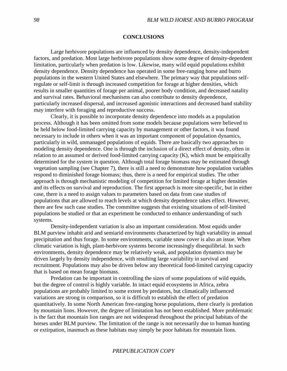
98 BLM WILD HORSE AND BURRO PROGRAM
PREPUBLICATION COPY
CONCLUSIONS
Large herbivore populations are influenced by density dependence, density-independent factors, and predation. Most large herbivore populations show some degree of density-dependent limitation, particularly when predation is low. Likewise, many wild equid populations exhibit density dependence. Density dependence has operated in some free-ranging horse and burro populations in the western United States and elsewhere. The primary way that populations self-regulate or self-limit is through increased competition for forage at higher densities, which results in smaller quantities of forage per animal, poorer body condition, and decreased natality and survival rates. Behavioral mechanisms can also contribute to density dependence, particularly increased dispersal, and increased agonistic interactions and decreased band stability may interfere with foraging and reproductive success.
Clearly, it is possible to incorporate density dependence into models as a population process. Although it has been omitted from some models because populations were believed to be held below food-limited carrying capacity by management or other factors, it was found necessary to include in others when it was an important component of population dynamics, particularly in wild, unmanaged populations of equids. There are basically two approaches to modeling density dependence. One is through the inclusion of a direct effect of density, often in relation to an assumed or derived food-limited carrying capacity (K), which must be empirically determined for the system in question. Although total forage biomass may be estimated through vegetation sampling (see Chapter 7), there is still a need to demonstrate how population variables respond to diminished forage biomass; thus, there is a need for empirical studies. The other approach is through mechanistic modeling of competition for limited forage at higher densities and its effects on survival and reproduction. The first approach is more site-specific, but in either case, there is a need to assign values to parameters based on data from case studies of populations that are allowed to reach levels at which density dependence takes effect. However, there are few such case studies. The committee suggests that existing situations of self-limited populations be studied or that an experiment be conducted to enhance understanding of such systems.
Density-independent variation is also an important consideration. Most equids under BLM purview inhabit arid and semiarid environments characterized by high variability in annual precipitation and thus forage. In some environments, variable snow cover is also an issue. When climatic variation is high, plant-herbivore systems become increasingly disequilibrial. In such environments, density dependence may be relatively weak, and population dynamics may be driven largely by density independence, with resulting large variability in survival and recruitment. Populations may also be driven below any theoretical food-limited carrying capacity that is based on mean forage biomass.
Predation can be important in controlling the sizes of some populations of wild equids, but the degree of control is highly variable. In intact equid ecosystems in Africa, zebra populations are probably limited to some extent by predators, but climatically influenced variations are strong in comparison, so it is difficult to establish the effect of predation quantitatively. In some North American free-ranging horse populations, there clearly is predation by mountain lions. However, the degree of limitation has not been established. More problematic is the fact that mountain lion ranges are not widespread throughout the principal habitats of the horses under BLM purview. The limitation of the range is not necessarily due to human hunting or extirpation, inasmuch as these habitats may simply be poor habitats for mountain lions.

POPULATION PROCESSES 99
PREPUBLICATION COPY
Mountain lions are ambush predators, requiring habitats with broken topography and tree cover, whereas horses tend to use areas that have extensive viewsheds. Wolves are cursorial and capable of chasing prey across open, flat topography. They have a great impact on a few populations on other continents and certain areas in Canada, but their distribution in the western United States has been severely reduced by humans, and very few, if any, free-ranging horse habitats are occupied by wolves.
Several case studies have demonstrated the potential outcomes of a self-limited equid population. Equids invariably have some effect on vegetation abundance and composition (see Chapter 7). Vegetation cover is usually reduced, and often there are shifts in species composition. There is limited evidence that erosion rates are increased. However, none of the case studies included scientific experimentation that showed that the changed vegetation cannot persist over a long period of time or that complete loss of vegetation cover is inevitable. Case studies have also reported increased competition with other wildlife species and adverse effects on habitats of some species. In some cases, vegetation changes were probably due in part to historical livestock grazing. In other cases, horse population reductions were not shown to reverse vegetation changes.
The results of the case studies are consistent with theoretical predictions that when a herbivore population is introduced, vegetation cover will initially change and productivity will often be reduced by herbivory. In some environments, however, moderate levels of herbivory have little effect or even beneficial effects on plant production (see Chapter 7). Vegetation production may decline, but it may stabilize at a lower level as herbivore populations come into quasiequilibrium with the altered vegetation cover. The reduction in plant cover may be great enough to cause accelerated soil erosion, an important indicator of reduced rangeland health. If erosion reduces soil-water holding capacity and soil fertility, the productive capacity of the vegetation and of the forage base will decline and the resulting feedback effects on equid population growth might reduce grazing pressure and further erosion. Whether unmanaged, quasiequilibrial soil-plant-equid ecosystems can persist over a long term on rangelands administered by BLM is unknown, but there are pertinent examples of unmanaged equids in Africa that have persisted for millennia, in some cases despite weak or no evidence of predator limitation. Feedbacks from the plant-soil system to equid population growth must have enough functionality for long-term ecosystem persistence. Such feedbacks may be disrupted by various human activities. Thus, there is a need to be able to predict equid population responses to decreased forage productivity concurrently with vegetation productivity declines in response to erosion in landscape ecosystems that are affected by human activities, such as habitat fragmentation.
The literature clearly demonstrates that density dependence due to food limitation will reduce population growth rates in equids and other large herbivores through reduced fecundity and survival. The total annual population increment will decline at higher densities (Figure 3-2A). Some of the reduction in annual population increment at high densities will probably be due to reduced fertility, and much of the reduction can also be expected to be due to increased mortality. The literature and the case studies show that although density dependence can regulate population sizes, responses will probably include increased numbers of animals in poor body condition and high numbers of animals dying from starvation. Those may be unacceptable outcomes for some stakeholders, particularly those who perceive that they result from human interference with natural processes of dispersal, access to key forage resources, or predation. If so, it could be argued that humans are potentially responsible for the starvation and mortality.
suzanneroy
Highlight
suzanneroy
Highlight

100 BLM WILD HORSE AND BURRO PROGRAM
PREPUBLICATION COPY
The committee was charged with addressing the question of compensatory reproduction in response to population controls. As discussed above, it is quite likely that there would be compensatory increases in recruitment and decreases in mortality in response to lower animal numbers, whether because of removals or contraception, because of decreased competition for forage, and or because of improved body condition. Mares in better body condition can be expected to have higher fertility rates, and foal survival can also be higher. An increased foaling rate has been observed in one population that was managed through foal removals, but the likelihood of observing that response generally is questionable, and, because horse populations on BLM lands are not managed by foal removals, this possibility is irrelevant in any event. Finally, there is no evidence that contraception stimulates reproduction through physiological mechanisms. On the contrary, the purpose of contraception is to decrease fertility.
A managerially important finding was that free-ranging horse populations are often limited by removals to levels below food-limited carrying capacity, so population growth rate could be increased by the removals through compensatory population growth related to decreased competition for forage. Thus, the number of animals that must be processed through holding facilities is probably increased by management.
REFERENCES
Andreasen, A. 2012. Presentation to the National Academy of Sciences’ Committee to Review the Bureau of Land Management Wild Horse and Burro Management Program, May 14, Washington, DC.
Ashley, M. and D. Holcombe. 2001. Effect of stress induced by gathers and removals on reproductive success of feral horses. Wildlife Society Bulletin 29:248-254.
Ashman, D.L., G.C. Christensen, M.L. Hess, G.K. Tsukamoto, and M.S. Wickersham. 1983. The Mountain Lion in Nevada. Reno: Nevada Department of Wildlife. 75pp.
Ballard, W.B., D. Lutz, T.W. Keegan, L.H. Carpenter, and J.C. DeVos, Jr. 2001. Deer-predator relationships: A review of recent North American studies with emphasis on mule and black-tailed deer. Wildlife Society Bulletin 29:99-115.
Berger, J. 1983a. Induced abortion and social factors in wild horses. Nature 303:59-61. Berger, J. 1983b. Ecology and catastrophic mortality in wild horses: Implications for interpreting
fossil assemblages. Science 220:1403-1404. Berger, J. 1983c. Predation, sex ratios, and male competition in equids (Mammalia:
Persiodactyla). Journal of Zoology (London) 201:205-216. Berger, J. 1986. Wild Horses of the Great Basin: Social Competition and Population Size.
Chicago: University of Chicago Press. Berman, D.M. 1991. The Ecology of Feral Horses in Central Australia. Ph.D. dissertation.
University of New England, Australia. Berryman, A.A. 2003. On principles, laws and theory in population ecology. Oikos 103:695-701. BLM (Bureau of Land Management). 1984. Herd Management Area Plan Pryor Mountain Wild
Horse Range. Billings, MT: U.S. Department of the Interior. Boertje, R.D., M.A. Keech, and T.F. Paragi. 2010. Science and values influencing predator
control for Alaska moose management. Journal of Wildlife Management 74:917-928. Bonenfant, C., J.M. Gaillard, T. Coulson, M. Festa-Bianchet, A. Loison, M. Garel, L.E. Loe, P.
Blanchard, N. Pettorelli, N. Owen-Smith, J. du Toit, and P. Duncan. 2009. Empirical

POPULATION PROCESSES 101
PREPUBLICATION COPY
evidences of density-dependence in populations of large herbivores. Advances in Ecological Research 41:313-357.
Boyd, L. 1979. The mare-foal demography of feral horses in Wyoming’s Red Desert. Proceedings of the Symposium on the Ecology and Behavior of Wild and Feral Equids:185-204.
Cameron, E.Z., W.L. Linklater, K.J. Stafford, and C.J. Veltman. 1999. Birth sex ratios relate to mare condition at conception in Kaimanawa horses. Behavioral Ecology 10:472-475.
Caughley, G. 1970. Eruption of ungulate populations with emphasis on Himalayan thar in New Zealand. Ecology 51:53-72.
Caughley, G. 1976. Wildlife management and the dynamics of ungulate populations. Pp. 183-246 in Applied Biology, Vol. 1, T.H. Coaker, ed. New York: Academic Press.
Caughley, G. 1979. What is this thing called carrying capacity? Pp. 2-8 in North American Elk: Ecology, Behaviour and Management, M.S. Boyce and L.D. Hayden-Wing, eds. Laramie: University of Wyoming.
Caughley, G. 1987. Ecological relationships. Pp. 158-187 in Kangaroos: Their Ecology and Management in Sheep Rangelands of Australia, G. Caughley, N. Shepard, and J. Short, eds. Cambridge, UK: Cambridge University Press.
Choquenot, D. 1991. Density-dependent growth, body condition and demography in feral donkeys: Testing the food hypothesis. Ecology 72:805-813.
Coughenour, M.B. 1992. Spatial modeling and landscape characterization of an African pastoral ecosystem: A prototype model and its potential use for monitoring drought. Pp. 787-810 in Ecological Indicators, D.H. McKenzie, D.E. Hyatt, and V.J. McDonald, eds. London and New York: Elsevier Applied Science.
Coughenour, M.B. 1999. Ecosystem Modeling of the Pryor Mountain Wild Horse Range. Final Report to U.S. Geological Survey Biological Resources Division, U.S. National Park Service, and U.S. Bureau of Land Management. Fort Collins, CO: Natural Resource Ecology Laboratory.
Coughenour, M.B. 2000. Ecosystem modeling of the Pryor Mountain Wild Horse Range: Executive summary. Pp. 125-131 in Managers’ Summary - Ecological Studies of the Pryor Mountain Wild Horse Range, 1992-1997, F.J. Singer and K.A. Schoenecker, compilers. Fort Collins, CO: U.S. Geological Survey.
Coughenour, M.B. 2002. Ecosystem modeling in support of the conservation of wild equids: The example of the Pryor Mountain Wild Horse Range. Pp. 154-162 in Equids: Zebras, Asses and Horses: Status Survey and Conservation Action Plan, P.D. Moehlman, ed. Gland, Switzerland: IUCN.
Coughenour, M.B. and F.J. Singer. 1996a. Yellowstone elk population responses to fire: A comparison of landscape carrying capacity and spatial-dynamic ecosystem modeling approaches. Pp. 169-180 in The Ecological Implications of Fire in Greater Yellowstone, J. Greenlee, ed. Fairfield, WA: International Association of Wildland Fire.
Coughenour, M.B. and F.J. Singer. 1996b. Elk population processes in Yellowstone National Park under the policy of natural regulation. Ecological Applications 6:573-593.
Dawson, M.J. and J. Hone. 2012. Demography and dynamics of three wild horse populations in the Australian Alps. Austral Ecology 37:97-102.
de Villalobos, A.E. and S.M. Zalba. 2010. Continuous feral horse grazing and grazing exclusion in mountain pampean grasslands in Argentina. Acta Oecologica 36:514-519.

102 BLM WILD HORSE AND BURRO PROGRAM
PREPUBLICATION COPY
de Villalobos, A.E., S.M. Zalba, and D.V. Pelaez. 2011. Pinus halepensis invasion in mountain pampean grassland: Effects of feral horses grazing on seeding establishment. Environmental Research 111: 953-959.
Duncan, P. 1992. Horses and Grasses: The Nutritional Ecology of Equids and Their Impact on the Camargue. Ecological Studies 87. New York: Springer-Verlag.
Eberhardt, L.L. 1977. Optimal management policies for marine mammals. Wildlife Society Bulletin 5:162-169.
Eberhardt, L.L. and J.M. Breiwick. 2012. A scheme for evaluating feral horse management strategies. International Journal of Ecology, Article ID 491858, 5pp.
Eberhardt, L.L., A.K. Majorowicz, and J.A. Wilcox. 1982. Apparent rates of increase for two feral horse herds. Journal of Wildlife Management 46:367-374.
Ellis, J.E. and D.M. Swift. 1988. Stability of African pastoral ecosystems: Alternate paradigms and implications for development. Journal of Range Management 41:450-459.
Feist, J.D. and D. McCullough. 1975. Reproduction in feral horses. Journal of Reproduction and Fertility Supplement 23:13-18.
Flux, J.E.C. 2001. Evidence of self-limitation in wild vertebrate populations. Oikos 92:555-557. Fowler, C.W. 1987. A review of density dependence in populations of large mammals. Pp. 401-
441 in Current Mammalogy, H.H. Genoways, ed. New York: Plenum Publishing Corporation.
Freeland, W.J. and D. Choquenot. 1990. Determinants of herbivore carrying capacity: Plants, nutrients, and Equus asinus in northern Australia. Ecology 71:589-597.
Gaidet, N. and J.M. Gaillard. 2008. Density-dependent body condition and recruitment in a tropical ungulate. Canadian Journal of Zoology-Revue Canadienne De Zoologie 86:24-32.
Gaillard, J.M., M. Festa-Bianchet, N.G. Yoccoz, A. Loison, and C. Toïgo. 2000. Temporal variation in fitness components and population dynamics of large herbivores. Annual Review of Ecology and Systematics 31:367-393.
Gaillard, J.M., R. Andersen, D. Delorme, and D.C. Linnell. 1998. Family effects on growth and survival of juvenile roe deer. Ecology 79:2878-2889.
Garrott, R.A. and L. Taylor. 1990. Dynamics of a feral horse population in Montana. Journal of Wildlife Management 54:603-612.
Garrott, R.A., T.C. Eagle, and E.D. Plotka. 1991. Age-specific reproduction in feral horses. Canadian Journal of Zoology-Revue Canadienne De Zoologie 69:738-743.
Gasaway, W.C., K.T. Gasaway, and H.H. Berry. 1996. Persistent low densities of plains ungulates in the Etosha National Park, Namibia: Testing the food-regulation hypothesis. Canadian Journal of Zoology-Revue Canadienne De Zoologie 74:1556-1572.
Georgiadis, N., M. Hack, and K. Turpin. 2003. The influence of rainfall on zebra population dynamics: Implications for management. Journal of Applied Ecology 40:125–136.
Georgiadis, N., J.G.N. Olwero, G. Ojwang, and S.S. Romanach. 2007. Savanna herbivore dynamics in a livestock-dominated landscape: I. Dependence on land use, rainfall, density, and time. Biological Conservation 137:461-472.
Getz, W.M. and N. Owen-Smith. 1999. A metaphysiological population model of storage in variable environments. Natural Resource Modeling 12:197-230.
Ginzburg, L.R. 1986. The theory of population dynamics: I. Back to first principles. Journal of Theoretical Biology 122:385-389.

POPULATION PROCESSES 103
PREPUBLICATION COPY
Ginsberg, J.R. 1989. The ecology of female behavior and male reproductive success in Grevy’s zebra, Equus grevyi. Symposia of the Zoological Society of London 61:89-110.
Grange, S. and P. Duncan. 2006. Bottom-up and top-down processes in African ungulate communities: Resources and predation acting on the relative abundance of zebra and grazing bovids. Ecography 29:899-907.
Grange, S., P. Duncan, J-M. Gaillard, A.R.E. Sinclair, P.J.P. Gogan, C. Packer, H. Hofer and M. East. 2004. What limits the Serengeti zebra population? Oecologia 140:523-532.
Grange, S., P. Duncan, and J.M. Gaillard. 2009. Poor horse traders: Large mammals trade survival for reproduction during the process of feralization. Proceedings of the Royal Society B 276:1911-1919.
Gray, M.E. and E.Z. Cameron. 2010. Does contraceptive treatment in wildlife result in side effects? A review of quantitative and anecdotal evidence. Reproduction 139:45-55.
Greger, P.D. and E.M. Romney. 1999. High foal mortality limits growth of a desert feral horse population in Nevada. Great Basin Naturalist 59:374-379.
Green, N.F. and H.D. Green. 1977. The wild horse population of Stone Cabin Valley: A preliminary report. Pp. 59-65 in Proceedings of the National Wild Horse Forum. Reno: University of Nevada, Cooperative Extension Service.
Gross, J.E. 2000. A dynamic simulation model for evaluating effects of removal and contraception on genetic variation and demography of Pryor Mountain wild horses. Biological Conservation 96:319-330.
Hansen, K.V. and J.C. Mosley. 2000. Effects of roundups on behavior and reproduction of feral horses. Journal of Range Management 53:479-482.
Hay, M.E. and J.T. Wells. 1991. Effects of Feral Horses on the Production, Distribution, Abundance, and Stability of Salt-Marsh Plants. Final Report. Washington, DC: National Oceanographic and Atmospheric Administration.
Hobbs, N.T. 1989. Linking energy balance to survival in mule deer: Development and test of a simulation model. Wildlife Monographs 101:3-39.
ICMO (International Commission on Management of the Oostvaardersplassen). 2006. Reconciling Nature and Human Interests. The Hague/Wageningen, the Netherlands: ICMO.
ICMO2 (International Commission on Management of the Oostvaardersplassen 2). 2010. Natural Processes, Animal Welfare, Moral Aspects and Management of the Oostvaardersplassen. The Hague/Wageningen, Netherlands: ICMO2.
Illius, A.W. and T.G. O’Connor. 1999. On the relevance of nonequilibrium concepts to semi-arid grazing systems. Ecological Applications 9:798-813.
Illius, A.W. and T.G. O’Connor. 2000. Resource heterogeneity and ungulate population dynamics. Oikos 89:283-294.
Jenkins, S.H. 2000. Density dependence in population dynamics of feral horses. Bureau of Land Management Resource Notes No. 26, 2 pp.
Joubert, E. 1974. Composition and limiting factors of a Khomas Hochland population of Hartmann’s zebra (Equus zebra hartmannae). Madoqua 1:49-50.
Kertson, B.N., R.D. Spencer, J.M. Marzluff, J. Hepenstall-Cymerman, and C.E. Gure. 2011. Cougar space use and movements in the wildland-urban landscape of western Washington. Ecological Applications 21:2866-2881.
King, S.R.B. and J. Gurnell. 2012. Vigilance and its links to social cohesion in a reintroduced equid. International Wild Equid Conference. September 18-22, Vienna, Austria.

104 BLM WILD HORSE AND BURRO PROGRAM
PREPUBLICATION COPY
Kirkpatrick, J.F. and J.W. Turner. 1991. Compensatory reproduction in feral horses. Journal of Wildlife Management 55:649-652.
Knopff, K.H. and M.S. Boyce. 2009. Prey specialization by individual cougars in multiprey systems. Transactions of the 74th North American Wildlife and Natural Resources Conference 72:195-210.
Knopff, K.H., A.A. Knopff, A. Kortello, and M.S. Boyce. 2010. Cougar kill rate and prey composition in a multiprey system. Journal of Wildlife Management 74:1435-1447.
Kruuk, H. 1972. The Spotted Hyena. Chicago: University of Chicago Press. Lagos, L. and F. Bárcena. 2012. Foal survival and wolf predation in a population of Galician
wild ponies (Equus ferus sp.). International Wild Equid Conference, September 18-22, Vienna, Austria.
Levin, P.S., J. Ellis, R. Petrik, and M.E. Hay. 2002. Indirect effects of feral horses on estuarine communities. Conservation Biology 16:1364-1371.
Linklater, W.L., E.Z. Cameron, E.O. Minot, and K.J. Stafford. 2004. Feral horse demography and population growth in the Kaimanawa Ranges, New Zealand. Wildlife Research 31:119-128.
Lubow, B.C., F.J. Singer, T.L. Johnson, and D.C. Bowden. 2002. Dynamics of interacting elk populations within and adjacent to Rocky Mountain National Park. Journal of Wildlife Management 66:757-775.
Mduma, S.A.R., A.R.E. Sinclair, and R. Hilborn. 1999. Food regulates the Serengeti wildebeest: A 40-year record. Journal of Animal Ecology 68:1101-1122.
Meriggi, A. and S. Lovari. 1996. A review of wolf predation in Southern Europe: Does the wolf prefer wild prey to livestock? Journal of Applied Ecology 33:1561-1571.
Mills, M.G.L., H.C. Biggs, and I.J. Whyte. 1995. The relationship between rainfall, lion predation and population trends in African herbivores. Wildlife Research 22:75-88.
Monard, A.M. and P. Duncan. 1996. Consequences of natal dispersal in female horses. Animal Behaviour 52:565-579.
Nelson, K.J. 1978. On the Question of Male-Limited Population Growth in Feral Horses (Equus caballus). M.S. thesis. New Mexico State University, Las Cruces.
NRC (National Research Council). 1994. Rangeland Health: New Methods to Classify, Inventory, and Monitor Rangelands. Washington, DC: National Academy Press.
Nuñez, C.M., J.S. Adelman, and D.I. Rubenstein. 2010. Immunocontraception in wild horses (Equus caballus) extends reproductive cycling beyond the normal breeding season. PLoS One 5:e13635.
Owen-Smith, R.N. 1983. Dispersal and the dynamics of large herbivore populations in enclosed areas: Implications for management. Pp. 127-143 in Management of Large Mammals in African Conservation Areas, R.N. Owen-Smith, ed. Pretoria: Haum Educational Publishers.
Owen-Smith, R.N. 2002a. Adaptive Herbivore Ecology: From Resources to Populations in Variable Environments. Cambridge, UK: Cambridge University Press.
Owen-Smith, N. 2002b. A metaphysiological modeling approach to stability in herbivore-vegetation systems. Ecological Modelling 149:153-178.
Owen-Smith, N., D.R. Mason, and J.O. Ogutu. 2005. Correlates of survival rates for 10 African ungulate populations: Density, rainfall and predation. Journal of Animal Ecology 74:774-788.

POPULATION PROCESSES 105
PREPUBLICATION COPY
Patalano, M. and S. Lovari. 1993. Food habits and trophic niche overlap of the wolf Canis lupus, L., 1758, and the red fox Vulpes vulpes (L., 1758) in a Mediterranean mountain area. Revue d’Ecologie (La Terre et la Vie) 48:23-38.
Pellant, M., P. Shaver, D.A. Pyke, and J.E. Herrick. 2005. Interpreting Indicators of Rangeland Health, Version 4: Technical Reference 1734-6. Denver, CO: U.S. Department of the Interior.
Pulliam, H.R. 1988. Sources, sinks, and population regulation. The American Naturalist 132:652-661.
Ricketts, M.J., R.S. Noggles, and B. Landgraf-Gibbons. 2004. Pryor Mountain Wild Horse Range Survey and Assessment. Bozeman, MT: U.S. Department of Agriculture, Natural Resources Conservation Service.
Riney, T. 1964. The impact of introductions of large herbivores on the tropical environment. IUCN Publications New Series 4:261-273.
Robinette, W.L., J.S. Gashwiler, and O.W. Morris. 1959. Food habits of the cougar in Utah and Nevada. Journal of Wildlife Management 23:261-273.
Roelle, J.E., F.J. Singer, L.C. Zeigenfuss, J.I. Ransom, L. Coates-Markle, and K.A. Schoenecker. 2010. Demography of the Pryor Mountain Wild Horses, 1993-2007. U.S. Geological Survey Scientific Investigations Report 2010-5125. Fort Collins, CO: U.S. Geological Survey.
Rogers, G.M. 1991. Kaimanawa feral horses and their environmental impacts. New Zealand Journal of Ecology 15:49-64.
Rubenstein, D.I. 1981. Behavioural ecology of island feral horses. Equine Veterinary Journal 13:27-34.
Rubenstein, D.I. 1986. Ecology and sociality in horses and zebras. Pp. 282-302 in Ecological Aspects of Social Evolution, D.I. Rubenstein and L.W. Wrangham, eds. Princeton, NJ: Princeton University Press.
Rubenstein, D.I. 1994. The ecology of female social behaviour in horses, zebras and asses. Pp. 13-28 in Animal Societies, Individuals, Interactions, and Organization, P.J. Jarman and A. Rossiter, eds. Kyoto, Japan: Kyoto University Press.
Rubenstein, D.I. 2010. Ecology, social behavior, and conservation in zebras. Advances in the Study of Behavior 42:231-258.
Rubenstein, D.I. and A. Dobson. 1996. Demographic and Genetic Dynamics of Island Feral Horses: Implications for Fertility Control. Report to the National Park Service, Washington, DC.
Rubenstein, D.I. and C. Nuñez. 2009. Sociality and reproductive skew in horses and zebras. Pp. 196-226 in Reproductive Skew in Vertebrates: Proximate and Ultimate Causes, R. Hager and C.B. Jones, eds. Cambridge, UK: Cambridge University Press.
Ryden, H. 1990. America’s Last Wild Horses. Revised and Updated. New York: E.P. Dutton & Co., Inc.
Saether, B-E. 1997. Environmental stochasicity and population dynamics of large herbivores: A search for mechanisms. Trends in Ecology and Evolution 12:143-149.
Saltz, D. and D. Rubenstein. 1995. Population dynamics of a reintroduced Asiatic wild ass (Equus hemious) herd. Ecological Applications 5:327-335.
Saltz, D., D.I. Rubenstein, and G.C. White. 2006. The impact of increased environmental stochasticity due to climate change on the dynamics of Asiatic wild ass. Conservation Biology 20:1402-1409.

106 BLM WILD HORSE AND BURRO PROGRAM
PREPUBLICATION COPY
Scorolli, A.L. and A.C. Lopez Cazorla. 2010. Demography of feral horses (Equus caballus): A long-term study in Tornquist Park, Argentina. Wildlife Research 37:207-214.
Schaller, G.B. 1972. The Serengeti Lion. Chicago: University of Chicago Press. Sinclair, A.R.E. 1989. Population regulation in animals. Pp. 197-241 in Ecological Concepts:
The Contribution of Ecology to an Understanding of the Natural World, J.M. Cherrett and A.D. Bradshaw, eds. Oxford: Blackwell Scientific Publications.
Sinclair, A.R.E. and M. Norton-Griffiths. 1982. Does competition or facilitation regulate migrant ungulate populations in the Serengeti? A test of hypotheses. Oecologia (Berlin) 53:364-369.
Singer, F.J., L. Zeigenfuss, L. Coates-Markle, and Rev. F. Schwieger. 2000. A demographic analysis, group dynamics, and genetic effective number in the Pryor Mountain wild horse population, 1992-1997. Pp. 73-89 in Managers’ Summary - Ecological Studies of the Pryor Mountain Wild Horse Range, 1992-1997, F.J. Singer, and K.A. Schoenecker, compilers. Fort Collins, CO: U.S. Geological Survey.
Siniff, D.B., J.R. Tester, and G.L. McMahon. 1986. Foaling rate and survival of feral horses in western Nevada. Journal of Range Management 39:296-297.
Solomatin, A.O. 1973. The Kulan. Pp. 249-276 in Wild Ungulates (in Russian), A.A. Kaletsky, ed. Moscow, Russia: Publishing House Lesnaya Promyschlenost.
Tatin, L., S.R.B. King, B. Munkhtuya, A.J.M. Hewison, and C. Feh. 2009. Demography of a socially natural herd of Przewalski’s horses: An example of a small, closed population. Journal of Zoology 277:134-140.
Thompson, H.V. and C.M. King. 1994. The European Rabbit. The History and Biology of a Successful Colonizer. Oxford: Oxford University Press.
Turner, A. and J.F. Kirkpatrick. 2002. Effects of immunocontraception on population, longevity and body condition in wild mares (Equus caballus). Reproduction Supplement 60:187-195.
Turner, J.W., Jr., M.L. Wolfe, and J.F. Kirkpatrick. 1992. Seasonal mountain lion predation on a feral horse population. Canadian Journal of Zoology 70:929-934.
Turner, J.W., Jr. and M.L. Morrison. 2001. Influence of predation by mountain lions on numbers and survivorship of a feral horse population. The Southwestern Naturalist 46:183-190.
Van Duyne, C., E. Ras, A.E.W. De Vos, W.F. De Boer, R.J.H.G. Henkens, and D. Usukhjargal. 2009. Wolf predation among reintroduced Przewalski horses in Hustai National Park, Mongolia. Journal of Wildlife Management 73:836-843.
Vulink, J.T. 2001. Hungry Herds: Management of Temperate Lowland Wetlands by Grazing. Ph.D. dissertation. University of Groningen, The Netherlands.
Walker, B.H., R.H. Emslie, R.N. Owen-Smith, and R.J. Scholes. 1987. To cull or not to cull: Lessons from a southern African drought. Journal of Applied Ecology 24:381-401.
Wallace, L.L., M.B. Coughenour, M.G. Turner, and W.H. Romme. 2004. Fire patterns and ungulate survival in Northern Yellowstone Park: The results of two separate models. Pp. 299-317 in After the Fires: The Ecology of Change in Yellowstone National Park, L.L. Wallace ed. New Haven, CT: Yale University Press.
Wallace, L.L., M.G. Turner, W.H. Romme, R.V. O’Neil, and Y. Wu. 1995. Scale of heterogeneity and winter foraging by elk and bison. Landscape Ecology 10:75-83.
Webb, N. 2009. Density, Demography, and Functional Response of a Harvested Wolf Population in West-Central Alberta, Canada. Ph.D. dissertation. University of Alberta, Canada.
POPULATION PROCESSES 107
PREPUBLICATION COPY
Wehausen, J.D. 1996. Effects of mountain lion predation on bighorn sheep in the Sierra Nevada and Granite Mountains of California. Wildlife Society Bulletin 24:471-479.
Weisberg, P., M. Coughenour, and H. Bugmann. 2006. Modelling of large herbivore - vegetation interactions in a landscape context. Pp. 348-382 in Large Herbivore Ecology and Ecosystem Dynamics, K. Danell, R. Bergstrom, P. Duncan, and J. Pastor, eds. Cambridge, UK: Cambridge University Press.
Wolff, J.O. 1997. Population regulation in mammals: An evolutionary perspective. Journal of Animal Ecology 66:1-13.
Wolfe, M.L., L.C. Ellis, and R. MacMullen. 1989. Reproductive rates of feral horses and burros. Journal of Wildlife Management 53:916-924.
Wood, G.W., M.T. Mengak, and M. Murphy. 1987. Ecological importance of feral ungulates at Shackleford Banks, North Carolina. American Midland Naturalist 118:236-244.
Wynne-Edwards, V.C. 1965. Self-regulating systems in populations of animals. Science 147: 1543-1548.
Zager, P. and J. Beecham. 2006. The role of black bears and brown bears as predators on ungulates in North America. Ursus 17:95-108.

108 BLM WILD HORSE AND BURRO PROGRAM
PREPUBLICATION COPY

109 PREPUBLICATION COPY
4
Methods and Effects of Fertility Management
This chapter reviews and assesses current options for controlling fertility of free-ranging
horses and burros. Investigation of potential fertility-control options was one of the mandates of the previous National Research Council studies. In the late 1970s and early 1980s, the Committee on Wild and Free-Roaming Horses and Burros reviewed the status of contraception, including sterilization, for population control in free-ranging herds. That committee reported on the feasibility of several techniques, including hormone injections for stallions and hormone treatments, intrauterine devices (IUDs), and surgery for mares. It concluded that endocrine contraception in stallions or mares was the most promising approach because IUDs often dislodged and surgery was impractical in field conditions (NRC, 1980). The 1980 report noted that studies of endocrine contraception in stallions were going on at the time and recommended a study of contraception in mares. In 1991, the Committee on Wild Horse and Burro Research reviewed the proposal for and later the results of a study that examined steroid implants in mares captured from the range and held in pens, steroid implants in free-ranging mares, and vasectomies of free-ranging dominant stallions. That committee found some steroid treatments to be effective in mares. Vasectomies were effective in sterilizing individual animals, but the committee questioned the technique’s effectiveness at a population level, given that only dominant stallions were treated (NRC, 1991).
Research on effective methods of fertility control remains important to the Bureau of Land Management (BLM) because fertility control is the major alternative to gathering and removing horses that is generally accepted by the public. In the 20 years since the last National Research Council report was completed, considerable progress has been made in developing and testing fertility control for wild animal populations, both free-ranging and captive. Research with captive animals has been especially valuable in allowing more extensive and careful monitoring and analysis of efficacy and safety of a wide array of products. In particular, pathological conditions associated with some types of contraceptive treatment have been detected and are under systematic investigation, which is difficult to accomplish in free-ranging populations.
Although the committee’s report includes information on burros as well as horses, the need for fertility control in horses is considered more pressing because their populations are much larger (BLM, 2003, revised 2005). In addition, many more studies have focused on horses,

110 BLM WILD HORSE AND BURRO PROGRAM
B PREPUBLICATION COPY
so considerably more data are available on them than on burros. Nevertheless, given similarities in reproductive physiology, the efficacy and safety of methods could be expected to be generally similar in the two species. Their social structures differ, however, as described in the following sections, and this could influence the effects of fertility-control methods on behavior and social organization.
Reversible contraception and permanent sterilization are achieved by interrupting reproductive processes, and the committee’s evaluation of these methods is based in part on understanding their effects on an animal’s reproductive physiology and behavior. Accordingly, this chapter starts with two reviews: one on equine social and mating behavior, social relationships, and social structure and a second on reproductive physiology in domestic horses and donkeys, with information on free-ranging horses and burros when available. The brief reviews are intended to serve as background for understanding the potential effects of fertility-control methods on behavior and reproductive processes. The chapter then evaluates available fertility-control treatments for both females and males and summarizes the advantages and disadvantages of the most promising methods.
EQUINE SOCIAL BEHAVIOR AND SOCIAL STRUCTURE
Horses, zebras, and asses (the primogenitors of donkeys and burros) are highly social animals, but their social structures vary. Klingel (1975) was the first to document that equids exhibit two types of social organization. In one, typified by horses and plains and mountain zebras, females and their young live in closed membership groups with one, and occasionally a second, male. In those so-called harem groups, females benefit by receiving material rewards from their males (Rubenstein, 1986). Enhanced male vigilance against potential intruder males not only reduces a male’s chances of being cuckolded but reduces harassment experienced by females. Consequently, females can devote more time to feeding and increase the likelihood that their offspring will survive to independence (Rubenstein, 1986). That type of society emerges under more mesic environmental conditions in which food is relatively abundant and distributed near predictable watering points.
In more arid areas, where abundant food is far from water, the second type of society appears, as typified by Grevy’s zebras and the wild asses, including the African wild ass that is the ancestor of the donkey. Arid and semiarid conditions make it difficult for females, whether with or without young foals, to remain together in closed-membership groups, meet their different physiological needs, and benefit from the extra foraging time that heightened male vigilance provides. Nonlactating females and mares that have older foals need drink only every 3-5 days (Ginsberg, 1989; Becker and Ginsberg, 1990), whereas ones that have foals 3 months old and younger must drink daily. The latter females stay near water whereas the others wander more widely in search of better pasture. Because both types of females are fertile and males cannot be with both simultaneously, males establish territories. The most dominant hold areas near water, where they have exclusive access to females that have young foals and intercept those coming to water every few days. Aridity thus alters the nature of relationships among both females and males and leads to a more fluid, fission-fusion type of social system (Rubenstein, 1994).
Although the two social systems emerge from differences in individual social relationships and environmental conditions, they share some important characteristics. First, the

FERTILITY MANAGEMENT 111
PREPUBLICATION COPY
mother-infant bond is strong in all equids. Second, sons and daughters leave their mothers when they reach sexual maturity; males join bachelor groups, and females are immediately integrated into adult society. Third, the female reproductive state influences female nutritional needs; meeting these needs sometimes permits long-term stable bonds to form but sometimes does not. Much depends on long-term evolutionary responses to ecological circumstances that lead to the emergence of different social systems. In free-ranging horses, the norm is a stable society in which females can meet their needs while benefiting from limited interruptions. In free-ranging burros, fluidity of social relationships is the norm in that close bonds among females and between males and females are precluded by the disjunctive nature of high-quality feeding and drinking locations.
REPRODUCTION IN DOMESTIC HORSES AND DONKEYS
This section provides an overview of the various points in the reproductive processes of male and female horses and burros that can be targeted for fertility control (see Asa, 2010, and Asa and Porton, 2010, for further details).
Sexual maturity in free-ranging male and female horses occurs at the age of about 18 months, but onset of reproduction is dependent on social parameters within the population. First reproduction for males is typically delayed for up to several years while they reach social maturity. Sexual maturity in domestic donkeys and free-ranging burros is reported to occur at the age of 1-2 years in females (Fielding, 1988; Pugh, 2002) and 1.5 years in males (Nipkin and Wrobel, 1997). The earliest possible age of puberty in males and females of both species is 1 year, so preventing reproduction in those animals would require that treatment begin before that age.
Both species have seasonal breeding patterns, but seasonality is less pronounced in domestic donkeys and free-ranging burros (Ginther et al., 1987). Seasonal reproduction is controlled primarily by photoperiod, but temperature and body condition can also influence reproductive timing (Sharp and Ginther, 1975; Guillaume et al., 2002). Thus, local conditions can affect the length of the breeding season, especially for female horses. Male domestic horses can produce sperm year round, but the quality declines during winter, the mares’ nonbreeding season (Pickett et al., 1975).
Most female free-ranging horses give birth in the spring, and this is followed within 5-12 days by postpartum estrus (foal heat), when conception is again possible. Female domestic donkeys also show postpartum estrus (Pugh, 2002). Nonpregnant female domestic donkeys also begin to have reproductive cycles in the spring, and domestic horses and donkeys both continue cycling until conception or the end of the breeding season.
For horses and donkeys, as for many other mammals, the ovarian or estrous cycle is divided into phases. During the follicular or estrous phase (when females will stand for mating), follicle growth is stimulated by gonadotropin-releasing hormone (GnRH) from the hypothalamus and follicle-stimulating hormone (FSH) and luteinizing hormone (LH) from the pituitary. The follicles produce estradiol, which stimulates estrous behavior. The estrous phase in donkeys and horses reportedly lasts about 6-9 days (Ginther, 1979; Vandeplassche et al., 1981).
During estrus, the female is attractive to males and receptive to mating. Courtship behaviors are generally similar in horses and donkeys with some important exceptions. Estrous horses often raise their tails, exposing the genital area, as they approach and follow males (Asa,

112 BLM WILD HORSE AND BURRO PROGRAM
B PREPUBLICATION COPY
1986). Tail raise is not as obvious in female donkeys, but they spend more time in proximity to males and respond to male vocalization by approaching (Henry et al., 1991). Courtship interactions tend to be more vigorous in donkeys and include more elements of aggression, such as kicking and chasing. Female horses urinate more frequently during estrus, and males assess urine via the flehmen response, which introduces pheromones into the vomeronasal organ for neural processing of the female’s reproductive status (Stahlbaum and Houpt, 1989). Vocalization appears to be more important in donkeys, males of which commonly initiate sexual interactions by vocalizing (Henry et al., 1991).
Ovulation occurs toward the end of the estrous phase, but courtship and mating may continue for an additional couple of days in both horses and donkeys. An LH surge triggers ovulation, which is followed by conversion of the follicles to corpora lutea (CL), which produce progesterone. Progesterone domination during the luteal phase, also called diestrus, inhibits further estrous behavior. The total cycle in horses lasts about 3 weeks but in donkeys may last as long as 28 days (Ginther, 1979; Vandeplassche et al., 1981; Fielding, 1988). Estradiol and progesterone prepare the uterus for implantation and nourishing the embryo.
Fertility rates in domestic horses are reported to range from about 80 to 100 percent per breeding season, depending on factors such as breed, age, and reproductive history (reviewed in Ginther, 1979). Fertility rates are lower in older and very young mares (Carnevale and Ginther, 1992; Vanderwall et al., 1993). Rates are also lower in domestic mares that have not previously foaled than in currently lactating mares (reviewed in Ginther, 1979). In one study of pasture breeding of domestic donkeys, all 14 females that were examined were pregnant (Henry et al., 1991).
Gestation length is 11 months in horses and 12-12.5 months in domestic donkeys (Ginther, 1979; Fielding, 1988). However, possible ovulation or spontaneous luteinization, resulting in the formation of secondary CL, around day 40 can confound calculation of gestation length in field studies. Estradiol secreted by the follicles that precede CL formation can stimulate estrous behavior in a small percentage of pregnant females (Tomasgard and Benjaminsen, 1975) and give the appearance of a natural estrous cycle.
With a gestation length of about a year, horses and donkeys can give birth every year. However, that may not occur, especially in nutritionally stressed females. In particular, nursing females, experiencing the energetic drain of lactation in addition to maintenance, may not succeed in sustaining a pregnancy. But lactation itself does not prevent estrous cycles, so conception may occur, although the embryo may be lost if the female is nutritionally stressed. Early embryo loss (defined as up to day 40 of pregnancy) is reported to be 5-15 percent even in well-fed domestic mares but can be 30 percent or higher in mares that are 18 years old or older (Vanderwall, 2008). Pregnancy loss may also be high in yearling mares (Mitchell and Allen, 1975). In a small study of domestic donkeys, three of 14 pregnant females experienced early embryo loss (Henry et al., 1991).
POTENTIAL METHODS OF FERTILITY CONTROL IN FREE-RANGING HORSES AND BURROS
First, it is important to note that, when the committee prepared its report, no fertility-control methods that were highly effective, easily delivered, and affordable were available for use across all BLM Herd Management Areas (HMAs). In addition, there were no fertility-control

FERTILITY MANAGEMENT 113
PREPUBLICATION COPY
methods that did not alter the behavior or physiology of free-ranging horses and burros in some way. Any method that prevents reproduction can do so only by affecting some aspect of the reproductive system. Even if the only effect were to prevent births, that would change the age structure of a herd by reducing the number of young and could enhance the health of females by reducing the caloric demands of reproduction. Thus, in evaluating fertility-control methods, it is important to compare them not only for obvious factors—such as efficacy, mode of delivery, and cost—but for the constellation of their effects on physiology, behavior, and social structure. It is also critical to extend the comparisons to the social-structure changes and behavioral and health effects that are caused by gathers.
The porcine zona pellucida (PZP) vaccine, an immunocontraceptive, is the most extensively tested method in free-ranging horses and may be the most promising option at present. Several other methods that are potentially useful in horse and burro populations will be considered in this chapter, but more research may be required before their application can be recommended. Fertility-control methods range from other types of vaccines to hormone agonists;1 some methods are more appropriate for treatment of females, and others could be used to control male fertility. Some of the methods are reversible—and allow the possibility of future restoration of fertility—but others are permanent sterilants that have the economic and logistical advantage of making repeated treatment unnecessary. In particular, nonsurgical approaches to sterilization will be evaluated.
Methods that are not considered permanent may not be 100-percent reversible in all animals. Even if a contraceptive, such as an implant, is removed or its effect wears off (in the case of an injectable contraceptive), other factors may slow or even prevent complete restoration of fertility. Many factors affect fertility and time to conception or birth even in females that have never been treated with contraceptives (reviewed in Asa, 2005). Female age is the most obvious factor, but parity (the number of times that a female has given birth), age at production of first offspring, time elapsed since last pregnancy, nutritional status, health, genetics, and other more subtle factors can also influence a female’s ability to conceive and maintain a pregnancy to term. Fertility of previously contracepted females can be affected by those factors and by lingering effects of the contraceptive itself. Individual differences are common.
The process of selecting the best method for the species and situation includes an evaluation of many equally important factors, such as delivery route, efficacy, duration of effect or reversibility, physiological side effects, and possible effects on behavior and social structure. It is also important to know whether a method is safe for prepubertal animals and whether females can be treated during pregnancy or lactation. Although methods can be male- or female-directed, more research in control of fertility in free-ranging equids has targeted females, specifically different formulations of the PZP vaccine, than males. The following review includes methods for both males and females and methods that have been tested with other species that could be considered for use in free-ranging equids.
ADJUSTMENT OF SEX RATIO TO LIMIT REPRODUCTIVE RATES
Adjustment of the sex ratio to favor males has been proposed for managing population growth rates of horse and burro populations. Sex ratio typically is somewhat adjusted after a gather in such a way that 60 percent of the horses returned to the range are male. At that ratio,
1A hormone agonist binds to a receptor of a cell and has the same action as the native hormone.

114 BLM WILD HORSE AND BURRO PROGRAM
B PREPUBLICATION COPY
however, population growth would be only slightly reduced: modeling by Bartholow (2004) suggests that birth rates could decline from about 20 percent to 15 percent a year if the proportion of males increased from 0.50 to 0.57. If more aggressive sex-ratio adjustments are initiated by drastically altering the number of females relative to males beyond a 40:60 ratio, care should be taken to assess possible additional consequences. In the Pryor Mountain Wild Horse Range, Singer and Schoeneker (2000) found that increases in the number of males on this HMA lowered the breeding male age but did not alter the birth rate. Because the existing females were distributed among many more small harems, estimates of genetic effective population size increased.2 In addition, bachelor males will likely continue to seek matings, thus increasing the overall level of male-male aggression (Rubenstein, 1986). Male condition may decline because of the increase in time spent in competing, and the disruption caused by male-male competition may affect female foraging success. Both those outcomes might reduce overall population growth more than would a reduction in the number of breeding females. Because horses and burros have polygynous mating systems (multiple females mate with one male), additional males would not be expected to affect the likelihood of reproduction in individual females. Reduction in reproductive rate would depend on the number of females remaining. Having a larger number of males competing could favor females by enhancing the opportunities for mate choice, could mean that males of higher genetic quality would achieve harem stallion status, or both. Given that the addition of males or the subtraction of females can lead to a similar sex ratio but have different effects on population growth rates, forecasting models tuned with population-specific survival and fecundity levels can be used to determine how to adjust sex ratios to limit population growth in individual populations effectively.
FEMALE-DIRECTED METHODS OF FERTILITY CONTROL
Potential methods of fertility control directed at female equids include surgical ovariectomy (removal of the ovaries); immunocontraceptives, which trigger the animal’s immune system to prevent pregnancy; GnRH agonists; steroid hormones; and intrauterine devices. The mode of action and effects of each method are reviewed below.
Surgical Ovariectomy
Surgical ovariectomy and ovariohysterectomy are commonly used in domestic species, such as cats and dogs (including feral cats and dogs), but seldom applied to other free-ranging species. Accessing the female reproductive tract, which lies within the body cavity, in contrast with the reproductive tract of males of most species, which have external testes, carries the risk of dehiscence of sutures or infection. However, an alternative vaginal approach, colpotomy, avoids an external incision and reduces the chances of surgical complications or infection (Rodgerson and Loesch, 2011). The mare is sedated and tranquilized while standing but restrained; a local anesthetic is sometimes used as well to reduce movement during surgery. An 2Effective population size is the size of an idealized population that would experience the same magnitude of random genetic drift as the population of interest. Populations that have experienced fluctuating sizes between generations, unequal sex ratios, or high variance in reproductive success are likely to have effective population sizes that are lower than the number of animals present. The concept of effective population size is discussed in Chapter 5.

FERTILITY MANAGEMENT 115
PREPUBLICATION COPY
incision is made through the wall of the vagina and then through the peritoneum to access the ovaries. Although the risks are lower than with transabdominal surgery, episioplasty (suturing to close the vulva) and stall restriction for 2-7 days are recommended to reduce the chance of evisceration. Monitoring for 24-48 hours for signs of hypovolemic shock due to internal bleeding is also recommended. The procedure is not without risk.
Duration and Efficacy
Removal of the ovaries is of course permanent and 100-percent effective. Ovariectomy during the first 2-3 months of pregnancy results in abortion because of the loss of progesterone from the corpus luteum (Holtan et al., 1979). Ovariectomy during the period of lactation would not be expected to affect milk production, inasmuch as gonadal hormones (estrogen and progesterone) are important during late pregnancy when mammary glands are developing but not after milk production is established.
Side Effects
Typical side effects associated with ovariectomy in many species include decreased activity and weight gain. The absence of gonadal hormones could affect sociosexual behavior but perhaps not as profoundly as in most other species. Although the cyclic production of estrogen by the ovaries is required for stimulation of estrus and mating behavior in virtually all species, the horse is an exception. The full repertoire of courtship and mating behavior has been displayed by ovariectomized mares and by anestrous mares during the nonbreeding season (Asa et al., 1980a; Hooper et al., 1993). The behavior was found to be hormonally supported by adrenal sex steroids (Asa et al., 1980b), for example, estrone and dehydroepiandrosterone, a weak estrogen and an androgen, respectively. In contrast with ovarian hormones, adrenal sex steroids are not secreted cyclically, so estrous behavior is displayed sporadically. No comparable study of the sexual behavior of free-ranging, nonpregnant mares has been conducted during the nonbreeding season. However, if free-ranging ovariectomized mares also show estrous behavior and occasionally allow copulation, interest of the stallion would be maintained, and this would foster band cohesion.
Immunocontraceptives
No other class of contraceptives has been as extensively researched in domestic and free-ranging equids as immunocontraceptives. Immunocontraception relies on the target species’ immune system to produce an immune reaction (usually in the form of antibodies) to some target tissue or biochemical that is required for successful reproduction. The immune response is most often triggered by inoculation of the target species with biochemicals or tissues from other species that are similar in structure to the biochemicals or tissues of the host. The target animal’s immune system responds to the foreign compounds injected into the body by producing antibodies that bind to both the injected, foreign compounds and the structurally similar tissues or biochemicals in the target species. The biological effects of the immunocontraceptive, aside from prevention of conception, depend on which biochemicals or tissues are the intended targets, the ability of the immunocontraceptive to induce an immune response (its immunogenicity), the specificity of the immune response to the target biochemicals or tissues, and the duration of the immune response.

116 BLM WILD HORSE AND BURRO PROGRAM
B PREPUBLICATION COPY
In equids, the two most studied immunocontraceptives are vaccines directed against GnRH, a peptide hormone produced by the hypothalamus, and the zona pellucida, the outer membrane layer surrounding the mammalian oocyte (egg). Both are discussed below in further detail with regard to delivery routes, efficacy, duration of effect or reversibility, and side effects. This review focuses on published studies of captive and free-ranging horses, where available; otherwise, results from studies of other ungulates are used to provide an approximation of what might occur after application of the treatment to horses.
Porcine Zona Pellucida Vaccine
Sperm must bind to the zona pellucida of the oocyte to initiate the sperm acrosome reaction that is required for fertilization. Anti-zona pellucida vaccines prevent conception late in the chain of events required for successful fertilization by preventing sperm from fertilizing eggs (Figure 4-1). There are three formulations of the PZP vaccine: a liquid formulation accompanied by a primer that is effective for 1 year (liquid PZP), a time-release pellet formulation that can be effective for up to 22 months (PZP-22), and a formulation in which PZP is encapsulated in liposomes3 to extend contraception efficacy (SpayVac®).
FIGURE 4-1 Mode of action of porcine zona pellucida vaccine. SOURCE: Illustration provided by I.K.M. Liu. It is important to note that PZP vaccines are not a homogeneous set of compounds. The term liquid PZP used below refers to a PZP vaccine prepared according to the methods originally outlined for the horse by Liu et al. (1989) in which pig ovaries are finely sliced to release oocytes from surrounding tissues. The PZP in SpayVac is different in two ways. First, it is prepared
3A liposome is an artificially prepared vesicle composed of a lipid bilayer that can incorporate drugs for
controlled delivery.
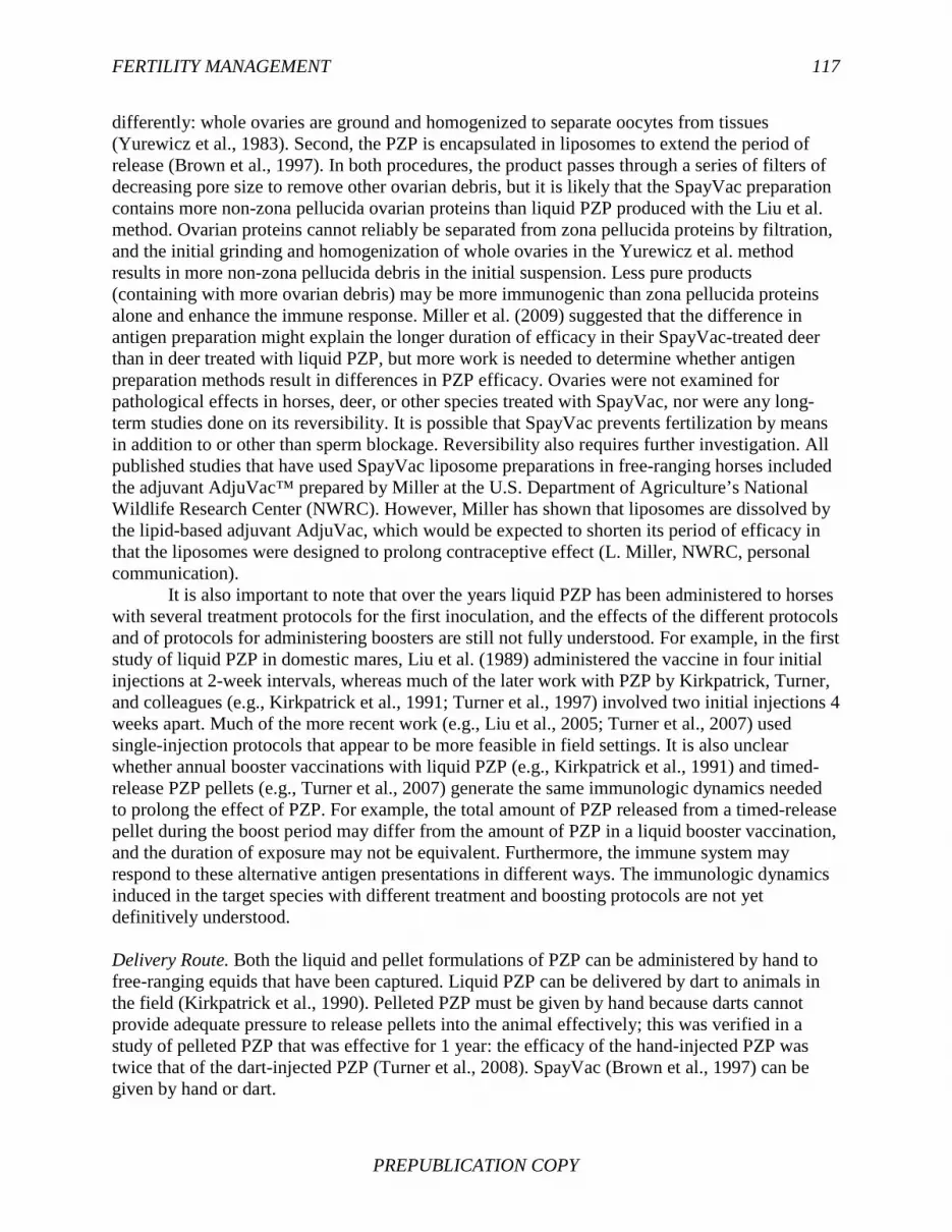
FERTILITY MANAGEMENT 117
PREPUBLICATION COPY
differently: whole ovaries are ground and homogenized to separate oocytes from tissues (Yurewicz et al., 1983). Second, the PZP is encapsulated in liposomes to extend the period of release (Brown et al., 1997). In both procedures, the product passes through a series of filters of decreasing pore size to remove other ovarian debris, but it is likely that the SpayVac preparation contains more non-zona pellucida ovarian proteins than liquid PZP produced with the Liu et al. method. Ovarian proteins cannot reliably be separated from zona pellucida proteins by filtration, and the initial grinding and homogenization of whole ovaries in the Yurewicz et al. method results in more non-zona pellucida debris in the initial suspension. Less pure products (containing with more ovarian debris) may be more immunogenic than zona pellucida proteins alone and enhance the immune response. Miller et al. (2009) suggested that the difference in antigen preparation might explain the longer duration of efficacy in their SpayVac-treated deer than in deer treated with liquid PZP, but more work is needed to determine whether antigen preparation methods result in differences in PZP efficacy. Ovaries were not examined for pathological effects in horses, deer, or other species treated with SpayVac, nor were any long-term studies done on its reversibility. It is possible that SpayVac prevents fertilization by means in addition to or other than sperm blockage. Reversibility also requires further investigation. All published studies that have used SpayVac liposome preparations in free-ranging horses included the adjuvant AdjuVac™ prepared by Miller at the U.S. Department of Agriculture’s National Wildlife Research Center (NWRC). However, Miller has shown that liposomes are dissolved by the lipid-based adjuvant AdjuVac, which would be expected to shorten its period of efficacy in that the liposomes were designed to prolong contraceptive effect (L. Miller, NWRC, personal communication).
It is also important to note that over the years liquid PZP has been administered to horses with several treatment protocols for the first inoculation, and the effects of the different protocols and of protocols for administering boosters are still not fully understood. For example, in the first study of liquid PZP in domestic mares, Liu et al. (1989) administered the vaccine in four initial injections at 2-week intervals, whereas much of the later work with PZP by Kirkpatrick, Turner, and colleagues (e.g., Kirkpatrick et al., 1991; Turner et al., 1997) involved two initial injections 4 weeks apart. Much of the more recent work (e.g., Liu et al., 2005; Turner et al., 2007) used single-injection protocols that appear to be more feasible in field settings. It is also unclear whether annual booster vaccinations with liquid PZP (e.g., Kirkpatrick et al., 1991) and timed-release PZP pellets (e.g., Turner et al., 2007) generate the same immunologic dynamics needed to prolong the effect of PZP. For example, the total amount of PZP released from a timed-release pellet during the boost period may differ from the amount of PZP in a liquid booster vaccination, and the duration of exposure may not be equivalent. Furthermore, the immune system may respond to these alternative antigen presentations in different ways. The immunologic dynamics induced in the target species with different treatment and boosting protocols are not yet definitively understood.
Delivery Route. Both the liquid and pellet formulations of PZP can be administered by hand to free-ranging equids that have been captured. Liquid PZP can be delivered by dart to animals in the field (Kirkpatrick et al., 1990). Pelleted PZP must be given by hand because darts cannot provide adequate pressure to release pellets into the animal effectively; this was verified in a study of pelleted PZP that was effective for 1 year: the efficacy of the hand-injected PZP was twice that of the dart-injected PZP (Turner et al., 2008). SpayVac (Brown et al., 1997) can be given by hand or dart.

118 BLM WILD HORSE AND BURRO PROGRAM
B PREPUBLICATION COPY
Although the ability to deliver liquid PZP via dart is a useful option, it is not clear how successful attempts would be to dart populations of horses at the desired level of treatment intensity, given the large number of animals needing treatment, variability in the temperament of the horses, and the terrain of HMAs. Two studies of free-ranging horses and one of white-tailed deer have found that over time, with repeated boosters, the difficulty of approaching animals on foot for darting increased (Kirkpatrick and Turner, 2008; Rutberg and Naugle, 2008; Ransom et al., 2011). At the time the report was prepared, the most effective and most reliable method of delivery was hand injection after a gather. However, alternative methods, such as trapping near water holes or blinds, have been used in other areas and could be useful in some HMAs.
Efficacy. Liquid PZP, the first formulation produced, has been assessed for efficacy more often than other PZP formulations. The overall mean of published efficacy values in horses is 88.4 percent (median, 89 percent). Kirkpatrick and Turner’s (2008) value of 95 percent is based on cumulative experience on Assateague Island4 and represents the most up-to-date information available to the committee on that site. Turner et al. (1997) evaluated several adjuvant formulations.5 If the less effective adjuvants in their study and another study that acknowledged poorly timed boosters in one population (Ransom et al., 2011) are eliminated, the mean efficacy increases to 91.5 percent (median, 90 percent), representing hundreds of animals across several sites. In most of the studies, efficacy was assessed by determining how many treated females had foals in the following foaling season or had pregnancy diagnosed with hormone assays. Only one study of any PZP formulation has been conducted in burros. Turner et al. (1996) found that liquid PZP significantly reduced fertility for a year after vaccination. A two-shot protocol was more effective (none of 13 females became pregnant) than a one-shot protocol (one of three became pregnant).
Turner et al. (2007) assessed a pelleted form designed to release PZP into the animal’s circulatory system at 1, 3, and 12 months in 96 free-ranging mares in Nevada. Fertility rates over 4 years after vaccination were 5.2 percent, 14.9 percent, 31.6 percent, and 46.2 percent, respectively, in treated mares. The formulation has come to be called PZP-22 because it remains about 85-percent effective after 22 months. Turner et al. (2008) concluded that the optimal time to administer PZP-22 for maximum duration of effect is fall or winter. BLM began using PZP-22 in free-ranging horses in the late 2000s. However, the efficacy has varied as treatment has been extended to additional field sites. Foaling has been reduced by 30-79 percent in the 2 years after a single injection of PZP-22 at various field sites (J.W. Turner, University of Toledo, personal communication, November 2012). The variability is believed to be due to the time of year of injection, whether delivery was by dart or by hand, the location of the injection (the hip is considered ideal, but that is not always possible when delivery is by dart), and possible differences in preparation in the field. In addition, there has been a change in vaccine production during the last few years: heat extrusion versus cold evaporation (J.W. Turner, University of Toledo, personal communication, November 2012).
4Assateague Island National Seashore is on a barrier island off the coast of Maryland and operated by the
U.S. Department of the Interior’s National Park Service (NPS). A free-ranging herd lives on the island. NPS is not subject to the Wild Free-Roaming Horses and Burros Act of 1971. Nevertheless, because it is a free-ranging population, results of studies of the use of liquid PZP on this herd can inform management of horses under BLM’s jurisdiction.
5An adjuvant enhances the immune response by encouraging the production of antibodies.
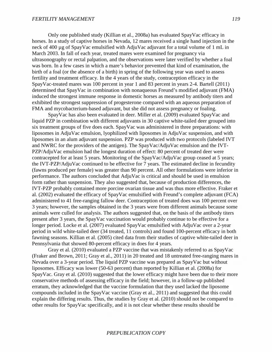
FERTILITY MANAGEMENT 119
PREPUBLICATION COPY
Only one published study (Killian et al., 2008a) has evaluated SpayVac efficacy in horses. In a study of captive horses in Nevada, 12 mares received a single hand injection in the neck of 400 µg of SpayVac emulsified with AdjuVac adjuvant for a total volume of 1 mL in March 2003. In fall of each year, treated mares were examined for pregnancy via ultrasonography or rectal palpation, and the observations were later verified by whether a foal was born. In a few cases in which a mare’s behavior prevented that kind of examination, the birth of a foal (or the absence of a birth) in spring of the following year was used to assess fertility and treatment efficacy. In the 4 years of the study, contraception efficacy in the SpayVac-treated mares was 100 percent in year 1 and 83 percent in years 2-4. Bartell (2011) determined that SpayVac in combination with nonaqueous Freund’s modified adjuvant (FMA) induced the strongest immune response in domestic horses as measured by antibody titers and exhibited the strongest suppression of progesterone compared with an aqueous preparation of FMA and mycobacterium-based adjuvant, but she did not assess pregnancy or foaling.
SpayVac has also been evaluated in deer. Miller et al. (2009) evaluated SpayVac and liquid PZP in combination with different adjuvants in 30 captive white-tailed deer grouped into six treatment groups of five does each. SpayVac was administered in three preparations: with liposomes in AdjuVac emulsion, lyophilized with liposomes in AdjuVac suspension, and with liposomes in an alum adjuvant suspension. PZP was produced with two protocols (labeled IVT and NWRC for the providers of the antigen). The SpayVac/AdjuVac emulsion and the IVT-PZP/AdjuVac emulsion had the longest duration of effect: 80 percent of treated deer were contracepted for at least 5 years. Monitoring of the SpayVac/AdjuVac group ceased at 5 years; the IVT-PZP/AdjuVac continued to be effective for 7 years. The estimated decline in fecundity (fawns produced per female) was greater than 90 percent. All other formulations were inferior in performance. The authors concluded that AdjuVac is critical and should be used in emulsion form rather than suspension. They also suggested that, because of production differences, the IVT-PZP probably contained more porcine ovarian tissue and was thus more effective. Fraker et al. (2002) evaluated the efficacy of SpayVac emulsified with Freund’s complete adjuvant (FCA) administered to 41 free-ranging fallow deer. Contraception of treated does was 100 percent over 3 years; however, the samples obtained in the 3 years were from different animals because some animals were culled for analysis. The authors suggested that, on the basis of the antibody titers present after 3 years, the SpayVac vaccination would probably continue to be effective for a longer period. Locke et al. (2007) evaluated SpayVac emulsified with AdjuVac over a 2-year period in wild white-tailed deer (34 treated, 11 controls) and found 100-percent efficacy in both fawning seasons. Killian et al. (2005) cited data from their studies of captive white-tailed deer in Pennsylvania that showed 80-percent efficacy in does for 4 years.
Gray et al. (2010) evaluated a PZP vaccine that was mistakenly referred to as SpayVac (Fraker and Brown, 2011; Gray et al., 2011) in 20 treated and 18 untreated free-ranging mares in Nevada over a 3-year period. The liquid PZP vaccine was prepared as SpayVac but without liposomes. Efficacy was lower (50-63 percent) than reported by Killian et al. (2008a) for SpayVac. Gray et al. (2010) suggested that the lower efficacy might have been due to their more conservative methods of assessing efficacy in the field; however, in a follow-up published erratum, they acknowledged that the vaccine formulation that they used lacked the liposome compounds included in the SpayVac vaccine (Gray et al., 2011) and suggested that this could explain the differing results. Thus, the studies by Gray et al. (2010) should not be compared to other results for SpayVac specifically, and it is not clear whether these results should be

120 BLM WILD HORSE AND BURRO PROGRAM
B PREPUBLICATION COPY
compared to those for liquid PZP. In both the Killian et al. (2008a) and Gray et al. (2010) studies, the AdjuVac adjuvant was combined with the vaccine.
Reversibility. Immunocontraception depends on the immune response to the vaccine reaching and staying above threshold concentration (Adams and Adams, 1990; Zeng et al., 2002). Reversibility of the contraceptive effect depends on the reduction of circulating antibody titers. Substantial variability in reversal time is likely and can be due to the vaccine formulation, the adjuvant used, the treatment protocol, genetic factors, and the nutritional status of the individual animal because these factors may affect the initial and continuing immune response to the vaccine (Homsy et al., 1986; Chandra and Amorin, 1992; Turner et al., 1997, 2001, 2007; Liu et al., 2005; Lyda et al., 2005; Bartell, 2011).
In the first study of liquid PZP in equids, Liu et al. (1989) found that, of 10 feral and six domestic mares, most mares had reversed within 8 months of treatment. Kirkpatrick et al. (1990) first demonstrated that three of seven free-ranging mares became fertile in the first year after 1 year of liquid-PZP treatment, although foaling rates of treated mares overall were lower after treatment than in control mares. Turner et al. (1997) found similar results in horses in Nevada, where 103 mares were treated with various combinations of PZP and adjuvants and 92 mares served as controls. Data from Assateague Island on reversibility continued to accumulate over the years, and Kirkpatrick and Turner (2002) stated that liquid PZP was 100-percent reversible in three mares treated for 4 consecutive years and two mares treated for 5 consecutive years. The time between final treatment and pregnancy ranged from 1 to 8 years. At the time the committee’s report was prepared, none of the five mares treated for 7 consecutive years had reversed after 7 years of monitoring. In a study of 16 burros, 46.1 percent of treated females were determined to be pregnant via fecal hormone monitoring during the second year after liquid-PZP treatment (Turner et al., 1996)
Studies of longer-acting PZP formulations, such as PZP-22 (pellets) and SpayVac, have assessed reversibility more in the context of measuring the duration of effect of the vaccine; declining infertility in years after vaccination reflects reversibility. In a study by Turner et al. (2007) of 96 treated mares, 15 percent of mares had not reversed after 22 months, 31.6 percent after 3 years, and 46.2 percent after 4 years. In that study, however, not every mare was assessed for reversibility every year. Turner et al. (2008) suggested that more rigorous study of reversibility in PZP-22 treated mares is warranted.
Ransom (2012) studied liquid PZP and PZP-22 in three horse populations in the western United States. Twenty-two mares on the Little Books Cliffs HMA and 38 mares on the Pryor Mountain Wild Horse Range were treated with liquid PZP up to 5 consecutive years. At the McCullough Peaks HMA, 28 mares were treated with PZP-22. Among all the sites, in mares that had foaled previously, the probability of not foaling was 74.4 percent after PZP treatment and 35.9 percent in control mares; this indicates that fertility may be suppressed after the planned period of infertility. At Little Book Cliffs and Pryor Mountains, the time from the last liquid-PZP injection to first parturition ranged from 1.5 to 8.1 years and was strongly affected by the total number of years in which the mares were treated. On average, time to parturition increased by 411 days per consecutive year of treatment. At McCullough Peaks, 64 percent of PZP-22 treated mares did not produce a foal during the posttreatment period (5 years). Return to parturition took 1.4-5.5 years. The results reinforce the notion that return to fertility after immunocontraception can be longer than expected.

FERTILITY MANAGEMENT 121
PREPUBLICATION COPY
SpayVac has not been thoroughly assessed for reversibility in captive or free-ranging horses, although the study by Killian et al. (2008a) demonstrated that two of 12 treated mares became pregnant 2-4 years after vaccination. The studies of SpayVac in deer described above did not systematically address reversibility, nor have they been of sufficient duration to detect decreases in vaccine efficacy (animals were contracepted at the same level of efficacy in all years of the study).
Side Effects: Physical and Physiological. Because the antigen target of PZP contraception (liquid, pellet, or SpayVac formula) is highly specific—the egg’s zona pellucida—there appear to be relatively few physical side effects. Barber and Fayrer-Hosken (2000) found that PZP antibodies did not bind to other somatic tissues in horses. Liu et al. (1989) found no evidence of pathological conditions in ovaries of mares treated for 1 year; however, this remains the only study of ovarian pathology in relation to liquid-PZP treatment in horses. Bartell (2011) found that the ovaries of SpayVac-treated domestic mares were lighter, had smaller oocytes, and had thinner zona pellucidae than control mares. Killian et al. (2008a) found that SpayVac-treated mares had unexplained higher rates of uterine edema, but they cited literature (Samper, 1997) suggesting that in healthy mares this is a sign of estrus when mares are under the influence of estrogen produced by ovarian follicles. Fraker (2012) also observed uterine edema in connection with SpayVac. It is not known whether the extent of edema observed in the SpayVac-treated mares was equivalent to that in normal estrous mares or more severe; the latter might be a possible indication of pathology. Because of the pathological potential, further research on uterine changes during and after treatment with SpayVac is warranted. There are no documented reports of persistent uterine edema after the use of liquid PZP or PZP-22, but comparable data on the effects identified with the use of SpayVac do not exist.
Mares that have been treated with liquid PZP for 3-7 consecutive years have been reported to have decreased ovulation rates in successive years of treatment (Kirkpatrick et al., 1992, 1995); this suggests that PZP may act at sites other than just the zona pellucida. Powell and Monfort (2001) did not find a statistically significant relationship between the likelihood of ovulatory failure and current contraception status (currently versus previously treated with PZP). It is possible that the likelihood of physiological side effects depends on the delivery of PZP as repeated vaccinations (for example, annually in the case of liquid PZP) as opposed to one long-term vaccination (in the case of PZP-22 and SpayVac).
There are many other possible causes of subfertility in horses (McCue and Ferris, 2011), but in none of the analyses described above were the same mares assessed for cyclicity before and after PZP treatment, so other possible factors contributing to subfertility were not assessed. It is estimated that about 20 percent of domestic horse mares are subfertile (I.K.M. Liu, University of California, Davis, personal communication, August 2012). Ovarian senescence has also been documented in some domestic mares over 20 years old, as evidenced by a longer follicular phase, a prolonged interovulatory interval, and later first ovulation of a breeding season (McCue and McKinnon, 2011) —all of which are reported in mares currently or previously treated with PZP (Powell and Monfort, 2001). Thus, assessing reproductive competence after many years of PZP treatment is confounded by the concomitant effects of aging.
There has been much discussion over the years of the effects of different adjuvants used in combination with PZP in relation to reactions at the injection site, which have included stiffness, swelling, nodules, and abscesses. The traditional application of liquid PZP involved an initial primer dose administered with FCA and a follow-up booster 2-4 weeks later with Freund’s

122 BLM WILD HORSE AND BURRO PROGRAM
B PREPUBLICATION COPY
incomplete adjuvant (FIA). Kirkpatrick et al. (1990) were the first to mention potential concerns with using FCA in wildlife, but in their study only three of 26 treated mares had injection-site abscesses, and all healed within 14 days. One concern with FCA is its ability to produce false positive results in tuberculosis tests; this in part led to the development of FMA, which did not produce such results (Lyda et al., 2005). Chapel and August (1976) also suggested that FCA could be hazardous to people exposed to it when administering injections.
In their study of FCA and FMA use in the primer liquid-PZP dose, Lyda et al. (2005) found only one case of injection-site abscess. The mare was treated with FMA in the primer dose and FIA in the booster. The abscess appeared after the FIA booster dose, and it drained and healed without incident. Antibody titers produced with FMA and FCA did not differ significantly. Neither adjuvant had an effect on the delivery of healthy foals. The authors cited unpublished data suggesting that the incidence of injection-site abscesses was less than 1 percent when injections were given in the hip, but it was higher when injections were given in the neck.
In a large study of free-ranging horses, Roelle and Ransom (2009) found no statistically significant differences in occurrence of dart-site reactions due to adjuvant (FCA or FMA) and suggested that reactions are probably more likely to be due to dart trauma or in some cases a combination of dart trauma and adjuvant. Hand injection led to fewer injection-site reactions than darting. Overall, abscesses in response to darting were rare, in accordance with other studies (Kirkpatrick et al., 1990; Turner and Kirkpatrick, 2002; Lyda et al., 2005). Nodules at the injection site were the most common reaction (25 percent of cases), and these persisted for up to a year or more but did not appear to affect the animals. Swelling was the second-most common reaction (11 percent and 33 percent at two study sites), and this disappeared within 30 days. Stiffness was the third-most common (1.4 percent and 11 percent at two study sites) and disappeared within 24 hours.
In their studies of both PZP and GonaCon™ (a GnRH vaccine), Gray et al. (2010, 2011) found no cases of abscesses after hand injection of either compound with AdjuVac as an adjuvant. Similar results have been found in deer when AdjuVac has been used (Fraker et al., 2002; Locke et al., 2007; Miller et al., 2009).
Contracepted females should generally be in better body condition than uncontracepted females because they do not face the energetic demands of pregnancy and lactation. Turner and Kirkpatrick (2002) found that body-condition scores of mares on Assateague Island were significantly higher in 1999 than in 1988 before PZP contraception was widely applied. Body-condition scores of lactating females at those two times were not significantly different, and this suggests that prevention of pregnancy can enhance body condition. Ransom et al. (2010) found no difference in body-condition scores between treated and untreated mares in three western populations of horses on the basis of a similar body-condition scoring index, but mares that had foals had lower body condition than mares that did not. The most likely reason for the absence of significant body-condition differences between treated and untreated mares is that most treated mares were already pregnant when the study began and therefore did have foals at their sides during the study. In addition, some treated mares that did not respond to contraception and produced foals were exposed to the same energetic demands of gestation and lactation as untreated mares (J. Ransom, National Park Service, personal communication, May 3, 2012). In contrast, Fraker et al. (2002) found that fallow deer does treated with SpayVac had lower stores of kidney fat than untreated does; treated does might have expended more energy during the rut because they were engaged in reproductive behavior more often than untreated does.

FERTILITY MANAGEMENT 123
PREPUBLICATION COPY
Side Effects: Pregnancy, Birth Seasonality, and Survival. Liquid PZP has been demonstrated to be safe to administer to pregnant mares in a number of studies (e.g., Kirkpatrick et al., 1990, 1991). Turner and Kirkpatrick (2002) found that foal survival to 1 year is equivalent between untreated mares and mares treated with liquid PZP during pregnancy; female foals born to PZP-treated females also successfully bred and reared offspring. Kirkpatrick and Turner (2003) analyzed birth records on Assateague Island and found that most foals born to treated and untreated mares are born in season (April-June): 75.8 percent of births to control mares, 64.9 percent of births to treated mares, and 68.9 percent of births attributed to contraceptive failure. None of those differences was significantly different. The authors did note that out-of-season births had been increasing on Assateague Island since 1984 (the contraception management program began there in 1994) for unknown reasons. Turner and Kirkpatrick (2002) found no difference in survival between in-season and out-of-season foals but stated that it probably depends on the environment (Kirkpatrick and Turner, 2003). On Shackleford Banks,6 PZP-treated mares foaled over a broader range of months than untreated mares (Nuñez et al., 2010). Mares given PZP in the year before they conceived gave birth 3-4 months later than untreated mares. Mares that had been on PZP at some point before the year in which they conceived gave birth almost a month later than untreated mares. However, in an investigation of PZP contraception in free-ranging mares in Nevada, Gray et al. (2010) found no differences in foal survival, birth seasonality, or foal sex ratio between treated and untreated mares. Ransom (2012) also studied the effect of liquid and pelleted PZP (PZP-22) on birth seasonality at three sites in the western United States. Overall, mares that gave birth to foals after treatment (liquid and PZP-22 considered together) did so an average of 31.5 days later (range, 17-46) than untreated mares. Ransom stated that that effect varied among sites and PZP formulations, but these factors were confounded because PZP-22 was used exclusively at one site and not at all at the others. In addition, a monsoon rain at one site allowed a second peak in spring vegetation quality. There was no effect of treatment on foal survival; however, foal survival did decrease the later a foal was born after the peak in spring vegetation quality. Ransom indicated that the average delay in birth of a posttreatment foal results in about a 4.2 percent reduction in survival probability and that this is probably why the treatment effect was not statistically significant (J. Ransom, National Park Service, email communication, July 6, 2012). Ransom also noted that posttreatment mares that gave birth “late” in a given year would often not foal in the following year but then would foal in the third year during the normal birthing season for that site; such factors as photoperiod and temperature might be able to “reset” a mare’s reproductive system so that conception and birth occur during the normal birth season in later years.
Studies of liquid PZP contraception in the Assateague Island horse population have also revealed effects on survival of mares. In the 4 years before 1994, when management-level contraception began, annual adult mortality was greater than 10 percent; in the first 4 years after contraception, adult mortality decreased to less than 4 percent (Turner and Kirkpatrick, 2002). It should be noted, however, that in 1990 and 1992 many deaths were attributable to an equine encephalitis outbreak and severe storms, respectively. Even so, mare mortality in 1991 and 1993 was about 3-4 percent; from 1994 to 1998, mare mortality was less than 2 percent (Turner and Kirkpatrick, 2002). There was also a shift upward in age classes in the entire herd, which
6Shackleford Banks, part of the Cape Lookout National Seashore, is home to a herd of free-ranging horses managed by the U.S. Department of the Interior’s National Park Service. Although they were not treated with PZP for as many years as the Assateague Island horses, the results of behavioral studies of the Shackleford Banks horses can inform management of horses under BLM’s jurisdiction.

124 BLM WILD HORSE AND BURRO PROGRAM
B PREPUBLICATION COPY
indicated increased survival and the attainment of new, older age classes (Turner and Kirkpatrick, 2002). In a later study (Kirkpatrick and Turner, 2007), untreated mares were compared with mares on PZP for less than 3 years and mares on PZP for more than 3 years. Mean age at death was significantly lower in untreated mares (6.47 years) than in treated mares, and mares on PZP for more than 3 years had a higher mean age at death (19.94 years) than mares on PZP for less than 3 years (10.27 years). At the time the committee’s report was prepared, pelleted PZP and SpayVac had not been examined for effects on adult survival or demographic changes.
Side Effects: Genetic. Concerns have been raised about possible unintended genetic effects of immunocontraception. In a review of ecological and immunogenetic issues surrounding immunocontraception, Cooper and Larsen (2006) suggested that because immunocontraceptives are rarely 100-percent effective and resistance to vaccines (contraceptive failures) might have a genetic basis, managers may be unintentionally selecting for animals that do not respond to immunocontraceptive techniques. Using Falconer’s (1965) equations, they suggested that if the proportion of nonresponding females is 10 percent, which could be considered a valid estimate for liquid PZP in horses, after one generation of selection via immunocontraception, the percentage of female offspring produced that would themselves be resistant would range from 15 to 23 percent, depending on the degree of heritability of resistance to immunocontraception. The authors also suggested that such selection for nonresponders could occur in the major histocompatibility complex or in genes that regulate the immune system, either of which could alter resistance to other pathogens.
However, when the committee’s report was prepared, there were no data on resistance to immunocontraception, the heritability of such resistance, or the identity of specific genes that might affect responses to immunocontraceptives. National Park Service staff reported on Assateague Island that there were no indications that resistance was developing or that responses to immunocontraception were changing over time, after 19 years of herd management with PZP. Contraceptive effectiveness continues to be high (A. Turner, Assateague Island National Seashore, email communication, February 24, 2013). The immune response to immunocontraceptives depends on many nongenetic factors, such as nutritional status (Homsy et al., 1986; Chandra and Amorin, 1992; Chandra, 1996; Demas et al., 2003; Houston et al., 2007), and it was not possible for the committee to determine whether resistance to immunocontraception could develop. Similarly, it was not clear whether immunocontraception could inadvertently select for less immune-robust animals because they would not mount a strong response to PZP and would thus remain fertile. Presumably, any genetic background that would predispose animals to being immunocompromised would be under strong selection to be eliminated; even in a small population in which a deleterious mutation that compromised the immune system could become fixed, selection could act against individual animals that have the mutation, although the pressure of selection is smaller in small populations. In addition, Falconer’s (1965) equations apply to threshold or “all-or-none” characters whereas lifetime reproductive success—which contraception affects—is a continuous variable that is not subject to some threshold, so it is not clear whether the Falconer model applies, although other models might. Cooper and Larsen (2006) suggested that immunocontraception could be appropriate for management of species that have long generation times, like horses, because genetic changes (if any) due to immunocontraception would take decades to develop. That would also assume that large numbers of individual animals are contracepted indefinitely and never allowed to breed;
FERTILITY MANAGEMENT 125
PREPUBLICATION COPY
this does not seem likely if populations are managed for genetic diversity. However, those concerns highlight the importance of monitoring genetic diversity in immunocontracepted populations (see Chapter 5).
At the population level, removing females even temporarily from the breeding pool is likely to reduce the effective population size (Ne) and genetic diversity of the population. As will be discussed in Chapter 5, reducing the number of breeders or increasing the variance in family size, which will occur as more females bear no young, will reduce Ne and increase the loss of genetic variability. (Tables 5-2 and 5-3 show that some populations display low levels of heterozygosity.)
Side Effects: Behavioral. There are two important considerations in evaluating the literature on contraceptive effects on particular aspects of behavior, particularly bonds between animals and stability of social groups. First, in no published study of immunocontraception have treatment and control groups been matched or balanced with respect to other variables that might affect behavior (such as age, dominance rank, tenure in the group, group size, social or reproductive history, and characteristics of other group members). Rather, investigators have had no control over those variables and thus only compared treated with untreated (or not currently treated) females. Studies in which those factors could be controlled or specifically have their effects measured would require large samples of animals of known history and would be virtually impossible to conduct in the field or even in captivity. Second, no study has been able to differentiate the behavioral effects of a contraceptive compound administered to an animal and the resulting absence of offspring. Thus, in no case can the committee conclude from the published research that the behavioral differences observed are due to a particular compound rather than to the fact that treated animals had no offspring during the study. That must be borne in mind particularly in interpreting long-term impacts of contraception (e.g., repeated years of reproductive “failure” due to contraception).
Gray (2009) and Gray et al. (2010, 2011) studied the effects of a liquid-PZP vaccine on behavior of free-ranging horses in Nevada during breeding and nonbreeding seasons. There were no treatment effects on activity budget, rates of sexual behavior, proximity between stallions and mares, attempts to initiate proximity, aggression given or received, or band changing by mares. Powell (1999) found no differences in spatial relationships, dominance rank, or aggression between mares currently on PZP and those not currently on PZP on Assateague Island; however, at the time of Powell’s studies, all mares had been treated with PZP at some point in the past, so true controls were not available. On Shackleford Banks, an island where some mares were never treated with PZP, changes in time budgets were observed. Many factors—such as the presence of a foal, the size of a harem, and features of the male associated with the harem—affected time spent in various activities, but a female’s contraceptive status also affected time budgets. In “best fit” general linear models attempting to identify individual and group characteristics that account for variation in the proportion of time spent in grazing and standing, a female’s contraceptive status and an interaction involving contraceptive status and a harem male’s identity had significant effects, as did total harem size and the interaction of male identity and total harem size. In general, PZP-treated females and females in large harems graze less and stand more than non–PZP-treated females and females in smaller groups, but these effects are related to the particular males with which they interact (Madosky et. al., in review).
In a study of liquid and pelleted PZP in three populations of horses in the western United States, Ransom et al. (2010) found no effect of treatment on activity budgets, but they did find

126 BLM WILD HORSE AND BURRO PROGRAM
B PREPUBLICATION COPY
that treated females engaged in significantly more reproductive behavior (0.05 behavior per hour in control mares versus 0.11 behavior per hour in treated mares), which could be expected with a contraceptive that causes females to cycle repeatedly during the breeding season. Powell (1999) also found no difference in activity budgets between mares currently on PZP and those not currently on PZP. Nuñez et al. (2009) saw significantly more sexual or courtship behavior in treated mares than in controls outside the breeding season but also cited data on other temperate equids that showed that out-of-season cycling is known to occur. Powell (1999) found a nonsignificant trend for currently treated mares to engage in more social behavior overall; however, when only sexual behavior was considered, there was no effect of current contraception status on behavior (Powell, 2000). Turner et al. (1996) did not discern any differences in reproductive behavior between liquid-PZP–treated burros and untreated burros, but they did not provide quantified behavioral data. No other studies of PZP contraception in burros have been published.
The effects of liquid PZP on harem stability in horses have been studied in Nevada during breeding and nonbreeding seasons by Gray (2009) and on Shackleford Banks during the nonbreeding season by Nuñez et al. (2009) and during the breeding season by Madosky et al. (2010). Stability was also assessed on Assateague Island by National Park Service staff (A. Turner, Assateague Island National Seashore, email communication, December 13, 2011). The studies on Shackleford Banks suggest that PZP is associated with increased harem changing by mares, whereas the Nevada and Assateague studies found no differences between treated and untreated mares in harem-changing. The studies all differ in methodological approaches, definitions of treated and untreated animals, and ecological and social contexts. No studies have been able to control all the factors that could affect harem stability in the field, which could include age, pregnancy status, characteristics of other mares and stallions in the harem, distribution of resources, stallion turnover rates, population size and demographics, and more. Finally, harem-changing by mares occurs to varied degrees in horse populations in varied ecological contexts in uncontracepted populations (see Feist and McCullough, 1975; Berger, 1977, 1986; Nelson, 1978; Rubenstein, 1981; Stevens, 1990; Goodloe, 1991; Jensen, 2000 for examples).
Figure 4-2 below shows a frequency distribution of the percentage of mares observed changing bands in population studies before or without contraception (Feist and McCullough, 1975; Nelson, 1978; Rubenstein, 1981; Berger, 1986; Rutberg, 1990; Stevens, 1990). Values range from 8-61 percent (mean, 27 percent; median, 25 percent). The study by Madosky et al. (2010) found that 70 percent of PZP-treated mares changed bands; that is, significantly higher than the percentage of mares that change bands in uncontracepted populations (Wilcoxon signed-ranks test, T = -18, p = 0.008, df = 7). The percentage of control mares changing bands (33.3 percent) did not differ from that of mares in uncontracepted herds (Wilcoxon signed ranks test, T = -6, p = 0.44, df = 7) (analysis provided by D. Rubenstein).

FERTILITY MANAGEMENT 127
PREPUBLICATION COPY
FIGURE 4-2 Percentage of band changes by mares as shown in a review of published literature. SOURCE: Feist and McCullough (1975), Nelson (1978), Rubenstein (1981), Berger (1986), Rutberg (1990), Stevens (1990).
Whether Shackleford Banks is a unique case or not, additional study is needed to
understand whether the absence of foaling as a result of contraception has an effect on band stability. Gray (2009) argued that sexual behavior and the ability to form consortships were adequate to maintain band stability in her study in Nevada. The studies on Shackleford Banks (Nuñez et al., 2009; Madosky et al., 2010) suggest that there is an interaction between pregnancy and social cohesion. The importance of harem stability to mare well-being is not clear, but considering the relatively large number of free-ranging mares that have been treated with liquid PZP in a variety of ecological settings, the likelihood of serious adverse effects seems low.
Side Effects: Demography and Population Processes. The easiest way to envision the effect of contraception on population processes is to examine its effect on demographic vital rates (e.g., birth and death rates) contained in the equation that approximates the intrinsic rate of population increase (r). The demographic vital rates are related to r via the Lotka-Euler equation; a reasonable approximation is
where is the net reproductive rate, and is the generation time, which is proportional to age at first reproduction (α) (May and Rubenstein, 1985); lx and mx are age-specific survival and fecundity rates, respectively (Stearns, 1992; Gotelli, 2001). Intuitively, female fertility control effectively reduces r by reducing mx. The degree to which r is reduced depends on the effectiveness of the fertility-control method used, the proportion of females of a given age class that are treated, and the age classes that are targeted for treatment.
Female fertility control would also have indirect and unintended consequences, which may include changes in ages at first (α) and last reproduction (ω), longevity, and the population’s

128 BLM WILD HORSE AND BURRO PROGRAM
B PREPUBLICATION COPY
age structure. If young females are targeted, fertility control can potentially increase the average α. Because treated females no longer have to sustain pregnancies or lactate, their energy needs will be reduced, their body condition will improve (e.g., Kirkpatrick and Turner, 2007), and they can potentially survive better, live longer, and possibly have a longer reproductive lifespan. Because r correlates negatively with α and positively with ω (Oli and Dobson, 2003; Stahl and Oli, 2006), these can have contrasting effects. However, elasticity (or proportional sensitivity) patterns in age-structured populations suggest that the elasticity of population growth rate to changes in age-specific vital rates declines with age and that growth rate generally is more strongly affected by changes in α than in ω (Caswell, 2001; Oli and Dobson, 2003; Stahl and Oli, 2006). Thus, targeting younger females for contraception would be the most effective strategy if the goal is to reduce r.
Evidence suggests that repeated application of PZP can lead to prolonged infertility (beyond the treatment period), so the effects on population growth may be more dramatic in later years and longer-lasting than might have been planned at the start of fertility control. Fertility control via PZP may also increase longevity in females (Kirkpatrick and Turner, 2007), and this would have both direct and indirect ecological effects. Females that survive longer will increase the number of animals using the range, and this is likely to affect the setting of appropriate management levels (see Chapter 7). However, females that live longer may or may not contribute to r via reproduction. In addition, targeting younger age classes for repeated and prolonged fertility control would affect a population’s age structure and the likelihood of a given animal’s contribution to the gene pool (see Chapters 3 and 5). The impact of those consequences will depend on a population’s initial size and structure and should be accounted for when strategies for fertility control are developed. Many of the behavioral changes associated with fertility control that are discussed in the preceding section are also likely to affect population dynamics. A longer breeding season could affect band stability and would probably extend male sexual activity into months when they normally recover strength and rebuild body condition. Such sexual activity in horses and other equids can involve males herding, pushing, and nudging females (and sometimes even forcing copulations [Berger, 1986]), which lower foraging success and freedom of movement (Rubenstein, 1986, 1994; Linklater et al., 1999; Cameron et al., 2009). Sexual harassment has been seen in many but not all equid populations. Where it occurs, if levels of harassment remain high year round, both males and females could enter the breeding season in lower condition, and fertility could be compromised. Fecundity (mx) and survival (lx) of nontreated females could be further reduced, again limiting the population growth rate (r). Whether that cascade of events will occur in particular horse or burro populations will depend on the magnitude and interaction of three factors: environmental harshness in the nonbreeding season, social instability, and improvement of body condition in treated females due to absence of energetic demands of pregnancy and lactation. It is known from studies on Assateague Island that PZP-treated mares tend to have higher body-condition scores than females that reproduce regularly (Kirkpatrick and Turner, 2007). More recent results from Shackleford Banks show increased longevity in PZP-treated mares, probably because of their increased body condition and general health (Stuska, 2012). However, it is known that social disruption and harsh conditions during stressful periods can lower body condition (Pollock, 1980). What is not known is how those factors may interact when PZP use is extended to populations in harsher habitats or during periods of harsher climatic conditions, such as drought. It is something that will need to be monitored.

FERTILITY MANAGEMENT 129
PREPUBLICATION COPY
Gonadotropin-Releasing Hormone Vaccine
GnRH stimulates the pituitary gland to produce follicle-stimulating hormone (FSH) and luteinizing hormone (LH), which then stimulate growth of follicles (which produce estrogen) and ovulation. GnRH vaccines prevent the action of GnRH, so that in the absence of FSH and LH the failure of follicle growth and ovulation prevents reproduction (Figure 4-3). Two formulations of the most common GnRH vaccine, GonaCon™, have been reported in the literature. Specifically, the GnRH peptide has been conjugated to a keyhole limpet hemocyanin protein (KLH) or to blue mollusk protein (B). Both formulations appear to work well, but the B formulation may be more effective (Killian et al., 2008a; Miller et al., 2008) and is less expensive to produce than the KLH formulation (K. Fagerstone, NWRC, personal communication, April 18, 2012). GnRH vaccines not identified as GonaCon in the literature will be labeled as experimental vaccines because they are formulated in a variety of ways.
Studies of GonaCon as a contraceptive in horses are rare in the published literature; studies of GonaCon in deer are more numerous. Two additional GnRH vaccines are available in other parts of the world: Equity™ and Improvac® are produced by Pfizer Animal Health, Australia. Results of studies of efficacy, reversibility, and side effects of these vaccines are discussed in this section.

130 BLM WILD HORSE AND BURRO PROGRAM
B PREPUBLICATION COPY
FIGURE 4-3 Mode of action of gonadotropin-releasing hormone (GnRH) vaccines. NOTE: Without GnRH to stimulate follicle-stimulating hormone (FSH) and luteinizing hormone (LH), there is no production of ovarian estrogen or progesterone and no ovulation. SOURCE: Adapted from Asa et al. (1996).

FERTILITY MANAGEMENT 131
PREPUBLICATION COPY
Delivery Route. GonaCon™ Equine, developed by NWRC and licensed by the U.S. Environmental Protection Agency (EPA) for use in horses, can be delivered by hand injection or by dart. An experimental version of GonaCon-KLH™ was delivered by dart to white-tailed deer in New York (Curtis et al., 2002).
Efficacy. Killian et al. (2008a) studied the efficacy of GonaCon-KLH in 16 penned horses (eight controls) in Nevada and found that efficacy over the 4 years of the study was 94 percent, 60 percent, 60 percent, and 40 percent, respectively. Gray et al. (2010) evaluated the efficacy of GonaCon-B™ in 24 free-ranging horses in Nevada and found efficacy of 61 percent, 58 percent, and 69 percent during each year of the 3-year study, respectively. As mentioned above, Gray et al. (2010) used a conservative method to estimate efficacy compared with most authors who have assessed contraceptive efficacy and suggested this as one possible explanation for the discrepancy between their results and others’ results. A second explanation put forward by the authors was potential differences in body condition between the captive and free-ranging mares used in the two studies. Research suggests that animals that have more energy reserves or are in better body condition have stronger immune systems and thus are able to mount stronger responses to foreign antigens (Chandra, 1996; Demas et al., 2003; Houston et al., 2007). In both studies GonaCon was emulsified with the AdjuVac adjuvant.
Botha et al. (2008) studied Improvac in a large sample (n=55 treated) of mares kept in very large pastures in South Africa. Mares were vaccinated twice (day 0 and day 35) in the middle of the breeding season. By day 35, only 14.5 percent of treated mares showed evidence of ovarian activity as assessed with ultrasonography; at day 70, no treated mare demonstrated ovarian activity. The authors indicated that the 14.5 percent of treated mares that had evidence of ovarian activity at day 35 received their first vaccination during the luteal phase and suggested that the timing of vaccination in the ovulatory cycle is important. Imboden et al. (2006) also evaluated Improvac in nine mares by vaccinating them twice, 4 weeks apart. Ovarian suppression occurred at 4 weeks and lasted a minimum of 23 weeks, but the authors found significant variability in duration and strength of suppression that did not correlate with antibody titers.
In a study of Equity in Australia, Elhay et al. (2007) vaccinated 24 domestic mares at day 0 and boosted them on day 28. All treated mares showed reduced ovarian activity; by 4 weeks after the booster, ovaries of treated mares resembled those of seasonally anovulatory mares.
The efficacy of GnRH vaccines has also been studied in other species. In an early study with an experimental version of GonaCon-KLH, Miller et al. (2000) reported an 88-percent reduction in fawning in eight white-tail does. In a series of studies of white-tailed deer in Maryland (n=28, Gionfriddo et al., 2009) and New Jersey (n=32, Gionfriddo et al., 2011a), GonaCon-KLH emulsified with AdjuVac resulted in 67- to 88-percent contraceptive efficacy in year 1 and 43- to 47-percent efficacy in year 2. Those values were lower than the ones reported for captive deer. Miller et al. (2008) found 100-percent efficacy in years 1 and 2 and 80-percent efficacy in years 3-5 for five does treated with GonaCon-B compared with 100 percent in year 1, 60 percent in year 2, 50 percent in years 3 and 4, and 25 percent in year 5 for GonaCon-KLH given as a single injection to five does. A two-injection protocol of GonaCon-KLH was identical in efficacy to GonaCon-B in years 1-2. Gionfriddo et al. (2011a) suggested that their efficacies were lower because their wild deer were in poorer nutritional condition and living in overgrazed habitats. However, Perry et al. (2006) found only 60-percent efficacy over 3 years in 28 captive black-tailed deer, so species differences also seem possible. Curtis et al. (2002) reported an 87-
132 BLM WILD HORSE AND BURRO PROGRAM
B PREPUBLICATION COPY
percent efficacy in 32 white-tailed deer over 2 years using an experimental version of GonaCon-KLH administered as a two-shot series in year 1 and a booster at year 2. In years 3 and 4 of their study, efficacy declined to 71 percent and 43 percent, respectively, in the absence of a booster. Fawning rates were significantly lower than those of controls in years 1 and 2.
Killian et al. (2009) evaluated two doses (1,000 or 2,000µg) of GonaCon-KLH in 22 captive female elk over a 3-year period. Low-dose efficacy was 92 percent, 90 percent, and 100 percent over the 3 years compared with high-dose efficacy of 90 percent, 100 percent, and 100 percent; these differences were not significantly different. Ten captive female Rocky Mountain elk treated with GonaCon-B had significantly reduced pregnancy rates for 3 years (90-percent reduction in year 1, 75-percent in year 2, and 50-percent in year 3) compared with controls (Powers et al., 2011).
Efficacy of GonaCon-KLH was 100 percent in six female bison for 1 year (Miller et al., 2004). In a short-term study (12-14 weeks) of six female wild boar, 100 percent of GonaCon-treated sows became infertile (Massei et al., 2008). In another short-term study (36 weeks) of feral swine treated with two different doses of GonaCon-KLH, Killian et al. (2006) found that none of the nine sows receiving the higher dose was pregnant at the end of the study and only 10 percent gave birth during the study. Of the 11 sows receiving the lower dose, 56 percent gave birth during the study and 11 percent were pregnant by the end of the study. The authors reported 80- to 90-percent efficacy in domestic pigs in previously published studies from their laboratory.
Reversibility. Elhay et al. (2007) found that in mares treated with Equity the duration of ovarian quiescence ranged from 4 to 23 weeks in 10 of 16 treated mares. The remaining six mares did not return to cyclicity during the study (the duration was about 34 weeks for a sample of mares monitored over a longer term). Three mares with short-duration effects (4-8 weeks) were characterized by low antibody titers. The most frequent duration of contraceptive effects was 23 weeks.
Massei et al. (2008) cited their own unpublished data on GonaCon treatment in wild boar sows that suggest that the vaccine works for several years. Miller et al. (2000) stated that their experimental version of GonaCon-KLH appeared to be reversible in white-tail does and that infertility appeared to last for 2 years without boosting.
Side Effects: Physical and Physiological. GonaCon-B-treated free-ranging mares showed no evidence of injection-site reactions to vaccination (Gray et al., 2010). Mares treated with Improvac demonstrated significantly reduced progesterone concentrations that were still at baseline at day 175; in addition, treated mares had reduced ovarian volume (Botha et al., 2008). Injection-site reactions were transient and disappeared by day 6. In the Imboden et al. (2006) study of Improvac, vaccination significantly affected the number, size, and types of ovarian follicles, corpora lutea, and progesterone concentrations but not estradiol. Most mares showed reactions to the injections, including swelling, pain, stiffness, pyrexia, and apathy, but these signs disappeared within 5 days. The difference between these Improvac studies in occurrence and severity of injection-site reactions could be related to injections being given in the neck (Imboden et al., 2006) instead of the hip (Botha et al., 2008). Mares treated with Equity have demonstrated reduced progesterone concentrations, reduction in ovary and follicle size, and absence of corpora lutea (Elhay et al., 2007).
Kirkpatrick et al. (2011) expressed concerns about GnRH vaccines, pointing out that GnRH receptors are found in various body tissues and that GnRH can act as a neurotransmitter.

FERTILITY MANAGEMENT 133
PREPUBLICATION COPY
GnRH can affect olfaction in rodents, can depress activity of the cerebral cortex, and is associated with two genetic disorders of the cerebellum. However, many of the results mentioned are from studies that used GnRH agonists that result in supranormal concentrations of GnRH. GnRH vaccines block rather than enhance any effects of GnRH, so the effects of the two methods would be expected to be opposite in some or all tissues that have GnRH receptors (see section below “Gonadotropin-Releasing Hormone Agonists”).
Side Effects: Pregnancy, Birth Seasonality, and Survival. In probably the earliest study of a GnRH vaccine, Goodloe (1991) found no differences in birth seasonality between treated and untreated mares on Cumberland Island, a barrier island off the coast of Georgia. She did observe significantly higher mortality in foals born to treated mares in 1 year and a nonsignificant trend in the same direction in the second year, but other possible effects (such as age, body condition, dominance rank, and habitat quality) were not considered. Gray et al. (2010) found no effects of GonaCon-B on birth seasonality, foal survival, or foal sex ratio in free-ranging horses. In a review of contraceptive vaccines in wildlife, Kirkpatrick et al. (2011) stated that GnRH vaccines should be safe for pregnant horses because pregnancy is maintained by the placenta in this species, but they presented no data. However, pituitary LH, which depends on GnRH, is needed for pregnancy maintenance during about the first 6 weeks of pregnancy, after which equine chorionic gonadotropin (eCG) takes over this role.
In other species, Powers et al. (2011) found that GonaCon-B administered mid-gestation to captive female Rocky Mountain elk did not affect calving or calf survival. Miller et al. (2000) found that fawns born to white-tail does treated with an experimental version of GonaCon-KLH were normal and healthy. They did find indications that some treated does were able to produce enough LH to conceive, but the progesterone produced by the corpus luteum was not adequate to carry pregnancy to term. In a study of an experimental GonaCon-KLH, Curtis et al. (2002) found that fawning dates of treated white-tail does were later than those of control does in the first 2 years of the study when efficacy was high but not significantly different when efficacy was lower (less than 71 percent). Female bison treated with GonaCon-KLH in the final months of pregnancy delivered healthy calves at calving dates comparable with those of controls (Miller et al., 2004); this suggests that it can be used safely in the last trimester of pregnancy in this species.
Side Effects: Genetic. Because a GnRH vaccine is an immunocontraceptive, its potential genetic side effects (that is, its selection against a stronger immune response) would be similar to those of PZP mentioned above.
Side Effects: Behavioral. Reviews of the effects of GnRH vaccines and independent studies have suggested that GnRH vaccines have a stronger suppressive effect on LH than on FSH, so sexual behavior may not be suppressed completely in females (Thompson, 2000; Stout and Colenbrander, 2004; Imboden et al., 2006; Powers et al., 2011). That is, continued production of FSH, and later of estradiol, may support estrous behavior but without ovulation, which requires LH. An additional or alternative explanation might be continued production of adrenal sex steroids in the absence of ovarian steroids; this has been shown to support estrous behavior in domestic horses during the nonbreeding season or after ovariectomy (Asa et al., 1980a). In Gray’s (2009) study of the effects of GonaCon on behavior of free-ranging horses in Nevada during both breeding and nonbreeding seasons, there were no treatment effects on activity

134 BLM WILD HORSE AND BURRO PROGRAM
B PREPUBLICATION COPY
budget, rates of sexual behavior, proximity between stallions and mares, attempts to initiate proximity, aggression given or received, or band-changing by mares. In white-tailed does previously treated with GonaCon, the recovery of estrous behavior in years 3, 4, and 5 after vaccination was suppressed when does received an additional vaccination with an anti–follicle-stimulating, hormone-releasing hormone (Killian et al., 2008b), a peptide similar in structure to GnRH.
Effects of GonaCon in Other Ungulate Species. Because GonaCon has not been tested extensively in equids, its effects in other ungulate species are reviewed in this section. Killian et al. (2008b) found that 10 white-tailed does treated with either formulation of GonaCon exhibited estrous behavior less frequently in the first 2 years after treatment, but in later years estrous behavior was displayed more often, even though does were still infertile; this suggests that estrous behavior may return before fertility is fully restored. Miller et al. (2000) found that eight does treated with an experimental version of GonaCon-KLH demonstrated the same number of estrous events, defined by bucks sniffing and chasing does, as control does during 30-44 days of observation during the rut. In their study of an experimental GonaCon-KLH, Curtis et al. (2002) found that treated does cycled later in the year during the second year of treatment than in the first year. Perry et al. (2006) found significantly reduced progesterone in female black-tailed deer treated with GonaCon-KLH. Gionfriddo et al. (2006) found no histopathological effects in a variety of tissues in 28 female white-tailed deer treated with GonaCon-KLH; 29 percent of treated does had injection-site reactions, but they were not discernible externally and were not considered serious. Gionfriddo et al. (2011a,b) found that ovaries and uteri of 32 GonaCon-KLH-treated white-tailed does were smaller than those of controls. Major organs, organ systems, and blood-chemistry parameters were normal in most treated deer (Gionfriddo et al., 2011b). When abnormalities were seen, they could not be clearly related to treatment, and treated does had higher body-condition scores than controls.
Captive female Rocky Mountain elk treated with GonaCon-B did not differ from controls in biochemistry or hematology parameters, and there was no effect on female precopulatory behavior (Powers et al., 2011). There was a nonsignificant trend for males to direct more precopulatory behavior toward treated does than at controls. Treated females did have more follicles than controls, but the follicles were smaller and fewer corpora lutea were present. The authors also commented that GonaCon-B used in conjunction with AdjuVac can cause a positive result on Johne’s disease antibody testing. Injection-site abscesses occurred in 35 percent of treated does, and some lasted for years, but most treated or sham-treated animals showed some level of reaction.
Adams and Adams (1990) vaccinated 30 heifers with GonaCon-KLH mixed with Freund’s complete adjuvant. All treated animals had significantly reduced progesterone, reduced uterine and ovarian tissue mass, and reduced GnRH receptor numbers. GonaCon-KLH-vaccinated female bison demonstrated suppressed progesterone (Miller et al., 2004).
Massei et al. (2008) found no effects of GonaCon on activity budgets, social rank, injection-site reactions, or hematology and biochemistry parameters in a 14-week study of wild boar sows. Treated sows gained more weight, but the gain was considered modest. In a short-term study (36 weeks) of feral swine treated with two different doses of GonaCon-KLH, Killian et al. (2006) found that treated sows had significantly reduced progesterone and numbers of corpora lutea, although females in both treatment groups showed some evidence of follicular activity. There was also evidence of regression of the uterine epithelium.

FERTILITY MANAGEMENT 135
PREPUBLICATION COPY
In studies of GonaCon, injection-site reactions were likely in most species, even if they were not externally visible, but these reactions appeared to be minor and relatively short-lived in most cases. Miller et al. (2008) explained that the water-in-oil emulsion that is often mixed with GonaCon is necessary to induce a long-term immune response, and it is generally accepted that some local reactions (cysts, granulomas, or sterile abscesses) at the injection site are common.
Gonadotropin-Releasing Hormone Agonists
As described above, GnRH, which is produced in the hypothalamus, initiates the cascade of reproductive hormones by causing pituitary release of FSH, which enhances follicle growth, and LH, which triggers ovulation. GnRH agonists (synthetic versions of GnRH that have activity similar to the natural hormone) are commonly used in many domestic species to stimulate follicle growth, estrus, and ovulation. Ovuplant® (deslorelin in a short-acting implant; Peptech Animal Health, Australia, now part of Virbac, France) was developed specifically to induce ovulation in domestic mares. Another GnRH agonist product, Suprelorin® (deslorelin in a slow-release implant matrix; Peptech Animal Health), was developed for use in domestic dogs and is now widely used for contraception in a broad array of captive wildlife species, including female ungulates. GnRH agonists can act as reversible contraceptives when treatment is extended for more than a few days. After the initial stimulation phase, continued administration results in down-regulation of the pituitary cells that synthesize FSH and LH. Without FSH and LH support, the ovaries become quiescent; this condition is sometimes referred to as reversible chemical ovariectomy.
Delivery Route and Efficacy
Suprelorin implants, similar in size to animal ID microchips, are inserted with a trocar, which requires brief restraint but not anesthesia. Two formulations that are active for a minimum of 6 or 12 months are available, but experience has shown that the duration of contraception is longer in most animals—an average of 12 and 18 months, respectively.7 At an adequate dose, GnRH agonists are effective in females of virtually all mammal species, but they have not been tested specifically as contraceptives in horses, burros, or wild equids. Short-term treatment to control ovulation and to investigate their action on pituitary function indicates that GnRH agonists could be effective in suppressing reproduction in mares (Montovan et al., 1990; Fitzgerald et al., 1993). For example, even the short-acting product Ovuplant, designed merely to stimulate but not down-regulate reproduction in mares, has delayed return to cycling in some animals (Johnson et al., 2002). That observation suggests that continued treatment with a long-acting, slow-release implant, such as Suprelorin, would be effective for fertility control, even though the mare appears to be more resistant to pituitary desensitization than other species (Porter and Sharp, 2002).
Reversibility
GnRH agonists are considered generally reversible, primarily on the basis of studies of domestic dogs (Junaidi et al., 2003; Ludwig et al., 2009), cats (Toydemir et al., 2012), and humans (Plosker and Brogden, 1994). However, the duration of effect is greater in some
7Database managed by the Association of Zoos and Aquariums Wildlife Contraception Center (St. Louis, MO). Accessed July 20, 2012.

136 BLM WILD HORSE AND BURRO PROGRAM
B PREPUBLICATION COPY
individual animals, and this confounded documentation of reversal before data collection stopped in a study of domestic cats (Munson et al., 2001). In addition, long-term treatment is associated with a longer time to recovery (Nejat et al., 2000). Other studies have reported what may be permanent effects, for example, during treatment of prostate cancer in men (Murthy et al., 2007).
Side Effects
GnRH agonists have not been used often during pregnancy, so potential effects have not been systematically investigated. Possible effects can be predicted by examining another role of LH: maintenance of corpora lutea (CL) that produce the progesterone required for pregnancy to become established. However, around day 40, increasing concentrations of eCG produced by specialized cells in the uterine endometrium assume the role of stimulating CL progesterone production. Later, the feto-placental unit takes over progesterone synthesis from the CL for the remainder of gestation. Because LH is needed for support of progesterone secretion only during very early pregnancy, treatment with a GnRH agonist after that time would be unlikely to cause abortion.
Data from captive wild canids (African wild dogs and Mexican wolves) treated with Suprelorin during pregnancy revealed an unexpected consequence of GnRH agonist treatment. Females given Suprelorin implants in early pregnancy gave birth but did not produce sufficient milk to feed their pups; this indicates that some aspect of mammary development and milk production was affected.8 However, initiation of treatment during lactation after milk production has been established appears to have no effect.
Effects of GnRH agonists on behavior, after the initial stimulation phase when estrous behavior might result, should be similar to those associated with ovariectomy. That is, estrous cycles would be absent, but sporadic expression of estrus supported by adrenal sex steroids might occur.
Repeated administration of various formulations of GnRH agonists (e.g., deslorelin acetate) for the induction and enhancement of ovulation and for the initiation of cyclicity in the transitional and anestrous phases of the estrous cycle in domestic mares is a standard and routine procedure used on broodmare farms worldwide (Squires, 2011). No adverse effects of repeated administration of these GnRH agonists have been reported in the literature over the last 2 decades since its acceptance, and they continue to be used in the manipulation of the estrous cycle in domestic mares (I.K.M. Liu, University of California, Davis, personal communication, August 2012). Because of the possibility of species differences in response, the relevance to free-ranging wildlife is unclear and deserves further study.
Steroid Hormone Treatments
Progesterone and estrogen are the hormones that change with estrous cycles and support pregnancy in mammals. However, administration of natural or synthetic forms can prevent pregnancy, usually by negative feedback on the reproductive hormone axis.
Natural and Synthetic Progestagens
In the luteal or diestrous phase of the ovarian cycle and during pregnancy, high levels of progesterone suppress the final stages of follicle growth and ovulation. Thus, synthetic 8Association of Zoos and Aquariums Wildlife Contraception Center database. Accessed July 20, 2012.
FERTILITY MANAGEMENT 137
PREPUBLICATION COPY
progestagens are attractive candidates for contraception and in fact are widely used for that purpose in women (e.g., Implanon® implants; etonorgestrel; Depo-Provera®, medroxyprogesterone acetate in a depot vehicle for injection) and in captive wild animals (MGA implants; melengestrol acetate, Wildlife Pharmaceuticals).
Delivery Route, Efficacy, and Reversibility. Progesterone or its synthetic equivalents can be administered as implants or as injections that might be delivered remotely by dart. With a sufficient dose, the efficacy rate approaches 100 percent. Silastic implants containing a progestagen can be effective for 2 years or more9 and generally have a high reversal rate. The likelihood that a female will reproduce after such treatment is subject to other factors that affect fertility, such as age, health, and parity before treatment. Reversal can be hastened by removing the implant.
The vast number of studies on the treatment of mares with progesterone or synthetic progestagens have been for short-term control and timing of ovulation, not for contraception (e.g., Pinto, 2011). However, results of this body of work have shown that only one synthetic progestagen, altrenogest, is consistently effective in suppressing reproductive function in mares. Two others have been effective at very high concentrations in only some studies (Storer et al., 2009; Pinto, 2011). Those results are attributed to the specificity of the progesterone receptor in mares (Nobelius, 1992). At the time this report was prepared, the only progestagen product approved for use in domestic mares was altrenogest (Regu-Mate®). The only studies of progestagen contraception in mares used native progesterone in silastic implants to treat feral mares in holding pens in Nevada. Those placed subcutaneously in the neck area were lost, became infected, or both and so were not effective for limiting reproduction (Plotka et al., 1988). In a later study of the same population of captive feral mares, insertion into the peritoneal cavity prevented loss, and no evidence of infection was reported (Plotka et al., 1992). However, the doses of progesterone used (implants contained either 8 or 24 g of progesterone) suppressed signs of estrous behavior but did not prevent ovulation and conception. That work was suspended also because of the invasive nature of the surgery and the unacceptable stress placed on mares (BLM, 2003, revised 2005). It is possible that treatment with altrenogest would be more successful than progesterone because synthetic steroid hormones typically have substantially higher bioactivity and affinity for the receptor and a lower metabolic clearance rate. The consequence is that smaller doses are needed for increased binding and efficacy. However, at the time of the committee’s study, there was no altrenogest product that was active for more than 30 days. Side Effects. Progesterone and synthetic progestagens support pregnancy but interfere with parturition by suppressing contractility of uterine smooth muscle. At doses high enough to be contraceptive, progestagens can block parturition, as documented, for example, in white-tailed deer (Plotka and Seal, 1989). Altrenogest is often used to maintain pregnancy and delay parturition in horses, but a study by Neuhauser et al. (2008) found that it did not prevent parturition, raising the question of its efficacy for maintaining pregnancy. However, there were some differences in health and survival of foals born to altrenogest-treated mares in that study. Although progesterone (as the “progestational” hormone) supports gestation, synthetic progestagens often have affinity for other steroid hormone receptors as well. For example, 9Wildlife Pharmaceuticals, Association of Zoos and Aquariums Wildlife Contraception Center database. Accessed July 20, 2012.

138 BLM WILD HORSE AND BURRO PROGRAM
B PREPUBLICATION COPY
binding to androgen receptors might masculinize female fetuses, depending on the dose and stage of fetal development. However, fillies born to mares treated with the synthetic progestagen altrenogest during pregnancy (but not around the time of expected parturition) showed normal reproductive development, hormone production, and fertility (Naden et al., 1990). Progestagen treatment during lactation would not be expected to have a deleterious effect on milk production and in fact might enhance it. There are no data specifically on horses, but progestagens are a preferred method of contraception in women (Tankeyoon et al., 1984) and are not contraindicated in other species.
Side effects of progestagens vary taxonomically. Progestagen treatment of carnivores is associated with life-threatening mammary and uterine pathological conditions, whereas several uterine pathological conditions in primates (including women) are reversed by treatment with progestagens. Information on long-term administration of progestagens in equids is lacking, but extrapolation of results in other ungulates suggests that hydrometra (fluid accumulation in the uterus) might be expected.
Natural and Synthetic Estrogens
Estrogen is instrumental in the sexual characteristics of mammals and in the regulation of the menstrual cycle. Estrogen treatment can reduce concentrations of FSH and LH in the blood stream and thus decrease the development of viable eggs. Delivery Route, Efficacy, and Reversibility. Both natural estradiol (a specific estrogen) and synthetic ethinyl estradiol, incorporated into silastic implants, have been tested as contraceptives in captive and free-ranging feral horses (Plotka et al., 1988, 1992; Eagle et al., 1992). In the trial with 8-g estradiol implants placed in the neck of 30 feral mares in holding pens (Plotka et al., 1988), loss of many implants compromised results, but most of the mares that retained the implants mated and conceived, probably because the dose was insufficient. In a subsequent trial at the same facility, 1.5-g, 3-g, and 8-g ethinyl estradiol implants were placed intraperitoneally to prevent loss in three groups of 8-10 mares each. Contraceptive efficacy of those implants was 75 percent, 75 percent, and 100 percent, respectively (Plotka et al., 1992). Extrapolation from assays of ethinyl estradiol from blood samples up through 21 or 30 months suggested contraceptive efficacy from 16 months (1.5-g implants) to 60 months (8-g implants). Efficacy was judged by the number of mares ovulating or pregnant according to cyclic or sustained increases in progesterone, respectively. On the basis of data on duration of efficacy, it appears that all treated mares returned to cycling, and this suggests reversibility. However, follow-up did not extend to production of young. Behavioral data were not collected, and no deleterious effects were reported.
Side Effects. Estrogens are more effective in suppressing follicle growth than progestagens, but at contraceptive doses they have been associated with serious side effects. A general action of estrogen is to stimulate cell proliferation, but it also can be mutagenic (Liehr, 2001). At the high doses required to achieve contraception, the result can be abnormal growth (hyperplasia) and even cancer (neoplasia) of organs that have estrogen receptors, such as the uterine endometrium, mammary glands, pituitary, and liver (Gass et al., 1964; Santen, 1998). In mares, estrogen is associated with uterine edema (Pelahach et al., 2002). Therefore, unopposed estrogen treatment is not prescribed; instead, estrogen is typically combined with a progestagen, which tempers its
FERTILITY MANAGEMENT 139
PREPUBLICATION COPY
effect on most target tissues. Almost all formulations of human birth-control pills contain synthetic estrogen plus progestagen; one contains only progestagen.
Treatment of mares with estrogen stimulates estrous behavior (Asa et al., 1984), but male-like behavior has been observed with continued treatment (Nishikawa, 1959), suggesting a shift in steroid metabolism to favor conversion to an androgen. Such male-type behavior was observed (C. Asa, unpublished) in free-ranging mares in Nevada treated with ethinyl estradiol (study by Eagle et al., 1992). However, no systematic observations were conducted on expression of social or sexual behavior in the studies by Plotka, Eagle, and colleagues (Plotka et al., 1988, 1992; Eagle et al. 1992).
Combination Estrogen Plus Progestagen
As mentioned above, all formulations of human birth-control pills except one contain synthetic estrogen plus progestagen. The major contraceptive action of estrogen is to inhibit follicle growth, whereas progestagen prevents ovulation, so the combination is more effective than progestagen-only contraceptive formulations (because of the associated pathological changes, there are no commercially available estrogen-only contraceptives). The addition of a progestagen allows the use of a lower estrogen dose and reduces the probability of side effects. In addition, progestagen counters some estrogen effects, such as inhibition of estrous behavior. In general, the hormonal effect of the combination is most analogous to pregnancy.
A combination of natural progesterone and ethinyl estradiol in silastic implants was tested in captive and free-ranging mares (Plotka et al., 1992; Eagle et al., 1992) and found to be effective in preventing pregnancy or foaling, respectively. Efficacy was 100 percent in captive mares and 84-90 percent in free-ranging mares; the discrepancy was attributed to the less exact methods of assigning foals to mares in the helicopter surveys of the free-ranging herds. The combination implants, inserted intraperitoneally, were effective for 2 or 3 years. As mentioned above in connection with estrogen alone, it appears that all treated mares returned to cycling, but follow-up did not extend to production of young. Although there are no other published reports on estrogen plus progesterone treatment of equids or other ungulates, results of studies of nonhuman primates indicate a high rate of reversal (Porton and DeMatteo, 2005). No behavioral data were collected, so effects on behavior or social organization are not available.
Intrauterine Devices
Intrauterine devices were first used in domestic animals (such as camels) perhaps thousands of years ago. IUDs were a nonhormonal alternative for women in the 1960s and early 1970s that fell out of favor in the late 1970s, mostly because of problems with the Dalkon Shield (Sivin, 1993). Later analyses of IUD use in women have shown the method to be both highly effective and safe (Chi, 1993; Sivin, 1993; Rivera and Best, 2002). The precise mechanism of action of IUDs is not well described but is thought to be low-grade inflammation of the uterine endometrium provoked by the presence of the foreign object. Thus, IUDs may more appropriately be considered antigestational devices in that endometrial inflammation is not conducive to embryo implantation. Although there have been few studies of IUD use in nonhuman animals, some species may be well suited to this method.
140 BLM WILD HORSE AND BURRO PROGRAM
B PREPUBLICATION COPY
Delivery Route, Efficacy, and Reversibility Two studies have evaluated IUDs in domestic and captive feral horses. The first (Daels
and Hughes, 1995) used a flexible, silastic O-ring, fabricated specially for the study, in six domestic mares; when compressed, it could be easily inserted into the cervix and later removed in the same way. During the breeding season after the IUDs were in place, none of the mares conceived, but all conceived after IUD removal during the next 2 years. Uterine health was monitored with palpation, ultrasonography, and vaginoscopy when samples were taken for uterine cytology and culture. Cytology and culture results were consistent with inflammation, which reversed within a week of IUD removal. It was concluded that the inflammatory response was sufficient to interfere with fertility. Mares that had IUDs in place continued to exhibit estrous cycles with the same frequency as control mares.
The second study (Killian et al., 2004), of 15 feral mares in a holding facility, used a commercially available copper-containing IUD, which is considered more effective because of the spermicidal action of copper ions (O’Brien et al., 2008). In a pilot study, the authors tested three types of copper-containing products on four mares and selected the copper T for the larger study of 15 mares. After 60 days with a stallion, 20 percent of the IUD-treated mares were pregnant compared with 75 percent of the control mares. After the second and third years, 71 and 86 percent were pregnant, respectively (Killian et al., 2006). The authors believed the pregnancies of the IUD-treated mares were due to loss of the relatively small IUDs, not to failure of efficacy, because no IUDs were found on ultrasound examination of the pregnant treated mares.
MALE-DIRECTED METHODS OF FERTILITY CONTROL
Potential methods of fertility control directed at male equids include castration, vasectomy (chemical or surgical), and immunocontraceptives. The mode of action and effects of each method are reviewed below.
Surgical or Chemical Sterilization
Sterilization of male equids can be accomplished through removal of the testes, permanent disruption of spermatogenesis, or blockage of the vas deferens to prevent the passage of sperm.
Castration Castration, also referred to as gelding in equids, eliminates the organs that produces sperm, thereby making the male infertile. Surgical castration has been common husbandry practice for domestic equids for over 2,000 years. Delivery, Efficacy, and Reversibility. Castration (gelding) is a routine operation for domestic male horses and is much less invasive or risky than the comparable surgery in mares. However, complications can occur at a rate of about 10 percent, including hemorrhage from the spermatic artery if not properly crushed; inadequate postoperative drainage that results in swelling, infection, or hydrocele (fluid accumulation); or even evisceration in rare cases (Blodgett, 2011).

FERTILITY MANAGEMENT 141
PREPUBLICATION COPY
Surgical castration is, of course, permanent and is 100-percent effective in eliminating the source of sperm.
An agent for chemical castration (formerly Neutersol®, now Esterilsol™, Ark Sciences, New York City) developed for and extensively tested in domestic dogs might also be effective in stallions. A solution of zinc gluconate with L-arginine is injected into each testicle, where it causes permanent disruption of the seminiferous tubules, where spermatogenesis occurs. However, given the much larger volume of stallion testes, the technique might need modification and would require testing under controlled conditions before application in the field could be considered.
Efficacy of Esterilsol is not well established, even in dogs, in that the product is relatively new. Available data indicate that efficacy depends primarily on proper injection of the solution so that it is distributed adequately throughout the testis. It is claimed to be virtually painless (ACC&D, 2012).
Side Effects. Because castration removes the primary source of androgen production, male-type aggressive and sexual behaviors are usually reduced. Adrenal androgens (such as dehydroepiandrosterone) are still produced, but they are weaker and have much less effect on behavior than testosterone. Some geldings show less alteration in behavior after castration, potentially because of the adrenal androgen action but more probably because of individual differences in temperament, prior experience, or both and because of development of behavior patterns that are slow to disappear. Males that do not retain sufficient sex drive and aggressive competitiveness to acquire and maintain a harem could be outcompeted or supplanted by intact, fertile males.
The effects of chemical castration on testosterone production are not clear. The mechanism of action (spermicidal action of zinc gluconate) is supposed to spare the Leydig cells, which produce testosterone. However, the generalized scarring that occurs, and that is necessary for the permanent changes in testicular architecture to prevent further sperm production or release, could also affect Leydig cell structure and compromise hormone synthesis and release. The extent of the effect on testosterone production would determine the possible effects on male-type behavior.
Individual males vary in their behavioral response to castration—for example, in the loss of male-type behavior, such as aggression and sexual interest, depending on the age and sexual experience of the male. However, some or total loss of sex drive would be likely in castrated stallions, and this is counter to the often-stated public interest in maintaining natural behaviors in free-ranging horses. The effect that gelding a portion of the males in a herd would have on reproduction and behavior could not be predicted at the time this report was prepared. Aside from variability in how much male-type behavior is lost in gelded animals, the effects of gelding on reproduction and behavior in the population will also depend on the roles that the males selected for gelding (whether harem males or bachelors) hold in the population, their reproductive and social history, and possibly their age. Keeping a portion of the male population nonreproducing by gelding could increase aggression and competition in herds or decrease it. Similarly, reproductive success may be reduced or increased. With respect to effects at the population level, it is not clear how castration of males would be better than vasectomy, which does not affect testosterone or male-type behaviors. Ultimately, the growth rate of any population that includes reproductive horses of both sexes will be commensurate with the number of fertile females in the population.

142 BLM WILD HORSE AND BURRO PROGRAM
B PREPUBLICATION COPY
Vasectomy Vasectomy, whether surgical or chemical, does not affect the production of sperm but does prevent ejaculation of sperm by blocking the epididymis (where sperm leave the testis) or the vas deferens (the duct that carries sperm to the urethra for ejaculation). Delivery and Efficacy. A potential disadvantage of both surgical and chemical castration is loss of testosterone and consequent reduction in or complete loss of male-type behaviors necessary for maintenance of social organization, band integrity, and expression of a natural behavior repertoire. Vasectomy blocks passage of sperm without affecting testosterone synthesis or secretion, sparing androgen-supported natural behaviors. The most widely used vasectomy method is surgical, although there are several variations that are meant to increase efficacy, reduce production of sperm granulomas, or facilitate microsurgical vasectomy reversal (Esho and Cass, 1978; Frenette et al., 1986; Moss, 1992; Silber, 1989). After either chemical or surgical vasectomy, the average delay to passage of all remaining sperm from the vas deferens is about 6 weeks, so treatment should occur well in advance of the mares’ breeding season to ensure infertility.
Surgical vasectomy in dominant stallions has been used successfully to control fertility in bands of free-ranging horses (Eagle et al., 1993; Asa, 1999). The vasectomy procedure was 100-percent effective in preventing foal production in stable bands that had no subordinate stallions, but some of the bands that had intact subordinate stallions contained foals. The stability of bands did not differ between treated and untreated groups. However, limiting treatment to dominant stallions leaves subordinate band stallions and bachelors fertile and thus reduces overall efficacy. In particular, bands that had subordinate stallions were vulnerable (Asa, 1999). The probability that subordinate stallions will mate is higher in bands that have a vasectomized dominant stallion because the females continue to have estrous cycles throughout the entire breeding season, whereas females with intact, fertile stallions are likely to conceive in the first month or so of the breeding season. Thus, females with vasectomized dominant stallions present many more opportunities for mating with a subordinate. For population control, a more effective approach would be to vasectomize a larger proportion of males, regardless of age or social status. The target number or proportion of males treated could be adjusted to achieve the level of population control recommended for each HMA.
Chemical vasectomy is a simpler, less invasive alternative to a surgical approach, but both require anesthesia. Several chemical agents have been assessed in domestic dogs and cats (Pineda et al., 1977; Pineda and Dooley, 1984). There are no published reports on chemical vasectomy in horses, but the procedure should not be difficult to adapt.
Reversibility. Both surgical vasectomy and chemical vasectomy should be considered permanent if properly done. Vasectomy reversal has been successful in humans in some cases (Silber, 1989), but it requires microsurgery by a highly skilled surgeon, so it would not be practical for field application. Spontaneous reversal has been reported after some surgical approaches—resulting from recanalization of the vas deferens (Esho and Cass, 1978)—so the choice of technique is critically important.
Side Effects. There are no reported side effects of vasectomy, a procedure that is considered safe and effective even in humans, in whom it has become commonplace. However, in free-ranging horse herds that have vasectomized males, females that do not conceive continue to undergo

FERTILITY MANAGEMENT 143
PREPUBLICATION COPY
estrous cycles until the end of the breeding season and continue to attract and mate with males (Asa, 1999). Thus, the number of months that males compete for and defend females is increased, and this increases the risk of injury to males and diverts time from foraging that, in some environments, could compromise a male’s body condition going into winter. Those problems did not occur in the single study of vasectomy for fertility control (Asa, 1999) but might be more likely under some conditions for some males. Winter survival of males that do lose condition may be reduced. That is likely to have a number of consequences for a population’s dynamics. A lost stallion would probably be replaced quickly by a bachelor male or the mares would be taken in by dominant stallions of other bands. However, the stability of the harems taken over by younger, less experienced males would be more likely to decline (Rubenstein, 1994), and this could reduce female fecundity via increased levels of male harassment. Turnover might enhance the genetic diversity of populations, in that more males would be contributing to the gene pool and thus enhancing effective population size.10
Steroid Hormone Treatments
High doses of androgen can suppress endogenous production of testosterone via negative feedback and have a suppressive effect on spermatogenesis. Turner and Kirkpatrick (1982) treated 10 free-ranging stallions with microencapsulated testosterone proprionate. Only 28.4 percent of bands that had treated stallions had foals compared with 87.5 percent of the untreated bands. Although increased concentrations of androgen could be expected to cause increased aggression, it was not reported. However, only territorial marking and sexual behaviors were analyzed. All stallions showed evidence of reversal in about 8 months. No side effects were noted.
GnRH Vaccines
As described in the section on the use of GnRH vaccines in females, treatment with GnRH vaccines interferes with the production of LH and FSH from the pituitary; in males, that results in failure of stimulation of testosterone, which is necessary for stimulation of spermatogenesis and expression of sexual behavior. However, the use of GonaCon or other experimental GnRH vaccines has not completely eliminated sperm production (Malmgren et al., 2001; Turkstra et al., 2005). Stout and Colenbrander (2004) reported that mature stallions treated with GnRH vaccines continued to produce sufficient semen to impregnate a mare.
Delivery Route, Efficacy, and Physical Side Effects
In possibly the first study of GnRH immunization in domestic stallions, Malmgren et al. (2001) evaluated an experimental GnRH vaccine used with the adjuvant Equimune® in four domestic stallions (one control, three treated) during the nonbreeding season. The vaccination protocol involved five shots at intervals of 2-4 weeks. All stallions showed a response, but one male had a significantly lower antibody response than the other two. Two of the treated stallions demonstrated decreases in testosterone and more pronounced decreases in testis size and semen
10Genetic diversity and effective population size are discussed further in Chapter 5.

144 BLM WILD HORSE AND BURRO PROGRAM
B PREPUBLICATION COPY
quality as well as changes in testicular histology, but these effects did not appear until 7-9 weeks after initial vaccination. There was no clear change in ejaculate volume.
Turkstra et al. (2005) evaluated two different adjuvants (Carbopol® and CoVaccine™ HT) with an experimental GnRH vaccine in previously hemicastrated stallions. Four animals were treated with Carbopol, and four animals were treated with CoVaccine HT. Stallions were treated during the breeding season with an initial vaccination, boosted at 6 weeks, and monitored for a total of 14 weeks after the initial vaccination. There were no injection-site reactions and no changes in body weight. The CoVaccine HT treatment was superior; treated stallions had undetectable testosterone from 2 weeks after the booster until the end of the study. Those stallions also had reduced sperm motility, but there were no adjuvant-related differences in semen volume, sperm concentration, or sperm count. Both adjuvants appeared to reduce testis size and alter testis histology in ways that would reduce fertility. The authors suggested that, aside from superior performance, CoVaccine HT is also desirable because time to effect was better defined.
Janett et al. (2009) evaluated the effects of Equity, given to five domestic stallions as three injections at intervals of 4-8 weeks, on testosterone concentrations, sexual behavior, and semen characteristics. Two stallions exhibited minor injection-site reactions that resolved in 2-3 days. Adverse effects on sperm quality were observed in four stallions, although there was individual variation in the strength and type of effect (lower sperm numbers, lower motility, and increased sperm defects), and one stallion had a weak immune response. Overall, those inhibitory effects lasted from 24 weeks to under 46 weeks.
Although not tested in stallions, GonaCon-KLH has been evaluated in a number of studies of male deer. Typical results include reduced testosterone concentrations and testis size (Killian et al., 2005; Miller et al., 2000, but see Gionfriddo et al., 2011a). Killian et al. (2005) found inactive Leydig cells and regressed seminiferous tubules that did not contain mature sperm in eight treated bucks. Gionfriddo et al. (2011b) found that 10 GonaCon-KLH-treated bucks had higher body-condition scores than untreated bucks.
One interesting finding in the Killian et al. (2005) study was that there was a high prevalence of pulmonary disease, the leading cause of mortality, in bucks in their Pennsylvania study site. The incidence of the disease was higher in treated bucks, but the authors reported that the microorganisms that cause the disease are endemic in captive deer herds in Pennsylvania. They speculated that vaccination with GonaCon could have lowered resistance to the disease. Reversibility
In four stallions treated with Equity, testosterone remained suppressed for 24, 36, 45, and 46 weeks (excluding one low-responding stallion) (Janett et al., 2009). In a study of eight deer bucks that received different treatment protocols, Killian et al. (2005) reported that suppressive effects of GonaCon-KLH on male reproductive physiology appear to last for 3 years, with testicular function beginning to recover in year 4; however, the authors suggested that a low level of sperm production might have persisted. Behavioral Side Effects
Malmgren et al. (2001) found that four stallions vaccinated with an experimental GnRH vaccine first began to demonstrate reduced sexual interest and behavior 4 weeks after the initial vaccination, and the reduction appeared to persist for about 13 weeks. Libido was reduced in four stallions treated with Equity, including one that did not respond with high vaccine titers.

FERTILITY MANAGEMENT 145
PREPUBLICATION COPY
The fifth stallion had a strong immune response and significantly reduced testosterone concentrations but maintained very strong, sustained sexual behavior (Janett et al., 2009). Kirkpatrick et al. (2011) expressed concern about the application of GnRH vaccines in stallions because testosterone-supported behaviors, which are necessary for keeping bands together, are suppressed; however, no data or citations are provided for this claim. It appears from the available data that sexual behaviors may be suppressed to various degrees by individual animal, but the effect of the suppression on other behaviors has not been assessed.
In other species, Killian et al. (2005) reported that eight GonaCon-KLH-treated white-tail bucks had reduced libido and interest in estrous does; bucks might mount does but not completely. Miller et al. (2000) found similar effects with an experimental version of GonaCon-KLH in four white-tail bucks and remarked that the rutting season was not extended in treated bucks. The inability of GnRH vaccines to suppress FSH completely, although central to maintenance of sexual behavior in treated females, is not likely to affect males. The possible effects on male behavior are probably limited to suppression of LH, inasmuch as LH alone is needed to support testosterone production. Thus, an adequate vaccine dose that suppressed LH should be accompanied by elimination of testosterone, a situation similar to castration. Whether male-type behavior would continue without testosterone support depends on the temperament and prior experience of the male.
Gonadotropin-Releasing Hormone Agonists
As discussed in the section on their use in females, GnRH agonists first stimulate then suppress production of pituitary and gonadal hormones involved in reproductive function. The pituitary hormones, LH and FSH, are the same as in females, but in males the gonadal hormone affected is testosterone; without testosterone, spermatogenesis is not supported. The outcome can be likened to a potentially reversible chemical castration (Junaidi et al., 2009). Although effective in males of some species, GnRH agonist treatment has had mixed results in male ungulates. In domestic stallions given various GnRH agonist formulations, some studies reported transient stimulation followed by return to baseline or lower concentrations of LH and testosterone (Montovan et al., 1990; Boyle et al., 1991), whereas others showed enhanced LH secretion or sexual behavior (Roser and Hughes, 1991; Sieme et al., 2004). No suppressive effects of what were considered high doses were detected by Brinsko et al. (1998); this led them to conclude that stallions are remarkably resistant to reproductive suppression by GnRH agonist treatment. Nevertheless, the ability of some agonists at some doses to achieve even slight suppression suggests that more potent analogues or higher doses might be effective. Newer, more potent agonists have not yet been tested adequately in stallions.
Delivery Route and Duration of Efficacy
Recent formulations, such as Suprelorin, in slow-release implants are more practical for contraceptive treatment than osmotic pumps or injections. As described in the section “Female-Directed Methods of Fertility Control,” Suprelorin is produced in 6-month and 12-month formulations. Those durations of efficacy represent minimums, and suppression continues for about twice as long in most species.

146 BLM WILD HORSE AND BURRO PROGRAM
B PREPUBLICATION COPY
Reversibility Suprelorin reversal rates have not been established for equids, but in male dogs the rate
nears 100 percent. However, the rate has been lower in some other species,11 so caution is recommended in treating a species for the first time.
Side Effects
The side effects of GnRH agonists are similar to those of castration, inasmuch as the treatment can be considered chemical gonadectomy. Because inhibition of spermatogenesis requires suppression of testosterone, any testosterone-supported secondary sex characteristics and behavior would be affected. However, as explained in the section on side effects of surgical castration, males with prior sexual experience may continue to show interest in estrous females but would probably not be able to compete successfully with untreated, intact males.
ADDITIONAL FACTORS IN EVALUATING METHODS OF FERTILITY CONTROL
The sections above included the information most relevant to understanding and choosing a method for fertility control: delivery route, efficacy, duration of effect, and possible side effects. There are, however, some additional effects that should be considered in evaluating the methods. For example, data on the effects of some contraceptive approaches on general health and longevity are accumulating. The energetic costs of pregnancy and lactation are high, and this burden is much greater on free-ranging females that must subsist on lower-quality forage than on domestic animals that have calorie- and nutrient-rich diets. Mares on Assateague Island treated with PZP that did not regularly produce foals were in better body condition and lived longer than females that were not contracepted and continued to reproduce (Turner and Kirkpatrick, 2002).
Several methods (such as vasectomy, PZP vaccines, and GnRH vaccines) are likely to be associated with a prolonged breeding season. That is, mares that are not pregnant continue to undergo estrous cycles until late summer or fall, when daylength is decreasing and no longer stimulates cycling (Sharp and Ginther, 1975). Although nonpregnant females that continue to cycle expend time and energy in courtship and mating, the expenditure is considerably lower than the energetic demands of pregnancy and lactation. Thus, any effect on health and well-being of females should be negligible. In contrast, the burden on males could be greater in that the length of the breeding season, and thus the time in which males compete for and defend estrous females, is prolonged. Time spent in defending and courting females also diverts males from grazing, and this could affect health and body condition under some conditions. However, no study has focused specifically on that issues, and it warrants further investigation.
Early studies of fertility control focused on steroid hormone treatments, mirroring approaches to contraception in humans (such as birth-control pills that contain synthetic estrogen and progestagen). However, serious concerns arose regarding the tissue accumulation of synthetic steroids (testosterone in males, estrogen and progestagen in females) because they become concentrated in fat and muscle (Lauderdale et al., 1977; Hageleit et al., 2000). The potential for those compounds to enter the food chain argues against their use in free-ranging wildlife.
11 Association of Zoos and Aquariums Wildlife Contraception Center database. Accessed July 20, 2012.

FERTILITY MANAGEMENT 147
PREPUBLICATION COPY
IDENTIFYING THE MOST PROMISING FERTILITY-CONTROL METHODS
The fertility-control methods discussed in this chapter vary considerably. The criteria most important in selecting promising fertility-control methods for free-ranging horses and burros are delivery method, availability, efficacy, duration of effect, and potential physiological and behavioral side effects. The relative importance of those criteria will probably vary with characteristics of the site (the HMA or HMA complex) and population characteristics of the equids at the site. The importance of a given criterion may also change.
The first criterion is delivery method. As they exist now, fertility-control methods can be distinguished by whether it is necessary to have an animal in hand for administration. In most cases, treatments must be delivered when animals are gathered. There are HMAs in which remote delivery (e.g., darting) is possible, but these seem to be exceptions, and investigators have reported increasing difficulty in darting animals repeatedly, as would be necessary with vaccines that require periodic boosters. In addition, some data suggest that hand injection of some contraceptives is more reliable than delivery by dart even if darting is possible for the method in question. Thus, given the current fertility-control options, remote delivery appears not to be a practical characteristic of an effective population-management tool, but it could be useful in some scenarios. However, alternative methods to gathering, such as trapping near water sources, should be considered. At the time the committee’s report was prepared, no product for oral delivery was available that would be species-specific and gender-specific. Although altrenogest, an oral progestagen product, has been used successfully in domestic mares to control estrus, it requires daily dosing during the breeding season. There is no mechanism to assure delivery to mares only, so consumption by stallions, nontargeted wildlife, and domestic grazing livestock could have deleterious effects.
The second criterion, availability of the fertility-control product, includes not only the ability to obtain the product but skilled personnel to administer or conduct it correctly. The methods discussed above range from experimental products to well-established surgical procedures. Two contraceptive vaccines (liquid PZP and GonaCon) are registered with EPA for use in horses; other immunocontraceptives are available only for research application (see Box 4-1). An ideal population-management tool for horses and burros would be readily available in sufficient quantities to achieve population-level effects with little regulatory and administrative burden.
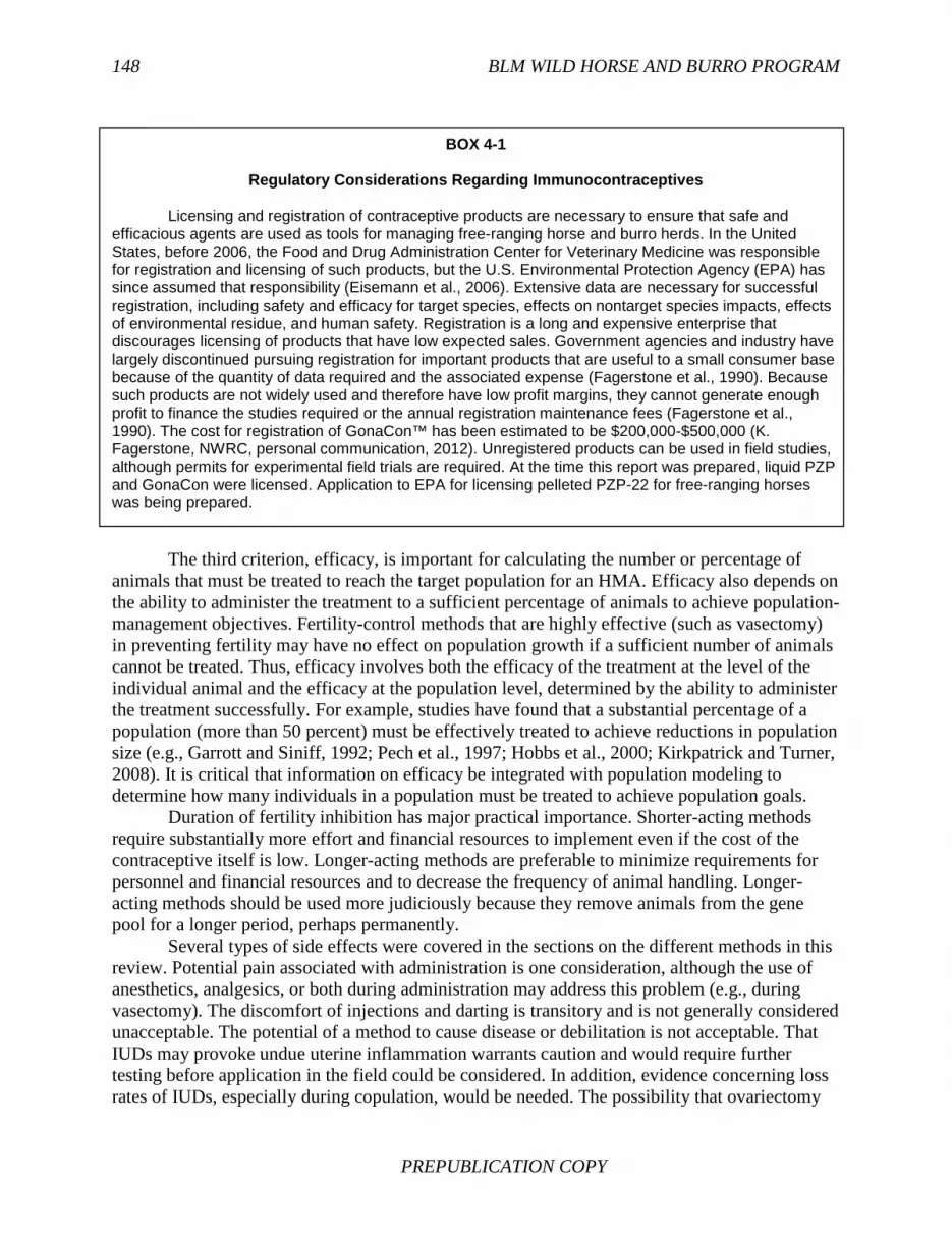
148 BLM WILD HORSE AND BURRO PROGRAM
B PREPUBLICATION COPY
BOX 4-1
Regulatory Considerations Regarding Immunocontraceptives
Licensing and registration of contraceptive products are necessary to ensure that safe and
efficacious agents are used as tools for managing free-ranging horse and burro herds. In the United States, before 2006, the Food and Drug Administration Center for Veterinary Medicine was responsible for registration and licensing of such products, but the U.S. Environmental Protection Agency (EPA) has since assumed that responsibility (Eisemann et al., 2006). Extensive data are necessary for successful registration, including safety and efficacy for target species, effects on nontarget species impacts, effects of environmental residue, and human safety. Registration is a long and expensive enterprise that discourages licensing of products that have low expected sales. Government agencies and industry have largely discontinued pursuing registration for important products that are useful to a small consumer base because of the quantity of data required and the associated expense (Fagerstone et al., 1990). Because such products are not widely used and therefore have low profit margins, they cannot generate enough profit to finance the studies required or the annual registration maintenance fees (Fagerstone et al., 1990). The cost for registration of GonaCon™ has been estimated to be $200,000-$500,000 (K. Fagerstone, NWRC, personal communication, 2012). Unregistered products can be used in field studies, although permits for experimental field trials are required. At the time this report was prepared, liquid PZP and GonaCon were licensed. Application to EPA for licensing pelleted PZP-22 for free-ranging horses was being prepared.
The third criterion, efficacy, is important for calculating the number or percentage of animals that must be treated to reach the target population for an HMA. Efficacy also depends on the ability to administer the treatment to a sufficient percentage of animals to achieve population-management objectives. Fertility-control methods that are highly effective (such as vasectomy) in preventing fertility may have no effect on population growth if a sufficient number of animals cannot be treated. Thus, efficacy involves both the efficacy of the treatment at the level of the individual animal and the efficacy at the population level, determined by the ability to administer the treatment successfully. For example, studies have found that a substantial percentage of a population (more than 50 percent) must be effectively treated to achieve reductions in population size (e.g., Garrott and Siniff, 1992; Pech et al., 1997; Hobbs et al., 2000; Kirkpatrick and Turner, 2008). It is critical that information on efficacy be integrated with population modeling to determine how many individuals in a population must be treated to achieve population goals.
Duration of fertility inhibition has major practical importance. Shorter-acting methods require substantially more effort and financial resources to implement even if the cost of the contraceptive itself is low. Longer-acting methods are preferable to minimize requirements for personnel and financial resources and to decrease the frequency of animal handling. Longer-acting methods should be used more judiciously because they remove animals from the gene pool for a longer period, perhaps permanently.
Several types of side effects were covered in the sections on the different methods in this review. Potential pain associated with administration is one consideration, although the use of anesthetics, analgesics, or both during administration may address this problem (e.g., during vasectomy). The discomfort of injections and darting is transitory and is not generally considered unacceptable. The potential of a method to cause disease or debilitation is not acceptable. That IUDs may provoke undue uterine inflammation warrants caution and would require further testing before application in the field could be considered. In addition, evidence concerning loss rates of IUDs, especially during copulation, would be needed. The possibility that ovariectomy

FERTILITY MANAGEMENT 149
PREPUBLICATION COPY
may be followed by prolonged bleeding or peritoneal infection makes it inadvisable for field application. Potential effects of GnRH vaccines and agonists on other tissues than the pituitary gonadotrophs have not been well studied or documented and warrant caution until further research has been conducted.
Any of the methods described may also affect behavior. Because all methods affect sexual function in some way, changes in expression of sexual and social behavior should be considered. The ideal method would not eliminate sexual behavior or change social structure substantially. Castration, ovariectomy, and the GnRH products (vaccines and agonists) eliminate or substantially reduce steroid hormone production and so have a potentially profound effect on the expression of sexual behavior. In contrast, vasectomy and the PZP vaccines result in a prolonged breeding season, with increased sexual interaction, because females continue to undergo estrous cycles but fail to conceive. That is not ideal because a prolonged breeding season can result in more fighting among males over access to females. However, the many studies of PZP vaccines and the single study of vasectomized stallions have not reported problems with increased aggression (e.g., more injuries or deaths among stallions).
Considering the above criteria, the methods judged most promising for application to free-ranging horses or burros are PZP vaccines, GonaCon vaccine, and chemical vasectomy. The advantages and disadvantages of each of these methods and their effects on behavior are shown in Tables 4-1 and 4-2, respectively. PZP vaccines are female-directed, chemical vasectomy is male-directed, and GnRH vaccines can be used to treat either males or females. Of the PZP vaccines, PZP-22 and SpayVac seem most appropriate and practical because of their longer duration of effect (especially PZP-22). They could be applied to herds immediately in a research framework, which is required because the products are not yet licensed. Research should address efficacy, duration, and side effects at the population and individual levels where possible. At the time the committee’s report was prepared, there was no evidence to suggest that PZP-22 or SpayVac would have different effects from liquid PZP apart from reports of uterine edema in SpayVac-treated animals. Although GonaCon can be used and has been tested in males, the effects are similar to those of chemical castration. To achieve the suppression of spermatogenesis needed to ensure infertility, testosterone must be suppressed to at or near zero. As with surgical castration, although sexually experienced males may continue to express learned behavioral patterns, they would probably not be successful in competing with intact males. Because preserving natural behaviors is an important criterion, GonaCon seems more appropriate for use in females. Although vaccines against GnRH interfere with its action on the pituitary (stimulating FSH and LH), FSH secretion is partially independent of GnRH (Padmanabhan and McNeilly, 2001). FSH is not required for stimulation of testosterone; LH is sufficient. In females, however, FSH is important for stimulating growth of follicles, which secrete estradiol, the hormone that supports estrous behavior. The role of LH is in the final stages of follicle growth and in inducing ovulation, so blockage of LH is sufficient to prevent conception. Investigations of GonaCon treatment of mares have reported continued estrous behavior and secretion of estradiol consistent with at least partial FSH independence from GnRH control. Thus, to the extent that GonaCon preserves natural behavior patterns while effectively preventing reproduction, it is a promising candidate as a female-directed fertility-control method. However, further studies of its behavioral effects are needed. Chemical vasectomy is promising as an alternative to or in combination with treating females. However, as stated above, vasectomizing more than dominant males would be practical in application at the population
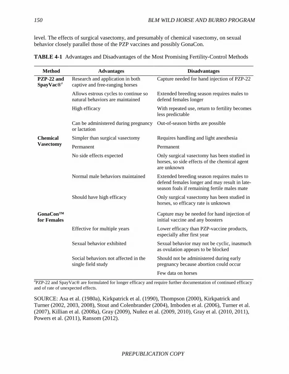
150 BLM WILD HORSE AND BURRO PROGRAM
B PREPUBLICATION COPY
level. The effects of surgical vasectomy, and presumably of chemical vasectomy, on sexual behavior closely parallel those of the PZP vaccines and possibly GonaCon. TABLE 4-1 Advantages and Disadvantages of the Most Promising Fertility-Control Methods
Method Advantages Disadvantages PZP-22 and SpayVac®a
Research and application in both captive and free-ranging horses
Capture needed for hand injection of PZP-22
Allows estrous cycles to continue so natural behaviors are maintained
Extended breeding season requires males to defend females longer
High efficacy With repeated use, return to fertility becomes less predictable
Can be administered during pregnancy or lactation
Out-of-season births are possible
Chemical Vasectomy
Simpler than surgical vasectomy Requires handling and light anesthesia Permanent Permanent No side effects expected Only surgical vasectomy has been studied in
horses, so side effects of the chemical agent are unknown
Normal male behaviors maintained Extended breeding season requires males to defend females longer and may result in late-season foals if remaining fertile males mate
Should have high efficacy Only surgical vasectomy has been studied in horses, so efficacy rate is unknown
GonaCon™ for Females
Capture may be needed for hand injection of initial vaccine and any boosters
Effective for multiple years Lower efficacy than PZP-vaccine products, especially after first year
Sexual behavior exhibited Sexual behavior may not be cyclic, inasmuch as ovulation appears to be blocked
Social behaviors not affected in the single field study
Should not be administered during early pregnancy because abortion could occur
Few data on horses aPZP-22 and SpayVac® are formulated for longer efficacy and require further documentation of continued efficacy and of rate of unexpected effects.
SOURCE: Asa et al. (1980a), Kirkpatrick et al. (1990), Thompson (2000), Kirkpatrick and Turner (2002, 2003, 2008), Stout and Colenbrander (2004), Imboden et al. (2006), Turner et al. (2007), Killian et al. (2008a), Gray (2009), Nuñez et al. (2009, 2010), Gray et al. (2010, 2011), Powers et al. (2011), Ransom (2012).

FERTILITY MANAGEMENT 151
PREPUBLICATION COPY
TABLE 4-2 Behavioral Effects of Fertility-Control Methods
Behavior
PZPa,b
GonaCon™ for Females
Vasectomy
Male sexual Increase or no change reported
No change reported
Longer breeding season
Female sexual Increase or no change reported
Decrease or no change reported
Longer breeding season
Social structure Possible decrease in band stability
No change reported
No change reported
Activity budget Females may graze less
No change reported
No change reported
Aggression Males may defend females longer
No change reported
Males defend females longer
Spatial relationships
Females may spend more time near male
No change reported
No change reported
aIncludes results of studies of both liquid and pelleted (PZP-22) formulations; not all studies reported results in all the behavioral categories, and not all studies detected changes. bThere are no published reports on behavioral effects of SpayVac®. SOURCE: Rubenstein (1994), Turner et al. (1996), Asa (1999), Powell (1999, 2000), Thompson (2000), Stout and Colenbrander (2004), Imboden et al. (2006), Killian et al. (2008b), Gray (2009), Nuñez et al. (2009), Ransom et al. (2010), Gray et al. (2010, 2011), Madosky et al. (2010, in review), Powers et al. (2011).
Although all three methods extend the breeding season, the implications of this effect after vasectomy are more serious because the likelihood of late-season mating and late births would be greater. Foals born later have less time to grow and accumulate fat stores for winter, and this jeopardizes their survival. The more intact males there are in a population, the more likely late-season birth would be because mares would have a greater chance of encountering and mating with a fertile male as the season progressed. Thus, vasectomy might be more appropriate in populations in which a relatively large percentage of males could be treated. The strategy of treating only dominant stallions should be avoided.
Late-season births could occur in mares treated with one of the vaccine products if reversal occurred during the breeding season, but because most free-ranging mares give birth every other year rather than yearly, conceptions and births should become re-established in spring or early summer. For mares that are able to maintain a pregnancy and give birth annually, reversal late in the season could have long-term consequences for all her future foals in that the 11-month gestation and the one or two ovulatory cycles needed to conceive can result in an about 12-month repeating cycle (see Garrott and Siniff, 1992).
Given that chemical vasectomy appears to be an effective means of reducing male reproduction with side effects that are likely to be minimal and not socially different from controlling female fertility, strategies that simultaneously control male and female fertility are likely to be most biologically and economically cost-effective. Because of the polygynous nature of horse and burro societies, the effect of chemically vasectomizing any one dominant harem-holding or territorial stallion will have a greater effect than contracepting any one fertile female.

152 BLM WILD HORSE AND BURRO PROGRAM
B PREPUBLICATION COPY
Moreover, because eventual male turnover is ensured, any long-term problems associated with chemical reproductive interventions are likely to be more reliably self-correcting in males than in females. When that safety factor is added to the problem of procuring large supplies of PZP vaccine in the short term, strategies of dual control allow large-scale and aggressive interventions that modeling (see Chapter 6) suggests will be necessary for regulating population growth in humane and ecologically sound ways.
Most of the PZP-vaccine research in horses (as reviewed in this chapter) has used the older, shorter-acting formulation that requires two initial injections and annual boosters. That formulation was the one licensed for use in horses at the time of the committee’s study. The longer-acting formulations (PZP-22 and SpayVac) were not licensed in the United States, so they were restricted to use for research purposes and not available for wide-spread application for management purposes. Similarly, GonaCon was registered with EPA for use in free-ranging horses in January 2013. Many state veterinary licensing agencies require that a vasectomy be performed by a licensed veterinarian, although the surgery is straightforward, but the simpler chemical vasectomy had not been systematically evaluated in horses, so testing in captive horses would be needed before widespread application in the field.
CONCLUSIONS
On the basis of the peer-reviewed literature and direct communication with scientists who are studying fertility control in horses and burros, the committee considers the three most promising methods of fertility control to be PZP-22, GonaCon, and chemical vasectomy. Chemical vasectomy requires capture and handling, which could be straightforward in areas where BLM regularly gathers horses. It is more problematic in areas where it could be difficult or impossible to capture a sufficient number of animals for treatment to achieve a population effect. In addition, the efficacy of the two vaccines is higher if they are hand-injected rather than delivered by dart. Even in the case of liquid formulations of the vaccines that can in principle be delivered by dart, adequate delivery cannot be ensured. In addition, darting typically entails following animals by helicopter, which could be as stressful as gathering. Alternative methods for gaining closer access to animals for delivering injections should be sought for areas where gathering is not practical or possible.
The vaccines can be effective for multiple years, but chemical vasectomy should be considered permanent. In cases in which reversibility is important and repeated treatment is practical, one of the vaccines would be preferable, with the caution that treatment for more than a few years may prolong recovery of fertility. A single treatment that induces lifetime infertility could be preferable in other situations.
Even if a large fraction of a population’s males are chemically vasectomized and the sterility is permanent, the effects of such an extensive intervention on the dynamics of the population will be self-correcting. If gathers are an average of 5 years apart, younger males rising through the ranks as bachelors or adopting alternative routes to adulthood (Rubenstein and Nuñez, 2009) will be adding new genes to the pool at an increasing rate. Given that virtually all burro and some horse populations exhibit low levels of genetic heterozygosity, virtual elimination of local male fertility for short periods to allow translocations of males that have desired genetic characteristics into the population may be warranted. Such large-scale local chemical vasectomies would allow managers to enhance genetic diversity and reduce inbreeding

FERTILITY MANAGEMENT 153
PREPUBLICATION COPY
of populations at risk. Moreover, it would be a self-correcting process as younger males that have the original genetic constitution mature and compete for reproductive opportunities with translocated males. Managing genetic diversity through translocation is discussed more thoroughly in the next chapter.
All three methods should preserve the basic social unit and expression of sexual behavior, although there have been conflicting reports on various effects of the vaccines on social interactions and on the cyclicity of estrous behavior. The major effect of the methods is that the typical breeding season would be extended for females that do not conceive (the implications are discussed at length above). No method has yet been developed that does not have some effect on physiology or behavior. However, the effects of not intervening to control or manage population numbers are potentially harsher than contraception; in the absence of natural predators, population numbers are likely to be limited by starvation (see Chapter 3 for discussion of the effect of density-dependent factors). Even if there were a method that had no effect other than preventing the production of young, the absence of young would alter the age structure of the population and could thereby affect harem dynamics. The most appropriate comparison that should be made in assessing the effects of any method of fertility control is with the current approach, gathering and removal. That is, to what extent does the prospective method affect health, herd structure, and the expression of natural behaviors relative to the effects of gathering? Three methods (PZP-22, GonaCon, and chemical vasectomy) are considered the most promising for managing fertility in free-ranging horses and burros because they have the fewest and least serious effects on those parameters. In addition, although their application requires handling the animals—gathering—that process is no more disruptive than the current method for controlling numbers, and it lacks the further disruption of removal and relocation to long-term holding facilities. Considering all the current options, the three methods, either alone or in combination, offer the most acceptable alternative for managing population numbers. However, further research is needed before they are ready for widespread deployment for horse population management.
The current major gaps in knowledge about PZP-22, SpayVac, and GonaCon include a thorough understanding for each vaccine of percentage and duration of efficacy and the extent of its reversibility. GonaCon should be examined to evaluate the extent to which treated females continue to exhibit sexual behavior, which is important for maintaining natural social interactions. A study is needed to assess the efficacy and safety of potential agents for chemical vasectomy before it is used in free-ranging stallions during gathers.
In light of the extensive research that has been conducted with liquid PZP, the likelihood that PZP-22 or SpayVac will produce new or unexpected effects, other than an extended duration of action, is small, and this should reduce the scope of research that would be needed. Furthermore, given the decades of research on the earlier liquid formulation of PZP and its successful application in numerous free-ranging horse herds, liquid PZP can be used in many herd areas now. It might be applied not only in herds that are amenable to darting but during gathers for horses that are turned back onto the range. Even without a booster in the months just after a gather, any later inoculation will serve as a booster and initiate a period of infertility (J.W. Turner, University of Toledo, personal communication, August 2012). Thus, liquid PZP could serve as an interim fertility-control method until one of the other longer-acting methods is available.

154 BLM WILD HORSE AND BURRO PROGRAM
B PREPUBLICATION COPY
REFERENCES
ACC&D (Alliance for Contraception in Cats & Dogs). 2012. Esterisol™ (“Zinc Neutering”). Product Profile and Position Paper. Available online at http://www.acc-d.org/ACCD%20docs/PPPP-Esterilsol.pdf/. Accessed November 14, 2012.
Adams, T.E. and B.M. Adams. 1990. Reproductive function and feedlot performance of beef heifers actively immunized against GnRH. Journal of Animal Science 68:2793-2802.
Asa, C.S. 1986. Sexual behavior of mares. Veterinary Clinics of North America: Equine Practice 2:519-534.
Asa, C.S. 1999. Male reproductive success in free-ranging feral horses. Behavioral Ecology and Sociobiology 47:89-93.
Asa, C.S. 2005. Assessing efficacy and reversibility. Pp. 53-65 in Wildlife Contraception: Issues, Methods and Application, C.S. Asa and I.J. Porton, eds. Baltimore, MD: Johns Hopkins University Press.
Asa, C.S. 2010. Reproductive physiology. Pp. 411-428 in Wild Mammals in Captivity: Principles and Techniques for Zoo Management, D.G. Kleiman, K.V. Thompson, and C.K. Baer, eds. 2nd edition. Chicago: University of Chicago Press.
Asa, C.S., D.A. Goldfoot, M.C. Garcia, and O.J. Ginther. 1980a. Sexual behavior in ovariectomized and seasonally anovulatory mares. Hormones and Behavior 14:46-54.
Asa, C.S., D.A. Goldfoot, M.C. Garcia, and O.J. Ginther. 1980b. Dexamethasone suppression of sexual behavior in ovariectomized mares. Hormones and Behavior 14:55-64.
Asa, C.S., D.A. Goldfoot, M.C. Garcia, and O.J. Ginther. 1984. The effect of estradiol and progesterone on the sexual behavior of ovariectomized mares. Physiology & Behavior 33:681-6.
Asa, C.S., I. Porton, A.M. Baker, and E.D. Plotka. 1996. Contraception as a management tool for controlling surplus animals. Pp. 451-467 in Wild Mammals in Captivity: Principles and Techniques, D.G. Kleiman, M.E. Allen, K.V. Thompson, and S. Lumpkin, eds. Chicago: University of Chicago Press.
Asa, C.S. and I.J. Porton. 2010. Contraception as a management tool for controlling surplus animals. Pp. 469-482 in Wild Mammals in Captivity: Principles and Techniques for Zoo Management, D.G. Kleiman, K.V. Thompson, and C.K. Baer, eds. 2nd edition. Chicago: University of Chicago Press.
Barber, M.R. and R.A. Fayrer-Hosken. 2000. Evaluation of somatic and reproductive immunotoxic effects of the porcine zona pellucida vaccination. Journal of Experimental Zoology Part A: Comparative and Experimental Biology 286:641-646.
Bartell, J.A. 2011. Porcine Zona Pellucida Immuncontraception Vaccine for Horses. M.S. thesis. Oregon State University.
Bartholow, J.M. 2004. Economic Analysis of Alternative Fertility Control and Associated Management Techniques for Three BLM Wild Horse Herds. Reston, VA: U.S. Geological Survey.
Becker, C.D. and J.R. Ginsberg. 1990. Mother-infant behaviour of wild Grevy’s zebra: Adaptations for survival in semi-desert East Africa. Animal Behaviour 40:1111-1118.
Berger, J. 1977. Organizational systems and dominance in feral horses in the Grand Canyon. Behavioral Ecology and Sociobiology 2:131-146.
Berger, J. 1986. Wild Horses of the Great Basin: Social Competition and Population Size. Chicago: University of Chicago Press.

FERTILITY MANAGEMENT 155
PREPUBLICATION COPY
BLM (Bureau of Land Management). 2003, revised 2005. Strategic Research Plan: Wild Horse and Burro Management. Fort Collins, CO: U.S. Department of the Interior.
Blodgett, G.P. 2011. Normal field castration. Pp. 1557-1561 in Equine Reproduction, A.O. McKinnon, E.L. Squires, W.E. Vaala, and D.D. Varner, eds. Oxford: Wiley-Blackwell.
Botha, A.E., M.L. Schulman, H.J. Bertschinger, A.J. Guthrie, C.H. Annandale, and S.B. Hughes. 2008. The use of a GnRH vaccine to suppress mare ovarian activity in a large group of mares under field conditions. Wildlife Research 35:548-554.
Boyle, M.S., J. Skidmore, J. Zhang, and J.E. Cox. 1991. The effects of continuous treatment of stallions with high levels of a potent GnRH analogue. Journal of Reproduction and Fertility Supplement 44:169-182.
Brinsko, S.P., E.L. Squires, B.W. Pickett, and T.M. Nett. 1998. Gonadal and pituitary responsiveness of stallions is not down-regulated by prolonged pulsatile administration of GnRH. Journal of Androlology 19:100-109.
Brown, R.G., W.D. Bowen, J.D. Eddington, W.C. Kimmins, M. Mezei, J.L. Parson, and B. Pohajdak. 1997. Temporal trends in antibody production in captive grey, harp and hooded seals to a single administration immunocontraceptive vaccine. Journal of Reproductive Immunology 35:53-64.
Cameron, E.Z., T.H. Setsaas, and W.L. Linklater. 2009. Social bonds between unrelated females increase reproductive success in feral horses. Proceedings of the National Academy of Sciences of the United States of America 106:13850-13853.
Carnevale, E.M. and O.J. Ginther. 1992. Relationships of age to uterine function and reproductive efficiency in mares. Theriogenology 37:1101-1115.
Caswell, H. 2001. Matrix Population Models. 2nd edition. Sunderland, MA: Sinauer Associates. Chandra, R.K. 1996. Nutrition, immunity and infection: From basic knowledge of dietary
manipulation of immune responses to practical application of ameliorating suffering and improving survival. Proceedings of the National Academy of Sciences of the United States of America 93:14304-14307.
Chandra, R.K. and S.A.D. Amorin. 1992. Lipids and immunoregulation. Nutritional Research 12:S137-S145.
Chapel, H.M. and P.J. August. 1976. Report of nine cases of accidental injury to man with Freund’s complete adjuvant. Clinical and Experimental Immunology 24:538-541.
Chi, I. 1993. What we have learned from recent IUD studies: A researcher's perspective. Contraception 48:81-108.
Cooper, D.W. and E. Larsen. 2006. Immunocontraception of mammalian wildlife: Ecological and immunogenetic issues. Reproduction 132:821-828.
Curtis, P.D., R.L. Pooler, M.E. Richmond, L.A. Miller, G.F. Mattfeld, and F.W. Quimby. 2002. Comparative effects of GnRH and porcine zona pellucida (PZP) immunocontraceptive vaccines for controlling reproduction in white-tailed deer (Odocoileus virginianus). Reproduction Supplement 60:131-141.
Daels, P.F. and J.P. Hughes. 1995. Fertility control using intrauterine devices: An alternative for population control in wild horses. Theriogenology 44:629-639.
Demas, G.E., D.L. Drazen, and R.J. Nelson. 2003. Reductions in total body fat decrease humoral immunity. Proceedings of the Royal Society B: Biological Sciences 270:905-911.
Eagle, T.C., E.D. Plotka, D.B. Siniff, and J.R. Tester. 1992. Efficacy of chemical contraception in feral mares. Wildlife Society Bulletin 20:211-216.

156 BLM WILD HORSE AND BURRO PROGRAM
B PREPUBLICATION COPY
Eagle, T.C., C.S. Asa, R.A. Garrott, and D.V. Siniff. 1993. Efficacy of dominant male contraception to reduce reproduction in feral horses. Wildlife Society Bulletin 21:116-121.
Eisemann, J.D., K.A. Fagerstone, and J.R. O’Hare. 2006. Wildlife contraceptives: A regulatory hot potato. Proceedings of the 22nd Vertebrate Pest Conference 22:63-66.
Elhay, M., A. Newbold, A. Britton, P. Turley, K. Dowsett, and J. Walker. 2007. Suppression of behavioural and physiological oestrus in the mare by vaccination against GnRH. Australian Veterinary Journal 85:39-45.
Esho, J.O. and A.S. Cass. 1978. Recanalization rate following methods of vasectomy using interposition of fascial sheath of vas deferens. Journal of Urology 120:178-179.
Fagerstone, K.A., R.M. Bullard, and C.A. Ramcy. 1990. Politics and economics of maintaining pesticide registrations. Vertebrate Pest Conference 14:8-11.
Falconer, D.S. 1965. The inheritance of liability to certain diseases, estimated from the incidence among relatives. Annals of Human Genetics 29:51-76.
Feist, J.D. and D.R. McCullough. 1975. Reproduction in feral horses. Journal of Reproduction and Fertility Supplement 23:13-18.
Fielding, D. 1988. Reproductive characteristics of the jenny donkey—Equus asinus: A review. Tropical Animal Health and Production 20:161-166.
Fitzgerald, B., K. Peterson, and P. Silvia. 1993. Effect of constant administration of a gonadotropin-releasing hormone agonist on reproductive activity in mares: Preliminary evidence on suppression of ovulation during the breeding season. American Journal of Veterinary Research 54:1746.
Fraker, M.A. 2012. SpayVac® for Wild Horses: A Lost-Lasting, Single-Dose pZP Contraceptive Vaccine. Webinar Presentation to the Bureau of Land Management and Members of the National Academy of Sciences’ Committee to Review the Bureau of Land Management Wild Horse and Burro Management Program, May 3.
Fraker, M.A., R.G. Brown, G.E. Gaunt, J.A. Kerr, and B. Pohajdak. 2002. Long-lasting single-dose immunocontraception of feral fallow deer in British Columbia. Journal of Wildlife Management 66:1141-1147.
Fraker, M.A. and R.B. Brown. 2011. Efficacy of SpayVac® is excellent: A comment on Gray et al. (2010). Wildlife Research 38:537-538.
Frenette, M.D., M.P. Dooley, and M.H. Pineda. 1986. Effect of flushing the vasa deferentia at the time of vasectomy on the rate of clearance of spermatozoa from the ejaculates of dogs and cats. American Journal of Veterinary Research 47:463-470.
Garrott, R.A. and D.B. Siniff. 1992. Limitations of male-oriented contraception for controlling feral horse populations. Journal of Wildlife Management 56:456-464.
Gass, G.H., D. Coats, and N. Graham. 1964. Carcinogenic dose-response curve to oral diethylstibestrol. Journal of the National Cancer Institute 33:971-977.
Ginsberg, J.R. 1989. The ecology of female behaviour and male mating success in the Grevy’s zebra. Symposium of the Zoological Society of London 61:89-110.
Ginther, O.J. 1979. Reproductive Biology of the Mare: Basic and Applied Aspects. Cross Plains, WI: EquiServices.
Ginther, O.J., S.T. Scraba, and D.R. Bergfelt. 1987. Reproductive seasonality of the jenny. Theriogenology 27:587-592.
Gionfriddo, J.P., J.D. Eisemann, K.J. Sullivan, R.S. Healey, L.A. Miller, K.A. Fagerstone, R.M. Engeman, and C.A. Yoder. 2009. Field test of a single-injection gonadotrophin-releasing

FERTILITY MANAGEMENT 157
PREPUBLICATION COPY
hormone immunocontraceptive vaccine in female white-tailed deer. Wildlife Research 36:177-184.
Gionfriddo, M.P., A.J. DeNicola, L.A. Miller, and K.A. Fagerstone. 2011a. Efficacy of GnRH immunocontraception of wild white-tailed deer in New Jersey. Wildlife Society Bulletin 35:142-148.
Gionfriddo, M.P., A.J. DeNicola, L.A. Miller, and K.A. Fagerstone. 2011b. Health effects of GnRH immunocontraception of wild white-tailed deer in New Jersey. Wildlife Society Bulletin 35:149-160.
Gionfriddo, J.P., J.D. Eisemann, K.J. Sullivan, R.S. Healey, and L.A. Miller. 2006. Field test of GonaCon™ immunocontraceptive vaccine in free-ranging female white-tailed deer. Proceedings of the 22nd Vertebrate Pest Conference 22:78-81.
Goodloe, R.B. 1991. Immunocontraception, Genetic Management, and Demography of Feral Horses on Four Eastern U.S. Barrier Islands. Ph.D. dissertation. University of Georgia.
Gotelli, N. 2001. A Primer of Ecology. 3rd edition. Sunderland, MA: Sinauer Associates. Gray, M.E. 2009. The Influence of Reproduction and Fertility Manipulation on The Social
Behavior of Feral Horses (Equus caballus). Ph.D. dissertation. University of Nevada, Reno.
Gray, M.E., D.S. Thain, E.Z. Cameron, and L.A. Miller. 2010. Multi-year fertility reduction in free-roaming feral horses with single-injection immunocontraceptive formulations. Wildlife Research 37:475-481.
Gray, M.E., D.S. Thain, E.Z. Cameron, and L.A. Miller. 2011. Corrigendum: Multi-year fertility reduction in free-roaming feral horses with single-injection immunocontraceptive formulations. Wildlife Research 38:260.
Guillaume, D., G. Duchamp, J. Salazar-Ortiz, and P. Nagy. 2002. Nutrition influences the winter ovarian inactivity in mares. Theriogenology 58:593-597.
Hageleit, M., A. Daxenberger, W.D. Kraetzl, A. Kettler, and H.H.D. Meyer. 2000. Dose-dependent effects of melengestrol acetate (MGA) on plasma levels of estradiol, progesterone and luteinizing hormone in cycling heifers and influence on oestrogen residues in edible tissues. Acta Pathologica Microbiologica and Immunologica Scandinavica 108:847-854.
Henry, M., S.M. McDonnell, L.D. Lodi, and E.L. Gastal. 1991. Pasture mating behaviour of donkeys (Equus asinus) at natural and induced oestrus. Journal of Reproduction and Fertility Supplement 44:77-86.
Hobbs, N.T., D.C. Bowden, and D.L. Baker. 2000. Effects of fertility control on populations of ungulates: General, stage-structured models. Journal of Wildlife Management 64:473-491.
Holtan, D.W., E.L. Squires, D.R. Lapin, and O.J. Ginther. 1979. Effect of ovariectomy on pregnancy in mares. Journal of Reproduction and Fertility Supplement 27:457-463.
Homsy, J., W.J.W. Morrow, and J.A. Levy. 1986. Nutrition and autoimmunity: A review. Clinical Experimental Immunology 65:473-488.
Hooper, R.N., T.S. Taylor, D.D. Varner, and T.L. Blanchard. 1993. Effects of bilateral ovariectomy via colpotomy in mares: 23 cases (1984-1990). Journal of the American Veterinary Medical Association 203:1043-1046.
Houston, A.I., J.M. McNamara, Z. Barta, and K.C. Klasing. 2007. The effect of energy reserves and food availability on optimal immune defence. Proceedings of the Royal Society B: Biological Sciences 274:2835-2842.

158 BLM WILD HORSE AND BURRO PROGRAM
B PREPUBLICATION COPY
Imboden, I., F. Janett, D. Burger, M.A. Crowe, M. Hassig, and R. Thun. 2006. Influence of immunization against GnRH on reproductive cyclicity and estrous behavior in the mare. Theriogenology 66:1866-1875.
Janett, F., R. Stump, D. Burger, and R. Thun. 2009. Suppression of testicular function and sexual behavior by vaccination against GnRH (Equity™) in the adult stallion. Animal Reproduction Science 115:88-102.
Jensen, H. 2000. Social Structure and Activity Patterns among Selected Pryor Mountain Wild Horses. Report to the Billings BLM Field Office.
Johnson, C., S. McMeen, and D. Thompson. 2002. Effects of multiple GnRH analogue (deslorelin acetate) implants on cyclic mares. Theriogenology 58:469-471.
Junaidi, A., P.E. Williamson, J.M. Cummins, G.B. Martin, M.A. Blackberry, and T.E. Trigg. 2003. Use of a new drug delivery formulation of the gonadotrophin-releasing hormone analogue Deslorelin for reversible long-term contraception in male dogs. Reproduction, Fertility and Development 15:317-322.
Junaidi, A., P.E. Williamson, G.B. Martin, M.A. Blackberry, J.M. Cummins, and T.E. Trigg. 2009. Dose-response studies for pituitary and testicular function in male dogs treated with the GnRH superagonist, deslorelin. Reproduction in Domestic Animals 44:725-34.
Killian, G., L.A. Miller, N.L. Diehl, J. Rhyan, and D. Thain. 2004. Evaluation of three contraceptive approaches for population control of wild horses. Proceedings of the 21st Vertebrate Pest Conference 21:263-268.
Killian, G., D. Thain, N.K. Diehl, J. Rhyan, and L. Miller. 2008a. Four-year contraception rates of mares treated with single-injection porcine zona pellucida and GnRH vaccines and intrauterine devices. Wildlife Research 35:531-539.
Killian, G., D. Wagner, K. Fagerstone, and L. Miller. 2008b. Long-term efficacy and reproductive behavior associated with Gonacon™ use in white-tailed deer (Odocoileus virginianus). Proceedings of the 23rd Vertebrate Pest Conference 23:240-243.
Killian, G., D. Wagner, and L. Miller. 2005. Observations on the use of the GnRH vaccine Gonacon™ in male white-tailed deer (Odocoileus virginianus). Proceedings of the 11th Wildlife Damage Management Conference 11:256-263.
Killian, G., T.J. Kreeger, J. Rhyan, K. Fagerstone, and L. Miller. 2009. Observations on the use of Gonacon™ in captive female elk (Cervus elaphus). Journal of Wildlife Diseases 45:184-188.
Killian, G., L. Miller, J. Rhyan, and H. Doten. 2006. Immunocontraception of Florida feral swine with a single-dose GnRH vaccine. American Journal of Reproductive Immunology 55:378-384.
Kirkpatrick, J.F. and A. Turner. 2002. Reversibility of action and safety during pregnancy of immunization against porcine zona pellucida in wild mares (Equus caballus). Reproduction Supplement 60:197-202.
Kirkpatrick, J.F. and A. Turner. 2003. Absence of effects from immunocontraception on seasonal birth patterns and foal survival among barrier island wild horses. Journal of Applied Animal Welfare Science 6:301-308.
Kirkpatrick, J.F. and A. Turner. 2007. Immunocontraception and increased longevity in equids. Zoo Biology 26:237-244.
Kirkpatrick, J.F. and A. Turner. 2008. Achieving population goals in a long-lived wildlife species (Equus caballus) with contraception. Wildlife Research 35:513-519.

FERTILITY MANAGEMENT 159
PREPUBLICATION COPY
Kirkpatrick, J.F., R.O. Lyda, and K.M. Frank. 2011. Contraceptive vaccines for wildlife: A review. American Journal of Reproductive Immunology 66:40-50.
Kirkpatrick, J.F., I.K.M. Liu, and J.W. Turner, Jr. 1990. Remotely-delivered immunocontraception in feral horses. Wildlife Society Bulletin 18:326-330.
Kirkpatrick, J.F., I.M.K. Liu, J.W. Turner, Jr., and M. Bernoco. 1991. Antigen recognition in feral mares previously immunized with porcine zona pellucida. Journal of Reproduction and Fertility Supplement 44:321-325.
Kirkpatrick, J.F., I.M.K. Liu, J.W. Turner, Jr., R. Naugle, and R. Keiper. 1992. Long-term effects of porcine zonae pellucidae immunocontraception on ovarian function in feral horses (Equus caballus). Journal of Reproduction and Fertility 94:437-444.
Kirkpatrick, J.F., R. Naugle, I.K.M. Liu, M. Bernoco, and J.W. Turner, Jr. 1995. Effects of seven consecutive years of porcine zona pellucida contraception on ovarian function in feral mares. Biology of Reproduction Monographs 1:411-418.
Klingel, H. 1975. Social organization and reproduction in equids. Journal of Reproduction and Fertility Supplement 23:7-11.
Lauderdale, J.W., L.S. Goyings, L.F. Krzeminski, and R.G. Zimbelman. 1977. Studies of a progestogen (MGA) as related to residues and human consumption. Journal of Toxicology and Environmental Health 3:5-33.
Liehr, J.G. 2001. Genotoxicity of the steroidal oestrogens oestrone and oestradiol: Possible mechanism of uterine and mammary cancer development. Human Reproduction Update 7:273-281.
Linklater, W.L., E.Z. Cameron, E.O. Minot, and K.J. Stafford. 1999. Stallion harassment and the mating system of horses. Animal Behavior 58:295-306.
Liu, I.K.M., M. Bernoco, and M. Feldman. 1989. Contraception in mares heteroimmunized with pig zona pellucidae. Journal of Reproduction and Fertility 85:19-28.
Liu, I.K.M., J.W. Turner, Jr., E.M.G. Van Leeuwen, D.R. Flanagan, J.L. Hedrick, K. Murata, V.M. Lane, and M.P. Morales-Levy. 2005. Persistence of anti-zonae pellucidae antibodies following a single inoculation of porcine zonae pellucidae in the domestic equine. Reproduction 129:181-190.
Locke, S.L., M.W. Cook, L.A. Harveson, D.S. Davis, R.R. Lopez, N.J. Silvy, and M.A. Fraker. 2007. Effectiveness of Spayvac® for reducing white-tailed deer fertility. Journal of Wildlife Diseases 43:726-30.
Ludwig, C., P.O. Desmoulins, M.A. Driancourt, S. Goericke-Pesch, and B. Hoffmann. 2009. Reversible downregulation of endocrine and germinative testicular function (hormonal castration) in the dog with the GnRH-agonist azagly-nafarelin as a removable implant “Gonazon”; a preclinical trial. Theriogenology 71:1037-1045.
Lyda, R.O., J.R. Hall, and J.F. Kirkpatrick. 2005. A comparison of Freund’s Complete and Freund’s Modified Adjuvants used with a contraceptive vaccine in wild horses (Equus caballus). Journal of Zoo and Wildlife Medicine 36:610-616.
Madosky, J., D. Rubenstein, J. Howard, and S. Stuska. 2010. The effect of immunocontraception on harem fidelity in a feral horse (Equus caballus) population. Applied Animal Behaviour Science 128:50-56.
Madosky, J., J. Howard, D. Rubenstein, and S. Stuska. In review. Synchrony of time budgets, social interactions, and harem stability in a feral horse population.

160 BLM WILD HORSE AND BURRO PROGRAM
B PREPUBLICATION COPY
Malmgren, L., O. Andresen, and A.M. Dalin. 2001. Effect of GnRH immunisation on hormonal levels, sexual behaviour, semen quality and testicular morphology in mature stallions. Equine Veterinary Journal 33:75-83.
Massei, G., D.P. Cowan, J. Coats, F. Gladwell, J.E. Lane, and L.A. Miller. 2008. Effect of the GnRH vaccine GonaCon on the fertility, physiology and behaviour of wild boar. Wildlife Research 35:540-547.
May, R.M. and D.I. Rubenstein. 1985. Reproductive strategies. Pp. 1-23 in Reproduction in Mammals, C.R. Austin and R.V. Short, eds. Cambridge, UK: Cambridge University Press.
McCue, P.M. and R.A. Ferris. 2011. The abnormal estrous cycle. Pp. 1754-1768 in Equine Reproduction, A.O. McKinnon, E.L. Squires, W.E. Vaala, and D.D. Varner, eds. 2nd edition. Hoboken, NJ: Wiley-Blackwell.
McCue, P.M. and A.O. McKinnon. 2011. Ovarian abnormalities. Pp. 2123-2136 in Equine Reproduction, A.O. McKinnon, E.L. Squires, W.E. Vaala, and D.D. Varner, eds. 2nd edition. Hoboken, NJ: Wiley-Blackwell.
Miller, L.A., B.E. Johns, and G.J. Killian. 2000. Immunocontraception of white-tailed deer with GnRH vaccine. American Journal of Reproductive Immunology 44:266-274.
Miller, L.A., J.P. Gionfriddo, J.C. Rhyan, K.A. Fagerstone, D.C. Wagner, and G.J. Killian. 2008. GnRH immunocontraception of male and female white-tailed deer fawns. Human-Wildlife Conflicts 2:93-101.
Miller, L.A., K.A. Fagerstone, D.C. Wagner, and G.J. Killian. 2009. Factors contributing to the success of a single-shot, multiyear PZP immunocontraceptive vaccine for white-tailed deer. Human-Wildlife Conflicts 3:103-115.
Miller, L.A., J.C. Rhyan, and M. Drew. 2004. Contraception of bison by GnRH vaccine: A possible means of decreasing transmission of brucellosis in bison. Journal of Wildlife Diseases 40:725-730.
Mitchell, D. and W.R. Allen. 1975. Observations on reproductive performance in the yearling mare. Journal of Reproduction and Fertility Supplement 23:531-536.
Montovan, S.M., P.F. Daels, J. Rivier, J.P. Hughes, G.H. Stabenfeldt, and B.L. Lasley. 1990. The effect of a potent GnRH agonist on gonadal and sexual activity in the horse. Theriogenology 33:1305-1321.
Moss, W.M. 1992. A comparison of open-ended versus closed-end vasectomies: A report on 6220 cases. Contraception 46:521-525.
Munson, L., J.E. Bauman, C.S. Asa, W. Jochle, and T.E. Trigg. 2001. Efficacy of the GnRH analogue deslorelin for suppression of oestrus cycle in cats. Journal of Reproduction and Fertility Supplement 57:269-273.
Murthy, V., A.R. Norman, Y. Barbachano, C.C. Parker, and D.P. Dearnaley. 2007. Long-term effects of a short course of neoadjuvant luteinizing hormone-releasing hormone analogue and radical radiotherapy on the hormonal profile in patients with localized prostate cancer. British Journal of Urology International 99:1380-1382.
Naden, J., E.L. Squires, and T.M. Nett. 1990. Effect of maternal treatment with altrenogest on age at puberty, hormone concentrations, pituitary response to exogenous GnRH, oestrous cycle characteristics and fertility of fillies. Journal of Reproduction and Fertility 88:185-195.

FERTILITY MANAGEMENT 161
PREPUBLICATION COPY
Nejat, R.J., H.H. Rashid, E. Bagiella, A.E. Katz, and M.C. Benson. 2000. A prospective analysis of time to normalization of serum testosterone after withdrawal of androgen deprivation therapy. Journal of Urology 164:1891-1894.
Nelson, K.J. 1978. On the Question of Male-Limited Population Growth in Feral Horses (Equus caballus). M.S. thesis. New Mexico State University, Las Cruces.
Neuhauser, S., F. Palm, F. Ambuehl, and C. Aurich. 2008. Effects of altrenogest treatment of mares in late pregnancy on parturition and on neonatal viability of their foals. Experimental and Clinical Endocrinology and Diabetes 116:423-428.
Nipken, C. and K.H. Wrobel. 1997. A quantitative morphological study of age-related changes in the donkey testis in the period between puberty and senium. Andrologia 29:149-161.
Nishikawa, Y. 1959. Studies on reproduction in horses. Tokyo: Japan Racing Association. Nobelius, A.M. 1992. Gestagens in the Mare: An Appraisal of the Effects of Gestagenic Steroids
on Suppression of Oestrus in Mares. M.S. thesis. Monash University, Australia. NRC (National Research Council). 1980. Wild and Free-Roaming Horses and Burros: Current
Knowledge and Recommended Research. Phase I Report. Washington, DC: National Academy Press.
NRC (National Research Council). 1991. Wild Horse Populations: Field Studies in Genetic and Fertility. Washington, DC: National Academy Press.
Nuñez, C.M.V., J.S. Adelman, C. Mason, and D.I. Rubenstein. 2009. Immunocontraception decreased group fidelity in a feral horse population during the non-breeding season. Applied Animal Behavior Science 117:74-83.
Nuñez, C.M.V., J.S. Adelman, and D.I. Rubenstein. 2010. Immunocontraception in wild horses (Equus caballus) extends reproductive cycling beyond the normal breeding season. PLoS One 5:e13635.
O’Brien, P.A., R. Kulier, F.M. Helmerhorst, M. Usher-Patel, and C. d’Arcangues. 2008. Copper-containing, framed intrauterine devices for contraception: A systematic review of randomized controlled trials. Contraception 77:318-27.
Oli, M.K. and F.S. Dobson. 2003. The relative importance of life-history variables to population growth rate in mammals: Cole’s prediction revisited. American Naturalist 161:422-440.
Padmanabhan, W. and A. McNeilly. 2001. Is there an FSH-releasing factor? Reproduction 121:21-30.
Pech, R., G.M. Hood, J. McIlroy, and G. Saunders. 1997. Can foxes be controlled by reducing their fertility? Reproduction, Fertility and Development 9:41-50.
Pelahach, L.M., H.E., Greaves, M.B. Porter, A. Desvousges, and D.C. Sharp. 2002. The role of estrogen and progesterone in the induction and dissipation of uterine edema in mares. Theriogenology 58:441-444.
Perry, K.R., W.M. Arjo, K.S. Bynum, and L.A. Miller. 2006. GnRH single-injection immunocontraception in black-tailed deer. Proceedings of the 22nd Vertebrate Pest Conference 22:72-77.
Pickett, B.W., L.C. Faulkner, and J.L. Voss. 1975. Effect of season on some characteristics of stallion semen. Journal of Reproduction and Fertility Supplement 23:25-28.
Pineda, M.H. and M.P. Dooley. 1984. Surgical and chemical vasectomy in the cat. American Journal of Veterinary Research 45:291-300.
Pineda, M.H., T.J. Reimers, L.C. Faulkner, M.C. Hopwood, and G.E. Seidel, Jr. 1977. Azoospermia in dogs induced by injection of schlerosing agents into the caudae of the epididymis. American Journal of Veterinary Research 38:831-838.

162 BLM WILD HORSE AND BURRO PROGRAM
B PREPUBLICATION COPY
Pinto, C.R.F. 2011. Progestagens and progesterone. Pp. 1811-1819 in Equine Reproduction, A.O. McKinnon, E.L. Squires, W.E. Vaala, and D.D. Varner, eds. 2nd edition. Oxford: Wiley-Blackwell.
Plosker, G.L. and R.N. Brogden. 1994. Leuprorelin. A review of its pharmacology and therapeutic use in prostatic cancer, endometriosis and other sex hormone-related disorders. Drugs 48:930-67.
Plotka, E.D. and U.S. Seal. 1989. Fertility control in female white-tailed deer. Journal of Wildlife Disease 25:643-646.
Plotka, E.D., T.C. Eagle, D.N. Vevea, A.L. Koller, D.B. Siniff, J.R. Tester, and U.S. Seal. 1988. Effects of hormone implants on estrus and ovulation in feral mares. Journal of Wildlife Disease 24:507-514.
Plotka, E.D., D.N. Vevea, T.C. Eagle, J.R. Tester, and D.B. Siniff. 1992. Hormonal contraception of feral mares with Silastic rods. Journal of Wildlife Disease 28:255-262.
Pollock, J.I. 1980. Behavioral ecology and body condition changes in New Forest ponies. Royal Society for the Prevention of Cruelty to Animals Scientific Publication 6. 113pp.
Porter, M. and D. Sharp. 2002. Gonadotropin-releasing hormone receptor trafficking may explain the relative resistance to pituitary desensitization in mares. Theriogenology 58:523-526.
Porton, I.J. and K. DeMatteo. 2005. Contraception in non-human primates. Pp. 119-148 in Wildlife Contraception: Issues, Methods, and Applications, C.S. Asa and I.J. Porton, eds. Baltimore, MD: Johns Hopkins University Press.
Powell, D.M. 1999. Preliminary evaluation of porcine zona pellucida (PZP) immunocontraception for behavioral effects. Journal of Applied Animal Welfare Science 2:321.
Powell, D.M. 2000. Evaluation of Effects of Contraceptive Population Control on Behavior and the Role of Social Dominance in Female Feral Horses, Equus caballus. Ph.D. dissertation. University of Maryland, College Park.
Powell, D.M. and S.L. Montfort. 2001. Assessment: Effects of porcine zona pellucida immunocontraception on estrous cyclicity in feral horses. Journal of Applied Animal Welfare Science 4:271-284.
Powers, J.G., D.L. Baker, T.L. Davis, M.M. Conner, A.H. Lothridge, and T.M. Nett. 2011. Effects of gonadotropin-releasing hormone immunization on reproductive function and behavior in captive female Rocky Mountain elk (Cervus elaphus nelsoni). Biology of Reproduction 85:1152-1160.
Pugh, D. 2002. Donkey reproduction. Proceedings of the American Association of Equine Practitioners 48:113-114.
Ransom, J.I. 2012. Population Ecology of Feral Horses in an Era of Fertility Control Management. Ph.D. dissertation. Colorado State University, Fort Collins.
Ransom, J.I., B.S. Cade, and N.T. Hobbs. 2010. Influences of immunocontraception on time budgets, social behavior, and body condition in feral horses. Applied Animal Behavior Science 124:51-60.
Ransom, J.I., J.E. Roelle, B.S. Cade, L. Coates-Markle, and A.J. Kane. 2011. Foaling rates in feral horses treated with the immunocontraceptive porcine zona pellucida. Wildlife Society Bulletin 35:343-352.
Rivera, R. and K. Best. 2002. Current opinion: Consensus statement on intrauterine contraception. Contraception 65:385-388.

FERTILITY MANAGEMENT 163
PREPUBLICATION COPY
Rodgerson, D.H. and D.A. Loesch. 2011. Ovariectomy. Pp. 2564-2573 in Equine Reproduction, A.O. McKinnon, E.L. Squires, W.E. Vaala, and D.D. Varner, eds. 2nd edition. Oxford: Wiley-Blackwell.
Roelle, J.E. and J.I. Ransom. 2009. Injection-site reactions in wild horses (Equus caballus) receiving an immunocontraceptive vaccine. U.S. Geological Survey Scientific Investigations Report 2009-5038. Fort Collins, CO: U.S. Geological Survey.
Roser, J.F. and J.P. Hughes. 1991. Prolonged pulsatile administration of gonadotropin-releasing hormone (GnRH) to fertile stallions. Journal of Reproduction and Fertility Supplement 44:155-168.
Rubenstein, D.I. 1981. Behavioural ecology of island feral horses. Equine Veterinary Journal 13:27-34.
Rubenstein, D.I. 1986. Ecology and sociality in horses and zebras. Pp. 282-302 in Ecological Aspects of Social Evolution, D.I. Rubenstein and L.W. Wrangham, eds. Princeton, NJ: Princeton University Press.
Rubenstein, D.I. 1994. The ecology of female social behaviour in horses, zebras and asses. Pp. 13-28 in Animal Societies, Individuals, Interactions, and Organization, P.J. Jarman and A. Rossiter, eds. Kyoto, Japan: Kyoto University Press.
Rubenstein, D.I. and C. Nuñez. 2009. Sociality and reproductive skew in horses and zebras. Pp. 196-226 in Reproductive Skew in Vertebrates: Proximate and Ultimate Causes, R. Hager and C.B. Jones, eds. Cambridge, UK: Cambridge University Press.
Rutberg, A.T. 1990. Intergroup transfer in Assateague pony mares. Animal Behaviour 40:945-942.
Rutberg, A.T. and R.E. Naugle. 2008. Population-level effects of immunocontraception in white-tailed deer (Odocoileus virginianus). Wildlife Research 35:494-501.
Samper, J.C. 1997. Ultrasonographic appearance and the pattern of uterine edema to time ovulation in mares. Proceedings of the American Association of Equine Practitioners 43:189-191.
Santen, R. 1998. Biological basis of the carcinogenic effects of estrogen. Obstetrical and Gynecological Survey 53:10S-18S.
Sharp, D.C. and O.J. Ginther. 1975. Stimulation of follicular activity and estrous behavior in anestrous mares with light and temperature. Journal of Animal Science 41:1368-1372.
Sieme, H., M.H.T. Troedsson, S. Weinrich, and E. Klug. 2004. Influence of exogenous GnRH on sexual behavior and frozen/thawed semen viability in stallions during the non-breeding season. Theriogenology 61:159-171.
Singer, F.J. and K.A. Schoenecker. 2000. Managers’ summary - Ecological studies of the Pryor Mountain Wild Horse Range, 1992-1997. Fort Collins, CO: U.S. Geological Survey.
Silber, S.J. 1989. Pregnancy after vasovasostomy for vasectomy reversal: A study of factors affecting long-term return of fertility in 282 patients followed for 10 years. Human Reproduction 4:318-322.
Sivin, I. 1993. Another look at the Dalkon Shield: Meta analysis underscores its problems. Contraception 48:1-12.
Squires, E.L. 2011. Gonadotropin releasing hormones. Pp. 1820-1824 in Equine Reproduction, A.O. McKinnon, E.L. Squires, W.E. Vaala, and D.D. Varner, eds. 2nd edition. Oxford: Wiley-Blackwell.
Stahl, J.T. and M.K. Oli. 2006. Relative importance of avian life-history variables to population growth rate. Ecological Modelling 198:183-194.

164 BLM WILD HORSE AND BURRO PROGRAM
B PREPUBLICATION COPY
Stahlbaum, C.C. and K.A. Houpt. 1989. The role of the flehmen response in the behavioral repertoire of the stallion. Physiology and Behavior 45:1207-1214.
Stearns, S.C. 1992. The Evolution of Life Histories. Oxford: Oxford University Press. Stevens, E.F. 1990. Instability of harems of feral horses in relation to season and presence of
subordinate stallions. Behaviour 112:149-161. Storer, W.A., D.L. Thompson, R.M. Gilley, and P.J. Burns. 2009. Evaluation of injectable
sustained release progestin formulations for suppression of estrus and ovulation in mares. Journal of Equine Veterinary Science 29:33-36.
Stout, T.A.E. and B. Colenbrander. 2004. Suppressing reproductive activity in horses using GnRH vaccines, antagonists or agonists. Animal Reproduction Science 82-83:633-643.
Stuska, S. 2012. Shackleford Banks Horse Herd Update. September 25. Beaufort, NC: Foundation for Shackleford Horses.
Tankeyoon, M., N. Dusitsin, S. Chalapati, S. Koetsawang, S. Saibiang, M. Sas, J.J. Gellen, O. Ayeni, R. Gray, A. Pinol, and L. Zegers. 1984. Effects of hormonal contraceptives on milk volume and infant growth: WHO Special Programme of Research and Development and Research Training in Human Reproduction. Contraception 30:505-522.
Thompson, D.L. 2000. Immunization against GnRH in male species (comparative aspects). Animal Reproduction Science 60:459-469.
Tomasgard, G. and E. Benjaminsen. 1975. Plasma progesterone in mares showing estrus during pregnancy. Nordisk Veterinærmedicin. 27:570-574.
Toydemir, T.S.F., M.R. Kılıçarslan, and V. Olgaç. 2012. Effects of the GnRH analogue deslorelin implants on reproduction in female domestic cats. Theriogenology 77:662-674.
Turkstra, J., F. Van Der Meer, J. Knaap, P. Rottier, K. Teerds, B. Colenbrander, and R. Meloen. 2005. Effects of GnRH immunization in sexually mature pony stallions. Animal Reproduction Science 86:247-259.
Turner, J.W., Jr. and J.F. Kirkpatrick. 1982. Androgens, behavior and fertility control in feral stallions. Journal of Reproduction and Fertility Supplement 32:79-87.
Turner, A. and J.F. Kirkpatrick. 2002. Effects of immunocontraception on population, longevity and body condition in wild mares (Equus caballus). Reproduction Supplement 60:187-195.
Turner, J.W., Jr., I.K.M. Liu, A.T. Rutberg, and J.F. Kirkpatrick. 1997. Immunocontraception limits foal production in free-roaming feral horses in Nevada. Journal of Wildlife Management 61:873-880.
Turner, J.W., Jr., I.K.M. Liu, D.R. Flanagan, A.T. Rutberg, and J.F. Kirkpatrick. 2007. Immunocontraception in wild horses: One inoculation provides two years of infertility. Journal of Wildlife Management 71:662-667.
Turner, J.W., Jr., I.K.M. Liu, and J.F. Kirkpatrick. 1996. Remotely delivered immuno-contraception in free-roaming feral burros (Equus asinus). Journal of Reproduction and Fertility 107:31-35.
Turner, J.W., Jr., I.K.M. Liu, D.R. Flanagan, A.T. Rutberg, and J.F. Kirkpatrick. 2001. Immunocontraception in feral horses: One inoculation provides one year of infertility. Journal of Wildlife Management 65:235-241.
Turner, J.W., A.T. Rutberg, R.E. Naugle, M.A. Kaur, D.R. Flanagan, H.J. Bertschinger, and I.K.M. Liu. 2008. Controlled-release components of PZP contraceptive vaccine extend duration of infertility. Wildlife Research 35:555-562.

FERTILITY MANAGEMENT 165
PREPUBLICATION COPY
Vandeplassche, G.M., J.A. Wesson, and O.J. Ginther. 1981. Behavioral, follicular and gonadotropin changes during the estrous cycle in donkeys. Theriogenology 16:239-249.
Vanderwall, D.K. 2008. Early embryonic loss in the mare. Journal of Equine Veterinary Science 28:691-702.
Vanderwall, D.K., G.L. Woods, D.A. Freeman, J.A. Weber, R.W. Rock, and D.F. Tester. 1993. Ovarian follicles, ovulations, and progesterone concentrations in aged versus young mares. Theriogenology 40:21-32.
Yurewicz, E.C., A.G. Sacco, and M.G. Subramanian. 1983. Isolation and preliminary characterization of a purified pig zona antigen (PPZA) from porcine oocytes. Biology of Reproduction 29:511-523.
Zeng, W., S. Ghosh, Y.F. Lau, L.E. Brown, and D.C. Jackson. 2002. Highly immunogenic and totally synthetic lipopeptides as self-adjuvanting immunocontraceptive vaccines. Journal of Immunology 169:4905-12.

166 BLM WILD HORSE AND BURRO PROGRAM
B PREPUBLICATION COPY

167 PREPUBLICATION COPY
5
Genetic Diversity in Free-Ranging Horse and Burro Populations
This chapter reviews the relationship between genetic diversity and the long-term health of free-ranging horse and burro herds. It does that by reviewing genetic studies conducted on 102 horse Herd Management Areas (HMAs) and 12 burro HMAs under the jurisdiction of the Bureau of Land Management (BLM) and comparing the results with those of studies of other species and herds for evidence of an optimal level of genetic diversity that might be used as a management target. It also examines the idea that BLM’s free-ranging horse and burro herds can be considered a metapopulation, or a “population of populations that are spatially discrete but connected through natural or assisted immigration” (Levins, 1969). Metapopulation theory can be used to suggest directions for management activities that might be undertaken to attain and maintain the level of genetic diversity that is needed for continued survival and reproduction and for adapting to changing environmental conditions.
THE CONCEPT AND COMPONENTS OF GENETIC DIVERSITY
Genetic studies provide essential data for the management of populations, including estimates of the levels and distribution of genetic diversity, assessments of ancestry, and the detection of genetically distinct populations. At the population level, genetic diversity can be measured as the mean number of variants of a gene (alleles) or as the proportion of individuals that have different variants of a gene (heterozygosity). Theoretical and empirical studies have demonstrated substantial fitness costs associated with the loss of genetic diversity in both free-ranging and captive populations (Lacy, 1997; Saccheri et al., 1998; Crnokrak and Roff, 1999; Slate et al., 2000; Brook et al., 2002; Keller and Waller, 2002; Spielman et al., 2004). In small populations or populations that suffer size bottlenecks,1 allelic diversity is lost relatively quickly through random genetic drift, but heterozygosity is less affected. In small populations that are isolated, inbreeding is inevitable and occurs within only a few generations. Whereas inbreeding does not change allele frequencies, it results in a change in the proportion of individuals that carry two alleles at a locus that are identical by descent and decreases heterozygosity. Thus, it is 1A population bottleneck is a large reduction in population size over one or more generations.

168 BLM WILD HORSE AND BURRO PROGRAM
PREPUBLICATION COPY
important to measure and monitor allelic diversity, observed and expected heterozygosity (Ho and He), and coefficients of inbreeding (Fis) in managed populations.
Genetic diversity in a population results from a number of evolutionary forces: mutation, natural selection, gene flow, and genetic drift. Although mutation is the ultimate source of all genetic variation, mutation rates of most genes are low and cannot replenish diversity quickly once it is lost (Lande, 1995). The effects of natural selection depend on whether it is directional, stabilizing, or balancing selection.2 Regardless of the kind of natural selection exerted on a population, when a population is small, only strong selection will affect the level of diversity (Frankham et al., 2010). In contrast, the recruitment of even a small number of unrelated breeding individuals into a population (gene flow) can increase genetic diversity or prevent its loss. Genetic drift—random change in allele frequencies between generations—is a strong force in small populations and can result in rapid loss of genetic diversity (Frankham et al., 2010).
A related issue is the detection of populations that are genetically distinct because of low gene flow and are thus functioning independently (Moritz, 1994). In such isolated populations, genetically based adaptations to local environmental conditions may arise. If management actions involve translocations (movement) of individuals among populations, genetic data will help to guide the choices of donor and recipient populations.
RESEARCH ON GENETIC DIVERSITY IN FREE-RANGING POPULATIONS SINCE 1980
In the late 1970s, when the National Research Council Committee on Wild and Free-Roaming Horses and Burros reviewed the state of the science, nothing was known about the genetics of free-ranging equids. The committee’s 1980 report found that “no information exists about these populations concerning . . . the amount of genetic variation within populations, the amount of genetic differentiation between populations, and the pattern of genetic relatedness (‘phylogeny’) of the wild populations and the domestic breeds” (NRC, 1980, p. 93). Furthermore, no information on the amount of genetic variation within or between breeds of domestic equids existed (NRC, 1980). Therefore, that committee recommended that genetic studies be conducted to assess the genetic health of the herds. The lack of information regarding the ancestry and lineages of free-ranging equids was also identified as a concern.
As a result, BLM awarded a grant to the University of California, Davis (UC Davis) for a study of free-ranging horse genetics. From December 1985 to October 1986, researchers collected 975 blood samples from five horse populations under BLM management in Oregon and Nevada. A total of 19 genetic loci known to be polymorphic3 in domestic horses were screened (seven red-cell antigens and 12 isoenzyme and serum proteins) and used to estimate levels of genetic diversity and differentiation among herds and to investigate herd ancestry. The results, which were reviewed by the Committee on Wild Horse and Burro Research and published in the
2Natural selection can take three forms in a population. In directional selection, the frequency of an allele increases because of its greater fitness (its ability to help the individual survive and reproduce). Stabilizing selection decreases the frequency of alleles that have lower fitness, that is, alleles that hinder an individual’s chances to reproduce. Directional and stabilizing selection can continue until a beneficial allele is fixed in the population or the detrimental allele is eliminated. In balancing selection, more than one variant of a gene is maintained in the population, and individuals carrying more than one variant of a gene may have a genetic advantage in their environment.
3Containing more than one allele.

GENETIC DIVERSITY 169
PREPUBLICATION COPY
National Research Council’s report Wild Horse Populations: Field Studies in Genetics and Fertility (NRC, 1991), indicated that free-ranging herds did not differ from domestic herds with respect to levels of genetic diversity (heterozygosity and allelic diversity) and that differentiation among herds was less than that among breeds of domestic horses. With regard to herd ancestry, the results were consistent with the hypothesis that herds originated from escaped or released domestic horses. Studies by E. Gus Cothran at the University of Kentucky and Texas A&M University have been conducted since 2000 to monitor genetic diversity in individual free-ranging horse herds and assess their genetic similarity to domestic horse lineages. The earliest of these studies used the same types of genetic loci used by the UC Davis researchers (17 isozyme and serum proteins), but more recent studies have used 12 highly polymorphic microsatellite DNA loci4 (Goldstein and Pollock, 1997). The more recent studies have made substantial progress in comparing existing populations with exemplars of New World and Old World domestic breeds and have yielded valuable information about herd ancestry and lineages. Furthermore, although the 1980 National Research Council report identified a lack of information on the genetic variation of both free-ranging horse and burro herds, the UC Davis study did not include samples from burros. Cothran has studied 12 burro herds with nine microsatellite loci. This chapter reviews the results of Cothran’s studies, comparing them with published results on genetic diversity of free-ranging donkey populations in Spain and Sicily (Aranguren-Mendez et al., 2001, 2002; Guastella et al., 2007; Bordonaro et al., 2012).
THE RELEVANCE OF GENETIC DIVERSITY TO LONG-TERM POPULATION HEALTH
The probability of natural gene flow in free-ranging horses and burros varies among herds. In some herds, management actions have included removals that had unknown effects on the levels and distribution of genetic diversity. Isolation and small population size, in combination with the effects of genetic drift, may reduce genetic diversity to the point where herds suffer from the reduced fitness often associated with inbreeding. That would compromise the ability of herds to persist under changing environmental conditions.
Inbreeding
Inbreeding depression, defined as a reduction in fitness due to the loss of diversity and the expression of deleterious genes that can accompany inbreeding, can be difficult to detect, especially in wild populations, and the relationship between inbreeding depression and extinction risk is not clear (Lacy, 1997). Crnokrak and Roff (1999) reviewed the literature on wild populations known to be inbreeding to determine what levels of inbreeding depression were occurring and whether they had important fitness effects. They found that most estimates of inbreeding depression (169 estimates in 35 species and 137 traits) were high enough to be biologically important, and most of the traits that they surveyed were directly related to fitness; this allowed them to conclude that inbreeding depression is detectable 54 percent of the time in
4Microsatellite loci contain tandem repeats of one to six base pairs and are commonly used as molecular
markers to detect genetic variation and relatedness among individuals in a population.

170 BLM WILD HORSE AND BURRO PROGRAM
PREPUBLICATION COPY
species known to be inbred. Keller and Waller (2002) established that inbreeding depression occurs in the wild, is measurable, and can influence population viability. They cited literature on agricultural systems that demonstrated that the cost of a 10-percent increase in inbreeding leads to a 5- to 10-percent loss of fitness. In fact, Lacy (1997) could find no evidence that any mammalian species is unaffected by inbreeding.
In addition to diseases related to genetic mutations, a species may demonstrate conditions or abnormalities and reduced fitness due to inbreeding. Some of the evidence on inbreeding depression or correlations between low genetic diversity and fitness traits in ungulates is reviewed below. There is evidence in horses that inbreeding avoidance occurs in the harem band as fathers and step-fathers avoid copulating with related young mares (Berger, 1986; Berger and Cunningham, 1987). However, that does not preclude inbreeding at the population level inasmuch as both sons and daughters disperse from the natal group and may associate later in life as adults. Reproductive Physiology, Reproductive Success, and Offspring Survival
Inbreeding results from reproduction by two related parents. If the ancestries of the parents are known with a high degree of certainty, a pedigree can be constructed, and the coefficient of relatedness (the inbreeding coefficient, F) of the offspring can be calculated on the basis of the relatedness of the parents. In free-ranging populations, however, relatedness among breeding individuals is rarely known but can be estimated by using biparentally inherited DNA markers such as microsatellite loci (Eggert et al., 2010) or single-nucleotide polymorphisms (SNPs; Li et al., 2011). The use of genetic markers to estimate pairwise relatedness between individuals can be problematic primarily because of incomplete sampling, the overall low variance in relatedness among individuals in natural populations, and the need for large numbers of markers to produce precise estimates (Csillery et al., 2006; Pemberton, 2008; Li et al., 2011). Genetic estimates of inbreeding coefficients at the population level can also be problematic; they have been found to be strongly affected by the size, history, and genetic diversity of the founders (Ruiz-Lopez et al., 2009). Thus, although there are potential problems with both pedigree-based and molecular genetics-based estimates of inbreeding, both can provide information about inbreeding that is useful for population management.
Data on inbred ungulates suggest a negative relationship between inbreeding and reproductive health. In Cuvier’s gazelle, Gomendio et al. (2000) found an inverse relationship between inbreeding levels and ejaculate quality. The Texas state bison herd, which was founded by only five individuals in the 1880s, has statistically significantly lower genetic diversity than herds in Yellowstone and Theodore Roosevelt National Parks. Halbert et al. (2004) found semen abnormalities in four of eight tested bulls from the Texas state herd. In Przewalski’s horse mares, Collins et al. (2012) found a significant association between mean urinary estrogen over an ovulatory cycle and mean kinship, a measure used to quantify relatedness between individuals in a population (Lacy et al., 1995). Mares that had higher mean kinship had lower estrogen concentrations.
In a study of sequential ejaculates from Shetland pony stallions, van Eldik et al. (2006) found that higher inbreeding coefficients based on pedigree data correlated with lower sperm quality in the form of lower percentages of progressively motile and morphologically normal sperm. Those effects were apparent even at relatively low inbreeding levels (F = 0.02) and worsened with increasing inbreeding. In contrast, Aurich et al. (2003) studied single ejaculates

GENETIC DIVERSITY 171
PREPUBLICATION COPY
from Noriker draught horse stallions and found no correlations between semen quality and heterozygosity at microsatellite loci.
Luis et al. (2007) analyzed the genetic structure of the Sorraia horse breed, which has populations in Germany and Portugal and is characterized by relatively high levels of inbreeding (F = 0.363). They found low genetic diversity compared with other breeds and stated that further analysis showed that inbreeding levels correlated negatively with adult fertility and juvenile survival (C. Luis, Universidade de Lisboa, Portugal, unpublished results). In addition to abnormalities in semen quality, the Texas state bison herd was characterized by lower natality and higher calf mortality than other captive bison herds (Halbert et al., 2004). In a study of red deer on the Isle of Rhum, Scotland, Slate et al. (2000) found that lifetime breeding success in both females and males (as measured by the number of calves produced) correlated positively with heterozygosity at nine microsatellite loci. Finally, in a study of 12 species of ungulates maintained in zoos, Ballou and Ralls (1982) demonstrated that infant mortality was higher in inbred than in noninbred offspring in 11 of 12 species of ungulates and that inbreeding was the only possible explanation for the observed differences. Disease
Sasidharan et al. (2011) found that populations of mountain zebra affected by sarcoid tumors, which are known to have a partially genetic basis, had lower genetic polymorphism, lower expected heterozygosity, and lower gene diversity and higher values of internal relatedness and homozygosity than populations that were not affected by these tumors. Although the trends were clear, the differences were not statistically significant. Ragland et al. (1966) described an outbreak of sarcoids in horses in which affected animals were related and originated from a highly inbred family line. Congenital Defects
Zachos et al. (2007) conducted a genetic analysis of a herd of about 50 red deer known to have descended from no more than eight individuals. The genetic diversity shown by data that the authors provided did not appear to be significantly lower than that in other red deer populations, but in this population a number of cases of brachygnathy,5 which is believed to be associated with inbreeding in deer (Renecker and Blake, 1992), have been observed.
In horses, the condition known as club foot is defined as “a flexural deformity of the coffin joint resulting in a raised heel; not to be confused with the club foot deformity of humans” (Siegal, 1996). Although the condition is suspected to have a genetic basis, to the committee’s knowledge this has not been confirmed. Club foot has been reported in free-ranging horse herds, but it is not a life-threatening or “limited-use” condition.
Clinical Issues Related to Genetics in Horses
Aside from concerns about the deleterious effects of inbreeding, there are concerns related to the genetics and health of horses. Similar concerns may exist for burros, but the committee could find no publications about clinical issues related to genetics.
According to Brosnahan et al. (2010) and Finno et al. (2009), 10 or 11 conditions in horses are known to be caused by genetic mutations. All are single-gene, autosomal mutations
5Brachygnathy, also known as parrot mouth, is the underdevelopment of the lower jaw.

172 BLM WILD HORSE AND BURRO PROGRAM
PREPUBLICATION COPY
inherited in a Mendelian fashion (Brosnahan et al., 2010). Although all are considered rare, they have had important effects on major breeds. Some of the conditions are lethal, but others are not, so the mutations can spread in herds, especially when inbreeding occurs. Commercial testing is available for all except the mutation involved in lavender foal syndrome. Very few of the conditions present clinical signs that would be unambiguous and discernible during a gather of horses that includes large numbers of unknown animals that are grouped for relatively short periods (e.g., days) and are not under constant, individual observation. However, because many of the conditions can be diagnosed via genetic screening of blood or hair samples, surveillance of the genetic mutations underlying them is possible in HMAs. Screening of samples from gathered horses could be used to generate frequencies of the alleles involved in these disorders, and the frequencies could be monitored during later gathers in order to determine whether a particular HMA has a higher occurrence of a given mutation that might affect the fitness of the herd. The conditions that seem to be immediately discernible on observation are discussed below on the basis of clinical data provided by Brosnahan et al. (2010) and Finno et al. (2009).
Junctional epidermolysis bullosa is a trait known to affect Belgians, other draft breeds, and American Saddlebred horses. The condition is most often observed in foals, which demonstrate irregular, reddened erosions and ulcerations on the skin and mouth over pressure points. Ocular and dental abnormalities co-occur in some cases. Another notable manifestation of the condition is complete sloughing of the hooves in foals, which is terminal. Overo lethal white foal syndrome or ileocolonic aganglionosis presents in the form of an all white or nearly all white hair coat in foals and an underlying intestinal obstruction. Affected breeds include American Paint Horse, Quarter Horse, and rarely Thoroughbreds. Diagnosis of the condition is difficult because of the wide variation in phenotype in these breeds and associated ambiguous language related to color patterns. The condition is terminal.
Grey horse melanoma is found in many breeds and is manifested as a gray coat in conjunction with dermal melanomas. The melanomas themselves are not typically life-threatening, but they may metastasize to other organs.
Arabian horses are the primary breed affected by lavender foal syndrome or coat color dilution lethal. Affected animals’ coats appear silver, pink, or lavender. Other clinical signs include seizures, dorsiflexion of the head and neck, hyperaesthesia, and recumbency. Progressive neurological dysfunction is also observed. The condition is terminal. Testing is not available commercially but was in development at the time of the committee’s study.
Hereditary equine regional dermal asthenia is known to affect Quarter horses and horses from a Quarter horse lineage. Signs include seromas, hematomas, open wounds, scars, and sloughing of the skin. In addition, the skin is loose and is easily separated from the underlying fascia. In areas of hair regrowth, white hairs are typical of this condition. Skin lesions can be treated, but euthanasia is the typical outcome. Testing is available.
For most of those clinical conditions, an aberration in coat color pattern is the most discernible and unambiguous cue. Although limb deformities or abnormal gait patterns are clinical signs in some conditions, they may be due to nongenetic factors. Regardless of the underlying causes, phenotypic data have not been recorded and integrated into the genetic management of free-ranging herds. Recording the occurrence of phenotypic data associated with diseases and clinical issues along with information on the age and sex of the affected animals would allow BLM to monitor the distribution and prevalence of a number of genetic conditions that have direct effects on herd health.
GENETIC DIVERSITY 173
PREPUBLICATION COPY
Genetics and Population Viability
The maintenance of genetic diversity in a population is a function of the genetic effective population size (Ne; Wright, 1931, 1938), which is defined as the size of an idealized population that would experience the same magnitude of random genetic drift as the population of interest (Conner and Hartl, 2004) and can be estimated with genetic or demographic data. Populations that have experienced fluctuating sizes between generations, unequal sex ratios, or high variance in reproductive success are likely to have effective population sizes that are lower than the number of animals present; Frankham’s (1995) review of effective population size estimates in wildlife concluded that they are usually at least an order of magnitude lower.
It was originally thought that an effective population size of at least 50 was necessary to avoid short-term inbreeding depression, but empirical work suggests that if maintenance of fitness is important, effective population sizes much larger than 50 are necessary. Theoretical studies suggest that the figure could be closer to 5,000 for several reasons. First, new genetic variation from mutations is added to a population more slowly than originally thought (Lande, 1995). Mutations with large effects tend to be detrimental and are removed from the population by natural selection, so the overall mutation rate does not accurately predict the infusion of new genetic variation. Second, the effects of inbreeding depression are likely to be more severe in stressful environments (Jimenez et al., 1994; Pray et al., 1994). Finally, slightly deleterious mutations may accumulate in smaller populations and lead to a decline in fitness (Lynch and Gabriel, 1990; Charlesworth et al., 1993; Lande, 1994).
A related concern is whether there is a general rule that would help managers to decide how large a population needs to be to remain genetically and demographically viable in the long term (Flather et al., 2011a,b). Flather et al. (2011a) argued that a general rule of thumb is not scientifically defensible given the variation among species, their evolutionary history, the habitats that they occupy, and the threats to their survival. However, they agreed with previous suggestions that multiple populations totaling thousands, rather than hundreds, of individuals will probably be necessary for long-term viability of species.
At the time of the committee’s study, the total population of horses on BLM land exceeded 31,000. When that population is considered as a whole, concerns regarding minimum viable population (MVP) size are not important. However, this population exists in many smaller, fragmented units. Only a small fraction of the HMAs or HMA complexes contain more than 1,000 horses, so no single HMA or complex could be considered to have an MVP size for the long term, although the analyses cited above suggest that horse populations on HMAs or HMA complexes that are larger than 1,000 do have a greater than 50-percent probability of survival for 100 years. In addition, it does not appear to be realistic to attempt to manage each HMA or HMA complex with a goal of a minimum of 5,000 animals. Therefore, management of the HMAs as a metapopulation, in the form of natural and assisted movement of animals between HMAs, will be necessary for long-term persistence of the horses at the HMA or HMA-complex level. Movement of animals will need to be guided by a number of genetic, demographic, behavioral, and logistical factors, discussed later in this chapter.
In contrast with horses, the total population of free-ranging burros is estimated at only about 5,000 and is therefore at what scientists would consider an MVP size. These animals exist in fragmented units, each of which has a population size well below the MVP size; as in the case of horses, it is unrealistic to consider increasing the population in each unit to 5,000. Genetic monitoring and movement of burros between HMAs is therefore more necessary than it is for

174 BLM WILD HORSE AND BURRO PROGRAM
PREPUBLICATION COPY
horses to maintain the overall population for the long term. The same factors that would inform movements of horses would apply to movements of burros.
IS THERE AN OPTIMAL LEVEL OF GENETIC DIVERSITY IN A MANAGED HERD OR POPULATION?
In a survey of genetic diversity levels in mammals, Garner et al. (2005) found an average heterozygosity value of 0.677 ± 0.010 in healthy populations. For 16 species, they compared healthy populations with ones that had experienced a demographic challenge and found a strong association between demographic threats and the loss of heterozygosity (healthy mean, 0.715 ± 0.240; demographically challenged mean, 0.525 ± 0.040). They also found evidence of differences in genetic diversity among families within orders of mammals. Genetic diversity in free-ranging horses and burros in HMAs should be compared with genetic diversity detected in other free-ranging and domestic herds to determine the health of a herd or population, depending on the management goal.
Genetic Diversity in Free-Ranging Horses
Table 5-1 compares estimates of genetic diversity of free-ranging populations (Sable Island, eastern Canada; Colonial Spanish horses known as the Marsh Tacky, found in South Carolina, the Florida Cracker, and populations on Shackleford Banks, Corolla, and Ocracoke Islands, North Carolina; southern European native horse breeds; and Assateague Island, Maryland), domestic breeds, and the endangered Sorraia horse breed (Portugal and Germany), which was founded in 1937 with three stallions and seven mares. The studies have shown that the mean observed heterozygosity was below that observed in healthy mammal populations for the Sorraia and Colonial Spanish horse populations and for some domestic breeds. Observed heterozygosity was on a par with that in healthy mammal populations of free-ranging horses on Sable Island and Assateague Island, breeds from Canada and Spain, some domestic breeds, and some southern European native breeds.

GENETIC DIVERSITY 175
PREPUBLICATION COPY
TABLE 5-1 Estimates of Genetic Diversity of Free-Ranging and Domestic Horses Population Allelic Diversity
Observed Heterozygosity
Fis
Reference
Sable Island 5.60 ± 1.35 SD 0.647 ± 0.035 SD 0.070 Lucas et al., 2009
Sorraia 3.32 ± 0.95 SD 0.450 ± 0.212 SD -0.061
to 0.018
Luis et al., 2007
Domestic breeds from Canada and Spain
5.50 ± 0.42 SE to
8.25 ± 0.57 SE
0.66 ± 0.02 SE to
0.79 ± 0.04 SE
-0.046 to
0.083
Plante et al., 2007
Southern European native horse breeds
5.75 ± 1.54 SD to
8.08 ± 1.93 SD
0.687 ± 0.170 SD to
0.772 ± 0.099 SD
Not estimated
Solis et al., 2005
Domestic breeds (10 breeds, 191 individuals)
3.6 ± 0.3 SE to
4.5 ± 0.4 SE
0.494 ± 0.057 SE to
0.626 ± 0.058 SE
Not estimated
Vilà et al., 2001
Colonial Spanish horse populations (five)
4.00 ± 1.27 SD to
7.73 ± 2.05 SD
0.54 ± 0.18 SD to
0.74 ± 0.10 SD
-0.069 to
0.058
Conant et al., 2012
Assateague Island 7.4 ± 1.8 SD 0.794 ± 0.102 SD Not estimated Eggert et al., 2010
NOTE: SD = Standard deviation; SE = Standard error. Genetic Diversity in Horses Managed by Bureau of Land Management
Genetic studies have been conducted by E. Gus Cothran for many of the HMAs (Table 5-2). The results of the studies have shown that genetic diversity varies among HMAs. Allelic diversity values range from 2.583 (Liggett Table, OR) to 8.000 (Warm Springs, OR, and Paisley Desert, OR), observed heterozygosity values range from 0.497 (Cibola-Trigo, AZ) to 0.815 (Hog Creek, OR), and inbreeding coefficient values range from -0.230 (Nut Mountain, CA) to 0.133 (Lahanton Reservoir, NV). The lowest allelic diversity and heterozygosity found in the HMAs are consistent with those in the endangered Sorraia breeds and the Colonial Spanish horse populations, all of which are small, isolated herds.
The management goal, as stated in the BLM’s Wild Horses and Burros Management Handbook (BLM, 2010), is to keep the observed heterozygosity (Ho) of all herds no lower than one standard deviation below the mean in the BLM herds. In the 2012 Cothran reports, the free-ranging feral horse mean Ho was listed at 0.716 with a standard deviation of 0.056, and the value below which a herd was considered at critical risk was listed in the BLM handbook as 0.66 for DNA estimates and 0.31 for blood group estimates. By those standards, herds in eight HMAs listed in Table 5-2 are at risk because of low heterozygosity. If the same criterion is applied to allelic diversity (mean number of alleles [MNA]), the goal would be 4.97 alleles/locus (mean, 6.06; standard deviation, 1.09), and an additional HMA would fall below the acceptable level. An examination of Table 5-2 reveals that herds in 34 HMAs have observed heterozygosity or allelic diversity values between the mean and the value at which a herd is considered at critical

176 BLM WILD HORSE AND BURRO PROGRAM
PREPUBLICATION COPY
risk and should be managed and monitored routinely to detect decreases in diversity or improvements as the result of management actions. One HMA—Liggett Table, OR—has low heterozygosity, extremely low allelic diversity, and a small appropriate management level (AML). Its low inbreeding coefficient is surprising, in that it is inconsistent with expectations under those conditions. The Cothran report for this HMA notes that one horse was destroyed because of an unspecified congenital defect.
Each of the Cothran reports includes information on the percentage of variants (microsatellite alleles) that have frequencies below 0.05 because these rare variants are the ones most likely to be lost if population size declines or not all individuals reproduce equally. It is important to note that although some microsatellite loci have been implicated in human disease (Wooster et al., 1994), the dinucleotide (2-bp repeat motif) microsatellite loci used in the Cothran studies are found in regions of DNA that are unlikely to directly affect the fitness of individuals. In those studies, microsatellite loci were used as proxies to test for overall levels of genetic diversity and to assess levels of inbreeding. Managing for the preservation of microsatellite alleles that are rare in an HMA would not be expected to increase fitness, and this approach is not recommended in any of the Cothran reports.
Evidence of Strong Associations with Spanish Bloodlines
Phenotypic similarities and historical records have suggested that several HMAs have high concentrations of old Spanish blood and thus may be assigned high priority for conservation. Cothran’s studies have addressed that, using both blood group polymorphisms, which reveal alleles that have strong associations with Spanish bloodlines, and microsatellite loci. Because the blood group polymorphisms provide clear evidence and the microsatellite loci do not, the results that he presented to the committee were based only on blood group data. He found evidence of Spanish blood in the Cerbat Mountains, AZ; Pryor Mountains, MT; and Sulphur, UT, HMAs. The Cerbat Mountains herd is largely isolated, but the reports show that the Pryor Mountain and Sulphur herds both have Spanish blood mixed with that of non-Spanish breeds. The Kiger, OR, herd, which contains morphologically distinct horses, may have had some Spanish ancestry, but it is not possible to distinguish between that and indirect ancestry through possible Quarter Horse introductions in the same area. The Lost Creek, WY, herd also has some evidence of Spanish ancestry that may be indirect.

GENETIC DIVERSITY 177
PREPUBLICATION COPY
TABLE 5-2 Genetic Diversity in Free-Ranging Horses in Herd Management Areas Determined by Using 12 Microsatellite Loci
Herd Management Area State N Year
Sampled AML Ho He Fis MNA Cothran Report Date - Comments Cerbat Mountains AZ 90 Evidence of Spanish blood Cibola-Trigo AZ 24 2005 150 0.497 0.490 -0.014 4.17 04/15/08
Arizona mean value 0.497 0.490 -0.014 4.17 Bitner CA 21 2012 25 0.734 0.713 -0.029 5.92 05/15/12 Buckhorn CA 31 2010 85 0.806 0.749 -0.076 6.42 10/20/10 Carter Reservoir CA 60 2009 35 0.689 0.688 -0.001 6.33 10/04/10 Centennial CA 69 2001 168 0.665 0.709 0.062 6.92 11/19/01 Chicago Valley CA 12 Coppersmith CA 53 2009 75 0.708 0.703 -0.007 6.33 10/05/10 Fort Sage CA 29 Fox Hog CA 115 2012 220 0.717 0.730 0.018 7.42 05/18/12 High Rock Canyon CA 35 2012 120 0.774 0.773 -0.001 7.75 05/17/02 Massacre Lakes CA 35 New Ravendale CA 25 Nut Mountain CA 47 2011 55 0.770 0.752 -0.230 7.33 05/14/12 Piper Mountain CA 17 Red Rock Lakes CA 25 Round Mountain CA 10 Twin Peaks - Gilman CA 13 2011 758 0.724 0.764 0.052 6.67 04/28/11 Twin Peaks - S Observ CA 52 2011 758 0.710 0.754 0.058 7.67 04/28/11 Twin Peaks - Skedaddle/Dry Valley CA 28 2011 758 0.673 0.744 0.096 6.92 04/28/11 Wall Canyon CA 14 2012 25 0.708 0.709 0.001 6.00 05/23/12
California mean value 0.723 0.732 0.005 6.81 Little Book Cliffs CO 29 2002 150 0.745 0.721 -0.034 6.25 05/28/03 Piceance-East Douglas Creek CO 32 2006 235 0.635 0.640 0.007 4.67 06/01/10 Sand Wash Basin CO 50 2001 362 0.730 0.723 -0.009 6.50 04/16/02 Spring Creek Basin CO 15 2007 65 0.689 0.702 0.018 5.08 06/21/10
Colorado mean value 0.700 0.696 -0.005 5.63 Black Mountain ID 25 2010 60 0.720 0.704 -0.023 6.42 03/03/11 Challis ID 46 2002 253 0.743 0.735 -0.010 6.42 09/15/03

178 BLM WILD HORSE AND BURRO PROGRAM
PREPUBLICATION COPY
Herd Management Area State N Year
Sampled AML Ho He Fis MNA Cothran Report Date - Comments Four Mile ID 25 2003 60 0.740 0.691 -0.071 5.75 06/14/04 Hard Trigger ID 30 2010 130 0.764 0.733 -0.042 6.50 03/01/11 Sand Basin ID 25 2003 64 0.782 0.726 -0.077 6.33 06/14/04 Saylor Creek ID 50 2010 50 0.767 0.748 -0.025 6.42 12/17/10
Idaho mean value 0.753 0.723 -0.041 6.31 Pryor Mountains MT 103 2009 120 0.757 0.762 0.007 6.58 09/02/10 Evidence of Spanish blood
Montana mean value 0.757 0.762 0.007 6.58
Antelope NV 324 Antelope Valley NV 28 2011 259 0.765 0.756 -0.012 6.75 06/13/11 Augusta Mountains NV 29 2011 308 0.770 0.756 -0.018 6.58 04/26/11 Bald Mountain NV 97 2009 215 0.759 0.775 0.021 7.58 08/13/10 Black Rock East NV 31 2012 93 0.710 0.753 0.057 7.00 05/30/12 Black Rock West NV 19 2012 93 0.675 0.654 -0.032 5.67 05/30/12 Monitor closely and consider
introducing two to four new mares Buffalo Hills NV 51 2009 314 0.724 0.729 0.008 7.00 08/05/10 Calico Mountains NV 40 2012 333 0.748 0.723 -0.035 6.92 05/24/12 Callaghan Austin Allot NV 40 2009 237 0.742 0.780 0.049 7.25 08/12/10 Callaghan East Allot NV 40 2009 incl 0.765 0.791 0.033 7.75 08/11/10 Clan Alpine NV 979 Desatoya NV 25 2003 180 0.703 0.707 0.005 6.00 05/05/04 Diamond NV 151 Diamond Hills North NV 37 Diamond Hills South NV 22 Dogskin Mountains NV 15 Eagle NV 210 Fish Creek NV 23 2005 180 0.790 0.758 -0.042 7.00 06/03/08 Fish Lake Valley NV 54 Flanigan NV 125 Fort Sage NV 36 Fox Lake Range NV 204 Garfield Flat NV 125 Goshute NV 28 2011 123 0.765 0.748 -0.022 6.50 06/15/11 Granite Peak NV 18 Granite Range NV 40 2012 258 0.760 0.737 -0.032 7.08 05/24/12
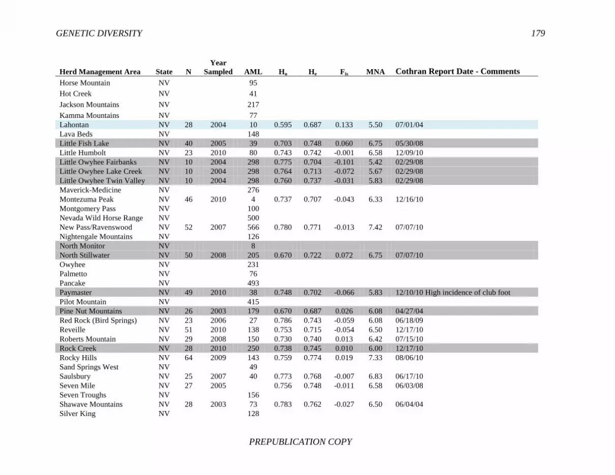
GENETIC DIVERSITY 179
PREPUBLICATION COPY
Herd Management Area State N Year
Sampled AML Ho He Fis MNA Cothran Report Date - Comments Horse Mountain NV 95 Hot Creek NV 41 Jackson Mountains NV 217 Kamma Mountains NV 77 Lahontan NV 28 2004 10 0.595 0.687 0.133 5.50 07/01/04 Lava Beds NV 148 Little Fish Lake NV 40 2005 39 0.703 0.748 0.060 6.75 05/30/08 Little Humbolt NV 23 2010 80 0.743 0.742 -0.001 6.58 12/09/10 Little Owyhee Fairbanks NV 10 2004 298 0.775 0.704 -0.101 5.42 02/29/08 Little Owyhee Lake Creek NV 10 2004 298 0.764 0.713 -0.072 5.67 02/29/08 Little Owyhee Twin Valley NV 10 2004 298 0.760 0.737 -0.031 5.83 02/29/08 Maverick-Medicine NV 276 Montezuma Peak NV 46 2010 4 0.737 0.707 -0.043 6.33 12/16/10 Montgomery Pass NV 100 Nevada Wild Horse Range NV 500 New Pass/Ravenswood NV 52 2007 566 0.780 0.771 -0.013 7.42 07/07/10 Nightengale Mountains NV 126 North Monitor NV 8 North Stillwater NV 50 2008 205 0.670 0.722 0.072 6.75 07/07/10 Owyhee NV 231 Palmetto NV 76 Pancake NV 493 Paymaster NV 49 2010 38 0.748 0.702 -0.066 5.83 12/10/10 High incidence of club foot Pilot Mountain NV 415 Pine Nut Mountains NV 26 2003 179 0.670 0.687 0.026 6.08 04/27/04 Red Rock (Bird Springs) NV 23 2006 27 0.786 0.743 -0.059 6.08 06/18/09 Reveille NV 51 2010 138 0.753 0.715 -0.054 6.50 12/17/10 Roberts Mountain NV 29 2008 150 0.730 0.740 0.013 6.42 07/15/10 Rock Creek NV 28 2010 250 0.738 0.745 0.010 6.00 12/17/10 Rocky Hills NV 64 2009 143 0.759 0.774 0.019 7.33 08/06/10 Sand Springs West NV 49 Saulsbury NV 25 2007 40 0.773 0.768 -0.007 6.83 06/17/10 Seven Mile NV 27 2005 0.756 0.748 -0.011 6.58 06/03/08 Seven Troughs NV 156 Shawave Mountains NV 28 2003 73 0.783 0.762 -0.027 6.50 06/04/04 Silver King NV 128

180 BLM WILD HORSE AND BURRO PROGRAM
PREPUBLICATION COPY
Herd Management Area State N Year
Sampled AML Ho He Fis MNA Cothran Report Date - Comments Snowstorm Castle Ridge NV 10 2004 140 0.659 0.718 0.082 5.42 02/29/08 Snowstorm Dryhill NV 9 2004 140 0.750 0.616 -0.218 4.25 02/29/08 South Shoshone NV 52 2008 100 0.761 0.770 0.012 7.33 07/21/10 South Stillwater NV 42 2003 16 0.705 0.716 0.015 5.58 04/07/04 Spruce-Pequop NV 26 2011 82 0.750 0.709 -0.058 5.75 06/16/11 Stone Cabin NV 50 2007 364 0.763 0.775 0.015 7.67 06/16/10 Some incidence of club foot Tobin Range NV 42 Triple B NV 518 Warm Springs Canyon NV 28 2010 175 0.729 0.719 -0.014 7.17 11/04/10 Wassuk NV 165 Wheeler Pass NV 26 2007 66 0.756 0.763 0.008 7.08 06/16/10 Whistler Mountain NV 24
Nevada mean value 0.739 0.734 -0.008 6.49 Bordo Atravesado NM 27 2011 60 0.787 0.749 -0.051 6.08 04/25/11 Carracas Mesa NM 23
New Mexico mean value 0.787 0.749 -0.051 6.08 Beaty’s Butte OR 32 2010 250 0.747 0.763 0.020 6.67 11/04/10 Cold Springs OR 24 2010 150 0.806 0.754 -0.068 6.00 11/11/10 Coyote Lake/Tule Springs OR 50 2011 390 0.792 0.766 -0.034 7.33 05/09/12 Hog Creek OR 14 2003 50 0.815 0.739 -0.103 6.00 05/13/04 Jackies Butte OR 40 2011 150 0.750 0.742 -0.010 7.17 04/30/12 Kiger OR 40 2011 82 0.671 0.695 0.034 5.83 03/29/12 Morphologically unique Spanish
blood not confirmed Liggett Table OR 17 2010 25 0.500 0.448 -0.115 2.58 11/12/10 Horse destroyed for unspecified
defect Murderers Creek OR 71 2009 35 0.696 0.707 0.015 6.25 09/23/10 Paisley Desert
OR 83 No year 150 0.743 0.780 0.047 8.00 E. G. Cothran, Texas A&M University,
email communication, December 21, 2011 Palomino Buttes OR 64 Pokegama OR 50 Riddle Mountain OR 21 2011 56 0.679 0.657 -0.034 5.50 03/29/12 Sand Springs OR 15 2011 200 0.772 0.759 -0.017 6.67 05/08/12 Sheepshead/Heath Creek OR 48 2011 302 0.790 0.787 -0.004 7.25 05/09/12 South Steens OR 31 2010 304 0.758 0.741 -0.023 6.92 10/19/10

GENETIC DIVERSITY 181
PREPUBLICATION COPY
Herd Management Area State N Year
Sampled AML Ho He Fis MNA Cothran Report Date - Comments Stinkingwater OR 24 2010 80 0.726 0.680 -0.067 5.50 04/07/10 Three Fingers OR 50 2011 150 0.710 0.753 0.058 7.250 04/30/12 Warm Springs OR 83 2010 202 0.766 0.778 0.015 8.00 04/05/11
Oregon mean value 0.733 0.722 -0.018 6.43 Bible Spring UT 60 Cedar Mountain UT 20 2002 390 0.742 0.726 -0.021 6.08 09/23/03 Chloride Canyon UT 30 Low diversity and dwarfism per 2001 Blawn Wash HMA report Choke Cherry UT 30 Confusion UT 115 Conger UT 80 Four Mile UT 60 Frisco UT 60 Kingtop UT 40 Mount Elinor UT 25 Muddy Creek UT 33 2001 125 0.619 0.638 0.029 5.33 01/03/02 North Hills UT 28 2002 36 0.807 0.710 -0.136 6.00 09/09/02 Onaqui Mountain UT 40 2005 210 0.298 0.282 -0.053 6/3/2008 Values for blood groups Range Creek UT 26 No year 125 0.663 0.707 0.061 5.25 E. G. Cothran, Texas A&M University,
email communication, December 21, 2011 Sulphur Herd N UT 53 2009 250 0.682 0.732 0.067 6.33 07/29/10 Evidence of Spanish blood Sulphur Herd S UT 41 2009 250 0.679 0.715 0.050 5.83 07/29/10 Evidence of Spanish blood Swasey UT 100 Tilly Creek UT 25 2002 50 0.609 0.617 0.013 5.08 04/29/03
Utah mean value 0.637 0.641 0.001 5.70 Adobe Town WY 103 2010 800 0.776 0.776 0.000 7.75 04/21/11 Antelope Hills WY 25 2004 82 0.747 0.733 -0.018 6.33 03/05/08 Conant Creek WY 22 2004 100 0.680 0.656 -0.035 5.50 03/06/08 Crooks Mountain WY 85 Dishpan Butte WY 30 2004 100 0.768 0.743 -0.034 6.33 03/06/08 Divide Basin WY 60 2011 600 0.785 0.787 0.003 7.75 05/15/12 Fifteen Mile WY 160 Green Mountain WY 300

182 BLM WILD HORSE AND BURRO PROGRAM
PREPUBLICATION COPY
Herd Management Area State N Year
Sampled AML Ho He Fis MNA Cothran Report Date - Comments Little Colorado WY 45 2011 100 0.761 0.768 0.009 6.67 05/07/12 Lost Creek WY 30 2009 82 0.775 0.788 0.017 6.67 10/14/10 McCullough Peaks WY 50 2004 140 0.755 0.715 -0.055 6.33 07/06/06 Muskrat Basin WY 27 2004 250 0.731 0.727 -0.006 6.00 03/06/08 Rock Creek Mountain WY 86 Salt Wells Creek East WY 33 2003 365 0.760 0.782 0.027 7.83 05/06/04 Salt Wells Creek West WY 25 2003 365 0.763 0.745 -0.025 6.58 05/06/04 Salt Wells Creek -Marvel Gap WY 25 2010 365 0.813 0.775 -0.050 6.67 04/11/11 Stewart Creek WY 30 2009 175 0.750 0.751 0.002 6.42 10/18/10 White Mountain WY 60 2011 300 0.701 0.715 0.020 7.58 04/30/12
Wyoming mean value 0.755 0.747 -0.010 6.74 Comparison from Cothran reports: Mean horse HMAs 0.716 0.710 -0.012 6.06 Standard deviations 0.056 0.059 0.071 1.09
NOTE: Blue shading indicates observed heterozygosity or MNA values below the mean minus one standard deviation. Gray shading indicates values below the mean, N = number of animals sampled, AML = appropriate management level, Ho = observed heterozygosity, He = expected heterozygosity under Hardy-Weinberg equilibrium, Fis = inbreeding coefficient, MNA = mean number of alleles per individual. For Herd Management Areas listed without genetic data, neither data nor reports were provided to the committee for review. SOURCE: Data from genetic analyses of Herd Management Areas provided by E. Gus Cothran. To access the data, contact the National Research Council’s Public Access Records Office at [email protected].

GENETIC DIVERSITY 183
PREPUBLICATION COPY
Genetic Diversity in Free-Ranging Burros
Far less research has been conducted on genetic diversity in free-ranging donkeys and burros than in horses. Aranguren-Mendez et al. (2001) studied five endemic Spanish donkey breeds using 14 polymorphic microsatellite loci. Their results indicated little differentiation among breeds and moderate genetic diversity within breeds (allelic diversity, 8.7 ± 4.4 alleles/locus; He, 0.637–0.684). In a similar study, Guastella et al. (2007) studied three Sicilian donkey breeds, including the endangered Pantesco breed, using 11 microsatellite loci. They also found low differentiation among breeds and moderate genetic diversity (allelic diversity, 4.1–6.5 alleles/locus; He, 0.500–0.618). However, they detected high levels of inbreeding in one of the breeds (Fis, 0.230). In a later study using 14 microsatellite loci, Bordonaro et al. (2012) confirmed low diversity (allelic diversity overall, 6.07 ± 0.72 alleles/locus; He, 0.581 ± 0.059) in the Sicilian breeds. Although the diversity in the Spanish breeds was within the confidence limits of levels in healthy mammalian populations (Garner et al., 2005), the lower allelic diversity and heterozygosity in the Sicilian breeds approached the levels in unhealthy populations. Genetic Diversity in Burros Managed by the Bureau of Land Management
Genetic studies of 12 burro HMAs have been conducted by Cothran and compared with his previous studies of domestic burro populations. The loci used for burros include nine of the 12 used for the free-ranging horse studies. Summary data for samples collected from domestic burro populations and genotyped in the Cothran laboratory are provided in Table 5-3.
All burro HMAs on which genetic data were obtained had diversity measures below 0.66, the value used for horse HMAs, and all had values lower than those reported for the Spanish and Sicilian donkeys. Five of the 12 HMAs had diversity values at least one standard deviation below the mean value obtained from the four domestic donkey breeds.
Cothran’s reports do not provide information regarding the provenance of the four domestic donkey breeds that he used for comparison, nor does he provide dates on which they were sampled. However, his results suggest that domestic donkeys in the western United States have lower genetic diversity than Spanish and Sicilian donkey breeds in that both allelic diversity and heterozygosity measures are lower. Only 12 of the 28 HMAs have had genetic studies of free-ranging burros. Of the remaining 16 HMAs, seven had AMLs over 50 and nine had AMLs under 50. All but one of the reports on burros provided to the committee involved samples collected during 2001-2005.

184 BLM WILD HORSE AND BURRO PROGRAM
PREPUBLICATION COPY
TABLE 5-3 Genetic Diversity in Free-Ranging Burros in Herd Management Areas Determined by Using Nine Microsatellite Loci
Herd Management Area State N Year
Sampled AML Ho He Fis MNA Cothran Report Date - Comments Alamo AZ 160 Big Sandy (Wikieup) AZ 10 2004 139 0.490 0.510 0.038 3.667 10/30/08 Black Mountain (Kingman) AZ 25 2004 478 0.551 0.553 0.003 4.111 10/30/08 Cibola-Trigo 2 AZ 28 2004 285 0.453 0.506 0.104 4.000 11/06/08 Havasu AZ 19 2004 166 0.487 0.498 0.021 3.889 11/06/08 Lake Pleasant AZ 208
Arizona mean value 0.495 0.517 0.042 3.917 Chemehuevi CA 52 2003 121 0.354 0.427 0.171 3.222 07/15/03 Chocolate Mule CA 55 2002 133 0.298 0.394 0.243 3.444 01/24/03 Lee Flats CA 2 No year 15 0.278 0.278 0.000 1.778 E. G. Cothran, Texas A&M University, email
communication, December 21, 2011 Twin Peaks CA 39 2011 116 0.487 0.526 0.075 3.444 10/5/12 Waucoba-Hunter Mountain CA 11
California mean value 0.354 0.406 0.122 2.972 Blue Wing NV 28 2003 28 0.252 0.268 0.059 2.556 08/03/04 Bullfrog NV 49 No year 91 0.492 0.502 0.199 3.889 E. G. Cothran, Texas A&M University, email
communication, December 21, 2011 Gold Butte NV 98 Gold Mountain NV 78 Goldfield NV 37 Johnnie NV 108 Lava Beds NV 16 Marietta Wild Burro Range NV 104 McGee Mountain NV 41 Red Rock (Bird Springs) NV 49 Seven Troughs NV 22 2005 46 0.245 0.339 0.277 2.667 11/13/08 Stonewall NV 8 Wheeler Pass NV 35 Hickison Summit NV 45
Nevada mean value 0.330 0.370 0.178 3.037 Warm Springs OR 25

GENETIC DIVERSITY 185
PREPUBLICATION COPY
Herd Management Area State N Year
Sampled AML Ho He Fis MNA Cothran Report Date - Comments Canyon Lands UT 100 Sinbad UT 30 No year 70 0.466 0.430 -0.084 3.000 E. G. Cothran, Texas A&M University, email
communication, December 21, 2011 Comparison with Cothran reports: Mean-domestic 4 0.450 0.550 0.153 4.143 Standard deviation 0.094 0.120 0.195 1.386 Mean -burro HMAs 12 0.408 0.441 0.093 3.333 Standard deviation 0.107 0.096 0.105 0.677 NOTE: Gray shading indicates observed heterozygosity or MNA values below the mean minus one standard deviation. N = number of animals sampled, AML = appropriate management level, Ho = observed heterozygosity, He = expected heterozygosity under Hardy-Weinberg equilibrium, Fis = inbreeding coefficient, MNA = mean number of alleles per individual. For Herd Management Areas listed without genetic data, neither data nor reports were provided to the committee for review. SOURCE: Data from genetic analyses of Herd Management Areas provided by E. Gus Cothran. To access the data, contact the National Research Council’s Public Access Records Office at [email protected]

186 BLM WILD HORSE AND BURRO PROGRAM
PREPUBLICATION COPY
Optimal Genetic Diversity in Herd Management Areas
Although the BLM Wild Horses and Burros Management Handbook (2010) does not differentiate between horses and burros, the target heterozygosity value for both clearly was derived from horse studies. The current method of maintaining free-ranging horse HMAs at observed heterozygosity (Ho) values that are no lower than one standard deviation below the mean will become problematic. When this value is recalculated with repeated surveys, it will decrease as allelic diversity is lost from herds when animals die or are removed to maintain AMLs (see Chapter 7). Unless there is gene flow between HMAs, inbreeding in individual HMAs is inevitable and will result in lower genetic diversity and individual fitness. The goal is to maintain as much as possible of the standing genetic diversity, so the mean heterozygosity and allelic diversity as they stand today are more appropriate targets over a reasonable timeframe (such as 100 years).
Monitoring of genetic diversity may be easiest if samples are collected during each gather. Blood samples may be collected from a representative sample of horses for analysis, and the first survey results can be used to determine a baseline value. If that value is below the mean of the BLM horse HMAs, that HMA should be identified as a target for translocation of horses from other HMAs (see “Translocation for Genetic Restoration” below). Samples should be collected from each HMA for genetic monitoring at least once every 5 years. If genetic diversity (either heterozygosity or allelic diversity) is statistically significantly lower than that detected in the previous survey, the HMA should be assigned high priority for genetic management.
The target level of diversity for free-ranging burros is unclear but appears to be based on levels in four domestic donkey breeds of unknown provenance previously studied by Cothran. Although they provide a local comparison, a more appropriate comparison would be with the free-ranging Spanish donkey breeds studied by Aranguren-Mendez et al. (2001).
The committee found that Cothran had conducted multiple genetic studies for several HMAs since 2000. Besides providing estimates of current genetic diversity, the second report on each of those HMAs discussed changes in diversity since the previous one. That valuable information allows BLM to evaluate the effectiveness of management actions aimed at preserving genetic diversity. To maintain the free-ranging horse and burro HMAs at the prescribed AMLs with the genetic diversity needed for long-term genetic health, continued monitoring and active management will be required.
MANAGEMENT ACTIONS TO ACHIEVE OPTIMAL GENETIC DIVERSITY
The goal of genetic management is to maintain as much as possible of the standing genetic diversity of a population and thereby provide the raw material needed to respond to environmental changes. Chapter 4 outlines a variety of techniques for controlling and reducing fertility in free-ranging horses and burros so that numbers can be kept at prescribed levels. Although dramatically limiting individual fertility will reduce a population’s size, it will also reduce its genetic effective population size, and this will have effects on genetic diversity.
Many HMAs are spatially isolated, and others are contiguous. Some of the contiguous HMAs have been grouped into complexes by BLM (see Figure 1-2); this suggests that they are exchanging migrants and may be considered a single unit. Within each of the HMAs, BLM could accomplish the goal of conserving genetic diversity through intensive management, as has been

GENETIC DIVERSITY 187
PREPUBLICATION COPY
done for the herds at Assateague Island and Shackleford Banks. Alternatively, BLM could consider the HMAs as a single population and use the principles of metapopulation management to guide its actions.
Effects of Fertility Control on Genetic Diversity
Changing the proportion of breeding males and females can have important effects on genetic diversity through reductions in effective population size. First, contracepting large numbers of females in the population will increase variance in family size in that many more females than normal will fail to produce offspring. Because Ne is inversely proportional to variance in family size, any increase in the number of nonreproducing but surviving females will decrease effective population size. Second, any movement of the sex ratio of breeders from 1:1 will also decrease effective population size. That effect can be subtle in polygynous species, such as horses and burros, inasmuch as the number of breeding males is usually less than the number of breeding females. Thus, although reducing the number of breeding females through female contraception may move the ratio closer to 1:1, the reductions in total numbers of breeders and increases in the variance in family size may still lead to an overall reduction in Ne.
Alternatively, if population size is reduced by decreasing the number of males, it might not reduce Ne depending on the pool of bachelor males available to become harem stallions. If the pool is large, it will leave the number of breeders and variance in family size unaffected.
It is important to consider those effects in the planning phase of management actions. A modeling approach (see Chapter 6) will allow managers to consider the effects of population-size reduction by using fertility-control methods and other important factors.
Individual-Based Genetic Management
Maximum retention of genetic diversity in each HMA (or HMA complex) and in the population as a whole could be achieved if horses and burros were managed as individuals. That entails knowing all individuals in the population unit, their relationships, and their reproductive performance over time. The detailed population monitoring and record-keeping required to accomplish this has been possible in some barrier-island horse populations, including Assateague Island (Eggert et al., 2010) and Shackleford Banks. This level of management would entail an important departure from a truly wild population that is subject to natural selection, a distinction that would need to be made clear to all interested parties. It would also differentiate the management of free-ranging horses and burros from that of other species in the landscape, with the exception of cattle. The committee believes individual-based genetic management might be possible in some HMAs in which habitat conditions and local or BLM knowledge of individual animals make it possible to track individuals (for example, Pryor Mountains). In addition to monitoring the genetics (via pedigree) and demographics of the population, individual-based genetic management would require actively controlling reproduction of individual animals so that they contribute to the gene pool equally and rare alleles or genotypes are not lost. The barrier islands of Assateague and Shackleford Banks provide some models of attempts to maximize genetic diversity in free-ranging animals through targeted contraception. Nuñez (2009) summarized the evolution of the contraceptive management programs on those islands. Software tools for keeping track of animal pedigrees, analyzing genetic relationships,

188 BLM WILD HORSE AND BURRO PROGRAM
PREPUBLICATION COPY
and monitoring population demography were developed for captive populations of animals in zoos; their application to the Assateague Island population was described by Ballou et al. (2008) and Eggert et al. (2010). In HMAs in which known individual animals can be reliably contracepted, either temporarily or permanently, this type of genetic management is possible. In HMAs in which following individual animals and managing their individual reproductive performance is not feasible, a less labor-intensive approach to genetic management is possible with the use of translocations.
Translocation for Genetic Restoration
HMAs exist in a mosaic of ecological habitats, anthropogenic effects, political jurisdictions, free-ranging horse and burro protection status, and property-ownership arrays. The likelihood of natural migration between HMAs is affected by many factors. Two of the most important are the distance over which dispersing animals must travel to reach other HMAs and the quality of the intervening habitat. Hampson et al. (2010) used GPS collars to study travel distances in two populations of free-ranging horses (12 horses) in Australia over 6-7 days at two sites that differed in vegetation and water abundance. There were no differences in daily travel distances between the two sites, but there was a wide range: 8.1-28.3 km. The mean daily travel distance was 15.9 km (18.2 km for males, 14.8 km for females). Some animals in the study were observed walking for 12 hours to reach water. Hampson et al. (2010) cited data from previous studies that showed travel distances of 17.9 km/day by free-ranging horses in Australia, 8.3 km/day by wild asses and 3.5 km/day by Przewalski’s horses in Mongolia, and 15 km per 12 hours by female zebras.
Given the distances between many pairs of HMAs, that movement of horses and burros for genetic or demographic reasons would probably need to be facilitated by BLM. The practice of moving individual animals between populations for genetic restoration, or translocation, is justified scientifically. Perhaps the most famous case is that of the Florida panther (Puma concolor coryi). Details on the background of that population, the issues and decision-making processes involved in the genetic restoration, and the outcomes may be found in Hedrick (2001), Pimm et al. (2006), Johnson et al. (2010), and Benson et al. (2011). Briefly, this subspecies of puma was reduced to a population of about 25 in the early to mid-1990s and demonstrated lower genetic diversity than other North American puma populations (Culver et al., 2000) and a number of traits that suggested that the influences of inbreeding and genetic drift had completely or nearly fixed genes for potentially deleterious traits that were previously rare. Introduction of female Texas panthers (Puma concolor stanleyana) into the population in 1995 resulted in the production of offspring (Land and Lacy, 2000) that lacked several of the deleterious traits (Shindle et al., 2000; Hedrick, 2001; Johnson et al., 2010). Offspring, particularly females, had survival rates almost twice those previously observed in the population (Pimm et al., 2006; Benson et al., 2011) and increases in survival rates were correlated with increased heterozygosity (Benson et al., 2011). Despite these successes in population growth and apparent health, Johnson et al. (2010) pointed out that the future of the Florida panther will require continuing intensive management, including regular infusions of new genetic material, in the face of anthropogenic threats, habitat loss, infectious diseases, and continued inbreeding.
Other case studies of translocation providing genetic and demographic benefits include African lions (Trinkel et al., 2008), adders (Madsen et al., 1996, 1999, 2004), and prairie chickens (Westemeier et al., 1998). Studies by Seddon et al. (2005), Vilà et al. (2003) and

GENETIC DIVERSITY 189
PREPUBLICATION COPY
Adams et al. (2011) described the favorable effect of a single natural immigrant into a wolf population. The case studies are supported by laboratory studies that have demonstrated genetic benefits, fitness benefits, or both of the infusion of new genetic material into small, inbred populations (e.g., Spielman and Frankham, 1992; Ebert et al., 2002; Saccheri and Brakefield, 2002). Selection of Animals for Translocation
As early as the 1930s, it was established that inbreeding depression in small, isolated populations could lead to loss of fitness and increased risk of extinction (Wright, 1931). Wright’s analyses led him to conclude that even small amounts of gene flow between isolated small populations could offset the adverse effects of genetic drift and inbreeding. That conclusion gave rise to a large body of work aimed at determining exactly how much gene flow, in the form of immigrants per generation, was necessary to offset the adverse effects of genetic deterioration. A rule of thumb of one immigrant per generation emerged (Kimura and Ohta, 1971; Lewontin, 1974; Spieth, 1974) and has been widely adopted in conservation practice. More recently, that rule of thumb has been challenged on the basis of the simplistic assumptions that were used in deriving it (e.g., Mills and Allendorf, 1996; Vucetich and Waite, 2000). At the time this report was prepared, it seemed likely that in real-world applications, one immigrant per generation would be an absolute minimum. Mills and Allendorf (1996) outlined a number of scenarios in which the number of immigrants per generations should probably exceed one, including scenarios in which at least one of the following is the case.
· Inbreeding depression is believed to be occurring already. · Immigrants are closely related to each other or to the receiving population. · Effective population size is much lower than the number of animals present. · Social, behavioral, ecological, or logistical factors prevent single animals from
immigrating successfully. · Immigrants are at a disadvantage in probability of survival and reproduction. · The receiving population has been isolated for many generations. · Extinction risk due to demographic or environmental variation is deemed to be
very high unless there is aggressive supplementation.
The authors concluded that up to 10 immigrants per generation might be necessary to effect genetic restoration in those situations. Vucetich and Waite (2000) extended the analyses by modeling variation in population fluctuation and suggested that more than 20 immigrants per generation may be necessary if high population fluctuation leads to drastically reduced effective population size.
In addition to the number of animals to translocate, the interval for doing so must be determined. There are important practical and logistical considerations involved, but the translocation of animals for genetic restoration is usually thought of as being conducted on a per-generation basis. Therefore, one starting point is to determine the generation time of free-ranging horses. Eggert et al. (2010) constructed a pedigree for the Assateague Island horse population on the basis of molecular analyses and herd records and derived an estimate of 10 years. Goodloe et al. (1991) also derived an estimate of 10 years for horses on Cumberland Island, Georgia. Similarly, historical pedigree data on zoo populations of wild equids in North America all have generation time estimates of about 10 years (range 9.6 years in Somali wild ass to 10.4 years in

190 BLM WILD HORSE AND BURRO PROGRAM
PREPUBLICATION COPY
Hartmann’s zebra6). Thus, it would be valid to consider 10 years as an appropriate interval for translocating animals between populations for genetic restoration. On the basis of the literature, it appears that translocation of 10 animals between populations every 10 years would be appropriate.
BLM is already experienced in the capture and transport of animals for population management, and the protocols for translocation would be similar to those currently used for gathers; only the destination of the removed animals would differ. Although the movement of animals among HMAs has the potential to facilitate the spread of pathogens (Champagnon et al., 2012), the probability of that could be minimized through observation and advance testing of source and target herds. Below is an outline of some factors to consider in selecting animals for translocation for genetic management. Genetic Factors. Because the goal of translocation is to supplement the genetic diversity in a herd and reduce the probability of inbreeding, it is advisable to select animals that are unrelated to the target herd. In most cases, pedigree information on free-ranging horse and burro populations will not be available, so absolute genetic relationships among individual animals will be unknown. The use of genetic information, however, will make it possible to choose individual animals that have moderate levels of differentiation from the target population.
The term outbreeding depression is used to describe a decrease in fitness due to hybridization between individuals from populations that have differentially adapted genomes (Frankham et al., 2011). Frankham et al. (2011) used empirical data and modeling to develop a decision tree for predicting the probability of outbreeding depression. Their tree proved robust when crosses that had known outcomes were used, and it suggested that outbreeding depression is likely when the populations being crossed are of different species, exhibit fixed chromosomal variants, have not exchanged genes in 500 years, or inhabit different environments. None of those risk factors seems to apply to free-ranging horses and burros in HMAs. Environments may differ between HMAs, but Frankham et al. (2011) suggested that environmental differences need to be substantial enough to select for different traits among populations. They recommended paying particular attention to the needs and resources to which a species is most sensitive and to the range of variation in important features of the environments under consideration. The adaptability of the horse and its associated ability to live in various environments appears to lessen the concern about environmental differences between possible translocation sites.
By using the genetic data generated for the evaluation of level of genetic diversity, it is possible to estimate the level of differentiation among HMAs. The fixation index (Fst) is a measure of genetic distance, or population differentiation, that is based on genetic polymorphisms (Wright, 1931). Polymorphic microsatellite loci constitute a powerful tool for predicting which populations are so similar (low Fst value) that translocating animals will probably not be successful in supplementing genetic diversity and which are so different (high Fst value) that genetic compatibility between individuals may not be optimal and may reduce the probability of successful translocation. Matrices of pair-wise Fst values for horse and burros based on genetic data from HMAs are in Appendix F and could be used to identify the mixtures that might be most successful because they exhibit moderate Fst values.
New genetic variation needed by an HMA does not necessarily need to come from another HMA. Mares in long-term holding facilities could also be used as sources of genetic diversity if necessary, assuming that they present no novel disease risk for free-ranging horses 6Association of Zoos and Aquariums website, www.aza.org. Accessed April 16, 2012.

GENETIC DIVERSITY 191
PREPUBLICATION COPY
and burros. The genetic tools described above can be used to identify free-ranging horses and burros on other public lands, in private sanctuaries, and in long-term holding facilities that could be used to infuse new genetic variation into an HMA. Behavior and Social Factors. Given the harem social structure of free-ranging horses and the fact that this structure means that more sexually mature females than sexually mature males are breeding at any one time, it appears that the most rapid way to infuse new genetic material into an HMA via translocation would be to move young, sexually mature mares between HMAs. Young mares new to an HMA are likely to be courted by bachelor males and to be open to forming consortships with them. Older mares would also probably be bred relatively quickly, but they may be more selective in forming consortships with bachelor males. Ideally, translocated mares would already be familiar with one another, if possible originating from the same harem. Kaseda et al. (1995) found that mares that had long-term bonds to harem stallions had higher reproductive success than mares that wandered between bands regularly or that had shorter bonds to stallions. Linklater et al. (1999) also found that single mares that were dispersing between bands had lower fecundity, reproductive success, and body condition; had higher parasite levels; and received more aggression from bachelor males than mares in established harems. Moving established groups of females may buffer some of those adverse effects, but it is possible that translocating bonded females without a harem stallion will lead to dissolution of bonds between mares (Rubenstein, 1994).
A second option and one that might further lessen adverse effects is to move intact harems if the harem members and associated stallions can be reliably identified during gathers. That would immediately add new genetic material to the site, but there would be a longer delay in getting that material into the gene pool because foals born into the harem would have to grow up, disperse, and interbreed with members of the resident population.
A third option would be to move bachelor males. This option carries the most risk with respect to getting new genes into the resident population. Stallions that have harems may be quite successful in spreading their genes rapidly via breeding with multiple mares, but obtaining a harem is not easy, and bachelor males may not survive to realize breeding opportunities.
Immediate and long-term infusion of new genetic material may be most likely if intact harems or groups of young mares (immediate) are translocated with a number of males (long term).
Burros are characterized by a less cohesive social structure in which the only long-term relationships are between females and their dependent offspring. Thus, there would be fewer challenges in integrating new females into a burro population, so females would be the first choice for translocation of animals for genetic restoration of burro populations. Males would also be viable candidates for genetic restoration, but introduced males would have to compete with resident males for access to breeding females.
Fertility Control and Implications for Translocation
Introductions of males or females are likely to have different consequences in that adding new females will increase numbers exponentially over time. If population regulation involves female contraception, adding new fertile females could be counterproductive, so adding novel males may be the best way to increase genetic diversity without increasing population size. However, to ensure that the new males become breeders, either a large number would need to be translocated or some of the resident males would need to have their fertility reduced.

192 BLM WILD HORSE AND BURRO PROGRAM
PREPUBLICATION COPY
Alternatively, if curtailing male fertility is the preferred means of population regulation, either a smaller number of novel males can be added to replace a disproportionate number of resident males that are made sterile, or novel females can be added inasmuch as whenever one of the few remaining resident males breeds, he will sire offspring that have genes from the novel females.
Which type of translocation is best to use will depend on a variety of factors, many of which can be tested with a modeling approach in the planning phase (see Chapter 6). Population size, fertility-control methods, and the effects of translocation on Ne will need to be considered. Although translocating males may require fewer total introductions when population size is being regulated because male additions increase the population growth arithmetically rather than exponentially, novel males may find it difficult to obtain harems (horses) or territories (burros), which are prerequisites for siring many offspring. Many tradeoffs will require sensitivity to context in designing effective translocation strategies that enhance genetic diversity without upsetting existing population regulatory strategies.
CONCLUSIONS
Genetic diversity is an important component of the health of free-ranging horses and burros on HMAs, in that it provides the raw material needed to respond to environmental changes. Maintenance of genetic diversity is a function of the effective population size (Ne), which is probably at least an order of magnitude lower than the number of animals present. Factors that reduce Ne include unequal sex ratios, variance in family sizes, and high variance in population sizes between generations. In small, isolated herds, inbreeding is inevitable and will occur within only a few generations. It is important to measure and monitor allelic diversity, observed and expected heterozygosity (Ho and He), and coefficients of inbreeding (Fis) in HMAs to detect the loss of diversity before the reduction in fitness that has been observed in many inbred populations becomes a problem.
In recognition of the importance of monitoring genetic diversity, and as recommended in previous National Research Council reports, BLM has collaborated with outside scientists since 1985 to monitor herd-specific diversity on the basis first of isozyme and serum proteins and later of nuclear microsatellite loci. The committee recommends that BLM continue to monitor genetic diversity as part of the routine management of both horse and burro HMAs. The BLM Wild Horses and Burros Management Handbook does not clearly state which HMAs should be monitored and how often studies should be repeated. The committee recommends routine monitoring at all gathers and collection and analysis of a sufficient number of samples to detect losses of diversity.
Genetic concerns involve both the potential for the reduced fitness associated with inbreeding and the effects of mutations that can cause phenotypic conditions that affect the fitness of a herd. The Cothran studies are excellent tools for BLM to use in managing herds to reduce the incidence of inbreeding, but they do not provide information about the effects of specific genes known to cause genetically based conditions. To the committee’s knowledge, no tests have been conducted to detect the presence of genetic mutations associated with those types of conditions. The committee recommends that BLM document the incidence of coat color or other morphological anomalies that may indicate the presence of deleterious mutations during all gathers. For herds in which phenotypic data suggest the presence of genetically based disorders,

GENETIC DIVERSITY 193
PREPUBLICATION COPY
the committee recommends testing and consultation with geneticists and equine veterinarians to devise appropriate management actions.
Monitoring of genetic diversity in burro HMAs has been conducted in only one herd since 2005. Genetic diversity in burro herds is lower than that in Spanish and Sicilian breeds, including endangered breeds, and many of the AML numbers are low to very low. The committee recommends that BLM resume the genetic monitoring of burro HMAs. Although the available literature does not report clinical issues in burros, the committee recommends that BLM routinely monitor and record the incidence of any morphological anomalies that may indicate the deleterious effects of inbreeding.
The committee recognizes that genetic management of some HMAs is complicated by other considerations. For herds that have strong associations with Spanish bloodlines—such as those of the Cerbat Mountain, AZ; Pryor Mountains, MT; and Sulphur, UT—or herds that contain unique morphological traits—such as the Kiger, OR, herd—BLM will need to balance concerns about maintaining breed ancestry with the need to maintain optimal genetic diversity. Herds that remain isolated over the long term will inevitably lose genetic diversity inasmuch as maintaining or slightly increasing herd sizes will not offset the effects of genetic drift. The public is interested in these herds, and it is particularly important that BLM seek opportunities to discuss the complexity of the situation with interested parties. It is true that the existence of a few genetic markers may indicate Spanish origin, but the remainder of the genome may not; rather, it may reflect horses that are well adapted to local conditions. If the latter is the case, isolation of the herd to maintain purity may be mistaken and may lead to unnecessary loss of genetic diversity. The committee recommends that BLM examine in more depth the genetic constitution of these herds and share the findings with the public so that informed decisions about the sustainability of the populations can be made (see Chapter 8).
The committee recommends that BLM consider some groups of HMAs to constitute a single population and manage them by using natural or assisted migration (translocation) whenever necessary to maintain or supplement genetic diversity. Although there is no magic number above which a population can be considered forever viable, studies suggest that thousands of animals will be needed for long-term viability and maintenance of genetic diversity. Very few of the HMAs are large enough to be buffered against the effects of genetic drift, and herd sizes must be maintained at prescribed AMLs, so managing the HMAs as a metapopulation will reduce the rate of reduction of genetic diversity in the long term.
Finally, the committee recommends that BLM stay abreast of advances in population genetics and genomics. New laboratory and data-analysis tools promise to reduce costs while providing more powerful methods for monitoring genetic diversity and resolving breed relationships. The 12 nuclear microsatellite loci that are currently used for estimating genetic diversity and genetic differentiation among herds were chosen largely from those approved by the International Society of Animal Genetics for their informativeness in equine genotyping. Thus, they are useful tools for estimating overall genetic diversity and population divergence. However, the small number of loci and the uncertainty about their evolution limit their power to resolve relationships among closely related lineages, such as equid breeds. Recently, the Illumina 50K SNP Beadchip, an equine SNP genotyping array with over 50,000 polymorphic loci, was developed and found to be informative in several equid species (McCue et al., 2012). The Equine Genetic Diversity Consortium successfully used that array to assess the effects of inbreeding and natural selection in 36 breeds from around the world, to infer relationships among breeds, and to detect signals of ancestral admixture (Petersen et al., 2012a). Genomic tools are also being used
194 BLM WILD HORSE AND BURRO PROGRAM
PREPUBLICATION COPY
to detect the genetic underpinnings of traits that are under positive natural selection (Petersen et al., 2012b) and mutations that are responsible for genetically based diseases, such as lavender foal syndrome (Brooks et al., 2010). Genomic analysis can provide much finer resolution of questions about breed associations and will soon be the method of choice for population-level analysis.
REFERENCES
Adams, J.R., L.M. Vucetich, P.W. Hedrick, R.O. Peterson, and J.A. Vucetich. 2011. Genomic sweep and potential genetic rescue during limiting environmental conditions in an isolated wolf population. Proceedings of the Royal Society of London Series B 278:3336-3344.
Aranguren-Mendez, J., J. Jordana, and M. Gomez. 2001. Genetic diversity in Spanish donkey breeds using microsatellite DNA markers. Genetics Selection Evolution 33:433-442.
Aranguren-Mendez, J., M. Gomez, and J. Jordana. 2002. Hierarchical analysis of genetic structure in Spanish donkey breeds using microsatellite markers. Heredity 89:207-211.
Aurich, C., R. Achmann, and J.E. Aurich. 2003. Semen parameters and level of microsatellite heterozygosity in Noriker draught horse stallions. Theriogenology 60:371-378.
Ballou, J. and K. Ralls. 1982. Inbreeding and juvenile mortality in small populations of ungulates: A detailed analysis. Biological Conservation 24:239-272.
Ballou, J.D., K. Traylor-Holzer, A.Turner, A.F. Malo, D. Powell, J. Maldonado, and L. Eggert. 2008. Simulation model for contraception management of the Assateague Island feral horse population using individual-based data. Wildlife Research 35:502-512.
Benson, J.F., J.A. Hostetler, D.P. Onorato, W.E. Johnson, M.E. Roelke, S.J. O’Brien, D. Jansen, and M.K. Oli. 2011. Intentional genetic introgression influences survival of adults and subadults in a small, inbred felid population. Journal of Animal Ecology 80:958-967.
Berger, J. 1986. Wild Horses of the Great Basin: Social Competition and Population Size. Chicago: University of Chicago Press.
Berger, J. and C. Cunningham. 1987. Influence of familiarity on frequency of inbreeding in wild horses. Evolution 41:229-231.
Bordonaro, S., A.M. Guastella, A. Criscione, A. Zuccaro, and D. Marletta. 2012. Genetic diversity and variability in endangered Pantesco and two other Sicilian donkey breeds assessed by microsatellite markers. Scientific World Journal 2012:648427.
Brook, B.W., D.W. Tonkyn, J.J. O’Grady, and R. Frankham. 2002. Contribution of inbreeding to extinction risk in threatened species. Conservation Ecology 6:16.
Brooks, S.A, N. Gabreski, D. Miller, A. Brisbin, H.E. Brown, C. Streetera, J. Mezey, D. Cook, and D.F. Antczak. 2010. Whole-genome SNP association in the horse: Identification of a deletion in myosin Va responsible for lavender foal syndrome. PLoS Genetics 6:e1000909.
Brosnahan, M.M., S.A. Brooks, and D.F. Antzcak. 2010. Equine clinical genomics: A clinician’s primer. Equine Veterinary Journal 42:658-670.
BLM (Bureau of Land Management). 2010. Wild Horses and Burros Management Handbook, H-4700-1. Washington, DC: U.S. Department of the Interior.

GENETIC DIVERSITY 195
PREPUBLICATION COPY
Champagnon, J., J. Elmberg, M. Guillemain, M. Guathier-Clerc, and J.D. Lebreton. 2012. Conspecifics can be aliens too: A review of effects of restocking practices in vertebrates. Journal for Nature Conservation 20:231-241.
Charlesworth, D., M.T. Morgan, and B. Charlesworth. 1993. Mutation accumulation in finite outbreeding and inbreeding populations. Genetical Research 61:39-56.
Collins, C.W., N.S. Songsasen, M.M. Vick, B.A. Wolfe, R.B. Weiss, C.L. Keefer, and S.L. Monfort. 2012. Abnormal reproductive patterns in Przewalski’s mares are associated with a loss in gene diversity. Biology of Reproduction 86:1-10.
Conant, E.K., R. Juras, and E.G. Cothran. 2012. A microsatellite analysis of five colonial Spanish horse populations of the southeastern United States. Animal Genetics 43:53-62.
Conner, J.K. and D.L. Hartl. 2004. A primer of ecological genetics. Sunderland, MA: Sinauer Associates, Inc.
Crnokrak, P. and D.A. Roff. 1999. Inbreeding depression in the wild. Heredity 83:260-270. Csillery, K, T. Johnson, D. Beraldi, T. Clutton-Brock, D. Coltman, B. Hansson, G. Spong, and J.
Pemberton. 2006. Performance of marker-based relatedness estimators in natural populations of outbred vertebrates. Genetics 173:2091-2101.
Culver, M., W.E. Johnson, J. Pecon-Slattery, and S.J. O’Brien. 2000. Genomic ancestry of the American puma (Puma concolor). Journal of Heredity 91:186-197.
Ebert, D., C. Haag, M. Kirkpatrick, M. Riek, J.W. Hottinger, and V.I. Pajunen. 2002. A selective advantage to immigrant genes in a Daphnia metapopulation. Science 295:485-488.
Eggert, L.S., D.M. Powell, J.D. Ballou, A.F. Malo, A. Turner, J. Kumer, C. Zimmerman, R.C. Fleischer, and J.E. Maldonado. 2010. Pedigrees and the study of the wild horse population of Assateague Island National Seashore. Journal of Wildlife Management 74: 963-973.
Finno, C.J., S.J. Spier, and S.J. Valberg. 2009. Equine diseases caused by known genetic mutations. Veterinary Journal 179:230-239.
Flather, C.H., G.D. Hayward, S.R. Beissinger, and P.A. Stephens. 2011a. Minimum viable populations: Is there a “magic number” for conservation practitioners? Trends in Ecology & Evolution 26:307-316.
Flather, C.H., G.D. Hayward, S.R. Beissinger, and P.A. Stephens. 2011b. A general target for MVPs: Unsupported and unnecessary. Trends in Ecology & Evolution 26:620-622.
Frankham, R. 1995. Inbreeding and extinction - A threshold effect. Conservation Biology 9:792-799.
Frankham, R., J.D. Ballou, and D.A. Briscoe. 2010. Introduction to Conservation Genetics. Cambridge, UK: Cambridge University Press.
Frankham, R., J.D. Ballou, M.D.B. Eldidge, R.C. Lacy, K. Ralls, M.R. Dudash, and C.B. Fenster. 2011. Predicting the probability of outbreeding depression. Conservation Biology 25:465-475.
Garner, A., J.L. Rahlow, and J.F. Hicks. 2005. Patterns of genetic diversity and its loss in mammalian populations. Conservation Biology 19:1215-1221.
Goldstein, D.B. and D.D. Pollock. 1997. Launching microsatellites: A review of mutation processes and methods of phylogenetic inference. Journal of Heredity 88:335-342.
Gomendio, M., J. Cassinello, and E.R.S. Roldan. 2000. A comparative study of ejaculate traits in three endangered ungulates with different levels of inbreeding: Fluctuating asymmetry as an indicator of reproductive and genetic stress. Proceedings of the Royal Society of London B 267:875-882.

196 BLM WILD HORSE AND BURRO PROGRAM
PREPUBLICATION COPY
Goodloe, R.B., R.J. Warren, E.G. Cothran, S.P. Bratron, and K.A. Trembicki. 1991. Genetic variation and its management applications in eastern U.S. feral horses. Journal of Wildlife Management 55:412-421.
Guastella, A.M., A. Zuccaro, S. Bordano, A. Criscione, D. Marletta, and G. D’Uros. 2007. Genetic diversity and relationship among the three autochthonous Sicilian donkey populations assessed by microsatellite markers. Italian Journal of Animal Science 6(Supplement 1):143.
Halbert, N.D., T. Raudsepp, B.P. Chowdhary, and J.N. Derr. 2004. Conservation genetic analysis of the Texas state bison herd. Journal of Mammalogy 85:924-931.
Hampson, B.A., M.A. de Laat, P.C. Mills, and C.C. Pollitt. 2010. Distances travelled by feral horses in ‘outback’ Australia. Equine Veterinary Journal 42(Supplement 38):582-586.
Hedrick, P.W. 2001. Conservation genetics: Where are we now? Trends in Ecology & Evolution 16:629-636.
Jiminez, J., H. Kimberly, G. Alaks, L. Graham, and R. Lacy. 1994. An experimental study of inbreeding depression in a natural habitat. Science 266:271-273.
Johnson, W.E., D.P. Onorato, M.E. Roelke, E.D Land, M. Cunningham, R.C. Belden, R. McBride, D. Jansen, M. Lotz, D. Shindle, J.G. Howard, D.E. Wildt, L.M. Penfold, J.A. Hostetler, M.K. Oli, and S.K. O’Brien. 2010. Genetic restoration of the Florida panther. Science 329:1641-1645.
Kaseda, Y., A.M. Khalil, and H. Ogawa. 1995. Harem stability and reproductive success of Misaki feral mares. Equine Veterinary Journal 27:368-372.
Keller, L.F. and D.M. Waller. 2002. Inbreeding effects in wild populations. Trends in Ecology & Evolution 17:230-241.
Kimura, M. and T. Ohta. 1971. Theoretical Aspects of Population Genetics. Princeton, NJ: Princeton University Press.
Lacy, R.C. 1997. Importance of genetic variation to the viability of mammalian populations. Journal of Mammalogy 78:320-335.
Lacy, R.C., J.D. Ballou, F. Princee, A. Starfield, and E.A. Thompson. 1995. Pedigree analysis for population management. Pp. 57-75 in Population Management for Survival and Recovery: Analytical Methods and Strategies in Small Population Conservation, J.D. Ballou, M. Gilpin, and T.J. Foose, eds. New York: Columbia University Press.
Land, E.D. and R.C. Lacy. 2000. Introgression level achieved through Florida panther genetic restoration. Endangered Species Update 17:100-105.
Lande, R. 1994. Risk of population extinction from fixation of new deleterious mutations. Evolution 48:1460-1469.
Lande, R. 1995. Mutation and conservation. Conservation Biology 9:782-791. Levins, R. 1969. Some demographic and genetic consequences of environmental heterogeneity
for biological control. Bulletin of the Entomological Society of America 15:237-240. Lewontin, R.C. 1974. The Genetic Basis of Evolutionary Change. New York: Columbia
University Press. Li, M.H., I. Stranden, T. Tiirikka, M.L. Sevon-Aimonen, J. Kantanen. 2011. A comparison of
approaches to estimate the inbreeding coefficient and pairwise relatedness using genomic and pedigree data in a sheep population. PLoS ONE 6:e26256.
Linklater, W.L., E.Z. Cameron, E.W. Minot, and K.J. Stafford. 1999. Stallion harassment and the mating system of horses. Animal Behaviour 58:295-306.

GENETIC DIVERSITY 197
PREPUBLICATION COPY
Lucas, Z.L., P.D. McLoughlin, D.W. Coltman, and C. Barber. 2009. Multiscale analysis reveals restricted gene flow and a linear gradient of heterozygosity for an island population of feral horses. Canadian Journal of Zoology 87:310-316
Luis, C., E.G. Cothran, and M. do Mar Oom. 2007. Inbreeding and genetic structure in the endangered Sorraia horse breed: Implications for its conservation and management. Journal of Heredity 98:232-237.
Lynch, M. and W. Gabriel. 1990. Mutation load and the survival of small populations. Evolution 44:1725-1737.
Madsen, T., B. Stille, and R. Shine. 1996. Inbreeding depression in an isolated population of adders (Vipera berus). Biological Conservation 75:113-118.
Madsen, T., R. Shine, M. Olsson, and H. Wittzell. 1999. Restoration of an inbred adder population. Nature 402:34-35.
Madsen, T., B. Ujvari, and M. Olsson. 2004. Novel genes continue to enhance population growth in adders (Vipera berus). Biological Conservation 120:145-147.
McCue, M.E., D.L. Bannasch, J.L. Petersen, J. Gurr, E. Bailey, M.M. Binns, O. Disti, G. Guérin, T. Hasegawa, E.W. Hill, T. Leeb, G. Lindgren, M.C.T. Penedo, K.H. Reed, O.A. Ryder, J.E. Swinburne, T. Tozaki, S.J. Valberg, M.Vaudin, K. Lindglad-Toh, C.M. Wade, and J.R. Mickelson. 2012. A high density SNP arrray for the domestic horse and extant Perissodactyla: Utility for association mapping, genetic diversity, and phylogeny studies. PLoS Genetics 8:e1002451.
Mills, L.S. and F.W. Allendorf. 1996. The one-migrant-per-generation rule in conservation and management. Conservation Biology 10:1509-1518.
Moritz, C. 1994. Defining ‘evolutionarily significant units’ for conservation. Trends in Ecology & Evolution 9:373-375.
NRC (National Research Council). 1980. Wild and Free-Roaming Horses and Burros: Current Knowledge and Recommended Research. Phase I Report. Washington, DC: National Academy Press.
NRC (National Research Council). 1991. Wild Horse Populations: Field Studies in Genetics and Fertility. Washington, DC: National Academy Press.
Nuñez, C.M.V. 2009. Management of wild horses with porcine zona pellucida: History, consequences, and future strategies. Pp. 85-98 in Horse: Biology, Domestication, and Human Interactions, J.E. Leffhalm, ed. Nova Science Publishers, Inc.
Pemberton, J.M. 2008. Wild pedigrees: The way forward. Proceedings of the Royal Society of London, Series B 275:613-621.
Petersen, J.L., J.R. Mickelson, E.G. Cothran, L.S. Andersson, J. Axelsson, E. Bailey, D. Bannasch, M.M. Binns, A.S. Borges, P. Brama, A. da Câmara Machado, O. Distl, M. Felicetti, L. Fox-Clipsham, K.T. Graves, G. Guérin, B. Haase, T. Hawsegawa, K. Hemmann, E.W. Hill, T. Leeb, G. Lindgren, H. Lohi, M.S. Lopes, B.A. McGivney, S. Mikko, N. Orr, M.C.T. Penedo, R.J. Piercy, M. Raekallio, S. Rieder, K.H. Røed, M. Silvestrelli, J. Swinburne, T. Tozaki, M. Vaudin, C.M. Wade, and M.E. MCue. 2012a. Genetic diversity in the modern horse illustrated from genome-wide SNP data. PLoS ONE 8:e54997.
Petersen, J.L., J.R. Mickelson, A.K. Rendahl, S.J. Valberg, L.S. Andersson, J. Axelsson, E. Bailey, D. Bannasch, M.M. Binns, A.S. Borges, P. Brama, A. da Câmara Machado, S. Capomaccio, K. Capelli, E.G. Cothran, O. Distl, L. Fox-Clipsham, K.T. Graves, G. Guérin, B. Haase, T. Hawsegawa, K. Hemmann, E.W. Hill, T. Leeb, G. Lindgren, H.

198 BLM WILD HORSE AND BURRO PROGRAM
PREPUBLICATION COPY
Lohi, M.S. Lopes, B.A. McGivney, S. Mikko, N. Orr, M.C.T. Penedo, R.J. Piercy, M. Raekallio, S. Rieder, K.H. Røed, J. Swinburne, T. Tozaki, M. Vaudin, C.M. Wade, and M. E. MCue. 2012b. Genome-wide analysis reveals selection for important traits in domestic horse breeds. PLoS Genetics 9:e1003211.
Pimm, S., L. Dollar, and O.L. Bass, Jr. 2006. The genetic rescue of the Florida panther. Animal Conservation 9:115-122.
Plante, Y., J.L. Vega-Pla, Z. Lucas, D. Colling, B. de March, and F. Buchanan. 2007. Genetic diversity in a feral horse population from Sable Island, Canada. Journal of Heredity 98:594-602.
Pray, L.A., J.M. Schwartz, C.J. Goodnight, and L. Stevens. 1994. Environmental dependency of inbreeding depression: Implications for conservation biology. Conservation Biology 8:562-568.
Ragland,W.L., G.H. Keown, and J.R. Gorham. 1966. An epizootic of equine sarcoid. Nature 210:1399.
Renecker, L.A. and J.E. Blake. 1992. Congenital defects in reindeer: A production issue. Agriculture & Forestry Experiment Station Circular 87.
Rubenstein, D.I. 1994. The ecology of female social behavior in horses, zebras, and asses. Pp. 13-28 in Animal Societies: Individuals, Interactions, and Organization, P. Jarman and A. Rossiter, eds. Kyoto, Japan: Kyoto University Press.
Ruiz-Lopez, M.J., E.R.S. Roldan, G. Espeso, and M. Gomendio. 2009. Pedigrees and microsatellites among endangered ungulates: What do they tell us? Molecular Ecology 18:1352-1364.
Saccheri, I., M. Kuussaari, M. Kankare, P. Vikman, W. Fortelius, and I. Hanski. 1998. Inbreeding and extinction in a butterfly metapopulation. Nature 392:491-494.
Saccheri, I.J. and P.M. Brakefield. 2002. Rapid spread of immigrant genomes into inbred populations. Proceedings of the Royal Society of London B 269:1073-1078.
Sasidharan, S.P., A. Ludwig, C. Harper, Y. Moodley, H.J. Bertschinger, and A.J. Guthrie. 2011. Comparative genetics of sarcoid tumor-affected and non-affected mountain zebra (Equus zebra) populations. South African Journal of Wildlife Research 41:36-49.
Seddon, J.M., H.G. Parker, E.A. Ostrander, and H. Ellegren. 2005. SNPs in ecological and conservation studies: A test in the Scandinavian wolf population. Molecular Ecology 14:503-511.
Shindle, D., D. Land, K. Charlton, and R. McBride. 2000. Florida Panther Genetic Restoration: Annual Performance Report 1999-2000. Naples, FL: Florida Fish and Wildlife Conservation Commission.
Siegal, M. 1996. UC Davis School of Veterinary Medicine Book of Horses: A Complete Medical Reference Guide for Horses and Foals. Davis, CA: University of California, Davis, School of Veterinary Medicine.
Slate, J., L.E.B. Kruuk, T.C. Marshall, J.M. Pemberton, and T.H. Clutton-Brock. 2000. Inbreeding depression influences lifetime breeding success in a wild population of red deer (Cervas elaphus). Proceedings of the Royal Society of London Series B 267:1657-1662.
Solis, A., B.M. Jugo, J.C. Meriaux, M. Iriondo, L.I. Mazon, A.I. Aguirre, A. Vicario, and A. Estomba. 2005. Genetic diversity within and among four south European native horse breeds based on microsatellite DNA analysis: Implications for conservation. Journal of Heredity 96:670-678.

GENETIC DIVERSITY 199
PREPUBLICATION COPY
Spielman, D., B.W. Brook, and R. Frankham. 2004. Most species are not driven to extinction before genetic factors impact them. Proceedings of the National Academy of Sciences of the United States of America 101:15261-15264.
Spielman, D. and R. Frankham. 1992. Modeling problems in conservation genetics using captive Drosophila populations: Improvement of reproductive fitness due to immigration of one individual into small partially inbred populations. Zoo Biology 11:343-351.
Spieth, H.T. 1974. Courtship behavior in Drosophila. Annual Review of Entomology19:385-405. Trinkel, M., N. Ferguson, A. Reid, C. Reid, M. Somers, L. Turelli, J. Graf, M. Szykman, D.
Cooper, P. Haverman, G. Kastberger, C. Packer, and R. Slotow. 2008. Translocating lions into an inbred lion population in the Hluhluwe-iMfolozi Park, South Africa. Animal Conservation 11:138-143.
van Eldik, P., E.H. van der Waaij, B. Ducro, A.W. Cooper, T.A.E. Stout, and B. Colenbrander. 2006. Possible negative effects of inbreeding on semen quality in Shetland pony stallions. Theriogeology 65:1159-1170.
Vilà, C., J.A. Leonard, A. Götherström, S. Marklund, K. Sandberg, K. Lindén, R.K. Wayne, and H. Ellegren. 2001. Widespread origins of domestic horse lineages. Science 291:474-477.
Vilà, C., A.K. Sundqvist, Ø. Flagstad, J. Seddon, S. Björnerfeldt, I. Kojola, A. Casulli, H. Sand, P. Wabakken, and H. Ellegren. 2003. Rescue of a severely bottlenecked wolf (Canis lupus) population by a single immigrant. Proceedings of the Royal Society of London B 270:91-97.
Vucetich, J.A. and T.A. Waite. 2000. Is one migrant per generation sufficient for the genetic management of fluctuating populations? Animal Conservation 3:261-266.
Westemeier, R.L., J.D. Brawn, S.A. Simpson, T.L. Esker, R.W. Jansen, J.W. Walk, E.L. Kershner, J.L. Bouzat, and K.N. Paige. 1998. Tracking the long-term decline and recovery of an isolated population. Science 282:1695-1698.
Wooster, R., A.-M. Cleton-Jansen, N. Colling, J. Mangion, R.S. Cornelis, C.S. Cooper, B.A. Gusterson, B.A.J. Ponder, A. von Deimling, O.D. Wiestler, C.J. Cornelisse, and M.R. Stratton. 1994. Instability of short tandem repeats (microsatellites) in human cancers. Nature Genetics 6:152-156.
Wright, S. 1931. Evolution in Mendelian populations. Genetics 16:97-259. Wright, S. 1938. Size of population and breeding structure in relation to evolution. Science 87:
430-431. Zachos, F.E., C. Althoff, Y.v. Steynitz, L. Eckert, and G.B. Hartl. 2007. Genetic analysis of an
isolated red deer (Cervus elaphus) population showing signs of inbreeding depression. European Journal of Wildlife Research 53:61-67.

200 BLM WILD HORSE AND BURRO PROGRAM
PREPUBLICATION COPY
201 PREPUBLICATION COPY
6
Population Models and Evaluation of Models
The Bureau of Land Management (BLM) Wild Horses and Burros Management Handbook states that the WinEquus model,1 developed by Stephen Jenkins at the University of Nevada, Reno, “will be used during gather or herd management area planning to analyze and compare the effects of proposed wild horse management” and “to identify whether any of the alternatives would be likely to ‘crash’ the population based on a number of stochastic factors (varying environmental conditions)” (BLM, 2010a, p. 28). This chapter briefly reviews the purpose and utility of modeling population dynamics and the kinds of models that have been applied to free-ranging horse and burro populations. It then examines models that have been developed specifically for the BLM Wild Horse and Burro Program. After reviewing their strengths and weaknesses, the chapter concludes with an overview of alternative modeling approaches that can be useful for managing the free-ranging equid populations on the western rangelands.
UTILITY OF POPULATION MODELS
Models of population dynamics (hereafter, referred to as population models) are useful tools for understanding, explaining, and predicting the dynamics and persistence of biological populations. From a management perspective, such models can be used for assessing the status of a population, diagnosing causes of population declines or explosive growth, prescribing management targets, and evaluating the prognosis of a population’s likely responses to alternative management actions (Caswell, 2001). For example, population modeling played an important role in reversing the decline of the endangered loggerhead sea turtle population in the United States (Crouse et al., 1987; Crowder et al., 1994; Caswell, 2001). Until the 1980s, sea turtle conservation efforts had focused on the protection of nests, eggs, and hatchlings on nesting beaches. Analysis of stage-structured population models revealed that the sea turtle population growth rate was proportionately most sensitive to changes in survival and that reducing mortality of subadult and adult turtles at sea would be a more efficient way of increasing population growth rate than protecting nests and hatchlings on nesting beaches. Informed in part by those
1The WinEquus program can be found at http://wolfweb.unr.edu/homepage/jenkins/.

202 BLM WILD HORSE AND BURRO PROGRAM
PREPUBLICATION COPY
findings, regulations were imposed to require turtle excluder devices (TEDs) in shrimp trawls in the sea turtle range. Although controversial initially, the use of TEDs was later endorsed by a National Research Council committee (NRC, 1990) and is thought to have had a substantial favorable effect on loggerhead sea turtle populations (Caswell, 2001).
Models of population dynamics can also help to predict populations’ responses to environmental changes, such as global climate change. Global climate change is predicted to influence arctic sea ice adversely, and this could affect the population dynamics and persistence of species that depend on sea ice environments. For example, polar bears depend on arctic sea ice for feeding and breeding. By integrating field data, climate-change models, and population models, Hunter et al. (2010) predicted that the polar bear population in the southern Beaufort Sea would experience a drastic decline because of a reduction in sea ice extent by the end of the 21st century.
Population models are also useful tools in the management of overabundant species. For example, the American bullfrog is an introduced species on Vancouver Island and is adversely affecting biodiversity on parts of the island. A modeling study by Govindarajulu et al. (2005) reported that the management strategy of targeting removal of tadpoles may not be effective because partial removal of tadpoles could lead to higher tadpole survival owing to reduced density-dependent effects. Their results revealed that culling metamorphs in fall would be most effective in controlling bullfrog populations. A theoretical study by Zipkin et al. (2009) suggested that control of overabundant species by harvest (or removal) could backfire because populations of species characterized by early maturity and high fecundity may experience rapid growth after harvest or removal as a result of density-dependent overcompensation. Other examples of the application of population models include assessing the influences of culling and fertility control on the population dynamics of an overabundant elk population (Bradford and Hobbs, 2008) and controlling the fertility of the koala on koala-forest dynamics (Todd et al., 2008), evaluating the efficacy of euthanasia versus trap-neuter-return for management of free-roaming cats (Andersen et al., 2004) and the efficacy of fertility control in a white-tailed deer population (Merrill et al., 2003), discerning mechanisms underlying a recent rapid population growth in yellow-bellied marmots (Ozgul et al., 2010), predicting effects of El Niño on the dynamics and persistence of the Galapagos penguin population (Vargas et al., 2007), assessing harvest impact on the persistence of dugongs (Heinsohn et al., 2004), and projecting the impact of anticipated climate change on the dynamics and persistence of emperor penguin populations (Jenouvrier et al., 2009).
POPULATION MODELS APPLIED TO HORSES AND BURROS
Population models have been applied to free-ranging horse populations to address a variety of ecological and management questions. The modeling frameworks used have ranged from simple, unstructured models to complex spatially explicit, individual-based simulation models. In the United States, Garrott and Taylor (1990) were among the first to report estimates of age-specific survival, reproductive rates, and population growth rates in a free-ranging horse population. Since then, several population modeling studies have been conducted, including those by Garrott et al. (1991, 1992), Garrott and Siniff (1992), Coughenour (1999, 2000, 2002), Gross (2000), Ballou et al. (2008), and Bartholow (2007). Outside the United States, population dynamics in free-ranging or semi–free-ranging horse populations have been studied and modeled
POPULATION MODELS 203
PREPUBLICATION COPY
in Australia (Walter, 2002; Dawson, 2005; Dawson and Hone, 2012), Argentina (Scorolli and Lopez Cazorla, 2010), New Zealand (Linklater et al., 2004), and France (Grange et al., 2009). Relatively few studies have examined demography and population dynamics of free-ranging asses or free-ranging burros either inside or outside the United States (Freeland and Choquenot, 1990; Choquenot, 1991; Saltz and Rubenstein, 1995; Saltz et al., 2006).
From a management perspective, free-ranging horse population modeling efforts have focused on management strategies to reduce population size and growth rate (Garrott and Siniff, 1992; Garrott et al., 1992; Gross 2000). The primary foci have been to determine the number (or proportion), sex, and age of animals to be removed or made infertile to achieve a target population size or growth rate and to determine the frequency of removal or fertility-control treatments necessary to achieve management objectives.
Motivated by a controversy regarding the sex of animals to be targeted for fertility control, Garrott and Siniff (1992) conducted a simulation study to determine the population effects of male-directed fertility control in free-ranging horses. They concluded that male-oriented contraception would result in only modest reductions in population growth rate and potentially would disrupt seasonal foaling patterns. In one of the first and most comprehensive modeling efforts, Garrott et al. (1992) used an age-structured population model and evaluated population effects and costs associated with five management alternatives: selective removal, nonselective removal, and three different fertility-control treatments. Their results revealed pros and cons of each management alternative but suggested that a female-directed fertility-control program can reduce the number of horses that need to be removed to keep the horse numbers within an acceptable range and can reduce associated costs of management activities.
Gross (2000) developed an individual-based model to simulate free-ranging horse population dynamics and genetic diversity and to evaluate the efficacy of alternative management strategies. The model operated on a yearly time step,2 followed each animal from birth to death, and was parameterized with (that is, based on) demographic data from the Pryor Mountain herd. Sex, age, reproductive status, and genetic constitution of each animal were explicitly considered, and such processes as breeding, recruitment, contraception, and removal were simulated. Genetic diversity was modeled by simulating Mendelian inheritance at 10 independent loci. Management strategies implemented included removals, contraceptive treatments, or both. Management strategies were “simulated by applying rules based on current population size, post-treatment population objective, sex and age of animals to be treated, the minimum number of horses in each sex/age class that were to be unaffected by the treatment, and for removals, the length of time since a previous removal” (Gross, 2000, p. 321). Model output included the number of animals by sex and age classes, the age and sex of animals removed, the age of animals given contraceptive treatment, and measures of genetic diversity for each year of simulation. Gross concluded that management strategies based on removal and fertility control were most effective in achieving management goals but advocated strategies that rely less on removal and more on fertility control; he also highlighted the importance of management actions to delay age at first reproduction and increase generation length to reduce population growth. The model was somewhat unique in that it tracked individual animals throughout their lives and simulated breeding and genetic diversity.
2In simulation models, the model user projects population size (or some other variable of interest) from one time “step” to the next, for example from year 1 to year 2 and then from year 2 to year 3 and so on. The length of the time step (e.g., day, month, or year) is specified by the model user.

204 BLM WILD HORSE AND BURRO PROGRAM
PREPUBLICATION COPY
Coughenour (1999, 2000) used a spatially explicit ecosystem model to simulate the ecosystem dynamics in the Pryor Mountains, of which free-ranging horses were a component. Coughenour’s model (SAVANNA; Coughenour, 1993) operated on weekly time steps and was driven by monthly weather data. The model simulated net primary productivity, litter decomposition and nitrogen cycling, animal forage intake and energy balance, and population dynamics of free-ranging horses and sympatric bighorn sheep. Horse populations were represented as age-sex classes, and birth and death rates were allowed to be affected by horse nutritional status, which in turn was affected by forage availability. The model was run to simulate a variety of management alternatives, including density-dependent self-regulation, that is, food-limited carrying capacity (see Chapter 3). Coughenour concluded that without culling horses have the capacity to increase to higher densities and can persist at quasiequilibrium with available forage, although vegetation cover would be reduced in many areas and horses would generally be in poorer condition and exhibit higher mortality (see Chapter 3). The model was unique in that it was process-oriented and explicitly linked free-ranging horse population dynamics with climate, vegetation, and ecosystem processes.
More recently, Bartholow (2007) used WinEquus (reviewed below) to simulate costs and demographic effects of removal and contraception in four horse populations managed by BLM: Challis, Little Book Cliffs, McCullough Peaks, and Pryor Mountains. Alternative scenarios simulated included status quo of selective removal, adoption, and sanctuary; changing the frequency and efficiency of roundups; and status quo plus a variety of contraceptive applications. Bartholow (2007) concluded that prudent use of contraceptives could lead to reductions in costs of management activities of up to 30 percent.
Ballou et al. (2008) used the program VORTEX3 (Miller and Lacy, 2005) to simulate population-dynamic and genetic effects of alternative management scenarios for horses on Assateague Island (managed by the National Park Service). Specifically, they examined the rate of population decline, the time to reach the management target, and the level of inbreeding under the existing contraceptive strategy and under an adaptive contraceptive strategy. They concluded that the continued use of the current fertility-control strategy would further reduce the population growth rate, cause a major shift in age structure in favor of older animals, and lead to a low percentage of females that have reproductive opportunities.
VORTEX was not developed specifically for horses, but it has many features that could be useful for modeling free-ranging horse population dynamics. It is an individual-based simulation model that allows users to evaluate potential effects of deterministic forces (e.g., density dependence) and stochastic forces (e.g., demographic and environmental stochasticity and catastrophes) on the dynamics and persistence of age-structured wildlife populations (Lacy, 2000; Miller and Lacy, 2005). The program allows users to create and analyze alternative management scenarios easily. The program has been in existence for many years, is fully and adequately documented, offers an easy-to-use graphical user interface, and has been one of the most popular population-viability analysis software packages (see Miller and Lacy [2005] for a bibliography of publications that use VORTEX). Age-structured or stage-structured matrix population models (Caswell, 2001) have often been used to explore questions relevant to free-ranging horse management. For example, Hobbs et al. (2000) used a female-only, density-dependent, stage-structured matrix model for theoretical exploration of questions pertaining to the effects of culling and fertility control on ungulate population dynamics. Only recruitment was assumed to be density-dependent. The effect of 3VORTEX can be downloaded at http://www.vortex9.org/vortex.html.

POPULATION MODELS 205
PREPUBLICATION COPY
fertility control was modeled by partitioning females of reproductive age into fertile and infertile categories, and removal was modeled by including a removal term that was a function of per capita removal rate. Zhang (2000) also used a density-dependent matrix model for theoretical analysis of the efficacy of fertility control and culling for wildlife population control. Similar population modeling frameworks have been used to evaluate the effect of fertility control on overabundant white-tailed deer populations in the United States (Merrill et al., 2003) and to simulate koala-forest dynamics in Australia (Todd et al., 2008). Although generally flexible, powerful, and amenable to theoretical explorations (Caswell, 2001), matrix models do not permit explicit consideration of such factors as allelic diversity, mating system, individual variation, and behavioral interactions, which can affect free-ranging horse population dynamics.
POPULATION-MODELING FRAMEWORK USED BY THE BUREAU OF LAND MANAGEMENT
The committee was asked to evaluate the strength and limitations of the population model used by BLM and the types of decisions that could be appropriately supported by the model. As mentioned previously, when the report was prepared, BLM used the population simulation model WinEquus.
WinEquus uses an individual-based approach—that is, each animal is tracked individually as opposed to the use of aggregated age-sex or stage classes—to simulate population dynamics and management of free-ranging horses in the framework of age-structured and sex-structured population models. Given appropriate data, it can incorporate the effects of environmental and demographic stochasticities, density dependence, and management actions and can simulate population dynamics for up to 20 years (Jenkins, 2011).
The basic data requirements include initial age and sex distributions, sex-specific and age-specific survival probabilities, age-specific foaling rates, and parameter values needed to implement density dependence, environmental stochasticity, and, if desired, management options (removal, contraception of females, or both). By default, WinEquus assumes a detection (or sighting) probability of 90 percent for typical BLM inventory surveys and increases the number of horses counted in each age-sex class accordingly. The assumption of 90-percent detection probability originated in a paper published by Garrott et al. (1991) that draws from a small sample of western herds with adequate data and likely represents an optimistic estimate of the typical proportion of horses detected in routine surveys (see Chapter 2). However, the user can disable that option in such a way that initial age and sex distributions are treated as exact and no adjustments for detection probability are made. Environmental stochasticity is incorporated by sampling survival and foaling rates from the logistic distribution with user-specified parameter values. However, there are no specific linkages among parameters of logistic distribution, climatic variability (e.g., variability in rainfall and winter severity), and vital rates (e.g., birth and death rates). Survival of both foals and adults are assumed to be perfectly correlated by default; however, the user can specify any correlation from -1 to +1 between survival and foaling rates if desired. Because the program uses an individual-based simulation approach, the effect of demographic stochasticity (random variation among individuals in survival and foaling rates) is automatically incorporated. By default, density dependence is not considered; however, the user may choose for foal-survival probability to be density-dependent, in which case WinEquus adjusts foal-survival probability as a nonlinear function of population density in such a way that

206 BLM WILD HORSE AND BURRO PROGRAM
PREPUBLICATION COPY
the finite population growth rate is 1.0 (births equal deaths) when population density reaches the carrying capacity (Jenkins, 2011). Management scenarios offered by the program include no management, removal only, female fertility control only, and both removal and female fertility control.
The user can specify various parameter values relevant to the selected management alternatives, including a gather schedule, target population size, population size above which removal is implemented, percentage of animals of different sex and age classes to be removed, effectiveness of fertility control over time, and percentage of mares of different ages to be treated with fertility-control agents. The program output includes time series and summaries of population size, information regarding the age and sex composition of the simulated population trajectories, and information on annual population growth rates. The output also includes summary information on results of management such as number of gathers, number of horses removed, and number of mares treated with fertility-control agents; this information can be used to assess the economic costs of management alternatives although the current version of the program does not offer options for calculating economic costs.
The committee evaluated WinEquus and concluded that it does what the author claims that it can do. It offers an easy-to-use user interface, provides default parameter values (age-specific foaling rates, age-specific and sex-specific survival rates, and sex and age composition), and allows users to choose management options to be simulated. A user manual was not available for the current version (Version 1.40) of the program, but the help files offer useful guidance. Results can be saved as text files for further analyses or viewed on a computer monitor. Under the assumptions of the model and given appropriate data, WinEquus can adequately simulate horse population dynamics under alternative management actions (no treatment, removal, female fertility control, and both removal and female fertility control). The committee found one peer-reviewed journal article that used WinEquus for modeling free-ranging horse population dynamics under alternative management scenarios (Bartholow, 2007).
How the Bureau of Land Management Uses WinEquus
As noted previously, the BLM handbook calls for the use of the WinEquus population model for Herd Management Area (HMA) planning that involves management interventions. Guidelines for the use of WinEquus have been developed and summarized by BLM for the Wild Horse and Burro Program staff in a document titled “How to Use and Interpret the WinEquus Population Modeling Program” (BLM, email communication, February 17, 2012). The document offers step-by-step instructions for specifying parameters and alternative management scenarios, running the model, and viewing or saving results.
The committee reviewed gather plans and environmental assessments of proposed management actions related to a sample of about 10 HMAs or HMA complexes and requested additional information from BLM administrators to aid in interpretation of information presented in the documents to evaluate how BLM uses WinEquus (see Appendix D). As stated variously in gather plans and environmental assessments, population modeling using WinEquus appeared to have two objectives: to evaluate potential population effects of alternative management actions and to determine whether any of the alternatives would crash the population or cause extremely low population numbers or growth rates. At least one gather plan (BLM, 2010b) reported that one of the objectives of population modeling was to assess the effects of different management
POPULATION MODELS 207
PREPUBLICATION COPY
alternatives on the genetic health of the herd, but WinEquus has no capability for simulating genetic diversity, so it cannot be used to address issues related to genetic health. Presentations of WinEquus results in the HMA gather plans and environmental assessments examined by the committee normally included a brief narrative in the body of the document and further details and graphic presentations of simulations in an appendix. Notably absent from most of the presentations was adequate information on the input parameter values used and the modeling options. Results of population simulations with WinEquus depend heavily on a large number of decisions that must be made by the user when setting up a simulation. As previously described, the decisions include data on or assumptions about animal abundance, sex and age structure, survival and foaling rates, parameters needed to model environmental stochasticity, and parameters associated with density dependence if it is incorporated into a simulation. In addition to model parameters that establish attributes of the population and the demographic processes to be simulated, the user must provide parameter values for management alternatives, which may include efficacy of fertility treatment, percentage of mares of different ages to be treated, percentage of horses to be removed by sex and age, and removal schedule. There are a large number of combinations of the input parameter values that, in turn, dictate model output. Default parameter values (estimated using data collected from the Garfield Flat, Granite Range, and Pryor Mountain HMAs) and options available in the program can be used; however, it was often not stated whether or which set of default parameter values were used. Results of WinEquus simulations cannot be adequately interpreted without knowledge of input parameters and the many decisions made by the user in setting up the simulations. Despite the importance of describing clearly and explicitly how WinEquus simulations were structured and the input parameter values used for each modeling exercise, there appeared to be no standardization of the amount of information presented in gather plans and environmental assessment documents. Many planning documents provided vague descriptions of input parameter values. For example, the Black Mountain gather plan stated that “data used in the statistical analysis of the Black Mountain and Hardtrigger HMAs was extrapolated from the census, and age and sex structure of the November 2010 CTR [capture, treat, release] gather” (BLM, 2012a, p. 79). Without further information, it is impossible to know how the data referred to in that statement were used to parameterize the WinEquus model or the actual values of any input parameters that might have been derived from the data. An exception in that respect was the High Rock Complex gather plan (BLM, 2011a), which provided a fair amount of relevant detail regarding input parameter values (with appropriate citations) and WinEquus options used. It specifically stated that demographic parameters for the Granite Range herd (a default option) were used, provided values of contraception and removal parameters, and stated that age and sex composition based on data from the High Rock HMA collected during 2006 were used in the results reported. However, many BLM planning documents reviewed by the committee, such as the Cold Spring HMA gather plan (BLM, 2010c), failed to provide any information regarding input parameter values or WinEquus options. The lack of relevant information regarding input or management parameters in gather plans or environmental assessments has attracted public attention. For example, multiple public comments were related to some aspects of input parameters or modeling options for the Twin Peak HMA gather plan (BLM, 2010d). In response to one such comment, BLM stated that “the model and parameters therein were developed by Stephen H. Jenkins of the Department of Biology, University of Nevada at Reno. Reference: Wild Horse Population Model, Version 3.2 User’s Guide, Stephen H. Jenkins, University of Nevada, 1996” (BLM, 2010e, p. 24). That

208 BLM WILD HORSE AND BURRO PROGRAM
PREPUBLICATION COPY
response is vague and uninformative but seems to imply that the simulations relied on one of the default parameter options available in WinEquus. Although it was rarely stated explicitly in planning documents, the committee concluded that one of the default age-specific survival and foaling rate datasets (Granite Peak, Garfield Flat, and Pryor Mountain HMAs) is typically used for WinEquus simulations. It was unclear whether or to what extent the chosen (default) datasets were representative of a specific HMA or HMA complex because no information that addressed this issue is typically provided in planning documents. In response to the committee’s queries, BLM noted that default parameter values were used because HMA-specific data were not available, and it offered lack of funding to collect HMA-specific data as justification. The committee recognized that limitation, but nearly all HMAs or HMA complexes are periodically gathered and substantial numbers of horses removed, sexed, aged, and placed into holding facilities. Those data, with sex- and age-composition data obtained in previous gathers and estimates of abundance from periodic population surveys (see Chapter 2), can provide some site-specific data that can be used in assigning values to parameters in WinEquus, and it is the committee’s impression that this information may have been used in most WinEquus simulations. However, that is an assumption; it was not explicitly stated in most gather plans or environmental assessments. Results of population modeling reported in gather plans or environmental assessments varied substantially, but they generally included graphic or numerical summaries of typical population trajectories, of statistics on population size at the end of the simulation period (usually 11 years), of descriptions of the realized population growth rate during the simulation period, and of the numbers of horses gathered, removed, and treated with a fertility-control agent under alternative management actions. Most gather plans and environmental assessments, however, simply copied and pasted WinEquus output and gave no explanation or interpretation of the results being reported. Although management options recommended or implemented appeared to be generally consistent with results of population modeling, most of the gather plans conveyed nothing about whether or how results of population modeling were used to make management decisions. In rare instances, how results of population modeling were used in management decisions was explicitly stated; for example, the Challis HMA gather plan specifically stated that the number, age, and sex of animals proposed for removal were based on the results of population modeling (BLM, 2012b). The committee queried BLM to gain additional insight into how results of WinEquus simulations were used in management decisions to determine whether there was a general agency policy on the use of WinEquus results. One BLM field office responded that “[results of population modeling] were not used to make direct management decisions regarding age or sex of horses to return to the range as these decisions were made based on horses actually captured and commensurate with our selective removal criteria” (BLM, email communication, March 20, 2012). A similar question had been submitted to BLM officials by a member of the public during public comment period for the Twin Peak environmental assessment. It elicited the response that “these modeling prediction numbers are not used for making specific management decisions, however these numbers are useful in making relative comparisons of the different alternatives and of the potential outcomes under different management options” (BLM, 2010e, p. 34). Thus, whether or how results of WinEquus analyses were used in management decisions at the HMA or HMA-complex level is unclear because of the inconsistency in statements found in the planning documents reviewed by the committee.

POPULATION MODELS 209
PREPUBLICATION COPY
The committee was also asked to determine the type of management decisions that can be appropriately supported by using WinEquus. Such a determination would require the committee knowing how BLM uses, or would like to use, WinEquus to make management decisions, specific questions to be addressed and management alternatives to be evaluated, and the availability of data needed to assign values to parameters in the model. As noted above, the committee could not determine with certitude whether or how BLM uses results of WinEquus population modeling in making management decisions. Specifically, it was difficult to determine whether results of population modeling were used to make management decisions or were offered as justification for management decisions that were made independently of modeling results. Furthermore, in the absence of at least some site-specific (or otherwise representative) data and relevant information regarding input parameters and WinEquus options, results of population modeling exercises would be difficult for a critical reader to accept as pertinent and meaningful. Nonetheless, given appropriate data, WinEquus can be used to simulate free-ranging horse population dynamics without management interventions or under alternative management regimes that are available in the program (removal only, female fertility control only, and both removal and female fertility control).
Strengths and Weaknesses of WinEquus
The committee understood that WinEquus was developed to fulfill BLM’s need for easy-to-use software for simulating horse population dynamics and its need for management scenarios that can be used by its staff with minimal training. WinEquus appears to fulfill those needs. The easy-to-use graphical user interface makes it easy to enter baseline demographic data manually or to choose from default datasets available in the program. When a management option is selected, the program offers intuitive data-input windows for relevant parameters. Likewise, the program makes it relatively painless to input a scale parameter to implement environmental stochasticity on age-specific survival and foaling rates or to implement density-dependent effects on foal survival rate. Ease of use, the ability to simulate population effects of management options (female fertility control, removal or both), and informative outputs were viewed as strengths of WinEquus. However, some modeling options that are not available in WinEquus would potentially be useful to BLM’s Wild Horse and Burro Program (see “Alternative Modeling Approaches” below).
THE WILD HORSE MANAGEMENT SYSTEM MODEL
The Humane Society of the United States (HSUS) has suggested to BLM that it use the Wild Horse Management System (WHMS) model as an alternative in the management of free-ranging horses and burros. The model was developed by EconFirst Associates, LLC, initially with HSUS’s financial support. Charles W. de Seve, the company’s president, gave two presentations to the committee (de Seve, 2011a, 2012) explaining how the model simulates free-ranging horse population dynamics, management actions, and associated costs.
According to de Seve (2011b), the WHMS is “a set of linked computer models to help control wild horse populations on the western rangelands managed by the Bureau of Land Management.” The model is described as a “dynamic management tool useful to guide BLM’s

210 BLM WILD HORSE AND BURRO PROGRAM
PREPUBLICATION COPY
activities toward the dual objectives of humane population control and cost containment.” It has four components.
· Dynamic population simulation model: This component is a stochastic population
simulation model that projects age and sex composition annually for up to 12 years. A sub-model projects age and sex composition of horses in the holding facilities;
· Economic costing model: This component calculates annual costs of horse management on the range and in holding facilities;
· Management intervention and optimization model: This module is described as a supervisory module that controls parameter input, simulation runs, and reports results; and
· Population and range database system: The database structure includes “current and historical data by range on age-sex counts, gathers, removals, releases and fertility control.” It is argued that the database “…is designed to improve the limited management data that are currently available” (de Seve, 2011b).
Economic costing and optimization options offered by the WHMS model could be useful to BLM. For example, the reverse-optimization technique in that model could be used to identify the most effective use of limited funds for managing horses given the simulated population dynamics of the horses, the effects of removals and contraception on horse population dynamics, and the economic costs of removals, contraception, and holding facilities. Other useful features of the model include the ability to model single or multiple HMAs and a built-in database-management system. It is claimed that the population dynamics submodel is the same as that used in WinEquus, but the committee could not verify that. The description of many aspects of the model provided in the handout and presentations was generally unclear or otherwise vague. The committee did not have access to the program or its user manual, so it could not objectively evaluate the WHMS model developed by EconFirst Associates, LLC, or verify the many claims made about its capabilities. The committee cautions that BLM should not adopt a complex model, such as the WHMS model, without a thorough evaluation of its program and appropriate documentation by independent experts.
ALTERNATIVE MODELING APPROACHES
The adequacy of a population model depends on a number of factors, including how (and for what purpose) BLM plans to use it, characteristics and processes that are considered important enough to be included, management alternatives that are to be simulated, and availability of data to assign to parameters. If BLM plans to use a population model for short-term population projection and to evaluate potential effects of the management alternatives (female fertility control, removal, or a combination of the two), WinEquus is probably sufficient to support current needs. However, BLM’s Wild Horse and Burro Program faces unique challenges, and population models are potentially valuable tools in devising and implementing both short-term and long-term management plans. Although the committee recognizes that a perfect model does not exist, it is instructive to consider features that would help BLM to meet its unique challenges.

POPULATION MODELS 211
PREPUBLICATION COPY
Basic Features
At the basic level, a good population model would accurately reflect free-ranging horse or burro life-history, social structure, and mating system. It would also incorporate factors and processes that can affect population dynamics, including environmental and demographic variability or stochasticity, and density dependence. Climatic variability can substantially affect population growth through its effects on forage availability and subsequently, survival and reproduction. Explicit linkages between weather data and demographic vital rates would markedly increase the realism of simulated scenarios. Chapter 3 reveals that several vital demographic rates can be potentially influenced by increased competition for forage at high population densities, especially if the populations are allowed to increase to food-limited carrying capacity. Thus, options to allow those vital rates to be density-dependent, and perhaps the inclusion of alternative functional forms for density-dependent effects, might be useful. There are, however, surprisingly few studies of mechanisms that generate density-dependent responses in free-ranging horse and burro populations, and data-based estimates of parameters that define relationships between population density, climatic variables, and demographic vital rates were not available at the time of the committee’s study. Until such data on free-ranging horses and burros become available, incorporating the aforementioned features would necessitate extrapolating insights gained from detailed demographic studies of other species, and caution should be exercised when making such extrapolations.
The committee understands that fertility control may become a major tool for management of free-ranging horses. Whereas WinEquus allows simulation of female fertility control, male fertility control cannot be simulated with the current version of it. As described in Chapter 4, male fertility control, perhaps via such minimally invasive methods as chemical vasectomy, remains a viable management option. Fertility control that targets both males and females may be more effective in reducing population growth than a strategy that targets only one sex. In addition, fertility control can trigger unintended consequences such as increased survival and longevity, changes in ages at first and last reproduction, and alteration of populations’ age structure (see Chapter 4). Many HMAs and HMA complexes hold fairly small numbers of horses, and Chapter 5 suggests that genetic diversity remains a concern. Maintenance of genetic diversity is especially important in the context of global climate change because further loss of genetic diversity may compromise free-ranging equids’ ability to respond to global climate change evolutionarily. Thus, the capacity to model population effects of fertility control that targets both males and females (and the ensuing compensatory responses) and options that allow simulation of allelic diversity (e.g., Gross, 2000; Lacy, 2000) might prove useful for short-term population management and the long-term goal of maintaining genetic diversity and evolutionary potential.
The earth’s climate is changing (IPCC, 2007). Most models of global climate change predict that the mean and variance of rainfall and temperature will be affected and that the frequency of extreme climatic events, such as severe drought, will increase. Thus, global climate change will undoubtedly affect free-ranging horses and burros because it will affect the arid environment that horses and burros inhabit (McLaughlin et al., 2002; Saltz et al., 2006; IPCC, 2007). Population models that would allow simulation of climate-change effects and catastrophic events (e.g., disease outbreaks) would be helpful in the long run.
Asymptotic and transient sensitivity analyses (sensitivity of asymptotic population growth rate, projected population size or probability of extinction to vital demographic rates and other input parameters) are useful tools and have been used in setting priorities for research and

212 BLM WILD HORSE AND BURRO PROGRAM
PREPUBLICATION COPY
making management decisions (Crowder et al., 1994; Caswell, 2001, 2005, 2007). WinEquus and other models developed for free-ranging horses do not offer options for sensitivity analysis. Options to perform transient and asymptotic sensitivity analyses would be helpful to BLM’s Wild Horse and Burro Program.
A “Metapopulation” Perspective and Budgetary Considerations
BLM’s Wild Horse and Burro Program manages free-ranging horse and burro populations on public rangelands, but it also manages captive populations of horses that have been removed from the rangelands. Horses and burros removed from public rangelands are processed in short-term holding facilities where a subset of animals are made available for adoption by the public and unadoptable horses are transferred to long-term holding facilities, where they are maintained indefinitely. Each of those populations has its own characteristic dynamics, and all three are linked inasmuch as BLM moves horses among the populations on the basis of management policies and actions, budgets, and other considerations that influence maintenance of the captive horses and burros. A major dilemma for the Wild Horse and Burro Program over the last decade has been the rapid increase in the number of horses removed from public rangelands that cannot be placed into private ownership through the Adopt-a-Horse Program and must be maintained in long-term holding facilities.
WinEquus and most other models developed for free-ranging horses are focused on capturing the dynamics of individual free-ranging horse populations and the influence of removals and various contraceptive interventions to alter growth rates of free-ranging horse herds (Garrott, 1991; Garrott et al., 1991, 1992; Garrott and Siniff, 1992; Gross, 2000; Roelle et al., 2010). An alternative model structure that could complement those efforts would use a metapopulation type of model that captures the dynamics of the free-ranging, short-term holding, and long-term holding populations and the movement of horses among these three populations—in essence, a model that captures the dynamics of all horses managed by the Wild Horse and Burro Program. Such a model could
· Elucidate the basic processes operating in the Wild Horse and Burro Program and
help to address BLM’s current programmatic challenges. · Project the changes in the numbers of horses maintained in short-term and long-term
holding facilities and the budgets that would be required under current and potential future management alternatives.
· Include economic costing, and possibly cost-optimization and population-optimization, options.
· Project the longevity of horses in the long-term holding facilities to plan for the long-term budgetary requirements to maintain them.
· Project changes in the number of horses in each subpopulation and the entire metapopulation4 and budgets that would be required if best available contraceptive tools are more aggressively used to reduce the growth rates of free-ranging populations as outlined in the 2011 Wild Horse and Burro Program strategic plan (BLM, 2011b).
4A metapopulation is a collection of smaller subpopulations that are connected through movement of individual animals.

POPULATION MODELS 213
PREPUBLICATION COPY
· Explore additional combinations of management actions that may help to meet the challenges of stabilizing the budget of the Wild Horse and Burro Program and to address the multiple goals of the program. If BLM finds that current management alternatives cannot meet program objectives within the budgetary constraints, it may be necessary to explore additional alternatives.
The WHMS model described above presumably has some of those capabilities and the capacity to calculate the economic costs incurred by keeping animals in holding facilities. However, the committee could not verify that because it did not have access to the WHMS software program.
An Ecosystem Modeling Approach
The population dynamics of free-ranging horses and burros are inextricably linked to ecosystem processes through their interactions with vegetation and other herbivore species, including livestock. Horse and burro populations respond to the quantity and quality of vegetation used as forage; their herbivory and trampling affects vegetation composition, quantity, and quality. Vegetation dynamics are in turn linked to climate, hydrology, nutrient cycling, and decomposition of plant matter in the soil. Ultimately, equid population dynamics are driven by forage abundance and forage dynamics. Forage abundance affects forage intake, which affects animal body condition, which then affects survival and foaling rates. Survival and foaling rates affect horse and burro abundance, which affects forage abundance. An ecosystem modeling approach (Coughenour, 1999, 2000, 2002; Weisberg et al., 2006) would capture these linkages between horse and burro population dynamics and ecosystem dynamics. It would go beyond the simple representations of fixed parameter values for survival and foaling rates, stochastic variation in the values of the parameters as represented in some models, or even correlative or regression-based linkages to climatic variables. Such a modeling framework would explicitly consider how or why horse and burro population sizes vary in response to forage, climate, and competition from other herbivore species over time and across the landscape. Density-dependent population controls could be represented mechanistically. In contrast with the traditional approach of invoking a carrying capacity term such as the “K” term in a logistic or theta-logistic population growth model (see section “Density-Dependent Factors” in Chapter 3), density dependence would be represented by simulating competition for forage among equids and other wildlife and livestock and the effects of forage limitation on body condition and the subsequent effects of body condition on population processes. As the herbivore population increases, available forage per animal decreases, average forage intake rate decreases in response to the decreased forage biomass, body condition begins to decline in response to decreased intake, survival and foaling rates decrease, and population growth slows. Density-independent population controls could also be represented mechanistically. The primary source of density-independent controls is climatic controls on forage biomass. An ecosystem model therefore would represent plant-productivity responses to climate in a realistic fashion. A second major source of density-independent population fluctuations for horse and burro populations occupying higher elevations and more northerly latitudes is variation in winter severity, particularly snow cover (Berger, 1986; Garrott and Taylor, 1990). Snow cover affects forage availability and energetic costs of foraging for large herbivores because of the need for animals to displace snow while moving and foraging (Parker and Robbins, 1984; Parker et al.,

214 BLM WILD HORSE AND BURRO PROGRAM
PREPUBLICATION COPY
1984). To simulate that effect, the model would have to simulate snow cover and its effect on forage intake rate. A third major source of density-independent population fluctuations for horses and burros occupying more southerly latitudes is variation in the availability of drinking water. Because such climatic variables as precipitation, temperature, snow cover, and water are not affected by population density of horses and burros, their effects on forage abundance and, later, on forage intake, body condition, survival, and foaling rates are density-independent.
Horses and burros are mobile and wide-ranging animals, capable of moving large distances daily. Consequently, they derive forage from landscapes that are spatially heterogeneous with respect to climate, soils, topography, water, and vegetation. It matters where horses and burros are on the landscape because forage biomass is spatially heterogeneous. If horses and burros have access to portions of the landscape that have increased forage, their forage intake will increase, with favorable effects on population dynamics as described above. Conversely, if they do not have access to forage areas because, for example, these areas are too far from a drinking-water source, there will be negative consequences for population growth. Thus, an ecosystem model would represent spatial variations in soil and climate and their effects on forage productivity. It would represent spatial variations in densities of horses or burros as they select habitats that have suitable forage, topography, water, snow, and vegetation cover. It would also represent spatial variations in forage offtake, inasmuch as this affects the spatial distribution of forage. Forage, drinking water, snow, and animal distributions are, of course, temporally variable. Some parts of the landscape can function as “key resource areas” that provide critical forage and drinking water during times of drought when most of the rest of the landscape is devoid of these resources. Consequently, an ecosystem model would need to be spatially explicit (that is, it would represent the spatial distributions of forage, water, and equids on the landscape); it should also represent the seasonal and annual changes in climatic variables and the spatial distribution of horses or burros and key resources to predict equid population responses to variability in their environments accurately.
Spatially explicit ecosystem models are useful for a mechanistic understanding of critical linkages involved in climate-vegetation-consumer dynamics and to capture spatial heterogeneity at various levels of ecological organization adequately. Such models would also be required for exploring short-term and long-term effects of global climate change and can be used to simulate the effect of management actions. On the basis of the committee’s evaluation of how BLM uses population models, basic outputs provided by WinEquus appear to satisfy the agency’s needs. However, spatially explicit, process-driven ecosystem models would provide capabilities for assessing population responses to climate, spatial distributions of accessible forage and water, density dependence, and consequences for vegetation as described in Chapter 7.
CONCLUSIONS
The committee views population models as tools that can be useful but are never perfect. The usefulness of the information obtained from population modeling is directly related to the reliability of the data that are used to assign values to parameters in a model and depends on how adequately the model structure reflects the life-history of the study organisms and whether and to what extent deterministic and stochastic factors and management actions that affect the study population are considered. Models that capture free-ranging horse or burro life-history, genetics, social structure, and behaviors adequately or that simulate ecosystem processes are likely to be
POPULATION MODELS 215
PREPUBLICATION COPY
more complex and require more parameters than simpler models, but HMA managers are often constrained by a lack of that information. Consequently, it is difficult for the committee to recommend specific modeling frameworks.
A suitable modeling framework, or suite of models, would have to simulate life history; social behavior; mating system and genetics; forage limitation; use of forage, water, and space; and effects of alternative management actions throughout horse or burro life spans to meet the challenges outlined in the preceding paragraphs and to incorporate appropriately the factors and processes that influence free-ranging equid population dynamics. Possibly, different models could be used to address different aspects of the overall problem. As discussed previously, BLM’s current practice of using default datasets for population modeling is relatively uninformative and potentially misleading in that free-ranging horse and burro populations are distributed over a wide geographic area that encompasses varied climatic conditions and ecoregions, states of rangeland vigor, and herd management histories. All those factors almost certainly interact to influence demographic vital rates and other model parameters that would be needed to reflect horse or burro population dynamics in any HMA or HMA complex accurately. Efforts should be made to ensure that future modeling exercises use data from the target HMA or HMA complex or a sentinel population that closely resembles the target population being modeled.
The free-ranging horse and burro populations under BLM management are unusual in that they are composed of a multitude of HMAs or HMA complexes, horses and burros in short-term holding facilities, and horses in long-term holding facilities; animals are moved among the free-ranging population and short-term and long-term holding facilities. In addition, horses exhibit strong social organization, and age-sex composition is likely to be important in modeling the projected outcomes of management actions. BLM faces management constraints and must work within the 1971 Wild Free-Roaming Horses and Burros Act (92 P.L. 195 as amended), budgetary constraints, and other congressional or administrative restrictions, which leave the agency with few management options (primarily fertility control and removal). As summarized in Chapter 4, some fertility-control treatments are suitable only for males and others are suitable only for females. Furthermore, some fertility-control measures sterilize treated animals for life, whereas others are effective only for a limited period and have changing degrees of efficacy over time. To make the matter more complicated, both fertility control and removal (the two management options available to BLM at the time of the committee’s review) can alter individual and population demographic attributes, social organization, behavior, and genetic diversity. As discussed in Chapter 5, loss of genetic variation remains a concern in connection with free-ranging horse and burro populations and cannot be ignored. In light of those complexities and budgetary constraints, population models could serve as helpful tools.
Although the committee appreciated BLM’s efforts to use population models in its Wild Horse and Burro Program, it also identified several shortcomings. Those included a lack of transparency regarding how values were assigned to model parameters in WinEquus and what information was used to determine those values, how (or whether) results were used in management decisions, and failure to make full use of the available capabilities of WinEquus. When the same default datasets are used to model population dynamics of most or all HMAs or HMA complexes, results will necessarily be similar (give or take the effect of environmental stochasticity and initial age and sex structure). It is therefore not surprising that most gather plans and environmental assessments arrived at identical conclusions regarding the potential effects of the management alternatives considered.

216 BLM WILD HORSE AND BURRO PROGRAM
PREPUBLICATION COPY
It may not be possible to collect site-specific demographic data because of budgetary constraints, but such site-specific data may not be necessary. Detailed study and monitoring of free-ranging horse populations in a few HMAs that are representative of the HMAs or HMA complexes in a given habitat or ecoregion (see Chapter 2) could, in the long-run, provide detailed and representative demographic data. In the interim, a default dataset that is most representative of the target HMA with site-specific sex-structure and age-structure data could be used. However, a clear description of input parameters, including those needed for various management alternatives, and a detailed description of and justification for the WinEquus options selected would help the general public to determine the reliability of modeling results. Furthermore, a clear explanation of whether or how results of population modeling were used would be helpful.
The committee noted that BLM’s population-modeling efforts have focused on the near-term (about 10-year) projection of population size. This modeling (and management) focus is understandable given the mandate that herd size be kept between upper and lower appropriate management levels. In the long run, however, management strategies aimed at reducing population growth to a modest rate (such as 5 percent per year) with methods described in Chapter 4 (e.g., a more aggressive fertility-control program targeting both males and females) might be most effective. Such a strategy would ensure that unpredictable variation in the environmental factors and catastrophic events and uncertainty in the effects of management interventions would not reduce populations to below acceptable size. Because only a small number of horses would have to be removed annually if the growth rate is modest, quick placement of removed horses could be possible. In addition, excessive reliance on a removal-based management strategy could backfire because removal can lead to rapid population increases due to density-dependent compensation (Zipkin et al. 2008, 2009). Compensatory (or overcompensatory) responses to removal may be contributing to the high growth rate realized by the free-ranging horse populations in many HMAs (see Chapters 2 and 3). Population models could identify an optimal mix of management interventions that would help to achieve management objectives in the face of (over)compensatory responses to removal, both in the short term and the long term.
Under the management regimes reviewed by the committee, BLM will have to remove free-ranging horses from western rangelands indefinitely unless very aggressive fertility-control programs are implemented (Garrott, 1991; Eagle et al., 1992; Garrott and Siniff, 1992; Gross, 2000; Bartholow, 2004, 2007). As briefly discussed in Chapter 2, there may be more horses in the short-term and long-term holding facilities than on the range. An average of more than 8,000 horses are moved from the free-ranging population to holding facilities annually, and almost 60 percent of the Wild Horse and Burro Program’s budget was allocated to the care and maintenance of captive animals in fiscal year 2012 (BLM, 2012c). The amount of money needed to care for horses in the long-term holding facilities will continue to increase and, in the long run, could consume the entire budget allocated to the Wild Horse and Burro Program. Thus, BLM may have to consider other management options, including male fertility control. Chapter 3 suggests that self-regulation via density-dependent and density-independent processes is possible if populations are allowed to increase to higher numbers. Virtually all population-modeling efforts under the auspices of BLM have been focused on HMAs or HMA complexes; a modeling study evaluating the entire free-ranging horse population on the range and in holding facilities was not available at the time the report was prepared.

POPULATION MODELS 217
PREPUBLICATION COPY
A comprehensive modeling study that evaluates population dynamics of horses in the western rangelands and in holding facilities and the costs and consequences of management alternatives, including those not currently available to BLM, would help in evaluating whether and to what extent stated management objectives are achievable under the current or projected funding situations and regulatory restrictions. Such a study could help to identify the most effective or cost-effective management options to achieve the objectives or achievable goals given available funding and policy constraints. However, the committee notes that usefulness and reliability of results of modeling exercises depends not only on the adequacy of the model itself but on the quality of data used to parameterize the model. As noted previously (see Chapter 2), data on representative sentinel herds can be used to obtain rigorous and representative estimates of demographic and management parameters. Monitoring of sentinel herds can also provide data that can be used to test models, that is, to evaluate how well predictions of the models under alternative management scenarios match observations. Models can be modified or updated as one learns from the management experiments and estimates of demographic and management parameters are refined. Consequently, the committee recommends that future modeling efforts be based on rigorous and reliable estimates of demographic and management parameters in an adaptive-management framework.
Adaptive management is an iterative decision-making process in the face of uncertainty (Williams et al., 2007; Nichols et al., 2011). It aims to reduce uncertainty by monitoring the state of the system, learning, and adjusting management decisions accordingly. Models of system behavior are an important component of adaptive management (Nichols et al., 2011). In the long run, free-ranging horse and burro population dynamics and management are best modeled in an adaptive-management framework (Williams et al., 2001, 2007; Nichols et al., 2011). Chapters 7 and 8 provide details regarding how an adaptive-management framework might be applied to free-ranging horse and burro population management.
REFERENCES
Andersen, M.C., B.J. Martin, and G.W. Roemer. 2004. Use of matrix population models to estimate the efficacy of euthanasia versus trap-neuter-return for management of free-roaming cats. Journal of the American Veterinary Medical Association 225:1871-1876.
Ballou, J.D., K. Traylor-Holzer, A.A. Turner, A.F. Malo, D. Powell, J. Maldonado, and L. Eggert. 2008. Simulation model for contraceptive management of the Assateague Island feral horse population using individual-based data. Wildlife Research 35:502-512.
Bartholow, J.M. 2004. An Economic Analysis of Alternative Fertility Control and Associated Management Techniques for Three BLM Wild Horse Herds. Fort Collins, CO: U.S. Geological Survey.
Bartholow, J.M. 2007. Economic benefit of fertility control in wild horse populations. Journal of Wildlife Management 71:2811-2819.
Berger, J. 1986. Wild Horses of the Great Basin: Social Competition and Population Size. Chicago: University of Chicago Press.
BLM (Bureau of Land Management). 2010a. Wild Horses and Burros Management Handbook, H-4700-1. Washington, DC: U.S. Department of the Interior.

218 BLM WILD HORSE AND BURRO PROGRAM
PREPUBLICATION COPY
BLM (Bureau of Land Management). 2010b. North Hills Wild Horse Management Plan Area (WHMPA) Wild Horse Gather Plan. Final Environmental Assessment. Cedar City, UT: U.S. Department of the Interior.
BLM (Bureau of Land Management). 2010c. Cold Springs Herd Management Area Wild Horse Gather Plan. Preliminary Environmental Assessment. Vale, OR: U.S. Department of the Interior.
BLM (Bureau of Land Management). 2010d. Twin Peaks Herd Management Area Wild Horse & Burro Gather Plan. Environmental Assessment. Susanville, CA: U.S. Department of the Interior.
BLM (Bureau of Land Management). 2010e. Notice of Field Manager’s Decision for Twin Peaks Herd Management Area and Horse & Burro Gather Plan. Susanville, CA: U.S. Department of the Interior.
BLM (Bureau of Land Management). 2011a. High Rock Complex Wild Horse Population Management Plan. Environmental Assessment. Cedarville, CA: U.S. Department of the Interior.
BLM (Bureau of Land Management). 2011b. Proposed Strategy: Details of the BLM’s Proposed Strategy for Future Management of American’s Wild Horses and Burros. Washington, DC: U.S. Department of the Interior.
BLM (Bureau of Land Management). 2012a. Black Mountain and Hardtrigger Herd Management Area Wild Horse Capture, Treat, Release, and Removal Plan. Preliminary Environmental Assessment. Boise, ID: U.S. Department of the Interior.
BLM (Bureau of Land Management). 2012b. Challis Wild Horse Gather Plan. Preliminary Environmental Assessment. Challis, ID: U.S. Department of the Interior.
BLM (Bureau of Land Management). 2012c. Minutes of the National Wild Horse and Burro Advisory Board Meeting, April 23-24, Reno, NV.
Bradford, J.B. and N.T. Hobbs. 2008. Regulating overabundant ungulate populations: An example of elk in Rocky Mountain National Park, Colorado. Journal of Environmental Management 86:520-528.
Caswell, H. 2001. Matrix Population Models: Construction, Analysis, and Interpretation. Sunderland, MA: Sinauer Associates.
Caswell, H. 2005. Sensitivity analysis of the stochastic growth rate: Three extensions. Australian & New Zealand Journal of Statistics 47:75-85.
Caswell, H. 2007. Sensitivity analysis of transient population dynamics. Ecology Letters 10:1-15.
Choquenot, D. 1991. Density-dependent growth, body condition and demography in feral donkeys: Testing the food hypothesis. Ecology 72:805-813.
Coughenour, M.B. 1993. The SAVANNA landscape model - Documentation and users guide. Fort Collins, CO: Natural Resource Ecology Laboratory.
Coughenour, M.B. 1999. Ecosystem modeling of the Pryor Mountain Wild Horse Range. Final Report to U.S. Geological Survey Biological Resources Division, U.S. National Park Service, and U.S. Bureau of Land Management. Fort Collins, CO: Natural Resource Ecology Laboratory.
Coughenour, M.B. 2000. Ecosystem modeling of the Pryor Mountain Wild Horse Range: Executive summary. Pp. 125-131 in Managers’ Summary - Ecological Studies of the Pryor Mountain Wild Horse Range, 1992-1997, F.J. Singer and K.A. Schoenecker, compilers. Fort Collins, CO: U.S. Geological Survey.

POPULATION MODELS 219
PREPUBLICATION COPY
Coughenour, M.B. 2002. Ecosystem modeling in support of the conservation of wild equids: The example of the Pryor Mountain Wild Horse Range. Pp. 154-162 in Equids: Zebras, Asses and Horses: Status Survey and Action Plan, P.D. Moehlman, ed. Gland, Switzerland: IUCN.
Crouse, D.T., L.B. Crowder and H. Caswell. 1987. A stage-based population model for loggerhead sea turtles and implications for conservation. Ecology 68:1412-1423.
Crowder, L.B., D.T. Crouse, S.S. Heppell, and T.H. Martin. 1994. Predicting the impact of turtle excluder devices on Loggerhead sea-turtle populations. Ecological Applications 4:437-445.
Dawson, M.J. 2005. The population ecology of feral horses in the Australian Alps: Management summary. Prepared for the Australian Alps Liaison Committee.
Dawson, M.J. and J. Hone. 2012. Demography and dynamics of three wild horse populations in the Australian Alps. Austral Ecology 37:97-109.
de Seve, C. 2011a. Wild Horse Management System: Population Projection & Costing Model. Presentation to the National Academy of Sciences’ Committee to Review the Bureau of Land Management Wild Horse and Burro Management Program, October 27, Reno, NV.
de Seve, C. 2011b. Wild Horse Management System: Descriptions, Inputs, and Controls. Handout given to the National Academy of Sciences’ Committee to Review the Bureau of Land Management Wild Horse and Burro Management Program, October 27, Reno, NV.
de Seve, C. 2012. Wild Horse Management System. Webinar Presentation to the Bureau of Land Management and Members of the National Academy of Sciences’ Committee to Review the Bureau of Land Management Wild Horse and Burro Management Program, March 14.
Eagle, T.C., E.D. Plotka, R.A. Garrott, D.B. Siniff, and J.R. Tester. 1992. Efficacy of chemical contraception in feral mares. Wildlife Society Bulletin 20:211-216.
Freeland, W.J. and D. Choquenot. 1990. Determinants of herbivore carrying capacity: Plants, nutrients, and Equus asinus in Northern Australia. Ecology 71:589-597.
Garrott, R.A. 1991. Feral horse fertility control: Potential and limitations. Wildlife Society Bulletin 19:52-58.
Garrott, R.A. and D.B. Siniff. 1992. Limitations of male-oriented contraception for controlling feral horse populations. Journal of Wildlife Management 56:456-464.
Garrott, R.A., D.B. Siniff, and L.L. Eberhardt. 1991. Growth rates of feral horse populations. Journal of Wildlife Management 55:641-648.
Garrott, R.A., D.B. Siniff, J.R. Tester, T.C. Eagle, and E.D. Plotka. 1992. A comparison of contraceptive technologies for feral horse management. Wildlife Society Bulletin 20:318-326.
Garrott, R.A. and L. Taylor. 1990. Dynamics of a feral horse population in Montana. Journal of Wildlife Management 54:603-612.
Govindarajulu, P., R. Altwegg, and B.R. Anholt. 2005. Matrix model investigation of invasive species control: Bullfrog on Vancouver Island. Ecological Applications 15:2161-2170.
Grange, S., P. Duncan, and J.M. Gaillard. 2009. Poor horse traders: Large mammals trade survival for reproduction during the process of feralization. Proceedings of the Royal Society B 276:1911-1919.

220 BLM WILD HORSE AND BURRO PROGRAM
PREPUBLICATION COPY
Gross, J.E. 2000. A dynamic simulation model for evaluating effects of removal and contraception on genetic variation and demography of Pryor Mountain wild horses. Biological Conservation 96:319-330.
Heinsohn, R., R.C. Lacy, D.B. Lindenmayer, H. Marsh, D. Kwan, and I.R. Lawler. 2004. Unsustainable harvest of dugongs in Torres Strait and Cape York (Australia) waters: Two case studies using population viability analysis. Animal Conservation 7:417-425.
Hobbs, N.T., D.C. Bowden, and D.L. Baker. 2000. Effects of fertility control on populations of ungulates: General, stage-structured models. Journal of Wildlife Management 64:473-491.
Hunter, C.M., H. Caswell, M.C. Runge, E.V. Regehr, S.C. Amstrup, and I. Stirling. 2010. Climate change threatens polar bear populations: A stochastic demographic analysis. Ecology 91:2883-2897.
IPCC (Intergovernmental Panel on Climate Change). 2007. Climate change 2007: Synthesis report. Contribution of Working Groups I, II, and III to the Fourth Assessment Report of the Intergovernmental Panel on Climate Change, R.K. Pachauri and A. Reisinger, eds. Geneva: IPCC. 104 pp.
Jenkins, S. 2011. Overview of WinEquus. Presentation to the National Academy of Sciences’ Committee to Review the Bureau of Land Management Wild Horse and Burro Management Program, October 27, Reno, NV.
Jenouvrier, S., H. Caswell, C. Barbraud, M. Holland, J. Stroeve, and H. Weimerskirch. 2009. Demographic models and IPCC climate projections predict the decline of an emperor penguin population. Proceedings of the National Academy of Sciences of the United States of America 106:1844-1847.
Lacy, R.C. 2000. Structure of the VORTEX simulation model for population viability analysis. Ecological Bulletins 48:191-203.
Linklater, W.L., E.Z. Cameron, E.O. Minot, and K.J. Stafford. 2004. Feral horse demography and population growth in the Kaimanawa Ranges, New Zealand. Wildlife Research 31:119-128.
McLaughlin, J.F., J.J. Hellemann, C.L. Boggs, and P.R. Ehrlich. 2002. Climate change hastens population extinctions. Proceedings of the National Academy of Sciences of the United States of America 99:6070-6074.
Merrill, J.A., E.G. Cooch, and P.D. Curtis. 2003. Time to reduction: Factors influencing management efficacy in sterilizing overabundant white-tailed deer. Journal of Wildlife Management 67:267-279.
Miller, P.S. and R.C. Lacy. 2005. VORTEX: A Stochastic Simulation of the Extinction Process. Version 9.50 User’s Manual. Apple Valley, MN: Conservation Breeding Specialist Group (SSC/IUCN).
Nichols, J.D., M.D. Koneff, P.J. Heglund, M.G. Knutson, M.E. Seamans, J.E. Lyons, J.M. Morton, M.T. Jones, G.S. Boomer, and B.K. Williams. 2011. Climate change, uncertainty, and natural resource management. Journal of Wildlife Management 75:6-18.
NRC (National Research Council). 1990. Decline of the Sea Turtles: Causes and Prevention. Washington, DC: National Academy Press.
Ozgul, A., D.Z. Childs, M.K. Oli, K.B. Armitage, D.T. Blumstein, L.E. Olson, S. Tuljapurkar, and T. Coulson. 2010. Coupled dynamics of body mass and population growth in response to environmental change. Nature 466:482-485.

POPULATION MODELS 221
PREPUBLICATION COPY
Parker, K.L. and C.T. Robbins. 1984. Thermoregulation in mule deer and elk. Canadian Journal of Zoology 62:1409-1422.
Parker, K.L., C.T. Robbins, and T.A. Hanley. 1984. Energy expenditures for locomotion by mule deer and elk. Journal of Wildlife Management 48:474-488.
Roelle, J.E., F.J. Singer, L.C. Zeigenfuss, J.I. Ransom, L. Coates-Markle, and K.A. Schoenecker. 2010. Demography of the Pryor Mountain wild horses, 1993-2007. U.S. Geological Survey Scientific Investigations Report 2010-5125. Fort Collins, CO: U.S. Geological Survey.
Saltz, D. and D.I. Rubenstein. 1995. Population dynamics of a reintroduced Asiatic wild ass (Equus hemionus) herd. Ecological Applications 5:327-335.
Saltz, D., D.I. Rubenstein, and G.C. White. 2006. The impact of increased environmental stochasticity due to climate change on the dynamics of Asiatic wild ass. Conservation Biology 20:1402-1409.
Scorolli, A.L. and A.C. Lopez Cazorla. 2010. Demography of feral horses (Equus caballus): A long-term study in Tornquist Park, Argentina. Wildlife Research 37:207-214.
Todd, C.R., D.M. Forsyth, and D. Choquenot. 2008. Modelling the effects of fertility control on koala-forest dynamics. Journal of Applied Ecology 45:568-578.
Vargas, F.H., R.C. Lacy, P.J. Johnson, A. Steinfurth, J.M. Crawford, P.D. Boersma, and D.W. McDonald. 2007. Modeling the effect of El Niño on the persistence of small populations: The Galapagos penguin as a case study. Biological Conservation 137:138-148.
Walter, M. 2002. The Population Ecology of Wild Horses in the Austalian Alps. Ph.D. dissertation. University of Canberra, Australia.
Weisberg, P., M.B. Coughenour, and H. Bugmann. 2006. Modelling of large herbivore: Vegetation interactions in a landscape context. Pp. 348-362 in Large Herbivore Ecology and Ecosystem Dynamics, K. Danell, R. Bergstrom, P. Duncan, and J. Pastor, eds. Cambridge, UK: Cambridge University Press.
Williams, B.K., J.D. Nichols, and M.J. Conroy. 2001. Analysis and Management of Animal Populations. San Diego, CA: Academic Press.
Williams, B.K., R.C. Szaro, and C.D. Shapiro. 2007. Adaptive Management: The U.S. Department of the Interior Technical Guide. Washington, DC: U.S. Department of the Interior.
Zhang, Z. 2000. Mathematical models of wildlife management by contraception. Ecological Modelling 132:105-113.
Zipkin, E.F., C.E. Kraft, E.G. Cooch, and P.J. Sullivan. 2009. When can efforts to control nuisance and invasive species backfire? Ecological Applications 19:1585-1585.
Zipkin, E.F., P.J. Sullivan, E.G. Cooch, C.E. Kraft, B.J. Shuter, and B.C. Weidel. 2008. Overcompensatory response of a smallmouth bass (Micropterus dolomieu) population to harvest: Release from competition? Canadian Journal of Fisheries and Aquatic Sciences 65:2279-2292.

222 BLM WILD HORSE AND BURRO PROGRAM
PREPUBLICATION COPY

223 PREPUBLICATION COPY
7
Establishing and Adjusting Appropriate Management Levels
The Wild Free-Roaming Horses and Burros Act of 1971 (92 P.L. 195), as amended by the Public Rangelands Improvement Act of 1978 (95 P.L. 514), requires the Bureau of Land Management (BLM) to “determine appropriate management levels for wild free-roaming horses and burros on [designated] public lands.” The legislation makes BLM responsible for deciding how these appropriate management levels (AMLs) of free-ranging horses and burros should be achieved within the agency’s multiple-use mandate, including consideration for wildlife, livestock, wilderness, and recreation. BLM is also directed to manage for a thriving natural ecological balance, to prevent deterioration of the range, and to use minimal management for free-ranging horses and burros.
An AML has been interpreted by BLM as being a population size with upper and lower bounds for each individual Herd Management Area (HMA). Options listed in the legislation for keeping horses and burros within set population levels include removal of animals from the range, destruction of animals,1 sterilization, and natural controls on population levels, although the legislation does not limit BLM to these actions or specify acceptable types of sterilization or natural controls. Much of the controversy surrounding the management of free-ranging horses and burros focuses on the appropriate limit, if any, for the numbers of these animals on the range and how to keep free-ranging equid populations within a prescribed limit. From submitted public comments and statements made by members of the public at information-gathering meetings, it was clear to the committee that stakeholders vary in their opinions about how AMLs are established and what constitutes an AML. Because AMLs are a focal point of controversy, how they are established, monitored, and adjusted should be transparent to stakeholders and supported by scientific information.
The committee was asked to · Evaluate BLM’s approach to establishing or adjusting AMLs as described in the Wild
Horses and Burros Management Handbook (BLM, 2010).
1The destruction of healthy, unadoptable free-ranging horses and burros has been restricted by a
moratorium instituted by the director of BLM since 1982 and by the annual congressional appropriations bill for the Department of the Interior since 1988.

224 BLM WILD HORSE AND BURRO PROGRAM
PREPUBLICATION COPY
· Determine, on the basis of scientific and technical considerations, whether there are other approaches to establishing or adjusting AMLs that BLM should consider.
· Suggest how BLM might improve its ability to validate AMLs.
To accomplish its assignment, the committee first investigated the basis of the Wild Horses and Burros Management Handbook approach to setting AMLs. The investigation included gaining an understanding of legislative definitions and interpretations that BLM has used to develop its AML policies. The committee then evaluated BLM’s approach to setting AMLs as described in the handbook. Finally, the committee explored alternative, improved approaches that BLM could consider in setting and validating AMLs.
Scientific methods can be used to assess the condition of rangeland and its ability to sustain foraging and browsing animals. However, decisions regarding what kinds of animals should occupy the land, how many species should be in an area, how the land should be used, and what the balance of different uses of the land should be are questions of policy, not science. The committee’s task in this chapter is to explore the science behind the establishment and adjustment of appropriate management levels.
THE HISTORY OF APPROPRIATE MANAGEMENT LEVELS
The Wild Horses and Burros Management Handbook was written in response to a critique by the Government Accountability Office (GAO) stating that, as of 2008, BLM had not provided formal guidance to its field offices on how AMLs should be established and that there was a lack of consistency in setting AMLs in the agency (GAO, 2008). The following summarizes the legislative context for establishing and adjusting AMLs. It then draws conclusions about the challenges inherent in establishing and adjusting AMLs on the basis of the committee’s review of the legislation.
The Legislative Setting for Establishment of Appropriate Management Levels
The Public Rangelands Improvement Act of 1978 amended the 1971 act to state that information from rangeland inventory and monitoring, land-use planning, and court-ordered environmental impact statements should be used to determine whether horses are exceeding AMLs. The 1978 Code of Federal Regulations (CFR) asserted that BLM should ascertain the optimum number of free-ranging equids supported by an area and that enough forage should be allocated to horses and burros to maintain them at that number in healthy conditions while considering an area’s soil and watershed conditions, wildlife, environmental quality, and domestic livestock (43 CFR §4730.3 [1978]). The concept of defining AMLs by the optimum number of horses that maintains a thriving natural ecological balance and avoids deterioration of the range was reaffirmed in Dahl v Clark supra 592 (1984) and by the Department of the Interior’s Interior Board of Land Appeals (IBLA) (Animal Protection Institute of America, 109 IBLA 112, 119 [1989]).
Under its enabling legislation, the 1976 Federal Land Policy and Management Act (94 P.L 579), BLM is required to manage public lands under the principles of multiple use and sustained yield. The agency’s objectives are

APPROPRIATE MANAGEMENT LEVELS 225
PREPUBLICATION COPY
1) to periodically and systematically inventory public lands and their resources and their present and future use projected through land-use planning processes; 2) to manage public lands on the basis of multiple use and sustained yield; 3) to manage public lands in a manner that will protect the quality of scientific, scenic, historical, ecological, environmental, air and atmospheric, water resource, and archaeological values; 4) where appropriate, to preserve and protect certain public lands in their natural condition; 5) to provide food and habitat for fish and wildlife and domestic animals; 6) to provide for outdoor recreation and human occupancy and use; and 7) to manage, maintain and improve the condition of the public rangelands so that they become as productive as feasible for all rangeland values in accordance with management objectives and the land use planning process. (BLM, 2001, p. I-1)
Those objectives originate with the Taylor Grazing Act of 1934 (73 P.L. 482), as amended and supplemented by the Federal Land Policy and Management Act of 1976, and the Public Rangelands Improvement Act of 1978. In addition, managers of free-ranging horses and burros must also be mindful of or necessarily follow (depending on the particular law) the guidance in the Wilderness Act of 1964 (88 P.L. 577), the National Historic Preservation Act of 1966 (89 P.L. 665), the Clean Water Act of 1972 (92 P.L. 500), the Endangered Species Act of 1973 (93 P.L. 205), and the Forest and Rangeland Renewable Resources Planning Act of 1974 (93 P.L. 378), and others. Managers of free-ranging horses and burros must balance a litany of complex and even conflicting considerations when setting and maintaining AMLs in the context of those laws. A Senate conference report that accompanied the Wild Free-Roaming Horses and Burros Act states
The principal goal of this legislation is to provide for the protection of the animals from man and not the single use management of areas for the benefit of wild free-roaming horses and burros. It is the intent of the committee that the wild free-roaming horses and burros be specifically incorporated as a component of the multiple-use plans governing the use of the public lands. (U.S. Senate, 1971, p. 3) Historically, BLM efforts to identify the appropriate number of free-ranging equids that
should inhabit each HMA have been challenging and controversial, even after the term optimum was replaced in the CFR with the charge to “consider the appropriate management level for the herd, the habitat requirements of the animals, [and] the relationships with other uses of the public and adjacent private lands” while continuing to manage free-ranging horses and burros on designated HMAs (43 CFR §4710.3-1 [1986]). Previous reviews of BLM’s setting of AMLs consistently reported that established AMLs were not based on thorough assessments of range conditions. The U.S. District Court for the District of Nevada, IBLA, and GAO all noted that AMLs of many HMAs in the 1970s and some in the 1980s were based on administrative decisions rather than information about the carrying capacity of the range (Dahl v Clark, 1984; 109 IBLA 119; GAO, 1990). The agency acknowledged in its 2003 strategic plan (updated in 2005) that diverse methods had been used to establish AMLs (BLM, 2003, revised 2005). In general, more consistent data collection has also been recommended for grazing management (Veblen et al., 2011).
Even though AML determination has been harmonized to derive from an agency-wide land-use planning process, diversity is still an issue because each state office conducts habitat

226 BLM WILD HORSE AND BURRO PROGRAM
PREPUBLICATION COPY
assessment in its own way (BLM, 2003, revised 2005). In addition to a critique that formal guidance on setting AMLs had not been given to field offices, the 2008 GAO report noted that as late as 2002, AMLs had not been set for two-thirds of HMAs.
Major Challenges in Defining Appropriate Management Levels in Prescribed Legislation
The committee identified three overarching challenges that permeate any consideration of how to set or adjust AMLs. These challenges stem from the historical and legislative background of AMLs and the institutional and environmental context of BLM in considering the setting and adjustment of AMLs.
First, although biological and physical measurements are used to estimate the capacity of rangelands to support free-ranging horses and burros, the allocation of forage among multiple users is a policy decision.
Second, the legislation includes requirements that seem contradictory. As reviewed in Chapter 1, the 1971 act (as amended) calls for horses and burros to be managed “as an integral part of the natural system of the public lands” and that “all management activities shall be at the minimal feasible level” but also requires the protection of a thriving natural ecological balance, which encompasses other species—especially threatened, endangered, and sensitive species—and avoidance of range deterioration caused by overpopulation. As a result, horses and burros are limited to specified areas, populations are controlled, and herds are largely protected from starvation and drought. Thus, the stipulations for their management are different from those for wildlife, which can be hunted or left to self-regulate naturally, and for livestock, which can be removed from the range by their owners at BLM request.
Equids have been able to inhabit western rangelands for hundreds of years without human intervention despite weather, predation, and disease. On most HMAs, horse populations have demonstrated an ability to reproduce at a rate sufficient to sustain themselves and, in most cases, to increase in abundance. However, their reproductive success may cause them to migrate or disperse in search of more resources or to have undesirable effects on soils and vegetation, both of which can bring them into conflict with other land uses. Population processes involved in food-limitation, climatically driven variations in food and water, fire, predation, or natural barriers that limit access to additional food can, in some circumstances, effectively operate to regulate populations without human intervention (see Chapter 3). However, allowing horses or burros to self-regulate by permitting them to starve or to suffer from disease outbreaks is unacceptable to a large portion of the public (see section “Consequences and Indicators of Self-Limitation” in Chapter 3) and herbivory-induced changes in soils and vegetation may be unacceptable to some. Restricting horses and burros to designated HMAs can interfere with processes involved in self-regulation when dispersal or migratory movements are disrupted, when key resource areas are made unavailable (see Chapter 3), or when natural predators are lacking (see section “Effects of Predation” in Chapter 3). Management interventions may become necessary as surrogates for self-regulation processes. Interventions likely involve removals because hunting, euthanasia, and sale for slaughter are not currently acceptable options.
Setting AMLs in light of conflicting mandates leads to expensive and controversial approaches to management of rangeland herbivores, including gathering and removing horses and burros, fertility control, manipulation of genetic attributes, adoption, and feeding or pasturing horses. Each of those actions takes management of free-ranging horses and burros
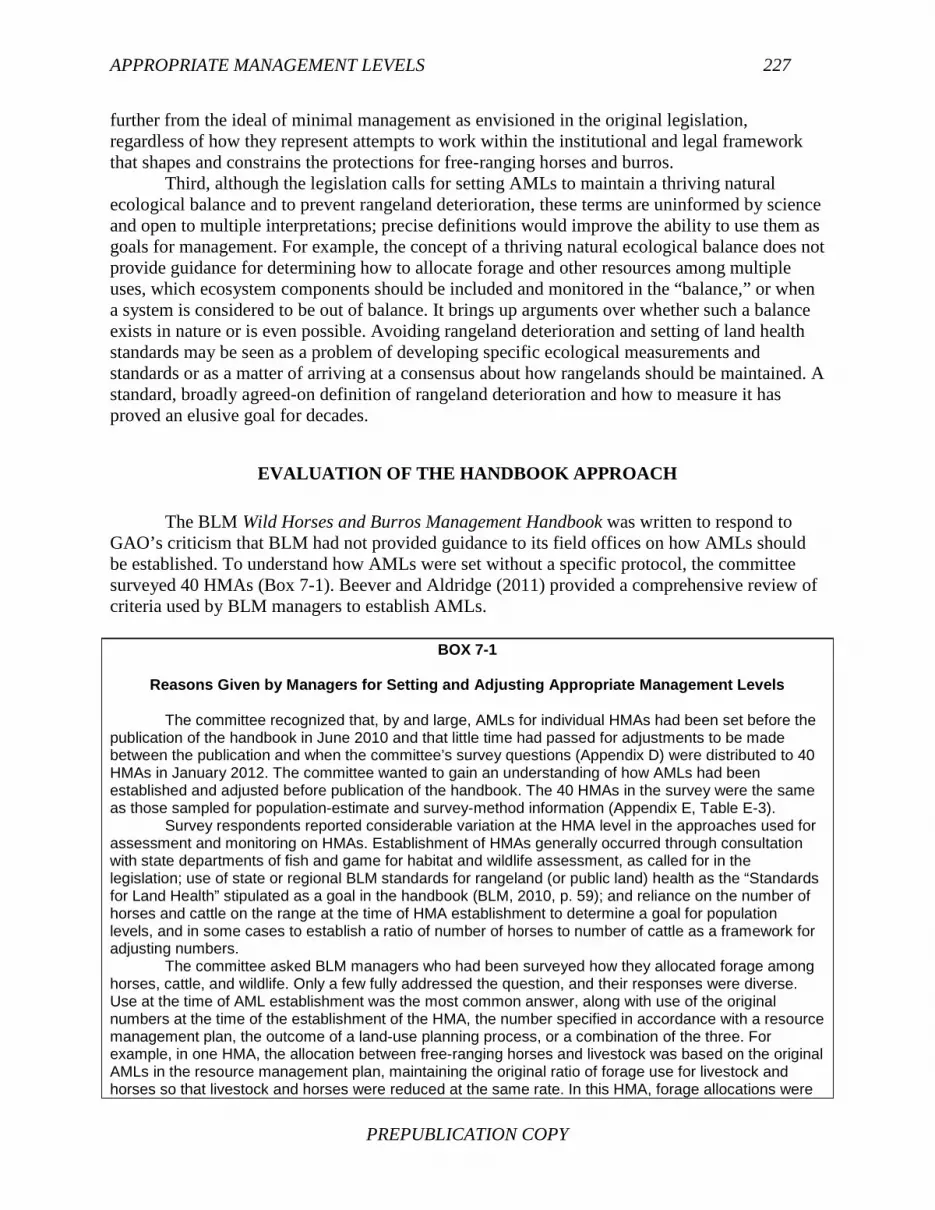
APPROPRIATE MANAGEMENT LEVELS 227
PREPUBLICATION COPY
further from the ideal of minimal management as envisioned in the original legislation, regardless of how they represent attempts to work within the institutional and legal framework that shapes and constrains the protections for free-ranging horses and burros.
Third, although the legislation calls for setting AMLs to maintain a thriving natural ecological balance and to prevent rangeland deterioration, these terms are uninformed by science and open to multiple interpretations; precise definitions would improve the ability to use them as goals for management. For example, the concept of a thriving natural ecological balance does not provide guidance for determining how to allocate forage and other resources among multiple uses, which ecosystem components should be included and monitored in the “balance,” or when a system is considered to be out of balance. It brings up arguments over whether such a balance exists in nature or is even possible. Avoiding rangeland deterioration and setting of land health standards may be seen as a problem of developing specific ecological measurements and standards or as a matter of arriving at a consensus about how rangelands should be maintained. A standard, broadly agreed-on definition of rangeland deterioration and how to measure it has proved an elusive goal for decades.
EVALUATION OF THE HANDBOOK APPROACH
The BLM Wild Horses and Burros Management Handbook was written to respond to GAO’s criticism that BLM had not provided guidance to its field offices on how AMLs should be established. To understand how AMLs were set without a specific protocol, the committee surveyed 40 HMAs (Box 7-1). Beever and Aldridge (2011) provided a comprehensive review of criteria used by BLM managers to establish AMLs.
BOX 7-1
Reasons Given by Managers for Setting and Adjusting Appropriate Management Levels
The committee recognized that, by and large, AMLs for individual HMAs had been set before the
publication of the handbook in June 2010 and that little time had passed for adjustments to be made between the publication and when the committee’s survey questions (Appendix D) were distributed to 40 HMAs in January 2012. The committee wanted to gain an understanding of how AMLs had been established and adjusted before publication of the handbook. The 40 HMAs in the survey were the same as those sampled for population-estimate and survey-method information (Appendix E, Table E-3).
Survey respondents reported considerable variation at the HMA level in the approaches used for assessment and monitoring on HMAs. Establishment of HMAs generally occurred through consultation with state departments of fish and game for habitat and wildlife assessment, as called for in the legislation; use of state or regional BLM standards for rangeland (or public land) health as the “Standards for Land Health” stipulated as a goal in the handbook (BLM, 2010, p. 59); and reliance on the number of horses and cattle on the range at the time of HMA establishment to determine a goal for population levels, and in some cases to establish a ratio of number of horses to number of cattle as a framework for adjusting numbers.
The committee asked BLM managers who had been surveyed how they allocated forage among horses, cattle, and wildlife. Only a few fully addressed the question, and their responses were diverse. Use at the time of AML establishment was the most common answer, along with use of the original numbers at the time of the establishment of the HMA, the number specified in accordance with a resource management plan, the outcome of a land-use planning process, or a combination of the three. For example, in one HMA, the allocation between free-ranging horses and livestock was based on the original AMLs in the resource management plan, maintaining the original ratio of forage use for livestock and horses so that livestock and horses were reduced at the same rate. In this HMA, forage allocations were

228 BLM WILD HORSE AND BURRO PROGRAM
PREPUBLICATION COPY
not increased because all the areas were stocked at or above carrying capacity. In another state, managers reported that in consultation with their department of fish and wildlife, the biologists at BLM made forage allocations to the native and exotic ungulates. Often, the forage allocated for existing livestock grazing privileges in an HMA was subtracted from total forage availability to determine the amount available to wildlife and horses.
Participating districts reported that measures of range condition and trend, upland utilization (amount of forage grazed, also termed “actual use” away from water), noxious weeds, and other types of rangeland and vegetation monitoring were considered relevant to adjusting and setting AMLs. One district used “negatively impacted vegetation functionality” as part of the justification to adjust an AML. Such considerations were frequent among reasons listed by managers for resetting or reaffirming AMLs. No data were provided on the metrics used to make the decisions, although some managers referred to other reports and multiple-use directives that were used in arriving at decisions. Monitoring of range and animal conditions; threatened, endangered, and sensitive species; and habitat was also conducted as part of setting, maintaining, or adjusting AMLs according to the survey. Most respondents to the committee’s survey reported that rangeland monitoring studies (upland utilization, upland and riparian trend, and noxious-weeds monitoring) were being used to assess and evaluate forage availability in HMAs.2
On one HMA in another state, the AML was set after an intensive 5-year monitoring program. Data that were used included actual use, range condition and trends, utilization, precipitation, range sites, observations, and frequency of concentration areas for free-ranging horses. To change the AML again, the district reported that it would need to conduct a similar monitoring program that would include re-examining the entire HMA and potentially reallocating forage for all animals.
One district reported that in the 1975 HMA planning process, forage-production calculations from 1952 were used to estimate how many animals could be supported on BLM-managed land in the HMA. That carrying capacity was revised in 1975 because of rangeland seedings conducted in the HMA in 1974. BLM then identified the forage allocated to existing livestock grazing privileges in the HMA and subtracted that amount to calculate forage available to horses and wildlife. The state Department of Fish and Wildlife was consulted to determine the forage required by wildlife. Forage allocations to livestock, wildlife, and free-ranging horses were made commensurate with the available forage within a reasonable distance from water and in consultation with the state wildlife agency.
Managers in one state reported limiting forage use to 55 percent of production. No details were provided as to how annual plant production was determined.
The committee received the most comprehensive response to the question of allowable use from managers who used forage production maps from 1958 to estimate total forage production and determined the forage available on the basis of 50-percent utilization rate. The biologists reported currently using monitoring studies to assess and evaluate forage allocations in the HMAs.
Because horses are on the range year-round but cattle are not, temporal separation has been used to distinguish horse and cattle effects on water holes and other features. Surveyed managers of districts in California, Oregon, and Wyoming cited effects on watersheds and riparian areas, riparian utilization, riparian trend, and insufficient or unreliable water as causes for adjustment. “Timing and duration of flow” was also provided as a reason for changing AMLs.
Managers of the 40 surveyed HMAs reported that AMLs often had been adjusted or reaffirmed
2“All Bureau of Land Management grazing allotments are periodically evaluated to assess rangeland health
and evaluate the trend in rangeland condition and the influence grazing management has on the multiple rangeland resources associated with these allotments. [As an example, one district] employs two methods of evaluating grazing allotments. The first strategy involves a one-time field assessment by an Interdisciplinary Team composed of various BLM resource specialists. This team completes an assessment based on observations of vegetation and soil conditions. The second, and most commonly used strategy, involves a formal allotment evaluation process. During this process, an interdisciplinary team composed of various resource specialists evaluates resource conditions and creates management recommendations for the allotment. The end product of this process is an allotment evaluation document which summarizes resource conditions and trend and makes recommendations for future grazing management and range improvements on the allotment. Typically allotment evaluations occur every five to 10 years depending on the resource concerns for a given allotment.” (Sharp, no date, p. 1)

APPROPRIATE MANAGEMENT LEVELS 229
PREPUBLICATION COPY
since 1971. For example, on one HMA, AMLs were changed 13 times from 1979 to 2007. Reasons for the changes were related either to four essential habitat components (forage, water, cover, and space) or to the political process. Examples of reasons included emergency gathers after extensive wildland fire, free-ranging horse distribution data, absence or inadequacy of winter range available for horses, climate and weather, and change in space available to free-ranging equids (for example, because of land closures, land trades, land-use planning efforts, boundary discrepancies, or a “checkerboard” jurisdictional pattern adjoining HMAs). Responders also cited splitting current herds into smaller groups, adverse effects of horses on cultural resources, improving vegetation conditions, enhancing wildlife habitat, and updating management plans as reasons for adjusting AMLs.
The handbook seeks to rectify the lack of guidelines for setting AMLs by making recommendations for their establishment and adjustment in several sections. Most specifically, Appendix 3 of the handbook defines AMLs and provides guidelines for setting them.
AML decisions determine the number of WH&B [wild horses and burros] to be managed within an HMA or complex of HMAs. AML is expressed as a population range with an upper and lower limit. The AML upper limit is the number of WH&B which results in a TNEB [thriving natural ecological balance] and avoids a deterioration of the range. The AML lower limit is normally set at a number that allows the population to grow to the upper limit over a 4-5 year period, without any interim gathers to remove excess wild horses and burros. (BLM, 2010, p. 67)
Table E-1 in Appendix E shows the upper limit set for HMAs as of May 2012. The handbook states that an AML should be evaluated or re-evaluated “when review of resource monitoring and population inventory data indicates the AML may no longer be appropriate” (BLM, 2010, p. 18). Reasons that may warrant a re-evaluation include changes in the environment; newly federally protected threatened, endangered, or sensitive species; and other relevant data.
The handbook prescribes processes for the decision-making aspects of setting and adjusting AMLs. Chapter 2 of the handbook, on land-use planning, suggests that the process of setting and adjusting AMLs should take place as part of comprehensive planning, should be based on monitoring and evaluation, and should follow required decision-making procedures.
AML may be adjusted (either up or down) through the site-specific environmental
analysis and decision process required by the National Environmental Policy Act of 1970 (NEPA) (P.L. 91-190). An analysis under NEPA is also required to establish a population range (upper and lower limit) for AMLs initially established as a single number. Development of a LUP [land-use plan] amendment or revision is not generally required. (BLM, 2010, p. 10)
The handbook states that an LUP should provide a process for adjusting AMLs once they are established. The process varies from one LUP area to another. If an LUP does not provide a process for adjusting AMLs, it may need to be revised or amended so that AML adjustments can be made.
In the committee’s view, the setting of an AML within a NEPA planning process when allocating resources among uses is in concert with the recognition that tradeoffs and values are parts of management decisions. The NEPA process provides for public comment and review and increases public participation in environmental decisions although the relationship is consultative rather than collaborative, tends to be bureaucratic, and does not foster deliberation (Hourdequin

230 BLM WILD HORSE AND BURRO PROGRAM
PREPUBLICATION COPY
et al., 2012). In any case, the decision-making process should be clearly distinguished from the data-gathering and analysis that provide the information used in decision-making. The committee’s focus is on the scientific analysis that feeds into decisions that ultimately must reflect social values, compromise, and economic realities.
A multitiered analysis process is stipulated by the handbook for establishing and adjusting AMLs. Tier One instructs managers of free-ranging horses and burros to “determine whether the four essential habitat components (forage, water, cover and space) are present in sufficient amounts to sustain healthy [wild horse and burro] populations and healthy rangelands over the long-term” (BLM, 2010, p. 67). Assessing the amount of sustainable forage available for the animals’ use is required by Tier Two. Tier Three concerns the genetic health of populations. Tiers One and Two are germane to this chapter; issues pertaining to Tier Three are discussed in Chapter 5.
The Tier One evaluation as described in the handbook for four habitat factors—forage, water, cover, and space—determines whether the features necessary to support horse and burro basic needs are present. It considers water, forage, space, and cover as limiting factors and requires evaluation of whether they are sufficient. Because of the inherent climatic variability of typical rangelands, the handbook recommends evaluating rangelands under conditions when they are likely to be low in forage production. Tier Two considers forage availability and quantity in detail. This section first reviews the handbook’s approach to water, cover, and space and then discusses its approach to forage. Forage availability is described in greater detail because it must be measured and used as a primary method for determining the number of herbivores that the range will support in Tier Two of the handbook-prescribed analysis. The section concludes with a review of problems related to terms and consistency in the handbook.
Water
In keeping with its approach of using limiting factors to evaluate habitat suitability for horses and burros, the handbook instructs managers that the amount of available water is to be calculated on the basis of the driest part of the year (BLM, 2010). However, the handbook does not expand beyond the limiting-factors concept and provides little information about the importance of water in sustaining populations or about specific protocols for water monitoring and assessment. Water quantity and availability are to be assessed, but the handbook does not discuss poor water quality (such as nutrient content, sediment load, and water temperature). One BLM district reported in the committee’s survey that in its 1975 HMA plan process, water was identified as a limiting factor for summer use in drought years; as a result, forage allocations to livestock, wildlife, and free-ranging horses were then made with specific attention to water supplies and carrying capacity. One concern of the committee would be the age of the data because water supplies, developments, and land use have often changed and are subject to further alterations because of climate change. Another concern would be the possibility of conflict arising from competition between BLM and state agencies with responsibilities for water management. For example, the Nevada Division of Environmental Protection is responsible for water-quality standards and monitoring in the state. To prevent overlapping or competitive efforts, cooperative interaction between that office and BLM would be valuable.
Although riparian condition has been used as one of a suite of criteria to justify removal of free-ranging equids, the handbook provides relatively little specificity on the criteria to use in

APPROPRIATE MANAGEMENT LEVELS 231
PREPUBLICATION COPY
such decisions. Areas near water should be considered foci of concentration for horses and burros and monitored accordingly. Analyses of habitat use by free-ranging horses in sagebrush (Artemisia spp.) communities reported that horses seek riparian habitats (Crane et al., 1997). Free-ranging horses typically range farther from water sources than domestic cattle but need more water than forage alone can provide in most seasons and locations. Free-ranging horses can travel to water every 3 days to twice a day, and numerous factors affect their drinking frequency, for example, ambient temperature, succulence of existing vegetation, wind speeds, and activity levels (Pellegrini, 1971; Meeker, 1979; Greyling et al., 2007). Horses’ use of water can affect water sources that influence vegetation, soils, and other species, so amounts and effects of current use should also be considered in evaluating water as a habitat component (Greyling et al., 2007). Use of areas near streams can increase runoff (Dyring, 1990a; Rogers, 1994), break down streambanks (Dyring, 1990b), reduce water quality (Nimmo and Miller, 2007), cause vegetation trampling, alterations in stream flow, and downstream siltation (Rogers, 1991), and accelerate gully erosion (Berman et al., 1988). Boggy habitats also can be altered by free-ranging horses (Dyring, 1990a; Rogers, 1991; Clemann, 2002). Similarly, soils, vegetation, and small mammals in and adjacent to springs can be markedly affected by free-ranging equids even when livestock have been absent for extended periods (Beever and Brussard, 2000).
There is evidence of interaction between forage characteristics and riparian-area use; the characteristics of forage may be affected by concentrated animal use near water. In the Sheldon National Wildlife Refuge in Nevada, 3 years of exclusion of free-ranging horses from grazing in riparian zones led to a 40-percent increase in cover of plant litter compared to bare ground and a 30-percent decrease in extent of bare ground, whereas these metrics remained generally constant in the paired riparian plots that continued to be grazed by horses (Boyd et al., 2012). In the nonexclosed areas, estimates of use from September to October based on standing biomass varied from negligible to nearly 100 percent (Boyd et al. 2012). In contrast, Greyling et al. (2007), studying areas of heavy use around a waterhole in Namibia, reported that the “expected degradation gradient radiating out from the water troughs due to over-utilization by the horses was not found. Neither vegetation species composition, density, nor standing biomass measured at various distances from the troughs confirmed a degradation gradient.”
Methods of measuring riparian condition are available. Proper functioning condition is a monitoring tool developed by BLM to assess the physical functioning of riparian and wetland areas (BLM, 1998). It provides a consistent approach that takes into consideration hydrology, vegetation, and soil-landform attributes and encourages a team approach which includes wildlife, hydrology, and plant-science expertise. This method is qualitative by design and thus lacks rigorous quantitative analysis and statistical inference. However, it can provide a framework for identifying sites where water impairments have occurred and where improved management of water resources is required. Measures of water quality (such as temperature, salinity, nutrients, dissolved oxygen, and sediment) or hydrogeomorphology (such as ground-water discharge, active floodplain, sinuosity, and width and depth ratio) do not appear to be actively used by BLM and might serve as indicators for modifying management decisions related to free-ranging horses and burros (BLM, 1998). Soil conditions—such as storing moisture, allowing infiltration, stabilizing vegetation, and balanced release of water—and preventing rill or sheet erosion by water-caused or wind-caused dust are also possible indicators. A new synthesis of literature pertaining to riparian management practices (George et al., 2011) may provide insights on how to manage free-ranging horses in riparian areas. Further, a standard range-improvement action for mitigating damage to riparian areas involves fencing sensitive areas and providing troughs at

232 BLM WILD HORSE AND BURRO PROGRAM
PREPUBLICATION COPY
locations away from natural waters. Given the extensive diversion, piping, and regulation of springs already in place across the western Unites States, additional use of troughs should be balanced against consideration for native fauna dependent on natural flows.
Cover and Space
Vegetation provides cover for free-ranging equids. For example, trees provide shade that allows equids to avoid direct insolation during the hottest times of the day, a rubbing surface that they can use to scratch topical irritations, visual concealment from predators, and forage (Pellegrini, 1971; Hanley, 1982). In the second paragraph of Chapter 3 of the handbook, an emphasis is placed on evaluating habitat suitability on the basis of access to “forage, water, or thermal or hiding cover.” The implication is that without access to those resources, horse removals may be necessary. Many models suggest that contemporary climate change may alter the distribution of trees and the balance of deciduous versus evergreen trees in parts of the domains of HMAs (Fuhlendorf et al., 1996, 2012; Tausch, 1999). The direct effects to horses of such changes are unknown. Before considering horse removals when cover and space are inadequate, where it does not cause conflict with other uses, managers may also consider increasing habitat availability by establishing greater connectivity between key habitats (through removing barriers and creating corridors for travel, habitat improvement, providing water at key points, land acquisition or other methods).
It is not clear from the handbook (BLM, 2010) what is meant by space, and there does not seem to be a good definition or way of measuring it in the scientific literature. The analysis of adequate “space” in the handbook apparently is derived largely from whether the horses and burros will stay in the habitat. For example, the handbook states that the animals “require sufficient space to allow the herd to move freely between water and forage within seasonal habitats” (BLM, 2010, p. 13). The need to adjust AMLs because of changes in the area available to equids was cited several times by surveyed managers—such changes as land closures, land trades, LUP efforts, boundary discrepancies, or a “checkerboard” jurisdictional pattern adjoining or within HMAs.
To be more specific, the discussion in the handbook should emphasize the spatial movements of free-ranging horses and burros relative to water, cover, and forage. Other aspects that might be considered include the influence of sunshine, shade, the viewshed, predator escape routes, and slope position (e.g., leeward for shelter from weather and windy gaps for insect avoidance). There is a direct relationship between space and access to spatially heterogeneous resources (such as those listed) in landscapes where horses and burros may be (Coughenour, 1991, 2008). Those resources are often dispersed patchily. As a result, the four key habitat components (forage, water, cover, and space) and other resources are naturally heterogeneous in distribution and availability and should be evaluated on the basis of their spatial and temporal variability.
Because horses and burros, like most ungulates (Hobbs, 1996), use landscapes heterogeneously, assessment ideally would occur at multiple spatial resolutions. In particular, free-ranging equids will use some portions of the landscape often (especially when equid densities are high) and use other parts rarely or never (e.g., areas more than 15 km from water sources, slopes of more than 50 percent [Ganskopp and Vavra, 1987], and areas dominated by large boulders or monoliths). Multiple-resolution assessment could be especially valuable in

APPROPRIATE MANAGEMENT LEVELS 233
PREPUBLICATION COPY
situations in which dynamics at one spatial resolution can influence dynamics at other spatial resolutions (cross-scale dynamics; Allen, 2007).
Forage Availability
In a case study in Appendix 3 of the handbook, the amount of forage available for sustainable use by herbivores, or the carrying capacity of an HMA, is the accessible, palatable biomass that grows on the site annually, modified by an allowable use factor (AU). An AU is the percentage of annual production that can be grazed without causing plants to decline in production and growth. Typical AUs are between 25 and 60 percent, meaning that 25 to 60 percent of the annual forage growth can safely be allocated to grazing; that is, it is available forage. However, AUs are often adjusted for local conditions, as it is in the case study, and for season of grazing; AUs are higher in dormant than in growing seasons. AUs are based on data about the effects of specific percentages of “use” on plant species and communities that are rarely available. Studies of the response of specific species and plant communities to herbivory and how the species and communities are influenced by season of grazing, the amount and frequency of herbivory, and varied growing conditions have been numerous but by no means comprehensive (e.g., Hanley, 1982; Paige and Whitham, 1987; Paige, 1992; Belsky et al., 1993; Hawkes and Sullivan, 2001). In fact, it is usually difficult to determine exactly how even widely used AUs were derived.
The handbook’s case study details the use of at least 3 years of grazing utilization and use mapping data with annual population estimates of horses to determine weighted utilization data, potential carrying capacity, and a proposed carrying capacity. It is not clear where the AU for plant species is acquired. In the case study, it appears that all the available forage will be allocated to horses and that only horse data are used, although at the end it is shown that the results can be converted for other herbivores (BLM, 2010). The explanation of how to calculate the weighted average forage utilization is relatively clear, but it is not clear how annually adjusted population estimates of horses, expressed in animal unit months (AUMs), are acquired. An AUM is a standardized unit of forage consumed per “animal unit” each month. Knowledge of annual herd population sizes for at least 3 years is critical for the prescribed method in that they are the basis for establishing annual forage availability, the most common habitat factor used for establishing AMLs.
Use of utilization and use mapping data to infer forage production levels is a pragmatic approach that takes multiple factors into account, including “background” consumption by all users of forage, areas of concentration, and site-specific production limitations. Ideally, however, direct forage production data should also be used to determine forage availability. Measuring how much forage is consumed by what species (horses and burros versus livestock versus wildlife) would be helpful in determining how many animals can be supported relative to forage supply, although the committee acknowledges that this can be difficult. The methods for assessing utilization are not described in the manual; however, examination of various BLM reports indicated that utilization was simply visually estimated. This method is prone to inaccuracy and is generally not well validated. More direct measures of utilization could be made through the use of grazing exclosures, particularly movable exclosures. Issues related to determining horse population size are detailed in Chapter 2.
Another complication is that a substantial part of the diet of horses may not be herbaceous plants, such as grass, and the case study includes only herbaceous growth to calculate

234 BLM WILD HORSE AND BURRO PROGRAM
PREPUBLICATION COPY
forage availability. A fair amount of research on diets of free-ranging horses of the western United States that occurred in the 1970s and 1980s confirmed that horses are typically grazers (that is, most of the food that they consume is grasses and graminoids) but that the proportions of individual food items and even of plant life forms consumed vary markedly annually, among seasons, by location, and among individuals, including variation by age, sex, and reproductive state and history (Hansen, 1976; Hubbard and Hansen, 1976; Hansen et al., 1977; Olsen and Hansen, 1977; Krysl et al., 1984; McInnis and Vavra, 1987). That is due in part to the fact that the nutritive value of plant species can vary markedly among seasons and years (Miraglia et al., 2008). Utilization of browse should be identified and incorporated into carrying-capacity calculations when it proves to be an important source of forage for horses.
The handbook guidelines recognize the high variability in forage production on arid rangelands, stipulating that forage-availability estimates should be based on 3-5 years of utilization and use-pattern mapping. In addition, that handbook states that to determine whether forage is sufficient for long-term sustainable equid grazing, production data, ecological site condition, trend, frequency, precipitation, and standards for land health may be used (BLM, 2010). It appears that each local office has a great deal of discretion in determining which methods to use. The handbook guidelines stipulate that years of above-average forage production are not to be used in calculations of forage availability—a conservative approach that aims to reduce the need for emergency gathers. Rangeland that is not commonly used is also not included. However, the committee considers 3 years of data to be inadequate typically for capturing variation in forage production on arid lands.
There are useful parallels between the setting of AMLs for free-ranging equids and the setting of sustainable stocking rates in managed livestock systems. Both endeavor to achieve ecological sustainability although management objectives and methods are quite different. Campbell et al. (2006) evaluated conditions that favor different ways of determining how to establish the number of livestock that can be supported on rangelands. They contrasted two types of strategies for setting a livestock stocking rate: conservative and tracking. A conservative strategy maintains a roughly constant stocking rate, which is set so that carrying capacity, the ability of the range to provide adequate forage, is unlikely to be exceeded even in dry years (Sandford, 1983, 2004; Tainton, 1999 in Campbell et al., 2006); this approach errs on the side of caution for dry years—in which overstocking can lead to livestock losses and vegetation deterioration—as does the handbook strategy. A strategy that tracks forage availability is less static and changes stocking rates to track variable forage supply; thus, more animals are on the range in years of high rainfall and fewer in dry years. Different conditions favor one strategy or the other (Table 7-1).
Campbell et al. (2006) summarized research that demonstrated that forage growth and distribution in semiarid rangelands are influenced by precipitation and are highly variable across time and space. Average annual rainfall is the key factor in temporal variation. Temporal variation increases as annual rainfall decreases (Ellis and Swift, 1988; Campbell et al., 2006; Briske et al., 2011). Because variability in rangelands also occurs on macro-scales (Campbell et al., 2006), even the largest HMA cannot buffer the variation in rainfall amount or distribution completely. As a result, variation in forage quality and quantity across space and time is high, and setting a static population level for herbivores runs counter to this complexity. The tracking strategy is argued to be more appropriate where environmental variability, such as in rainfall, is more predictable, allowing managers to anticipate need for adjustments in stocking, and a conservative strategy is more appropriate for locations with high variability and low

APPROPRIATE MANAGEMENT LEVELS 235
PREPUBLICATION COPY
predictability of environmental variability, such as in rainfall, because it reduces the number of years when drought would reduce forage production below levels adequate to support the animals (Campbell et al., 2006). As previously discussed, allowing free-ranging horses and burros to suffer from inadequate forage is precluded.
TABLE 7-1 Conditions That Influence the Number of Livestock That can be Supported by Forage Production in Pastoral Systems Environmental Conditions
Conservative Strategy—Setting numbers below average that can be supported over the long term is more likely to be optimal if:
Tracking Strategy— Managing animal numbers to follow changes in forage supply annually is more likely to be optimal if:
Predictability of environmental variability
Environmental variability is high and unpredictable.
Environmental variability is highly predictable.
State changes and thresholds
The system is prone to state changes and thresholds that limit reversibility through management.
The system has high resilience and changes are likely to be reversible with management.
SOURCE: Adapted from Campbell et al. (2006).
Extreme droughts will inevitably occur at unpredictable times. The location-specific effects of climate change are as yet largely uncertain. Studies suggest that temperature stress on ecosystems will be markedly higher (especially in summer) in the western United States, and there will probably be an increased frequency of extreme climatic conditions (Christensen et al., 2007; Mote and Redmond, 2012). It is clear that AMLs will need to be adaptable and periodically reassessed over the long run and subject to rapid adjustment in the short run. Gathers are the major means of adjusting the number of animals in response to drought. BLM may consider other options, which might include temporary supplemental forage or temporary movement or expansion by animals into unused range (if there were not conflicts with other resources). That might be accomplished through provision of water where there is no natural supply. However, unused range areas are quite possibly rare, and those options will only delay the need for a gather unless population growth is reduced.
In the case study in Appendix 3 of the handbook, despite that fact that allowable use was originally established to consider “year-round grazing” by horses, AUMs for horses are converted to their equivalents for other species, including livestock that are not on the range year-round (BLM, 2010). That highlights the difficulty of evaluating forage availability independently of allocation to various grazing animals. BLM considers a horse to be a single animal unit, consuming 1.0 AUM of forage per month. Horses consume more forage per unit of body weight than do ruminants (Hanley and Hanley, 1982), and the standard measure of an animal unit is a 1,000-lb cow and nursing calf. Several references to animal units for horses

236 BLM WILD HORSE AND BURRO PROGRAM
PREPUBLICATION COPY
report that they consume more than 1.0 animal unit per month (1.2,3 1.3,4 or 1.0 for a 2-year-old horse and 1.5 for a horse 3 years old and older5). BLM should explain its choice of 1.0 animal unit for a horse.
Problematic Terms
As discussed in the section “Major Challenges in Defining Appropriate Management Levels in Prescribed Legislation,” vague definitions in the Wild Free-Roaming Horses and Burros Act and related legislation have created difficulty in implementing and assessing management strategies for free-ranging equids. The handbook does not provide any greater clarity. The committee reviewed two terms in detail to illustrate the problem: land health standards and thriving natural ecological balance. Land Health Standards
The handbook states that horses “should be managed in a manner that assures significant progress is made toward achieving the Land Health Standards for upland vegetation and riparian plant communities, watershed function, and habitat quality for animal populations, as well as other site-specific or landscape-level objectives, including those necessary to protect and manage threatened, endangered, and sensitive species” (BLM, 2010, p. 17). The basis for setting land health standards is not described in the handbook but is described elsewhere (BLM, 2001). However, land health standards are not specifically incorporated into the AML-setting process as outlined in the handbook, and this reflects a disconnect between AMLs and BLM land-health assessment procedures. If land health standards are to be at the crux of AMLs, a handbook should include procedures for their scientific determination or specific references to established procedures published elsewhere and recommendations for using such procedures to set AMLs.
The BLM land health standards policy has been in effect for over 15 years. BLM developed regulations for livestock grazing administration beginning in 1995-1997. One of the regulations was that each BLM state director would, in consultation with the Resource Advisory Council in that state, develop standards for public-land health. BLM posts a number of state-level land health guidelines developed accordingly.6 The purpose of the standards is to provide a measure to determine land health and methods or guidelines to improve the health of public rangelands (BLM, 2001). Rangeland health is defined as “the degree to which the integrity of the soil and ecological processes of rangeland ecosystems are sustained. Rangeland health exists when ecological processes are functioning properly to maintain the structure, organization and activity of the system over time” (BLM, 2001, p. I-7). That is significant in that it calls for assessments not only of states but of ecosystem processes. Processes of interest pertain to hydrology, nutrient cycling, primary production, and vegetation dynamics. The 2001 document outlines a set of general procedures that should be followed to assess and achieve rangeland 3Available online: http://www.gov.mb.ca/agriculture/crops/forages/bjb00s17.html/. Accessed October 8, 2012. 4Available online: http://cals.arizona.edu/pubs/animal/az1352.pdf/. Accessed October 8, 2012. 5Available online: http://www1.agric.gov.ab.ca/$department/deptdocs.nsf/all/faq6722/. Accessed October 8, 2012. 643 CFR §4180. Available online: http://ecfr.gpoaccess.gov/cgi/t/text/text-idx?c=ecfr&sid=5d253348ae12c9c0d76a8114b7eec027&rgn=div5&view=text&node=43:2.1.1.4.92&idno=43#43:2.1.1.4.92.9/. Accessed October 8, 2012.

APPROPRIATE MANAGEMENT LEVELS 237
PREPUBLICATION COPY
health. Notably, they include not only a call to assess current land health but a determination of the causal factors that have led to the current state on the basis of the best data and resource information available. That would require the development of conceptual or quantitative models of ecosystem functioning.
“Deterioration,” like “health” or “condition,” is determined by some measure of the difference between the current state of the system and some reference state. The question is, What is the appropriate reference state of a minimally managed free-ranging equid system? The difficulty of defining that state is similar to the difficulty of defining what constitutes overgrazing. Overgrazing is a level of herbivory that leads to some level of rangeland deterioration. However, overgrazing in a livestock production system may be defined differently from overgrazing in a system that is being managed for natural processes. Coughenour and Singer (1991) reported that definitions of overgrazing also depend on differences in theories of how ecosystems that have abundant large herbivores function without human intervention. Indicators of deterioration in rangeland health may or may not constitute evidence of overgrazing, depending on management objectives and the theory or conceptual model that the management is based on. Differences in definitions used by livestock producers and wildlife managers are particularly relevant here. It is problematic to define overgrazing where there is a call for minimal management and “wildness.” Thriving Natural Ecological Balance
The handbook does not provide guidance on how to assess a thriving natural ecological balance as called for in the legislation. It is also easily conflated with the allocation process, which is a policy-driven and sometimes court-adjudicated decision rather than something derived directly from currently available scientific information. The Wild Free-Roaming Horses and Burros Act is clear that habitat for wildlife and threatened, endangered, and sensitive species is not to be harmed by free-ranging horses and burros. Among the districts responding to the implementation survey, BLM consultation with state wildlife agencies (as instructed in the legislation) was fairly consistent. Wildlife considerations were mentioned in responses from several HMAs as reasons for adjusting AMLs, either explicitly in some HMAs or implicitly as reflected in allocation of forage. Concern for species listed as threatened, endangered, or sensitive under the U.S. Endangered Species Act was referred to by only one HMA complex in the survey sample to protect greater sage-grouse (Centrocercus urophasianus), an endangered species candidate, in Wyoming.
There are several possible interpretations of what constitutes a thriving natural ecological balance. It is not a scientific term. Wildlife and Plant Diversity. BLM relies largely on state wildlife agencies to determine how to consider wildlife in the setting of AMLs. However, BLM has a responsibility to make sure that key indicators of free-ranging horse and burro effects are included in assessments of impacts to wildlife habitat.
Monitoring of wildlife and plant abundance and diversity is key to determining whether a thriving natural ecological balance is being preserved. Free-ranging horses and burros can affect species richness in a variety of habitats (Levin et al., 2002; Zalba and Cozzani, 2004). Manipulative experiments illustrate a dramatic array of indirect pathways by which free-ranging horses can affect components of marsh ecosystems (Levin et al., 2002). In addition to direct interference and other types of competition possibly experienced by large ungulates in areas that

238 BLM WILD HORSE AND BURRO PROGRAM
PREPUBLICATION COPY
have free-ranging equids, wildlife sharing the range with free-ranging horses and burros can be subject to equids’ effects on the structure, composition, and function of vegetation. Vegetation provides perching habitat for raptors, nesting habitat for breeding birds (including cavity-nesting and stick-nest–creating birds), concealment cover for greater sage-grouse and other ground-nesting birds (Beever and Aldridge, 2011), shade and thermal refuge, refuge from predators, and nutrients and energy for diverse animals. Numerous species are affected by equid impacts to soil. Recovery of some species has been attributed to removal of free-ranging horses (Nano et al., 2003). Wildlife and plant abundance has been reported to be influenced by free-ranging horses’ presence (Coventry and Robertson, 1980; Mansergh, 1982; Gillespie et al., 1995; Beever and Brussard, 2000, 2004; Greyling, 2005). Reptile species richness was significantly lower at horse-used sites than at horse-removed sites studied in the western Great Basin (Beever and Brussard, 2004) and in the Austrian Alps (Coventry and Robertson, 1980; Mansergh, 1982), and reptiles are important as prey for numerous other species and as predators that influence biological integrity. Horse presence has been identified as potentially affecting ant mounds in the Great Basin (Beever and Herrick, 2006). Interactions with Native Grazers. Native herbivores may have forage, space, water, and cover needs that overlap with those of free-ranging horses and burros. Therefore, monitoring of the status of native ungulates is crucial. In some cases, the presence of free-ranging horses has increased forage available to native species, as in the case of bitterbrush (Purshia tridentata) in Utah (Reiner and Urness, 1982). Horses and burros can dominate other herbivores and exclude them from water sources, forcing a change in the habitat use of native grazers (Meeker, 1979; Berger, 1985; Ganskopp and Vavra, 1987; Coates and Schemnitz, 1994). The degree of overlap in diets and habitats determines the potential for competition. Elk and bison diets overlap with those of horses, but there have been few cases of concern about their interactions with horses. Elk inhabit low-elevation sagebrush-steppe habitats (Hobbs et al., 1996; Manier and Hobbs, 2007) and are found in some areas that have horses (Hansen et al., 1977), but their preferred habitats tend to be more mesic (moderately moist) and at higher elevations. Bison are primarily residents of the Great Plains and portions of the Rocky Mountains (Mack and Thompson, 1982); there is little sharing of range with horses.
In some areas, there has been concern about potential competition for forage between free-ranging equids and bighorn sheep. In the Pryor Mountains, Coates and Schimnetz (1994) found partial dietary overlap year-round, and Kissel (1996) found little overlap except in summer. Dietary overlap was minimized by the fact that a substantial fraction of bighorn sheep diets was shrubs, particularly the evergreen shrub mountain mahogany (Cercocarpus spp.), but shrubs were insignificant in horse diets. Horses and bighorn sheep also used markedly different habitats and overlapped little spatially. Modeling studies including consideration of diets and the extent of overlap in spatial ranges of the bighorns and horses also supported the idea that there was only a small degree of competition (Coughenour, 1999). Kissel (1996) concluded that there was little if any competition between horses and mule deer, inasmuch as the latter are primarily browsers and horses primarily grazers. Those two species had little spatial overlap because their habitat preferences are different. In contrast, competitive interactions between burros and bighorn sheep are important inasmuch as burros are mixed feeders and have substantial quantities of browse in their diets (Walters and Hansen, 1978; Seegmiller and Ohmart, 1981).

APPROPRIATE MANAGEMENT LEVELS 239
PREPUBLICATION COPY
Interactions with Livestock. Free-ranging horses and livestock overlap in demands for forage and habitats. Cattle and horses are both primarily generalist grazers, consumers of palatable herbaceous vegetation. Horses and burros, however, are able to use lower-quality forage than cattle because of their cecal-digestive system (Hanley, 1982; Hanley and Hanley, 1982). Burros preferentially consume woody vegetation (shrubs, dwarf shrubs, stemmy forbs, and small trees). Horses and cattle use similar habitats, but they also diverge with respect to mobility and accessibility. Horses can travel great distances in a short time, they can travel further from water, and they can use rugged topography more readily than can cattle (Ganskopp and Vavra, 1987; Hampson et al., 2010).
Although it is often assumed that cattle, horses and burros, or wildlife always compete, recent research on zebras and cattle and on cattle and donkeys (donkeys served as surrogates for zebras in controlled experiments) showed that it is not always the case (Odadi et al., 2011a,b). When cattle were reared with donkeys, both grew faster than when each species was allowed to graze on its own. Facilitation occurred because the donkeys consumed tough, fibrous stems, allowing the cows to eat the more nutritious leaves, forbs, and regrowth; and the cattle helped to dilute the effects of ticks that plagued the donkeys. In semiarid habitat, the occurrence of light rains allowed grasses to continue growing after joint cropping by the two species changed the structure of the sward, thus improving forage quality. The extent to which horses and cattle can facilitate each other and improve rangeland in temperate grasslands requires further study and most certainly depends on the specifics of the ecosystem being considered. It is also critical to note that the Odadi et al. (2011a,b) research was carried out in African grasslands, which have a long, continuous coevolutionary history of herbivory by numerous ungulates and can have biomass and graminoid diversity one to two magnitudes higher than some areas encompassed by HMAs of the western United States. (Mack and Thompson, 1982). However, assuming that cattle and equids must compete because they share the same range is not necessarily warranted (du Toit, 2011). Endangered Species. Of particular concern is the interaction of horses and greater sage-grouse. Possible interactions of free-ranging equids with greater sage-grouse were thoroughly outlined by Beever and Aldridge (2011). They described numerous mechanisms by which equids can influence their environment, and greater sage-grouse are known to be sensitive to those aspects of the environment (e.g., the height of herbaceous plants is important as concealment cover for nests), but no field research has directly addressed the relationships between equids and grouse. The authors outlined numerous research questions that might be addressed, given the continuing effort and concern related to greater sage-grouse and other sagebrush-associated species in western North America.
Possible alterations of the small-mammal community by free-ranging equids may be important because of the role of small mammals in aeration and bioturbation of soils, as prey for numerous terrestrial and aerial predators, in seed and nutrient redistribution, and as part of biotic integrity. Numerous other ecosystem processes and components are critically important for conserving the potential of BLM-administered landscapes to provide ecosystem services (e.g., clean water, noneroded soils, food, and fiber) and for allowing cost-effective maintenance of ecological function and biological diversity. All these are mandated by numerous laws, policies, and statutes related to rangeland health, water quality, endangered species, and other topics.
240 BLM WILD HORSE AND BURRO PROGRAM
PREPUBLICATION COPY
Challenges to Managing for a Thriving Natural Ecological Balance. Although allowing an equid ecosystem to self-regulate could be one approach to establishing a balance, it is also evident that this may not be a realistic objective in many cases, owing to human effects that are beyond the purview of BLM. Thus, as a result of human disruptions, a self-regulated system is not necessarily natural. Land use is a foremost human effect that constrains natural horse movements, dispersals, or migrations. In natural wildlife systems, herbivores are free to seek forage and avoid situations of depleted forage. Fragmentation of habitats due to land use or ownership that does not permit such movements is problematic for herbivore and vegetation sustainability (Coughenour, 2008). Another human intervention that disrupts natural ecological processes is the development of water sources that make otherwise unavailable areas of the landscape available for equid use. Water-scarce areas would naturally be refugia from horse use for a variety of plant and animal species that are less tolerant of horses’ presence. The recent incursion of invasive plant species, such as the Bromus species which includes cheatgrass (Bromus tectorum), is another example of human effects that alter the possibility of a natural balance, as is the extirpation of predators, such as wolves, in some environments where they would otherwise occur. There are scientific approaches for assessing human effects on such ecosystems and the degree to which they impair free-ranging horse and burro numbers and management. They include scientifically based modeling studies of alternative scenarios of the presence or absence of human effects. Methods that meet the objective of minimal management could be identified, targeted, and justified to mitigate the adverse human effects. For example, if landscape fragmentation has altered the capacity of the habitat to support horses, model-based assessments would be able to quantify how this has occurred and therefore provide support for management interventions that mitigate it. Similar assessments could address lack of predation, invasive plants, and water development.
Managing horse and burro populations as free-ranging with the minimal management called for in the Wild Free-Roaming Horses and Burros Act thus entails conceptual challenges associated with defining what constitutes land deterioration or health. The handbook does not help in such definition. The handbook should address the challenge of defining terms used as management criteria, including appropriate, thriving, natural, in balance, healthy, and deteriorated. The approach would involve the development of a conceptual model for ecosystem functioning relative to management objectives and the development of indicators that can be used to measure the degree of departure from a scientifically informed conceptual model of an “appropriately” functioning free-ranging equid ecosystem.
Specificity of Methods and Their Consistency among Herd Management Areas
The handbook does not adequately respond to GAO’s request for guidance; the level of detail that the handbook supports is too limited. The handbook does provide for some degree of consistency in goals, forage allocation, and general habitat considerations and should help to improve consistency in how AMLs are set. However, it does not provide detail on monitoring and assessment methods. That is intended to allow BLM managers to decide what specific approaches fit local environmental conditions and administrative capacity, but it makes it difficult to review the program’s on-the-ground methods. A better approach would be to provide specific options. Similar issues were identified with respect to establishing AMLs, population

APPROPRIATE MANAGEMENT LEVELS 241
PREPUBLICATION COPY
inventory, use patterns, animal distribution, other site-specific and landscape-level management objectives, and forage allocation (BLM, 2010). For example, the handbook states that the amount of forage available to allocate to free-ranging horses and burros shall be determined through in-depth evaluation of resource-monitoring data after a site-specific environmental assessment and multiple-use decision process7 that includes public involvement. There is no explanation of any of the data-collection methods. The handbook would be more informative if it provided guidelines on how various kinds of assessments are to be carried out even if a variety of appropriate methods available, or referenced appropriate sources, linking them to particular settings or situations. In general, the handbook lacks clear protocols for evaluating habitat components other than forage availability. That is critical because without clear protocols specific enough to ensure repeatability, the monitoring organization cannot determine whether observed change is due to changes in condition or to changes in methods. Protocols should also include establishment of controls when the goal is to distinguish treatment or management effects from other causes of change.
ESTABLISHING AND VALIDATING APPROPRIATE MANAGEMENT LEVELS: SCIENCE AND PERCEPTIONS
The committee was asked to recommend methods for establishing and validating AMLs. The establishment of AMLs should be linked to consistent, scientifically supported models of range and herbivore interactions. Validating AMLs requires methods that draw on information on rangeland, equid, and wildlife dynamics for adaptive decision-making. Improved and more consistent monitoring is also needed. Processes for establishing and validating AMLs should be open and understood by stakeholders, and ultimately AMLs should be amenable to adaptation in light of new information and environmental and social change.
7The multiple-use decision (MUD) is generally used to establish livestock grazing, AMLs for free-ranging
horses and burros, and recommendations for wildlife habitat management. This process begins with an evaluation of range conditions; the evaluation assesses whether or not management and stocking levels for livestock, wild horses and/or burros, and wildlife are achieving rangeland objectives. If rangeland health objectives are not being met, changes in management or stocking levels are proposed. Proposed changes are analyzed in an environmental assessment and a proposed multiple-use decision is issued. Proposed decisions are subject to review and protest by parties affected by the proposal. BLM considers all protests filed and then issues a final multiple-use decision. BLM’s final decisions are subject to administrative review (appeal). (Appropriate Management Level. http http://www.blm.gov/nv/st/en/prog/wh_b/appropriate_management.print.html. Accessed February 21, 2013) At the conclusion of the decision process the management actions are implemented and monitoring continues until the next evaluation. All decisions issued as a result of completion of an allotment evaluation are issued in the MUD format. The MUD format has four sections: Introduction; Livestock Grazing Management Decision; Wild Horse and Burro Management Decision; and Wildlife Decision. Each of these sections includes a rationale, citation of appropriate authority, and information about protests and appeal procedures. (Multiple Use Decision Process. http://www.blm.gov/nv/st/en/prog/grazing/multiple_use_decision.html. Accessed December 3, 2012)
242 BLM WILD HORSE AND BURRO PROGRAM
PREPUBLICATION COPY
Understanding Ecosystem Dynamics
Numerous developments in ecological theory, in technologies and methods for assessing ecosystem status and trends at multiple resolutions, and in understanding arid rangelands dynamics and function have occurred since publication of the earlier National Research Council reports on free-ranging horses and burros (NRC, 1980, 1982). Developments in ecological research challenge the notion that a reliable minimum annual forage production that would allow the establishment of a static carrying capacity, or AML, over the long term can be determined. The research highlights the role of unpredictability on arid rangelands (Ellis and Swift, 1988; Westoby et al., 1989; Smith et al., 1995; Bestelmeyer et al., 2003; Briske et al., 2005; Vetter, 2005) and the importance of abiotic factors, such as weather events and fire, relative to biotic factors, such as competitive interactions among plants or grazing pressure, in determining vegetation expression. In short, the effects of a severe drought on forage availability often have more influence than herd population management.
It is important to distinguish between two foci for applying the concept of nonequilibrial rangeland dynamics. The first is a focus on plant-herbivore equilibria or nonequilibria. It was once theorized that plants and herbivores would come into a natural ecological balance or equilibrium if left undisturbed. Herbivore population growth would be slowed to zero at equilibrium because of density-dependent feedbacks arising from food limitation (see section “Density-Dependent Factors” in Chapter 3). However, it has been understood that population regulation also has density-independent terms, for example, weather variability (see section “Density-Independent Population Controls” in Chapter 3). Caughley (1987), who developed much of the theory of plant-herbivore dynamics, observed that, when abiotic variability is high, plant-herbivore systems exhibit nonequilibrial dynamics. That line of thought was further developed by others (DeAngelis and Waterhouse, 1987; Ellis and Swift, 1988; Behnke and Scoones, 1993; Illius and O’Connor, 1999). An important outcome of nonequilibrial plant-herbivore dynamics is that herbivore populations in such natural systems, where natural controls apply, cannot attain numbers high enough to degrade vegetation. Vegetation dynamics are driven largely by climate rather than herbivory. Vetter (2005) cited evidence from arid environments with annual rainfall coefficients of variation8 (CV) over 33 percent that suggests that these systems better fit the nonequilibrium plant-herbivore model (Ellis and Swift, 1988; Ward et al., 1998, 2000; Sullivan, 1998 cited in Sullivan and Rohde, 2002; Fernandez-Gimenez and Allen-Diaz, 1999 cited in Vetter, 2005). In such areas, vegetation cover, composition, and productivity are influenced largely by rainfall and other abiotic factors, and grazing intensity has been reported to have much less influence on these three aspects of the vegetation (Vetter, 2005). In more mesic sites with lower annual rainfall variation or reliable soil moisture, grazing has been reported to cause such changes as brush encroachment (Desta and Coppock, 2002) and alteration of grassland species composition (Fernandez-Gimenez and Allen-Diaz, 1999). Those sites may occur in or be intermixed with arid rangelands. Caughley (1987) first observed that plant-herbivore equilibria diminish markedly in strength above an annual rainfall CV of 33 percent. Ellis and Swift (1988) extended the theoretical 33-percent CV threshold. On a regional scale, HMAs are most commonly in areas that have an annual rainfall CV exceeding 33 percent (Figure 7-1).
8The coefficient of variation is the ratio of the standard deviation to the mean.

APPROPRIATE MANAGEMENT LEVELS 243
PREPUBLICATION COPY
Precipitation CV
FIGURE 7-1 Coefficient of variation of annual rainfall in the contiguous United States. SOURCE: Adapted from Lettenmaier et al. (2008) and Maurer et al. (2002).
The second focus for the application of nonequilibrial rangeland dynamics has been more
broadly on vegetation dynamics and the multiplicity of factors that drive them, including climate and disturbance. A wealth of evidence and observation, perhaps beginning with Westoby et al. (1989) and Laycock (1991) if not Gleason (1917, 1926, 1927), supports the idea that vegetation dynamics in arid climates do not necessarily follow the theory of linear successional dynamics first proposed by Clements (1916), which provided the basis for assessing rangeland condition in the United States for several decades (Dyksterhuis, 1949; Briske et al., 2003). The ecological dynamics of vegetation on arid rangelands are now commonly characterized by using state-and-transition models that posit that relatively stable configurations of vegetation, or “states,” exist and that they may “transition” to other such states as a result of the influence of biotic or abiotic factors, such as grazing, precipitation, species invasions, fire, and seed sources (Westoby et al. 1989, Bestelmeyer et al., 2003, Stringham et al. 2003; Briske et al., 2005, 2006). An inherent aspect of this concept is the acknowledgment that there may be thresholds between states and nonlinear dynamics: instead of a predictable, directional pattern of change, a state may transition to one of several alternative states, may not do so in any predictable timeframe, and may not transition back after a change (Belovsky, 1986; van de Koppel et al., 1997; Rietkerk et al., 2002; Peters et al., 2006; Bisigato et al., 2008). The state-and-transition framework does not exclude the occurrence of changes that follow linear successional trajectories (Bestelmeyer et al., 2003; Briske et al. 2005, 2006).

244 BLM WILD HORSE AND BURRO PROGRAM
PREPUBLICATION COPY
When an ecological threshold is crossed and an HMA or part of an HMA has entered an alternative state, the simple removal of horses or burros may not result in a return to the conditions of the previous state and AMLs may need adjustment. If recovery of biological structure and ecological processes that promote self-repair and facilitate long-term sustainability can be expected at all, such areas require additional resources and time. Areas that were suitable for horses or burros may become unsuitable, and areas that were unsuitable may become suitable.
In addition to the unpredictability and irregularity of rangeland dynamics, climate and social change add another level of uncertainty about future conditions. Setting of AMLs takes place in a context of ecological and social change (Bestelmeyer and Briske, 2012). Vegetation change, soil degradation, invasive species, and changing climate have already altered many rangelands, and such state changes are expected to occur more frequently (Williams and Jackson, 2007; Stafford Smith et al., 2007; Dai, 2011). Social values, economic conditions, and land use in HMAs as well as stakeholders, markets, and policies influencing ecosystem management are all undergoing change (Holmes, 2002; Sheridan, 2007; Brunson and Huntsinger, 2008). Ultimately, the challenges of these numerous sources of unpredictability demand that AMLs be adaptable.
State-and-transition models are synthetic, conceptual models that describe soil and vegetation dynamics (Bestelmeyer et al., 2003; Briske et al., 2005, 2006; Herrick et al., 2012). Models are refined as data become available, and they become increasingly data-driven rather than conceptual over time. Monitoring and site selection can be improved through identification of ecological sites with state-and-transition models (Herrick et al., 2012). The inventorying of ecological sites and linking of them to state-and-transition models are important efforts that BLM is already participating in with the U.S. Department of Agriculture’s Natural Resources Conservation Service (NRCS). Such models offer the opportunity to capture information about the influence of management and both linear and nonlinear dynamics of ecosystem change, and they are useful in modeling efforts. Good conceptual models implicitly or explicitly identify influences and short-term response indicators in the description of transitions and pathways (Herrick et al., 2012). Information about free-ranging horse and burro management should be linked to ecological sites whenever possible. Over time, the outcomes of adaptive management can be used to improve the state-and-transition models.
The NRCS effort to develop state-and-transition models to guide rangeland management throughout the West is a valuable opportunity to create a standardized basis for managing for desirable ecosystem states that will go a long way to maintaining a thriving natural ecological balance as mandated by the Wild Free-Roaming Horses and Burros Act as amended (see Box 7-2). The committee recognizes that the development of state-and-transition models is in its infancy, is difficult, and may be beyond the purview of BLM and instead be in the domain of NRCS or other natural-resources management agencies and the scientific community. Increased and better defined collaboration between such agencies, the scientific community, and BLM is needed.
An encouraging initiative in this direction is the collection of rangeland data on BLM lands by NRCS staff familiar with the National Resource Inventory data collection methods for rangelands that have been used since 2003 (L. Jolley, NRCS [retired], personal communication, February 2013). Those data are linked to development of state-and-transition models for specific ecological sites. Eventually, this will allow BLM to the use of the nationwide National Resource

APPROPRIATE MANAGEMENT LEVELS 245
PREPUBLICATION COPY
Inventory Resource Assessment database.9 This would be a valuable contribution to standardizing BLM methods and data nationwide.
BOX 7-2
The Pryor Mountain Wild Horse Range Example of the Natural Resources Conservation Service
Approach
The Pryor Mountain Wild Horse Range is probably the most well-studied HMA in the nation (e.g., Garrott and Taylor, 1990; Singer and Schoenecker, 2000; Fahnestock and Detling, 1999a,b; Coughenour, 1999; Ricketts et al., 2004; Roelle et al., 2010). Widespread concern about the ability of the range to support wild ungulate populations prompted BLM to ask NRCS to perform a comprehensive inventory and assessment of the health of range in 2002-2003 (Ricketts et al., 2004). According to NRCS, its report was the most detailed assessment of any wild horse range to date (this presumably referred to all the HMAs under BLM purview). Although the Pryor Mountain Wild Horse Range supported 161 horses in 2003, the NRCS assessment determined carrying capacity should be 45-142 horses on the basis of the percent of rangeland in poor condition, the low similarities of vegetation to potential climax vegetation, a perceived downward trend in range condition, and evidence of severe erosion.
The approach taken by NRCS was different than that described in the BLM handbook. A more exhaustive methodology was used by NRCS, and this approach serves as an example of potential improvements to the BLM handbook approach. Nevertheless, it too has had notable limitations.
The approach used a systematic sampling of the entire landscape. The landscape was stratified into ecological sites on the basis of an earlier Soil Conservation Service soil survey. Transects were distributed among ecological sites within broader-scale inventory units by using stratified random sampling. Along each transect, 10 circular plots were sampled at 10- or 20-foot intervals. Vegetation biomass was determined by harvesting and weighing all plants, by double sampling with some being visually estimated, or by visual estimation only. Total forage availability was used to determine stocking rates. A “harvest efficiency” was applied in the same way as a proper use factor would be applied in the BLM approach. It was assumed, on the basis of an earlier literature review (Holecheck, 1999), that 35- to 45-percent use is moderate for desert and semidesert environments. A value of 30 percent was used for preferred and desirable species and 10 percent for undesirables. Estimates were subjectively adjusted on the basis of judgments of whether plants had reached peak biomass and to account for grazing removals. Forage availability was further modified by distance from water and slope class. This approach is a more direct way of assessing forage biomass than the BLM handbook approach, but it is still subject to uncertainty in that visual estimates of biomass are used without clear evidence of calibration against actual measured weights; samples were taken in open, grazed vegetation, and a subjective and unsubstantiated method of adjusting for grazing removal was used; sampling occurred only once in the growing season, but biomass is dynamic through the season; sampling occurred in only 1 year, but precipitation is highly variable among years (the BLM approach is superior in accounting for such variability); and a source based on pre-1976 range literature was cited for setting proper use levels. Proper use levels are based on available site-specific research, local experience, and trend data and should be adjusted through adaptive management (Swanson et al., 2006). Updates were not mentioned.
Rangeland condition was based on similarity in composition to that inside reference long-term exclosures. The underlying assumption was the traditional one: climax, ungrazed plant communities are in the best condition, as in the BLM method. However, plant communities grazed by herbivores cannot be expected to be like communities exclosed from grazing. They may be different, but they may be stable and productive. An attempt was made to assess trends in conditions relative to the presumed climax community, as evidenced by conditions in long-term exclosures. However, the assessment was based on judgments of condition at one time as determined by comparison to the presumed ungrazed climax condition rather than observations of changes over time. That underscores the need for long-term
9Available online: http://www.nrcs.usda.gov/wps/portal/nrcs/detail/national/technical/nra/nri/?&cid=stelprdb1041620. Accessed February 21, 2013.

246 BLM WILD HORSE AND BURRO PROGRAM
PREPUBLICATION COPY
monitoring. It was not established that the vegetation community was changing, only that it was different from that in the ungrazed area. It is noteworthy that the grazed and ungrazed plots have not become more similar despite the fact that management removals have, for the most part, kept the horse population near the AMLs for many years. There is little evidence that all but elimination of the horses would result in such a convergence and no evidence that one “condition” is generally superior to the other.
Rangeland health was assessed by using a number of indicators “relative to soil and site stability, watershed and hydrologic function, and soil and plant community integrity” (Ricketts et al., 2004, p. 104). They included hydrological indicators—such as pedestaled plants, rills, gullies, and soil loss—and observations of plant mortality, bare ground, and litter (detritus). Although there was evidence of erosion due to overland flow and wind, it was not established how long it had been occurring, that it was not going on in the absence of grazing, or that changes in herbivore density would reduce erosion rates.
Finally, the assessment did not make substantial references to or comparisons with more detailed studies of vegetation and ecosystem functioning that used a greater number of grazing exclosures, measures of live and dead biomass dynamics over time, experimental design, statistics, and spatially explicit ecosystem modelling (Coughenour, 1999; Fahnestock and Detling, 1999a,b; Singer and Schoenecker, 2000).
Assessing Rangeland Deterioration
The handbook assumption appears to be that if forage and habitat components are adequate, range deterioration will not occur. Habitat structural characteristics and amount of forage available can be measured in a straightforward way, but what defines “range condition”—the “health” of the range—has been a subject of debate in scientific and management communities for decades, and the handbook provides no additional clarity. As noted above, concepts underlying range-condition assessments in the 1970s, when the Wild Free-Roaming Horses and Burros Act was written, are now viewed as simplistic and not in line with current thinking regarding vegetation dynamics in arid lands. Although the handbook focuses primarily on the level of forage utilization as a determinant of AML, forage consumption is only one process associated with grazers’ use of the landscape. Horses and burros have mechanical effects on plants and soils through trampling and on shrubs through rubbing (Beever et al., 2008). Therefore, other factors sensitive to equid presence may indicate ecosystem change due to equid grazing, including insect activity, soil compaction, species richness, condition of woody vegetation, and cover of plants (Beever et al., 2003). Areas used by free-ranging horses have been reported to exhibit soil loss, compaction, and erosion (Dale and Weaver, 1974; Dyring, 1990a; Whinam et al., 1994; Nimmo and Miller, 2007); soil was the ecosystem component that differed most between horse-occupied and horse-removed sites in the western Great Basin study (Beever and Herrick, 2006).
Although invasive species are receiving increased management and conservation attention (both in and outside BLM), the committee observed that there was relatively little guidance in the handbook on the effects of invasive species on AMLs. Invasive species may be brought in by free-ranging equids (Campbell and Gibson, 2001) and spread by them (Dyring, 1990a; Rogers, 1991; Weaver and Adams, 1996; Campbell and Gibson, 2001; Loydi and Zalba, 2009). Most seeds pass through the equine digestive tract in less than 2 days, but some can be carried and remain viable for much longer periods (Janzen, 1981) and so can be transferred long distances. Seeds are also carried on the animal body. It can be difficult in practice to ascribe

APPROPRIATE MANAGEMENT LEVELS 247
PREPUBLICATION COPY
causation of invasive-plant presence and density to free-ranging equids, especially without controlled experiments. It is likewise unclear whether alterations (either decreases or increases) in grazing intensity can be expected to reverse or halt the spread of invasive species. Although invasive-plant ecology is still an emerging field, the handbook should offer some guidance based on what is known. Given the importance of invasive plants in altered fire regimes in the domain of BLM HMAs, the topic of how free-ranging equids relate to distribution and abundance of invasive plants may deserve increased research attention.
Livestock grazing has been reported to alter soil properties via compaction, hoof action and consequent erosion, and redistribution of nutrients such as nitrogen (Archer and Smeins, 1991; van de Koppel et al., 1997). However, hoof action may break physical surface crusts that impede infiltration and seed germination. Soil surface horizons are involved in numerous biotic and abiotic pathways in communities (Thurow, 1991; Belsky and Blumenthal, 1997; Beever and Herrick, 2006). Given the importance of soil chemistry and physical attributes (e.g., related to compaction) for ecological function, the tight connection of soil measures to so many BLM mandates and arid-lands monitoring frameworks, and the relative dearth of information on equid-soil relationships, Beever and Aldridge (2011) reported that further research on these relationships would increase ecological understanding and identify the implications of the relationships for the management of equid influence on soil resources. For example, they asked provocative questions, including the following: To what depth below the soil surface does compaction extend? Under what conditions will treading by equids lead to favorable or adverse hydrological outcomes? What factors (such as soil texture or percentage of clays, concentration of calcium carbonate, and depth to water or an impervious layer) most strongly modify soil responses to horse and burro densities? Consideration of such factors and interactions would strengthen assessments used to set AMLs.
Beever et al. (2003) reported that 19 horse-grazed and horse-removed sites could not be clearly discriminated on the basis of the cover of key plant species consumed by horses (species measured by BLM specialists in horse-effects monitoring) or by using cover or frequency of all plant species. However, horse-occupied and horse-removed sites were clearly discriminated by using a diverse suite of variables that research had suggested were sensitive to grazing disturbance. The variables included density of ant mounds, soil-surface hardness, species richness, grass cover, forb cover, and shrub cover (Beever et al., 2003).
Monitoring and Assessing Forage Availability
Once AMLs are established it is essential to determine whether forage consumption is at the predicted level. To account for factors other than grazing (such as weather) that can affect rangeland condition, determining effects of equid foraging ultimately requires comparisons of vegetation in areas where foraging occurs and where it is prevented. Consumption levels can then be compared with rangeland productivity. Grazing and browsing effects are typically measured by comparing vegetation production and composition in areas where grazing occurs with those in areas where it is excluded.
One of the easiest and most effective ways to compare vegetation features in grazed and ungrazed areas is to establish pairs of exclosed and grazed plots. Plots are chosen at random with one plot at each site as a control and the other enclosed by an exclosure device such as a 1-m3 cage covered in wire mesh. With grazing excluded, changes in vegetation height, biomass, and percentage cover in cages provide estimates of productivity. In the paired plots outside cages,

248 BLM WILD HORSE AND BURRO PROGRAM
PREPUBLICATION COPY
grazing will reduce vegetation biomass. Thus, differences between vegetation biomass inside and outside cages provide estimates of consumption. Clipping-based estimates are more accurate than visual estimates. Cages are moved regularly (one to three times per year) to prevent the cages themselves from altering productivity. The temporary exclosures can be used to determine whether current herbivore densities, as set through management removals, are achieving anticipated or target levels of offtake. Larger, permanent exclosures can also be established to determine the extent to which grazing changes vegetation cover and composition over time. Such exclosures can also be used to test the hypothesis that removal of grazing results in vegetation recovery.
Temporary exclosures are easy to deploy and relatively inexpensive to implement, but many replicates in habitats are required because each cage and the control paired with it provides estimates of productivity and consumption over only a small area. Moreover, small cages generally exclude trees and shrubs that provide browse for burros. Care must be taken to avoid statistical pseudoreplication because samples in each permanent exclosure are likely to be spatially correlated to a greater extent than samples among exclosures, for example, in different vegetation types or patches of vegetation and soils in the larger-scale matrix of landscape heterogeneity.
Although small-scale and large-scale exclosures are similar in many respects, they differ in important ways. Fenced areas allow detection of long-term changes in vegetation where grazing is excluded, whereas 1-m3 cages enable frequent and easy movement for measurement of annual production. Long-term exclosures may foster the development of vegetation and soil conditions different from those in areas routinely grazed by large herbivores, whereas small, movable exclosures maintain conditions more similar to the conditions of grazed vegetation. The different approaches have two implications. First, the conditions inside long-term exclosures may enhance or suppress plant growth compared with grazed vegetation. Reduced growth could arise from self-shading, rainfall interception, and lower rates of nutrient cycling in the ungrazed than in the grazed vegetation. As a result, growth (primary production) of the vegetation that is grazed cannot be estimated from data collected in long-term exclosures. Comparisons of vegetation in and outside large permanent exclosures provide different estimates of production and consumption from those of temporary exclosures because vegetation that develops within long-term exclosures often becomes quite different from that outside the exclosure. The vegetation that develops in long-term exclosures should not be considered “natural” or “desirable” if the objective is to conserve free-ranging populations of large herbivores.
Beever and Brussard (2000) concluded that exclosures are nonetheless an excellent monitoring and experimental design tool that had been underused to quantify influences of free-ranging horses on vegetation and wildlife. That is particularly relevant for BLM managers of free-ranging equids because numerous exclosures have been in place for some time, and a strategically placed network of large exclosures could provide BLM with robust data for quantifying the effects of free-ranging equids among HMAs, seasons, and years of different weather.
Sampling vegetation in and outside either type of exclosure is labor-intensive. As a result, techniques that relay easily acquired, remotely sensed data have become popular (see Box 7-3), even though the data are relatively coarse and generally cannot be used to monitor exclosures. Images from satellites routinely measure many spectral bands of reflected light from vegetation and provide long-term time series for examining changes in vegetation. The Normalized Difference Vegetation Index (NDVI) is widely used and compares infrared and near infrared

APPROPRIATE MANAGEMENT LEVELS 249
PREPUBLICATION COPY
reflectance to measure vegetation abundance and quality. However, interpretation of those values in relation to actual rangeland quality requires “ground-truthing” based on actual measurements of vegetation. Moreover, sample ground-truthing in and outside large-scale exclosures remains essential for estimating consumption levels from remotely sensed spectral indexes and thus foraging effects on large areas. Care must also be taken in interpreting the meaning of reflectance values because they are affected by the abundance of bare ground and the abundance of grasses and forbs relative to trees and shrubs. Once predictive statistical models are developed, remotely gathered data on large spatiotemporal scales can be used to measure changes in rangeland quality repeatedly. In that way, the effects of AMLs can be monitored from remote sensing and adjusted on a regular and timely basis.

250 BLM WILD HORSE AND BURRO PROGRAM
PREPUBLICATION COPY
BOX 7-3
Use of Remote Sensing
Remote sensing is an effective and universal tool adapted to a wide array of applications in
natural-resources science and management (Gross et al., 2006, Kennedy et al., 2009). It has utility for landscape assessment ranging from site-specific habitat management to broad landscape-scale predictions. Remote sensing can be used effectively to characterize heterogeneous landscapes on the basis of detection of abrupt changes or gradual trends and patterns. It can provide consistent and reliable information on ecological effects and can be used to monitor landscape change and to extract unique or important features from complex ecosystems (Kennedy et al., 2009). It is an excellent tool for landscape-level applications, such as range assessment, ecological monitoring, weed-invasion detection, and woodland-encroachment assessment.
The spatial resolution of an image refers to the size of the smallest object that can be detected (resolved) on the ground. In raster-based information, the resolution of an image is limited by the smallest pixel size. High-resolution information is characterized by small pixel sizes and low resolution by large pixel sizes. When comparing images or datasets from different HMAs, it is critical that the resolution of the images be known and preferable that they be comparable. The accuracy and reliability of an analyzed (classified) remotely sensed image may depend on its resolution.
Diverse sensor types and remote-sensing platforms are available, each with specific-resolution and spatial-extent parameters. Which sensor is chosen depends on management objectives and expected outcomes. Several of the sensors provide specific advantages for management of free-ranging horses and burros (Table 7-2). TABLE 7-2 Description of Remote-Sensing Types and Their Advantages in Management of Free-Ranging Equids Attribute Image Type Advantages and Opportunities
Patch-size detection
Fine grain: IKONOS,a Quickbird,b Aerial photographyc
High spatial resolution. Delineation of habitat heterogeneity. Characterization of primary horse grazing and drinking areas.
Gradual landscape change
Fine grain: IKONOS, Quickbird, Aerial photography
Fine scale habitat structure and change in HMAs. Monitoring of effects and resource availability.
Moderate grain: Landsat, ASTERd
Regional disturbance assessment, forage detection availability, and landscape change detection.
Coarse grain (MODIS,e AVHRRf)
Atmospheric influences and surface detection across broad spatial areas. Monitor regional shifts in vegetation structure.
Abrupt landscape change
Fine grain: IKONOS, Quickbird, Aerial photography
Inference of land use and land-use change by image analysis and interpretation. Annual or seasonal effect detection in HMAs.
Moderate grain: Landsat, ASTER, SPOT, hyperspectral, AVRIS
Detection of disturbance events in large areas.
Coarse grain (MODIS,e AVHRRf)
Large-scale disturbance and regional vegetation change such as drought. Cloud screening. NDVI of large areas for vegetation cover and predicted annual forage production.
APPROPRIATE MANAGEMENT LEVELS 251
PREPUBLICATION COPY
aThe IKONOS sensor is a high-resolution satellite that captures 3.2-m multispectral images and 1-m panchromatic data. It has wide application in natural-resources assessment and mapping, agriculture, forestry, natural disasters, change detection and so on. It collects reflected wavelength bands that include panchromatic, blue, green, red, and near-infrared wavelengths; it can also be used to develop digital elevation models that represent the earth’s topographic surface (http://www.satimagingcorp.com/satellite-sensors).
bQuickbird is a high-resolution satellite sensor that collects 0.61-m resolution imagery. It is an excellent sensor for land use and change detection, environmental analysis, and resource management. It has a short revisit time (93.5 minutes), making it effective in abrupt to gradual time-change analysis. Data come in panchromatic, red, blue, green, and near-infrared bands. It can be used to map and analyze fine-scale HMA features.
cSeveral types of aerial photography are available or can be produced, depending on the type of information needed. Since 2006, the National Agricultural Imaging Program (NAIP) has provided color, and for some states and dates, color-infrared imagery. The images have a 1-m resolution and can be used to identify and map landscape features. In contrast with most high-resolution satellite sensors, which can be expensive, NAIP imagery is free to the consumer.
dASTER (Advanced Spaceborne Thermal Emission and Reflection Radiometer) is used to obtain information on surface temperatures, reflectance patterns, and elevation changes. It is used to predict variability and trends in climate, weather, and surface structure (http://asterweb.jpl.nasa.gov/index.asp).
eMODIS (Moderate Resolution Imaging Spectroradiometer) views the earth every 1-2 days, collecting data in 36 spectral bands. It is used to measure global dynamics and processes, including prediction of global climate change, to assist policy-makers in land protection. With a 250-m pixel size, the resolution can be considered relatively coarse-grained.
fAVHRR (Advanced Very High Resolution Radiometer) is a satellite sensor that collects earth reflectance in five wide spectral bands (red, two near-infrared, and two thermal).
Analytical and Modeling Approaches
Scientifically defensible approaches have been developed over the last 2 decades for assessing vegetation, herbivore, and ecosystem dynamics in spatially heterogeneous environments from landscape through regional and even to global scales. A wide variety of models have been developed that are capable of simulating vegetation, biogeochemistry, and hydrology dynamics in response to soils, changing climate, and, to a lesser extent, herbivory. A body of science in this field does exist focusing on vegetation and ecosystem responses to herbivory. Some models are capable of simulating interactive responses to herbivory, climate, and soils. Although computer modeling has been adopted by BLM to predict horse population responses to management and to assist in the setting of the lower bounds of AMLs (see Chapter 6), modeling has not been used to set the upper bounds of AMLs or to inform AML decisions. That would necessitate models of vegetation and ecosystem dynamics and the ability of such models to represent ecosystem dynamics in spatially heterogeneous environments and mobile herbivore populations. Assessments of AMLs could be made more robust and more informative by using the powerful analytical and modeling approaches. A first step would be to use geographic information systems (GIS) and remote sensing to a greater extent in setting and evaluating AMLs. BLM uses GIS to some extent to quantify vegetation and forage production potentials in different range sites, as delineated by NRCS or older Soil Conservation Service soil surveys. Forage production estimates for each range site have been combined or scaled up by using GIS to derive forage production. However, there is a potential to do more with spatial data and to derive additional data from remote sensing, for example,
· Overlay spatial data on equid distributions, which are temporally variable, on to forage-production estimates to predict percentage utilization across the landscape. Even if the equid distributions are coarse or estimated, they represent what is known.
· Use spatial modeling of equid habitat selection on a seasonal basis to provide estimates of equid distributions. Equid habitat-selection patterns will be influenced by distance to water, topography, forage quantity and quality, shrub and tree cover,

252 BLM WILD HORSE AND BURRO PROGRAM
PREPUBLICATION COPY
barriers to movement, conflicting land uses, forage offtake by livestock, and other factors. All those can be represented as GIS data layers.
· Use remote-sensing data to cross-check and augment estimates of forage production. · Use spatially explicit precipitation maps that account for patchy rainfall and
topographic gradients to refine estimates of forage production. · Estimate snowpack distributions by using remote-sensing products, SNOTEL data,
snowpack modeling, and spatial interpolation to estimate areas that are available to horses in winter. The snowpack in turn affects the forage supply for the horses in winter.
As just noted, various vegetation and biophysical-ecosystem models have been developed
over the last 3 decades. All have capabilities of simulating realistic scenarios of plant production and vegetation dynamics in response to soils and climate. However, few have focused on simulating vegetation or ecosystem responses to herbivory. Few have explicitly represented herbivores or their dynamic distributions on the landscape. However, one example that does is the application of the SAVANNA ecosystem model to the Pryor Mountain Wild Horse Range (Coughenour, 1999) and to a variety of other large herbivore ecosystems in the western United States, East Africa, and elsewhere.
To be useful in informing and assessing AMLs, key capabilities of such an ecosystem model would include
· Prediction of plant-biomass dynamics and production responses to climatic variations
and soils. Dynamics must be represented at least seasonally and ideally on a weekly or even daily basis. Dry, wet, and average years should be realistically simulated. Seasonal dynamics are important because forage biomass varies greatly owing to intraseasonal and interseasonal precipitation patterns and herbivore offtake on different parts of the landscape at different times throughout the year.
· Realistic simulation of plant-production responses to herbivory, including undercompensatory and overcompensatory responses.
· Simulation of changes in vegetation cover over multiyear periods. · Differentiation of simulated plants into functional groups, including preferred and
nonpreferred species for herbivores. · Representation of spatially variable patterns of precipitation and temperature and their
effects on vegetation. Spatial patterns of precipitation can be thought of as dynamic precipitation maps in the model.
· Simulation of dynamic snowpack distributions across the landscape because these affect forage availability and herbivore distributions.
· Simulation of dynamic herbivore habitat selection and resulting spatial distributions in response to water, forage, topography, cover, and barriers.
· Simulation of herbivore forage intake and resulting effects on herbivore body condition.
· Representation of key nutrient cycles, particularly nitrogen and soil-carbon dynamics. · Representation of key hydrological responses, particularly runoff and infiltration
responses to changes in vegetation cover, which may result from herbivory.

APPROPRIATE MANAGEMENT LEVELS 253
PREPUBLICATION COPY
· Simulation of interactions with other species via competition for forage, water, and habitat and effects on other species resulting from equid-induced habitat alterations. Ecosystem modeling can represent forage competition, and effects on habitats could be represented by linkages to habitat models for other species.
With those modeling capabilities, it would be possible to predict the effects of different horse or burro densities and distributions on ecosystem dynamics and to assess whether horse or burro densities are sustainable in the long term. It would also be possible to infer or directly represent interactions with other species, including wildlife and livestock. Competition between livestock, wildlife, and horses or burros is affected by the degree of overlap in species forage preferences and spatial distributions. Modeling could also be used to assess the effects of restrictions on horse or burro movements that arise from fencing and other land uses. Such habitat fragmentation results in reduced opportunities for herbivores to access key grazing areas in times of food shortages on primary ranges. Restrictions of movement can also result in higher herbivore densities and grazing pressures than would occur if the animals could disperse or migrate. Vegetation or ecosystem models must be verified through comparisons with monitoring data described above. It is recognized that no single model is completely accurate; however, iterative adjustment of a model on the basis of data will improve it and make it more useful.
Adaptive Management
Environmental variability and change, changes in social values, and the discovery of new information require that AMLs be adaptable. Perhaps the most fundamental approach in this regard is adaptive management (Holling, 1978; Williams et al., 2009). Adaptive management can be used in a variety of social decision-making settings (see Chapter 8). Herrick et al. (2012) defined adaptive management as an iterative decision-making process that incorporates development of management objectives, actions to address the objectives, monitoring of results, and repeated adaptation of management until desired results are achieved. A key tenet of adaptive management that is relevant to managing free-ranging horses and burros is the treatment of management actions as testable hypotheses. In turn, maximizing long-term knowledge of the system and thereby improving management (balanced with achieving optimal short-term outcomes, given current knowledge; Stankey and Allan, 2009) hinges on several fundamental tenets of research and monitoring design. Those tenets include use of control plots (against which to evaluate the effects of a given management “treatment,” such as erecting exclosures, administering immunocontraception broadly in a population, or removing or transferring animals from a population); use of replication to increase confidence that results are generalizable rather than anomalous; and controlling for variability (such as that due to annual differences in precipitation and thus productivity), for example, through Before-After Control-Impact designs (Underwood, 1992, 1994). Also essential for adaptive management specifically and for applied ecology generally is the explicit incorporation of uncertainty (such as the use of 95-percent confidence intervals, standard errors or standard deviations, and probability density functions) into estimated measures (such as herd size, utilization rate in a site or HMA, and average penetration resistance in a landscape).
Several other approaches to analysis and interpretation of management actions and monitoring data can improve confidence in the results. First, if there is interest in understanding whether or how a particular factor (e.g., average site growing-season precipitation) affects the

254 BLM WILD HORSE AND BURRO PROGRAM
PREPUBLICATION COPY
degree of ecosystem alteration caused by a given density of free-ranging horses and burros, ecosystem attributes mentioned above should be measured at numerous sites with comparable horse and burro density across a broad range of that factor (gradient analyses; Austin, 1985; Gosz, 1992). Such approaches provide quantitative information on the major driving variables, permit the generation of information for extrapolating between sites and across scales, and begin to address mechanistic explanations of phenomena relevant to management (Gosz, 1992). Although ideally other important factors would remain constant in all sites along the gradient, that is rarely the case; for example, soils may differ markedly along the gradient. In those situations, explicitly accounting for this key factor (e.g., soils) can be approached in a manner comparable with complete factorial or blocked designs (e.g., Underwood, 1994, 1997; Sokal and Rohlff, 2012). A related example might be the use of landscape-scale analyses to identify portions of the landscape most likely to be early-warning indicators of deterioration of landscape condition, such as areas of heavy use.
Numerous relatively recent advances in ecological monitoring that can further increase confidence in results are relevant and noteworthy for the Wild Horse and Burro Program. For example, if a particular question is being addressed in terms of testing of the null hypothesis and the null hypothesis fails to be rejected (that is, no effect of a management action or “treatment” was found), a post hoc power analysis can be performed to assess how likely the effort was to detect an existing effect (what power the effort had) given the sample sizes used for and the variability among replicates in the various groups. Over time, however, a priori power analyses have generally come to be regarded more favorably than post hoc analyses. A priori analyses can tell managers and researchers what level of effect size (i.e., only if a 50-percent difference exists) can be detected for given levels of power, sample size, and variability within groups. BLM managers should note that the error structure (e.g., partitioning of degrees of freedom) in these analyses reflects the design of their monitoring. In more complex designs, simulation analyses can be a more realistic alternative. Concepts related to power can improve setting and adjusting of AMLs by providing quantification of sensitivity of a monitoring system, that is, the ability to be an early-warning system of environmental change as opposed to confirming that a system has already been dramatically altered and perhaps crossed an ecological threshold.
The committee believes that the above principles could be more thoroughly integrated into the Wild Horse and Burro Program to increase the defensibility and scientific validity of management actions. Generally speaking, when the domain is as spatially vast and biotically heterogeneous as the area managed by BLM for free-ranging equids, a compromise approach can be taken. The compromise seeks to balance the incorporation of as much repeatability as possible (to permit analyses at numerous hierarchical spatial and temporal scales) with the ability to tailor management and monitoring efforts to local biota, interests, and priorities (to allow stakeholder involvement and investment and have relevance on both local and broader scales). That may mean, for example, that a core suite of field methods and monitoring indicators are used and that databases and analysis templates exist for all HMAs (Box 7-4). In contrast, individual HMAs or district offices may add to the core suite by creating standard monitoring approaches for monitoring locally important rare plants or animals or may add additional metrics for a given field method that are important to local interest groups.

APPROPRIATE MANAGEMENT LEVELS 255
PREPUBLICATION COPY
Validity for Stakeholders
Because AMLs are a focal point for controversy, it is important to develop and maintain standards for transparency, quality, and equity in the establishment, adjustment, and monitoring of AMLs. Research suggests that transparency is an important contributor to the development of trust between agencies and stakeholders (Rowe and Frewer, 2000; Webler and Tuler, 2000). The public should be able to understand the methods used and how they are implemented and should be able to access the data used to make decisions. Transparency will also encourage adherence to a high level of quality in data acquisition and use. The data and methods used to inform decisions must be scientifically defensible. Allocation of resources to management of free-ranging horses and burros takes place in a context of contending uses for BLM lands, all of which have some standing in the agency’s charge for multiple-use management. The law makes clear that rangeland resources are to be protected from deterioration, but there is no known formula for creating a balance among such uses as cattle grazing, wildlife, hunting, mining, recreation, and free-ranging horses.
From submitted public comments and statements made by members of the public at information-gathering meetings, it is clear that stakeholders vary in their opinions about AMLs. Some believe that herd numbers should be higher and should take precedence over other rangeland uses administered and managed by BLM. Some believe that equid population size needs to be increased to protect genetic diversity or to ensure survival of the herds in an unpredictable environment. Some believe that herd levels are too high or that AMLs are not adequately adhered to and that free-ranging horses and burros are damaging habitat and taking resources away from other uses. Some argue that HMAs should be managed exclusively or primarily for horses and that other uses should be considered secondarily or excluded from allocation of forage and habitat resources. Different ideas about what constitutes rangeland health and a thriving natural ecological balance pervade such debates. The multiple, and often conflicting, views regarding AMLs emphasize the need for robust data and transparent processes in the setting of AMLs. Data and transparency will of course not fully resolve differing public viewpoints about allocation. Chapter 8 discusses approaches to working with stakeholders.
256 BLM WILD HORSE AND BURRO PROGRAM
PREPUBLICATION COPY
BOX 7-4
Development of a Comprehensive Monitoring Strategy
BLM’s 2011 report Assessment, Inventory, and Monitoring Strategy for Integrated Renewable Resources Management (BLM, 2011), also known as the AIM strategy, is part of a laudable effort to standardize and improve monitoring and assessment agency-wide. The strategy will help considerably with the transparency of how AMLs are set and adjusted, and the committee strongly supports the effort. As the document states, “the AIM Strategy is intended to reach across programs, jurisdictions, stakeholders, and agencies to provide data and information valuable to decisionmakers.” The type of date to be acquired is described as follows
To effectively manage renewable resources, the BLM needs information at multiple scales about resource extent, condition and trend, stressors, and the location and nature of authorized uses, disturbances, and projects, Acquiring and assessing this information will be accomplished through the integration of several fundamental processes, including the: (1) development and application of a consistent set of ecosystem indicators and methods for measuring them (i.e., core quantitative indicators and consistent methods for monitoring); (2) development and implementation of a statistically valid sampling framework; (3) application and integration of remote sensing technologies; and (4) implementation of related data acquisition and management plans (e.g., Geospatial Services Strategic Plan, Enterprise Geographic Information System architecture, and rapid eco-regional assessments). (BLM, 2011, p. 1)
The AIM strategy is based on the premise that a few carefully evaluated integrative indicators can be used to monitor complex ecological processes. Herrick et al. (2012) evaluated how to integrate such monitoring into a “holistic strategy for adaptive land management.” The report points out that monitoring cannot be separated from its objectives and that processes to be monitored include driving processes, short-term responses, and long-term responses. In the context of free-ranging horses and burros, short-term indicators of management effectiveness would include vegetation measurements to learn whether offtake levels are as predicted and to see whether the horse and burro populations are within the bounds of AMLs. Long-term indicators would include measures of vegetation composition and cover, soil fertility and hydrological properties, and riparian ecosystem functioning. Monitoring must always include climate; it is the foremost driving variable because it occurs outside the realm of management but affects system dynamics. The set of indicators used in the AIM strategy should be reviewed for their applicability to the objectives of the Wild Horse and Burro Program. The committee recognizes and the AIM strategy report observes that BLM has limited staff and resources and that it is therefore difficult to make complete, distributed, and recurring assessments and evaluations. The report makes suggestions for setting priorities for assessment, data collection, and increased use of remote-sensing technologies (BLM, 2011). The AIM strategy argues that “remote-sensing indicators can complement and even replace ground-based indicators where spatially and temporally consistent relationships can be established” (Herrick et al., 2012).

APPROPRIATE MANAGEMENT LEVELS 257
PREPUBLICATION COPY
CONCLUSIONS
Establishing and validating AMLs could involve six steps.
· Inventorying the landscape to assess the current states of the system quantitatively and qualitatively.
· Developing conceptual models and hypotheses for the processes that have led to the current states, particularly differentiating the relative roles of climate, horses and burros, livestock, wildlife, and other factors.
· Developing predictions of future changes based on conceptual and quantitative models, particularly of changes in response to alternative management practices that are hypothesized to lead to alternative desired states.
· Developing monitoring approaches to assess the success of the adopted management approach in bringing about a hypothesized, predicted change.
· Refining the models to improve accuracy and predictive power in setting AMLs. · Providing transparent information about the data and decision-making process to
stakeholders and obtaining their responses.
Essentially, this is an adaptive-management approach in that it calls for the development of a model or set of hypotheses, predictions of responses to management and environmental variables, learning from observed responses to management, and refinement of the model. It can fit a state-and-transition format.
To carry out this adaptive management process, BLM needs to solve five major challenges, which its handbook does not adequately address. Specifically, BLM should
· Increase the specificity and consistency of its protocols for establishing and
adjusting AMLs. · Develop a scientific approach to identifying objectively the constraints on equid
populations and their explicit effects on the expression of natural processes under minimal management.
· Improve transparency of forage allocation. · Manage for change and unpredictability in ecosystems and in social contexts. · Improve the scientific validity of the concept of a thriving natural ecological
balance.
Increased Specificity and Consistency
BLM should continue moving toward consistency in its protocols for setting and adjusting AMLs; repeatability is a hallmark of ecological monitoring. The BLM handbook should define terms explicitly and precisely, use them consistently, and include citations of research or methodological references in the text. An intermediate approach that achieves continuity and comparability among spatial resolutions for numerous ecological components and attributes (by using standardized methods) but allows for “stepping-down” or options in monitoring approaches to address issues or resources of local or regional concern may be an ideal compromise approach.

258 BLM WILD HORSE AND BURRO PROGRAM
PREPUBLICATION COPY
Direct forage-production measures should augment the inference of production from visual estimates of percentage utilization; back-calculations involving total offtake based on equid counts, which may not be accurate; and assumed per-animal intake requirements. The use of small, temporary exclosures implemented in a spatially representative and statistically robust sampling design would provide more transparent and scientifically supported data. BLM should also develop approaches for quantitatively distinguishing horse or burro use from livestock and wildlife uses of forage, riparian areas, and other resources to verify utilization partitioning between livestock, horses, burros, and other herbivores. Table 7-2 describes various remote-sensing methods. BLM should use the ones that are applicable in monitoring and assessment for particular locations. GIS and spatial modeling could be used to map and overlay total and percentage utilization by the different species in the landscape. The committee believes that BLM should continue to develop the AIM strategy and to participate in development of state-and-transition models for western rangelands with NRCS.
As is the case with all large herbivores, free-ranging horses and burros not only use the environment but change it, and these effects need to be considered in assessment of AMLs. Effects of trampling and concentrated use on soils, insects, small mammals, and plants should be monitored in addition to forage consumption. Given BLM’s multiple-use mandate, it may want to consider wider monitoring of one or more aspects of ecological condition and function that are not tied solely to equid health. Metrics related to such aspects should reflect the effects of processes that large-bodied herbivores impose on ecosystems—namely, patch creation, redistribution of nutrients via selective herbivory and later urination and defecation, compaction of upper soil horizons, and rubbing and trampling of vegetation. Although it can be challenging to measure ecological function directly, there are numerous methods and techniques for indexing ecological services, such as loss of soil by wind or water erosion; riparian-channel function; clean water; and physical structure of vegetation for perching, resting, or escape cover. Explicit attention to a reasonable subset of ecological services and ecosystem components is a good idea fiscally because conserving the potential of landscapes to remain resilient and to resist degradation may make expensive remediation, rehabilitation, or emergency recovery efforts unnecessary. Native threatened, endangered, and sensitive species require focused conservation attention. Such attention provides BLM with a mosaic of conservation elements that reflect diverse disturbance regimes, including parts of the landscape with no nonnative herbivores. Many disturbance-sensitive species seem likely to become increasingly rare, especially in the arid and semiarid landscapes of western North America that are being affected by invasive plants, climate change, and uncharacteristic fire regimes.
Water quality needs to be considered in addition to water supply in looking at availability for multiple species. Numerous methods have been developed to perform such monitoring, including ones that involve robust statistical designs, have been used specifically for grazing systems, and have been used by many local, state, and federal agencies that have diverse stakeholders (Beever and Pyke, 2004; Herrick et al., 2005a,b; Thoma et al., 2009). Consultation and collaboration with state and federal agencies charged with water quality responsibilities are necessary.
BLM should use a strategically placed network of large, long-term exclosures to quantify the long-term effects of free-ranging equids, livestock, and wildlife among HMAs, seasons, and years of different weather.

APPROPRIATE MANAGEMENT LEVELS 259
PREPUBLICATION COPY
The Challenge of Minimal Management
The way that AMLs are established and adjusted ensures that population growth rate is maximized (see Chapters 2 and 3). The density-dependent and environmental constraints that would reduce population growth rate and keep a natural population in check are precluded by management removals to avoid range deterioration. In a self-regulating, food-limited system, a lack of adequate food eventually suppresses the population if predation does not (see Chapter 3), and this sometimes results in effects on vegetation, soils, and other species. Removals to prevent those effects also prevent self-regulation of the horse population and in fact may allow it to reach its maximum potential growth rate. Therefore, there is a need to predict and state explicitly the population-level outcomes of managing for vegetation conditions that may be expected in a sustainable but differently functioning ecosystem that includes large herbivores.
A program of continuing, ad infinitum removals may not be economically sustainable or socially acceptable. However, letting horses become food-limited, having many horses in poor condition, and having horses die of starvation on the range are not acceptable to a sizable proportion of the public. The use of more benign methods to control population growth rate (such as contraception) may reduce (but perhaps not minimize) the level of management intervention while avoiding the unacceptable outcome of food limitation. Various fertility-control mechanisms are described in Chapter 4 with their consequences for population processes (see Chapters 3, 4, and 6) and genetic processes (see Chapter 5).
A scientific approach is needed to identify objectively the constraints on horse and burro populations and their effects on the expression of natural processes under minimal management. The ecosystem might look different and function differently in the presence of more minimally managed equid populations from how it does with no or markedly reduced populations, but it may nevertheless be sustainable over time. Such a scientific approach would provide a more solid justification of management interventions. For example, the anticipated effects of different equid densities on vegetation and rangeland ecosystem functioning should have a scientific basis. Likewise there should be a basis for assertions that barriers to dispersal or barriers to access to critical habitats preclude natural processes; and the assertions should be explicitly described and justified for a specific HMA on the basis of an understanding of how ecosystems would function with large herbivores and minimal management. Ideally, from a research standpoint, such questions would be addressed in a replicated spatial mosaic in which some herds or areas would be allowed to self-regulate and others would be managed as they are currently being managed.
Allocation versus Assessment
Transparent processes for allocation should be developed, such as participatory adaptive approaches. Participatory approaches are discussed in Chapter 8.
Managing for Unpredictability
The committee examined traditional pastoral systems adapted to arid ecosystems. BLM is charged with using “minimal” management for free-ranging horses and burros, so extensive pastoral systems adapted to arid rangelands that use little or no supplemental feeding, energy, and physical infrastructure might offer some insight into how to manage free-ranging equids.

260 BLM WILD HORSE AND BURRO PROGRAM
PREPUBLICATION COPY
Traditional pastoral systems emphasize mobility, flexibility, and reserves (Oba et al., 2000). Mobility is the movement of animals from one area to another on scales from the local to across biomes; flexibility is being able to adjust boundaries, herd sizes and components, and timing and patterns of mobility. Reserves are areas that are grazed only during extreme events. The origins of those practices owe much to the natural movements and behaviors of free-ranging herds. Can BLM use this information in developing strategies for coping with the unpredictability of arid rangeland environments?
How much and within what kinds of bounds in nonequilibrium environments grazing influences vegetation trajectories is debatable; however, it is indisputable that there is great unpredictability in forage production and that grazing management cannot reduce it (Vetter, 2005). BLM’s system of calculating forage availability without including years of high production attempts to adjust for this unpredictability by removing high-productivity years from the calculation; however, there will always be extreme events in nonequilibrium conditions. Even with a conservative approach, an important lesson from traditional pastoral systems is that the extreme events need to be planned for and that flexibility in numbers, timing, and boundaries is important. From the theoretical developments in rangeland ecological dynamics, it is also known that some sites will be permanently altered by unpredictable events. There will be a constant need for adaptation, so an adaptive-management process for setting and adjusting AMLs should be explored. In addition to intensive monitoring of grazing utilization, rangeland ecological condition and trend, actual use and climate data, using NRCS ecological site descriptions and associated state-and-transition models for horse-occupied habitat would not only help to standardize ecological information agency-wide, but it would build on substantial previous work and facilitate use of the already existing National Resource Inventory database. That would provide value to the consistent investment by BLM that is needed at this time. Ecological site descriptions are land-classification systems that identify and stratify lands on the basis of soil-, climate-, and herbivory-influenced ecological potential and ecosystem dynamics. State-and-transition models are included in individual ecological site descriptions that characterize thresholds, community phases within states, and irreversible transitions that degrade ecological processes and lead to alternative states (Stringham et al., 2003). In fact, BLM has already recognized the need to develop such models for BLM lands in its 2011 AIM monitoring strategy. Conceptual ecological models based on science and other expert input are being developed to provide a common language that addresses ecosystem sustainability, a means of identifying indicators of key ecosystem attributes, and a basis for resource decisions predicated on maintaining or restoring ecosystem capacities.
Managing for a Thriving Natural Ecological Balance and to Prevent Rangeland Deterioration
If maintaining a thriving natural ecological balance and preventing rangeland deterioration are to be used as scientific justifications for setting AMLs, these goals need a more scientific basis and clear definition. Recently developed concepts that might be of use in helping to set and adjust AMLs include those of ecological sustainability (Smith et al., 1995; Turner et al., 2003; Weltz and Dunn, 2003; Mitchell, 2010) and ecosystem resilience (Briske et al., 2008; Carpenter et al., 2001; Walker et al., 2006). As those concepts are developed and tested
APPROPRIATE MANAGEMENT LEVELS 261
PREPUBLICATION COPY
scientifically, adopting a sustainability or resilience framework would be a marked advancement, and it would be more likely that such a framework would have a credible scientific basis.
REFERENCES
Allen, C. 2007. Interactions across spatial scales among forest dieback, fire and erosion in northern New Mexico landscapes. Ecosystems 10:797-808.
Archer, S. and F.E. Smeins. 1991. Ecosystem-level processes. Pp. 109-139 in Grazing Management: An Ecological Perspective, R.K. Heitschmidt and J.W. Stuth, eds. Portland, OR: Timber Press, Inc.
Austin, M.P. 1985. Models for analysis of species response to environmental gradients. Pp. 10-11 in Theory and Models in Vegetation Science: Abstracts, R. Leemans, I.C. Prentice, and E. Van Der Maarel, eds. Stockholm: Almqvist & Wiksell International.
Beever, E.A. and C.L. Aldridge. 2011. Influences of free-roaming equids on sagebrush ecosystems, with a focus on Greater Sage-Grouse. Pp. 273-290 in Greater Sage-Grouse: Ecology and Conservation of a Landscape Species and its Habitats, S.T. Knick and J.W. Connelly, eds. Berkeley: University of California Press.
Beever, E.A. and P.F. Brussard. 2000. Examining ecological consequences of feral horse grazing using exclosures. Western North American Naturalist 60:236-254.
Beever, E.A. and P.F. Brussard. 2004. Community- and landscape-level responses of reptiles and small mammals to feral-horse grazing in the Great Basin. Journal of Arid Environments 59:271-297.
Beever, E.A. and J.E. Herrick. 2006. Effects of feral horses in Great Basin landscapes on soils and ants: Direct and indirect mechanisms. Journal of Arid Environments 66:96-112.
Beever, E.A. and D.A. Pyke. 2004. Integrated monitoring of hydrogeomorphic, vegetative, and edaphic conditions in riparian ecosystems of Great Basin National Park, Nevada. U.S. Geological Survey, Scientific Investigations Report 2004-5185. Reston, VA: U.S. Geological Survey.
Beever, E.A., R.J. Tausch, and P.F. Brussard. 2003. Characterizing grazing disturbance in semiarid ecosystems across broad scales, using diverse indices. Ecological Applications 13:119-136.
Beever, E.A., R.J. Tausch, and W.E. Thogmartin. 2008. Multi-scale responses of vegetation to removal of horse grazing from Great Basin (USA) mountain ranges. Plant Ecology 196:163-184.
Behnke, R.H. and I. Scoones. 1993. Rethinking range ecology: Implications for rangeland management in Africa. Pp. 1-30 in Range Ecology at Disequilibrium: New Models of Natural Variability and Pastoral Adaptation in African Savannas, R.H. Behnke, I. Scoones, and C. Kerven, eds. London: Overseas Development Institute.
Belovsky, G.E. 1986. Generalist herbivore foraging and its role in competitive interactions. American Zoologist 26:51-69.
Belsky, A.J., W.P. Carson, C.L. Jensen, and G.A. Fox. 1993. Overcompensation by plants: Herbivore optimization or red herring. Evolutionary Ecology 7:109-121.
Belsky, A.J. and D.M. Blumenthal. 1997. Effects of livestock grazing on stand dynamics and soils in upland forests of the Interior West. Conservation Biology 11:315-327.
262 BLM WILD HORSE AND BURRO PROGRAM
PREPUBLICATION COPY
Berger, J. 1985. Interspecific interaction and dominance among wild Great Basin ungulates. Journal of Mammalogy 66:571-573.
Berman, D., P. Jarman, and A.J. Bowman. 1988. Feral Horses in the Northern Territory. Alice Springs, Australia: Conservation Commission of the Northern Territory.
Bestelmeyer, B.T., J.R. Brown, K.M. Havstad, R. Alexander, G. Chavez, and J.E. Herrick. 2003. Development and use of state and transition models for rangelands. Journal of Range Management 56:114-126.
Bestelmeyer, B. and D. Briske. 2012. Grand challenges for resilience-based management of rangelands. Rangeland Ecology & Management 65:654-663.
Bisigato, A.J., R.M.L. Laphitz, and A.L. Carrera. 2008. Non-linear relationships between grazing pressure and conservation of soil resources in Patagonian Monte shrublands. Journal of Arid Environments 72:1464-1475
BLM (Bureau of Land Management). 1998. Riparian Area Management: Process for Assessing Proper Functioning Condition. Technical Reference 1737-9. Available online: ftp://ftp.blm.gov/pub/nstc/techrefs/Final%20TR%201737-9.pdf/. Accessed October 8, 2012.
BLM (Bureau of Land Management). 2001. Rangeland Health Standards, H-4180-1. Washington, DC: U.S. Department of the Interior.
BLM (Bureau of Land Management). 2003, revised 2005. Strategic Research Plan: Wild Horse and Burro Management. Fort Collins, CO: U.S. Department of the Interior.
BLM (Bureau of Land Management). 2010. Wild Horses and Burros Management Handbook, H-4700-1. Washington, DC: U.S. Department of the Interior.
BLM (Bureau of Land Management). 2011. Assessment, Inventory, and Monitoring Strategy for Integrated Renewable Resources Management. Washington, DC: U.S. Department of the Interior.
Boyd, C., K. Davies, G. Collins, and S. Petersen. 2012. Feral horse impacts to riparian areas and adjacent uplands. Presentation to the Society for Range Management Symposium on Free-Roaming, Wild, and Feral Horses. Spokane, WA. January 31.
Briske, D.D., S. D. Fuhlendorf, and F.E. Smeins. 2003. Vegetation dynamics on rangelands: A critique of the current paradigms. Journal of Applied Ecology 40:601-614.
Briske, D.D., S.D. Fuhlendorf, and F.E. Smeins. 2005. State-and-transition models, thresholds, and rangeland health: A synthesis of ecological concepts and perspectives. Rangeland Ecology & Management 58:1-10.
Briske, D.D., S.D. Fuhlendorf, and F.E. Smeins. 2006. A unified framework for assessment and application of ecological thresholds. Rangeland Ecology & Management 59:225-236.
Briske, D.D., B.T. Bestelmeyer, T.S. Stringham, and P.L. Shaver. 2008. Recommendations for development of resilience-based state and transition models. Rangeland Ecology & Management 61:359-367.
Briske, D.D., J.D. Derner, D.G. Milchunas, and K.W. Tate. 2011. An evidence-based assessment of prescribed grazing practices. Pp. 21-74 in Conservation Benefits of Rangeland Practices: Assessment, Recommendations, and Knowledge Gaps, D.D. Briske, ed. U.S. Department of Agriculture, Natural Resources Conservation Service.
Brunson, M. and L. Huntsinger. 2008. Can old ranchers save the new west? Rangeland Ecology & Management 61:137-147.
Campbell, J.E. and D.J. Gibson. 2001. The effects of seeds of exotic species transported via horse dung on vegetation along trail corridors. Plant Ecology 157:23-35.

APPROPRIATE MANAGEMENT LEVELS 263
PREPUBLICATION COPY
Campbell, B.M., I.J. Gordon, M.K. Luckert, L. Petheram, and S. Vetter. 2006. In search of optimal stocking regimes in semi-arid grazing lands: One size does not fit all. Ecological Economics 60:75-85.
Carpenter, S., B. Walker, J.M. Anderies, and N. Abel. 2001. From metaphor to measurement: Resilience of what to what? Ecosystems 4:765-781.
Caughley, G. 1987. Ecological relationships. Pp. 158-187 in Kangaroos: Their Ecology and Management in the Sheep Rangelands of Australia, G. Caughley, N. Shepherd, and J. Short, eds. Cambridge, UK: Cambridge University Press.
Christensen, J.H., B. Hewitson, A. Busuioc, A. Chen, X. Gao, I. Held, R. Jones, R.K. Kolli, W.-T. Kwon, R. Laprise, V. Magaña Rueda, L. Mearns, C.G. Menéndez, J. Räisänen, A. Rinke, A. Sarr, and P. Whetton. 2007. Regional climate projections. Pp. 847-940 in Climate Change 2007: The Physical Science Basis. Contribution of Working Group I to the Fourth Assessment Report of the Intergovernmental Panel on Climate Change, S. Solomon, D. Qin, M. Manning, Z. Chen, M. Marquis, K.B. Averyt, M. Tignor, and H.L. Miller, eds. Cambrige, UK, and New York: Cambridge University Press.
Clemann, N. 2002. A herpetofauna survey of the Victorian alpine region, with a review of threats to these species. Victorian Naturalist 119:48-59.
Clements, F.E. 1916. Plant Succession: An Analysis of the Development of Vegetation. Washington, DC: Carnegie Institution of Washington.
Coates, K.P. and S.D. Schemnitz. 1994. Habitat use and behavior of male mountain sheep in foraging associations with wild horses. Great Basin Naturalist 54:86-90
Coughenour, M.B. 1991. Spatial components of plant-herbivore interactions in pastoral, ranching, and native ungulate ecosystems. Journal of Range Management 44:530-542.
Coughenour, M.B. 1999. Ecosystem Modeling of the Pryor Mountain Wild Horse Range. Final Report to U.S. Geological Survey Biological Resources Division, U.S. National Park Service, and U.S. Bureau of Land Management. Fort Collins, CO: Natural Resource Ecology Laboratory.
Coughenour, M.B. 2008. Causes and consequences of herbivore movement in landscape ecosystems. Pp. 45-91 in Fragmentation of Semi-Arid and Arid Landscapes: Consequences for Human and Natural Systems, K.A. Galvin, R.S. Reid, R.H. Behnke, Jr., and N.T. Hobbs, eds. Dordrecht, The Netherlands: Springer.
Coughenour, M.B. and F.J. Singer. 1991. The concept of overgrazing and its application to Yellowstone’s northern range. Pp. 209-230 in The Greater Yellowstone Ecosystem: Redefining America’s Wilderness Heritage, R.B. Keiter, and M.S. Boyce, eds. New Haven, CT: Yale University Press.
Coventry, A.J. and P. Robertson. 1980. New records of scincid lizards from Victoria. Victorian Naturalist 97:190-193.
Crane, K.K., Smith, M.A., and D. Reynolds. 1997. Habitat selection patterns of feral horses in southcentral Wyoming. Journal of Range Management 50:374-380.
Dai, A. 2011. Drought under global warming: A review. Wiley Interdisciplinary Reviews: Climate Change 2:45-65.
Dale, D. and T. Weaver. 1974. Trampling effects on vegetation of trail corridors of north Rocky-Mountain forests. Journal of Applied Ecology 11:767-772.
DeAngelis, D.L. and J.C. Waterhouse. 1987. Equilibrium and nonequilibrium concepts in ecological models. Ecological Monographs 57:1-21.

264 BLM WILD HORSE AND BURRO PROGRAM
PREPUBLICATION COPY
Desta, S. and D.L. Coppock. 2002. Cattle population dynamics in the southern Ethiopian rangelands, 1980-97. Journal of Range Management 55:439-451.
du Toit, J.T. 2011. Coexisting with cattle. Science 333:1710-1711. Dyksterhuis, E.J. 1949. Condition and management of rangeland based on quantitative ecology.
Journal of Range Management 2:104-115. Dyring, J. 1990a. The Impact of Feral Horses (Equus caballus) on Sub-Alpine and Montane
Environments in Australia. M.A. thesis. University of Canberra, Australia. Dyring, J. 1990b. Management Implications of the 1988-1990 Study: The Impact of Feral Horses
(Equus caballus) on Sub-alpine and Montane Environments in Australia. Canberra, Australia: University of Canberra, Applied Ecology Research Group.
Ellis, J.E. and D.M. Swift. 1988. Stability of African pastoral ecosystems: Alternate paradigms and implications for development. Journal of Range Management 41:450-459.
Fahnestock, J.T. and J.K. Detling. 1999a. Plant responses to defoliation and resource supplementation in the Pryor Mountains. Journal of Range Management 52: 263-270
Fahnestock, J.T. and J.K. Detling. 1999b.The influence of herbivory on plant cover and species composition in the Pryor Mountain Wild Horse Range, USA. Plant Ecology 144:145-157.
Fernandez-Gimenez, M.E. and B. Allen-Diaz. 1999. Testing a non-equilibrium model of rangeland vegetation dynamics in Mongolia. Journal of Applied Ecology 36:871-885.
Fuhlendorf, S.D., F.E. Smeins; and W.E. Grant. 1996. Simulation of a fire-sensitive ecological threshold: A case study of Ashe juniper on the Edwards Plateau of Texas, USA. Ecological Modelling 90:245-255.
Fuhlendorf, S.D., R.F. Limb, D.M. Engle, and R.F. Miller. 2012. Assessment of prescribed fire as a conservation practice. Pp. 75-104 in Conservation Benefits of Rangeland Practices: Assessment, Recommendations, and Knowledge Gaps, D.D. Briske, ed. U.S. Department of Agriculture, Natural Resources Conservation Service.
GAO (U.S. General Accounting Office). 1990. Rangeland Management: Improvements Needed in Federal Wild Horse Program. Washington, DC: U.S. General Accounting Office.
GAO (U.S. Government Accountability Office). 2008. Effective Long-Term Options Needed to Manage Unadoptable Wild Horses. Washington, DC: U.S. Government Accountability Office.
Ganskopp, D. and M. Vavra. 1987. Slope use by cattle, feral horses, deer, and bighorn sheep. Northwest Science 61:74-81.
Garrott, R.A. and L. Taylor. 1990. Dynamics of a feral horse population in Montana. Journal of Wildlife Management 54:603-612.
George, M.R., R.D. Jackson, C.S. Boyd, and K.W. Tate. 2011 A scientific assessment of the effectiveness of riparian management practices. Pp. 214-252 in Conservation Benefits of Rangeland Practices, Assessment, Recommendations, and Knowledge Gaps, D.D Briske, ed. Lawrence, KS: Allen Press.
Gillespie, G.R., W.S. Osborne, and N.A. McElhinney. 1995. The Conservation Status of Frogs in the Australian Alps: A Review. Canberra, Australia: Australian Alps Liaison Committee.
Gleason, H.A. 1917. The structure and development of the plant association. Bulletin of the Torrey Botanical Club 44:463-481.
Gleason, H.A. 1926. The individualistic concept of the plant association. Bulletin of the Torrey Botanical Club 53:7-26.
Gleason, H.A. 1927. Further views of the succession-concept. Ecology 8:299-326.

APPROPRIATE MANAGEMENT LEVELS 265
PREPUBLICATION COPY
Gosz, J.R. 1992. Gradient analysis of ecological change in time and space: Implications for forest management. Ecological Applications 2:248-261.
Greyling, T. 2005. Factors Affecting Possible Management Strategies for the Namib Wild Horses. Ph.D. dissertation. North-West University, Potchesfstroom, South Africa.
Greyling, T., S.S. Cilliers, and H. Van Hamburg 2007. Vegetation studies of feral horse habitat in the Namib Naukluft Park, Namibia. South African Journal of Botany 73:328.
Gross, J.E., R.R. Nemani, W. Turner, and F. Melton, F. 2006. Remote sensing for the national parks. Park Science 24:30-36.
Hampson, B.A., M.A. de Laat, P.C. Mills, and C.C. Pollitt. 2010. Distances travelled by feral horses in ‘outback’ Australia. Equine Veterinarian Journal Supplemental 38:582-586.
Hanley, T.A. 1982. The nutritional basis for food selection by ungulates. Journal of Range Management 35:146-151.
Hanley, T.A. and K.A. Hanley. 1982. Food resource partitioning by sympatric ungulates on Great Basin rangeland. Journal of Range Management 35:152-158.
Hansen, R.M. 1976. Foods of free-roaming horses in southern New Mexico. Journal of Range Management 29:347.
Hansen, R.M., R.C. Clark, and W. Lawhorn. 1977. Foods of wild horses, deer and cattle in the Douglas Mountain area, Colorado. Journal of Range Management 30:116-118.
Hawkes, C.V. and J.J. Sullivan. 2001. The impact of herbivory on plants in different resource conditions: A meta-analysis. Ecology 82:2045-2058.
Herrick, J.E., J.W. Van Zee, K.M. Havstad, L.M. Burkett, and W.G. Whitford. 2005a. Riparian channel vegetation survey. Pp. 69-73 in Monitoring Manual for Grassland, Shrubland, and Savannah Ecosystems. Vol 2: Design, Supplementary Methods and Interpretation. Las Cruces, NM: U.S. Department of Agriculture.
Herrick, J.E., J.W. Van Zee, K.M. Havstad, L.M. Burkett, and W.G. Whitford. 2005b. Riparian channel and gully profile. Pp. 74-78 in Monitoring Manual for Grassland, Shrubland, and Savannah Ecosystems. Vol 2: Design, Supplementary Methods and Interpretation. Las Cruces, NM: U.S. Department of Agriculture.
Herrick, J.E, M.C. Duniway, D.A. Pyke, B.T. Bestelmeyer, S.A Wills, J.R. Brown, J.W. Karl, and K.M. Havstad. 2012. A holistic strategy for adaptive land management. Journal of Soil and Water Conservation 67:105A-113A.
Hobbs, N. T. 1996. Modification of ecosystems by ungulates. Journal of Wildlife Management 60:695-713.
Hobbs, N.T., D.L. Baker, G.D. Bear, and D.C. Bowden. 1996. Ungulate grazing in sagebrush grassland: Effects of resource competition on secondary production. Ecological Applications 6:218-227.
Holechek, J.L., H. Gomez, M. Francisco, and D. Galt. 1999. Grazing studies: What we’ve learned. Rangelands 21:12-16.
Holling, C.S. 1978. Adaptive Environmental Assessment and Management. Laxenburg, Austria: International Institute for Applied Systems Analysis.
Holmes, J. 2002. Diversity and change in Australia’s rangelands: A post-productivist transition with a difference? Transactions: Institute of British Geographers 27:362-384.
Hourdequin, M., P. Landres, M.J. Hanson, and D.R. Craig. 2012. Ethical implications of democratic theory for U.S. public participation in environmental impact assessment. Environmental Impact Assessment Review 35:37-44.

266 BLM WILD HORSE AND BURRO PROGRAM
PREPUBLICATION COPY
Hubbard, R.E. and R.M. Hansen. 1976. Diets of wild horses, cattle, and mule deer in the Piceance Basin, Colorado. Journal of Range Management 29:389-392.
Illius, A.W. and T.G. O’Connor. 1999. On the relevance on nonequlibrium concepts to arid and semiarid grazing systems. Ecological Applications 9:798-813.
Janzen, D.H. 1981. Enterolobium cyclocarpum seed passage rate and survival in horses, Costa Rican Pleistocene seed dispersal agents. Ecology 62:593-601.
Kennedy, R.E., P.A. Townsend, J.E. Gross, W.B. Cohen, A.P. Bolstad, Y.Q. Wang, and P. Adams. 2009. Remote sensing change detection tools for natural resource managers: Understanding concepts and tradeoffs in the design of landscape monitoring projects. Remote Sensing of Environment 113:1382-1396.
Kissell, R.E. 1996. Population Dynamics, Food Habits, Seasonal Habitat Use, and Spatial Relationships of Bighorn Sheep, Mule Deer, and Feral Horses in the Pryor Mountains, Montana/Wyoming. M.S. thesis. Montana State University, Bozeman.
Krysl, L.F., M.E. Hubbert, B.F. Sowell, G.E. Plumb, T.K. Jewell, M.A. Smith, and J.W. Waggoner. 1984. Horse and cattle grazing in the Wyoming Red Desert, II. Dietary Quality. Journal of Range Management 37:252-256.
Laycock, W.A. 1991. Stable states and thresholds of range condition on North American rangelands: A viewpoint. Journal of Range Management 44:427-433.
Lettenmaier, D., D. Major, L. Poff, and S. Running. 2008. Water resources. Pp. 121-150 in The Effects of Climate Change on Agriculture, Land Resources, Water Resources, and Biodiversity in the United States, Synthesis and Assessment Product 4.3, P. Backlund, A. Janetos, and D. Schimel, lead authors. Washington, DC: U.S. Climate Change Science Program and the Subcommittee on Global Change Research.
Levin, P.S., J. Ellis, R. Petrik, and M.E. Hay. 2002. Indirect effects of feral horses on estuarine communities. Conservation Biology 16:1364-1371.
Loydi, A. and S.M. Zalba. 2009. Feral horses dung piles as potential invasion windows for alien plant species in natural grasslands. Plant Ecology 201:471-480.
Mack, R.N. and J.N. Thompson. 1982. Evolution in steppe with few large herbivores. American Naturalist 119:757-773.
Manier, D.J. and N.T. Hobbs. 2007. Large herbivores in sagebrush steppe ecosystems: Livestock and wild ungulates influence structure and function. Oecologia 152:739-750.
Mansergh, I. 1982. Notes on the range extension of the alpine water skink (Spenomorphus kosciuskoi) in Victoria. Victorian Naturalist 99:123-124.
Maurer, E.P., A.W. Wood, J.C. Adam, D.P. Lettenmaier, and B. Nijssen, 2002. A long-term hydrologically-based data set of land surface fluxes and states for the conterminous United States. Journal of Climate 15:3237-3251.
McInnis, M.L. and M. Vavra. 1987. Dietary relationships among feral horses, cattle, and pronghorn in southeastern Oregon. Journal of Range Management 40:60-66.
Meeker, J.O. 1979. Interactions Between Pronghorn Antelope and Feral Horses in Northwestern Nevada. M.S. thesis. University of Nevada, Reno.
Miraglia, N., M. Costantini, M. Polidori, G. Meineri, and P.G. Peiretti. 2008. Exploitation of a natural pasture by wild horses: Comparison between nutritive characteristics of the land and the nutrient requirements of the herds over a 2-year period. Animal 2:410-418.
Mitchell, J.E., ed. 2010. Criteria and Indicators of Sustainable Rangeland Management. Laramie,WY: University of Wyoming Extension Publication.

APPROPRIATE MANAGEMENT LEVELS 267
PREPUBLICATION COPY
Mote, P.W. and K.T. Redmond. 2012. Western climate change. Pp. 3-26 in Ecological Consequences of Climate Change: Mechanisms, Conservation, and Management, E.A. Beever and J.L. Belant, eds. Boca Raton, FL: CRC Press.
Nano, T.J., C.M. Smith, and E. Jefferys. 2003. Investigation into the diet of the central rock-rat (Zyzomys pedunculatus). Wildlife Research 30:513-518.
NRC (National Research Council). 1980. Wild and Free-Roaming Horses and Burros: Current Knowledge and Recommended Research. Phase I Report. Washington, DC: National Academy Press.
NRC (National Research Council). 1982. Wild and Free-Roaming Horses and Burros: Current Knowledge and Recommended Research. Final Report. Washington, DC: National Academy Press.
Nimmo, D.G. and K.K. Miller. 2007. Ecological and human dimensions of management of feral horses in Australia: A review. Wildlife Research 34:408-417.
Oba, G., N.C. Stenseth, and W.J. Lusigi. 2000. New perspectives on sustainable grazing management in arid zones of sub-Saharan Africa. BioScience 50:35-51.
Odadi, W.O., M. Jain, S.E. Van Wieren, H.H.T. Prins, and D.I. Rubenstein. 2011a. Facilitation between bovids and equids on an African Savanna. Evolutionary Ecology Research 13:237-252.
Odadi, W.O., M.K. Karachi, S.A. Abdulrazak, and T.P. Young. 2011b. African wild ungulates compete with or facilitate cattle depending on season. Science 333:1753-1755.
Olsen, F.W. and R.M. Hansen. 1977. Food relations of wild free-roaming horses to livestock and big game, Red Desert, Wyoming. Journal of Range Management 30:17-20.
Paige, K.N. 1992. Overcompensation in response to mammalian herbivory: From mutualistic to antagonistic interactions. Ecology 73:2076-2085.
Paige, K.N. and T.G. Whitham. 1987. Overcompensation in response to mammalian herbivory: The advantage of being eaten. American Naturalist 129:407-416.
Pellegrini, S.W. 1971. Home Range, Territoriality and Movement Patterns of Wild Horses in the Wassuck Range of Western Nevada. M.S. thesis. University of Nevada, Reno.
Peters, D.P.C., B.T. Bestelmeyer, J.E. Herrick, E.L. Fredrickson, H.C. Monger, and K.M. Havstad. 2006. Disentangling complex landscapes: New insights into arid and semiarid system dynamics. BioScience 56:491-501.
Reiner, R.J. and P.J Urness. 1982. Effect of grazing horses managed as manipulators of big game winter range. Journal of Range Management 35:567-571.
Rietkerk, M.M., C. Boerlijst, F. van Langevelde, R. HilleRisLambers, J. van de Koppel, L. Kumar, H.H.T. Prins, and A.M. de Roos. 2002. Self-organization of vegetation in arid ecosystems. American Naturalist 160:524-530.
Ricketts, M.J., R.S. Noggles, and B. Landgraf-Gibbons. 2004. Pryor Mountain Wild Horse Range Survey and Assessment. Bozeman, MT: U.S. Department of Agriculture, Natural Resources Conservation Service.
Roelle, J.E., F.J. Singer, L.C. Zeigenfuss, J.I. Ransom, L. Coates-Markle, and K.A. Schoenecker. 2010. Demography of the Pryor Mountain wild horses, 1993-2007. U.S. Geological Survey Scientific Investigations Report 2010-5125. Reston, VA: U.S. Geological Survey.
Rogers, G.M. 1991. Kaimanawa feral horses and their environmental impacts. New Zealand Journal of Ecology 15:49-64.
Rogers, G.M. 1994. North-island seral tussock grasslands. 1. Origins and land-use history. New Zealand Journal of Botany 32:271-286.

268 BLM WILD HORSE AND BURRO PROGRAM
PREPUBLICATION COPY
Rowe, G. and L.J. Frewer. 2000. Public participation methods: A framework for evaluation. Science, Technology, and Human Values 25:3-31.
Sandford, S. 1983. Management of Pastoral Development in the Third World. New York: Wiley Press.
Sandford, S. 2004. Factors affecting the economic assessment of opportunistic and conservative stocking strategies in African livestock systems. Pp. 56-67 in Rangelands at Equilibrium and Non-equilibrium: Recent Developments in the Debate Around Rangeland Ecology and Management, S. Vetter, ed. Papers from the International Workshop on Rangelands at Equilibrium and Nonequilibrium. VIIth International Rangeland Congress, Durban, 26-27 July 2003. Bellville: Programme for Land and Agrarian Studies.
Seegmiller, R.F. and R.D. Ohmart. 1981. Ecological relationships of feral burros and desert bighorn sheep. Wildlife Monographs 78:3-58.
Sharp, R. No date. Evaluating BLM grazing allotments. Burns BLM. Available online: http://extension.oregonstate.edu/harney/sites/default/files/Evaluating_BLM_Grazing_Allotments.pdf/. Accessed October 8, 2012.
Sheridan, T.E. 2007. Embattled ranchers, endangered species, and urban sprawl: The political ecology of the new American West. Annual Review of Anthropology 36:121-138.
Singer, F.J. and K.A. Schoenecker (compilers). 2000. Managers’ Summary - Ecological Studies of the Pryor Mountain Wild Horse Range, 1992-1997. Fort Collins, CO: U.S. Geological Survey.
Sokal, R.R. and F.J. Rohlf. 2011. Biometry: The Principles and Practices of Statistics in Biological Research, 4th ed. New York: W.H. Freeman.
Smith, E.L., P.S. Johnson, G. Ruyle, F. Smeins, D. Loper, D. Whetsell, D. Child, P. Sims, R. Smith, L. Volland, M. Hemstrom, E. Bainter, A. Mendenhall, K. Wadman, D. Franzen, M. Suthers, J. Willoughby, N. Habich, T. Gaven, and J. Haley. 1995. New concepts for assessment of rangeland condition. Journal of Range Management 48:271-282.
Stafford Smith, D.M., G.M. McKeon, I.W. Watson, B.K. Henry, G.S. Stone, W.B. Hall, and S.M. Howden. 2007. Learning from episodes of degradation and recovery in variable Australian rangelands. Proceedings of the National Academy of Sciences of the United States of America 104: 20690-20695.
Stankey, G.H. and C. Allan. 2009. Adaptive Environmental Management: A Practitioner’s Guide. Dordrecht, The Netherlands: Springer.
Stringham, T.K., W.C. Krueger, and P.L. Shaver. 2003. State and transition modeling: An ecological process approach. Journal of Range Management 56:106-113.
Swanson, S., B. Bruce, R. Cleary, B. Dragt, G. Brackley, G. Fults, J. Linebaugh, G. McCuin, V. Metscher, B. Perryman, P. Tueller, D. Weaver, and D. Wilson. 2006. Nevada Rangeland Monitoring Handbook. 2nd Edition. Reno, NV: University of Nevada Cooperative Extension. Available onlineat http://www.unce.unr.edu/publications/files/ag/2006/eb0603.pdf/. Accessed October 8, 2012.
Sullivan, S. and R. Rohde. 2002. On non-equilibrium in arid and semi-arid grazing systems. Journal of Biogeography 29:1595-1618.
Tainton, N.M.1999. Veld Management in South Africa. Pietermaritzburg, South Africa: University of Natal Press.
Tausch, R.J. 1999. Transitions and thresholds: Influences and implications for management in pinyon and Utah juniper woodlands. Pp. 61-65 in Proceedings: Ecology and Management

APPROPRIATE MANAGEMENT LEVELS 269
PREPUBLICATION COPY
of Pinyon-juniper Communities within the Interior West, S.B. Monsen, R. Stevens, R.J. Tausch, R. Miller, and S. Goodrich, eds. USDA Forest Service, Rocky Mountain Research Station, General Technical Report, RMRS-P-9.
Thoma, D., D. Sharrow, K. Wynn, J. Brown, M. Beer, and H. Thomas. 2009. Water Quality Vital Signs Monitoring Protocol for Park Units in the Northern Colorado Plateau Network (ver. 1). U.S. Department of the Interior, National Park Service Inventory and Monitoring Program 2007.
Thurow, T.L. 1991. Hydrology and erosion. Pp. 141-159 in Grazing Management: An Ecological Perspective, R.K. Heitschmidt and J.W. Stuth, eds. Portland, OR: Timber Press, Inc.
Turner. B.L. R.E. Kasperson, P.A. Matson, J.J. McCarthy, R.W. Corell, L. Christensen, N. Eckley, J.X. Kasperson, A. Luerse, M.L. Martello, C. Polsky, A. Pulsipher, and A.Schiller. 2003. A framework for vulnerability analysis in sustainability science. Proceedings of the National Academy of Sciences of the United States of America 100: 8074-8079.
Underwood, A.J. 1992. Beyond BACI: The detection of environmental impacts on populations in the real, but variable, world. Journal of Experimental Marine Biology and Ecology 161:145-178.
Underwood, A.J. 1994. On beyond BACI: Sampling designs that might reliably detect environmental disturbances. Ecological Applications 4:3-15.
Underwood, A.J. 1997. Experiments in Ecology: Their Logical Design and Interpretation Using Analysis of Variance. Cambridge, UK: Cambridge University Press.
U.S. Senate, Committee on Interior Insular Affairs, Subcommittee on Public Lands. 1971. Protection Management and Control of Wild Free-Roaming Horses and Burros on Public Lands: Report to Accompany S. 1116. No. 92-242. Washington, DC: U.S. Government Printing Office.
van de Koppel, J., M. Rietkerk, and F.J. Weissing. 1997. Catastrophic vegetation shifts and soil degradation in terrestrial grazing systems. Trends in Ecology & Evolution 12:352-356.
Veblen, K.E., D.A. Pyke, C.L. Aldridge, M.L. Casazza, T.J. Assal, and M.A. Farinha. 2011, Range-Wide Assessment of Livestock Grazing Across the Sagebrush Biome. Reston, VA: U.S. Geological Survey.
Vetter, S. 2005. Rangelands at equilibrium and non-equilibrium: Recent developments in the debate. Journal of Arid Environments 62:321-341.
Walker, B., D. Salt, and W. Reid. 2006. Resilience Thinking: Sustaining Ecosystems and People in a Changing World. Washington, DC: Island Press.
Ward, D., B.T. Ngairorue, J. Kathena, R. Samuels, and Y. Ofran. 1998. Land degradation is not a necessary outcome of communal pastoralism in arid Namibia. Journal of Arid Environments 40:357-371.
Ward, D., B.T. Ngairorue, J. Karamata, and I. Kapofi. 2000. The effects of communal and commercial pastoralism on vegetation and soils in an arid and a semi-arid region of Namibia. Pp. 344-347 in Vegetation Science in Retrospect and Perspective, P.S. White, L. Mucina, J. Leps, and E. van der Maarel, eds. Proceedings of the 41st IAVS Symposium. Uppsala, Sweden: Opulus Press.
Walters, J.E. and R.M. Hansen. 1978. Evidence of feral burro competition with desert bighorn sheep in Grand Canyon National Park. Desert Bighorn Council Transactions 22:10-16.
Webler, T. and S. Tuler. 2000. Fairness and competence in citizen participation: Theoretical reflections from a case study. Administration and Society 32:566-595.

270 BLM WILD HORSE AND BURRO PROGRAM
PREPUBLICATION COPY
Weaver, V. and R. Adams. 1996. Horses as vectors in the dispersal of weeds into native vegetation. Proceedings of the 11th Australian Weeds Conference 11:383-387.
Weltz, M.A. and G. Dunn. 2003. Ecological sustainability of rangelands. Arid Land Research and Management 17:369-388.
Westoby, M., B. Walker, and I. Noy-Meir. 1989. Opportunistic management for rangelands not at equilibrium. Journal of Range Management 42:266-274.
Whinam, J., E.J. Cannell, J.B. Kirkpatrick, and M. Comfort. 1994. Studies on the potential impact of recreational horseriding on some alpine environments of the Central Plateau, Tasmania. Journal of Environmental Management 40:103-117.
Williams, J.W. and S.T. Jackson. 2007. Novel climates, no-analog communities, and ecological surprises. Frontiers in Ecology and the Environment 5:475-482
Williams, B.K., R.C. Szaro, and C.D. Shapiro. 2009. Adaptive Management: The U.S. Department of the Interior Technical Guide. Washington, DC: U.S. Department of the Interior.
Zalba, S.M. and N.C. Cozzani. 2004. The impact of feral horses on grassland bird communities in Argentina. Animal Conservation 7:35-44.

271 PREPUBLICATION COPY
8
Social Considerations in Managing Free-Ranging Horses and Burros
This chapter focuses on the Bureau of Land Management (BLM) request for guidance on addressing divergent and conflicting perspectives about free-ranging horse and burro management and on considering stakeholder concerns while protecting land and animal health.
BLM is obliged to manage free-ranging horse and burro populations in a way that satisfies the requirements of the Wild Free-Roaming Horses and Burros Act (92 P.L. 195). In making decisions about how to do so, it must also address the public’s concerns and expectations under the National Environmental Planning Act (91 P.L. 190). As was pointed out in Chapter 7, the Wild Free-Roaming Horses and Burros Act leaves considerable room for interpretation of its mandates. In 1982, the National Research Council noted that public opinion was the “major motivation behind the wild horse and burro protection program and a primary criterion of management success,” suggesting that control strategies must be responsive to public attitudes and preferences and could not be based only on biological or cost considerations (NRC, 1982, p. 54).
A variety of stakeholders want to participate in shaping policy and management decisions before proposed actions are taken, and there are ways for BLM to make use of their input. This chapter discusses several approaches for improving communication with the public and leveraging public participation to increase confidence in decisions about the free-ranging horses and burros under BLM management. While not repeating information easily available elsewhere, the report highlights important elements of various techniques and approaches to working with the public.
The possible approaches include conducting research to understand stakeholder values and the economics of different management regimes better; using appreciative inquiry to reduce the tension between polarized views; and creating opportunities for greater public participation through structured decision-making, adaptive management, and citizen science. The likelihood of success in improving communication, earning the support of different segments of the public, and improving management decisions, will be substantially increased if the activities to engage the public are themselves planned, evaluated, and monitored with public collaboration under the guidance of practitioners of social science with a process called analytic deliberation. Using

272 BLM WILD HORSE AND BURRO PROGRAM
PREPUBLICATION COPY
those tools successfully will require BLM to make a commitment to public engagement and provide the staff and resources to enhance the potential for success.
DISPARATE VALUES RELATED TO FREE-RANGING HORSES AND BURROS
In a comprehensive study of attitudes toward animals, Kellert and Berry (1980) found that of 50 species of animals, the horse was the second-most liked animal by U.S. respondents, behind only the dog. Horses maintain immense cultural value as symbols of grace, beauty, companionship, and courage (Nimmo and Miller, 2007; UHC, 2009).
Given the complexity of issues surrounding free-ranging horses and burros, it is not surprising that Nimmo and Miller (2007) refer to them as having a pluralistic status: their bodies and behavior are sites of conflict. Various members of the public (including all those interested in or affected by a decision [Dewey, 1923]) differ in the values that they attach to free-ranging horses and burros, and some parties have strongly held perspectives on the issue (Symanski, 1994; White and Ward, 2010). In some citizen groups, horses are highly valued and beloved animals that should receive a greater share of BLM resources. In other organizations, free-ranging horses are competition for agriculture and wildlife and an interloper and stressor of fragile ecosystems.1
Differing values and beliefs regarding the “tameness” of animals may cause some stakeholders to value them differently. The dispute regarding whether the free-ranging horse is a re-established native species was reviewed by the National Research Council (1980, 1982), but there is more recent science on the issue (see Weinstock et al., 2005). The viewpoint that the free-ranging horses are an invasive species may factor into the decision-making of those who consider them an unnatural addition to the landscape of the United States (Coates, 2006; Rikoon, 2006; Nimmo and Miller, 2007). The view of the horse as an invasive species contrasts sharply with the iconography of the horse as central to the “traditional” West and native to the North American landscape.
Scientists note that the morphology of horses—including their flexible lips, elongated head, and digestive system—make them unique consumers on the American West landscape, using resources differently from other grazers, such as cattle (NRC, 1980; Beever, 2003). Horses consume more rangeland forage per unit of body weight than their ruminant counterparts (see review in NRC, 1980). That disparity in forage consumption is argued by many stakeholder groups to cause inequitable resource allocation because calculations used by BLM to set stocking rates consider a horse to be the equivalent of a cow-calf pair in terms of forage consumption (see Chapter 7).
These conflicts illustrate why policy to manage the free-ranging population should be carefully attentive to divergent public values. It is important to have a management plan that
1During the public comment sessions of the committee’s meetings and in written comments submitted to the committee, it heard from representatives of such groups as the American Farm Bureau Federation, the American Society for the Prevention of Cruelty to Animals, the American Wild Horse Preservation Campaign, the Animal Welfare Institute, the Cloud Foundation, the Equine Welfare Association, the National Association of Conservation Districts, the National Cattlemen’s Beef Association, the Nevada Cattlemen’s Association, the Public Lands Council, the Western Watersheds Project, the White River and Douglas Creek Conservation Districts, and the Wildlife Foundation and from many members of the public expressing a wide variety of opinions on the management of horses and burros on public lands.
SOCIAL CONSIDERATIONS 273
PREPUBLICATION COPY
accounts for the opinions and concerns of a variety of stakeholders—not only scientists and advocates but a variety of community members and parties that may have strongly held perspectives on the issue (Symanski, 1994; White and Ward, 2010). Decisions will have to take these values into account.
It is unlikely that all the values involved can be monetized in a way that is satisfactory to all parties, so use of economic policy tools such as benefit-cost analysis and contingent valuation, although potentially informative, is not able to resolve value differences fully and is not adequate to support decisions. In particular, a vocal, mobilized segment of the public argues that the free-ranging horse and burro population has the right to exist because the animals have intrinsic value. It considers free-ranging equids a “cultural service,” and such services are notoriously hard to monetize (NRC, 2005; Reid et al., 2005; Chan et al., 2012). Beever and Brussard (2000) note that managers often cannot satisfy all interest groups, but they can help to shape public attitudes if they communicate research findings transparently.
However, the flow of ideas should not be unidirectional, from scientists to the public. It is important to recognize that values are the lens through which the public views scientific issues related to free-ranging horses and burros. Values come into play in creating conflict, for example, where the economic and regulatory environment determines in large part whether a species is considered a “pest” or a “resource” (Zivin et al., 2000) or “feral” or “native,” with all the attendant implications for management (see Box 8-1). Conflict can also emerge with uncertain information or poor management performance. For the public, the priority that BLM gives to free-ranging horses and burros on federal lands, relative to other uses, reflects the values of BLM.
BOX 8-1
Management of Animals Perceived as both Wild and Feral
Polarization of opinion on the value of particular species has been demonstrated in community debates concerning the management of deer (Wright, 2009), feral pigs (Zivin et al., 2000), buffalo (Albrecht et al., 2009), feral cats (Lloyd and Miller, 2010) and free-ranging horses (Rikoon, 2006). The differing public opinions regarding the management of particular species, especially those considered to be feral, have inspired resource managers to adopt innovative approaches to managing wildlife populations. Feral describes animals that are wild but descended from domesticated stock. Recreational hunting has been proposed to manage feral pigs (Zivin et al., 2000), and initiatives to trap, neuter, and return feral cats are common across the United States (Lloyd and Miller, 2010). In each of those examples, the cultural role of a species in a given society is a factor in how individual animals are treated and managed, and different cultures have different views on management. Taking careful account of those views acknowledges that policy should inevitably be based on both scientific evidence and human values. As Bhattacharyya et al. (2011) noted, the debate over whether free-ranging horses are wild or feral is highly complex and involves a wide variety of issues, including the behavioral and physiological traits of different horse populations, their effects in different ecosystems, and disparate human values and perceptions of nature.
For example, some members of the public, arguing that horses should be treated as a
native species, point to recent molecular genetic evidence showing that today’s free-ranging horses are similar to the native horses that roamed North America before their extinction more than 7,000 years ago (Weinstock et al., 2005). Others say that they are domestic in that U.S. free-ranging horses descend from European stock and cannot be considered “native” because the

274 BLM WILD HORSE AND BURRO PROGRAM
PREPUBLICATION COPY
complex of animals and vegetation has changed since horses were extirpated from North America. Whether the split between the ancient and modern lineages is sufficiently old for them to be considered two species still needs to be clarified (B. Shapiro, Pennsylvania State University, email communication, August 23, 2012). However, a more pertinent set of questions is related to whether the distinctions should matter and, if so, how in the management of free-ranging horse and burro populations.
Acquiring a better understanding of such perspectives and their implications for management policy was recommended by previous National Research Council reports (1980, 1982) that addressed BLM’s Wild Horse and Burro Program. The reports highlighted the need for research into the social context for free-ranging horse and burro management, including a recommendation to fund studies that would evaluate what aspects of free-ranging horses and burros were most important to the public.
The 1980 report addressed social considerations. That report noted the lack of empirical data on public attitudes about free-ranging horses and burros or on the relative values associated with free-ranging horses. That committee noted one study by Rey (1975), who surveyed recreationists and other resource groups in the Pryor Mountains area regarding wildlife and the benefits associated with free-ranging horses. It also noted that other sociopolitical analyses had been written (see Appendix C of the 1980 report). That committee recommended research projects (a sentiment echoed in the 1982 report) to provide a base of socioeconomic and political data to facilitate decision-making in connection with equid management. Suggestions for research, listed by priority, were the following
· Taxonomy of values and benefits of free-ranging horses and burros. · Costs of free-ranging horse and burro management alternatives. · Economics of management alternatives drawn from proposed research programs. · Public preferences for alternative management and control strategies. · Analysis and evaluation of demands for excess free-ranging horses and burros. · Nonmarket values of free-ranging horses and burros. · Public attitudes, behaviors, and knowledge regarding free-ranging horses and burros. · Conceptual development of public-rangeland management models. (NRC, 1980)
It is unfortunate that BLM did not conduct this suggested research because a better understanding of the knowledge and values that frame public opinion about free-ranging horses and burros would give BLM managers insight and possibly help them to find more ways to bring polarized groups into a deliberative process. Such research is needed to help BLM design constructive opportunities for public participation in BLM’s decision-making process—a key to gaining public support for free-ranging horse and burro management.
When ecological science is combined with social science, an ecologically and sociopolitically sound management program is possible (Nimmo and Miller, 2007). The preceding chapters in this report and earlier reports by the National Research Council make it clear that decisions regarding the management of free-ranging horses and burros should draw on the best available scientific information. It is equally clear that scientists and managers will continue to make decisions despite unanswered questions and a high degree of uncertainty. For example, the effects of climate change on horse and burro habitats cannot be projected with certainty. Even as substantial effort is being allocated to “downscaled” climate models that will

SOCIAL CONSIDERATIONS 275
PREPUBLICATION COPY
improve projections at scales useful for ecosystem management, uncertainty in projections of key parameters will persist (White and Ward, 2010). Fertility control also presents uncertainty. What is the timeline for a longer-term fertility-suppression drug to be developed and made available to BLM? Additional information is needed about how the various fertility-control treatments affect horse social behaviors and interactions, in addition to information about how the drugs are administered, in order to improve understanding of how fertility-treatment outcomes might compare to those from gathers.
One possible method to gather the latest information from experts and to focus it on a particular problem is to use a Delphi process. This process involves iterative engagement with experts via anonymous surveys or group meetings (Webler et al., 1991). The eventual outcome is a summary of agreement among the experts that has been steadily developed over the course of the process (Dietz, 1987a; Rowe and Wright, 2001).
As more is learned and uncertainty is reduced, will it reduce controversy about management strategies? Without understanding the reasons for differing values and coming to grips with why different publics see things in different ways, it will be difficult to build broader support for management decisions. The remainder of this chapter discusses ways of engaging the public in decision-making so that polarization can be reduced and BLM can formulate plans that draw on the research, experience, and values that are essential to informing decision-making. In order to create more socially and ecologically sustainable approaches to free-ranging horse and burro management, it is necessary to increase levels of public acceptance of and confidence in BLM management decisions by engaging the public in a clearly articulated and transparent process of public participation and decision-making.
THE CASE FOR PUBLIC PARTICIPATION
During the committee’s information-gathering sessions, some individuals and groups provided comments to the committee that expressed a lack of confidence in BLM management, some using the phrase “managing to extinction” to characterize the agency’s attitude, and some taking issue with the agency’s transparency, whether in reporting accurate numbers of horses on the range, projecting reproduction and population growth, describing the underlying rationale for the development of appropriate management levels (AMLs), reporting the effects of roundups on animal welfare, managing the health of horses in captivity, or assessing the physiological and behavioral effects of different contraceptive approaches. Some of those issues involve scientific information examined in the preceding chapters of this report, in which the committee found varied completeness, consistency, uncertainty, and transparency (Box 8-2). Left unaddressed, or at least unacknowledged, such shortcomings in the scientific information used for management undermine confidence in agency decisions, especially when it seems that efforts are made to reduce the visibility of the knowledge and information gaps.
BOX 8-2
Transparency
Transparency involves openness, communication, and accountability and is important in building trust and relationships with the public. Considered essential to effective public participation, a transparent process ensures continuing communication and public access to information and is critical from the earliest through the final stages of the process (NRC, 2008).

276 BLM WILD HORSE AND BURRO PROGRAM
PREPUBLICATION COPY
Attempts to resolve conflicts in which values and opinions about land management are polarized often turn to principles of community-based public participation and engagement in decision-making. Slocum and Thomas-Slatyer (1995) argued that communities need to be empowered to participate in decisions that affect them because they have knowledge relevant to the solutions needed. Free-ranging horse populations are situated in specific geographic locations, and it is necessary that local communities that interact with the animals or are affected by management decisions be represented in some way in the decision-making process, along with nonlocals, including national lobbying groups. A community-based approach can incorporate science, the mass media, and public opinion into the decision-making process, and this facilitates a deeper understanding of the issue at hand. However, although public participation and engagement are popular phrases in policy discussions, they have not always been implemented in ways that enhance knowledge and public support. Effective public participation can be identified by the degree to which consensus is able to emerge from the gathering, sharing, and processing of pertinent information by and with all the relevant parties (Rowe and Frewer, 2005). The literature provides numerous examples of effective engagement of public values in making natural-resources policy decisions. The next section begins with a review of public engagement in framing plans for managing free-ranging horses in the United States, Australia, and New Zealand, and then discusses the use of specific processes to engage the public in wildlife management.
Studies of Public Participation in Management of Free-Ranging Equids
In a study of public engagement in management of free-ranging horses in Australia, Chapple (2005) discovered that when top-down management systems and aerial culling were imposed on free-ranging horses, there was a lack of community support. The author found that the role of expert scientific advice was insignificant in the decision process (a policy ban on aerial culling was instituted contrary to scientific recommendations) and that there was a low level of commitment to community involvement that alienated community members. In addition, community forums did not adequately respond to community concerns. Nimmo and Miller (2007) conducted a comprehensive review of the human dimensions of management of free-ranging horses in Australia, New Zealand, and the United States. They noted that no studies of the human dimensions of managing free-ranging horses appeared in the peer-reviewed literature at the time of their writing, although horses had been the focus of some “gray literature” social research. That literature included the results of opinion surveys in a number of locations, including Kellert and Berry’s 1980 survey. In 1997, free-ranging horses were considered pests by 13.6 percent of survey respondents in Victoria, Australia (Johnston and Marks, 1997); by 2005, that number had risen to 21 percent (Nimmo, 2005). In the same study, 50 percent of respondents indicated that aerial culling was “never acceptable” and that alternative (nonfatal) methods were preferred. Most of those surveyed by Fraser (2001) responded that they would like to see free-ranging horses in the New Zealand countryside. Finch and Baxter (2007) found that most Queensland respondents thought that free-ranging horses were not pests (25 percent) or were only slight pests (26.1 percent). In New South Wales, 40 percent of respondents indicated a desire for free-ranging horses in national parks (Ballard, 2005).

SOCIAL CONSIDERATIONS 277
PREPUBLICATION COPY
Nimmo and Miller (2007) discussed case studies in each country. They found, not surprisingly, that in the United States there has been great contention over the management of free-ranging horses. The 1971 Wild Free-Roaming Horses and Burros Act states that the horses are a “national treasure” and a symbol of the “historic and pioneering spirit of the West.” When BLM took action in 1978 (Public Rangelands Improvement Act, 95 P.L. 514) to reduce the increasing numbers of free-ranging horses, the American public objected (Symanski, 1996). In Australia, the Australian Conservation Commission of the Northern Territory (now the Parks and Wildlife Commission of the Northern Territory) offered to assist pastoralists who wanted free-ranging horses gone from their land when it discovered that free-ranging horse populations had reached over 200,000 in the mid-1980s. However, animal-rights organizations around the world objected, and the International Court of Justice for Animal Rights tried and convicted members of the Australian government for the massacre of horses (International Court of Justice for Animal Rights, 1987; Symanski, 1994). Eventually, a government report concluded that reducing horse populations was most effectively accomplished by aerial culling, but that this course of action, and any management plan for horses, needed to involve all interested parties (Dobbie et al., 1993). The targeted shooting of animals was supported by the Australian Veterinary Association (AVA) at the time, which deemed shooting acceptable as a last resort option. AVA stated that only trained, licensed marksmen familiar with horse anatomy should take part in well-regulated culls (AVA, 2002). The culling of 600 horses in New South Wales in 2000 resulted in an outcry from citizens and social groups, as there were reports of inhumane practices (Reuters, 2000) and interested parties were not adequately consulted in advance (Berman, 2011). The cull occurred in an area of habitat that AVA said was not suitable for aerial culling and was one of the largest removals that had ever been conducted. Since then, additional methods of managing the horses have been explored, including passive trapping and rehoming (adoption). The Australian management agency formed a working group to involve local communities in management decisions about free-ranging horses. In New Zealand, the southern Kaimanawa Mountains hosted a small population of free-ranging horses in the early 1980s. Because of their low numbers (under 200), the horses were given protected status, and over the next decade the population grew to an estimated 1,100. Concerns about deteriorating range health caused by the growing horse population led to the formation of a working group that amended a management plan. Aerial culling was one of the management methods included in the plan, but it engendered public opposition. The New Zealand government compromised and, in place of aerial culling, implemented a gather and adoption plan. The first year saw over 1,000 animals removed; some were adopted, and others were slaughtered. Since then, the program has removed about 100 animals each year, most of which have been adopted out successfully.
Bureau of Land Management Processes for Engaging the Public
There is a continuum of potential levels of participation in decision-making processes, ranging from simply informing stakeholders to sharing decision-making authority with them (Figure 8-1). BLM tends to operate in a consultative manner, mid-way along the continuum. Although public participation in federal land management is mandated by the National Environmental Policy Act of 1969 (NEPA), the law has been interpreted to mean that the agency must inform the public and listen to comment (Moote et al., 1997).

278 BLM WILD HORSE AND BURRO PROGRAM
PREPUBLICATION COPY
FIGURE 8-1 Types of public involvement in agency decision-making. SOURCE: Adapted by A. Sulak from CEQ (2007) and Germain et al. (2001).
NEPA requires that “all federal agencies involve interested publics in their decision-making, consider reasonable alternatives to proposed actions, develop measures to mitigate environmental impacts, and prepare environmental documents which disclose the impacts of proposed actions and alternatives.”2 The agency publishes an environmental impact statement or an environmental assessment showing what the environmental effects of a proposed action will be or showing “no significant impact” and requests public comments and information.
BLM can consult with the public in many different ways within the confines of the Federal Advisory Committee Act (FACA) of 1972 (92 P.L. 463) and the Administrative Procedures Act (APA) of 1946 (79 P.L. 404). Under FACA, a process for establishing, operating, overseeing, and terminating advisory bodies is formalized with the goal of ensuring that advice by the various advisory committees formed over the years is accessible to the public. APA requires that agency rules line up with the U.S. Constitution and with an agency’s statutory commands from Congress. Legal scholars have argued that final decision-making authority must remain with the agency and cannot be devolved or abdicated outside Congress’s reach (Coggins, 1995, 1999; Moote et al., 1997). One study concluded that the “concept of shared decision-making is in direct conflict with federal officers’ responsibilities to Congress” (Moote et al., 1997). These restrictions have been interpreted as limiting BLM to a “consultation” model for public interaction. Whatever the participatory or collaborative model, agency personnel should be absolutely clear about the laws, regulations, and policies at play so the collaborative solution falls within acceptable legal parameters (BLM, 2007). 2National Environmental Policy Act. http://www.blm.gov/wy/st/en/info/NEPA.html, accessed February 19, 2013.

SOCIAL CONSIDERATIONS 279
PREPUBLICATION COPY
BLM has worked to bring stakeholders into the decision-making process through advisory boards and committees, such as the Wild Horse and Burro Advisory Board, a national BLM advisory body that holds public meetings, and the Resource Advisory Councils (RACs), 29 regional and state groups that advise BLM on resource-management issues. Such entities do not make decisions but have input into them.
The Wild Horse and Burro Advisory Board meets regularly to discuss issues and to advise BLM. Board members are selected to represent various interests: free-ranging horse and burro advocacy groups, free-ranging horse and burro research institutions, veterinarians, natural-resources organizations, humane advocacy groups, wildlife associations, livestock organizations, and the general public. Board members are appointed by the secretary of the Department of the Interior and the secretary of the Department of Agriculture. Board meetings and calls for board nominees are published in the Federal Register.
The RACs in the western states have direct effects on horse and burro management because of their role in the development of Land Health Standards and Guidelines. These guidelines are generally used to assess whether the “rangeland deterioration” prohibited by the Wild Free-Roaming Horses and Burros Act of 1971 (as amended) is taking place. The RACs also advise BLM on other aspects of managing free-ranging horses and burros. In fact, RAC recommendations address all public-land issues, including land-use planning and recreation. According to the website for the RACs,
Each RAC consists of 12 to 15 members from diverse interests in local communities. . . . Each Council must include representatives of three broad categories: commercial/commodity interests; environmental and historical groups (including wild horse and burro and dispersed recreation); state and local government, Indian tribes, and the public at large.3 BLM has attempted to go beyond consultation to more collaborative “land use planning
processes,” as described and recommended in its Land Use Planning Handbook (BLM, 2005). AMLs for free-ranging horses are established and maintained through a land-use planning (LUP) process, the multiple-use decision-making process4 that is associated with an allotment evaluation, or both processes. Appendix A of the Land Use Planning Handbook provides a guide to collaborative planning that states that “collaboration implies that Tribal, state, and local governments, other Federal agencies, and the public will be involved well before the planning process is officially initiated, rather than only at specific points stipulated by regulation and policy” (BLM, 2005, p. A-1). That document makes a number of recommendations and highlights the legal and political responsibilities of BLM, including consultation with tribes. It recommends inclusiveness, accountability, full disclosure of agency responsibilities and roles of the participants, and recognition of the limitations of the process.
Although the objectives of the LUP process include better decisions, improved relationships, and leveraged resources, many of the frustrations experienced by stakeholders (as described to the committee in information-gathering sessions) are related to the opacity of the
3Resource Advisory Councils. http://www.blm.gov/wo/st/en/info/resource_advisory.html, accessed November 20, 2012. 4Available online at http://www.blm.gov/nv/st/en/prog/grazing/multiple_use_decision.html/. Accessed October 11, 2012.

280 BLM WILD HORSE AND BURRO PROGRAM
PREPUBLICATION COPY
sources of information that feed into the process of establishing AMLs, which undermines the transparency of the LUP process.
Finally, although volunteer and observation programs are not decision-making efforts, they do facilitate direct interaction with the public and may help to build trust and relationships with stakeholders. BLM has a volunteer program that engages the public in the adoption program in particular. Volunteers mentor those who are adopting horses, help with compliance checks on adopted horses, and help with rangeland improvement. When it is feasible for horse and human safety, the public may be invited to observe gathers.
Methods for Successful Public Participation
Moving into more collaborative processes would be helpful in creating long-term constructive relationships with the concerned public. Although it is true that not all decisions are appropriate for collaborative processes, the committee believes that in the case of planning for the management of free-ranging horses and burros, substantive public participation is warranted because of the depth and breadth of public concern and the need for a long-term, sustainable program. In all these processes, however, the limitations on what BLM can and cannot do collaboratively should be clear to all participants from the outset.
There are a number of well-developed methods for encouraging public participation in public-lands decision-making and management. The goal is not only to reduce conflict but to improve the quality of decisions. Here, the committee reviews four methods of participatory decision-making that focus on helping the public, scientists, and managers to work together: appreciative inquiry, structured decision-making, participatory adaptive management, and analytic deliberation. The four frameworks are not mutually exclusive; many of their criteria overlap. For example, the adaptive-management model in which management is designed as an experiment could be part of any of the other three decision-making processes. After discussing the four approaches, citizen science is reviewed. There is considerable interest emerging in citizen science; it is one way for the public to participate in science as part of participatory adaptive management or any other decision-making framework.
At the heart of all the participatory processes is the fostering of the development of a shared understanding of the ecosystem, of an appreciation of the viewpoints of others, and of working relationships, which some characterize as based on trust but which the committee might argue may be based on transparency and balance of power. Some researchers have described the development of a “hybrid culture” of shared norms and values as a key to creating an effective management and decision-making process with participants of diverse backgrounds and viewpoints (Earley and Mosakowski, 2000; Sulak and Huntsinger, 2012). Appreciative Inquiry The contentions that often divide the public from experts can lead to resentment on the part of all involved, whether because of the perception that public participation is a hindrance to an investigation or the notion that experts consult with the public only to push an agenda (NRC, 2008). As part of a well-planned initiative, the Cooperrider et al. (2008) tenets of appreciative inquiry (AI) can be used to ameliorate some of the tensions that may arise when people who have differing opinions are asked to weigh in on a highly contested subject. AI advocates for the reframing of problem statements to focus foremost on a community’s strengths. Every project,

SOCIAL CONSIDERATIONS 281
PREPUBLICATION COPY
this approach argues, should begin with appreciation of what is working well in the social system. Central goals of AI are to identify and describe the characteristics of the system that are positive and to reinforce the capability of society members as agents of change and transformation (Cooperrider et al., 2008).
Rather than initially “problematizing” the issue of free-ranging horses and burros with negative language, AI encourages members of the public and investigators to look at what is functioning well in the system and to build on existing strengths. For example, rather than focusing exclusively on the fact that there are more horses in need of adoption than there are adopters, a task force using AI may reframe the problem statement to acknowledge that thousands of horse owners in the United States have taken an active role in horse management by choosing to adopt free-ranging horses and that these adopters could potentially be used as a resource in other aspects of the management plan. The tone and frame of community engagement can set the stage for cooperation, trust, and collaboration. AI is intended to inspire members to work within a framework of positivity and common experience and could be useful in engaging people who might have to capitulate on their views. In an AI process, Wright (2009) used “deliberative dialogue” to resolve citizen conflict around the contested issue of the management of free-ranging deer in a local community. A series of key steps were initiated to achieve deliberation: awareness and education, task-force planning and proposal development, submission of task-force proposal to public for input, presentation of task-force proposal to the city council, implementation of the plan, and monitoring of actions and plan modification. The public forums were held on three occasions, which gave residents a chance to voice their views. During the forums, citizens were urged to consider the long-term and short-term effects of each tactic in their deliberations. Wright concluded that dialogue and deliberation as problem-solving tools must be grounded in the historical and material realities of individuals as well as the situated character of local knowledge. The participants found that they could elucidate their opinions and values more effectively after the dialogue and deliberation of the forums and in turn were more able to comprehend the ideals and concerns of their peers. In short, having an improved understanding of others’ experiences can reduce conflict among stakeholders. Structured Decision-Making Structured decision-making is a process by which a problem is methodically analyzed and decisions are reached to facilitate the achievement of clearly defined objectives. The process is made up of simple steps that allow flexibility in problem-solving and deals directly with the issues of transparency and legal compliance. It incorporates public opinion, while maintaining a firm foundation in scientific evidence. Each component of the decision-making process—objectives, available actions, and potential outcomes—can be analyzed separately for more effective execution. This method of decision-making lends itself particularly well to complex issues that involve government agencies, public stakeholders, and the scientific community. Berkes (2010) exemplifies structured decision-making by outlining the stages of incorporation of community participation and adaptive comanagement into environmental conservation: deliberation; visioning; building social capital, trust, and institutions; capacity-building through networks and partnerships; and action-reflection-action loops for social learning. For example, Blumenthal and Jannink (2000) documented ways to incorporate change and growth into existing program models by continuous monitoring, re-evaluation, and information collection.

282 BLM WILD HORSE AND BURRO PROGRAM
PREPUBLICATION COPY
In the case of management of free-ranging horses, Chapple (2005), like Blumenthal and Jannink (2000) and Berkes (2010), recommended implementing policy that can adapt and adjust to new information, feedback, and knowledge. Analysis of a management program’s effectiveness is a part of the cycle, and new data gleaned through careful monitoring can be incorporated into practice to make an initiative more effective (Kelsey, 2003; Garmendia and Stagl, 2010). Stringer et al. (2006) documented that different types of stakeholders can play key participatory roles at different stages in the management process and that multiple participatory mechanisms can be used at different stages. Although there is a demonstrated need for adaptability in participatory research, strong planning and structure ensure that adaptive measures fall within sound program designs (Von Korff et al., 2010).
Planning might include research on how to approach the next step of a discussion with the public. For example, to analyze which approaches to communication about risk would improve decision-making, Arvai et al. (2001) had six to eight groups of seven to 10 people participate in one of two types of risk-communication workshops: alternative-focused (risk-focused) and value-focused. By comparing groups that focused on potential adverse outcomes with groups that reframed the issue with favorable outcomes, the authors determined that focusing on values led to more thoughtful discussions and better-informed decisions. Thus, the exploration, a priori, of the terms in which a problem is framed for the public discussion is a possible step in the use of structured decision-making. That is an example of how background research like that recommended by previous National Research Council reports (NRC, 1980, 1982) could help in preparation for public participation.
Because of its somewhat formulaic and hierarchical nature, structured decision-making lacks the flexibility of some other participation processes, such as adaptive management and analytic deliberation. Adaptive Management Holling (1978) and Walters (1986) first developed adaptive management for the stewardship of natural resources, and it has since been used for agricultural and sociopolitical issues (Lee, 1994; Stankey et al., 2005). A process that emphasizes flexibility and continual learning (Holling and Meffe, 1996; Walters, 1997), the adaptive-management framework, as originally proposed, calls for designing management actions as experiments, learning from the experiments, and adjusting management as more is learned about the system (Herrick et al., 2012). Gradually, a model or body of knowledge about a system that enables improvements in management capacity is developed. Adaptive management has been identified as particularly appropriate in the context of climate-change uncertainty (Nichols et al., 2011) and could be adapted for such situations as management of free-ranging horses and burros, in which knowledge of the complex interactions between free-ranging equids and their environment and other species is insufficient, the climatic trajectories of arid rangelands are in flux, and the annual variation in weather, forage production, and horse populations is high and difficult to predict. Chapter 7 discusses the potential use of adaptive management for examining the basis of setting AMLs. Involving the public, scientists, and managers in adaptive management is suggested as a means of creating an enhanced learning-based and research-based setting for management (McLain and Lee, 1996).
In a participatory process, stakeholders may participate in the setting of goals, design of experiments, monitoring and interpretation of results, and adjustment of management practices to

SOCIAL CONSIDERATIONS 283
PREPUBLICATION COPY
various degrees that depend on the situation. Indigenous knowledge can be incorporated in an adaptive-management approach but, like scientific perspectives, needs to be tested (Toledo et al., 2003). Rather than a process of trial and error, adaptive management is ideally a hypothesis-driven exercise carried out by managers and stakeholders (Walters, 1997) who use controls and replication.
A participatory adaptive-management process for the setting and adjustment of AMLs, for example, might involve testing the effects of different herd levels on wildlife habitat. With the objective of meeting the stipulation of the Wild Free-Roaming Horses and Burros Act of 1971(as amended) to protect wildlife, stakeholders—including scientists, the public, and managers—could decide on an AML to be tested, examine together the outcomes of monitoring (or even participate together in monitoring), and, on the basis of the results, propose adjustments of the AML. For adaptive management to be effective, objectives and hypotheses must be clearly defined. Agreed-on goals or objectives will serve as the baseline against which changes or progress can be measured (Stankey et al., 2005). As noted in Chapter 7, the explicit incorporation of measures of uncertainty into studies is essential.
Adaptive management could provide much-needed transparency for BLM’s management of free-ranging horses and burros. Because it is a flexible system (Holling and Meffe, 1996; Huntsinger, 1997), it allows managers to experiment with a variety of policies and actions to determine which provide the desired management outcomes (Walters, 1997). That could be particularly useful for BLM, given the number and variety of stakeholders involved in this issue. BLM could implement “experimental” policies to determine whether they produce desired outcomes. Later, management actions could be adapted on the basis of the previous outcomes, and BLM could provide a clear view of its practices to stakeholders.
However, even complete transparency in practices and information sources will not resolve the issues faced by BLM because of fundamental differences in values unless stakeholders engage with and buy into the process. Hence, public participation is crucial in any adaptive-management process that involves free-ranging horses and burros. Recognizing that different groups bring different values and agendas to public participation, adaptive management can foster both a common understanding and acknowledgement of others’ views (Fernandez-Gimenez et al., 2008) and increase confidence in the information generated.
An example of the importance of participation in adaptive management was provided by Kelsey (2003), who argued that it must be used in conservation measures to incorporate lay and traditional ecological knowledge that may not be available to scientific authorities. In a study of Canadian biodiversity, traditional knowledge was found to be underrepresented and undervalued despite its important implications for conservation. To remedy that knowledge gap, public participation and the inclusion of other stakeholders were used.
Williams (2011a) provided a precautionary note, pointing out that Gunderson (1999) reported that for some institutions engaged in natural-resources management, history and tradition may pose barriers to implementing adaptive-management approaches that require greater flexibility and tolerance of uncertainty. Yet Williams (2011a) concluded that “utilizing management itself in an experimental context may in many instances be the only feasible way to gain the understanding needed to improve management.”
Adaptive management in its original form—management as “experiments”—has also been criticized for its expense and for the length of time it takes to adjust management on the basis of field experiments (Herrick et al., 2012). Various alterations of the original model have been promoted, including “passive” adaptive management that does not require experiments

284 BLM WILD HORSE AND BURRO PROGRAM
PREPUBLICATION COPY
(Walters, 1986; Williams, 2011b) and incorporation into a “holistic” framework (Herrick et al., 2012). The recently published Department of the Interior Applications Guide for adaptive management provides guidelines for federal agencies, including BLM, on using adaptive management (Williams and Brown, 2012). Analytic Deliberation
For more than a decade, the National Research Council has urged an approach to environmental and resource-management problems that has come to be called analytic deliberation (AD) (NRC, 1996, 1999, 2007, 2008, 2011). AD takes its name from a hybrid of scientific analysis and public deliberation, two activities that have often been pursued as separate endeavors by resource-management or regulatory agencies but that can be mutually informing and supportive when conducted in coordination with one another. In a sense, the AD approach acknowledges that the public has a form of expert knowledge that complements and informs scientific analysis (Dietz, 1987b). The AD approach emphasizes the importance of sound science but also recognizes that there will be multiple views on the part of the public and that the public can be skeptical of scientific analysis applied to policy and management decisions.
A substantial body of research, summarized in Public Participation in Environmental Assessment and Decision Making (NRC, 2008), shows that carefully designed AD processes that engage the public can substantially reduce conflict over natural-resources decision-making. In particular, that report concluded that in the case of local to regional issues, where face-to-face engagement over time is feasible, it is possible to develop highly effective processes for public participation that not only improve the quality of agency decisions but make the decisions more transparent from the perspective of the citizens involved, increasing the chances that the decisions will be supported and implemented. Many of the issues involved in horse and burro management are local to regional in scope—for instance, management techniques that are suitable for one ecosystem may not be applicable to another, and different Herd Management Areas (HMAs) will be managed for different needs and uses (U.S. Congress, 1997). Those are the types of cases in which AD has been used most effectively. There are four principles for the design of a participatory process: inclusiveness of participation, collaborative problem formulation and process design, transparency of the process, and good-faith communication (NRC, 2008). The AD approach calls for iterative interactions between agency representatives, the public, and social-science practitioners in a shared stewardship of the participatory process itself, beginning when a problem or question to be addressed is defined (Dietz and Stern, 1998; Tuler and Webler, 1999; Webler and Tuler, 2005; NRC, 2008). In a “best-process regime,” the participants collectively identify important difficulties in or challenges to the effectiveness of the process on which they are about to embark. Challenges might include, for example, a high level of uncertainty related to the available scientific data, legal constraints on the agency, and disparate views of the participants. Box 8-3 contains a list of questions suggested for the diagnostic phase of the process to prepare a solid footing for effective participation (NRC, 2008). After diagnosis, participants collaboratively design tools and techniques for addressing or mitigating the challenges identified, whether joint fact-finding about the uncertainty of information, ensuring the airing of all views, or, in light of disparate values, seeking commonality in outcomes. Deliberative or social mapping could provide a way to assess the areas in which stakeholders hold similar or divergent opinions (Fiorino, 1990; Burgess et al., 2007) and what key issues are most important to them. With this
SOCIAL CONSIDERATIONS 285
PREPUBLICATION COPY
information, outcomes can be used to inform further actions (Burgess et al., 2007). As the participatory process (in whatever format it may take) unfolds, the practitioners, participants, and agency representatives continue to evaluate the process, formally or informally, to understand whether and how well the previously identified hurdles are being overcome and to adapt or implement changes when they are needed. Using AD to shape and monitor the participatory process helps to build public confidence in the scientific analysis for those who might otherwise be skeptical or simply reject the science underpinning management decisions (Chilvers, 2007), reducing the extent to which value differences are confused with differences about facts (NRC, 2008).
BOX 8-3
Diagnostic Questions to Assess the Challenges to Public Participation in a Particular Context
Questions about scientific context 1. What information is currently available on the issues? How adequate is available information for giving a clear understanding of the problem? Do the various parties agree about the adequacy of the information? 2. Is the uncertainty associated with the information well characterized, interpretable, and capable of being incorporated into the assessment or decision? 3. Is the information accessible to and interpretable by interested and affected parties? 4. Is the information trustworthy? Questions about convening and implementing agencies 1. Where is the decision-making authority? Who would implement any agreements reached? Are there multiple forums in which the issues are being or could be debated and decided? 2. Are there legal or regulatory mandates or constraints on the convening agency? What laws or policies need to be considered? Questions about the abilities of and constraints on the participants 1. Are there interested and affected parties who may have difficulty being adequately represented?
a. What does the scale of the problem, especially its geographic scale, imply for the range of affected parties?
b. Are there disparities in the attributes of individual potential participants that may affect the likelihood of participation?
c. Are there interests that are diffused, unorganized, or difficult to reach? d. Are there disparities across groups of participants in terms of their financial, technical, or other
resources that may influence participation? 2. What are the differences in values, interests, cultural views, and perspectives among the parties? Are the participants polarized on the issue? 3. Are there substantial disparities across participant groups in their power to influence the process? 4. To what degree can the individuals at the table act for the parties they are assumed to represent? 5. Are there significant problems of trust among the agency, the scientists, and the interested and affected parties?
a. Are there indications that some participants are likely to proceed insincerely or to breach the rules of the process?
b. Are some participants concerned that the convening agency will proceed in bad faith? c. Do some participants view the scientists as partisan advocates and so mistrust them?
SOURCE: NRC, 2008, Table 9-1.

286 BLM WILD HORSE AND BURRO PROGRAM
PREPUBLICATION COPY
The 2008 National Research Council report on public participation in decision-making developed key principles for carrying out public involvement that are particularly relevant to the social considerations aspect of the Wild Horse and Burro Program (see Box 8-4).
BOX 8-4
Basic Principles for Carrying Out Public Involvement
1. Clear purpose: The convening organization and the participants should agree on the goals and objectives, the scope of legally possible actions, and the constraints on the process. 2. Agency commitment: The agency responsible for the relevant decision should be committed to the process and take seriously the results. 3. Adequate capacity and resources: The process should be scaled to the level of resources available, but also the convening organization should make sure the resources are sufficient to run an acceptable process. Resources include more than just money; having continuity of staff is also known to be important. 4. Timeliness in relation to decisions: The process should be designed so that it can come to closure in time for the results to have an influence on the decision-making. 5. Focus on implementation: Processes should be designed to relate in clear ways to the decision. Agencies need to be clear about what they can and cannot do. 6. Commitment to learning: The process should be adaptable and should use mid-course formative evaluation to enable the convening organization to learn how to run a better process. 7. Inclusiveness: Better processes involve the full spectrum of interested and affected parties. 8. Collaborative problem formation and process design: People should be meaningfully involved early on to substantively shape the focus and structure of the process. 9. Intense deliberation: Processes are more successful when people spend more time in face-to-face interaction. 10. Transparency: It is better for processes to have clear objectives and purposes and for the conveners to give clear information about the way the process will unfold, opportunities to participate, and information and other inputs that are available. 11. Have a competent discussion: This requires having transparent decision-relevant information and analysis, attending to facts and values, being explicit about assumptions, acknowledging uncertainties, having independent reviews, and iterating between technical analysis and stakeholder deliberation. SOURCE: NRC, 2008. There is a substantial literature describing the design of the analytic-deliberative process (Dietz and Pfund, 1988; Dietz and Stern, 1998; Renn, 1999; Tuler and Webler, 1999; Kinney and Leschine, 2002; Jasanoff, 2003; Webler and Tuler, 2005; Burgess et al., 2007; Chilvers, 2007). Box 8-5 describes two analytic-deliberative design recommendations that might serve as a

SOCIAL CONSIDERATIONS 287
PREPUBLICATION COPY
starting point for BLM, but the committee emphasizes that the details of the design should be tailored to the specific context (NRC, 2008).
BOX 8-5
Examples of Specific Principles Suggested for Deliberative Policy Decisions
Dietz and Stern (1998, p. 442) provided four main principles to be considered in conflict over biodiversity policy.
· The deliberation should involve all perspectives that can offer insights into the policies under consideration.
· The deliberation should begin early, when the policy and scientific questions are first being formulated, and continue in iteration with other forms of analysis until a decision is made.
· The deliberative process must be carefully structured so that it promotes discussion, not posturing.
· Deliberation does not need to produce a consensus or resolve all of the conflicts.
Renn (1999, p. 4) advocated three consecutive steps in a “cooperative discourse model” on energy policy and waste disposal issues.
· Identification and selection of concerns and evaluative criteria. All relevant stakeholder groups are asked to reveal their values and criteria for judging different options. All relevant value groups must be represented.
· Identification and measurement of impacts and consequences related to different policy options. Evaluative criteria are operationalized and transformed into indicators by the research team or an external expert group and then reviewed by the participating stakeholder groups. Once approved by all parties, the indicators are used to evaluate the performance of each policy option on all value dimensions.
· Conducting a discourse with randomly selected citizens as jurors and representation of interest groups as witnesses. These panels evaluate and design policy options based on the knowledge of the likely consequences and their own values and preferences. Random selection ensures that all potentially affected persons have an equal chance to be included in the sample, including people with nonpolarized views which facilitates mutual understanding and consensus seeking.
Finally, three of the recommendations of the 2008 National Research Council report on public participation in decision-making are particularly relevant to the social considerations aspect of the Wild Horse and Burro Program: clarity of purpose and commitment to the process of participation, provision of adequate funding and staff for implementation, and a commitment to self-assessment and learning from experience. It is important to note that one of the most strongly argued points of that report is that the only way to develop effective public-participation processes is for the agency, practitioners, and public participants to work together to address the diagnostic questions developed in the report to assess the situation and then follow the best process regime described in it. Thus, the committee cannot provide recommendations about the practice of public participation save to reiterate what that report says. The 1996 and 2008

288 BLM WILD HORSE AND BURRO PROGRAM
PREPUBLICATION COPY
National Research Council reports are explicit that the development of a specific set of operations can only be done in context because each is situation-specific. However, given the high level of public concern regarding the management of free-ranging horses and burros, the diverse values that come to bear on the issue, and the substantial scientific uncertainty that is inevitable in dealing with such complex issues, effective public-participation practices are essential. Therefore, BLM should engage with the public in ways that allow public input to influence agency decisions, develop an iterative process between public deliberation and scientific discovery, and codesign the participatory process with representatives of the public. In addition, because there are also concerns about horses and burros among the national, not just the local and regional, public, it would be appropriate for BLM to support research by using survey methods that go beyond opinion polls to capture tradeoffs in public concerns and thus improve understanding of public perceptions, values, and preferences regarding horse and burro management. The mixture of AD and AM can be cost-effective. It is true that sound AD and AM require a commitment of resources, but minimizing public controversy with effective AD and finding successful policies and practices through AM reduce costs in the long run, especially if they reduce the number and scope of lawsuits. For example, BLM could link AD and AM to figure out how to sterilize the right number of animals each year and in each location to achieve an unknown ideal free-ranging population while minimizing the number of animals gathered and put into holding facilities. The AD process could help to clarify issues of public concern while informing the public about the issues that BLM faces. Thus, AD forms the basis for designing AM experiments. After the experiments have run for a reasonable time, another AD process could be used to extract management lessons learned from the AM experiments. Citizen Science
In recent years, public participation has moved toward more active interaction and collaboration between stakeholders and managers in research and monitoring processes (Fortmann, 2008). Joint monitoring, in which stakeholders participate in or observe monitoring efforts associated with management, has been shown to build trust and improve relationships among participants (Fernandez-Gimenez et al., 2008). Miller-Rushing et al. (2012, p. 285) noted that members of the public have been actively engaged in scientific research for centuries (usually observing the world around them), producing “important datasets, specimen collections, and scientific insights of all types.”5 Citizen science expands the role of the public in scientific research, and this leads to a more informed public and enhanced scientific education and insights (Miller-Rushing et al., 2012). Henderson (2012) argued that citizen scientists need to be more fully engaged in the scientific process beyond data collection; they should be involved in the development of research projects and in the interpretation and reporting of results.
A review of citizen-science collaborative monitoring efforts concluded that they provided a focal point for resolving conflicting interests, encouraged collective learning, and raised awareness about the interdependence between human systems and natural ecology (Fernandez-Gimenez et al., 2008). Adaptive-management processes can incorporate stakeholders into decisions about research topics, monitoring regimes, and interpretation of results. Although there 5The past, present and future of citizen engagement in science were reviewed in a special issue of Frontiers in Ecology and the Environment (Vol. 10, August 2012).

SOCIAL CONSIDERATIONS 289
PREPUBLICATION COPY
is no doubt that satisfying the demands of scientific rigor is challenging (Fernandez-Gimenez et al., 2008), for an issue that has been so contentious it may be worth time and effort to develop such programs for free-ranging horses and burros.
Interactive websites that allow participants to discuss issues and report observations can broaden opportunities for participation to the global level (Kelly et al., 2012). In a study of the role of the Internet in collaborative adaptive-management processes, the authors found that the Internet played an important role throughout the adaptive-management cycle by supporting communication through the dissemination of information to the public and increasing the transparency of the scientific process. The Internet also played a small but important role in public consultation by providing a forum for targeted questions and feedback from the public. In the BLM context, the Internet could be an important complement of more face-to-face local interactions. Meetings and local activities privilege some stakeholders, but the Internet can allow a more widely scattered group or those who have heavy family and work obligations to participate.
Austin et al. (2009) offered a good example of the use of citizen science to engage the public in decision-making. They used participatory GIS to give stakeholders opportunities to document deer abundance on landscape-scale maps. The method was useful in contributing to incomplete scientific knowledge about abundance data, and this informed wildlife research and management. Investigating further, Austin et al. (2010) found that the management priorities of private-sector managers of deer differed from those of private landowners. Deer caused ecological and economic damage to private property, making landowners bear a disproportionate share of the costs of deer management.
FeralScan6 is an online tool that allows users in Australia to map the presence of “pest” species, document movements and damages caused, and share that information with other users. At the time this report was prepared, horses were not included in the species in the program.
The use of “scout” programs has been found to enhance public engagement in free-ranging zebra conservation and management in Africa. A scout program that paid local pastoralists 2 days each week to record the number of Grevy’s zebras seen during the course of a day brought valuable income to the community, but it was observed that “just as important is the empowerment that comes from gathering the data and owning the results, whether good or bad” (Rubenstein, 2010). Similarly, scouts recruited from communities in the Samburu District of Kenya kept records on the location, group structure, and habitat of Grevy’s zebra herds. Those records were valuable for conservation planning. Scout participation also served to develop greater understanding of and a more favorable attitude toward wildlife conservation in the community. When citizens are involved in management, both agencies and citizens ideally learn to appreciate the needs and concerns of other participants.
OPPORTUNITIES FOR THE BUREAU OF LAND MANAGEMENT TO ENGAGE THE PUBLIC
BLM has involved the public in a consultative way in the past, but to move to the right in Figure 8-1 toward a collaborative process, BLM and the public must come together to work in new ways and with a new spirit. To accomplish that goal, the committee offers some specific
6Available online at http://www.feral.org.au/feralscan/. Accessed March 14, 2013.

290 BLM WILD HORSE AND BURRO PROGRAM
PREPUBLICATION COPY
suggestions for getting the public engaged in the decision-making processes surrounding the management of free-ranging horses and burros.
As the 1980 and 1982 National Research Council reports noted, research on a number of topics related to social and economic valuation of free-ranging horses and burros would provide a foundation for analytic deliberation and other means of public participation. BLM may have already laid some of the groundwork for the exploration of possible fronts on which to engage the public in participatory decision-making. In 2010, the BLM Office of the Inspector General noted that
In June 2010, BLM invited interested stakeholders to offer their opinions and suggestions about its “Working Toward Sustainable Management of America’s Wild Horses and Burros – Draft Goals, Objectives and Possible Management Actions – June 2010” document. BLM planned to develop its strategy to find solutions that are best for wild horses and burros, wildlife, and the many other uses of the public lands by working closely with partners, stakeholders, the public, and employees to develop a strategy. In October 2010, BLM announced key findings based on the public response to the strategy development document, which included the following: many Americans continue to be passionate about wild horses and burros and their management; there continue to be very different views about how America’s wild horses and burros should be managed. These include 1) focusing management on a smaller number of “Treasured Herds” on “preserves” or sanctuaries in the West; 2) reducing the AML of wild horses and burros or implementing aggressive population suppression; and 3) returning wild horses and burros to their original 1971 Herd Areas or expanding the use areas to other places on public lands, while allowing natural processes to adjust population size. (OIG, 2010, p. 12)
The differing views about appropriate management strategies offer potential platforms for the use of the approaches described in this chapter.
The 1982 National Research Council report concluded that on the basis of the available data on public attitudes toward equid management, three factors needed to be considered in designing equid-removal programs: the humaneness of the control procedure, the specificity of its effects, and its cost-effectiveness. That report emphasized that the public was especially concerned about the possibility of pain and cruelty during equid removals. The public is also concerned about the treatment of animals after removal from public lands (in adoption or under the care of BLM) (GAO, 2008). Those may be important topics around which the public could be engaged in analysis and the development of solutions. The committee suggests that BLM continue its volunteer programs in horse and burro adoption and the public observation of gathers; these actions would facilitate the agency’s direct interaction with the public and may help build trust and relationship with stakeholders.
BLM could do more with how people want to feel close to the animals, such as making it possible for people to see them easily in at least one or two places. That was also suggested in the 1982 National Research Council report. It would be useful to consider a webcam set up in a few places where the animals come often. That would build on the affection that people have for the animals and give them a chance to see for themselves that the animals are there. The public might participate in some kinds of monitoring with the webcams. When it is feasible, BLM should develop ways for stakeholders to participate in research and monitoring. Interactive web

SOCIAL CONSIDERATIONS 291
PREPUBLICATION COPY
technology can facilitate stakeholder participation in gathering and reporting information about free-ranging horses and burros.
Also of potential use in involving the public in the management of the free-ranging horses and burros would be reporting all equid sightings and their numbers and distinguishing markings if possible as part of the official counts of free-ranging equids. The public could provide high-quality photographs of horses to be used in mark-resight population counts as part of the official counts of free-ranging equids. It would be important that photographs are taken of both the marked (distinguishable) and unmarked (undistinguishable) horses to provide accurate count estimates, and care should be taken to avoid resighting animals that are more commensal with humans and animals that are less “camera-shy.” The image data would be most credible and valuable for BLM if photographs were automatically date-stamped and time-stamped and linked to GPS locations.
In addition, the creation of a large citizen-science network would be helpful. Cornell University sponsors the Christmas Bird Count in which people go out 1 day a year and in a systematic way count all birds that they see and send in the data. Such data are being used to see whether range changes are resulting from climate change. As the committee learned from the invited public presentations, mark-resight studies are the best way to estimate population-size changes, habitat use, and movements that potentially can connect HMAs and thus help to mitigate loss of genetic heterozygoisty. They would constitute a powerful strategy for engaging the public and improving the available information. Volunteer groups have engaged with BLM and have been trained by Dr. Jay Kirkpatrick to dart horses with the porcine zona pellucida vaccine. As of January 2013, these volunteer groups treated five herds of less than 150 animals in four states (Philipps, 2012). In addition, BLM has partnered with the Nevada Department of Corrections and the Nevada Department of Agriculture to gentle and train free-ranging horses and burros for adoption.7
Many citizens and some scientists (see Kirkpatrick, 2010) view free-ranging horses as native to North America, and addressing this question would increase the validity of this report of BLM’s management strategy for some stakeholders (and indeed some people may decide to shelve the report for not addressing the issue). The committee suggests that convening a forum of experts on the biology and ecology behind the horse’s status as native or feral might be one way to address these issues. The forum should be open to the public so that all can listen and learn.
The management of free-ranging horse and burro populations is an issue of concern in many countries of the world and in the eastern part of the United States. BLM could provide links on its website to national horse management associations in other countries and to the National Park Service management of horses on Assateague Island, Shackleford Banks, and Cumberland Island. Access to that information would provide the American public with a broader view of international and national equid management issues, strategies, and solutions and an improved understanding of BLM management objectives and operations.
In addition, developing and updating a public website on BLM’s management of horses and burros would be valuable. The committee recommends that BLM develop and maintain such a site. Timely updating and the inclusion of public comments (and BLM’s responses) would be essential to maintain good faith in the process.
7Bureau of Land Management Saddle Horse Training Program. Northern Nevada Correctional Center/Stewart Conservation Camp. Available online at http://www.blm.gov/nv/st/en/prog/wh_b/warm_springs_correctional.html. Accessed February 13, 2013.

292 BLM WILD HORSE AND BURRO PROGRAM
PREPUBLICATION COPY
Ultimately, BLM itself will have to determine which types of questions are amenable to participatory processes and can best serve the purposes of informing management decisions and increasing public confidence, although public input into the initial determination could also be useful. As noted earlier, such efforts will require a commitment to public engagement and the resources to carry out the process, which are necessary if the agency is to achieve its mission.
CONCLUSIONS
Horse and burro management and control strategies cannot be based on biological or cost considerations alone; management should engage interested and affected parties and also be responsive to public attitudes and preferences. Three decades ago, the National Research Council reported that public opinion was the major reason that the Wild Horse and Burro Program existed and public opinion was a primary indicator of management success (NRC, 1982). The same holds true today. To complicate matters, the public holds disparate values related to free-ranging horses and burros. Some groups perceive free-ranging horses as highly valued animals native to North America, icons of the Western landscape, and deserving of more BLM resources; others see free-ranging horses and burros as invasive “feral” species in competition for rangelands and stressors of fragile ecosystems. Values are the lens through which the public understanding of scientific issues related to free-ranging horses and burros is focused, and management decisions should navigate these divergent public values.
Regardless of the diversity of public opinion on free-ranging horses and burros, there is broad consensus that the current management conditions for these animals are not sustainable (GAO, 2008) and that the ever-increasing number of horses kept in long-term holding facilities should be mitigated. BLM is faced with the problem of finding and implementing a cost-effective management strategy that is based not only on the best scientific evidence but on reducing polarization and increasing public confidence in its decision-making.
The committee believes that attempts to resolve polarized public values and opinions should draw on the principle of community-based public participation and engagement in decision-making, an analytic-deliberative process that engages lay people and experts in a constructive consideration of management options. Local communities that interact with the animals or are affected by management decisions should be represented in the decision-making process in a collaborative process that engages the public, scientists, and managers and that fosters the development of a shared understanding of the ecosystem, appreciation of the viewpoints of others, and the development of good working relationships based on transparency and the balance of power. A forum of experts could be convened to address one of the most contentious issues among the public: the biology and ecology related to the horse’s status as native or feral. The forum should be open to the public so that all can listen and learn.
The committee encourages BLM to develop new ways to engage the public in the management of free-ranging horses and burros. For example, citizen-science networks may be used more extensively to collect data on herd population-size changes and habitat use. Other efforts tailored to local needs should be explored.
With respect to formal, long-standing participatory processes that BLM could use, the committee reviewed four—appreciative inquiry, structured decision-making, adaptive management, and analytic deliberation—and concludes that the analytic-deliberative approach is

SOCIAL CONSIDERATIONS 293
PREPUBLICATION COPY
the most appropriate for use in the Wild Horse and Burro Program. Carefully designed analytic-deliberative processes that engage the public have been found to substantially reduce conflict over natural-resources decision-making, improve the quality of agency decisions, make the decisions more transparent from the perspective of the citizens involved, and increase the chances that the decisions will be supported and implemented (NRC, 2008).
The analytic-deliberative approach is particularly relevant to resolving the conflicts surrounding the Wild Horse and Burro Program because it is founded on the principles of inclusiveness of participation, collaborative problem formulation and process design, transparency, and good-faith communication (NRC, 2008). When public participation is shaped and monitored by the analytic-deliberative process, public understanding and confidence in the scientific analysis can be improved and conflict over values can be mitigated. To ensure the effectiveness of the analytic-deliberative process, BLM should have clarity of purpose and commitment to the participatory process, should provide adequate funding and staff for implementation, and should commit to self-assessment and learning from experience.
REFERENCES
Albrecht, G., C.R. McMahon, D.M.J.S. Bowman, and C.J.A. Bradshaw. 2009. Convergence of culture, ecology, and ethics: Management of feral swamp buffalo in Northern Australia. Journal of Agricultural and Environmental Ethics 22:361-378.
Arvai, J.L., R. Gregory, and T.L. McDaniels. 2001. Testing a structured decision approach: Value-focused thinking for deliberative risk communication. Risk Analysis 21:1065-1076.
Austin, Z., S. Cinderby, J.C.R. Smart, D. Raffaelli, and P.C.L. White. 2009. Mapping wildlife: Integrating stakeholder knowledge with modeled patterns of deer abundance by using participatory GIS. Wildlife Research 36:553-564.
Austin, Z., J.C.R. Smart, S. Yearley, R.J. Irvine, and P.C.L. White. 2010. Identifying conflicts and opportunities for collaboration in the management of a wildlife resource: A mixed-methods approach. Wildlife Research 37:647-657.
AVA (Australian Veterinary Association). 2002. 13.3 Control of feral horses. Available online at http://www.ava.com.au/policy/133-control-feral-horses. Accessed February 13, 2013.
Ballard, G. 2005. Understanding people to improve wildlife management: Case studies in human dimensions research from NSW, Australia. Ph.D. dissertation. University of New England, Australia.
Beever, E. 2003. Management implications of the ecology of free-roaming horses in semi-arid ecosystems of the western United States. Wildlife Society Bulletin 31:887-895.
Beever, E. and P.F. Brussard. 2000. Charismatic megafauna or exotic pest? Interactions between popular perceptions of feral horses (Equus caballus) and their management and research. Pp. 413-418 in Proceedings of the 19th International Vertebrate Pest Conference, T.P. Salmon and A.C. Crabb, eds. University of California, Davis.
Berkes, F. 2010. Devolution of environment and resources governance: Trends and future. Environmental Conservation 37:489-500.
Berman, D. 2011. Australian Wild Horse Science and Management. Presentation at the Symposium on Free Roaming Wild and Feral Horses at the Society for Range Management 65th Annual Meeting, January 31, Spokane, WA.

294 BLM WILD HORSE AND BURRO PROGRAM
PREPUBLICATION COPY
Bhattacharyya, J., D.S. Slocombe, and S.D. Murphy. 2011. The “wild” or “feral” distraction: Effects of cultural understandings on management controversy over free-ranging horses (Equus ferus caballus). Human Ecology 39:613-625.
BLM (Bureau of Land Management). 2005. Land Use Planning Handbook, H-1601-1. Washington, DC: U.S. Department of the Interior.
BLM (Bureau of Land Management). 2007. Collaboration Desk Guide Attachment 1. Available online at http://www.blm.gov/pgdata/etc/medialib/blm/wo/Law_Enforcement/nlcs/partnerships.Par.36368.File.dat/Collaboration_Desk_Guide.pdf. Accessed March 10, 2013.
Blumenthal, D. and J.L. Jannink. 2000. A classification of collaborative management methods. Conservation Ecology 4:13.
Burgess, J., A. Stirling, J. Clark, G. Davies, M. Eames, K. Staley, and S. Williamson. 2007. Deliberative mapping: A novel analytic-deliberative methodology to support contested science-policy decisions. Public Understanding of Science 16:299-322.
CEQ (Council on Environmental Quality). 2007. Collaboration in NEPA: A Handbook for Practitioners. Washington, DC: Executive Office of the President of the United States.
Chan, K.M.A., A.D. Guerry, P. Balvanera, S. Klain, T. Satterfield, X. Basurto, A. Bostrom, R. Chuenpagdee, R. Gould, B.S. Halpern, N. Hannahs, J. Levine, B. Norton, M. Ruckelshaus, R. Russell, J. Tam, and U. Woodside. 2012. Where are cultural and social in ecosystem services? A framework for constructive engagement. BioScience 62:744-756.
Chapple, R. 2005. The politics of feral horse management in Guy Fawkes River National Park, NSW. Australian Zoologist 33:233-246.
Chilvers, J. 2007. Towards analytic-deliberative forms of risk governance in the UK? Reflecting on learning in radioactive waste. Journal of Risk Research 10:197-222.
Coates, P. 2006. American Perceptions of Immigrant and Invasive Species: Strangers on the Land. Berkeley and Los Angeles, CA: University of California Press.
Coggins, G.C. 1995. Legal problems and powers inherent in ecosystem management. Natural Resources and Environmental Issues 5:36-41.
Coggins, G.C. 1999. Regulating federal natural resources: A summary case against devolved collaboration. Ecology Law Quarterly 25:602-610.
Cooperrider, D.L, D. Whitney, and J.M. Stavos. 2008. Appreciative Inquiry Handbook. 2nd ed. Brunswick, OH: Crown Custom Publishing, Inc.
Dewey, J. 1923. The Public and Its Problems. New York: Henry Holt. Dietz, T. 1987a. Methods for analyzing data from Delphi panels: Some evidence from a
forecasting study. Technological Forecasting and Social Change 31:79-85. Dietz, T. 1987b. Theory and method in social impact assessment. Sociological Inquiry 57:54-69. Dietz, T. and A. Pfund. 1988. An impact identification method for development program
evaluation. Policy Studies Review 8:137-145. Dietz, T. and P.C. Stern. 1998. Science, values, and biodiversity. BioScience 48:441-444. Dobbie, W.R., D.McK. Berman, and M.L. Braysher. 1993. Managing Vertebrate Pests: Feral
Horses. Canberra, Australia: Australian Government Publishing Service. Earley, C.P. and E. Mosakowski. 2000. Creating hybrid team cultures: An empirical test of
transnational team functioning. The Academy of Management Journal 43:26-49.
SOCIAL CONSIDERATIONS 295
PREPUBLICATION COPY
Fernandez-Gimenez, M.E., H.L. Ballard, and V.E. Sturtevant. 2008. Adaptive management and social learning in collaborative and community-based monitoring: A study of five community-based forestry organizations in the western USA. Ecology and Society 13:4.
Finch, N.A. and G.S. Baxter. 2007. Oh deer, what can the matter be? Landholder attitudes to deer management in Queensland. Wildlife Research 34:211-217.
Fiorino, D.J. 1990. Citizen participation and environmental risk: A survey of institutional mechanisms. Science, Technology, & Human Values 15:226-243.
Fortmann, L. 2008. Participatory Research in Conservation and Rural Livelihoods: Doing Science Together. Chichester, UK: Wiley-Blackwell.
Fraser, W. 2001. Introduced Wildlife in New Zealand: A Survey of General Public Views. Lincoln, New Zealand: Manaaki Whenua Press.
GAO (U.S. Government Accountability Office). 2008. Effective Long-term Options Needed to Manage Unadoptable Wild Horses. Washington, DC: U.S. Government Accountability Office.
Garmendia, E. and S. Stagl. 2010. Public participation for sustainability and social learning: Concepts and lessons from three case studies in Europe. Ecological Economics 69:1712-1722.
Germain, R.H., D.W. Floyd, and S.V. Stehman. 2001. Public perceptions of the USDA Forest Service public participation process. Forest Policy and Economics 3:133-124.
Gunderson, L. 1999. Resilience, flexibility and adaptive management – Antidotes for spurious certitude? Conservation Ecology 3:7.
Henderson, S. 2012. Citizen science comes of age. Frontiers in Ecology and the Environment 10:283.
Herrick, J.E., M.C. Duniway, D.A. Pyke, B.T. Bestelmeyer, S.K. Wills, J.R. Brown, J.W. Karl, and K.M. Havstad. 2012. A holistic strategy for adaptive land management. Journal of Soil and Water Conservation 67:105A-113A.
Holling, C.S. 1978. Adaptive Environmental Assessment and Management. Laxenburg, Austria: International Institute for Applied Systems Analysis.
Holling, C.S. and G.K. Meffe. 1996. Command and control and the pathology of natural resource mangement. Conservation Biology 10:328-337.
Huntsinger, L. 1997. Managing nature: Stories of dynamic equilibrium. Proceedings of the Sixth Biennial Watershed Management Conference, Watershed Management Council. October 23-25, Lake Tahoe, California/Nevada. University of California Water Resources Center.
International Court of Justice for Animal Rights. 1987. Verdict of the International Court of Justice for Animal Rights in the Case of the Massacre of Horses in Australia.
Zurich: International Court of Justice for Animal Rights. Jasanoff, S. 2003. Technologies of humility: Citizen participation in governing science. Minerva
41:223-244. Johnston, M.J. and C.A. Marks. 1997. Attitudinal Survey of Vertebrate Pest Management in
Victoria. Melbourne, Australia: Victorian Department of Natural Resources and Environment.
Kellert, S.R. and J.K. Berry. 1980. Knowledge, Affection and Basic Attitudes Towards Animals in American Society: Phase III. Washington, DC: U.S. Fish and Wildlife Service.
Kelly, M., S. Ferranto, S. Lei, K. Ueda, and L. Huntsinger. 2012. Expanding the table: The web as a tool for participatory adaptive management in California forests. Journal of Environmental Management 109:1-11.
296 BLM WILD HORSE AND BURRO PROGRAM
PREPUBLICATION COPY
Kelsey, E. 2003. Integrating multiple knowledge systems into environmental decision-making: Two case studies of participatory biodiversity initiatives in Canada and their implications for conceptions of education and public involvement. Environmental Values 12:381-396.
Kinney, A.G. and T.M. Leschine. 2002. A procedural evaluation of an analytic-deliberative process: The Columbia river comprehensive impact assessment. Risk Analysis 22:83-100.
Kirkpatrick, J.F. 2010 (Revised May). Wild Horses as Native North American Wildlife. Billings, MT: The Science and Conservation Center, ZooMontana.
Lee, K.N. 1994. Compass and Gyroscope: Integrating Science and Politics for the Environment. Washington, DC: Island Press.
Lloyd, K.A. and C.A. Miller. 2010. Factors related to preferences for trap-neuter–release management of feral cats among Illinois homeowners. Journal of Wildlife Management 74:160-165.
McLain, R.J. and R.G. Lee. 1996. Adaptive management: Promises and pitfalls. Environmental Management 20:437-448.
Miller-Rushing, A., R. Primack, and R. Bonney. 2012. The history of public participation in ecological research. Frontiers in Ecology and the Environment 10:285-290.
Moote, M.A, M.P. McClaran, and D.K. Chickering. 1997. Theory in practice: Applying participatory democracy theory to public land planning. Environmental Management 21:877-889.
Nichols, J.D., M.D. Koneff, P.J. Heglund, M.G. Knutson, M.E. Seamans, J.E. Lyons, J.M. Morton, M.T. Jones, G.S. Boomer, and B.K. Williams. 2011. Climate change, uncertainty, and natural resource management. Journal of Wildlife Management 75:6-18.
Nimmo, D.G. 2005. Managing wild horses in Victoria, Australia – a study of community attitudes and perceptions. B.Sc.(Honours) thesis. Deakin University, Melbourne, Australia.
Nimmo, D.G. and K.K. Miller. 2007. Ecological and human dimensions of management of feral horses in Australia: A review. Wildlife Research 34:408-417.
NRC (National Research Council). 1980. Wild and Free-Roaming Horses and Burros: Current Knowledge and Recommended Research. Phase I Report. Washington, DC: National Academy Press.
NRC (National Research Council). 1982. Wild and Free-Roaming Horses and Burros: Current Knowledge and Recommended Research. Final Report. Washington, DC: National Academy Press.
NRC (National Research Council). 1996. Understanding Risk: Informing Decisions in a Democratic Society. P.C. Stern and H. Fineberg, eds. Washington, DC: National Academy Press.
NRC (National Research Council). 1999. Perspectives on Biodiversity: Valuing its Role in an Everchanging World. Washington, DC: National Academy Press.
NRC (National Research Council). 2005. Valuing Ecosystem Services: Toward Better Environmental Decision-Making. Washington, DC: National Academies Press.
NRC (National Research Council). 2007. Analysis of Global Change Assessments: Lessons Learned. Washington, DC: National Academies Press.

SOCIAL CONSIDERATIONS 297
PREPUBLICATION COPY
NRC (National Research Council). 2008. Public Participation in Environmental Assessment and Decision Making. T. Dietz and P.C. Stern, eds. Washington, DC: National Academies Press.
NRC (National Research Council). 2011. America’s Climate Choices. Washington, DC: National Academies Press.
OIG (Office of Inspector General). 2010. Bureau of Land Management Wild Horse and Burro Program. Report no. C-IS-BLM-0018-2010. Washington, DC: U.S. Department of the Interior.
Philipps, D. 2012. Is There a Way Through the West’s Bitter Wild Horses Wars? High Country News. November 12. Available online at http://www.hcn.org/issues/44.19/is-there-a-way-through-the-wests-bitter-wild-horse-wars/article_view?b_start:int=0. Accessed March 14, 2013.
Rey, M. 1975. An Evaluation of the Recreation and Interpretive Potential of the Pryor Mountain Wild Horse Range. Boulder, CO: Western Interstate Commission for Higher Education.
Reid, W.V., H.A. Mooney, A. Cropper, D. Capistrano, S.R. Carpenter, K.Chopra, P. Dasgupta, T. Dietz, A. Kumar Duraiappah, R. Hassan, R. Kasperson, R. Leemans, R.M. May, T.(A.J.) McMichael, P. Pingali, C. Samper, R. Sholes, R.T. Watson, A.H. Zakri, Z. Shidong, N.J. Ash, E. Bennett, P. Kumar, M.J. Lee, C. Raudsepp-Hearne, H. Simons, J. Thonell, and M.B. Zurek. 2005. Ecosystems and Human Well-Being: Synthesis. Washington, DC: Island Press.
Renn, O. 1999. A model for an analytic-deliberative process in risk management. Environmental Science & Technology 33:3049-3055.
Reuters. 2000. Australia culls 600 wild horses in scorched park. October 31. Available online at http://archives.cnn.com/2000/ASIANOW/australasia/10/30/australia.horses.reut/index.html. Accessed February 13, 2013.
Rikoon, J.S. 2006. Wild horses and the political ecology of nature restoration in the Missouri Ozarks. Geoforum 37:200-211.
Rowe, G. and L. Frewer. 2005. A typology of public engagement mechanisms. Science, Technology, & Human Values 30:251-290.
Rowe, G. and G. Wright. 2001. Expert opinions in forecasting: The role of the Delphi technique. Pp. 125-144 in Principles of Forecasting, J. Armstrong, ed. Boston: Kluwer Academic.
Rubenstein, D. 2010. Ecology, social behavior, and conservation in zebras. Advances in the Study of Behavior 42:231-258.
Slocum, R. and B. Thomas-Slatyer 1995. Participation, empowerment and sustainable development. Pp. 3-8 in Power, Process and Participation: Tools for Change, R. Slocum, L. Wichhart, D. Rocheleau and B. Thomas-Slatyer, eds. London: Intermediate Technology Publications.
Stankey, G.H., R.N. Clark, and B.T. Bormann. 2005. Adaptive Management of Natural Resources: Theory, Concepts, and Management Institutions. General Technical Report PNW-GTR-654. Portland, OR: U.S. Department of Agriculture, Forest Service, Pacific Northwest Research Station.
Stringer, L.C., A.J. Dougill, E. Fraser, K. Hubacek, C. Prell, and M.S. Reed. 2006. Unpacking ‘participation’ in the adaptive management of socio-ecological systems: A critical review. Ecology and Society 11:39.

298 BLM WILD HORSE AND BURRO PROGRAM
PREPUBLICATION COPY
Sulak, A. and L. Huntsinger. 2012. Perceptions of forest health among stakeholders in an adaptive management project in the Sierra Nevada of California. Journal of Forestry 110:312-317.
Symanski, R. 1994. Contested realities: Feral horses in outback Australia. Annals of the Association of American Geographers 84:251-269.
Symanski, R. 1996. Dances with horses: Lessons from the environmental fringe. Conservation Biology 10:708-712.
Toledo, V.M., B. Ortiz-Espejel, L. Cortés, P. Moguel, and M.D.J. Ordoñez. 2003. The multiple use of tropical forests by indigenous peoples in Mexico: A case of adaptive management. Conservation Ecology 7:9.
Tuler, S. and T. Webler. 1999. Designing an analytic deliberative process for environmental health policy making in the US nuclear weapons complex. Risk: Health, Safety and Environment 10:65-87.
UHC (Unwanted Horse Coalition). 2009. Unwanted horses survey. Washington, DC: Unwanted Horse Coalition.
U.S. Congress. Senate. 1997. Senate report to accompany H.R. 765, Shackleford Banks Wild Horses Protection Act. 105th Congress, 1st session. Washington, DC: U.S. Government Printing Office.
Von Korff, Y., P. d’Aquino, K.A. Daniell, and R. Bijlsma. 2010. Designing participation processes for water management and beyond. Ecology and Society 15:1.
Walters, C.J. 1986. Adaptive Management of Renewable Resources. New York: MacMillan Press.
Walters, C.J. 1997. Challenges in adaptive management of riparian and coastal ecosystems. Conservation Ecology 1:1.
Webler, T. and S. Tuler. 2005. Integrating technical analysis with deliberation in regional watershed management planning: Applying the National Research Council approach. Policy Studies Journal 27:530-543.
Webler, T., D. Levine, H. Rakel, and O. Renn. 1991. A novel approach to reducing uncertainty: The group Delphi. Technological Forecasting and Social Change 39:253-263.
Weinstock, J., E. Willerslev, A. Sher, W. Tong, S.Y.W. Ho, D. Rubenstein, J. Storer, J. Burns, L. Martin, C. Bravi, A. Prieto, D. Froese, E. Scott, L. Xulong, and A. Cooper. 2005. Evolution, systematics, and phylogeography of pleistocene horses in the new world: A molecular perspective. PLoS Biology 3:1373-1379.
White, P.C.L. and A.I. Ward. 2010. Interdisciplinary approaches for the management of existing and emerging human-wildlife conflicts. Wildlife Research 37:623-629.
Williams, B.K. 2011a. Adaptive management of natural resources–framework and issues. Journal of Environmental Management 92:1346-1353.
Williams, B.K. 2011b. Passive and active adaptive management: Approaches and an example. Journal of Environmental Management 92:1371-1378.
Williams, B.K. and E.D. Brown. 2012. Adaptive Management: The U.S. Department of the Interior Applications Guide. Washington, DC: U.S. Department of the Interior.
Wright, W. 2009. Deer, dissension, and dialogue: A university-community collaboration in public deliberation. Journal of Higher Education Outreach and Engagement 13:17-44.

SOCIAL CONSIDERATIONS 299
PREPUBLICATION COPY
Zivin, J., B.M. Hueth, and D. Zilberman. 2000. Managing a multiple-use resource: The case of feral pig management in California rangeland. Journal of Environmental Economics and Management 39:189-204.

300 BLM WILD HORSE AND BURRO PROGRAM
PREPUBLICATION COPY

301 PREPUBLICATION COPY
9
A Way Forward
On the basis of its assessment of the issues contained in the statement of task, the committee concluded that tools available to the Bureau of Land Management (BLM) could help the agency to address formidable challenges facing the Wild Horse and Burro Program successfully. Using those tools would require changes in common practices, and new approaches would probably be more expensive than standard procedures in the short term. Over the long term, however, improvements may be cost-effective and help to improve the public’s confidence in BLM with respect to the management of free-ranging horses and burros in the context of the agency’s multiple-use mandate for public lands.
THE PROBLEM WITH “BUSINESS AS USUAL”
In its presentation to the committee (Bolstad, 2011), BLM highlighted two goals developed in response to the U.S. Senate Committee on Appropriations’ 2009 demand for a comprehensive, long-term plan for the Wild Horse and Burro Program: to balance removals with adoptions and to achieve appropriate management levels (AMLs). The committee found that it may be possible to meet those program goals but not with the system in place at the time of the committee’s study. Chapters 1 and 6 stated that the program reportedly spent almost 60 percent of its fiscal year 2012 budget, or over $40 million, caring for more than 45,000 animals that had been removed from the range (BLM, 2012). Over 30,000 of those animals, almost all horses, were in long-term holding. From 2002 to 2011, the number of horses removed from the range each year averaged over 8,000; roughly half those removed were ultimately placed in long-term holding. The continued removal of horses perpetuates a supply of animals that outstrips adoptions each year. The Government Accountability Office (GAO, 2008) concluded that holding-facility costs would “continue to overwhelm the program” if adjustments were not made; the committee concurs with this assessment. “Business as usual” practices will probably also continue to alienate interested parties concerned about the free-ranging nature of the animals and the program’s fiscal sustainability.

302 BLM WILD HORSE AND BURRO PROGRAM
PREPUBLICATION COPY
Furthermore, as discussed in Chapters 2 and 3, the management strategy of removing free-ranging horses and burros from the range leaves the animals that remain on the range unaffected by density-dependent population processes. Thus, population growth is not regulated by self-limiting pressures, such as lack of water or forage, and this allows horse, and possibly burro, populations to grow at an annual rate of 15-20 percent. Such successful herd productivity hampers BLM’s ability to keep population sizes within AMLs and affects the agency’s ability to maintain rangeland health.
THE TOOLBOX
Fortunately, tools that could help BLM to tackle many of those challenges already exist. Available improvements of common management practices on the range have been reviewed in this report and, if broadly and completely implemented, could address concerns about animal welfare and program expense. More immediately, they could help BLM to respond to two chief criticisms of the Wild Horse and Burro Program: unsubstantiated estimates for Herd Management Areas (HMAs) populations and of the population as a whole and lack of evidence that management decisions are informed by science. Addressing those issues could help increase public confidence in the agency.
Improving Population Estimates and Informing Management Actions with Science
Consistently conducted surveys of horse and burro populations that use scientifically sound methods of population estimation would substantially increase the credibility of the numbers reported by the Wild Horse and Burro Program. Improving the methods of horse and burro surveys was also called for by the National Research Council Committee on Wild and Free-Roaming Horses and Burros in its 1980 and 1982 reports. BLM has already taken a step in that direction through its collaboration with the U.S. Geological Survey (USGS). This cooperative work has demonstrated that survey methods available to BLM can increase the accuracy and quantify the uncertainty of population estimates. Statistically rigorous and scientifically defensible estimates of demographic parameters and population sizes of horses and burros constitute essential data for any model that could project the outcome of different management decisions. As reviewed in Chapters 3 and 6, the absence of such data limits the applicability of modeled outcomes projected by WinEquus because the input parameters used in the model are most likely based on default datasets available within WinEquus rather than on the specific population being modeled. It is unknown whether the default datasets are representative of other horse herds or even of the populations studied, given that the default parameters were estimated from data collected more than 2 decades ago. There are no representative population data on burros. Inaccurate data on demographic and management parameters and population size and structure undermine the relevance of modeling effects of management decisions. Similarly, it undercuts efforts to develop forage production estimates made using forage utilization data as recommended in the Wild Horses and Burros Management Handbook. In addition to more accurate demographic and population-size data, the Wild Horse and Burro Program would benefit from a more comprehensive model or suite of models. WinEquus can capture effects of contracepting mares, changing the sex ratio, or removing animals from the

A WAY FORWARD 303
PREPUBLICATION COPY
range, but it cannot model the implications of contracepting males, forecast the effects of management decisions on genetic diversity, or link the effect of climatic variability on forage availability with survival and reproductive success. It also lacks sensitivity-analysis and economic-optimization capabilities, both of which could help managers of equid populations to set priorities for management actions. A model that captures the population-level effects of contracepting males and females could help in designing efficacious, herd-specific contraceptive treatment plans to meet management goals. According to BLM’s presentation to the committee, the agency treated an average of 500 mares a year with the porcine zona pellucida (PZP) vaccine from 2004 to 2010; just over 1,000 were treated in 2011 (Bolstad, 2011). Contracepting 500-1,000 mares a year with a 2-year vaccine will not substantially lower the rate of growth of a population of over 30,000 horses. To reduce the population growth rate with contraception, a much higher proportion of the population would need to be treated in a comprehensive, strategic fashion, making use of PZP (in the PZP-22 or SpayVac® formulation) and GonaCon™ for females and chemical vasectomy for males. Recording information on the date and type of treatment applied would allow BLM to measure the success of its contraception management actions and adapt its strategy accordingly. It would also contribute to knowledge about the effects of contraception on individual reproductive success if the contraceptive is administered multiple times, on the longevity of treated mares, and on behavior in individuals, harems, or the larger population. Tracking responses to a large-scale fertility-control strategy would be particularly important for BLM to be able to respond quickly and appropriately to known and unknown side effects that may affect population or genetic health. Any information learned from analysis of management actions could be used to modify the model or models to continually improve their predictive ability and hence their utility going forward. Another way to reduce the growth rate is to allow horses and burros to self-limit. As reviewed in Chapter 3, few scientific studies have been conducted on equid self-limitation. However, there is substantial evidence in wild ungulate populations that self-limitation will involve shortages of forage and water for the population, which will increase the number of animals that are in poor body condition and dying, either directly from lack of food and water or indirectly from increased vulnerability to disease. Although increased mortality would reduce population growth rates, it is unclear how much the growth rate would be lowered and what affect this strategy would have on the health of the rangeland and on the welfare of other animals on the range. Without further research, experimentation, and modeling exercises, it is difficult to predict mortality, body conditions of all animals, and rangeland ecological conditions at the point of horse and burro self-limitation. An issue that is vitally important for improving the operation and the image of the Wild Horse and Burro Program is the connection of the establishment of AMLs to results of scientific research. AMLs involve policies that allocate rangeland resources among many uses of the land, but information regarding the interaction of horses and burros with the environment and other species, which informs these policies, should be robust and of the best quality possible. The committee suggests that a science-based assessment of the range and the interaction of animals with the range, consistently applied over time and among districts, could inform the establishment of AMLs more accurately. The committee could not identify a science-based rationale used by BLM to allocate forage and habitat resources to various uses within the constraints of protecting rangeland health and listed species and given the multiple-use mandate.

304 BLM WILD HORSE AND BURRO PROGRAM
PREPUBLICATION COPY
The committee also finds that, if AMLs remain set at their 2012 levels (Appendix E, Table E-1), contraception or self-limitation strategies may not reduce horse and burro populations to target levels. To manage horses at 2012 AMLs, horses may first have to be removed. Large-scale removal would require the public to accept gathers on a number of HMAs over a short period, probably within less than 5 years, which would be expensive. Once horses were removed, this approach would also require the culling of thousands of animals or the warehousing of many more thousands of horses in long-term holding. If contraception or self-limitation strategies could curtail population growth rates after a large-scale removal, the costs of long-term holding would eventually decline as fewer horses were placed into these facilities and the horses in holding would eventually leave through sale or death.
In most HMAs managed for populations of burros, 2012 AMLs were exceeded. However, the total population of burros is much smaller than that of horses; in 2012, BLM reported 5,841 burros in HMAs. That number needs to be verified with appropriate survey methods, but if it is accurate, removing burros permanently from the range could jeopardize the genetic health of the total population. The burro population is more fragmented than the horse population. Burro HMAs exist in five states; no state-aggregated AML exceeds 1,500 burros; and the cumulative, program-wide AML for burros is 2,923. Translocation of burros between HMAs would need to occur more often than it would for horses to compensate for the geographic fragmentation and small size of the population. BLM may also need to assess whether the AMLs set for burros can sustain a genetically healthy total population. It is possible that a more accurate population estimate could reveal that there are already enough previously unaccounted-for animals on the range to support genetic health at the total population level. However, if more animals were needed to sustain a healthy population, burros from HMAs that are above their AMLs could be relocated to HMAs that have AMLs set for burros but few or no animals on them.
Cultivating Public Confidence
A statement that the committee heard often in public comment sessions was that the public has no confidence in the information that BLM provides about the Wild Horse and Burro Program. Skepticism of BLM’s credibility applied to all aspects of the program, including population estimates and population growth rates, genetic health of the animals, consequences of population-control strategies, AML establishment, and public-land allocation to free-ranging horses and burros. The committee acknowledges that science cannot transform how BLM is perceived by all members of the public. However, having a scientific underpinning for its decisions would help BLM to explain and defend its management actions. For example, improving the accuracy and quantifying the uncertainty of population estimates would allow BLM to respond with data to criticism about the numbers of equids that it reports on public lands. Recording information on genetics and on animals treated with contraception would strengthen input data for models and thereby increase their predictive power with respect to the effects of management actions, such as translocation and contraceptive treatment. Even in decisions that are largely policy-driven management decisions, such as the proportion of rangeland resources that should be allocated to horses or burros, science-based information about forage availability can help BLM to explain one of the constraints underlying forage-allocation decisions.

A WAY FORWARD 305
PREPUBLICATION COPY
Making the data that it collects available to the public would also be an opportunity to increase public confidence that BLM could explore. For example, improving population estimates through statistically rigorous survey methods probably will not enhance public confidence in the agency unless the methods and the numbers produced by the surveys are made available to the public. The committee is aware that BLM has already taken steps towards creating such a database. Fully populating the database on a timely and routine basis and making it accessible to the public is an example of an action that BLM could take to increase the transparency of its decisions. Another opportunity would be to include in gathering plans and environmental assessments a clear explanation of how models are used to inform management decisions. Finally, BLM districts need resources and training to develop consistently applied monitoring and allocation methods. Investment in BLM’s own human capital through training, interaction with professional and research organizations, and interaction throughout the agency is needed as a foundation for improved and consistently applied methods.
Greater public participation in BLM decision-making and data-gathering could increase public confidence in agency actions, and the committee recommends the analytic-deliberative approach to engaging the public in management decisions and increasing trust through transparency. Social-science research may help to identify opportunities and improved processes for cooperation between BLM and the public. Finally, citizen-scientist reports could be used to bolster BLM-collected data on sentinel populations and rangeland conditions.
A NEW APPROACH
The committee believes that the tools suggested above would entail more intensive management of horses and burros than it observed during its review of the Wild Horse and Burro Program. The horses at Assateague Island in Maryland and at Shackleford Banks in North Carolina are not subject to the Wild Free-Roaming Horses and Burros Act (92 P.L. 195), but intensive management has proved successful on these islands. Those locations have advantages over many BLM HMAs from a management perspective in that the animals are confined to discrete spaces and the herds are small enough for each animal to be uniquely identified. Nevertheless, they stand as scientifically studied examples of how intensive management can work and what effects BLM could expect from reducing population size and implementing contraception more consistently and widely. As has been seen on Assateague Island and Shackleford Banks, fertility control can help to stabilize population size (Kirkpatrick and Turner, 2008; S. Stuska, National Park Service, email communication, November 1, 2012). Such an outcome on BLM HMAs could be achieved with intensive management if contraceptives were applied every year, as is the case on eastern barrier islands. Although more frequent gathers would be required to achieve similar results on large HMAs in the western United States, any application of contraceptives or chemical vasectomies to a large percentage of horses in a gather would reduce growth rate and thus the number of horses that BLM would have to remove to meet management goals. The committee recognizes that the multipronged approach of science-based tools that it is proposing would require substantial financial resources from BLM in the short term. It therefore recommends the identification of sentinel populations and HMAs. As suggested in Chapter 2, select HMAs representative of diverse ecological settings could be studied more intensively to improve assessment of population dynamics and ecosystem responses to changes in animal

306 BLM WILD HORSE AND BURRO PROGRAM
PREPUBLICATION COPY
density, management interventions, and variation in seasonal weather and trends in climate. The results of such studies could be used to inform population and ecosystem modeling efforts for HMAs that have similar characteristics. Selecting sentinel HMAs would be more cost-effective than studying every herd, and it is a scientifically sound strategy. The committee views the population and ecosystem research conducted by USGS on the HMAs of Little Book Cliffs, McCullough Peaks, and Pryor Mountains as a step in that direction and encourages BLM to continue working with USGS and perhaps ecologists in academic institutions on the identification of and research on representative HMAs for both horses and burros. That complex, intensive approach would substantially benefit from a commitment by BLM to support an integrated team of competent, dedicated scientists. Cooperation among reproductive experts, animal behavior specialists, rangeland and ecosystem scientists, wildlife population modelers and demographers, and geneticists would help to achieve the program’s goals. By supporting such a team, BLM would be able to generate the scientific data needed to inform, explain, and defend management decisions.
Furthermore, as recommended strongly by the National Research Council Committee on Wild and Free-Roaming Horses and Burros in its 1980 and 1982 reports and by the authoring committee of this report, using social science to proactively identify issues that may cause tension with parties interested in horses, burros, and the multiple uses of public lands could help BLM to address some of the criticisms expressed to the committee by members of the public. Increasing the transparency of data used to inform management decisions would probably also improve how the agency is perceived by the public.
In the short term, more intensive management of free-ranging horses and burros would be expensive. However, addressing the problem immediately with a long-term view is probably a more affordable option than continuing to remove horses to long-term holding facilities. The committee recognizes that for over 40 years BLM has managed horses and burros in an environment in which there are often incongruent mandates and mandates not accompanied by the required financial resources, attempting to manage the land for multiple uses (including but not limited to free-ranging horses and burros), to preserve a thriving natural ecological balance, to prevent rangeland deterioration, and to respond to concerns voiced by a variety of stakeholders. Meeting those myriad, and often conflicting, demands may not be possible. At the time the committee was preparing its report, BLM districts seemed to be struggling with many of these demands independently. However, there are steps that BLM can take and, in cases has already taken (such as its work with USGS), that could help the agency to address its mandates more successfully. Further investment in science-based management approaches and in helping districts to apply them consistently cannot solve the problem instantly, but it could lead the Wild Horse and Burro Program to a more financially sustainable path that manages healthy horses and burros with greater public confidence.

A WAY FORWARD 307
PREPUBLICATION COPY
REFERENCES
BLM (Bureau of Land Management). 2012. Minutes of the National Wild Horse and Burro Advisory Board Meeting, April 23-24, Reno, NV.
Bolstad, D. 2011. Wild Horse and Burro Program. Presentation to the National Academy of Sciences’ Committee to Review the Bureau of Land Management Wild Horse and Burro Management Program, October 27, Reno, NV.
GAO (U.S. Government Accountability Office). 2008. Effective Long-term Options Needed to Manage Unadoptable Wild Horses. Washington, DC: U.S. Government Accountability Office.
Kirkpatrick, J.F. and A. Turner. 2008. Achieving population goals in a long-lived wildlife species (Equus caballus) with contraception. Wildlife Research 35:513-519.
NRC (National Research Council). 1980. Wild and Free-Roaming Horses and Burros: Current Knowledge and Recommended Research. Phase I Report. Washington, DC: National Academy Press.
NRC (National Research Council). 1982. Wild and Free-Roaming Horses and Burros. Final Report. Washington, DC: National Academy Press.

308 BLM WILD HORSE AND BURRO PROGRAM
PREPUBLICATION COPY
309 PREPUBLICATION COPY
Appendix A
Biographical Sketches Guy H. Palmer (Chair) is director, Creighton chair, and Regents Professor in the Paul G. Allen School for Global Animal Health of Washington State University. Dr. Palmer’s goal is to improve control of animal diseases that have direct effects on human health and well-being. With that focus, he leads global health-research programs in sub-Saharan Africa and Latin America. For his research at the interface of animal disease and human public health, Dr. Palmer was elected to membership in the Institute of Medicine and serves on its Board on Global Health. He is also a member of and serves on the Board of Directors of the Washington State Academy of Sciences, which provides expert scientific and engineering analysis to inform public policy. Dr. Palmer has been recognized with the Merck Award for Creativity, the Schalm Lectureship at the University of California, the National Institutes of Health (NIH) Distinguished Scientist Lecture, and the Sahlin Award for Research, Scholarship, and the Arts; he is a fellow of the American Association for the Advancement of Science. Dr. Palmer serves as an adviser to NIH, the International Science Foundation, the Northwest Regional Center for Excellence in Infectious Diseases, and the Bill and Melinda Gates Foundation and is on the external boards of several universities in the United States and Latin America. He received his BS summa cum laude and DVM from Kansas State University and his PhD from Washington State University. Dr. Palmer he is board-certified in anatomic pathology. Cheryl S. Asa is director of research at the St. Louis Zoo and director of the Association of Zoos and Aquariums (AZA) Wildlife Contraception Center. She is adjunct professor in the Biology Department of St. Louis University and in the Department of Forest, Range and Wildlife Sciences of Utah State University and teaches at Washington University in St. Louis. She previously worked on a Bureau of Land Management project on control of fertility in feral horses in Nevada and Oregon. Dr. Asa is a member of many professional organizations, including AZA, the AZA Contraception Advisory Group, and the Society for the Study of Reproduction. In 2005, she was coauthor of a book titled Wildlife Contraception: Issues, Methods, and Applications in addition to her many publications in scientific journals. Dr. Asa received her MS and PhD from the University of Wisconsin--Madison in endocrinology and reproductive physiology. Erik A. Beever is a research ecologist with the U.S. Geological Survey, Northern Rocky Mountain Science Center. His specializations are disturbance ecology, mechanisms of biotic responses to climate change, and monitoring in conservation reserves—all at community to landscape scales. His greatest research experience is with mammals, but he has also studied plants, soils, reptiles, amphibians, ants, birds, and fishes. Dr. Beever worked with the U.S. National Park Service as a quantitative ecologist. He is currently a member of the American Society of Mammalogists, the Society for Conservation Biology, and the Wildlife Society in which he is a past chair of the Biological Diversity Working Group. Dr. Beever received his PhD from the Department of Ecology, Evolution, and Conservation Biology at University of Nevada, Reno, specializing in grazing ecology of free-ranging horses and in patterns of persistence of mountain-dwelling mammals. In his postdoctoral research, he studied grazing ecology of free-ranging burros, horses, and livestock in various contexts across the western United States.

310 BLM WILD HORSE AND BURRO PROGRAM
PREPUBLICATION COPY
Michael B. Coughenour is senior research scientist at the Natural Resource Ecology Laboratory at Colorado State University. He was a joint principal investigator on the South Turkana Ecosystem Project, investigating a native pastoral ecosystem in northern Kenya. He has carried out several major modeling and field studies of grazing ecosystems and assessments of ungulate carrying capacities in Yellowstone National Park, Rocky Mountain National Park, and the Pryor Mountain Wild Horse Range. He has developed three ecosystem models that have enjoyed wide success: GRASS-CSOM, GEMTM, and SAVANNA. He has been involved in research on pastoral and grazing ecosystems in Tanzania, Kenya, South Africa, Australia, Inner Mongolia, Kazakhstan, Venezuela, and Canada and has consulted on grazing ecosystem ecology in many other locations around the world. He has carried out ecosystem modeling studies of grassland responses to atmospheric change and has worked with atmospheric scientists to develop one of the first linked ecosystem-atmosphere models (RAMS-GEMTM). Dr. Coughenour received his PhD from Colorado State University, specializing in systems ecology and nutrient cycling in southern Montana grasslands. He later studied the Serengeti grazing ecosystem of Tanzania, using simulation modeling and experimental studies to determine how the ecosystem supports the world’s largest ungulate herds. Lori S. Eggert is an associate professor in the Division of Biological Sciences of the University of Missouri–Columbia. Research in her laboratory uses the tools of molecular genetics to study wildlife species that are difficult or dangerous to study with traditional methods. By combining intensive field studies with individual-based genetic analyses, she asks questions about the ecology and evolution of species that would be almost impossible to study in any other way. Current projects include field and laboratory studies aimed at refining the methods that Dr. Eggert uses for “genetic censusing” of elusive species in the forests of Africa and Asia. Using DNA extracted from elephant dung samples, she has applied multilocus genotypes as genetic tags for estimating population sizes and sex-specific markers to estimate sex ratios. Previously, Dr. Eggert had been a research and postdoctoral associate at the Smithsonian Institution National Museum of Natural History in Washington, DC. She received her MS in ecology from San Diego State University and her PhD in biology from the University of California, San Diego. Robert Garrott is a faculty member in the Department of Ecology of Montana State University and director of the Fish and Wildlife Ecology and Management Program. The focus of his research is understanding the abiotic and biotic ecological processes that influence mammalian populations and communities. He works in both terrestrial and marine ecosystems and contributes to basic science and applied wildlife management and conservation through collaborations with state and federal natural-resources agencies. Dr. Garrott teaches undergraduate courses in wildlife management techniques and principles of fish and wildlife management. He received his MS in wildlife management from Pennsylvania State University and his PhD in wildlife conservation from the University of Minnesota. Lynn Huntsinger is professor in the Department of Environmental Science, Policy, and Management of the University of California, Berkeley. She is a rangeland ecologist whose work focuses on the conservation and management of rangelands and ranching. Current studies include research on oak woodland landowners and management in California and Spain, land fragmentation and conservation in oak woodlands, and participatory management strategies. She is a team leader in the Sierra Nevada Adaptive Management Project, working with the U.S. Forest Service and state agencies to restore forest health. She continues to pursue lines of inquiry and theory that she has found useful in her work: ecological models for disequilibrium systems as tools to understand the linkages between human relationships and ecological change, work in political ecology founded on basic notions of who wins and who loses in struggles over access to natural resources, and adaptive management as arbitrator in landscape and resource management. Dr. Huntsinger is a California-certified rangeland manager. She received her PhD in rangeland ecology and management from the University of California, Berkeley.

APPENDIX A 311
PREPUBLICATION COPY
Linda E. Kalof is a professor of sociology, animal studies, and environmental science and policy at Michigan State University and founding director of the university’s interdisciplinary graduate specialization in animal studies: humanities and social-science perspectives. Her research interests include cultural representations of animals, public perceptions of wildlife, and conservation and conflict management of urban carnivores. She has published widely in animal studies, including Making Animal Meaning (MSU Press, 2011), Looking at Animals in Human History (University of Chicago/Reaktion, 2007), The Animals Reader (Berg, 2007), and The Earthscan Reader in Environmental Values (Earthscan, 2005). She edited the multivolume A Cultural History of Animals (which received the 2008 Choice Award for Outstanding Academic Title) and currently edits The Oxford Handbook of Animal Studies (Oxford University Press) and The Animal Turn book series (MSU Press). Paul R. Krausman is the Boone and Crockett Professor of Wildlife Conservation in the University of Montana Wildlife Biology Program. He received his PhD from the University of Idaho in wildlife science. His professional interests lie in the study of large mammals, especially as influenced by anthropogenic factors. Projects he is conducting include those on ecology of desert mule deer in southeastern California, winter ecology of mule deer in Montana and Idaho, predator-prey relationships between wolves and ungulates in Arizona, bison use of water in Montana, caribou calving shifts in Newfoundland, use of clearcuts by caribou in Newfoundland, and diet quality of bighorn sheep during dry and wet periods. He belongs to many professional organizations, including The Wildlife Society (TWS), the Society for Range Management, and the American Society of Mammalogists. He is a fellow and honorary member of TWS and received its Aldo Leopold Award in 2006. Other awards include the Desert Ram Award from the Desert Bighorn Council and the O. C. “Charlie” Wallmo Award from the Western States and Provinces. He has also received awards for his editing and for books and monographs from TWS. He was the editor of Transactions of the Desert Bighorn Council, The Journal of Wildlife Management, and Wildlife Monographs and is the editor of the TWS-Johns Hopkins University Press Wildlife Book Series. Madan K. Oli is a professor in the Department of Wildlife Ecology of the University of Florida. He seeks to understand factors and processes that influence dynamics, regulation, and persistence of populations and to contribute to science-based management of wildlife populations. His research addresses both basic theoretical questions and practical solutions to ecological problems and uses a combination of ecological theory, mathematical and statistical models, and field data. He was granted the University of Florida Foundation Research Professor Award in 2010 to fund his projects. Dr. Oli is the author or coauthor of over 100 publications. He received his PhD from Auburn University. Steven Petersen is an associate professor at Brigham Young University (BYU), where he teaches landscape ecology, natural-resources planning, GIS, remote sensing, and forest ecology and management. He conducts research on the spatiotemporal effects of juniper invasion on natural resources, sage-grouse habitat assessment on broad spatial scales, and the effects of free-ranging–horse distribution patterns on plant community structure. He advises graduate and undergraduate students, is the coach for the BYU plant team, and is an adviser for the range and wildlife club. He was employed by the department to teach a suite of rangeland classes including arid-land plant identification, ecophysiology, landscape ecology, and rangeland ecology and management. Dr. Petersen received his PhD from the Oregon State University Department of Rangeland Ecology and Management. David M. Powell is a research associate at the Smithsonian Institution’s National Zoological Park and associate curator of mammals at the Bronx Zoo, overseeing hoofed animals and carnivores. His research interests lie in studies of the role of dominance and subordinance in animal societies. As a zoo biologist, Dr. Powell is interested in application of behavioral knowledge to management of animals in captivity with the goal of promoting captive breeding, preparing animals for reintroduction, and ensuring optimal animal welfare. He has also studied the application of captive population genetic-management techniques to wild populations. He has studied a variety of species both in captivity and in the field including feral

312 BLM WILD HORSE AND BURRO PROGRAM
PREPUBLICATION COPY
horses, gorillas, flamingos, lions, golden lion tamarins, kori bustards, octopuses, small carnivores, and giant pandas. He is a member of the Association of Zoos and Aquariums (AZA) Animal Welfare Committee, Equid Taxon Advisory Group, Caprine Taxon Advisory Group, and Contraceptive Advisory Board. Dr. Powell also participated in the International Union for Conservation of Nature Conservation Breeding Group’s Horses of Assateague Island Population and Habitat Viability assessment workshop. He received his BS in Biology from the University of Miami, and his PhD in zoology from the University of Maryland. Daniel I. Rubenstein is chair of the Department of Ecology and Evolutionary Biology of Princeton University. His research focuses on decision-making in animals. Dr. Rubenstein develops simple mathematical models to generate predictions that can be tested with data gathered from structured field observations or experimental manipulations. Much of his recent research on the adaptive value of behavior has centered on understanding the social dynamics of equids—horses, zebras and asses. How risks are assessed, how decisions are made, and how conflicts of interest among individuals of differing phenotypes with differing needs are avoided is the focus of his research on the control of behavior. His latest research focuses on one such problem—the rules governing animal movements and migration—and involves the interaction of “self-organizing” behavioral movement rules, ecological information, and habitat structure on multiple spatial scales to understand how migratory animal movements respond to human-induced land-use change and how the changes in movement in turn affect population stability. Dr. Rubenstein has received his BA from the University of Michigan, MS degrees from Cambridge and Oxford Universities and his PhD from Duke University. David S. Thain is a consulting veterinarian. Previously he was an assistant professor and state extension veterinarian at the University of Nevada, Reno (UNR). Prior to his work at UNR, Dr. Thain was the state veterinarian at the Nevada Department of Agriculture where he managed the state’s Virginia Range Estray Horse Program. While in this position he developed his expertise in techniques to manage feral horse populations. Dr. Thain’s research was some of the first to assess new contraceptive products in the field setting to evaluate efficacy and safety as well as cost-effective practical methods for maintaining viable herds without the need for routine gathers to reduce excess numbers of horses. Early in his career he was a private practitioner in Wyoming and Nevada. He received his DVM from Colorado State University.
313 PREPUBLICATION COPY
Appendix B
Previous National Research Council Reports on Free-Ranging Horses and Burros
Unlike the Committee to Review the Bureau of Land Management Wild Horse and Burro Management Program, the committee for the 1980 and 1982 reports (Committee on Wild and Free-Roaming Horses and Burros) and the committee for the 1991 report (Committee on Wild Horse and Burro Research) were asked to develop and evaluate specific research programs and activities related to free-ranging horses and burros. In 1979, the Committee on Wild and Free-Roaming Horses and Burros was charged to develop a research program that would
· Develop data on the biology of wild horses and burros, including the population dynamics of wild horse and burro herds;
· Identify principles and procedures for managing populations of wild horses and burros in accordance with the policies and objectives of this Act;
· Develop information concerning the availability and use of forage and water resources, dietary and habitat overlaps, and other factors relevant to the determination of the number of wild freeroaming [sic] horses and burros that a herd area can sustain; and
· Provide the Secretaries of Interior and Agriculture with scientific information upon which to make the determination as to excess animals required by this Act. (NRC, 1980, p. 13-14)
That committee fulfilled its statement of task in a three-phase study. The first phase reviewed the existing knowledge of free-ranging horses and burros and from that developed 18 research projects that it recommended that the Bureau of Land Management (BLM) pursue to fill gaps in knowledge that would contribute to the sound management of free-ranging horses and burros. In Phase II, the committee reviewed requests for proposals that were issued by BLM for research on census methods, habitat selection, range effects, comparative nutrition of range horses and cattle, pregnancy rates in horses and burros, and horse survival rates. The report published in 1982 summarized the results on the six research topics and reiterated the necessity of a more thorough research program, as laid out in the Phase I report, to inform management decisions related to free-ranging horses and burros. The 1982 report completed the third phase of the study. In 1985, the Committee on Wild Horse and Burro Research was asked to
· Review research on wild horses and burros completed since 1982; · Assess the research recommendations of an earlier committee of the National
Research Council in light of current issues, and update these recommendations if necessary;
· Develop guidelines to assist the BLM in contracting for additional studies; · Monitor the progress of contracted research projects; and

314 BLM WILD HORSE AND BURRO PROGRAM
PREPUBLICATION COPY
· Evaluate the final reports of the research projects and prepare a final committee report. (NRC, 1991, p. 1)
That committee recommended research topics and guidelines that were based on BLM’s identification of high-priority research. BLM funded research on two subjects: wild horse population genetics and control of fertility in wild horses. The National Research Council committee reviewed the research proposals that were submitted on those topics after a BLM request for proposals. BLM ultimately funded one project in each. The committee’s report, published in 1991, reviewed the design and results of the two projects. The study committee formed in 2011, the Committee to Review the Bureau of Land Management Wild Horse and Burro Management Program, was not asked to evaluate specific current research projects funded by BLM or to design research activities and then review the results. Instead, it was charged to use the previous reports and later relevant research to inform an independent evaluation of the science, methods, and technical decision-making approaches of BLM’s management program.
COMMONALITY IN NATIONAL RESEARCH COUNCIL STUDIES ON FREE-RANGING HORSES AND BURROS
Although the Committee to Review the Bureau of Land Management Wild Horse and Burro Management Program was not tasked with designing a research program or reviewing specific research projects, its statement of task echoed many of the issues addressed in the earlier reports. Like the committee that prepared the present report, the Committee on Wild and Free-Roaming Horses and Burros examined issues related to genetic diversity, fertility control, population estimates, population growth rates, forage use, and societal opinions; it looked specifically at the results of a free-ranging horse genetics study and a project on fertility control.
Genetic Diversity
The 1980 report flagged two management issues related to the genetic diversity of free-ranging horses and burros. First, it noted that a population that can sustain itself must have enough genetic variability to survive a multitude of environmental contingencies. Genetic information could be used to determine the size of a sustaining population for a given area that had particular environmental characteristics, and populations could be managed with that size as an objective. Second, the committee recognized that there was considerable disagreement about the origins of the free-ranging herds. One position held that the horses were the descendants of Spanish mustangs. Another took the view that the horse herds were the result of released or escaped cavalry mounts and work animals. At the time that the 1980 report was written, no data existed to answer questions about the amount of genetic variation within and between populations and the relatedness of free-ranging equid populations to domestic horses and donkeys. Therefore, the report recommended that studies be carried out to determine the genetic variation between populations of free-ranging horses and burros and the genetic similarity between free-ranging equids and domestic breeds. The research was not carried out in Phase II of the study by the Committee on Wild and Free-Roaming Horses and Burros, but it was one of the research projects overseen by the

APPENDIX B 315
PREPUBLICATION COPY
Committee on Wild Horse and Burro Research. Blood samples were collected from nearly 1,000 horses at seven trap sites in Nevada and Oregon from December 1985 and October 1986. The objectives of the research project were to
· Assess the average and individual heterozygosity in the populations to determine if there has been loss of heterozygosity or inbreeding through genetic drift, selection, removals, or management restrictions;
· Estimate the contributions of the original wild mustangs (descendants of animals released by the Spanish) and the current domestic lineages (13 breeds) to the present feral horse populations;
· Evaluate the several populations for possible divergence in gene frequencies and for the development of population substructure; and
· Determine parentage and particularly paternity within bands to evaluate the proportion of foals sired by the dominant band stallion. (NRC, 1991, p. 3-4)
The data showed that there was less difference between populations of horses in the Nevada and Oregon herds than there was between domestic horse breeds. It also supported the hypothesis that the free-ranging horses in that region descended from escaped or released domestic draft, saddle, and cavalry animals. Dominant stallions did not sire about one-third of the foals born in intact harem bands. There was no evidence of loss of herterozygosity in the populations studied.
Census Techniques, Population Estimates, and Population Growth Rate
The committee that prepared 1980 report identified many problems with counting free-ranging herd populations that raised questions about the accuracy of the population estimates and about the rate of growth of free-ranging horse and burro populations.
Herds on BLM land were not counted at a consistent frequency. The frequency of counts of each herd varied between 1 and 11 years, and the number of counts conducted ranged from 1 to 18 for each herd. The herds were not counted at the same time each year, and this negated the ability to compare counts of a single herd in different years. Horse herd population size varied with the time of the year, increasing in spring because of foaling and declining in the rest of the year because of deaths (NRC, 1980). Foaling in burros can occur throughout the year, although it is largely in spring. Counts made before or after foaling in different years are not comparable. In addition the counting method used was not standardized among herds and was not tested for robustness. Most BLM surveys sought a complete count of the animals from the air, but the ability to count animals was strongly affected by terrain, vegetation cover, and the skill of the census counter and the pilot. To address the variation and inconsistencies, the committee recommended a research project to compare the accuracy and precision of three methods: complete counts, mark-resight estimates, and strip–transect estimates. It suggested that the agency develop a set of criteria to determine the appropriate approach for a given habitat. Research conducted during Phase II of the study confirmed that free-ranging horses and burros were usually undercounted, particularly in areas of tree cover and dissected topography. Burros are particularly difficult to see because they tend to stand still in response to an airplane or helicopter, and their coloring does not stand out from the terrain. The 1982 report concluded that mark-resight, capture-recapture, or counting animals immediately before and after a gather would be needed to improve accuracy. It also concluded that contemporary BLM counts of free-

316 BLM WILD HORSE AND BURRO PROGRAM
PREPUBLICATION COPY
ranging horses and burros were conservative. The committee suggested that conducting a count of a herd every 2 or 3 years would be adequate for managing populations at a specified level.
Because herd populations are affected by the rate of reproduction, the Committee on Wild and Free-Roaming Horses and Burros extensively reviewed the available literature on free-ranging horse and burro reproduction. The 1980 report examined the information available about the age at which free-ranging females first successfully foal and compared these observations with those of domestic female horses and burros. It also looked at the fecundity of domestic and free-ranging females over their lifespan and at how the age distribution of a free-ranging herd affects its growth rate.
The committee found that data on reproductive rates and on survival rates of free-ranging horses were insufficient and resulted in a wide range of population growth rates of herds (NRC, 1980). Burro reproductive and survival rates were also uncertain because of deficiencies in data on foaling rates, foal survival, adult survival, and the response of reproductive activity to environmental conditions (NRC, 1980).
The research funded during Phase II of the Committee on Wild and Free-Roaming Horses and Burros was not sufficient to ascertain the population growth rate of free-ranging horse and burro herds. The committee concluded that growth rates probably vary because of a number of conditions: annual variations in forage conditions due to year-to-year weather changes or longer-term changes in climate, variations in forage conditions related to equid population densities, and variations in forage conditions related to the population density of other herbivores. The committee posited that because of those factors, population growth rates vary spatially and temporally. The 1982 report noted that more research would be needed to ascertain the relationships between variations in forage conditions and population growth rates.
The committee also investigated whether free-ranging horse and burro populations will self-limit. It noted that there was little information to demonstrate whether populations limit themselves at densities below those which would affect ecosystems or to support the theory that populations will not limit themselves until severe ecosystem damage has occurred. The committee cited a few examples in which members of a population had starved over the winter but added this caveat
We do not cite these examples to imply in any way that these kinds of severe
impact are widespread or common in the wild horse and burro ranges of western United States. In fact, we have seen very few areas with heavy vegetation impacts, although we have asked the BLM to show them to us.
Our purpose here is simply to convey our impression that, while there may be some density-dependent tendencies in the demography of these equids, they do not appear effective enough to prevent populations from increasing to the point of significant impact on other ecosystem components. What population control policy this dictates depends on the management goal for any given piece of land. If the goal is solely equid management that is experimental and “natural” as possible, a laissez-faire approach may be appropriate. The equids and other ecosystem components could be allowed to seek their own balance. But where the goal is a multiple-use one, as set forth in PRIA [Public Rangelands Improvement Act of 1978], and there is concern for the values of other ecosystem components, it seems likely to us that horse and burro populations will need to be limited artificially by human action to avoid undesirable effects on other ecosystem components. (NRC, 1982, p. 17-18)

APPENDIX B 317
PREPUBLICATION COPY
Fertility Control
The 1980 report did not advocate the use of contraception in free-ranging horses and burros, because such a decision was related to policy rather than to science. However, that committee did review the research conducted on equine contraception up to that time and recommended research that could advance the use of contraception in free-ranging horses and burros. Research on a population of burros that included vasectomized dominant male burros had reported that female burros were later bred by younger males. The committee found that reversible endocrine contraception was feasible for both mares and stallions. The report noted that tests looking at the efficacy of fertility suppression in free-ranging and captive stallions over the course of a single breeding season were underway at the time of the committee’s review. When reviewing the options for females, the committee determined that hormone manipulation, intrauterine devices (IUDs), and surgery could be used as methods for equine contraception. However, at that time, hormone manipulation research on female equids was in its infancy, treatments were effective for only a year, IUDs required skilled fitting and frequently became dislodged, and surgery on mares in the field posed a risk of infection and required too much time. Therefore, the committee recommended a research project that would develop a method of reproductive inhibition in mares that would be at least 95-percent effective, require only one treatment in field conditions, could last for up to 7 years, could be reversed, and would not adversely affect the health or behavior of the animals. Such research was not undertaken in Phase II of the study and remained a recommendation of the committee in its 1982 report. The 1982 report also concluded that sterilization of only the dominant stallions in a harem was unlikely to successfully control populations. The 1991 report reviewed fertility-control results of steroid treatments in corralled and free-ranging mares and vasectomies in free-ranging dominant harem stallions. Three series of experiments were conducted on corralled mares. In the three series, 18 combinations of hormone treatments were administered to 500 mares via silicone rods. The first series of steroid implants were found to be ineffective in preventing pregnancy. The results of the other two series demonstrated greater success: some hormone treatment combinations contracepted more than 90 percent of the mares through two breeding seasons. Two of the hormone treatments used on the corralled horses were implanted into free-ranging mares on two different Herd Management Areas (HMAs) in Nevada. Foaling rates were determined with aerial surveys. The combined foaling rate in observed mares treated with either hormone implant on the two HMAs in 1988 and 1989 was 9 percent, (22 of 255 mares) compared with 51 percent (114 of 222) of observed mares given placebos (NRC, 1991). Dominant stallions in 20 bands in northwestern Nevada were vasectomized in December 1985, and 20 more dominant stallions were vasectomized on a less mountainous HMA in Oregon in February 1986. Aerial surveys were conducted 2 years later to observe the effects on foaling rates. The efficacy of treating only dominant stallions was questionable. Reductions in foaling rates appeared to depend not only on the vasectomized stallion but on the stability of the harem band and its isolation. Fewer foals were observed in the stable bands on the more mountainous HMA in Nevada than on the flatter HMA in Oregon, where bands mingled more. The findings of the genetic study that one-third of foals were not sired by the dominant stallion also raised doubts about the efficacy of vasectomizing only dominant harem stallions as a fertility-control method.

318 BLM WILD HORSE AND BURRO PROGRAM
PREPUBLICATION COPY
Sex-Ratio Adjustment
The Committee on Wild and Free-Roaming Horses and Burros focused much of its thesis on identifying “excess” horses or burros because excess could be related to the number of equids that exerted detrimental effects on their own welfare, the number of equids that adversely affected the ecosystem, or the number of equids that interfered with other management objectives for public rangeland. The 1980 report’s research projects were designed to help BLM to determine what excess meant. It also suggested projects to assist BLM in determining the value of “excess” equids and the most cost-effective ways of managing them.
The 1982 report reviewed the merits of removing some sex-age classes from a herd to decrease population growth. The committee found that the theory had potential but that more thorough analysis of this management approach than had been conducted was needed.
Forage Utilization by Free-Ranging Horses and Burros
The Committee on Wild and Free-Roaming Horses and Burros reviewed the forage practices, preferences, and requirements of equids and reported that hardly any information existed on daily forage intake by horses or on the nutritional value of range-plant communities as relative to equid dietary needs. It also found that possible competition for forage between free-ranging equids and cattle or between free-ranging equids and wildlife species was poorly documented. Similarly, little empirical research existed on the effects of free-ranging equid grazing on range vegetation or hydrology. The committee determined that such information would be needed to ascertain whether free-ranging horses and burros can sustain themselves on the land without adversely affecting an ecosystem or to ascertain at what quantity free-ranging horses and burros should be managed to ensure a thriving natural ecological balance. The information was particularly necessary because most of BLM’s forage allocations for livestock and wildlife had been determined before the agency became responsible for free-ranging horses and burros and few forage areas for equids had been established. The committee recommended three research projects to address the information gaps on the interaction of free-ranging equids and range ecosystems.
The research conducted in Phase II of the study was an insufficient response to the committee’s call for information about the vegetation, soil, and water potential of herd areas: the number of herbivores with varied feeding types that could be carried on an area without diminishing the area’s potential; the kinds and amounts of forage required by the herbivores; and the effects of herbivores on vegetation. However, three projects were undertaken that provided some data on those topics. BLM-funded research projects examined the distribution of and habitat use by cattle, free-ranging horses, and pronghorn near Rock Springs, Wyoming; the specifics of diet selection and grazing effects on forage plants in the presence of known densities of horses and cattle in the same area; and the quantity of forage consumed by free-ranging horses compared with cows and in relation to animal size and physiological status. Many questions remained to be answered, but the research provided greater specificity as to horse diets, including variation by season and nutrient-use efficiency, and as to horse dietary overlap with cattle. It also provided evidence that short grazing periods have fewer adverse effects on plant communities.
The committee also investigated research that had taken place since Phase I was completed that was not part of Phase II, particularly on the interaction on the range between free-ranging horses and burros and wildlife. Although the results were far from definitive, the

APPENDIX B 319
PREPUBLICATION COPY
committee found that because free-ranging horses are grazers, they generally did not compete with ungulate browsers even if they occupied the same area temporally. However, vegetation may still be adversely affected on degraded rangeland if herbivore density is high. Adverse competition between bighorn sheep and free-ranging burros seemed likely on the basis of the number of observations, but the evidence was often circumstantial. The committee recommended that conclusive research be done to determine the degree and effects of competition between bighorn sheep and free-ranging burros (NRC, 1982). It also reiterated its conclusion from the 1980 report that research on semiarid and arid rangeland needs to be conducted for 7-10 years to capture the biological and climate variation in those regions.
Societal Considerations
The committee that prepared the 1980 report recognized that little information existed about the direct costs of free-ranging horse and burro management and the indirect costs of free-ranging horse and burro management as related to other range management objectives. Range managers needed data to guide them in managing the free-ranging horses and burros in the context of these other objectives. The committee also noted that BLM should have information on the attitude of the public toward the free-ranging equids, including the public’s awareness of the issue and its nonmarket valuation of the animals. The 1980 report therefore recommended six research projects on socioeconomic and political issues that included surveying interested parties and the general public for their opinions on free-ranging horses and burros. However, no requests for proposals on socioeconomic or political issues were issued by BLM after the committee recommendations. Those issues were not within the mandate of the Committee on Wild Horse and Burro Research and therefore were not addressed in the 1991 report.
REFERENCES
NRC (National Research Council). 1980. Wild and Free-Roaming Horses and Burros: Current Knowledge and Recommended Research. Phase I Report. Washington, DC: National Academy Press.
NRC (National Research Council). 1982. Wild and Free-Roaming Horses and Burros. Final Report. Washington, DC: National Academy Press.
NRC (National Research Council). 1991. Wild Horse Populations: Field Studies in Genetic and Fertility. Washington, DC: National Academy Press.

320 BLM WILD HORSE AND BURRO PROGRAM
PREPUBLICATION COPY

321 PREPUBLICATION COPY
Appendix C
Presentations to the Committee
OCTOBER 27, 2011
Presentation by Sponsor Dean Bolstad, Bureau of Land Management Genetic Testing of Feral Horses E. Gus Cothran, Texas A&M University Overview of WinEquus Stephen Jenkins, University of Nevada, Reno Wild Horse Management System: Population Projection and Costing Model Charles de Seve, EconFirst Associates, LLC
JANUARY 27, 2012
U.S. Geological Survey (USGS) Science Support for Managing America’s Wild Horses Jason Ransom, USGS Fort Collins Science Center Porcine Zona Pellucida (PZP) Vaccine for Wild Horse Contraception John W. Turner, Jr., University of Toledo
MARCH 19, 2012
Predation on Feral Equids Michael L. Wolfe, Utah State University Wild Horse Population Management with Fertility Control Allen Rutberg, Tufts University Cummings School of Veterinary Medicine Wild Horses and Burros: Appropriate Management Levels and Social Considerations J. Edward de Steiguer, University of Arizona

322 BLM WILD HORSE AND BURRO PROGRAM
PREPUBLICATION COPY
MAY 3, 2012
SpayVac® for Wild Horses: A Long-Lasting, Single-Dose pZP Contraceptive Vaccine Mark Fraker, TerraMar Environmental Research Ltd
MAY 14, 2012
Structured Decision-Making and Adaptive Management of Natural Resources James D. Nichols, U.S. Geological Survey Thinking Scientifically about Science Communication Dan M. Kahan, Yale Law School Behavioral Ecology of the African Wild Ass (Equus africanus) and Their Descendants the Feral Ass (Wild Burro) Patricia Moehlman, IUCN/SSC Equid Specialist Group Predation on Free-Ranging Horses by Mountain Lions in Nevada Alyson Andreasen, University of Nevada, Reno
JUNE 12, 2012 Feral Horse Management on the Sheldon National Wildlife Refuge Gail Collins, U.S. Fish and Wildlife Service

323 PREPUBLICATION COPY
Appendix D
Questions and Requests from the Committee1
POPULATION SURVEY TECHNIQUES
For a representative sample of six to eight of the larger Herd Management Areas (HMAs) that have received more-intense distributional-survey effort, please provide point locations from census flights (.shp, .shx, etc.) if available. Please summarize which techniques for population enumeration and estimation have been employed across all HMAs during the last 10 years? If not obvious from their descriptions of the techniques, have there been any HMAs during the last 10 years where efforts have been made to analytically estimate detectability (other than the current U.S. Geological Survey research program)? If so, can you please describe.
· If BLM horse and burro specialists use a static constant as a “correction factor” for “sightability,”, what is the value used if one is used, and did the value vary across habitat types within a HMA (e.g., forest versus valley-bottom, low-sage habitats) or across HMAs? What factors do wild horse and burro biologists believe most strongly affect detectability (e.g., cover type, type of aircraft, elevation flown, snow versus no snow)?
What design (or factors) were used to determine which portions of an HMA were to be flown over for aerial censuses, and did those areas (or lines) change over time? The Bureau of Land Management (BLM) spoke about using reversible and permanent contraceptives to “maintain the health of the herd” at the first committee meeting in Reno. How does contraceptive that is reversible relates to the health of the herd? How or why would reversibility provide greater health, other than to increase stochasticity due to greater numbers of applications of contraception?
POPULATION ESTIMATES
Complete spreadsheet with annual sums of horses (do not include burros) for all western rangelands at some fixed point in time in BLM’s annual cycle for each of the categories below.
· Total free-ranging population · Total number removed
1All questions and requests were submitted to the Bureau of Land Management except where noted.

324 BLM WILD HORSE AND BURRO PROGRAM
PREPUBLICATION COPY
· Total number in short-term holding facilities · Total number adopted · Total number moved from short- to long-term holding facilities · Total number ‘lost’ from long-term holding facilities · ‘Lost’ from long-term holding facilities
Complete spreadsheet with annual sums of horses (do not include burros) for each western state at some fixed point in BLM’s annual cycle for each of the categories below.
· Total free-ranging population · Total number removed
Complete spreadsheet with the number of animals of each age-sex category removed from each HMA on a given date. Complete spreadsheet with number of animals in each age-sex category that were adopted (removed) from short-term holding facilities each year. Complete spreadsheet with number of animals in each age-sex category that were removed from short-term holding facilities and placed in long-term holding facilities each year. Complete spreadsheet with number of animals in each age-sex category that were lost (removed) from long-term holding facilities each year due to deaths or any other causes. Complete spreadsheet with herd-specific annual counts, date of count, type of craft (helicopter, fixed-wing plane, vehicle, or horseback), populations estimates, percent of HMA inventoried, and methods used for inventory for a committee-selected sample of 40 HMAs for the years 2000-2011. Provide counts, population estimates, and removals for each HMA for the last 2 years. Based on the census and population estimate records provided by BLM for a sample of HMAs, it is difficult to understand how these data are converted into the annual national population estimates for free-ranging horses reported by the national program office. It is important for the committee to understand the process used for converting and aggregating the HMA numbers into a national statistic. The committee requests an explanation of how this is done and some documentation of the process for the past several years. The committee is specifically seeking documentation of the national statistics and requests that BLM provide the HMA estimates the national office received for the last 5 to 10 years that were used to generate the annual state and national estimates.

APPENDIX D 325
PREPUBLICATION COPY
GENETIC INFORMATION
Can BLM provide any information or impressions it has regarding genetic issues or genetic defects in the herds in any of the HMAs? Obviously quantitative data (that is, number of cases) would be best, but even information on presence or absence of genetic issues would be useful as well as just any suspicions it has about genetic issues in any of the herds. BLM has indicated that genetic defect conditions have been observed in the past (e.g., club foot, blindness) on some HMAs, but no information about which HMAs these conditions have been observed in was provided. Can BLM tell the committee which HMAs have shown evidence of any of the conditions mentioned in the previous BLM response and, if known, how many cases of the condition were observed or when they were seen? In previous correspondence, BLM has indicated that periodically it does move horses or burros between HMAs for genetic or other reasons. Are there any protocols in place or procedures used to determine when to translocate animals and how to get them established at their new sites? For example, are translocations only done during certain times of year? Are horses held at the destination site in captivity before being released? Are translocated horses supported in any way (supplemental feed or water)? Is there any kind of post-release monitoring in place when a translocation is done? Please provide the committee with copies of the genetics reports submitted to BLM.2 In a summary table please include:
· Population name (or other identifier) · Estimated population size · Number of samples analyzed · Number and identity of the genes (loci) analyzed · Estimated allelic diversity (average number of alleles/locus) · Estimated heterozygosity · Fis value (estimated inbreeding coefficient) · Any suspected genetically based health issues
It would be useful to know results of the estimated the degree of genetic differentiation (Fst) among some or all of the BLM populations if this exists. Please provide the committee with the following information
· Report of genetic studies on burro populatioins · Fst values based on microsatellite studies between burro herds within states and between
states · Dates of individual surveys for horse genetics reports · Description of information provided in the fourth column of the horse genetics reports. · Fst values based on microsatellite studies between horse herds within states and between
states
2This question and the remaining under “Genetic Information” were submitted to Dr. Gus Cothran of Texas
A&M University.

326 BLM WILD HORSE AND BURRO PROGRAM
PREPUBLICATION COPY
Is any more genetic information available about herds that may have evidence of Spanish genetics that has not been provided in reports already submitted?
THE USE AND APPLICATION OF WINEQUUS
For a representative sample of six to eight HMAs throughout the western United States, please provide copies of the herd management assessments prepared prior to each roundup-removal action, fertility-control treatment, or both and respond to the following questions:
· For each HMA, what were the parameter values [survival and reproductive rates, carrying capacity (K), removal (by age/sex), contraceptive effectiveness] used each time WinEquus was used?
· How were the above parameters estimated? If based on data, how were those data used? If estimated, what were the rationales?
· What were the results of the above analyses? · How precisely were the above results used in management, for example, to make
decisions about how many females of what age class to remove or to treat with contraceptives?
APPROPRIATE MANAGEMENT LEVELS
How often have appropriate management levels (AMLs) been reset since 1971 for the subset of 40 HMAs selected by the committee? What are the reasons they were reset? Please give the committee three more detailed examples of how the need to reset an AML was determined. What criteria and measurements were used? What was the relative importance of different criteria? How does BLM decide between animal unit month allocation to wildlife species, horses, and livestock? Please provide three cases of how the decision was made and what data was used to make the decision. Please provide the BLM report on acres that have been removed from Wild Horse and Burro Management Program. Are “land health standards” defined in: a) 43 CFR § 4180.1.; b) H-4180-1 [Rel. 4-107, dated 1/19/2001; c) 60 Federal Register (FR) at 9954; d) 43 CFR § 4180.2(b); or e) are a) and b) the same document? The most concise statement seems to be found in 43 CFR § 4180.1. Is this statement the most correct for defining Land Health Standards?
FERTILITY CONTROL
Could BLM provide a list of projects and any associated reports related to work it is conducting on SpayVac with Mark Fraker/TerraMar Environmental Research Ltd?

327 PREPUBLICATION COPY
Appendix E
Herd Management Areas

328 BLM WILD HORSE AND BURRO PROGRAM
PREPUBLICATION COPY
TABLE E-1 All Herd Management Areas (HMA) Sorted by Total Estimated Equid Population
Herd Management Area Species Managed on HMA
Horse AML Higha
Estimated Horse
Population
Burro AML Higha
Estimated Burro
Population
Total Estimated Equid
Population State
Cibola-Trigo Both 150 367 285 805 1,172 AZ Twin Peaks Both 758 952 116 192 1,144 CA Pancake Horses 493 1,005 0 0 1,005 NV Little Owyhee Horses 298 936 0 0 936 NV Adobe Town Horses 800 886 0 0 886 WY Black Mountain Horses 0 0 478 800 800 AZ Jackson Mountains Horses 217 660 0 0 660 NV Antelope Valley Horses 259 608 0 0 608 NV Clan Alpine Horses 979 560 0 0 560 NV Desatoya Horses 180 543 0 0 543 NV Beatys Butte Horses 250 532 0 0 532 OR Eagle Horses 210 522 0 0 522 NV Wassuk Horses 165 519 0 0 519 NV Wheeler Pass Both 66 328 35 182 510 NV Spruce-Pequop Horses 82 508 0 0 508 NV Buffalo Hills Horses 314 498 0 0 498 NV Maverick-Medicine Horses 276 489 0 0 489 NV Cedar Mountain Horses 390 464 0 0 464 UT New Pass-Ravenswood Horses 566 459 0 0 459 NV Pilot Mountain Horses 415 442 0 0 442 NV Augusta Mountains Horses 308 437 0 0 437 NV Triple B Horses 518 415 0 0 415 NV

APPENDIX E 329
PREPUBLICATION COPY
Herd Management Area Species Managed on HMA
Horse AML Higha
Estimated Horse
Population
Burro AML Higha
Estimated Burro
Population
Total Estimated Equid
Population State
Lake Pleasant Burros 0 0 208 411 411 AZ Muskrat Basin Horses 250 405 0 0 405 WY Divide Basin Horses 600 400 0 0 400 WY Snowstorm Mountains Horses 140 400 0 0 400 NV Seven Troughs Both 156 298 46 88 386 NV Johnnie Burros 0 86 108 290 376 NV Lava Beds Both 148 340 16 22 362 NV Salt Wells Creek Horses 365 360 0 0 360 WY Alamo Burros 0 0 160 351 351 AZ Nevada Wild Horse Range Horses 500 312 0 38 350 NV Antelope Horses 324 349 0 0 349 NV Sand Wash Basin Horses 362 327 0 0 327 CO Challis Horses 253 322 0 0 322 ID Sulphur Horses 250 320 0 0 320 UT Swasey Horses 100 292 0 0 292 UT Rock Creek Horses 250 288 0 0 288 NV Diamond Horses 151 287 0 0 287 NV Fox-Lake Range Horses 204 285 0 0 285 NV Calico Mountains Horses 333 267 0 0 267 NV Silver King Horses 128 262 0 0 262 NV Green Mountain Horses 300 258 0 0 258 WY North Stillwater Horses 205 255 0 0 255 NV Big Sandy Burros 0 0 139 250 250 AZ

330 BLM WILD HORSE AND BURRO PROGRAM
PREPUBLICATION COPY
Herd Management Area Species Managed on HMA
Horse AML Higha
Estimated Horse
Population
Burro AML Higha
Estimated Burro
Population
Total Estimated Equid
Population State
South Shoshone Horses 100 250 0 0 250 NV Callaghan Horses 237 249 0 0 249 NV Stone Cabin Horses 364 246 0 0 246 NV Diamond Hills South Horses 22 246 0 0 246 NV Bible Spring Horses 60 241 0 0 241 UT South Steens Horses 304 229 0 0 229 OR Roberts Mountain Horses 150 229 0 0 229 NV Pine Nut Mountains Horses 179 218 0 0 218 NV Fish Creek Horses 180 215 0 0 215 NV Granite Range Horses 258 207 0 0 207 NV Onaqui Mountain Horses 210 206 0 0 206 UT White Mountain Horses 300 205 0 0 205 WY Sand Springs West Horses 49 200 0 0 200 NV Coyote Lake/Alvord Tules Springs Horses 390 198 0 0 198 OR Confusion Horses 115 188 0 0 188 UT Piceance-East Douglas Creek Horses 235 183 0 0 183 CO Range Creek Horses 125 179 0 0 179 UT Gold Butte Burros 0 0 98 176 176 NV Diamond Hills North Horses 37 176 0 0 176 NV Warm Springs Canyon Both 175 140 24 34 174 NV Massacre Lakes Horses 35 172 0 0 172 CA Pryor Mountain Wild Horse Range Horses 120 170 0 0 170 MT Warm Springs Both 202 133 25 35 168 OR

APPENDIX E 331
PREPUBLICATION COPY
Herd Management Area Species Managed on HMA
Horse AML Higha
Estimated Horse
Population
Burro AML Higha
Estimated Burro
Population
Total Estimated Equid
Population State
Frisco Horses 60 168 0 0 168 UT Marietta Wild Burro Range Burros 0 20 104 144 164 NV Sheepshead/Heath Creek Horses 302 161 0 0 161 OR Bald Mountain Horses 215 160 0 0 160 NV Owyhee Horses 231 156 0 0 156 NV Little Fish Lake Horses 39 154 0 0 154 NV Paisley Desert Horses 150 146 0 0 146 OR Kamma Mountains Horses 77 146 0 0 146 NV Little Book Cliffs Wild Horse Range Horses 150 145 0 0 145 CO Chocolate-Mule Mountains Burros 0 0 133 144 144 CA Chemehuevi Burros 0 0 121 143 143 CA McCullough Peaks Horses 140 143 0 0 143 WY Nightengale Mountains Horses 63 126 0 17 143 NV Havasu Burros 0 0 166 142 142 AZ Shawave Mountains Horses 73 140 0 0 140 NV Rocky Hills Horses 143 139 0 0 139 NV Dishpan Butte Horses 100 139 0 0 139 WY Goshute Horses 123 136 0 0 136 NV Seven Mile Horses 50 129 0 0 129 NV Fox Hog Horses 220 126 0 0 126 CA Stewart Creek Horses 175 124 0 0 124 WY Fifteen Mile Horses 160 122 0 0 122 WY Conant Creek Horses 100 123 0 0 123 WY

332 BLM WILD HORSE AND BURRO PROGRAM
PREPUBLICATION COPY
Herd Management Area Species Managed on HMA
Horse AML Higha
Estimated Horse
Population
Burro AML Higha
Estimated Burro
Population
Total Estimated Equid
Population State
Red Rock Both 27 58 49 65 123 NV Saulsbury Horses 40 121 0 0 121 NV Hard Trigger Horses 130 119 0 0 119 ID Bullfrog Burros 0 0 91 118 118 NV Montezuma Peak Horses 4 47 0 67 114 NV Sinbad Burros 0 0 70 113 113 UT Centennial Horses 34 40 0 69 109 CA Canyon Lands Burros 0 0 100 104 104 UT Reveille Horses 138 101 0 0 101 NV Montgomery Pass Horses 80 100 0 0 100 NV Bordo Atravesado Horses 60 96 0 0 96 NM Blue Wing Mountains Both 36 63 28 32 95 NV Carter Reservoir Horses 35 95 0 0 95 CA Conger Horses 80 91 0 0 91 UT Cold Spring Horses 150 90 0 0 90 OR Buckhorn Horses 85 88 0 0 88 CA Muddy Creek Horses 125 86 0 0 86 UT Flanigan Horses 125 80 0 0 80 NV Garfield Flat Horses 125 83 0 0 83 NV Rock Creek Mountain Horses 86 83 0 0 83 WY High Rock Horses 120 78 0 0 78 CA Lost Creek Horses 82 77 0 0 77 WY Antelope Hills Horses 82 76 0 0 76 WY

APPENDIX E 333
PREPUBLICATION COPY
Herd Management Area Species Managed on HMA
Horse AML Higha
Estimated Horse
Population
Burro AML Higha
Estimated Burro
Population
Total Estimated Equid
Population State
Silver Peak Burros 0 75 6 0 75 NV Jackies Butte Horses 150 75 0 0 75 OR Three Fingers Horses 150 75 0 0 75 OR Sand Springs Horses 200 74 0 0 74 OR Black Rock Range East Horses 93 74 0 0 74 NV Black Rock Range West Horses 93 74 0 0 74 NV Crooks Mountain Horses 85 72 0 0 72 WY Little Colorado Horses 100 70 0 0 70 WY Fort Sage Horses 29 67 0 0 67 CA Coppersmith Horses 75 64 0 0 64 CA Black Mountain Horses 60 61 0 0 61 ID Cerbat Mountains Horses 90 60 0 0 60 AZ Four Mile Horses 60 59 0 0 59 UT Chloride Canyon Horses 30 59 0 0 59 UT Hickison Summit Burros 0 0 45 57 57 NV Four Mile Horses 60 54 0 0 54 ID Murderers Creek Horses 35 53 0 0 53 OR Kiger Horses 82 51 0 0 51 OR Goldfield Burros 0 20 37 30 50 NV Sand Basin Horses 64 49 0 0 49 ID Whistler Mountain Horses 24 49 0 0 49 NV Stinkingwater Horses 80 48 0 0 48 OR Palomino Buttes Horses 64 47 0 0 47 OR

334 BLM WILD HORSE AND BURRO PROGRAM
PREPUBLICATION COPY
Herd Management Area Species Managed on HMA
Horse AML Higha
Estimated Horse
Population
Burro AML Higha
Estimated Burro
Population
Total Estimated Equid
Population State
Tilly Creek Horses 50 46 0 0 46 UT McGee Mountain Burros 0 0 41 45 45 NV Pokegama Horses 50 45 0 0 45 OR Hog Creek Horses 50 43 0 0 43 OR Spring Creek Basin Horses 65 42 0 0 42 CO North Hills Horses 36 40 0 0 40 UT Saylor Creek Horses 50 35 0 0 35 ID Wall Canyon Horses 25 34 0 0 34 CA Waucoba-Hunter Mountain Burros 0 0 11 33 33 CA Riddle Mountain Horses 56 33 0 0 33 OR Tobin Range Horses 42 32 0 0 32 NV Nut Mountain Horses 55 31 0 0 31 CA Choke Cherry Horses 30 30 0 0 30 UT Fish Lake Valley Horses 54 29 0 0 29 NV Round Mountain Horses 10 27 0 0 27 CA Paymaster Horses 38 26 0 0 26 NV New Ravendale Horses 25 24 0 0 24 CA Red Rock Lakes Horses 25 23 0 0 23 CA Little Humboldt Horses 80 22 0 0 22 NV North Monitor Horses 8 22 0 0 22 NV Hot Creek Horses 41 21 0 0 21 NV Liggett Table Horses 25 20 0 0 20 OR Lahontan Horses 10 20 0 0 20 NV

APPENDIX E 335
PREPUBLICATION COPY
Herd Management Area Species Managed on HMA
Horse AML Higha
Estimated Horse
Population
Burro AML Higha
Estimated Burro
Population
Total Estimated Equid
Population State
Stonewall Burros 0 0 8 19 19 NV South Stillwater Horses 16 19 0 0 19 NV Bitner Horses 25 15 0 0 15 CA Mount Elinor Horses 25 15 0 0 15 UT Dogskin Mountains Horses 15 14 0 0 14 NV Carracas Mesa Horses 23 12 0 0 12 NM Granite Peak Horses 18 11 0 0 11 NV Kingtop Horses 40 10 0 0 10 UT Gold Mountain Burros 0 8 78 1 9 NV Chicago Valley Horses 12 6 0 0 6 CA Muddy Mountains 0 6 0 0 6 NV Piper Mountain Both 17 0 82 0 0 CA Horse Mountain Horses 95 0 0 0 0 NV Palmetto Horses 76 0 0 0 0 NV Lee Flat Burros 0 0 15 0 0 CA Fort Sage Horses 36 0 0 0 0 NV Amargosa Valley 0 0 0 0 0 NV Ash Meadows 0 0 0 0 0 NV El Dorado Mountains 0 0 0 0 0 NV
aUpper bound of appropriate management level (AML).
SOURCE: Bureau of Land Management. 2012. Wild Horse and Burro Program Data. Available online: http://www.blm.gov/pgdata/etc/medialib/blm/wo/Planning_and_Renewable_Resources/wild_horses_and_burros/statistics_and_maps.Par.13260.File.dat/HAHMAstats2012Final.pdf. Accessed October 23, 2012.

336 BLM WILD HORSE AND BURRO PROGRAM
PREPUBLICATION COPY
TABLE E-2 All Horse-Only Herd Management Areas Sorted by Population-Size Estimate
Herd Management Area Horse AML Higha
Horse AML Lowb
Estimated Horse
Population
Most Recent Inventory
Month-Year Last Gather Month-Year State Sampled
Saylor Creek 50 50 5 Sep-2010 Sep-2010 ID Chicago Valley 12 0 6 Jan-2011 Oct-2010 CA Nut Mountain 55 30 6 Jun-2010 Sep-2007 CA Carter Reservoir 35 25 7 Jun-2010 Sep-2009 CA Kingtop 40 20 10 Feb-2006 Aug-2000 UT Carracas Mesa 23 no low 12 Dec-2005 NM Mount Elinor 25 15 15 Feb-2010 Jan-2011 UT Fish Lake Valley 54 no low 16 Feb-2010 Feb-2005 NV Lahontan 10 7 17 Nov-2010 Nov-2010 NV Hot Creek 41 no low 18 Aug-2007 Dec-2004 NV Red Rock Lakes 25 16 19 Oct-2010 Feb-2011 CA South Stillwater 16 8 19 NV New Ravendale 25 10 20 Nov-2009 Sep-2009 CA Paymaster 38 23 20 Feb-2010 Oct-2006 NV Round Mountain 10 0 23 Oct-2009 CA Liggett Table 25 10 24 Aug-2009 Sep-2009 OR Tobin Range 42 25 26 Sep-2010 Nov-2009 NV Dogskin Mountains 15 10 30 Apr-2010 Dec-2005 NV Choke Cherry 30 no low 30 Dec-2009 Jan-2011 UT North Monitor 8 no low 31 Sep-2007 Aug-2005 NV North Hills 36 12 33 Feb-2011 Dec-2010 UT Fort Sage 29 24 34 Sep-2008 Sep-1998 CA
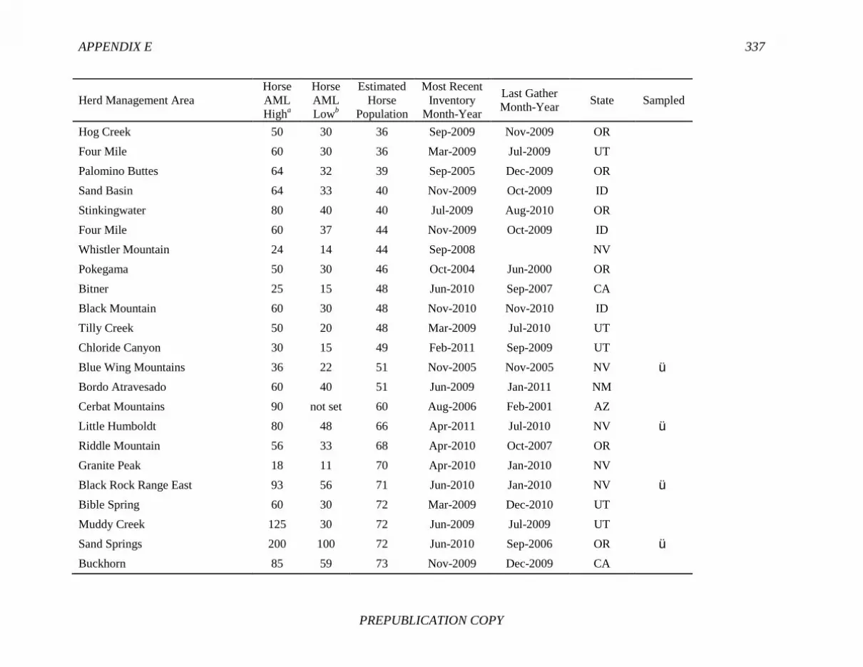
APPENDIX E 337
PREPUBLICATION COPY
Herd Management Area Horse AML Higha
Horse AML Lowb
Estimated Horse
Population
Most Recent Inventory
Month-Year Last Gather Month-Year State Sampled
Hog Creek 50 30 36 Sep-2009 Nov-2009 OR Four Mile 60 30 36 Mar-2009 Jul-2009 UT Palomino Buttes 64 32 39 Sep-2005 Dec-2009 OR Sand Basin 64 33 40 Nov-2009 Oct-2009 ID Stinkingwater 80 40 40 Jul-2009 Aug-2010 OR Four Mile 60 37 44 Nov-2009 Oct-2009 ID Whistler Mountain 24 14 44 Sep-2008 NV Pokegama 50 30 46 Oct-2004 Jun-2000 OR Bitner 25 15 48 Jun-2010 Sep-2007 CA Black Mountain 60 30 48 Nov-2010 Nov-2010 ID Tilly Creek 50 20 48 Mar-2009 Jul-2010 UT Chloride Canyon 30 15 49 Feb-2011 Sep-2009 UT Blue Wing Mountains 36 22 51 Nov-2005 Nov-2005 NV ü Bordo Atravesado 60 40 51 Jun-2009 Jan-2011 NM Cerbat Mountains 90 not set 60 Aug-2006 Feb-2001 AZ Little Humboldt 80 48 66 Apr-2011 Jul-2010 NV ü Riddle Mountain 56 33 68 Apr-2010 Oct-2007 OR Granite Peak 18 11 70 Apr-2010 Jan-2010 NV Black Rock Range East 93 56 71 Jun-2010 Jan-2010 NV ü Bible Spring 60 30 72 Mar-2009 Dec-2010 UT Muddy Creek 125 30 72 Jun-2009 Jul-2009 UT Sand Springs 200 100 72 Jun-2010 Sep-2006 OR ü Buckhorn 85 59 73 Nov-2009 Dec-2009 CA
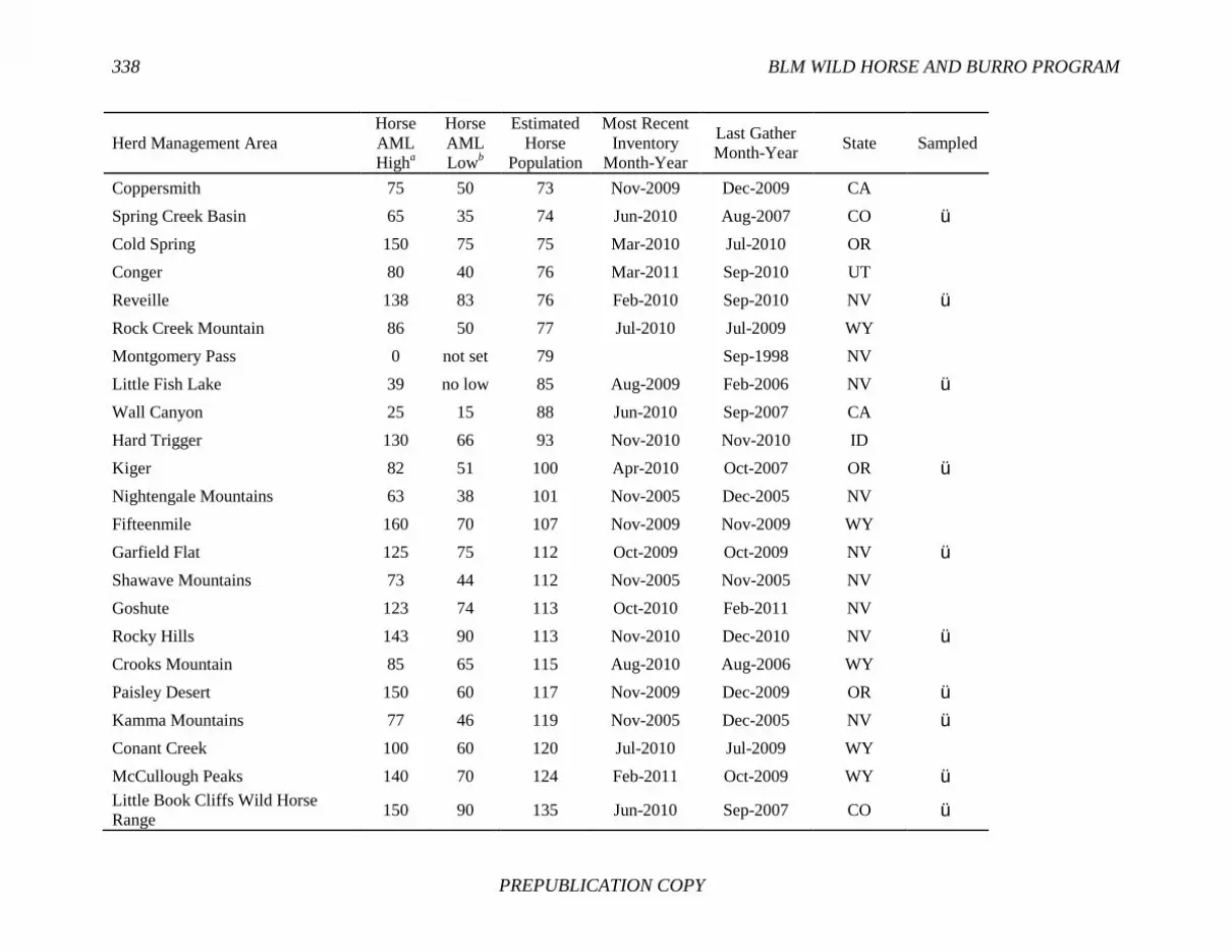
338 BLM WILD HORSE AND BURRO PROGRAM
PREPUBLICATION COPY
Herd Management Area Horse AML Higha
Horse AML Lowb
Estimated Horse
Population
Most Recent Inventory
Month-Year Last Gather Month-Year State Sampled
Coppersmith 75 50 73 Nov-2009 Dec-2009 CA Spring Creek Basin 65 35 74 Jun-2010 Aug-2007 CO ü Cold Spring 150 75 75 Mar-2010 Jul-2010 OR Conger 80 40 76 Mar-2011 Sep-2010 UT Reveille 138 83 76 Feb-2010 Sep-2010 NV ü Rock Creek Mountain 86 50 77 Jul-2010 Jul-2009 WY Montgomery Pass 0 not set 79 Sep-1998 NV Little Fish Lake 39 no low 85 Aug-2009 Feb-2006 NV ü Wall Canyon 25 15 88 Jun-2010 Sep-2007 CA Hard Trigger 130 66 93 Nov-2010 Nov-2010 ID Kiger 82 51 100 Apr-2010 Oct-2007 OR ü Nightengale Mountains 63 38 101 Nov-2005 Dec-2005 NV Fifteenmile 160 70 107 Nov-2009 Nov-2009 WY Garfield Flat 125 75 112 Oct-2009 Oct-2009 NV ü Shawave Mountains 73 44 112 Nov-2005 Nov-2005 NV Goshute 123 74 113 Oct-2010 Feb-2011 NV Rocky Hills 143 90 113 Nov-2010 Dec-2010 NV ü Crooks Mountain 85 65 115 Aug-2010 Aug-2006 WY Paisley Desert 150 60 117 Nov-2009 Dec-2009 OR ü Kamma Mountains 77 46 119 Nov-2005 Dec-2005 NV ü Conant Creek 100 60 120 Jul-2010 Jul-2009 WY McCullough Peaks 140 70 124 Feb-2011 Oct-2009 WY ü Little Book Cliffs Wild Horse Range 150 90 135 Jun-2010 Sep-2007 CO ü

APPENDIX E 339
PREPUBLICATION COPY
Herd Management Area Horse AML Higha
Horse AML Lowb
Estimated Horse
Population
Most Recent Inventory
Month-Year Last Gather Month-Year State Sampled
Bald Mountain 215 129 136 Nov-2010 Dec-2010 NV Frisco 60 12 140 Jan-2010 Aug-2006 UT Black Rock Range West 93 56 143 Jun-2010 Feb-2010 NV ü Diamond Hills North 37 22 145 Mar-2010 Jul-2004 NV Jackies Butte 150 75 147 Mar-2010 Oct-2007 OR ü Massacre Lakes 35 25 149 Jun-2010 Oct-1988 CA ü Range Creek 125 75 149 Feb-2010 Jul-2006 UT Dishpan Butte 100 50 155 Jul-2010 Jul-2009 WY Lost Creek 82 60 155 Aug-2010 Nov-2009 WY ü Confusion 115 70 157 Mar-2010 Sep-2010 UT Onaqui Mountain 210 121 159 Feb-2010 Oct-2009 UT Pryor Mountain Wild Horse Range 120 100 159 MT ü Granite Range 258 155 160 Jun-2010 Feb-2005 NV Antelope Hills 82 60 162 Aug-2010 Nov-2009 WY Seven Mile 50 no low 162 Sep-2007 Aug-2005 NV ü Fish Creek 180 108 163 Sep-2007 Feb-2006 NV Saulsbury 40 24 172 Aug-2009 Feb-2007 NV Owyhee 231 139 180 Apr-2011 Jul-2010 NV ü Pine Nut Mountains 179 118 182 Nov-2010 Dec-2010 NV Rock Creek 250 83 185 Apr-2011 Jul-2010 NV South Steens 304 159 191 Jul-2009 Nov-2009 OR ü Murderers Creek 35 13 198 Jan-2011 Feb-2011 OR Eagle 210 126 200 Oct-2010 Jan-2011 NV

340 BLM WILD HORSE AND BURRO PROGRAM
PREPUBLICATION COPY
Herd Management Area Horse AML Higha
Horse AML Lowb
Estimated Horse
Population
Most Recent Inventory
Month-Year Last Gather Month-Year State Sampled
Silver King 128 76 200 Sep-2010 Oct-2010 NV ü Diamond Hills South 22 no low 202 Mar-2010 Jul-2004 NV Coyote Lake/Alvord Tule Springs 390 198 212 Jun-2010 Nov-2008 OR North Stillwater 205 123 214 Jul-2008 Jul-2008 NV ü Nevada Wild Horse Range 500 300 216 Sep-2009 Jul-2008 NV Callaghan 237 147 221 Nov-2010 Jan-2011 NV South Shoshone 100 60 224 Oct-2009 Jan-2009 NV ü Antelope 324 194 239 Oct-2010 Feb-2011 NV Swasey 100 60 243 Mar-2011 Jul-2007 UT Diamond 151 91 244 Mar-2010 Jul-2004 NV ü Fox-Lake Range 204 122 244 Jul-2008 Jul-2008 NV Roberts Mountain 150 90 248 Sep-2008 Jan-2008 NV Augusta Mountains 308 185 256 Jan-2011 Feb-2011 NV ü Little Colorado 100 69 256 Apr-2010 Dec-2007 WY Three Fingers 150 75 261 Mar-2010 Aug-2006 OR Sulphur 250 165 267 Nov-2010 Dec-2010 UT ü Sand Wash Basin 362 163 270 Jun-2010 Oct-2008 CO Challis 253 185 270 Jul-2010 Dec-2009 ID ü Stewart Creek 175 125 275 Aug-2010 Nov-2009 WY ü Lava Beds 148 89 277 Nov-2005 Dec-2005 NV Flanigan 125 80 278 Apr-2010 Oct-2006 NV Sand Springs West 49 29 285 Apr-2008 Jan-2006 NV ü Sheepshead/Heath Creek 302 161 293 Jun-2010 Nov-2008 OR

APPENDIX E 341
PREPUBLICATION COPY
Herd Management Area Horse AML Higha
Horse AML Lowb
Estimated Horse
Population
Most Recent Inventory
Month-Year Last Gather Month-Year State Sampled
Salt Wells Creek 365 251 300 Sep-2010 Nov-2010 WY Piceance-East Douglas Creek 235 135 320 Mar-2010 Oct-2010 CO ü Snowstorm Mountains 140 90 320 Apr-2011 Oct-2006 NV Muskrat Basin 250 160 359 Jul-2010 Jul-2009 WY Cedar Mountain 390 190 362 Feb-2009 Dec-2008 UT ü Wassuk 165 109 362 Apr-2010 NV Centennial 168 134 366 May-2010 Oct-2010 CA New Pass-Ravenswood 566 no low 396 Nov-2010 Jan-2011 NV ü Pilot Mountain 415 249 402 Jan-2011 Jan-2005 NV Buffalo Hills 314 188 415 Jan-2009 Jan-2009 NV Beatys Butte 250 100 416 Nov-2009 Sep-2009 OR ü Spruce-Pequop 82 49 423 Oct-2010 Feb-2011 NV Calico Mountains 333 200 450 Jun-2010 Feb-2010 NV High Rock 120 78 458 Jun-2010 Sep-2006 CA ü Stone Cabin 364 218 476 Aug-2009 Feb-2007 NV Fox Hog 220 120 479 Jun-2010 Aug-2005 CA Green Mountain 300 170 490 Aug-2010 Oct-2009 WY ü Clan Alpine 979 619 503 Dec-2010 Oct-2006 NV Antelope Valley 259 155 519 Oct-2010 Feb-2011 NV Desatoya 180 127 520 Apr-2010 Feb-2004 NV ü Jackson Mountains 217 130 520 Sep-2007 Sep-2007 NV White Mountain 300 205 545 Apr-2010 Nov-2007 WY Maverick-Medicine 276 166 553 Nov-2010 Aug-2006 NV ü

342 BLM WILD HORSE AND BURRO PROGRAM
PREPUBLICATION COPY
Herd Management Area Horse AML Higha
Horse AML Lowb
Estimated Horse
Population
Most Recent Inventory
Month-Year Last Gather Month-Year State Sampled
Adobe Town 800 610 738 Sep-2010 Nov-2010 WY Little Owyhee 298 194 780 Apr-2011 Nov-2004 NV Triple B 518 312 1,217 Nov-2010 NV ü Pancake 493 296 1,291 Jan-2006 NV Divide Basin 600 415 1,355 Nov-2009 Sep-2007 WY aUpper bound of appropriate management level (AML). bLower bound of appropriate management level. NOTE: The following HMAs were removed from Table E-1: All HMAs with zero animals, AMLs of zero, or both; all HMAs with mixed burros and horses; and all burro-only HMAs. All remaining HMAs were numerically ordered by most recent population-size estimate. All HMAs with fewer than 50 horses were excluded. Every third HMA was systematically selected, resulting in 36 HMAs. Four additional HMAs that were used in Eberhardt et al. (1982) and Garrott et al. (1991a) were added to total 40 HMAs sampled. SOURCE: Spreadsheet and survey request based on information provided to the committee by the Bureau of Land Management in December 2011. Referenced articles are included in Chapter 4.

APPENDIX E 343
PREPUBLICATION COPY
TABLE E-3 Surveyed Horse Herd Management Areas Sorted by Population-Size Estimate
Herd Management Area Horse AML Higha
Horse AML Lowb
Estimated Horse
Population
Most Recent Inventory
Month-Year Last Gather Month-Year State
Blue Wing Mountains 36 22 51 Nov-2005 Nov-2005 NV Little Humboldt 80 48 66 Apr-2011 Jul-2010 NV Black Rock Range East 93 56 71 Jun-2010 Jan-2010 NV Sand Springs 200 100 72 Jun-2010 Sep-2006 OR Spring Creek Basin 65 35 74 Jun-2010 Aug-2007 CO Reveille 138 83 76 Feb-2010 Sep-2010 NV Little Fish Lake 39 no low 85 Aug-2009 Feb-2006 NV Kiger 82 51 100 Apr-2010 Oct-2007 OR Garfield Flat 125 75 112 Oct-2009 Oct-2009 NV Rocky Hills 143 90 113 Nov-2010 Dec-2010 NV Paisley Desert 150 60 117 Nov-2009 Dec-2009 OR Kamma Mountains 77 46 119 Nov-2005 Dec-2005 NV McCullough Peaks 140 70 124 Feb-2011 Oct-2009 WY Little Book Cliffs Wild Horse Range 150 90 135 Jun-2010 Sep-2007 CO Black Rock Range West 93 56 143 Jun-2010 Feb-2010 NV Jackies Butte 150 75 147 Mar-2010 Oct-2007 OR Massacre Lakes 35 25 149 Jun-2010 Oct-1988 CA Lost Creek 82 60 155 Aug-2010 Nov-2009 WY Pryor Mountain Wilde Horse Range 120 100 159 MT Seven Mile 50 no low 162 Sep-2007 Aug-2005 NV Owyhee 231 139 180 Apr-2011 Jul-2010 NV South Steens 304 159 191 Jul-2009 Nov-2009 OR

344 BLM WILD HORSE AND BURRO PROGRAM
PREPUBLICATION COPY
Herd Management Area Horse AML Higha
Horse AML Lowb
Estimated Horse
Population
Most Recent Inventory
Month-Year Last Gather Month-Year State
Silver King 128 76 200 Sep-2010 Oct-2010 NV North Stillwater 205 123 214 Jul-2008 Jul-2008 NV South Shoshone 100 60 224 Oct-2009 Jan-2009 NV Diamond 151 91 244 Mar-2010 Jul-2004 NV Augusta Mountains 308 185 256 Jan-2011 Feb-2011 NV Sulphur 250 165 267 Nov-2010 Dec-2010 UT Challis 253 185 270 Jul-2010 Dec-2009 ID Stewart Creek 175 125 275 Aug-2010 Nov-2009 WY Sand Springs West 49 29 285 Apr-2008 Jan-2006 NV Piceance-East Douglas Creek 235 135 320 Mar-2010 Oct-2010 CO Cedar Mountain 390 190 362 Feb-2009 Dec-2008 UT New Pass-Ravenswood 566 no low 396 Nov-2010 Jan-2011 NV Beatys Butte 250 100 416 Nov-2009 Sep-2009 OR High Rock 120 78 458 Jun-2010 Sep-2006 CA Green Mountain 300 170 490 Aug-2010 Oct-2009 WY Desatoya 180 127 520 Apr-2010 Feb-2004 NV Maverick-Medicine 276 166 553 Nov-2010 Aug-2006 NV Triple B 518 312 1,217 Nov-2010 NV
aUpper bound of appropriate management level (AML). bLower bound of appropriate management level. SOURCE: Spreadsheet and survey request based on information provided to the committee by the Bureau of Land Management in December 2011.

345 PREPUBLICATION COPY
Appendix F
Pairwise Values of Genetic Distance (Fst)

346 BLM WILD HORSE AND BURRO PROGRAM
PREPUBLICATION COPY
TABLE F-1 Pairwise Values of Genetic Distance (Fst) Between Burro Herd Management Areas Based on 12 Polymorphic Microsatellite DNA Loci
ki rc pa bv sv lf cm co sr ce si yu ci pm bw Kingman, AZ ki 0.000 Picacho, CA rc 0.094 0.000 Pannaments, CA pa 0.070 0.105 0.000 Butte Valley, CA bv 0.063 0.102 0.040 0.000 Saline Valley, CA sv 0.070 0.118 0.052 0.048 0.000 Lee Flats, CA lf 0.155 0.072 0.180 0.155 0.191 0.000 Clark Mtn., CA cm 0.101 0.078 0.064 0.064 0.079 0.150 0.000 Chocolate Mule, CA co 0.096 0.010 0.095 0.093 0.118 0.064 0.087 0.000 Slate Range, CA sr 0.055 0.078 0.036 0.035 0.033 0.143 0.049 0.087 0.000 Centennial, CA ce 0.075 0.113 0.067 0.064 0.044 0.185 0.081 0.116 0.018 0.000 Sinbad, UT si 0.093 0.078 0.110 0.097 0.115 0.158 0.108 0.069 0.087 0.136 0.000 Yuma 1, AZ yu 0.066 0.061 0.089 0.066 0.091 0.119 0.082 0.050 0.058 0.100 0.047 0.000 Chemehuevi, CA ci 0.147 0.116 0.119 0.129 0.138 0.126 0.125 0.114 0.108 0.147 0.148 0.113 0.000 Park Moab, CA pm 0.241 0.246 0.223 0.220 0.229 0.259 0.222 0.239 0.210 0.240 0.291 0.236 0.091 0.000 Blue Wing, NV bw 0.251 0.227 0.257 0.241 0.247 0.354 0.219 0.251 0.222 0.246 0.234 0.209 0.240 0.294 0.000 Seven Tanks, NV st 0.168 0.147 0.194 0.163 0.159 0.219 0.123 0.157 0.137 0.159 0.176 0.124 0.220 0.293 0.161 Ed's Camp, AZ ec 0.152 0.165 0.173 0.145 0.144 0.227 0.151 0.175 0.126 0.143 0.167 0.126 0.166 0.202 0.103 Cibola-Trigo 2, AZ ct 0.065 0.076 0.091 0.070 0.088 0.124 0.084 0.068 0.060 0.094 0.054 0.030 0.117 0.231 0.188 Big Sandy, NV bs 0.062 0.067 0.054 0.054 0.060 0.123 0.061 0.067 0.047 0.080 0.061 0.057 0.113 0.217 0.185 Havasu, AZ hv 0.170 0.168 0.174 0.166 0.181 0.218 0.173 0.173 0.150 0.181 0.185 0.158 0.114 0.104 0.140 Cibola-Trigo 2, AZ k2 0.185 0.200 0.180 0.174 0.189 0.257 0.180 0.203 0.159 0.193 0.199 0.166 0.125 0.107 0.139 East Mohave, CA em 0.173 0.208 0.175 0.167 0.162 0.262 0.204 0.213 0.160 0.179 0.197 0.180 0.163 0.141 0.150 Montezuma, CA mz 0.405 0.398 0.416 0.389 0.451 0.539 0.397 0.374 0.373 0.424 0.409 0.329 0.262 0.355 0.470 Twin Peaks, CA tp 0.210 0.210 0.235 0.211 0.199 0.250 0.223 0.214 0.188 0.204 0.191 0.173 0.154 0.142 0.171 Bullfrog, NV bf 0.220 0.281 0.255 0.229 0.241 0.321 0.269 0.272 0.219 0.238 0.242 0.188 0.198 0.184 0.224
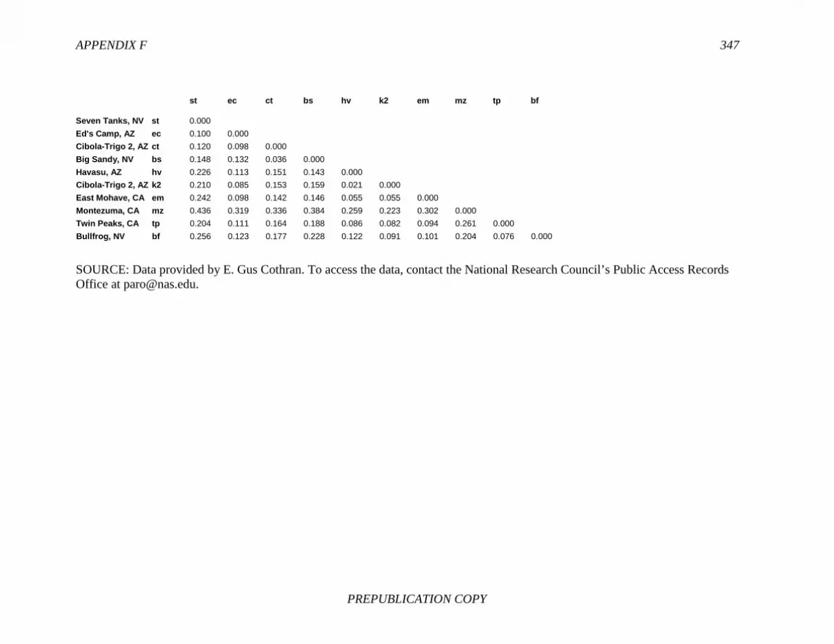
APPENDIX F 347
PREPUBLICATION COPY
st ec ct bs hv k2 em mz tp bf
Seven Tanks, NV st 0.000 Ed's Camp, AZ ec 0.100 0.000 Cibola-Trigo 2, AZ ct 0.120 0.098 0.000 Big Sandy, NV bs 0.148 0.132 0.036 0.000 Havasu, AZ hv 0.226 0.113 0.151 0.143 0.000 Cibola-Trigo 2, AZ k2 0.210 0.085 0.153 0.159 0.021 0.000 East Mohave, CA em 0.242 0.098 0.142 0.146 0.055 0.055 0.000 Montezuma, CA mz 0.436 0.319 0.336 0.384 0.259 0.223 0.302 0.000 Twin Peaks, CA tp 0.204 0.111 0.164 0.188 0.086 0.082 0.094 0.261 0.000 Bullfrog, NV bf 0.256 0.123 0.177 0.228 0.122 0.091 0.101 0.204 0.076 0.000
SOURCE: Data provided by E. Gus Cothran. To access the data, contact the National Research Council’s Public Access Records Office at [email protected].

348 BLM WILD HORSE AND BURRO PROGRAM
PREPUBLICATION COPY
TABLE F-2 Pairwise Values of Genetic Distance (Fst) Values Between Horse Herd Management Areas Based on 12 Polymorphic Microsatellite DNA Loci
Cibola-Trigo, AZ Painted
Rock, AZ Bitner, CA
(2011) Buckhorn, CA Buckhorn, CA
(2010) Carter
Reservoir, CA Centennial, CA
Cibola-Trigo, AZ 0.000
Painted Rock, AZ 0.249 0.000
Bitner, CA (2011) 0.149 0.147 0.000
Buckhorn, CA 0.144 0.129 0.035 0.000
Buckhorn, CA (2010) 0.141 0.134 0.035 0.009 0.000
Carter Reservoir, CA 0.142 0.099 0.064 0.053 0.060 0.000
Centennial, CA 0.134 0.158 0.058 0.048 0.039 0.071 0.000
Coppersmith, CA 0.159 0.170 0.061 0.057 0.054 0.093 0.053
Fox Hog, CA (2011) 0.123 0.144 0.041 0.028 0.023 0.063 0.040
High Rock, CA 0.103 0.120 0.037 0.027 0.023 0.046 0.033
Nut Mountain, CA (2011) 0.122 0.123 0.033 0.035 0.032 0.044 0.044
Santa Cruz Island, CA 0.161 0.212 0.153 0.108 0.104 0.149 0.143
Twin Peaks, CA 0.121 0.122 0.037 0.015 0.014 0.048 0.033
Twin Peaks, CA (All, 2011) 0.120 0.135 0.029 0.022 0.023 0.046 0.029
Twin Peaks, CA (Gilman SP) 0.129 0.141 0.039 0.031 0.032 0.053 0.029
Twin Peaks, CA (S Observa) 0.131 0.136 0.032 0.022 0.022 0.048 0.035
Twin Peaks, CA (Skeddle) 0.116 0.149 0.037 0.036 0.037 0.056 0.035
Wall Canyon, CA (2011) 0.111 0.137 0.053 0.048 0.044 0.057 0.052
Barcus Creek, CO 0.161 0.152 0.065 0.059 0.057 0.075 0.069
East Douglas, CO 0.178 0.137 0.084 0.076 0.078 0.081 0.090
Little Book Cliffs, CO 0.149 0.130 0.048 0.040 0.038 0.055 0.046
Mesa, CO 0.135 0.147 0.047 0.041 0.037 0.063 0.033
Sand Wash, CO 0.162 0.138 0.044 0.041 0.038 0.048 0.050
Spring Creek, CO 0.161 0.141 0.083 0.065 0.060 0.082 0.072
Spring Creek Basin, CO 0.161 0.150 0.074 0.063 0.059 0.079 0.069
West Douglas, CO 0.140 0.166 0.083 0.062 0.061 0.091 0.077

APPENDIX F 349
PREPUBLICATION COPY
Cibola-Trigo, AZ Painted
Rock, AZ Bitner, CA
(2011) Buckhorn, CA Buckhorn, CA
(2010) Carter
Reservoir, CA Centennial, CA
West Douglas, CO (2006) 0.134 0.173 0.096 0.069 0.067 0.099 0.077
Black Mountain, ID 0.163 0.145 0.060 0.068 0.069 0.084 0.074
Black Mountain, ID (2010) 0.156 0.133 0.052 0.055 0.053 0.070 0.060
Challis, ID 0.142 0.139 0.050 0.037 0.039 0.061 0.056
Hard Trigger, ID 0.141 0.138 0.046 0.046 0.040 0.060 0.055
Hard Trigger, ID (2010) 0.156 0.142 0.046 0.049 0.044 0.061 0.060
Idaho, ID (BLM) 0.153 0.169 0.051 0.052 0.046 0.083 0.053
Sand Basin, ID 0.127 0.158 0.046 0.043 0.039 0.065 0.050
Saylor Creek, ID 0.154 0.136 0.037 0.037 0.037 0.063 0.058
Pryor Mountains, MT (2001) 0.146 0.175 0.077 0.072 0.069 0.088 0.078
Pryor Mountains, MT (2009) 0.121 0.140 0.049 0.040 0.038 0.058 0.055
Bordo Atravisado, NM 0.152 0.158 0.052 0.041 0.040 0.065 0.043
El Rito, NM 0.147 0.137 0.049 0.033 0.028 0.060 0.038
Jicarilla, NM 0.137 0.135 0.050 0.034 0.034 0.064 0.052
Jarita, NM 0.169 0.129 0.079 0.056 0.047 0.089 0.064
Jicarilla, NM 0.210 0.138 0.090 0.063 0.050 0.111 0.073
Antelope Valley, NV 0.138 0.135 0.046 0.030 0.032 0.053 0.045
Antelope Valley, NV (2011) 0.145 0.129 0.048 0.034 0.037 0.053 0.042
Augusta Mountains, NV 0.128 0.125 0.051 0.036 0.038 0.057 0.042
Bald Mountain, NV 0.116 0.121 0.039 0.023 0.023 0.044 0.040
Black Rock East, NV (2005) 0.145 0.148 0.050 0.051 0.048 0.066 0.066
Black Rock East, NV (2010) 0.131 0.138 0.049 0.046 0.042 0.065 0.058
Black Rock East, NV (2011) 0.140 0.123 0.053 0.041 0.039 0.060 0.047
Black Rock West, NV (2005) 0.110 0.153 0.046 0.050 0.045 0.067 0.058
Black Rock West, NV (2010) 0.113 0.159 0.047 0.050 0.043 0.073 0.053
Black Rock West, NV (2011) 0.129 0.177 0.064 0.072 0.061 0.094 0.052
Buffalo Hills, NV 0.174 0.151 0.051 0.039 0.037 0.071 0.065
Buffalo Hills, NV (2009) 0.152 0.137 0.045 0.027 0.026 0.057 0.053
Calico, NV 0.120 0.136 0.035 0.024 0.020 0.052 0.035

350 BLM WILD HORSE AND BURRO PROGRAM
PREPUBLICATION COPY
Cibola-Trigo, AZ Painted
Rock, AZ Bitner, CA
(2011) Buckhorn, CA Buckhorn, CA
(2010) Carter
Reservoir, CA Centennial, CA
Calico Mountains, NV 0.148 0.140 0.042 0.033 0.033 0.068 0.057
Calico Mountains, NV (2011) 0.134 0.141 0.034 0.029 0.025 0.058 0.037
Callaghan, NV (Austin Allot) 0.134 0.110 0.047 0.024 0.024 0.047 0.040
Callaghan, NV (East Allot) 0.118 0.118 0.041 0.025 0.028 0.036 0.037
Catnip Herd, NV 0.143 0.155 0.051 0.044 0.039 0.078 0.059
Chimney Creek, NV 0.129 0.150 0.050 0.046 0.042 0.064 0.057
Desatoya Mountain, NV 0.154 0.155 0.090 0.060 0.066 0.095 0.088
Dolly Varden, NV 0.128 0.144 0.052 0.037 0.029 0.067 0.035
Dry Lake, NV 0.161 0.147 0.062 0.034 0.039 0.080 0.057
Fish Creek, NV 0.135 0.124 0.055 0.039 0.039 0.061 0.044
Goshute, NV 0.167 0.172 0.067 0.047 0.046 0.078 0.046
Goshute, NV (2011) 0.150 0.155 0.062 0.049 0.049 0.069 0.047
Granite, NV 0.127 0.140 0.041 0.027 0.027 0.050 0.038
Granite Range, NV 0.125 0.145 0.044 0.030 0.025 0.052 0.042
Granite Range, NV (2011) 0.126 0.137 0.043 0.025 0.021 0.052 0.031
Grass Valley, NV 0.123 0.119 0.052 0.029 0.030 0.050 0.044
Hall Creek, NV 0.149 0.112 0.051 0.024 0.025 0.055 0.042
Jakes Wash, NV 0.161 0.151 0.078 0.060 0.066 0.081 0.083
Johnnie, NV 0.154 0.118 0.077 0.054 0.058 0.072 0.071
Lahanton Reservoir, NV 0.159 0.169 0.068 0.062 0.056 0.086 0.058
Little Fish Lake, NV 0.159 0.134 0.066 0.051 0.054 0.061 0.044
Little Highrock Canyon, NV 0.148 0.163 0.044 0.039 0.027 0.083 0.042
Little Humboldt, NV 0.168 0.128 0.057 0.045 0.050 0.061 0.068
Little Humboldt, NV (2010) 0.145 0.120 0.043 0.032 0.036 0.052 0.048
Little Owyhee, NV (Fairbanks) 0.156 0.123 0.072 0.043 0.045 0.065 0.054
Little Owyhee, NV (Lake Creek) 0.155 0.129 0.055 0.040 0.035 0.062 0.056
Little Owyhee, NV (Twin Valley) 0.105 0.140 0.057 0.038 0.035 0.065 0.048
Marvel Gap, NV (SWC 2010) 0.140 0.137 0.035 0.033 0.030 0.060 0.049
McGee Mountain, NV 0.121 0.133 0.041 0.032 0.038 0.054 0.050
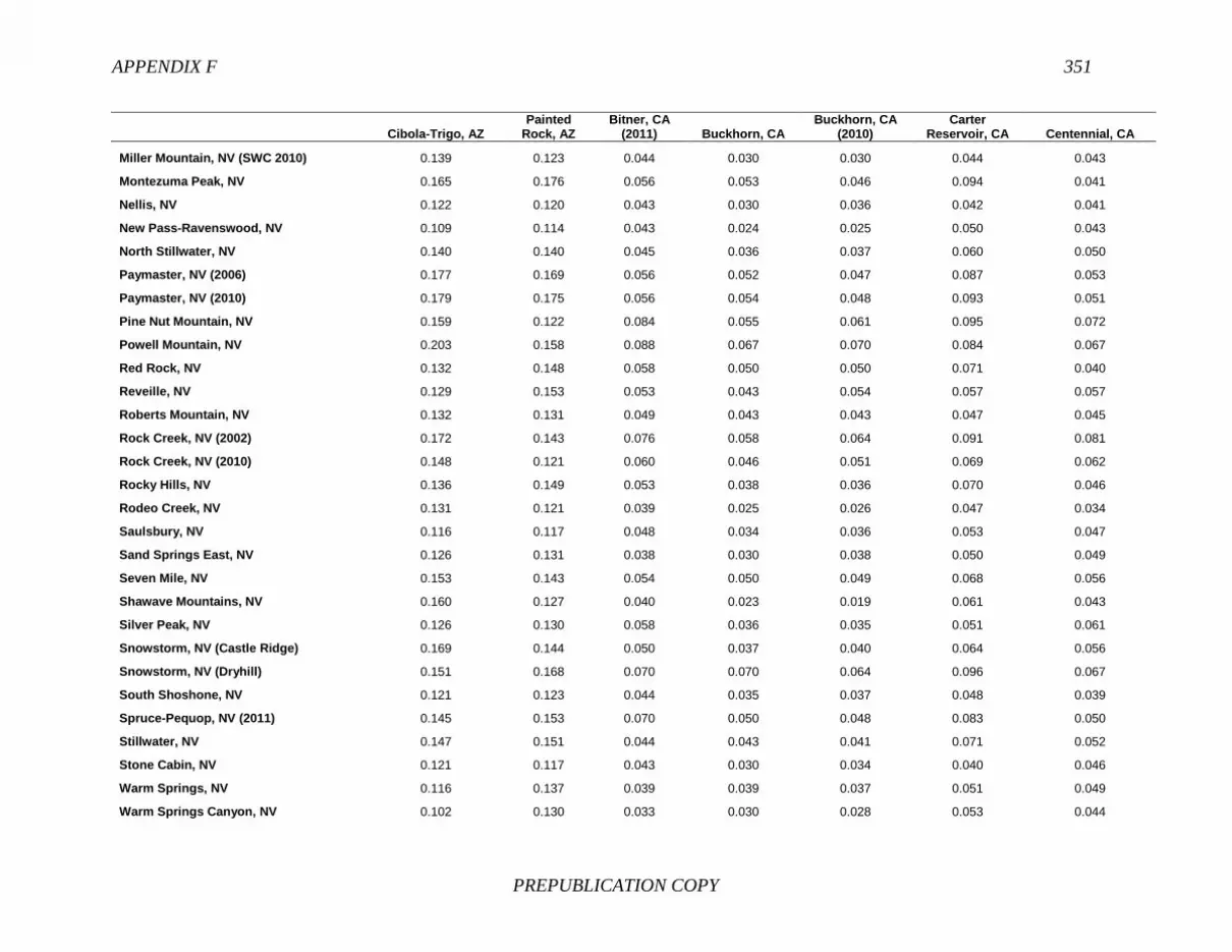
APPENDIX F 351
PREPUBLICATION COPY
Cibola-Trigo, AZ Painted
Rock, AZ Bitner, CA
(2011) Buckhorn, CA Buckhorn, CA
(2010) Carter
Reservoir, CA Centennial, CA
Miller Mountain, NV (SWC 2010) 0.139 0.123 0.044 0.030 0.030 0.044 0.043
Montezuma Peak, NV 0.165 0.176 0.056 0.053 0.046 0.094 0.041
Nellis, NV 0.122 0.120 0.043 0.030 0.036 0.042 0.041
New Pass-Ravenswood, NV 0.109 0.114 0.043 0.024 0.025 0.050 0.043
North Stillwater, NV 0.140 0.140 0.045 0.036 0.037 0.060 0.050
Paymaster, NV (2006) 0.177 0.169 0.056 0.052 0.047 0.087 0.053
Paymaster, NV (2010) 0.179 0.175 0.056 0.054 0.048 0.093 0.051
Pine Nut Mountain, NV 0.159 0.122 0.084 0.055 0.061 0.095 0.072
Powell Mountain, NV 0.203 0.158 0.088 0.067 0.070 0.084 0.067
Red Rock, NV 0.132 0.148 0.058 0.050 0.050 0.071 0.040
Reveille, NV 0.129 0.153 0.053 0.043 0.054 0.057 0.057
Roberts Mountain, NV 0.132 0.131 0.049 0.043 0.043 0.047 0.045
Rock Creek, NV (2002) 0.172 0.143 0.076 0.058 0.064 0.091 0.081
Rock Creek, NV (2010) 0.148 0.121 0.060 0.046 0.051 0.069 0.062
Rocky Hills, NV 0.136 0.149 0.053 0.038 0.036 0.070 0.046
Rodeo Creek, NV 0.131 0.121 0.039 0.025 0.026 0.047 0.034
Saulsbury, NV 0.116 0.117 0.048 0.034 0.036 0.053 0.047
Sand Springs East, NV 0.126 0.131 0.038 0.030 0.038 0.050 0.049
Seven Mile, NV 0.153 0.143 0.054 0.050 0.049 0.068 0.056
Shawave Mountains, NV 0.160 0.127 0.040 0.023 0.019 0.061 0.043
Silver Peak, NV 0.126 0.130 0.058 0.036 0.035 0.051 0.061
Snowstorm, NV (Castle Ridge) 0.169 0.144 0.050 0.037 0.040 0.064 0.056
Snowstorm, NV (Dryhill) 0.151 0.168 0.070 0.070 0.064 0.096 0.067
South Shoshone, NV 0.121 0.123 0.044 0.035 0.037 0.048 0.039
Spruce-Pequop, NV (2011) 0.145 0.153 0.070 0.050 0.048 0.083 0.050
Stillwater, NV 0.147 0.151 0.044 0.043 0.041 0.071 0.052
Stone Cabin, NV 0.121 0.117 0.043 0.030 0.034 0.040 0.046
Warm Springs, NV 0.116 0.137 0.039 0.039 0.037 0.051 0.049
Warm Springs Canyon, NV 0.102 0.130 0.033 0.030 0.028 0.053 0.044

352 BLM WILD HORSE AND BURRO PROGRAM
PREPUBLICATION COPY
Cibola-Trigo, AZ Painted
Rock, AZ Bitner, CA
(2011) Buckhorn, CA Buckhorn, CA
(2010) Carter
Reservoir, CA Centennial, CA
Wheeler Pass, NV 0.156 0.141 0.091 0.070 0.074 0.084 0.078
Wheeler Pass, NV (2007) 0.141 0.120 0.050 0.036 0.036 0.056 0.042
Alvord Tule, OR 0.119 0.136 0.059 0.040 0.040 0.056 0.061
Beatys Butte, OR 0.126 0.129 0.039 0.026 0.023 0.046 0.035
Beatys Butte, OR (2010) 0.145 0.133 0.036 0.026 0.020 0.051 0.031
Big Summit, OR (2010) 0.220 0.215 0.129 0.092 0.102 0.121 0.128
Cold Spring, OR 0.119 0.128 0.055 0.038 0.035 0.061 0.044
Cold Spring, OR (2010) 0.140 0.140 0.061 0.041 0.039 0.069 0.048
Coyote Lake, OR 0.125 0.132 0.067 0.043 0.047 0.052 0.062
Coyote Lake, OR (2011) 0.126 0.128 0.051 0.032 0.036 0.049 0.052
Fishnet, OR 0.140 0.147 0.045 0.041 0.041 0.065 0.050
Hog Creek, OR 0.124 0.127 0.060 0.031 0.036 0.059 0.040
Jackies Butte, OR 0.140 0.143 0.062 0.055 0.055 0.074 0.050
Jackies Butte, OR (2011) 0.118 0.140 0.045 0.042 0.041 0.068 0.041
Kiger, OR (2011) 0.163 0.133 0.055 0.039 0.038 0.062 0.060
Kiger Herd, OR (2009) 0.153 0.120 0.058 0.045 0.047 0.052 0.070
Liggett Table, OR 0.196 0.298 0.173 0.164 0.149 0.205 0.157
Murderers Creek, OR (2001) 0.197 0.128 0.088 0.079 0.076 0.091 0.094
Murderers Creek, OR (2009) 0.183 0.122 0.080 0.067 0.063 0.077 0.082
Paisley Desert, OR 0.119 0.119 0.036 0.026 0.029 0.041 0.038
Riddle Herd, OR (2009) 0.150 0.149 0.061 0.051 0.046 0.074 0.073
Riddle Mountain, OR 0.155 0.149 0.063 0.050 0.043 0.079 0.073
Riddle Mountain, OR (2011) 0.149 0.148 0.067 0.058 0.053 0.076 0.080
Sand Springs, OR (2011) 0.145 0.133 0.050 0.025 0.029 0.056 0.055
Sheepshead, OR 0.144 0.104 0.054 0.036 0.036 0.044 0.051
Sheepshead, OR (2011) 0.142 0.115 0.049 0.032 0.032 0.051 0.048
South Steens, OR 0.118 0.118 0.046 0.031 0.029 0.051 0.045
South Steens, OR (2010) 0.125 0.122 0.045 0.032 0.029 0.054 0.034
Stinkingwater, OR 0.151 0.152 0.075 0.065 0.065 0.082 0.066

APPENDIX F 353
PREPUBLICATION COPY
Cibola-Trigo, AZ Painted
Rock, AZ Bitner, CA
(2011) Buckhorn, CA Buckhorn, CA
(2010) Carter
Reservoir, CA Centennial, CA
Three Fingers, OR 0.159 0.143 0.047 0.050 0.045 0.069 0.063
Three Fingers, OR (2011) 0.140 0.132 0.048 0.047 0.046 0.065 0.058
Warm Springs, OR 0.117 0.121 0.038 0.033 0.034 0.057 0.046
Warm Springs, OR (2010) 0.111 0.121 0.040 0.033 0.031 0.056 0.044
Blawn Wash, UT 0.135 0.191 0.085 0.075 0.076 0.096 0.064
Cedar Mountain, UT 0.096 0.129 0.065 0.046 0.046 0.061 0.053
Cedar Ridge, UT 0.176 0.161 0.086 0.069 0.068 0.096 0.093
Cedar Ridge, UT (trap) 0.182 0.170 0.091 0.069 0.069 0.102 0.092
Cold Springs, UT (2006) 0.147 0.212 0.081 0.091 0.090 0.136 0.112
Cold Springs, UT (trap) 0.132 0.176 0.071 0.065 0.072 0.099 0.086
Delta, UT 0.136 0.107 0.048 0.027 0.031 0.042 0.042
Hill Creek, UT 0.141 0.128 0.048 0.033 0.034 0.056 0.052
Muddy Creek, UT 0.179 0.196 0.108 0.078 0.089 0.109 0.087
North Hills, UT 0.162 0.145 0.092 0.072 0.070 0.089 0.081
Range Creek, UT 0.127 0.149 0.051 0.046 0.045 0.080 0.069
Sinbad, UT 0.201 0.149 0.090 0.056 0.064 0.091 0.086
Sulphur, UT 0.212 0.185 0.118 0.100 0.101 0.104 0.097
Sulphur Herd, UT (South, 2006) 0.163 0.122 0.071 0.051 0.049 0.073 0.083
Tilley Creek, UT 0.199 0.211 0.076 0.070 0.066 0.103 0.070
Winter Ridge, UT 0.159 0.117 0.051 0.036 0.034 0.054 0.040
Adobe Town, WY 0.154 0.129 0.043 0.028 0.030 0.053 0.040
Adobe Town, WY (2011) 0.138 0.137 0.029 0.026 0.021 0.055 0.033
Antelope Hills, WY 0.144 0.135 0.057 0.038 0.037 0.062 0.062
Conant Creek, WY (Lander) 0.180 0.162 0.076 0.062 0.064 0.070 0.065
Cooper Creek, WY 0.134 0.120 0.053 0.034 0.038 0.049 0.046
Dishpan Butte, WY (Lander) 0.168 0.150 0.064 0.042 0.047 0.067 0.057
Divide Basin, WY 0.127 0.110 0.042 0.021 0.022 0.044 0.041
Divide Basin, WY (2011) 0.137 0.113 0.043 0.022 0.025 0.046 0.040
Eagles Nest, WY 0.159 0.143 0.078 0.050 0.054 0.062 0.072

354 BLM WILD HORSE AND BURRO PROGRAM
PREPUBLICATION COPY
Cibola-Trigo, AZ Painted
Rock, AZ Bitner, CA
(2011) Buckhorn, CA Buckhorn, CA
(2010) Carter
Reservoir, CA Centennial, CA
Happy Creek Springs, WY 0.169 0.152 0.068 0.046 0.052 0.071 0.077
Little Colorado, WY 0.130 0.139 0.050 0.042 0.037 0.066 0.050
Little Colorado, WY (2011) 0.130 0.134 0.047 0.039 0.033 0.064 0.043
Lost Creek, WY 0.126 0.107 0.054 0.027 0.028 0.045 0.045
Lost Creek, WY (combined) 0.127 0.115 0.054 0.027 0.030 0.048 0.046
McCullough Peaks, WY 0.151 0.128 0.058 0.040 0.041 0.060 0.064
Muskrat Basin, WY (Lander) 0.161 0.146 0.069 0.046 0.052 0.059 0.062
Salt Wells, WY (East) 0.116 0.134 0.040 0.030 0.027 0.051 0.029
Salt Wells, WY (West) 0.139 0.117 0.044 0.028 0.029 0.046 0.045
Stewart Creek, WY 0.132 0.115 0.064 0.038 0.039 0.051 0.063
Stewart Creek, WY (2009) 0.150 0.125 0.058 0.038 0.041 0.047 0.059
White Mountain, WY (2011) 0.160 0.147 0.049 0.039 0.033 0.060 0.028
Coppersmith, CA Fox Hog, CA
(2011) High Rock,
CA Nut Mountain,
CA (2011) Santa Cruz Island, CA Twin Peaks, CA
Twin Peaks, CA (All, 2011)
Coppersmith, CA 0.000
Fox Hog, CA (2011) 0.059 0.000
High Rock, CA 0.052 0.021 0.000
Nut Mountain, CA (2011) 0.060 0.031 0.013 0.000
Santa Cruz Island, CA 0.143 0.119 0.102 0.114 0.000
Twin Peaks, CA 0.041 0.021 0.018 0.024 0.095 0.000
Twin Peaks, CA (All, 2011) 0.042 0.027 0.019 0.025 0.109 0.009 0.000
Twin Peaks, CA (Gilman SP) 0.048 0.030 0.024 0.032 0.128 0.021 0.012
Twin Peaks, CA (S Observa) 0.047 0.031 0.024 0.029 0.110 0.010 0.003
Twin Peaks, CA (Skeddle) 0.048 0.034 0.025 0.031 0.116 0.020 0.006
Wall Canyon, CA (2011) 0.070 0.048 0.018 0.022 0.106 0.036 0.037
Barcus Creek, CO 0.078 0.057 0.054 0.066 0.152 0.051 0.043
East Douglas, CO 0.096 0.075 0.073 0.071 0.163 0.064 0.070
Little Book Cliffs, CO 0.059 0.043 0.033 0.044 0.121 0.028 0.024
Mesa, CO 0.044 0.040 0.033 0.042 0.116 0.024 0.019

APPENDIX F 355
PREPUBLICATION COPY
Coppersmith, CA Fox Hog, CA
(2011) High Rock,
CA Nut Mountain,
CA (2011) Santa Cruz Island, CA Twin Peaks, CA
Twin Peaks, CA (All, 2011)
Sand Wash, CO 0.064 0.037 0.040 0.043 0.151 0.034 0.030
Spring Creek, CO 0.085 0.059 0.042 0.050 0.115 0.052 0.059
Spring Creek Basin, CO 0.076 0.057 0.045 0.046 0.120 0.049 0.056
West Douglas, CO 0.093 0.063 0.051 0.063 0.117 0.050 0.054
West Douglas, CO (2006) 0.089 0.075 0.056 0.070 0.109 0.054 0.059
Black Mountain, ID 0.075 0.073 0.054 0.052 0.151 0.057 0.059
Black Mountain, ID (2010) 0.067 0.057 0.045 0.044 0.153 0.043 0.047
Challis, ID 0.071 0.035 0.034 0.033 0.102 0.028 0.030
Hard Trigger, ID 0.056 0.047 0.039 0.038 0.139 0.037 0.044
Hard Trigger, ID (2010) 0.059 0.053 0.042 0.036 0.148 0.042 0.048
Idaho, ID (BLM) 0.057 0.052 0.049 0.046 0.154 0.045 0.050
Sand Basin, ID 0.056 0.039 0.036 0.041 0.149 0.039 0.042
Saylor Creek, ID 0.064 0.046 0.039 0.036 0.144 0.032 0.035
Pryor Mountains, MT (2001) 0.092 0.062 0.056 0.059 0.145 0.061 0.063
Pryor Mountains, MT (2009) 0.073 0.034 0.031 0.037 0.123 0.034 0.036
Bordo Atravisado, NM 0.059 0.040 0.040 0.046 0.112 0.028 0.031
El Rito, NM 0.059 0.043 0.032 0.044 0.133 0.027 0.032
Jicarilla, NM 0.059 0.039 0.032 0.039 0.135 0.029 0.035
Jarita, NM 0.081 0.066 0.055 0.069 0.157 0.048 0.055
Jicarilla, NM 0.097 0.076 0.070 0.087 0.174 0.056 0.072
Antelope Valley, NV 0.060 0.037 0.035 0.038 0.101 0.026 0.028
Antelope Valley, NV (2011) 0.060 0.044 0.035 0.041 0.109 0.027 0.031
Augusta Mountains, NV 0.061 0.046 0.035 0.048 0.108 0.026 0.029
Bald Mountain, NV 0.050 0.032 0.023 0.030 0.098 0.014 0.016
Black Rock East, NV (2005) 0.072 0.059 0.041 0.040 0.113 0.032 0.031
Black Rock East, NV (2010) 0.064 0.052 0.036 0.038 0.104 0.028 0.029
Black Rock East, NV (2011) 0.061 0.047 0.034 0.040 0.111 0.025 0.028
Black Rock West, NV (2005) 0.067 0.049 0.028 0.027 0.106 0.033 0.034
Black Rock West, NV (2010) 0.068 0.048 0.030 0.031 0.102 0.031 0.031

356 BLM WILD HORSE AND BURRO PROGRAM
PREPUBLICATION COPY
Coppersmith, CA Fox Hog, CA
(2011) High Rock,
CA Nut Mountain,
CA (2011) Santa Cruz Island, CA Twin Peaks, CA
Twin Peaks, CA (All, 2011)
Black Rock West, NV (2011) 0.081 0.069 0.040 0.043 0.136 0.055 0.053
Buffalo Hills, NV 0.067 0.032 0.048 0.056 0.143 0.038 0.036
Buffalo Hills, NV (2009) 0.063 0.024 0.036 0.049 0.127 0.028 0.029
Calico, NV 0.052 0.008 0.016 0.026 0.111 0.015 0.018
Calico Mountains, NV 0.078 0.022 0.033 0.045 0.132 0.030 0.036
Calico Mountains, NV (2011) 0.067 0.013 0.019 0.030 0.136 0.024 0.023
Callaghan, NV (Austin Allot) 0.052 0.029 0.026 0.036 0.105 0.015 0.018
Callaghan, NV (East Allot) 0.047 0.033 0.022 0.029 0.104 0.017 0.016
Catnip Herd, NV 0.075 0.039 0.035 0.044 0.124 0.036 0.042
Chimney Creek, NV 0.055 0.033 0.032 0.042 0.128 0.033 0.035
Desatoya Mountain, NV 0.094 0.074 0.065 0.071 0.130 0.048 0.064
Dolly Varden, NV 0.057 0.037 0.029 0.036 0.104 0.025 0.031
Dry Lake, NV 0.061 0.034 0.041 0.053 0.137 0.027 0.032
Fish Creek, NV 0.057 0.035 0.028 0.039 0.123 0.021 0.027
Goshute, NV 0.067 0.049 0.046 0.052 0.137 0.034 0.041
Goshute, NV (2011) 0.064 0.048 0.040 0.046 0.133 0.034 0.038
Granite, NV 0.065 0.021 0.027 0.033 0.124 0.018 0.018
Granite Range, NV 0.066 0.019 0.028 0.037 0.118 0.020 0.022
Granite Range, NV (2011) 0.058 0.015 0.021 0.031 0.119 0.015 0.015
Grass Valley, NV 0.059 0.034 0.029 0.039 0.107 0.022 0.028
Hall Creek, NV 0.057 0.037 0.034 0.043 0.107 0.020 0.021
Jakes Wash, NV 0.099 0.073 0.058 0.068 0.136 0.051 0.050
Johnnie, NV 0.074 0.065 0.042 0.050 0.112 0.039 0.045
Lahanton Reservoir, NV 0.070 0.058 0.059 0.060 0.149 0.044 0.048
Little Fish Lake, NV 0.068 0.054 0.050 0.059 0.157 0.037 0.039
Little Highrock Canyon, NV 0.052 0.025 0.031 0.043 0.137 0.029 0.032
Little Humboldt, NV 0.071 0.064 0.060 0.056 0.143 0.040 0.043
Little Humboldt, NV (2010) 0.058 0.044 0.040 0.038 0.120 0.029 0.029
Little Owyhee, NV (Fairbanks) 0.087 0.046 0.045 0.063 0.130 0.041 0.041

APPENDIX F 357
PREPUBLICATION COPY
Coppersmith, CA Fox Hog, CA
(2011) High Rock,
CA Nut Mountain,
CA (2011) Santa Cruz Island, CA Twin Peaks, CA
Twin Peaks, CA (All, 2011)
Little Owyhee, NV (Lake Creek) 0.065 0.048 0.042 0.054 0.134 0.041 0.045
Little Owyhee, NV (Twin Valley) 0.062 0.038 0.031 0.035 0.115 0.028 0.032
Marvel Gap, NV (SWC 2010) 0.045 0.042 0.033 0.034 0.123 0.025 0.030
McGee Mountain, NV 0.065 0.038 0.032 0.034 0.119 0.027 0.027
Miller Mountain, NV (SWC 2010) 0.053 0.040 0.027 0.037 0.117 0.023 0.021
Montezuma Peak, NV 0.068 0.045 0.044 0.054 0.157 0.042 0.041
Nellis, NV 0.052 0.032 0.028 0.033 0.115 0.019 0.018
New Pass-Ravenswood, NV 0.048 0.027 0.023 0.030 0.090 0.013 0.018
North Stillwater, NV 0.063 0.037 0.030 0.047 0.124 0.034 0.031
Paymaster, NV (2006) 0.077 0.051 0.052 0.055 0.167 0.041 0.041
Paymaster, NV (2010) 0.074 0.044 0.052 0.056 0.167 0.042 0.041
Pine Nut Mountain, NV 0.086 0.063 0.051 0.067 0.140 0.046 0.054
Powell Mountain, NV 0.095 0.069 0.070 0.072 0.156 0.057 0.054
Red Rock, NV 0.068 0.053 0.044 0.052 0.131 0.033 0.033
Reveille, NV 0.067 0.056 0.049 0.054 0.128 0.038 0.029
Roberts Mountain, NV 0.067 0.047 0.032 0.042 0.136 0.031 0.031
Rock Creek, NV (2002) 0.088 0.075 0.055 0.053 0.137 0.051 0.054
Rock Creek, NV (2010) 0.070 0.061 0.044 0.042 0.119 0.038 0.040
Rocky Hills, NV 0.057 0.041 0.032 0.038 0.122 0.022 0.027
Rodeo Creek, NV 0.053 0.032 0.025 0.032 0.111 0.020 0.018
Saulsbury, NV 0.061 0.032 0.033 0.040 0.104 0.024 0.025
Sand Springs East, NV 0.064 0.038 0.033 0.034 0.123 0.027 0.026
Seven Mile, NV 0.073 0.043 0.041 0.045 0.149 0.040 0.045
Shawave Mountains, NV 0.058 0.030 0.031 0.040 0.113 0.022 0.029
Silver Peak, NV 0.073 0.041 0.033 0.045 0.123 0.029 0.030
Snowstorm, NV (Castle Ridge) 0.061 0.050 0.046 0.043 0.141 0.033 0.031
Snowstorm, NV (Dryhill) 0.065 0.062 0.056 0.063 0.153 0.062 0.055
South Shoshone, NV 0.051 0.040 0.028 0.034 0.122 0.023 0.025
Spruce-Pequop, NV (2011) 0.080 0.055 0.045 0.058 0.106 0.038 0.045

358 BLM WILD HORSE AND BURRO PROGRAM
PREPUBLICATION COPY
Coppersmith, CA Fox Hog, CA
(2011) High Rock,
CA Nut Mountain,
CA (2011) Santa Cruz Island, CA Twin Peaks, CA
Twin Peaks, CA (All, 2011)
Stillwater, NV 0.064 0.049 0.036 0.052 0.127 0.041 0.038
Stone Cabin, NV 0.058 0.035 0.028 0.033 0.117 0.023 0.023
Warm Springs, NV 0.063 0.041 0.020 0.021 0.120 0.029 0.025
Warm Springs Canyon, NV 0.056 0.030 0.014 0.022 0.098 0.021 0.021
Wheeler Pass, NV 0.087 0.082 0.057 0.066 0.136 0.053 0.055
Wheeler Pass, NV (2007) 0.055 0.042 0.031 0.041 0.122 0.023 0.025
Alvord Tule, OR 0.082 0.038 0.027 0.031 0.097 0.034 0.036
Beatys Butte, OR 0.052 0.028 0.026 0.033 0.112 0.016 0.019
Beatys Butte, OR (2010) 0.047 0.028 0.026 0.030 0.122 0.020 0.027
Big Summit, OR (2010) 0.125 0.117 0.110 0.116 0.182 0.093 0.103
Cold Spring, OR 0.056 0.038 0.029 0.042 0.098 0.021 0.025
Cold Spring, OR (2010) 0.055 0.046 0.036 0.047 0.110 0.025 0.029
Coyote Lake, OR 0.076 0.041 0.034 0.043 0.105 0.031 0.036
Coyote Lake, OR (2011) 0.062 0.031 0.026 0.031 0.098 0.022 0.025
Fishnet, OR 0.062 0.041 0.035 0.043 0.139 0.031 0.026
Hog Creek, OR 0.058 0.037 0.029 0.038 0.109 0.024 0.026
Jackies Butte, OR 0.063 0.044 0.040 0.043 0.126 0.040 0.037
Jackies Butte, OR (2011) 0.055 0.030 0.025 0.029 0.114 0.030 0.027
Kiger, OR (2011) 0.083 0.040 0.044 0.046 0.140 0.031 0.029
Kiger Herd, OR (2009) 0.086 0.044 0.042 0.045 0.134 0.036 0.034
Liggett Table, OR 0.179 0.157 0.131 0.139 0.219 0.142 0.148
Murderers Creek, OR (2001) 0.109 0.082 0.077 0.079 0.166 0.070 0.075
Murderers Creek, OR (2009) 0.098 0.059 0.066 0.071 0.161 0.056 0.062
Paisley Desert, OR 0.049 0.028 0.023 0.030 0.107 0.017 0.015
Riddle Herd, OR (2009) 0.095 0.052 0.047 0.047 0.134 0.040 0.038
Riddle Mountain, OR 0.093 0.054 0.046 0.045 0.126 0.036 0.039
Riddle Mountain, OR (2011) 0.102 0.060 0.053 0.054 0.148 0.046 0.044
Sand Springs, OR (2011) 0.069 0.031 0.032 0.040 0.117 0.021 0.028
Sheepshead, OR 0.073 0.036 0.030 0.037 0.119 0.024 0.032

APPENDIX F 359
PREPUBLICATION COPY
Coppersmith, CA Fox Hog, CA
(2011) High Rock,
CA Nut Mountain,
CA (2011) Santa Cruz Island, CA Twin Peaks, CA
Twin Peaks, CA (All, 2011)
Sheepshead, OR (2011) 0.059 0.038 0.029 0.036 0.114 0.019 0.023
South Steens, OR 0.053 0.031 0.020 0.028 0.098 0.023 0.027
South Steens, OR (2010) 0.055 0.024 0.019 0.029 0.114 0.025 0.026
Stinkingwater, OR 0.074 0.070 0.048 0.052 0.125 0.051 0.053
Three Fingers, OR 0.075 0.054 0.048 0.049 0.162 0.036 0.036
Three Fingers, OR (2011) 0.069 0.054 0.041 0.041 0.146 0.033 0.034
Warm Springs, OR 0.053 0.033 0.025 0.028 0.110 0.023 0.026
Warm Springs, OR (2010) 0.049 0.033 0.027 0.030 0.108 0.020 0.024
Blawn Wash, UT 0.092 0.066 0.058 0.069 0.158 0.060 0.051
Cedar Mountain, UT 0.070 0.041 0.035 0.049 0.109 0.034 0.034
Cedar Ridge, UT 0.104 0.067 0.067 0.066 0.155 0.059 0.064
Cedar Ridge, UT (trap) 0.107 0.074 0.071 0.074 0.146 0.067 0.068
Cold Springs, UT (2006) 0.104 0.076 0.080 0.087 0.168 0.084 0.091
Cold Springs, UT (trap) 0.088 0.062 0.060 0.066 0.130 0.062 0.062
Delta, UT 0.060 0.038 0.030 0.037 0.109 0.021 0.023
Hill Creek, UT 0.061 0.040 0.037 0.047 0.120 0.032 0.033
Muddy Creek, UT 0.110 0.087 0.085 0.100 0.158 0.071 0.070
North Hills, UT 0.082 0.077 0.077 0.077 0.147 0.053 0.066
Range Creek, UT 0.072 0.038 0.041 0.044 0.124 0.039 0.044
Sinbad, UT 0.110 0.066 0.064 0.071 0.150 0.055 0.064
Sulphur, UT 0.115 0.098 0.100 0.115 0.206 0.083 0.088
Sulphur Herd, UT (South, 2006) 0.081 0.058 0.055 0.063 0.132 0.043 0.052
Tilley Creek, UT 0.084 0.074 0.072 0.077 0.191 0.057 0.050
Winter Ridge, UT 0.055 0.039 0.033 0.041 0.136 0.029 0.034
Adobe Town, WY 0.053 0.047 0.036 0.040 0.121 0.027 0.028
Adobe Town, WY (2011) 0.040 0.030 0.027 0.031 0.119 0.021 0.022
Antelope Hills, WY 0.079 0.040 0.040 0.042 0.116 0.032 0.040
Conant Creek, WY (Lander) 0.095 0.070 0.051 0.068 0.169 0.055 0.045
Cooper Creek, WY 0.062 0.039 0.034 0.042 0.125 0.022 0.025

360 BLM WILD HORSE AND BURRO PROGRAM
PREPUBLICATION COPY
Coppersmith, CA Fox Hog, CA
(2011) High Rock,
CA Nut Mountain,
CA (2011) Santa Cruz Island, CA Twin Peaks, CA
Twin Peaks, CA (All, 2011)
Dishpan Butte, WY (Lander) 0.075 0.062 0.042 0.049 0.143 0.035 0.033
Divide Basin, WY 0.051 0.027 0.024 0.026 0.103 0.013 0.020
Divide Basin, WY (2011) 0.052 0.033 0.027 0.033 0.112 0.016 0.022
Eagles Nest, WY 0.085 0.068 0.050 0.057 0.129 0.047 0.053
Happy Creek Springs, WY 0.081 0.051 0.047 0.054 0.154 0.038 0.046
Little Colorado, WY 0.063 0.046 0.031 0.035 0.117 0.031 0.033
Little Colorado, WY (2011) 0.055 0.038 0.026 0.029 0.117 0.025 0.028
Lost Creek, WY 0.057 0.035 0.025 0.031 0.105 0.021 0.027
Lost Creek, WY (combined) 0.060 0.038 0.024 0.033 0.110 0.022 0.027
McCullough Peaks, WY 0.065 0.044 0.029 0.036 0.133 0.032 0.034
Muskrat Basin, WY (Lander) 0.082 0.064 0.047 0.054 0.136 0.038 0.037
Salt Wells, WY (East) 0.043 0.028 0.023 0.030 0.111 0.022 0.021
Salt Wells, WY (West) 0.059 0.041 0.033 0.041 0.110 0.020 0.020
Stewart Creek, WY 0.077 0.041 0.031 0.038 0.113 0.031 0.037
Stewart Creek, WY (2009) 0.072 0.048 0.037 0.039 0.133 0.032 0.036
White Mountain, WY (2011) 0.059 0.033 0.033 0.035 0.149 0.028 0.027
Twin Peaks, CA
(Gilman SP) Twin Peaks, CA
(S Observa) Twin Peaks, CA (Skeddle)
Wall Canyon, CA (2011)
Barcus Creek, CO
East Douglas, CO
Little Book Cliffs, CO
Twin Peaks, CA (Gilman SP) 0.000
Twin Peaks, CA (S Observa) 0.023 0.000
Twin Peaks, CA (Skeddle) 0.016 0.016 0.000
Wall Canyon, CA (2011) 0.043 0.042 0.043 0.000
Barcus Creek, CO 0.056 0.047 0.048 0.073 0.000
East Douglas, CO 0.073 0.073 0.079 0.077 0.094 0.000
Little Book Cliffs, CO 0.039 0.025 0.032 0.060 0.048 0.089 0.000
Mesa, CO 0.032 0.023 0.022 0.048 0.035 0.074 0.030
Sand Wash, CO 0.035 0.035 0.037 0.065 0.059 0.067 0.045
Spring Creek, CO 0.060 0.062 0.070 0.059 0.087 0.106 0.067
Spring Creek Basin, CO 0.059 0.058 0.067 0.060 0.087 0.099 0.071

APPENDIX F 361
PREPUBLICATION COPY
Twin Peaks, CA
(Gilman SP) Twin Peaks, CA
(S Observa) Twin Peaks, CA (Skeddle)
Wall Canyon, CA (2011)
Barcus Creek, CO
East Douglas, CO
Little Book Cliffs, CO
West Douglas, CO 0.052 0.062 0.059 0.067 0.096 0.076 0.076
West Douglas, CO (2006) 0.059 0.065 0.065 0.072 0.105 0.094 0.076
Black Mountain, ID 0.069 0.060 0.071 0.067 0.096 0.082 0.077
Black Mountain, ID (2010) 0.056 0.048 0.058 0.060 0.075 0.080 0.059
Challis, ID 0.041 0.032 0.039 0.044 0.066 0.070 0.047
Hard Trigger, ID 0.043 0.048 0.055 0.054 0.091 0.076 0.062
Hard Trigger, ID (2010) 0.051 0.053 0.057 0.056 0.090 0.080 0.066
Idaho, ID (BLM) 0.053 0.053 0.060 0.068 0.085 0.086 0.063
Sand Basin, ID 0.046 0.046 0.049 0.066 0.075 0.103 0.053
Saylor Creek, ID 0.039 0.039 0.044 0.052 0.070 0.060 0.059
Pryor Mountains, MT (2001) 0.063 0.071 0.065 0.070 0.094 0.079 0.067
Pryor Mountains, MT (2009) 0.035 0.044 0.040 0.049 0.073 0.075 0.058
Bordo Atravisado, NM 0.035 0.034 0.039 0.051 0.063 0.078 0.047
El Rito, NM 0.032 0.037 0.039 0.060 0.063 0.081 0.040
Jicarilla, NM 0.032 0.041 0.044 0.059 0.076 0.076 0.046
Jarita, NM 0.055 0.060 0.065 0.082 0.088 0.105 0.067
Jicarilla, NM 0.077 0.074 0.085 0.101 0.101 0.125 0.073
Antelope Valley, NV 0.039 0.031 0.036 0.057 0.059 0.086 0.035
Antelope Valley, NV (2011) 0.038 0.035 0.038 0.055 0.060 0.086 0.036
Augusta Mountains, NV 0.034 0.034 0.035 0.056 0.057 0.067 0.046
Bald Mountain, NV 0.025 0.020 0.020 0.036 0.046 0.063 0.030
Black Rock East, NV (2005) 0.047 0.033 0.038 0.038 0.071 0.074 0.059
Black Rock East, NV (2010) 0.040 0.031 0.036 0.035 0.068 0.071 0.056
Black Rock East, NV (2011) 0.034 0.031 0.036 0.039 0.065 0.057 0.052
Black Rock West, NV (2005) 0.045 0.038 0.038 0.021 0.078 0.074 0.066
Black Rock West, NV (2010) 0.046 0.035 0.034 0.027 0.073 0.081 0.061
Black Rock West, NV (2011) 0.061 0.060 0.054 0.033 0.102 0.118 0.083
Buffalo Hills, NV 0.043 0.041 0.043 0.074 0.050 0.102 0.048
Buffalo Hills, NV (2009) 0.031 0.034 0.037 0.063 0.048 0.081 0.040

362 BLM WILD HORSE AND BURRO PROGRAM
PREPUBLICATION COPY
Twin Peaks, CA
(Gilman SP) Twin Peaks, CA
(S Observa) Twin Peaks, CA (Skeddle)
Wall Canyon, CA (2011)
Barcus Creek, CO
East Douglas, CO
Little Book Cliffs, CO
Calico, NV 0.028 0.020 0.026 0.039 0.047 0.068 0.032
Calico Mountains, NV 0.039 0.039 0.046 0.062 0.059 0.080 0.049
Calico Mountains, NV (2011) 0.030 0.027 0.031 0.043 0.046 0.075 0.036
Callaghan, NV (Austin Allot) 0.022 0.022 0.025 0.046 0.048 0.055 0.038
Callaghan, NV (East Allot) 0.024 0.021 0.022 0.037 0.051 0.070 0.031
Catnip Herd, NV 0.044 0.049 0.046 0.053 0.070 0.074 0.070
Chimney Creek, NV 0.041 0.042 0.039 0.045 0.076 0.064 0.059
Desatoya Mountain, NV 0.064 0.070 0.071 0.078 0.114 0.079 0.093
Dolly Varden, NV 0.037 0.036 0.036 0.047 0.058 0.089 0.040
Dry Lake, NV 0.040 0.036 0.037 0.066 0.075 0.071 0.056
Fish Creek, NV 0.031 0.031 0.033 0.054 0.063 0.075 0.041
Goshute, NV 0.049 0.046 0.047 0.062 0.078 0.095 0.057
Goshute, NV (2011) 0.045 0.044 0.041 0.057 0.071 0.093 0.057
Granite, NV 0.026 0.020 0.027 0.044 0.048 0.073 0.038
Granite Range, NV 0.030 0.023 0.033 0.055 0.059 0.088 0.037
Granite Range, NV (2011) 0.024 0.018 0.023 0.047 0.044 0.080 0.030
Grass Valley, NV 0.029 0.033 0.034 0.046 0.057 0.067 0.045
Hall Creek, NV 0.028 0.024 0.030 0.051 0.053 0.056 0.042
Jakes Wash, NV 0.063 0.055 0.051 0.080 0.080 0.094 0.068
Johnnie, NV 0.047 0.048 0.056 0.054 0.078 0.081 0.050
Lahanton Reservoir, NV 0.058 0.054 0.051 0.078 0.098 0.089 0.076
Little Fish Lake, NV 0.037 0.046 0.046 0.068 0.076 0.077 0.059
Little Highrock Canyon, NV 0.042 0.034 0.041 0.063 0.067 0.095 0.038
Little Humboldt, NV 0.051 0.044 0.054 0.076 0.076 0.089 0.058
Little Humboldt, NV (2010) 0.041 0.030 0.040 0.062 0.067 0.070 0.042
Little Owyhee, NV (Fairbanks) 0.044 0.045 0.050 0.064 0.066 0.082 0.058
Little Owyhee, NV (Lake Creek) 0.044 0.049 0.054 0.061 0.078 0.080 0.057
Little Owyhee, NV (Twin Valley) 0.039 0.035 0.040 0.047 0.073 0.086 0.049
Marvel Gap, NV (SWC 2010) 0.032 0.034 0.039 0.051 0.053 0.064 0.045

APPENDIX F 363
PREPUBLICATION COPY
Twin Peaks, CA
(Gilman SP) Twin Peaks, CA
(S Observa) Twin Peaks, CA (Skeddle)
Wall Canyon, CA (2011)
Barcus Creek, CO
East Douglas, CO
Little Book Cliffs, CO
McGee Mountain, NV 0.031 0.032 0.034 0.043 0.066 0.065 0.052
Miller Mountain, NV (SWC 2010) 0.025 0.027 0.026 0.045 0.057 0.067 0.038
Montezuma Peak, NV 0.046 0.048 0.045 0.073 0.075 0.125 0.060
Nellis, NV 0.026 0.023 0.023 0.042 0.054 0.064 0.043
New Pass-Ravenswood, NV 0.031 0.021 0.025 0.038 0.058 0.056 0.038
North Stillwater, NV 0.034 0.038 0.035 0.059 0.051 0.092 0.038
Paymaster, NV (2006) 0.050 0.046 0.046 0.077 0.075 0.114 0.059
Paymaster, NV (2010) 0.049 0.047 0.044 0.079 0.074 0.115 0.063
Pine Nut Mountain, NV 0.064 0.057 0.062 0.076 0.082 0.097 0.061
Powell Mountain, NV 0.067 0.055 0.064 0.093 0.088 0.079 0.075
Red Rock, NV 0.036 0.038 0.039 0.059 0.060 0.101 0.040
Reveille, NV 0.036 0.034 0.033 0.060 0.084 0.080 0.057
Roberts Mountain, NV 0.039 0.035 0.039 0.048 0.054 0.068 0.046
Rock Creek, NV (2002) 0.070 0.054 0.066 0.080 0.092 0.096 0.066
Rock Creek, NV (2010) 0.050 0.043 0.049 0.065 0.073 0.073 0.057
Rocky Hills, NV 0.036 0.031 0.033 0.054 0.067 0.069 0.048
Rodeo Creek, NV 0.025 0.022 0.025 0.048 0.057 0.081 0.030
Saulsbury, NV 0.032 0.032 0.026 0.048 0.064 0.061 0.043
Sand Springs East, NV 0.030 0.030 0.033 0.045 0.065 0.065 0.050
Seven Mile, NV 0.045 0.052 0.050 0.062 0.073 0.081 0.056
Shawave Mountains, NV 0.034 0.030 0.040 0.051 0.063 0.071 0.039
Silver Peak, NV 0.039 0.035 0.035 0.056 0.058 0.089 0.050
Snowstorm, NV (Castle Ridge) 0.051 0.031 0.039 0.070 0.070 0.075 0.050
Snowstorm, NV (Dryhill) 0.064 0.060 0.060 0.076 0.072 0.126 0.075
South Shoshone, NV 0.031 0.030 0.033 0.046 0.052 0.070 0.038
Spruce-Pequop, NV (2011) 0.051 0.051 0.050 0.063 0.083 0.104 0.055
Stillwater, NV 0.043 0.044 0.041 0.066 0.068 0.105 0.045
Stone Cabin, NV 0.030 0.028 0.027 0.044 0.057 0.072 0.037
Warm Springs, NV 0.036 0.028 0.030 0.016 0.063 0.076 0.050

364 BLM WILD HORSE AND BURRO PROGRAM
PREPUBLICATION COPY
Twin Peaks, CA
(Gilman SP) Twin Peaks, CA
(S Observa) Twin Peaks, CA (Skeddle)
Wall Canyon, CA (2011)
Barcus Creek, CO
East Douglas, CO
Little Book Cliffs, CO
Warm Springs Canyon, NV 0.027 0.027 0.026 0.018 0.065 0.071 0.043
Wheeler Pass, NV 0.054 0.062 0.061 0.076 0.092 0.111 0.066
Wheeler Pass, NV (2007) 0.030 0.028 0.035 0.050 0.048 0.067 0.035
Alvord Tule, OR 0.042 0.039 0.043 0.041 0.053 0.067 0.053
Beatys Butte, OR 0.026 0.024 0.024 0.044 0.057 0.059 0.038
Beatys Butte, OR (2010) 0.029 0.031 0.034 0.039 0.065 0.064 0.043
Big Summit, OR (2010) 0.112 0.104 0.116 0.138 0.136 0.170 0.117
Cold Spring, OR 0.036 0.028 0.032 0.051 0.064 0.071 0.043
Cold Spring, OR (2010) 0.036 0.032 0.036 0.060 0.069 0.083 0.045
Coyote Lake, OR 0.039 0.042 0.041 0.052 0.062 0.070 0.056
Coyote Lake, OR (2011) 0.030 0.029 0.032 0.045 0.052 0.061 0.047
Fishnet, OR 0.035 0.033 0.027 0.057 0.052 0.075 0.044
Hog Creek, OR 0.031 0.030 0.034 0.049 0.067 0.080 0.045
Jackies Butte, OR 0.043 0.043 0.041 0.056 0.068 0.070 0.067
Jackies Butte, OR (2011) 0.032 0.033 0.032 0.040 0.060 0.078 0.049
Kiger, OR (2011) 0.036 0.034 0.036 0.062 0.060 0.077 0.043
Kiger Herd, OR (2009) 0.040 0.039 0.041 0.055 0.060 0.071 0.048
Liggett Table, OR 0.144 0.159 0.148 0.137 0.219 0.210 0.189
Murderers Creek, OR (2001) 0.075 0.082 0.079 0.098 0.108 0.112 0.084
Murderers Creek, OR (2009) 0.064 0.070 0.066 0.090 0.096 0.089 0.075
Paisley Desert, OR 0.016 0.021 0.022 0.043 0.048 0.063 0.032
Riddle Herd, OR (2009) 0.048 0.041 0.045 0.059 0.080 0.096 0.052
Riddle Mountain, OR 0.051 0.041 0.046 0.059 0.089 0.093 0.055
Riddle Mountain, OR (2011) 0.056 0.046 0.052 0.067 0.083 0.103 0.053
Sand Springs, OR (2011) 0.039 0.029 0.039 0.057 0.056 0.076 0.046
Sheepshead, OR 0.036 0.035 0.042 0.053 0.058 0.062 0.038
Sheepshead, OR (2011) 0.034 0.024 0.033 0.053 0.054 0.063 0.031
South Steens, OR 0.028 0.031 0.035 0.035 0.051 0.071 0.037
South Steens, OR (2010) 0.029 0.032 0.033 0.036 0.056 0.074 0.039
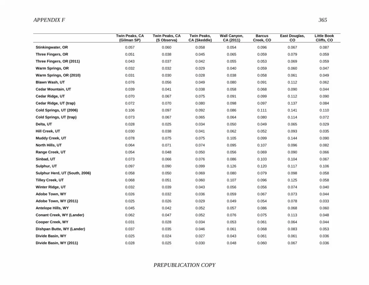
APPENDIX F 365
PREPUBLICATION COPY
Twin Peaks, CA
(Gilman SP) Twin Peaks, CA
(S Observa) Twin Peaks, CA (Skeddle)
Wall Canyon, CA (2011)
Barcus Creek, CO
East Douglas, CO
Little Book Cliffs, CO
Stinkingwater, OR 0.057 0.060 0.058 0.054 0.096 0.067 0.087
Three Fingers, OR 0.051 0.038 0.045 0.065 0.059 0.079 0.059
Three Fingers, OR (2011) 0.043 0.037 0.042 0.055 0.053 0.069 0.059
Warm Springs, OR 0.032 0.032 0.029 0.040 0.059 0.060 0.047
Warm Springs, OR (2010) 0.031 0.030 0.028 0.038 0.058 0.061 0.049
Blawn Wash, UT 0.076 0.056 0.049 0.080 0.091 0.112 0.062
Cedar Mountain, UT 0.039 0.041 0.038 0.058 0.068 0.090 0.044
Cedar Ridge, UT 0.070 0.067 0.075 0.091 0.099 0.112 0.090
Cedar Ridge, UT (trap) 0.072 0.070 0.080 0.098 0.097 0.137 0.084
Cold Springs, UT (2006) 0.106 0.097 0.092 0.086 0.111 0.141 0.110
Cold Springs, UT (trap) 0.073 0.067 0.065 0.064 0.080 0.114 0.072
Delta, UT 0.028 0.025 0.034 0.050 0.049 0.065 0.029
Hill Creek, UT 0.030 0.038 0.041 0.062 0.052 0.093 0.035
Muddy Creek, UT 0.078 0.075 0.075 0.105 0.099 0.144 0.090
North Hills, UT 0.064 0.071 0.074 0.095 0.107 0.096 0.082
Range Creek, UT 0.054 0.048 0.050 0.056 0.069 0.090 0.066
Sinbad, UT 0.073 0.066 0.076 0.086 0.103 0.104 0.067
Sulphur, UT 0.097 0.090 0.099 0.126 0.120 0.117 0.106
Sulphur Herd, UT (South, 2006) 0.058 0.050 0.069 0.080 0.079 0.098 0.058
Tilley Creek, UT 0.068 0.051 0.060 0.107 0.096 0.125 0.058
Winter Ridge, UT 0.032 0.039 0.043 0.056 0.056 0.074 0.040
Adobe Town, WY 0.026 0.032 0.036 0.059 0.067 0.073 0.044
Adobe Town, WY (2011) 0.025 0.026 0.029 0.049 0.054 0.078 0.033
Antelope Hills, WY 0.045 0.042 0.052 0.057 0.086 0.068 0.060
Conant Creek, WY (Lander) 0.062 0.047 0.052 0.076 0.075 0.113 0.048
Cooper Creek, WY 0.031 0.028 0.034 0.053 0.061 0.064 0.044
Dishpan Butte, WY (Lander) 0.037 0.035 0.046 0.061 0.068 0.083 0.053
Divide Basin, WY 0.025 0.024 0.027 0.043 0.061 0.061 0.036
Divide Basin, WY (2011) 0.028 0.025 0.030 0.048 0.060 0.067 0.036

366 BLM WILD HORSE AND BURRO PROGRAM
PREPUBLICATION COPY
Twin Peaks, CA
(Gilman SP) Twin Peaks, CA
(S Observa) Twin Peaks, CA (Skeddle)
Wall Canyon, CA (2011)
Barcus Creek, CO
East Douglas, CO
Little Book Cliffs, CO
Eagles Nest, WY 0.062 0.055 0.063 0.067 0.093 0.101 0.071
Happy Creek Springs, WY 0.047 0.052 0.052 0.069 0.086 0.072 0.068
Little Colorado, WY 0.038 0.036 0.041 0.044 0.064 0.072 0.053
Little Colorado, WY (2011) 0.032 0.033 0.034 0.042 0.060 0.066 0.048
Lost Creek, WY 0.033 0.030 0.034 0.041 0.060 0.064 0.041
Lost Creek, WY (combined) 0.032 0.030 0.037 0.040 0.060 0.071 0.039
McCullough Peaks, WY 0.043 0.036 0.044 0.044 0.074 0.063 0.048
Muskrat Basin, WY (Lander) 0.047 0.038 0.047 0.064 0.056 0.084 0.056
Salt Wells, WY (East) 0.023 0.029 0.024 0.046 0.056 0.069 0.037
Salt Wells, WY (West) 0.035 0.021 0.029 0.050 0.058 0.064 0.034
Stewart Creek, WY 0.045 0.039 0.046 0.047 0.061 0.070 0.051
Stewart Creek, WY (2009) 0.038 0.040 0.044 0.048 0.078 0.072 0.051
White Mountain, WY (2011) 0.035 0.030 0.036 0.051 0.063 0.077 0.042
Mesa, CO Sand Wash, CO Spring Creek,
CO Spring Creek
Basin, CO West Douglas,
CO
West Douglas, CO (2006)
Black Mountain, ID
Mesa, CO 0.000
Sand Wash, CO 0.042 0.000
Spring Creek, CO 0.062 0.083 0.000
Spring Creek Basin, CO 0.060 0.078 0.013 0.000
West Douglas, CO 0.070 0.064 0.072 0.073 0.000
West Douglas, CO (2006) 0.072 0.078 0.071 0.075 0.011 0.000
Black Mountain, ID 0.066 0.060 0.080 0.077 0.092 0.097 0.000
Black Mountain, ID (2010) 0.051 0.042 0.072 0.075 0.073 0.082 0.018
Challis, ID 0.044 0.040 0.061 0.062 0.058 0.071 0.066
Hard Trigger, ID 0.057 0.041 0.072 0.068 0.076 0.083 0.036
Hard Trigger, ID (2010) 0.057 0.046 0.073 0.068 0.079 0.086 0.035
Idaho, ID (BLM) 0.054 0.047 0.087 0.079 0.080 0.082 0.048
Sand Basin, ID 0.051 0.037 0.083 0.077 0.071 0.079 0.059

APPENDIX F 367
PREPUBLICATION COPY
Mesa, CO Sand Wash, CO Spring Creek,
CO Spring Creek
Basin, CO West Douglas,
CO
West Douglas, CO (2006)
Black Mountain, ID
Saylor Creek, ID 0.051 0.038 0.079 0.076 0.054 0.071 0.055
Pryor Mountains, MT (2001) 0.067 0.069 0.110 0.096 0.079 0.091 0.105
Pryor Mountains, MT (2009) 0.047 0.042 0.080 0.072 0.057 0.071 0.077
Bordo Atravisado, NM 0.041 0.046 0.075 0.069 0.067 0.074 0.071
El Rito, NM 0.042 0.039 0.073 0.068 0.059 0.065 0.074
Jicarilla, NM 0.053 0.044 0.081 0.077 0.061 0.070 0.082
Jarita, NM 0.070 0.067 0.100 0.101 0.085 0.090 0.103
Jicarilla, NM 0.083 0.079 0.104 0.110 0.106 0.111 0.106
Antelope Valley, NV 0.033 0.034 0.069 0.066 0.062 0.068 0.057
Antelope Valley, NV (2011) 0.034 0.044 0.061 0.058 0.062 0.066 0.064
Augusta Mountains, NV 0.035 0.045 0.074 0.071 0.061 0.067 0.063
Bald Mountain, NV 0.026 0.037 0.060 0.058 0.050 0.057 0.067
Black Rock East, NV (2005) 0.039 0.058 0.085 0.082 0.074 0.084 0.072
Black Rock East, NV (2010) 0.036 0.062 0.070 0.067 0.067 0.074 0.069
Black Rock East, NV (2011) 0.035 0.052 0.064 0.062 0.051 0.060 0.055
Black Rock West, NV (2005) 0.043 0.065 0.070 0.062 0.069 0.077 0.069
Black Rock West, NV (2010) 0.040 0.064 0.070 0.064 0.069 0.074 0.070
Black Rock West, NV (2011) 0.061 0.089 0.092 0.084 0.096 0.097 0.093
Buffalo Hills, NV 0.044 0.048 0.076 0.076 0.086 0.097 0.096
Buffalo Hills, NV (2009) 0.040 0.034 0.072 0.072 0.066 0.078 0.086
Calico, NV 0.027 0.032 0.054 0.053 0.063 0.073 0.064
Calico Mountains, NV 0.049 0.047 0.073 0.071 0.073 0.086 0.080
Calico Mountains, NV (2011) 0.036 0.037 0.067 0.066 0.070 0.082 0.071
Callaghan, NV (Austin Allot) 0.030 0.028 0.056 0.056 0.049 0.059 0.053
Callaghan, NV (East Allot) 0.028 0.034 0.047 0.044 0.048 0.053 0.061
Catnip Herd, NV 0.046 0.057 0.062 0.054 0.058 0.074 0.083
Chimney Creek, NV 0.042 0.044 0.087 0.083 0.064 0.082 0.071
Desatoya Mountain, NV 0.088 0.086 0.098 0.097 0.067 0.082 0.109
Dolly Varden, NV 0.034 0.045 0.068 0.065 0.064 0.065 0.066

368 BLM WILD HORSE AND BURRO PROGRAM
PREPUBLICATION COPY
Mesa, CO Sand Wash, CO Spring Creek,
CO Spring Creek
Basin, CO West Douglas,
CO
West Douglas, CO (2006)
Black Mountain, ID
Dry Lake, NV 0.045 0.045 0.083 0.084 0.049 0.064 0.072
Fish Creek, NV 0.040 0.043 0.063 0.064 0.071 0.082 0.061
Goshute, NV 0.048 0.054 0.083 0.069 0.080 0.085 0.080
Goshute, NV (2011) 0.047 0.051 0.081 0.067 0.074 0.078 0.076
Granite, NV 0.034 0.036 0.071 0.070 0.080 0.090 0.076
Granite Range, NV 0.036 0.039 0.067 0.066 0.072 0.081 0.080
Granite Range, NV (2011) 0.024 0.030 0.062 0.063 0.069 0.077 0.070
Grass Valley, NV 0.038 0.040 0.053 0.053 0.045 0.054 0.066
Hall Creek, NV 0.035 0.032 0.067 0.065 0.049 0.061 0.058
Jakes Wash, NV 0.066 0.071 0.097 0.096 0.071 0.083 0.093
Johnnie, NV 0.057 0.070 0.058 0.069 0.057 0.060 0.065
Lahanton Reservoir, NV 0.060 0.066 0.089 0.073 0.081 0.090 0.092
Little Fish Lake, NV 0.049 0.041 0.088 0.080 0.067 0.075 0.083
Little Highrock Canyon, NV 0.041 0.043 0.078 0.073 0.065 0.066 0.078
Little Humboldt, NV 0.056 0.049 0.095 0.090 0.083 0.090 0.078
Little Humboldt, NV (2010) 0.044 0.039 0.077 0.072 0.072 0.076 0.070
Little Owyhee, NV (Fairbanks) 0.049 0.060 0.089 0.088 0.077 0.088 0.082
Little Owyhee, NV (Lake Creek) 0.049 0.046 0.081 0.078 0.077 0.088 0.072
Little Owyhee, NV (Twin Valley) 0.048 0.059 0.076 0.072 0.077 0.081 0.063
Marvel Gap, NV (SWC 2010) 0.037 0.035 0.055 0.051 0.059 0.068 0.049
McGee Mountain, NV 0.042 0.042 0.071 0.064 0.051 0.066 0.065
Miller Mountain, NV (SWC 2010) 0.037 0.037 0.072 0.068 0.062 0.071 0.062
Montezuma Peak, NV 0.052 0.054 0.083 0.074 0.088 0.090 0.085
Nellis, NV 0.029 0.034 0.057 0.056 0.057 0.068 0.064
New Pass-Ravenswood, NV 0.031 0.038 0.053 0.051 0.040 0.045 0.052
North Stillwater, NV 0.043 0.037 0.074 0.072 0.068 0.076 0.075
Paymaster, NV (2006) 0.055 0.049 0.090 0.084 0.082 0.087 0.080
Paymaster, NV (2010) 0.053 0.048 0.089 0.082 0.079 0.085 0.083
Pine Nut Mountain, NV 0.069 0.079 0.087 0.099 0.080 0.093 0.093

APPENDIX F 369
PREPUBLICATION COPY
Mesa, CO Sand Wash, CO Spring Creek,
CO Spring Creek
Basin, CO West Douglas,
CO
West Douglas, CO (2006)
Black Mountain, ID
Powell Mountain, NV 0.058 0.052 0.113 0.101 0.084 0.098 0.077
Red Rock, NV 0.039 0.061 0.075 0.073 0.065 0.068 0.075
Reveille, NV 0.055 0.056 0.092 0.088 0.076 0.089 0.080
Roberts Mountain, NV 0.034 0.049 0.065 0.063 0.069 0.078 0.064
Rock Creek, NV (2002) 0.065 0.079 0.070 0.071 0.079 0.081 0.080
Rock Creek, NV (2010) 0.053 0.056 0.066 0.062 0.062 0.066 0.062
Rocky Hills, NV 0.036 0.045 0.056 0.054 0.043 0.051 0.063
Rodeo Creek, NV 0.035 0.031 0.057 0.056 0.049 0.053 0.073
Saulsbury, NV 0.041 0.032 0.072 0.071 0.041 0.052 0.071
Sand Springs East, NV 0.042 0.039 0.074 0.066 0.055 0.070 0.063
Seven Mile, NV 0.054 0.051 0.065 0.062 0.048 0.065 0.075
Shawave Mountains, NV 0.044 0.036 0.066 0.062 0.061 0.069 0.067
Silver Peak, NV 0.047 0.052 0.073 0.077 0.079 0.083 0.086
Snowstorm, NV (Castle Ridge) 0.045 0.042 0.086 0.076 0.081 0.090 0.072
Snowstorm, NV (Dryhill) 0.061 0.083 0.102 0.092 0.122 0.124 0.099
South Shoshone, NV 0.034 0.031 0.058 0.053 0.052 0.057 0.048
Spruce-Pequop, NV (2011) 0.052 0.066 0.086 0.085 0.072 0.076 0.077
Stillwater, NV 0.050 0.050 0.086 0.082 0.079 0.083 0.080
Stone Cabin, NV 0.030 0.033 0.064 0.064 0.055 0.065 0.064
Warm Springs, NV 0.037 0.052 0.071 0.067 0.074 0.081 0.074
Warm Springs Canyon, NV 0.036 0.046 0.060 0.056 0.053 0.060 0.066
Wheeler Pass, NV 0.073 0.085 0.085 0.095 0.080 0.078 0.090
Wheeler Pass, NV (2007) 0.031 0.035 0.066 0.068 0.050 0.056 0.054
Alvord Tule, OR 0.051 0.046 0.059 0.061 0.050 0.062 0.075
Beatys Butte, OR 0.026 0.034 0.061 0.059 0.051 0.060 0.061
Beatys Butte, OR (2010) 0.035 0.035 0.071 0.066 0.066 0.073 0.058
Big Summit, OR (2010) 0.125 0.117 0.143 0.146 0.143 0.136 0.149
Cold Spring, OR 0.033 0.047 0.053 0.055 0.047 0.047 0.054
Cold Spring, OR (2010) 0.040 0.051 0.061 0.062 0.060 0.053 0.062

370 BLM WILD HORSE AND BURRO PROGRAM
PREPUBLICATION COPY
Mesa, CO Sand Wash, CO Spring Creek,
CO Spring Creek
Basin, CO West Douglas,
CO
West Douglas, CO (2006)
Black Mountain, ID
Coyote Lake, OR 0.052 0.049 0.062 0.062 0.057 0.071 0.071
Coyote Lake, OR (2011) 0.039 0.034 0.059 0.057 0.055 0.068 0.058
Fishnet, OR 0.034 0.043 0.074 0.072 0.074 0.088 0.075
Hog Creek, OR 0.039 0.050 0.054 0.059 0.063 0.066 0.066
Jackies Butte, OR 0.050 0.054 0.079 0.074 0.059 0.070 0.067
Jackies Butte, OR (2011) 0.040 0.049 0.064 0.061 0.053 0.062 0.061
Kiger, OR (2011) 0.042 0.043 0.075 0.076 0.070 0.085 0.096
Kiger Herd, OR (2009) 0.048 0.053 0.068 0.073 0.073 0.083 0.093
Liggett Table, OR 0.168 0.199 0.173 0.162 0.195 0.199 0.188
Murderers Creek, OR (2001) 0.074 0.082 0.089 0.085 0.109 0.111 0.113
Murderers Creek, OR (2009) 0.062 0.059 0.086 0.079 0.087 0.097 0.104
Paisley Desert, OR 0.029 0.031 0.055 0.054 0.048 0.055 0.052
Riddle Herd, OR (2009) 0.054 0.057 0.082 0.085 0.082 0.092 0.099
Riddle Mountain, OR 0.055 0.058 0.084 0.083 0.067 0.078 0.090
Riddle Mountain, OR (2011) 0.059 0.064 0.087 0.092 0.087 0.097 0.104
Sand Springs, OR (2011) 0.042 0.033 0.077 0.073 0.065 0.076 0.063
Sheepshead, OR 0.038 0.034 0.058 0.058 0.049 0.061 0.057
Sheepshead, OR (2011) 0.034 0.032 0.058 0.056 0.045 0.053 0.054
South Steens, OR 0.038 0.040 0.048 0.048 0.046 0.056 0.054
South Steens, OR (2010) 0.038 0.041 0.057 0.056 0.051 0.063 0.061
Stinkingwater, OR 0.058 0.076 0.072 0.069 0.065 0.072 0.070
Three Fingers, OR 0.043 0.042 0.081 0.078 0.085 0.102 0.066
Three Fingers, OR (2011) 0.038 0.043 0.073 0.071 0.070 0.083 0.052
Warm Springs, OR 0.034 0.040 0.062 0.058 0.041 0.050 0.042
Warm Springs, OR (2010) 0.032 0.040 0.064 0.061 0.047 0.055 0.048
Blawn Wash, UT 0.055 0.079 0.113 0.112 0.084 0.089 0.094
Cedar Mountain, UT 0.048 0.059 0.074 0.081 0.072 0.079 0.080
Cedar Ridge, UT 0.073 0.062 0.074 0.076 0.093 0.100 0.096
Cedar Ridge, UT (trap) 0.079 0.070 0.074 0.083 0.101 0.101 0.106

APPENDIX F 371
PREPUBLICATION COPY
Mesa, CO Sand Wash, CO Spring Creek,
CO Spring Creek
Basin, CO West Douglas,
CO
West Douglas, CO (2006)
Black Mountain, ID
Cold Springs, UT (2006) 0.084 0.111 0.118 0.118 0.132 0.140 0.123
Cold Springs, UT (trap) 0.054 0.082 0.090 0.091 0.089 0.095 0.098
Delta, UT 0.032 0.034 0.054 0.057 0.057 0.063 0.062
Hill Creek, UT 0.044 0.044 0.064 0.067 0.070 0.073 0.078
Muddy Creek, UT 0.087 0.102 0.111 0.104 0.097 0.105 0.132
North Hills, UT 0.067 0.081 0.087 0.089 0.083 0.086 0.100
Range Creek, UT 0.045 0.051 0.060 0.062 0.077 0.084 0.075
Sinbad, UT 0.081 0.073 0.118 0.122 0.088 0.104 0.112
Sulphur, UT 0.097 0.090 0.150 0.150 0.122 0.134 0.135
Sulphur Herd, UT (South, 2006) 0.074 0.067 0.089 0.089 0.084 0.090 0.097
Tilley Creek, UT 0.057 0.065 0.102 0.104 0.109 0.111 0.091
Winter Ridge, UT 0.043 0.039 0.058 0.061 0.077 0.079 0.064
Adobe Town, WY 0.044 0.038 0.066 0.062 0.064 0.071 0.053
Adobe Town, WY (2011) 0.032 0.031 0.059 0.054 0.064 0.071 0.051
Antelope Hills, WY 0.056 0.048 0.070 0.067 0.070 0.087 0.089
Conant Creek, WY (Lander) 0.050 0.058 0.097 0.098 0.102 0.112 0.094
Cooper Creek, WY 0.043 0.039 0.071 0.072 0.054 0.066 0.066
Dishpan Butte, WY (Lander) 0.048 0.051 0.074 0.072 0.071 0.078 0.075
Divide Basin, WY 0.034 0.029 0.052 0.049 0.048 0.053 0.059
Divide Basin, WY (2011) 0.031 0.031 0.056 0.055 0.054 0.058 0.062
Eagles Nest, WY 0.069 0.065 0.077 0.069 0.081 0.084 0.093
Happy Creek Springs, WY 0.065 0.056 0.080 0.080 0.071 0.083 0.084
Little Colorado, WY 0.036 0.053 0.051 0.050 0.054 0.054 0.050
Little Colorado, WY (2011) 0.031 0.048 0.047 0.045 0.051 0.052 0.049
Lost Creek, WY 0.040 0.037 0.058 0.056 0.054 0.060 0.067
Lost Creek, WY (combined) 0.042 0.040 0.058 0.055 0.048 0.051 0.068
McCullough Peaks, WY 0.044 0.047 0.075 0.073 0.069 0.080 0.067
Muskrat Basin, WY (Lander) 0.044 0.054 0.075 0.074 0.077 0.082 0.078
Salt Wells, WY (East) 0.029 0.030 0.061 0.057 0.049 0.056 0.058
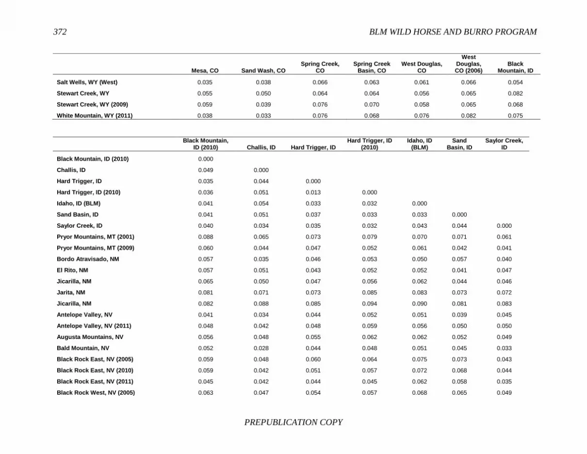
372 BLM WILD HORSE AND BURRO PROGRAM
PREPUBLICATION COPY
Mesa, CO Sand Wash, CO Spring Creek,
CO Spring Creek
Basin, CO West Douglas,
CO
West Douglas, CO (2006)
Black Mountain, ID
Salt Wells, WY (West) 0.035 0.038 0.066 0.063 0.061 0.066 0.054
Stewart Creek, WY 0.055 0.050 0.064 0.064 0.056 0.065 0.082
Stewart Creek, WY (2009) 0.059 0.039 0.076 0.070 0.058 0.065 0.068
White Mountain, WY (2011) 0.038 0.033 0.076 0.068 0.076 0.082 0.075
Black Mountain,
ID (2010) Challis, ID Hard Trigger, ID Hard Trigger, ID
(2010) Idaho, ID
(BLM) Sand
Basin, ID Saylor Creek,
ID
Black Mountain, ID (2010) 0.000
Challis, ID 0.049 0.000
Hard Trigger, ID 0.035 0.044 0.000
Hard Trigger, ID (2010) 0.036 0.051 0.013 0.000
Idaho, ID (BLM) 0.041 0.054 0.033 0.032 0.000
Sand Basin, ID 0.041 0.051 0.037 0.033 0.033 0.000
Saylor Creek, ID 0.040 0.034 0.035 0.032 0.043 0.044 0.000
Pryor Mountains, MT (2001) 0.088 0.065 0.073 0.079 0.070 0.071 0.061
Pryor Mountains, MT (2009) 0.060 0.044 0.047 0.052 0.061 0.042 0.041
Bordo Atravisado, NM 0.057 0.035 0.046 0.053 0.050 0.057 0.040
El Rito, NM 0.057 0.051 0.043 0.052 0.052 0.041 0.047
Jicarilla, NM 0.065 0.050 0.047 0.056 0.062 0.044 0.046
Jarita, NM 0.081 0.071 0.073 0.085 0.083 0.073 0.072
Jicarilla, NM 0.082 0.088 0.085 0.094 0.090 0.081 0.083
Antelope Valley, NV 0.041 0.034 0.044 0.052 0.051 0.039 0.045
Antelope Valley, NV (2011) 0.048 0.042 0.048 0.059 0.056 0.050 0.050
Augusta Mountains, NV 0.056 0.048 0.055 0.062 0.062 0.052 0.049
Bald Mountain, NV 0.052 0.028 0.044 0.048 0.051 0.045 0.033
Black Rock East, NV (2005) 0.059 0.048 0.060 0.064 0.075 0.073 0.043
Black Rock East, NV (2010) 0.059 0.042 0.051 0.057 0.072 0.068 0.044
Black Rock East, NV (2011) 0.045 0.042 0.044 0.045 0.062 0.058 0.035
Black Rock West, NV (2005) 0.063 0.047 0.054 0.057 0.068 0.065 0.049

APPENDIX F 373
PREPUBLICATION COPY
Black Mountain,
ID (2010) Challis, ID Hard Trigger, ID Hard Trigger, ID
(2010) Idaho, ID
(BLM) Sand
Basin, ID Saylor Creek,
ID
Black Rock West, NV (2010) 0.061 0.047 0.056 0.061 0.067 0.064 0.049
Black Rock West, NV (2011) 0.087 0.078 0.072 0.077 0.081 0.080 0.076
Buffalo Hills, NV 0.070 0.066 0.071 0.073 0.075 0.064 0.063
Buffalo Hills, NV (2009) 0.063 0.049 0.056 0.065 0.069 0.054 0.046
Calico, NV 0.047 0.031 0.043 0.050 0.053 0.038 0.040
Calico Mountains, NV 0.066 0.046 0.054 0.060 0.062 0.053 0.043
Calico Mountains, NV (2011) 0.052 0.038 0.052 0.057 0.052 0.041 0.043
Callaghan, NV (Austin Allot) 0.041 0.033 0.040 0.048 0.049 0.046 0.032
Callaghan, NV (East Allot) 0.047 0.029 0.040 0.043 0.048 0.039 0.037
Catnip Herd, NV 0.075 0.055 0.061 0.066 0.069 0.063 0.056
Chimney Creek, NV 0.062 0.048 0.043 0.047 0.060 0.047 0.041
Desatoya Mountain, NV 0.091 0.071 0.083 0.095 0.096 0.096 0.068
Dolly Varden, NV 0.053 0.046 0.046 0.056 0.049 0.045 0.052
Dry Lake, NV 0.052 0.051 0.063 0.067 0.067 0.056 0.044
Fish Creek, NV 0.051 0.043 0.050 0.055 0.066 0.048 0.045
Goshute, NV 0.068 0.060 0.065 0.072 0.072 0.062 0.063
Goshute, NV (2011) 0.064 0.056 0.058 0.064 0.068 0.058 0.056
Granite, NV 0.060 0.031 0.049 0.059 0.063 0.051 0.044
Granite Range, NV 0.059 0.039 0.048 0.061 0.061 0.046 0.050
Granite Range, NV (2011) 0.048 0.031 0.047 0.055 0.052 0.037 0.045
Grass Valley, NV 0.053 0.040 0.044 0.049 0.048 0.044 0.037
Hall Creek, NV 0.042 0.036 0.052 0.056 0.054 0.052 0.033
Jakes Wash, NV 0.080 0.067 0.083 0.094 0.092 0.079 0.071
Johnnie, NV 0.056 0.056 0.066 0.073 0.087 0.073 0.060
Lahanton Reservoir, NV 0.082 0.068 0.066 0.071 0.069 0.070 0.067
Little Fish Lake, NV 0.068 0.051 0.055 0.066 0.062 0.057 0.047
Little Highrock Canyon, NV 0.059 0.051 0.053 0.060 0.046 0.046 0.052
Little Humboldt, NV 0.065 0.046 0.049 0.059 0.056 0.057 0.047
Little Humboldt, NV (2010) 0.061 0.036 0.046 0.052 0.045 0.042 0.040

374 BLM WILD HORSE AND BURRO PROGRAM
PREPUBLICATION COPY
Black Mountain,
ID (2010) Challis, ID Hard Trigger, ID Hard Trigger, ID
(2010) Idaho, ID
(BLM) Sand
Basin, ID Saylor Creek,
ID
Little Owyhee, NV (Fairbanks) 0.075 0.061 0.071 0.079 0.084 0.074 0.060
Little Owyhee, NV (Lake Creek) 0.071 0.059 0.047 0.050 0.060 0.051 0.055
Little Owyhee, NV (Twin Valley) 0.058 0.045 0.048 0.053 0.061 0.048 0.058
Marvel Gap, NV (SWC 2010) 0.038 0.039 0.032 0.039 0.037 0.039 0.036
McGee Mountain, NV 0.054 0.033 0.047 0.055 0.059 0.047 0.031
Miller Mountain, NV (SWC 2010) 0.053 0.040 0.045 0.048 0.057 0.048 0.040
Montezuma Peak, NV 0.074 0.064 0.068 0.071 0.057 0.054 0.064
Nellis, NV 0.050 0.033 0.047 0.049 0.057 0.044 0.036
New Pass-Ravenswood, NV 0.044 0.033 0.047 0.048 0.050 0.041 0.038
North Stillwater, NV 0.055 0.049 0.057 0.059 0.068 0.040 0.051
Paymaster, NV (2006) 0.065 0.063 0.067 0.065 0.062 0.058 0.055
Paymaster, NV (2010) 0.067 0.065 0.072 0.070 0.063 0.058 0.057
Pine Nut Mountain, NV 0.068 0.061 0.087 0.095 0.103 0.085 0.058
Powell Mountain, NV 0.060 0.060 0.077 0.082 0.074 0.074 0.065
Red Rock, NV 0.061 0.057 0.064 0.068 0.067 0.059 0.056
Reveille, NV 0.067 0.049 0.059 0.068 0.072 0.064 0.054
Roberts Mountain, NV 0.050 0.049 0.052 0.054 0.060 0.055 0.037
Rock Creek, NV (2002) 0.078 0.063 0.079 0.078 0.078 0.079 0.061
Rock Creek, NV (2010) 0.058 0.047 0.058 0.059 0.059 0.060 0.040
Rocky Hills, NV 0.048 0.040 0.046 0.048 0.047 0.049 0.036
Rodeo Creek, NV 0.052 0.035 0.048 0.055 0.052 0.044 0.035
Saulsbury, NV 0.054 0.026 0.050 0.057 0.055 0.048 0.034
Sand Springs East, NV 0.052 0.033 0.045 0.052 0.057 0.045 0.031
Seven Mile, NV 0.056 0.043 0.048 0.054 0.051 0.044 0.043
Shawave Mountains, NV 0.057 0.035 0.045 0.051 0.051 0.049 0.036
Silver Peak, NV 0.068 0.053 0.060 0.063 0.068 0.056 0.055
Snowstorm, NV (Castle Ridge) 0.062 0.039 0.052 0.050 0.052 0.047 0.045
Snowstorm, NV (Dryhill) 0.097 0.089 0.081 0.081 0.082 0.069 0.089
South Shoshone, NV 0.034 0.039 0.044 0.049 0.050 0.033 0.042

APPENDIX F 375
PREPUBLICATION COPY
Black Mountain,
ID (2010) Challis, ID Hard Trigger, ID Hard Trigger, ID
(2010) Idaho, ID
(BLM) Sand
Basin, ID Saylor Creek,
ID
Spruce-Pequop, NV (2011) 0.070 0.065 0.072 0.079 0.079 0.068 0.070
Stillwater, NV 0.066 0.061 0.060 0.060 0.069 0.045 0.056
Stone Cabin, NV 0.047 0.032 0.043 0.045 0.051 0.041 0.031
Warm Springs, NV 0.061 0.042 0.056 0.058 0.064 0.058 0.048
Warm Springs Canyon, NV 0.056 0.033 0.044 0.049 0.055 0.047 0.036
Wheeler Pass, NV 0.079 0.078 0.080 0.088 0.091 0.084 0.071
Wheeler Pass, NV (2007) 0.037 0.034 0.047 0.054 0.054 0.046 0.036
Alvord Tule, OR 0.059 0.036 0.065 0.068 0.068 0.054 0.052
Beatys Butte, OR 0.047 0.035 0.039 0.044 0.049 0.041 0.035
Beatys Butte, OR (2010) 0.044 0.042 0.036 0.040 0.039 0.037 0.037
Big Summit, OR (2010) 0.133 0.105 0.106 0.113 0.102 0.117 0.105
Cold Spring, OR 0.047 0.039 0.041 0.048 0.054 0.053 0.046
Cold Spring, OR (2010) 0.056 0.046 0.047 0.051 0.053 0.058 0.053
Coyote Lake, OR 0.064 0.043 0.058 0.066 0.076 0.058 0.050
Coyote Lake, OR (2011) 0.049 0.029 0.047 0.053 0.059 0.044 0.036
Fishnet, OR 0.062 0.058 0.065 0.060 0.074 0.052 0.054
Hog Creek, OR 0.052 0.045 0.055 0.058 0.057 0.048 0.055
Jackies Butte, OR 0.051 0.049 0.060 0.059 0.063 0.055 0.047
Jackies Butte, OR (2011) 0.047 0.038 0.051 0.050 0.052 0.039 0.042
Kiger, OR (2011) 0.069 0.048 0.070 0.075 0.075 0.068 0.055
Kiger Herd, OR (2009) 0.069 0.052 0.073 0.080 0.082 0.075 0.061
Liggett Table, OR 0.195 0.170 0.160 0.168 0.168 0.174 0.177
Murderers Creek, OR (2001) 0.107 0.092 0.083 0.093 0.093 0.098 0.097
Murderers Creek, OR (2009) 0.088 0.074 0.073 0.084 0.081 0.082 0.076
Paisley Desert, OR 0.039 0.035 0.038 0.046 0.052 0.041 0.033
Riddle Herd, OR (2009) 0.076 0.051 0.072 0.081 0.082 0.072 0.066
Riddle Mountain, OR 0.068 0.048 0.069 0.074 0.075 0.068 0.060
Riddle Mountain, OR (2011) 0.079 0.058 0.081 0.088 0.089 0.075 0.075
Sand Springs, OR (2011) 0.046 0.038 0.051 0.055 0.056 0.043 0.044

376 BLM WILD HORSE AND BURRO PROGRAM
PREPUBLICATION COPY
Black Mountain,
ID (2010) Challis, ID Hard Trigger, ID Hard Trigger, ID
(2010) Idaho, ID
(BLM) Sand
Basin, ID Saylor Creek,
ID
Sheepshead, OR 0.039 0.035 0.043 0.049 0.052 0.045 0.038
Sheepshead, OR (2011) 0.037 0.029 0.043 0.048 0.050 0.046 0.034
South Steens, OR 0.043 0.039 0.043 0.048 0.054 0.038 0.044
South Steens, OR (2010) 0.047 0.041 0.048 0.051 0.055 0.039 0.046
Stinkingwater, OR 0.074 0.074 0.067 0.066 0.091 0.080 0.068
Three Fingers, OR 0.047 0.050 0.048 0.050 0.060 0.058 0.039
Three Fingers, OR (2011) 0.041 0.043 0.041 0.041 0.050 0.047 0.032
Warm Springs, OR 0.037 0.035 0.036 0.035 0.041 0.039 0.029
Warm Springs, OR (2010) 0.040 0.037 0.036 0.035 0.042 0.039 0.030
Blawn Wash, UT 0.071 0.077 0.096 0.089 0.089 0.068 0.079
Cedar Mountain, UT 0.070 0.051 0.062 0.066 0.070 0.048 0.065
Cedar Ridge, UT 0.080 0.052 0.069 0.069 0.076 0.067 0.066
Cedar Ridge, UT (trap) 0.089 0.063 0.081 0.080 0.077 0.072 0.080
Cold Springs, UT (2006) 0.111 0.090 0.104 0.110 0.112 0.100 0.100
Cold Springs, UT (trap) 0.081 0.060 0.088 0.093 0.089 0.073 0.080
Delta, UT 0.048 0.033 0.048 0.056 0.056 0.051 0.039
Hill Creek, UT 0.058 0.051 0.056 0.063 0.059 0.044 0.054
Muddy Creek, UT 0.113 0.082 0.111 0.122 0.121 0.104 0.102
North Hills, UT 0.091 0.076 0.066 0.074 0.077 0.086 0.075
Range Creek, UT 0.061 0.036 0.053 0.055 0.060 0.049 0.048
Sinbad, UT 0.089 0.054 0.094 0.097 0.095 0.085 0.063
Sulphur, UT 0.113 0.113 0.104 0.115 0.108 0.111 0.092
Sulphur Herd, UT (South, 2006) 0.088 0.068 0.067 0.082 0.078 0.070 0.070
Tilley Creek, UT 0.078 0.070 0.077 0.078 0.066 0.071 0.080
Winter Ridge, UT 0.051 0.050 0.045 0.054 0.043 0.051 0.049
Adobe Town, WY 0.045 0.046 0.035 0.042 0.046 0.044 0.035
Adobe Town, WY (2011) 0.039 0.040 0.031 0.034 0.033 0.027 0.036
Antelope Hills, WY 0.073 0.039 0.051 0.064 0.071 0.062 0.044
Conant Creek, WY (Lander) 0.073 0.072 0.081 0.085 0.092 0.074 0.075
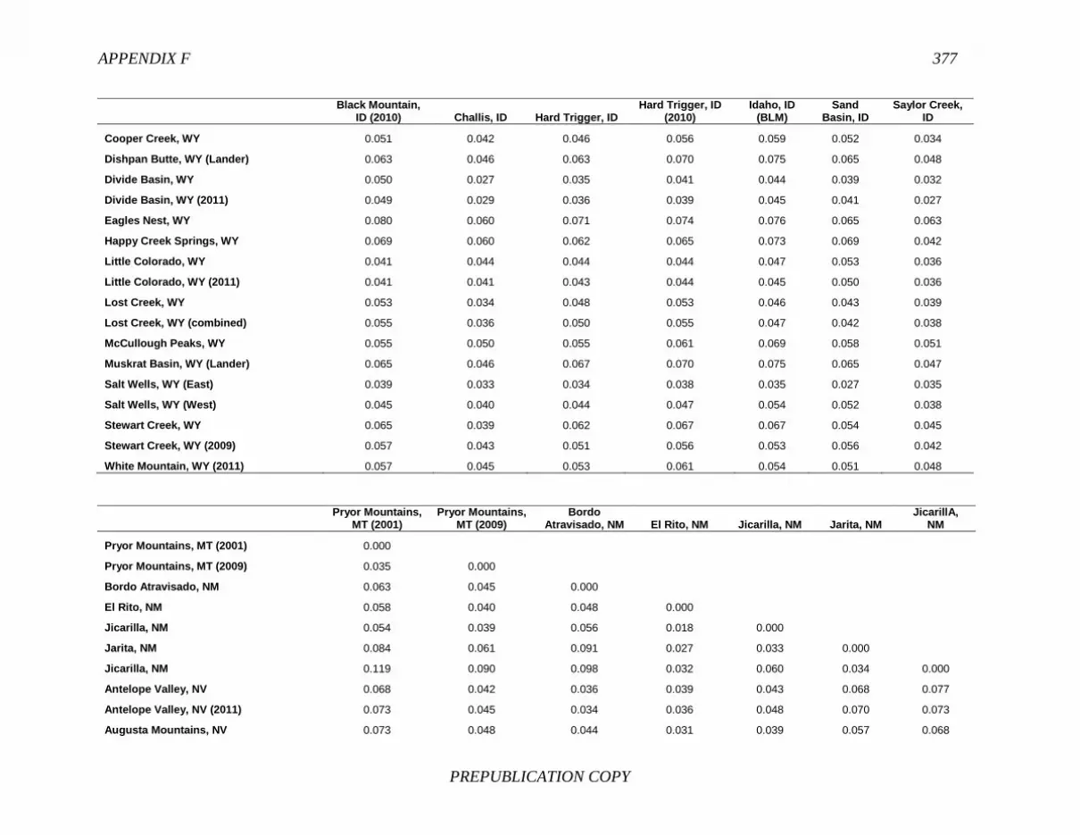
APPENDIX F 377
PREPUBLICATION COPY
Black Mountain,
ID (2010) Challis, ID Hard Trigger, ID Hard Trigger, ID
(2010) Idaho, ID
(BLM) Sand
Basin, ID Saylor Creek,
ID
Cooper Creek, WY 0.051 0.042 0.046 0.056 0.059 0.052 0.034
Dishpan Butte, WY (Lander) 0.063 0.046 0.063 0.070 0.075 0.065 0.048
Divide Basin, WY 0.050 0.027 0.035 0.041 0.044 0.039 0.032
Divide Basin, WY (2011) 0.049 0.029 0.036 0.039 0.045 0.041 0.027
Eagles Nest, WY 0.080 0.060 0.071 0.074 0.076 0.065 0.063
Happy Creek Springs, WY 0.069 0.060 0.062 0.065 0.073 0.069 0.042
Little Colorado, WY 0.041 0.044 0.044 0.044 0.047 0.053 0.036
Little Colorado, WY (2011) 0.041 0.041 0.043 0.044 0.045 0.050 0.036
Lost Creek, WY 0.053 0.034 0.048 0.053 0.046 0.043 0.039
Lost Creek, WY (combined) 0.055 0.036 0.050 0.055 0.047 0.042 0.038
McCullough Peaks, WY 0.055 0.050 0.055 0.061 0.069 0.058 0.051
Muskrat Basin, WY (Lander) 0.065 0.046 0.067 0.070 0.075 0.065 0.047
Salt Wells, WY (East) 0.039 0.033 0.034 0.038 0.035 0.027 0.035
Salt Wells, WY (West) 0.045 0.040 0.044 0.047 0.054 0.052 0.038
Stewart Creek, WY 0.065 0.039 0.062 0.067 0.067 0.054 0.045
Stewart Creek, WY (2009) 0.057 0.043 0.051 0.056 0.053 0.056 0.042
White Mountain, WY (2011) 0.057 0.045 0.053 0.061 0.054 0.051 0.048
Pryor Mountains,
MT (2001) Pryor Mountains,
MT (2009) Bordo
Atravisado, NM El Rito, NM Jicarilla, NM Jarita, NM JicarillA,
NM
Pryor Mountains, MT (2001) 0.000
Pryor Mountains, MT (2009) 0.035 0.000
Bordo Atravisado, NM 0.063 0.045 0.000
El Rito, NM 0.058 0.040 0.048 0.000
Jicarilla, NM 0.054 0.039 0.056 0.018 0.000
Jarita, NM 0.084 0.061 0.091 0.027 0.033 0.000
Jicarilla, NM 0.119 0.090 0.098 0.032 0.060 0.034 0.000
Antelope Valley, NV 0.068 0.042 0.036 0.039 0.043 0.068 0.077
Antelope Valley, NV (2011) 0.073 0.045 0.034 0.036 0.048 0.070 0.073
Augusta Mountains, NV 0.073 0.048 0.044 0.031 0.039 0.057 0.068

378 BLM WILD HORSE AND BURRO PROGRAM
PREPUBLICATION COPY
Pryor Mountains,
MT (2001) Pryor Mountains,
MT (2009) Bordo
Atravisado, NM El Rito, NM Jicarilla, NM Jarita, NM JicarillA,
NM
Bald Mountain, NV 0.060 0.034 0.026 0.030 0.034 0.058 0.068
Black Rock East, NV (2005) 0.079 0.060 0.052 0.059 0.063 0.089 0.095
Black Rock East, NV (2010) 0.072 0.056 0.052 0.050 0.055 0.074 0.083
Black Rock East, NV (2011) 0.068 0.048 0.045 0.039 0.050 0.066 0.068
Black Rock West, NV (2005) 0.067 0.050 0.054 0.059 0.059 0.089 0.100
Black Rock West, NV (2010) 0.072 0.056 0.053 0.055 0.062 0.085 0.092
Black Rock West, NV (2011) 0.088 0.073 0.076 0.068 0.077 0.097 0.108
Buffalo Hills, NV 0.091 0.057 0.059 0.051 0.059 0.076 0.078
Buffalo Hills, NV (2009) 0.069 0.039 0.042 0.037 0.039 0.061 0.071
Calico, NV 0.058 0.032 0.035 0.035 0.037 0.057 0.068
Calico Mountains, NV 0.075 0.048 0.040 0.051 0.047 0.080 0.091
Calico Mountains, NV (2011) 0.067 0.039 0.039 0.037 0.041 0.064 0.070
Callaghan, NV (Austin Allot) 0.062 0.035 0.033 0.030 0.035 0.049 0.060
Callaghan, NV (East Allot) 0.060 0.036 0.030 0.028 0.035 0.058 0.071
Catnip Herd, NV 0.077 0.043 0.057 0.054 0.059 0.082 0.099
Chimney Creek, NV 0.062 0.042 0.051 0.049 0.048 0.076 0.093
Desatoya Mountain, NV 0.092 0.068 0.073 0.060 0.065 0.080 0.087
Dolly Varden, NV 0.069 0.040 0.042 0.036 0.048 0.061 0.067
Dry Lake, NV 0.084 0.056 0.053 0.050 0.047 0.071 0.078
Fish Creek, NV 0.069 0.042 0.049 0.040 0.041 0.061 0.071
Goshute, NV 0.081 0.057 0.054 0.048 0.064 0.079 0.079
Goshute, NV (2011) 0.072 0.045 0.049 0.050 0.065 0.080 0.090
Granite, NV 0.066 0.041 0.038 0.042 0.041 0.063 0.078
Granite Range, NV 0.063 0.038 0.043 0.041 0.038 0.057 0.080
Granite Range, NV (2011) 0.063 0.035 0.039 0.030 0.036 0.049 0.060
Grass Valley, NV 0.062 0.036 0.032 0.033 0.037 0.061 0.071
Hall Creek, NV 0.066 0.040 0.036 0.036 0.040 0.053 0.060
Jakes Wash, NV 0.089 0.063 0.075 0.057 0.066 0.073 0.104
Johnnie, NV 0.096 0.067 0.067 0.059 0.061 0.084 0.089

APPENDIX F 379
PREPUBLICATION COPY
Pryor Mountains,
MT (2001) Pryor Mountains,
MT (2009) Bordo
Atravisado, NM El Rito, NM Jicarilla, NM Jarita, NM JicarillA,
NM
Lahanton Reservoir, NV 0.098 0.074 0.072 0.054 0.075 0.088 0.084
Little Fish Lake, NV 0.072 0.050 0.043 0.043 0.051 0.061 0.088
Little Highrock Canyon, NV 0.070 0.050 0.050 0.037 0.044 0.060 0.066
Little Humboldt, NV 0.088 0.060 0.052 0.059 0.061 0.077 0.099
Little Humboldt, NV (2010) 0.072 0.050 0.047 0.043 0.045 0.068 0.084
Little Owyhee, NV (Fairbanks) 0.084 0.051 0.056 0.050 0.056 0.073 0.085
Little Owyhee, NV (Lake Creek) 0.087 0.053 0.059 0.040 0.042 0.060 0.077
Little Owyhee, NV (Twin Valley) 0.070 0.044 0.060 0.043 0.035 0.054 0.080
Marvel Gap, NV (SWC 2010) 0.063 0.039 0.036 0.037 0.042 0.064 0.079
McGee Mountain, NV 0.053 0.035 0.044 0.044 0.043 0.069 0.091
Miller Mountain, NV (SWC 2010) 0.065 0.041 0.037 0.037 0.039 0.065 0.078
Montezuma Peak, NV 0.089 0.067 0.056 0.049 0.061 0.077 0.089
Nellis, NV 0.064 0.036 0.034 0.043 0.046 0.072 0.088
New Pass-Ravenswood, NV 0.064 0.038 0.040 0.038 0.042 0.058 0.069
North Stillwater, NV 0.068 0.042 0.053 0.033 0.038 0.056 0.068
Paymaster, NV (2006) 0.087 0.067 0.057 0.053 0.065 0.078 0.091
Paymaster, NV (2010) 0.087 0.067 0.058 0.055 0.064 0.080 0.092
Pine Nut Mountain, NV 0.098 0.072 0.077 0.059 0.062 0.067 0.073
Powell Mountain, NV 0.076 0.066 0.064 0.063 0.071 0.093 0.100
Red Rock, NV 0.080 0.053 0.047 0.044 0.056 0.073 0.083
Reveille, NV 0.080 0.055 0.046 0.058 0.060 0.091 0.109
Roberts Mountain, NV 0.062 0.043 0.043 0.043 0.052 0.076 0.087
Rock Creek, NV (2002) 0.094 0.077 0.081 0.066 0.065 0.090 0.106
Rock Creek, NV (2010) 0.078 0.057 0.060 0.051 0.052 0.073 0.089
Rocky Hills, NV 0.066 0.047 0.043 0.040 0.049 0.072 0.074
Rodeo Creek, NV 0.061 0.040 0.037 0.033 0.034 0.056 0.070
Saulsbury, NV 0.061 0.038 0.039 0.037 0.038 0.055 0.071
Sand Springs East, NV 0.054 0.035 0.043 0.045 0.043 0.070 0.093
Seven Mile, NV 0.071 0.053 0.049 0.041 0.051 0.069 0.077

380 BLM WILD HORSE AND BURRO PROGRAM
PREPUBLICATION COPY
Pryor Mountains,
MT (2001) Pryor Mountains,
MT (2009) Bordo
Atravisado, NM El Rito, NM Jicarilla, NM Jarita, NM JicarillA,
NM
Shawave Mountains, NV 0.069 0.041 0.041 0.034 0.039 0.052 0.059
Silver Peak, NV 0.084 0.053 0.063 0.051 0.050 0.060 0.083
Snowstorm, NV (Castle Ridge) 0.084 0.058 0.052 0.049 0.053 0.081 0.094
Snowstorm, NV (Dryhill) 0.102 0.075 0.089 0.075 0.077 0.082 0.113
South Shoshone, NV 0.063 0.038 0.040 0.031 0.039 0.059 0.068
Spruce-Pequop, NV (2011) 0.092 0.059 0.052 0.056 0.068 0.081 0.087
Stillwater, NV 0.073 0.050 0.058 0.037 0.048 0.059 0.076
Stone Cabin, NV 0.059 0.034 0.034 0.034 0.035 0.065 0.077
Warm Springs, NV 0.063 0.042 0.055 0.052 0.050 0.072 0.093
Warm Springs Canyon, NV 0.055 0.033 0.039 0.041 0.039 0.063 0.084
Wheeler Pass, NV 0.109 0.081 0.078 0.073 0.081 0.106 0.108
Wheeler Pass, NV (2007) 0.075 0.047 0.036 0.037 0.045 0.066 0.067
Alvord Tule, OR 0.066 0.042 0.050 0.051 0.044 0.073 0.100
Beatys Butte, OR 0.060 0.035 0.038 0.032 0.037 0.057 0.064
Beatys Butte, OR (2010) 0.062 0.036 0.034 0.031 0.033 0.058 0.063
Big Summit, OR (2010) 0.152 0.123 0.100 0.115 0.127 0.145 0.157
Cold Spring, OR 0.072 0.045 0.039 0.042 0.046 0.056 0.081
Cold Spring, OR (2010) 0.077 0.057 0.039 0.045 0.052 0.064 0.084
Coyote Lake, OR 0.074 0.047 0.046 0.053 0.044 0.083 0.106
Coyote Lake, OR (2011) 0.058 0.035 0.037 0.043 0.038 0.069 0.092
Fishnet, OR 0.078 0.047 0.064 0.052 0.056 0.081 0.094
Hog Creek, OR 0.078 0.051 0.048 0.045 0.044 0.063 0.083
Jackies Butte, OR 0.064 0.041 0.050 0.054 0.056 0.076 0.090
Jackies Butte, OR (2011) 0.058 0.033 0.046 0.046 0.046 0.070 0.082
Kiger, OR (2011) 0.078 0.048 0.062 0.053 0.048 0.065 0.079
Kiger Herd, OR (2009) 0.080 0.051 0.067 0.063 0.056 0.076 0.092
Liggett Table, OR 0.162 0.161 0.183 0.172 0.166 0.190 0.224
Murderers Creek, OR (2001) 0.111 0.080 0.093 0.075 0.087 0.099 0.118
Murderers Creek, OR (2009) 0.082 0.056 0.078 0.061 0.071 0.080 0.102

APPENDIX F 381
PREPUBLICATION COPY
Pryor Mountains,
MT (2001) Pryor Mountains,
MT (2009) Bordo
Atravisado, NM El Rito, NM Jicarilla, NM Jarita, NM JicarillA,
NM
Paisley Desert, OR 0.056 0.031 0.034 0.030 0.032 0.059 0.074
Riddle Herd, OR (2009) 0.083 0.056 0.077 0.062 0.057 0.072 0.090
Riddle Mountain, OR 0.083 0.052 0.072 0.061 0.056 0.073 0.088
Riddle Mountain, OR (2011) 0.091 0.063 0.086 0.067 0.059 0.076 0.096
Sand Springs, OR (2011) 0.076 0.044 0.044 0.043 0.041 0.068 0.083
Sheepshead, OR 0.064 0.040 0.040 0.036 0.038 0.063 0.074
Sheepshead, OR (2011) 0.065 0.043 0.036 0.035 0.038 0.060 0.073
South Steens, OR 0.059 0.038 0.042 0.030 0.024 0.049 0.072
South Steens, OR (2010) 0.060 0.039 0.045 0.030 0.029 0.048 0.066
Stinkingwater, OR 0.094 0.057 0.079 0.073 0.073 0.103 0.125
Three Fingers, OR 0.081 0.052 0.050 0.060 0.068 0.087 0.098
Three Fingers, OR (2011) 0.066 0.044 0.049 0.050 0.059 0.075 0.091
Warm Springs, OR 0.052 0.029 0.044 0.033 0.036 0.048 0.070
Warm Springs, OR (2010) 0.055 0.031 0.043 0.034 0.038 0.049 0.070
Blawn Wash, UT 0.095 0.081 0.083 0.081 0.082 0.116 0.120
Cedar Mountain, UT 0.082 0.051 0.059 0.052 0.051 0.069 0.086
Cedar Ridge, UT 0.108 0.071 0.066 0.085 0.077 0.109 0.127
Cedar Ridge, UT (trap) 0.119 0.081 0.073 0.085 0.087 0.112 0.125
Cold Springs, UT (2006) 0.113 0.088 0.107 0.115 0.107 0.131 0.157
Cold Springs, UT (trap) 0.082 0.067 0.080 0.088 0.080 0.107 0.136
Delta, UT 0.068 0.042 0.039 0.033 0.037 0.051 0.068
Hill Creek, UT 0.078 0.055 0.051 0.037 0.041 0.070 0.067
Muddy Creek, UT 0.132 0.086 0.075 0.091 0.102 0.119 0.144
North Hills, UT 0.106 0.071 0.079 0.078 0.070 0.093 0.122
Range Creek, UT 0.076 0.046 0.052 0.066 0.058 0.086 0.106
Sinbad, UT 0.087 0.075 0.068 0.070 0.070 0.086 0.094
Sulphur, UT 0.134 0.105 0.096 0.088 0.091 0.120 0.132
Sulphur Herd, UT (South, 2006) 0.090 0.063 0.078 0.057 0.053 0.068 0.091
Tilley Creek, UT 0.116 0.095 0.086 0.072 0.076 0.095 0.105
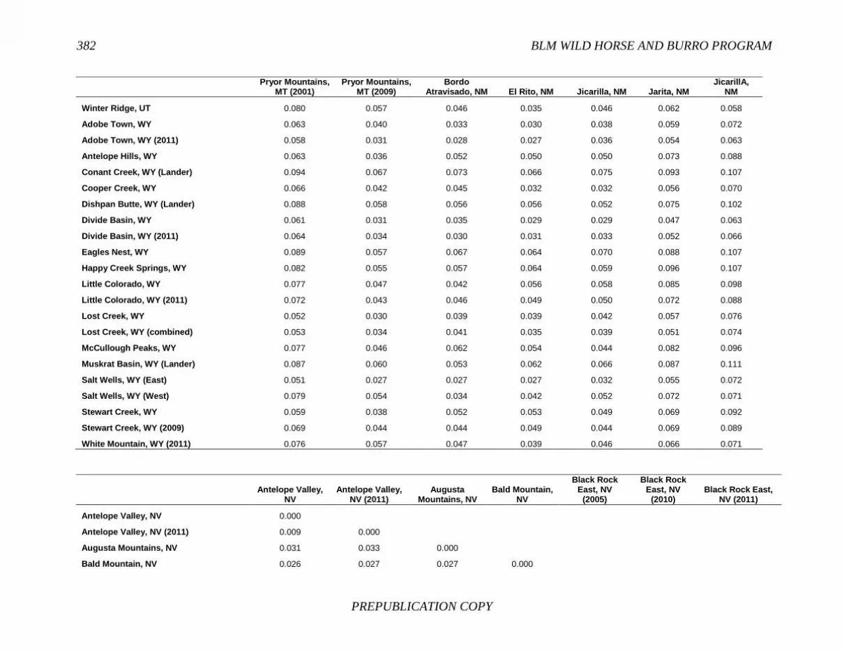
382 BLM WILD HORSE AND BURRO PROGRAM
PREPUBLICATION COPY
Pryor Mountains,
MT (2001) Pryor Mountains,
MT (2009) Bordo
Atravisado, NM El Rito, NM Jicarilla, NM Jarita, NM JicarillA,
NM
Winter Ridge, UT 0.080 0.057 0.046 0.035 0.046 0.062 0.058
Adobe Town, WY 0.063 0.040 0.033 0.030 0.038 0.059 0.072
Adobe Town, WY (2011) 0.058 0.031 0.028 0.027 0.036 0.054 0.063
Antelope Hills, WY 0.063 0.036 0.052 0.050 0.050 0.073 0.088
Conant Creek, WY (Lander) 0.094 0.067 0.073 0.066 0.075 0.093 0.107
Cooper Creek, WY 0.066 0.042 0.045 0.032 0.032 0.056 0.070
Dishpan Butte, WY (Lander) 0.088 0.058 0.056 0.056 0.052 0.075 0.102
Divide Basin, WY 0.061 0.031 0.035 0.029 0.029 0.047 0.063
Divide Basin, WY (2011) 0.064 0.034 0.030 0.031 0.033 0.052 0.066
Eagles Nest, WY 0.089 0.057 0.067 0.064 0.070 0.088 0.107
Happy Creek Springs, WY 0.082 0.055 0.057 0.064 0.059 0.096 0.107
Little Colorado, WY 0.077 0.047 0.042 0.056 0.058 0.085 0.098
Little Colorado, WY (2011) 0.072 0.043 0.046 0.049 0.050 0.072 0.088
Lost Creek, WY 0.052 0.030 0.039 0.039 0.042 0.057 0.076
Lost Creek, WY (combined) 0.053 0.034 0.041 0.035 0.039 0.051 0.074
McCullough Peaks, WY 0.077 0.046 0.062 0.054 0.044 0.082 0.096
Muskrat Basin, WY (Lander) 0.087 0.060 0.053 0.062 0.066 0.087 0.111
Salt Wells, WY (East) 0.051 0.027 0.027 0.027 0.032 0.055 0.072
Salt Wells, WY (West) 0.079 0.054 0.034 0.042 0.052 0.072 0.071
Stewart Creek, WY 0.059 0.038 0.052 0.053 0.049 0.069 0.092
Stewart Creek, WY (2009) 0.069 0.044 0.044 0.049 0.044 0.069 0.089
White Mountain, WY (2011) 0.076 0.057 0.047 0.039 0.046 0.066 0.071
Antelope Valley,
NV Antelope Valley,
NV (2011) Augusta
Mountains, NV Bald Mountain,
NV
Black Rock East, NV
(2005)
Black Rock East, NV
(2010) Black Rock East,
NV (2011)
Antelope Valley, NV 0.000
Antelope Valley, NV (2011) 0.009 0.000
Augusta Mountains, NV 0.031 0.033 0.000
Bald Mountain, NV 0.026 0.027 0.027 0.000

APPENDIX F 383
PREPUBLICATION COPY
Antelope Valley,
NV Antelope Valley,
NV (2011) Augusta
Mountains, NV Bald Mountain,
NV
Black Rock East, NV
(2005)
Black Rock East, NV
(2010) Black Rock East,
NV (2011)
Black Rock East, NV (2005) 0.050 0.053 0.047 0.038 0.000
Black Rock East, NV (2010) 0.046 0.047 0.041 0.035 0.012 0.000
Black Rock East, NV (2011) 0.041 0.042 0.034 0.031 0.026 0.013 0.000
Black Rock West, NV (2005) 0.052 0.054 0.050 0.037 0.018 0.015 0.028
Black Rock West, NV (2010) 0.049 0.050 0.048 0.039 0.013 0.013 0.027
Black Rock West, NV (2011) 0.076 0.071 0.074 0.061 0.052 0.045 0.052
Buffalo Hills, NV 0.047 0.050 0.062 0.046 0.062 0.064 0.060
Buffalo Hills, NV (2009) 0.033 0.036 0.046 0.033 0.055 0.055 0.048
Calico, NV 0.030 0.035 0.035 0.024 0.044 0.039 0.036
Calico Mountains, NV 0.045 0.049 0.047 0.037 0.065 0.058 0.050
Calico Mountains, NV (2011) 0.039 0.041 0.041 0.031 0.052 0.048 0.043
Callaghan, NV (Austin Allot) 0.035 0.036 0.031 0.018 0.048 0.041 0.029
Callaghan, NV (East Allot) 0.026 0.025 0.032 0.013 0.047 0.038 0.030
Catnip Herd, NV 0.049 0.047 0.044 0.038 0.065 0.058 0.056
Chimney Creek, NV 0.044 0.054 0.046 0.038 0.041 0.035 0.033
Desatoya Mountain, NV 0.076 0.071 0.057 0.055 0.073 0.068 0.058
Dolly Varden, NV 0.019 0.019 0.037 0.028 0.057 0.047 0.042
Dry Lake, NV 0.048 0.052 0.048 0.039 0.055 0.053 0.041
Fish Creek, NV 0.046 0.047 0.037 0.032 0.058 0.053 0.043
Goshute, NV 0.035 0.035 0.052 0.043 0.060 0.053 0.046
Goshute, NV (2011) 0.038 0.037 0.054 0.040 0.060 0.051 0.044
Granite, NV 0.033 0.040 0.038 0.024 0.047 0.039 0.038
Granite Range, NV 0.032 0.040 0.042 0.030 0.054 0.045 0.045
Granite Range, NV (2011) 0.028 0.035 0.035 0.024 0.044 0.039 0.037
Grass Valley, NV 0.035 0.033 0.034 0.018 0.059 0.050 0.036
Hall Creek, NV 0.035 0.038 0.035 0.020 0.047 0.045 0.032
Jakes Wash, NV 0.067 0.063 0.055 0.055 0.082 0.079 0.070
Johnnie, NV 0.048 0.047 0.053 0.045 0.054 0.045 0.035
Lahanton Reservoir, NV 0.073 0.064 0.064 0.053 0.071 0.061 0.054
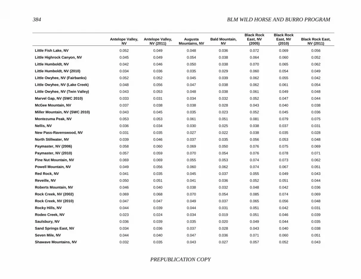
384 BLM WILD HORSE AND BURRO PROGRAM
PREPUBLICATION COPY
Antelope Valley,
NV Antelope Valley,
NV (2011) Augusta
Mountains, NV Bald Mountain,
NV
Black Rock East, NV
(2005)
Black Rock East, NV
(2010) Black Rock East,
NV (2011)
Little Fish Lake, NV 0.052 0.049 0.048 0.036 0.072 0.069 0.056
Little Highrock Canyon, NV 0.045 0.049 0.054 0.038 0.064 0.060 0.052
Little Humboldt, NV 0.042 0.046 0.050 0.038 0.070 0.065 0.062
Little Humboldt, NV (2010) 0.034 0.036 0.035 0.029 0.060 0.054 0.049
Little Owyhee, NV (Fairbanks) 0.052 0.052 0.045 0.039 0.062 0.055 0.042
Little Owyhee, NV (Lake Creek) 0.048 0.056 0.047 0.038 0.062 0.061 0.054
Little Owyhee, NV (Twin Valley) 0.043 0.053 0.048 0.038 0.061 0.049 0.048
Marvel Gap, NV (SWC 2010) 0.033 0.031 0.034 0.032 0.052 0.047 0.044
McGee Mountain, NV 0.037 0.038 0.038 0.028 0.043 0.040 0.038
Miller Mountain, NV (SWC 2010) 0.043 0.045 0.035 0.023 0.052 0.045 0.036
Montezuma Peak, NV 0.053 0.053 0.061 0.051 0.081 0.079 0.075
Nellis, NV 0.036 0.034 0.030 0.025 0.038 0.037 0.031
New Pass-Ravenswood, NV 0.031 0.035 0.027 0.022 0.038 0.035 0.028
North Stillwater, NV 0.039 0.046 0.037 0.035 0.056 0.053 0.048
Paymaster, NV (2006) 0.058 0.060 0.069 0.050 0.076 0.075 0.069
Paymaster, NV (2010) 0.057 0.059 0.070 0.054 0.076 0.078 0.071
Pine Nut Mountain, NV 0.069 0.069 0.055 0.053 0.074 0.073 0.062
Powell Mountain, NV 0.049 0.056 0.060 0.062 0.074 0.067 0.051
Red Rock, NV 0.041 0.035 0.045 0.037 0.055 0.049 0.043
Reveille, NV 0.050 0.051 0.041 0.036 0.052 0.051 0.044
Roberts Mountain, NV 0.046 0.040 0.038 0.032 0.048 0.042 0.036
Rock Creek, NV (2002) 0.069 0.068 0.070 0.054 0.085 0.074 0.069
Rock Creek, NV (2010) 0.047 0.047 0.049 0.037 0.065 0.056 0.048
Rocky Hills, NV 0.044 0.039 0.044 0.031 0.051 0.042 0.031
Rodeo Creek, NV 0.023 0.024 0.034 0.019 0.051 0.046 0.039
Saulsbury, NV 0.036 0.039 0.035 0.020 0.049 0.044 0.035
Sand Springs East, NV 0.034 0.036 0.037 0.028 0.043 0.040 0.038
Seven Mile, NV 0.044 0.040 0.047 0.036 0.071 0.060 0.051
Shawave Mountains, NV 0.032 0.035 0.043 0.027 0.057 0.052 0.043

APPENDIX F 385
PREPUBLICATION COPY
Antelope Valley,
NV Antelope Valley,
NV (2011) Augusta
Mountains, NV Bald Mountain,
NV
Black Rock East, NV
(2005)
Black Rock East, NV
(2010) Black Rock East,
NV (2011)
Silver Peak, NV 0.054 0.062 0.047 0.037 0.060 0.055 0.054
Snowstorm, NV (Castle Ridge) 0.044 0.049 0.051 0.030 0.066 0.062 0.056
Snowstorm, NV (Dryhill) 0.079 0.088 0.076 0.073 0.088 0.085 0.084
South Shoshone, NV 0.032 0.031 0.030 0.028 0.053 0.050 0.041
Spruce-Pequop, NV (2011) 0.031 0.032 0.040 0.042 0.063 0.058 0.050
Stillwater, NV 0.049 0.053 0.039 0.042 0.064 0.061 0.057
Stone Cabin, NV 0.031 0.033 0.031 0.017 0.044 0.040 0.034
Warm Springs, NV 0.050 0.052 0.050 0.031 0.032 0.034 0.041
Warm Springs Canyon, NV 0.038 0.040 0.035 0.023 0.030 0.027 0.032
Wheeler Pass, NV 0.059 0.056 0.065 0.052 0.068 0.058 0.048
Wheeler Pass, NV (2007) 0.028 0.027 0.031 0.022 0.038 0.036 0.028
Alvord Tule, OR 0.040 0.045 0.039 0.033 0.062 0.056 0.051
Beatys Butte, OR 0.027 0.028 0.031 0.020 0.040 0.034 0.030
Beatys Butte, OR (2010) 0.032 0.035 0.037 0.023 0.047 0.047 0.040
Big Summit, OR (2010) 0.104 0.096 0.121 0.095 0.138 0.131 0.120
Cold Spring, OR 0.039 0.040 0.032 0.031 0.054 0.045 0.038
Cold Spring, OR (2010) 0.047 0.047 0.040 0.038 0.062 0.055 0.045
Coyote Lake, OR 0.044 0.049 0.033 0.032 0.064 0.057 0.051
Coyote Lake, OR (2011) 0.031 0.039 0.029 0.027 0.048 0.045 0.038
Fishnet, OR 0.055 0.059 0.046 0.038 0.063 0.058 0.049
Hog Creek, OR 0.044 0.043 0.039 0.036 0.061 0.054 0.042
Jackies Butte, OR 0.051 0.052 0.055 0.046 0.058 0.048 0.034
Jackies Butte, OR (2011) 0.042 0.045 0.050 0.037 0.049 0.040 0.032
Kiger, OR (2011) 0.051 0.052 0.058 0.036 0.062 0.060 0.056
Kiger Herd, OR (2009) 0.058 0.057 0.061 0.041 0.063 0.061 0.056
Liggett Table, OR 0.193 0.193 0.175 0.157 0.176 0.152 0.169
Murderers Creek, OR (2001) 0.089 0.081 0.079 0.069 0.111 0.096 0.085
Murderers Creek, OR (2009) 0.073 0.069 0.070 0.058 0.097 0.084 0.070
Paisley Desert, OR 0.025 0.027 0.028 0.019 0.041 0.035 0.029

386 BLM WILD HORSE AND BURRO PROGRAM
PREPUBLICATION COPY
Antelope Valley,
NV Antelope Valley,
NV (2011) Augusta
Mountains, NV Bald Mountain,
NV
Black Rock East, NV
(2005)
Black Rock East, NV
(2010) Black Rock East,
NV (2011)
Riddle Herd, OR (2009) 0.064 0.069 0.076 0.045 0.065 0.063 0.066
Riddle Mountain, OR 0.059 0.065 0.070 0.042 0.061 0.061 0.061
Riddle Mountain, OR (2011) 0.070 0.076 0.078 0.047 0.077 0.074 0.075
Sand Springs, OR (2011) 0.034 0.043 0.037 0.032 0.054 0.055 0.046
Sheepshead, OR 0.032 0.034 0.033 0.027 0.051 0.046 0.036
Sheepshead, OR (2011) 0.033 0.034 0.032 0.023 0.044 0.043 0.035
South Steens, OR 0.029 0.033 0.031 0.028 0.050 0.041 0.037
South Steens, OR (2010) 0.031 0.035 0.036 0.031 0.052 0.043 0.035
Stinkingwater, OR 0.076 0.070 0.054 0.058 0.067 0.059 0.053
Three Fingers, OR 0.056 0.057 0.055 0.040 0.055 0.053 0.049
Three Fingers, OR (2011) 0.049 0.051 0.043 0.037 0.051 0.045 0.038
Warm Springs, OR 0.035 0.038 0.034 0.026 0.047 0.039 0.029
Warm Springs, OR (2010) 0.036 0.041 0.032 0.025 0.045 0.035 0.026
Blawn Wash, UT 0.066 0.076 0.075 0.057 0.076 0.070 0.064
Cedar Mountain, UT 0.042 0.052 0.040 0.033 0.069 0.061 0.055
Cedar Ridge, UT 0.070 0.081 0.081 0.056 0.104 0.097 0.084
Cedar Ridge, UT (trap) 0.069 0.080 0.088 0.062 0.117 0.112 0.095
Cold Springs, UT (2006) 0.101 0.108 0.103 0.087 0.107 0.103 0.114
Cold Springs, UT (trap) 0.064 0.072 0.074 0.062 0.080 0.077 0.081
Delta, UT 0.028 0.025 0.031 0.023 0.054 0.048 0.039
Hill Creek, UT 0.040 0.041 0.046 0.030 0.062 0.056 0.053
Muddy Creek, UT 0.080 0.074 0.084 0.069 0.110 0.101 0.095
North Hills, UT 0.063 0.062 0.067 0.058 0.095 0.083 0.073
Range Creek, UT 0.052 0.061 0.058 0.038 0.071 0.066 0.065
Sinbad, UT 0.073 0.077 0.071 0.063 0.079 0.082 0.073
Sulphur, UT 0.094 0.092 0.083 0.086 0.117 0.116 0.097
Sulphur Herd, UT (South, 2006) 0.066 0.068 0.059 0.058 0.084 0.071 0.069
Tilley Creek, UT 0.065 0.076 0.082 0.067 0.095 0.084 0.084
Winter Ridge, UT 0.038 0.034 0.046 0.035 0.060 0.056 0.047

APPENDIX F 387
PREPUBLICATION COPY
Antelope Valley,
NV Antelope Valley,
NV (2011) Augusta
Mountains, NV Bald Mountain,
NV
Black Rock East, NV
(2005)
Black Rock East, NV
(2010) Black Rock East,
NV (2011)
Adobe Town, WY 0.034 0.032 0.035 0.031 0.059 0.051 0.040
Adobe Town, WY (2011) 0.027 0.026 0.036 0.027 0.051 0.046 0.039
Antelope Hills, WY 0.052 0.052 0.051 0.040 0.055 0.050 0.046
Conant Creek, WY (Lander) 0.069 0.072 0.076 0.054 0.074 0.076 0.073
Cooper Creek, WY 0.040 0.039 0.035 0.029 0.049 0.045 0.034
Dishpan Butte, WY (Lander) 0.055 0.057 0.053 0.039 0.063 0.061 0.057
Divide Basin, WY 0.025 0.029 0.030 0.017 0.045 0.040 0.037
Divide Basin, WY (2011) 0.025 0.028 0.029 0.016 0.045 0.042 0.036
Eagles Nest, WY 0.062 0.059 0.055 0.053 0.085 0.078 0.068
Happy Creek Springs, WY 0.072 0.070 0.060 0.048 0.068 0.064 0.052
Little Colorado, WY 0.041 0.043 0.044 0.029 0.050 0.046 0.040
Little Colorado, WY (2011) 0.040 0.041 0.042 0.028 0.047 0.042 0.037
Lost Creek, WY 0.037 0.035 0.033 0.025 0.050 0.047 0.040
Lost Creek, WY (combined) 0.040 0.040 0.039 0.029 0.054 0.051 0.042
McCullough Peaks, WY 0.055 0.058 0.051 0.036 0.051 0.054 0.049
Muskrat Basin, WY (Lander) 0.050 0.053 0.046 0.036 0.062 0.061 0.057
Salt Wells, WY (East) 0.026 0.026 0.030 0.021 0.050 0.043 0.036
Salt Wells, WY (West) 0.037 0.039 0.035 0.022 0.043 0.042 0.030
Stewart Creek, WY 0.050 0.052 0.043 0.035 0.064 0.057 0.050
Stewart Creek, WY (2009) 0.049 0.050 0.048 0.039 0.060 0.062 0.053
White Mountain, WY (2011) 0.045 0.044 0.050 0.041 0.056 0.053 0.047
Black Rock West, NV
(2005)
Black Rock West, NV
(2010)
Black Rock West, NV
(2011) Buffalo Hills,
NV Buffalo Hills,
NV (2009) Calico, NV Calico
Mountains, NV
Black Rock West, NV (2005) 0.000
Black Rock West, NV (2010) 0.007 0.000
Black Rock West, NV (2011) 0.025 0.026 0.000
Buffalo Hills, NV 0.074 0.067 0.100 0.000

388 BLM WILD HORSE AND BURRO PROGRAM
PREPUBLICATION COPY
Black Rock West, NV
(2005)
Black Rock West, NV
(2010)
Black Rock West, NV
(2011) Buffalo Hills,
NV Buffalo Hills,
NV (2009) Calico, NV Calico
Mountains, NV
Buffalo Hills, NV (2009) 0.063 0.059 0.088 0.017 0.000
Calico, NV 0.039 0.037 0.060 0.035 0.023 0.000
Calico Mountains, NV 0.065 0.061 0.084 0.050 0.030 0.021 0.000
Calico Mountains, NV (2011) 0.049 0.044 0.062 0.039 0.028 0.009 0.015
Callaghan, NV (Austin Allot) 0.050 0.049 0.068 0.044 0.030 0.026 0.035
Callaghan, NV (East Allot) 0.043 0.043 0.059 0.047 0.034 0.029 0.039
Catnip Herd, NV 0.044 0.052 0.067 0.065 0.052 0.040 0.048
Chimney Creek, NV 0.035 0.039 0.056 0.059 0.042 0.029 0.048
Desatoya Mountain, NV 0.074 0.075 0.102 0.084 0.073 0.066 0.086
Dolly Varden, NV 0.049 0.047 0.058 0.051 0.041 0.033 0.052
Dry Lake, NV 0.062 0.059 0.088 0.053 0.039 0.031 0.046
Fish Creek, NV 0.061 0.060 0.080 0.059 0.045 0.028 0.044
Goshute, NV 0.056 0.052 0.069 0.061 0.055 0.040 0.069
Goshute, NV (2011) 0.052 0.051 0.063 0.064 0.056 0.039 0.064
Granite, NV 0.045 0.044 0.068 0.048 0.032 0.013 0.028
Granite Range, NV 0.051 0.050 0.071 0.043 0.027 0.014 0.028
Granite Range, NV (2011) 0.045 0.040 0.063 0.035 0.027 0.009 0.030
Grass Valley, NV 0.053 0.055 0.071 0.049 0.034 0.035 0.039
Hall Creek, NV 0.054 0.052 0.074 0.050 0.034 0.033 0.044
Jakes Wash, NV 0.088 0.080 0.107 0.081 0.075 0.060 0.072
Johnnie, NV 0.058 0.057 0.086 0.074 0.060 0.053 0.068
Lahanton Reservoir, NV 0.067 0.062 0.079 0.079 0.073 0.057 0.081
Little Fish Lake, NV 0.073 0.072 0.088 0.073 0.049 0.047 0.057
Little Highrock Canyon, NV 0.061 0.057 0.071 0.050 0.040 0.023 0.042
Little Humboldt, NV 0.078 0.077 0.101 0.071 0.062 0.057 0.058
Little Humboldt, NV (2010) 0.061 0.058 0.078 0.065 0.051 0.038 0.042
Little Owyhee, NV (Fairbanks) 0.069 0.068 0.084 0.060 0.042 0.043 0.052
Little Owyhee, NV (Lake Creek) 0.065 0.067 0.081 0.060 0.045 0.047 0.056
Little Owyhee, NV (Twin Valley) 0.051 0.053 0.065 0.065 0.053 0.036 0.059

APPENDIX F 389
PREPUBLICATION COPY
Black Rock West, NV
(2005)
Black Rock West, NV
(2010)
Black Rock West, NV
(2011) Buffalo Hills,
NV Buffalo Hills,
NV (2009) Calico, NV Calico
Mountains, NV
Marvel Gap, NV (SWC 2010) 0.048 0.049 0.074 0.048 0.040 0.038 0.051
McGee Mountain, NV 0.040 0.043 0.061 0.062 0.042 0.031 0.045
Miller Mountain, NV (SWC 2010) 0.049 0.051 0.066 0.057 0.037 0.034 0.041
Montezuma Peak, NV 0.078 0.071 0.078 0.061 0.055 0.050 0.065
Nellis, NV 0.041 0.040 0.067 0.042 0.033 0.026 0.041
New Pass-Ravenswood, NV 0.037 0.035 0.061 0.049 0.039 0.021 0.041
North Stillwater, NV 0.059 0.056 0.077 0.048 0.033 0.030 0.045
Paymaster, NV (2006) 0.081 0.073 0.088 0.059 0.055 0.054 0.066
Paymaster, NV (2010) 0.082 0.071 0.087 0.052 0.050 0.050 0.061
Pine Nut Mountain, NV 0.085 0.079 0.111 0.074 0.063 0.050 0.069
Powell Mountain, NV 0.080 0.082 0.105 0.091 0.067 0.063 0.080
Red Rock, NV 0.054 0.051 0.068 0.056 0.048 0.045 0.065
Reveille, NV 0.058 0.057 0.085 0.067 0.055 0.046 0.062
Roberts Mountain, NV 0.048 0.047 0.068 0.056 0.047 0.037 0.049
Rock Creek, NV (2002) 0.077 0.078 0.093 0.105 0.087 0.065 0.076
Rock Creek, NV (2010) 0.061 0.060 0.078 0.083 0.066 0.051 0.061
Rocky Hills, NV 0.048 0.045 0.074 0.058 0.047 0.037 0.051
Rodeo Creek, NV 0.050 0.048 0.060 0.043 0.026 0.029 0.037
Saulsbury, NV 0.048 0.047 0.069 0.059 0.037 0.030 0.044
Sand Springs East, NV 0.042 0.045 0.063 0.059 0.041 0.032 0.045
Seven Mile, NV 0.062 0.065 0.086 0.064 0.051 0.042 0.055
Shawave Mountains, NV 0.055 0.055 0.068 0.044 0.028 0.030 0.039
Silver Peak, NV 0.060 0.056 0.078 0.049 0.047 0.037 0.049
Snowstorm, NV (Castle Ridge) 0.066 0.066 0.087 0.069 0.066 0.044 0.060
Snowstorm, NV (Dryhill) 0.085 0.083 0.100 0.065 0.079 0.057 0.086
South Shoshone, NV 0.049 0.047 0.070 0.054 0.045 0.029 0.047
Spruce-Pequop, NV (2011) 0.066 0.059 0.079 0.072 0.059 0.047 0.064
Stillwater, NV 0.066 0.061 0.071 0.058 0.045 0.042 0.054
Stone Cabin, NV 0.045 0.047 0.067 0.047 0.034 0.030 0.042
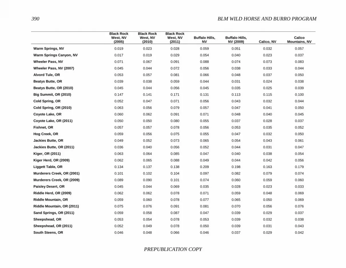
390 BLM WILD HORSE AND BURRO PROGRAM
PREPUBLICATION COPY
Black Rock West, NV
(2005)
Black Rock West, NV
(2010)
Black Rock West, NV
(2011) Buffalo Hills,
NV Buffalo Hills,
NV (2009) Calico, NV Calico
Mountains, NV
Warm Springs, NV 0.019 0.023 0.028 0.059 0.051 0.032 0.057
Warm Springs Canyon, NV 0.017 0.019 0.029 0.054 0.040 0.023 0.037
Wheeler Pass, NV 0.071 0.067 0.091 0.088 0.074 0.073 0.083
Wheeler Pass, NV (2007) 0.045 0.044 0.072 0.056 0.038 0.033 0.044
Alvord Tule, OR 0.053 0.057 0.081 0.066 0.048 0.037 0.050
Beatys Butte, OR 0.039 0.038 0.059 0.044 0.031 0.024 0.038
Beatys Butte, OR (2010) 0.045 0.044 0.056 0.045 0.035 0.025 0.039
Big Summit, OR (2010) 0.147 0.141 0.171 0.131 0.113 0.115 0.100
Cold Spring, OR 0.052 0.047 0.071 0.056 0.043 0.032 0.044
Cold Spring, OR (2010) 0.063 0.056 0.079 0.057 0.047 0.041 0.050
Coyote Lake, OR 0.060 0.062 0.091 0.071 0.048 0.040 0.045
Coyote Lake, OR (2011) 0.050 0.050 0.080 0.055 0.037 0.028 0.037
Fishnet, OR 0.057 0.057 0.078 0.056 0.053 0.035 0.052
Hog Creek, OR 0.059 0.056 0.075 0.055 0.047 0.032 0.050
Jackies Butte, OR 0.049 0.052 0.073 0.065 0.054 0.043 0.061
Jackies Butte, OR (2011) 0.036 0.040 0.056 0.052 0.044 0.031 0.047
Kiger, OR (2011) 0.063 0.064 0.085 0.047 0.040 0.038 0.054
Kiger Herd, OR (2009) 0.062 0.065 0.088 0.049 0.044 0.042 0.056
Liggett Table, OR 0.134 0.137 0.138 0.209 0.198 0.163 0.179
Murderers Creek, OR (2001) 0.101 0.102 0.104 0.097 0.082 0.079 0.074
Murderers Creek, OR (2009) 0.089 0.090 0.101 0.074 0.060 0.059 0.060
Paisley Desert, OR 0.045 0.044 0.069 0.035 0.028 0.023 0.033
Riddle Herd, OR (2009) 0.062 0.062 0.078 0.071 0.059 0.048 0.069
Riddle Mountain, OR 0.059 0.060 0.078 0.077 0.065 0.050 0.069
Riddle Mountain, OR (2011) 0.075 0.076 0.091 0.081 0.070 0.056 0.076
Sand Springs, OR (2011) 0.059 0.058 0.087 0.047 0.039 0.029 0.037
Sheepshead, OR 0.053 0.054 0.078 0.053 0.039 0.032 0.038
Sheepshead, OR (2011) 0.052 0.049 0.078 0.050 0.039 0.031 0.043
South Steens, OR 0.046 0.048 0.066 0.046 0.037 0.029 0.042

APPENDIX F 391
PREPUBLICATION COPY
Black Rock West, NV
(2005)
Black Rock West, NV
(2010)
Black Rock West, NV
(2011) Buffalo Hills,
NV Buffalo Hills,
NV (2009) Calico, NV Calico
Mountains, NV
South Steens, OR (2010) 0.047 0.047 0.059 0.044 0.035 0.026 0.041
Stinkingwater, OR 0.051 0.062 0.081 0.101 0.084 0.063 0.083
Three Fingers, OR 0.058 0.059 0.086 0.064 0.055 0.047 0.057
Three Fingers, OR (2011) 0.051 0.052 0.076 0.064 0.057 0.046 0.058
Warm Springs, OR 0.040 0.041 0.058 0.055 0.044 0.028 0.040
Warm Springs, OR (2010) 0.039 0.039 0.055 0.053 0.044 0.026 0.040
Blawn Wash, UT 0.068 0.064 0.082 0.101 0.086 0.056 0.084
Cedar Mountain, UT 0.063 0.063 0.088 0.064 0.051 0.038 0.054
Cedar Ridge, UT 0.100 0.103 0.127 0.096 0.080 0.067 0.063
Cedar Ridge, UT (trap) 0.115 0.114 0.135 0.092 0.079 0.074 0.070
Cold Springs, UT (2006) 0.084 0.088 0.114 0.115 0.097 0.070 0.097
Cold Springs, UT (trap) 0.068 0.068 0.093 0.090 0.073 0.053 0.072
Delta, UT 0.060 0.058 0.079 0.047 0.028 0.029 0.037
Hill Creek, UT 0.064 0.062 0.081 0.041 0.034 0.042 0.049
Muddy Creek, UT 0.104 0.104 0.135 0.108 0.095 0.080 0.103
North Hills, UT 0.095 0.098 0.122 0.086 0.073 0.076 0.074
Range Creek, UT 0.060 0.063 0.088 0.070 0.055 0.036 0.045
Sinbad, UT 0.093 0.089 0.115 0.092 0.070 0.062 0.065
Sulphur, UT 0.129 0.127 0.145 0.108 0.087 0.094 0.092
Sulphur Herd, UT (South, 2006) 0.082 0.084 0.101 0.072 0.057 0.058 0.060
Tilley Creek, UT 0.096 0.090 0.117 0.092 0.086 0.066 0.089
Winter Ridge, UT 0.060 0.055 0.072 0.046 0.037 0.037 0.047
Adobe Town, WY 0.059 0.059 0.073 0.055 0.039 0.042 0.050
Adobe Town, WY (2011) 0.048 0.047 0.062 0.037 0.032 0.027 0.043
Antelope Hills, WY 0.053 0.057 0.087 0.063 0.046 0.032 0.047
Conant Creek, WY (Lander) 0.081 0.080 0.092 0.081 0.067 0.055 0.070
Cooper Creek, WY 0.057 0.054 0.074 0.049 0.035 0.034 0.041
Dishpan Butte, WY (Lander) 0.068 0.069 0.086 0.073 0.057 0.054 0.059
Divide Basin, WY 0.042 0.043 0.065 0.046 0.032 0.022 0.035
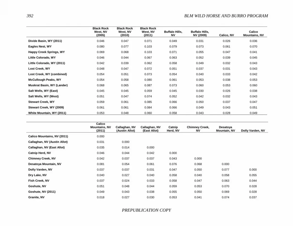
392 BLM WILD HORSE AND BURRO PROGRAM
PREPUBLICATION COPY
Black Rock West, NV
(2005)
Black Rock West, NV
(2010)
Black Rock West, NV
(2011) Buffalo Hills,
NV Buffalo Hills,
NV (2009) Calico, NV Calico
Mountains, NV
Divide Basin, WY (2011) 0.046 0.047 0.071 0.049 0.031 0.026 0.036
Eagles Nest, WY 0.080 0.077 0.103 0.079 0.073 0.061 0.070
Happy Creek Springs, WY 0.069 0.068 0.103 0.071 0.055 0.047 0.041
Little Colorado, WY 0.046 0.044 0.067 0.063 0.052 0.039 0.045
Little Colorado, WY (2011) 0.042 0.039 0.062 0.058 0.049 0.032 0.043
Lost Creek, WY 0.048 0.047 0.072 0.051 0.037 0.031 0.043
Lost Creek, WY (combined) 0.054 0.051 0.073 0.054 0.040 0.033 0.042
McCullough Peaks, WY 0.054 0.058 0.080 0.061 0.053 0.038 0.053
Muskrat Basin, WY (Lander) 0.068 0.065 0.087 0.073 0.060 0.053 0.060
Salt Wells, WY (East) 0.045 0.045 0.059 0.045 0.030 0.026 0.038
Salt Wells, WY (West) 0.051 0.047 0.074 0.052 0.042 0.032 0.043
Stewart Creek, WY 0.059 0.061 0.085 0.066 0.050 0.037 0.047
Stewart Creek, WY (2009) 0.061 0.061 0.084 0.066 0.049 0.043 0.051
White Mountain, WY (2011) 0.053 0.048 0.060 0.058 0.043 0.028 0.049
Calico Mountains, NV
(2011) Callaghan, NV (Austin Allot)
Callaghan, NV (East Allot)
Catnip Herd, NV
Chimney Creek, NV
Desatoya Mountain, NV Dolly Varden, NV
Calico Mountains, NV (2011) 0.000
Callaghan, NV (Austin Allot) 0.031 0.000
Callaghan, NV (East Allot) 0.035 0.014 0.000
Catnip Herd, NV 0.046 0.044 0.042 0.000
Chimney Creek, NV 0.042 0.037 0.037 0.043 0.000
Desatoya Mountain, NV 0.081 0.054 0.061 0.076 0.068 0.000
Dolly Varden, NV 0.037 0.037 0.031 0.047 0.050 0.077 0.000
Dry Lake, NV 0.040 0.027 0.040 0.058 0.040 0.058 0.055
Fish Creek, NV 0.037 0.024 0.033 0.058 0.047 0.063 0.044
Goshute, NV 0.051 0.048 0.044 0.059 0.053 0.070 0.028
Goshute, NV (2011) 0.049 0.043 0.038 0.055 0.050 0.069 0.028
Granite, NV 0.018 0.027 0.030 0.053 0.041 0.074 0.037

APPENDIX F 393
PREPUBLICATION COPY
Calico Mountains, NV
(2011) Callaghan, NV (Austin Allot)
Callaghan, NV (East Allot)
Catnip Herd, NV
Chimney Creek, NV
Desatoya Mountain, NV Dolly Varden, NV
Granite Range, NV 0.025 0.030 0.030 0.050 0.039 0.075 0.038
Granite Range, NV (2011) 0.014 0.023 0.027 0.045 0.038 0.071 0.029
Grass Valley, NV 0.042 0.013 0.012 0.042 0.041 0.054 0.033
Hall Creek, NV 0.038 0.007 0.020 0.049 0.045 0.059 0.039
Jakes Wash, NV 0.065 0.047 0.055 0.070 0.081 0.080 0.071
Johnnie, NV 0.060 0.046 0.047 0.073 0.063 0.068 0.054
Lahanton Reservoir, NV 0.063 0.051 0.050 0.061 0.063 0.077 0.063
Little Fish Lake, NV 0.057 0.033 0.033 0.056 0.053 0.074 0.055
Little Highrock Canyon, NV 0.025 0.043 0.044 0.064 0.052 0.091 0.038
Little Humboldt, NV 0.063 0.045 0.042 0.066 0.068 0.088 0.047
Little Humboldt, NV (2010) 0.042 0.034 0.030 0.055 0.054 0.080 0.040
Little Owyhee, NV (Fairbanks) 0.044 0.029 0.040 0.072 0.055 0.083 0.049
Little Owyhee, NV (Lake Creek) 0.054 0.036 0.038 0.061 0.042 0.085 0.053
Little Owyhee, NV (Twin Valley) 0.045 0.036 0.036 0.065 0.045 0.069 0.042
Marvel Gap, NV (SWC 2010) 0.044 0.029 0.028 0.036 0.047 0.068 0.036
McGee Mountain, NV 0.041 0.030 0.030 0.044 0.034 0.058 0.046
Miller Mountain, NV (SWC 2010) 0.036 0.017 0.022 0.050 0.041 0.065 0.047
Montezuma Peak, NV 0.053 0.049 0.045 0.067 0.070 0.100 0.047
Nellis, NV 0.036 0.021 0.019 0.043 0.034 0.055 0.044
New Pass-Ravenswood, NV 0.033 0.020 0.024 0.040 0.034 0.048 0.037
North Stillwater, NV 0.034 0.033 0.033 0.058 0.050 0.082 0.048
Paymaster, NV (2006) 0.055 0.044 0.048 0.074 0.071 0.097 0.055
Paymaster, NV (2010) 0.051 0.045 0.050 0.070 0.070 0.097 0.056
Pine Nut Mountain, NV 0.061 0.051 0.060 0.082 0.072 0.063 0.074
Powell Mountain, NV 0.068 0.048 0.056 0.090 0.073 0.103 0.060
Red Rock, NV 0.051 0.045 0.040 0.063 0.062 0.078 0.039
Reveille, NV 0.054 0.040 0.037 0.076 0.056 0.059 0.065
Roberts Mountain, NV 0.042 0.030 0.028 0.060 0.052 0.072 0.047
Rock Creek, NV (2002) 0.074 0.050 0.049 0.076 0.078 0.096 0.072

394 BLM WILD HORSE AND BURRO PROGRAM
PREPUBLICATION COPY
Calico Mountains, NV
(2011) Callaghan, NV (Austin Allot)
Callaghan, NV (East Allot)
Catnip Herd, NV
Chimney Creek, NV
Desatoya Mountain, NV Dolly Varden, NV
Rock Creek, NV (2010) 0.061 0.035 0.036 0.063 0.060 0.075 0.051
Rocky Hills, NV 0.046 0.026 0.023 0.045 0.043 0.064 0.041
Rodeo Creek, NV 0.033 0.023 0.015 0.048 0.045 0.067 0.028
Saulsbury, NV 0.037 0.020 0.021 0.051 0.036 0.057 0.039
Sand Springs East, NV 0.041 0.029 0.029 0.046 0.036 0.059 0.045
Seven Mile, NV 0.048 0.043 0.035 0.041 0.046 0.063 0.047
Shawave Mountains, NV 0.033 0.026 0.029 0.045 0.046 0.067 0.030
Silver Peak, NV 0.043 0.031 0.036 0.056 0.053 0.073 0.050
Snowstorm, NV (Castle Ridge) 0.049 0.035 0.033 0.059 0.057 0.087 0.051
Snowstorm, NV (Dryhill) 0.067 0.076 0.073 0.086 0.080 0.126 0.072
South Shoshone, NV 0.036 0.025 0.023 0.045 0.048 0.068 0.038
Spruce-Pequop, NV (2011) 0.053 0.051 0.047 0.066 0.064 0.076 0.023
Stillwater, NV 0.046 0.042 0.041 0.064 0.054 0.084 0.051
Stone Cabin, NV 0.037 0.020 0.015 0.051 0.035 0.053 0.040
Warm Springs, NV 0.034 0.041 0.035 0.046 0.037 0.075 0.046
Warm Springs Canyon, NV 0.027 0.032 0.027 0.036 0.028 0.059 0.036
Wheeler Pass, NV 0.079 0.058 0.055 0.092 0.075 0.079 0.059
Wheeler Pass, NV (2007) 0.033 0.027 0.030 0.052 0.050 0.067 0.035
Alvord Tule, OR 0.040 0.036 0.033 0.049 0.058 0.072 0.040
Beatys Butte, OR 0.031 0.023 0.022 0.033 0.032 0.056 0.029
Beatys Butte, OR (2010) 0.028 0.027 0.029 0.043 0.038 0.065 0.030
Big Summit, OR (2010) 0.116 0.103 0.087 0.145 0.137 0.154 0.096
Cold Spring, OR 0.042 0.024 0.028 0.045 0.046 0.063 0.038
Cold Spring, OR (2010) 0.047 0.031 0.034 0.057 0.059 0.074 0.046
Coyote Lake, OR 0.046 0.027 0.030 0.050 0.053 0.072 0.051
Coyote Lake, OR (2011) 0.035 0.021 0.025 0.045 0.042 0.066 0.039
Fishnet, OR 0.040 0.031 0.037 0.045 0.049 0.092 0.053
Hog Creek, OR 0.039 0.029 0.031 0.062 0.055 0.069 0.049
Jackies Butte, OR 0.047 0.040 0.039 0.063 0.052 0.072 0.049

APPENDIX F 395
PREPUBLICATION COPY
Calico Mountains, NV
(2011) Callaghan, NV (Austin Allot)
Callaghan, NV (East Allot)
Catnip Herd, NV
Chimney Creek, NV
Desatoya Mountain, NV Dolly Varden, NV
Jackies Butte, OR (2011) 0.033 0.036 0.032 0.051 0.043 0.073 0.038
Kiger, OR (2011) 0.043 0.031 0.040 0.050 0.060 0.082 0.049
Kiger Herd, OR (2009) 0.046 0.035 0.043 0.058 0.068 0.081 0.057
Liggett Table, OR 0.167 0.149 0.153 0.135 0.164 0.180 0.167
Murderers Creek, OR (2001) 0.078 0.063 0.064 0.075 0.096 0.126 0.083
Murderers Creek, OR (2009) 0.064 0.045 0.052 0.064 0.072 0.099 0.071
Paisley Desert, OR 0.029 0.019 0.019 0.046 0.041 0.053 0.030
Riddle Herd, OR (2009) 0.053 0.041 0.049 0.066 0.067 0.095 0.062
Riddle Mountain, OR 0.057 0.040 0.049 0.060 0.064 0.086 0.057
Riddle Mountain, OR (2011) 0.061 0.046 0.051 0.077 0.077 0.105 0.067
Sand Springs, OR (2011) 0.033 0.025 0.033 0.054 0.049 0.069 0.041
Sheepshead, OR 0.036 0.022 0.026 0.043 0.045 0.062 0.040
Sheepshead, OR (2011) 0.037 0.021 0.024 0.047 0.047 0.061 0.040
South Steens, OR 0.036 0.025 0.024 0.048 0.041 0.060 0.032
South Steens, OR (2010) 0.030 0.028 0.026 0.045 0.035 0.064 0.033
Stinkingwater, OR 0.073 0.057 0.060 0.046 0.068 0.093 0.070
Three Fingers, OR 0.053 0.037 0.039 0.049 0.052 0.087 0.058
Three Fingers, OR (2011) 0.051 0.031 0.036 0.047 0.046 0.079 0.049
Warm Springs, OR 0.035 0.022 0.024 0.041 0.033 0.057 0.035
Warm Springs, OR (2010) 0.036 0.021 0.024 0.043 0.029 0.055 0.035
Blawn Wash, UT 0.062 0.068 0.059 0.091 0.066 0.118 0.074
Cedar Mountain, UT 0.047 0.039 0.034 0.060 0.047 0.073 0.046
Cedar Ridge, UT 0.072 0.056 0.054 0.076 0.088 0.125 0.079
Cedar Ridge, UT (trap) 0.075 0.064 0.057 0.093 0.105 0.138 0.077
Cold Springs, UT (2006) 0.087 0.100 0.098 0.091 0.090 0.146 0.105
Cold Springs, UT (trap) 0.065 0.072 0.066 0.080 0.075 0.120 0.077
Delta, UT 0.034 0.021 0.022 0.052 0.053 0.056 0.033
Hill Creek, UT 0.042 0.029 0.028 0.067 0.062 0.078 0.043
Muddy Creek, UT 0.090 0.079 0.070 0.092 0.114 0.109 0.084

396 BLM WILD HORSE AND BURRO PROGRAM
PREPUBLICATION COPY
Calico Mountains, NV
(2011) Callaghan, NV (Austin Allot)
Callaghan, NV (East Allot)
Catnip Herd, NV
Chimney Creek, NV
Desatoya Mountain, NV Dolly Varden, NV
North Hills, UT 0.089 0.061 0.058 0.074 0.083 0.094 0.065
Range Creek, UT 0.045 0.043 0.042 0.049 0.056 0.101 0.059
Sinbad, UT 0.063 0.058 0.068 0.096 0.078 0.090 0.084
Sulphur, UT 0.101 0.081 0.082 0.114 0.096 0.111 0.098
Sulphur Herd, UT (South, 2006) 0.064 0.046 0.050 0.070 0.067 0.085 0.064
Tilley Creek, UT 0.073 0.066 0.061 0.095 0.083 0.134 0.074
Winter Ridge, UT 0.035 0.030 0.030 0.058 0.057 0.081 0.037
Adobe Town, WY 0.046 0.022 0.027 0.052 0.052 0.064 0.037
Adobe Town, WY (2011) 0.030 0.026 0.024 0.045 0.041 0.070 0.028
Antelope Hills, WY 0.045 0.044 0.046 0.051 0.051 0.057 0.058
Conant Creek, WY (Lander) 0.059 0.048 0.047 0.085 0.074 0.117 0.074
Cooper Creek, WY 0.038 0.021 0.027 0.059 0.044 0.048 0.044
Dishpan Butte, WY (Lander) 0.057 0.033 0.038 0.061 0.068 0.079 0.055
Divide Basin, WY 0.030 0.020 0.021 0.035 0.038 0.053 0.028
Divide Basin, WY (2011) 0.036 0.023 0.020 0.040 0.038 0.061 0.031
Eagles Nest, WY 0.067 0.053 0.047 0.071 0.088 0.087 0.063
Happy Creek Springs, WY 0.047 0.038 0.049 0.064 0.067 0.079 0.073
Little Colorado, WY 0.044 0.034 0.033 0.046 0.055 0.081 0.041
Little Colorado, WY (2011) 0.037 0.030 0.032 0.041 0.049 0.078 0.038
Lost Creek, WY 0.036 0.023 0.023 0.045 0.049 0.054 0.036
Lost Creek, WY (combined) 0.036 0.025 0.024 0.050 0.054 0.059 0.040
McCullough Peaks, WY 0.043 0.035 0.041 0.060 0.048 0.083 0.056
Muskrat Basin, WY (Lander) 0.057 0.035 0.039 0.062 0.069 0.082 0.053
Salt Wells, WY (East) 0.029 0.021 0.017 0.042 0.036 0.061 0.027
Salt Wells, WY (West) 0.038 0.020 0.024 0.057 0.047 0.063 0.044
Stewart Creek, WY 0.043 0.032 0.034 0.052 0.058 0.070 0.050
Stewart Creek, WY (2009) 0.042 0.033 0.035 0.064 0.062 0.072 0.051
White Mountain, WY (2011) 0.027 0.037 0.039 0.060 0.054 0.091 0.037

APPENDIX F 397
PREPUBLICATION COPY
Dry Lake,
NV Fish Creek, NV Goshute,
NV Goshute, NV
(2011) Granite, NV Granite Range,
NV Granite Range,
NV (2011)
Dry Lake, NV 0.000
Fish Creek, NV 0.043 0.000
Goshute, NV 0.056 0.055 0.000
Goshute, NV (2011) 0.057 0.053 0.009 0.000
Granite, NV 0.045 0.027 0.048 0.047 0.000
Granite Range, NV 0.042 0.038 0.050 0.049 0.015 0.000
Granite Range, NV (2011) 0.036 0.030 0.040 0.041 0.011 0.011 0.000
Grass Valley, NV 0.039 0.035 0.051 0.047 0.038 0.037 0.037
Hall Creek, NV 0.031 0.031 0.051 0.049 0.034 0.039 0.030
Jakes Wash, NV 0.058 0.067 0.077 0.068 0.073 0.069 0.061
Johnnie, NV 0.053 0.052 0.063 0.059 0.063 0.066 0.059
Lahanton Reservoir, NV 0.061 0.060 0.059 0.062 0.066 0.069 0.052
Little Fish Lake, NV 0.050 0.052 0.054 0.046 0.047 0.049 0.044
Little Highrock Canyon, NV 0.044 0.050 0.056 0.054 0.041 0.036 0.029
Little Humboldt, NV 0.067 0.060 0.072 0.065 0.050 0.047 0.049
Little Humboldt, NV (2010) 0.055 0.048 0.061 0.056 0.036 0.036 0.035
Little Owyhee, NV (Fairbanks) 0.055 0.046 0.060 0.057 0.041 0.047 0.043
Little Owyhee, NV (Lake Creek) 0.059 0.054 0.069 0.071 0.054 0.050 0.046
Little Owyhee, NV (Twin Valley) 0.054 0.032 0.059 0.058 0.036 0.038 0.033
Marvel Gap, NV (SWC 2010) 0.054 0.040 0.058 0.055 0.043 0.042 0.038
McGee Mountain, NV 0.039 0.032 0.046 0.041 0.032 0.034 0.036
Miller Mountain, NV (SWC 2010) 0.039 0.030 0.060 0.053 0.032 0.037 0.034
Montezuma Peak, NV 0.062 0.052 0.056 0.056 0.055 0.056 0.044
Nellis, NV 0.032 0.026 0.047 0.041 0.029 0.036 0.030
New Pass-Ravenswood, NV 0.028 0.029 0.042 0.042 0.031 0.034 0.025
North Stillwater, NV 0.053 0.040 0.055 0.054 0.036 0.035 0.027
Paymaster, NV (2006) 0.053 0.055 0.061 0.055 0.057 0.057 0.048
Paymaster, NV (2010) 0.048 0.056 0.058 0.054 0.058 0.057 0.046

398 BLM WILD HORSE AND BURRO PROGRAM
PREPUBLICATION COPY
Dry Lake,
NV Fish Creek, NV Goshute,
NV Goshute, NV
(2011) Granite, NV Granite Range,
NV Granite Range,
NV (2011)
Pine Nut Mountain, NV 0.048 0.046 0.085 0.083 0.064 0.067 0.054
Powell Mountain, NV 0.062 0.061 0.071 0.069 0.060 0.062 0.053
Red Rock, NV 0.056 0.050 0.051 0.045 0.050 0.050 0.045
Reveille, NV 0.049 0.042 0.070 0.066 0.040 0.049 0.050
Roberts Mountain, NV 0.055 0.036 0.057 0.050 0.037 0.040 0.039
Rock Creek, NV (2002) 0.066 0.064 0.085 0.077 0.072 0.070 0.068
Rock Creek, NV (2010) 0.055 0.052 0.062 0.053 0.055 0.056 0.054
Rocky Hills, NV 0.035 0.038 0.050 0.046 0.045 0.046 0.039
Rodeo Creek, NV 0.041 0.034 0.047 0.043 0.029 0.025 0.027
Saulsbury, NV 0.030 0.039 0.053 0.047 0.033 0.038 0.030
Sand Springs East, NV 0.040 0.032 0.046 0.041 0.030 0.032 0.035
Seven Mile, NV 0.046 0.055 0.053 0.051 0.054 0.048 0.045
Shawave Mountains, NV 0.043 0.038 0.043 0.045 0.035 0.037 0.034
Silver Peak, NV 0.051 0.049 0.066 0.062 0.040 0.034 0.029
Snowstorm, NV (Castle Ridge) 0.053 0.052 0.060 0.054 0.044 0.051 0.040
Snowstorm, NV (Dryhill) 0.094 0.075 0.091 0.083 0.070 0.073 0.061
South Shoshone, NV 0.045 0.034 0.043 0.038 0.037 0.038 0.030
Spruce-Pequop, NV (2011) 0.065 0.050 0.036 0.041 0.053 0.058 0.048
Stillwater, NV 0.065 0.045 0.060 0.058 0.050 0.045 0.039
Stone Cabin, NV 0.036 0.034 0.048 0.043 0.033 0.036 0.031
Warm Springs, NV 0.059 0.048 0.058 0.054 0.034 0.042 0.033
Warm Springs Canyon, NV 0.046 0.040 0.050 0.045 0.032 0.034 0.030
Wheeler Pass, NV 0.071 0.072 0.072 0.062 0.075 0.074 0.071
Wheeler Pass, NV (2007) 0.038 0.036 0.050 0.046 0.035 0.042 0.030
Alvord Tule, OR 0.057 0.044 0.071 0.066 0.038 0.041 0.038
Beatys Butte, OR 0.032 0.030 0.041 0.041 0.028 0.028 0.022
Beatys Butte, OR (2010) 0.041 0.037 0.042 0.044 0.031 0.032 0.026
Big Summit, OR (2010) 0.123 0.124 0.142 0.129 0.114 0.112 0.109
Cold Spring, OR 0.040 0.037 0.055 0.048 0.042 0.039 0.034

APPENDIX F 399
PREPUBLICATION COPY
Dry Lake,
NV Fish Creek, NV Goshute,
NV Goshute, NV
(2011) Granite, NV Granite Range,
NV Granite Range,
NV (2011)
Cold Spring, OR (2010) 0.049 0.044 0.063 0.057 0.047 0.047 0.038
Coyote Lake, OR 0.051 0.036 0.070 0.065 0.040 0.043 0.043
Coyote Lake, OR (2011) 0.045 0.024 0.056 0.052 0.027 0.033 0.028
Fishnet, OR 0.047 0.034 0.063 0.059 0.041 0.052 0.037
Hog Creek, OR 0.036 0.032 0.065 0.066 0.035 0.040 0.032
Jackies Butte, OR 0.047 0.053 0.066 0.052 0.051 0.051 0.044
Jackies Butte, OR (2011) 0.040 0.043 0.056 0.045 0.041 0.040 0.034
Kiger, OR (2011) 0.043 0.046 0.064 0.065 0.039 0.040 0.034
Kiger Herd, OR (2009) 0.049 0.046 0.079 0.075 0.043 0.045 0.042
Liggett Table, OR 0.192 0.155 0.180 0.171 0.162 0.160 0.155
Murderers Creek, OR (2001) 0.097 0.088 0.107 0.098 0.084 0.078 0.074
Murderers Creek, OR (2009) 0.070 0.073 0.083 0.074 0.068 0.057 0.055
Paisley Desert, OR 0.037 0.026 0.043 0.037 0.025 0.024 0.022
Riddle Herd, OR (2009) 0.061 0.051 0.079 0.079 0.047 0.047 0.042
Riddle Mountain, OR 0.052 0.053 0.073 0.073 0.054 0.049 0.044
Riddle Mountain, OR (2011) 0.069 0.056 0.089 0.088 0.053 0.052 0.048
Sand Springs, OR (2011) 0.034 0.034 0.054 0.053 0.032 0.031 0.025
Sheepshead, OR 0.039 0.039 0.052 0.046 0.040 0.034 0.031
Sheepshead, OR (2011) 0.036 0.033 0.048 0.043 0.039 0.037 0.029
South Steens, OR 0.042 0.033 0.051 0.049 0.037 0.033 0.032
South Steens, OR (2010) 0.034 0.033 0.047 0.047 0.035 0.032 0.029
Stinkingwater, OR 0.066 0.058 0.086 0.078 0.075 0.078 0.072
Three Fingers, OR 0.061 0.047 0.069 0.058 0.047 0.046 0.043
Three Fingers, OR (2011) 0.059 0.040 0.062 0.049 0.046 0.052 0.044
Warm Springs, OR 0.032 0.033 0.048 0.040 0.039 0.038 0.033
Warm Springs, OR (2010) 0.034 0.030 0.050 0.044 0.034 0.034 0.031
Blawn Wash, UT 0.057 0.078 0.078 0.075 0.067 0.064 0.054
Cedar Mountain, UT 0.060 0.042 0.075 0.071 0.039 0.040 0.034
Cedar Ridge, UT 0.089 0.065 0.109 0.099 0.065 0.072 0.066

400 BLM WILD HORSE AND BURRO PROGRAM
PREPUBLICATION COPY
Dry Lake,
NV Fish Creek, NV Goshute,
NV Goshute, NV
(2011) Granite, NV Granite Range,
NV Granite Range,
NV (2011)
Cedar Ridge, UT (trap) 0.100 0.074 0.120 0.110 0.073 0.080 0.072
Cold Springs, UT (2006) 0.108 0.100 0.125 0.118 0.086 0.091 0.089
Cold Springs, UT (trap) 0.078 0.078 0.097 0.091 0.064 0.067 0.063
Delta, UT 0.039 0.028 0.052 0.050 0.030 0.031 0.028
Hill Creek, UT 0.057 0.044 0.063 0.061 0.043 0.042 0.037
Muddy Creek, UT 0.084 0.099 0.091 0.078 0.085 0.085 0.076
North Hills, UT 0.077 0.076 0.101 0.098 0.080 0.070 0.076
Range Creek, UT 0.064 0.048 0.083 0.075 0.041 0.047 0.043
Sinbad, UT 0.059 0.062 0.089 0.091 0.069 0.070 0.061
Sulphur, UT 0.094 0.097 0.124 0.119 0.094 0.089 0.093
Sulphur Herd, UT (South, 2006) 0.070 0.065 0.084 0.074 0.065 0.048 0.055
Tilley Creek, UT 0.077 0.084 0.086 0.089 0.069 0.064 0.054
Winter Ridge, UT 0.058 0.046 0.054 0.055 0.040 0.047 0.032
Adobe Town, WY 0.046 0.037 0.053 0.048 0.043 0.042 0.040
Adobe Town, WY (2011) 0.045 0.036 0.044 0.041 0.034 0.033 0.028
Antelope Hills, WY 0.055 0.045 0.068 0.063 0.038 0.034 0.038
Conant Creek, WY (Lander) 0.070 0.063 0.078 0.069 0.058 0.049 0.047
Cooper Creek, WY 0.033 0.032 0.059 0.054 0.035 0.034 0.033
Dishpan Butte, WY (Lander) 0.054 0.045 0.061 0.056 0.049 0.046 0.045
Divide Basin, WY 0.034 0.032 0.040 0.036 0.028 0.028 0.024
Divide Basin, WY (2011) 0.036 0.035 0.044 0.039 0.031 0.031 0.029
Eagles Nest, WY 0.080 0.060 0.077 0.069 0.067 0.062 0.059
Happy Creek Springs, WY 0.049 0.054 0.078 0.070 0.057 0.058 0.052
Little Colorado, WY 0.050 0.051 0.064 0.057 0.047 0.043 0.042
Little Colorado, WY (2011) 0.043 0.043 0.055 0.051 0.041 0.038 0.034
Lost Creek, WY 0.044 0.036 0.051 0.043 0.036 0.035 0.028
Lost Creek, WY (combined) 0.044 0.041 0.052 0.044 0.041 0.038 0.031
McCullough Peaks, WY 0.044 0.040 0.065 0.065 0.048 0.048 0.041
Muskrat Basin, WY (Lander) 0.065 0.046 0.059 0.052 0.047 0.051 0.046

APPENDIX F 401
PREPUBLICATION COPY
Dry Lake,
NV Fish Creek, NV Goshute,
NV Goshute, NV
(2011) Granite, NV Granite Range,
NV Granite Range,
NV (2011)
Salt Wells, WY (East) 0.039 0.035 0.047 0.041 0.033 0.029 0.025
Salt Wells, WY (West) 0.035 0.033 0.050 0.049 0.032 0.040 0.033
Stewart Creek, WY 0.057 0.041 0.065 0.055 0.041 0.040 0.039
Stewart Creek, WY (2009) 0.052 0.048 0.064 0.058 0.049 0.052 0.045
White Mountain, WY (2011) 0.042 0.046 0.046 0.049 0.031 0.038 0.024
Grass Valley,
NV Hall Creek, NV Jakes Wash,
NV Johnnie, NV
Lahonton Reservoir,
NV Little Fish Lake,
NV Little Highrock
Canyon, NV
Grass Valley, NV 0.000
Hall Creek, NV 0.021 0.000
Jakes Wash, NV 0.059 0.054 0.000
Johnnie, NV 0.049 0.052 0.083 0.000
Lahanton Reservoir, NV 0.062 0.058 0.088 0.090 0.000
Little Fish Lake, NV 0.033 0.040 0.065 0.077 0.064 0.000
Little Highrock Canyon, NV 0.051 0.048 0.084 0.066 0.062 0.066 0.000
Little Humboldt, NV 0.046 0.051 0.079 0.072 0.073 0.046 0.068
Little Humboldt, NV (2010) 0.038 0.038 0.064 0.062 0.055 0.043 0.048
Little Owyhee, NV (Fairbanks) 0.034 0.033 0.078 0.061 0.086 0.057 0.062
Little Owyhee, NV (Lake Creek) 0.037 0.045 0.089 0.064 0.078 0.056 0.056
Little Owyhee, NV (Twin Valley) 0.043 0.045 0.077 0.052 0.068 0.068 0.052
Marvel Gap, NV (SWC 2010) 0.029 0.036 0.065 0.052 0.064 0.049 0.051
McGee Mountain, NV 0.034 0.035 0.059 0.049 0.058 0.039 0.052
Miller Mountain, NV (SWC 2010) 0.029 0.026 0.061 0.050 0.063 0.041 0.048
Montezuma Peak, NV 0.050 0.057 0.088 0.094 0.068 0.052 0.046
Nellis, NV 0.022 0.028 0.055 0.045 0.053 0.035 0.051
New Pass-Ravenswood, NV 0.027 0.023 0.049 0.039 0.045 0.045 0.039
North Stillwater, NV 0.044 0.035 0.069 0.068 0.074 0.056 0.047
Paymaster, NV (2006) 0.051 0.052 0.080 0.084 0.070 0.051 0.049
Paymaster, NV (2010) 0.053 0.052 0.079 0.088 0.067 0.053 0.046
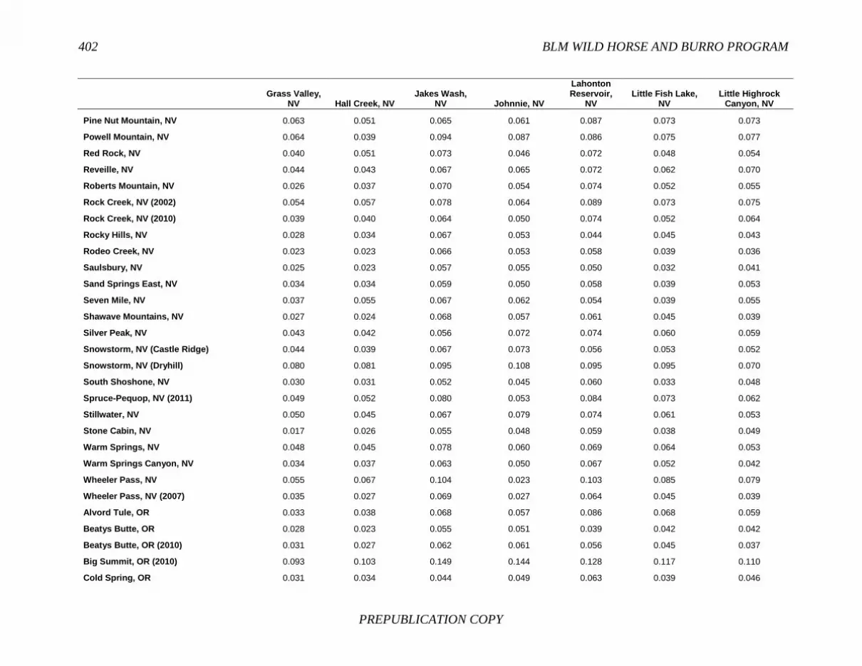
402 BLM WILD HORSE AND BURRO PROGRAM
PREPUBLICATION COPY
Grass Valley,
NV Hall Creek, NV Jakes Wash,
NV Johnnie, NV
Lahonton Reservoir,
NV Little Fish Lake,
NV Little Highrock
Canyon, NV
Pine Nut Mountain, NV 0.063 0.051 0.065 0.061 0.087 0.073 0.073
Powell Mountain, NV 0.064 0.039 0.094 0.087 0.086 0.075 0.077
Red Rock, NV 0.040 0.051 0.073 0.046 0.072 0.048 0.054
Reveille, NV 0.044 0.043 0.067 0.065 0.072 0.062 0.070
Roberts Mountain, NV 0.026 0.037 0.070 0.054 0.074 0.052 0.055
Rock Creek, NV (2002) 0.054 0.057 0.078 0.064 0.089 0.073 0.075
Rock Creek, NV (2010) 0.039 0.040 0.064 0.050 0.074 0.052 0.064
Rocky Hills, NV 0.028 0.034 0.067 0.053 0.044 0.045 0.043
Rodeo Creek, NV 0.023 0.023 0.066 0.053 0.058 0.039 0.036
Saulsbury, NV 0.025 0.023 0.057 0.055 0.050 0.032 0.041
Sand Springs East, NV 0.034 0.034 0.059 0.050 0.058 0.039 0.053
Seven Mile, NV 0.037 0.055 0.067 0.062 0.054 0.039 0.055
Shawave Mountains, NV 0.027 0.024 0.068 0.057 0.061 0.045 0.039
Silver Peak, NV 0.043 0.042 0.056 0.072 0.074 0.060 0.059
Snowstorm, NV (Castle Ridge) 0.044 0.039 0.067 0.073 0.056 0.053 0.052
Snowstorm, NV (Dryhill) 0.080 0.081 0.095 0.108 0.095 0.095 0.070
South Shoshone, NV 0.030 0.031 0.052 0.045 0.060 0.033 0.048
Spruce-Pequop, NV (2011) 0.049 0.052 0.080 0.053 0.084 0.073 0.062
Stillwater, NV 0.050 0.045 0.067 0.079 0.074 0.061 0.053
Stone Cabin, NV 0.017 0.026 0.055 0.048 0.059 0.038 0.049
Warm Springs, NV 0.048 0.045 0.078 0.060 0.069 0.064 0.053
Warm Springs Canyon, NV 0.034 0.037 0.063 0.050 0.067 0.052 0.042
Wheeler Pass, NV 0.055 0.067 0.104 0.023 0.103 0.085 0.079
Wheeler Pass, NV (2007) 0.035 0.027 0.069 0.027 0.064 0.045 0.039
Alvord Tule, OR 0.033 0.038 0.068 0.057 0.086 0.068 0.059
Beatys Butte, OR 0.028 0.023 0.055 0.051 0.039 0.042 0.042
Beatys Butte, OR (2010) 0.031 0.027 0.062 0.061 0.056 0.045 0.037
Big Summit, OR (2010) 0.093 0.103 0.149 0.144 0.128 0.117 0.110
Cold Spring, OR 0.031 0.034 0.044 0.049 0.063 0.039 0.046

APPENDIX F 403
PREPUBLICATION COPY
Grass Valley,
NV Hall Creek, NV Jakes Wash,
NV Johnnie, NV
Lahonton Reservoir,
NV Little Fish Lake,
NV Little Highrock
Canyon, NV
Cold Spring, OR (2010) 0.040 0.043 0.056 0.057 0.066 0.044 0.050
Coyote Lake, OR 0.028 0.037 0.060 0.055 0.083 0.055 0.069
Coyote Lake, OR (2011) 0.026 0.027 0.056 0.051 0.066 0.048 0.055
Fishnet, OR 0.044 0.039 0.061 0.068 0.068 0.065 0.054
Hog Creek, OR 0.032 0.034 0.058 0.052 0.065 0.055 0.052
Jackies Butte, OR 0.044 0.040 0.076 0.063 0.067 0.065 0.059
Jackies Butte, OR (2011) 0.038 0.039 0.072 0.051 0.063 0.061 0.043
Kiger, OR (2011) 0.041 0.032 0.063 0.074 0.064 0.056 0.059
Kiger Herd, OR (2009) 0.044 0.039 0.066 0.064 0.079 0.069 0.067
Liggett Table, OR 0.158 0.164 0.204 0.192 0.163 0.182 0.187
Murderers Creek, OR (2001) 0.073 0.080 0.091 0.102 0.089 0.077 0.089
Murderers Creek, OR (2009) 0.055 0.060 0.072 0.095 0.072 0.055 0.070
Paisley Desert, OR 0.024 0.023 0.051 0.039 0.057 0.044 0.041
Riddle Herd, OR (2009) 0.057 0.045 0.077 0.079 0.068 0.072 0.064
Riddle Mountain, OR 0.056 0.042 0.071 0.075 0.064 0.071 0.062
Riddle Mountain, OR (2011) 0.059 0.050 0.080 0.087 0.082 0.079 0.073
Sand Springs, OR (2011) 0.035 0.029 0.059 0.061 0.070 0.053 0.043
Sheepshead, OR 0.026 0.026 0.050 0.047 0.069 0.039 0.050
Sheepshead, OR (2011) 0.031 0.023 0.045 0.043 0.058 0.040 0.040
South Steens, OR 0.024 0.030 0.054 0.039 0.077 0.056 0.045
South Steens, OR (2010) 0.026 0.030 0.058 0.044 0.062 0.053 0.039
Stinkingwater, OR 0.063 0.059 0.089 0.061 0.081 0.082 0.085
Three Fingers, OR 0.045 0.042 0.082 0.078 0.068 0.053 0.067
Three Fingers, OR (2011) 0.037 0.039 0.065 0.060 0.068 0.048 0.064
Warm Springs, OR 0.025 0.030 0.043 0.046 0.055 0.044 0.040
Warm Springs, OR (2010) 0.025 0.030 0.052 0.050 0.052 0.044 0.043
Blawn Wash, UT 0.078 0.066 0.099 0.089 0.088 0.095 0.071
Cedar Mountain, UT 0.040 0.046 0.077 0.059 0.081 0.063 0.064
Cedar Ridge, UT 0.058 0.064 0.103 0.103 0.107 0.074 0.090

404 BLM WILD HORSE AND BURRO PROGRAM
PREPUBLICATION COPY
Grass Valley,
NV Hall Creek, NV Jakes Wash,
NV Johnnie, NV
Lahonton Reservoir,
NV Little Fish Lake,
NV Little Highrock
Canyon, NV
Cedar Ridge, UT (trap) 0.060 0.066 0.112 0.106 0.126 0.088 0.087
Cold Springs, UT (2006) 0.101 0.111 0.136 0.127 0.142 0.118 0.094
Cold Springs, UT (trap) 0.075 0.076 0.093 0.088 0.122 0.089 0.077
Delta, UT 0.025 0.024 0.052 0.040 0.058 0.036 0.047
Hill Creek, UT 0.030 0.032 0.083 0.053 0.077 0.065 0.048
Muddy Creek, UT 0.076 0.084 0.091 0.102 0.109 0.075 0.102
North Hills, UT 0.052 0.069 0.096 0.081 0.094 0.073 0.088
Range Creek, UT 0.045 0.052 0.085 0.080 0.090 0.061 0.059
Sinbad, UT 0.071 0.054 0.084 0.082 0.101 0.078 0.074
Sulphur, UT 0.073 0.087 0.128 0.128 0.119 0.086 0.107
Sulphur Herd, UT (South, 2006) 0.049 0.058 0.078 0.066 0.088 0.071 0.067
Tilley Creek, UT 0.083 0.073 0.103 0.105 0.091 0.086 0.066
Winter Ridge, UT 0.037 0.036 0.082 0.054 0.063 0.051 0.043
Adobe Town, WY 0.028 0.026 0.057 0.052 0.064 0.043 0.054
Adobe Town, WY (2011) 0.027 0.031 0.062 0.054 0.057 0.046 0.035
Antelope Hills, WY 0.048 0.047 0.074 0.063 0.063 0.061 0.056
Conant Creek, WY (Lander) 0.064 0.049 0.084 0.093 0.100 0.069 0.074
Cooper Creek, WY 0.025 0.028 0.053 0.046 0.059 0.043 0.048
Dishpan Butte, WY (Lander) 0.045 0.039 0.069 0.056 0.086 0.044 0.070
Divide Basin, WY 0.025 0.026 0.052 0.041 0.053 0.033 0.037
Divide Basin, WY (2011) 0.022 0.026 0.061 0.046 0.060 0.028 0.039
Eagles Nest, WY 0.051 0.060 0.080 0.073 0.083 0.069 0.075
Happy Creek Springs, WY 0.046 0.050 0.080 0.060 0.083 0.066 0.063
Little Colorado, WY 0.037 0.041 0.076 0.048 0.074 0.057 0.048
Little Colorado, WY (2011) 0.038 0.037 0.068 0.043 0.063 0.054 0.040
Lost Creek, WY 0.023 0.026 0.058 0.045 0.061 0.041 0.045
Lost Creek, WY (combined) 0.026 0.032 0.053 0.042 0.064 0.038 0.041
McCullough Peaks, WY 0.047 0.039 0.069 0.052 0.075 0.068 0.052
Muskrat Basin, WY (Lander) 0.043 0.041 0.065 0.060 0.089 0.048 0.078

APPENDIX F 405
PREPUBLICATION COPY
Grass Valley,
NV Hall Creek, NV Jakes Wash,
NV Johnnie, NV
Lahonton Reservoir,
NV Little Fish Lake,
NV Little Highrock
Canyon, NV
Salt Wells, WY (East) 0.021 0.026 0.058 0.054 0.055 0.040 0.036
Salt Wells, WY (West) 0.031 0.024 0.056 0.054 0.050 0.044 0.047
Stewart Creek, WY 0.032 0.036 0.063 0.052 0.079 0.057 0.056
Stewart Creek, WY (2009) 0.040 0.040 0.067 0.056 0.076 0.052 0.056
White Mountain, WY (2011) 0.051 0.039 0.077 0.071 0.046 0.048 0.032
Little
Humboldt, NV
Little Humboldt, NV
(2010) Little Owyhee, NV (Fairbanks)
Little Owyhee, NV (Lake
Creek)
Little Owyhee,NV
(Twin Valley) Marvel Gap, NV
(SWC 2010) McGee
Mountain, NV
Little Humboldt, NV 0.000
Little Humboldt, NV (2010) 0.017 0.000
Little Owyhee, NV (Fairbanks) 0.071 0.059 0.000
Little Owyhee, NV (Lake Creek) 0.057 0.047 0.046 0.000
Little Owyhee, NV (Twin Valley) 0.059 0.048 0.051 0.039 0.000
Marvel Gap, NV (SWC 2010) 0.042 0.039 0.063 0.046 0.045 0.000
McGee Mountain, NV 0.043 0.034 0.048 0.046 0.039 0.036 0.000
Miller Mountain, NV (SWC 2010) 0.052 0.040 0.044 0.041 0.041 0.035 0.036
Montezuma Peak, NV 0.080 0.064 0.075 0.061 0.059 0.050 0.054
Nellis, NV 0.048 0.037 0.041 0.047 0.043 0.030 0.023
New Pass-Ravenswood, NV 0.047 0.031 0.047 0.042 0.033 0.034 0.026
North Stillwater, NV 0.071 0.051 0.049 0.051 0.054 0.044 0.044
Paymaster, NV (2006) 0.070 0.063 0.074 0.069 0.065 0.052 0.050
Paymaster, NV (2010) 0.077 0.066 0.075 0.070 0.066 0.055 0.053
Pine Nut Mountain, NV 0.082 0.071 0.075 0.088 0.064 0.070 0.056
Powell Mountain, NV 0.081 0.063 0.061 0.086 0.074 0.071 0.063
Red Rock, NV 0.062 0.057 0.052 0.066 0.050 0.046 0.040
Reveille, NV 0.064 0.049 0.062 0.067 0.058 0.052 0.037
Roberts Mountain, NV 0.060 0.050 0.039 0.054 0.050 0.038 0.035
Rock Creek, NV (2002) 0.063 0.044 0.078 0.072 0.059 0.067 0.052
Rock Creek, NV (2010) 0.041 0.026 0.062 0.055 0.048 0.049 0.034

406 BLM WILD HORSE AND BURRO PROGRAM
PREPUBLICATION COPY
Little
Humboldt, NV
Little Humboldt, NV
(2010) Little Owyhee, NV (Fairbanks)
Little Owyhee, NV (Lake
Creek)
Little Owyhee,NV
(Twin Valley) Marvel Gap, NV
(SWC 2010) McGee
Mountain, NV
Rocky Hills, NV 0.058 0.047 0.062 0.064 0.051 0.034 0.035
Rodeo Creek, NV 0.044 0.030 0.042 0.047 0.043 0.033 0.028
Saulsbury, NV 0.050 0.035 0.046 0.047 0.045 0.044 0.029
Sand Springs East, NV 0.038 0.030 0.046 0.047 0.038 0.034 0.001
Seven Mile, NV 0.053 0.049 0.071 0.062 0.062 0.041 0.036
Shawave Mountains, NV 0.050 0.038 0.038 0.038 0.041 0.035 0.037
Silver Peak, NV 0.053 0.046 0.061 0.052 0.045 0.048 0.053
Snowstorm, NV (Castle Ridge) 0.034 0.019 0.063 0.052 0.052 0.047 0.045
Snowstorm, NV (Dryhill) 0.091 0.079 0.089 0.074 0.069 0.074 0.083
South Shoshone, NV 0.042 0.033 0.056 0.054 0.045 0.027 0.027
Spruce-Pequop, NV (2011) 0.075 0.067 0.052 0.063 0.058 0.055 0.057
Stillwater, NV 0.071 0.051 0.061 0.053 0.058 0.047 0.046
Stone Cabin, NV 0.046 0.037 0.039 0.042 0.039 0.037 0.029
Warm Springs, NV 0.065 0.050 0.065 0.056 0.040 0.044 0.035
Warm Springs Canyon, NV 0.060 0.042 0.051 0.045 0.037 0.037 0.030
Wheeler Pass, NV 0.077 0.067 0.073 0.076 0.071 0.068 0.059
Wheeler Pass, NV (2007) 0.044 0.036 0.046 0.051 0.049 0.034 0.035
Alvord Tule, OR 0.061 0.047 0.056 0.063 0.048 0.036 0.043
Beatys Butte, OR 0.041 0.031 0.049 0.041 0.033 0.034 0.027
Beatys Butte, OR (2010) 0.051 0.036 0.044 0.035 0.038 0.032 0.037
Big Summit, OR (2010) 0.083 0.084 0.131 0.126 0.130 0.111 0.118
Cold Spring, OR 0.052 0.044 0.049 0.051 0.042 0.033 0.042
Cold Spring, OR (2010) 0.056 0.047 0.064 0.060 0.051 0.034 0.051
Coyote Lake, OR 0.059 0.048 0.049 0.057 0.051 0.040 0.041
Coyote Lake, OR (2011) 0.044 0.034 0.042 0.050 0.039 0.029 0.030
Fishnet, OR 0.076 0.056 0.066 0.064 0.054 0.042 0.049
Hog Creek, OR 0.064 0.046 0.050 0.058 0.038 0.039 0.041
Jackies Butte, OR 0.072 0.058 0.062 0.078 0.059 0.051 0.053
Jackies Butte, OR (2011) 0.065 0.050 0.054 0.064 0.045 0.042 0.040

APPENDIX F 407
PREPUBLICATION COPY
Little
Humboldt, NV
Little Humboldt, NV
(2010) Little Owyhee, NV (Fairbanks)
Little Owyhee, NV (Lake
Creek)
Little Owyhee,NV
(Twin Valley) Marvel Gap, NV
(SWC 2010) McGee
Mountain, NV
Kiger, OR (2011) 0.058 0.049 0.065 0.065 0.055 0.051 0.046
Kiger Herd, OR (2009) 0.064 0.055 0.067 0.070 0.057 0.051 0.048
Liggett Table, OR 0.188 0.178 0.198 0.175 0.138 0.148 0.153
Murderers Creek, OR (2001) 0.086 0.071 0.086 0.076 0.092 0.068 0.082
Murderers Creek, OR (2009) 0.073 0.061 0.069 0.067 0.082 0.061 0.066
Paisley Desert, OR 0.039 0.034 0.038 0.046 0.034 0.029 0.027
Riddle Herd, OR (2009) 0.067 0.056 0.081 0.069 0.051 0.063 0.047
Riddle Mountain, OR 0.062 0.053 0.084 0.069 0.050 0.060 0.046
Riddle Mountain, OR (2011) 0.070 0.060 0.087 0.076 0.055 0.069 0.055
Sand Springs, OR (2011) 0.048 0.040 0.047 0.051 0.040 0.036 0.039
Sheepshead, OR 0.050 0.043 0.040 0.051 0.053 0.035 0.038
Sheepshead, OR (2011) 0.046 0.038 0.046 0.053 0.048 0.030 0.034
South Steens, OR 0.052 0.042 0.044 0.037 0.030 0.029 0.036
South Steens, OR (2010) 0.057 0.042 0.041 0.039 0.030 0.039 0.035
Stinkingwater, OR 0.093 0.073 0.079 0.080 0.074 0.052 0.056
Three Fingers, OR 0.053 0.055 0.072 0.069 0.064 0.030 0.045
Three Fingers, OR (2011) 0.049 0.048 0.061 0.063 0.053 0.026 0.034
Warm Springs, OR 0.045 0.036 0.046 0.041 0.031 0.033 0.026
Warm Springs, OR (2010) 0.041 0.035 0.048 0.039 0.027 0.035 0.027
Blawn Wash, UT 0.103 0.080 0.092 0.106 0.075 0.094 0.070
Cedar Mountain, UT 0.064 0.049 0.062 0.050 0.037 0.049 0.051
Cedar Ridge, UT 0.065 0.060 0.097 0.080 0.081 0.060 0.073
Cedar Ridge, UT (trap) 0.080 0.066 0.100 0.086 0.089 0.068 0.090
Cold Springs, UT (2006) 0.128 0.109 0.129 0.114 0.104 0.085 0.083
Cold Springs, UT (trap) 0.095 0.078 0.095 0.092 0.082 0.067 0.057
Delta, UT 0.036 0.027 0.041 0.046 0.035 0.033 0.031
Hill Creek, UT 0.059 0.046 0.047 0.047 0.052 0.040 0.047
Muddy Creek, UT 0.101 0.095 0.097 0.117 0.109 0.086 0.085
North Hills, UT 0.058 0.058 0.089 0.071 0.069 0.058 0.071

408 BLM WILD HORSE AND BURRO PROGRAM
PREPUBLICATION COPY
Little
Humboldt, NV
Little Humboldt, NV
(2010) Little Owyhee, NV (Fairbanks)
Little Owyhee, NV (Lake
Creek)
Little Owyhee,NV
(Twin Valley) Marvel Gap, NV
(SWC 2010) McGee
Mountain, NV
Range Creek, UT 0.061 0.049 0.077 0.063 0.059 0.040 0.045
Sinbad, UT 0.083 0.069 0.076 0.088 0.079 0.086 0.061
Sulphur, UT 0.082 0.079 0.100 0.100 0.115 0.103 0.100
Sulphur Herd, UT (South, 2006) 0.054 0.047 0.067 0.060 0.060 0.050 0.057
Tilley Creek, UT 0.072 0.060 0.112 0.087 0.076 0.074 0.083
Winter Ridge, UT 0.058 0.043 0.051 0.044 0.054 0.032 0.052
Adobe Town, WY 0.043 0.036 0.046 0.045 0.045 0.021 0.037
Adobe Town, WY (2011) 0.046 0.036 0.048 0.038 0.038 0.015 0.037
Antelope Hills, WY 0.056 0.042 0.067 0.063 0.057 0.048 0.039
Conant Creek, WY (Lander) 0.084 0.072 0.062 0.071 0.077 0.077 0.064
Cooper Creek, WY 0.043 0.035 0.040 0.046 0.040 0.040 0.031
Dishpan Butte, WY (Lander) 0.047 0.045 0.057 0.055 0.054 0.042 0.037
Divide Basin, WY 0.032 0.023 0.044 0.033 0.033 0.030 0.028
Divide Basin, WY (2011) 0.031 0.024 0.044 0.033 0.041 0.032 0.029
Eagles Nest, WY 0.048 0.042 0.083 0.071 0.068 0.054 0.056
Happy Creek Springs, WY 0.073 0.061 0.068 0.073 0.076 0.051 0.058
Little Colorado, WY 0.045 0.040 0.063 0.052 0.047 0.033 0.039
Little Colorado, WY (2011) 0.045 0.036 0.059 0.048 0.040 0.032 0.035
Lost Creek, WY 0.040 0.029 0.046 0.045 0.043 0.027 0.032
Lost Creek, WY (combined) 0.041 0.031 0.049 0.044 0.042 0.031 0.032
McCullough Peaks, WY 0.061 0.046 0.056 0.051 0.047 0.051 0.043
Muskrat Basin, WY (Lander) 0.043 0.042 0.056 0.062 0.058 0.043 0.039
Salt Wells, WY (East) 0.046 0.033 0.044 0.043 0.041 0.022 0.036
Salt Wells, WY (West) 0.049 0.037 0.047 0.048 0.048 0.043 0.039
Stewart Creek, WY 0.044 0.035 0.054 0.060 0.047 0.042 0.036
Stewart Creek, WY (2009) 0.055 0.047 0.060 0.051 0.050 0.038 0.044
White Mountain, WY (2011) 0.062 0.041 0.062 0.060 0.054 0.049 0.048

APPENDIX F 409
PREPUBLICATION COPY
Miller Mountain, NV
(Swc 2010) Montezuma
Peak, NV Nellis, NV
New Pass-Ravenswood,
NV North
Stillwater, NV Paymaster, NV
(2006) Paymaster, NV
(2010)
Miller Mountain, NV (SWC 2010) 0.000
Montezuma Peak, NV 0.060 0.000
Nellis, NV 0.026 0.050 0.000
New Pass-Ravenswood, NV 0.032 0.053 0.021 0.000
North Stillwater, NV 0.042 0.052 0.043 0.038 0.000
Paymaster, NV (2006) 0.058 0.018 0.049 0.053 0.058 0.000
Paymaster, NV (2010) 0.061 0.014 0.048 0.049 0.057 0.004 0.000
Pine Nut Mountain, NV 0.065 0.089 0.054 0.048 0.062 0.085 0.085
Powell Mountain, NV 0.063 0.082 0.062 0.059 0.062 0.083 0.082
Red Rock, NV 0.049 0.054 0.035 0.044 0.058 0.052 0.055
Reveille, NV 0.033 0.077 0.022 0.037 0.058 0.077 0.079
Roberts Mountain, NV 0.038 0.062 0.028 0.036 0.047 0.062 0.065
Rock Creek, NV (2002) 0.066 0.086 0.061 0.050 0.080 0.079 0.083
Rock Creek, NV (2010) 0.048 0.075 0.043 0.036 0.063 0.071 0.074
Rocky Hills, NV 0.034 0.052 0.027 0.030 0.058 0.052 0.052
Rodeo Creek, NV 0.032 0.037 0.027 0.031 0.029 0.041 0.042
Saulsbury, NV 0.032 0.051 0.026 0.020 0.039 0.049 0.049
Sand Springs East, NV 0.035 0.055 0.023 0.027 0.043 0.049 0.052
Seven Mile, NV 0.049 0.059 0.042 0.043 0.061 0.059 0.061
Shawave Mountains, NV 0.036 0.047 0.037 0.033 0.039 0.047 0.047
Silver Peak, NV 0.036 0.067 0.041 0.037 0.042 0.066 0.066
Snowstorm, NV (Castle Ridge) 0.043 0.065 0.042 0.038 0.060 0.060 0.063
Snowstorm, NV (Dryhill) 0.082 0.076 0.066 0.065 0.068 0.091 0.086
South Shoshone, NV 0.034 0.058 0.026 0.023 0.038 0.053 0.054
Spruce-Pequop, NV (2011) 0.059 0.066 0.049 0.042 0.059 0.076 0.074
Stillwater, NV 0.050 0.049 0.047 0.043 0.013 0.054 0.055
Stone Cabin, NV 0.028 0.052 0.015 0.025 0.039 0.051 0.053
Warm Springs, NV 0.036 0.067 0.036 0.035 0.050 0.070 0.070

410 BLM WILD HORSE AND BURRO PROGRAM
PREPUBLICATION COPY
Miller Mountain, NV
(Swc 2010) Montezuma
Peak, NV Nellis, NV
New Pass-Ravenswood,
NV North
Stillwater, NV Paymaster, NV
(2006) Paymaster, NV
(2010)
Warm Springs Canyon, NV 0.032 0.056 0.030 0.025 0.039 0.061 0.061
Wheeler Pass, NV 0.063 0.092 0.059 0.058 0.077 0.087 0.094
Wheeler Pass, NV (2007) 0.030 0.062 0.031 0.028 0.040 0.055 0.058
Alvord Tule, OR 0.044 0.065 0.041 0.035 0.042 0.072 0.073
Beatys Butte, OR 0.029 0.053 0.026 0.020 0.040 0.051 0.050
Beatys Butte, OR (2010) 0.031 0.047 0.035 0.031 0.038 0.048 0.047
Big Summit, OR (2010) 0.120 0.125 0.109 0.111 0.126 0.126 0.132
Cold Spring, OR 0.034 0.055 0.029 0.022 0.046 0.050 0.051
Cold Spring, OR (2010) 0.033 0.052 0.035 0.033 0.054 0.049 0.050
Coyote Lake, OR 0.030 0.070 0.034 0.036 0.044 0.075 0.075
Coyote Lake, OR (2011) 0.029 0.058 0.025 0.026 0.033 0.062 0.060
Fishnet, OR 0.032 0.064 0.030 0.037 0.049 0.064 0.063
Hog Creek, OR 0.037 0.054 0.024 0.024 0.050 0.059 0.058
Jackies Butte, OR 0.045 0.075 0.041 0.044 0.054 0.072 0.069
Jackies Butte, OR (2011) 0.038 0.059 0.033 0.035 0.042 0.059 0.056
Kiger, OR (2011) 0.044 0.071 0.038 0.041 0.054 0.064 0.063
Kiger Herd, OR (2009) 0.043 0.084 0.039 0.042 0.059 0.076 0.075
Liggett Table, OR 0.150 0.168 0.165 0.149 0.176 0.162 0.169
Murderers Creek, OR (2001) 0.069 0.094 0.079 0.075 0.093 0.095 0.099
Murderers Creek, OR (2009) 0.059 0.082 0.061 0.059 0.076 0.077 0.077
Paisley Desert, OR 0.028 0.053 0.024 0.024 0.030 0.051 0.051
Riddle Herd, OR (2009) 0.054 0.078 0.054 0.046 0.058 0.067 0.070
Riddle Mountain, OR 0.052 0.078 0.056 0.042 0.064 0.066 0.069
Riddle Mountain, OR (2011) 0.062 0.086 0.061 0.052 0.065 0.074 0.080
Sand Springs, OR (2011) 0.035 0.048 0.034 0.031 0.039 0.047 0.046
Sheepshead, OR 0.034 0.059 0.032 0.031 0.036 0.054 0.056
Sheepshead, OR (2011) 0.032 0.052 0.027 0.024 0.035 0.045 0.047
South Steens, OR 0.035 0.051 0.032 0.025 0.033 0.055 0.054
South Steens, OR (2010) 0.036 0.044 0.029 0.024 0.035 0.048 0.045
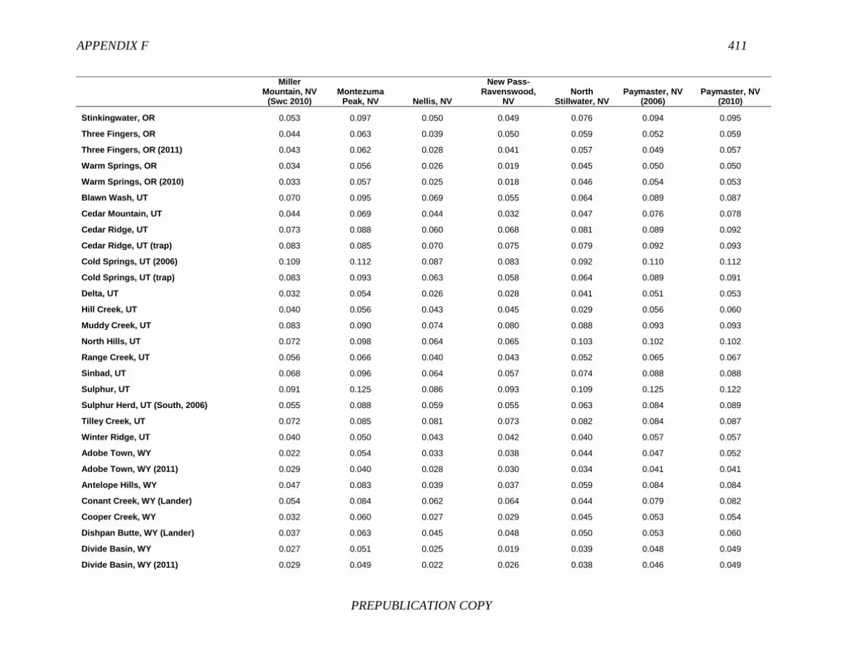
APPENDIX F 411
PREPUBLICATION COPY
Miller Mountain, NV
(Swc 2010) Montezuma
Peak, NV Nellis, NV
New Pass-Ravenswood,
NV North
Stillwater, NV Paymaster, NV
(2006) Paymaster, NV
(2010)
Stinkingwater, OR 0.053 0.097 0.050 0.049 0.076 0.094 0.095
Three Fingers, OR 0.044 0.063 0.039 0.050 0.059 0.052 0.059
Three Fingers, OR (2011) 0.043 0.062 0.028 0.041 0.057 0.049 0.057
Warm Springs, OR 0.034 0.056 0.026 0.019 0.045 0.050 0.050
Warm Springs, OR (2010) 0.033 0.057 0.025 0.018 0.046 0.054 0.053
Blawn Wash, UT 0.070 0.095 0.069 0.055 0.064 0.089 0.087
Cedar Mountain, UT 0.044 0.069 0.044 0.032 0.047 0.076 0.078
Cedar Ridge, UT 0.073 0.088 0.060 0.068 0.081 0.089 0.092
Cedar Ridge, UT (trap) 0.083 0.085 0.070 0.075 0.079 0.092 0.093
Cold Springs, UT (2006) 0.109 0.112 0.087 0.083 0.092 0.110 0.112
Cold Springs, UT (trap) 0.083 0.093 0.063 0.058 0.064 0.089 0.091
Delta, UT 0.032 0.054 0.026 0.028 0.041 0.051 0.053
Hill Creek, UT 0.040 0.056 0.043 0.045 0.029 0.056 0.060
Muddy Creek, UT 0.083 0.090 0.074 0.080 0.088 0.093 0.093
North Hills, UT 0.072 0.098 0.064 0.065 0.103 0.102 0.102
Range Creek, UT 0.056 0.066 0.040 0.043 0.052 0.065 0.067
Sinbad, UT 0.068 0.096 0.064 0.057 0.074 0.088 0.088
Sulphur, UT 0.091 0.125 0.086 0.093 0.109 0.125 0.122
Sulphur Herd, UT (South, 2006) 0.055 0.088 0.059 0.055 0.063 0.084 0.089
Tilley Creek, UT 0.072 0.085 0.081 0.073 0.082 0.084 0.087
Winter Ridge, UT 0.040 0.050 0.043 0.042 0.040 0.057 0.057
Adobe Town, WY 0.022 0.054 0.033 0.038 0.044 0.047 0.052
Adobe Town, WY (2011) 0.029 0.040 0.028 0.030 0.034 0.041 0.041
Antelope Hills, WY 0.047 0.083 0.039 0.037 0.059 0.084 0.084
Conant Creek, WY (Lander) 0.054 0.084 0.062 0.064 0.044 0.079 0.082
Cooper Creek, WY 0.032 0.060 0.027 0.029 0.045 0.053 0.054
Dishpan Butte, WY (Lander) 0.037 0.063 0.045 0.048 0.050 0.053 0.060
Divide Basin, WY 0.027 0.051 0.025 0.019 0.039 0.048 0.049
Divide Basin, WY (2011) 0.029 0.049 0.022 0.026 0.038 0.046 0.049

412 BLM WILD HORSE AND BURRO PROGRAM
PREPUBLICATION COPY
Miller Mountain, NV
(Swc 2010) Montezuma
Peak, NV Nellis, NV
New Pass-Ravenswood,
NV North
Stillwater, NV Paymaster, NV
(2006) Paymaster, NV
(2010)
Eagles Nest, WY 0.052 0.087 0.050 0.046 0.070 0.086 0.087
Happy Creek Springs, WY 0.038 0.092 0.044 0.046 0.063 0.081 0.080
Little Colorado, WY 0.039 0.062 0.040 0.035 0.059 0.059 0.061
Little Colorado, WY (2011) 0.038 0.056 0.038 0.027 0.055 0.053 0.054
Lost Creek, WY 0.029 0.054 0.024 0.021 0.042 0.053 0.054
Lost Creek, WY (combined) 0.029 0.051 0.028 0.023 0.043 0.049 0.050
McCullough Peaks, WY 0.038 0.080 0.040 0.037 0.057 0.080 0.080
Muskrat Basin, WY (Lander) 0.043 0.068 0.040 0.045 0.053 0.058 0.065
Salt Wells, WY (East) 0.024 0.045 0.025 0.029 0.031 0.048 0.047
Salt Wells, WY (West) 0.021 0.057 0.025 0.022 0.045 0.053 0.054
Stewart Creek, WY 0.040 0.076 0.036 0.027 0.049 0.073 0.074
Stewart Creek, WY (2009) 0.032 0.069 0.038 0.035 0.056 0.066 0.066
White Mountain, WY (2011) 0.041 0.044 0.042 0.039 0.050 0.047 0.044
Pine Nut
Moutain, NV Powell Mountain,
NV Red Rock, NV Reveille, NV Roberts
Mountain, NV Rock Creek, NV
(2002) Rock Creek,
NV (2010)
Pine Nut Mountain, NV 0.000
Powell Mountain, NV 0.099 0.000
Red Rock, NV 0.068 0.081 0.000
Reveille, NV 0.071 0.073 0.053 0.000
Roberts Mountain, NV 0.071 0.062 0.040 0.046 0.000
Rock Creek, NV (2002) 0.072 0.089 0.077 0.089 0.069 0.000
Rock Creek, NV (2010) 0.062 0.069 0.055 0.066 0.052 0.013 0.000
Rocky Hills, NV 0.063 0.065 0.042 0.051 0.037 0.056 0.042
Rodeo Creek, NV 0.057 0.051 0.038 0.043 0.035 0.057 0.042
Saulsbury, NV 0.054 0.056 0.045 0.040 0.045 0.058 0.039
Sand Springs East, NV 0.058 0.058 0.041 0.033 0.034 0.054 0.035
Seven Mile, NV 0.068 0.081 0.045 0.063 0.056 0.069 0.053
Shawave Mountains, NV 0.065 0.062 0.044 0.056 0.043 0.065 0.049
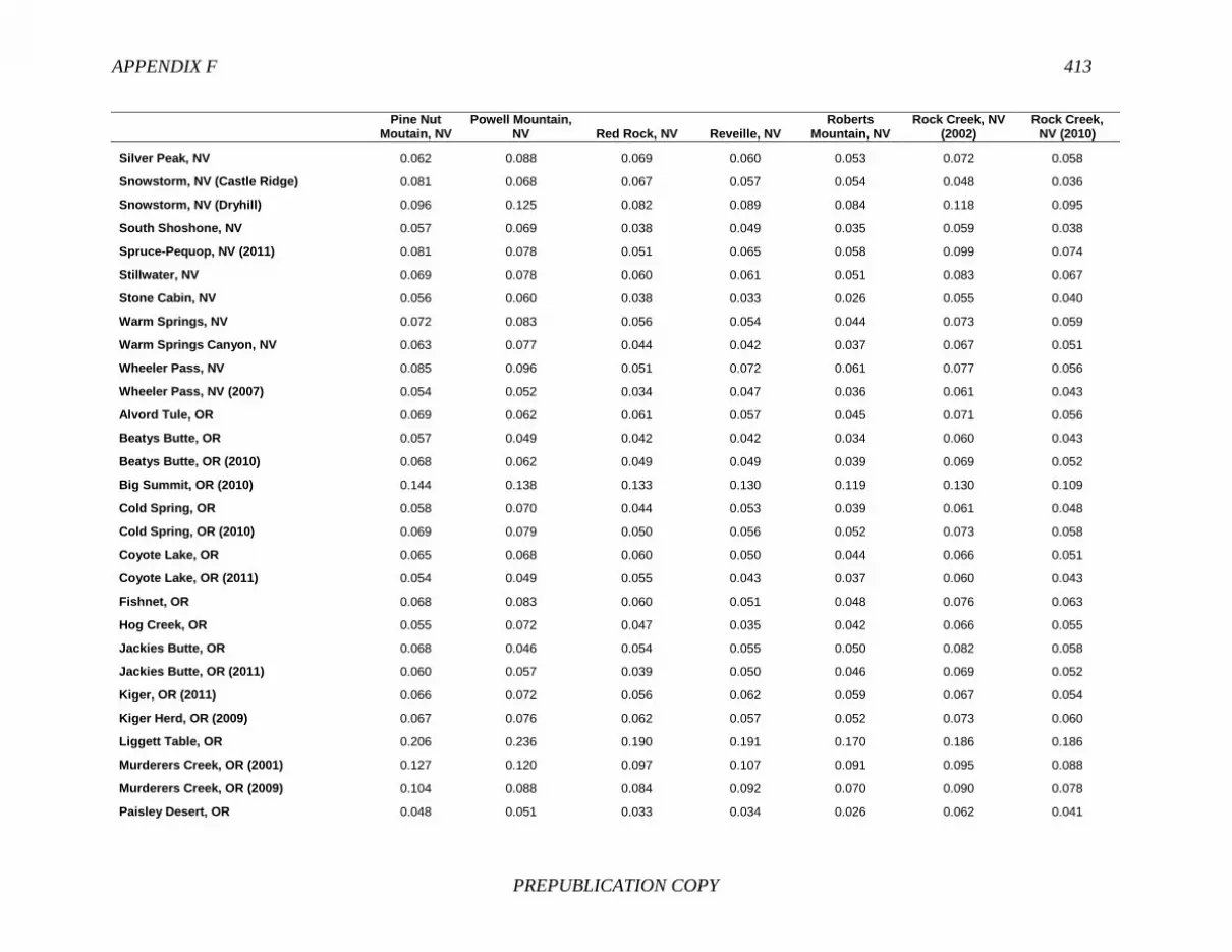
APPENDIX F 413
PREPUBLICATION COPY
Pine Nut
Moutain, NV Powell Mountain,
NV Red Rock, NV Reveille, NV Roberts
Mountain, NV Rock Creek, NV
(2002) Rock Creek,
NV (2010)
Silver Peak, NV 0.062 0.088 0.069 0.060 0.053 0.072 0.058
Snowstorm, NV (Castle Ridge) 0.081 0.068 0.067 0.057 0.054 0.048 0.036
Snowstorm, NV (Dryhill) 0.096 0.125 0.082 0.089 0.084 0.118 0.095
South Shoshone, NV 0.057 0.069 0.038 0.049 0.035 0.059 0.038
Spruce-Pequop, NV (2011) 0.081 0.078 0.051 0.065 0.058 0.099 0.074
Stillwater, NV 0.069 0.078 0.060 0.061 0.051 0.083 0.067
Stone Cabin, NV 0.056 0.060 0.038 0.033 0.026 0.055 0.040
Warm Springs, NV 0.072 0.083 0.056 0.054 0.044 0.073 0.059
Warm Springs Canyon, NV 0.063 0.077 0.044 0.042 0.037 0.067 0.051
Wheeler Pass, NV 0.085 0.096 0.051 0.072 0.061 0.077 0.056
Wheeler Pass, NV (2007) 0.054 0.052 0.034 0.047 0.036 0.061 0.043
Alvord Tule, OR 0.069 0.062 0.061 0.057 0.045 0.071 0.056
Beatys Butte, OR 0.057 0.049 0.042 0.042 0.034 0.060 0.043
Beatys Butte, OR (2010) 0.068 0.062 0.049 0.049 0.039 0.069 0.052
Big Summit, OR (2010) 0.144 0.138 0.133 0.130 0.119 0.130 0.109
Cold Spring, OR 0.058 0.070 0.044 0.053 0.039 0.061 0.048
Cold Spring, OR (2010) 0.069 0.079 0.050 0.056 0.052 0.073 0.058
Coyote Lake, OR 0.065 0.068 0.060 0.050 0.044 0.066 0.051
Coyote Lake, OR (2011) 0.054 0.049 0.055 0.043 0.037 0.060 0.043
Fishnet, OR 0.068 0.083 0.060 0.051 0.048 0.076 0.063
Hog Creek, OR 0.055 0.072 0.047 0.035 0.042 0.066 0.055
Jackies Butte, OR 0.068 0.046 0.054 0.055 0.050 0.082 0.058
Jackies Butte, OR (2011) 0.060 0.057 0.039 0.050 0.046 0.069 0.052
Kiger, OR (2011) 0.066 0.072 0.056 0.062 0.059 0.067 0.054
Kiger Herd, OR (2009) 0.067 0.076 0.062 0.057 0.052 0.073 0.060
Liggett Table, OR 0.206 0.236 0.190 0.191 0.170 0.186 0.186
Murderers Creek, OR (2001) 0.127 0.120 0.097 0.107 0.091 0.095 0.088
Murderers Creek, OR (2009) 0.104 0.088 0.084 0.092 0.070 0.090 0.078
Paisley Desert, OR 0.048 0.051 0.033 0.034 0.026 0.062 0.041

414 BLM WILD HORSE AND BURRO PROGRAM
PREPUBLICATION COPY
Pine Nut
Moutain, NV Powell Mountain,
NV Red Rock, NV Reveille, NV Roberts
Mountain, NV Rock Creek, NV
(2002) Rock Creek,
NV (2010)
Riddle Herd, OR (2009) 0.078 0.090 0.069 0.074 0.072 0.066 0.060
Riddle Mountain, OR 0.076 0.086 0.067 0.075 0.075 0.061 0.054
Riddle Mountain, OR (2011) 0.083 0.098 0.074 0.080 0.076 0.068 0.064
Sand Springs, OR (2011) 0.057 0.060 0.056 0.050 0.043 0.069 0.056
Sheepshead, OR 0.057 0.055 0.042 0.056 0.035 0.062 0.048
Sheepshead, OR (2011) 0.047 0.055 0.039 0.046 0.038 0.055 0.042
South Steens, OR 0.057 0.062 0.043 0.048 0.035 0.056 0.042
South Steens, OR (2010) 0.053 0.058 0.042 0.044 0.038 0.060 0.048
Stinkingwater, OR 0.092 0.090 0.075 0.071 0.059 0.087 0.075
Three Fingers, OR 0.075 0.074 0.062 0.064 0.045 0.081 0.066
Three Fingers, OR (2011) 0.069 0.070 0.048 0.058 0.037 0.066 0.049
Warm Springs, OR 0.054 0.059 0.040 0.047 0.033 0.042 0.029
Warm Springs, OR (2010) 0.055 0.060 0.042 0.045 0.034 0.049 0.032
Blawn Wash, UT 0.087 0.075 0.075 0.082 0.076 0.086 0.077
Cedar Mountain, UT 0.060 0.089 0.056 0.056 0.058 0.078 0.063
Cedar Ridge, UT 0.105 0.100 0.105 0.096 0.091 0.078 0.067
Cedar Ridge, UT (trap) 0.112 0.107 0.107 0.100 0.099 0.085 0.076
Cold Springs, UT (2006) 0.116 0.159 0.112 0.117 0.101 0.130 0.122
Cold Springs, UT (trap) 0.089 0.111 0.077 0.084 0.077 0.101 0.089
Delta, UT 0.047 0.056 0.035 0.044 0.036 0.049 0.035
Hill Creek, UT 0.074 0.071 0.046 0.057 0.040 0.075 0.058
Muddy Creek, UT 0.104 0.123 0.068 0.083 0.091 0.125 0.106
North Hills, UT 0.105 0.108 0.070 0.087 0.075 0.092 0.069
Range Creek, UT 0.077 0.091 0.076 0.072 0.062 0.068 0.059
Sinbad, UT 0.064 0.087 0.085 0.080 0.078 0.093 0.084
Sulphur, UT 0.119 0.105 0.105 0.103 0.085 0.126 0.099
Sulphur Herd, UT (South, 2006) 0.082 0.097 0.069 0.084 0.071 0.072 0.060
Tilley Creek, UT 0.111 0.094 0.086 0.101 0.092 0.073 0.069
Winter Ridge, UT 0.074 0.070 0.052 0.066 0.046 0.073 0.055

APPENDIX F 415
PREPUBLICATION COPY
Pine Nut
Moutain, NV Powell Mountain,
NV Red Rock, NV Reveille, NV Roberts
Mountain, NV Rock Creek, NV
(2002) Rock Creek,
NV (2010)
Adobe Town, WY 0.064 0.057 0.044 0.040 0.039 0.060 0.043
Adobe Town, WY (2011) 0.068 0.064 0.036 0.042 0.035 0.069 0.050
Antelope Hills, WY 0.058 0.075 0.063 0.047 0.052 0.075 0.058
Conant Creek, WY (Lander) 0.088 0.074 0.082 0.080 0.055 0.082 0.075
Cooper Creek, WY 0.047 0.058 0.040 0.039 0.033 0.058 0.040
Dishpan Butte, WY (Lander) 0.066 0.077 0.061 0.065 0.051 0.056 0.046
Divide Basin, WY 0.053 0.062 0.041 0.045 0.042 0.042 0.028
Divide Basin, WY (2011) 0.052 0.059 0.038 0.045 0.037 0.042 0.026
Eagles Nest, WY 0.089 0.097 0.076 0.067 0.053 0.078 0.060
Happy Creek Springs, WY 0.081 0.091 0.081 0.066 0.051 0.082 0.068
Little Colorado, WY 0.072 0.078 0.049 0.061 0.042 0.050 0.035
Little Colorado, WY (2011) 0.066 0.073 0.047 0.060 0.040 0.042 0.031
Lost Creek, WY 0.061 0.060 0.049 0.045 0.034 0.058 0.042
Lost Creek, WY (combined) 0.059 0.069 0.048 0.049 0.039 0.055 0.042
McCullough Peaks, WY 0.062 0.077 0.072 0.055 0.052 0.063 0.053
Muskrat Basin, WY (Lander) 0.073 0.073 0.059 0.064 0.041 0.059 0.045
Salt Wells, WY (East) 0.064 0.051 0.039 0.037 0.032 0.066 0.047
Salt Wells, WY (West) 0.056 0.062 0.047 0.029 0.039 0.065 0.046
Stewart Creek, WY 0.063 0.068 0.066 0.060 0.039 0.054 0.041
Stewart Creek, WY (2009) 0.077 0.078 0.060 0.053 0.055 0.071 0.054
White Mountain, WY (2011) 0.072 0.058 0.058 0.062 0.054 0.072 0.061
Rocky Hills,
NV Rodeo Creek,
NV Saulsbury, NV Sand Springs
East, NV Seven Mile, NV
Shawave Mountains,
NV Silver Peak, NV
Rocky Hills, NV 0.000
Rodeo Creek, NV 0.033 0.000
Saulsbury, NV 0.031 0.023 0.000
Sand Springs East, NV 0.038 0.026 0.031 0.000
Seven Mile, NV 0.031 0.042 0.038 0.037 0.000

416 BLM WILD HORSE AND BURRO PROGRAM
PREPUBLICATION COPY
Rocky Hills,
NV Rodeo Creek,
NV Saulsbury, NV Sand Springs
East, NV Seven Mile, NV
Shawave Mountains,
NV Silver Peak, NV
Shawave Mountains, NV 0.043 0.022 0.031 0.036 0.047 0.000
Silver Peak, NV 0.055 0.043 0.046 0.051 0.066 0.049 0.000
Snowstorm, NV (Castle Ridge) 0.046 0.041 0.042 0.041 0.054 0.046 0.052
Snowstorm, NV (Dryhill) 0.090 0.076 0.087 0.082 0.098 0.072 0.072
South Shoshone, NV 0.031 0.033 0.034 0.028 0.037 0.043 0.050
Spruce-Pequop, NV (2011) 0.062 0.044 0.056 0.056 0.069 0.049 0.069
Stillwater, NV 0.065 0.035 0.048 0.045 0.067 0.041 0.049
Stone Cabin, NV 0.030 0.024 0.020 0.029 0.038 0.034 0.041
Warm Springs, NV 0.050 0.038 0.044 0.036 0.062 0.045 0.039
Warm Springs Canyon, NV 0.042 0.028 0.030 0.031 0.049 0.032 0.038
Wheeler Pass, NV 0.065 0.055 0.065 0.060 0.077 0.071 0.075
Wheeler Pass, NV (2007) 0.036 0.030 0.033 0.033 0.041 0.036 0.055
Alvord Tule, OR 0.049 0.033 0.039 0.042 0.055 0.045 0.048
Beatys Butte, OR 0.030 0.024 0.027 0.026 0.039 0.025 0.036
Beatys Butte, OR (2010) 0.044 0.029 0.036 0.035 0.049 0.020 0.045
Big Summit, OR (2010) 0.105 0.089 0.102 0.115 0.125 0.099 0.113
Cold Spring, OR 0.034 0.036 0.033 0.043 0.048 0.038 0.035
Cold Spring, OR (2010) 0.038 0.040 0.044 0.051 0.054 0.045 0.038
Coyote Lake, OR 0.047 0.039 0.040 0.041 0.056 0.049 0.043
Coyote Lake, OR (2011) 0.040 0.029 0.034 0.029 0.052 0.037 0.037
Fishnet, OR 0.041 0.048 0.047 0.049 0.065 0.054 0.045
Hog Creek, OR 0.039 0.034 0.037 0.040 0.056 0.043 0.046
Jackies Butte, OR 0.043 0.044 0.043 0.050 0.056 0.053 0.063
Jackies Butte, OR (2011) 0.037 0.035 0.037 0.039 0.045 0.039 0.053
Kiger, OR (2011) 0.047 0.038 0.038 0.045 0.058 0.038 0.042
Kiger Herd, OR (2009) 0.056 0.043 0.046 0.046 0.067 0.044 0.040
Liggett Table, OR 0.163 0.166 0.175 0.156 0.189 0.165 0.142
Murderers Creek, OR (2001) 0.087 0.072 0.075 0.083 0.087 0.074 0.083
Murderers Creek, OR (2009) 0.067 0.058 0.054 0.066 0.068 0.062 0.064

APPENDIX F 417
PREPUBLICATION COPY
Rocky Hills,
NV Rodeo Creek,
NV Saulsbury, NV Sand Springs
East, NV Seven Mile, NV
Shawave Mountains,
NV Silver Peak, NV
Paisley Desert, OR 0.033 0.019 0.030 0.024 0.042 0.031 0.035
Riddle Herd, OR (2009) 0.060 0.049 0.046 0.049 0.074 0.049 0.051
Riddle Mountain, OR 0.051 0.049 0.043 0.048 0.066 0.048 0.053
Riddle Mountain, OR (2011) 0.067 0.054 0.052 0.056 0.079 0.057 0.056
Sand Springs, OR (2011) 0.043 0.033 0.037 0.036 0.054 0.035 0.037
Sheepshead, OR 0.036 0.029 0.032 0.038 0.036 0.033 0.043
Sheepshead, OR (2011) 0.028 0.026 0.028 0.034 0.038 0.033 0.041
South Steens, OR 0.043 0.030 0.036 0.036 0.043 0.036 0.041
South Steens, OR (2010) 0.042 0.028 0.033 0.034 0.041 0.032 0.046
Stinkingwater, OR 0.058 0.066 0.067 0.056 0.077 0.070 0.086
Three Fingers, OR 0.041 0.043 0.053 0.043 0.054 0.055 0.055
Three Fingers, OR (2011) 0.035 0.044 0.047 0.033 0.047 0.050 0.054
Warm Springs, OR 0.029 0.034 0.025 0.027 0.036 0.035 0.043
Warm Springs, OR (2010) 0.031 0.034 0.025 0.029 0.040 0.038 0.037
Blawn Wash, UT 0.063 0.060 0.057 0.070 0.081 0.085 0.077
Cedar Mountain, UT 0.056 0.041 0.038 0.052 0.056 0.051 0.041
Cedar Ridge, UT 0.071 0.062 0.066 0.073 0.081 0.071 0.072
Cedar Ridge, UT (trap) 0.085 0.061 0.075 0.089 0.096 0.069 0.082
Cold Springs, UT (2006) 0.108 0.099 0.090 0.086 0.111 0.099 0.111
Cold Springs, UT (trap) 0.086 0.066 0.064 0.058 0.087 0.073 0.086
Delta, UT 0.040 0.020 0.028 0.029 0.042 0.024 0.041
Hill Creek, UT 0.053 0.025 0.045 0.044 0.059 0.034 0.051
Muddy Creek, UT 0.088 0.075 0.073 0.083 0.081 0.087 0.101
North Hills, UT 0.062 0.063 0.066 0.070 0.073 0.063 0.080
Range Creek, UT 0.056 0.046 0.045 0.046 0.062 0.051 0.057
Sinbad, UT 0.073 0.061 0.056 0.062 0.076 0.060 0.082
Sulphur, UT 0.093 0.085 0.085 0.096 0.101 0.095 0.104
Sulphur Herd, UT (South, 2006) 0.067 0.053 0.064 0.057 0.068 0.049 0.051
Tilley Creek, UT 0.061 0.068 0.077 0.081 0.078 0.076 0.070

418 BLM WILD HORSE AND BURRO PROGRAM
PREPUBLICATION COPY
Rocky Hills,
NV Rodeo Creek,
NV Saulsbury, NV Sand Springs
East, NV Seven Mile, NV
Shawave Mountains,
NV Silver Peak, NV
Winter Ridge, UT 0.044 0.030 0.044 0.051 0.055 0.032 0.048
Adobe Town, WY 0.038 0.029 0.042 0.033 0.048 0.031 0.047
Adobe Town, WY (2011) 0.035 0.027 0.038 0.034 0.041 0.024 0.046
Antelope Hills, WY 0.049 0.044 0.044 0.038 0.054 0.046 0.058
Conant Creek, WY (Lander) 0.074 0.052 0.066 0.062 0.090 0.066 0.058
Cooper Creek, WY 0.039 0.029 0.029 0.030 0.047 0.034 0.042
Dishpan Butte, WY (Lander) 0.054 0.039 0.054 0.035 0.063 0.044 0.042
Divide Basin, WY 0.033 0.023 0.021 0.029 0.035 0.024 0.033
Divide Basin, WY (2011) 0.032 0.021 0.022 0.029 0.037 0.026 0.039
Eagles Nest, WY 0.060 0.051 0.062 0.055 0.074 0.062 0.053
Happy Creek Springs, WY 0.048 0.055 0.053 0.059 0.072 0.060 0.055
Little Colorado, WY 0.035 0.036 0.043 0.041 0.051 0.046 0.045
Little Colorado, WY (2011) 0.032 0.035 0.039 0.036 0.048 0.042 0.043
Lost Creek, WY 0.034 0.025 0.029 0.032 0.047 0.033 0.038
Lost Creek, WY (combined) 0.036 0.028 0.032 0.034 0.045 0.035 0.037
McCullough Peaks, WY 0.046 0.047 0.051 0.043 0.066 0.051 0.051
Muskrat Basin, WY (Lander) 0.060 0.041 0.055 0.036 0.066 0.049 0.040
Salt Wells, WY (East) 0.029 0.020 0.026 0.034 0.035 0.032 0.042
Salt Wells, WY (West) 0.030 0.031 0.029 0.037 0.048 0.034 0.037
Stewart Creek, WY 0.046 0.036 0.040 0.037 0.056 0.044 0.045
Stewart Creek, WY (2009) 0.048 0.037 0.036 0.045 0.057 0.040 0.049
White Mountain, WY (2011) 0.044 0.033 0.036 0.047 0.056 0.038 0.054
Snowstorm, NV (Castle
Ridge) Snowstorm, NV (Dryhill)
South Shoshone, NV
Spruce-Pequop, NV
(2011) Stillwater, NV Stone Cabin,
NV Warm Springs,
NV
Snowstorm, NV (Castle Ridge) 0.000
Snowstorm, NV (Dryhill) 0.082 0.000
South Shoshone, NV 0.041 0.075 0.000
Spruce-Pequop, NV (2011) 0.075 0.094 0.053 0.000

APPENDIX F 419
PREPUBLICATION COPY
Snowstorm, NV (Castle
Ridge) Snowstorm, NV (Dryhill)
South Shoshone, NV
Spruce-Pequop, NV
(2011) Stillwater, NV Stone Cabin,
NV Warm Springs,
NV
Stillwater, NV 0.065 0.072 0.045 0.059 0.000
Stone Cabin, NV 0.039 0.079 0.030 0.052 0.044 0.000
Warm Springs, NV 0.054 0.072 0.043 0.067 0.055 0.038 0.000
Warm Springs Canyon, NV 0.052 0.072 0.037 0.047 0.040 0.029 0.014
Wheeler Pass, NV 0.083 0.125 0.066 0.064 0.082 0.058 0.074
Wheeler Pass, NV (2007) 0.042 0.090 0.028 0.046 0.052 0.032 0.044
Alvord Tule, OR 0.057 0.080 0.042 0.056 0.056 0.041 0.044
Beatys Butte, OR 0.039 0.070 0.032 0.046 0.045 0.025 0.033
Beatys Butte, OR (2010) 0.042 0.064 0.035 0.050 0.042 0.032 0.035
Big Summit, OR (2010) 0.109 0.146 0.118 0.135 0.129 0.109 0.139
Cold Spring, OR 0.050 0.076 0.032 0.045 0.043 0.033 0.050
Cold Spring, OR (2010) 0.057 0.081 0.039 0.054 0.050 0.043 0.056
Coyote Lake, OR 0.057 0.088 0.039 0.058 0.060 0.036 0.053
Coyote Lake, OR (2011) 0.043 0.068 0.030 0.048 0.046 0.031 0.043
Fishnet, OR 0.049 0.073 0.037 0.067 0.057 0.041 0.044
Hog Creek, OR 0.054 0.067 0.035 0.056 0.055 0.031 0.048
Jackies Butte, OR 0.061 0.074 0.049 0.067 0.069 0.048 0.055
Jackies Butte, OR (2011) 0.056 0.060 0.039 0.059 0.054 0.039 0.039
Kiger, OR (2011) 0.055 0.089 0.049 0.082 0.067 0.038 0.044
Kiger Herd, OR (2009) 0.068 0.087 0.053 0.086 0.073 0.043 0.040
Liggett Table, OR 0.184 0.196 0.159 0.194 0.167 0.174 0.129
Murderers Creek, OR (2001) 0.090 0.134 0.077 0.110 0.092 0.076 0.090
Murderers Creek, OR (2009) 0.073 0.126 0.063 0.095 0.079 0.057 0.078
Paisley Desert, OR 0.042 0.062 0.024 0.040 0.038 0.021 0.039
Riddle Herd, OR (2009) 0.063 0.100 0.056 0.097 0.066 0.051 0.041
Riddle Mountain, OR 0.058 0.107 0.052 0.089 0.070 0.050 0.045
Riddle Mountain, OR (2011) 0.069 0.108 0.057 0.103 0.073 0.052 0.050
Sand Springs, OR (2011) 0.041 0.076 0.036 0.058 0.049 0.037 0.049
Sheepshead, OR 0.047 0.084 0.030 0.053 0.047 0.026 0.051

420 BLM WILD HORSE AND BURRO PROGRAM
PREPUBLICATION COPY
Snowstorm, NV (Castle
Ridge) Snowstorm, NV (Dryhill)
South Shoshone, NV
Spruce-Pequop, NV
(2011) Stillwater, NV Stone Cabin,
NV Warm Springs,
NV
Sheepshead, OR (2011) 0.037 0.080 0.026 0.051 0.040 0.026 0.047
South Steens, OR 0.050 0.059 0.029 0.045 0.041 0.028 0.042
South Steens, OR (2010) 0.049 0.055 0.035 0.044 0.041 0.029 0.040
Stinkingwater, OR 0.078 0.098 0.055 0.080 0.085 0.068 0.059
Three Fingers, OR 0.052 0.096 0.043 0.082 0.065 0.045 0.053
Three Fingers, OR (2011) 0.047 0.082 0.030 0.071 0.057 0.034 0.047
Warm Springs, OR 0.041 0.068 0.027 0.046 0.047 0.024 0.038
Warm Springs, OR (2010) 0.042 0.065 0.029 0.048 0.048 0.022 0.034
Blawn Wash, UT 0.076 0.113 0.066 0.089 0.079 0.060 0.065
Cedar Mountain, UT 0.064 0.074 0.043 0.059 0.053 0.040 0.052
Cedar Ridge, UT 0.062 0.113 0.066 0.109 0.093 0.062 0.086
Cedar Ridge, UT (trap) 0.075 0.110 0.078 0.109 0.090 0.071 0.096
Cold Springs, UT (2006) 0.123 0.123 0.088 0.126 0.097 0.096 0.084
Cold Springs, UT (trap) 0.095 0.102 0.059 0.093 0.072 0.067 0.063
Delta, UT 0.042 0.079 0.031 0.049 0.046 0.022 0.045
Hill Creek, UT 0.056 0.079 0.040 0.063 0.040 0.034 0.054
Muddy Creek, UT 0.089 0.117 0.079 0.085 0.104 0.081 0.108
North Hills, UT 0.080 0.115 0.074 0.095 0.107 0.061 0.089
Range Creek, UT 0.057 0.084 0.044 0.083 0.062 0.045 0.052
Sinbad, UT 0.082 0.124 0.069 0.087 0.079 0.060 0.083
Sulphur, UT 0.093 0.145 0.096 0.120 0.117 0.079 0.115
Sulphur Herd, UT (South, 2006) 0.070 0.094 0.058 0.088 0.065 0.060 0.068
Tilley Creek, UT 0.056 0.120 0.070 0.110 0.093 0.074 0.084
Winter Ridge, UT 0.053 0.077 0.040 0.057 0.053 0.045 0.048
Adobe Town, WY 0.043 0.081 0.035 0.050 0.045 0.034 0.053
Adobe Town, WY (2011) 0.040 0.055 0.029 0.042 0.036 0.031 0.043
Antelope Hills, WY 0.058 0.084 0.051 0.076 0.070 0.044 0.054
Conant Creek, WY (Lander) 0.065 0.105 0.061 0.094 0.057 0.056 0.062
Cooper Creek, WY 0.042 0.079 0.035 0.060 0.053 0.026 0.047

APPENDIX F 421
PREPUBLICATION COPY
Snowstorm, NV (Castle
Ridge) Snowstorm, NV (Dryhill)
South Shoshone, NV
Spruce-Pequop, NV
(2011) Stillwater, NV Stone Cabin,
NV Warm Springs,
NV
Dishpan Butte, WY (Lander) 0.048 0.098 0.043 0.074 0.054 0.048 0.051
Divide Basin, WY 0.030 0.067 0.026 0.044 0.048 0.024 0.036
Divide Basin, WY (2011) 0.031 0.071 0.030 0.048 0.046 0.020 0.042
Eagles Nest, WY 0.056 0.098 0.047 0.080 0.072 0.056 0.063
Happy Creek Springs, WY 0.068 0.113 0.051 0.086 0.080 0.050 0.063
Little Colorado, WY 0.049 0.089 0.037 0.064 0.064 0.038 0.042
Little Colorado, WY (2011) 0.044 0.080 0.032 0.060 0.061 0.038 0.037
Lost Creek, WY 0.042 0.074 0.028 0.050 0.048 0.027 0.037
Lost Creek, WY (combined) 0.045 0.070 0.027 0.053 0.050 0.030 0.039
McCullough Peaks, WY 0.046 0.082 0.041 0.077 0.069 0.040 0.039
Muskrat Basin, WY (Lander) 0.045 0.100 0.043 0.068 0.051 0.042 0.049
Salt Wells, WY (East) 0.038 0.070 0.028 0.041 0.036 0.022 0.041
Salt Wells, WY (West) 0.036 0.074 0.035 0.052 0.051 0.027 0.047
Stewart Creek, WY 0.050 0.081 0.036 0.068 0.058 0.037 0.045
Stewart Creek, WY (2009) 0.058 0.091 0.039 0.062 0.067 0.038 0.045
White Mountain, WY (2011) 0.046 0.076 0.041 0.063 0.060 0.047 0.042
Warm Springs
Canyon, NV Wheeler Pass, NV
Wheeler Pass, NV (2007)
Alvord Tule, OR Beatys Butte, OR
Beatys Butte, OR (2010)
Big Summit, OR (2010)
Warm Springs Canyon, NV 0.000
Wheeler Pass, NV 0.061 0.000
Wheeler Pass, NV (2007) 0.036 0.040 0.000
Alvord Tule, OR 0.037 0.073 0.043 0.000
Beatys Butte, OR 0.029 0.063 0.027 0.040 0.000
Beatys Butte, OR (2010) 0.029 0.074 0.036 0.046 0.018 0.000
Big Summit, OR (2010) 0.123 0.130 0.109 0.115 0.099 0.107 0.000
Cold Spring, OR 0.032 0.067 0.036 0.045 0.030 0.039 0.115
Cold Spring, OR (2010) 0.040 0.071 0.041 0.055 0.038 0.044 0.112
Coyote Lake, OR 0.043 0.068 0.042 0.021 0.039 0.047 0.124

422 BLM WILD HORSE AND BURRO PROGRAM
PREPUBLICATION COPY
Warm Springs
Canyon, NV Wheeler Pass, NV
Wheeler Pass, NV (2007)
Alvord Tule, OR Beatys Butte, OR
Beatys Butte, OR (2010)
Big Summit, OR (2010)
Coyote Lake, OR (2011) 0.036 0.067 0.033 0.018 0.028 0.035 0.107
Fishnet, OR 0.043 0.088 0.051 0.052 0.041 0.047 0.148
Hog Creek, OR 0.039 0.071 0.045 0.039 0.036 0.038 0.115
Jackies Butte, OR 0.049 0.073 0.044 0.044 0.039 0.051 0.117
Jackies Butte, OR (2011) 0.033 0.062 0.036 0.038 0.034 0.040 0.111
Kiger, OR (2011) 0.048 0.091 0.049 0.054 0.028 0.039 0.125
Kiger Herd, OR (2009) 0.047 0.082 0.050 0.047 0.031 0.044 0.128
Liggett Table, OR 0.131 0.199 0.178 0.171 0.143 0.151 0.275
Murderers Creek, OR (2001) 0.078 0.114 0.089 0.100 0.078 0.073 0.160
Murderers Creek, OR (2009) 0.065 0.105 0.074 0.084 0.060 0.062 0.151
Paisley Desert, OR 0.029 0.048 0.024 0.031 0.018 0.028 0.098
Riddle Herd, OR (2009) 0.049 0.096 0.059 0.065 0.039 0.048 0.143
Riddle Mountain, OR 0.048 0.094 0.055 0.063 0.036 0.045 0.137
Riddle Mountain, OR (2011) 0.057 0.105 0.066 0.067 0.046 0.055 0.147
Sand Springs, OR (2011) 0.038 0.075 0.035 0.033 0.035 0.031 0.104
Sheepshead, OR 0.035 0.061 0.029 0.034 0.030 0.032 0.115
Sheepshead, OR (2011) 0.034 0.058 0.023 0.036 0.031 0.035 0.111
South Steens, OR 0.028 0.058 0.034 0.022 0.033 0.032 0.118
South Steens, OR (2010) 0.030 0.063 0.035 0.030 0.027 0.027 0.121
Stinkingwater, OR 0.054 0.092 0.057 0.056 0.052 0.060 0.162
Three Fingers, OR 0.053 0.089 0.046 0.059 0.042 0.050 0.130
Three Fingers, OR (2011) 0.046 0.073 0.039 0.052 0.041 0.048 0.127
Warm Springs, OR 0.028 0.064 0.035 0.042 0.023 0.032 0.106
Warm Springs, OR (2010) 0.027 0.067 0.037 0.043 0.022 0.032 0.107
Blawn Wash, UT 0.066 0.096 0.065 0.077 0.053 0.069 0.167
Cedar Mountain, UT 0.041 0.065 0.050 0.045 0.037 0.046 0.122
Cedar Ridge, UT 0.078 0.120 0.073 0.067 0.069 0.073 0.125
Cedar Ridge, UT (trap) 0.084 0.116 0.077 0.069 0.078 0.076 0.109
Cold Springs, UT (2006) 0.075 0.153 0.105 0.100 0.099 0.093 0.207
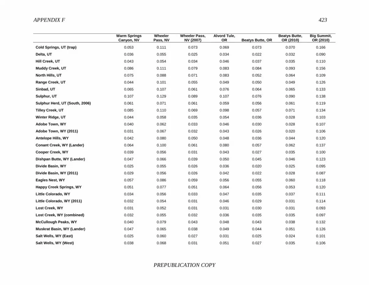
APPENDIX F 423
PREPUBLICATION COPY
Warm Springs
Canyon, NV Wheeler Pass, NV
Wheeler Pass, NV (2007)
Alvord Tule, OR Beatys Butte, OR
Beatys Butte, OR (2010)
Big Summit, OR (2010)
Cold Springs, UT (trap) 0.053 0.111 0.073 0.069 0.073 0.070 0.166
Delta, UT 0.036 0.055 0.025 0.034 0.022 0.032 0.090
Hill Creek, UT 0.043 0.054 0.034 0.046 0.037 0.035 0.110
Muddy Creek, UT 0.086 0.111 0.079 0.083 0.084 0.093 0.156
North Hills, UT 0.075 0.088 0.071 0.083 0.052 0.064 0.109
Range Creek, UT 0.044 0.101 0.055 0.049 0.050 0.049 0.126
Sinbad, UT 0.065 0.107 0.061 0.076 0.064 0.065 0.133
Sulphur, UT 0.107 0.129 0.089 0.107 0.076 0.090 0.138
Sulphur Herd, UT (South, 2006) 0.061 0.071 0.061 0.059 0.056 0.061 0.119
Tilley Creek, UT 0.085 0.110 0.069 0.098 0.057 0.071 0.134
Winter Ridge, UT 0.044 0.058 0.035 0.054 0.036 0.028 0.103
Adobe Town, WY 0.040 0.062 0.033 0.046 0.030 0.028 0.107
Adobe Town, WY (2011) 0.031 0.067 0.032 0.043 0.026 0.020 0.106
Antelope Hills, WY 0.042 0.080 0.050 0.048 0.036 0.044 0.120
Conant Creek, WY (Lander) 0.064 0.100 0.061 0.080 0.057 0.062 0.137
Cooper Creek, WY 0.039 0.056 0.031 0.043 0.027 0.035 0.100
Dishpan Butte, WY (Lander) 0.047 0.066 0.039 0.050 0.045 0.046 0.123
Divide Basin, WY 0.025 0.055 0.026 0.036 0.020 0.025 0.095
Divide Basin, WY (2011) 0.029 0.056 0.026 0.042 0.022 0.028 0.087
Eagles Nest, WY 0.057 0.086 0.059 0.056 0.055 0.060 0.118
Happy Creek Springs, WY 0.051 0.077 0.051 0.064 0.056 0.053 0.120
Little Colorado, WY 0.034 0.056 0.033 0.047 0.035 0.037 0.111
Little Colorado, WY (2011) 0.032 0.054 0.031 0.046 0.029 0.031 0.114
Lost Creek, WY 0.031 0.052 0.031 0.031 0.030 0.031 0.093
Lost Creek, WY (combined) 0.032 0.055 0.032 0.036 0.035 0.035 0.097
McCullough Peaks, WY 0.040 0.079 0.043 0.048 0.043 0.038 0.132
Muskrat Basin, WY (Lander) 0.047 0.065 0.038 0.049 0.044 0.051 0.126
Salt Wells, WY (East) 0.025 0.060 0.027 0.031 0.025 0.024 0.101
Salt Wells, WY (West) 0.038 0.068 0.031 0.051 0.027 0.035 0.106

424 BLM WILD HORSE AND BURRO PROGRAM
PREPUBLICATION COPY
Warm Springs
Canyon, NV Wheeler Pass, NV
Wheeler Pass, NV (2007)
Alvord Tule, OR Beatys Butte, OR
Beatys Butte, OR (2010)
Big Summit, OR (2010)
Stewart Creek, WY 0.042 0.069 0.041 0.029 0.038 0.043 0.111
Stewart Creek, WY (2009) 0.039 0.077 0.045 0.046 0.045 0.037 0.113
White Mountain, WY (2011) 0.042 0.086 0.040 0.051 0.032 0.029 0.112
Cold Spring, OR Cold Spring,
OR (2010) Coyote Lake,
OR Coyote Lake,
OR (2011) Fishnet, OR Hog Creek, OR Jackies Butte,
OR
Cold Spring, OR 0.000
Cold Spring, OR (2010) 0.011 0.000
Coyote Lake, OR 0.036 0.048 0.000
Coyote Lake, OR (2011) 0.032 0.040 0.010 0.000
Fishnet, OR 0.047 0.054 0.047 0.040 0.000
Hog Creek, OR 0.034 0.035 0.042 0.033 0.041 0.000
Jackies Butte, OR 0.050 0.058 0.055 0.039 0.060 0.051 0.000
Jackies Butte, OR (2011) 0.044 0.052 0.048 0.034 0.047 0.041 0.011
Kiger, OR (2011) 0.055 0.062 0.059 0.048 0.040 0.047 0.063
Kiger Herd, OR (2009) 0.054 0.060 0.051 0.043 0.047 0.045 0.059
Liggett Table, OR 0.145 0.150 0.162 0.154 0.165 0.165 0.183
Murderers Creek, OR (2001) 0.068 0.069 0.088 0.085 0.084 0.078 0.115
Murderers Creek, OR (2009) 0.052 0.060 0.073 0.067 0.069 0.071 0.087
Paisley Desert, OR 0.029 0.036 0.028 0.018 0.037 0.031 0.032
Riddle Herd, OR (2009) 0.064 0.074 0.070 0.056 0.055 0.058 0.082
Riddle Mountain, OR 0.058 0.068 0.069 0.056 0.056 0.059 0.078
Riddle Mountain, OR (2011) 0.070 0.081 0.073 0.063 0.059 0.061 0.091
Sand Springs, OR (2011) 0.038 0.042 0.035 0.024 0.041 0.031 0.056
Sheepshead, OR 0.027 0.040 0.030 0.027 0.050 0.038 0.049
Sheepshead, OR (2011) 0.019 0.028 0.033 0.027 0.044 0.035 0.050
South Steens, OR 0.033 0.045 0.027 0.023 0.044 0.031 0.044
South Steens, OR (2010) 0.039 0.050 0.037 0.029 0.043 0.027 0.038
Stinkingwater, OR 0.054 0.065 0.056 0.054 0.053 0.059 0.057
Three Fingers, OR 0.050 0.056 0.059 0.045 0.046 0.062 0.058

APPENDIX F 425
PREPUBLICATION COPY
Cold Spring, OR Cold Spring,
OR (2010) Coyote Lake,
OR Coyote Lake,
OR (2011) Fishnet, OR Hog Creek, OR Jackies Butte,
OR
Three Fingers, OR (2011) 0.037 0.044 0.052 0.037 0.041 0.051 0.052
Warm Springs, OR 0.023 0.037 0.042 0.031 0.039 0.036 0.034
Warm Springs, OR (2010) 0.025 0.037 0.042 0.030 0.038 0.034 0.036
Blawn Wash, UT 0.074 0.088 0.079 0.073 0.073 0.069 0.061
Cedar Mountain, UT 0.042 0.050 0.044 0.039 0.053 0.041 0.064
Cedar Ridge, UT 0.067 0.068 0.068 0.051 0.079 0.070 0.090
Cedar Ridge, UT (trap) 0.076 0.074 0.078 0.061 0.087 0.069 0.099
Cold Springs, UT (2006) 0.090 0.107 0.106 0.096 0.094 0.105 0.120
Cold Springs, UT (trap) 0.065 0.080 0.075 0.065 0.073 0.067 0.089
Delta, UT 0.030 0.035 0.037 0.027 0.049 0.029 0.050
Hill Creek, UT 0.055 0.059 0.046 0.040 0.054 0.046 0.060
Muddy Creek, UT 0.075 0.082 0.078 0.082 0.101 0.081 0.080
North Hills, UT 0.062 0.069 0.073 0.069 0.089 0.066 0.091
Range Creek, UT 0.045 0.053 0.052 0.039 0.053 0.053 0.070
Sinbad, UT 0.074 0.078 0.080 0.064 0.090 0.068 0.089
Sulphur, UT 0.096 0.112 0.091 0.084 0.119 0.109 0.098
Sulphur Herd, UT (South, 2006) 0.054 0.063 0.050 0.050 0.078 0.072 0.076
Tilley Creek, UT 0.074 0.075 0.091 0.083 0.078 0.086 0.096
Winter Ridge, UT 0.045 0.043 0.051 0.041 0.057 0.046 0.057
Adobe Town, WY 0.034 0.034 0.039 0.031 0.047 0.036 0.043
Adobe Town, WY (2011) 0.034 0.035 0.048 0.034 0.042 0.032 0.038
Antelope Hills, WY 0.056 0.066 0.053 0.038 0.061 0.049 0.053
Conant Creek, WY (Lander) 0.068 0.084 0.074 0.064 0.067 0.078 0.082
Cooper Creek, WY 0.037 0.047 0.034 0.026 0.051 0.037 0.043
Dishpan Butte, WY (Lander) 0.041 0.044 0.046 0.038 0.061 0.056 0.069
Divide Basin, WY 0.025 0.031 0.034 0.027 0.044 0.036 0.045
Divide Basin, WY (2011) 0.029 0.035 0.039 0.031 0.046 0.040 0.046
Eagles Nest, WY 0.053 0.056 0.055 0.045 0.074 0.059 0.076
Happy Creek Springs, WY 0.051 0.054 0.047 0.045 0.051 0.061 0.067

426 BLM WILD HORSE AND BURRO PROGRAM
PREPUBLICATION COPY
Cold Spring, OR Cold Spring,
OR (2010) Coyote Lake,
OR Coyote Lake,
OR (2011) Fishnet, OR Hog Creek, OR Jackies Butte,
OR
Little Colorado, WY 0.033 0.037 0.046 0.040 0.055 0.045 0.057
Little Colorado, WY (2011) 0.030 0.037 0.043 0.036 0.046 0.038 0.054
Lost Creek, WY 0.031 0.036 0.033 0.025 0.048 0.032 0.045
Lost Creek, WY (combined) 0.031 0.032 0.036 0.028 0.051 0.034 0.050
McCullough Peaks, WY 0.053 0.062 0.046 0.039 0.040 0.044 0.066
Muskrat Basin, WY (Lander) 0.038 0.043 0.042 0.034 0.061 0.058 0.075
Salt Wells, WY (East) 0.028 0.034 0.035 0.028 0.042 0.030 0.030
Salt Wells, WY (West) 0.031 0.032 0.043 0.035 0.039 0.034 0.050
Stewart Creek, WY 0.042 0.053 0.031 0.025 0.054 0.046 0.057
Stewart Creek, WY (2009) 0.042 0.041 0.041 0.038 0.059 0.047 0.062
White Mountain, WY (2011) 0.049 0.050 0.054 0.043 0.047 0.041 0.053
Jackies Butte,
OR (2011) Kiger, OR
(2011) Kiger Herd, OR (2009)
Liggett Table, OR
Murderers Creek, OR
(2001)
Murderers Creek, OR
(2009) Paisley
Desert, OR
Jackies Butte, OR (2011) 0.000
Kiger, OR (2011) 0.050 0.000
Kiger Herd, OR (2009) 0.046 0.012 0.000
Liggett Table, OR 0.160 0.176 0.177 0.000
Murderers Creek, OR (2001) 0.097 0.081 0.086 0.192 0.000
Murderers Creek, OR (2009) 0.078 0.063 0.070 0.187 0.018 0.000
Paisley Desert, OR 0.027 0.039 0.037 0.157 0.078 0.060 0.000
Riddle Herd, OR (2009) 0.060 0.017 0.027 0.146 0.086 0.075 0.053
Riddle Mountain, OR 0.057 0.019 0.034 0.148 0.084 0.073 0.053
Riddle Mountain, OR (2011) 0.068 0.021 0.030 0.161 0.091 0.082 0.056
Sand Springs, OR (2011) 0.044 0.046 0.049 0.171 0.080 0.063 0.027
Sheepshead, OR 0.040 0.042 0.046 0.169 0.067 0.049 0.023
Sheepshead, OR (2011) 0.040 0.044 0.049 0.167 0.070 0.054 0.023
South Steens, OR 0.033 0.047 0.046 0.159 0.087 0.072 0.020
South Steens, OR (2010) 0.029 0.043 0.044 0.157 0.092 0.074 0.024
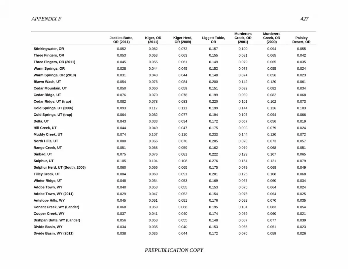
APPENDIX F 427
PREPUBLICATION COPY
Jackies Butte,
OR (2011) Kiger, OR
(2011) Kiger Herd, OR (2009)
Liggett Table, OR
Murderers Creek, OR
(2001)
Murderers Creek, OR
(2009) Paisley
Desert, OR
Stinkingwater, OR 0.052 0.082 0.072 0.157 0.100 0.094 0.055
Three Fingers, OR 0.053 0.053 0.063 0.155 0.081 0.065 0.042
Three Fingers, OR (2011) 0.045 0.055 0.061 0.149 0.079 0.065 0.035
Warm Springs, OR 0.028 0.044 0.045 0.152 0.073 0.055 0.024
Warm Springs, OR (2010) 0.031 0.043 0.044 0.148 0.074 0.056 0.023
Blawn Wash, UT 0.054 0.076 0.084 0.200 0.142 0.120 0.061
Cedar Mountain, UT 0.050 0.060 0.059 0.151 0.092 0.082 0.034
Cedar Ridge, UT 0.076 0.070 0.078 0.199 0.089 0.082 0.068
Cedar Ridge, UT (trap) 0.082 0.078 0.083 0.220 0.101 0.102 0.073
Cold Springs, UT (2006) 0.093 0.117 0.111 0.199 0.144 0.126 0.103
Cold Springs, UT (trap) 0.064 0.082 0.077 0.194 0.107 0.094 0.066
Delta, UT 0.043 0.033 0.034 0.172 0.067 0.056 0.019
Hill Creek, UT 0.044 0.049 0.047 0.175 0.090 0.079 0.024
Muddy Creek, UT 0.074 0.107 0.110 0.233 0.144 0.120 0.072
North Hills, UT 0.080 0.066 0.070 0.205 0.078 0.073 0.057
Range Creek, UT 0.051 0.058 0.059 0.162 0.079 0.068 0.051
Sinbad, UT 0.075 0.076 0.081 0.222 0.129 0.107 0.065
Sulphur, UT 0.105 0.104 0.108 0.276 0.154 0.121 0.079
Sulphur Herd, UT (South, 2006) 0.060 0.066 0.065 0.175 0.079 0.068 0.049
Tilley Creek, UT 0.084 0.069 0.091 0.201 0.125 0.108 0.068
Winter Ridge, UT 0.048 0.054 0.053 0.169 0.067 0.060 0.034
Adobe Town, WY 0.040 0.053 0.055 0.153 0.075 0.064 0.024
Adobe Town, WY (2011) 0.029 0.047 0.052 0.154 0.075 0.064 0.025
Antelope Hills, WY 0.045 0.051 0.051 0.176 0.092 0.070 0.035
Conant Creek, WY (Lander) 0.068 0.059 0.068 0.195 0.104 0.083 0.054
Cooper Creek, WY 0.037 0.041 0.040 0.174 0.079 0.060 0.021
Dishpan Butte, WY (Lander) 0.056 0.053 0.055 0.148 0.087 0.077 0.039
Divide Basin, WY 0.034 0.035 0.040 0.153 0.065 0.051 0.023
Divide Basin, WY (2011) 0.038 0.036 0.044 0.172 0.076 0.059 0.026

428 BLM WILD HORSE AND BURRO PROGRAM
PREPUBLICATION COPY
Jackies Butte,
OR (2011) Kiger, OR
(2011) Kiger Herd, OR (2009)
Liggett Table, OR
Murderers Creek, OR
(2001)
Murderers Creek, OR
(2009) Paisley
Desert, OR
Eagles Nest, WY 0.069 0.078 0.069 0.170 0.097 0.079 0.052
Happy Creek Springs, WY 0.058 0.066 0.062 0.173 0.080 0.063 0.048
Little Colorado, WY 0.045 0.055 0.053 0.150 0.072 0.065 0.033
Little Colorado, WY (2011) 0.042 0.048 0.048 0.141 0.064 0.057 0.030
Lost Creek, WY 0.038 0.046 0.043 0.140 0.065 0.048 0.028
Lost Creek, WY (combined) 0.039 0.050 0.048 0.142 0.066 0.052 0.030
McCullough Peaks, WY 0.051 0.047 0.047 0.181 0.086 0.071 0.037
Muskrat Basin, WY (Lander) 0.066 0.059 0.058 0.159 0.092 0.078 0.039
Salt Wells, WY (East) 0.025 0.049 0.053 0.156 0.073 0.055 0.021
Salt Wells, WY (West) 0.044 0.042 0.046 0.176 0.081 0.068 0.026
Stewart Creek, WY 0.049 0.051 0.044 0.156 0.087 0.068 0.036
Stewart Creek, WY (2009) 0.051 0.053 0.049 0.170 0.072 0.064 0.041
White Mountain, WY (2011) 0.044 0.044 0.053 0.170 0.081 0.067 0.040
Riddle Herd, OR
(2009) Riddle
Mountain, OR
Riddle Mountain, OR
(2011) Sand Springs,
OR (2011) Sheepshead,
OR Sheepshead,
OR (2011) South
Steens, OR
Riddle Herd, OR (2009) 0.000
Riddle Mountain, OR 0.007 0.000
Riddle Mountain, OR (2011) 0.006 0.011 0.000
Sand Springs, OR (2011) 0.056 0.051 0.061 0.000
Sheepshead, OR 0.058 0.052 0.061 0.025 0.000
Sheepshead, OR (2011) 0.054 0.047 0.058 0.025 0.009 0.000
South Steens, OR 0.057 0.055 0.058 0.030 0.026 0.028 0.000
South Steens, OR (2010) 0.054 0.053 0.057 0.034 0.033 0.035 0.010
Stinkingwater, OR 0.094 0.084 0.104 0.068 0.062 0.061 0.056
Three Fingers, OR 0.062 0.058 0.067 0.043 0.043 0.038 0.056
Three Fingers, OR (2011) 0.063 0.060 0.067 0.045 0.038 0.031 0.045
Warm Springs, OR 0.051 0.045 0.054 0.041 0.034 0.031 0.025
Warm Springs, OR (2010) 0.049 0.044 0.052 0.040 0.037 0.035 0.026

APPENDIX F 429
PREPUBLICATION COPY
Riddle Herd, OR
(2009) Riddle
Mountain, OR
Riddle Mountain, OR
(2011) Sand Springs,
OR (2011) Sheepshead,
OR Sheepshead,
OR (2011) South
Steens, OR
Blawn Wash, UT 0.080 0.074 0.081 0.074 0.066 0.063 0.075
Cedar Mountain, UT 0.062 0.064 0.063 0.048 0.046 0.047 0.039
Cedar Ridge, UT 0.077 0.075 0.077 0.065 0.064 0.060 0.069
Cedar Ridge, UT (trap) 0.085 0.088 0.085 0.070 0.075 0.071 0.070
Cold Springs, UT (2006) 0.109 0.114 0.116 0.103 0.113 0.106 0.098
Cold Springs, UT (trap) 0.077 0.082 0.081 0.071 0.073 0.069 0.065
Delta, UT 0.045 0.046 0.048 0.031 0.028 0.027 0.028
Hill Creek, UT 0.055 0.063 0.058 0.040 0.036 0.039 0.030
Muddy Creek, UT 0.129 0.121 0.135 0.079 0.074 0.073 0.085
North Hills, UT 0.085 0.074 0.087 0.075 0.061 0.069 0.064
Range Creek, UT 0.058 0.060 0.061 0.049 0.054 0.048 0.050
Sinbad, UT 0.085 0.079 0.093 0.058 0.056 0.053 0.069
Sulphur, UT 0.130 0.126 0.135 0.101 0.088 0.098 0.092
Sulphur Herd, UT (South, 2006) 0.072 0.070 0.076 0.058 0.048 0.048 0.048
Tilley Creek, UT 0.076 0.069 0.075 0.077 0.077 0.067 0.079
Winter Ridge, UT 0.065 0.070 0.075 0.044 0.037 0.037 0.043
Adobe Town, WY 0.067 0.063 0.075 0.035 0.034 0.031 0.031
Adobe Town, WY (2011) 0.058 0.056 0.065 0.034 0.034 0.032 0.026
Antelope Hills, WY 0.059 0.058 0.072 0.046 0.044 0.044 0.046
Conant Creek, WY (Lander) 0.062 0.066 0.067 0.063 0.053 0.053 0.063
Cooper Creek, WY 0.051 0.050 0.057 0.034 0.029 0.031 0.029
Dishpan Butte, WY (Lander) 0.056 0.053 0.061 0.038 0.039 0.032 0.044
Divide Basin, WY 0.044 0.040 0.052 0.031 0.024 0.022 0.025
Divide Basin, WY (2011) 0.051 0.046 0.056 0.035 0.027 0.025 0.030
Eagles Nest, WY 0.083 0.079 0.090 0.053 0.060 0.052 0.055
Happy Creek Springs, WY 0.081 0.076 0.091 0.047 0.048 0.046 0.058
Little Colorado, WY 0.058 0.050 0.063 0.041 0.038 0.034 0.040
Little Colorado, WY (2011) 0.050 0.043 0.056 0.038 0.036 0.031 0.036
Lost Creek, WY 0.055 0.053 0.062 0.032 0.030 0.026 0.030
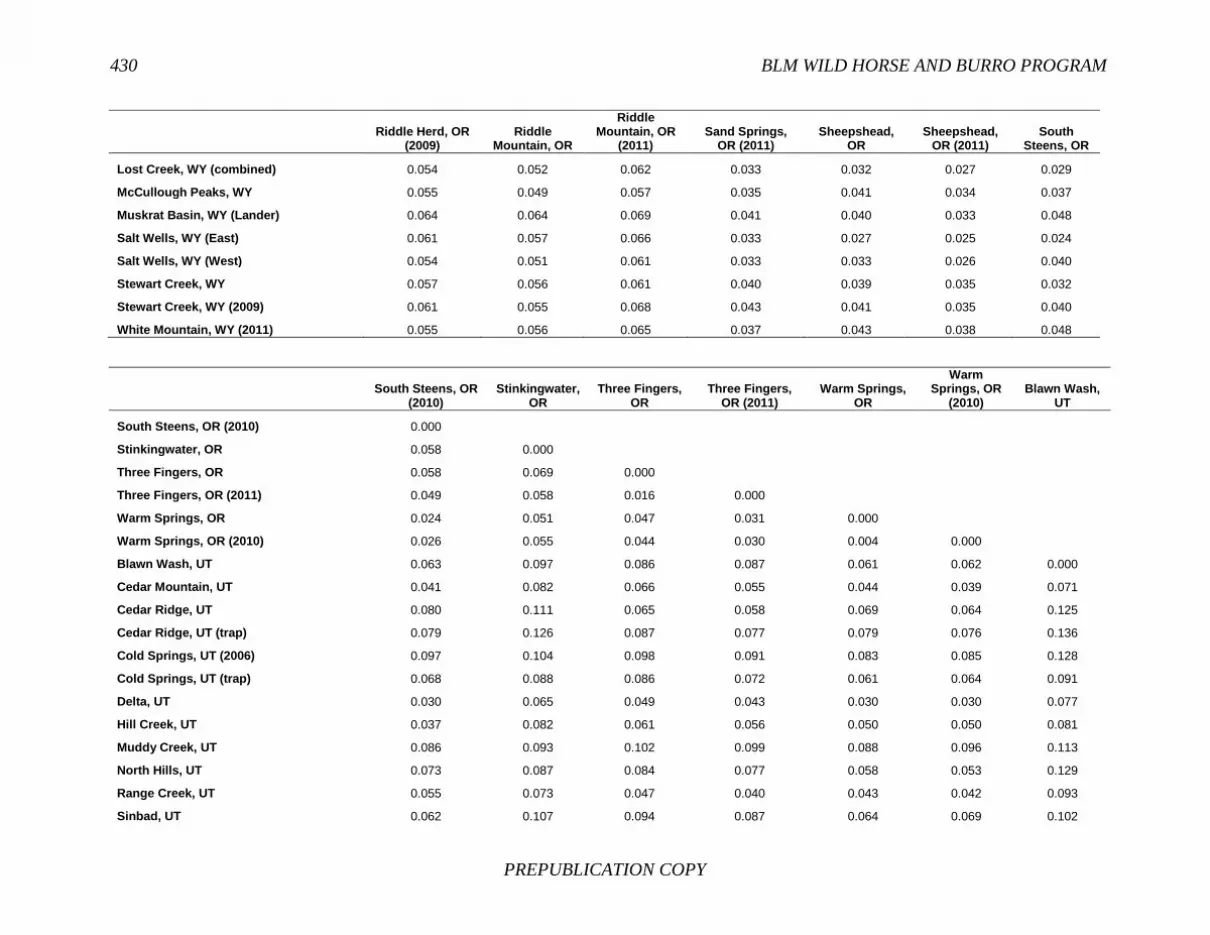
430 BLM WILD HORSE AND BURRO PROGRAM
PREPUBLICATION COPY
Riddle Herd, OR
(2009) Riddle
Mountain, OR
Riddle Mountain, OR
(2011) Sand Springs,
OR (2011) Sheepshead,
OR Sheepshead,
OR (2011) South
Steens, OR
Lost Creek, WY (combined) 0.054 0.052 0.062 0.033 0.032 0.027 0.029
McCullough Peaks, WY 0.055 0.049 0.057 0.035 0.041 0.034 0.037
Muskrat Basin, WY (Lander) 0.064 0.064 0.069 0.041 0.040 0.033 0.048
Salt Wells, WY (East) 0.061 0.057 0.066 0.033 0.027 0.025 0.024
Salt Wells, WY (West) 0.054 0.051 0.061 0.033 0.033 0.026 0.040
Stewart Creek, WY 0.057 0.056 0.061 0.040 0.039 0.035 0.032
Stewart Creek, WY (2009) 0.061 0.055 0.068 0.043 0.041 0.035 0.040
White Mountain, WY (2011) 0.055 0.056 0.065 0.037 0.043 0.038 0.048
South Steens, OR
(2010) Stinkingwater,
OR Three Fingers,
OR Three Fingers,
OR (2011) Warm Springs,
OR
Warm Springs, OR
(2010) Blawn Wash,
UT
South Steens, OR (2010) 0.000
Stinkingwater, OR 0.058 0.000
Three Fingers, OR 0.058 0.069 0.000
Three Fingers, OR (2011) 0.049 0.058 0.016 0.000
Warm Springs, OR 0.024 0.051 0.047 0.031 0.000
Warm Springs, OR (2010) 0.026 0.055 0.044 0.030 0.004 0.000
Blawn Wash, UT 0.063 0.097 0.086 0.087 0.061 0.062 0.000
Cedar Mountain, UT 0.041 0.082 0.066 0.055 0.044 0.039 0.071
Cedar Ridge, UT 0.080 0.111 0.065 0.058 0.069 0.064 0.125
Cedar Ridge, UT (trap) 0.079 0.126 0.087 0.077 0.079 0.076 0.136
Cold Springs, UT (2006) 0.097 0.104 0.098 0.091 0.083 0.085 0.128
Cold Springs, UT (trap) 0.068 0.088 0.086 0.072 0.061 0.064 0.091
Delta, UT 0.030 0.065 0.049 0.043 0.030 0.030 0.077
Hill Creek, UT 0.037 0.082 0.061 0.056 0.050 0.050 0.081
Muddy Creek, UT 0.086 0.093 0.102 0.099 0.088 0.096 0.113
North Hills, UT 0.073 0.087 0.084 0.077 0.058 0.053 0.129
Range Creek, UT 0.055 0.073 0.047 0.040 0.043 0.042 0.093
Sinbad, UT 0.062 0.107 0.094 0.087 0.064 0.069 0.102

APPENDIX F 431
PREPUBLICATION COPY
South Steens, OR
(2010) Stinkingwater,
OR Three Fingers,
OR Three Fingers,
OR (2011) Warm Springs,
OR
Warm Springs, OR
(2010) Blawn Wash,
UT
Sulphur, UT 0.087 0.138 0.112 0.112 0.085 0.081 0.131
Sulphur Herd, UT (South, 2006) 0.058 0.091 0.071 0.062 0.054 0.055 0.116
Tilley Creek, UT 0.081 0.127 0.078 0.080 0.069 0.070 0.076
Winter Ridge, UT 0.044 0.079 0.058 0.055 0.046 0.048 0.088
Adobe Town, WY 0.034 0.056 0.042 0.038 0.034 0.037 0.086
Adobe Town, WY (2011) 0.026 0.061 0.039 0.036 0.029 0.031 0.074
Antelope Hills, WY 0.045 0.064 0.052 0.057 0.046 0.044 0.096
Conant Creek, WY (Lander) 0.064 0.102 0.063 0.072 0.066 0.068 0.071
Cooper Creek, WY 0.028 0.066 0.050 0.044 0.028 0.027 0.072
Dishpan Butte, WY (Lander) 0.053 0.068 0.048 0.046 0.052 0.055 0.093
Divide Basin, WY 0.029 0.053 0.047 0.040 0.022 0.022 0.071
Divide Basin, WY (2011) 0.032 0.058 0.043 0.038 0.025 0.024 0.070
Eagles Nest, WY 0.061 0.078 0.071 0.065 0.055 0.055 0.112
Happy Creek Springs, WY 0.065 0.063 0.056 0.058 0.051 0.054 0.097
Little Colorado, WY 0.048 0.058 0.045 0.041 0.033 0.033 0.068
Little Colorado, WY (2011) 0.039 0.051 0.047 0.041 0.026 0.027 0.064
Lost Creek, WY 0.033 0.053 0.044 0.038 0.030 0.032 0.077
Lost Creek, WY (combined) 0.032 0.061 0.051 0.041 0.029 0.032 0.080
McCullough Peaks, WY 0.040 0.056 0.059 0.055 0.045 0.045 0.076
Muskrat Basin, WY (Lander) 0.058 0.076 0.047 0.038 0.051 0.050 0.090
Salt Wells, WY (East) 0.024 0.054 0.042 0.038 0.026 0.027 0.059
Salt Wells, WY (West) 0.038 0.068 0.044 0.044 0.035 0.033 0.063
Stewart Creek, WY 0.036 0.063 0.053 0.045 0.035 0.037 0.082
Stewart Creek, WY (2009) 0.047 0.068 0.060 0.055 0.037 0.040 0.091
White Mountain, WY (2011) 0.038 0.070 0.059 0.061 0.048 0.048 0.065
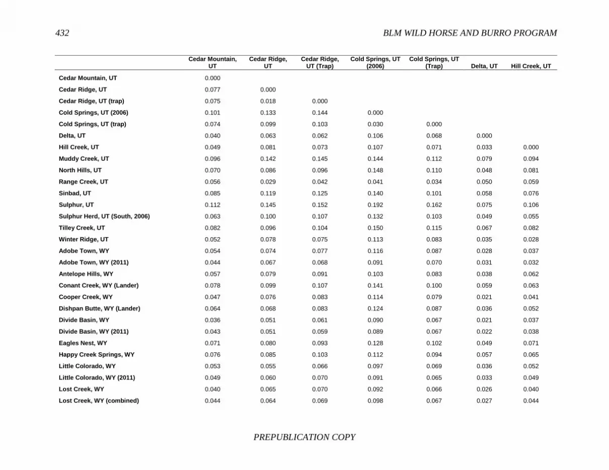
432 BLM WILD HORSE AND BURRO PROGRAM
PREPUBLICATION COPY
Cedar Mountain,
UT Cedar Ridge,
UT Cedar Ridge,
UT (Trap) Cold Springs, UT
(2006) Cold Springs, UT
(Trap) Delta, UT Hill Creek, UT
Cedar Mountain, UT 0.000
Cedar Ridge, UT 0.077 0.000
Cedar Ridge, UT (trap) 0.075 0.018 0.000
Cold Springs, UT (2006) 0.101 0.133 0.144 0.000
Cold Springs, UT (trap) 0.074 0.099 0.103 0.030 0.000
Delta, UT 0.040 0.063 0.062 0.106 0.068 0.000
Hill Creek, UT 0.049 0.081 0.073 0.107 0.071 0.033 0.000
Muddy Creek, UT 0.096 0.142 0.145 0.144 0.112 0.079 0.094
North Hills, UT 0.070 0.086 0.096 0.148 0.110 0.048 0.081
Range Creek, UT 0.056 0.029 0.042 0.041 0.034 0.050 0.059
Sinbad, UT 0.085 0.119 0.125 0.140 0.101 0.058 0.076
Sulphur, UT 0.112 0.145 0.152 0.192 0.162 0.075 0.106
Sulphur Herd, UT (South, 2006) 0.063 0.100 0.107 0.132 0.103 0.049 0.055
Tilley Creek, UT 0.082 0.096 0.104 0.150 0.115 0.067 0.082
Winter Ridge, UT 0.052 0.078 0.075 0.113 0.083 0.035 0.028
Adobe Town, WY 0.054 0.074 0.077 0.116 0.087 0.028 0.037
Adobe Town, WY (2011) 0.044 0.067 0.068 0.091 0.070 0.031 0.032
Antelope Hills, WY 0.057 0.079 0.091 0.103 0.083 0.038 0.062
Conant Creek, WY (Lander) 0.078 0.099 0.107 0.141 0.100 0.059 0.063
Cooper Creek, WY 0.047 0.076 0.083 0.114 0.079 0.021 0.041
Dishpan Butte, WY (Lander) 0.064 0.068 0.083 0.124 0.087 0.036 0.052
Divide Basin, WY 0.036 0.051 0.061 0.090 0.067 0.021 0.037
Divide Basin, WY (2011) 0.043 0.051 0.059 0.089 0.067 0.022 0.038
Eagles Nest, WY 0.071 0.080 0.093 0.128 0.102 0.049 0.071
Happy Creek Springs, WY 0.076 0.085 0.103 0.112 0.094 0.057 0.065
Little Colorado, WY 0.053 0.055 0.066 0.097 0.069 0.036 0.052
Little Colorado, WY (2011) 0.049 0.060 0.070 0.091 0.065 0.033 0.049
Lost Creek, WY 0.040 0.065 0.070 0.092 0.066 0.026 0.040
Lost Creek, WY (combined) 0.044 0.064 0.069 0.098 0.067 0.027 0.044

APPENDIX F 433
PREPUBLICATION COPY
Cedar Mountain,
UT Cedar Ridge,
UT Cedar Ridge,
UT (Trap) Cold Springs, UT
(2006) Cold Springs, UT
(Trap) Delta, UT Hill Creek, UT
McCullough Peaks, WY 0.063 0.078 0.092 0.113 0.083 0.046 0.053
Muskrat Basin, WY (Lander) 0.062 0.066 0.079 0.121 0.084 0.035 0.053
Salt Wells, WY (East) 0.039 0.064 0.068 0.093 0.066 0.029 0.030
Salt Wells, WY (West) 0.047 0.067 0.075 0.116 0.085 0.029 0.046
Stewart Creek, WY 0.050 0.068 0.077 0.098 0.076 0.037 0.050
Stewart Creek, WY (2009) 0.058 0.075 0.083 0.115 0.084 0.038 0.057
White Mountain, WY (2011) 0.065 0.087 0.091 0.110 0.082 0.037 0.053
Muddy Creek, UT North Hills, UT
Range Creek, UT Sinbad, UT Sulphur, UT
Sulphur Herd, UT (South, 2006)
Tilley Creek, UT
Muddy Creek, UT 0.000
North Hills, UT 0.129 0.000
Range Creek, UT 0.109 0.082 0.000
Sinbad, UT 0.122 0.118 0.094 0.000
Sulphur, UT 0.162 0.086 0.130 0.128 0.000
Sulphur Herd, UT (South, 2006) 0.114 0.070 0.081 0.092 0.103 0.000
Tilley Creek, UT 0.140 0.095 0.086 0.122 0.128 0.089 0.000
Winter Ridge, UT 0.097 0.076 0.061 0.080 0.097 0.056 0.072
Adobe Town, WY 0.079 0.067 0.061 0.072 0.094 0.055 0.073
Adobe Town, WY (2011) 0.074 0.066 0.046 0.075 0.098 0.056 0.066
Antelope Hills, WY 0.094 0.070 0.057 0.066 0.104 0.064 0.098
Conant Creek, WY (Lander) 0.117 0.117 0.083 0.094 0.113 0.085 0.081
Cooper Creek, WY 0.086 0.049 0.060 0.062 0.043 0.043 0.078
Dishpan Butte, WY (Lander) 0.088 0.082 0.060 0.076 0.115 0.057 0.077
Divide Basin, WY 0.073 0.051 0.037 0.057 0.090 0.045 0.061
Divide Basin, WY (2011) 0.072 0.053 0.036 0.058 0.080 0.054 0.061
Eagles Nest, WY 0.102 0.088 0.069 0.092 0.119 0.071 0.102
Happy Creek Springs, WY 0.105 0.087 0.064 0.077 0.115 0.072 0.103
Little Colorado, WY 0.097 0.057 0.042 0.094 0.106 0.068 0.068

434 BLM WILD HORSE AND BURRO PROGRAM
PREPUBLICATION COPY
Muddy Creek, UT North Hills, UT
Range Creek, UT Sinbad, UT Sulphur, UT
Sulphur Herd, UT (South, 2006)
Tilley Creek, UT
Little Colorado, WY (2011) 0.097 0.053 0.041 0.084 0.104 0.063 0.060
Lost Creek, WY 0.076 0.062 0.045 0.059 0.092 0.043 0.081
Lost Creek, WY (combined) 0.076 0.068 0.047 0.058 0.099 0.041 0.080
McCullough Peaks, WY 0.115 0.080 0.060 0.070 0.111 0.063 0.082
Muskrat Basin, WY (Lander) 0.093 0.087 0.058 0.083 0.112 0.064 0.084
Salt Wells, WY (East) 0.068 0.063 0.046 0.066 0.081 0.057 0.069
Salt Wells, WY (West) 0.082 0.075 0.057 0.064 0.090 0.069 0.069
Stewart Creek, WY 0.098 0.079 0.049 0.065 0.101 0.045 0.094
Stewart Creek, WY (2009) 0.092 0.075 0.060 0.068 0.112 0.057 0.087
White Mountain, WY (2011) 0.086 0.090 0.064 0.067 0.104 0.073 0.063
Winter Ridge,
UT Adobe Town,
WY Adobe Town,
WY (2011) Antelope Hills,
WY Conant Creek, WY (Lander)
Cooper Creek, WY
Dishpan Butte, WY (Lander)
Winter Ridge, UT 0.000
Adobe Town, WY 0.034 0.000
Adobe Town, WY (2011) 0.028 0.013 0.000
Antelope Hills, WY 0.061 0.046 0.044 0.000
Conant Creek, WY (Lander) 0.071 0.066 0.063 0.080 0.000
Cooper Creek, WY 0.041 0.033 0.036 0.040 0.056 0.000
Dishpan Butte, WY (Lander) 0.054 0.036 0.047 0.062 0.047 0.042 0.000
Divide Basin, WY 0.032 0.027 0.024 0.028 0.060 0.027 0.034
Divide Basin, WY (2011) 0.036 0.027 0.026 0.033 0.056 0.030 0.036
Eagles Nest, WY 0.065 0.053 0.054 0.050 0.090 0.058 0.054
Happy Creek Springs, WY 0.053 0.051 0.056 0.053 0.079 0.048 0.055
Little Colorado, WY 0.044 0.041 0.038 0.054 0.072 0.045 0.039
Little Colorado, WY (2011) 0.038 0.039 0.035 0.048 0.070 0.040 0.039
Lost Creek, WY 0.033 0.031 0.028 0.033 0.063 0.032 0.040
Lost Creek, WY (combined) 0.036 0.033 0.030 0.038 0.062 0.031 0.035
McCullough Peaks, WY 0.056 0.052 0.051 0.049 0.061 0.044 0.046

APPENDIX F 435
PREPUBLICATION COPY
Winter Ridge,
UT Adobe Town,
WY Adobe Town,
WY (2011) Antelope Hills,
WY Conant Creek, WY (Lander)
Cooper Creek, WY
Dishpan Butte, WY (Lander)
Muskrat Basin, WY (Lander) 0.057 0.041 0.051 0.070 0.056 0.045 0.014
Salt Wells, WY (East) 0.031 0.018 0.013 0.042 0.057 0.032 0.045
Salt Wells, WY (West) 0.044 0.032 0.033 0.047 0.053 0.031 0.046
Stewart Creek, WY 0.053 0.047 0.046 0.039 0.070 0.040 0.047
Stewart Creek, WY (2009) 0.040 0.039 0.039 0.051 0.077 0.039 0.048
White Mountain, WY (2011) 0.035 0.044 0.037 0.053 0.065 0.044 0.055
Divide Basin,
WY Divide Basin, WY
(2011) Eagles Nest,
WY Happy Creek Springs, WY
Little Colorado, WY
Little Colorado, WY (2011)
Lost Creek, WY
Divide Basin, WY 0.000
Divide Basin, WY (2011) 0.007 0.000
Eagles Nest, WY 0.039 0.045 0.000
Happy Creek Springs, WY 0.040 0.044 0.053 0.000
Little Colorado, WY 0.030 0.030 0.045 0.050 0.000
Little Colorado, WY (2011) 0.024 0.029 0.044 0.046 0.005 0.000
Lost Creek, WY 0.019 0.024 0.026 0.033 0.034 0.029 0.000
Lost Creek, WY (combined) 0.019 0.025 0.024 0.033 0.033 0.029 0.006
McCullough Peaks, WY 0.037 0.041 0.061 0.048 0.043 0.036 0.039
Muskrat Basin, WY (Lander) 0.038 0.037 0.049 0.062 0.039 0.040 0.038
Salt Wells, WY (East) 0.023 0.023 0.051 0.048 0.035 0.032 0.022
Salt Wells, WY (West) 0.028 0.027 0.057 0.053 0.038 0.039 0.038
Stewart Creek, WY 0.030 0.034 0.029 0.041 0.042 0.036 0.014
Stewart Creek, WY (2009) 0.024 0.033 0.041 0.033 0.042 0.039 0.022
White Mountain, WY (2011) 0.033 0.037 0.068 0.060 0.051 0.040 0.040
Lost Creek,
WY (Combined)
McCullough Peaks, WY
Muskrat Basin, WY (Lander)
Salt Wells, WY (East)
Salt Wells, WY (West)
Stewart Creek, WY
Stewart Creek, WY
(2009)
White Mountain, WY (2011)
Lost Creek, WY (combined) 0.000
McCullough Peaks, WY 0.040 0.000

436 BLM WILD HORSE AND BURRO PROGRAM
PREPUBLICATION COPY
Lost Creek,
WY (Combined)
McCullough Peaks, WY
Muskrat Basin, WY (Lander)
Salt Wells, WY (East)
Salt Wells, WY (West)
Stewart Creek, WY
Stewart Creek, WY
(2009)
White Mountain, WY (2011)
Muskrat Basin, WY (Lander) 0.037 0.057 0.000
Salt Wells, WY (East) 0.028 0.045 0.047 0.000
Salt Wells, WY (West) 0.037 0.041 0.045 0.035 0.000
Stewart Creek, WY 0.017 0.040 0.040 0.039 0.050 0.000
Stewart Creek, WY (2009) 0.018 0.046 0.053 0.039 0.041 0.032 0.000
White Mountain, WY (2011) 0.041 0.046 0.063 0.037 0.039 0.054 0.045 0.000
SOURCE: Data provided by E. Gus Cothran. To access the data, contact the National Research Council’s Public Access Records Office at [email protected].


![HC[Final]-BLM and Paul Kruger, Gauteng.pdf](https://static.fdokumen.com/doc/165x107/63236790be5419ea700e96f1/hcfinal-blm-and-paul-kruger-gautengpdf.jpg)