Using R

(with applications in Time Series Analysis)

Dr. Gavin Shaddick

January 2004

These notes are based on a set produced by Dr R. Salway for the MA20035 course.

Contents

1 R Basics 41.1 Introduction to R . . . . . . . . . . . . . . . . . . . . . . . . . . . . . . . . . . . . . . . . . . . . . 4

1.1.1 What is R? . . . . . . . . . . . . . . . . . . . . . . . . . . . . . . . . . . . . . . . . . . . . 41.1.2 Advantages of R . . . . . . . . . . . . . . . . . . . . . . . . . . . . . . . . . . . . . . . . . 41.1.3 Using R on the Library PCs . . . . . . . . . . . . . . . . . . . . . . . . . . . . . . . . . . . 41.1.4 Downloading R . . . . . . . . . . . . . . . . . . . . . . . . . . . . . . . . . . . . . . . . . . 5

1.2 Getting Started in R . . . . . . . . . . . . . . . . . . . . . . . . . . . . . . . . . . . . . . . . . . . 51.2.1 Starting R . . . . . . . . . . . . . . . . . . . . . . . . . . . . . . . . . . . . . . . . . . . . . 51.2.2 Entering Commands . . . . . . . . . . . . . . . . . . . . . . . . . . . . . . . . . . . . . . . 51.2.3 Command history . . . . . . . . . . . . . . . . . . . . . . . . . . . . . . . . . . . . . . . . 61.2.4 Getting Help . . . . . . . . . . . . . . . . . . . . . . . . . . . . . . . . . . . . . . . . . . . 61.2.5 Quitting . . . . . . . . . . . . . . . . . . . . . . . . . . . . . . . . . . . . . . . . . . . . . . 6

1.3 Commands and Objects . . . . . . . . . . . . . . . . . . . . . . . . . . . . . . . . . . . . . . . . . 61.3.1 Simple Arithmetic . . . . . . . . . . . . . . . . . . . . . . . . . . . . . . . . . . . . . . . . 61.3.2 Simple Numeric Functions . . . . . . . . . . . . . . . . . . . . . . . . . . . . . . . . . . . . 71.3.3 Variables . . . . . . . . . . . . . . . . . . . . . . . . . . . . . . . . . . . . . . . . . . . . . 71.3.4 Logical Values . . . . . . . . . . . . . . . . . . . . . . . . . . . . . . . . . . . . . . . . . . 8

1.4 Data . . . . . . . . . . . . . . . . . . . . . . . . . . . . . . . . . . . . . . . . . . . . . . . . . . . . 81.4.1 Vectors . . . . . . . . . . . . . . . . . . . . . . . . . . . . . . . . . . . . . . . . . . . . . . 8

1.4.1.1 Creating Vectors . . . . . . . . . . . . . . . . . . . . . . . . . . . . . . . . . . . . 91.4.2 Manipulating Vectors . . . . . . . . . . . . . . . . . . . . . . . . . . . . . . . . . . . . . . 101.4.3 Functions of Vectors . . . . . . . . . . . . . . . . . . . . . . . . . . . . . . . . . . . . . . . 111.4.4 Data Frames . . . . . . . . . . . . . . . . . . . . . . . . . . . . . . . . . . . . . . . . . . . 11

1.5 Input and Output . . . . . . . . . . . . . . . . . . . . . . . . . . . . . . . . . . . . . . . . . . . . 121.5.1 Entering Data . . . . . . . . . . . . . . . . . . . . . . . . . . . . . . . . . . . . . . . . . . 121.5.2 Saving Data . . . . . . . . . . . . . . . . . . . . . . . . . . . . . . . . . . . . . . . . . . . . 131.5.3 Using Scripts . . . . . . . . . . . . . . . . . . . . . . . . . . . . . . . . . . . . . . . . . . . 131.5.4 Recording Output . . . . . . . . . . . . . . . . . . . . . . . . . . . . . . . . . . . . . . . . 13

1.6 Saving Graphics . . . . . . . . . . . . . . . . . . . . . . . . . . . . . . . . . . . . . . . . . . . . . 131.6.1 Printing . . . . . . . . . . . . . . . . . . . . . . . . . . . . . . . . . . . . . . . . . . . . . . 14

1

1.6.2 Saving to a �le . . . . . . . . . . . . . . . . . . . . . . . . . . . . . . . . . . . . . . . . . . 141.6.3 Including a graph in Word . . . . . . . . . . . . . . . . . . . . . . . . . . . . . . . . . . . . 14

2 Exploratory Data Analysis in R 162.0.4 Summarising Data . . . . . . . . . . . . . . . . . . . . . . . . . . . . . . . . . . . . . . . . 16

2.0.4.1 Numerical Data . . . . . . . . . . . . . . . . . . . . . . . . . . . . . . . . . . . . 162.0.4.2 Categorical Data . . . . . . . . . . . . . . . . . . . . . . . . . . . . . . . . . . . . 172.0.4.3 Making Numerical Data Categorical . . . . . . . . . . . . . . . . . . . . . . . . . 17

2.0.5 Graphs and Plots . . . . . . . . . . . . . . . . . . . . . . . . . . . . . . . . . . . . . . . . . 182.0.5.1 Univariate Data . . . . . . . . . . . . . . . . . . . . . . . . . . . . . . . . . . . . 182.0.5.2 Bivariate Data . . . . . . . . . . . . . . . . . . . . . . . . . . . . . . . . . . . . . 192.0.5.3 Miscellaneous Graphics Commands . . . . . . . . . . . . . . . . . . . . . . . . . 20

3 Time series analysis in R 223.1 Introduction . . . . . . . . . . . . . . . . . . . . . . . . . . . . . . . . . . . . . . . . . . . . . . . . 223.2 Removing a trend . . . . . . . . . . . . . . . . . . . . . . . . . . . . . . . . . . . . . . . . . . . . . 24

3.2.1 Using the CO dataset . . . . . . . . . . . . . . . . . . . . . . . . . . . . . . . . . . . . . . 243.3 Removing a periodic e�ect . . . . . . . . . . . . . . . . . . . . . . . . . . . . . . . . . . . . . . . . 24

3.3.1 Using the nottem dataset . . . . . . . . . . . . . . . . . . . . . . . . . . . . . . . . . . . . 243.4 Taking account of a regime shift . . . . . . . . . . . . . . . . . . . . . . . . . . . . . . . . . . . . 25

3.4.1 Using the UKDriverDeaths dataset . . . . . . . . . . . . . . . . . . . . . . . . . . . . . . . 253.4.2 Using the sunspots dataset . . . . . . . . . . . . . . . . . . . . . . . . . . . . . . . . . . . 25

3.5 Fitting ARIMA models . . . . . . . . . . . . . . . . . . . . . . . . . . . . . . . . . . . . . . . . . 263.5.1 AR models . . . . . . . . . . . . . . . . . . . . . . . . . . . . . . . . . . . . . . . . . . . . 26

2

About this Document

These notes provide an introduction to using the statistical software package R, for the course MA20035:Statistical Inference 2. They do not demonstrate all the features of R but concentrate on those that are mostuseful for the course.Throughout this document I will use the following conventions:The names of R commands in the text will appear in a di�erent font, with parentheses; for example, summary().The names of R objects in the text will also appear in a di�erent font, but have no parentheses; for example,bird.data.Commands that you should type in will appear indented in a di�erent font, preceded by the symbol `> '; youdo not need to type `> ' when entering commands. For example,

> min(data)

R output will appear indented in a di�erent font; for example,[1] 38

3

Chapter 1

R Basics

1.1 Introduction to R

1.1.1 What is R?

R is a freely available language and environment for statistical computing and graphics providing a wide varietyof statistical and graphical techniques. It is very similar to a commercial statistics package called S-Plus, whichis widely used.R is a command-line driven package. This means that for most commands you have to type the commandfrom the keyboard. The advantage of this is that it is very exible to add di�erent options to a command; forexample,

> hist(weights)

will draw a histogram of the data weights using the default options. However you may also specify some ofthose options more exactly:

> hist(weights, breaks=5, freq=F, col='lightblue', main='Histogram of Weights')

The disadvantage of a command-line driven program is that it may take a little time to learn the commands.However, most of the commands in R are intuitive. R also provides some commands in the menus; these mainlyrelate to managing your R session.

1.1.2 Advantages of R

� R is free and available for all major platforms.� It has excellent built-in help.� It has excellent graphical capacities.� It is easy to use S-Plus once you have learnt R (and vice versa).� It is powerful with many built-in statistical functions.� It is easy to extend with user-de�ned functions.

1.1.3 Using R on the Library PCs

R is available on the PCs in the library. From the Start button choosePrograms ! Departments ! Mathematical Sciences ! R ! R 1.8.1

4

1.1.4 Downloading R

Since R is freely available under the GNU Public License, you may download a copy for use on your owncomputer. Versions are available for Windows, Unix, Linux and Macintosh.The R software itself and documentation can be obtained from the Comprehensive R Archive Network (CRAN)athttp://cran.uk.r-project.org.To download a self-extracting set-up �le for Windows, select the Windows (95 or later) option from the 'Pre-compiled Binary Distributions' section and click on base/. The most recent version of R at the time of writingis version 1.8.1, and the set up program is the �le rw1081.exe; click on it to download. (If a more recent versionis available, it will be the �le beginning rw.) This �le is around 20 Mb, so may take some time. When you havedownloaded it on to your computer, double click on the �le and follow the instructions to install R choosing thedefault options. You will require around 35-40Mb of free space on your hard drive for a standard installation.

1.2 Getting Started in R

1.2.1 Starting R

When R starts you should see a window with the following text (the text may di�er slightly depending on theversion you are using):

R : Copyright 2003, The R Foundation for Statistical ComputingVersion 1.8.1 (2003-11-21), ISBN 3-900051-00-3R is free software and comes with ABSOLUTELY NO WARRANTY.You are welcome to redistribute it under certain conditions.Type 'license()' or 'licence()' for distribution details.R is a collaborative project with many contributors.Type 'contributors()' for more information and'citation()' on how to cite R in publications.Type 'demo()' for some demos, 'help()' for on-line help, or'help.start()' for a HTML browser interface to help.Type 'q()' to quit R.>

The symbol `> ' appears in red, and is called the prompt; it indicates that R is waiting for you to type acommand. If a command is too long to �t on a line a `+' is used to indicate that the command is continuedfrom the previous line. All commands that you type in appear in red, and R output appears in blue.In the code examples that follow, you do not need to type the prompt `> '.

1.2.2 Entering Commands

The easiest way of using R is to enter commands directly in this window. For example, try typing 2+2 at thecommand prompt and pressing enter. You should see the output:

[1] 4

The [1] indicates that the answer is a vector of length one; we will return to this later.You can use the cursor keys to edit the command line as normal. Use the up and down cursor keys to scrollbackward and forward through your previous commands; this can save you a lot of typing.The main window is called the command window. Other windows you may come across are the commandhistory window and graphics windows.

5

1.2.3 Command history

Rather than scrolling through a long list of previous commands using the cursor keys, R provides another wayof retrieving previous commands. Type history() and a new window will appear listing the last 25 commandsand you can copy and paste the command or commands you want. To retrieve more previous commands, forexample the last 100, use history(100).

1.2.4 Getting Help

R provides two types of help, both available through the Help menu. The easiest to use is the Html help; selectHelp ! R language (html). This displays help in Internet Explorer just like a web page. The main pagehas several categories. `An Introduction to R' provides basic help similar to this document. `Search Engine &Keywords' allows you to search for di�erent commands by keyword, or sorted into topics.Use the html help to read the page on the command history().

1.2.5 Quitting

To close R, use the command

> q()

or choose Exit from the File menu. You will be asked if you wish to save the workspace; you should answeryes to this if you want to keep any data you have created.

1.3 Commands and Objects

R is an object-oriented language. This means that every piece of information is a type of object, for exampledata, vectors and results of analysis, and each object has a name. The user can perform actions on these objectsvia functions. Some functions behave di�erently depending on the type of object.Although this sounds complicated, in practice it makes R very easy to use. Most of the time you don't need toknow or understand how this works. We will discuss this further later on.

1.3.1 Simple Arithmetic

An expression typed at the prompt is evaluated and the result printed. You can use simple arithmetic:

> 1 + 2 + 3 # addition[1] 6

> 3 * 4 + 2 # multiplication is done first[1] 14

> 1 + 3/2 # so is division[1] 2.5

> (1 + 3)/2 # Use brackets to change the order[1] 2

> 4**2 # use ** for power...[1] 16

6

> 4^2 # ...or use ^[1] 16

The hash # in the commands above simply means a comment; R ignores everything after the hash. This allowsus to insert comments to explain the code; this is particularly useful in a long and complicated analysis.

1.3.2 Simple Numeric Functions

More complicated mathematical expressions can be calculated using functions. These have a name and anargument. For example, the function to calculate a square root has the name sqrt(). The argument is thevalue we want to �nd the square root of; to call the function, place the argument inside the bracket. So, to �ndthe square root of 2, the argument is 2, so we type:

> sqrt(2)[1] 1.414214

Similarly,> log(3.14159) # log of pi[1] 1.144729

> > log(pi) # pi can be used as a given constant[1] 1.14473

A table of commonly used mathematical functions is given below.abs() Absolute value (without +/-)sign() 1 if argument is positive, -1 if it is negative.sqrt() square rootlog() natural logarithmexp() exponentialsin(), asin() sin and sin�1cos(), acos() cos and cos�1tan(), atan() tan and tan�1

1.3.3 Variables

Variables are called objects in R. You can assign a value to an object using "=" or the assignment operator <�(a 'less than' sign followed by a minus sign); the two are interchangeable.

> x <� 5

>From now on you can use x in place of the number 5:> x + 2[1] 7

> sqrt(x)[1] 2.236068

> y = sqrt(x)

Typing the name of an object prints the value of it to screen.> y[1] 2.236068

7

1.3.4 Logical Values

A logical value is either TRUE or FALSE.

> x = 10 # Set x equal to 10> x > 10 # is x strictly greater than 10 ?[1] FALSE> x <= 10 # is x strictly less than or equal to 10?[1] TRUE> x == 10 # is x equal to 10?[1] TRUE

To test if an object is equal to something, you must use the == operator, with a double equals sign. Be carefulwith this; it is easy to make a mistake and use "=" instead.

1.4 Data

Statistics is about the analysis of data, so R provides lots of functions to store, manipulate and perform statisticalanalysis on all sorts of data.

1.4.1 Vectors

A vector is simply a collection of numbers or variables. Vectors are convenient ways to store a series of data,for example a list of measurements. In R, vectors are also objects. To create a vector, use the c() function (cstands for 'concatenate').For example,

> x <- c(2,3,5,7) # the first 4 prime numbers> x[1] 2 3 5 7

Functions and logical operations work on each element of the vector.

> x^2[1] 4 9 25 49> log(x)[1] 0.6931472 1.0986123 1.6094379 1.9459101> x>5[1] FALSE FALSE FALSE TRUE

Two vectors are combined element by element:> > y = c(1,2,3,4)> x + y[1] 3 5 8 11> x * y[1] 2 6 15 28

Notice that x * y does not calculate the vector cross product. To get the cross product use:

8

> > x %*% y[1] 51

When two vectors have di�erent lengths, the shorter is repeated to match the longer one. This is called therecycling rule. If the length of the shorter vector is not a multiple of the length of the other a warning is printed.

> y= c(1,2)> x + y[1] 3 5 6 9

Here, x is of length 4 while y is of length 2. To produce x+y the variable y is repeated to make c(1,2,1,2) andthen added to x as usual.This can cause mistakes if you're not used to it;

1.4.1.1 Creating Vectors

Often you need to create a vector that is a sequence of numbers, or perhaps with all elements the same. Thereare several shortcuts to doing this.To create a list of numbers between 10 and 50, we use

> x = 10:50> x[1] 10 11 12 13 14 15 16 17 18 19 20 21 22 23 24 25 26 27 28[20] 29 30 31 32 33 34 35 36 37 38 39 40 41 42 43 44 45 46 47[39] 48 49 50

The numbers in square brackets tell you which element of the vector starts the new line. So the �rst line startswith the �rst element (10), the second line starts with the 20th element (29) etc. This is why previously R put[1] before each answer; if the answer is just a single number this is the same as a vector of length 1.You can achieve the same result using the seq() function:

> x = seq(10,50,by=1)

This creates a sequence of numbers between 10 and 50 inclusive, incrementing by 1 each time. Alternatively,you can specify how many numbers in the result; numbers will be equally spaced:

> x = seq(10,50,length=41)x = seq(10,50,length=40) # The result need not be integer values!

Another useful function is rep(); this can be used to create a vector by repeating a number a set number oftimes. For example, to repeat a number 5 times:

> rep(3,5)[1] 3 3 3 3 3

The arguments to rep() can also be vectors.See if you can predict what the following will do, and then check:

1. seq(1,10,2)2. seq(5,1,-1)

9

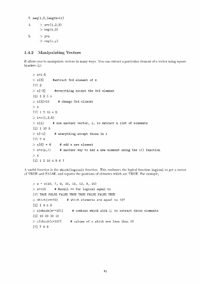
3. seq(1,5,length=11)4. > x=c(1,2,3)

> rep(x,3)5. > y=x

> rep(x,y)

1.4.2 Manipulating Vectors

R allows you to manipulate vectors in many ways. You can extract a particular element of a vector using squarebrackets []:

> x=1:5> x[3] #extract 3rd element of x[1] 3> x[-3] #everything except the 3rd element[1] 1 2 4 5> x[3]=10 # change 3rd element> x[1] 1 2 10 4 5> i=c(1,3,5)> x[i] # use another vector, i, to extract a list of elements[1] 1 10 5> x[-i] # everything except those in i[1] 2 4> x[6] = 6 # add a new element> x=c(x,7) # another way to add a new element using the c() function> x[1] 1 2 10 4 5 6 7

A useful function is the which(logical) function. This evaluates the logical function logical to get a vectorof TRUE and FALSE, and reports the positions of elements which are TRUE. For example,

> x = c(10, 7, 9, 10, 10, 12, 9, 10)> x==10 # Recall == for logical equal to[1] TRUE FALSE FALSE TRUE TRUE FALSE FALSE TRUE> which(x==10) # which elements are equal to 10?[1] 1 4 5 8> x[which(x==10)] # combine which with [] to extract those elements[1] 10 10 10 10> x[which(x<10)] # values of x which are less than 10[1] 7 9 9

10

1.4.3 Functions of Vectors

The simple functions we saw earlier work on each element of a vector. There are also some useful functions thatwork on the whole vector to give a single answer.Function name Value returnedlength(x) The number of elements in xmax(x) The largest value of xmin(x) The smallest value in the vector xsum(x) The sum of elements in xprod(x) The product of elements in xmean(x) The mean of elements in xsd(x) The standard deviation of elements in xvar(x) The variance of elements in x

For example, to �nd the length of a vector, use the length() function:> length(x)[1] 8

1.4.4 Data Frames

A data frame is another type of object in R that is used to store a dataset. For example, if the dataset is all theweights and heights of 10 people, the data frame in R will be a matrix with 10 rows, one for each person, and 2columns, one for weight and one for height. Data frames also have row and column labels, making them idealfor storing datasets. Data in a data frame is much like data in a spreadsheet. Usually, we have one column foreach variable, and one row for each observation.For example, height and weight data might be stored in a data frame called hgtdata:

> hgtdataheight weight

1 169 612 167 693 166 704 172 765 162 606 185 587 165 618 171 729 170 5510 163 63

You can access just the heights using the column name with the $ operator:> hgtdata$height[1] 169 167 166 172 162 185 165 171 170 163

This returns the height column as a vector. You can then use the functions above, for example:> mean(hgtdata$height)[1] 169

The names() function will give you the names of the columns:> names(hgtdata)[1] "height" "weight"

11

1.5 Input and Output

1.5.1 Entering Data

Often you will need to read in data from another source. If the data is stored in a text �le you can read it intoR using read.table(). This function has a lot of optional arguments depending on how the data is written inthe �le. The basic function is simple, however:

> data = read.table("h:/data.dat")

By default, each variable (column) will be labelled V1, V2, . . . . Often text �les of data specify the columnnames in the �rst line, you can get R to use these labels by specifying header==T:

> data = read.table("h:/data.dat", header=T)

Another useful option is to specify what character has been used to separate one variable from the next. Often,a comma is used; to tell R this use

> data = read.table("h:/data.dat", header=T, sep=",")

If the data are tab-separated, use the special character combination `nt':> data = read.table("h:/data.dat", header=T, sep="nt")

Use the help command to �nd out about other options.Suppose the data �le looks like this:

height, weight169, 61167, 69...163, 63

The �rst line contains the names of the variables, and variables are separated on each row using a comma. Sowe would read this into R using

> hgtdata = read.table("h:/hgtdata.dat", header=T, sep=",")

This creates the hgtdata data frame in Section 1.4.4. This is the format I will use for all data �les in this course.For convenience, you can also use the quicker function

> data = read.csv("h:/hgtdata.dat")

which is identical.In this course, you can combine read.table() with the function url() which will download a �le from theinternet. I will make data available on my website, which you can then read directly into R:

> hgtdata = read.csv(url("http://www.bath.ac.uk/~masres/MA35/hgtdata.dat"))

Note that this will only work if you are connected to the Internet. Once the data has been read into R, it issaved as the object hgtdata and you do not need to be connected to use it.

12

1.5.2 Saving Data

If you have a data frame you want to save, use the function write.table(). Again, this has many options. Tosave a data frame in the same format I use in this course, use

> write.table(hgtdata, file="h:/hgtdata.dat", col.names=T, sep=",")

Note that write.table() uses the option col.names instead of header to save the column names as the �rstline of the �le.Check the help �le for more details.

1.5.3 Using Scripts

It can often be useful to read in a list of commands from a separate �le, for example, if you want to keep arecord of what you did or have a long or complicated piece of R code that you need to repeat. This is called ascript �le.Write your script �le in Notepad and save it (Word is not suitable since a script �le needs to be plain text).From the R File menu choose 'Source R code'. This will read in and run all the commands in your script �le.You can also use the command:

> > source("h:/analysis.txt")

Both methods will run all the commands in the �le in order, as if you had typed them directly into the commandwindow.If you just want to run selected parts of your �le, from the R File menu choose 'Display �le'. This will open thescript �le in a new window where you can copy and paste selected commands. You cannot edit the �le in R.

1.5.4 Recording Output

Usually R output prints directly to the screen. You can change this so it prints to a �le instead, by using thesink() command:

> sink("h:/results.r") # create a new file in h: directory> mean(x) # no output to screen> sink() # close the file> mean(x) # this output appears on screen

If the �le h:/results.r already exists it will be overwritten without any warning, so take care you don'toverwrite important results.There is no way to get the output written to the screen and to a �le at the same time. This is an occasion whenit might be useful to use a script �le:

> source("h:/analysis.txt") # print output to screen and check its OK> sink("h:/results.r")> source("h:/analysis.txt") # print the same output to file> sink()

1.6 Saving Graphics

Typically you will want to save a copy of any graphs produced by R, and perhaps include them in anotherpackage, for example in a Word document.Suppose you have produced a histogram of the heights in hgtdata.dat:

13

> hist(hgtdata$height)

We will explore the histogram function, hist() in more detail later, but for now note that it opens a newwindow in R, called the Graphics Window, containing the graph. When this window is active, the menu optionsalso change.

1.6.1 Printing

To print the graph directly, use Print... from the File menu.

1.6.2 Saving to a �le

You can save the �le in several di�erent formats from Save As (also in the File menu).

� Word can read any of Meta�le, Bmp, Png, Jpeg.� Postscript is suitable if you use LATEXto write documents.� Jpeg is a good choice if you want to include it on a webpage.

The di�erent formats can vary greatly in size. The following table compares the �le size of the histogram graphin each format:

Meta�le 18Postscript 4PDF 4Png 5Bmp 440Jpeg 50% 18Jpeg 100% 37

Meta�le is probably the best option for including in a Word document.

1.6.3 Including a graph in Word

You can copy and paste the graph directly into Word, by clicking on the Graphics Window and using 'Ctrl +C' to copy the �le. Then in Word you can paste the image using 'Ctrl + V', or Paste from the Edit menu.Alternatively you can save the graph as above, and then import it into Word. From the Insert menu choosePicture ! From File and select the saved image.Both these methods will work. I prefer the second since you then have two copies of the graph, one on its ownand one as part of the Word document. If you delete the graph by mistake in Word when moving text andgraphics around it is simple to insert the saved �le again, rather than having to go back and recreate the graphin R.

Exercises 1

The times taken waiting for a bus to the university in minutes for ten days are as follows:

3 11 6 9 9 16 10 7 9 5

1. Create a vector of this data called wait.2. Find the minimum, mean and maximum time.

14

3. The fourth time was a mistake; it should have been 8. Correct this and �nd the new mean.4. How often did I wait for more than ten minutes?

[Hint: sum(x>y) counts the number of times x>y is true.]5. What percentage of the time did I wait less than 8 minutes?

On the same days, the time taken for the bus to reach the university was as follows:

14 12 13 11 13 10 13 11 11 136. Create a vector called bustime.7. Find the minimum, mean and maximum bus time.8. Create a new vector of the total time it takes to get into university, that is the waiting time plus the time

up the hill.9. If I get to the bus stop at 8:55, how many times was I late for my 9:15 lecture?10. On which days was I late?

15

Chapter 2

Exploratory Data Analysis in R

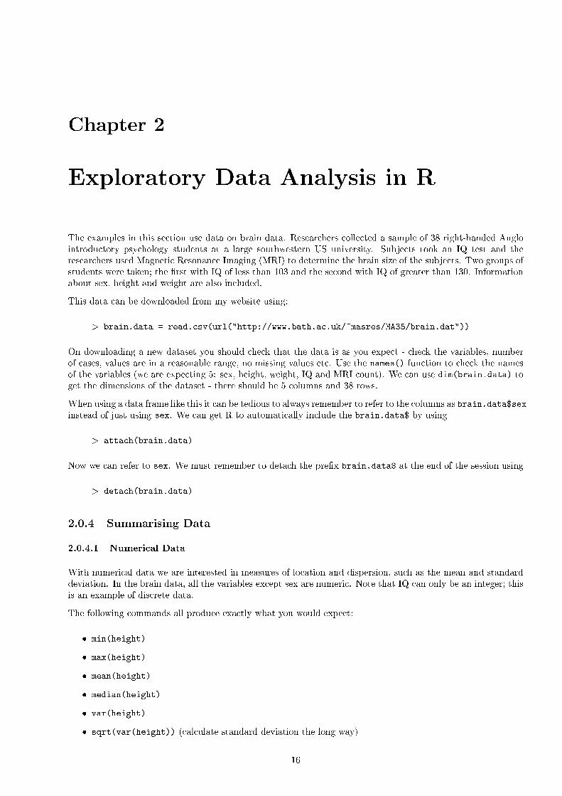
The examples in this section use data on brain data. Researchers collected a sample of 38 right-handed Anglointroductory psychology students at a large southwestern US university. Subjects took an IQ test and theresearchers used Magnetic Resonance Imaging (MRI) to determine the brain size of the subjects. Two groups ofstudents were taken; the �rst with IQ of less than 103 and the second with IQ of greater than 130. Informationabout sex, height and weight are also included.This data can be downloaded from my website using:

> brain.data = read.csv(url("http://www.bath.ac.uk/~masres/MA35/brain.dat"))

On downloading a new dataset you should check that the data is as you expect - check the variables, numberof cases, values are in a reasonable range, no missing values etc. Use the names() function to check the namesof the variables (we are expecting 5: sex, height, weight, IQ and MRI count). We can use dim(brain.data) toget the dimensions of the dataset - there should be 5 columns and 38 rows.When using a data frame like this it can be tedious to always remember to refer to the columns as brain.data$sexinstead of just using sex. We can get R to automatically include the brain.data$ by using

> attach(brain.data)

Now we can refer to sex. We must remember to detach the pre�x brain.data$ at the end of the session using> detach(brain.data)

2.0.4 Summarising Data

2.0.4.1 Numerical Data

With numerical data we are interested in measures of location and dispersion, such as the mean and standarddeviation. In the brain data, all the variables except sex are numeric. Note that IQ can only be an integer; thisis an example of discrete data.The following commands all produce exactly what you would expect:

� min(height)� max(height)� mean(height)� median(height)� var(height)� sqrt(var(height)) (calculate standard deviation the long way)

16

� sd(height) (or the quick way)We can also calculate these summaries directly:

� sum(height)/length(height) (using formula for the mean)The quantile() function can calculate any quantile between 0 and 1. So, for example, the median is the pointat which half the sample lies below, so it is given by

quantile(height,0.5)

� Use the quantile function to �nd the lower and upper quantiles, and hence the interquartile range.� Check your answer using the built-in function IQR().

Another useful function is summary(). Which statistics does it give you?

2.0.4.2 Categorical Data

Categorical data is data that records categories, for example, sex or age groups. Often there is no order to suchdata (for example, male and female). Summary statistics such as the mean have no meaning for categoricaldata, so we turn to other ways of summarising.The categorical data in brain.data is sex.The table() command allows us to summarise categorical data by table.Try the following:

� mean(sex) (this should produce an error because we are dealing with categorical data.)� table(sex) (frequencies)� table(sex)/length(sex) (proportions)� table(weight) (this is why we wouldn't use table() on continuous data, especially if we had a largenumber of cases!)

Trying to �nd the mean of sex gives an error because R knows that sex is a categorical vector and storesit di�erently. How does it know? Because when we read in the dataset it contained characters rather thannumbers. R stores categorical data using factors. The data is classi�ed into di�erent levels, or factors. In thiscase the factors are Male and Female. If you type

> levels(sex)

this tells you the names of the levels.You can also use the function summary() on categorical data. How does the result di�er from using it withheight?summary() is an example of a function that behaves di�erently depending on the type of object you have.height is a numerical object, whereas sex is a factor object. How does summary() behave with a data frame?Try summary(brain.data) to �nd out.

2.0.4.3 Making Numerical Data Categorical

Categorical data can be derived from numerical data by grouping values together. For example, there are twogroups of students; those with high IQs (greater than 130) and those with lower IQs (less than 103). We cancreate a new variable that groups the subjects into these two groups.We need to specify the cut-o� points; since there are no students with IQ between 103 and 130, we'll use 0, 116,200. Note that we have added minimum and maximum values, so the �rst category is 0-116 and the secondcategory is 117-200. The default is to include the cut-o� points in the lowest category.

17

> IQ.cats = cut(IQ, breaks=c(0, 116, 200))

The resulting vector, IQ.cats, is automatically created as a factor. The levels areLevels: (0,116] (116,200]

We can change the labels directly:> levels(IQ.cats) = c("low IQ","high IQ")

Now try summarising the variable IQ.cats.

2.0.5 Graphs and Plots

Often the easiest way to spot patterns in data is to view them graphically. R allows you all the standard plots,plus lots of exibility over the appearance.

2.0.5.1 Univariate Data

Most graphs have many options that allow you control over what they plot and how they appear. Most ofthese have default options, which make sensible choices. We will concentrate on the most useful options; readthe help �les for further options. The best way to learn about the di�erent options and how they a�ect theresulting plot is to try them.For categorical data, the most useful plot is a bar chart. The most basic bar chart is produces by barplot(x),where x is a vector of heights of the bars, one for each bar in the plot. Try the following:

� barplot(c(20,18)) not very informative� barplot(table(sex)) same data but now it adds the factor names� barplot(table(sex)/length(sex)) with proportions� barplot(table(sex),col=c("blue","lightblue")) a change of colour scheme� barplot(table(sex),col="black",density=16) better for printing in black and white

Similar to the bar chart, but used for continuous data, is the histogram. Again the hist() only needs oneargument, which is a vector of data. Using the default options will attempt to make sensible choices about thechoices of categories. Try the following:

� hist(IQ)� hist(IQ, breaks=15) more categories� hist(IQ, breaks=c(75,80,85,90,95,100,105,130,135,140,145)) specify the break points� hist(IQ, breaks=seq(75,145,5), freq=F) same break points, using seq(); plot on the density scaleinstead of frequencies

R can also produce stem and leaf plots:� stem(IQ) basic stem and leaf� stem(IQ, scale=2) alter the scale so its longer

Boxplots are another useful way to summarise continuous data.

18

� boxplot(MRI.Count) basic boxplot.The centre line in the median, and the box is the interquartile range. The whiskers extend to cover mostof the data (but not extreme points)

� summary(MRI.Count) compare with actual values� boxplot(MRI.Count,range=1) control how far the whiskers extend - this e�ectively de�nes what youclass as extreme values. This sets the whiskers to 1 interquartile range away from the median. The defaultis 1.5.

2.0.5.2 Bivariate Data

Often we are interested in the relationship between two variables.

Two Categorical Variables

The table() function extends to count the numbers in two or more categories. For example,� table(sex,IQ.cats)� prop.table(table(sex,IQ.cats),1) row proportions� prop.table(table(sex,IQ.cats),2) column proportions� prop.table(table(sex,IQ.cats)) cell proportions

We can also plot bar charts of one category within another:� barplot(table(IQ.cats,sex)) IQ groups within sex� barplot(table(IQ.cats,sex), beside=T) plot bars side by side� barplot(table(IQ.cats,sex), beside=T, legend.text=T) add legend

Continuous and Categorical Variable

In this case we are interested in how the levels of the continuous variable depend on which category an individualis in. So, for example, we might wish to see how the heights and weights in our dataset di�er between malesand females.To get summary statistics for each group, use

� summary(height[sex=="Male"]) extract the elements of height which have sex equal to "Male", andsummarise the resulting vector

� summary(height[sex=="Female"])

Boxplots are a good way to compare the heights in this way:� boxplot(height~sex)The ~symbol is a special character used in R to indicate a formula. We will see more of it later. Here,the variable to the left of the ~is the continuous variable, and we wish to see how it depends upon thecategorical variable to the right.

� All the boxplot() options from before can be used here.Try comparing the MRI count between the two IQ categories. Does it look like weight of the brain (measuredby MRI count) is related to IQ?An alternative plot for small amounts of data is a dot chart. The horizontal axis is the continuous variable, anda dot is plotted for each data point, grouped within categories:

19

> dotchart(height,groups=sex)

Produce a dot chart to compare the MRI count between the two IQ categories.The advantage of using a boxplot is that it can summarise large amounts of data, and the key features of severalgroups can be easily compared. The main advantage of using a dot chart is that you can see the actual values;sometimes this can be useful to spot patterns. For example, try the following to compare some hypotheticaldata on reaction times for 5 patients before (B) and after (A) a drug:

> drug.data=data.frame(time=c(12,14,17,13,14,17,19,22,18,19), when=c("B","B","B","B","B","A","A","A","A","A"))boxplot(drug.data$time ~drug.data$when)dotchart(drug.data$time, groups=drug.data$when)

The boxplot clearly shows that the after times are longer than the before times. However, the dot chart alsoshows that each person's time has been shifted by the same amount.

Two Continuous Variables

To study the relationship between two continuous variables, a scatterplot is a good choice.

� plot(MRI.Count, IQ) basic scatterplot� plot(MRI.Count, IQ, type="l") joints the points with straight lines. This is not very useful for thisdata.

� However, we can do things like this:

> x=seq(0,3,length=100)> plot(x, exp(x), type="l")

A plot of the exponential function.

2.0.5.3 Miscellaneous Graphics Commands

Multiple Plots

Plots are shown in a separate graphics window. The default is one plot at a time; however, you can show severalplots on the same window using the command:

> par(mfrow=c(2,3))

This is one of the less obvious commands in R. The function par() deals with many options to do with plotting.This splits the graphics window into 2 rows and 3 columns; plots are drawn across the rows �rst. When thelast area is �lled, the next plot will clear the screen and start again in the top left. To set back to one plot ata time, use par(mfrow=c(2,3)).

Titles

Most plots will produce default titles. However, these may not always be what you want. You can change theaxes and main title by using the following options in the plotting command:

� xlab="X axis label"� ylab="Y axis label"� main="Main Title of Plot"

20

So, for example,> hist(height) # default optionshist(height, main="Histogram of heights, in inches") # new title

Adding to Plots

The plot commands above all create a new plot. There are also functions that allow you to add lines and pointsto the current plot.

� points(x,y) This adds the point (x, y) to the current plot. x and y can be vectors to plot a series ofpoints. You can change the character used to plot the point via the option pch. For example, points(x,y,pch=3) produces a `+'. To see a full list of these, type example(points).

� lines(x,y) This connects the points (x, y) with straight lines. The option lty alters the line type. Forexample, lines(x,y, lty=2) produces a dashed line.

� abline(a,b) This draws the line y = a + bx on the plot. Again, you can use the lty option to controlthe style of the line.

For example,> plot(height, weight, pch=4) #You can use pch with plot() as well> abline(-130, 4) # plot the regression line y=-130+4x> which(height==min(height)) # find the smallest...[1] 21> which(height==max(height)) # ...and largest[1] 26> lines(height[c(21,26)], weight[c(21,26)], lty=2) # join these two observationswith a dotted line

Exercises 2

Download the data �le http://www.bath.ac.uk/~masres/MA35/pollution.dat. This contains data on 60US cities; annual rainfall, mortality, the proportion of the population that is nonwhite (in four categories) andthe nitrogen oxide level.Using descriptive summaries and plots, explore the data. In particular, we are interested in whether there seemsto be a relationship between mortality and the other variables.

21

Chapter 3

Time series analysis in R

3.1 Introduction

The �rst thing to do is to typelibrary(ts)

at the time series parts of the package are not at your disposal until you have loaded them. We already knowhow to load built-in datasets, but to load our own we have to use one of R's functions, such as scan or read.table;consult the help pages for details, but I will now suppose that I have read in a �le of data called "recife" to befound in the course directory (or downloaded from the webpage) using the commandrecdat scan (``recife'')

Note that this assumes the R session was started in the course directory - you should make your own workingdirectory and copy the data �les across in order for this to work.Now take a look at the data using the commandplot(recdat, type=''l'')

What happens if you just type plot(recdat)? Notice the regular annual pattern of this temperature data. Oncewe have discussed the basic theory of time series, we will �nd that many of the standard analyses and estimatorsof the subject are available in R, but the exercises for this lecture go no further than practising loading datasetsinto R and taking a look at them, always the �rst step of any statistical procedure!

22

Exercises

1. On physical grounds, it seems a reasonable guess that the volume of a tree should be related to the girthand height by

V olume / Height� (Girth)2;indeed, if the tree(-trunk) were a perfect cylinder, we would have

V olume = c�Height� (Girth)2;where 4�c = 1. To check this out, perform a �t using the following sequence of commands:data(trees)lt log(trees); attach(lt);fit lm(Volume $nsim$ Girth + Height)summary(fit)

Observe that the conjectured relation is supported by the results of the analysis; the slope of the log-linearregression on Height is not signi�cantly di�erent from 1, and the slope of the regression on Girth is notsigni�cantly di�erent from 2. What is the estimated value of the intercept? What would be the value ofthe intercept if the cylinder model was correct? What explanation can you propose for the di�erence?

2. We shall later look in more detail at some of the built-in datasets including: air-miles, co2, discoveries,

nhtemp, sunspots, BJsales, EuStockMarkets, LakeHuron, UKDriverDeaths, USAccDeaths, lh, lynx, not-

tem, presidents, treering. Load each of these datasets into R, and view them using the plot command (orthe plot.ts command). In each case, answer the questions: (a) does there appear to be any trend in thedata (that is, a tendency for the values to rise, or to fall)? (b) does there appear to any periodic behaviourof the data? (c) does there appear to be any change of regime in the data? (d) do there appear to be anyanomalous values in the data? Comment on any interesting features you observe.On the following pages, some of the datasets are plotted out for you to see. How did R produce theseplots? The commands used to produce the third set of pictures were the following:> postscript(file=s3.ps,horizontal=F,paper=''a4'')> par(mfrow=c(3,2))> plot(presidents)> plot(clarks)> plot(garch)> plot(recife)> dev.off()

This created a PostScript �le ts3.ps which was embedded into the LaTeX document you are now reading.Note that in order to make the various datasets available for plotting, we �rst have to load them, and thecommands for this were (for example)> data(presidents)> recife as.ts(scan(''recife''))

Note the use of the function as.ts, which converts the vector of data produced by the scan command into atime series. This is largely a point of style, but if we had not used this, then the plot of the recife datasetwould have been as a sequence of circles at the datapoints, rather that the joined up line trace we see here.

23

3.2 Removing a trend

3.2.1 Using the CO dataset

In the lecture, we saw a large number of datasets, displayed using R. This course is about stationary processes,which we shall shortly de�ne, but a stationary process is informally a random process which looks the same if wewere to make a constant shift of the time axis. So for example, the dataset co2 does not look stationary, becauseit has a strong up ward trend; the same is true of clarks. The dataset recife is presumably not stationary, sinceshifting the data be six months would move highs to lows. However, as we shall later see, it is possible fora stationary process to have a very regular periodic structure provided the phase of the periodic structure issuitably random, so we could (and shall) attempt to model data such as recife, or USAccDeaths, using timeseries building blocks.When faced with a time series, the �rst thing to do is to look as it; you have seen how to use R to do this.The next thing to do is to remove any obvious non-stationarities, and we shall see some examples shortly. Oncethis is done, we may try to �t the residual data by some autoregressive or moving-average model, and later on,when we have de�ned these things, we will see how to do that. But the objective for today is to take some ofour datasets, and try to reduce them to something which looks nearer to stationarity. Here are a few workedexamples.

This data looks like it is trending upward, so we �rst remove that trend by �tting a linear regression; thecommands used to do this were> t 1:length(co2)> ft lm(co2�t)

The �rst command sets up the vector of times at which the observations were taken (the independent or ex-planatory variable), and the second �ts the linear regression. To see what happened, type> summary(ft)

to see the estimates of the regression coe�cients and t-values for their signi�cance. The R object ft is an objectof class lm, and is a list of various things. To extract the coe�cients of the �t, for example, type> ft$coefficients

See the help page for lm for a full description of what has been produced by the command lm. Of interest tous here is the vector of residuals, obtained and displayed by> v ft$residuals> plot.ts(v)

Describe what you now see. Has the trend been removed?

3.3 Removing a periodic e�ect

3.3.1 Using the nottem dataset

How would we remove the clear periodic e�ect in the dataset nottem? We could �t the monthly factor as follows:

24

> fac gl(12,1,length=240,labels=c(``jan'',''feb'',''mar'',''apr'',''may'', + ``jun'',''jul'',''aug'',''sep'',''oct'',''nov'',''dec'',))> ft lm(nottem�fac)> summary(ft)> plot(ft$residuals)

It is not necessary to supply the vector of factor levels, but I have done this for clarity. Does there appear tobe any trend or periodicity in the residuals?

What would you expect to see if you plotted out the �tted values from this �t?

Try it ans see!

3.4 Taking account of a regime shift

3.4.1 Using the UKDriverDeaths dataset

. In this dataset, monthly �gures over a 16 year period, the �nal 24 months were �gures from after the intro-duction of seatbelts laws. We can now try to estimate the e�ect of this legislation as follows:> safe array(0, dim=c(length(UKDriverDeaths),1) )> safe[169:192] 1> ft lm(UKDriverDeaths�safe)> summary(ft)> plot(ft$residuals)

Read the help page on array and be sure you understand the syntax of the �rst line. Do the residuals show any

trend, regime shift, or periodicity? What e�ect did the introduction of seatbelt legislation have on the number

of drivers killed per month on UK roads?

3.4.2 Using the sunspots dataset

Let's now examine the sunspot data: this data appears to show cycels of sunspot activity, so we could forexample try to remove the month-of-the-year e�ect as for nottem. Do this: what do you see? Discuss.

There does appear to be some periodic behaviour in the data, and we need some systematic way of investigatingthis - see later.Exercises

1. Find the largest value in the dataset garch and replace it with \NA" using the commands> summary(garch)> which.max(garch)> garch[which.max(garch)] ''NA''> plot(garch, type=''1'')

Does this time series now appear to have any trend, periodicity, outliers, or regime change?

25

2. Extract the ftse dataset from EuStockMarkets with the commandff EuStockMarkets[,4]

take logs, and remove any trend. Print out a plot of the residuals; does it appear to have any trend,periodicity, outliers, or regime change?

3. After transforming the clarks data appropiately, �rst identify and remove any trend, then identify andremove any seasonal e�ect. Printo out the plots of the resulting time series, and the commands you usedto obtain them.

4. There is obvious periodicity in the sunspot data, but it is not on an annual cycle. By inspection of thedata, try to guess the period, and remove that seasonal trend. Print out a plot of the residuals after theeasonal e�ect has been removed.

5. (Optional, for those who like programming). Build a function which will remove trend from a given timeseries. Its input and output should both be time series.

1. Using R, compute the annual moving average of the recife dataset, using the following script:> dat as.ts(scan(''recife''))> v array(1/12, dim=c(12,1))> y filter(dat, v, sides=1)>plot(dat)> lines(y,col=''blue'')

What is the object v created by this script? What is the object y created by this script? Explain whateach of the three arguments to the �lter command are doing. Comment on what the plot shows

3.5 Fitting ARIMA models

3.5.1 AR models

We are now going to load up some of the datasets and try to �t ARIMA models to themExercise 1. Load up the dataset beavers from R, and then analyse the temperature data in the dataframebeaver1: plot it, then inspect the ACF, then try �tting AR models using the ar command in its various forms;ar.yw, ar.burg, ar.mle. Using the �rst 80 observations, predict ahead the remaining 34: I had stored thetemperatures in a time-series object y, so I did> new y[1:80]> pr predict.ar(F2,new,n.ahead=34)> plot(y)s > lines(pr$pred,col=''red'')

Comment on what you have found.

Exercise 2. Load up the dataset austres, and plot it. What do you see?

Take di�erences, and inspect the ACF. Try �tting various AR models. Ifda is the di�erence sequence, try thefollowing commands:

26

> var(da)> F1 ar.yw(da)> F1$ar> F1$var.pred> F2 ar.burg(da)> F2$ar> F2$var.pred> acf(F2$resid,na.action=na.omit,lag.max=30)> acf(F1$resid,na.action=na.omit,lag.max=30)> F3 ar.burg(da, aic=F, order.max=4)> F3$ar> F3$var.pred> acf(F3$resid,na.action=na.omit,lag.max=30)

There are three models �tted here; which would you prefer to use and why?

Exercise 3. Load up the dataset treering, and plot it. Does it appear that the data should be transformed? Dothere appear to be outlying values? Inspect the ACF. Does this suggest a possible model for the data?

Try some of the following.>var(treering)> F1 ar.yw(treering);F2 ar.burg(treering)> F1$ar; F2$ar> F1$var.pred; F2$var.pred> F3 ar.burg(treering, aic=F, order.max=3)> F3$ar> F3$var.pred

Exercise 4. Following the lines of the earlier examples, �nd an apporpriate model for the data in the R datasetlh. If you choose something other than an AR(1) model, compare your choice with an AR(1) and explain whyyou think your choice is to be preferred.Exercise 5. See what you make of the lynx data.Exercise 6. And lastly, �nd some model to �t the sunspot.month data.

27