This article appeared in a journal published by Elsevier. The attachedcopy is furnished to the author for internal non-commercial researchand education use, including for instruction at the authors institution

and sharing with colleagues.

Other uses, including reproduction and distribution, or selling orlicensing copies, or posting to personal, institutional or third party

websites are prohibited.

In most cases authors are permitted to post their version of thearticle (e.g. in Word or Tex form) to their personal website orinstitutional repository. Authors requiring further information

regarding Elsevier’s archiving and manuscript policies areencouraged to visit:

http://www.elsevier.com/copyright

Author's personal copy

Novel approaches for online playout delay predictionin VoIP applications using time series models

José B. Aragão Jr., Guilherme A. Barreto *

Department of Teleinformatics Engineering, Federal University of Ceará, Av. Mister Hull, S/N – Campus of Pici, Center of Technology, CP 6007,CEP 60455-970, Fortaleza, Ceará, Brazil

a r t i c l e i n f o

Article history:Received 25 September 2009Accepted 11 December 2009Available online 18 January 2010

Keywords:Neural networksSignal predictionVoIP applicationsAutoregressive models

a b s t r a c t

Voice over IP (VoIP) applications requires a buffer at the receiver to minimize the packetloss due to late arrival. Several algorithms are available in the literature to estimate theplayout buffer delay. Classic estimation algorithms are non-adaptive, i.e. they differ frommore recent approaches basically due to the absence of learning mechanisms. This paperintroduces two new formulations of adaptive algorithms for online learning and predictionof the playout buffer delay, the first one being based on the standard Box–Jenkins autore-gressive model, while the second one being based on the feedforward and recurrent neuralnetworks. The obtained results indicate that the proposed algorithms present better overallperformance than the classic ones.

� 2009 Elsevier Ltd. All rights reserved.

1. Introduction

Voice over IP (VoIP) technology has become an important communication paradigm in today’s portfolio of multimediaapplications over the internet [1,2]. This is happening in such a very fast pace that it has drawn wide interest among bothresearch and commercial communities alike. However, the Internet was not originally designed to replace the circuitswitched networks that traditionally carry voice traffic over the public switched telephone network. To move through theInternet, user’s continuous speech must be converted to IP packets. As a consequence, the statistical nature of data trafficand the dynamic routing techniques employed in packet-switched networks results in a varying network delay (jitter) expe-rienced by IP packets, which can considerably degrade the quality of the service.

Technically speaking, jitter is the measure of the variability over time of the latency across a network. A widely used solu-tion to alleviate the effects of jitter is to buffer the received audio packets before playing them out in the correct temporalorder they were generated [3]. The playout of received audio packets from this buffer is postponed by a certain amount oftime, to allow subsequent longer delayed packets to arrive at the receiver ahead of their scheduled playout times. The pack-ets that still do not arrive within their delayed playout schedules are considered lost and are discarded.

The playout delay (or, more accurately, end-to-end application-to-application delay) is defined to be the difference be-tween the playout time at the receiver and the generation time at the sender. If the playout delay in jitter buffer is increasedthen less packet are lost due to late arrival, but more delay is added to the voice call. A reduction in the playout delay turnsout in less delay but more packet loss. The playout delay of the voice packets needs to be continuously adapted in order tomaintain an acceptable compromise between late packet loss and tolerable additional delay over the entire duration of thevoice call.

0045-7906/$ - see front matter � 2009 Elsevier Ltd. All rights reserved.doi:10.1016/j.compeleceng.2009.12.006

* Corresponding author. Tel.: +55 85 3366 9467; fax: +55 85 3366 9468.E-mail addresses: jraragao@gmail.com (J.B. Aragão Jr.), guilherme@deti.ufc.br (G.A. Barreto).URL: http://www.deti.ufc.br/~guilherme (G.A. Barreto).

Computers and Electrical Engineering 36 (2010) 536–544

Contents lists available at ScienceDirect

Computers and Electrical Engineering

journal homepage: www.elsevier .com/ locate /compeleceng

Author's personal copy

The most commonly implemented solution for playout delay adaptation is suited for use in silence suppressed speechtransmission scenarios, where the playout delay is set for individual talkspurts (periods of audio activity). Using an estimateof the network delay of upcoming voice packets, the playout delay is varied only at the beginning of a new talkspurt resultingin either compression or expansion of silent periods while the temporal structure of packets within a talkspurt is maintainedintact. Standard algorithms for playout delay prediction are based on simple descriptive statistics of the studied phenome-non, such as mean and standard deviation of the end-to-end delay during previous talkspurts.

More recently, several works have attempted to introduce adaptive mechanisms into playout delay prediction algorithm,such as Hidden–Markov models (HMM) [4], least-mean squares (LMS) filtering [5,6], moving-average (MA) models [7], andneural networks [8].

In this paper, we introduce two novel formulations for the prediction of the playout delay for individual talkspurts usinglinear/nonlinear time series models. The first one is based on the standard (Box–Jenkins) linear autoregressive (AR) model,while the second one is based on feedforward and recurrent neural networks. A special feature of the proposed approaches isthat the models are trained in an online fashion, i.e. the parameters of a given model are being estimated as the talkspurts arebeing available. The performances of all proposed models are compared with standard playout delay prediction algorithms.

The remainder of the paper is organized as follows. In Section 2 we present three classic algorithms for the prediction ofthe playout delay. In Section 3 we introduce the proposed approach based on the standard Box–Jenkins time series models.The results of the performance evaluation of the classic and proposed algorithms is carried out in Section 4. The paper is con-cluded in Section 5.

2. Playout delay prediction: classic methods

The following notation will be used throughout this paper to describe the packet-audio stream. Fig. 1 helps understandingthe timing information of audio packets in a talkspurt.

� M: Number of talkspurts in a given trace.1

� tik: Sender timestamp of the i-th packet in the k-th talkspurt.

� aik: Receiver timestamp of the i-th packet in the k-th talkspurt.

� nk: Number of packets in the k-th talkspurt. Here, we only consider those packets actually received at the receiver.� di

k: Delay between the generation of the i-th packet of the k-th talkspurt at the sender and its reception at the receiver,namely di

k ¼ aik � ti

k.� d: Smallest network delay in a trace, i.e. d ¼min1 6 k 6 M;1 6 i 6 nk

ðdikÞ.

� dik: Normalized delay of the i-th packet of the k-th talkspurt, i.e. di

k ¼ dik � d. This normalization is required to compensate

for the asynchrony between the sender and receiver clocks.� dðiÞk : i-th smallest normalized delay in the k-th talkspurt.� v i

k: Delay variation from the 1st to the i-th packet of the k-th talkspurt.� ek: Estimated excess delay for the k-th talkspurt. It is the amount of delay imposed by the buffer to the k-th talkspurt.� pk: Predicted playout delay for the k-th talkspurt. It is the total elapsed time between the emission of the k-th talkspurt

and its execution at the receiver.� pi

k: Time when the receiver plays out the i-th of the k-th talkspurt.� alp: Average lost packet rate in a trace.

Fig. 1. Timings associated with the i-th packet in the k-th talkspurt (adapted from [9]).

1 Roughly speaking, a trace is a time series containing the actual network delays experienced by each packet.

J.B. Aragão Jr., G.A. Barreto / Computers and Electrical Engineering 36 (2010) 536–544 537

Author's personal copy

2.1. Algorithm 1: optimal algorithm for a single talkspurt

This algorithm is actually a non-causal method to compute the optimal playout delay [9,10]. It is non-causal because theplayout delay is computed after the arrival of all packets of the k-th talkspurt. Thus, it is useful only as a reference for com-paring the performances of other prediction algorithms.

Algorithm 1 allows the user to assess a posteriori which would have been the playout delay to be applied to the k-th talk-spurt in order to ensure the loss of nk � i packets. So, the optimal playout delay is computed as

pk ¼ dðiÞk ; where i ¼ nkð1� alpÞ: ð1Þ

Once the value of pk is computed, it is used to estimate the value of ek as follows:

ek ¼ pk � dfk; ð2Þ

where dfk is the network delay of the 1st packet of the k-th talkspurt to arrive at the receiver. Then, the ek is used as the excess

delay for the (kþ 1)-th talkspurt.

2.2. Algorithm 2: temporal smoothing of network delays

This algorithm, proposed by [11], predicts the playout delay of the k-th talkspurt (i.e. pk) through the linear combinationof the estimated values of the network delays of all packets in a trace and their corresponding estimated standard deviations.First, the network delays are estimated by the following recursive equations:

dik ¼ adi�1

k þ ð1� aÞdik; 2 6 i 6 nk;1 6 k 6 M; ð3Þ

and

d1k ¼ adnk�1

k�1 þ ð1� aÞd1k ; 1 6 k 6 M; ð4Þ

where dik is the estimated network delay of the i-th packet of the k-th talkspurt, dnk

k is the estimated delay for the last packetof the k-th talkspurt and a ¼ 0:998002 is a constant weight responsible for the exponentially decaying memory of the algo-rithm. Second, the estimated delay variation for the i-th packet of the k-th talkspurt is computed as

v ik ¼ av i�1

k þ ð1� aÞjdik � di

kj; 1 6 i 6 nk;1 6 k 6 M: ð5Þ

Finally, the predicted playout delay for the k-th talkspurt is given by

pk ¼ dnk�1k�1 þ bvnk�1

k�1 ; 1 6 k 6 M; ð6Þ

where the constant b is usually set to 4. Eq. (2) is also used to compute the excess delay ek.

2.3. Algorithm 3: histogram-based method

This algorithm was proposed by [12] and it is based on the computation of the network delays for w packets. For visu-alization purposes a histogram may be constructed as illustrated in Fig. 2. Once defined an acceptable alp (e.g. 0.05) forthe problem, pk is computed as the 100ð1� alpÞ-th percentile2 of the packet delay distribution.

After some experimentation with the data we set w ¼ 150, since it is the value providing the best results for this algo-rithm. Eq. (2) is also used to compute the excess delay ek.

3. Playout delay prediction: times series models

A common feature of the algorithms to be described in this section is the use of learning or adaptive strategies for pre-dicting the playout delay. By learning we roughly mean the ability of an algorithm to change its parameters according to thenetwork conditions so that a better estimation of the playout delay is expected to be provided.

3.1. Algorithm 4: proposed model 1

It is commonly assumed that the pk can be decomposed as

pk ¼ JlðdkÞ þ LrðdkÞ; ð7Þ

where J and L are, respectively, the weights associated with the mean (lðdkÞ) and standard deviation (rðdkÞ) of the networkdelays for the k-th talkspurt. The values of lðdkÞ and rðdkÞ are computed over fixed-length blocks of packets.

2 The percentile of a distribution is a number z such that a percentage p of the population values are less than or equal to z. For example, the 75th percentile isa value (z) such that 75% of the values of the variable fall below that value.

538 J.B. Aragão Jr., G.A. Barreto / Computers and Electrical Engineering 36 (2010) 536–544

Author's personal copy

Let us further assume that the dynamics of pk can be modeled by a linear autoregressive (AR) model of order n [13]. Thus,we have:

pk ¼ h1pk�1 þ h2pk�2 þ � � � þ hnpk�n; ð8Þ

where n denotes the length of the sliding window that includes the n most recent talkspurts previous to the current one.If we substitute the definition in Eq. (7) into Eq. (8) we can write:

pk ¼ h1J1lðdk�1Þ þ h1L1rðdk�1Þ þ h2J2lðdk�2Þ þ h2L2rðdk�2Þ þ � � � þ hnJnlðdk�nÞ þ hnLnrðdk�nÞ: ð9Þ

Since hiJi and hiLi, 1 6 i 6 n, are also constants, we can rewrite Eq. (9) as

pk ¼ hl1lðdk�1Þ þ hr

1rðdk�1Þ þ hl2lðdk�2Þ þ hr

2rðdk�2Þ þ � � � þ hlnlðdk�nÞ þ hr

nrðdk�nÞ: ð10Þ

We use the standard least-squares (LS) method for estimating the parameters of the model in Eq. (10) [14]. For this, con-sidering a trace with M talkspurts and a sliding window of length n, the matrix form of Eq. (10) is given by

p ¼ Xh; ð11Þ

where the matrix X 2 RM�2n is defined as

X ¼

lðdnÞ rðdnÞ � � � lðd1Þ rðd1Þlðdnþ1Þ rðdnþ1Þ � � � lðd2Þ rðd2Þ

..

. ... ..

. ... ..

.

lðdM�2Þ rðdM�2Þ � � � lðdM�n�1Þ rðdM�n�1ÞlðdM�1Þ rðdM�1Þ � � � lðdM�nÞ rðdM�nÞ

266666664

377777775

M�2n

; ð12Þ

and the vectors h 2 R2n and p 2 RM are given by

h ¼ ½hl1 hr

1 � � � hln hr

n �T and p ¼ ½pnþ1 pnþ2 � � � pM�1 pM�

T; ð13Þ

with the superscript T denoting matrix transposition. The LS estimate of h is then given by

h ¼ ½XT X��1XT p: ð14Þ

In practical scenarios, the matrix XT X may be ill-conditioned and, hence, non-invertible. In these cases, the LS estimatormust be replaced by its regularized version [14,15]:

h ¼ ½XT Xþ kI��1XT p; ð15Þ

where 0 < k� 1 is the regularization parameter and I 2 R2n�2n is the identity matrix. Optimal values for k can be determinedby cross-validation, but typical values for this parameter are k ¼ 0:01 or 0.001.

Fig. 2. Packet delay histogram for w packets.

J.B. Aragão Jr., G.A. Barreto / Computers and Electrical Engineering 36 (2010) 536–544 539

Author's personal copy

For predicting pk we insert the estimated parameter vector h into Eq. (10) and run this equation. As before, Eq. (2) is usedto compute the excess delay ek. In this paper we set n ¼ 2 for Algorithm 4.

It is worth emphasizing the differences between proposed approach (Algorithm 4) and Algorithm 2, proposed by [11].Algorithm 2 can be understood as providing AR estimates of order n ¼ 1 – AR(1) – of the network delay (di

k) and jitter(v i

k). This estimates are then combined through Eq. (6) to provide an estimate of the playout delay buffer. Instead of estimat-ing quantities that measure network fluctuations, it is possible to use AR models to predict the network delay directly, asintroduced by [5,6], who used the AR model trained with the LMS adaptation algorithm. Instead of the network delay(dk), we estimate the playout buffer delay (pk) directly through Eq. (8), a proposal that led to the development of the Algo-rithm 4.

3.2. Algorithm 5: proposed model 2

In this algorithm we assume that dynamics of the playout delay is modeled by a nonlinear AR (NAR) model of order n [16].Thus, we have:

pk ¼ F pk�1; pk�2; . . . ; pk�nð Þ; ð16Þ

where F : Rn ! R is an unknown mapping. In this paper we use the multilayer perceptron (MLP) network to approximate themapping Fð�Þ. Thus, using the MLP and substituting Eq. (7) into the right-hand side of Eq. (16), it is straightforward to showthat this equation can be re-written as

pk ¼ G l dk�1ð Þ;r dk�1ð Þ;l dk�2ð Þ;r dk�2ð Þ; . . . ; l dk�nð Þ;r dk�nð Þð Þ; ð17Þ

where G : R2n ! R is also an unknown nonlinear mapping. We approximate the nonlinear mapping Gð�Þ through an MLP net-work with 2nþ 1 inputs (including bias), one hidden layer with Q neurons, and one output neuron (see Fig. 3).

The hidden and output neurons use hyperbolic tangent activation functions. Weights and biases are randomly initializedin the range ½�0:5;0:5� and adjusted through the standard gradient descent backpropagation algorithm with learning rate setto 0.05. For this algorithm, the memory order is set to n ¼ 5.

As shown in Fig. 3, the output of the MLP provides an estimate of the playout delay for the k-th talkspurt, i.e. OmlpðkÞ ¼ pk.As always, Eq. (2) is used to compute the excess delay ek.

It is clear that compared with Algorithm 4, which is linear, Algorithm 5 is nonlinear. Besides this major difference be-tween them, there are more two important ones. First, Algorithm 4 is trained in batch mode, while Algorithm 5 is trainedin a pattern-by-pattern mode. Second, there is no training phase for Algorithm 5 in the usual neural-network sense. Thisalgorithm is used as an adaptive filter, i.e. there is no freezing of the weights and biases after a training period. In otherwords, once the MLP network is initialized, its output starts to predict the playout delay and its weights (and biases) areallowed to change in response to every input vector.

The proposed MLP-based NAR model for predicting the playout delay is similar to the neural-network algorithm proposedin [8], differing from it basically in the definition of the neural-network output. While the former requires only one outputsince it predicts pk directly, the latter requires two outputs, one for predicting the network delay (lðdkÞ) for the k-th talkspurtand other for predicting its standard deviation (rðdkÞ). These outputs are then combined as in Eq. (7) to predict pk.

Fig. 3. Proposed MLP network architecture for predicting the playout delay.

540 J.B. Aragão Jr., G.A. Barreto / Computers and Electrical Engineering 36 (2010) 536–544

Author's personal copy

3.3. Algorithms 6 and 7: Elman and Jordan recurrent networks

Algorithms 6 and 7 are similar to Algorithm 5. The main differences among them are concerned with the input vector thateach one processes. More specifically, for the k-th talkspurt, the input vector of the Algorithm 5 is defined as

xðkÞ ¼ x0ðkÞ x1ðkÞ x2ðkÞ � � � x2n�1ðkÞ x2nðkÞ½ �T ¼ �1 lðdk�1Þ rðdk�1Þ � � � lðdk�nÞ rðdk�nÞ½ �T : ð18Þ

Elman and Jordan neural networks are recurrent models, in the sense that these architectures present feedback connec-tions. In other words, previous activations of hidden or output neurons are fed back to the network input. Thus, the corre-sponding input vectors for the Elman and Jordan recurrent network are defined, respectively, as follows:

xeðkÞ ¼ xðkÞ j y1ðk� 1Þ y2ðk� 1Þ � � � yQ ðk� 1Þ� �T

; ð19ÞxjðkÞ ¼ xðkÞ j xcðkÞ½ �T ; ð20Þ

where yiðk� 1Þ, i ¼ 1;2; . . . ; Q , are the previous outputs of the hidden neurons of the Elman network, andxcðkÞ ¼ cxcðk� 1Þ þ OJordanðk� 1Þ is the context unit of the Jordan network, with 0 < c < 1 as the memory parameter andOJordanðk� 1Þ as the previous output of the Jordan network.

Once the input vector at each time step has been defined for the Elman and Jordan networks, training is performedthrough the standard backpropagation algorithm [17,18] using the same training parameters as the MLP network ofAlgorithm 5.

4. Simulation results

The performance evaluation of the seven algorithms previously described is carried out using the same six traces pro-vided by [9]. Their summary statistics, shown in Table 1, indicate the presence of delay spikes in the time series, makingthe prediction task very challenging.

Two figures of merit were used to quantify the performance of the algorithms, namely: (i) alp – average percentage of lostpackets and (ii) ted – average total end-to-end delay. These were chosen because the computation of the optimal playoutdelay is basically a trade-off between them. A low ted for a voice audio stream is desirable to the end user. However, a lowerted typically results in more lost packets due to late arrival. A decrease in the ted, therefore, typically causes an increase inthe number of average lost packets. By the same token, a low alp is desirable to the end user since the conference quality ofservice may be affected if the vocoder cannot compensate accordingly. To obtain a lower alp, however, there is usually anincrease in the ted.

In the computation of the alp we considered only the packets lost due to late arrival. We ignore packets dropped by thenetwork due to congestion at routers and assumes that they are compensated for by the vocoder at the receiver. As pointedout previously, the Algorithm 1 is used only as a reference for performance comparison since it can not be used in practice(real-time prediction). The results for this algorithm were obtained for a pre-specified value of alp ¼ 0:05ð5%Þ.

It is worth emphasizing that even though traces were available beforehand, we assumed that they were not, in order tosimulate online learning scenarios for the proposed algorithms. The memory orders for the Algorithms 4 and 5 are set ton ¼ 2 and n ¼ 5, respectively. For all the evaluated neural-network models, the number of hidden neurons is heuristically3

set to Q ¼ 5. No normalization of the input data ranges is carried out. Algorithms 6 and 7 (recurrent networks) use the samememory order of the Algorithm 5 (MLP). The results for all the algorithms and all the traces are shown in Table 2.

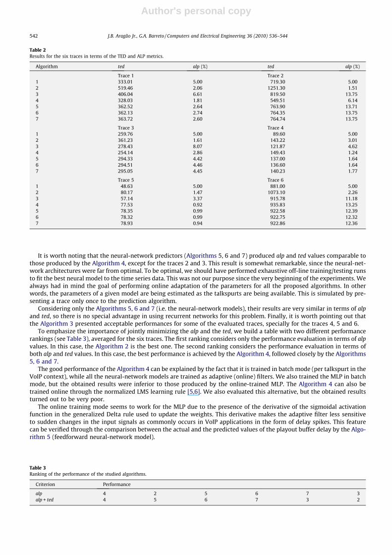
As we can infer from this table, the best performance among the proposed algorithms for the six traces is achieved by theAlgorithm 4, i.e. the linear AR model. For judging this, we should recall that a good performance requires low ted and low alp.For example, for the traces 2, 3 and 6, the (classic) Algorithm 2 produced the lowest alp values, but at the expenses of thehighest ted values.

Table 1Summary statistics of the studied traces.

Trace Network delay (ms)

Min Med Max Std

1 0 210.03 2464 239.962 0 505.87 3200 357.273 0 181.88 844 75.984 0 48.92 1080 65.725 0 30.72 360 16.716 0 820.02 1540 123.65

3 The heuristic was to set Q equal to the memory order n ¼ 5.

J.B. Aragão Jr., G.A. Barreto / Computers and Electrical Engineering 36 (2010) 536–544 541

Author's personal copy

It is worth noting that the neural-network predictors (Algorithms 5, 6 and 7) produced alp and ted values comparable tothose produced by the Algorithm 4, except for the traces 2 and 3. This result is somewhat remarkable, since the neural-net-work architectures were far from optimal. To be optimal, we should have performed exhaustive off-line training/testing runsto fit the best neural model to the time series data. This was not our purpose since the very beginning of the experiments. Wealways had in mind the goal of performing online adaptation of the parameters for all the proposed algorithms. In otherwords, the parameters of a given model are being estimated as the talkspurts are being available. This is simulated by pre-senting a trace only once to the prediction algorithm.

Considering only the Algorithms 5, 6 and 7 (i.e. the neural-network models), their results are very similar in terms of alpand ted, so there is no special advantage in using recurrent networks for this problem. Finally, it is worth pointing out thatthe Algorithm 3 presented acceptable performances for some of the evaluated traces, specially for the traces 4, 5 and 6.

To emphasize the importance of jointly minimizing the alp and the ted, we build a table with two different performancerankings (see Table 3), averaged for the six traces. The first ranking considers only the performance evaluation in terms of alpvalues. In this case, the Algorithm 2 is the best one. The second ranking considers the performance evaluation in terms ofboth alp and ted values. In this case, the best performance is achieved by the Algorithm 4, followed closely by the Algorithms5, 6 and 7.

The good performance of the Algorithm 4 can be explained by the fact that it is trained in batch mode (per talkspurt in theVoIP context), while all the neural-network models are trained as adaptive (online) filters. We also trained the MLP in batchmode, but the obtained results were inferior to those produced by the online-trained MLP. The Algorithm 4 can also betrained online through the normalized LMS learning rule [5,6]. We also evaluated this alternative, but the obtained resultsturned out to be very poor.

The online training mode seems to work for the MLP due to the presence of the derivative of the sigmoidal activationfunction in the generalized Delta rule used to update the weights. This derivative makes the adaptive filter less sensitiveto sudden changes in the input signals as commonly occurs in VoIP applications in the form of delay spikes. This featurecan be verified through the comparison between the actual and the predicted values of the playout buffer delay by the Algo-rithm 5 (feedforward neural-network model).

Table 3Ranking of the performance of the studied algorithms.

Criterion Performance

alp 4 2 5 6 7 3alp + ted 4 5 6 7 3 2

Table 2Results for the six traces in terms of the TED and ALP metrics.

Algorithm ted alp (%) ted alp (%)

Trace 1 Trace 21 333.01 5.00 719.30 5.002 519.46 2.06 1251.30 1.513 406.04 6.61 819.50 13.754 328.03 1.81 549.51 6.145 362.52 2.64 763.90 13.716 362.13 2.74 764.35 13.757 363.72 2.60 764.74 13.75

Trace 3 Trace 41 259.76 5.00 89.60 5.002 361.23 1.61 143.22 3.013 278.43 8.07 121.87 4.624 254.14 2.86 149.43 1.245 294.33 4.42 137.00 1.646 294.51 4.46 136.60 1.647 295.05 4.45 140.23 1.77

Trace 5 Trace 61 48.63 5.00 881.00 5.002 80.17 1.47 1073.10 2.263 57.14 3.37 915.78 11.184 77.53 0.92 935.83 13.255 78.35 0.99 922.58 12.396 78.32 0.99 922.75 12.327 78.93 0.94 922.86 12.36

542 J.B. Aragão Jr., G.A. Barreto / Computers and Electrical Engineering 36 (2010) 536–544

Author's personal copy

Fig. 4 and 4 show the actual and predicted values for the traces 1 and 3. We can note that the two predicted time seriesfollows faithfully the dynamics of the actual ones, presenting lower values exactly at the delay spikes.

5. Conclusion

In this paper we introduced two novel approaches for the prediction of the playout delay for individual talkspurts. Thefirst one was based on the linear AR model, while the second one was based on nonlinear feedforward and recurrent neu-ral-network models. The obtained results indicated that the proposed algorithms present better overall performance thanthe classic non-adaptive ones.

We are currently trying to improve the performance of the Algorithms 6 and 7 (recurrent neural models). Other machinelearning algorithms, such as echo-state networks [19] and support-vector machines [20,21], are also being evaluated in thetask of estimating the playout buffer delay.

Acknowledgment

The authors thank CAPES (a Brazilian research agency) for its financial support.

0 200 400 600 800 10000

500

1000

1500

2000

2500

Number of talkspurts

Tim

e (m

s)

optimal pkestimated pk

100 200 300 400 500 600

200

400

600

800

1000

1200

Number of talkspurts

Tim

e (m

s)

optimal pkestimated pk

(a)

(b)

Fig. 4. Predicting the playout delay on (a) trace 1, (b) trace 3.

J.B. Aragão Jr., G.A. Barreto / Computers and Electrical Engineering 36 (2010) 536–544 543

Author's personal copy

References

[1] Davidson J, Peters J, Bhatia M, Kalidindi S, Mukherjee S. Voice over IP fundamentals. 2nd ed. Cisco Press; 2006.[2] Nagireddi S. VoIP voice and fax signal processing. Wiley-Interscience; 2008.[3] Montgomery WA. Techniques for packet voice synchronization. IEEE J Sel Area Commun 1983;1(6):1022–8.[4] Yensen T, Lariviere JP, Lambadaris I, Goubran RA. HMM delay prediction technique for VoIP. IEEE Trans Multimedia 2003;5(3):444–57.[5] Shallwani A, Kabal P. An adaptive playout algorithm with delay spike detection for real-time VoIP. In: Proceedings of the IEEE Canadian conference on

electrical and computer engineering (CCECE’03), vol. 2; 2003. p. 997–1000.[6] DeLeon P, Sreenan CJ. An adaptive predictor for media playout buffering. In: Proceedings of the IEEE international conference on acoustics, speech, and

signal processing (ICASSP’99); vol. 6, 1999. p. 3097–3100.[7] Ramos VMR, Barakat C, Altman E. A moving-average predictor for playout delay control in VoIP. In: Lecture notes in computer science – (IWQoS’03),

vol. 2707; 2003. p. 155–73.[8] Ranganathan MK, Kilmartin L. Neural and fuzzy computational techniques for playout delay adaptation in VoIP networks. IEEE Trans Neural Networ

2005;16(5):1174–94.[9] Moon SB, Kurose J, Towsley D. Packet audio playout delay adjustment: performance bounds and algorithms. Multimedia Syst 1998;6(1):17–28.

[10] Rosenberg J, Qiu L, Schulzrinne H. Integrating packet FEC into adaptive voice playout buffer algorithms on the internet. In: Proceedings of the 19thannual joint conference of the IEEE computer and communications societies (INFOCOM’00), vol. 3; 2000. p. 1705–14.

[11] Ramjee R, Kurose J, Towsley D. Adaptive playout mechanisms for packetized audio applications in wide-area networks. In: Proceedings of the 13th IEEEannual conference on computer communications (INFOCOM’94), vol. 2; 1994. p. 680–8.

[12] Sreenan CJ, Chen JC, Agrawal P, Narendran B. Delay reduction techniques for playout buffering. IEEE Trans Multimedia 2000;2(2):100–12.[13] Box G, Jenkins GM, Reinsel G. Time series analysis: forecasting and control. 3rd ed. Prentice Hall; 1994.[14] Wolberg J. Data analysis using the method of least squares: extracting the most information from experiments. Springer; 2006.[15] Bishop CM. Neural networks for pattern recognition. Oxford University Press; 1996.[16] Box G, Jenkins GM, Reinsel G. Nonlinear time series analysis. 2nd ed. Cambridge University Press; 2004.[17] Haykin S. Neural networks: a comprehensive foundation. 2nd ed. Prentice Hall; 1998.[18] Rumelhart DE, Hinton GE, Williams RJ. Learning representations by backpropagating errors. Nature 1986;323:533–6.[19] Steil JJ. Online reservoir adaptation by intrinsic plasticity for backpropagation–decorrelation and echo state learning. Neural Networks

2007;20(3):353–64.[20] Sapankevych NI, Sankar R. Time series prediction using support vector machines: a survey. IEEE Comput Intell Mag 2009;4(2):24–38.[21] Müller K-R, Smola AJ, Rütsch G, Schölkopf B, Kohlmorgen J, Vapnik V. Using support vector machines for time series prediction. In: Schölkopf B, Burges

CJ, Smola AJ, editors. Advances in Kernel methods: support vector learning. MIT Press; 1999. p. 243–53.

José Belo A. Júnior was born in Fortaleza, Ceará, Brazil, in 1981. He received the B.S. degree in Teleinformatics from the FederalCenter for Technological Education (CEFET) of Ceará in 2005 and in Mathematics from the Cear State University. In 2008, heobtained a M.Sc. degree in Teleinformatics Engineering at the Federal University of Cear, working on the development of timeseries approaches for adaptive playout delay prediction for multimedia applications. His main research interests are in the areasof neural networks, pattern recognition, and adaptive signal processing.

Guilherme A. Barreto was born in Fortaleza, Ceará, Brazil, in 1973. He received his B.S. degree in Electrical Engineering from theFederal University of Ceará in 1995, and both the M.Sc. and Ph.D. degrees in Electrical Engineering from the University of SãoPaulo in 1998 and 2003, respectively. In 2000, he developed part of his Ph.D. studies at the Neuroinformatics Group of theUniversity of Bielefeld, Germany. He is in the organizing committee of the Brazilian Symposium on Neural Networks (SBRN) andhas been serving as reviewer for several neural-network related journals (IEEE TNN, IEEE TSMC, IEEE TKDE, IEEE TSP, Neuro-computing and IJCIA) and conferences (IJCNN, ICASSP, SBRN, among others). Currently, he is with the Department of Telein-formatics Engineering, Federal University of Ceará. His main research interests are self-organizing neural networks for signaland image processing, time series prediction, pattern recognition and robotics.

544 J.B. Aragão Jr., G.A. Barreto / Computers and Electrical Engineering 36 (2010) 536–544