Hindawi Publishing CorporationJournal of Biomedicine and BiotechnologyVolume 2008, Article ID 513701, 10 pagesdoi:10.1155/2008/513701

Methodology ReportUsing Growing Self-Organising Maps to Improvethe Binning Process in Environmental Whole-GenomeShotgun Sequencing

Chon-Kit Kenneth Chan,1 Arthur L. Hsu,1 Sen-Lin Tang,2 and Saman K. Halgamuge1

1 Dynamic Systems & Control Group, Department of Mechanical Engineering, University of Melbourne, VIC 3010, Australia2 Research Center for Biodiversity, Academia Sinica, Taipei 115, Taiwan

Correspondence should be addressed to Chon-Kit Kenneth Chan, c.chan22@pgrad.unimelb.edu.au

Received 31 August 2007; Accepted 18 November 2007

Recommended by Daniel Howard

Metagenomic projects using whole-genome shotgun (WGS) sequencing produces many unassembled DNA sequences and smallcontigs. The step of clustering these sequences, based on biological and molecular features, is called binning. A reported strat-egy for binning that combines oligonucleotide frequency and self-organising maps (SOM) shows high potential. We improve thisstrategy by identifying suitable training features, implementing a better clustering algorithm, and defining quantitative measuresfor assessing results. We investigated the suitability of each of di-, tri-, tetra-, and pentanucleotide frequencies. The results showthat dinucleotide frequency is not a sufficiently strong signature for binning 10 kb long DNA sequences, compared to the otherthree. Furthermore, we observed that increased order of oligonucleotide frequency may deteriorate the assignment result in somecases, which indicates the possible existence of optimal species-specific oligonucleotide frequency. We replaced SOM with growingself-organising map (GSOM) where comparable results are obtained while gaining 7%–15% speed improvement.

Copyright © 2008 Chon-Kit Kenneth Chan et al. This is an open access article distributed under the Creative CommonsAttribution License, which permits unrestricted use, distribution, and reproduction in any medium, provided the original work isproperly cited.

1. INTRODUCTION

Metagenomics is an emerging area of genome research thatallows culture-independent, functional, and sequence-basedstudies of microbial communities in environmental sam-ples. Whole-genome shotgun (WGS) sequencing has beenapplied to most of the metagenomic projects [1–6]. Theseprojects have unveiled remarkable information on microbialgenomics and also brought an unprecedentedly comprehen-sive and clearer picture of microbial communities. In theWGS sequencing approach, random sampling of DNA frag-ments of all microbes that form a community in an environ-mental sample is performed. The individual DNA fragmentsare sequenced and then assembled into genomes by us-ing computing techniques. However, a fundamental limit ofWGS sequencing is that only the genomes of high-abundancespecies can be completely or near-completely assembled [7]due to the requirement of multiple overlapping fragmentsfor a confident assembly. In one of the prominent metage-nomic studies conducted by Venter et al. [2], about 1 Gb of

DNA sequences has been successfully sequenced from Sar-gasso Sea samples. This study has clearly indicated the exis-tence of far more diverse microbial communities than pre-viously thought. Most of the environmental genomes se-quenced to date contain only few high-abundance speciesbut many low-abundance species in the communities thataccount for a large portion of the total genome size of an en-vironmental sample. The presence of large amount of DNAfragments from the low-abundance species poses a prob-lem for assembling genomes. In order to infer the biologicalfunctions of a microbial community from sequences, a pro-cess named “binning” is used to group these unassembledDNA sequence fragments and small contigs into biologicallymeaningful “bins,” such as phylogenetic groups [8].

There are a number of tools currently available for thebinning process. These include Chisel System [9, 10], Meta-Clust [4, 11], TETRA [12, 13], PhyloPythia [14], and thecombination of oligonucleotide frequency and SOM [15].The Chisel System helps binning the sequences according tothe identification, characterisation, and comparative analysis

2 Journal of Biomedicine and Biotechnology

of taxonomic and evolutionary variations of enzymes. Theremaining above-listed tools use the method of analysingnucleotide composition of sequences that is considered tohave the potential of working well for the binning processin WGS sequencing [8]. MetaClust computes different DNAsignatures followed by the use of a clustering algorithm toassign sequences into bins. TETRA bins the species-specificsequences by the use of tetranucleotide-derived z-score cor-relations. PhyloPythia uses a supervised-learning approachwhere it trains a multiclass support vector machine (SVM)classifier using all the known genome sequences in the ex-isting database then assigns the unknown environmental se-quences to the closest clade in the selected taxonomic level.This method has been demonstrated to be able to classifymost DNA sequence fragments with high accuracy. However,considering the current amount of known genomes which isfar less than 1% of the entire microbial genomes [7], it is rea-sonable to assume that the currently available training data isinsufficient to represent all the extremely diverse microbialgenomes for supervised-learning methods. Unsupervised-learning may provide the answer to this problem. The com-bination of oligonucleotide frequency and the well-knownunsupervised learning method self-organising map (SOM)was used by Abe et al. [15] to explore genome signatures.They used the di-, tri-, and tetranucleotide frequencies as thetraining features of SOM to cluster the 1 kb and 10 kb DNAsequence fragments derived from 65 bacteria and 6 eukary-otes. Clear species-specific separations of sequences were ob-tained in the 10 kb fragment tests. Their results showed thatthe combination of oligonucleotide frequency and SOM canbe used as a powerful tool to cluster or bin the DNA sequencefragments after WGS sequencing.

In order to successfully bin the DNA sequence frag-ments, using an appropriate genome signature as the train-ing feature is important. In recent years, researchers havefound that, due to oligonucleotide frequency bias in vari-ous prokaryotic genomes, the oligonucleotide frequency canbe used as a possible genome signature. The di-, tri-, andtetranucleotide frequencies, which are the frequencies us-ing two, three, and four nucleotides respectively, have beenwell studied. Karlin et al. [16, 17] has shown the compo-sitional bias of the di- and tetranucleotide contents of 15prokaryotic genomes. Weinel et al. [18] found that 80% ofPseudomonas putida KT2440 genome have a similar bias inGC contents and di- and tetranucleotide contents. Teelinget al. [12] showed that the tetranucleotide frequency hasa higher discriminatory power than GC content and usedit for the assignment of genomic fragments to the taxo-nomic group. In addition, Sandberg et al. [19] employed aBayesian approach to classify the short sequences and foundthat the classification accuracy increases with a higher-orderoligonucleotide frequency. Above-mentioned papers provideevidences that there is a trend of using oligonucleotide fre-quency as prokaryotic genome signature, rather than the GCcontent. Thus, high-order oligonucleotide frequency mayalso be an appropriate training feature for binning DNA se-quence fragments by unsupervised clustering methods.

Since the combination of oligonucleotide frequency andSOM appears as a promising binning strategy that can be

further explored, we focus in this paper on improving thetraining features and the clustering algorithm. In Abe et al.’swork [15], there was no systematic way of comparing thequality of the SOM results. We tested the traditional cluster-ing evaluation measures (recall, precision, and F-measure)and discovered the inadequacy of using them for examin-ing the similarity of phylogenetic levels. Therefore, we in-troduce a method to quantitatively measure and assess theresults of clustering DNA sequence fragments from a col-lection of species. In the investigation of evaluating suitabletraining features, we attempt to compare results for the di-,tri-, and tetranucleotide frequencies as well as the pentanu-cleotide frequency (the frequency usage of five nucleotides)to test if higher-order oligonucleotide frequency yields betterbinning of DNA sequence fragments. We also study the effec-tiveness and efficiency of the combination of oligonucleotidefrequency and SOM by employing alternative clustering al-gorithms. We compare SOM with a variant of it called grow-ing self-organising map (GSOM), which has been success-fully applied in several different applications [20–25] includ-ing microarray clustering [26]. These comparisons allow usto suggest a better compositional binning strategy for WGSsequencing using the method of combining oligonucleotidefrequency and SOM-based clustering algorithm.

This paper is organized as follows: Section 2.1 gives abrief introduction to the SOM and GSOM clustering algo-rithms; Section 2.2 proposes a method of measuring insep-arable species when DNA sequence fragments are clustered;Section 2.3 describes the procedures of preparing the threedatasets used in this paper, and the data preprocessing stepfor preparing the input vectors; and Section 2.4 shows thedetails of the algorithm settings and the experiment set upfor repeatability of the experiments. Section 3 presents theresults of comparing the four orders of oligonucleotide fre-quencies and the comparison between SOM and GSOM; Fi-nally, Section 4 gives the discussion, conclusion, and futurework.

2. METHODS

2.1. Growing self-organising map

Growing self-organising map (GSOM) [27, 28] is an exten-sion of self-organising map (SOM) [29]. GSOM is a dynamicSOM which overcomes the weakness of a static map structureof SOM. Both SOM and GSOM are used for clustering high-dimensional data. This is achieved by projecting the high-dimensional data onto a two- or three-dimensional featuremap with lattice structure where every point of interest in thelattice represents a neuron or a node in the map. The map-ping preserves the data topology, so that similar samples canbe found close to each other on the 2D/3D feature map.

The SOM training consists of three phases: initialisationphase, ordering phase, and fine-tuning phase. The initialisa-tion is crucial to achieve a quality-clustering result. The fol-lowing parameters are determined in this phase:

(i) the map topology (either rectangular or hexagonal);(ii) the number of nodes which is the resolution of the

map;

Chon-Kit Kenneth Chan et al. 3

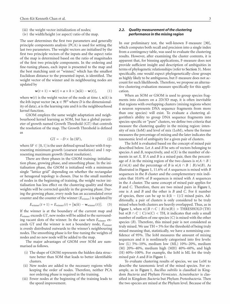
(iii) the weight vector initialization of nodes;(iv) the width/height (or aspect) ratio of the map.

The user determines the first two parameters and generallyprinciple components analysis (PCA) is used for setting thelast two parameters. The weight vectors are initialised by thefirst two principle vectors of the inputs and the aspect ratioof the map is determined based on the ratio of magnitudesof the first two principle components. In the ordering andfine-tuning phases, each input is presented to the map andthe best matching unit or “winner,” which has the smallestEuclidean distance to the presented input, is identified. Theweight vector of the winner and its neighbouring nodes areupdated by

w(t + 1) = w(t) + α× h× [x(k)−w(t)], (1)

where w(t) is the weight vector of the node at time t, x(k) isthe kth input vector (w, x ∈ RD where D is the dimensional-ity of data), α is the learning rate and h is the neighbourhoodkernel function.

GSOM employs the same weight adaptation and neigh-bourhood kernel learning as SOM, but has a global param-eter of growth named Growth Threshold (GT) that controlsthe resolution of the map. The Growth Threshold is definedas

GT = −D × ln (SF), (2)

where SF ∈ [0, 1] is the user defined spread factor with 0 rep-resenting minimum growth (coarsest resolution) and 1 rep-resenting maximum growth (finest resolution).

There are three phases in the GSOM training: initialisa-tion phase, growing phase, and smoothing phase. In the ini-tialisation phase, the GSOM is initialised with a minimumsingle “lattice grid” depending on whether the rectangularor hexagonal topology is chosen. Due to the small numberof nodes in the beginning of training, the weight vector ini-tialisation has less effect on the clustering quality and theseweights will be corrected quickly in the growing phase. Dur-ing the growing phase, every node has an accumulated errorcounter and the counter of the winner (Ewinner) is updated by

Ewinner(t + 1) = Ewinner(t) +∥∥x(k)−wwinner(t)

∥∥. (3)

If the winner is at the boundary of the current map andEwinner exceeds GT, new nodes will be added to the surround-ing vacant slots of the winner. In the case when Ewinner ex-ceeds GT and the winner is not a boundary node, Ewinner

is evenly distributed outwards to the winner’s neighbouringnodes. The smoothing phase is for fine-tuning the weights ofnodes and no new node will be added to the map.

The major advantages of GSOM over SOM are sum-marised as follows.

(i) The shape of GSOM represents the hidden data struc-ture better than SOM that leads to better identifiableclusters.

(ii) New nodes are added to the necessary regions whilekeeping the order of nodes. Therefore, neither PCAnor ordering phase is required in the training.

(iii) Fewer nodes at the beginning of the training leads tothe speed improvement.

2.2. Quality measurement of the clusteringperformance in the mixing region

In our preliminary test, the well-known F-measure [30],which computes both recall and precision into a single indexfrom a contingency table, was used to evaluate the clusteringresults. However, after examining the cluster contents, it isapparent that, for binning applications, F-measure does notprovide sufficient insight and description of ambiguities interms of phylogenetic relationships (refer to Section 3). Morespecifically, one would expect phylogenetically-close groupsas highly likely to be ambiguous, but F-measure does not ac-count for such likelihoods. Therefore, we propose an alterna-tive clustering evaluation measure specifically for this appli-cation.

When an SOM or GSOM is used to group species frag-ments into clusters on a 2D/3D map, it is often inevitablethat regions with overlapping clusters (mixing regions wherea neuron represents DNA sequence fragments from morethan one species) will exist. To evaluate a clustering al-gorithm’s ability to group DNA sequence fragments intospecies-specific or “pure” clusters, we define two criteria thatmeasure the clustering quality in the mixing region: inten-sity of mix (IoM) and level of mix (LoM), where the formermeasures the percentage of mixing and the later indicates thetaxonomic level of ambiguity for a given pair of clusters.

The IoM is evaluated based on the concept of mixed pairdescribed below. Let A and B be sets of vectors belonging tospecies A and B, respectively, and n(X) is the number of ele-ments in set X. If A and B is a mixed pair, then the percent-age of A in the mixing region of the two classes is n(A ∩ B |A)/n(A) and the percentage of B is n(A ∩ B | B)/n(B). Asillustrated in Figure 1, 11.6% of A sequences is mixed with Bsequences in the B cluster and the complementary mix indi-cates that 10.6% of B sequences is mixed with A sequencesin the A cluster. The same concept of mixed pair applies forB and C. Therefore, there are two mixed pairs in Figure 1,one is A and B and the other is B and C. For k numberof species, there can be up to k(k − 1)/2 mixed pairs. Ad-ditionally, a pair of clusters is only considered to be trulymixed when both clusters are heavily overlapped. Thus, as inFigure 1, when n((B ∩ C | B)/n(B)) > THRESHOLD (TH)but n(B ∩ C | C)/n(C) < TH, it indicates that only a smallnumber of outliers of one species (C) is mixed with the otherspecies (B). Therefore, this mixed pair is not considered astruly mixed. We use TH = 5% for the threshold of being trulymixed meaning that, statistically, we have a nonmixing con-fidence of 95%. The IoM measures the amount of mixingsequences and it is nonlinearly categorised into five levels:low (L) 5%–10%, medium low (ML) 10%–20%, medium(M) 20%–40%, medium high (MH) 40%–60%, and high(H) 60%–100%. For example, the IoM is ML for the trulymixed pair A and B in Figure 1.

To evaluate clustering results of species, we use LoM todescribe the taxonomic level of the mixed species. For ex-ample, as in Figure 1, Bacillus subtilis is classified in King-dom Bacteria and Phylum Firmicutes. Acinetobacter is clas-sified in Kingdom Bacteria but Phylum Proteobacteria. Thenthe two species are mixed at the Phylum level. Because of the

4 Journal of Biomedicine and Biotechnology

10.6 % of B

11.6 % of A 1 % of C

6.9 % of B

A B C

A: Acinetobacter sp.B: Bacillus subtilisC: Treponema pallidum

Figure 1: Concept of mixed pair: the mixed pair between A andB is truly mixed (IoM = ML and LoM = Phylum). The mixed pairbetween B and C is not truly mixed because n(B∩C |C)/n(C)<5%.

evolution of organisms, nucleotide composition of genomesbelonging to the same lower taxonomic levels can be verysimilar. Clustering organisms at higher level of taxonomyshould be easier than at lower level of taxonomy. Therefore,if truly mixed pair occurs, lower LoM (e.g., Species) is moreacceptable and more desirable than higher LoM (e.g., King-dom).

In summary, the proposed two measures are defined as

IoM ∈ L, ML, M, MH, H,LoM ∈ Species, Genus, Family, Order, Class,

Phylum, Kingdom.(4)

The two proposed measures, IoM and LoM, are only de-fined for truly mixed pairs to evaluate the clustering qualityin the mixing regions of a map by the following steps.

(i) Find truly mixed pairs for all pairs of species where ifn(X ∩ Y | Y)/n(Y) ≥ TH and n(X ∩ Y | X)/n(X) ≥TH, then X and Y is a truly mixed pair.

(ii) If X and Y are truly mixed, determine IoM accordingto minn(X ∩ Y | Y)/n(Y),n(X ∩ Y | X)/n(X).

(iii) Identify LoM of X and Y.

Clustering results can now be assessed based on three cri-teria: number of truly mixed pairs, IoM, and LoM. How-ever, which criterion should have higher priority may varybetween applications. Therefore, in our assessment, one re-sult is better than another only when it is superior on at leasttwo of the three measures.

2.3. Dataset preparation and data preprocessing

The NCBI database (http://www.ncbi.nlm.nih.gov) contains370 completed microbial genomes in early 2006, which in-cludes 28 Archaea and 342 Bacteria. As the investigationseeks to cluster sequences of species, genomes are filtered sothat there is no duplicating species. One strain was arbitrar-ily chosen if the same species genome contains more than onestrain. After this process, there were 283 genomes remaining.Considering the available computing resources and the algo-rithm comparison focus of this paper, two artificial sets ofprokaryotic DNA sequences (each of 10 different species outof the 283 species) were randomly sampled from the NCBIdatabase.

In addition, three simulated metagenomic datasets werecreated by Mavromatis et al. [31] to facilitate benchmark-ing of metagenomic data processing methods, which include,but not limited to, binning methods. The three datasets varyin relative abundance and number of species that repre-sent different complexity levels of real-world microbial com-munities. The sequence fragments in the simulated datasetswere assembled using three commonly used sequence assem-bling programs: JAZZ, Arachne, and Phrap at U.S. Depart-ment of Energy (Wash, USA), DOE Joint Genome Institute(Calif, USA). In this paper, we tested one of the three sim-ulated datasets named simMC and was assembled by Phrap(http://www.phrap.com). For simplicity, this dataset will berepresented as simMC Phrap throughout the paper.

The taxonomic distributions of the three sets of speciesare displayed graphically in Figure 3. Each letter representsa single species and species within a single rectangle havethe same taxonomy at the specific level. The names of thespecies can be found in Section 1 of the supplementarymaterial which consists of 6 sections showing the speciesnames in Section 1, clustering evaluation methods in Sec-tions 2 and 3, and the labelled cluster maps in Section 4 to6 (http://www.mame.mu.oz.au/∼ckkc/Binning). The num-bers below the taxonomic levels in Figure 3 indicate the max-imum possible number of mixed pairs at that taxonomiclevel. For example, in Figure 3(a), the maximum number ofmixed pairs at taxonomic level of Class is 12, which consistsa mixed pair each from (a,j) and (c,e) and 5 pairs each from(c,b,d,g,h,i) and (e,b,d,g,h,i).

In the experiments of Abe et al. [15] that attempts to sep-arate 1 kb and 10 kb DNA sequence fragments of 65 bacteriagenomes containing 54 different species, it is visually shownthat 1 kb DNA sequence fragments do not carry enough dis-criminatory information and hence could not completelyseparate the fragments into species-specific groups. There-fore, a sequence fragment length of 10 kb is used for theanalysis in the two artificial datasets to ensure appropriateseparation of species-specific groups. Sequences used in thetwo artificial datasets are produced from complete genomesequences to simulate the environment of WGS sequencing.Such a complete genome sequence is segmented into 10 kbnonoverlapping fragments. A sliding window with the size nis used for counting the oligonucleotide frequency for each ofthe fragments in which n is the nucleotide length. For exam-ple, the dinucleotide frequency (n = 2) for a short sequence“AATACTTT” is shown graphically in Figure 2. The oligonu-cleotide frequency count for each of the fragments yields asingle input vector for clustering. The input vectors to theclustering algorithm will have 4n dimensions.

Whereas, the simMC Phrap was preprocessed by extract-ing all sequences with contig length ≥ 8 kb. The oligonu-cleotide frequency count is applied to these sequences to gen-erate the input vectors for clustering. Finally, each input vec-tor is normalised by the sequence length.

2.4. Algorithms parameters and experiment details

In order to avoid the algorithm implementation bias, anin-house clustering program was developed consisting a

Chon-Kit Kenneth Chan et al. 5

AA1

CA0

GA0

TA1

AC1

CC0

GC0

TC0

AT1

CT1

GT0

TT2

AG0

CG0

GG0

TG0

A A T A C T T T

Figure 2: Dinucleotide frequency counting for the short sequence “AATACTTT.”

Kingdom9

Phylum14

Class12

Order7

Family0

Genus0

Species3

f

a b c de g h i j

a j

b c de g h i

a

j

c

e

b dg h i

g

i

b d h b d h b d h

b

d

h

(a)

Kingdom0

Phylum30

Class9

Order6

a b cd e f gh i j

a

b

c

e

d f gh i j

f

j

d g h i

d

g

h

i

(b)

Class3

Order0

Family0

Genus2

Species0

Strain1

d

a b c a b c a b ca

b c b cb

c

(c)

Figure 3: The taxonomy distribution of the 10 species in (a) Set 1, (b) Set 2, and the 4 species in (c) simMC Phrap. Each letter represents asingle species. The numbers below the taxonomic levels indicate the maximum number of mixed pairs at that taxonomic level. For example,in (a), the maximum number of mixed pairs at taxonomic level of Class is 12, which consists (a,j), (c,e), (c,b,d,g,h,i), and (e,b,d,g,h,i)mixed pairs.

Table 1: Training parameters used for the SOM and GSOM train-ing.

Training parameter Phase 2 Phase 3

Learning length 15 epochs 70 epochs

Learning rate 0.1 0.05

Neighbourhood size 3 1

data preprocessor, both SOM and GSOM algorithms, anda graphical neuron-map output. The program is written inC# with a Windows form interface. This program can be re-quested from the author for academic use. Since the hexag-onal topology has better topology preservation [26, 29], it isused in both SOM and GSOM. In addition, the tests wereconducted on a Pentium 4 3.2 GHz desktop PC runningWindows XP and the same parameter settings are used inboth algorithms for a fair computational speed comparison(as listed in Table 1).

To compare results from the 4 orders of oligonucleotidefrequencies, we obtain similar map resolution (number ofnodes) for both algorithms and for all nucleotide frequen-cies. Since the GSOM algorithm automatically determinesthe number of nodes, it can be used to determine the total

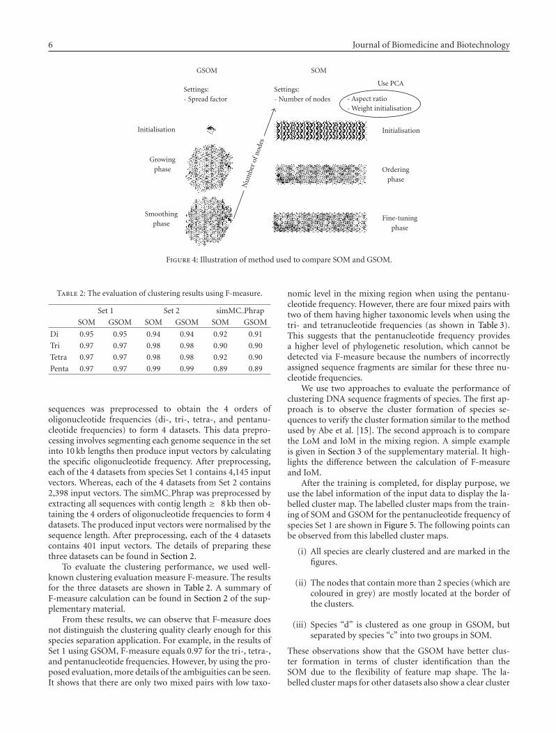
number of nodes of SOM. This can be achieved by train-ing GSOM with a specified resolution (we used SF = 0.4) forthe dinucleotide frequency then the final number of nodes inGSOM is used to set the number of nodes in SOM, as wellas determine the SF for other nucleotide frequencies. Usingthis scheme, we set SF = 0.4 for dinucleotide frequency (for ahigher-resolution map) and experimentally determined thatSF = 0.6 for trinucleotide frequency, SF = 0.8 for tetranu-cleotide frequency and SF = 0.9 for pentanucleotide fre-quency will result in similar map resolution. The SOM alsorequires setting the aspect ratio of the map and initializingthe weight vectors. These two parameters are set by usingPCA. The schematic diagram of this approach is shown inFigure 4.

3. RESULTS

The proposed binning method is tested on two ar-tificial datasets and a simulated metagenomic dataset(simMC Phrap) which was created and published for bench-marking the metagenomic data processing methods. The twoartificial datasets of prokaryotic DNA sequences (each of10 different species out of the 283 species) were randomlysampled from the NCBI database. Each set of the genome

6 Journal of Biomedicine and Biotechnology

Initialisation

Growingphase

Smoothingphase

GSOM

Num

ber

ofno

des

Settings:- Spread factor

Settings:- Number of nodes

SOM

Use PCA

- Aspect ratio- Weight initialisation

Initialisation

Orderingphase

Fine-tuningphase

Figure 4: Illustration of method used to compare SOM and GSOM.

Table 2: The evaluation of clustering results using F-measure.

Set 1 Set 2 simMC Phrap

SOM GSOM SOM GSOM SOM GSOM

Di 0.95 0.95 0.94 0.94 0.92 0.91

Tri 0.97 0.97 0.98 0.98 0.90 0.90

Tetra 0.97 0.97 0.98 0.98 0.92 0.90

Penta 0.97 0.97 0.99 0.99 0.89 0.89

sequences was preprocessed to obtain the 4 orders ofoligonucleotide frequencies (di-, tri-, tetra-, and pentanu-cleotide frequencies) to form 4 datasets. This data prepro-cessing involves segmenting each genome sequence in the setinto 10 kb lengths then produce input vectors by calculatingthe specific oligonucleotide frequency. After preprocessing,each of the 4 datasets from species Set 1 contains 4,145 inputvectors. Whereas, each of the 4 datasets from Set 2 contains2,398 input vectors. The simMC Phrap was preprocessed byextracting all sequences with contig length ≥ 8 kb then ob-taining the 4 orders of oligonucleotide frequencies to form 4datasets. The produced input vectors were normalised by thesequence length. After preprocessing, each of the 4 datasetscontains 401 input vectors. The details of preparing thesethree datasets can be found in Section 2.

To evaluate the clustering performance, we used well-known clustering evaluation measure F-measure. The resultsfor the three datasets are shown in Table 2. A summary ofF-measure calculation can be found in Section 2 of the sup-plementary material.

From these results, we can observe that F-measure doesnot distinguish the clustering quality clearly enough for thisspecies separation application. For example, in the results ofSet 1 using GSOM, F-measure equals 0.97 for the tri-, tetra-,and pentanucleotide frequencies. However, by using the pro-posed evaluation, more details of the ambiguities can be seen.It shows that there are only two mixed pairs with low taxo-

nomic level in the mixing region when using the pentanu-cleotide frequency. However, there are four mixed pairs withtwo of them having higher taxonomic levels when using thetri- and tetranucleotide frequencies (as shown in Table 3).This suggests that the pentanucleotide frequency providesa higher level of phylogenetic resolution, which cannot bedetected via F-measure because the numbers of incorrectlyassigned sequence fragments are similar for these three nu-cleotide frequencies.

We use two approaches to evaluate the performance ofclustering DNA sequence fragments of species. The first ap-proach is to observe the cluster formation of species se-quences to verify the cluster formation similar to the methodused by Abe et al. [15]. The second approach is to comparethe LoM and IoM in the mixing region. A simple exampleis given in Section 3 of the supplementary material. It high-lights the difference between the calculation of F-measureand IoM.

After the training is completed, for display purpose, weuse the label information of the input data to display the la-belled cluster map. The labelled cluster maps from the train-ing of SOM and GSOM for the pentanucleotide frequency ofspecies Set 1 are shown in Figure 5. The following points canbe observed from this labelled cluster maps.

(i) All species are clearly clustered and are marked in thefigures.

(ii) The nodes that contain more than 2 species (which arecoloured in grey) are mostly located at the border ofthe clusters.

(iii) Species “d” is clustered as one group in GSOM, butseparated by species “c” into two groups in SOM.

These observations show that the GSOM have better clus-ter formation in terms of cluster identification than theSOM due to the flexibility of feature map shape. The la-belled cluster maps for other datasets also show a clear cluster

Chon-Kit Kenneth Chan et al. 7

Table 3: Training results in the mixing regions for species Set 1.

Algorithm SOM GSOM

Nucleotide Freq. Di Tri Tetra Penta Di Tri Tetra Penta

Kingdom — — — — — — — —

Phylum — — — — — — — —

Class ML, ML, L — — — ML, ML, L — — —

Order ML, ML ML, L ML L M, L ML, L L, L —

Family — — — — — — — —

Genus — — — — — — — —

Species M, L M, L ML ML M, L M, L ML, L ML, L

(a)

(b)

Figure 5: The labelled cluster maps for clustering species Set 1by (a) SOM, (b) GSOM with the pentanucleotide frequency. Eachhexagon represents a single node. If a node contains input samplesfrom only a single species, it is displayed with a letter that uniquelyidentifies the species. Grey colour nodes correspond to two or morespecies in the node and the number of species is displayed on thenode. A node without label means that there is no input sample“hits.”

formation and can be found in Sections 4, 5, and 6 of thesupplementary material.

We also interpret the clustering results of the species mix-ing regions by summarising the IoM and LoM in Tables 3, 4,and 5 for Set 1, Set 2, and simMC Phrap, respectively.

By comparing the results of the four orders of oligonu-cleotide frequencies for Set 1, the number of truly mixedpairs for dataset that uses the dinucleotide frequency is al-most twice the number of truly mixed pairs of the higher-order oligonucleotide frequencies as shown in Table 3. In ad-dition, the LoM is also high for the dinucleotide frequency.Similarly in Table 4, there are three to four truly mixed pairswhen using the dinucleotide frequency, but no more thanone truly mixed pair when higher-order oligonucleotide fre-quencies are used. All four truly mixed pairs are of a very

high LoM at the Phylum level. Since there are only very fewspecies and number of sequence fragments in simMC Phrap,the difference of using different nucleotide frequencies is notobvious. Nevertheless, the results of our two artificial sets in-dicate that dinucleotide frequency is not a strong signaturefor clustering the 10 kb fragments of species.

Furthermore, from Set 1, we can see that IoM and LoMtend to decrease as the order of oligonucleotide frequencyincreases. One would naturally suspect that higher-orderoligonucleotide frequencies may carry more information sothey can be used to achieve better clustering results. How-ever, it is not the case for Set 2 and simMC Phrap. In Set2, there is a truly mixed pair in the tetranucleotide frequencybut no mixed pair in the tri- and pentanucleotide frequencieswhen using SOM. For the GSOM algorithm, a truly mixedpair appears in the pentanucleotide frequency but not in thetri- and tetranucleotide frequencies. A detailed examinationshows that they are the same pair, Acinetobacter sp.ADP1 andBacillus subtilis subsp. subtilis str. 168, in both cases. Both ofthe IoM is low indicating a much better result than the din-ucleotide frequency. As in Table 5 for simMC Phrap, GSOMperforms well for all four orders of nucleotide frequencies,whereas SOM shows inconsistent clustering quality for dif-ferent nucleotide frequencies. There are two mixed pairs inthe di- and pentanucleotide frequencies but only one mixedpair in the other two nucleotide frequencies. The mixed pairin the tetranucleotide frequency has the lowest IoM (IoM =M). These results also do not support the hypothesis thathigher-order oligonucleotide frequencies are better cluster-ing features. Therefore, we can only conclude that higher-order oligonucleotide frequencies are better features for clus-tering the species than using dinucleotide frequency. How-ever, the optimal oligonucleotide frequency may vary in dif-ferent species.

In terms of clustering quality, both SOM and GSOM havesimilar results. However, besides the mixing quality compar-ison, we also compare the training speed of them. The speedcomparisons for the first two training phases and the overalltraining time of both algorithms for all 12 datasets are shownin Tables 6 and 7, respectively.

Comparing the time taken for SOM and GSOM to fin-ish the first two training phases (as in Table 6), GSOM hasmore than 37% speed improvement than SOM. This speedimprovement can be explained by considering the initial for-mation of the map structure. As discussed in Section 2, PCA

8 Journal of Biomedicine and Biotechnology

Table 4: Training results in the mixing regions for species Set 2.

Algorithm SOM GSOM

Nucleotide Freq. Di Tri Tetra Penta Di Tri Tetra Penta

Kingdom — — — — — — — —

Phylum MH, ML, ML — L — H, ML, L, L — — L

Class — — — — — — — —

Order — — — — — — — —

Family — — — — — — — —

Genus — — — — — — — —

Species — — — — — — — —

Table 5: Training results in the mixing regions for the contigs ≥8 kb from simMC Phrap.

Algorithm SOM GSOM

Nucleotide Freq. Di Tri Tetra Penta Di Tri Tetra Penta

Kingdom — — — — — — — —

Phylum — — — — — — — —

Class — — — — — — — —

Order — — — — — — — —

Family — — — — — — — —

Genus MH MH M MH MH MH MH MH

Species — — — — — — — —

Strain L — — L — — — —

is used to initialise SOM. However, it increases the computa-tional cost exponentially when the data dimension and sizeincreases. Therefore, even though time consumed for PCAinitialisation in this experiment is negligible, it is expectedto be significant in large-scale metagenomic analysis. In ad-dition, SOM starts with all nodes fully covering the wholeinput space then adjusts the weights of all nodes to repre-sent the input data better. On the other hand, GSOM startswith the minimum number of nodes and grows more nodesin the required direction to get an abstract representation ofthe input data while still correcting the weights of existingnodes. At the end of the second phase, both algorithms willbe roughly representing the abstraction of the data. However,GSOM saves time by avoiding PCA calculation and operateson fewer numbers of nodes in the first two phases. Althoughthe last training phase is basically identical for both algo-rithms and the learning length of the last training phase ismuch longer than the first two phases, GSOM still has 7%–15% of speed improvement for the overall training. It was re-ported that the use of this strategy involving SOM was usedfor analysing a large amount of eukaryote genomes and oneof the highest performance supercomputers in the world wasrequired [32]. For the large-scale analysis, which can takeweeks to complete, 7%–15% of speed improvement means1-2 days of time saving for a two-week computation.

Besides using Tables 6 and 7 to compare the trainingspeed of SOM and GSOM, the tables also show that the train-ing time grows exponentially from one order of oligonu-cleotide frequency to the higher-order oligonucleotide fre-

quency. It is because of the rapid increment of dimensionswhen the order of oligonucleotide frequency increases.

4. DISCUSSION, CONCLUSION, AND FUTURE WORK

We have investigated four orders of oligonucleotide frequen-cies: di-, tri-, tetra-, and pentanucleotide frequencies on twoartificial sets of species and a published simulated metage-nomic dataset. Each of the two artificial sets contains 10 ran-domly selected species from NCBI database. We noticed thatthe F-measure can not distinguish the clustering quality forthis application. Therefore, two methods have been definedfor evaluating the performance of clustering DNA sequencefragments of species. This is done by observing the clusterformation with the labelled cluster map and then qualita-tively and quantitatively comparing the LoM and IoM in themixing region.

The results have shown that dinucleotide frequency is nota sufficiently strong signature for the tested 10 kb DNA se-quences on the SOM-based algorithm. Similar to other re-ports, we also found that higher-order oligonucleotide fre-quencies, such as tri-, tetra-, and pentanucleotide frequen-cies, are carrying reasonably adequate genomic informationto group intraspecies sequences and separate interspecies se-quences [12, 19]; but the required computational power in-creases exponentially for each increased order of oligonu-cleotide frequency. Additionally, we noticed that increaseof the order of oligonucleotide frequency may deterioratethe assignment of DNA sequence fragments to classes insome cases, which indicates the possible existence of optimalspecies-specific oligonucleotide frequency. For example, thetrinucleotide frequency has a better discrimination power forAcinetobacter sp. ADP1 and Bacillus subtilis subsp. subtilis str.168 then the tetra- and pentanucleotide frequencies. There-fore, analysts are recommended to start with trinucleotidefrequency in large-scale projects and higher-order oligonu-cleotide frequencies may not always be better.

We also compare the SOM and GSOM algorithms forclustering the DNA sequence fragments of species. BothSOM and GSOM have shown similar results. However, interm of speed comparison, GSOM has more than 37% speedimprovement over SOM in the first two training phases and

Chon-Kit Kenneth Chan et al. 9

Table 6: Speed comparisons for the first two training phases of SOM and GSOM, in which the improvement columns represent the per-centage of speed improvement for GSOM comparing to SOM.

Species Set 1 Species Set 2 simMC Phrap

SOM (sec) GSOM (sec) Improvement SOM (sec) GSOM (sec) Improvement SOM (sec) GSOM (sec) Improvement

Di 54 34 37% 24 15 38% 2 1 50%

Tri 188 115 39% 74 45 39% 7 4 43%

Tetra 779 475 39% 236 147 38% 31 18 42%

Penta 3031 1847 39% 878 518 41% 144 80 44%

Table 7: Speed comparisons for the overall training time of SOM and GSOM, in which the improvement columns represent the percentageof speed improvement for GSOM comparing to SOM.

Species Set 1 Species Set 2 simMC Phrap

SOM (sec) GSOM (sec) Improvement SOM (sec) GSOM (sec) Improvement SOM (sec) GSOM (sec) Improvement

Di 313 274 12% 133 121 9% 11 10 9%

Tri 1048 942 10% 427 387 9% 39 36 8%

Tetra 4639 3932 15% 1297 1203 7% 173 158 9%

Penta 16839 15709 7% 4702 4387 7% 720 662 8%

7%–15% speed improvement in the overall training. There-fore, GSOM is potentially a better alternative clustering tool.As a result of this study, we would suggest to use GSOMand a higher-order oligonucleotide frequency (at least trinu-cleotide frequency) to improve the strategy proposed by Abeet al. [15] for the binning process after WGS sequencing.

The method of combining oligonucleotide frequency andthe SOM-based algorithm has provided a promising way ofbinning after WGS sequencing. However, there are limita-tions with this method. Since SOM-based algorithms are es-sentially data visualisation techniques, it is difficult to iden-tify the exact cluster boundaries when clusters severely over-lap with each other. The overlapping cluster can often bemisinterpreted as a single cluster when no label is available.Therefore, a further development to overcome this cluster-overlapping problem is necessary for such SOM-based bin-ning method to be fully practical. Additionally, at the cur-rent state, due to the high diversity of microbial communitiesand the nature of WGS sequencing, most of the unassem-bled sequences are less than 10 kb. In order to maximize theuse of this binning strategy, more investigation on the opti-mal sequence length will need to be performed in the futurework. On the other hand, the rapidly advancing sequencingtechnology and techniques that are capable of faster sequenc-ing, higher coverage, and longer contig length are continu-ously being developed [33, 34]. The length of the unassem-bled fragment is expected to increase in the near future.Therefore, this binning strategy is useful for the analysis af-ter WGS sequencing. Alternatively, when one is attemptingto identify a specific species in the metagenome, which hasalready been sequenced, supervised learning methods can beapplied. While PhyloPythia employs SVM as its supervisedlearning classifier, one can opt for other well-known super-vised learning methods that has been used in other variousapplications [35, 36].

REFERENCES

[1] G. W. Tyson, J. Chapman, P. Hugenholtz, et al., “Commu-nity structure and metabolism through reconstruction of mi-crobial genomes from the environment,” Nature, vol. 428,no. 6978, pp. 37–43, 2004.

[2] J. C. Venter, K. Remington, J. F. Heidelberg, et al., “Environ-mental genome shotgun sequencing of the sargasso sea,” Sci-ence, vol. 304, no. 5667, pp. 66–74, 2004.

[3] S. G. Tringe, C. Von Mering, A. Kobayashi, et al., “Com-parative metagenomics of microbial communities,” Science,vol. 308, no. 5721, pp. 554–557, 2005.

[4] T. Woyke, H. Teeling, N. N. Ivanova, et al., “Symbiosis in-sights through metagenomic analysis of a microbial consor-tium,” Nature, vol. 443, no. 7114, pp. 950–955, 2006.

[5] D. B. Rusch, A. L. Halpern, G. Sutton, et al., “The sorcerer IIglobal ocean sampling expedition: northwest atlantic througheastern tropical pacific,” PLoS Biology, vol. 5, no. 3, p. e77,2007.

[6] S. Yooseph, G. Sutton, D. B. Rusch, et al., “The sorcerer IIglobal ocean sampling expedition: expanding the universe ofprotein families,” PLoS Biology, vol. 5, no. 3, p. e16, 2007.

[7] K. Chen and L. B. Pachter, “Bioinformatics for whole-genomeshotgun sequencing of microbial communities,” PLoS Compu-tational Biology, vol. 1, no. 2, p. e24, 2005.

[8] J. A. Eisen, “Environmental shotgun sequencing: its potentialand challenges for studying the hidden world of microbes,”PLoS Biology, vol. 5, no. 3, p. e82, 2007.

[9] A. Rodriguez, Y. Zhang, N. Maltsev, and E. Marland, “Chisel—a framework for identification and characterization of taxo-nomic and phenotypic versions of enzymes,” in Proceedings ofthe Institute of Structural Molecular Biology (ISMB ’06), Fort-aleza, Brazil, 2006.

[10] N. Maltsev, M. Syed, A. Rodriguez, B. Gopalan, and F. Brock-man, “A novel binning approach and its application to ametagenome from a multiple extreme environment,” in Pro-ceedings of the Joint Genomics: GTL Awardee Workshop V and

10 Journal of Biomedicine and Biotechnology

Metabolic Engineering and USDA-DOE Plant Feedstock Ge-nomics for Bioenergy Awardee Workshop, North Bethesda, Md,USA, 2007.

[11] M. Huntemann, “MetaClust—entwicklung eines modularenProgramms zum Clustern von Metagenomfragmenten an-hand verschiedener intrinsischer DNA-Signaturen,” Diplomathesis, University of Bremen, Germany, 2006.

[12] H. Teeling, A. Meyerdierks, M. Bauer, R. Amann, and F. O.Glockner, “Application of tetranucleotide frequencies for theassignment of genomic fragments,” Environmental Microbiol-ogy, vol. 6, no. 9, pp. 938–947, 2004.

[13] H. Teeling, J. Waldmann, T. Lombardot, M. Bauer, and F. O.Glockner, “TETRA: a web-service and a stand-alone programfor the analysis and comparison of tetranucleotide usage pat-terns in DNA sequences,” BMC Bioinformatics, vol. 5, no. 163,2004.

[14] A. C. McHardy, H. G. Martın, A. Tsirigos, P. Hugenholtz, andI. Rigoutsos, “Accurate phylogenetic classification of variable-length DNA fragments,” Nature Methods, vol. 4, no. 1, pp. 63–72, 2007.

[15] T. Abe, S. Kanaya, M. Kinouchi, Y. Ichiba, T. Kozuki, and T.Ikemura, “Informatics for unveiling hidden genome signa-tures,” Genome Research, vol. 13, no. 4, pp. 693–702, 2003.

[16] S. Karlin, J. Mrazek, and A. M. Campbell, “Compositionalbiases of bacterial genomes and evolutionary implications,”Journal of Bacteriology, vol. 179, no. 12, pp. 3899–3913, 1997.

[17] S. Karlin, “Global dinucleotide signatures and analysis of ge-nomic heterogeneity,” Current Opinion in Microbiology, vol. 1,no. 5, pp. 598–610, 1998.

[18] C. Weinel, K. E. Nelson, and B. Tummler, “Global features ofthe Pseudomonas putida KT2440 genome sequence,” Environ-mental Microbiology, vol. 4, no. 12, pp. 809–818, 2002.

[19] R. Sandberg, G. Winberg, C.-I. Branden, A. Kaske, I. Ern-berg, and J. Coster, “Capturing whole-genome characteristicsin short sequences using a naıve Bayesian classifier,” GenomeResearch, vol. 11, no. 8, pp. 1404–1409, 2001.

[20] Y. Z. Zhai, A. Hsu, and S. K. Halgamuge, “Scalable dynamicself-organising maps for mining massive textual data,” in Pro-ceedings of the Lecture Notes in Computer Science (includingsubseries: Lecture Notes in Artificial Intelligence and LectureNotes in Bioinformatics), vol. 4234, LNCS III, pp. 260–267,Springer, Berlin, Germany, 2006.

[21] R. Amarasiri and D. Alahakoon, “Applying dynamic self orga-nizing maps for identifying changes in data sequences,” in De-sign and Application of Hybrid Intelligent Systems, pp. 682–691,IOS Press, Amsterdam, The Netherlands, 2003.

[22] S. Chen, D. Alahakoon, and M. Indrawan, “Backgroundknowledge driven ontology discovery,” in Proceedings of theIEEE International Conference on e-Technology, e-Commerceand e-Service, (EEE ’05), pp. 202–207, 2005.

[23] H. Wang, F. Azuaje, and N. Black, “Improving biomolecularpattern discovery and visualization with hybrid self-adaptivenetworks,” IEEE Transactions on Nanobioscience, vol. 1, no. 4,pp. 146–166, 2002.

[24] H. Wang, F. Azuaje, and N. Black, “Interactive GSOM-Based approaches for improving biomedical pattern discoveryand visualization,” in Computational and Information Science,vol. 3314 of Lecture Notes in Computer Science, pp. 556–561,Springer, Berlin, Germany, 2004.

[25] M. A. Karim, S. Halgamuge, A. J. R. Smith, and A. L. Hsu,“Manufacturing yield improvement by clustering,” in NeuralInformation Processing, vol. 4234 of Lecture Notes in ComputerScience, pp. 526–534, Springer, Berlin, Germany, 2006.

[26] A. L. Hsu, S.-L. Tang, and S. K. Halgamuge, “An unsupervisedhierarchical dynamic self-organizing approach to cancer classdiscovery and marker gene identification in microarray data,”Bioinformatics, vol. 19, no. 16, pp. 2131–2140, 2003.

[27] A. L. Hsu and S. K. Halgamuge, “Enhancement of topologypreservation and hierarchical dynamic self-organising mapsfor data visualisation,” International Journal of ApproximateReasoning, vol. 32, no. 2-3, pp. 259–279, 2003.

[28] D. Alahakoon, S. K. Halgamuge, and B. Srinivasan, “Dynamicself-organizing maps with controlled growth for knowledgediscovery,” IEEE Transactions on Neural Networks, vol. 11,no. 3, pp. 601–614, 2000.

[29] T. Kohonen, Self-Organizing Maps, Springer, Berlin, Germany,2nd edition, 1997.

[30] C. J. van Rijsbergen, Information Retrieval, Butterworths, Lon-don, UK, 2nd edition, 1979.

[31] K. Mavromatis, N. Ivanova, K. Barry, et al., “Use of simulateddata sets to evaluate the fidelity of metagenomic processingmethods,” Nature Methods, vol. 4, no. 6, pp. 495–500, 2007.

[32] T. Abe, H. Sugawara, S. Kanaya, M. Kinouchi, and T. Ike-mura, “Self-Organizing Map (SOM) unveils and visualizeshidden sequence characteristics of a wide range of eukaryotegenomes,” Gene, vol. 365, no. 1-2, pp. 27–34, 2006.

[33] T. Jarvie, L. Du, and J. Knight, “Shotgun sequencing andassembly of microbial genomes: comparing 454 and Sangermethods,” Biochemica, pp. 11–14, 2005.

[34] L. Bonetta, “Genome sequencing in the fast lane,” NatureMethods, vol. 3, no. 2, pp. 141–146, 2006.

[35] S. K. Halgamuge and M. Glesner, “Fuzzy neural networks: be-tween functional equivalence and applicability,” InternationalJournal of Neural Systems, vol. 6, no. 2, pp. 185–196, 1995.

[36] S. K. Halgamuge, “Self-evolving neural networks for rule-based data processing,” IEEE Transactions on Signal Processing,vol. 45, no. 11, pp. 2766–2773, 1997.