ISSN 1440-771X

Australia

Department of Econometrics and Business Statistics

http://www.buseco.monash.edu.au/depts/ebs/pubs/wpapers/

June 2012

Working Paper 13/12

Using Engel Curves to Measure CPI Bias for Indonesia

Susan Olivia and John Gibson

June, 2012

Using Engel Curves to Measure CPI Bias for Indonesia

Susan Olivia*

and

John Gibson**

Abstract

To measure real income growth over time a price index is needed to adjust for changes in the

cost of living. The Consumer Price Index (CPI) is often used for this task but studies from

several countries show the CPI is a biased measure of changes in the cost of living, leading to

potentially wrong estimates of the rate of growth of real income. In this paper CPI bias for

Indonesia is calculated by estimating food Engel curves for households with the same level of

CPI-deflated incomes at four different points in time between 1993 and 2008. The results

suggest CPI bias was initially negative during the Asian Crisis but has been positive since

2000. Over the entire period, CPI bias has averaged four percent annually, equivalent to

almost one-third of the measured inflation rate.

Keywords: CPI bias, Engel curve, Inflation, Measurement error

JEL: C43, E31

Acknowledgements:

The authors are grateful to Iyut Ria Muttaqun and Yunita Rusanti for assistance and to seminar audiences at the

SMERU Research Institute, Jakarta. Olivia acknowledges support from the Monash University Category 1

Research Grant Incentive Scheme.

** Corresponding author: Department of Econometrics and Business Statistics, Monash University, Wellington Road,

Clayton VIC 3800, Australia. E-mail: susan.olivia@monash.edu

** Department of Economics, University of Waikato, Private Bag 3105, Hamilton, New Zealand. E-mail:

jkgibson@waikato.ac.nz

1

I. Introduction

Almost every country in the world uses a Consumer Price Index (CPI) to measure changes in

the price of consumer goods and services purchased by households. The CPI is also used to

convert nominal variables to real ones, such as real income and real economic growth, by

adjusting for the effects of inflation so that nominal variables can be compared over time at a

constant price level. Correct adjustment for differences in the price level is critical for

understanding changing living standards in a country like Indonesia, which has periodically

suffered from bouts of high inflation, especially during the financial crisis of the late 1990s.

Yet evidence is accumulating from both developed and developing countries of

substantial bias in the CPI, usually in the direction of exaggerating rises in the cost of living.

As a measure of changed costs of living, the CPI has four biases inherent in its calculation:

i) substitution bias, ii) quality change bias, iii) outlet substitution bias, and iv) new goods

bias.1 These biases may be especially salient for fast-growing countries subject to periodic

price shocks, such as Indonesia, since price shocks cause substitution between goods while

longer term changes in retail structure and consumer purchasing patterns and in access to new

and improved goods may outpace the monitoring efforts of statisticians.

The purpose of this paper is to present evidence on bias in the CPI for Indonesia, using

the Engel curve method introduced by Hamilton (2001). The method is increasingly used,

with published applications to historical U.S. data (Costa, 2001), and to contemporary

Canada (Beatty and Larsen, 2005), Norway (Larsen, 2007), Russia (Gibson, Stillman and Le,

2008), Korea (Chung, Gibson and Kim, 2010), Australia (Barrett and Brzozowski, 2010),

New Zealand (Gibson and Scobie, 2010), and Brazil and Mexico (Filho and Chamon, 2012).

1 Substitution bias occurs when a Laspeyres type index does not recognize that consumers make economizing

substitutions away from items that have become more expensive than they were in the base period when the CPI

basket of goods was formed. Similarly, if shoppers respond to lower prices by switching outlets while price

surveyors do not, outlet bias results. Quality change bias occurs when improved goods have quality upgrades

reflected in higher prices, which is wrongly treated as inflation. The delayed introduction of new goods into the

basket creates a bias since there is often a rapid fall in the quality-adjusted price early in the product lifecycle,

and this falling cost occurs before the good is incorporated into the CPI. A fifth bias sometimes mentioned is

due to the formula used to aggregate individual price observations into an index of price relativities, but this is

more easily under the control of statistical authorities.

2

With the exception of the study by Larsen (2007) for Norway and some of the historical U.S.

periods examined by Costa (2001), in all other settings and time periods this method has

indicated an upward bias in the CPI, such that the rate of real income growth is understated.

Results for two of these previously-studied countries hold special interest for Indonesia,

which is often grouped together with Brazil and Russia (along with China, India and South

Africa) as part of the BRIICS. In Russia, CPI bias added one percentage point per month to

an actual inflation rate of two percentage points per month from 1994 to 2001 (Gibson et al,

2008). This bias understated growth in the Russian economy during the early transition to a

market economy, with real per capita GDP in 2001 up to thirty percent lower than what a

bias-corrected deflator would show. In Brazil, the CPI bias averaged three percentage points

per year from 1988 to 2003, and once this bias is accounted for the annual rate of growth in

real per capita household income averages 4.5 percent per year rather than the more anemic

1.5 percent per year suggested by the official data (Filho and Chamon, 2012).

The approach adopted in these previous studies for estimating bias in the CPI relies on

Engel‟s Law, which states that food‟s budget share is inversely related to household real

income. It is worth noting an observation by Houthakker (1987, p.143):

“of all empirical regularities observed in economic data, Engel‟s Law is

probably the best established; indeed it holds not only in the cross-section data

where it was first observed, but has often been confirmed in time-series

analysis as well.”

Provided a researcher can control for movements in relative prices and relevant household

characteristics, it should then be possible to infer changes in real incomes from movements in

the budget share for food. For example, if the food budget share fell when CPI-deflated

income had not risen commensurately, it suggests that real income may be understated,

perhaps because of bias in the price deflator. In other words, the method looks for „drift‟ in

the Engel curve, after all incomes have supposedly been put on a common temporal basis by

deflating them by the CPI. The data requirements for the method are relatively modest, with

3

just a time-series of consistent household budget data needed, along with a CPI for food, non-

food and all consumption that can be broken down by sub-national regions. But the method

does not show which of the possible sources of CPI bias is most important.2 Thus, it is most

useful as a diagnostic for claims about the trends in real income, rather than as an aid to

statistical authorities on what steps to take to improve their price index methodology.

Although the current paper is the first to apply Hamilton‟s method for measuring CPI

bias to Indonesia, a long-standing literature examines potential biases in both spatial and

temporal deflators used in Indonesia. For example, using the 1981 National Socio-economic

Survey (SUSENAS) for Java to account for urban-rural differences in housing costs and rice

prices, Ravallion and van de Walle (1991) find only small differences in the cost of living (of

about 10 percent for the poor), which implied a lower penalty for urban living than previous

estimates. Similarly, Ravallion and Bidani (1994) examined the urban and rural poverty lines

developed by the Biro (now Badan) Pusat Statistik (BPS, the national statistics agency),

finding the reference food bundle cost about 12 percent more in urban areas than in rural

areas in 1990, which was much less than the 55 percent urban premium in the BPS poverty

line. In other words, the official poverty line overestimated the urban cost of living, and

hence overestimated the proportion of the urban population who were poor. More recently,

Kaiser et al. (2001) use urban and rural price data and consumption data from SUSENAS to

estimate cost of living changes from 1996 to 1999, finding that failure to account for

substitution bias causes the estimated fall in real living standards during the financial crisis to

be overstated by between 6 to 14 percent.

2 This method only partially accounts for quality change and does not recover the consumer surplus from new

goods. Thus, even after correcting official statistics for CPI bias, living standards may be understated.

4

II. The Consumer Price Index for Indonesia

The Indonesian Statistical Agency (BPS) collects monthly price observations for 45 cities

(30 provincial capital cities, and 15 other big cities) throughout the country.3 On average,

about 350 goods and services are priced in each city. The precise specifications vary across

cities to reflect heterogeneity in consumption patterns throughout the country. The number of

outlets surveyed in each city also varies, but for items whose prices are observed only once

per month there are typically 3-4 outlets surveyed per city. Some items such as rice and basic

necessities have prices collected daily or fortnightly and then aggregated up to monthly

averages prior to the calculation of the CPI for all urban areas of Indonesia.4

The Indonesian CPI is a modified Laspeyres Index, which measures current period

prices of a base period basket of goods and services. The budget share weights that reflect the

importance of each item in the base period basket are revised approximately every five years

to reflect changes in the consumption pattern of households.5 These weights come from the

Cost of Living Survey (Survey Biaya Hidup), whose respondents keep a detailed expenditure

diary for a week to provide details on the budget shares for various items in the CPI basket

and on the appropriate specifications to be priced. Over time, the Cost of Living Survey has

covered a larger sample, but it remains exclusively urban in scope. The monthly price surveys

also are restricted to urban areas.6 Given that the CPI really only applies to urban areas,

despite often being used as a deflator for all Indonesian households, our analysis of CPI bias

will be restricted to urban Indonesia.

3 Prior to 1996, the geographic coverage was 27 provincial capital cities in Indonesia. Starting in June 2008, the

coverage has been expanded to 33 provincial capital cities and 33 other big cities. Given that our sample spans

the period from November 1993 to February 2008 (see Section III), we base our description of the CPI on how it

was within most of the studied period. 4 http://stats.oecd.org/mei/default.asp?lang=e&subject=8&country=IDN

5 http://www.bi.go.id/NR/rdonlyres/712BB89D-B49A-41AC-A7DC-F94C6F8D4F3D/10672/Boks2.pdf

6 The CPI weights for 1993-97 relied on the consumption patterns of households from 27 provincial capital

cities in the 1988 Cost of Living Survey. Since then, the number of cities surveyed has expanded; to 44 in the

1996 Cost of Living Survey (with between 249 and 353 commodities in the basket in each city), and 45 cities in

the 2002 Cost of Living Survey (with between 283 and 397 commodities in the basket in each city).

5

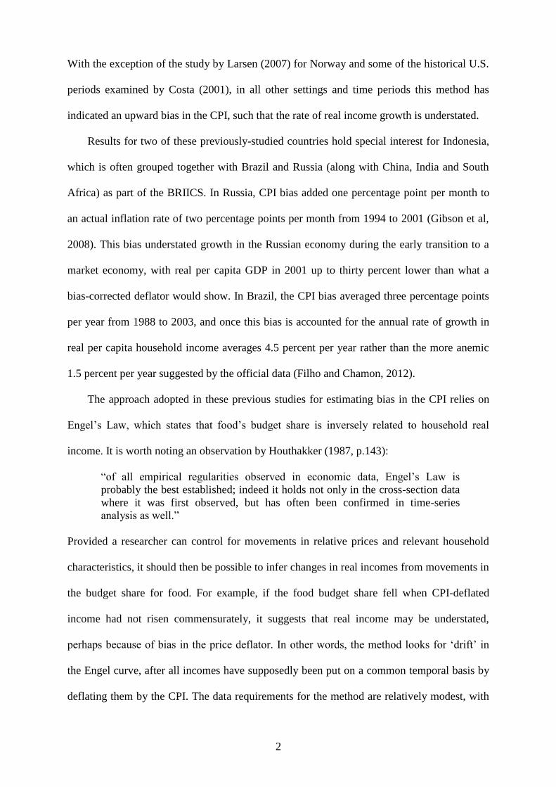
Figure 1 shows the evolution of the CPI for urban Indonesia over 1993-2008, which

spans the different periods for which we have household budget data. These budget data

come from the first four waves of the Indonesian Family Life Survey (IFLS), with the timing

of the IFLS fieldwork shown by the shaded bands in Figure 1. The first wave of the IFLS was

fielded in the relatively low inflation environment preceding the Asian Crisis. The second

wave of the ILFS was fielded while the CPI was increasing most rapidly during the Asian

Crisis, which began for Indonesia in late 1997. During the crisis and its immediate aftermath,

the year-on-year inflation rate exceeded 50 percent between May 1998 and February 1999.

Since then, the inflation rate has stabilized, with only a modest rate of price increases, except

for a temporary surge in October 2005 when the removal of fuel price subsidies caused the

year-on-year inflation rate to approach 20 percent.

The cumulative impact of these episodes of high inflation is that the price level faced

by households in the third wave of the IFLS was almost three times as high, and in the fourth

wave was over five times as high, as the price level faced by households in the initial survey

in 1993. Such a substantial rise in prices likely induces various consumer responses that can

make it difficult for a deflator to accurately measure the changing cost of living. For example,

over the same period that the CPI for urban Indonesia rose to an index level of almost 600,

the CPI for Australia only reached 150 (both starting from a base of August 1993=100). Yet

even with this much more modest increase in the CPI for Australia, a substantial CPI bias

was observed by Barrett and Brzozowski (2010) so there is the potential for even larger

biases to be found in the CPI for Indonesia.

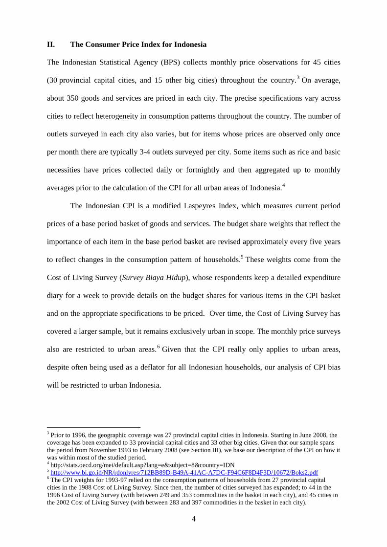
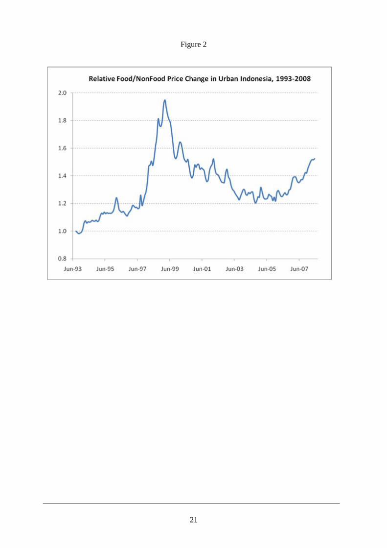
In addition to the overall CPI each month, the BPS also reports sub-aggregates for

food and several non-food components. To show how the inflationary episodes illustrated in

Figure 1 are also associated with shifts in relative prices, the ratio of the food to non-food CPI

is plotted in Figure 2. It is apparent that during the Asian Crisis, food prices rose by more

than non-food prices, with the peak occurring in February 1999 when the food price index

6

exceeded 400 compared with just over 200 for the non-food index (from a base of August

1993=100).7 This large shift in relative prices during an inflationary episode is challenging

for a fixed-weight deflator like the CPI, since it is likely to have induced households into

making economizing substitutions that are not reflected in the price surveys and index

calculations.

Moreover, one feature of the CPI in Indonesia has already been identified in the

literature as a source of possible bias when measuring trends in real living standards during

this large shift in relative prices. Some authors note that that food shares in the CPI basket are

lower than average food shares from various household surveys in Indonesia (Frankenberg,

Thomas and Beegle, 1999; Suryahadi, Sumarto and Pritchett, 2003). For example, for the

1993-97 CPI the share of food in the basket was 39 percent, falling to 38 percent for the

basket for the 1998-2003 CPI and then rising to 43 percent for the basket in use from 2004 to

2007. Yet the average food budget shares in the same periods for urban households in the

annual SUSENAS survey are 56, 55 and 51 percent. Although the SUSENAS surveys use a

short consumption questionnaire with aggregated commodity groups, this difference in

design from what is used in the Cost of Living Survey is unlikely to fully account for the

substantially higher food shares reported in SUSENAS. Moreover, in the IFLS data used

below, the average share of urban household budgets devoted to food at home was

47 percent, for surveys conducted from 1997 to 2000, which is considerably higher than the

38 percent share for food in the basket of the CPI in use at that time. Since food prices rose

more than non-food prices during the 1997/98 financial crisis, and the CPI appears to gives a

7 Food prices rose faster during the Asian Financial Crisis than during the 2005 inflationary episode, due to the

additional effects of a severe drought (from the El Nino weather pattern) which reduced the availability of basic

food stuffs. For instance, rice prices increased by 50 percent in Java during the Asian crisis (Tradeport, 1999).

7

lower weight to food, the cost of living increase during the Asian Crisis is potentially

understated.8

III. Data and Estimation Framework

The data used in this paper are drawn from the Indonesia Family Life Survey (IFLS),

an on-going longitudinal survey that collects extensive socioeconomic information on the

lives of respondents. The information includes detailed expenditures and consumption, from

a one-week recall for food and a one-month or annual recall for non-foods, which enables us

to calculate a consistent time-series of food budget shares at the household level. We use data

from the first four waves of the IFLS, fielded in 1993/94, 1997/98, 2000 and 2007/08. The

first wave of the IFLS covered over 30,000 individuals in 7,224 households, comprised of

3,436 urban households and 3,788 rural households. These households were spread across

13 provinces from the islands of Java, Sumatra, Bali, Kalimantan, Sulawesi and Nusa

Tenggara, selected to “maximize representation of the population, capture the cultural and

socioeconomic diversity of Indonesia, and be cost-effective to survey given the size and

terrain of the country” (Frankenberg and Thomas, 2000, p. 4).9 In total, these 13 provinces

held 83 percent of the Indonesian population at the time of the first survey.

Other surveys of household budgets, such as SUSENAS, have fully national coverage,

while IFLS is best described as “almost national” but we use IFLS for our analysis because it

uses a more comprehensive consumption questionnaire. Specifically, the IFLS has 35 food

groups and 25 non-food groups, whereas the annual SUSENAS survey has just 15 food

groups and eight non-food groups. Since accurate and consistent measurement of food budget

shares is crucial for the method we use to calculate CPI bias, the IFLS lends itself to this

purpose better than does the annual SUSENAS survey. On the other hand, while there is

8 Frankenberg, Thomas and Beegle (1999) suggest that actual inflation during the financial crisis may be as

much as 15 percent higher than the BPS-derived inflation estimates, since food prices rose much faster than

non-food prices and the BPS figures put a smaller weight on food than is suggested by other surveys. 9 These provinces are North Sumatra, West Sumatra, South Sumatra, Lampung, DKI Jakarta, West Java, Central

Java, DI Yogyakarta, East Java, Bali, West Nusa Tenggara, South Kalimantan and South Sulawesi.

8

extremely detailed data in the triennial SUSENAS expenditure module, these data are not

freely available for researchers, unlike the IFLS data.

A feature of the IFLS is that the attrition rate is very low and about 90 percent of the

original target households were re-interviewed in wave 4, which is as high as most

longitudinal surveys in the United States and Europe. In fact, despite this slight attrition, the

sample had grown to 13,535 households by wave 4, because the IFLS tracks and interviews

households who split off from the original sampled households. These split-offs are

interviewed, regardless of where in Indonesia they move, but for our purposes we include

them in the sample only if they stay in an urban area in the same province in which their

original household resided in the first survey in 1993. The reason for this restriction is

because we merge the budget share data for each household with the CPI for the cities in the

IFLS provinces, to allow for spatial and temporal variation in inflation patterns. For the

households who move out of the original IFLS provinces, the linkage of the CPI in those non-

IFLS provinces will be to very few households and may be unreliable compared with the far

greater number of observations in each of the IFLS provinces.

Two other selection rules were applied to the sample, to reduce the impact from any

outliers and to have a more homogenous group of households. Noting that the Engel curve

relationship should hold for any group of people after properly controlling for taste variables,

a better estimate of CPI bias can therefore be obtained by focusing on a fairly homogeneous

group. The first rule was to exclude households whose reported share of expenditure devoted

to food was either less than 0.02 or greater than 0.95, since these extreme food shares may

indicate problems of data quality. Similar approaches to trimming the sample have been used

by Hamilton (2001) and in the subsequent applications of his method to other datasets. The

second rule was to consider only those households where the household head was aged

between 21 and 75 years old, to provide a more homogeneous group. After these rules were

9

applied and observations with missing values of any of the explanatory variables were

dropped, we were left with an estimation sample of n=11,348.

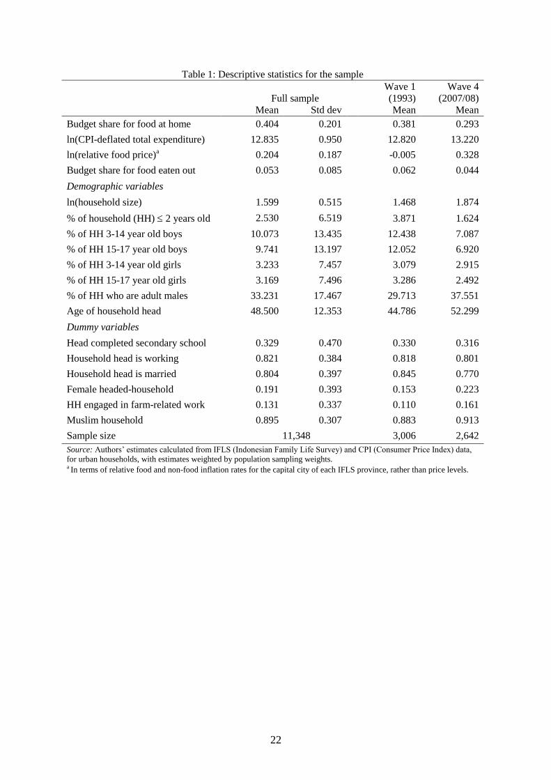
A description of the dependent and explanatory variables is in Table 1. To show how

food shares, CPI-deflated expenditures, relative prices and household characteristics have

changed over time, the averages for the first wave (1993) and fourth wave (2007/08) of the

IFLS are reported, in addition to the full-sample average. The dependent variable, which is

the share of consumption devoted to food at home, averages 40 percent but has seen a

considerable fall, of nine percentage points between the first and fourth waves of the IFLS.

This fall indicates improved living standards, according to Engel‟s Law and the estimation

framework outlined below can show if this fall is commensurate with the recorded increase in

CPI-deflated income. Moreover, it is clear from Table 1 that several other changes have

occurred during the course of the IFLS, with an increase in the relative price of food and

changes in the demographic structure of households.10

Thus, these changes in relative prices

and in demographic characteristics of the sample may account for some of the fall in food

shares, so multiple regression analysis is needed to see how much drift there is in the food

Engel curve after these factors have been controlled for.

The particular form of multiple regression analysis that is required is:

tji

J

j

jj

T

t

tttjtjitjNtjFtji uDDYw ,,

11

,,,,,,,,, 1lnln1ln1lnˆ

X

where wi,j,t is the budget share for food-at-home for household i in region j and time period t,

ΠF,j,t, ΠN,j,t, and Πj,t represent the cumulative percentage increase in the CPI-measured price

of food, non-food, and all goods in region j from year 0 to year t, Yi,j,t is the household‟s

nominal total expenditures, X is a vector of individual household characteristics, the Dt are

time dummy variables that capture the potential CPI bias, the Dj are spatial dummy variables

that allow for unequal food shares across areas, while ui,j,t is the disturbance. The parameters

10

Since IFLS is a panel survey, the changing demographics are not reflective of average changes occurring in

Indonesia, since the population in the panel survey age while refreshed samples drawn every year would not.

This aging is unlikely to affect the CPI bias estimates, since Gibson et al (2008) obtain almost identical CPI bias

estimates from panel and cross-sectional data for Russia.

10

to be estimated are: γ, the response to relative food-nonfood inflation, β, the effect of real

household income, θ, the effect of household characteristics, and δ, the budget share variation

over time and space after other factors are accounted for. Since the Engel curve method for

measuring CPI bias does not require the use of longitudinal data, and can be applied to

repeated cross-sections (for example, Costa, 2001), we initially ignore the panel structure of

the data in our analyses.11

But as a further check on the robustness of the results, the results

with household fixed effects are reported as a sensitivity analysis.

The full derivation of this specification, and the assumptions needed to derive CPI

bias from it, are described in Appendix A. Intuitively, the aim of the regression is to control

for movements in relative prices and in relevant household characteristics that may affect

food shares, and then see if there is any difference over time in food shares for households

who have the same level of CPI-deflated income. This possible drift in the Engel curve is

picked up by the time dummy variables, with the key parameters being the coefficient on real

income, β and the coefficients on the time dummy variables, δt. The cumulative percentage

CPI bias at period t is given by a simple ratio of estimated coefficients: )ˆˆexp(1 t .

IV. Results

Table 2 presents the Ordinary Least Squares (OLS) and Instrumental Variables (IV)

estimates of the Engel functions for food-at-home. The negative coefficient on CPI-deflated

total expenditure indicates that food budget shares fall as households become richer, which is

precisely why food is used as the indicator good here. It is also apparent from comparing the

quadratic and linear results that, regardless of whether using OLS or IV, the relationship

between the logarithm of total expenditures and the food share is best described as linear. The

squared term is weakly significant in the OLS results (but not at all in the IV results) but the

1111

The hypothesis test results that we report are based on standard errors that are clustered at the enumeration

area (n=247). If we instead cluster at the household level (n=3769), which is possible since there are repeated

observations on households, the standard errors would be slightly smaller.

11

quadratic provides no additional explanatory power and the pattern of the time dummy

variables is identical across all four columns of Table 2. This indicates a robust pattern which

is not sensitive to the choice of functional form for the Engel curve.

It is also apparent from the results in Table 2 that food budget shares show almost no

response to movements in relative inflation rates for food and non-food.12

In order for

cumulative CPI bias to be calculated from a simple ratio of coefficients ))ˆˆexp(1( t

from Table 2, it requires either that relative food price changes have just a small effect on

food budget shares or that CPI bias is similar for food and non-food (see equation (7) of

Appendix A). Since there is such a small effect of relative price changes, there is no need to

rely on further assumptions about equality of CPI bias for food and non-food.

The regression results for the various household characteristics in Table 2 are of less

interest, since these are just control variables to ensure that any movement in the food Engel

curve is not because of changes in some omitted relevant characteristics. The coefficients for

these control variables show that food shares are higher for larger households, for Muslim

households, and those where the household head is either married, is female or is working.

The budget share for food at home is lower for households with young adults and for

households that spend more of their budget on food eaten out.

The key results in Table 2 concern the temporal dummy variables for each wave of

the IFLS. The coefficients on these dummy variables allow a test for whether the Engel curve

has moved after all incomes have supposedly been put on a common temporal basis by

deflating by the CPI. In contrast to their level at the time of the first wave of the IFLS, which

was centered on November 1993, food budget shares are significantly higher in wave 2

(November 1997) and wave 3 (September 2000) and significantly lower in wave 4 (centered

on February 2008). Each of the incremental time changes, such as between waves 2 and 3,

12

Even if the area fixed effects are ignored (which they should not be, based on the highly significant F-tests at

the foot of Table 2), the relative food price terms become only weakly significant and still have a magnitude less

than one-half of that of the real income terms.

12

and waves 3 and 4, also show statistically significant changes in food shares (for example, as

shown by the “F-test (wave 2=wave 3)” at the bottom of Table 2). Finally, the fall in the food

shares between waves 2 and 4 is also highly statistically significant. In other words,

households in urban Indonesia appear to have allocated their budgets in ways which make

them appear alternately worse off, and then better off, than their CPI-deflated total

expenditures would suggest.

The instrumental variables estimates are reported to allay concern that potential error

in the total expenditures variable could bias the results.13

Fortunately, the IFLS also collects

detailed information on various income sources (public and private sector wages, net income

from farm and business profits and asset income) and these variables have a high correlation

with total expenditures (shown by the highly significant value for the “F-test (instrument=0

in first stage)” reported at the bottom of Table 2). While these income variables also may be

measured with error, there is no obvious reason why any misreporting should be correlated

with measurement error in expenditures, which is recorded using a separate survey form and

a different reporting period. Moreover, J-test results for over-identification (which are

possible since there is a „surplus‟ of instrumental variables used) find no evidence that any of

these instrumental variables are invalid.14

The final test reported in Table 2 is a Hausman test for the consistency (unbiasedness)

of the OLS results. The test suggests that there are no systematic differences between the

OLS and IV results, implying that the OLS results are consistent and unbiased (since the IV

results are consistent even in the presence of measurement error). Since the OLS estimator is

more efficient, in the sense of having more precise standard errors, the preferred results in

13

Unlike the standard situation where random measurement error would attenuate the estimate of β, and

therefore increase the estimate of the cumulative CPI bias (since β is in the denominator of equation (7) in the

Appendix), in the current case expenditures are also in the denominator of the dependent variable so it is not

possible to determine a priori the direction of any bias. 14

The particular instrumental variables used are quadratics in annual income from wages, assets and business

net profits, and dummy variables for households having nil wage income and for having government workers.

13

Table 2 for calculating the CPI bias come from column (1), which is for OLS on the linear

functional form for the food Engel curve.

The final robustness check that was carried out before calculating the CPI bias was to

exploit the longitudinal nature of the sample by adding n=3,769 household fixed effects to the

OLS regression reported in column 1 of Table 2.15

There was almost no change in the results

from what was reported in Table 2. The details for the main coefficients of interest (with

robust t-statistics in ( )) are:

The coefficients on the time dummy variables are almost exactly the same as their OLS

counterparts from Table 2 (varying by less than five percent), while the coefficient on real

income has become 0.006 points smaller than in the OLS results. Hence it appears unlikely

that the apparent upward and then downward drift of the food Engel curve between

subsequent waves of the IFLS is due to omitted but relevant time-invariant unobservable

characteristics of households.

The estimates of cumulative CPI bias, between the first wave of the IFLS and each

successive wave, are reported in column 4 of Table 3. The centered dates of each wave

(weighting each month of fieldwork by the number of interviews) and the gap in years

between these centered dates are shown in the first columns. Since the IFLS waves are not

evenly spaced, the CPI bias estimates are also presented as an annual average, in the sixth

column of Table 3, alongside the average year-on-year official CPI inflation rate for the same

period. In the bottom rows of the table, the CPI bias estimates are reported in terms of the

incremental bias, moving forward from one IFLS wave to the next wave.

In the initial period between wave 1 and wave 3 of the IFLS (that is, between 1993

and 2000), the CPI bias was negative, in the sense of households allocating their budgets as if

15

The n=247 fixed effects for enumeration areas that are included (but unreported) in the Table 2 results are

obliterated by the addition of these household fixed effects. Otherwise the specification of the fixed effects

model is the same as the specification that is reported in Table 2.

657.0

)68.6(

088.0

)66.5(

071.0

)91.6(

055.01lnln

)08.18(

103.024

**

3

**

2

**,,,

**

,,

R

controlsDDDYw wavewavewavetjtjitji

14

their cost of living was rising at a faster rate than indicated by the CPI (that is, their food

shares are rising, all else the same). The incremental bias estimates in the lower rows of

Table 3 suggest that it was especially between 1993 and 1997 that the CPI did not keep up

with the rising cost of living.16

In this period the CPI indicates a year-on-year inflation rate

that averaged 8.4 percent per year but the annual bias suggests that the true rate of increase in

the cost of living was more than 25 percent per year. This is consistent with previous

literature, which points out that the low weight put on food prices by the CPI, and the rapid

increase in food prices during the Asian Crisis, meant that the increase in the cost of living

during the crisis was greatly understated (Frankenberg et al, 1999).

However the CPI bias switches from negative to positive after the third wave of the

IFLS (that is, after the year 2000). For the 7.5 years between wave 3 and wave 4 the

cumulative bias is 0.796 (±0.019) which is equivalent to an annual bias of 10.6 percentage

points. This switch in the direction of the bias is sufficiently large that over the full period,

from 1993 to 2008, there is a cumulative positive bias of 0.581 (±0.045). Equivalently, the

annual bias over that full period is positive and averages four percentage points, which

compares with a measured inflation rate that averaged 13.5 percent per year over the same

period. In other words, almost one-third of the long-run average in measured inflation rates in

urban Indonesia may be due to an upward bias in the CPI when it is being used as a cost-of-

living deflator. Thus long-run upward bias is the net effect of two opposites – a substantial

understatement of the rising cost of living during the early years, which coincides with the

Asian crisis, and a substantial overstatement of the rise in the cost of living in later years.

V. Discussion and Conclusions

16

In contrast, the annual CPI bias in the 1997 to 2000 period is less than one-third as large, and the 95 percent

confidence interval (based on two standard errors) for the cumulative bias in the 1997-2000 period includes

zero. All of the other cumulative bias estimates in Table 3 are precisely estimated and do not have confidence

intervals that cover zero.

15

In this paper, we use food Engel curves to estimate bias in the Indonesian CPI as a

true cost of living indicator. To the best of our knowledge, this paper provides the first

estimates of CPI bias in Indonesia. We find that the official Indonesian CPI greatly

understated the increase in the cost of living prior to the year 2000 and most especially over

the period 1993 and 1997. However, from 2000 through to 2008, when our data ends, the

estimated CPI bias is found to be positive. Since we only have four waves of data spread over

14 years we are not able to identify the particular year during which the CPI bias changed

direction. There are no annual data for Indonesia that appear ideal for estimating CPI bias,

since there is just an abbreviated consumption module in the annual SUSENAS survey, so it

is unclear whether future research could more precisely date the change in direction of the

CPI bias.

Nevertheless, the substantial decline in food shares from 2000 to 2008 suggests that

households in urban Indonesia have behaved (based on their budget allocations) as if they

have been getting richer at a faster rate than is implied by the rate of growth in CPI-deflated

income. In other words, the CPI appears to exaggerate recent increases in the cost of living.

Over the entire period being considered (1993–2008), CPI bias has averaged four percentage

points annually, equivalent to almost one-third of the average annual rate of measured

inflation over the same period. In terms of comparisons to other developing countries, our

estimate of CPI bias is quite similar to what has recently been reported for Brazil, which was

also over a similar time-span of 14 years (Filho and Chamon, 2012).

The main implication of these findings on CPI bias is for studies of long-run changes

in real living standards in urban Indonesia. The trend rate of improvement is likely better than

what official data suggest, while the disruption to that trend improvement during the Asian

Crisis is much worse than in the official record. Another potential implication concerns

inflation targeting, which has been implemented by the Central Bank of Indonesia since

16

2001.17

Gibson and Scobie (2010) note that if the goal of an inflation target is to preserve the

value of money, then it should aim for CPI increases that equal the rate of (positive)

measurement bias in the CPI. But, there are two caveats to recommending this for Indonesia.

First, the measurement of CPI bias is simply too volatile in the period examined for it to

provide a practical basis for setting an inflation target. Indeed, it is for this reason that further

study of CPI bias in Indonesia should be undertaken, using alternative data and methods.

Second, the bias that has been measured is in the use of a CPI for understanding changing

living standards over time, which is subtly different from changing value of money over time.

An index for the value of money gives equal weight to every Rupiah, which implies unequal

weights for people, since some have many more Rupiah than do others. This is most likely

the reason why the food share in the Indonesian CPI is much lower than the food share from

household surveys, which instead attempt to weight people equally in their goal of measuring

living standards. Thus the CPI bias that we find is in terms of using the CPI as a measure of

changes in the true cost of living, which may be a more ambitious goal than what the CPI is

intended for, even if many studies of long-run living standards resort to using it for this task.

17

http://www.bi.go.id/web/en/Moneter/Inflasi/Bank+Indonesia+dan+Inflasi/penetapan.htm

17

References

Barrett, G. and Brzozowski, M. 2010. “Using Engel Curves to estimate the bias in the

Australian CPI” Economic Record 86(272): 1-14.

Beatty, T. and Larsen, E. 2005. “Using Engel Curves to estimate bias in the Canadian CPI as a

cost of living index” Canadian Journal of Economics 38(2): 482-99.

Chung, C., Gibson, J. and Kim, B. 2010. “CPI mismeasurements and their impacts on

economic management in Korea” Asian Economic Papers 9(1): 1-15.

Costa, D. 2001. “Estimating real income in the United States from 1888 to 1994: Correcting

CPI bias using Engel Curves” Journal of Political Economy 109(6): 1288-1310.

Filho, I. and Chamon, M. 2012. “The myth of post-reform income stagnation: Evidence from

Brazil and Mexico” Journal of Development Economics 97(2): 368-386.

Frankenberg, E., Thomas, D. and Beegle, K. 1999. “The real costs of the Indonesian

economic crisis: Preliminary findings from the Indonesia Family Life Surveys” RAND

Working Paper 99-04 Santa Monica: RAND.

Gibson, J., Stillman, S. and Le, T. 2008. “CPI Bias and real living standards in Russia during

the transition” Journal of Development Economics 87(1): 140-160.

Gibson, J. and Scobie, G. 2010. “Using Engel Curves to estimate CPI bias in a small, open,

inflation-targeting economy” Applied Financial Economics 20(17): 1327-1335.

Hamilton, B. 2001. “Using Engel‟s Law to estimate CPI bias” American Economic Review

91(3): 619-630.

Houthakker, H. 1987. “Engel‟s Law” in J.Eatwell, M.Milgate and P.Newman (eds.) The New

Palgrave Dictionary of Economics Vol. 2 (London: McMillan), pp. 143-144.

Kaiser, K., Levine, D., Molyneaux, J., Choesni, T.A. and Gertler, P. 2001. “The cost of living

over time and space in Indonesia” mimeo Washington, D.C.: World Bank.

Larsen, E. 2007. “Does the CPI mirror the cost of living? Engel‟s Law suggests not in

Norway” Scandinavian Journal of Economics 109(1): 177-195.

Ravallion, M. and van de Walle, D. 1991. “Urban-rural cost of living differentials in a

developing economy” Journal of Urban Economics 29(1): 113-127.

Ravallion, M. and Bidani, B. 1994. “How robust is a poverty profile” World Bank Economic

Review 8(1): 75-102.

Strauss, J., Beegel, K., Sikoki, B., Dwiyanto, A., Herawati, Y. and Witoelar, F. 2004. The

Third Wave of the Indonesia Family Life Survey: Overview and Field Report. March

2004. WR144/1-NIA/NICHD.

Suryahadi, A., Sumarto, A. and Pritchett, L. 2003. “The evolution of poverty during the crisis

in Indonesia” SMERU Working Paper. Jakarta: SMERU.

Tradeport, 1999. “Economic trends and outlook: Indonesia 1998” [On-line]. Available at

http://www.tradeport.org/ts/countries/indonesia/trends.html

18

APPENDIX A

Description of the Method for Estimating CPI Bias

This appendix briefly describes the method of Hamilton (2001) for measuring CPI bias from

a food Engel curve estimated on different years of household budget data. The budget share

of food for household i in region j and time period t, wi,j,t is treated as a linear function of the

logarithm of real household income, a relative price term and control variables:

)1(lnlnlnln ,,,,,,,,,,, tjitjtjitjNtjFtji uPYPPw X

where PF,j,t, PN,j,t, and Pj,t are the true but unobserved prices of food, non-food, and all goods,

Y is total expenditure (permanent income proxy), X control variables and u the disturbance.

The true cost of living is a geometric weighted average of food and non-food prices:

)2(ln1lnln ,,,,, tjNtjFtj PPP

but prices of a good G (either food, non-food, or all goods) are measured with error,

where G,j,t is the cumulative percentage increase in the CPI-measured price of good G from

period 0 to period t and EG,t is the period-t cumulative measurement error in the cost-of-living

index since the base period. Inserting equations (2) and (3) into equation (1) gives:

)4(.lnlnln

1ln1ln1ln

1lnln

1ln1ln

,,0,0,,0,,

,,

,,,

,,,,,,

tjijjNjF

ttNtF

tjtji

tjNtjFtji

uPPP

EEE

Y

w

X

An estimable version of equation (4) using a time-series of cross-sectional household budget

data and a temporal CPI for food, non-food and all consumption is:

)5(

1lnln

1ln1lnˆ

,,

11

,,,

,,,,,,

tji

J

j

jj

T

t

tt

tjtji

tjNtjFtji

uDD

Y

w

X

)3(.1ln1lnlnln ,,,0,,,, tGtjGjGtjG EPP

19

where Dt are time dummy variables, with coefficients t, Dj are regional dummies, and ̂ is

the intercept from equation (4), plus the coefficients of the omitted time and region dummies.

The time dummy variables are crucial to the measurement of CPI bias because:

)6(.1ln1ln1ln ,, ttNtFt EEE

If the degree of CPI-bias in food and non-food is approximately equal (or if relative price

movements have only small effects on food budget shares) then Hamilton (2001) shows that:

)7(.1ln

ttE

In other words, the cumulative percentage CPI bias at period t, Et, is given by a simple ratio

of estimated coefficients from equation (5), .)ˆˆexp(1 t

20

Figure 1

21

Figure 2

22

Table 1: Descriptive statistics for the sample

Full sample

Wave 1

(1993)

Wave 4

(2007/08)

Mean Std dev Mean Mean

Budget share for food at home 0.404 0.201 0.381 0.293

ln(CPI-deflated total expenditure) 12.835 0.950 12.820 13.220

ln(relative food price)a

0.204 0.187 -0.005 0.328

Budget share for food eaten out 0.053 0.085 0.062 0.044

Demographic variables

ln(household size) 1.599 0.515 1.468 1.874

% of household (HH) 2 years old 2.530 6.519 3.871 1.624

% of HH 3-14 year old boys 10.073 13.435 12.438 7.087

% of HH 15-17 year old boys 9.741 13.197 12.052 6.920

% of HH 3-14 year old girls 3.233 7.457 3.079 2.915

% of HH 15-17 year old girls 3.169 7.496 3.286 2.492

% of HH who are adult males 33.231 17.467 29.713 37.551

Age of household head 48.500 12.353 44.786 52.299

Dummy variables

Head completed secondary school 0.329 0.470 0.330 0.316

Household head is working 0.821 0.384 0.818 0.801

Household head is married 0.804 0.397 0.845 0.770

Female headed-household 0.191 0.393 0.153 0.223

HH engaged in farm-related work 0.131 0.337 0.110 0.161

Muslim household 0.895 0.307 0.883 0.913

Sample size 11,348 3,006 2,642

Source: Authors‟ estimates calculated from IFLS (Indonesian Family Life Survey) and CPI (Consumer Price Index) data,

for urban households, with estimates weighted by population sampling weights. a In terms of relative food and non-food inflation rates for the capital city of each IFLS province, rather than price levels.

23

Table 2: Food Engel curves estimated from IFLS data

OLS estimates IV estimates

Linear Quadratic Linear Quadratic

ln(CPI-deflated total expenditure) -0.097 -0.190 -0.096 -0.393

(29.07)** (3.53)** (11.95)** (1.42)

[ln(CPI-deflated total expenditure)]2

0.004 0.011

(1.72)+ (1.08)

ln(relative food price) 0.004 0.005 0.004 0.009

(0.20) (0.25) (0.17) (0.42)

ln(household size) 0.046 0.048 0.045 0.054

(8.81)** (8.96)** (7.24)** (5.36)**

% of household < 2 years old 0.028 0.029 0.028 0.029

(0.99) (1.04) (0.98) (1.02)

% of HH 3-14 year old boys 0.001 0.003 0.001 0.006

(0.06) (0.22) (0.08) (0.43)

% of HH 3-14 year old girls -0.014 -0.012 -0.014 -0.010

(0.91) (0.80) (0.88) (0.61)

% of HH 15-17 year old boys -0.046 -0.042 -0.046 -0.032

(1.84)+ (1.66)+ (1.84)+ (1.09)

% of HH 15-17 year old girls -0.078 -0.075 -0.078 -0.067

(3.32)** (3.19)** (3.33)** (2.54)*

%of HH who are adult males 0.014 0.016 0.014 0.021

(0.99) (1.16) (0.99) (1.28)

Age of household head 0.000 0.000 0.000 0.000

(0.87) (0.64) (0.87) (0.15)

Head completed secondary school -0.003 -0.002 -0.003 0.000

(0.72) (0.54) (0.80) (0.06)

Head is working 0.012 0.012 0.012 0.011

(2.14)* (2.04)* (2.14)* (1.86)+

Head is married 0.020 0.021 0.020 0.023

(2.47)* (2.55)* (2.40)* (2.49)*

Female headed-household 0.017 0.017 0.017 0.017

(2.03)* (2.02)* (2.04)* (1.97)+

HH engaged in farm related work 0.005 0.005 0.005 0.006

(0.80) (0.87) (0.79) (1.04)

Muslim household 0.017 0.017 0.017 0.016

(2.29)* (2.30)* (2.28)* (2.13)*

Share of budget on food eaten out -0.519 -0.517 -0.518 -0.516

(24.43)** (23.96)** (22.65)** (22.25)**

IFLS wave 2 (08/97--03/98) 0.056 0.057 0.056 0.058

(8.88)** (8.93)** (7.83)** (8.00)**

IFLS wave 3 (06/00--12/00) 0.070 0.071 0.070 0.073

(6.92)** (6.97)** (6.67)** (6.61)**

IFLS wave 4 (11/07--05/08) -0.084 -0.083 -0.084 -0.081

(8.87)** (8.66)** (8.88)** (7.69)**

Constant 1.462 2.062 1.450 3.378

(39.58)** (5.93)** (16.03)** (1.88)+ R-squared 0.444 0.445 0.444 0.442

F-test (time dummies = 0) 264.7** 267.7** 175.6** 164.2**

F-test (wave 2 = wave 3) 4.5* 4.7* 4.5* 4.8*

F-test (wave 2 = wave 4) 411.9** 411.6** 304.1** 264.7**

F-test (wave 3 = wave 4) 681.5** 686.6** 503.4** 480.1**

F-test (area dummies = 0) 17231** 4518** 5872** 4476**

F-test (instrument = 0 in first stage) 216.5** 222.6**

J-test (over-identification – χ2

(5 df) 8.6 7.3

F-test (Hausman test for consistency of OLS) 0.9 1.4 Notes: Absolute value of t-statistics in ( ) correct for weighting and clustering; +, *, ** significant at 10%, 5%, 1%. N=11348.

24

Table 3: Cumulative CPI bias, standard errors, and annual average bias estimates

Years Cumulative bias Std error Annual bias

(%) Average year-on-year

inflation rate (%)

Relative to 1993

Wave 1 to Wave 2 4.1 -0.775 0.119 -18.90 8.42

(11/93 to 11/97)

Wave 1 to Wave 3 7.0 -1.053 0.220 -15.04 17.36

(11/93 to 09/00)

Wave 1 to Wave 4 14.3 0.581 0.045 4.06 13.46

(11/93 to 02/08)

Incremental changes

Wave 1 to Wave 2 4.1 -0.775 0.119 -18.90 8.42

(11/93 to 11/97)

Wave 2 to Wave 3 2.9 -0.157 0.080 -5.41 30.00

(11/97 to 09/00)

Wave 3 to Wave 4 7.5 0.796 0.019 10.61 9.42

(09/00 to 02/08)

Wave 2 to Wave 4 10.3 0.764 0.023 7.42 15.23

(11/97 to 02/08) Notes: Based on author‟s calculations from the coefficient results in Table 2, using equation (7) from Appendix A. The dates in ( )

are the centered dates of each wave, that is, the month when the average interview occurred.