
User Manual - georadar-expert
209
SOFTWARE SYSTEM FOR AUTOMATED PROCESSING OF GPR DATA GEORADAR-EXPERT User Manual Rev. March 31, 2022 gpr-soft.com [email protected]
-
Upload
khangminh22 -
Category
Documents
-
view
0 -
download
0
Transcript of User Manual - georadar-expert

S O F T W A R E S Y S T E M F O R A U T O M A T E D P R O C E S S I N G
O F G P R D A T A
GEORADAR-EXPERT
U s e r M a n u a l R e v . M a r c h 3 1 , 2 0 2 2
g p r - s o f t . c o m
i n f o @ g p r - s o f t . c o m

G E O R A D A R - E X P E R T Software System for Automated Processing of GPR Data
USER MANUAL
______________________________________________________________
______________________________________________________________
gpr-soft.com [email protected] 2
TABLE OF CONTENTS
BRIEF INTRODUCTION ........................................................................................................................................ 7
ABOUT THE SOFTWARE ...................................................................................................................................... 8
Automated BSEF Analysis ..................................................................................................................................... 8 Summing Sections or Cross-Sections of 3D Assemblies ....................................................................................... 13 Digital Signal Processing GPR Profile .................................................................................................................. 14 User Interface ..................................................................................................................................................... 19 Similarities and Differences from Other Manufacturers Software ..................................................................... 26
SUPPORTED DATA FORMATS .......................................................................................................................................... 29 COMPILED HELP FILE .................................................................................................................................................... 30 SOFTWARE REQUIREMENTS AND INSTALLATION ................................................................................................................. 30 USING TWO OR MORE MONITORS .................................................................................................................................. 31
USER INTERFACE .............................................................................................................................................. 32
MESSAGE BOX............................................................................................................................................................. 32 TABBED PANELS ........................................................................................................................................................... 32 RESIZING TABBED PANELS .............................................................................................................................................. 33 TITLE BAR ................................................................................................................................................................... 33 MENU BAR ................................................................................................................................................................. 33 STATUS BAR ................................................................................................................................................................ 33 TOOLTIPS ................................................................................................................................................................... 34 PROGRESS BAR ............................................................................................................................................................ 34 WAITING INDICATOR .................................................................................................................................................... 34 WORKSPACE IN 2D MODE ............................................................................................................................................. 35 WORKSPACE IN 3D VISUALIZATION MODE ........................................................................................................................ 37 SCREENSHOT ............................................................................................................................................................... 40 OPENING THE CURRENT DIRECTORY IN WINDOWS EXPLORER ............................................................................................... 40
GETTING STARTED ............................................................................................................................................ 41
GPR PROFILE OPENING................................................................................................................................................. 41 GPR PROFILE VISUALIZATION PARAMETERS ...................................................................................................................... 42
Size Panel ............................................................................................................................................................ 42 Navigator Panel .................................................................................................................................................. 42 Adjusting Image Panel ........................................................................................................................................ 43 AGC Panel ........................................................................................................................................................... 44 Zero Point Level Setting ...................................................................................................................................... 45
AXIS AND MOUSE POINTER PROPERTIES ........................................................................................................................... 45 EDITING PARAMETERS GPR PROFILE ............................................................................................................................... 46 CUT GPR PROFILE ........................................................................................................................................................ 47 DIVIDING GPR PROFILE INTO FRAGMENTS ........................................................................................................................ 47 ADDING GPR PROFILE .................................................................................................................................................. 48 REVERSING GPR PROFILE .............................................................................................................................................. 48 SAVING GPR PROFILE ................................................................................................................................................... 48 SCOPE OF WORK .......................................................................................................................................................... 49 MEASUREMENT OF WAVE VELOCITY MANUALLY ................................................................................................................ 50
PROCESSING OF GPR SIGNALS .......................................................................................................................... 51
FREQUENCY FILTERING .................................................................................................................................................. 51 2D MEDIAN FILTERING .................................................................................................................................................. 54 SMOOTHING ............................................................................................................................................................... 54 HILBERT TRANSFORM.................................................................................................................................................... 55 AVERAGE BACKGROUND SUBTRACTION ............................................................................................................................ 56 DETRENDING ............................................................................................................................................................... 57

G E O R A D A R - E X P E R T Software System for Automated Processing of GPR Data
USER MANUAL
______________________________________________________________
______________________________________________________________
gpr-soft.com [email protected] 3
EMPHASIS ................................................................................................................................................................... 57 WAVELET DECOMPOSITION AND INCREASE DEPTH RESOLUTION ............................................................................................ 57 RESAMPLING ............................................................................................................................................................... 58 SIGNAL DECOMPOSITION IN COMPONENTS ....................................................................................................................... 58 INTERFERENCE REJECTION USING SPATIAL FILTER AND REPLACING THE GPR TRACES ................................................................. 61
Spatial Filtering ................................................................................................................................................... 61 Replacing the GPR Traces ................................................................................................................................... 62
B-DETECTOR ............................................................................................................................................................... 63 PROCESSING HISTORY ................................................................................................................................................... 64 SAVING AND LOADING PROCESSING HISTORY .................................................................................................................... 65 BATCH PROCESSING ...................................................................................................................................................... 65 CLEAR PROCESSING HISTORY .......................................................................................................................................... 66 PROCESSING SIGNALS IN BLOCK MODE ............................................................................................................................. 66 MUTING ..................................................................................................................................................................... 67 CORRECTION OF THE GPR TRACES POSITION VERTICALLY ..................................................................................................... 67 CORRECTION OF THE GPR TRACES POSITION HORIZONTALLY ................................................................................................ 68 SURFACE LEVEL CORRECTION ON GPR PROFILE ................................................................................................................. 69 COMBINING MULTI-CHANNEL GPR DATA ........................................................................................................................ 69 CONVERT GPR PROFILE PICTURE TO EFD FORMAT ............................................................................................................ 71
AUTOMATED ANALYSIS BSEF ............................................................................................................................ 73
THE IDEA OF THE METHOD ............................................................................................................................................. 73 TERMINOLOGY ............................................................................................................................................................. 73
Local Object ........................................................................................................................................................ 73 Diffracted Reflection ........................................................................................................................................... 73 Back-Scattering Electromagnetic Field (BSEF) .................................................................................................... 73 Analysis Point (Measuring Point) ........................................................................................................................ 73 Basic Attributes ................................................................................................................................................... 74 BSEF Analysis Errors ............................................................................................................................................ 74 Corrective Function (CF) ...................................................................................................................................... 74 Histograms of Basic Attributes ........................................................................................................................... 75 Limiting the Range of the Basic Attribute ........................................................................................................... 76 Node Point .......................................................................................................................................................... 76 Section ................................................................................................................................................................ 76
LIMITATIONS ............................................................................................................................................................... 76 PARAMETERS OF THE GPR PROFILING .............................................................................................................................. 77 DATA PREPROCESSING .................................................................................................................................................. 78 BSEF ANALYSIS AND SAVING ANALYSIS RESULTS ................................................................................................................ 80
CREATING SECTION BASED ON THE BSEF ANALYSIS RESULTS ............................................................................. 81
SECTION ATTRIBUTES .................................................................................................................................................... 81 LOADING A FILE WITH THE BSEF ANALYSIS RESULT ............................................................................................................. 83 VISUALIZATION OF BSEF ANALYSIS RESULTS ...................................................................................................................... 83 LIMITATION THE RANGE OF BASIC ATTRIBUTES................................................................................................................... 84 CORRECTIVE FUNCTION SETTINGS ................................................................................................................................... 85 CREATING CORRECTIVE FUNCTION IN AUTOMATIC MODE .................................................................................................... 86 CREATING CORRECTIVE FUNCTION IN MANUAL MODE ........................................................................................................ 87
The most commonly used types of CF created manually .................................................................................... 87 CENTER FREQUENCY REPLACING WITH WEIGHTED AVERAGE FREQUENCY FOR CF CALCULATING ................................................. 89 ADDITIONAL OPTIMIZATION OF BSEF ANALYSIS RESULTS ..................................................................................................... 90 SECTION CREATION SETTINGS ......................................................................................................................................... 91
Section panel ....................................................................................................................................................... 92 Settings for Attribute Permittivity panel ............................................................................................................. 93 Settings for All Attributes panel .......................................................................................................................... 94
G E O R A D A R - E X P E R T Software System for Automated Processing of GPR Data
USER MANUAL
______________________________________________________________
______________________________________________________________
gpr-soft.com [email protected] 4
CREATING SECTION ...................................................................................................................................................... 95 CREATING SECTION IN BATCH MODE ............................................................................................................................... 96
SECTION VISUALIZATION SETTINGS .................................................................................................................. 96
POST PROCESSING PANEL .............................................................................................................................................. 96 OVERLAY OF SECTION TO GPR PROFILE ............................................................................................................................ 98 RECTANGULAR SEGMENTATION ...................................................................................................................................... 99 ROUNDING ATTRIBUTE VALUES ..................................................................................................................................... 100 IGNORING USER-SPECIFIED DATA PART FOR SECTION CREATING ......................................................................................... 100 INVERTING SECTION ATTRIBUTE VALUES ......................................................................................................................... 101 ATTRIBUTE DISPLAY RANGE .......................................................................................................................................... 102 AXIS AND MOUSE POINTER PROPERTIES FOR SECTION AND TERRAIN CORRECTION TABS .......................................................... 102 FILLED CONTOUR PLOT ............................................................................................................................................... 103
COLORMAP AND COLOR SCHEME CUSTOMIZING ............................................................................................ 104
BUILT-IN COLORMAPS ................................................................................................................................................. 104 COLORMAP GENERATOR .............................................................................................................................................. 104 COLORMAP EDITING ................................................................................................................................................... 104
Color Assignment Using Controls ...................................................................................................................... 105 Color Assignment Using Colorbar ..................................................................................................................... 106
EDITING COLORBAR TICKS ............................................................................................................................................ 106 COLORMAP LIMITATION .............................................................................................................................................. 106 NAVIGATING THE STEPS OF COLORMAP EDITING .............................................................................................................. 108 SAVING AND LOADING COLORMAP ................................................................................................................................ 108
SAVING AND EXPORTING DATA ...................................................................................................................... 109
SAVING IN GRAPHIC FORMAT ....................................................................................................................................... 109 SAVING SECTION TO XZD FORMAT ................................................................................................................................ 111 SAVING TO EFD FORMAT ............................................................................................................................................ 112 SAVING AND LOADING CREATION PARAMETERS OF SECTION ............................................................................................... 112 EXPORTING DATA TO TXT FORMAT ............................................................................................................................... 112 EXPORT DATA TO GRD FORMAT (SURFER) ..................................................................................................................... 113
TERRAIN CORRECTION.................................................................................................................................... 115
CLUSTER ANALYSIS OF THE PERMITTIVITY ...................................................................................................... 116
SPATIAL ANALYSIS OF ATTRIBUTES ................................................................................................................. 118
LAYERS BOUNDARIES CREATING ..................................................................................................................... 122
LAYOUT OF LAYERS BOUNDARIES................................................................................................................................... 122 BOUNDARIES OF LAYERS PANEL ..................................................................................................................................... 123 CREATING LAYER BOUNDARY BY NODES ......................................................................................................................... 125 CREATING LAYER BOUNDARY BY DRAWING ..................................................................................................................... 126 CREATING LAYER BOUNDARY IN SEMI-AUTOMATIC MODE ................................................................................................. 127
Adding Nodes to Boundary Curve ..................................................................................................................... 128 Splitting Boundary into Two Parts .................................................................................................................... 128 Cropping of Boundary ....................................................................................................................................... 128 Merging of Two Boundary ................................................................................................................................ 129 Deleting Nodes .................................................................................................................................................. 129
BOUNDARY LAYER INPUT BOX ...................................................................................................................................... 129 SECTION CREATING WITH LAYER PROPERTIES ACCOUNTING ................................................................................................ 132 LOCAL CORRECTIVE FUNCTION FOR LAYER ....................................................................................................................... 133 SETTING LAYERS VISUALIZATION ON SECTION .................................................................................................................. 136 SAVE AND LOAD LAYER BOUNDARIES ............................................................................................................................. 137 EXPORTING LAYER BOUNDARIES TO MS EXCEL ................................................................................................................ 137
G E O R A D A R - E X P E R T Software System for Automated Processing of GPR Data
USER MANUAL
______________________________________________________________
______________________________________________________________
gpr-soft.com [email protected] 5
3D ASSEMBLY ................................................................................................................................................. 140
CREATING 3D ASSEMBLY BASED ON XY COORDINATES ...................................................................................................... 141 CREATING 3D ASSEMBLY BASED ON XYZ COORDINATES .................................................................................................... 145
Creating XYZ Coordinate Table Manually ......................................................................................................... 146 Creating XYZ Coordinate Table Using GPS Data Converter ............................................................................... 146 3D Assembly by XYZ Coordinates ...................................................................................................................... 149
LOADING 3D ASSEMBLY .............................................................................................................................................. 149 ORTHOGONAL SLICES .................................................................................................................................................. 150
Positioning the Slices with the Mouse .............................................................................................................. 150 USER INTERFACE IN 3D VISUALIZATION .......................................................................................................................... 151
Position X-Y on Z-axis, Position X-Z on Y-axis and Position Y-Z on X-axis Panels .............................................. 151 Cube Components Display Panel ...................................................................................................................... 153 Rounding Panel ................................................................................................................................................. 154 Smoothing Panel ............................................................................................................................................... 155 Axes Labels, Grid and Limits Panel .................................................................................................................... 155 Axis Ratio Panel ................................................................................................................................................ 156 Cube View Panel ............................................................................................................................................... 156 Cube Cut and Alpha Panel ................................................................................................................................. 157 Light Source Panel............................................................................................................................................. 159 Visible Range Panel ........................................................................................................................................... 159 Isosurface Panel ................................................................................................................................................ 160 Cut Area Panel .................................................................................................................................................. 162 Contours on 2D Views Panel ............................................................................................................................. 163 Settings of Colormap Panel ............................................................................................................................... 165 Attribute Features Panel ................................................................................................................................... 165 User Section Panel ............................................................................................................................................ 166
ARBITRARY CROSS-SECTION ......................................................................................................................................... 167 Change the position of the node point.............................................................................................................. 169 Saving and Loading Arbitrary Cross-Section ..................................................................................................... 170
LOGGING TRACE ........................................................................................................................................................ 170 VISUALIZATION GPR PROFILES POSITION ON 3D ASSEMBLY ............................................................................................... 171 ROTATE 3D ASSEMBLY ................................................................................................................................................ 172 VOLUME TABLE ......................................................................................................................................................... 173 SAVE 3D ASSEMBLY AND SLICES IN GRAPHICAL FORMAT ................................................................................................... 174 SAVING OF MULTIPLE IMAGES OF CROSS-SECTIONS .......................................................................................................... 174 SAVING CROSS-SECTIONS IN THE LOCATION OF GPR PROFILES ........................................................................................... 175 SPATIAL ANALYSIS ATTRIBUTES FOR 3D ASSEMBLY ............................................................................................................ 175
FLAW DETECTION OF BUILDING STRUCTURES MADE OF CONCRETE ................................................................ 176
FLAW DETECTION - ORDER OF USER ACTIONS ................................................................................................................. 178 DEFECTS TABLE SUMMARY CREATION ............................................................................................................................ 179
STATISTICAL ANALYSIS ................................................................................................................................... 182
STATISTICAL INDICATORS ............................................................................................................................................. 185 CREATING, SAVING AND LOADING STATISTICS DATA FILE ................................................................................................... 185 VISUALIZATION OF STATISTICAL INFORMATION ................................................................................................................. 186 THRESHOLD STATISTICS PROCESSING .............................................................................................................................. 188 USING THE LAYER PICKING PANEL ................................................................................................................................. 191 SAVING LAYERS POSITION MAP .................................................................................................................................... 192 EXPORT SUMMARY STATISTICAL TABLE ........................................................................................................................... 193 EXPORT STATISTICS TO TEXT FORMAT ............................................................................................................................ 194 SAVING STATISTICAL PLOT ........................................................................................................................................... 194
2D DATA SUMMATION ................................................................................................................................... 196

G E O R A D A R - E X P E R T Software System for Automated Processing of GPR Data
USER MANUAL
______________________________________________________________
______________________________________________________________
gpr-soft.com [email protected] 6
SUMMATION PANEL ................................................................................................................................................... 198 PREPARING DATA FOR SUMMATION .............................................................................................................................. 199 LOADING AND DELETING SUMMATION ITEMS .................................................................................................................. 199 INVERTING DATA ....................................................................................................................................................... 199 SUMMATION ............................................................................................................................................................. 201 SUMMATION MODES .................................................................................................................................................. 201 SELECTING ELEMENTS FOR SUMMATION ......................................................................................................................... 201 LOCAL EXTREMA ........................................................................................................................................................ 202 SAVING IN GRAPHIC FORMAT ....................................................................................................................................... 205
ANNEXES ....................................................................................................................................................... 206
TYPICAL SEQUENCE OF USER ACTIONS FOR THE SECTION CREATION ..................................................................................... 206 LINKS TO THE DESCRIPTION OF PANELS ........................................................................................................................... 207
Left Tabbed Panel ............................................................................................................................................. 207 Bottom Tabbed Panel in 2D Mode .................................................................................................................... 207 Bottom Tabbed Panel in 3D Mode .................................................................................................................... 208
USEFUL LINKS ............................................................................................................................................................ 209
G E O R A D A R - E X P E R T Software System for Automated Processing of GPR Data
USER MANUAL
______________________________________________________________
______________________________________________________________
gpr-soft.com [email protected] 7
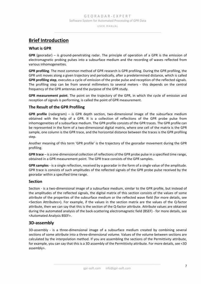
Brief Introduction What is GPR GPR (georadar) – is ground-penetrating radar. The principle of operation of a GPR is the emission of electromagnetic probing pulses into a subsurface medium and the recording of waves reflected from various inhomogeneities.
GPR profiling. The most common method of GPR research is GPR profiling. During the GPR profiling, the GPR unit moves along a given trajectory and periodically, after a predetermined distance, which is called GPR profiling step, executes a cycle of emission of the probe pulse and reception of the reflected signals. The profiling step can be from several millimeters to several meters - this depends on the central frequency of the GPR antennas and the purpose of the GPR study.
GPR measurement point. The point on the trajectory of the GPR, in which the cycle of emission and reception of signals is performing, is called the point of GPR measurement.
The Result of the GPR Profiling GPR profile (radargram) – is GPR depth section, two-dimensional image of the subsurface medium obtained with the help of a GPR. It is a collection of reflections of the GPR probe pulse from inhomogeneities of a subsurface medium. The GPR profile consists of the GPR traces. The GPR profile can be represented in the form of a two-dimensional digital matrix, where one cell of the matrix is the GPR sample, one column is the GPR trace, and the horizontal distance between the traces is the GPR profiling step.
Another meaning of this term ‘GPR profile’ is the trajectory of the georadar movement during the GPR profiling.
GPR trace – is a one-dimensional collection of reflections of the GPR probe pulse in a specified time range, obtained in a GPR measurement point. The GPR trace consists of the GPR samples.
GPR samples - is a single reflection, received by a georadar in the form of a single value of the amplitude. GPR trace is consists of such amplitudes of the reflected signals of the GPR probe pulse received by the georadar within a specified time range.
Section Section - is a two-dimensional image of a subsurface medium, similar to the GPR profile, but instead of the amplitudes of the reflected signals, the digital matrix of this section consists of the values of some attribute of the properties of the subsurface medium or the reflected wave field (for more details, see <Section Attributes>). For example, if the values in the section matrix are the values of the Q-factor attribute, then we can say that this is the section of the Q-factor attribute. Attribute values are obtained during the automated analysis of the back-scattering electromagnetic field (BSEF) - for more details, see <Automated Analysis BSEF>.
3D-assembly 3D-assembly - is a three-dimensional image of a subsurface medium created by combining several sections of some attribute into a three-dimensional volume. Values of the volume between sections are calculated by the interpolation method. If you are assembling the sections of the Permittivity attribute, for example, you can say that this is a 3D assembly of the Permittivity attribute. For more details, see <3D assembly>.

G E O R A D A R - E X P E R T Software System for Automated Processing of GPR Data
USER MANUAL
______________________________________________________________
______________________________________________________________
gpr-soft.com [email protected] 8
About the Software
The idea of developing the GEORADAR-EXPERT software system arose as a result of the generalization of many years of experience in professional activities in the field of GPR research. Practical skills acquired at all stages of investigations with GPR (communication with the customer, development of field survey methods and their implementation, GPR data processing and the creation of a technical report) allowed the developers of GEORADAR-EXPERT to form their opinion on what capabilities should have modern software for processing GPR data and in what form should the final result of this processing be presented.
As a result, three main areas of software development for GPR were identified. The first is the development and implementation of algorithms that serve to increase the depth of GPR research and increase the resolution of GPR data. The second direction concerns the final result of processing GPR data. This is a refusal to present GPR data on the subsurface environment as a set of amplitudes of the reflected signals in the form of a radarogram and the transition to the final processing result in the form of a section that contains the characteristics of this environment. The third area is the minimization of the influence of the human factor on the process of processing GPR information and the automation of this process, which is important for growing volumes of GPR research from year to year, worldwide.
The GEORADAR-EXPERT software system was developed taking into account all these aspects. This software includes both standard options for processing GPR data implemented in applications from numerous manufacturers of GPR software, as well as algorithms and methods developed specifically for GEORADAR-EXPERT that increase the informativeness and depth of GPR research. The main such development is the automated analysis of the BSEF (Back-Scattering Electromagnetic Field). The final result of processing GPR data by the BSEF automated analysis method are sections of the attributes of the electrophysical characteristics of the subsurface environment and the wave field recorded by GPR.
Automated BSEF Analysis
Professionals using ground penetrating radars may encounter a situation where the quality of the results of GPR profiling differs for the worse from the samples presented in advertising materials of manufacturers of geophysical equipment. On such advertising radarograms, one can easily find the boundaries between the layers, as well as diffracted reflections from local objects, by which it is easy to determine the speed of propagation of waves in a subsurface subsurface environment and permittivity. As a rule, such results can be obtained during the GPR study of subsurface with low losses and the presence of sharp changes in the electrophysical characteristics in the contact zone of the layers. In practice, one has to study not only low-loss subsurface, but also subsurface environment that have high
G E O R A D A R - E X P E R T Software System for Automated Processing of GPR Data
USER MANUAL
______________________________________________________________
______________________________________________________________
gpr-soft.com [email protected] 9
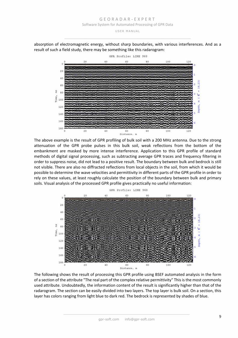
absorption of electromagnetic energy, without sharp boundaries, with various interferences. And as a result of such a field study, there may be something like this radarogram:
The above example is the result of GPR profiling of bulk soil with a 200 MHz antenna. Due to the strong attenuation of the GPR probe pulses in this bulk soil, weak reflections from the bottom of the embankment are masked by more intense interference. Application to this GPR profile of standard methods of digital signal processing, such as subtracting average GPR traces and frequency filtering in order to suppress noise, did not lead to a positive result. The boundary between bulk and bedrock is still not visible. There are also no diffracted reflections from local objects in the soil, from which it would be possible to determine the wave velocities and permittivity in different parts of the GPR profile in order to rely on these values, at least roughly calculate the position of the boundary between bulk and primary soils. Visual analysis of the processed GPR profile gives practically no useful information:
The following shows the result of processing this GPR profile using BSEF automated analysis in the form of a section of the attribute "The real part of the complex relative permittivity" This is the most commonly used attribute. Undoubtedly, the information content of the result is significantly higher than that of the radarogram. The section can be easily divided into two layers. The top layer is bulk soil. On a section, this layer has colors ranging from light blue to dark red. The bedrock is represented by shades of blue.

G E O R A D A R - E X P E R T Software System for Automated Processing of GPR Data
USER MANUAL
______________________________________________________________
______________________________________________________________
gpr-soft.com [email protected] 10
By studying the change in the color gamut of the section, one can learn about changes in the electro physical characteristics of the soil inside each layer. For a more accurate representation of changes in the attribute of a section, you can use the statistical module implemented in the GEORADAR-EXPERT software system and obtain data for each layer, for each layer boundary, or for the entire section as a whole in the form of graphs and tables by twelve statistical indicators. The figure below shows a graph of the changes in the average permittivity in a layer of bulk soil. The area of the graph that exceeds the user-defined threshold is colored in red:
Obviously, the transition from the presentation of data on the subsurface environment in the form of a set of amplitudes of the reflected signals (in the form of a radarogram) to the characteristics of this subsurface obtained as a result of applying the BSEF automated analysis method (in the form of an
G E O R A D A R - E X P E R T Software System for Automated Processing of GPR Data
USER MANUAL
______________________________________________________________
______________________________________________________________
gpr-soft.com [email protected] 11
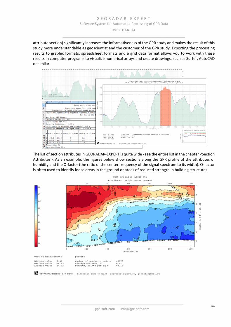
attribute section) significantly increases the informativeness of the GPR study and makes the result of this study more understandable as geoscientist and the customer of the GPR study. Exporting the processing results to graphic formats, spreadsheet formats and a grid data format allows you to work with these results in computer programs to visualize numerical arrays and create drawings, such as Surfer, AutoCAD or similar.
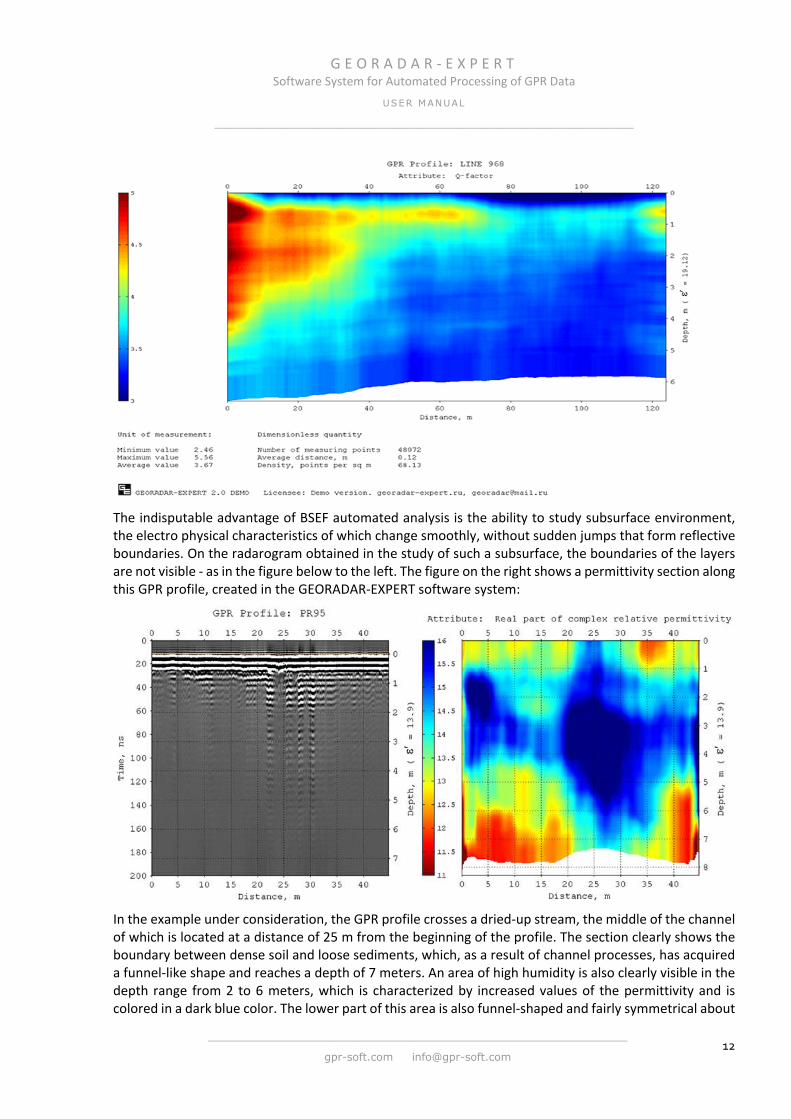
The list of section attributes in GEORADAR-EXPERT is quite wide - see the entire list in the chapter <Section Attributes>. As an example, the figures below show sections along the GPR profile of the attributes of humidity and the Q-factor (the ratio of the center frequency of the signal spectrum to its width). Q-factor is often used to identify loose areas in the ground or areas of reduced strength in building structures.
G E O R A D A R - E X P E R T Software System for Automated Processing of GPR Data
USER MANUAL
______________________________________________________________
______________________________________________________________
gpr-soft.com [email protected] 12
The indisputable advantage of BSEF automated analysis is the ability to study subsurface environment, the electro physical characteristics of which change smoothly, without sudden jumps that form reflective boundaries. On the radarogram obtained in the study of such a subsurface, the boundaries of the layers are not visible - as in the figure below to the left. The figure on the right shows a permittivity section along this GPR profile, created in the GEORADAR-EXPERT software system:
In the example under consideration, the GPR profile crosses a dried-up stream, the middle of the channel of which is located at a distance of 25 m from the beginning of the profile. The section clearly shows the boundary between dense soil and loose sediments, which, as a result of channel processes, has acquired a funnel-like shape and reaches a depth of 7 meters. An area of high humidity is also clearly visible in the depth range from 2 to 6 meters, which is characterized by increased values of the permittivity and is colored in a dark blue color. The lower part of this area is also funnel-shaped and fairly symmetrical about

G E O R A D A R - E X P E R T Software System for Automated Processing of GPR Data
USER MANUAL
______________________________________________________________
______________________________________________________________
gpr-soft.com [email protected] 13
the middle of the stream. The application of the BSEF automated analysis method to this GPR profile made it possible to obtain much more useful information than the GPR profile could provide before this method was applied.
The runtime spent on performing automated BSEF analysis and creating attribute section is relatively small. For example, the processing of this GPR profile was carried out for several minutes on a computer with a processor frequency of 2.4 MHz. Significant time savings occur in the case of processing a large amount of the same type of GPR data - for example, such as roads or railway profiling results. The user, having configured the parameters of automated processing and starting the processing, can switch to other tasks, and GEORADAR-EXPERT will independently load GPR profiles and save the processing results to the computer`s hard disk.
Using the BSEF automated analysis method has the following advantages over other methods of digital processing of GPR signals:
• The depth of GPR research is increasing - the data processing algorithm by the BSEF automated analysis method has high noise immunity and works well in areas of strong noise of signals located in the lower zone of the GPR profile;
• The information content of GPR studies increases - a attribute section according to the results of an automated BSEF analysis allows obtaining information on the structure of the investigated subsurface environment even in the conditions of a smooth change in the electrophysical characteristics of this environment, i.e. in the absence of layer boundaries on the radarogram. If these boundaries are present, then a change in the electrophysical characteristics inside each layer also represents undoubted benefit;
• Significantly increases the speed of processing GPR data, which is important for constantly increasing volumes of GPR works, especially in the road and railway industries;
• The areas of application of the GPR method are expanding and the list of tasks to be solved with the help of this method is increasing;
• The influence of the human factor on the processing and interpretation of GPR data is reduced;
• Provides greater opportunities for the study of complexly constructed subsurface environments.
Summing Sections or Cross-Sections of 3D Assemblies
The GEORADAR-EXPERT software system contains a fairly wide range of wave field attributes and characteristics of the subsurface environment intended for various purposes. There are frequent cases when information about the object under study is not contained in full by one section of the attribute, but is distributed over the sections of several attributes. In this case, summing a set of attributes allows you to combine disparate information about an object within a single summary section.
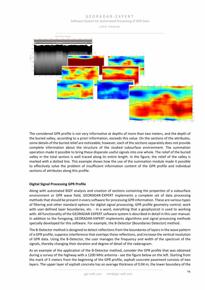
The figure below shows images of the GPR profile obtained during the study of the buried valley, a set of attribute sections for summation obtained because of an automated BSEF analysis of this GPR profile and the result of summing these sections. At the same time, as a result of the summation, artifacts caused by the accumulation of errors in the process of collecting and processing GPR information are eliminated.
G E O R A D A R - E X P E R T Software System for Automated Processing of GPR Data
USER MANUAL
______________________________________________________________
______________________________________________________________
gpr-soft.com [email protected] 14
The considered GPR profile is not very informative at depths of more than two meters, and the depth of the buried valley, according to a priori information, exceeds this value. On the sections of the attributes, some details of the buried relief are noticeable; however, each of the sections separately does not provide complete information about the structure of the studied subsurface environment. The summation operation made it possible to bring these disparate useful signals into one whole. The relief of the buried valley in the total section is well traced along its entire length. In the figure, the relief of the valley is marked with a dotted line. This example shows how the use of the summation module made it possible to effectively solve the problem of insufficient information content of the GPR profile and individual sections of attributes along this profile.
Digital Signal Processing GPR Profile
Along with automated BSEF analysis and creation of sections containing the properties of a subsurface environment or GPR wave field, GEORADAR-EXPERT implements a complete set of data processing methods that should be present in every software for processing GPR information. These are various types of filtering and other standard options for digital signal processing; GPR profile geometry control; work with user-defined layer boundaries, etc. - In a word, everything that a geophysicist is used to working with. All functionality of the GEORADAR-EXPERT software system is described in detail in this user manual. In addition to the foregoing, GEORADAR-EXPERT implements algorithms and signal processing methods specially developed for this software. For example, the B-Detector (Boundaries Detector) method.
The B-Detector method is designed to detect reflections from the boundaries of layers in the wave pattern of a GPR profile, suppress interference that overlaps these reflections, and increase the vertical resolution of GPR data. Using the B-Detector, the user manages the frequency and width of the spectrum of the signals, thereby changing their duration and degree of detail of the radarogram.
As an example of the application of the B-Detector method, consider the GPR profile that was obtained during a survey of the highway with a 1200 MHz antenna - see the figure below on the left. Starting from the mark of 5 meters from the beginning of the GPR profile, asphalt concrete pavement consists of two layers. The upper layer of asphalt concrete has an average thickness of 0.04 m, the lower boundary of the
G E O R A D A R - E X P E R T Software System for Automated Processing of GPR Data
USER MANUAL
______________________________________________________________
______________________________________________________________
gpr-soft.com [email protected] 15
second layer of asphalt concrete lies in the depth range from 0.12 to 0.15 m from the surface. Under the asphalt concrete there is a layer of crushed stone base with an average thickness of about 0.15 m. But not all of these boundaries are visible on the GPR profile. For example, the boundary between the layers of asphalt concrete is not visible. This fact allows us to conclude that the resolution of the 1200 MHz antenna is not enough to detect the boundaries of the structural layers of the pavement.
In addition, determining the exact position of the boundaries on the wave pattern of a given GPR profile vertically is also difficult, because phase displacements of signals as a result of superposition of reflections from the neighboring boundaries of the layers introduce distortions. Regardless of how the user will determines the position of the boundaries - by the extrema of the same phases of the signals or by the line of changing the sign of the amplitude of the signals, or something else - these phase distortions will affect the accuracy of positioning.
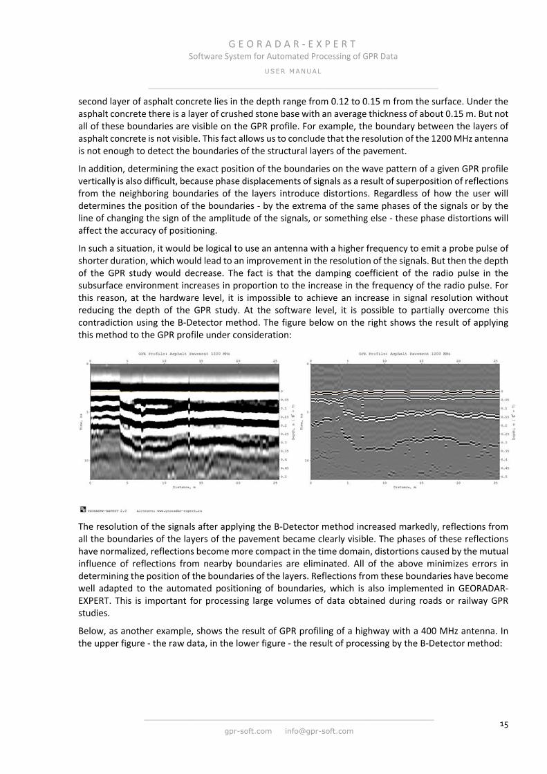
In such a situation, it would be logical to use an antenna with a higher frequency to emit a probe pulse of shorter duration, which would lead to an improvement in the resolution of the signals. But then the depth of the GPR study would decrease. The fact is that the damping coefficient of the radio pulse in the subsurface environment increases in proportion to the increase in the frequency of the radio pulse. For this reason, at the hardware level, it is impossible to achieve an increase in signal resolution without reducing the depth of the GPR study. At the software level, it is possible to partially overcome this contradiction using the B-Detector method. The figure below on the right shows the result of applying this method to the GPR profile under consideration:
The resolution of the signals after applying the B-Detector method increased markedly, reflections from all the boundaries of the layers of the pavement became clearly visible. The phases of these reflections have normalized, reflections become more compact in the time domain, distortions caused by the mutual influence of reflections from nearby boundaries are eliminated. All of the above minimizes errors in determining the position of the boundaries of the layers. Reflections from these boundaries have become well adapted to the automated positioning of boundaries, which is also implemented in GEORADAR-EXPERT. This is important for processing large volumes of data obtained during roads or railway GPR studies.
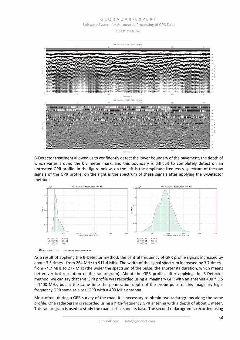
Below, as another example, shows the result of GPR profiling of a highway with a 400 MHz antenna. In the upper figure - the raw data, in the lower figure - the result of processing by the B-Detector method:
G E O R A D A R - E X P E R T Software System for Automated Processing of GPR Data
USER MANUAL
______________________________________________________________
______________________________________________________________
gpr-soft.com [email protected] 16
B-Detector treatment allowed us to confidently detect the lower boundary of the pavement, the depth of which varies around the 0.2 meter mark, and this boundary is difficult to completely detect on an untreated GPR profile. In the figure below, on the left is the amplitude-frequency spectrum of the raw signals of the GPR profile, on the right is the spectrum of these signals after applying the B-Detector method:
As a result of applying the B-Detector method, the central frequency of GPR profile signals increased by about 3.5 times - from 264 MHz to 911.4 MHz. The width of the signal spectrum increased by 3.7 times - from 74.7 MHz to 277 MHz (the wider the spectrum of the pulse, the shorter its duration, which means better vertical resolution of the radarogram). About the GPR profile, after applying the B-Detector method, we can say that this GPR profile was recorded using a imaginary GPR with an antenna 400 * 3.5 = 1400 MHz, but at the same time the penetration depth of the probe pulse of this imaginary high-frequency GPR same as a real GPR with a 400 MHz antenna.
Most often, during a GPR survey of the road, it is necessary to obtain two radarograms along the same profile. One radarogram is recorded using a high-frequency GPR antenna with a depth of about 1 meter. This radarogram is used to study the road surface and its base. The second radarogram is recorded using
G E O R A D A R - E X P E R T Software System for Automated Processing of GPR Data
USER MANUAL
______________________________________________________________
______________________________________________________________
gpr-soft.com [email protected] 17
a mid-frequency GPR antenna with a depth of 3 - 5 meters, which is used to study the subbase and subgrade.
If the GPR used for road research does not have the ability to simultaneously record several GPR profiles, then in order to obtain two radarograms it is necessary to go through the same profile two times with different antennas. In this case, using the B-Detector method makes it possible to abandon the high-frequency antenna and record not two, but only one GPR profile of the road using a mid-frequency antenna. For example, 400 MHz - as in this example. In this case, the volume of field and cameral work will be halved. Considering the significant volume of GPR profiling in road research, this is a tangible saving. Even in the case of using a multi-channel GPR, which allows you to simultaneously record more than one GPR profile, using the B-Detector method reduces the amount of cameral work and improves the quality of processing GPR data.
Another argument in favor of using the B-Detector method. A small design and surveying company company may not have a complete set of GPR units that cover the entire frequency range used in georadiolocation. The purchase of a large amount of this equipment requires significant financial costs. In this case, the application of the B-Detector method will compensate for the absence of high-frequency antennas by using low-frequency antennas in those areas of GPR research in which high-frequency antennas are used. Thus, the range of tasks to be expanded, which will lead to an increase in the number of GPR research customers.
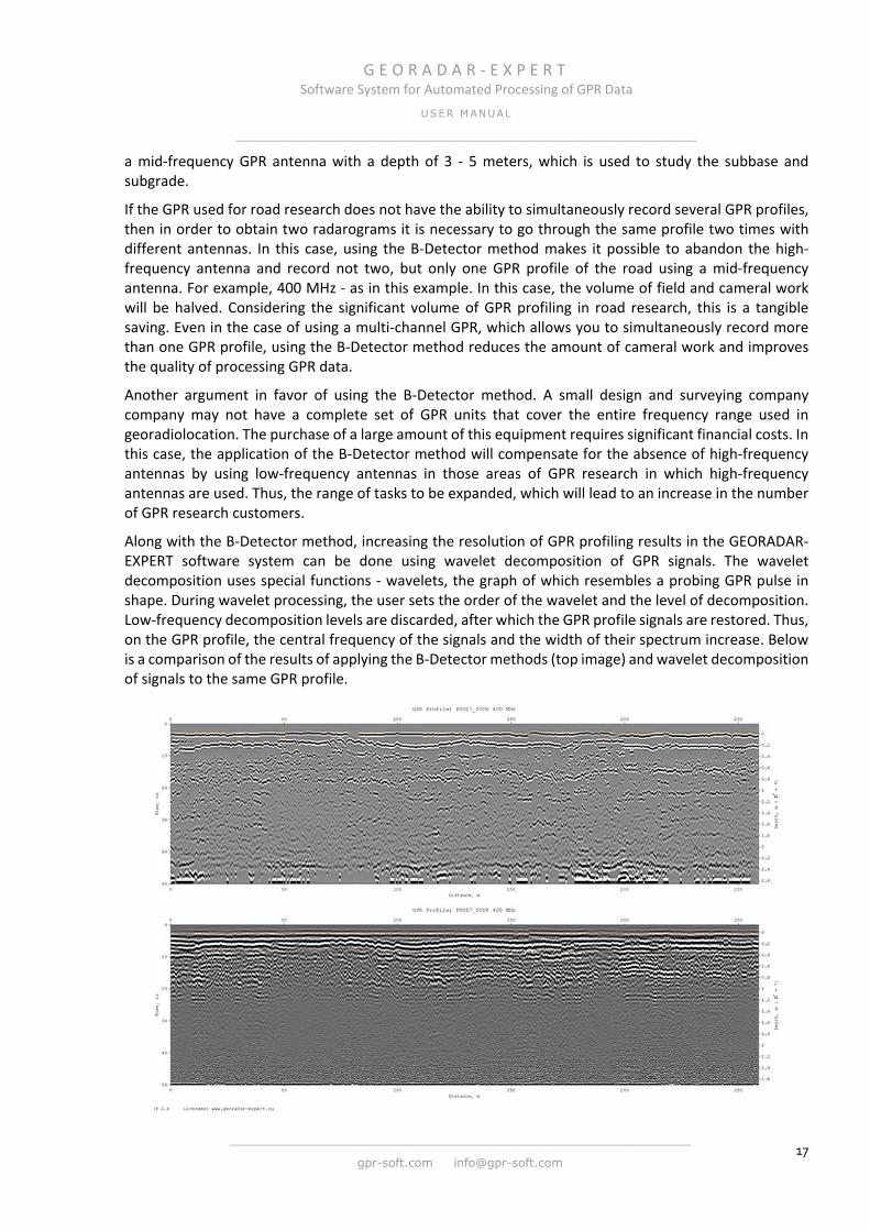
Along with the B-Detector method, increasing the resolution of GPR profiling results in the GEORADAR-EXPERT software system can be done using wavelet decomposition of GPR signals. The wavelet decomposition uses special functions - wavelets, the graph of which resembles a probing GPR pulse in shape. During wavelet processing, the user sets the order of the wavelet and the level of decomposition. Low-frequency decomposition levels are discarded, after which the GPR profile signals are restored. Thus, on the GPR profile, the central frequency of the signals and the width of their spectrum increase. Below is a comparison of the results of applying the B-Detector methods (top image) and wavelet decomposition of signals to the same GPR profile.

G E O R A D A R - E X P E R T Software System for Automated Processing of GPR Data
USER MANUAL
______________________________________________________________
______________________________________________________________
gpr-soft.com [email protected] 18
Each of these methods has its advantages. The user, depending on the features of the GPR profile signals and the tasks of the GPR study, can choose which of these methods to use in each case.
One of the problems a geophysicist encounters when processing GPR data is the suppression of reflections from objects located on the ground surface. These so-called air reflections can have a high level of amplitudes and effectively mask useful signals, crossing them with their inclined fragments. Using shielding for GPR antennas may not give the expected effect. The results of profiling by dipole low-frequency antennas, for which shielding is not provided, are most susceptible to this interference. Also, diffracted reflections from contrasting local objects located in a subsurface medium can be a source of interference. These reflections can also mask less intense reflections from the boundaries of the layers.
The spatial filter implemented in the GEORADAR-EXPERT software system allows solving this problem. Consider a GPR profile that crosses tram tracks. The figure below, on the left, shows this GPR profile before processing. Profile obtained by GPR with a 150 MHz low-frequency antenna. On this profile, intense reflections from metal rails and infrastructure objects of tram tracks cross weaker reflections from the boundaries of layers in the ground and mask them. The result of spatial filtering is shown on the right. As a result of filtering, the interference in the form of diffracted reflections removed; instead of this interference, reflections from the boundaries of the layers became visible.
Options for digital processing of GPR profile signals, of which there are more than two dozen in GERADAR-EXPERT, allow to solve practically the whole range of problems that users face during GPR data processing. Automation of the user's actions frees him from the obligation of constant presence at the computer. The user can save the sequence of data processing procedures to a file and apply this sequence in the future. In batch processing mode, the user only needs to select a group of GPR data files, after which the load, processing and saving of the result is performed automatically, without user intervention. All functionality of the GEORADAR-EXPERT software system is described in detail in this user manual.

G E O R A D A R - E X P E R T Software System for Automated Processing of GPR Data
USER MANUAL
______________________________________________________________
______________________________________________________________
gpr-soft.com [email protected] 19
User Interface
The graphical user interface of the GEORADAR-EXPERT software system is a set of tabs, each of which serves for specific tasks and contains panels with controls for these tasks. Tabs are located in the main program window. At the top of this window is the standard menu bar. The user can change the aspect ratio of the tabs or hide them. GEORADAR-EXPERT provides two modes of the main program window - 2D and 3D. 2D mode is designed to work with two-dimensional data - GPR profiles and sections created by the results of an automated BSEF analysis. The 3D mode is used to visualize the three-dimensional volume of GPR data, as well as slices of this volume. The three-dimensional volume is formed from attribute sections created by the BSEF analysis of a set of GPR profiles obtained during the areal GPR surveying. The main window mode changes automatically, depending on the type of data loaded into GEORADAR-EXPERT.
The following shows the main window of the GEORADAR-EXPERT software system in 2D mode. The upper group of tabs serves to visualize two-dimensional data, graphs of the spectrum of signals and statistical information. In this example, the section visualization tab is active. Nearby are inactive tabs for visualizing the GPR profile and the amplitude-frequency spectrum of the signals of this profile. To activate a tab, the user needs to click on this tab, after which the data on this tab will be available, and the data on the other tabs from this group will be hidden.
In the left part of the GEORADAR-EXPERT main window there are tabs intended for graphical presentation of the BSEF analysis results, as well as controls for creating and visualizing the section based on the results of this analysis. In the lower part of the main window there is a group of tabs intended for placing control elements for displaying the radarogram, GPR profile properties and profile processing settings. All three groups of tabs are separated by two separators - vertical and horizontal, which contain buttons for controlling the size of the tabs.

G E O R A D A R - E X P E R T Software System for Automated Processing of GPR Data
USER MANUAL
______________________________________________________________
______________________________________________________________
gpr-soft.com [email protected] 20
The main window of GEORADAR-EXPERT with the active tab for visualizing the GPR profile is shown below. Unlike the previous example, the ratio of the tab groups has been changed - the size of the left tab group has increased due to a decrease in the size of the upper and lower groups:
The main window of the GEORADAR-EXPERT with the active tab for displaying the amplitude-frequency spectrum of GPR profile signals is shown below. The sizes of the upper and lower groups of tabs are increased by reducing the size of the left group of tabs:

G E O R A D A R - E X P E R T Software System for Automated Processing of GPR Data
USER MANUAL
______________________________________________________________
______________________________________________________________
gpr-soft.com [email protected] 21
The tab of the section created with the terrain correction is shown below. The last tab is active in the left group of tabs. The area of this tab is only partially occupied by the settings panels for creating and visualizing the section:
The section visualization tab with terrain correction in the attribute visibility constraint mode is shown below. In this mode, section areas containing attribute values that go beyond the boundaries of a user-defined range are not rendered. Hidden areas are not taken into account in the process of statistical analysis and analysis of the spatial distribution of attribute values. Thus, the user can exclude part of the section from these calculations, if necessary.
G E O R A D A R - E X P E R T Software System for Automated Processing of GPR Data
USER MANUAL
______________________________________________________________
______________________________________________________________
gpr-soft.com [email protected] 22
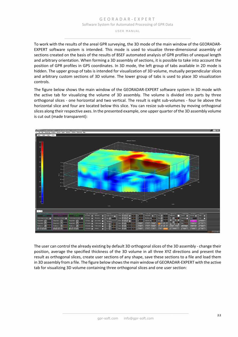
To work with the results of the areal GPR surveying, the 3D mode of the main window of the GEORADAR-EXPERT software system is intended. This mode is used to visualize three-dimensional assembly of sections created on the basis of the results of BSEF automated analysis of GPR profiles of unequal length and arbitrary orientation. When forming a 3D assembly of sections, it is possible to take into account the position of GPR profiles in GPS coordinates. In 3D mode, the left group of tabs available in 2D mode is hidden. The upper group of tabs is intended for visualization of 3D volume, mutually perpendicular slices and arbitrary custom sections of 3D volume. The lower group of tabs is used to place 3D visualization controls.
The figure below shows the main window of the GEORADAR-EXPERT software system in 3D mode with the active tab for visualizing the volume of 3D assembly. The volume is divided into parts by three orthogonal slices - one horizontal and two vertical. The result is eight sub-volumes - four lie above the horizontal slice and four are located below this slice. You can resize sub-volumes by moving orthogonal slices along their respective axes. In the presented example, one upper quarter of the 3D assembly volume is cut out (made transparent):
The user can control the already existing by default 3D orthogonal slices of the 3D assembly - change their position, average the specified thickness of the 3D volume in all three XYZ directions and present the result as orthogonal slices, create user sections of any shape, save these sections to a file and load them in 3D assembly from a file. The figure below shows the main window of GEORADAR-EXPERT with the active tab for visualizing 3D volume containing three orthogonal slices and one user section:

G E O R A D A R - E X P E R T Software System for Automated Processing of GPR Data
USER MANUAL
______________________________________________________________
______________________________________________________________
gpr-soft.com [email protected] 23
The tab below shows the development of this curved user section. Vertical lines indicate the position of the nodal points of the curve through which this section passes. The names of the points are located on the upper boundary of the section. For each point, it is possible to obtain a logging curve and a table of its values.
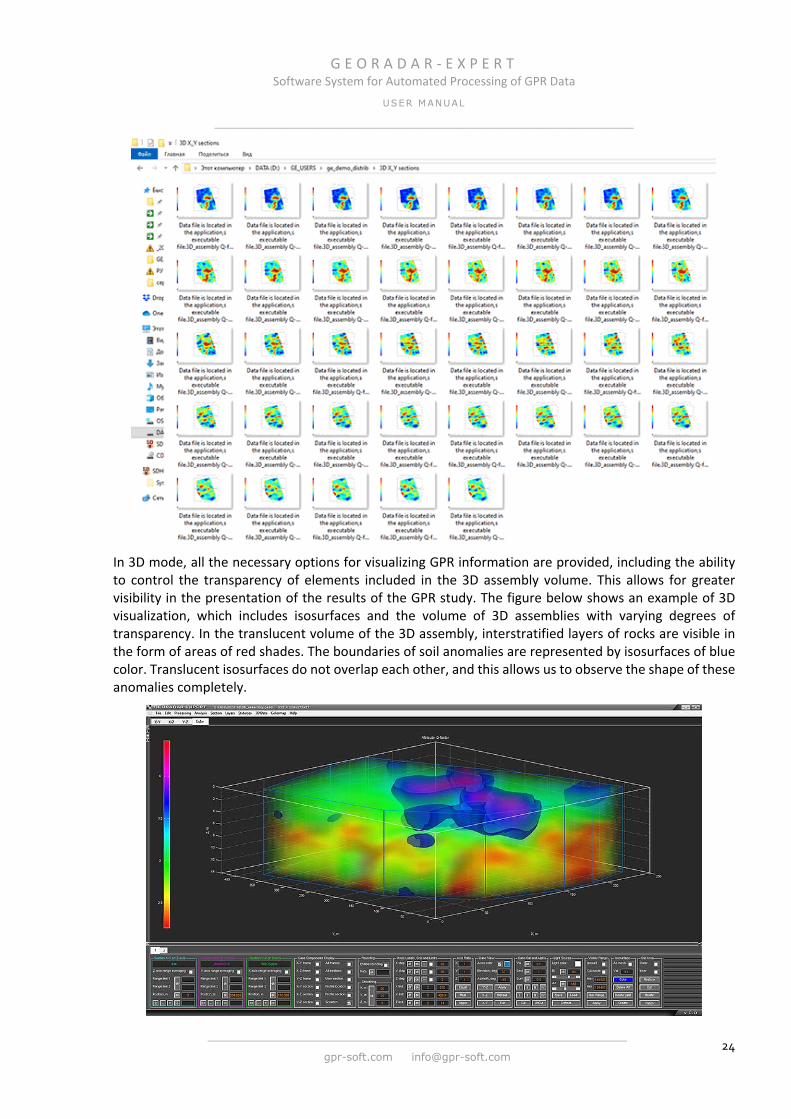
The user can save a series of images of orthogonal slices of 3D volume in the computer`s hard disk in automatic mode with a specified step along the corresponding axis. Compared to the manual mode for saving slices, automatic mode saves time. In manual mode, you first need to perform actions to move the slice to the desired point on the axis, and then interact with the save dialog box. When the number of slices is several tens, or even hundreds, the manual saving process is extended for a long time. The figure below shows a Windows Explorer window with a directory for saving a set of horizontal slices of 3D volume.
G E O R A D A R - E X P E R T Software System for Automated Processing of GPR Data
USER MANUAL
______________________________________________________________
______________________________________________________________
gpr-soft.com [email protected] 24
In 3D mode, all the necessary options for visualizing GPR information are provided, including the ability to control the transparency of elements included in the 3D assembly volume. This allows for greater visibility in the presentation of the results of the GPR study. The figure below shows an example of 3D visualization, which includes isosurfaces and the volume of 3D assemblies with varying degrees of transparency. In the translucent volume of the 3D assembly, interstratified layers of rocks are visible in the form of areas of red shades. The boundaries of soil anomalies are represented by isosurfaces of blue color. Translucent isosurfaces do not overlap each other, and this allows us to observe the shape of these anomalies completely.

G E O R A D A R - E X P E R T Software System for Automated Processing of GPR Data
USER MANUAL
______________________________________________________________
______________________________________________________________
gpr-soft.com [email protected] 25
Below is a variant of visualization of the 3D assembly volume, in which full transparency is defined by the user-specified range of attribute values, and the isosurface is the boundary between the transparent and opaque regions:
If the 3D assembly contains isosurfaces, then these isosurfaces divide the volume of the 3D assembly into parts. The user can create isosurfaces so that they pass along the contact boundaries of the layers of the investigated subsurface. The ability to obtain information about the volume of these layers is of undoubted practical interest. GEORADAR-EXPERT provides this opportunity. The figure below on the left shows the axes of the 3D assembly from the previous example, on which orthogonal slices and two isosurfaces are placed - one yellow, the other purple. The values through which these isosurfaces pass are shown in the lower left corner of the image in the rectangles of the corresponding colors. The right-hand side of the image shows an automatically generated table of volumes bounded by these isosurfaces. Similarly, you can get information about layer area in square meters in 2D mode. Only in this case the layers do not limit the isosurfaces, but the lines of the boundaries of the layers.
Below is an example of a 3D assembly, which was created taking into account the coordinates of the GPS positioning system. In a three-dimensional view, the positions of GPR profiles and vertical slices along these profiles are visualized. An isosurface passes through the 3D assembly volume, showing the contact

G E O R A D A R - E X P E R T Software System for Automated Processing of GPR Data
USER MANUAL
______________________________________________________________
______________________________________________________________
gpr-soft.com [email protected] 26
position of soils with various electro physical characteristics. For isosurface and 3D assembly volume, various degrees of transparency are specified.
Undoubtedly, GEORADAR-EXPERT, developed as a result of summarizing many years of experience in processing GPR data, is an effective tool for solving a wide range of GPR tasks, including in cases where the use of software for processing GPR data from other manufacturers does not lead to positive results. High informativeness and quality of cameral work performed using the GEORADAR-EXPERT software system will help to attract new customers and ensure stable competitiveness in the geophysical services market.
Similarities and Differences from Other Manufacturers Software
Similarity
The GEORADAR-EXPERT software system implements a complete set of data processing options, which should be present in each software for processing GPR information. These are various types of filtering and other standard options for digital signal processing, managing GPR profile parameters, working with user-defined layer boundaries, etc. That is, everything that a specialist in processing GPR data is used to using in his professional activity.
Differences
The main difference of GEORADAR-EXPERT from other manufacturers' software is the increased informativeness of GPR data processing results and the low level of human factor influence on the final processing result. The ability to batch process data and automate user actions provides good processing speed for large volumes of information. Algorithms and methods implemented in the GEORADAR-EXPERT software system provide more opportunities for researching complexly constructed subsurface environments. GEORADAR-EXPERT includes the following options specially designed for this software:
• Automated BSEF (Back-Scattering Electromagnetic Field) electromagnetic field analysis. Carries out the transition from the presentation of data on the subsurface in the form of a set of amplitudes of the reflected signals in the form of a radarogram to the characteristics of this subsurface in the form of an attribute section. Such a presentation makes the result of
G E O R A D A R - E X P E R T Software System for Automated Processing of GPR Data
USER MANUAL
______________________________________________________________
______________________________________________________________
gpr-soft.com [email protected] 27
processing GPR data more understandable both to geophysicists and to specialists in related fields. For example, geologists or design-and-planning engineers. BSEF analysis works well in areas of strong noise located at the bottom of the GPR profile, which allows increasing the depth of GPR research. Along with this, the BSEF analysis provides information on the structure of the investigated subsurface environment even under conditions of a smooth change in its electrophysical characteristics, i.e. in the absence of layer boundaries on the radarogram.
• B-Detector Method (Boundaries Detector). This method is designed to detect reflections from the boundaries of layers in the wave pattern of a GPR profile, suppress interference that overlaps these reflections, and increase the vertical resolution of GPR data. Using the B-Detector, the user manages the frequency and width of the spectrum of the signals, thereby changing their duration and degree of detail of the radarogram. As a result of processing by the B-Detector GPR method, the profile obtained by the low-frequency antenna looks as if the frequency of the GPR antenna during recording of this profile was several times higher. The resolution of signals on this GPR profile is also several times higher. If necessary, it is possible, and vice versa, to lower the central frequency of the radarogram signals.
• Method for decomposing a radarogram into components. This is not a wavelet decomposition of signals, although it is also implemented in the GEORADAR-EXPERT. This method converts a signals matrix of GPR profile into a set of matrices. Each matrix from this set contains only one unique type of reflected waves. The user discards the matrices with those types of waves, which he defined as interference, and then summarizes the remaining matrices. Thus, interference are excluded from the GPR profile signals. Using the same method, it is possible to remove diffracted reflections, including air ones, leaving behind only the boundaries of the layers on the radarogram. This is useful, for example, for road research. Or vice versa, you can remove all the boundaries of the layers, leaving only diffracted reflections. For example, to better detect reinforcement in a concrete structure.
• Statistical analysis module. This module is intended to summarize the results of GPR profiling and to better presentation the variability of the electrophysical characteristics of the GPR profile. Using the results of statistical analysis, presented in the form of tables and graphs, it is possible to establish a relationship between the physicomechanical characteristics of the investigated subsurface environment (for example, soil or building structures) and various statistical indicators. Thus, a feature set is created that can be used in the future to assess the state of similar objects. Statistical data sources are GPR profiles, attribute sections, which are calculated based on the results of BSEF automated analysis, and slices of the 3D assembly. If the user has drawn the boundaries of the layers on the GPR profile, on the attribute section or on the 3D assembly slice, the statistical indicators are calculated inside each layer, along the boundary of each layer and for the whole object, without regard to separation into layers. Using the statistical analysis module implemented by GEORADAR-EXPERT raises the quality of GPR research results to a new, higher level.
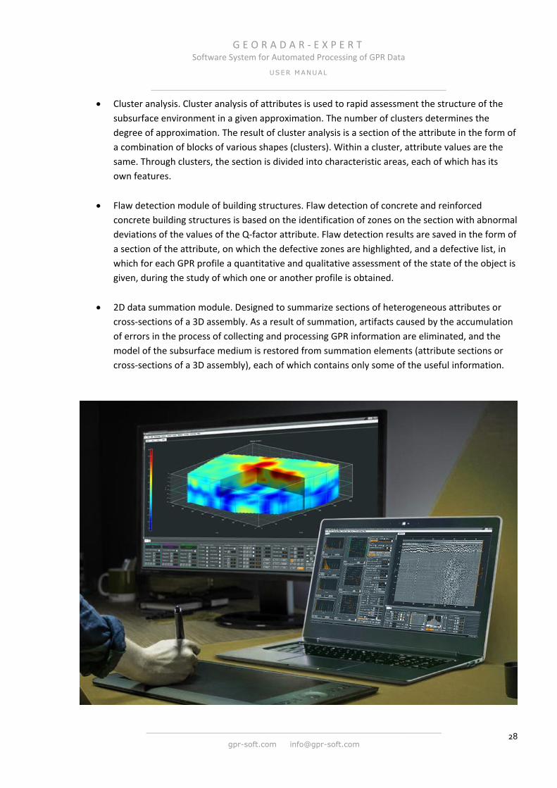
G E O R A D A R - E X P E R T Software System for Automated Processing of GPR Data
USER MANUAL
______________________________________________________________
______________________________________________________________
gpr-soft.com [email protected] 28
• Cluster analysis. Cluster analysis of attributes is used to rapid assessment the structure of the subsurface environment in a given approximation. The number of clusters determines the degree of approximation. The result of cluster analysis is a section of the attribute in the form of a combination of blocks of various shapes (clusters). Within a cluster, attribute values are the same. Through clusters, the section is divided into characteristic areas, each of which has its own features.
• Flaw detection module of building structures. Flaw detection of concrete and reinforced concrete building structures is based on the identification of zones on the section with abnormal deviations of the values of the Q-factor attribute. Flaw detection results are saved in the form of a section of the attribute, on which the defective zones are highlighted, and a defective list, in which for each GPR profile a quantitative and qualitative assessment of the state of the object is given, during the study of which one or another profile is obtained.
• 2D data summation module. Designed to summarize sections of heterogeneous attributes or cross-sections of a 3D assembly. As a result of summation, artifacts caused by the accumulation of errors in the process of collecting and processing GPR information are eliminated, and the model of the subsurface medium is restored from summation elements (attribute sections or cross-sections of a 3D assembly), each of which contains only some of the useful information.
G E O R A D A R - E X P E R T Software System for Automated Processing of GPR Data
USER MANUAL
______________________________________________________________
______________________________________________________________
gpr-soft.com [email protected] 29
Supported Data Formats GEORADAR-EXPERT supports the following formats of GPR data:
GSSI SIR and other (*.dzt) ;
OKO (*.gpr) ;
OKO (*.gpr2) ;
ZOND and other SEG-Y (*.sgy) ;
LOZA and other, export data in ASCII data file format, three columns - coordinates of X, Y, and the signal amplitude A (*.txt) ;
IDS (*.dt) ;
PULSE EKKO (*.dt1) ;
Geoscanners AB (*.gsf) ;
MALA Ramac (*.rd3) ;
MALA, ReflexW and other (*.??t, “??” are different digits in the file extension) ;
If the GEORADAR-EXPERT does not support any format of GPR data, support for this format can be implemented at the user's request.
The following file formats are specialized formats of GEORADAR-EXPERT:
efd - data file containing the GPR profile signals, its parameters and the results of the automated analysis of the BSEF, if this analysis was performed (see the chapter <Saving to EFD Format>);
xzd - section data file used to create the 3D assembly (see the chapter <Saving Section to XZD Format>);
gexyz - GPS coordinate file used to create a 3D assembly (see the chapter <Creating 3D Assembly Based on XYZ Coordinates>);
ge3d - data file of the 3D assembly (see the chapter <3D assembly>);
geprm - data file containing the section creation settings (see the chapter <Saving and Loading Creation Parameters of Section>);
gecmap - data file for the color map of a section or a 3D assembly (see the chapter <Saving and Loading Colormap>);
gepro - data file containing the signal processing parameters of the GPR profile (see the chapter <Saving and Loading Processing History>);
gelay - data file containing the boundaries of layers that were created by the user (see the chapter <Save and Load Layer Boundaries>);
ge3ucs – arbitrary (curved) cross-sectional data file of the 3D assembly (see the chapter <Arbitrary Cross-Section>);
gedda – data file containing information about the position of the data deletion areas on the section (see the chapter <Ignoring User-Specified Data Part for Section Creating>).

G E O R A D A R - E X P E R T Software System for Automated Processing of GPR Data
USER MANUAL
______________________________________________________________
______________________________________________________________
gpr-soft.com [email protected] 30
Compiled Help File To open the compiled help file in the format CHM (Compiled Help Modules), click the menu item User Manual located in the menu group Help in the menu bar. As a result, a pop-up dialog box appears with a warning that before the compiled help window opens, the GEORADAR-EXPERT will be minimized. If the user clicks No, the process of opening the help file will be canceled. If the user clicks Yes, the GEORADAR-EXPERT is minimized and the help file is opened.
Software Requirements and Installation GEORADAR-EXPERT runs on personal computers with Intel Pentium processor or similar to it with a clock speed of at least 2 GHz under the operating system MS Windows XP and later versions of Windows 32-bit or 64-bit. For satisfactory operation of GEORADAR-EXPERT in the 3D visualization mode, it is recommended to have at least 4 GB of system RAM and 512 MB of video RAM.
The installation and registration manual for the GEORADAR-EXPERT software system is provided to the user along with the distribution. To create a 3D assembly and the ability to export data about the position of the boundaries of layers and some other data in a spreadsheet format, Microsoft Excel software is required.

G E O R A D A R - E X P E R T Software System for Automated Processing of GPR Data
USER MANUAL
______________________________________________________________
______________________________________________________________
gpr-soft.com [email protected] 31
Using Two or More Monitors If one or more additional monitors are connected to the computer, in this case, immediately after starting the GEORADAR-EXPERT software system, the monitor selection panel will open. The main window of the GEORADAR-EXPERT will be placed on the selected monitor. The monitor selection pane contains a list of available monitors.
In the selection panel, the main monitor is designated as Primary monitor, additional monitors are designated as Second monitor. To the right of the monitor designation there is information about the screen resolution in pixels and a selection checkbox. By default, the selection check box is checked on the secondary monitor. To change the selection, the user must check the box next to the desired monitor and click OK.
After pressing the OK button, the selection panel is closed and the elements of the GEORADAR-EXPERT graphical user interface are displayed on the screen of the selected monitor. The main window GEORADAR-EXPERT can be displayed only on one screen, the extension of the main window beyond the selected monitor is not provided.
The ability to select a monitor at the start of GEORADAR-EXPERT is available only when the mode of extending the desktop onto the screens of additional monitors is selected in the display settings.
You can quickly access the display mode selection in Windows by simultaneously pressing the Windows logo key and the P key on your computer keyboard (WIN + P). After pressing the combination of these keys, a window for selecting modes will open, in which you need to select the Extend.
Alternatively, you can right-click in the desktop area and select Display Settings from the menu that opens. This will open the Windows settings window in the Display section. In this section, you need to set the Multiple displays option to Extend these displays item. The list of available modes is contained in the drop-down list.
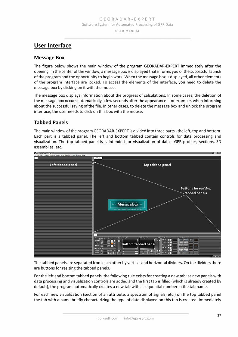
G E O R A D A R - E X P E R T Software System for Automated Processing of GPR Data
USER MANUAL
______________________________________________________________
______________________________________________________________
gpr-soft.com [email protected] 32
User Interface
Message Box The figure below shows the main window of the program GEORADAR-EXPERT immediately after the opening. In the center of the window, a message box is displayed that informs you of the successful launch of the program and the opportunity to begin work. When the message box is displayed, all other elements of the program interface are locked. To access the elements of the interface, you need to delete the message box by clicking on it with the mouse.
The message box displays information about the progress of calculations. In some cases, the deletion of the message box occurs automatically a few seconds after the appearance - for example, when informing about the successful saving of the file. In other cases, to delete the message box and unlock the program interface, the user needs to click on this box with the mouse.
Tabbed Panels The main window of the program GEORADAR-EXPERT is divided into three parts - the left, top and bottom. Each part is a tabbed panel. The left and bottom tabbed contain controls for data processing and visualization. The top tabbed panel is is intended for visualization of data - GPR profiles, sections, 3D assemblies, etc.
The tabbed panels are separated from each other by vertical and horizontal dividers. On the dividers there are buttons for resizing the tabbed panels.
For the left and bottom tabbed panels, the following rule exists for creating a new tab: as new panels with data processing and visualization controls are added and the first tab is filled (which is already created by default), the program automatically creates a new tab with a sequential number in the tab name.
For each new visualization (section of an attribute, a spectrum of signals, etc.) on the top tabbed panel the tab with a name briefly characterizing the type of data displayed on this tab is created. Immediately
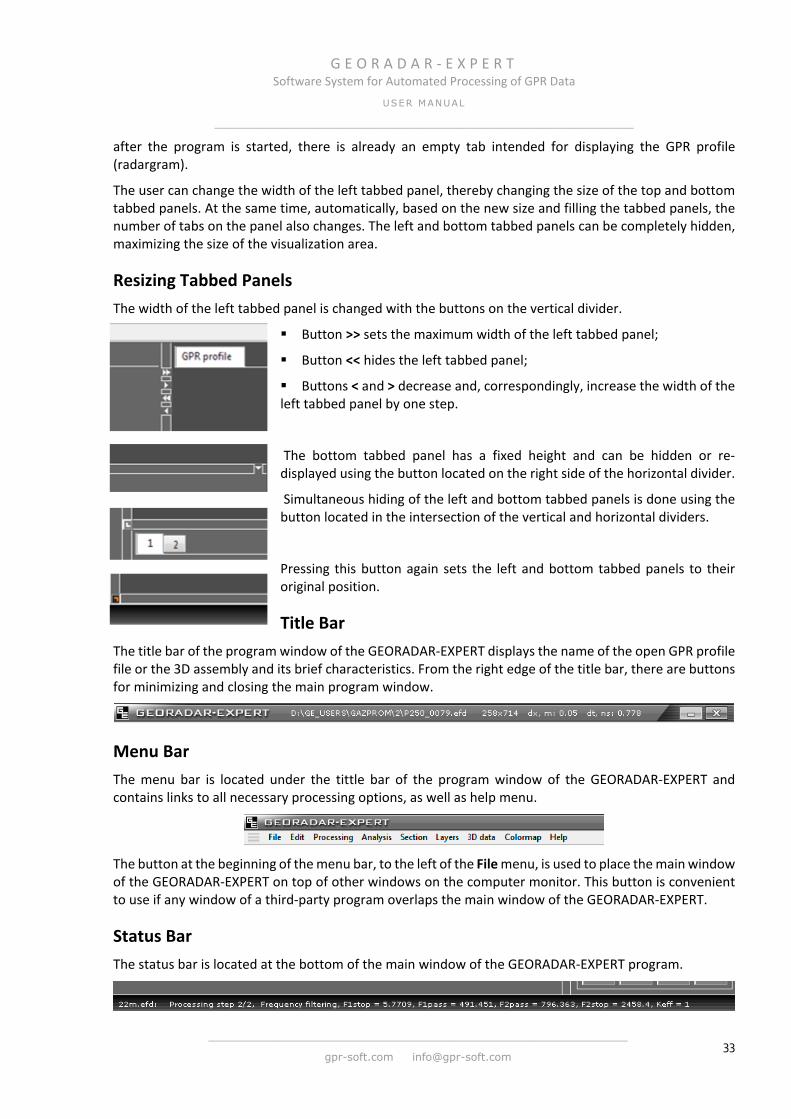
G E O R A D A R - E X P E R T Software System for Automated Processing of GPR Data
USER MANUAL
______________________________________________________________
______________________________________________________________
gpr-soft.com [email protected] 33
after the program is started, there is already an empty tab intended for displaying the GPR profile (radargram).
The user can change the width of the left tabbed panel, thereby changing the size of the top and bottom tabbed panels. At the same time, automatically, based on the new size and filling the tabbed panels, the number of tabs on the panel also changes. The left and bottom tabbed panels can be completely hidden, maximizing the size of the visualization area.
Resizing Tabbed Panels The width of the left tabbed panel is changed with the buttons on the vertical divider.
Button >> sets the maximum width of the left tabbed panel;
Button << hides the left tabbed panel;
Buttons < and > decrease and, correspondingly, increase the width of the left tabbed panel by one step.
The bottom tabbed panel has a fixed height and can be hidden or re-displayed using the button located on the right side of the horizontal divider.
Simultaneous hiding of the left and bottom tabbed panels is done using the button located in the intersection of the vertical and horizontal dividers.
Pressing this button again sets the left and bottom tabbed panels to their original position.
Title Bar The title bar of the program window of the GEORADAR-EXPERT displays the name of the open GPR profile file or the 3D assembly and its brief characteristics. From the right edge of the title bar, there are buttons for minimizing and closing the main program window.
Menu Bar The menu bar is located under the tittle bar of the program window of the GEORADAR-EXPERT and contains links to all necessary processing options, as well as help menu.
The button at the beginning of the menu bar, to the left of the File menu, is used to place the main window of the GEORADAR-EXPERT on top of other windows on the computer monitor. This button is convenient to use if any window of a third-party program overlaps the main window of the GEORADAR-EXPERT.
Status Bar The status bar is located at the bottom of the main window of the GEORADAR-EXPERT program.
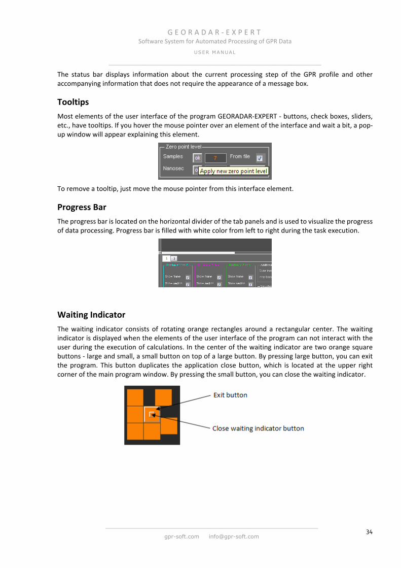
G E O R A D A R - E X P E R T Software System for Automated Processing of GPR Data
USER MANUAL
______________________________________________________________
______________________________________________________________
gpr-soft.com [email protected] 34
The status bar displays information about the current processing step of the GPR profile and other accompanying information that does not require the appearance of a message box.
Tooltips Most elements of the user interface of the program GEORADAR-EXPERT - buttons, check boxes, sliders, etc., have tooltips. If you hover the mouse pointer over an element of the interface and wait a bit, a pop-up window will appear explaining this element.
To remove a tooltip, just move the mouse pointer from this interface element.
Progress Bar The progress bar is located on the horizontal divider of the tab panels and is used to visualize the progress of data processing. Progress bar is filled with white color from left to right during the task execution.
Waiting Indicator The waiting indicator consists of rotating orange rectangles around a rectangular center. The waiting indicator is displayed when the elements of the user interface of the program can not interact with the user during the execution of calculations. In the center of the waiting indicator are two orange square buttons - large and small, a small button on top of a large button. By pressing large button, you can exit the program. This button duplicates the application close button, which is located at the upper right corner of the main program window. By pressing the small button, you can close the waiting indicator.
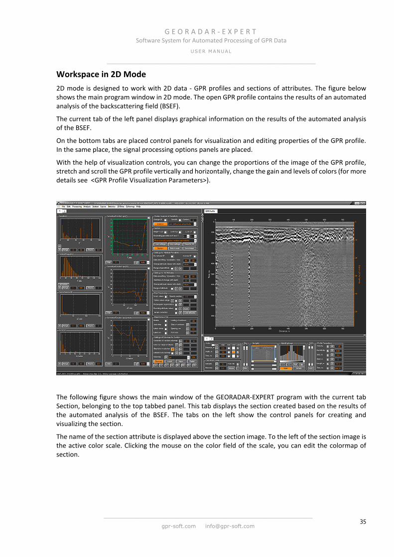
G E O R A D A R - E X P E R T Software System for Automated Processing of GPR Data
USER MANUAL
______________________________________________________________
______________________________________________________________
gpr-soft.com [email protected] 35
Workspace in 2D Mode 2D mode is designed to work with 2D data - GPR profiles and sections of attributes. The figure below shows the main program window in 2D mode. The open GPR profile contains the results of an automated analysis of the backscattering field (BSEF).
The current tab of the left panel displays graphical information on the results of the automated analysis of the BSEF.
On the bottom tabs are placed control panels for visualization and editing properties of the GPR profile. In the same place, the signal processing options panels are placed.
With the help of visualization controls, you can change the proportions of the image of the GPR profile, stretch and scroll the GPR profile vertically and horizontally, change the gain and levels of colors (for more details see <GPR Profile Visualization Parameters>).
The following figure shows the main window of the GEORADAR-EXPERT program with the current tab Section, belonging to the top tabbed panel. This tab displays the section created based on the results of the automated analysis of the BSEF. The tabs on the left show the control panels for creating and visualizing the section.
The name of the section attribute is displayed above the section image. To the left of the section image is the active color scale. Clicking the mouse on the color field of the scale, you can edit the colormap of section.
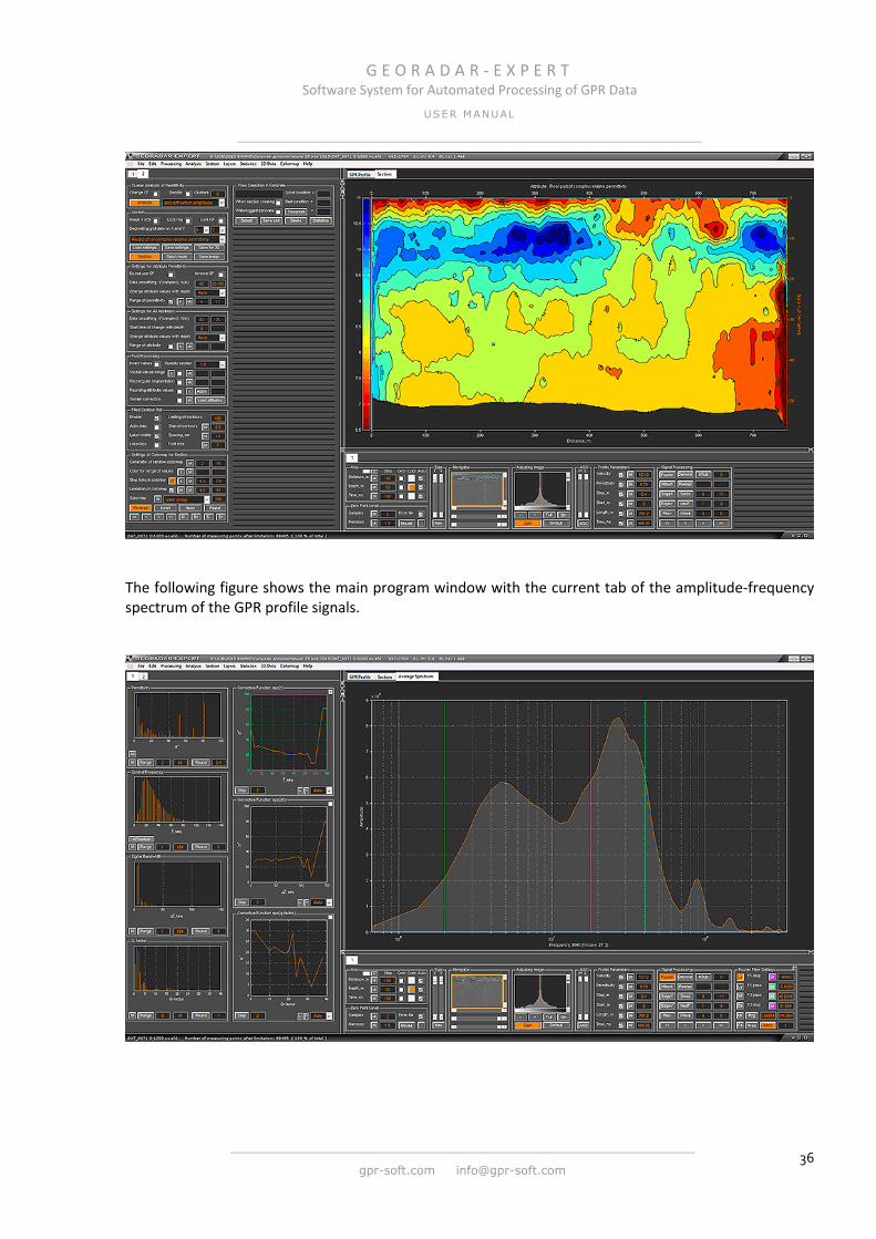
G E O R A D A R - E X P E R T Software System for Automated Processing of GPR Data
USER MANUAL
______________________________________________________________
______________________________________________________________
gpr-soft.com [email protected] 36
The following figure shows the main program window with the current tab of the amplitude-frequency spectrum of the GPR profile signals.
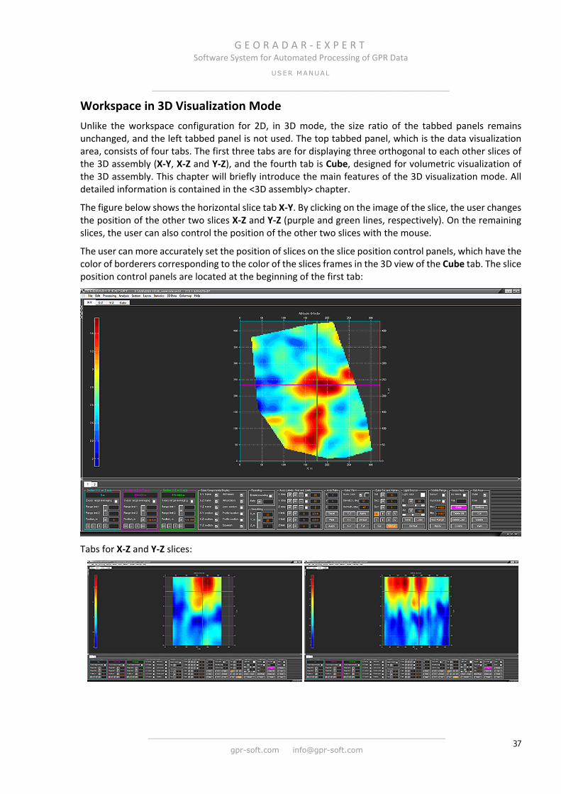
G E O R A D A R - E X P E R T Software System for Automated Processing of GPR Data
USER MANUAL
______________________________________________________________
______________________________________________________________
gpr-soft.com [email protected] 37
Workspace in 3D Visualization Mode Unlike the workspace configuration for 2D, in 3D mode, the size ratio of the tabbed panels remains unchanged, and the left tabbed panel is not used. The top tabbed panel, which is the data visualization area, consists of four tabs. The first three tabs are for displaying three orthogonal to each other slices of the 3D assembly (X-Y, X-Z and Y-Z), and the fourth tab is Cube, designed for volumetric visualization of the 3D assembly. This chapter will briefly introduce the main features of the 3D visualization mode. All detailed information is contained in the <3D assembly> chapter.
The figure below shows the horizontal slice tab X-Y. By clicking on the image of the slice, the user changes the position of the other two slices X-Z and Y-Z (purple and green lines, respectively). On the remaining slices, the user can also control the position of the other two slices with the mouse.
The user can more accurately set the position of slices on the slice position control panels, which have the color of borderers corresponding to the color of the slices frames in the 3D view of the Cube tab. The slice position control panels are located at the beginning of the first tab:
Tabs for X-Z and Y-Z slices:
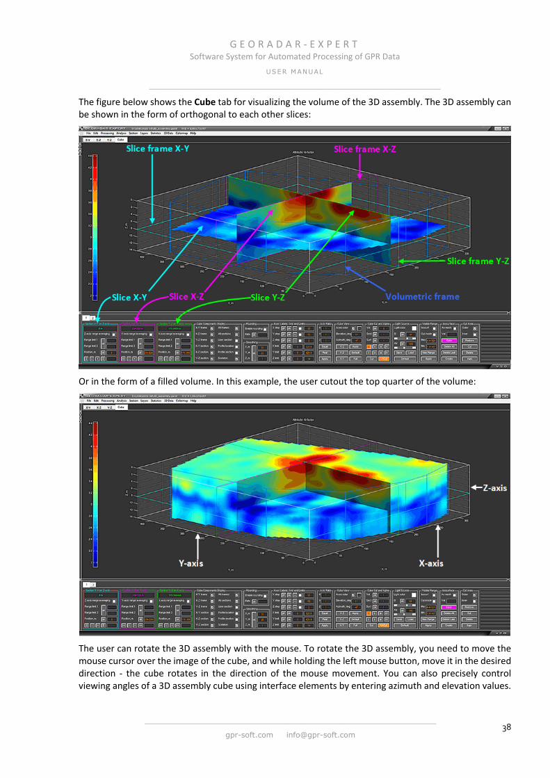
G E O R A D A R - E X P E R T Software System for Automated Processing of GPR Data
USER MANUAL
______________________________________________________________
______________________________________________________________
gpr-soft.com [email protected] 38
The figure below shows the Cube tab for visualizing the volume of the 3D assembly. The 3D assembly can be shown in the form of orthogonal to each other slices:
Or in the form of a filled volume. In this example, the user cutout the top quarter of the volume:
The user can rotate the 3D assembly with the mouse. To rotate the 3D assembly, you need to move the mouse cursor over the image of the cube, and while holding the left mouse button, move it in the desired direction - the cube rotates in the direction of the mouse movement. You can also precisely control viewing angles of a 3D assembly cube using interface elements by entering azimuth and elevation values.

G E O R A D A R - E X P E R T Software System for Automated Processing of GPR Data
USER MANUAL
______________________________________________________________
______________________________________________________________
gpr-soft.com [email protected] 39
The user can control the visibility of the 3D assembly array depending on the specified range of attribute values or by determining the location of visible areas, as well as the degree of transparency of sections, 3D assembly volume and isosurfaces on isometric projection axes. The figure below shows the result of limiting the attribute range. Areas of 3D assembly with values outside the specified range are hidden, and areas of the visible range are set by the user to translucency:
To visualize the boundaries passing through the given attribute values, the user can create isosurfaces. Using isosurfaces, it is convenient to select areas of 3D assembly containing a user-defined range of attribute values - see the figure below. For each area bounded by the isosurface, volume can be calculated.
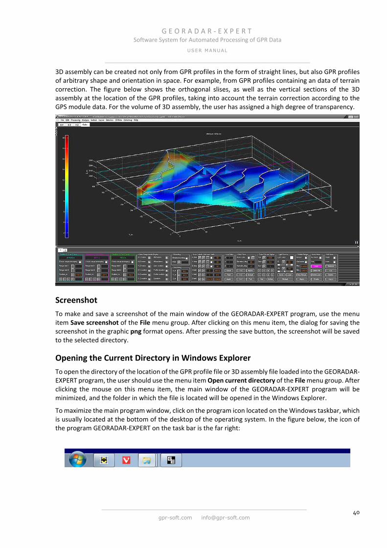
G E O R A D A R - E X P E R T Software System for Automated Processing of GPR Data
USER MANUAL
______________________________________________________________
______________________________________________________________
gpr-soft.com [email protected] 40
3D assembly can be created not only from GPR profiles in the form of straight lines, but also GPR profiles of arbitrary shape and orientation in space. For example, from GPR profiles containing an data of terrain correction. The figure below shows the orthogonal slises, as well as the vertical sections of the 3D assembly at the location of the GPR profiles, taking into account the terrain correction according to the GPS module data. For the volume of 3D assembly, the user has assigned a high degree of transparency.
Screenshot To make and save a screenshot of the main window of the GEORADAR-EXPERT program, use the menu item Save screenshot of the File menu group. After clicking on this menu item, the dialog for saving the screenshot in the graphic png format opens. After pressing the save button, the screenshot will be saved to the selected directory.
Opening the Current Directory in Windows Explorer To open the directory of the location of the GPR profile file or 3D assembly file loaded into the GEORADAR-EXPERT program, the user should use the menu item Open current directory of the File menu group. After clicking the mouse on this menu item, the main window of the GEORADAR-EXPERT program will be minimized, and the folder in which the file is located will be opened in the Windows Explorer.
To maximize the main program window, click on the program icon located on the Windows taskbar, which is usually located at the bottom of the desktop of the operating system. In the figure below, the icon of the program GEORADAR-EXPERT on the task bar is the far right:
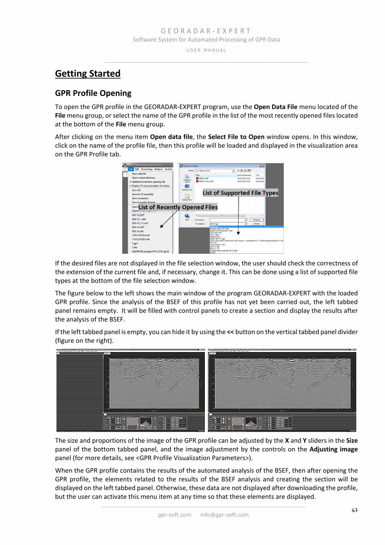
G E O R A D A R - E X P E R T Software System for Automated Processing of GPR Data
USER MANUAL
______________________________________________________________
______________________________________________________________
gpr-soft.com [email protected] 41
Getting Started
GPR Profile Opening To open the GPR profile in the GEORADAR-EXPERT program, use the Open Data File menu located of the File menu group, or select the name of the GPR profile in the list of the most recently opened files located at the bottom of the File menu group.
After clicking on the menu item Open data file, the Select File to Open window opens. In this window, click on the name of the profile file, then this profile will be loaded and displayed in the visualization area on the GPR Profile tab.
If the desired files are not displayed in the file selection window, the user should check the correctness of the extension of the current file and, if necessary, change it. This can be done using a list of supported file types at the bottom of the file selection window.
The figure below to the left shows the main window of the program GEORADAR-EXPERT with the loaded GPR profile. Since the analysis of the BSEF of this profile has not yet been carried out, the left tabbed panel remains empty. It will be filled with control panels to create a section and display the results after the analysis of the BSEF.
If the left tabbed panel is empty, you can hide it by using the << button on the vertical tabbed panel divider (figure on the right).
The size and proportions of the image of the GPR profile can be adjusted by the X and Y sliders in the Size panel of the bottom tabbed panel, and the image adjustment by the controls on the Adjusting image panel (for more details, see <GPR Profile Visualization Parameters>).
When the GPR profile contains the results of the automated analysis of the BSEF, then after opening the GPR profile, the elements related to the results of the BSEF analysis and creating the section will be displayed on the left tabbed panel. Otherwise, these data are not displayed after downloading the profile, but the user can activate this menu item at any time so that these elements are displayed.
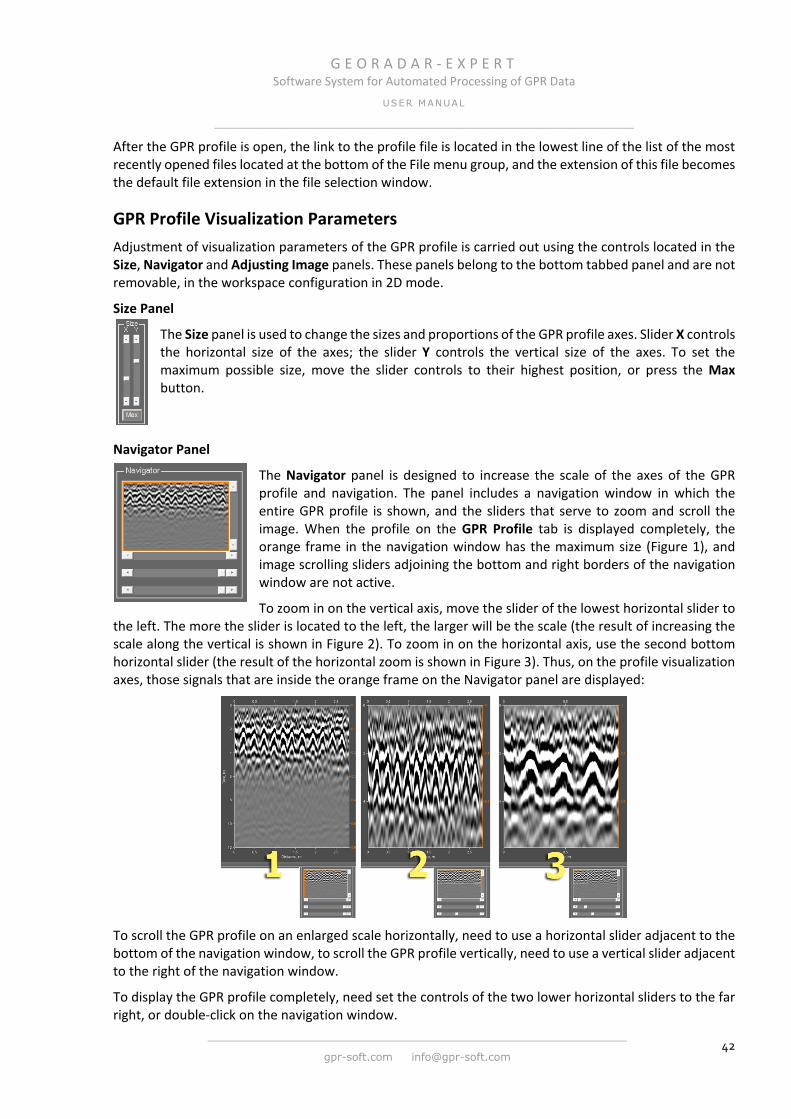
G E O R A D A R - E X P E R T Software System for Automated Processing of GPR Data
USER MANUAL
______________________________________________________________
______________________________________________________________
gpr-soft.com [email protected] 42
After the GPR profile is open, the link to the profile file is located in the lowest line of the list of the most recently opened files located at the bottom of the File menu group, and the extension of this file becomes the default file extension in the file selection window.
GPR Profile Visualization Parameters Adjustment of visualization parameters of the GPR profile is carried out using the controls located in the Size, Navigator and Adjusting Image panels. These panels belong to the bottom tabbed panel and are not removable, in the workspace configuration in 2D mode.
Size Panel
The Size panel is used to change the sizes and proportions of the GPR profile axes. Slider X controls the horizontal size of the axes; the slider Y controls the vertical size of the axes. To set the maximum possible size, move the slider controls to their highest position, or press the Max button.
Navigator Panel
The Navigator panel is designed to increase the scale of the axes of the GPR profile and navigation. The panel includes a navigation window in which the entire GPR profile is shown, and the sliders that serve to zoom and scroll the image. When the profile on the GPR Profile tab is displayed completely, the orange frame in the navigation window has the maximum size (Figure 1), and image scrolling sliders adjoining the bottom and right borders of the navigation window are not active.
To zoom in on the vertical axis, move the slider of the lowest horizontal slider to the left. The more the slider is located to the left, the larger will be the scale (the result of increasing the scale along the vertical is shown in Figure 2). To zoom in on the horizontal axis, use the second bottom horizontal slider (the result of the horizontal zoom is shown in Figure 3). Thus, on the profile visualization axes, those signals that are inside the orange frame on the Navigator panel are displayed:
To scroll the GPR profile on an enlarged scale horizontally, need to use a horizontal slider adjacent to the bottom of the navigation window, to scroll the GPR profile vertically, need to use a vertical slider adjacent to the right of the navigation window.
To display the GPR profile completely, need set the controls of the two lower horizontal sliders to the far right, or double-click on the navigation window.
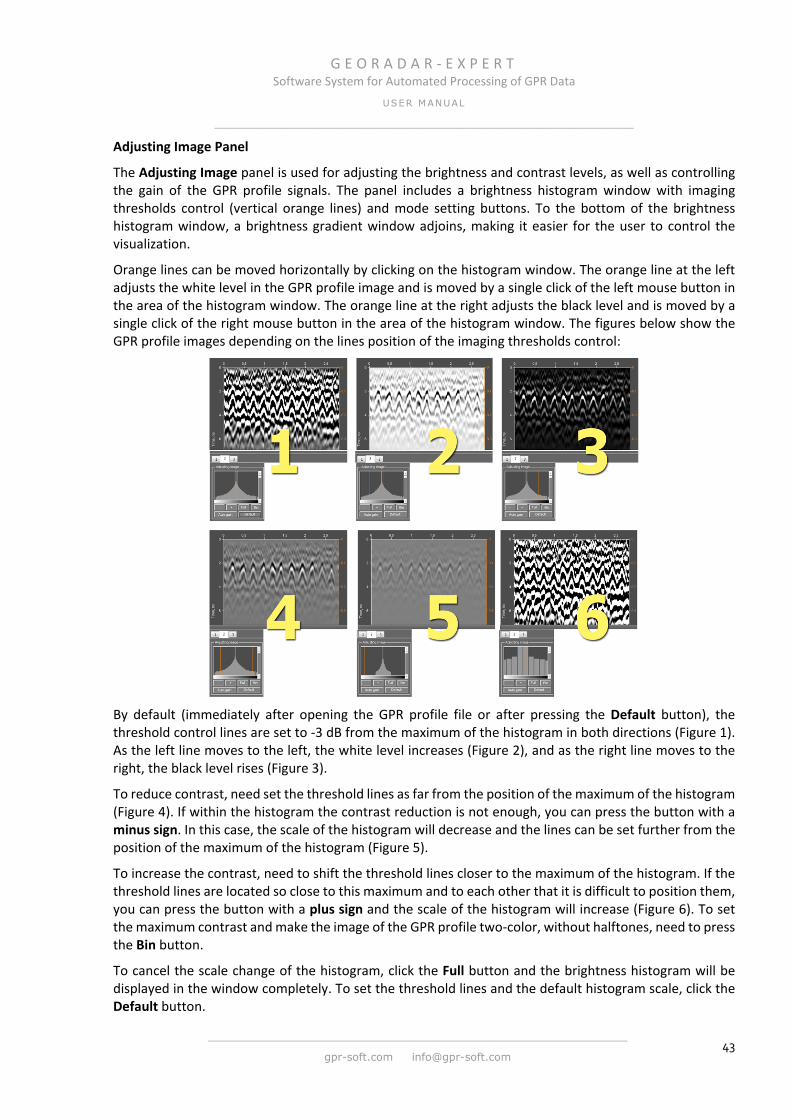
G E O R A D A R - E X P E R T Software System for Automated Processing of GPR Data
USER MANUAL
______________________________________________________________
______________________________________________________________
gpr-soft.com [email protected] 43
Adjusting Image Panel
The Adjusting Image panel is used for adjusting the brightness and contrast levels, as well as controlling the gain of the GPR profile signals. The panel includes a brightness histogram window with imaging thresholds control (vertical orange lines) and mode setting buttons. To the bottom of the brightness histogram window, a brightness gradient window adjoins, making it easier for the user to control the visualization.
Orange lines can be moved horizontally by clicking on the histogram window. The orange line at the left adjusts the white level in the GPR profile image and is moved by a single click of the left mouse button in the area of the histogram window. The orange line at the right adjusts the black level and is moved by a single click of the right mouse button in the area of the histogram window. The figures below show the GPR profile images depending on the lines position of the imaging thresholds control:
By default (immediately after opening the GPR profile file or after pressing the Default button), the threshold control lines are set to -3 dB from the maximum of the histogram in both directions (Figure 1). As the left line moves to the left, the white level increases (Figure 2), and as the right line moves to the right, the black level rises (Figure 3).
To reduce contrast, need set the threshold lines as far from the position of the maximum of the histogram (Figure 4). If within the histogram the contrast reduction is not enough, you can press the button with a minus sign. In this case, the scale of the histogram will decrease and the lines can be set further from the position of the maximum of the histogram (Figure 5).
To increase the contrast, need to shift the threshold lines closer to the maximum of the histogram. If the threshold lines are located so close to this maximum and to each other that it is difficult to position them, you can press the button with a plus sign and the scale of the histogram will increase (Figure 6). To set the maximum contrast and make the image of the GPR profile two-color, without halftones, need to press the Bin button.
To cancel the scale change of the histogram, click the Full button and the brightness histogram will be displayed in the window completely. To set the threshold lines and the default histogram scale, click the Default button.
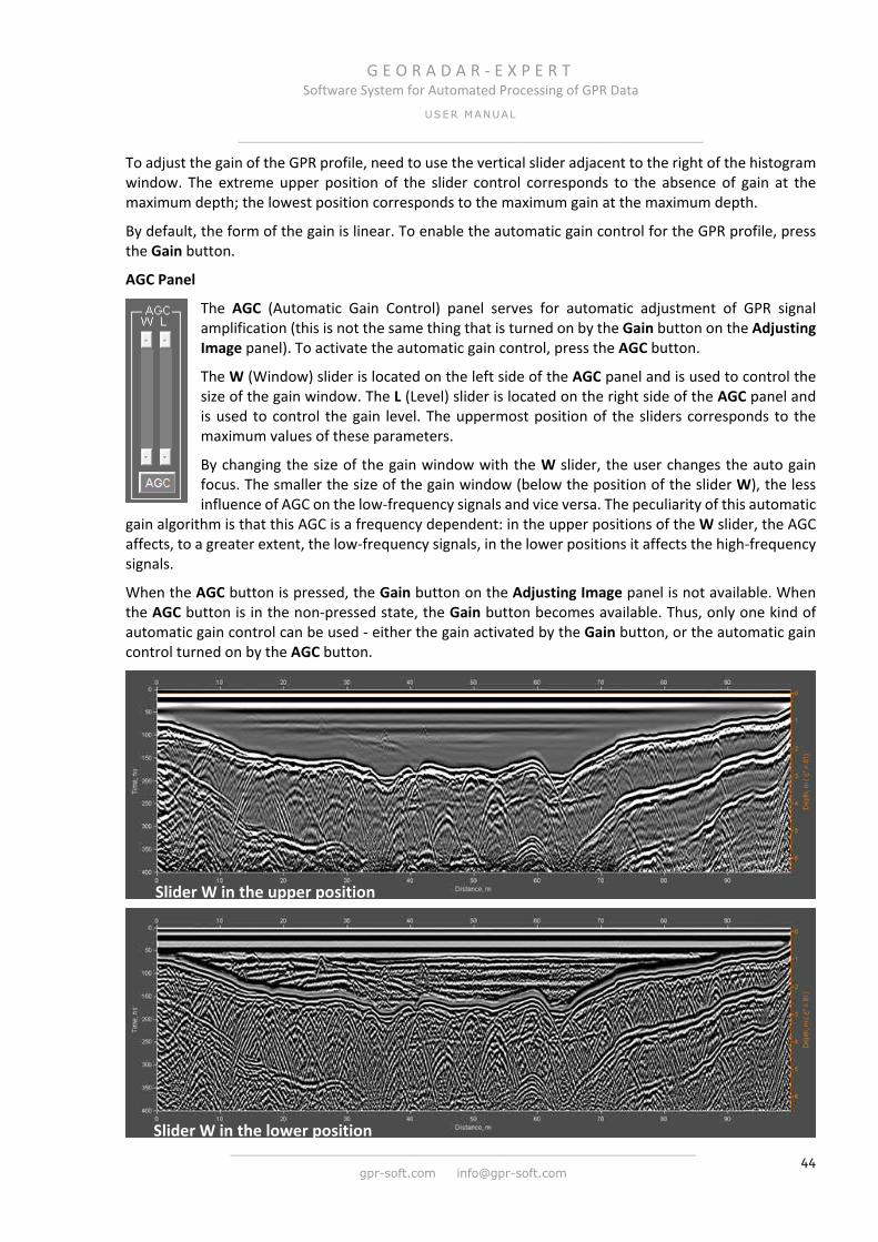
G E O R A D A R - E X P E R T Software System for Automated Processing of GPR Data
USER MANUAL
______________________________________________________________
______________________________________________________________
gpr-soft.com [email protected] 44
To adjust the gain of the GPR profile, need to use the vertical slider adjacent to the right of the histogram window. The extreme upper position of the slider control corresponds to the absence of gain at the maximum depth; the lowest position corresponds to the maximum gain at the maximum depth.
By default, the form of the gain is linear. To enable the automatic gain control for the GPR profile, press the Gain button.
AGC Panel
The AGC (Automatic Gain Control) panel serves for automatic adjustment of GPR signal amplification (this is not the same thing that is turned on by the Gain button on the Adjusting Image panel). To activate the automatic gain control, press the AGC button.
The W (Window) slider is located on the left side of the AGC panel and is used to control the size of the gain window. The L (Level) slider is located on the right side of the AGC panel and is used to control the gain level. The uppermost position of the sliders corresponds to the maximum values of these parameters.
By changing the size of the gain window with the W slider, the user changes the auto gain focus. The smaller the size of the gain window (below the position of the slider W), the less influence of AGC on the low-frequency signals and vice versa. The peculiarity of this automatic
gain algorithm is that this AGC is a frequency dependent: in the upper positions of the W slider, the AGC affects, to a greater extent, the low-frequency signals, in the lower positions it affects the high-frequency signals.
When the AGC button is pressed, the Gain button on the Adjusting Image panel is not available. When the AGC button is in the non-pressed state, the Gain button becomes available. Thus, only one kind of automatic gain control can be used - either the gain activated by the Gain button, or the automatic gain control turned on by the AGC button.
Slider W in the upper position
Slider W in the lower position

G E O R A D A R - E X P E R T Software System for Automated Processing of GPR Data
USER MANUAL
______________________________________________________________
______________________________________________________________
gpr-soft.com [email protected] 45
Zero Point Level Setting
The position of the zero point level of the depth scale of the GPR profile is adjusted on the Zero point level panel which is placed on the bottom tabbed panel in the 2D mode workspace configuration. The user can adjust the zero point level in several ways:
Enter the value of the zero point level position in nanoseconds in the Nanosec input window, and then press the ok button located to the left;
Enter the sample number of the GPR trace in the Samples input box, and then press the ok button located to the left;
Switch the Mouse button to the pressed position, move the mouse pointer over the GPR profile image, click once with the left mouse button. After clicking, the zero level will take the position of the mouse pointer. To exit the zero-setting mode with the mouse, need to move the Mouse button to the unpressed position;
Switch the Mouse button to the pressed position and and then switch the A button to the pressed position. As a result, the automatic zero-setting mode is activated. Move the mouse pointer over the GPR profile image and click once with the left mouse button. After that, the zero level will take the position of the nearest local maximum of the envelope of the averaged GPR trace. To exit the automatic zero-setting mode, need to move the Mouse button to the unpressed position.
If the From file checkbox is activated, the information on the position of the zero level is read from the profile's GPR file during the opening process. If there is no information about the zero position in the GPR profile file, the zero level position is set to 0 nanoseconds (or sample 1).
If the checkbox From file is not checked, then when the next profile is opened, the zero point position will be read from the Samples input window.
Axis and Mouse Pointer Properties The properties of the axes and the mouse pointer are set in the Axis panel that belongs to the bottom tabbed panel in the 2D workspace configuration. For each type of axes, there is a single-type set of parameters. On the left are the names of the axes:
Distance, m - horizontal axis of the length of the GPR profile or section in meters;
Depth, m – axis of the depth scale, located on the right edge of the image of the GPR profile or section. Graduates in meters;
Time, ns – axis of the two-way travel time of a GPR waves in nanoseconds. This axis is only on the image of the GPR profile and is located on the left edge.
Next are the ok buttons, which apply the labels steps for the respective axes, according to the values in the Step input box to the right of these buttons.
The Grid checkbox controls the display of the grid lines perpendicular to the respective axis, and when the Color button is pressed, a pop-up window for selecting the color of the respective axis appears. The Color button has the color of its axis.

G E O R A D A R - E X P E R T Software System for Automated Processing of GPR Data
USER MANUAL
______________________________________________________________
______________________________________________________________
gpr-soft.com [email protected] 46
When the Auto checkbox is selected, the axes properties are set by default based on the length of the GPR profile and the time of the two-way travel time of the wave. If this checkbox is not checked, then when open a new GPR profile file, the already set properties of the axes do not change.
The image of a section or GPR profile saved in a graphical format has the same properties of the axes as in the program workspace.
If the button + is in the pressed state and the mouse pointer is within the axes of the GPR profile or section image, this pointer will be in the information mode. In this mode, the mouse pointer has the form of a crosshair passing through the entire visualization area. Next to the crosshair is the text box, which contains the parameters of the point, which is located in the crosshairs of the pointer (see the figure on the left).
By default, the background color of the text box is transparent, and the text font is white. If you click on the spacebar on the computer's keyboard, the color of the box text will turn orange. If you click spacebar again, the color becomes transparent again.
To change the color of the box's font, click the font color selection button located to the left of the button +. Activation of the information mode is
performed only for the current tab. When you switch to another tab where this mode is not activated, the mouse pointer will be an arrow.
To exit the information mode of the mouse pointer, you need to set the button + to the unpressed state.
Note: The information mode is available not only on the tabs for visualization of the GPR profile and sections, but also on the tab of the amplitude-frequency spectrum.
Editing Parameters GPR Profile You can edit the parameters of the GPR Profile on the Profile Parameters panel that belongs to the bottom tabbed panel in the 2D workspace configuration.
For each parameter of the GPR profile, there is a one-type set of interface elements. The name of the parameter is on the left. More to the right is the checkbox, which determines the source of information on this parameter. If the checkbox is checked, the parameter information is read from this file during the opening of the GPR profile file. If the checkbox is not checked, the data is read from the input window of this parameter, located to the right. The ok buttons
are used to apply user-defined parameter values to the GPR profile.
On the Profile Parameters panel, you can edit the following parameters of the GPR profile:
Velosity – the average speed of propagation of electromagnetic waves in cm/ns;
Permittivity – the average value of the real part of the complex relative permittivity. Velocity of the
waves and the real part of the complex relative permittivity are related as follows: v = c / ′ε , where c is the speed of light in a vacuum, and v is the velocity of an electromagnetic wave in a subsurface medium. If you change the permittivity value in the input window and press the ok button, the value in the velosity input window will change according to the above formula. And

G E O R A D A R - E X P E R T Software System for Automated Processing of GPR Data
USER MANUAL
______________________________________________________________
______________________________________________________________
gpr-soft.com [email protected] 47
conversely, changing the value of the velocity, the value of the permittivity changes. As a result of a change in the permittivity or velocity, the axis of the depth scale changes;
Step, m - GPR profiling step (distance between GPR traces) in meters. After changing this parameter, the length of the GPR profile changes (parameter Length, m);
Start, m – the position of the 1-st GPR trace on the distance scale (the start of the GPR profile) in meters. Most often has a zero value;
Length, m – the length of the GPR profile in meters. After changing this parameter, the value of the profiling step changes (parameter Step, m);
Time, ns – the value of the two-way travel time of a GPR waves in nanoseconds.
Cut GPR Profile The cutting or cropping of the GPR profile is set in the Cut panel. To call the Cut panel, click the Cut GPR Profile menu item located in the Edit menu group. The panel will be located in the bottom tabbed panel. You can remove the Cut panel using the close button X located in the upper right corner of the Cut panel.
The horizontal cutting borders are specified by the parameters X1, m and X2, m and are measured in meters. The cutting borders along the vertical are specified by the parameters Y1, ns and Y2, ns and are measured in nanoseconds. To determine the boundaries of the cropping, it is convenient to use the mouse pointer in the information mode (for more
details, see <Axis and Mouse Pointer Properties>).
When the Cut edges button is pressed, the GPR profile areas of the profile are located outside the specified borders. When you click the Cut within button, the area within the specified borders is deleted.
If you want to crop the horizontal profile of the horizontal only from the right edge, you only need to enter one value of X2, m and click the Cut edges button. If you need to crop only from the left edge, you only need to enter one value X1, m and click the Cut edges button. The same principle also applies to vertical borders.
Dividing GPR Profile into Fragments Long GPR profiles can be divided into shorter fragments. This will optimize the resources of the computer while processing the GPR data. You can also divide the sections saved in the XZD format file, from which the 3D assemblies are created.
To start the process of dividing the GPR profiles into fragments, use the Divide GPR Profile or XZD menu item located in the Edit menu group. After the user clicks on this menu item, a pop-up window will appear in the center of the main program window with the parameters of the dividing. The user must specify the fragment length in the Length of fragments, m window, then click the Current or Open button.
The Current button starts the process of dividing the open GPR profile. The Open button starts the process of dividing the GPR profiles that are not yet open. After clicking on this button, the file selection window opens, where you can select one or several GPR profiles. After selecting files, the window closes and the partitioning process starts automatically.
To save the results of the dividing, he program creates a new folder in the directory of the profile being dividing. The folder name is formed as follows: for example, the filename of the GPR profile is FILENAME.gpr. Let's assume that this GPR profile has a length of 2.5 m and is divided into fragments
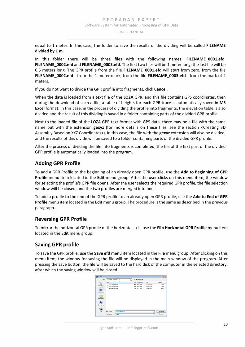
G E O R A D A R - E X P E R T Software System for Automated Processing of GPR Data
USER MANUAL
______________________________________________________________
______________________________________________________________
gpr-soft.com [email protected] 48
equal to 1 meter. In this case, the folder to save the results of the dividing will be called FILENAME divided by 1 m.
In this folder there will be three files with the following names: FILENAME_0001.efd, FILENAME_0002.efd and FILENAME_0003.efd. The first two files will be 1 meter long; the last file will be 0.5 meters long. The GPR profile from the file FILENAME_0001.efd will start from zero, from the file FILENAME_0002.efd - from the 1 meter mark, from the file FILENAME_0003.efd - from the mark of 2 meters.
If you do not want to divide the GPR profile into fragments, click Cancel.
When the data is loaded from a text file of the LOZA GPR, and this file contains GPS coordinates, then during the download of such a file, a table of heights for each GPR trace is automatically saved in MS Excel format. In this case, in the process of dividing the profile into fragments, the elevation table is also divided and the result of this dividing is saved in a folder containing parts of the divided GPR profile.
Next to the loaded file of the LOZA GPR text format with GPS data, there may be a file with the same name but with the extension gexyz (for more details on these files, see the section <Creating 3D Assembly Based on XYZ Coordinates>). In this case, the file with the gexyz extension will also be divided, and the results of this divide will be saved to a folder containing parts of the divided GPR profile.
After the process of dividing the file into fragments is completed, the file of the first part of the divided GPR profile is automatically loaded into the program.
Adding GPR Profile To add a GPR Profile to the beginning of an already open GPR profile, use the Add to Beginning of GPR Profile menu item located in the Edit menu group. After the user clicks on this menu item, the window for selecting the profile's GPR file opens. After the user selects the required GPR profile, the file selection window will be closed, and the two profiles are merged into one.
To add a profile to the end of the GPR profile to an already open GPR profile, use the Add to End of GPR Profile menu item located in the Edit menu group. The procedure is the same as described in the previous paragraph.
Reversing GPR Profile To mirror the horizontal GPR profile of the horizontal axis, use the Flip Horizontal GPR Profile menu item located in the Edit menu group.
Saving GPR profile To save the GPR profile, use the Save efd menu item located in the File menu group. After clicking on this menu item, the window for saving the file will be displayed in the main window of the program. After pressing the save button, the file will be saved to the hard disk of the computer in the selected directory, after which the saving window will be closed.

G E O R A D A R - E X P E R T Software System for Automated Processing of GPR Data
USER MANUAL
______________________________________________________________
______________________________________________________________
gpr-soft.com [email protected] 49
In the GEORADAR-EXPERT, the GPR profile data is saved only in the efd format. The file in this format contains the data of both the GPR profile itself and the results of the analysis of the BSEF of this profile, if this analysis was performed earlier.
Note: If the GPR profile has been preprocessed before the analysis of BSEF, then those GPR profile signals are stored in the efd file at the processing step that is currently being visualized. The processing flow to the efd file is not saved. For this purpose, a file with the gepro extension is intended. To save the processing thread (history) to a file with the gepro extension, use the menu item Save Processing History, located in the Processing menu group.
Scope of Work The table of the scope of work consists of two columns. The first column contains the names of the GPR profiles; the second column contains the lengths of these GPR profiles in meters. The last two bottom rows contain information about the number of GPR profiles in the table and their total length.
To create a table of the scope of work in MS EXCEL format, use the Scope of Work menu item located in the Analysis menu group. After the user clicks the Scope of Work menu item, the file selection window opens, in which need select the GPR profile files and click the Open button.
After clicking the Open button, the process of creating the table starts. During the creation of the table, the program alternately reads the lengths of the GPR profiles from the files and puts these values in the table, while informing the user about the name of the current GPR profile and its sequence number using the message box.
After the table is fully formed, it is automatically saved in the directory of the location of the GPR profile files, into a spreadsheet format file of MS EXCEL under the name Summary table - scope of work, after which information about the completion of the table creation process is displayed on the message box.
To open the directory in which the file of the table of the scope of work is saved, it is convenient to use the menu item Open Current Directory, located in the group of the File menu.
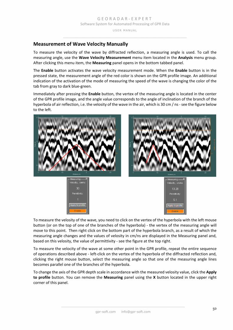
G E O R A D A R - E X P E R T Software System for Automated Processing of GPR Data
USER MANUAL
______________________________________________________________
______________________________________________________________
gpr-soft.com [email protected] 50
Measurement of Wave Velocity Manually To measure the velocity of the wave by diffracted reflection, a measuring angle is used. To call the measuring angle, use the Wave Velocity Measurement menu item located in the Analysis menu group. After clicking this menu item, the Measuring panel opens in the bottom tabbed panel.
The Enable button activates the wave velocity measurement mode. When the Enable button is in the pressed state, the measurement angle of the red color is shown on the GPR profile image. An additional indication of the activation of the mode of measuring the speed of the wave is changing the color of the tab from gray to dark blue-green.
Immediately after pressing the Enable button, the vertex of the measuring angle is located in the center of the GPR profile image, and the angle value corresponds to the angle of inclination of the branch of the hyperbola of air reflection, i.e. the velosity of the wave in the air, which is 30 cm / ns - see the figure below to the left.
To measure the velosity of the wave, you need to click on the vertex of the hyperbola with the left mouse button (or on the top of one of the branches of the hyperbola) - the vertex of the measuring angle will move to this point. Then right click on the bottom part of the hyperbola branch, as a result of which the measuring angle changes and the values of velosity in cm/ns are displayed in the Measuring panel and, based on this velosity, the value of permittivity - see the figure at the top right.
To measure the velocity of the wave at some other point in the GPR profile, repeat the entire sequence of operations described above - left-click on the vertex of the hyperbola of the diffracted reflection and, clicking the right mouse button, select the measuring angle so that one of the measuring angle lines becomes parallel one of the branches of the hyperbola.
To change the axis of the GPR depth scale in accordance with the measured velosity value, click the Apply to profile button. You can remove the Measuring panel using the X button located in the upper right corner of this panel.

G E O R A D A R - E X P E R T Software System for Automated Processing of GPR Data
USER MANUAL
______________________________________________________________
______________________________________________________________
gpr-soft.com [email protected] 51
Processing of GPR Signals Control elements for setting and starting the options for processing the GPR profile signals are located on the Signal Processing panel. This panel is located on the bottom tabbed panel in the workspace configuration in 2D mode. In the lowest row of the Signal Processing panel, there are buttons for moving through the processing steps.
The input box located in one row and the nearest button on the left belong to one processing option. For example, the MedF button starts the median filtering process, the parameters of which are specified in the input box to
the right of this button. Buttons that do not have input box adjacent to them on the right belong to processing that do not have any settings.To display a tooltip for controls, you need to hover the mouse over the desired item and wait a bit until the tooltip appears.
Unlike other buttons, pressing the Fourier button does not start the processing process, but calls up the frequency filtering settings panel and creates a new tab in the top tabbed panel to display the signal spectrum (for more details, see <Frequency Filtering>).
The processing is carried out as follows: the user enters the processing parameters (if they are provided) and presses the start button of the process. After the processing is completed, the GPR profile image is updated on the GPR Profile tab, and the parameters and the modified signals of the GPR profile are added to the processing history.
Frequency Filtering To call the Fourier Filter Settings panel, click the Fourier button and the Fourier Filter Settings panel will appear in the bottom tabbed panel. At the same time, the Average Spectrum tab appears in the top tabbed panel. This tab serves to visualize the averaged amplitude-frequency spectrum of the GPR profile signals (or a user-defined profile fragment).
On the axis of the spectrum, there is visualization of the filter boundaries in the form of vertical lines, the position of which corresponds to the specified values. The boundaries of the stop frequencies have a violet color; the pass frequency boundaries are green.
Filter boundaries defined by the following values (in MHz):
F1 stop – frequency at the edge of the start of the first stop band;
F1 pass – frequency at the edge of the start of the pass band;
F2 pass – frequency at the edge of the end of the pass band;
F2 stop – frequency at the edge of the start of the second stop band.
For clarity, the buttons for applying the filtering boundaries and the corresponding boundary lines on the spectrum graph have the same color. To specify the exact values of the filter boundary in megahertz, enter the value in the corresponding input window and press the ok button to the left of the input window, after which the boundary lines will occupy the position in accordance with the entered values.
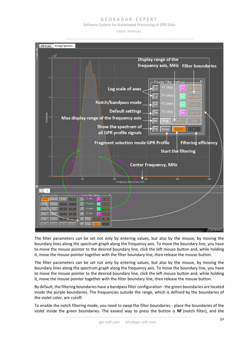
G E O R A D A R - E X P E R T Software System for Automated Processing of GPR Data
USER MANUAL
______________________________________________________________
______________________________________________________________
gpr-soft.com [email protected] 52
The filter parameters can be set not only by entering values, but also by the mouse, by moving the boundary lines along the spectrum graph along the frequency axis. To move the boundary line, you have to move the mouse pointer to the desired boundary line, click the left mouse button and, while holding it, move the mouse pointer together with the filter boundary line, then release the mouse button.
The filter parameters can be set not only by entering values, but also by the mouse, by moving the boundary lines along the spectrum graph along the frequency axis. To move the boundary line, you have to move the mouse pointer to the desired boundary line, click the left mouse button and, while holding it, move the mouse pointer together with the filter boundary line, then release the mouse button.
By default, the filtering boundaries have a bandpass filter configuration - the green boundaries are located inside the purple boundaries. The frequencies outside the range, which is defined by the boundaries of the violet color, are cutoff.
To enable the notch filtering mode, you need to swap the filter boundaries - place the boundaries of the violet inside the green boundaries. The easiest way to press the button is Nf (notch filter), and the
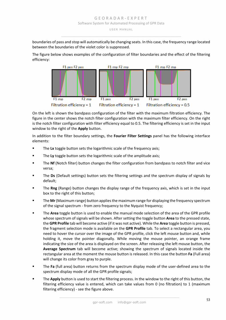
G E O R A D A R - E X P E R T Software System for Automated Processing of GPR Data
USER MANUAL
______________________________________________________________
______________________________________________________________
gpr-soft.com [email protected] 53
boundaries of pass and stop will automatically be changing seats. In this case, the frequency range located between the boundaries of the violet color is suppressed.
The figure below shows examples of the configuration of filter boundaries and the effect of the filtering efficiency:
On the left is shown the bandpass configuration of the filter with the maximum filtration efficiency. The figure in the center shows the notch filter configuration with the maximum filter efficiency. On the right is the notch filter configuration with filter efficiency equal to 0.5. The filtering efficiency is set in the input window to the right of the Apply button.
In addition to the filter boundary settings, the Fourier Filter Settings panel has the following interface elements:
The Lx toggle button sets the logarithmic scale of the frequency axis;
The Ly toggle button sets the logarithmic scale of the amplitude axis;
The Nf (Notch filter) button changes the filter configuration from bandpass to notch filter and vice versa;
The Ds (Default settings) button sets the filtering settings and the spectrum display of signals by default;
The Rng (Range) button changes the display range of the frequency axis, which is set in the input box to the right of this button;
The Mr (Maximum range) button applies the maximum range for displaying the frequency spectrum of the signal spectrum - from zero frequency to the Nyquist frequency;
The Area toggle button is used to enable the manual mode selection of the area of the GPR profile whose spectrum of signals will be shown. After setting the toggle button Area to the pressed state, the GPR Profile tab will become active (if it was not active). While the Area toggle button is pressed, the fragment selection mode is available on the GPR Profile tab. To select a rectangular area, you need to hover the cursor over the image of the GPR profile, click the left mouse button and, while holding it, move the pointer diagonally. While moving the mouse pointer, an orange frame indicating the size of the area is displayed on the screen. After releasing the left mouse button, the Average Spectrum tab will become active; showing the spectrum of signals located inside the rectangular area at the moment the mouse button is released. In this case the button Fa (Full area) will change its color from gray to purple.
The Fa (full area) button returns from the spectrum display mode of the user-defined area to the spectrum display mode of all the GPR profile signals;
The Apply button is used to start the filtering process. In the window to the right of this button, the filtering efficiency value is entered, which can take values from 0 (no filtration) to 1 (maximum filtering efficiency) - see the figure above.

G E O R A D A R - E X P E R T Software System for Automated Processing of GPR Data
USER MANUAL
______________________________________________________________
______________________________________________________________
gpr-soft.com [email protected] 54
You can remove the Fourier Filter Settings panel by pressing the X button in the upper right corner of the panel, or by pressing the Fourier button on the Signal Processing panel. Simultaneously with deleting the Fourier Filter Settings panel, the Average Spectrum tab is deleted.
2D median filtering Median filtering can effectively deal with random short-duration interference.
The MedF button runs the median filtering process. In the input box located to the right of this button, the values of the median filter window size are entered. In the window closest to the MedF button, enter the size of the median filter window horizontally (in the GPR traces), in the next window - the size of the median filter window in the vertical (in samples).
The following is an illustration of the operation of the median filter. In the figure to the left, a GPR profile with high-amplitude interference in the form of a short peak is shown. This interference is displayed as a bright white dot at the bottom of the GPR profile between 150 and 200 meters on the distance scale. The figure on the right shows the result of applying a median filter with a filter window of size 1x1.
Smoothing The Smoo button starts the process of smoothing of the GPR profile signals with a 2D averaging filter. The size of smoothing window is specified using the input box that are located to the right of the Smoo button. In the window closest to this button, specifies the size of the smoothing window horizontally (in meters), in the other window the vertical size of the window (in the samples) is specified.
Smoothing can be effectively applied in an excessively detailed wave pattern of the GPR profile. When the reflection from the extended layer boundary is disturbed by numerous diffracted reflections from the bed of gravel above, for example. After applying 2D smoothing, this layer boundary on the GPR profile will look better.

G E O R A D A R - E X P E R T Software System for Automated Processing of GPR Data
USER MANUAL
______________________________________________________________
______________________________________________________________
gpr-soft.com [email protected] 55
Hilbert Transform The process of envelope detection of signals for the traces of GPR profile by means of the Hilbert transform is started by the Hilbert button. This processing option has no settings. The following figure shows an example of applying a Hilbert transform. Figure 1 shows a GPR profile obtained during a survey of a reinforced concrete slab with one row of reinforcement. It is required to show the reflection from the lower boundary of this reinforced concrete slab. Direct wave has already been removed using the processing Subtract average (ASub button, parameter 0).
To do this, apply the envelope detection of the GPR profile signals (Figure 2) and smooth the signals horizontally with a small window = 0.25 m (Figure 3). As a result of these actions, there are unipolar signals of low frequency, the spectrum of which is shown in figure 4. To increase the detail of the signals after the envelope detection and smoothing, need to suppress the lower frequencies. To do this, perform band-pass filtering, leaving the region of high-amplitude low frequencies outside the filter boundaries. On figure 4 shows the position of the bandpass filter boundaries. As a result of the above actions, the desired boundary is visible at a depth of about 0.2 meters (Figure 5).
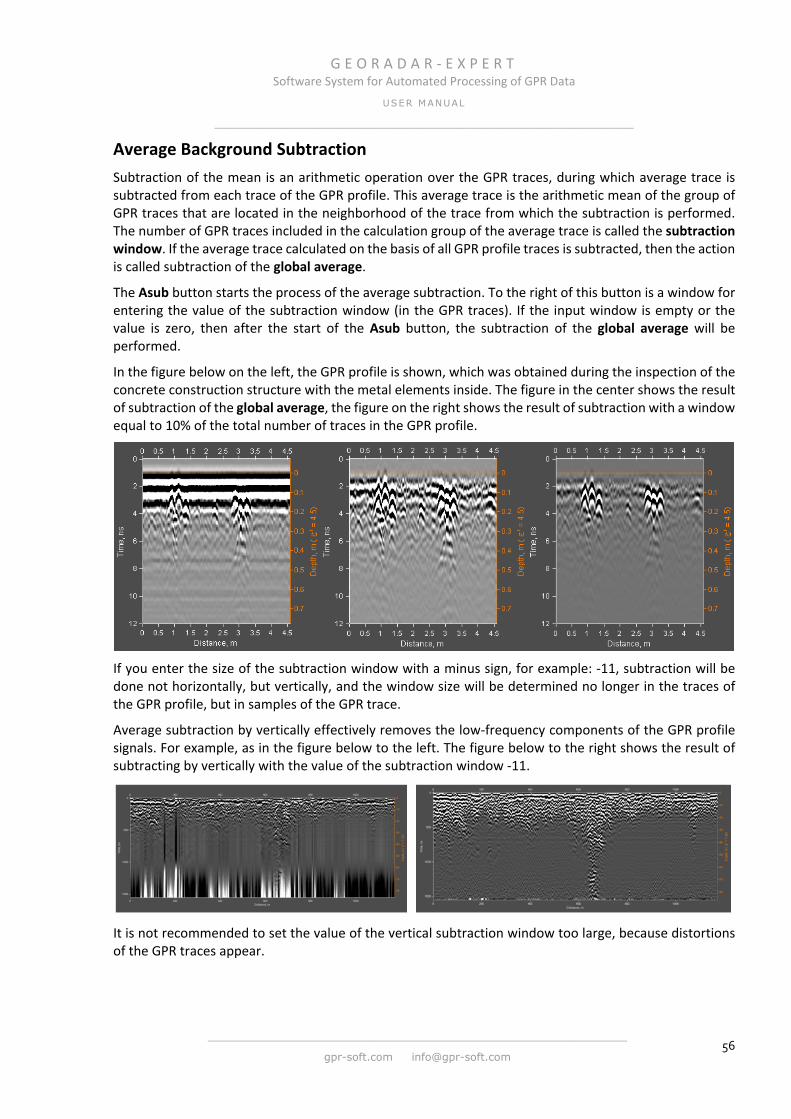
G E O R A D A R - E X P E R T Software System for Automated Processing of GPR Data
USER MANUAL
______________________________________________________________
______________________________________________________________
gpr-soft.com [email protected] 56
Average Background Subtraction Subtraction of the mean is an arithmetic operation over the GPR traces, during which average trace is subtracted from each trace of the GPR profile. This average trace is the arithmetic mean of the group of GPR traces that are located in the neighborhood of the trace from which the subtraction is performed. The number of GPR traces included in the calculation group of the average trace is called the subtraction window. If the average trace calculated on the basis of all GPR profile traces is subtracted, then the action is called subtraction of the global average.
The Asub button starts the process of the average subtraction. To the right of this button is a window for entering the value of the subtraction window (in the GPR traces). If the input window is empty or the value is zero, then after the start of the Asub button, the subtraction of the global average will be performed.
In the figure below on the left, the GPR profile is shown, which was obtained during the inspection of the concrete construction structure with the metal elements inside. The figure in the center shows the result of subtraction of the global average, the figure on the right shows the result of subtraction with a window equal to 10% of the total number of traces in the GPR profile.
If you enter the size of the subtraction window with a minus sign, for example: -11, subtraction will be done not horizontally, but vertically, and the window size will be determined no longer in the traces of the GPR profile, but in samples of the GPR trace.
Average subtraction by vertically effectively removes the low-frequency components of the GPR profile signals. For example, as in the figure below to the left. The figure below to the right shows the result of subtracting by vertically with the value of the subtraction window -11.
It is not recommended to set the value of the vertical subtraction window too large, because distortions of the GPR traces appear.

G E O R A D A R - E X P E R T Software System for Automated Processing of GPR Data
USER MANUAL
______________________________________________________________
______________________________________________________________
gpr-soft.com [email protected] 57
Detrending Sometimes, on the GPR profile, one can observe interference in the form of flare or darkening of some of its areas, caused by the presence of a trend in GPR traces. The detail of the wave pattern in such areas is noticeably reduced. Using the option to remove the trend, you can eliminate this negative influence, and thereby improve the visualization of the GPR profile.
The process of deleting a trend is started by the Detrend button and has no configurable parameters. The figure below shows the manifestation of a trend on the GPR profile (figure on the left) and the result of removing this trend (figure on the right):
Emphasis The processing procedure opposite to smoothing is started using the EdgeX and EdgeY buttons. The EdgeX button launches the emphases horizontally, and the EdgeY button launches the emphases vertically. In these cases, Sobel's discrete differential operator is applied to the signals of the GPR profile, the result of which is the emphasizing of minor changes in the amplitude gradient.
Wavelet Decomposition and Increase Depth Resolution To improve the resolution of the GPR profile in depth, one can use the wavelet decomposition of the GPR profile traces. The wavelet decomposition process is started using the Wave button on the Signal Processing panel. The input boxes to the right of this button are used to adjust the wavelet decomposition. In the nearest window to the button Wave, the wavelet order is entered, in the second window - the decomposition level.
The user, choosing the wavelet order, as it were, sets the shape of the probing pulse. From the decomposition level depends the central frequency of the GPR profile signals after performing wavelet decomposition. The smaller the value of the decomposition level, the wider the spectrum and the higher the center frequency of the signals. The higher the center frequency, the better the resolution of the GPR signals.
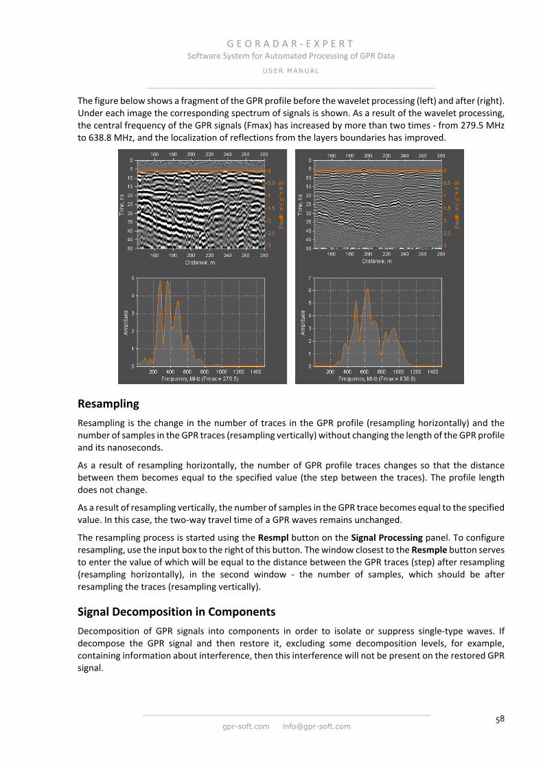
G E O R A D A R - E X P E R T Software System for Automated Processing of GPR Data
USER MANUAL
______________________________________________________________
______________________________________________________________
gpr-soft.com [email protected] 58
The figure below shows a fragment of the GPR profile before the wavelet processing (left) and after (right). Under each image the corresponding spectrum of signals is shown. As a result of the wavelet processing, the central frequency of the GPR signals (Fmax) has increased by more than two times - from 279.5 MHz to 638.8 MHz, and the localization of reflections from the layers boundaries has improved.
Resampling Resampling is the change in the number of traces in the GPR profile (resampling horizontally) and the number of samples in the GPR traces (resampling vertically) without changing the length of the GPR profile and its nanoseconds.
As a result of resampling horizontally, the number of GPR profile traces changes so that the distance between them becomes equal to the specified value (the step between the traces). The profile length does not change.
As a result of resampling vertically, the number of samples in the GPR trace becomes equal to the specified value. In this case, the two-way travel time of a GPR waves remains unchanged.
The resampling process is started using the Resmpl button on the Signal Processing panel. To configure resampling, use the input box to the right of this button. The window closest to the Resmple button serves to enter the value of which will be equal to the distance between the GPR traces (step) after resampling (resampling horizontally), in the second window - the number of samples, which should be after resampling the traces (resampling vertically).
Signal Decomposition in Components Decomposition of GPR signals into components in order to isolate or suppress single-type waves. If decompose the GPR signal and then restore it, excluding some decomposition levels, for example, containing information about interference, then this interference will not be present on the restored GPR signal.

G E O R A D A R - E X P E R T Software System for Automated Processing of GPR Data
USER MANUAL
______________________________________________________________
______________________________________________________________
gpr-soft.com [email protected] 59
Each level of decomposition contains the characteristic features of the signals. The lower (first) levels of expansion correspond to the spatially extended signals of the GPR profile and, the higher the level of decomposition, the spatially shorter components become.
The number of decomposition levels is automatically selected and is equal to the number of GPR profile traces if this value is less than the number of samples of the GPR trace, or is equal to the number of samples, if this value is less than the number of GPR profile traces.
Next, several examples of processing GPR data will be considered.
The figure below is an example of a GPR profile that contains various types of waves - horizontally extended signals and diffracted reflections. The size of the matrix of signals of this GPR profile is 512x265 (512 samples in the GPR traces, the number of traces is 265). This means that the decomposition can be done at 265 levels.
On the left, the original, unprocessed GPR profile is shown. The center shows the result of the reconstruction of the GPR profile at the first levels of decomposition 1 to 21. It is noteworthy that signals from the diffracted waves disappeared from the GPR profile. On the right is the result of recovery at all levels of decomposition, except for the range 1 to 21. In this case, information about spatially extended signals is discarded, and information about diffracted reflections is preserved without distortion.
Below left is a GPR profile with intense periodic interference. Such an interference can be effectively removed by decomposing the matrix of the signals of the GPR profile into components and reconstructing, discarding the very first level of decomposition. The first level of decomposition corresponds to the most spatially extended signals on the GPR profile. It is these signals that are a interference on this GPR profile. The result of reconstruction is shown on the right.
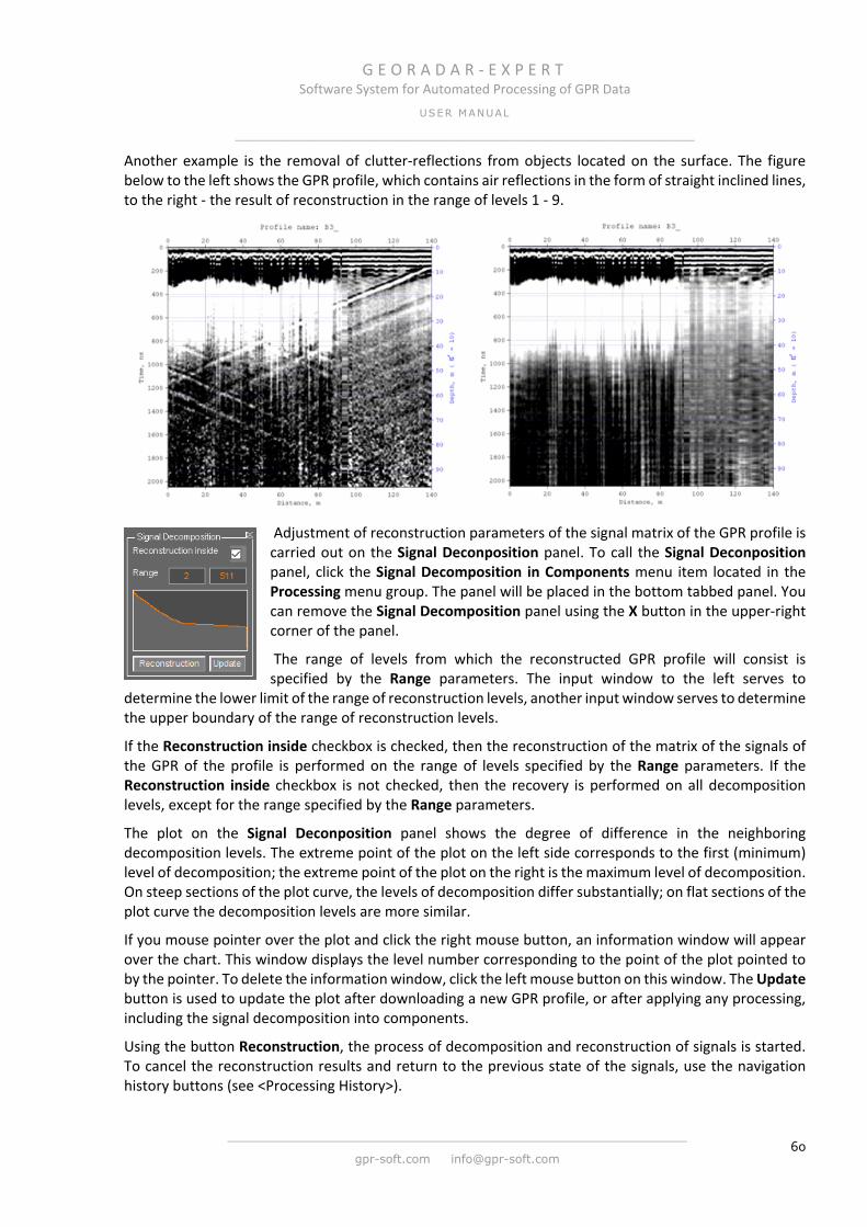
G E O R A D A R - E X P E R T Software System for Automated Processing of GPR Data
USER MANUAL
______________________________________________________________
______________________________________________________________
gpr-soft.com [email protected] 60
Another example is the removal of clutter-reflections from objects located on the surface. The figure below to the left shows the GPR profile, which contains air reflections in the form of straight inclined lines, to the right - the result of reconstruction in the range of levels 1 - 9.
Adjustment of reconstruction parameters of the signal matrix of the GPR profile is carried out on the Signal Deconposition panel. To call the Signal Deconposition panel, click the Signal Decomposition in Components menu item located in the Processing menu group. The panel will be placed in the bottom tabbed panel. You can remove the Signal Decomposition panel using the X button in the upper-right corner of the panel.
The range of levels from which the reconstructed GPR profile will consist is specified by the Range parameters. The input window to the left serves to
determine the lower limit of the range of reconstruction levels, another input window serves to determine the upper boundary of the range of reconstruction levels.
If the Reconstruction inside checkbox is checked, then the reconstruction of the matrix of the signals of the GPR of the profile is performed on the range of levels specified by the Range parameters. If the Reconstruction inside checkbox is not checked, then the recovery is performed on all decomposition levels, except for the range specified by the Range parameters.
The plot on the Signal Deconposition panel shows the degree of difference in the neighboring decomposition levels. The extreme point of the plot on the left side corresponds to the first (minimum) level of decomposition; the extreme point of the plot on the right is the maximum level of decomposition. On steep sections of the plot curve, the levels of decomposition differ substantially; on flat sections of the plot curve the decomposition levels are more similar.
If you mouse pointer over the plot and click the right mouse button, an information window will appear over the chart. This window displays the level number corresponding to the point of the plot pointed to by the pointer. To delete the information window, click the left mouse button on this window. The Update button is used to update the plot after downloading a new GPR profile, or after applying any processing, including the signal decomposition into components.
Using the button Reconstruction, the process of decomposition and reconstruction of signals is started. To cancel the reconstruction results and return to the previous state of the signals, use the navigation history buttons (see <Processing History>).
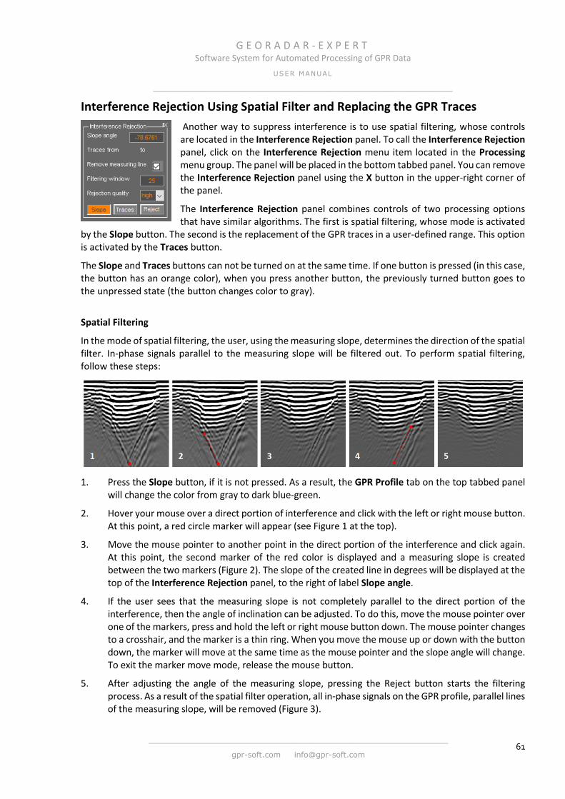
G E O R A D A R - E X P E R T Software System for Automated Processing of GPR Data
USER MANUAL
______________________________________________________________
______________________________________________________________
gpr-soft.com [email protected] 61
Interference Rejection Using Spatial Filter and Replacing the GPR Traces Another way to suppress interference is to use spatial filtering, whose controls are located in the Interference Rejection panel. To call the Interference Rejection panel, click on the Interference Rejection menu item located in the Processing menu group. The panel will be placed in the bottom tabbed panel. You can remove the Interference Rejection panel using the X button in the upper-right corner of the panel.
The Interference Rejection panel combines controls of two processing options that have similar algorithms. The first is spatial filtering, whose mode is activated
by the Slope button. The second is the replacement of the GPR traces in a user-defined range. This option is activated by the Traces button.
The Slope and Traces buttons can not be turned on at the same time. If one button is pressed (in this case, the button has an orange color), when you press another button, the previously turned button goes to the unpressed state (the button changes color to gray).
Spatial Filtering
In the mode of spatial filtering, the user, using the measuring slope, determines the direction of the spatial filter. In-phase signals parallel to the measuring slope will be filtered out. To perform spatial filtering, follow these steps:
1. Press the Slope button, if it is not pressed. As a result, the GPR Profile tab on the top tabbed panel
will change the color from gray to dark blue-green.
2. Hover your mouse over a direct portion of interference and click with the left or right mouse button. At this point, a red circle marker will appear (see Figure 1 at the top).
3. Move the mouse pointer to another point in the direct portion of the interference and click again. At this point, the second marker of the red color is displayed and a measuring slope is created between the two markers (Figure 2). The slope of the created line in degrees will be displayed at the top of the Interference Rejection panel, to the right of label Slope angle.
4. If the user sees that the measuring slope is not completely parallel to the direct portion of the interference, then the angle of inclination can be adjusted. To do this, move the mouse pointer over one of the markers, press and hold the left or right mouse button down. The mouse pointer changes to a crosshair, and the marker is a thin ring. When you move the mouse up or down with the button down, the marker will move at the same time as the mouse pointer and the slope angle will change. To exit the marker move mode, release the mouse button.
5. After adjusting the angle of the measuring slope, pressing the Reject button starts the filtering process. As a result of the spatial filter operation, all in-phase signals on the GPR profile, parallel lines of the measuring slope, will be removed (Figure 3).
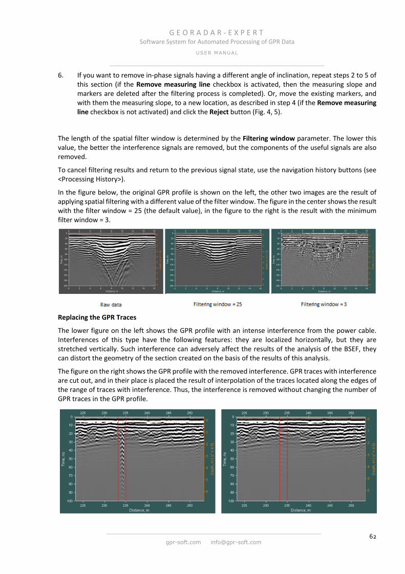
G E O R A D A R - E X P E R T Software System for Automated Processing of GPR Data
USER MANUAL
______________________________________________________________
______________________________________________________________
gpr-soft.com [email protected] 62
6. If you want to remove in-phase signals having a different angle of inclination, repeat steps 2 to 5 of this section (if the Remove measuring line checkbox is activated, then the measuring slope and markers are deleted after the filtering process is completed). Or, move the existing markers, and with them the measuring slope, to a new location, as described in step 4 (if the Remove measuring line checkbox is not activated) and click the Reject button (Fig. 4, 5).
The length of the spatial filter window is determined by the Filtering window parameter. The lower this value, the better the interference signals are removed, but the components of the useful signals are also removed.
To cancel filtering results and return to the previous signal state, use the navigation history buttons (see <Processing History>).
In the figure below, the original GPR profile is shown on the left, the other two images are the result of applying spatial filtering with a different value of the filter window. The figure in the center shows the result with the filter window = 25 (the default value), in the figure to the right is the result with the minimum filter window = 3.
Replacing the GPR Traces
The lower figure on the left shows the GPR profile with an intense interference from the power cable. Interferences of this type have the following features: they are localized horizontally, but they are stretched vertically. Such interference can adversely affect the results of the analysis of the BSEF, they can distort the geometry of the section created on the basis of the results of this analysis.
The figure on the right shows the GPR profile with the removed interference. GPR traces with interference are cut out, and in their place is placed the result of interpolation of the traces located along the edges of the range of traces with interference. Thus, the interference is removed without changing the number of GPR traces in the GPR profile.

G E O R A D A R - E X P E R T Software System for Automated Processing of GPR Data
USER MANUAL
______________________________________________________________
______________________________________________________________
gpr-soft.com [email protected] 63
To cut out the interference, the user needs to manually determine the edges of the range of the area with interference on the image of the GPR profile, and click the Reject button. To create the edges of the range, follow these steps:
1. Press the Traces button, if it is not pressed. As a result, the GPR Profile tab on the top tabbed panel will change the color from gray to dark blue-green.
2. Move the mouse pointer to one of the edges of the interference area and click with the left or right mouse button. At this point, a vertical red line appears which will be one of the edges.
3. Move the mouse pointer to the other edge of the interference area and click with the left or right mouse button. As a result, another vertical line of red appears which will be the second edge.
4. If you want to adjust the position of the edges, you should point the mouse at one of the edge lines, press and hold the left or right mouse button. The edge line will change from red to green. When you move the mouse left and right with the button pressed, the selected edge line will move simultaneously with the mouse pointer. To exit the edges movement mode, release the mouse button.
If the Remove measuring line checkbox is enabled, after the process of replacing the GPR profile traces is completed, the edge lines are deleted. If the Remove measuring line checkbox is not activated, then after completion of the replacement process, the edge lines are not deleted and they can be moved to a new location.
The quality of trace interpolation is set by the Rejection quality parameter. There are three levels of quality: high, mid and low - high, medium and low. By default, high interpolation quality is selected. The use of poor quality saves computation time and memory (important when working on older computers).
To cancel the results of replacing GPR profile traces, and return to the previous signal state, use the navigation history buttons (see <Processing History>).
B-Detector Method B-Detector (Boundaries Detector) is designed to detect boundaries of layers and increase the vertical resolution of signals of the GPR data. The figure below to the left shows the result of profiling the road with a GPR with an antenna of 400 MHz, on the right - the result of processing using the B-Detector method:
As a result of signal processing by the B-Detector method, reflections from the layer boundaries are improved, the positioning accuracy of these boundaries is improved, and the GPR profile becomes well adapted for automated picking of the layer boundaries.

G E O R A D A R - E X P E R T Software System for Automated Processing of GPR Data
USER MANUAL
______________________________________________________________
______________________________________________________________
gpr-soft.com [email protected] 64
The parameters of this processing option are set in the B-Detector panel. To call the B-Detector panel, click on the B-Detector menu item located in the Processing menu group. The panel will be placed in the bottom tabbed panel. You can remove the B-Detector panel using the X button in the upper-right corner of the panel.
The B-Detector panel contains the following controls (listing from top to bottom):
Background - if this checkbox is not activated, the oscillation of the signals is removed from the result of processing by the B-Detector option, if these interfere with the visualization;
Full details – the mode of the maximum possible detail of the result of processing with the option B-Detector. When this checkbox is activated, the Dfactor input window is unavailable;
Dfactor - the detail factor. With increasing this factor, the detail of the result of processing by the B-Detector option increases. Excessive detailing can have a poor effect on the display of layer boundaries;
Ffactor – frequency multiplier. The higher the value of the multiplier, the higher the center frequency of the GPR profile signals, and better the vertical resolution of the GPR data;
Speed x – speedier processing with loss of resolution horizontally. Speed increase is convenient for setting B-Detector parameters when processing long GPR profiles, when you need to start the process several times. After setting the B-Detector parameters, Speed x = 1 is set and the final processing is performed without losing the horizontal resolution;
Start – B-Detector start button.
Processing History After the completion of any operation for signal processing or profile editing, all the changes caused by this action, together with its parameters, are remembered. The user can go to a particular processing step, using the buttons navigate through the processing history. Navigation buttons are located in the bottom row of the Signal Processing panel and perform the following actions:
<< - return to the original (not processed) data. If after returning to the original data and pressing the same button again, the processing history is deleted after the user presses the Yes button on the confirmation pop-up panel;
< - go to the previous step of processing;
> - go to the next processing step;
>> - go to the last step of processing.
Information about the current processing step, the total number of processing steps, as well as information about the parameters of the current processing step is displayed in the information line that is located at the bottom edge of the main program window. The figure below shows an example of an information line after frequency filtering:
If the user has moved to the processing stage, which is not the last one, and at this stage applied some other kind of processing to the GPR profile, the parameters of this processing will be added to the processing history. In this case, all further steps in the processing history, if any, are deleted from memory.
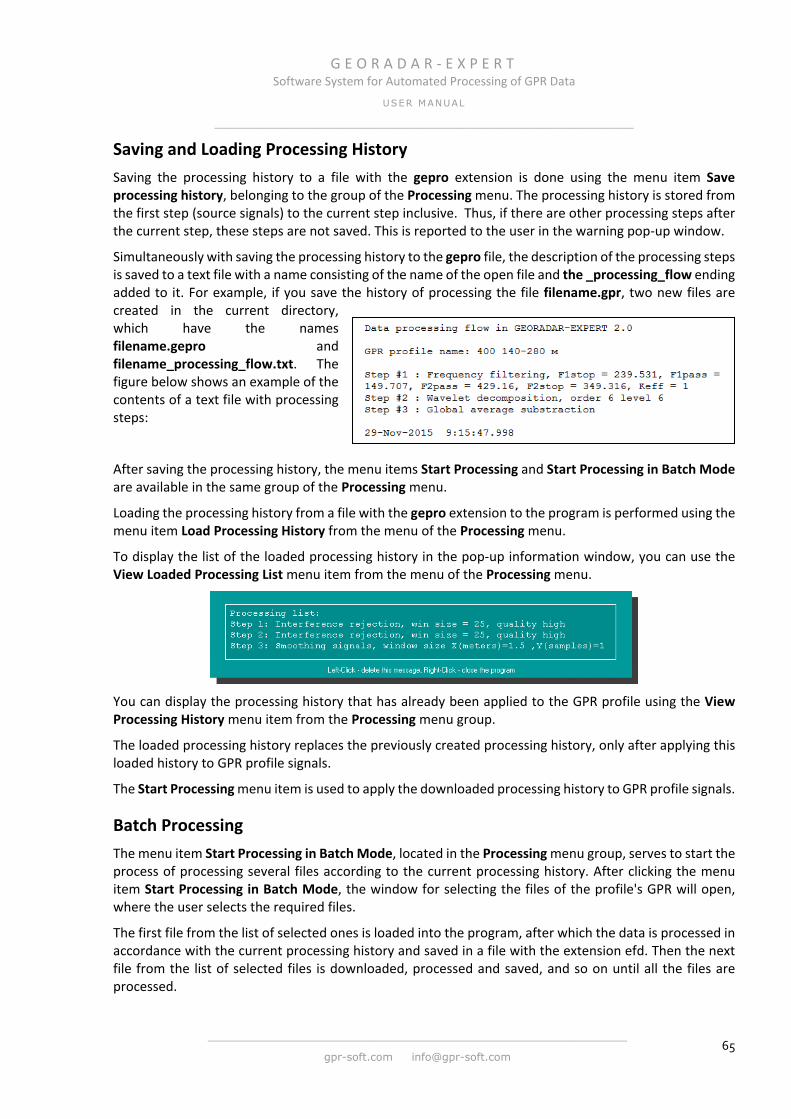
G E O R A D A R - E X P E R T Software System for Automated Processing of GPR Data
USER MANUAL
______________________________________________________________
______________________________________________________________
gpr-soft.com [email protected] 65
Saving and Loading Processing History Saving the processing history to a file with the gepro extension is done using the menu item Save processing history, belonging to the group of the Processing menu. The processing history is stored from the first step (source signals) to the current step inclusive. Thus, if there are other processing steps after the current step, these steps are not saved. This is reported to the user in the warning pop-up window.
Simultaneously with saving the processing history to the gepro file, the description of the processing steps is saved to a text file with a name consisting of the name of the open file and the _processing_flow ending added to it. For example, if you save the history of processing the file filename.gpr, two new files are created in the current directory, which have the names filename.gepro and filename_processing_flow.txt. The figure below shows an example of the contents of a text file with processing steps:
After saving the processing history, the menu items Start Processing and Start Processing in Batch Mode are available in the same group of the Processing menu.
Loading the processing history from a file with the gepro extension to the program is performed using the menu item Load Processing History from the menu of the Processing menu.
To display the list of the loaded processing history in the pop-up information window, you can use the View Loaded Processing List menu item from the menu of the Processing menu.
You can display the processing history that has already been applied to the GPR profile using the View Processing History menu item from the Processing menu group.
The loaded processing history replaces the previously created processing history, only after applying this loaded history to GPR profile signals.
The Start Processing menu item is used to apply the downloaded processing history to GPR profile signals.
Batch Processing The menu item Start Processing in Batch Mode, located in the Processing menu group, serves to start the process of processing several files according to the current processing history. After clicking the menu item Start Processing in Batch Mode, the window for selecting the files of the profile's GPR will open, where the user selects the required files.
The first file from the list of selected ones is loaded into the program, after which the data is processed in accordance with the current processing history and saved in a file with the extension efd. Then the next file from the list of selected files is downloaded, processed and saved, and so on until all the files are processed.

G E O R A D A R - E X P E R T Software System for Automated Processing of GPR Data
USER MANUAL
______________________________________________________________
______________________________________________________________
gpr-soft.com [email protected] 66
If before the start of the batch processing the Save in graphic format settings panel is open (for more details see <Saving in Graphic Format>), then along with saving the processing results to the efd file, the image of the processed profile is saved to the graphic format file in according to the settings in the Save in graphic format panel. If the batch processing process is performed with the Save in graphic format panel open and the processing list is empty, then in this case the image of each loaded GPR profile is saved without any processing to the current directory.
The Change GPR Profile Parameters in Batch Mode menu item, located in the Processing menu group, is used to apply the parameters of the GPR profile contained in the Profile Parameter panel to several GPR profiles in batch mode. In order for the value of the parameter contained in the Profile Parameter panel (for more details see <Editing Parameters GPR Profile>) to be applied to the loaded file, the checkbox next to the name of this parameter must be unchecked. If the checkbox is checked, the parameter value is read from the GPR profile file, and not from the parameter input window.
Using the Change GPR Profile Parameters in Batch Mode menu, for example, it is convenient to assign the same length to a group of GPR profiles. To do this, the user enters the value of the GPR profile length into the Length, m input box on the Profile Parameter panel, unchecks this parameter and, using the Change GPR Profile Parameters in Batch Mode menu, selects the GPR profile files for processing. The selected files are loaded into GEORADAR-EXPERT one by one, the profile length value specified in the Length, m input window is applied to the GPR profile, and then the changes are saved.
Clear Processing History You can clear the memory of the processing history using the Clear Processing History menu item located in the Processing menu group. Or, use the navigation button on the processing history << to go to the unprocessed signals, and again click on the same button. A confirmation pop-up window will appear, where the user should click Yes to continue, or the No button for failure.
Processing Signals in Block Mode When processing long GPR profiles with the number of GPR traces of several tens of thousands, there may be a shortage of computer RAM and, as a consequence, a significant reduction in processing speed. To prevent this from happening, it is recommended to process long GPR profiles in block mode. In this mode, the GPR profile is processed not entirely, but gradually, by blocks of user-defined length.
The parameters of this processing option are set in the Block panel. To call the Block panel, click on the Block-by-block Processing menu item located in the Processing menu group. The panel will be placed in the bottom tabbed panel. You can remove the Block panel
using the X button in the upper-right corner of the panel.
The Block panel contains the following controls:
Enable – if this checkbox is activated, the GPR profile data for processing is loaded into the computer memory not entirely, but by blocks of the specified length. First the first block is loaded, processed and unloaded from memory. Then the next block is loaded and so on until all the blocks are processed;
In traces – In traces - if this checkbox is activated, then the length of the block is set in the GPR traces;
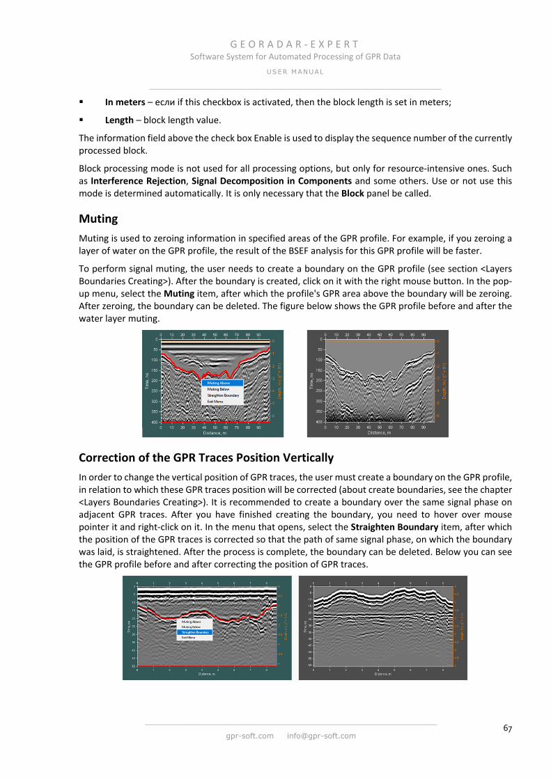
G E O R A D A R - E X P E R T Software System for Automated Processing of GPR Data
USER MANUAL
______________________________________________________________
______________________________________________________________
gpr-soft.com [email protected] 67
In meters – если if this checkbox is activated, then the block length is set in meters;
Length – block length value.
The information field above the check box Enable is used to display the sequence number of the currently processed block.
Block processing mode is not used for all processing options, but only for resource-intensive ones. Such as Interference Rejection, Signal Decomposition in Components and some others. Use or not use this mode is determined automatically. It is only necessary that the Block panel be called.
Muting Muting is used to zeroing information in specified areas of the GPR profile. For example, if you zeroing a layer of water on the GPR profile, the result of the BSEF analysis for this GPR profile will be faster.
To perform signal muting, the user needs to create a boundary on the GPR profile (see section <Layers Boundaries Creating>). After the boundary is created, click on it with the right mouse button. In the pop-up menu, select the Muting item, after which the profile's GPR area above the boundary will be zeroing. After zeroing, the boundary can be deleted. The figure below shows the GPR profile before and after the water layer muting.
Correction of the GPR Traces Position Vertically In order to change the vertical position of GPR traces, the user must create a boundary on the GPR profile, in relation to which these GPR traces position will be corrected (about create boundaries, see the chapter <Layers Boundaries Creating>). It is recommended to create a boundary over the same signal phase on adjacent GPR traces. After you have finished creating the boundary, you need to hover over mouse pointer it and right-click on it. In the menu that opens, select the Straighten Boundary item, after which the position of the GPR traces is corrected so that the path of same signal phase, on which the boundary was laid, is straightened. After the process is complete, the boundary can be deleted. Below you can see the GPR profile before and after correcting the position of GPR traces.

G E O R A D A R - E X P E R T Software System for Automated Processing of GPR Data
USER MANUAL
______________________________________________________________
______________________________________________________________
gpr-soft.com [email protected] 68
Correction of the GPR Traces Position Horizontally The user can correct the position of the GPR traces on the GPR profile, setting the correspondence between the number of the GPR trace and the position of this trace on the GPR profile in meters. The GPR trace number can be seen by switching the mouse pointer to the information mode (for more details see <Axis and Mouse Pointer Properties>). Correspondence is set using a spreadsheet in MS EXCEL format. The first column of the table contains the numbers of GPR traces; the second column is the position of GPR traces on the GPR profile in meters. Under the array of numerical values, the user must specify the data type for the second column of the table.
The data in the second column are of two types. If the distance type is specified, then the values in the second column are the positions of the GPR traces on the GPR profile in meters. If the increment type is specified, then increments of the distance in meters from the previous GPR trace indicated in the table are indicated (i.e., from the number of the GPR trace located in the table one line above). The distance increment for the GPR trace number indicated in the table in the first line is calculated from the first GPR trace of the GPR profile.
To change the position of the GPR traces on the GPR profile, the user needs to create the above table and use the Traces Reposition menu located in the Edit menu group to load this table. The process of changing the position of the GPR traces will automatically begin after loading the table into the program.
The following is an example of a change in the position of the GPR traces in accordance with the table below. The table contains one line of correspondence in which the GPR trace 473 is set to the position 100 m from the beginning of the GPR profile (the data type of the second column is distance).
The upper figure shows the GPR profile before the change, the lower figure shows the result of the change in the position of the GPR traces. The red line shows the position of the GPR of trace 473. As a result, the length of the GPR profile has changed, and in order to maintain the same distance (step) between the GPR traces, additional GPR traces were added on the 0 - 100 m sector, which are the result of interpolation.
The following is an example of a change in the position of GPR traces in accordance with the table below, where the data type of the second column is the increment of distances. The positions of the GPR traces, the numbers of which are indicated in the table, are shown in red lines on the GPR profile.
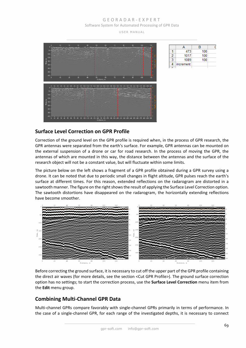
G E O R A D A R - E X P E R T Software System for Automated Processing of GPR Data
USER MANUAL
______________________________________________________________
______________________________________________________________
gpr-soft.com [email protected] 69
Surface Level Correction on GPR Profile
Correction of the ground level on the GPR profile is required when, in the process of GPR research, the GPR antennas were separated from the earth's surface. For example, GPR antennas can be mounted on the external suspension of a drone or car for road research. In the process of moving the GPR, the antennas of which are mounted in this way, the distance between the antennas and the surface of the research object will not be a constant value, but will fluctuate within some limits.
The picture below on the left shows a fragment of a GPR profile obtained during a GPR survey using a drone. It can be noted that due to periodic small changes in flight altitude, GPR pulses reach the earth's surface at different times. For this reason, extended reflections on the radarogram are distorted in a sawtooth manner. The figure on the right shows the result of applying the Surface Level Correction option. The sawtooth distortions have disappeared on the radarogram, the horizontally extending reflections have become smoother.
Before correcting the ground surface, it is necessary to cut off the upper part of the GPR profile containing the direct air waves (for more details, see the section <Cut GPR Profile>). The ground surface correction option has no settings; to start the correction process, use the Surface Level Correction menu item from the Edit menu group.
Combining Multi-Channel GPR Data
Multi-channel GPRs compare favorably with single-channel GPRs primarily in terms of performance. In the case of a single-channel GPR, for each range of the investigated depths, it is necessary to connect
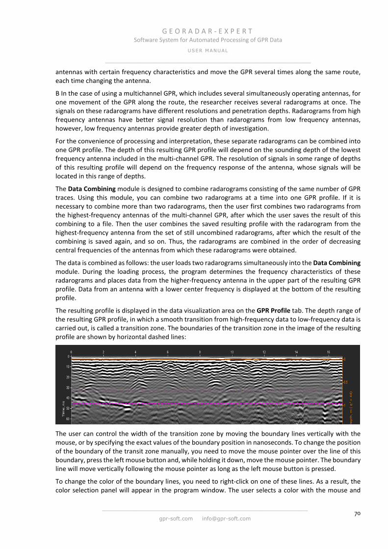
G E O R A D A R - E X P E R T Software System for Automated Processing of GPR Data
USER MANUAL
______________________________________________________________
______________________________________________________________
gpr-soft.com [email protected] 70
antennas with certain frequency characteristics and move the GPR several times along the same route, each time changing the antenna.
В In the case of using a multichannel GPR, which includes several simultaneously operating antennas, for one movement of the GPR along the route, the researcher receives several radarograms at once. The signals on these radarograms have different resolutions and penetration depths. Radarograms from high frequency antennas have better signal resolution than radarograms from low frequency antennas, however, low frequency antennas provide greater depth of investigation.
For the convenience of processing and interpretation, these separate radarograms can be combined into one GPR profile. The depth of this resulting GPR profile will depend on the sounding depth of the lowest frequency antenna included in the multi-channel GPR. The resolution of signals in some range of depths of this resulting profile will depend on the frequency response of the antenna, whose signals will be located in this range of depths.
The Data Combining module is designed to combine radarograms consisting of the same number of GPR traces. Using this module, you can combine two radarograms at a time into one GPR profile. If it is necessary to combine more than two radarograms, then the user first combines two radarograms from the highest-frequency antennas of the multi-channel GPR, after which the user saves the result of this combining to a file. Then the user combines the saved resulting profile with the radarogram from the highest-frequency antenna from the set of still uncombined radarograms, after which the result of the combining is saved again, and so on. Thus, the radarograms are combined in the order of decreasing central frequencies of the antennas from which these radarograms were obtained.
The data is combined as follows: the user loads two radarograms simultaneously into the Data Combining module. During the loading process, the program determines the frequency characteristics of these radarograms and places data from the higher-frequency antenna in the upper part of the resulting GPR profile. Data from an antenna with a lower center frequency is displayed at the bottom of the resulting profile.
The resulting profile is displayed in the data visualization area on the GPR Profile tab. The depth range of the resulting GPR profile, in which a smooth transition from high-frequency data to low-frequency data is carried out, is called a transition zone. The boundaries of the transition zone in the image of the resulting profile are shown by horizontal dashed lines:
The user can control the width of the transition zone by moving the boundary lines vertically with the mouse, or by specifying the exact values of the boundary position in nanoseconds. To change the position of the boundary of the transit zone manually, you need to move the mouse pointer over the line of this boundary, press the left mouse button and, while holding it down, move the mouse pointer. The boundary line will move vertically following the mouse pointer as long as the left mouse button is pressed.
To change the color of the boundary lines, you need to right-click on one of these lines. As a result, the color selection panel will appear in the program window. The user selects a color with the mouse and
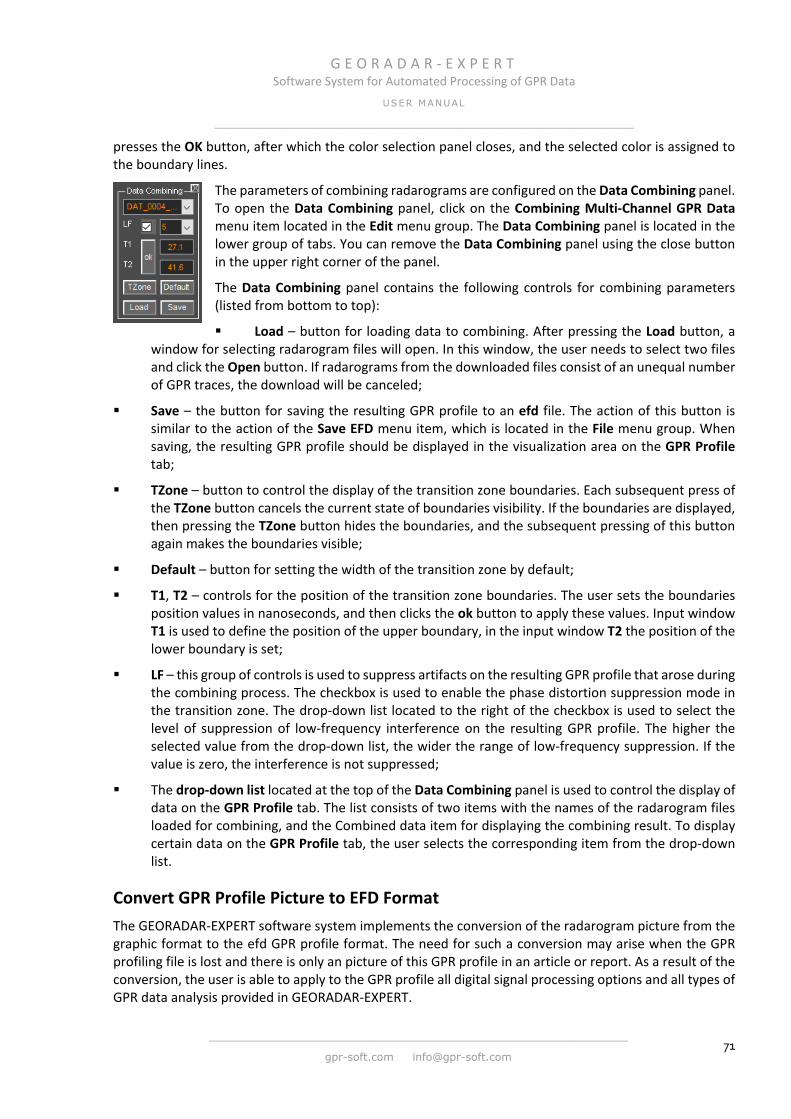
G E O R A D A R - E X P E R T Software System for Automated Processing of GPR Data
USER MANUAL
______________________________________________________________
______________________________________________________________
gpr-soft.com [email protected] 71
presses the OK button, after which the color selection panel closes, and the selected color is assigned to the boundary lines.
The parameters of combining radarograms are configured on the Data Combining panel. To open the Data Combining panel, click on the Combining Multi-Channel GPR Data menu item located in the Edit menu group. The Data Combining panel is located in the lower group of tabs. You can remove the Data Combining panel using the close button in the upper right corner of the panel.
The Data Combining panel contains the following controls for combining parameters (listed from bottom to top):
Load – button for loading data to combining. After pressing the Load button, a window for selecting radarogram files will open. In this window, the user needs to select two files and click the Open button. If radarograms from the downloaded files consist of an unequal number of GPR traces, the download will be canceled;
Save – the button for saving the resulting GPR profile to an efd file. The action of this button is similar to the action of the Save EFD menu item, which is located in the File menu group. When saving, the resulting GPR profile should be displayed in the visualization area on the GPR Profile tab;
TZone – button to control the display of the transition zone boundaries. Each subsequent press of the TZone button cancels the current state of boundaries visibility. If the boundaries are displayed, then pressing the TZone button hides the boundaries, and the subsequent pressing of this button again makes the boundaries visible;
Default – button for setting the width of the transition zone by default;
T1, T2 – controls for the position of the transition zone boundaries. The user sets the boundaries position values in nanoseconds, and then clicks the ok button to apply these values. Input window T1 is used to define the position of the upper boundary, in the input window T2 the position of the lower boundary is set;
LF – this group of controls is used to suppress artifacts on the resulting GPR profile that arose during the combining process. The checkbox is used to enable the phase distortion suppression mode in the transition zone. The drop-down list located to the right of the checkbox is used to select the level of suppression of low-frequency interference on the resulting GPR profile. The higher the selected value from the drop-down list, the wider the range of low-frequency suppression. If the value is zero, the interference is not suppressed;
The drop-down list located at the top of the Data Combining panel is used to control the display of data on the GPR Profile tab. The list consists of two items with the names of the radarogram files loaded for combining, and the Combined data item for displaying the combining result. To display certain data on the GPR Profile tab, the user selects the corresponding item from the drop-down list.
Convert GPR Profile Picture to EFD Format
The GEORADAR-EXPERT software system implements the conversion of the radarogram picture from the graphic format to the efd GPR profile format. The need for such a conversion may arise when the GPR profiling file is lost and there is only an picture of this GPR profile in an article or report. As a result of the conversion, the user is able to apply to the GPR profile all digital signal processing options and all types of GPR data analysis provided in GEORADAR-EXPERT.
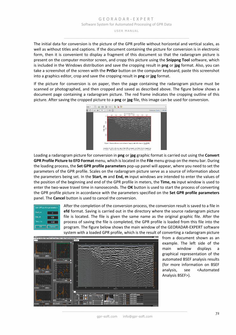
G E O R A D A R - E X P E R T Software System for Automated Processing of GPR Data
USER MANUAL
______________________________________________________________
______________________________________________________________
gpr-soft.com [email protected] 72
The initial data for conversion is the picture of the GPR profile without horizontal and vertical scales, as well as without titles and captions. If the document containing the picture for conversion is in electronic form, then it is convenient to display a fragment of this document so that the radarogram picture is present on the computer monitor screen, and cropp this picture using the Snippng Tool software, which is included in the Windows distribution and save the cropping result in png or jpg format. Also, you can take a screenshot of the screen with the PrtScr button on the computer keyboard, paste this screenshot into a graphics editor, crop and save the cropping result in png or jpg format.
If the picture for conversion is on paper, then the page containing the radarogram picture must be scanned or photographed, and then cropped and saved as described above. The figure below shows a document page containing a radarogram picture. The red frame indicates the cropping outline of this picture. After saving the cropped picture to a png or jpg file, this image can be used for conversion.
Loading a radarogram picture for conversion in png or jpg graphic format is carried out using the Convert GPR Profile Picture to EFD Format menu, which is located in the File menu group on the menu bar. During the loading process, the Set GPR profile parameters pop-up panel will appear, where you need to set the parameters of the GPR profile. Scales on the radarogram picture serve as a source of information about the parameters being set. In the Start, m and End, m input windows are intended to enter the values of the position of the beginning and end of the GPR profile in meters, the Time, ns input window is used to enter the two-wave travel time in nanoseconds. The OK button is used to start the process of converting the GPR profile picture in accordance with the parameters specified on the Set GPR profile parameters panel. The Cancel button is used to cancel the conversion.
After the completion of the conversion process, the conversion result is saved to a file in efd format. Saving is carried out in the directory where the source radarogram picture file is located. The file is given the same name as the original graphic file. After the process of saving the file is completed, the GPR profile is loaded from this file into the program. The figure below shows the main window of the GEORADAR-EXPERT software system with a loaded GPR profile, which is the result of converting a radarogram picture
from a document shown as an example. The left side of the main window displays a graphical representation of the automated BSEF analysis results (for more information on BSEF analysis, see <Automated Analysis BSEF>).

G E O R A D A R - E X P E R T Software System for Automated Processing of GPR Data
USER MANUAL
______________________________________________________________
______________________________________________________________
gpr-soft.com [email protected] 73
Automated Analysis BSEF
The Idea of the Method The idea of the method of automated analysis of the back-scattering electromagnetic field (BSEF) consists in the detection of signals of the GPR profile that have the features of diffracted reflections and the creation of a subsurface medium model based on the measured kinematic and dynamic characteristics of these signals.
In this method, a subsurface medium is considered as a spatially distributed set of local inhomogeneities. According to the characteristics of the diffracted waves generated by these inhomogeneities, one can judge the characteristics of this medium.
Theoretically, if the subsurface medium under investigation does not contain local inhomogeneities, the application of the automated analysis of BSEF becomes impossible. In reality, such subsurface mediums almost never occur. In natural and artificial strata, there are always enough objects of different scales, which are the source of diffracted waves.
Terminology This section provides an explanation of basic concepts that will be used hereinafter.
Local Object
A local object (local heterogeneity) is an object of a subsurface medium. The electrophysical characteristics of this object differ from the medium that accommodates this object, and the linear dimensions of this object are comparable with the wavelength of the probe pulse GPR. Local heterogeneities of soil, stones of various sizes, underground communications, places of sharp changes in the geometry of subsurface objects (corners of building structures in the ground, places of rupture of layers) can act as local objects.
Diffracted Reflection
A local object in a subsurface medium generates diffracted wave carrying information about the scattering object and the characteristics of the medium that accommodates this object. The detection of the diffraction component from the total wave field of the GPR profile is the main task at the initial stage of the automated analysis of the BSEF.
Back-Scattering Electromagnetic Field (BSEF)
Back-scattering electromagnetic field (BSEF) is a secondary electromagnetic field that arises from the reflection of probing pulses from local objects. Reflections from local objects (diffracted reflections) are present on the GPR profile in the form of in-phase signals, which in form resemble a hyperbola. More often, only a small part of the diffracted reflections is displayed on the GPR profile. The remaining diffracted reflections are masked by more intense reflections from the boundaries of the layers, air reflections and noises. Identification of diffracted reflections is one of the stages of the automated analysis of BSEF.
Analysis Point (Measuring Point)
The analysis point (or in other words the measuring point) is a point on the GPR profile having the coordinates X [m] and Y [ns], which correspond to the position of the vertex of the hyperbola of the diffracted reflection. The kinematic and dynamic characteristics of this diffracted reflection are attributes of this analysis point.

G E O R A D A R - E X P E R T Software System for Automated Processing of GPR Data
USER MANUAL
______________________________________________________________
______________________________________________________________
gpr-soft.com [email protected] 74
Basic Attributes
The basic attributes of analysis points are attributes, on the basis of which all other attributes are calculated. The following attributes are basic:
ε′ - the real part of the complex relative permittivity. The greater the value ε′ of the medium, the lower the propagation velocity of the electromagnetic wave in this medium;
f - the central frequency of the spectrum of diffracted reflection signals;
Δf - the width of the spectrum (bandwidth) of diffracted reflection signals, the frequency band in which the main signal energy is concentrated;
Q-factor – the ratio of the center frequency to the bandwidth of the spectrum of the diffracted reflection signals. The Q-factor shows how many times the energy reserves of the electromagnetic wave are greater than the energy losses in one oscillation period. The higher the value of Q-factor, the less energy loss for each period of wave oscillations and the slower they damped;
Probability – the probability of the presence of a backscattered field. This is the probability that a combination of GPR profile signals identified by the BSEF analysis as a reflection from a local object is indeed part of the diffracted reflection. The measure of probability is the ratio of the number of in-phase signals on the line of the hyperbola passing through the maxima of the diffracted reflection to the length of this line. Thus, if all diffracted reflection maxima consist of signals of the same phase, the probability of the presence of a backscattered field is 100%.
BSEF Analysis Errors
Errors in the analysis of BSEF can occur as a result of the influence of interference when measuring the characteristics of diffracted reflections. To minimize possible errors in the analysis of BSEF, a corrective function (CF) is used.
Corrective Function (CF)
The pulse radiated into the subsurface medium changes its frequency characteristics f and Δf as the depth of penetration increases. This is due to the frequency dependent nature of the damping. For example, in many subsurface media, the high-frequency components of electromagnetic waves damped more rapidly than low-frequency components. Thus, there is a relationship between frequency and depth.
The change in the permittivity of a subsurface medium with increasing depth occurs according to a certain law, which depends on the features of this medium. Thus, we can say that for the GPR profile there will be a relationship between the dielectric constant and the frequency characteristics of the reflected signals f, Δf and Q-factor, as well as the Probability attribute.
The corrective function (CF) is a regression equation that determines the dependence of ε' on f (or Δf, or Q-factor or Probability - according to the user's choice) for the GPR profile. Applying CF as the filter mask to the set of pairs [ε' f] (or [ε' Δf], [ε' Q-factor] or [ε′ Probability] - according to the user's choice), it is possible to minimize the effect of possible errors of the automated analysis of the BSEF.
The corrective function is calculated automatically or set manually using the mouse (for more details, see <Creating Corrective Function in Manual Mode>). The user can influence the parameters of the corrective function created in automatic mode by changing the ranges of the ε′, f, Δf, Q-factor or Probability attributes, based on the visual information of the corresponding histograms.
CF plots are displayed in the left tabbed panel (on the tab, the CF panels are located one above the other):

G E O R A D A R - E X P E R T Software System for Automated Processing of GPR Data
USER MANUAL
______________________________________________________________
______________________________________________________________
gpr-soft.com [email protected] 75
Practice has shown that in the overwhelming majority of cases, the dependence of ε′ on f is used as the CF. This type of corrective function is selected for constructing the section by default (the CF selection checkbox in the upper right corner of the panel is checked, the CF plot axes are colored green). For details on CF settings, see <Corrective Function (CF)>.
Histograms of Basic Attributes
The histograms of the basic attributes serve to visually evaluate the results of the automated analysis of the BSEF, as well as to select the range of attributes, if necessary. The histograms are displayed in the left tabbed panel and have the following appearance (on the tab, the histogram panels are located one above the other):
The histogram shows the distribution of the number of analysis points by attribute values. The higher the histogram elements for some attribute value, the more analysis points have this attribute value.
G E O R A D A R - E X P E R T Software System for Automated Processing of GPR Data
USER MANUAL
______________________________________________________________
______________________________________________________________
gpr-soft.com [email protected] 76
Limiting the Range of the Basic Attribute
Limiting the range of basic attributes - is another, in addition to the corrective function, the ability to minimize BSEF error analysis. The user decides to limit the range of the attribute using a priori information about the subsurface medium and the histograms ε', f, Δf, Q-factor and Probability. For more information about range limiting, see <Limiting the Range of the Basic Attribute>.
Node Point
Node points are a subset of the BSEF analysis points after applying the limitations of the range of basic attributes. Based on the node points, the section (subsurface medium model) is calculated by the Delaunay triangulation method.
Section
The section (attribute section) is a 2D model of the subsurface medium, which is calculated on the basis of the results of the automated analysis of the BSEF. The user, depending on the purpose of the GPR survey, selects one attribute from the list of available attributes and creates a section that contains much more information than the GPR profile image, especially in the noise area. From several sections, you can create a 3D model of the subsurface environment.
Most often, the following attributes are used to create a section: dielectric permeability, central frequency, and the Q-factor. Attribute The real part of the complex relative permittivity (Re(permittivity)) is set by default to create a section.
Limitations The limitation of the method of automated analysis of BSEF is that the method can not work correctly in the absence of diffracted waves on the GPR profile. The main reasons for the absence of diffracted waves on the GPR profile are listed below.
No Local Objects
Theoretically, if a subsurface medium does not contain local objects, then the application of the automated analysis method of BSEF is impossible. In practice, homogeneous media are very rare. In natural and artificial strata there is always enough number of local objects of different scale and nature, which are the source of diffracted waves, for successful analysis of the BSEF analysis. Even in the water column there are local objects - air bubbles, water flora and fauna.
A Wide Step of the GPR Profiling
If the GPR profiling is performed with profiling step (the distance between the GPR traces) exceeding a certain value, which depends on the directivity pattern and the central frequency of the GPR antenna, the diffracted waves on the GPR profile will be absent. The figure below shows the effect of the profiling step on the result. For example, the central frequency of the probing pulses is 250 MHz.

G E O R A D A R - E X P E R T Software System for Automated Processing of GPR Data
USER MANUAL
______________________________________________________________
______________________________________________________________
gpr-soft.com [email protected] 77
Figure 1 schematically shows a subsurface medium with two local objects and diffracted reflections from these objects. The vertical lines on the schema show the position of the GPR traces. The distance between the GPR traces is the profiling step. The profiling step is equal to 0.7 m. The attenuation in the medium is quite high - let it be a moist loam.
Figure 2 shows the GPR profile obtained in the course of the profiling of this medium. The vertical lines show the position of the GPR traces. With such a large profiling step (for a given type of antenna), diffracted reflections from local objects can not be formed on the GPR profile. This is because for each reflection from the local object, there is only one or two of the GPR traces. The reflection in this case has the form of a small layer boundary.
Figure 3 shows the same scheme as in Figure 1, only the profiling step has been reduced to 0.1 meters. It is obvious that at such a step value, the diffracted reflections from local objects will be well displayed on the GPR profile - see Figure 4. Each diffracted reflection already consists of more than a dozen GPR traces.
In the <Parameters of the GPR Profiling> recommendations are given for the optimal parameters for recording GPR profiles for their subsequent processing using the automated analysis of BSEF.
Parameters of the GPR Profiling For the correct execution of the automated analysis of BSEF, the parameters of the GPR profile must satisfy the following conditions:
The distance between the GPR traces should be the same. The GPR profiling should be coordinated with the GPR displacement sensor, or be carried out step by step. It is possible to use GPR profiles obtained without a displacement sensor provided that the GPR moves uniformly, at a constant speed, throughout the profiling process, and the exact length of the GPR profile is known.
The parameters of the GPR profile, if possible, should not exceed the limits of the following values (valid for dipole antennas with a 120 degree radiation pattern in subsurface environments with moderate absorption of electromagnetic waves):
The center frequency of the GPR antenna, MHz
Profiling step, m Two-way travel time, ns

G E O R A D A R - E X P E R T Software System for Automated Processing of GPR Data
USER MANUAL
______________________________________________________________
______________________________________________________________
gpr-soft.com [email protected] 78
1700 0.05 50
400 0.05 200
250 0.1 300
150 0.3 400
70 0.5 500
50 0.7 600
25 1 1000
Note: In subsurface media with high damping of electromagnetic waves (wet loamy soils, wet peatlands, etc.), the profiling step should be reduced by at least two times.
Data Preprocessing Sometimes, before the beginning of the automated analysis of BSEF, it is required to perform the preliminary processing of the GPR profile signals. Here are the most common cases for this:
Very small distance between the GPR traces
Very small, in comparison with recommended in the <Parameters of the GPR Profiling>, the profiling step. It is necessary to increase the distance between the GPR traces - that is, to thinning them. There is nothing wrong with this, because with a very small profiling step, the neighboring GPR traces are almost identical and there will not be a significant deterioration in the informative of the GPR profile. To increase the profiling step and, correspondingly, reduce the number of traces in the GPR profile, you should use the horizontal resampling of the profile - see the section <Resampling>.
For example, an GPR profile with a 0.01 m profiling step was obtained by a 250 MHz antenna. The table indicates that for a frequency of 250 MHz, the recommended profiling step for optimal performance of automated BSEF analysis is 0.1 m. The user should enter a value of 0.1 to the right of the Resmpl button in the Signal Processing panel and press the Resmpl button.
A noticeable part of the spectrum of signals is occupied by high-frequency noise
The figure below to the left shows the frequency spectrum of the GPR profile signals obtained by the 400 MHz antenna. Before performing a BSEF analysis, it is possible to suppress high-frequency components, which in this case are located above the 400 MHz frequency.
The spectrum shows that the main energy of the reflected signals is concentrated in the frequency range below 400 MHz. The rise of the spectrum line in the range exceeding 400 MHz is due to the influence of noise. There are no useful signals in this range. If the frequencies of this range are not suppressed before the BSEF analysis, the results of the analysis may be distorted by the influence of random values derived from noise.

G E O R A D A R - E X P E R T Software System for Automated Processing of GPR Data
USER MANUAL
______________________________________________________________
______________________________________________________________
gpr-soft.com [email protected] 79
The figure on the right shows the result of suppressing the signals of the noise range. A band-pass filter was applied, the boundaries of which are indicated by green and magenta vertical lines in the spectrum image. For more information on frequency filtering, see <Frequency Filtering>.
Practice has shown that the filtration before the analysis of BSEF is required for data obtained by medium-frequency and high-frequency GPR antennas. For low-frequency antennas, most often, pre-filtering is not required.
Note: Generally, manufacturers indicate the value of the central frequency of the GPR antenna, measured in the air. The subsurface environment affects the properties of the antenna, usually by lowering its center frequency. This explains the fact that the Fmax value in the figure is 224.1 MHz, although the GPR data has been obtained by a 400 MHz antenna.
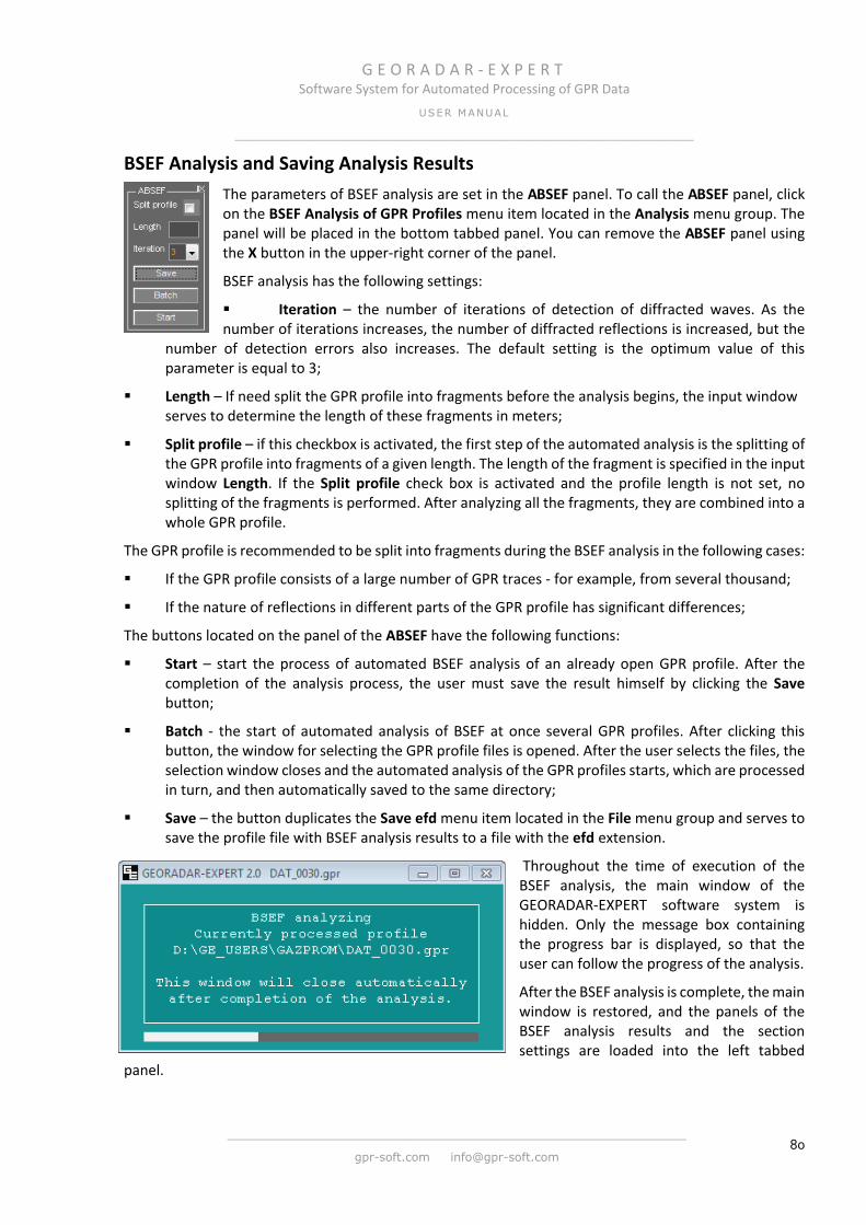
G E O R A D A R - E X P E R T Software System for Automated Processing of GPR Data
USER MANUAL
______________________________________________________________
______________________________________________________________
gpr-soft.com [email protected] 80
BSEF Analysis and Saving Analysis Results The parameters of BSEF analysis are set in the АBSEF panel. To call the АBSEF panel, click on the BSEF Analysis of GPR Profiles menu item located in the Analysis menu group. The panel will be placed in the bottom tabbed panel. You can remove the АBSEF panel using the X button in the upper-right corner of the panel.
BSEF analysis has the following settings:
Iteration – the number of iterations of detection of diffracted waves. As the number of iterations increases, the number of diffracted reflections is increased, but the
number of detection errors also increases. The default setting is the optimum value of this parameter is equal to 3;
Length – If need split the GPR profile into fragments before the analysis begins, the input window serves to determine the length of these fragments in meters;
Split profile – if this checkbox is activated, the first step of the automated analysis is the splitting of the GPR profile into fragments of a given length. The length of the fragment is specified in the input window Length. If the Split profile check box is activated and the profile length is not set, no splitting of the fragments is performed. After analyzing all the fragments, they are combined into a whole GPR profile.
The GPR profile is recommended to be split into fragments during the BSEF analysis in the following cases:
If the GPR profile consists of a large number of GPR traces - for example, from several thousand;
If the nature of reflections in different parts of the GPR profile has significant differences;
The buttons located on the panel of the ABSEF have the following functions:
Start – start the process of automated BSEF analysis of an already open GPR profile. After the completion of the analysis process, the user must save the result himself by clicking the Save button;
Batch - the start of automated analysis of BSEF at once several GPR profiles. After clicking this button, the window for selecting the GPR profile files is opened. After the user selects the files, the selection window closes and the automated analysis of the GPR profiles starts, which are processed in turn, and then automatically saved to the same directory;
Save – the button duplicates the Save efd menu item located in the File menu group and serves to save the profile file with BSEF analysis results to a file with the efd extension.
Throughout the time of execution of the BSEF analysis, the main window of the GEORADAR-EXPERT software system is hidden. Only the message box containing the progress bar is displayed, so that the user can follow the progress of the analysis.
After the BSEF analysis is complete, the main window is restored, and the panels of the BSEF analysis results and the section settings are loaded into the left tabbed
panel.
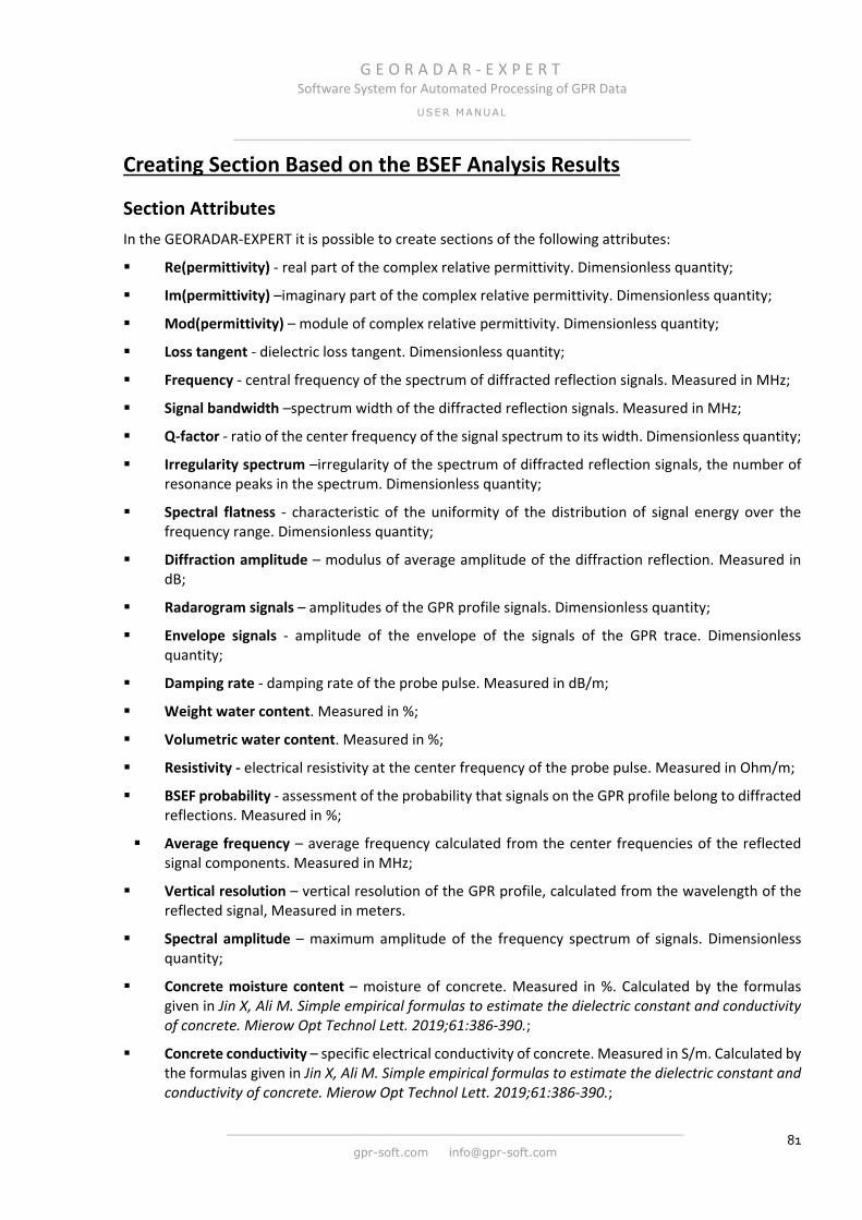
G E O R A D A R - E X P E R T Software System for Automated Processing of GPR Data
USER MANUAL
______________________________________________________________
______________________________________________________________
gpr-soft.com [email protected] 81
Creating Section Based on the BSEF Analysis Results
Section Attributes In the GEORADAR-EXPERT it is possible to create sections of the following attributes:
Re(permittivity) - real part of the complex relative permittivity. Dimensionless quantity;
Im(permittivity) –imaginary part of the complex relative permittivity. Dimensionless quantity;
Mod(permittivity) – module of complex relative permittivity. Dimensionless quantity;
Loss tangent - dielectric loss tangent. Dimensionless quantity;
Frequency - central frequency of the spectrum of diffracted reflection signals. Measured in MHz;
Signal bandwidth –spectrum width of the diffracted reflection signals. Measured in MHz;
Q-factor - ratio of the center frequency of the signal spectrum to its width. Dimensionless quantity;
Irregularity spectrum –irregularity of the spectrum of diffracted reflection signals, the number of resonance peaks in the spectrum. Dimensionless quantity;
Spectral flatness - characteristic of the uniformity of the distribution of signal energy over the frequency range. Dimensionless quantity;
Diffraction amplitude – modulus of average amplitude of the diffraction reflection. Measured in dB;
Radarogram signals – amplitudes of the GPR profile signals. Dimensionless quantity;
Envelope signals - amplitude of the envelope of the signals of the GPR trace. Dimensionless quantity;
Damping rate - damping rate of the probe pulse. Measured in dB/m;
Weight water content. Measured in %;
Volumetric water content. Measured in %;
Resistivity - electrical resistivity at the center frequency of the probe pulse. Measured in Ohm/m;
BSEF probability - assessment of the probability that signals on the GPR profile belong to diffracted reflections. Measured in %;
Average frequency – average frequency calculated from the center frequencies of the reflected signal components. Measured in MHz;
Vertical resolution – vertical resolution of the GPR profile, calculated from the wavelength of the reflected signal, Measured in meters.
Spectral amplitude – maximum amplitude of the frequency spectrum of signals. Dimensionless quantity;
Concrete moisture content – moisture of concrete. Measured in %. Calculated by the formulas given in Jin X, Ali M. Simple empirical formulas to estimate the dielectric constant and conductivity of concrete. Mierow Opt Technol Lett. 2019;61:386-390.;
Concrete conductivity – specific electrical conductivity of concrete. Measured in S/m. Calculated by the formulas given in Jin X, Ali M. Simple empirical formulas to estimate the dielectric constant and conductivity of concrete. Mierow Opt Technol Lett. 2019;61:386-390.;
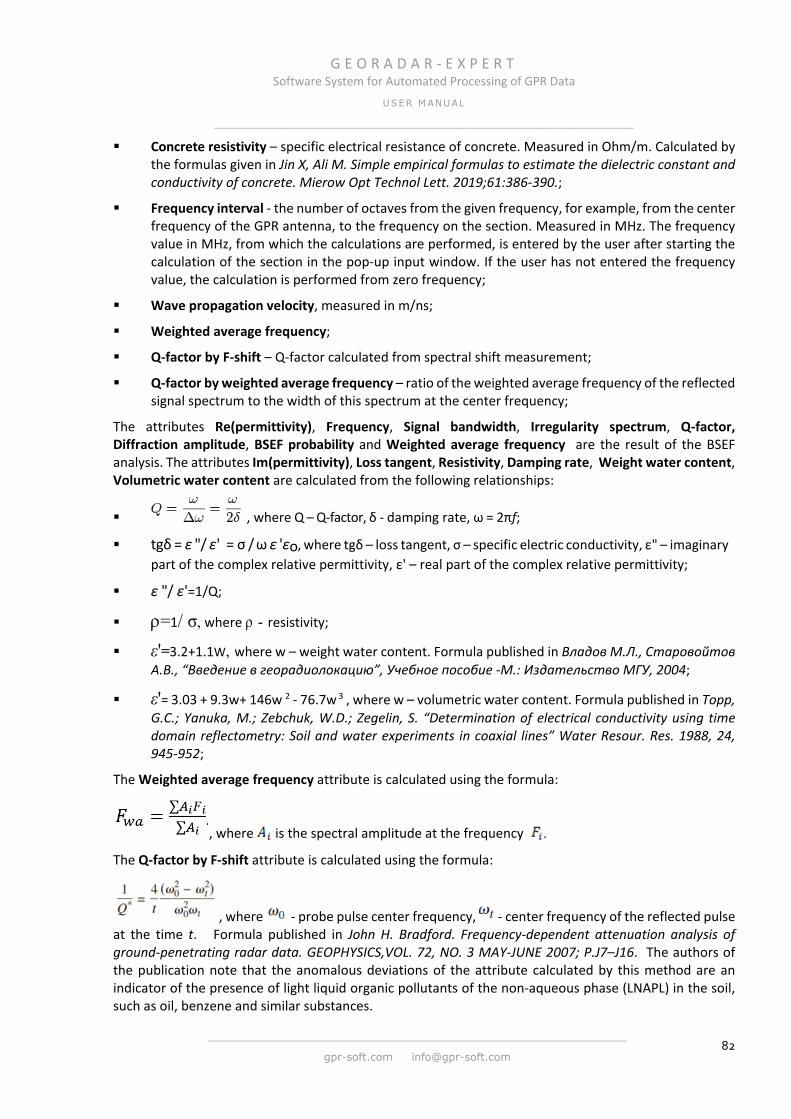
G E O R A D A R - E X P E R T Software System for Automated Processing of GPR Data
USER MANUAL
______________________________________________________________
______________________________________________________________
gpr-soft.com [email protected] 82
Concrete resistivity – specific electrical resistance of concrete. Measured in Ohm/m. Calculated by the formulas given in Jin X, Ali M. Simple empirical formulas to estimate the dielectric constant and conductivity of concrete. Mierow Opt Technol Lett. 2019;61:386-390.;
Frequency interval - the number of octaves from the given frequency, for example, from the center frequency of the GPR antenna, to the frequency on the section. Measured in MHz. The frequency value in MHz, from which the calculations are performed, is entered by the user after starting the calculation of the section in the pop-up input window. If the user has not entered the frequency value, the calculation is performed from zero frequency;
Wave propagation velocity, measured in m/ns;
Weighted average frequency;
Q-factor by F-shift – Q-factor calculated from spectral shift measurement;
Q-factor by weighted average frequency – ratio of the weighted average frequency of the reflected signal spectrum to the width of this spectrum at the center frequency;
The attributes Re(permittivity), Frequency, Signal bandwidth, Irregularity spectrum, Q-factor, Diffraction amplitude, BSEF probability and Weighted average frequency are the result of the BSEF analysis. The attributes Im(permittivity), Loss tangent, Resistivity, Damping rate, Weight water content, Volumetric water content are calculated from the following relationships:
, where Q – Q-factor, δ - damping rate, ω = 2πf;
tgδ = ε "/ ε' = σ / ω ε 'εо, where tgδ – loss tangent, σ – specific electric conductivity, ε" – imaginary part of the complex relative permittivity, ε' – real part of the complex relative permittivity;
ε "/ ε'=1/Q;
ρ=1/ σ, where ρ - resistivity;
ε'=3.2+1.1W, where w – weight water content. Formula published in Владов М.Л., Старовойтов А.В., “Введение в георадиолокацию”, Учебное пособие -М.: Издательство МГУ, 2004;
ε'= 3.03 + 9.3w+ 146w 2 - 76.7w 3 , where w – volumetric water content. Formula published in Topp, G.C.; Yanuka, M.; Zebchuk, W.D.; Zegelin, S. “Determination of electrical conductivity using time domain reflectometry: Soil and water experiments in coaxial lines” Water Resour. Res. 1988, 24, 945-952;
The Weighted average frequency attribute is calculated using the formula:
, where is the spectral amplitude at the frequency .
The Q-factor by F-shift attribute is calculated using the formula:
, where - probe pulse center frequency, - center frequency of the reflected pulse at the time t. Formula published in John H. Bradford. Frequency-dependent attenuation analysis of ground-penetrating radar data. GEOPHYSICS,VOL. 72, NO. 3 MAY-JUNE 2007; P.J7–J16. The authors of the publication note that the anomalous deviations of the attribute calculated by this method are an indicator of the presence of light liquid organic pollutants of the non-aqueous phase (LNAPL) in the soil, such as oil, benzene and similar substances.

G E O R A D A R - E X P E R T Software System for Automated Processing of GPR Data
USER MANUAL
______________________________________________________________
______________________________________________________________
gpr-soft.com [email protected] 83
Loading a File with the BSEF Analysis Result The load of the GPR profile file with the results of the BSEF analysis, which has the efd extension, is carried out in the same way as loading any other format of the GPR profile file that is supported in the GEORADAR-EXPERT software system. To do this, use the Open Data File menu located in the File menu group, or selects the profile name in the list of the most recently opened files located at the bottom of the File menu group. For a detailed description of the BSEF analysis result display panels, see <Visualization of BSEF Analysis Results>.
Visualization of BSEF Analysis Results The histograms of the basic attributes of the BSEF analysis ε', f, Δf, Q-factor and Probability are used to evaluate the results of the analysis and the settings of the section creation.
The histogram shows the distribution of the number of analysis points by attribute values. The higher the histogram elements for some attribute value, the more analysis points have this attribute value. Histograms are located on panels that have the same type of controls, which are located at the bottom of the panel.
These controls are listed below and explanations are given on the functions they perform (the list goes from left to right):
The M button sets the maximum range of the attribute;
The Range button starts the process of limiting the range of the attribute in accordance with the specified values in the input box that are located to the right of this button. The input window closest to the Range button is designed to set the lower bound of the range, the next input window is to set the upper bound of the range;
The Round button serves to apply the rounding value of the attribute values for the histogram in accordance with the value specified in the input window to the right of this button. As the rounding value increases, the number of histogram elements decreases.
The histogram panel of the Permittivity attribute has an All button above the M button. This button sets the maximum attribute range for all histograms at once.
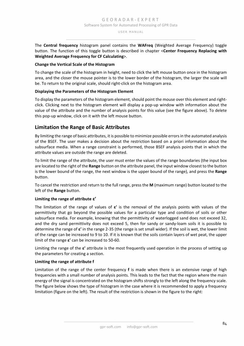
G E O R A D A R - E X P E R T Software System for Automated Processing of GPR Data
USER MANUAL
______________________________________________________________
______________________________________________________________
gpr-soft.com [email protected] 84
The Central frequency histogram panel contains the WAFreq (Weighted Average Frequency) toggle button. The function of this toggle button is described in chapter <Center Frequency Replacing with Weighted Average Frequency for CF Calculating>.
Change the Vertical Scale of the Histogram
To change the scale of the histogram in height, need to click the left mouse button once in the histogram area, and the closer the mouse pointer is to the lower border of the histogram, the larger the scale will be. To return to the original scale, should right-click on the histogram area.
Displaying the Parameters of the Histogram Element
To display the parameters of the histogram element, should point the mouse over this element and right-click. Clicking next to the histogram element will display a pop-up window with information about the value of the attribute and the number of analysis points for this value (see the figure above). To delete this pop-up window, click on it with the left mouse button.
Limitation the Range of Basic Attributes By limiting the range of basic attributes, it is possible to minimize possible errors in the automated analysis of the BSEF. The user makes a decision about the restriction based on a priori information about the subsurface media. When a range constraint is performed, those BSEF analysis points that in which the attribute values are outside the range are deleted.
To limit the range of the attribute, the user must enter the values of the range boundaries (the input box are located to the right of the Range button on the attribute panel, the input window closest to the button is the lower bound of the range, the next window is the upper bound of the range), and press the Range button.
To cancel the restriction and return to the full range, press the M (maximum range) button located to the left of the Range button.
Limiting the range of attribute ε′
The limitation of the range of values of ε' is the removal of the analysis points with values of the permittivity that go beyond the possible values for a particular type and condition of soils or other subsurface media. For example, knowing that the permittivity of waterlogged sand does not exceed 32, and the dry sand permittivity does not exceed 5, then for sandy or sandy-loam soils it is possible to determine the range of ε' in the range 2-35 (the range is set small wider). If the soil is wet, the lower limit of the range can be increased to 9 to 10. If it is known that the soils contain layers of wet peat, the upper limit of the range ε' can be increased to 50-60.
Limiting the range of the ε' attribute is the most frequently used operation in the process of setting up the parameters for creating a section.
Limiting the range of attribute f
Limitation of the range of the center frequency f is made when there is an extensive range of high frequencies with a small number of analysis points. This leads to the fact that the region where the main energy of the signal is concentrated on the histogram shifts strongly to the left along the frequency scale. The figure below shows the type of histogram in the case where it is recommended to apply a frequency limitation (figure on the left). The result of the restriction is shown in the figure to the right:
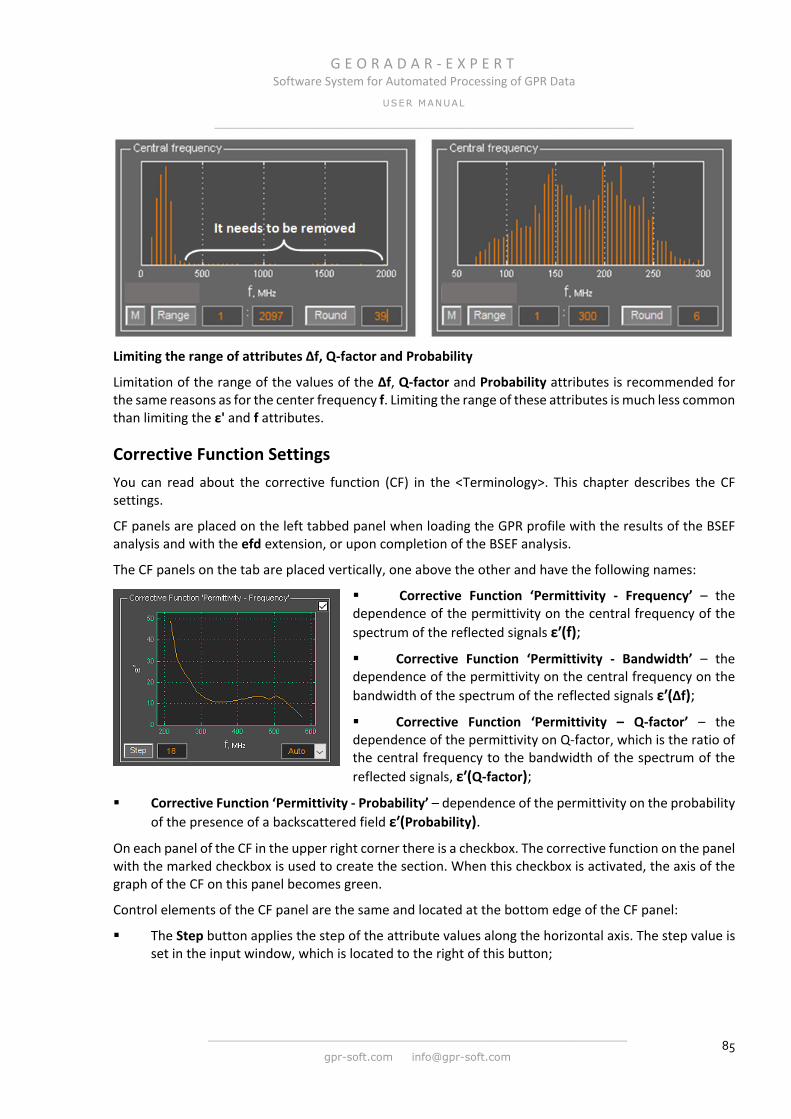
G E O R A D A R - E X P E R T Software System for Automated Processing of GPR Data
USER MANUAL
______________________________________________________________
______________________________________________________________
gpr-soft.com [email protected] 85
Limiting the range of attributes Δf, Q-factor and Probability
Limitation of the range of the values of the Δf, Q-factor and Probability attributes is recommended for the same reasons as for the center frequency f. Limiting the range of these attributes is much less common than limiting the ε' and f attributes.
Corrective Function Settings You can read about the corrective function (CF) in the <Terminology>. This chapter describes the CF settings.
CF panels are placed on the left tabbed panel when loading the GPR profile with the results of the BSEF analysis and with the efd extension, or upon completion of the BSEF analysis.
The CF panels on the tab are placed vertically, one above the other and have the following names:
Corrective Function ‘Permittivity - Frequency’ – the dependence of the permittivity on the central frequency of the spectrum of the reflected signals ε′(f);
Corrective Function ‘Permittivity - Bandwidth’ – the dependence of the permittivity on the central frequency on the bandwidth of the spectrum of the reflected signals ε′(Δf);
Corrective Function ‘Permittivity – Q-factor’ – the dependence of the permittivity on Q-factor, which is the ratio of the central frequency to the bandwidth of the spectrum of the reflected signals, ε′(Q-factor);
Corrective Function ‘Permittivity - Probability’ – dependence of the permittivity on the probability of the presence of a backscattered field ε′(Probability).
On each panel of the CF in the upper right corner there is a checkbox. The corrective function on the panel with the marked checkbox is used to create the section. When this checkbox is activated, the axis of the graph of the CF on this panel becomes green.
Control elements of the CF panel are the same and located at the bottom edge of the СF panel:
The Step button applies the step of the attribute values along the horizontal axis. The step value is set in the input window, which is located to the right of this button;
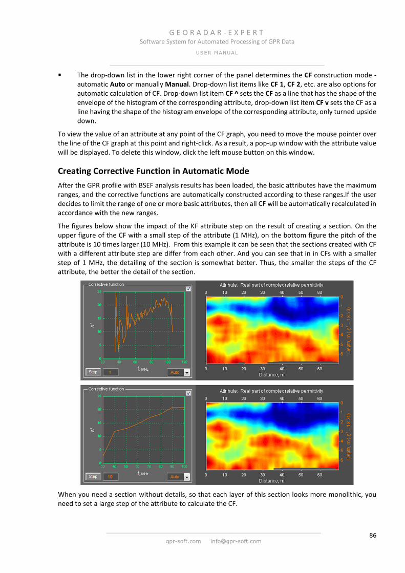
G E O R A D A R - E X P E R T Software System for Automated Processing of GPR Data
USER MANUAL
______________________________________________________________
______________________________________________________________
gpr-soft.com [email protected] 86
The drop-down list in the lower right corner of the panel determines the CF construction mode - automatic Auto or manually Manual. Drop-down list items like CF 1, CF 2, etc. are also options for automatic calculation of CF. Drop-down list item CF ^ sets the CF as a line that has the shape of the envelope of the histogram of the corresponding attribute, drop-down list item CF v sets the CF as a line having the shape of the histogram envelope of the corresponding attribute, only turned upside down.
To view the value of an attribute at any point of the CF graph, you need to move the mouse pointer over the line of the CF graph at this point and right-click. As a result, a pop-up window with the attribute value will be displayed. To delete this window, click the left mouse button on this window.
Creating Corrective Function in Automatic Mode After the GPR profile with BSEF analysis results has been loaded, the basic attributes have the maximum ranges, and the corrective functions are automatically constructed according to these ranges.If the user decides to limit the range of one or more basic attributes, then all CF will be automatically recalculated in accordance with the new ranges.
The figures below show the impact of the KF attribute step on the result of creating a section. On the upper figure of the CF with a small step of the attribute (1 MHz), on the bottom figure the pitch of the attribute is 10 times larger (10 MHz). From this example it can be seen that the sections created with CF with a different attribute step are differ from each other. And you can see that in in CFs with a smaller step of 1 MHz, the detailing of the section is somewhat better. Thus, the smaller the steps of the СF attribute, the better the detail of the section.
When you need a section without details, so that each layer of this section looks more monolithic, you need to set a large step of the attribute to calculate the CF.

G E O R A D A R - E X P E R T Software System for Automated Processing of GPR Data
USER MANUAL
______________________________________________________________
______________________________________________________________
gpr-soft.com [email protected] 87
Sometimes there are cases when CF calculated in the automatic mode lead to unsatisfactory result when creating a section.
This occurs if in the lower part of the GPR profiles there are intense multiple repeated reflections from the boundaries and local objects located at the top of the GPR profile. This happens in the study of subsurface media with low energy absorption of the GPR impulses - frozen soils, for example.
As a result, signals having characteristics that are inherent in near-surface reflections are mixed with reflections at depth, thereby introducing an error in the calculation of the corrective function. In these cases, the manual mode of constructing the CF, described in the section <Creating Corrective Function in Manual Mode> or using the options for automatic calculation of the corrective function CF 1, CF 2, etc., helps to solve the problem.
Creating Corrective Function in Manual Mode To activate the manual mode of creating the corrective function, use the drop-down list located in the lower right corner of the СF panel and select Manual.
When the manual mode is activated, buttons for changing the range of basic attributes are disabled. When the manual mode is activated, the CF curve, which was created in the automatic mode, has a light gray color.
Creation of the CF in manual mode occurs as follows: the user, moving the mouse pointer over the CF axes area, clicks the left mouse button, creating the nodal points of the corrective function. These nodal points are red. In the process of creating them, they automatically connect to each other, depending on the position along the horizontal axis, and not in the order of their creation. You can create, move, and remove nodal points.
Moving nodal points
To move a node point, you need to move the mouse pointer over that point and, while holding the left mouse button down, move the mouse pointer, jointly with the anchor point, inside the CF axes. After the left mouse button is released, the graph of the CF will be updated in accordance with the new position of the node points.
Removing nodal points
To remove the nodal point, move the mouse pointer over this point and right-click, then a pop-up menu will appear with the following items:
Remove node – remove the anchor point on which the mouse pointer;
Remove all nodes – remove all node points of the CF. After removing all the nodes, you can creating the corrective function manually again.
The most commonly used types of CF created manually
The attenuation of the GPR pulses in a subsurface medium is frequency dependent - high-frequency components attenuated more rapidly than low-frequency components. Thus, for the vast majority of subsurface media, the general principle operates - the deeper, the lower the frequency of the reflected GPR pulse.
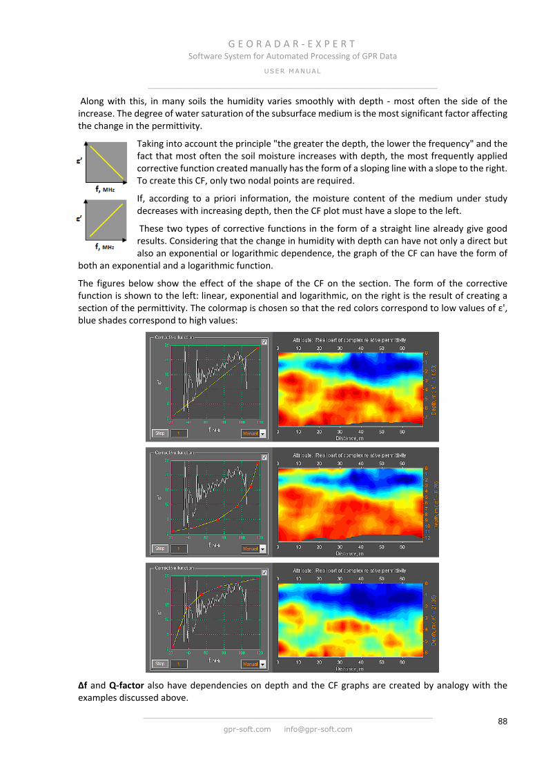
G E O R A D A R - E X P E R T Software System for Automated Processing of GPR Data
USER MANUAL
______________________________________________________________
______________________________________________________________
gpr-soft.com [email protected] 88
Along with this, in many soils the humidity varies smoothly with depth - most often the side of the increase. The degree of water saturation of the subsurface medium is the most significant factor affecting the change in the permittivity.
Taking into account the principle "the greater the depth, the lower the frequency" and the fact that most often the soil moisture increases with depth, the most frequently applied corrective function created manually has the form of a sloping line with a slope to the right. To create this CF, only two nodal points are required.
If, according to a priori information, the moisture content of the medium under study decreases with increasing depth, then the CF plot must have a slope to the left.
These two types of corrective functions in the form of a straight line already give good results. Considering that the change in humidity with depth can have not only a direct but also an exponential or logarithmic dependence, the graph of the CF can have the form of
both an exponential and a logarithmic function.
The figures below show the effect of the shape of the CF on the section. The form of the corrective function is shown to the left: linear, exponential and logarithmic, on the right is the result of creating a section of the permittivity. The colormap is chosen so that the red colors correspond to low values of ε', blue shades correspond to high values:
Δf and Q-factor also have dependencies on depth and the CF graphs are created by analogy with the examples discussed above.

G E O R A D A R - E X P E R T Software System for Automated Processing of GPR Data
USER MANUAL
______________________________________________________________
______________________________________________________________
gpr-soft.com [email protected] 89
Center Frequency Replacing with Weighted Average Frequency for CF Calculating The histogram panel of the Central frequency attribute contains the WAFreq (Weighted Average Frequency) togglebutton. When this button is pressed state, the values of the center frequency are replaced by the values of the weighted average frequency on the Central frequency histogram and in the calculation of the correction function eps (f). If the GPR profile contains many diffracted reflections from local objects, then such a replacement can correct some errors in the BSEF analysis associated with determining the frequency of reflected signals, and increase the reliability of the result of calculating the section of the real part of the complex relative permittivity Re (permittivity).
The figures below show histograms of frequency distribution, corrective function plots and Re(permittivity) sections. The section shown above was created according to the correction function eps(f), which was calculated using the center frequency (the WAFreq button is not pressed state). The section shown below was created in accordance with the correction function eps(f), which was calculated using the weighted average frequency (the WAFreq button on pressed state).
For the GPR profile, according to the BSEF analysis results of which the above sections were created, the section in the lower figure, calculated using the weighted average frequency, more accurately reflects the structure of the object under study, which is the ballast prism of the railway track. There are no unequivocal recommendations for replacing the center frequency with a weighted average frequency. Decisions on such a replacement should be based on a priori information about the object under study, which should be used when comparing the fidelity of the sections created using corrective functions calculated on the basis of both the center frequency and the weighted average frequency.

G E O R A D A R - E X P E R T Software System for Automated Processing of GPR Data
USER MANUAL
______________________________________________________________
______________________________________________________________
gpr-soft.com [email protected] 90
Additional Optimization of BSEF Analysis Results В In the GEORADAR-EXPERT software system, the corrective function minimizes the influence of possible errors in the automated BSEF analysis on the reliability of the section. The corrective function is the main data optimization tool for creating a section. Along with the corrective function, there is a tool for additional optimization of BSEF analysis results, which is not used in all cases. Additional data optimization shows the greatest efficiency for a horizontally layered subsurface. For example, for GPR profiles obtained as a result of the survey of building structures or road pavements.
As an example, the figure below shows the GPR profile obtained during the study of a reinforced concrete slab with a thickness of about 0.2 m, which lies on a sand layer with a thickness of about 0.2 m. Below the image of the GPR profile, sections of the Concrete moisture content attribute are shown, calculated without performing additional data optimization (left) and using additional data optimization.
The section, which was created using additional data optimization, clearly shows the slab layer and the distribution of moisture within this layer, as well as a more humid layer of sand that acts as a drain. The section calculated without additional data optimization shows a less accurate model of the studied subsurface. The reason for this is the partial shielding of the GPR pulses by metal bars of reinforcement, as well as the overlapping of reflections from these bars, which generate a measurement error during the automated BSEF analysis.
In the process of additional optimization, the average values of the center frequency of the reflected signals are calculated over the entire depth range of the GPR profile. These values, for brevity, will hereinafter be referred to as MFV (mid-frequency vector). Frequencies measured during BSEF analysis at a certain depth and deviating from the MFV value for this depth beyond the user-specified threshold are considered erroneous and are not accepted for calculation when creating a section. If the WAFreq toggle button is pressed on the frequency histogram panel, then in the process of additional optimization the calculations are performed using the values of not the central, but the weighted average frequency (for more details see <Center Frequency Replacing with Weighted Average Frequency for CF Calculating>).
The controls for additional data optimization are located in the Additional Data Optimization panel, which opens in the left tab group when loading an efd file that contains the result of an
automated BSEF analysis. The Additional Data Optimization panel contains the following controls:
On - toggle button to activate the additional data optimization mode. When this button is pushed down, additional optimization of the BSEF automated analysis data is performed;
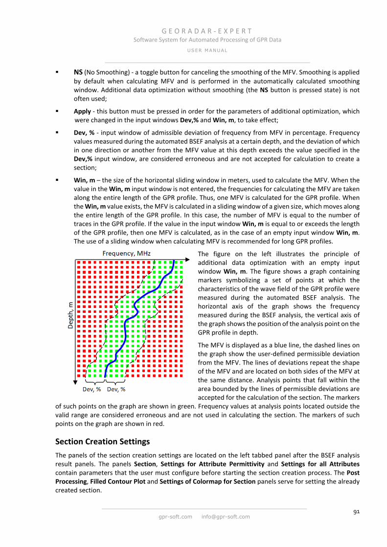
G E O R A D A R - E X P E R T Software System for Automated Processing of GPR Data
USER MANUAL
______________________________________________________________
______________________________________________________________
gpr-soft.com [email protected] 91
NS (No Smoothing) - a toggle button for canceling the smoothing of the MFV. Smoothing is applied by default when calculating MFV and is performed in the automatically calculated smoothing window. Additional data optimization without smoothing (the NS button is pressed state) is not often used;
Apply - this button must be pressed in order for the parameters of additional optimization, which were changed in the input windows Dev,% and Win, m, to take effect;
Dev, % - input window of admissible deviation of frequency from MFV in percentage. Frequency values measured during the automated BSEF analysis at a certain depth, and the deviation of which in one direction or another from the MFV value at this depth exceeds the value specified in the Dev,% input window, are considered erroneous and are not accepted for calculation to create a section;
Win, m – the size of the horizontal sliding window in meters, used to calculate the MFV. When the value in the Win, m input window is not entered, the frequencies for calculating the MFV are taken along the entire length of the GPR profile. Thus, one MFV is calculated for the GPR profile. When the Win, m value exists, the MFV is calculated in a sliding window of a given size, which moves along the entire length of the GPR profile. In this case, the number of MFV is equal to the number of traces in the GPR profile. If the value in the input window Win, m is equal to or exceeds the length of the GPR profile, then one MFV is calculated, as in the case of an empty input window Win, m. The use of a sliding window when calculating MFV is recommended for long GPR profiles.
The figure on the left illustrates the principle of additional data optimization with an empty input window Win, m. The figure shows a graph containing markers symbolizing a set of points at which the characteristics of the wave field of the GPR profile were measured during the automated BSEF analysis. The horizontal axis of the graph shows the frequency measured during the BSEF analysis, the vertical axis of the graph shows the position of the analysis point on the GPR profile in depth.
The MFV is displayed as a blue line, the dashed lines on the graph show the user-defined permissible deviation from the MFV. The lines of deviations repeat the shape of the MFV and are located on both sides of the MFV at the same distance. Analysis points that fall within the area bounded by the lines of permissible deviations are accepted for the calculation of the section. The markers
of such points on the graph are shown in green. Frequency values at analysis points located outside the valid range are considered erroneous and are not used in calculating the section. The markers of such points on the graph are shown in red.
Section Creation Settings The panels of the section creation settings are located on the left tabbed panel after the BSEF analysis result panels. The panels Section, Settings for Attribute Permittivity and Settings for all Attributes contain parameters that the user must configure before starting the section creation process. The Post Processing, Filled Contour Plot and Settings of Colormap for Section panels serve for setting the already created section.
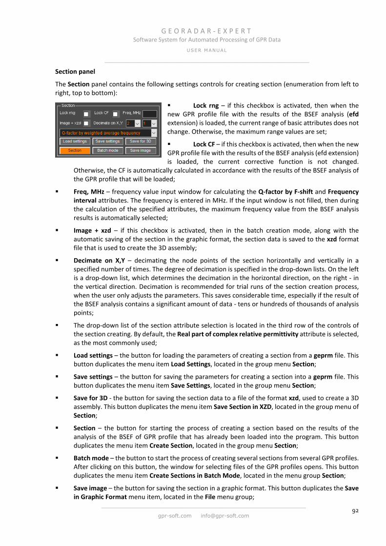
G E O R A D A R - E X P E R T Software System for Automated Processing of GPR Data
USER MANUAL
______________________________________________________________
______________________________________________________________
gpr-soft.com [email protected] 92
Section panel
The Section panel contains the following settings controls for creating section (enumeration from left to right, top to bottom):
Lock rng – if this checkbox is activated, then when the new GPR profile file with the results of the BSEF analysis (efd extension) is loaded, the current range of basic attributes does not change. Otherwise, the maximum range values are set;
Lock CF – if this checkbox is activated, then when the new GPR profile file with the results of the BSEF analysis (efd extension) is loaded, the current corrective function is not changed.
Otherwise, the CF is automatically calculated in accordance with the results of the BSEF analysis of the GPR profile that will be loaded;
Freq, MHz – frequency value input window for calculating the Q-factor by F-shift and Frequency interval attributes. The frequency is entered in MHz. If the input window is not filled, then during the calculation of the specified attributes, the maximum frequency value from the BSEF analysis results is automatically selected;
Image + xzd – if this checkbox is activated, then in the batch creation mode, along with the automatic saving of the section in the graphic format, the section data is saved to the xzd format file that is used to create the 3D assembly;
Decimate on X,Y – decimating the node points of the section horizontally and vertically in a specified number of times. The degree of decimation is specified in the drop-down lists. On the left is a drop-down list, which determines the decimation in the horizontal direction, on the right - in the vertical direction. Decimation is recommended for trial runs of the section creation process, when the user only adjusts the parameters. This saves considerable time, especially if the result of the BSEF analysis contains a significant amount of data - tens or hundreds of thousands of analysis points;
The drop-down list of the section attribute selection is located in the third row of the controls of the section creating. By default, the Real part of complex relative permittivity attribute is selected, as the most commonly used;
Load settings – the button for loading the parameters of creating a section from a geprm file. This button duplicates the menu item Load Settings, located in the group menu Section;
Save settings – the button for saving the parameters for creating a section into a geprm file. This button duplicates the menu item Save Settings, located in the group menu Section;
Save for 3D - the button for saving the section data to a file of the format xzd, used to create a 3D assembly. This button duplicates the menu item Save Section in XZD, located in the group menu of Section;
Section – the button for starting the process of creating a section based on the results of the analysis of the BSEF of GPR profile that has already been loaded into the program. This button duplicates the menu item Create Section, located in the group menu Section;
Batch mode – the button to start the process of creating several sections from several GPR profiles. After clicking on this button, the window for selecting files of the GPR profiles opens. This button duplicates the menu item Create Sections in Batch Mode, located in the menu group Section;
Save image – the button for saving the section in a graphic format. This button duplicates the Save in Graphic Format menu item, located in the File menu group;

G E O R A D A R - E X P E R T Software System for Automated Processing of GPR Data
USER MANUAL
______________________________________________________________
______________________________________________________________
gpr-soft.com [email protected] 93
Settings for Attribute Permittivity panel
The Settings for Attribute Permittivity panel contains controls for creating the section of the ε' (real part of the complex relative permittivity) attribute. The section of this attribute is used as an auxiliary during the calculation of the sections of the remaining attributes. Based on the values of ε 'of this section, the position of the components of other sections in depth is corrected.
The Settings for Attribute Permittivity panel contains the following controls for creating the section (enumeration from left to right, top to bottom):
Do not use CF - if this checkbox is checked, then the corrective function is not used to calculate the section;
Inverse CF - if this checkbox is checked, the inverse of the values of the attribute is performed when calculating the section, as if the curve of the corrective function was mirrored with respect to the horizontal axis;
Data smoothing Y(samples) X(m) – values for smoothing the section. In the input window, located to the left, the value of vertically smoothing value in the GPR trace samples is entered. In the input window, located to the right, the horizontally smoothing value in meters;
Change attribute values with depth – the drop-down list of the rule for changing the attribute with increasing depth. By default, the item As is is selected - in this case no rules are applied when calculating the section. If Increase is selected, then it works like this: if the value of the attribute at the current section point is less than in the neighboring higher-lying point, the value at the current point changes to the value at the neighboring higher-lying point. If the value at the current point is greater, or is equal, than at the higher-lying point, then this value does not change. As a result, the section values will increase with depth. This rule is valid from the time specified by the Start time for rule of change attribute values parameter in the Settings for All Attributes panel. If Decrease is selected, then it works in reverse than Increase: if the value of the attribute at the current section point is greater than at the neighboring higher-lying point, the value at the current point changes to the value at the neighboring higher-lying point. If the value at the current point is less than at the higher-lying point, or is equal, this value does not change. As a result, the values of the sections will decrease with increasing depth. The application of the Increase and Decrease rules gives good results when there is a disruption in the integrity of the layers of the section (due to interference and other causes) and we know that this should not be;
Range of Permittivity – this group of parameters sets the recalculation of the values of ε' to a user-defined range and has the following settings (enumeration from left to right):
Checkbox for recalculation activation. If this checkbox is checked, when creating the section, the values of ε' will be recalculated according to the range specified in the input box;
x is the reset button to the original values of ε'. Applicable in the case when the section is already created and the range of values of ε' has been recalculated;
ok – the button for starting the process of recalculating the values of the attribute ε' in accordance with the user-defined range. As a result of the recalculation, the parameters of
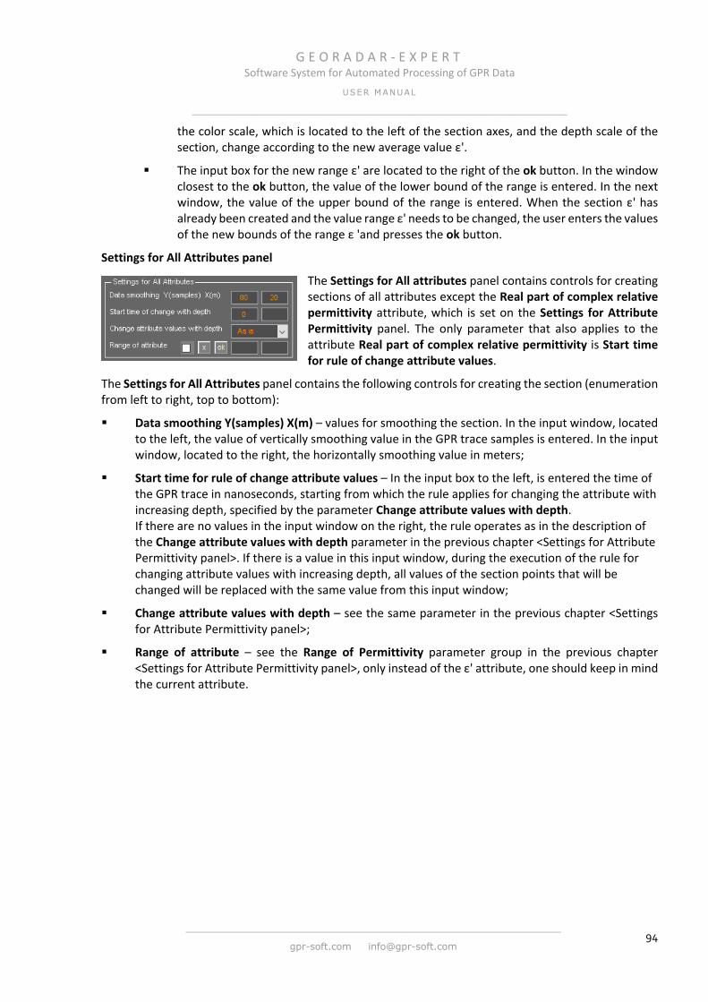
G E O R A D A R - E X P E R T Software System for Automated Processing of GPR Data
USER MANUAL
______________________________________________________________
______________________________________________________________
gpr-soft.com [email protected] 94
the color scale, which is located to the left of the section axes, and the depth scale of the section, change according to the new average value ε'.
The input box for the new range ε' are located to the right of the ok button. In the window closest to the ok button, the value of the lower bound of the range is entered. In the next window, the value of the upper bound of the range is entered. When the section ε' has already been created and the value range ε' needs to be changed, the user enters the values of the new bounds of the range ε 'and presses the ok button.
Settings for All Attributes panel
The Settings for All attributes panel contains controls for creating sections of all attributes except the Real part of complex relative permittivity attribute, which is set on the Settings for Attribute Permittivity panel. The only parameter that also applies to the attribute Real part of complex relative permittivity is Start time for rule of change attribute values.
The Settings for All Attributes panel contains the following controls for creating the section (enumeration from left to right, top to bottom):
Data smoothing Y(samples) X(m) – values for smoothing the section. In the input window, located to the left, the value of vertically smoothing value in the GPR trace samples is entered. In the input window, located to the right, the horizontally smoothing value in meters;
Start time for rule of change attribute values – In the input box to the left, is entered the time of the GPR trace in nanoseconds, starting from which the rule applies for changing the attribute with increasing depth, specified by the parameter Change attribute values with depth. If there are no values in the input window on the right, the rule operates as in the description of the Change attribute values with depth parameter in the previous chapter <Settings for Attribute Permittivity panel>. If there is a value in this input window, during the execution of the rule for changing attribute values with increasing depth, all values of the section points that will be changed will be replaced with the same value from this input window;
Change attribute values with depth – see the same parameter in the previous chapter <Settings for Attribute Permittivity panel>;
Range of attribute – see the Range of Permittivity parameter group in the previous chapter <Settings for Attribute Permittivity panel>, only instead of the ε' attribute, one should keep in mind the current attribute.
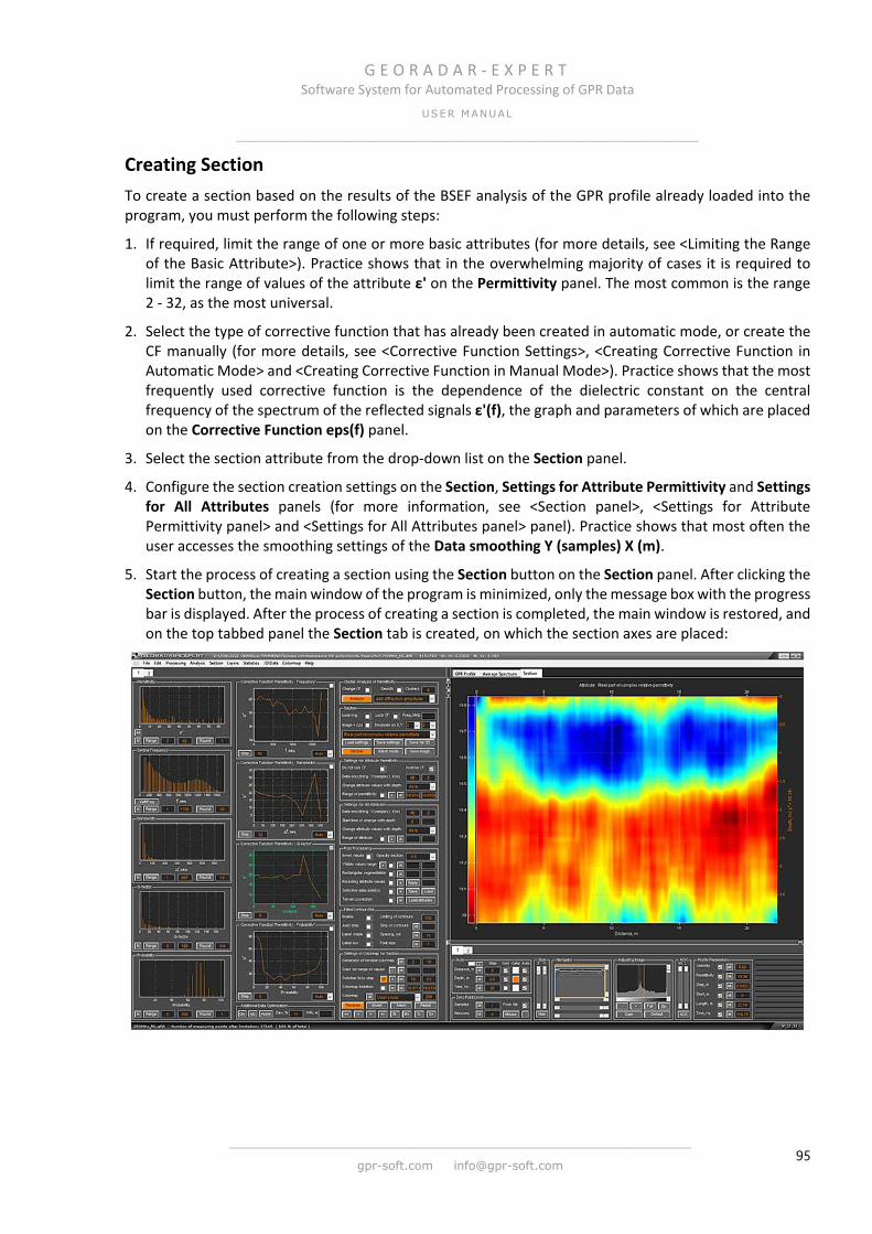
G E O R A D A R - E X P E R T Software System for Automated Processing of GPR Data
USER MANUAL
______________________________________________________________
______________________________________________________________
gpr-soft.com [email protected] 95
Creating Section To create a section based on the results of the BSEF analysis of the GPR profile already loaded into the program, you must perform the following steps:
1. If required, limit the range of one or more basic attributes (for more details, see <Limiting the Range of the Basic Attribute>). Practice shows that in the overwhelming majority of cases it is required to limit the range of values of the attribute ε' on the Permittivity panel. The most common is the range 2 - 32, as the most universal.
2. Select the type of corrective function that has already been created in automatic mode, or create the CF manually (for more details, see <Corrective Function Settings>, <Creating Corrective Function in Automatic Mode> and <Creating Corrective Function in Manual Mode>). Practice shows that the most frequently used corrective function is the dependence of the dielectric constant on the central frequency of the spectrum of the reflected signals ε'(f), the graph and parameters of which are placed on the Corrective Function eps(f) panel.
3. Select the section attribute from the drop-down list on the Section panel.
4. Configure the section creation settings on the Section, Settings for Attribute Permittivity and Settings for All Attributes panels (for more information, see <Section panel>, <Settings for Attribute Permittivity panel> and <Settings for All Attributes panel> panel). Practice shows that most often the user accesses the smoothing settings of the Data smoothing Y (samples) X (m).
5. Start the process of creating a section using the Section button on the Section panel. After clicking the Section button, the main window of the program is minimized, only the message box with the progress bar is displayed. After the process of creating a section is completed, the main window is restored, and on the top tabbed panel the Section tab is created, on which the section axes are placed:
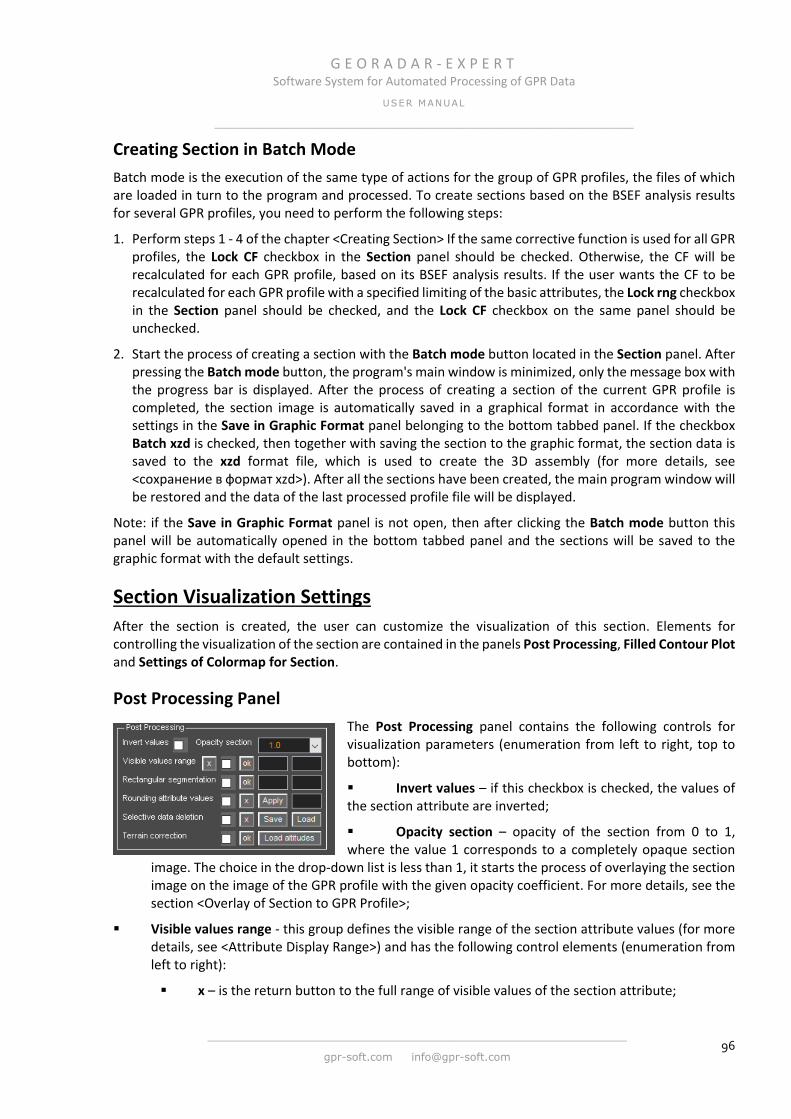
G E O R A D A R - E X P E R T Software System for Automated Processing of GPR Data
USER MANUAL
______________________________________________________________
______________________________________________________________
gpr-soft.com [email protected] 96
Creating Section in Batch Mode Batch mode is the execution of the same type of actions for the group of GPR profiles, the files of which are loaded in turn to the program and processed. To create sections based on the BSEF analysis results for several GPR profiles, you need to perform the following steps:
1. Perform steps 1 - 4 of the chapter <Creating Section> If the same corrective function is used for all GPR profiles, the Lock CF checkbox in the Section panel should be checked. Otherwise, the CF will be recalculated for each GPR profile, based on its BSEF analysis results. If the user wants the CF to be recalculated for each GPR profile with a specified limiting of the basic attributes, the Lock rng checkbox in the Section panel should be checked, and the Lock CF checkbox on the same panel should be unchecked.
2. Start the process of creating a section with the Batch mode button located in the Section panel. After pressing the Batch mode button, the program's main window is minimized, only the message box with the progress bar is displayed. After the process of creating a section of the current GPR profile is completed, the section image is automatically saved in a graphical format in accordance with the settings in the Save in Graphic Format panel belonging to the bottom tabbed panel. If the checkbox Batch xzd is checked, then together with saving the section to the graphic format, the section data is saved to the xzd format file, which is used to create the 3D assembly (for more details, see <сохранение в формат xzd>). After all the sections have been created, the main program window will be restored and the data of the last processed profile file will be displayed.
Note: if the Save in Graphic Format panel is not open, then after clicking the Batch mode button this panel will be automatically opened in the bottom tabbed panel and the sections will be saved to the graphic format with the default settings.
Section Visualization Settings After the section is created, the user can customize the visualization of this section. Elements for controlling the visualization of the section are contained in the panels Post Processing, Filled Contour Plot and Settings of Colormap for Section.
Post Processing Panel The Post Processing panel contains the following controls for visualization parameters (enumeration from left to right, top to bottom):
Invert values – if this checkbox is checked, the values of the section attribute are inverted;
Opacity section – opacity of the section from 0 to 1, where the value 1 corresponds to a completely opaque section
image. The choice in the drop-down list is less than 1, it starts the process of overlaying the section image on the image of the GPR profile with the given opacity coefficient. For more details, see the section <Overlay of Section to GPR Profile>;
Visible values range - this group defines the visible range of the section attribute values (for more details, see <Attribute Display Range>) and has the following control elements (enumeration from left to right):
x – is the return button to the full range of visible values of the section attribute;

G E O R A D A R - E X P E R T Software System for Automated Processing of GPR Data
USER MANUAL
______________________________________________________________
______________________________________________________________
gpr-soft.com [email protected] 97
The checkbox applies a range of visibility limits for attribute values. If this checkbox is checked, then when calculating a section, the display of attribute values will be limited in accordance with the specified range limits;
ok – the button starts the process of limiting the range of visibility of the section attribute;
The input box for the range of the visibility of the attribute are located to the right of the ok button. In the input window, located closer to the ok button, the value of the lower limit of the range is entered. In the next input window, the value of the upper range limit is entered. The user enters the values of the visibility range limits and presses the ok button, after which the values that go beyond the specified limits become completely transparent.
Rectangular segmentation - this group of parameters refers to the mode of rectangular segmentation of a section (in more detail - in the section <Rectangular Segmentation>), which has the following control elements (enumeration from left to right):
Checkbox to enable the mode of rectangular segmentation. If this checkbox is checked before the section creation process starts, the created section will be displayed as a set of rectangular segments. In case the segmentation has already been performed, unchecking the checkbox returns a section to the original image;
ok – the button starts the process of rectangular segmentation according to the specified segment sizes;
The segment size input box are located to the right of the ok button. In the window closest to the ok button, enter the segment size vertically in meters. In the next window - the size of the segment horizontally in meters. The user enters the segment size and presses the ok button, after which the section takes a segmented view.
Rounding attribute values - this group of controls to rounding of the the section attribute values (in more detail - in the section <Rounding Attribute Values>), which has the following settings (enumeration from left to right):
Checkbox for rounding the section. If this checkbox is selected before the section is created, then the values of the attribute of the created section will be rounded according to the specified rounding accuracy;
x – this button cancels the rounding of the section attribute values;
Apply – the button starts the rounding process;
The rounding accuracy value input window is located to the right of the Apply button. The user enters a rounding accuracy value and presses the Apply button, after which the section values are rounded.
Selective data deletion – With the help of this group of controls, the BSEF analysis results that are inside the user-defined rectangular areas on the section image are not used during the subsequent section creation (for more details, see the <Ignoring User-Specified Data Part for Section Creating> chapter). This option has the following settings (listed from left to right):
checkbox for activating data deletion mode. If this checkbox is checked, the user, using the mouse, can create one or more data deletion areas on the section, which are displayed on the section as rectangular frames;
x – using this button, all data deletion areas created by the user are deleted. Deleting a specific area is carried out by right-clicking on the frame that bounds this area and selecting the Delete This Frame item in the context menu that opens;
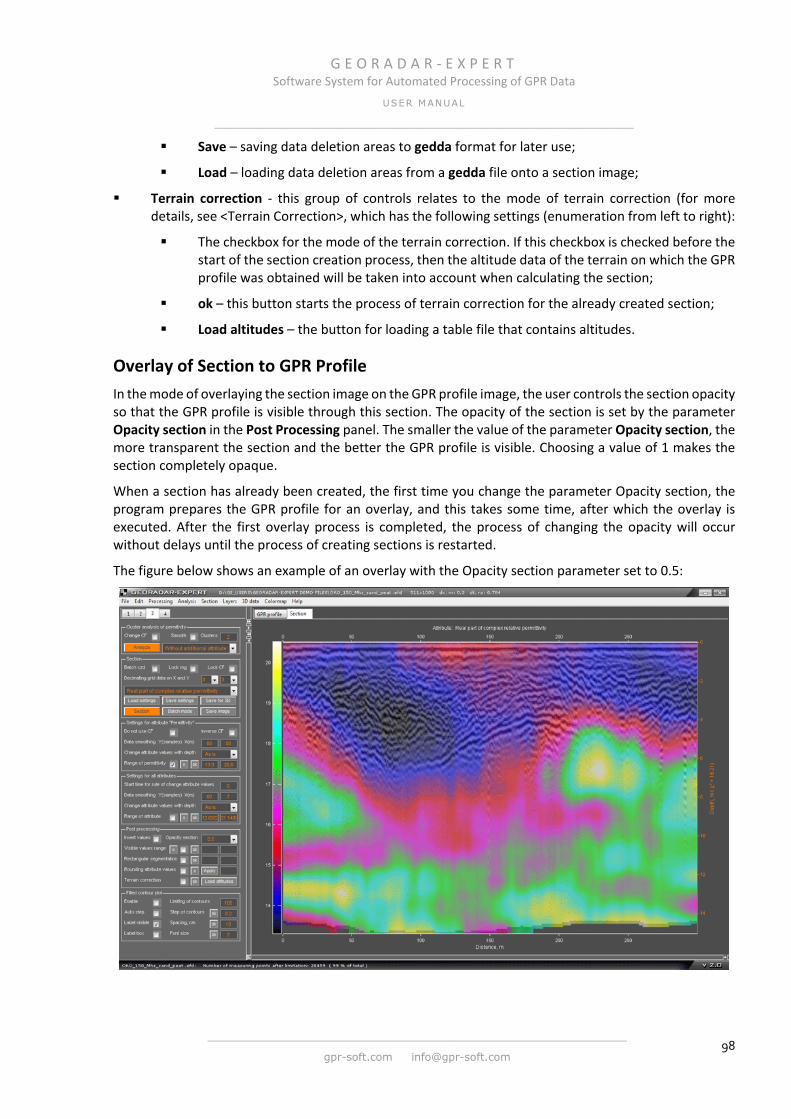
G E O R A D A R - E X P E R T Software System for Automated Processing of GPR Data
USER MANUAL
______________________________________________________________
______________________________________________________________
gpr-soft.com [email protected] 98
Save – saving data deletion areas to gedda format for later use;
Load – loading data deletion areas from a gedda file onto a section image;
Terrain correction - this group of controls relates to the mode of terrain correction (for more details, see <Terrain Correction>, which has the following settings (enumeration from left to right):
The checkbox for the mode of the terrain correction. If this checkbox is checked before the start of the section creation process, then the altitude data of the terrain on which the GPR profile was obtained will be taken into account when calculating the section;
ok – this button starts the process of terrain correction for the already created section;
Load altitudes – the button for loading a table file that contains altitudes.
Overlay of Section to GPR Profile In the mode of overlaying the section image on the GPR profile image, the user controls the section opacity so that the GPR profile is visible through this section. The opacity of the section is set by the parameter Opacity section in the Post Processing panel. The smaller the value of the parameter Opacity section, the more transparent the section and the better the GPR profile is visible. Choosing a value of 1 makes the section completely opaque.
When a section has already been created, the first time you change the parameter Opacity section, the program prepares the GPR profile for an overlay, and this takes some time, after which the overlay is executed. After the first overlay process is completed, the process of changing the opacity will occur without delays until the process of creating sections is restarted.
The figure below shows an example of an overlay with the Opacity section parameter set to 0.5:

G E O R A D A R - E X P E R T Software System for Automated Processing of GPR Data
USER MANUAL
______________________________________________________________
______________________________________________________________
gpr-soft.com [email protected] 99
Rectangular Segmentation In rectangular segmentation mode, the section image is represented as rectangular segments, the size of which is specified in the Rectangular segmentation group in the Post Processing panel (see <Post Processing Panel>).
In the input window, located closer to the ok button, you enter the segment size in vertical in meters. In the next window - the size of the segment horizontally in meters. The ok button is used to start the segmentation process. When the section is already segmented, the checkbox, which is located to the left of the ok button, is checked. To return to the original, non-segmented section, you need to uncheck this checkbox. If this checkbox is checked and values are entered in the segment size input box, segmentation will be performed automatically when the process of creating the section creation starts.
The figure below shows the section that was created on the basis of the results of the BSEF analysis of the GPR profile that was obtained during a survey of a concrete slab about 0.3 m thick:
The figure below shows the result of segmentation of a section with a vertical segment size of 0.1 m. The colormap of the section was chosen so that the driest areas in which the permittivity values have small values are colored red, the moderately wet areas have a light blue color, and the very wet places have a dark blue color:
As a result, the concrete slab and the moisture distribution in its thickness are well displayed on the segmented section, as well as the wettest areas under this concrete slab. Also, the places of water leakage from the surface of the concrete slab through the cracks down (shown by arrows) are also clearly visible.

G E O R A D A R - E X P E R T Software System for Automated Processing of GPR Data
USER MANUAL
______________________________________________________________
______________________________________________________________
gpr-soft.com [email protected] 100
Rounding Attribute Values In the rounding mode the attribute values, the segmentation of the section takes place with a step that is equal to the value of the rounding accuracy. The rounding accuracy input window is located to the right of the Apply button in the Rounding attribute values group on the Post Processing panel (see <Post Processing Panel>).
The Apply button is used to start the rounding process. To return to the original, non-rounded values of the section attribute, you must press the x button. If the checkbox to the left of the Apply button is activated before the start of the rounding process starts and there is a rounding accuracy value in the parameter input window, the rounding will be performed during the section creation.
The figures below show a section with different rounding accuracy values:
Ignoring User-Specified Data Part for Section Creating The user has the ability to set one or more rectangular areas on the section so that during the subsequent calculation of the section, the data of the field analysis points (see in <Analysis Point (Measuring Point)>), the coordinates of which are inside these areas, were not used. With this feature, for example, you can remove edge effects on a section. The figure below shows a section before (left) and after deleting user-defined areas. Data deletion areas on the section are displayed as black and white frames.
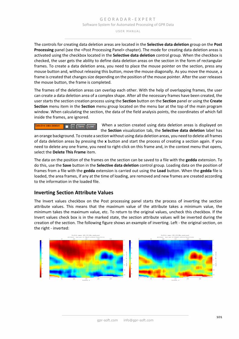
G E O R A D A R - E X P E R T Software System for Automated Processing of GPR Data
USER MANUAL
______________________________________________________________
______________________________________________________________
gpr-soft.com [email protected] 101
The controls for creating data deletion areas are located in the Selective data deletion group on the Post Processing panel (see the <Post Processing Panel> chapter). The mode for creating data deletion areas is activated using the checkbox located in the Selective data deletion control group. When the checkbox is checked, the user gets the ability to define data deletion areas on the section in the form of rectangular frames. To create a data deletion area, you need to place the mouse pointer on the section, press any mouse button and, without releasing this button, move the mouse diagonally. As you move the mouse, a frame is created that changes size depending on the position of the mouse pointer. After the user releases the mouse button, the frame is completed.
The frames of the deletion areas can overlap each other. With the help of overlapping frames, the user can create a data deletion area of a complex shape. After all the necessary frames have been created, the user starts the section creation process using the Section button on the Section panel or using the Create Section menu item in the Section menu group located on the menu bar at the top of the main program window. When calculating the section, the data of the field analysis points, the coordinates of which fall inside the frames, are ignored.
When a section created using data deletion areas is displayed on the Section visualization tab, the Selective data deletion label has
an orange background. To create a section without using data deletion areas, you need to delete all frames of data deletion areas by pressing the x button and start the process of creating a section again. If you need to delete any one frame, you need to right-click on this frame and, in the context menu that opens, select the Delete This Frame item.
The data on the position of the frames on the section can be saved to a file with the gedda extension. To do this, use the Save button in the Selective data deletion control group. Loading data on the position of frames from a file with the gedda extension is carried out using the Load button. When the gedda file is loaded, the area frames, if any at the time of loading, are removed and new frames are created according to the information in the loaded file.
Inverting Section Attribute Values The Invert values checkbox on the Post processing panel starts the process of inverting the section attribute values. This means that the maximum value of the attribute takes a minimum value, the minimum takes the maximum value, etc. To return to the original values, uncheck this checkbox. If the Invert values check box is in the marked state, the section attribute values will be inverted during the creation of the section. The following figure shows an example of inverting. Left - the original section, on the right - inverted:
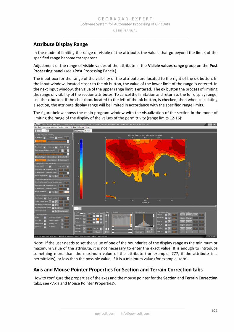
G E O R A D A R - E X P E R T Software System for Automated Processing of GPR Data
USER MANUAL
______________________________________________________________
______________________________________________________________
gpr-soft.com [email protected] 102
Attribute Display Range In the mode of limiting the range of visible of the attribute, the values that go beyond the limits of the specified range become transparent.
Adjustment of the range of visible values of the attribute in the Visible values range group on the Post Processing panel (see <Post Processing Panel>).
The input box for the range of the visibility of the attribute are located to the right of the ok button. In the input window, located closer to the ok button, the value of the lower limit of the range is entered. In the next input window, the value of the upper range limit is entered. The ok button the process of limiting the range of visibility of the section attributes. To cancel the limitation and return to the full display range, use the x button. If the checkbox, located to the left of the ok button, is checked, then when calculating a section, the attribute display range will be limited in accordance with the specified range limits.
The figure below shows the main program window with the visualization of the section in the mode of limiting the range of the display of the values of the permittivity (range limits 12-16):
Note: If the user needs to set the value of one of the boundaries of the display range as the minimum or maximum value of the attribute, it is not necessary to enter the exact value. It is enough to introduce something more than the maximum value of the attribute (for example, 777, if the attribute is a permittivity), or less than the possible value, if it is a minimum value (for example, zero).
Axis and Mouse Pointer Properties for Section and Terrain Correction tabs How to configure the properties of the axes and the mouse pointer for the Section and Terrain Correction tabs; see <Axis and Mouse Pointer Properties>.
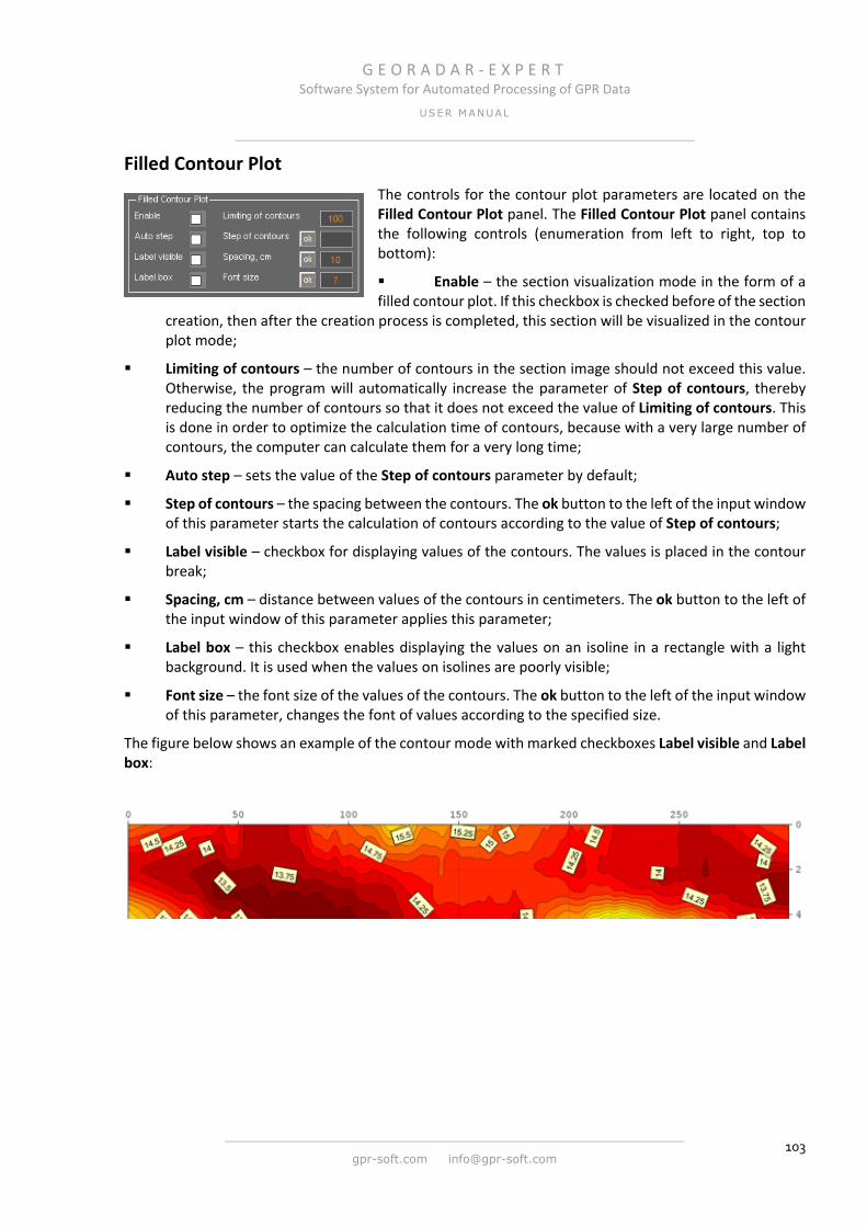
G E O R A D A R - E X P E R T Software System for Automated Processing of GPR Data
USER MANUAL
______________________________________________________________
______________________________________________________________
gpr-soft.com [email protected] 103
Filled Contour Plot The controls for the contour plot parameters are located on the Filled Contour Plot panel. The Filled Contour Plot panel contains the following controls (enumeration from left to right, top to bottom):
Enable – the section visualization mode in the form of a filled contour plot. If this checkbox is checked before of the section
creation, then after the creation process is completed, this section will be visualized in the contour plot mode;
Limiting of contours – the number of contours in the section image should not exceed this value. Otherwise, the program will automatically increase the parameter of Step of contours, thereby reducing the number of contours so that it does not exceed the value of Limiting of contours. This is done in order to optimize the calculation time of contours, because with a very large number of contours, the computer can calculate them for a very long time;
Auto step – sets the value of the Step of contours parameter by default;
Step of contours – the spacing between the contours. The ok button to the left of the input window of this parameter starts the calculation of contours according to the value of Step of contours;
Label visible – checkbox for displaying values of the contours. The values is placed in the contour break;
Spacing, cm – distance between values of the contours in centimeters. The ok button to the left of the input window of this parameter applies this parameter;
Label box – this checkbox enables displaying the values on an isoline in a rectangle with a light background. It is used when the values on isolines are poorly visible;
Font size – the font size of the values of the contours. The ok button to the left of the input window of this parameter, changes the font of values according to the specified size.
The figure below shows an example of the contour mode with marked checkboxes Label visible and Label box:

G E O R A D A R - E X P E R T Software System for Automated Processing of GPR Data
USER MANUAL
______________________________________________________________
______________________________________________________________
gpr-soft.com [email protected] 104
Colormap and Color Scheme Customizing Colormaps define a color scheme for visualizing the GPR profile, section or 3D assembly. For the visualization of the GPR profile, only the black and white color scheme is available, since it best conveys the character of the wave mapping of the GPR profile. For the sections and 3D assembly, there are many built-in colormaps available. The user can edit existing colormaps and create new colormaps. The user can save the colormap to a file with the gecmap extension and load it from the file.
Colorbars illustrate the relationship between the colors of the colormap and the values of the section attribute. The colorbar is located to the left of the section or 3D assembly image (except for the image saved in scale - in this case the colorbar is positioned horizontally at the bottom edge of the image).
The controls for the color scheme of the section and colorbar parameters are located in the Settings of Colormap for Section panel. This panel is loaded automatically when the GPR profile with the BSEF analysis results is loaded, or at the end of the BSEF analysis, and when loading the 3D assembly file.
The following is a description of the controls that the Settings of Colormap for Section panel contains.
Built-in Colormaps To select a built-in colormap, use the Colormap group of controls. The drop-down list contains several dozens of different color schemes.
To the right of the drop-down list of the selection of colormaps is the input window for number of color gradations contained in the color scheme. The number of gradations can not exceed 256.
To the left of the drop-down list of the colormap selection is the ok button, which serves to apply the color map to the image on the current tab.
Note: The colormap is applicable only to the image of the section, the section with the terrain correction and for all views of 3D assemblies. GPR profile has an unchanging color scheme, consisting of gradations of gray color. Practice shows that such a color scheme is optimal for displaying the GPR profile signals.
Colormap Generator To create color schemes using the random number generator, use the Generator of random colormap group (this option is not available for the 3D assembly mode). Start the process of creating a color scheme with the ok button. Each time after clicking the ok button, a new color scheme is generated, the creation parameters of which are set in the input box to the right of the ok button.
In the input window next to the ok button, you enter the minimum number of gradations of the color scheme; the next window is used to enter the maximum number of color gradations. If you want to set a fixed value for color gradations, you must enter the same value in each input window.
Colormap Editing You can edit the colormap in two ways: by using the controls in the Settings of Colormap for Section panel or using Colorbar, which is interactive. After editing the built-in color scheme, the name of the current color scheme in the drop-down list of colormap selection changes to User cmap.
At the bottom of the Settings of Colormap for Section panel are the buttons for editing the color scheme:
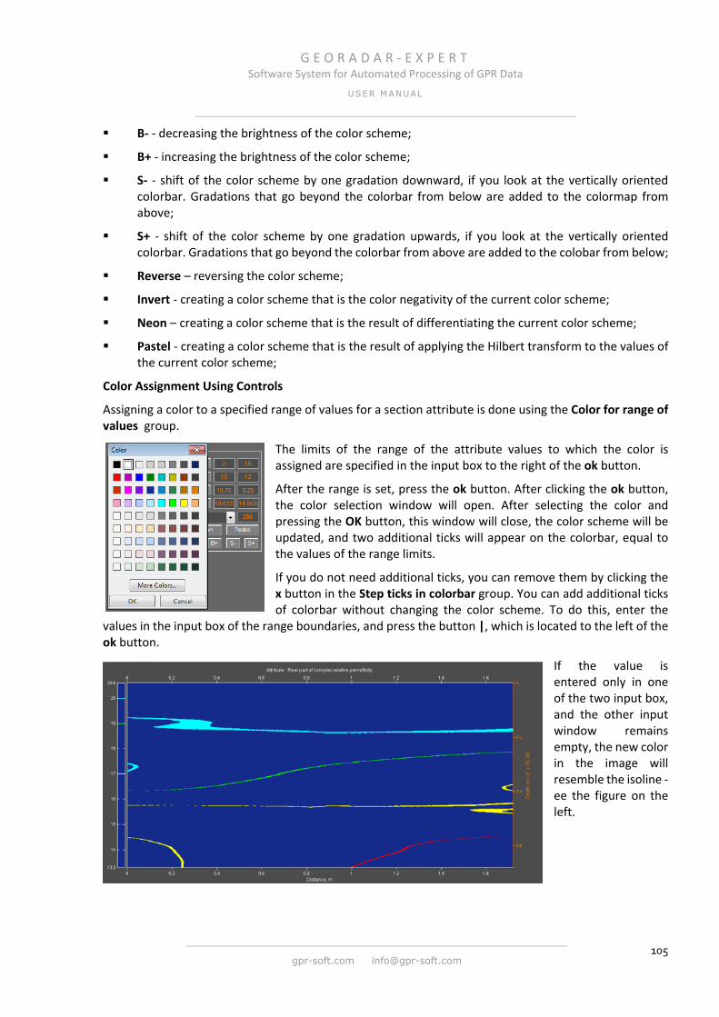
G E O R A D A R - E X P E R T Software System for Automated Processing of GPR Data
USER MANUAL
______________________________________________________________
______________________________________________________________
gpr-soft.com [email protected] 105
B- - decreasing the brightness of the color scheme;
B+ - increasing the brightness of the color scheme;
S- - shift of the color scheme by one gradation downward, if you look at the vertically oriented colorbar. Gradations that go beyond the colorbar from below are added to the colormap from above;
S+ - shift of the color scheme by one gradation upwards, if you look at the vertically oriented colorbar. Gradations that go beyond the colorbar from above are added to the colobar from below;
Reverse – reversing the color scheme;
Invert - creating a color scheme that is the color negativity of the current color scheme;
Neon – creating a color scheme that is the result of differentiating the current color scheme;
Pastel - creating a color scheme that is the result of applying the Hilbert transform to the values of the current color scheme;
Color Assignment Using Controls
Assigning a color to a specified range of values for a section attribute is done using the Color for range of values group.
The limits of the range of the attribute values to which the color is assigned are specified in the input box to the right of the ok button.
After the range is set, press the ok button. After clicking the ok button, the color selection window will open. After selecting the color and pressing the OK button, this window will close, the color scheme will be updated, and two additional ticks will appear on the colorbar, equal to the values of the range limits.
If you do not need additional ticks, you can remove them by clicking the x button in the Step ticks in colorbar group. You can add additional ticks of colorbar without changing the color scheme. To do this, enter the
values in the input box of the range boundaries, and press the button |, which is located to the left of the ok button.
If the value is entered only in one of the two input box, and the other input window remains empty, the new color in the image will resemble the isoline - ee the figure on the left.
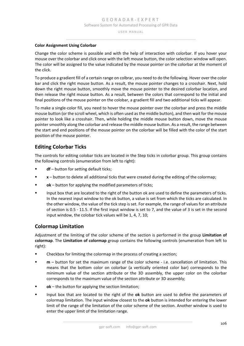
G E O R A D A R - E X P E R T Software System for Automated Processing of GPR Data
USER MANUAL
______________________________________________________________
______________________________________________________________
gpr-soft.com [email protected] 106
Color Assignment Using Colorbar
Change the color scheme is possible and with the help of interaction with colorbar. If you hover your mouse over the colorbar and click once with the left mouse button, the color selection window will open. The color will be assigned to the value indicated by the mouse pointer on the colorbar at the moment of the click.
To produce a gradient fill of a certain range on colbrar, you need to do the following. Hover over the color bar and click the right mouse button. As a result, the mouse pointer changes to a crosshair. Next, hold down the right mouse button, smoothly move the mouse pointer to the desired colorbar location, and then release the right mouse button. As a result, between the colors that correspond to the initial and final positions of the mouse pointer on the colobar, a gradient fill and two additional ticks will appear.
To make a single-color fill, you need to hover the mouse pointer over the colorbar and press the middle mouse button (or the scroll wheel, which is often used as the middle button), and then wait for the mouse pointer to look like a crosshair. Then, while holding the middle mouse button down, move the mouse pointer smoothly along the colorbar and release the middle mouse button. As a result, the range between the start and end positions of the mouse pointer on the colorbar will be filled with the color of the start position of the mouse pointer.
Editing Colorbar Ticks The controls for editing colobar ticks are located in the Step ticks in colorbar group. This group contains the following controls (enumeration from left to right):
df – button for setting default ticks;
x – button to delete all additional ticks that were created during the editing of the colormap;
ok – button for applying the modified parameters of ticks;
Input box that are located to the right of the button ok are used to define the parameters of ticks. In the nearest input window to the ok button, a value is set from which the ticks are calculated. In the other window, the value of the tick step is set. For example, the range of values for an attribute of section is 0.5 - 11.5. If the first input window is set to 7, and the value of 3 is set in the second input window, the colobar tick values will be 1, 4, 7, 10;
Colormap Limitation Adjustment of the limiting of the color scheme of the section is performed in the group Limitation of colormap. The Limitation of colormap group contains the following controls (enumeration from left to right):
Checkbox for limiting the colormap in the process of creating a section;
m – button for set the maximum range of the color scheme - i.e. cancellation of limitation. This means that the bottom color on colorbar (a vertically oriented color bar) corresponds to the minimum value of the section attribute or the 3D assembly, the upper color on the colorbar corresponds to the maximum value of the section attribute or 3D assembly;
ok – the button for applying the section limitation;
Input box that are located to the right of the ok button are used to define the parameters of colormap limitation. The input window closest to the ok button is intended for entering the lower limit of the range of the limitation of the color scheme of the section. Another window is used to enter the upper limit of the limitation range.
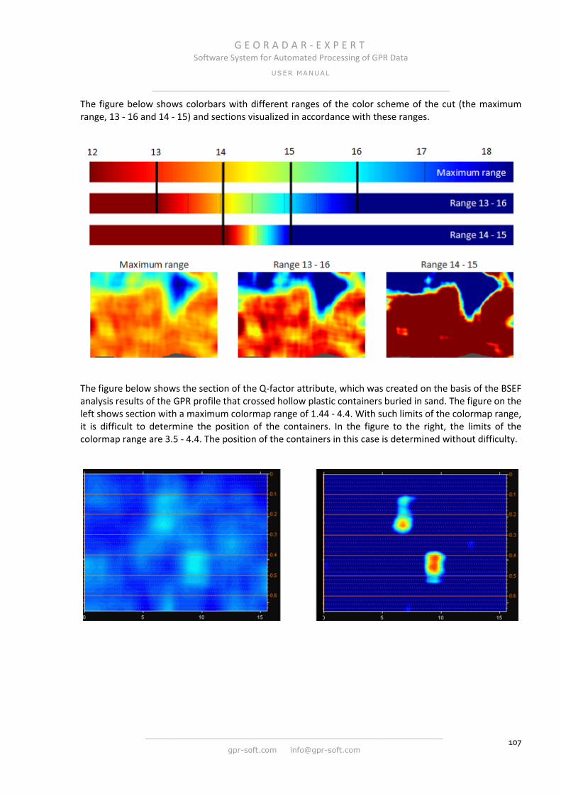
G E O R A D A R - E X P E R T Software System for Automated Processing of GPR Data
USER MANUAL
______________________________________________________________
______________________________________________________________
gpr-soft.com [email protected] 107
The figure below shows colorbars with different ranges of the color scheme of the cut (the maximum range, 13 - 16 and 14 - 15) and sections visualized in accordance with these ranges.
The figure below shows the section of the Q-factor attribute, which was created on the basis of the BSEF analysis results of the GPR profile that crossed hollow plastic containers buried in sand. The figure on the left shows section with a maximum colormap range of 1.44 - 4.4. With such limits of the colormap range, it is difficult to determine the position of the containers. In the figure to the right, the limits of the colormap range are 3.5 - 4.4. The position of the containers in this case is determined without difficulty.
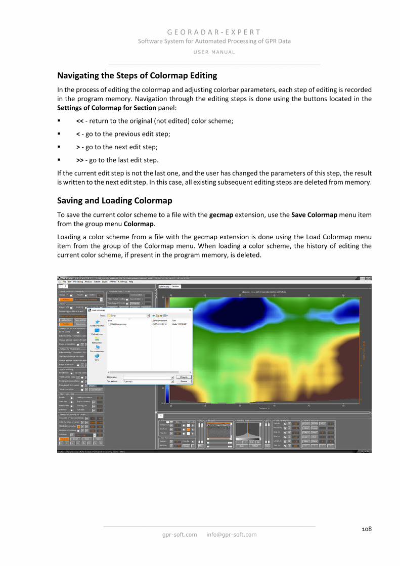
G E O R A D A R - E X P E R T Software System for Automated Processing of GPR Data
USER MANUAL
______________________________________________________________
______________________________________________________________
gpr-soft.com [email protected] 108
Navigating the Steps of Colormap Editing In the process of editing the colormap and adjusting colorbar parameters, each step of editing is recorded in the program memory. Navigation through the editing steps is done using the buttons located in the Settings of Colormap for Section panel:
<< - return to the original (not edited) color scheme;
< - go to the previous edit step;
> - go to the next edit step;
>> - go to the last edit step.
If the current edit step is not the last one, and the user has changed the parameters of this step, the result is written to the next edit step. In this case, all existing subsequent editing steps are deleted from memory.
Saving and Loading Colormap To save the current color scheme to a file with the gecmap extension, use the Save Colormap menu item from the group menu Colormap.
Loading a color scheme from a file with the gecmap extension is done using the Load Colormap menu item from the group of the Colormap menu. When loading a color scheme, the history of editing the current color scheme, if present in the program memory, is deleted.

G E O R A D A R - E X P E R T Software System for Automated Processing of GPR Data
USER MANUAL
______________________________________________________________
______________________________________________________________
gpr-soft.com [email protected] 109
Saving and Exporting Data
Saving in Graphic Format The settings for saving the images of the GPR profile, section or 3D assembly in a graphic format are performed on the Save in Graphic Format panel. This panel does not open automatically during the process of opening the GPR profile. As necessary, the Save in Graphic Format panel is invoked by the user using the Save in Graphic Format menu item from the File menu group, or the Save image button on the Section panel <Section panel>. The Save in Graphic Format panel is located on the bottom tabbed panel.
The process of saving the image is started using the Save image button on the Save in Graphic Format panel, using the Save in graphic format menu item from the group of the File menu, or using the Save image button on the Section panel.
The Save in Graphic Format panel contains the following controls (enumeration from left to right, top to bottom):
Saving scale – saving the image on a specified scale, the values of which are defined in the input box Scale on X and Scale on Y. When the Saving scale checkbox is checked, instead of the On X: mm in 1 m parameter, there is a Show image size button, which serves to call up the message box, where the sizes of the saved image are displayed depending on the specified scale. This information allows you to avoid getting too small or very large image sizes due to the wrong user-selected scale;
Info in scale mode – displaying statistical information on an attribute in a section image or a 3D assembly if it is saved on a given scale;
Show image – if this checkbox is checked, then on the axes the sections or views of 3D assemblies are mapped. If this checkbox is not checked, only the empty axes will be visible on the saved image;
On X: mm in 1 m – this parameter sets the horizontal scale of the image and indicates the number of millimeters of the horizontal axis of the image corresponding to one meter on the distance scale. If the horizontal axis of the cut extends beyond the sheet, the horizontal size of the sheet increases. If the input window of the On X: mm in 1 m parameter is empty, then the cut axes occupy the full width of the sheet on the saved image, without changing its horizontal dimension;
Show boundaries - if there are any layer boundaries created by the user on the section or on the GPR profile, these boundaries on the saved image will also be present if this checkbox is checked;
Resolution, dpi - resolution of the saved image in dots per inch;
Add radarogram - Adding an image of the GPR profile (radargram) to a section image on one sheet for saving;
Image format – drop-down list for selecting the file format in which the image is saved;
Save image – the button to start the process of saving the image. If the section image is saved, that two files are saved - a file with a section image and a file with parameters for creating a section in the geprm format;
The drop-down list to the right of the Save image button is used to select the image size and orientation of the sheet. For example, the default value of format A4 landscape sets the image dimensions for insertion into an MS WORD document in A4 size in landscape orientation.

G E O R A D A R - E X P E R T Software System for Automated Processing of GPR Data
USER MANUAL
______________________________________________________________
______________________________________________________________
gpr-soft.com [email protected] 110
The figure below shows the saved section image for inserting a landscape orientation into the MS WORD document sheet with the marked checked Add radarogram:
At the top of the sheet is an image of the GPR profile in the form in which it was displayed in the program window at the time of saving. Above the image of the GPR profile is placed its name - FILE52.
Under the image of the GPR profile, a section image is placed above which the attribute name of this section is located. To the left of the section image is placed a color bar of the color scheme of the section.
The depth scale contains information on the average value of the real part of the complex relative permittivity ε', in accordance with which the depth scales of GPR profile and the section were calculated.
At the bottom of the sheet, reference information is placed. It contains the following items:
Unit of measurement – unit of measurement of the attribute. Since the permittivity attribute is a dimensionless, this is indicated by the inscription Dimensionless quantity;
Minimum value – minimum value of the section attribute;
Maximum value – minimum value of the section attribute;
Average value – arithmetic mean of the section attribute;
Number of measuring points – the number of analysis points (measuring points) that were used to calculate the section;
Average distance, m – average distance between analysis points in meters;
Density, points per sq m – average number of analysis points per square meter of section.
At the bottom of the sheet is the logo of GEORADAR-EXPERT and information about the licensee.

G E O R A D A R - E X P E R T Software System for Automated Processing of GPR Data
USER MANUAL
______________________________________________________________
______________________________________________________________
gpr-soft.com [email protected] 111
The figure below shows the saved section image in the contour plot mode for inserting a full-page album orientation into the MS WORD document sheet (checkbox Add radarogram not checked):
Saving Section to XZD Format The file with the extension xzd (abbreviation of x-coordinate and z-coordinate data) contains the matrix of the values of the section attribute and the accompanying information - the name of the attribute, the step of the data along vertically and horizontally, and so on.
Files of the xzd format are used to create a 3D assembly (for more details, see <3D Assembly Creating>). Also, the file with the extension xzd can be loaded into the program and apply to it the entire signal processing items, as for the GPR profile.
To save the section data to the xzd file, use the Save for 3D button on the Section panel or use the Save Section in XZD menu item located in the Section menu group or use the Save XZD menu item located in the File menu group.
If need to save the sections in the batch creation mode, not only in the graphical format, but also in the xzd format, before starting the batch mode, need to check the Batch xzd checkbox on the Section panel.
Note: after the xzd format file is loaded into the program as a GPR profile, it is recommended to enable automatic image adjustment. To do this, in the lower tabbed panel, the Gain button in the Adjusting Image panel or the AGC button on the AGC panel should be pressed.

G E O R A D A R - E X P E R T Software System for Automated Processing of GPR Data
USER MANUAL
______________________________________________________________
______________________________________________________________
gpr-soft.com [email protected] 112
Saving to EFD Format GPR profiles of various formats, opened in the GEORADAR-EXPERT, can be saved only in the efd format. To save the GPR profile to efd format, use the Save EFD menu item located in the File menu group.
The efd format contains information about the parameters of the GPR profile and the results of the BSEF analysis, if this analysis was performed.
Saving and Loading Creation Parameters of Section The section creation parameters can be saved to a file with the geprm extension using the menu item Save Settings, located in the group menu Section or by using the Save settings button on the Section panel.
If the user has created layer boundaries on the GPR profile, these boundaries are also saved to the section creation parameter file.
To load the parameters for creating a section, use the menu item Load Settings, located in the group menu Section or the button Load settings in the panel Section. After loading the geprm file, the controls for the section creation parameters will match the loaded values.
If the geprm file contains layer boundaries data, the Boundaries of Layers layer creation options panel opens (if it was not opened) and the boundaries will be created on the GPR profile image located on the GPR Profile tab.
If the geprm file is loaded, but the Section tab in the top tabbed panel is missing, since no section has been created yet, the Section tab is automatically created and on this tab empty axes for the section are created.
Exporting Data to TXT Format The export of the amplitude of the GPR profile, the values of the section attribute or the 3D assembly slice to the txt format table is carried out in the form of a three-column table. The first column of the table is the horizontal coordinate X, the second column is the vertical coordinate Y, the third column is the amplitude of the signal or the value of the attribute A at the point with the coordinates [X Y].
The controls of the export into the table are contained in the Export to Table panel. This panel is loaded into the bottom tabbed panel using the Export to Text Table XYA menu, which is located in the File menu group. You can remove the Export to Table
panel using the close button X, which is located in the upper-right corner of the panel. The Export to Table panel contains the following controls:
Min step by X, m – export with the minimum possible horizontal step. For the GPR profile, this is the distance between the GPR traces (the GPR profiling step);
Min step by Y, m – export without decimation of the data by vertically;
Decimal places – the number of characters after the decimal point in the table values;
Step by X, m – horizontal export step in meters;
Step by Y, m – the export step in vertical in meters, if the button to the left of the input window is in the not pressed state. If this button is pressed state, then its name m changes to ns, which means that the export step will be set in nanoseconds. The status of this button is only relevant for the georadar profile. For sections and slices of the 3D assembly, the vertical export step is set only in meters;

G E O R A D A R - E X P E R T Software System for Automated Processing of GPR Data
USER MANUAL
______________________________________________________________
______________________________________________________________
gpr-soft.com [email protected] 113
Export data – button to start the process of exporting data.
Export Data to GRD Format (Surfer) The export data of GPR profile, section or slice of the 3D assembly to GRD grid format is carried out using the menu Export to Surfer Grid File, which is located in the group of the File menu. Export to GRD format has no settings. After clicking on the menu item Export to Surfer Grid File, the standard file saving window opens, where you can change the name of the saved file and the save directory, and then click the Save button.
The result of exporting data from GEORADAR-EXPERT in GRD format can be loaded into the software Golden Software Surfer as Image Map. To do this, in Surfer, you need to create a new document (Ctrl + N key combination) and then, in the Map menu group, select New and select Image Map. In the window that opens, select the Open Grid file to select a file in GRD format.
If the GRD file was created based on the GPR profile or section, then the data loaded to Surfer can be displayed in upside down form. To fix this, select the Left Axis parameter group in the Object Manager panel of the Surfer program, then select the Scaling tab in the Property Manager panel mark the Reverse axis checkbox located in the Axis Direction group (see the figure below).
To adjust the image size on the sheet, in the Object Manager panel, select the Map parameters group, and then in the Property Manager panel select the Scale tab, which contains all the necessary settings. If you want to adjust the size of each axis independently, you need to uncheck Proportional XY scaling:
To customize the color scheme for displaying loaded data, on the Object Manager panel, select the Image-(file name) parameter group, then on the Property Manager panel select the General tab and use the
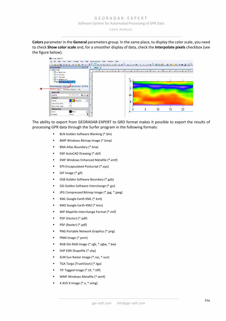
G E O R A D A R - E X P E R T Software System for Automated Processing of GPR Data
USER MANUAL
______________________________________________________________
______________________________________________________________
gpr-soft.com [email protected] 114
Colors parameter in the General parameters group. In the same place, to display the color scale, you need to check Show color scale and, for a smoother display of data, check the Interpolate pixels checkbox (see the figure below).
The ability to export from GEORADAR-EXPERT to GRD format makes it possible to export the results of processing GPR data through the Surfer program in the following formats:
BLN Golden Software Blanking (*.bln)
BMP Windows Bitmap Image (*.bmp)
BNA Atlas Boundary (*.bna)
DXF AutoCAD Drawing (*.dxf)
EMF Windows Enhanced Metafile (*.emf)
EPS Encapsulated Postscript (*.eps)
GIF Image (*.gif)
GSB Golden Software Boundary (*.gsb)
GSI Golden Software Interchange (*.gsi)
JPG Compressed Bitmap Image (*.jpg, *.jpeg)
KML Google Earth KML (*.kml)
KMZ Google Earth KMZ (*.kmz)
MIF MapInfo Interchange Format (*.mif)
PDF (Vector) (*.pdf)
PDF (Raster) (*.pdf)
PNG Portable Network Graphics (*.png)
PNM Image (*.pnm)
RGB SGI-RGB Image (*.rgb, *.rgba, *.bw)
SHP ESRI Shapefile (*.shp)
SUN Sun Raster Image (*.ras, *.sun)
TGA Targa (TrueVision) (*.tga)
TIF Tagged Image (*.tif, *.tiff)
WMF Windows Metafile (*.wmf)
X AVS X-Image (*.x, *.ximg)
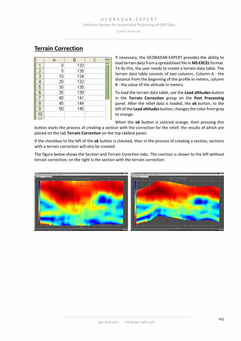
G E O R A D A R - E X P E R T Software System for Automated Processing of GPR Data
USER MANUAL
______________________________________________________________
______________________________________________________________
gpr-soft.com [email protected] 115
Terrain Correction If necessary, the GEORADAR-EXPERT provides the ability to load terrain data from a spreadsheet file in MS EXCEL format. To do this, the user needs to create a terrain data table. The terrain data table consists of two columns. Column A - the distance from the beginning of the profile in meters, column B - the value of the altitude in meters.
To load the terrain data table, use the Load altitudes button in the Terrain Correction group on the Post Processing panel. After the relief data is loaded, the ok button, to the left of the Load altitudes button, changes the color from gray to orange.
When the ok button is colored orange, then pressing this button starts the process of creating a section with the correction for the relief, the results of which are placed on the tab Terrain Correction on the top tabbed panel.
If the checkbox to the left of the ok button is checked, then in the process of creating a section, sections with a terrain correction will also be created.
The figure below shows the Section and Terrain Corection tabs. The csection is shown to the left without terrain correction; on the right is the section with the terrain correction:
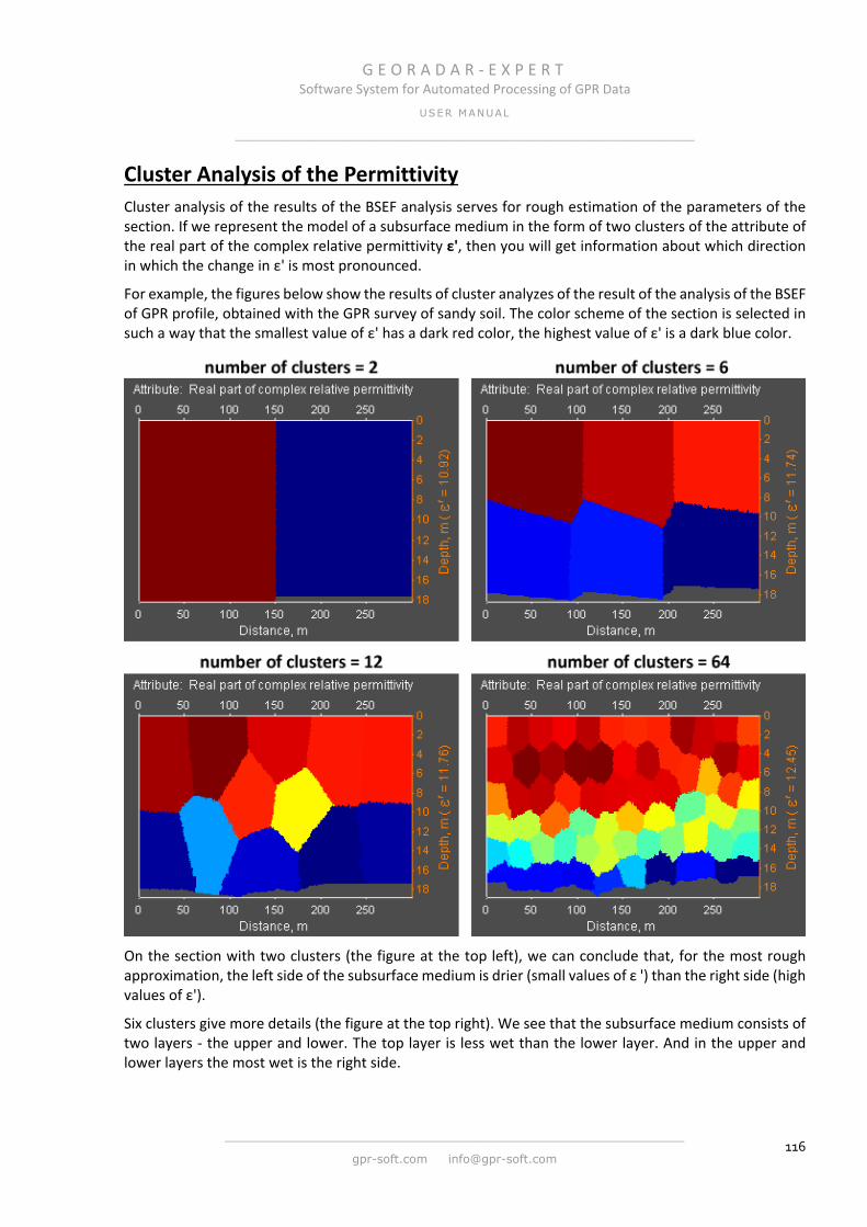
G E O R A D A R - E X P E R T Software System for Automated Processing of GPR Data
USER MANUAL
______________________________________________________________
______________________________________________________________
gpr-soft.com [email protected] 116
Cluster Analysis of the Permittivity Cluster analysis of the results of the BSEF analysis serves for rough estimation of the parameters of the section. If we represent the model of a subsurface medium in the form of two clusters of the attribute of the real part of the complex relative permittivity ε', then you will get information about which direction in which the change in ε' is most pronounced.
For example, the figures below show the results of cluster analyzes of the result of the analysis of the BSEF of GPR profile, obtained with the GPR survey of sandy soil. The color scheme of the section is selected in such a way that the smallest value of ε' has a dark red color, the highest value of ε' is a dark blue color.
On the section with two clusters (the figure at the top left), we can conclude that, for the most rough approximation, the left side of the subsurface medium is drier (small values of ε ') than the right side (high values of ε').
Six clusters give more details (the figure at the top right). We see that the subsurface medium consists of two layers - the upper and lower. The top layer is less wet than the lower layer. And in the upper and lower layers the most wet is the right side.
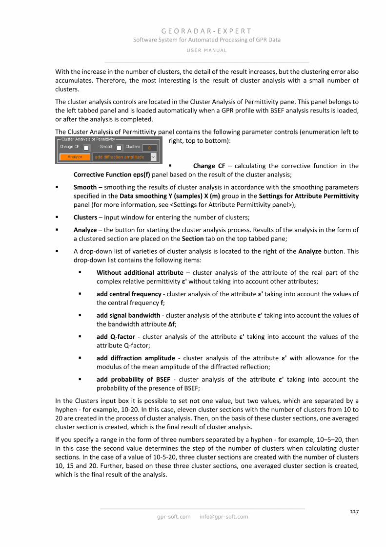
G E O R A D A R - E X P E R T Software System for Automated Processing of GPR Data
USER MANUAL
______________________________________________________________
______________________________________________________________
gpr-soft.com [email protected] 117
With the increase in the number of clusters, the detail of the result increases, but the clustering error also accumulates. Therefore, the most interesting is the result of cluster analysis with a small number of clusters.
The cluster analysis controls are located in the Cluster Analysis of Permittivity pane. This panel belongs to the left tabbed panel and is loaded automatically when a GPR profile with BSEF analysis results is loaded, or after the analysis is completed.
The Cluster Analysis of Permittivity panel contains the following parameter controls (enumeration left to right, top to bottom):
Change CF – calculating the corrective function in the Corrective Function eps(f) panel based on the result of the cluster analysis;
Smooth – smoothing the results of cluster analysis in accordance with the smoothing parameters specified in the Data smoothing Y (samples) X (m) group in the Settings for Attribute Permittivity panel (for more information, see <Settings for Attribute Permittivity panel>);
Clusters – input window for entering the number of clusters;
Analyze – the button for starting the cluster analysis process. Results of the analysis in the form of a clustered section are placed on the Section tab on the top tabbed pane;
A drop-down list of varieties of cluster analysis is located to the right of the Analyze button. This drop-down list contains the following items:
Without additional attribute – cluster analysis of the attribute of the real part of the complex relative permittivity ε' without taking into account other attributes;
add central frequency - cluster analysis of the attribute ε' taking into account the values of the central frequency f;
add signal bandwidth - cluster analysis of the attribute ε' taking into account the values of the bandwidth attribute Δf;
add Q-factor - cluster analysis of the attribute ε' taking into account the values of the attribute Q-factor;
add diffraction amplitude - cluster analysis of the attribute ε' with allowance for the modulus of the mean amplitude of the diffracted reflection;
add probability of BSEF - cluster analysis of the attribute ε' taking into account the probability of the presence of BSEF;
In the Clusters input box it is possible to set not one value, but two values, which are separated by a hyphen - for example, 10-20. In this case, eleven cluster sections with the number of clusters from 10 to 20 are created in the process of cluster analysis. Then, on the basis of these cluster sections, one averaged cluster section is created, which is the final result of cluster analysis.
If you specify a range in the form of three numbers separated by a hyphen - for example, 10–5–20, then in this case the second value determines the step of the number of clusters when calculating cluster sections. In the case of a value of 10-5-20, three cluster sections are created with the number of clusters 10, 15 and 20. Further, based on these three cluster sections, one averaged cluster section is created, which is the final result of the analysis.
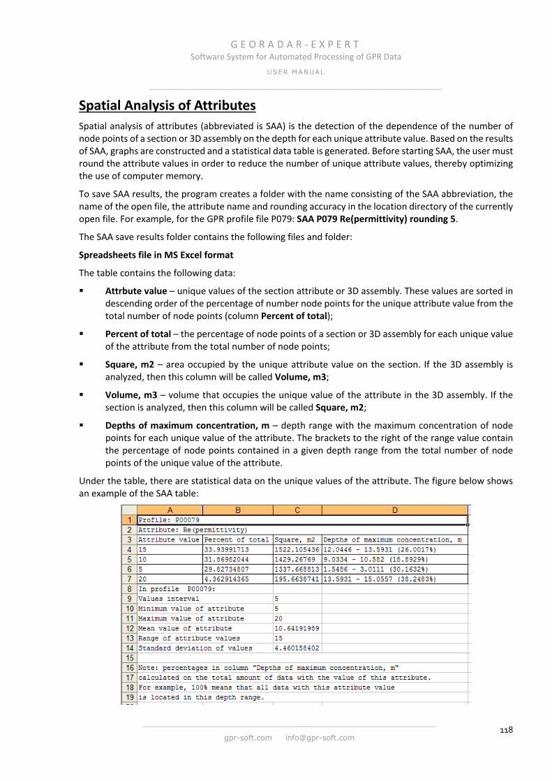
G E O R A D A R - E X P E R T Software System for Automated Processing of GPR Data
USER MANUAL
______________________________________________________________
______________________________________________________________
gpr-soft.com [email protected] 118
Spatial Analysis of Attributes Spatial analysis of attributes (abbreviated is SAA) is the detection of the dependence of the number of node points of a section or 3D assembly on the depth for each unique attribute value. Based on the results of SAA, graphs are constructed and a statistical data table is generated. Before starting SAA, the user must round the attribute values in order to reduce the number of unique attribute values, thereby optimizing the use of computer memory.
To save SAA results, the program creates a folder with the name consisting of the SAA abbreviation, the name of the open file, the attribute name and rounding accuracy in the location directory of the currently open file. For example, for the GPR profile file P079: SAA P079 Re(permittivity) rounding 5.
The SAA save results folder contains the following files and folder:
Spreadsheets file in MS Excel format
The table contains the following data:
Attrbute value – unique values of the section attribute or 3D assembly. These values are sorted in descending order of the percentage of number node points for the unique attribute value from the total number of node points (column Percent of total);
Percent of total – the percentage of node points of a section or 3D assembly for each unique value of the attribute from the total number of node points;
Square, m2 – area occupied by the unique attribute value on the section. If the 3D assembly is analyzed, then this column will be called Volume, m3;
Volume, m3 – volume that occupies the unique value of the attribute in the 3D assembly. If the section is analyzed, then this column will be called Square, m2;
Depths of maximum concentration, m – depth range with the maximum concentration of node points for each unique value of the attribute. The brackets to the right of the range value contain the percentage of node points contained in a given depth range from the total number of node points of the unique value of the attribute.
Under the table, there are statistical data on the unique values of the attribute. The figure below shows an example of the SAA table:

G E O R A D A R - E X P E R T Software System for Automated Processing of GPR Data
USER MANUAL
______________________________________________________________
______________________________________________________________
gpr-soft.com [email protected] 119
The plot of the dependence of the number of node points from the depth for each unique attribute value - of the type 'all in one'.
The 'all in one' plot is saved to a file named All graphs on one sheet.png. This plot shows the distribution of the number of node points for each unique attribute value in depth. The figure below shows an example of the plot 'all in one'.
At the top of the plot are the name of the GPR profile or 3D assembly, the name of the attribute and the precision of rounding.
The vertical axis of the graph is the depth of the section or the 3D assembly in meters. The horizontal axis of the graph is the percentage of the total number of node points of the section or 3D assembly.
For each unique attribute value, a curve of a unique color and line type is created. Information on the correspondence between the values of the attribute and the color and type of curves is placed to the right of the graph. At the bottom of the graph are statistics of the attribute.
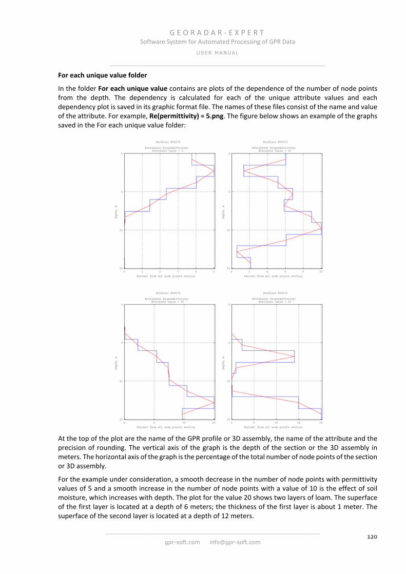
G E O R A D A R - E X P E R T Software System for Automated Processing of GPR Data
USER MANUAL
______________________________________________________________
______________________________________________________________
gpr-soft.com [email protected] 120
For each unique value folder
In the folder For each unique value contains are plots of the dependence of the number of node points from the depth. The dependency is calculated for each of the unique attribute values and each dependency plot is saved in its graphic format file. The names of these files consist of the name and value of the attribute. For example, Re(permittivity) = 5.png. The figure below shows an example of the graphs saved in the For each unique value folder:
At the top of the plot are the name of the GPR profile or 3D assembly, the name of the attribute and the precision of rounding. The vertical axis of the graph is the depth of the section or the 3D assembly in meters. The horizontal axis of the graph is the percentage of the total number of node points of the section or 3D assembly.
For the example under consideration, a smooth decrease in the number of node points with permittivity values of 5 and a smooth increase in the number of node points with a value of 10 is the effect of soil moisture, which increases with depth. The plot for the value 20 shows two layers of loam. The superface of the first layer is located at a depth of 6 meters; the thickness of the first layer is about 1 meter. The superface of the second layer is located at a depth of 12 meters.

G E O R A D A R - E X P E R T Software System for Automated Processing of GPR Data
USER MANUAL
______________________________________________________________
______________________________________________________________
gpr-soft.com [email protected] 121
For spatial analysis of attributes, need perform the following steps:
Open the GPR profile file containing the BSEF analysis results or perform a BSEF analysis if this analysis was not performed (for more details, see <BSEF Analysis and Saving Analysis Results>);
Select an attribute and create a section (for more details, see <Creating Section Based on the BSEF Analysis Results>);
Set the rounding accuracy in the Post Processing panel, in the Rounding attribute values group, and round the attribute values (for more information, see <Rounding Attribute Values>). Rounding is necessary to reduce the number of unique attribute values. If rounding is not performed, then because of the large number of unique values, computer memory may overflow;
To start the process of spatial analysis of attributes, click on the Spatial Analysis Attributes menu item located in the Analysis menu group;
After the completion of the SAA process, the message box (see figure below) about the end of the analysis will be displayed and the question whether the user wants to open the directory containing the results of the analysis. If the user clicks the Yes button, the main window of the program is minimized and the folder with the results of the SAA analysis opens in Windows Explorer.
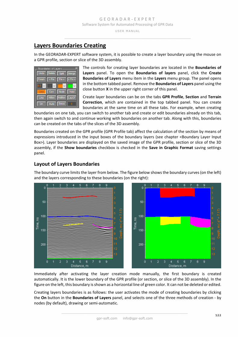
G E O R A D A R - E X P E R T Software System for Automated Processing of GPR Data
USER MANUAL
______________________________________________________________
______________________________________________________________
gpr-soft.com [email protected] 122
Layers Boundaries Creating In the GEORADAR-EXPERT software system, it is possible to create a layer boundary using the mouse on a GPR profile, section or slice of the 3D assembly.
The controls for creating layer boundaries are located in the Boundaries of Layers panel. To open the Boundaries of layers panel, click the Create Boundaries of Layers menu item in the Layers menu group. The panel opens in the bottom tabbed panel. Remove the Boundaries of Layers panel using the close button X in the upper right corner of this panel.
Create layer boundaries can be on the tabs GPR Profile, Section and Terrain Correction, which are contained in the top tabbed panel. You can create boundaries at the same time on all these tabs. For example, when creating
boundaries on one tab, you can switch to another tab and create or edit boundaries already on this tab, then again switch to and continue working with boundaries on another tab. Along with this, boundaries can be created on the tabs of the slices of the 3D assembly.
Boundaries created on the GPR profile (GPR Profile tab) affect the calculation of the section by means of expressions introduced in the input boxes of the boundary layers (see chapter <Boundary Layer Input Box>). Layer boundaries are displayed on the saved image of the GPR profile, section or slice of the 3D assembly, if the Show boundaries checkbox is checked in the Save in Graphic Format saving settings panel.
Layout of Layers Boundaries The boundary curve limits the layer from below. The figure below shows the boundary curves (on the left) and the layers corresponding to these boundaries (on the right):
Immediately after activating the layer creation mode manually, the first boundary is created automatically. It is the lower boundary of the GPR profile (or section, or slice of the 3D assembly). In the figure on the left, this boundary is shown as a horizontal line of green color. It can not be deleted or edited.
Creating layers boundaries is as follows: the user activates the mode of creating boundaries by clicking the On button in the Boundaries of Layers panel, and selects one of the three methods of creation - by nodes (by default), drawing or semi-automatic.
G E O R A D A R - E X P E R T Software System for Automated Processing of GPR Data
USER MANUAL
______________________________________________________________
______________________________________________________________
gpr-soft.com [email protected] 123
In the first case, the user clicks the left mouse button within the axes, thereby creating the nodes of the boundary curve. In the second case, the user, while holding the left mouse button down, moves the mouse pointer within the axes, drawing a boundary curve. In the third case, the user specifies the interval vertically, within a specified interval, the program creates a boundary curve using the extremes of the GPR profile values or the section attribute (3D assembly slice) as the nodes of these curve.
Clicking the left mouse button on the curve of the boundary that has already been created allows this boundary to be accessible for editing. In edit mode, the boundary differs in color from the other boundaries and displays nodes (if the Node button is pressed). The user can move nodes within axes or delete. Exiting the editing mode is done using the Finish button or one of the buttons from the same row.
Detailed descriptions of user actions for creating, editing, saving layer boundaries and other actions with layers are presented in the further sections of this user manual.
Boundaries of Layers panel The Boundaries of Layers panel contains the following controls for creating the layer boundaries (enumeration from left to right, top to bottom):
Undo – button to delete the last created boundary curve node. This button is used in the process of creating a boundary;
Delete – button to delete the layer boundaries. To delete, the boundary must be in edit mode. If there is no boundary in the edit mode, then after pressing the Delete button, all existing boundaries are deleted, except for the lowest boundary, which was automatically created when the boundaries creation mode was activated with the On button;
Split – button to enabling the split mode or crop the boundary. For more details, see <Splitting Boundary into Two Parts>;
Merge – button for enabling the mode of merging two boundaries. For more details, see <Merging of Two Boundary>;
Finish – button to finish editing the boundary. In this case, the positions of the nodes at the beginning and at the end of the boundary curve do not change the position;
<Fin - button to finish editing the boundary. Wherein the boundary curve is extended horizontally to the left;
Fin> - button to finish editing the boundary. Wherein the boundary curve is extended horizontally to the right;
<Fin> - button to finish editing the boundary. Wherein the boundary curve is extended horizontally to the left and right;
Drop-down list for selecting the thickness of the boundary curve at points (1 points = 1/72 inch). If one of the boundaries is in edit mode, then using this drop-down list the thickness of the curve is set only for this boundary. If there are no boundaries in the editing mode, then the thickness of the curve is set for all boundaries;
Drop-down list for selecting the type of the boundary curve. If one of the boundaries is in edit mode, then using this drop-down list, the curve type is set only for this boundary. If there is no boundary in the edit mode, then the curve type is set for all existing boundaries;
Drop-down list for selecting the color of the boundary curve, which is in edit or create mode;
Drop-down list of the color selection of the boundaries curve, which are not in the editing mode;

G E O R A D A R - E X P E R T Software System for Automated Processing of GPR Data
USER MANUAL
______________________________________________________________
______________________________________________________________
gpr-soft.com [email protected] 124
Cick – button to select how to create the boundary. If the Cick button is pressed state (by default), then the boundary is created using nodes (for more details, see <Creating Layer Boundary by Nodes>). If the button is unpressed state, the boundary is created by the method of drawing with the mouse (for more details, see <Creating Layer Boundary by Drawing>);
Corr – button for selecting the method for adjusting the boundary curve in the editing mode. If the Corr button is pressed state (by default), you can add nodes both inside the curve and outside it. If this button is in the unpressed state, then you can add nodes only outside the horizontal coordinates of the curve. The curve can be extended to the left or right, but you can not make corrections to existing nodes, or add new nodes to the boundary curve;
Node –button for displaying the nodes of the boundary curve in the editing mode. When the Node button is pressed, the nodes are rendered as dots. When this button is in the unpressed state, the nodes are hidden;
Hold – button to save the boundary color after exiting edit mode. If the Hold button is in the unpressed state (by default), after exiting the edit mode, the color of the boundary curve changes to the color that is selected in the drop-down list of the curve color selection in the non-editable state (rightmost of the row of drop-down lists). If the Hold button is in the pressed state, then after exiting the editing mode, the boundary curve retains its color;
Line – button for selecting the type of connection of nodes when creating or editing a boundary. If the Line button is in the unpressed state (by default), then the nodes are connected with each other by spline, if the Line button is pressed, then the nodes are connected with each other by straight lines;
inBox – button for creating or deleting the input boxes for the boundaries of the layers (for more details, see <Boundary Layer Input Box>). If one of the boundaries is in edit mode, then after pressing the inBox button, the input box is created only for this boundary. If there is no boundary in the edit mode, then an input box is created for all boundaries at once. To delete an input box from one of the boundary, click the mouse on its curve to turn the boundary to edit mode and click the inBox button once. Pressing this button again will create an input box for this boundary. To remove all the input boxes at the same time, you need to ensure that no boundaries are in the editable state. In this case, after a single press of the inBox button, all the input boxes are deleted.
hidBox – button for hiding the input box of conditions without deleting them. If the input boxes are hidden, then the background color of the hidBox button becomes darker. To display the hidden input boxes, you need to click the hidBox button again. If one of the boundaries is in edit mode, the hidBox button works only for the editable boundary;
LayCF – button for creating a local corrective function for the layer. For more details, see <Local Corrective Function for Layer>;
On – button to activate the layers boundaries creation mode. When the On button is pressed state, the background color of the current tab changes from gray to dark blue-green;
Auto – button for activating the semi-automatic way of creating layer boundaries. For more information, see <Creating Layer Boundary in Semi-Automatic Mode>.
Smoo – button for starting the process of smoothing the boundary curve. The boundary must be created in semi-automatic mode and is in the editing state. The window for entering the smoothing value in meters is located to the right of the Smoo button;
The input window for entering the smoothing value in meters. When creating a boundary in semi-automatic mode, it will be smoothed according to the specified value. If the boundary is already created in semi-automatic mode, you can change the degree of smoothing. To do this, you need to
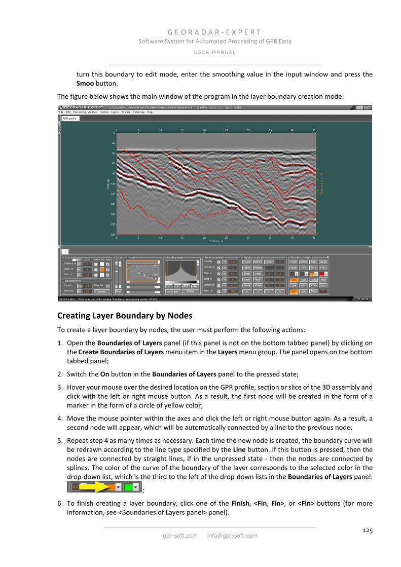
G E O R A D A R - E X P E R T Software System for Automated Processing of GPR Data
USER MANUAL
______________________________________________________________
______________________________________________________________
gpr-soft.com [email protected] 125
turn this boundary to edit mode, enter the smoothing value in the input window and press the Smoo button.
The figure below shows the main window of the program in the layer boundary creation mode:
Creating Layer Boundary by Nodes To create a layer boundary by nodes, the user must perform the following actions:
1. Open the Boundaries of Layers panel (if this panel is not on the bottom tabbed panel) by clicking on the Create Boundaries of Layers menu item in the Layers menu group. The panel opens on the bottom tabbed panel;
2. Switch the On button in the Boundaries of Layers panel to the pressed state;
3. Hover your mouse over the desired location on the GPR profile, section or slice of the 3D assembly and click with the left or right mouse button. As a result, the first node will be created in the form of a marker in the form of a circle of yellow color;
4. Move the mouse pointer within the axes and click the left or right mouse button again. As a result, a second node will appear, which will be automatically connected by a line to the previous node;
5. Repeat step 4 as many times as necessary. Each time the new node is created, the boundary curve will be redrawn according to the line type specified by the Line button. If this button is pressed, then the nodes are connected by straight lines, if in the unpressed state - then the nodes are connected by splines. The color of the curve of the boundary of the layer corresponds to the selected color in the drop-down list, which is the third to the left of the drop-down lists in the Boundaries of Layers panel:
;
6. To finish creating a layer boundary, click one of the Finish, <Fin, Fin>, or <Fin> buttons (for more information, see <Boundaries of Layers panel> panel).
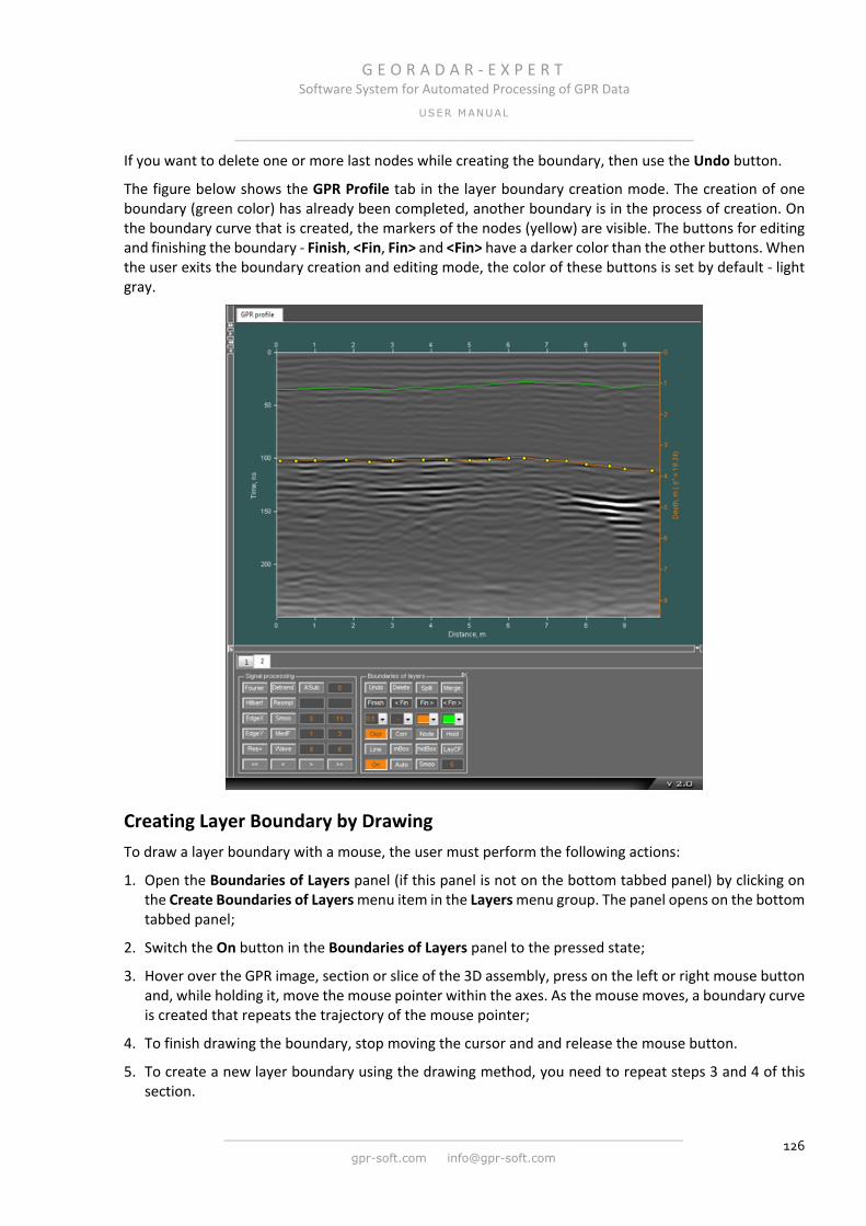
G E O R A D A R - E X P E R T Software System for Automated Processing of GPR Data
USER MANUAL
______________________________________________________________
______________________________________________________________
gpr-soft.com [email protected] 126
If you want to delete one or more last nodes while creating the boundary, then use the Undo button.
The figure below shows the GPR Profile tab in the layer boundary creation mode. The creation of one boundary (green color) has already been completed, another boundary is in the process of creation. On the boundary curve that is created, the markers of the nodes (yellow) are visible. The buttons for editing and finishing the boundary - Finish, <Fin, Fin> and <Fin> have a darker color than the other buttons. When the user exits the boundary creation and editing mode, the color of these buttons is set by default - light gray.
Creating Layer Boundary by Drawing To draw a layer boundary with a mouse, the user must perform the following actions:
1. Open the Boundaries of Layers panel (if this panel is not on the bottom tabbed panel) by clicking on the Create Boundaries of Layers menu item in the Layers menu group. The panel opens on the bottom tabbed panel;
2. Switch the On button in the Boundaries of Layers panel to the pressed state;
3. Hover over the GPR image, section or slice of the 3D assembly, press on the left or right mouse button and, while holding it, move the mouse pointer within the axes. As the mouse moves, a boundary curve is created that repeats the trajectory of the mouse pointer;
4. To finish drawing the boundary, stop moving the cursor and and release the mouse button.
5. To create a new layer boundary using the drawing method, you need to repeat steps 3 and 4 of this section.
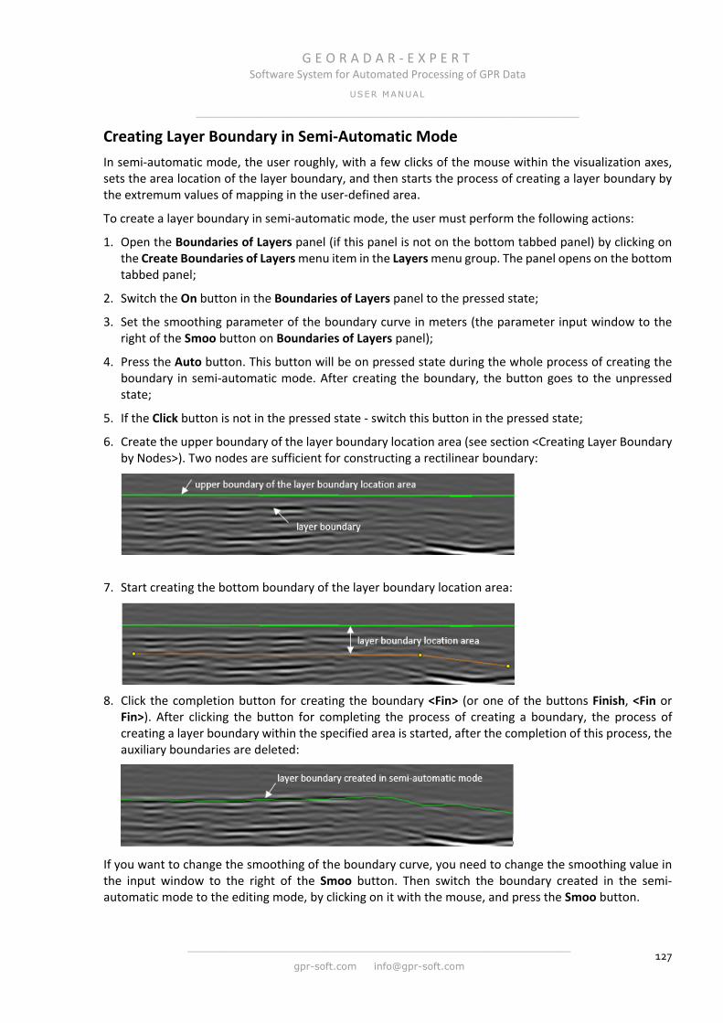
G E O R A D A R - E X P E R T Software System for Automated Processing of GPR Data
USER MANUAL
______________________________________________________________
______________________________________________________________
gpr-soft.com [email protected] 127
Creating Layer Boundary in Semi-Automatic Mode In semi-automatic mode, the user roughly, with a few clicks of the mouse within the visualization axes, sets the area location of the layer boundary, and then starts the process of creating a layer boundary by the extremum values of mapping in the user-defined area.
To create a layer boundary in semi-automatic mode, the user must perform the following actions:
1. Open the Boundaries of Layers panel (if this panel is not on the bottom tabbed panel) by clicking on the Create Boundaries of Layers menu item in the Layers menu group. The panel opens on the bottom tabbed panel;
2. Switch the On button in the Boundaries of Layers panel to the pressed state;
3. Set the smoothing parameter of the boundary curve in meters (the parameter input window to the right of the Smoo button on Boundaries of Layers panel);
4. Press the Auto button. This button will be on pressed state during the whole process of creating the boundary in semi-automatic mode. After creating the boundary, the button goes to the unpressed state;
5. If the Click button is not in the pressed state - switch this button in the pressed state;
6. Create the upper boundary of the layer boundary location area (see section <Creating Layer Boundary by Nodes>). Two nodes are sufficient for constructing a rectilinear boundary:
7. Start creating the bottom boundary of the layer boundary location area:
8. Click the completion button for creating the boundary <Fin> (or one of the buttons Finish, <Fin or
Fin>). After clicking the button for completing the process of creating a boundary, the process of creating a layer boundary within the specified area is started, after the completion of this process, the auxiliary boundaries are deleted:
If you want to change the smoothing of the boundary curve, you need to change the smoothing value in the input window to the right of the Smoo button. Then switch the boundary created in the semi-automatic mode to the editing mode, by clicking on it with the mouse, and press the Smoo button.

G E O R A D A R - E X P E R T Software System for Automated Processing of GPR Data
USER MANUAL
______________________________________________________________
______________________________________________________________
gpr-soft.com [email protected] 128
Editing Layer Boundary To switch the layer boundary to the editing mode, you have to click on it with the left or right mouse button. The boundary curve will change color boundary and the node markers will be displayed (if the Node button on pressed state). In the editing mode, the following operations on the boundary curve are available:
Adding Nodes to Boundary Curve
Adding nodes to the boundary curve is performed according to the state of the Corr button. If the Corr button is not pressed, then you can add nodes only along the edges of the boundary, clicking the mouse to the left or to the right of the curve. If the Corr button on pressed state (by default), you can add nodes not only to the left or to the right of the boundary, but also between existing nodes. To do this, move the mouse pointer under or over the boundary and click with the mouse. As a result, a node will be created at the location of the mouse pointer, and the boundary will be redrawing. If the mouse pointer is under or above an existing node, then by clicking with mouse button, this node moves along the vertical coordinate to the position of the mouse pointer position.
Splitting Boundary into Two Parts
To split a boundary into two parts, you must delete one or a group of nodes on the boundary curve. To do this, switch the Split button on Boundaries of Layers panel to the pressed state, move the mouse pointer over the boundary curve, click the left mouse button and while holding it, move the mouse pointer diagonally, creating a selection box that grabs the nodes for deletion:
After the mouse button is released, the nodes inside the selection area are deleted, after which two new layer boundaries are created, and the Split button is switched to the unpressed state:
Cropping of Boundary
Actions for cropping the boundary are like actions to splitting the boundary into two parts. The mouse pointer in the initial stage of creating the selection box should be under or above the boundary, and in the final stage, before the mouse button is released, the pointer should be outside the boundary horizontally. In the final stage, the pointer can be outside the limits of the mapping axes:

G E O R A D A R - E X P E R T Software System for Automated Processing of GPR Data
USER MANUAL
______________________________________________________________
______________________________________________________________
gpr-soft.com [email protected] 129
Merging of Two Boundary
To merge two boundaries into one, one of the boundaries should be switched to editing mode by clicking on it with the mouse:
After switching one of the boundaries to the editing mode, you must switch the Merge button on Boundaries of Layers panel to the pressed state and click on the second boundary with the mouse. As a result, the two boundaries merge into one, and the Merge button will switch to an unpressed state:
Deleting Nodes
To delete nodes of the boundary curve, you first need to perform the actions for splitting the boundary into two parts (for more details, see <Splitting Boundary into Two Parts>), and then the actions for merging the resulting two boundaries into one whole (for more details, see <Merging of Two Boundary>).
Boundary Layer Input Box If the boundaries of layers have been created on the GPR profile, then when creating a section of the properties of these layers, they will be taken into account. To enter the properties of the layers, the input boxes is used, which are attached to the boundary curves and look like rectangles of orange color:
When creating a section, the property is applied to a layer that is bounded from below the curve to which the input box belongs that contains the property. On top, this layer is bounded either by the boundary of another layer or by the zero point of the GPR scale of the profile (see chapter <Layout of Layers Boundaries>).
The input box is created with the inBox button. If one of the boundaries is in editable mode, then by pressing the button inBox the input box is created only for this boundary. If there are no boundaries in the editable mode, then by pressing the inBox button, input boxes for all boundaries are created. To delete input boxes, need to press the inBox button again. The hidBox button turns off/on the visibility of the input boxes.
To enter a layer property, click on the input field, then the cursor appears inside this field and the user can enter the properties of the layer using the keyboard of the computer. The layer property is entered as one expression, or two expressions, between which the vertical separator is located: Expression1|Expression2.

G E O R A D A R - E X P E R T Software System for Automated Processing of GPR Data
USER MANUAL
______________________________________________________________
______________________________________________________________
gpr-soft.com [email protected] 130
Expression1 is a layer property for the section of the attribute Re(permittivity), which is always calculated, regardless of the section attribute. The section of the attribute Re(permittivity) is created during the calculation of sections of all other attributes (except its own) as an auxiliary. Based on the values of the section of the attribute Re(permittivity), in the process of creating a section, this section is corrected in depth.
Expression2 is a layer property for the section of the main attribute. If a section of the Re(permittivity) attribute is created, the layer properties in the input field consist of a single expression, with no vertical separator.
If the section of the attribute is not Re(permittivity) and for the auxiliary attribute Re(permittivity) not need to define the layer property, but the layer property is required only for the main attribute, then the expression consists only of the vertical separator and the second expression: |Expression2.
Below is a list of expressions for the layer property:
Numeric values - all values of the section attribute within the layer take the specified values. For example:
- all values inside the layer on the section of the attribute Re(permittivity) are 9;
- all values inside the layer on the auxiliary section of the attribute Re(permittivity) are 9, and all values inside this layer on the section of the main attribute are equal to 5;
- all values inside the layer on the auxiliary section of the attribute Re(permittivity) do not change, but all values inside this layer on the section of the main attribute are equal to 5;
Value ranges - all values of the section within the layer are recalculated in accordance with the specified range of values. For example:
- all values inside the layer on the section of the attribute Re(permittivity) are recalculated in the range from 4.5 to 9;
- all values inside the layer on the section of the attribute Re(permittivity) are recalculated in the range from 4.5 to 9, and inside this layer on the section of the main attribute the values are recalculated in the range from 250 to 350;
- all values inside the layer on the auxiliary section of the attribute Re(permittivity) do not change, but within this layer on the section of the main attribute the values are recalculated in the range from 250 to 350;
Equal sign = - all values inside the layer take the average value of the attribute inside this layer. For example:
- all values within the layer on the section of the attribute Re(permittivity) are equal to the average value of the attribute inside this layer;
- all values inside the layer on the section of the attribute Re(permittivity) are recalculated in the range from 9 to 12, and inside this layer on the section of the main attribute the values are equal to the average of this layer;
== – the values of each column of the attribute matrix of the section within the layer become equal to the average arithmetic value of this column. For example, ;
min - all values of the section within the layer take the minimum value of the attribute inside this layer;

G E O R A D A R - E X P E R T Software System for Automated Processing of GPR Data
USER MANUAL
______________________________________________________________
______________________________________________________________
gpr-soft.com [email protected] 131
max - all values of the section within the layer take the maxmum value of the attribute inside this layer;
min= - the values of each column of the attribute matrix of the section within the layer become equal to the minimum value from this column. For example, . For more details, see <Section Creating with Layer Properties Accounting>;
max= - the values of each column of the attribute matrix of the section within the layer become equal to the maximum value from this column. For example, . For more details, see <Section Creating with Layer Properties Accounting>;
All of the above expressions are applied to input fields that belong to the boundaries created on the GPR profile on the GPR Profile tab. For boundaries that belong to an already created section on the Section tab, only two expressions apply that affect the process of re-creating the section:
& - below the boundary with the input box containing this symbol, the value of the attribute decreases as the depth increases, if it is smaller than the previous one, or becomes equal to the previous one if it is greater than the previous value;
&& - below the boundary with the input field containing this symbol, the value of the attribute increases as the depth increases, if it is greater than the previous one, or becomes equal to the previous one if it is less than the previous value.
The figure below to the left shows the section on which the user created a boundary with an input box containing the && expression - ie. increase the value of the attribute with increasing depth. The figure on the right shows the result of re-creating a section with this expression in mind.
The figure below to the left shows the section on which the user created a boundary with an input box containing the & expression - ie. reducing the value of the attribute with increasing depth. The figure on the right shows the result of re-creating a section with this expression in mind.
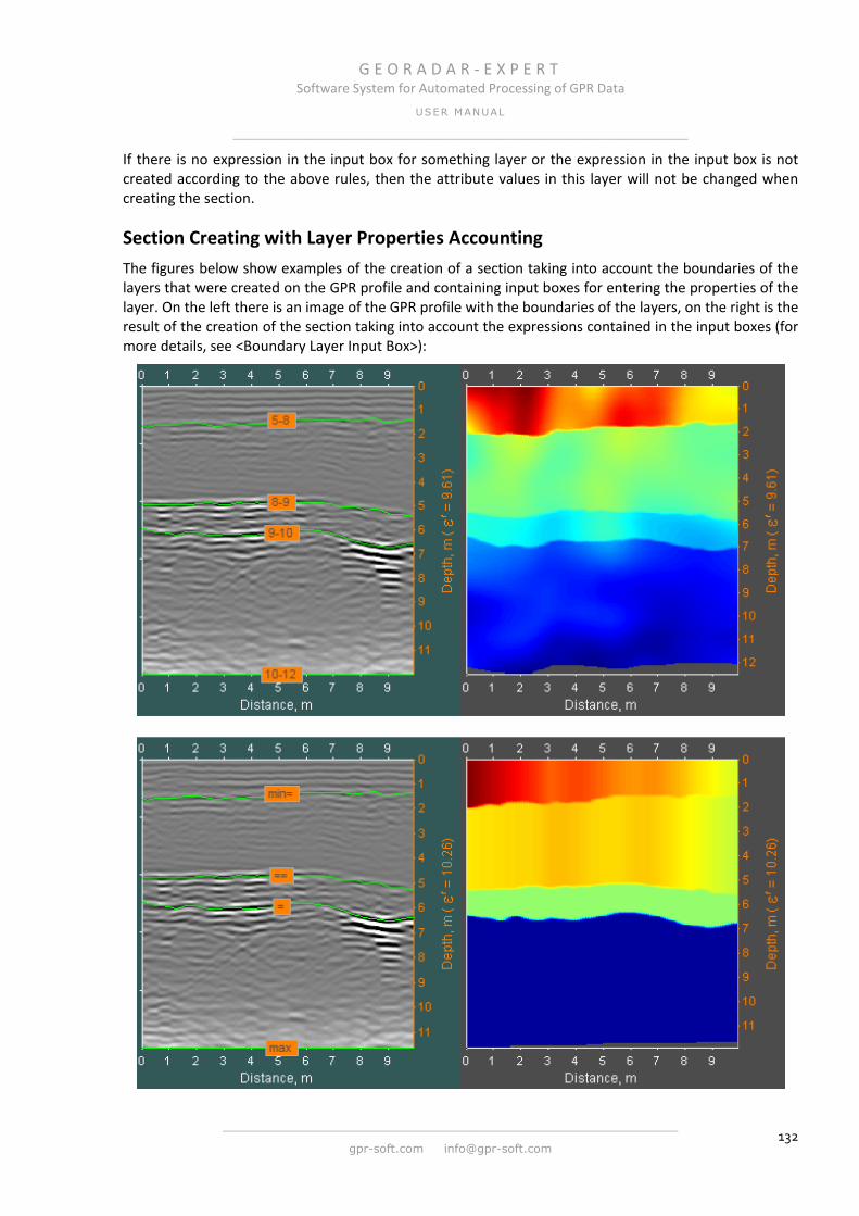
G E O R A D A R - E X P E R T Software System for Automated Processing of GPR Data
USER MANUAL
______________________________________________________________
______________________________________________________________
gpr-soft.com [email protected] 132
If there is no expression in the input box for something layer or the expression in the input box is not created according to the above rules, then the attribute values in this layer will not be changed when creating the section.
Section Creating with Layer Properties Accounting The figures below show examples of the creation of a section taking into account the boundaries of the layers that were created on the GPR profile and containing input boxes for entering the properties of the layer. On the left there is an image of the GPR profile with the boundaries of the layers, on the right is the result of the creation of the section taking into account the expressions contained in the input boxes (for more details, see <Boundary Layer Input Box>):
G E O R A D A R - E X P E R T Software System for Automated Processing of GPR Data
USER MANUAL
______________________________________________________________
______________________________________________________________
gpr-soft.com [email protected] 133
If there is no input field at the border of something layer, or there is no expression in the input field, or this expression was not created according to the rules described in the chapter <Boundary Layer Input Box> the presence of the boundary is not taken into account when creating a section.
Local Corrective Function for Layer Information about the corrective function (CF) can be found in the chapters <Corrective Function (CF)>, <Corrective Function Settings>, <Creating Corrective Function in Automatic Mode> and <Creating Corrective Function in Manual Mode>. In these chapters, the CF is a corrective function that is calculated based on the results of the BSEF automated analysis of the entire GPR profile.
However, the corrective function can be calculated not only for the entire GPR profile, but for each layer of the GPR profile individually. The corrective function, calculated from the BSEF analysis data that is contained within the layer, is called the local corrective function (LCF). When creating a section, the LCF adjusts the data only within its own layer.
To calculate LCF for a layer, need to perform the following actions (it is assumed that layer boundaries have already been created):
1. Switch the layer boundary to the editing mode by clicking on this boundary with the left or right mouse button;
2. Click the LayCF button in the Boundaries of Layers panel. After the LayCF button switches to the pressed state, the BSEF analysis data visualization panels and corrective functions in the left tabbed panel will display data not of the entire GPR profile, but of the layer whose bottom is the boundary in the editing mode. The input box of this boundary will change its color from orange to green, after the LayCF button is switched to the pressed state. If the input field is missing, it will be created automatically and it will have a green color;
3. If necessary, specify the ranges of the basic attributes (see section <Limitation the Range of Basic Attributes>), select the LCF type and its creation parameters (see <Corrective Function Settings> and <Creating Corrective Function in Automatic Mode>). It is possible to create the LCF manually (see <Creating Corrective Function in Manual Mode>). If after clicking the LayCF button the LCF does not need to be set up, you can go directly to the next item in the list of actions.
4. Switch the LayCF button to the unpressed state. As a result, the corrective function data for the layer will be saved for later use during the section creation process. After switching the LayCF button to the unpressed state, the input box will change its color from green to orange, and will contain the % character, which is an expression for applying the LCF when creating a section: . If the boundary of the layer contains LCF data, but there is no % in the input box, then the LCF will not be applied during the creation of the section.
If you save the data of the layer boundaries to a file with the gelay extension, the LCF data is also saved. For more information about saving and loading data for layer boundaries, see <Save and Load Layer Boundaries>.
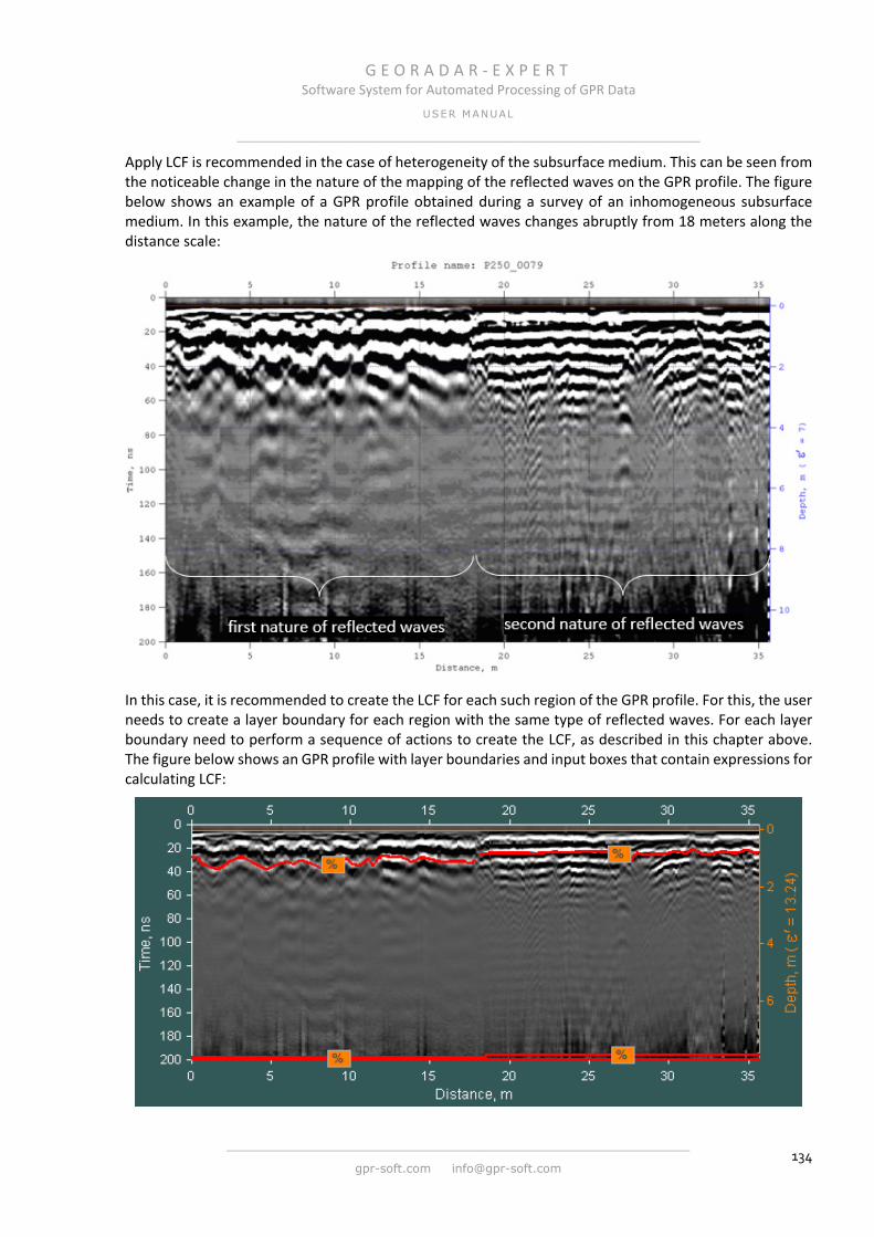
G E O R A D A R - E X P E R T Software System for Automated Processing of GPR Data
USER MANUAL
______________________________________________________________
______________________________________________________________
gpr-soft.com [email protected] 134
Apply LCF is recommended in the case of heterogeneity of the subsurface medium. This can be seen from the noticeable change in the nature of the mapping of the reflected waves on the GPR profile. The figure below shows an example of a GPR profile obtained during a survey of an inhomogeneous subsurface medium. In this example, the nature of the reflected waves changes abruptly from 18 meters along the distance scale:
In this case, it is recommended to create the LCF for each such region of the GPR profile. For this, the user needs to create a layer boundary for each region with the same type of reflected waves. For each layer boundary need to perform a sequence of actions to create the LCF, as described in this chapter above. The figure below shows an GPR profile with layer boundaries and input boxes that contain expressions for calculating LCF:
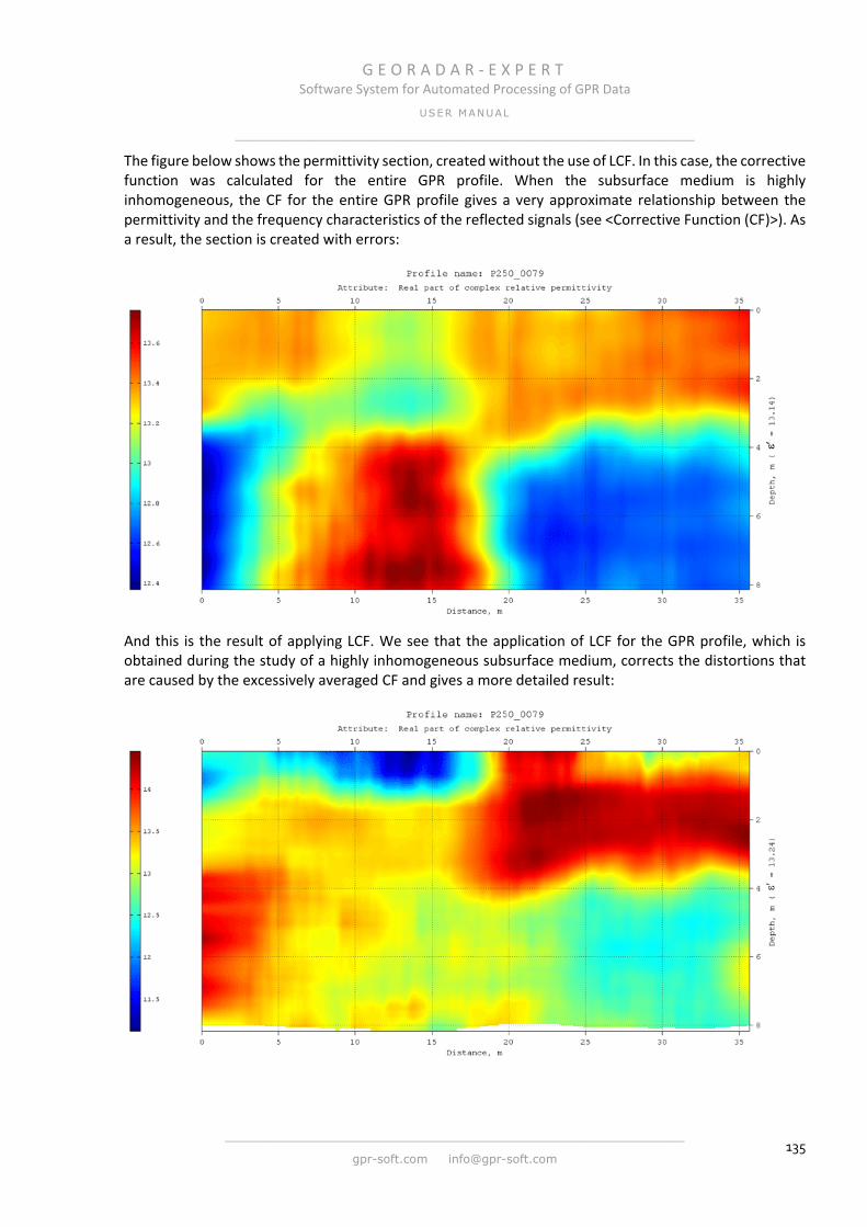
G E O R A D A R - E X P E R T Software System for Automated Processing of GPR Data
USER MANUAL
______________________________________________________________
______________________________________________________________
gpr-soft.com [email protected] 135
The figure below shows the permittivity section, created without the use of LCF. In this case, the corrective function was calculated for the entire GPR profile. When the subsurface medium is highly inhomogeneous, the CF for the entire GPR profile gives a very approximate relationship between the permittivity and the frequency characteristics of the reflected signals (see <Corrective Function (CF)>). As a result, the section is created with errors:
And this is the result of applying LCF. We see that the application of LCF for the GPR profile, which is obtained during the study of a highly inhomogeneous subsurface medium, corrects the distortions that are caused by the excessively averaged CF and gives a more detailed result:

G E O R A D A R - E X P E R T Software System for Automated Processing of GPR Data
USER MANUAL
______________________________________________________________
______________________________________________________________
gpr-soft.com [email protected] 136
Setting Layers Visualization on Section The user can manually create layer boundaries not only on the GPR profile, but also on the attribute section or 3D assembly cross-sections. In this case, different layers visualization options are available. It can be a single color fill of a layer, where the fill color will be determined by the maximum, minimum or average value of an attribute within this layer. Or the specified values will be calculated for each column of the numerical matrix of the section within the boundaries of the layer. Rendering conditions can be selected for each layer separately, or for all layers at once. Layer visualization is configured using the controls located in the visualization settings pop-up window.
To open the layer visualization settings window, you need to switch the visualization area of the section or the 3D assembly cross-sections to the layer visualization settings mode. To do this, right-click on one of the created layer boundaries and select the Fill Layer Mode context menu item, after which this mode becomes active. In this case, the background of the section display area changes to dark brown, and the creation or editing of layer boundaries will not be available.
When the layer visualization setting mode is active, right-clicking on the section calls up a message box, which displays the coordinates of the section point where the mouse pointer was at the moment of clicking, and the value of the section attribute at this point. Left-clicking on the section image opens a pop-up window for layer visualization settings - see the figure on the left.
In the upper part of this pop-up window there is information about the maximum, minimum and average values of the attribute in the layer, within
which the mouse pointer was located at the time of the opening of the layer visualization settings window. Next is the group of All over layer controls. Using the controls of this group, you can set the parameters of a single-color fill of a layer or layers.
The type of fill value is selected from the drop-down list included in the All over layer control group - the average value of the attribute calculated for the selected layer, the maximum value of the attribute in the selected layer, or the minimum value of the attribute. The ok button is used to fill only one layer, within which the mouse pointer was at the moment of calling the visualization settings window. The All button is used to fill all layers; within each layer there will be its own fill value. After starting the filling process with the All or ok buttons, the settings management window is automatically deleted. To call it again, you need to left-click again on the section image within the required layer.
The By columns group of controls is used to fill the columns of the numerical matrix of the section. This group has the same controls as the All over layer group, only the values for the fill are calculated not for the whole layer or layers, but for each column of the numerical matrix of the section within the layer. The figure below shows the result of filling all layers in the All over layer mode on the left, and in the By columns mode on the right:
To return to the original view of the section for one layer within which the mouse pointer was located at the time of the opening of the layer visualization settings window, use the Initial Lay button. To return to
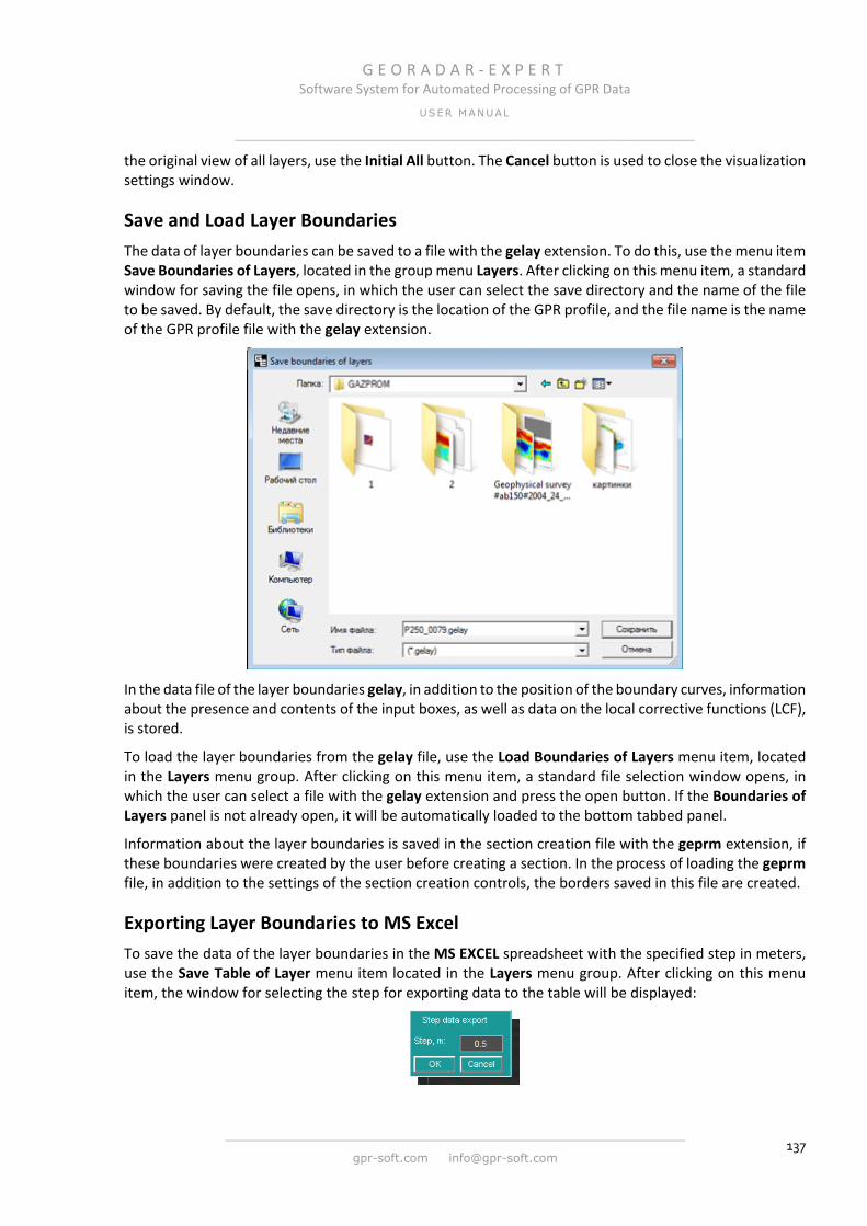
G E O R A D A R - E X P E R T Software System for Automated Processing of GPR Data
USER MANUAL
______________________________________________________________
______________________________________________________________
gpr-soft.com [email protected] 137
the original view of all layers, use the Initial All button. The Cancel button is used to close the visualization settings window.
Save and Load Layer Boundaries The data of layer boundaries can be saved to a file with the gelay extension. To do this, use the menu item Save Boundaries of Layers, located in the group menu Layers. After clicking on this menu item, a standard window for saving the file opens, in which the user can select the save directory and the name of the file to be saved. By default, the save directory is the location of the GPR profile, and the file name is the name of the GPR profile file with the gelay extension.
In the data file of the layer boundaries gelay, in addition to the position of the boundary curves, information about the presence and contents of the input boxes, as well as data on the local corrective functions (LCF), is stored.
To load the layer boundaries from the gelay file, use the Load Boundaries of Layers menu item, located in the Layers menu group. After clicking on this menu item, a standard file selection window opens, in which the user can select a file with the gelay extension and press the open button. If the Boundaries of Layers panel is not already open, it will be automatically loaded to the bottom tabbed panel.
Information about the layer boundaries is saved in the section creation file with the geprm extension, if these boundaries were created by the user before creating a section. In the process of loading the geprm file, in addition to the settings of the section creation controls, the borders saved in this file are created.
Exporting Layer Boundaries to MS Excel To save the data of the layer boundaries in the MS EXCEL spreadsheet with the specified step in meters, use the Save Table of Layer menu item located in the Layers menu group. After clicking on this menu item, the window for selecting the step for exporting data to the table will be displayed:

G E O R A D A R - E X P E R T Software System for Automated Processing of GPR Data
USER MANUAL
______________________________________________________________
______________________________________________________________
gpr-soft.com [email protected] 138
By default, the value of the export step in the parameter window Step, m is equal to the step of the GPR profiling. After clicking OK, the table creation process will start. After the table is created, it will be automatically saved to the directory of the location of the GPR profile file. Together with the saving of the table of layers, the map of the location of the layers is saved in a graphical format. With the help of this map, the user can easily find the layer with the required number on the section, which makes it easier to work with the table of layers. The figure below shows a GPR profile with layer boundaries, the result of exporting data of which will be presented below as an example.
In the table, layers are assigned sequential numbers in accordance with the average value of the depth of the lower boundary of the layer (see section <Layout of Layers Boundaries>). The layer with the lowest value of the average depth is assigned the number 1, and so on, in order of increasing average depth.
The table for each layer is located on a separate tab, the layer numbers are indicated on the tabs. Also, the tables have a Summary tab that contains a summary of each layer.
The layer table consists of the following columns:
Distance, m – distance from the beginning of the GPR profile in meters;
Top, m – position of the upper boundary of the layer in meters by depth;
Bottom, m – position of the bottom boundary of the layer in meters by depth;
Thickness, m – layer thickness in meters.
In the upper part of the layer table, the name of the profile (or attribute section or 3D assembly file, on the section of which the boundaries of the layers were created) and the layer number are displayed. Below the table are the minimum, maximum and mean values calculated for each column of the table, and the value of the layer area in square meters.
The Summary table contains the following columns:
Layer Number – the serial number of the layer;
Start, m – the position of the beginning of the layer on the distance scale in meters;
End, m – the position of the end of the layer on the distance scale in meters;
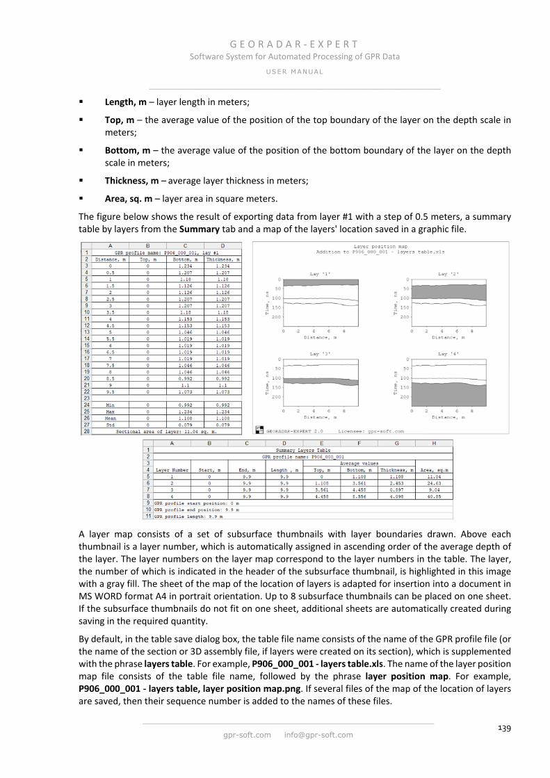
G E O R A D A R - E X P E R T Software System for Automated Processing of GPR Data
USER MANUAL
______________________________________________________________
______________________________________________________________
gpr-soft.com [email protected] 139
Length, m – layer length in meters;
Top, m – the average value of the position of the top boundary of the layer on the depth scale in meters;
Bottom, m – the average value of the position of the bottom boundary of the layer on the depth scale in meters;
Thickness, m – average layer thickness in meters;
Area, sq. m – layer area in square meters.
The figure below shows the result of exporting data from layer #1 with a step of 0.5 meters, a summary table by layers from the Summary tab and a map of the layers' location saved in a graphic file.
A layer map consists of a set of subsurface thumbnails with layer boundaries drawn. Above each thumbnail is a layer number, which is automatically assigned in ascending order of the average depth of the layer. The layer numbers on the layer map correspond to the layer numbers in the table. The layer, the number of which is indicated in the header of the subsurface thumbnail, is highlighted in this image with a gray fill. The sheet of the map of the location of layers is adapted for insertion into a document in MS WORD format A4 in portrait orientation. Up to 8 subsurface thumbnails can be placed on one sheet. If the subsurface thumbnails do not fit on one sheet, additional sheets are automatically created during saving in the required quantity.
By default, in the table save dialog box, the table file name consists of the name of the GPR profile file (or the name of the section or 3D assembly file, if layers were created on its section), which is supplemented with the phrase layers table. For example, P906_000_001 - layers table.xls. The name of the layer position map file consists of the table file name, followed by the phrase layer position map. For example, P906_000_001 - layers table, layer position map.png. If several files of the map of the location of layers are saved, then their sequence number is added to the names of these files.

G E O R A D A R - E X P E R T Software System for Automated Processing of GPR Data
USER MANUAL
______________________________________________________________
______________________________________________________________
gpr-soft.com [email protected] 140
3D assembly In the GEORADAR-EXPERT software system, it is possible to create a 3D model of a subsurface medium based on sections created as a result of an automated analysis of the BSEF of a set of GPR profiles. These GPR profiles may be of unequal length and arbitrary orientation. A set of sections that is visualized as a three-dimensional object is called a Cube or a 3D assembly. This three-dimensional object is a subsurface medium model.
The workspace in the 3D visualization mode differs from the 2D mode. For details, see <Workspace in 3D Visualization Mode>.
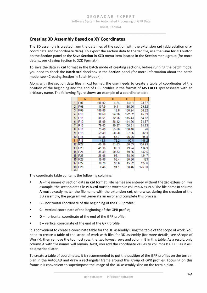
G E O R A D A R - E X P E R T Software System for Automated Processing of GPR Data
USER MANUAL
______________________________________________________________
______________________________________________________________
gpr-soft.com [email protected] 141
Creating 3D Assembly Based on XY Coordinates The 3D assembly is created from the data files of the section with the extension xzd (abbreviation of x-coordinate and z-coordinate data). To export the section data to the xzd file, use the Save for 3D button on the Section panel or the Save Section in XZD menu item located in the Section menu group (for more details, see <Saving Section to XZD Format>).
To save the data in xzd format in the batch mode of creating sections, before running the batch mode, you need to check the Batch xzd checkbox in the Section panel (for more information about the batch mode, see <Creating Section in Batch Mode>).
Along with the section data files in xzd format, the user needs to create a table of coordinates of the position of the beginning and the end of GPR profiles in the format of MS EXCEL spreadsheets with an arbitrary name. The following figure shows an example of a coordinate table:
The coordinate table contains the following columns:
A – file names of section data in xzd format. File names are entered without the xzd extension. For example, the section data file P18.xzd must be written in column A as P18. The file name in column A must exactly match the file name with the extension xzd, otherwise, during the creation of the 3D assembly, the program will generate an error and complete this process;
B – horizontal coordinate of the beginning of the GPR profile;
С – vertical coordinate of the beginning of the GPR profile;
D – horizontal coordinate of the end of the GPR profile;
E – vertical coordinate of the end of the GPR profile.
It is convenient to create a coordinate table for the 3D assembly using the table of the scope of work. You need to create a table of the scope of work with files for 3D assembly (for more details, see <Scope of Work>), then remove the topmost row, the two lowest rows and column B in this table. As a result, only column A with file names will remain. Next, you add the coordinate values to columns B C D E, as it will be described later.
To create a table of coordinates, it is recommended to put the position of the GPR profiles on the terrain plan in the AutoCAD and draw a rectangular frame around this group of GPR profiles. Focusing on this frame it is convenient to superimpose the image of the 3D assembly slice on the terrain plan.

G E O R A D A R - E X P E R T Software System for Automated Processing of GPR Data
USER MANUAL
______________________________________________________________
______________________________________________________________
gpr-soft.com [email protected] 142
In the figure below, the position of the GPR profiles is shown in orange, the profile names are located at the beginning of the GPR profile, the end of the GPR profile corresponds to the arrowhead, the GPR profiles are enclosed in a red frame:
To get the coordinates values for writing to a table, it is convenient to use the Rectangle:
Click the left mouse button on the Rectangle icon (the yellow arrow in the figure above points to this icon). When the Rectangle is activated, the mouse pointer becomes a crosshair, along with which the coordinates of the pointer are displayed. The window on the left serves to display the horizontal coordinate, the vertical coordinate is displayed in the window to the right:
To create an origin point (zero vertically and horizontally), the user hovers the crosshairs of the mouse pointer to the bottom left corner of the frame (which is around the GPR profiles), and one click with the left mouse button. Thus, the first corner of the rectangle is fixed, from which all distances will be measured.

G E O R A D A R - E X P E R T Software System for Automated Processing of GPR Data
USER MANUAL
______________________________________________________________
______________________________________________________________
gpr-soft.com [email protected] 143
For more accurate positioning, you can enable object snapping (hot key F3). After fixing the corner of the rectangle in the beginning of the coordinate, the user moves the mouse pointer to the beginning of the GPR profile. For example, the figure below shows the coordinates of the beginning of the profile P18.
The user writes the value from the window on the left (43.6) to the cell of column B located in the line with the name of the profile P18, and the value from the window to the right (73.2) - to the cell of column C, after which the mouse pointer moves to the end of the GPR profile:
The user writes the value from the window on the left (90.8) to the cell of column D, and the value from the second window (106.2) - to the cell of column E. This completes the recording of the coordinates of the GPR profile. The user moves the mouse pointer to the beginning of the next GPR profile and repeats the steps to get and write coordinates to the table. After the table of coordinates is completely filled, the user saves this table to the directory of the location of the files with the extension xzd. The table name can be arbitrary.
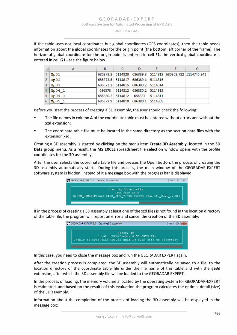
G E O R A D A R - E X P E R T Software System for Automated Processing of GPR Data
USER MANUAL
______________________________________________________________
______________________________________________________________
gpr-soft.com [email protected] 144
If the table uses not local coordinates but global coordinates (GPS coordinates), then the table needs information about the global coordinates for the origin point (the bottom left corner of the frame). The horizontal global coordinate for the origin point is entered in cell F1, the vertical global coordinate is entered in cell G1 - see the figure below.
Before you start the process of creating a 3D assembly, the user should check the following:
The file names in column A of the coordinate table must be entered without errors and without the xzd extension;
The coordinate table file must be located in the same directory as the section data files with the extension xzd.
Creating a 3D assembly is started by clicking on the menu item Create 3D Assembly, located in the 3D Data group menu. As a result, the MS EXCEL spreadsheet file selection window opens with the profile coordinates for the 3D assembly.
After the user selects the coordinate table file and presses the Open button, the process of creating the 3D assembly automatically starts. During this process, the main window of the GEORADAR-EXPERT software system is hidden; instead of it a message box with the progress bar is displayed:
If in the process of creating a 3D assembly at least one of the xzd files is not found in the location directory of the table file, the program will report an error and cancel the creation of the 3D assembly:
In this case, you need to close the message box and run the GEORADAR EXPERT again.
After the creation process is completed, the 3D assembly will automatically be saved to a file, to the location directory of the coordinate table file under the file name of this table and with the ge3d extension, after which the 3D assembly file will be loaded to the GEORADAR EXPERT.
In the process of loading, the memory volume allocated by the operating system for GEORADAR-EXPERT is estimated, and based on the results of this evaluation the program calculates the optimal detail (size) of the 3D assembly.
Information about the completion of the process of loading the 3D assembly will be displayed in the message box:
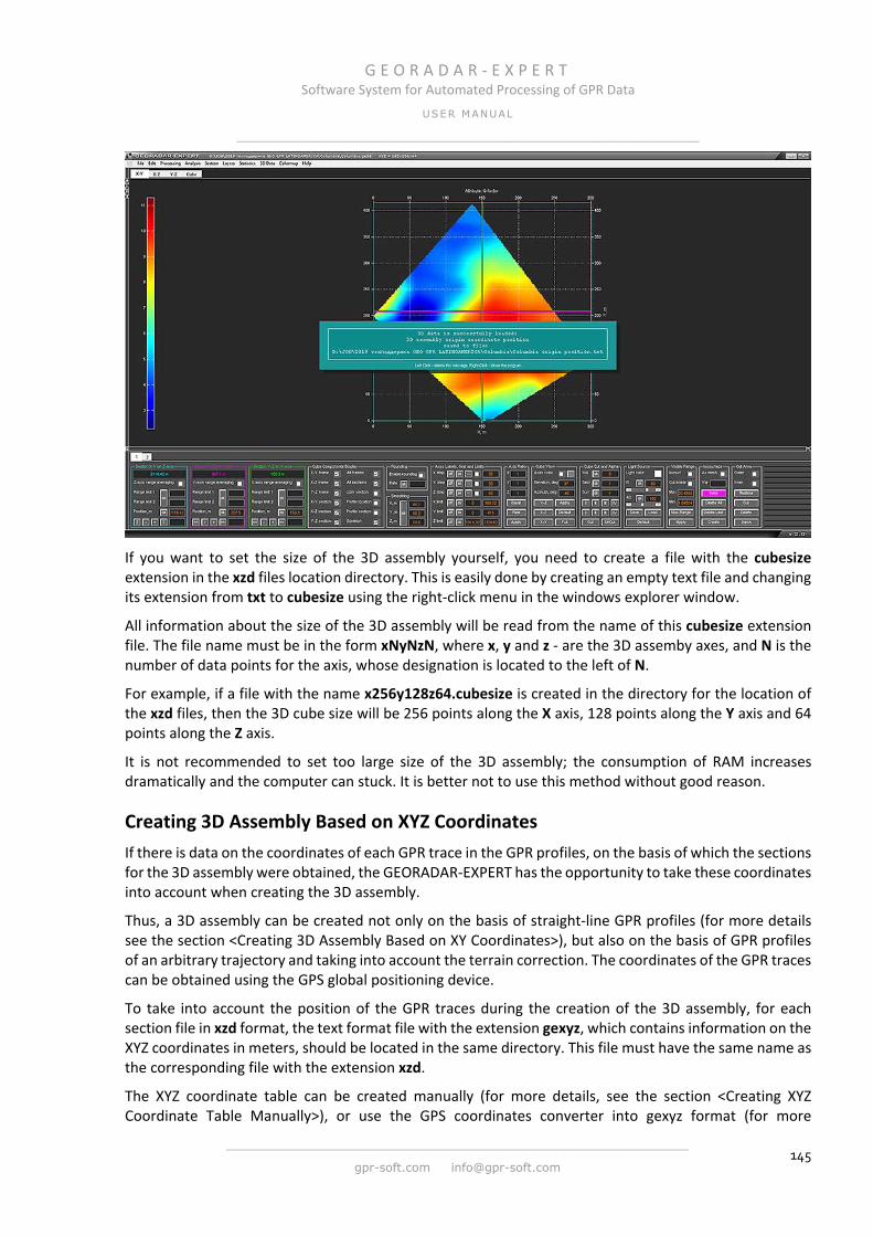
G E O R A D A R - E X P E R T Software System for Automated Processing of GPR Data
USER MANUAL
______________________________________________________________
______________________________________________________________
gpr-soft.com [email protected] 145
If you want to set the size of the 3D assembly yourself, you need to create a file with the cubesize extension in the xzd files location directory. This is easily done by creating an empty text file and changing its extension from txt to cubesize using the right-click menu in the windows explorer window.
All information about the size of the 3D assembly will be read from the name of this cubesize extension file. The file name must be in the form xNyNzN, where x, y and z - are the 3D assemby axes, and N is the number of data points for the axis, whose designation is located to the left of N.
For example, if a file with the name x256y128z64.cubesize is created in the directory for the location of the xzd files, then the 3D cube size will be 256 points along the X axis, 128 points along the Y axis and 64 points along the Z axis.
It is not recommended to set too large size of the 3D assembly; the consumption of RAM increases dramatically and the computer can stuck. It is better not to use this method without good reason.
Creating 3D Assembly Based on XYZ Coordinates If there is data on the coordinates of each GPR trace in the GPR profiles, on the basis of which the sections for the 3D assembly were obtained, the GEORADAR-EXPERT has the opportunity to take these coordinates into account when creating the 3D assembly.
Thus, a 3D assembly can be created not only on the basis of straight-line GPR profiles (for more details see the section <Creating 3D Assembly Based on XY Coordinates>), but also on the basis of GPR profiles of an arbitrary trajectory and taking into account the terrain correction. The coordinates of the GPR traces can be obtained using the GPS global positioning device.
To take into account the position of the GPR traces during the creation of the 3D assembly, for each section file in xzd format, the text format file with the extension gexyz, which contains information on the XYZ coordinates in meters, should be located in the same directory. This file must have the same name as the corresponding file with the extension xzd.
The XYZ coordinate table can be created manually (for more details, see the section <Creating XYZ Coordinate Table Manually>), or use the GPS coordinates converter into gexyz format (for more
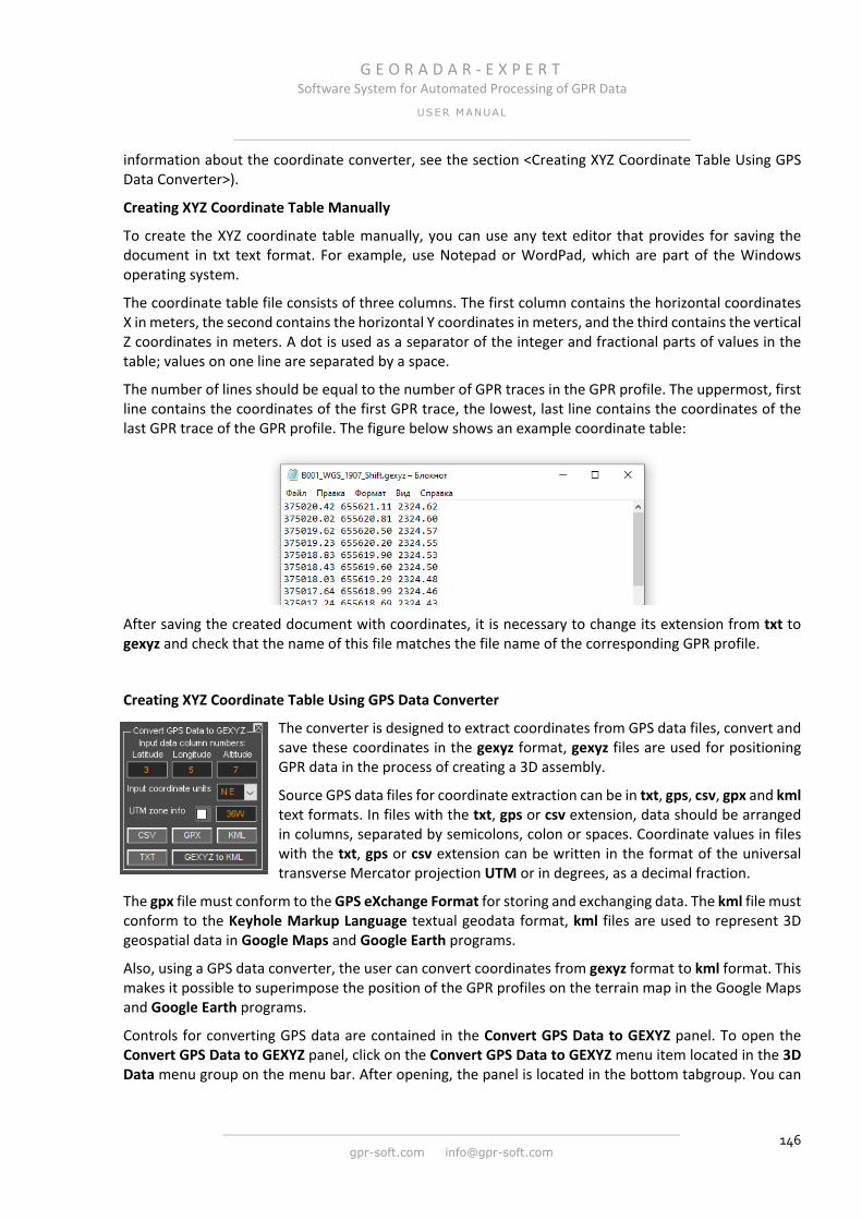
G E O R A D A R - E X P E R T Software System for Automated Processing of GPR Data
USER MANUAL
______________________________________________________________
______________________________________________________________
gpr-soft.com [email protected] 146
information about the coordinate converter, see the section <Creating XYZ Coordinate Table Using GPS Data Converter>).
Creating XYZ Coordinate Table Manually
To create the XYZ coordinate table manually, you can use any text editor that provides for saving the document in txt text format. For example, use Notepad or WordPad, which are part of the Windows operating system.
The coordinate table file consists of three columns. The first column contains the horizontal coordinates X in meters, the second contains the horizontal Y coordinates in meters, and the third contains the vertical Z coordinates in meters. A dot is used as a separator of the integer and fractional parts of values in the table; values on one line are separated by a space.
The number of lines should be equal to the number of GPR traces in the GPR profile. The uppermost, first line contains the coordinates of the first GPR trace, the lowest, last line contains the coordinates of the last GPR trace of the GPR profile. The figure below shows an example coordinate table:
After saving the created document with coordinates, it is necessary to change its extension from txt to gexyz and check that the name of this file matches the file name of the corresponding GPR profile.
Creating XYZ Coordinate Table Using GPS Data Converter
The converter is designed to extract coordinates from GPS data files, convert and save these coordinates in the gexyz format, gexyz files are used for positioning GPR data in the process of creating a 3D assembly.
Source GPS data files for coordinate extraction can be in txt, gps, csv, gpx and kml text formats. In files with the txt, gps or csv extension, data should be arranged in columns, separated by semicolons, colon or spaces. Coordinate values in files with the txt, gps or csv extension can be written in the format of the universal transverse Mercator projection UTM or in degrees, as a decimal fraction.
The gpx file must conform to the GPS eXchange Format for storing and exchanging data. The kml file must conform to the Keyhole Markup Language textual geodata format, kml files are used to represent 3D geospatial data in Google Maps and Google Earth programs.
Also, using a GPS data converter, the user can convert coordinates from gexyz format to kml format. This makes it possible to superimpose the position of the GPR profiles on the terrain map in the Google Maps and Google Earth programs.
Controls for converting GPS data are contained in the Convert GPS Data to GEXYZ panel. To open the Convert GPS Data to GEXYZ panel, click on the Convert GPS Data to GEXYZ menu item located in the 3D Data menu group on the menu bar. After opening, the panel is located in the bottom tabgroup. You can
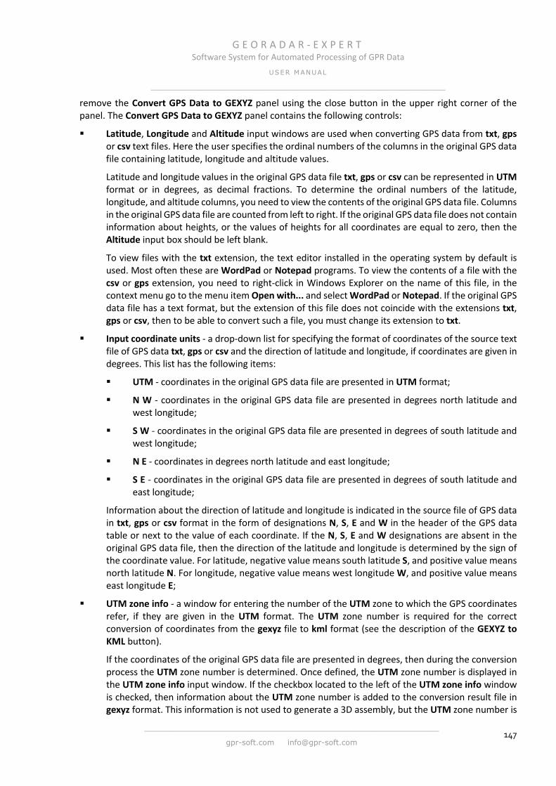
G E O R A D A R - E X P E R T Software System for Automated Processing of GPR Data
USER MANUAL
______________________________________________________________
______________________________________________________________
gpr-soft.com [email protected] 147
remove the Convert GPS Data to GEXYZ panel using the close button in the upper right corner of the panel. The Convert GPS Data to GEXYZ panel contains the following controls:
Latitude, Longitude and Altitude input windows are used when converting GPS data from txt, gps or csv text files. Here the user specifies the ordinal numbers of the columns in the original GPS data file containing latitude, longitude and altitude values.
Latitude and longitude values in the original GPS data file txt, gps or csv can be represented in UTM format or in degrees, as decimal fractions. To determine the ordinal numbers of the latitude, longitude, and altitude columns, you need to view the contents of the original GPS data file. Columns in the original GPS data file are counted from left to right. If the original GPS data file does not contain information about heights, or the values of heights for all coordinates are equal to zero, then the Altitude input box should be left blank.
To view files with the txt extension, the text editor installed in the operating system by default is used. Most often these are WordPad or Notepad programs. To view the contents of a file with the csv or gps extension, you need to right-click in Windows Explorer on the name of this file, in the context menu go to the menu item Open with... and select WordPad or Notepad. If the original GPS data file has a text format, but the extension of this file does not coincide with the extensions txt, gps or csv, then to be able to convert such a file, you must change its extension to txt.
Input coordinate units - a drop-down list for specifying the format of coordinates of the source text file of GPS data txt, gps or csv and the direction of latitude and longitude, if coordinates are given in degrees. This list has the following items:
UTM - coordinates in the original GPS data file are presented in UTM format;
N W - coordinates in the original GPS data file are presented in degrees north latitude and west longitude;
S W - coordinates in the original GPS data file are presented in degrees of south latitude and west longitude;
N E - coordinates in degrees north latitude and east longitude;
S E - coordinates in the original GPS data file are presented in degrees of south latitude and east longitude;
Information about the direction of latitude and longitude is indicated in the source file of GPS data in txt, gps or csv format in the form of designations N, S, E and W in the header of the GPS data table or next to the value of each coordinate. If the N, S, E and W designations are absent in the original GPS data file, then the direction of the latitude and longitude is determined by the sign of the coordinate value. For latitude, negative value means south latitude S, and positive value means north latitude N. For longitude, negative value means west longitude W, and positive value means east longitude E;
UTM zone info - a window for entering the number of the UTM zone to which the GPS coordinates refer, if they are given in the UTM format. The UTM zone number is required for the correct conversion of coordinates from the gexyz file to kml format (see the description of the GEXYZ to KML button).
If the coordinates of the original GPS data file are presented in degrees, then during the conversion process the UTM zone number is determined. Once defined, the UTM zone number is displayed in the UTM zone info input window. If the checkbox located to the left of the UTM zone info window is checked, then information about the UTM zone number is added to the conversion result file in gexyz format. This information is not used to generate a 3D assembly, but the UTM zone number is
G E O R A D A R - E X P E R T Software System for Automated Processing of GPR Data
USER MANUAL
______________________________________________________________
______________________________________________________________
gpr-soft.com [email protected] 148
required to correctly convert coordinates from the gexyz file to kml format (see the description of the GEXYZ to KML button);
The TXT button is used to load and convert one or more text files of GPS data with the txt or gps extension into the gexyz format. In this case, it is necessary to fill in the input boxes Latitude, Longitude. The Altitude input box needs to be filled only when the original GPS data file contains information about altitudes;
The CSV button is used to load and convert one or more text files of GPS data with the csv extension into the gexyz format. In this case, it is necessary to fill in the input boxes Latitude, Longitude. The Altitude input box needs to be filled only when the original GPS data file contains information about altitudes;
Using the GPX button, one or more GPS data files in the GPS eXchange Format (extension gpx) are loaded and converted into gexyz format. In this case, the information from the Latitude, Longitude and Altitude input boxes is not used;
Using the KML button, one or more GPS data files in the Keyhole Markup Language format (extension kml) are loaded and converted into gexyz format. In this case, the information from the Latitude, Longitude and Altitude input boxes is not used;
Using the GEXYZ to KML button, coordinates are converted from the gexyz format to the Keyhole Markup Language geodata format with the kml extension. As a result, it becomes possible to load coordinates into Google Maps and Google Earth programs and overlay the position of GPR profiles on a terrain map. For correct conversion, information about the number of the UTM zone, to which the converted coordinates belong, is required. If the table of the source file in the gexyz format contains information about the UTM zone number, then during the conversion process the UTM zone number is read from this file. If the source file of the gexyz format does not contain information about the UTM zone number, then the UTM zone number is read from the UTM zone info input window.
Converting coordinates to gexyz format is as follows. The user, if necessary, having previously configured the conversion parameters using the Latitude, Longitude and Altitude input windows, as well as the Input coordinate units drop-down list, presses one of the TXT, CSV, GPX or KML buttons (depending on the source file format), after which the window appears file selection, in which the user selects one or more files. After the files are selected, the file selection window closes and the conversion process starts. If the coordinates are given in degrees in the original GPS data file, then the UTM zone number determined during the conversion process is displayed in the UTM zone info input window.
Saving the result of converting to the gexyz format occurs automatically, in the directory where the original GPS data files are located. The conversion result file has the same name as the original GPS data file and has the gexyz extension.
Converting coordinates from gexyz format to kml format is as follows. The user clicks the GEXYZ to KML button, after which the file selection window opens, in which the user selects one or more files with the gexyz extension. After the files are selected, the file selection window closes and the conversion process starts. The conversion result is saved to kml format automatically, in the directory where the source files are located with the gexyz extension. The converted file has the same name as the original file and has a kml extension.
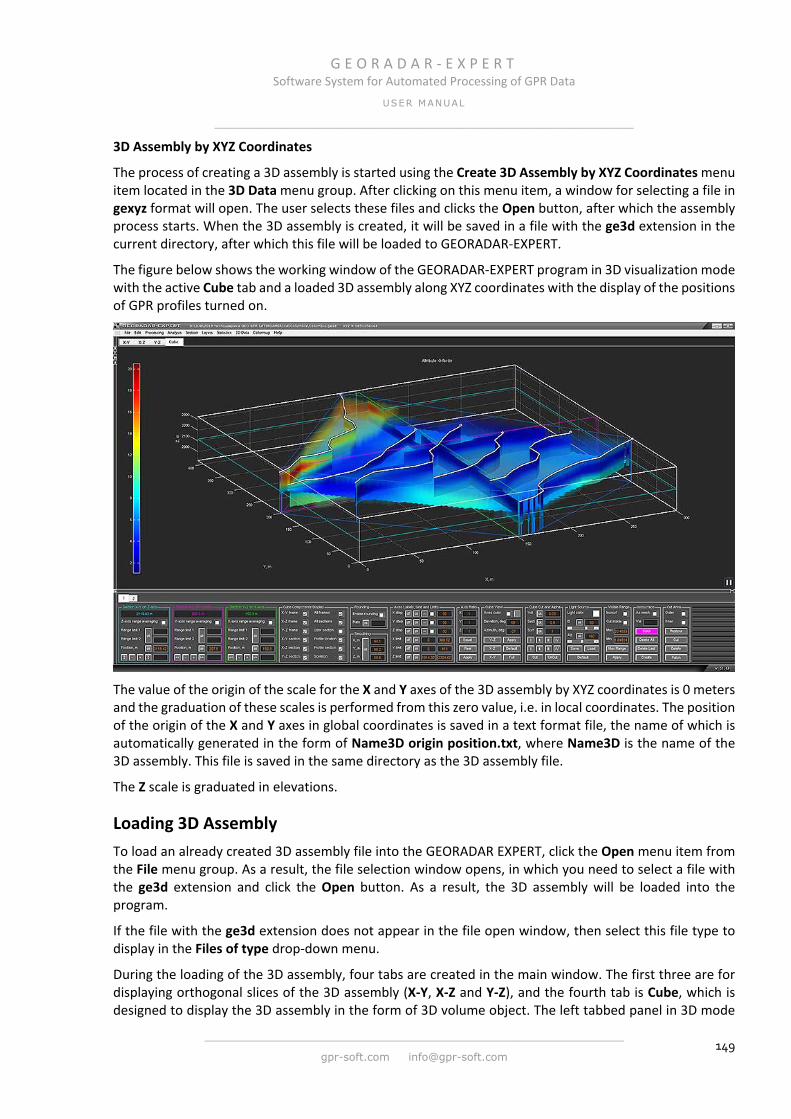
G E O R A D A R - E X P E R T Software System for Automated Processing of GPR Data
USER MANUAL
______________________________________________________________
______________________________________________________________
gpr-soft.com [email protected] 149
3D Assembly by XYZ Coordinates
The process of creating a 3D assembly is started using the Create 3D Assembly by XYZ Coordinates menu item located in the 3D Data menu group. After clicking on this menu item, a window for selecting a file in gexyz format will open. The user selects these files and clicks the Open button, after which the assembly process starts. When the 3D assembly is created, it will be saved in a file with the ge3d extension in the current directory, after which this file will be loaded to GEORADAR-EXPERT.
The figure below shows the working window of the GEORADAR-EXPERT program in 3D visualization mode with the active Cube tab and a loaded 3D assembly along XYZ coordinates with the display of the positions of GPR profiles turned on.
The value of the origin of the scale for the X and Y axes of the 3D assembly by XYZ coordinates is 0 meters and the graduation of these scales is performed from this zero value, i.e. in local coordinates. The position of the origin of the X and Y axes in global coordinates is saved in a text format file, the name of which is automatically generated in the form of Name3D origin position.txt, where Name3D is the name of the 3D assembly. This file is saved in the same directory as the 3D assembly file.
The Z scale is graduated in elevations.
Loading 3D Assembly To load an already created 3D assembly file into the GEORADAR EXPERT, click the Open menu item from the File menu group. As a result, the file selection window opens, in which you need to select a file with the ge3d extension and click the Open button. As a result, the 3D assembly will be loaded into the program.
If the file with the ge3d extension does not appear in the file open window, then select this file type to display in the Files of type drop-down menu.
During the loading of the 3D assembly, four tabs are created in the main window. The first three are for displaying orthogonal slices of the 3D assembly (X-Y, X-Z and Y-Z), and the fourth tab is Cube, which is designed to display the 3D assembly in the form of 3D volume object. The left tabbed panel in 3D mode
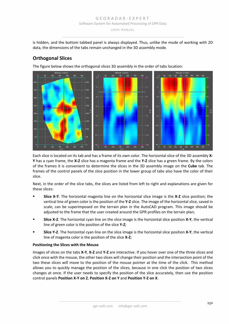
G E O R A D A R - E X P E R T Software System for Automated Processing of GPR Data
USER MANUAL
______________________________________________________________
______________________________________________________________
gpr-soft.com [email protected] 150
is hidden, and the bottom tabbed panel is always displayed. Thus, unlike the mode of working with 2D data, the dimensions of the tabs remain unchanged in the 3D assembly mode.
Orthogonal Slices The figure below shows the orthogonal slices 3D assembly in the order of tabs location:
Each slice is located on its tab and has a frame of its own color. The horizontal slice of the 3D assembly X-Y has a cyan frame, the X-Z slice has a magenta frame and the Y-Z slice has a green frame. By the colors of the frames it is convenient to determine the slices in the 3D assembly image on the Cube tab. The frames of the control panels of the slice position in the lower group of tabs also have the color of their slice.
Next, in the order of the slice tabs, the slices are listed from left to right and explanations are given for these slices:
Slice X-Y. The horizontal magenta line on the horizontal slice image is the X-Z slice position; the vertical line of green color is the position of the Y-Z slice. The image of the horizontal slice, saved in scale, can be superimposed on the terrain plan in the AutoCAD program. This image should be adjusted to the frame that the user created around the GPR profiles on the terrain plan;
Slice X-Z. The horizontal cyan line on the slice image is the horizontal slice position X-Y, the vertical line of green color is the position of the slice Y-Z;
Slice Y-Z. The horizontal cyan line on the slice image is the horizontal slice position X-Y, the vertical line of magenta color is the position of the slice X-Z;
Positioning the Slices with the Mouse
Images of slices on the tabs X-Y, X-Z and Y-Z are interactive. If you hover over one of the three slices and click once with the mouse, the other two slices will change their position and the intersection point of the two these slices will move to the position of the mouse pointer at the time of the click. This method allows you to quickly manage the position of the slices, because in one click the position of two slices changes at once. If the user needs to specify the position of the slice accurately, then use the position control panels Position X-Y on Z, Position X-Z on Y and Position Y-Z on X.
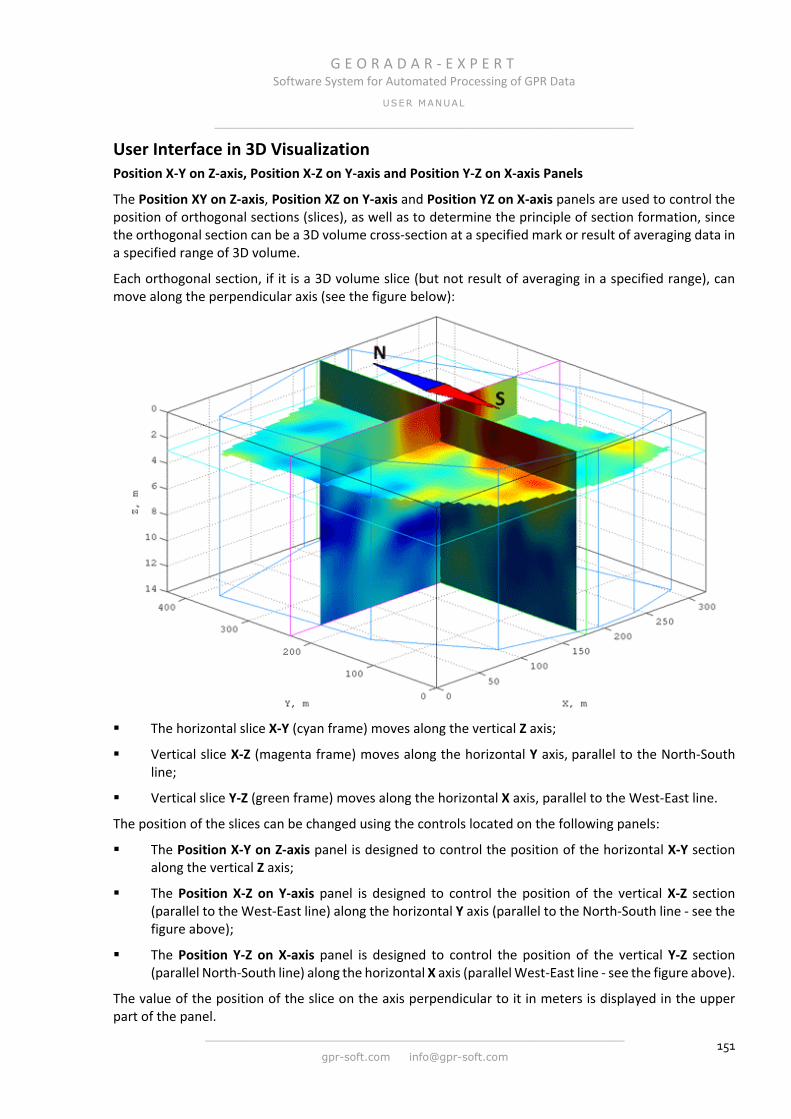
G E O R A D A R - E X P E R T Software System for Automated Processing of GPR Data
USER MANUAL
______________________________________________________________
______________________________________________________________
gpr-soft.com [email protected] 151
User Interface in 3D Visualization Position X-Y on Z-axis, Position X-Z on Y-axis and Position Y-Z on X-axis Panels
The Position XY on Z-axis, Position XZ on Y-axis and Position YZ on X-axis panels are used to control the position of orthogonal sections (slices), as well as to determine the principle of section formation, since the orthogonal section can be a 3D volume cross-section at a specified mark or result of averaging data in a specified range of 3D volume.
Each orthogonal section, if it is a 3D volume slice (but not result of averaging in a specified range), can move along the perpendicular axis (see the figure below):
The horizontal slice X-Y (cyan frame) moves along the vertical Z axis;
Vertical slice X-Z (magenta frame) moves along the horizontal Y axis, parallel to the North-South line;
Vertical slice Y-Z (green frame) moves along the horizontal X axis, parallel to the West-East line.
The position of the slices can be changed using the controls located on the following panels:
The Position X-Y on Z-axis panel is designed to control the position of the horizontal X-Y section along the vertical Z axis;
The Position X-Z on Y-axis panel is designed to control the position of the vertical X-Z section (parallel to the West-East line) along the horizontal Y axis (parallel to the North-South line - see the figure above);
The Position Y-Z on X-axis panel is designed to control the position of the vertical Y-Z section (parallel North-South line) along the horizontal X axis (parallel West-East line - see the figure above).
The value of the position of the slice on the axis perpendicular to it in meters is displayed in the upper part of the panel.
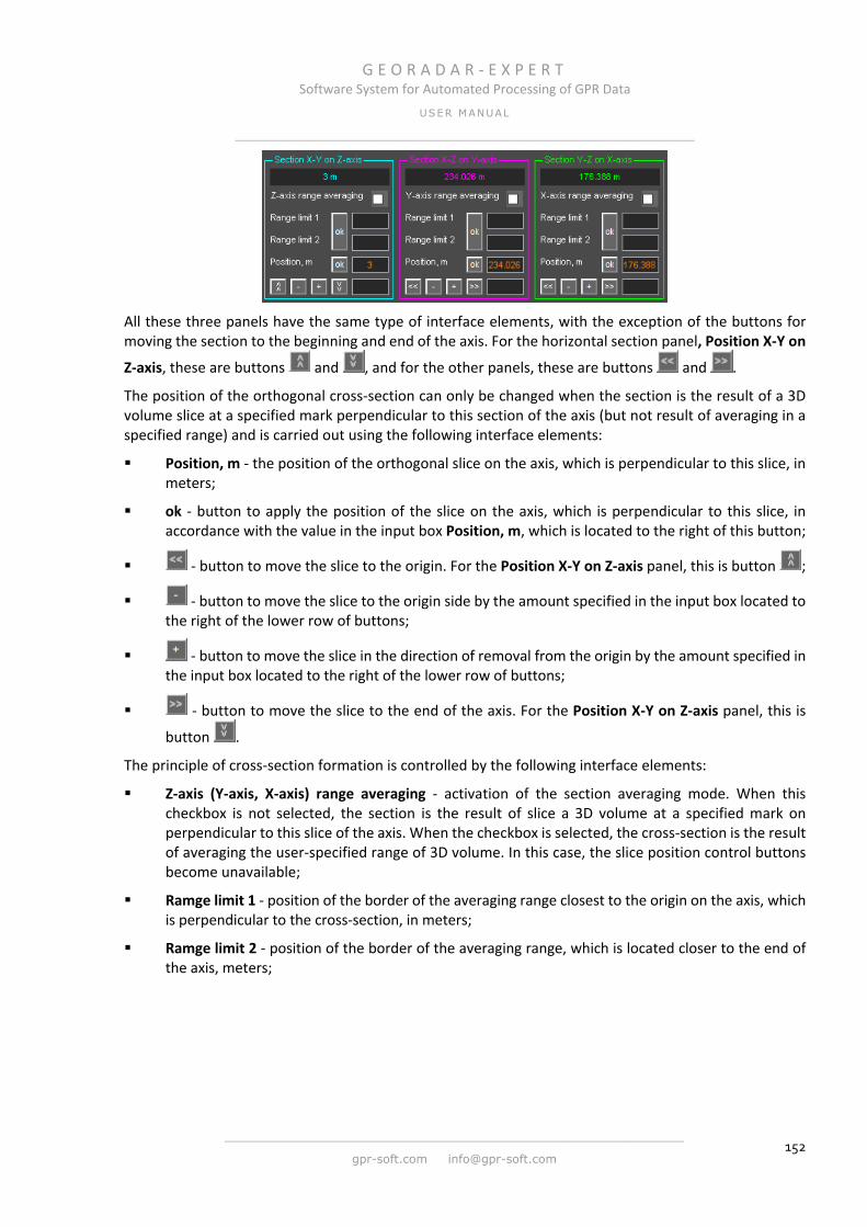
G E O R A D A R - E X P E R T Software System for Automated Processing of GPR Data
USER MANUAL
______________________________________________________________
______________________________________________________________
gpr-soft.com [email protected] 152
All these three panels have the same type of interface elements, with the exception of the buttons for moving the section to the beginning and end of the axis. For the horizontal section panel, Position X-Y on
Z-axis, these are buttons and , and for the other panels, these are buttons and .
The position of the orthogonal cross-section can only be changed when the section is the result of a 3D volume slice at a specified mark perpendicular to this section of the axis (but not result of averaging in a specified range) and is carried out using the following interface elements:
Position, m - the position of the orthogonal slice on the axis, which is perpendicular to this slice, in meters;
ok - button to apply the position of the slice on the axis, which is perpendicular to this slice, in accordance with the value in the input box Position, m, which is located to the right of this button;
- button to move the slice to the origin. For the Position X-Y on Z-axis panel, this is button ;
- button to move the slice to the origin side by the amount specified in the input box located to the right of the lower row of buttons;
- button to move the slice in the direction of removal from the origin by the amount specified in the input box located to the right of the lower row of buttons;
- button to move the slice to the end of the axis. For the Position X-Y on Z-axis panel, this is
button .
The principle of cross-section formation is controlled by the following interface elements:
Z-axis (Y-axis, X-axis) range averaging - activation of the section averaging mode. When this checkbox is not selected, the section is the result of slice a 3D volume at a specified mark on perpendicular to this slice of the axis. When the checkbox is selected, the cross-section is the result of averaging the user-specified range of 3D volume. In this case, the slice position control buttons become unavailable;
Ramge limit 1 - position of the border of the averaging range closest to the origin on the axis, which is perpendicular to the cross-section, in meters;
Ramge limit 2 - position of the border of the averaging range, which is located closer to the end of the axis, meters;

G E O R A D A R - E X P E R T Software System for Automated Processing of GPR Data
USER MANUAL
______________________________________________________________
______________________________________________________________
gpr-soft.com [email protected] 153
For cross-sections that were formed in the averaging mode, on the axes that are on the Cube tab, additional frames of the corresponding color are displayed along the boundaries of the averaging range, and the resulting section is located in the middle of the averaging range - see the figure below, where all three orthogonal cross-sections are the result of averaging. In this example, the X-Y section is the result of averaging the range from 1 to 2 meters along the Z axis, the X-Z section is the averaging of the range from 200 to 300 m along the Y axis, the Y-Z section is the averaging of the range 150 - 200 m along the X axis.
Cube Components Display Panel
Checkboxes located on the Cube Components Display panel are designed to control the visibility of the elements included in the 3D assembly visualization on the Cube tab. If the checkbox is not checked, then the corresponding element is not visible; if the checkbox is checked, then this element becomes visible.
The following are elements of the visualization of the 3D assembly, the display of which can be controlled on the Cube Components Display panel:
X-Y frame - frame of horizontal orthogonal cross-section X-Y of blue color;
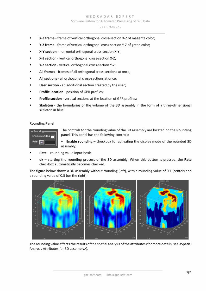
G E O R A D A R - E X P E R T Software System for Automated Processing of GPR Data
USER MANUAL
______________________________________________________________
______________________________________________________________
gpr-soft.com [email protected] 154
X-Z frame - frame of vertical orthogonal cross-section X-Z of magenta color;
Y-Z frame - frame of vertical orthogonal cross-section Y-Z of green color;
X-Y section - horizontal orthogonal cross-section X-Y;
X-Z section - vertical orthogonal cross-section X-Z;
Y-Z section - vertical orthogonal cross-section Y-Z;
All frames - frames of all orthogonal cross-sections at once;
All sections - all orthogonal cross-sections at once;
User section - an additional section created by the user;
Profile location - position of GPR profiles;
Profile section - vertical sections at the location of GPR profiles;
Skeleton - the boundaries of the volume of the 3D assembly in the form of a three-dimensional skeleton in blue.
Rounding Panel
The controls for the rounding value of the 3D assembly are located on the Rounding panel. This panel has the following controls:
Enable rounding – checkbox for activating the display mode of the rounded 3D assembly;
Rate – rounding value input boxl;
ok – starting the rounding process of the 3D assembly. When this button is pressed, the Rate checkbox automatically becomes checked.
The figure below shows a 3D assembly without rounding (left), with a rounding value of 0.1 (center) and a rounding value of 0.5 (on the right).
The rounding value affects the results of the spatial analysis of the attributes (for more details, see <Spatial Analysis Attributes for 3D assembly>).

G E O R A D A R - E X P E R T Software System for Automated Processing of GPR Data
USER MANUAL
______________________________________________________________
______________________________________________________________
gpr-soft.com [email protected] 155
Smoothing Panel
The smoothing controls of the 3D assembly are located on the Smoothing panel. This panel has the following controls:
X, m – value of smoothing along the X axis in meters;
Y, m – value of smoothing along the Y axis in meters;
Z, m – value of smoothing along the Z axis in meters;
ok – smoothing process start button.
After creating and loading the 3D assembly, the smoothing value for each axis is set as 15% of the length of the respective axis. If you save the 3D assembly to a file with the ge3d extension, the smoothing settings are also saved.
Axes Labels, Grid and Limits Panel
The controls for setting axes parameters for visualizing slices and 3D assembly are located in the Axes Labels, Grid and Limits panel. This panel contains the following controls:
X step (Y step, Z step) – group of control elements that determine interval between axis labels along the respective axis (enumeration of group of the controls from left to right):
df – set the interval value between axis labels by default;
ok – applying the interval value to the axes;
-- - enable or disable displaying grid lines that are perpendicular to the respective axis;
The checkbox for displays the axis label with the maximum value of the axis. The following is the X axis with the unmarked checkbox (top figure) and with the marked checkbox (bottom figure):
Input window for the value of the interval between the axis labels in meters.
X limit (Y limit, Z limit) – axes range control group. The axis range is changed, not the display area of the 3D assembly in accordance with this range. Sometimes this is necessary to correct the errors of anchoring the GPR profiles on the terrain. Enumeration of group of the controls from left to right:
df – setting the original range value of the respective axis;
ok – application of the range value for the respective axis;
The input window for the minimum value of the respective axis in meters (the default is zero);
The input window for the maximum value of the respective axis in meters.
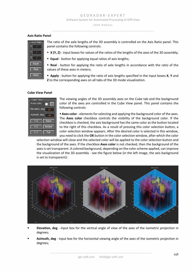
G E O R A D A R - E X P E R T Software System for Automated Processing of GPR Data
USER MANUAL
______________________________________________________________
______________________________________________________________
gpr-soft.com [email protected] 156
Axis Ratio Panel
The ratio of the axle lengths of the 3D assembly is controlled on the Axis Ratio panel. This panel contains the following controls:
X (Y, Z) - input boxes for values of the ratios of the lengths of the axes of the 3D assembly;
Equal - button for applying equal ratios of axis lengths;
Real - button for applying the ratio of axle lengths in accordance with the ratio of the values of these axes in meters;
Apply - button for applying the ratio of axis lengths specified in the input boxes X, Y and Z to the corresponding axes on all tabs of the 3D mode visualization.
Cube View Panel
The viewing angles of the 3D assembly axes on the Cube tab and the background color of the axes are controlled in the Cube View panel. This panel contains the following controls:
Axes color - elements for selecting and applying the background color of the axes. The Axes color checkbox controls the visibility of the background color. If the checkbox is checked, the axis background has the same color as the button located to the right of this checkbox. As a result of pressing this color selection button, a color selection window appears. After the desired color is selected in this window, you need to click the OK button in the color selection window, after which the color
selection window will close and the selected color will be applied to the color selection button and the background of the axes. If the checkbox Axes color is not checked, then the background of the axes is set transparent. A colored background, depending on the color scheme applied, can improve the visualization of the 3D assembly - see the figure below (in the left image, the axis background is set to transparent):
Elevation, deg - input box for the vertical angle of view of the axes of the isometric projection in
degrees;
Azimuth, deg - input box for the horizontal viewing angle of the axes of the isometric projection in degrees;
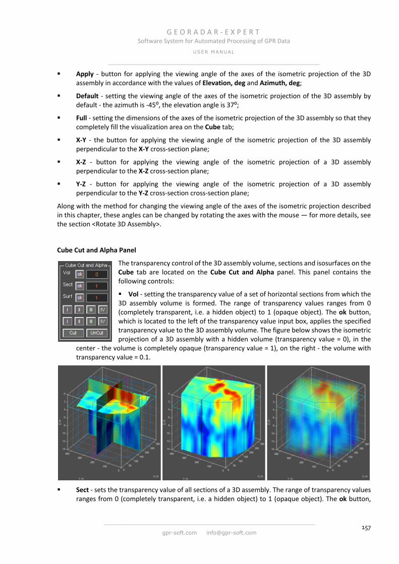
G E O R A D A R - E X P E R T Software System for Automated Processing of GPR Data
USER MANUAL
______________________________________________________________
______________________________________________________________
gpr-soft.com [email protected] 157
Apply - button for applying the viewing angle of the axes of the isometric projection of the 3D assembly in accordance with the values of Elevation, deg and Azimuth, deg;
Default - setting the viewing angle of the axes of the isometric projection of the 3D assembly by default - the azimuth is -45⁰, the elevation angle is 37⁰;
Full - setting the dimensions of the axes of the isometric projection of the 3D assembly so that they completely fill the visualization area on the Cube tab;
X-Y - the button for applying the viewing angle of the isometric projection of the 3D assembly perpendicular to the X-Y cross-section plane;
X-Z - button for applying the viewing angle of the isometric projection of a 3D assembly perpendicular to the X-Z cross-section plane;
Y-Z - button for applying the viewing angle of the isometric projection of a 3D assembly perpendicular to the Y-Z cross-section cross-section plane;
Along with the method for changing the viewing angle of the axes of the isometric projection described in this chapter, these angles can be changed by rotating the axes with the mouse — for more details, see the section <Rotate 3D Assembly>.
Cube Cut and Alpha Panel
The transparency control of the 3D assembly volume, sections and isosurfaces on the Cube tab are located on the Cube Cut and Alpha panel. This panel contains the following controls:
Vol - setting the transparency value of a set of horizontal sections from which the 3D assembly volume is formed. The range of transparency values ranges from 0 (completely transparent, i.e. a hidden object) to 1 (opaque object). The ok button, which is located to the left of the transparency value input box, applies the specified transparency value to the 3D assembly volume. The figure below shows the isometric projection of a 3D assembly with a hidden volume (transparency value = 0), in the
center - the volume is completely opaque (transparency value = 1), on the right - the volume with transparency value = 0.1.
Sect - sets the transparency value of all sections of a 3D assembly. The range of transparency values
ranges from 0 (completely transparent, i.e. a hidden object) to 1 (opaque object). The ok button,

G E O R A D A R - E X P E R T Software System for Automated Processing of GPR Data
USER MANUAL
______________________________________________________________
______________________________________________________________
gpr-soft.com [email protected] 158
which is located to the left of the input box for the transparency value, applies the value of transparency to all sections of the 3D assembly;
Surf - setting the transparency value of all isosurfaces of the 3D assembly. The range of transparency values ranges from 0 (completely transparent, i.e. a hidden object) to 1 (opaque object). The ok button, which is located to the left of the transparency input box, applies the transparency value to all isosurfaces;
I II III IV – toggle buttons for selecting the rectangular region of the 3D assembly volume for cutting - see the figure on the left. These buttons are arranged in two rows. Using the buttons of the upper
row, the regions for cutting located above the horizontal X-Y cross-section are selected, with the buttons of the lower row; the regions located below the horizontal cross-section X-Y are selected. The button in the pressed position - the region is selected, in the unpressed position - the region for cutting is not selected. The selected region before clicking the Cut button is displayed as a rectangular block of blue-green color (see the figure below, in the center).
Cut - the button for applying the cut of rectangular regions in accordance with the states of the toggle buttons I, II, III, and IV. The clipped regions of the 3D assembly volume become invisible;
UnCut - restore of cut rectangular regions. Cut regions become visible. When the 3D assembly volume has cut regions, the UnCut button is orange.
The figure below on the left shows the volume of 3D assembly without cut regions. To cut one or several rectangular regions from the 3D assembly volume, the user needs to perform the following actions:
1. Use the toggle buttons to select a region. As an example, the upper regions I and III, the lower regions II and IV were selected. Selected regions are displayed in the form of rectangular blocks of blue-green color (picture in the center);
2. Press the Cut button, after which the selected regions of the 3D assembly volume become completely transparent (figure below to the right).
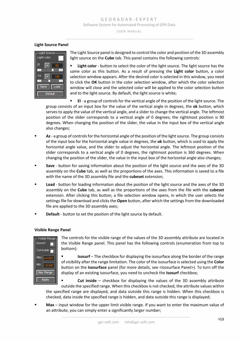
G E O R A D A R - E X P E R T Software System for Automated Processing of GPR Data
USER MANUAL
______________________________________________________________
______________________________________________________________
gpr-soft.com [email protected] 159
Light Source Panel
The Light Source panel is designed to control the color and position of the 3D assembly light source on the Cube tab. This panel contains the following controls:
Light color - button to select the color of the light source. The light source has the same color as this button. As a result of pressing the Light color button, a color selection window appears. After the desired color is selected in this window, you need to click the OK button in the color selection window, after which the color selection window will close and the selected color will be applied to the color selection button and to the light source. By default, the light source is white;
El - a group of controls for the vertical angle of the position of the light source. The group consists of an input box for the value of the vertical angle in degrees, the ok button, which serves to apply the value of the vertical angle, and a slider to change the vertical angle. The leftmost position of the slider corresponds to a vertical angle of 0 degrees; the rightmost position is 90 degrees. When changing the position of the slider, the value in the input box of the vertical angle also changes;
Az - a group of controls for the horizontal angle of the position of the light source. The group consists of the input box for the horizontal angle value in degrees, the ok button, which is used to apply the horizontal angle value, and the slider to adjust the horizontal angle. The leftmost position of the slider corresponds to a vertical angle of 0 degrees, the rightmost position is 360 degrees. When changing the position of the slider, the value in the input box of the horizontal angle also changes;
Save - button for saving information about the position of the light source and the axes of the 3D assembly on the Cube tab, as well as the proportions of the axes. This information is saved to a file with the name of the 3D assembly file and the cubeset extension;
Load - button for loading information about the position of the light source and the axes of the 3D assembly on the Cube tab, as well as the proportions of the axes from the file with the cubeset extension. After clicking this button, a file selection window opens, in which the user selects the settings file for download and clicks the Open button, after which the settings from the downloaded file are applied to the 3D assembly axes;
Default - button to set the position of the light source by default.
Visible Range Panel
The controls for the visible range of the values of the 3D assembly attribute are located in the Visible Range panel. This panel has the following controls (enumeration from top to bottom):
Isosurf – The checkbox for displaying the isosurface along the border of the range of visibility after the range limitation. The color of the isosurface is selected using the Color button on the Isosurface panel (for more details, see <Isosurface Panel>). To turn off the display of an existing isosurface, you need to uncheck the Isosurf checkbox;
Cut inside – checkbox for displaying the values of the 3D assembly attribute outside the specified range. When this checkbox is not checked, the attribute values within
the specified range are displayed, and data outside this range is hidden. When this checkbox is checked, data inside the specified range is hidden, and data outside this range is displayed;
Max – input window for the upper limit visible range. If you want to enter the maximum value of an attribute, you can simply enter a significantly larger number;

G E O R A D A R - E X P E R T Software System for Automated Processing of GPR Data
USER MANUAL
______________________________________________________________
______________________________________________________________
gpr-soft.com [email protected] 160
Min – input window for the lower limit visible range. If you want to enter a minimum value for an attribute, you can simply enter a lower number;
Max range – button to set the maximum visibility range of the 3D assembly attribute - i.e. cancellation of range limitation;
Apply – button to apply the visible range.
Visible range affects the results of spatial analysis of attributes (for more details, see <Spatial Analysis Attributes for 3D assembly>). Spatial analysis of attributes is performed only for the visible range of the values of the 3D assembly attribute.
The figure below left shows the 3D assembly and slices after the visible range limitation. The figures on the right show a 3D assembly without an isosurface (top) and an isosurface along the visible range border (bottom).
Isosurface Panel
The isosurface connects values of the 3D assembly that have the specified value. The color of the isosurface will have the color of the Color button on the Isosurface panel. The default color is magenta.
The isosurface creation controls are located on the Isosurface panel. This panel has the following controls (enumeration from left to right, top to bottom):
As mesh – checkbox for displaying the isosurface as a polygonal mesh. If this checkbox is not marked, the isosurface is displayed as a solid surface;
Value – the value of the 3D assembly attribute through which the isosurface passes;
Color – color isosurface selection button. After clicking on this button, the color selection window opens. After the user selects the color and closes the color selection window, the background color of the Color button changes its color to the selected color;
Delete all – button to delete all created isosurfaces;
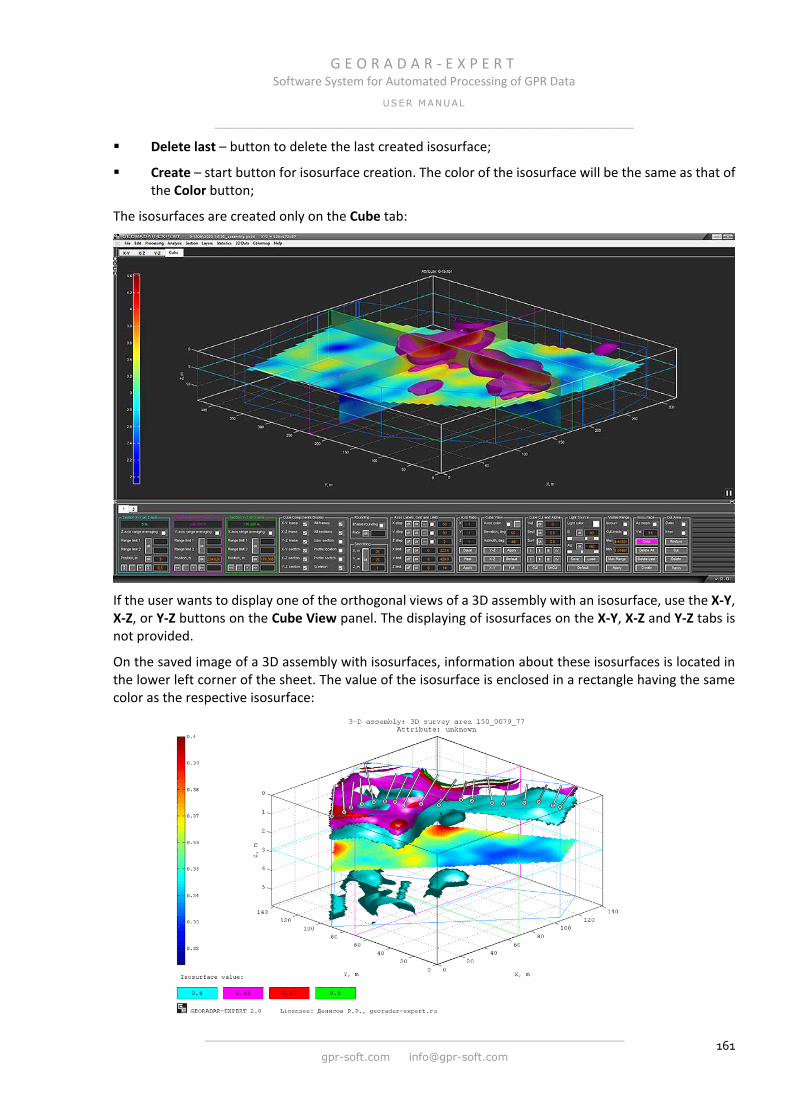
G E O R A D A R - E X P E R T Software System for Automated Processing of GPR Data
USER MANUAL
______________________________________________________________
______________________________________________________________
gpr-soft.com [email protected] 161
Delete last – button to delete the last created isosurface;
Create – start button for isosurface creation. The color of the isosurface will be the same as that of the Color button;
The isosurfaces are created only on the Cube tab:
If the user wants to display one of the orthogonal views of a 3D assembly with an isosurface, use the X-Y, X-Z, or Y-Z buttons on the Cube View panel. The displaying of isosurfaces on the X-Y, X-Z and Y-Z tabs is not provided.
On the saved image of a 3D assembly with isosurfaces, information about these isosurfaces is located in the lower left corner of the sheet. The value of the isosurface is enclosed in a rectangle having the same color as the respective isosurface:
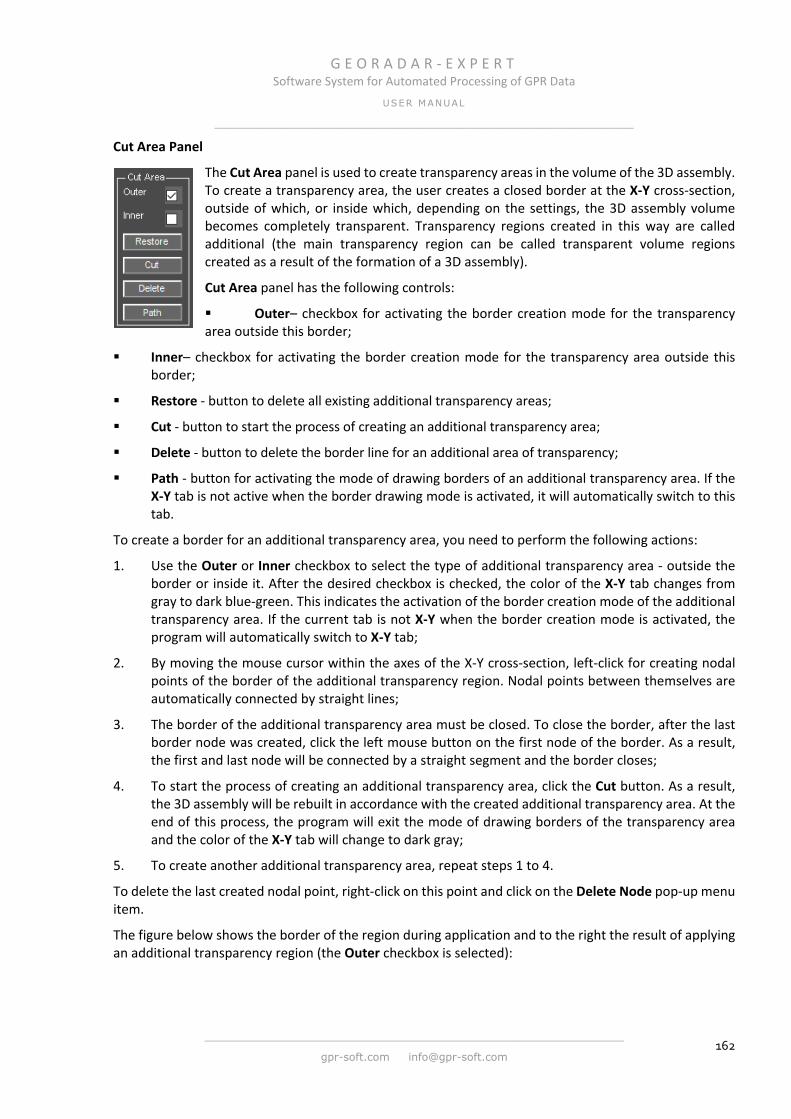
G E O R A D A R - E X P E R T Software System for Automated Processing of GPR Data
USER MANUAL
______________________________________________________________
______________________________________________________________
gpr-soft.com [email protected] 162
Cut Area Panel
The Cut Area panel is used to create transparency areas in the volume of the 3D assembly. To create a transparency area, the user creates a closed border at the X-Y cross-section, outside of which, or inside which, depending on the settings, the 3D assembly volume becomes completely transparent. Transparency regions created in this way are called additional (the main transparency region can be called transparent volume regions created as a result of the formation of a 3D assembly).
Cut Area panel has the following controls:
Outer– checkbox for activating the border creation mode for the transparency area outside this border;
Inner– checkbox for activating the border creation mode for the transparency area outside this border;
Restore - button to delete all existing additional transparency areas;
Cut - button to start the process of creating an additional transparency area;
Delete - button to delete the border line for an additional area of transparency;
Path - button for activating the mode of drawing borders of an additional transparency area. If the X-Y tab is not active when the border drawing mode is activated, it will automatically switch to this tab.
To create a border for an additional transparency area, you need to perform the following actions:
1. Use the Outer or Inner checkbox to select the type of additional transparency area - outside the border or inside it. After the desired checkbox is checked, the color of the X-Y tab changes from gray to dark blue-green. This indicates the activation of the border creation mode of the additional transparency area. If the current tab is not X-Y when the border creation mode is activated, the program will automatically switch to X-Y tab;
2. By moving the mouse cursor within the axes of the X-Y cross-section, left-click for creating nodal points of the border of the additional transparency region. Nodal points between themselves are automatically connected by straight lines;
3. The border of the additional transparency area must be closed. To close the border, after the last border node was created, click the left mouse button on the first node of the border. As a result, the first and last node will be connected by a straight segment and the border closes;
4. To start the process of creating an additional transparency area, click the Cut button. As a result, the 3D assembly will be rebuilt in accordance with the created additional transparency area. At the end of this process, the program will exit the mode of drawing borders of the transparency area and the color of the X-Y tab will change to dark gray;
5. To create another additional transparency area, repeat steps 1 to 4.
To delete the last created nodal point, right-click on this point and click on the Delete Node pop-up menu item.
The figure below shows the border of the region during application and to the right the result of applying an additional transparency region (the Outer checkbox is selected):

G E O R A D A R - E X P E R T Software System for Automated Processing of GPR Data
USER MANUAL
______________________________________________________________
______________________________________________________________
gpr-soft.com [email protected] 163
The following figure shows the 3D assembly on the Cube tab before creating an additional transparency area (on the left) and after (on the right):
Contours on 2D Views Panel
Cross-sections of the 3D assembly on the X-Y, X-Z and Y-Z tabs, the user section on the User Cross-Section tab can be visualized in the form of contour plots with a fill, in accordance with the current color map of the visualization. Contour graph property controls are located in the Contours on 2D views panel. This panel has the following controls:
Enable - the checkbox for activating the section visualization mode on the X-Y, X-Z, Y-Z and User Cross-Section tabs in the form of a contour plot;
Fill - checkbox for choosing the type of color filling between the contours. When this checkbox is selected, the areas inside the contours are filled with one tone, in accordance with the color map. When this checkbox is deselected, smooth color transitions are applied between the contours;

G E O R A D A R - E X P E R T Software System for Automated Processing of GPR Data
USER MANUAL
______________________________________________________________
______________________________________________________________
gpr-soft.com [email protected] 164
Auto - checkbox for setting the step of values between contours by default;
Labels - checkbox to show the value of contours;
Box - checkbox for setting a light background box for contour values. It is used when values are poorly read;
Line clr - button to select the color of the contours. After clicking on this button, a color selection window opens, in which the user selects the desired color with the mouse and presses the OK button, after which this window closes. After closing the window, the selected color is applied to the Line clr button and contours in sections;
Level limiting - the maximum possible number of levels for calculating the contours. If the user set a very small step in calculating the contours, then these values can be very many and the computer will need a lot of memory and time to draw the contours. To prevent this from happening, the Level limiting parameter limits the maximum number of levels for calculating the contours to a reasonable amount. If, when calculating levels, their number exceeds this parameter, then in this case the Level step value will be automatically increased so that the number of contours in the cross-section image is close to the Level limiting value, but does not exceed this value;
Line style - select the type of contour line;
Line style - the choice of the thickness of the contour line in millimeters;
Level step - a step of values between contours. The ok button to the left of the Level step input box starts the contour calculation process in accordance with the level step value;
Spacing - the distance between the position of the attribute value labels on the contour in centimeters. The ok button to the left of the Spacing input box applies the Spacing value to the contour plot;
Font size - font size of the attribute value label on the contour. The ok button to the left of the Font size input box applies the specified font size.

G E O R A D A R - E X P E R T Software System for Automated Processing of GPR Data
USER MANUAL
______________________________________________________________
______________________________________________________________
gpr-soft.com [email protected] 165
Settings of Colormap Panel
3D assembly visualization color map controls are located in the Settings of Colormap panel. The Settings of Colormap panel in 3D mode has some differences from the Settings of Colormap for Section panel for 2D mode (for details on the Settings of colormap for section panel, see <Colormap and Color Scheme Customizing>.
In addition to the name of the panels, the differences are as follows:
The Settings of Colormap panel lacks a group of parameters for creating a color scheme based on the operation of the random number generator;
On the Cube tab, the color scheme scale is not interactive. Editing a color scheme with the mouse (for more details see <Color Assignment Using Colorbar>) is possible only on the X-Y, X-Z, or Y-Z tabs. The color map created in this mode is also applied for the Cube tab;
The Limit parameter group in the Settings of Colormap panel differs from the Limitation of colormap parameter group in the Settings of Colormap for Section panel by the Max for each tab button, which is used to apply maximum display thresholds for the contents of each 3D visualization tab. For different tabs, the maximum threshold values may be different;
The m button in the Limit parameter group on the Settings of Colormap panel is used to apply the maximum range colormap for the current (selected) tab. Moreover, for all other tabs, the colormap limitations will be equal to this value - i.e. on all tabs, the colormap limitations will be the same. For more information about colormap limitations, see <Colormap Limitation>.
Attribute Features Panel
The Attribute Features panel controls the parameters of the 3D assembly attribute. Using this panel, you can change the name and range of the attribute values, as well as enter the name of the GPR survey. This panel has the following controls:
The Settings of Colormap panel lacks a group of parameters for creating a color scheme based on the operation of the random number generator;
The Attribute name control group is used to change the attribute name, which is shown on saved section images and 3D assembly views, as well as in spreadsheets. To apply a new name, this name should be entered in the input
box and click ok button. When 3D assembly is loading, the attribute name is read from the downloaded file and, after the load is completed, is displayed in this input box;
The GPR research name window is used to enter the name of the GPR survey, which will be shown on saved section images and 3D assembly views, as well as in spreadsheets;
The Range control group is used to change the range of values of the 3D assembly attribute. In the input box on the left, the minimum value of the attribute range of the 3D assembly is specified; in the input box on the right, the maximum value of the attribute range is specified;
Attribute flatness - equalization coefficient of attribute values. If the value of Attribute flatness is greater than unity, then the transition from high attribute values to small in the 3D assembly array

G E O R A D A R - E X P E R T Software System for Automated Processing of GPR Data
USER MANUAL
______________________________________________________________
______________________________________________________________
gpr-soft.com [email protected] 166
occurs more sharply, and the higher the value of this coefficient, the sharper the transition. If the value of Attribute flatness is less than one, then this transition is smoother. The absence of a value in the Attribute flatness parameter input box, or this value is 0 or 1, means the initial relationship between the attribute values. In the figure below, on the left, there is a cross-section with the initial range of attribute values, in the figure in the middle - the Attribute flatness parameter is 0.01, in the figure on the right - the Attribute flatness parameter is 5:
Initial - button for setting the initial values of the attribute range and its name in the corresponding
input boxes;
Apply - button for applying attribute range values and equalization coefficient to 3D assembly. To return the 3D assembly to its original values, click the Initial button, and then click the Apply button.
User Section Panel
The User Section panel is used to create a user vertical section of 3D assembly. To display the User Section panel, click on the User Cross-Section menu item located in the 3D Data menu group. The panel is located in the bottom tab group. You can remove the User Section panel using the close button in the upper right corner of these panel.
This chapter gives a brief description of the functionality of the User Section panel interface elements. The user’s actions for creating a section are described in more detail in the <Arbitrary Cross-Section>. The User Section panel has the following controls:
Path - toggle button to activate the creation mode of an arbitrary line on the X-Y cross-section. A vertical user section passes through this line;
Create - button to start the process of creating a user section;
Load - button for loading a user section previously saved in a ge3ucs format file;
Save - button to save the user section into a ge3ucs file;
Labels - button for displaying the names of the nodal points of the line through which the user section passes;
Xsize - button for controlling the size of the horizontal axis of the user section on the User Cross-Section tab. The horizontal axis size value is set in the input box, which is located to the right of the Xsize button. This value shows how many times the size of the horizontal axis differs from the size of the vertical axis. If the value is 1, then the dimensions of the horizontal and vertical axes are equal. If the value is greater than one, then the horizontal axis is longer than the vertical one by a specified number of times, if less than one, then the horizontal axis is smaller than the vertical axis.

G E O R A D A R - E X P E R T Software System for Automated Processing of GPR Data
USER MANUAL
______________________________________________________________
______________________________________________________________
gpr-soft.com [email protected] 167
Arbitrary Cross-Section In addition to orthogonal slices, which are created by default, the user can create vertical cross-section of 3D assemblies of arbitrary shape. The user can save arbitrary cross-section to a file with the extension ge3ucs and load them from the file into a 3D assembly.
Before creating an arbitrary vertical cross-section, need open the User Section panel in the main program window using the User Cross-Section menu, which is located in the 3D Data menu group. You can remove the User Section panel using the close button X, which is located in the upper-right corner of this panel.
To activate the mode of creating an arbitrary vertical cross-section, need to press the Path toggle button, after which the program will switch to the horizontal orthogonal slice X-Y tab (if another tab was active) and the color of this tab will change from gray to blue-green.
Moving the mouse pointer over the X-Y slice image and clicking with the left or right mouse button, the user creates nodes of polyline through which the vertical cross-section will pass. During the creation of a polyline, the nodes are automatically joined together by straight segments:
When the polyline is finished, need to click the Create button, which results in the vertical cross-section being created and placed on the User Cross-Section tab. The vertical lines on the cross-section image show the position of the polyline nodes on the basis of which this cross-section was created.
Above each vertical line, the name of the corresponding node of polyline is displayed. By default, when creating a node, it is assigned a name consisting of the letter P (point) and the sequence number of this node. In the future, the user can change the node name.
The figure below shows the User Cross-Section tab with the image of an arbitrary vertical section:

G E O R A D A R - E X P E R T Software System for Automated Processing of GPR Data
USER MANUAL
______________________________________________________________
______________________________________________________________
gpr-soft.com [email protected] 168
To display the names of node points, press the Labels button:
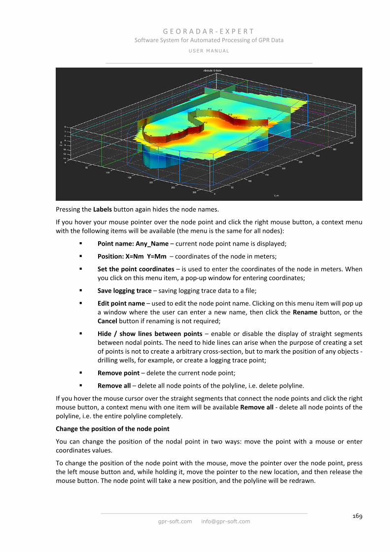
G E O R A D A R - E X P E R T Software System for Automated Processing of GPR Data
USER MANUAL
______________________________________________________________
______________________________________________________________
gpr-soft.com [email protected] 169
Pressing the Labels button again hides the node names.
If you hover your mouse pointer over the node point and click the right mouse button, a context menu with the following items will be available (the menu is the same for all nodes):
Point name: Any_Name – current node point name is displayed;
Position: X=Nm Y=Mm – coordinates of the node in meters;
Set the point coordinates – is used to enter the coordinates of the node in meters. When you click on this menu item, a pop-up window for entering coordinates;
Save logging trace – saving logging trace data to a file;
Edit point name – used to edit the node point name. Clicking on this menu item will pop up a window where the user can enter a new name, then click the Rename button, or the Cancel button if renaming is not required;
Hide / show lines between points – enable or disable the display of straight segments between nodal points. The need to hide lines can arise when the purpose of creating a set of points is not to create a arbitrary cross-section, but to mark the position of any objects - drilling wells, for example, or create a logging trace point;
Remove point – delete the current node point;
Remove all – delete all node points of the polyline, i.e. delete polyline.
If you hover the mouse cursor over the straight segments that connect the node points and click the right mouse button, a context menu with one item will be available Remove all - delete all node points of the polyline, i.e. the entire polyline completely.
Change the position of the node point
You can change the position of the nodal point in two ways: move the point with a mouse or enter coordinates values.
To change the position of the node point with the mouse, move the pointer over the node point, press the left mouse button and, while holding it, move the pointer to the new location, and then release the mouse button. The node point will take a new position, and the polyline will be redrawn.

G E O R A D A R - E X P E R T Software System for Automated Processing of GPR Data
USER MANUAL
______________________________________________________________
______________________________________________________________
gpr-soft.com [email protected] 170
To change the position of the node point by the method of specifying coordinates, need to right-click on this node point. In the context menu that opens, select Set the point coordinates, and the coordinate input window will be displayed. Enter the coordinates in meters and click OK - the node point will take the position in accordance with the entered coordinates, and the polyline will be redrawn.
If the polyline shape has been changed, an arbitrary cross-section needs to be updated with the Create button. Until this is done, the arbitrary cross-section tab User Cross-Section will have a dark red color:
Saving and Loading Arbitrary Cross-Section
To save the data of an arbitrary cross-section to a file with the ge3ucs extension, need to click the Save button on the User Section panel, after which the file save window opens, where you can change the name of the saved file and the directory, and then click the save button in this window.
To load the arbitrary cross-section data from the ge3ucs file, click the Load button in the User Section panel, then select the file with the ge3ucs extension in the file selection window and click the Open button in this window. During the load process, the existing arbitrary cross-section (if any) is deleted. As a result of loading the data of an arbitrary cross-section, a polyline is created, through which the cross-Arbitrary Cross-Sectionbutton in the User Section panel.
Logging Trace Logging trace allows you to obtain a graph of the values of the 3D assembly attribute in depth at a given point on a horizontal X-Y slice. As a logging trace point, the user can use the already created spline node of an arbitrary arbitrary cross-section, or if there is no spline - create a point in the same way as the spline node - for more details, see <>.
To obtain and save logging trace data, right-click on the logging trace point and select Save logging trace from the pop-up menu. After clicking on this menu item, two files will be saved in the current directory - graphic and text.

G E O R A D A R - E X P E R T Software System for Automated Processing of GPR Data
USER MANUAL
______________________________________________________________
______________________________________________________________
gpr-soft.com [email protected] 171
These files have the same names, but different extensions are png for the graphic file and txt for the text file. The file names consist of the name of the 3D assembly, the phrase "logging trace" and the number of the point at which logging trace data was obtained. For example: 3Dname logging trace in P23.png, where 3Dname is the name of the 3D assembly file, and P23 is the name of the logging trace point.
The file in the graphical format contains a curve of the changes in the values of the 3D assembly attribute in depth (see the figure below on the left), the file in text format contains a table of two columns with a space separator, where the first column is the depth in meters, the second column is the value of the attribute (see figure below on the right).
At the top of the plot is the name of the 3D assembly file, the attribute name and information about the logging trace point - its name and coordinates. The vertical axis of the graph is the depth in meters; the horizontal axis is the value of the attribute. The limits of the horizontal axis of the graph are the same for all 3D logging trace points and are equal to the minimum and maximum values of the 3D assembly attribute.
If the purpose of creating polyline dots is not to create a arbitrary cross-section, but to acquire logging trace data, the user, after creating all logging trace points, can turn off the display of connecting segments between nodes using the menu item Hide / show lines between points. This menu item is contained in the pop-up menu, which is called by right-clicking on any of the logging trace points.
Visualization GPR Profiles Position on 3D Assembly To display the position of the GPR profiles, based on the results of the BSEF analysis, sections for the 3D assembly have been created; select the Profile location checkbox on the Cube Components Display panel.
The position of the GPR profiles is displayed on the horizontal X-Y slice (X-Y tab) and on the volume image of the 3D assembly (Cube tab). GPR profiles are displayed as white lines with a black outline; the beginning of the profile is surrounded by a small circle. If you right-click on the GPR profile line, a pop-up window will appear that shows the GPR profile name. To hide this pop-up window, you need to click on this window.
It is recommended to enable the display of the position of the GPR profiles to visually check the coordinate table for possible errors. This is especially actual for 3D assemblies created on the basis of a large number of sections.

G E O R A D A R - E X P E R T Software System for Automated Processing of GPR Data
USER MANUAL
______________________________________________________________
______________________________________________________________
gpr-soft.com [email protected] 172
The figures below show the position of the GPR profiles on the X-Y slice (figure on the left) and on the volume of the 3D assembly (figure on the right):
Rotate 3D Assembly As soon as the mouse pointer appears inside the 3D assembly axes on the Cube tab, the rotation mode of the 3D assembly by the mouse is activated. In this mode, the mouse pointer takes the form of a looped arrow symbolizing rotation.
To start rotating the 3D assembly, you need to press and hold the left mouse button down. This will show the rotation frame of the 3D assembly in a yellow color, which repeats the shape of the 3D assembly axes. The user, while holding the left mouse button down, moves the mouse, thereby rotating the 3D assembly frame to the desired angle. After releasing the left mouse button, the 3D assembly axes accepts the rotation frame position, after which the rotation frame is deleted.
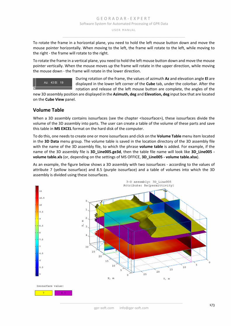
G E O R A D A R - E X P E R T Software System for Automated Processing of GPR Data
USER MANUAL
______________________________________________________________
______________________________________________________________
gpr-soft.com [email protected] 173
To rotate the frame in a horizontal plane, you need to hold the left mouse button down and move the mouse pointer horizontally. When moving to the left, the frame will rotate to the left, while moving to the right - the frame will rotate to the right.
To rotate the frame in a vertical plane, you need to hold the left mouse button down and move the mouse pointer vertically. When the mouse moves up the frame will rotate in the upper direction, while moving the mouse down - the frame will rotate in the lower direction.
During rotation of the frame, the values of azimuth Az and elevation angle El are displayed in the lower left corner of the Cube tab, under the colorbar. After the rotation and release of the left mouse button are complete, the angles of the
new 3D assembly position are displayed in the Azimuth, deg and Elevation, deg input box that are located on the Cube View panel.
Volume Table When a 3D assembly contains isosurfaces (see the chapter <Isosurface>), these isosurfaces divide the volume of the 3D assembly into parts. The user can create a table of the volume of these parts and save this table in MS EXCEL format on the hard disk of the computer.
To do this, one needs to create one or more isosurfaces and click on the Volume Table menu item located in the 3D Data menu group. The volume table is saved in the location directory of the 3D assembly file with the name of the 3D assembly file, to which the phrase volume table is added. For example, if the name of the 3D assembly file is 3D_Line005.ge3d, then the table file name will look like 3D_Line005 - volume table.xls (or, depending on the settings of MS OFFICE, 3D_Line005 - volume table.xlsx).
As an example, the figure below shows a 3D assembly with two isosurfaces - according to the values of attribute 7 (yellow isosurface) and 8.5 (purple isosurface) and a table of volumes into which the 3D assembly is divided using these isosurfaces.

G E O R A D A R - E X P E R T Software System for Automated Processing of GPR Data
USER MANUAL
______________________________________________________________
______________________________________________________________
gpr-soft.com [email protected] 174
The table header contains information about the name of the 3D assembly file and the name of the attribute. The table consists of three columns. The Range attribute value column contains attribute values that are the boundaries of the volume. Since two isosurfaces were created in this example, the table contains information on volumes for three parts of the 3D assembly: the volume of the first part is limited by the minimum attribute value and the value 7. The volume of the second part is limited by the values of isosurfaces. The volume of the third part is limited to 8.5 and the maximum attribute value.
The Volume cubic m column contains the volumes of the 3D assembly parts in cubic meters. The Additional information column is used to place additional information by the user after creating the table, if necessary. Under the table is information about the minimum, average and maximum values of the attribute, as well as the size of the range of attribute values of the 3D assembly.
Save 3D Assembly and Slices in Graphical Format The controls for saving images of 3D assembly and slices are located on the Save in Graphic Format panel. The same panel is used to save section images in 2D mode (processing of the GPR profile and creation of sections based on the BSEF analysis). For more details, see <Saving in Graphic Format>
Saving of Multiple Images of Cross-Sections To save multiple images of X-Y, X-Z, or Y-Z sections, the user must select the desired X-Y, X-Z, or Y-Z tab. Next, in the Step parameter input box on the corresponding panel Position X-Y on Z, Position X-Z on Y or Position Y-Z on X, set the value of the saving step in meters and click the Get Slice menu item from the 3D Data menu group.
After performing these steps, the program will automatically move the section along the corresponding axis at equal distances specified by the Step value and save the section images in accordance with the parameters defined on the settings panel for saving data in the graphic format Save in graphic format. Saving is done in the location directory of the 3D assembly file.
The name of the saved image file is automatically generated and consists of the name of the 3D assembly file, the name of the 3D assembly attribute, the name of the section and the position of this section on the corresponding axis. For example, from the name of the file 3D_Line005 Re(permittivity) Section X-Z, 10 m on Y-axis.png it follows that the name of the 3D assembly is 3D_Line005, the attribute of the 3D assembly is Re(permittivity), the section is X-Z, the position of this section on the Y-axis is 10 meters from the origin.
If the Save in graphic format panel was not opened at the beginning of the automated save process, this panel will automatically open before the first save, and the save will be performed in accordance with the default settings.

G E O R A D A R - E X P E R T Software System for Automated Processing of GPR Data
USER MANUAL
______________________________________________________________
______________________________________________________________
gpr-soft.com [email protected] 175
Saving Cross-Sections in the Location of GPR Profiles To save vertical cross-sections at the location of georadar profiles, according to the results of the automated BSEF analysis of which a 3D assembly was created, click the Get Profile Slice menu item from the 3D Data menu group. After clicking on the menu item Get Profile Slice, the program will start saving images in a graphic format in accordance with the parameters defined on the settings panel for saving data in a graphic format Save in graphic format. Saving is done in the location directory of the 3D assembly file.
The name of the saved image file is automatically generated and consists of the name of the 3D assembly file, the name of the 3D assembly attribute and the name of the GPR profile file. For example, the name of the cross-sectional image file by the location of the 3D_Line005 Re(permittivity) PR0007.png profile shows that the name of the 3D assembly is 3D_Line005, the 3D assembly attribute is Re(permittivity), and the profile name is PR0007.
If the Save in graphic format panel was not opened at the beginning of the automated save process, this panel will automatically open before the first save, and the save will be performed in accordance with the default settings.
Spatial Analysis Attributes for 3D assembly Spatial Analysis Attributes SAA for 3D assembly is similar to the SAA for the section in 2D mode. For more information, see <Spatial Analysis of Attributes>.
To SAA for 3D assembly need perform the following steps:
Open the 3D assembly file (see <Loading 3D Assembly>);
Set the rounding value of Value of rounding in the Rounding panel, and click the ok button in this panel (for more information, see <Rounding 3D Assembly>). Rounding is necessary to reduce the
number of unique attribute values. If rounding is not performed, then because of the large number of unique values, computer memory may overflow;
To start the SAA process, click on the Spatial Analysis Attributes menu item located in the Analysis menu group;
After the completion of the SAA process, the message box about the end of the analysis will be displayed and the question whether the user wants to open the directory containing the results of the analysis. If the user clicks the Yes button, the main window of the program is minimized and the folder with the results of the SAA analysis opens in Windows Explorer.
Note: SAA is performed only for the visible range of the 3D assembly attribute. About limitation the visible range, see <Visible Range>.
The figure shows the All graphs on one sheet.png image from the SAA analysis results folder 3D_assembly Q-factor rounding 0.2:
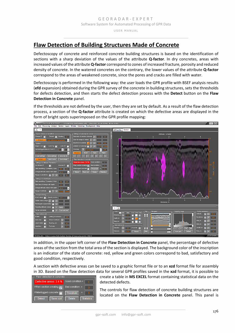
G E O R A D A R - E X P E R T Software System for Automated Processing of GPR Data
USER MANUAL
______________________________________________________________
______________________________________________________________
gpr-soft.com [email protected] 176
Flaw Detection of Building Structures Made of Concrete Defectoscopy of concrete and reinforced concrete building structures is based on the identification of sections with a sharp deviation of the values of the attribute Q-factor. In dry concretes, areas with increased values of the attribute Q-factor correspond to zones of increased fracture, porosity and reduced density of concrete. In the watered concretes on the contrary, the lower values of the attribute Q-factor correspond to the areas of weakened concrete, since the pores and cracks are filled with water.
Defectoscopy is performed in the following way: the user loads the GPR profile with BSEF analysis results (efd expansion) obtained during the GPR survey of the concrete in building structures, sets the thresholds for defects detection, and then starts the defect detection process with the Detect button on the Flaw Detection in Concrete panel.
If the thresholds are not defined by the user, then they are set by default. As a result of the flaw detection process, a section of the Q-factor attribute is created on which the defective areas are displayed in the form of bright spots superimposed on the GPR profile mapping:
In addition, in the upper left corner of the Flaw Detection in Concrete panel, the percentage of defective areas of the section from the total area of the section is displayed. The background color of the inscription is an indicator of the state of concrete: red, yellow and green colors correspond to bad, satisfactory and good condition, respectively.
A section with defective areas can be saved to a graphic format file or to an xzd format file for assembly in 3D. Based on the flaw detection data for several GPR profiles saved in the xzd format, it is possible to
create a table in MS EXCEL format containing statistical data on the detected defects.
The controls for flaw detection of concrete building structures are located on the Flaw Detection in Concrete panel. This panel is
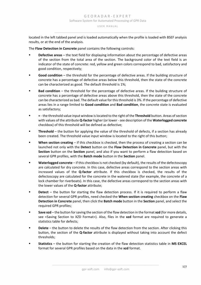
G E O R A D A R - E X P E R T Software System for Automated Processing of GPR Data
USER MANUAL
______________________________________________________________
______________________________________________________________
gpr-soft.com [email protected] 177
located in the left tabbed panel and is loaded automatically when the profile is loaded with BSEF analysis results, or at the end of the analysis.
The Flaw Detection in Concrete panel contains the following controls:
Defective areas – the text field for displaying information about the percentage of defective areas of the section from the total area of the section. The background color of the text field is an indicator of the state of concrete: red, yellow and green colors correspond to bad, satisfactory and good condition, respectively;
Good condition – the threshold for the percentage of defective areas. If the building structure of concrete has a percentage of defective areas below this threshold, then the state of the concrete can be characterized as good. The default threshold is 1%;
Bad condition – the threshold for the percentage of defective areas. If the building structure of concrete has a percentage of defective areas above this threshold, then the state of the concrete can be characterized as bad. The default value for this threshold is 3%. If the percentage of defective areas lies in a range limited to Good condition and Bad condition, the concrete state is evaluated as satisfactory;
= - the threshold value input window is located to the right of the Threshold button. Areas of section with values of the attribute Q-factor higher (or lower - see description of the Waterlogged concrete checkbox) of this threshold will be defined as defective;
Threshold – the button for applying the value of the threshold of defects, if a section has already been created. The threshold value input window is located to the right of this button;
When section creating – if this checkbox is checked, then the process of creating a section can be launched not only with the Detect button on the Flaw Detection in Concrete panel, but with the Section button on the Section panel, and also if you want to perform a flaw detection based on several GPR profiles, with the Batch mode button in the Section panel.
Waterlogged concrete – if this checkbox is not checked (by default), the results of the defectoscopy are calculated for dry concrete. In this case, defective areas correspond to the section areas with increased values of the Q-factor attribute. If this checkbox is checked, the results of the defectoscopy are calculated for the concrete in the watered state (for example, the concrete of a lock chamber for riverboats). In this case, the defective areas correspond to the section areas with the lower values of the Q-factor attribute;
Detect – the button for starting the flaw detection process. If it is required to perform a flaw detection for several GPR profiles, need checked the When section creating checkbox on the Flaw Detection in Concrete panel, then click the Batch mode button in the Section panel, and select the required GPR profiles;
Save xzd – the button for saving the section of the flaw detection in the format xzd (for more details, see <Saving Section to XZD Format>). Also, files in the xzd format are required to generate a statistics table for defects;
Delete – the button to delete the results of the flaw detection from the section. After clicking this button, the section of the Q-factor attribute is displayed without taking into account the defect thresholds;
Statistics – the button for starting the creation of the flaw detection statistics table in MS EXCEL format for several GPR profiles based on the data in the xzd format.
G E O R A D A R - E X P E R T Software System for Automated Processing of GPR Data
USER MANUAL
______________________________________________________________
______________________________________________________________
gpr-soft.com [email protected] 178
Flaw Detection - Order of User Actions For the detection of defective areas in a concrete or reinforced concrete construction structure, the GPR profiles are required that contain the results of the automated BSEF analysis. To perform the BSEF analysis, you should follow steps 1 through 6 of <Typical Sequence of User Actions for the Section Creation>.
In this chapter, the definition of "GPR profiles group" means GPR profiles that were obtained during the GPR survey of the same type of building structures - for example, reinforced concrete floor beams of one of the floors of the building.
Before performing flaw detection on the basis of the GPR profile group, it is necessary to adjust the flaw detection thresholds and the type of concrete humidity. For this, it is required to perform the following actions (for example, for dry concrete):
1. Open the GPR profile file with the extension efd, which contains the BSEF analysis results. This GPR profile should be obtained during the GPR survey of a concrete or reinforced concrete structure with a known good state of concrete;
2. Delete values (if any) from the input box of the Good condition, Bad condition and from the input window of the threshold value of the defects located to the right of the Threshold button.
3. Press the Detect button to start the flaw detection process. If the input box are empty, the program automatically sets the thresholds of defects = 5 and the thresholds Good condition = 1% and Bad condition = 3%. This means that if the proportion of areas with a value of Q-factor > 5 in the section is less than 1% of the total area of the section, the condition of the construction structure is assessed as good, if the area of defective areas is 1 to 3 percent, then the construction structure is in satisfactory condition, and if more than 3% - then in bad condition.
4. After the flaw detection process is completed, you need to select the threshold values for the defects (the input window to the right of the Threshold button, after each change of the value in this window, press the Threshold button) so that the percentage of defective areas is less than the value of Good condition. The percentage of defective areas Defective areas are displayed in the text field located in the upper left corner of the Flaw Detection in Concrete panel. The background color of this text field is an indicator of the state of concrete: red, yellow and green colors correspond to bad, satisfactory and good condition, respectively.
5. Next, you need to open a GPR profile file with the extension efd, which contains the BSEF analysis results. This GPR profile should be obtained during the GPR survey of a concrete or reinforced concrete structure with a clearly bad state of concrete (for example, cracks and other integrity violations are visible on the surface of the concrete).
6. Press the Detect button to start the flaw detection process. Since the input window for the threshold of defects, as well as the Good condition and Bad condition windows are no longer empty, the flaw detection will be carried out in accordance with these parameters. If, at the end of the flaw detection process, the Defective areas value is greater than the Bad condition value, then the defect threshold value (the window to the right of the Threshold button) is selected correctly and you can run the flaw detection in batch mode with the Batch mode button on the Section panel. If the Defective areas value is less than the Bad condition value, then changing the value of the defect threshold (the window to the right of the Threshold button) and the Bad condition value, and applying these changes with the Threshold button, you should ensure that the Defective areas value is greater than the Bad condition value.
7. After the threshold value of the defects, as well as the Good condition and Bad condition are set, it is possible to perform flaw detection process for the entire group of GPR profiles. To do this,
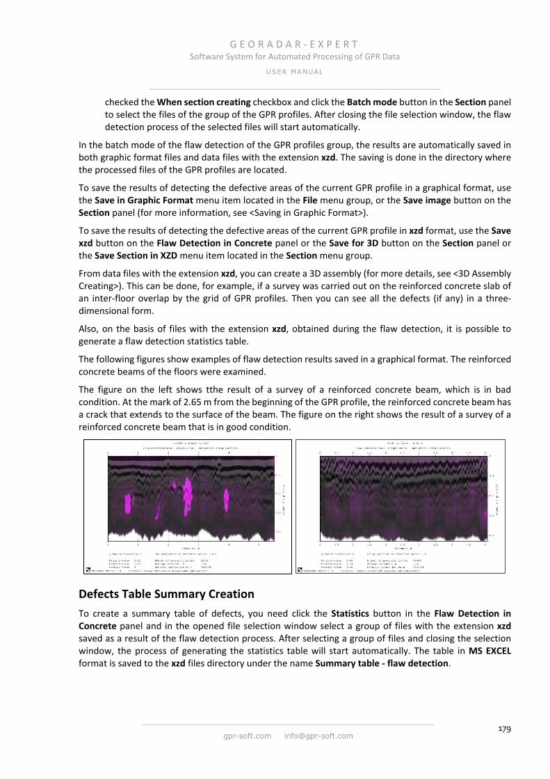
G E O R A D A R - E X P E R T Software System for Automated Processing of GPR Data
USER MANUAL
______________________________________________________________
______________________________________________________________
gpr-soft.com [email protected] 179
checked the When section creating checkbox and click the Batch mode button in the Section panel to select the files of the group of the GPR profiles. After closing the file selection window, the flaw detection process of the selected files will start automatically.
In the batch mode of the flaw detection of the GPR profiles group, the results are automatically saved in both graphic format files and data files with the extension xzd. The saving is done in the directory where the processed files of the GPR profiles are located.
To save the results of detecting the defective areas of the current GPR profile in a graphical format, use the Save in Graphic Format menu item located in the File menu group, or the Save image button on the Section panel (for more information, see <Saving in Graphic Format>).
To save the results of detecting the defective areas of the current GPR profile in xzd format, use the Save xzd button on the Flaw Detection in Concrete panel or the Save for 3D button on the Section panel or the Save Section in XZD menu item located in the Section menu group.
From data files with the extension xzd, you can create a 3D assembly (for more details, see <3D Assembly Creating>). This can be done, for example, if a survey was carried out on the reinforced concrete slab of an inter-floor overlap by the grid of GPR profiles. Then you can see all the defects (if any) in a three-dimensional form.
Also, on the basis of files with the extension xzd, obtained during the flaw detection, it is possible to generate a flaw detection statistics table.
The following figures show examples of flaw detection results saved in a graphical format. The reinforced concrete beams of the floors were examined.
The figure on the left shows tthe result of a survey of a reinforced concrete beam, which is in bad condition. At the mark of 2.65 m from the beginning of the GPR profile, the reinforced concrete beam has a crack that extends to the surface of the beam. The figure on the right shows the result of a survey of a reinforced concrete beam that is in good condition.
Defects Table Summary Creation To create a summary table of defects, you need click the Statistics button in the Flaw Detection in Concrete panel and in the opened file selection window select a group of files with the extension xzd saved as a result of the flaw detection process. After selecting a group of files and closing the selection window, the process of generating the statistics table will start automatically. The table in MS EXCEL format is saved to the xzd files directory under the name Summary table - flaw detection.

G E O R A D A R - E X P E R T Software System for Automated Processing of GPR Data
USER MANUAL
______________________________________________________________
______________________________________________________________
gpr-soft.com [email protected] 180
The figure below shows an example of a summary table based on the results of flaw detection for a group of GPR profiles:
The table contains the following elements:
Profile – the column contains profile names without extension;
Length, m – the column contains the lengths of the GPR profiles in meters;
Percentage of defect - the column contains the percentage of the defective areas of the section from the total area of the section. The background color of this cells is an indicator of the state of concrete: red, yellow and green colors correspond to bad, satisfactory and good condition, respectively;
Average value of Q-factor – the column contains the average values of the Q-factor attribute for the section. If the cell contains the value of the Q-factor attribute, which is lower than the value in the cell Global average value of Q-factor, this cell has a blue color. Cells with values higher than the Global average value of Q-factor have a pink color;
Total length –the total length (in meters) of the GPR profiles included in the table;
Number of profiles - the number of GPR profiles in the table;
Of them in bad condition – the number and percentage of GPR profiles from the total number of GPR profiles that detect a bad condition of concrete. Such cells in the Percentage of defect column are red;
Of them in satisfactory condition – the number and percentage of GPR profiles from the total number of GPR profiles that detect a satisfactory condition of concrete. Such cells in the Percentage of defect column are yellow;
G E O R A D A R - E X P E R T Software System for Automated Processing of GPR Data
USER MANUAL
______________________________________________________________
______________________________________________________________
gpr-soft.com [email protected] 181
Of them in good condition – the number and percentage of GPR profiles from the total number of GPR profiles that detect a good condition of concrete. Such cells in the Percentage of defect column are green;
Global average value of Q-factor - the average value of the attribute Q-factor, calculated on the basis of all sections;
Color cells where values > global average value - information about the color of the cells in the column Average value of Q-factor, whose values are higher than the value in the row Global average value of Q-factor;
Color cells where values < global average value - information about the color of the cells in the column Average value of Q-factor, whose values are lower than the value in the row Global average value of Q-factor;
Note:
The value of the threshold of defects (which is specified in the input window to the right of the Threshold button) is affected by the values of the smoothing coefficients of the Q-factor attribute when calculating the section. The values of the smoothing coefficients are specified in the group Data smoothing Y (samples) X (m) located in the Settings for All Attributes panel. It is recommended to set these parameters by Y = 80 samples and by X = 0.3 meters.
As practice has shown, these are optimal smoothing parameters for flaw detection based on the data obtained by the GPR with a center frequency above 1 GHz, the number of samples in the GPR trace 512 and the profiling step of 0.005 m. As the smoothing values increase, the threshold value of the defects decreases, and as the smoothing values decrease, the value of the defect threshold increases.
It is recommended to set the range of the permittivity of the section in the Range of Permittivity parameter group in the Settings for Attribute Permittivity panel from 4 to 9. No other limitations of the basic attribute ranges are required for flaw detection (for more information, see <Limitation the Range of Basic Attributes>).
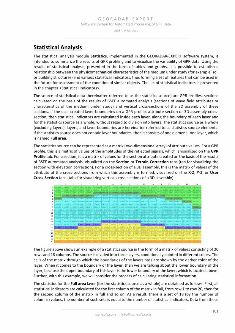
G E O R A D A R - E X P E R T Software System for Automated Processing of GPR Data
USER MANUAL
______________________________________________________________
______________________________________________________________
gpr-soft.com [email protected] 182
Statistical Analysis The statistical analysis module Statistics, implemented in the GEORADAR-EXPERT software system, is intended to summarize the results of GPR profiling and to visualize the variability of GPR data. Using the results of statistical analysis, presented in the form of tables and graphs, it is possible to establish a relationship between the physicomechanical characteristics of the medium under study (for example, soil or building structures) and various statistical indicators, thus forming a set of features that can be used in the future for assessment of the condition of similar objects. The list of statistical indicators is presented in the chapter <Statistical Indicators>.
The source of statistical data (hereinafter referred to as the statistics source) are GPR profiles, sections calculated on the basis of the results of BSEF automated analysis (sections of wave field attributes or characteristics of the medium under study) and vertical cross-sections of the 3D assembly of these sections. If the user created layer boundaries on a GPR profile, attribute section or 3D assembly cross-section, then statistical indicators are calculated inside each layer, along the boundary of each layer and for the statistics source as a whole, without regard to division into layers. The statistics source as a whole (excluding layers), layers, and layer boundaries are hereinafter referred to as statistics source elements. If the statistics source does not contain layer boundaries, then it consists of one element - one layer, which is named Full area.
The statistics source can be represented as a matrix (two-dimensional array) of attribute values. For a GPR profile, this is a matrix of values of the amplitudes of the reflected signals, which is visualized on the GPR Profile tab. For a section, it is a matrix of values for the section attribute created on the basis of the results of BSEF automated analysis, visualized on the Section or Terrain Correction tabs (tab for visualizing the section with elevation correction). For a cross-section of a 3D assembly, this is the matrix of values of the attribute of the cross-sections from which this assembly is formed, visualized on the X-Z, Y-Z, or User Cross-Section tabs (tabs for visualizing vertical cross-sections of a 3D assembly).
The figure above shows an example of a statistics source in the form of a matrix of values consisting of 20 rows and 18 columns. The source is divided into three layers, conditionally painted in different colors. The cells of the matrix through which the boundaries of the layers pass are shown by the darker color of the layer. When it comes to the boundary of the layer, then we are talking about the lower boundary of the layer, because the upper boundary of this layer is the lower boundary of the layer, which is located above. Further, with this example, we will consider the process of calculating statistical information.
The statistics for the Full area layer (for the statistics source as a whole) are obtained as follows. First, all statistical indicators are calculated for the first column of the matrix in full, from row 1 to row 20, then for the second column of the matrix in full and so on. As a result, there is a set of 18 (by the number of columns) values, the number of such sets is equal to the number of statistical indicators. Data from these

G E O R A D A R - E X P E R T Software System for Automated Processing of GPR Data
USER MANUAL
______________________________________________________________
______________________________________________________________
gpr-soft.com [email protected] 183
sets is visualized as statistical curves on the Statistics tab. Along with this, statistical indicators are calculated for the entire area of the Full area layer, the top row of the summary statistics table is formed from these values - see the chapter <Export Summary Statistical Table>.
Next, statistics are calculated for each layer. Consider a blue layer as an example of obtaining statistical information. First, all statistical indicators are calculated for the fragment of the first column, from the 6th to the 15th row, then for the fragment of the second column, the 5th to the 15th row, and so on. As a result, for the blue layer there is a set of 18 values, the number of such sets is equal to the number of statistical indicators. Data from these sets is visualized as statistical curves on the Statistics tab when this layer is selected on the layer picking panel (for more details see the chapter <Using the Layer Picking Panel>), and the Add Above and On Boundary checkboxes (for more details see the chapter <Visualization of Statistical Information>) are not marked.
Further, statistical indicators are calculated for the area starting from the first row of the matrix and bounded by the lower boundary of the blue layer below. Such information is in demand when it is necessary to be able to display (in road studies, for example) not only data on any layer of pavement, but also data on the entire road structure as a whole, from the surface of the road surface to the lower boundary of the lowest layer of the road structure.
In this case, first, all statistical indicators are calculated for the fragment of the first column, from 1 to 15 rows, then for the fragment of the second column, from 1 to 15 rows and so on. As a result, for the layer consisting of the blue layer and the area above, there is a set of 18 values; the number of these sets is equal to the number of statistical indicators. Data from these sets is visualized as statistical curves on the Statistics tab, when this layer is selected in the layer selection panel, the Add Above checkbox is checked, and the On Boundary checkbox is not checked.
Then, statistical indicators are calculated for the entire area of the layer, consisting of a blue layer and the area above. From these values, the rows of the summary statistics table are formed for layers marked add above (for more details see the chapter <Export Summary Statistical Table>).
Next, the values are read from the cells of the matrix through which the lower boundary of the layer passes. For the considered, as an example, layer of blue color, these are cells painted in dark blue. These values corresponding to the position of the layer boundary are visualized as a statistic graph on the Statistics tab, when this layer is selected on the layer selection panel and the On Boundary checkbox is checked. In this case, the ability to select statistical indicators is blocked, because for each column there is only one value, and not several, as is the case with layers. Statistical indicators for the layer boundary are calculated only by the values of the matrix of the statistics source through which this boundary passes. From these values, the rows of the summary statistics table are formed for layers marked on boundary (for more details see the chapter <Export Summary Statistical Table>).
For the lowest layer (yellow), the lower border is the bottom row of the matrix of values of the statistics source. Therefore, the statistics for this layer in the layer + area above mode (the Add Above checkbox is checked), and the Full area layer will be the same.
The Statistics module provides the ability to set a threshold, the values above or below which are displayed in red on the graphs, and the position of these areas on the GPR profile and their statistical characteristics are saved in the MS EXCEL table at the same time as the statistical plot is saved in graphical format. Setting the threshold on the statistical graph allows you to make more effective the process of identifying various defects of the investigated object, if a sign of a defect is a violation of a certain threshold attribute value.
To use the results of statistical analysis in third-party programs, it is provided to export all statistics indicators for all elements of the statistics source to ASCII encoded text format tables. It also provides for exporting the statistics plot image to a graphic format file.

G E O R A D A R - E X P E R T Software System for Automated Processing of GPR Data
USER MANUAL
______________________________________________________________
______________________________________________________________
gpr-soft.com [email protected] 184
The figure below shows a fragment of the GEORADAR-EXPERT user interface with the Statistics tab active for displaying the statistics plot, the Statistics control panel, and the layer selection panel as the statistics source Layer Picker for Statistics statistics.
The figure below shows a fragment of the GEORADAR-EXPERT user interface with the Statistics tab active for displaying the statistics plot, the Statistics control panel, as well as the Layer Picker for Statistics panel, which is used to select the layer whose data will be displayed on the statistics plot.
The threshold is shown in the graph as a horizontal line in blue. The threshold rule in this example is configured so that sections of the statistical curve that exceed the specified value are colored in red.
The plot header contains the name of the statistics source file Source File Name, a statistical indicator (for this plot the arithmetic mean), the name of the attribute (for this graph, the amplitude of the GPR profile GPR Signals), threshold value, percentage of the total length of the threshold exceeding areas from the length of the GPR profile Exceeding and the total length of the areas of violation total length.

G E O R A D A R - E X P E R T Software System for Automated Processing of GPR Data
USER MANUAL
______________________________________________________________
______________________________________________________________
gpr-soft.com [email protected] 185
Statistical Indicators The statistical analysis module provides for the calculation of the following statistical indicators:
Min – minimum values;
Max – maximum values;
Mean – arithmetic mean;
Med – median of values;
Corr – correlation coefficient for neighboring GPR traces or columns of the matrix of section values;
PAR – peak to average ratio;
Var – variance of values (the mathematical expectation of the standard deviation of the values from the mathematical expectation of these values);
Std – standard deviation of values (square root of variance);
CV – coefficient of variation (the ratio of the standard deviation of the values to the mathematical expectation of these values);
MAD – mean absolute deviation;
Range – range of values;
IQR – interquartile range (difference between the 75th and the 25th percentiles of the values);
Creating, Saving and Loading Statistics Data File The source of statistical information is data visualized on the current tab. Listed below are tabs on which visualized data can be used as a statistics source.
GPR Profile – visualization of GPR signals;
Section – sections of wave field attributes or characteristics of the studied medium, created on the basis of BSEF automated analysis;
Terrain Correction - attribute sections created on the basis of automated BSEF analysis with allowance for terrain correction;
X-Z – vertical slice of a 3D section assembly perpendicular to the Y axis;
Y-Z – vertical slice of a 3D section assembly perpendicular to the X axis;
User Сross-section – user vertical section of the 3D assembly;
If the statistics source contains user-created layer boundaries, then the statistical analysis process calculates statistical indicators for each layer, for each layer boundary and for the entire statistics source area. If there are no layer boundaries, then the calculations are performed only over the entire area of the statistics source — the GPR profile, attribute section, or 3D assembly section.
The statistical analysis process has no settings. The statistical analysis process is launched by clicking the Create File button on the Statistics control panel or using the Create Statistics File menu, which is located in the Statistics menu group. The user can load the Statistics control panel into the lower group of tabs using the Statistics Control Panel menu from the Statistics menu group. If the Statistics panel is not
G E O R A D A R - E X P E R T Software System for Automated Processing of GPR Data
USER MANUAL
______________________________________________________________
______________________________________________________________
gpr-soft.com [email protected] 186
loaded, it will open automatically, during the completion of the statistical analysis process, while loading the analysis results.
After the process of statistical calculations is completed, the results of statistical analysis are automatically saved to a file with the gestat extension in the directory of the file location of the analyzed GPR profile or 3D assembly. If the data from the Section or Terrain Correction tabs is analyzed, the name of the statistical data file will be composed of the name of the GPR profile file and the name of the section attribute. If the statistics source belongs to the GPR Profile tab, then the phrase GPR Signals will be added to the name of the GPR profile file.
If 3D assembly data from the X-Z or Y-Z tabs is analyzed, the name of the statistical data file will be composed of the name of the 3D assembly file, the name of the attribute, the 3D word, the name of the analyzed section and the position of the section on the corresponding axis. If 3D assembly data from the User Cross-Section tab is analyzed, the name of the statistics file will be composed of the name of the 3D assembly file, the name of the attribute and the phrase 3D User Section.
If the source of statistical information contains user-created layer boundaries, then the word Layer is added to the end of the statistics file name.
After the statistical analysis process is completed and the statistics file with the gestat extension is saved to the hard disk, this file is automatically loaded into the program. If the Statistics control panel is not open, it will open in the lower group of tabs during the loading of the statistics file, and in the upper group of tabs the tab for visualization of statistical information Statistics will open.
If the downloaded statistics file contains data for the layers, then during the loading process the Layer Picker for Statistics layer selection panel additionally opens, if one has not been previously loaded. This panel is located in the lower group of tabs, to the right of the Statistics panel. If the Layer Picker for Statistics layer selection panel is open, and the downloaded statistics file does not contain layered data, this panel is deleted.
To load the statistics file saved on the hard disk, you need to use the Load Statistics File menu item from the Statistics menu group or click the Load File button on the Statistics control panel. To display the name of the downloaded statistics file, use the Loaded Statistics File Name menu item from the Statistics menu group. After clicking on this menu item, in the working window of the program, an information panel with the name of the statistics file will be displayed.
In the course of using the results of statistical analysis, the user can configure data visualization parameters - change data smoothing, set various thresholds for various statistical indicators, and perform other settings. Changes made to the visualization of statistical data can be saved in the statistics file. To do this, use the Save Statistics File menu item from the Statistics menu group or click the Save File button in the Statistics panel. As a result of these actions, the current visualization settings are saved in the statistics file and during subsequent downloads of this file the settings will be automatically applied.
Visualization of Statistical Information The results of statistical analysis are visualized in the form of a graph on the Statistics tab, which belongs to the upper group of tabs. Each point in the graph represents the value of the selected statistical indicator, calculated from the columns of the matrix of values for the section attribute, 3D assembly section, or GPR profile signals. If the statistics graph is displayed for the statistics source as a whole (the source does not have layers or the source with layers, but the Full Area checkbox is activated), then the graph shows the statistics calculated over the entire column of the matrix of values of the statistics source. If the source has layers and any layer is selected, then the graph shows statistical indicators calculated only for that fragment of columns that are inside the layer (see in more detail <Statistical Analysis>).
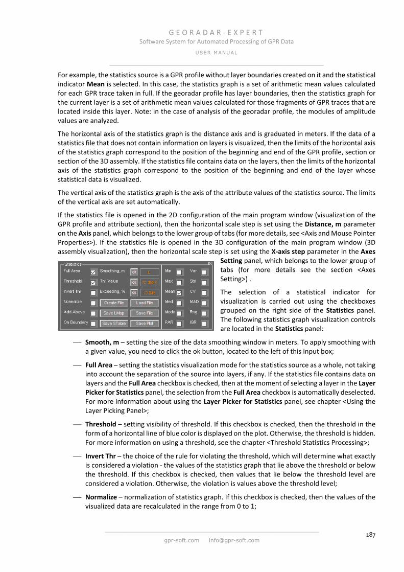
G E O R A D A R - E X P E R T Software System for Automated Processing of GPR Data
USER MANUAL
______________________________________________________________
______________________________________________________________
gpr-soft.com [email protected] 187
For example, the statistics source is a GPR profile without layer boundaries created on it and the statistical indicator Mean is selected. In this case, the statistics graph is a set of arithmetic mean values calculated for each GPR trace taken in full. If the georadar profile has layer boundaries, then the statistics graph for the current layer is a set of arithmetic mean values calculated for those fragments of GPR traces that are located inside this layer. Note: in the case of analysis of the georadar profile, the modules of amplitude values are analyzed.
The horizontal axis of the statistics graph is the distance axis and is graduated in meters. If the data of a statistics file that does not contain information on layers is visualized, then the limits of the horizontal axis of the statistics graph correspond to the position of the beginning and end of the GPR profile, section or section of the 3D assembly. If the statistics file contains data on the layers, then the limits of the horizontal axis of the statistics graph correspond to the position of the beginning and end of the layer whose statistical data is visualized.
The vertical axis of the statistics graph is the axis of the attribute values of the statistics source. The limits of the vertical axis are set automatically.
If the statistics file is opened in the 2D configuration of the main program window (visualization of the GPR profile and attribute section), then the horizontal scale step is set using the Distance, m parameter on the Axis panel, which belongs to the lower group of tabs (for more details, see <Axis and Mouse Pointer Properties>). If the statistics file is opened in the 3D configuration of the main program window (3D assembly visualization), then the horizontal scale step is set using the X-axis step parameter in the Axes
Setting panel, which belongs to the lower group of tabs (for more details see the section <Axes Setting>) .
The selection of a statistical indicator for visualization is carried out using the checkboxes grouped on the right side of the Statistics panel. The following statistics graph visualization controls are located in the Statistics panel:
Smooth, m – setting the size of the data smoothing window in meters. To apply smoothing with a given value, you need to click the ok button, located to the left of this input box;
Full Area – setting the statistics visualization mode for the statistics source as a whole, not taking into account the separation of the source into layers, if any. If the statistics file contains data on layers and the Full Area checkbox is checked, then at the moment of selecting a layer in the Layer Picker for Statistics panel, the selection from the Full Area checkbox is automatically deselected. For more information about using the Layer Picker for Statistics panel, see chapter <Using the Layer Picking Panel>;
Threshold – setting visibility of threshold. If this checkbox is checked, then the threshold in the form of a horizontal line of blue color is displayed on the plot. Otherwise, the threshold is hidden. For more information on using a threshold, see the chapter <Threshold Statistics Processing>;
Invert Thr – the choice of the rule for violating the threshold, which will determine what exactly is considered a violation - the values of the statistics graph that lie above the threshold or below the threshold. If this checkbox is checked, then values that lie below the threshold level are considered a violation. Otherwise, the violation is values above the threshold level;
Normalize – normalization of statistics graph. If this checkbox is checked, then the values of the visualized data are recalculated in the range from 0 to 1;
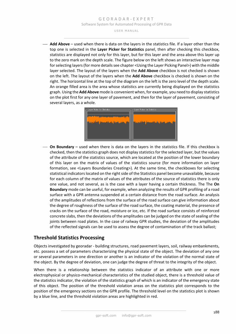
G E O R A D A R - E X P E R T Software System for Automated Processing of GPR Data
USER MANUAL
______________________________________________________________
______________________________________________________________
gpr-soft.com [email protected] 188
Add Above – used when there is data on the layers in the statistics file. If a layer other than the top one is selected in the Layer Picker for Statistics panel, then after checking this checkbox, statistics are displayed not only for this layer, but for this layer and the area above this layer up to the zero mark on the depth scale. The figure below on the left shows an interactive layer map for selecting layers (for more details see chapter <Using the Layer Picking Panel>) with the middle layer selected. The layout of the layers when the Add Above checkbox is not checked is shown on the left. The layout of the layers when the Add Above checkbox is checked is shown on the right. The horizontal line at the top of the diagram on the left is the zero level of the depth scale. An orange filled area is the area whose statistics are currently being displayed on the statistics graph. Using the Add Above mode is convenient when, for example, you need to display statistics on the plot first for any one layer of pavement, and then for the layer of pavement, consisting of several layers, as a whole.
On Boundary – used when there is data on the layers in the statistics file. If this checkbox is
checked, then the statistics graph does not display statistics for the selected layer, but the values of the attribute of the statistics source, which are located at the position of the lower boundary of this layer on the matrix of values of the statistics source (for more information on layer formation, see <Layers Boundaries Creating>). At the same time, the checkboxes for selecting statistical indicators located on the right side of the Statistics panel become unavailable, because for each column of the matrix of values of the attributes of the source of statistics there is only one value, and not several, as is the case with a layer having a certain thickness. The The On Boundary mode can be useful, for example, when analyzing the results of GPR profiling of a road surface with a GPR antenna suspended at a certain distance from the road surface. An analysis of the amplitudes of reflections from the surface of the road surface can give information about the degree of roughness of the surface of the road surface, the coating material, the presence of cracks on the surface of the road, moisture or ice, etc. If the road surface consists of reinforced concrete slabs, then the deviations of the amplitudes can be judged on the state of sealing of the joints between road plates. In the case of railway GPR studies, the deviation of the amplitudes of the reflected signals can be used to assess the degree of contamination of the track ballast;
Threshold Statistics Processing Objects investigated by georadar - building structures, road pavement layers, soil, railway embankments, etc. possess a set of parameters characterizing the physical state of the object. The deviation of any one or several parameters in one direction or another is an indicator of the violation of the normal state of the object. By the degree of deviation, one can judge the degree of threat to the integrity of the object.
When there is a relationship between the statistics indicator of an attribute with one or more electrophysical or physico-mechanical characteristics of the studied object, there is a threshold value of the statistics indicator, the violation of the statistics graph of which is an indicator of the emergency state of this object. The position of the threshold violation areas on the statistics plot corresponds to the position of the emergency sections on the GPR profile. The threshold level on the statistics plot is shown by a blue line, and the threshold violation areas are highlighted in red.

G E O R A D A R - E X P E R T Software System for Automated Processing of GPR Data
USER MANUAL
______________________________________________________________
______________________________________________________________
gpr-soft.com [email protected] 189
To enter an accurate threshold value, use the Thr Value input box in the Statistics panel. To apply the threshold value, you need to click the ok button, located to the left of the threshold value input box. The Exceeding,% input box in the Statistics panel is used to enter the percentage of the total length of the violation areas from the length of the statistics source - GPR profile, attribute section or section of 3D assembly. To apply the percentage value of the total length, you need to click the ok button, located to the left of this input box. Changing values in the input box Thr Value affects the value in the input box Exceeding,% and vice versa.
Along with this, the threshold level can be set by right-clicking within the axes of the statistics plot. After a mouse click, the threshold level line moves to the cursor position, and the values in the Thr Value and Exceeding,% input boxes are recalculated in accordance with the new position of the threshold line. If you right-click within the axes of the statistics plot, a pop-up menu will appear with two items - Set Threshold by Mean and Set Threshold by Median. Using these menu items, the threshold level is set, respectively, by the arithmetic mean or median of the statistics curve values.
Using the Invert Thr checkbox in the Statistics panel, a threshold rule is set. If this checkbox is not checked, then the threshold level is exceeded. If this checkbox is checked, then areas of the statistics plot whose values are below the threshold level are considered a violation. An example of a statistical plot with the Invert Thr checkbox selected is shown below.
If there is a threshold level line on the statistics graph, then in the process of saving the statistics plot image in graphic format, the MS EXCEL format table with data on the position of the threshold violation regions with the characteristics of these regions is saved. Below is an example of a table of regions of threshold violation and a description of the elements of this table.
The table consists of a heading that occupies rows 1 - 10 and a list of violation regions with their characteristics. The header consists of the following rows:
Row 1 – information about the threshold rule that was used for the statistical plot on the basis of which this table was generated. This row may contain the following definitions: Areas where values are above the threshold or Areas where values are below the threshold;
Row 2 – имя файла источника статистики (георадарного профиля или 3D сборки) Source file name;
Row 3 – имя файла статистики Statistics file name. Файл статистики имеет расширение gestat;

G E O R A D A R - E X P E R T Software System for Automated Processing of GPR Data
USER MANUAL
______________________________________________________________
______________________________________________________________
gpr-soft.com [email protected] 190
Row 4 – название слоя Layer name. Если файл статистики не имеет информации по слоям, то слоем считается вся площадь источника статистики и этому слою присваивается название Full area;
Row 5 – наименование атрибута источника статистики Attribute;
Row 6 – значение порога Threshold value;
Row 7 – протяжённость слоя в метрах Layer length (длина слоя соответствует длине нижней границы слоя. О формировании слоёв более подробно см. в <Принцип формирования слоёв>). Если файл статистики не имеет послойной информации, то в данной строке указывается протяжённость источника статистики – георадарного профиля, разреза или сечения 3D сборки;
Row 8 – шаг данных источника статистики по горизонтали Data step horizontally. Для георадарного профиля это расстояние между георадиолокационными трассами;
Row 9 – суммарная протяжённость областей нарушения порога в метрах. Если отмечен чекбокс Invert Thr, то данный параметр называется Total length of below the threshold, в противном случае - Total length of exceeding the threshold;
Row 10 – доля суммарной протяженности областей нарушения порога от протяжённости источника статистики в процентах. Если отмечен чекбокс Invert Thr, то данный параметр называется Percentage of areas below the threshold from layer length, в противном случае - Percentage excesses from layer length.
Row 11 contains the column headers of the table:
№ - conditional number of the violation area. Assigned in ascending order of remoteness of areas from the origin;
Start, m – position of the beginning of the violation area on the distance scale in meters;
End, m – position of the end of the violation area on the distance scale in meters;
Number of traces – the number of columns of the matrix of values of the attribute of the statistics source per area of violation. If the statistics source is a GPR profile, then this value is the number of GPR traces;
Length, m – length of violation area in meters. If the length of the violation region is 0, then this is a point violation, i.e. the violation area consists of one column of the matrix of values of the attribute of the statistics source. If the source of statistics is a georadar profile, then this violation consists of one GPR trace;
Extreme position, m – position on the distance scale of the maximum deviation of the statistics curve from the threshold level within the violation area;
Extreme value – value of the maximum deviation of the statistics curve from the threshold level within the violation area;
Exceeding threshold, % - percentage of the maximum deviation of the statistics curve from the threshold value within the violation area. If the Invert Thr checkbox is checked, then this column is called Below threshold,% (below the threshold in percent), otherwise - Exceeding threshold,% (above the threshold in percent). Using the values in this column, you can assess the degree of threat to the integrity of the investigated object - the higher the percentage of deviation, the higher the likelihood of an emergency at the investigated object.

G E O R A D A R - E X P E R T Software System for Automated Processing of GPR Data
USER MANUAL
______________________________________________________________
______________________________________________________________
gpr-soft.com [email protected] 191
Below the table there is information about normalization of values of the statistics curve Normalizing and the size of the window of smoothing statistical data in meters Data smoothing. If the value of Data smoothing is equal to zero, the statistical data are not smoothed.
The use of threshold analysis implemented in the GEORADAR-EXPERT software system improves the quality and productivity of non-destructive quality control of construction or monitoring geological hazards. The ability to separate the statistics source (GPR profile, attribute section or 3D assembly section) into layers allows you to carry out such studies in more detail - to carry out a threshold analysis not only of the entire investigated thickness, but also of each layer of the diagnosed structure individually. Particularly effective is the use of threshold analysis to process the results of GPR monitoring of long objects - roads and railways.
Using the Layer Picking Panel When a statistics source (GPR profile, attribute section or 3D assembly section) contains user-created layer boundaries (for more details, see the chapter <Layers Boundaries Creating>) then statistical analysis calculates statistical indicators for both the entire statistics source and for each layer separately, and along the border of each layer. The choice of the layer whose data you want to display on the statistics graph is carried out in the Layer Picker for Statistics panel.
The Layer Picker for Statistics panel automatically opens when the loaded file contains statistics for the layers. This panel is located in the bottom group of tabs. When the Layer Picker for Statistics panel is already open, but a statistics file is loaded that does not contain layer data, the Layer Picker for Statistics panel is removed during the loading of such a file.
The Layer Picker for Statistics panel displays the boundaries of the statistics source layers as orange lines. If the source of statistics is a GPR profile, then the zero level of the depth scale is shown on the Layer Picker for Statistics panel as a horizontal orange straight line, below which the layer boundaries are located.
When a statistics file with layers has just been loaded, there is no selected layer yet, and statistics are displayed for the statistics source as a whole (the Full Area checkbox is checked in the Statistics panel). To display statistics for a specific layer, you need to select that layer in the Layer Picker for Statistics panel. To do this, move the mouse pointer to the required layer, right-click and, in the pop-up menu that appears, select the Select This Layer item. As a result of these actions, statistical information for the selected layer is displayed on the Statistics tab. The selected layer in the Layer Picker for Statistics panel is colored orange.
There is another way to select a layer - using the Select Layer From Layer List pop-up menu item. Using this menu item, a pop-up window for selecting a layer is called, containing a drop-down list of layer numbers. Layer numbers are assigned automatically, in ascending order of the average depth of the layer, and are the
default layer names. The user selects a layer number from the list and presses the Select button, after which the layer selection window closes, and the statistical information on this layer is displayed on the Statistics tab.
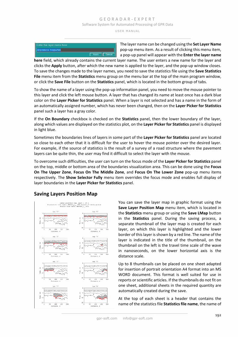
G E O R A D A R - E X P E R T Software System for Automated Processing of GPR Data
USER MANUAL
______________________________________________________________
______________________________________________________________
gpr-soft.com [email protected] 192
The layer name can be changed using the Set Layer Name pop-up menu item. As a result of clicking this menu item, a pop-up panel will appear with the Enter the layer name
here field, which already contains the current layer name. The user enters a new name for the layer and clicks the Apply button, after which the new name is applied to the layer, and the pop-up window closes. To save the changes made to the layer names, you need to save the statistics file using the Save Statistics File menu item from the Statistics menu group on the menu bar at the top of the main program window, or click the Save File button on the Statistics panel, which is located in the bottom group of tabs.
To show the name of a layer using the pop-up information panel, you need to move the mouse pointer to this layer and click the left mouse button. A layer that has changed its name at least once has a dark blue color on the Layer Picker for Statistics panel. When a layer is not selected and has a name in the form of an automatically assigned number, which has never been changed, then on the Layer Picker for Statistics panel such a layer has a gray color.
If the On Boundary checkbox is checked on the Statistics panel, then the lower boundary of the layer, along which values are displayed on the statistics plot, on the Layer Picker for Statistics panel is displayed in light blue.
Sometimes the boundaries lines of layers in some part of the Layer Picker for Statistics panel are located so close to each other that it is difficult for the user to hover the mouse pointer over the desired layer. For example, if the source of statistics is the result of a survey of a road structure where the pavement layers can be quite thin, the user may find it difficult to select the layer with the mouse.
To overcome such difficulties, the user can turn on the focus mode of the Layer Picker for Statistics panel on the top, middle or bottom area of the boundaries visualization area. This can be done using the Focus On The Upper Zone, Focus On The Middle Zone, and Focus On The Lower Zone pop-up menu items respectively. The Show Selector Fully menu item overrides the focus mode and enables full display of layer boundaries in the Layer Picker for Statistics panel.
Saving Layers Position Map You can save the layer map in graphic format using the Save Layer Position Map menu item, which is located in the Statistics menu group or using the Save LMap button in the Statistics panel. During the saving process, a separate thumbnail of the layer map is created for each layer, on which this layer is highlighted and the lower border of this layer is shown by a red line. The name of the layer is indicated in the title of the thumbnail, on the thumbnail on the left is the travel time scale of the wave in nanoseconds, on the lower horizontal axis is the distance scale.
Up to 8 thumbnails can be placed on one sheet adapted for insertion of portrait orientation A4 format into an MS WORD document. This format is well suited for use in reports or scientific articles. If the thumbnails do not fit on one sheet, additional sheets in the required quantity are automatically created during the save.
At the top of each sheet is a header that contains the name of the statistics file Statistics file name, the name of
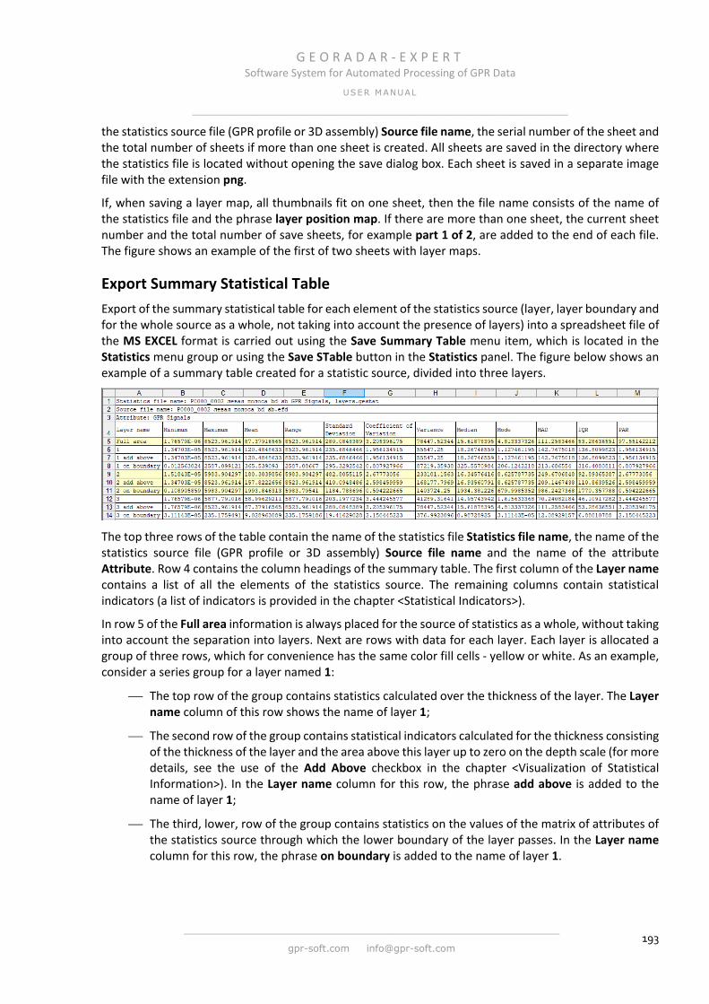
G E O R A D A R - E X P E R T Software System for Automated Processing of GPR Data
USER MANUAL
______________________________________________________________
______________________________________________________________
gpr-soft.com [email protected] 193
the statistics source file (GPR profile or 3D assembly) Source file name, the serial number of the sheet and the total number of sheets if more than one sheet is created. All sheets are saved in the directory where the statistics file is located without opening the save dialog box. Each sheet is saved in a separate image file with the extension png.
If, when saving a layer map, all thumbnails fit on one sheet, then the file name consists of the name of the statistics file and the phrase layer position map. If there are more than one sheet, the current sheet number and the total number of save sheets, for example part 1 of 2, are added to the end of each file. The figure shows an example of the first of two sheets with layer maps.
Export Summary Statistical Table Export of the summary statistical table for each element of the statistics source (layer, layer boundary and for the whole source as a whole, not taking into account the presence of layers) into a spreadsheet file of the MS EXCEL format is carried out using the Save Summary Table menu item, which is located in the Statistics menu group or using the Save STable button in the Statistics panel. The figure below shows an example of a summary table created for a statistic source, divided into three layers.
The top three rows of the table contain the name of the statistics file Statistics file name, the name of the statistics source file (GPR profile or 3D assembly) Source file name and the name of the attribute Attribute. Row 4 contains the column headings of the summary table. The first column of the Layer name contains a list of all the elements of the statistics source. The remaining columns contain statistical indicators (a list of indicators is provided in the chapter <Statistical Indicators>).
In row 5 of the Full area information is always placed for the source of statistics as a whole, without taking into account the separation into layers. Next are rows with data for each layer. Each layer is allocated a group of three rows, which for convenience has the same color fill cells - yellow or white. As an example, consider a series group for a layer named 1:
The top row of the group contains statistics calculated over the thickness of the layer. The Layer name column of this row shows the name of layer 1;
The second row of the group contains statistical indicators calculated for the thickness consisting of the thickness of the layer and the area above this layer up to zero on the depth scale (for more details, see the use of the Add Above checkbox in the chapter <Visualization of Statistical Information>). In the Layer name column for this row, the phrase add above is added to the name of layer 1;
The third, lower, row of the group contains statistics on the values of the matrix of attributes of the statistics source through which the lower boundary of the layer passes. In the Layer name column for this row, the phrase on boundary is added to the name of layer 1.

G E O R A D A R - E X P E R T Software System for Automated Processing of GPR Data
USER MANUAL
______________________________________________________________
______________________________________________________________
gpr-soft.com [email protected] 194
Export Statistics to Text Format To use the results of statistical analysis in third-party programs, it is possible to export all statistics indicators for all elements of the statistics source (layers and layer boundaries, if any) to text format tables with the txt extension, in ASCII encoding. The export process is started using the menu item Export Statistics to Text Files, which is located in the menu group Statistics.
After clicking the menu item Export Statistics to Text Files, a folder with a name is created in the directory where the statistics file is located, consisting of the phrase Export from file and the name of the statistics file. As an example, the figure below shows a diagram of the contents of the statistics export folder by source, divided into three layers. The names of the folders with the export results correspond to the list of statistics source elements from the Layer name column of the summary statistical table (for more details see the chapter <Export Summary Statistical Table>). In the diagram, folders are shown as they look in Windows Explorer. Inside the blue frames, the contents of the folders are shown.
In the folders where the data for the layer boundary is located, there is only one table file with the values of the attribute of the statistics source at the location where the layer boundary passes.
The remaining folders contain table files for each statistic indicator; the file name consists of the name of the statistic indicator. ASCII encoded tables consist of two columns. The first column is the horizontal distance from the origin; the second column is the statistic value. If there is layered data, the folder with the export results contains a file (or files) with a layers position map in png format.
Saving Statistical Plot The statistics plot is saved in graphical format using the Save Plot menu item, which is located in the Statistics menu group or using the Save Plot button in the Statistics panel. Save settings are made in the Save in graphic format panel - for more details see the chapter <Saving in Graphic Format>. If the Save in graphic format panel is not open, it will automatically open after clicking on the button or menu item Save Plot, and the saving process will be interrupted so that the user can configure the save settings.
The statistical plot can be saved taking into account the horizontal scale. To do this, in the Save in graphic format panel, check the Saving scale checkbox and specify the scale in the Scale on X parameter input box.
If a threshold is displayed on the statistics plot, then the data on the location of the threshold violation areas with the characteristics of these areas are saved in the MS EXCEL format table at the same time as the statistics plot image is saved (for more details on the threshold violation table, see chapter <Threshold Statistics Processing>).
The figure below shows an example of a saved image of a statistics plot. The plot title contains the name of the statistics source file Source File Name, information about the statistical indicator (for this plot, the

G E O R A D A R - E X P E R T Software System for Automated Processing of GPR Data
USER MANUAL
______________________________________________________________
______________________________________________________________
gpr-soft.com [email protected] 195
mean arithmetic Mean), the name of the attribute (for this plot, the amplitude of the GPR profile GPR Signals), the threshold value Threshold, the percentage of the total length of the threshold exceeding areas from the length of the GPR profile Exceeding and the total length of areas exceeding the total length. The threshold level on the plot is shown by a red line. Areas of violation of the threshold rule are also shown in red.
Under the plot axes, in the lower left part of the sheet, there are statistical indicators of the plot curve Min, Max, Mean and Std (for more details on statistics indicators, see the chapter <Statistical Indicators>), the name of the layer is Layer name (if the statistics file does not have information about layers, then the layer is called Full area), the size of the data smoothing window in meters Smoothing (if the value is 0, then the statistical data is displayed without smoothing) and information about the normalization of statistical data Normalizing. If the statistics file contains information on the layers, then a map of the location of the layer is placed in the lower right part of the sheet. The layer whose statistics are displayed on the chart is highlighted with a fill.
The figure below shows the result of saving the statistical plot taking into account the horizontal scale. All information about the plot indicated in the previous paragraph is concentrated in the lower left corner of the image. The vertical scale of attribute values or statistical indicator is located on the right edge of the image; the horizontal distance scale is located at the top edge of the image.
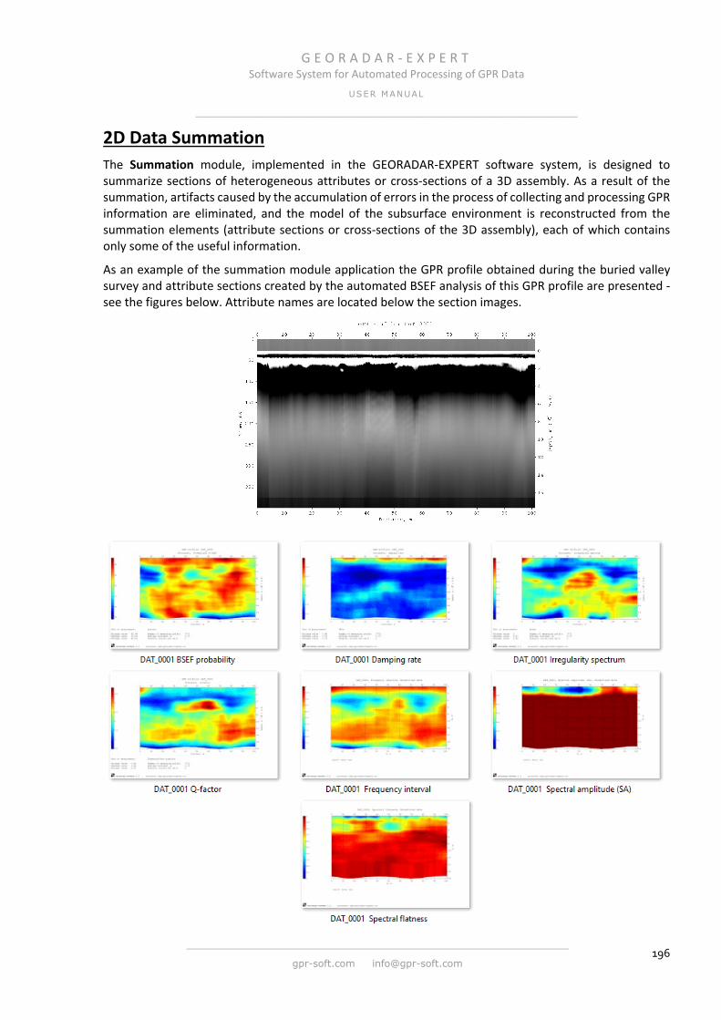
G E O R A D A R - E X P E R T Software System for Automated Processing of GPR Data
USER MANUAL
______________________________________________________________
______________________________________________________________
gpr-soft.com [email protected] 196
2D Data Summation The Summation module, implemented in the GEORADAR-EXPERT software system, is designed to summarize sections of heterogeneous attributes or cross-sections of a 3D assembly. As a result of the summation, artifacts caused by the accumulation of errors in the process of collecting and processing GPR information are eliminated, and the model of the subsurface environment is reconstructed from the summation elements (attribute sections or cross-sections of the 3D assembly), each of which contains only some of the useful information.
As an example of the summation module application the GPR profile obtained during the buried valley survey and attribute sections created by the automated BSEF analysis of this GPR profile are presented - see the figures below. Attribute names are located below the section images.
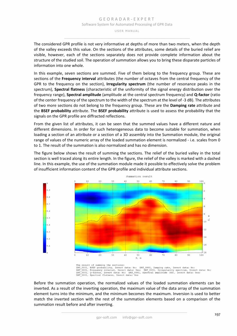
G E O R A D A R - E X P E R T Software System for Automated Processing of GPR Data
USER MANUAL
______________________________________________________________
______________________________________________________________
gpr-soft.com [email protected] 197
The considered GPR profile is not very informative at depths of more than two meters, when the depth of the valley exceeds this value. On the sections of the attributes, some details of the buried relief are visible, however, each of the sections separately does not provide complete information about the structure of the studied soil. The operation of summation allows you to bring these disparate particles of information into one whole.
In this example, seven sections are summed. Five of them belong to the frequency group. These are sections of the Frequency interval attributes (the number of octaves from the central frequency of the GPR to the frequency on the section), Irregularity spectrum (the number of resonance peaks in the spectrum), Spectral flatness (characteristic of the uniformity of the signal energy distribution over the frequency range), Spectral amplitude (amplitude at the central spectrum frequency) and Q-factor (ratio of the center frequency of the spectrum to the width of the spectrum at the level of -3 dB). The attributes of two more sections do not belong to the frequency group. These are the Damping rate attribute and the BSEF probability attribute. The BSEF probability attribute is used to assess the probability that the signals on the GPR profile are diffracted reflections.
From the given list of attributes, it can be seen that the summed values have a different nature and different dimensions. In order for such heterogeneous data to become suitable for summation, when loading a section of an attribute or a section of a 3D assembly into the Summation module, the original range of values of the numeric array of the loaded summation element is normalized - i.e. scales from 0 to 1. The result of the summation is also normalized and has no dimension.
The figure below shows the result of summing the sections. The relief of the buried valley in the total section is well traced along its entire length. In the figure, the relief of the valley is marked with a dashed line. In this example, the use of the summation module made it possible to effectively solve the problem of insufficient information content of the GPR profile and individual attribute sections.
Before the summation operation, the normalized values of the loaded summation elements can be inverted. As a result of the inverting operation, the maximum value of the data array of the summation element turns into the minimum, and the minimum becomes the maximum. Inversion is used to better match the inverted section with the rest of the summation elements based on a comparison of the summation result before and after inverting.
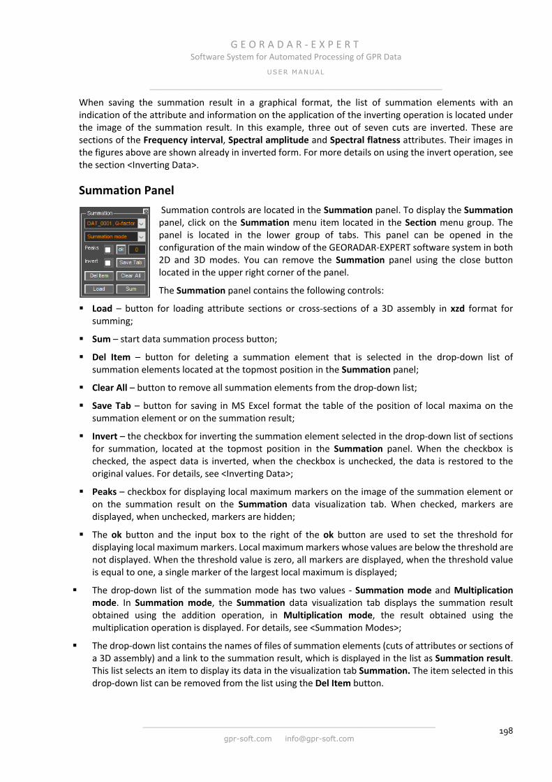
G E O R A D A R - E X P E R T Software System for Automated Processing of GPR Data
USER MANUAL
______________________________________________________________
______________________________________________________________
gpr-soft.com [email protected] 198
When saving the summation result in a graphical format, the list of summation elements with an indication of the attribute and information on the application of the inverting operation is located under the image of the summation result. In this example, three out of seven cuts are inverted. These are sections of the Frequency interval, Spectral amplitude and Spectral flatness attributes. Their images in the figures above are shown already in inverted form. For more details on using the invert operation, see the section <Inverting Data>.
Summation Panel Summation controls are located in the Summation panel. To display the Summation panel, click on the Summation menu item located in the Section menu group. The panel is located in the lower group of tabs. This panel can be opened in the configuration of the main window of the GEORADAR-EXPERT software system in both 2D and 3D modes. You can remove the Summation panel using the close button located in the upper right corner of the panel.
The Summation panel contains the following controls:
Load – button for loading attribute sections or cross-sections of a 3D assembly in xzd format for summing;
Sum – start data summation process button;
Del Item – button for deleting a summation element that is selected in the drop-down list of summation elements located at the topmost position in the Summation panel;
Clear All – button to remove all summation elements from the drop-down list;
Save Tab – button for saving in MS Excel format the table of the position of local maxima on the summation element or on the summation result;
Invert – the checkbox for inverting the summation element selected in the drop-down list of sections for summation, located at the topmost position in the Summation panel. When the checkbox is checked, the aspect data is inverted, when the checkbox is unchecked, the data is restored to the original values. For details, see <Inverting Data>;
Peaks – checkbox for displaying local maximum markers on the image of the summation element or on the summation result on the Summation data visualization tab. When checked, markers are displayed, when unchecked, markers are hidden;
The ok button and the input box to the right of the ok button are used to set the threshold for displaying local maximum markers. Local maximum markers whose values are below the threshold are not displayed. When the threshold value is zero, all markers are displayed, when the threshold value is equal to one, a single marker of the largest local maximum is displayed;
The drop-down list of the summation mode has two values - Summation mode and Multiplication mode. In Summation mode, the Summation data visualization tab displays the summation result obtained using the addition operation, in Multiplication mode, the result obtained using the multiplication operation is displayed. For details, see <Summation Modes>;
The drop-down list contains the names of files of summation elements (cuts of attributes or sections of a 3D assembly) and a link to the summation result, which is displayed in the list as Summation result. This list selects an item to display its data in the visualization tab Summation. The item selected in this drop-down list can be removed from the list using the Del Item button.

G E O R A D A R - E X P E R T Software System for Automated Processing of GPR Data
USER MANUAL
______________________________________________________________
______________________________________________________________
gpr-soft.com [email protected] 199
Preparing Data for Summation 2D data in xzd format are used as summation elements. These can be attribute sections or cross-sections of 3D assemblies of the sections. To save the section data into an xzd file, use the Save for 3D button on the Section panel or use the Save Section in XZD menu item located in the Section menu group, as well as using the Save XZD menu item from the File menu group.
In the first two cases, saving is carried out without opening the save window, with which you can change the name of the saved file. For these cases, the file name is identical to the file name of the GPR profile from which the section was created, or the file name of the 3D assembly. Only the file extension is changed to xzd. Saving is performed in the directory where the GPR profile file or 3D assembly is located. However, these saving methods are still better suited for preparing data for a 3D assembly than for summing.
In the case of saving using the Save XZD menu item from the File menu group, the file name is formed from the name of the GPR profile or 3D assembly file with the addition of the section attribute name or 3D assembly attribute name. During the saving process, a window opens in which you can change the save directory and the name of the saved file. This method is preferable when saving xzd files for summing, since the file name contains the name of the attribute, which simplifies the user's orientation in the list of summing elements.
The sizes of the two-dimensional data arrays of the summation elements must be the same. If the program detects at least one size mismatch, the summation operation will be interrupted and a message will appear on the screen containing information about the sizes of each summation element. With the help of this hint, the user can easily detect the size mismatch and remove the element that caused the error by selecting this element in the drop-down list of summation elements and pressing the Del Item button.
Loading and Deleting Summation Items The prepared data for summation in xzd format is loaded using the Load button on the Summation panel. The file names of the loaded summation elements are displayed in the drop-down list located at the topmost position in the Summation panel. Adding data to the list of summation elements is also carried out using the Load button.
After loading the summation elements, the Summation tab opens in the data visualization area, displaying the data of the current summation element, the name of which is selected in the drop-down list. When you change the selection of a summation item in the drop-down list, the image on the Summation tab also changes in accordance with the data of the selected item.
To delete a summation item selected in the drop-down list, press the Del Item button on the Summation panel. To remove all summation elements from the list, click the Clear All button on the Summation panel. As a result of this action, the drop-down list of summation items will become empty, and the Summation tab in the data visualization area will close.
Using the drop-down list of summation elements, it is convenient to quickly change the display of data on the visualization tab Summation and analyze the aggregate of this data for applicability to individual summation elements of the operation of inverting or removing an element from the list.
Inverting Data In the process of inverting, its maximum value is subtracted from the numeric data array of the summation element, after which the result of this subtraction is taken modulo. Thus, the maximum value of the attribute becomes the minimum, and the minimum becomes the maximum. Inverting is used to better combine the inverted section with the rest of the summation elements based on the comparison of the

G E O R A D A R - E X P E R T Software System for Automated Processing of GPR Data
USER MANUAL
______________________________________________________________
______________________________________________________________
gpr-soft.com [email protected] 200
summation result before inverting and after, taking into account a priori information about the object under study.
The figure below shows the horizontal cross-sections of a 3D assembly with the Re (permittivity) and Frequency attributes (real part of the complex relative permittivity and center frequency).
Visual analysis shows that both cross-sections have a similar structure, but where there are increased attribute values on one cross-section, lower values are most often present in the same place on the other cross-section. For a better combination of these cross-sections during the summation, one of the cross-sections must be inverted. The figure below shows a comparison of cross-sections in the case when the values of the Frequency attribute are inverted.
Below are the results of summing elements without inverting the values of the Frequency attribute (figure on the left) and with inverting (figure on the right).
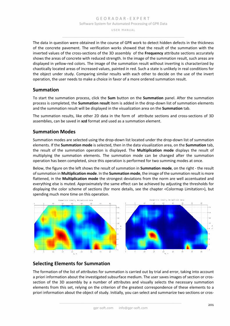
G E O R A D A R - E X P E R T Software System for Automated Processing of GPR Data
USER MANUAL
______________________________________________________________
______________________________________________________________
gpr-soft.com [email protected] 201
The data in question were obtained in the course of GPR work to detect hidden defects in the thickness of the concrete pavement. The verification works showed that the result of the summation with the inverted values of the cross-sections of the 3D assembly of the Frequency attribute sections accurately shows the areas of concrete with reduced strength. In the image of the summation result, such areas are displayed in yellow-red colors. The image of the summation result without inverting is characterized by chaotically located areas of increased values, painted in red. Such a state is unlikely in real conditions for the object under study. Comparing similar results with each other to decide on the use of the invert operation, the user needs to make a choice in favor of a more ordered summation result.
Summation To start the summation process, click the Sum button on the Summation panel. After the summation process is completed, the Summation result item is added in the drop-down list of summation elements and the summation result will be displayed in the visualization area on the Summation tab.
The summation results, like other 2D data in the form of attribute sections and cross-sections of 3D assemblies, can be saved in xzd format and used as a summation element.
Summation Modes Summation modes are selected using the drop-down list located under the drop-down list of summation elements. If the Summation mode is selected, then in the data visualization area, on the Summation tab, the result of the summation operation is displayed. The Multiplication mode displays the result of multiplying the summation elements. The summation mode can be changed after the summation operation has been completed, since this operation is performed for two summing modes at once.
Below, the figure on the left shows the result of summation in Summation mode, on the right - the result of summation in Multiplication mode. In the Summation mode, the image of the summation result is more flattened, in the Multiplication mode the strongest deviations from the norm are well accentuated and everything else is muted. Approximately the same effect can be achieved by adjusting the thresholds for displaying the color scheme of sections (for more details, see the chapter <Colormap Limitation>), but spending much more time on this operation.
Selecting Elements for Summation The formation of the list of attributes for summation is carried out by trial and error, taking into account a priori information about the investigated subsurface medium. The user saves images of section or cros-section of the 3D assembly by a number of attributes and visually selects the necessary summation elements from this set, relying on the criterion of the greatest correspondence of these elements to a priori information about the object of study. Initially, you can select and summarize two sections or cros-

G E O R A D A R - E X P E R T Software System for Automated Processing of GPR Data
USER MANUAL
______________________________________________________________
______________________________________________________________
gpr-soft.com [email protected] 202
sections of the 3D assembly, then add one more to them and see if the summation result has improved. If not, you can try to invert the section data by checking the Invert checkbox. If the summation element does not improve the result, the user removes that element from the list and tries to use section or cros-section of the 3D assembly another attribute, and so on.
In the example of using summation to study the relief of a buried valley (see chapter <2D Data Summation>), the user first selected and summed sections of two attributes - Damping rate and Frequency interval, since some parts of these sections corresponded to a priori information about the buried valley. Moreover, in order for both of these cuts to complement each other as a result of summation, the cut of the Frequency interval attribute was inverted. Then the user added another cut and, depending on the summation result, left it in the list of summation elements or deleted it. Thus, gradually, from scattered data, a model of the subsurface environment was created, which maximally corresponded to the a priori information about the object under study.
Local Extrema In addition to summing data, the Summation module implements the function of detecting local maxima on the summation elements and the summation result. This opportunity is used in the search and detection of defects in building or road structures, as well as for the search for local subsurface objects of various nature.
Latent defects, like local objects, are areas of the subsurface space that differ in their electrophysical characteristics from the strata enclosing them. Such areas are manifested by characteristic deviations of attribute values on section or cross-section of a 3D assembly. These deviations can be of varying intensity. The strongest deviation corresponds to the strongest manifestation of a defect or the position of a large local object. Using the function of detecting local maxima, the user quickly obtains marks of the position of local maxima using markers on the image of the summation element or the summation result on the Summation tab, as well as a list of coordinates of these markers with the values of local maxima.
To display local maximum markers on the image of the summation element or the summation result, check the Peaks checkbox in the Summation panel. The marker size depends on the value at the local
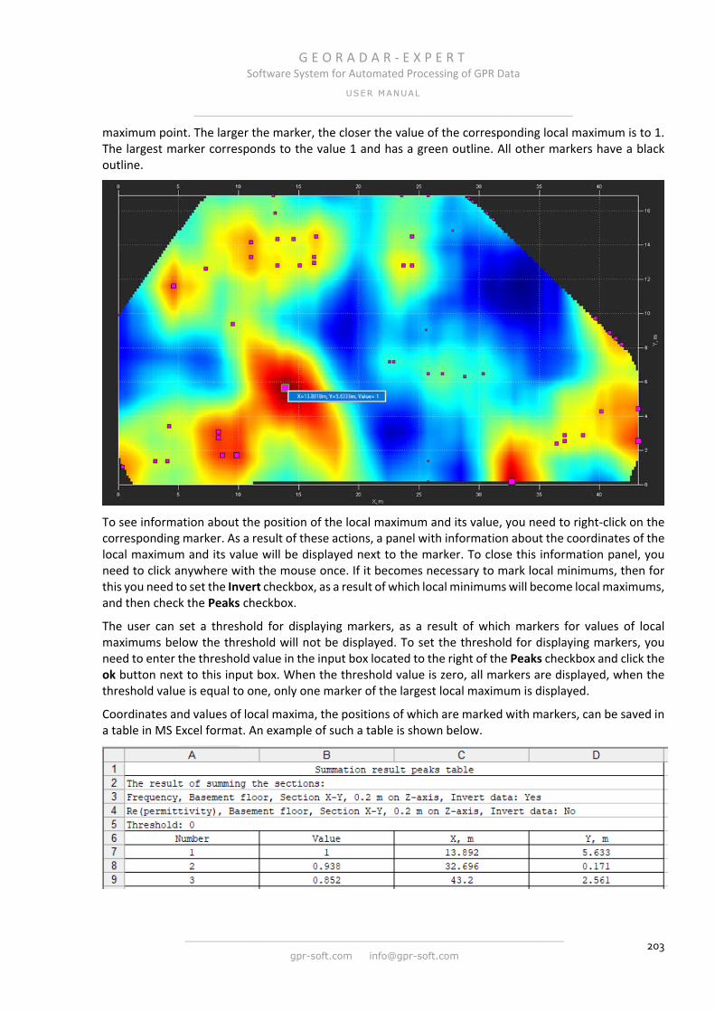
G E O R A D A R - E X P E R T Software System for Automated Processing of GPR Data
USER MANUAL
______________________________________________________________
______________________________________________________________
gpr-soft.com [email protected] 203
maximum point. The larger the marker, the closer the value of the corresponding local maximum is to 1. The largest marker corresponds to the value 1 and has a green outline. All other markers have a black outline.
To see information about the position of the local maximum and its value, you need to right-click on the corresponding marker. As a result of these actions, a panel with information about the coordinates of the local maximum and its value will be displayed next to the marker. To close this information panel, you need to click anywhere with the mouse once. If it becomes necessary to mark local minimums, then for this you need to set the Invert checkbox, as a result of which local minimums will become local maximums, and then check the Peaks checkbox.
The user can set a threshold for displaying markers, as a result of which markers for values of local maximums below the threshold will not be displayed. To set the threshold for displaying markers, you need to enter the threshold value in the input box located to the right of the Peaks checkbox and click the ok button next to this input box. When the threshold value is zero, all markers are displayed, when the threshold value is equal to one, only one marker of the largest local maximum is displayed.
Coordinates and values of local maxima, the positions of which are marked with markers, can be saved in a table in MS Excel format. An example of such a table is shown below.
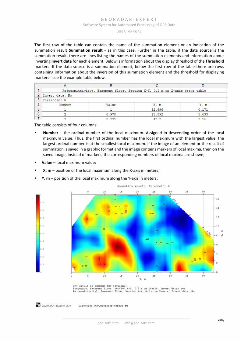
G E O R A D A R - E X P E R T Software System for Automated Processing of GPR Data
USER MANUAL
______________________________________________________________
______________________________________________________________
gpr-soft.com [email protected] 204
The first row of the table can contain the name of the summation element or an indication of the summation result Summation result - as in this case. Further in the table, if the data source is the summation result, there are lines listing the names of the summation elements and information about inverting Invert data for each element. Below is information about the display threshold of the Threshold markers. If the data source is a summation element, below the first row of the table there are rows containing information about the inversion of this summation element and the threshold for displaying markers - see the example table below.
The table consists of four columns:
Number – the ordinal number of the local maximum. Assigned in descending order of the local maximum value. Thus, the first ordinal number has the local maximum with the largest value, the largest ordinal number is at the smallest local maximum. If the image of an element or the result of summation is saved in a graphic format and the image contains markers of local maxima, then on the saved image, instead of markers, the corresponding numbers of local maxima are shown;
Value – local maximum value;
X, m – position of the local maximum along the X-axis in meters;
Y, m – position of the local maximum along the Y-axis in meters;
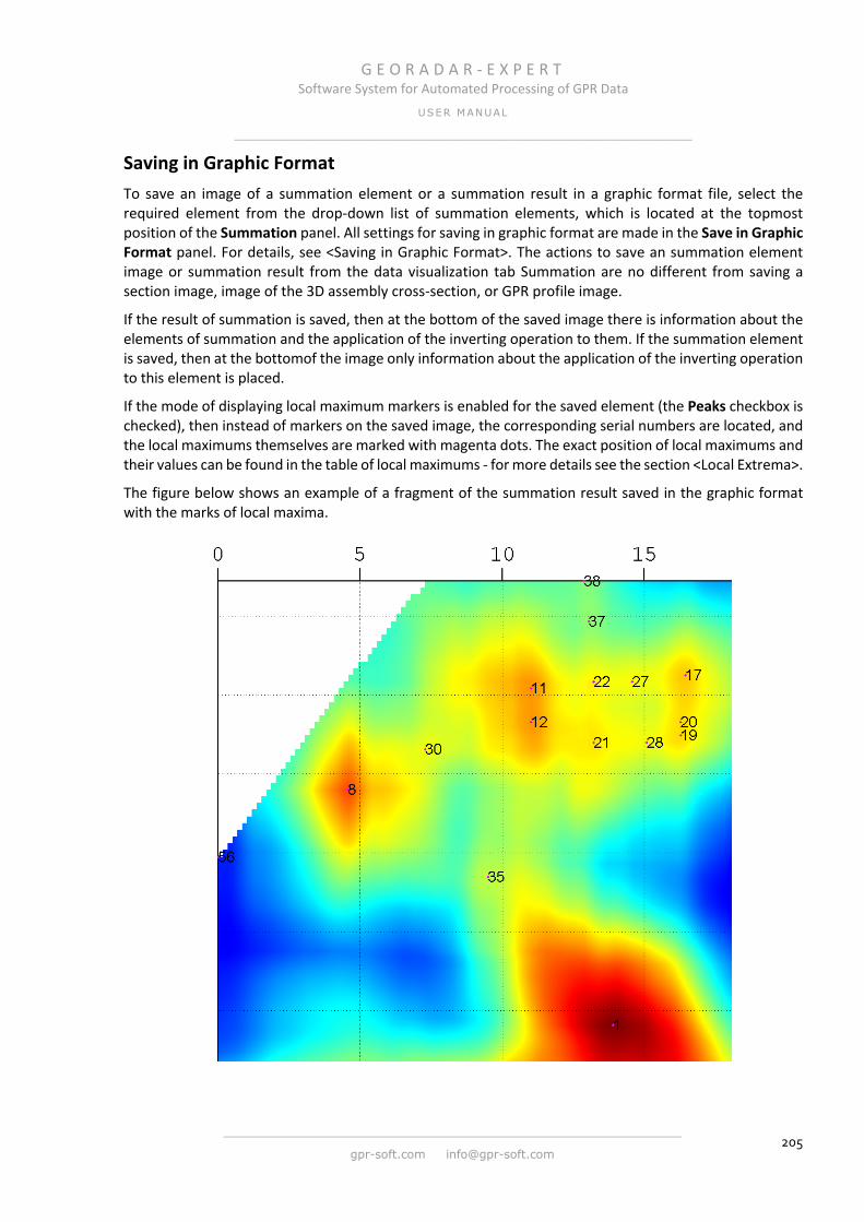
G E O R A D A R - E X P E R T Software System for Automated Processing of GPR Data
USER MANUAL
______________________________________________________________
______________________________________________________________
gpr-soft.com [email protected] 205
Saving in Graphic Format To save an image of a summation element or a summation result in a graphic format file, select the required element from the drop-down list of summation elements, which is located at the topmost position of the Summation panel. All settings for saving in graphic format are made in the Save in Graphic Format panel. For details, see <Saving in Graphic Format>. The actions to save an summation element image or summation result from the data visualization tab Summation are no different from saving a section image, image of the 3D assembly cross-section, or GPR profile image.
If the result of summation is saved, then at the bottom of the saved image there is information about the elements of summation and the application of the inverting operation to them. If the summation element is saved, then at the bottomof the image only information about the application of the inverting operation to this element is placed.
If the mode of displaying local maximum markers is enabled for the saved element (the Peaks checkbox is checked), then instead of markers on the saved image, the corresponding serial numbers are located, and the local maximums themselves are marked with magenta dots. The exact position of local maximums and their values can be found in the table of local maximums - for more details see the section <Local Extrema>.
The figure below shows an example of a fragment of the summation result saved in the graphic format with the marks of local maxima.
G E O R A D A R - E X P E R T Software System for Automated Processing of GPR Data
USER MANUAL
______________________________________________________________
______________________________________________________________
gpr-soft.com [email protected] 206
Annexes
Typical Sequence of User Actions for the Section Creation To create a section of an attribute of a subsurface medium or of an attribute of a GPR electromagnetic wave field, the user must perform the following steps. Corner brackets refer to the relevant sections of this user manual:
1. Obtain the GPR profile in accordance with the recommended parameters of the GPR profiling. For more information, see <Parameters of the GPR Profiling>;
2. Open the GPR profile in the program GEORADAR-EXPERT. For more details, see <GPR Profile Opening>;
3. Perform pre-processing of the GPR profile, if this is required. For more details, see <Data Preprocessing>;
4. Open the ABSEF panel by clicking on the BSEF Analysis of GPR Profiles menu item located in the Analysis menu group. For more details, see <BSEF Analysis and Saving Analysis Results>;
5. Use the Start or Batch button on the ABSEF panel to start the process of automated analysis of the back-scattering electromagnetic field (BSEF). For more details, see <BSEF Analysis and Saving Analysis Results>;
6. After the completion of the BSEF analysis, if the BSEF analysis process was started with the Start button (ie analysis of the current GPR profile), save the analysis result by clicking on the Save efd menu item located in the File menu group or by clicking the Save button on the ABSEF panel. If the BSEF analysis process was started with the Batch button, then in the batch analysis mode, each GPR profile containing the result of the BSEF analysis is saved with the extension efd to the current directory automatically. For more details, see <BSEF Analysis and Saving Analysis Results>;
7. If required, load the required GPR profile with the extension efd and contain the result of the analysis of the BSEF to the GEORADAR-EXPERT program. Or operate with an already loaded GPR profile containing the result of the analysis of the BSEF. For more details, see <Loading a File with the BSEF Analysis Result>
8. If required, perform actions to limit the range of basic attributes. For more details, see <Limitation the Range of Basic Attributes>;
9. Select the type of corrective function (CF) and, if required, make additional adjustments to the CF. For more details, see <Corrective Function Settings> <Creating Corrective Function in Automatic Mode> <Creating Corrective Function in Manual Mode> <The most commonly used types of CF created manually>;
10. Select a section attribute. For more details, see <Section Attributes> <Section Creation Settings>.
11. Set the vertical and horizontal section data smoothing parameters in the Data smoothing Y (samples) X (m) group in the Settings for Attribute Permittivity panel and / or the Settings for All Attributes panel. For more details, see <Settings for Attribute Permittivity panel> <Settings for All Attributes panel>;
12. Start the process of creating a section using the Section or Batch mode buttons located on the Section panel, or by clicking the Create Section or Create Section in Batch Mode menu item located in the group menu of Section. For more details, see <Creating Section> <Creating Section in Batch Mode>;
G E O R A D A R - E X P E R T Software System for Automated Processing of GPR Data
USER MANUAL
______________________________________________________________
______________________________________________________________
gpr-soft.com [email protected] 207
13. After the section creation process is complete, if necessary, configure the section visualization parameters. For more details, see <Section Visualization Settings> <Attribute Display Range> <Colormap and Color Scheme Customizing>;
Links to the Description of Panels Left Tabbed Panel
Permittivity <Visualization of BSEF Analysis Results>
Central Frequency <Visualization of BSEF Analysis Results>
Signal Bandwidth <Visualization of BSEF Analysis Results>
Q-factor <Visualization of BSEF Analysis Results>
Corrective Function eps(f) <Corrective Function Settings>
Corrective Function eps(df) <Corrective Function Settings>
Corrective Function eps(q-factor) <Corrective Function Settings>
Additional Data Optimization <Additional Optimization of BSEF Analysis Results>
Cluster Analysis of Permittivity <Cluster Analysis of the Permittivity>
Section <Section panel>
Settings for Attribute Permittivity <Settings for Attribute Permittivity panel>
Settings for All Attributes <Settings for All Attributes panel>
Post Processing <Post Processing Panel>
Filled Contour Plot <Filled Contour Plot>
Settings of Colormap for Section <Colormap and Color Scheme Customizing>
Flaw Detection in Concrete <Flaw Detection of Building Structures Made of Concrete>
Bottom Tabbed Panel in 2D Mode
Axis <Axis and Mouse Pointer Properties>
Zero Point Level <Zero Point Level Setting>
Size <Size Panel>
Navigator <Navigator Panel>
Adjusting Image <Adjusting Image Panel>
AGC <AGC Panel>
Profile Parameters <Editing Parameters GPR Profile>
Signal Processing <Processing of GPR Signals>
Fourier Filter Settings <Frequency Filtering>
Block-by-block Processing <Processing Signals in Block Mode>
Interference Rejection <Interference Rejection Using Spatial Filter and Replacing the GPR Traces>
G E O R A D A R - E X P E R T Software System for Automated Processing of GPR Data
USER MANUAL
______________________________________________________________
______________________________________________________________
gpr-soft.com [email protected] 208
Signal Decomposition in Components <Signal Decomposition in Components>
Cut <Cut GPR Profile>
Measuring <Measurement of Wave Velocity Manually>
АBSEF <BSEF Analysis and Saving Analysis Results>
Boundaries of Layers <Boundaries of Layers panel>
Save in Graphic Format <Saving in Graphic Format>
Export into Table <Exporting Data to TXT Format>
B-Detector <B-Detector>
Statistics <Statistical Analysis>, <Visualization of Statistical Information>
Layer Picker for Statistics <Using the Layer Picking Panel>
Summation <Summation Panel>
Convert GPS Data to GEXYZ <Creating XYZ Coordinate Table Using GPS Data Converter>
Data Combining <Combining Multi-Channel GPR Data>
Bottom Tabbed Panel in 3D Mode
Position X-Y on Z-axis <Position X-Y on Z-axis, Position X-Z on Y-axis and Position Y-Z on X-axis Panels>
Position X-Z on Y-axis <Position X-Y on Z-axis, Position X-Z on Y-axis and Position Y-Z on X-axis Panels>
Position Y-Z on X-axis <Position X-Y on Z-axis, Position X-Z on Y-axis and Position Y-Z on X-axis Panels>
Cube Components Display <Cube Components Display Panel>
Rounding <Rounding Panel>
Smoothing <Smoothing Panel>
Axes Labels, Grid and Limits <Axes Labels, Grid and Limits Panel>
Axis Ratio <Axis Ratio Panel>
Cube View <Cube View Panel>
Cube Cut and Alpha <Cube Cut and Alpha Panel>
Light Source <Light Source Panel>
Visible Range <Visible Range Panel>
Isosurface <Isosurface Panel>
Cut Area <Cut Area Panel>
Contours on 2D Views <Contours on 2D Views Panel>
Settings of Colormap <Settings of Colormap Panel>
Attribute Features <Attribute Features Panel>
User Section <User Section Panel>
Statistics <Statistical Analysis>, <Visualization of Statistical Information>
G E O R A D A R - E X P E R T Software System for Automated Processing of GPR Data
USER MANUAL
______________________________________________________________
______________________________________________________________
gpr-soft.com [email protected] 209
Layer Picker for Statistics <Using the Layer Picking Panel>
Summation <Summation Panel>
Useful Links
The GEORADAR-EXPERT web site: https://gpr-soft.com/
The GEORADAR-EXPERT user manual: https://gpr-soft.com/download/georadar_expert_manual_eng.pdf
Watch or download video tutorials: https://gpr-soft.com/Video.html
Information brochures: https://gpr-soft.com/download/ge_software_review_eng.pdf
https://gpr-soft.com/download/ge_brochure_eng.pdf
Technical support: [email protected]