Optical Spectroscopy for Noninvasive Monitoring of Stem Cell Differentiation
Upload
khangminh22Category
view
1download
0
Use of Optical Fibers for Structural Health
Monitoring of Aircraft Components
by
Prem Anand
A thesis submitted to
the Faculty of Graduate and Postdoctoral Affairs
in partial fulfilment of
the requirements for the degree of
Master of Applied Science
in
Aerospace Engineering
Ottawa-Carleton Institute for Mechanical and Aerospace Engineering
Department of Mechanical and Aerospace Engineering
Carleton University
Ottawa, Ontario, Canada
April 2017
Copyright c©
2017 - Prem Anand
The undersigned recommend to
the Faculty of Graduate and Postdoctural Affairs
acceptance of the thesis
Use of Optical Fibers for Structural Health Monitoring of
Aircraft Components
Submitted by Prem Anand
in partial fulfilment of the requirements for the degree of
Master of Applied Science
Professor Jeremy Laliberte, Supervisor
Professor Marcias Martinez, Co-Supervisor
Dr. Ronald E. Miller, Department Chair
Carleton University
2017
ii
Abstract
Structural Health Monitoring (SHM) systems for composites are being devel-
oped to improve the in-flight monitoring and safety of new aircraft structures. One of
the emerging techniques for SHM which is becoming popular in the aircraft industry
involves the use of optical fiber sensors due to their ease of integration, resistance
to electromagnetic interference and low signal attenuation over long distances. This
thesis describes a validated technique for optical fiber embedment and extraction of
data from optical fiber data to measure strain.
In this research, a novel method to address ingress/egress points of optical fiber
has been developed; a surface mounted component has been designed and manu-
factured using rapid prototyping for the protection of embedded optical fibers at
the ingress/egress points. This single component can provide safety and integrity to
optical fibers during manufacturing as well as cutting operation. The thesis also fo-
cuses on the study of mechanical strength of composites with embedded optical fibers.
Composite panels were manufactured with integrated optical fibers using Vacuum As-
sisted Resin Transfer Molding. Tensile, flexural and impact tests were conducted on
these coupons and their results were compared to identify any effects of the embedded
fibers on the part performance. Finally, strain experienced by the material while it
was in loading and unloading condition was calculated using integrated optical fiber
sensors and the values were compared with extensometer data.
iii

Acknowledgments
I would like to thank my supervisor Professor Jeremy Laliberte for offering
me this challenging and rewarding opportunity. His professionalism, guidance and
support made it very easy for me to go through the process of graduate school. I
would also like to thank my co-supervisor Professor Marcias Martinez for introducing
me to the FBG based Structural Health Monitoring system.
My gratitude goes out to all the great people who helped me along the way.
Especially I would like to thank Professor Jacques Albert for making his equipments
and laboratory available to me for this research work. Many thanks are owed to
Albane Laronche for her help in making Fiber Bragg Gratings. I am also grateful to
Steve Truttman for assisting me with tensile tests. I am thankful to Alex Proctor,
Ian Lloy and Kevin Sangster for helping me in the Machine Shop. Finally I would like
to thank my family whose love and support has guided me throughout my life.
iv

Table of Contents
Abstract iii
Acknowledgments iv
Table of Contents v
List of Tables viii
List of Figures ix
List of Acronyms xiii
List of Symbols xiv
1 Introduction 1
1.1 Background . . . . . . . . . . . . . . . . . . . . . . . . . . . . . . . . 2
1.1.1 Structural Health Monitoring . . . . . . . . . . . . . . . . . . 2
1.1.2 Importance of SHM . . . . . . . . . . . . . . . . . . . . . . . . 3
1.1.3 Non-Destructive Testing Methods . . . . . . . . . . . . . . . . 4
1.2 Optical Fiber Sensors for Structural Health Monitoring . . . . . . . . 4
1.3 Challenges Associated with Optical Fibers . . . . . . . . . . . . . . . 6
1.4 Motivation and Scope of Research . . . . . . . . . . . . . . . . . . . . 7
1.5 Organization of the Thesis . . . . . . . . . . . . . . . . . . . . . . . . 8
v
1.6 Research Contributions . . . . . . . . . . . . . . . . . . . . . . . . . . 9
2 Literature Review 10
2.1 Integration of Optical Fiber Sensors in Composites . . . . . . . . . . 10
2.2 Types of Optical Fiber Sensors . . . . . . . . . . . . . . . . . . . . . 11
2.2.1 Bragg Gratings . . . . . . . . . . . . . . . . . . . . . . . . . . 12
2.2.2 Rayleigh Fibers . . . . . . . . . . . . . . . . . . . . . . . . . . 14
2.2.3 Fabry-Perot Sensors . . . . . . . . . . . . . . . . . . . . . . . 15
2.3 Ingress and Egress Points: Challenges . . . . . . . . . . . . . . . . . . 15
2.4 Mechanical Testing: with and without Integrated Optical Fibers . . . 20
2.5 SHM Applications . . . . . . . . . . . . . . . . . . . . . . . . . . . . 22
3 Experimental Methodology 23
3.1 Composite Panels with Embedded Optical Fibers . . . . . . . . . . . 24
3.2 3D Printed Fixture for Optical Fiber Ingress/Egress Points . . . . . . 30
3.2.1 First Design . . . . . . . . . . . . . . . . . . . . . . . . . . . . 32
3.2.2 Second Design . . . . . . . . . . . . . . . . . . . . . . . . . . . 33
3.2.3 Third Design . . . . . . . . . . . . . . . . . . . . . . . . . . . 35
3.2.4 Fourth Design . . . . . . . . . . . . . . . . . . . . . . . . . . . 36
3.2.5 Fifth Design . . . . . . . . . . . . . . . . . . . . . . . . . . . . 37
3.2.6 Production Testing Using VARTM . . . . . . . . . . . . . . . 39
3.3 Mechanical Testing . . . . . . . . . . . . . . . . . . . . . . . . . . . . 47
3.3.1 Tensile Test Specimen Fabrication . . . . . . . . . . . . . . . . 48
3.3.2 Tensile Test Procedure . . . . . . . . . . . . . . . . . . . . . . 49
3.3.3 Compliance Calculation . . . . . . . . . . . . . . . . . . . . . 54
3.4 Impact Test . . . . . . . . . . . . . . . . . . . . . . . . . . . . . . . . 56
3.4.1 Specimen Fabrication . . . . . . . . . . . . . . . . . . . . . . . 56
3.4.2 Impact Test Procedure . . . . . . . . . . . . . . . . . . . . . . 58
vi

3.5 Flexural Test . . . . . . . . . . . . . . . . . . . . . . . . . . . . . . . 62
3.5.1 Specimen Fabrication . . . . . . . . . . . . . . . . . . . . . . . 64
3.5.2 Flexural Test Procedure . . . . . . . . . . . . . . . . . . . . . 64
3.6 Measurement of the Strain Calibration Factor for Fiber Bragg Grating 67
4 Results and Discussion 72
4.1 Tensile Test Results . . . . . . . . . . . . . . . . . . . . . . . . . . . . 72
4.2 Impact Test Results . . . . . . . . . . . . . . . . . . . . . . . . . . . . 74
4.3 Flexural Test Results . . . . . . . . . . . . . . . . . . . . . . . . . . . 80
4.4 Tensile Strain Measurement Using Embedded Optical Fibers . . . . . 83
5 Conclusions and Recommendations 106
5.1 Conclusions . . . . . . . . . . . . . . . . . . . . . . . . . . . . . . . . 106
5.2 Recommendations . . . . . . . . . . . . . . . . . . . . . . . . . . . . . 108
References 110
Appendix A Model Parameters and Material Properties 116
A.1 Data sheet of optical fiber . . . . . . . . . . . . . . . . . . . . . . . . 116
Appendix B Testing parameters 121
B.1 Calculation of Young’s Modulus Using Compliance . . . . . . . . . . 121
B.2 Stress-strain curves . . . . . . . . . . . . . . . . . . . . . . . . . . . . 123
Appendix C Data Sheet of Epoxy Resin 128
vii

List of Tables
3.1 Summary of fixture design iterations . . . . . . . . . . . . . . . . . . 31
3.2 Machine’s compliance measured using SS304 . . . . . . . . . . . . . . 56
3.3 Dimensions of impact test specimens . . . . . . . . . . . . . . . . . . 60
3.4 Dimensions of flexural test specimens . . . . . . . . . . . . . . . . . . 65
3.5 Strain calibration values from first optical fiber . . . . . . . . . . . . 69
3.6 Strain calibration values from second optical fiber . . . . . . . . . . . 69
4.1 Tensile test results from first panel . . . . . . . . . . . . . . . . . . . 73
4.2 Tensile test results from second panel . . . . . . . . . . . . . . . . . . 74
4.3 Energy absorbed by the impact specimen . . . . . . . . . . . . . . . . 76
4.4 Impact velocity of all the samples . . . . . . . . . . . . . . . . . . . . 78
4.5 Codes for failure mode, area and location . . . . . . . . . . . . . . . . 80
4.6 Results of flexural test . . . . . . . . . . . . . . . . . . . . . . . . . . 81
4.7 Comparison of modulus of elasticity in AA6061 . . . . . . . . . . . . 91
4.8 Modulus measured by all the gratings of AA6061 . . . . . . . . . . . 96
4.9 Modulus of Elasticity in fbg01 . . . . . . . . . . . . . . . . . . . . . . 96
4.10 Modulus of Elasticity in fbg02 . . . . . . . . . . . . . . . . . . . . . . 97
4.11 Modulus of Elasticity in fbg03 . . . . . . . . . . . . . . . . . . . . . . 100
4.12 Modulus of elasticity measured by all the gratings in fbg02 . . . . . . 102
4.13 Modulus of elasticity measured by all the gratings in fbg03 . . . . . . 104
viii

List of Figures
1.1 Size comparison of optical fiber and strain gage . . . . . . . . . . . . 5
1.2 Right wing of Ikhana aIrcraft . . . . . . . . . . . . . . . . . . . . . . 7
2.1 Microscopy of composite with and without optical fiber . . . . . . . . 11
2.2 Production of sensing tape using sandwich technique . . . . . . . . . 12
2.3 Reflected and transmitted light through a Bragg Grating . . . . . . . 13
2.4 (a) Extrinsic FPI sensor made by forming an external air cavity, and
(b) intrinsic FPI sensor formed by two reflecting components, R1 and
R2, along a fiber . . . . . . . . . . . . . . . . . . . . . . . . . . . . . 15
2.5 Fiber sealing technique . . . . . . . . . . . . . . . . . . . . . . . . . . 16
2.6 Optical fiber connector . . . . . . . . . . . . . . . . . . . . . . . . . . 17
2.7 Optical fiber reinforcement using tube. (a) using rubber tube and (b)
using metal and plastic tube . . . . . . . . . . . . . . . . . . . . . . . 18
2.8 Protection of optical fibers against curing environment . . . . . . . . 18
2.9 connection using part fixture.(a)horizontal connection, (b) vertical con-
nection) . . . . . . . . . . . . . . . . . . . . . . . . . . . . . . . . . . 19
3.1 Fiberglass panel . . . . . . . . . . . . . . . . . . . . . . . . . . . . . . 24
3.2 Making guideway for optical fibers . . . . . . . . . . . . . . . . . . . 25
3.3 Sealant tape around fiberglass . . . . . . . . . . . . . . . . . . . . . . 25
3.4 Perforated film over fiberglass . . . . . . . . . . . . . . . . . . . . . . 26
3.5 Resin infusion mesh over fiberglass . . . . . . . . . . . . . . . . . . . 26
ix

3.6 T-connectors and spiral tubes on both ends of fiberglass . . . . . . . 27
3.7 VARTM setup . . . . . . . . . . . . . . . . . . . . . . . . . . . . . . . 27
3.8 Tube in clamped position . . . . . . . . . . . . . . . . . . . . . . . . . 28
3.9 Mixing resin and hardener . . . . . . . . . . . . . . . . . . . . . . . . 28
3.10 Resin flow path under vacuum . . . . . . . . . . . . . . . . . . . . . . 29
3.11 Fiberglass panel after curing . . . . . . . . . . . . . . . . . . . . . . . 30
3.12 Parts of the first design . . . . . . . . . . . . . . . . . . . . . . . . . . 32
3.13 Assembly of the first design . . . . . . . . . . . . . . . . . . . . . . . 33
3.14 Parts of the second design . . . . . . . . . . . . . . . . . . . . . . . . 34
3.15 Assembly of second design in vacuum . . . . . . . . . . . . . . . . . . 35
3.16 Parts of third design . . . . . . . . . . . . . . . . . . . . . . . . . . . 35
3.17 Assembly of third design in vacuum . . . . . . . . . . . . . . . . . . . 36
3.18 Side part design . . . . . . . . . . . . . . . . . . . . . . . . . . . . . . 37
3.19 Assembly of Fourth design . . . . . . . . . . . . . . . . . . . . . . . . 37
3.20 Assembly of the fourth design in vacuum . . . . . . . . . . . . . . . . 38
3.21 Side part of the fifth design . . . . . . . . . . . . . . . . . . . . . . . 38
3.22 Fifth design in vacuum . . . . . . . . . . . . . . . . . . . . . . . . . . 39
3.23 Applying PVA over fixture . . . . . . . . . . . . . . . . . . . . . . . . 40
3.24 Optical fiber entering the fixture . . . . . . . . . . . . . . . . . . . . . 40
3.25 Use of wax to fill the gaps . . . . . . . . . . . . . . . . . . . . . . . . 41
3.26 Layout of four tensile specimens . . . . . . . . . . . . . . . . . . . . . 42
3.27 Optical fibers in the fixture . . . . . . . . . . . . . . . . . . . . . . . 42
3.28 Coiling optical fiber in the fixture . . . . . . . . . . . . . . . . . . . . 43
3.29 Complete assembly of the fixture with optical fiber coiled inside . . . 43
3.30 Resin infusion mesh over the fixtures . . . . . . . . . . . . . . . . . . 44
3.31 VARTM setup with fixtures . . . . . . . . . . . . . . . . . . . . . . . 44
3.32 Resin flow direction . . . . . . . . . . . . . . . . . . . . . . . . . . . . 45
x
3.33 Cured fiberglass . . . . . . . . . . . . . . . . . . . . . . . . . . . . . . 46
3.34 Disassembling of fixture . . . . . . . . . . . . . . . . . . . . . . . . . 46
3.35 Optical fiber taken out from the fixture . . . . . . . . . . . . . . . . . 47
3.36 Checking the integrity of embedded optical fiber . . . . . . . . . . . . 48
3.37 Schematic of ply orientation in tensile test coupons . . . . . . . . . . 49
3.38 AA6061 with optical fiber bonded on the surface . . . . . . . . . . . . 50
3.39 Tensile test . . . . . . . . . . . . . . . . . . . . . . . . . . . . . . . . 50
3.40 Stress-strain curve of fiberglass with and without embedded optical fiber 52
3.41 Splicing of optical fiber . . . . . . . . . . . . . . . . . . . . . . . . . . 53
3.42 Tensile testing of composite with embedded optical fiber . . . . . . . 53
3.43 Load vs displacement for SS304 sample1 . . . . . . . . . . . . . . . . 55
3.44 Schematic of ply orientation in impact test specimen . . . . . . . . . 57
3.45 Manufactured panel for impact test specimen . . . . . . . . . . . . . 58
3.46 Cutting layout schematic of impact and flexural test specimen . . . . 59
3.47 Fiberglass impact specimen without (left) and with embedded optical
fiber (right) . . . . . . . . . . . . . . . . . . . . . . . . . . . . . . . . 59
3.48 Impact test base . . . . . . . . . . . . . . . . . . . . . . . . . . . . . 61
3.49 Impact test setup . . . . . . . . . . . . . . . . . . . . . . . . . . . . . 62
3.50 Aluminium sample after impact test . . . . . . . . . . . . . . . . . . . 63
3.51 Fiberglass sample after impact test . . . . . . . . . . . . . . . . . . . 63
3.52 Flexural test specimen with embedded optical fiber . . . . . . . . . . 64
3.53 Schematic of three point bend test . . . . . . . . . . . . . . . . . . . 65
3.54 Three point bend test . . . . . . . . . . . . . . . . . . . . . . . . . . . 66
3.55 Wavelength shift in optical fiber during strained condition . . . . . . 70
3.56 Measurement of the strain calibration factor of optical fiber . . . . . . 71
4.1 Young’s Modulus of specimens from the first panel . . . . . . . . . . 75
4.2 Young’s Modulus of specimens from the second panel . . . . . . . . . 75
xi
4.3 Energy vs time for all the impact specimens . . . . . . . . . . . . . . 77
4.4 Energy absorbed by impact specimens . . . . . . . . . . . . . . . . . 78
4.5 Velocity vs time for all the impact specimens . . . . . . . . . . . . . . 79
4.6 Stress-strain curve for flexural test . . . . . . . . . . . . . . . . . . . 82
4.7 Strain in AA6061 during loading cycle . . . . . . . . . . . . . . . . . 85
4.8 Strain in AA6061 during unloading cycle . . . . . . . . . . . . . . . . 86
4.9 Strain in fbg01 during loading cycle . . . . . . . . . . . . . . . . . . . 87
4.10 Strain in fbg01 during unloading cycle . . . . . . . . . . . . . . . . . 88
4.11 Strain in fbg02 during loading cycle . . . . . . . . . . . . . . . . . . . 89
4.12 Strain in fbg02 during unloading cycle . . . . . . . . . . . . . . . . . 90
4.13 Strain in fbg03 during loading cycle . . . . . . . . . . . . . . . . . . . 92
4.14 Strain in fbg03 during unloading cycle . . . . . . . . . . . . . . . . . 93
4.15 Strain in AA6061 : full cycle . . . . . . . . . . . . . . . . . . . . . . . 94
4.16 Strain in fbg02: full cycle . . . . . . . . . . . . . . . . . . . . . . . . . 95
4.17 Modulus measured by all the gratings in AA6061 . . . . . . . . . . . 97
4.18 Comparison of modulus (GPa) of fbg02 during loading and unloading
cycle . . . . . . . . . . . . . . . . . . . . . . . . . . . . . . . . . . . . 98
4.19 Comparison of modulus (GPa) of fbg03 during loading and unloading
cycle . . . . . . . . . . . . . . . . . . . . . . . . . . . . . . . . . . . . 99
4.20 Modulus measured by all the gratings in fbg02 . . . . . . . . . . . . . 102
4.21 Strain measured by all the gratings in fbg02 . . . . . . . . . . . . . . 103
4.22 Modulus measured by all the gratings in fbg03 . . . . . . . . . . . . . 104
4.23 Strain measured by all the gratings in fbg03 . . . . . . . . . . . . . . 105
xii
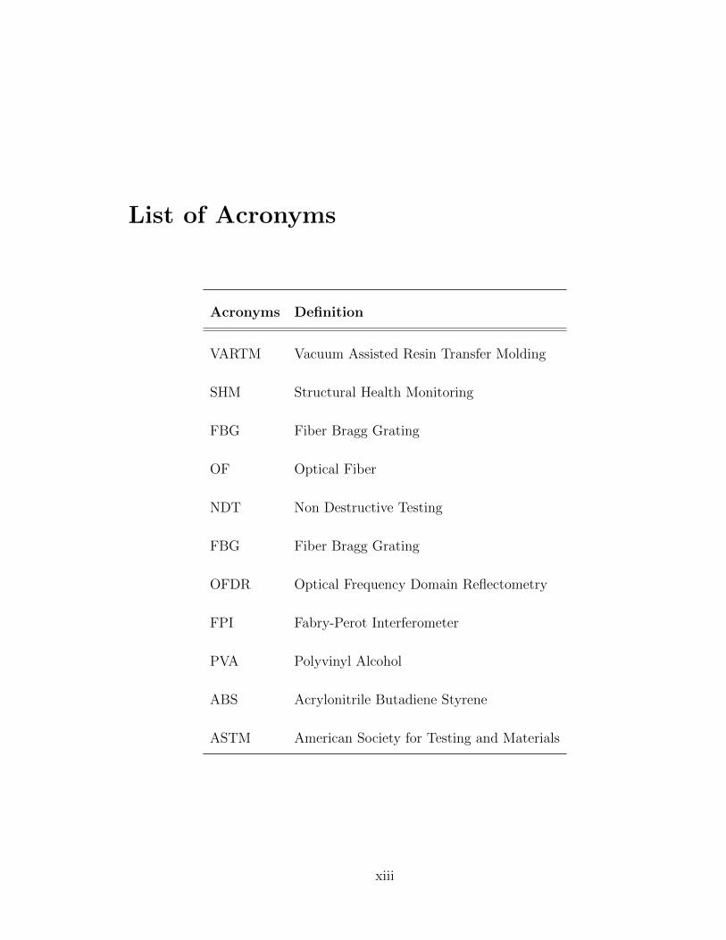
List of Acronyms
Acronyms Definition
VARTM Vacuum Assisted Resin Transfer Molding
SHM Structural Health Monitoring
FBG Fiber Bragg Grating
OF Optical Fiber
NDT Non Destructive Testing
FBG Fiber Bragg Grating
OFDR Optical Frequency Domain Reflectometry
FPI Fabry-Perot Interferometer
PVA Polyvinyl Alcohol
ABS Acrylonitrile Butadiene Styrene
ASTM American Society for Testing and Materials
xiii

List of Symbols
Symbols Definition
n Refractive index
λB Bragg wavelength
Λ Grating period
ε Strain
λ Wavelength
ξ Thermal optic coefficient
∆T Change in temperature
E Young’s Modulus
A Cross sectional area
L Gage length
Ep Potential Energy
Ek Kinetic Energy
m Mass
xiv

g Acceleration due to gravity
h Height
Cm Machine’s compliance
Cmat Material’s compliance
CT Total compliance
xv

Chapter 1
Introduction
Composite materials are widely used in military as well as transport aircraft.
They were initially restricted to secondary structures such as fairings, doors and con-
trol surfaces. With advancements of technology, their application in primary struc-
tures such as wings and fuselages has increased [1, 2].
At present, carbon fiber and fiberglass reinforced polymers are being used in al-
most all modern aerospace structures as a primary structural material. However, it is
still difficult to precisely manufacture large complex composite structures and ensure
their structural integrity during operation. Hence, development of innovative tech-
niques to monitor the internal behavior of composites is required. Novel methods to
utilize these data to improve the structural design and maintenance methods are also
needed. As of now various sensors (Strain Gauges/Crack Gauges, Surface Mount-
able Crack Sensors (SMC), piezoceramic, optical fiber sensors and Internal Strain
Gauge Sensors (ISG)) are being used to locate and assess the damage inside com-
posite structures. Among the existing systems, optical fiber sensors have attracted
considerable attention since they are small, lightweight, immune to electromagnetic
interference, environmentally stable and have very little signal attenuation over long
distances. Also, they possess sufficient flexibility to be embedded into composite
1
2
laminates [3, 4]. Optical fiber sensors such as Fiber Bragg Gratings (FBG), are be-
ing used for stress analysis and health monitoring of structures [5–7]. Optical fibers
can be integrated within composite structures as they are small in size and fibrous
in nature. However these fibers are vulnerable at ingress and egress points of the
composite structure. This poses challenges in the manufacturing process [5]. Since
the composite materials are usually applied in the form of plies or sheets, sensors
have to be embedded within the structure during the manufacturing process. As a
consequence of embedding the sensors, there may be a significant decrease in the
mechanical properties of the composite material [8]. The most common type of op-
tical fiber sensors are Intrinsic Fabry-Perot Intereferometers, Extrinsic Fabry-Perot
Intereferometers and Fiber Bragg Gratings. The most advantageous sensor is the
Bragg Grating sensor because its simple construction leaves the continuous fiber in-
tact and strain levels can be deduced from optical wavelength shifts [9]. It is possible
to write a series of identical Bragg gratings on a long section of optical fiber and read
them individually [6, 9, 10].
This thesis presents a novel approach to embed optical fibers within composite
structures and to identify a crack/defect on the surface as well as within the structure.
1.1 Background
1.1.1 Structural Health Monitoring
Structural Health Monitoring (SHM) can be defined as the process by which
on-board sensors are utilized to identify and quantify structural damage through a
continuous in-service monitoring [4]. It is possible that damage can initiate in com-
posites during their life cycle. Hence, there is a need to develop a system which can
3
detect internal damage as early as possible [11]. Composites, being multiphase ma-
terials, have distinct anisotropic properties. The initiation of flaws within or on the
composite’s surface and the propagation of the flaw through the composite volume,
leading to an ultimate failure is complicated. Describing a damage evolution and
fracture behavior in composites remains a challenging task [12, 13]. On impact, ma-
trix cracks can appear, grow and interact, leading to delamination. It is also possible
that fiber breakage appears on the opposite side to the impact and is thus, difficult to
detect. Damage can be induced in composites during fabrication as well. It may be
due to incorrect operations during manufacturing or assembly, aging or service con-
dition [12]. Hence, it becomes important to devise a method to assess the structural
integrity of composite aircraft structures.
1.1.2 Importance of SHM
Often impact damage in composite structures such as de-bonding of core and
skins, delamination of carbon fiber or epoxy laminate skins and deformation of honey-
comb core in sandwich structures are barely visible externally [14, 15]. Although the
initial defect may be small, it can grow with time and cause catastrophic structural
failure [16]. This will eventually require either repair of the structure or replacement
with a new part. Structural repairs increase the cost of transportation in two ways.
First, repair or replacement implies direct costs. Second, as the particular part is
being repaired, the aircraft remains out of service for a considerable period of time.
This will incur cost due to loss of operation time or as a result of leasing a substi-
tute system. Hence structural health monitoring becomes an issue of cost savings as
well [17]. Although SHM methods costs money, it provides real time data. Availabil-
ity of real time data requires the aircraft to be taken out of service only when the
defect is above a well-defined threshold level. Thus, it obviates the need for a part’s
inspection after every flight.
4
1.1.3 Non-Destructive Testing Methods
During manufacturing of composite structures, random porosities may appear
inside the part. In their life cycle, an impact may result in delamination or debond-
ing, affecting the mechanical properties of the material. These defects are revealed
using Non-Destructive Testing (NDT) methods [18, 19]. Common NDT methods are
ultrasonic, X-ray, thermography and eddy current methods [20,21]. Structural Health
Monitoring (SHM), an emerging technique developed from NDT, uses sensors with
intelligent algorithms to investigate the structural health condition. Unlike NDT,
a real-time and online damage detection can be achieved in SHM. The advantages
of SHM include improving reliability and safety, reducing inspection time and im-
provising designs of composite materials [12]. These methods are carried out using
complicated, heavy equipments and are labor-extensive and time-consuming espe-
cially for large-scale structures. Moreover, the structure to be tested may need to
be disassembled to make the inspection area accessible, which increases maintenance
costs.
1.2 Optical Fiber Sensors for Structural Health
Monitoring
While the conventional methods have their own advantages and disadvantages,
optical fibers have been shown to be an efficient tool for SHM [6,17,22]. Optical fibers
are extremely light and are about the diameter of a human hair. In the aerospace
industry, where weight is extremely crucial to the mission, this feature provides an
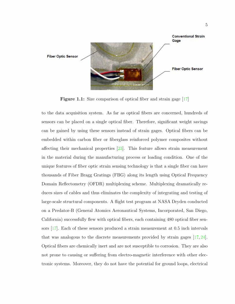
attractive advantage [17]. For example, Figure 1.1 shows a size comparison between
a strain gage and an analogous optical fiber sensor. As seen in the picture, the strain
gage sensor itself is larger and its installations requires copper wires which connect
5
Figure 1.1: Size comparison of optical fiber and strain gage [17]
to the data acquisition system. As far as optical fibers are concerned, hundreds of
sensors can be placed on a single optical fiber. Therefore, significant weight savings
can be gained by using these sensors instead of strain gages. Optical fibers can be
embedded within carbon fiber or fiberglass reinforced polymer composites without
affecting their mechanical properties [23]. This feature allows strain measurement
in the material during the manufacturing process or loading condition. One of the
unique features of fiber optic strain sensing technology is that a single fiber can have
thousands of Fiber Bragg Gratings (FBG) along its length using Optical Frequency
Domain Reflectometry (OFDR) multiplexing scheme. Multiplexing dramatically re-
duces sizes of cables and thus eliminates the complexity of integrating and testing of
large-scale structural components. A flight test program at NASA Dryden conducted
on a Predator-B (General Atomics Aeronautical Systems, Incorporated, San Diego,
California) successfully flew with optical fibers, each containing 480 optical fiber sen-
sors [17]. Each of these sensors produced a strain measurement at 0.5 inch intervals
that was analogous to the discrete measurements provided by strain gages [17, 24].
Optical fibers are chemically inert and are not susceptible to corrosion. They are also
not prone to causing or suffering from electro-magnetic interference with other elec-
tronic systems. Moreover, they do not have the potential for ground loops, electrical
6
faults, arcing or Joule heating [17].
1.3 Challenges Associated with Optical Fibers
According to the Federal Aviation Administration (FAA) advisory circular AC-
20-10-107B for aircraft composites, the discrepancies during manufacturing and fab-
rication of composites should be substantiated by mechanical testing of coupons [25].
In order to meet this requirement, the composite panels manufactured with integrated
optical fibers were tested to study the effect of embedment on the mechanical strength
of the host material.
The locations where the optical fiber exits the composite structure are critical as
they are susceptible to the environment, vibration and/or severe work conditions. For
SHM applications of optical fiber sensors, practical approaches such as sensor instal-
lation, mechanical properties of sensors, connection of ingress/egress to an exterior
system etc. should be studied [26].
Optical fibers are embedded within the plies during the manufacturing of com-
posite panels. These are then brought in contact with resins in vacuum. The readings
of optical fibers might be affected if they come in contact with resin. For the purpose
of conducting tensile tests, these panels are to be cut into standard sized coupons
as per ASTM 3039 standard [27]. The cutting operation might damage or break the
fiber as they are protruding out from the composite panels. Moreover, during tensile
testing, the specimen is held tightly in between the grips of the testing machine which
might damage the fiber as well.
Considering the above mentioned problems, there is a need for development of a
novel system which can protect the fiber from resin during cure, maintain its integrity
7
during cutting operation and ensure its safety during mechanical tests.
1.4 Motivation and Scope of Research
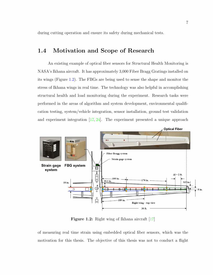
An existing example of optical fiber sensors for Structural Health Monitoring is
NASA’s Ikhana aircraft. It has approximately 3,000 Fiber Bragg Gratings installed on
its wings (Figure 1.2). The FBGs are being used to sense the shape and monitor the
stress of Ikhana wings in real time. The technology was also helpful in accomplishing
structural health and load monitoring during the experiment. Research tasks were
performed in the areas of algorithm and system development, environmental qualifi-
cation testing, system/vehicle integration, sensor installation, ground test validation
and experiment integration [17, 24]. The experiment presented a unique approach
Figure 1.2: Right wing of Ikhana aircraft [17]
of measuring real time strain using embedded optical fiber sensors, which was the
motivation for this thesis. The objective of this thesis was not to conduct a flight

8
test to obtain real time data but it was to develop the process of embedding optical
fibers within composites during the manufacturing processes. The goal was to aid
in improving the methods of manufacturing composite panels with integrated optical
fibers and to protect the ingress/egress points of embedded optical fibers during cut-
ting and post-processing. Finally, data from the embedded optical fibers were used
to measure strain while the material was in loading condition.
1.5 Organization of the Thesis
This thesis presents the method of embedding optical fiber sensors inside the
composite material, design of fixture to protect ingress and egress points of optical
fibers, a study of the mechanical properties of composite material after embedding,
extraction of data from embedded sensors and correlation of the obtained data to
strain value within the material.
Chapter 2 contains a literature review on embedding optical fibers in composite
materials, their effect on mechanical properties of materials and process of extraction
of data from optical fiber sensors. In Chapter 3, the method of embedding optical
fibers within fiberglass composite, fabrication of specimen for tensile, impact and
flexural testing is explained. The chapter also provides the evolution and design of a
fixture to protect ingress/egress points of embedded optical fibers. Chapter 4 contains
the test results of tensile, impact and flexural tests of the fiberglass reinforced epoxy
and fiberglass reinforced epoxy with embedded optical fibers and their comparisons. It
also demonstrates the method of extracting data from embedded optical fiber sensors
during loading and unloading conditions. Lastly, Chapter 5 summarizes the results
of this research and provides recommendations for future work that can be carried
out from the information provided in this thesis.

9
1.6 Research Contributions
The following are contributions made through this thesis towards the advance-
ment of SHM based on embedded optical fiber sensors:
1. Methods of embedding optical fiber sensors were explored and used to embed
optical fibers in between the plies of fiberglass composites. Structural integrity of the
embedded fibers were evaluated by passing Red Laser Light of wavelength 630 nm.
It was observed that optical fibers remained undamaged during manufacturing and
cutting.
2. A unique 3D printed fixture was designed to protect the ingress/egress points of
embedded optical fibers during manufacturing and cutting operation.
3. Tensile, impact and flexural tests were carried out on fiberglass specimens with and
without embedded optical fibers and the results were compared to study the effect of
embedment on the host material.
4. Data from embedded optical fiber sensors were used to calculate the strain in
fiberglass materials during loading and unloading cycles and were compared with the
strain values of the extensometer.
The information provided in this research can be put to practice in optical fiber
sensor based SHM system. The data generated form the embedded optical fibers can
be used to calculate the strain values and modulus of the material. This method can
also be used to obtain real time data in flight.
Chapter 2
Literature Review
Available literature shows that various attempts have been made to integrate
optical fibers to composite structures during manufacturing processes. One of the
most important factors of integration is the orientation of optical fibers with respect
to composite ply layup. Points at which these fibers enters and exit the composite
structure are vulnerable to damage during fabrication and machining. Researchers
have conducted mechanical tests to study the effect of embedding optical fiber on
the parent material. Once integrated successfully, optical fibers are used for strain
analysis using a reflectometer.
2.1 Integration of Optical Fiber Sensors in Com-
posites
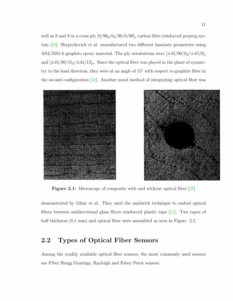
Brown et al. embedded optical fibers in unidirectional epoxy and PETI-5
composites and performed microscopic analysis to study the void content of the
fiber/composite interface [28] (Figure 2.1). They also performed 0◦ and 90◦ flex
tests on coupons with and without embedded fibers to analyze the effect on stresses
and the modulus of the composite [28]. Liu et al. embedded two optical fibers in
a 16 ply composite layup. The sensors were embedded in between plies 2 and 3 as
10
11
well as 8 and 9 in a cross ply [0/902/02/90/0/90]s carbon fibre reinforced prepreg sys-
tem [29]. Shyprykevich et al. manufactured two different laminate geometries using
AS4/3501-6 graphite epoxy material. The ply orientations were [±45/90/02/±45/0]s
and [±45/90/152/±45/15]s. Since the optical fiber was placed in the plane of symme-
try to the load direction, they were at an angle of 15◦ with respect to graphite fiber in
the second configuration [30]. Another novel method of integrating optical fiber was
Figure 2.1: Microscopy of composite with and without optical fiber [28]
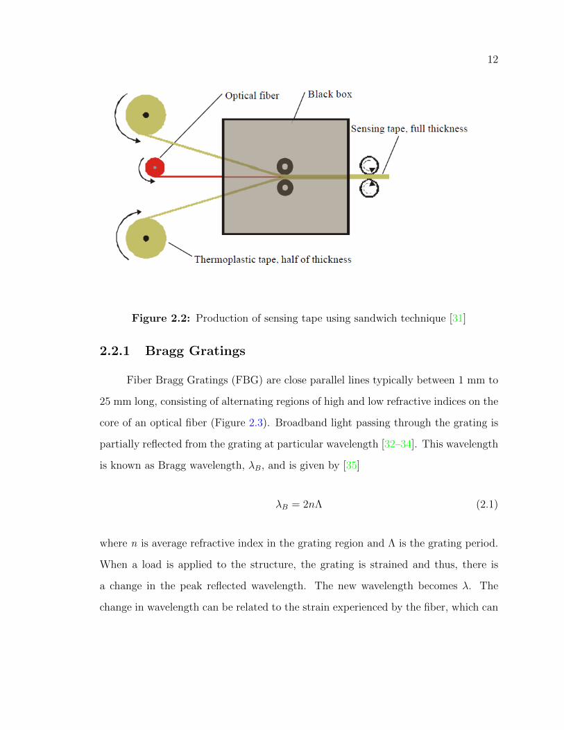
demonstrated by Glisic et al. They used the sandwich technique to embed optical
fibers between unidirectional glass fibers reinforced plastic tape [31]. Two tapes of
half thickness (0.1 mm) and optical fiber were assembled as seen in Figure 2.2.
2.2 Types of Optical Fiber Sensors
Among the readily available optical fiber sensors, the most commonly used sensors
are Fiber Bragg Gratings, Rayleigh and Fabry Perot sensors.
12
Figure 2.2: Production of sensing tape using sandwich technique [31]
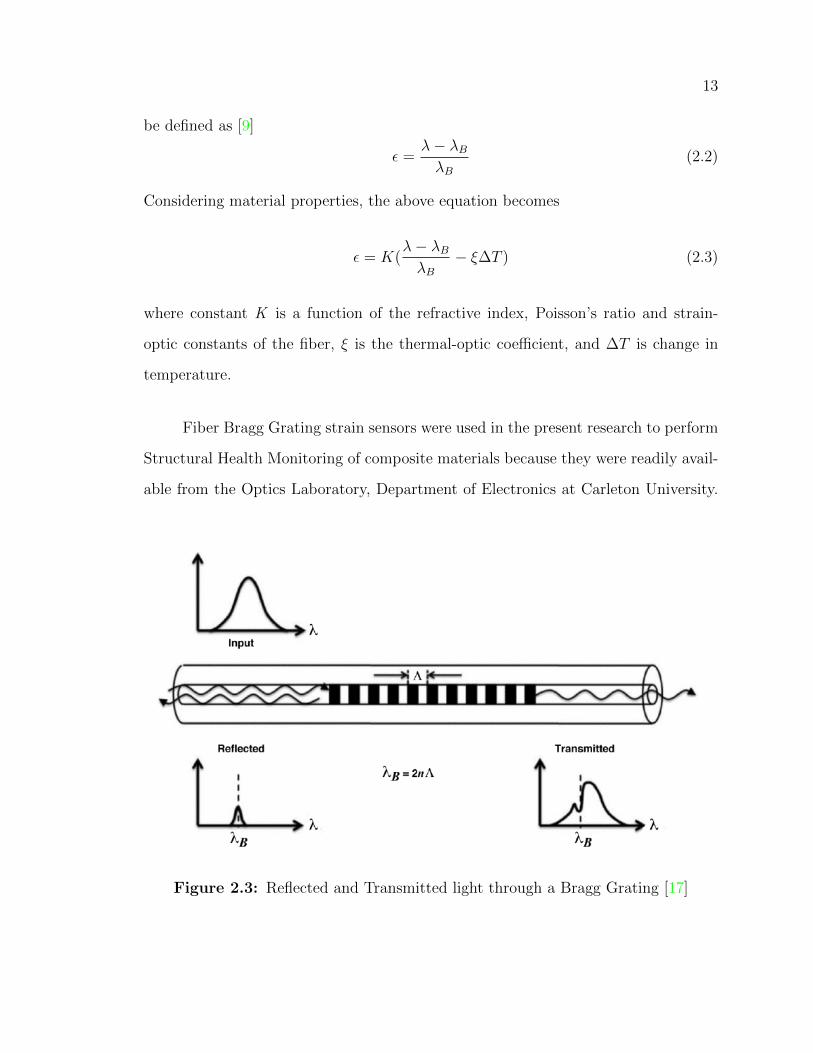
2.2.1 Bragg Gratings
Fiber Bragg Gratings (FBG) are close parallel lines typically between 1 mm to
25 mm long, consisting of alternating regions of high and low refractive indices on the
core of an optical fiber (Figure 2.3). Broadband light passing through the grating is
partially reflected from the grating at particular wavelength [32–34]. This wavelength
is known as Bragg wavelength, λB, and is given by [35]
λB = 2nΛ (2.1)
where n is average refractive index in the grating region and Λ is the grating period.
When a load is applied to the structure, the grating is strained and thus, there is
a change in the peak reflected wavelength. The new wavelength becomes λ. The
change in wavelength can be related to the strain experienced by the fiber, which can
13
be defined as [9]
ε =λ− λBλB
(2.2)
Considering material properties, the above equation becomes
ε = K(λ− λBλB
− ξ∆T ) (2.3)
where constant K is a function of the refractive index, Poisson’s ratio and strain-
optic constants of the fiber, ξ is the thermal-optic coefficient, and ∆T is change in
temperature.
Fiber Bragg Grating strain sensors were used in the present research to perform
Structural Health Monitoring of composite materials because they were readily avail-
able from the Optics Laboratory, Department of Electronics at Carleton University.
Figure 2.3: Reflected and Transmitted light through a Bragg Grating [17]
14
2.2.2 Rayleigh Fibers
In a non-excited state, each fiber has a specific local geometry and distribution
of impurities or irregularities within it. When the optical fiber experiences strain
and/or temperature changes, those features also change. As a result of these vari-
ations, the optical backscattering changes as well. Taking the non-excited state as
reference and comparing with its later states, the difference can be used for strain or
temperature measurements. Within the distributed sensing systems there are three
measurement methods: Raman, Brillouin and Rayleigh. They differ from each other
in terms of the wavelength of backscattering. Different interactions within the fiber
produces different wavelengths. The Raman method obtains scattering due to inter-
action between light photons and thermal vibration of silica molecules of the mate-
rial. The Brillouin method employs photon-photon interaction due to local geometry
variations of the fiber core. Raman and Brillouin methods can provide good global
strain and temperature measurements over lengths in the range of kilometers [36].
The spatial resolution of Raman and Brillouin backscatter signals are limited to 1
m. The Rayleigh method produces intensity reflections greater compared with the
other methods with its spatial resolution being in the range of millimeters [37]. Us-
ing Rayleigh scattering technique allows the entire length of optical fiber to act as
a sensor. Rayleigh scattering is based on Optical Frequency Domain Reflectometry
(OFDR) which measures the scattering amplitude and phase of the scattered signal
produced by optical fiber. The reflected spectrum is in the form of random pattern
from inherent variations of the optical fiber. An application of strain or temperature
causes the spectrum to shift at the location where they are applied. The new spec-
trum is compared with the reference reading at nominal strain and temperature to
calculate the strain experienced by the optical fiber [38, 39].
15
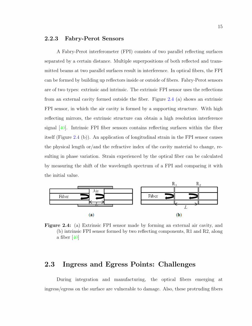
2.2.3 Fabry-Perot Sensors
A Fabry-Perot interferometer (FPI) consists of two parallel reflecting surfaces
separated by a certain distance. Multiple superpositions of both reflected and trans-
mitted beams at two parallel surfaces result in interference. In optical fibers, the FPI
can be formed by building up reflectors inside or outside of fibers. Fabry-Perot sensors
are of two types: extrinsic and intrinsic. The extrinsic FPI sensor uses the reflections
from an external cavity formed outside the fiber. Figure 2.4 (a) shows an extrinsic
FPI sensor, in which the air cavity is formed by a supporting structure. With high
reflecting mirrors, the extrinsic structure can obtain a high resolution interference
signal [40]. Intrinsic FPI fiber sensors contains reflecting surfaces within the fiber
itself (Figure 2.4 (b)). An application of longitudinal strain in the FPI sensor causes
the physical length or/and the refractive index of the cavity material to change, re-
sulting in phase variation. Strain experienced by the optical fiber can be calculated
by measuring the shift of the wavelength spectrum of a FPI and comparing it with
the initial value.
Figure 2.4: (a) Extrinsic FPI sensor made by forming an external air cavity, and(b) intrinsic FPI sensor formed by two reflecting components, R1 and R2, alonga fiber [40]
2.3 Ingress and Egress Points: Challenges
During integration and manufacturing, the optical fibers emerging at
ingress/egress on the surface are vulnerable to damage. Also, these protruding fibers
16
can easily be damaged while performing cutting operations on the manufactured com-
posite panels. As data extraction from optical fibers requires connecting their ends
to the reflectometer, there is a need for development of a system which can provide a
protective environment to optical fibers at the ingress/egress points. Several authors
have suggested and published the development of certain connectors which serves the
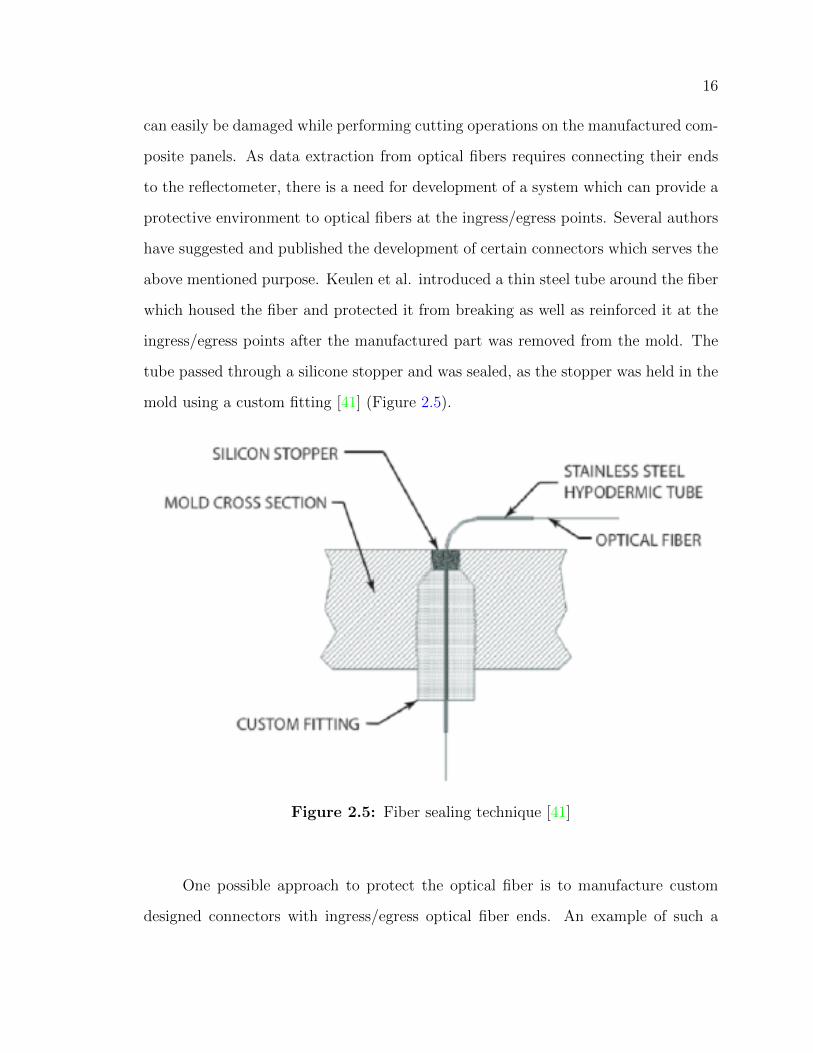
above mentioned purpose. Keulen et al. introduced a thin steel tube around the fiber
which housed the fiber and protected it from breaking as well as reinforced it at the
ingress/egress points after the manufactured part was removed from the mold. The
tube passed through a silicone stopper and was sealed, as the stopper was held in the
mold using a custom fitting [41] (Figure 2.5).
Figure 2.5: Fiber sealing technique [41]
One possible approach to protect the optical fiber is to manufacture custom
designed connectors with ingress/egress optical fiber ends. An example of such a
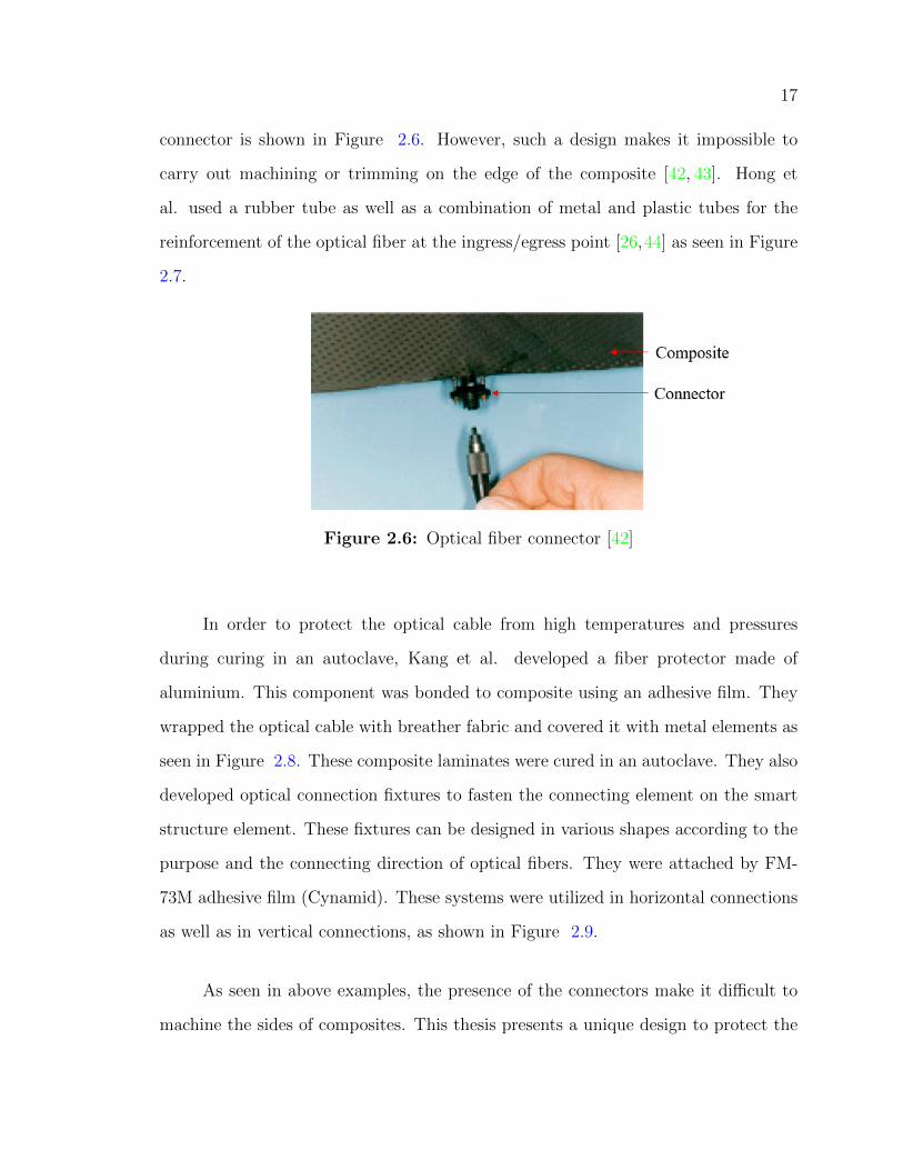
17
connector is shown in Figure 2.6. However, such a design makes it impossible to
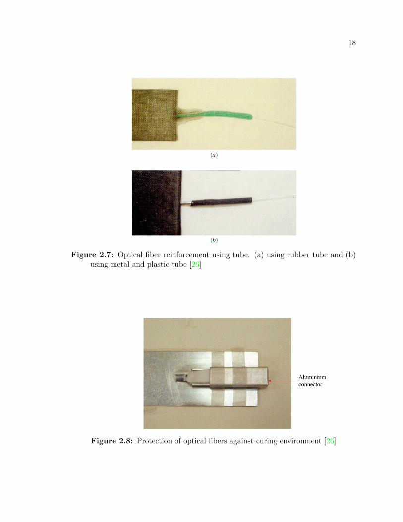
carry out machining or trimming on the edge of the composite [42, 43]. Hong et
al. used a rubber tube as well as a combination of metal and plastic tubes for the
reinforcement of the optical fiber at the ingress/egress point [26,44] as seen in Figure
2.7.
Figure 2.6: Optical fiber connector [42]
In order to protect the optical cable from high temperatures and pressures
during curing in an autoclave, Kang et al. developed a fiber protector made of
aluminium. This component was bonded to composite using an adhesive film. They
wrapped the optical cable with breather fabric and covered it with metal elements as
seen in Figure 2.8. These composite laminates were cured in an autoclave. They also
developed optical connection fixtures to fasten the connecting element on the smart
structure element. These fixtures can be designed in various shapes according to the
purpose and the connecting direction of optical fibers. They were attached by FM-
73M adhesive film (Cynamid). These systems were utilized in horizontal connections
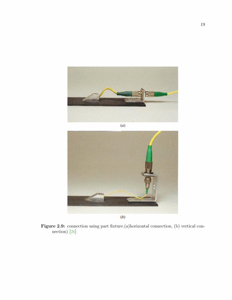
as well as in vertical connections, as shown in Figure 2.9.
As seen in above examples, the presence of the connectors make it difficult to
machine the sides of composites. This thesis presents a unique design to protect the
18
Figure 2.7: Optical fiber reinforcement using tube. (a) using rubber tube and (b)using metal and plastic tube [26]
Figure 2.8: Protection of optical fibers against curing environment [26]
19
Figure 2.9: connection using part fixture.(a)horizontal connection, (b) vertical con-nection) [26]
20
ingress and egress points of optical fibers during manufacturing as well as cutting
operation.
2.4 Mechanical Testing: with and without Inte-
grated Optical Fibers
Optical fibers are made up of glass inscribed within a different coating material.
These are very distinct and separate from the composites they are embedded in.
Embedding can only be justified if the system can measure the strain values in the
local environment without affecting the structural integrity and strength of the parent
material. Hence, it is important to study the mechanical behavior of the composites
with embedded optical fibers and compare it with that of host material without
embedded fibers. Hadzic et al. manufactured composite laminates from commercial
AS4/3501-6 (carbon-epoxy) tape [45]. The pre-preg stacks were laminated as eight
ply[904/04]s and 16 ply[908/08]s panels. Optical fibers were embedded in the mid-
plane or near the surface of the laminate. They also made a laminate from Fibredux
914 unidirectional carbon pre-preg. Optical fibers were embedded below the surface
and near the bottom of the laminate. Laminates contained 0.24% optical fibers. In
all the cases, the optical fibers were aligned with the carbon fibres and placed between
two plies of same orientation. The samples were cured in an autoclave. Tensile tests
and compression tests were conducted in accordance with ASTM-D3039M-93 and
ASTM-D3410-87 respectively.
For tensile tests, specimens were subjected to continuously increasing tensile
loads. The obtained results indicated that the presence of optical fibers did not seri-
ously degrade the mechanical properties of the host material. However, on the Fibre-
dux panels, the failure load of composite laminates with comparatively more densely

21
embedded OF decreased by approximately 33% [45]. Lee et al. fabricated tensile
specimens from HFG GU-300 pre-preg and fatigue specimens from Sunkyung Indus-
try Co. UGN-150 prepreg [46]. Two types of stacking sequences: unidirectional[06]T
and crossply[0/902]s for static tests and unidirectional[010]T and crossply[0/904]s for
fatigue tests, were chosen. The effects of embedding optical fiber parallel and per-
pendicular to adjacent reinforcing fibers on the mechanical properties of laminates
were investigated. The acrylate coating of embedded optical fiber was removed to
increase the sensitivity to damage. The deviation of stiffness, strength and Poisson’s
ratio was found to be less than 5% of their mean value. It was thus concluded that
optical fibers embedded at low volume fractions did not have significant effects on
the tensile properties of composite laminates [46].
Jensen et al. manufactured tensile and compressive specimens from unidirec-
tional Gr/BMI pre-preg tape with embedded optical fibers [47]. They reported that
the effect of embedded optical fiber orientation on the laminate tensile mechanical
properties was of the order of 10% or less. The results indicated that optical fibers
embedded perpendicular to the loading direction in composite laminates induce the
largest degradation in their mechanical performance. They concluded that optical
fibers should be embedded parallel to both the loading direction and adjacent rein-
forcing fibers for minimal intrusion, when possible [47]. They also reported a 70%
reduction in the compressive strength of composites in the presence of optical fibers.
Another observation was that the largest compressive strength reductions occured in
composite laminates with optical fibers embedded perpendicular to both the loading
direction and the adjacent graphite fibers [48].
22
Based on the recommendations provided above, all the specimens manufactured
for this research work had optical fibres embedded parallel to the reinforcing lami-
nates. Also the configuration was chosen in such a way that they remained parallel
to the loading direction in the case of tensile testing.
2.5 SHM Applications
Embedded optical fibers have been used for real time strain measurements as
described in available literatures. Pedrazzani et al. used Rayleigh scattering based
fiber optic strain sensing to monitor the distributed strain during fatigue testing of a
9-meter CX-100 wind turbine blade with intentionally introduced defects [49]. Ampli-
tude and phase of the light reflected from the fibers were measured using a commercial
Optical Frequency Domain Reflectometer (OFDR). Changes in these parameters were
used to determine strain along the entire length of fiber. Fatigue testing was carried
out on the wing blade and optical fiber data was taken with the blade under no load,
-375 lbs and ±500 lbs load. The strain values were found to be comparable with the
resistance strain gage data. They concluded that embedded optical fibers have the
potential to measure strain throughout the life cycle of composite components [49].
Torres et al. used embedded FBG-based optical fiber to measure strain within com-
posite samples. The sensors were placed on the surface of material and they were
subjected to uniform tension, compression and bending. The readings of the FBG
sensors were found comparable to those of the strain gauges, with a maximum differ-
ence of only 3% [50].
This thesis contains the results of the strain values as measured by the embedded
optical fibers in fiberglass reinforced epoxy samples. The values have been compared
with the extensometer readings during tensile loading of the specimens.
Chapter 3
Experimental Methodology
The first step of embedding optical fibers was to choose a suitable manufactur-
ing method. Since the optical fibers were to be embedded manually, the best option
was to work with dry fabric instead of pre-preg. Pre-pregs are the composite fibres
pre-impregnated by resin [51]. The presence of resin might bond the optical fibers
to pre-preg’s surface during manual embedment and make it difficult to move and
position them at the desired location. Readings of optical fibers can be affected by
the application of heat. Since the study of thermal effect on the optical fibers was
not a part of this thesis, a room temperature manufacturing method was required.
Vacuum Assisted Resin Transfer Molding (VARTM) met all of these criteria and all
the apparatus required for VARTM was available in Composites Laboratory at Car-
leton University. Hence, VARTM was chosen for the manufacturing of the composite
panels with embedded optical fibers. Optical fibers were embedded in the fiberglass
fabric during the layup process. The ingress and egress points were protected using a
custom 3D printed structure. After the sample was cured, test samples were cut from
the panels using a diamond saw. Coupons with and without embedded optical fibers
were fabricated. For final tests, optical fibers with six inscribed Bragg Gratings were
provided by the Optics Laboratory, Department of Electronics at Carleton University.
23
24
3.1 Composite Panels with Embedded Optical
Fibers
Unidirectional non-crimp fiberglass fabric was used to make all the samples. A
glass sheet was used as the tooling plate. The steps involved in the manufacturing of
composites using VARTM are as follows:
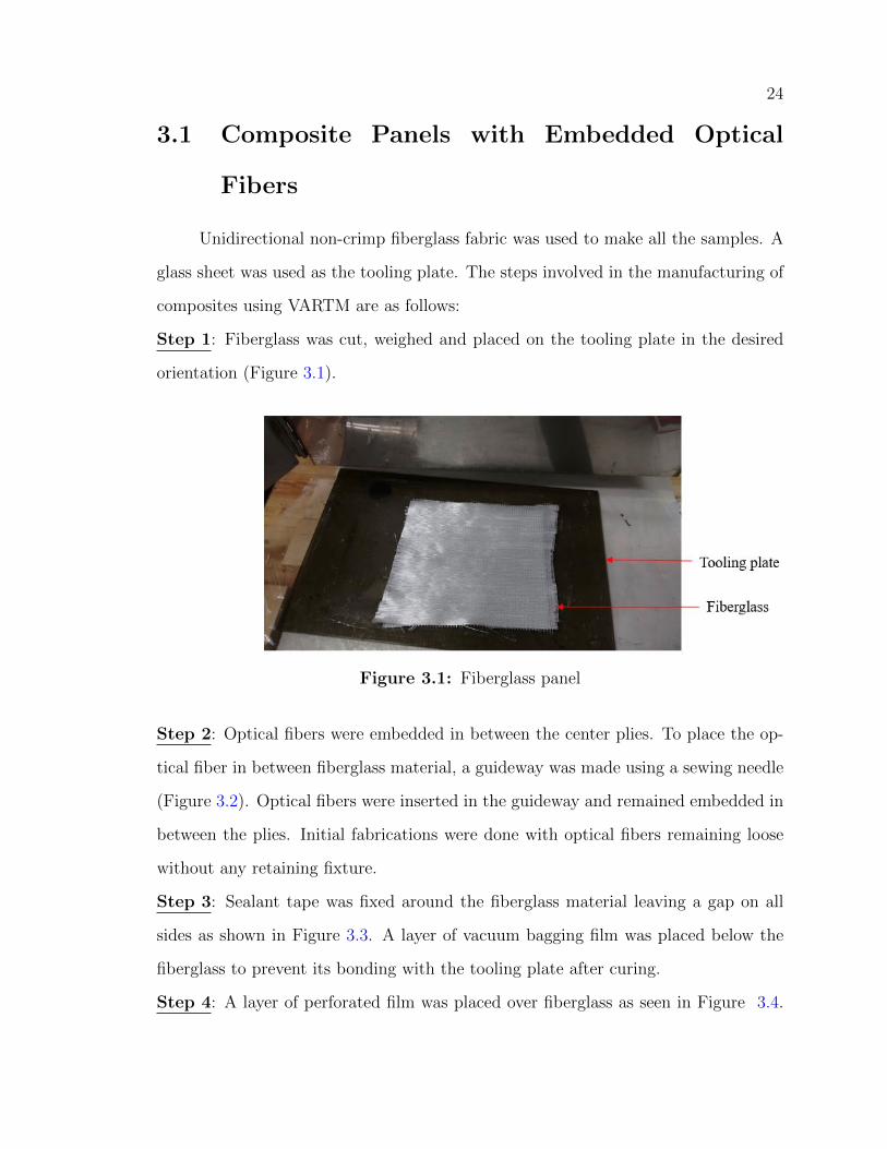
Step 1: Fiberglass was cut, weighed and placed on the tooling plate in the desired
orientation (Figure 3.1).
Figure 3.1: Fiberglass panel
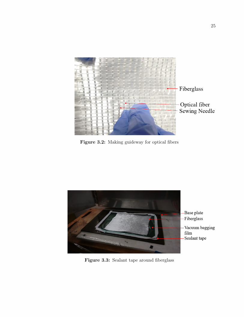
Step 2: Optical fibers were embedded in between the center plies. To place the op-
tical fiber in between fiberglass material, a guideway was made using a sewing needle
(Figure 3.2). Optical fibers were inserted in the guideway and remained embedded in
between the plies. Initial fabrications were done with optical fibers remaining loose
without any retaining fixture.
Step 3: Sealant tape was fixed around the fiberglass material leaving a gap on all
sides as shown in Figure 3.3. A layer of vacuum bagging film was placed below the
fiberglass to prevent its bonding with the tooling plate after curing.
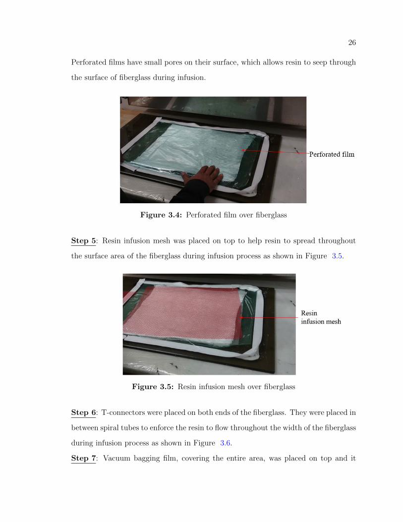
Step 4: A layer of perforated film was placed over fiberglass as seen in Figure 3.4.
25
Figure 3.2: Making guideway for optical fibers
Figure 3.3: Sealant tape around fiberglass
26
Perforated films have small pores on their surface, which allows resin to seep through
the surface of fiberglass during infusion.
Figure 3.4: Perforated film over fiberglass
Step 5: Resin infusion mesh was placed on top to help resin to spread throughout
the surface area of the fiberglass during infusion process as shown in Figure 3.5.
Figure 3.5: Resin infusion mesh over fiberglass
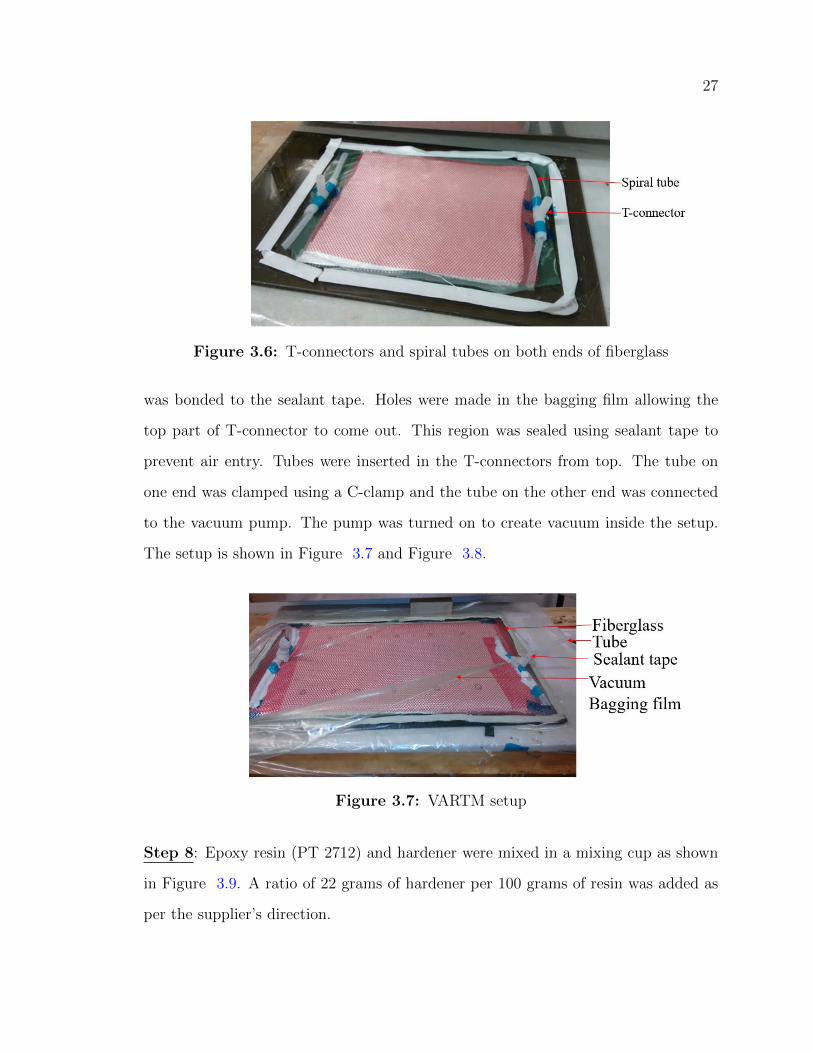
Step 6: T-connectors were placed on both ends of the fiberglass. They were placed in
between spiral tubes to enforce the resin to flow throughout the width of the fiberglass
during infusion process as shown in Figure 3.6.
Step 7: Vacuum bagging film, covering the entire area, was placed on top and it
27
Figure 3.6: T-connectors and spiral tubes on both ends of fiberglass
was bonded to the sealant tape. Holes were made in the bagging film allowing the
top part of T-connector to come out. This region was sealed using sealant tape to
prevent air entry. Tubes were inserted in the T-connectors from top. The tube on
one end was clamped using a C-clamp and the tube on the other end was connected
to the vacuum pump. The pump was turned on to create vacuum inside the setup.
The setup is shown in Figure 3.7 and Figure 3.8.
Figure 3.7: VARTM setup
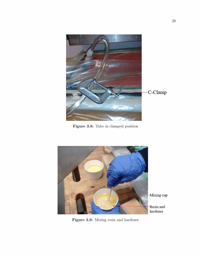
Step 8: Epoxy resin (PT 2712) and hardener were mixed in a mixing cup as shown
in Figure 3.9. A ratio of 22 grams of hardener per 100 grams of resin was added as
per the supplier’s direction.
28
Figure 3.8: Tube in clamped position
Figure 3.9: Mixing resin and hardener
29
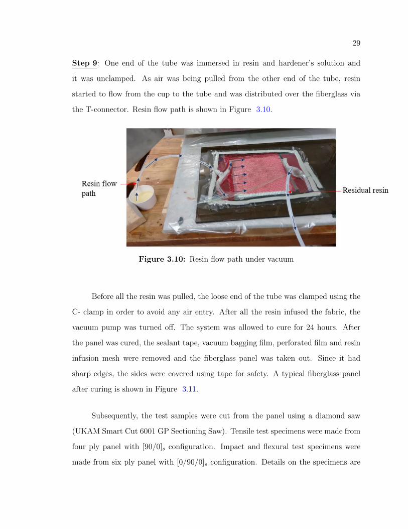
Step 9: One end of the tube was immersed in resin and hardener’s solution and
it was unclamped. As air was being pulled from the other end of the tube, resin
started to flow from the cup to the tube and was distributed over the fiberglass via
the T-connector. Resin flow path is shown in Figure 3.10.
Figure 3.10: Resin flow path under vacuum
Before all the resin was pulled, the loose end of the tube was clamped using the
C- clamp in order to avoid any air entry. After all the resin infused the fabric, the
vacuum pump was turned off. The system was allowed to cure for 24 hours. After
the panel was cured, the sealant tape, vacuum bagging film, perforated film and resin
infusion mesh were removed and the fiberglass panel was taken out. Since it had
sharp edges, the sides were covered using tape for safety. A typical fiberglass panel
after curing is shown in Figure 3.11.
Subsequently, the test samples were cut from the panel using a diamond saw
(UKAM Smart Cut 6001 GP Sectioning Saw). Tensile test specimens were made from
four ply panel with [90/0]s configuration. Impact and flexural test specimens were
made from six ply panel with [0/90/0]s configuration. Details on the specimens are

30
Figure 3.11: Fiberglass panel after curing
provided in Chapter 4.
3.2 3D Printed Fixture for Optical Fiber
Ingress/Egress Points
The points where optical fibers enter and exit the composite panel are vulnerable
to damage during manufacturing and cutting operations. In order to protect the
optical fibers, a 3D printed structure was made. Three considerations were made
during its design:
1. Optical fibers should be fully placed inside the structure and remain undamaged
during VARTM processing.
2. The design should be compatible with VARTM without negatively affecting the
process in any way.
3. After curing, the fixture should be easy to remove.
The objective was to keep the optical fiber coiled inside this fixture during the

31
VARTM process. Various designs were developed for this purpose and were tested
under vacuum. All the proposed designs were able to accommodate coiled optical
fibers within them fulfilling the first requirement. Applying mold release wax and
PolyVinyl Alcohol (PVA) release film before placing them over fiberglass for VARTM
would allow them to be removed after the curing process. Thus, the third requirement
was also met. The challenge was to come up with a design which would satisfy the
second requirement. All the designs were printed using rapid prototyping and were
observed in VARTM setup. It was observed that the structure made the vacuum
bagging film follow their profile and in this process, created a gap between the bagging
film and fiberglass. This gap could allow resin to collect during infusion process.
Therefore, modifications were made in the structure to allow the bagging film to sit on
it while the vacuum was created. These changes led to the design and manufacturing
of the final design which consisted of 5 parts. It was easy to assemble and disassemble
and did not create any gap between bagging film and fiberglass, thus, fulfilling the
second requirement. Table 3.1 summarizes all the designs and their corresponding
requirement fulfillments.
Table 3.1: Summary of fixture design iterations
Design Description Requirement 1 Requirement 2 Requirement 3
1 2 part plug Yes No Yes
2 Sloped 3 parts Yes No Yes
3 Curved 3 parts Yes No Yes
4 Curved with side parts Yes No Yes
5Curved with modified
side partsYes Yes Yes
The design and evolution of the fixture is described in the following sections.
32
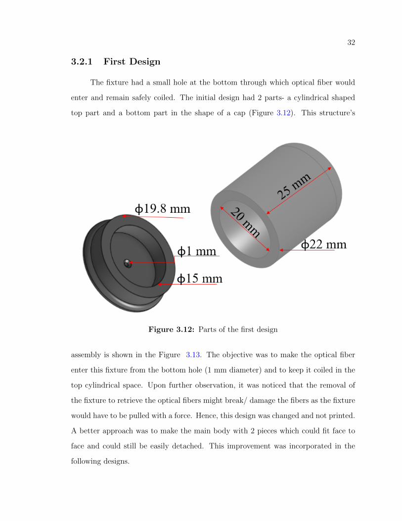
3.2.1 First Design
The fixture had a small hole at the bottom through which optical fiber would
enter and remain safely coiled. The initial design had 2 parts- a cylindrical shaped
top part and a bottom part in the shape of a cap (Figure 3.12). This structure’s
Figure 3.12: Parts of the first design
assembly is shown in the Figure 3.13. The objective was to make the optical fiber
enter this fixture from the bottom hole (1 mm diameter) and to keep it coiled in the
top cylindrical space. Upon further observation, it was noticed that the removal of
the fixture to retrieve the optical fibers might break/ damage the fibers as the fixture
would have to be pulled with a force. Hence, this design was changed and not printed.
A better approach was to make the main body with 2 pieces which could fit face to
face and could still be easily detached. This improvement was incorporated in the
following designs.
33
Figure 3.13: Assembly of the first design
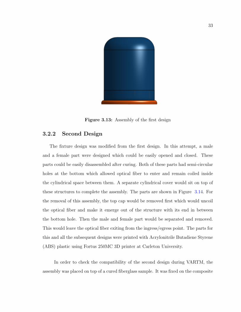
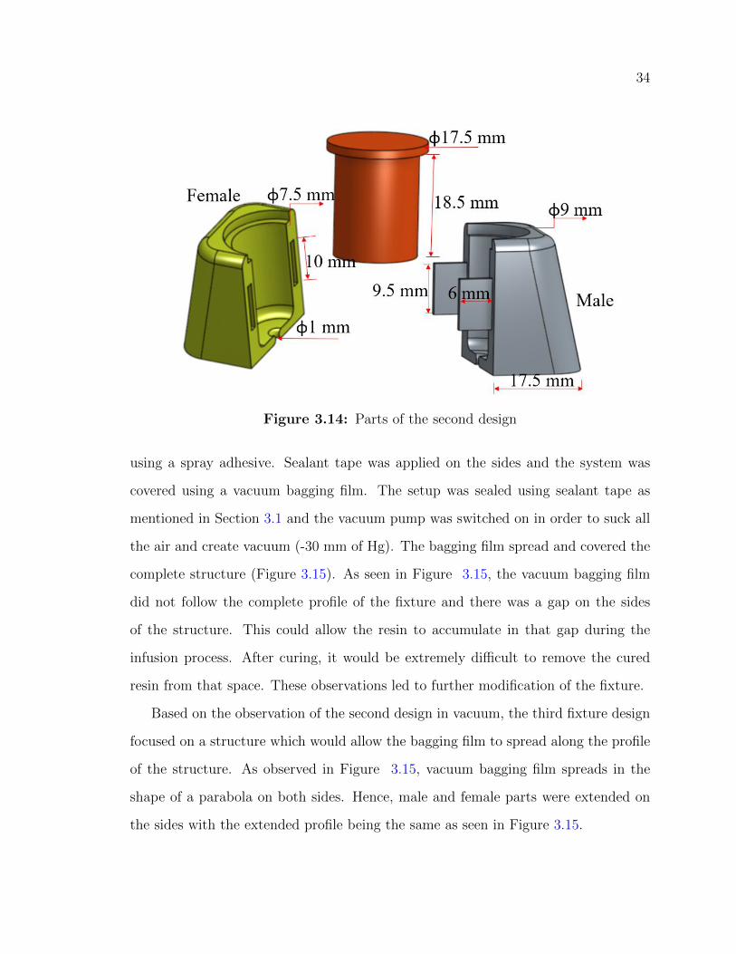
3.2.2 Second Design
The fixture design was modified from the first design. In this attempt, a male
and a female part were designed which could be easily opened and closed. These
parts could be easily disassembled after curing. Both of these parts had semi-circular
holes at the bottom which allowed optical fiber to enter and remain coiled inside
the cylindrical space between them. A separate cylindrical cover would sit on top of
these structures to complete the assembly. The parts are shown in Figure 3.14. For
the removal of this assembly, the top cap would be removed first which would uncoil
the optical fiber and make it emerge out of the structure with its end in between
the bottom hole. Then the male and female part would be separated and removed.
This would leave the optical fiber exiting from the ingress/egress point. The parts for
this and all the subsequent designs were printed with Acrylonitrile Butadiene Styrene
(ABS) plastic using Fortus 250MC 3D printer at Carleton University.
In order to check the compatibility of the second design during VARTM, the
assembly was placed on top of a cured fiberglass sample. It was fixed on the composite
34
Figure 3.14: Parts of the second design
using a spray adhesive. Sealant tape was applied on the sides and the system was
covered using a vacuum bagging film. The setup was sealed using sealant tape as
mentioned in Section 3.1 and the vacuum pump was switched on in order to suck all
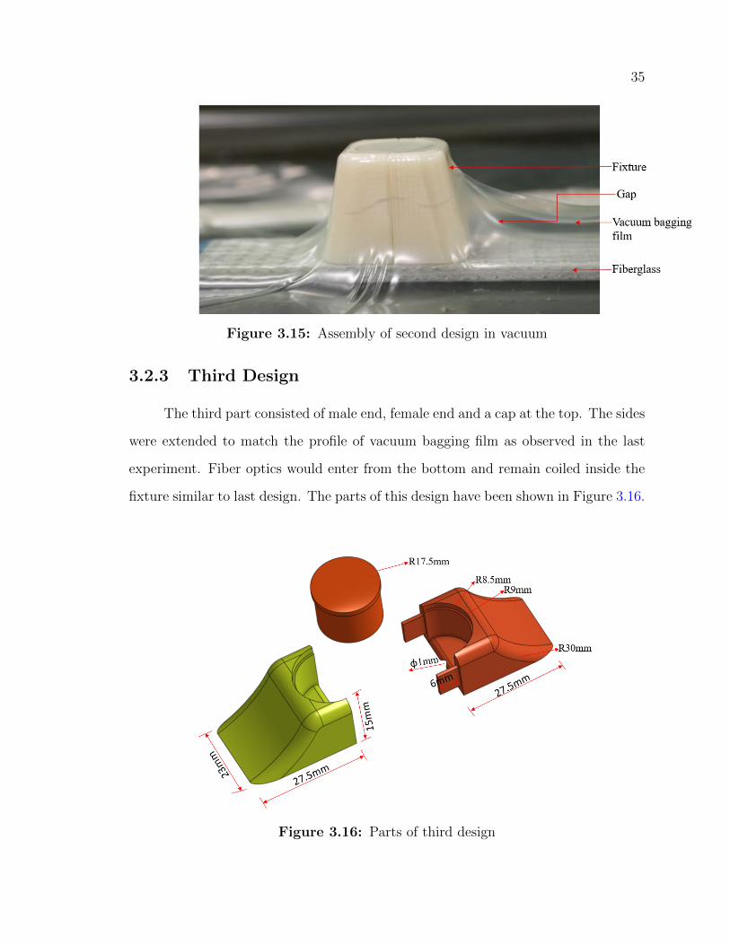
the air and create vacuum (-30 mm of Hg). The bagging film spread and covered the
complete structure (Figure 3.15). As seen in Figure 3.15, the vacuum bagging film
did not follow the complete profile of the fixture and there was a gap on the sides
of the structure. This could allow the resin to accumulate in that gap during the
infusion process. After curing, it would be extremely difficult to remove the cured
resin from that space. These observations led to further modification of the fixture.
Based on the observation of the second design in vacuum, the third fixture design
focused on a structure which would allow the bagging film to spread along the profile
of the structure. As observed in Figure 3.15, vacuum bagging film spreads in the
shape of a parabola on both sides. Hence, male and female parts were extended on
the sides with the extended profile being the same as seen in Figure 3.15.
35
Figure 3.15: Assembly of second design in vacuum
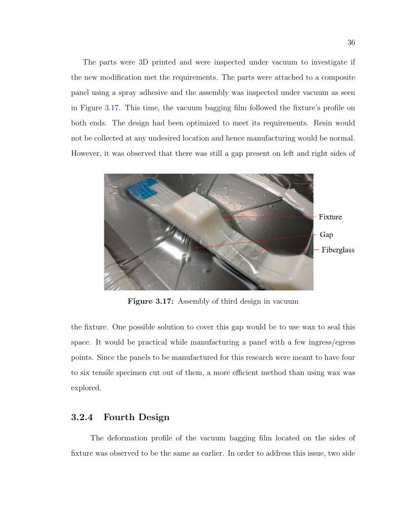
3.2.3 Third Design
The third part consisted of male end, female end and a cap at the top. The sides
were extended to match the profile of vacuum bagging film as observed in the last
experiment. Fiber optics would enter from the bottom and remain coiled inside the
fixture similar to last design. The parts of this design have been shown in Figure 3.16.
Figure 3.16: Parts of third design
36
The parts were 3D printed and were inspected under vacuum to investigate if
the new modification met the requirements. The parts were attached to a composite
panel using a spray adhesive and the assembly was inspected under vacuum as seen
in Figure 3.17. This time, the vacuum bagging film followed the fixture’s profile on
both ends. The design had been optimized to meet its requirements. Resin would
not be collected at any undesired location and hence manufacturing would be normal.
However, it was observed that there was still a gap present on left and right sides of
Figure 3.17: Assembly of third design in vacuum
the fixture. One possible solution to cover this gap would be to use wax to seal this
space. It would be practical while manufacturing a panel with a few ingress/egress
points. Since the panels to be manufactured for this research were meant to have four
to six tensile specimen cut out of them, a more efficient method than using wax was
explored.
3.2.4 Fourth Design
The deformation profile of the vacuum bagging film located on the sides of
fixture was observed to be the same as earlier. In order to address this issue, two side

37
parts were made which would go on the left and right of the structure respectively
(Figure 3.18). The complete assembly drawing of the fixture is shown in Figure 3.19.
Figure 3.18: Side part design
Figure 3.19: Assembly of Fourth design
After the parts were printed, they were assembled over the fiberglass fabric and
placed in vacuum. Stretchlon film was used as the vacuum bagging material in this
experiment. As expected, this design performed better than the third design. The
bagging film followed the complete profile of the fixture as shown in Figure 3.20.
There was however, a very small noticeable gap in the corners as seen in Figure 3.20.
This demonstrated that there was still a need for improvement in the existing design.
3.2.5 Fifth Design
In order to cover the small gap observed in Design 4, a curvature was added
to the side part (Figure 3.21). This made the ends run smoother and allowed the
bagging film to follow the complete profile of the fixture under vacuum.

38
Figure 3.20: Assembly of the fourth design in vacuum
Figure 3.21: Side part of the fifth design
39
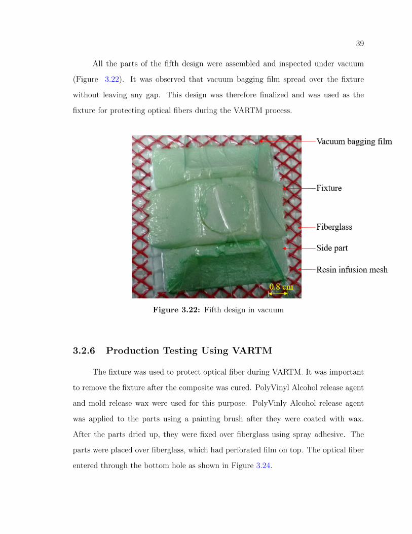
All the parts of the fifth design were assembled and inspected under vacuum
(Figure 3.22). It was observed that vacuum bagging film spread over the fixture
without leaving any gap. This design was therefore finalized and was used as the
fixture for protecting optical fibers during the VARTM process.
Figure 3.22: Fifth design in vacuum
3.2.6 Production Testing Using VARTM
The fixture was used to protect optical fiber during VARTM. It was important
to remove the fixture after the composite was cured. PolyVinyl Alcohol release agent
and mold release wax were used for this purpose. PolyVinly Alcohol release agent
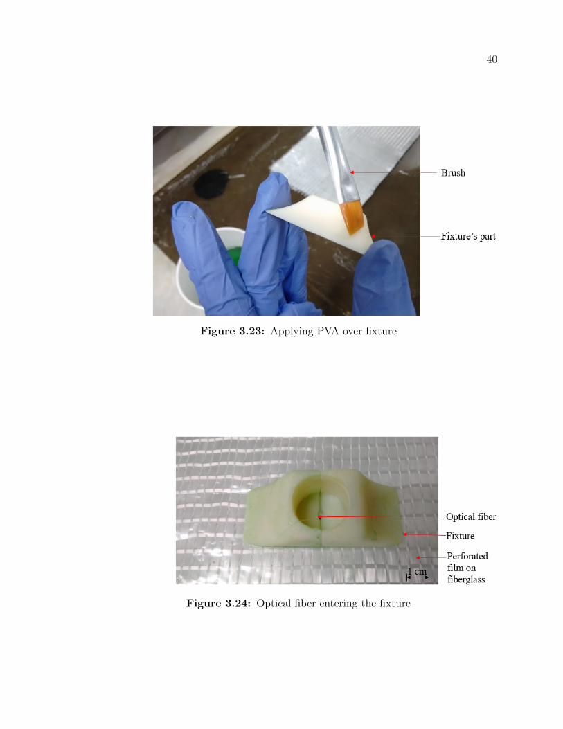
was applied to the parts using a painting brush after they were coated with wax.
After the parts dried up, they were fixed over fiberglass using spray adhesive. The
parts were placed over fiberglass, which had perforated film on top. The optical fiber
entered through the bottom hole as shown in Figure 3.24.
40
Figure 3.23: Applying PVA over fixture
Figure 3.24: Optical fiber entering the fixture
41
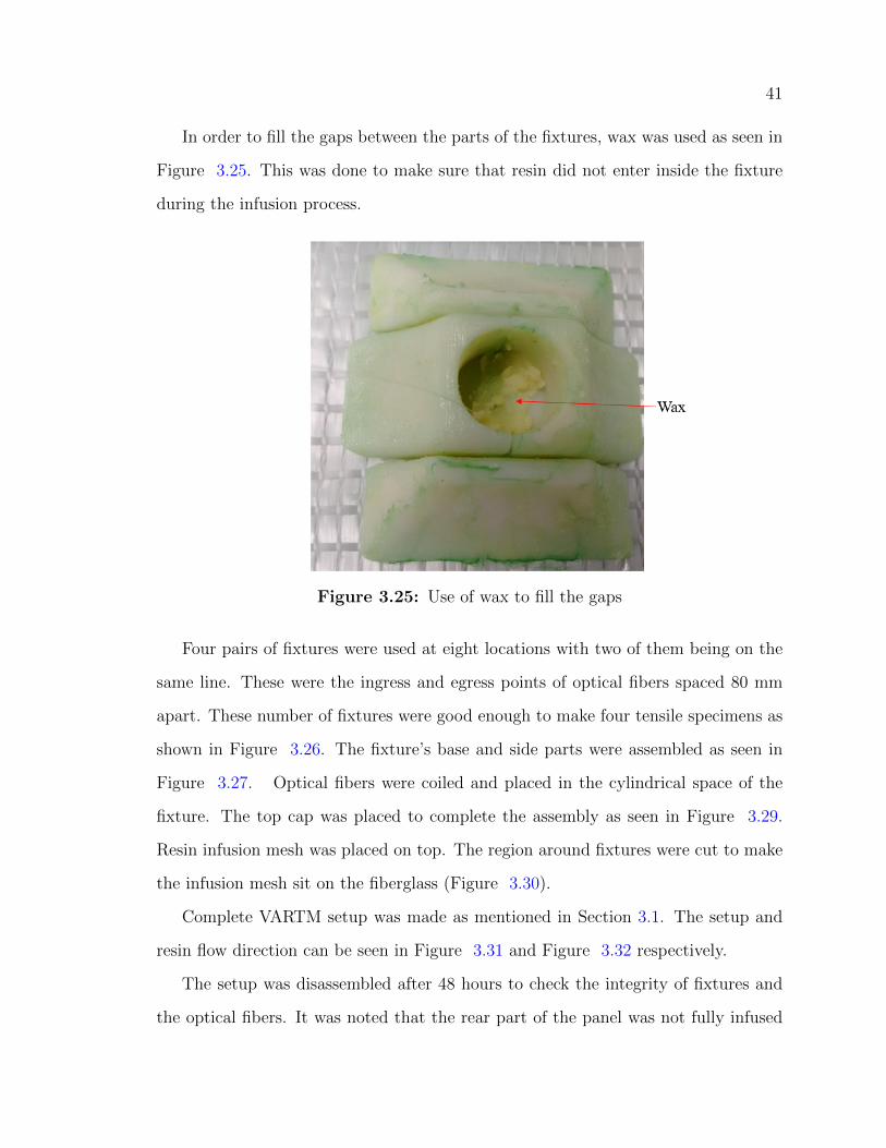
In order to fill the gaps between the parts of the fixtures, wax was used as seen in
Figure 3.25. This was done to make sure that resin did not enter inside the fixture
during the infusion process.
Figure 3.25: Use of wax to fill the gaps
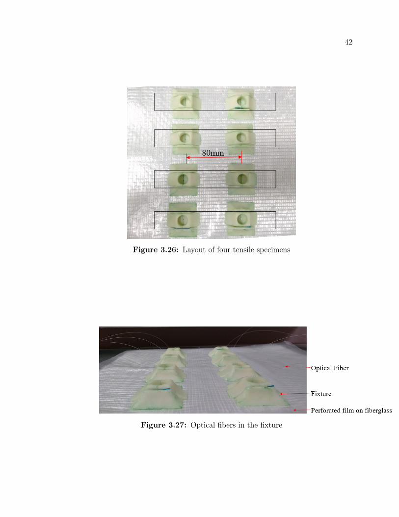
Four pairs of fixtures were used at eight locations with two of them being on the
same line. These were the ingress and egress points of optical fibers spaced 80 mm
apart. These number of fixtures were good enough to make four tensile specimens as
shown in Figure 3.26. The fixture’s base and side parts were assembled as seen in
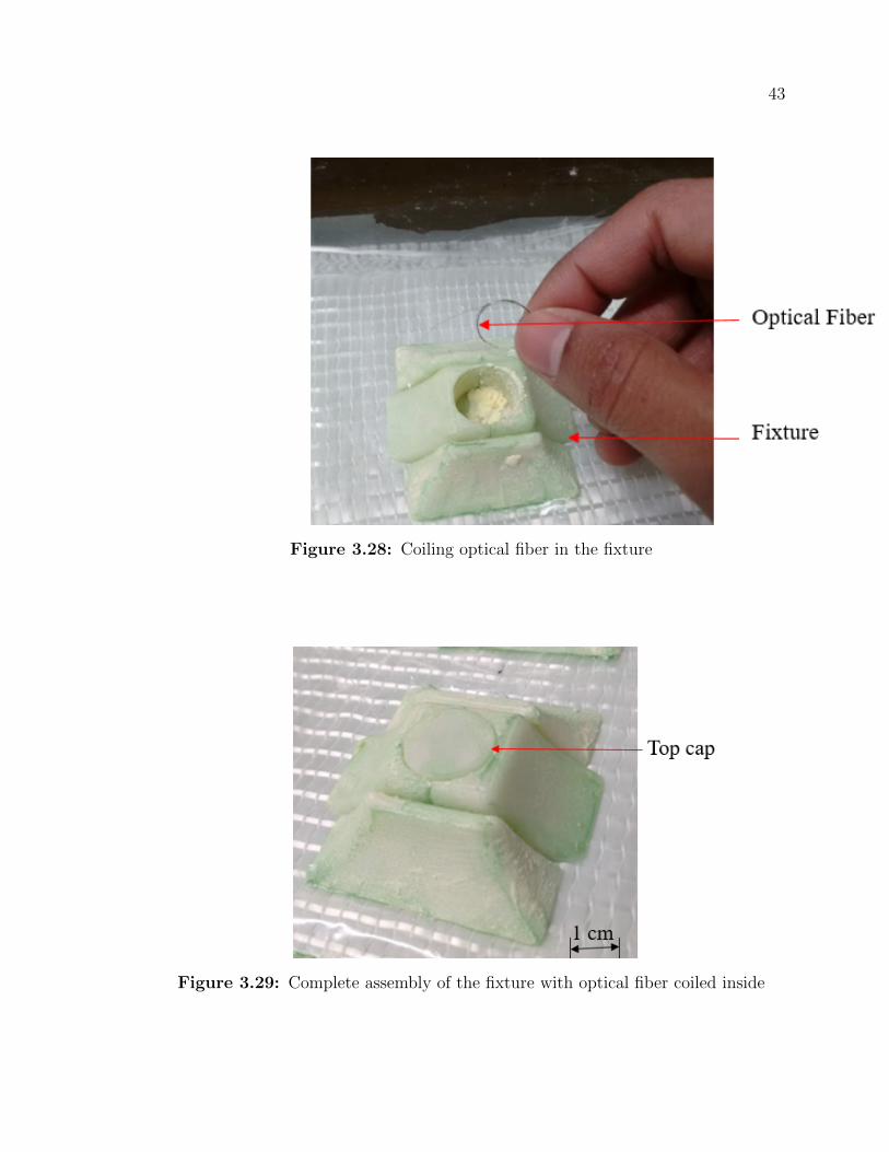
Figure 3.27. Optical fibers were coiled and placed in the cylindrical space of the
fixture. The top cap was placed to complete the assembly as seen in Figure 3.29.
Resin infusion mesh was placed on top. The region around fixtures were cut to make
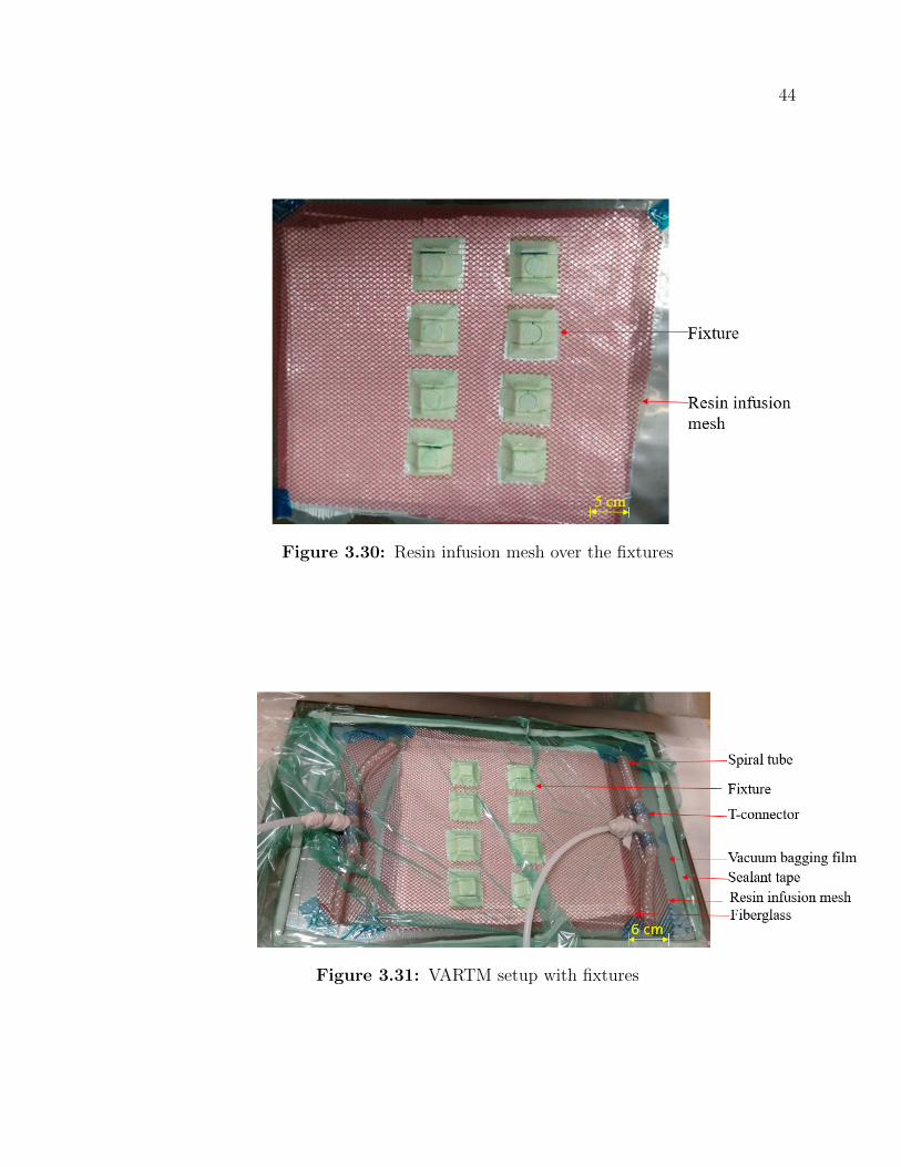
the infusion mesh sit on the fiberglass (Figure 3.30).
Complete VARTM setup was made as mentioned in Section 3.1. The setup and
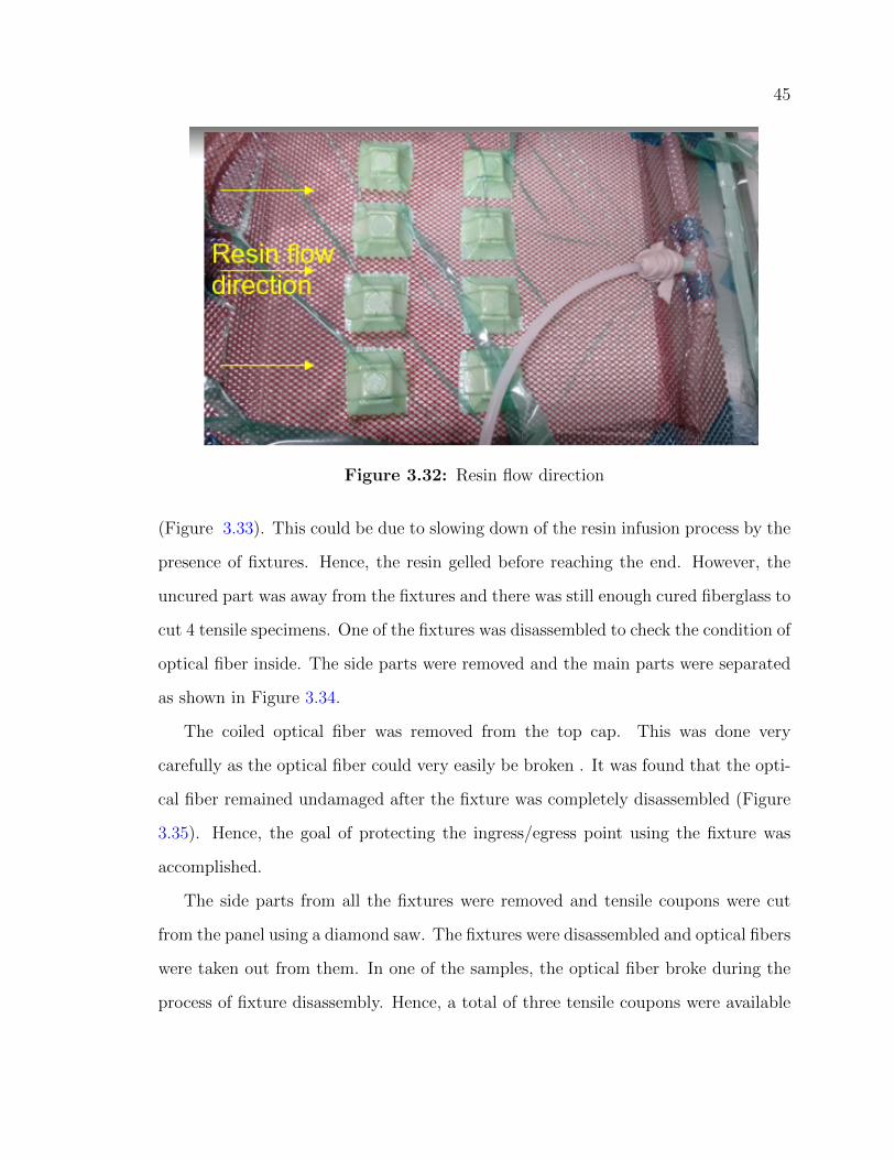
resin flow direction can be seen in Figure 3.31 and Figure 3.32 respectively.
The setup was disassembled after 48 hours to check the integrity of fixtures and
the optical fibers. It was noted that the rear part of the panel was not fully infused
42
Figure 3.26: Layout of four tensile specimens
Figure 3.27: Optical fibers in the fixture
43
Figure 3.28: Coiling optical fiber in the fixture
Figure 3.29: Complete assembly of the fixture with optical fiber coiled inside
44
Figure 3.30: Resin infusion mesh over the fixtures
Figure 3.31: VARTM setup with fixtures
45
Figure 3.32: Resin flow direction
(Figure 3.33). This could be due to slowing down of the resin infusion process by the
presence of fixtures. Hence, the resin gelled before reaching the end. However, the
uncured part was away from the fixtures and there was still enough cured fiberglass to
cut 4 tensile specimens. One of the fixtures was disassembled to check the condition of
optical fiber inside. The side parts were removed and the main parts were separated
as shown in Figure 3.34.
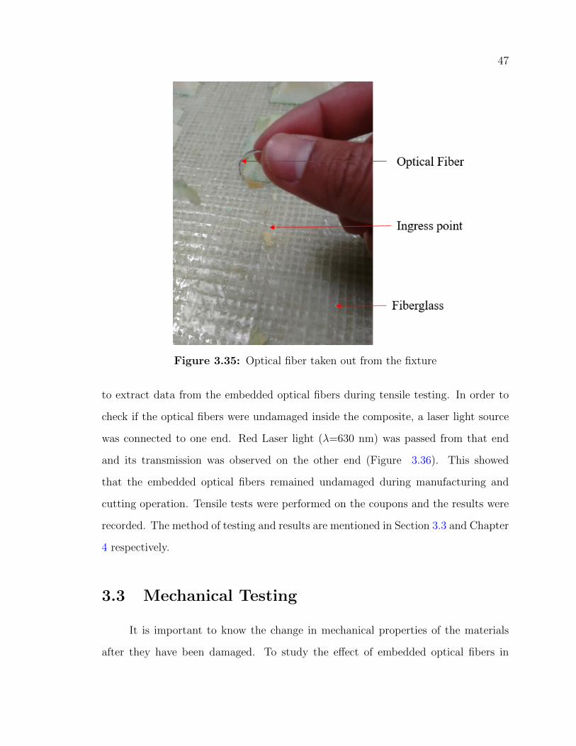
The coiled optical fiber was removed from the top cap. This was done very
carefully as the optical fiber could very easily be broken . It was found that the opti-
cal fiber remained undamaged after the fixture was completely disassembled (Figure
3.35). Hence, the goal of protecting the ingress/egress point using the fixture was
accomplished.
The side parts from all the fixtures were removed and tensile coupons were cut
from the panel using a diamond saw. The fixtures were disassembled and optical fibers
were taken out from them. In one of the samples, the optical fiber broke during the
process of fixture disassembly. Hence, a total of three tensile coupons were available

46
Figure 3.33: Cured fiberglass
Figure 3.34: Disassembling of fixture
47
Figure 3.35: Optical fiber taken out from the fixture
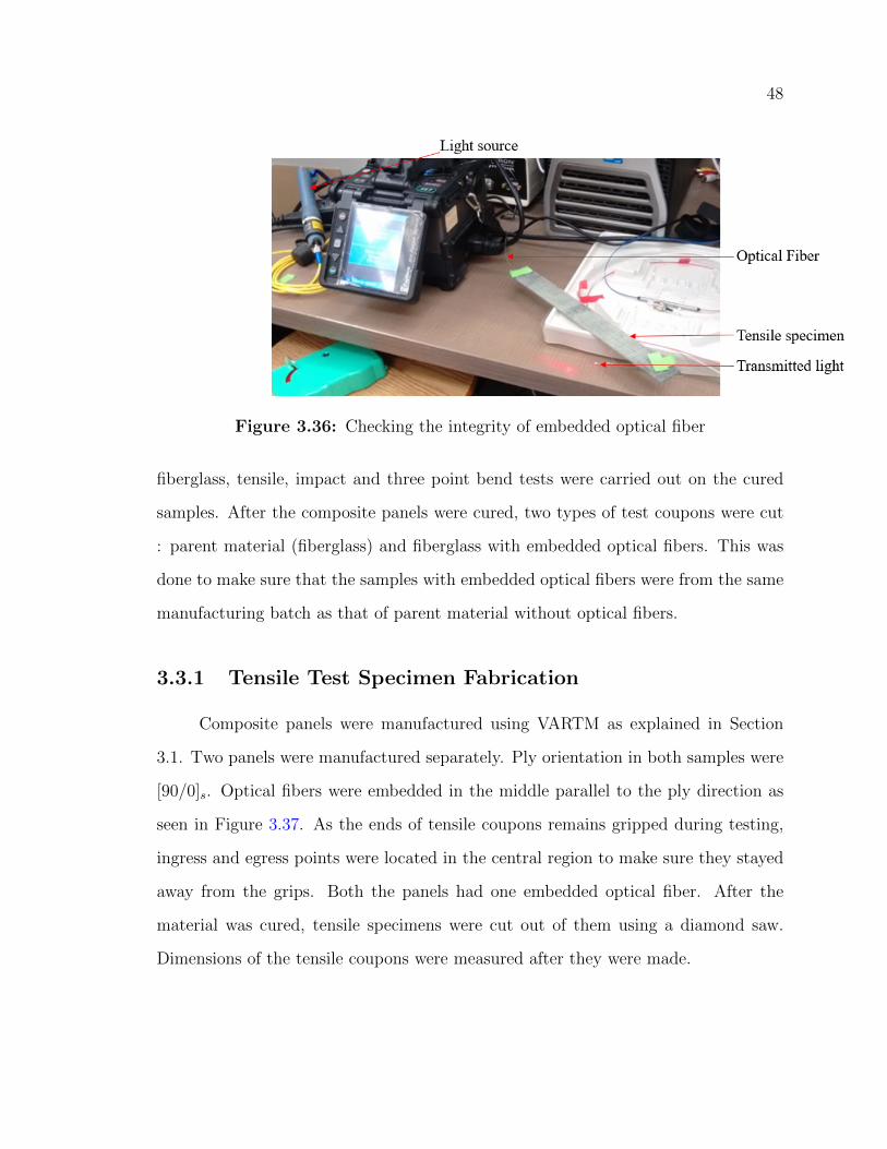
to extract data from the embedded optical fibers during tensile testing. In order to
check if the optical fibers were undamaged inside the composite, a laser light source
was connected to one end. Red Laser light (λ=630 nm) was passed from that end
and its transmission was observed on the other end (Figure 3.36). This showed
that the embedded optical fibers remained undamaged during manufacturing and
cutting operation. Tensile tests were performed on the coupons and the results were
recorded. The method of testing and results are mentioned in Section 3.3 and Chapter
4 respectively.
3.3 Mechanical Testing
It is important to know the change in mechanical properties of the materials
after they have been damaged. To study the effect of embedded optical fibers in
48
Figure 3.36: Checking the integrity of embedded optical fiber
fiberglass, tensile, impact and three point bend tests were carried out on the cured
samples. After the composite panels were cured, two types of test coupons were cut
: parent material (fiberglass) and fiberglass with embedded optical fibers. This was
done to make sure that the samples with embedded optical fibers were from the same
manufacturing batch as that of parent material without optical fibers.
3.3.1 Tensile Test Specimen Fabrication
Composite panels were manufactured using VARTM as explained in Section
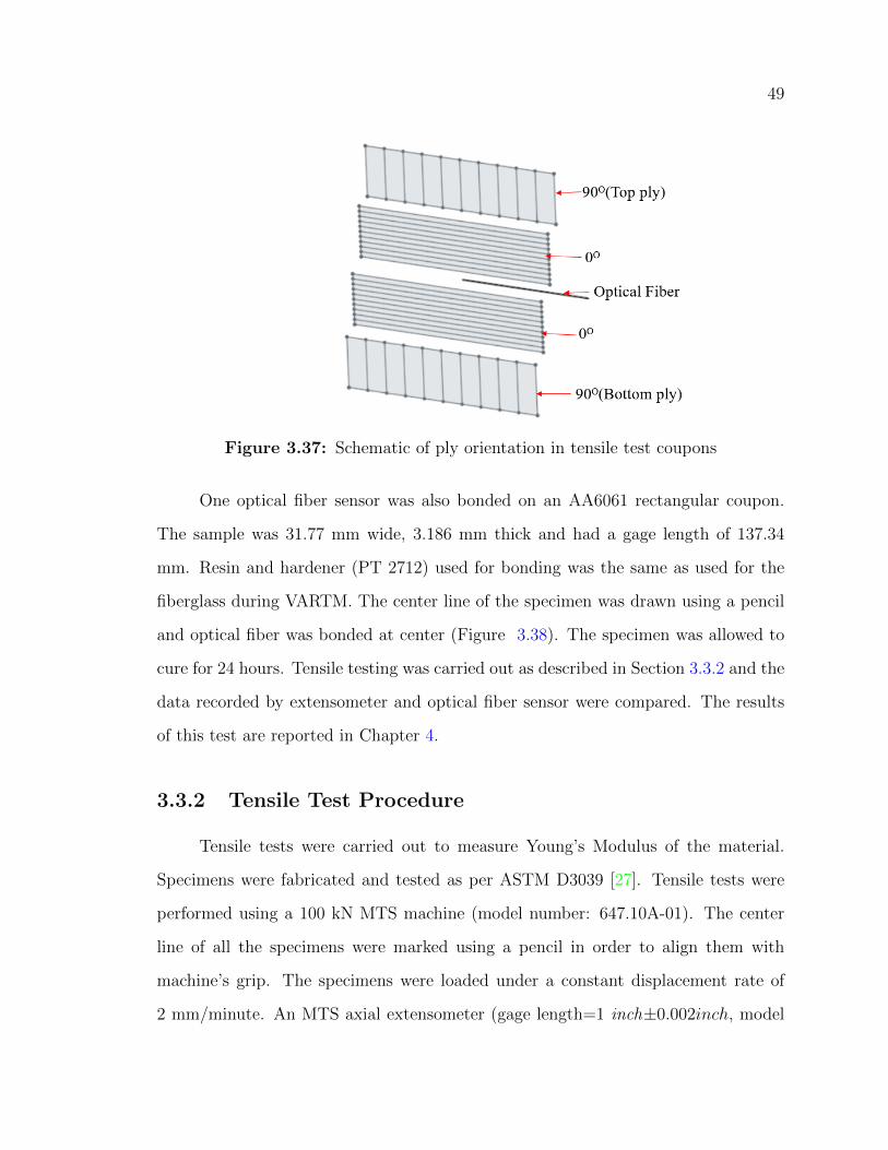
3.1. Two panels were manufactured separately. Ply orientation in both samples were
[90/0]s. Optical fibers were embedded in the middle parallel to the ply direction as
seen in Figure 3.37. As the ends of tensile coupons remains gripped during testing,
ingress and egress points were located in the central region to make sure they stayed
away from the grips. Both the panels had one embedded optical fiber. After the
material was cured, tensile specimens were cut out of them using a diamond saw.
Dimensions of the tensile coupons were measured after they were made.
49
Figure 3.37: Schematic of ply orientation in tensile test coupons
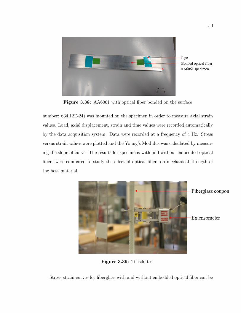
One optical fiber sensor was also bonded on an AA6061 rectangular coupon.
The sample was 31.77 mm wide, 3.186 mm thick and had a gage length of 137.34
mm. Resin and hardener (PT 2712) used for bonding was the same as used for the
fiberglass during VARTM. The center line of the specimen was drawn using a pencil
and optical fiber was bonded at center (Figure 3.38). The specimen was allowed to
cure for 24 hours. Tensile testing was carried out as described in Section 3.3.2 and the
data recorded by extensometer and optical fiber sensor were compared. The results
of this test are reported in Chapter 4.
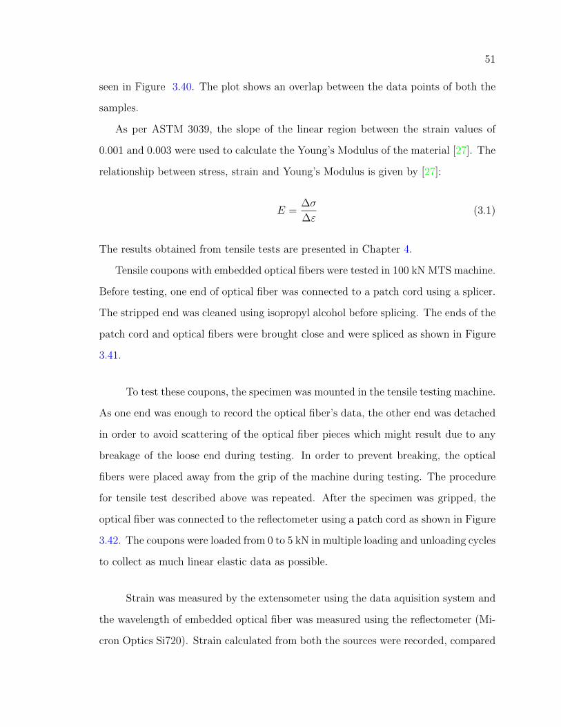
3.3.2 Tensile Test Procedure
Tensile tests were carried out to measure Young’s Modulus of the material.
Specimens were fabricated and tested as per ASTM D3039 [27]. Tensile tests were
performed using a 100 kN MTS machine (model number: 647.10A-01). The center
line of all the specimens were marked using a pencil in order to align them with
machine’s grip. The specimens were loaded under a constant displacement rate of
2 mm/minute. An MTS axial extensometer (gage length=1 inch±0.002inch, model
50
Figure 3.38: AA6061 with optical fiber bonded on the surface
number: 634.12E-24) was mounted on the specimen in order to measure axial strain
values. Load, axial displacement, strain and time values were recorded automatically
by the data acquisition system. Data were recorded at a frequency of 4 Hz. Stress
versus strain values were plotted and the Young’s Modulus was calculated by measur-
ing the slope of curve. The results for specimens with and without embedded optical
fibers were compared to study the effect of optical fibers on mechanical strength of
the host material.
Figure 3.39: Tensile test
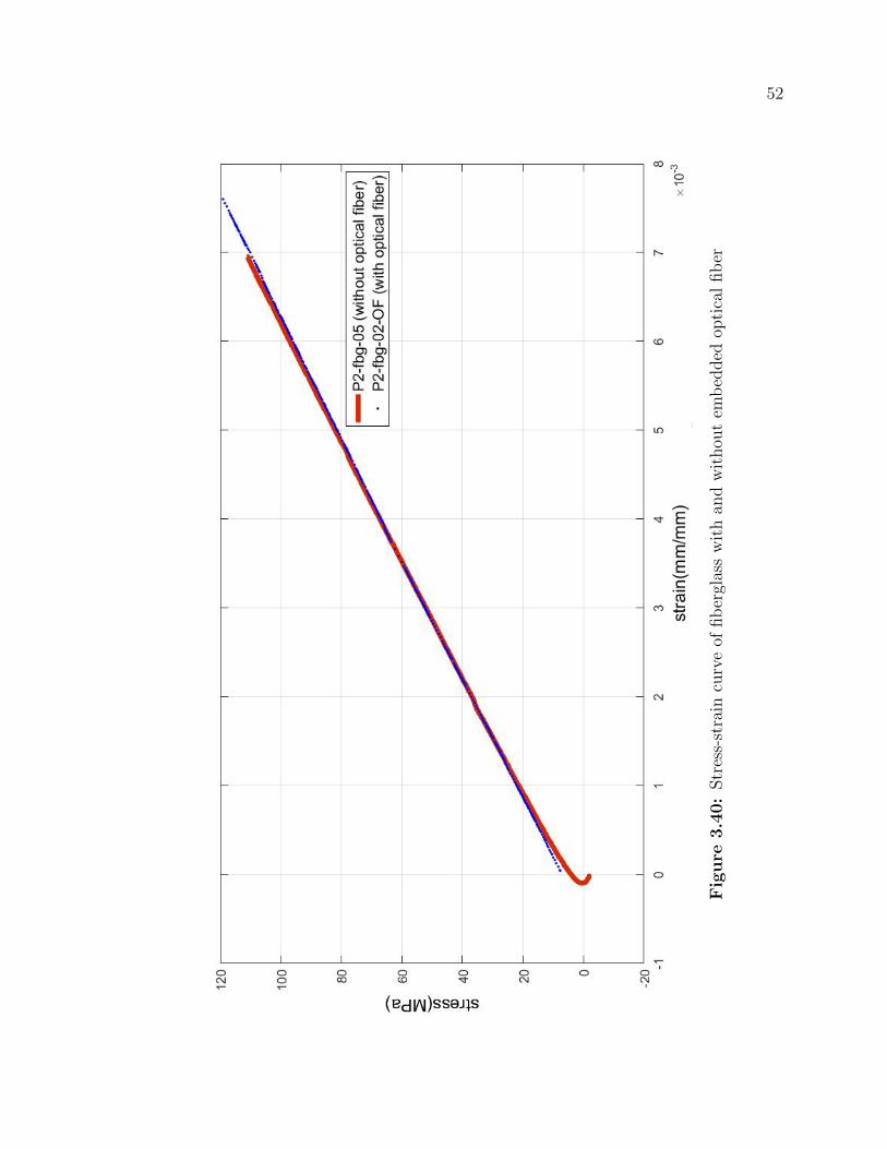
Stress-strain curves for fiberglass with and without embedded optical fiber can be
51
seen in Figure 3.40. The plot shows an overlap between the data points of both the
samples.
As per ASTM 3039, the slope of the linear region between the strain values of
0.001 and 0.003 were used to calculate the Young’s Modulus of the material [27]. The
relationship between stress, strain and Young’s Modulus is given by [27]:
E =∆σ
∆ε(3.1)
The results obtained from tensile tests are presented in Chapter 4.
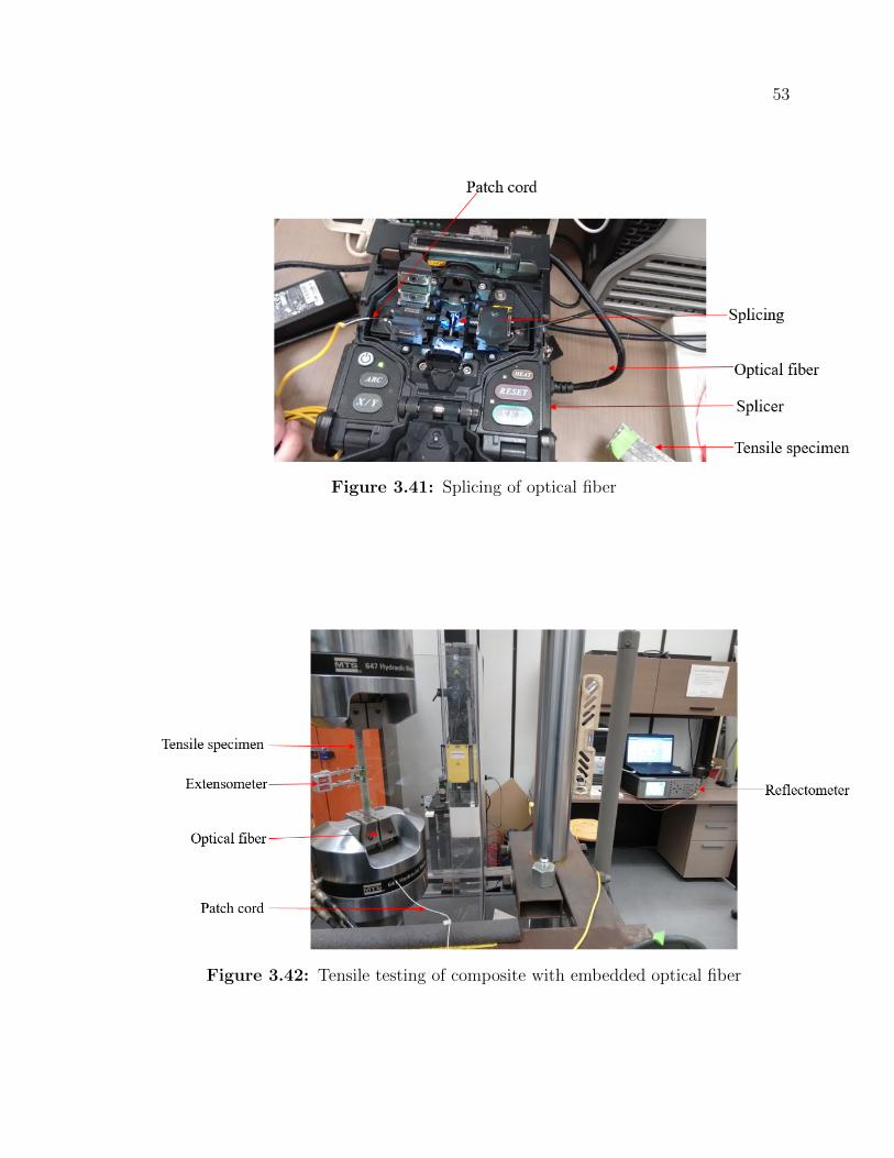
Tensile coupons with embedded optical fibers were tested in 100 kN MTS machine.
Before testing, one end of optical fiber was connected to a patch cord using a splicer.
The stripped end was cleaned using isopropyl alcohol before splicing. The ends of the
patch cord and optical fibers were brought close and were spliced as shown in Figure
3.41.
To test these coupons, the specimen was mounted in the tensile testing machine.
As one end was enough to record the optical fiber’s data, the other end was detached
in order to avoid scattering of the optical fiber pieces which might result due to any
breakage of the loose end during testing. In order to prevent breaking, the optical
fibers were placed away from the grip of the machine during testing. The procedure
for tensile test described above was repeated. After the specimen was gripped, the
optical fiber was connected to the reflectometer using a patch cord as shown in Figure
3.42. The coupons were loaded from 0 to 5 kN in multiple loading and unloading cycles
to collect as much linear elastic data as possible.
Strain was measured by the extensometer using the data aquisition system and
the wavelength of embedded optical fiber was measured using the reflectometer (Mi-
cron Optics Si720). Strain calculated from both the sources were recorded, compared
52
Fig
ure
3.4
0:
Str
ess-
stra
incu
rve
offib
ergl
ass
wit
han
dw
ithou
tem
bed
ded
opti
cal
fib
er
53
Figure 3.41: Splicing of optical fiber
Figure 3.42: Tensile testing of composite with embedded optical fiber
54
and are explained in Chapter 4.
3.3.3 Compliance Calculation
Tensile tests on the coupons manufactured from first panel were done without
an extensometer due to its non-availability. In the absence of an extensometer, axial
strain values were not recorded by the data acquisition system. In order to calculate
the material’s Young’s Modulus of Elasticity (E), the compliance of the tensile testing
machine was calculated and reported. Using the compliance value, E was generated
for all the coupons.
Compliance was obtained through tensile testing of rectangular SS304 stainless
steel specimens with 130 mm gage length, 31 mm width and 3 mm thickness. The test
was started in displacement control mode at a rate of 2 mm/minute with the loading
of 0 to 35 kN. The upper limit of load was reached within 33 seconds. In order to keep
the test running for a longer duration and record more data points, the mode was
changed to load control with a rate of 20kN/minute. An MTS extensometer (gage
length=1 inch) mounted on the mid-section of test coupon measured strain in the
material during the loading condition. The crosshead displacement was recorded by
the data aquisition system. The compliance measured by the crosshead displacement
(CT ) is the sum of the material’s compliance (Cmat) and the machine’s compliance
(Cm). This relation can be represented by the following equation [52]:
Cmat + Cm = CT (3.2)
Compliance is calculated by taking the inverse of the load-displacement curve
and it has a unit of mm/kN. Cmat is calculated using the load value recorded by
the data aquisition system and the displacement value obtained from the strain data
55
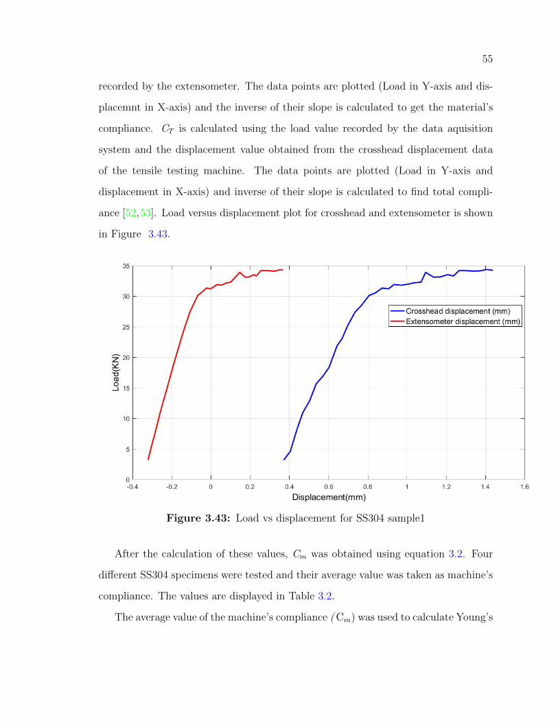
recorded by the extensometer. The data points are plotted (Load in Y-axis and dis-
placemnt in X-axis) and the inverse of their slope is calculated to get the material’s
compliance. CT is calculated using the load value recorded by the data aquisition
system and the displacement value obtained from the crosshead displacement data
of the tensile testing machine. The data points are plotted (Load in Y-axis and
displacement in X-axis) and inverse of their slope is calculated to find total compli-
ance [52,53]. Load versus displacement plot for crosshead and extensometer is shown
in Figure 3.43.
Figure 3.43: Load vs displacement for SS304 sample1
After the calculation of these values, Cm was obtained using equation 3.2. Four
different SS304 specimens were tested and their average value was taken as machine’s
compliance. The values are displayed in Table 3.2.
The average value of the machine’s compliance ( Cm) was used to calculate Young’s

56
Table 3.2: Machine’s compliance measured using SS304
Sample Number Machine Compliance,Cm (mm/kN)
1 0.0075
2 0.0083
3 0.0078
4 0.0071
Average 0.0077±0.0005
Modulus (E) of the fiberglass using Equation 3.3 [52]
E =ET
1 − CmETAL
(3.3)
where, ET is the elastic modulus calculated with the machine’s crosshead displace-
ment, A is the cross-sectional area and L is the gage length of the test specimen.
Derivation of the above equation is included in Appendix 1.
3.4 Impact Test
Impact tests were conducted to determine the damage resistance of composite
materials subjected to drop-weight impact. Fabrication and testing of the materials
were carried out according to ASTM7136 [54].
3.4.1 Specimen Fabrication
The test samples were 150 mm long, 100 mm wide and 6 mm thick. A total of
six plies [0/90/0]s were used to achieve this thickness. Optical fibers were embedded
between the center plies and were parallel to the resin flow direction. A total of
six impact test specimens were fabricated from the same panel. Three of them had
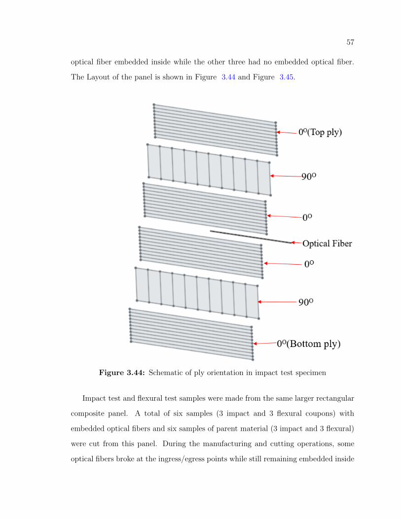
57
optical fiber embedded inside while the other three had no embedded optical fiber.
The Layout of the panel is shown in Figure 3.44 and Figure 3.45.
Figure 3.44: Schematic of ply orientation in impact test specimen
Impact test and flexural test samples were made from the same larger rectangular
composite panel. A total of six samples (3 impact and 3 flexural coupons) with
embedded optical fibers and six samples of parent material (3 impact and 3 flexural)
were cut from this panel. During the manufacturing and cutting operations, some
optical fibers broke at the ingress/egress points while still remaining embedded inside

58
Figure 3.45: Manufactured panel for impact test specimen
the fiberglass. The cutting layout and resin flow direction is shown in Figure 3.46.
The top three samples show the impact test specimens with embedded optical fiber.
The three coupons in the second row show the impact test specimens without optical
fiber. Three coupons in the last row show flexural test specimens with embedded
optical fiber and the row above them are the fiberglass’ flexural test specimens without
optical fiber. At the end, two more flexural samples were cut from the remaining
material between the second and third row. The dimensions of the flexural test
specimens are mentioned in Section 3.5.
The specimen dimensions were measured using a Vernier Caliper and are men-
tioned in the Table 3.3.
3.4.2 Impact Test Procedure
Impact tests were performed using an Instron Dynatup drop tower machine
(model number: 7800-056). During the drop tower impact tests, a hemispherical
impactor was set at a known height from the test specimen. The mass of the impactor
was provided by the supplier. At this position, the impactor possesses potential energy
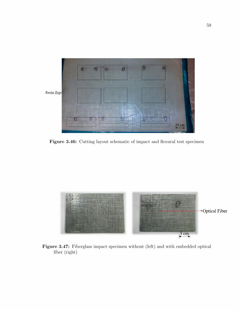
59
Figure 3.46: Cutting layout schematic of impact and flexural test specimen
Figure 3.47: Fiberglass impact specimen without (left) and with embedded opticalfiber (right)

60
Table 3.3: Dimensions of impact test specimens
Specimen Length(mm) Width(mm) Thickness(mm)
1-OF 149.22±0.32 99.79±0.17 6.23±0.24
2-OF 148.46±0.65 98.78±0.50 6.17±0.17
3-OF 148.38±0.31 99.93±0.39 5.98±0.15
4 149.46±1.50 98.23±0.55 5.89±0.67
5 146.51±0.12 99.89±1.33 5.87±0.06
6 149.04±1.26 99.74±0.59 5.97±0.15
(Ep), which is given by
Ep = mgh (3.4)
where, m is mass of the impactor, g is acceleration due to gravity and h is height of
the impactor from test specimen.
The specimen was placed and gripped on the base (Figure 3.49). As the impactor
was released, it hit the specimen at its center. Optical fibers were embedded away
from the center line in order to protect them during the test. After the impactor
was released, it fell under gravity. Potential energy converted into kinetic energy by
virtue of its motion and can be given by
Ek =1
2mv2 (3.5)
where, m is mass of the impactor and v is its velocity.
Time (t), load (F ), displacement (δ) and velocity (vi) were recorded using the
data acquisition system. Impactor velocity (vt) at any time, t is given by [54]
vt = vi + gt−∫ t
0
F (t)
mdt (3.6)
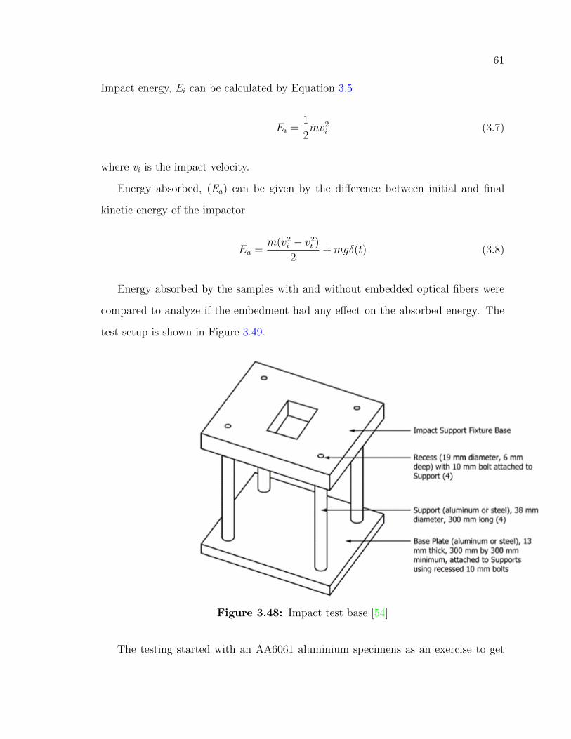
61
Impact energy, Ei can be calculated by Equation 3.5
Ei =1
2mv2i (3.7)
where vi is the impact velocity.
Energy absorbed, (Ea) can be given by the difference between initial and final
kinetic energy of the impactor
Ea =m(v2i − v2t )
2+mgδ(t) (3.8)
Energy absorbed by the samples with and without embedded optical fibers were
compared to analyze if the embedment had any effect on the absorbed energy. The
test setup is shown in Figure 3.49.
Figure 3.48: Impact test base [54]
The testing started with an AA6061 aluminium specimens as an exercise to get
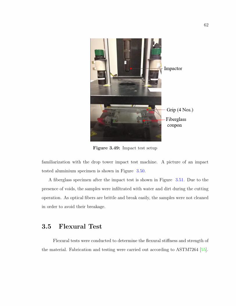
62
Figure 3.49: Impact test setup
familiarization with the drop tower impact test machine. A picture of an impact
tested aluminium specimen is shown in Figure 3.50.
A fiberglass specimen after the impact test is shown in Figure 3.51. Due to the
presence of voids, the samples were infiltrated with water and dirt during the cutting
operation. As optical fibers are brittle and break easily, the samples were not cleaned
in order to avoid their breakage.
3.5 Flexural Test
Flexural tests were conducted to determine the flexural stiffness and strength of
the material. Fabrication and testing were carried out according to ASTM7264 [55].
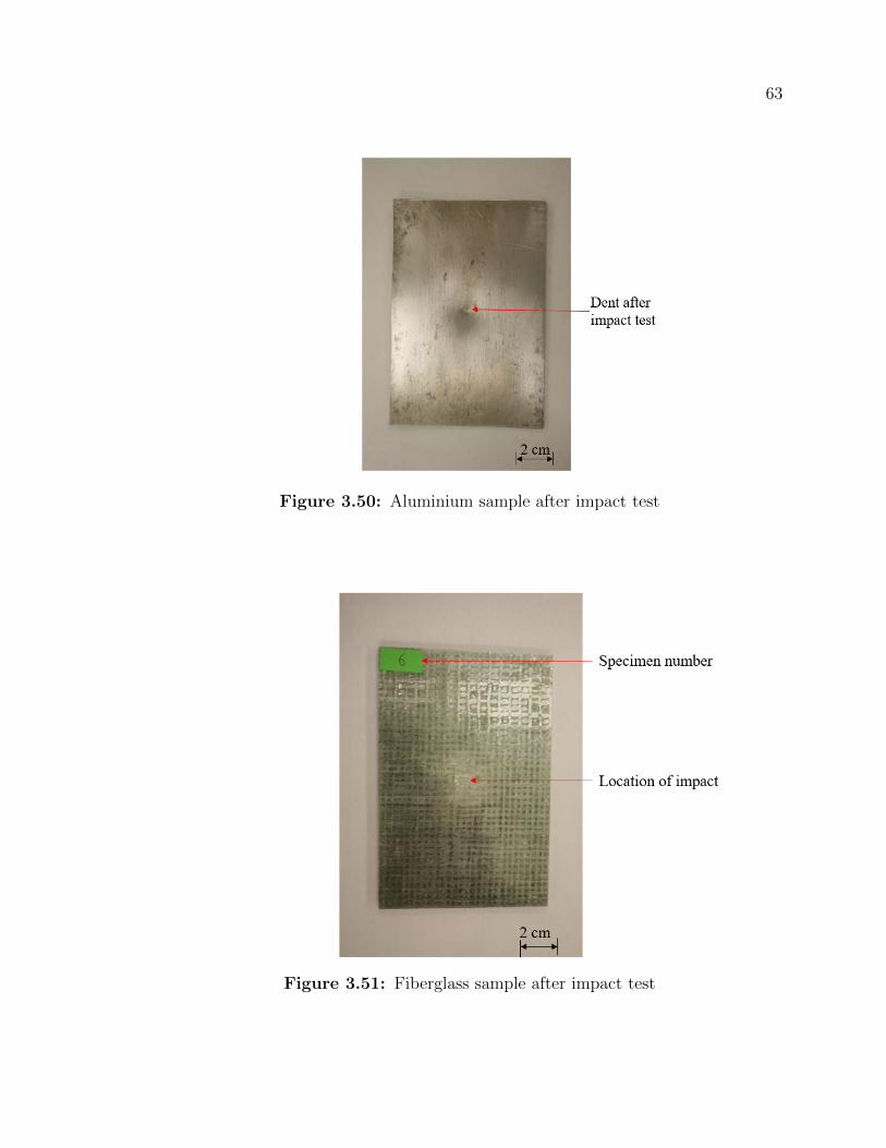
63
Figure 3.50: Aluminium sample after impact test
Figure 3.51: Fiberglass sample after impact test
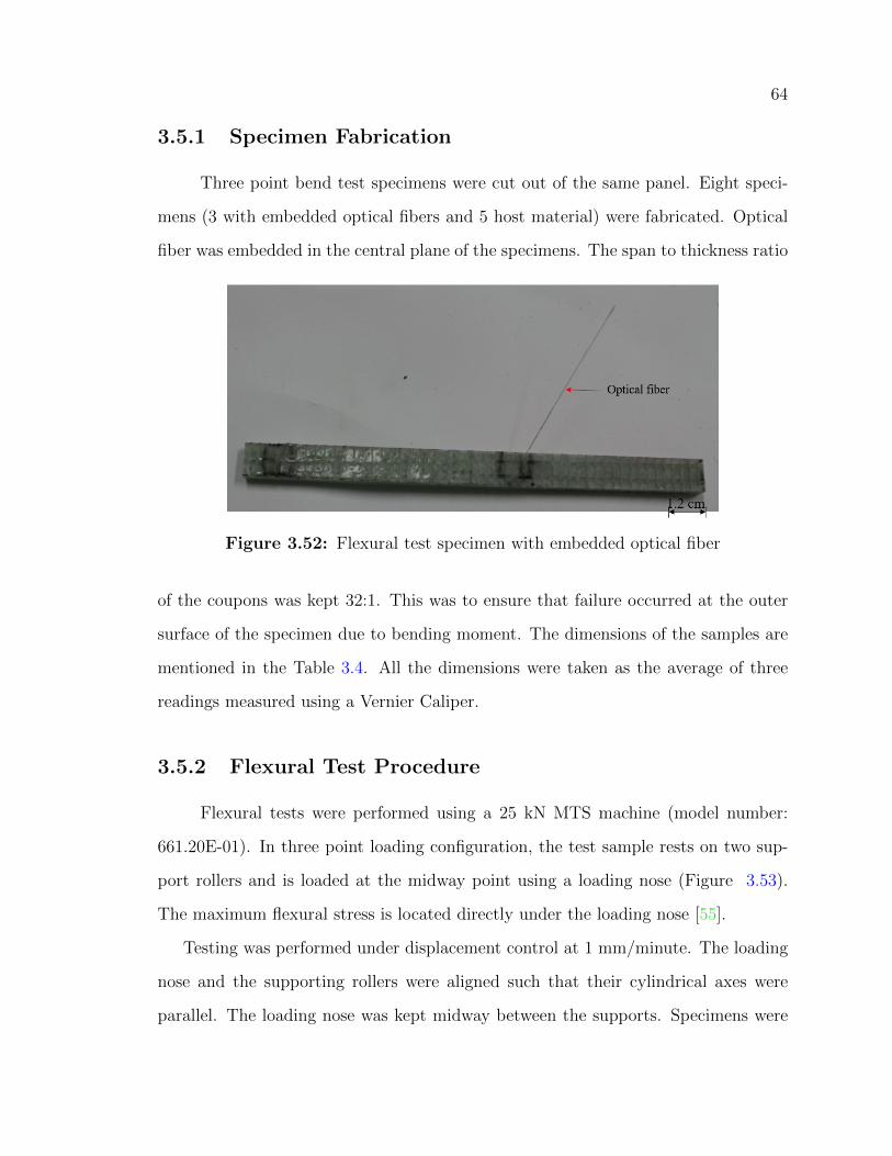
64
3.5.1 Specimen Fabrication
Three point bend test specimens were cut out of the same panel. Eight speci-
mens (3 with embedded optical fibers and 5 host material) were fabricated. Optical
fiber was embedded in the central plane of the specimens. The span to thickness ratio
Figure 3.52: Flexural test specimen with embedded optical fiber
of the coupons was kept 32:1. This was to ensure that failure occurred at the outer
surface of the specimen due to bending moment. The dimensions of the samples are
mentioned in the Table 3.4. All the dimensions were taken as the average of three
readings measured using a Vernier Caliper.
3.5.2 Flexural Test Procedure
Flexural tests were performed using a 25 kN MTS machine (model number:
661.20E-01). In three point loading configuration, the test sample rests on two sup-
port rollers and is loaded at the midway point using a loading nose (Figure 3.53).
The maximum flexural stress is located directly under the loading nose [55].
Testing was performed under displacement control at 1 mm/minute. The loading
nose and the supporting rollers were aligned such that their cylindrical axes were
parallel. The loading nose was kept midway between the supports. Specimens were
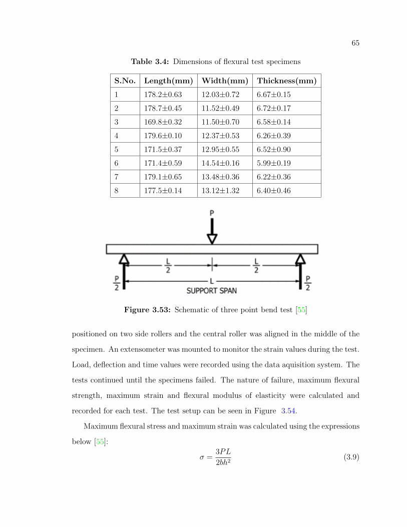
65
Table 3.4: Dimensions of flexural test specimens
S.No. Length(mm) Width(mm) Thickness(mm)
1 178.2±0.63 12.03±0.72 6.67±0.15
2 178.7±0.45 11.52±0.49 6.72±0.17
3 169.8±0.32 11.50±0.70 6.58±0.14
4 179.6±0.10 12.37±0.53 6.26±0.39
5 171.5±0.37 12.95±0.55 6.52±0.90
6 171.4±0.59 14.54±0.16 5.99±0.19
7 179.1±0.65 13.48±0.36 6.22±0.36
8 177.5±0.14 13.12±1.32 6.40±0.46
Figure 3.53: Schematic of three point bend test [55]
positioned on two side rollers and the central roller was aligned in the middle of the
specimen. An extensometer was mounted to monitor the strain values during the test.
Load, deflection and time values were recorded using the data aquisition system. The
tests continued until the specimens failed. The nature of failure, maximum flexural
strength, maximum strain and flexural modulus of elasticity were calculated and
recorded for each test. The test setup can be seen in Figure 3.54.
Maximum flexural stress and maximum strain was calculated using the expressions
below [55]:
σ =3PL
2bh2(3.9)

66
Figure 3.54: Three point bend test
where, σ is flexural stress, P is applied Load, L is support span’s length, b is width
and h is thickness of the specimen.
ε =6δh
L2(3.10)
where, ε is maximum strain, δ is deflection of mid-span, L is support span’s length
and h is thickness of the specimen.
Since the length of smallest specimen was 169.8 mm (Sample 3), the fixture was
adjusted such that sample 3 could fit in. The same configuration was maintained
for all the samples without changing the distance between the anvils. The overall
length of the available fixture was 150 mm and the diameter of the loading roller was
10 mm. The overall length of the sample accounts for 20% more than its span [55].
From Figure 3.53, 1.2L = 169.8 mm. Solving for L gives the distance between the
support rollers as 141.5 mm. Hence, length of support span used in the calculation
was 141.5 mm.
The slope of the stress-strain curve gives the flexural chord modulus of elasticity.
67
Maximum value of stress prior to failure gives the flexural strength of the material.
The results of flexural tests are presented in Chapter 4.
3.6 Measurement of the Strain Calibration Factor
for Fiber Bragg Grating
The strain value obtained by observing the shift in wavelength of Bragg Gratings
was correlated to the strain experienced by the optical fiber. A single optical fiber with
six Bragg Gratings was wrapped between two rollers in 100 N MTS LF Plus loading
machine (Figure 3.56). An initial wavelength reading of the gratings was recorded
using Micron Optics Si720. As there were six Bragg Gratings, six peaks were recorded
in the graph (Figure 3.55). The fiber was stretched in the loading machine, which
caused the wavelength patterns to shift from their original position. Optical fiber was
given extensions in increments of 0.2 mm. For every increment, the force value was
recorded. Young’s Modulus and the cross sectional area of optical fiber was provided
by the manufacturer. The wavelength readings were recorded using the reflectometer
for every extension. Actual strain was calculated using Young’s Modulus of the fiber,
their cross sectional area and applied force values. The following set of equations
shows the method of calculating strain using this method:
E =σ
ε(3.11)
Using the definition of stress
σ =F
A(3.12)

68
Substituting this term in the first line
E =F
Aε(3.13)
Solving for strain,
ε =F
AE(3.14)
Strain can also be measured using wavelength shift of Bragg Grating. The wavelength
of the first peak was used to calculate strain. Strain was calculated by its initial and
displaced position using Equation 2.2.
εgrating =λ− λBλB
(3.15)
Strain calilbration factor,K is the ratio of both the measured value of strain.
K =εgratingε
(3.16)
This test was performed on two optical fibers. Seven set of readings were taken
on both the optical fibers and the average value of strain calibration factor, K was
used for calculations. The results of these experiments are reported in Table 3.5. The
initial wavelength of the first peak in both the optical fibers was 1543.01 nm.
The average value of the strain calibration factors from both the fibers was 0.771.
This value of K was considered for final calculations.
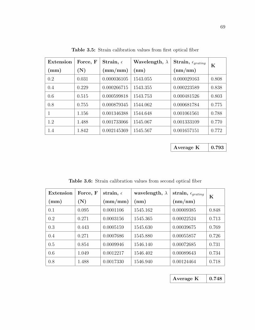
69
Table 3.5: Strain calibration values from first optical fiber
Extension
(mm)
Force, F
(N)
Strain, ε
(mm/mm)
Wavelength, λ
(nm)
Strain, εgrating
(nm/nm)K
0.2 0.031 0.000036105 1543.055 0.000029163 0.808
0.4 0.229 0.000266715 1543.355 0.000223589 0.838
0.6 0.515 0.000599818 1543.753 0.000481526 0.803
0.8 0.755 0.000879345 1544.062 0.000681784 0.775
1 1.156 0.001346388 1544.648 0.001061561 0.788
1.2 1.488 0.001733066 1545.067 0.001333109 0.770
1.4 1.842 0.002145369 1545.567 0.001657151 0.772
Average K 0.793
Table 3.6: Strain calibration values from second optical fiber
Extension
(mm)
Force, F
(N)
strain, ε
(mm/mm)
wavelength, λ
(nm)
strain, εgrating
(nm/nm)K
0.1 0.095 0.0001106 1545.162 0.00009385 0.848
0.2 0.271 0.0003156 1545.365 0.00022524 0.713
0.3 0.443 0.0005159 1545.630 0.00039675 0.769
0.4 0.271 0.0007686 1545.880 0.00055857 0.726
0.5 0.854 0.0009946 1546.140 0.00072685 0.731
0.6 1.049 0.0012217 1546.402 0.00089643 0.734
0.8 1.488 0.0017330 1546.940 0.00124464 0.718
Average K 0.748
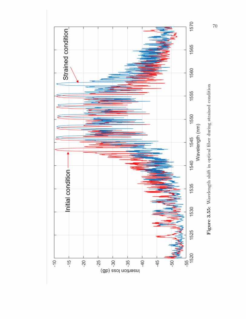
70
Fig
ure
3.5
5:
Wav
elen
gth
shif
tin
opti
cal
fib
erduri
ng
stra
ined
condit
ion

71
Figure 3.56: Measurement of the strain calibration factor of optical fiber

Chapter 4
Results and Discussion
This thesis includes two stages of tests:
1. Mechanical testing (Tensile, Flexural and Impact) to study the effect of embeding
optical fiber on composite.
2. Extraction of data from embedded optical fiber sensors using a reflectometer to
measure strain.
Finally the strain values obtained by extensometer during tensile test were com-
pared with the strain measured using embedded optical fiber sensors. The results of
these tests are described in the following sections.
4.1 Tensile Test Results
The specimens starting with P1 were made from the first panel and the ones
starting with P2 were from the second panel. The specimens with embedded optical
fibers have been named with OF. All the results have been reported up to three
decimal places. As the specimens made from the first panel were tested without an
extensometer, their Young’s Modulus were calculated using the machine’s compliance
value as described in Section 3.3.3.
72
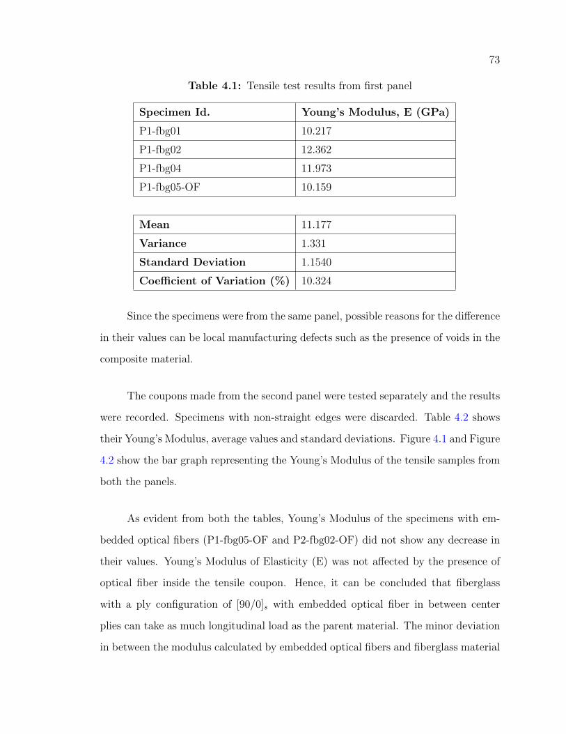
73
Table 4.1: Tensile test results from first panel
Specimen Id. Young’s Modulus, E (GPa)
P1-fbg01 10.217
P1-fbg02 12.362
P1-fbg04 11.973
P1-fbg05-OF 10.159
Mean 11.177
Variance 1.331
Standard Deviation 1.1540
Coefficient of Variation (%) 10.324
Since the specimens were from the same panel, possible reasons for the difference
in their values can be local manufacturing defects such as the presence of voids in the
composite material.
The coupons made from the second panel were tested separately and the results
were recorded. Specimens with non-straight edges were discarded. Table 4.2 shows
their Young’s Modulus, average values and standard deviations. Figure 4.1 and Figure
4.2 show the bar graph representing the Young’s Modulus of the tensile samples from
both the panels.
As evident from both the tables, Young’s Modulus of the specimens with em-
bedded optical fibers (P1-fbg05-OF and P2-fbg02-OF) did not show any decrease in
their values. Young’s Modulus of Elasticity (E) was not affected by the presence of
optical fiber inside the tensile coupon. Hence, it can be concluded that fiberglass
with a ply configuration of [90/0]s with embedded optical fiber in between center
plies can take as much longitudinal load as the parent material. The minor deviation
in between the modulus calculated by embedded optical fibers and fiberglass material
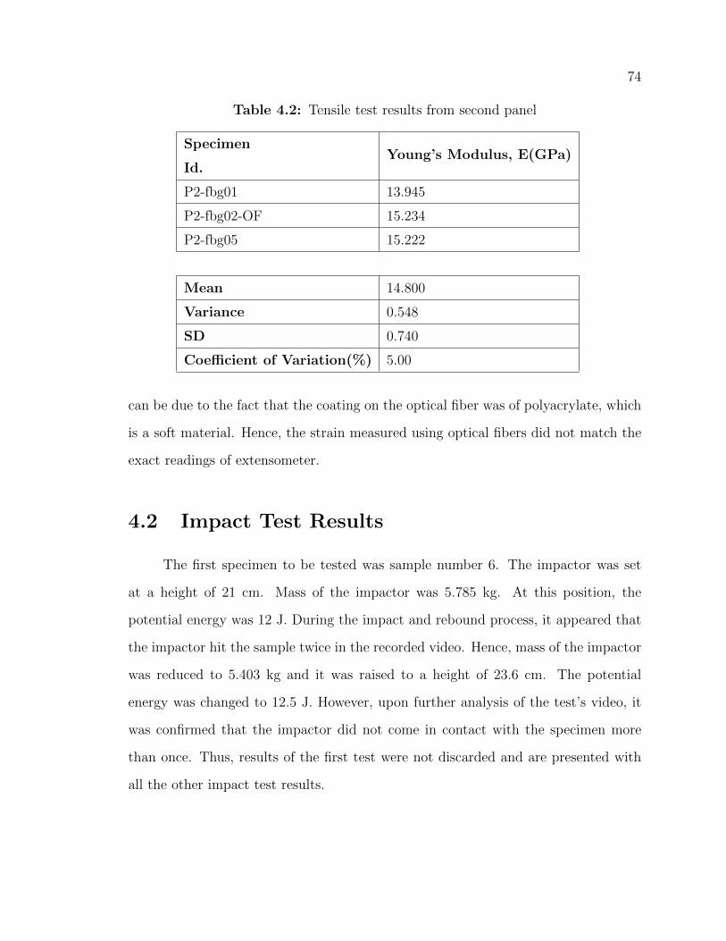
74
Table 4.2: Tensile test results from second panel
Specimen
Id.Young’s Modulus, E(GPa)
P2-fbg01 13.945
P2-fbg02-OF 15.234
P2-fbg05 15.222
Mean 14.800
Variance 0.548
SD 0.740
Coefficient of Variation(%) 5.00
can be due to the fact that the coating on the optical fiber was of polyacrylate, which
is a soft material. Hence, the strain measured using optical fibers did not match the
exact readings of extensometer.
4.2 Impact Test Results
The first specimen to be tested was sample number 6. The impactor was set
at a height of 21 cm. Mass of the impactor was 5.785 kg. At this position, the
potential energy was 12 J. During the impact and rebound process, it appeared that
the impactor hit the sample twice in the recorded video. Hence, mass of the impactor
was reduced to 5.403 kg and it was raised to a height of 23.6 cm. The potential
energy was changed to 12.5 J. However, upon further analysis of the test’s video, it
was confirmed that the impactor did not come in contact with the specimen more
than once. Thus, results of the first test were not discarded and are presented with
all the other impact test results.
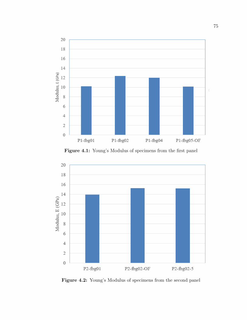
75
Figure 4.1: Young’s Modulus of specimens from the first panel
Figure 4.2: Young’s Modulus of specimens from the second panel
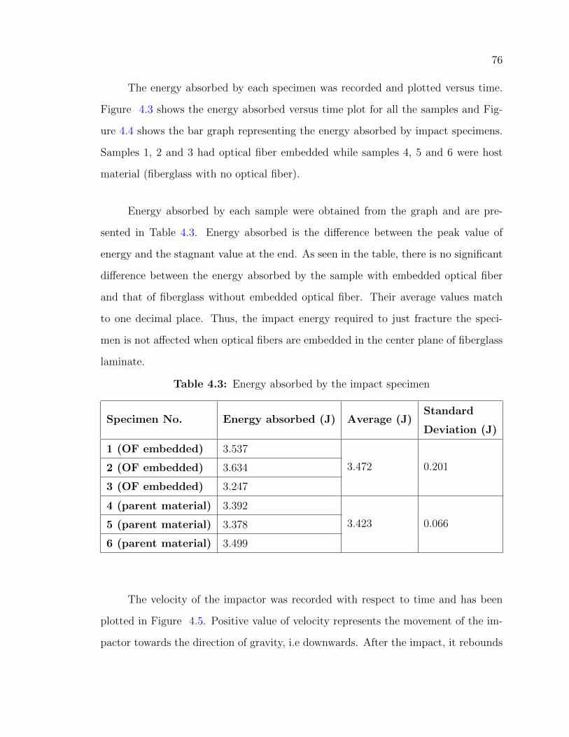
76
The energy absorbed by each specimen was recorded and plotted versus time.
Figure 4.3 shows the energy absorbed versus time plot for all the samples and Fig-
ure 4.4 shows the bar graph representing the energy absorbed by impact specimens.
Samples 1, 2 and 3 had optical fiber embedded while samples 4, 5 and 6 were host
material (fiberglass with no optical fiber).
Energy absorbed by each sample were obtained from the graph and are pre-
sented in Table 4.3. Energy absorbed is the difference between the peak value of
energy and the stagnant value at the end. As seen in the table, there is no significant
difference between the energy absorbed by the sample with embedded optical fiber
and that of fiberglass without embedded optical fiber. Their average values match
to one decimal place. Thus, the impact energy required to just fracture the speci-
men is not affected when optical fibers are embedded in the center plane of fiberglass
laminate.
Table 4.3: Energy absorbed by the impact specimen
Specimen No. Energy absorbed (J) Average (J)Standard
Deviation (J)
1 (OF embedded) 3.537
3.472 0.2012 (OF embedded) 3.634
3 (OF embedded) 3.247
4 (parent material) 3.392
3.423 0.0665 (parent material) 3.378
6 (parent material) 3.499
The velocity of the impactor was recorded with respect to time and has been
plotted in Figure 4.5. Positive value of velocity represents the movement of the im-
pactor towards the direction of gravity, i.e downwards. After the impact, it rebounds

77
Fig
ure
4.3
:E
ner
gyvs
tim
efo
ral
lth
eim
pac
tsp
ecim
ens
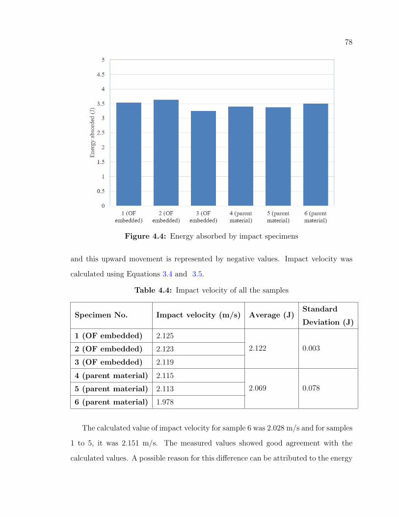
78
Figure 4.4: Energy absorbed by impact specimens
and this upward movement is represented by negative values. Impact velocity was
calculated using Equations 3.4 and 3.5.
Table 4.4: Impact velocity of all the samples
Specimen No. Impact velocity (m/s) Average (J)Standard
Deviation (J)
1 (OF embedded) 2.125
2.122 0.0032 (OF embedded) 2.123
3 (OF embedded) 2.119
4 (parent material) 2.115
2.069 0.0785 (parent material) 2.113
6 (parent material) 1.978
The calculated value of impact velocity for sample 6 was 2.028 m/s and for samples
1 to 5, it was 2.151 m/s. The measured values showed good agreement with the
calculated values. A possible reason for this difference can be attributed to the energy
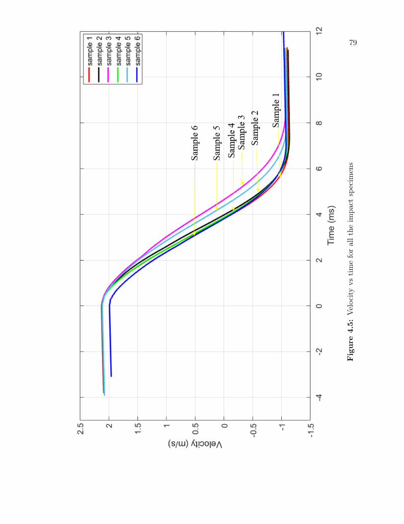
79
Fig
ure
4.5
:V
eloci
tyvs
tim
efo
ral
lth
eim
pac
tsp
ecim
ens
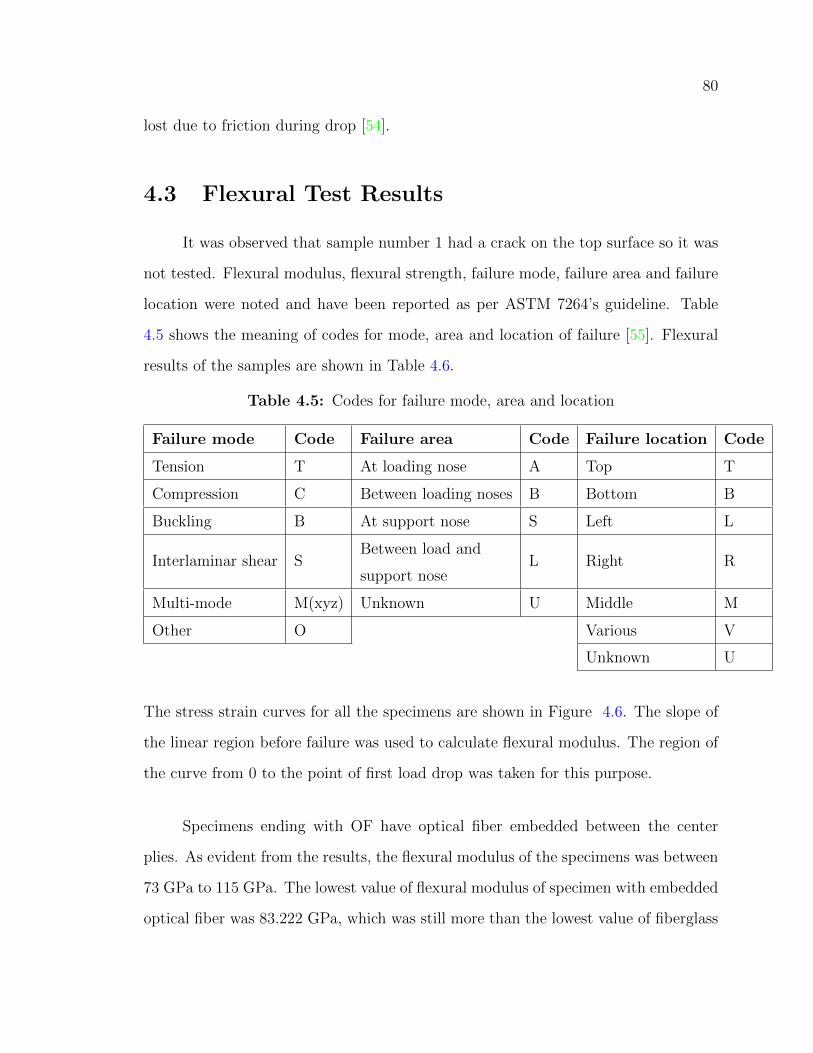
80
lost due to friction during drop [54].
4.3 Flexural Test Results
It was observed that sample number 1 had a crack on the top surface so it was
not tested. Flexural modulus, flexural strength, failure mode, failure area and failure
location were noted and have been reported as per ASTM 7264’s guideline. Table
4.5 shows the meaning of codes for mode, area and location of failure [55]. Flexural
results of the samples are shown in Table 4.6.
Table 4.5: Codes for failure mode, area and location
Failure mode Code Failure area Code Failure location Code
Tension T At loading nose A Top T
Compression C Between loading noses B Bottom B
Buckling B At support nose S Left L
Interlaminar shear SBetween load and
support noseL Right R
Multi-mode M(xyz) Unknown U Middle M
Other O Various V
Unknown U
The stress strain curves for all the specimens are shown in Figure 4.6. The slope of
the linear region before failure was used to calculate flexural modulus. The region of
the curve from 0 to the point of first load drop was taken for this purpose.
Specimens ending with OF have optical fiber embedded between the center
plies. As evident from the results, the flexural modulus of the specimens was between
73 GPa to 115 GPa. The lowest value of flexural modulus of specimen with embedded
optical fiber was 83.222 GPa, which was still more than the lowest value of fiberglass
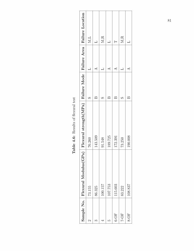
81
Table
4.6
:R
esult
sof
flex
ura
lte
st
Sam
ple
No.
Fle
xura
lM
odulu
s(G
Pa)
Fle
xura
lst
rength
(MP
a)
Failure
Mode
Failure
Are
aFailure
Loca
tion
273
.155
76.2
60S
LM
,L
386
.325
143.
509
BA
L
410
0.15
791
.548
SL
M,R
510
7.75
318
9.72
5B
AL
6-O
F11
5.60
317
2.39
1B
AT
7-O
F83
.222
73.2
50S
LM
,R
8-O
F10
8.83
719
0.00
8B
AL
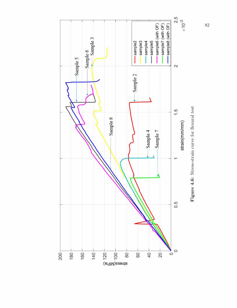
82
Fig
ure
4.6
:Str
ess-
stra
incu
rve
for
flex
ura
lte
st
83
specimen without embedded optical fiber (73.155 GPa for sample 2). Specimen 6-OF,
which was embedded with optical fiber had the highest flexural modulus among all the
samples tested. The values obtained were not consistent for all the samples. However,
it can be observed that embedding optical fiber in fiberglass did not deteriorate the
flexural modulus of the host material.
Flexural strength of all the specimen except sample 3 lie between 24.33 MPa
and 44.29 MPa. As observed in Figure 4.6, specimen 3 did not experience failure until
131.181 MPa. The specimen with the lowest value of flexural strength was Sample
2 (without embedded optical fiber). Two of the samples with optical fiber (6 and 7)
have close values of flexural strength while the third sample (sample 8) has a higher
value. The results lead to the conclusion that embedding optical fiber in between
center plies of fiberglass has no significant effect on their flexural strengths.
The failure modes of all the samples was either buckling or interlaminar shear.
The reason for interlaminar shear could be due the presence of voids in the sample as
a result of manufacturing defects. Four specimens failed at the loading nose and three
of them failed between the loading nose and support nose. Failure locations varied
between the samples. Three specimens were observed to have failed at two locations
(samples 2, 4 and 7).
4.4 Tensile Strain Measurement Using Embedded
Optical Fibers
Strain during tensile tests were measured by an extensometer. Optical fiber
data was recorded using the reflectometer during loading and unloading conditions.
Coordinates of the peak values combined with strain calibration factor were used
84
to measure strain using Equation 2.2. The testing was started with an aluminium
AA6061 coupon with an optical fiber bonded on its surface. The specimen was loaded
in displacement mode with increments of 0.05 mm until 0.6 mm and then unloaded
in the same increments. Strain and modulus of elasticity were calculated from both
curves. The stress-strain curve for loading and unloading condition can be seen in
Figure 4.7 and Figure 4.8. The slope of these curves were calculated to find the
modulus of elasticity, which were compared for loading and unloading cycle.
The stress-strain curves of fiberglass reinforced epoxy with embedded optical
fiber was plotted using the values obtained by extensometer and optical fiber (Figure
4.9 and Figure 4.10). The data points corresponding to the extensometer and that of
optical fibers did not seem to match in the curve. Possible reason for this mismatch
could be that the optical fiber was not bonded well within fiberglass. Modulus of
elasticity for all the loading and unloading cycles was calculated for both the readings.
The values did not seem to match, giving an evidence of poor bonding between optical
fiber and the host material. One way to confirm the nature of bonding between the
embedded optical fiber and the fiberglass material can be cutting the specimen at
various locations and observing the cross section under a microscope. However, this
exercise was not carried out for this thesis.
The plot of the second specimen with embedded optical fiber showed good
correlation between the strain values of the extensometer and that of optical fiber as
shown in Figure 4.11 and Figure 4.12. Data were recorded during four loading and
four unloading cycles and compared to examine the agreement of strain values and
modulus of elasticity. Unlike the first sample, the values showed good correlation.
It also proved that embedded optical fiber was well bonded within the fiberglass
composite.
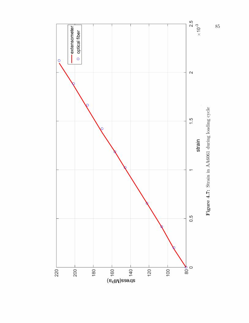
85
Fig
ure
4.7
:Str
ain
inA
A60
61duri
ng
load
ing
cycl
e
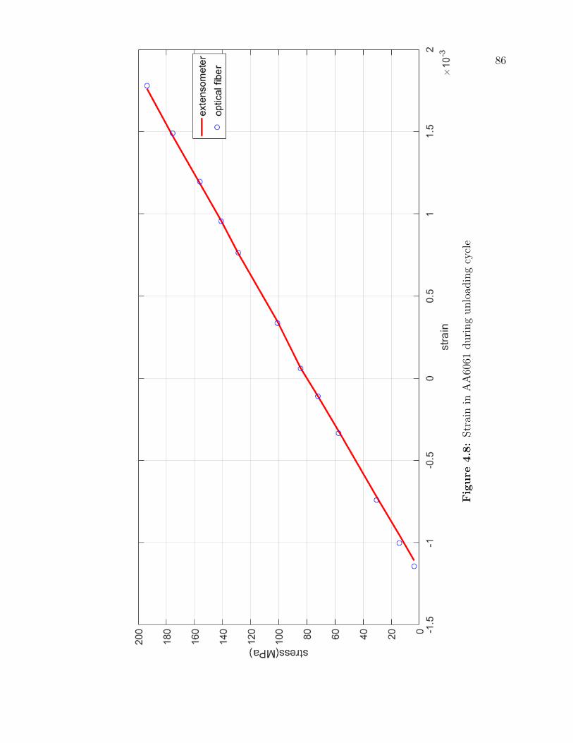
86
Fig
ure
4.8
:Str
ain
inA
A60
61duri
ng
unlo
adin
gcy
cle
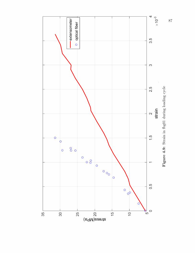
87
Fig
ure
4.9
:Str
ain
infb
g01
duri
ng
load
ing
cycl
e
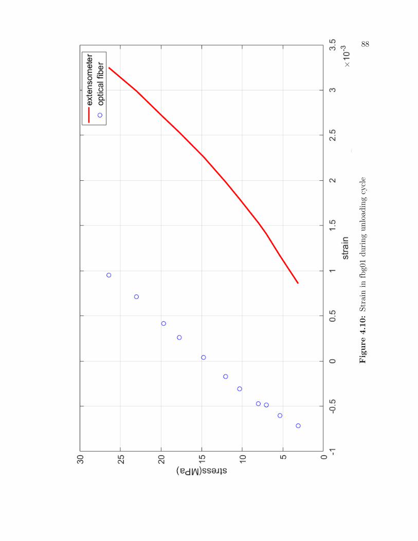
88
Fig
ure
4.1
0:
Str
ain
infb
g01
duri
ng
unlo
adin
gcy
cle
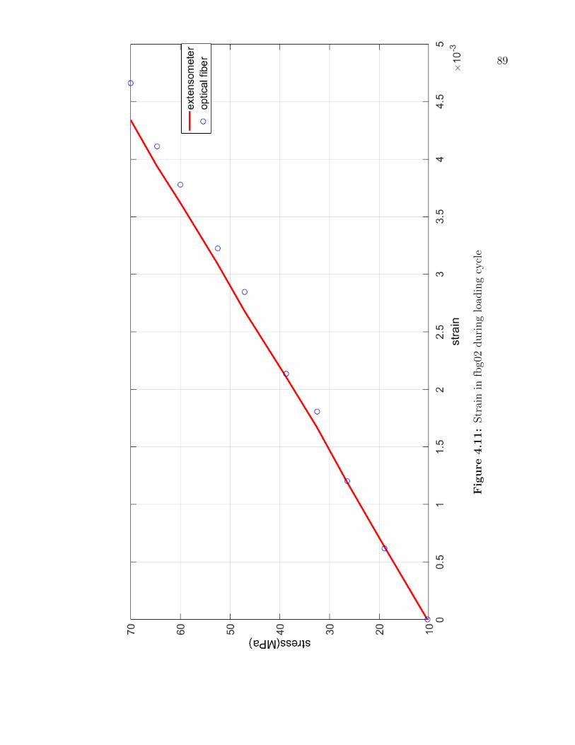
89
Fig
ure
4.1
1:
Str
ain
infb
g02
duri
ng
load
ing
cycl
e
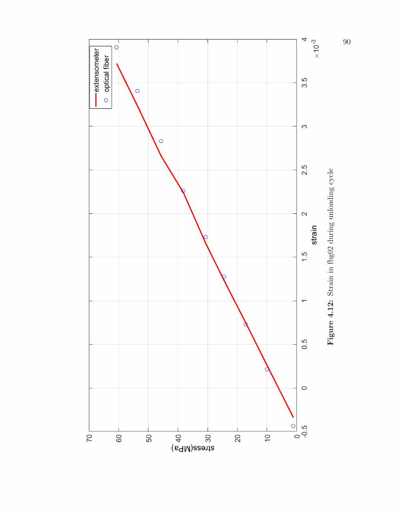
90
Fig
ure
4.1
2:
Str
ain
infb
g02
duri
ng
unlo
adin
gcy
cle

91
The stress-strain curve of the third sample with embedded optical fiber also
showed good agreement between the strain values obtained by extensometer and that
of the optical fiber. Plots are shown in Figure 4.13 and Figure 4.14.
The stress comparison for the full cycle in AA6061 aluminium is shown in Figure
4.15 and that of fiberglass with embedded optical fiber is shown in Figure 4.16. The
strain values measured from both methods seem to follow the same pattern with some
minor deviations with the exception being the first fiberglass coupon whose optical
fiber was not properly bonded with the parent material. However, the conclusion on
the nature of bonding can only be confirmed by cutting the sample and observing the
cross sectional area under a microscope.
The calculated data prove that the optical fibers recorded the correct strain
measurement during loading and unloading cycles while they were bonded on the
surface (in case of AA6061) as well as when they were embedded within the fiberglass.
Modulus of elasticity was calculated for each loading and unloading cycle from
the stress-strain curve. The values obtained for AA6061 using an extensometer and
embedded optical fiber are shown in Table 4.7. Modulus of Elasticity for fiberglass
coupons are displayed in Table 4.9, Table 4.10 and Table 4.11. Modulus calculated
from all the grating of the optical fiber were close with a standard deviation of 0.340
GPa as seen in Table 4.8.
Table 4.7: Comparison of modulus of elasticity in AA6061
Specimen Cycle E extensometer (GPa) E optical fiber (GPa)
Al01Loading 65.096 64.246
Unloading 66.122 64.970
Average 65.609 64.608
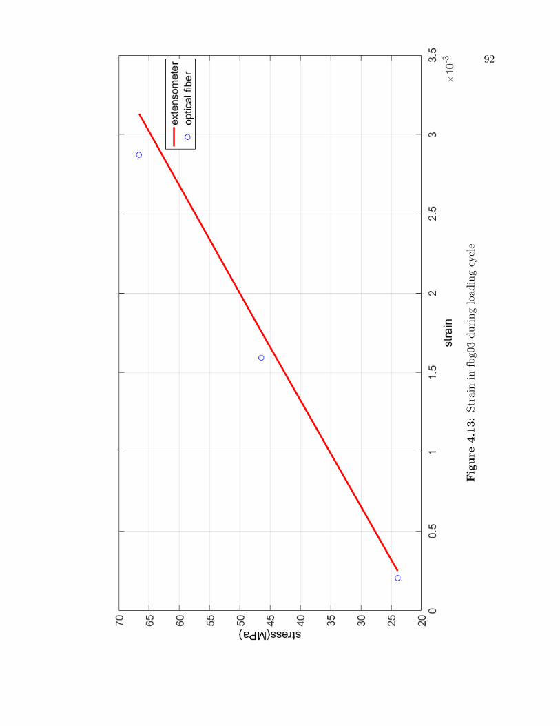
92
Fig
ure
4.1
3:
Str
ain
infb
g03
duri
ng
load
ing
cycl
e
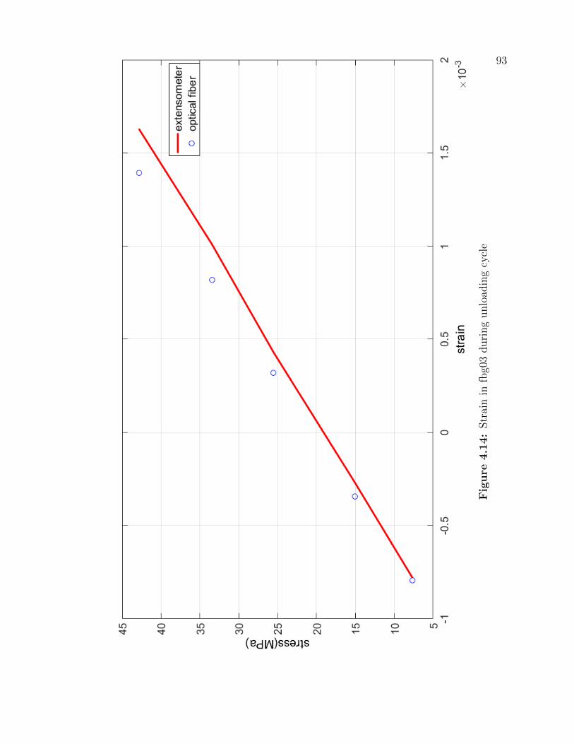
93
Fig
ure
4.1
4:
Str
ain
infb
g03
duri
ng
unlo
adin
gcy
cle
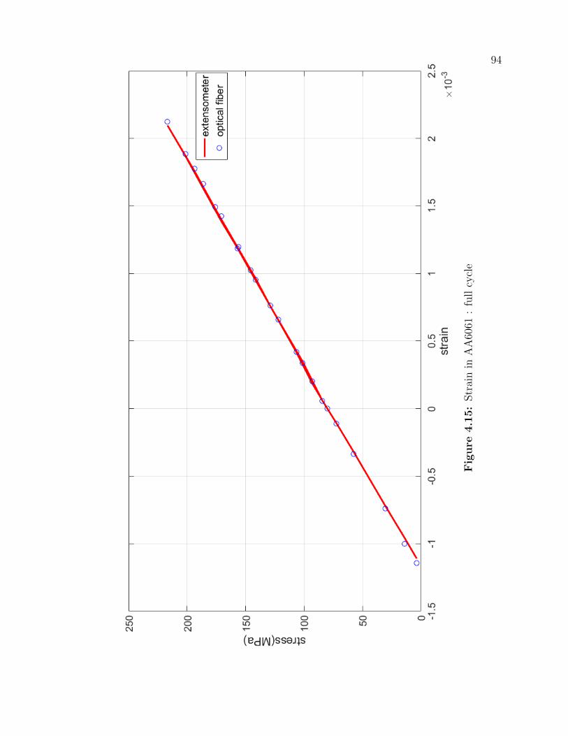
94
Fig
ure
4.1
5:
Str
ain
inA
A60
61:
full
cycl
e

95
Fig
ure
4.1
6:
Str
ain
infb
g02:
full
cycl
e

96
Table 4.8: Modulus measured by all the gratings of AA6061
Source E (GPa) Average (GPa) Standard Deviation (GPa)
Grating 1 64.353
64.459 0.340
Grating 2 63.941
Grating 3 64.583
Grating 4 64.842
Grating 5 64.2624
Grating 6 64.772
Extensometer 65.609
Table 4.9: Modulus of Elasticity in fbg01
Specimen Cycle E extensometer (GPa) E optical fiber (GPa)
fbg01
Loading1 7.142 18.116
Unloading1 9.755 13.569
Loading2 9.664 14.14
Unoading2 10.131 11.337
Loading3 10.484 14.457
Unloading3 11.556 -1.184
Average 9.788±1.46 11.739±6.69
As seen in Table 4.7, the average value of Modulus of Elasticity shows good
agreement with extensometer and optical fiber. In the case of fbg01, all the values
do not match with each other. This was expected as the stress-strain plot showed
that the strain values were not in coordination with each other. A possible reason for
this behaviour was that the embedded optical fiber was not properly bonded with the
host material. Also, E calculated by optical fiber was negative in the third unloading
cycle. The negative value of E in third unloading cycle affected the standard deviation
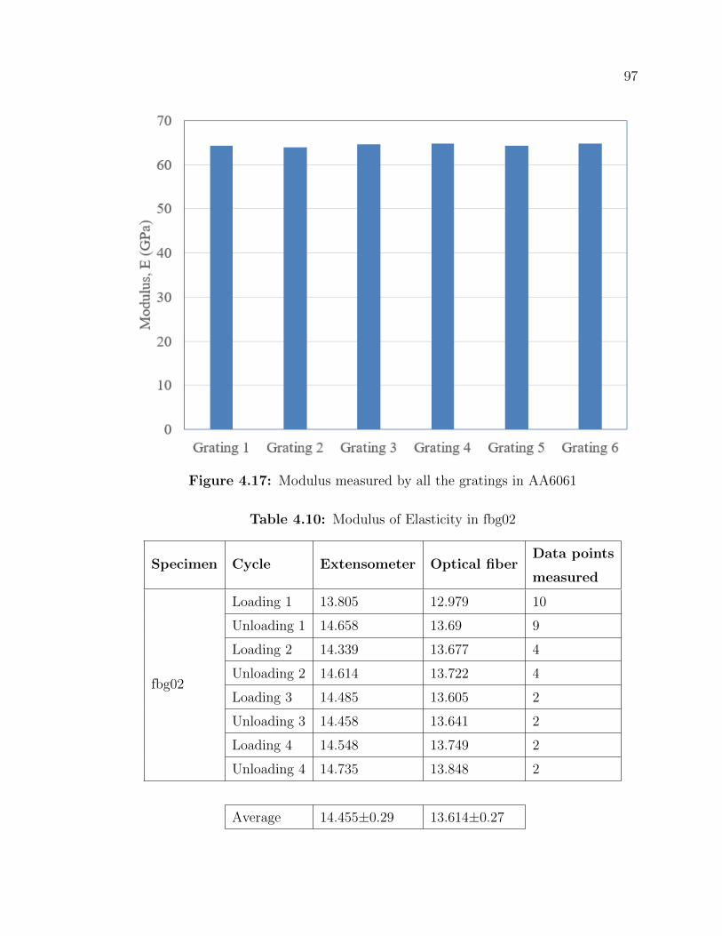
97
Figure 4.17: Modulus measured by all the gratings in AA6061
Table 4.10: Modulus of Elasticity in fbg02
Specimen Cycle Extensometer Optical fiberData points
measured
fbg02
Loading 1 13.805 12.979 10
Unloading 1 14.658 13.69 9
Loading 2 14.339 13.677 4
Unloading 2 14.614 13.722 4
Loading 3 14.485 13.605 2
Unloading 3 14.458 13.641 2
Loading 4 14.548 13.749 2
Unloading 4 14.735 13.848 2
Average 14.455±0.29 13.614±0.27
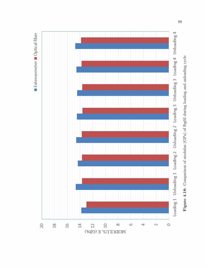
98
Fig
ure
4.1
8:
Com
par
ison
ofm
odulu
s(G
Pa)
offb
g02
duri
ng
load
ing
and
unlo
adin
gcy
cle
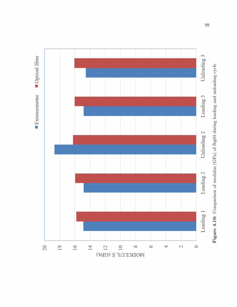
99
Fig
ure
4.1
9:
Com
par
ison
ofm
odulu
s(G
Pa)
offb
g03
duri
ng
load
ing
and
unlo
adin
gcy
cle
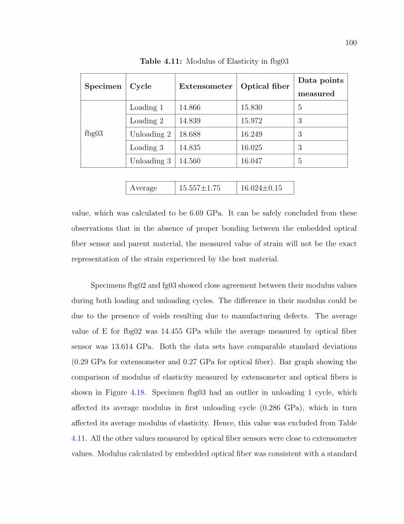
100
Table 4.11: Modulus of Elasticity in fbg03
Specimen Cycle Extensometer Optical fiberData points
measured
fbg03
Loading 1 14.866 15.830 5
Loading 2 14.839 15.972 3
Unloading 2 18.688 16.249 3
Loading 3 14.835 16.025 3
Unloading 3 14.560 16.047 5
Average 15.557±1.75 16.024±0.15
value, which was calculated to be 6.69 GPa. It can be safely concluded from these
observations that in the absence of proper bonding between the embedded optical
fiber sensor and parent material, the measured value of strain will not be the exact
representation of the strain experienced by the host material.
Specimens fbg02 and fg03 showed close agreement between their modulus values
during both loading and unloading cycles. The difference in their modulus could be
due to the presence of voids resulting due to manufacturing defects. The average
value of E for fbg02 was 14.455 GPa while the average measured by optical fiber
sensor was 13.614 GPa. Both the data sets have comparable standard deviations
(0.29 GPa for extensometer and 0.27 GPa for optical fiber). Bar graph showing the
comparison of modulus of elasticity measured by extensometer and optical fibers is
shown in Figure 4.18. Specimen fbg03 had an outlier in unloading 1 cycle, which
affected its average modulus in first unloading cycle (0.286 GPa), which in turn
affected its average modulus of elasticity. Hence, this value was excluded from Table
4.11. All the other values measured by optical fiber sensors were close to extensometer
values. Modulus calculated by embedded optical fiber was consistent with a standard
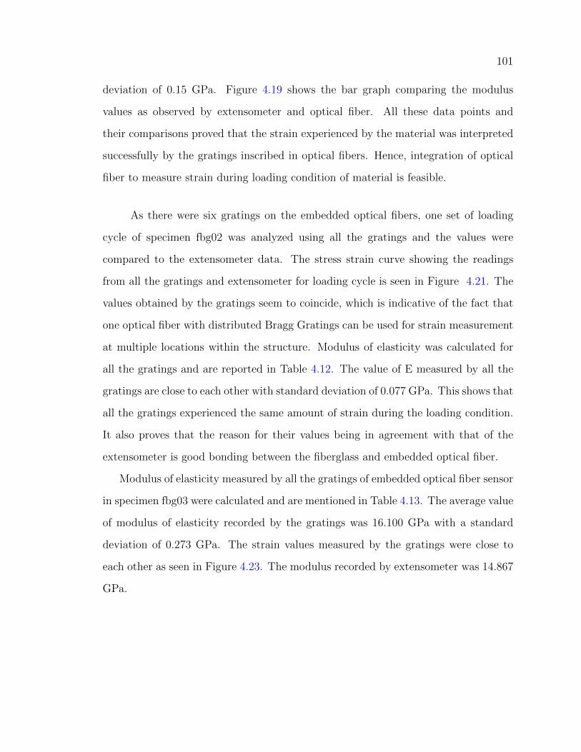
101
deviation of 0.15 GPa. Figure 4.19 shows the bar graph comparing the modulus
values as observed by extensometer and optical fiber. All these data points and
their comparisons proved that the strain experienced by the material was interpreted
successfully by the gratings inscribed in optical fibers. Hence, integration of optical
fiber to measure strain during loading condition of material is feasible.
As there were six gratings on the embedded optical fibers, one set of loading
cycle of specimen fbg02 was analyzed using all the gratings and the values were
compared to the extensometer data. The stress strain curve showing the readings
from all the gratings and extensometer for loading cycle is seen in Figure 4.21. The
values obtained by the gratings seem to coincide, which is indicative of the fact that
one optical fiber with distributed Bragg Gratings can be used for strain measurement
at multiple locations within the structure. Modulus of elasticity was calculated for
all the gratings and are reported in Table 4.12. The value of E measured by all the
gratings are close to each other with standard deviation of 0.077 GPa. This shows that
all the gratings experienced the same amount of strain during the loading condition.
It also proves that the reason for their values being in agreement with that of the
extensometer is good bonding between the fiberglass and embedded optical fiber.
Modulus of elasticity measured by all the gratings of embedded optical fiber sensor
in specimen fbg03 were calculated and are mentioned in Table 4.13. The average value
of modulus of elasticity recorded by the gratings was 16.100 GPa with a standard
deviation of 0.273 GPa. The strain values measured by the gratings were close to
each other as seen in Figure 4.23. The modulus recorded by extensometer was 14.867
GPa.
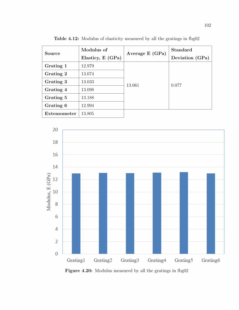
102
Table 4.12: Modulus of elasticity measured by all the gratings in fbg02
SourceModulus of
Elasticy, E (GPa)Average E (GPa)
Standard
Deviation (GPa)
Grating 1 12.979
13.061 0.077
Grating 2 13.074
Grating 3 13.033
Grating 4 13.098
Grating 5 13.188
Grating 6 12.994
Extensometer 13.805
Figure 4.20: Modulus measured by all the gratings in fbg02

103
Fig
ure
4.2
1:
Str
ain
mea
sure
dby
all
the
grat
ings
infb
g02
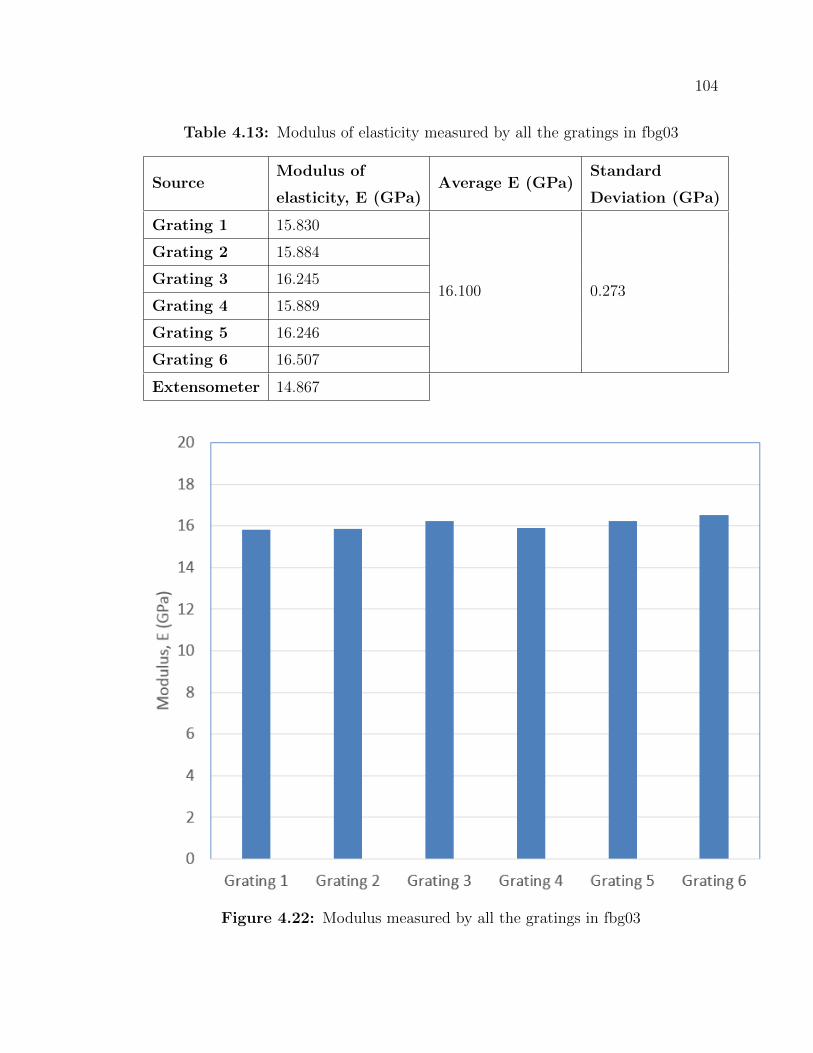
104
Table 4.13: Modulus of elasticity measured by all the gratings in fbg03
SourceModulus of
elasticity, E (GPa)Average E (GPa)
Standard
Deviation (GPa)
Grating 1 15.830
16.100 0.273
Grating 2 15.884
Grating 3 16.245
Grating 4 15.889
Grating 5 16.246
Grating 6 16.507
Extensometer 14.867
Figure 4.22: Modulus measured by all the gratings in fbg03
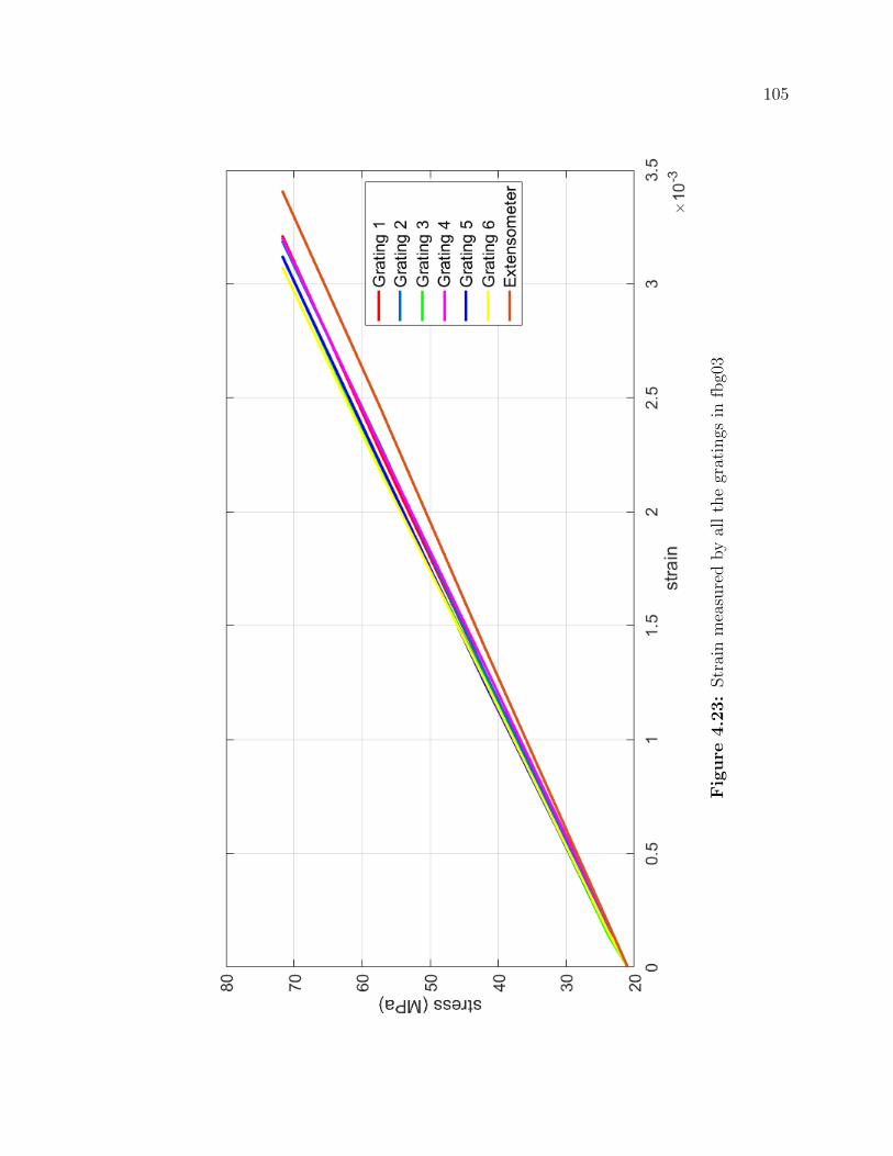
105
Fig
ure
4.2
3:
Str
ain
mea
sure
dby
all
the
grat
ings
infb
g03

Chapter 5
Conclusions and Recommendations
The conclusions drawn from this thesis and the recommendations for future
work are discussed in this chapter.
5.1 Conclusions
1. Based on available literature, optical fiber was embedded parallel to the ply
orientation. This was done because optical fiber embedded in other orientations has
an adverse effects on the mechanical properties of the host material.
2. In order to insert optical fiber within the fibers of fiberglass, a sewing needle
was used to make a guideway. Embedded optical fibers had ingress and egress points
at the ends of this guideway.
3. Optical fibers were placed in between the center plies of fiberglass, which were
oriented in the longitudinal direction. As the literature review suggested that there
was a deterioration in the tensile values when the optical fibers were not embedded
parallel to the fiberglass fabric, the optical fibers were placed in between the plies of
0◦ orientation.
4. A unique fixture consisting of five parts was designed to protect ingress and
egress points of embedded optical fibers. The parts can be easily assembled and
106
107
disassembled before and after the fabrication process. The optical fiber remained
coiled within the fixture during the manufacturing and cutting operation. It was
found that the ingress and egress points were safe during the entire process. As the
ingress/egress points were used to extract data from the embedded optical fibers to
measure the strain experienced by the material, protection of those points was im-
portant during manufacturing and cutting process. The design proposed was unique
for this research and it successfully served its purpose of protecting the ingress and
egress points.
5. Red laser light was used to check the structural integrity of the embedded
optical fibers after the specimens were made. Light was sent through one end and
its transmission was observed on the other end. This confirmed that the embedded
optical fibers remained undamaged during the manufacturing and cutting operation.
6. Tensile tests were conducted on fiberglass with and without embedded optical
fibers. The results showed that there was no adverse effect of embedding optical fibers
within fiberglass. It was found that modulus of elasticity of both types of specimens
were comparable within 10.324 % coefficient of variation.
7. The results of the impact tests showed that the impact energy required to
initiate fracture of the specimen was not affected when the specimen had embedded
optical fiber in their central plane.
8. The results of the flexural test showed that there was no deterioration in flexural
strength and flexural modulus of fiberglass when they had optical fibers embedded
within them.
9. The strain values recorded by embedded optical fiber sensors were found to be
in good agreement with extensometer data. Modulus of elasticity measured by the
optical fibers were comparable to the values measured using an extensometer during
loading and unloading cycles. The results showed that embedded optical fiber sensors
can be used to measure strain within the material as long as there is strong bonding
108
between the sensor and host material.
10. The strain and modulus values shown by all the gratings within the same
optical fiber were in agreement with each other, which proved that a single optical
fiber sensor can be used to detect strain at various locations in the material.
11. The design of the support fixture successfully protected the ingress and
egress points of embedded optical fibers. The strain experienced by the material
was recorded by embedded optical fibers. The objective of this research work was
met as both the aforementioned goals were achieved. In conclusion, it was shown that
optical fibers are a viable option for Structural Health Monitoring of out-of-autoclave
composite materials.
5.2 Recommendations
The following recommendations were made based on the performed research
work:
1. The work involved mechanical testing at room temperature. It would be
useful to examine the response of embedded optical fiber sensors at higher and lower
temperatures as an aircraft experiences both high and low temperatures during its
flight.
2. The fixture designed to protect ingress/egress points can be made from a
different material in order to serve its purpose at higher or cryogenic temperatures.
3. Data from embedded optical fibers were extracted using reflectometer, which is
a big and heavy instrument. It would be beneficial to use a smaller data acquisition
system, which could be easily carried on the aircraft and operated in flights to get
real time data.
4. It would be worthwhile to study fatigue tests of composite material with em-
bedded optical fibers to see if the embedment has any effect on the life of material.

109
5. The reason for mismatch between the strain values of optical fiber and ex-
tensometer should be explored by cutting the fiberglass specimen at various cross
sections and observing them under a microscope to inspect the nature of bonding
between fiberglass and embedded optical fiber.
6. More mechanical testing on composites with embedded optical fibers should be
done to build a statistical database.
References
[1] Deo R. B., Starnes Jr J. H., and Holzwarth R. C. Low-cost composite materials
and structures for aircraft applications. 2003.
[2] Botelho E. C., Silva R.A., Pardini L.C., and M.C.Rezend. A review on the devel-
opment and properties of continuous fiber/epoxy/aluminum hybrid composites
for aircraft structures. Materials Research, 9(3):247–256, 2006.
[3] Minakuchi S. and Takeda N. Recent advancement in optical fiber sensing for
aerospace composite structures. Photonic Sensors, 3(4):345–354, 2013.
[4] Habib F., Martinez M., Artemev A., and Brothers M. Structural health monitor-
ing of bonded composite repairs-a critical comparison between ultrasonic lamb
wave approach and surface mounted crack sensor approach. Composites Part B:
Engineering, 47:26–34, 2013.
[5] Beukema R.P. Embedding technologies of fbg sensors in composites: Technolo-
gies, applications and practical use. In Proceedings of the 6th European Workshop
on Structural Health Monitoring, Dresden, Germany, volume 3, 2012.
[6] Wu M.C, Winfree W.P, and Moore J.P. Fiber optic thermal health monitoring
of composites. In Proc. SPIE, volume 7648, page 764808, 2010.
[7] Furlong P.A.C. Strain Measurement of Composite Materials Using Fibre Optic
Sensors. PhD thesis, Carleton University, Ottawa, 2007.
[8] Glisic B. and Inaudi D. Integration of long-gage fiber optic sensor into a fiber-
reinforced composite sensing tape. In Smart Structures and Materials, pages
179–186. International Society for Optics and Photonics, 2003.
[9] Anastasi R. F and Lopatin C. Application of a fiber optic distributed strain
sensor system to woven e-glass composite. 2001.
110

111
[10] Giurgiutiu V. Structural Health Monitoring of Aerospace Composites. Academic
Press, 2015.
[11] Lissenden C. J and Rose J. L. Structural health monitoring of composite lami-
nates through ultrasonic guided wave beam forming. In NATO Applied Vehilce
Technology Symp. on Military Platform Ensured Availability Proc, 2008.
[12] Cai J., Liang D., Qiu L., Shi L., Liu P., and Yuan S. Structural Health Monitoring
for Composite Materials. INTECH Open Access Publisher, 2012.
[13] Rouchon J. Fatigue and damage tolerance evaluation of structures: the composite
materials response, 22nd plantema memorial lecture. In 25th Symposium of the
International Committee on Aeronautical Fatigue, volume 27, 2009.
[14] Kalhori H., Ye L., and Mustapha S. Inverse estimation of impact force on a com-
posite panel using a single piezoelectric sensor. Journal of Intelligent Material
Systems and Structures.
[15] Boller C. Next generation structural health monitoring and its integration into
aircraft design. International Journal of Systems Science, 31(11):1333–1349,
2000.
[16] Ko J.M. and Ni Y.Q. Technology developments in structural health monitoring
of large-scale bridges. Engineering structures, 27(12):1715–1725, 2005.
[17] Richards W.L, Parker Jr A. R, Ko W. L, Piazza A., and Chan P. Application of
fiber optic instrumentation. 2012.
[18] Fahr A. Aeronautical applications of non-destructive testing. DEStech Publica-
tions, Inc, 2013.
[19] Garnier C., Pastor M.L., Eyma F., and Lorrain B. The detection of aeronautical
defects in situ on composite structures using non destructive testing. Composite
structures, 93(5):1328–1336, 2011.
[20] Cawley P. The rapid non-destructive inspection of large composite structures.
Composites, 25(5):351–357, 1994.
[21] Bates D., Smith G., Lu D., and Hewitt J. Rapid thermal non-destructive testing
of aircraft components. Composites Part B: Engineering, 31(3):175–185, 2000.
[22] Prosser W.H, Allison S.G, Woodard S.E, Wincheski R.A, Cooper E.G, Price
D.C, Hedley M., Prokopenko M., Scott D.A, and Tessler A. Structural health
management for future aerospace vehicles. 2004.
112
[23] Satori K., Fukuchi K., Kurosawa Y., Hongo A., and Takeda N. Polyimide-
coated small-diameter optical fiber sensors for embedding in composite laminate
structures. In SPIE’s 8th Annual International Symposium on Smart Structures
and Materials, pages 285–294. International Society for Optics and Photonics,
2001.
[24] Richards L., Parker A.R, Ko W. L, and Piazza A. Fiber optic wing shape sensing
on nasa’s ikhana uav. 2008.
[25] Advisory Circular. Circular 20-107b. composite aircraft structure. Federal Avi-
ation Administration, 2009.
[26] Kang H.K, Park J.W, Ryu C.Y, Hong C.S, and Kim C.G. Development of fibre
optic ingress/egress methods for smart composite structures. Smart materials
and structures, 9(2):149, 2000.
[27] ASTM Standard et al. Standard test method for tensile properties of polymer
matrix composite materials. ASTM D3039/D 3039M, 2008.
[28] Brown T.L, Wood K. H, Childers B.A, Cano R.J, Jensen B.J, and Rogowski R.S.
Fiber optic sensors for health monitoring of morphing aircraft. In 1999 Sympo-
sium on Smart Structures and Materials, pages 60–71. International Society for
Optics and Photonics, 1999.
[29] Liu T., Wu M., Rao Y., Jackson D. A, and Fernando G. F. A multiplexed optical
fibre-based extrinsic fabry-perot sensor system for in-situ strain monitoring in
composites. Smart materials and structures, 7(4):550, 1998.
[30] Shyprykevich P., Fogg B.R, Murphy K.A, and Claus R.O. Performance of extrin-
sic fabry-perot optical fiber strain sensors in the presence of cyclic loads. In 1993
North American Conference on Smart Structures and Materials, pages 388–399.
International Society for Optics and Photonics, 1993.
[31] Glisic B. and Inaudi D. Integration of long-gage fiber optic sensor into a fiber-
reinforced composite sensing tape. In Smart Structures and Materials, pages
179–186. International Society for Optics and Photonics, 2003.
[32] Pant S. Lamb Wave Propagation and Material Characterization of Metallic
and Composite Aerospace Structures for Improved Structural Health Monitoring
(SHM). PhD thesis, Carleton University, Ottawa, 2014.
113
[33] Panopoulou A., Loutas T., Roulias D., Fransen S., and Kostopoulos V. Dynamic
fiber bragg gratings based health monitoring system of composite aerospace
structures. Acta Astronautica, 69(7):445–457, 2011.
[34] Kreuzer M. Strain measurement with fiber bragg grating sensors. HBM, Darm-
stadt, S2338-1.0 e, 2006.
[35] Tennyson R.C, Mufti A.A, Rizkalla S., Tadros G., and Benmokrane B. Structural
health monitoring of innovative bridges in canada with fiber optic sensors. Smart
materials and Structures, 10(3):560, 2001.
[36] Bueno P. M. Structural Design,FEM Analysis and Manufacturing of a Composite
Optic Fibre Instrumented UAV Wing. Masters thesis, TU Delft, 2014.
[37] Samiec D. Distributed fibre-optic temperature and strain measurement with
extremely high spatial resolution. Photonik international, 1:10–13, 2012.
[38] Soller B., Peairs D., Sang A., and Fernandez A. Monitoring carbon composite
structures with optical fiber sensors. National Aeronautics and Space Adminis-
tration (NASA) Tech Briefs, 2010.
[39] Zhou D.P, Li W., L.Chen, and Bao X. Distributed temperature and strain
discrimination with stimulated brillouin scattering and rayleigh backscatter in
an optical fiber. Sensors, 13(2):1836–1845, 2013.
[40] Lee B.H., Kim Y.H, Park K.S, Eom J.B., Kim M.J., Rho B.S., and Choi H.Y.
Interferometric fiber optic sensors. Sensors, 12(3):2467–2486, 2012.
[41] Keulen C., Rocha B., Yildiz M., and Suleman A. Embedded fiber optic sensors
for monitoring processing, quality and structural health of resin transfer molded
components. In Journal of Physics: Conference Series, volume 305, page 012135.
IOP Publishing, 2011.
[42] Ramakrishnan M., Rajan G., Semenova Y., and Farrell G. Overview of fiber op-
tic sensor technologies for strain/temperature sensing applications in composite
materials. Sensors, 16(1):99, 2016.
[43] Green A.K, Darvish S., and Shafir E. Practical terminations for optical fibres
embedded in composite materials. In 3rd International Conference on Intelligent
Materials, pages 209–212. International Society for Optics and Photonics, 1996.

114
[44] Hong C.S, Park J.W, Ryu C.Y, and Kang H.K. Signal characteristics of efpi in
the delaminated composites. In Optical Fiber Sensors, volume 3746, page 192,
1999.
[45] Hadzic R., John S., and I. Herszberg. Structural integrity analysis of embedded
optical fibres in composite structures. Composite structures, 47(1):759–765, 1999.
[46] Lee D.C, Lee J.J, and Yun S.J. The mechanical characteristics of smart composite
structures with embedded optical fiber sensors. Composite Structures, 32(1-
4):39–50, 1995.
[47] Jensen D.W, Pascual J., and August J.A. Performance of graphite/bismaleimide
laminates with embedded optical fibers. part i. uniaxial tension. Smart Materials
and Structures, 1(1):24, 1992.
[48] Jensen D.W, Pascual J., and August J.A. Performance of graphite/bismaleimide
laminates with embedded optical fibers.part ii. uniaxial compression. Smart
Materials and Structures, 1(1):24, 1992.
[49] Pedrazzani J.R., Klute S.M, Gifford D.K, Sang A.K, and Froggatt M.E. Em-
bedded and surface mounted fiber optic sensors detect manufacturing defects
and accumulated damage as a wind turbine blade is cycled to failure. Luna
Innovations Inc, 2012.
[50] Torres B., Paya-Zaforteza I., Caldero P.A, and Adam J.M. Analysis of the
strain transfer in a new fbg sensor for structural health monitoring. Engineering
Structures, 33(2):539–548, 2011.
[51] Pilling M.W, Yates B., Black M.A, and Tattersall P. The thermal conductivity
of carbon fibre-reinforced composites. Journal of Materials Science, 14(6):1326–
1338, 1979.
[52] Huerta E., Corona J.E, Oliva A.I, Aviles F., and Gonzalez-Hernandez J. Univer-
sal testing machine for mechanical properties of thin materials. Revista mexicana
de fısica, 56(4):317–322, 2010.
[53] Oliver W.C and Pharr G.M. Measurement of hardness and elastic modulus
by instrumented indentation: Advances in understanding and refinements to
methodology. Journal of materials research, 19(01):3–20, 2004.
[54] ASTM Standard. D7136: Standard test method for measuring the damage re-
sistance of a fiber-reinforced polymer matrix composite to a drop-weight impact
event. ASTM International: West Conshohocken, 2005.

115
[55] ASTM Standard. Standard test method for flexural properties of polymer matrix
composite materials. ASTM D7264/ D7264-M.

Appendix A
Model Parameters and Material
Properties
A.1 Data sheet of optical fiber
116
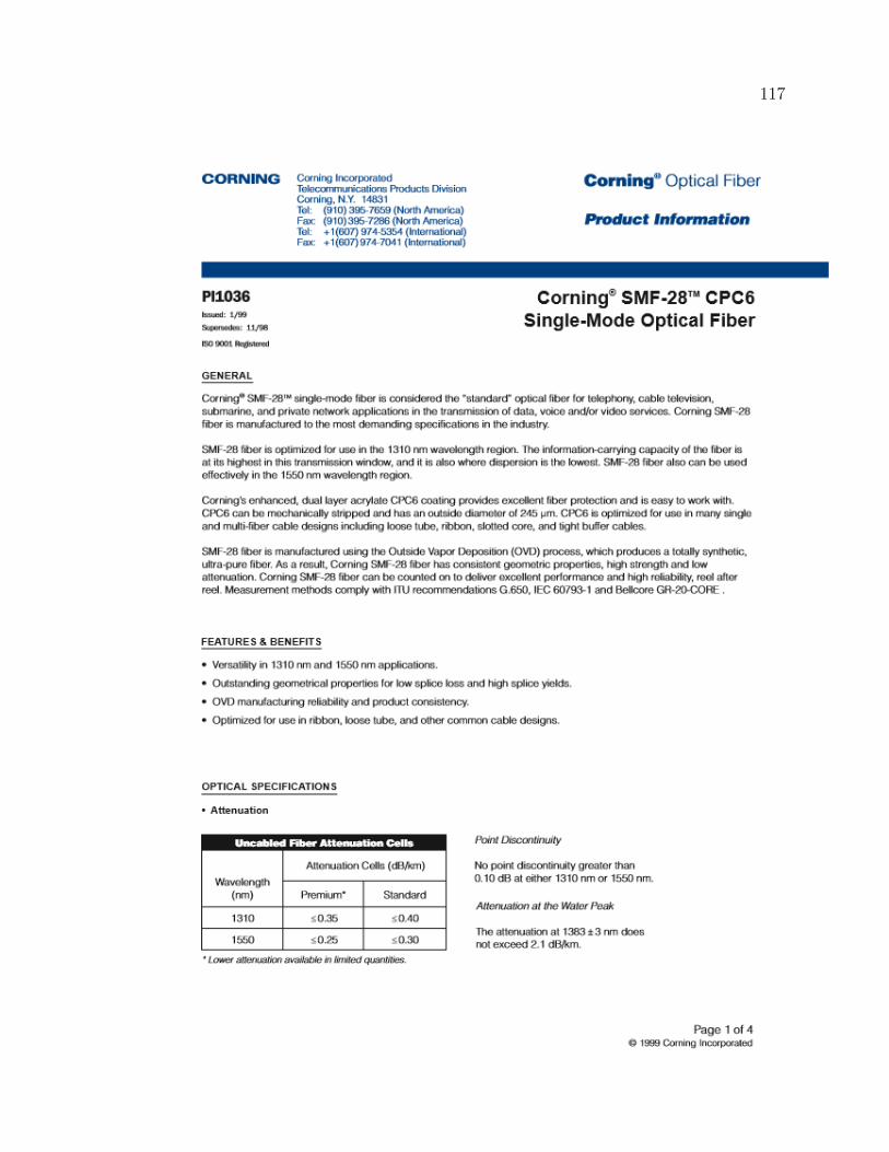
117
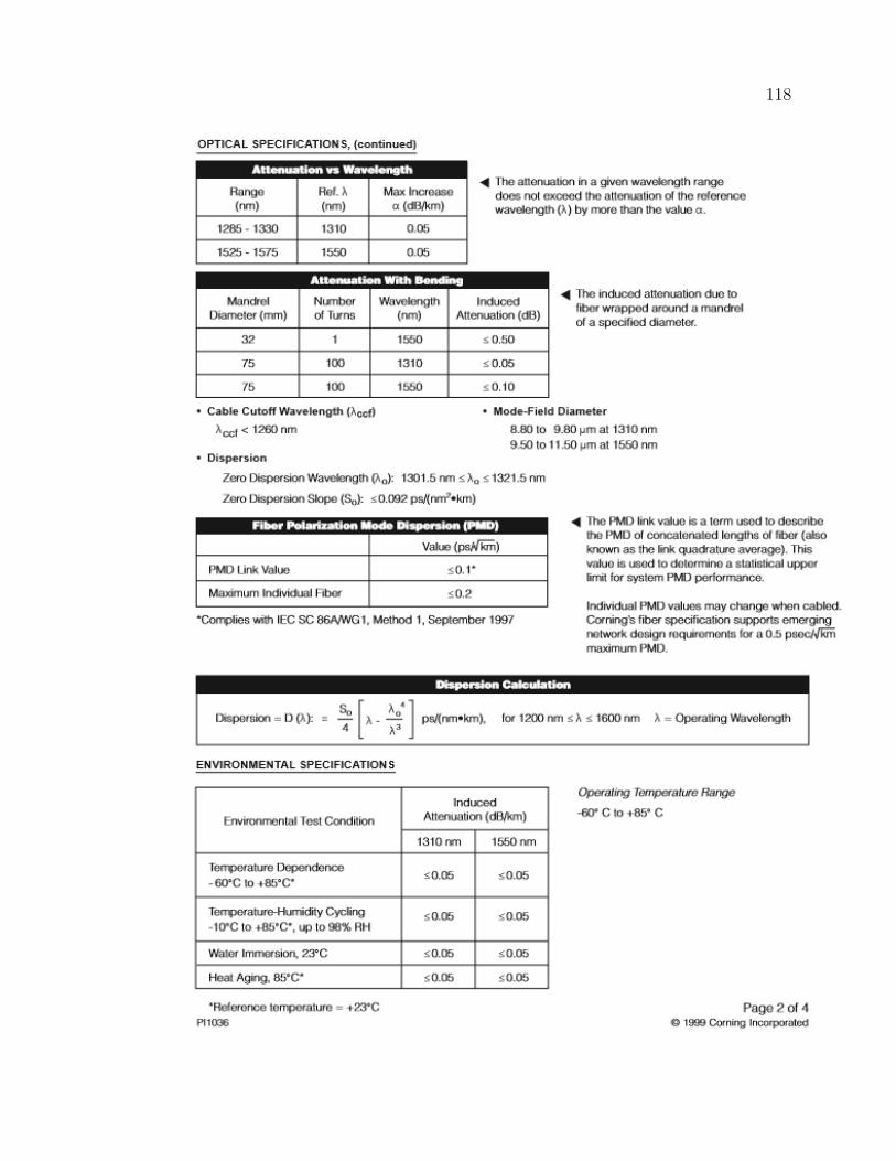
118

119
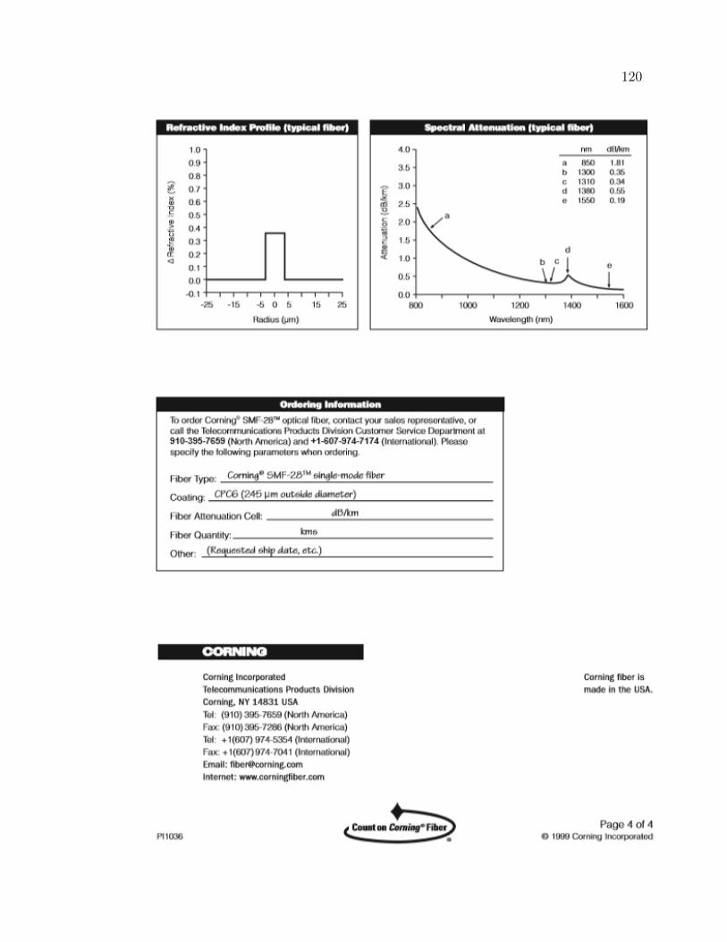
120

Appendix B
Testing parameters
B.1 Calculation of Young’s Modulus Using Com-
pliance
Total compliance (CT ) measured by the crosshead during tensile testing is the
sum of the material’s compliance (Cmat) and the machine’s compliance (Cm) [52].
CT = Cmat + Cm
The load vs displacement curves of stainless steel was plotted using the crosshead
and extensometer displacements and can be seen in Figure 3.43. Compliance is the
inverse of the slope of the load-displacement curve [52,53]. For a test coupon of cross
sectional area, A and gage length, L, the modulus, E is defined as :
E =σ
ε=
FL
A∆L
where, σ is the stress and ε is the strain experienced by the material.
121
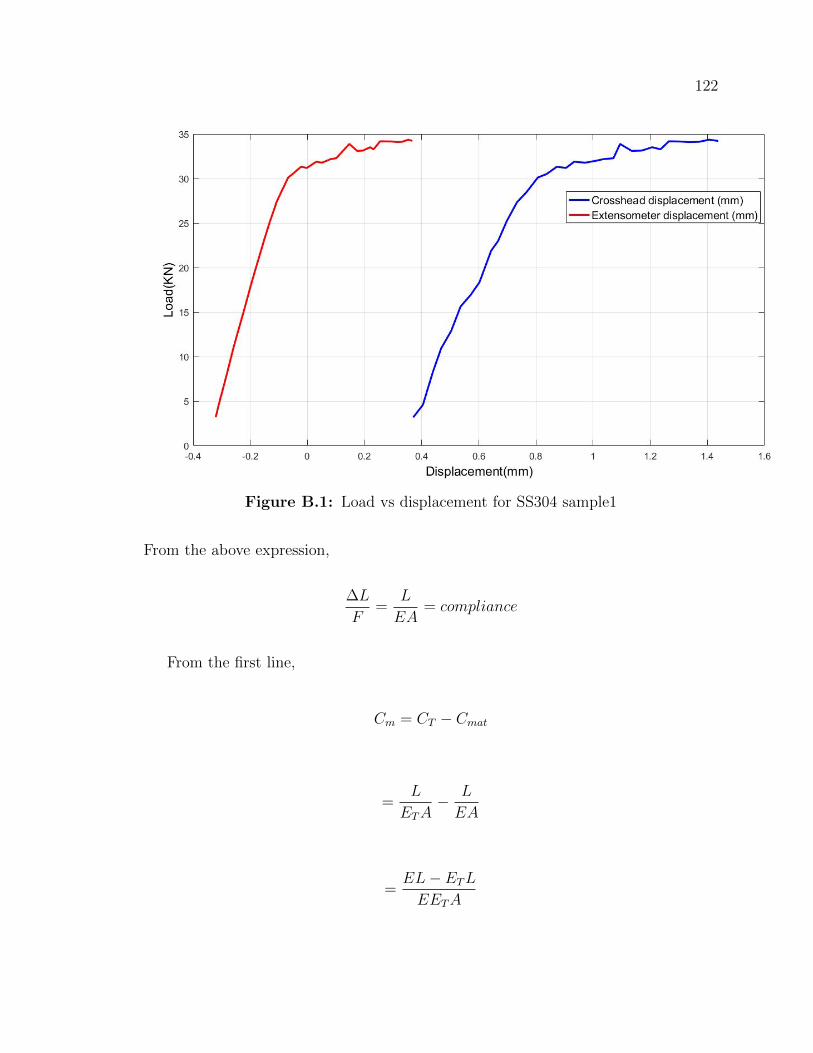
122
Figure B.1: Load vs displacement for SS304 sample1
From the above expression,
∆L
F=
L
EA= compliance
From the first line,
Cm = CT − Cmat
=L
ETA− L
EA
=EL− ETL
EETA

123
EL− ETL = CmEETA
E − CmEETA
L= ET
E(1 − CmETA
L) = ET
E =ET
1 − CmETAL
This equation is used to calculate modulus of material, E using machine’s com-
pliance, Cm.
B.2 Stress-strain curves
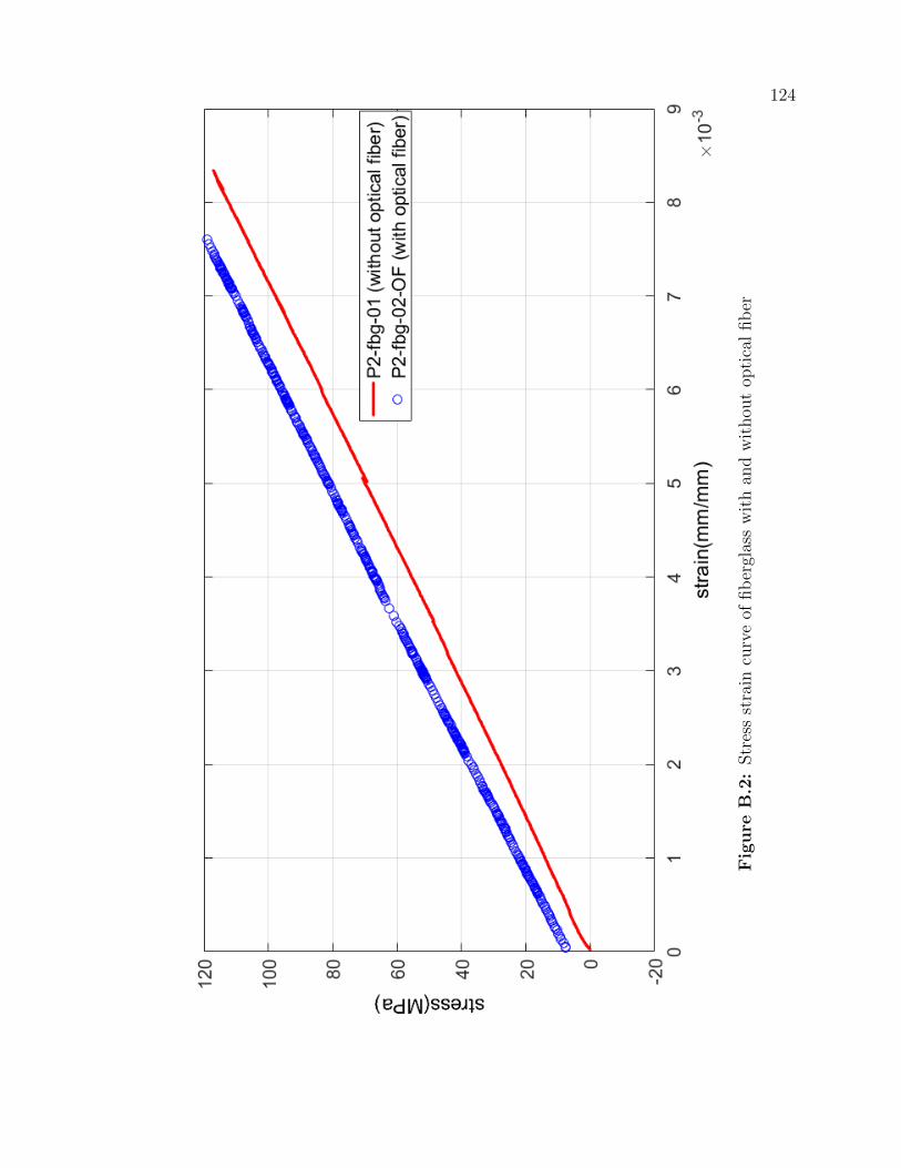
124
Fig
ure
B.2
:Str
ess
stra
incu
rve
offib
ergl
ass
wit
han
dw
ithou
top
tica
lfib
er
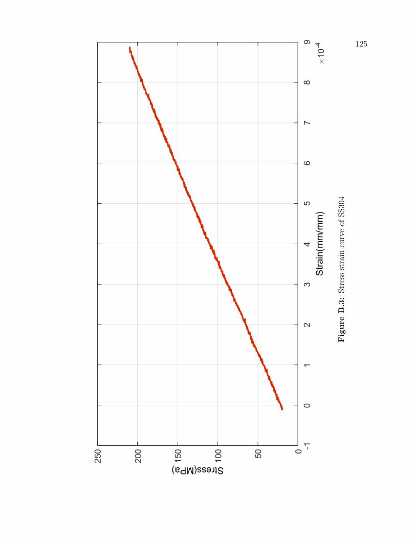
125
Fig
ure
B.3
:Str
ess
stra
incu
rve
ofSS30
4
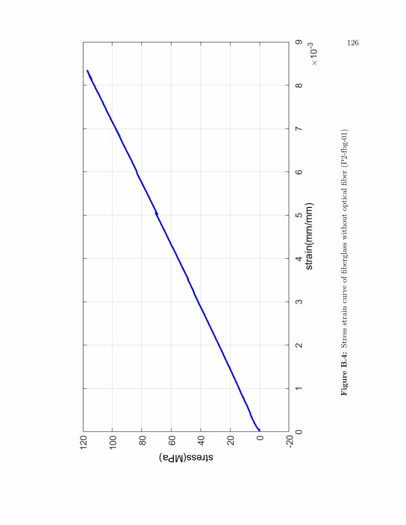
126
Fig
ure
B.4
:Str
ess
stra
incu
rve
offib
ergl
ass
wit
hou
top
tica
lfib
er(P
2-fb
g-01
)
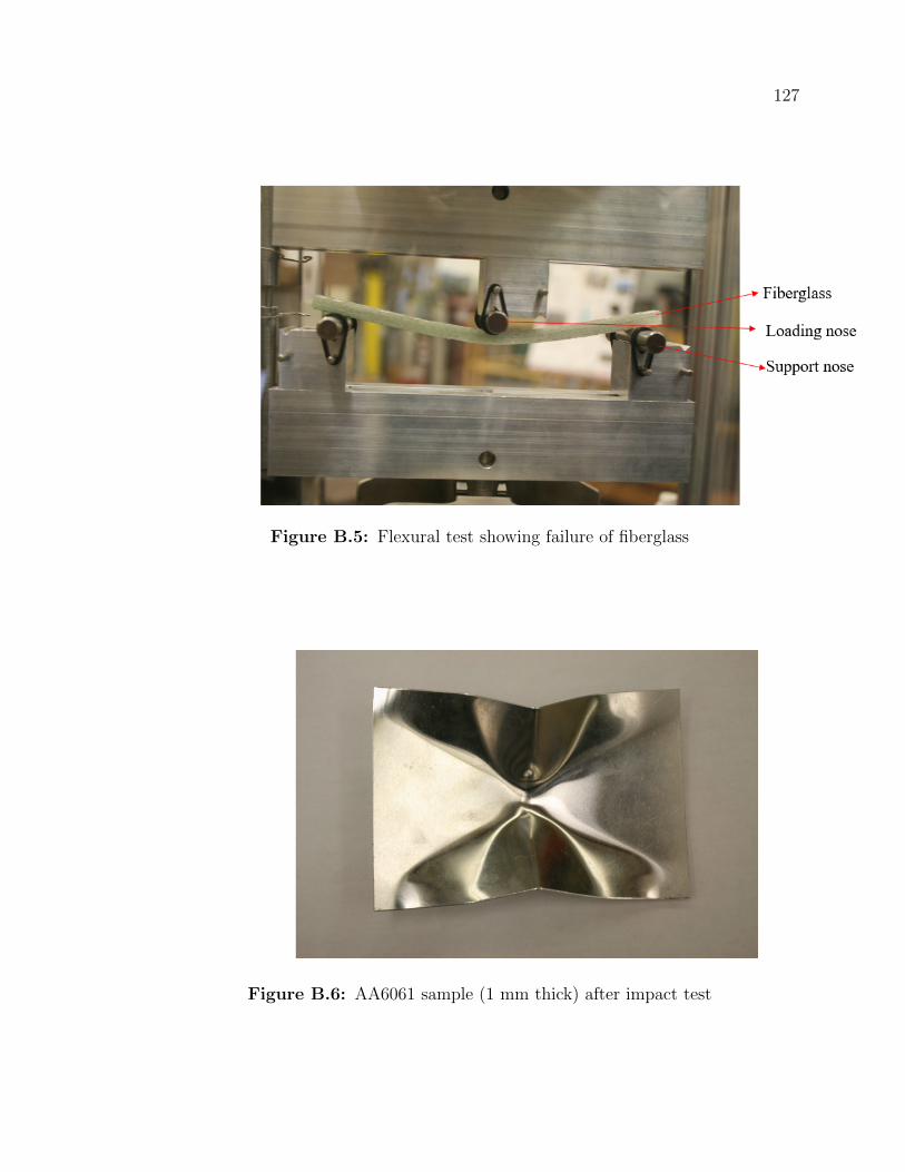
127
Figure B.5: Flexural test showing failure of fiberglass
Figure B.6: AA6061 sample (1 mm thick) after impact test

Appendix C
Data Sheet of Epoxy Resin
128
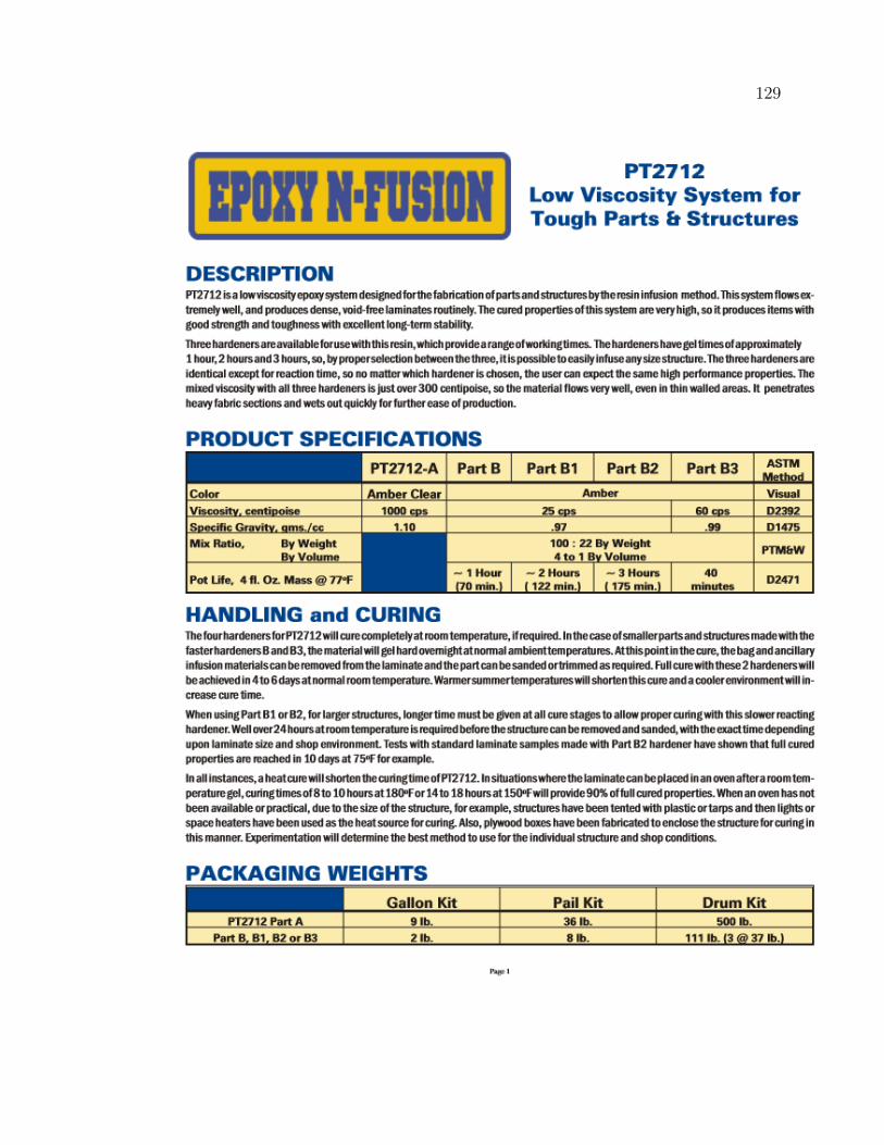
129

130
Copyright © 2022 FDOKUMEN