USE OF GRAPH THEORY AND NETWORKS IN BIOLOGY
10
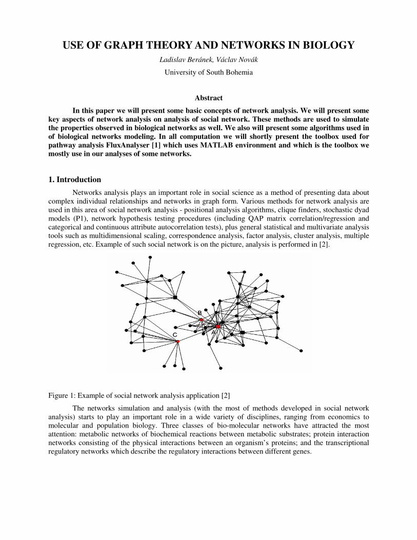
USE OF GRAPH THEORY AND NETWORKS IN BIOLOGY Ladislav Beránek, Václav Novák University of South Bohemia Abstract In this paper we will present some basic concepts of network analysis. We will present some key aspects of network analysis on analysis of social network. These methods are used to simulate the properties observed in biological networks as well. We also will present some algorithms used in of biological networks modeling. In all computation we will shortly present the toolbox used for pathway analysis FluxAnalyser [1] which uses MATLAB environment and which is the toolbox we mostly use in our analyses of some networks. 1. Introduction Networks analysis plays an important role in social science as a method of presenting data about complex individual relationships and networks in graph form. Various methods for network analysis are used in this area of social network analysis - positional analysis algorithms, clique finders, stochastic dyad models (P1), network hypothesis testing procedures (including QAP matrix correlation/regression and categorical and continuous attribute autocorrelation tests), plus general statistical and multivariate analysis tools such as multidimensional scaling, correspondence analysis, factor analysis, cluster analysis, multiple regression, etc. Example of such social network is on the picture, analysis is performed in [2]. Figure 1: Example of social network analysis application [2] The networks simulation and analysis (with the most of methods developed in social network analysis) starts to play an important role in a wide variety of disciplines, ranging from economics to molecular and population biology. Three classes of bio-molecular networks have attracted the most attention: metabolic networks of biochemical reactions between metabolic substrates; protein interaction networks consisting of the physical interactions between an organism’s proteins; and the transcriptional regulatory networks which describe the regulatory interactions between different genes.
-
Upload
independent -
Category
Documents
-
view
0 -
download
0
Transcript of USE OF GRAPH THEORY AND NETWORKS IN BIOLOGY
USE OF GRAPH THEORY AND NETWORKS IN BIOLOGY
Ladislav Beránek, Václav Novák
University of South Bohemia
Abstract
In this paper we will present some basic concepts of network analysis. We will present some
key aspects of network analysis on analysis of social network. These methods are used to simulate
the properties observed in biological networks as well. We also will present some algorithms used in
of biological networks modeling. In all computation we will shortly present the toolbox used for
pathway analysis FluxAnalyser [1] which uses MATLAB environment and which is the toolbox we
mostly use in our analyses of some networks.
1. Introduction
Networks analysis plays an important role in social science as a method of presenting data about
complex individual relationships and networks in graph form. Various methods for network analysis are
used in this area of social network analysis - positional analysis algorithms, clique finders, stochastic dyad
models (P1), network hypothesis testing procedures (including QAP matrix correlation/regression and
categorical and continuous attribute autocorrelation tests), plus general statistical and multivariate analysis
tools such as multidimensional scaling, correspondence analysis, factor analysis, cluster analysis, multiple
regression, etc. Example of such social network is on the picture, analysis is performed in [2].
Figure 1: Example of social network analysis application [2]
The networks simulation and analysis (with the most of methods developed in social network
analysis) starts to play an important role in a wide variety of disciplines, ranging from economics to
molecular and population biology. Three classes of bio-molecular networks have attracted the most
attention: metabolic networks of biochemical reactions between metabolic substrates; protein interaction
networks consisting of the physical interactions between an organism’s proteins; and the transcriptional
regulatory networks which describe the regulatory interactions between different genes.
2. Key Concepts of Network Analysis
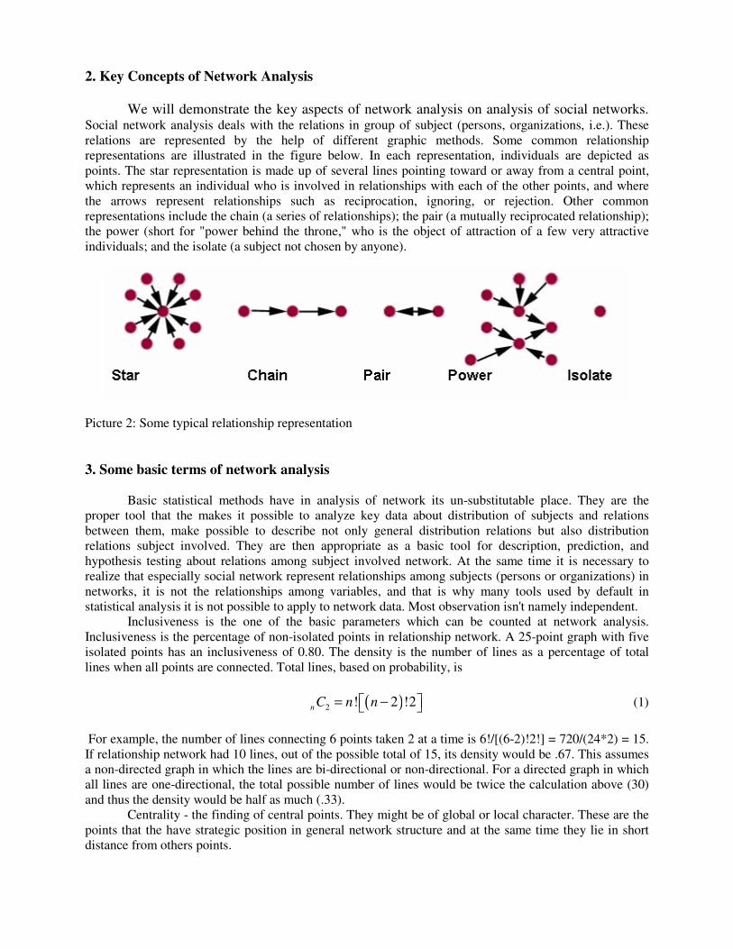
We will demonstrate the key aspects of network analysis on analysis of social networks. Social network analysis deals with the relations in group of subject (persons, organizations, i.e.). These
relations are represented by the help of different graphic methods. Some common relationship
representations are illustrated in the figure below. In each representation, individuals are depicted as
points. The star representation is made up of several lines pointing toward or away from a central point,
which represents an individual who is involved in relationships with each of the other points, and where
the arrows represent relationships such as reciprocation, ignoring, or rejection. Other common
representations include the chain (a series of relationships); the pair (a mutually reciprocated relationship);
the power (short for "power behind the throne," who is the object of attraction of a few very attractive
individuals; and the isolate (a subject not chosen by anyone).
Picture 2: Some typical relationship representation
3. Some basic terms of network analysis Basic statistical methods have in analysis of network its un-substitutable place. They are the
proper tool that the makes it possible to analyze key data about distribution of subjects and relations
between them, make possible to describe not only general distribution relations but also distribution
relations subject involved. They are then appropriate as a basic tool for description, prediction, and
hypothesis testing about relations among subject involved network. At the same time it is necessary to
realize that especially social network represent relationships among subjects (persons or organizations) in
networks, it is not the relationships among variables, and that is why many tools used by default in
statistical analysis it is not possible to apply to network data. Most observation isn't namely independent.
Inclusiveness is the one of the basic parameters which can be counted at network analysis.
Inclusiveness is the percentage of non-isolated points in relationship network. A 25-point graph with five
isolated points has an inclusiveness of 0.80. The density is the number of lines as a percentage of total
lines when all points are connected. Total lines, based on probability, is
( )2 ! 2 !2nC n n= − (1)
For example, the number of lines connecting 6 points taken 2 at a time is 6!/[(6-2)!2!] = 720/(24*2) = 15.
If relationship network had 10 lines, out of the possible total of 15, its density would be .67. This assumes
a non-directed graph in which the lines are bi-directional or non-directional. For a directed graph in which
all lines are one-directional, the total possible number of lines would be twice the calculation above (30)
and thus the density would be half as much (.33).
Centrality - the finding of central points. They might be of global or local character. These are the
points that the have strategic position in general network structure and at the same time they lie in short
distance from others points.
The representation in form of matrix is used for practical calculations. Matrix has a square shape
matrix with proportion n x n and represents individual persons involved in rows and columns.
Relationships can be expressed by various values. For example the question „ whom would you preferably
work with?" could be rate by values: interest in cooperation = +1, incuriousness = 0, entire rejection (I
shan't him like) = -1. This information can be for example used for creating of an index of popularity in a
group by comparison of relationships of members which were chosen like desirable working partners with
relationships in all of group. Likewise the relationship matrix is often used that records only existence or
non-existence of relationship between couple of persons involved or for example whether among couple
person involved happens to exchange information or no. Valuation of such relationship is dichotomous
and established matrix matches the adjacency matrix used in graph theory.
4. Visual exploration of network
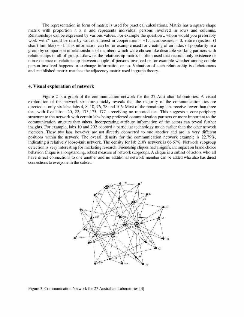
Figure 2 is a graph of the communication network for the 27 Australian laboratories. A visual
exploration of the network structure quickly reveals that the majority of the communication tics are
directed at only six labs: labs 4, 8, 10, 76, 78 and 106. Most of the remaining labs receive fewer than three
ties, with five labs - 20, 22, 173,175, 177 - receiving no reported ties. This suggests a core-periphery
structure to the network with certain labs being preferred communication partners or more important to the
communication structure than others. Incorporating attribute information of the actors can reveal further
insights. For example, labs 10 and 202 adopted a particular technology much earlier than the other network
members. These two labs, however, are not directly connected to one another and are in very different
positions within the network. The overall density for the communication network example is 22.79%,
indicating a relatively loose-knit network. The density for lab 210's network is 66.67%. Network subgroup
detection is very interesting for marketing research. Friendship cliques had a significant impact on brand choice
behavior. Clique is a longstanding, robust measure of network subgroups. A clique is a subset of actors who all
have direct connections to one another and no additional network member can be added who also has direct
connections to everyone in the subset.
Figure 3: Communication Network for 27 Australian Laboratories [3]

4. Some basic statistical methods
4.1 Use descriptive statistics
It is possible to demonstrate the use of descriptive statistical methods on data [4]. They reflect
relationships (information and financial resources exchange) among ten organizations providing social
service.
Picture 3: Relationship matrix between ten organizations providing social services [4]
The matrix is representing relationship - information exchange. If Xij = 1, the the information exchange
between appropriate couple of organization exists, if Xij = 0, then no exchange exists.
Picture 4: The basic data of descriptive statistics calculated by the help of the program UCINET
Here for example we have 100 observations. However the relationship of each subject to itself
(on main diagonal) are not purposeful. Hence the number of observations is N * N - 10 = 90. Number of
relationships is 49. Average value of relationship is 49/90 = 0,544. It labels the probability, that the
between the two person there has been relation. Next data descriptive statistics can be performed
according to standard procedures.
We can describe the distribution of relationship for all subjects in network or we also can calculate the
distribution for individual subjects.

4.2 Testing hypothesis Analogous to other applications and in network analyses the frequent problem is to compare e.g.
the statistics Z of observed network with its theoretic value µ. An example can be the network by its help
it is possible to simulate the viral infection spread. Here it pays, that the bigger density of the network the
faster and reliable virus extends. On the basis of theoretic considerations it was proven, the threshold
value of network density exists. If the network density is lower than this threshold value, then epidemic
won't evolve, if the value is higher than threshold then epidemic will evolve. Therefore at simulation of
epidemic it is solved the question, whether the density of the given network is smaller or greater than the
critical value.
Standard access in this situation is to define null hypothesis that affirms that the network density is
lower than parameter µ. This hypothesis is rejected in the event that the observed statistics is sufficiently
greater than parameter relative to standard error of observation parameter value. Statistics has form:
Zt
µ
σ
−= (2)
We reject null hypothesis if t is greater than 1.645, which is the critical value for single tail test of
standardized normal distribution for α = 0.05.
It is possible to demonstrate the procedure on data from literature. Let us take the network of friendship
ties among 67 prison [5]. Supposed, that the theoretic "tipping point" that the separates epidemic from its
extinction occurs at density 3%. The observed density for this network is 0.0412, standard error is 0.0060.
Converting to standard error units, we get (0.0412 - 0.03)/0.0060 = 1.87. This value is larger than 1.645.
Therefore, we reject null hypothesis and provisionally conclude that the prison population is in danger.
4.3 Comparing two networks
Another important application area is the comparison for two different groups (eventually
comparison different part one’s nets). For example, Ziegler et al. [8] published corporate interlocks among
major German business entities (15 in total). Stockman et al [7] published interlocks among major Dutch
business entities (16 in total). Data are accessible also in software tool UCINET 5 for network analyses
[6]. Question that the on the basis these accessible data we can lay up is: is the level of interlocks similar
or different in the two countries?
The observed density of the Dutch network was 0.5, while density of the German network was
0.6381, for an observed difference of 0.1381.
We will formulate the null hypothesis in the statement: “the network density is the same in both
network”. Testing statistics will have form
1 2
2 2
1 2
Z Zt
SE SE
−=
+ (3)
where SE1 and SE2 are standard errors usually estimated from standard deviation of the measured variable
in each sample. The standard errors of the Dutch and German nets are 0.0902 and 0.1083 respectively.
After substitution the testing statistics takes the value of 0.9798. We reject the null hypothesis. It is
impossible to conclude, that the Dutch and German economy have develop different level of corporate
interlock.
Analogous to this it is possible to compare the relationship of the same subjects in the same
network but at in the different time, to test hypotheses about relations inside/among groups of subjects in
network, to test hypotheses about relationships and subjects location in network ant other.
5. Other methods used in network analysis
From other methods used in network analysis it is especially:
Path diagrams (can be but not necessarily) based on actual path analysis, represent variables or groups as
circles, relationships (which may be correlations, communications, formal associations, or other
interactions) as arrows, and, often, magnitude of relationship by thickness of the arrow.
Cluster diagrams represent variables or groups as points on one or more two-dimensional
scatterplots or polar plots, with the proximity of points representing their similarity on the dimensions, and
clusters of points may be highlighted by perimeter lines around each cluster (including the possibility of
intersecting perimeters where a point may belong to two or more clusters).
Factor plots similarly represent variables or groups as points on one or more two-dimensional
scatterplots, where the dimensions are factors (see factor analysis); optionally, factor space may be
divided into non-intersecting quadrants to highlight similarities among points.
Centrality plots are polar plots in which the heavier the loading of the variable or group on the
dimension, the closer it is located to the center of the plot. Optionally, concentric circles may highlight
which points share a similar degree of centrality on the depicted dimension. Loadings may reflect factor
loadings, path distances, or an index of the author's devising. Centrality index numbers, if assigned to
points, are usually coded such that heavier loadings are represented as lower numbers. In centrality plots,
direction of location with respect to the center (up/down, left/right) often has no meaning other than
aesthetics of placement, but direction can be used to depict a second and third dimension.
Spatial network diagrams. In the context of geographic information systems, various software
implement network analysis modules which generate map graphics depicting such things as shortest route
between two objects, optimal route passing through a series of objects, or service areas (by best time or
shortest distance) associated with multiple points.
6. Biological networks
6.1 Structural aspects
In biological networks following three structural aspects are mostly used for analysis:
(i) Degree distribution,
(ii) Characteristic path length,
(iii) Modular structure and local clustering properties.
Degree of distribution measures ratio of nodes in the network having the degree k:
n
nkP
k=)( (4)
where nk is the number of nodes in the network of degree k and n is the size of the network.
The degree distributions of the Internet and the WWW are described [9] to have degree of distribution in
the form:
1,)( <= − γγkkP (5)
Networks with degree distributions of this form are now commonly denoted to as scale-free networks.
Characteristic Path Length
Path lengths and diameters of bio-molecular networks are “small” in comparison to network size.
Specifically, if the size of a network is n, the average path length and diameter are of the same order of
magnitude as log(n) or even smaller. This property has been previously noted for a variety of other
technological and social networks [2], and is often referred to as the small world property. This
phenomenon has now been observed in metabolic, genetic and protein interaction networks [10, 11].
In a sense, the average path length in a network is an indicator of how readily “information” can be
transmitted through it. Thus, the small world property observed in biological networks suggests that such
networks are efficient in the transfer of biological information.
Clustering and Modularity
In a highly clustered network, the neighbors of a given node are very likely to be themselves linked by an
edge. Typically, the first step in studying the clustering and modular properties of a network is to calculate
its average clustering coefficient, C, and the related function, C(k), which gives the average clustering
coefficient of nodes of degree k in the network. The form of this function can give insights into the global
network structure.
6.2 Models of interaction networks
These models could be used to assess the reliability of experimental results on network structure and to
assist in experimental design. Several different mathematical models of complex networks have been
proposed in the literature. A number of these were not developed with specifically biological networks in
mind, but rather to account for some of the topological features observed in real networks in Biology and
elsewhere. On the other hand, in the recent past several models for protein interaction and genetic
networks have been proposed based on biological assumptions.
Classical Models and Scale-free Graphs
The most used model is the graph Barabasi-Albert (BA) model.The core idea of Barabasi and Albert was
to consider a network as an evolving entity and to model the dynamics of network growth. The simple BA
model is now well known and is usually described in the following manner [12]. Given a positive integer,
m and an initial network, G0, the network evolves according to the following rules (note that this is a
discrete-time process):
(i) Firstly, the BA model is not based on specific biological considerations. Rather, it is a mathematical
model for the dynamical growth of networks that replicates the degree distributions, and some other
properties, observed in studies of the WWW and other networks. In particular, it should be kept in mind
that the degree distribution is just one property of a network and that networks with the same degree
distribution can differ substantially in other important structural aspects [13].
(ii) Many of the results on BA and related networks have only been empirically established through
simulation, and a fully rigorous understanding of their properties is still lacking. A number of authors have
started to address this issue in the recent past but this work is still in an early stage. Also, as noted above,
the definition of BA graphs frequently given in the literature is ambiguous [14].
(iii) Most significantly, from a practical point of view, the observations of scale-free and power law
behaviour in biological networks are based on partial and inaccurate data. The techniques used to identify
protein interactions and transcriptional regulation are prone to high levels of false positive and false
negative errors [15]. Moreover, the networks being studied typically only contain a fraction of the genes
or proteins in an organism. Thus, we are in effect drawing conclusions about the topology of an entire
network based on a sample of its nodes, and a noisy sample at that. In order to do this reliably, a thorough
understanding of the effect of sampling on network statistics, such as distributions of node degrees and
clustering coefficients, is required.
However, as with BA models, there is no clear biological motivation for choosing geometric graphs to
model protein interaction networks and, furthermore, the comparisons presented in [16] are based on a
very small number of sample random networks. On the other hand, the authors of this paper make the
important point that the accuracy of network models is crucial if we are to use these to assess the
reliability of experimental data or in the design of experiments for determining network structure.
Duplication and Divergence Models
Many of the recent models for network evolution are founded on some variation of the basic mechanisms
of growth and preferential attachment. However, there are other, more biologically motivated models
which have been developed specifically for protein interaction and genetic regulatory networks. As with
the models discussed above, these are usually based on two fundamental processes: duplication and
divergence. The hypothesis underpinning these so-called Duplication-Divergence (DD) models is that
gene and protein networks evolve through the occasional copying of individual genes/proteins, followed
by subsequent mutations. Over a long period of time, these processes combine to produce networks
consisting of genes and proteins, some of which, while distinct, will have closely related properties due to
common ancestry.
To illustrate the main idea behind DD models, we shall give a brief description of the model for protein
interaction networks suggested in [17].
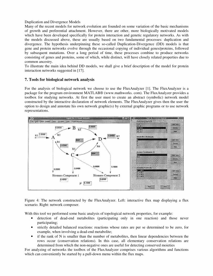
7. Tools for biological network analysis
For the analysis of biological network we choose to use the FluxAnalyzer [1]. The FluxAnalyzer is a
package for the program environment MATLAB® (www.mathworks. com). The FluxAnalyzer provides a
toolbox for studying networks. At first the user must to create an abstract (symbolic) network model
constructed by the interactive declaration of network elements. The FluxAnalyzer gives then the user the
option to design and annotate his own network graphic(s) by external graphic programs or to use network
representations.
Figure 4: The network constructed by the FluxAnalyzer. Left: interactive flux map displaying a flux
scenario. Right: network composer.
With this tool we performed some basic analysis of topological network properties, for example:
• detection of dead-end metabolites (participating only in one reaction) and those never
participating;
• strictly detailed balanced reactions: reactions whose rates are per se determined to be zero, for
example, when involving a dead-end metabolite;
• if the rank of N is smaller than the number of metabolites, then linear dependencies between the
rows occur (conservation relations). In this case, all elementary conservation relations are
determined from which the non-negative ones are useful for detecting conserved moieties
For analyzing of networks the toolbox of the FluxAnalyzer comprises various algorithms and functions
which can conveniently be started by a pull-down menu within the flux maps.

8. Conclusions and future research
Our aim in this article has been to provide brief overview of the problems of network analysis especially
of biological network. We want to study further some properties of biological network especially motifs,
modules and the hierarchical structure of biological networks. Motifs of a network represent statistically
significant patterns, their precise biological significance and the mechanisms behind their emergence are
only partially understood. We believe that analysis of the motif profiles in mathematical network models
is a potentially rich source of open and challenging problems.
References
[1] Klamt, S., Stelling, J., Ginkel, M., Gilles, E.,D.: FluxAnalyzer: exploring structure, pathways, and flux
distributions in metabolic networks on interactive flux map, Bioinformatics, 19:261-269, 2003
[2] KREBS, V. - 2002. Uncloaking terrorist networks. First Monday 7(4): September
http://www.firstmonday.dk/issues/issue7_4/krebs/index.html
[3] lacobucci, D., 1996. Networks in Marketing. Sage Publications, Thousand Oaks
[4] Knoke, D. - Kuklinski, J. H. 1981. Network analysis. Beverly Hills: Sage, 1982
[5] MACRAE, D. 1960. Direct factor analysis of sociometric data. Sociometry, 23, s. 360-371
[6] BORGATTI, S. - EVERETT, M.- FREEMAN, L. 1999. UCINET V User’s Guide. Natick, MA:
Analytic Technologies. (http://www.analytictech.com/ucinet/ucinet.htm)
[7] STOKMAN F., WASSEUR F. AND ELSAS D. 1985. The Dutch network: Types of interlocks and
network structure. In F. Stokman, R. Ziegler & J. Scott (eds), Networks of corporate power. Cambridge:
Polity Press, 1985
[8] ZIEGLER R. - BENDER R. - BIEHLER H. 1985. Industry and banking in the German corporate
network. In F. Stokman, R. Ziegler & J. Scott (eds), Networks of corporate power. Cambridge: Polity
Press, 1985
[9] Barabasi, L., Albert, R.: Emergence of scaling in random networks. Science, 286:509–512, 1999
[10] Yook, S., Oltvai, Z., Barabasi, A.: Functional and topological characterization of protein interaction
networks. Proteomics, 4:928–942, 2004
[11] Yu, H et al.: Genomic analysis of essentiality within protein networks. Trends in Genetics,
20(6):227–231, 2004
[12] Albert, R., Barabasi, A.: The statistical mechanics of complex networks. Reviews of Modern Physics,
74:47–97, 2002
[13] Volchenkov, D., Volchenkova,L., Blanchard, Ph.: Epidemic spreading in a variety of scale-free
networks. Physical Review E, 66:046137, 2002
[14] Bollobas, B. et al.: The degree-sequence of a scale-free random graph process. Random Structures
and Algorithms, 18:279–290, 2001
[15] Von Mering, C. et al.: Comparative assessment of large-scale data sets of protein-protein inter-
actions. Nature, 417:399–403, 2002
[16] Przulj,N., Corneil,D., Jurisica, I.: Modeling interactome: scale-free or geometric. Bioinfor-matics,
20(18):3508–3515, 2004
[17] Vazquez, A. et al.: Modeling of protein interaction networks, ComPlexUs, 1:38–46, 2003.
[5] Alm, E., Arkin, A.: Biological networks, Current Opinion in Structural Biology, 13:193–202, 2003.
[18] Chung, F.: et al.: Duplication models for biological networks, Journal of Computational Biology,
10(5):677–687, 2003
[19] Itzkovitz, S., Alon, U.: Subgraphs and network motifs in geometric networks, Physical Review E,
71:026117, 2005
[20] May, R.M., Lloyd, A.L.: Infection dynamics on scale-free networks, Physical Review E, 64:066112,
2001
[21] Watts, D., Strogatz, S.: Collective dynamics of small-world networks, Nature, 393:440–442, 1998

_____________________________________________________________________________________
Ladislav Beránek
Contact information
Dept. of Computer Science
University of South Bohemia
Jeronýmova 10
37001 České Budějovice
Czech Republic
Václav Novák
Contact information
Dept. of Computer Science
University of South Bohemia
Jeronýmova 10
37001 České Budějovice
Czech Republic