Graph Networks as Learnable Physics Engines for Inference and Control

Alvaro Sanchez-Gonzalez 1 Nicolas Heess 1 Jost Tobias Springenberg 1 Josh Merel 1 Martin Riedmiller 1

Raia Hadsell 1 Peter Battaglia 1

AbstractUnderstanding and interacting with everydayphysical scenes requires rich knowledge aboutthe structure of the world, represented either im-plicitly in a value or policy function, or explic-itly in a transition model. Here we introduce anew class of learnable models—based on graphnetworks—which implement an inductive biasfor object- and relation-centric representations ofcomplex, dynamical systems. Our results showthat as a forward model, our approach supportsaccurate predictions from real and simulated data,and surprisingly strong and efficient generaliza-tion, across eight distinct physical systems whichwe varied parametrically and structurally. Wealso found that our inference model can performsystem identification. Our models are also differ-entiable, and support online planning via gradient-based trajectory optimization, as well as offlinepolicy optimization. Our framework offers newopportunities for harnessing and exploiting richknowledge about the world, and takes a key steptoward building machines with more human-likerepresentations of the world.

1. IntroductionMany domains, such as mathematics, language, and physicalsystems, are combinatorially complex. The possibilitiesscale rapidly with the number of elements. For example, amulti-link chain can assume shapes that are exponential inthe number of angles each link can take, and a box full ofbouncing balls yields trajectories which are exponential inthe number of bounces that occur. How can an intelligentagent understand and control such complex systems?

A powerful approach is to represent these systems in terms

1DeepMind, London, United Kingdom. Correspondence to: Al-varo Sanchez-Gonzalez<alvarosg@google.com>, Peter Battaglia<peterbattaglia@google.com>.

Proceedings of the 35 th International Conference on MachineLearning, Stockholm, Sweden, PMLR 80, 2018. Copyright 2018by the author(s).

Pendulum Cartpole Acrobot Swimmer6

Cheetah Walker2d JACO

Real JACO

Sample 1

Sample 2

Figure 1. (Top) Our experimental physical systems. (Bottom) Sam-ples of parametrized versions of these systems (see videos: link).

of objects2 and their relations, applying the same object-wise computations to all objects, and the same relation-wisecomputations to all interactions. This allows for combina-torial generalization to scenarios never before experienced,whose underlying components and compositional rules arewell-understood. For example, particle-based physics en-gines make the assumption that bodies follow the same dy-namics, and interact with each other following similar rules,e.g., via forces, which is how they can simulate limitlessscenarios given different initial conditions.

Here we introduce a new approach for learning and con-trolling complex systems, by implementing a structural in-ductive bias for object- and relation-centric representations.Our approach uses “graph networks” (GNs), a class of neu-ral networks that can learn functions on graphs (Scarselliet al., 2009b; Li et al., 2015; Battaglia et al., 2016; Gilmeret al., 2017). In a physical system, the GN lets us represent

2“Object” here refers to entities generally, rather than physicalobjects exclusively.

Graph Networks as Learnable Physics Engines for Inference and Control

the bodies (objects) with the graph’s nodes and the joints(relations) with its edges. During learning, knowledge aboutbody dynamics is encoded in the GN’s node update func-tion, interaction dynamics are encoded in the edge updatefunction, and global system properties are encoded in theglobal update function. Learned knowledge is shared acrossthe elements of the system, which supports generalizationto new systems composed of the same types of body andjoint building blocks.

Across seven complex, simulated physical systems, and onereal robotic system (see Figure 1), our experimental resultsshow that our GN-based forward models support accurateand generalizable predictions, inference models3 supportsystem identification in which hidden properties are abducedfrom observations, and control algorithms yield competitiveperformance against strong baselines. This work repre-sents the first general-purpose, learnable physics engine thatcan handle complex, 3D physical systems. Unlike classicphysics engines, our model has no specific a priori knowl-edge of physical laws, but instead leverages its object- andrelation-centric inductive bias to learn to approximate themvia supervised training on current-state/next-state pairs.

Our work makes three technical contributions: GN-basedforward models, inference models, and control algorithms.The forward and inference models are based on treatingphysical systems as graphs and learning about them usingGNs. Our control algorithm uses our forward and inferencemodels for planning and policy learning.

(For full algorithm, implementation, and methodologicaldetails, as well as videos from all of our experiments, pleasesee the Supplementary Material.)

2. Related WorkOur work draws on several lines of previous research. Cog-nitive scientists have long pointed to rich generative modelsas central to perception, reasoning, and decision-making(Craik, 1967; Johnson-Laird, 1980; Miall & Wolpert, 1996;Spelke & Kinzler, 2007; Battaglia et al., 2013). Our coremodel implementation is based on the broader class of graphneural networks (GNNs) (Scarselli et al., 2005; 2009a;b;Bruna et al., 2013; Li et al., 2015; Henaff et al., 2015; Du-venaud et al., 2015; Dai et al., 2016; Defferrard et al., 2016;Niepert et al., 2016; Kipf & Welling, 2016; Battaglia et al.,2016; Watters et al., 2017; Raposo et al., 2017; Santoroet al., 2017; Bronstein et al., 2017; Gilmer et al., 2017). Oneof our key contributions is an approach for learning physi-cal dynamics models (Grzeszczuk et al., 1998; Fragkiadakiet al., 2015; Battaglia et al., 2016; Chang et al., 2016; Wat-

3We use the term “inference” in the sense of “abductiveinference”—roughly, constructing explanations for (possibly par-tial) observations—and not probabilistic inference, per se.

ters et al., 2017; Ehrhardt et al., 2017; Amos et al., 2018).Our inference model shares similar aims as approaches forlearning system identification explicitly (Yu et al., 2017;Peng et al., 2017), learning policies that are robust to hiddenproperty variations (Rajeswaran et al., 2016), and learningexploration strategies in uncertain settings (Schmidhuber,1991; Sun et al., 2011; Houthooft et al., 2016). We useour learned models for model-based planning in a similarspirit to classic approaches which use pre-defined models(Li & Todorov, 2004; Tassa et al., 2008; 2014), and our workalso relates to learning-based approaches for model-basedcontrol (Atkeson & Santamaria, 1997; Deisenroth & Ras-mussen, 2011; Levine & Abbeel, 2014). We also explorejointly learning a model and policy (Heess et al., 2015; Guet al., 2016; Nagabandi et al., 2017). Notable recent, concur-rent work (Wang et al., 2018) used a GNN to approximate apolicy, which complements our use of a related architectureto approximate forward and inference models.

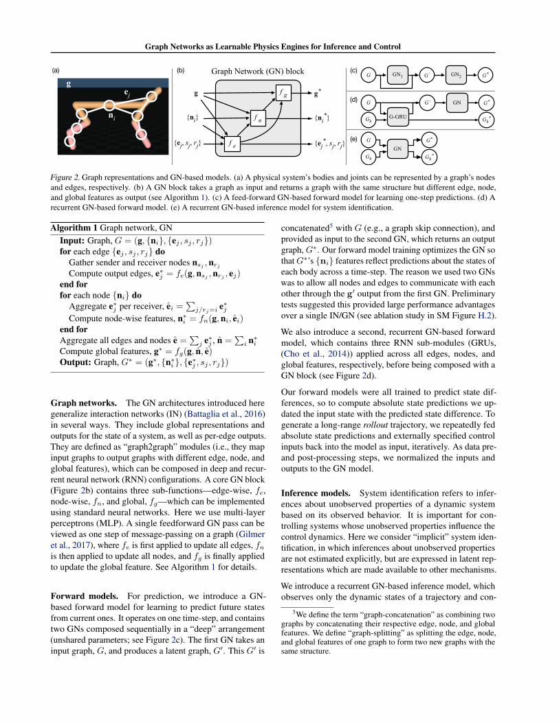
3. ModelGraph representation of a physical system. Our ap-proach is founded on the idea of representing phys-ical systems as graphs: the bodies and joints corre-spond to the nodes and edges, respectively, as de-picted in Figure 2a. Here a (directed) graph is de-fined as G = (g, {ni}i=1···Nn , {ej , sj , rj}j=1···Ne), whereg is a vector of global features, {ni}i=1···Nn is a set ofnodes where each ni is a vector of node features, and{ej , sj , rj}j=1···Ne is a set of directed edges where ej is avector of edge features, and sj and rj are the indices of thesender and receiver nodes, respectively.

We distinguish between static and dynamic properties in aphysical scene, which we represent in separate graphs. Astatic graph Gs contains static information about the param-eters of the system, including global parameters (such as thetime step, viscosity, gravity, etc.), per body/node parameters(such as mass, inertia tensor, etc.), and per joint/edge pa-rameters (such as joint type and properties, motor type andproperties, etc.). A dynamic graph Gd contains informationabout the instantaneous state of the system. This includeseach body/node’s 3D Cartesian position, 4D quaternion ori-entation, 3D linear velocity, and 3D angular velocity.4 Ad-ditionally, it contains the magnitude of the actions appliedto the different joints in the corresponding edges.

4Some physics engines, such as Mujoco (Todorov et al., 2012),represent systems using “generalized coordinates”, which sparselyencode degrees of freedom rather than full body states. Gen-eralized coordinates offer advantages such as preventing bodiesconnected by joints from dislocating (because there is no degree offreedom for such displacement). In our approach, however, suchrepresentations do not admit sharing as naturally because there aredifferent input and output representations for a body depending onthe system’s constraints.

Graph Networks as Learnable Physics Engines for Inference and Control

Figure 2. Graph representations and GN-based models. (a) A physical system’s bodies and joints can be represented by a graph’s nodesand edges, respectively. (b) A GN block takes a graph as input and returns a graph with the same structure but different edge, node,and global features as output (see Algorithm 1). (c) A feed-forward GN-based forward model for learning one-step predictions. (d) Arecurrent GN-based forward model. (e) A recurrent GN-based inference model for system identification.

Algorithm 1 Graph network, GNInput: Graph, G = (g, {ni}, {ej , sj , rj})for each edge {ej , sj , rj} do

Gather sender and receiver nodes nsj ,nrjCompute output edges, e∗j = fe(g,nsj ,nrj , ej)

end forfor each node {ni} do

Aggregate e∗j per receiver, ei =∑j/rj=i

e∗jCompute node-wise features, n∗i = fn(g,ni, ei)

end forAggregate all edges and nodes e =

∑j e∗j , n =

∑i n∗i

Compute global features, g∗ = fg(g, n, e)Output: Graph, G∗ = (g∗, {n∗i }, {e∗j , sj , rj})

Graph networks. The GN architectures introduced heregeneralize interaction networks (IN) (Battaglia et al., 2016)in several ways. They include global representations andoutputs for the state of a system, as well as per-edge outputs.They are defined as “graph2graph” modules (i.e., they mapinput graphs to output graphs with different edge, node, andglobal features), which can be composed in deep and recur-rent neural network (RNN) configurations. A core GN block(Figure 2b) contains three sub-functions—edge-wise, fe,node-wise, fn, and global, fg—which can be implementedusing standard neural networks. Here we use multi-layerperceptrons (MLP). A single feedforward GN pass can beviewed as one step of message-passing on a graph (Gilmeret al., 2017), where fe is first applied to update all edges, fnis then applied to update all nodes, and fg is finally appliedto update the global feature. See Algorithm 1 for details.

Forward models. For prediction, we introduce a GN-based forward model for learning to predict future statesfrom current ones. It operates on one time-step, and containstwo GNs composed sequentially in a “deep” arrangement(unshared parameters; see Figure 2c). The first GN takes aninput graph, G, and produces a latent graph, G′. This G′ is

concatenated5 with G (e.g., a graph skip connection), andprovided as input to the second GN, which returns an outputgraph, G∗. Our forward model training optimizes the GN sothatG∗’s {ni} features reflect predictions about the states ofeach body across a time-step. The reason we used two GNswas to allow all nodes and edges to communicate with eachother through the g′ output from the first GN. Preliminarytests suggested this provided large performance advantagesover a single IN/GN (see ablation study in SM Figure H.2).

We also introduce a second, recurrent GN-based forwardmodel, which contains three RNN sub-modules (GRUs,(Cho et al., 2014)) applied across all edges, nodes, andglobal features, respectively, before being composed with aGN block (see Figure 2d).

Our forward models were all trained to predict state dif-ferences, so to compute absolute state predictions we up-dated the input state with the predicted state difference. Togenerate a long-range rollout trajectory, we repeatedly fedabsolute state predictions and externally specified controlinputs back into the model as input, iteratively. As data pre-and post-processing steps, we normalized the inputs andoutputs to the GN model.

Inference models. System identification refers to infer-ences about unobserved properties of a dynamic systembased on its observed behavior. It is important for con-trolling systems whose unobserved properties influence thecontrol dynamics. Here we consider “implicit” system iden-tification, in which inferences about unobserved propertiesare not estimated explicitly, but are expressed in latent rep-resentations which are made available to other mechanisms.

We introduce a recurrent GN-based inference model, whichobserves only the dynamic states of a trajectory and con-

5We define the term “graph-concatenation” as combining twographs by concatenating their respective edge, node, and globalfeatures. We define “graph-splitting” as splitting the edge, node,and global features of one graph to form two new graphs with thesame structure.

Graph Networks as Learnable Physics Engines for Inference and Control

Initialstate

Gro

und t

ruth

After 25control steps 50 steps 75 steps 100 steps

Pre

dic

tion

(a)

Posi

tion [

au]

(b)

Linear

velo

city

[au]

(d)

0 20 40 60 80 100

Timestep

Ori

enta

tion [

au]

(c)

0 20 40 60 80 100

Timestep

Angula

r velo

city

[au]

(e)

groundtruth

rolloutprediction

Figure 3. Evaluation rollout in a Swimmer6. Trajectory videos are here: link-P.F.S6. (a) Frames of ground truth and predicted statesover a 100 step trajectory. (b-e) State sequence predictions for link #3 of the Swimmer. The subplots are (b) x, y, z-position, (c)q0, q1, q2, q3-quaternion orientation, (d) x, y, z-linear velocity, and (e) x, y, z-angular velocity. [au] indicates arbitrary units.

structs a latent representation of the unobserved, static prop-erties (i.e., performs implicit system identification). It takesas input a sequence of dynamic state graphs, Gd, undersome control inputs, and returns an output, G∗(T ), after Ttime steps. This G∗(T ) is then passed to a one-step forwardmodel by graph-concatenating it with an input dynamicgraph, Gd. The recurrent core takes as input, Gd, and hid-den graph, Gh, which are graph-concatenated5 and passedto a GN block (see Figure 2e). The graph returned by theGN block is graph-split5 to form an output, G∗, and up-dated hidden graph, G∗h. The full architecture can be trainedjointly, and learns to infer unobserved properties of the sys-tem from how the system’s observed features behave, anduse them to make more accurate predictions.

Control algorithms. For control, we exploit the fact thatthe GN is differentiable to use our learned forward andinference models for model-based planning within a clas-sic, gradient-based trajectory optimization regime, alsoknown as model-predictive control (MPC). We also developan agent which simultaneously learns a GN-based modeland policy function via Stochastic Value Gradients (SVG)(Heess et al., 2015). 6

4. MethodsEnvironments. Our experiments involved seven actu-ated Mujoco simulation environments (Figure 1). Sixwere from the “DeepMind Control Suite” (Tassa et al.,2018)—Pendulum, Cartpole, Acrobot, Swimmer, Cheetah,Walker2d—and one was a model of a JACO commercialrobotic arm. We generated training data for our forwardmodels by applying simulated random controls to the sys-

6MPC and SVG are deeply connected: in MPC the controlinputs are optimized given the initial conditions in a single episode,while in SVG a policy function that maps states to controls isoptimized over states experienced during training.

tems, and recording the state transitions. We also trainedmodels from recorded trajectories of a real JACO roboticunder human control during a stacking task.

In experiments that examined generalization and systemidentification, we created a dataset of versions of several ofour systems—Pendulum, Cartpole, Swimmer, Cheetah andJACO— with procedurally varied parameters and structure.We varied continuous properties such as link lengths, bodymasses, and motor gears. In addition, we also varied thenumber of links in the Swimmer’s structure, from 3-15 (werefer to a swimmer with N links as SwimmerN ).

MPC planning. We used our GN-based forward model toimplement MPC planning by maximizing a dynamic-state-dependent reward along a trajectory from a given initialstate. We used our GN forward model to predict the N -steptrajectories (N is the planning horizon) induced by proposedaction sequences, as well as the total reward associatedwith the trajectory. We optimized these action sequences bybackpropagating gradients of the total reward with respect tothe actions, and minimizing the negative reward by gradientdescent, iteratively.

Model-based reinforcement learning. To investigatewhether our GN-based model can benefit reinforcementlearning (RL) algorithms, we used our model within anSVG regime (Heess et al., 2015). The GN forward modelwas used as a differentiable environment simulator to obtaina gradient of the expected return (predicted based on thenext state generated by a GN) with respect to a parame-terized, stochastic policy, which was trained jointly withthe GN. For our experiments we used a single step predic-tion (SVG(1)) and compared to sample-efficient model-freeRL baselines using either stochastic policies (SVG(0)) ordeterministic policies via the Deep Deterministic PolicyGradients (DDPG) algorithm (Lillicrap et al., 2016) (whichis also used as a baseline in the MPC experiments).

Graph Networks as Learnable Physics Engines for Inference and Control

10-4

10-3

10-2

10-1

100

Rel. o

ne-s

tep e

rror Constant prediction baseline(a)

Individual Fixed System Models

Individual ParametrizedSystem Models

Individual System IDModels

Single Model, Multiple Systems(Pendulum,Cartpole,Acrobot,Swimmer6)

Single Model, Multiple Systems(Pendulum,Cartpole,Acrobot,Swimmer6,Cheetah)

Single Model, Multiple ParametrizedSystems (Pendulum,Cartpole,Acrobot)

10-4

10-3

10-2

10-1

100

Rel. r

ollo

ut

err

or

PendulumCartpole

SwimmerAcrobot

Cheetah JACOWalker2d

Constant prediction baseline(b)

Figure 4. (a) One-step and (b) 100-step rollout errors for differentmodels and training (different bars) on different test data (x-axislabels), relative to the constant prediction baseline (black dashedline). Blue bars are GN models trained on single systems. Redand yellow bars are GN models trained on multiple systems, with(yellow) and without (red) parametric variation. Note that includ-ing Cheetah in multiple system training caused performance todiminish (light red vs dark red bars), which suggests sharing mightnot always be beneficial.

Baseline comparisons. As a simple baseline, we com-pared our forward models’ predictions to a constant pre-diction baseline, which copied the input state as the outputstate. We also compared our GN-based forward model witha learned, MLP baseline, which we trained to make for-ward predictions using the same data as the GN model. Wereplaced the core GN with an MLP, and flattened and con-catenated the graph-structured GN input and target data intoa vector suitable for input to the MLP. We swept over 20unique hyperparameter combinations for the MLP architec-ture, with up to 9 hidden layers and 512 hidden nodes perlayer.

As an MPC baseline, with a pre-specified physical model,we used a Differential Dynamic Programming algorithm(Tassa et al., 2008; 2014) that had access to the ground-truth Mujoco model. We also used the two model-free RLagents mentioned above, SVG(0) and DDPG, as baselinesin some tests. Some of the trajectories from a DDPG agentin Swimmer6 were also used to evaluate generalization ofthe forward models.

Prediction performance evaluation. Unless otherwisespecified, we evaluated our models on squared one-stepdynamic state differences (one-step error) and squared tra-jectory differences (rollout error) between the predictionand the ground truth. We calculated independent errorsfor position, orientation, linear velocity angular velocity,and normalized them individually to the constant prediction

0.0

0.2

0.4

0.6

0.8

1.0

1.2 Best MLPbaseline

Rel. o

ne-s

tep e

rror (a)

0.0

0.5

1.0

1.5

2.0

2.5

1.2

1.1

2.7

2.4

Rel. o

ne-s

tep e

rror

Swimmer6

(c)

Randomtrain data

Randomvalid data

DDPG agenttest data

Pendulu

m

Cart

pole

Acr

obot

Sw

imm

er6

Cheeta

h

Walk

er2

d

JAC

O

0.0

0.2

0.4

0.6

0.8

1.0

1.2 Best MLPbaseline

Rel. r

ollo

ut

err

or (b)

Best MLPBest GN

0.0

0.5

1.0

1.5

2.5

2

3.2

2.9

Rel. r

ollo

ut

err

or

Swimmer6

(d)

Figure 5. Prediction errors, on (a) one-step and (b) 20-step evalua-tions, between the best MLP baseline and the best GN model after72 hours of training. Swimmer6 prediction errors, on (c) one-stepand (d) 20-step evaluations, between the best MLP baseline andthe best GN model for data in the training set (dark), data in thevalidation set (medium), and data from DDPG agent trajectories(light). The numbers above the bars indicate the ratio between thecorresponding generalization test error (medium or light) and thetraining error (dark).

baseline. After normalization, the errors were averaged to-gether. All errors reported are calculated for 1000 100-stepsequences from the test set.

5. Results: PredictionLearning a forward model for a single system. Our re-sults show that the GN-based model can be trained to makevery accurate forward predictions under random control. Forexample, the ground truth and model-predicted trajectoriesfor Swimmer6 were both visually and quantitatively indistin-guishable (see Figure 3). Figure 4’s black bars show that thepredictions across most other systems were far better thanthe constant prediction baseline. As a stronger baseline com-parison, Figures 5a-b show that our GN model had lowererror than the MLP-based model in 6 of the 7 simulatedcontrol systems we tested. This was especially pronouncedfor systems with much repeated structure, such as the Swim-mer, while for systems with little repeated structure, suchas Pendulum, there was negligible difference between theGN and MLP baseline. These results suggest that a GN-based forward model is very effective at learning predictivedynamics in a diverse range of complex physical systems.

We also found that the GN generalized better than the MLPbaseline from training to test data, as well as across differentaction distributions. Figures 5c-d show that for Swimmer6,the relative increase in error from training to test data, andto data recorded from a learned DDPG agent, was smallerfor the GN model than for the MLP baseline. We speculatethat the GN’s superior generalization is a result of implicit

Graph Networks as Learnable Physics Engines for Inference and Control

3 4 5 6 7 8 9 10 11 12 13 14 15Number of links in SwimmerN

10-3

10-2

10-1

100

Rel. r

ollo

ut

err

or

Constant prediction baselineSystems usedfor training

Zero-shotprediction

Figure 6. Zero-shot dynamics prediction. The bars show the 100-step rollout error of a model trained on a mixture of 3-6 and 8-9link Swimmers, and tested on Swimmers with 3-15 links. The darkbars indicate test Swimmers whose number of links the model wastrained on (video: link-P.F.SN), the light bars indicate Swimmersit was not trained on (video: link-P.F.SN(Z)).

regularization due to its inductive bias for sharing parame-ters across all bodies and joints; the MLP, in principle, coulddevote disjoint subsets of its computations to each body andjoint, which might impair generalization.

Learning a forward model for multiple systems. An-other important feature of our GN model is that it is veryflexible, able to handle wide variation across a system’sproperties, and across systems with different structure. Wetested how it learned forward dynamics of systems withcontinuously varying static parameters, using a new datasetwhere the underlying systems’ bodies and joints had differ-ent masses, body lengths, joint angles, etc. These staticstate features were provided to the model via the inputgraphs’ node and edge attributes. Figure 4 shows that theGN model’s forward predictions were again accurate, whichsuggests it can learn well even when the underlying systemproperties vary.

We next explored the GN’s inductive bias for body- andjoint-centric learning by testing whether a single modelcan make predictions across multiple systems that vary intheir number of bodies and the joint structure. Figure 6shows that when trained on a mixed dataset of Swimmerswith 3-6, 8-9 links, the GN model again learned to makeaccurate forward predictions. We pushed this even furtherby training a single GN model on multiple systems, withcompletely different structures, and found similarly positiveresults (see Figure 4, red and yellow bars). This highlightsa key difference, in terms of general applicability, betweenGN and MLP models: the GN can naturally operate onvariably structured inputs, while the MLP requires fixed-size inputs.

The GN model can even generalize, zero-shot, to systemswhose structure was held out during training, as long as theyare composed of bodies and joints similar to those seen dur-ing training. For the GN model trained on Swimmers with3-6, 8-9 links, we tested on held-out Swimmers with 7 and10-15 links. Figure 6 shows that zero-shot generalizationperformance is very accurate for 7 and 10 link Swimmers,and degrades gradually from 11-15 links. Still, their tra-

Ori

enta

tion

[au]

(a)

0 20 40 60 80 100Timestep

Angula

rvelo

city

[au]

(b)

Jointangle

Jointvelocity

10-2

10-1

100

Rel. r

ollo

ut

err

or Constant prediction

baseline(c)

Ground truth Feed-forward model Recurrent model

Figure 7. Real and predicted test trajectories of a JACO robot arm.The recurrent model tracks the ground truth (a) orientations and(b) angular velocities closely. (c) The total 100-step rollout errorwas much better for the recurrent model, though the feed-forwardmodel was still well below the constant prediction baseline. Avideo of a Mujoco rendering of the true and predicted trajectories:link-P.F.JR.

jectories are visually very close to the ground truth (video:link-P.F.SN(Z)).

Real robot data. To evaluate our approach’s applicabilityto the real world, we trained GN-based forward models onreal JACO proprioceptive data; under manual control bya human performing a stacking task. We found the feed-forward GN performance was not as accurate as the recur-rent GN forward model7: Figure 7 shows a representativepredicted trajectory from the test set, as well as overall per-formance. These results suggest that our GN-based forwardmodel is a promising approach for learning models in realsystems.

6. Results: InferenceIn many real-world settings the system’s state is partiallyobservable. Robot arms often use joint angle and velocitysensors, but other properties such as mass, joint stiffness, etc.are often not directly measurable. We applied our systemidentification inference model (see Model Section 3) to asetting where only the dynamic state variables (i.e., position,orientation, and linear and angular velocities) were observed,and found it could support accurate forward predictions(during its “prediction phase”) after observing randomlycontrolled system dynamics during an initial 20-step “IDphase” (see Figure 8).

To further explore the role of our GN-based system identi-fication, we contrasted the model’s predictions after an IDphase, which contained useful control inputs, against an IDphase that did not apply control inputs, across three differ-ent Pendulum systems with variable, unobserved lengths.Figure 9 shows that the GN forward model with an identifi-able ID phase makes very accurate predictions, but with anunidentifiable ID phase its predictions are very poor.

7This might result from lag or hysteresis which induces long-range temporal dependencies that the feed-forward model cannotcapture.

Graph Networks as Learnable Physics Engines for Inference and Control

10-3

10-2

10-1

100

N/ARel. r

ollo

ut

err

or

PendulumCartpole

SwimmerCheetah JACO

Constant prediction baseline

Trained ignoring parameters

Using true parameters

System ID

System ID for a different system

Figure 8. System identification performance. The y-axis repre-sents 100-step rollout error, relative to the trivial constant predic-tion baseline (black dashed line). The baseline GN-based model(black bars) with no system identification module performs worst.A model which was always provided the true static parameters(medium blue bars) and thus did not require system identificationperformed best. A model without explicit access to the true staticparameters, but with a system identification module (light bluebars), performed generally well, sometimes very close to the modelwhich observed the true parameters. But when that same modelwas presented with an ID phase whose hidden parameters weredifferent (but from the same distribution) from its prediction phase(red bars), its performance was similar or worse than the model(black) with no ID information available. (The N/A column isbecause our Swimmer experiments always varied the number oflinks as well as parameters, which meant the inferred static graphcould not be concatenated with the initial dynamic graph.)

0 20 40 60 80 100Timestep

−1

0

1

Pendulu

m

pro

ject

ion

expectedprediction

−101

A

ctio

n

magnit

ude

(a)

(b)

ID phase Prediction phase

0 20 40 60 80 100Timestep

Len: 0.1Len: 0.2Len: 0.3

(c)

(d)

ID phase Prediction phase

Figure 9. System identification analysis in Pendulum. (a) Controlinputs are applied to three Pendulums with different, unobservablelengths during the 20-step ID phase, which makes the systemidentifiable. (b) The model’s predicted trajectories (dashed curves)track the ground truth (solid curves) closely in the subsequent80-step prediction phase. (c) No control inputs are applied tothe same systems during the ID phase, which makes the systemidentifiable. (d) The model’s predicted trajectories across systemsare very different from the ground truth.

A key advantage of our system ID approach is that once theID phase has been performed for some system, the inferredrepresentation can be stored and reused to make trajectorypredictions from different initial states of the system. Thiscontrasts with an approach that would use an RNN to bothinfer the system properties and use them throughout thetrajectory, which thus would require identifying the samesystem from data each time a new trajectory needs to bepredicted given different initial conditions.

7. Results: ControlDifferentiable models can be valuable for model-based se-quential decision-making, and here we explored two ap-

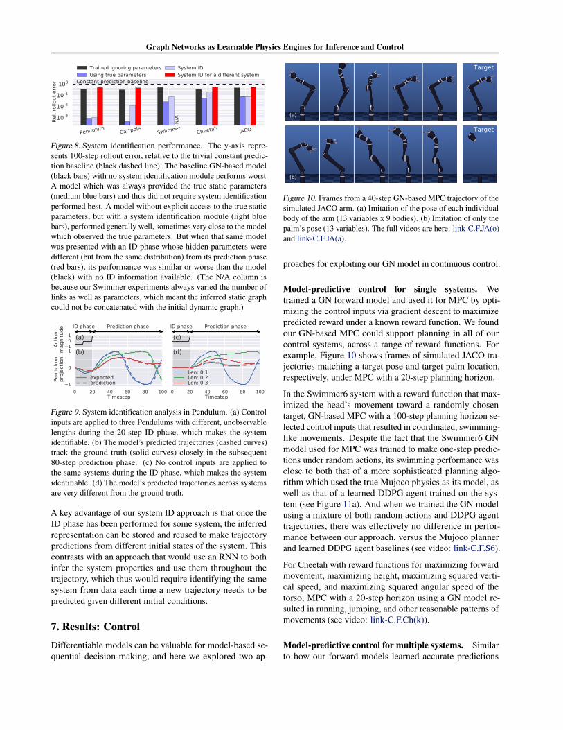
Target

(a)

Target

(b)

Figure 10. Frames from a 40-step GN-based MPC trajectory of thesimulated JACO arm. (a) Imitation of the pose of each individualbody of the arm (13 variables x 9 bodies). (b) Imitation of only thepalm’s pose (13 variables). The full videos are here: link-C.F.JA(o)and link-C.F.JA(a).

proaches for exploiting our GN model in continuous control.

Model-predictive control for single systems. Wetrained a GN forward model and used it for MPC by opti-mizing the control inputs via gradient descent to maximizepredicted reward under a known reward function. We foundour GN-based MPC could support planning in all of ourcontrol systems, across a range of reward functions. Forexample, Figure 10 shows frames of simulated JACO tra-jectories matching a target pose and target palm location,respectively, under MPC with a 20-step planning horizon.

In the Swimmer6 system with a reward function that max-imized the head’s movement toward a randomly chosentarget, GN-based MPC with a 100-step planning horizon se-lected control inputs that resulted in coordinated, swimming-like movements. Despite the fact that the Swimmer6 GNmodel used for MPC was trained to make one-step predic-tions under random actions, its swimming performance wasclose to both that of a more sophisticated planning algo-rithm which used the true Mujoco physics as its model, aswell as that of a learned DDPG agent trained on the sys-tem (see Figure 11a). And when we trained the GN modelusing a mixture of both random actions and DDPG agenttrajectories, there was effectively no difference in perfor-mance between our approach, versus the Mujoco plannerand learned DDPG agent baselines (see video: link-C.F.S6).

For Cheetah with reward functions for maximizing forwardmovement, maximizing height, maximizing squared verti-cal speed, and maximizing squared angular speed of thetorso, MPC with a 20-step horizon using a GN model re-sulted in running, jumping, and other reasonable patterns ofmovements (see video: link-C.F.Ch(k)).

Model-predictive control for multiple systems. Similarto how our forward models learned accurate predictions

Graph Networks as Learnable Physics Engines for Inference and Control

6

0

20

40

60

80

100

Maxim

um

pro

gre

ss t

o t

arg

et

aft

er

70

0 c

ontr

ol st

eps

[%]

(a)

Trained onSwimmer6

3 4 5 6 7 8 9 10 11 12 13 14 15Number of Swimmer links

(b)

Single model trained onSwimmer{3,4,5,6,8,9}

DPG agent

Mujoco-based planner

Learned model (random data) planner

Learned model (random+DPG data) planner

Figure 11. GN-based MPC performance (% distance to target after700 steps) for (a) model trained on Swimmer6 and (b) modeltrained on Swimmers with 3-15 links (see Figure 6). In (a), GN-based MPC (blue point) is almost as good as the Mujoco-basedplanner (black line) and trained DDPG (grey line) baselines. Whenthe GN-based MPC’s model is trained on a mixture of random andDDPG agent Swimmer6 trajectories (red point), its performance isas good as the strong baselines. In (b) the GN-based MPC (bluepoint) (video: link-C.F.SN) is competitive with a Mujoco-basedplanner baseline (black) (video: link-C.F.SN(b)) for 6-10 links,but is worse for 3-5 and 11-15 links. Note, the model was nottrained on the open points, 7 and 10-15 links, which correspondto zero-shot model generalization for control. Error bars indicatemean and standard deviation across 5 experimental runs.

across multiple systems, we also found they could supportMPC across multiple systems (in this video, a single modelis used for MPC in Pendulum, Cartpole, Acrobot, Swim-mer6 and Cheetah: link-C.F.MS). We also found GN-basedMPC could support zero-shot generalization in the controlsetting, for a single GN model trained on Swimmers with3-6, 8-9 links, and tested on MPC on Swimmers with 7,10-15 links. Figure 11b shows that it performed almost aswell as the Mujoco baseline for many of the Swimmers.

Model-predictive control with partial observations.Because real-world control settings are often partially ob-servable, we used the system identification GN model (seeSections 3 and 5) for MPC under partial observations inPendulum, Cartpole, SwimmerN, Cheetah, and JACO. Themodel was trained as in the forward prediction experiments,with an ID phase that applied 20 random control inputs toimplicitly infer the hidden properties. Our results show thatour GN-based forward model with a system identificationmodule is able to control these systems (Cheetah video:link-C.I.Ch. All videos are in SM Table A.2).

Model-based reinforcement learning. In our second ap-proach to model-based control, we jointly trained a GNmodel and a policy function using SVG (Heess et al., 2015),where the model was used to backpropagate error gradientsto the policy in order to optimize its parameters. Crucially,our SVG agent does not use a pre-trained model, but rather

0.0 0.2 0.4 0.6 0.8 1.0Training episodes 1e4

-4e3

-3e3

-2e3

-1e3

Avera

ge

epis

ode r

ew

ard SVG(0)

SVG(1)

Figure 12. Learning curves for Swimmer6 SVG agents. The GN-based agent (blue) asymptotes earlier, and at a higher performance,than the model-free agent (red). The lines represent median perfor-mance for 6 random seeds, with 25 and 75% confidence intervals.

the model and policy were trained simultaneously.8 Com-pared to a model-free agent (SVG(0)), our GN-based SVGagent (SVG(1)) achieved a higher level performance af-ter fewer episodes (Figure 12). For GN-based agents withmore than one forward step (SVG(2-4)), however, the per-formance was not significantly better, and in some caseswas worse (SVG(5+)).

8. DiscussionThis work introduced a new class of learnable forward andinference models, based on “graph networks” (GN), whichimplement an object- and relation-centric inductive bias.Across a range of experiments we found that these modelsare surprisingly accurate, robust, and generalizable whenused for prediction, system identification, and planning inchallenging, physical systems.

While our GN-based models were most effective in systemswith common structure among bodies and joints (e.g., Swim-mers), they were less successful when there was not muchopportunity for sharing (e.g., Cheetah). Our approach alsodoes not address a common problem for model-based plan-ners that errors compound over long trajectory predictions.

Some key future directions include using our approach forcontrol in real-world settings, supporting simulation-to-realtransfer via pre-training models in simulation, extending ourmodels to handle stochastic environments, and performingsystem identification over the structure of the system aswell as the parameters. Our approach may also be usefulwithin imagination-based planning frameworks (Hamricket al., 2017; Pascanu et al., 2017), as well as integratedarchitectures with GN-like policies (Wang et al., 2018).

This work takes a key step towards realizing the promise ofmodel-based methods by exploiting compositional represen-tations within a powerful statistical learning framework, andopens new paths for robust, efficient, and general-purposepatterns of reasoning and decision-making.

8In preliminary experiments, we found little benefit of pre-training the model, though further exploration is warranted.

Graph Networks as Learnable Physics Engines for Inference and Control

ReferencesAmos, B., Dinh, L., Cabi, S., Rothrl, T., Muldal, A., Erez,

T., Tassa, Y., de Freitas, N., and Denil, M. Learningawareness models. ICLR, 2018.

Atkeson, C. G. and Santamaria, J. C. A comparison of di-rect and model-based reinforcement learning. In Roboticsand Automation, 1997. Proceedings., 1997 IEEE Interna-tional Conference on, volume 4, pp. 3557–3564. IEEE,1997.

Battaglia, P., Pascanu, R., Lai, M., Rezende, D. J., et al.Interaction networks for learning about objects, relationsand physics. In NIPS, pp. 4502–4510, 2016.

Battaglia, P. W., Hamrick, J. B., and Tenenbaum, J. B. Sim-ulation as an engine of physical scene understanding.Proceedings of the National Academy of Sciences, 110(45):18327–18332, 2013.

Bronstein, M. M., Bruna, J., LeCun, Y., Szlam, A., and Van-dergheynst, P. Geometric deep learning: going beyondeuclidean data. IEEE Signal Processing Magazine, 34(4):18–42, 2017.

Bruna, J., Zaremba, W., Szlam, A., and LeCun, Y. Spec-tral networks and locally connected networks on graphs.arXiv preprint arXiv:1312.6203, 2013.

Chang, M. B., Ullman, T., Torralba, A., and Tenenbaum,J. B. A compositional object-based approach to learningphysical dynamics. arXiv preprint arXiv:1612.00341,2016.

Cho, K., Van Merrienboer, B., Bahdanau, D., and Bengio, Y.On the properties of neural machine translation: Encoder-decoder approaches. arXiv preprint arXiv:1409.1259,2014.

Craik, K. J. W. The nature of explanation, volume 445. CUPArchive, 1967.

Dai, H., Dai, B., and Song, L. Discriminative embeddingsof latent variable models for structured data. In ICML,pp. 2702–2711, 2016.

Defferrard, M., Bresson, X., and Vandergheynst, P. Con-volutional neural networks on graphs with fast localizedspectral filtering. In NIPS, pp. 3844–3852, 2016.

Deisenroth, M. and Rasmussen, C. Pilco: A model-basedand data-efficient approach to policy search. In ICML 28,pp. 465–472. Omnipress, 2011.

Duvenaud, D. K., Maclaurin, D., Iparraguirre, J., Bom-barell, R., Hirzel, T., Aspuru-Guzik, A., and Adams, R. P.Convolutional networks on graphs for learning molecularfingerprints. In NIPS, pp. 2224–2232, 2015.

Ehrhardt, S., Monszpart, A., Mitra, N. J., and Vedaldi, A.Learning a physical long-term predictor. arXiv preprintarXiv:1703.00247, 2017.

Fragkiadaki, K., Agrawal, P., Levine, S., and Malik, J.Learning visual predictive models of physics for play-ing billiards. CoRR, abs/1511.07404, 2015.

Gilmer, J., Schoenholz, S. S., Riley, P. F., Vinyals, O., andDahl, G. E. Neural message passing for quantum chem-istry. In ICML, pp. 1263–1272, 2017.

Grzeszczuk, R., Terzopoulos, D., and Hinton, G. Neuroan-imator: Fast neural network emulation and control ofphysics-based models. In Proceedings of the 25th an-nual conference on Computer graphics and interactivetechniques, pp. 9–20. ACM, 1998.

Gu, S., Lillicrap, T. P., Sutskever, I., and Levine, S. Con-tinuous deep q-learning with model-based acceleration.CoRR, abs/1603.00748, 2016.

Hamrick, J. B., Ballard, A. J., Pascanu, R., Vinyals, O.,Heess, N., and Battaglia, P. W. Metacontrol for adap-tive imagination-based optimization. arXiv preprintarXiv:1705.02670, 2017.

Heess, N., Wayne, G., Silver, D., Lillicrap, T., Erez, T.,and Tassa, Y. Learning continuous control policies bystochastic value gradients. In NIPS, pp. 2944–2952, 2015.

Henaff, M., Bruna, J., and LeCun, Y. Deep convolu-tional networks on graph-structured data. arXiv preprintarXiv:1506.05163, 2015.

Houthooft, R., Chen, X., Duan, Y., Schulman, J., Turck,F. D., and Abbeel, P. Curiosity-driven exploration indeep reinforcement learning via bayesian neural networks.CoRR, abs/1605.09674, 2016.

Johnson-Laird, P. N. Mental models in cognitive science.Cognitive science, 4(1):71–115, 1980.

Kingma, D. P. and Welling, M. Auto-encoding variationalbayes. In ICLR, 2014.

Kipf, T. N. and Welling, M. Semi-supervised classifica-tion with graph convolutional networks. arXiv preprintarXiv:1609.02907, 2016.

Levine, S. and Abbeel, P. Learning neural network poli-cies with guided policy search under unknown dynamics.In Ghahramani, Z., Welling, M., Cortes, C., Lawrence,N. D., and Weinberger, K. Q. (eds.), NIPS 27, pp. 1071–1079. Curran Associates, Inc., 2014.

Li, W. and Todorov, E. Iterative linear quadratic regulatordesign for nonlinear biological movement systems. InICINCO (1), pp. 222–229, 2004.

Graph Networks as Learnable Physics Engines for Inference and Control

Li, Y., Tarlow, D., Brockschmidt, M., and Zemel, R.Gated graph sequence neural networks. arXiv preprintarXiv:1511.05493, 2015.

Lillicrap, T. P., Hunt, J. J., Pritzel, A., Heess, N., Erez, T.,Tassa, Y., Silver, D., and Wierstra, D. Continuous controlwith deep reinforcement learning. In ICLR, 2016.

Miall, R. C. and Wolpert, D. M. Forward models for physio-logical motor control. Neural networks, 9(8):1265–1279,1996.

Nagabandi, A., Kahn, G., Fearing, R. S., and Levine, S.Neural network dynamics for model-based deep rein-forcement learning with model-free fine-tuning. arXivpreprint arXiv:1708.02596, 2017.

Niepert, M., Ahmed, M., and Kutzkov, K. Learning convo-lutional neural networks for graphs. In ICML, pp. 2014–2023, 2016.

Pascanu, R., Li, Y., Vinyals, O., Heess, N., Buesing, L.,Racaniere, S., Reichert, D., Weber, T., Wierstra, D., andBattaglia, P. Learning model-based planning from scratch.arXiv preprint arXiv:1707.06170, 2017.

Peng, X. B., Andrychowicz, M., Zaremba, W., and Abbeel,P. Sim-to-real transfer of robotic control with dynamicsrandomization. CoRR, abs/1710.06537, 2017.

Rajeswaran, A., Ghotra, S., Levine, S., and Ravindran, B.Epopt: Learning robust neural network policies usingmodel ensembles. CoRR, abs/1610.01283, 2016.

Raposo, D., Santoro, A., Barrett, D., Pascanu, R., Lilli-crap, T., and Battaglia, P. Discovering objects and theirrelations from entangled scene representations. arXivpreprint arXiv:1702.05068, 2017.

Rezende, D. J., Mohamed, S., and Wierstra, D. Stochas-tic backpropagation and approximate inference in deepgenerative models. In ICML 31, 2014.

Santoro, A., Raposo, D., Barrett, D. G., Malinowski, M.,Pascanu, R., Battaglia, P., and Lillicrap, T. A simpleneural network module for relational reasoning. In NIPS,pp. 4974–4983, 2017.

Scarselli, F., Yong, S. L., Gori, M., Hagenbuchner, M., Tsoi,A. C., and Maggini, M. Graph neural networks for rank-ing web pages. In Web Intelligence, 2005. Proceedings.The 2005 IEEE/WIC/ACM International Conference on,pp. 666–672. IEEE, 2005.

Scarselli, F., Gori, M., Tsoi, A. C., Hagenbuchner, M., andMonfardini, G. Computational capabilities of graph neu-ral networks. IEEE Transactions on Neural Networks, 20(1):81–102, 2009a.

Scarselli, F., Gori, M., Tsoi, A. C., Hagenbuchner, M., andMonfardini, G. The graph neural network model. IEEETransactions on Neural Networks, 20(1):61–80, 2009b.

Schmidhuber, J. Curious model-building control systems.In Proc. Int. J. Conf. Neural Networks, pp. 1458–1463.IEEE Press, 1991.

Spelke, E. S. and Kinzler, K. D. Core knowledge. Develop-mental science, 10(1):89–96, 2007.

Sun, Y., Gomez, F. J., and Schmidhuber, J. Planning tobe surprised: Optimal bayesian exploration in dynamicenvironments. In AGI, volume 6830 of Lecture Notes inComputer Science, pp. 41–51. Springer, 2011.

Tassa, Y., Erez, T., and Smart, W. D. Receding horizondifferential dynamic programming. In NIPS, pp. 1465–1472, 2008.

Tassa, Y., Mansard, N., and Todorov, E. Control-limiteddifferential dynamic programming. In Robotics and Au-tomation (ICRA), 2014 IEEE International Conferenceon, pp. 1168–1175. IEEE, 2014.

Tassa, Y., Doron, Y., Muldal, A., Erez, T., Li, Y., Casas, D.d. L., Budden, D., Abdolmaleki, A., Merel, J., Lefrancq,A., et al. Deepmind control suite. arXiv preprintarXiv:1801.00690, 2018.

Todorov, E., Erez, T., and Tassa, Y. Mujoco: A physicsengine for model-based control. In Intelligent Robotsand Systems (IROS), 2012 IEEE/RSJ International Con-ference on, pp. 5026–5033. IEEE, 2012.

Wang, T., Liao, R., Ba, J., and Fidler, S. Nervenet: Learn-ing structured policy with graph neural networks. ICLR,2018.

Watters, N., Zoran, D., Weber, T., Battaglia, P., Pascanu, R.,and Tacchetti, A. Visual interaction networks: Learninga physics simulator from video. In NIPS, pp. 4542–4550,2017.

Yu, W., Liu, C. K., and Turk, G. Preparing for the un-known: Learning a universal policy with online systemidentification. CoRR, abs/1702.02453, 2017.