U1

Ma

b

T

a

ARRA

KUTSMLSRG

1

a2aNtcdtdiapt

DM

0h

International Journal of Applied Earth Observation and Geoinformation 21 (2013) 493–505

Contents lists available at SciVerse ScienceDirect

International Journal of Applied Earth Observation andGeoinformation

jo u r n al hom epage: www.elsev ier .com/ locate / jag

rban growth and transport infrastructure interaction in Jeddah between980 and 2007

ohammed Aljoufiea,∗, Mark Brusselb, Mark Zuidgeestb, Martin van Maarseveenb

Department of Urban and Regional Planning, Faculty of Environmental Design, King Abdulaziz University, Jeddah, Saudi ArabiaDepartment of Urban and Regional Planning and Geo-information Management, Faculty of Geo-Information Science and Earth Observation (ITC), University of Twente, Enschede,he Netherlands

r t i c l e i n f o

rticle history:eceived 6 December 2011eceived in revised form 6 June 2012ccepted 9 July 2012

eywords:rban growthransportation infrastructurepatial–temporal analysisoran I

ISA

a b s t r a c t

This paper aims to use spatial statistical tools to explore the reciprocal spatial–temporal effects of trans-port infrastructure and urban growth of Jeddah city, a fast developing polycentric city in Saudi Arabia.Global spatial autocorrelation (Moran’s I) and local indicators of spatial association (LISA) are first used toanalyze the spatial–temporal clustering of urban growth and transport infrastructure from 1980 to 2007.Then, spatial regression analysis is conducted to investigate the mutual spatial–temporal effects of urbangrowth and transport infrastructure. Results indicate a significant positive global spatial autocorrelationof all defined variables between 1980 and 2007. LISA results also reveal a constant significant spatial asso-ciation of transport infrastructure expansion and urban growth variables from 1980 to 2007. The resultsnot only indicate a mutual spatial influence of transport infrastructure and urban growth but also revealthat spatial clustering of transport infrastructure seems to be influenced by other factors. This study

patial regressionemote sensingIS

shows that transport infrastructure is a constant and strong spatial influencing factor of urban growth inthe polycentric urban structure that Jeddah has. Overall, this study demonstrates that exploratory spatialdata analysis and spatial regression analysis are able to detect the spatial–temporal mutual effects oftransport infrastructure and urban growth. Further studies on the reciprocal relationship between urbangrowth and transport infrastructure using the study approach for the case of monocentric urban structurecities are necessary and encouraged.

. Introduction

Rapid urban growth is a key concern for urban planners as it has considerable urban environmental impact (Müller et al., 2010). In009, over 3.4 billion people in the world resided in urban areas,nd this figure is estimated to increase to 6.5 billion by 2050 (Unitedations, 2009).This increase implies that urban areas will con-

inuously witness rapid urban growth, which will impose furtherhallenges to urban planners. Understanding urban growth and itsrivers is vital to deal with such challenges. New approaches tohe planning and management of urban areas, such as sustainableevelopment and smart growth, will depend upon improvements

n our knowledge of causes and drivers of urban growth (Longley

nd Mesev, 2000; Herold et al., 2003). Moreover, spatial and tem-oral analyses of the factors that drive urban growth are criticalo predict future changes and their potential environmental effects

∗ Corresponding author at: King Abdulaziz University, Faculty of Environmentalesign, P.O. Box 80200, Jeddah 21598, Saudi Arabia.obile: +966564559133.

E-mail addresses: aljoufie@itc.nl, mjoufie@hotmail.com (M. Aljoufie).

303-2434/$ – see front matter © 2012 Elsevier B.V. All rights reserved.ttp://dx.doi.org/10.1016/j.jag.2012.07.006

© 2012 Elsevier B.V. All rights reserved.

in order to mitigate the negative aspects of urban growth (Aguayoet al., 2007).

In essence, a variety of social and economic factors trigger urbangrowth, including transportation and communication (Hall andPfeiffer, 2000; Hart, 2001), internal and international migration(Thorns, 2002) and public policies (Carruthers, 2002). Transporta-tion as such plays a crucial role in urban development through theaccessibility it provides to land and activities (Meyer and Miller,2001). Several studies have demonstrated that transportation infra-structure is one of the main driving forces of urban growth (e.g.,Hall and Pfeiffer, 2000; Hart, 2001; Liu et al., 2002; Handy, 2005;Xie et al., 2005; Jha et al., 2006; Ma and Xu, 2010; Müller et al.,2010). Other studies have pointed out the effect of developmentof high-speed roads on urban expansion and population growth(Brotchie, 1991; Parker, 1995; Priemus et al., 2001). Moreover, mostof the urban models use accessibility to transport infrastructure asa main driver of growth and change (see for example Batty, 2000;Liu and Phinn, 2003; Al-Ahmadi et al., 2009; Feng et al., 2011).

Nevertheless, only one previous study (Fan et al., 2009) has ana-lyzed the effects of different transportation infrastructure types onurban growth. This study used a geographical information system(GIS) spatial proximity (buffer) analysis to evaluate the influence of

4 arth O

doitp

sirptp(sfaisiseceDdelaiit

si

94 M. Aljoufie et al. / International Journal of Applied E

ifferent types of roads on spatial expansion of Guangzhou; a devel-ped monocentric city in China between 1979 and 2003. Thus, theres a lack of research on the spatial and temporal effects of differentypes of transport infrastructure on urban growth and vice versa,articularly in the context of fast developing and polycentric cities.

The study of urban growth factors and its driving forces requiresophisticated methods and tools. Recent advances in remote sens-ng (RS), GIS, spatial analysis and spatial statistics tools provide aich opportunity for in-depth study of the complex urban growthrocess and its interaction with the transportation. RS, GIS and spa-ial analysis functionalities support the examination of geographicatterns, trends, and relationships in between urban systemsBenenson and Torrens, 2004). Newer methods of spatial analysis,patial statistics in particular, have proven relevance and usefulnessor urban analysis (Paez and Scott, 2004). Exploratory spatial datanalysis (ESDA), including global spatial autocorrelation (Moran Index) and local indicators of spatial association (LISA), and thepatial regression analysis have gained attention in urban stud-es. Bamount (2004) has used ESDA to analyze the intra-urbanpatial distributions of population and employment in the agglom-ration of Dijon, France. Orford (2004) has identified and comparedhanges in the spatial concentrations of urban poverty and afflu-nce for the case of inner London using a Moran I index and LISA.eng et al. (2010) has used LISA and spatial regression models toemonstrate the relationship between economic growth and thexpansion of urban land for the case of Beijing in China. Neverthe-ess, up to now only a few studies have been conducted using ESDAnd spatial regression analysis in urban studies. In particular, theres a lack of research using these analyses for exploring and analyz-ng the complex urban growth phenomenon, and its drivers and

heir interaction.

This paper attempts to use ESDA and spatial regression analy-is to explore the spatial–temporal reciprocal effects of transportnfrastructure and urban growth for the case of Jeddah city, a

Fig. 1. (a) Geographic location o

bservation and Geoinformation 21 (2013) 493–505

developing, polycentric and fast growing city in Saudi Arabia. First,RS and GIS techniques are used to quantify and prepare the dataon spatial–temporal urban growth and transport infrastructurein Jeddah city during the period 1980–2007. Next, global spa-tial autocorrelation (Moran’s I) and LISA are detected to analyzethe spatial–temporal clustering of urban growth and transportinfrastructure. Finally, spatial regression analysis is conducted toinvestigate the reciprocal spatial–temporal effects of urban growthand transport infrastructure.

2. Material and methods

2.1. Study area

Jeddah is the second largest city in the Kingdom of Saudi Ara-bia, with a population exceeding three million. Jeddah is located onthe west coast of the Kingdom, at the confluence of latitude 29.21north and longitude 39.7 east, in the middle of the eastern shoreof the Red Sea, and it is surrounded by the plains of the Tahoma inthe east (Fig. 1). Saudi Arabia has experienced high urban growthrates over the last four decades, and the major cities in Saudi Ara-bia have experienced a rapid population increase (Al-Hathloul andMughal, 2004). Compared to the total Saudi population, the urbanpopulation has increased, from 21% in 1950 to 58% in 1975 and 81%in 2005 (Al-Ahmadi et al., 2009). This huge increase has createdexcessive spatial expansion and demand for transportation infra-structure in the major Saudi cities, including Jeddah (Al-Hathlouland Mughal, 1991, Al-Hathloul and Mughal, 2004), and this demandimposes constant urban planning challenges. Jeddah has experi-enced rapid urban growth, spatial expansion and transportation

infrastructure expansion over the last 40 years, with rates of changeranging from 0% to over 100%, indicating a wide variability acrossspace and a complex urban dynamic (Aljoufie et al., 2011). The high-est level of urban growth and transport infrastructure expansion

f Jeddah, (b) Jeddah city.

arth O

hbdlbJu(9e(t2Jgct

2

2

ipd2lais1t

2

att

M. Aljoufie et al. / International Journal of Applied E

as occurred and escalated significantly during the country’s oiloom from 1970 to 1980 (Aljoufie et al., 2012). During this period,ifferent urban growth abrupt changes and patterns have estab-

ished. For instance, airport and some major public places haveeen relocated during this period (Aljoufie et al., 2012). After 1980,eddah has experienced a tremendous and more homogenous grad-al urban growth pattern and transport infrastructure expansionAljoufie et al., 2012). Jeddah’s population has grown rapidly, from60,000 in 1980 to 3,247,134 in 2007. Jeddah’s urban mass has alsoxpanded dramatically, from 32,500 ha in 1980 to 54,175 ha in 2007Aljoufie et al., 2011). The transportation infrastructure at the sameime has also expanded significantly, from 435 km in to 826 km in007 (Aljoufie et al., 2011). As a result, the local government ineddah currently faces unprecedented challenges related to urbanrowth and transportation. However, no systematic study has beenonducted on the spatial–temporal dynamics of urban growth andransportation changes and their reciprocal relationship in Jeddah.

.2. Data and image processing

.2.1. Data acquisition, collection and geo-referencingThis study utilizes a time series of aerial photos and satellite

mages to quantify the spatial–temporal urban growth and trans-ortation infrastructure situation from 1980 to 2007. Aerial photoata from 1980 and spot satellite image data from 1993, 2002 and007 were used. Moreover, a variety of secondary data was col-

ected to facilitate the spatial–temporal analysis of urban growthnd transportation infrastructure. These data include the follow-ng: Jeddah’s master plans for 1980, 1987, and 2004; transportationtudies of Jeddah for 1980, 1995, 2004 and 2007; census data for993 and 2005; an urban growth boundary study for 1986; andopographic maps of Jeddah for 2000.

.2.2. Image processing

Given the inconsistent spatial and temporal resolution of the

vailable RS data for this study and the different formats, a consis-ent method of quantifying spatial and temporal urban growth andransportation infrastructure changes was critical. Visual image

Fig. 2. Visual interpretation method use

bservation and Geoinformation 21 (2013) 493–505 495

interpretation continues to be extensively used even with thedevelopment of digital image processing techniques (Jensen, 2000).It has been widely used in urban applications with high accuracy(Liu and Chen, 2008). RS data can be interpreted either visuallyby human experts or automatically by digital image processingand pattern recognition methods (Jensen, 2000). Human expertscan comprehensively use shape, size, color, orientation, pattern,texture and context in their interpretations (Zhou et al., 2010).Although these characteristics are crucial for identifying urbanlandscape patterns, they are difficult to incorporate into conven-tional digital image processing techniques (Richards and Jia, 2006;Shao and Wu, 2008). Hence, combining of both human knowledgeand computer processing will be more conducive in the extractionof information from RS data.

Accordingly, a cooperative visual interpretation method (Fig. 2)was adopted to quantify temporal urban land use and trans-portation infrastructure as the main aspects of urban growth andtransportation in Jeddah. Cooperative interpretation is a methodin which people work with computers to interpret RS data (Liuand Chen, 2008). This method cooperatively combines the com-puter automatic interpretation, reference land use and transportinfrastructure data, and human experience.

First, an image-to-image registration strategy was adopted togeo-reference the various images using a second-order polynomialfunction in ERDAS IMAGINE. Subsequently, a cooperative visualinterpretation method was applied. The process started with anunsupervised image classification to differentiate between urbanbuilt-up elements and non-built-up elements using the ISODATAclustering algorithm in ERDAS IMAGINE. This process shows thespatial pattern of the urban built-up area in Jeddah, which facili-tates better understanding of the elements of built-up areas, suchas buildings, road infrastructure and green areas. Next, land useand transportation infrastructure reference data from master plansand transportation study reports were integrated with built-up

and non-built-up images, using the overlay function in ArcGIS.Ten urban land use classes were specified for extraction: resi-dential, commercial, industrial, institutional, informal settlements,airport, port, roads, vacant lands and green areas. Then, visual

d to process various data sources.

4 arth O

iesCadA1wpawr(

2

ceugocsaetot

sarvdyasia

2

dttro

2

gdpc

TD

96 M. Aljoufie et al. / International Journal of Applied E

nterpretation indicators, such as pattern, shape and size, werextensively used to identify features from aerial photographs andatellite images based on field knowledge of local urban planners.onsequently, a final interpretation was conducted incorporatingll the aforementioned processes in ArcGIS v9.3 using on-screenigitizing, overlay tools and area of interest (AOI) functionality.ccordingly, land use and transportation infrastructure maps for983, 1993 and 2007 were obtained. Finally, accuracy assessmentsere performed based on a comparison of the cooperative inter-retation outputs with the reference data. The average overallccuracy of land use maps produced by this approach was 90%,hich exceeds the minimum 85% accuracy for land use data as

equired by Anderson et al. (1976) for satisfactory land use mapsAnderson et al., 1976).

.2.3. Variables, data disaggregation and preparation for analysisUrban growth is a complex process involving spatial–temporal

hanges of socio-economic and physical components at differ-nt scales (Han et al., 2009). The socio-economic components ofrban growth are related to urban population growth and economicrowth (Black and Henderson, 1999), while physical componentsf urban growth are related to spatial expansion, land coverhange and land use change (Thapa and Murayama, 2011). In thistudy, urban growth is defined and expressed using three vari-bles population growth, spatial expansion and residential land usexpansion. Transport infrastructure expansion is expressed usinghree variables: highway expansion, main road expansion and sec-ndary road expansion. Table 1 shows the defined variables withemporal aggregated data and their unit of measurement.

To fulfill the practical requirements of a spatial statistical analy-is, the extracted RS data (Fig. 3) was disaggregated to district level,n urban administrative unit in the study area. Because the tempo-al population data were collected at the district level, other definedariables of urban growth and transportation infrastructure wereisaggregated to the same spatial level. The spatial statistical anal-sis considered 117 districts that constituted Jeddah’s entire urbanuthority. A GIS-based approach was conducted to disaggregate thetudy’s defined variables (population growth, spatial expansion, res-dential land use expansion, highway expansion, main road expansionnd secondary road expansion).

.3. Spatial statistical analysis

Choosing an appropriate model and analytical techniqueepends on the type of variable under investigation and the objec-ive of the analysis. Accordingly, to achieve the objectives ofhis study, we applied spatial autocorrelation analysis and spatialegression analysis to capture the mutual spatial–temporal effectsf the defined urban growth and transport infrastructure variables.

.3.1. Spatial autocorrelation analysisTo analyze the reciprocal spatial–temporal effects of urban

rowth and transportation, a spatial cluster analysis was con-ucted. A spatial autocorrelation indicator, Moran’s Index, waserformed in GeoDa software to capture the global spatial auto-orrelation and local spatial clustering of urban growth and

able 1escription of the defined variables’ characteristics at the aggregated level.

Variables Unit 1980

Spatial expansion Hectare 32,50Population growth Person 960,00Residential land use expansion Hectare 872Highways expansion Kilometer (length) 11Main roads expansion Kilometer (length) 15Secondary roads expansion Kilometer (length) 16

bservation and Geoinformation 21 (2013) 493–505

transportation infrastructure variables. Spatial autocorrelationstatistics have been widely used to measure the correlation amongneighboring observations in a pattern and the levels of spatial clus-tering among neighboring districts (Boots and Getis, 1998). Moran’sIndex, in particular, has been used to study urban structure, com-plex urban growth and the intra-urban spatial distribution of socio-economic factors (Frank, 2003; Baumont et al., 2004; Orford, 2004;Yu and Wei, 2008).

To analyze the spatial distribution and capture the global spatialautocorrelation of urban growth and transportation infrastructurevariables (population growth, spatial expansion, residential land useexpansion, highway expansion, main road expansion and secondaryroad expansion), the Global Moran’s Index IM statistic, which is sim-ilar to the Pearson correlation coefficient (Moran, 1950; Cliff andOrd, 1980) and LISA were calculated for the years 1980, 1993, 2002and 2007. The Moran’s Index test statistic is given by:

IM =

⎛⎜⎜⎝ n∑

i

∑j

Wij

⎞⎟⎟⎠

∑i

∑jWij(Y(R)i − Y (R))(Y(R)j − Y (R))∑

i(Y(R)i − Y (R))2

, (1)

where Wij is the element in the spatial weights matrix corre-sponding to the district pairs i, j, and Y(R)i and Y(R)j are the differenturban growth and transportation infrastructure variables (e.g., pop-ulation growth or residential expansion) for districts i and j with themean urban growth and transportation variables expansion rateY (R). Because the weights are not row-standardized, the scaling fac-tor n/

∑i

∑jWij is applied. Moran’s Index indicates the strength

of the spatial similarity or dissimilarity of neighboring districts.A positive Moran’s I indicates the presence and degree of spatialautocorrelation.

The first step in the analysis of spatial autocorrelation is toconstruct a spatial weights matrix that contains information onthe neighborhood structure for each location. The (i, j) element ofthe matrix W, denoted Dist ij, quantifies the spatial dependencybetween district i and j. Collectively, the Wij defines the neighbor-ing structure over the entire area. A first-order connectivity weightmatrix was constructed. This weight matrix was selected hence thelocal connectivity of transport infrastructure is defined by a gridpattern, which is more compatible with the rook weight matrix.In addition, the spatial configurations of districts in the study area(Fig. 4) support the rook weight matrix. In this approach, spatialunits (districts) are defined as neighbors if they share a commonboundary. Accordingly:

Wij ={

1 if districts i and j share common boundary

0 Otherwise.

Finally, a significance test against the null hypothesis of nospatial autocorrelation through a permutation procedure of 999Monte Carlo replications was used to test for the significance of thestatistic.

1993 2002 2007

0 40,739 49,700 54,1750 2,046,000 2,560,000 3,247,1344 14,921 19,318 21,3652 132 132 1325 163 163 1838 217 380 475

M. Aljoufie et al. / International Journal of Applied Earth Observation and Geoinformation 21 (2013) 493–505 497

tial–t

2

(soctofT

Fig. 3. Jeddah’ spa

.3.2. Spatial regression analysisWhen standard linear regression (i.e., ordinary least square

OLS)) models are estimated for cross-sectional data on neighboringpatial units, the presence of spatial dependency may cause seri-us problems with model misspecification. Spatial relationshipsan be modeled in a variety of ways. One way is to hypothesize

hat the value of the dependent variable (e.g. spatial expansion)bserved at a particular location is partially determined by someunction of the value of the dependent variable of its neighbors.he variable measuring these effects is typically formulated as a

emporal changes.

spatially weighted average of the neighboring values of the depend-ent variable, where the neighbors are specified through the useof a so-called spatial weights matrix (Anselin, 1988). The method-ologies for spatial regression consist of examining and testing forthe potential presence of such misspecification and providing moreappropriate modeling that incorporates the spatial dependence

(Anselin et al., 1997; Varga, 1998). Spatial dependency can be incor-porated into the OLS model in two distinct ways: as an additionalpredictor in the form of a spatially lagged dependent variable (spa-tial lag model) or in the error structure (spatial error model).

498 M. Aljoufie et al. / International Journal of Applied Earth O

Fr

l

Y

wtcrte

mttsaam

y

aa

sst

ig. 4. Spatial configurations of districts in study area; district 1 and 2 used for LISAesults analysis.

Specifically, in matrix notation, the general form of the spatialag model is given by:

= �Wy + X ̌ + ε, (2)

where y is the dependent variable; W is a spatial weights matrix,hich specifies the neighbors used in the averaging (resulting in

he spatially lagged dependent variable Wy); � is an autoregressiveoefficient of the lag variable; X is the explanatory variables; ̌ is aegression coefficient; and ε is an error term. The model is appliedo measure the level of spatial dependency and to determine theffect of different groups of variables.

The other method of incorporating spatial relationships is byodeling the effects through the spatial dependence that enters

he relationship through the error term. When accounting for spa-ial dependence through the error term, the model accounts for aituation in which the errors associated with any one observationre spatially weighted (or neighborhood) averages of the errors plus

random error component. Specifically, the spatial error model inatrix form is given by:

= X ̌ + ε where ε = �W + �, (3)

where ε is a vector of spatially autocorrelated error terms; � is vector of errors; and � is a scalar parameter, known as the spatialutoregressive coefficient.

Spatial dependency was used in this study to investigate thepatial patterns and to determine the factors that contribute to thepatial similarity or dissimilarity for urban growth and transporta-ion variables. The spatial effect of transportation infrastructure on

bservation and Geoinformation 21 (2013) 493–505

urban growth was investigated using different explanatory vari-ables on the dependent variable, as follows:

Population growth

= f (Highway expansion, Main road expansion,

Secondary road expansion) (4)

Spatial expansion

= f (Highway expansion, Main road expansion,

Secondary road expansion) (5)

Residential land use expansion

= f (Highway expansion, Main road expansion,

Secondary road expansion). (6)

Conversely, the spatial influence of urban growth variables onthe different transport infrastructure types was investigated as fol-lows:

Highway expansion

= f (Population growth, Spatial expansion,

Residential land use expansion) (7)

Main road expansion

= f (Population growth, Spatial expansion,

Residential land use expansion) (8)

Secondary road expansion

= f (Population growth, Spatial expansion,

Residential land use expansion). (9)

Before modeling spatial dependency, the nature of spatialdependency (in terms of spatial lag or spatial error) was first deter-mined in order to choose the most appropriate alternative model(spatial lag model or spatial error model). To determine this, aLagrange Multiplier (LM) test was conducted (Anselin and Florax,1995; Anselin et al., 1996).

3. Results

3.1. Spatial autocorrelation analysis

The extent to which neighboring values are correlated was mea-sured using the Global Moran’s Index. A Moran’s Index analysisis conducted by generating scatter plots with the log of the dif-ferent urban growth and transportation infrastructure variables.In essence, the scatter plots illustrate the Global Moran’s I (e.g.,Fig. 5), which is a commonly used test statistic for spatial autocorre-lation. A significance assessment through a permutation procedurewas implemented to determine the significance of the computed

Moran’s Index. Table 2 shows the values of the Global Moran’s Istatistic for all variables. Moran’s Index is positive and statisticallysignificant (p < 0.05) for all urban growth and transportation infra-structure variables. This result indicates that nearby districts tend

M. Aljoufie et al. / International Journal of Applied Earth Observation and Geoinformation 21 (2013) 493–505 499

tMcifoctsanatpta

utuaobhilctv

gp

TM

Table 3LISA statistics of district 1.

Variables 1980 1993 2002 2007

Population growth HH** HH** HH** HH**

Spatial expansion HH** HH** HH** HH**

Residential land use HH** HH HH** HH**

Highway expansion HH* Ns HH* HH*

Main roads expansion HH* HH** HH** HH**

Secondary roads expansion HH** HH** HH** HH*

(� 1993 = 0.485, � 2002 = 0.554 and � 2007 = 0.603) and highlysignificant. This result indicates the presence of spatial depend-

Fig. 5. Spatial autocorrelation Moran scatter plot (Ln population for 1980).

o have similar attributes. It is noted that the values of the Globaloran’s I change from 1980 to 2007 for all variables. The highest

lustering of nearly all variables occurred in 1980. The decreasen values of population growth and spatial expansion variablesrom 1980 to 2002 reflects the sprawl pattern of development thatccurred in Jeddah wherein developments were not very muchoncentrated in space, but took place in several parts of the city athe same time. In addition, population growth and spatial expan-ion during this period were more autocorrelated in the city centerrea, whereas for the other parts this was less the case. It is alsooted that the values of the transportation infrastructure variablesre lower than the urban growth variables. This result indicateshat the values of transportation infrastructure variables are inde-endently clustered with similar values. Although Moran’s I for theransportation infrastructure variables shows low values, the spacemong other factors catalyzed the expansion of these variables.

The results of the LISA identify the local spatial clustering ofrban growth and transportation infrastructure variables at the dis-rict level. Fig. 6 and Fig. 7 show the temporal LISA for differentrban growth and transportation infrastructure expansion vari-bles. Districts with a significant LISA are classified by the typef spatial correlation: bright red for the high–high association,right blue for low–low, light blue for low–high, and light red forigh–low. The high–high and low–low locations suggest cluster-

ng of similar values of one variable, whereas the high–low andow–high locations indicate spatial outliers of the same variable. Byomparing these figures, it is possible to identify the significant spa-ial clustering of urban growth and transportation infrastructure

ariables from 1980 to 2007.

In general, this study finds that the spatial clustering of urbanrowth variables coincides with the spatial clustering of trans-ortation infrastructure expansion variables. It is observed that

able 2oran’s I statistics.

Variables 1980 1993 2002 2007

Population growth 0.674 0.428 0.571 0.611Spatial expansion 0.700 0.448 0.759 0.621Residential land use 0.618 0.619 0.741 0.625Highway expansion 0.335 0.285 0.249 0.283Main roads expansion 0.338 0.462 0.683 0.560Secondary roads expansion 0.730 0.420 0.351 0.203

Ns: not significant.* Significant at 5%.

** Significant at 1%.

the temporal–spatial clustering of population growth is associ-ated, to some extent, with the temporal–spatial clustering ofhighway expansion. It is also noted that the temporal–spatialclustering of the spatial expansion variable largely overlaps withthe temporal–spatial clustering of the variable of main roadexpansion. Additionally, the temporal–spatial clustering of the res-idential land-use expansion variable largely coincides with thetemporal–spatial clustering of the secondary road expansion vari-able.

In addition, Tables 3 and 4 summarize LISA’s results of each vari-able over time for the case of two districts in study area (Fig. 4).These tables depict a constant high–high spatial association oftransport infrastructure expansion and urban growth variablesover time. This indicates that spatial influence of transportationinfrastructure expansion on the clustering of population growth,spatial expansion and residential land-use expansion is significantand constant over time and vice versa.

3.2. Spatial regression analysis

Table 5 depicts the result of the LM test. Results indicate thatboth LM Lag and LM Error tests are significant for all dependent vari-ables and over time. In contrast, the results also indicate that onlythe Robust LM Lag statistic is significant for all dependent variablesand over time, while the Robust LM Error statistic is not. Follow-ing the spatial regression model selection decision rule (Anselin,2005) we conclude that the spatial lag model is the proper alter-native. Accordingly, spatial lag models have been estimated for allspecified dependent variables (Eqs. (4)–(9)).

The estimates of the coefficients produced by the spatial regres-sion (econometric) models are presented in Tables 6–11. Table 6shows the effect of different transport infrastructure types onpopulation growth dependent variable (Eq. (4)). The spatial autore-gressive coefficient � (the coefficient on the spatial lag of thedependent variable) is positive (0.732) and is highly significantat the 5% level for the observations in 1980. Similarly, the coef-ficient for the observations in 1993, 2002 and 2007 is positive

ence, implying that the interaction between neighbors significantly

Table 4LISA statistics of district 2.

Variables 1980 1993 2002 2007

Population growth HH** HH** HH** HH**

Spatial expansion HH* HH** HH** HH**

Residential land use HH** HH** HH** HH**

Highway expansion HH* HH** HH* HH*

Main roads expansion Ns HH* HH* HH*

Secondary roads expansion HH** HH** HH* Ns

Ns: not significant.* Significant at 5%.

** Significant at 1%.

500 M. Aljoufie et al. / International Journal of Applied Earth Observation and Geoinformation 21 (2013) 493–505

s of u

atvctitag

s(eoofisc

Fig. 6. LISA cluster map

ffects the growth of Jeddah’s urban population. Furthermore,he coefficients of the highway, main road, and secondary roadariables are positive and significant, and the magnitude of theoefficients increases over time. This means that the expansion ofhe transport infrastructure across space contributes to the increasen the urban population over this period. Thus, the findings revealhat the expansion of highways, main roads and secondary roads is

contributing factor for the spatial clustering of urban populationrowth.

Table 7 depicts the spatial influence of different transport infra-tructure types on the spatial expansion dependent variable (Eq.5)). The analysis of the spatial relationship among the differ-nt urban transport infrastructures reveals that the coefficientsf highways and secondary roads are significantly positive for thebservations in 1980, 1993, 2002 and 2007, whereas the coefficient

or main roads is only positively significant for the observationsn 2002 and 2007 (Table 7). This result demonstrates that thepatial expansion of highways, main roads and secondary roadsontributes to the increase in urban spatial expansion over the

rban growth variables.

study period, which, in turn, implies that transport infrastructureexpansion is a contributing factor to the spatial clustering of urbanspatial expansion.

Table 8 presents the spatial influence of different transportinfrastructures on residential land use development dependentvariable (Eq. (6)). Examining the effect of different urban trans-port infrastructures, the analysis reveals that the coefficients ofhighways and main roads for the observations in 1993 are sig-nificantly positive, whereas the coefficients for secondary roads in1980 and 2007 are positive and significant at 5% (Table 8). This find-ing demonstrates that spatial expansion in transport infrastructurecontributes to the increase in urban residential development overthe indicated period, which, in turn, implies that transport infra-structure expansion is a contributing factor to the spatial clusteringof urban residential development.

Table 9 shows the effect of urban growth variables on highwayexpansion dependent variable (Eq. (7)). The coefficient of the res-idential development variable is negative for 1980 and 2002 andsignificant at 5%, and the magnitude of the coefficient increases

M. Aljoufie et al. / International Journal of Applied Earth Observation and Geoinformation 21 (2013) 493–505 501

transp

odoptithne

rdToosbs

Fig. 7. LISA cluster maps of

ver time, implying that the spatial expansion of residentialevelopment negatively contributes to the increase in highwaysver this period. In contrast, the coefficient for spatial expansion isositive and significant only for the year 2007 (Table 5), indicatinghat the increase in spatial expansion contributes positively to thencrease in highways for 2007. Thus, the result reveals that popula-ion growth contributes positively to the spatial clustering of urbanighway expansion, whereas residential development expansionegatively contributes to the spatial clustering in urban highwayxpansion.

The results of the effects of urban growth variables on the mainoad dependent variable (Eq. (8)) and secondary road expansionependent variable (Eq. (9)) are given in Tables 10 and 11 below.he spatial autoregressive coefficient � for both main and sec-ndary roads is positive and significant at the 5% level for the

bservations in 1980, 1993, 2002 and 2007. This result demon-trates the existence of spatial dependence, implying a relationetween urban growth and transportation infrastructure expan-ion. Moreover, the coefficient of the residential development

ort infrastructure variables.

variable is significantly positive for the year 1993, showing thatthe spatial expansion of residential development positively con-tributes to the increase in the main roads for 1993 (Table 10).In contrast, the coefficients of spatial expansion for the obser-vations in 1993, 2002 and 2007 are positive and significantat 5% and 1% (Table 11), indicating that spatial expansion isa contributing factor to the spatial increase in secondary roads andhighways for 2007. The analysis further indicates that the coeffi-cient of the population for the observation in 2007 is significantlynegative, implying that population growth contributes negativelyto the spatial clustering of urban secondary roads (Table 11).

4. Discussion

Spatial autocorrelation analysis results indicate a significant

positive global spatial autocorrelation of all defined variablesbetween 1980 and 2007. The results of the LISA revealed that thespatial clustering of urban growth variables coincided with the spa-tial clustering of transportation infrastructure expansion variables.

502 M. Aljoufie et al. / International Journal of Applied Earth Observation and Geoinformation 21 (2013) 493–505

Table 5LM test results for different dependent variables.

Dependent variable Test 1980 1993 2002 2007

Value p Value p Value p Value p

Ln (population growth) (4) LM (lag) 32.55 0.000 12.21 0.000 25.37 0.000 33.85 0.000Robust LM (lag) 8.6 0.003 7.77 0.005 7.55 0.005 12.17 0.000LM (Error) 24.3 0.000 4.98 0.025 18.1 0.000 21.81 0.000Robust LM (Error) 0.41 0.521 0.551 0.457 0.283 0.594 0.135 0.712

Ln (spatial expansion) (5) LM (lag) 70.2 0.000 12.95 0.000 90.87 0.000 49.44 0.000Robust LM (lag) 9.57 0.001 3.54 0.041 28.63 0.000 27.11 0.000LM (Error) 62.7 0.000 9.42 0.002 64.44 0.000 22.44 0.000Robust LM (Error) 1.9 0.157 0.016 0.899 2.209 0.137 0.126 0.722

Ln (Residential land use expansion) (6) LM (lag) 24.95 0.000 42.8 0.000 60.06 0.000 50.41 0.000Robust LM (lag) 14.28 0.000 22.21 0.000 22.24 0.000 13.18 0.000LM (Error) 11.92 0.000 20.96 0.000 37.85 0.000 38.11 0.000Robust LM (Error) 1.26 0.261 0.372 0.541 0.038 0.844 0.878 0.348

Ln (Highway expansion) (7) LM (lag) 27.4 0.000 17.9 0.000 17.11 0.000 15.96 0.000Robust LM (lag) 5.27 0.021 1.15 0.028 6.858 0.008 4.93 0.026LM (Error) 22.4 0.000 16.9 0.000 11.22 0.000 11.3 0.000Robust LM (Error) 0.33 0.561 0.162 0.686 0.962 0.326 0.279 0.596

Ln (Main road expansion) (8) LM (lag) 10.82 0.001 9.84 0.001 41.6 0.000 24.94 0.000Robust LM (lag) 4.21 0.04 5.96 0.014 7.33 0.006 5.81 0.015LM (Error) 7.8 0.005 4.61 0.031 35.32 0.304 19.52 0.000Robust LM (Error) 1.18 0.275 0.724 0.394 1.05 0.000 0.39 0.530

Ln (Secondary road expansion) (9) LM (lag) 50 0.000 9.36 0.002 18.63 0.000 8.94 0.001Robust LM (lag) 12.95 0.000 3.32 0.041 11.64 0.000 4.66 0.030LM (Error) 37.76 0.000 6.08 0.013 8.35 0.000 6.42 0.011Robust LM (Error) 0.708 0.399 0.047 0.827 1.37 0.241 0.425 0.514

Table 6The maximum likelihood estimation result of the spatial lag model: dependent variable—ln of population.

1980 1993 2002 2007Lag Lag Lag Lag

Ln (Highways) 0.089 (1.44) 0.192 (2.13)* 0.248 (2.66)* 0.280 (3.15)*

Ln (Main roads) 0.012 (0.154) 0.210 (1.99)* 0.320 (3.37)* 0.352 (4.07)*

Ln (Secondary roads) 0.329 (4.37)* 0.386 (3.91)* 0.174 (1.77)** 0.035 (0.34)� 0.732 (13.13)* 0.485 (6.04)* 0.554 (7.52)* 0.603 (8.77)*

Adjusted R2 0.73 0.54 0.65 0.68

Notes: Absolute values of z-statistics in parentheses.* Significant at 5%.

** Significant at 1%.

Table 7The maximum likelihood estimation result of the spatial lag model: dependent variable—ln spatial expansion.

1980 1993 2002 2007Lag Lag Lag Lag

Ln (Highways) 0.199 (1.94)** 0.157 (1.92)** 0.185 (1.80)** 0.196 (2.34)*

Ln (Main roads) −0.007 (0.057) 0.123 (0.760) 0.217 (2.13)* 0.295 (3.72)*

Ln (Secondary roads) 0.211 (1.93)** 0.353 (2.31)* 0.317 (2.89)* 0.283 (2.89)*

� 0.858 (23.89)* 0.552 (6.81)* 0.696 (13.05)* 0.503 (5.62)*

Adjusted R2 0.69 0.38 0.66 0.57

Notes: Absolute values of z-statistics in parentheses.* Significant at 5%

** Significant at 1%.

Table 8The maximum likelihood estimation result of the spatial lag model: dependent variable—ln residential development.

1980 1993 2002 2007Lag Lag Lag Lag

Ln (Highways) −0.091 (0.091) 0.205 (2.01)* 0.0215 (0.213) 0.119 (1.06)Ln (Main roads) −0.069 (0.579) 0.376 (3.16)* 0.129 (1.33) 0.146 (1.41)Ln (Secondary roads) 0.458 (4.15)* 0.104 (0.947) 0.261 (2.43) 0.394 (2.97)*

� 0.81 (18.10)* 0.752 (14.72)* 0.839 (22.18)* 0.78 (16.67)*

Adjusted R2 0.70 0.69 0.71 0.60

N

otes: Absolute values of z-statistics in parentheses.* Significant at 5%.** Significant at 1%.

M. Aljoufie et al. / International Journal of Applied Earth Observation and Geoinformation 21 (2013) 493–505 503

Table 9The maximum likelihood estimation result of the spatial lag model: dependent variable—ln of highways.

1980 1993 2002 2007Lag Lag Lag Lag

Ln (Population) 0.214 (1.92)** 0.084 (0.83) 0.291 (2.71)* 0.112 (1.23)Ln (Residential develop.) −0.202 (2.63)* 0.01 (0.13) −0.162 (2.00)* −0.003 (−0.045)Ln (Spatial expansion) 0.085 (1.47) 0.002 (0.04) 0.065 (0.99) 0.141 (1.75)**

� 0.722 (11.7)* 0.702 (10.6)* 0.489 (6.25)* 0.515 (5.87)*

Adjusted R2 0.38 0.25 0.42 0.33

Notes: Absolute values of z-statistics in parentheses.* Significant at 5%.

** Significant at 1%.

Table 10The maximum likelihood estimation result of the spatial lag model: dependent variable—ln of main roads.

1980 1993 2002 2007Lag Lag Lag Lag

Ln (Population) 0.016 (0.17) 0.052 (0.60) 0.108 (1.47) 0.219 (2.83)*

Ln (Residential dev.) 0.008 (0.13) 0.183 (2.72)* −0.072 (−1.30) −0.062 (1.03)Ln (Spatial expansion) −0.001 (0.022) 0.002 (0.05) 0.039 (0.87) 0.097 (1.45)� 0.81 (16.6)* 0.488 (5.61)* 0.938 (49.61)* 0.645 (9.4)*

Adjusted R2 0.33 0.49 0.67 0.53

Notes: Absolute values of z-statistics in parentheses.* Significant at 5%.** Significant at 1%.

Table 11The maximum likelihood estimation result of the spatial lag model: dependent variable—ln of Secondary roads.

1980 1993 2002 2007Lag Lag Lag Lag

Ln (Population) 0.129 (2.04)* 0.332 (3.48) 0.099 (0.95) −0.151 (1.90)**

Ln (Residential dev. 0.055 (1.26) −0.072 (−1.02)* 0.006 (0.08) 0.157 (2.67)*

Ln (Spatial expansion) −0.022 (0.687) 0.158 (1.82)** 0.121 (1.97)* 0.220 (3.19)*

� 0.845 (22.66)* 0.532 (6.44)* 0.348 (3.66)* 0.152 (1.58)Adjusted R2 0.80 0.46 0.26 0.29

N

sttssasis

rlidr

vlsTddtsFss

otes: Absolute values of z-statistics in parentheses.* Significant at 5%.

** Significant at 1%.

The results of the spatial statistical analysis reveal reciprocalpatial–temporal effects of urban growth and transport infrastruc-ure for the city of Jeddah. Interestingly, this study indicates thathe spatial influence of variables related to transportation infra-tructure expansion (highway expansion, main road expansion andecondary road expansion) on the clustering of population growthnd spatial expansion is constant over time. This finding reflects theignificant role of the expansion of different types of transportationnfrastructures on the spatial clustering of population growth andpatial expansion.

In contrast, this study finds that the spatial influence of variableselated to transportation infrastructure expansion on residentialand use expansion changes over time (Tables 6–8). This find-ng indicates that different types of transport infrastructures haveifferent spatial–temporal influences on the spatial clustering ofesidential land use expansion.

It is also observed that the spatial influence of urban growthariables (population growth, spatial expansion, and residentialand use expansion) on the clustering of transportation infra-tructure expansion variables changes over time (Tables 9–11).his finding indicates that different urban growth variables haveifferent spatial–temporal influences on the spatial clustering ofifferent types of transport infrastructures. This study finds thathe spatial clustering of population growth and spatial expansion

timulates the spatial clustering of urban highways expansion.urthermore, population growth and residential land use expan-ion contribute to the spatial clustering of main roads, whereaspatial expansion catalyzes the spatial expansion of secondary

roads in Jeddah. Although, population growth amongst other urbangrowth variables seems to play stronger effect on the spatialclustering of transport infrastructure in Jeddah, transportationinfrastructure seems to be influenced by other factors. In essence,urban transportation systems are complex networks shapedby various geographical, social, economic, and environmentalfactors (Wang et al., 2008).

The results of this study reveal that transport infrastruc-ture is a constantly strong spatial influencing factor of urbangrowth in Jeddah city. The polycentric urban structure of Jed-dah city and an arterial grid pattern of transport infrastructurewith high connectivity seem to support this finding. In addi-tion, Jeddah car-oriented transport system characteristics alsoseem to support this finding. Other developed monocentric urbanstructure cities are expected to show different results. The influ-ence of transport infrastructure on urban growth is expected belower as compared to a polycentric urban structure like Jeddahcity.

This study shows that ESDA and spatial regression analy-sis are sophisticated tools to study the mutual effects of urbangrowth and transportation infrastructure expansion for the caseof a developing, polycentric and fast growing city. These toolswere able to detect the spatial–temporal reciprocal effects oftransport infrastructure and urban growth. This in turn enriches

insight, strengthens the understanding of the relationship betweenthe complex urban growth phenomenon and transportation, andextends the knowledge of urban analysis using these tools. Inessence, spatial and temporal analysis of the factors that drive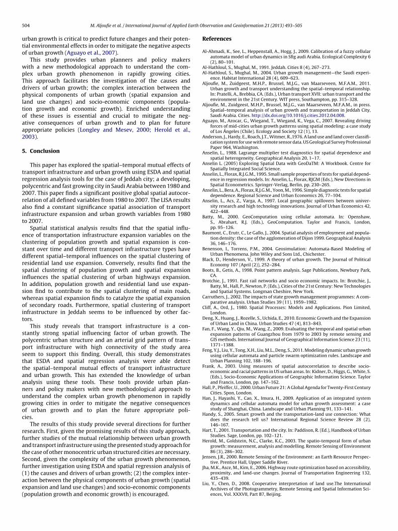

5 arth O

uto

wpTdpltoaa2

5

trp2rait

ecsdrsiIswoit

sppsttaanugoc

rfatSf(ae(

04 M. Aljoufie et al. / International Journal of Applied E

rban growth is critical to predict future changes and their poten-ial environmental effects in order to mitigate the negative aspectsf urban growth (Aguayo et al., 2007).

This study provides urban planners and policy makersith a new methodological approach to understand the com-lex urban growth phenomenon in rapidly growing cities.his approach facilitates the investigation of the causes andrivers of urban growth; the complex interaction between thehysical components of urban growth (spatial expansion and

and use changes) and socio-economic components (popula-ion growth and economic growth). Enriched understandingf these issues is essential and crucial to mitigate the neg-tive consequences of urban growth and to plan for futureppropriate policies (Longley and Mesev, 2000; Herold et al.,003).

. Conclusion

This paper has explored the spatial–temporal mutual effects ofransport infrastructure and urban growth using ESDA and spatialegression analysis tools for the case of Jeddah city; a developing,olycentric and fast growing city in Saudi Arabia between 1980 and007. This paper finds a significant positive global spatial autocor-elation of all defined variables from 1980 to 2007. The LISA resultslso find a constant significance spatial association of transportnfrastructure expansion and urban growth variables from 1980o 2007.

Spatial statistical analysis results find that the spatial influ-nce of transportation infrastructure expansion variables on thelustering of population growth and spatial expansion is con-tant over time and different transport infrastructure types haveifferent spatial–temporal influences on the spatial clustering ofesidential land use expansion. Conversely, results find that thepatial clustering of population growth and spatial expansionnfluences the spatial clustering of urban highways expansion.n addition, population growth and residential land use expan-ion find to contribute to the spatial clustering of main roads,hereas spatial expansion finds to catalyze the spatial expansion

f secondary roads. Furthermore, spatial clustering of transportnfrastructure in Jeddah seems to be influenced by other fac-ors.

This study reveals that transport infrastructure is a con-tantly strong spatial influencing factor of urban growth. Theolycentric urban structure and an arterial grid pattern of trans-ort infrastructure with high connectivity of the study areaeem to support this finding. Overall, this study demonstrateshat ESDA and spatial regression analysis were able detecthe spatial–temporal mutual effects of transport infrastructurend urban growth. This has extended the knowledge of urbannalysis using these tools. These tools provide urban plan-ers and policy makers with new methodological approach tonderstand the complex urban growth phenomenon in rapidlyrowing cities in order to mitigate the negative consequencesf urban growth and to plan the future appropriate poli-ies.

The results of this study provide several directions for furtheresearch. First, given the promising results of this study approach,urther studies of the mutual relationship between urban growthnd transport infrastructure using the presented study approach forhe case of other monocentric urban structured cities are necessary.econd, given the complexity of the urban growth phenomenon,urther investigation using ESDA and spatial regression analysis of

1) the causes and drivers of urban growth; (2) the complex inter-ction between the physical components of urban growth (spatialxpansion and land use changes) and socio-economic componentspopulation growth and economic growth) is encouraged.

bservation and Geoinformation 21 (2013) 493–505

References

Al-Ahmadi, K., See, L., Heppenstall, A., Hogg, J., 2009. Calibration of a fuzzy cellularautomata model of urban dynamics in Sfig audi Arabia. Ecological Complexity 6(2), 80–101.

Al-Hathloul, S., Mughal, M., 1991. Jeddah. Cities 8 (4), 267–273.Al-Hathloul, S., Mughal, M., 2004. Urban growth management—the Saudi experi-

ence. Habitat International 28 (4), 609–623.Aljoufie, M., Zuidgeest, M.H.P., Brussel, M.J.G., van Maarseveen, M.F.A.M., 2011.

Urban growth and transport understanding the spatial–temporal relationship.In: Pratelli, A., Brebbia, CA. (Eds.), Urban transport XVII: urban transport and theenvironment in the 21st Century. WIT press, Southampton, pp. 315–328.

Aljoufie, M., Zuidgeest, M.H.P., Brussel, M.J.G., van Maarseveen, M.F.A.M., in press.Spatial–temporal analysis of urban growth and transportation in Jeddah City,Saudi Arabia. Cities. http://dx.doi.org/10.1016/j.cities.2012.04.008.

Aguayo, M., Azocar, G., Wiegand, T., Wiegand, K., Vega, C., 2007. Revealing drivingforces of mid-cities urban growth patterns using spatial modeling: a case studyof Los Ángeles (Chile). Ecology and Society 12 (1), 13.

Anderson, J., Hardy, E., Roach, J.T., Witmer, R.,1976. A land use and land cover classifi-cation system for use with remote sensor data. US Geological Survey ProfessionalPaper 964, Washington.

Anselin, L., 1988. Lagrange multiplier test diagnostics for spatial dependence andspatial heterogeneity. Geographical Analysis 20, 1–17.

Anselin L. (2005) Exploring Spatial Data with GeoDaTM: A Workbook. Centre forSpatially Integrated Social Science.

Anselin, L., Florax, R.J.G.M., 1995. Small sample properties of tests for spatial depend-ence in regression models. In: Anselin, L., Florax, RJGM (Eds.), New Directions inSpatial Econometrics. Springer-Verlag, Berlin, pp. 230–265.

Anselin, L., Bera, A., Florax, R.J.G.M., Yoon, M., 1996. Simple diagnostic tests for spatialdependence. Regional Science and Urban Economics 26, 77–104.

Anselin, L., Acs, Z., Varga, A., 1997. Local geographic spillovers between univer-sity research and high technology innovations. Journal of Urban Economics 42,422–448.

Batty, M., 2000. GeoComputation using cellular automata. In: Openshaw,S., Abrahart, R.J. (Eds.), GeoComputation. Taylor and Francis, London,pp. 95–126.

Baumont, C., Erutr, C., Le Gallo, J., 2004. Spatial analysis of employment and popula-tion density: the case of the agglomeration of Dijon 1999. Geographical Analysis36, 146–176.

Benenson, I., Torrens, P.M., 2004. Geosimulation: Automata-Based Modeling ofUrban Phenomena. John Wiley and Sons Ltd., Chichester.

Black, D., Henderson, V., 1999. A theory of urban growth. The Journal of PoliticalEconomy 107 (April (2)), 252–284.

Boots, B., Getis, A., 1998. Point pattern analysis. Sage Publications, Newbury Park,CA.

Brotchie, J., 1991. Fast rail networks and socio economic impacts. In: Brotchie, J.,Batty, M., Hall, P., Newton, P. (Eds.), Cities of the 21st Century: New Technologiesand Spatial Systems. Longman Cheshire, New York.

Carruthers, J., 2002. The impacts of state growth management programmes: A com-parative analysis. Urban Studies 39 (11), 1959–1982.

Cliff, A., Ord, J., 1980. Spatial Processes: Models and Applications. Pion Limited,London.

Deng, X., Huang, J., Rozelle, S., Uchida, E., 2010. Economic Growth and the Expansionof Urban Land in China. Urban Studies 47 (4), 813–843.

Fan, F., Wang, Y., Qiu, M., Wang, Z., 2009. Evaluating the temporal and spatial urbanexpansion patterns of Guangzhou from 1979 to 2003 by remote sensing andGIS methods. International Journal of Geographical Information Science 23 (11),1371–1388.

Feng, Y.J., Liu, Y., Tong, X.H., Liu, M.L., Deng, S., 2011. Modeling dynamic urban growthusing cellular automata and particle swarm optimization rules. Landscape andUrban Planning 102, 188–196.

Frank, A., 2003. Using measures of spatial autocorrelation to describe socio-economic and racial patterns in US urban areas. In: Kidner, D., Higgs, G., White, S.(Eds.), Socio-Economic Applications of Geographic Information Science. Taylorand Francis, London, pp. 147–162.

Hall, P., Pfeiffer, U., 2000. Urban Future 21: A Global Agenda for Twenty-First CenturyCities. Spon, London.

Han, J., Hayashi, Y., Cao, X., Imura, H., 2009. Application of an integrated systemdynamics and cellular automata model for urban growth assessment: a casestudy of Shanghai, China. Landscape and Urban Planning 91, 133–141.

Handy, S., 2005. Smart growth and the transportation-land use connection: Whatdoes the research tell us? International Regional Science Review 28 (2),146–167.

Hart, T., 2001. Transportation and the city. In: Paddison, R. (Ed.), Handbook of UrbanStudies. Sage, London, pp. 102–121.

Herold, M., Goldstein, N.C., Clarke, K.C., 2003. The spatio-temporal form of urbangrowth: measurement, analysis and modelling. Remote Sensing of Environment86 (3), 286–302.

Jensen, J.R., 2000. Remote Sensing of the Environment: an Earth Resource Perspec-tive. Prentice Hall, Upper Saddle River.

Jha, M.K., Asce, M., Kim, E., 2006. Highway route optimization based on accessibility,

proximity, and land-use changes. Journal of Transportation Engineering 132,435–439.

Liu, Y., Chen, D., 2008. Cooperative interpretation of land use.The InternationalArchives of the Photogrammetry, Remote Sensing and Spatial Information Sci-ences, Vol. XXXVII, Part B7, Beijing.

arth O

L

L

L

M

M

MM

O

P

P

P

M. Aljoufie et al. / International Journal of Applied E

iu, Y., Phinn, S.R., 2003. Modelling urban development with cellular automata incor-porating fuzzy-set approaches. Computers Environment and Urban System 27,637–658.

iu, S., Sylvia, P., Li, X., 2002. Spatial patterns of urban land use growth in Beijing.Journal of Geographical Sciences 12 (3), 266–274.

ongley, P.A., Mesev, V., 2000. On the measurement and generalization of urbanform. Environment and Planning A 32 (3), 473–488.

a, Y., Xu, R., 2010. Remote sensing monitoring and driving force analysis ofurban expansion in Guangzhou city, China. Habitat International 34 (2), 228–235.

eyer, M.D., Miller, E.J., 2001. Urban Transportation Planning, 2nd ed. McGraw Hill,New York.

oran, P., 1950. Notes on continuous stochastic phenomena. Biometrika 37, 17–23.üller, K., Steinmeier, C., Küchler, M., 2010. Urban growth along motorways in

Switzerland. Landscape and Urban Planning 98 (1), 3–12.rford, S., 2004. Identifying and comparing changes in the spatial concentrations of

urban poverty and affluence: a case study of inner London. Computers, Environ-ment and Urban Systems 28 (6), 701–717.

aez, A., Scott, D., 2004. Spatial statistics for urban analysis: a review of techniques

with examples. GeoJournal 61 (1), 53–67.

arker, A., 1995. Patterns of federal urban spending: central cities and their suburbs,1983–1992. Urban Affairs Review 31 (2), 184–205.

riemus, H., Nijkamp, P., Banister, D., 2001. Mobility and spatial dynamics: an uneasyrelationship. Journal of Transportation Geography 9 (3), 167–171.

bservation and Geoinformation 21 (2013) 493–505 505

Richards, J.A., Jia, X., 2006. Remote Sensing Digital Image Analysis. Springer, NewYork.

Shao, G., Wu, J., 2008. On the accuracy of landscape pattern analysis using remotesensing data. Landscape Ecology 23, 505–511.

Thapa, R.B., Murayama, Y., 2011. Urban growth modeling of Kathmandu metropoli-tan region, Nepal. Computers, Environment and Urban Systems 35 (1), 25–34.

Thorns, D.C., 2002. The transformation of cities: Urban theory and urban life. Pal-grave Macmillan, New York.

United Nations, 2009. World Population Prospects, 2008 Revision, PopulationDatabase.

Varga, A., 1998. University research and regional innovations: a spatial econometricsanalysis of academic technology transfer. Kluwer Academic Publishers, Boston,Massachusetts.

Wang, J., Lu, H., Peng, H., 2008. System dynamics model of urban transportationsystem and its application. Journal of Transportation Systems Engineering andInformation Technology 8 (3), 83–89.

Xie, Y., Mei, Y., Guangjin, T., Xuerong, X., 2005. Socio-economic driving forces ofarable land conversion: a case study of Wuxian City, China. Global Environmen-tal Change 15 (3), 238–252.

Yu, D., Wei, Y.D., 2008. Spatial data analysis of regional development in GreaterBeijing, China, in a GIS environment. Papers in Regional Science 87 (1), 97–117.

Zhou, W.Q., Schwarz, K., et al., 2010. Mapping urban landscape heterogeneity:agreement between visual interpretation and digital classification approaches?Landscape Ecology 25 (1), 53–67.