
Untitled - IRIS
289
-
Upload
khangminh22 -
Category
Documents
-
view
0 -
download
0
Transcript of Untitled - IRIS


Contents
List of Algorithms ix
List of Figures x
List of Tables xii
I Introduction 1
1 Context 3
1.1 Learning . . . . . . . . . . . . . . . . . . . . . . . . . . . . . . . . . . . . . . 4
1.2 Logic . . . . . . . . . . . . . . . . . . . . . . . . . . . . . . . . . . . . . . . 5
1.3 Probability . . . . . . . . . . . . . . . . . . . . . . . . . . . . . . . . . . . . . 6
1.4 Probabilistic Logic Learning Formalisms . . . . . . . . . . . . . . . . . . . . 7
Reasoning tasks . . . . . . . . . . . . . . . . . . . . . . . . . . . . . . . . . . 9
Applications . . . . . . . . . . . . . . . . . . . . . . . . . . . . . . . . . . . . 9
1.5 Ontologies and Probability . . . . . . . . . . . . . . . . . . . . . . . . . . . . 10
Reasoning tasks: inference . . . . . . . . . . . . . . . . . . . . . . . . . . . . 11
Applications . . . . . . . . . . . . . . . . . . . . . . . . . . . . . . . . . . . . 11
2 Thesis Aims 13
3 Structure of the text 15
4 Publications 18
i

II Foundations of Logic and Probability 21
5 Logic 23
5.1 Propositional Logic . . . . . . . . . . . . . . . . . . . . . . . . . . . . . . . . 23
Syntax . . . . . . . . . . . . . . . . . . . . . . . . . . . . . . . . . . . . . . . 23
Semantics . . . . . . . . . . . . . . . . . . . . . . . . . . . . . . . . . . . . . 25
5.2 First Order Logic . . . . . . . . . . . . . . . . . . . . . . . . . . . . . . . . . 25
Syntax . . . . . . . . . . . . . . . . . . . . . . . . . . . . . . . . . . . . . . . 26
Semantics . . . . . . . . . . . . . . . . . . . . . . . . . . . . . . . . . . . . . 29
5.3 Logic Programming . . . . . . . . . . . . . . . . . . . . . . . . . . . . . . . . 31
Definite Logic Programming . . . . . . . . . . . . . . . . . . . . . . . . . . . 32
SLD resolution principle . . . . . . . . . . . . . . . . . . . . . . . . . . . . . 33
5.4 Inductive Logic Programming . . . . . . . . . . . . . . . . . . . . . . . . . . 38
Structuring the Search Space . . . . . . . . . . . . . . . . . . . . . . . . . . . 41
Progol Aleph . . . . . . . . . . . . . . . . . . . . . . . . . . . . . . . . . . . 45
6 Probability Theory 49
6.1 Event Spaces . . . . . . . . . . . . . . . . . . . . . . . . . . . . . . . . . . . 49
6.2 Probability Distributions . . . . . . . . . . . . . . . . . . . . . . . . . . . . . 50
6.3 Interpretations of Probability . . . . . . . . . . . . . . . . . . . . . . . . . . . 50
6.4 Conditional Probability . . . . . . . . . . . . . . . . . . . . . . . . . . . . . . 51
6.5 Random Variables and Distributions . . . . . . . . . . . . . . . . . . . . . . . 52
Random Variables . . . . . . . . . . . . . . . . . . . . . . . . . . . . . . . . . 52
Marginal and Joint Distributions . . . . . . . . . . . . . . . . . . . . . . . . . 53
Independence . . . . . . . . . . . . . . . . . . . . . . . . . . . . . . . . . . . 54
6.6 Querying a Distribution . . . . . . . . . . . . . . . . . . . . . . . . . . . . . . 55
Probability Queries . . . . . . . . . . . . . . . . . . . . . . . . . . . . . . . . 55
MAP Queries . . . . . . . . . . . . . . . . . . . . . . . . . . . . . . . . . . . 55
Marginal MAP Queries . . . . . . . . . . . . . . . . . . . . . . . . . . . . . . 56
6.7 Expectation of a Random Variable . . . . . . . . . . . . . . . . . . . . . . . . 57
7 Decision Diagrams 58
7.1 Multivalued Decision Diagrams . . . . . . . . . . . . . . . . . . . . . . . . . 58
7.2 Binary Decision Diagrams . . . . . . . . . . . . . . . . . . . . . . . . . . . . 58
ii

8 Expectation Maximization Algorithm 61
8.1 Formulation of the algorithm . . . . . . . . . . . . . . . . . . . . . . . . . . . 62
8.2 Properties of the algorithm . . . . . . . . . . . . . . . . . . . . . . . . . . . . 65
III Statistical Relational Learning 66
9 Distribution Semantics and Logic Programs with Annotated Disjunctions 68
9.1 Distribution Semantics . . . . . . . . . . . . . . . . . . . . . . . . . . . . . . 68
9.2 LPADs . . . . . . . . . . . . . . . . . . . . . . . . . . . . . . . . . . . . . . . 70
Causality . . . . . . . . . . . . . . . . . . . . . . . . . . . . . . . . . . . . . 70
Syntax . . . . . . . . . . . . . . . . . . . . . . . . . . . . . . . . . . . . . . . 71
Semantics . . . . . . . . . . . . . . . . . . . . . . . . . . . . . . . . . . . . . 72
Inference . . . . . . . . . . . . . . . . . . . . . . . . . . . . . . . . . . . . . 74
10 Parameter Learning of LPADs 81
10.1 Parameter Learning of Probabilistic Models . . . . . . . . . . . . . . . . . . . 81
10.2 The EMBLEM Algorithm . . . . . . . . . . . . . . . . . . . . . . . . . . . . . 83
Construction of the BDDs . . . . . . . . . . . . . . . . . . . . . . . . . . . . 84
EM Cycle . . . . . . . . . . . . . . . . . . . . . . . . . . . . . . . . . . . . . 89
Expectation Step . . . . . . . . . . . . . . . . . . . . . . . . . . . . . . . . . 89
Execution Example . . . . . . . . . . . . . . . . . . . . . . . . . . . . 95
Maximization Step . . . . . . . . . . . . . . . . . . . . . . . . . . . . . . . . 98
10.3 Related Work . . . . . . . . . . . . . . . . . . . . . . . . . . . . . . . . . . . 98
Binary Decision Diagrams . . . . . . . . . . . . . . . . . . . . . . . . . . . . 98
Parameter Learning in Probabilistic Logic Languages . . . . . . . . . . . . . . 99
10.4 Experiments . . . . . . . . . . . . . . . . . . . . . . . . . . . . . . . . . . . . 102
Datasets . . . . . . . . . . . . . . . . . . . . . . . . . . . . . . . . . . . . . . 102
Estimating Classifier Performance . . . . . . . . . . . . . . . . . . . . . . . . 104
Methodology . . . . . . . . . . . . . . . . . . . . . . . . . . . . . . . . . . . 108
10.5 Conclusions . . . . . . . . . . . . . . . . . . . . . . . . . . . . . . . . . . . . 120
iii

11 Structure Learning of LPADs 122
11.1 Structure Learning of Probabilistic Models . . . . . . . . . . . . . . . . . . . . 123
11.2 The SLIPCASE Algorithm . . . . . . . . . . . . . . . . . . . . . . . . . . . . 124
The Language Bias . . . . . . . . . . . . . . . . . . . . . . . . . . . . . . . . 125
11.3 The SLIPCOVER Algorithm . . . . . . . . . . . . . . . . . . . . . . . . . . . 127
Search in the Space of Clauses . . . . . . . . . . . . . . . . . . . . . . . . . . 127
Search in the Space of Theories . . . . . . . . . . . . . . . . . . . . . . . . . . 132
Execution Example . . . . . . . . . . . . . . . . . . . . . . . . . . . . . . . . 133
11.4 Related Work . . . . . . . . . . . . . . . . . . . . . . . . . . . . . . . . . . . 135
SLIPCASE & SLIPCOVER . . . . . . . . . . . . . . . . . . . . . . . . . . . 135
Structure Learning in Probabilistic Logic Languages . . . . . . . . . . . . . . 136
11.5 Experiments . . . . . . . . . . . . . . . . . . . . . . . . . . . . . . . . . . . . 138
Datasets . . . . . . . . . . . . . . . . . . . . . . . . . . . . . . . . . . . . . . 138
Estimating Performance . . . . . . . . . . . . . . . . . . . . . . . . . . . . . . 139
Methodology . . . . . . . . . . . . . . . . . . . . . . . . . . . . . . . . . . . 139
IV Foundations of Description Logics 158
12 The Present and the Future of the Web 160
12.1 The Syntactic Web . . . . . . . . . . . . . . . . . . . . . . . . . . . . . . . . 160
12.2 The Semantic Web . . . . . . . . . . . . . . . . . . . . . . . . . . . . . . . . 161
13 Ontologies in Computer Science 165
13.1 Defining the term Ontology . . . . . . . . . . . . . . . . . . . . . . . . . . . . 165
13.2 Classification of Ontologies . . . . . . . . . . . . . . . . . . . . . . . . . . . . 166
13.3 Ontology Representation . . . . . . . . . . . . . . . . . . . . . . . . . . . . . 168
13.4 Ontology Description Languages . . . . . . . . . . . . . . . . . . . . . . . . . 168
13.5 Applications . . . . . . . . . . . . . . . . . . . . . . . . . . . . . . . . . . . . 172
14 Knowledge Representation in Description Logics 173
14.1 Syntax . . . . . . . . . . . . . . . . . . . . . . . . . . . . . . . . . . . . . . . 174
Concept and Role constructors . . . . . . . . . . . . . . . . . . . . . . . . . . 175
Knowledge Bases . . . . . . . . . . . . . . . . . . . . . . . . . . . . . . . . . 176
TBox . . . . . . . . . . . . . . . . . . . . . . . . . . . . . . . . . . . 177
iv

RBox . . . . . . . . . . . . . . . . . . . . . . . . . . . . . . . . . . . 178
ABox . . . . . . . . . . . . . . . . . . . . . . . . . . . . . . . . . . . 179
Description Logics Nomenclature . . . . . . . . . . . . . . . . . . . . . . . . 180
Syntax of SHOIN(D) . . . . . . . . . . . . . . . . . . . . . . . . . . . . . . . 181
14.2 Semantics . . . . . . . . . . . . . . . . . . . . . . . . . . . . . . . . . . . . . 183
Satisfaction of Axioms . . . . . . . . . . . . . . . . . . . . . . . . . . . . . . 186
Semantics via Embedding into FOL . . . . . . . . . . . . . . . . . . . . . . . 187
Semantics of SHOIN(D) . . . . . . . . . . . . . . . . . . . . . . . . . . . . . 189
14.3 Reasoning Tasks . . . . . . . . . . . . . . . . . . . . . . . . . . . . . . . . . 190
Closed- vs. Open-world Semantics . . . . . . . . . . . . . . . . . . . . . . . . 192
Algorithmic Approaches . . . . . . . . . . . . . . . . . . . . . . . . . . . . . 193
The Tableau Algorithm . . . . . . . . . . . . . . . . . . . . . . . . . . 194
The Pellet Reasoner . . . . . . . . . . . . . . . . . . . . . . . . . . 197
V Probability in Description Logics (DLs) 199
15 Probabilistic Extensions for DLs 201
16 Probabilistic DLs under the Distribution Semantics 206
16.1 Syntax . . . . . . . . . . . . . . . . . . . . . . . . . . . . . . . . . . . . . . . 206
16.2 Semantics . . . . . . . . . . . . . . . . . . . . . . . . . . . . . . . . . . . . . 211
Properties of Composite Choices . . . . . . . . . . . . . . . . . . . . . . . . . 212
Probability Measure . . . . . . . . . . . . . . . . . . . . . . . . . . . 215
16.3 Inference . . . . . . . . . . . . . . . . . . . . . . . . . . . . . . . . . . . . . 216
Examples . . . . . . . . . . . . . . . . . . . . . . . . . . . . . . . . . . . . . 217
17 The Probabilistic Reasoner BUNDLE 223
17.1 Axiom Pinpointing in Pellet . . . . . . . . . . . . . . . . . . . . . . . . . . 224
Function TABLEAU . . . . . . . . . . . . . . . . . . . . . . . . . . . . . . . . 224
Function BLACKBOXPRUNING . . . . . . . . . . . . . . . . . . . . . . . . . 225
Hitting Set Algorithm . . . . . . . . . . . . . . . . . . . . . . . . . . . . . . . 227
17.2 Instantiated Axiom Pinpointing . . . . . . . . . . . . . . . . . . . . . . . . . . 230
Function BUNDLETABLEAU . . . . . . . . . . . . . . . . . . . . . . . . . . . 232
Function BUNDLEBLACKBOXPRUNING . . . . . . . . . . . . . . . . . . . . 237
v

BUNDLE Hitting Set Algorithm . . . . . . . . . . . . . . . . . . . . . . . . . . 239
17.3 Overall BUNDLE . . . . . . . . . . . . . . . . . . . . . . . . . . . . . . . . . 240
17.4 Computational Complexity . . . . . . . . . . . . . . . . . . . . . . . . . . . . 244
17.5 Experiments . . . . . . . . . . . . . . . . . . . . . . . . . . . . . . . . . . . . 245
Dataset . . . . . . . . . . . . . . . . . . . . . . . . . . . . . . . . . . . . . . 245
Methodology . . . . . . . . . . . . . . . . . . . . . . . . . . . . . . . . . . . 247
Results . . . . . . . . . . . . . . . . . . . . . . . . . . . . . . . . . . . . . . . 248
VI Summary and Future Work 250
18 Thesis Summary 252
19 Future Work 255
References 256
vi


List of Algorithms
1 Probability of a query computed by traversing a BDD. . . . . . . . . . . . . . 79
2 Function EMBLEM . . . . . . . . . . . . . . . . . . . . . . . . . . . . . . . . 89
3 Function Expectation . . . . . . . . . . . . . . . . . . . . . . . . . . . . . . . 90
4 Computation of the forward probability F (n) in all BDD nodes n. . . . . . . . 95
5 Computation of the backward probability B(n) in all BDD nodes n, updating
of η and ς . . . . . . . . . . . . . . . . . . . . . . . . . . . . . . . . . . . . . . 96
6 Procedure Maximization . . . . . . . . . . . . . . . . . . . . . . . . . . . . . 98
7 Function SLIPCASE . . . . . . . . . . . . . . . . . . . . . . . . . . . . . . . 125
8 Function BoundedEMBLEM . . . . . . . . . . . . . . . . . . . . . . . . . . . 126
9 Function INITIALBEAMS . . . . . . . . . . . . . . . . . . . . . . . . . . . . . 128
10 Function SATURATION . . . . . . . . . . . . . . . . . . . . . . . . . . . . . . 129
11 Function SLIPCOVER . . . . . . . . . . . . . . . . . . . . . . . . . . . . . . 131
12 Function CLAUSEREFINEMENTS . . . . . . . . . . . . . . . . . . . . . . . . . 132
13 Tableau algorithm. . . . . . . . . . . . . . . . . . . . . . . . . . . . . . . . . 196
14 Splitting algorithm to generate a set K ′ of mutually incompatible composite
choices, equivalent to the input set K. . . . . . . . . . . . . . . . . . . . . . . 214
15 Probability of a Boolean function computed by traversing its BDD. . . . . . . . 217
16 Algorithm for the computation of a single minimal axiom set MinA. . . . . . . 225
17 Black-box pruning algorithm. . . . . . . . . . . . . . . . . . . . . . . . . . . . 227
18 Hitting Set Tree Algorithm for computing all minimal axiom sets ALL-MINAS. 229
19 BUNDLE SINGLEMINA algorithm, a modified version of Algorithm 16 for the
BUNDLE system. . . . . . . . . . . . . . . . . . . . . . . . . . . . . . . . . . 232
20 BUNDLE TABLEAU algorithm, a modified version of Algorithm 13 for the
BUNDLE system. . . . . . . . . . . . . . . . . . . . . . . . . . . . . . . . . . 233
21 BUNDLE black-box pruning algorithm, for pruning the output of Algorithm 20. 238
viii

22 BUNDLE TABLEAU for black-box pruning, called from Algorithm 21. . . . . . 238
23 BUNDLE Hitting Set Algorithm. . . . . . . . . . . . . . . . . . . . . . . . . . 239
24 Function BUNDLE: computation of the probability of an axiom Q on a given
ontology. . . . . . . . . . . . . . . . . . . . . . . . . . . . . . . . . . . . . . 241
ix

List of Figures
1.1 Two examples of datasets from which one may want to capture characteristics
of interest of the unknown underlying probability distribution. . . . . . . . . . 8
5.1 SLD-tree of← grandfather(a,X) (using Prolog’s computation rule). . . . . . 37
7.1 Representing an ROBDD with ordering x1 < x2 < x3 < x4. The numbers in
the var column show the index of the variables in the ordering. The constants
are assigned an index which is the number of variables in the ordering plus one
(4+1=5). . . . . . . . . . . . . . . . . . . . . . . . . . . . . . . . . . . . . . . 60
9.1 Decision diagrams for Example 21. . . . . . . . . . . . . . . . . . . . . . . . . 78
9.2 BDD built to compute the probability of the query Q = eruption for Example
21. The probabilities P of each node represent the intermediate values com-
puted by Algorithm 1 when traversing the BDD. The probability of the query
(0.588) is returned at the root node. . . . . . . . . . . . . . . . . . . . . . . . . 80
10.1 Forward and Backward probabilities for Example 3. F indicates the Forward
probability and B the Backward probability of each node n. . . . . . . . . . . 97
11.1 PR curves for HIV. . . . . . . . . . . . . . . . . . . . . . . . . . . . . . . . . 145
11.2 ROC curves for HIV. . . . . . . . . . . . . . . . . . . . . . . . . . . . . . . . 146
11.3 PR curves for UW-CSE. . . . . . . . . . . . . . . . . . . . . . . . . . . . . . 147
11.4 ROC curves for UW-CSE. . . . . . . . . . . . . . . . . . . . . . . . . . . . . 148
11.5 PR curves for WebKB. . . . . . . . . . . . . . . . . . . . . . . . . . . . . . . 149
11.6 ROC curves for WebKB. . . . . . . . . . . . . . . . . . . . . . . . . . . . . . 150
11.7 PR curves for Mutagenesis. . . . . . . . . . . . . . . . . . . . . . . . . . . . . 151
x

11.8 ROC curves for Mutagenesis. . . . . . . . . . . . . . . . . . . . . . . . . . . . 152
11.9 PR curves for Hepatitis. . . . . . . . . . . . . . . . . . . . . . . . . . . . . . . 153
11.10ROC curves for Hepatitis. . . . . . . . . . . . . . . . . . . . . . . . . . . . . . 154
12.1 Themes related to the Semantic Web. . . . . . . . . . . . . . . . . . . . . . . . 162
13.1 An architecture for the Semantic Web. . . . . . . . . . . . . . . . . . . . . . . 169
13.2 Different approaches to the language according to (Uschold and Gruninger,
2004). Typically, logical languages are eligible for the formal, explicit specifi-
cation, and thus for ontologies. . . . . . . . . . . . . . . . . . . . . . . . . . . 171
14.1 Structure of DL interpretations. . . . . . . . . . . . . . . . . . . . . . . . . . . 184
14.2 SHOIN(D) Tableau expansion rules. . . . . . . . . . . . . . . . . . . . . . . . 198
16.1 BDD for Example 32. . . . . . . . . . . . . . . . . . . . . . . . . . . . . . . . 218
16.2 BDD for Example 33. . . . . . . . . . . . . . . . . . . . . . . . . . . . . . . . 220
17.1 Pellet tableau expansion rules. . . . . . . . . . . . . . . . . . . . . . . . . 226
17.2 Finding ALL-MINAS(C, a,KB) using the Hitting Set Algorithm: each distinct
node is outlined in a box and represents a set in ALL-MINAS(C, a,KB). . . . 230
17.3 BUNDLE tableau expansion rules modified in Pellet. . . . . . . . . . . . . . 231
17.4 Completion Graphs for Example 36. Nominals are omitted from node labels
for brevity. . . . . . . . . . . . . . . . . . . . . . . . . . . . . . . . . . . . . . 234
17.5 Completion graph for rule→ ∀. . . . . . . . . . . . . . . . . . . . . . . . . . 237
17.6 Comparison between BUNDLE and PRONTO. . . . . . . . . . . . . . . . . . . 249
xi
List of Tables
10.1 Characteristics of the datasets used with EMBLEM: target predicates, number
of constants, of predicates, of tuples (ground atoms), of positive and negative
training and testing examples for target predicate(s), of folds. The number of
tuples includes the target positive examples. . . . . . . . . . . . . . . . . . . . 111
10.2 Parameter settings for the experiments with EMBLEM, RIB, CEM, LeProbLog
LFI-ProbLog. NR indicates the number of restarts only for EMBLEM, NI
indicates the maximum number of iterations only for LFI-ProbLog. . . . . . 112
10.3 Results of the experiments on all datasets in terms of Area Under the ROC
Curve averaged over the folds. me means memory error during learning; no
means that the algorithm was not applicable. . . . . . . . . . . . . . . . . . . . 117
10.4 Results of the experiments on all datasets in terms of Area Under the PR Curve
averaged over the folds. me means memory error during learning; no means
that the algorithm was not applicable. . . . . . . . . . . . . . . . . . . . . . . 117
10.5 Execution time in hours of the experiments, averaged over the folds. . . . . . . 118
10.6 Results of t-test on all datasets, relative to AUCROC. p is the p-value of a
paired two-tailed t-test between EMBLEM and the other systems (significant
differences in favor of EMBLEM at the 5% level in bold). E is EMBLEM, LeP is
LeProbLog, A is Alchemy, C is CEM, LFI is LFI-ProbLog. . . . . . . . 119
10.7 Results of t-test on all datasets, relative to AUCPR. p is the p-value of a paired
two-tailed t-test between EMBLEM and the other systems (significant differ-
ences in favor of EMBLEM at the 5% level in bold). E is EMBLEM, LeP is
LeProbLog, A is Alchemy, C is CEM, LFI is LFI-ProbLog. . . . . . . . 120
xii

11.1 Characteristics of the datasets used with SLIPCASE and SLIPCOVER: target
predicates, number of constants, of predicates, of tuples (ground atoms), of
positive and negative training and testing examples for target predicate(s), of
folds. The number of tuples includes the target positive examples. . . . . . . . 141
11.2 Parameter settings for the experiments with SLIPCASE. ‘-’ means the param-
eter is not relevant. . . . . . . . . . . . . . . . . . . . . . . . . . . . . . . . . 142
11.3 Parameter settings for the experiments with SLIPCOVER. ‘-’ means the pa-
rameter is not relevant. . . . . . . . . . . . . . . . . . . . . . . . . . . . . . . 142
11.4 Results of the experiments in terms of the Area Under the PR Curve averaged
over the folds. ‘-’ means that the algorithm is not applicable. The standard
deviations are also shown. . . . . . . . . . . . . . . . . . . . . . . . . . . . . 154
11.5 Results of the experiments in terms of the Area Under the ROC Curve averaged
over the folds. ‘-’ means that the algorithm is not applicable. The standard
deviations are also shown. . . . . . . . . . . . . . . . . . . . . . . . . . . . . 155
11.6 Normalized Area Under the PR Curve for the high-skew datasets. The skew is
the proportion of positive examples on the total testing examples. . . . . . . . . 155
11.7 Execution time in hours of the experiments on all datasets. ‘-’ means that the
algorithm is not applicable. . . . . . . . . . . . . . . . . . . . . . . . . . . . . 156
11.8 Results of t-test on all datasets relative to AUCPR. p is the p-value of a paired
two-tailed t-test between SLIPCOVER and the other systems (significant dif-
ferences in favor of SLIPCOVER at the 5% level in bold). SC is SLIPCASE,
SO is SLIPCOVER, L is LSM, SEM is SEM-CP-Logic, A is Aleph, A++ is
ALEPH++ExactL1. . . . . . . . . . . . . . . . . . . . . . . . . . . . . . . . 156
11.9 Results of t-test on all datasets relative to AUCROC. p is the p-value of a paired
two-tailed t-test between SLIPCOVER and the other systems (significant dif-
ferences in favor of SLIPCOVER at the 5% level in bold). SC is SLIPCASE,
SO is SLIPCOVER, L is LSM, SEM is SEM-CP-Logic, A is Aleph, A++ is
ALEPH++ExactL1. . . . . . . . . . . . . . . . . . . . . . . . . . . . . . . . 156
14.1 Examples of Description Logic concept expressions. . . . . . . . . . . . . . . 176
14.2 Examples of axioms of a DL Knowledge Base. . . . . . . . . . . . . . . . . . 179
14.3 Definition of axiom sets AE s. t. KB |= E iff KB ∪AE is unsatisfiable. . . . . 192
16.1 Variables which have to be instantiated for each kind of axiom. . . . . . . . . . 207
xiii


Part I
Introduction
1


Chapter 1
Context
Early work on Machine Learning (ML) often focused on learning deterministic logical con-
cepts. This approach of machine learning fell out of vogue for many years because of problems
in handling noise and large-scale data. During that time, the ML community shifted attention
to statistical methods that ignored relational aspects of the data (e.g., neural networks, decision
trees, and generalized linear models). These methods led to major boosts in accuracy in many
problems in low-level vision and natural language processing. However, their focus was on the
propositional or attribute-value representation.
The major exception has been the inductive logic programming (ILP) community. Specifically,
ILP is a research field at the intersection of machine learning and logic programming. The
ILP community has concentrated its efforts on learning (deterministic) first-order rules from
relational data (Lavrac and Dzeroski, 1994). Initially the ILP community focused its attention
solely on the task of program synthesis from examples and background knowledge. However,
recent research has tackled the discovery of useful rules from larger databases. The ILP com-
munity has had successes in a number of application areas including discovery of 2D structural
alerts for mutagenicity/carcinogenicity (Srinivasan et al., 1997, 1996), 3D pharmacophore dis-
covery for drug design (Finn et al., 1998) and analysis of chemical databases (Turcotte et al.,
1998). Among the strong motivations for using a relational model is its ability to model de-
pendencies between related instances. Intuitively, we would like to use our information about
one object to help us reach conclusions about other, related objects. For example, in web data,
we should be able to propagate information about the topic of a document to documents it has
links to and documents that link to it. These, in turn, would propagate information to yet other
documents.
3

Recently, both the ILP community and the statistical ML community have begun to in-
corporate aspects of their complementary technology. Many ILP researchers are developing
stochastic and probabilistic representations and algorithms (Cussens, 1999; Kersting et al.,
2001; Muggleton, 2000). In more traditional ML circles, researchers who have in the past
focused on attribute-value or propositional learning algorithms are exploring methods for in-
corporating relational information.
We refer to this emerging area of research as statistical relational learning (SRL). SRL
research attempts to represent, reason, and learn in domains with complex relational and rich
probabilistic structure. Other terms that have been used recently include probabilistic logic
learning. Learning is the third fundamental component in any SRL approach: the aim of
SRL is to build rich representations of domains including objects, relations and uncertainty,
that one can effectively learn and carry out inference with. Over the last 25 years there has
been a considerable body of research to close the gap between logical and statistical Artificial
Intelligence (AI).
We overview in the following the foundations of the SRL area - learning, logic and proba-
bility - and give some research problems, representations and applications of SRL approaches.
1.1 Learning
Machine learning and data mining techniques essentially search a space of possible patterns,
models or regularities. Depending on the task, different search algorithms and principles apply.
Data mining is the process of computing the set of patterns Th(Q,D,L) (Mannila and
Toivonen, 1997). The search space consists of all patterns expressible within a language of
patterns L; the data set D consists of the examples that need to be generalized; and, finally, the
constraint Q specifies which patterns are of interest.
A slightly different perspective is given by the machine learning view, which is often for-
mulated as that of finding a particular function h (again belonging to a language of possible
functions L) that minimizes a loss function l(h,D) on the data. An adequate loss function is
the accuracy, that is, the fraction of database queries that is correctly predicted. The machine
learning and data mining views can be reconciled, for instance, by requiring that the constraint
Q(h,D) succeeds only when l(h,D) is minimal.
Machine learning algorithms are described as either ‘supervised’ or ‘unsupervised’. The dis-
tinction is drawn from how the learner classifies data. In supervised algorithms, the classes
4

are predetermined. These classes can be conceived of as a finite set, previously arrived at by a
human. In practice, a certain segment of data will be labeled with these classifications. Unsu-
pervised learners are not provided with classifications. In fact, the basic task of unsupervised
learning is to develop classification labels automatically. Unsupervised algorithms seek out
similarity between pieces of data in order to determine whether they can be characterized as
forming a group. These groups are termed clusters.
The computation of the solutions proceeds typically by searching the space of possible
patterns or hypotheses L according to generality. One pattern or hypothesis is more general
than another if all examples that are covered by (satisfy) the latter pattern are also covered by
the former.
1.2 Logic
Using logical description languages provides not only a high expressivity in representation,
useful in relational domains, but also an excellent theoretical foundation for learning.
Logical learning typically employs a form of reasoning known as inductive inference. This
form of reasoning generalizes specific facts into general laws. The idea is that knowledge can
be obtained by careful experimenting, observing, generalizing and testing of hypotheses. Rela-
tional learning has investigated computational approaches to inductive reasoning, i.e. general-
purpose inductive reasoning systems that could be applied across different application domains.
Supporting the discovery process across different domains requires a solution to two important
computational problems. First, an expressive formalism is needed to represent many learned
theories. Second, the inductive reasoning process should be able to employ the available back-
ground knowledge to obtain meaningful hypotheses. These two problems can be solved to a
large extent by using logical representations for learning. For logical learning the set of patterns
expressible in the language L will typically be a set of clauses.
Since the mid-1960s a number of researchers proposed to use (variants of) predicate logic
as a formalism for machine learning. Theoretical properties of generalization and specializa-
tion were also studied by various researchers. In the 1990s inductive logic programming (ILP)
developed firm theoretical foundations, built on logic programming concepts, for logical learn-
ing and various well-known inductive logic programming systems (Muggleton, 1987, 1995;
Muggleton and Buntine, 1988; Muggleton and Feng, 1990).
5

The vast majority of statistical learning literature assumes the data is represented by points
in a high-dimensional space. For many task, such as learning to detect a face in an image
or classify an email message as spam or not, we can usually construct the relevant low-level
features (e.g., pixels, filters, words, URLs) and solve the problem using standard tools for the
vector representation. This abstraction hides the rich logical structure of the underlying data
that is crucial for solving more general and complex problems. We may like to detect that
an email message is not only not-spam but is a request for a meeting tomorrow with three
colleagues, etc. We are ultimately interested in not just answering an isolated yes/no question,
but in producing structured representations of the data, involving objects described by attributes
and participating in relationships, actions, and events. The challenge is to develop formalisms,
models, and algorithms that enable effective and robust reasoning about this type of object-
relational structure of the data.
Logic is inherently relational, expressive, understandable, and interpretable, and it is well
understood. It provides solid theoretical foundations for many developments within artificial
intelligence and knowledge representation. At the same time, it enables one to specify and
employ background knowledge about the domain, which is often also a key factor in many
applications of artificial intelligence. Predicate logic adds relations, individuals and quantified
variables, allowing to treat cases where the values in the database are names of individuals,
and it is the properties of the individuals and the relationship between the individuals that are
modeled. We often want to build the models before we know which individuals exist in a
domain, so that the models can be applied to diverse populations. Moreover, we would like to
make probabilistic predictions about properties and relationships among individuals; this issue
is tackled under probability theory, see next Section.
1.3 Probability
Probability theory provides an elegant and formal basis for reasoning about uncertainty.
Dealing with real data, like images and text, inevitably requires the ability to handle the un-
certainty that arises from noise and incomplete information (e.g., occlusions, misspellings). In
relational problems, uncertainty arises on many levels. Beyond uncertainty about the attributes
of an object, there may be uncertainty about an object’s type, the number of objects, and the
identity of an object (what kind, which, and how many entities are depicted or written about),
as well as relationship membership, type, and number (which entities are related, how, and
6

how many times). Solving interesting relational learning tasks robustly requires sophisticated
treatment of uncertainty at these multiple levels of representation.
In the past few decades, several probabilistic knowledge representation formalisms have
been developed to cope with uncertainty, and many of these formalisms can be learned from
data. Unfortunately, most such formalisms are propositional, and hence they suffer from the
same limitations as traditional propositional learning systems. In the 1990s a development took
place also in the uncertainty in artificial intelligence community. Researchers started to develop
expressive probabilistic logics and to study learning in these frameworks soon afterward, see
next Section.
1.4 Probabilistic Logic Learning Formalisms
Probability-logic formalisms have taken one of two routes to defining probabilities.
In the directed approach there is a nonempty set of formulae all of whose probabilities are
explicitly stated: they are called probabilistic facts, similarly to Sato (Sato, 1995). Other prob-
abilities are defined recursively with the probabilistic facts acting as base cases. A probability-
logic model using the directed approach will be closely related to a recursive graphical model
(Bayesian net).
Most probability-logic formalisms fall into this category: for example, probabilistic logic
programming (PLP) by Ng and Subrahmanian (Ng and Subrahmanian, 1992); probabilistic
Horn abduction (PHA) by Poole (Poole, 1993) and its later expansion the independent choice
logic (ICL) (Poole, 1997); probabilistic knowledge bases (PKBs) by Ngo and Haddawy (Ngo
and Haddawy, 1996); Bayesian logic programs (BLPs) by Kersting and De Raedt (Kersting
and Raedt, 2001); relational Bayesian networks (RBNs) by (Jaeger, 1997); stochastic logic
programs (SLPs) by Muggleton (Muggleton, 2000); the PRISM system by Sato (Sato and
Kameya, 2001); Logic Programs with Annotated Disjunctions (LPADs) by (Vennekens et al.,
2004); ProbLog by (De Raedt et al., 2007) and CP-logic by (Vennekens et al., 2009). This wide
variety of probabilistic logics that are available today are described in two recent textbooks
(Getoor and Taskar, 2007; Raedt, 2008).
In order to upgrade logic programs to a probabilistic logic, two changes are necessary:
1. The most basic requirement of such formalisms is to explicitly state that a given ground
atomic formula has some probability of being true: clauses are annotated with probability
values;
7

2. the “covers” relation (a rule covers an example, if the example satisfies the body of
the rule) becomes a probabilistic one: rather than stating in absolute terms whether the
example is covered or not, a probability will be assigned to the example being covered.
The logical coverage relation can be re-expressed as a probabilistic one by stating that
the probability is 1 or 0 of being covered.
In all these cases, possible worlds semantics are explicitly invoked: these programs define a
probability distribution over normal logic programs (called instances or possible worlds). They
differ in the way they define the distribution over logic programs.
The second approach is undirected, where no formula has its probability explicitly stated.
Relational Markov networks (RMNs) (Taskar et al., 2002) and Markov Logic networks (MLNs)
(Richardson and Domingos, 2006) are examples of this approach. In the undirected approach,
the probability of each possible world is defined in terms of its “features” where each feature
has an associated real-valued parameter.
To understand the needs for such a combination between predicate logic and probabil-
ity, consider learning from the two datasets in Figure 1.1 (taken from (Poole and Mackworth,
2010)).
Figure 1.1: Two examples of datasets from which one may want to capture characteristics ofinterest of the unknown underlying probability distribution.
Dataset (a) can be used by supervised learning algorithms to learn a decision tree, a neural
network, or a support vector machine to predict UserAction. A belief network learning algo-
rithm can be used to learn a representation of the distribution over all of the features. Dataset
8
(b), from which we may want to predict what Joe likes, is different. Many of the values in the
table cannot be used directly in supervised learning. Instead, it is the relationship among the
individuals in the world that counts: for example, we may want to learn that Joe likes resorts
that are near sandy beaches.
Reasoning tasks
One typically distinguishes two problems within the statistical learning community:
• Learning: there are two variants of the learning task: parameter estimation and structure
learning. In the parameter estimation task, we assume that the qualitative structure of the
SRL model is known; in this case, the learning task is simply to fill in the parameters
characterizing the model. In the structure learning task, there is no additional required
input (although the user can, if available, provide prior knowledge about the structure,
e.g., in the form of constraints). The goal is to extract structure as well as parameters,
from the training data (database) alone; the search can make use of certain biases defined
over the model space.
• Inference: having defined a probability distribution in a logic-based formalism there re-
mains the problem of computing probabilities to answer specific queries, such as “What’s
the probability that Tweety flies?”. The major problem is the computational complex-
ity of probabilistic inference. For a large number of models, in fact, exact inference is
intractable and we resort to approximations.
Applications
Statistical relational models have been used for estimating the result size of complex database
queries, for clustering gene expression data, and for discovering cellular processes from gene
expression data. They have also been used for understanding tuberculosis epidemiology. Prob-
abilistic relational trees have discovered publication patterns in high-energy physics. They have
also been used to learn to rank brokers with respect to the probability that they would commit
a serious violation of securities regulations in the near future. Relational Markov networks
have been used for semantic labeling of 3D scan data. They have also been used to compactly
represent object maps and to estimate trajectories of people. Relational hidden Markov models
have been used for protein fold recognition. Markov logic networks have been proven to be
9

successful for joint unsupervised coreference resolution and unsupervised semantic parsing.
for classification, link prediction and for learning to rank search results.
1.5 Ontologies and Probability
Ontology in Computer Science is a way of representing a common understanding of a domain.
Informally, an ontology consists of a hierarchical description of important and precisely defined
concepts in a particular domain, along with the description of the properties (of the instances)
of each concept and the relations among them. In the AI perspective, an ontology refers to the
specification of knowledge in a bounded universe of discourse only. As a result, a number of
bounded-universe ontologies have been created over the last decade: the Chemicals ontology
in the chemistry area, the Enterprise ontologies for enterprise modeling, an ontology of air
campaign planning in the defense area, the GALEN ontology in the medical informatics area.
Data that are reliable and people care about, particularly in the sciences, are being represented
using the vocabulary defined in formal ontologies (Fox et al., 2006).
The next stage in this line of research is to represent scientific hypotheses as formal ontolo-
gies that are able to make probabilistic predictions that can be judged against data (Poole et al.,
2008).
Ontologies play also a crucial role in the development of the Semantic Web as a means for
defining shared terms in web resources. Semantic Web aims at an extension of the current Web
by standards and technologies that help machines to understand the information on the Web so
that they can support richer discovery, data integration, navigation, and automation of tasks.
Ontologies in the Semantic Web are formulated in web ontology languages (such as OWL),
which are based on expressive Description Logics (DL). Description logics aim at providing a
decidable first-order formalism with a simple well-established declarative semantics to capture
the meaning of structured representations of knowledge.
However, classical ontology languages and Description Logics are less suitable in all those
domains where the information to be represented comes along with (quantitative) uncertainty.
Formalisms for dealing with uncertainty and vagueness have started to play an important role
in research related to the Web and the Semantic Web. For example, the order in which Google
returns the answers to a web search query is computed by using probabilistic techniques. Fur-
thermore, formalisms for dealing with uncertainty in ontologies have been successfully applied
in ontology matching, data integration, and information retrieval. Vagueness and imprecision
10

also abound in multimedia information processing and retrieval. To overcome this deficiency,
approaches for integrating probabilistic logic and fuzzy logic into Description Logics have been
proposed.
Reasoning tasks: inference
In addition to the ability to describe (uncertain) concepts formally, one also would like to
employ the description of a set of concepts to ask questions about the concepts and instances
described. The most common inference problems are basic questions like instance checking (is
a particular instance a member of a given concept?) and relation checking (does a relation/role
hold between two instances?), and global questions like subsumption (is a concept a subset of
another concept?), and concept consistency (the concept is necessarily empty?).
These works combine all of the issues of relational probabilistic modeling as well as the
problems of describing the world at multiple level of abstraction and detail and handling mul-
tiple heterogeneous data sets.
Applications
As pointed out, there is a plethora of applications with an urgent need for handling probabilistic
knowledge in ontologies, especially in areas like web, medicine, biology, defense, and astron-
omy. Some of the arguments for the critical need of dealing with probabilistic uncertainty in
ontologies are:
• in addition to being logically related, the concepts of an ontology are generally also
probabilistically related. For example, two concepts either may be logically related via a
subset or disjointness relationship, or they may show a certain degree of overlap. Proba-
bilistic ontologies allow for quantifying these degrees of overlap, reasoning about them,
and using them in semantic-web applications. The degrees of concept overlap may also
be exploited in personalization and recommender systems;
• like the current Web, the Semantic Web will necessarily contain ambiguous and contro-
versial pieces of information in different web sources. This can be handled via proba-
bilistic data integration by associating a probability describing the degree of reliability
with every web source;
11

• an important application for probabilistic ontologies is information retrieval: fuzzy de-
scription logics, that are not treated in this thesis, have first been proposed for logic-based
information retrieval, for multimedia data, in the medical domain, for the improvement
of search and comparison of products in electronic markets, etc.
12

Chapter 2
Thesis Aims
Statistical relational learning is a young field. There are many opportunities to develop new
methods and apply the tools to compelling real-world problems. Today, the challenges and
opportunities of dealing with structured data and knowledge have been taken up by the artificial
intelligence community at large and form the motivation for a lot of ongoing research.
First, this thesis addresses the two problems of parameter estimation and structure
learning for the probabilistic logic language of Logic Programs with Annotated Disjunc-
tions (LPADs) (Vennekens and Verbaeten, 2003), a formalism based on disjunctive logic pro-
grams and the distribution semantics. The basis provided by disjunctive logic programs makes
LPADs particularly suitable when reasoning about actions and effects, where we have causal
independence among the possible different outcomes for a given action. In this formalism,
each of the disjuncts in the head of a logic clause is annotated with a probability, for instance:
heads(Coin) : 0.6 ∨ tails(Coin) : 0.4 ← toss(Coin), biased(Coin). states that a biased
coin lands on heads with probability 0.6 and on tails with probability 0.4. Viewing such set
of probabilistic disjunctive clauses as a probabilistic disjunction of normal logic programs al-
lows to derive a possible world semantics. This semantics offers a natural way of describing
complex probabilistic knowledge in terms of a number of simple choices.
The distribution semantics is one of the most prominent approaches to define the semantics
of probabilistic logic languages, in fact it underlies Probabilistic Logic Programs, Probabilistic
Horn Abduction, PRISM, Independent Choice Logic (ICL), pD, Logic Programs with Anno-
tated Disjunctions, ProbLog and CP-logic. The approach is particularly appealing for its in-
tuitiveness and because efficient inference algorithms have been developed, which use Binary
Decision Diagrams (BDDs) for the computation of the probability of queries.
13

LPADs are not a radically new formalism with respect to other probabilistic logic lan-
guages, but, although they may be similar in terms of theoretical expressive power, they are
quite different in their practical modeling properties. For example, ICL (Poole, 1997) is suited
for problem domains such as diagnosis or theory revision, where we express uncertainty on the
causes of certain effects; the more flexible syntax of LPADs makes them also suited for mod-
eling indeterminate actions, in which it is most natural to express uncertainty on the effects of
certain causes. The algorithms developed for LPADs are also applicable to other probabilis-
tic programming languages, since there are transformations with linear complexity that can
convert each one into the others. We exploit the graphical structures of BDDs for efficient
inference.
The goal of the thesis is also to show how techniques of Logic Programming for inference
and learning of probabilistic logic languages following the distribution semantics can compete
with the techniques for inference and learning of Markov Logic Networks. MLNs combine
probabilistic graphical models and first-order logic but are not logic programming-based.
The effectiveness of the algorithms developed for LPADs is tested on several machine
learning tasks: text classification, entity resolution, link prediction, information extraction,
recommendation systems.
Second, the thesis addresses the issues of (1) integrating probability in SHOIN(D) De-
scription Logic and (2) performing efficient inference in probabilistic ontologies expressed in
this language. SHOIN(D) is an expressive description logic which plays an important role in
the Semantic Web, being the theoretical counterparts of OWL DL, a sublanguage of the Web
Ontology Language for the Semantic Web.
Both issues draw inspiration from the SRL field in terms of semantics and inference tech-
niques. To our knowledge, there are no other approaches to probabilistic DLs based on the
distribution semantics.
14

Chapter 3
Structure of the text
The thesis is divided into six parts: Introduction, preliminaries of Logic and Probability, Sta-
tistical Relational Learning, where our algorithms for Logic Programs with Annotated Dis-
junctions are described, preliminaries on Description Logics and Semantic Web, Probabilistic
Description Logics, where a new semantics and inference algorithm are proposed, Summary
and Future works.
Part I starts with an introductory chapter clarifying the nature, motivations and goals of this
thesis. Chapter 4 lists the publications related to the themes treated herein.
Part II recalls basic concepts required in the course of this thesis. In particular, Chapter 5
provides an introduction to logic and logic programming, which will be used throughout the
thesis as the representation language. Chapter 6 provides an introduction to probability theory
to understand the probabilistic component of SRL formalisms. Chapter 7 reviews Decision Di-
agrams and in particular the Binary ones (BDDs) that are used by LPADs inference techniques.
Chapter 8 describes the Expectation Maximization (EM) algorithm, which is the core of our
learning algorithms, since it is the basis of parameter optimization in LPAD’s clauses.
Part III covers statistical relational learning and the new contributions promoted by this
thesis. Chapter 9 illustrates the probabilistic logic language of LPADs and its semantic basis,
the so-called Distribution Semantics. Chapters 10 and 11 present one parameter estimation
algorithm (EMBLEM) and two structure learning algorithms (SLIPCASE and SLIPCOVER)
for LPADs, respectively; detailed descriptions of the algorithms are provided, together with
the descriptions of the real world datasets used for testing, the performance estimation mea-
sures and an extensive comparison among these algorithms and many state-of-the-art learning
systems. Chapters 10 compares EMBLEM’s performance with the following systems: Rela-
15

tional Information Bottleneck (RIB), created for a sub-class of SRL languages that can be
converted to Bayesian networks, CEM, an implementation of EM based on the cplint infer-
ence library (Riguzzi, 2007b, 2009), a learning algorithm for Causal Probabilistic-Logic (CP-
Logic), LeProblog and LFI-Problog for the ProbLog language, Alchemy for Markov
Logic Networks. Chapter 11 compares SLIPCASE and SLIPCOVER with the following sys-
tems: Aleph, SEM-CP-Logic, which applies structural EM to CP-Logic, LSM for Learning
MLNs using Structural Motifs, ALEPH++ExactL1, which incorporates Aleph for structure
learning and an evolution of the basic algorithm in Alchemy for weight learning.
Part IV recalls basic concepts on ontologies and their languages (DLs). Chapter 12 begins
with a forecast on the future of the current Web. Chapter 13 summarizes the meaning of the
word ‘ontology’ in Computer Science, its building blocks, the languages for Semantic Web
ontologies and application fields. Chapter 14 covers knowledge representation in description
logics in terms of syntax, semantics and inference.
Part V is dedicated to probabilistic approaches to description logics and the new contri-
butions presented by this thesis. In particular, after an introduction regarding previous proba-
bilistic extensions in Chapter 15, Chapter 16 illustrates how, inspired by the work of (Halpern,
1990) about the different interpretations of the meaning of probability, a probabilistic frame-
work based on the distribution semantics for probabilistic logic languages can be built for the
SHOIN(D) DL. Chapter 17 presents a probabilistic reasoner (BUNDLE) built upon this frame-
work for computing the probability of queries. It also presents experimental evaluations of
inference performances in comparison with another state-of-the-art system for P− SHIQ(D)
DL on a real world probabilistic ontology.
Part VI summarizes the research work conducted in this dissertation and presents directions
for future work.
Implementation
The parameter learning algorithm EMBLEM and the structure learning algorithm SLIPCASE
are available in the cplint package in the source tree of Yap Prolog, which is open source;
user manuals can be found at http://sites.google.com/a/unife.it/ml/emblem and
http://sites.unife.it/ml/slipcase.
16

The structure learning algorithm SLIPCOVER will be available in the source code reposi-
tory of the development version of Yap. More information on the system, including a user man-
ual and the datasets used, will be published at http://sites.unife.it/ml/slipcover.
As regards the SRL algorithms, the BDDs are manipulated by means of the CUDD library1 and the experiments were conducted by means of the YAP Prolog system (COSTA et al.,
2012).
As regards the probabilistic DL reasoner, the BDDs are manipulated by means of the
CUDD library through JavaBDD2, which is used as an interface to it; the system was built
upon the Pellet reasoner (Sirin et al., 2007), which is written in Java. BUNDLE is available
for download from http://sites.unife.it/ml/bundle together with the datasets used
in the experiments.
1http://vlsi.colorado.edu/~fabio/2http://javabdd.sourceforge.net/
17

Chapter 4
Publications
Papers containing the work described in this thesis were presented in various venues:
• Journals
– Bellodi, E. and Riguzzi, F. (2012a). Expectation Maximization over binary deci-
sion diagrams for probabilistic logic programs. Intelligent Data Analysis, 16(6).
– Bellodi, E. and Riguzzi, F. (2012b). Experimentation of an expectation maximiza-
tion algorithm for probabilistic logic programs. Intelligenza Artificiale, 8(1):3-18.
– Riguzzi, F. and Bellodi, E. (submitted). Structure learning of probabilistic logic
programs by searching the clause space. Theory and Practice of Logic Program-
ming.
• Conferences
– Bellodi, E. and Riguzzi, F. (2011a). EM over binary decision diagrams for proba-
bilistic logic programs. In Proceedings of the 26th Italian Conference on Compu-
tational Logic (CILC2011), Pescara, Italy, 31 August 31-2 September, 2011.
– Bellodi, E. and Riguzzi, F. (2011b). Learning the structure of probabilistic logic
programs. In Inductive Logic Programming, 21th International Conference, ILP
2011, London, UK, 31 July-3 August, 2011.
– Bellodi, E., Riguzzi, F., and Lamma, E. (2010a). Probabilistic declarative process
mining. In Bi, Y. and Williams, M.-A. editors, Proceedings of the 4th International
Conference on Knowledge Science, Engineering & Management (KSEM 2010),
18

Belfast, UK, September 1-3, 2010, volume 6291 of Lecture Notes in Computer
Science, pages 292-303, Heidelberg, Germany. Springer.
– Bellodi, E., Riguzzi, F., and Lamma, E. (2010b). Probabilistic logic-based process
mining. In Proceedings of the 25th Italian Conference on Computational Logic
(CILC2010), Rende, Italy, July 7-9, 2010, number 598 in CEUR Workshop Pro-
ceedings, Aachen, Germany. Sun SITE Central Europe.
– Riguzzi, F., Bellodi, E., and Lamma, E. (2012). Probabilistic ontologies in
Datalog+/-. In Proceedings of the 27th Italian Conference on Computational Logic
(CILC2012), Roma, Italy, 6-7 June 2012, number 857 in CEUR Workshop Pro-
ceedings, pages 221-235, Aachen, Germany. Sun SITE Central Europe.
• Workshops
– Bellodi, E., Lamma, E., Riguzzi, F., and Albani, S. (2011). A distribution semantics
for probabilistic ontologies. In Proceedings of the 7th International Workshop on
Uncertainty Reasoning for the Semantic Web, Bonn, Germany, 23 October, 2011,
number 778 in CEUR Workshop Proceedings, Aachen, Germany. Sun SITE Cen-
tral Europe.
– Bellodi, E. and Riguzzi, F. (2011). An expectation maximization algorithm for
probabilistic logic programs. In Workshop on Mining Complex Patterns
(MCP2011), Palermo, Italy, 17 September, 2011.
– Riguzzi, F., Bellodi, E., and Lamma, E. (2012a). Probabilistic Datalog+/- under the
distribution semantics. In Kazakov, Y.,Lembo, D., and Wolter, F., editors, Proceed-
ings of the 25th International Workshop on Description Logics (DL2012), Roma,
Italy, 7-10 June 2012, number 846 in CEUR Workshop Proceedings, Aachen, Ger-
many. Sun SITE Central Europe.
– Riguzzi, F., Bellodi, E., Lamma, E., and Zese, R. (2012b). Epistemic and statisti-
cal probabilistic ontologies. In Proceedings of the 8th International Workshop on
Uncertainty Reasoning for the Semantic Web, Boston, USA, 11 November, 2012,
number 900 in CEUR Workshop Proceedings, Aachen, Germany. Sun SITE Cen-
tral Europe.
– Riguzzi, F., Lamma, E., Bellodi, E., and Zese, R. (2012c). Semantics and infer-
ence for probabilistic ontologies. In Baldoni, M., Chesani, F., Magnini, B., Mello,
19

P., and Montai, M., editors, Popularize Artificial Intelligence. Proceedings of the
AI*IA Workshop and Prize for Celebrating 100th Anniversary of Alan TuringŠs
Birth (PAI 2012), Rome, Italy, June 15, 2012, number 860 in CEUR Workshop
Proceedings, pages 41-46, Aachen, Germany. Sun SITE Central Europe.
20

Part II
Foundations of Logic and Probability
21


Chapter 5
Logic
This chapter is dedicated to introducing the language of logic. In particular Section 5.1 presents
propositional logic, Section 5.2 first order logic, Section 5.3 logic programming and finally
Section 5.4 Inductive Logic Programming. For a detailed coverage of these aspects see (Nilsson
and Maluszynski, 1990), (Lobo et al., 1992).
5.1 Propositional Logic
In this section, we introduce propositional logic, a formal system whose original purpose,
dating back to Aristotle, was to model reasoning. In more recent times, this system has proved
useful as a design tool. Many systems for automated reasoning, including theorem provers,
program verifiers, and applications in the field of artificial intelligence, have been implemented
in logic-based programming languages. These languages generally use predicate logic, a more
powerful form of logic that extends the capabilities of propositional logic. We shall meet
predicate logic in the next Section.
Syntax
In propositional logic there are atomic assertions (or atoms, or propositional symbols) and
compound assertions built up from the atoms. The atomic facts stand for any statement that can
have one of the truth values, true or false. Compound assertions express logical relationships
between the atoms and are called propositional formulae.
The alphabet for propositional formulae consists of:
1. A countable set PS of propositional symbols or variables: P0, P1, P2,...;
23

2. The logical connectives: ∧ (and), ∨ (or),→ or ⊃ (implication), ¬ (not), ≡ or↔ (equiv-
alence) and the constant ⊥ (false);
3. Auxiliary symbols: “(”(left parenthesis), “)”(right parenthesis).
The set PROP of propositional formulae (or “propositions”) is defined inductively as the
smallest set of strings over the alphabet, such that:
1. Every proposition symbol Pi and ⊥ are in PROP; these are the atomic operands;
2. Whenever A is in PROP, ¬ A is also in PROP;
3. Whenever A, B are in PROP, (A ∨ B), (A ∧ B), (A→ B) and (A≡ B) are also in PROP.
4. A string is in PROP only if it is formed by applying the rules (1),(2),(3).
The proposition (A ∧ B) is called conjunction and A,B conjuncts. The proposition (A ∨B) is called disjunction and A,B disjuncts. The proposition (A→ B) is called implication, A
(to the left of the arrow) is called the antecedent and B (to the right of the arrow) is called the
consequent.
Example 1 The following strings are propositions.P1 P2 (P1 ∨ P2)
((P1→ P2) ≡ (¬P1 ∨ P2)) (¬P1 ≡ (P1→ ⊥)) (P1 ∨ ¬P1)
On the other hand, strings such as (P1 ∨ P2)∧ are not propositions, because they cannot beconstructed from PS and ⊥ and the logical connectives.
In order to minimize the number of parentheses, a precedence is assigned to the logical
connectives and it is assumed that they are left associative. Starting from highest to lowest
precedence we have:
¬
∧
∨
→,≡
24

Semantics
The semantics of propositional logic assigns a truth function to each proposition in PROP.
First, it is necessary to define the meaning of the logical connectives. The set of truth values is
the set BOOL = T,F. Each logical connective is interpreted as a function with range BOOL.
The logical connectives are interpreted as follows.
P Q ¬P P ∧Q P ∨Q P → Q P ≡ QT T F T T T T
T F F F T F F
F T T F T T F
F F T F F T T
The logical constant ⊥ is interpreted as F.
The above table is what is called a truth table. A truth assignment or valuation is a function
assigning a truth value in BOOL to all the propositional symbols. Once the symbols have
received an interpretation, the truth value of a propositional formula can be computed, by
means of truth tables. A function that takes truth assignments as arguments and returns either
TRUE or FALSE is called Boolean function.
If a propositional formula A contains n propositional letters, one constructs a truth table
in which the truth value of A is computed for all valuations depending on n arguments. Since
there are 2n such valuations, the size of this truth table is 2n.
Example 2 The expression A = P ∧ (P ∨ Q), for the truth assignment P = T and Q = F,evaluates to T. One can evaluate A for the other three truth assignments, and thus build theentire Boolean function that A represents.
A proposition is satisfiable if there is a valuation (or truth assignment) v such that v(A) =
T. A proposition is unsatisfiable if it is not satisfied by any valuation. The proposition A in
example 2 is satisfied with the given assignment.
5.2 First Order Logic
Propositional logic is not powerful enough to represent all types of assertions that are used in
computer science and mathematics, or to express certain types of relationship between propo-
sitions.
25

If one wants to say in general that, if a person knows a second person, then the second
person knows the first, propositional logic is inadequate; it gives no way of encoding this more
general belief. Predicate Logic solves this problem by providing a finer grain of representation.
In particular, it provides a way of talking about individual objects and their interrelationships.
It introduces two new features: predicates and quantifiers. In particular we shall introduce
First Order predicate logic.
Syntax
The syntax of First Order Logic is based on an alphabet.
Definition 1 A first order alphabet Σ consists of the following classes of symbols:
1. variables, denoted by alphanumeric strings starting with an uppercase character;
2. function symbols (or functors), denoted by alphanumeric strings starting with a lower-case character;
3. predicate symbols, alphanumeric strings starting with a lowercase character;
4. propositional constants, true and false;
5. logical connectives (negation, disjunction, conjunction, implication and equivalence;
6. quantifiers, ∃ (there exists or existential quantifier) and ∀ (for all or universal quantifier);
7. punctuation symbols, ‘(’ and ‘)’ and ‘,’.
Associated with each predicate symbol and function symbol there is a natural number
called arity. If a function symbol has arity 0 it is called a constant. If a predicate symbol
has arity 0 it is called a propositional symbol.
A term is either a variable or a functor applied to a tuple of terms of length equal to the
arity of the functor.
Definition 2 A (well-formed) formula (wff) is defined as follows:
1. If p in an n-ary predicate symbol and t1, ...tn are terms, then p(t1, ...tn) is a formula(called atomic formula or more simply atom);
2. true and false are formulas;
26

3. If F and G are formulas, then so are (¬F ), (F ∧G), (F ∨G), (F → G), (F ← G) and(F ↔ G);
4. If F is a formula and X is a variable, then so are (∃XF ) and (∀XF ).
Definition 3 A First Order language is defined as the set of all well-formed formulas con-structible from a given alphabet.
A literal is either an atom a or its negation ¬a. In the first case it is called a positive literal,
in the latter case it is called a negative literal.
An occurrence of a variable is free if and only if it is not in the scope of a quantifier of
that variable. Otherwise, it is bound. For example, Y is free and X is bound in the following
formula: ∃Xp(X,Y ).
A formula is open if and only if it has free variables. Otherwise, it is closed. For example,
the formula ∀X∀Y path(X,Y ) is closed.
The following precedence hierarchy among the quantifiers and logical connectives is used
to avoid parentheses in a large formula:
¬,∀,∃
∨
∧
→,←,↔
A clause is a formula C of the form
∀Xh1 ∨ . . . ∨ hn ← b1, . . . , bm
where X is the set of variables appearing in C, h1, . . . , hn and b1, . . . , bm are atoms, whose
separation by means of commas represents a ; usually the quantifier is omitted. A clause can
be seen as a set of literals, e.g., C can be seen as
h1, . . . , hn,¬b1, . . . ,¬bm.
In this representation, the disjunction among the elements of the set is left implicit.
Which form of a clause is used in the following will be clear from the context. h1∨ . . .∨hnis called the head of the clause and b1, . . . , bm is called the body. We will use head(C) to
27

indicate either h1 ∨ . . . ∨ hn or h1, . . . , hn, and body(C) to indicate either b1, . . . , bm or
b1, . . . , bm, the exact meaning will be clear from the context.
When m = 0 and n = 1, C is called a fact. When n = 1, C is called a definite clause and
represents a clause with exactly one positive literal. When n = 0 - that is, the head is empty
- C is called a goal; each bi(i = 1, ...m) is called a subgoal of the goal clause. The empty
clause, denoted as , is a clause with both head and body empty; it is interpreted as false. A
query is a formula of the form
∃(A1 ∧ ... ∧An)
where n ≥ 0 and A1, ...An are atoms with all variables existentially quantified. Observe that a
goal clause
← A1, ...An
is the negation of the query defined above. The logical meaning of a goal can be explained by
referring the equivalent universally quantified formula:
∀X1...∀Xn¬(A1 ∧ ... ∧An)
where X1, ..., Xn are all variables that occur in the goal. This is equivalent to:
¬∃X1...∃Xn(A1 ∧ ... ∧An)
This, in turn, can be seen as an existential question and the system attempts to deny it by
constructing a counter-example. That is, it attempts to find terms t1, ..., tn such that the formula
obtained from A1 ∧ ... ∧ An when replacing the variable Xi by ti (1 ≤ i ≤ n), is true in any
model of the program, i.e. to construct a logical consequence of the program which is an
instance of a conjunction of all subgoals in the goal.
A clause is range restricted if all the variables that appear in the head appear as well in
positive literals in the body.
A term, atom, literal, goal, query or clause is ground if it does not contain variables. A
substitution θ is an assignment of variables to terms: θ = V1/t1, . . . , Vn/tn. The application
of a substitution to a term, atom, literal, goal, query or clause C, indicated with Cθ, is the
replacement of the variables appearing in C and in θ with the terms specified in θ.
A theory P is a set of clauses. A definite theory is a finite set of definite clauses.
The Herbrand universe HU (P ) of a theory P is the set of all the ground terms that can be
built from functors and constants appearing in P . The Herbrand base HB(P ) is the set of all
28

the ground atomic formulas. It is assumed that the theory contains at least one constant (since
otherwise, the domain would be empty). A Herbrand interpretation of P is a set of ground
atoms, i.e. a subset of HB(P ). A Herbrand model of a set of (closed) formulas is a Herbrand
interpretation which is a model of every formula in the set. In order to determine if a Herbrand
interpretation I is a model of a universally quantified formula ∀F it is necessary to check if all
ground instances of F are true in I . For the restricted language of definite theories, in order
to determine whether an atomic formula A is a logical consequence of a definite theory P it
suffices to check that every Herbrand model of P is also a Herbrand model of A. The least
Herbrand modelMP of a definite theory P is the set of all ground atomic logical consequences
of the theory. That is, MP = A ∈ HB(P ) | P |= A. In the following, we will omit the word
‘Herbrand’.
A grounding of a clause C is obtained by replacing the variables of C with terms from
HU (P ). The grounding g(P ) of a theory P is the program obtained by replacing each clause
with the set of all of its groundings.
Semantics
The semantics of a First Order theory provides the meaning of the theory based on some in-
terpretation. Interpretations provide specific meaning to the symbols of the language and are
used to provide meaning to a set of well-formed formulas. They also determine a domain of
discourse that specifies the range of the quantifiers. The result is that each term is assigned to
an object, and each formula is assigned to a truth value.
The domain of discourse D is a nonempty set of “objects” of some kind. Intuitively, a First
Order formula is a statement about these objects; for example, ∃Xp(X) states the existence of
an object X such that the predicate p is true. The domain of discourse is the set of considered
objects. For example, one can take it to be the set of integer numbers. The interpretation of
a function symbol is a function. For example, if the domain of discourse consists of integers,
a function symbol f of arity 2 can be interpreted as the function that gives the sum of its
arguments. In other words, the symbol f is associated with the function I(f) which, in this
interpretation, is addition.
An interpretation I is a model of a closed formula φ if φ evaluates to true with respect to I.
Let us now define the truth of a formula in an interpretation.
Let I be an interpretation and φ a formula, φ is true in I , written I |= φ if
29

• a ∈ I , if φ is a ground atom a;
• a ∈ I , if φ is a ground negative literal ¬a;
• I |= a and I |= b, if φ is a conjunction a ∧ b;
• I |= a or I |= b, if φ is a disjunction a ∨ b;
• I |= ψθ if φ = ∀Xψ for all θ that assign a value to all the variables of X;
• I |= ψθ if φ = ∃Xψ for a θ that assigns a value to all the variables of X.
Let S be a set of closed formulas, then I is a model of S if I is a model of each formula of
S. This is denoted as I |= S. Let S be a set of closed formulas and F a closed formula. F is a
logical consequence of S if for each model M of S, M is also a model of F. This is denoted as
S |= F .
A clause C of the form
h1 ∨ . . . ∨ hn ← b1, . . . , bm
is a shorthand for the formula
∀X h1 ∨ . . . ∨ hn ← b1, . . . , bm
where X is a vector of all the variables appearing in C. Therefore, C is true in an interpretation
I iff, for all the substitutions θ grounding C, if I |= body(C)θ then I |= head(C)θ, i.e., if
(I |= body(C)θ)→ (head(C)θ ∩ I = ∅). Otherwise, it is false. In particular, a definite clause
is true in an interpretation I iff, for all the substitutions θ grounding C, (I |= body(C)θ) →h ∈ I .
A theory P is true in an interpretation I iff all of its clauses are true in I and we write
I |= P.
If P is true in an interpretation I we say that I is a model of P . It is sufficient for a single
clause of a theory P to be false in an interpretation I for P to be false in I .
We usually are interested in deciding whether a query Q is a logical consequence of a
theory P , expressed as
P |= Q
30

This means thatQ must be true in every modelM(P ) of P that is assigned to P as its meaning
by one of the semantics that have been proposed for normal logic programs (e.g. (Clark, 1978;
Gelfond et al., 1988; Van Gelder et al., 1991)).
For theories, we are interested in deciding whether a given theory or a given clause is true
in an interpretation I . This will be explained in the next paragraph.
5.3 Logic Programming
The idea of logic programming is to use a computer for drawing conclusions from declarative
descriptions. Thus, the idea has its roots in research on automatic theorem proving. The first
programs based on logic were developed in 1972 at the University of Marseilles where the
logic programming language Prolog was developed. Kowalski (Kowalski, 1974) published the
first paper that formally described logic as a programming language in 1974. Van Emden and
Kowalski laid down the theoretical foundation for logic programming.
Disjunctive logic programming is an extension of logic programming and is useful in rep-
resenting and reasoning with indefinite information.
A disjunctive logic program consists of a finite set of implicitly quantified universal clauses of
the form
a1, . . . , an ← b1, . . . , bm n > 0 and m ≥ 0 (5.1)
where the ai and the bj are atoms. The formula is read as “a1 or a2 or ... or an if b1 and b2 and
... and bm.” If the body of the formula is empty and the head is not, it is referred to as a fact.
If both are not empty the formula is referred to as a procedure. A procedure of a fact is also
referred to as a logic program clause. A finite set of such logic program clauses constitutes
a disjunctive logic program. If clauses of the form 5.1 contain literals in the body (the bi),
they are referred to as normal (when the head is an atom) or general disjunctive logic program
clauses.
A definite logic program is a special case of disjunctive logic program, where the head of
a logic program clause consists of a single atom. This is stated by the following definitions.
Definition 4 A definite logic program clause is a program clause of the form:
a← b1, . . . , bm(m ≥ 0)
where a is an atom and b1, . . . , bm are literals. Looking at these clauses in conjunctive normalform one can see that each clause has only one positive literal.
31

Definition 5 A definite logic program (or Horn program) is a finite set of definite logic programclauses.
Such a delineation provides a declarative meaning for a clause in that the consequent is true
when the antecedent is true. It also translates into a procedural meaning where the consequent
can be viewed as a problem which is to be solved by reducing it to a set of sub-problems given
by the antecedent. This is tackled in the next section.
Definite Logic Programming
In 1976 paper, van Emden and Kowalski (van Emden and Kowalski, 1976) defined different
semantics for a definite logic program. These are referred to as model-theoretic, proof theoretic
(or procedural) and fixpoint (or denotational) semantics. Since we are dealing with logic, a
natural semantics is to state that the meaning of a definite logic program is given by a Herbrand
model of the theory. Hence, the meaning of the logic program is the set of atoms that are in the
model. However, this definition is too broad as there may be atoms in the Herbrand model that
one would not want to conclude to be true. For example, in the logic program given in Example
3, M2 includes atoms edge(c, c), path(b, a), path(a, a). It is clear that the logic program does
not state that any of these atoms are true.
Example 3 Consider the following definite logic program P :
path(X,Y )← edge(X,Y ).
path(X,Y )← edge(X,Z), path(Z, Y ).
edge(a, b).
edge(b, c).
M1 = edge(a, b), edge(b, c), path(a, b), path(b, c), path(a, c)M2 = edge(a, b), edge(b, c), edge(c, c), path(a, b), path(b, c), path(a, c), path(b, a),path(a, a)
are two Herbrand models of P.
The authors showed that for definite logic programs, the intersection of all Herbrand mod-
els of a logic program is a Herbrand model of the logic program. This property is called the
Herbrand model intersection property: the intersection is the least Herbrand model as it is con-
tained within all models. The least model captures all the ground atomic logical consequences
32

of the logic program and represents the least amount of information that can be specified as
true.
Example 4 Consider the definite logic program P given in Example 3. The least Herbrandmodel of P is given by MP = edge(a, b), edge(b, c), path(a, b), path(b, c), path(a, c).These are the only ground atoms which are logical consequences of P .
A second semantics that can be associated with logic programs is a procedural semantics.
Gödel showed that one obtains the same results with proof theory as one does from model
theory. Van Emden and Kowalski showed that if one uses a proof procedure called linear res-
olution with selection function for definite logic programs (SLD-resolution), the ground atoms
that are derivable using SLD from the logic program, forming the SLD-success set of the logic
program, are exactly the same atoms in the least Herbrand model MP . SLD-resolution is a
reduction type of processing and derives a sequence of queries, starting from a query.
A third semantics is obtained by defining a mapping, T , from Herbrand interpretations to
Herbrand interpretations. By a fixpoint of a mapping T , we mean an element I of the domain
of T that satisfies the formula T (I) = I . The least fixpoint of T exists if the domain over
which T is defined is a complete lattice and the mapping is continuous, in fact it is computed
by applying T on the lattice. Herein we are not interested in this kind of semantics.
The major result is that the model theoretic, the procedural and fixpoint semantics, all cap-
ture the same meaning to a logic program: the set of ground atoms that are logical consequences
of the logic program.
SLD resolution principle
Reasoning can be seen as the process of manipulating formulas, which from a given set of
formulas, called the premises, produces a new formula called the conclusion. One of the objec-
tives is to formalize reasoning principles as formal re-write rules that can be used to generate
new formulas from given ones. These rules are called inference rules. It is required that the
inference rules correspond to correct ways of reasoning - whenever the premises are true in
any world under consideration, any conclusion obtained by the application of an inference rule
should also be true in this world. The transition from experimental theorem proving to applied
logic programming requires improved efficiency of the system. This is achieved by introducing
restrictions on the language of formulas, restrictions that make it possible to use the powerful
33

inference rule called SLD-resolution principle.
Logic programs consist of logical formulas and computation is the process of deduction or
proof construction. One of the main ingredients in this inference mechanism is the process of
making two atomic formulas syntactically equivalent. This process is called unification.
Definition 6 (Unifier) Let s and t be terms. A substitution θ such that sθ and tθ are identical(denoted sθ = tθ) is called a unifier of s and t.
For instance, the substitution X/a, Y/a is a unifier of terms f(X, g(Y )), f(a, g(X)).
Definition 7 (Generality of substitutions) A substitution θ is said to be more general than asubstitution σ (denoted σ ≼ θ) iff there exists a substitution ω such that σ = θω.
Definition 8 (Most general unifier) A unifier θ is said to be a most general unifier (mgu) oftwo terms iff θ is more general than any other unifier of the terms.
Definition 9 (Renaming) A substitution X1/Y1, ..., Xn/Yn is called a renaming substitutioniff Y1, ..., Yn are new variables.
Such a substitution always preserves the structure of a term.
The reasoning method at the base of SLD-resolution is summarized as the following infer-
ence rule (using logic programming notation):
← a1, ...ai−1, ai, ai+1, ..., am b0 ← b1, ..., bn← (a1, ...ai−1, b1, ..., bn, ai+1, ..., am)θ
where
1. a1, ..., am are atomic formulas;
2. b0 ← b1, ..., bn is a (renamed) definite clause in P (n ≥ 0);
3. mgu(ai, b0) = θ.
The rule has two premises - a goal clause and a definite clause. The goal clause may include
several atomic formulas which unify with the head of some clause in the program. In this case it
may be desirable to introduce some deterministic choice of the selected atom ai for unification.
34

In what follows it is assumed that this is given by some function which for a given goal selects
the subgoal for unification. This function is called selection function or computation rule. For
example, Prolog’s computation rule always selects the leftmost subgoal.
This is a version of the inference rule called resolution principle, which was introduced
by J. A. Robinson in 1965. The resolution principle applies to clauses. Since definite clauses
are restricted clauses the corresponding restricted form of resolution presented is called SLD-
resolution (Linear resolution for Definite clauses with Selection function).
In the following the use of the SLD-resolution principle is discussed for a given definite
program P. The starting point is a definite goal clause G0 of the form:
← a1, ..., am(m ≥ 0)
From this goal a subgoal ai is selected by the computation rule. A new goal clause G1
is constructed by selecting (if possible) some renamed program clause b0 ← b1, ..., bn whose
head unifies with ai (resulting in an mgu θ). If so, G1 will be of the form:
(a1, ...ai−1, b1, ..., bn, ai+1, ..., am)θ1
(the variables of the program clause are being renamed so that they are different from those of
G0). Now it is possible to apply the resolution principle to G1 thus obtaining G2, etc. This
process may or may not terminate. There are two cases when it is not possible to obtain Gi+1
from Gi:
• when the selected subgoal cannot be resolved (i.e. is not unifiable) with the head of any
program clause;
• when Gi = (i.e. the empty goal).
A goal Gi+1 is said to be derived (directly) from Gi and Ci via the computation rule (or
alternatively, Gi and Ci resolve into Gi+1).
Definition 10 (SLD-derivation) Let G0 be a definite goal, P a definite program and R a com-putation rule. An SLD-derivation of G0 (using P and R) is a finite or infinite sequence ofgoals:
G0 C0 G1 · · ·Gn−1
Cn−1 Gn...
where each Gi+1 is derived directly from Gi and a renamed program clause Ci via R.
35

A finite SLD-derivation where Gn+1 = is called an SLD-refutation of G0.
SLD-derivations that end in the empty goal (and the bindings of variables in the initial goal of
such derivations) are of special importance since they correspond to refutations of (and provide
answers to) the initial goal. If the initial goal is seen as a query, the computed substitutions θ
of the refutation restricted to its variables is an answer to this query.
Not all SLD-derivations lead to refutations. If the selected subgoal cannot be unified with
any clause, it is not possible to extend the derivation any further and the derivation is called
failed.
By a complete derivation we mean a refutation, a failed derivation or an infinite derivation.
A given initial goal clause G0 may have many complete derivations via a given computation
rule R. This happens if the selected subgoal of some goal can be resolved with more than one
program clause. All such derivations may be represented by a possibly infinite tree called the
SLD-tree of G0 (using P and R).
Example 5 Consider the following definite program:
1 : grandfather(X,Z)← father(X,Y ), parent(Y, Z).
2 : parent(X,Y )← father(X,Y ).
3 : parent(X,Y )← mother(X,Y ).
4 : father(a, b).
5 : mother(b, c).
The SLD-tree of the goal← grandfather(a,X) is depicted in Figure 5.1.
The SLD-trees of a goal clause G0 are often distinct for different computation rules. It
may even happen that the SLD-tree for G0 under one computation rule is finite whereas the
SLD-tree of the same goal under another computation rule is infinite. A refutation corresponds
to a complete path in the SLD-tree that end in . Thus the problem reduces to a systematic
search of the SLD-tree. Existing Prolog systems often exploit some ordering on the program
clauses, e.g. the textual ordering in the source program (Prolog). This imposes the ordering on
the outgoing edges of the SLD-tree. The tree is then traversed in a depth-first manner follow-
ing this ordering. Whenever a leaf node of the SLD-tree is reached the traversal continues by
backtracking to the last preceding node of the path with unexplored branches. If it is the empty
goal the answer substitution of the completed refutation is reported.
36

Figure 5.1: SLD-tree of← grandfather(a,X) (using Prolog’s computation rule).
The soundness of SLD-resolution is an essential property which guarantees that the con-
clusions produced by the system are correct. Correctness in this context means that they are
logical consequences of the program. That is, that they are true in every model of the program.
Moreover the refutation completeness of resolution can be demonstrated, that is, if a goal G
can be solved by a program P, then there is a refutation of P ∪ G by resolution.
Prolog is incomplete, since even if a formula is a logical consequence of the program, the
interpreter may go into an infinite loop on infinite SLD-trees, because of depth-first traversal
and not because of resolution. Consider for example the definite program:
sibling(X,Y ) : −sibling(Y,X).sibling(b, a).
When trying to answer sibling(a,X) the subgoal is unified with the rule yielding a new goal,
identical to the initial one, which is again resolved with the rule yielding the same initial goal.
This process will obviously go on forever. The misbehavior can, to some extent, be avoided by
moving the rule textually after the fact. By doing so it is possible to find all refutations before
going into an infinite loop.
37

5.4 Inductive Logic Programming
Inductive Logic Programming (ILP) has been defined by (Muggleton and De Raedt, 1994) as a
research field at the intersection of Machine Learning and Logic Programming. It is concerned
with the development of learning algorithms that adopt logic programs for representing the
input data and learn a general theory from specific examples (induction). Logic proved to be
a powerful tool for representing the complexity that is typical of the real world. In particular,
logic can represent in a compact way domains in which the entities of interest are composed of
subparts connected by a network of relationships. Logic has some important advantages over
other approaches used in machine learning:
• Logic in general, and First Order Logic in particular, is a very well developed mathemat-
ical field, providing ILP with a large stock of concept, techniques and results.
• Logic provides a uniform and very expressive means of representation: the background
knowledge, the examples and the induced theory can all be represented as formulas in a
clausal language. Theory and background knowledge just derive from different sources:
the first comes from inductive learning, the second in provided by the user of the system.
See (Nienhuys-Cheng and de Wolf, 1997) for an introduction to ILP.
The problem that is faced by ILP can be expressed as follows:
Given:
• a space of possible theories H;
• a set E+ of positive examples;
• a set E− of negative examples;
• a background theory B.
Find a theory H ∈ H such that
• all the positive examples are covered by H (completeness);
• no negative example is covered by H (consistency).
If a theory does not cover an example we say that it rules the example out so the last condition
can be expressed by saying the “all the negative examples are ruled out by H”.
38

Learning settings The general form of the problem can be instantiated in different ways by
choosing appropriate forms for the theories in input and output, for the examples and for the
covering relation (Raedt, 1997).
1. In the learning from entailment setting, the theories are normal logic programs, the ex-
amples are (most often) ground facts and the coverage relation is entailment, i.e., a theory
H covers an example e iff
H ∪B |= e.
Example 6 Let us consider the domain of animals and assume that we have a blackbirdthat flies. This bird could be represented using the following clause e:
flies← black, bird, hasFeathers, hasWings, normal, laysEggs
Let H be the theory:
flies← bird, normal
flies← insect, hasWings, normal
Because H |= e, the hypothesis H covers the example e.
2. In the learning from interpretations setting, the theories are composed of clauses, the
examples are Herbrand interpretations and the coverage relation is truth in an interpreta-
tion, i.e., a theory H covers an example interpretation I iff
I |= H.
Similarly, we say that a clause C covers an example interpretation I iff I |= C.
In this setting examples are a kind of partial interpretations I (set of facts) and are com-
pleted by taking the minimal Herbrand model M(B ∪ I) of background theory B plus
I . The minimal Herbrand model of a definite clause theory contains the set of all ground
facts that are logically entailed by that theory. The formal and specific definition for
learning from interpretations is the following.
Given:
• a space of possible theories H;
• a set E+ of positive interpretations;
39

• a set E− of negative interpretations;
• a background theory (normal logic program) B,
Find a clausal theory H ∈ H such that;
• for all P ∈ E+, H is true in the interpretation M(B ∪ P ) (completeness);
• for all N ∈ E−, H is false in the interpretation M(B ∪N) (consistency).
The background knowledge B is used to encode each interpretation parsimoniously, by
storing separately the rules that are not specific to a single interpretation but are true for
every interpretation.
The truth of a range restricted clause C on a finite interpretation I can be tested by
asking the goal ?-body(C),¬head(C) on a database containing the atoms of I as facts,
using a theorem prover (such as Prolog). By ¬head(C) we mean ¬h1, . . . ,¬hm. If
the query finitely fails, C is true in I , otherwise C is false in I . When we are not
given an interpretation I completely but only a partial one, if B is composed only of
range restricted clauses one can test the truth of a clause C on M(B ∪ I) by running
the query ?-body(C),¬head(C) against a Prolog database containing the atoms of I as
facts together with the rules of B. If the query fails, C is true in M(B ∪ I), otherwise C
is false in M(B ∪ I).
Example 7 The previous example can be represented using the interpretation I:
flies, black, bird, hasFeathers, hasWings, normal, laysEggs
This interpretation is a model for the theory H shown in the previous example.
There is a subtle difference in meaning between the two representations (Raedt, 2008). By
representing the bird using an interpretation, it is assumed that all propositions not in the inter-
pretation are false. Thus, in the example, the interpretation implies that the proposition insect
is known to be false. This assumption is not made using the clausal representation of the bird.
A further difference is that in the clausal representation, there is a distinguished predicate, the
predicate flies, that is entailed by the set of conditions. In contrast, using interpretations, all
predicates are treated uniformly. The former representation can be more natural when learn-
ing a specific concept as a predicate definition, such as the concept of flying things: positive
40

examples describe the desired input-output behavior of the unknown target program, and neg-
ative ones specify a wrong output for a given input; the latter representation is more natural to
describe a set of characteristics of the examples.
Learning from entailment setting is more popular than the learning from interpretations, and
represents the setting adopted in Part III for the development of learning algorithms.
Structuring the Search Space
Within this view, the goal is to discover those hypotheses in the search space that satisfy
desiderable properties and that provide information about the examples. Finding a satisfac-
tory theory means that we have to search among the permitted clauses: learning is searching
for a correct theory.
The two basics steps in the search for a correct theory are specialization and generaliza-
tion. If the current theory together with the background knowledge does not imply all positive
examples, one needs to weaken the theory, finding a more general theory such that all positive
examples are implied. This is called generalization. On the other hand, if the current the-
ory together with the background knowledge contradicts the negative examples, one needs to
strengthen it, finding a more specific theory such that is consistent with respect to the negative
examples. This is specialization. In general, finding a correct theory amounts to repeatedly
adjusting the theory to the examples by means of steps of both kinds. If we start with an initial
non-empty theory to be corrected, the learning task is also called theory revision.
One natural way to structure the search space is to employ the generality relation. Let the
set of examples covered by hypothesis h be denoted as c(h). The generality relation is defined
as follows:
Definition 11 Let h1, h2 ∈ H. Hypothesis h1 is more general than hypothesis h2, notationh1 ≼ h2, if and only if all examples covered by h2 are also covered by h1, that is, c(h2) ⊆c(h1).
We also say that h2 is a specialization of h1, h1 is a generalization of h2. Furthermore, when
h1 ≼ h2 but h1 covers examples not covered by h2, we say that h1 is a proper generalization
of h2, and we write h1 ≺ h2. The hypotheses can be single clauses or sets of clauses (that is,
clausal theories).
When learning from entailment, the following property holds:
41

Definition 12 A hypothesis D is more general than a hypothesis C iff D logically entails C,that is, D |= C.
Indeed, D is more general than C iff c(C) ⊆ c(D), if and only if for all examples e: (C |=e)→ (D |= e), and this happens iff D |= C.
However, using logical implication as a generality relation is impractical because of its
high computational cost. Therefore, the syntactic relation of θ-subsumption is used in place of
implication.
Definition 13 D θ-subsumes C (written D ≥ C) if there exist a substitution θ such that Dθ ⊆C. If D ≥ C then D |= C and thus D is more general than C.
The opposite, however, is not true, so θ-subsumption is only an approximation of the generality
relation.
Example 8 The clause
father(X, john)← male(X),male(john), parent(X, john)
is θ-subsumed (with substitution Y/X,Z/john) by
father(Y, Z)← male(Y ), parent(Y,Z)
The clause
p(X,Y,X)← q(Y )
θ-subsumes (with substitution X/U, Y/U)
p(U,U, U)← q(U), r(a)
Refinements Operators Refinements operators generate a set of specializations (or general-
izations) of a given hypothesis for traversing the search space.
Definition 14 A generalization operator ρg : H→ 2H is a function such that
∀h ∈ H : ρg(h) ⊆ k ∈ H | k ≽ h
This operator maps a hypothesis onto a set of its generalizations.
From the definition of θ-subsumption, it follows that a clause can be generalized by apply-
ing one of the following operations:
42

• deleting antecedents from the body, such that the remaining literals are linked;
• adding a new atom to the head;
• turning constants into variables.
Example 9 Generalizations of
student(S) : −advisedBy(S, ford), professor(ford)
include
student(S) ∨ assistant(S) : −advisedBy(S, ford), professor(ford)
by adding a new atom to the head,
student(S) : −advisedBy(S, P ), professor(P )
by turning constants into variables,
student(S) : −advisedBy(S, ford)
by deleting a literal.
Definition 15 A specialization operator ρs : H→ 2H is a function such that
∀h ∈ H : ρs(h) ⊆ k ∈ H | h ≽ k
This operator maps a hypothesis onto a set of its specializations.
A clause can be specialized by applying one of the following operations:
• adding a literal to the body of a clause;
• removing an atom from the head;
• grounding variables.
Example 10 Specializations of
student(S) : −advisedBy(S, P )
includestudent(S) : −advisedBy(S, ford)
by grounding variables,
student(S) : −advisedBy(S, P ), professor(P )
by adding a literal.
43

While top-down approaches successively specialize a very general starting hypothesis,
bottom-up approaches successively generalize a very specific hypothesis.
Thus, ILP approaches iteratively modify the current hypothesis syntactically and test it repeat-
edly against the examples and background theory. The syntactic modifications are done using
the refinement operators.
Biases Practical ILP systems fight the inherent complexity of the problem by imposing con-
straints, mostly of syntactic in nature. Such constraints include language and search biases,
and are sometimes summarized as declarative biases. Bias is typically defined as anything
other than the training instances that influences the results of the learner.
The language bias imposes syntactic or semantic restrictions on the hypotheses to be in-
duced. The syntactic ones define the well-formed elements in the language of hypotheses by
employing some type of grammar. A great variety of formalisms to specify such grammars has
been developed in the inductive logic programming literature, but there exist a few principles
that underlie all syntactic biases employed. These include the use of predicate, type and mode
declarations.
The predicate declarations specify the predicates to be used, the type declarations the corre-
sponding types of the arguments of the predicates, the modes declarations the restrictions on the
order of literals in clauses. The first two are written as type(pred(type1, ..., typen)), where
pred denotes the name of the predicate and typeis denote the names of the types. Mode
declarations are used to describe the input-output behaviour of predicate definitions through
the form mode(pred(m1, ..., mn)), where the mi are different modes. Three modes are distin-
guished: input (denoted by ‘+’), output (denoted by ‘-’) and ground (denoted by ‘#’). The input
mode specifies that at the time of calling the predicate the corresponding argument must be in-
stantiated, the output mode specifies that the argument will be instantiated after a successful
call to the predicate, and the constant mode specifies that the argument must be ground (and
possibly belong to a specified type). A clause h← b1, . . . , bn is mode-conform if and only if
1. any input variable in a literal bi appears as an output variable in a literal bj (with j < i)
or as an input variable in the literal h,
2. any output variable in h appears as an output variable in some bi,
3. any arguments of predicates required to be ground are ground.
44

The following example show mode-conform clauses.
Example 11 Given the declarations:
mode(molecule(-)). mode(atom(+,-,#,#)). mode(bond(+,+,-,#)).
type(molecule(m)). type(atom(m,a,at,r)). type(bond(m,a,a,bt)).
Then the clauses
molecule(M) :- atom(M,A,c,3).
molecule(M) :- atom(M,A,c,3), bond(M,A,B,double).
are mode-conform.
There are also syntactic biases in which the language of hypotheses is defined as a function
of a set of parameters: for instance, one can restrict the number of literals, variables or simply
the size of clauses.
Search bias has to do with the way a system searches its space of permitted clauses. One
extreme is exhaustive search, which searches the space completely, but it would take far too
much time, so the search has to be guided by certain heuristics. These indicate which parts of
the space are searched, and which are ignored: this may cause the system to overlook some
good theories, so here there is a trade-off between efficiency and the quality of the final theory.
If a system has found that a correct theory is not available using its present language and search
bias, it can try again using a more general language and/or a more thorough search procedure.
This is called a bias shift.
Progol Aleph
Aleph1 is an acronym for A Learning Engine for Proposing Hypotheses and is an Inductive
Logic Programming (ILP) system. Earlier incarnations (under the name P-Progol) originated
in 1993 at Oxford University. The main purpose was to understand ideas of inverse entailment
which eventually appeared in Stephen Muggleton’s 1995 paper: Inverse Entailment and Pro-
gol (Muggleton, 1995). Since then, the implementation has evolved to emulate some of the
functionality of several other ILP systems. Some of these of relevance to Aleph are: CProgol,
FOIL, FORS, Indlog, MIDOS, SRT, Tilde, and WARMR.
Aleph follows a very simple procedure that can be described in 4 steps:
1http://www.cs.ox.ac.uk/activities/machlearn/Aleph/aleph.html
45

1. Select example. Select an example to be generalized. If none exist, stop, otherwise
proceed to the next step.
2. Build most-specific-clause. Construct the most specific clause that entails the example
selected, and is within language restrictions provided. This is usually a definite clause
with many literals, and is called the “bottom clause”. This step is sometimes called the
saturation step.
3. Search. Find a clause more general than the bottom clause. This is done by searching
for some subset of the literals in the bottom clause that has the best score. Two points
should be noted. First, confining the search to subsets of the bottom clause does not
produce all the clauses more general than it, but is good enough for this thumbnail sketch.
Second, the exact nature of the score of a clause is not really important here. This step is
sometimes called the reduction step.
4. Remove redundant. The clause with the best score is added to the current theory, and all
examples made redundant are removed. This step is sometimes called the cover removal
step. Note here that the best clause may make clauses other than the examples redundant.
Again, this is ignored here. Return to Step 1.
A more advanced use of Aleph allows alteration to each of these steps.
Background knowledge is in the form of Prolog clauses that encode information relevant
to the domain. Also language and search restrictions have to be specified for Aleph. The most
basic amongst these refer to modes, types and determinations.
Mode declarations These declare the mode of call for predicates that can appear in any
clause hypothesized by Aleph. They take the form:
mode(RecallNumber,PredicateMode).
where RecallNumber bounds the non-determinacy of a form of predicate call, and
PredicateMode specifies a legal form for calling a predicate.
RecallNumber can be either (a) a number specifying the number of successful calls to the
predicate; or (b) *, specifying that the predicate has bounded non-determinacy. It is usually
easier to specify RecallNumber as *. PredicateMode is a template of the form:
p(ModeType, ModeType,...)
46

Each ModeType is either (a) simple or (b) structured. A simple ModeType is one of: (a) +T
specifying that when a literal with predicate symbol p appears in a hypothesized clause, the
corresponding argument should be an input variable of type T ; (b) −T specifying that the
argument is an output variable of type T ; or (c) #T specifying that it should be a constant
of type T . A structured ModeType is of the form f(..) where f is a function symbol, each
argument of which is either a simple or structured ModeType.
With these directives Aleph ensures that for any hypothesized clause of the form
H : −B1, B2, ..., Bm:
1. Input variables. Any input variable of type T in a body literal Bi appears as an output
variable of type T in a body literal that appears beforeBi, or appears as an input variable
of type T in H .
2. Output variables. Any output variable of type T in H appears as an output variable of
type T in Bi.
3. Constants. Any arguments denoted by #T in the modes have only ground terms of type
T .
Type specifications Types have to be specified for every argument of all predicates to be used
in constructing a hypothesis. This specification is done within a mode(..., ...) statement (see
previous paragraph). For Aleph types are just names, and no type-checking is done. Variables
of different types are treated distinctly, even if one is a sub-type of the other.
Determinations Determination statements declare the predicates that can be used to con-
struct a hypothesis. They take the form:
determination(TargetName/Arity,BackgroundName/Arity).
The first argument is the name and arity of the target predicate, that is, the predicate that
will appear in the head of hypothesized clauses. The second argument is the name and arity
of a predicate that can appear in the body of such clauses. Typically there will be many de-
termination declarations for a target predicate, corresponding to the predicates thought to be
relevant in constructing hypotheses. If no determinations are present Aleph does not construct
any clauses. Determinations are only allowed for 1 target predicate on any given run of Aleph:
if multiple target determinations occur, the first one is chosen.
47

Positive and negative examples of a concept to be learned with Aleph are provided as
input. Aleph is capable of learning from positive examples only. This is done using a Bayesian
evaluation function.
Earlier incarnations of Aleph (called P-Progol) have been applied to a number of real-world
problems. Prominent amongst these concern the construction of structure-activity relations
for biological activity. In particular, the results for mutagenic and carcinogenic activity have
received some attention. Also prominent has been the use for identifying pharmacophores –
the three-dimensional arrangement of functional groups on small molecules that enables them
to bind to drug targets. Applications to problems in natural language processing have been also
done.
48

Chapter 6
Probability Theory
Causality connotes lawlike necessity, whereas probabilities connote exceptionality, doubt, and
lack of regularity. There are two compelling reasons for probabilistic analysis of causality:
• The first reason rests on the observation that causal expressions are often used in situa-
tions that are plagued with uncertainty: for example, if we say “you will fail the course
because of your laziness”, we know quite well that the antecedents merely tend to make
the consequences more likely, not absolutely certain. Any theory of causality that aims at
accommodating such expressions must use a language that distinguishes various shades
of likelihood - namely, the language of probabilities, which accounts for the relative
strengths of those causal connections;
• Even the most assertive causal expressions in natural language are subject to exceptions,
for instance “My neighbor’s roof gets wet whenever mine does, except when it is cov-
ered with plastic, or when my roof is hosed, etc.”. Probability theory is able to tolerate
unexplicated exceptions.
This chapter discusses the basic concepts and terminology of probability theory. For a
detailed view see (Pearl, 2000), (Neapolitan, 2003) and (Koller and Friedman, 2009).
6.1 Event Spaces
Before discussing the representation of probability, we need to define what the events are to
which a probability is assigned. Probability theory has to do with experiments that have a set
of distinct outcomes: the different outcomes of throwing a die, the outcome of a horse race,
49

etc. The collection of all outcomes is called the sample space, denoted as Ω; for example, if we
consider dice, Ω = 1, 2, 3, 4, 5, 6. In addition, there is a set of measurable events S to which
assigning probabilities. Each event α ∈ S is a subset of Ω; in the die example, the event 6represents the outcome 6. The event space satisfies three basic properties:
• It contains the empty event ∅ and the trivial event Ω;
• If α, β ∈ S, then so is α ∪ β (union);
• If α ∈ S, then so is Ω− α (complementation).
6.2 Probability Distributions
Definition 16 A probability distribution P over (Ω, S) is a mapping from events in S to realvalues that satisfies the following conditions:
• P (α) ≥ 0 for all α in S
• P (Ω) = 1
• If α, β ∈ S and α ∩ β = ∅, then P (α ∪ β) = P (α) + P (β).
Probabilities are not negative. The maximal possible probability is 1. The probability that
one of two mutually disjoint events will occur is the sum of their probabilities. These conditions
imply that P (∅) = 0 and P (α ∪ β) = P (α) + P (β)− P (α ∩ β).
6.3 Interpretations of Probability
There are two common interpretations for probabilities.
The frequentist interpretation views probabilities as frequencies of events: the probability
of an event is the fraction of times the event occurs if we repeat the experiment indefinitely. If
we consider the outcome of a particular die roll, the statement P (α) = 0.3 for α = 1, 3, 5states that if we repeatedly roll this die and record the outcome, the limit of the sequence
of fractions of times the outcomes in α will occur is 0.3. This interpretation fails when we
consider events such as “It will rain tomorrow”, since we expect it to occur exactly once.
An alternative interpretation views probabilities as subjective degrees of belief : the state-
ment P (α) = 0.3 represents one’s own degree of belief that the event α will come about,
although the event occurs only once.
50

Both interpretations lead to the same mathematical rules, so the technical definitions hold
for both.
6.4 Conditional Probability
Example 12 Consider a distribution over a population of students taking a certain course. Thespace of outcomes is the set of all students. We define the event α to denote “all students withgrade A” and event β to denote “all students with high intelligence”. Using the distribution,one can consider the probability of these events and the probability of α∩β (the set of intelligentstudents who got grade A).
If new evidence α is given - a student has received grade A - we want to update our beliefabout her intelligence (β). The answer is given by conditional probability:
P (β | α) = P (α ∩ β)P (α)
The probability that β is true given that we know α is the relative proportion of outcomes
satisfying β among these that satisfy α.
From the definition of the conditional distribution, it results that
P (α ∩ β) = P (α)P (β | α)
known as the chain rule of conditional probabilities. More generally, if α1, ..., αk are events,
one can write
P (α1 ∩ ... ∩ αk) = P (α1)P (α2 | α1) · · ·P (αk | α1 ∩ ... ∩ αk−1)
The probability of a combination of several events is expressed in terms of the probability of
the first, the probability of the second given the first, etc. This expression may be expanded
using any order of events.
Another immediate consequence of the definition of conditional probability is Bayes’ rule
P (α | β) = P (β | α)P (α)P (β)
This operation takes one distribution and returns another over the same probability space.
A more general conditional version of this rule, where all our probabilities are conditioned on
some background event γ, also holds:
P (α | β ∩ γ) = P (β | α ∩ γ)P (α | γ)P (β | γ)
.
51

Example 13 Consider the student population, and let Smart denote smart students andGradeA denote students who got grade A. We believe (perhaps based on estimates from paststatistics) that P (GradeA | Smart) = 0.6, and now we learn that a particular student re-ceived grade A. Estimating the probability that the student is smart, according to Bayes’ rule,depends on our prior probability for students being smart (before we learn anything aboutthem) and the prior probability of students receiving high grades. For example, suppose thatP (Smart) = 0.3 and P (GradeA) = 0.2, then we have that P (Smart | GradeA) =
0.6 ⋆ 0.3/0.2 = 0.9. That is, an A grade strongly suggests that the student is smart. On theother hand, if the test was easier and high grades were more common, say P (GradeA) = 0.4,then we would get that P (Smart | GradeA) = 0.6 ⋆ 0.3/0.2 = 0.45.
6.5 Random Variables and Distributions
Random Variables
In many cases, it would be more natural to consider attributes of the outcome of an event. In the
example of a distribution over a population of students in a course, one can use an event such
as ‘GradeA’ to denote the subset of students who received the grade A; however it becomes
rather cumbersome if we also want to consider students with grade B, grade C, and so on.
The formal way for discussing attributes and their values in different outcomes are random
variables, so called because their value is subject to variations due to chance. For example, if a
random variable Grade reports the final grade of a student, than the statement P (Grade = A)
is another notation for P (GradeA).
A random variable is a function that associates with each outcome in Ω a value. For exam-
ple, Grade is defined by a function fGrade that maps each person in Ω to his/her grade (say,
one of A, B, C). The event Grade = A is a shorthand for the event ω ∈ Ω : fGrade(ω) = A.Random variables can be classified as either discrete (i.e. may assume any of a specified list
of exact values) or as continuous (i.e. may assume any numerical value in an interval or col-
lection of intervals). The mathematical function describing the possible values of a random
variable and their associated probabilities is the probability distribution. Val(X) denotes the
set of discrete values that a random variable X can take. Uppercase letters X, Y, Z are used to
denote random variables; lowercase letters refer to a value of a random variable. Thus, we use
x to refer to a generic value of X. The distribution over such a variable is called a multinomial.
In the case of a binary-valued random variable X, where Val(X)=false, true, the distribution
is called a Bernoulli distribution. Sets of random variables are denoted by boldface type (X,
52

Y, Z). P (x) is a shorthand for P (X = x);
x refers to a sum over all possible values that
X can take. Finally, with conjunction, rather than write P ((X = x) ∩ (Y = y)) we write
P (X = x, Y = y) or just P (x, y).
When we want to reason about continuous quantities such as weight, height, duration that
take real numbers, in order to define probability over a continuous random variable we have to
define probability density functions.
Definition 17 A function p : R →→ R is a probability density function or PDF for a randomvariable X if it is a non negative integrable function such that
V al(X)p(x)dx = 1
The integral over the set of possible values of X is 1.
The PDF defines a distribution for X as follows:
P (X ≤ a) =a
−∞
p(x)dx.
Marginal and Joint Distributions
The distribution over events that can be described using a random variable X is referred to as
the marginal distribution over X; it is denoted by P (X).
Example 14 Consider the random variable Intelligence for the student population example,taking the discrete values high,low. The marginal distribution over Intelligence assignsprobability to specific events P (Intelligence = high) and P (Intelligence = low), as wellas to the trivial event P (Intelligence ∈ high, low). The marginal distribution is a proba-bility distribution satisfying the properties of definition 16.
When we are interested in questions that involve values of several random variables, for
example “Intelligence = high and Grade = A”, we need to consider the joint distribution over
these two random variables. The joint distribution over a set χ = X1, ..., Xn is denoted by
P (X1, ..., Xn) and assigns probabilities to events that are specified in terms of these random
variables. ξ refers to a full assignment to the variables in χ. The marginal distribution P (x)
can be computed from the joint distribution of two random variables as:
P (x) =y
P (x, y).
53

Given a joint distribution over the variables χ and a choice of values x1, ..., xn for all the
variables, the outcome space is a space where each outcome corresponds to a joint assignment
to X1, ..., Xn. For example, if χ = Intelligence,Grade and Grade takes values in A,B,C
there are six atomic outcomes (all combinations of intelligence and grade).
The notion of conditional probability seen above for events extends to induced distributions
over random variables. The following notations are often used:
• P (X | Y ): a set of conditional probability distributions. For each value of Y , this object
assigns a probability to values of X;
• chain rule: P (X,Y ) = P (X)P (Y | X);
• chain rule for multiple variables: P (X1, ..., Xk) = P (X1)P (X2 | X1) · · ·P (Xk |X1, ..., Xk−1);
• Bayes’ rule:
P (X | Y ) =P (X)P (Y | X)
P (Y )
Note that the conditional distribution over a random variable given an observation of the
values of another one is not the same as the marginal distribution. The latter represents our
prior knowledge before learning anything else, while the conditional distribution represents
our more informed distribution after learning something. There is a particular case in which
the two probabilities coincide, as it is explained in the next subsection.
Independence
Definition 18 An event α is independent of an event β in P , denoted P |= (α ⊥ β), if P (α |β) = P (α) or if P (β) = 0.
Definition 19 Let X,Y,Z be sets of random variables. X is conditionally independent of Ygiven Z in a distribution P if P (X = x,Y = y | Z = z) = P (X | Z)P (Y | Z) for all valuesof X,Y,Z. The variables in the set Z are said to be observed. If the set Z is empty, then(X ⊥ Y) and we say that X and Y are marginally independent.
An independence statement over random variables is a universal quantification over all
possible values of the random variables.
The distribution P satisfies (X ⊥ Y | Z) iff P (X,Y | Z) = P (X | Z)P (Y | Z). The
following properties must also hold in the distribution.
54
• Simmetry: (X ⊥ Y | Z)⇒ (Y ⊥ X | Z)
• Decomposition: (X ⊥ Y,W | Z)⇒ (X ⊥ Y | Z)
• Weak union: (X ⊥ Y,W | Z)⇒ (X ⊥ Y | Z,W)
• Contraction: (X ⊥W | Z,Y)&(X ⊥ Y | Z)⇒ (X ⊥ Y,W | Z)
6.6 Querying a Distribution
Often a joint distribution over multiple random variables is used to answer queries of interest.
Probability Queries
A common query type is the probability query. It consists of two parts:
• The evidence: a subset E of random variables in the model, and an instantiation e to
these variables;
• the query variables: a subset Y of random variables.
The task is to compute
P (Y | E = e)
that is, the posterior probability distribution over the values y of Y, conditioned on the fact
that E = e.
MAP Queries
A second type of task is that of finding a high-probability joint assignment to some subset
of variables. This is called the MAP (Maximum A Posteriori) query (also most probable ex-
planation (MPE)), whose aim is to find the most likely assignment to all of the non-evidence
variables.
If W = χ−E, the task is to find the most likely assignment to the variables in W given
the evidence E = e :
MAP (W | e) = argmaxwP (w, e)
where in general argmaxxf(x) represents the value of x for which f(x) is maximal.
55

In a MAP query one is finding the most likely joint assignment to W. To find the most
likely assignment to a single variable A, one could simply compute P (A | e) and then pick
the most likely value. However, the assignment where each variable individually picks its
most likely value can be quite different from the most likely joint assignment to all variables
simultaneously.
Example 15 Consider two binary variables A and B and the assumed values as ax and bx,with x = 0, 1. Assume that:
a0 a1
0.4 0.6
A b0 b1
a0 0.1 0.9a1 0.5 0.5
P (a1) > P (a0), so that MAP (A) = a1. However, MAP (A,B) = (a0, b1): both valuesof B have the same probability given a1. Thus, the most likely assignment containing a1 hasprobability 0.6 · 0.5 = 0.3. On the other hand, the distribution over values of B is more skewedgiven a0, and the most likely assignment (a0, b1) has probability 0.4 · 0.9 = 0.36. Thus,argmaxa,bP (a, b) = (argmaxaP (a), argmaxbP (b)).
Marginal MAP Queries
Consider a medical diagnosis problem, where the most likely disease has multiple possible
symptoms, each of which with some not overwhelming probability. On the other hand, a
somewhat rare disease might have only a few symptoms, each of which is very likely given the
disease. The MAP assignment to the data and the symptoms might be higher for the second
disease than for the first one. The solution here is to look for the most likely assignment to the
disease variable(s) only, rather than to both the disease and symptom variables.
In the marginal MAP query there is a subset of variables Y that forms the query. The task
is to find the most likely assignment to the variables in Y given the evidence E = e:
MAP (Y | e) = argmaxyP (y | e).
If Z = χ−Y −E the marginal MAP task is to compute:
MAP (Y | e) = argmaxYZ
P (Y,Z | e).
It contains elements of both a conditional probability query and a MAP query.
56

6.7 Expectation of a Random Variable
Let X be a discrete random variable that takes numerical values; the expectation of X under
the distribution P is
EP [X] =x
x · P (x)
For example, if X is the outcome of rolling a fair die with probability 1/6 for each outcome,
then E[X] = 1 · 1/6 + 2 · 1/6 + · · · + 6 · 1/6 = 3.5. On the other hand, if we consider
a biased die where P (X = 6) = 0.5 and P (X = x) = 0.1 for x < 6, then E[X] =
1 · 0.1 + · · ·+ 5 · 0.1 + 6 · 0.5 = 4.5.
Often we are interested in expectations of a function of a random variable, such as a func-
tion that map values of one or more random variables to numerical values: one such function
used quite often is the indicator function, denoted by IX = x, which takes value 1 when
X = x and 0 otherwise.
Some properties of expectations of a random variable hold:
• E[a ·X + b] = aE[X] + b;
• E[X+Y ] = E[X]+E[Y ]: the expectation of a sum of two random variables is the sum
of expectations (linearity); this is true even when the variables are not independent, and
is key in simplifying many complex problems;
• E[X · Y ] = E[X] · E[Y ], if X and Y are independent.
The conditional expectation of X given some evidence y is
EP [X | y] =x
x · P (x | y).
57

Chapter 7
Decision Diagrams
Decision diagrams are graphical structures that have been extensively used for representing and
manipulating logic functions in varied areas. This chapter describes first Multivalued and then
Binary Decision Diagrams, that are used by the inference and learning algorithms on LPADs.
7.1 Multivalued Decision Diagrams
A Multivalued Decision Diagram (MDD) (Thayse et al., 1978) is able to represent a function
f(X) taking Boolean values on a set of multivalued variables X by means of a rooted, directed
acyclic graph that has one level for each variable. Each node is associated with the variable
of its level and has one child for each possible value of the variable. The leaves store either 0
(false) or 1 (true). Given values for all the variables X, one can compute the value of f(X)
by traversing the graph starting from the root and returning the value associated with the leaf
that is reached. MDDs can be built by combining simpler MDDs using Boolean operators.
While building MDDs, simplification operations can be applied that delete or merge nodes.
Merging is performed when the diagram contains two identical sub-diagrams, while deletion
is performed when all arcs from a node point to the same node. In this way a reduced MDD is
obtained, often with a much smaller number of nodes with respect to the original MDD.
Most packages for the manipulation of decision diagrams are however restricted to work
on Binary Decision Diagrams (BDD).
7.2 Binary Decision Diagrams
A Binary Decision Diagram is a rooted, directed acyclic graph with
58

• two terminal nodes of out-degree zero labeled 0 or 1, and
• a set of variables nodes of out-degree two. Given a variable node n, the two outgoing
edges are given by two functions low(n) and high(n) (in pictures, these are shown as
dotted and solid lines, respectively). A variable var(n) is associated with each variable
node.
A BDD is Ordered (OBDD) if on all paths through the graph the variables respect a given
linear order X1 < X2 < · · · < Xn. An (O)BDD is Reduced (R(O)BDD) if
• (uniqueness) no two distinct nodes u and v have the same variable name and low- and
high child, and
• (non-redundancy tests) no variable node u has identical low- and high- child
ROBDDs have some interesting properties. They provide compact representations of
Boolean functions, and there are efficient algorithms for performing all kinds of logical opera-
tions on them. They are all based on the crucial fact that for any function f : Bn → B there is
exactly one ROBDD representing it.
The ordering of variables chosen when constructing an (RO)BDD has a great impact on
the size of the (RO)BDD. State-of-the-art BDD implementations therefore employ heuristics
to automatically reorder the variables during BDD construction, which help to control the com-
binatorial explosion and make it representable in memory.
Since BDDs represent a Boolean formula as a decision graph, one can compute the value
of the function given an assignment to the Boolean variables by navigating the graph from the
root to a leaf. The next node is chosen on the basis of the value of the variable associated to
that level: if the value is 1 the high child is chosen, if the value is 0 the low child is. When a
leaf is reached the value stored there is returned.
An example of ROBDD is shown in Figure 7.1, representing the Boolean function (X1 ⇔X2) ∧ (X3 ⇔ X4). The logical equivalence is true if the operands are both true or if they are
both false. Nodes are represented as numbers 0,1,2,...with 0 and 1 reserved for the terminal
nodes. The variables in the ordering X1 < X2 < · · · < Xn are represented by their indexes.
The ROBDD is stored in a table T : n →→ (i, l, h) which maps a node n to its three attributes
var(n) = i, low(n) = l, high(n) = h.
59

Figure 7.1: Representing an ROBDD with ordering x1 < x2 < x3 < x4. The numbers in the varcolumn show the index of the variables in the ordering. The constants are assigned an index whichis the number of variables in the ordering plus one (4+1=5).
60

Chapter 8
Expectation Maximization Algorithm
The Expectation-Maximization (EM) algorithm is a broadly applicable approach to the iterative
computation of maximum likelihood (ML) estimates, useful in a variety of incomplete data
problems. On each iteration of the EM algorithm, there are two steps - called the Expectation
step or the E-step and the Maximization step or the M-step. Because of this, the algorithm
is called the EM algorithm. This name was given by Dempster, Laird, and Rubin (1977) in
their fundamental paper. The situations where the EM algorithm is profitably applied can be
described as incomplete-data problems, where ML estimation is made difficult by the absence
of some part of data. The basic idea of the EM algorithm is to associate the given incomplete-
data problem with a complete-data problem for which ML estimation is computationally more
tractable; for instance, the complete-data problem chosen may yield a closed form solution
to the maximum likelihood estimate (MLE) or may be amenable to ML computation with a
standard computer package. Even when a problem does not at first appear to be an incomplete-
data one, computation of the MLE is often greatly facilitated by artificially formulating it to be
as such. In ML estimation, we wish to estimate the model parameter(s) for which the observed
data are the most likely.
The E-step consists in manufacturing data for the complete-data problem, using the ob-
served data set of the incomplete-data problem and the current value of the model parameters,
so that the simpler M-step computation can be applied to this “completed data set”. More
precisely, it is the log likelihood of the complete-data problem that is “manufactured” in the
E-step. As it is based partly on unobservable data, it is replaced by its conditional expectation
given the observed data, where this E-step is effected using the current fit for the unknown
parameters. In the M-step, the likelihood function is maximized under the assumption that the
61

missing data are known. Starting from suitable initial parameter values, the E- and M-steps are
repeated until convergence.
In the next two Sections we formally define the algorithm and its main properties. See
(McLachlan and Krishnan, 1996) and (Dempster et al., 1977) for a detailed introduction.
8.1 Formulation of the algorithm
Let Y be a p-dimensional random vector with probability density function (p.d.f.) g(y;Ψ) on
Rp, corresponding to the observed data y, where Ψ = (Ψ1, ...,Ψd)T is the vector containing
the unknown parameters with parameter space Ω.
For example, if w1, ...,wn denotes an observed random sample of size n on some random
vector W with p.d.f f(w;Ψ), then
y = (wT1 , ...,w
Tn )
T
and
g(y;Ψ) =n
j=1
f(wj ;Ψ)
The vector Ψ is to be estimated by maximum likelihood. The likelihood function for Ψ formed
from the observed data y is given by
L(Ψ) = g(y;Ψ).
An estimate Ψ of Ψ can be obtained as a solution of the likelihood equation
∂L(Ψ)/∂Ψ = 0,
or equivalently,
∂logL(Ψ)/∂Ψ = 0.
The aim of ML estimation is to determine an estimate Ψ, so that it defines a sequence of
roots of the likelihood equation corresponding to local maxima in the interior of the parameter
space.
62

The observed data vector y is viewed as being incomplete and is regarded as an observable
function of the so-called complete data. The notion of ‘incomplete data’ includes the conven-
tional sense of missing data, but it also applies to situations where the complete data represent
what would be available from some hypothetical experiment. In the latter case, the complete
data may contain some variables that are never observable in a data sense. Within this frame-
work, we let x denote the vector containing the augmented or so-called complete data, and we
let z denote the vector containing the additional data, referred to as the unobservable or missing
data. gc(x;Ψ) will denote the p.d.f. of the random vector X corresponding to the complete-
data vector x . Then the complete-data log likelihood function that could be formed for Ψ if x
were fully observable is given by
log Lc(Ψ) = log gc(x;Ψ).
Formally, we have two samples spaces X and Y and a many-to-one mapping from X to Y.
Instead of observing the complete-data vector x in X, we observe the incomplete-data vector
y = y(x) in Y.
The EM algorithm approaches the problem of solving the incomplete-data likelihood equa-
tion indirectly by proceeding iteratively in terms of the complete-data log likelihood function,
log Lc(Ψ). As it is unobservable, it is replaced by its conditional expectation given y, using
the current fit for Ψ.
More specifically, let Ψ(0) be some initial value for Ψ. Then on the first iteration, the
E-step requires the calculation of
Q(Ψ;Ψ(0)) = EΨ(0) [log Lc(Ψ) | y].
The M-step requires the maximization of Q(Ψ;Ψ(0)) with respect to Ψ over the parameter
space Ω. That is, we choose Ψ(1) such that
Q(Ψ(1);Ψ(0)) ≥ Q(Ψ;Ψ(0))
for all Ψ ∈Ω. The E- and M-steps are then carried out again, but this time with Ψ(0) replaced
by the current fit Ψ(1). On the (k+1)th iteration, the E- and M-steps are defined as follows:
E-step. Calculate Q(Ψ;Ψ(k)), where
Q(Ψ;Ψ(k)) = EΨ(k) [log Lc(Ψ) | y].
63

M-step. Choose Ψ(k+1) to be any value of Ψ ∈ Ω that maximizes Q(Ψ;Ψ(k)); that is,
Q(Ψ(k+1);Ψ(k)) ≥ Q(Ψ;Ψ(k))
for all Ψ ∈ Ω.
The E- and M-steps are alternated repeatedly until the difference
L(Ψ(k+1))− L(Ψ(k))
changes by an arbitrarily small amount.
Another way of expressing M-step is to say that Ψ(k+1) belongs to
M(Ψ(k)) = arg maxΨQ(Ψ;Ψ(k)),
which is the set of points that maximize Q(Ψ;Ψ(k)).
In the case of a discrete random vector, we wish to find Ψ such that P(Y | Ψ) is a maxi-
mum, and the log likelihood function is defined as
L(Ψ) = log P (Y | Ψ).
P(Y | Ψ) may be written in terms of the hidden variables z as
P (Y | Ψ) =z
P (Y | z,Ψ)P (z | Ψ).
Since we want to maximize the difference
L(Ψ)− L(Ψ(k)) = P (Y | Ψ)− P (Y | Ψ(k)),
we may substitute P (Y | Ψ) with the above equivalence. It can be shown that the following
expression for the E-step is reached:
Q(Ψ;Ψ(k)) =z
P (z | Y,Ψ(k))log P (Y, z | Ψ) = EZ|Y,Ψ(k) [log P (Y, z | Ψ)].
All that is necessary is the specification of the complete-data vector x and the conditional
probability density of X given the observed data vector y. Specification of this conditional
probability density is needed in order to carry out the E-step. As the choice of the complete-
data vector x is not unique, it is chosen for computational convenience with respect to carrying
out the E- and M-steps.
64

8.2 Properties of the algorithm
• The EM algorithm is numerically stable, with each EM iteration increasing the likelihood
(except at a fixed point of the algorithm); since log(x) is a strictly increasing function,
the value of Ψ which maximizes g or P also maximizes L.
• The EM algorithm is typically easily implemented, because it relies on complete-data
computations: the E-step of each iteration only involves taking expectations over com-
plete data conditional distributions and the M-step of each iteration only requires com-
plete data ML estimation, which is often in simple closed form.
• The EM algorithm is generally easy to program, since no evaluation of the likelihood nor
its derivatives is involved.
• The cost per iteration is generally low, which can offset the larger number of iterations
needed for the EM algorithm compared to other competing procedures.
• By watching the monotone increase in likelihood (if evaluated easily) over iterations, it
is easy to monitor convergence.
• The EM algorithm can be used to provide estimated values of the missing data.
• The EM algorithm does not guarantee convergence to the global maximum when there
are multiple maxima. Further, in this case, the estimate obtained depends upon the initial
value Ψ(0).
65

Part III
Statistical Relational Learning
66


Chapter 9
Distribution Semantics and LogicPrograms with AnnotatedDisjunctions
This chapter reviews LPADs, the probabilistic logic programming language used in this thesis.
We begin by outlining the basic concepts of its semantics in Section 9.1, and then describing
syntax, semantics and inference in this language in Section 9.2.
9.1 Distribution Semantics
The concept of Distribution Semantics has been introduced by (Sato, 1995), with the objective
to provide basic components for a unified symbolic-statistical information processing system
in the framework of logic programming. It provides a semantic basis for probabilistic compu-
tation: the possibility of learning the parameters of a distribution.
A definite clause program DB = F ∪ R in a first order language is composed of a set of
facts F and a set of rules R. It is assumed that DB is ground (if not, it is reduced to the set of
all possible ground instantiations of clauses), infinite and no atom in F unifies with the head of
a rule in R (disjoint condition). A ground atom A is treated as a random variable taking value
1 (when A is true) or 0 (when A is false).
A basic distribution for F PF is a probability measure on the algebra of the sample space
ΩF of all possible interpretations ω (assignments of truth values) for F . The corresponding
distribution function if P (n)F (A1 = x1, ..., An = xn), where xi is the truth value of Ai. ω, by
68

assigning xi to atoms Ai, identifies a Herbrand model. Each interpretation ω ∈ ΩF determines
a set Fω ⊂ F of true ground atoms. So the logic program is Fω ∪ R and its least model
MDB(ω).
Example 16 We show MDB(ω) for a finite program DB1.
DB1 = F1 ∪R1
F1 = A1, A2
R1 = B1 ← A1, B1 ← A2, B2 ← A2
ΩF1 = 0, 11 × 0, 12 and ω = (x1, x2) ∈ ΩF1 means Ai takes xi(i = 1, 2) as its truthvalue. The MDB is:
ω F1ω MDB1(ω)
(0,0) (1,0) A1 A1, B1(0,1) A2 A2, B1, B2(1,1) A1, A2 A1, A2, B1, B2
To move from PF to PDB , the distribution over the logic program, we do not have to
consider the atoms Ai ∈ F anymore, but all the atoms Ai ∈ DB. PF can be extended to a
probability measure PDB over ΩDB , the set of all possible interpretations for ground atoms
appearing in DB. If ωF ′ is a sample from PF and F ′ the set of atoms made true by ωF ′ , it
is possible to construct the least Herbrand model MDB(ω)F ′ of the definite program F ′ ∪ R.
It determines the truth value of every ground atom and by construction every ground atom is
a measurable function of ωF ′ with respect to PF . It follows that PF can be extended to PDB
on the set of possible Herbrand models for DB. If PF puts the probability mass on a single
interpretation, PDB puts the probability mass on the least model MDB(ω)F ′ also. Intuitively,
PDB is identified with an infinite joint distribution PDB = (A1 = x1, A2 = x2, ...) on the
probabilistic ground atoms A1, A2, ... in the Herbrand base of DB where xi ∈ 0, 1 (Sato,
2009). This way, a program denotes a distribution in this semantics.
If G is an arbitrary formula whose predicates are among DB, [G] = ω ∈ ΩDB | ω |=G. Then the probability of G is defined as PDB([G]). Intuitively, PDB([G]) represents the
probability mass assigned to the set of interpretations (possible worlds) satisfying G.
69

Example 17 Considering example 16 again, ω = (x1, x2, y1, y2) ∈ ΩDB1 indicates thatxi (i = 1, 2) is the value of Ai and yj (j = 1, 2) is the value of Bj , respectively.
PDB1(x1, x2, y1, y2) can be computed from PF1(x1, x2).
9.2 LPADs
This section presents Logic Programs with Annotated Disjunctions (LPADs), the probabilistic
logic programming language used in this thesis, which was introduced by J. Vennekens and S.
Verbaeten in (Vennekens and Verbaeten, 2003; Vennekens et al., 2004).
Causality
The formalism of LPADs is based on disjunctive logic programming where probabilistic ele-
ments are added; for this reason it is referred as a “probabilistic logic programming language”.
These languages are the natural way of representing causal knowledge about probabilistic pro-
cesses. The choice of disjunctive logic programs itself, i.e. of sets of rules h1 ∨ · · · ∨ hn ← φ,
allows to represent a kind of uncertainty. They are highly inspired by the concept of experi-
ment:
• a simple experiment (a “part” of the program) is represented by a single logical disjunc-
tion in which the disjuncts correspond to all its possible outcomes; by adding precondi-
tions φ to the disjunctions through logical implication, the relationship between causes
and indeterminate results of the experiment is established;
• these simple experiments are combined into a more complex one: the meaning of an
entire program.
The fundamental idea is that a reason is represented for some event E by a formula φ, by
writing “φ causes E” as: r = E ← φ (Vennekens et al., 2006). This is called a Causal
Probabilistic event (CP-event). The head E of r is a disjunction of effects hi, so that its
intuitive reading is “φ causes a non-deterministic event, that causes precisely one of h1, ..., hn.
Many events might be involved in determining the truth of the same proposition, that is, the
same effect might have a number of independent causes: this will be represented by a number
of rules r with the same head E and different causes φ. If each atom hi appearing in the event
E is assigned a probability αi, such that
n αi ≤ 1, we get a probabilistic logic disjunction
(h1 : α1) ∨ · · · ∨ (hn : αn) read as: “At most one of the hi will become true as a result of this
70
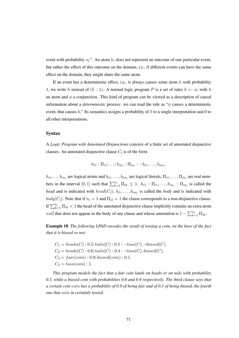
event with probability αi”. An atom hi does not represent an outcome of one particular event,
but rather the effect of this outcome on the domain, i.e., if different events can have the same
effect on the domain, they might share the same atom.
If an event has a deterministic effect, i.e., it always causes some atom h with probability
1, we write h instead of (h : 1). A normal logic program P is a set of rules h ← φ, with h
an atom and φ a conjunction. This kind of program can be viewed as a description of causal
information about a deterministic process: we can read the rule as “φ causes a deterministic
event, that causes h.” Its semantics assigns a probability of 1 to a single interpretation and 0 to
all other interpretations.
Syntax
A Logic Program with Annotated Disjunctions consists of a finite set of annotated disjunctive
clauses. An annotated disjunctive clause Ci is of the form
hi1 : Πi1; . . . ;hini : Πini : −bi1, . . . , bimi .
hi1, . . . hini are logical atoms and bi1, . . . , bimi are logical literals, Πi1, . . . ,Πini are real num-
bers in the interval [0, 1] such thatni
k=1Πik ≤ 1. hi1 : Πi1, . . . , hini : Πini is called the
head and is indicated with head(Ci); bi1, . . . , bimi is called the body and is indicated with
body(Ci). Note that if ni = 1 and Πi1 = 1 the clause corresponds to a non-disjunctive clause.
Ifni
k=1Πik < 1 the head of the annotated disjunctive clause implicitly contains an extra atom
null that does not appear in the body of any clause and whose annotation is 1−ni
k=1Πik.
Example 18 The following LPAD encodes the result of tossing a coin, on the base of the factthat it is biased or not:
C1 = heads(C) : 0.5; tails(C) : 0.5 : −toss(C),¬biased(C).C2 = heads(C) : 0.6; tails(C) : 0.4 : −toss(C), biased(C).C3 = fair(coin) : 0.9; biased(coin) : 0.1.
C4 = toss(coin) : 1.
This program models the fact that a fair coin lands on heads or on tails with probability0.5, while a biased coin with probabilities 0.6 and 0.4 respectively. The third clause says thata certain coin coin has a probability of 0.9 of being fair and of 0.1 of being biased, the fourthone that coin in certainly tossed.
71

C1, for instance, expresses the fact that for each coin c, precisely one of the followingclauses will hold: heads(c) : −toss(c),¬biased(c) or tails(c) : −toss(c),¬biased(c), bothwith a probability of 0.5.
Semantics
An LPAD rule containing variables represents a number of simple experiments, one for each
ground instantiation of this rule. The semantics of a LPAD program P will be defined using
its grounding and restricting to its Herbrand base HB(P ) and to the set of all its Herbrand
interpretations IP . We denote the set of all ground LPADs as PG and by ground(P ) the
grounding of one LPAD P . The semantics is defined by a probability distribution π on IP : π
is a mapping from IP to real numbers in [0,1] such that
I∈IP π(I) = 1.
Each ground instantiation of a clause represents a probabilistic choice between a number
of non-disjunctive clauses, equal to the number of the atoms in its head. This choice is made
according to a selection function; some preliminary concepts have to be introduced now. An
atomic choice is a triple (Ci, θj , k) where Ci ∈ P , θj is a substitution that grounds Ci and
k ∈ 1, . . . , ni. (Ci, θj , k) means that, for ground clause Ciθj , the head hik was chosen. A
set of atomic choices κ is consistent if (C, θ, i) ∈ κ, (C, θ, j) ∈ κ⇒ i = j, i.e., only one head
is selected for a ground clause. A composite choice κ is a consistent set of atomic choices. The
probability P (κ) of a composite choice κ is the product of the probabilities of the individual
atomic choices, i.e. P (κ) =
(Ci,θj ,k)∈κΠik.
A selection σ is a composite choice that, for each clause Ciθj in ground(P ), contains an
atomic choice (Ci, θj , k). We denote the set of all selections σ of a program P by SP and we
let g(i) be the set of indexes of substitutions grounding Ci, i.e., g(i) = j|θj is a substitution
grounding Ci. Each selection σ defines an instance of the LPAD, that is a normal logic
program wσ defined as wσ = (hik ← body(Ci))θj |(Ci, θj , k) ∈ σ. wσ is also called a world
of P . This semantics means that a probabilistic rule in an LPAD expresses the fact that exactly
one atom in the head holds with a certain probability as a consequence of the body of the
rule being true.
Each selection σ in SP is assigned a probability, which induces a probability on the corre-
sponding program wσ. We assume independence between the selections made for each rule.
The probability P (σ) of a selection σ is the probability of a composite choice κ, thus is given
72

by the product of the probabilities of its individual atomic choices:
P (σ) =
(Ci,θj ,k)∈σ
Πik.
Moreover P (σ) is equal to the probability of the world P (wσ), since selections define worlds.
Example 19 If we consider the grounding of the LPAD in Example 18 with the variable Cassuming value coin, 8 different instances (2 · 2 · 2) can be generated by choosing one of thepossibilities for each clause, for example one is:
C1 = heads(coin) : −toss(coin),¬biased(coin).C2 = heads(coin) : −toss(coin), biased(coin).C3 = fair(coin).
C4 = toss(coin).
Each rule is independent of the other, since dependence is modeled within a rule, and aprobability can be assigned to each instance: 0.5 · 0.6 · 0.9 · 1 = 0.27.
The meaning of the above instance of the coin program is given by the interpretation
toss(coin), fair(coin), heads(coin). The instances of an LPAD therefore define a prob-
ability distribution on the set of interpretations of the program: the probability of a certain
interpretation I is the sum of the probability of all instances for which I is a model.
Example 20 Returning to the example, there is one other instance of this LPAD which hastoss(coin), fair(coin), heads(coin) as its model, namely
C1 = heads(coin) : −toss(coin),¬biased(coin).C2 = tails(coin) : −toss(coin), biased(coin).C3 = fair(coin).
C4 = toss(coin).
The probability of this instance is 0.5 · 0.4 · 0.9 · 1 = 0.18. Therefore the probability of theinterpretation is 0.27+0.18=0.45.
We consider only sound LPADs, where the meaning of an instance wσ is given by its well
founded model WFM(wσ) and require that all these models are two-valued.
Given a sound LPAD P , for each of its interpretations I in IP , the probability π∗P (I)
assigned by P to I is the sum of the probabilities of all selections which lead to I , with S(I)
73

being the set of all selections σ for which WFM(wσ) = I:
π∗P (I) =
σ∈S(I)
P (σ).
There is a strong connection between the interpretations for which π∗P (I) > 0 and the well
established non-probabilistic semantics of logic programming, since each interpretation I for a
program P is a traditional logic model for P (when ignoring the probabilities); moreover each
logic program is also an LPAD and its semantics will assign probability 1 to its well founded
model (and zero to all other interpretations).
Inference
Besides probabilities of interpretations, the basic inference task of probabilistic logic programs
under the semantics π∗P is calculating probabilities of queries, i.e., of existentially quantified
conjunctions, according to a LPAD and possibly some evidence.
The set of all instances of a LPAD P is denoted as WP . A composite choice κ identifies
a set of instances ωκ = wσ|σ ∈ SP , σ ⊇ κ. A set of composite choices K identifies a
set of instances ωK =
κ∈K ωκ. A composite choice κ is an explanation for a query Q if Q
is entailed by every instance (world) of ωκ. A set of composite choices K is covering with
respect to Q if every world wσ in which Q is true is in ωK .
The probability of a queryQ given an instancew is the conditional probability P (Q | w) =1 if w |= Q and 0 otherwise.
The probability of a query Q is thus given by:
P (Q) =
w∈WP
P (Q,w) =
w∈WP
P (Q|w)P (w) =
w∈WP :w|=Q
P (w). (9.1)
The probability distribution over normal logic programs (instances) P (w) is extended to
queries and the probability of a query is obtained by marginalizing the joint distribution of the
query and the programsP (Q,w). The trivial way of computingP (Q) proceeds by enumerating
all possible ground instances of a LPAD P , that is often unfeasible for large programs. Instead,
the number of proofs for a query is much more limited, as shown in Example 21.
Example 21 Consider the following LPAD P inspired by the morphological characteristics ofthe Stromboli Italian island, on which we want to compute the probability of the query eruption:
74

C1 = eruption : 0.6 ; earthquake : 0.3 :− sudden_energy_release,fault_rupture(X).
C2 = sudden_energy_release : 0.7.C3 = fault_rupture(southwest_northeast).C4 = fault_rupture(east_west).
The Stromboli island is located at the intersection of two geological faults, one in the southwest-northeast direction, the other in the east-west direction, and contains one of the three volcanoesthat are active in Italy. This program models the possibility that an eruption or an earthquakeoccurs at Stromboli. If there is a sudden energy release under the island and there is a faultrupture (C1), then there can be an eruption of the volcano on the island with probability 0.6, anearthquake in the area with probability 0.3 or no event (the implicit null atom) with probability0.1. The energy release occurs with probability 0.7 while we are sure that ruptures occur inboth faults.
P defines 18 (3 · 3 · 2) possible instances: the first rule with three head atoms has twopossible groundings X = southwest_northeast and X = east_west (3 · 3) and the secondrule has two head atoms. The query eruption is true only in 5 of them. Its probability, accordingto Equation 9.1, is P (eruption) = 0.6 · 0.6 · 0.7 + 0.6 · 0.3 · 0.7 + 0.6 · 0.1 · 0.7 + 0.3 · 0.6 ·0.7 + 0.1 · 0.6 · 0.7 = 0.588.
For instance, the first term 0.6 · 0.6 · 0.7 is obtained from the instance:eruption : 0.6 :− sudden_energy_release, fault_rupture(southwest_northeast).eruption : 0.6 :− sudden_energy_release, fault_rupture(east_west).
sudden_energy_release : 0.7.
fault_rupture(southwest_northeast).fault_rupture(east_west).
while the last term 0.1 · 0.6 · 0.7 from the instance:null : 0.1 :− sudden_energy_release, fault_rupture(southwest_northeast).eruption : 0.6 :− sudden_energy_release, fault_rupture(east_west).
sudden_energy_release : 0.7.
fault_rupture(southwest_northeast).fault_rupture(east_west).
Since it is often unfeasible to find all the instances where the query is true, inference al-
gorithms search for covering set of explanations for the query instead. If we establish the
following correspondences:
Ciθj → multivalued random variable Xij
atomic choice (Ci, θj , k) → assignment Xij = k, k ∈ 1, . . . , ni
the problem of computing the probability of a query Q can be reduced to computing the prob-
75

ability of the Boolean function defined over the vector of variables X:
fQ(X) =
κ∈E(Q)
(Ci,θj ,k)∈κ
Xij = k (9.2)
It is a Disjunctive Normal Form (DNF) formula (a disjunction of conjunctive clauses), where
E(Q) is a covering set of explanations for Q and Xij = k indicates that the kth atom has
been chosen in the head of clause Ci grounded with substitution θj . Equations for a single
explanation κ are conjoined and the conjunctions for the different explanations are disjointed.
The probability that goal Q succeeds equals to the probability that the disjunction of these
conjunctions is true (takes value 1), and this happens if the values of the variables correspond
to an explanation for the query.
Example 22 (Example 21 cont.) Clause C1 has two groundings, C1θ1 withθ1 = X/southwest_northeast and C1θ2 with θ2 = X/east_west, corresponding to therandom variables X11 and X12 respectively. Clause C2 has only one grounding C2∅ insteadand it corresponds to the single random variableX21. X11 andX12 can take three values sinceC1 has three head atoms; similarly X21 can take two values since C2 has two head atoms.
The query eruption has the covering set of explanations E(eruption) = κ1, κ2 where:
κ1 = (C1, X/southwest_northeast, 1), (C2, , 1)κ2 = (C1, X/east_west, 1), (C2, , 1)
Each atomic choice (Ci, θj , k) ∈ κi is represented by the propositional equationXij = k:
(C1, X/southwest_northeast, 1) → X11 = 1
(C2, , 1) → X21 = 1
(C1, X/east_west, 1) → X12 = 1
The set of explanations E(eruption) can be encoded, according to the formula 9.2, by thefunction:
feruption(X) = (X11 = 1 ∧X21 = 1) ∨ (X12 = 1 ∧X21 = 1)
While each of these explanations can be assigned a probability, it is incorrect to sum them up in
order to compute P(Q), since they are not statistically independent, differently from instances.
In fact, the probability of the DNF formula
P (feruption(X)) = P ((X11 = 1 ∧X21 = 1) ∨ (X12 = 1 ∧X21 = 1))
76

is
P (feruption(X)) = P (X11 = 1 ∧X21 = 1) + P (X12 = 1 ∧X21 = 1) −
P (X11 = 1 ∧X21 = 1)P (X12 = 1 ∧X21 = 1).(9.3)
If we simply summed up P (X11 = 1 ∧X21 = 1) and P (X12 = 1 ∧X21 = 1) we would
get 0.6 · 0.7+0.6 · 0.7 = 0.84 = 0.588, while according to Equation 9.3 we correctly compute
0.6 ·0.7+0.6 ·0.7−0.6 ·0.6 ·0.7 = 0.588, cf Example 21. The third product term in Equation
9.3 represents a joint event, indicating that explanations have first to be made disjoint (mutually
exclusive) so that a summation can be computed. In the literature, the problem of computing
the probability of DNF formulae is an NP-hard problem even if all variables are independent,
and this is the problem of transforming sum-of-products into sum-of-disjoint-products. Some
algorithms have been developed, however they seem to be limited to a few dozens of variables
and a few hundreds of sums.
The most efficient technique up to now is represented by Multivalued Decision Diagrams
(MDD). The advantage of MDDs is that they represent the Boolean function f(X) by means
of a generalization of the Shannon’s expansion
f(X) = (X1 = 1) ∧ fX1=1(X) ∨ · · · ∨ (X1 = n) ∧ fX1=n(X)
where X1 is the variable associated with the root node of the diagram and fX1=i(X) is the
function associated to the i−th child of the root node. The expansion can be applied recursively
to the functions fX1=i(X). This expansion allows the probability of f(X) to be expressed by
means of the following recursive formula
P (f(X)) = P (X1 = 1) · P (fX1=1(X)) + ...+ P (X1 = n) · P (fX1=n(X))
because the disjuncts are mutually exclusive due to the presence of the X1 = i equations. In
this way the MDD split paths on the basis of the values of a multi-valued variable and the
branches are mutually disjoint, thus the probability of f(X) can be computed by means of
a dynamic programming algorithm that traverses the MDD and sums up probabilities. The
reduced MDD corresponding to the query eruption from Example 21 is shown in Figure 9.1a.
The labels on the edges represent the values of the variable associated with the source node.
Since most packages for the manipulation of decision diagrams are restricted to work
on Binary Decision Diagrams, multivalued variables have to be represented by means of bi-
nary variables (De Raedt et al., 2008a; Sang et al., 2005). For a multi-valued variable Xij ,
77
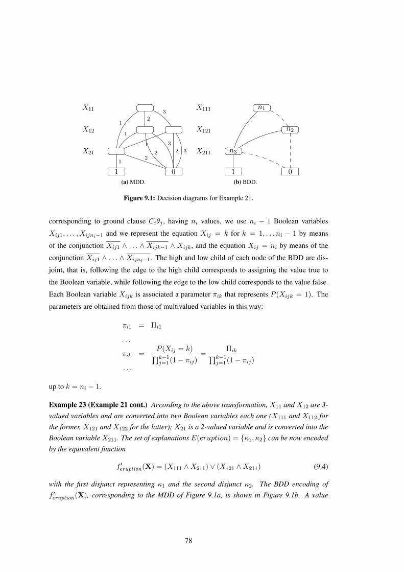
X11
12
3
X12 1
2
312 3X21
12
1 0
(a) MDD.
X111 n1
X121 n2
X211 n3
1 0
(b) BDD.
Figure 9.1: Decision diagrams for Example 21.
corresponding to ground clause Ciθj , having ni values, we use ni − 1 Boolean variables
Xij1, . . . , Xijni−1 and we represent the equation Xij = k for k = 1, . . . ni − 1 by means
of the conjunction Xij1 ∧ . . . ∧ Xijk−1 ∧ Xijk, and the equation Xij = ni by means of the
conjunction Xij1 ∧ . . . ∧ Xijni−1. The high and low child of each node of the BDD are dis-
joint, that is, following the edge to the high child corresponds to assigning the value true to
the Boolean variable, while following the edge to the low child corresponds to the value false.
Each Boolean variable Xijk is associated a parameter πik that represents P (Xijk = 1). The
parameters are obtained from those of multivalued variables in this way:
πi1 = Πi1
. . .
πik =P (Xij = k)k−1j=1(1− πij)
=Πikk−1
j=1(1− πij). . .
up to k = ni − 1.
Example 23 (Example 21 cont.) According to the above transformation, X11 and X12 are 3-valued variables and are converted into two Boolean variables each one (X111 and X112 forthe former, X121 and X122 for the latter); X21 is a 2-valued variable and is converted into theBoolean variable X211. The set of explanations E(eruption) = κ1, κ2 can be now encodedby the equivalent function
f ′eruption(X) = (X111 ∧X211) ∨ (X121 ∧X211) (9.4)
with the first disjunct representing κ1 and the second disjunct κ2. The BDD encoding off ′eruption(X), corresponding to the MDD of Figure 9.1a, is shown in Figure 9.1b. A value
78

of 1 for the Boolean variables X111 and X121 means that, for the ground clauses C1θ1 andC1θ2, the head h11 = eruption is chosen and the 1-branch from nodes n1 and n2 must befollowed, regardless of the other variables for C1 (X112, X122) that are in fact omitted fromthe diagram.
Having built the BDD representing the Boolean function f ′Q(X), in order to compute the
probability a dynamic programming algorithm traverses the diagram from the root node to
all leaves (De Raedt et al., 2007). At each inner node, probabilities from both children are
calculated recursively and combined afterwards as it is done in Algorithm 1.
Algorithm 1 Probability of a query computed by traversing a BDD.1: function BDD_PROBABILITY(node n)2: if n is 1-terminal then3: return 14: end if5: if n is 0-terminal then6: return 07: end if8: let h and l be the high and low children of n9: prob(h) = BDD_PROBABILITY(h)
10: prob(l) = BDD_PROBABILITY(l)11: return pn · prob(h) + (1− pn) · prob(l)12: end function
For each node, the probability that the sub-BDD starting at that node is true is computed by
summing the probability of the high and low child, weighted by the probability of the node’s
variable being assigned true and false respectively. Intermediate results are cached, and the
algorithm has a time and space complexity linear in the size of the BDD. The probability of
the root node corresponds to the probability of the query P (Q), i.e., the probability of f ′Q(X)
taking value 1. The application of the Algorithm 1 to the BDD of Example 23 is illustrated in
Figure 9.2. The probabilities computed by Algorithm 1 on the two sub-BDDs can be summed
up as the corresponding events are statistically independent.
Even if BDDs allow to compactly represent explanations for queries, they might have an
exponential growth in large programs characterized by many random variables. In order to
contain the number of variables and thus simplify inference, we may consider grounding only
some of the variables of clauses, at the expenses of the accuracy in modeling the domain. A
typical compromise between accuracy and complexity is to consider the grounding of variables
in the head only: in this way, a ground atom entailed by two separate ground instances of a
clause is assigned the same probability, all other things being equal, of a ground atom entailed
79

X111 n1P = 0.588
= 0.6·0.7+0.4·0.42
0.6
0.4
X121 n2P = 0.42
= 0.6 · 0.7+0.4 · 00.6
0.4X211 n3P = 0.7
= 0.7 · 1 + 0.3 · 00.7
0.3
1 0
Figure 9.2: BDD built to compute the probability of the query Q = eruption for Example 21.The probabilities P of each node represent the intermediate values computed by Algorithm 1 whentraversing the BDD. The probability of the query (0.588) is returned at the root node.
by a single ground clause, while in the full semantics the first would have a larger probability,
as more evidence is available for its entailment. This simplified semantics can be interpreted as
stating that a ground atom is entailed by a clause with the probability given by its annotation if
there is a substitution for the variables appearing in the body only such that the body is true.
Example 24 (Example 21 cont.) In the simplified semantics, C1 is associated with a singlerandom variable X11. In this case T has 6 (3 · 2) instances, the query eruption is true in 1 ofthem and its probability is P (eruption) = 0.6 · 0.7 = 0.42. So eruption is assigned a lowerprobability with respect to the full semantics because the two independent groundings of clauseC1, differing in the fault name, are not considered separately anymore.
Reducing the size of the BDD allows to apply parameter learning for LPADs on large-scale
real world datasets.
One of the algorithms developed in this thesis is a variant of the BDD traversal algorithm
for computing the probability of a query. In Section 10.2 we extend the computation on the
BDD to optimize the parameters of an LPAD program with respect to a training set, by adding
a “forward” traversal of the diagram to the current recursive “backward” traversal.
80

Chapter 10
Parameter Learning of LPADs
One typically distinguishes two problems within the statistical learning field. First, there is
the problem of parameter estimation, where the goal is to estimate appropriate values for the
parameters of a model, whose structure is fixed, and second, there is the problem of structure
learning, where the learner must infer both the structure and the parameters of the model from
data (Raedt, 2008). The first problem is tackled is this chapter, the second one in the next
Chapter.
This chapter presents, after a general introduction about the parameter estimation problem
in probabilistic models (Section 10.1), the parameter learning algorithm EMBLEM for LPADs
based on the Expectation Maximization approach, where the expectations are computed di-
rectly using BDDs (Section 10.2). The chapter also features related works (Section 10.3) and
experimental results on real world datasets (Section 10.4). Conclusive considerations can be
found in Section 10.5.
10.1 Parameter Learning of Probabilistic Models
The problem of parameter estimation can be formalized as follows:
Given
• a set of examples E,
• a probabilistic model M = (S, λ) with structure S and parameters λ,
• a probabilistic coverage relation P (e|M) that computes the probability of observing the
example e given the model M ,
81

• a scoring function score(E,M) that employs the probabilistic coverage relationP (e|M)
Find the parameters λ∗ that maximize score(E,M), that is,
λ∗ = arg maxλ score(E, (S, λ))
This problem specification abstracts the specific class of models considered, and actually can
be instantiated w.r.t. the different representation languages. The problem specification shows
that parameter estimation is essentially an optimization problem that depends on the scoring
function and type of model employed.
The standard scoring function is the probability of the model or hypothesis given the data.
This yields the maximum a posteriori hypothesis HMAP
HMAP = arg maxHP (H|E) = arg maxHP (E|H)P (H)
P (E)
It can be simplified into the maximum likelihood hypothesis HML by applying Bayes’ law and
assuming that all hypotheses H are, a priori, equally likely, yielding:
HML = arg maxHP (E|H) (10.1)
which is called the likelihood function.
It is typically assumed that the examples are independently and identically distributed
(i.i.d.), which allows one to rewrite the expression in the following form (where the ei cor-
respond to the different examples):
HML = arg maxHei∈E
P (ei|H)
The probabilistic coverage relation P (e|H) is employed, and it indicates the likelihood of
observing e given the hypothesis (model)H . Typically, the goal is to learn a generative model,
that is, a model that could have generated the data.
This contrasts with the traditional inductive logic programming setting, which is discrim-
inative: positive examples have a strictly positive probabilistic coverage (P (e|H) > 0), the
negative ones have a 0 probabilistic coverage. Within the above problem specification discrim-
inative learning can be modeled by choosing an alternative scoring function, that maximizes
the conditional likelihood function
HCL = arg maxHei∈E
P (class(ei)|des(ei), H) (10.2)
82

where the examples ei are split up into the class of interest (also called target) class(ei) and
the description of the example des(ei). This function can be maximized by maximizing its
logarithm instead, which is easier because the logarithm is a monotonic function. In literature
it is thus referred as the conditional log likelihood (LL) function.
10.2 The EMBLEM Algorithm
The parameter estimation algorithm for LPADs, which is presented in the following, tackles a
problem of discriminative learning defined as follows.
Given
• a set of training examplesQi, corresponding to ground atoms for a set of target or output
predicates,
• a background knowledge with ground facts for other non-target or input predicates, or-
ganized as a set of logical interpretations or “mega-examples”,
• a probabilistic logical model M corresponding to a LPAD program P , composed of
annotated disjunctive clauses Ci with unknown parameters (probabilities) λ = Π =
⟨Πi1, ...,Πini⟩ in the heads,
Find the maximum likelihood probabilities Π∗, i.e. those that maximize the conditional prob-
ability of the examples given the model and the input predicates.
EMBLEM algorithm learns maximum likelihood parameters of a LPAD by applying the
Expectation Maximization algorithm where the expectations are computed directly on BDDs.
It is based on the algorithms proposed in (Inoue et al., 2009; Ishihata et al., 2008a,b; Thon
et al., 2008).
The application of the EM algorithm has the following justifications. Each training example
Qi corresponds to a query to the LPAD and the background data. In order to determine the
probabilities Πik, the number of times a head hik has been chosen in an application of a rule
Ci to find an explanation for the query is required. This frequency is indicated as cik and
is not directly observable. Given the set of clauses involved in the SLD-derivation of the
query, there are many possible selections σ which allows one to find a proof for the query: the
information about which selection has been used is unknown. The Expectation Maximization
(EM) algorithm deals with the case where the data are not fully observable, but only partially
83

observable; if values for some variables are occasionally unobserved, there is missing data,
while if values for some variables are always unobserved, the variables are called latent. In
our case, the mega-examples record the truth value of all ground facts, but not the selections
(that is, the atomic choices) which represent the latent variables, and the random variables cikrepresent a sufficient statistics, whose value contains all the information needed to compute any
estimate of the unknown parameters. As introduced in Chapter 8, we would like to maximize
the (log-)likelihood L of the data, which is a function of the parameters Π of the model L(Π).
This function depends on the unobserved values and a way of dealing with these values is to
compute the expected likelihood functionQ(Π), where the expectation is taken over the hidden
variables. The algorithm assumes that there is a current model M(Π) and uses it to compute
the expected values of the variables cik, that is E[cik|M,Π]. After randomly initializing the
model parameters, the EM algorithm repeatedly performs the following two operations until
the parameters have converged:
• E Step: Uses the current model and the observed data to determine the conditional dis-
tribution of the unobserved random variables cik;
• M Step: Uses the observed random variables together with the distribution of the unob-
served random variables to estimate the model parameters using frequency counting;
In the following the two steps of the algorithm are described in detail.
Construction of the BDDs
Among all predicates describing the domain, some of them have to be specified as target by
the user, while the remainder are referred as background. The ground atoms in the mega-
examples for the target predicates correspond to as many queries Qi for which the BDDs are
built, encoding the disjunction of their explanations; these atoms will be referred afterwards
as (target) examples. The mega-examples must contain also negative atoms for target predi-
cates, expressed as neg(atom). These predicates are called target or output since EM tries
to maximize the conditional log-likelihood only for the positive and negative facts of those
predicates.
The predicates can be treated as closed-world or open-world. In the first case, the body
of clauses is resolved only with facts in the mega-example. In the second case, the body of
clauses is resolved both with facts and with clauses in the theory. If the latter option is set
84

and the program is cyclic (see Def. 20), EMBLEM uses a depth bound on SLD-derivations to
avoid going into infinite loops, as proposed by (Gutmann et al., 2010a), withD the value of the
bound: derivations exceeding the limit D are cut.
Definition 20 (Acyclic programs) A level mapping for a program T is a function| |: HB(T )→ N of ground atoms to natural numbers. For A ∈ HB(T ) | A | is the level of A.
Given a level mapping | |, we extend it to ground negative literals by defining | ¬A |=| A |.
• A clause of T is called acyclic with respect to a level mapping | |, if for every groundinstance A ← B of it, the level of A is greater then the level of each literal in the bodyB.
• A program T is called acyclic with respect to a level mapping | |, if all its clauses are. Tis called acyclic if it is acyclic with respect to some level mapping.
We extend this definition to LPADs by requiring that the level of each atom in the head is
greater than the level of each literal in the body. This ensures that each instance of the LPAD
is an acyclic logic program.
Example 25 Consider the program T that defines the predicate path/2 such that path(x, y)is true if there is a path from x to y in a directed graph. Such a program contains the clauses
path(X,Y )← edge(X,Y ).
path(X,Y )← edge(X,Z), path(Z, Y ).
plus a set E of ground facts for the edge/2 relation that represent the edges between nodes ofthe graph. path/2 defines the transitive closure of edge/2.Suppose E contains the only fact edge(a, b). This program is not acyclic because it containsthe ground rule
path(a, a)← edge(a, a), path(a, a).
that imposes the contradictory constraint |path(a, a)| > |path(a, a)|.
The search for proofs of a query Q is performed in practice by employing SLD-resolution
in Prolog, against a database composed of the mega-examples. The paths from the root to
individual leaves of the SLD-tree represent either a successful or a failed proof. Each successful
proof in the SLD-tree has a set of clauses (and head atoms) employed in that proof, represented
by a covering set of explanations, that is independent of other clauses in the LPAD. The set
of composite choices leading to successful proofs is graphically represented as the set of paths
from the root the the 1-leaf of a BDD.
85

Program transformation into a BDD For generating the BDD for a query (example) Q the
algorithm “Probabilistic Inference with Tabling and Answer subsumption” (PITA) (Riguzzi
and Swift, 2010) is applied, which builds explanations for every subgoal encountered during a
derivation of the query. The input LPAD is transformed into a normal logic program in which
the subgoals have an extra argument storing a BDD that represents their explanations.
The first step of the algorithm is to apply a program transformation to a LPAD to create a
normal program that contains calls for manipulating BDDs. In the implementation, these calls
provide a Prolog interface to the CUDD1 C library, where BDDs are represented as pointers to
their root node, and use the following predicates:
• init, end: for allocation and deallocation of a BDD manager, a data structure used to keep
track of the memory for storing BDD nodes;
• zero(-BDD), one(-BDD), and(+BDD1,+BDD2,-BDDO), or(+BDD1,+BDD2, -BDDO),
not(+BDDI,-BDDO): Boolean operations between BDDs;
• add_var(+NVal,+Probs,-Var): addition of a new multi-valued variable with NVal values
and parameters Probs;
• equality(+Var,+Value,-BDD): BDD represents V ar = V alue, i.e., the random variable
V ar is assigned V alue in the BDD;
• ret_prob(+BDD,-P): returns the probability of the formula encoded by BDD.
add_var(+NVal,+Probs,-Var) adds a new random variable associated with a new instan-
tiation of a rule with NV al head atoms and parameters list Probs. The auxiliary predicate
get_var_n/4 is used to wrap add_var/3 and avoid adding a new variable when one already ex-
ists for an instantiation. As shown below, a new fact var(R,S,Var) is asserted each time a new
random variable is created, where R is an identifier for the LPAD rule, S is a list of constants,
one for each variable of the clause, and V ar is a integer that identifies the random variable
associated with clause R under a specific grounding. The auxiliary predicate has the following
definition:
get_var_n(R,S, Probs, V ar)← (var(R,S, V ar)→ true;
length(Probs, L), add_var(L,Probs, V ar), assert(var(R,S, V ar))).
1http://vlsi.colorado.edu/~fabio/
86

where Probs is a list of real numbers that stores the parameters in the head of rule R. R,S and
Probs are input arguments while V ar is an output argument.
The transformation applies to clauses, literals and atoms:
• If h is an atom, PITAh(h) is h with the variable BDD added as the last argument;
• If bj is an atom, PITAb(bj) is bj with the variable Bj added as the last argument.
• If bj is negative literal ¬aj , PITAb(bj) is the conditional
(PITA′b(aj)→ not(BNj , Bj); one(Bj)), where PITA′b(aj) is aj with the
variable BNj added as the last argument; the BDD BNj for a is negated if it exists (i.e.
PITA′b(aj) succeeds); otherwise the BDD for the constant function 1 is returned.
• A non-disjunctive fact Cr = h is transformed into the clause
PITA(Cr) = PITAh(h)← one(BDD).
• A disjunctive fact Cr = h1 : Π1; . . . ;hn : Πn. where the parameters sum to 1, is
transformed into the set of clauses PITA(Cr)PITA(Cr, 1) = PITAh(h1)← get_var_n(r, [], [Π1, . . . ,Πn], V ar),
equality(V ar, 1, BDD).. . .P ITA(Cr, n) = PITAh(hn)← get_var_n(r, [], [Π1, . . . ,Πn], V ar),
equality(V ar, n,BDD).
When the parameters do not sum to one, the clause is first transformed into h1 : Π1∨. . .∨
hn : Πn∨null : 1−n
1 Πi and then into the clauses above, where the list of parameters
is [Π1, . . . ,Πn, 1−n
1 Πi] but the (n + 1)-th clause (for null) is not generated.
• The definite clause Cr = h← b1, b2, . . . , bm. is transformed into the clausePITA(Cr) = PITAh(h)← PITAb(b1), P ITAb(b2), and(B1, B2, BB2),
..., P ITAb(bm), and(BBm−1, Bm, BDD).
• The disjunctive clause Cr = h1 : Π1; . . . ;hn : Πn ← b1, b2, . . . , bm.
where the parameters sum to 1, is transformed into the set of clauses PITA(Cr)
87

PITA(Cr, 1) = PITAh(h1)← PITAb(b1), P ITAb(b2), and(B1, B2, BB2),...,P ITAb(bm), and(BBm−1, Bm, BBm),get_var_n(r, V C, [Π1, ...,Πn], V ar),equality(V ar, 1, B), and(BBm, B,BDD).
. . .P ITA(Cr, n) = PITAh(hn)← PITAb(b1), P ITAb(b2), and(B1, B2, BB2),
...,P ITAb(bm), and(BBm−1, Bm, BBm),get_var_n(r, V C, [Π1, ...,Πn], V ar),equality(V ar, n,B), and(BBm, B,BDD).
where V C is a list containing each variable appearing in Cr. If the parameters do not
sum to 1, the same technique used for disjunctive facts is used.
In order to answer queries, the goal solve(Goal, P ) is used, which is defined for the cases
a depth D is used or not to derive the goal:solve(Goal, P )← init, retractall(v(_, _, _)),
add_bdd_arg(Goal,BDD0, GoalOut),(bagof(BDD0, GoalOut, L)→ or_list(L,BDD); zero(BDD)),ret_prob(BDD,P ),end.
solve(Goal, P )← init, setting(depth_bound, true), !,setting(depth,DB), retractall(v(_, _, _)),add_bdd_arg_db(Goal,BDD0, DB,GoalOut),(bagof(BDD0, GoalOut, L)→ or_list(L,BDD); zero(BDD)),ret_prob(BDD,P ),end.
Example 26 Clause C1 from the LPAD of Example 21 is translated intoeruption(BDD) ← sudden_energy_release(B1), fault_rupture(X,B2),
and(B1, B2, BB2),
get_var_n(1, [X], [0.6, 0.3, 0.1], V ar),
equality(V ar, 0, B), and(BB2, B,BDD).
earthquake(BDD) ← sudden_energy_release(B1), fault_rupture(X,B2),
and(B1, B2, BB2),
get_var_n(1, [X], [0.6, 0.3, 0.1], V ar),
equality(V ar, 1, B), and(BB2, B,BDD).
Clause C2 is translated intosudden_energy_release(BDD) ← get_var_n(2, [], [0.7, 0.3], V ar),
equality(V ar, 0, BDD).
88

Clause C3 is translated into
fault_rupture(southwest_northeast,BDD) ← one(BDD).
EM Cycle
After building the BDDs for each target example Q, EMBLEM starts the EM cycle, in which the
steps of Expectation and Maximization are repeated until the LL of the examples reaches a local
maximum or a maximum number of steps (NEM ) is reached. EMBLEM is shown in Algorithm
2, where with Theory we mean the LPAD program: it consists of a cycle where the procedures
EXPECTATION and MAXIMIZATION are repeatedly called; procedure EXPECTATION returns
the LL of the data that is used in the stopping criterion. EMBLEM stops when the difference
between the LL of the current and the previous iteration drops below a threshold ϵ or when this
difference is below a fraction δ of the current LL.
Algorithm 2 Function EMBLEM1: function EMBLEM(Theory,D,NEM, ϵ, δ)2: Build BDDs by SLD derivations with depth bound D
3: LL = −inf4: N = 0
5: repeat Start of EM cycle6: LL0 = LL
7: LL = EXPECTATION(BDDs)8: MAXIMIZATION
9: N = N + 1
10: until LL− LL0 < ϵ ∨ LL− LL0 < −LL · δ ∨N > NEM
11: Update parameters of Theory
12: return LL, Theory
13: end function
Expectation Step
The Expectation phase (see Algorithm 3) takes as input a list of BDDs, one for each target fact
Q, and computes the probabilities P (Xijk = x|Q) for all Cis, k = 1, . . . , ni − 1, j ∈ g(i) :=j|θj is a substitution grounding Ci and x ∈ 0, 1. From P (Xijk = x|Q) one can compute
the expectations E[cik0|Q] and E[cik1|Q] where cikx is the number of times a Boolean variable
Xijk takes value x for x ∈ 0, 1 and for all j ∈ g(i). i.e, the ground head hik has been used
(1) or not (0) in a proof. E[cikx|Q] is given by
E[cikx|Q] =j∈g(i)
P (Xijk = x|Q)
89

Finally, the expectations E[cik0] and E[cik1] of the counts over all queries are computed as
E[cikx] =Q
E[cikx|Q]
Algorithm 3 Function Expectation1: function EXPECTATION(BDDs)2: LL = 0
3: for all BDD ∈ BDDs do4: for all i ∈ Rules do5: for k = 1 to ni − 1 do6: η0(i, k) = 0; η1(i, k) = 0
7: end for8: end for9: for all variables X do
10: ς(X) = 0
11: end for12: GETFORWARD(root(BDD))13: Prob=GETBACKWARD(root(BDD))14: T = 0
15: for l = 1 to levels(BDD) do16: Let Xijk be the variable associated with level l17: T = T + ς(l)
18: η0(i, k) = η0(i, k) + T × (1− πik)
19: η1(i, k) = η1(i, k) + T × πik
20: end for21: for all i ∈ Rules do22: for k = 1 to ni − 1 do23: E[cik0] = E[cik0] + η0(i, k)/Prob
24: E[cik1] = E[cik1] + η1(i, k)/Prob
25: end for26: end for27: LL = LL+ log(Prob)
28: end for29: return LL
30: end function
The conditional probability P (Xijk = x|Q) is given by P (Xijk=x,Q)P (Q) (cf. Section 6.4),
where
P (Xijk = x,Q) =
wσ∈WP :wσ |=Q
P (Q,Xijk = x, σ)
=
wσ∈WP :wσ |=Q
P (Q|σ)P (Xijk = x|σ)P (σ)
=
wσ∈WP :wσ |=Q
P (Xijk = x|σ)P (σ)
90

Now suppose only the merge rule is applied when building the BDD, fusing together iden-
tical sub-diagrams. The resulting diagram, that we call Complete Binary Decision Diagram
(CBDD), is such that every path contains a node for every level.
Since there is a one to one correspondence between the instances whereQ is true (wσ |= Q)
and the paths to a 1 leaf in a CBDD,
P (Xijk = x,Q) =
ρ∈R(Q)
P (Xijk = x|ρ)d∈ρ
π(d)
where ρ is a path, R(Q) is the set of paths in the CBDD for query Q that lead to a 1 leaf and,
if the selection σ corresponds to ρ, then P (Xijk = x|σ) = P (Xijk = x|ρ). d is an edge of
ρ and π(d) is the probability associated with the edge: if d is the 1-branch outgoing of a node
associated with a variable Xijk, then π(d) = πik, if d is the 0-branch, then π(d) = 1 − πik.
See subsection 9.2 for the definition of πik.
Given a path ρ ∈ R(Q), P (Xijk = x|ρ) = 1 if ρ contains an x-branch from a node
associated with variable Xijk and 0 otherwise, so P (Xijk = x,Q) can be further expanded as
P (Xijk = x,Q) =
ρ∈R(Q)∧(Xijk=x)∈ρ
d∈ρ
π(d)
where (Xijk = x) ∈ ρ means that ρ contains an x-branch from the node associated with Xijk.
We can then write
P (Xijk = x,Q) =
n∈N(Q)∧v(n)=Xijk∧ρn∈Rn(Q)∧ρn∈Rn(Q,x)
d∈ρn
π(d)d∈ρn
π(d)
where N(Q) is the set of BDD nodes for query Q, v(n) is the variable associated with node n,
Rn(Q) is the set containing the paths from the root to n and Rn(Q, x) is the set of paths from
n to the 1 leaf through its x-child. So
P (Xijk = x,Q) =
n∈N(Q)∧v(n)=Xijk
ρn∈Rn(Q)
ρn∈Rn(Q,x)
d∈ρn
π(d)d∈ρn
π(d)
=
n∈N(Q)∧v(n)=Xijk
ρn∈Rn(Q)
d∈ρn
π(d)
ρn∈Rn(Q,x)
d∈ρn
π(d)
=
n∈N(Q)∧v(n)=Xijk
F (n)B(childx(n))πikx (10.3)
91

where πikx is πik if x = 1 and (1− πik) if x = 0,
F (n) =
ρn∈Rn(Q)
d∈ρn
π(d)
is the forward probability (Ishihata et al., 2008b), the probability mass (i.e., sum of the proba-
bilities) of the paths from the root to n, and
B(n) =
ρn∈Rn(Q)
d∈ρn
π(d)
is the backward probability (Ishihata et al., 2008b), the probability mass of paths from n to the
1 leaf.
The intuitive meaning of equation (10.3) is the following. Each path from the root of the
BDD to the 1 leaf corresponds to an assignment of values to the variables that satisfies the
Boolean formula represented by the BDD. The expression F (n)B(childx(n))πikx represents
the sum of the probabilities of all the paths passing through the x-edge of node n. In every
node n, the backward probability is the probability that starting from n one will reach the 1
leaf and represents the probability that the logical formula encoded by the sub-BDD rooted at
n is true; the forward probability is the probability that starting at the root one will reach n.
Hence in equation (10.3) we compute the probability that a person starting at the root reaches
n, and ends up in the 1 leaf when leaving n through the x child.
By indicating with ex(n) the product in equation (10.3) we get
P (Xijk = x,Q) =
n∈N(Q),v(n)=Xijk
ex(n) (10.4)
The counts of equation (10.4) are stored in the variables ηx(i, k) for x ∈ 0, 1 in Algorithm
5, i.e., in the end ηx(i, k) contains j∈g(i)
P (Xijk = x,Q).
Formula (10.4) is correct only for CBDDs, while for BDDs - generated by applying also
the deletion rule - it is no longer valid since also paths where there is no node associated to
Xijk can contribute to P (Xijk = x,Q): the contribution of deleted paths must be taken into
account. Suppose that levels are numbered in increasing order from top to bottom and that a
node n is associated with variable Y , that has a level lower than variable Xijk, and child1(n)
is associated with variable W , that has a level higher than variable Xijk. The nodes associated
92

with variable Xijk have been deleted from the paths from n to child1(n). In Figure 9.1b this
happens with n = n1, Y = X111, Xijk = X121, child1(n) = n3, W = X211: the path
connecting n1 to n3 does not contain a node at the level of X121. One can imagine that the
current BDD has been obtained from a BDD having a node m associated with variable Xijk
that is a descendant of n along the 1-branch and whose outgoing edges both point to child1(n).
The original BDD can be reobtained by applying a deletion operation that merges the two paths
passing throughm. The probability mass of the two paths that were merged was e0(n)(1−πik)
and e0(n)πik for the paths passing through the 0-child and 1-child of m respectively.
Formally, let Delx(X) be the set of nodes n such that the level of X is higher than that
of n and is lower that of childx(n), i.e., X is deleted between n and childx(n). For the BDD
in Figure 9.1b, for example, Del1(X121) = n1, Del0(X121) = , Del1(X221) = ,
Del0(X221) = n2. Then
P (Xijk = 0, Q) =
n∈N(Q),v(n)=Xijk
ex(n) +
(1− πik)
n∈Del0(Xijk)
e0(n) +
n∈Del1(Xijk)
e1(n)
P (Xijk = 1, Q) =
n∈N(Q),v(n)=Xijk
ex(n) +
πik
n∈Del0(Xijk)
e0(n) +
n∈Del1(Xijk)
e1(n)
EXPECTATION Function (Algorithm 3) This function first calls GETFORWARD and GET-
BACKWARD and computes ηx(i, k) for non-deleted paths only. Then it updates ηx(i, k) to take
into account deleted paths.
Procedure GETFORWARD, shown in Algorithm 4, computes the value of the forward prob-
abilities. It traverses the diagram one level at a time starting from the root level and propagating
the values downwards. For each level it considers each node n and computes its contribution to
the forward probabilities of its children. Then the forward probabilities of its children, stored
in table F , are updated.
Forward probabilities express the likelihood of reaching a node n when starting from the
root node and following edges according to their probability. It is defined as F (root) = 1 for
93

the root node of the BDD. For any other node it is defined as:
F (n) =
p∈Nodesn=child1(p),var(p)=Xijk
F (p) · πik +
p∈Nodesn=child0(p),var(p)=Xijk
F (p) · (1− πik).
The first sum considers all possible parent nodes p of n connected by a 1-branch. When be-
ing in p one will choose this edge to reach n with probability πik; the second sum considers all
possible parent nodes that are linked to n by a 0-branch, which will be chosen with probability
1− πik. At the beginning F (n) is 0 for all nodes n except the root.
Function GETBACKWARD, shown in Algorithm 5, computes the backward probability of
nodes by traversing recursively the tree from the root to the leaves. When the calls of GET-
BACKWARD for both children of a node n return, values are propagated upwards from the
leaves,and we have all the information that is needed to compute the ex(n) values and update
the values of ηx(i, k) for non-deleted paths.
The backward probabilities express the likelihood of reaching the 1 leaf when starting from
a particular node n and proceeding to the high child child1(n) with probability πik and to the
low child child0(n) with probability 1− πik. For the terminal nodes they are defined as
B(0) = 0 B(1) = 1,
and for inner nodes, as
B(n) = B(child1(n)) · πik +B(child0(n)) · (1− πik).
Computing the forward and the backward probabilities of BDD nodes requires two traver-
sals of the graph, so the cost is linear in the number of nodes. If root is the root of a tree for
a query Q then B(root) = P (Q), i.e., the backward probability at the root node corresponds
to the probability of the query, as was computed by Algorithm 1 in subsection 9.2. P (Q) is
needed to compute P (Xijk = x|Q). Moreover, P (Q) = F (1) and 1− P (Q) = F (0).
Finally the problem of deleted paths is solved, as in (Ishihata et al., 2008a), by keeping an
array ς with an entry for every level l, that stores an algebraic sum of ex(n): those for nodes in
lower levels that do not have a descendant in level l minus those for nodes in lower levels that
have a descendant in level l. In this way it is possible to add the contributions of the deleted
paths by starting from the root level and accumulating ς(l) for the various levels in a variable
T : an ex(n) value which is added to the accumulator T for level l means that n is an ancestor
for nodes in this level. When the x-branch from n reaches a node in a level l′ such that l′ ≥ l,
94

ex(n) is subtracted from the accumulator, as it is not relative to a deleted node on the path
anymore. This is implemented in a post processing phase in Algorithm 3.
Algorithm 4 Computation of the forward probability F (n) in all BDD nodes n.1: procedure GETFORWARD(root)2: F (root) = 1
3: F (n) = 0 for all nodes4: for l = 1 to levels do levels is the number of levels of the BDD rooted at root5: Nodes(l) = ∅6: end for7: Nodes(1) = root8: for l = 1 to levels do9: for all node ∈ Nodes(l) do
10: Let Xijk be v(node), the variable associated with node
11: if child0(node) is not terminal then12: F (child0(node)) = F (child0(node)) + F (node) · (1− πik)13: Add child0(node) to Nodes(level(child0(node))) level(node) returns the level of node14: end if15: if child1(node) is not terminal then16: F (child1(node)) = F (child1(node)) + F (node) · πik
17: Add child1(node) to Nodes(level(child1(node)))
18: end if19: end for20: end for21: end procedure
Execution Example
Suppose you have the program of Example 21 and you have the single exampleQ = eruption.
The BDD of Figure 9.1b is built and passed to EXPECTATION in the form of a pointer to its
root node n1. F and B values computed by this function are shown in Figure 10.1.
After initializing the η counters to 0, GETFORWARD is called with argument n1. The F
table for n1 is set to 1 since this is the root. F is computed for the 0-child, n2, as 0+1·0.4 = 0.4
and n2 is added to Nodes(2), the set of nodes for the second level. Then F is computed for
the 1-child, n3, as 0 + 1 · 0.6 = 0.6, and n3 is added to Nodes(3). At the next iteration of the
cycle, level 2 is considered and node n2 is fetched from Nodes(2). The 0-child is a terminal
so it is skipped, while the 1-child is n3 and its F value is updated as 0.6 + 0.4 · 0.6 = 0.84. In
the third iteration, node n3 is fetched but, since its children are leaves, F is not updated.
Then GETBACKWARD is called on n1. The function calls GETBACKWARD(n2) that in
turn calls GETBACKWARD(0). The latter call returns 0 because it is a terminal node. Then
GETBACKWARD(n2) calls GETBACKWARD(n3) that in turn calls GETBACKWARD(1) and
95

Algorithm 5 Computation of the backward probability B(n) in all BDD nodes n, updating ofη and ς .1: function GETBACKWARD(node)2: if node is a terminal then3: return value(node)
4: else5: Let Xijk be v(node)
6: B(child0(node)) =GETBACKWARD(child0(node))7: B(child1(node)) =GETBACKWARD(child1(node))8: e0(node) = F (node) ·B(child0(node)) · (1− πik)
9: e1(node) = F (node) ·B(child1(node)) · πik
10: η0(i, k) = η0t (i, k) + e0(node)
11: η1(i, k) = η1t (i, k) + e1(node)
12: l = l(node)) l(node) returns the level of node13: ς(l + 1) = ς(l + 1) + e0(node) + e1(node)
14: ς(l(child0(node))) = ς(l(child0(node)))− e0(node)
15: ς(l(child1(node))) = ς(l(child1(node)))− e1(node)
16: return B(child0(node)) · (1− πik) +B(child1(node)) · πik
17: end if18: end function
GETBACKWARD(0), returning respectively 1 and 0. Then GETBACKWARD(n3) computes
e0(n3) and e1(n3) in the following way:
e0(n3) = F (n3) ·B(0) · (1− π21) = 0.84 · 0 · 0.3 = 0
e1(n3) = F (n3) ·B(1) · (π21) = 0.84 · 1 · 0.7 = 0.588
whereB(n) and F (n) are respectively the backward and forward probabilities of node n. Now
the counters for clause C2 are updated:
η0(2, 1) = 0
η1(2, 1) = 0.588
while we do not show the update of ς since its value for the level of the leaves is not used
afterwards. GETBACKWARD(n3) now returns the backward probability of n3:
B(n3) = 1 · 0.7 + 0 · 0.3 = 0.7. GETBACKWARD(n2) can proceed to compute
e0(n2) = F (n2) ·B(0) · (1− π11) = 0.4 · 0.0 · 0.4 = 0
e1(n2) = F (n2) ·B(n3) · (π11) = 0.4 · 0.7 · 0.6 = 0.168
and η0(1, 1) = 0, η1(1, 1) = 0.168. The level following the one of X121 is 3 so ς(3) =
e0(n2) + e1(n2) = 0 + 0.168 = 0.168. Since X121 is also associated with the 1-child n3,
ς(3) = ς(3)− e1(n2) = 0. The 0-child is a leaf so we do not show the update of ς .
GETBACKWARD(n2) then returns B(n2) = 0.7 · 0.6 + 0 · 0.4 = 0.42 to GETBACK-
WARD(n1), that computes e0(n1) and e1(n1) as
96
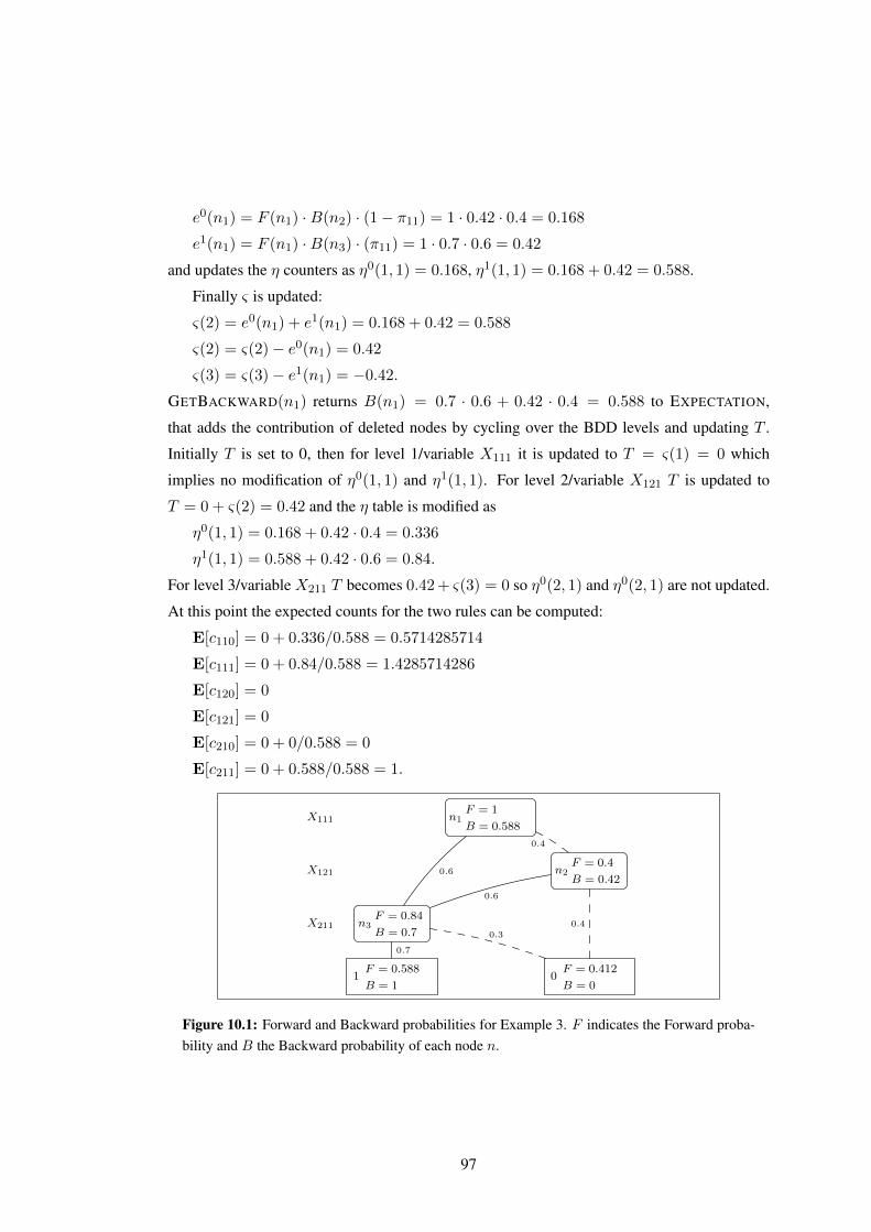
e0(n1) = F (n1) ·B(n2) · (1− π11) = 1 · 0.42 · 0.4 = 0.168
e1(n1) = F (n1) ·B(n3) · (π11) = 1 · 0.7 · 0.6 = 0.42
and updates the η counters as η0(1, 1) = 0.168, η1(1, 1) = 0.168 + 0.42 = 0.588.
Finally ς is updated:
ς(2) = e0(n1) + e1(n1) = 0.168 + 0.42 = 0.588
ς(2) = ς(2)− e0(n1) = 0.42
ς(3) = ς(3)− e1(n1) = −0.42.GETBACKWARD(n1) returns B(n1) = 0.7 · 0.6 + 0.42 · 0.4 = 0.588 to EXPECTATION,
that adds the contribution of deleted nodes by cycling over the BDD levels and updating T .
Initially T is set to 0, then for level 1/variable X111 it is updated to T = ς(1) = 0 which
implies no modification of η0(1, 1) and η1(1, 1). For level 2/variable X121 T is updated to
T = 0 + ς(2) = 0.42 and the η table is modified as
η0(1, 1) = 0.168 + 0.42 · 0.4 = 0.336
η1(1, 1) = 0.588 + 0.42 · 0.6 = 0.84.
For level 3/variable X211 T becomes 0.42+ ς(3) = 0 so η0(2, 1) and η0(2, 1) are not updated.
At this point the expected counts for the two rules can be computed:
E[c110] = 0 + 0.336/0.588 = 0.5714285714
E[c111] = 0 + 0.84/0.588 = 1.4285714286
E[c120] = 0
E[c121] = 0
E[c210] = 0 + 0/0.588 = 0
E[c211] = 0 + 0.588/0.588 = 1.
X111 n1F = 1
B = 0.588
0.6
0.4
X121 n2F = 0.4
B = 0.42
0.6
0.4X211 n3F = 0.84
B = 0.7
0.7
0.3
1F = 0.588
B = 10
F = 0.412
B = 0
Figure 10.1: Forward and Backward probabilities for Example 3. F indicates the Forward proba-bility and B the Backward probability of each node n.
97

Maximization Step
In the Maximization phase (see Algorithm 6), the πik parameters are computed for all rules Ci
and k = 1, . . . , ni − 1 as
πik =E[cik1]
E[cik0] +E[cik1]
for the next EM iteration.
Algorithm 6 Procedure Maximization1: procedure MAXIMIZATION
2: for all i ∈ Rules do3: for k = 1 to ni − 1 do4: πik =
E[cik1]E[cik0]+E[cik1]
5: end for6: end for7: end procedure
10.3 Related Work
Binary Decision Diagrams
The use of Binary Decision Diagrams for probabilistic logic programming inference is related
to their use for performing inference in Bayesian Networks. (Minato et al., 2007) presented a
method for compiling BNs into exponentially-sized Multi-Linear Functions using a compact
Zero-suppressed BDD representation. (Ishihata et al., 2011) compiled a BN with multiple
evidence sets into a single Shared BDD, which shares common sub-graphs in multiple BDDs.
(Darwiche, 2004) described an algorithm for compiling propositional formulas in conjunctive
normal form into Deterministic Decomposable Negation Normal Form (d-DNNF) - a tractable
logical form for model counting in polynomial time - with techniques from the Ordered BDD
literature.
(Ishihata et al., 2008a,b) proposed an EM algorithm for learning the parameters of Boolean
random variables given observations of a Boolean function over them, represented by a BDD.
EMBLEM is an application of that algorithm to probabilistic logic programs. (Inoue et al., 2009)
applies the algorithm of (Ishihata et al., 2008a,b) to the problem of computing the probabilistic
parameters of abductive explanations.
98
Parameter Learning in Probabilistic Logic Languages
The approaches for learning probabilistic logic programs can be classified into three categories:
those that employ constraint techniques, those that use EM and those that adopt gradient de-
scent.
In the first class, (Riguzzi, 2004, 2007a, 2008) learn a subclass of ground programs by first
finding a large set of clauses satisfying certain constraints and then applying mixed integer
linear programming to identify a subset of the clauses that form a solution.
The following works fall into the second category.
(Thon et al., 2008) proposed an EM algorithm which computes expectations over decision
diagrams; it learns parameters for the CPT-L language, a simple probabilistic logic language
for describing sequences of relational states, that is less expressive than LPADs.
In (Koller and Pfeffer, 1997) the authors start out with a knowledge base consisting of
partially specified first-order probabilistic logic rules with probabilistic parameters unknown;
given a set of data cases they use a standard KBMC (Knowledge-Based Model Construction)
algorithm to generate the network structure for each case. The conditional probability tables in
the resulting networks are related to the parameters corresponding to the rules in the knowledge
base. They use an extension to the standard EM algorithm for learning the parameters of these
belief networks with fixed structure and hidden variables.
PRISM is a probabilistic logic (Sato, 1995; Sato and Kameya, 2001) introduced to im-
prove the efficiency of the inference procedure under the distribution semantics, by imposing
restrictions on the language. The same philosophy was followed by Probabilistic Horn Ab-
duction (PHA) (Poole, 1993) and the Independent Choice Logic (ICL) (Poole, 1997). The key
assumption is that the explanations for a goal are mutually exclusive, which overcomes the
disjoint-sum problem. If the different explanations of a fact do not overlap, then its probability
is simply the sum of the probabilities of its explanations.
In addition, PHA, ICL and PRISM employ disjoint statements of the form
disjoint(p1 : a1; . . . ; pn : an), where the ai are atoms for a particular predicate, and the piprobability values that sum up to 1. For instance, the statement
disjoint(0.3 : gene(P, a); 0.15 : gene(P, b); 0.55 : gene(P, o))←
states that 1) the probabilities that (an instance) of the corresponding fact for gene is true, and
2) an atom of the form gene(P,X) instantiates to exactly one of these options.
99

The PRISM system is one of the first learning algorithms based on EM: it exploits logic pro-
gramming techniques for computing expectations.
Causal Probabilistic Logic (CP− logic) (Vennekens et al., 2009) is a probabilistic mod-
eling language that is especially designed for representing causal relations. A CP-theory is a
set of CP-events or rules of the same form of LPADs, hence these two languages are syntacti-
cally equivalent but define their semantics quite differently. (Blockeel and Meert, 2007; Meert
et al., 2007, 2008) proposed to use the EM algorithm to induce parameters of ground CP-Logic
theories, which works on the underlying Bayesian network.
Relational Information Bottleneck (RIB) (Riguzzi and Di Mauro, 2012) is an algorithm
that learns the parameters of SRL languages reducible to Bayesian Networks. In particular, it is
presented by the authors the specialization of RIB to LPADs, so this system will be compared to
EMBLEM in the next Section relative to experiments. Since the resulting network involve hidden
variables, the use of techniques for learning from incomplete data such as the Expectation
Maximization algorithm is required. RIB has shown good performances especially when some
logical atoms are unobserved and is particularly suitable when learning from interpretations
that share the same Herbrand base.
CEM is an implementation of EM based on the cplint inference library (Riguzzi,
2007b, 2009); this library allows to compute the probability of LPADs and CP-logic queries
by using BDDs, when the program in one of these languages is acyclic. This system will be
compared to EMBLEM in the next experimental Section.
ProbLog is a probabilistic extension of Prolog where some probabilistic facts f are la-
beled with a probability value. This value indicates the degree of belief, that is the probability
that any ground instance fθ of f is true. It is also assumed that the fθ are marginally indepen-
dent. The probabilistic facts are then augmented with a set of definite clauses defining further
predicates (which should be disjoint from the probabilistic ones). An example is the program:0.9 : edge(a, c).0.6 : edge(d, c).0.9 : edge(d, b).0.7 : edge(c, b).path(X,Y )← edge(X,Y ).path(X,Y )← edge(X,Z), path(Z, Y ).
which specifies, with the first probabilistic fact, that with probability 0.9 there is an edge from
a to c.
(Gutmann et al., 2011) presented the LFI-ProbLog algorithm that performs EM for learning
100

the parameters of a ProbLog program. EMBLEM differs from this work in the construction
of BDDs: while they build a BDD for an interpretation we focus on a target predicate, the
one for which we want to obtain good predictions, and we build BDDs starting from atoms
for the target predicate. Moreover, while we compute the contributions of deleted paths with
the ς table, LFI-ProbLog treats missing nodes as if they were there and updates the counts
accordingly. This system will be compared with EMBLEM in the next experimental Section.
Among the works that use a gradient descent technique, LeProbLog (Gutmann et al.,
2010a, 2008) is a system developed again for ProbLog language. It starts from a set of queries
annotated with a probability and from a ProbLog program. It tries to find the values of the
parameters of the program that minimize the mean squared error of the probabilities of the
queries. LeProbLog uses the Binary Decision Diagrams that represent the queries to compute
the gradient.
Markov Logic Networks A different approach is taken by Markov Logic (Richardson and
Domingos, 2006), that combines first-order logic with Markov networks. The idea is to view
logical formulae as soft constraints on the possible worlds. The more formulae a world satisfies,
the more likely it becomes. In a Markov logic network (MLN), this is realized by associating a
weight with each formula that reflects how strong the constraint is, for example:1.5 : cancer(P )← smoking(P )1.1 : smoking(X)← friends(X,Y ), smoking(Y )1.1 : smoking(Y )← friends(X,Y ), smoking(X)
The first clause states the soft constraint that smoking causes cancer. So, interpretations in
which persons that smoke have cancer are more likely than those where they do not (under
the assumptions that other properties remain constant). Note that, with respect to all previous
probabilistic languages, Markov Logic attaches to formulae weights, which are not probabili-
ties but reflect how a world is probable depending on the number of formulae that it violates.
For MLNs, Alchemy is a state-of-the-art system that offers various tools for inference, weight
learning and structure learning of MLNs. (Lowd and Domingos, 2007) discusses how to per-
form weight learning by applying gradient descent of the conditional likelihood of queries for
target predicates. This system will be compared with EMBLEM in the next experimental Sec-
tion.
101

10.4 Experiments
The experiments are directed at verifying:
• the quality of the estimated parameters
• the algorithm performance in comparison with other state of the art SRL systems.
In the following a description of the datasets and performance evaluation metrics used is
provided.
Datasets
The Internet Movie DataBase (Mihalkova and Mooney, 2007)1 contains five mega-examples,
each of which describes four movies, their directors, and the first-billed actors who appear in
them. Each director is ascribed genres based on the genres of the movies he or she directed.
The ‘gender’ predicate is used to state the genders of actors.
Cora (McCallum et al., 2000) is a collection of 1295 different citations to 112 computer
science research papers from the Cora Computer Science Research Paper Engine. We used the
version of the dataset of (Singla and Domingos, 2005)2. For each citation we know the title,
authors, venue and the words that appear in it. The dataset encodes a problem of information
integration from multiple sources and in particular an entity resolution problem: citations of the
same paper often appear differently and the task is to determine which citations are referring
to the same paper. The database is composed of five mega-examples and contains facts for the
predicates samebib(Citation1, Citation2), sameauthor(Author1, Author2),
sametitle(Title1, Title2), samevenue(Venue1, Venue2) and
haswordauthor(Author, Word), haswordtitle(Title, Word),
haswordvenue(Venue, Word).
UW-CSE (Richardson and Domingos, 2006)3 records information about the Department of
Computer Science and Engineering at the University of Washington; the domain is described
through 10 types, that include: publication, person, course, project, academic quarter, etc.
Instead, predicates include: professor(Person), student(Person), area(X, Area) (with X
ranging over publications, persons, courses and projects), publication(Title, Person),
1Available at http://alchemy.cs.washington.edu/data/imdb.2Available at http://alchemy.cs.washington.edu/data/cora.3Available at http://alchemy.cs.washington.edu/data/uw-cse.
102

advisedBy(Person, Person), yearsInProgram(Person, Years),
courseLevel(Course, Level), taughtBy(Course, Person, Quarter), etc. Additionally,
there are some equality predicates: samePerson(Person, Person),
sameCourse(Course, Course), etc. which always have known, fixed values that are true iff
the two arguments are the same constant. Here the problem is one of link prediction, as we
wish to infer the truth of advisedBy(Person, Person). The database is split into five mega-
-examples, each with data for a particular departmental area (AI, graphics, programming lan-
guages, systems and theory).
WebKB (Craven and Slattery, 2001)1 consists of labeled web pages from the Computer
Science departments of four universities, along with the words on the web pages and the links
among them. We used the same set of training examples of (Craven and Slattery, 2001) which
differs from the one used in (Gutmann et al., 2011; Lowd and Domingos, 2007). The dataset
is split into four mega-examples, one for each university. Each web page is labeled with some
subset of the following categories: student, faculty, research project and course. This dataset
may be seen as a text classification problem, since we wish to infer the page’s class given the
information about words and links.
MovieLens (Herlocker et al., 1999) contains information about movies, users and ratings
that users expressed about movies. We used the version of the dataset of (Khosravi et al.,
2010)2. For each movie the dataset records the genres to which it belongs, by means of predi-
cates of the form <genre>(Movie,
<gen_value>), where< genre > can be either drama, action or horror and gen_value
is either <genre>_0, if the movie does not belong to the genre, or <genre>_1, if the movie
belongs to the genre. Users’ age, gender and occupation are recorded. Ratings from users
on the movies range from 1 to 5. This dataset can be used to build a recommender system,
i.e. a system that suggests items of interest to users based on their previous preferences, the
preferences of other users, and attributes of users and items. We split the dataset into five
mega-examples.
Mutagenesis (Srinivasan et al., 1996) contains information about a number of aromatic
and heteroaromatic nitro drugs, including their chemical structures in terms of atoms, bonds
and a number of molecular substructures such as six and five membered rings, benzenes,
phenantrenes and others. The problem here is to predict the mutagenicity of the drugs. The
1Available at http://alchemy.cs.washington.edu/data/webkb.2Available at http://www.cs.sfu.ca/~oschulte/jbn/dataset.html.
103

prediction of mutagenesis is important as it is relevant to the understanding and prediction of
carcinogenesis, and not all compounds can be empirically tested for mutagenesis, e.g. antibi-
otics. Of the compounds, those having positive levels of log mutagenicity are labeled “active”
and constitute the positive examples, the remaining ones are “inactive” and constitute the neg-
ative examples. The data is split into two subsets (188+42 examples). We considered the
first one, composed of 125 positive and 63 negative compounds. We split the dataset into ten
mega-examples.
Estimating Classifier Performance
The recommended procedure for evaluating a Machine Learning algorithm considers:
1. Use of k-fold cross-validation (k=5 or 10) for computing performance estimates;
2. Report of mean values of performance estimates with their standard deviations and 95%
confidence intervals.
1. Use of k-fold cross-validation for computing performance estimates Given a model
with unknown parameters and a data set which the model has to fit (the training data set), the
fitting process optimizes the model parameters to make the model fit the training data as well
as possible. If we then take an independent sample of validation data from the same population
as the training data, it will generally turn out that the model does not fit the validation data as
well as it fits the training data. This is called overfitting, and is particularly likely to happen
when the size of the training data set is small, or when the number of parameters in the model
is large. Cross-validation is a way to predict the fitting of a model to a hypothetical validation
set when an explicit validation set is not available. One round of cross-validation involves
partitioning the data set into complementary subsets, performing the analysis on one subset
(called the training set), and validating the analysis on the other subset (called the validation
set or testing set). To reduce variability, multiple rounds of cross-validation are performed
using different partitions, and the validation results are averaged over the rounds to produce a
single estimation. K-fold cross-validation needs to get k training/validation set pairs as follows:
the dataset is randomly divided into k parts. To get each pair, k-1 parts are combined to form
the training set and the remaining part is the validation set. This is done k times where for each
pair, another of the k parts is left out as the validation set. The advantage of this method over
repeated random sub-sampling is that all observations are used for both training and validation,
104

and each observation is used for validation exactly once. 10-fold cross-validation is commonly
used.
2. Report mean values of performance estimates with their standard deviations and 95%
confidence intervals
• Performance estimates. In recent years Receiver Operating Characteristics (ROC) graphs
and Precision Recall (PR) graphs have been increasingly adopted in the machine learning
and data mining research communities, to visualize classifiers performance. In particular,
the Area Under the Curve (AUC) for both the PR curve (AUCPR) and the ROC curve
(AUCROC) are computed to numerically compare performances.
The use of these graphs is widespread when evaluating algorithms that output proba-
bilities of binary class membership values. In our case, the class is given by the target
predicate(s) chosen for each dataset: for instance, for the Cora dataset, the predicate
samebib(citation1,citation2) discriminates ground examples among those
representing the same citation (positive instances) and those representing different ones.
ROC graphs are two-dimensional graphs in which True Positive (TP) rate (also called
recall) is plotted on the Y axis and False Positive (FP) rate is plotted on the X axis.
These rates of a classifier are estimated as:
tp rate =Positives correctly classified
Total positives
fp rate =Negatives incorrectly classified
Total negatives
A ROC graph depicts relative trade-offs between benefits (true positives) and costs (false
positives). The AUCROC is equal to the probability that a classifier will rank a randomly
chosen positive instance higher than a randomly chosen negative one. Given two classi-
fiers and their AUCROC, the one with the greater area has better average performance.
The parameter learning algorithms are probabilistic classifiers that output a probability
that each test set example is positive: we can next sort this list in ascending order to rank
the examples from the least positive ones (which are more likely to belong to the negative
class) to the most positive ones (which are more likely to belong to the positive class).
These probabilities give an indication of how likely it is that the positive class label
applies. Such probability estimators are used with a threshold on the output probabilities
105

to produce a discrete binary classifier: if their output is above the threshold a Yes is
returned, else a No is returned, and each threshold value produces a different point in
ROC space. One may imagine varying a threshold from 0 to 1 and tracing a curve through
ROC space. Each point in the space represents a specific classifier, with a threshold for
calling an example positive: this means that we have obtained a set of discrete classifiers.
When dealing with highly skewed datasets, Precision-Recall (PR) curves have been
found to give a more informative picture of an algorithm’s performance: when the num-
ber of negative examples greatly exceeds the number of positives examples, a large
change in the number of false positives can lead to a small change in the false posi-
tive rate used in ROC analysis. In PR space one plots Recall on the X axis and Precision
on the Y axis. Precision - defined as Positives correctly classifiedTrue and false positives - by comparing false pos-
itives to true positives rather than true negatives, mitigates the effect of the large number
of negative examples on the algorithm’s performance. Given two algorithms with com-
parable area in ROC space, in PR space one of them can show a clear advantage over the
other by having a larger area.
• 95% Confidence Intervals. They are a common way to describe the uncertainy associated
with an estimate. In this context it is utilized in relation to a paired two-tailed t-test.
A paired t-test is used to compare two population means, where there are two samples in
which observations in one sample can be paired with observations in the other sample.
Examples of where this might occur are: (1) before-and-after observations on the same
subjects; (2) a comparison of two different methods of measurement or two different
treatments where the measurements are applied to the same subjects. The experiments
belong to case (2), where a comparison of different SRL algorithms over the same data
sets is performed: the variations in AUCROC and AUCPR of EMBLEM compared to the
other systems are computed and differences are reported as significant if a two-tailed,
paired t-test produces a p-value less than 0.05.
The null hypothesis is the statement that we want to test, stating, in general, that things
are the same as each other, i.e., the two evaluated methods are equivalent. One has to
take into account that almost certainly some difference in the means, just due to chance,
may appear. So we need to consider “what’s the probability of getting a difference in the
means of a certain value, just by chance, if the null hypothesis is really true”. Only when
that probability is low we can reject the null hypothesis that the two methods (algorithms)
106

are equivalent. The goal of statistical hypothesis testing is to estimate the probability of
getting the observed results under the null hypothesis.
Given the pairs i = 1, ..., k from k-fold validation, two classifiers are trained on the
training set and are tested on the validation set, and their errors are recorded as xi, yi,
where x, y indicate the two classifiers. The difference is di = yi − xi; when this is
done k times we have a distribution of di containing k points. For large samples the
corresponding error estimates follow the Normal distribution, and their difference di is
also Normal. The null hypothesis is equivalent to say that this distribution has zero mean:
H0 : µ = 0, while the alternative hypothesis is H1 : µ = 0.
To test the null hypothesis that the mean difference is zero (i.e. the two classifiers have
the same error rate and so are equivalent), the complete procedure is as follows:
– Compute the difference (di) between the two observations in each pair;
– Compute the mean difference, d;
– Compute the standard deviation of the differences, sd, and use this to calculate the
standard error of the mean difference, SE(d) = sd√k
;
– Compute the t-statistic T = d/SE(d); under the null hypothesis that µ = 0, this
statistic follows a t-distribution with k − 1 degrees of freedom;
– Use tables of the t-distribution to compare the value of T to the tα,k−1 distribution
and rejects the null hypothesis if |T | > tα,k−1, with α significance level (see be-
low). The value of α such that |T | = tα,k−1 is the p-value for the paired t-test,
defined as the probability of accepting that the null hypothesis is true. The t-test
has been applied in the experiments to the differences in AUCROC and AUCPR,
i.e, the xi/yi values correspond to the area values computed for each fold i and for
each algorithm.
So for example p = 0.03 is a shorthand way of saying “The probability of accepting the
null hypothesis that the two methods are equivalent, is 0.03; the probability that a method, not
by chance, performs better than the other one, is 1− p”. A convention in most research is used
which sets a significance level α of 0.05. This means that if the probability value p is less than
α, the null hypothesis is rejected and an algorithm is better than another one; such results are
referred to as ‘statistically significant’. If p is greater than or equal to α, the null hypothesis
is accepted. In some situations it is convenient to express the statistical significance as 1 − α:
107

this value is called the test confidence, since statistical significance can be considered to be the
confidence one has in a given result. A 95% confidence interval for the true mean difference
is an interval of values that is expected with probability 95% to contain the true difference
(where the true mean difference is likely to lie). Smaller levels of α increase confidence in the
determination of significance, but run an increased risk of failing to reject a false null hypothesis
(false negative determination), and so have less statistical power. Statistical significance is a
statistical assessment of whether the observations reflect a pattern rather than just chance, since
any given hypothesis is subject to random error. A result is deemed statistically significant if
it is so extreme (without external variables which would influence the correlation results of the
test) that such a result would be expected to arise simply by chance only in rare circumstances.
Hence the result provides enough evidence to reject the hypothesis of ‘no effect’.
Finally, the test is named after the tail of data under the far left and far right of a bell-shaped
Normal data distribution, or bell curve. However, the terminology is extended to tests relating
to distributions other than Normal. In general a test is called two-tailed if the null hypothesis
is rejected for values of the test statistic falling into either tail of its sampling distribution, and
it is called one-sided or one-tailed if the null hypothesis is rejected only for values of the test
statistic falling into one specified tail of its sampling distribution. For example, if the alternative
hypothesis is µ = µ0, the null hypothesis of µ = µ0 is rejected for small or for large values
of the sample mean, the test is called two-tailed or two-sided. If the alternative hypothesis is
µ > µ0, the null hypothesis of µ ≤ µ0 is rejected only for large values of the sample mean
and the test is called one-tailed or one-sided. If a 5% significance level is used, both tests
have a region of rejection, 0.05, however, in the two-tailed case the rejection region must be
split between both tails of the distribution - 0.025 in the upper tail and 0.025 in the lower tail -
because the hypothesis specifies only a difference, not a direction.
Methodology
EMBLEM is implemented in Yap Prolog1 and is compared with
• a few systems for parameter learning of Probabilistic Logic Programs:
– RIB (Riguzzi and Di Mauro, 2012)
– CEM (Riguzzi, 2007b, 2009)
1http://www.dcc.fc.up.pt/~vsc/Yap/
108

– LeProbLog (Gutmann et al., 2010a, 2008)
– LFI-ProbLog (Gutmann et al., 2010b, 2011)
• one system for parameter learning of Markov Logic Networks (MLNs):
– Alchemy (Richardson and Domingos, 2006)
All experiments were performed on Linux machines with an Intel Core 2 Duo E6550 (2333
MHz) processor and 4 GB of RAM.
To compare the results with LeProblog, the translation of LPADs into ProbLog proposed
in (De Raedt et al., 2008a) is exploited, in which a disjunctive clause with k head atoms and
vector of variables X is modeled with k ProbLog clauses and k − 1 probabilistic facts with
variables X .
To compare the results with Alchemy, the translation between LPADs and MLN of
(Riguzzi and Di Mauro, 2012) is exploited, inspired by the translation between ProbLog and
MLNs proposed in (Gutmann et al., 2010a). An MLN clause is translated into an LPAD clause
in which the head atoms of the LPAD clause are the null atom plus the positive literals of the
MLN clause while the body atoms are the negative literals.
For the Probabilistic Logic Programming systems we consider various options:
1. The first consists in choosing between associating a distinct random variable to each
grounding of a probabilistic clause or a single random variable to a non-ground proba-
bilistic clause expressing whether the clause is used or not. The latter case makes the
problem easier. All experiments have been run first with the most difficult setting (a
single random variable for each grounding) and have been re-run with the second easy
setting only if EMBLEM failed to terminate under the first one.
2. The second option allows to set a limit on the depth of derivations as done in (Gutmann
et al., 2010a), thus eliminating explanations associated to derivations exceeding the depth
limit. This is necessary for problems that contain cyclic clauses, such as transitive closure
clauses.
3. The third option allows to set the number of restarts for EM based algorithms. EMBLEM
has been run with a number of restarts chosen to match its execution time with that of
the fastest other algorithm.
109

All experiments except one (see below) for the Probabilistic Logic Programming systems
have been performed using open-world predicates, meaning that, when resolving a literal for a
target predicate, both facts in the database and rules are used to prove it. All experiments use
the same value of the thresholds ϵ and δ for stopping the EM cycle.
The parameter settings for the PLP systems on the domains can be found in Table 10.2.
The datasets are divided into four, five or ten mega-examples, where each mega-example
contains a connected group of facts and individual mega-examples are independent of each
other. A k-fold (k = 4, 5, 10) cross-validation approach is adopted. The terms “fold” and
“mega-example” will be used interchangeably in the following. Statistics on the domains are
reported in Table 10.1. The number of negative testing examples is sometimes different from
that of negative training examples because, while in training we explicitly provide negative ex-
amples, in testing we consider as negatives all the ground instantiations of the target predicates
that are not positive.
As part of the test, Precision-Recall and Receiver Operating Characteristics curves are
drawn using the methods reported in (Fawcett, 2006) and (Davis and Goadrich, 2006), the
Area Under the Curve (AUCPR and AUCROC) is computed and, finally, average values on the
k folds are reported in Tables 10.3 and 10.4. Table 10.5 shows the learning times in hours.
Tables 10.6 and 10.7 show the p-value of a paired two-tailed t-test at the 5% significance
level of the difference in AUCPR and AUCROC between EMBLEM and the other systems on
all datasets (significant differences in favor of EMBLEM in bold).
IMDB Four different LPADs are used, two for predicting the target predicate
sameperson(Person1, Person2), and two for predicting samemovie(Movie1, Movie2), on
the basis of the relations among actors, their movies and their directors. There is one positive
example for each fact that is true in the data, while we sampled from the complete set of false
facts three times the number of true facts in order to generate negative examples.
1. For predicting sameperson/2 this LPAD is used:
sameperson(X,Y):p:- movie(M,X),movie(M,Y).
sameperson(X,Y):p:- actor(X),actor(Y),workedunder(X,Z),
workedunder(Y,Z).
sameperson(X,Y):p:- gender(X,Z),gender(Y,Z).
sameperson(X,Y):p:- director(X),director(Y),genre(X,Z),genre(Y,Z).
110
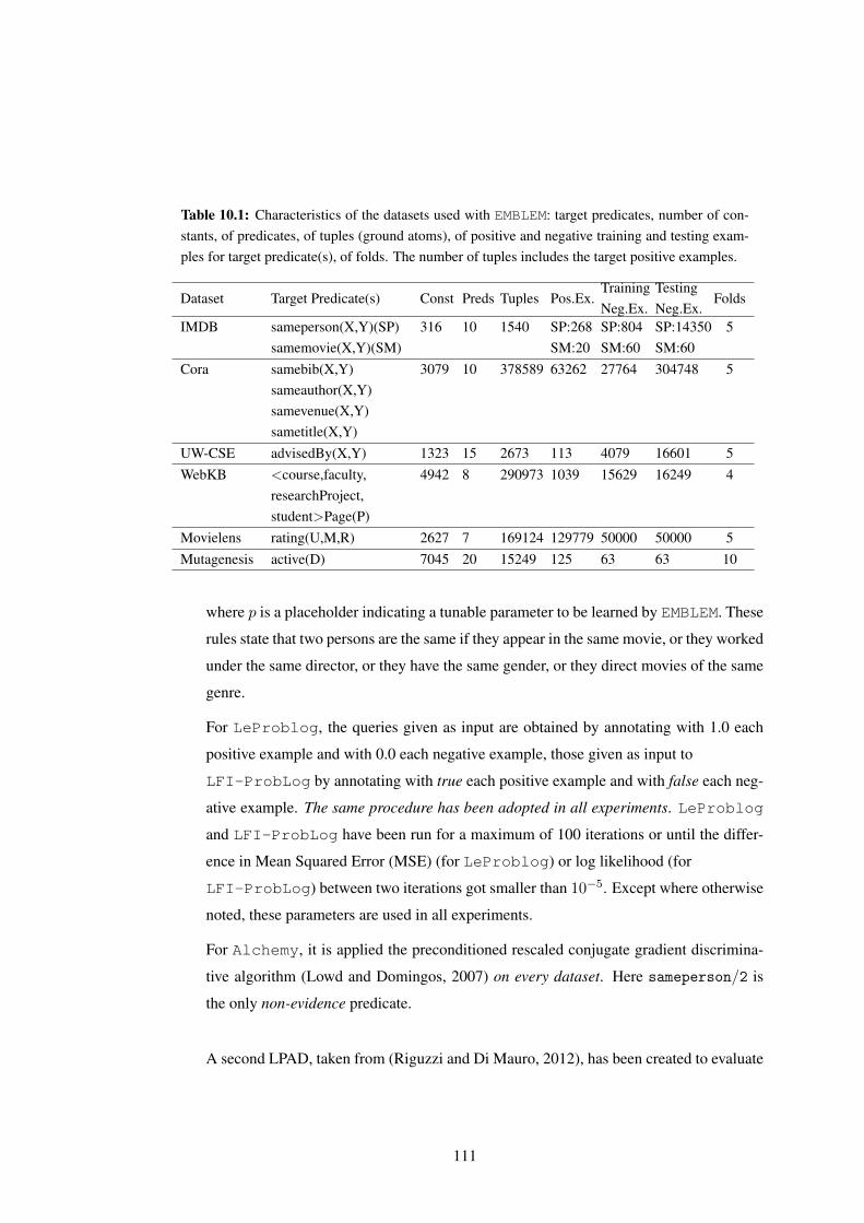
Table 10.1: Characteristics of the datasets used with EMBLEM: target predicates, number of con-stants, of predicates, of tuples (ground atoms), of positive and negative training and testing exam-ples for target predicate(s), of folds. The number of tuples includes the target positive examples.
Dataset Target Predicate(s) Const Preds Tuples Pos.Ex.TrainingNeg.Ex.
TestingNeg.Ex.
Folds
IMDB sameperson(X,Y)(SP)samemovie(X,Y)(SM)
316 10 1540 SP:268SM:20
SP:804SM:60
SP:14350SM:60
5
Cora samebib(X,Y)sameauthor(X,Y)samevenue(X,Y)sametitle(X,Y)
3079 10 378589 63262 27764 304748 5
UW-CSE advisedBy(X,Y) 1323 15 2673 113 4079 16601 5WebKB <course,faculty,
researchProject,student>Page(P)
4942 8 290973 1039 15629 16249 4
Movielens rating(U,M,R) 2627 7 169124 129779 50000 50000 5Mutagenesis active(D) 7045 20 15249 125 63 63 10
where p is a placeholder indicating a tunable parameter to be learned by EMBLEM. These
rules state that two persons are the same if they appear in the same movie, or they worked
under the same director, or they have the same gender, or they direct movies of the same
genre.
For LeProblog, the queries given as input are obtained by annotating with 1.0 each
positive example and with 0.0 each negative example, those given as input to
LFI-ProbLog by annotating with true each positive example and with false each neg-
ative example. The same procedure has been adopted in all experiments. LeProblog
and LFI-ProbLog have been run for a maximum of 100 iterations or until the differ-
ence in Mean Squared Error (MSE) (for LeProblog) or log likelihood (for
LFI-ProbLog) between two iterations got smaller than 10−5. Except where otherwise
noted, these parameters are used in all experiments.
For Alchemy, it is applied the preconditioned rescaled conjugate gradient discrimina-
tive algorithm (Lowd and Domingos, 2007) on every dataset. Here sameperson/2 is
the only non-evidence predicate.
A second LPAD, taken from (Riguzzi and Di Mauro, 2012), has been created to evaluate
111

Table 10.2: Parameter settings for the experiments with EMBLEM, RIB, CEM, LeProbLogLFI-ProbLog. NR indicates the number of restarts only for EMBLEM, NI indicates the maxi-mum number of iterations only for LFI-ProbLog.
.Dataset NI(LFI-ProbLog) NR(EMBLEM) LPAD cyclicity depth D semanticsIMDB-SP 100 500 no no standardIMDBu-SP 100 40 no no standardIMDB-SM 100 1 no no standardIMDBu-SM 100 1 no no standardCORA 10 120 no no standardCORAT 10 1 yes 2 simplifiedUW-CSE 100 1 yes 2 simplifiedWebKB 10 1 yes no(close-world) standardMovielens 100 1 yes 2 simplifiedMutagenesis 100 1 no no standard
the algorithms’ performance when some atoms are unseen:
sameperson_pos(X,Y):p:- movie(M,X),movie(M,Y).
sameperson_pos(X,Y):p:- actor(X),actor(Y),workedunder(X,Z),
workedunder(Y,Z).
sameperson_pos(X,Y):p:- director(X),director(Y),genre(X,Z),genre(Y,Z).
sameperson_neg(X,Y):p:- movie(M,X),movie(M,Y).
sameperson_neg(X,Y):p:- actor(X),actor(Y),workedunder(X,Z),
workedunder(Y,Z).
sameperson_neg(X,Y):p:- director(X),director(Y),genre(X,Z),genre(Y,Z).
sameperson(X,Y):p:- \+sameperson_pos(X,Y),sameperson_neg(X,Y).
sameperson(X,Y):p:- \+sameperson_pos(X,Y),\+sameperson_neg(X,Y).
sameperson(X,Y):p:- sameperson_pos(X,Y),sameperson_neg(X,Y).
sameperson(X,Y):p:- sameperson_pos(X,Y),\+sameperson_neg(X,Y).
The sameperson_pos/2 and sameperson_neg/2 predicates are unseen in the data.
Alchemy has been run with the −withEM option that turns on EM learning. The other
parameters for all systems are set as before.
Results are shown respectively in the IMDB-SP and IMDBu-SP rows of tables 10.3, 10.4,
10.5. Learning time matches CEM time, the fastest system among the others.
2. For predicting samemovie/2 this LPAD is used:
samemovie(X,Y):p:- movie(X,M),movie(Y,M),actor(M).
112

samemovie(X,Y):p:- movie(X,M),movie(Y,M),director(M).
samemovie(X,Y):p:- movie(X,A),movie(Y,B),actor(A),director(B),
workedunder(A,B).
samemovie(X,Y):p:- movie(X,A),movie(Y,B),director(A),director(B),
genre(A,G),genre(B,G).
To test the behavior when unseen predicates are present, the program for samemovie/2
is transformed as for sameperson/2, thus introducing the unseen predicates
samemovie_pos/2 and samemovie_neg/2. The systems have been run with the same
settings as IMDB-SP and IMDBu-SP, replacing sameperson/2 with samemovie/2. Re-
sults are shown respectively in the IMDB-SM and IMDBu-SM rows of tables 10.3, 10.4,
10.5. RIB and LFI-Problog in this case give a memory error (indicated with “me”),
due to the exhaustion of the available stack space during the execution of the algorithm.
Cora The Cora database contains citations to computer science research papers, and the task
is to determine which citations are referring to the same paper, by predicting the predicate
samebib(Citation1, Citation2).
From the MLN proposed in (Singla and Domingos, 2006)1 two LPADs have been obtained.
The MLN contains 26 clauses stating regularities like: if two citations are the same, their
authors, venues, etc., are the same, and vice-versa; if two fields of the same type have many
words in common, they are the same.
The first LPAD contains 559 rules and differs from the direct translation of the MLN be-
cause rules involving words are instantiated with the different constants, only positive literals
for the hasword predicates are used and transitive rules are not included:
samebib(B,C):p:- author(B,D),author(C,E),sameauthor(D,E).
samebib(B,C):p:- title(B,D),title(C,E),sametitle(D,E).
samebib(B,C):p:- venue(B,D),venue(C,E),samevenue(D,E).
samevenue(B,C):p:- haswordvenue(B,word_06), haswordvenue(C,word_06).
...
sametitle(B,C):p:- haswordtitle(B,word_10), haswordtitle(C,word_10).
....
sameauthor(B,C):p:- haswordauthor(B,word_a), haswordauthor(C,word_a).
.....
The dots stand for the rules for all the possible words. Positive and negative examples for
the four target predicates are already available in the version of the dataset.1Available at http://alchemy.cs.washington.edu/mlns/er.
113

In this case LFI-ProbLog has been run for a maximum of only 10 iterations (or until the
difference in MSE between two iterations got smaller than 10−5) due to its long learning time.
The second LPAD adds to the previous one the transitive rules for the predicates samebib/2,
samevenue/2, sametitle/2 and sameauthor/2:
samebib(A,B):p:- samebib(A,C), samebib(C,B).
sameauthor(A,B):p:- sameauthor(A,C), sameauthor(C,B).
sametitle(A,B):p:- sametitle(A,C), sametitle(C,B).
samevenue(A,B):p:- samevenue(A,C), samevenue(C,B).
for a total of 563 rules. In this case stricter settings are imposed for EMBLEM, LeProbLog,
CEM and LFI-ProbLog, since the theory is cyclic (cf. table 10.2).
For LeProbLog, the four predicates are separately learned because learning the whole
theory at once gives a lack of memory error. This is equivalent to using a closed-world setting.
For Alchemy, the four predicates are specified as non-evidence.
Results are shown respectively in the Cora and CoraT (Cora Transitive) rows of Tables
10.3, 10.4, 10.5. On CoraT Alchemy, CEM and LFI-ProbLog give a memory error, for a
segmentation fault the first one (by the learnwts command) and for memory exhaustion the
others, while RIB is not applicable because it is not possible to split the input examples into
smaller independent interpretations as required by it.
UW-CSE The interest in this dataset has emerged in the context of social network analysis,
where one seeks to reason about a group of people: in particular link prediction tackles the
problem of predicting relationships from people’s attributes, and UW-CSE represents a bench-
mark in that direction if we try to predict which professors advise which graduate students.
Hence, the target predicate is advisedBy(Person1, Person2).
The theory used has been obtained from the MLN of (Singla and Domingos, 2005)1 and
contains 86 rules, such as (S stands for student and P for professor):
advisedby(S,P):p:- courselevel(C,level_500), taughtby(C,P,Q), ta(C,S,Q).
advisedBy(S,P):p:- publication(Pub,S), publication(Pub,P), student(S).
student(S):p:- advisedBy(S,P).
1Available at http://alchemy.cs.washington.edu/mlns/uw-cse.
114

As one can see from this example, the theory is cyclic. The negative examples have
been generated by considering all couple of persons (a,b) where a and b appear in an
advisedby/2 fact in the data and by adding a negative example advisedBy(a,b) if
it is not in the data.
For Alchemy, advisedBy/2 is the only non-evidence predicate. RIB and LFI-ProbLog
in this case exhaust the available memory.
WebKB The goal is to predict the four predicates coursePage(Page), facultyPage(Page),
studentPage(Page) and researchProjectPage(Page), representing the various possible
pages’ classes, for which the dataset contains both positive and negative examples.
The theory is obtained by translating the MLN of (Lowd and Domingos, 2007)1 into an
LPAD with 3112 rules. It contains a rule of the form
<class1>Page(Page1):p:- linkTo(Page2,Page1), <class2>Page(Page2).
for each couple of classes (<class1>,<class2>), and rules of the form
<class>Page(Page):p:- has(<word>,Page).
for each possible page class and word. The first type of rule states that Page1 of class class1
is linked to Page2 of class class2 with probability p; the second type states that the page Page
of class class contains the word word with probability p. Examples of rules are:
coursePage(Page1):p:- linkTo(Page2,Page1),coursePage(Page2).
coursePage(Page):p:- has(‘abstract’,Page).
As one can see from this example, the theory is cyclic. Running EMBLEM with a depth bound
equal to the lowest value (two) and an open-world setting gives a lack of memory error, so
a closed-world setting is needed for the target predicates in the body of clauses (target pred-
icates are resolved only with facts in the database). LeProbLog and LFI-ProbLog have
been run on a sample containing respectively 5% and 1% of the training set since the com-
plete set leads to exceedingly long learning times, and in addition LFI-ProbLog has been
run for a maximum of 10 iterations; despite that, it spends anyway a considerable time. For
Alchemy, the four target predicates are specified as non-evidence predicates; we also set the
flag −noAddUnitClauses to 1 (unit predicates are not added to the MLN) since otherwise
inference would give a lack of memory error. RIB and CEM in this case terminate for lack of
memory.1Available at http://alchemy.cs.washington.edu/mlns/webkb.
115

MovieLens The target predicate is rating(User, Movie, Rating): we wish to predict the
rating on a movie by a user. The LPAD contains 4 rules:
rating(A,B,R):p:- rating(A,C,R),B\==C,drama(B,drama_1),drama(C,drama_1).
rating(A,B,R):p:- rating(A,C,R),B\==C,action(B,action_1),action(C,action_1).
rating(A,B,R):p:- rating(A,C,R),B\==C,horror(B,horror_1),horror(C,horror_1).
rating(A,B,R):p:- rating(C,B,R),A\==C.
The first three rules state that a user A assigns the same rating R to two different movies B and
C, if they belong to the same genre, either drama or action or horror, with probability p; the
last one states that two different users equally rate the same movie with probability p.
In this case stricter settings are imposed for EMBLEM, LeProbLog, CEM and LFI-ProbLog,
since the theory is cyclic (cf. table 10.2). For Alchemy, rating/3 is specified as non-
evidence predicate.
RIB, CEM, Alchemy and LFI-ProbLog give a memory error.
Mutagenesis To predict the mutagenicity of the drugs, we remind that the compounds having
positive levels of log mutagenicity are labeled “active”, so the goal is to predict if a drug is
active, i.e. the target predicate active(Drug).
The fundamental Prolog facts are bond(compound,atom1,atom2,bondtype) -
stating that in compound a bond of type bondtype can be found between the atoms atom1 and
atom2 - and atm(compound,atom,element,atomtype,charge), stating that com-
pound’s atom is of element element, is of type atomtype and has partial charge charge. From
these facts many elementary molecular substructures can be defined, and we used the tabula-
tion of these, available in the dataset, rather than the clause definitions based on bond/4 and
atm/5. This greatly sped up learning.
The theory has been obtained by running Aleph1 on the database with a ten-fold cross-
validation and choosing randomly one of the ten theories for parameter learning. The selected
theory contains 17 rules, such as:
active(A):p:- bond(A,B,C,2), bond(A,C,D,1), ring_size_5(A,E).
relating the activity of drug A to its atoms’ bonds and its structure. Predicates representing
molecular substructures use function symbols to represent lists of atoms, for example, in
ring_size_5(Drug, Ring), Ring is a list of atoms composing a 5-membered ring in the drug’s
1http://www.cs.ox.ac.uk/activities/machlearn/Aleph/aleph.html
116

structure. Alchemy is not applicable to this dataset because it does not handle function sym-
bols.
Table 10.3: Results of the experiments on all datasets in terms of Area Under the ROC Curveaveraged over the folds. me means memory error during learning; no means that the algorithm wasnot applicable.
Dataset EMBLEM LeProbLog Alchemy RIB CEM LFI-ProbLog
IMDB-SP 0.93 0.87 0.91 0.93 0.93 0.89IMDBu-SP 0.90 0.92 0.50 0.90 0.89 0.50IMDB-SM 1.00 0.98 0.93 me 0.71 meIMDBu-SM 1.00 0.98 0.54 me 0.44 meCora 1.00 0.99 0.70 0.99 0.99 0.99CoraT 0.999 0.998 me no me meUW-CSE 0.99 0.94 0.96 me 0.87 meWebKB 0.85 0.51 0.88 me me 0.55MovieLens 0.84 0.77 me me me meMutagenesis 0.99 0.98 no 0.90 0.92 0.89
Table 10.4: Results of the experiments on all datasets in terms of Area Under the PR Curveaveraged over the folds. me means memory error during learning; no means that the algorithm wasnot applicable.
Dataset EMBLEM LeProbLog Alchemy RIB CEM LFI-ProbLog
IMDB-SP 0.20 0.1 0.11 0.19 0.20 0.14IMDBu-SP 0.18 0.13 0.02 0.17 0.12 0.02IMDB-SM 1.00 0.93 0.82 me 0.54 meIMDBu-SM 1.00 0.93 0.34 me 0.56 meCora 0.995 0.91 0.47 0.94 0.995 0.996CoraT 0.99 0.98 me no me meUW-CSE 0.75 0.28 0.29 me 0.64 meWebKB 0.34 0.07 0.50 me me 0.07MovieLens 0.87 0.82 me me me meMutagenesis 0.992 0.991 no 0.95 0.96 0.93
Overall remarks From the results we can observe that:
• on IMDB-SP EMBLEM has better performance than the other systems in both AUCPR
and AUCROC (except for CEM/AUCPR), with six differences out of ten statistically
117

Table 10.5: Execution time in hours of the experiments, averaged over the folds.
Dataset EMBLEM LeProbLog Alchemy RIB CEM LFI-ProbLog
IMDB-SP 0.010 0.350 1.540 0.016 0.010 0.037IMDBu-SP 0.010 0.230 1.540 0.0098 0.012 0.057IMDB-SM 3.6e-4 0.005 0.003 - 0.005 -IMDBu-SM 3.220 0.012 0.011 - 0.047 -Cora 2.480 13.25 1.300 2.490 11.95 44.07CoraT 0.380 5.670 - - - -UW-CSE 2.810 2.920 1.950 - 0.530 -WebKB 0.048 0.114 0.052 - - 11.32MovieLens 0.070 20.01 - - - -Mutagenesis 2.49e-5 0.130 - 0.040 0.040 0.019
significant. Moreover, it takes less time than all other systems except CEM. On IMDBu-
SP EMBLEM has the best performance except for LeProbLog/AUCROC, again with six
significant differences.
• On IMDB-SM, EMBLEM reaches value 1 for PR and ROC areas with only one restart, in
less time than the other systems, so in this case we did not execute it to match the learning
time of another algorithm. Two out of six differences are significant; on IMDBu-SM, it
still reaches the highest area but with the longest execution time associated with one
restart, so it was not possible to match its time with the one of another system. One out
of six differences are significant. RIB and LFI-ProbLog are not able to terminate on
this dataset.
• On Cora, EMBLEM shows the best performance along with CEM and LFI-ProbLog,
but in much less time, with four significant differences out of ten. On CoraT, it has
comparable performance, but with a much lower learning time, than LeProbLog - the
only other system able to complete learning on this more complex theory.
• On UW-CSE, it has better performance with respect to all the algorithms for AUCPR and
AUCROC with five out of six differences significant. Again RIB and LFI-ProbLog
are not able to terminate.
• On WebKB, EMBLEM shows significantly better areas with respect to LeProbLog and
LFI-ProbLog, and worse areas with respect to Alchemy, with the differences being
118

Table 10.6: Results of t-test on all datasets, relative to AUCROC. p is the p-value of a paired two-tailed t-test between EMBLEM and the other systems (significant differences in favor of EMBLEMat the 5% level in bold). E is EMBLEM, LeP is LeProbLog, A is Alchemy, C is CEM, LFI isLFI-ProbLog.
Dataset E-LeP E-A E-R E-C E-LFI
IMDB-SP 0.001 0.015 0.344 0.351 0.006IMDBu-SP 0.140 1e-5 0.217 0.002 5.3e-7IMDB-SM 0.374 0.256 - 0.018 -IMDBu-SM 0.374 0.256 - 0.055 -Cora 0.069 0.033 0.049 0.457 0.766CoraT 0.131 - - - -UW-CSE 0.028 0.005 - 0.291 -WebKB 0.002 0.171 - - 0.005MovieLens 7.6e-7 - - - -Mutagenesis 0.199 - 0.109 0.196 5.4e-4
statistically significant except one case. We remind that this dataset is one of the most
problematic: it is the only one where EMBLEM has been run with a closed-world setting
for the target predicates (simpler than an open-world setting, which failed in this case)
and the size of the training set for LeProbLog and LFI-ProbLog has been reduced
in order to contain the computation time.
• On MovieLens, EMBLEM achieves higher areas with respect to LeProbLog in a sig-
nificantly lower time, with the differences statistically significant, while all the others
systems are not able to complete.
• On Mutagenesis, EMBLEM shows better performance than all other systems, with the
differences being statistically significant in three out of eight cases. Moreover, it is the
fastest.
Looking at the overall results, LeProbLog seems to be the closest system to EMBLEM
from the point of view of performances, being able to always complete learning as EMBLEM, but
with longer times (except for two cases). On the contrary, RIB and LFI-ProbLog incurred in
many difficulties in treating the datasets. EMBLEM’s AUCPR and AUCROC are higher or equal
than those of the other systems except on IMDBu-SP, where LeProbLog achieves a non-
statistically significant higher AUCROC, WebKB, where Alchemy achieves a non-statistically
significant higher AUCROC and a statistically significant higher AUCPR, and Cora, where
119
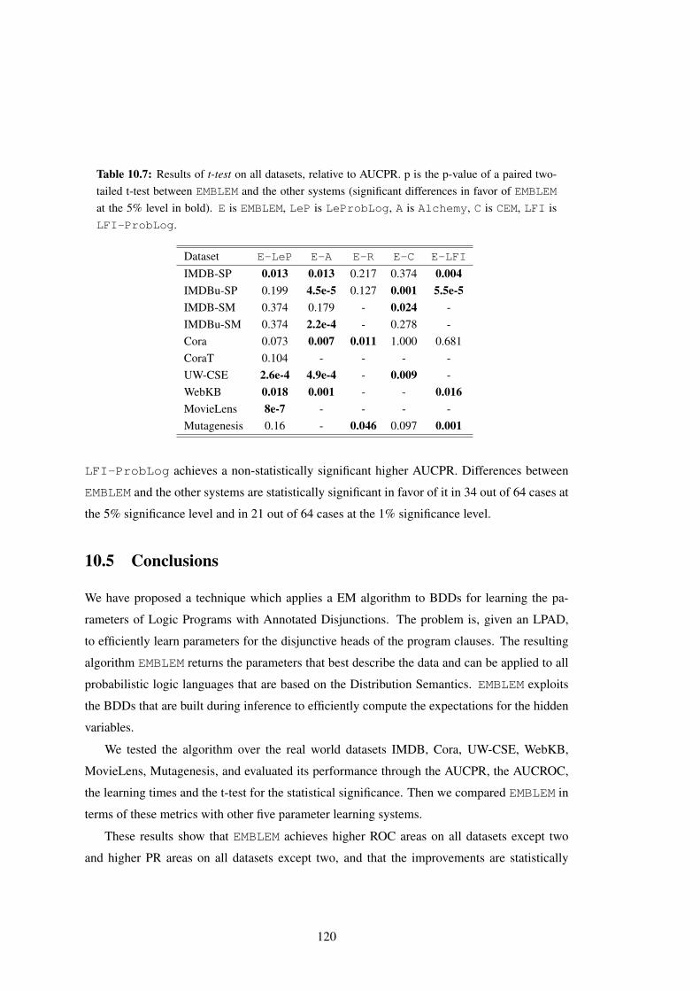
Table 10.7: Results of t-test on all datasets, relative to AUCPR. p is the p-value of a paired two-tailed t-test between EMBLEM and the other systems (significant differences in favor of EMBLEMat the 5% level in bold). E is EMBLEM, LeP is LeProbLog, A is Alchemy, C is CEM, LFI isLFI-ProbLog.
Dataset E-LeP E-A E-R E-C E-LFI
IMDB-SP 0.013 0.013 0.217 0.374 0.004IMDBu-SP 0.199 4.5e-5 0.127 0.001 5.5e-5IMDB-SM 0.374 0.179 - 0.024 -IMDBu-SM 0.374 2.2e-4 - 0.278 -Cora 0.073 0.007 0.011 1.000 0.681CoraT 0.104 - - - -UW-CSE 2.6e-4 4.9e-4 - 0.009 -WebKB 0.018 0.001 - - 0.016MovieLens 8e-7 - - - -Mutagenesis 0.16 - 0.046 0.097 0.001
LFI-ProbLog achieves a non-statistically significant higher AUCPR. Differences between
EMBLEM and the other systems are statistically significant in favor of it in 34 out of 64 cases at
the 5% significance level and in 21 out of 64 cases at the 1% significance level.
10.5 Conclusions
We have proposed a technique which applies a EM algorithm to BDDs for learning the pa-
rameters of Logic Programs with Annotated Disjunctions. The problem is, given an LPAD,
to efficiently learn parameters for the disjunctive heads of the program clauses. The resulting
algorithm EMBLEM returns the parameters that best describe the data and can be applied to all
probabilistic logic languages that are based on the Distribution Semantics. EMBLEM exploits
the BDDs that are built during inference to efficiently compute the expectations for the hidden
variables.
We tested the algorithm over the real world datasets IMDB, Cora, UW-CSE, WebKB,
MovieLens, Mutagenesis, and evaluated its performance through the AUCPR, the AUCROC,
the learning times and the t-test for the statistical significance. Then we compared EMBLEM in
terms of these metrics with other five parameter learning systems.
These results show that EMBLEM achieves higher ROC areas on all datasets except two
and higher PR areas on all datasets except two, and that the improvements are statistically
120

significant in 34 out of 66 cases. Its speed allows to perform a large number of restarts making it
escape local maxima and achieve higher AUCPR and AUCROC. Moreover it uses less memory
than RIB, CEM, LFI-ProbLog and Alchemy, allowing it to solve larger problems, and often
in lower time. Finally, all the other systems except Le-ProbLog are not able to terminate on
some domains, differently from EMBLEM.
EMBLEM is available in the cplint package in the source tree of Yap Prolog and infor-
mation on its use can be found at http://sites.google.com/a/unife.it/ml/emblem.
121

Chapter 11
Structure Learning of LPADs
So far, we have addressed only the parameter estimation problem, and have assumed that the
structure of the probabilistic model is given and fixed.
This chapter presents, after a general introduction about the problem of learning the struc-
ture of probabilistic models (Section 11.1), two structure learning algorithms for LPADs called
SLIPCASE and SLIPCOVER (Sections 11.2 and 11.3) - the second being an evolution of the
first. The chapter also features related works (Section 11.4) and experimental results (Section
11.5).
The algorithms learn both the structure and the parameters of Logic Programs with An-
notated Disjunctions, by exploiting the EM algorithm over Binary Decision Diagrams pro-
posed in (Bellodi and Riguzzi, 2012a). They can be applied to all probabilistic logic lan-
guages that are based on the distribution semantics. We tested them over the real datasets HIV,
UW-CSE, WebKB, Mutagenesis and Hepatitis and evaluated its performance - in comparison
with SEM-CP-Logic, LSM, Aleph and ALEPH++ExactL1 - through the AUCPR, the AU-
CROC and the AUCNPR on Mutagenesis and Hepatitis, the learning times and the t-test for
the statistical significance.
SLIPCOVER achieves the largest values under all metrics in most cases; SLIPCASE often
follows SLIPCOVER.
This shows that the application of well known ILP and PLP techniques to the SRL field
gives results that are competitive or superior to the state of the art.
122
11.1 Structure Learning of Probabilistic Models
The structure learning problem can be defined as follows:
Given
• a set of examples E,
• a language LM of possible models of the form M = (S, λ) with structure S and param-
eters λ,
• a probabilistic coverage relation P (e|M) that computes the probability of observing the
example e given the model M ,
• a scoring function score(E,M) that employs the probabilistic coverage relationP (e|M)
Find the model M∗ = (S, λ) that maximizes score(E,M), that is,
M∗ = argmaxM score(E,M)
This problem is essentially a search problem. There is a space of possible models to be con-
sidered, defined by LM , and the goal is to find the best one according to the scoring function.
So solution techniques traverse the space of possible models in LM , by using operators for
traversing the space and determining extreme points in the search space. For instance, in the
case of Bayesian networks, the extreme points could be fully connected Bayesian networks
(where there is an edge between any random variable and those that precede it in a given order)
and one that contains no links at all. One of the possible techniques to evaluate a candidate
structure S is based first on estimating the parameters λ (using the methods developed earlier),
and then using the scoring function to determine the overall score of the resulting model.
Structure Learning in Logic Programs with Annotated Disjunctions
The structure learning algorithms for LPADs, which are presented in the next Section, tackle a
problem of discriminative learning defined as follows.
Given
• a set of training examplesQi, corresponding to ground atoms for a set of target or output
predicates,
123

• a background knowledge with ground facts for other non-target or input predicates, or-
ganized as a set of logical interpretations or “mega-examples”,
• a probabilistic logical model M corresponding to a trivial LPAD or an empty LPAD P,
with unknown parameters (probabilities) Π,
• a language bias to guide the construction of the refinements of the models,
Find the maximum likelihood LPAD P∗ and probabilities Π∗ such that maximize the condi-
tional probability of the atoms for the output predicates given the atoms of the input predicates.
11.2 The SLIPCASE Algorithm
SLIPCASE learns the structure and the parameters of an LPAD by starting from an initial
user-defined one: a good starting point is a trivial theory composed of one probabilistic clause
with empty body of the form target_predicate(V ) : 0.5. for each target predicate, where V is
a tuple of variables. The algorithm performs a beam search in the space of refinements of the
theory guided by the log likelihood of the data.
First the parameters of the initial theory are optimized by EMBLEM and the theory is inserted
in the beam (see Algorithm 7). Then an iterative phase begins, where at each step the theory
with the highest log likelihood is drawn from the beam. Such a theory is the first since the
theories are kept ordered in the beam according to decreasing LL.
Then SLIPCASE finds the set of refinements of the selected theory that are allowed by
the language bias: modeh and modeb declarations in Progol style are used to this purpose (see
below). Following (Ourston and Mooney, 1994; Richards and Mooney, 1995) the admitted
refinements are: the addition of a literal to a clause, the removal of a literal from a clause
and the addition of a clause with an empty body, in order to generalize the current theory;
the removal of a clause to specialize the current theory. For each refinement, a log likelihood
estimate is computed by running the procedure BOUNDEDEMBLEM (see Algorithm 8) that
performs a limited number of Expectation-Maximization steps. BOUNDEDEMBLEM differs
from EMBLEM only in line 10, where it imposes that iterations are at most NMax. The eval-
uated refinements are inserted in order of LL in the beam and if they exceed the maximum
allowed beam size b, those with the lowest LL (at the bottom of the beam) are removed. The
highest-LL refinement is recorded as the Best Theory found so far.
124

Beam search ends when one of the following occurs first: the maximum number of steps
is reached, the beam is empty, the difference between the LL of the current theory or the best
previous LL drops below a threshold ϵ. At that stage the parameters of theBest Theory found
so far are re-computed with EMBLEM and the resulting theory is returned.
Algorithm 7 Function SLIPCASE1: function SLIPCASE(Th,MaxSteps, ϵ, ϵ1, δ, b,NMax)2: Build BDDs
3: (LL, Th) =EMBLEM(Th, ϵ,δ) Th = initial theory
4: Beam = [(Th, LL)]
5: BestLL = LL
6: BestTh = Th
7: Steps = 1
8: repeat9: Remove the first couple (Th, LL) from Beam
10: Find all refinements Ref of Th
11: for all Th′ in Ref do12: (LL′′, Th′′) =BOUNDEDEMBLEM(Th′, ϵ, δ,NMax)13: if LL′′ > BestLL then14: Update BestLL,BestTh
15: end if16: Insert (Th′′, LL′′) in Beam in order of LL′′
17: if size(Beam) > b then18: Remove the last element of Beam
19: end if20: end for21: Steps = Steps+ 1
22: until Steps > MaxSteps or Beam is empty or (BestLL− Previous_BestLL) < ϵ1
23: (LL, ThMax) =EMBLEM(BestTh, ϵ,δ)24: return ThMax
25: end function
The Language Bias
The language bias is used to limit the search space of theories since the algorithm knows that
certain restrictions must apply to the output theory. These are expressed by means of:
• input/output modes: they specify the output (target) and the input (non-target) predi-
cates of the domain (with their arity), by means of the declarations output/1, input/1;
• mode declarations: following (Muggleton, 1995), a mode declaration m is either a head
declaration
modeh(r, s) or a body declaration modeb(r, s), where s, the schema, is a ground literal
and r is an integer called the recall. A schema is a template for literals in the head or body
125

Algorithm 8 Function BoundedEMBLEM1: function BOUNDEDEMBLEM(Theory, ϵ, δ,NMax)2: Build BDDs
3: LL = −inf4: N = 0
5: repeat6: LL0 = LL
7: LL = EXPECTATION(BDDs)8: MAXIMIZATION
9: N = N + 1
10: until LL− LL0 < ϵ ∨ LL− LL0 < −LL · δ ∨N > NMax
11: Update the parameters of Theory
12: return LL, Theory
13: end function
of a clause and can contain constants of the domain or the placemarker terms of the form
#type, +type and −type, which stand, respectively, for ground terms, input variables
and output variables of a type (cf. Section 5.4). An input variable in a body literal must
be either an input variable in the head or an output variable in a preceding body literal of
a clause in the language bias. If M is a set of mode declarations, L(M) is the language
of M , i.e. the set of clauses C = h1; . . . ;hn :− b1, . . . , bm such that the head atoms hi(resp. body literals bi) are obtained from some head (resp. body) declaration in M by
replacing all # placemarkers with ground terms and + (resp. -) placemarkers with input
(resp. output) variables and by maintaining the constants.
An example of language bias for the UW-CSE domain is:
/* input/output modes */
output(advisedby/2). (target predicate)
input(student/1).
input(professor/1).
input(inphase/2).
input(hasposition/2).
input(publication/2).
input(yearsinprogram/2).
input(taughtby/3).
input(ta/3).
input(courselevel/2).
input(tempadvisedby/2).
input(projectmember/2).
input(sameperson/2).
input(samecourse/2).
input(sameproject/2).
126

/* mode declarations */
modeh(*,advisedby(+person,+person)). (allowed in the head)
modeb(*,professor(+person)). (allowed in the body)
modeb(*,student(+person)).
modeb(*,courselevel(+course, -level)).
modeb(*,hasposition(+person, -position)).
modeb(*,inphase(+person, -phase)).
modeb(*,tempadvisedby(+person, -person)).
modeb(*,yearsinprogram(+person, -year)).
modeb(*,publication(-title, +person)).
modeb(*,hasposition(+person, faculty)).
modeb(*,hasposition(+person, faculty_affiliate)).
modeb(*,hasposition(+person, faculty_adjunct)).
modeb(*,hasposition(+person, faculty_visiting)).
modeb(*,hasposition(+person, faculty_emeritus)).
modeb(*,projectmember(-project, +person)).
modeb(*,taughtby(+course, -person, -quarter)).
modeb(*,ta(+course, -person, -quarter)).
modeb(*,taughtby(-course, +person, -quarter)).
modeb(*,ta(-course, +person, -quarter)).
...
11.3 The SLIPCOVER Algorithm
SLIPCOVER learns an LPAD by first identifying good candidate clauses and then searching
for a theory guided by the LL of the data. As EMBLEM, it takes as input a set of mega-examples
and an indication of which predicates are target. The mega-examples must contain positive
and negative examples for all predicates that may appear in the head of clauses, either target or
non-target (background predicates).
Search in the Space of Clauses
SLIPCOVER performs a cycle on the set of predicates that can appear in the head of clauses,
either target or background, and, for each predicate, it performs a beam search in the space of
clauses. The set of initial beams is returned by function INITIALBEAMS shown in Algorithm
9.
Function INITIALBEAMS The search over the space of clauses is performed according to a
language bias expressed by means of mode declarations, as done for SLIPCASE, cf. Section
127

11.2.
Algorithm 9 Function INITIALBEAMS
1: function INITIALBEAMS(NInt,NS,NA)2: IB ← ∅3: for all predicates P/Ar do4: Beam← []
5: for all modeh declarations modeh(r, s) with P/Ar predicate of s do6: for i = 1→ NInt do7: Select randomly a mega-example I
8: for j = 1→ NA do9: Select randomly an atom h from I matching schema(s)
10: Bottom clause BC ←SATURATION(h, r,NS), let BC be Head :− Body
11: Beam← [((Head,Body),−∞)|Beam]
12: end for13: end for14: end for15: for all modeh declarations modeh(r, [s1, . . . , sn], [a1, . . . , an], PL) with P/Ar in PL appearing in s1, . . . , sn
do16: for i = 1→ NInt do17: Select randomly a mega-example I
18: for j = 1→ NA do19: Select randomly a set of atoms h1, . . . , hn from I matching schema(s1), . . . , schema(sn)
20: Bottom clause BC ←SATURATION((h1, . . . , hn), r,NS), let BC be Head :− Body
21: Beam← [((Head,Body),−∞)|Beam]
22: end for23: end for24: end for25: IB ← IB ∪ (P/Ar,Beam)26: end for27: return IB
28: end function
We extend this type of mode declaration with placemarker terms of the form “-#” which are
treated as “#” when defining L(M) but differ in the creation of the bottom clauses (see below).
The initial set of beams IBs, one for each predicate appearing in a head declaration, is gen-
erated by SLIPCOVER by building a set of bottom clauses as in Progol (Muggleton, 1995), see
Algorithm 9. In order to generate a bottom clause for a mode declaration m = modeh(r, s),
an input mega-example is selected and an answer h for the goal schema(s) is selected, where
schema(s) denotes the literal obtained from s by replacing all placemarkers with distinct vari-
ables X1, . . . , Xn. Then, h is saturated with body literals using Progol’s saturation method
(see Algorithm 10), a deductive procedure used to find atoms related to h. The terms in h are
used to initialize a growing set of input terms InTerms: these are the terms corresponding to
+ placemarkers in s. Then, each body declaration m is considered in turn. The terms from t
128

Algorithm 10 Function SATURATION
1: function SATURATION(Head, r,NS)2: InTerms = ∅,3: BC = ∅ BC: bottom clause4: for all arguments t of Head do5: if t corresponds to a +type then6: add t to InTerms
7: end if8: end for9: Let BC’s head be Head
10: repeat11: Steps← 1
12: for all modeb declarations modeb(r, s) do13: for all possible subs. σ of variables corresponding to +type in schema(s) by terms from InTerms do14: for j = 1→ r do15: if goal b = schema(s) succeeds with answer substitution σ′ then16: for all v/t ∈ σ and σ′ do17: if v corresponds to a −type or −#type then18: add t to the set InTerms if not already present19: end if20: end for21: Add b to BC’s body22: end if23: end for24: end for25: end for26: Steps← Steps+ 1
27: until Steps > NS
28: Replace constants with variables in BC, using the same variable for equal terms29: return BC
30: end function
are substituted into the + placemarkers of m to generate a set Q of goals. Each goal is then ex-
ecuted against the database and up to r (the recall) successful ground instances (or all if r = ⋆)
are added to the body of the clause. Each term corresponding to a - or -# placemarker in m
is inserted into InTerms if it is not already present. This cycle is repeated for a user defined
number NS of times.
The resulting ground clause h :− b1, . . . , bm is then processed to obtain a program clause
by replacing each term in a + or - placemarker with a variable, using the same variable for
identical terms. Terms corresponding to # or -# placemarker are instead kept in the clause. The
initial beam associated with predicate P/Ar of h will contain the clause with the empty body
h : 0.5. for each bottom clause h :− b1, . . . , bm (cf. line 15 of Algorithm 9). This process
is repeated for a number NInt of input mega-examples and a number NA of answers, thus
obtaining NInt ·NA bottom clauses.
129

We extended the mode declaration by allowing head declarations of the form
modeh(r, [s1, . . . , sn], [a1, . . . , an], [P1/Ar1, . . . , Pk/Ark]). These mode declarations are
used to generate clauses with more than two head atoms. In them, s1, . . . , sn are schemas,
a1, . . . , an are atoms such that ai is obtained from si by replacing placemarkers with variables,
Pi/Ari are the predicates admitted in the body with their arity. a1, . . . , an is used to indicate
which variables should be shared by the atoms in the head: in order to generate the head, the
goal a1, . . . , an is called and NA answers that ground all ais are kept. From these, the set of
input terms t is built and body literals are computed as above. The resulting bottom clauses
then have the form a1 ; . . . ; an :− b1, . . . , bm and the initial beam will contain clauses with
an empty body of the form a1 :1
n+1 ; . . . ; an : 1n+1 .
Clause Beam Search After having built the initial bottom clauses, SLIPCOVER, shown in
Algorithm 11, performs a cycle for each predicate that can appear in the head of clauses, either
target or background. In each iteration, it performs a beam search in the space of clauses for
the predicate (line 9).
For each clause Cl of the form Head :− Body, with Literals admissible in the body, the
CLAUSEREFINEMENTS function, shown in Algorithm 12, computes refinements by adding a
literal from Literals to the body. Furthermore, the refinements must respect the input-output
modes of the bias declarations, must be connected (i.e., each body literal must share a variable
with the head or a previous body literal) and their number of variables must not exceed a user
defined number NV . The tuple (Cl′, Literals′) indicates a refined clause Cl′ together with
the new set Literals′ of literals allowed in its body.
At line 13 of Algorithm 11, parameter learning is executed for a theory composed of the
single refined clause. For each goal for the current predicate, EMBLEM builds the BDD encod-
ing its explanations by deriving them from the single-clause theory (together with the facts in
the mega-examples); derivations exceeding the depth limit D are cut. Then the parameters and
the LL of the data are computed by the EM algorithm; LL is used as score of the updated clause
(Cl′′, Literals′). This clause is then inserted into a list of promising clauses.
130

Algorithm 11 Function SLIPCOVER1: function SLIPCOVER(NInt,NS,NA,NI,NV,NB,NTC,NBC,D,NEM, ϵ, δ)2: IBs =INITIALBEAMS(NInt,NS,NA)3: TC ← []
4: BC ← []
5: for all (PredSpec,Beam) ∈ IBs do6: Steps← 1
7: NewBeam← []
8: repeat Clause search9: while Beam is not empty do
10: Remove the first couple ((Cl, Literals), LL) from Beam Remove the first bottom clause11: Refs←CLAUSEREFINEMENTS((Cl, Literals), NV ) Find all refinements Refs of (Cl, Literals)
with at most NV variables12: for all (Cl′, Literals′) ∈ Refs do13: (LL′′, Cl′′)←EMBLEM(Cl′, D,NEM, ϵ, δ)14: NewBeam←INSERT((Cl′′, Literals′), LL′′, NewBeam,NB)15: if Cl′′ is range restricted then16: if Cl′′ has a target predicate in the head then17: TC ←INSERT((Cl′′, Literals′), LL′′, TC,NTC)18: else19: BC ←INSERT((Cl′′, Literals′), LL′′, BC,NBC)20: end if21: end if22: end for23: end while24: Beam← NewBeam
25: Steps← Steps+ 1
26: until Steps > NI
27: end for28: Th← ∅, ThLL← −∞ Theory search29: repeat30: Remove the first couple (Cl, LL) from TC
31: (LL′, Th′)←EMBLEM(Th ∪ Cl, D,NEM, ϵ, δ)32: if LL′ > ThLL then33: Th← Th′, ThLL← LL′
34: end if35: until TC is empty36: Th← Th
(Cl,LL)∈BCCl
37: (LL, Th)←EMBLEM(Th,D,NEM, ϵ, δ)38: return Th
39: end function
Two lists are used, TC for target predicates andBC for background predicates. The clause
is inserted in TC if a target predicate appears in its head, otherwise in BC. The insertion is in
order of LL. If the clause is not range restricted, i.e., if some of the variables in the head do not
appear in a positive literal in the body, then it is inserted neither in TC nor in BC. These lists
have a maximum size: if an insertion increases the size over the maximum, the last element is
removed. In Algorithm 11, the function INSERT(I, Score, List,N ) is used to insert a clause
131

Algorithm 12 Function CLAUSEREFINEMENTS
1: function CLAUSEREFINEMENTS((Cl, Literals), NV ) Cl = h : 0.5 :− true.
2: Refs = ∅, Nvar = 0; Nvar: number of different variables in a clause3: for all b ∈ Literals do4: Literals′ ← Literals \ b5: Add b to Cl body obtaining Cl′
6: Nvar ← number of Cl′ variables7: if Cl′ is connected ∧Nvar < NV then8: Refs← Refs ∪ (Cl′, Literals′)9: end if
10: end for11: return Refs
12: end function
I with score Score in a list List with at most N elements. Beam search is repeated until the
beam becomes empty or a maximum number NI of iterations is reached.
The separate search for clauses has similarity with the covering loop of ILP systems such as
Aleph and Progol. Differently from the ILP case, however, the test of an example requires the
computation of all its explanations, while in ILP the search stops at the first matching clause.
The only interaction among clauses in probabilistic logic programming happens if the clauses
are recursive. If not, then adding clauses to a theory only adds explanations for the example
increasing its probability, so clauses can be added individually to the theory. If the clauses are
recursive, the examples for the head predicates are used to resolve literals in the body, thus the
test of examples on individual clauses approximates the case of the test on a complete theory.
As will be shown by the experiments, this approximation is often sufficient for identifying good
clauses.
Search in the Space of Theories
After the clause search phase, SLIPCOVER performs a greedy search in the space of theories:
it starts with an empty theory and adds a target clause at a time from the list TC. After each
addition, it runs EMBLEM and computes the LL of the data as the score of the resulting theory. If
the score is better than the current best, the clause is kept in the theory, otherwise it is discarded.
This is done for each clause in TC.
Finally, SLIPCOVER adds all the clauses in BC to the theory and performs parameter
learning on the resulting theory. The clauses that are never used to derive the examples will
get a value of 0 for the parameters of atoms in their head and are removed in a post processing
phase.
132

Execution Example
We now show an example of execution on the UW-CSE dataset.
Language bias The language bias contains modeh declarations for one-head clauses such as
modeh(*,advisedby(+person,+person)). (target p.)
modeh(*,taughtby(+course, +person, +quarter)). (background p.)
and modeh declarations for disjunctive head clauses such as
modeh(*,[advisedby(+person,+person),tempadvisedby(+person,+person)],
[advisedby(A,B),tempadvisedby(A,B)],
[professor/1,student/1,hasposition/2,inphase/2,
taughtby/3,ta/3,courselevel/2,yearsinprogram/2]).
modeh(*,[student(+person),professor(+person)],
[student(P),professor(P)],
[hasposition/2,inphase/2,taughtby/3,ta/3,courselevel/2,
yearsinprogram/2,advisedby/2,tempadvisedby/2]).
modeh(*,[inphase(+person,pre_quals),inphase(+person,post_quals),
inphase(+person,post_generals)],
[inphase(P,pre_quals),inphase(P,post_quals),inphase(P,post_generals)],
[professor/1,student/1,taughtby/3,ta/3,courselevel/2,
yearsinprogram/2,advisedby/2,tempadvisedby/2,hasposition/2]).
Moreover, the bias contains modeb declarations such as
modeb(*,courselevel(+course, -level)).
modeb(*,courselevel(+course, #level)).
Bottom clauses An example of a bottom clause that is generated from the first modeh decla-
ration and the example advisedby(person155,person101) is
advisedby(A,B):0.5 :- professor(B),student(A),hasposition(B,C),
hasposition(B,faculty),inphase(A,D),inphase(A,pre_quals),
yearsinprogram(A,E),taughtby(F,B,G),taughtby(F,B,H),taughtby(I,B,J),
taughtby(I,B,J),taughtby(F,B,G),taughtby(F,B,H),
ta(I,K,L),ta(F,M,H),ta(F,M,H),ta(I,K,L),ta(N,K,O),ta(N,A,P),
ta(Q,A,P),ta(R,A,L),ta(S,A,T),ta(U,A,O),ta(U,A,O),ta(S,A,T),
ta(R,A,L),ta(Q,A,P),ta(N,K,O),ta(N,A,P),ta(I,K,L),ta(F,M,H).
An example of a bottom clause generated from the second modeh declaration for disjunctive
head clauses and the atoms student(person218),professor(person218) is
student(A):0.33; professor(A):0.33 :- inphase(A,B),inphase(A,post_generals),
yearsinprogram(A,C).
133

Search in the space of clauses When searching in the space of clauses for the advisedby/2
predicate, an example of a refinement generated from the first bottom clause is
advisedby(A,B):0.5 :- professor(B).
EMBLEM is then applied to the theory composed of this single clause, using the positive and
negative facts for advisedby/2 as queries for which to build BDDs. The only parameter is
updated obtaining:
advisedby(A,B):0.108939 :- professor(B).
Successively, the clause is further refined in
advisedby(A,B):0.108939 :- professor(B),hasposition(B,C).
An example of a refinement that is generated from the second bottom clause is
student(A):0.33; professor(A):0.33 :- inphase(A,B).
The updated refinement after EMBLEM is
student(A):0.5869;professor(A):0.09832 :- inphase(A,B).
Search in the space of theories When searching the space of theories, SLIPCOVER gener-
ates the program
advisedby(A,B):0.1198 :- professor(B),inphase(A,C).
advisedby(A,B):0.1198 :- professor(B),student(A).
with a LL of -350.01. After EMBLEM we get
advisedby(A,B):0.05465 :- professor(B),inphase(A,C).
advisedby(A,B):0.06893 :- professor(B),student(A).
with a LL of -318.17. Since the LL increased, the last clause is retained and at the next iteration
a new clause is added:
advisedby(A,B):0.12032 :- hasposition(B,C),inphase(A,D).
advisedby(A,B):0.05465 :- professor(B),inphase(A,C).
advisedby(A,B):0.06893 :- professor(B),student(A).
134

11.4 Related Work
SLIPCASE & SLIPCOVER
Our work on structure learning for Probabilistic Logic Programs makes extensive use of well
known ILP techniques: the Inverse Entailment algorithm (Muggleton, 1995) for finding the
most specific clauses allowed by the language bias and the strategy for the identification of
good candidate clauses are exploited by the SLIPCOVER algorithm. This makes SLIPCOVER
closely related to the ILP systems Progol (Muggleton, 1995) and Aleph (Srinivasan, 2012),
that perform structure learning of a pure logical theory by building a set of clauses where spec-
ified background predicates can appear in the body. Aleph is compared with SLIPCOVER in
the experimental Section.
The use of log likelihood as heuristics rather than a scoring function as proposed in (Fried-
man, 1998) for SEM depends on the fact that it was giving better results with a limited additional
cost. We think that is due to the fact that, while in SEM the number of incomplete or unseen
variables is fixed, in SLIPCASE/SLIPCOVER the revisions can introduce or remove unseen
variables from the underlying Bayesian Network.
SLIPCOVER is based on SLIPCASE - of which it is an evolution - (Bellodi and Riguzzi,
2012b) and on EMBLEM (Bellodi and Riguzzi, 2012a) for performing parameter learning. The
two algorithms for structure learning differ mainly in the search strategy: SLIPCASE performs
a beam search in the space of theories, starting from a trivial LPAD and using the LL of the
data as the guiding heuristics. At each step of the search, the theory with the highest LL is
removed from the beam and a set of refinements is generated and evaluated by means of LL;
then they are inserted in order of LL in the beam.
SLIPCOVER search strategy differs because is composed of two phases: (1) beam search in
the space of clauses in order to find a set of promising clauses and (2) greedy search in the space
of theories. The beam searches performed by the two algorithms differ because SLIPCOVER
generates refinements of a single clause at a time, which are evaluated through LL. The search
in the space of theories starts from an empty theory which is iteratively extended with one
clause at a time from those generated in the previous beam search. Moreover, in SLIPCOVER
background clauses, the ones with a non-target predicate in the head, are treated separately,
by adding them en bloc to the best theory for target predicates. SLIPCOVER search strategy
allows a more effective exploration of the search space, resulting both in time savings and in a
higher quality of the final theories, as shown by the experiments.
135

Structure Learning in Probabilistic Logic Languages
Previous works on learning the structure of probabilistic logic programs include (Kersting and
De Raedt, 2008) that proposed a scheme for learning both the probabilities and the structure
of Bayesian Logic Programs, by combining techniques from the learning from interpretations
setting of ILP with score-based techniques for learning Bayesian Networks. We share with this
approach the scoring function, the LL of the data given a candidate structure and the greedy
search in the space of structures.
(De Raedt et al., 2008b) presented an algorithm for performing theory compression on
ProbLog programs. Theory compression means removing as many clauses as possible from
the theory in order to maximize the likelihood w.r.t. a set of positive and negative examples.
No new clause can be added to the theory.
SEM−CP− Logic (Meert et al., 2008) learns parameters and structure of ground CP-
logic programs. It performs learning by considering the Bayesian networks equivalent to CP-
logic programs and by applying techniques for learning Bayesian networks. In particular, it
applies the Structural Expectation Maximization (SEM) algorithm (Friedman, 1998): it itera-
tively generates refinements of the equivalent Bayesian network and it greedily chooses the one
that maximizes the BIC score (Schwarz, 1978). In SLIPCOVER, we use the LL as a score be-
cause experiments with BIC were giving inferior results. Moreover, SLIPCOVER differs from
SEM-CP-Logic because it searches the clause space and it refines clauses with standard ILP
refinement operators, which allow to learn non ground theories. This system will be compared
with SLIPCASE and SLIPCOVER in the experimental Section.
(Getoor et al., 2007) described a comprehensive framework for learning statistical models
called Probabilistic Relational Models (PRMs). These extend Bayesian networks with the
concepts of objects, their properties, and relations between them, and specify a template for
a probability distribution over a database. The template includes a relational component, that
describes the relational schema for the domain, and a probabilistic component, that describes
the probabilistic dependencies that hold in it. A method for the automatic construction of a
PRM from an existing database is shown, together with parameter estimation, structure scoring
criteria and a definition of the model search space.
(Costa et al., 2003) presented an extension of logic programs that makes it possible to
specify a joint probability distribution over missing values in a database or logic program,
in analogy to PRMs. This extension is based on constraint logic programming (CLP) and is
136

called CLP(BN). Existing ILP systems like Aleph can be used to learn CLP(BN) programs
with simple modifications.
(Paes et al., 2006) described the first theory revision system for SRL, PFORTE for “Prob-
abilistic First-Order Revision of Theories from Examples”, which starts from an approxi-
mate initial theory and applies modifications in places that performed badly in classification.
PFORTE uses a two step-approach. The completeness component uses generalization opera-
tors to address failed proofs and the classification component addresses classification problems
using generalization and specialization operators. It is presented as an alternative to algorithms
that learn from scratch.
Markov Logic Networks Structure learning has been thoroughly investigated for Markov
Logic Networks (MLN): in (Kok and Domingos, 2005) the authors proposed two approaches.
The first is a beam search that adds a clause at a time to the theory using weighted pseudo-
likelihood as a scoring function. The second is called shortest-first search and adds the k best
clauses of length l before considering clauses with length l + 1.
(Mihalkova and Mooney, 2007) proposed a bottom-up algorithm for learning Markov Logic
Networks (MLNs) called BUSL that is based on relational pathfinding: paths of true ground
atoms that are linked via their arguments are found and generalized into First Order rules.
(Huynh and Mooney, 2008) introduced a two-step method for MLNs structure learning:
(1) learning a large number of promising clauses through a specific configuration of Aleph
(ALEPH++), followed by (2) the application of a new discriminative MLN parameter learning
algorithm. This algorithm differs from the standard weight learning one (Lowd and Domingos,
2007) in the use of an exact probabilistic inference method and of a L1-regularization of the
parameters, in order to encourage assigning low weights to clauses. The complete method is
defined ALEPH++ExactL1; it is compared with SLIPCOVER in the experimental Sec-
tion.
In (Kok and Domingos, 2009), the structure of Markov Logic theories is learned by ap-
plying a generalization of relational pathfinding. A database is viewed as a hypergraph with
constants as nodes and true ground atoms as hyperedges. Each hyperedge is labeled with a
predicate symbol. First a hypergraph over clusters of constants is found, then pathfinding is
applied on this “lifted” hypergraph. The resulting algorithm is called LHL.
(Kok and Domingos, 2010) presented the algorithm “Learning Markov Logic Networks
using Structural Motifs” (LSM). It is based on the observation that relational data frequently
137

contain recurring patterns of densely connected objects called structural motifs. LSM limits
the search to these patterns. Like LHL, LSM views a database as a hypergraph and groups
nodes that are densely connected by many paths and the hyperedges connecting the nodes into
a motif. Then it evaluates whether the motif appears frequently enough in the data and finally
it applies relational pathfinding to find rules. This process, called createrules step, is followed
by weight learning with the Alchemy system. LSM was experimented on various datasets and
found to be superior to other methods, thus representing the state of the art in Markov Logic
Networks’ structure learning and in Statistical Relational Learning in general. It is compared
with SLIPCOVER in the experimental Section.
A different approach is taken in (Biba et al., 2008) where the algorithm “Discriminative
Structure Learning” (DSL) is presented, that performs learning of MLNs by repeatedly adding
a clause to the network through iterated local search, which performs a walk in the space of
local optima. We share with this approach the discriminative nature of the algorithm and the
scoring function.
11.5 Experiments
The experiments are directed to verify:
• the quality of the estimated LPAD structure and parameters;
• the algorithm performance in comparison with other state of the art SRL systems.
Datasets
HIV (Beerenwinkel et al., 2005) records mutations in HIV reverse transcriptase gene in patients
that are treated with the drug zidovudine. It contains 364 examples, each of which specifies the
presence or not of six classical zidovudine mutations, denoted by atoms of the form “41L”.
These atoms indicate the location where the mutation occurred (e.g., 41) and the amino acid to
which the position mutated (e.g., L for Leucine). The goal is to discover causal relations be-
tween the occurrences of mutations in the virus. The database is split into five mega-examples.
138

For UW-CSE (Richardson and Domingos, 2006)1, WebKB (Craven and Slattery, 2001)2 and
Mutagenesis(Srinivasan et al., 1996) cf. Section 10.4.
Hepatitis3 (Khosravi et al., 2012) is derived from the PKDD02 Discovery Challenge database
(Berka et al., 2002) and contains information on the laboratory examinations of hepatitis B and
C infected patients. Seven tables are used to store this information. The goal is to predict the
type of hepatitis of a patient. The database is split into five mega-examples.
Estimating Performance
Similarly to the experiments for EMBLEM,
• A k-fold (k = 4, 5, 10) cross-validation approach is adopted;
• Precision-Recall and Receiver Operating Characteristics curves are drawn, and the Area
Under the Curve (AUCPR and AUCROC respectively) is computed. Recently, (Boyd
et al., 2012) showed that the AUCPR is not adequate to evaluate the performance of
learning algorithms when the skew is larger than 0.5: skew is the ratio between the num-
ber of positive examples and the total number of examples. Since for Mutagenesis and
Hepatitis domains the skew is close to 0.5, it has been computed for them the Normalized
Area Under the PR Curve (AUCNPR) (Boyd et al., 2012);
• a paired two-tailed t-test at the 5% significance level is performed.
Methodology
SLIPCASE and SLIPCOVER exploit EMBLEM, that learns LPAD parameters and is described
in detail in Section 10.2. They are implemented in Yap Prolog4 and are compared with
• two systems for structure learning of Probabilistic Logic Programs:
– SEM-CP-Logic (Meert et al., 2008)
– Aleph (Srinivasan, 2012)
• two systems for structure learning of Markov Logic Networks:
1Available at http://alchemy.cs.washington.edu/data/uw-cse.2Available at http://alchemy.cs.washington.edu/data/webkb.3http://www.cs.sfu.ca/~oschulte/jbn/dataset.html4http://www.dcc.fc.up.pt/~vsc/Yap/
139

– LSM (Kok and Domingos, 2010)
– ALEPH++ExactL1 (Huynh and Mooney, 2008)
All experiments were performed on Linux machines with an Intel Core 2 Duo E6550 (2333
MHz) processor and 4 GB of RAM.
SLIPCASE offers the following options:
1. the options provided by EMBLEM for parameter learning, in particular we recall: the limit
on the depthD of derivations, for structures that contain cyclic clauses, such as transitive
closure clauses; ϵ and δ for stopping the EM cycle;
2. the number of theory refinement iterations, NIT ;
3. the number of iterations for BOUNDEDEMBLEM, NMax;
4. the size of the beam, NB;
5. the maximum number of variables in a clause, NV ;
6. the maximum number of rules in the learned theory, NR;
7. ϵs, δs, which are respectively the minimum difference and relative difference between
the LL of a theory in two consecutive refinement iterations;
8. the semantics (standard or simplified).
All experiments with SLIPCASE have been performed using ϵs = 10−4 and δs = 10−5
(except Mutagenesis where we set ϵs = 10−20 and δs = 10−20) and NMax = +∞ since
EMBLEM usually converges quickly. EMBLEM’s parameters ϵ, δ for stopping the EM cycle are
always set as ϵ = 10−4 and δ = 10−5.
SLIPCOVER offers the following options:
1. the options provided by EMBLEM for parameter learning, in particular we recall: the limit
on the depthD of derivations, for structures that contain cyclic clauses, such as transitive
closure clauses; ϵ and δ for stopping EM cycle; NEM , maximum number of steps of
the EM cycle;
2. the number of mega-examples from which to build the bottom clauses, NInt;
140

3. the number of bottom clauses to be built for each mega-example, NA;
4. the number of saturation steps, NS; it is always set to 1 to limit the size of the bottom
clauses;
5. the maximum number of clause search iterations, NI;
6. the maximum number of variables in a rule, NV ;
7. the size of the beam, NB;
8. the maximum numbers NTC and NBC of target and background clauses, respectively;
9. the semantics (standard or simplified).
The parameters NV , NB and the semantics are shared with SLIPCASE.
For all experiments with SLIPCOVER, we set ϵ = 10−4, δ = 10−5 and NEM = +∞,
since we observed that EMBLEM usually converges quickly.
All the other parameters have been chosen to avoid lack of memory errors and to keep
computation time within 24 hours. This is true also for the depth bound D used in domains
where the language bias allows recursive clauses. The values for D are typically 2 or 3; when
the theory is not cyclic this parameter is not relevant.
Statistics on the domains are reported in Table 11.1.
Table 11.1: Characteristics of the datasets used with SLIPCASE and SLIPCOVER: target predi-cates, number of constants, of predicates, of tuples (ground atoms), of positive and negative train-ing and testing examples for target predicate(s), of folds. The number of tuples includes the targetpositive examples.
Dataset Target Predicate(s) Const Preds Tuples Pos.Ex.TrainingNeg.Ex.
TestingNeg.Ex.
Folds
HIV41L,67N,70R,210W,215FY,219EQ
0 6 2184 590 1594 1594 5
UW-CSE advisedby(X,Y) 1323 15 2673 113 4079 16601 5WebKB <course,faculty,
researchProject,student>Page(P)
4942 8 290973 1039 15629 16249 4
Mutagenesis active(D) 7045 20 15249 125 63 63 10Hepatitis type(X,T) 6491 19 71597 500 500 500 5
141

The parameter settings for for SLIPCASE and SLIPCOVER on the domains can be found
in Tables 11.2 and 11.3.
Table 11.2: Parameter settings for the experiments with SLIPCASE. ‘-’ means the parameter isnot relevant.
Dataset NIT NV NB NR D semanticsHIV 10 - 5 10 3 standardUW-CSE 10 5 20 10 - standardWebKB 10 5 20 10 - simplifiedMutagenesis 10 5 20 10 - standardHepatitis 10 5 20 10 - standard
Table 11.3: Parameter settings for the experiments with SLIPCOVER. ‘-’ means the parameter isnot relevant.
Dataset NInt NS NA NI NV NB NTC NBC D semanticsHIV 1 1 1 10 - 10 50 - 3 standardUW-CSE 1 1 1 10 5 100 10000 200 2 simplifiedWebKB 1 1 1 5 4 15 50 - 2 standardMutagenesis 1 1 1 10 5 20 100 - - standardHepatitis 1 1 1 10 5 20 1000 - - simplified
For Aleph, we modified the standard settings as follows: the maximum number of literals
in a clause is set to 7 (instead of the default 4) for UW-CSE and Mutagenesis, since here clause
bodies are generally long. The minimum number of positive examples covered by an acceptable
clause is set to 2. The search strategy is forced to continue until all remaining elements in
the search space are definitely worse than the current best element (normally, search would
stop when all remaining elements are no better than the current best), by setting the explore
parameter to true. The induce command is used to learn the clauses.
We report results only for UW-CSE, WebKb and Mutagenesis since on HIV and Hepatitis
Aleph returns the set of examples as the final theory, not being able to find good enough
generalizations. In the tests, the head of each learned clause is annotated with probability
0.5 in order to turn the sharp logical classifier into a probabilistic one and to assign higher
probability to those examples that have more successful derivations.
For SEM-CP-logic, we report the results only on HIV as the system learns only ground
theories and the other datasets require theories with variables.
142

For LSM, the weight learning step can be generative or discriminative, according to whether
the aim is to accurately predict all or a specific predicate respectively; for the discriminative
case we use the preconditioned scaled conjugate gradient technique, because it was found to
be the state of the art (Lowd and Domingos, 2007).
For ALEPH++ExactL1, we use the induce_cover command and the parameter settings
for Aleph specified in (Huynh and Mooney, 2008), on the datasets on which Aleph can
return a theory.
Tables 11.4 and 11.5 show respectively the AUCPR and AUCROC averaged over the folds
for all algorithms and datasets. Table 11.6 shows the AUCNPR for all algorithms tested on
the datasets Mutagenesis and Hepatitis. Table 11.7 shows the learning times in hours; times
for SEM-CP-logic on HIV cannot be included since they are not mentioned in (Meert et al.,
2008).
Tables 11.8 and 11.9 show the p-value of a paired two-tailed t-test at the 5% significance
level of the difference in AUCPR and AUCROC between SLIPCOVER and SLIPCASE/LSM/
SEM-CP-logic/Aleph/ALEPH++ExactL1 on all datasets (significant differences in fa-
vor of SLIPCOVER in bold).
Figures 11.1, 11.3, 11.5, 11.7 and 11.9 show the PR curves for all datasets, while Fig-
ures 11.2, 11.4, 11.6, 11.8 and 11.10 show ROC curves. These curves have been obtained
by collecting the testing examples, together with the probabilities assigned to them in testing,
in a single set and then building the curves with the methods of (Davis and Goadrich, 2006;
Fawcett, 2006).
HIV The goal is to discover causal relations between the occurrences of mutations in the
virus, so all the predicates 41L, 67N, 70R, 210W, 215FY and 219EQ corresponding to the muta-
tions are set as target. We created each fold as the grouping of 72 or 73 examples.
The input trivial theory for SLIPCASE is composed of six probabilistic clauses of the form
<mutation>:0.2. The language bias allows each of the six atoms to appear in the head and
in the body, so the theory is recursive.
The language bias for SLIPCOVER allows each atom to appear in the head and in the body
(cyclic theory). NBC is not relevant since all predicates are target.
143

For testing, we compute the probability of each mutation in each example given the value of
the remaining mutations. The presence of a mutation in an example is considered as a positive
example, while its absence as a negative example.
For SEM-CP-Logic, we test the learned theory reported in (Meert et al., 2008) over each
of the five folds.
For LSM, we use the generative training algorithm to learn weights, because all the predi-
cates are target, and the MC-SAT algorithm for inference over the test fold, by specifying all
the six mutations as query atoms.
Results The medical literature states that 41L, 215FY and 210W tend to occur together,
and that 70R and 219EQ tend to occur together as well. SLIPCASE and LSM find only one
of these two connections and the simple MLN learned by LSM may explain its low AUCs.
SLIPCOVER instead learns many more clauses where both connections are found, with higher
probabilities than the other clauses. The longer learning time with respect to the other systems
mainly depends on the theory search phase, since the TC list can contain up to 50 clauses and
the final theories have on average 40, so many theory refinement steps are executed.
In the following we show examples of rules that are learned by the systems, focusing on
those expressing the above connections.
SLIPCOVER learns the clauses
70R:0.950175 :- 219EQ.
41L:0.24228 :- 215FY,210W.
41L:0.660481 :- 210W.
41L:0.579041 :- 215FY.
219EQ:0.470453 :- 67N,70R.
219EQ:0.400532 :- 70R.
215FY:0.795429 :- 210W,219EQ.
215FY:0.486133 :- 41L,219EQ.
215FY:0.738664 :- 67N,210W.
215FY:0.492516 :- 67N,41L.
215FY:0.475875 :- 210W.
215FY:0.924251 :- 41L.
210W:0.425764 :- 41L.
SLIPCASE instead learns
41L:0.68 :- 215FY.
215FY:0.95 ; 41L:0.05 :- 41L.
210W:0.38 ; 41L:0.25 :- 41L, 215FY.
144

0 0.2 0.4 0.6 0.8 10
0.1
0.2
0.3
0.4
0.5
0.6
0.7
0.8
0.9
1
Recall
Precision
HIV
SLIPCOVERSLIPCASESEM-CP-LogicLSM
Figure 11.1: PR curves for HIV.
The clauses learned by SEM-CP-Logic that include the two connections are
70R:0.30 :- 219EQ.
215FY:0.90 :- 41L.
210W:0.01 :- 215FY.
LSM learns
1.19 !g41L(a1) v g215FY(a1)
0.28 g41L(a1) v !g215FY(a1)
UW-CSE The goal is to predict the advisedby(X, Y) predicate, namely the fact that a person
X is advised by another person Y.
The input theory for SLIPCASE is composed of two clauses of the form
advisedby(X,Y):0.5. The language bias allows advisedby/2 to appear only in the head
and all the other predicates only in the body, so the algorithm can be run with no depth bound.
The language bias for SLIPCOVER allows all predicates to appear in the head and in the
body of clauses; all except advisedby/2 are background predicates. Moreover, nine modeh
facts declare disjunctive heads, as shown in Section 11.3. These modeh facts have been defined
by looking at the hand crafted theory used for parameter learning in (Bellodi and Riguzzi,
2012a): for each disjunctive clause in the theory, a modeh fact is derived. The clauses of the
145

0 0.2 0.4 0.6 0.8 10
0.1
0.2
0.3
0.4
0.5
0.6
0.7
0.8
0.9
1
False positive rate
True positive rate
HIV
SLIPCOVERSLIPCASESEM-CP-LogicLSM
Figure 11.2: ROC curves for HIV.
final theories have one to five head atoms. The simplified semantics has been used to limit
learning time.
For LSM, we use the discriminative training algorithm for learning the weights, by specify-
ing advisedby/2 as the only non-evidence predicate, and the MC-SAT algorithm for inference
over the test folds, by specifying advisedby/2 as the query predicate.
For Aleph and ALEPH++ExactL1 the language bias allows advisedby/2 to appear in
the head only and all the other predicates in the body only.
Results SLIPCASE, due to the restrictive language bias (only advisedby/2 in the clauses’
head), learns simple programs composed by a single clause per fold; this also explains the low
learning time. In two folds out of five it learns the theory
advisedby(A,B):0.264403 :- professor(B), student(A).
An example of a theory learned by LSM is
3.77122 professor(a1) v !advisedBy(a2,a1)
0.03506 !professor(a1) v !advisedBy(a2,a1)
2.27866 student(a1) v !advisedBy(a1,a2)
1.25204 !student(a1) v !advisedBy(a1,a2)
0.64834 hasPosition(a1,a2) v !advisedBy(a3,a1)
1.23174 !advisedBy(a1,a2) v inPhase(a1,a3)
146

0 0.2 0.4 0.6 0.8 10
0.1
0.2
0.3
0.4
0.5
0.6
0.7
0.8
0.9
1
Recall
Pre
cisi
on
UW−CSE
SLIPCOVERSLIPCASEAlephLSMALEPH++ExactL1
Figure 11.3: PR curves for UW-CSE.
SLIPCOVER learns theories able to better model the domain, at the expense of a longer
learning time, which is however the lowest after SLIPCASE. Examples of clauses learned
by SLIPCOVER are
advisedby(A,B):0.205829 ; tempadvisedby(A,B):0.20422 :- inphase(A,C),
professor(B).
advisedby(A,B):0.0750594 :- hasposition(B,C),inphase(A,D).
advisedby(A,B):0.118801 :- hasposition(B,C),student(A).
hasposition(A,faculty):0.3197;hasposition(A,fac_affiliate):0.2174;
hasposition(A,fac_adjunct):0.1479;hasposition(A,fac_emeritus):0.1006;
hasposition(A,fac_visiting):0.0684751 :- professor(A).
hasposition(A,faculty):0.5673;hasposition(A,fac_affiliate):0.2454;
hasposition(A,fac_adjunct):0.1061;hasposition(A,fac_emeritus):0.0459;
hasposition(A,fac_visiting):0.0198 :- taughtby(B,A,C),courselevel(B,D).
hasposition(A,faculty):0.5984 :- professor(A),taughtby(B,A,C).
professor(A):0.402283 :- hasposition(A,B).
professor(A):0.936545 :- taughtby(B,A,C),taughtby(D,A,E),
hasposition(A,faculty).
student(A):0.869182 :- ta(B,A,C).
student(A):0.737475 ; professor(A):0.193594 :- ta(B,A,C).
yearsinprogram(A,year_1):0.4151;yearsinprogram(A,year_2):0.2428:-student(A).
Aleph and ALEPH++ExactL1 mainly differ in the number of learned clauses, while body
literals and their ground arguments are essentially the same. ALEPH++ExactL1 works on
more complex MLNs than LSM, and performs slightly better.
147

0 0.2 0.4 0.6 0.8 10
0.1
0.2
0.3
0.4
0.5
0.6
0.7
0.8
0.9
1
False positive rate
Tru
e p
osi
tive
ra
te
UW−CSE
SLIPCOVERSLIPCASEAlephLSMALEPH++ExactL1
Figure 11.4: ROC curves for UW-CSE.
WebKB The goal is to predict the web pages four categories coursePage, studentPage,
facultyPage, researchProjectPage.
The input theory for SLIPCASE is composed of four clauses of the form
< class > Page(P) : 0.5. with class = course, faculty, researchProject, student.
The language bias allows predicates representing the four categories both in the head and in
the body of clauses, so the theory is recursive. Moreover, the body can contain the atom
linkTo(Id, Page1, Page2) (linking two pages) and the atom has(word, Page) with word a
constant. The target predicates are treated as closed world, so their literals in clause bodies are
resolved only with examples in the background and not with other clauses to limit execution
time, therefore the depth D is not relevant. We use a single random variable for each clause in-
stead of one for each grounding of each clause as on option for EMBLEM (simplified semantics)
to limit the learning time.
The language bias for SLIPCOVER allows predicates representing the four categories both
in the head and in the body of clauses.
LSM fails on this dataset because the weight learning phase quickly exhausts the available
memory on our machines (4 GB). This dataset is in fact quite large, with 15 MB input files on
average.
For Aleph and ALEPH++ExactL1, we overcame the limit of one target predicate per
run by executing Aleph four times on each fold, once for each target predicate. In each run,
148

0 0.2 0.4 0.6 0.8 10
0.1
0.2
0.3
0.4
0.5
0.6
0.7
0.8
0.9
1
Recall
Precision
WEBKB
SLIPCOVERSLIPCASEAlephALEPH++ExactL1
Figure 11.5: PR curves for WebKB.
we remove the target predicate from the modeb declarations to prevent Aleph from testing
cyclic theories and going into a loop.
Results A fragment of a theory learned by SLIPCOVER is
studentPage(A):0.9398:- linkTo(B,C,A),has(paul,C),has(jame,C),has(link,C).
researchProjectPage(A):0.0321475:- linkTo(B,C,A),has(project,C),
has(depart,C), has(nov,A),has(research,C).
facultyPage(A):0.436275 :- has(professor,A),has(comput,A).
coursePage(A):0.0630934 :- has(date,A),has(gmt,A).
Aleph and ALEPH++ExactL1 learn many more clauses for every target predicate than
SLIPCOVER. For the coursePage predicate for example ALEPH++ExactL1 learns
coursePage(A) :- has(file,A), has(instructor,A), has(mime,A).
coursePage(A) :- linkTo(B,C,A), has(digit,C), has(theorem,C).
coursePage(A) :- has(instructor,A), has(thu,A).
coursePage(A) :- linkTo(B,A,C), has(sourc,C), has(syllabu,A).
coursePage(A) :- linkTo(B,A,C), has(homework,C), has(syllabu,A).
coursePage(A) :- has(adapt,A), has(handout,A).
coursePage(A) :- has(examin,A), has(instructor,A), has(order,A).
coursePage(A) :- has(instructor,A), has(vector,A).
coursePage(A) :- linkTo(B,C,A), has(theori,C), has(syllabu,A).
coursePage(A) :- linkTo(B,C,A), has(zpl,C), has(topic,A).
coursePage(A) :- linkTo(B,C,A), has(theori,C), has(homework,A).
coursePage(A) :- has(decemb,A), has(instructor,A), has(structur,A).
149

0 0.2 0.4 0.6 0.8 10
0.1
0.2
0.3
0.4
0.5
0.6
0.7
0.8
0.9
1
False positive rate
True positive rate
WEBKB
SLIPCOVERSLIPCASEAlephALEPH++ExactL1
Figure 11.6: ROC curves for WebKB.
coursePage(A) :- has(apr,A), has(client,A), has(cours,A).
...
In this domain SLIPCASE learns fewer clauses (many with an empty body) for each fold than
SLIPCOVER. Moreover, SLIPCASE search strategy generates thousands of refinements for
each theory extracted from the beam, while SLIPCOVER beam search generates less than a
hundred refinements from four bottom clauses (one for each target predicate), thus achieving a
lower learning time.
Mutagenesis The goal is to predict if a drug is active, i.e. the target predicate active(drug).
For a more detailed description of the dataset see Section 10.4.
The input theory for SLIPCASE is composed of two clauses of the form active(A):0.5.
The language bias for SLIPCASE and SLIPCOVER allows active/1 only in the head, so D
is not relevant.
LSM failed on this dataset because the structure learning phase (createrules step) quickly
gives a memory allocation error when generating bond/4 groundings.
Results On this dataset, SLIPCOVER learns more complex programs with respect to those
learned by SLIPCASE, that contain only two or three clauses for each fold.
150

0 0.2 0.4 0.6 0.8 10
0.1
0.2
0.3
0.4
0.5
0.6
0.7
0.8
0.9
1
Recall
Precision
Mutagenesis
SLIPCOVERSLIPCASEAlephALEPH++ExactL1
Figure 11.7: PR curves for Mutagenesis.
(Srinivasan et al., 1994) report the results of the application of Progol to this dataset. In
the following we presents the clauses learned by Progol paired with the most similar clauses
learned by SLIPCOVER and ALEPH++ExactL1.
Progol learned
active(A) :- atm(A,B,c,10,C),atm(A,D,c,22,E),bond(A,D,B,1).
where a carbon atom c of type 22 is known to be in an aromatic ring.
SLIPCOVER learns
active(A):9.41508e-06 :- bond(A,B,C,7), atm(A,D,c,22,E).
active(A):1.14234e-05 :- benzene(A,B), atm(A,C,c,22,D).
where a bond of type 7 is an aromatic bond and benzene is a 6-membered carbon aromatic ring.
Progol learned
active(A) :- atm(A,B,o,40,C), atm(A,D,n,32,C).
SLIPCOVER instead learn:
active(A):5.3723e-04 :- bond(A,B,C,7), atm(A,D,n,32,E).
The clause learned by Progol
active(A):- atm(A,B,c,27,C),bond(A,D,E,1),bond(A,B,E,7).
151

0 0.2 0.4 0.6 0.8 10
0.1
0.2
0.3
0.4
0.5
0.6
0.7
0.8
0.9
1
False positive rate
True positive rate
Mutagenesis
SLIPCOVERSLIPCASEAlephALEPH++ExactL1
Figure 11.8: ROC curves for Mutagenesis.
where a carbon atom c of type 27 merges two 6-membered aromatic rings, is similar to
SLIPCOVER’s
active(A):0.135014 :- benzene(A,B), atm(A,C,c,27,D).
ALEPH++ExactL1 instead learns from all the folds
active(A) :- atm(A,B,c,27,C), lumo(A,D), lteq(D,-1.749).
The Progol clauses
active(A) :- atm(A,B,h,3,0.149).
active(A) :- atm(A,B,h,3,0.144).
mean that a compound with a hydrogen atom h of type 3 with partial charge 0.149 or 0.144 is
active. Very similar charge values (0.145) are found by ALEPH++ExactL1.
SLIPCOVER learns
active(A):0.945784 :- atm(A,B,h,3,C),lumo(A,D),D=<-2.242.
active(A):0.01595 :- atm(A,B,h,3,C),logp(A,D),D>=3.26.
active(A):0.00178048 :- benzene(A,B),ring_size_6(A,C),atm(A,D,h,3,E).
SLIPCASE instead learned clauses that relate the activity mainly to benzene compounds and
energy and charge values; for instance the theory learned from one fold is:
active(A):0.299495 :- benzene(A,B),lumo(A,C),lteq(C,-1.102),benzene(A,D),
logp(A,E),lteq(E,6.79),gteq(E,1.49),gteq(C,-2.14),gteq(E,-0.781).
active(A) :- lumo(A,B),lteq(B,-2.142),lumo(A,C),gteq(B,-3.768),lumo(A,D),
gteq(C,-3.768).
152

0 0.2 0.4 0.6 0.8 10
0.1
0.2
0.3
0.4
0.5
0.6
0.7
0.8
0.9
1
Recall
Precision
Hepatitis
SLIPCOVERSLIPCASELSM
Figure 11.9: PR curves for Hepatitis.
Hepatitis The goal is to predict the type of hepatitis of a patient, so the target predicate is
type(patient, type) where type can be type_b or type_c. We generated negative exam-
ples for type/2 by adding, for each fact type(patient, type_b), the fact
neg(type(patient, type_c)) and for each fact type(patient, type_c), the fact
neg(type(patient, type_b)).
The input theory for SLIPCASE contains the two clauses type(A,type_b):0.5. and
type(A,type_c):0.5.
The language bias for SLIPCASE and textttSLIPCOVER allows type/2 only in the head
and all the other predicates in the body of clauses, hence the depth D is not relevant. NBC
is not relevant as only type/2 can appear in clause heads and the simplified semantics is
necessary to limit learning time.
For LSM, we use the discriminative training algorithm for learning the weights, by specify-
ing type/2 as the only non-evidence predicate, and the MC-SAT algorithm for inference over
the test fold, by specifying type/2 as the query predicate.
Results Examples of clause learned by SLIPCOVER are
type(A,type_b):0.344348 :- age(A,age_1).
type(A,type_b):0.403183 :- b_rel11(B,A),fibros(B,C).
type(A,type_c):0.102693 :- b_rel11(B,A),fibros(B,C),b_rel11(D,A),
fibros(D,C),age(A,age_6).
type(A,type_c):0.0933488 :- age(A,age_6).
153

0 0.2 0.4 0.6 0.8 10
0.1
0.2
0.3
0.4
0.5
0.6
0.7
0.8
0.9
1
False positive rate
True positive rate
Hepatitis
SLIPCOVERSLIPCASELSM
Figure 11.10: ROC curves for Hepatitis.
type(A,type_c):0.770442 :- b_rel11(B,A),fibros(B,C),b_rel13(D,A).
Examples of clauses learned by SLIPCASE are
type(A,type_b):0.210837.
type(A,type_c):0.52192 :- b_rel11(B,A),fibros(B,C),b_rel11(D,A),fibros(B,E).
type(A,type_b):0.25556.
LSM long execution time is mainly affected by the createrules phase, where LSM counts
the true groundings of all possible unit and binary clauses to find those that are always true in
the data: it takes 17 hours on all folds; moreover this phase produces only one short clause in
every fold.
Table 11.4: Results of the experiments in terms of the Area Under the PR Curve averaged over thefolds. ‘-’ means that the algorithm is not applicable. The standard deviations are also shown.
System HIV UW-CSE WebKB Mutagenesis Hepatitis
SLIPCOVER 0.82± 0.05 0.11± 0.08 0.47± 0.05 0.95± 0.01 0.80± 0.01
SLIPCASE 0.78± 0.05 0.03± 0.01 0.31± 0.21 0.92± 0.08 0.71± 0.05
LSM 0.37± 0.03 0.07± 0.02 - - 0.53± 0.04
SEM-CP-L. 0.58± 0.03 - - - -Aleph - 0.07± 0.02 0.15± 0.05 0.73± 0.09 -ALEPH++ - 0.05± 0.006 0.37± 0.16 0.95± 0.009 -
154

Table 11.5: Results of the experiments in terms of the Area Under the ROC Curve averaged overthe folds. ‘-’ means that the algorithm is not applicable. The standard deviations are also shown.
System HIV UW-CSE WebKB Mutagenesis Hepatitis
SLIPCOVER 0.95± 0.01 0.95± 0.01 0.76± 0.01 0.89± 0.05 0.74± 0.01
SLIPCASE 0.93± 0.01 0.89± 0.03 0.70± 0.03 0.87± 0.05 0.66± 0.06
LSM 0.60± 0.003 0.85± 0.21 - - 0.52± 0.06
SEM-CP-L. 0.72± 0.02 - - - -Aleph - 0.55± 0.001 0.59± 0.04 0.53± 0.04 -ALEPH++ - 0.58± 0.07 0.73± 0.27 0.90± 0.004 -
Table 11.6: Normalized Area Under the PR Curve for the high-skew datasets. The skew is theproportion of positive examples on the total testing examples.
System Mutagenesis Hepatitis
Skew 0.66 0.5SLIPCOVER 0.91 0.71SLIPCASE 0.86 0.58LSM - 0.32Aleph 0.51 -ALEPH++ 0.91 -
Overall remarks From the results we can observe that:
• On HIV, SLIPCOVER achieves significantly higher areas with respect to SLIPCASE,
SEM-CP-Logic and LSM; in turn, SLIPCASE is able to achieve higher AUCPR and
AUCROC with respect to LSM and SEM-CP-logic;
• On UW-CSE, SLIPCOVER achieves higher AUCPR and significantly higher AUCROC
than all other systems. SLIPCASE achieves higher AUCROC after SLIPCOVER, but
the lowest AUCPR. This is a difficult dataset, as testified by the low values of areas
achieved by all systems, and represents a challenge for structure learning algorithms;
• On WebKB, SLIPCOVER achieves higher AUCPR and AUCROC than the other systems
but the differences are not statistically significant;
• On Mutagenesis, SLIPCOVER achieves higher AUCPR and AUCROC than the other
systems, except ALEPH++ExactL1, which achieves the same AUCPR as SLIPCOVER
155

Table 11.7: Execution time in hours of the experiments on all datasets. ‘-’ means that the algorithmis not applicable.
System HIV UW-CSE WebKB Mutagenesis Hepatitis
SLIPCOVER 0.115 0.040 0.807 20.924 0.036SLIPCASE 0.010 0.018 5.689 1.426 0.073LSM 0.003 2.653 - - 25Aleph - 0.079 0.200 0.002 -ALEPH++ - 0.061 0.320 0.050 -
Table 11.8: Results of t-test on all datasets relative to AUCPR. p is the p-value of a pairedtwo-tailed t-test between SLIPCOVER and the other systems (significant differences in favor ofSLIPCOVER at the 5% level in bold). SC is SLIPCASE, SO is SLIPCOVER, L is LSM, SEM isSEM-CP-Logic, A is Aleph, A++ is ALEPH++ExactL1.
System Couple HIV UW-CSE WebKB Mutagenesis Hepatitis
SO-SC 0.02 0.13 0.24 0.15 0.04SO-L 4.11e-5 0.40 - - 3.18e-4SO-SEM 4.82e-5 - - - -SO-A - 0.11 0.06 2.84e-4 -SO-A++ - 0.18 0.57 0.90 -
Table 11.9: Results of t-test on all datasets relative to AUCROC. p is the p-value of a pairedtwo-tailed t-test between SLIPCOVER and the other systems (significant differences in favor ofSLIPCOVER at the 5% level in bold). SC is SLIPCASE, SO is SLIPCOVER, L is LSM, SEM isSEM-CP-Logic, A is Aleph, A++ is ALEPH++ExactL1.
System Couple HIV UW-CSE WebKB Mutagenesis Hepatitis
SO-SC 0.008 0.025 0.14 0.49 0.050SO-L 2.52e-5 0.29 - - 0.003SO-SEM 6.16e-5 - - - -SO-A - 4.26e-6 0.11 3.93e-5 -SO-A++ - 3.15e-4 0.88 0.66 -
156

and non statistically significant higher AUCROC. The differences between SLIPCOVER
and Aleph are instead statistically significant. SLIPCASE has lower areas than
SLIPCOVER and ALEPH++ExactL1.
• On Hepatitis, SLIPCOVER achieves significantly higher AUCPR and AUCROC than
SLIPCASE and LSM. Our algorithms are both much faster than LSM, which takes several
hours.
Thus SLIPCOVER achieves larger areas than all the other systems in both AUCPR and
AUCROC, for all datasets except Mutagenesis, where ALEPH++ExactL1 behaves slightly
better in terms of AUCROC. SLIPCOVER always outperforms SLIPCASE due to the more
advanced language bias and search strategy. SLIPCASE outperforms the remaining systems
on three datasets out of five for AUCROC and two datasets for AUCPR.
We experimented with various SLIPCASE parameters in order to obtain an execution time
similar to SLIPCOVER’s and the best match we could find is the one shown. Increasing the
number of SLIPCASE iterations often gave a memory error when building BDDs so we could
not find a closer match.
Both SLIPCOVER and SLIPCASE always outperform Aleph, showing that a probabilis-
tic ILP system can better model the domain than a purely logical one.
SLIPCOVER’s advantage over LSM lies in a smaller memory footprint, that allows it to be
applied in larger domains, and in the effectiveness of the bottom clauses in guiding the search,
in comparison with the more complex clause construction process in LSM.
SLIPCOVER improves on ALEPH++ExactL1 by being able to learn disjunctive clauses
and by more tightly combining the structure and parameter searches.
The similarity in learning times between HIV and UW-CSE for SLIPCASE despite the
difference in the number of predicates for the two domains is due to the different specifications
in the language bias for the theory refinements’ generation: every predicate in HIV can be used
in the clauses’ body and in the head, while in UW-CSE only one is allowed for the head.
The long learning time spent on WebKB is probably due to the knowledge base size and to the
cyclicity of the LPAD.
The area differences between SLIPCOVER and the other systems are statistically signifi-
cant in its favor in 15 out of 30 cases at the 5% significance level.
157

Part IV
Foundations of Description Logics
158


Chapter 12
The Present and the Future of the Web
Today the Web provides the simplest way to share information and literally everyone writes
Web pages. The Hypertext Markup Language (HTML) is typically the language used to code
information about renderization (font size, color, position on screen, etc.) and hyperlinks to
other Web pages or resources (files, e-mail addresses, etc.) on the Web. The Web keeps grow-
ing very fast, however most pages are still designated for human consumption and cannot be
processed by machines. Computers are used only to display the information, that is to decode
the color schema, headers and links.
Web search engines, the most popular tools to help retrieve Web pages, do not offer support
to interpret the results; this situation is progressively getting worse as the size of search results
is becoming too large, since most users only browse through the top results, discarding the
remaining ones. Finding relevant information on the Web is not as easy as we would desire.
In the next two Sections we discuss the characteristics of the current “syntactic” Web and
of its (possible) future “semantic” Web. For a detailed coverage of these aspects see (Breitman
et al., 2007).
12.1 The Syntactic Web
Today’s Web may be defined as the Syntactic Web, where information presentation is carried
out by computers, and the interpretation and identification of relevant information is delegated
to human beings. Because the volume of digital data is growing at an exponential rate, it is
becoming impossible for human beings to manage its complexity. This phenomenon, called
information overload, poses a question: why can’t computers do this job for us?
160

One of the reasons resides in the fact that Web pages do not contain information about
themselves, i.e., about their contents and the subjects to which they refer.
Web search engines help identify relevant Web pages, but they suffer from the following
limitations:
• Search results might contain a large number of entries, but they might have low precision
(being of little interest);
• Search results are sensitive to the vocabulary used. Indeed, users frequently formulate
their search in a vocabulary different from that which the relevant Web pages adopt;
• Search results are a list of references to individual Web pages but, among them, there are
many entries that belong to the same Web site.
The semantic content, that is, the meaning of the information in a Web page, is coded in
a way that is accessible to human beings alone. There is a need to add more semantics to the
Web pages so that they can be processed by machines as well as by humans.
12.2 The Semantic Web
In 2001, Berners-Lee, Hendler and Lassila published a revolutionary article in Scientific Amer-
ican, entitled “The Semantic Web: a new form of Web Content That Is Meaningful to Com-
puters Will Unleash a Revolution of New Possibilities”, where they describe future scenarios
in which the Semantic Web will have a fundamental role in the day life of individuals.
In one of these scenarios, Lucy needs to schedule a series of medical consultations for her
mother. A series of restrictions applies to this scenario: Lucy’s tight schedule, geographical
location constraints, doctor’s qualifications, adherence to their Social Security plan. To help
Lucy find a solution, there is a software agent, capable of negotiating among different parties:
the doctor, Lucy’s agenda and medical services directory. Although each party codes its infor-
mation in a different way, because of a semantic layer, they are able to interact and exchange
data in a meaningful way. The enabling technology is what the authors called the Semantic
Web. Most of the actions described in the scenario can be achieved in the Syntactic Web of
today, but with many comes-and-goes between different Web sites.
In order to organize Web content, artificial intelligence researchers proposed a series of
conceptual models. The central idea is to categorize information similarly to classify living
161

beings: biologists use the Linnaean taxonomy, adopted by the scientific community worldwide.
On the other hand, in the same environment we can find Web sites designed for specialists,
personal Web pages, vendors’ Web sites: in this anarchical scenario it is difficult to imagine
that a single organization model could prevail. Hendler’s prediction is that every business,
enterprise, university and organization on the Web of the future will have its own organizational
model.
The most important concepts of Semantic Web are discussed in the remainder of this sec-
tion and are graphically represented in Figure 12.1.
Figure 12.1: Themes related to the Semantic Web.
Metadata Metadata are data about data and serve to index Web pages in the Semantic Web,
allowing other computers to acknowledge what the Web page is about. The number of institu-
tions and objects - Web pages - to be catalogued are both enormous and distributed all over the
world, coded in different languages, by different groups.
Ontologies The word ontology comes from the Greek ontos (being) + logos (word). It was
introduced in philosophy in the XIX century by German philosophers:
The subject of Ontology is the study of the categories of things that exist in some domain.
The product of such a study, called an ontology, is a catalogue of the types of things that are
assumed to exist in a domain of interest D from the perspective of a person who uses a language
L for the purpose of talking about D. The types in the ontology represent the predicates, word
senses, or concept and relation types of L. (Sowa 1997)
In computer science, ontologies were adopted in AI to facilitate knowledge sharing and
reuse. Today they are used in areas such as intelligent information integration, cooperative
162

information systems, agent-based software engineering and electronic commerce. Ontologies
are conceptual models that capture the vocabulary used in semantic applications, guaranteeing
communication free of ambiguities. They will be the language of the Semantic Web. In Chapter
13 we discuss ontologies, their formalisms, types and basic elements.
Formal Systems Formal systems provide the ability to deduce new sentences from existing
sentences using specific inference rules. Logical inference is an essential component of a
Semantic Web ontology formalism. Because First Order Logic is intractable, the Semantic
Web community has been exploring Description Logic as the paradigm formal system. In
Chapter 14 we introduce Description Logic.
Ontology description languages Ontology description languages are designed to define on-
tologies. They are sometimes called lightweight or markup or Web-based ontology languages.
The Resource Description Framework (RDF) is a general purpose language for representing
information about resources in the Web and, to some extent, a lightweight ontology language.
The lack of expressiveness of RDF was partly eased with the introduction of the RDF Vo-
cabulary Description Language 1.0: RDF Schema, which offers primitives to model hierar-
chies of classes and properties. The Ontology Inference Layer (Oil) is the result of the On-
To-Knowledge Project and is based on Description Logic. The Defense Advanced Research
Projects Agency (DARPA) sponsored the DARPA Agent Markup Language (DAML) Program.
These two languages were amalgamated into DAML+Oil. A reformatted version of it served
as a starting point for the Web Ontology Language (OWL). In Section 13.4 we review OWL.
Methodologies and Tools for Ontology Development The number of tools for ontology
editing, visualization and verification grows. The best examples are the Protégé and OilEd
tools, which sprung from large cooperation projects involving many universities and countries.
Crafting an ontology today is possibly no harder than creating a Web page. The number of
lightweight ontologies, that is, developed by independent groups and organizations rather than
by knowledge engineers, is rapidly growing as can be verified by visiting some of the public
ontology repositories, such as the DAML one.
163

Applications of Semantic Web Technologies Applications are not limited to indexing Web
pages. Other areas provide challenges, for example consider software agents, defined as au-
tonomous software applications that act for the benefit of their users. A personal agent in the
Semantic Web will be responsible for understanding the desired tasks and user preferences,
searching for information on available resources, communicating with other agents, and com-
paring information to provide adequate answers. So the solution developed must allow infor-
mation sharing and have efficient communication. In Section 13.5 examples of applications are
provided.
164

Chapter 13
Ontologies in Computer Science
This chapter introduces the fundamental building blocks about ontologies. Section 13.1 sum-
marizes the various uses of the term ontology in computer science. Section 13.2 reports differ-
ent classifications of ontologies known in literature. Section 13.3 describes the main compo-
nents of an ontology and Section 13.4 the background for a better understanding of ontology
description languages and tools. Section 13.5 illustrates application fields of ontologies.
13.1 Defining the term Ontology
The word ontology can be used as an uncountable noun (“Ontology” with the uppercase initial)
and as a countable noun (an “ontology” with lowercase initial).
In the first case it refers to a philosophical discipline, that deals with the nature and structure
of things per se, even independently of their actual existence.
In the second case, used in Computer Science, it refers to a special kind of information
object or computational artifact. The path followed by the Ontology concept from Philosophy
to Computer Science was the result of different requirements in various fields:
• In the field of Artificial Intelligence (AI) the need for knowledge representation came
from the goal to make an agent do tasks autonomously and systematically: the agent’s
decisions must be made based on knowledge. So it was necessary to find a method for
representing knowledge in a computational environment.
• The object-oriented paradigm gave Software Engineering a new style of representing
elements, by classifying the world into objects with attributes (properties) and methods
165

(possible actions that they could do). Object-orientation is a hierarchical way of thinking
about the world where an object inherits properties and methods from its parents. At a
higher level, software engineers found that representing concepts - the meaning of things
- may also help to simplify some problems like systems interoperability.
• The Database community needed conceptual high level models to give an abstract rep-
resentation of a problem domain without considering implementation issues.
Therefore, three different areas have the same problem of representation of concepts. This
representation is a starting point to generate knowledge. Differently from Philosophy, Com-
puter Science assumes that everything that can be represented is real: concepts are primary
principles and all the things that exist in the world are susceptible to being represented by a
concept which captures its meaning (process of conceptualization).
Currently, the most common definition of ontology in Computer Science is Gruber’s: on-
tology is an “explicit specification of a conceptualization”.
Example 27 A computational ontology can be used to formally model the structure of a sys-tem, the relevant entities and relations: an example can be a company with all its employeesand their interrelationships. The ontology engineer analyzes the relevant entities (subjects,objects, processes, etc.) and organizes them into concepts and relations. The backbone of anontology consists of a generalization/specialization hierarchy of concepts, i.e., a taxonomy.
Here Person, Manager and Researcher might be relevant concepts, where the first is su-perconcept of the latter two. Cooperates-with can be a relevant relation. A concrete personworking in a company would then be an instance of some concepts.
For detailed references on ontologies see (Staab and Studer, 2009) and (Sharman et al.,
2007).
13.2 Classification of Ontologies
There are several classifications of ontologies, based on different parameters. Guarino (1998)
classifies them by their level of generality in:
• top-level ontologies, which describe domain-independent concepts such as space, time,
etc., and which are independent of specific problems;
166

• domain and task ontologies which describe, respectively, the vocabulary related to a
generic domain and a generic task;
• application ontologies, which describe concepts depending on a particular domain and
task.
Van Heijst, Schreiber and Wielinga (1997) classify them according to their use in:
• terminological ontologies, which specify which terms are used to represent the knowl-
edge;
• information ontologies, which specify storage structure data;
• knowledge modeling ontologies, which specify the conceptualization of the knowledge.
Fensel (2004) classifies ontologies in:
• domain ontologies, which capture the knowledge valid for a particular domain;
• metadata ontologies, which provide a vocabulary for describing the content of on-line
information sources;
• generic ontologies, which capture general knowledge about the world providing basic
notions for things like time, space, state, etc;
• representational ontologies, that define the basic concepts for the representation of
knowledge;
• method and tasks ontologies, which provide terms specific for particular tasks and meth-
ods.
Gomez-Perez, Fernandez-Lopez and Corcho (2003) classify ontology based on the level of
specification of relationships among the terms, in:
• lightweight ontologies, which include concepts, concept taxonomies, relationships be-
tween concepts and properties that describe concepts;
• heavyweight ontologies, which add axioms and constraints to lightweight ontologies.
Those axioms and constraints clarify the intended meaning of the terms involved into the
ontology.
167

13.3 Ontology Representation
Ontology comprises four main components: concepts, instances, relations and axioms. A gen-
eral definition of these components is provided in the following.
• A Concept (also known as a class or a term) is an abstract group, set or collection of
objects. It is the fundamental element of the domain and usually represents a group
or class whose members share common properties. This component is represented in
hierarchical graphs that look similar to object-oriented systems. A concept can be a
“super-class”, representing a parent class, or a “subclass” which represents a subordinate
or child class. For instance, person could represent a class with many subclasses, such
as students, employees, retirees.
• An Instance (also known as an individual) is the ‘ground-level’ component of an ontol-
ogy which represents a specific object or element of a concept or class. For example,
“Italy” could be an instance of the class “European countries” or simply “countries”.
• A Relation (also known as a slot) is used to express relationships between instances of
two concepts. More specifically, it describes the relationship between instances of a first
concept, representing the domain, and instances of a second concept, representing the
range. For example, “study” could be a relationship between individuals of the concept
“person” (which is a domain concept) and individuals of “university” or “college” (which
is a range concept).
• An Axiom is used to impose constraints on classes or instances, so axioms are generally
expressed using logic-based languages; they are used to verify the consistency of the
ontology.
13.4 Ontology Description Languages
Ontology description languages are specifically designed to define ontological knowledge sys-
tems. They recently received considerable attention, boosted by the emergence of the Semantic
Web. Such languages should be easily understood by computers.
On 10 February, 2004, the World Wide Web Consortium (W3C) announced its support for
two Semantic Web technology standards, RDF and OWL. A layered model for the Semantic
168

Web can be constructed to correlate ontology description languages, OWL, RDF and RDF
Schema, XML, as depicted in Figure 13.1.
Figure 13.1: An architecture for the Semantic Web.
The bottom layer offers character encoding (Unicode) and referencing (URI) mechanisms.
The second introduces XML as the document exchange standard. The third layer accommo-
dates RDF and RDF Schema as mechanisms to describe the resources available on the Web.
XML is designed for syntax, while RDF is intended for semantics. RDF can be used in sev-
eral applications, one of the most important being resource discovery, used to enhance search
engine capabilities. The RDF model is based on triples: a resource (the subject), the object
and the predicate. It is possible to say that <subject> has a property <predicate> valued by
<object>. RDFS is used to define RDF vocabularies.
Ontology description languages appear in the fourth layer to capture more semantics; they
are also called ontology languages, Web ontology languages or markup ontology languages.
Examples are:
• Ontology Interchange Language (OIL), which provides modelling primitives used in
frame-based and DL-oriented ontologies.
• DARPA Agent Markup Language (DAML) + Ontology Inference Layer (OIL), or
DAML+OIL. DAML+OIL has many limitations: it lacks property constructors, it has no
composition or transitive closure, its only property types are transitive and symmetrical,
sets are the only collection type (there are no bags or lists), there is no comparison in
data value, it allows only unary and binary relations, and there are neither default values
nor variables.
169

• Web Ontology Language (OWL): was built using RDF to remedy the weaknesses in
DAML+OIL. It provides a richer integration and interoperability of data between com-
munities and domains. OWL is an extension of RDF Schema; in other words, it builds
on RDF and RDFS, using XML syntax and the RDF meaning of classes and properties.
W3C classifies OWL into three sublanguages: OWL Lite, OWL DL and OWL Full.
OWL Lite is the simplest version of OWL and provides a classification hierarchy and
simple constraints; it permits only the expression of relationships with maximum cardi-
nality equal to 0 or 1, thus being designed for easy implementation. The disadvantage of
this sublanguage is restricted expressiveness.
OWL DL is so called because it uses Description Logic to represent the relations be-
tween objects and their properties. Indeed, it provides maximum expressiveness while
preserving the completeness of reasoning. OWL Lite is a sublanguage of OWL DL.
The sublanguage OWL Full provides the highest expressiveness and the syntactic free-
dom of RDF but without preserving guarantees on computational complexity. OWL Lite
and OWL DL are sublanguages of OWL Full.
OWL is supported by tools and infrastructure:
– APIs (e.g., OWL API, Thea, OWLink)
– Development environments (e.g., Protégé, Swoop, TopBraid Composer, Neon)
– Reasoners and Information Systems (e.g., Pellet, Racer, HermiT, Quonto, etc.)
The topmost layer introduces expressive rule languages, that provide knowledge represen-
tation structures. In practical applications, as well as in human communication, we need to use
a language L to refer to the elements of a conceptualization: for instance, to express the fact
that person a cooperates with b, we have to introduce a specific symbol (a predicate symbol),
cooperates-with, which is intended to represent a certain conceptual relation.
Looking at Figure 13.2, at one extreme we have rather informal approaches for the language
L that may allow the definitions of terms only, with little or no specification of the meaning
of the term. At the other end, we have formal approaches, i.e., logical languages that allow
specifying formal logical theories. As we move along the spectrum, the amount of meaning
specified and the degree of formality increases (reducing ambiguity); there is also increasing
support for automated reasoning.
170

Figure 13.2: Different approaches to the language according to (Uschold and Gruninger, 2004).Typically, logical languages are eligible for the formal, explicit specification, and thus for ontolo-gies.
In practice, the rightmost category of logical languages is usually considered as formal.
Here one encounters the trade-off between expressiveness and efficiency:
• higher-order logic, full First Order Logic or modal logic are very expressive, but do
often not allow for sound and complete reasoning and if they do, reasoning sometimes
remains intractable. Gruber proposes using frames and First Order Logic. This schema
uses classes, relations, functions, formal axioms and instances. Classes are the represen-
tation of relevant concepts in the domain; classes are organized in taxonomies. Relations
represent different types of associations between individuals in a domain. Functions are
a special case of relations. Formal axioms are sentences always true and are used to gen-
erate new knowledge and to verify the consistency of the ontology. Instances represent
elements in the ontology.
• just before the above logics, there are less stringent subsets of First Order Logic, which
feature decidable and more efficient reasoners. They can be split in two major paradigms.
1. First, languages from the family of Description Logics (DL), e.g., OWL-DL, are
strict subsets of First Order Logic; the proposal of their use for modeling ontologies
comes from (Baader, Horrocks and Sattler, 2004): they are described in detail in
Chapter 14.
2. The second comes from the tradition of logic programming with one prominent
representative being F-Logic. Though logic programming (LP) often uses a syntax
171

comparable to First Order Logic, it assumes a different interpretations of formulae:
LP selects only a subset of models to judge semantic entailment of formulae.
In the middle of the spectrum one can find some other relevant languages:
• Software Engineering techniques like Unified Modeling Language (UML) are used for
modeling ontologies, in particular the lightweight ones; for heavyweight ontologies it
is necessary to enrich UML with, for example, the Object Constraint Language (OCL),
which is the language for describing constraints in UML. In UML class diagrams each
class represents a concept. The instances of classes are represented by objects. Concept
taxonomies are represented through generalization relationships. Binary relations are
represented through association relationships.
• Database technologies are another possibility to represent ontologies using for example
Entity-Relationship (ER) diagrams. Concepts can be represented using entities, which
have attributes that are properties of the concept, with name and type. Relations between
concepts are represented by relationships, which have a cardinality.
13.5 Applications
Database systems, Software Engineering and Artificial Intelligence are the three most impor-
tant fields where ontologies have been used to construct solutions.
The main purpose for using ontologies is as means of integrating several platforms or ap-
plications, by looking for the most natural way to inter-communicate. So, it is important to
have a set of concepts that form the vocabulary used by the applications and a set of rules for
solving semantic heterogeneity. This allows transforming data from one application to another.
Another use of ontologies is for domain modelling. Ontologies hope to represent an objective
point of view of a part of the reality, and they include the main characteristics that would be
used by any application that gives a particular solution in a modeled domain.
In Database systems, the ontologies help to model a specific domain and facilitate the
integration with other databases, and improve information search.
In Software Engineering, a specific ontology could be taken as a reference point to validate
a system acting over a particular domain.
In Artificial Intelligence ontologies help to ease the inference process.
172

Chapter 14
Knowledge Representation inDescription Logics
Description Logic denotes a family of knowledge representation (KR) formalisms that model
the application domain by defining the relevant concepts of the domain and using them to spec-
ify properties of objects and individuals in the domain (Baader and Nutt, 2003). Description
Logics received attention recently because they provide a formal framework for the Web on-
tology language OWL, proposed as a standard (cf. Section 13.4). The history of Description
Logics goes back to the discussion about knowledge representation formalisms in the 1980s.
At the heart of the discussion was the categorization into non-logic-based and logic-based for-
malisms.
The non-logic-based formalisms claimed to be closer to one’s intuition and easier to compre-
hend: they include semantic networks, frames, rule-based representations. Most of them lack
a consistent semantics and adopt ad-hoc reasoning procedures.
The second category borrows the basic syntax, semantics and proof theory of First Order Logic,
which is considered to be able to describe facts about the real world, so these formalisms have
a solid foundation. The full power of First Order Logic was not necessary to achieve an ad-
equate level of expressiveness. As a result, research on the so-called terminological systems
began. Recently, the term Description Logics (DLs) was adopted to emphasize the importance
of the underlying logical system. It is considered to define subsets of First Order Logic (FOL).
Like FOL, syntax defines which collections of symbols are legal expressions in a Description
Logic, and semantics determines the meaning. Unlike FOL, a DL may have several well known
syntactic variants.
173

Section 14.1 introduces the basic concepts about DLs general syntax, with a dedicated
subsection relative to SHOIN(D). Section 14.2 explains general semantics, principles of the
satisfaction of axioms, translation of DL axioms to first order logic predicates, semantics of
SHOIN(D) DL. Section 14.3 discusses the kinds of reasoning that one can perform on a DL
knowledge base and the practical available algorithmic approaches, among which Pellet.
14.1 Syntax
The basic syntactic building blocks are the following three disjoint sets:
• atomic concepts, which denote types, categories, or classes of entities, usually charac-
terized by common properties, e.g., Cat, Country,Doctor; they are equivalent to FOL
unary predicates;
• atomic roles, which denote binary relationships between individuals of a domain, e.g.,
hasParent, loves, locatedIn; they are equivalent to FOL binary predicates;
• individuals, that correspond to all names used to denote singular entities (be they persons,
objects or anything else) in the domain, like Mary,Boston, Italy; they are equivalent
to FOL constants.
According to a convention widely adopted, we capitalize concept names’ initial whereas
individual and role names are written with lower case initial. Camelcase is used for names
corresponding to multi-word units in natural language.
Elementary descriptions are atomic concepts and atomic roles, which constitute the
vocabulary or signature of an application domain. Complex descriptions of concepts and roles
can be built from them inductively with concept and role constructors, the range of which is
dependent on the particular Logic. Some constructors are related to logical constructors in
First Order Logic, other constructors have no corresponding construction in FOL, including
restrictions on roles, inverse, transitivity and functionality for example. In abstract notation,
A denotes an atomic concept and C,D denote concept descriptions (complex concepts); P
denotes an atomic role and R a role description (complex role); a denote an individual.
174

Concept and Role constructors
For concepts, the available operators usually include some or all of the standard logical connec-
tives, conjunction (denoted ⊓), disjunction (denoted ⊔) and negation (denoted ¬). In addition,
the universal concept top (denoted⊤, and equivalent to A⊔¬A) and the incoherent concept bot-
tom (denoted⊥, and equivalent to A⊓¬A) are often predefined. Top contains all the individuals
of the domain, while bottom is the empty concept.
Other commonly supported operators include restricted forms of quantification called exis-
tential role restrictions (denoted ∃R.C) and universal role restrictions (denoted ∀R.C). Some
DLs also support qualified number restrictions (denoted ≤ n.PC and ≥ n.PC), operators that
place cardinality restrictions on the roles relating instances of a concept to instances of some
other concept. Cardinality restrictions are often limited to the forms ≤ n.P⊤ and ≥ n.P⊤,
that are called unqualified number restrictions, or simply number restrictions, and are often
abbreviated to ≤ n.P and ≥ n.P. The roles that can appear in cardinality restriction concepts
are usually restricted to being atomic.
Role forming operators may also be supported, and in some very expressive logics roles can
be expressions formed using union (denoted ⊔), composition (denoted ), reflexive-transitive
closure (denoted *) and identity operators (denoted id), possibly augmented with the inverse
(also known as converse) operator (denoted −). In most implemented systems, however, roles
are restricted to being atomic names.
Given these constructors, we now inductively define complex concepts or concepts expres-
sions (also simply called concepts).
Let NC, NR and NI be sets of atomic concepts (or concept names), roles and individuals,
respectively. Then the ordered triple (NC,NR,NI) is the signature.
1. The following are concepts:
• ⊤ (top)
• ⊥ (bottom)
• every A ∈ NC (all atomic concepts are concepts)
• for every finite set a1, . . . , an ∈ NI of individual names, a1, . . . , an is a con-
cept; they are called nominal concepts
2. If C and D are concepts and R ∈ NR then the following are concepts:
175

• (C ⊓D) (the intersection of two concepts is a concept)
• (C ⊔D) (the union of two concepts is a concept)
• ¬C (the complement of a concept is a concept)
• ∃R.C (the existential restriction of a concept by a role is a concept)
• ∀R.C (the universal restriction of a concept by a role is a concept)
• for a natural number n, ∃R.Self (self restriction, which expresses reflexivity of a
role); ≥ nR (at-least restriction) and ≤ nR (at-most restriction) (the unqualified
number restrictions on roles are concepts); ≥ nR.C and ≤ nR.C (the qualified
number restrictions on roles are concepts)
In Table 14.1 are illustrated some examples of complex concepts.
Table 14.1: Examples of Description Logic concept expressions.
Construct Example Meaning
intersection Person ⊓ Female those persons that are femaleunion Mother ⊔ Father individuals are mother or fathercomplement ¬Male those individuals who are not malesa1, ..., an john,mary the set of individuals john,mary∀R.C ∀hasChild.Female those individuals all of whose children are female∃R.C ∃hasChild.Female those individuals whose child is a female∃R.a ∃citizenOf.USA those individuals who are USA citizens∃R.Self ∃likes.Self those individuals who are narcist (like themselves)≥ nR(minCardinality) ≥ 2hasChild those individuals who have at least 2 children≤ nR(maxCardinality) ≤ 1hasChild those individuals who have no more than one child≥ nR.C ≥ 2hasChild.Female those individuals who have at least 2 daughters≤ nR.C ≤ 1hasChild.Male those individuals who have no more than one son
Knowledge Bases
A KR system based on Description Logic provides facilities to set up knowledge bases, to
reason about their content, and to manipulate them. A knowledge base (KB) comprises two
components, the intensional knowledge (TBox and RBox), i.e., general knowledge about the
problem domain, and extensional knowledge (ABox), i.e., knowledge about a specific situation.
The TBox introduces the terminology, i.e., the vocabulary of an application domain, while the
ABox contains assertions about named individuals in terms of this vocabulary.
176

TBox
The TBox (terminological box) contains all the concept definitions. Moreover, it is built
through declarations that describe general properties of concepts. Terminological axioms make
statements about how concepts are related to each other. The axioms of a TBox can be divided
into:
• definitions: C ≡ D
• subsumptions: C ⊑ D
where C,D are concepts.
Definitions Axioms of the first kind are called concept equalities, since they state that a
concept C is equivalent to another concept D (atomic or complex). Definitions are used to
introduce symbolic names for complex descriptions. For instance, by the axiom
Mother ≡Woman ⊓ ∃hasChild.Person.
we associate to the description on the right-hand side the name Mother. Symbolic names
may be used as abbreviations in other descriptions. If, for example, we have defined Father
analogously to Mother, we can define Parent as
Parent ≡ Mother ⊔ Father.
We call a finite set of definitions T a terminology or TBox if no symbolic name is defined more
than once, that is, if for every atomic conceptA there is at most one axiom whose left-hand side
is A. We divide the atomic concepts in T into two sets, the name symbols NT that occur on the
left-hand side of some axiom and the base symbols BT that occur only on the right-hand side of
axioms. Name symbols are often called defined concepts and base symbols primitive concepts.
We expect that the terminology defines the name symbols in terms of the base symbols.
Subsumptions For certain concepts we may be unable to define them completely. In this
case, we can still state necessary conditions for concept membership using an inclusion. In
particular, axioms of the second kind are called concept inclusions since state that a concept
C is a subclass of the concept D and is often read “C is subsumed by D”. We call an in-
clusion whose left-hand side is atomic a specialization. Sometimes, this axiom type is also
177

referred to as an is-a relationship (e.g. “a cat is a mammal" would be a typical verbalization of
Cat ⊑ Mammal). We use C ≡ D to abbreviate C ⊑ D and D ⊑ C.
For example, if one thinks that the definition of Woman as Woman ≡ Person ⊓ Female is
not satisfactory, but if one also feels that is not able to define the concept in all detail, one can
require that every woman is a person with the specialization
Woman ⊑ Person.
A set of axioms T is a generalized terminology if the left-hand side of each axiom is an
atomic concept and for every atomic concept there is at most one axiom where it occurs on the
left-hand side.
A TBox T is a finite set of general concept inclusion axioms (GCIs). The kind of axioms
that can appear in T depends on the DL.
RBox
The RBox (Role box) is a set of statements about the characteristics of roles. A role is either a
universal role U , an atomic role R ∈ NR or the inverse R− of an atomic role R. The universal
role interconnects any two individuals of the domain and also every individual with itself. We
use N−R to denote the set of all inverses of roles in NR.
An RBox R is a finite set of statements of the form
• Func(R) or R ∈ F, where F ⊆ NR is the set of functional roles (e.g., since one can
have at most one father, the role hasFather is functional);
• Trans(R) or R ∈ NR+ , where NR+ ⊆ NR is the set of transitive roles (e.g., the role
partOf );
• R ⊑ S, called role inclusions (e.g. isComponent ⊑ partOf ); R ≡ S, called role
equivalence, which is an abbreviation for (R ⊑ S) and (S ⊑ R). R and S are roles in
NR ∪NR−.
Statements in R are called role axioms. The kinds of role axioms that can appear in R
depend on the expressiveness the Description Logic. Many DLs, e.g. ALC, do not provide any
role axioms at all; for the S-family of DLs, however, the RBox is a very important component
in a DL knowledge base, since S itself provides transitive role axioms.
178

ABox
The ABox (assertional box) provides the world description, a specific state of affairs of an
application domain in terms of concepts and roles. Some of the concept and role atoms in the
ABox may be defined names of the TBox. In the ABox, one introduces individuals (instances),
by giving them names, and one asserts properties of these individuals. We denote individual
names as a, b, c. Using concepts C and rolesR, one can make assertions of the following kinds
in an ABox:
1. a : C, called concept assertions, stating that a belongs to C;
2. (a, b) : R, called role assertions, stating that c is a filler of the role R for b, i.e., b is
R-related to c;
3. equality assertions a = b between individuals;
4. inequality axioms a = b between individuals.
An ABox, denoted as A, is a finite set of such assertions. Sometimes, it is convenient to
allow individual names (also called nominals) not only in the ABox, but also in the description
language. Some concept constructors employing individuals occur in systems and have been
investigated in the literature. The most basic one is the set (or one-of ) constructor, written
a1, . . . , an, where a1, . . . an are individual names, cf. subsection 14.1. With sets in the
description language one can for instance define the concept of permanent members of the UN
security council as CHINA,FRANCE,RUSSIA,UK,USA.In Table 14.2 are illustrated some examples of TBox, RBox and ABox axioms.
Table 14.2: Examples of axioms of a DL Knowledge Base.
Construct Example Box
Subsumption Human ⊑ Animal ⊓ Biped TBoxDefinition Man ≡ Human ⊓Male TBoxRole inclusion hasDaughter ⊑ hasChild RBoxRole equiv. & Inversion hasChild ≡ hasParent− RBoxRole incl. & Transitivity ancestor+ ⊑ ancestor RBoxIndividuals Equality PresidentBush = GWBush ABoxIndividuals Inequality john = peter ABox
179

Description Logics Nomenclature
There is a well-established naming convention for DLs. The naming scheme for mainstream
DLs can be summarized as follows:
((ALC | FL | EL | S) [ H ] | SR) [ O ][ I ][ F | E | U | N | Q ] (D)
The meaning of the name constituents is as follows:
• ALC is an abbreviation for attributive language with complements. This is the base
language which allows atomic negation, concept intersection, complex concept negation
(letter C), universal restrictions, limited existential quantification. This DL disallows
RBox axioms as well as role inverses, cardinality constraints, nominal concepts, and self
concepts.
• FL is an abbreviation for frame based description language. This DL allows concept in-
tersection, universal restrictions, limited existential quantification, role restriction. FL−
is a sub-language of FL, which is obtained by disallowing role restriction. FLo is a sub-
language of FL−, which is obtained by disallowing limited existential quantification.
• EL allows concept operators and concept axioms (⊑,≡), but no role/axioms operators.
EL++ is an alias for ELRO.
• By S we denote ALC where we additionally allow transitivity statements. The name
goes back to the name of a modal logic called S.
• ALC and S can be extended by role hierarchies (obtaining ALCH or SH) which allow
for simple role inclusions, i.e., role chain axioms of the form R ⊑ S.
• SR denotes ALC extended with all kinds of RBox axioms as well as self concepts, e.g.,
hasParent hasBrother ⊑ hasUncle.
• The letter O in the name of a DL indicates that nominal concepts are supported, e.g.
Italy.
• When a DL contains I then it features role inverses, e.g. isChildOf ≡ hasChild−.
• The letter F at the end of a DL name enables support for role functionality statements
which can be expressed as ≤ 1R.⊤, e.g. ≤ 1hasMother.
180

• The letter E enables full existential quantification.
• The letter U allows concept union.
• N at the end of a DL name allows for unqualified cardinality restrictions, i.e., concepts
of the shape ≥ 2hasChild and ≤ 3hasChild.
• Q indicates support for arbitrary qualified cardinality restrictions, i.e.,
≥ 2hasChild.Doctor.
• (D) indicates the use of datatype properties.
Example 28 Some examples belonging to the family of Description Logics are (M., 2011):
• ALC, which is a centrally important Description Logic;
• SHOIN(D): it is a type of Description Logic that provides a high level of expressivity andoffers full negation, disjunction within inverse roles and a restricted form of existentialquantification; it is therefore called “concept description”. It additionally supports rea-soning with concrete data-types. At present, OWL DL is correspondent to SHOIN(D).The Protégé ontology editor supports SHOIN(D).
• SHIQ(D): it is distinguished from SHOIN(D) essentially by not supporting nominalconcepts (or named objects), allowing qualified number restrictions of the concept andsimple roles. There is a mapping or translation from DAML+OIL to the SHIQ(D) lan-guage. SHIQ is the logic ALC plus extended cardinality restrictions, and transitive andinverse roles.
• SHIF(D): it is just SHOIN(D) with the exclusion of the oneOf constructor and theinclusion of the (at-least) and (at-most) constructors limited to 0 and 1. In fact, OWLLite can be translated to SHIF(D) to allow for reasoning.
• Three major bioinformatic terminology bases, Snomed, Galen, and GO, are expressiblein EL (with additional role properties).
Syntax of SHOIN(D)
This subsection illustrates the syntax of SHOIN(D) DL, which will be the subject of Chapter
16.
The Description Logic SHOIN is the logic underlying OWL-DL, and results from ALC
plus all constructs and syntax of the S, H, O, I and N languages:
181

• S: Role transitivity (e.g. Trans(ancestor))
• H: Role hierarchy (e.g. parent ⊑ ancestor)
• O: Nominals of the form a and a1, . . . , an (one-of construct) (cf. subsection
14.1)
• I: Role Inverses (e.g. parent−)
• N: Unqualified number restrictions
A knowledge base KB in SHOIN consists of a TBox T, an RBox R and an ABox A.
The Description Logic SHOIN(D) is a generalization of SHOIN by datatypes, such as
strings and integers. The elementary ingredients are as follows. We assume a set of data
values, a set of elementary datatypes, and a set of datatype predicates, where each datatype
predicate has a predefined arity n ≥ 1. A datatype is an elementary datatype or a finite set
of data values. So we can define four disjoint sets NC,NRA,NRD
,NI for atomic concepts,
abstract roles, datatype roles and individuals, respectively.
For example, over the integers, ≥20 may be a unary predicate denoting the set of integers
greater or equal to 20, and thus Person ⊓ ∃age. ≥20 may denote a person whose age is at least
20.
To consider datatypes we extend:
• The inductive definition of concepts. IfD is an n-ary datatype predicate and T, T1, ..., Tn∈RD, then ∃T1, ..., Tn.D, ∀T1, ..., Tn.D,≥ nT , and≤ nT are concepts (called datatype
exists, value, at-least, and at-most restriction, respectively) for an integer n ≥ 0. For
example, we may write the concept
Flower ⊓ ∃hasPetalWidth. ≥20mm ⊓ ∃hasPetalWidth. ≤ 40mm ⊓ ∃hasColor.Red
to denote the set of flowers having petal’s dimension within 20mm and 40mm (where
we assume that every flower has exactly one associated petal width) whose color is red.
Here, ≥20mm and ≤40mm are datatype predicates.
• the RBox content. It consists of a finite set of transitivity axioms and role inclusion
axioms R ⊑ S, where either R,S ∈ NRA∪NR−
Aor R,S ∈ NRD
.
• the ABox content. It is a finite set of axioms as specified in subsection 14.1 plus role
membership axioms (a, v) : T , where a ∈ NI and v is a data value.
182

14.2 Semantics
Like for any other logic, the definition of a formal semantics for DLs aims at providing a
consequence relation that determines whether an axiom logically follows from (also: is entailed
by) a given set of axioms. The semantics of Description Logics is defined in a model-theoretic
way and concepts are given a set-theoretic interpretation: a concept is interpreted as a set of
individuals and roles are interpreted as sets of pairs of individuals. The domain of interpretation
can be chosen arbitrarily, and it can be infinite. The non-finiteness of the domain and the open-
world assumption are distinguishing features of Description Logics.
One central notion is that of an interpretation. An interpretation, normally denoted with
I, provides
• a nonempty set ∆I, called the domain or also universe of discourse, which can be under-
stood as the entirety of individuals or things existing in the ‘world’ that I represents,
• a function ·I, called interpretation function, which connects the vocabulary elements
(i.e., the individual, concept, and role names) to ∆I, by providing
– for each individual name a ∈ NI a corresponding individual aI ∈ ∆I from the do-
main,
– for each atomic concept A ∈ NC a corresponding set AI ⊆ ∆I of domain elements
(as opposed to the domain itself, AI is allowed to be empty), and
– for each atomic role R ∈ NR a corresponding (also possibly empty) set
R ⊆ ∆I ×∆I of ordered pairs of domain elements,
where NI,NC,NR are respectively the set of individual names, of concept names and of role
names. Figure 14.1 depicts this definition graphically. For domain elements δ, δ′ ∈ ∆I, the
intuitive meaning of δ ∈ AI is that the individual δ belongs to the class described by the concept
name A, while (δ, δ′) ∈ RI means that δ is connected to δ′ by the relation denoted by the role
name R.
To avoid confusion, it is important to strictly separate syntactic notions (referring to the
vocabulary and axioms) from the semantic notions (referring to the domain and domain ele-
ments). Individual names, concept names and role names are syntactic entities and so are roles
and concepts. Individuals are elements of ∆I and hence semantic entities. In order to refer
to the semantic counterparts of concepts and roles, one would use the terms concept extension
183

Figure 14.1: Structure of DL interpretations.
or role extension, respectively. Single elements of the extension of a concept or role are also
called concept instances or role instances.
The domain is not required to be finite, but can also be an infinite set. It is also possible
to consider only interpretations with finite domains, but then one explicitly talks about finite
models or finite satisfiability. There are logics where infinite interpretations are “dispensable”
as there are always finite ones that do the same job, these logics are said to have the finite model
property. SHOIN does not have the finite model property.
Example 29 As an example of an interpretation, with an infinite domain, consider the follow-ing vocabulary:
• NI = zero
• NC = Prime,Positive
• NR = hasSuccessor, lessThan,multipleOf
We define I as follows: let ∆I = N = 0, 1, 2, ..., i.e., the set of all natural numbersincluding zero.
Furthermore, we let zeroI = 0, as well as PrimeI = n|n is a prime number andPositiveI = n|n > 0.
For the roles, we define:
• hasSuccessorI = (n, n+ 1) | n ∈ N
• lessThanI = (n, n′) | n < n′, n, n′ ∈ N
184

• multipleOfI = (n, n′) | ∃k.n = k · n′, n, n′, k ∈ N
We have seen that an interpretation determines the semantic counterparts of vocabulary el-
ements. However, in order to determine the truth of complex axioms, it is necessary to also find
the counterparts of complex concepts and roles. The semantics of a complex language expres-
sion can be obtained from the semantics of its constituents (thereby following the principle of
compositional semantics): atomic concepts are subsets of the interpretation domain, while the
semantics of the other concepts is then specified on the basis of the construct. Formally, this is
done by extending the interpretation function to these complex expressions:
1. ·I is extended from role names to roles by letting uI = ∆I×∆I (that is: the universal role
interconnects any two individuals of the domain and also every individual with itself),
and the set of all pairs (δ, δ′) of domain elements for which (δ′, δ) is contained in RI is
assigned to inverted role names R−.
2. ·I is extended to concept descriptions this way
• ⊤ is the concept which is true for every individual of the domain, hence ⊤I = ∆I
• ⊥ is the concept which has no instances, hence ⊥I = ∅
• a1, . . . , an is the concept containing exactly the individuals denoted by
a1, . . . , an, therefore a1, . . . , anI = aI1, . . . , aIn
• ¬C is supposed to denote the set of all those domain individuals that are not con-
tained in the extension of C, i.e., (¬C)I = ∆I \ CI
• C ⊓ D is the concept comprising all individuals that are simultaneously in C and
D, thus (C ⊓D)I = CI ∩DI
• C⊔D contains individuals being present inC orD (or both), therefore (C⊔D)I =
CI ∪DI
• ∀R.C denotes the set of individuals δ ∈ ∆I with the following property: whenever
δ is connected to some domain individual δ′ ∈ ∆I via the relation denoted by R,
then δ′ belongs to the extension of the concept C, formally: (∀R.C)I = δ ∈ ∆I |∀δ′ ∈ ∆I.((δ, δ′) ∈ RI → δ′ ∈ CI)
• ∃R.C is the concept that holds for an individual δ ∈ ∆I exactly if there is some
domain individual δ′ ∈ ∆I such that δ is connected to δ′ via the relation denoted
185

by R and δ′ belongs to the extension of the concept C, formally: (∃R.C)I = δ ∈∆I | ∃δ′ ∈ ∆I.((δ, δ′) ∈ RI ∧ δ′ ∈ CI)
• ∃R.Self comprises those domain individuals which are R-related to themselves,
thus we let (∃R.Self)I = x ∈ ∆I | (x, x) ∈ RI
• ≤ nR refers to the domain elements δ ∈ ∆I for which no more than n individuals
exist to which δ is R-related, formally: (≤ nR)I = δ ∈ ∆I | #δ′ ∈ ∆I |(δ, δ′) ∈ RI ≤ n (#S is used to denote the cardinality of a set S),
• ≤ nR.C refers to the domain elements δ ∈ ∆I for which no more than n indi-
viduals exist to which δ is R-related and that are in the extension of C, formally:
(≤ nR.C)I = δ ∈ ∆I | #δ′ ∈ ∆I | (δ, δ′) ∈ RI ∧ δ′ ∈ CI ≤ n,
• ≥ nR and≥ nR.C, duals to the case before, denote those domain elements having
at least n such R-related elements: (≥ nR)I = δ ∈ ∆I | #δ′ ∈ ∆I | (δ, δ′) ∈RI ≥ n; (≥ nR.C)I = δ ∈ ∆I | #δ′ ∈ ∆I | (δ, δ′) ∈ RI ∧ δ′ ∈ CI ≥ n.
Satisfaction of Axioms
The final purpose of the extended interpretation function is to determine the satisfaction of
axioms. In the following, we define when an axiom E is true (holds), given a specific interpre-
tation I. If this is the case, we also say that I is a model of E or that I satisfies E and we write
I |= E.
• A role inclusion axiom R ⊑ S holds in I (I |= R ⊑ S) iff RI ⊆ SI
• A role transitivity statement Trans(R) is true in I iff RI is transitive, i.e., if, for every
individual x, y, z, (x, y) ∈ RI, (y, z) ∈ RI → (x, z) ∈ RI
• A general concept inclusion C ⊑ D is satisfied by I, if every instance of C is also an
instance of D. An alternative wording would be that the extension of C is contained in
the extension of D, formally CI ⊆ DI
• A general concept equality C ≡ D is satisfied by I, if the instances of C and D refer to
the same set of domain elements
• A concept assertion a : C holds in I (I |= a : C) if the individual with the name a is an
instance of the concept C, that is aI ∈ CI
186

• A role assertion (a, b) : R holds in I if the individual denoted by a is R-connected to
the individual denoted by b, i.e. the extension of R contains the corresponding pair of
domain elements: (aI, bI) ∈ RI
• The equality statement a = b holds in I if the individual names a and b refer to the same
domain individual, i.e. aI = bI; I is a model of a = b exactly if it is not a model of a = b
(aI = bI)
Now that we have defined when an interpretation I is a model of an axiom, we can easily
extend this notion to whole knowledge bases: I is a model of a given knowledge base KB
(also: I satisfies KB), written I |= KB, if it satisfies all the axioms of KB, i.e., if I |= E for
every E ∈ KB. In particular:
• An interpretation I is a model of a Tbox T (denoted by I |= T) iff it satisfies all GCIs of
T.
• An interpretation I is a model of a RBox R (denoted by I |= R) iff it satisfies all role
inclusion axioms of R.
• An interpretation I is a model of an ABox A (denoted by I |= A) iff it satisfies all
assertions in A. An ABox A is consistent with respect to a Rbox R and a Tbox T if there
is a model I for R and T such that I |= A.
A knowledge base KB is called satisfiable or consistent if it has a model, and unsatisfiable
or inconsistent or contradictory otherwise.
An axiom E is a logical consequence of (also entailed by) a knowledge base KB (written:
KB |= E) if every model of KB is also a model of E, i.e. for every I with I |= KB, it also
holds I |= E.
A concept C is satisfiable relative to KB iff there exists an interpretation I such that CI =∅.
Semantics via Embedding into FOL
Most description logics are fragments of First Order predicate Logic (FOL). This statement
may be somewhat misleading since, from a syntax point of view, most DL axioms are not FOL
formulae. However, DL interpretations have the same structure as FOL interpretations if one
conceives individual names as constants, concept names as unary predicates and role names as
187

binary predicates. Under this assumption, one can define an easy syntactic translation π which,
applied to a DL axiom E, yields a FOL sentence π(E) such that the model sets of E and π(E)
coincide, that is an interpretation I is a model of E exactly if it is a model of π(E). An atomic
concept A is translated into the formulaA(x); the constructors intersection, union, and negation
are translated into logical conjunction, disjunction, and negation, respectively. Consequently,
every reasoning problem in a DL is easily transferable to an equivalent reasoning problem in
FOL. The semantics of Description Logics can - as an alternative to the previously introduced
way - be defined by reducing it to the semantics of FOL via the mentioned translation.
We provide here a definition of π. Every knowledge base KB thus translates via π to a
theory π(KB) in First Order predicate Logic with equality. We define
π(KB) =
E∈KB
π(E),
i.e., we translate every axiom of the knowledge base separately into a FOL sentence. How
exactly π(E) is defined depends on the type of the axiom E.
First we have to define auxiliary translation functions πR : R× V ar × V ar → FOL for
roles and πC : C×V ar → FOL for concepts (where V ar = x0, x1, ... is a set of variables):
πR(u, xi, xj) = true
πR(R, xi, xj) = R(xi, xj)
πR(R−, xi, xj) = R(xj , xi)
πC(A, xi) = A(xi)
πC(⊤, xi) = true
πC(⊥, xi) = false
πC(a1, . . . , an, xi) =
1≤j≤n xi = aj
πC(¬C, xi) = ¬πC(C, xi)
πC(C ⊓D,xi) = πC(C, xi) ∧ πC(D,xi)
πC(C ⊔D,xi) = πC(C, xi) ∨ πC(D,xi)
πC(∃R.C, xi) = ∃xi+1.(πR(R, xi, xi+1) ∧ πC(C, xi+1))
πC(∃R−.C, xi) = ∃xi+1.(πR(R, xi+1, xi) ∧ πC(C, xi+1))
πC(∀R.C, xi) = ∀xi+1.(πR(R, xi, xi+1)→ πC(C, xi+1))
πC(∀R−.C, xi) = ∀xi+1.(πR(R, xi+1, xi)→ πC(C, xi+1))
πC(∃R.Self, xi) = πR(R, xi, xi)
πC(≥ nR.C, xi) = ∃xi+1...xi+n.(
i+1≤j<k≤i+n(xj = xk)∧i+1≤j≤i+n(πR(R, xi, xj) ∧ πC(C, xj)))
πC(≥ nR, xi) = ∃xi+1...xi+n.(
i+1≤j<k≤i+n(xj = xk)∧i+1≤j≤i+n πR(R, xi, xj))
πC(≥ nR−, xi) = ∃xi+1...xi+n.(
i+1≤j<k≤i+n(xj = xk)∧i+1≤j≤i+n πR(R, xj , xi))
πC(≤ nR.C, xi) = ¬πC(≥ (n+ 1)R.C, xi)
πC(≤ nR, xi) = ¬πC(≥ (n+ 1)R, xi)
πC(≤ nR−, xi) = ¬πC(≥ (n+ 1)R−, xi)
188

Obviously, the translation assigns a FOL formula with (at most) two free variables to a role
and a FOL formula with (at most) one free variable to a concept.
Now it is possible to translate axioms:
π(R ⊑ S) = ∀x0, x1(πR(R, x0, x1)→ πR(S, x0, x1))π(Trans(R)) = ∀x, y, z(πR(R, x, z) ∧ πR(R, z, y)→ πR(R, x, y))
π(C ⊑ D) = ∀x0(πC(C, x0)→ πC(D,x0))π(a : C) = πC(C, x0)[x0/a] = C(a)
π((a, b) : R) = πR(C, x0, x1)[x0/a, x1/b] = R(a, b)π(a = b) = a = bπ(a = b) = a = b
We can now define instantiations of FOL formulas obtained by translating a DL knowledge
base. Here we assume a fixed interpretation domain ∆I that is non-empty and possibly infinite.
Given a predicate logic formula F and a domain ∆I, a substitution θ is a set of couples x/a
where x is a variable universally quantified in the outermost quantifier in F and a ∈ NI.
The application of θ to F , indicated by Fθ, is called an instantiation of F and is obtained by
replacing x with a in F and by removing x from the external quantification for every couple
x/a in θ. Moreover, given a substitution θ, let V ar(θ) = x|x/a ∈ θ be the set of variables
of θ and let θ|V ar = x/i|x ∈ V ar be the restriction of θ to the variables of V ar. Formulas
not containing variables are called ground. A substitution θ is grounding for a formula F if Fθ
is ground.
Semantics of SHOIN(D)
This subsection illustrates the semantics of SHOIN(D), as done in Subsection 14.1 for the
syntax. The SHOIN(D) semantics is a simple generalization of all the previous definitions
with datatypes, such as strings and integers.
A datatype theory D = (∆D, ·D) consists of a datatype domain ∆D and a mapping ·D
that assigns to each data value an element of ∆D, to each elementary datatype a subset of ∆D,
and to each datatype predicate of arity n a relation over ∆D of arity n. We extend ·D to all
datatypes by v1, ...D = vD1 , ....Let NC,NRA
,NRD,NI be four disjoint sets of atomic concepts, abstract roles, datatype
roles and individuals, respectively.
An interpretation I = (∆I, ·I) relative to a datatype theory consists of a nonempty abstract
domain ∆I, disjoint from ∆D, and an interpretation function ·I that assigns to each a ∈ NI an
element in ∆I, to each C ∈ NC a subset of ∆I, to each R ∈ NRAa subset of ∆I × ∆I, to
189

each T ∈ NRDa subset of ∆I ×∆D and to every data value, datatype, and datatype predicate
the same value as ·D. The mapping ·I is extended to all roles and concepts as usual:
(∀T1, . . . , Tn.d)I = x ∈ ∆I | T I1(x)× . . .× T I
n(x) ⊆ dI(∃T1, . . . , Tn.d)I = x ∈ ∆I | T I
1(x)× . . .× T In(x) ∩ dI = ∅
The satisfaction of an axiom E in an interpretation I is defined, for a data value v, as:
I |= (a, v) : T iff (aI, vD) ∈ T I.
14.3 Reasoning Tasks
A knowledge representation system based on DLs is able to perform specific kinds of reason-
ing. A knowledge base comprising TBox and ABox has a semantics that makes it equivalent
to a set of axioms in First Order predicate Logic. Thus, like any other set of axioms, it contains
implicit knowledge that can be made explicit through inferences. The different kinds of rea-
soning performed by a DL system are defined as logical inferences. In the following, we shall
discuss these inferences, first for concepts, then for TBoxes and ABoxes. It will turn out that
there is one main inference problem, namely the consistency check for ABoxes, to which all
other inferences can be reduced.
The inference services provided by DL systems for concept consistency and TBox rea-
soning can be summarized as follows:
• Concept Satisfiability or Consistency (w.r.t a TBox): given a TBox T, a concept C is
called satisfiable with respect to T, if it may contain individuals, i.e. there is a model I
of T that maps C to a nonempty set, formally: CI = ∅. We get yes or no as an answer.
A concept is unsatisfiable if CI = ∅, which can be rewritten into CI ⊆ ∅, and further
into CI ⊆ ⊥I for every model I of T. This means I |= C ⊑ ⊥ for every model I of T.
Hence, unsatisfiability of a conceptC with respect to a TBox can be decided by checking
whether T entails the GCI C ⊑ ⊥.
• Concept subsumption (w.r.t. a TBox): given a TBox T, a concept C is subsumed by a
concept D if in every model of T the set denoted by C is a subset of the set denoted by
D, formally: CI ⊆ DI for every model I of T. In this case we write T |= C ⊑ D.
Algorithms that check subsumption are also employed to organize the concepts of a
TBox in a taxonomy according to their generality.
190

• Consistency of a TBox: this task verifies that there exists at least one interpretation I for
a given TBox T (T |= ⊥).
Traditionally, the basic reasoning mechanism provided by DL systems checked the sub-
sumption of concepts. This is, in fact, sufficient to implement also the other inferences, as can
be seen by the following reductions.
For concepts C,D we have:
• C is unsatisfiable⇔ C is subsumed by ⊥;
• C and D are equivalent⇔ C is subsumed by D and D is subsumed by C;
• C and D are disjoint⇔ C ∩D is subsumed by ⊥.
The inference services for the ABox are:
• ABox consistency (w.r.t. a TBox): An ABox A is consistent with respect to a TBox T, if
there is an interpretation that is a model of both A and T.
• Instance check w.r.t. an ABox, also called Axiom entailment: checking whether an as-
sertion E is entailed by an ABox (A |= E) can be seen as the prototypical reasoning
task for querying knowledge. If E is of the form C(a) - i.e. we want to check if a given
individual a belongs to a particular concept C - we can reduce the instance check to the
consistency problem for ABoxes because there is the following connection: A |= C(a)
iff A ∪ ¬C(a) is inconsistent. The problem of checking axiom entailment in general
can be reduced to consistency checking, i.e., whether a concept is (un)satisfiable. The
idea behind this reduction is proof by contradiction: we show that something holds by
assuming the opposite and deriving a contradiction from that assumption. The corre-
spondences for all types of axioms are given in Table 14.3.
• Instance retrieval is the problem of finding all individuals a mentioned in an ABox that
are an instance of a given concept C w.r.t. a TBox, formally A |= C(a).
• The set of fillers of a role R for an individual i w.r.t. a TBox T and an ABox T is defined
as x | (T,A) |= (i, x) : R.
• The set of roles between two individuals i and j w.r.t. a knowledge base (T,A) is defined
as R | (T,A) |= (i, j) : R.
191

In many DL systems, there are some auxiliary supported queries: retrieval of concept
names or individuals mentioned in a knowledge base, retrieval of the set of roles, retrieval
of the role parents and children, retrieval of the set of individuals in the domain and in the
range of a role, etc.
Table 14.3: Definition of axiom sets AE s. t. KB |= E iff KB ∪AE is unsatisfiable.
E AE
R ⊑ S ¬S(x, y), R(x, y)C ⊑ D (C ∩ ¬D(x)C(a) ¬C(a)
R(a, b) ¬R(a, b)a = b a = b
a = b a = b
Other reasoning tasks, called non-standard, have a somewhat different goal:
• Induction: as opposed to the aforementioned deductive methods, inductive approaches
usually take an amount of factual (assertional) data and try to generalize them by gen-
erating hypotheses expressed as terminological axioms or complex concepts. This task
draws inspiration from inductive logic programming;
• Abduction: In ontology engineering, abductive reasoning services come handy when a
wanted consequence (say E) is not entailed by the knowledge base KB and one wants
to determine what information KB′ is missing, such that KB ∪KB′ |= E;
• Explanation: the goal is to give an account on the cause why some axiom is entailed
by the knowledge base, in other words to give an explanation for it. More precisely, a
justification for the entailment is a knowledge base KB′ ⊆ KB such that KB′ |= E.
There might be more than one justification for an entailment.
Closed- vs. Open-world Semantics
Often, an analogy is established between databases on the one hand and DL knowledge bases
on the other hand. The schema of a database is compared to the TBox and the instance with
the actual data is compared to the ABox. However, the semantics of ABoxes differs from the
192

usual semantics of database instances. While a database instance represents exactly one in-
terpretation, namely the one where classes and relations in the schema are interpreted by the
objects and tuples in the instance, an ABox represents many different interpretations, namely
all its models. As a consequence, absence of information in a database instance is interpreted as
negative information, while absence of information in an ABox only indicates lack of knowl-
edge. For example, if the only assertion about Peter is hasChild(PETER,HARRY), then in
a database this is understood as a representation of the fact that Peter has only one child. In
an ABox, the assertion only expresses that, in fact, Harry is a child of Peter. However, the
ABox has several models, some in which Harry is the only child and others in which he has
brothers or sisters. The only way of stating in an ABox that Harry is the only child is by adding
the assertion (≤ 1hasChild)(PETER). The semantics of ABoxes is therefore an open-world
semantics, while the traditional semantics of databases is a closed-world semantics.
This view has consequences for the way queries are answered. A database (in the sense
introduced above) is a listing of a single finite interpretation. Answering a query, represented
by a complex concept C, over that database amounts to computing CI, which is equivalent to
evaluate a formula in a fixed finite model. Since an ABox represents possibly infinitely many
interpretations, namely its models, query answering is more complex.
Algorithmic Approaches
Various reasoning paradigms have been investigated with respect to their applicability to DLs.
Most of them originate from well-known approaches for theorem proving in a first-order logic
setting. However, in contrast to the unavoidable downside that reasoning methods for first-
order logic cannot be sound, complete, and terminating, approaches to reasoning in DLs aim
at being sound and complete decision procedures, whence the reasoning techniques have to
guarantee termination.
In general, reasoning methods can be subdivided into model-theoretic methods on one hand
and proof-theoretic methods on the other.
Model-theoretic methods essentially try to construct models of a given knowledge base in an
organized way. If this succeeds, the knowledge base has obviously been shown to be satisfiable,
if the construction fails, unsatisfiability has been established. Typical reasoning paradigms of
that sort are tableau procedures and automata-based approaches.
Proof-theoretic approaches operate more on the syntactic side: starting out from a normalized
version of the knowledge base, deduction rules are applied to derive further logical statements
193

about a potential model. If, in the course of these derivations a contradiction is derived, the
considered knowledge base has shown to be unsatisfiable.
The majority of state-of-the art OWL reasoners, such as Pellet (Sirin et al., 2007),
FaCT++, or
RacerPro use tableau methods with good performance results, but even those successful
systems are not applicable in all practical scenarios. This motivates the search for alternative
reasoning approaches that employ different methods in order to address cases where tableau
algorithms exhibit certain weaknesses. Successful examples in this respect are the works based
on resolution and hypertableaux as well as consequence-based approaches.
In Chapter 17 we will use Pellet as an OWL-DL reasoner to return explanations of
queries on a (probabilistic) ontology, so a brief illustration of its main services is reported. For
a complete description of its architecture and functionalities see the main reference (Sirin et al.,
2007).
The Tableau Algorithm
Tableau procedures aim at constructing a model that satisfies all axioms of the given knowledge
base. The strategy here is to maintain a set D of elements representing domain individuals (in-
cluding anonymous ones) and acquire information about their concept memberships and role
interrelatedness. D is initialized by all the individual names and the according ABox facts.
Normally, the partial model thus constructed does not satisfy all the TBox and RBox axioms.
Thus, the intermediate model is “repaired” as required by the axioms. This may mean to
establish new concept membership or role interrelatedness information about the maintained
elements, yet sometimes it may also be necessary to extend the set of considered domain indi-
viduals. Now and again, it might be required to make case distinctions and backtrack later. If
we arrive at a state, where the intermediate model satisfies all the axioms and hence does not
need to be repaired further, the knowledge base is satisfiable. If the intermediate model contains
overt contradictions (such as an element marked as instance of a conceptC and its negation ¬Cor an element marked as an instance of ⊥), we can be sure that repairing it further by adding
more information will never lead to a proper model, hence we are in a “dead end” and we need
to backtrack. If every alternative branch thus followed leads into such a “dead end”, we can
be sure that no model can exist. However, note that the continued “repairing” performed in a
tableau procedure does not necessarily terminate, since performing one repair might cause the
194

need for another repair and so forth ad infinitum. Therefore, in order to be applicable as a deci-
sion procedure, these infinite computations must be prevented to ensure termination. This can
be achieved by a strategy called blocking, where certain domain elements are blocked (which
essentially means that they are exempt from the necessity of being repaired) by other domain
individuals which “look the same” in terms of concept memberships. For more advanced DLs,
more complicated blocking strategies are needed.
Let’s see how the procedure, shown in Algorithm 13, works in detail.
Tableaux are completion graphs where each node a represents an individual a, labeled with
the set of concepts L(a) it belongs to. Each edge ⟨a, b⟩ in the graph is labeled with the set of
roles to which the couple (a, b) belongs. The reasoner repeatedly applies a set of consistency
preserving tableau expansion rules until a clash (i.e., a contradiction) is detected or a clash-free
graph is found to which no more rules are applicable. Some of the rules are non-deterministic,
i.e., they generate a finite set of tableaux. Thus the algorithm keeps a set of tableaux that is
consistent if there is any tableau in it that is consistent, i.e., that is clash-free.
Given a concept C, to prove the axiom C(a) an individual a is assumed to be in ¬C, thus
¬C is assigned to the label of a. The entailment of any type of axiom by a knowledge base can
be checked by means of the tableau algorithm as shown in Table 14.3.
Formally, a completion graph for a knowledge base KB is a tuple G = (V,E,L, ˙=) in
which (V,E) is a directed graph. Each node a ∈ V is labeled with a set of concepts L(a) and
each edge e = ⟨a, b⟩ is labeled with a set L(e) of role names. The binary predicate ˙= is used
to specify the inequalities between nodes.
In order to manage non-determinism, the algorithm keeps a set T of completion graphs.
T is initialized with a single completion graph G0 that contains a node for each individual a
asserted in the knowledge base, labeled with the nominal a plus all concepts C such that
a : C ∈ KB, and an edge e = ⟨a, b⟩ labeled with R for each assertion (a, b) : R ∈ KB.
At each step of the algorithm, an expansion rule is applied to a completion graph G from
T : G is removed from T , the rule is applied and the results are inserted in T . The rules for
SHOIN(D) are shown in Figure 14.2. For example, if the rule→ ⊓ is applied, a concept C⊓Din the label of a node a causes C and D to be added to L(a), because the individual that a
represents must be an instance of both C and D.
If a non-deterministic rule is applied to a graph G in T , then G is replaced by the resulting
set of graphs. For example, if the disjunction C ⊔D is present in the label of a node, the rule
195

Algorithm 13 Tableau algorithm.1: function TABLEAU(C, a,KB)2: Input: C, a (the concept and the individual to test)3: Input: KB (the knowledge base)4: Output: S (a set of axioms) or null5: Let G0 be an initial completion graph from KB containing an anonymous individual a and ¬C ∈ L(a)
6: T ← G0 T: set of completion graphs7: repeat8: Select a rule r applicable to a clash-free graph G from T
9: T ← T \ G10: Let G = G′
1, ..., G′n be the result of applying r to G
11: T ← T ∪ G
12: until All graphs in T have a clash or no rule is applicable13: if All graphs in T have a clash then14: S ← ∅15: for all G ∈ T do16: let sG the result of τ for the clash of G17: S ← S ∪ sG
18: end for19: S ← S \ ¬C(a)20: return S
21: else22: return null
23: end if24: end function
→ ⊔ generates two graphs, one in which C is added to the node’s label and the other in which
D is added to the node’s label.
An event during the execution of the algorithm can be (Kalyanpur, 2006): 1) Add(C, a),
the addition of a concept C to L(a); 2) Add(R, ⟨a, b⟩), the addition of a role R to L(⟨a, b⟩); 3)
Merge(a, b), the merging of the nodes a, b; 4) ˙=(a, b), the addition of the inequality a ˙=b to
the relation ˙=; 5) Report(g), the detection of a clash g. We use E to denote the set of events
recorded during the execution of the algorithm. A clash is either:
• a couple (C, a) whereC and ¬C are present in the label of a node, i.e. C,¬C ⊆ L(a);
• a couple (Merge(a, b), ˙=(a, b)), where the events Merge(a, b) and ˙=(a, b) belong to
E.
Each time a clash is detected in a completion graph G, the algorithm stops applying rules to G.
Once every completion graph in T contains a clash or no more expansion rules can be applied
196

to it, the algorithm terminates. If all the completion graphs in the final set T contain a clash,
the algorithm returns unsatisfiable as no model can be found. Otherwise, any one clash-free
completion graph in T represents a possible model for the concept and the algorithm returns
satisfiable.
The Pellet Reasoner
Pellet is the first complete OWL-DL consistency checker, that “takes a document as input,
and returns one word being Consistent, Inconsistent, or Unknown”. OWL-DL is a syntactic
variant of the very expressive Description Logic SHOIN(D). Pellet covers all of OWL-DL
including inverse and transitive properties, cardinality restrictions, datatype reasoning for an
extensive set of built-ins as well as user defined simple XML schema datatypes, enumerated
classes (nominals) and instance assertions.
This practical OWL reasoner provides the “standard” set of Description Logic inference
services, namely Consistency checking of an ontology (checking the consistency of an ABox
with respect to a TBox), Concept satisfiability, Classification (creating the complete class hi-
erarchy), Realization (finding the most specific classes that an individual belongs to). It is
standard to reduce them all to Consistency checking, as Pellet does. These basic services
can be accessed by querying the reasoner. Pellet also supports some less standard services.
The core of the system is the tableaux reasoner, which has only one functionality: checking
the consistency of an ontology. According to the OWL model-theoretic semantics, an ontology
is consistent if there is an interpretation that satisfies all the facts and axioms in the ontology.
Such an interpretation is called a model of the ontology. The tableaux reasoner searches for
such a model.
All other reasoning tasks can be defined in terms of consistency checking. For example,
checking whether an individual is an instance of a concept or not can be tested by assert-
ing that the individual is an instance of the complement of that class and then checking for
(in)consistency.
Pellet is written in Java and is open source. It is used in a number of projects, from pure
research to industrial settings.
197

→ unfold: if A ∈ L(a), A atomic and (A ⊑ D) ∈ K, thenif D /∈ L(a), then Add(D,L(a))
(D, a) := ((A, a) ∪ A ⊑ D)→ CE: if (C ⊑ D) ∈ K, with C not atomic, a not blocked then
if (¬C ⊔D) /∈ L(a), then Add((¬C ⊔D), a)
((¬C ⊔D), a) := C ⊑ D→ ⊓: if (C1 ⊓ C2) ∈ L(a), a is not indirectly blocked, then
if C1, C2 ⊆ L(a), then Add(C1, C2, a)(Ci, a) := ((C1 ⊓ C2), a)
→ ⊔: if (C1 ⊔ C2) ∈ L(a), a is not indirectly blocked, thenif C1, C2 ∩ L(a) = ∅, then
Generate graphs Gi := G for each i ∈ 1, 2Add(Ci, a) in Gi for each i ∈ 1, 2(Ci, a) := ((C1 ⊔ C2), a)
→ ∃: if ∃S.C ∈ L(a), a is not blocked thenif a has no S-neighbour b with C ∈ L(b),then create new node b, Add(S, ⟨a, b⟩), Add(C, b)
(C, b) := ((∃S.C), a); (S, ⟨a, b⟩) := ((∃S.C), a)
→ ∀: if ∀(S.C) ∈ L(a), a is not indirectly blocked and there is an S-neighbor b of a, thenif C /∈ L(b), then Add(C, b)
(C, b) := (((∀S.C), a) ∪ (S, ⟨a, b⟩))→ ∀+: if ∀(S.C) ∈ L(a), a is not indirectly blocked
and there is an R-neighbor b of a, Trans(R) and R ⊑ S, thenif ∀R.C /∈ L(b), then Add(∀R.C, b)
((∀R.C), b) := ((∀S.C), a) ∪ ((R, ⟨a, b⟩) ∪ Trans(R) ∪ R ⊑ S)→≥: if (≥ nS) ∈ L(a), a is not blocked, then
if there are no n safe S-neighbors b1, ..., bn of a with bi = bj , thencreate n new nodes b1, ..., bn; Add(S, ⟨a, bi⟩); ˙=(bi, bj)
(S, ⟨a, bi⟩) := ((≥ nS), a); ( ˙=(bi, bj)) := ((≥ nS), a)
→≤: if (≤ nS) ∈ L(a), a is not indirectly blocked and there are m S-neighbors b1, ..., bm of a with m > n, thenFor each possible pair bi, bj , 1 ≤ i, j ≤ m; i = j then
Generate a graph G′
(Merge(bi, bj)) := (((≤ nS), a) ∪ (S, ⟨a, b1⟩)... ∪ (S, ⟨a, bm⟩))if bj is a nominal node, then Merge(bi, bj) in G′,else if bi is a nominal node or ancestor of bj , then Merge(bj , bi)
else Merge(bi, bj) in G′
if bi is merged into bj , then for each concept Ci in L(bi),(Add(Ci,L(bj))) := (Add(Ci,L(bi))) ∪ (Merge(bi, bj))
(similarly for roles merged, and correspondingly for concepts in bj if merged into bi)→ O: if, o ∈ L(a) ∩ L(b) and not a ˙=b, then Merge(a, b)
(Merge(a, b)) := (o, a) ∪ (o, b)For each concept Ci in L(a), (Add(Ci,L(b))) := (Add(Ci,L(a))) ∪ (Merge(a, b))
(similarly for roles merged, and correspondingly for concepts in L(b))→ NN : if (≤ nS) ∈ L(a), a nominal node, b blockable S-predecessor of a and there is no m
s.t. 1 ≤ m ≤ n, (≤ mS) ∈ L(a) and there exist m nominal S-neighbours c1, ..., cm of a s.t. ci ˙=cj , 1 ≤ j ≤ m,then generate new Gm for each m, 1 ≤ m ≤ n and do the following in each Gm:
Add(≤ mS, a), ((≤ mS), a) := ((≤ nS), a) ∪ ((S, ⟨b, a⟩)create b1, ..., bm; add bi ˙=bj for 1 ≤ i ≤ j ≤ m. ( ˙=(bi, bj) := ((≤ nS), a) ∪ (S, ⟨b, a⟩)Add(S, ⟨a, bi⟩); Add(oi, bi);(S, ⟨a, bi⟩) := ((≤ nS), a) ∪ (S, ⟨b, a⟩); (oi, bi) := ((≤ nS), a) ∪ (S, ⟨b, a⟩)
Figure 14.2: SHOIN(D) Tableau expansion rules.
198

Part V
Probability in Description Logics(DLs)
199


Chapter 15
Probabilistic Extensions for DLs
Description Logics have been extended by features not available in the basic framework, but
considered important for using them as a modeling language. Examples concern: concrete
domain constraints; modal, epistemic, and temporal operators; probabilities and fuzzy logic;
defaults. These extensions are “non-classical” in the sense that defining their semantics is not
obvious and requires an extension of the model-theoretic framework considered until now.
In order to represent vague and uncertain knowledge, different approaches based on prob-
abilistic (Heinsohn, 1994; Jaeger, 1994; Koller et al., 1997; Lukasiewicz and Straccia, 2008;
Yelland, 2000), possibilistic (Hollunder, 1994), and fuzzy logics (Straccia, 1998, 2001; Tresp
and Molitor, 1998) have been proposed, since Description Logics whose semantics is based on
classical first-order logic cannot express that kind of knowledge.
We review here the probabilistic extensions that have been proposed lately, before pre-
senting our probabilistic approach applied to the SHOIN(D) Description Logic in the next
Chapter. First, how to extend the terminological (TBox) formalism is considered.
In classical Description Logics, one has very restricted means of expressing (and testing for)
relationships between concepts. Given two concepts C and D, subsumption tells whether C is
contained in D, and the satisfiability test (applied to C ⊓D) tells us whether C and D are dis-
joint. Relationships that are in-between (e.g., 90% of all Cs are Ds) can neither be expressed
nor be derived.
This deficiency is overcome in (Heinsohn, 1994; Jaeger, 1994) by allowing for probabilistic
terminological axioms of the form
P (C | D) = p,
201

where C,D are concept descriptions and 0 < p < 1 is a real number. (Heinsohn, 1994)
actually uses a different notation and allows for more expressive axioms stating that P (C | D)
belongs to an interval [pl; pu], with 0 ≤ pl ≤ pu ≤ 1 for the Description Logic ALC. Such an
axiom states that the conditional probability for an object known to be in D to belong to C is
p. A given finite interpretation I satisfies P (C | D) = p iff
|(C ⊓D)I||DI|
= p.
More generally, the formal semantics of the extended language is defined in terms of probability
measures on the set of all concept descriptions.
Given a knowledge base P consisting of probabilistic terminological axioms, the main
inference task is then to derive optimal bounds for additional conditional probabilities: P |=P (C|D) ∈ [p, q] iff in all probability measures satisfying P the conditional probability belongs
to the interval [p, q]. One is interested in finding the maximal p and minimal q such that
P |= P (C|D) ∈ [p, q] is true. (Heinsohn, 1994) introduces local inference rules that can
be used to derive bounds for conditional probabilities, but these rules are not complete, that is,
in general they are not sufficient to derive the optimal bounds. (Jaeger, 1994) only describes
a naive method for computing optimal bounds. A more sophisticated version of that method
reduces the inference problem to a linear optimization problem.
(Jaeger, 1994) also extends the assertional formalism by allowing for probabilistic asser-
tions of the form
P (C(a)) = p,
where C is a concept description, a an individual name, and p a real number between 0 and 1.
This kind of probabilistic statement is quite different from the one introduced by the termino-
logical formalism. Whereas probabilistic terminological axioms state statistical information,
which is usually obtained by observing a large number of objects, probabilistic assertions ex-
press a degree of belief in assertions for specific individuals. The formal semantics of proba-
bilistic assertions is again defined with the help of probability measures on the set of all concept
descriptions, one for each individual name. Intuitively, the measure for a tells for each concept
C how likely it is (believed to be) that a belongs to C.
Given a knowledge base P consisting of probabilistic terminological axioms and assertions,
the main inference task is now to derive optimal bounds for additional probabilistic assertions.
However, if the probabilistic terminological axioms are supposed to have an impact on this
202

inference problem, the semantics as sketched until now is not sufficient. In fact, until now
there is no connection between the probability measure used for the terminological part and the
measures for the assertional part. (Jaeger, 1994) uses cross entropy minimization in order to
give a formal meaning to this intuition. Until now, there is no algorithm for computing optimal
bounds for P (C(a)), given a knowledge base consisting of probabilistic terminological axioms
and assertions.
The work reported in (Koller et al., 1997), which is restricted to the terminological compo-
nent, has a focus that is quite different. In the previous works, the probabilistic terminological
axioms provide constraints on the set of admissible probability measures, that may still be sat-
isfied by a large set of distributions. In contrast, (Koller et al., 1997) present a framework for
the specification of a unique probability distribution on the set of all concept descriptions (mod-
ulo equivalence). Since there are infinitely many such descriptions, providing such a (finite)
specification is a nontrivial task. They employ Bayesian networks as the basic representa-
tion language for the required probabilistic specifications. The probability P (C) of a concept
description C can then be computed by using inference algorithms developed for Bayesian
networks. The complexity of this computation is linear in the length of C.
(Yelland, 2000) also combines Bayesian networks and Description Logics. In contrast to
(Koller et al., 1997), this work extends Bayesian networks by Description Logic features rather
than the other way round. The Description Logic used is rather inexpressive, but this allows
the author to avoid restrictions on the network that had to be imposed by (Koller et al., 1997).
The distinction between assertions with statistical information and assertions expressing
a degree of belief dates back to (Halpern, 1990)’s work, which presented two approaches to
giving semantics to first-order logics of probability. The first approach puts a probability on
the domain and is appropriate for giving semantics to formulas involving statistical information
such as “The probability that a randomly chosen bird flies is greater than 0.9”. It is equivalent
to say that 90% of the individuals in a population have the property P of flying. The second
approach puts a probability on possible worlds, and is appropriate for giving semantics to
formulas describing degrees of belief, such as “The probability that Tweety (a particular bird)
flies is greater than 0.9”. The first statement seems to assume only one possible world (the real
one), and some probability distribution over the set of birds: if we consider a bird chosen at
random, with probability greater than 0.9 it will fly. The second statement implicitly assumes
the existence of a number of possibilities (in some of which Tweety flies, while in others
doesn’t), with some probability over these possibilities.
203

(Halpern, 1990) also shows how the two approaches can be combined in one framework,
allowing simultaneous reasoning, for example to express the statement “The probability that
Tweety flies is greater than the probability that a randomly chosen bird flies.”
(Ding and Peng, 2004) proposes a probabilistic extension of OWL that admits a translation
into Bayesian networks. This semantics assigns a probability distribution P (a) over individu-
als, i.e.a P (a) = 1, and assigns a probability to a class C as P (C) =
a∈C P (a).
PR-OWL (Carvalho et al., 2010; Costa et al., 2008) is an upper ontology that provides a
framework for building probabilistic ontologies. It allows to use the first-order probabilistic
logic MEBN (Laskey and Costa, 2005) for representing uncertainty in ontologies.
In (Giugno and Lukasiewicz, 2002; Lukasiewicz, 2002, 2008) the authors use probabilistic
lexicographic entailment from probabilistic default reasoning. They use the DL P-SHIQ(D)
and allow both terminological and assertional probabilistic knowledge about instances of con-
cepts and roles. Probabilistic knowledge is expressed using conditional constraints of the form
(D|C)[l, u] as previously seen in (Heinsohn, 1994). PRONTO (Klinov, 2008) is a system that
allows to perform inference in this semantics; in particular it is the first probabilistic Nilsson-
style (see below) Description Logic reasoner capable of processing knowledge bases containing
about a thousand of probabilistic axioms.
Similarly to (Jaeger, 1994), the terminological knowledge is interpreted statistically while
the assertional knowledge is interpreted in an epistemic way by assigning degrees of beliefs to
assertions. Moreover it also allows to express default knowledge about concepts that can be
overridden in subconcepts and whose semantics is given by Lehmann’s lexicographic default
entailment. These works are based on Nilsson’s probabilistic logic (Nilsson, 1986), where a
probabilistic interpretation Pr defines a probability distribution over the set of interpretations
Int. The probability of a logical formula F according to Pr, denoted Pr(F ), is the sum of
all Pr(I) such that I ∈ Int and I |= F . A probabilistic knowledge base KB is a set of
probabilistic formulas of the form F ≥ p. A probabilistic interpretation Pr satisfies F ≥ p
iff Pr(F ) ≥ p. Pr satisfies KB, or Pr is a model of KB, iff Pr satisfies all F ≥ p ∈ KB.
Pr(F ) ≥ p is a tight logical consequence of KB iff p is the infimum of Pr(F ) subject to all
models Pr of KB. Computing tight logical consequences from probabilistic knowledge bases
can be done by solving a linear optimization problem.
Other approaches, such as (d’Amato et al., 2008; Gottlob et al., 2011), combine a light-
weight ontology language, DL-Lite and Datalog+/- respectively, with graphical models,
204

Bayesian networks and Markov networks respectively. In both cases, an ontology is composed
of a set of annotated axioms and a graphical model and the annotations are sets of assignments
of random variables from the graphical model. The semantics is assigned by considering the
possible worlds of the graphical model and by stating that an axiom holds in a possible world
if the assignments in its annotation hold. The probability of a conclusion is then the sum of the
probabilities of the possible worlds where the conclusion holds.
205

Chapter 16
Probabilistic DLs under theDistribution Semantics
This chapter is dedicated to presenting a new approach for the integration of probability theory
and DLs, that draws on the Distribution Semantics (Sato, 1995) described in Chapter 9. The
integrated framework is applied to SHOIN(D), that is the basis of the OWL-DL language, and
takes the name of DISPONTE for DIstribution Semantics for Probabilistic ONTologiEs (Bel-
lodi et al., 2011),(Riguzzi et al., 2012a), (Riguzzi et al., 2012b). This approach is also inspired
by (Halpern, 1990) since DISPONTE allows to represent both statistical and epistemic (i.e.,
about degree of belief) information and combine them in hybrid forms. Syntax and semantics
are illustrated in Sections 16.1 and 16.2 respectively. Inference under DISPONTE semantics is
presented with several examples in Section 16.3.
16.1 Syntax
The basic idea of DISPONTE is to annotate axioms with a probability and assume that each
axiom is independent of the others. We have followed an approach similar to (Halpern, 1990)
for the assignment of probabilities.
A probabilistic knowledge base KB is a set of certain axioms or probabilistic axioms.
• Certain axioms take the form of regular DL axioms;
• Probabilistic axioms take the form
p ::V ar E (16.1)
206

Axiom Variables allowed in the subscriptABox axiom none
C ⊑ D x
R ⊑ S x, y
Trans(R) x, y, z
Table 16.1: Variables which have to be instantiated for each kind of axiom.
where p is a real number in [0, 1], V ar is a set of variables from x, y, z and E is a
DL axiom. V ar is usually written as a string, so xy indicates the subset x, y. If V ar
is empty, then the :: symbol has no subscript. The variables in V ar must appear in the
FOL version ofE. Variables allowed by the different types of axioms are shown in Table
16.1.
In order to give a semantics to such probabilistic knowledge bases, we consider their trans-
lation into First Order predicate Logic and then we use the model-theoretic semantics of the
resulting theory. The translation functions for roles and concepts are described in Section 14.2,
where the set V ar = x0, x1, x2 corresponds to the set here referred as x, y, z.in order to associate independent Boolean random variables to (instantiations of) the FOL
formulas. By assigning values to every random variable we obtain a world: in particular, a
world is identified by the set of FOL formulas whose random variables is assigned value 1. We
fix a domain ∆I of interpretation and each individual a appearing in KB is replaced with aI.
Every formula translated from a certain axiom is included in a world w. For each probabilis-
tic axiom, we generate all the substitutions for the variables of the equivalent predicate logic
formula that are indicated in the subscript. There may be an infinite number of instantiations.
Each instantiated formula may be included or not in w.
In this way we obtain a FOL theory to which a model-theoretic semantics may be assigned.
V ar in Formula (16.1) indicates the set of variables of the axiom that should be replaced by
random individuals. In other words, it indicates which instantiated forms of the axiom should
be considered. Similarly to (Halpern, 1990), this allows to assign a different interpretation to
the probabilistic axioms depending on the variables that have to be instantiated and allows for
a fine-grained modeling of the domain.
If V ar is empty, the probability p can be interpreted as an epistemic probability, i.e., as
the degree of our belief in axiom E, while if V ar is equal to the set of all variables appearing
207

in E (given in Table 16.1), p can be interpreted as a statistical probability, i.e., as information
regarding random individuals from the domain. If V ar is nor empty neither the set of all
allowed variables, an hybrid interpretation can be given, in which a degree of belief is assigned
to instantiations of the axiom with random individuals.
Probabilistic concept assertions
A probabilistic concept assertion
p :: a : C
means that we have degree of belief p in C(a), i.e., we believe with probability p that the
individual a belongs to concept C. The statement that “Tweety flies with probability 0.9” of
(Halpern, 1990) can be expressed as
0.9 :: tweety : Flies
A probabilistic concept inclusion axiom of the form
p :: C ⊑ D (16.2)
represents the fact that we believe in the truth of C ⊑ D with probability p.
A probabilistic concept inclusion axiom of the form
p ::x C ⊑ D (16.3)
instead means that a random individual x of class C has probability p of belonging to D.
The first two examples use p as an epistemic probability, while the third one represents the
statistical information that a fraction p of the individuals of C belongs to D. In this way, the
overlap between C and D is quantified by the probability p. For example, the statement that
“90% of birds fly"’ (Halpern, 1990) can be expressed as
0.9 ::x Bird ⊑ Flies (16.4)
The difference between axioms 16.2 and 16.3 is that, if two individuals belong to class
C, the probability that they both belong to D according to (16.2) is p, since p represents the
truth of the formula as a whole, while according to (16.3) is p · p, since each randomly chosen
individual has probability p of belonging to class D and the two events are independent.
On the other hand, if a query Q to a knowledge base containing Formula (16.3) can be
proved true in two ways, using axiom C ⊑ D instantiated with individual a or instantiated
208

with individual b, and no other probabilistic axiom is used for deriving the query, the truth of
the query is given by the disjunction of two independent random variables (associated to the
two instantiations) each having probability p of being true. Thus the probability of the query
will result in P (Q) = p + p − p · p. If the knowledge base contains axiom (16.2) instead, the
probability of the query would be P (Q) = p.
The larger the number of variables specified in V ar is, the more fine-grained is the model
of the domain, in which different ways of reaching a conclusion are taken into account and
each provides a contribution to the probability. This results in considering more probable
conclusions that have multiple supporting derivations at the expense of complexity, since more
random variables must be considered.
Example 30 Consider the knowledge base KB:
0.7 ::x Schoolchild ⊑ European
0.4 ::x Schoolchild ⊑ OnlyChild
0.6 ::x European ⊑ GoodInMath
0.5 ::x OnlyChild ⊑ GoodInMath
It states that 70% of school children are Europeans, 40% of school children are only children,60% of Europeans are good in math and 50% of only children are good in math.
Probabilistic role assertions
A role inclusion axiom R ⊑ S can be subscripted with:
• nothing:
p :: R ⊑ S
p expresses a degree of belief in the inclusion in its entirety.
• xy:
p ::xy R ⊑ S
given a random couple of individuals a and b, if R(a, b) holds, then S(a, b) holds with
probability p. In other words, a randomly chosen couple of individuals which is R-
related, has probability p of being S-related.
209

• x or y:
p ::x R ⊑ S
given a random individual x, we have degree of belief p in the formula
∀y.R(x, y)→ S(x, y)
• a transitivity axiom can be subscripted with all subsets of x, y, z:
p ::xyz Trans(R) (16.5)
means that, given three random individuals a, b and c, if R(a, b) and R(b, c) hold, then
R(a, c) holds with probability p, i.e., the formula
R(a, b) ∧R(b, c)→ R(a, c) (16.6)
has degree of belief p. Note that if two different instantiations of the transitivity formula
are used to derive a query, they are considered as independent random variables with
axiom (16.5).
Instead, the probabilistic transitivity axiom
p′ ::xy Trans(R) (16.7)
indicates that we consider versions in which the variables x and y are instantiated: given
a random couple of individuals a and b, we have degree of belief p′ in the formula
∀z.R(a, b) ∧R(b, z)→ R(a, z)
Note that we may have the same axiom with different subscripts in the knowledge base. In this
case, each probabilistic axiom represents independent evidence for the instantiated versions.
If Formula (16.6) is found to be necessary to entail a query and the knowledge base contains
both (16.5) and (16.7), the probability of such a formula is given by the disjunction of two
Boolean random variables, one with probability p and the other with probability p′.
Example 31 The knowledge base
kevin : ∀friend.Person
(kevin, laura) : friend
(laura, diana) : friend
0.4 ::xyz Trans(friend)
210

means that all individuals in the friend relation with kevin are persons, kevin is a friendof laura, laura is a friend of diana and given three randomly chosen individuals a, b and c,there is 40% probability that if a is a friend of b and b is a friend of c, a will be a friend of c.In particular, we have 40% probability that, if kevin is laura’s friend and laura is diana’sfriend, then kevin is diana’s friend. Since the first two are certain facts, kevin is diana’sfriend with probability 40%.
16.2 Semantics
While we follow (Halpern, 1990) with respect to the syntax and to the kinds of information
captured by a probabilistic statement, the semantics in this context is only defined on the basis
of possible worlds, rather than on probability structures with two separate probability measures,
one over the individuals of the domain and the other over possible worlds. The full machinery
of (Halpern, 1990) is not required because possible worlds correspond to sets of formulas rather
than to interpretations and the language is much simpler as it does not allow unlimited nesting
of the operator w, used by (Halpern, 1990) to indicate a statement’s probability.
Instead, the DISPONTE semantics for SHOIN(D) is based on the Distribution Semantics
for Probabilistic Logic Programs (PLP), described in Chapter 9. Since the domain ∆I may be
infinite, we have to apply the Distribution Semantics for PLP with function symbols, that has
an infinite domain of interpretation as well. Here we follow the approach of (Poole, 2000).
An atomic choice in this context is a triple (Fi, θj , k) where Fi is the formula obtained by
translating the ith probabilistic axiom, θj is a substitution and k ∈ 0, 1; θj instantiates the
variables indicated in the V ar subscript of the ith probabilistic axiom, i.e., V ar(θj) = V ar in
16.1, while k indicates whether Fiθj is chosen to be included in a world (k = 1) or not (k = 0).
Note that, differently from the Distribution Semantics for PLP, substitutions need not ground
formulas but this is not a core requirement of the semantics.
A composite choice κ is a consistent set of atomic choices, i.e., (Fi, θj , k) ∈ κ, (Fi, θj ,m)
∈ κ ⇒ k = m (only one decision for each formula). The probability of composite choice κ
is P (κ) =
(Fi,θj ,1)∈κ pi
(Fi,θj ,0)∈κ(1− pi), where pi is the probability associated to axiom
Fi.
A selection σ is a total composite choice, i.e., it contains an atomic choice (Fi, θj , k) for
every instantiation Fiθj of every probabilistic axiom of the theory. Since the domain may be
infinite, selections may, too. Let us indicate with SK the set of all selections. A selection σ
identifies a theory wσ called a world in this way: wσ = C ∪ Fiθj |(Fi, θj , 1) ∈ σ where C is
211

the set of the certain axioms translated in FOL. Let WK be the set of all worlds. A composite
choice κ identifies a set of worlds ωκ = wσ|σ ∈ SK, σ ⊇ κ. We define the set of worlds
identified by a set of composite choices K as ωK =
κ∈K ωκ.
Properties of Composite Choices
We review in the following a few interesting properties of composite choices for the purposes
of inference tasks.
• A composite choice κ is an explanation for a query Q if Q is entailed by every world of
ωκ. A set K of composite choices is covering with respect to Q if every world wσ ∈ SK
in which Q is entailed is such that wσ ∈ ωK .
• Two composite choices κ1 and κ2 are incompatible if their union is inconsistent. For
example, the composite choices κ1 = (Fi, θj , 1) and κ2 = (Fi, θj , 0) are incompat-
ible.
A setK of composite choices is mutually incompatible if for all κ1 ∈ K,κ2 ∈ K,κ1 =κ2 ⇒ κ1 and κ2 are incompatible. For example
K = κ1, κ2 (16.8)
with
κ1 = (Fi, θj , 1)
and
κ2 = (Fi, θj , 0), (Fl, θm, 1) (16.9)
is mutually incompatible.
We define the probability of a mutually incompatible set K of composite choices as
P (K) =κ∈K
P (κ) (16.10)
• Two sets of composite choices K1 and K2 are equivalent if ωK1 = ωK2 , i.e., if they
identify the same set of worlds. For example, K in (16.8) is equivalent to
K ′ = κ′1, κ′2 (16.11)
212

with
κ′1 = (Fi, θj , 1)
and
κ′2 = (Fl, θm, 1) (16.12)
• If Fθ is an instantiated formula and κ is a composite choice such that
κ ∩ (F, θ, 0), (F, θ, 1) = ∅, the split of κ on Fθ is the set of composite choices
Sκ,Fθ = κ ∪ (F, θ, 0), κ ∪ (F, θ, 1). It is easy to see that κ and Sκ,Fθ identify
the same set of possible worlds, i.e., that ωκ = ωSκ,Fθ. For example, the split of κ′2 in
(16.12) on Fiθj contains κ2 of Formula (16.9) and (Fi, θj , 1), (Fl, θm, 1).
Following (Poole, 2000), we can prove the following results.
Theorem 1 (Splitting algorithm) Given a finite set K of finite composite choices, there ex-ists a finite set K ′ of mutually incompatible finite composite choices such that K and K ′ areequivalent.
Proof 1 Given a finite set of finite composite choices K, there are two possibilities to form anew set K ′ of composite choices so that K and K ′ are equivalent:
1. removing dominated elements: if κ1, κ2 ∈ K and κ1 ⊂ κ2, let K ′ = K \ κ2.
2. splitting elements: if κ1, κ2 ∈ K are compatible (and neither is a superset of the other),there is a (F, θ, k) ∈ κ1 \ κ2. We replace κ2 by the split of κ2 on Fθ. Let K ′ =K \ κ2 ∪ Sκ2,F θ.
In both cases ωK = ωK′ . If we repeat this two operations until neither of them is applicablewe obtain a splitting algorithm (see Figure 14) that terminates because K is a finite set offinite composite choices. The resulting set K ′ is mutually incompatible and is equivalent to theoriginal set. For example, the splitting algorithm applied to K ′ of Formula (16.11) can resultin K of Formula (16.8).
Theorem 2 IfK1 andK2 are both mutually incompatible finite sets of finite composite choicessuch that they are equivalent, then P (K1) = P (K2).
Proof 2 The theorem is the same as Lemma A.8 in (Poole, 1993). We report here the proof forthe sake of clarity.
213

Algorithm 14 Splitting algorithm to generate a set K ′ of mutually incompatible compositechoices, equivalent to the input set K.
1: procedure SPLIT(K)2: Input: finite set of composite choices K3: Output: mutually incompatible set K ′ of composite choices, equivalent to K4: loop5: if ∃κ1, κ2 ∈ K and κ1 ⊂ κ2 then6: K ← K \ κ27: else8: if ∃κ1, κ2 ∈ K compatible then9: choose (F, θ, k) ∈ κ1 \ κ2
10: K ← K \ κ2 ∪ Sκ2,F θ Sκ2,F θ is the split of κ2 on Fθ11: else12: exit and return K13: end if14: end if15: end loop16: end procedure
Consider the setD of all instantiated formulas Fθ that appear in an atomic choice in eitherK1 or K2. This set is finite. Each composite choice in K1 and K2 has atomic choices for asubset of D. For both K1 and K2, we repeatedly replace each composite choice κ of K1 andK2 with its split K ′ on an Fiθj from D that does not appear in κ. This procedure does notchange the total probability as the probabilities of (Fi, θj , 0) and (Fi, θj , 1) sum to 1.
At the end of this procedure the two sets of composite choices will be identical. In fact, anydifference can be extended to a possible world belonging to ωK1 but not to ωK2 or vice versa.
For example, K in (16.8) and K ′′ = κ′′1, κ′′2 with κ′′1 = (Fi, θj , 1), (Fl, θm, 0) and
κ′′2 = (Fl, θm, 1) of (16.9) are equivalent and are both mutually incompatible. Their proba-
bilities are
P (K) = pi + (1− pi)pl = pi + pl − pipl
and
P (K ′′) = pi(1− pl) + pl = pi + pl − pipl
Note that if we compute the probability ofK ′ in (16.11) with Formula (16.10) we would obtain
pi + pl which is different from the probabilities of K and K ′′ above, even if K ′ is equivalent
214

to K and K ′′. The reason is that K ′ is not mutually exclusive.
Probability Measure
(Kolmogorov, 1950) defined probability functions (or measures) µ as real-valued functions
over a σ-algebra Ω of subsets of a set W called the sample space. ⟨W,Ω, µ⟩ is called a proba-
bility space. The set Ω of subsets of W is a σ-algebra of W iff
1. W ∈ Ω,
2. Ω is closed under complementation, i.e., ω ∈ Ω→ (W \ ω) ∈ Ω, and
3. Ω is closed under countable union, i.e., if ωi ∈ Ω for i = 1, 2, . . . then
i ωi ∈ Ω.
The elements of Ω are called measurable sets. Not every subset of W need be present in Ω.
Given a sample space W and an algebra Ω of subsets of W, a probability measure is a
function µ : Ω→ R that satisfies the following axioms:
1. µ(ω) ≥ 0 for all ω ∈ Ω,
2. µ(W) = 1,
3. µ is countably additive, i.e., if O = ω1, ω2, . . . ⊆ Ω is a countable collection of
pairwise disjoint sets, then ∪ω∈Oω =
i µ(ωi).
Here the finite additivity version of probability spaces (Halpern, 2003) is assumed. In this
version, we impose a stronger condition on Ω, namely that it is an algebra: condition (3) above
is replaced by (3′) Ω is closed under finite union, i.e., ω1 ∈ Ω, ω2 ∈ Ω → (ω1 ∪ ω2) ∈ Ω. In
this case, a measure µ must satisfy the following modification of axiom (3): (3′) µ is finitely
additive, i.e., ω1 ∩ ω2 = ∅ → µ(ω1 ∪ ω2) = µ(ω1) + µ(ω2) for all ω1, ω2 ∈ Ω.
We now define a different unique probability measure µ : ΩK → [0, 1] where ΩK is defined
as the algebra of sets of worlds identified by finite sets of finite composite choices: ΩK =
ωK |K is a finite set of finite composite choices. It is easy to see that ΩK is an algebra over
WK.
µ is defined by µ(ωK) = P (K ′) where K ′ is a mutually incompatible set of compos-
ite choices equivalent to K. ⟨WK,ΩK, µ⟩ is a probability space according to Kolmogorov’s
definition.
215

16.3 Inference
The basic inference task of probabilistic ontologies in SHOIN(D) DL under the Distribution
Semantics is calculating probabilities of queries, i.e., axioms regarding concept and roles, ac-
cording to a knowledge base KB.
The probability of a query Q - according to the probability measure µ just defined in the
previous subsection - is given by P (Q) = µ(w|w ∈WK ∧ w |= Q). If Q has a finite set K
of finite explanations such that K is covering then w|w ∈ WK ∧ w |= Q = ωK ∈ ΩK and
P (Q) is well-defined. The problem of computing the probability of a query can thus be reduced
to that of finding a covering set of explanations K and then making it mutually incompatible,
so that the probability can be computed with a summation as in Formula (16.10). To obtain a
mutually incompatible set of explanations, the splitting algorithm can be applied.
Alternatively, given a covering set K of explanations (not necessarily mutually incompat-
ible) for a query Q, we can define the Disjunctive Normal Form (DNF) Boolean formula fK
fK(X) =κ∈K
(Fi,θj ,1)
Xij
(Fi,θj ,0)
Xij (16.13)
The variables X = Xij | ∃k (Fi, θj , k) ∈ κ, κ ∈ K are independent Boolean random
variables. The probability that fK(X) assumes value 1 is equal to P (Q). We can now apply
knowledge compilation to the propositional formula fK(X) (Darwiche and Marquis, 2002),
i.e., translate it to a target language that allows to answer queries in polynomial time. A target
language that was found to give good performances is the one of Binary Decision Diagrams
(BDD). From a BDD we can compute the probability of the query P (Q) with a dynamic
programming algorithm that is linear in the size of the BDD (De Raedt et al., 2007). (Riguzzi,
2009) showed that this approach is faster than the splitting algorithm. For a detailed description
of BDDs see Section 7.2.
A BDD performs a Shannon expansion of the Boolean formula fK(X), so that if X is the
variable associated with the root level of a BDD, the formula fK(X) can be represented as
fK(X) = X ∧ fXK (X) ∨ X ∧ fXK (X) where fXK (X) (fXK (X)) is the formula obtained from
fK(X) by setting X to 1 (0). Now the two disjuncts are mutually exclusive and the probability
of fK(X) can be computed as P (fK(X)) = P (X)P (fXK (X)) + (1 − P (X))P (fXK (X)). In
this way BDDs make the explanations mutually incompatible.
Having built the BDD representing the Boolean function of Boolean variables fK(X), in
order to compute its probability and making inference, the dynamic programming algorithm
216

traverses the diagram from the leaves, as shown in Figure 15, which it is recalled from subsec-
tion 9.2.
Algorithm 15 Probability of a Boolean function computed by traversing its BDD.
1: function BDD_PROBABILITY(node n)2: Input: a BDD node3: Output: the probability of the Boolean function encoded by the BDD4: if n is 1-terminal then5: return 16: end if7: if n is 0-terminal then8: return 09: end if
10: let X be v(n) v(n) is the variable associated with node n11: let h and l be the high and low children of n12: Ph =BDD_PROBABILITY(h)13: Pl ←BDD_PROBABILITY(l)14: return P (X) · Ph + (1− P (X)) · Pl
15: end function
Examples
In the following we show how inference is performed over different probabilistic knowledge
bases.
Example 32 The following probabilistic knowledge base is inspired by the people+petsontology proposed in (Patel-Schneider et al., 2003):
∃hasAnimal.Pet ⊑ NatureLover
(kevin,fluffy) : hasAnimal
(kevin, tom) : hasAnimal
0.4 :: fluffy : Cat
0.3 :: tom : Cat
0.6 :: Cat ⊑ Pet
The KB indicates that the individuals that own an animal which is a pet are nature lovers andthat kevin owns the animals fluffy and tom. Moreover, we believe in the fact that fluffy and
217

tom are cats and that cats are pets with a certain probability.The predicate logic formulas (without external quantifiers) equivalent to the probabilistic ax-ioms are
F1 = Cat(fluffy)
F2 = Cat(tom)
F3 = Cat(x)→ Pet(x)
A covering set of explanations for the query axiom Q = kevin : NatureLover isK = κ1, κ2 where κ1 = (F1, ∅, 1), (F3, ∅, 1) and κ2 = (F2, ∅, 1), (F3, ∅, 1).
P(Q) may be computed by means of two alternatives:
1. An equivalent mutually incompatible setK ′ of explanations can be obtained by applyingthe splitting algorithm. In this case K ′ = κ′1, κ′2 whereκ′1 = (F1, ∅, 1), (F3, ∅, 1), (F2, ∅, 0) andκ′2 = (F2, ∅, 1), (F3, ∅, 1).
So P (Q) = 0.4 · 0.6 · 0.7 + 0.3 · 0.6 = 0.348.
2. If we associate the random variables X11 with (F1, ∅), X21 with (F2, ∅) and X31 with(F3, ∅), the BDD associated with the set K of explanations is shown in Figure 16.1.
By applying the dynamic programming algorithm 15 we get
BDD_PROBABILITY(n3) = 0.6 · 1 + 0.4 · 0 = 0.6
BDD_PROBABILITY(n2) = 0.4 · 0.6 + 0.6 · 0 = 0.24
BDD_PROBABILITY(n1) = 0.3 · 0.6 + 0.7 · 0.24 = 0.348
so P (Q) = PROB(n1) = 0.348.
X11 n1
X21 n2
X31 n3
1 0
Figure 16.1: BDD for Example 32.
218

Example 33 If we replace the axiom
0.6 :: Cat ⊑ Pet
in Example 32 with0.6 ::x Cat ⊑ Pet
we are expressing the knowledge that 60% of cats are pets. In this case the query would havethe explanations K = κ1, κ2 whereκ1 = (F1, ∅, 1), (F3, x/fluffy, 1) andκ2 = (F2, ∅, 1), (F3, x/tom, 1).
P(Q) may be computed by means of two alternatives:
1. An equivalent mutually incompatible set K ′ of explanations obtained by applying thesplitting algorithm is K ′ = κ′1, κ′2, κ′3 whereκ′1 = (F1, ∅, 1), (F3, x/fluffy, 1), (F2, ∅, 0),κ′2 = (F1, ∅, 1), (F3, x/fluffy, 1), (F2, ∅, 1), (F3, x/tom, 0) andκ′3 = (F2, ∅, 1), (F3, x/tom, 1).
So P (Q) = 0.4 · 0.6 · 0.7 + 0.4 · 0.6 · 0.3 · 0.4 + 0.3 · 0.6 = 0.3768.
2. If we associate the random variables X11 with (F1, ∅), X21 with (F2, ∅), X31 with(F3, x/fluffy) and X32 to (F3, x/tom), the BDD associated with the set K of ex-planations is shown in Figure 16.2.
By applying Algorithm 15 we get
BDD_PROBABILITY(n4) = 0.6 · 1 + 0.4 · 0 = 0.6
BDD_PROBABILITY(n3) = 0.3 · 0.6 + 0.7 · 0 = 0.18
BDD_PROBABILITY(n2) = 0.6 · 1 + 0.4 · 0.18 = 0.672
BDD_PROBABILITY(n1) = 0.4 · 0.672 + 0.6 · 0.18 = 0.3768
so P (Q) = PROB(n1) = 0.3768.
Example 34 Let us consider a slightly different knowledge base:
0.5 ::x ∃hasAnimal.Pet ⊑ NatureLover
(kevin,fluffy) : hasAnimal
(kevin, tom) : hasAnimal
fluffy : Cat
tom : Cat
0.6 ::x Cat ⊑ Pet
219

X11 n1
X31 n2
X21 n3
X32 n4
1 0
Figure 16.2: BDD for Example 33.
Here the ABox assertions are certain, the overlap between cats and pets is defined as in Exam-ple 33 and moreover we say that 50% of people who have an animal that is a pet are naturelovers. The predicate logic formulas (without external quantifiers) equivalent to the probabilis-tic axioms are
F1 = ∃y.hasAnimal(x, y) ∧ Pet(y)→ NatureLover(x)
F2 = Cat(x)→ Pet(x)
A covering set of explanations for the query axiom Q = kevin : NatureLover is K =
κ1, κ2 whereκ1 = (F1, x/kevin, 1), (F2, x/fluffy, 1) andκ2 = (F1, x/kevin, 1), (F2, x/ tom, 1).
P(Q) may be computed by means of two alternatives:
1. An equivalent mutually incompatible set K ′ of explanations obtained by applying thesplitting algorithm is K ′ = κ′1, κ′2 whereκ′1 = (F1, x/kevin, 1), (F2, x/fluffy, 1), (F2, x/tom, 0) andκ′2 = (F1, x/kevin, 1), (F2, x/tom, 1).So P (Q) = 0.5 · 0.6 · 0.4 + 0.5 · 0.6 = 0.42.
2. If we associate the random variables X31 with (F1, x/kevin), X11 with(F2, x/fluffy) and X21 with (F2, x/tom), the BDD associated with the set K ofexplanations is shown in Figure 16.1.
By applying Algorithm 15 we get
BDD_PROBABILITY(n3) = 0.5 · 1 + 0.5 · 0 = 0.5
BDD_PROBABILITY(n2) = 0.6 · 0.5 + 0.4 · 0 = 0.3
BDD_PROBABILITY(n1) = 0.6 · 0.5 + 0.4 · 0.3 = 0.42
220

so P (Q) = PROB(n1) = 0.42.
Example 35 Let us consider the knowledge base from Example 30:
0.7 ::x Schoolchild ⊑ European
0.4 ::x Schoolchild ⊑ OnlyChild
0.6 ::x European ⊑ GoodInMath
0.5 ::x OnlyChild ⊑ GoodInMath
The predicate logic formulas (without external quantifiers) equivalent to the probabilistic ax-ioms are:
F1 = Schoolchild(x)→ European(x)
F2 = Schoolchild(x)→ OnlyChild(x)
F3 = European(x)→ GoodInMath(x)
F4 = OnlyChild(x)→ GoodInMath(x)
A covering set of explanations for the query axiom Q = Schoolchild ⊑ GoodInMath isK = κ1, κ2 where κ1 = (F1, x/a, 1), (F3, x/a, 1) andκ2 = (F2, x/a, 1), (F4, x/a, 1), where a is an anonymous member of ∆I.
P(Q) may be computed by means of two alternatives:
1. After splitting we get K ′ = κ′1, κ′2, κ′3 whereκ′1 = (F1, x/a, 1), (F3, x/a, 1),κ′2 = (F1, x/a, 0), (F2, x/a, 1), (F4, x/a, 1) andκ′3 = (F1, x/a, 1), (F3, x/a, 0), (F2, x/a, 1), (F4, x/a, 1).So P (Q) = 0.7 · 0.6 + 0.3 · 0.4 · 0.5 + 0.7 · 0.6 · 0.5 = 0.536.
2. If we associate the random variables X11 with (F1, x/a), X21 with (F3, x/a), X31
with (F2, x/a) and X32 with (F4, x/a), the BDD associated with the set K of ex-planations is shown in Figure 16.2.
By applying Algorithm 15 we get
BDD_PROBABILITY(n4) = 0.5 · 1 + 0.5 · 0 = 0.5
BDD_PROBABILITY(n3) = 0.4 · 0.5 + 0.6 · 0 = 0.2
BDD_PROBABILITY(n2) = 0.6 · 1 + 0.4 · 0.2 = 0.68
BDD_PROBABILITY(n1) = 0.7 · 0.68 + 0.3 · 0.2 = 0.536
so P (Q) = PROB(n1) = 0.536.
221

Example 36 Let us consider the knowledge base of Example 31:
kevin : ∀friend.Person
(kevin, laura) : friend
(laura, diana) : friend
0.4 ::xyz Trans(friend)
The predicate logic formula (without external quantifiers) equivalent to the transitivity proba-bilistic axiom is
F1 = friend(x, y) ∧ friend(y, z)→ friend(x, z)
A covering set of explanations for the query axiom Q = diana : Person is K = κ1 whereκ1 = (F1, x/kevin, y/laura, z/diana, 1), so P (Q) = 0.4.
Example 37 The following knowledge base contains transitivity and subrole axioms:
kevin : ∀kin.Person
(kevin, laura) : friend
(laura, diana) : friend
0.8 ::xy friend ⊑ kin
0.4 ::xyz Trans(friend)
The subrole axiom states that, given two randomly chosen individuals a and b, there is 80%probability that if a is a friend of b then a is kin to b. The predicate logic formulas (withoutexternal quantifiers) equivalent to the probabilistic axioms are F1 as in Example 36 and
F2 = friend(x, y)→ kin(x, y)
A covering set of explanations for the query axiom Q = diana : Person is K = κ1 whereκ1 = (F1, x/kevin, y/laura, z/diana, 1), (F2, x/kevin, y/diana, 1).So P (Q) = 0.4 · 0.3 = 0.12.
222

Chapter 17
The Probabilistic Reasoner BUNDLE
This chapter presents the algorithm BUNDLE for Binary decision diagrams for Uncertain rea-
soNing on Description Logic thEories, that performs inference over DISPONTE SHOIN(D)
DL. It exploits an underlying reasoner such as Pellet (Sirin et al., 2007) that returns explana-
tions for queries, introduced in subsection 14.3. BUNDLE, whose preliminary version appeared
in (Riguzzi et al., 2012c), uses the inference techniques developed for Probabilistic Logic Pro-
grams under the Distribution Semantics, in particular Binary Decision Diagrams.
BUNDLE is available for download from http://sites.unife.it/ml/bundle together
with the dataset used in the experiments.
Section 17.1 describes the algorithms on which Pellet is based to return explanations for
queries; Section 17.2 shows how these algorithms have been modified to BUNDLE needs. The
complete system is summarized in Section 17.3. BUNDLE’s complexity is dealt with in Section
17.4, while the results of its application on a real world dataset, in comparison with the system
PRONTO, are illustrated in Section 17.5.
The problem of finding explanations for a query has been investigated by various authors
(Horridge et al., 2009; Kalyanpur, 2006; Kalyanpur et al., 2007; Schlobach and Cornet, 2003).
(Schlobach and Cornet, 2003) call it axiom pinpointing and consider it as a non-standard
reasoning service useful for debugging ontologies. In particular, (Schlobach and Cornet, 2003)
define minimal axiom sets or MinAs for short.
Definition 21 (MinA) Let KB be a knowledge base and E an axiom that follows from it, i.e.,KB |= E. We call a set M ⊆ KB a minimal axiom set or MinA for E in KB if M |= E andit is minimal w.r.t. set inclusion.
223

The problem of enumerating all MinAs is called MIN-A-ENUM and is characterized by:
Input: A knowledge base KB and an axiom E such that KB |= E.
Output: The set ALL-MINAS(E,KB) of all MinAs for E in KB.
The set of all MinAs can be used to derive a covering set of explanations. Axiom pinpointing
has been thoroughly discussed in (Halaschek-Wiener et al., 2006; Kalyanpur et al., 2005a,
2007, 2005b) for the purpose of tracing derivations and debugging ontologies. The techniques
proposed in these papers have been integrated into the Pellet reasoner (Sirin et al., 2007).
Pellet solves MIN-A-ENUM by finding a single MinA by means of a tableau algorithm and
then uses a hitting set tree algorithm to find all the other MinAs.
BUNDLE is based on Pellet and uses it for solving the MIN-A-ENUM problem. However,
BUNDLE needs, besides ALL-MINAS(E,KB), also the individuals to which axioms were ap-
plied for each probabilistic axiom appearing in ALL-MINAS(E,KB). We call this problem
instantiated axiom pinpointing and Pellet has been modified to solve it.
In the following, first Pellet is illustrated for solving MIN-A-ENUM (Section 17.1), then
the modified version of Pellet for solving instantiated axiom pinpointing follows (Section
17.2). Finally we summarize the whole BUNDLE algorithm in Section 17.3.
17.1 Axiom Pinpointing in Pellet
The algorithm for computing a single MinA (Function SINGLEMINA in Algorithm 16) takes
advantage of (1) Function TABLEAU (Algorithm 13) and (2) Function BLACKBOXPRUNING
(Algorithm 17). TABLEAU exploits the “tableau algorithm” (Schmidt-Schauß and Smolka,
1991), introduced in subsection 14.3: it tries to prove the unsatisfiability of a concept C by
showing that the assumption of non empty C leads to contradiction. This is done by assuming
that C has an instance and by trying to build a model for the knowledge base. If no model can
be built, thenC is unsatisfiable, otherwise the model is a counter example forC unsatisfiability.
Function TABLEAU
In order to find a MinA Pellet modifies the tableau expansion rules so that a tracing function
τ is updated as well (Halaschek-Wiener et al., 2006; Kalyanpur, 2006; Kalyanpur et al., 2005a).
τ associates sets of axioms with events in the derivation. The tracing function τ maps
each event ε ∈ E to a fragment of KB. For example, (τ(Add(C, a)),τ(Add(R, ⟨a, b⟩))) is the
224

Algorithm 16 Algorithm for the computation of a single minimal axiom set MinA.1: function SINGLEMINA(C, a,KB)2: Input: C (the concept to be tested for unsatisfiability, an individual a)3: Input: KB (the knowledge base)4: Output: S (a MinA for the unsatisfiability of C w.r.t. KB) or null5: S ←TABLEAU(C, a,KB) cf. Alg. 136: if S = null then7: return null
8: else9: return BLACKBOXPRUNING(C, a, S)
10: end if11: end function
set of axioms needed to explain the event Add(C, a) (Add(R, ⟨a, b⟩)). We can also define τ
for couples (concept, individual) and (role, couple of individuals) as τ(C, a) = τ(Add(C, a))
and τ(R, ⟨a, b⟩) = τ(Add(R, ⟨a, b⟩)) respectively.
The function τ is initialized as the empty set for all the elements of its domain except for
τ(C, a) and τ(R, ⟨a, b⟩) to which the values a : C and (a, b) : R are assigned, if a : C
and (a, b) : R are in the ABox respectively. The expansion rules (Figure 17.1) add axioms to
values of τ . For a clash g of the form (C, a), τ(Report(g)) = τ(Add(C, a))∪τ(Add(¬C, a)).For a clash of the form (Merge(a, b), ˙=(a, b)), τ(Report(g)) = τ(Merge(a, b))∪τ( ˙=(a, b)).
If g1, ..., gn are the clashes, one for each of the elements of the final set of tableaux and
τ(Report(gi)) = sgi , the output of Function TABLEAU is S =
i∈1,...,n sgi \ ¬C(a)where C(a) is the assertion to test. However, this set may be redundant because additional
axioms are also included in τ (Kalyanpur, 2006), e.g., during the→≤ rule; these axioms are
responsible for each of the S successor edges.
Function BLACKBOXPRUNING
The set S, returned by Function TABLEAU in the previous phase, is pruned using a “black-
box approach” shown in Algorithm 17 (Kalyanpur, 2006). This algorithm executes a loop on
S, from which it removes an axiom at each iteration and checks whether the concept C turns
satisfiable w.r.t. S, in which case the axiom is reinserted into S. The process continues until
all axioms in S have been tested and then returns S.
The output S of Function SINGLEMINA is guaranteed to be a MinA, as established by
Theorem 3 (Kalyanpur, 2006), where ALL-MINAS(C, a,KB) stands for the set of MinAs in
225

→ unfold: if A ∈ L(a), A atomic and (A ⊑ D) ∈ K, thenif D /∈ L(a), then Add(D,L(a))
τ(D, a) := (τ(A, a) ∪ A ⊑ D)→ CE: if (C ⊑ D) ∈ K, with C not atomic, a not blocked then
if (¬C ⊔D) /∈ L(a), then Add((¬C ⊔D), a)
τ((¬C ⊔D), a) := C ⊑ D→ ⊓: if (C1 ⊓ C2) ∈ L(a), a is not indirectly blocked, then
if C1, C2 ⊆ L(a), then Add(C1, C2, a)τ(Ci, a) := τ((C1 ⊓ C2), a)
→ ⊔: if (C1 ⊔ C2) ∈ L(a), a is not indirectly blocked, thenif C1, C2 ∩ L(a) = ∅, then
Generate graphs Gi := G for each i ∈ 1, 2Add(Ci, a) in Gi for each i ∈ 1, 2τ(Ci, a) := τ((C1 ⊔ C2), a)
→ ∃: if ∃S.C ∈ L(a), a is not blocked thenif a has no S-neighbor b with C ∈ L(b),then
create new node b, Add(S, ⟨a, b⟩), Add(C, b)
τ(C, b) := τ((∃S.C), a); τ(S, ⟨a, b⟩) := τ((∃S.C), a)
→ ∀: if ∀(S.C) ∈ L(a), a is not indirectly blocked and there is an S-neighbor b of a, thenif C /∈ L(b), then Add(C, b)
τ(C, b) := (τ((∀S.C), a) ∪ τ(S, ⟨a, b⟩))→ ∀+: if ∀(S.C) ∈ L(a), a is not indirectly blocked and there is an R-neighbor b of a, Trans(R) and R ⊑ S, then
if ∀R.C /∈ L(b), then Add(∀R.C, b)
τ((∀R.C), b) := τ((∀S.C), a) ∪ (τ(R, ⟨a, b⟩) ∪ Trans(R) ∪ R ⊑ S)→≥: if (≥ nS) ∈ L(a), a is not blocked, then
if there are no n safe S-neighbors b1, ..., bn of a with bi = bj , thencreate n new nodes b1, ..., bn; Add(S, ⟨a, bi⟩); ˙=(bi, bj)
τ(S, ⟨a, bi⟩) := τ((≥ nS), a); τ( ˙=(bi, bj)) := τ((≥ nS), a)
→≤: if (≤ nS) ∈ L(a), a is not indirectly blocked and there are m S-neighbors b1, ..., bm of a with m > n, thenFor each possible pair bi, bj , 1 ≤ i, j ≤ m; i = j then
Generate a graph G′
τ(Merge(bi, bj)) := (τ((≤ nS), a) ∪ τ(S, ⟨a, b1⟩)... ∪ τ(S, ⟨a, bm⟩))if bj is a nominal node, then Merge(bi, bj) in G′,else if bi is a nominal node or ancestor of bj , then Merge(bj , bi)
else Merge(bi, bj) in G′
if bi is merged into bj , then for each concept Ci in L(bi),τ(Add(Ci,L(bj))) := τ(Add(Ci,L(bi))) ∪ τ(Merge(bi, bj))
(similarly for roles merged, and correspondingly for concepts in bj if merged into bi)→ O: if, o ∈ L(a) ∩ L(b) and not a ˙=b, then Merge(a, b)
τ(Merge(a, b)) := τ(o, a) ∪ τ(o, b)For each concept Ci in L(a), τ(Add(Ci,L(b))) := τ(Add(Ci,L(a))) ∪ τ(Merge(a, b))
(similarly for roles merged, and correspondingly for concepts in L(b))→ NN : if (≤ nS) ∈ L(a), a nominal node, b blockable S-predecessor of a and there is no m
s.t. 1 ≤ m ≤ n, (≤ mS) ∈ L(a) and there exist m nominal S-neighbors c1, ..., cm of a s.t. ci ˙=cj , 1 ≤ j ≤ m,then generate new Gm for each m, 1 ≤ m ≤ n and do the following in each Gm:
Add(≤ mS, a), τ((≤ mS), a) := τ((≤ nS), a) ∪ (τ(S, ⟨b, a⟩)create b1, ..., bm; add bi ˙=bj for 1 ≤ i ≤ j ≤ m. τ( ˙=(bi, bj) := τ((≤ nS), a) ∪ τ(S, ⟨b, a⟩)Add(S, ⟨a, bi⟩); Add(oi, bi);τ(S, ⟨a, bi⟩) := τ((≤ nS), a) ∪ τ(S, ⟨b, a⟩); τ(oi, bi) := τ((≤ nS), a) ∪ τ(S, ⟨b, a⟩)
Figure 17.1: Pellet tableau expansion rules.
226

Algorithm 17 Black-box pruning algorithm.1: function BLACKBOXPRUNING(C, a, S)2: Input: C, a (the concept and the individual to test)3: Input: S (the set of axioms to be pruned)4: Output: S (the pruned set of axioms)5: for all axioms E ∈ S do6: S ← S − E7: if C(a) ∪ S is satisfiable then8: S ← S ∪ E9: end if
10: end for11: return S
12: end function
which C is unsatisfiable.
Theorem 3 Let C(a) be an entailed assertion w.r.t. KB and let S be the output of the algo-rithm SINGLEMINA with input C, a, KB; then S ∈ ALL-MINAS(C, a,KB).
Proof 3 We need to prove that the output S′ of Function TABLEAU includes at least one ex-planation, i.e., S ∪ C(a) is unsatisfiable.Let E be the sequence of events generated by TABLEAU with inputs C, a and KB. Let T ′, E′
be the corresponding sets of completion graphs and events generated. For each event εi ∈ E,it is possible to perform εi in the same sequence as before. This is because, for each event εi,the set of axioms in KB responsible for εi have been included in the output S′ by constructionof the tracing function τ in Figure 17.1. Thus, given E′ = E, a clash occurs in each of thecompletion graphs in T ′ and the algorithm finds S ∪ C(a) unsatisfiable.BLACKBOXPRUNING removes axioms while keeping the unsatisfiability.
Hitting Set Algorithm
Function SINGLEMINA returns a single MinA. To compute all MinAs, Pellet uses the hitting
set algorithm (Reiter, 1987).
Formally, let us consider a universal set U and a set of conflict sets CS ⊆ PU , where
P denotes the powerset operator. The set HS ⊆ U is a hitting set for CS if each Si ∈ CS
contains at least one element of HS, i.e. if Ci ∩HS = ∅ for all 1 ≤ i ≤ n. We say that HS
is a minimal hitting set for CS if HS is a hitting set for CS and no HS′ ⊂ HS is a hitting set
for CS. The hitting set problem with input CS, U is to compute all the minimal hitting sets for
CS.
227

Reiter’s algorithm for solving this problem (Reiter, 1987) constructs a labeled tree called
Hitting Set Tree (HST). In an HST a node v is labeled with OK or X or a set L(v) ∈ CS and
an edge e is labeled with an element of U . Let H(v) be the set of edge labels on the path from
the root of the HST to node v. For each element E ∈ L(v), v has a successor w connected to
v by an edge with E in its label. If L(v) = OK, then H(v) is a hitting set for CS.
The algorithm, described in detail in (Kalyanpur, 2006) and shown in Algorithm 18, starts
from a MinA S and initializes an HST with S as the label of its root v. Then it selects an
arbitrary axiom E in S, it removes it from KB, generating a new knowledge base KB′ =
KB−E, and it tests the unsatisfiability. If KB′ is unsatisfiable, we obtain a new explanation
for C(a). The algorithm adds a new node w in the tree and a new edge ⟨v, w⟩, then it assigns
this new explanation to the label of w and the axiom E to the label of the edge. The algorithm
repeats this process until the unsatisfiability test returns negative, in which case it labels the
new node with OK. The algorithm also eliminates extraneous unsatisfiability tests based on
previous results: once a hitting set path is found, any superset of that path is guaranteed to
be a hitting set as well, and thus no additional unsatisfiability test is needed for that path, as
indicated by X in the label of the node. When the HST is fully built, all leaves of the tree are
labeled with OK or X .
The distinct non-leaf nodes of the tree collectively represent the set ALL-MINAS for the
unsatisfiability of C.
Example 38 Let us consider a knowledge base KB with ten axioms and an entailed assertionC(a). For the purpose of the example, we denote the axioms in KB with natural numbers.Suppose ALL-MINAS(C, a,KB) is
ALL-MINAS(C, a,KB) = 1, 2, 3, 1, 5, 2, 3, 4, 4, 7, 3, 5, 6, 2, 7
Figure 17.2 shows the HST generated by the algorithm. It starts by computing a single expla-nation, in our case with the tableau algorithm, that returns S = 2, 3, 4. The next step isto initialize a hitting set tree HST with a root node v and S as its label. Then, the algorithmselects an arbitrary axiom in S, say 2, generates a new node w and a new edge ⟨v, w⟩ withaxiom 2 as its label. The algorithm tests the unsatisfiability of KB− 2. If it is unsatisfiable,as in our case, we obtain a new explanation for unsatisfiability of KB − 2, say 1, 5. Weadd this set to CS and also assign it to the label of the new node w.
The algorithm repeats this process - i.e. removing an axiom, adding a node and checkingunsatisfiability - until the unsatisfiability test turns negative, in which case we mark the newnode with OK. Then, it recursively repeats these operations until the HST is fully built.
228

Algorithm 18 Hitting Set Tree Algorithm for computing all minimal axiom sets ALL-MINAS.1: procedure HITTINGSETTREE(C,KB, CS,HS,w, α, p)2: Input: C (concept to be tested for satisfiability)3: Input: KB (knowledge base)4: Input/Output: CS (a set of conflict sets, initially containing a single explanation)5: Input/Output: HS (a set of Hitting Sets)6: Input: w (the last node added to the Hitting Set Tree)7: Input: E (the last axiom removed from KB)8: Input: p (the current edge path)9: if there exists a set h ∈ HS s.t. (L(p) ∪ E) ⊆ h then
10: L(w)← X
11: return12: else13: if C is unsatisfiable w.r.t. KB then14: m←SINGLEMINA(C,KB)15: CS ← CS ∪ m16: create a new node w′ and set L(w′)← m
17: if w = null then18: create an edge e = ⟨w,w′⟩ with L(e) = E
19: p← p ∪ e
20: end if21: loop for each axiom F ∈ L(w′)
22: HITTINGSETTREE(A, (KB− F), CS,HS,w′, F, p)23: end loop24: else25: L(w)← OK
26: HS ← HS ∪ L(p)
27: end if28: end if29: end procedure
The correctness and completeness of the hitting set algorithm is given by the following
theorem.
Theorem 4 (Kalyanpur, 2006) Let KB |= C(a), then the set of explanations returned by thehitting set algorithm (we will call it EXPHST(C, a,KB)) is equal to the set of all explanationsof C(a) w.r.t. KB, so
EXPHST(C, a,KB) = ALL-MINAS(C, ,KB)
229

2, 3, 42
34
1, 55
1
4,77 4
3,5,63
56
4, 74
7
4, 7
47
1, 51
5
2, 72
7
X 2, 72
7
1, 51
5
OK OK OK OK 1, 51
5
1, 51
5X 2, 7
27
2, 72
7
3,5,63
56
3,5,6
35
6X X X X 1,2,3
12
3OK OK X 1,2,3
1
23
OK X OK OK X OK OK OK X OK X X
Figure 17.2: Finding ALL-MINAS(C, a,KB) using the Hitting Set Algorithm: each distinct nodeis outlined in a box and represents a set in ALL-MINAS(C, a,KB).
17.2 Instantiated Axiom Pinpointing
In instantiated axiom pinpointing we are interested in instantiated minimal sets of axioms that
entail an axiom. We call this type of explanations InstMinA.
An instantiated axiom set is a finite set F = (F1, θ1), . . . , (Fn, θn) where F1, . . . , Fn are
axioms and θ1, . . . , θn are substitutions.
Given two instantiated axiom sets F = (F1, θ1), . . . , (Fn, θn) and E = (E1, δ1), . . . ,
(Em, δm), we say that F precedes E, written F ≼ E, iff, for each (Fi, θi) ∈ F, there exists an
(Ej , δj) ∈ E and a substitution η such that Fjθj = Eiδiη.
Definition 22 (InstMinA) Let KB be a knowledge base and E an axiom that follows from it,i.e., KB |= E. We call (F1, θ1), . . . , (Fn, θn) an instantiated minimal axiom set or InstMinAfor E in KB if F1θ1, . . . , Fnθn |= E and is minimal w.r.t. precedence.
Minimality w.r.t. precedence means that axioms in a InstMinA are as instantiated as possible.
We call INST-MIN-A-ENUM the problem of enumerating all InstMinAs:
Problem: INST-MIN-A-ENUM
Input: A knowledge base KB, and an axiom E such that KB |= E.
Output: The set ALL-INSTMINAS(E,KB) of all InstMinAs for E in KB.
230

→ unfold: if A ∈ L(a), A atomic and (A ⊑ D) ∈ K, thenif D /∈ L(a), then Add(D,L(a))
τ(D, a) := τ(A, a) ∪ (A ⊑ D, a)→ CE: if (C ⊑ D) ∈ K, with C not atomic, a not blocked then
if (¬C ⊔D) /∈ L(a), then Add(¬C ⊔D, a)
τ(¬C ⊔D, a) := (C ⊑ D, a)→ ∀: if ∀(S1, C) ∈ L(a1), a1 is not indirectly blocked and there is an S1-neighbor b of a1, then
if C /∈ L(b), then Add(C, b)
if there is a chain of individuals a2, . . . , an and roles S2, . . . , Sn such thatni=2(Trans(Si−1), ai, ai−1), (Si−1 ⊑ Si, ai) ⊆ τ(∀S1.C, a1)
and ¬∃an+1 : (Trans(Sn), an+1, an), (Sn ⊑ Sn+1, an+1) ⊆ τ(∀S1.C, a1) thenτ(C, b) := τ(∀S1.C, a1) \
ni=2(Trans(Si−1), ai, ai−1), (Si−1 ⊑ Si, ai)n
i=2(Trans(Si−1), ai, ai−1, b), (Si−1 ⊑ Si, ai, b) ∪ τ(S1, ⟨a1, b⟩)else
τ(C, b) := τ(∀S1.C, a1) ∪ τ(S1, ⟨a1, b⟩)→ ∀+: if ∀(S.C) ∈ L(a), a is not indirectly blocked and there is an R-neighbor b of a, Trans(R) and R ⊑ S, then
if ∀R.C /∈ L(b), then Add(∀R.C, b)
τ(∀R.C, b) := τ(∀S.C, a) ∪ τ(R, ⟨a, b⟩) ∪ (Trans(R), a, b), (R ⊑ S, a)
Figure 17.3: BUNDLE tableau expansion rules modified in Pellet.
In order to solve INST-MIN-A-ENUM, the Tableau expansion rules have been modified to return
a set of pairs (axiom, substitution) instead of a set of axioms only.
In particular, we modified the rules → unfold , → CE, → ∀ and → ∀+ as shown in Fig-
ure 17.3, where (A ⊑ D, a) is the abbreviation of (A ⊑ D, x/a), (Trans(R), a, b, c) of
(Trans(R), x/a, y/b, z/c), (Trans(R), a, b) of (Trans(R), x/a, y/b) and (R ⊑ S, a) of
(R ⊑ S, x/a), with a, b, c individuals and x, y, z variables.
The tracing function τ now stores, together with information regarding concepts and roles,
also information concerning individuals involved in the expansion rules, which will be returned
at the end of the derivation process together with the axioms. For rules→ unfold and→ CE,
the individual to which the subsumption axiom is applied is the one associated with the node.
For rule→ ∀+, the individuals considered are those connected by the role R, while rule→ ∀
makes a distinction between the case in which ∀S1.C was added to L(a1) by ∀+ or not. In the
first case, it fully instantiates the transitivity and subrole axioms. In the latter case, it simply
combines the explanation of ∀S1.C(a1) with that of (a1, b) : S1.
Function BUNDLESINGLEMINA, shown in Algorithm 19, is BUNDLE version of Function
SINGLEMINA and differs from it because it calls specialized versions of Functions TABLEAU
and BLACKBOXPRUNING (indicated with the prefix BUNDLE) and it takes as input an extra
argument, BannedInstAxioms.
231

Function BUNDLETABLEAU
Function BUNDLETABLEAU, shown in Algorithm 20, differs from TABLEAU because it uses
the expansion rules of Figure 17.3 and takes an extra argument, BannedInstAxioms, that is
used to specify a set of instantiated axioms to be avoided when expanding the tableau.
For the moment we assume that BUNDLESINGLEMINA is called with an empty set
BannedInstAxioms, the case of a non empty set will be explained below. In this case the
behavior of BUNDLETABLEAU is simply that of TABLEAU with an updated set of rules.
Algorithm 19 BUNDLE SINGLEMINA algorithm, a modified version of Algorithm 16 for theBUNDLE system.
1: function BUNDLESINGLEMINA(C, a,KB, BannedInstAxioms)2: Input: C, a (the concept and individual to test)3: Input: KB (knowledge base)4: Input: BannedInstAxioms (set of banned instantiated axioms)5: Output: S (a MinA for C(a)) or null6: S ←BUNDLETABLEAU(C, a,KB, BannedInstAxioms)7: if S = null then8: return null
9: else10: return BUNDLEBLACKBOXPRUNING(C, S,BannedInstAxioms)11: end if12: end function
The following example clarifies how the rules→ ∀ and→ ∀+ work.
Example 39 Let us consider the knowledge base presented in Example 36 with the query Q =
diana : Person.
1. BUNDLE starts from the tableau shown in Figure 17.4a.
2. It applies the → ∀+ rule to kevin, adding ∀friend.Person to the label of laura. Inthis case friend is considered as a subrole of itself. The tracing function τ is updatedas:
τ(∀friend.Person, laura) = (kevin : ∀friend.Person),((kevin, laura) : friend),
(Trans(friend), kevin, laura)
equivalent to the following predicate logic theory:
232

Algorithm 20 BUNDLE TABLEAU algorithm, a modified version of Algorithm 13 for theBUNDLE system.
1: function BUNDLETABLEAU(C, a,KB, BannedInstAxioms)2: Input: C, a (the concept and individual to test)3: Input: KB (knowledge base)4: Input: BannedInstAxioms (set of banned instantiated axioms)5: Output: S (a set of axioms)6: Let G0 be an initial completion graph from KB containing an anonymous individual a and ¬C ∈ L(a)
7: T ← G08: repeat9: Select a rule r applicable to a clash-free graph G from T such that no axiom
10: from BannedInstAxioms is added to τ
11: T ← T \ G12: Let G = G′
1, ..., G′n be the result of applying r to G
13: T ← T ∪ G
14: until All graphs in T have a clash or no rule is applicable15: if All graphs in T have a clash then16: S ← ∅17: for all G ∈ T do18: let sG be the result of τ for the clash of G19: S ← S ∪ sG
20: end for21: S ← S \ ¬C(a)22: return S
23: else24: return null
25: end if26: end function
τ(∀friend.Person, laura) = ∀y.friend(kevin, y)→ Person(y),
friend(kevin, laura),
∀z.friend(kevin, laura) ∧ friend(laura, z)→ friend(kevin, z)
3. BUNDLE applies the→ ∀ rule to laura adding Person to diana. The tracing functionτ is modified as:
τ(Person, diana) = (kevin : ∀friend.Person),((kevin, laura) : friend), ((laura, diana) : friend),
(Trans(friend), kevin, laura, diana)
233

equivalent to the following predicate logic theory:
τ(Person, diana) = ∀y.friend(kevin, y)→ Person(y),
friend(kevin, laura),
friend(laura, diana),
friend(kevin, laura) ∧ friend(laura, diana)→ friend(kevin, diana)
4. At this point the tableau contains a clash so the algorithm stops and returns theMinA = τ(Person, diana) ∪ τ(¬Person, diana) \ diana : ¬Person =τ(Person, diana).
The final tableau is shown in Figure 17.4b.
kevin
friend
L(kevin) =∀friend.Person
laura
friend
L(laura) = ∅
dianaL(diana) =¬Person
(a) Initial Tableau.
kevin
friend
L(kevin) =∀friend.Person
laura
friend
L(laura) =∀friend.Person,
Person
dianaL(diana) =
Person,¬Person
(b) Final Tableau.
Figure 17.4: Completion Graphs for Example 36. Nominals are omitted from node labels forbrevity.
234

Example 40 Let us consider the knowledge base
kevin : ∀kin.Person
(kevin, laura) : relative
(laura, diana) : ancestor
(diana, andrea) : ancestor
Trans(relative)
Trans(ancestor)
relative ⊑ kin
ancestor ⊑ relative
The query andrea : Person has the InstMinA (in predicate logic):τ(Person, andrea) = ∀y.kin(kevin, y)→ Person(y),
relative(kevin, laura),
ancestor(laura, diana),
ancestor(diana, andrea),
relative(kevin, laura) ∧ relative(laura, andrea)→ relative(kevin, andrea),
ancestor(laura, diana) ∧ ancestor(diana, andrea)→ ancestor(laura, andrea),
relative(kevin, andrea)→ kin(kevin, andrea),
ancestor(laura, andrea)→ relative(laura, andrea)
We can prove the analogous of Theorem 3 for our modified tableau algorithm. In the
following, by (E1, θ1), ..., (En, θn) |= E we mean E1θ1, ..., Enθn |= E.
Theorem 5 Let C(a) be such that KB |= C(a) and let S be the output of FunctionBUNDLETABLEAU with input C, a,KB, then S ∈ ALL-INSTMINAS(C(a),KB).
Proof 4 Following the proof of Theorem 3, we need to prove that the output S ofBUNDLETABLEAU (before it is pruned) includes one explanation, i.e., S ∪ C(a) is unsatis-fiable. The sequence of events generated by the tableau algorithm of Figure 14.2 is the sameas the one generated by the algorithm with the rules of Figure 17.3 since only the constructionof τ has changed. To prove that τ , applied to an event, returns a set of instantiated axioms thatentails the event, we proceed by induction on the number of rule applications. We have to dothis only for the rules that have been modified.
Let us consider the case of one rule application.
235

For rule → unfold, from A ∈ L(a) and A ⊑ D we conclude that D ∈ L(a) andwe set τ(D, a) = τ(A, a) ∪ (A ⊑ D, a). Since this is the first rule application, thenτ(A, a) = a : A. From A(a) and A(a)→ D(a) if follows that D(a) is true.
For rule→ CE, fromC ⊑ D we conclude that ¬C⊔D ∈ L(a) and we set τ(¬C⊔D, a) =(C ⊑ D), a). From C(a)→ D(a) if follows that ¬C(a) ∨D(a).
For rule→ ∀, since this is the first rule application,n
i=2(Trans(Si−1), ai, ai−1), (Si−1 ⊑Si, ai) ⊆ τ(∀S1.C, a1) does not hold because these axioms can be added only by rule→ ∀+.Thus τ is modified as τ(C, b) := τ(∀S1.C, a1) ∪ τ(S1, ⟨a1, b⟩), resulting in τ(C, b) = a1 :
∀S1.C, (a1, b) : S1). From ∀y.S1(a1, y)→ C(y) and S1(a1, b) it follows that C(b).For rule→ ∀+, τ is modified as
τ(∀R.C, b) := τ(∀S.C, a) ∪ τ(R, ⟨a, b⟩) ∪ (Trans(R), a, b), (R ⊑ S, a), resulting inτ(∀R.C, b) := a : ∀S.C, (a, b) : R, (Trans(R), a, b), (R ⊑ S, a).FromR(a, b), ∀z.R(a, b)∧R(b, z)→ R(a, z), ∀y.R(a, y)→ S(a, y) and ∀y.S(a, y)→ C(y)
it follows that ∀y.R(b, y)→ C(y).
For the inductive case, suppose the thesis is true for m rules applications, we prove that istrue for m + 1 rule applications. Again we have to do this only for the rules that have beenmodified.
For rule → unfold, we set τ(D, a) = τ(A, a) ∪ (A ⊑ D), a). For the inductivehypothesis τ(A, a) |= A(a), so from τ(A, a) and A(a)→ D(a) if follows that D(a) is true.
For rule→ CE, the same reasoning as in the base case can be applied.For rule→ ∀, if
ni=2
(Trans(Si−1), ai, ai−1), (Si−1 ⊑ Si, ai) ⊆ τ(∀S1.C, a1) (17.1)
does not hold, we can apply the same reasoning as in the base case.If (17.1) holds, τ(∀S1.C, a1) contains also τ(Si−1, ⟨ai, ai−1⟩) added by previous applicationsof → ∀+ to ai having ∀Si.C ∈ L(ai) for i = 2, . . . , n. The completion graph thus looks asin Figure 17.5. We prove by induction on n that Sn(an, b) holds. From this and the fact that∀Sn.C ∈ L(an) we can conclude C(b) holds.
For the case of n = 2, τ(∀S1.C, a1) contains
τ(S1, ⟨a2, a1⟩) ∪ ∀z.S1(a2, a1) ∧ S1(a1, z)→ S1(a2, z), ∀y.S1(a2, y)→ S2(a2, y)
If we replace y and z with b we obtain
τ(S1, ⟨a2, a1⟩) ∪ S1(a2, a1) ∧ S1(a1, b)→ S1(a2, b), S1(a2, b)→ S2(a2, b)
that, together with τ(S1, ⟨a1, b⟩), entails S2(a2, b).
236

L(an) = ∀Sn.C L(a2) = ∀S2.C L(a1) = ∀S1.C L(b) = C
anSn−1
. . .S2
a2S1
a1S1
b
Figure 17.5: Completion graph for rule→ ∀.
For the case of n, suppose Sn−1(an−1, b) holds. τ(∀S1.C, a1) contains
τ(Sn−1, ⟨an, an−1⟩)∪∀z.Sn−1(an, an−1) ∧ Sn−1(an−1, z)→ Sn−1(an, z), ∀y.Sn−1(an, y)→ Sn(an, y)
If we replace y and z with b we obtain
τ(Sn−1, ⟨an, an−1⟩) ∪ Sn−1(an, an−1) ∧ Sn−1(an−1, b)→ Sn−1(an, b), Sn−1(an, b)→ Sn(an, b)
that, together with the inductive hypothesis Sn−1(an−1, b), entails Sn(an, b).
It is clear that the expansion rules add only maximally instantiated axioms to τ , i.e., ifS = (F1, θ1), . . . , (Fn, θn) is returned by BUNDLETABLEAU, no setS′ = (F ′1, θ′1), . . . , (F ′n, θ′n) exists such that S′ entails the query, Fiθiηi = F ′iθ
′i for i =
1, . . . , n and at least one ηi is non empty.
Function BUNDLEBLACKBOXPRUNING
Since the instantiated axiom set S that is returned by BUNDLETABLEAU may contain redun-
dant instantiated axioms as for TABLEAU, black-box pruning is applied. Function BUNDLE-
BLACKBOXPRUNING, shown in Algorithm 21, uses a specialized version of BUNDLETABLEAU,
called BUNDLEINSTTABLEAU and shown in Algorithm 22, that takes as input also a set of in-
stantiated axioms InstAxioms. BUNDLEINSTTABLEAU checks that every instantiated axiom
added to τ belongs to InstAxioms, so that instantiated axioms can be removed one by one by
the black-box algorithm in order to test their necessity.
237

Algorithm 21 BUNDLE black-box pruning algorithm, for pruning the output of Algorithm 20.1: function BUNDLEBLACKBOXPRUNING(C, a, S)2: Input: C, a3: Input: S (the set of instantiated axiom to be pruned)4: Input: InstAxioms (set of instantiated axioms)5: Output: S (the pruned set of axioms)6: for all axiom (E, θ) ∈ S do7: S ← S − (E, θ)8: KB← F |(F, θ) ∈ S9: if BUNDLEINSTTABLEAU(C, a,KB, S)= null then
10: S ← S ∪ (E, θ)11: end if12: end for13: return S
14: end function
Algorithm 22 BUNDLE TABLEAU for black-box pruning, called from Algorithm 21.1: function BUNDLEINSTTABLEAU(C, a,KB, InstAxioms)2: Input: C, a3: Input: KB (knowledge base)4: Input: InstAxioms (set of instantiated axioms)5: Output: S (a set of axioms)6: Let G0 be an initial completion graph from KB containing an anonymous individual a and ¬C ∈ L(a)
7: T ← G08: repeat9: Select a rule r applicable to a clash-free graph G from T such all axioms added to τ are
10: from InstAxioms
11: T ← T \ G12: Let G = G′
1, ..., G′n be the result of applying r to G
13: T ← T ∪ G
14: until All graphs in T have a clash or no rule is applicable15: if All graphs in T have a clash then16: S ← ∅17: for all G ∈ T do18: let sG be the result of τ for the clash of G19: S ← S ∪ sG
20: end for21: S ← S \ ¬C(a)22: return S
23: else24: return null
25: end if26: end function
238

BUNDLE Hitting Set Algorithm
Algorithm 23 BUNDLE Hitting Set Algorithm.1: procedure BUNDLEHITTINGSETTREE(C, a,KB, CS,HS,w,E, p,BannedInstAxioms)2: Input: C, a3: Input: KB (knowledge base)4: Input: CS (a set of conflict sets, initially containing a single explanation)5: Input: HS (a set of Hitting Sets)6: Input: w (the last node added to the Hitting Set Tree)7: Input: α (the last axiom removed from KB)8: Input: p (the current edge path)9: Input: BannedInstAxioms (a set of instantiated axioms)
10: if there exists a set h ∈ HS s.t. (L(p) ∪ E) ⊆ h then11: L(w)← X
12: return13: else14: if C is unsatisfiable w.r.t. KB then15: m←BUNDLESINGLEMINA(C, a,KB, BannedInstAxioms)16: CS ← CS ∪ m17: create a new node w′ and set L(w′)← m
18: if w = null then19: create an edge e = ⟨w,w′⟩ with L(e) = E
20: p← p ∪ e
21: end if22: loop for each Fθ ∈ L(w′)
23: if F is certain then24: BUNDLEHITTINGSETTREE(A, (KB− F), CS,HS,w′, F, p, BannedInstAxioms)25: else26: BUNDLEHITTINGSETTREE(A,KB, CS,HS,w′, F θ, p,BannedInstAxioms ∪ Fθ)27: end if28: end loop29: else30: L(w)← OK
31: HS ← HS ∪ L(p)
32: end if33: end if34: end procedure
As in Pellet, to compute ALL-INSTMINAS(E,KB) we use the Hitting Set Algorithm that
calls the BUNDLESINGLEMINA algorithm for computing single explanations. BUNDLEHIT-
TINGSETTREE, shown in Algorithm 23, besides removing axioms from the knowledge base
KB, also keeps a set of instantiated banned axioms, BannedInstAxioms, where it stores
239

the instantiated axioms that have to be removed from the knowledge base. This set is used by
BUNDLESINGLEMINA and thus by BUNDLETABLEAU (Algorithm 20), in this way: before
applying a rule, BUNDLETABLEAU checks whether one of the instantiated axioms to be added
to τ is in BannedInstAxioms. If so, it does not apply the rule.
In BUNDLEHITTINGSETTREE, if the axiom to be removed is certain, the behavior is the
same as in Pellet. If the axiom is probabilistic, BUNDLEHITTINGSETTREE adds the instan-
tiated axiom to BannedInstAxioms and calls BUNDLESINGLEMINA with this updated set.
The correctness and completeness of this approach is proved by the following theorem, based
on Theorem 4:
Theorem 6 Let C(a) be such that KB |= C(a), then the set of explanations returned bythe hitting set algorithm (we will call it INSTEXPHST(C, a,KB)) is equal to the set of allexplanations of C(a) w.r.t. KB, so
INSTEXPHST(C, a,KB) = ALL-INSTMINAS(C(a),KB)
Proof 5 Theorem 4 can be applied to this case by observing that BUNDLETABLEAU behavesas if the knowledge base does not contain the instantiated axioms in BannedInstAxioms.
17.3 Overall BUNDLE
BUNDLE, shown in Algorithm 24, first builds a data structure PMap that associates each
DL axiom E with a set of couples (V ar, p), one for each probabilistic axiom p ::V ar E
in the knowledge base KB. Then it calls Functions BUNDLESINGLEMINA and BUNDLE-
HITTINGSETTREE to compute all MinAs for C(a). ALL-INSTMINAS(C(a),KB) will be
assigned to the set of conflict sets CS.
240

Algorithm 24 Function BUNDLE: computation of the probability of an axiom Q on a givenontology.
1: function BUNDLE(KB, C, a)2: Input: KB (knowledge base)3: Input: C, a4: Output: the probability of C(a) w.r.t. KB
5: Build Map PMap from DL axioms to sets of couples (V ar, probability)
6: MinA←BUNDLESINGLAMINA(C,KB, ∅)7: L(root)←MinA; CS ← MinA; HS ← ∅8: loop for each axiom Fθ ∈ L(root)
9: if F is certain then10: BUNDLEHITTINGSETTREE(C, (KB− F), CS,HS, root, F, ∅, ∅)11: else12: BUNDLEHITTINGSETTREE(C,KB, CS,HS, root, Fθ, ∅, Fθ)13: end if14: end loop15: Initialize V arAxAnn to empty V arAxAnn is an array of triples (Axiom, θ, Prob)
16: BDD ←BDDZERO
17: for all MinA ∈ CS do18: BDDE ←BDDONE
19: for all (Ax, θ) ∈MinA do20: if KB contains a certain axiom Ax then21: BDDA←BDDONE
22: else23: Res← the set of all couples (V ar, p) in PMap(Ax) such that V ar ⊆ V ar(θ)
24: BBDA←BDDZERO
25: for all (V ar, p) ∈ Res do26: θ′ ← θ|V ar
27: Scan V arAxAnn looking for (Ax, θ′)
28: if !found then29: Add to V arAxAnn a new cell containing (Ax, θ′, p)
30: end if31: Let i be the position of (Ax, θ′, p) in V arAxAnn
32: B ← BDDGETITHVAR(i)33: BDDA←BDDOR(BDDA,B)34: end for35: end if36: BDDE ←BDDAND(BDDE,BDDA)37: end for38: BDD ←BDDOR(BDD,BDDE)39: end for40: return BDD_PROBABILITY(BDD) V arAxAnn is used to compute P (X) in this function41: end function
241

Two data structures are initialized: V arAxAnn is an array that maintains the association
between Boolean random variables (whose index is the array index) and triples
(axiom, substitution, probability), and BDD stores a BDD. BDD is initialized to the
Zero Boolean function.
Then BUNDLE performs three nested loops that build a BDD representing the set of expla-
nations. To manipulate BDDs we used JavaBDD1 that is an interface to a number of underlying
BDD manipulation packages: as the underlying package we exploit CUDD.
In the outermost loop BUNDLE combines BDDs for different explanations. In the interme-
diate loop, BUNDLE generates the BDD for a single explanation, while in the innermost loop
it generates the BDD associated to each axiom. Since the same axiom can appear multiple
times with different V ar annotations, for each instantiated axiom in a MinA the disjunction of
random variables associated to all the applicable probabilistic axioms is computed, since the
instantiated axiom is true if one of the axiom in the knowledge base is true.
In the outermost loop, BDDE is initialized to the One Boolean function. In the interme-
diate loop, the couples (axiom, substitution) of a MinA are considered one by one. If the
axiom is certain, the One Boolean function is conjoined with BDDE. Otherwise, the set of
couples (V ar, p) associated with the axiom, such that the variables in the substitution are a sub-
set of V ar, are extracted from PMap. Then, BDDA is initialized to the Zero Boolean func-
tion and, for each couple (V ar, p), the restriction of the substitution to V ar is computed and
the tuple (axiom, restrictedsubstitution, probability) is searched for in V arAxAnn
to see if it has already been assigned a random variable. If not, a cell is added to V arAxAnn to
store the tuple. At this point we know the tuple position i in V arAxAnn and so the index of its
Boolean variable Xi in the BDD. A BDD is built representing Xi = 1 with BDDGETITHVAR
and it is disjointed with BDDA. At the end of the innermost loop, BDDA is conjoined with
BDDE and, at the end of the intermediate loop, the BDD for the current explanation,BDDE,
is disjointed with BDD. After the three cycles, function BDD_PROBABILITY of Algorithm
15 is called over BDD and its result is returned to the user.
1Available at http://javabdd.sourceforge.net/
242

Example 41 Consider the knowledge base
kevin : ∀kin.Person
anna : ∀kin.Person
(kevin, laura) : friend
(anna, laura) : friend
Trans(friend)
0.8 ::x friend ⊑ kin
The query laura : ∀friend.Person has two InstMinAs, one is
∀y.kin(kevin, y)→ Person(y),
friend(kevin, laura),
∀z.friend(kevin, laura) ∧ friend(laura, z)→ friend(kevin, z),
∀y.friend(kevin, y)→ kin(kevin, y)
The other is
∀y.kin(anna, y)→ Person(y),
friend(anna, laura),
∀z.friend(anna, laura) ∧ friend(laura, z)→ friend(anna, z),
∀y.friend(anna, y)→ kin(anna, y)
If we indicate with F the formula of the only probabilistic axiom, we have the covering setof explanations K = κ1, κ2 with κ1 = (F, x/kevin, 1 and κ2 = (F, x/anna, 1).Since V ar = x, when building the BDD Fx/kevin and Fx/anna are associated withdifferent random variables so the BDD computes the disjunction of the two variables and theprobability of the query is 0.8 + 0.8− 0.8 · 0.8 = 0.96.
If the subscript of the probabilistic axiom is removed, then when building the BDD the twoinstantiated formulae are mapped to the same random variable, thus the BDD computes thedisjunction of two equal variables obtaining the variable itself. Thus the probability of thequery in this case is 0.8.
If the subscript of the probabilistic axiom is changed to xy, then the two instantiated for-mulae are not valid forms of the axiom and the two explanations are discarded, leading to a 0probability.
243

17.4 Computational Complexity
The computational complexity of computing the probability of an axiom can be studied by
considering the two problems that must be solved:
• The first problem is that of axiom pinpointing, whose computational complexity has been
studied in a number of works (Peñaloza and Sertkaya, 2009, 2010a,b).
(Baader et al., 2007) showed that there can be exponentially many MinAs for a very sim-
ple DL that is a subset of SHOIN(D), thus the number of explanations for SHOIN(D)
may be even larger. Given this fact, we do not consider complexity with respect to the
input only. We say an algorithm runs in output polynomial time (Johnson et al., 1988) if
computes all the output in time polynomial in the overall size of the input and the output.
Corollary 15 in (Peñaloza and Sertkaya, 2010b) shows that MINA-ENUM cannot be
solved in output polynomial time for DL-Litebool TBoxes unless P = NP . Since DL-
Litebool is a sublogic of SHOIN(D), this result also holds for SHOIN(D).
• The second problem is computing the probability of a sum-of-products, that is
Problem: SUM-OF-PRODUCTS
Input: Let S be a Boolean expression in disjunctive normal form (DNF), or a sum-of-
products, in the variables v1, . . . , vn and let P (vi) be the probability that vi is true
with i = 1, . . . , n.
Output: The probability of S: P (S), assuming all variables are independent.
This problem was shown to be #P − hard (see e.g. (Rauzy et al., 2003)). The class
#P (Valiant, 1979) describe counting problems associated with decision problems in
NP . More formally, #P is the class of function problems of the form “compute f(x)”,
where f is the number of accepting paths of a nondeterministic Turing machine running
in polynomial time.
#P problems were shown very hard. First, a #P problem must be at least as hard as
the corresponding NP problem. Second, (Toda, 1989) showed that a polynomial-time
machine with a #P oracle (P#P) can solve all problems in PH , the entire polynomial
hierarchy.
244

Given that the input of the SUM-OF-PRODUCTS problem is at least of exponential size,
this means that computing the probability of an axiom from a SHOIN(D) knowledge
base is highly intractable.
However, the algorithms that have been proposed for solving the two problems were shown
to be able to work on input of realistic size. For example, all MinAs have been found for
various entailments over many real world ontologies within a few seconds (Kalyanpur, 2006;
Kalyanpur et al., 2007). As regards the SUM-OF-PRODUCTS problem, algorithms based on
BDDs were able to solve problems with hundred of thousand of variables (see e.g. the works
on inference on Probabilistic Logic Programs (De Raedt et al., 2007; Kimmig et al., 2011;
Riguzzi, 2007b, 2009; Riguzzi and Swift, 2010, 2012)). Moreover, Section 17.5 shows that in
practice we can compute the probability of entailments on ontologies of realistic size.
17.5 Experiments
The experiments are directed to verify the performance of the probabilistic Description Logic
reasoner Bundle in comparison with another state of the art system.
In the following a description of the dataset is provided before the experimental part.
Dataset
The dataset is a probabilistic ontology for breast cancer risk assessment (BRCA). The BRCA
ontology was created as an attempt to model the problem of breast cancer risk assessment in a
clear, ontological manner. The central idea behind the design the ontology was to reduce risk
assessment to probabilistic entailment in P− SHIQ(D).
The ontology consists of two major parts: a classical OWL ontology and a probabilistic
part that represents domain uncertainty. The ontology aims at modeling two types of risk of
developing breast cancer. The probabilistic part contains conditional constraints of the form
(D | C)[l, u].First, the ontology models absolute risk, i.e., the risk that can be measured without refer-
ence to specific categories of women. A statement like “an average woman has up to 12.3% of
developing breast cancer in her lifetime” is an example. Such risk is modeled using subclasses
of WomanUnderAbsoluteBRCRisk. Subclasses distinguish between the risk of developing
cancer over a lifetime vs. in the short term (e.g., ten years).
245

Second, the ontology models relative breast cancer risk. This is useful for representing the
impact of various risk factors by describing how they increase or decrease the risk compared
to an average woman. A statements like “having BRCA1 gene mutation increases the risk of
developing breast cancer by a factor of four” is an example.
The ontology defines risk factors that are relevant to breast cancer using subclasses of
RiskFactor. It makes the distinction between the factors that should be known to a woman,
and those that can only be inferred on the basis of other factors or by examination, e.g., BRCA
gene mutation, etc. It also defines different categories of women: first, those that have certain
risk factors (subclasses of WomanWithRiskFactors); and, second, those defined in terms of the
risk of developing cancer (subclasses of WomanUnderBRCRisk).
With this classical ontology, it is possible to assess the risk in terms of probabilistic en-
tailment. The problem is to compute the conditional probability that a certain woman is an in-
stance of some subclass of WomanUnderBRCRisk given probabilities that she is an instance of
some subclasses of WomanWithRiskFactors. This requires probabilistic entailment of ABox
axioms. In addition, it might also be useful to infer the generic probabilistic relationships
between classes under WomanUnderBRCRisk and under WomanWithRiskFactors.
The KB contains a set of probabilistic ABox (PAbox) and TBox (PTbox) axioms. The
PABox axioms define risk factors that are relevant to a particular individual. The PTBox axioms
model generic probabilistic relationships between classes in the ontology, i.e., those that are
assumed to hold for a randomly chosen individual.
The model represents absolute risk using the subclasses of WomanUnderAbsoluteBRCRisk
as conclusions in conditional constraints. For example, the above statement that an average
woman has risk up to 12.3% can be expressed as the following TBox axiom:
(WomanUnderAbsoluteBRCRisk |Woman)[0, 0.123].
Relative risk can be captured analogously by using the subclasses of
WomanUnderRelativeBRCRisk as conclusions.
The model also allows to express various inter-relationships between risk factors. One
possibility is to represent how the presence of one risk factor allows to guess on the presence of
others. This is the principal method of inferring risk factors, i.e., those unknown to a woman.
For example, BRCA gene mutation is more likely to be statistically developed by certain ethnic
groups.
246

In addition, the model allows to represent how different risk factors strengthen or weaken
the effect of each other. The classical part of the ontology provides classes that are combina-
tions of multiple risk factors. For example, Woman50PlusMotherBRCA is a subclass of both
WomanAged50Plus and WomanWithMotherBRCA, i.e., it represents women after the age of
50 whose mothers developed breast cancer in the past. The model can define the risk for such
women to be much higher than if they had just one of the factors.
Informally, PTBox axioms for the combination of factors, such as:
(WomanUnderStrongBRCRisk|Woman50PlusMotherBRCA)[0.9, 1]
override the axioms for each individual factor, thus allowing the system to make a more relevant
and objective inference.
Finally, the ontology contains a number of PABoxes that represent risk factors for specific
individuals. The motivation is that, while the generic probabilistic model provides all the nec-
essary statistics that can be developed and maintained by a central cancer research institute,
individual women can supply the knowledge about the risk factors that are known to them,
e.g., age. It is also possible to express uncertainty in having some particular risk factor.
Methodology
In order to evaluate the performance of BUNDLE , we follow the methodology of (Klinov and
Parsia, 2008) where the probabilistic reasoner PRONTO is used to answer queries to increas-
ingly complex ontologies obtained by randomly sampling axioms from the BRCA ontology.
Currently the full version of BRCA ontology cannot be handled by P− SHIQ(D) reasoners,
so in (Klinov and Parsia, 2008) the authors decided to evaluate the performance on selected
fragments.
Problem instances are generated using simple random sampling: each sample is an inde-
pendent probabilistic KB with the full classical part of the BRCA ontology and a subset of the
PTBox constraints. The number of conditional constraints varies from 9 to 15 and, for each
number, ontologies are repeatedly sampled and tested for consistency; we stop sampling when
we obtain 100 consistent ontologies for each number of constraints.
In order to generate a query, an individual a is added to the ontology. a is randomly
assigned to each class that appears in the sampled conditional constraints with probability 0.6.
If the class is composite, as for example PostmenopausalWomanTakingTestosterone, a is
247

assigned to the component classes rather than to the composite one. In the example above, a
will be added to PostmenopausalWoman and WomanTakingTestosterone classes.
The ontologies are then translated into the DISPONTE semantics by replacing the con-
straint (D|C)[l, u] with the axiom u ::x C ⊑ D. For instance, the statement that an average
woman has up to 12.3% chance of developing breast cancer in her lifetime, expressed by
(WomanUnderAbsoluteBRCRisk|Woman)[0, 0.123]
is translated into
0.123 ::x WomanUnderAbsoluteBRCRisk ⊑Woman
For each ontology the query a : C is asked, where the class C is randomly selected among
those that represent women under increased risk and lifetime risk, such as
WomanUnderLifetimeBRCRisk and WomanUnderStronglyIncreasedBRCRisk.
Results
We compared BUNDLE and PRONTO with regard to:
• the execution time in performing inference: Figure 17.6a shows the execution times
averaged over the 100 knowledge bases as a function of the number of axioms;
• the amount of memory used, shown in Figure 17.6b, as a function of the number of
axioms.
Execution times are similar for small knowledge bases, but the difference between the two
reasoners rapidly increases for larger knowledge bases.
The memory usage for BUNDLE is always less than 53% with respect to PRONTO.
The results show that, despite the high worst case complexity, BUNDLE can be applied
effectively to real world domains and is competitive with PRONTO.
248

9 10 11 12 13 14 150
1
2
3x 10
5
N. Of Axioms
Tim
e (m
s)
BUNDLEPronto
(a) Execution times of inference (ms).
9 10 11 12 13 14 15
0.5
1
1.5
2
x 106
N. Of AxiomsM
emor
y N
eede
d (k
)
BUNDLEPronto
(b) Memory used (Kb).
Figure 17.6: Comparison between BUNDLE and PRONTO.
249

Part VI
Summary and Future Work
250


Chapter 18
Thesis Summary
Learning probabilistic logic programming languages has received an increased attention and
various systems have been made available for learning the parameters or both the structure and
the parameters of these languages.
The first aim of this thesis was to improve the learning algorithms for parameters and
structure of directed probabilistic logic models, by employing logic programming techniques.
The efficiency of these algorithms rely on inference techniques recently developed, based on
Binary Decision Diagrams.
Logic Programs with Annotated Disjunctions (LPADs) have been used as a representa-
tive of the probabilistic logic programming paradigm, although this formalism can easily be
translated into other languages; in fact we related this formalism to a variety of other known
languages in the field of probabilistic logical learning and compared the corresponding param-
eter/structure learning systems. LPADs’ main characteristic is to be intuitive and compact from
a knowledge representation point of view. The syntax and semantics are as simple as possi-
ble to make it easy to learn the language, and provide a natural representation of relational
probabilistic knowledge.
• We have presented the EMBLEM system, that learns probabilities in LPAD clauses us-
ing the Expectation Maximization (EM) algorithm, where the values of expectations
are computed directly on BDDs. Experimental results over many real world datasets
showed equal or superior performances both in terms of speed and memory usage with
respect to other state-of-the-art learning systems. It is able to perform learning on larger
datasets, where other systems are not able to terminate. The main issues raised by these
experiments are related to datasets’ size and programs’ cyclicity: for large datasets it is
252

impossible to store all BDDs in memory, and we had to set a depth bound on the query
derivations and to use a “simplified” distribution semantics;
• We have presented the SLIPCASE and SLIPCOVER algorithms that learn both the
structure and the parameters of LPADs, by exploiting EMBLEM. The first performs a
beam search in the space of probabilistic theories using the log likelihood of the data as
the guiding heuristics; the second is an evolution in the sense that uses a more complex
search strategy, which first searches the space of clauses storing all the promising ones,
and then performs greedy search in the space of theories. Like EMBLEM, they can be
applied to all languages that are based on the distribution semantics. The experimen-
tal results show that SLIPCOVER’s double search for clauses and theories separately is
quite effective in achieving higher performances in most datasets tested.
The second purpose of the thesis was to propose a fresh research line in probabilistic De-
scription Logics, by embedding (1) the distribution semantics for probabilistic logic languages
in SHOIN(D) and (2) inference techniques based on Binary Decision Diagrams.
1. The proposed semantics, called DISPONTE, differs from previous proposals because
it minimally extends the description language and provides a unified framework for
representing different types of probabilistic knowledge, “epistemic” and “statistical”.
Moreover, it allows to seamlessly represent probabilistic assertional and terminological
knowledge.
The distribution semantics allows us to define a “possible worlds” semantics over a prob-
abilistic knowledge base, which in turn leads to reduce the inference problem of comput-
ing the probability of a query to that of finding a covering set of mutually incompatible
explanations, as for the case of LPADs.
2. The inference system (BUNDLE) takes advantage of the proposed semantics for comput-
ing the probability of queries against a probabilistic ontology which follows DISPONTE
semantics. Its complexity in the worst case is large since the explanations may grow
exponentially and the computation of the probability through Binary Decision Diagrams
has a #P-complexity in the number of explanations. Nevertheless, experiments applied
on a real world dataset on breast cancer risk assessment, proved that it is able to handle
domains of significant size, in less time and with less memory consumption than the
inference system PRONTO for P− SHIQ(D).
253

In the future, we plan to consider the case of countably infinite covering sets of explanations
and to investigate the application of BUNDLE to other real life ontologies, with particular
reference to health science. Moreover, we intend to experiment with various BDD packages, in
particular those employing sophisticated techniques for choosing the variable order (Grumberg
et al., 2003).
254

Chapter 19
Future Work
In the SRL field, learning the structure of probabilistic logical models is a hard problem.
Further steps in our work would be:
• the test of the SLIPCOVER system on other real world domains;
• the analysis of the effects of refining the clause heads and of background knowledge on
the performance;
• the development of other search strategies (such as local search in the space of refine-
ments).
The rising popularity of description logics and their use, and the need to deal with uncertainty,
especially in the Semantic Web, is increasingly attracting the attention of many researchers and
practitioners towards description logics able to cope with uncertainty by means of probability
theory. As regards the current results, we would like to:
• test the probabilistic reasoner on other real life ontologies, with particular reference to
health science;
• improve the efficiency of its inference step by experimenting with various BDD pack-
ages, in particular those employing sophisticated techniques for choosing the variable
order (Grumberg et al., 2003);
• consider the case of countably infinite covering sets of explanations.
A new important path concerns the development of parameter/structure learning systems for
probabilistic OWL DL ontologies under the distribution semantics.
255

References
Baader, F. and Nutt, W. (2003). Basic description logics. In Baader, F., Calvanese, D., McGuin-
ness, D., Nardi, D., and Patel-Schneider, P. F., editors, The Description Logic Handbook:
Theory, Implementation, and Applications, pages 43–95. Cambridge University Press.
Baader, F., Peñaloza, R., and Suntisrivaraporn, B. (2007). Pinpointing in the description logic
el+. In Annual German Conference on AI, volume 4667 of LNCS, pages 52–67. Springer.
Beerenwinkel, N., Rahnenführer, J., Däumer, M., Hoffmann, D., Kaiser, R., Selbig, J., and
Lengauer, T. (2005). Learning multiple evolutionary pathways from cross-sectional data. J.
Comput. Biol., 12(6):584–598.
Bellodi, E., Lamma, E., Riguzzi, F., and Albani, S. (2011). A distribution semantics for prob-
abilistic ontologies. In Proceedings ot the 7th International Workshop on Uncertainty Rea-
soning for the Semantic Web, Bonn, Germany, 23 October, 2011, number 778 in CEUR
Workshop Proceedings, Aachen, Germany. Sun SITE Central Europe.
Bellodi, E. and Riguzzi, F. (2012a). Expectation Maximization over binary decision diagrams
for probabilistic logic programs. Intel. Data Anal., 16(6). To appear.
Bellodi, E. and Riguzzi, F. (2012b). Learning the structure of probabilistic logic programs. In
Inductive Logic Programming, 21th International Conference, ILP 2011, London, UK, 31
July-3 August, 2011, volume 7207 of LNCS, pages 61–75, Heidelberg, Germany. Springer.
The original publication is available at http://www.springerlink.com.
Berka, P., Rauch, J., and Tsumoto, S., editors (2002). ECML/PKDD2002 Discovery Challenge.
Biba, M., Ferilli, S., and Esposito, F. (2008). Discriminative structure learning of markov logic
networks. In International Conference on Inductive Logic Programming, volume 5194 of
LNCS, pages 59–76. Springer.
256

Blockeel, H. and Meert, W. (2007). Towards learning non-recursive LPADs by transforming
them into Bayesian networks. In Blockeel, H., Ramon, J., Shavlik, J. W., and Tadepalli, P.,
editors, Proceedings of the 17th International Conference on Inductive Logic Programming,
volume 4894 of LNCS, pages 94–108. Springer.
Boyd, K., Costa, V. S., Davis, J., and Page, D. (2012). Unachievable region in precision-
recall space and its effect on empirical evaluation. In International Conference on Machine
Learning, volume abs/1206.4667.
Breitman, K., Casanova, M., Truszkowski, W., Aeronautics, U. S. N., and Administration, S.
(2007). Semantic Web: Concepts, Technologies and Applications. NASA Monographs in
Systems and Software Engineering Series. Springer-Verlag London Limited.
Carvalho, R. N., Laskey, K. B., and Costa, P. C. G. (2010). PR-OWL 2.0 - bridging the gap
to OWL semantics. In International Workshop on Uncertainty Reasoning for the Semantic
Web.
Clark, K. L. (1978). Negation as failure. In Logic and Databases. Plenum Press.
Costa, P. C. G., Laskey, K. B., and Laskey, K. J. (2008). PR-OWL: A Bayesian ontology
language for the semantic web. In International Workshop on Uncertainty Reasoning for the
Semantic Web, volume 5327 of LNCS, pages 88–107. Springer.
Costa, V. S., Page, D., Qazi, M., and Cussens, J. (2003). CLP(BN): Constraint logic program-
ming for probabilistic knowledge. In Meek, C. and Kjærulff, U., editors, Conference in
Uncertainty in Artificial Intelligence, pages 517–524. Morgan Kaufmann.
COSTA, V. S., ROCHA, R., and DAMAS, L. (2012). The yap prolog system. Theory and
Practice of Logic Programming, 12:5–34.
Craven, M. and Slattery, S. (2001). Relational learning with statistical predicate invention:
Better models for hypertext. Mach. Learn., 43(1/2):97–119.
Cussens, J. (1999). Loglinear models for first-order probabilistic reasoning. In UAI, pages
126–133.
d’Amato, C., Fanizzi, N., and Lukasiewicz, T. (2008). Tractable reasoning with Bayesian de-
scription logics. In International Conference on Scalable Uncertainty Management, volume
5291 of LNCS, pages 146–159. Springer.
257

Darwiche, A. (2004). New advances in compiling cnf into decomposable negation normal
form. In ECAI, pages 328–332.
Darwiche, A. and Marquis, P. (2002). A knowledge compilation map. J. Artif. Intell. Res.,
17:229–264.
Davis, J. and Goadrich, M. (2006). The relationship between Precision-Recall and ROC curves.
In International Conference on Machine Learning, volume 148 of ACM International Con-
ference Proceeding Series, pages 233–240. ACM.
De Raedt, L., Demoen, B., Fierens, D., Gutmann, B., Janssens, G., Kimmig, A., Landwehr, N.,
Mantadelis, T., Meert, W., Rocha, R., Santos Costa, V., Thon, I., and Vennekens, J. (2008a).
Towards digesting the alphabet-soup of statistical relational learning. In NIPS Workshop on
Probabilistic Programming: Universal Languages, Systems and Applications.
De Raedt, L., Kersting, K., Kimmig, A., Revoredo, K., and Toivonen, H. (2008b). Compressing
probabilistic prolog programs. Mach. Learn., 70(2-3):151–168.
De Raedt, L., Kimmig, A., and Toivonen, H. (2007). ProbLog: A probabilistic prolog and its
application in link discovery. In International Joint Conference on Artificial Intelligence,
pages 2462–2467. AAAI Press.
Dempster, A. P., Laird, N. M., and Rubin, D. B. (1977). Maximum likelihood from incomplete
data via the EM algorithm. Journal of the Royal Statistical Society. Series B (Methodologi-
cal), 39(1):1–38.
Ding, Z. and Peng, Y. (2004). A probabilistic extension to ontology language OWL. In Hawaii
International Conference On System Sciences. IEEE.
Fawcett, T. (2006). An introduction to roc analysis. Patt. Recog. Lett., 27(8):861–874.
Finn, P. W., Muggleton, S., Page, D., and Srinivasan, A. (1998). Pharmacophore discovery
using the inductive logic programming system progol. Machine Learning, 30(2-3):241–
270.
Fox, P., McGuinness, D., Middleton, D., Cinquini, L., Darnell, J. A., Garcia, J., West, P., Bene-
dict, J., and Solomon, S. (2006). Semantically-enabled large-scale science data repositories.
In Proceedings of the 5th international conference on The Semantic Web, ISWC’06, pages
792–805, Berlin, Heidelberg. Springer-Verlag.
258

Friedman, N. (1998). The Bayesian structural EM algorithm. In Conference on Uncertainty in
Artificial Intelligence, pages 129–138. Morgan Kaufmann.
Gelfond, M., Lifschitz, V., and Lifschitz, V. (1988). The stable model semantics for logic
programming. In ICLP/SLP, pages 1070–1080.
Getoor, L., Friedman, N., Koller, D., Pfeffer, A., and Taskar, B. (2007). Probabilistic relational
models. In Getoor, L. and Taskar, B., editors, Introduction to Statistical Relational Learning.
MIT Press.
Getoor, L. and Taskar, B., editors (2007). Introduction to Statistical Relational Learning. MIT
Press.
Giugno, R. and Lukasiewicz, T. (2002). P-SHOQ(D): A probabilistic extension of SHOQ(D)
for probabilistic ontologies in the semantic web. In European Conference on Logics in
Artificial Intelligence, volume 2424 of LNCS, pages 86–97. Springer.
Gottlob, G., Lukasiewicz, T., and Simari, G. I. (2011). Conjunctive query answering in prob-
abilistic Datalog+/- ontologies. In International Conference on Web Reasoning and Rule
Systems, volume 6902 of LNCS, pages 77–92. Springer.
Grumberg, O., Livne, S., and Markovitch, S. (2003). Learning to order bdd variables in verifi-
cation. J. Artif. Intell. Res. (JAIR), 18:83–116.
Gutmann, B., Kimmig, A., Kersting, K., and Raedt, L. (2010a). Parameter estimation in
ProbLog from annotated queries. Technical Report CW 583, KU Leuven.
Gutmann, B., Kimmig, A., Kersting, K., and Raedt, L. D. (2008). Parameter learning in proba-
bilistic databases: A least squares approach. In European Conference on Machine Learning
and Knowledge Discovery in Databases, volume 5211 of LNCS, pages 473–488. Springer.
Gutmann, B., Thon, I., and De Raedt, L. (2010b). Learning the parameters of probabilistic
logic programs from interpretations. Technical Report CW 584, KU Leuven.
Gutmann, B., Thon, I., and Raedt, L. D. (2011). Learning the parameters of probabilistic
logic programs from interpretations. In European Conference on Machine Learning and
Knowledge Discovery in Databases, volume 6911 of LNCS, pages 581–596. Springer.
259

Halaschek-Wiener, C., Kalyanpur, A., and Parsia, B. (2006). Extending tableau tracing for
ABox updates. Technical report, University of Maryland. http://www.mindswap.
org/papers/2006/aboxTracingTR2006.pdf.
Halpern, J. H. (2003). Reasoning About Uncertainty. MIT Press.
Halpern, J. Y. (1990). An analysis of first-order logics of probability. Artif. Intell., 46(3):311–
350.
Heinsohn, J. (1994). Probabilistic description logics. In Conference on Uncertainty in Artificial
Intelligence, pages 311–318. Morgan Kaufmann.
Herlocker, J. L., Konstan, J. A., Borchers, A., and Riedl, J. (1999). An algorithmic framework
for performing collaborative filtering. In International ACM SIGIR Conference on Research
and Development in Information Retrieval, pages 230–237. ACM.
Hollunder, B. (1994). An alternative proof method for possibilistic logic and its application to
terminological logics. In UAI, pages 327–335.
Horridge, M., Parsia, B., and Sattler, U. (2009). Explaining inconsistencies in owl ontologies.
In International Conference on Scalable Uncertainty Management, volume 5785 of LNCS,
pages 124–137. Springer.
Huynh, T. N. and Mooney, R. J. (2008). Discriminative structure and parameter learning for
markov logic networks. In ICML, pages 416–423.
Inoue, K., Sato, T., Ishihata, M., Kameya, Y., and Nabeshima, H. (2009). Evaluating abductive
hypotheses using an em algorithm on bdds. In Boutilier, C., editor, Proceedings of the 21st
International Joint Conference on Artificial Intelligence (IJCAI), pages 810–815. Morgan
Kaufmann Publishers Inc.
Ishihata, M., Kameya, Y., Sato, T., and Minato, S. (2008a). Propositionalizing the em algo-
rithm by bdds. In Late Breaking Papers of the International Conference on Inductive Logic
Programming, pages 44–49.
Ishihata, M., Kameya, Y., Sato, T., and Minato, S. (2008b). Propositionalizing the em algo-
rithm by bdds. Technical Report TR08-0004, Dep. of Computer Science, Tokyo Institute of
Technology.
260

Ishihata, M., Sato, T., and ichi Minato, S. (2011). Compiling bayesian networks for parameter
learning based on shared bdds. In Australasian Conference on Artificial Intelligence, volume
7106 of LNCS, pages 203–212. Springer.
Jaeger, M. (1994). Probabilistic reasoning in terminological logics. In International Conference
on Principles of Knowledge Representation and Reasoning, pages 305–316.
Jaeger, M. (1997). Relational Bayesian networks. In Geiger, D. and Shenoy, P. P., editors,
Proceedings of the 13th Conference on Uncertainty in Artificial Intelligence, pages 266–
273. Morgan Kaufmann.
Johnson, D. S., Papadimitriou, C. H., and Yannakakis, M. (1988). On generating all maximal
independent sets. Inf. Process. Lett., 27(3):119–123.
Kalyanpur, A. (2006). Debugging and Repair of OWL Ontologies. PhD thesis, The Graduate
School of the University of Maryland.
Kalyanpur, A., Parsia, B., Cuenca-Grau, B., and Sirin, E. (2005a). Tableaux tracing in SHOIN.
Technical Report 2005-66, University of Maryland. http://www.mindswap.org/
papers/TR-tracingSHOIN.pdf.
Kalyanpur, A., Parsia, B., Horridge, M., and Sirin, E. (2007). Finding all justifications of OWL
DL entailments. In International Semantic Web Conference, volume 4825 of LNCS, pages
267–280. Springer.
Kalyanpur, A., Parsia, B., Sirin, E., and Hendler, J. A. (2005b). Debugging unsatisfiable classes
in OWL ontologies. J. Web Sem., 3(4):268–293.
Kersting, K. and De Raedt, L. (2008). Basic principles of learning Bayesian logic programs. In
De Raedt, L., Frasconi, P., Kersting, K., and Muggleton, S., editors, Probabilistic Inductive
Logic Programming, volume 4911 of LNCS, pages 189–221. Springer.
Kersting, K. and Raedt, L. D. (2001). Bayesian logic programs. CoRR, cs.AI/0111058.
Kersting, K., Raedt, L. D., and Kramer, S. (2001). Interpreting bayesian logic programs. In
PROCEEDINGS OF THE WORK-IN-PROGRESS TRACK AT THE 10TH INTERNATIONAL
CONFERENCE ON INDUCTIVE LOGIC PROGRAMMING, pages 138–155.
261

Khosravi, H., Schulte, O., Hu, J., and Gao, T. (2012). Learning compact Markov logic networks
with decision trees. Machine Learning. To appear.
Khosravi, H., Schulte, O., Man, T., Xu, X., and Bina, B. (2010). Structure learning for Markov
logic networks with many descriptive attributes. In AAAI Conference on Artificial Intelli-
gence, pages 1–493. AAAI Press.
Kimmig, A., Demoen, B., De Raedt, L., Santos Costa, V., and Rocha, R. (2011). On the imple-
mentation of the probabilistic logic programming language problog. Theory and Practice of
Logic Programming, 11(2-3):235–262.
Klinov, P. (2008). Pronto: A non-monotonic probabilistic description logic reasoner. In Euro-
pean Semantic Web Conference, volume 5021 of LNCS, pages 822–826. Springer.
Klinov, P. and Parsia, B. (2008). Optimization and evaluation of reasoning in probabilistic de-
scription logic: Towards a systematic approach. In International Semantic Web Conference,
volume 5318 of LNCS, pages 213–228. Springer.
Kok, S. and Domingos, P. (2005). Learning the structure of markov logic networks. In Inter-
national Conference on Machine Learning, pages 441–448. ACM.
Kok, S. and Domingos, P. (2009). Learning markov logic network structure via hypergraph
lifting. In International Conference on Machine Learning, page 64. ACM.
Kok, S. and Domingos, P. (2010). Learning markov logic networks using structural motifs. In
International Conference on Machine Learning, pages 551–558. Omnipress.
Koller, D. and Friedman, N. (2009). Probabilistic Graphical Models - Principles and Tech-
niques. MIT Press.
Koller, D., Levy, A. Y., and Pfeffer, A. (1997). P-CLASSIC: A tractable probablistic descrip-
tion logic. In National Conference on Artificial Intelligence, pages 390–397.
Koller, D. and Pfeffer, A. (1997). Learning probabilities for noisy first-order rules. In Proceed-
ings of the 15th International Joint Conference on Artifical Intelligence, volume 2, pages
1316–1321. Morgan Kaufmann.
Kolmogorov, A. N. (1950). Foundations of the Theory of Probability. Chelsea Publishing
Company, New York.
262

Kowalski, R. A. (1974). Predicate logic as programming language. In IFIP Congress, pages
569–574.
Laskey, K. B. and Costa, P. C. G. (2005). Of starships and Klingons: Bayesian logic for the
23rd century. In Conference in Uncertainty in Artificial Intelligence, pages 346–353. AUAI
Press.
Lavrac, N. and Dzeroski, S. (1994). Inductive logic programming - techniques and applica-
tions. Ellis Horwood series in artificial intelligence. Ellis Horwood.
Lobo, J., Minker, J., and Rajasekar, A. (1992). Foundations of disjunctive logic programming.
Logic Programming. MIT Press.
Lowd, D. and Domingos, P. (2007). Efficient weight learning for Markov logic networks. In
Kok, J. N., Koronacki, J., de Mántaras, R. L., Matwin, S., Mladenic, D., and Skowron, A.,
editors, Proceedings of the 18th European Conference on Machine Learning, volume 4702
of LNCS, pages 200–211. Springer.
Lukasiewicz, T. (2002). Probabilistic default reasoning with conditional constraints. Ann.
Math. Artif. Int., 34(1-3):35–88.
Lukasiewicz, T. (2008). Expressive probabilistic description logics. Artif. Int., 172(6-7):852–
883.
Lukasiewicz, T. and Straccia, U. (2008). Managing uncertainty and vagueness in description
logics for the semantic web. J. Web Sem., 6(4):291–308.
M., M. T. (2011). Web-based ontology languages and its based description logics. International
Journal of ACM Jordan, 2:19.
Mannila, H. and Toivonen, H. (1997). Levelwise search and borders of theories in knowl-
edgediscovery. Data Min. Knowl. Discov., 1(3):241–258.
McCallum, A., Nigam, K., Rennie, J., and Seymore, K. (2000). Automating the construction
of internet portals with machine learning. Information Retrieval, 3(2):127–163.
McLachlan, G. and Krishnan, T. (1996). The EM Algorithm and Extensions. Wiley series in
probability and statistics. Wiley.
263

Meert, W., Struyf, J., and Blockeel, H. (2007). Learning ground CP-logic theories by means of
bayesian network techniques. In Malerba, D., Appice, A., and Ceci, M., editors, Proceedings
of the 6th International Workshop on Multi-Relational Data Mining, pages 93–104.
Meert, W., Struyf, J., and Blockeel, H. (2008). Learning ground CP-Logic theories by leverag-
ing Bayesian network learning techniques. Fundam. Inform., 89(1):131–160.
Mihalkova, L. and Mooney, R. J. (2007). Bottom-up learning of markov logic network struc-
ture. In International Conference on Machine Learning, pages 625–632. ACM.
Minato, S., Satoh, K., and Sato, T. (2007). Compiling bayesian networks by symbolic proba-
bility calculation based on zero-suppressed bdds. In IJCAI, pages 2550–2555.
Muggleton, S. (1987). Duce, an oracle-based approach to constructive induction. In IJCAI,
pages 287–292.
Muggleton, S. (1995). Inverse entailment and progol. New Generation Comput., 13(3&4):245–
286.
Muggleton, S. (2000). Learning stochastic logic programs. Electron. Trans. Artif. Intell.,
4(B):141–153.
Muggleton, S. and Buntine, W. L. (1988). Machine invention of first order predicates by
inverting resolution. In ML, pages 339–352.
Muggleton, S. and De Raedt, L. (1994). Inductive logic programming: Theory and methods.
JLP, 19/20:629–679.
Muggleton, S. and Feng, C. (1990). Efficient induction of logic programs. In ALT, pages
368–381.
Neapolitan, R. (2003). Learning Bayesian Networks. Prentice Hall, Upper Saddle River, NJ.
Ng, R. T. and Subrahmanian, V. S. (1992). Probabilistic logic programming. Inf. Comput.,
101(2):150–201.
Ngo, L. and Haddawy, P. (1996). Answering queries from context-sensitive probabilistic
knowledge bases. Theoretical Computer Science, 171:147–177.
264

Nienhuys-Cheng, S.-H. and de Wolf, R., editors (1997). Foundations of Inductive Logic Pro-
gramming, volume 1228 of Lecture Notes in Computer Science. Springer.
Nilsson, N. J. (1986). Probabilistic logic. Artif. Intell., 28(1):71–87.
Nilsson, U. and Maluszynski, J. (1990). Logic, programming and Prolog. Wiley.
Ourston, D. and Mooney, R. J. (1994). Theory refinement combining analytical and empirical
methods. Artif. Intell., 66(2):273–309.
Paes, A., Revoredo, K., Zaverucha, G., and Costa, V. S. (2006). Pforte: Revising probabilistic
fol theories. In Ibero-American Conference on AI, volume 4140 of Lecture Notes in Com-
puter Science, pages 441–450. Springer.
Patel-Schneider, P, F., Horrocks, I., and Bechhofer, S. (2003). Tutorial on OWL.
Pearl, J. (2000). Causality: Models, Reasoning, and Inference. Cambridge U.P.
Peñaloza, R. and Sertkaya, B. (2009). Axiom pinpointing is hard. In International Workshop
on Description Logics, volume 477 of CEUR Workshop Proceedings. CEUR-WS.org.
Peñaloza, R. and Sertkaya, B. (2010a). Complexity of axiom pinpointing in the dl-lite family.
In International Workshop on Description Logics, volume 573 of CEUR Workshop Proceed-
ings. CEUR-WS.org.
Peñaloza, R. and Sertkaya, B. (2010b). Complexity of axiom pinpointing in the dl-lite family
of description logics. In European Conference on Artificial Intelligence, pages 29–34. IOS
Press.
Poole, D. (1993). Probabilistic horn abduction and Bayesian networks. Artif. Intell., 64(1):81–
129.
Poole, D. (1997). The Independent Choice Logic for modelling multiple agents under uncer-
tainty. Artif. Intell., 94(1-2):7–56.
Poole, D. (2000). Abducing through negation as failure: stable models within the independent
choice logic. J. Log. Program., 44(1-3):5–35.
Poole, D. and Mackworth, A. K. (2010). Artificial Intelligence - Foundations of Computational
Agents. Cambridge University Press.
265

Poole, D., Smyth, C., and Sharma, R. (2008). Semantic science: Ontologies, data and proba-
bilistic theories. In In P.C. da. Springer. URL.
Raedt, L. D. (1997). Logical settings for concept-learning. Artif. Intell., 95(1):187–201.
Raedt, L. D. (2008). Logical and relational learning. Cognitive Technologies. Springer.
Rauzy, A., Châtelet, E., Dutuit, Y., and Bérenguer, C. (2003). A practical comparison of
methods to assess sum-of-products. Reliability Engineering and System Safety, 79(1):33–
42.
Reiter, R. (1987). A theory of diagnosis from first principles. Artif. Intell., 32(1):57–95.
Richards, B. L. and Mooney, R. J. (1995). Automated refinement of first-order Horn-clause
domain theories. Machine Learning, 19(2):95–131.
Richardson, M. and Domingos, P. (2006). Markov logic networks. Machine Learning, 62(1-
2):107–136.
Riguzzi, F. (2004). Learning logic programs with annotated disjunctions. In Camacho, R.,
King, R. D., and Srinivasan, A., editors, Proceedings of the 14th International Conference
on Inductive Logic Programming, volume 3194 of LNCS, pages 270–287. Springer.
Riguzzi, F. (2007a). ALLPAD: Approximate learning of logic programs with annotated dis-
junctions. In Muggleton, S., Otero, R. P., and Tamaddoni-Nezhad, A., editors, Proceed-
ings of the 16th International Conference on Inductive Logic Programming, volume 4455 of
LNCS, pages 43–45. Springer.
Riguzzi, F. (2007b). A top-down interpreter for LPAD and CP-Logic. In Basili, R. and
Pazienza, M. T., editors, Proceedings of the 10th Congress of the Italian Association for
Artificial Intelligence, volume 4733 of LNCS, pages 109–120. Springer.
Riguzzi, F. (2008). ALLPAD: approximate learning of logic programs with annotated disjunc-
tions. Machine Learning, 70(2-3):207–223.
Riguzzi, F. (2009). Extended semantics and inference for the Independent Choice Logic. Logic
Journal of the IGPL, 17(6):589–629.
266

Riguzzi, F., Bellodi, E., and Lamma, E. (2012a). Probabilistic Datalog+/- under the distribution
semantics. In Kazakov, Y., Lembo, D., and Wolter, F., editors, Proceedings of the 25th Inter-
national Workshop on Description Logics (DL2012), Roma, Italy, 7-10 June 2012, number
846 in CEUR Workshop Proceedings, Aachen, Germany. Sun SITE Central Europe.
Riguzzi, F. and Di Mauro, N. (2012). Applying the information bottleneck to statistical rela-
tional learning. Machine Learning, 86(1):89–114. The original publication is available at
http://www.springerlink.com.
Riguzzi, F., Lamma, E., Bellodi, E., and Zese, R. (2012b). Epistemic and statistical proba-
bilistic ontologies. In Uncertainty Reasoning for the Semantic Web, number 900 in CEUR
Workshop Proceedings, pages 3–14. Sun SITE Central Europe.
Riguzzi, F., Lamma, E., Bellodi, E., and Zese, R. (2012c). Semantics and inference for prob-
abilistic ontologies. In Baldoni, M., Chesani, F., Magnini, B., Mello, P., and Montai, M.,
editors, Popularize Artificial Intelligence. Proceedings of the AI*IA Workshop and Prize for
Celebrating 100th Anniversary of Alan Turing’s Birth (PAI 2012), Rome, Italy, June 15,
2012, number 860 in CEUR Workshop Proceedings, pages 41–46, Aachen, Germany. Sun
SITE Central Europe.
Riguzzi, F. and Swift, T. (2010). Tabling and Answer Subsumption for Reasoning on Logic
Programs with Annotated Disjunctions. In Hermenegildo, M. V. and Schaub, T., editors,
Technical Communications of the 26th International Conference on Logic Programming,
volume 7 of LIPIcs, pages 162–171. Schloss Dagstuhl-Leibniz-Zentrum fuer Informatik.
Riguzzi, F. and Swift, T. (2012). Well-definedness and efficient inference for probabilistic logic
programming under the distribution semantics. Theor. Prac. Log. Prog., Convegno Italiano
di Logica Computazionale Special Issue. to appear.
Sang, T., Beame, P., and Kautz, H. A. (2005). Performing bayesian inference by weighted
model counting. In AAAI, pages 475–482.
Sato, T. (1995). A statistical learning method for logic programs with distribution semantics.
In International Conference on Logic Programming, pages 715–729. MIT Press.
Sato, T. (2009). Generative modeling by prism. In ICLP, pages 24–35.
267

Sato, T. and Kameya, Y. (2001). Parameter learning of logic programs for symbolic-statistical
modeling. Journal of Artificial Intelligence Research, 15:391–454.
Schlobach, S. and Cornet, R. (2003). Non-standard reasoning services for the debugging of
description logic terminologies. In International Joint Conference on Artificial Intelligence,
pages 355–362. Morgan Kaufmann.
Schmidt-Schauß, M. and Smolka, G. (1991). Attributive concept descriptions with comple-
ments. Artif. Intell., 48(1):1–26.
Schwarz, G. (1978). Estimating the dimension of a model. Ann. Statist., 6(2):461–464.
Sharman, R., Kishore, R., and Ramesh, R. (2007). Ontologies: A Handbook of Principles,
Concepts and Applications in Information Systems. Integrated Series in Information Sys-
tems, 14. Springer Science+Business Media.
Singla, P. and Domingos, P. (2005). Discriminative training of Markov logic networks. In
National Conference on Artificial Intelligence, pages 868–873. AAAI Press/The MIT Press.
Singla, P. and Domingos, P. (2006). Entity resolution with Markov logic. In Proceedings of
the 6th IEEE International Conference on Data Mining, pages 572–582. IEEE Computer
Society.
Sirin, E., Parsia, B., Cuenca-Grau, B., Kalyanpur, A., and Katz, Y. (2007). Pellet: A practical
OWL-DL reasoner. J. Web Sem., 5(2):51–53.
Srinivasan, A. (2012). Aleph. http://www.cs.ox.ac.uk/activities/machlearn/Aleph/aleph.html.
Srinivasan, A., King, R. D., Muggleton, S., and Sternberg, M. J. E. (1997). Carcinogenesis
predictions using ilp. In ILP, pages 273–287.
Srinivasan, A., Muggleton, S., King, R., and Sternberg, M. (1994). Mutagenesis: ILP experi-
ments in a non-determinate biological domain. In Wrobel, S., editor, International Inductive
Logic Programming Workshop, volume 237 of GMD-Studien. Gesellschaft fur Mathematik
und Datenverarbeitung MBH.
Srinivasan, A., Muggleton, S., Sternberg, M. J. E., and King, R. D. (1996). Theories for
mutagenicity: A study in first-order and feature-based induction. Artificial Intelligence,
85(1-2):277–299.
268

Staab, S. and Studer, R. (2009). Handbook on Ontologies. International Handbooks on Infor-
mation Systems. Springer London, Limited.
Straccia, U. (1998). A fuzzy description logic. In AAAI/IAAI, pages 594–599.
Straccia, U. (2001). Reasoning within fuzzy description logics. J. Artif. Intell. Res. (JAIR),
14:137–166.
Taskar, B., Abbeel, P., and Koller, D. (2002). Discriminative probabilistic models for relational
data. In UAI, pages 485–492.
Thayse, A., Davio, M., and Deschamps, J. P. (1978). Optimization of multivalued decision
algorithms. In International Symposium on Multiple-Valued Logic, pages 171–178. IEEE
Computer Society Press.
Thon, I., Landwehr, N., and Raedt, L. D. (2008). A simple model for sequences of relational
state descriptions. In European conference on Machine Learning and Knowledge Discovery
in Databases, volume 5212 of LNCS, pages 506–521. Springer.
Toda, S. (1989). On the computational power of pp and +p. In Annual Symposium on Founda-
tions of Computer Science, pages 514–519. IEEE Computer Society.
Tresp, C. and Molitor, R. (1998). A description logic for vague knowledge. In ECAI, pages
361–365.
Turcotte, M., Muggleton, S., and Sternberg, M. J. E. (1998). Application of inductive logic pro-
gramming to discover rules governing the three-dimensional topology of protein structure.
In ILP, pages 53–64.
Uschold, M. and Gruninger, M. (2004). Ontologies and semantics for seamless connectivity.
SIGMOD Rec., 33(4):58–64.
Valiant, L. G. (1979). The complexity of enumeration and reliability problems. SIAM J. Comp.,
8(3):410–421.
van Emden, M. H. and Kowalski, R. A. (1976). The semantics of predicate logic as a program-
ming language. J. ACM, 23(4):733–742.
269

Van Gelder, A., Ross, K. A., and Schlipf, J. S. (1991). The well-founded semantics for general
logic programs. Journal of the ACM, 38(3):620–650.
Vennekens, J., Denecker, M., and Bruynooghe, M. (2006). Representing causal information
about a probabilistic process. In Proceedings of the 10th European Conference on Logics in
Artificial Intelligence, LNAI. Springer.
Vennekens, J., Denecker, M., and Bruynooghe, M. (2009). CP-logic: A language of causal
probabilistic events and its relation to logic programming. The. Pra. Log. Program.,
9(3):245–308.
Vennekens, J. and Verbaeten, S. (2003). Logic programs with annotated disjunctions. Technical
Report CW386, KU Leuven.
Vennekens, J., Verbaeten, S., and Bruynooghe, M. (2004). Logic programs with annotated
disjunctions. In International Conference on Logic Programming, volume 3131 of LNCS,
pages 195–209. Springer.
Yelland, P. M. (2000). An alternative combination of bayesian networks and description logics.
In KR, pages 225–234.
270