Unsupervised 3D deconvolution method for retinal imaging: principleand preliminary validation on experimental data.

G. Chenegrosa, L. M. Mugniera, C. Alhenc-Gelasa, F. Lacombeb, M. Glancc and M. Nicolasa,c

aOffice National d’Études et de Recherches Aérospatiales (ONERA), Optics Department, BP 72,F-92322 Châtillon cedex, France

bMauna Kea Technologies, 9 rue d’Enghien 75010 Paris, FrancecObservatoire de Paris-Meudon, Laboratoire d’Études Spatiales et d’Instrumentation en

Astrophysique (LESIA), 5 place Jules Janssen, 92195 Meudoncedex, France

ABSTRACT

High resolution wide-field imaging of the human retina callsfor a 3D deconvolution. In this communication, we reporton a regularized 3D deconvolution method, developed in a Bayesian framework in view of retinal imaging, which is fullyunsupervised,i.e., in which all the usual tuning parameters, a.k.a. “hyper-parameters”, are estimated from the data. Thehyper-parameters are the noise level and all the parametersof a suitably chosen model for the object’s power spectraldensity (PSD). They are estimated by a maximum likelihood (ML) method prior to the deconvolution itself.

This 3D deconvolution method takes into account the 3D nature of the imaging process, can take into account thenon-homogeneous noise variance due to the mixture of photonand detector noises, and can enforce a positivity constrainton the recovered object. The performance of the ML hyper-parameter estimation and of the deconvolution are illustratedboth on simulated 3D retinal images and on non-biological 3Dexperimental data.

Keywords: 3D deconvolution, retinal imaging, three-dimensional microscopy, hyper-parameter estimation, unsupervisedestimation, regularization, inverse problems.

1. INTRODUCTION

Early detection of pathologies of the human retina call for an in vivo exploration of the retina at the cell scale. Directobservation from the outside suffers from the poor optical quality of the eye. The time-varying aberrations of the eye canbe compensateda posterioriif measured simultaneously with the image acquisition; this technique is known asdeconvo-lution from wavefront sensing1, 2 and has been successfully applied to the human retina.3 These aberrations can also becompensated for in real-time, by use of adaptive optics (AO).4 Yet, the correction is always partial.5–7 Additionally, theobject under examination (the retina) is three-dimensional (3D) and each recorded image contains contributions from thewhole object’s volume. For these two reasons, a deconvolution of the recorded images is necessary.

In two-dimensional (2D) deconvolution, each image is deconvolved separately,i.e., only one object plane is assumedto contribute to each image. This is an appropriate image model in astronomy for instance, but is a crude approximationin microscopy, as it does not properly account for the halo ineach image that comes from the parts of the observed objectthat are out-of-focus.

Three-dimensional deconvolution is an established technique in microscopy, and in particular in conventional fluores-cence microscopy.8 The combination of a conventional microscope with deconvolution is often referred to as deconvolu-tion microscopy or even “digital confocal”, because the useof 3D deconvolution can notably improve the resolution of therecorded conventional images, especially in the longitudinal (a.k.a. axial) dimension, while remaining simpler and cheaperthan a confocal microscope. Yet, to the best of our knowledge, deconvolution of retinal images has so far been performedwith 2D deconvolution techniques, both in deconvolution from wavefront sensing3 and in deconvolution of AO-correctedimages.9

Besides, because deconvolution is an ill-posed inverse problem,10–12most modern deconvolution methods use regular-ization in order to avoid an uncontrolled amplification of the noise.

Further author information: G.C. is now with Observatoire de Paris-Meudon /LESIA. E-mail: Guillaume.Chenegros@obspm.fr.L.M.M.’s E-mail is Laurent.Mugnier@onera.fr.

2. 3D DECONVOLUTION METHOD

The image formation is modeled as a 3D convolution:

i = h⋆o + n (1)

wherei is the (3D) pile of (2D) recorded images,o is the 3D unknown observed object,h is the 3D point spread function(PSF),n is the noise and⋆ denotes the 3D convolution operator.

For a system withN images ofN object planes, this 3D convolution can be rewritten as:

ik =

N−1∑

j=0

hk−j ⋆ oj

+ nk (2)

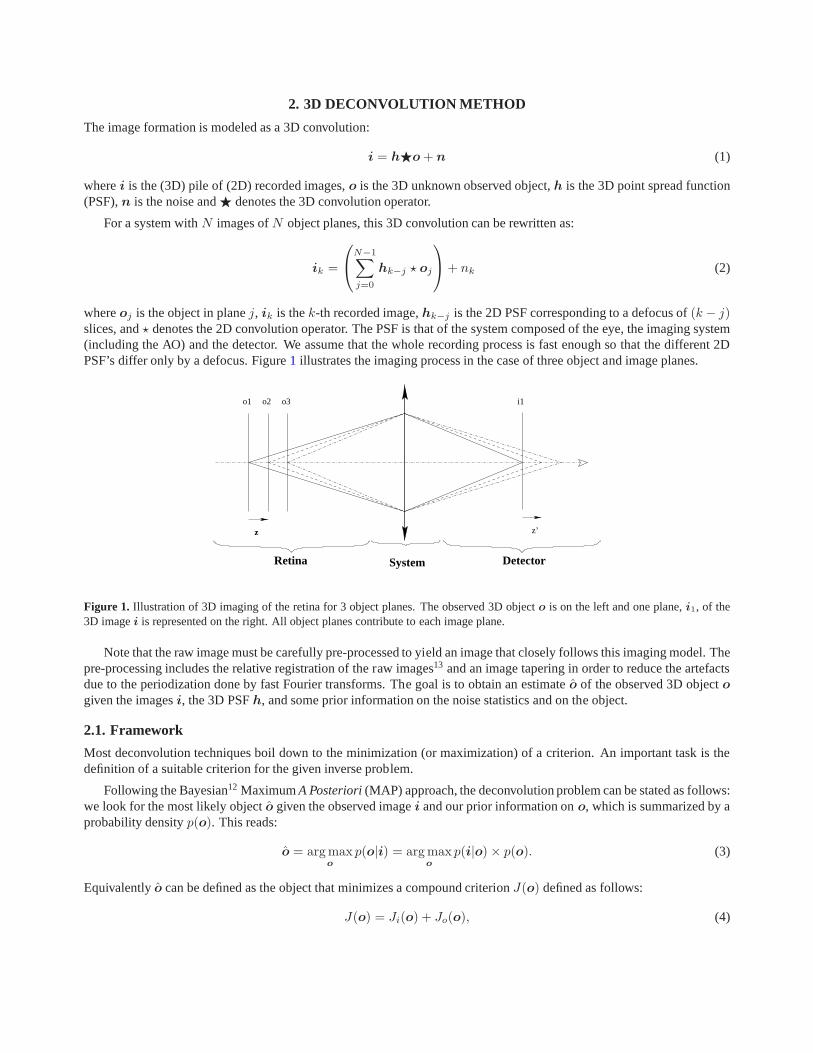
whereoj is the object in planej, ik is thek-th recorded image,hk−j is the 2D PSF corresponding to a defocus of(k − j)slices, and⋆ denotes the 2D convolution operator. The PSF is that of the system composed of the eye, the imaging system(including the AO) and the detector. We assume that the wholerecording process is fast enough so that the different 2DPSF’s differ only by a defocus. Figure1 illustrates the imaging process in the case of three object and image planes.

z

o1 o2 o3

z’

i1

Retina DetectorSystem

Figure 1. Illustration of 3D imaging of the retina for 3 object planes.The observed 3D objecto is on the left and one plane,i1, of the3D imagei is represented on the right. All object planes contribute toeach image plane.

Note that the raw image must be carefully pre-processed to yield an image that closely follows this imaging model. Thepre-processing includes the relative registration of the raw images13 and an image tapering in order to reduce the artefactsdue to the periodization done by fast Fourier transforms. The goal is to obtain an estimateo of the observed 3D objectogiven the imagesi, the 3D PSFh, and some prior information on the noise statistics and on the object.

2.1. Framework

Most deconvolution techniques boil down to the minimization (or maximization) of a criterion. An important task is thedefinition of a suitable criterion for the given inverse problem.

Following the Bayesian12 MaximumA Posteriori(MAP) approach, the deconvolution problem can be stated as follows:we look for the most likely objecto given the observed imagei and our prior information ono, which is summarized by aprobability densityp(o). This reads:

o = arg maxo

p(o|i) = arg maxo

p(i|o) × p(o). (3)

Equivalentlyo can be defined as the object that minimizes a compound criterionJ(o) defined as follows:

J(o) = Ji(o) + Jo(o), (4)

where the negative log-likelihoodJi = − ln p(i|o) is a measure of fidelity to the data andJo = − ln p(o) is a regularizationor penalty term, so the MAP solution can equivalently be called a penalized-likelihood solution. Note that the Bayesianapproach does not require thato truly be the outcome of a stochastic process; rather,p(o) should be designed to embodythe available prior information ono, which means thatJo should have higher values for objects that are less compatiblewith our prior knowledge,11 e.g. that are very oscillating.

Wheno is not the outcome of a stochastic process,Jo usually includes a scaling factor or global hyper-parameter,denoted byµ in the following, which adjusts the balance between fidelityto the data and fidelity to the prior information.Because the optimal balance between data and prior depends on the flux of each object plane, in the following we proposea regularization term with one such hyper-parameterper object plane. And we shall show in Section3 how to estimatethese hyper-parameters.

2.2. Object prior

The choice of a Gaussian prior probability distribution forthe object can be justified from an information theory standpointas being the least informative, given the first two moments ofthe distribution.

Additionally, we assume that the different object planes are independent because firstly, the retina is composed ofpotentially very different slices, and secondly we would like to improve the axial resolution in the restored object, whichwould be hampered by a regularization in the axial dimension. The regularization criterion is thus quadratic (or “L2” inshort) and given by:

Jo(o) =1

2

N−1∑

l=0

∑

f

∣

∣ol(f) − ol(f)∣

∣

2

Sol(f)

(5)

whereSolis the 2D power spectral density (PSD) of object planel.

A reasonable model of the PSD of each object plane can be found14 and used with potentially different parameters foreach plane in the above equation. It reads:

Sol(f) =

1

µl

(

1 +(

|f |f0

l

)pl) , (6)

where

• µl is inversely proportional to the energy of object planel;

• pl characterizes the spectral richness of object planel – in practice,p goes from0 for point like objects to4 for verysmooth extended objects;

• f0

l represents the inverse of the 2D object size for finite support objects. This parameter is very difficult to adjust byhand for objects extended beyond the field of view.

With such a fine PSD model per plane (3 ×NP parameters forNP object planes), the MAP method can optimallyadjust the balance between the resolution and the robustness to noise not only for each plane foreach spatial frequencyin each plane, provided the PSD model parameters are correctly tuned. Tuning all these hyper-parameters in a supervisedfashion (i.e., manually) is unrealistic, so we developed a method to estimate these hyper-parameters in an unsupervisedway directly from the data, before performing the deconvolution. Before we derive this method in Section3, in the nextsubsection we give some details about the noise model that isincorporated into our method.

2.3. Noise model

The noise is a mixture of photon noise and detector noise. Photon noise is non-stationary, white, Poisson-distributed andcan be well modeled as non stationary white Gaussian as soon as the flux level is a few tens of photo-electrons per pixel.15

Detector noise is, to a good approximation, stationary white Gaussian, so the sum of these two noises can reasonably bemodeled as non stationary white Gaussian. The neg-log-likelihood of the data is thus the following weighted least-squaredifference between the actual datai and our model of the data for a given object,h ⋆ o:

Ji(o) =1

2

N−1∑

k=0

Npix−1∑

p,q=0

1

σ2

k(p, q)

∣

∣

∣

∣

∣

ik(p, q) −

N−1∑

l=0

[hk−l ⋆ ol] (p, q)

∣

∣

∣

∣

∣

2

(7)

3. UNSUPERVISED HYPER-PARAMETER ESTIMATION

In this section, we estimate the parameters of the object 3D PSD by Maximum Likelihood (ML). The proposed procedureis an extension to 3D imaging of the method developed by Blancet al. in the context of phase diversity wavefront-sensing16

and applied by Gratadouret al. to the restoration of AO-corrected astronomical images.17 With the parametric PSD modelof Eq. (6), the 3D object PSD is determined by three parameters per object plane. In this subsection (and only here), wemake the additional approximation that the noise is stationary, of varianceσ2

k, within each image planek; this makes theobject PSD estimation much more tractable, and is justified by the fact that the images considered here are illuminatedrather uniformly due to all the out-of-focus object planes contributing to each image. Therefore, for each plane there arefour parameters to be estimated, which will be jointly denoted byΘk: Θk = (µk, f0

k , pk, σ2

k).

If we denote byHk−j the operator performing the 2D convolution with PSFhk−j , the convolution product fromEq. (2) can be rewritten as:

ik ,

N−1∑

j=0

Hk−joj + nk (8)

whereH is the matrix of the convolution product. The mean of an imageplanek is given by :

ik =N−1∑

j=0

hk−j ⋆ oj , (9)

whereoj is the mean of the object planej. In practice we takeoj = 0 ∀j, so thatik = 0 too. The covariance matrix ofimage planek is given by:

Cik=

N−1∑

j=0

Hk−jCojH

tk−j + Cnk

(10)

whereCojis the covariance matrix of the object planej andCnk

is the covariance matrix of image planek.

Becauseoj − oj is assumed stationary, the object covariance matrixCojis Toeplitz (more precisely, block-Toeplitz

with Toeplitz blocks). Because the noise’s covariance matrix is Cnk= σ2

k.I, the image covariance matrixCikis Toeplitz

too. Thus all matrices of Eq. (10) are approximately diagonalized by fast Fourier transforms (FFT), which yields thefollowing expression for the PSDSik

of imageik:

Sik(f, Θk) =

N−1∑

j=0

∣

∣

∣hk−j

∣

∣

∣

2

Soj(f, Θj) + Snk

(f, Θk) (11)

Because only transfer functionshk−j close to focus (k − j ≃ 0) carry high frequency information, the latter equationcan be approximated by:

Sik(f, Θk) ≃

N−1∑

j=0

∣

∣

∣hk−j

∣

∣

∣

2

Sok(f, Θk) + Snk

(f, Θk) (12)

except at very low frequencies.

With the above Gaussian model for the object prior probability distribution and for the noise distribution, Eq. (8) showsthat the probability distribution of each image plane is Gaussian too. The likelihood of imageik is given by:

p(ik|Θk) =1

(2π)N/2√

det(Cik). exp

[

1

2(ik − ik)tCi

−1

k (ik − ik)

]

(13)

The negative log-likelihood is thus given by :

L(Θk) = − ln(p(ik|Θk) =1

2

∑

f

ln(Sik(f, Θk)) +

1

2

∑

f

∣

∣

∣ik(f) − ik(f)∣

∣

∣

2

Sik(f, Θk)

(14)

whereik is given by Eq. (9) andSik(f, Θk) by Eq. (12).

Finally, for each image plane we are able to determine the three object PSD parameters by minimizingL(Θk) numeri-cally, as a function ofΘk = (µk, f0

k , pk, σ2

k). These parameters can then be used in the deconvolution.

4. VALIDATION ON SIMULATED DATA

4.1. Simulated object and images

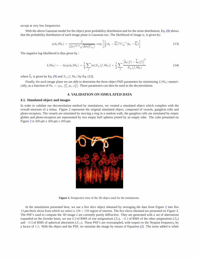
In order to validate our deconvolution method by simulations, we created a simulated object which complies with theoverall structure of a retina. Figure2 represents the original simulated object, composed of vessels, ganglion cells andphoto-receptors. The vessels are simulated by moving a ringin a random walk, the ganglion cells are simulated by emptyglobes and photo-receptors are represented by two empty half spheres joined by an empty tube. The cube presented onFigure2 is 300 µm x300 µm x300 µm.

Figure 2. Perspective view of the 3D object used for the simulations.

In the simulations presented here, we use a five slice object obtained by averaging the data from Figure2 into five13 µm-thick slices from which we select a128× 128 region of interest. The five slices obtained are presented onFigure3.The PSF’s used to compute the 3D imagei are currently purely diffractive. They are generated with aset of aberrationsexpanded on the Zernike basis; we use0.2 rd RMS of one astigmatism (Z5), −0.1 rd RMS of the other astigmatism (Z6)and−0.5 rd RMS of spherical aberration (Z11). These PSF’s are oversampled, with respect to the Nyquist frequency, bya factor of1.5. With the object and the PSF, we simulate the image by means ofEquation (2). The noise added is white

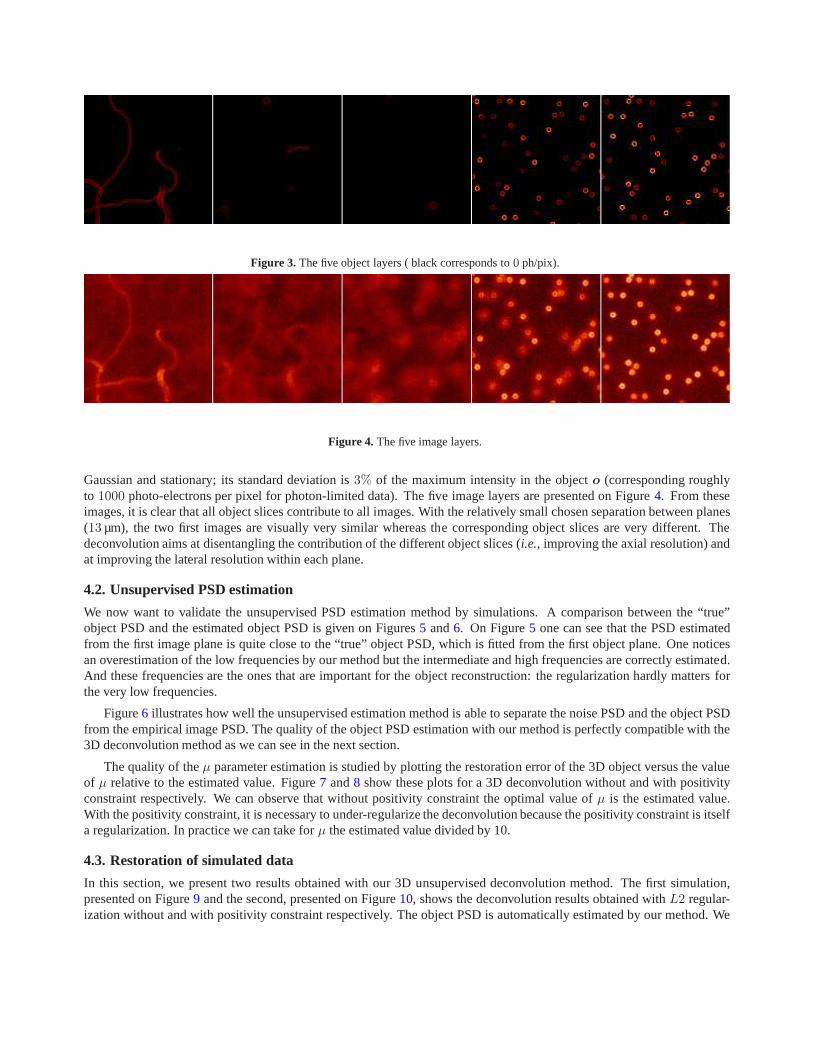
Figure 3. The five object layers ( black corresponds to0 ph/pix).

Figure 4. The five image layers.

Gaussian and stationary; its standard deviation is3% of the maximum intensity in the objecto (corresponding roughlyto 1000 photo-electrons per pixel for photon-limited data). The five image layers are presented on Figure4. From theseimages, it is clear that all object slices contribute to all images. With the relatively small chosen separation betweenplanes(13 µm), the two first images are visually very similar whereas the corresponding object slices are very different. Thedeconvolution aims at disentangling the contribution of the different object slices (i.e., improving the axial resolution) andat improving the lateral resolution within each plane.

4.2. Unsupervised PSD estimation

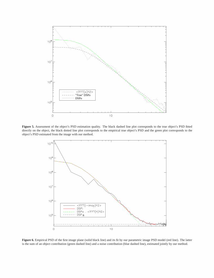
We now want to validate the unsupervised PSD estimation method by simulations. A comparison between the “true”object PSD and the estimated object PSD is given on Figures5 and6. On Figure5 one can see that the PSD estimatedfrom the first image plane is quite close to the “true” object PSD, which is fitted from the first object plane. One noticesan overestimation of the low frequencies by our method but the intermediate and high frequencies are correctly estimated.And these frequencies are the ones that are important for theobject reconstruction: the regularization hardly mattersforthe very low frequencies.

Figure6 illustrates how well the unsupervised estimation method isable to separate the noise PSD and the object PSDfrom the empirical image PSD. The quality of the object PSD estimation with our method is perfectly compatible with the3D deconvolution method as we can see in the next section.

The quality of theµ parameter estimation is studied by plotting the restoration error of the 3D object versus the valueof µ relative to the estimated value. Figure7 and8 show these plots for a 3D deconvolution without and with positivityconstraint respectively. We can observe that without positivity constraint the optimal value ofµ is the estimated value.With the positivity constraint, it is necessary to under-regularize the deconvolution because the positivity constraint is itselfa regularization. In practice we can take forµ the estimated value divided by 10.

4.3. Restoration of simulated data

In this section, we present two results obtained with our 3D unsupervised deconvolution method. The first simulation,presented on Figure9 and the second, presented on Figure10, shows the deconvolution results obtained withL2 regular-ization without and with positivity constraint respectively. The object PSD is automatically estimated by our method.We

DSPo"True" DSPo

Figure 5. Assessment of the object’s PSD estimation quality. The black dashed line plot corresponds to the true object’s PSD fitteddirectly on the object, the black dotted line plot corresponds to the empirical true object’s PSD and the green plot corresponds to theobject’s PSD estimated from the image with our method.

n

Figure 6. Empirical PSD of the first image plane (solid black line) and its fit by our parametric image PSD model (red line). The latteris the sum of an object contribution (green dashed line) and anoise contribution (blue dashed line), estimated jointly by our method.

Obj

ect r

econ

stru

ctio

n er

ror

Hyperparameter

3D deconvolution without positivity constraint. Noise: 3%

Object

Figure 7. Plot of the 3D object restoration error without positivity constraint versus the relativeµ value.

Object

Hyperparameter

Obj

ect r

econ

stru

ctio

n er

ror

(%)

3D deconvolution with positivity constraint. Noise: 3%

Figure 8. Plot of the 3D object restoration error with positivity constraint versus the relativeµ value.

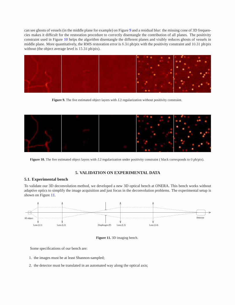
can see ghosts of vessels (in the middle plane for example) onFigure9 and a residual blur: the missing cone of 3D frequen-cies makes it difficult for the restoration procedure to correctly disentangle the contribution of all planes. The positivityconstraint used in Figure10 helps the algorithm disentangle the different planes and visibly reduces ghosts of vessels inmiddle plane. More quantitatively, the RMS restoration error is8.34 ph/pix with the positivity constraint and10.31 ph/pixwithout (the object average level is15.34 ph/pix).

Figure 9. The five estimated object layers withL2 regularization without positivity constraint.

Figure 10. The five estimated object layers withL2 regularization under positivity constraint ( black corresponds to0 ph/pix).

5. VALIDATION ON EXPERIMENTAL DATA

5.1. Experimental bench

To validate our 3D deconvolution method, we developed a new 3D optical bench at ONERA. This bench works withoutadaptive optics to simplify the image acquisition and just focus in the deconvolution problems. The experimental setupisshown on Figure11.

3D object

Lens (L2)Lens (L1) Diaphragm (P) Lens (L3) Lens (L4)

Detector

Figure 11. 3D imaging bench.

Some specifications of our bench are:

1. the images must be at least Shannon-sampled;

2. the detector must be translated in an automated way along the optical axis;

3. the aberrations must be the same in the field (no anisoplanatism).

The bench presented on Figure11 takes into account all these constraints.L1 is a microscope objective (16X, NA=0.32);L2 is a biconvex lens (f = 62.9 mm andd = 25.4 mm); P is the pupil of the system;L3 andL4 perform a re-imaging ofthe object through the diaphragm P. We can use two objects with our bench: a pinhole (1 µm diameter) to measure the 3DPSF, and a micrometer rule tilted with respect to the opticalaxis (by 35 degrees) as a 3D object.

5.2. Restoration of experimental data

We present here the rule images and the 3D PSF. The 3D rule image has 30 different planes. The Figure12 presents twoplanes, taken at two different depths (the distance betweenthe two planes is3.2 cm).

Figure 12. Two planes of the 3D rule image. On the left, the detector is focused at the very top of the rule. On the right, the detector isfocused on about one quarter of the image from the top of the rule.

We performed an unsupervised 3D deconvolution of this 3D image of the rule with the PSD model introduced insection3 and the positivity constraint. The object PSD is estimated from each image plane with the method presented insection3. With the positivity constraint, the parameterµ is divided by 10 in practice as shown in simulations. One cannotice on Figure13 the lateral resolution increase due to the deconvolution method (the width of each line is 6 pixel in animage and only 1 pixel on the solution). The restored width iscompatible with real dimensions of the rule because each lineis about1 µm wide. This restored object is very encouraging and demonstrates the effectiveness of our 3D unsuperviseddeconvolution method.

6. CONCLUSION AND PERSPECTIVES

A 3D deconvolution method has been derived in a Bayesian framework for the restoration of adaptive-optics correctedimages of the human retina; it incorporates a positivity constraint and a regularization metric in order to avoid uncontrollednoise amplification. An unsupervised method has been proposed to estimate the 3D object PSD from the 3D image andthe 3D PSF. We have demonstrated the effectiveness of the method, on realistic simulated data and on experimental dataobtained the 3D optical bench developed at ONERA.

Future work includes the processing of adaptive-optics corrected retinal images. For this purpose, it is of paramountimportance to estimate the PSF precisely in order not to produce deconvolution artefacts. This can be achieved by recon-structing the residual wavefront from the wavefront sensordata of the adaptive-optics loop.

Figure 13. Two object planes restored with positivity constraint. On the left, the detector is focused at the very top of the rule. Ontheright, the detector is focused on about one quarter of the image from the top of the rule.

REFERENCES

1. J. Primot, G. Rousset, and J.-C. Fontanella, “Deconvolution from wavefront sensing: a new technique for compen-sating turbulence-degraded images,”J. Opt. Soc. Am. A7(9), pp. 1598–1608, 1990.

2. L. M. Mugnier, C. Robert, J.-M. Conan, V. Michau, and S. Salem, “Myopic deconvolution from wavefront sensing,”J. Opt. Soc. Am. A18, pp. 862–872, Apr. 2001.

3. D. Catlin and C. Dainty, “High-resolution imaging of the human retina with a Fourier deconvolution technique,”J.Opt. Soc. Am. A19, pp. 1515–1523, Aug. 2002.

4. G. Rousset, J.-C. Fontanella, P. Kern, P. Gigan, F. Rigaut, P. Léna, C. Boyer, P. Jagourel, J.-P. Gaffard, and F. Merkle,“First diffraction-limited astronomical images with adaptive optics,”Astron. Astrophys.230, pp. 29–32, 1990.

5. M. C. Roggemann, “Limited degree-of-freedom adaptive optics and image reconstruction,”Appl. Opt. 30(29),pp. 4227–4233, 1991.

6. J. M. Conan, P. Y. Madec, and G. Rousset, “Image formation in adaptive optics partial correction,” inActive andAdaptive Optics, F. Merkle, ed.,ESO Conference and Workshop Proceedings48, pp. 181–186, ESO/ICO, (Garchingbei München, Germany), 1994.

7. J.-M. Conan,Étude de la correction partielle en optique adaptative. PhD thesis, Université Paris XI Orsay, Oct. 1994.8. J. G. McNally, T. Karpova, J. Cooper, and J. A. Conchello, “Three-dimensional imaging by deconvolution mi-

croscopy,”Methods19, pp. 373–385, 1999.9. J. C. Christou, A. Roorda, and D. R. Williams, “Deconvolution of adaptive optics retinal images,”J. Opt. Soc. Am.

A 21, pp. 1393–1401, Aug. 2004.10. A. Tikhonov and V. Arsenin,Solutions of Ill-Posed Problems, Winston, DC, 1977.11. G. Demoment, “Image reconstruction and restoration: Overview of common estimation structures and problems,”

IEEE Trans. Acoust. Speech Signal Process.37, pp. 2024–2036, Dec. 1989.12. J. Idier, ed.,Bayesian Approach for Inverse Problems, ISTE, London, 2008.13. D. Gratadour, L. M. Mugnier, and D. Rouan, “Sub-pixel image registration with a maximum likelihood estimator,”

Astron. Astrophys.443, pp. 357–365, Nov. 2005.

14. J.-M. Conan, L. M. Mugnier, T. Fusco, V. Michau, and G. Rousset, “Myopic deconvolution of adaptive optics imagesby use of object and point spread function power spectra,”Appl. Opt.37, pp. 4614–4622, July 1998.

15. L. M. Mugnier, T. Fusco, and J.-M. Conan, “MISTRAL: a myopic edge-preserving image restoration method, withapplication to astronomical adaptive-optics-corrected long-exposure images.,”J. Opt. Soc. Am. A21, pp. 1841–1854,Oct. 2004.

16. A. Blanc, L. M. Mugnier, and J. Idier, “Marginal estimation of aberrations and image restoration by use of phasediversity,” J. Opt. Soc. Am. A20(6), pp. 1035–1045, 2003.

17. D. Gratadour, D. Rouan, L. M. Mugnier, T. Fusco, Y. Clénet, E. Gendron, and F. Lacombe, “Near-IR AO dissectionof the core of NGC 1068 with NaCo,”Astron. Astrophys.446, pp. 813–825, Feb. 2006.