Unobtrusive and Ubiquitous In-Home Monitoring: AMethodology for Continuous Assessment of Gait Velocity inElders

Stuart Hagler,Biomedical Engineering division, Oregon Health and Science University, Portland, OR 97239USA, (haglers@bme.ogi.edu)

Daniel Austin [Member, IEEE],Biomedical Engineering division, Oregon Health and Science University, Portland, OR 97239USA, (austidan@bme.ogi.edu)

Tamara L. Hayes [Member, IEEE],Biomedical Engineering division, Oregon Health and Science University, Portland, OR 97239USA, (hayest@bme.ogi.edu)

Jeffrey Kaye [Member, IEEE], andDepartment of Neurology, Oregon Health and Science University, Portland, OR 97239 USA(kaye@ohsu.edu)

Misha Pavel [Member, IEEE]Biomedical Engineering division, Oregon Health and Science University, Portland, OR 97239USA, (pavel@bme.ogi.edu)

AbstractGait velocity has been shown to quantitatively estimate risk of future hospitalization, has beenshown to be a predictor of disability, and has been shown to slow prior to cognitive decline. In thispaper, we describe a system for continuous and unobtrusive in-home assessment of gait velocity, acritical metric of function. This system is based on estimating walking speed from noisy time andlocation data collected by a “sensor line” of restricted view passive infrared (PIR) motiondetectors. We demonstrate the validity of our system by comparing with measurements from thecommercially available GAITRite® Walkway System gait mat. We present the data from 882walks from 27 subjects walking at three different subject-paced speeds (encouraged to walkslowly, normal speed, or fast) in two directions through a sensor line. The experimental resultsshow that the uncalibrated system accuracy (average error) of estimated velocity was 7.1cm/s (SD= 11.3cm/s), which improved to 1.1cm/s (SD = 9.1cm/s) after a simple calibration procedure.Based on the average measured walking speed of 102 cm/s our system had an average error of lessthan 7% without calibration and 1.1% with calibration.

Index TermsEldercare; unobtrusive monitoring; ubiquitous computing; gait; walking speed; passive infrared(PIR) motion detectors

Correspondence to: Daniel Austin.

NIH Public AccessAuthor ManuscriptIEEE Trans Biomed Eng. Author manuscript; available in PMC 2011 April 1.

Published in final edited form as:IEEE Trans Biomed Eng. 2010 April ; 57(4): 813–820. doi:10.1109/TBME.2009.2036732.

NIH

-PA Author Manuscript

NIH

-PA Author Manuscript

NIH

-PA Author Manuscript

I. IntroductionImproving quality of life and providing adequate medical care for the rising number ofelderly while keeping health care costs under control has in recent years become a majorproblem [1]. Several methodologies have been proposed to address this problem that includethe use of technology to develop systems that promote aging in place [2] and the use ofpervasive healthcare [3] to help alleviate the burden placed on health care providers. One ofthe underlying themes of these approaches is to employ technology such as wirelessnetworks combined with novel sensing systems to gather and interpret data in non-healthcare settings such as the home environment.

Many systems have been proposed that use these methodologies to assist the elderly. Forexample, passive infrared sensors have been used in-home for the estimation of amount [4]and type [5] of daily activity and in-hospital for classification of patient movements [6].Other systems have been proposed that detect falls in elders [7], infer activities of dailyliving (ADLs) [8], use computer interactions to detect cognitive changes [9], and forcontinuous and unobtrusive in-home behavioral monitoring [10]. Other recent applicationsof pervasive healthcare and wireless sensor networks for supporting elder healthcare foraging in place include multimodal sensing and computer vision [11,12] while systems forsupporting independence in assisted living are described in [13,14]. For completeness wemention that a comprehensive literature review of pervasive computing in health care from2002 to 2006 is available [15] including applications to eldercare.

One specific measure of particular interest for unobtrusive assessment for health monitoringis walking speed. Walking speed has been shown to be a quantitative estimate of risk offuture hospitalization [16]. Slower walking speed has been demonstrated in dementiapatients compared to controls [17] and has been shown to precede cognitive impairment [18]and dementia [19], and timed walk has been used as a partial characterization of lowerextremity function which has been shown to predict disability [20,21]. Other studies haveshown a relationship between walking speed and cognition [22,23]. Current evaluation ofwalking speed is typically done both infrequently and in the clinic setting which suffersfrom at least five shortcomings. First, frequent assessment visits are impractical and costprohibitive since either it is difficult for patients to make frequent trips to a doctor's office orother clinical settings or in the case of research assessments, inconvenient for the researchteam to visit homes frequently. Second, for longitudinal study each testing session istypically scheduled in increments of six months or a year after a baseline visit making itdifficult both to evaluate the validity or stability of baseline measurements and to detectshort and long term variability [24]. Third, there may be an intentional [16] change inwalking speed in the clinical setting or an unintentional [24] change in abilities during asingle assessment. These pacing considerations themselves may have important implicationsfor predicting outcomes [23]. Fourth, infrequent measurements report only the net changebetween measurement times and cannot distinguish between functional changes occurringslowly over time and abrupt functional changes, which may have different causes. Fifth,infrequent measurements do not detect changes when they happen which may reduce theability of a clinician to provide intervention or reduce the effect of an intervention. Byshifting to continuous in-home monitoring of walking speed from the current paradigm, theeffect of all of these short comings can be significantly reduced or removed.

There have been several systems proposed for monitoring walking speed and other gaitfeatures outside of the clinical setting [25-27]. These systems typically consist of somewearable combination of gyroscopes and/or accelerometers and have demonstrated accuracyand precision in the field. However, these systems suffer from several limitations such asshort battery life, the need to download the data or introduce additional hardware and

Hagler et al. Page 2

IEEE Trans Biomed Eng. Author manuscript; available in PMC 2011 April 1.

NIH

-PA Author Manuscript

NIH

-PA Author Manuscript

NIH

-PA Author Manuscript

complexity for wireless data collection, and the inconvenience of both a wearable deviceand having to remember to wear a device. For these reasons the wearable devices arecurrently inadequate for long-term, in-home, unobtrusive monitoring.

In order to address these concerns and to improve diagnostic ability for clinicians andresearchers, we propose a methodology for continuous in-home monitoring of walkingspeed using passive infrared motion sensors. Specifically, we describe the hardwarepreparation and deployment, the techniques for data collection, and the data processingalgorithms for continuous in-home assessment of walking speed in elders. Finally, wevalidate our approach by comparing the results of our method for walking speed estimationwith the commercially available GAITRite® Walkway System gait mat.

II. System Description and Data CollectionIn this section, we describe the hardware and methodology used to deploy the walking speedmeasurement system in a residence. A partial description of this system has been describedelsewhere [4,10] in the more general context of total activity monitoring, as has a simplerversion of the proposed approach [28]. Here we specialize and describe in more detail thespecific nature of the walking speed measurement system. We begin by describing thesensors and how they are placed in a residence and follow with a description of the wirelessnetwork based data collection.

To detect motion we used the X10 model MS16A (X10.com) passive infrared motion sensorwhich emits a unique programmable bit code at 310 MHz when motion is detected. Werestricted the field of view of each motion sensor to ±4 degrees and installed four sensorssequentially on the ceiling (average height of 2.54 m) approximately 61cm apart in aconfined area such as a hallway or other corridor. This combination tends to force a residentto walk linearly through each sensor pair in the sensor line and ensures that each sensor willonly fire when someone passes directly below. Limiting the field of view precisely andplacing sensors in exact locations is not possible, and therefore there is some variability inthe physical locations which cause the sensors to fire, as will be discussed shortly. Fig.1shows how these sensors look from a resident's point of view when entering the sensor line.

To collect the wirelessly transmitted sensor firings, we use a WGL 800 wireless transceiverconnected to a desktop computer installed in the residence. Simultaneous sensor firings orother interfering sources can result in lost data due to collisions at the wireless transceiver.However, these have been shown to be minor, with a less than 2% overall data loss [4]. Thecomputer timestamps the sensor firings and the data pair is both stored locally and sent via asecure Internet connection to a central database for analysis.

Our experience with the described technology comes from the deployment and monitoringof approximately 250 Portland (OR, USA) metropolitan area homes and retirementcommunity dwellings from between 6 months to over 2 years in ongoing studies. We haveinstrumented both single and multi person dwellings and have collected data from over1,200,000 walking events from single person homes with minimal technical challenge orsophistication needed for setup. Installation of the complete system (including additionaltechnologies described elsewhere [4]) takes an average of 1.5 to 2 hours with 2 people.Deploying only the equipment necessary to measure walking speed (computer, sensors,wireless transceiver, and internet) is estimated to take 1 person approximately 1 hour – if thehome already contains an Internet-connected computer, this could be done in 20 minutes.The technologies are managed remotely using custom systems management software thatsupports data viewing, remote software updates, and remote computer reboots if needed.Other issues, such as replacing motion sensor batteries (battery life is about 1 year) or

Hagler et al. Page 3

IEEE Trans Biomed Eng. Author manuscript; available in PMC 2011 April 1.

NIH

-PA Author Manuscript

NIH

-PA Author Manuscript

NIH

-PA Author Manuscript

changing sensors if they become unreliable or defective can typically be handled in a veryshort visit to the residence, typically 10-15 minutes. Overall, we have found the system hasbeen simple to install, unobtrusive in the sense of both passive sensor technology andminimal outside intervention, and easy to maintain.

III. Data Modeling and AnalysisIn this section we introduce and discuss both the proposed linear model and the estimator fordetermining the gait velocity from noisy motion sensor data. We start by describing how todetermine the precise spatial separation of the sensors from the sensor firings since they willnot, as mentioned, be the same as the measured values due to a combination of installationvariability and differences between individual sensors. We then use this information tomodel the walking speed as a linear function of the measured data degraded by two sourcesof additive noise. The first source of noise is in units of distance and is due to the sensorfiring in slightly different locations during each pass through the sensor line. This error isbased on the field of view and sensitivity of an individual sensor. The second source of erroris in units of time and is due to the discrepancy between when a sensor fires and when thecomputer timestamps the firing, which generally causes positive time errors. We concludethe section by proposing a walking speed estimator that minimizes the combination of theseerrors followed by a discussion of model calibration in the presence of ground-truth dataversus estimating the calibration factor when ground-truth data is unavailable.

A. The Linear ModelWe start by assuming the sensors are placed at physical positions {xi} in some spatial

coordinate system. For a particular walking event the sensors fire at times where kindexes the particular sensor line walking event and i indexes the particular sensor whichfired. We then define {xi} to be the average position at which the walker is when the ithsensor fires. In other words, for a particular walking event the ith sensor fires when thewalker is at some random location {xi+εi} with the errors {εi} being independent randomvariables with zero expected value. Fig. 2 illustrates this arrangement.

The differences {xi – xi} represent likely biases due to the field of view of the sensor and thedirection of movement as shown in fig. 2. For the sake of simplicity we restrict the presentdiscussion to the analysis of movement in one direction.

Now assuming a walker moves with some known velocity ν through a sensor line and wehave some absolute reference time, {τi} can be defined as the time at which the walker isexpected to be at location {xi} and trigger the ith sensor. If we now include the errors indetection location {εi} explicitly in the measured time we find that the measured times

should be .

By further assuming that there is some random delay {ηi} between when a sensor fires atlocation {xi + εi} and when the computer time-stamps the sensor firing data, the measured

time can be written as where the {ηi} are independent random variableswith some common non-negative expected value and the explicit dependence on themeasured time from both position errors and time errors is shown.

Hagler et al. Page 4

IEEE Trans Biomed Eng. Author manuscript; available in PMC 2011 April 1.

NIH

-PA Author Manuscript

NIH

-PA Author Manuscript

NIH

-PA Author Manuscript

Now, consider an event k to comprise a person walking past the line of sensors with aconstant, but unknown velocity νk. Then for any pair of sensors, i,j we have

, from which we find:

(1)

Using (1) we can solve for the velocity νk, for any three sensors i,j,m:

(2)

We now economize the notation and define and for i,j,m.Rewriting (2) yields:

(3)

Taking the expectation of both sides and using the facts that: , , and

for i ≠ j, results in:

(4)

which simplifies to:

(5)

From this we may conclude that:

(6)

The expected value of the random variable can therefore be used to estimate the spatialseparation of the sensors up to a scale factor by computing the average values over a largenumber of events.

By explicitly writing (6) with the proportionality constant c we have:

Hagler et al. Page 5

IEEE Trans Biomed Eng. Author manuscript; available in PMC 2011 April 1.

NIH

-PA Author Manuscript

NIH

-PA Author Manuscript

NIH

-PA Author Manuscript

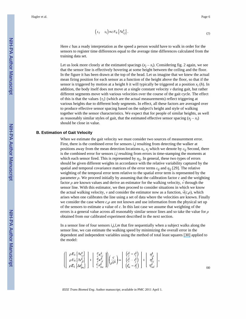
(7)

Here c has a ready interpretation as the speed a person would have to walk in order for thesensors to register time differences equal to the average time differences calculated from thetraining data set.

Let us look more closely at the estimated spacings (xj – xi). Considering fig. 2 again, we seethat the sensor line is effectively hovering at some height between the ceiling and the floor.In the figure it has been drawn at the top of the head. Let us imagine that we knew the actualmean firing position for each sensor as a function of the height above the floor, so that if thesensor is triggered by motion at a height h it will typically be triggered at a position xi (h). Inaddition, the body itself does not move at a single constant velocity ν during gait, but ratherdifferent segments move with various velocities over the course of the gait cycle. The effectof this is that the values {τi} (which are the actual measurements) reflect triggering atvarious heights due to different body segments. In effect, all these factors are averaged overto produce effective sensor spacing based on the subject's height and style of walkingtogether with the sensor characteristics. We expect that for people of similar heights, as wellas reasonably similar styles of gait, that the estimated effective sensor spacing (xj – xi)should be close in value.

B. Estimation of Gait VelocityWhen we estimate the gait velocity we must consider two sources of measurement error.First, there is the combined error for sensors i,j resulting from detecting the walker atpositions away from the mean detection locations xi, xj which we denote by εij Second, thereis the combined error for sensors i,j resulting from errors in time-stamping the moments atwhich each sensor fired. This is represented by ηij. In general, these two types of errorsshould be given different weights in accordance with the relative variability captured by thespatial and temporal covariance matrices of the error terms εij and ηij [29]. The relativeweighting of the temporal error term relative to the spatial error term is represented by theparameter ρ. We proceed initially by assuming that the calibration factor c and the weightingfactor ρ are known values and derive an estimator for the walking velocity, ν through thesensor line. With this estimator, we then proceed to consider situations in which we knowthe actual walking velocity, ν and consider the estimator now as a function, ν(c,ρ), whicharises when one calibrates the line using a set of data where the velocities are known. Finallywe consider the case where c,ρ are not known and use information from the physical set upof the sensors to estimate a value of c. In this last case we assume that weighting of theerrors is a general value across all reasonably similar sensor lines and so take the value for ρobtained from our calibrated experiment described in the next section.

In a sensor line of four sensors i,j,l,m that fire sequentially when a subject walks along thesensor line, we can estimate the walking speed by minimizing the overall error in thedependent and independent variables using the method of total least squares [30] applied tothe model:

(8)

Hagler et al. Page 6

IEEE Trans Biomed Eng. Author manuscript; available in PMC 2011 April 1.

NIH

-PA Author Manuscript

NIH

-PA Author Manuscript

NIH

-PA Author Manuscript

where we have rewritten the linear equations in matrix notation, used the fact that to keep the noise term in (8) in the standard additive form, and used the estimate of thespatial sensor separation as in (7). We proceed assuming that c,ρ are fixed and knownconstants for the sensor line.

To compute the velocity estimates, we now construct a matrix containing as column vectorsthe distances between adjacent sensors, and the time differences between adjacent sensorfirings:

(9)

This matrix may be factored per the singular value decomposition into a trio of matrices Ak

(ρ), Bk (ρ), Σk (ρ) so that the equation Mk (ρ) = Ak (ρ)Σk (ρ)Bk* (ρ) is satisfied. Letting, denote the appropriate elements of the matrix Bk (ρ), the estimated velocity is

given by:

(10)

C. The Calibrated Sensor LineTaking the weighting factor ρ still to be fixed and known, we now treat the calibration factorc as a variable whose value we may estimate using known velocity data. We are given a set

of training data consisting of sensor firing times and true gait velocities {νk} for asample set of walks through the sensor line. We assume the actual walking speeds and theestimated walking speeds satisfy the linear model:

(11)

where the {ωk}are independent random variables with zero expected value. By collecting all

the measurements into vectors ν,b(ρ), we can estimate the calibration factorwith linear least squares:

(12)

If we knew the actual value ρ we would be done at this point as we could estimate thecalibration factor c given the measured time and velocity values. However, where we do notknow the actual value of ρ, we would like to choose a value which yields the best

Hagler et al. Page 7

IEEE Trans Biomed Eng. Author manuscript; available in PMC 2011 April 1.

NIH

-PA Author Manuscript

NIH

-PA Author Manuscript

NIH

-PA Author Manuscript

performance of the method for estimating velocities. In particular we would like to find avalue of ρ which gives the best performance across many sensor-lines. Let us consider thecalibration factor for the nth sensor-line as a function of ρ, that is:

(13)

We may consider the set of velocity estimates also as functions of ρ:

(14)

This expresses the estimated velocity for the kth walk along the nth sensor-line (ρ)entirely in terms of the measured time, the measured velocity, and the unknown parameter ρ.The weighting factor may now be found as a value which gives the best sensor-lineperformance on average.

In practical situations where calibration data are not available we use an average value of ρdetermined from existing data. In particular, we found that the average value that minimizedthe estimation error in our controlled experiments, described in the next section, was ρ =0.75.

D. The Uncalibrated Sensor LineIf the velocity is not known, then the training data set will contain only the sensor firing

times . In this case we must estimate the value for c using the values for the physicalsensor positions {xi}. Choosing any pair of sensors i,j we may make the estimate:

(15)

We would like to choose our pair of sensors so that the expected value xj – xi is as near invalue as possible to the distance between mean detection positions xj – xi. In general theexpected error will be minimized by choosing the pair consisting of the outermost sensors ofthe line.

We do note that care should be taken when using the uncalibrated sensor line cross-sectionally, especially over small samples, as the individual instantiations of a sensor linecan have sizable differences between ĉ and c as shown in fig. 5.

IV. Experimental VerificationA. Experimental Description

27 subjects (9 male and 18 female, aged 75 to 95 years, mean age 85.2 years, 145cm to185cm in height, average height 164.8 cm) participated in the experiment; all providedinformed consent. The experiment was conducted in a common use room at the facilitywhere the participants live. A single sensor line of eight (8) restricted-field PIR motion

Hagler et al. Page 8

IEEE Trans Biomed Eng. Author manuscript; available in PMC 2011 April 1.

NIH

-PA Author Manuscript

NIH

-PA Author Manuscript

NIH

-PA Author Manuscript

sensors was placed on the ceiling with sensors physically spaced at 61cm (2ft) intervals. Theceiling height was 240cm (7.8ft). Beneath the sensor line an 854cm (14ft) long GAITRite®Walkway System gait mat was placed so that the ends of the mat aligned with the outermostsensors. Participants were instructed to walk at self-determined “slow”, “normal”, and “fast”walking speeds. A total of 30 walks were recorded for most participants such that eachparticipant walked five times at each of the three speeds in the two directions available alongthe sensor line. Five participants did a larger number of walks (36, 42, 42, 44, and 46) buttheir larger group of walks included the basic 30 which all participants did. Their precisewalking speed for each trial was calculated using the gait mat data. Firing times werecollected for each PIR sensor during each trial and used to determine the accuracy of thePIR sensors for measuring walking speed.

Based on our experience with several hundred homes, a reasonable sensor line configurationwhich may be installed under the space constraints of typical small homes consists of foursensors placed in a line at approximately 61cm (2ft) intervals. The choice of four sensorswas influenced by a few different factors. First, since the sensors are known to be noisy, wewanted multiple measurements of the walking speed to use in our estimator to reduceestimator variance. Experiments showed, for example, that moving from three sensors tofour sensors reduced variance by a factor of approximately 3.8. Second, due to spaceconstraints in the homes and retirement communities we found that four sensors are all thatwould reliably fit in most homes. Third, the probability of an individual sensor firing isapproximately 0.937. With four sensors in place and assuming we use walks where eitherthree or four sensors fire, we can capture almost 98% of walking events in the home.Finally, we note that using two sensors in not sufficient as this causes equation (8) to reduceto a single equation with a single unknown which can be solved exactly, and therefore doesnot allow mitigation for known noise effects. In accordance with this we have consideredsensor data in groups of four adjacent sensors. Thus our line of eight sensors is treated asfive individual sensor lines. Furthermore as there is no reason to suppose that the effectivesensor spacing is the same in the two directions along which the line may be walked, – in the“forward” or “return” direction through the line (with respect to the experimenter) – weevaluated each direction independently.

For each sensor line of four sensors in each direction only those walking events in which all4 sensors fired were considered for the purposes of calculating the effective sensor spacingand calibration factor. However, to estimate the velocity for walking events we used all thesensor line data in which 3 or 4 of the 4 sensors fired.

B. Experimental ResultsA total of 882 walks from the 27 participants (mean age 85.2 years) were recorded duringthis experiment with 441 in the “forward” direction and 441 in the “return” direction (asreferenced by the experimenter). The numbers of “slow”, “normal”, and “fast” speed walkswere the same in either direction for each given participant. The 8 ceiling-mounted PIRsensors were divided into 5 sensor lines of 4 sensors with a regular 61cm (2ft) physicalspacing for analysis. In the “forward” direction the sensor lines had all four sensors fire 350± 36 times, and in the “return” direction all 4 sensors fired 330 ± 29 times. The effectivesensor spacing for each sensor line was calculated and normalized as in the foregoing usingonly the events where all 4 sensors fired.

Participants walked in the “forward” direction with a speed of 104 ± 30.6cm/s, and in the“return” direction with a speed of 100 ± 29.3cm/s as measured by the gait mat. Weestimated velocity using a sensor line only in those cases where 3 or 4 of the 4 sensors in theline fired. Fig. 3 shows the directional walking speed estimates versus the measured valuesfor the combined sensor line data after calibration using velocity data from the gait mat. Fig.

Hagler et al. Page 9

IEEE Trans Biomed Eng. Author manuscript; available in PMC 2011 April 1.

NIH

-PA Author Manuscript

NIH

-PA Author Manuscript

NIH

-PA Author Manuscript

4 shows the directional walking speed estimates using estimated calibration factors. In bothfigures the “return” direction is differentiated from the “forward direction” by introducing anegative sign on all the velocity estimates. Additionally, in both figures the line x = y(corresponding to perfect estimation) has been plotted as a dashed line to demonstrate thatboth calibrated and uncalibrated estimates are distributed around the correct values. Further,the distribution of points in fig.4 is wider than in fig. 3 demonstrating that the calibrationprocedure does improve estimation. Also, of particular note is the fact that distribution ofestimates in both figures is more centered and densely packed around the true value in the“return” direction, indicating that velocity estimates in the “return” direction are better thanin the “forward” direction (i.e., the same sensors performed better in one direction than inthe other).

To be more precise about the discussion of the walking speed estimates, we denote theestimated speed for the kth walk through sensor line i for both directions by and the actualspeed by νk. The accuracy of the system was evaluated by computing the average difference

. For the case of the calibrated sensor lines the mean of this difference is 1.1cm/sand the standard deviation is 9.1cm/s. In the case of the uncalibrated sensor lines the mean is7.1cm/s, and the standard deviation is 11.3cm/s.

Figure 5 shows the relationship of the estimated calibration factors to the true (measured)calibration factors, with the line x = y drawn for comparison. This shows that theuncalibrated sensor line with ĉ as in (15) tends to underestimate the true calibration factor,this making the velocity estimates slightly higher than in the calibrated case. This alsodemonstrates the need to be careful when comparing uncalibrated sensor line estimatescross-sectionally.

V. DiscussionThe proposed system for unobtrusive and continuous monitoring of in home walking speedshas been shown to accurately estimate velocity when compared to the GAITRite® WalkwaySystem gait mat standard. The mean estimation errors of 7.1cm/s and 1.1cm/s for theuncalibrated and calibrated sensor lines when compared to the average speed of 102cm/sresult in average errors of 6.96% and 1.08%, respectively. Further, the standard deviationsof the error distributions for the uncalibrated and calibrated sensor lines are 11.1% and8.92% when compared to the average speed of walking. This shows that each individualestimate is accurate, and local averaging and other statistical techniques can be used toincrease precision (reduce the error variance further).

These positive results demonstrate the feasibility of the proposed method and addressseveral deficits in the current paradigm of assessing gait episodically or in clinic settings.First, with this system the variability of walking speed can now be monitored continuouslyover the short term (e.g., walk-to-walk variability) in addition to longer time scales (e.g.,month-to-month yearly) without expensive and inconvenient clinic visits. Second, subjectsin high-risk groups can be monitored more closely and rapidly than is currently feasible.Third, researchers can have access to more frequent measurements of walking speed, whichfacilitates the refinement and better understanding of walking speed as it relates to healthoutcomes and correlations presently in the literature that are based on single or infrequentmeasurements. Fourth, wide scale analysis of multiple subjects can be performed relativelyeasily which we anticipate will open further areas of population-based research anddiagnostic ability not discussed here. We do note that while our proposed system is lessexpensive than repeated clinical visits, the cost of the sensors, computer, internet service,and transceiver may currently be cost prohibitive for studies that might involve thousands of

Hagler et al. Page 10

IEEE Trans Biomed Eng. Author manuscript; available in PMC 2011 April 1.

NIH

-PA Author Manuscript

NIH

-PA Author Manuscript

NIH

-PA Author Manuscript

subjects who are widely dispersed. However, since historically the cost of equipment andservices has continued to drop as better and faster technology becomes available in themarketplace, it is likely that deployment of these kinds of systems to larger cohorts will befacilitated. In addition, less expensive motion sensors may work adequately and simpleapplication specific computers may be built cheaper than off the shelf models which couldbe deployed today. Further work is needed to identify the most cost efficient approaches tomaximize scalability of in-home assessment platforms.

One of the largest challenges to the broad use of our approach to continuous monitoring ofwalking speed, and to in-home monitoring in general, is the differentiation of multipleresidents. This problem is typically addressed by requiring the participants to wear or carrysome type of radio frequency identification (RFID) tag. We are currently working on bothpattern recognition and model-based approaches to distinguish between multiple residentsbased on the walking events. This will allow the expansion of this methodology from singleresident homes to multiple resident dwellings without the need for additional equipment orhardware.

Future work will address comparisons of the in-home continuous method with standardclinical tests of walking, mobility, and physical performance such as the Short PhysicalPerformance Battery, Unified Parkinson's Disease Rating Scale, and various other timedwalks of different durations (e.g., 4-meter, 10-meter, 400 meter) thus facilitatinginterpretation of these established clinical metrics with our new framework. Other futurework will include relaxing the assumption that velocity is fixed over a walking event inorder to measure the step-to-step variability in each walking event. In this case the velocityof the kth walking event becomes some function of time ν(t). Retaining our definition of theerror {εi} above we find that the time at which the sensor fires may be expressed as {τi + υi},where {υi} satisfies:

(16)

The values {ηi} are still defined as above which gives a relation to the measured time values

of . Finally, for any pair of sensors we have the relation:

(17)

which generalizes (1). We anticipate that adjusting the model along the lines of (16) willallow us to derive additional gait parameters from the current and future data.

VI. ConclusionIn this paper we have proposed a new system for continuous in home assessment of walkingspeed based on PIR sensors and a wireless network for data collection. We have shown thatthis method is both accurate and precise when compared to the standard of the GAITRite®Walkway System gait mat. This method allows the convenient in home collection of a largenumber of walking events otherwise gathered infrequently in a clinical setting. Sincewalking speed has been shown to be an indicator or predictor of many diseases and other

Hagler et al. Page 11

IEEE Trans Biomed Eng. Author manuscript; available in PMC 2011 April 1.

NIH

-PA Author Manuscript

NIH

-PA Author Manuscript

NIH

-PA Author Manuscript

health issues such as cognitive decline and hospitalization, we feel that the continuousmonitoring of this measure and its applications is an important and useful area of futureresearch.

AcknowledgmentsThe authors would like to thank the volunteer subjects who participated in this research and the staff from theOregon Center for Aging & Technology who assisted in this study.

This work was supported in part by the National Institute of Health and the National Institute on Aging underGrants R01AG024059, P30 AG024978, and P30AG008017. This work was also partially funded by IntelCorporation.

References1. Kaye, JA.; Zitzelberger, TA. Overview of Healthcare, Disease, and Disability. In: Bardram, JE.;

Mihailidis, A.; Wan, D., editors. Pervasive Computing in Healthcare. CRC Press; 2006.2. Dishman E. Inventing wellness systems for aging in place. Computer 2004;37:4–34.3. Varshney U. Pervasive Healthcare. Computer 2003;36:138–140.4. Hayes TL, Abendroth F, Adami A, Pavel M, Zitzelberger TA, Kaye JA. Unobtrusive assessment of

activity patterns associated with mild cognitive impairment. Alzheimers Dement 2008;4:395–405.[PubMed: 19012864]

5. Logan, B.; Healey, J.; Philipose, M.; Tapia, EM.; Intille, S. A long-term evaluation of sensingmodalities for activity recognition. Lnnsbruck, Austria: 2007.

6. Banerjee S, Steenkeste F, Couturier P, Debray M, Franco A. Telesurveillance of elderly patients byuse of passive infra-red sensors in a ‘smart’ room. J Telemed Telecare 2003;9:23–9. [PubMed:12641889]

7. Sixsmith A, Johnson N. A smart sensor to detect the falls of the elderly. IEEE Pervasive Computing2004;3:42–47.

8. Philipose M, Fishkin KP, Perkowitz M, Patterson DJ, Fox D, Kautz H, Hahnel D. Inferring activitiesfrom interactions with objects. IEEE Pervasive Computing 2004;3:50–57.

9. Jimison H, Pavel M, McKanna J, Pavel J. Unobtrusive monitoring of computer interactions to detectcognitive status in elders. IEEE Transactions on Information Technology in Biomedicine2004;8:248–252. [PubMed: 15484429]

10. Hayes TL, Pavel M, Larimer N, Tsay IA, Nutt J, Adami AG. Distributed healthcare: Simultaneousassessment of multiple individuals. IEEE Pervasive Computing 2007;6:36–43.

11. Perry M, Dowdall A, Lines L, Hone K. Multimodal and ubiquitous computing systems: supportingindependent-living older users. IEEE Trans Inf Technol Biomed 2004;8:258–70. [PubMed:15484431]

12. Mihailidis A, Carmichael B, Boger J. The use of computer vision in an intelligent environment tosupport aging-in-place, safety, and independence in the home. IEEE Trans Inf Technol Biomed2004;8:238–47. [PubMed: 15484428]

13. Lymberopoulos D, Teixeira T, Savvides A. Macroscopic human behavior interpretation usingdistributed imager and other sensors. Proceedings of the IEEE 2008;96:1657–1677.

14. Stanford V. Using pervasive computing to deliver elder care. IEEE Pervasive Computing2002;1:10–13.

15. Orwat C, Graefe A, Faulwasser T. Towards pervasive computing in health care - a literaturereview. BMC Med Inform Decis Mak 2008;8:26. [PubMed: 18565221]

16. Studenski S, Perera S, Wallace D, Chandler JM, Duncan PW, Rooney E, Fox M, Guralnik JM.Physical performance measures in the clinical setting. J Am Geriatr Soc 2003;51:314–22.[PubMed: 12588574]

17. Bramell-Risberg E, Jarnlo GB, Minthon L, Elmstahl S. Lower gait speed in older women withdementia compared with controls. Dement Geriatr Cogn Disord 2005;20:298–305. [PubMed:16166777]

Hagler et al. Page 12

IEEE Trans Biomed Eng. Author manuscript; available in PMC 2011 April 1.

NIH

-PA Author Manuscript

NIH

-PA Author Manuscript

NIH

-PA Author Manuscript

18. Camicioli R, Howieson D, Oken B, Sexton G, Kaye J. Motor slowing precedes cognitiveimpairment in the oldest old. Neurology 1998;50:1496–8. [PubMed: 9596020]

19. Beauchet O, Allali G, Berrut G, Hommet C, Dubost V, Assal F. Gait analysis in dementedsubjects: Interests and perspectives. Neuropsychiatr Dis Treat 2008;4:155–60. [PubMed:18728766]

20. Guralnik JM, Ferrucci L, Pieper CF, Leveille SG, Markides KS, Ostir GV, Studenski S, BerkmanLF, Wallace RB. Lower extremity function and subsequent disability: consistency across studies,predictive models, and value of gait speed alone compared with the short physical performancebattery. J Gerontol A Biol Sci Med Sci 2000;55:M221–31. [PubMed: 10811152]

21. Guralnik JM, Ferrucci L, Simonsick EM, Salive ME, Wallace RB. Lower-extremity function inpersons over the age of 70 years as a predictor of subsequent disability. N Engl J Med1995;332:556–61. [PubMed: 7838189]

22. Holtzer R, Verghese J, Xue X, Lipton RB. Cognitive processes related to gait velocity: results fromthe Einstein Aging Study. Neuropsychology 2006;20:215–23. [PubMed: 16594782]

23. Fitzpatrick AL, Buchanan CK, Nahin RL, Dekosky ST, Atkinson HH, Carlson MC, WilliamsonJD. Associations of gait speed and other measures of physical function with cognition in a healthycohort of elderly persons. J Gerontol A Biol Sci Med Sci 2007;62:1244–51. [PubMed: 18000144]

24. Kaye J. Home-based technologies: a new paradigm for conducting dementia prevention trials.Alzheimers Dement 2008;4:S60–6. [PubMed: 18632003]

25. Aminian K, Robert P, Jequier E, Schutz Y. Incline, speed, and distance assessment duringunconstrained walking. Med Sci Sports Exerc 1995;27:226–34. [PubMed: 7723646]

26. Miyazaki S. Long-term unrestrained measurement of stride length and walking velocity utilizing apiezoelectric gyroscope. IEEE Trans Biomed Eng 1997;44:753–9. [PubMed: 9254988]

27. Sabatini AM, Martelloni C, Scapellato S, Cavallo F. Assessment of walking features from footinertial sensing. IEEE Trans Biomed Eng 2005;52:486–94. [PubMed: 15759579]

28. Hayes, TL.; Hagler, S.; Austin, D.; Kaye, J.; Pavel, M. Unobtrusive assessment of walking speedin the home using inexpensive PIR sensors. presented at 31st Annual International Conference ofthe IEEE Engineering in Medicine and Biology Society; Minneapolis, MN. 2009;

29. Bjorck, A. Numerical Methods for Least Squares Problems. SIAM; 1996.30. Golub, GH.; Loan, CFV. Matrix Computations. third. The John Hopkins University Press; 1996.

BiographiesStuart Hagler received the degrees of B.A. degree in philosophy, B.S. degree in physics,and M.S. degree in physics from the University of Washington, Seattle, Washington, USA.

He is currently working as a Biomedical Researcher at the Oregon Health and ScienceUniversity, Portland, OR, USA.

Daniel Austin (M'05) received the B.S. degree in electronic engineering technology fromthe Oregon Institute of Technology, Portland, OR, USA in 2006, the M.S. degree inelectrical engineering from the University of Southern California, Los Angeles, CA, USA in2008, and is currently working toward the Ph.D. degree in biomedical engineering at theOregon Health and Science University, Portland, OR, USA.

Hagler et al. Page 13

IEEE Trans Biomed Eng. Author manuscript; available in PMC 2011 April 1.

NIH

-PA Author Manuscript

NIH

-PA Author Manuscript

NIH

-PA Author Manuscript

He is currently working as a Biomedical Researcher for the Point of Care Laboratory at theOregon Health and Science University, Portland, OR. His research interests include signalprocessing and modeling with applications to biosignal analysis and early detection ofphysical and cognitive decline.

Tamara L. Hayes (M '01) received the M.S. in electrical engineering from the University ofToronto, Toronto, Canada and the Ph.D. degree in behavioral neuroscience from theUniversity of Pittsburgh, Pittsburgh, PA, USA.

She is an assistant professor in the Division of Biomedical Engineering at Oregon Healthand Science University, Portland, OR. Her research interests include using ubiquitouscomputing to deliver healthcare in the home, with the goal of changing the current paradigmof clinic-centered healthcare to a less costly, more effective model, which lets individualsparticipate more fully in their health care.

Dr. Hayes is also a member of the Sleep Research Society.

Hagler et al. Page 14

IEEE Trans Biomed Eng. Author manuscript; available in PMC 2011 April 1.

NIH

-PA Author Manuscript

NIH

-PA Author Manuscript

NIH

-PA Author Manuscript

Jeffrey Kaye (M '05) received his M.D. degree at New York Medical College, New York,NY, USA in 1980 and trained in neurology at Boston University, Boston, MA USA from1981-1984.

He was a fellow in movement disorders at Boston University and then a Medical StaffFellow in brain aging at the National Institute on Aging, National Institutes of Health from1984 to 1988. He is currently Professor of Neurology and Biomedical Engineering, directorof the Oregon Center for Aging & Technology (ORCATECH), and director of the LaytonAging & Alzheimer's Disease Center, at the Oregon Health and Science University,Portland, OR, USA. His research interests include the design, study and application of

Hagler et al. Page 15

IEEE Trans Biomed Eng. Author manuscript; available in PMC 2011 April 1.

NIH

-PA Author Manuscript

NIH

-PA Author Manuscript

NIH

-PA Author Manuscript

ubiquitous unobtrusive technologies and systems for home-based health research and theidentification of behavioral and biological biomarkers of healthy aging.

Dr. Kaye chairs the Working Group on Technology of the US National Alzheimer'sAssociation and is a Commissioner for the Center for Aging Services and Technology,Washington, DC, USA.

Misha Pavel (M'69) received the B.S. in electrical engineering from Polytechnic Institute ofBrooklyn, New York, NY, USA, the M.S. degree in electrical engineering from Stanford

Hagler et al. Page 16

IEEE Trans Biomed Eng. Author manuscript; available in PMC 2011 April 1.

NIH

-PA Author Manuscript

NIH

-PA Author Manuscript

NIH

-PA Author Manuscript

University, Stanford, CA, USA, and the Ph.D. degree in experimental/mathematicalpsychology at New York University, New York, NY, USA.

He is a Professor and Head of the Division of Biomedical Engineering with a jointappointment in Medical Informatics and Biomedical Computer Science at the Oregon Healthand Science University, Portland, OR, USA. He is also the director of the Point of CareLaboratory which focuses on unobtrusive monitoring and neurobehavioral assessment, andcomputational modeling with applications to care for the aging population. Previously hewas a Technology Leader at AT&T Laboratories developing networked, wireless, andmobile applications for information access and context aware interactions. Other pastpositions include Faculty at New York University and Stanford where he worked on sensorfusion, modeling of pattern recognition in sensory motor systems and human computercommunications systems and Member of Technical Staff at Bell Labs where he wasdeveloping new approaches to network analysis and modeling by incorporatingcharacteristics of human behavior.

Hagler et al. Page 17

IEEE Trans Biomed Eng. Author manuscript; available in PMC 2011 April 1.

NIH

-PA Author Manuscript

NIH

-PA Author Manuscript

NIH

-PA Author Manuscript

Fig. 1.A motion sensor line for measuring walking speed where the four sensors are placed 0.61 mapart and are installed on a ceiling typically 2.54 m high.

Hagler et al. Page 18

IEEE Trans Biomed Eng. Author manuscript; available in PMC 2011 April 1.

NIH

-PA Author Manuscript

NIH

-PA Author Manuscript

NIH

-PA Author Manuscript

Fig. 2.Schematic of a person walking through a sensor line containing four sensors with the fieldsof view and the locations of the xi and xi shown.

Hagler et al. Page 19

IEEE Trans Biomed Eng. Author manuscript; available in PMC 2011 April 1.

NIH

-PA Author Manuscript

NIH

-PA Author Manuscript

NIH

-PA Author Manuscript

Fig. 3.Combined walking speed data for all subjects for the 5 sensor lines of 4 sensors (the variousshapes indicate data from different sensor lines), using a calibration factor calibrated to thewalking speed measured by the gait mat. The sign of the estimated speed differentiates“forward” walks (positive values) versus “return” walks (negative values).

Hagler et al. Page 20

IEEE Trans Biomed Eng. Author manuscript; available in PMC 2011 April 1.

NIH

-PA Author Manuscript

NIH

-PA Author Manuscript

NIH

-PA Author Manuscript

Fig. 4.Combined walking speed data for all subjects for the 5 sensor lines of 4 sensors (the variousshapes indicate data from different sensor lines), using estimated calibration factors. Thesign of the estimated speed differentiates “forward” walks (positive values) versus “return”walks (negative values).

Hagler et al. Page 21

IEEE Trans Biomed Eng. Author manuscript; available in PMC 2011 April 1.

NIH

-PA Author Manuscript

NIH

-PA Author Manuscript

NIH

-PA Author Manuscript

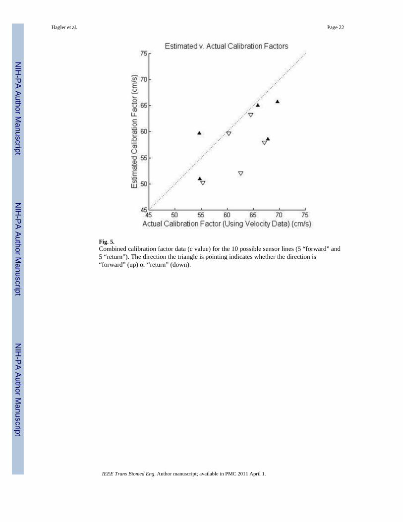
Fig. 5.Combined calibration factor data (c value) for the 10 possible sensor lines (5 “forward” and5 “return”). The direction the triangle is pointing indicates whether the direction is“forward” (up) or “return” (down).

Hagler et al. Page 22

IEEE Trans Biomed Eng. Author manuscript; available in PMC 2011 April 1.

NIH

-PA Author Manuscript

NIH

-PA Author Manuscript

NIH

-PA Author Manuscript