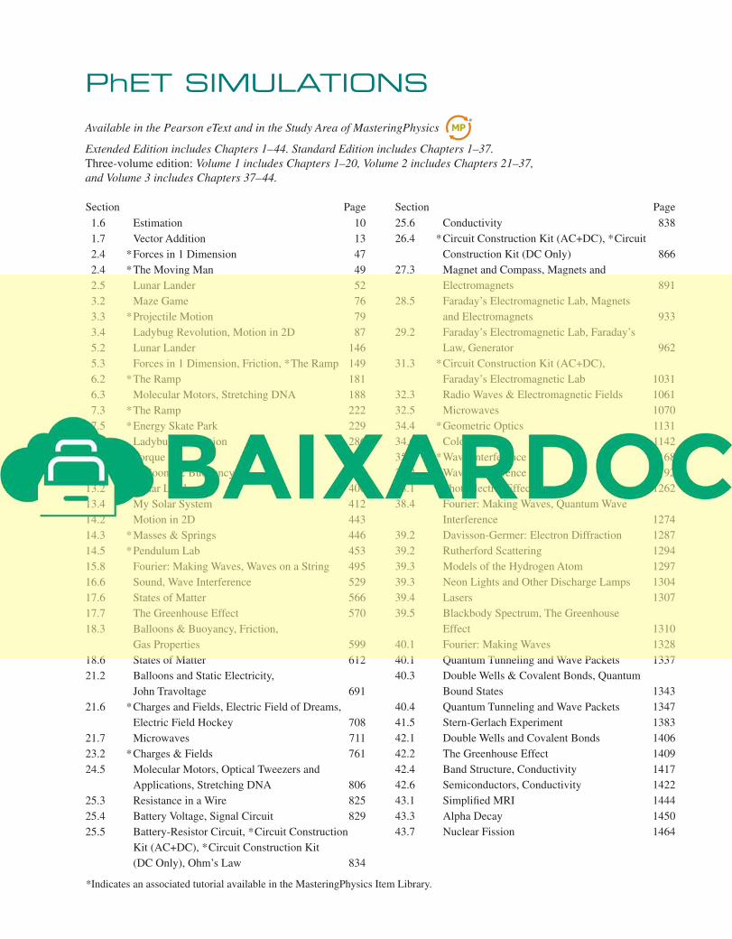
PhET SIMULATIONS

Available in the Pearson eText and in the Study Area of MasteringPhysics

*Indicates an associated tutorial available in the MasteringPhysics Item Library.

1.6 Estimation 10

1.7 Vector Addition 13

2.4 *Forces in 1 Dimension 47

2.4 *The Moving Man 49

2.5 Lunar Lander 52

3.2 Maze Game 76

3.3 *Projectile Motion 79

3.4 Ladybug Revolution, Motion in 2D 87

5.2 Lunar Lander 146

5.3 Forces in 1 Dimension, Friction, *The Ramp 149

6.2 *The Ramp 181

6.3 Molecular Motors, Stretching DNA 188

7.3 *The Ramp 222

7.5 *Energy Skate Park 229

9.3 Ladybug Revolution 286

10.6 Torque 326

12.3 Balloons & Buoyancy 380

13.2 Lunar Lander 406

13.4 My Solar System 412

14.2 Motion in 2D 443

14.3 *Masses & Springs 446

14.5 *Pendulum Lab 453

15.8 Fourier: Making Waves, Waves on a String 495

16.6 Sound, Wave Interference 529

17.6 States of Matter 566

17.7 The Greenhouse Effect 570

18.3 Balloons & Buoyancy, Friction,

Gas Properties 599

18.6 States of Matter 612

21.2 Balloons and Static Electricity,

John Travoltage 691

21.6 *Charges and Fields, Electric Field of Dreams,

Electric Field Hockey 708

21.7 Microwaves 711

23.2 *Charges & Fields 761

24.5 Molecular Motors, Optical Tweezers and

Applications, Stretching DNA 806

25.3 Resistance in a Wire 825

25.4 Battery Voltage, Signal Circuit 829

25.5 Battery-Resistor Circuit, *Circuit Construction

Kit (AC+DC), *Circuit Construction Kit

(DC Only), Ohm’s Law 834

Extended Edition includes Chapters 1–44. Standard Edition includes Chapters 1–37.

Three-volume edition: Volume 1 includes Chapters 1–20, Volume 2 includes Chapters 21–37,

and Volume 3 includes Chapters 37–44.

25.6 Conductivity 838

26.4 *Circuit Construction Kit (AC+DC), *Circuit

Construction Kit (DC Only) 866

27.3 Magnet and Compass, Magnets and

Electromagnets 891

28.5 Faraday’s Electromagnetic Lab, Magnets

and Electromagnets 933

29.2 Faraday’s Electromagnetic Lab, Faraday’s

Law, Generator 962

31.3 *Circuit Construction Kit (AC+DC),

Faraday’s Electromagnetic Lab 1031

32.3 Radio Waves & Electromagnetic Fields 1061

32.5 Microwaves 1070

34.4 *Geometric Optics 1131

34.6 Color Vision 1142

35.2 *Wave Interference 1168

36.2 *Wave Interference 1192

38.1 Photoelectric Effect 1262

38.4 Fourier: Making Waves, Quantum Wave

Interference 1274

39.2 Davisson-Germer: Electron Diffraction 1287

39.2 Rutherford Scattering 1294

39.3 Models of the Hydrogen Atom 1297

39.3 Neon Lights and Other Discharge Lamps 1304

39.4 Lasers 1307

39.5 Blackbody Spectrum, The Greenhouse

Effect 1310

40.1 Fourier: Making Waves 1328

40.1 Quantum Tunneling and Wave Packets 1337

40.3 Double Wells & Covalent Bonds, Quantum

Bound States 1343

40.4 Quantum Tunneling and Wave Packets 1347

41.5 Stern-Gerlach Experiment 1383

42.1 Double Wells and Covalent Bonds 1406

42.2 The Greenhouse Effect 1409

42.4 Band Structure, Conductivity 1417

42.6 Semiconductors, Conductivity 1422

43.1 Simplified MRI 1444

43.3 Alpha Decay 1450

43.7 Nuclear Fission 1464

Section Page Section Page

ACTIVPHYSICS ONLINE™

ACTIVITIES

1.1 Analyzing Motion Using Diagrams

1.2 Analyzing Motion Using Graphs

1.3 Predicting Motion from Graphs

1.4 Predicting Motion from Equations

1.5 Problem-Solving Strategies for

Kinematics

1.6 Skier Races Downhill

1.7 Balloonist Drops Lemonade

1.8 Seat Belts Save Lives

1.9 Screeching to a Halt

1.10 Pole-Vaulter Lands

1.11 Car Starts, Then Stops

1.12 Solving Two-Vehicle Problems

1.13 Car Catches Truck

1.14 Avoiding a Rear-End Collision

2.1.1 Force Magnitudes

2.1.2 Skydiver

2.1.3 Tension Change

2.1.4 Sliding on an Incline

2.1.5 Car Race

2.2 Lifting a Crate

2.3 Lowering a Crate

2.4 Rocket Blasts Off

2.5 Truck Pulls Crate

2.6 Pushing a Crate Up a Wall

2.7 Skier Goes Down a Slope

2.8 Skier and Rope Tow

2.9 Pole-Vaulter Vaults

2.10 Truck Pulls Two Crates

2.11 Modified Atwood Machine

3.1 Solving Projectile Motion Problems

3.2 Two Balls Falling

3.3 Changing the x-Velocity

3.4 Projectile x- and y-Accelerations

3.5 Initial Velocity Components

3.6 Target Practice I

3.7 Target Practice II

4.1 Magnitude of Centripetal Acceleration

4.2 Circular Motion Problem Solving

4.3 Cart Goes Over Circular Path

4.4 Ball Swings on a String

4.5 Car Circles a Track

4.6 Satellites Orbit

5.1 Work Calculations

5.2 Upward-Moving Elevator Stops

5.3 Stopping a Downward-Moving Elevator

5.4 Inverse Bungee Jumper

5.5 Spring-Launched Bowler

5.6 Skier Speed

5.7 Modified Atwood Machine

6.1 Momentum and Energy Change

6.2 Collisions and Elasticity

6.3 Momentum Conservation and Collisions

6.4 Collision Problems

6.5 Car Collision: Two Dimensions

6.6 Saving an Astronaut

6.7 Explosion Problems

6.8 Skier and Cart

6.9 Pendulum Bashes Box

6.10 Pendulum Person-Projectile Bowling

7.1 Calculating Torques

7.2 A Tilted Beam: Torques and Equilibrium

7.3 Arm Levers

7.4 Two Painters on a Beam

7.5 Lecturing from a Beam

7.6 Rotational Inertia

7.7 Rotational Kinematics

7.8 Rotoride–Dynamics Approach

7.9 Falling Ladder

7.10 Woman and Flywheel Elevator–Dynamics

Approach

7.11 Race Between a Block and a Disk

7.12 Woman and Flywheel Elevator–Energy

Approach

7.13 Rotoride–Energy Approach

7.14 Ball Hits Bat

8.1 Characteristics of a Gas

8.2 Maxwell-Boltzmann

Distribution–Conceptual Analysis

8.3 Maxwell-Boltzmann

Distribution–Quantitative Analysis

8.4 State Variables and Ideal Gas Law

8.5 Work Done By a Gas

8.6 Heat, Internal Energy, and First Law

of Thermodynamics

8.7 Heat Capacity

8.8 Isochoric Process

8.9 Isobaric Process

8.10 Isothermal Process

8.11 Adiabatic Process

8.12 Cyclic Process–Strategies

8.13 Cyclic Process–Problems

8.14 Carnot Cycle

9.1 Position Graphs and Equations

9.2 Describing Vibrational Motion

9.3 Vibrational Energy

9.4 Two Ways to Weigh Young Tarzan

9.5 Ape Drops Tarzan

9.6 Releasing a Vibrating Skier I

9.7 Releasing a Vibrating Skier II

9.8 One-and Two-Spring Vibrating Systems

9.9 Vibro-Ride

9.10 Pendulum Frequency

9.11 Risky Pendulum Walk

9.12 Physical Pendulum

10.1 Properties of Mechanical Waves

10.2 Speed of Waves on a String

10.3 Speed of Sound in a Gas

10.4 Standing Waves on Strings

10.5 Tuning a Stringed Instrument:

Standing Waves

10.6 String Mass and Standing Waves

10.7 Beats and Beat Frequency

10.8 Doppler Effect: Conceptual Introduction

10.9 Doppler Effect: Problems

10.10 Complex Waves: Fourier Analysis

11.1 Electric Force: Coulomb’s Law

11.2 Electric Force: Superposition Principle

11.3 Electric Force: Superposition Principle

(Quantitative)

11.4 Electric Field: Point Charge

11.5 Electric Field Due to a Dipole

11.6 Electric Field: Problems

11.7 Electric Flux

11.8 Gauss’s Law

11.9 Motion of a Charge in an Electric Field:

Introduction

11.10 Motion in an Electric Field: Problems

11.11 Electric Potential: Qualitative

Introduction

11.12 Electric Potential, Field, and Force

11.13 Electrical Potential Energy and Potential

12.1 DC Series Circuits (Qualitative)

12.2 DC Parallel Circuits

12.3 DC Circuit Puzzles

12.4 Using Ammeters and Voltmeters

12.5 Using Kirchhoff’s Laws

12.6 Capacitance

12.7 Series and Parallel Capacitors

12.8 RC Circuit Time Constants

13.1 Magnetic Field of a Wire

13.2 Magnetic Field of a Loop

13.3 Magnetic Field of a Solenoid

13.4 Magnetic Force on a Particle

13.5 Magnetic Force on a Wire

13.6 Magnetic Torque on a Loop

13.7 Mass Spectrometer

13.8 Velocity Selector

13.9 Electromagnetic Induction

13.10 Motional emf

14.1 The RL Circuit

14.2 The RLC Oscillator

14.3 The Driven Oscillator

15.1 Reflection and Refraction

15.2 Total Internal Reflection

15.3 Refraction Applications

15.4 Plane Mirrors

15.5 Spherical Mirrors: Ray Diagrams

15.6 Spherical Mirror: The Mirror Equation

15.7 Spherical Mirror: Linear Magnification

15.8 Spherical Mirror: Problems

15.9 Thin-Lens Ray Diagrams

15.10 Converging Lens Problems

15.11 Diverging Lens Problems

15.12 Two-Lens Optical Systems

16.1 Two-Source Interference: Introduction

16.2 Two-Source Interference: Qualitative

Questions

16.3 Two-Source Interference: Problems

16.4 The Grating: Introduction and Qualitative

Questions

16.5 The Grating: Problems

16.6 Single-Slit Diffraction

16.7 Circular Hole Diffraction

16.8 Resolving Power

16.9 Polarization

17.1 Relativity of Time

17.2 Relativity of Length

17.3 Photoelectric Effect

17.4 Compton Scattering

17.5 Electron Interference

17.6 Uncertainty Principle

17.7 Wave Packets

18.1 The Bohr Model

18.2 Spectroscopy

18.3 The Laser

19.1 Particle Scattering

19.2 Nuclear Binding Energy

19.3 Fusion

19.4 Radioactivity

19.5 Particle Physics

20.1 Potential Energy Diagrams

20.2 Particle in a Box

20.3 Potential Wells

20.4 Potential Barriers

www.masteringphysics.com

UNIVERSITYPHYSICS

13TH EDITION

HUGH D. YOUNGCARNEGIE MELLON

UNIVERSITY

ROGER A. FREEDMANUNIVERSITY

OF CALIFORNIA,

SANTA BARBARA

CONTRIBUTING AUTHOR

A. LEWIS FORD

TEXAS A&M UNIVERSITY

WITH MODERN PHYSICS

SEARS AND ZEMANSKY’S

Publisher: Jim Smith

Executive Editor: Nancy Whilton

Project Editor: Chandrika Madhavan

Director of Development: Michael Gillespie

Editorial Manager: Laura Kenney

Senior Development Editor: Margot Otway

Editorial Assistant: Steven Le

Associate Media Producer: Kelly Reed

Managing Editor: Corinne Benson

Production Project Manager: Beth Collins

Production Management and Composition: Nesbitt Graphics

Copyeditor: Carol Reitz

Interior Designer: Elm Street Publishing Services

Cover Designer: Derek Bacchus

Illustrators: Rolin Graphics

Senior Art Editor: Donna Kalal

Photo Researcher: Eric Shrader

Manufacturing Buyer: Jeff Sargent

Senior Marketing Manager: Kerry Chapman

ISBN 13: 978-0-321-69686-1; ISBN 10: 0-321-69686-7 (Student edition)

ISBN 13: 978-0-321-69685-4; ISBN 10: 0-321-69685-9 (Exam copy)

1 2 3 4 5 6 7 8 9 10—VHC—14 13 12 11 10

Cover Photo Credits: Getty Images/Mirko Cassanelli; Mirko Cassanelli

Credits and acknowledgments borrowed from other sources and reproduced, with permis-

sion, in this textbook appear on the appropriate page within the text or on p. C-1.

Copyright ©2012, 2008, 2004 Pearson Education, Inc., publishing as Addison-Wesley,

1301 Sansome Street, San Francisco, CA, 94111. All rights reserved. Manufactured in the

United States of America. This publication is protected by Copyright and permission should

be obtained from the publisher prior to any prohibited reproduction, storage in a retrieval

system, or transmission in any form or by any means, electronic, mechanical, photocopying,

recording, or likewise. To obtain permission(s) to use material from this work, please sub-

mit a written request to Pearson Education, Inc., Permissions Department, 1900 E. Lake

Ave., Glenview, IL 60025. For information regarding permissions, call (847) 486-2635.

Many of the designations used by manufacturers and sellers to distinguish their products are

claimed as trademarks. Where those designations appear in this book, and the publisher was

aware of a trademark claim, the designations have been printed in initial caps or all caps.

Mastering Physics® is a registered trademark, in the U.S. and/or other countries, of Pearson

Education, Inc. or its affiliates.

Library of Congress Cataloging-in-Publication Data

Young, Hugh D.

Sears and Zemansky's university physics : with modern physics. -- 13th ed.

/ Hugh D. Young, Roger A. Freedman ; contributing author, A. Lewis Ford.

p. cm.

Includes bibliographical references and index.

ISBN-13: 978-0-321-69686-1 (student ed. : alk. paper)

ISBN-10: 0-321-69686-7 (student ed. : alk. paper)

ISBN-13: 978-0-321-69685-4 (exam copy)

ISBN-10: 0-321-69685-9 (exam copy)

1. Physics--Textbooks. I. Freedman, Roger A. II. Ford, A. Lewis (Albert

Lewis) III. Sears, Francis Weston, 1898-1975. University physics. IV. Title.

V. Title: University physics.

QC21.3.Y68 2012

530--dc22

2010044896

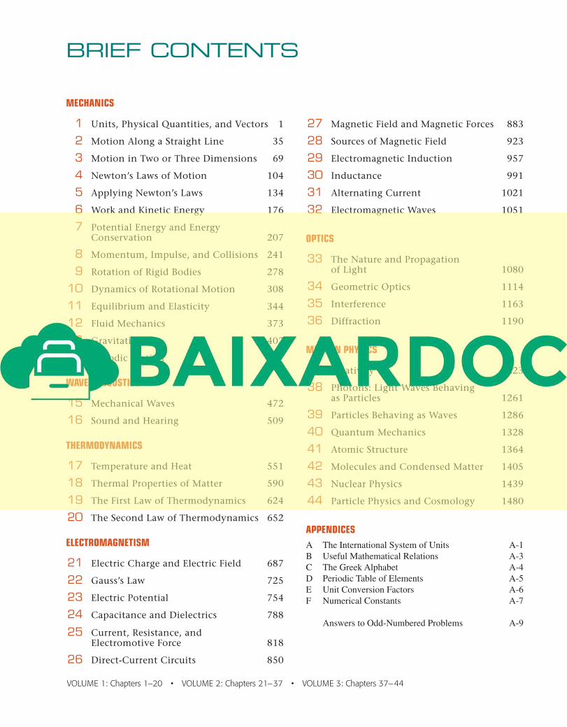
BRIEF CONTENTS

MECHANICS

27 Magnetic Field and Magnetic Forces 883

28 Sources of Magnetic Field 923

29 Electromagnetic Induction 957

30 Inductance 991

31 Alternating Current 1021

32 Electromagnetic Waves 1051

OPTICS

33 The Nature and Propagation of Light 1080

34 Geometric Optics 1114

35 Interference 1163

36 Diffraction 1190

MODERN PHYSICS

37 Relativity 1223

38 Photons: Light Waves Behaving as Particles 1261

39 Particles Behaving as Waves 1286

40 Quantum Mechanics 1328

41 Atomic Structure 1364

42 Molecules and Condensed Matter 1405

43 Nuclear Physics 1439

44 Particle Physics and Cosmology 1480

APPENDICES

A The International System of Units A-1

B Useful Mathematical Relations A-3

C The Greek Alphabet A-4

D Periodic Table of Elements A-5

E Unit Conversion Factors A-6

F Numerical Constants A-7

Answers to Odd-Numbered Problems A-9

1 Units, Physical Quantities, and Vectors 1

2 Motion Along a Straight Line 35

3 Motion in Two or Three Dimensions 69

4 Newton’s Laws of Motion 104

5 Applying Newton’s Laws 134

6 Work and Kinetic Energy 176

7 Potential Energy and EnergyConservation 207

8 Momentum, Impulse, and Collisions 241

9 Rotation of Rigid Bodies 278

10 Dynamics of Rotational Motion 308

11 Equilibrium and Elasticity 344

12 Fluid Mechanics 373

13 Gravitation 402

14 Periodic Motion 437

WAVES/ACOUSTICS

15 Mechanical Waves 472

16 Sound and Hearing 509

THERMODYNAMICS

17 Temperature and Heat 551

18 Thermal Properties of Matter 590

19 The First Law of Thermodynamics 624

20 The Second Law of Thermodynamics 652

ELECTROMAGNETISM

21 Electric Charge and Electric Field 687

22 Gauss’s Law 725

23 Electric Potential 754

24 Capacitance and Dielectrics 788

25 Current, Resistance, and Electromotive Force 818

26 Direct-Current Circuits 850

VOLUME 1: Chapters 1–20 • VOLUME 2: Chapters 21–37 • VOLUME 3: Chapters 37–44

Build Skills

Problem-Solving Strategy 5.2 Newton’s Second Law: Dynamics of Particles

IDENTIFY the relevant concepts: You have to use Newton’s second

law for any problem that involves forces acting on an accelerating

body.

Identify the target variable—usually an acceleration or a force.

If the target variable is something else, you’ll need to select another

concept to use. For example, suppose the target variable is how

fast a sled is moving when it reaches the bottom of a hill. Newton’s

second law will let you find the sled’s acceleration; you’ll then use

the constant-acceleration relationships from Section 2.4 to find

velocity from acceleration.

SET UP the problem using the following steps:

1. Draw a simple sketch of the situation that shows each moving

body. For each body, draw a free-body diagram that shows all

the forces acting on the body. (The acceleration of a body is

determined by the forces that act on it, not by the forces that it

exerts on anything else.) Make sure you can answer the ques-

tion “What other body is applying this force?” for each force in

your diagram. Never include the quantity in your free-body

diagram; it’s not a force!

2. Label each force with an algebraic symbol for the force’s

magnitude. Usually, one of the forces will be the body’s weight;

it’s usually best to label this as

3. Choose your x- and y-coordinate axes for each body, and show

them in its free-body diagram. Be sure to indicate the positive

direction for each axis. If you know the direction of the acceler-

ation, it usually simplifies things to take one positive axis along

that direction. If your problem involves two or more bodies that

= mg.

maS

accelerate in different directions, you can use a different set of

axes for each body.

4. In addition to Newton’s second law, identify any

other equations you might need. For example, you might need

one or more of the equations for motion with constant accelera-

tion. If more than one body is involved, there may be relation-

ships among their motions; for example, they may be connected

by a rope. Express any such relationships as equations relating

the accelerations of the various bodies.

EXECUTE the solution as follows:

1. For each body, determine the components of the forces along

each of the body’s coordinate axes. When you represent a force

in terms of its components, draw a wiggly line through the orig-

inal force vector to remind you not to include it twice.

2. Make a list of all the known and unknown quantities. In your

list, identify the target variable or variables.

3. For each body, write a separate equation for each component of

Newton’s second law, as in Eqs. (5.4). In addition, write any

additional equations that you identified in step 4 of “Set Up.”

(You need as many equations as there are target variables.)

4. Do the easy part—the math! Solve the equations to find the tar-

get variable(s).

EVALUATE your ans er: Does your answer have the correct units?

(When appropriate, use the conversion ) Does it

have the correct algebraic sign? When possible, consider particular

values or extreme cases of quantities and compare the results with

i t iti t ti A k “D thi lt k ?”

1 N = 1 kg # m>s2.

gFS

� maS

,

Example 5.17 Toboggan ride with friction II

The same toboggan with the same coefficient of friction as in

Example 5.16 accelerates down a steeper hill. Derive an expres-

sion for the acceleration in terms of g, and w.

SOLUTION

IDENTIFY and SET UP: The toboggan is accelerating, so we must

use Newton’s second law as given in Eqs. (5.4). Our target variable

is the downhill acceleration.

Our sketch and free-body diagram (Fig. 5.23) are almost the

same as for Example 5.16. The toboggan’s y-component of accel-

eration is still zero but the x-component is not, so we’ve

drawn the downhill component of weight as a longer vector than

the (uphill) friction force.

EXECUTE: It’s convenient to express the weight as Then

Newton’s second law in component form says

aFy = n + 1-mg cos a2 = 0

aFx = mg sin a + 1-ƒk2 = max

w = mg.

axay

mk,a,

From the second equation and Eq. (5.5) we get an expression for

We substitute this into the x-component equation and solve for :

EVALUATE: As for the frictionless toboggan in Example 5.10, the

acceleration doesn’t depend on the mass m of the toboggan. That’s

because all of the forces that act on the toboggan (weight, normal

force, and kinetic friction force) are proportional to m.

Let’s check some special cases. If the hill is vertical ( )

so that and we have (the toboggan

falls freely). For a certain value of the acceleration is zero; this

happens if

This agrees with our result for the constant-velocity toboggan in

Example 5.16. If the angle is even smaller, is greater than

and is negative; if we give the toboggan an initial down-

hill push to start it moving, it will slow down and stop. Finally, if

the hill is frictionless so that , we retrieve the result of

Example 5.10: .

Notice that we started with a simple problem (Example 5.10)

and extended it to more and more general situations. The general

result we found in this example includes all the previous ones as

special cases. Don’t memorize this result, but do make sure you

understand how we obtained it and what it means.

Suppose instead we give the toboggan an initial push up the

hill. The direction of the kinetic friction force is now reversed, so

the acceleration is different from the downhill value. It turns out

that the expression for is the same as for downhill motion except

that the minus sign becomes plus. Can you show this?

ax

ax = g sin a

mk = 0

axsin a

mk cos a

sin a = mk cos a and mk = tan a

a

ax = gcos a = 0,sin a = 1

a = 90°

ax = g1sin a - mk cos a2

mg sin a + 1-mkmgcos a2 = max

ax

ƒk = mkn = mkmg cos a

n = mg cos a

ƒk:

(a) The situation (b) Free-body diagram for toboggan

5.23 Our sketches for this problem.

Problem-Solving Strategies coach students in how to approach specific types of problems.

This text’s uniquely extensive set of Examples enables students

to explore problem-solving challenges in exceptional detail.

ConsistentThe Identify / Set Up /

Execute / Evaluate format, used in all Examples, encourages students

to tackle problems thoughtfully rather than skipping to the math.

FocusedAll Examples and Problem-

Solving Strategies are revised to be more concise and focused.

VisualMost Examples employ a diagram—

often a pencil sketch that shows what a student should draw.

NEW! Video Tutor Solution for Every ExampleEach Example is explained and solved by an instructor in a Video Tutor solution provided in the Study Area of MasteringPhysics® and in the Pearson eText.

NEW! Mathematics Review TutorialsMasteringPhysics offers an extensive set of assignable mathematics review tutorials—covering differential and integral calculus as well as algebra and trigonometry.

Learn basic and advanced skills that help solve a broad range of physics problems.

Build Confidence

NEW! Bridging ProblemsAt the start of each problem set, a Bridging Problem helps students

make the leap from routine exercises to challenging problems

with confidence and ease.

Each Bridging Problem poses a moderately difficult, multi-concept

problem, which often draws on earlier chapters. In place of a full solution,

it provides a skeleton solution guide consisting of questions and hints.

A full solution is explained ina Video Tutor, provided in the

Study Area of MasteringPhysics®

and in the Pearson eText.

A cue ball (a uniform solid sphere of mass m and radius R) is at

rest on a level pool table. Using a pool cue, you give the ball a

sharp, horizontal hit of magnitude F at a height h above the center

of the ball (Fig. 10.37). The force of the hit is much greater

than the friction force ƒ that the table surface exerts on the ball.

The hit lasts for a short time . (a) For what value of

h will the ball roll without slipping? (b) If you hit the ball dead

center , the ball will slide across the table for a while, but

eventually it will roll without slipping. What will the speed of its

center of mass be then?

1h = 02

¢t

BRIDGING PROBLEM Billiard Physics

3. Draw two free-body diagrams for the ball in part (b): one show-

ing the forces during the hit and the other showing the forces

after the hit but before the ball is rolling without slipping.

4. What is the angular speed of the ball in part (b) just after the

hit? While the ball is sliding, does increase or decrease?

Does increase or decrease? What is the relationship between

and when the ball is finally rolling without slipping?

EXECUTE

5. In part (a), use the impulse–momentum theorem to find the

speed of the ball’s center of mass immediately after the hit.

Then use the rotational version of the impulse–momentum the-

orem to find the angular speed immediately after the hit. (Hint:

To write down the rotational version of the impulse–momentum

theorem, remember that the relationship between torque and

angular momentum is the same as that between force and linear

momentum.)

6. Use your results from step 5 to find the value of h that will

cause the ball to roll without slipping immediately after the hit.

7. In part (b), again find the ball’s center-of-mass speed and

angular speed immediately after the hit. Then write Newton’s

second law for the translational motion and rotational motion

of the ball as it is sliding. Use these equations to write

expressions for and as functions of the elapsed time

t since the hit.

8. Using your results from step 7, find the time t when and

have the correct relationship for rolling without slipping. Then

find the value of at this time.

EVALUATE

9. If you have access to a pool table, test out the results of parts

(a) and (b) for yourself!

10. Can you show that if you used a hollow cylinder rather than a

solid ball, you would have to hit the top of the cylinder to

cause rolling without slipping as in part (a)?

vcm

vvcm

vvcm

vvcm

v

vcm

mass mh

R

10.37

SOLUTION GUIDE

See MasteringPhysics® study area for a Video Tutor solution.

IDENTIFY and SET UP

1. Draw a free-body diagram for the ball for the situation in part (a),

including your choice of coordinate axes. Note that the cue

exerts both an impulsive force on the ball and an impulsive

torque around the center of mass.

2. The cue force applied for a time gives the ball’s center of

mass a speed , and the cue torque applied for that same

time gives the ball an angular speed . What must be the

relationship between and for the ball to roll without

slipping?

vvcm

v

vcm

¢t

In response to professors, the Problem Sets now include more biomedically oriented problems (BIO), more difficult problems requiring calculus (CALC), and more cumulative problems that draw on earlier chapters (CP).

About 20% of problems are new or revised. These revisions are driven by detailed student-performance data gathered nationally through MasteringPhysics.

Problem difficulty is now indicated by a three-dot ranking system based on data from MasteringPhysics.

NEW! Enhanced End-of-Chapter Problems in MasteringPhysicsSelect end-of-chapter problems will now offer additional support such as problem-solving strategy hints, relevant math review and practice, and links to the eText. These new enhanced problems bridge the gap between guided tutorials and traditional homework problems.

Develop problem-solving confidence through a range of practice options—from guided to unguided.

Deepen knowledge of physics by building connections to the real world.

Bring Physics to Life

NEW! PhET Simulations and TutorialsSixteen assignable PhET Tutorials enable students to make connections between real-life phenomena and the underlying physics. 76 PhET simulations are provided in the Study Area of MasteringPhysics® and in the Pearson eText.

The comprehensive library of ActivPhysics applets and applet-based tutorials is also available.

NEW! Video Tutor Demonstrations and Tutorials“Pause and predict” demonstration videos of key physics concepts engage students by asking them to submit a prediction before seeing the outcome. These videos are available through the Study Area of MasteringPhysics and in the Pearson eText. A set of assignable tutorials based on these videos challenge students to transfer their understanding of the demonstration to a related problem situation.

Biomedically Based End-of-Chapter ProblemsTo serve biosciences students, the text adds a substantial number of problems based on

biological and biomedical situations.

21.24 .. BIO Base Pairing in DNA, II. Refer to Exercise 21.23.

Figure E21.24 shows the bonding of the cytosine and guanine mol-

ecules. The and distances are each 0.110 nm. In this

case, assume that the bonding is due only to the forces along the

and combinations, and

assume also that these three combinations are parallel to each other.

Calculate the net force that cytosine exerts on guanine due to the

preceding three combinations. Is this force attractive or repulsive?

O¬H¬NN¬H¬N,O¬H¬O,

H¬NO¬H

H

H

H H

H

H

H

H

H

C

C

C

C

C

C C C

C

C

Thymine Adenine

0.280nm

0.300nm

N

N

N

N

N

N

N

O

O

2

2

2

2

1

1

1

Figure E21.23

NEW! Applications of Physics Throughout the text, free-standing captioned photos

apply physics to real situations, with particular emphasis on applications of biomedical and general interest.

Application Moment of Inertia of aBird’s WingWhen a bird flaps its wings, it rotates the

wings up and down around the shoulder. A

hummingbird has small wings with a small

moment of inertia, so the bird can make its

wings move rapidly (up to 70 beats per sec-

ond). By contrast, the Andean condor (Vultur

gryphus) has immense wings that are hard to

move due to their large moment of inertia.

Condors flap their wings at about one beat per

second on takeoff, but at most times prefer to

soar while holding their wings steady.

Application Tendons Are NonidealSpringsMuscles exert forces via the tendons that

attach them to bones. A tendon consists of

long, stiffly elastic collagen fibers. The graph

shows how the tendon from the hind leg of

a wallaby (a small kangaroo) stretches in

response to an applied force. The tendon does

not exhibit the simple, straight-line behavior of

an ideal spring, so the work it does has to be

found by integration [Eq. (6.7)]. Note that the

tendon exerts less force while relaxing than

while stretching. As a result, the relaxing ten-

don does only about 93% of the work that was

done to stretch it.

Application Listening for TurbulentFlowNormal blood flow in the human aorta is lami-

nar, but a small disturbance such as a heart

pathology can cause the flow to become turbu-

lent. Turbulence makes noise, which is why

listening to blood flow with a stethoscope is a

useful diagnostic technique.