Introduction to Management Science 13th Edition Anderson ...

2 - 1 © 2011 Cengage Learning. All Rights Reserved. This edition is intended for use outside of the U.S. only, with content that may be different from

the U.S. Edition. May not be scanned, copied, duplicated, or posted to a publicly accessible website, in whole or in part.

Chapter 2 An Introduction to Linear Programming Learning Objectives 1. Obtain an overview of the kinds of problems linear programming has been used to solve. 2. Learn how to develop linear programming models for simple problems. 3. Be able to identify the special features of a model that make it a linear programming model. 4. Learn how to solve two variable linear programming models by the graphical solution procedure. 5. Understand the importance of extreme points in obtaining the optimal solution. 6. Know the use and interpretation of slack and surplus variables. 7. Be able to interpret the computer solution of a linear programming problem. 8. Understand how alternative optimal solutions, infeasibility and unboundedness can occur in linear

programming problems. 9. Understand the following terms: problem formulation feasible region constraint function slack variable objective function standard form solution redundant constraint optimal solution extreme point nonnegativity constraints surplus variable mathematical model alternative optimal solutions linear program infeasibility linear functions unbounded feasible solution

I n t r o d u c t i o n t o M a n a g e m e n t S c i e n c e 1 3 t h E d i t i o n A n d e r s o n S o l u t i o n s M a n u a lF u l l D o w n l o a d : h t t p : / / a l i b a b a d o w n l o a d . c o m / p r o d u c t / i n t r o d u c t i o n - t o - m a n a g e m e n t - s c i e n c e - 1 3 t h - e d i t i o n - a n d e r s o n - s o l u t i o n s - m a n u a l /

T h i s s a m p l e o n l y , D o w n l o a d a l l c h a p t e r s a t : a l i b a b a d o w n l o a d . c o m

http://alibabadownload.com/product/introduction-to-management-science-13th-edition-anderson-solutions-manual/

Chapter 2



Solutions: 1. a, b, and e, are acceptable linear programming relationships. c is not acceptable because of 22B

d is not acceptable because of 3 A

f is not acceptable because of 1AB c, d, and f could not be found in a linear programming model because they have the above nonlinear

terms. 2. a.

8

4

4 80

B

A

b.

B

A

8

4

4 80 c.

B

A

8

4

4 80

Points on lineare only feasiblepoints

An Introduction to Linear Programming



3. a.

B

A0

(0,9)

(6,0) b.

B

A0

(0,60)

(40,0) c.

B

A 0

(0,20)

(40,0)

Points on line are only feasible solutions

4. a.

B

A(20,0)

(0,-15)

Chapter 2



b.

B

A

(0,12)

(-10,0)

c.

B

A0

(10,25)

Note: Point shown wasused to locate position ofthe constraint line

5.

B

A 0 100 200 300

100

200

300

a

b

c




6. 7A + 10B = 420 is labeled (a) 6A + 4B = 420 is labeled (b) -4A + 7B = 420 is labeled (c)

80

40

40 80

B

A

20

60

100

20 600 100-20-40-60 -80 -100

(c)

(a)

(b)

7.

0

B

A

15050 100 200 250

50

100

Chapter 2



8.

A

0

200

-200 -100 100 200

133 1/3 (100,200)

B

9.

B

A0

200

100

-100

-200

200 300

(150,225)

(150,100)

100




10.

0

1

2

3

4

5

B

1 2 3 4 5 6

Optimal SolutionA = 12/7, B = 15/7

Value of Objective Function = 2(12/7) + 3(15/7) = 69/7

A

A + 2B = 6 (1)

5A + 3B = 15 (2)(1) × 5 5A + 10B = 30 (3)

(2) - (3) - 7B = -15

B = 15/7 From (1), A = 6 - 2(15/7) = 6 - 30/7 = 12/7

Chapter 2



11.

0

100

B

100 200

Optimal SolutionA = 100, B = 50

Value of Objective Function = 750

A

A = 100

B = 80

12. a.

(0,0)

1

2

3

4

5

B

1 2 3 4 5 6

Optimal SolutionA = 3, B = 1.5Value of Objective Function = 13.5

6

(4,0)

(3,1.5)

A




b.

(0,0)

1

2

3

B

1 2 3 4 5 6

Optimal Solution

A = 0, B = 3Value of Objective Function = 18

A7 8 9 10

c. There are four extreme points: (0,0), (4,0), (3,1,5), and (0,3). 13. a.

0

2

4

6

8

B

2 4 6 8

Feasible Regionconsists of this linesegment only

A

b. The extreme points are (5, 1) and (2, 4).

Chapter 2



c.

0

2

4

6

8

B

2 4 6 8

Optimal Solution

A

A = 2, B = 4

14. a. Let F = number of tons of fuel additive S = number of tons of solvent base

Max 40F + 30Ss.t. 2/5F + 1/2 S 200 Material 1

1/5 S 5 Material 2

3/5 F + 3/10 S 21 Material 3

F, S 0




b.

.

x2

x10 10 20 30 40 50

10

20

30

40

50

60

70

Feasible Region

Tons of Fuel Additive

Material 2

Optimal Solution(25,20)

Material 3

Material 1

Ton

s of

Sol

vent

Bas

e

c. Material 2: 4 tons are used, 1 ton is unused. d. No redundant constraints. 15. a.

600

400

200

200 400

D

S

100

300

500

100 300 500 600 7000

(300,400)

(540,252)

Optimal Solution

z = 10,560

S

F

Chapter 2



b. Similar to part (a): the same feasible region with a different objective function. The optimal solution occurs at (708, 0) with a profit of z = 20(708) + 9(0) = 14,160.

c. The sewing constraint is redundant. Such a change would not change the optimal solution to the

original problem. 16. a. A variety of objective functions with a slope greater than -4/10 (slope of I & P line) will make

extreme point (0, 540) the optimal solution. For example, one possibility is 3S + 9D. b. Optimal Solution is S = 0 and D = 540. c.

Department Hours Used Max. Available Slack Cutting and Dyeing 1(540) = 540 630 90 Sewing

5/6(540) = 450 600 150 Finishing

2/3(540) = 360 708 348 Inspection and Packaging

1/4(540) = 135 135 0

17. Max 5A + 2B + 0S1 + 0S2 + 0S3 s.t. 1A - 2B + 1S1 = 420

2A + 3B + 1S2 = 610

6A - 1B + 1S3 = 125

A, B, S1, S2, S3 0

18. a.

Max 4A + 1B + 0S1 + 0S2 + 0S3 s.t. 10A + 2B + 1S1 = 30

3A + 2B + 1S2 = 12

2A + 2B + 1S3 = 10

A, B, S1, S2, S3 0




b.

0

2

4

6

8

B

2 4 6 8

Optimal Solution

A

A = 18/7, B = 15/7, Value = 87/7

10

12

14

10 c. S1 = 0, S2 = 0, S3 = 4/7

19. a.

Max 3A + 4B + 0S1 + 0S2 + 0S3 s.t. -1A + 2B + 1S1 = 8 (1) 1A + 2B + 1S2 = 12 (2) 2A + 1B + 1S3 = 16 (3)

A, B, S1, S2, S3 0

Chapter 2



b.

0

2

4

6

8

B

2 4 6 8

Optimal Solution

A

A = 20/3, B = 8/3Value = 30 2/3

10

12

14

10 12

(2)

(1)

(3)

c. S1 = 8 + A – 2B = 8 + 20/3 - 16/3 = 28/3

S2 = 12 - A – 2B = 12 - 20/3 - 16/3 = 0

S3 = 16 – 2A - B = 16 - 40/3 - 8/3 = 0

20. a.

Max 3A + 2Bs.t. A + B - S1 = 4

3A + 4B + S2 = 24

A - S3 = 2

A - B - S4 = 0

A, B, S1, S2, S3, S4 0




b.

c. S1 = (3.43 + 3.43) - 4 = 2.86

S2 = 24 - [3(3.43) + 4(3.43)] = 0

S3 = 3.43 - 2 = 1.43

S4 = 0 - (3.43 - 3.43) = 0

Chapter 2



21. a. and b.

0

10

20

30

40

B

10 20 30 40

Optimal Solution

A

2A + 3B = 60

50

60

70

50 60

80

70 80

90

90 100

Constraint 3

Constraint 2

Constraint 1

Feasible Region

c. Optimal solution occurs at the intersection of constraints 1 and 2. For constraint 2, B = 10 + A Substituting for B in constraint 1 we obtain

5A + 5(10 + A) = 400 5A + 50 + 5A = 400

10A = 350 A = 35

B = 10 + A = 10 + 35 = 45 Optimal solution is A = 35, B = 45 d. Because the optimal solution occurs at the intersection of constraints 1 and 2, these are binding

constraints.




e. Constraint 3 is the nonbinding constraint. At the optimal solution 1A + 3B = 1(35) + 3(45) = 170. Because 170 exceeds the right-hand side value of 90 by 80 units, there is a surplus of 80 associated with this constraint.

22. a.

0

500

1000

1500

2000

C

500 1000 1500 2000

Feasible Region

A

5A + 4C = 4000

2500

3000

3500

2500 3000

Inspection andPackaging

Cutting andDyeing

Sewing

Number of All-Pro Footballs

5

4

3

2

1

b.

Extreme Point Coordinates Profit 1 (0, 0) 5(0) + 4(0) = 0 2 (1700, 0) 5(1700) + 4(0) = 8500 3 (1400, 600) 5(1400) + 4(600) = 9400 4 (800, 1200) 5(800) + 4(1200) = 8800 5 (0, 1680) 5(0) + 4(1680) = 6720

Extreme point 3 generates the highest profit. c. Optimal solution is A = 1400, C = 600 d. The optimal solution occurs at the intersection of the cutting and dyeing constraint and the

inspection and packaging constraint. Therefore these two constraints are the binding constraints. e. New optimal solution is A = 800, C = 1200 Profit = 4(800) + 5(1200) = 9200

Chapter 2



23. a. Let E = number of units of the EZ-Rider produced L = number of units of the Lady-Sport produced

Max 2400E + 1800L s.t. 6E + 3L 2100 Engine time L 280 Lady-Sport maximum 2E + 2.5L 1000 Assembly and testing

E, L 0 b.

c. The binding constraints are the manufacturing time and the assembly and testing time. 24. a. Let R = number of units of regular model. C = number of units of catcher’s model.

Max 5R + 8C s.t.

1R + 3/2 C 900 Cutting and sewing

1/2 R + 1/3 C 300 Finishing

1/8 R + 1/4 C 100 Packing and Shipping

R, C 0

0

L

Profit = $960,000

Optimal Solution

100

200

300

400

500

600

700

100 200 300 400 500E

Engine Manufacturing Time

Frames for Lady-Sport

Assembly and Testing

E = 250, L = 200

Number of Lady-Sport Produced

Nu

mb

er o

f E

Z-R

ide r

Pro

du

c ed




b.

800

400

400 800

C

R

200

600

1000

200 6000 1000

Optimal Solution

(500,150)

F

C & S

P & S

Regular Model

Cat

cher

's M

odel

c. 5(500) + 8(150) = $3,700 d. C & S 1(500) + 3/2(150) = 725

F 1/2(500) + 1/3(150) = 300

P & S 1/8(500) + 1/4(150) = 100

e.

Department Capacity Usage Slack C & S 900 725 175 hours

F 300 300 0 hours P & S 100 100 0 hours

25. a. Let B = percentage of funds invested in the bond fund S = percentage of funds invested in the stock fund

Max 0.06 B + 0.10 S s.t.

B 0.3 Bond fund minimum 0.06 B + 0.10 S 0.075 Minimum return

B + S = 1 Percentage requirement b. Optimal solution: B = 0.3, S = 0.7 Value of optimal solution is 0.088 or 8.8%

Chapter 2



26. a. Let N = amount spent on newspaper advertising R = amount spent on radio advertising

Max 50N + 80R s.t. N + R = 1000 Budget

N 250 Newspaper min.

R 250 Radio min.

N -2R 0 News 2 Radio N, R 0 b.

500

500

R

N0

1000

1000

Optimal SolutionN = 666.67, R = 333.33

Value = 60,000

Newspaper Min

Budget

Radio Min

Feasible regionis this line segment

N = 2 R

27. a. Let I = Internet fund investment in thousands B = Blue Chip fund investment in thousands

Max 0.12I + 0.09B s.t.

1I + 1B 50 Available investment funds

1I 35 Maximum investment in the internet fund 6I + 4B 240 Maximum risk for a moderate investor

I, B 0




Internet fund $20,000 Blue Chip fund $30,000 Annual return $ 5,100 b. The third constraint for the aggressive investor becomes 6I + 4B 320 This constraint is redundant; the available funds and the maximum Internet fund investment

constraints define the feasible region. The optimal solution is: Internet fund $35,000 Blue Chip fund $15,000 Annual return $ 5,550 The aggressive investor places as much funds as possible in the high return but high risk Internet

fund. c. The third constraint for the conservative investor becomes 6I + 4B 160 This constraint becomes a binding constraint. The optimal solution is Internet fund $0 Blue Chip fund $40,000 Annual return $ 3,600

0

B

ObjectiveFunction0.12I + 0.09B

Optimal Solution

10

20

30

40

50

60

6010 20 30 40 50I

Risk Constraint

MaximumInternet Funds

Available Funds$50,000

I = 20, B = 30$5,100

Internet Fund (000s)

Blu

e C

hip

Fu

nd

(0

00

s )

Chapter 2



The slack for constraint 1 is $10,000. This indicates that investing all $50,000 in the Blue Chip fund is still too risky for the conservative investor. $40,000 can be invested in the Blue Chip fund. The remaining $10,000 could be invested in low-risk bonds or certificates of deposit.

28. a. Let W = number of jars of Western Foods Salsa produced M = number of jars of Mexico City Salsa produced

Max 1W + 1.25M s.t.

5W 7M 4480 Whole tomatoes

3W + 1M 2080 Tomato sauce

2W + 2M 1600 Tomato paste

W, M 0 Note: units for constraints are ounces b. Optimal solution: W = 560, M = 240 Value of optimal solution is 860 29. a. Let B = proportion of Buffalo's time used to produce component 1 D = proportion of Dayton's time used to produce component 1

Maximum Daily Production Component 1 Component 2 Buffalo 2000 1000 Dayton 600 1400

Number of units of component 1 produced: 2000B + 600D Number of units of component 2 produced: 1000(1 - B) + 600(1 - D) For assembly of the ignition systems, the number of units of component 1 produced must equal the

number of units of component 2 produced. Therefore, 2000B + 600D = 1000(1 - B) + 1400(1 - D) 2000B + 600D = 1000 - 1000B + 1400 - 1400D 3000B + 2000D = 2400 Note: Because every ignition system uses 1 unit of component 1 and 1 unit of component 2, we can

maximize the number of electronic ignition systems produced by maximizing the number of units of subassembly 1 produced.

Max 2000B + 600D In addition, B 1 and D 1.




The linear programming model is:

Max 2000B + 600D s.t. 3000B + 2000D = 2400 B 1 D 1 B, D 0

b. The graphical solution is shown below.

Optimal Solution: B = .8, D = 0 Optimal Production Plan Buffalo - Component 1 .8(2000) = 1600 Buffalo - Component 2 .2(1000) = 200 Dayton - Component 1 0(600) = 0 Dayton - Component 2 1(1400) = 1400 Total units of electronic ignition system = 1600 per day.

0

D

B.2 .4 .6 .8 1.0 1.2

.2

.4

.6

.8

1.0

1.2

3000B + 2000D = 2400

2000B + 600D = 300

OptimalSolution

Chapter 2



30. a. Let E = number of shares of Eastern Cable C = number of shares of ComSwitch

Max 15E + 18C s.t. 40E + 25C 50,000 Maximum Investment 40E 15,000 Eastern Cable Minimum 25C 10,000 ComSwitch Minimum 25C 25,000 ComSwitch Maximum

E, C 0 b.

c. There are four extreme points: (375,400); (1000,400);(625,1000); (375,1000) d. Optimal solution is E = 625, C = 1000 Total return = $27,375

0500 1000

500

1000

C

E1500

1500

2000 Minimum Eastern Cable

Maximum Comswitch

Minimum Conswitch

Maximum Investment

Number of Shares of Eastern Cable

Nu

mb

er o

f S

har

es o

f C

om

Sw

itch




31.

0

2

4

B

2 4

Optimal Solution

A

A = 3, B = 1

6

6

3A + 4B = 13

FeasibleRegion

Objective Function Value = 13 32.

600

200

x2

x1

100

300

500

100 3000

(125,225)(250,100)

(125,350)

Minimum x1 = 125Processing Time

Production

200 400

400

A

A

B

B

A

Chapter 2



Extreme Points

Objective Function Value

Surplus Demand

Surplus Total Production

Slack Processing Time

(A = 250, B = 100) 800 125 — — (A = 125, B = 225) 925 — — 125 (A = 125, B = 350) 1300 — 125 —

33. a.

x2

x10 2 4 6

2

4

6

Optimal Solution: A = 3, B = 1, value = 5 b.

(1) 3 + 4(1) = 7 Slack = 21 - 7 = 14(2) 2(3) + 1 = 7 Surplus = 7 - 7 = 0(3) 3(3) + 1.5 = 10.5 Slack = 21 - 10.5 = 10.5(4) -2(3) +6(1) = 0 Surplus = 0 - 0 = 0

B

A




c.

x2

x10 2 4 6

2

4

6

Optimal Solution: A = 6, B = 2, value = 34 34. a.

0 1 2 3 4 5

1

2

3

4

6

x2

x1

(21/4, 9/4)

(4,1)

Feasible Region

b. There are two extreme points: (A = 4, B = 1) and (A = 21/4, B = 9/4) c. The optimal solution is A = 4, B = 1

B

A

B

A

Chapter 2



35. a. Min 6A + 4B + 0S1 + 0S2 + 0S3 s.t.

2A + 1B - S1 = 12 1A + 1B - S2 = 10 1B + S3 = 4

A, B, S1, S2, S3 0

b. The optimal solution is A = 6, B = 4. c. S1 = 4, S2 = 0, S3 = 0.

36. a. Let T = number of training programs on teaming P = number of training programs on problem solving

Max 10,000T + 8,000P s.t. T 8 Minimum Teaming P 10 Minimum Problem Solving T + P 25 Minimum Total 3 T + 2 P 84 Days Available

T, P 0




b.

c. There are four extreme points: (15,10); (21.33,10); (8,30); (8,17) d. The minimum cost solution is T = 8, P = 17 Total cost = $216,000 37.

Regular Zesty Mild 80% 60% 8100

Extra Sharp 20% 40% 3000 Let R = number of containers of Regular Z = number of containers of Zesty Each container holds 12/16 or 0.75 pounds of cheese Pounds of mild cheese used = 0.80 (0.75) R + 0.60 (0.75) Z = 0.60 R + 0.45 Z Pounds of extra sharp cheese used = 0.20 (0.75) R + 0.40 (0.75) Z = 0.15 R + 0.30 Z

010 20

10

20

P

T30

30

40 Minimum Teaming

MinimumTotal

Days Available

Minimum Problem Solving

Number of Teaming Programs

Nu

mb

er o

f P

rob

lem

-So

lvi n

g P

rog r

ams

Chapter 2



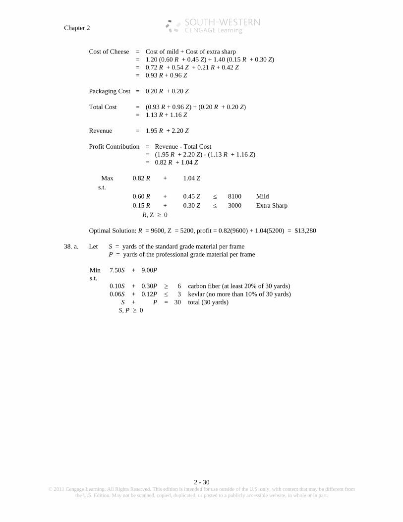
Cost of Cheese = Cost of mild + Cost of extra sharp = 1.20 (0.60 R + 0.45 Z) + 1.40 (0.15 R + 0.30 Z) = 0.72 R + 0.54 Z + 0.21 R + 0.42 Z = 0.93 R + 0.96 Z Packaging Cost = 0.20 R + 0.20 Z Total Cost = (0.93 R + 0.96 Z) + (0.20 R + 0.20 Z) = 1.13 R + 1.16 Z Revenue = 1.95 R + 2.20 Z Profit Contribution = Revenue - Total Cost = (1.95 R + 2.20 Z) - (1.13 R + 1.16 Z) = 0.82 R + 1.04 Z

Max 0.82 R + 1.04 Z s.t.

0.60 R + 0.45 Z 8100 Mild

0.15 R + 0.30 Z 3000 Extra Sharp R, Z 0 Optimal Solution: R = 9600, Z = 5200, profit = 0.82(9600) + 1.04(5200) = $13,280 38. a. Let S = yards of the standard grade material per frame P = yards of the professional grade material per frame

Min 7.50S + 9.00P s.t. 0.10S + 0.30P 6 carbon fiber (at least 20% of 30 yards) 0.06S + 0.12P 3 kevlar (no more than 10% of 30 yards) S + P = 30 total (30 yards)

S, P 0




b.

c.

Extreme Point Cost (15, 15) 7.50(15) + 9.00(15) = 247.50 (10, 20) 7.50(10) + 9.00(20) = 255.00

The optimal solution is S = 15, P = 15 d. Optimal solution does not change: S = 15 and P = 15. However, the value of the optimal solution is

reduced to 7.50(15) + 8(15) = $232.50. e. At $7.40 per yard, the optimal solution is S = 10, P = 20. The value of the optimal solution is

reduced to 7.50(10) + 7.40(20) = $223.00. A lower price for the professional grade will not change the S = 10, P = 20 solution because of the requirement for the maximum percentage of kevlar (10%).

39. a. Let S = number of units purchased in the stock fund M = number of units purchased in the money market fund

Min 8S + 3Ms.t.

50S + 100M 1,200,000 Funds available

5S + 4M 60,000 Annual income

M 3,000 Minimum units in money market S, M, 0

P

S

Pro

fess

ion

al G

rade

(ya

rds)

Standard Grade (yards)

0 10 20 30 40 50 60

10

20

30

40

50

total

Extreme PointS = 10 P = 20

Feasible region is theline segment

kevlar

Extreme PointS = 15 P = 15

carbon fiber

Chapter 2



.

x2

x1

8x1 + 3x2 = 62,000

0 5000 10000 15000 20000

20000

15000

10000

5000

Units of Stock Fund

Uni

ts o

f M

oney

Mar

ket F

und

Optimal Solution

Optimal Solution: S = 4000, M = 10000, value = 62000 b. Annual income = 5(4000) + 4(10000) = 60,000 c. Invest everything in the stock fund. 40. Let P1 = gallons of product 1

P2 = gallons of product 2

Min 1P1 + 1P2 s.t.

1P1 + 30 Product 1 minimum

1P2 20 Product 2 minimum

1P1 + 2P2 80 Raw material

P1, P2 0

M

S

8S + 3M = 62,000




Optimal Solution: P1 = 30, P2 = 25 Cost = $55

41. a. Let R = number of gallons of regular gasoline produced P = number of gallons of premium gasoline produced

Max 0.30R + 0.50P s.t. 0.30R + 0.60P 18,000 Grade A crude oil available 1R + 1P 50,000 Production capacity 1P 20,000 Demand for premium

R, P 0

0

20

40

P1

60

80

Number of Gallons of Product 1

Nu

mb

er o

f G

allo

ns

of

Pro

du

ct 2

20 40 60 80

P2

1P1 +1P

2 = 55

(30,25)

Use 80 gals.

FeasibleRegion

Chapter 2



b.

Optimal Solution: 40,000 gallons of regular gasoline 10,000 gallons of premium gasoline Total profit contribution = $17,000 c.

Constraint

Value of Slack Variable

Interpretation

1 0 All available grade A crude oil is used 2 0 Total production capacity is used 3 10,000 Premium gasoline production is 10,000 gallons less than

the maximum demand d. Grade A crude oil and production capacity are the binding constraints.

0

P

Optimal Solution

10,000

20,000

30,000

40,000

50,000

60,000

60,00010,000 20,000 30,000 40,000 50,000R

Production Capacity

Maximum Premium

Grade A Crude Oil

R = 40,000, P = 10,000$17,000

Gallons of Regular Gasoline

Gal

lon

s o

f P

rem

ium

Gas

oli

ne




42.

x2

x10 2 4 6 8 10

2

4

6

8

10

12

14

12

Satisfies Constraint #2

Satisfies Constraint #1

Infeasibility

43.

0 1 2 3

1

2

3

4

x2

x1

Unbounded

44. a.

2

4

2 40

Optimal Solution(30/16, 30/16)Value = 60/16

Objective Function

x2

x1

b. New optimal solution is A = 0, B = 3, value = 6.

B

A

B

A

B

A

Chapter 2



45. a.

8

4

4 8

x2

x1

2

6

10

2 6 10C

onst

rain

t #1

Constr

aint #

2

Objective Function = 3

Optimal Solutionx2 = 0x1 = 3,

Value = 3

FeasibleRegion

b. Feasible region is unbounded. c. Optimal Solution: A = 3, B = 0, z = 3. d. An unbounded feasible region does not imply the problem is unbounded. This will only be the case

when it is unbounded in the direction of improvement for the objective function. 46. Let N = number of sq. ft. for national brands G = number of sq. ft. for generic brands Problem Constraints:

N + G 200 Space available

N 120 National brands

G 20 Generic

B

A

A B




0 100 200

100

200

Minimum Generic

Minimum National

Shelf Space

N

G

Extreme Point N G1 120 202 180 203 120 80

a. Optimal solution is extreme point 2; 180 sq. ft. for the national brand and 20 sq. ft. for the generic

brand. b. Alternative optimal solutions. Any point on the line segment joining extreme point 2 and extreme

point 3 is optimal.

c. Optimal solution is extreme point 3; 120 sq. ft. for the national brand and 80 sq. ft. for the generic brand.

Chapter 2



47.

600

400

200

200 400

x2

x1

100

300

500

100 3000

(125,225)

(250,100)

Processing Time

Alternate optima

Alternative optimal solutions exist at extreme points (A = 125, B = 225) and (A = 250, B = 100). Cost = 3(125) + 3(225) = 1050 or Cost = 3(250) + 3(100) = 1050 The solution (A = 250, B = 100) uses all available processing time. However, the solution (A = 125, B = 225) uses only 2(125) + 1(225) = 475 hours. Thus, (A = 125, B = 225) provides 600 - 475 = 125 hours of slack processing time which may be

used for other products.

B

A




48.

600

400

200

200 400

B

A

100

300

500

100 3000 600

OriginalFeasibleSolution

Feasible solutions forconstraint requiring 500gallons of production

Possible Actions: i. Reduce total production to A = 125, B = 350 on 475 gallons. ii. Make solution A = 125, B = 375 which would require 2(125) + 1(375) = 625 hours of processing

time. This would involve 25 hours of overtime or extra processing time. iii. Reduce minimum A production to 100, making A = 100, B = 400 the desired solution. 49. a. Let P = number of full-time equivalent pharmacists

T = number of full-time equivalent physicians The model and the optimal solution obtained using The Management Scientist is shown below:

MIN 40P+10T S.T. 1) 1P+1T>250 2) 2P-1T>0 3) 1P>90 OPTIMAL SOLUTION Objective Function Value = 5200.000 Variable Value Reduced Costs -------------- --------------- ------------------ P 90.000 0.000 T 160.000 0.000

Chapter 2



Constraint Slack/Surplus Dual Prices -------------- --------------- ------------------ 1 0.000 -10.000 2 20.000 0.000 3 0.000 -30.000 The optimal solution requires 90 full-time equivalent pharmacists and 160 full-time equivalent

technicians. The total cost is $5200 per hour. b.

Current Levels Attrition Optimal Values New Hires Required Pharmacists 85 10 90 15 Technicians 175 30 160 15

The payroll cost using the current levels of 85 pharmacists and 175 technicians is 40(85) + 10(175)

= $5150 per hour. The payroll cost using the optimal solution in part (a) is $5200 per hour.

Thus, the payroll cost will go up by $50 50. Let M = number of Mount Everest Parkas R = number of Rocky Mountain Parkas

Max 100M + 150R s.t.

30M + 20R 7200 Cutting time 45M + 15R 7200 Sewing time 0.8M - 0.2R 0 % requirement

Note: Students often have difficulty formulating constraints such as the % requirement constraint.

We encourage our students to proceed in a systematic step-by-step fashion when formulating these types of constraints. For example:

M must be at least 20% of total production M 0.2 (total production) M 0.2 (M + R) M 0.2M + 0.2R 0.8M - 0.2R 0




R

M0 100 200 300

100

200

300

400

400

500

Cutting

Sewing

% Requirement

Optimal Solution

Profit = $30,000

(65.45,261.82)

The optimal solution is M = 65.45 and R = 261.82; the value of this solution is z = 100(65.45) +

150(261.82) = $45,818. If we think of this situation as an on-going continuous production process, the fractional values simply represent partially completed products. If this is not the case, we can approximate the optimal solution by rounding down; this yields the solution M = 65 and R = 261 with a corresponding profit of $45,650.

51. Let C = number sent to current customers N = number sent to new customers Note: Number of current customers that test drive = .25 C Number of new customers that test drive = .20 N Number sold = .12 ( .25 C ) + .20 (.20 N ) = .03 C + .04 N

Max .03C + .04Ns.t. .25 C 30,000 Current Min

.20 N 10,000 New Min

.25 C - .40 N 0 Current vs. New

4 C + 6 N 1,200,000 Budget

C, N, 0

Chapter 2



52. Let S = number of standard size rackets O = number of oversize size rackets

Max 10S + 15O

s.t. 0.8S - 0.2O 0 % standard

10S + 12O 4800 Time

0.125S + 0.4O 80 Alloy

S, O, 0

O

S0 100 200

500

400

300 400 500

300

200

100

Optimal Solution

Alloy

% Requirement

Time

(384,80)

0

100,000

200,000

100,000 200,000 300,000

N

C

Current 2 New

Current Min.

Budget

.03C + .04N = 6000

New Min.

Optimal SolutionC = 225,000, N = 50,000

Value = 8,750




53. a. Let R = time allocated to regular customer service N = time allocated to new customer service

Max 1.2R + N s.t. R + N 80

25R + 8N 800

-0.6R + N 0

R, N, 0 b.

Optimal solution: R = 50, N = 30, value = 90 HTS should allocate 50 hours to service for regular customers and 30 hours to calling on new

customers. 54. a. Let M1 = number of hours spent on the M-100 machine

M2 = number of hours spent on the M-200 machine

Total Cost 6(40)M1 + 6(50)M2 + 50M1 + 75M2 = 290M1 + 375M2

Total Revenue 25(18)M1 + 40(18)M2 = 450M1 + 720M2

Profit Contribution (450 - 290)M1 + (720 - 375)M2 = 160M1 + 345M2

OPTIMAL SOLUTION Objective Function Value = 90.000 Variable Value Reduced Costs -------------- --------------- ------------------ R 50.000 0.000 N 30.000 0.000 Constraint Slack/Surplus Dual Prices -------------- --------------- ------------------ 1 0.000 1.125 2 690.000 0.000 3 0.000 -0.125

Chapter 2



Max 160 M1 + 345M2 s.t.

M1 15 M-100 maximum M2 10 M-200 maximum M1 5 M-100 minimum M2 5 M-200 minimum 40 M1 + 50 M2 1000 Raw material available

M1, M2 0

b.

The optimal decision is to schedule 12.5 hours on the M-100 and 10 hours on the M-200.

OPTIMAL SOLUTION Objective Function Value = 5450.000 Variable Value Reduced Costs -------------- --------------- ------------------ M1 12.500 0.000 M2 10.000 0.000 Constraint Slack/Surplus Dual Prices -------------- --------------- ------------------ 1 2.500 0.000 2 0.000 145.000 3 7.500 0.000 4 5.000 0.000 5 0.000 4.000

CP - 1 © 2011 Cengage Learning. All Rights Reserved. This edition is intended for use outside of the U.S. only, with content that may be

different from the U.S. Edition. May not be scanned, copied, duplicated, or posted to a publicly accessible website, in whole or in part.

Chapter 1 Introduction Case Problem: Scheduling a Golf League Note to Instructor: This case problem illustrates the value of the rational management science approach. The problem is easy to understand and, at first glance, appears simple. But, most students will have trouble finding a solution. The solution procedure suggested involves decomposing a larger problem into a series of smaller problems that are easier to solve. The case provides students with a good first look at the kinds of problems where management science is applied in practice. The problem is a real one that one of the authors was asked by the Head Professional at Royal Oak Country Club for help with. Solution: Scheduling problems such as this occur frequently, and are often difficult to solve. The typical approach is to use trial and error. An alternative approach involves breaking the larger problem into a series of smaller problems. We show how this can be done here using what we call the Red, White, and Blue algorithm. Suppose we break the 18 couples up into 3 divisions, referred to as the Red, White, and Blue divisions. The six couples in the Red division can then be identified as R1, R2, R3, R4, R5, R6; the six couples in the White division can be identified as W1, W2,…, W6; and the six couples in the Blue division can be identified as B1, B2,…, B6. We begin by developing a schedule for the first 5 weeks of the season so that each couple plays every other couple in its own division. This can be done fairly easily by trial and error. Shown below is the first 5-week schedule for the Red division.

Week 1 Week 2 Week 3 Week 4 Week 5 R1 vs. R2 R1 vs. R3 R1 vs. R4 R1 vs. R5 R1 vs. R6 R3 vs. R4 R2 vs. R5 R2 vs. R6 R2 vs. R4 R2 vs. R3 R5 vs. R6 R4 vs. R6 R3 vs. R5 R3 vs. R6 R4 vs. R5

Similar 5-week schedules can be developed for the White and Blue divisions by replacing the R in the above table with a W or a B. To develop the schedule for the next 3 weeks, we create 3 new six-couple divisions by pairing 3 of the teams in each division with 3 of the teams in another division; for example, (R1, R2, R3, W1, W2, W3), (B1, B2, B3, R4, R5, R6), and (W4, W5, W6, B4, B5, B6). Within each of these new divisions, matches can be scheduled for 3 weeks without any couples playing a couple they have played before. For instance, a 3-week schedule for the first of these divisions is shown below:

Week 6 Week 7 Week 8 R1 vs. W1 R1 vs. W2 R1 vs. W3 R2 vs. W2 R2 vs. W3 R2 vs. W1 R3 vs. W3 R3 vs. W1 R3 vs. W2

A similar 3-week schedule can be easily set up for the other two new divisions. This will provide us with a schedule for the first 8 weeks of the season. For the final 9 weeks, we continue to create new divisions by pairing 3 teams from the original Red, White and Blue divisions with 3 teams from the other divisions that they have not yet been paired with. Then a 3-week schedule is developed as above. Shown below is a set of divisions for the next 9 weeks.

Chapter 1



Weeks 9-11 (R1, R2, R3, W4, W5, W6) (W1, W2, W3, B1, B2, B3) (R4, R5, R6, B4, B5, B6)

Weeks 12-14

(R1, R2, R3, B1, B2, B3) (W1, W2, W3, B4, B5, B6) (W4, W5, W6, R4, R5, R6)

Weeks 15-17

(R1, R2, R3, B4, B5, B6) (W1, W2, W3, R4, R5, R6) (W4, W5, W6, B1, B2, B3)

This Red, White and Blue scheduling procedure provides a schedule with every couple playing every other couple over the 17-week season. If one of the couples should cancel, the schedule can be modified easily. Designate the couple that cancels, say R4, as the Bye couple. Then whichever couple is scheduled to play couple R4 will receive a Bye in that week. With only 17 couples a Bye must be scheduled for one team each week. This same scheduling procedure can obviously be used for scheduling sports teams and or any other kinds of matches involving 17 or 18 teams. Modifications of the Red, White and Blue algorithm can be employed for 15 or 16 team leagues and other numbers of teams.



Chapter 2 An Introduction to Linear Programming Case Problem 1: Workload Balancing

1.

Production Rate (minutes per printer)

Model Line 1 Line 2 Profit Contribution ($) DI-910 3 4 42 DI-950 6 2 87

Capacity: 8 hours 60 minutes/hour = 480 minutes per day Let D1 = number of units of the DI-910 produced D2 = number of units of the DI-950 produced

Max 42D1 + 87D2 s.t. 3D1 + 6D2 480 Line 1 Capacity 4D1 + 2D2 480 Line 2 Capacity

D1, D2 0 Using The Management Scientist, the optimal solution is D1 = 0, D2 = 80. The value of the optimal

solution is $6960. Management would not implement this solution because no units of the DI-910 would be produced. 2. Adding the constraint D1 D2 and resolving the linear program results in the optimal solution D1 =

53.333, D2 = 53.333. The value of the optimal solution is $6880. 3. Time spent on Line 1: 3(53.333) + 6(53.333) = 480 minutes Time spent on Line 2: 4(53.333) + 2(53.333) = 320 minutes Thus, the solution does not balance the total time spent on Line 1 and the total time spent on Line 2.

This might be a concern to management if no other work assignments were available for the employees on Line 2.

4. Let T1 = total time spent on Line 1 T2 = total time spent on Line 2 Whatever the value of T2 is, T1 T2 + 30 T1 T2 - 30 Thus, with T1 = 3D1 + 6D2 and T2 = 4D1 + 2D2 3D1 + 6D2 4D1 + 2D2 + 30 3D1 + 6D2 4D1 + 2D2 30

Chapter 2



Hence, 1D1 + 4D2 30 1D1 + 4D2 30 Rewriting the second constraint by multiplying both sides by -1, we obtain 1D1 + 4D2 30 1D1 4D2 30 Adding these two constraints to the linear program formulated in part (2) and resolving using The

Management Scientist, we obtain the optimal solution D1 = 96.667, D2 = 31.667. The value of the optimal solution is $6815. Line 1 is scheduled for 480 minutes and Line 2 for 450 minutes. The effect of workload balancing is to reduce the total contribution to profit by $6880 - $6815 = $65 per shift.

5. The optimal solution is D1 = 106.667, D2 = 26.667. The total profit contribution is 42(106.667) + 87(26.667) = $6800 Comparing the solutions to part (4) and part (5), maximizing the number of printers produced

(106.667 + 26.667 = 133.33) has increased the production by 133.33 - (96.667 + 31.667) = 5 printers but has reduced profit contribution by $6815 - $6800 = $15. But, this solution results in perfect workload balancing because the total time spent on each line is 480 minutes.

Case Problem 2: Production Strategy 1. Let BP100 = the number of BodyPlus 100 machines produced BP200 = the number of BodyPlus 200 machines produced

Max 371BP100 + 461BP200 s.t. 8BP100 + 12BP200 600 Machining and Welding 5BP100 + 10BP200 450 Painting and Finishing 2BP100 + 2BP200 140 Assembly, Test, and Packaging -0.25BP100 + 0.75BP200 0 BodyPlus 200 Requirement

BP100, BP200 0

Solutions to Case Problems



.

10

20

40

30

50

60

70

80

0 10 20 30 40 50 60 70 80 90 100Number of BodyPlus 100

Num

ber

of B

odyP

lus

200

Optimal Solution

BodyPlus 200 Requirement

Painting and Finishing

Assembly, Test, and Packaging

Machining and Welding

BP100

BP200

Optimal solution: BP100 = 50, BP200 = 50/3, profit = $26,233.33. Note: If the optimal solution is rounded to BP100 = 50, BP200 = 16.67, the value of the optimal solution will differ from the value shown. The value we show for the optimal solution is the same as the value that will be obtained if the problem is solved using a linear programming software package such as The Management Scientist.

2. In the short run the requirement reduces profits. For instance, if the requirement were reduced

to at least 24% of total production, the new optimal solution is BP100 = 1425/28, BP200 = 225/14, with a total profit of $26,290.18; thus, total profits would increase by $56.85. Note: If the optimal solution is rounded to BP100 = 50.89, BP200 = 16.07, the value of the optimal solution will differ from the value shown. The value we show for the optimal solution is the same as the value that will be obtained if the problem is solved using a linear programming software package such as The Management Scientist.

3. If management really believes that the BodyPlus 200 can help position BFI as one of the

leader's in high-end exercise equipment, the constraint requiring that the number of units of the BodyPlus 200 produced be at least 25% of total production should not be changed. Since the optimal solution uses all of the available machining and welding time, management should try to obtain additional hours of this resource.

Chapter 2



Case Problem 3: Hart Venture Capital 1. Let S = fraction of the Security Systems project funded by HVC M = fraction of the Market Analysis project funded by HVC

Max 1,800,000S + 1,600,000M s.t.

600,000S + 500,000M 800,000 Year 1 600,000S + 350,000M 700,000 Year 2 250,000S + 400,000M 500,000 Year 3 S 1 Maximum for S M 1 Maximum for M S,M 0

The solution obtained using The Management Scientist software package is shown below:

OPTIMAL SOLUTION Objective Function Value = 2486956.522 Variable Value Reduced Costs -------------- --------------- ------------------ S 0.609 0.000 M 0.870 0.000 Constraint Slack/Surplus Dual Prices -------------- --------------- ------------------ 1 0.000 2.783 2 30434.783 0.000 3 0.000 0.522 4 0.391 0.000 5 0.130 0.000 OBJECTIVE COEFFICIENT RANGES Variable Lower Limit Current Value Upper Limit ------------ --------------- --------------- --------------- S No Lower Limit 1800000.000 No Upper Limit M No Lower Limit 1600000.000 No Upper Limit RIGHT HAND SIDE RANGES Constraint Lower Limit Current Value Upper Limit ------------ --------------- --------------- --------------- 1 No Lower Limit 800000.000 822950.820 2 669565.217 700000.000 No Upper Limit 3 461111.111 500000.000 No Upper Limit 4 0.609 1.000 No Upper Limit 5 0.870 1.000 No Upper Limit

Solutions to Case Problems



Thus, the optimal solution is S = 0.609 and M = 0.870. In other words, approximately 61% of the Security Systems project should be funded by HVC and 87% of the Market Analysis project should be funded by HVC.

The net present value of the investment is approximately $2,486,957.

2.

Year 1 Year 2 Year 3 Security Systems $365,400 $365,400 $152,250 Market Analysis $435,000 $304,500 $348,000

Total $800,400 $669,900 $500,250 Note: The totals for Year 1 and Year 3 are greater than the amounts available. The reason for this is

that rounded values for the decision variables were used to compute the amount required in each year. To see why this situation occurs here, first note that each of the problem coefficients is an integer value. Thus, by default, when The Management Scientist prints the optimal solution, values of the decision variables are rounded and printed with three decimal places. To increase the number of decimal places shown in the output, one or more of the problem coefficients can be entered with additional digits to the right of the decimal point. For instance, if we enter the coefficient of 1 for S in constraint 4 as 1.000000 and resolve the problem, the new optimal values for S and D will be rounded and printed with six decimal places. If we use the new values in the computation of the amount required in each year, the differences observed for year 1 and year 3 will be much smaller than we obtained using the values of S = 0.609 and M = 0.870.

3. If up to $900,000 is available in year 1 we obtain a new optimal solution with S = 0.689 and M =

0.820. In other words, approximately 69% of the Security Systems project should be funded by HVC and 82% of the Market Analysis project should be funded by HVC.

The net present value of the investment is approximately $2,550,820. The solution obtained using The Management Scientist software package follows: OPTIMAL SOLUTION Objective Function Value = 2550819.672 Variable Value Reduced Costs -------------- --------------- ------------------ S 0.689 0.000 M 0.820 0.000 Constraint Slack/Surplus Dual Prices -------------- --------------- ------------------ 1 77049.180 0.000 2 0.000 2.098 3 0.000 2.164 4 0.311 0.000 5 0.180 0.000 OBJECTIVE COEFFICIENT RANGES Variable Lower Limit Current Value Upper Limit ------------ --------------- --------------- --------------- S No Lower Limit 1800000.000 No Upper Limit M No Lower Limit 1600000.000 No Upper Limit

Chapter 2



RIGHT HAND SIDE RANGES Constraint Lower Limit Current Value Upper Limit ------------ --------------- --------------- --------------- 1 822950.820 900000.000 No Upper Limit 2 No Lower Limit 700000.000 802173.913 3 No Lower Limit 500000.000 630555.556 4 0.689 1.000 No Upper Limit 5 0.820 1.000 No Upper Limit 4. If an additional $100,000 is made available, the allocation plan would change as follows:

Year 1 Year 2 Year 3

Security Systems $413,400 $413,400 $172,250 Market Analysis $410,000 $287,000 $328,000

Total $823,400 $700,400 $500,250

5. Having additional funds available in year 1 will increase the total net present value. The value of the objective function increases from $2,486,957 to $2,550,820, a difference of $63,863. But, since the allocation plan shows that $823,400 is required in year 1, only $23,400 of the additional $100,00 is required. We can also determine this by looking at the slack variable for constraint 1 in the new solution. This value, 77049.180, shows that at the optimal solution approximately $77,049 of the $900,000 available is not used. Thus, the amount of funds required in year 1 is $900,000 - $77,049 = $822,951. In other words, only $22,951 of the additional $100,000 is required. The differences between the two values, $23,400 and $22,951, is simply due to the fact that the value of $23,400 was computed using rounded values for the decision variables. The value of $22,951 is computed internally in The Management Scientist output and is not subject to this rounding. Thus, the most accurate value is $22,951.

Introduction to Management Science 13th Edition Anderson Solutions ManualFull Download: http://alibabadownload.com/product/introduction-to-management-science-13th-edition-anderson-solutions-manual/

This sample only, Download all chapters at: alibabadownload.com

http://alibabadownload.com/product/introduction-to-management-science-13th-edition-anderson-solutions-manual/

Introduction to Management Science 13th Edition Anderson ...

Documents

Transcript of Introduction to Management Science 13th Edition Anderson ...