
UNIVERSITY OF NAPLES “FEDERICO II” - fedOA
210
UNIVERSITY OF NAPLES “FEDERICO II” “SCUOLA POLITECNICA E DELLE SCIENZE DI BASE” DEPARTMENT OF INDUSTRIAL ENGINEERING (Mechanic and Energetic Section) DOCTOR OF PHYLOSOPHY IN MECHANICAL SYSTEMS ENGINEERING (XXVIII Cycle) DOCTORAL THESIS MODELING OF TURBULENCE, COMBUSTION AND KNOCK FOR PERFORMANCE PREDICTION, CALIBRATION AND DESIGN OF A TURBOCHARGED SPARK IGNITION ENGINE COORDINATOR OF DOCTORAL SCHOOL: Prof. Fabio Bozza Tutors: Candidate: Prof. Fabio Bozza Eng. Luigi Teodosio Eng. Vincenzo De Bellis
-
Upload
khangminh22 -
Category
Documents
-
view
0 -
download
0
Transcript of UNIVERSITY OF NAPLES “FEDERICO II” - fedOA

UNIVERSITY OF NAPLES “FEDERICO II”
“SCUOLA POLITECNICA E DELLE SCIENZE DI BASE”
DEPARTMENT OF INDUSTRIAL ENGINEERING
(Mechanic and Energetic Section)
DOCTOR OF PHYLOSOPHY IN MECHANICAL SYSTEMS ENGINEERING
(XXVIII Cycle)
DOCTORAL THESIS
MODELING OF TURBULENCE, COMBUSTION AND KNOCK FOR
PERFORMANCE PREDICTION, CALIBRATION AND DESIGN OF A
TURBOCHARGED SPARK IGNITION ENGINE
COORDINATOR OF DOCTORAL SCHOOL:
Prof. Fabio Bozza
Tutors: Candidate:
Prof. Fabio Bozza Eng. Luigi Teodosio
Eng. Vincenzo De Bellis

ii

iii
Acknowledgments
At the end of the Doctoral course there are many people I would like to thank.
First and foremost, I would like to express my sincere gratitude to Prof. Fabio Bozza, my
supervisor of this thesis work, who always gave me his full availability and support during the
course of this project, not only by a professional point of view but also on a personal level. The
realization of this thesis work would have not been possible without him.
I want to thank Eng. Vincenzo De Bellis and Prof. Alfredo Gimelli for their availability,
competence and also personal support, which contributed to the resolution of many of the problems
faced during the course of this work.
I want to give special thanks and my endless gratitude to my father, my mother and my brothers,
who were always there for me in any moment: without their unconditional support nothing could
have been possible.
Last but not least, thanks to all the friends who spent with me these years at University of Naples:
the path was hard but it surely would have been harder without your friendship.

iv
Contents
Abstract 15
Introduction 17
1. Description of characteristics and operation of modern Spark Ignition
Engines 21
1.1 Description of Spark Ignition internal combustion engine 21
1.2 Modern technologies for gasoline engine 25
1.2.1 Downsizing by Turbocharging 25
1.2.2 Variable Valve Actuation Systems and strategies 26
1.2.3 Cylinder deactivation 32
1.2.4 Compression ratio adjustment 32
1.2.5 Stratified charge by direct injection 33
1.2.6 Homogeneous Charge Compression Ignition (HCCI) 34
1.2.7 EGR systems and water injection technology 35
1.2.8 Engine friction reduction 36
1.3 Turbulent Combustion in Spark Ignition Engine 36
1.3.1 Turbulence phenomenon 40
1.3.2 Turbulent premixed flames 43
1.3.3 Flame propagation within the combustion chamber 46
1.4 Cycle by cycle variation 48
1.5 Knock phenomenon 54
1.6 Engine system description 58
1.6.1 Experimental activities 60
1.6.2 Engine calibration issues 63
1.7 Structure of this work 65
2. Modeling of Internal Combustion engines and in-cylinder processes 67
2.1 Modeling Approaches 67
2.1.1 Zero-dimensional Approach 68
2.1.2 One-dimensional Approach 71
2.1.3 Three-dimensional Approach 77
2.2 Integration of Modeling Approaches: 1D/3D methodology 80

v
2.3 0D Combustion Modeling: “Fractal Combustion Model” 82
2.4 Turbulence Modeling in 3D codes: RANS technique and “k-ε model” 85
2.4.1 0D/3D hierarchical approach for turbulence modeling 89
2.5 0D Turbulence Modeling: K-k model 89
3. Engine Model Validation 93
3.1 0D-1D Models Description 93
3.1.1 Air Intake System 93
3.1.2 Compressor 94
3.1.3 Intercooler 95
3.1.4 Intake Manifold and Runners 95
3.1.5 Intake Pipes and Fuel Injectors 96
3.1.6 Engine Cylinders and Intake/Exhaust valves 97
3.1.7 Exhaust System and Turbine Object 98
3.1.8 Model Subroutines 99
3.2 0D Turbulence model validation 100
3.3 Engine Model Tuning at Full Load Operation 104
3.4 Engine Model Tuning at Part Load Operation 107
4. Experimental Knock Detection and Modeling 110
4.1 Overview of knock detection 110
4.2 Experimental Approaches for knock detection 114
4.2.1 Maximum Amplitude of Pressure Oscillation (MAPO) Analysis 114
4.2.2 ARMA Technique 115
4.3 Cyclic dispersion through random perturbation of combustion parameters 119
4.4 Cycle by cycle variation model and validation 121
4.5 Knock model description and validation 125
5. EGR System Employment to reduce the fuel consumption and the knock
occurrence 128
5.1 Adoption of EGR Systems for SI Engine 128
5.2 Numerical analyses description 131
5.3 Results of Cooled EGR Analyses 134

vi
6. Port Water Injection to improve fuel economy and reduce knock
occurrence 140
6.1 Employment of water injection technique for Spark Ignition engine 140
6.2 Numerical set-up for water injection investigation 142
6.3 Results discussion 145
6.4 Comparison between cooled EGR and water injection techniques 150
7. Gas-dynamic noise prediction and re-design of the air-filter box to
improve the acoustic performance 155
7.1 Introduction 155
7.2 Air Box device: 1D/3D Models Description 158
7.2.1 1D Model 158
7.2.2 3D Model 158
7.3 Refined Turbocharger Modeling 160
7.4 Gas-dynamic noise: Validation at Full Load 161
7.5 Air-box redesign 166
7.6 Transmission Loss: 3D FEM Model and Results 170
7.7 Gas-dynamic noise: 3D CFD results at Full and part Load Operation 172
8. Virtual Engine Calibration through optimization code 176
8.1 Introduction and formulation of Multi-objectives Optimization 176
8.1.1 Description of Genetic Algorithms for Multi-objectives Optimization 177
8.2 Engine Model Validation for Full Lift and EIVC Strategies 181
8.3 Optimization Procedure Description at Full Load 184
8.4 Results Discussion at Full Load 185
8.5 Optimization Procedure Description at Part Load 191
8.6 Results Discussion at Part Load 192
Conclusions 196
List of papers during doctoral studies 199
References 200

vii
Nomenclature
Abbreviations
0D Zero dimensional
1D One dimensional
3D Three dimensional
A/F Air to fuel ratio
AFTDC After Top dead centre
AIC Akaike information criterion
A/R Auto Regressive
ARMA Auto Regressive Moving Average
BC Boundary condition
BDC Bottom dead centre
BMEP Brake mean effective pressure
BSFC Brake specific fuel consumption
CAD Computer Aided Design
CCV Cycle by cycle variation
CD Cylinder deactivation
CFD Computational fluid dynamic
CI Compression Ignition
CoV Coefficient of variation
DFT Discrete Fourier Transform
DI Direct Injection
DISC Direct injection stratified charge
DMOEA Dynamic Multi-objective evolutionary algorithm
DNA Deoxyribonucleic acid

viii
DNS Direct Numerical Simulation
ECU Electronic control unit
EGR Exhaust gas recirculation
EIVC Early intake valve closure
ETBE Ethyl tertiary butyl ether
EVM Eddy viscosity models
EVO Exhaust valve opening
FEM Finite element method
FL Full Lift
FTDC Firing Top dead centre
GA Genetic algorithm
HCCI Homogeneous charge compression ignition
HP-EGR High pressure exhaust gas recirculation
HVA Hydraulic valve lash adjustment
ICEs Internal combustion engines
IMEP Indicated mean effective pressure
IMPO Integral of Modulus of pressure oscillations
ISFC Indicated specific fuel consumption
IVC Intake valve closure
IVO Intake valve opening
KLSA Knock limited spark advance
LES Large eddy simulation
LHV Lower heating value
LIVO Late intake valve opening
LP Low pressure
LP-EGR Low pressure exhaust gas recirculation
MAPO Maximum Amplitude of pressure oscillation
MBT Maximum Brake Torque

ix
MEA Multi-objective Evolutionary Algorithm
MFB Mass fraction burned
MKE Mean flow kinetic energy
ML Multi lift
MOGA Multi-objective Genetic Algorithm
MTBE Methyl tertiary butyl ether
NA Naturally aspirated
NEDC New European driving cycle
NPGA Niched Pareto Genetic Algorithm
NSGA Nondominated Sorting Genetic Algorithm
NV Noise Variance
OEM Original equipment manufacturer
ORC Organic Rankine cycle
PAES Pareto-Archived Evolution Strategy
PESA Pareto Envelope-based Selection Algorithm
PFI Port Fuel injection
PID Proportional Integral Derivative
PMEP Pumping mean effective pressure
RANS Reynolds averaged Navier Stokes
RDGA Rank-Density Based Genetic Algorithm
RWGA Random Weighted Genetic Algorithm
SA Spark Advance
SI Spark Ignition
SMC Second Moment Closure
SPEA Strength Pareto Evolutionary Algorithm
SPL Sound pressure level
TDC Top dead centre
TIT Turbine inlet temperature

x
TKE Turbulent kinetic energy
TL Transmission loss
VCR Variable compression ratio
VEGA Vector evaluated Genetic Algorithm
VVA Variable valve actuation
VVL Variable valve lift
VVT Variable valve timing
WBGA Weight-based Genetic Algorithm
W/F Water fuel ratio
WG Wastegate valve
WI Water injection
WOT Wide open throttle
Latin Letters
a Speed of sound
A Area of surface S
AL Laminar flame surface
AT Turbulent flame surface
c Perimeter of the single pipe
ci CoVIMEP correlation parameters
ck Concentration of k-th chemical species
cp Specific heat at constant pressure
cv Specific heat at constant volume
di CoVpmax correlation parameters
D Molecular diffusivity
D3 Fractal dimension

xi
Da Damköhler number
Dr Rate of dissipation of turbulent kinetic energy
e Specific energy
E Total energy
fa Friction coefficient
F Vector of flows
gi Gravity acceleration
G Production/destruction of turbulent kinetic energy k due to mass forces
hi Specific enthalpy
hmax Maximum valve lift
H Total enthalpy
k Turbulent kinetic energy
K Mean kinetic energy
Ka Karlovitz number
L Energy in terms of mechanical work
LT Integral length scale
Lmax Maximum flame wrinkling scale
Lmin Minimum flame wrinkling scale
m Mass
P Production of turbulent kinetic energy
p Pressure
Thermal power
Heat exchange through the wall per unit time and fluid mass
R Constant of gas
Re Reynolds number
S Vector of source term
SL Laminar flame speed
Sij Mean rate of strain

xii
t Time
T Temperature
u Velocity
U Vector of conservative variables
V Volume
x Mass fraction
xb Burnt mass fraction
xi Axis coordinate
Greek Letters
α Air to fuel ratio
Geometrical parameter in 1D continuity equation
β Throttle opening angle
Ratio between cp and cv
δ Flame thickness
ε Dissipation rate of kinetic energy
Kinematic viscosity
T Kolmogorov length scale
Crank angle
Fluctuation part of Temperature for turbulent flows
λ Thermal conductivity
μ Dynamic viscosity
Kinematic viscosity
ρ Density
τ Time
τij Stress tensor

xiii
φ Intake valve angle
χ Spark ignition timing
ω Fluctuation part of single parameter for turbulent flows
Mean part of single parameter for turbulent flow
Subscripts
air Referred to air flow
avg Referred to average pressure cycle
b Burned gas
c Referred to chamber of Helmholtz resonator
ch Referred to Chemical time scale
cyl cylinder
EGR Referred to the exhaust gas recirculation
fu Fuel
f Flame
h Referred to high pressure cycle
IMEP Referred to the indicated mean effective pressure
k Referred to the Kolmogorov length scale
knock Referred to the knock phenomenon
L Referred to the Laminar flows
max maximum value
MBT Referred to the Maximum brake torque condition
min minimum value
n Referred to the neck of the Helmholtz resonator
pist Referred to the engine piston
pmax maximum pressure

xiv
r Referred to the residual gas
T Referred to the turbulent flows
trans Referred to the transition from laminar to turbulent flame
tumb Referred to the tumble motion
u unburned gas
valve Referred to the engine valve
w Referred to the water
wall Referred to the wall
wc Referred to the wall combustion
wr Referred to the wrinkling of the flame front

15
Abstract
In this thesis work, a downsized VVA Spark Ignition engine is numerically and experimentally
studied. In particular, the following topics are considered:
In-cylinder turbulence and combustion processes;
Knock and cycle by cycle variation (CCV) phenomena;
Techniques aiming to mitigate knock occurrence and improve fuel economy such as EGR
and water injection methods;
Intake system redesign to reduce the emitted gas-dynamic noise;
Engine calibration.
A deep experimental campaign is carried out to characterize the engine behaviour. Indeed, engine
system is investigated both in terms of the overall performance (torque, power, fuel consumption,
air flow rate, boost pressure etc.) and of the intake gas-dynamic noise at full load operation. In
addition, proper experimental analyses are peformed on the engine to characterize the CCV
phenomenon and the knock occurrence. Measured data are post-processed to derive experimental
parameters which syntetize CCV and knock levels, according to the engine operating conditions. A
1D CFD model of the whole engine is realized in GT-PowerTM
environment. Refined “in-house
developed” sub-models capable to reproduce turbulence, combustion, CCVs and knock processes
are introduced into 1D code through user routines. First of all, the whole engine model is validated
against the experimental data both in terms of overall performance parameters and ensemble
averaged pressure cycles and intake gas-dynamic noise at part and full load operation. Cycle by
cycle variation is reproduced through a proper correlation and consequently a representative faster
than average in-cylinder pressure cycle is obtained. Then, the knock model, with reference to the
latter pressure cycle, allows to evaluate a proper knock index and to identify the knock limited
spark advance (KLSA), basing on the same threshold level adopted in experimental knock analysis.
In this way, the knock model taking into account the CCV is validated at full load operation. Once
validated, the original engine architecture is modified by virtually installing a “Low pressure” EGR
system. 1D simulations accounting for various EGR rates and mixture leaning are performed at full
load points, showing improvements in the fuel economy with the same knock intensity of the base
engine configuration. Water injection technique is also investigated by virtually mounting a water
injector in the intake runners for each engine cylinder. In a similar way, 1D analyses are carried out

16
for various water/fuel and air-to-fuel ratios, highlightinig BSFC improvements at full load
operation. Since the engine under study is characterized by higher intake gas-dynamic noise levels,
a partial redesign of the intake system is properly identified and subsequently tested with 1D and
3D CFD simulations to numerically quantify the gains in terms of reduction in the gas-dynamic
noise emitted at the intake mouth. Finally, a numerical methodology aiming to calibrate the
considered engine at high load knock-limited and at part load operations is developed. First, it
shows the capability to identify with satisfactory accuracy the experimentally advised engine
calibration. In addition, it allows the comparison of different intake valve strategies, underlining, in
certain engine operating conditions, the fuel consumption benefits of an early intake valve closure
(EIVC) strategy with respect to a Full Lift one, due to a better combustion phasing and a reduced
mixture over-fuelling. The developed automatic procedure presents the capability to realize a
“virtual” engine calibration on completely theoretical basis and proves to be very helpful in
reducing time and costs related to experimental activities at the test bench.

17
Introduction
Nowadays the growing demand for sustainable worldwide transportation poses as the main
challenge for internal combustion engines, as well as for thermal machines, the reduction of the
pollutant emissions and the improvement in the specific fuel consumption. The spark ignition (SI)
engines show a relevant contribution to the problem of the air pollution, since this type of engine is
widely employed as propulsion system for vehicles within the transport sector [1]. The worldwide
growing of the total number of vehicles, needed to meet the increased demand of transportation, has
led to a consequently increase in the global fuel consumption and CO2 emissions. As an example,
Figure I shows the trend of the world car production over 30 years and it can be noted that more
than 56 millions of cars have been produced till the 2013 [2].
Figure I – World production of cars as function of years and countries [2]
In the future, the people of emerging countries (such as China, India, South Corea, etc.) will
contribute to the worsening of the global fuel consumption through the increased sales of vehicles.
Table A reports the average numbers of vehicles per 1000 people in different regions of the world.
As expected, the above table confirms that the presence of vehicle is high for very rich countries
like USA, Canada, Western Europe while vehicle owernship is low in developing countries (like
Africa and Indonesia).

18
Vehicles per 1,000 people
Country/Region 2003 2013
Africa 22.6 34.6
Asia, Far East 45.0 81.9
Asia, Middle East 85.5 129.5
Brazil 114.8 197.5
Canada 580.0 646.1
Central & South America 114.2 184.6
China 18.7 88.6
Europe, East 224.5 332.4
Europe, West 565.7 589.6
India 10.1 26.6
Indonesia 28.1 77.2
Pacific 515.3 576.2
United States 816.1 808.6
Table A – Number of vehicles per 1000 inhabitants in variuos regions (Years 2003 and 2013) [2].
It is the case to highlight that the developing countries are characterized by a continuous growing
population and for this reason the number of vehicles will increase even more than expected
prevision. This involves additional problems for the reduction of the global fuel consumption and
emissions. Referring to the pollutant emissions, several studies [3] demonstrate that the
transportation sector (including the movement of people and goods by cars, trucks, trains, ships,
airplanes and other vehicles) represents one of the major causes for the production of the
greenhouse gas as shown in Figure III.
Figure III – EU-27 greenhouse gas emission by source sector (2009).

19
The majority of greenhouse gas emissions from transportation are CO2 emissions resulting from the
combustion of petroleum-based products, like gasoline, in internal combustion engines. The largest
sources of transportation-related greenhouse gas emissions include passenger cars and light-duty
trucks, such as sport utility vehicles, pickup trucks, and minivans. For the case of Spark Ignition
internal combustion engines, carbon dioxide emission is in strong correlation with the fuel economy
and it depends on the engine efficiency. The reduction in CO2 emissions, or the increase of the SI
engine efficiency, has both environment and economic reasons. For the scope of global CO2
emission, the European Commission has developed an ambitious mandatory CO2 emission
reduction program, with a fleet-average CO2 emission target of 130 g/km to be reached by 2015,
and a long-term target of 95 g CO2/km to be reached from 2020. As said, internal combustion
engines are widely adopted for passenger cars and they are responsible not only for CO2 emissions
but also for the production of other noxious species. In particular, the SI engines, representing the
most employed engines for vehicles, show three main pollutant emissions: nitrogen oxides (NOx),
carbon monoxide (CO) and unburned hydrocarbons (HC). These emissions are dangerous for
human health [4]. Specific limitations for SI engine emissions have been defined in different
countries such as USA, European Union and Japan. In Figure IV emission limitations for passenger
cars with SI engines in European Union over the years are presented [5].
Figure IV – Emission limitations for passenger vehicles with SI engines in European Union [5].

20
The above Figure IV highlights that the reduction of pollutants emitted by cars equipped with SI
engines has been intensified during the years. Indeed, the European Union imposes mandatory
emission reduction for new produced vehicles. The direction which may lead to the achivement of
this goal together with reduction of fuel consumption is represented by the optimization of the
present SI-ICEs technology. Improved gasoline engines are expected to remain competitive in
vehicle applications for the near future. If the adopted technologies to improve gasoline engines can
obtain a better “cost to benefit” ratio in terms of both pollutant emissions and fuel consumption
reduction, it will be commercially attractive to introduce them into the new car fleet mix. In
addition, SI engines are more technically mature with respect to hydrogen and electric vehicles and
they can be deployed using the existing infrastructure. Furthermore, they can offer near-term
solutions to cope with the enviromental issues, with affordable costs for customers. Different
technologies are currently under study with a greater or lesser interest by various car manufacturers.
Some of these technologies can be combined with a synergic approach while others are mutually
exclusive. During last years, many OEMs introduced in their fleet Spark Ignition engines with a
high level of downsizing, allowing to a lower fuel consumption at part load operation thanks to the
shift of load points towards more efficient zones of the engine map, while performance are being
preserved or even enhanced despite the smaller displacement by the adoption of a turbocharger.
Even if a significant CO2 reduction on the NEDC cycle is realized, the operation of downsized
engine is negatively affected by knocking occurrence that involves substantial efficiency losses.
Anyway, this issue can be easily overcome by the employment of other engine sub-systems like
EGR systems, water injection technologies and by a proper control of combustion process. Further
improvements for downsized engines can be obtained through the adoption of a VVA system
applied on the intake camshaft. More recent VVA systems also allow for innovative intake valve lift
strategies (EIVC, LIVO, Multi-Lift, Pre-Lift). The latter solutions may determine further BSFC
reductions at part load operation. In conclusion, the downsized SI engine represents for the coming
years one of the more promising engine architecture which, together with other engine sub-systems,
will allow the passenger vehicle to meet the stringent limitations on pollutant emissions and to
achieve the fuel consumption targets.

Chapter 1 : Description of characteristics and operation of modern Spark Ignition Engines
21
CHAPTER 1
Description of characteristics and operation of modern Spark Ignition
Engines
1.1 Description of Spark-Ignition internal combustion engine
Internal combustion engines (ICEs) allow to obtain mechanical power from the chemical energy
contained in the fuel, which is burned inside the engine itself. Due to this configuration, the
working fluids of internal combustion engines are the air-fuel mixture (before the combustion
process) and the exhaust gases (after the combustion process); the interaction between these
working fluids and the mechanical parts of the engine provides the desired power output.
For their simplicity and favorable power-weight ratio, two types of internal combustion engines
have found wide application in transport and power generation sectors: the spark-ignition engines
(called also Otto engines, or gasoline engines) and the compression-ignition or Diesel engines.
The development of internal combustion engines started in the mid of the 19th century but, despite
the technological evolution, today the engines are still continuously subjected to improvements
related to efficiency, power output and reduction of the emissions, thanks to research activities
which keep on providing increasingly efficient technologies and better materials.
There are different types of internal combustion engines. They can be classified according to the
main technical differences:
Basic design of the engine: reciprocating engines (in-line, radial or V disposition of the cylinders)
and rotary engines (the most famous being the Wankel disposal).
Used fuel: for example, gasoline (or petrol), diesel fuel, hydrogen, natural gas, alcohols (ethanol
or methanol).
Method of mixture preparation: carburetion (by means of a carburetor), indirect fuel injection into
the intake ports or manifolds and direct fuel injection (directly into the engine cylinder).
Method of ignition: it corresponds to the previously mentioned diversification between petrol
engines (spark ignition, SI) and Diesel engines (compression ignition, CI).
Method of engine cooling: water cooled, air cooled (forced convection) or cooling by natural
convection and radiation.
Working cycle of the engine: four-stroke cycle, which can be naturally aspirated or turbocharged;
two-stroke cycle (crankcase scavenged or turbocharged).

Chapter 1 : Description of characteristics and operation of modern Spark Ignition Engines
22
The majority of internal combustion engines are characterized by a four-stroke working cycle,
where each piston of the engine is subjected to four strokes (corresponding to two revolutions of the
crankshaft) for every cycle. As an example, Figure 1.1 depicts the strokes for a SI engine.
The four-stroke full cycle is now going to be briefly described, and the theory which will be
reported is to be considered valid for both CI and SI engines.
Figure 1.1 – Strokes for a 4-strokes Spark Ignition engine.
Intake Stroke: during this phase the piston moves from the Top Dead Center (TDC) to the Bottom
Dead Center (BDC). The opening of the intake valve allows the fresh air/fuel mixture to enter the
cylinder. In presence of an Exhaust Gas Recirculation (EGR) system, the exhaust gases from
previous cycles and fresh mixture are introduced into cylinder. To optimize the cylinder filling the
intake valve opening (IVO) is usually realized before TDC (typically 0-40 degrees) while the intake
valve closure (IVC) occurs after the BDC (typically 50 degrees after BDC).
Compression Stroke: this phase starts when the intake valves are closed and the mixture in
cylinder is formed by fresh charge of premixed fuel and air and exhaust gases of previous cycles
(internal EGR). The piston moves from BDC to TDC by increasing both pressure and temperature
of gas inside the cylinder. Towards the end of the compression stroke (some degrees before TDC)
the combustion process starts and thus the pressure and temperature inside the cylinder increase
even more rapidly.
Expansion Stroke: it begins when the piston is at TDC and finishes when the exhaust valve opens.
Expansion stroke allows to obtain useful work thanks to the energy released by the combustion
process. Indeed, the chemical energy of the fuel is transformed into mechanical work by the force
that the high-pressure gases exert on the piston.
Exhaust Stroke: it starts with the opening of the exhaust valve. Exhaust valve opening (EVO)
happens before the piston reaches the Bottom Dead Center (BDC). This phase can be divided into

Chapter 1 : Description of characteristics and operation of modern Spark Ignition Engines
23
two sub-phases: spontaneous exhaust and forced exhaust. In the former phase the pressure of the
gases within the cylinder is substantially higher than the pressure in the exhaust manifold. For the
latter phase, the piston moves from BDC to TDC and pushes the burnt gases to the exhaust valve.
As the piston approaches the TDC the inlet valve opens and just after the TDC the exhaust valve
closes and the cycle starts again. Figure 1.2, related to a four strokes of a SI engine, shows that an
overlap period when both intake and exhaust valves remain opened occurs. As known, this overlap
is properly designed for the optimization of the engine exhaust gas process.
Figure 1.2 – Strokes for a 4-strokes Spark Ignition engine.
Referring to the 4-strokes SI engine cycle, Figure 1.3 shows a typical in-cylinder pressure trace in
firing condition (solid line) and in motored condition (dashed line) together with the in-cylinder
volume variation and mass fraction burned as a function of the engine crank angle. In the actual
engine operation, air and fuel are usually mixed together in the intake system, before entering the
cylinder by using a fuel injection system (port injection). The mass flow rate and consequently the
engine power is controlled by adjusting the throttle valve. The intake manifold is usually heated to
promote faster evaporation of the liquid fuel and to obtain more uniform fuel distribution between
cylinders. With port-injection, fuel is injected through individual injectors from a low pressure fuel
supply system into each intake port. There are several types of injection systems but the one widely
adopted is the electronically controlled injection system.

Chapter 1 : Description of characteristics and operation of modern Spark Ignition Engines
24
Figure 1.3 – In-cylinder pressure traces (a), volume and mass fraction burned (b) as a function of
crank angle for a typical automotive SI engine.
As shown in Figure 1.3a, after the intake valve closure the cylinder contents (air, fuel and residual
gases) are compressed and during this phase, heat transfer to the piston, cylinder head, and cylinder
walls occurs but it exterts only a modest influence on the unburned gas properties. An electric
discharge across the spark plug is realized with a certain advance before the top dead centre
(between 10 and 40 degrees), allowing the combustion process to take place within the engine
cylinder. A turbulent flame develops from the spark discharge, propagates across the mixture in the
cylinder and extinguishes at the combustion chamber wall. The duration of the burning process may
vary with engine design and operation but typically it covers a interval between 40 and 60 degrees
(Figure 1.3). In presence of combustion the in-cylinder pressure rises above the level due to the sole
compression (motored or non-firing condition). In a spark ignition engine, due to differences in
flow pattern and mixture composition between cylinders and differences among consecutive engine
cycles in a sigle cylinder, not negligible variations in the development of each combustion process
occur. As a consequence, significant variations in combustion process development for consecutive
engine cycles in a single cylinder have to be expected. This phenomenon is known as cycle by cycle
variation of SI engines. In addition, these engines are also affected by knock occurrence in certain
engine operating conditions, especially at high loads and low speeds. Knock phenomenon
represents the most important abnormal combustion process for gasoline engines. It derives from
the noise which results by the auto-ignition of a part of the gas mixture ahead the advancing flame
front. Knocking combustions have to be avoided during the normal engine operation or reduced at a
very low level because they cause severe engine damages and reduce the engine efficiency. This
(a)
(b)

Chapter 1 : Description of characteristics and operation of modern Spark Ignition Engines
25
phenomenon bounds the maximum allowable engine compression ratio, especially in the case of
turbocharged SI engines, and it causes limitations on the engine efficiency.
1.2 Modern technologies for gasoline engines
Modern gasoline engines are characterized by advanced technologies which involve the adoption of
a variety of new components and sub-systems, aiming to improve the fuel consumption and to
reduce the noxious emissions. These technical solutions are here listed and will be briefly discussed
in the following:
Downsizing with turbocharging;
Variable Valve Actuation (VVA);
Cylinder Deactivation (CD);
Compression ratio adjustment;
Stratified charge by direct injection;
Homogeneous Charge Compression Ignition (HCCI);
EGR systems and water injection technology;
Engine friction reduction.
1.2.1 Downsizing with turbocharging
“Downsizing concept” represents one of the most promising solution to reduce the fuel
consumption, the CO2 emissions and to improve the drivability of Spark Ignition engines.
Downsizing philosophy consists in the engine total displacement reduction (lower friction surfaces)
while the power/torque performance is restored through the adoption of a turbocharger group. This
solution causes an increase in the thermo-mechanical load, that involves a more robust engine
design. Downsized engine allows for a BSFC reduction at part load with respect to the naturally
aspirated engine delivering a similar power output. In fact, for an assigned torque request, a smaller
displacement determines a higher Brake Mean Effective Pressure (BMEP) level. In this way, the
engine frequently works in a more efficient zone of its operating plane, where the intake throttling
is less relevant [6], [7] and the mechanical efficiency is higher, as well. Furthermore, the efficiency
of downsized engine may be greatly penalized when the boost level increases, since pre-ignitions or
heavy knocking combustions may arise [8], [9]. Knock phenomenon represents the main problem to
take into account when supercharging a Spark Ignition engine. This problem is particularly difficult
to solve when compression ratio has to be high in order to avoid the lowering of thermodynamic

Chapter 1 : Description of characteristics and operation of modern Spark Ignition Engines
26
efficiency of SI engines. However, turbocharged engines have lower geometrical compression ratio
than the naturally aspirated engines due to the increased knocking occurrence as the in-cylinder
pressure increases. knock phenomenon for downsized engines, which occurs at high load
operations, is usually controlled by retarding the combustion phasing in the expansion stroke with
efficiency penalizations. In addition, the latter action involves an increase in the turbine inlet
temperature that is usually compensated through an enrichment of the air-fuel mixture with further
fuel economy penalizations. Another potential benefit for downsized engine can be obtained
through the adoption of twin-entry turbine which better utilize the pulsating energy of the exhaust
gas [10]. Even if twin-entry turbines present higher cost of production, especially for complex
geometry, they allow for reduced turbocharger lag, providing improved vehicle drivability.
1.2.2 Variable Valve Actuation Systems and strategies
Variable Valve Actuation systems allow to control the lift, duration and timing of the intake (or
exhaust) valves for air flow adjustment. Furthermore, these systems allow to control the swirl and
tumble charge motions in the cylinder by changing the valve lift and timing of the intake valves,
thus improving charging and combustion efficiencies over the entire range of engine speeds and
loads. Two main variants can be identified: variable valve timing (VVT) systems and variable valve
lift (VVL) systems. Referring to VVT system, which is a widely adopted technology for gasoline
engines, different types of mechanisms are used to control the timing of the intake and exhaust
valves. The employment of VVT systems allows to improve the “full load” volumetric efficiency,
which results in increased torque, and to reduce the pumping losses and consequently the fuel
consumption at part-load operations. Another advantage of VVT systems is the reduction in CO2
emissions (1-4%, depending on the VVT design), if compared with fixed valve engines. The
variable valve lift (VVL) system controls the valve lift by using two approaches: discrete VVL and
continuous VVL. VVL system allows for reduction in pumping losses and improvements in the fuel
consumption at low load. A small reduction in valve train friction may be also obtain in the case of
low valve lift. Anyway, VVA systems represent a key technology in gasoline engines for their
capability to increase engine efficiency, especially at part load. There are many ways in which a
VVA can be achieved, ranging from mechanical devices to electro-hydraulic and cam-less systems.
Regarding their architecture, VVA systems can be classified as:

Chapter 1 : Description of characteristics and operation of modern Spark Ignition Engines
27
mechanical VVA;
electro-mechanical VVA; Equipped with a cam
electro-hydraulic VVA;
electro-magnetic VVA;
electro-hydraulic VVA Cam-less
pneumatic VVA;
Despite their full flexibility the cam-less systems are not yet in production due to their high cost and
the difficulties in the management of possible failures. On the other hand, the electro-mechanical
and the electro-hydraulic VVAs combine a good valve lift control flexibility with an acceptable
cost, and they are therefore currently already being adopted by some OEMs. Since all the
experimental and numerical activities of this thesis have been carried out on a Multi-air engine, a
particular focus is given to this electro-hydraulic system.
MultiAir is an electro-hydraulic system for dynamic and direct control of air and combustion,
cylinder-by-cylinder and stroke-by-stroke. The key parameter to control gasoline engine
combustion, and therefore performance, emission and fuel consumption is the quantity and the
characteristics of fresh air charge in the cylinders. MultiAir system is based on direct air charge
metering at the cylinder inlet ports by means of an advanced electronic actuation and control of the
intake valves, while maintaining a constant upstream pressure. This electro-hydraulic valve
actuation technology is based on the interposition, between cam and engine intake valve, of an oil
volume (high pressure chamber) that can be adjusted through the adoption of an “on-off” solenoid
valve, controlled by a dedicated electronic control unit. The system has been so far applied to the
intake valves of gasoline engines, but it could be extended to also actuate exhaust valves and to
Diesel engines.
Different valve strategies (Early Intake Valve Closing, Late Intake Valve Opening or Multi-Lift)
can be used to optimize combustion efficiency, with notable benefits in terms of brake power,
torque, fuel consumption and emissions. Moreover, the constant air pressure upstream the valves
and the high actuation dynamics of the system (from partial load to full load in single engine cycle)
allow for an increasing and prompt engine torque response, both for naturally aspirated and
turbocharged engines, enhancing the so called “Fun-To-Drive”.

Chapter 1 : Description of characteristics and operation of modern Spark Ignition Engines
28
MultiAir system includes an actuator activated by a camshaft with an integrated fast-acting solenoid
valve and valve control software. The considered system is applied to intake valves and the
operating principle is described in the following: a piston, moved by a mechanical intake cam lobe,
is connected to the intake valve through an hydraulic chamber, which is controlled by a normally
open on/off Solenoid Valve (Figure 1.4).
Figure 1.4 – Main Components of MultiAir System.
When the solenoid valve is open, the hydraulic chamber and the intake valves are de-coupled; the
intake valves do not follow the intake cam profiles anymore and close under the valve spring action.
Shortly before the valve reaches the seat, a hydraulic brake engages to ensure a soft and regular
landing phase in any engine operating condition. Through Solenoid Valve opening and closing time
control, a wide range of optimum intake valve opening schedules can be easily obtained. This
allows cyclical and individual setting of the valve lift curves for the relevant cylinders and intake
valves by controlling the solenoid valves. Hydraulic Valve lash Adjustment (HVA) is also
implemented in the system. When the solenoid valve is open, the pressure accumulator feeds the
retained oil volume back to the high-pressure chamber to refill the chamber and minimize energy
losses. For maximum power, the Solenoid Valve is always closed and full valve opening is
achieved following completely the mechanical cam, which was specifically designed to maximize
power at high engine speed (long opening time). At part load operation, the solenoid valve opens
earlier causing partial valve openings to control the trapped air mass as a function of the required
torque. Alternatively the intake valves can be partially opened by closing the Solenoid Valve once
the mechanical cam action has already started. In this case, the air stream into the cylinder is faster
and results in higher in-cylinder turbulence.

Chapter 1 : Description of characteristics and operation of modern Spark Ignition Engines
29
The MultiAir technology enables an extremely high flexibility in the control of the valve lift, and
allows for different strategies to achieve the engine‟s requirements in all operating conditions. A list
of the main valve strategies is proposed below:
full lift mode;
early intake valve closing (EIVC) mode;
late intake valve opening (LIVO) mode;
multi lift mode;
no lift mode.
The above mentioned strategies are described in the following with reference to the valve lift profile
and to the solenoid actuation required.
Full Lift (FL) Mode
Full valve lift mode is mainly used at maximum engine power. In this mode, the solenoid valve
remains closed during the entire cam lift phase and hence the engine is controlled as a standard one,
by means of a throttle valve (Figure 1.5).
Figure 1.5 – Full Lift Mode.
Early Intake Valve Closing (EIVC) Mode
If the solenoid valve is open before the cam has returned to the base circle, this is called Early
Intake Valve Closing (EIVC) mode. Here, the engine valve spring forces the valve towards
“closing”. The oil is forced out of the high-pressure chamber to the so-called intermediate pressure
chamber that is connected with a pressure accumulator. During early intake valve closing (Figure
1.6), the intake valve always performs a ballistic flight phase. This ballistic flight phase is forced by
the engine valve spring.

Chapter 1 : Description of characteristics and operation of modern Spark Ignition Engines
30
Figure 1.6 – Early Intake Valve Closing Strategy.
The EIVC mode is used for engine part-load operation. During this phase only partial valve lifts are
performed and the air flow to the cylinder is adjusted according to the torque requirement. EIVC is
the most promising mode in order to reduce pumping losses. However, the use of EIVC strategy
suffers from poor in-cylinder turbulence especially at low loads; the dissipation of the kinetic
energy of the intake air mainly occurs from the EIVC to the BDC, because the intake valves are
closed and there is no energy source available to supply the viscosity losses in the trapped air
charge. At low loads, the EIVC is further advanced towards the TDC, because a lower amount of
charge is required, and this results in higher turbulence dissipation if compared with medium-high
loads. This is the main drawback of the system, which can be mitigated with combustion chamber
modifications, designed to increase the in-cylinder turbulence levels [11].
Late Intake Valve Opening (LIVO) Mode
To enable late opening of the intake valve (LIVO), the solenoid valve is not fed with current and
remains open. The cam forces oil into the pressure accumulator via the pump piston. The solenoid
valve is closed in good time before the engine valve opens. This mode and Multi-Lift operations
(engine intake valve opens twice in the same cycle) are permitted only at crankshaft speeds up to
3000 rpm (Figure 1.7).

Chapter 1 : Description of characteristics and operation of modern Spark Ignition Engines
31
Figure 1.7 – Late Intake Valve Opening Strategy.
Multi-Lift (ML) Mode
Multi-Lift is a combination of the early intake valve closing with another late intake valve opening
(Figure 1.8).
Figure 1.8 – Multi Lift Strategy.
No Lift Mode
In this mode of valve actuation, the intake valve is kept closed during the entire cam-lift phase.
Thanks to the high flexibility offered by this technology, the MultiAir system allows to obtain
different benefits for gasoline engines which can be summarized as follows:
The pumping loss decrease involves a 10% reduction in the fuel consumption and CO2
emissions on NEDC cycle, both in naturally aspirated and turbocharged engines with the
same displacement.
On NEDC cycle, MultiAir downsized engines can achieve up to 25% of fuel economy
improvement over conventional naturally aspirated engines with the same level of
performance.

Chapter 1 : Description of characteristics and operation of modern Spark Ignition Engines
32
Optimum valve control strategies during engine warm-up and internal exhaust gas
recirculation, realized by re-opening the intake valves during the exhaust stroke, result in
emissions emission reduction from 40% for HC / CO to 60% for NOx.
Constant upstream air pressure, atmospheric for Naturally Aspirated and higher for
turbocharged engines, together with the extremely fast air mass control, cylinder-by-cylinder
stroke, result in a higher dynamic engine response.
High drivability response to the pedal request, better fun to drive and reduced turbo-lag
phenomenon for turbocharged engines.
1.2.3 Cylinder Deactivation
It represents a technology allowing an engine to run on a part of its cylinders during part load
operation. As an example, a 8-cylinder (V8) engine will run on all cylinders under high load
condition or during an acceleration maneuver and a switching to four cylinders will be realized for
cruising or low speed drive. The considered technology is very helpful for large capacity engines
such as V6, V8 and V12 engines. In this way, pumping losses are significantly reduced during the
engine operation in cylinder deactivation mode. The adoption of this technology allows for a CO2
reduction, too.
1.2.4 Compression ratio adjustment
Variable compression ratio (VCR) system allows the geometrical compression ratio of an engine to
be automatically adjusted in order to optimise the combustion process under different load and
speed conditions. In general, compression ratio for SI PFI engines varies from 8 to 12. The main
solution to prevent knock occurrence during full load operation is to reduce the volumetric
compression ratio. However, this method lowers engine efficiency and performance at part load
operating points, where pressure and temperature conditions do not favor knocking combustion.
VCR system is capable to automatically adjust the compression ratio as a function of the operating
point. With the adoption of this system, the compression ratio is limited at high loads, where the
probability of knock occurrence is higher, while it is increased at low loads. This technology is still
in research stage and it is not commercially available yet due to its mechanical complexity.

Chapter 1 : Description of characteristics and operation of modern Spark Ignition Engines
33
Anyway, research done by the European Commission Community showed that VCR engines can
achieve a reduction in fuel consumption up to 9%, compared to state-of-the-art turbocharged
gasoline engines with a constant compression ratio of 8.9 [12].
1.2.5 Stratified charge by direct injection
Charge stratification within the combustion chamber of a gasoline engine allows to realize a
relatively rich mixture close to the spark-plug while the mixture gets progressively leaner in the
remainder of the chamber. Charge stratification ensures repeatable ignition without misfire and
stable combustion process by using oveall very lean air-to-fuel ratio that is otherwise not possible
with homogeneous mixture. A typical engine combustion system which allows for stratification of
the charge is depicted in Figure 1.9.
Figure 1.9 – Scheme of direct injection stratified charge (DISC) engine.
Liquid fuel is direct injected into the combustion chamber. Fuel spray is directed by air motion or
by the geometry of the piston crown or by the combination of both towards the spark plug. When
fuel spray reaches the spark plug electrodes some fuel gets vaporized and forms combustible
mixture with air. The vaporized fuel is then ignited by spark, so combustion begins and the flame
spreads in the combustion chamber. Anyway, different methods of charge stratification and
combustion have been studied and some of these employed in production gasoline engines. Three
types of methods can be identified: spray controlled, wall controlled and flow controlled [13]. The

Chapter 1 : Description of characteristics and operation of modern Spark Ignition Engines
34
main purpose of the charge stratification is to produce a stratified mixture within the combustion
chamber (overall lean mixture) so that the unthrottled operation can be realized and the engine
power can be controlled by varying only the injected fuel flow. In this way, the pumping losses are
significantly reduced. Stratified charge engine may operate in at least two modes, depending on the
load level and speed. During low-load and low-speed operation, the engine runs with a stratified
charge and with overall lean mixtures. At high-load and high-speed operation, the engine operates
as a stoichiometric (or slightly rich mixture) homogeneous charge DI engine. These engines offer
several advantages including:
Good ignition characteristics and stable combustion process;
Very lean mixture (reaching 50:1), giving high fuel efficiency;
Reduced knock tendency, thanks to a lean mixture in end gas zone and to slow
precombustion reactions. Hence, higher compression ratio can be adopted with further
improvements in the fuel consumption;
CO2 reduction than homogenous charge DI engines, ranging from 8-14% compared to PFI
and multi-point injection [14],[15],[16].
Faster dynamic response, thanks to the direct injection of gasoline.
1.2.6 Homogeneous Charge Compression Ignition (HCCI)
HCCI represents an alternative engine operating mode which does not need the spark event to
initiate the combustion process. In the HCCI engine, fuel and air are premixed in order to form a
homogeneous mixture; during compression phase, combustion process takes place by self-ignition
at multiple sites [17]. HCCI operates with a very lean air-fuel mixture or with a diluited mixture
through exhaust gases [18], [19]. The main advantage of HCCI is the low level of NOx emissions
due to the lower in-cylinder peak temperature. Soot emissions are also very low or negligible due to
the homogeneous premixed charge. Conversely, high CO and unburned hydrocarbons emissions
can be obtained due to the incomplete reaction in cool wall boundary layers, but conventional three-
way catalysts are efficient for the reduction of this emissions. This technology can lead to fuel
economy improvement for a simulated European drive cycle, compared to a homogeneous DI
gasoline engine. The major challenges of HCCI are the control of ignition timing and the operation
over a wide range of engine speed and loads [20]. While in diesel engines auto-ignition and
combustion phasing can be controlled by injection timing, HCCI is controlled primarily by in-

Chapter 1 : Description of characteristics and operation of modern Spark Ignition Engines
35
cylinder temperature level and distribution. This requires variable exhaust gases recirculation
(EGR) rates, as well as sophisticated variable-valve actuation and control systems. The major
drawback of HCCI is the reduced operation range. Indeed, this kind of engines operate in a limited
speed/load range, and consequently the commercial applications are likely to operate in a “dual-
mode” between HCCI and Spark Ignition (SI) application. However, HCCI implementation still
requires a lot of time for a high-volume production.
1.2.7 EGR system and water injection technology
Recirculating exhaust gas (EGR) on gasoline engines is employed primarily to reduce throttling loss
at part load range in order to reduce fuel consumption, and secondarily, to reduce NOx emission
levels. EGR can also improve fuel economy and inhibit the tendency of engine towards knock.
Indeed, cooled EGR reduces the temperature of the charge at beginning of the compression phase
and consequently allows to reduce the NOx emissions. In addition, the reduction in the in-cylinder
temperature leads to less risk of knocking combustions. On the contrary, hot EGR favors knock
occurrence. Typical mass fraction of recirculated exhaust gas in SI engine ranges from 0 to 15%.
However, the maximum possible EGR rate is limited by high cyclic variations, misfire, the decrease
of total efficiency and the increase of HC emission. Water Injection (WI) technology represents a
promising method for gasoline engines capable to furnish several advantages. In particular, water
injection within the intake manifold proves to drastically reduce temperature of the gases within the
combustion chamber and at turbine inlet for turbocharged engine. The reduction in gas temperature
reduces the knock tendency, mainly thanks to the heat subtracted by the water evaporation. The
adoption of port water injection method allows to improve the fuel consumption of turbocharged
gasoline engines while preserving engine performance and knock safety margin [21].

Chapter 1 : Description of characteristics and operation of modern Spark Ignition Engines
36
1.2.8 Engine friction reduction
Modern technologies for friction reduction include materials, components and sub-systems capable
to minimize the friction between the moving parts in the engine. For an internal combustion engine,
several friction reduction opportunities can be identified such as piston surface and rings, camshaft
design, innovative material coatings and roller cam followers. A reduction in engine friction results
in higher efficiency, lower fuel consumption and reduced emissions. These are desirable objectives
for today's engine manufacturers as they strive to improve engine performance while trying to meet
increasingly stringent emission regulations. As an example, different studies suggest that the
potential reduction in CO2 emissions thanks to the engine friction reduction solutions may vary
from 1% to 5 % [14], [16], [22].
1.3 Turbulent combustion in Spark Ignition Engine
In a traditional PFI SI engine the fuel and air are premixed together within the intake system and
introduced through the intake valve into the cylinder, where the fresh charge is mixed with the
residual gas and then the compression phase takes place. In normal engine operating conditions,
combustion process starts before the end of the compression stroke, thanks to the electric discharge
in the spark-plug gap. In this phase the flow field inside the cylinder is highly turbulent. A flame
kernel is developed within the electrodes of the spark-plug. The flame of the initial kernel is laminar
and it grows when iteracts with the turbulent flow field. Consequently, the flame gradually becomes
turbulent. Turbulence flow field allows to increase the flame speed with respect to the laminar
flame and creates wrinkles and corrugations on the flame front. Wrinkles and corrugations increase
the flame surface where the chemical reactions occur. Turbulent flame propagates through the
combustion chamber until it reaches the wall of the chamber and then estinghishes. Figure 1.10
shows additional features of the combustion process referred to acquired consecutive engine cycles
for a Spark Ignition engine.

Chapter 1 : Description of characteristics and operation of modern Spark Ignition Engines
37
Figure 1.10 –In-cylinder pressure cycles (a) and mass fraction burned (b) for five consecutive
engine cycles in a SI engine as a function of crank angle. Ignition timing 30 deg BTDC, WOT, 1044
rpm, Φ=0.98 [23].
Following the spark discharge, initially the energy released by the developing flame is too small for
the in-cylinder pressure rise due to the combustion. While the flame continues to grow and it
propagates across the combustion chamber the in-cylinder pressure steadly rises above the pressure
level related to the motored condition (absence of combustion). The in-cylinder peak pressure
occurs after the Top Dead Center but before the mixture is fully burned. In-cylinder pressure level
decreases during the expansion phase because of the increase in the cylinder volume. In SI engine,
the flame development and propagation show a cycle-by-cycle variation since the in-cylinder
pressure traces and mass fraction burned curves significantly differ for consecutive engine cycles.
This phenomenon is associated to the growth of the flame which depends on the local mixture
motion and composition close to the spark plug. These parameters may vary for consecutive engine
cycles referring to a single cylinder and they may vary cylinder-to-cylinder, as well. In particular,
mixture motion and composition close to the spark plug at the time of the spark discharge play a
very important role for the development of the flame front. Indeed, these phenomena govern the
early stage of flame development. A special attention has to be dedicated to cycle-by-cycle and
(a)
(b)

Chapter 1 : Description of characteristics and operation of modern Spark Ignition Engines
38
cylinder-to-cylinder variations because the extreme cycles limit the engine operation. Combustion
process for SI engines can be divided into four phases:
1. Spark ignition;
2. Early flame development;
3. Flame propagation;
4. Flame termination.
In order to obtain the maximum brake torque and power the combustion process has to be properly
phased, i.e. it has to be located around the TDC. Typical duration of combustion process is between
30 and 90 crank angle degrees. Combustion begins before the end of the compression phase and it
continues for the early part of the expansion stroke and finally ends after the crank angle related to
the in-cylinder peak pressure. Spark timing has to be properly selected because it exterts a
considerable influence on the pressure cycle. The effect of various spark timing values on the
pressure cycle is shown in Figure 1.11, allowing to understand why the engine torque varies as the
spark timing is modified with reference to the TDC.
Figure 1.11 – (a) In-cylinder pressure for overadvanced spark timing (50 deg), MBT timing (30
deg) and retarded timing (10 deg); (b) Effect of spark timing on brake torque at constant speed, A/F
ratio at WOT [23].
If the start of combustion is progressively advanced before the TDC peak pressure increases and the
compression work increases, too. On the other hand, if combustion is delayed by retarding the spark

Chapter 1 : Description of characteristics and operation of modern Spark Ignition Engines
39
timing the in-cylinder peak pressure occurs later during the expansion stroke and it is also reduced.
The optimum spark timing value, capable to furnish the maximum brake torque (MBT) occurs
when the magnitude of this opposite trends just offset each other. Of course, a spark timing different
from the MBT involves a lower brake torque. The optimum spark setting depends on the rate of
flame development and propagation, length of the flame path across the combustion chamber, the
details of the flame termination after it reaches the wall chamber. The latter phenomena depend on
the engine design and operation, on the properties of fuel, air and burned gas mixture. For instance,
Figure 1.11 shows that for the case of optimum spark timing, the in-cylinder peak pressure occurs at
about 16 degrees after TDC while the 50% of the in-cylinder charge is burned at about 10 degrees
after TDC. As previously said, in the normal combustion case the flame moves steadily across the
combustion chamber until the fresh charge is fully burned. Anyway, different conditions such as
engine design and parameters and combustion deposits may cause abnormal combustion. In
particular in SI engines two types of abnormal combustion can be identified: knock and surface
ignition. Referring to the first phenomenon, it represent the most important abnormal combustion in
SI engine which has to be properly avoid in normal engine operating conditions. The name of this
phenomenon derives from the noise resulting by the auto-ignition of a portion of the mixture (fuel,
air and residual gas) ahead of the advancing flame. During the flame propagation within the
combustion chamber, the unburned mixture ahead of the flame (the so called end-gas zone) is
compressed and its pressure, temperature and density are increased. Chemical reactions may
generate within the air-fuel mixture of the end-gas zone before the normal combustion process. In
this way, a rapid and spontaneous release of a part or all of their chemical energy occurs. So the
end-gas burns very rapidly and the chemical energy is released at a rate from 5 to 25 times than the
characteristic one of the normal combustion. This causes a high frequency pressure oscillations
inside the engine cylinder which produce the sharp metallic noise called knock. Knock will not
occur if the flame front consumes the un-burned zone before the auto-ignition reactions while it
verify if the pre-combustion reactions produce auto-ignition before the normal propagation of the
flame front. As said before, another important abnormal combustion is the Surface ignition. It
represents the ignition of the air-fuel charge which is not generated by the spark-plug and it is
caused by overheated valves or spark plugs, by glowing combustion chamber deposits or by other
hot spot within the combustion chamber. Surface ignition may occur before the spark-plug ignites
the charge (pre-ignition) or after the normal ignition (post-ignition). Effects of surface ignition are
most severe when it resuts from pre-ignition. Surface ignition may result in knock. More details
about knock phenomenon are discussed in following chapter 4.

Chapter 1 : Description of characteristics and operation of modern Spark Ignition Engines
40
1.3.1 Turbulence phenomenon
Turbulence represents a complex phenomenon and it is very difficult to simulate even for non
reactive flows. As known, turbulent flows are 3D unsteady, rotational and highly diffusive flows.
Turbulent flows are characterized by a large spectrum of active scales. As reported in the Figure
1.12, a continuous energy cascade mechanism with a large band of integral length scale is observed.
Referring to the spectrum of turbulent kinetic energy k cascade, three different regions can be
identified related to specific physical processes. Each considered region has a proper characteristic
length scale.
Figure 1.12 – Turbulent energy cascade.
The description of the characteristic length scales is the same for reactive and non-reactive flows.
According to the decomposition of Reynolds, turbulent flows are composed by a mean velocity
field ( ) and a turbulent velocity field ( ). In this way the resultant velocity is:
(1.1)
It is well known that the correct prediction of combustion process needs the estimation of the global
turbulent intensity ( ). This global property exists only for an homogeneous and isotropic turbulent
flow. For the combustion phase of spark ignition engines, turbulence process can be characterized

Chapter 1 : Description of characteristics and operation of modern Spark Ignition Engines
41
as homogeneous and isotropic. For this turbulence three characteristic length scales can be
identified:
Integral length scale: the eddies of the integral length scale are the largest and they contain most of
the turbulent kinetic energy. They are chacarterized by low frequency and large fluctuations. For the
case of internal combustion engine, the integral length scale (LT) is limited by cylinder head, intake
valve geometry and piston position.
Taylor microscale: these eddies dissipate the kinetic energy through Joule effect. Their scale is the
Tayor microscale. The eddies of Taylor microscale mantain the greatest part of the flow enstrophy
(integral of the square of the vorticity). Taylor length scale can be approximated by the equation:
√
(1.2)
Kolmogorov length scale: this length scale indicates the length of the smallest eddies, which
dissipate the turbulent kinetic energy. The considered eddies are characterized of small length and
high frequency. The assumption of homogeneous and isotropic turbulent flow is valid for this
region of turbulent kinetic energy. These structures are characterized by the Kolmogorov length
scale (ηk) which can be defined by the equation (1.3):
.
/
(1.3)
In order to reproduce the turbulent combustion, combustion models require a proper estimation of
the turbulent intensity ( ) and of the integral length scale (LT). In addition, the main flow pattern of
the charge within the engine cylinder has to be properly known to support the development of a
semplified yet representative turbulence model for in-cylinder flow field.

Chapter 1 : Description of characteristics and operation of modern Spark Ignition Engines
42
Figure 1.13 – Main in-cylinder motions.
Referring to the case of Port Fuel Injection (PFI) engines, which are those of interest for the purpose
of the present thesis work, three main aerodynamic motions within the combustion chamber can be
identified: the Tumble, the Swirl and the Squish (Figure 1.13) [24]. It is well known that swirl and
tumble flows require energy to generate the vortex during the intake stroke. This energy primarily
derives from the kinetic energy of the gases entering by the intake valves into the cylinder. Among
the different technologies employed to increase the turbulence levels in the combustion chamber of
SI engines, the most usual technology is that capable to amplify the Tumble motion because it
allows for the conservation of a high volumetric efficiency [24]. Therefore, tumble motion is
predominant for the creation of turbulence in SI engines. Several modeling approaches for the
phenomenology of the turbulence are reported in the literature. In this work a 0D K-k modeling
approach is chosen since it allows to calculate outcomes near the 3D results by the adoption of a
single set of tuning coefficients for different engine operating points. K-k model is specified
through two conservation equations: one for the mean kinetic energy (K) and the other one for the
turbulent kinetic energy k [25], [26], [27]. These two equations describe the rate of change of the
kinetic energy of the mean flow field and the kinetic energy of the turbulent field. More details
about this turbulence modeling will be furnished in the following chapter 2.
Chapter 1 : Description of characteristics and operation of modern Spark Ignition Engines
43
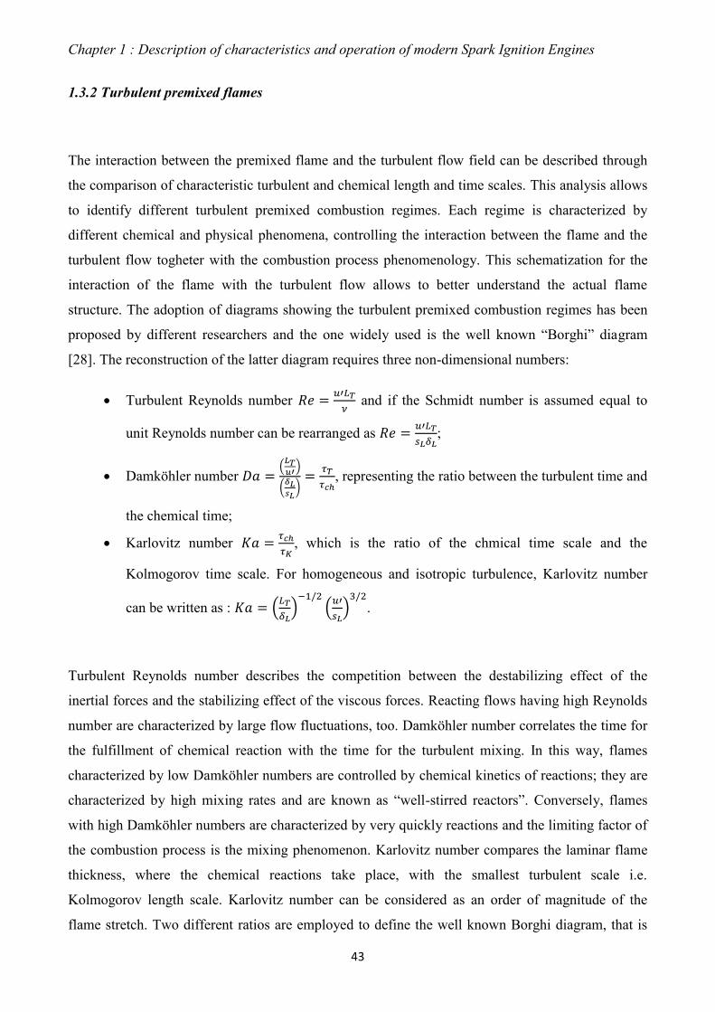
1.3.2 Turbulent premixed flames
The interaction between the premixed flame and the turbulent flow field can be described through
the comparison of characteristic turbulent and chemical length and time scales. This analysis allows
to identify different turbulent premixed combustion regimes. Each regime is characterized by
different chemical and physical phenomena, controlling the interaction between the flame and the
turbulent flow togheter with the combustion process phenomenology. This schematization for the
interaction of the flame with the turbulent flow allows to better understand the actual flame
structure. The adoption of diagrams showing the turbulent premixed combustion regimes has been
proposed by different researchers and the one widely used is the well known “Borghi” diagram
[28]. The reconstruction of the latter diagram requires three non-dimensional numbers:
Turbulent Reynolds number
and if the Schmidt number is assumed equal to
unit Reynolds number can be rearranged as
;
Damköhler number .
/
(
)
, representing the ratio between the turbulent time and
the chemical time;
Karlovitz number
, which is the ratio of the chmical time scale and the
Kolmogorov time scale. For homogeneous and isotropic turbulence, Karlovitz number
can be written as : .
/
.
/
.
Turbulent Reynolds number describes the competition between the destabilizing effect of the
inertial forces and the stabilizing effect of the viscous forces. Reacting flows having high Reynolds
number are characterized by large flow fluctuations, too. Damköhler number correlates the time for
the fulfillment of chemical reaction with the time for the turbulent mixing. In this way, flames
characterized by low Damköhler numbers are controlled by chemical kinetics of reactions; they are
characterized by high mixing rates and are known as “well-stirred reactors”. Conversely, flames
with high Damköhler numbers are characterized by very quickly reactions and the limiting factor of
the combustion process is the mixing phenomenon. Karlovitz number compares the laminar flame
thickness, where the chemical reactions take place, with the smallest turbulent scale i.e.
Kolmogorov length scale. Karlovitz number can be considered as an order of magnitude of the
flame stretch. Two different ratios are employed to define the well known Borghi diagram, that is

Chapter 1 : Description of characteristics and operation of modern Spark Ignition Engines
44
the ratio of the integral length scale to the laminar flame thickness (LT/δL) and the ratio between the
turbulent intensity to the laminar flame speed (u‟/sL). The above defined non-dimensional numbers
can be adopted to correlate the ratios (LT/δL) and (u‟/sL):
.
/
(1.4)
(1.5)
.
/
(1.6)
The adoption of the above equations (1.4), (1.5) and (1.6) allows to reconstruct the Borghi Diagram
(Figure 1.14), in which the turbulent premixed combustion is categorized in different regions.
Figure 1.14 – Borghi Diagram of turbulent premixed combustion [29].
As said, various regimes of turbulent premixed combustion can be identify by the Borghi Diagram
and they are summarized in the following Table 1.1, reporting the characteristics of each regime. In
addition, for each combustion regime a flame depiction is provided. In particular, the flame front
(thick black line) propagates from the burnt gases (white region) to the fresh gases (grey region).
Flame depictions in Table 1.1 describe the flame morphology according to the combustion regime.

Chapter 1 : Description of characteristics and operation of modern Spark Ignition Engines
45
In the following a brief description of combustion regimes showed by the Borghi diagram is
reported. In the case of wrinkled flamelets, turbulent intensity is smaller than the laminar flame
speed. So the laminar propagation is stronger than the mechanism of corrugations of the flame
front. The thickness of the flame front is not altered by the turbulent eddies because the smaller
eddies cannot enter the flame front structure since they are greater than flame thickness (Ka<1). In
this regime chemical kinetics are not sensitive to the presence of the turbulent flow field. For
corrugated flames regime, turbulent intensity is greater than the laminar flame speed. The
corrugation mechanism is the strongest. Because of the strong folding of the flame front, pockets of
the fresh gases may be detached from the continuous flame front and appear in the zone of the burnt
gases. In addition, pockets of burnt gases may appear in zone of the fresh gases. Anyway, turbulent
fluctuations do not alter the flame structure which remains quasi-steady. Corrugated flames region
expands till the borderline with Ka=1. This line defines wrinkled and corrugated flamelet regimes in
which chemical kinetics can be described by the laminar flame properties (sL, δL).
Table 1.1 – Turbulent premixed combustion regimes [29].
Basing on the latter consideration, premixed turbulent combustion of these regions (i.e. corrugated
and wrinkled flamelets) can be modeled by the principles of laminar flamelets, since that the
interaction between the turbulent flow and the flame front is of kinematic nature. The regime of thin
reactions is realized for Karlovitz numbers greater than the unit. In this case, the smallest turbulent

Chapter 1 : Description of characteristics and operation of modern Spark Ignition Engines
46
eddies may enter into the pre-heat zone of the flame but they do not enter into the reaction zone.
Indeed, turbulent eddies are greater than the thickness of the reaction zone. Heat and mass transfer
mechanisms are accelerated whitin the pre-heat zone thanks to the turbulent convection. In the
regime of well-stirred reactor, Damköhler number is smaller than the unit and so the time scale of
turbulent mixing is smaller than the chemical time scale. For this reason combustion process is
controlled by chemical kinetics. For the considered regime, the turbulent mixing is so intense to
cause a perfect stirring between the reactants and the products of combustion. Consequently, no
flame front can be distinguished. In broken reaction zones regime (Ka>100), turbulent eddies enter
into the reaction zone since turbulent eddies are smaller than flame thickness. High heat loss is
obtained from the reaction zone to the preheat zone, due to turbulent convection. The temperature
of the reaction zone quickly decreases. For this regime a premixed flame cannot exist and so no
flame picture is presented in Table 1.1.
1.3.3 Flame Propagation within the combustion chamber
It is well known that in SI engine the spark discharge generates a high temperature kernel of about 1
mm in diameter between the electrodes of the spark plug [23]. Initial flame kernel is characterized
by a quasi-laminar growth and it is highly stretched. The local flow field increasingly distorts the
flame front and so a gradual transition to a turbulent flame occurs. The flame kernel is also
convected away from the spark plug electrodes [30], [31], [32] by the mean and turbulent flow
fields. The flame front is wrinkled by both mean and turbulent flows and its shape may be modified
from spherical to elliptical. At the end of the transition stage, the flame kernel is not convected by
the flow since the the enflamed mass is too important to be convected by the flow field. At this
stage, the heat release rate due to combustion process is very low if compared to the fuel energy
content. Consequently, the increase in the in-cylinder pressure is low. With the fully development
of the flame, turbulent flow wrinkles the flame front and so the flame propagates throughout the
chamber. At this stage the highest part of the fuel energy is released. A microscopic exam of
wrinkled turbulent flame shows that its structure is laminar with a thin thickness. Figure 1.15
depicts the turbulent flame front.

Chapter 1 : Description of characteristics and operation of modern Spark Ignition Engines
47
Figure 1.15 – Wrinkled turbulent flame with corrugations [29].
The contour of the turbulent flame front is represented through a reaction sheet characterized by a
small thickness. The considered sheet presents intense wrinkles and corrugations at different length
scales. The total contour surface is generally called turbulent flame surface AT, while a fictitious
mean flame surface AL can be defined and spherical assumed for 0D modeling approach. The
contours which define the entire flame front allows to identify the turbulent flame thickness δT. The
speed of the flame propagation in the fresh gases is the turbulent flame speed sT. Every flame
element (i.e. small part of reaction zone) presents a laminar flame thickness δL and propagates
toward the fresh gases with laminar flame speed sL. The laminar flame speed depends on the fuel
type, the air-to-fuel (A/F) ratio, the in-cylinder pressure p, the temperature of the fresh gases Tu,
and the presence of the residual gas. The impact of the flame stretch, that is high at the beginning of
the combustion process, on the laminar flame speed has to be properly take into account. The
turbulent flame propagation can be observed till it comes in contact with the walls of the
combustion chamber and consequently the extinction mechanisms take place till the flame is
completely estinguished. During the considered phase the wrinkling of the flame front diminishes
under the impact of the flow boundary layer, of the increased heat losses towards the cold wall and
of the confinement of the flame by the combustion chamber wall.

Chapter 1 : Description of characteristics and operation of modern Spark Ignition Engines
48
1.4 Cycle by cycle variation
In-cylinder pressure measurements of consecutive engine cycles for a Spark Ignition engine show
that a not negligible variation on a cycle-by-cycle basis exists. In addition to these variations
occurring in each individual engine cylinder, significant differences in combustion process and in-
cylinder pressure cycle between the cylinders of a multi-cylinder engine may occur. In particular,
cyclic dispersion is caused by variations in the in-cylinder mixture motion at spark time, variations
in air flow and fuel flow to the single cylinder at each cycle, variations in the mixing of the fresh
charge with residual gas within the single cylinder at each cycle, especially near the spark plug.
Cycle-by-cycle variation represents an important phenomenon to properly take into account for two
main reasons. First, the optimum spark timing is set for the average cycle, and consequently faster-
than-average cycles present advanced spark timing while slower-than-average cycles have retarded
timing and so power and efficiency losses may occur. Second, the extremes of cyclic variations
limit the engine operation. Indeed, the fastest burning cycles with its overadvanced spark timing are
most likely to knock. These cycles limit the compression ratio and determine the fuel octane
requirement. On the other hand, the slowest burning cycles are most likely to burn incompletely and
set the practical lean operating limit of the engine. Morever, too large cyclic variations have a
negative impact on the engine drivability. Variations in the in-cylinder pressure reflect in variations
of the brake torque which directly relate to vehicle drivability. As an example of cycle-by-cycle
variations, Figure 1.16 shows measured 300 consecutive in-cylinder pressure traces as a function of
crank angle, with a sampling resolution of 0.2 crank angles, for a point at 7000 rpm and full load of
a high performance SI engine.
Figure 1.16 – Instantaneous and average in-cylinder pressure cycles at 7000 rpm and Base SA.

Chapter 1 : Description of characteristics and operation of modern Spark Ignition Engines
49
It can be noted that the faster burning cycles present higher value of the maximum in-cylinder
pressure than the slower burning cycles. In addition, the peak pressure of the faster burning cycle is
reached closer to the TDC. Cycle-by-cycle variations are observed in the early stages of the flame
development and especially during the rapid burning phase of the combustion process, involving
variations in the maximum burning rate. In presence of an excess of air or diluition with high
fractions of residual gas the cycle-by cycle variations increases. In this condition some engine
cycles are characterized by slower combustion process and partial burning phenomenon may occur
(combustion not completed at Exhaust valve opening). For more lean or diluite mixture misfire
limit may be reached. Anyway, spark-ignition engine can operates with reduced percentage of
cycles showing partial-burn or misfire but these phenomena cause negative effects on engine
efficiency, hydrocarbon emissions, torque variations and roughness. Cyclic variation has been
observed and intensively studied over the last decades. From an experimental point of view, the
study of CCV is typically based on the acquisition and the post-processing of consecutive in-
cylinder pressure traces (ranging from 300 up to 2000 cycles, [33]). Moreover, in-depth analyses of
the origins of the phenomenon have been performed through optically accessible engines [34], [35],
[36], [37] and by 3D-CFD simulations [38], [39]. Cycle-by-cycle variation can be characterized by
adopting various measure. In particular, CCV can be defined in terms of variations between
different in-cylinder pressure cycles or in terms of variations in parameters of the burning process.
The following listed parameters have been adopted to measure the cyclic variation:
1. Pressure related parameters: maximum in-cylinder pressure pmax, crank angle of maximum
pressure value θpmax, maximum rate of pressure rise (dp/dθ)max, crank angle of maximum
rate of pressure rise and IMEP;
2. Combustion related parameters: the maximum heat release rate, maximum mass burning
rate, combustion duration (MFB10, MFB10-90);
3. Flame front position parameters: flame radius, flame front area, burned volume, all at given
times.
Referring to the pressure data, the coefficient of variation of the indicated mean effective pressure
and the coefficient of variation of the in-cylinder peak pressure represent relevant measure of cyclic
variation. While CoVIMEP clearly affects the engine drivability, a more relevant role is played by
CoVpmax, since it exerts a direct influence on knock occurrence. Different studies are reported in the
current literature to relate the CCV to engine operating parameters such as engine speed, spark
advance, equivalence ratio, or fuel properties and combustion parameters (combustion phasing and

Chapter 1 : Description of characteristics and operation of modern Spark Ignition Engines
50
duration). As an example, an overview of the spark timing impact on IMEP and pmax dispersions
(vertical dots) can be noted from the following Figure 1.17 and Figure 1.18, respectively.
Figure 1.17 – IMEP vs SA, 7000 rpm at full load.
Figure 1.18 – In-cylinder peak pressure vs SA, 7000 rpm at full load.
These figures refer to a high performance naturally aspirated SI engine operating at 7000 rpm and at
full load. Related CoVs and average levels are also reported as continuous lines. It can be observed
that delayed spark advance (SAbase+6, late combustion phasing) determines an increase of CoVs
level. The Spark advance realizing the Maximum Brake Torque (MBT), can be easily determined as
shown in Figure 1.17, and, correspondingly, CoVIMEP attains approximately its minimum. Also the
studies by Young [40] underline that CCV is minimized at the ignition timing realizing the MBT. In
addition, it is moreover confirmed that pmax dispersion (Figure 1.18) is much higher than IMEP one,

Chapter 1 : Description of characteristics and operation of modern Spark Ignition Engines
51
for each tested SA. For the same considered engine system, the effect of the engine speed on IMEP
and pmax distributions can be indeed derived from Figure 1.19 and Figure 1.20, referring to full load
operation and Base SA. It is once again confirmed that dispersion of pmax is much higher than IMEP
one for each tested operating condition. The related CoVs, moreover, do not clearly depend on the
engine speed. Higher CoVs are actually detected at 4000 rpm, since Base SA is farther from the
angle of MBT (θMBT), than the other speeds.
Figure 1.19 – IMEP vs engine speed, Base SA.
Figure 1.20 – In-cylinder peak pressure vs engine speed,
Base SA.

Chapter 1 : Description of characteristics and operation of modern Spark Ignition Engines
52
Figure 1.21 – (a) CoVIMEP vs averaged MFB50 and (b) CoVIMEP vs averaged combustion duration
Δθb.
Figure 1.22 – (a) CoVpmax vs averaged MFB50 and (b) CoVpmax vs averaged combustion duration
Δθb.
CoV relationship with average combustion-related parameters are also presented in Figure 1.21 and
Figure 1.22, once again referring to a high performance naturally-aspirated SI engine [41]. CoVIMEP
presents high values for delayed combustions. Its minimum is reached at an angular position
roughly corresponding to the MBT in each operating condition. The CoVIMEP indeed does not
exhibit a well-defined trend with the averaged combustion duration, although it more clearly
increases for the slower combustion processes. The CoVpmax, on the contrary, exhibits a clear
increasing trend with the combustion phasing, highlighting that a more delayed combustion process
leads to higher pmax variations. As stated above, a more dispersed trend establishes between CoVpmax
and the averaged combustion duration. A longer combustion process however still determines a
higher CoVpmax.
(a) (b)
(a) (b)
deg deg
deg deg

Chapter 1 : Description of characteristics and operation of modern Spark Ignition Engines
53
Referring to the influence of equivalence ratio on CCV, Pundir et al. [42], as an example, have been
observed that the CoVpmax reaches the minimum level when stoichiometric mixtures are adopted,
while variations in the equivalence ratio inevitably lead to increased CCV. Hassaneen et al. [43]
tested an 8-cylinder natural gas SI engine and found that CoVpmax and CoVIMEP rised by 33% as the
equivalence ratio decreased from 1 to 0.6. Ozdor et al. [44] studied CCV for a four-stroke, 4-
cylinder engine for various excesses of air, always maintaining the spark timing at MBT. The
results showed that CCV were minimum for a stoichiometric mixture. Finally, Maurya and Agarwal
[45] investigated the effect of two different fuels (gasoline and ethanol) on CoVIMEP relationship
with combustion phasing and combustion duration and for HCCI combustion. The considered fuels
shown the same behaviour: longer combustions and late phasing involved higher IMEP variations
for both fuels and a second order polynomial correlation between CoVIMEP and combustion duration
was developed. To this aim, in order to characterize the CCV phenomenon, different correlation of
CoVs with average combustion-related parameters have been investigated and reported in the
current literature. As an example, an experimental study on a high performance SI engine [41]
showed that the combustion parameters which better correlate with the CoV levels are the
combustion phasing and conventional duration (MFB50 and Δb). In particular, two polynomial
correlations have been identified:
(1.7)
(1.8)
where ci and di (i=0,..,4) are the constants realizing the best fit with the experimental data. The latter
correlations allow to take into account the cycle-by-cycle variations from a numerical point of view
by computing through a proper engine model (including a refined combustion sub-model) the
parameters of correlation (MFB50 and Δθb) referring to the average cycle. In addition, CCV
correlations provide the advantage to properly predict the faster-than-average pressure cycles
allowing to estimate the knock limited spark advance with reference to the more critical pressure
cycle.

Chapter 1 : Description of characteristics and operation of modern Spark Ignition Engines
54
1.5 Knock phenomenon
Knock phenomenon represents one of the most important abnormal combustion process for Spark
ignition engine because it causes limitations on engine performance and efficiency and at the same
time imposes restricting constraints to the employed fuels. It is well known that intense knock can
cause major engine damages and it represents a source of noise by the engine even in the case of
soft knock. Indeed, knock is the name associated to the noise which is transmitted to the engine
structure when air/fuel charge molecules in the end-gas zone spontaneously ignite before they have
been reached by the propagating flame front. If this abnormal combustion takes place an extremely
rapid release of much of the chemical energy in the end gas occurs, causing very high local pressure
values and the propagation of the pressure waves of significant amplitude across the combustion
chamber. When auto-ignition occurs repeatedly (i.e. more than occasionaly) during otherwise
normal combustion event, the phenomenon is named “spark knock”. Knock phenomenon may vary
substantially cycle-by-cycle and cylinder-by-cylinder in multi-cylinder engines and it does not
occur every engine cycle. Spark knock can be controlled by acting on the spark timing. Indeed, an
advanced spark timing increases the knock intensity while retarding the spark a decrease in the
knock intensity is obtained. Knock may be an outcome following the occurence of surface ignition,
since the latter usually causes a more rapid rise in the end-gas pressure and temperature than the
case of normal combustion operation. Anyway while surface ignition represents a problem that can
be solved by acting on the engine design, fuel type and lubricant quality, in contrast, knock is an
inherent constraint on engine performance and efficiency because it limits the maximum
compression ratio for any given fuel. Knock primarily establishes under wide open throttle (WOT)
operating conditions, since higher in-cylinder pressure and temperature levels occur. The
occurrence and the severity of knock depend on the fuel type (knock resistance) and on the anti-
knock characteristics of the engine. Knock resistance of a predefined fuel is measured by the octane
number. Higher octane number indicates greater resistance to knock. Gasoline knock resistance can
be improved by refining processes such as catalytic cracking and reforming or by the adoption of
antiknock additives. Engine design exterts a not negligible effect on the knock occurrence, i.e.
combustion chamber, spark-plug position, etc. Besides the quality of the available fuels, knock
depends on the ability of the engine designer to ensure the desired normal combustion behaviour
reducing the engine knock tendency at minimum. The in-cylinder pressure trace allows to evaluate
the actual pressure variation within the cylinder during knocking combustions. As an example,
Figure 1.23 shows the in-cylinder pressure variation for three single engine cycles characterized by
normal combustion, slight knock and heavy knock, respectively [23].

Chapter 1 : Description of characteristics and operation of modern Spark Ignition Engines
55
Figure 1.23 – In-cylinder pressure traces of cycle with (a) normal combustion, (b) light knock, and
(c) heavy knock (WOT, 4000 rpm, 381 cm3 displacement single cylinder engine) [23].
When knocking combustions occur, high frequency pressure oscillations are observed whose
amplitudes are gradually reduced over time. For the considered engine and the tested operating
point of Figure 1.23, some engine cycles do not present knock phenomenon (Figure 1.23a) while for
the remaining cycles (Figure 1.23b-c) knock phenomena of different intensity occur. In slight knock
case (Figure 1.23b), the considered phenomenon occurs late in the burning process and the
amplitudes of the pressure oscillations are very small. For heavy knock case (Figure 1.23c),
obtained with a more advanced spark timing, knock occurs closer to the TDC and earlier in the
combustion process with initial amplitudes of the pressure oscillations more larger than the previous
cases. Higher amplitudes of the pressure oscillations are the result of the spontaneous release of a
great part of the fuel chemical energy in the end gas zone. The presence of knock involves that the
pressure distribution across the combustion chamber is no longer uniform. Consequently,
transducers located at different point of the combustion chamber will record different pressure
values at a predefined time. To this aim, many methods of knock detection and characterization
have been adopted. In particular, knock detection systems usually respond to the vibration driven
acceleration of parts of the engine block caused by pressure waves generated by knocking
combustion. Optical probes and ionization detectors have been used, too. Indeed, a high intensity
flash is observed when knock occurs together with a sharp increase in the ionization. A useful
measure of knock intensity is represented by the amplitude of the pressure fluctuations since they
depend on the amount of the end-gas which ignites spontaneously. The adoption of this measure of
knock intensity allows to highlight that a cycle-by-cycle variation of knock severity exists [23].

Chapter 1 : Description of characteristics and operation of modern Spark Ignition Engines
56
Figure 1.24 shows knock intensity for 100 consecutive engine cycles for a single cylinder of a V8
SI engine at WOT and mid-engine speed (2400 rpm).
Figure 1.24 – Knock intensity for 100 consecutive engine cycles (single cylinder V8 SI engine at
WOT operation and 2400 rpm).
It can be observed that knock intensity varies randomly, covering knock free and heavy knock
conditions. In addition, cylinder-to-cylinder variations in knock intensity may occur due to
variations in compression ratio, mixture composition, burn rate and combustion chamber cooling. It
is the case to underline that knock generates a non-uniform condition within the cylinder and
different details of this phenomenon in each cycle and each cylinder are obtained. For this reason, a
definition of knock intensity is extremely difficult. A well recognized measure of knock severity is
represented by the maximum amplitude of the pressure oscillation occurring in knocking
combustion. The in-cylinder pressure signal, measured through an high frequency response pressure
transducer, is properly filtered in such a way to obtain only the components of the pressure signal
that correspond to the fluctatuations due to knock. Knock intensities reported in the previous Figure
1.24 are determined by employing the above discussed method. Since pressure fluctuations are
caused by wave propagation phenomenon, the location of pressure transducer with respect to the
location of the end-gas zone and the shape of the combustion chamber will affect the maximum
amplitude of pressure fluctuation. Knock phenomenon may exterts a significant impact on engine
system according to its intensity and duration [23]. Soft knock has not significant effects on engine
performance and durability while heavy knock can lead to extensive engine damages. For
automotive application, knock characterized by short duration and low intensity (soft knock) is
unlikely to cause damages. Instead, heavy knock at constant speed can easily lead to pre-ignition,

Chapter 1 : Description of characteristics and operation of modern Spark Ignition Engines
57
runaway knock and gradual erosion of regions of the combustion chamber. The engine can be
damaged by knock phenomenon in different ways: cylinder and head erosion, piston crown and top
land erosion, piston melting and holing, piston ring sticking, etc. As an example, Figure 1.25 shows
component damage due to abnormal engine combustions (pre-ignition and knock). Referring to the
mechanisms which cause damages, when heavy knock occurs heat is transferred to the combustion
chamber walls together with a rapid overheating of the cylinder head and piston. Under this
condition, knock is not stable. Indeed, the overheating increases the knock intensity, making this
phenomenon heavier and heavier and without a proper control it can lead to engine failure in a short
time. In conclusion, in order to avoid severe engine damages during the engine operating condition,
knock phenomenon has to be properly controlled and reduced at very low intensity.
Figure 1.25 – Component damages from abnormal combustion [23]: (a) piston holing by pre-
ignition; (b) piston crown erosion after 10 hours of high-speed knocking; (c) cylinder head gasket
splitting failure due to heavy knock; (d) erosion of aluminum cylinder head along the top of cylinder
liner due to heavy knock.

Chapter 1 : Description of characteristics and operation of modern Spark Ignition Engines
58
1.6 Engine system description
The engine under study is a commercial small-size twin-cylinder turbocharged SI engine,
representing a typical downsized engine. A simple engine schematic layout is shown in Figure 1.26.
Engine system is equipped with gasoline port-fuel injectors and with a variable valve actuation
(VVA) module, capable to control the intake valve lift profile. The valve actuation is provided by
an electro-hydraulic system that modulates the valve lift according to the operating conditions. In
many cases, the valve lift greatly differs from the cam-derived profile. The system consists of a
small capacity between the cam and the valve filled with lubricant oil, whose emptying is regulated
by an electronically controlled electro-valve [46]. The main features of the tested engine are
reported in following Table 1.2. The latter shows that the engine compression ratio is limited to 9.9,
in order to avoid the knock occurrence at high load operation. Since the full load performance of a
downsized engine is restored by the turbocharger group, as the boost pressure increases knocking
combustions may occur. This phenomenon represents one of main problems of the analyzed engine
because it limits the specific fuel consumption levels at full load operation.
Figure 1.26 – Engine Schematic Layout : C: Compressor, T:Turbine, C1,2 :engine cylinders, AMB.:
external ambient, Inj.: Fuel injector.
In addition to the discussed BSFC advantages of the downsized architecture at low loads, the
adoption of VVA system allows for further improvements at low/medium BMEP operation [47],
[48], [49], [50]. Indeed, the flexibility of the VVA systems allows to adjust the engine load with
very limited butterfly valve throttling [51], [52], which drastically reduces the pumping work at
low/medium load. Moreover, a reduction in NOx emissions and an improved combustion stability at

Chapter 1 : Description of characteristics and operation of modern Spark Ignition Engines
59
idle were experimentally verified [53], [54], [55], [56]. Consequently, reductions in specific fuel
consumption may be achived at part load operation.
Model 2 cylinders, 8 valves, VVA,
Turbocharged and Intercooled
Displacement 875 cm3
Stroke / Bore 86 mm / 80.5 mm
Connecting rod length 136.85 mm
Compression Ratio 9.9
Max Brake Power 64.6 kW @ 5500 rpm
Max Brake Torque 146.1 Nm @ 2500 rpm
Table 1.2 – Main Engine Characteristics.
The intake valve lift strategies which can be realized by the valve actuation system equipping the
analyzed engine include Late Intake Valve Opening (LIVO), Early Intake Valve Closure (EIVC), a
combination of the previous ones and a multi-lift (ML) strategy. As known, the same load level can
be achieved by employing different valve strategies. A typical drawback derived by the VVA
system is the worsening of intake gas-dynamic noise emissions at low loads. The reduced throttling
of the intake ducts, while allowing a reduction in the pumping work, also results in a less effective
attenuation of the pressure wave in the intake system [57], [58]. At very low loads, the decreased
duration of the intake phase may determine a reduced turbulence level at the spark time and a
slower burning speed. For the above reasons, precise engine control parameter settings must be
specified to obtain the best compromise among different objectives.
The analyzed engine presents various degrees of freedom allowing for the opportunity to operate in
a specified speed-load point using different control strategies. In particular, it is possible to
independently define the following parameters:
air to fuel ratio (A/F);
throttle opening angle;
χ spark ignition timing;
1 intake valve opening angle;
2 intake valve closing angle;
WG turbine waste-gate valve opening.

Chapter 1 : Description of characteristics and operation of modern Spark Ignition Engines
60
, , and χ are traditionally used to calibrate a naturally-aspirated SI engine, while 1, 2 and WG
are related to the control of the VVA system and the turbocharger, respectively. This set of
parameters has to be properly defined in order to achieve the required performance targets. The
experimental identification of this set of engine variables, for a predefined operating condition,
poses some problems which can be overcome through the adoption of numerical models and
methodologies. This kind of issues will be deeply discussed in the following.
1.6.1 Experimental activities
The considered engine is installed at the test-bench and both high and part load operations are
investigated for different speeds (1500-5500 rpm) and intake valve strategies. Acquired data include
fuel flow, air flow, power, torque, pollutant emissions and fuel consumption. Instantaneous in-
cylinder pressure measurements are also carried out in both cylinders and the indicated parameters
(IMEP, maximum pressure, angle of maximum pressure, angles of 10%, 50%, 90% of Mass
Fraction Burned – MFB10, MFB50, MFB90, etc.) are derived. In particular, a sequence of 200
consecutive in-cylinder pressure traces are acquired for each tested speed at full load. A sampling
resolution of 0.5 crank angles is adopted at each speed. A higher sampling frequency (0.1 deg) is
instead specified during combustion angular window (-10 ,75 deg). As an example, cycle-by-cycle
WOT pressure measurements at 2100 rpm and 4000 rpm are shown in Figure 1.27a and Figure
1.27b, superimposed with ensemble averaged ones.
Figure 1.27 – Average and instantaneous in-cylinder pressure cycles at 2100 rpm (a) and 4000 rpm
(b) in WOT condition.

Chapter 1 : Description of characteristics and operation of modern Spark Ignition Engines
61
A relevant cyclic dispersion can be observed, with differences on the peak pressure of about 20-30
bar, and an IMEP Coefficient of Variation (CoV – defined as the ratio between the standard
deviation of the IMEP and the related average level) around 5% in both cases. As said, the electro-
hydraulic system equipping the engine allows for different intake valve settings. In order to simplify
the experimental investigation, among the various available strategies, only the EIVC strategy is
tested in the present work. Typical valve lift profiles are shown in Figure 1.28, characterized by a
different closure angles, labelled in the following as 2. In particular, in Figure 1.28 the continuous
curve represents a Full Lift strategy, while dashed ones depict EIVC strategy.
Figure 1.28 – Typical valve lift profiles for different closure angles.
A complete fuel consumption map is collected for a Full Lift valve strategy, where the load is
adjusted by the throttle valve at low load, and by the waste-gate valve at high load (Figure 1.29a). A
second fuel consumption map is measured, where the intake closure angle 2 is added as further
control parameter (Figure 1.29b). In the latter case, only the region of the operating plane
characterized by lower BMEP levels is investigated, where intake throttling and EIVC strategy are
properly combined to improve the fuel consumption. The EIVC strategy is also employed to
measure a full load curve, recording a single operating point for each engine speed. In this case, 2
angle is adjusted according to the speed in order to realize the highest volumetric efficiency, namely
tuning the intake valve closure event with the natural pressure oscillation in the intake line. At
medium and low load, the spark advance is set to realize the maximum brake torque, usually
corresponding to MFB50 of about 4-10 degrees after FTDC (Figure 1.30). The air-to-fuel ratio is
fixed at a stoichiometric value, so to guarantee optimal operation for the catalytic converter (Figure

Chapter 1 : Description of characteristics and operation of modern Spark Ignition Engines
62
1.31). At high load, a delayed combustion phasing is realized due to knock limitations (Figure
1.30). This is particularly true in case of low speeds, since a higher knock tendency verifies. Air-to-
fuel ratio has to be particularly enriched at high engine speeds (Figure 1.31), mainly to maintain the
Turbine Inlet Temperature (TIT) below a prescribed threshold level of 950 °C. However, the heat
subtracted by the fuel evaporation contributes to reduce knock risks and a more favourable MFB50
setting can be set at high speeds. As expected, both the above control strategies, although
mandatory, strongly penalize the fuel consumption at high load (Figure 1.29).
Figure 1.29 – Measured fuel consumption map (g/kWh) for Full Lift (a) and EIVC (b) strategies.
Figure 1.30 – Measured MFB50 map (crank angle degree after FTDC) for Full Lift (a) and EIVC
(b) strategies.

Chapter 1 : Description of characteristics and operation of modern Spark Ignition Engines
63
Figure 1.31 – Measured air-to-fuel ratio map for Full Lift (a) and EIVC (b) strategies.
The engine performance are also limited by the compressor operating domain (surge, choke and a
maximum speed of 255000 rpm for the compressor of the considered engine). Further limitations
are posed for the maximum allowable boost level (2.2 bar), required to guarantee proper operation
for the fuel injectors and a certain safety margin for the intake plenum.
1.6.2 Engine calibration issues
Once the engine under study has been deeply specified in terms of sub-systems and all the operating
parameters (i.e. degrees of freedom of the engine system) have been properly defined as well as the
performance requirements, the engine calibration phase is realized with aim to identify the optimum
set of engine variables for various operating conditions by taking into account the system
performance targets (minimum fuel consumption and pollutant emissions at part load, maximum
power and torque at full load, combustion stability at idle, etc.). As general consideration, modern
spark ignition engines are characterized by complex architectures, showing a significant number of
sub-systems and operating variables, making the engine calibration a challenging phase during the
system development. Indeed, from an experimental point of view, the calibration requires an high
number of tests to explore the whole operating domain of the control parameters and the entire
engine operating map. This involves a negative impact on the engine development time and costs.
In order to avoid the latter problems, the engine calibration phase is often supported by numerical

Chapter 1 : Description of characteristics and operation of modern Spark Ignition Engines
64
tools and methodologies. As an example, Design of Experiment (DoE) methodologies are
successfully employed to reduce the number of experimental tests. A further reduction in the
experimental activity can be obtained using proper numerical models that, once tuned, are able to
achieve a pre-calibration of the engine, following a fully-numerical approach. Consequently,
activity at test-bench can, hence, be limited to verify and refine the desired performance targets. For
numerical calibration purposes, among several modeling approaches, 1D engine model, properly
validated, coupled to an optimizer tool has been successfully employed to perform multi-objective
analyses allowing to numerically identify the optimal set of engine parameters. First, the considered
optimization approach shows the capability to reproduce with good accuracy the experimentally
advised optimal calibration. Second, for a predefined engine operating point, it is possible to select
the new optimal set of engine variables capable to achieve the desired trade-off among different
performance requirements. For the downsized engine under study, as said before, the performance
at high and full load operation are mainly limited by the knock onset, which influences the engine
calibration, causing the adoption of delayed spark timing and over-fuelling mixture. For this reason,
the use of proper sub-model for the description of knock phenomenon is mandatory. Only in this
way, the reliability of an integrated 1D model/optimizer approach can be ensured and an overall
“virtual” calibration of the engine, including all the control variables (i.e. valve strategy,
combustion phasing, mixture quality, throttle opening, WG opening) can be accomplished. In
particular, the virtual calibration at high loads, for a selected engine speed and intake valve lift
strategy, is oriented to the identification of engine parameters allowing to maximize the brake
torque while simultaneously minimize the fuel consumption under knock limited condition. In this
way, the adopted numerical approach can also underline the potentiality of an engine calibration at
high load, based on the actuation of innovative intake valve lift strategies by the VVA sub-system
rather than a purely throttle based calibration. A similar virtual engine calibration can be also
performed at part load for various VVA strategies. In conclusion, once the 1D engine model is
validated against the experimental data, the discussed numerical approach allows for a virtual
engine calibration on theoretical basis and it proves to be an useful tool to support and reduce the
experimental costs and the engine time-to-market.

Chapter 1 : Description of characteristics and operation of modern Spark Ignition Engines
65
1.7 Structure of this work
This work is mainly focused on the study of turbulence, combustion, knock and cycle-by-cycle
variation of a downsized VVA Spark Ignition engine. A 0D/1D modeling approach is here adopted
to reproduce the engine behavior in different operating conditions. Gas-dynamic noise at intake
mouth for the considered engine is also taken into account by testing redesign solutions of the
intake system through a 3D CFD model. Engine calibration is also analyzed from a numerical point
of view and a proper methodology is presented aiming to perform fully numerical calibrations.
Thesis work is organized into eight chapters. A brief description of the content of each of them is
reported below:
The present introductory chapter provides a description of characteristics and operation of Spark
ignition engines and of the main technologies for SI engines capable to obtain efficiency
improvements as well as pollutant emission reductions. Then, a description of SI turbulent
combustion process, knock and cycle by cycle variation phenomena is also presented. Finally, the
engine under study is analyzed, mainly focusing on the experimenal activities and calibration
issues. Numerical methodologies to support the calibration phase are discussed, too.
The second chapter furnishes on overview of the modeling approaches for internal combustion
engines, with particular reference to the in-cylinder processes. The benefits of a proper integration
of modeling approaches are also discussed. The 0D modeling approach is mostly analyzed: factal
combustion model and “in-house developed” turbulence model are described in detail as well as the
0D/3D hierarchical approach for turbulence modeling.
The third chapter describes the 0D/1D model of the whole engine, developed in GT-PowerTM
environment. The single models of the main engine sub-systems and the numerical routines are
considered. Once turbulence and combustion sub-models are tuned, the engine model is validated
against the experimental data at full and part load operations.
In the fourth chapter various experimental knock detection techniques are analyzed. In particular,
two different knock detection methods are utilized to perform a knock analysis for the examined
engine. Knock and cyclic dispersion models are discussed and then the knock model taking into
account the cycle by cycle variation is validated at full load operation.

Chapter 1 : Description of characteristics and operation of modern Spark Ignition Engines
66
The fifth chapter deals with the adoption of an external EGR system for the engine under study.
Starting from the validated 1D engine model, a Low pressure EGR circuit is virtually mounted and
the new engine configuration is tested by 1D simulations. Numerical results show that the adoption
of the EGR circuit allows for fuel consumption reduction at full load points.
In the sixth chapter water injection technique at the engine intake ports is investigated by a 1D
approach. The effects of the above technique are studied in various full load knock limited
operating points and for various A/F levels and water content. The presented results highlight that
the considered solution involves significant BSFC improvements, especially in the operating
conditions at medium engine speeds.
In the seventh chapter the gas-dynamic noise emitted at the engine intake mouth is firstly
reproduced by 1D and 3D CFD models. Once the models are validated at full load, some redesign
solutions for the air-box device are proposed and numerically tested to evaluate the reduction in the
gas-dynamic noise.
The eighth chapter deals with virtual engine calibration by employing 1D model coupled to external
optimizer. Starting from the model validation for two different intake valve strategies, multi-
objective optimizations at part and full load are performed, showing the capability to reproduce the
experimentally identified calibrations. The effect of intake valve strategy on the fuel consumption is
also discussed for various load levels.

Chapter 2 : Modeling of Internal Combustion engines and in-cylinder processes
67
CHAPTER 2
Modeling of Internal Combustion engines and in-cylinder processes
2.1 Modeling Approaches for engine development
In the automobile industry, system modeling and numerical simulation are widely employed for the
development of new engines, thanks to the possibility to study different solution with acceptable
computational time. During the development phase of an internal combustion engine (ICE) different
requirements have to be considered. Indeed, engine manufacturers have to guarantee proper
power/torque performance, fuel consumption and pollutant emissions, aiming to comply with the
stringent emission limitations and to obtain the desired vehicle drivability. The above tasks, often
conflicting, require proper architectures of the ICEs. In order to analyze new engine architectures
and to take into account the engine behavior at development stage, virtual design tools and
numerical models can be successfully employed to guide and limit the expensive experimental
analyses [59], [60], [61]. Numerical simulation and system modeling are utilized at different levels
and phases of an ICE developing project. The global engine system, which has to be studied, is
usually decomposed into various less-complex sub-systems, on the basis of a functional criterion. In
this way, each sub-system can be properly analyzed by evaluating the performace and taking into
account the links with the other parts of the system. The main advantage of this kind of approach is
that the single sub-system can be modeled separately and subsequently it may be integrated within
the entire model of the system. For a given sub-system, several models can be adopted according to
the engineering application. Their complexity may vary starting from simple mathematical models
to phenomenological and CFD models. As said, system simulation tool may vary significantly
according to the engine part which has to be modeled. In particular, in the case of ICEs analysis,
three main modeling approaches has been adopted over the time:
Zero-dimensional models;
One-dimensional models;
Three-dimensional models.
In the above classification the level of detail and physical contents increases as one proceeds
downward and the complexity of those models increases, too. Zero-dimensional models are the

Chapter 2 : Modeling of Internal Combustion engines and in-cylinder processes
68
simplest ones due to their computational speed. Anyway, they present different levels of detail,
including mathematical and physical models. They are generally employed to study in-cylinder
processes. One-dimensional models are based on the integration of 1D unsteady flow equations and
they are usually adopted to study the intake and the exhaust systems of ICEs with good accuracy
and reduced computational efforts. One dimensional model can give important information at
system levels, i.e about performance and internal flows of the entire system. 3D CFD models, based
on the integration of Navier Stokes equations, give detailed flui-dynamic information for complex
3D domains, allowing to capture the local 3D features of the flow. Anyway, the latter models
require higher computational costs. For ICEs study, 3D CFD techniques play an increasingly role
during the development phase. As an example, CFD analysis becomes a very powerful tool to
analyze the in-cylinder flow structure evolution under actual engine operations, as well as to
address the influence of port design on the in-cylinder flow field [62]. Furthermore, they allow for a
better understanding of how combustion takes place in new combustion concepts, and consequently
low cost testing of different chamber geometries and concepts can be performed in order to design
the final product [63]. Although 3D CFD models provide considerable amount of spatial
information and allow for a better description of combustion phenomenon and noxious emissions,
they still employ phenomenological sub-models and require high computational time and storage.
The latter constraints still preclude 3D models from routine use for engine design purposes. On the
other hand, 0D and 1D models can be easily used for ICEs modeling because they improve the time
delays and diminish the cost of production. 0D-1D models are often used for ICEs modeling either
for the engine control or for the optimization of engine performance, fuel consumption and
emission. 0D-1D models as support tools for engines development have to cope the challenge of the
compromise between the computational time and the accuracy of models. In the following, a brief
description of the above listed modeling approaches will be provided.
2.1.1 Zero-dimensional Approach
Zero dimensional model are generally conceived from empirical and semi-empirical approaches. In
general, they are considered as simple modeling approach to study different systems and processes.
The results obtained from more complex simulations (for example CFD) or from the experimental
tests are used for the validation of 0D models. The outcomes of 0D models has to be in good
agreement with the experimental or CFD ones. 0D models can present different complexity levels,
depending on the modeled system and on the desired outputs. The complexity of the 0D models

Chapter 2 : Modeling of Internal Combustion engines and in-cylinder processes
69
may vary from the simple mathematical models to phenomenological models. 0D models are
currently employed for the simulation of systems and sub-systems for automobile industry. As an
example, 0D models can be adopted for a fist satisfactory evaluation of engine performance,
consumption, noise or thermal fluxes [29] but they do not take into account the flow modeling i.e.
geometric/dimensional features of the flow motion. For the latter reason they are called zero-
dimensional. The most important advantage of 0D modelling approach is the very low
computational time and it is comparable with the one of the real time application. The latter
characteristic makes these models very attractive for automobile industry. Another relevant
advantage of this modeling approach is that it can be extended to different sectors, allowing to
simulate several types of system, including mechanical, thermal, electrical etc. In the case of
internal combustion engines simulation, 0D modeling approach is widely adopted in order to
reproduce the in-cylinder phenomena. It is also employed to reproduce the intake and exhaust flow
when the wave propagation effects within pipes can be neglected. In many cases a 0D/1D modeling
approach is preferred for the simulation of ICEs: 0D model for volume elements (i.e. cylinders) and
1D model for pipes (i.e. intake/exhaust systems). In particular, as said, 0D modeling approach has
been widely adopted in the past and it is still used for the simulation of in-cylinder phenomena,
including the turbulent combustion process both for Spark-Ignition and Diesel engines and 0D
models. Indeed, various 0D phenomenological models have been developed and oriented to
primarily reproduce the turbulent combustion phenomenon and then the performance and
emissions. As known, with the adoption of a zero-dimensional approach the variables which
characterize the thermodynamic state of fluid within the engine cylinder are considered to be
uniform in the cylinder volume while they are time-dependent. For the engine cylinder a 0D
dimensional model provides the resolution of the mass and energy conservation equations. These
equations, for the volume of an engine cylinder, are generally written in terms of crank angle:
mass conservation equation:
∑
∑
(2.1)
energy conservation equation: ( )
∑
(2.2)
where:
is the heat realeased by combustion process,
( )
is the variation of the internal energy of the
system,
represents the mechanical power exchanged by fluid with the piston,
is the heat

Chapter 2 : Modeling of Internal Combustion engines and in-cylinder processes
70
exchanged through the walls of the combustion chamber and ∑
is the energy term due to the
flux of mass through the control surface.
Normally, the enthalpy term and the system mass variation, due to leakage, are neglected. In this
case, ∑
and by considering the idel gas law, the energy conservation equation (2.2) can
be rearranged as follows:
(2.3)
Once the engine system is assigned, the heat release rate is known, the in-cylinder heat exchange is
modeled as reported in the literature [64], [65] and by take into account the ideal gas law, the
energy equation allows to obtain the in-cylinder pressure trace as a function of the crank angle.
Referring to the in-cylinder models, the zero-dimensional ones are the simplest and most suitable to
evaluate the effects of variations in the engine operating parameters on the overall heat release rates
and in-cylinder pressure evolutions.
Zero dimensional models are further sub-divided into:
1. Single zone models;
2. Two zone models;
3. Multi-zone models.
In single zone models, the working fluid in the engine is assumed to be a thermodynamic system,
which undergoes energy and/or mass exchange with the surroundings and the energy released
during the combustion process is obtained by applying the first law of thermodynamics to the
system. In two zone models, the working fluid consists of two zones, an unburned zone and a
burned zone. These zones are actually two distinct thermodynamic systems with energy and mass
interactions between themselves and their common surroundings, the cylinder walls. The mass-
burning rate (or the in-cylinder pressure), as a function of crank angle, is then numerically
computed by solving the simplified equations resulting from applying the first law to the two zones.
Single zone and to zone models can be employed in two different directions:
1. In one way, both these models can predict the in-cylinder pressure as a function of crank
angle from an assumed energy release or mass burned profile (Wiebe equation);

Chapter 2 : Modeling of Internal Combustion engines and in-cylinder processes
71
2. Another use of these models lies in determining the energy release/mass burning rate as a
function of crank angle from experimental in-cylinder pressure data.
Multi-zone models consider energy and mass balances over several zones, thus obtaining results
that are closer to reality. Concerning the modeling of the combustion process, many combustion
models have been developed to date and they essentially allow to predict the rate of fuel burning. In
the case of Spark Ignition ICEs, various approaches for combustion modeling have been proposed
and used trying to reproduce the flame development inside a turbulent flow field [23]. Among the
different approaches, the “fractal” combustion model appears to be the one which better describes
the turbulent flame propagation phenomenon inside an internal combustion engine [6], [7], [66],
[67]. It is based on the hypothesis that aerodynamic turbulence enhances the burn rate by increasing
the surface of the flame front with respect the laminar extent and does not alter significantly the
inner flame structure. All turbulent length scales are assumed to be larger than the flame front
thickness (flame is in the so called “wrinkled flamelet” regime). This combustion model will be
described in the following.
2.1.2 One-dimensional Approach
One dimensional modeling is widely adopted for the numerical study of internal combustion
engines because it allows for the description of the entire engine system with satisfactory accuracy,
lower computational effort and reduced computational time. Indeed, this approach is usually
employed during the engine development phase to study the global engine system. The 1D
modeling of the entire engine, thanks to the above discussed advantages, allows to analyze (in
addition to steady state engine operation) more complex processes such as the transient operation of
the engine, unsteady behavior of engine and its sub-systems, including turbocharger group, cooling
system behavior, etc. Furthermore, the 1D approach allows to analyze different engine architectures
(including VVA/VVT systems, EGR circuits, water injection systems, turbocharging systems,
components for the abatement of pollutant emissions, exhaust and muffler systems) and to rapidly
test the effects of the modified engine configurations on its overall performances (torque/power,
fuel consumption, noxious emissions, gas-dynamic noise, etc.). 1D model also furnishes the
possibility to investigate a wide range of engine operating conditions such as engine operations
which differ in the air-to-fuel ratio, speed, fuel injection strategies, etc. In particular, as said before,

Chapter 2 : Modeling of Internal Combustion engines and in-cylinder processes
72
1D models are usually employed for the description of the unsteady flow within the intake and the
exhaust manifolds of internal combustion engines. In this way, the wave propagation within the
intake and exhaust systems is taken into account. This approach is particularly suited for the
intake/exhust system design, since that fluid-dynamic effects on intake/exhast flow and many
geometrical variables determing the overall filling/emptying performance can be considered. These
variables include length and cross-sectional area of both primary and secondary runners, volumes
and locations of plenums or junctions connecting the various runners, entrance and exit angle of
runners at a junction, number of cylinders and dimension, intake and exhaust ports and valve
design, etc. 1D models consider mass, momentum and energy conservation equations to describe
the un-steady flow within the intake/exhaust systems [23]. Normally, the intake and the exhaust
flows of a ICE are properly linked by a thermodynamic analysis of the in-cylinder processes
performed through the adoption of a zero-dimensional modeling approach. Referring to numerical
method, method of characteristics was used in the past to solve the 1D unsteady flow equations. It
presents first order numerical accuracy in space and time and requires a large numbers of
computational points if the resolution of the short-wave-length variations is important [23]. In
recent years, the finite difference techniques are employed for intake and exhaust flow models.
They have high order numerical accuracy in space and time and prove to be more efficient: this
numerical method is now preferred. The basic assumptions and equations of the 1D models will be
now briefly reviewed. The flow through the control volume within a straight pipe (Figure 2.1) is
considered. It is assumed that:
only a reduced change in the area over the length dx of the control volume occurs;
the length of the pipe is greater than its diameter;
the radius of curvature of pipe bends is higher than pipe diameter. In these conditions the
flow is essentially one-dimensional.
Figure 2.1 – Control volume for unsteady 1D flow analysis.

Chapter 2 : Modeling of Internal Combustion engines and in-cylinder processes
73
Under the hypothesis of 1D flow, all the parameters which identify the fluid conditions are
considered to be uniform for each cross section of the pipe and consequently these variables depend
on a single spatial coordinate (the one along the curvilinear axis of the system) and time. The area
of surfaces S1, S2 and S3 are, less than high order infinitesimal, , .
/ and ,
respectively. represents the area of the cross section of the pipe while c is its perimeter. In order
to derive the typical equations for one-dimensional flows it has to remember that:
1. Surface S3 is impervious to the flow;
2. For S2 and S3 sections all the variables are uniform and so they can be brought out of the
integral sign;
3. For volume integral, all parameters can be brought out of the integral sign, because of the
infinitesimal control volume.
Mass conservation requires that the rate of change for mass within the control volume of Figure 2.1
equals the net flow into the control volume:
( )
0
( ) 1 (2.4)
Considering only the first order quantities and imposing
, equation (2.4) simplifies in:
( ) (1D continuity) (2.5)
The momentum conservation equation states that the net pressure forces plus the wall shear force
acting on the control volume surface equal the rate of change of momentum within the control
volume plus the net flow of momentum out of the control volume.
Pressure forces:
.
/ .
/
(2.6)
Shear stress at wall (which opposes to the direction of motion):
| | (2.7)
where fa is the friction coefficient.
Friction forces:
| | (2.8)

Chapter 2 : Modeling of Internal Combustion engines and in-cylinder processes
74
The second law of motion by neclecting the weight force of gas is:
| |
( )
( ) (2.9)
By adopting the equation of continuity the above momentum equation (2.9) can be rearranged as
reported in equation (2.10):
( )
( )
| | (2.10)
Referring to the energy conservation equation, the energy within the control volume may vary due
to the heat transfer and the net flow of total enthalpy through the surfaces of the control volume.
The total enthalpy of the fluid is:
(2.11)
where “e” represents the specific internal energy of fluid and in the case of ideal gas while
the specific enthalpy for an ideal gas is .
The thermal power which is transferred to the working fluid in the control volume is:
where represents the heat exchange through the wall of the system per unit time and fluid mass.
The temporal variation of the energy within the control volume is:
( )
with
The net flux of total enthalpy through the surface of the control volume can be write as follows:
( )
and the energy equation is furnished by the equation (2.12):
( )
( )
( )
( ) (2.12)
The one-dimensional unsteady flow equations are given by the system of equations (2.13):

Chapter 2 : Modeling of Internal Combustion engines and in-cylinder processes
75
{
( )
( )
( )
( )
| | ( )
( )
( ) ( )
(2.13)
The energy equation (III) in (2.13) can be rewritten by employing both the mass and momentum
conservation equations as reported below:
.
/ ( ) .
| |/ (2.14)
where
and “a” represents the velocity of sound in fluid medium which for a ideal gas gives:
√ (2.15)
The one-dimensional unsteady flow equations can be upgraded by take into account the latter
energy equation (2.14). In this way, the one-dimensional flow model is formulated in the primitive
variables (ρ, u, p):
{
( )
( )
( )
( )
| | ( )
.
/ ( ) .
| |/ ( )
(2.16)
The above system (2.16) is formed by hyperbolic partial differential equations in the variables (x,t)
and it allows to describe the flow field within the space-temporal domain, once the initial and
boundary conditions for each instant of time are assigned [68]. For the resolution of the above
system (2.16), the equations are set in the conservative form in order to bring their to a formulation
and a technique of uniform solution. A typical formulation of the system (2.16), with invariance of
molecular species and in absence of thermal flows and friction terms, is reported in the following
equation (2.17):
( )
(2.17)
where U is the vector of the conservative variables, F is the vector of flows and S is the vector of
source terms:

Chapter 2 : Modeling of Internal Combustion engines and in-cylinder processes
76
{
} {
} {
}
For the simulation of the flow within the intake and the exhaust pipes of an ICE the above system of
equations (2.16) has to be properly generalized, by including the source terms related to the friction
and the heat exchange phenomena. For this reason, two further scalar transport equations, one for
the exhaust gases and the other one for the fuel, are considered with the aim to take into account the
gas composition within the intake and exhaust systems [68].
The system (2.17) is now re-written in (2.18):
{
}
{
}
{
.
| |/
.
/
}
(2.18)
is the fraction of residual gases,
is the fraction of fuel. Concerning the friction
coefficient , two different correlations are adopted according to the flow regime. For laminar
flows the friction coefficient is:
( )
For turbulent flows the friction coefficient is:
( )
The heat exchange through the system walls is evaluated by the following relationship:
| | ( ) with
From an analytical point of view, the integration of the system with five equations (2.18) leads to
the determination of the function ( ), requiring the assignment of the initial conditions for the
entire spatial domain ( ) and of the boundary conditions such as ( ) and ( ).
Finally, the considered formulation of system (2.18) is well suited for the numerical integration
through finite difference schemes or finite volume schemes.

Chapter 2 : Modeling of Internal Combustion engines and in-cylinder processes
77
2.1.3 Three-dimensional Approach
Three dimensional or multi-dimensional models present the capability to reproduce the main
chemical and fluid-dynamic (local and temporal) details of the in-cylinder phenomena, including
the in-cylinder flow field, combustion and heat exchange process. The increased computational
potentialities of modern computers have led to the development of 3D codes capable to furnish
acceptable forecasts of the in-cylinder processes, especially for the prediction of the in-cylinder
flow field. The comparison of 3D numerical results with experimental outcomes allows for a
continuous improvement of codes thanks to the advanced diagnostic techniques. The considered
models solve the Navier Stokes equations, based on the resolution of mass (continuity), momentum,
energy and chemical species equations, depending on spatial coordinates and time. According to the
continuity equation in differential form, the rate of change of mass in a chosen control volume has
to be identical to the total mass which flows through said control volume boundaries:
( ) (2.19)
The momentum equation, reported below in its differential conservative form, shows that the rate of
change of momentum on a fluid elements must be equal to the sum of forces acting on it, according
to Newton‟s second law:
* (
)+
(2.20)
where the term in square brackets is the viscous stress .
The energy equation for an element of fluid states that the rate of change of its total energy must be
equal to the net rate of heat and work flow over its boundaries:
(
)
( )
(
) (2.21)
For reactive flows, the conservation equation for each individual chemical species has to be
considered. The equation for the concentration of the k-th chemical species is:
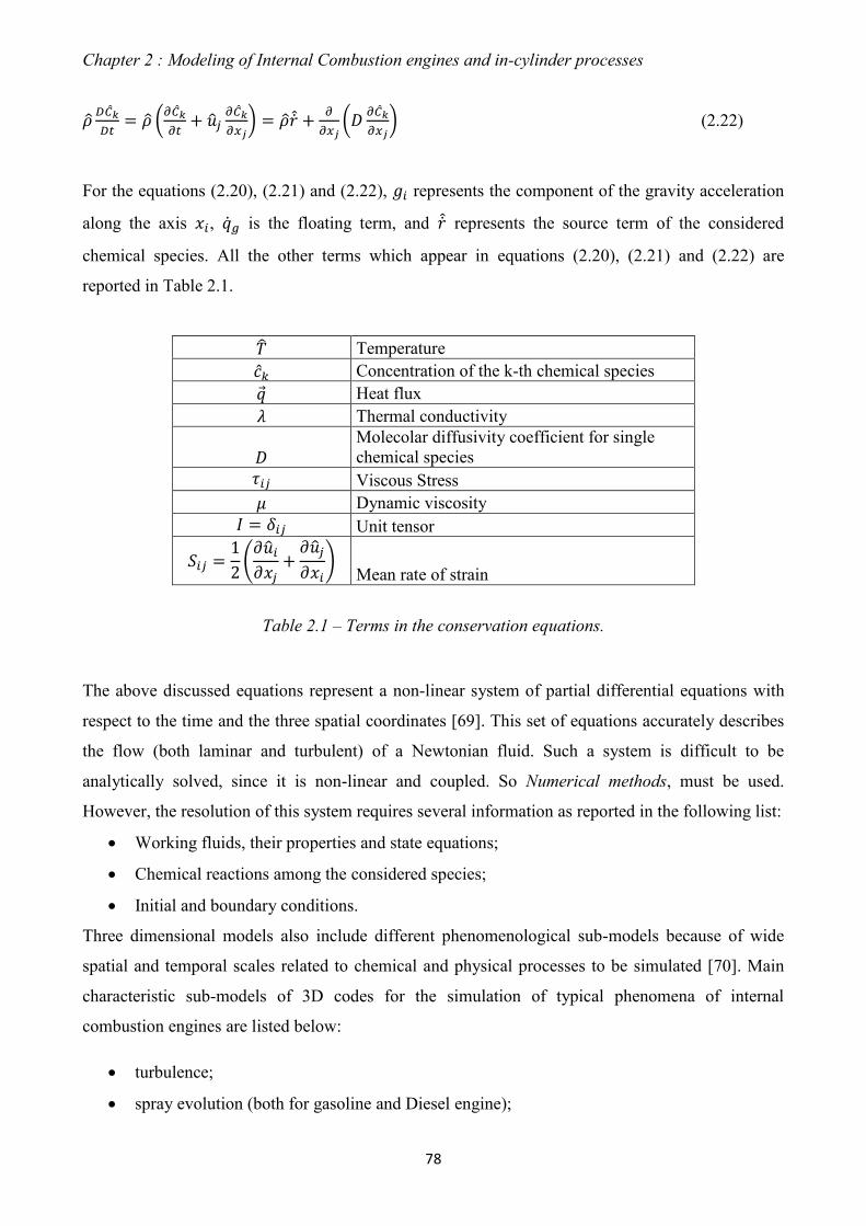
Chapter 2 : Modeling of Internal Combustion engines and in-cylinder processes
78
(
)
(
) (2.22)
For the equations (2.20), (2.21) and (2.22), represents the component of the gravity acceleration
along the axis , is the floating term, and represents the source term of the considered
chemical species. All the other terms which appear in equations (2.20), (2.21) and (2.22) are
reported in Table 2.1.
Temperature
Concentration of the k-th chemical species
Heat flux
Thermal conductivity
Molecolar diffusivity coefficient for single
chemical species
Viscous Stress
Dynamic viscosity
Unit tensor
(
)
Mean rate of strain
Table 2.1 – Terms in the conservation equations.
The above discussed equations represent a non-linear system of partial differential equations with
respect to the time and the three spatial coordinates [69]. This set of equations accurately describes
the flow (both laminar and turbulent) of a Newtonian fluid. Such a system is difficult to be
analytically solved, since it is non-linear and coupled. So Numerical methods, must be used.
However, the resolution of this system requires several information as reported in the following list:
Working fluids, their properties and state equations;
Chemical reactions among the considered species;
Initial and boundary conditions.
Three dimensional models also include different phenomenological sub-models because of wide
spatial and temporal scales related to chemical and physical processes to be simulated [70]. Main
characteristic sub-models of 3D codes for the simulation of typical phenomena of internal
combustion engines are listed below:
turbulence;
spray evolution (both for gasoline and Diesel engine);

Chapter 2 : Modeling of Internal Combustion engines and in-cylinder processes
79
combustion and knock processes;
generation of pollutant emissions.
In general, a 3D CFD analysis for a predefined system requires the definition of a proper
computational grid. Indeed, the 3D volume of interest has to be divided into a discrete number of
elements with selected shape and consequently a certain number of nodes are defined, too. In this
way, the computational mesh associated to the system under study is realized. Partial differential
equations are discretized on the computational grid, by adopting a combination of formal
integration and approximation within each volume element, in such a way to transform system of
differential equations in a system of algebraic equations. The latter system of mathematical
equations is solved through a proper iterative numerical algorithm. For 3D CFD analyses,
computational grid generation represents a relevant step during pre-processing phase. Indeed 3D
results are affected by the resolution of the computational grid. A fine mesh which presents a high
number of nodes and elements allows for accurate solutions but conversely it involves greater
computational efforts or high performance workstation. For these reasons, in general, a preliminary
grid invariance analysis has to be perfomed with the aim to select a proper mesh for the analyzed
system which simultaneously shows an acceptable computational effort and a good accurancy for
numerical findings. The computational grid has to be realized by taking into account, in addition to
the geometrical features of the considered system, the characteristics related to the system
operation, too. For instance, if the examined system does not present moving parts a static mesh has
to be properly realized. On the other hand, dynamic grid has to be employed to simulate moving
computational domains. The latter case is usually for the simulation of ICE phenomena such as the
in-cylinder flow field and processes, turbocharging group operation, etc. A moving mesh takes into
account the the motion of certain boundaries which refer to moving mechanical parts. As an
example, in the case of simulation of the in-cylinder processes a moving grid allows to consider the
motions of intake and exhaust valves and the piston motion. In the case of moving mesh, the
computational domain for the numerical integration of the above discussed equations is
continuously modified. In order to avoid a greater cells deformation a mesh upgrade during the
simulation is mandatory. The updating operation mainly consists in a new distribution of cells and
this process is well known as “rezone” of mesh. 3D code geometrically interpolates the different
generated grids allowing the continuous deformation of the mesh. In addition, during the rezone
process a re-mapping of numerical variables on the new grid is realized. Summarizing a dynamic
mesh requires particular attention to be properly realized with respect to the generation of a static
mesh. Referring to the definition of the fluid-dynamic problem before starting with the running

Chapter 2 : Modeling of Internal Combustion engines and in-cylinder processes
80
phase, proper selection of surfaces is needed in order to define the boundary conditions.
Computational domain has to be associated to a well defined fluid, the desired phenomenological
sub-models have to be enabled to describe fluid-dynamic processes of interest and the case under
study requires a proper fluid-dynamic initialization. Finally, an appropriate solution method has to
be selected for the numerical integration of Navier Stokes equations.
2.2 Integration of Modeling Approaches: 1D/3D methodology
For the numerical simulation of ICEs behavior, as discussed before, several modeling approaches
can be adopted according to the analysis type, the desired results and their level of detail. During
the last years, three-dimensional codes have been more and more used to describe various thermo-
fluidynamic processes, allowing for detailed and accurate prediction of fluid-dynamic conditions
within the intake and exhaust manifolds and engine cylinders. In particular, 3D analyses are very
helpful to study the in-cylinder phenomena, including turbulence and combustion processes, ab-
normal combustion (knock phenomenon), fuel spray evolution, fuel evaporation, mixing process
and pollutant species generation. Even if 3D CFD models allow to be closer to the actual engine
fluid-dynamic behavior, they still require high computational times, which grows with the engine
dimensions, making the considered models not compatible with the development phase of ICEs. For
this reason, the employment of a sole 3D CFD model for ICEs is limited to few cases and oriented
to better understanding the physical phenomena and to find information which cannot be easily
obtained with the experimental tests. On the other hand, 0D/1D models allow to describe the whole
engine system (including external sub-systems such as turbocharger) with reduced computational
times and satisfactory accuracy. With this modeling approach, virtual analyses of new engine
configurations can be performed. The main drawbacks of 0D/1D models are usually represented by
the description of the in-cylinder phenomena, because an inadequate formulation of in-cylinder
processes (especially for combustion process) leads to not correct assessment of engine
performance and engine-turbocharger matching. A very promising numerical methodology showing
the potentialities to support the engine development phase and to overcome the limits of both
0D/1D and 3D models, is represented by a proper integration of these types of models. The role of
each model within the integrated 0D-1D/3D methodology is univocally identified. As an example, a
brief description of an integrated procedure for the simulation of SI ICEs performance is here
reported and it is adopted within this work. The considered integrated method requires, as the initial
step, the engine geometrical data provided by the manufacturer. They are used to build the 1D

Chapter 2 : Modeling of Internal Combustion engines and in-cylinder processes
81
model of the whole engine and to carry out preliminary 1D simulations under motored operations.
Then, multi-cycle motored 3D analyses, applying 1D computed time-varying pressure and
temperature traces as boundary conditions, are performed. Detailed information about the in-
cylinder mean and turbulent flow fields are extracted from the 3D analyses over a whole engine
cycle. The results obtained by the latter analyses are utilized to calibrate a 0D turbulence model
coupled to a proper phenomenological combustion model, which will be discussed in detail in the
following paragragh. Once the turbulence sub-model is tuned, the 1D engine simulation is carried
out under fired operations. The combustion process description is properly linked to the previously
tuned in-cylinder turbulence model. The combustion model is tuned in order to fit the in-cylinder
pressure cycles at full load operation. Once validated, the 1D model is capable to reproduce the
engine perfoemance and it can be employed for further numerical analyses, including the
description of knock occurrence and cycle-by-cycle variations. In Figure 2.2, a flowchart of the
described integrated 1D/3D methodology is fully summarized.
Figure 2.2 – Flowchart of the integrated 1D/3D hierarchical methodology.

Chapter 2 : Modeling of Internal Combustion engines and in-cylinder processes
82
2.3 0D Combustion Modeling: “Fractal Combustion Model”
Fractal Combustion Model is a phenomenological 0D model, based on the fractal description of the
flame front and it is able to sense both the combustion system geometry and the operating
parameters, such as air-to-fuel ratio, spark advance, boost level, residual gas content etc. This model
is capable to take into account the in-cylinder turbulence evolution thanks to a proper 0D turbulence
sub-model. Referring to the 0D combustion modelling, in the wrinkled-flamelet regime of
combustion occurring inside an ICE [71], [72], [73], the burning rate can be expressed as:
.
/ (2.23)
ρu being the unburned gas density. Equation (2.23) puts into evidence that the burning rate is mainly
increased by the wrinkling of the flame surface AT determined by the turbulent flow field, with
respect to the corresponding smooth surface AL, occurring in a laminar combustion process. Flame
propagation indeed locally proceeds at the stretched laminar flame speed, SL, which is a function of
the fuel type, air-to-fuel ratio and residual gas fraction. The employed correlation also accounts for
flame stretch mainly occurring during the first phase of burning process [74]. Under this
schematization, moreover, the burning rate can be easily computed once the increase in flame area
has been established. Basing on the concepts of the fractal geometry, the latter can be easily
expressed as a function of a minimum and maximum flame wrinkling scales, Lmin-Lmax, and to its
fractal dimension D3 as reported in equation (2.24):
.
/
(2.24)
Lmin is assumed equal to the Kolmogorov length scale, which, under the hypothesis of isotropic
turbulence, follows the expression (2.25):
(2.25)
u being the kinematic viscosity of the unburned mixture. The turbulent intensity and the integral
length scale LT are given by the K-k model described in the following. Lmax, indeed, representing the
dimension of the maximum flame front wrinkling, is related to some characteristic dimension the

Chapter 2 : Modeling of Internal Combustion engines and in-cylinder processes
83
flame front, such as the flame radius or the square root of the laminar surface. In the present version
of the model, the latter choice is followed, and the Lmax is computed according to equation (2.26):
√ (2.26)
cwrk being a tuning constant. The D3 dimension only depends on the ratio between the turbulence
intensity and the laminar flame speed SL, reported in [73].
The above described fractal model is really valid for a fully developed and freely expanding
turbulent flame. During both early flame development and combustion completion, a different
approach is required. Initial flame development is in fact dominated by the kernel formation phase;
its duration is calculated by an Arrhenius-like formulation, also accounting for residual fraction
contents. At the end of the kernel formation time, the computation of the combustion process starts
with a stable and spherically-shaped smooth flame, of radius r0. Flame wrinkling process also starts
at a rate, ωwr (equation (2.27)), which increases with the normalized elapsed time after the
combustion start.
(2.27)
The transition time, ttrans, in the above equation (2.27) is hence considered as a time scale during
which the flame front evolves from an initial smooth surface – corresponding to a laminar-like
combustion – to a fully developed turbulent wrinkled flame. The transition time is assumed
proportional to a characteristic turbulent time scale, calculated as reported in equation (2.28):
(2.28)
ctrans being a tuning constant, while k and Dr are the turbulence kinetic energy and its dissipation
rate. Flame wrinkling rate ωwr affects the calculation of the maximum fractal dimension of the
flame, according to equation (2.29):
( ) (2.29)
WF being the well-known Wiebe function. In this way, the D3 expression in [73] is redefined as:

Chapter 2 : Modeling of Internal Combustion engines and in-cylinder processes
84
(2.30)
With this formulation, the first phase of the combustion process (w1~ 0) is characterized by a fractal
dimension close to 2.00, corresponding to an initial laminar burning process.
A different combustion rate is also specified when the flame front reaches the combustion chamber
walls (wall combustion phase). Wall-combustion burning rate is simply described by an exponential
decay, as reported in equation (2.31):
.
/
(2.31)
η being the characteristic time scale of the above process. The overall burning rate is consequently
defined as a weighted mean of the two described combustion rates in (2.32):
.
/ .
/
( ) .
/
(2.32)
The switch between the two combustion modes gradually starts when a threshold value, cwc, of the
burned gas fraction is reached (transition time, twc). At this time, the characteristic time scale in
equation (2.31) is computed assuming that the wall combustion burning rate equals the one derived
from the fractal model, equation (2.23), hence:
( )
( )
( ) (2.33)
The above η value is then kept fixed during the subsequent wall combustion process. The weight
factor w2 indeed increases with time, depending on the instantaneous unburned mass (m - mb),
compared to the one occurring at the transition time, twc. In this way, a smooth transition between
the two modes is easily obtained. It is important to note that the above schematization of the wall
combustion, based on the analysis of typical heat release data, does not include any additional
tuning constant. Finally, two corrections are introduced in the turbulent flame front area calculation,
as shown in equation (2.34):
.
/
, ( )- 0
1 (2.34)

Chapter 2 : Modeling of Internal Combustion engines and in-cylinder processes
85
Ka in the above equation is the Karlovitz number which is computed as reported in equation (2.35):
(
)
(2.35)
f being the flame front thickness. The first correction accounts for the enhanced species mixing in
the flame front and is activated only when the Ka > 1 inequality verifies. In this case, in fact, the
flame thickness is larger than the Kolmogorov turbulence micro-scale and turbulent eddies are able
to enhance the burning speed. This verifies in the case of high turbulence levels (high engine speed)
or slow laminar flame speed (large amount of trapped EGR, very lean or very reach mixtures, for
instance). Simultaneously, at very high Karlovitz numbers, the flame deformation determined by
the turbulent flow field can be so intense to produce a multiple connected flame front, with
“islands” of unburned mixture trapped within the burned gas zone. This is mainly due to the
increased convective action of the turbulent field, that can stretch and break the flame, determining
pockets of unburned mixture within the burned gas zone. As a consequence, the reaction surface
and the burning speed increase.
The second correction term is justified by the possibility of a flame front distortion, that may occur
when an intense mean flow is present in the cylinder. Each term is weighted by additional tuning
constants, and .
2.4 Turbulence modeling in 3D codes: RANS technique and k-ε model
As said before, the description of the turbulent flow fields inside internal combustion engines is
obtained through the solution of Navier Stokes equations, as well. Regarding the turbulent flows,
various resolution methods are available and adopted according to the simulation application. To
this aim, three turbulence modeling approaches can be identified:
Direct Numerical simulation (DNS): it represents the most detailed approach, since it
resolves the complete equations locally and without any modeling for the reactive flows.
This approach requires a very high number of grid points and accurate schemes for
numerical discretization. DNS approach is rarely adopted into the industrial sector, due to its
very high computational costs. Consequently, DNS is limited to university research to
reproduce very difficult experimental tests and to understand the involved physical
phenomena.
Reynolds Averaged Navier Stokes (RANS): it is an enesemble average approach, based on

Chapter 2 : Modeling of Internal Combustion engines and in-cylinder processes
86
the assumption that the flow field variables can be expressed as a sum of mean value and the
fluctuation value. The ensemble average method is applied to the usual Navier Stokes
equations and consequently additional terms containing the fluctuation value appears and
need to be modeled. Since every length scales of turbulence is modeled, RANS technique
offers a correct description of the mean flow field with a relatively low computational needs.
For these reasons, RANS is well suited for industrial use.
Large Eddy Simulation (LES): this technique offers a compromise between computational
efforts and description of physical phenomenon. In this case, Navier Stokes equations are
solved for large eddies while small eddies are modeled. Indeed, large scale eddies are highly
anisotropic and so difficult to be modeled while small scale eddies enhance the dissipation
and they may be modeled similarly to the RANS approach. LES technique is capable to
furnish a description of the flow field close to the DNS response but the computational time
is close to the RANS technique. Anyway, LES calculation still remains expensive for
industrial practice.
The above classification highlights that the RANS approach is the most simple one and it is widely
utilized for the study of the mean flow characteristics of turbulent flow inside the ICEs. For this
reason, among the discussed turbulence modeling techniques, RANS model is here analyzed in
more detail with respect to the other models. According to Reynolds decomposition, the
mathematical description of turbulent flow field is obtained by expressing the single instantaneous
property (i.e. velocity, pressure, density, temperature, etc.) as sum of mean part Ω and the
fluctuation part ω:
(2.36)
where the mean part is defined by the integral:
( )
∫ ( )
(2.37)
where δt is a sufficiently long interval of time compared to the fluctuation period of variable Ω.
According to the Reynolds decomposition the instantaneous velocity, temperature, pressure and
enthalpy are expressed as follows:

Chapter 2 : Modeling of Internal Combustion engines and in-cylinder processes
87
(2.38)
The well known Reynolds-averaged equations can be obtained by applying the averaging operation
to mass, momentum, energy and chemical species equations. The latter are reported below:
Averaged mass equation in the case of incompressible flows:
(2.39)
Averaged Momentum equation:
( ) (2.40)
Averaged energy equation:
(
)
( )
(
) (2.41)
Averaged equation for single chemical species:
(
)
(
) (2.42)
where the terms of diffusive transport due to the turbulence are represented by:
turbulent stress tensor
turbulent heat flux vector
turbulent mass flux vector of the individual chemical species
It can be noted that the above Reynlods averaged equations contain unknown variables as a
consequence of the averaging operation [69]. In order to close the set of equations, these variables
require additional equations to derive the solution for the turbulent flow field. This issue is well
known as “Turbulence closure” problem. Further algebraic or differential equations have to be
added to the Reynlods averaged equations. A set of mathamatical equations involving the unknown

Chapter 2 : Modeling of Internal Combustion engines and in-cylinder processes
88
variables, resulting from the averaging operation, is usually called closure model for the turbulence.
Two different types of closure models are mainly adopted:
First Order closure models, i.e. Eddy Viscosity/Diffusivity Models (EVM);
Second Moment Closure models (SMC).
Concerning the first order closure models, the turbulent stress tensor depends on the turbulent
viscosity (the so called Eddy viscosity) and on the gradient of average velocity; for the second order
closure models, transport equations are solved for the individual turbulent flux of momentum and
scalars which appear in the mean flow equation. Second order models are expensive with respect to
the first order models. Consequently, the latter models are often employed for 3D CFD simulations
of turbulent flows in many industrial applications, including the automotive ones. Even if various
forms of eddy viscosity model exist, the widely adopted is represented by the two equations
Standard k-ε model. In this case, transport equations for turbulent kinetic energy k and dissipation
rate ε are solved. The equations of Standard k-ε model can be applied for near equilibrium flows
and characterized by high Reynolds numbers:
(
) (2.43)
.
/
(
) (2.44)
P represents the term of production of turbulent kinetic energy k, due to the deformation of the
mean flux [69], G is the production or destruction of turbulent kinetic energy k due to mass forces
(gravity):
, ( ) -( ) (2.45)
(2.46)
S represents the strain tensor. Finally, the constant values of k-ε model are recommended by
Launder and Spalding (1974) and they are reported in Table 2.2.
Cμ Cε1 Cε2 Cε3 Cε4 ζk ζε ζρ
0.09 1.44 1.92 0.8 0.33 1 1.3 0.9
Table 2.2 – Constants of k-ε turbulence model.

Chapter 2 : Modeling of Internal Combustion engines and in-cylinder processes
89
2.4.1 0D/3D hierarchical approach for turbulence modeling
It is commonly recognized that for ICEs applications, 3D turbulence models are capable to describe
the evolution of the in-cylinder flow field and the sub-sequent combustion process with good
accuracy. However, 3D models require too high computational time to analyze the in-cylinder flow
characteristics, turbulence levels and the engine performance for the whole operating domain. On
the other hand, this task is easily accomplished by 1D codes, where, the combustion process is
usually derived from experimental in-cylinder pressure measurements (Wiebe correlation). This
method is poorly predictive for the simulation of operating conditions relevantly different from the
experimental ones. To overcome the above issue, 1D code has to include enhanced physical models
for the description of in-cylinder turbulence evolution and combustion. Referring to the
phenomenological turbulence sub-model to be implemented in 1D engine model, once it has been
fully developed, a proper tuning is required. To this aim, reference in-cylinder turbulent variables
are needed and they are not easily derived by experimental tests. On the contrary, the turbulence
phenomenological model can be validated against in-cylinder results provided by 3D CFD analysis
carried out for a limited number of engine operating conditions. In the latter case, a hierarchical
1D/3D approach for the description of in-cylinder turbulence is identified. Indeed, information from
3D CFD analyses, in terms of temporal evolution and spatially averaged in-cylinder flow fields,
both mean and turbulent, are utilized to set-up and calibrate the phenomenological 0D turbulence
model. The discussed methodology, once tuned, shows the potentialities to accurately estimate the
temporal evolution of the in-cylinder turbulence according to the engine operating conditions with
reduced computational time.
2.5 0D Turbulence modeling: K-k model
A 0D turbulence model aiming to syntetize very complex 3D phenomena based on the assumption
that turbulence is both homogenous (i.e. equally distributed in the space) and isotropic (i.e. without
a preferential direction in space). Several 0D turbulence models are available in the technical
literature. The so called K-k model family describes the energy cascade mechanism from the
average flow field kinetic energy (K) to the turbulence fluctuation kinetic energy (k) by an ordinary
derivative two-equation system [75]. In other cases, macro-scale kinetic energy is imposed [76],
while balance equations are solved for the turbulence fluctuation kinetic energy and the dissipation
rate [77], [78]. Further approaches require the computation of the ordinated flow fields (swirl and

Chapter 2 : Modeling of Internal Combustion engines and in-cylinder processes
90
tumble), apart from the turbulent kinetic energy and the dissipation rate [79], [80]. Referring to K-k
turbulence model, it describes the temporal rates of the mean and turbulent kinetic energies as
reported in equations (2.47), (2.48):
.
/
(2.47)
.
/
(2.48)
The first term in both equations accounts for the kinetic energy produced by the flow through the
valves (both intake and exhaust). PK and Pk represent the K decay and the k production term,
respectively. In both the equations, the third term accounts for the kinetic energy production due to
the piston motion close to compression TDC; in particular, in equation (2.47), this term mimics the
tumble macro-vortex compression responsible for the increase of the mean-flow velocity, while, in
equation (2.48), it simply describes an isotropic compression according to the theory [81], [82]. The
compression terms are multiplied by the constants, ctumb, K and ctumb,k , respectively. They depend
on a single tuning constant, ctumb, and on the maximum valve lift, hmax according to:
(2.49)
The fourth terms accounts for the convective flow through the exhaust valves. Last term in equation
(2.47) takes into account the effects of piston motion, at velocity upist, on the mean flow field. As
shown below, this contribution is relevant especially during the expansion stoke, while in the
remaining portion of the cycle it is masked by the other effects. The D term in equation (2.48) is the
dissipation rate of k into heat, derived as follows:
(2.50)
LT being the integral length scale. The production term related to the flow through the valves in
equation (2.47) is calculated as:
.
/
.
| |
/
(2.51)

Chapter 2 : Modeling of Internal Combustion engines and in-cylinder processes
91
being , , , and the mass flow rates and the flow speeds through the intake and the
exhaust valves, respectively. The above terms are taken into account only when the gas flows from
the ports towards the cylinder (i.e. direct intake flow and reverse exhaust flow). Direct flow through
the exhaust valve is indeed considered in the last term, with reference to an exhaust flow related
mean velocity , evaluated as follows:
(2.52)
Concerning the equation of turbulent kinetic energy (2.48), the valve related production term is
more simply computed as:
.
/
.
| |
/ (2.53)
, and parameters in equations (2.51) and (2.53) are tuning constants; the only one given
as an input is , while the others are derived from:
(2.54)
The terms PK and Pk are calculated according to:
(2.55)
and being additional tuning constants. tK and tk are the characteristic time scales of K
decay and of k production, evaluated as:
(2.56)
Previous investigations [26] showed that the time evolution of the integral length scale LT is only
slightly depending on engine operating conditions. It can be hence prescribed as an assigned
sequence of Wiebe-like functions (see 0D turbulence model validation in chapter 3). The control
points of these equations are given as an input; they represent additional tuning constants for the
turbulence model.

Chapter 2 : Modeling of Internal Combustion engines and in-cylinder processes
92
As said before, information from 3D CFD analyses, in terms of the in-cylinder mean and turbulent
flow fields, are utilized to set-up and calibrate the examined turbulence model. In particular, the
mass averaged integral length scale, specific turbulent kinetic energy and mean flow kinetic energy,
equation (2.57) are calculated all over the 3D domain.
∑
∑
∑
∑
∑
∑ (2.57)
i, Vi, Ui, ki, and LT,i are the density, the volume, the mean flow velocity, the specific turbulent
kinetic energy and the integral length scale within the i-th cell, respectively. LT,i is defined as a
function of the local dissipation rate i, while the mean flow velocity accounts for its three local
components, ui, vi, wi:
√
(2.58)
In order to compare 3D and 0D results, the following 3D-derived mean flow and turbulent velocities
are defined:
√
√ (2.59)

Chapter 3 : Engine Model Validation
93
CHAPTER 3
Engine Model Validation
3.1 0D-1D Models Description
A one-dimensional model of the considered engine has been developed with the aim to faithfully
reproduce the behavior of different engine parts. The commercial software adopted for 1D fluid-
dynamic simulation of the considered engine is the well-known GT-PowerTM
software of Gamma
Technologies. Single parts of the engine system will be deeply described in the following, including
intake/exhaust sub-systems, turbocharger group, intercooler, injection system, cylinders, valves and
User Subroutines. The latter have been employed to include the user sub-models within the whole
engine model.
3.1.1 Air Intake System
As shown in Figure 3.1 the „Air Intake system‟ is made up of the elements between the external
ambient and the Compressor inlet. The considered system is reproduced by:
the intake (ambient) environment with air temperature at 20°C;
seven pipes located upstream the air-filter box; they allow the ambient air to be introduced
into the filter box component;
air-filter box, which is modeled by two “Flow-Split” objects (IN and OUT);
five pipes, located downstream the filter box (convergent section up to the Compressor
inlet). They allow the clean air to be elaborated by Compressor.

Chapter 3 : Engine Model Validation
94
Figure 3.1 – Air Intake System including the filter box.
3.1.2 Compressor
The air flow is introduced at Compressor inlet through a proper air intake system described before.
Compressor performances are reproduced by adopting a “Map Based” approach. In particular, the
experimental compressor maps, in terms of pressure ratio (Figure 3.2a) and efficiency (Figure 3.2b)
as a function of corrected mass flow rate are specified for this component by “Map object attribute”.
As known, a proper mechanical link between Compressor and Turbine components is considered
through the object named „Alberino Turbo‟ (Figure 3.3).
Figure 3.2 – Compressor pressure ratio map (a) and Compressor efficiency map (b).

Chapter 3 : Engine Model Validation
95
Figure 3.3 – Turbocharger group schematization.
3.1.3 Intercooler
The air compression involves an increase in the air temperature and a reduction in the air density. In
addition, the exhaust gas processed by the turbine causes a further increase in the air temperature
within the intake system, because of the heat exchange. Consequently, a reduced engine filling has
to be expected. Intercooler represents a system which allows for a reduction in the air temperature,
through a proper cooling circuit. Consequently, an increase in the air density and improved engine
filling performances are obtained. The engine model includes an intercooler device which is
properly schematized. The inlet and outlet pipes of intercooler object are modeled, too. Inlet pipes
connect the compressor outlet to the intecooler while the outlet pipes allow the intake manifold to
be reached by the air flow. The actual intercooler is schematized as a simple pipe of rectangular
section, presenting a wall temperature equal to 50°C.
3.1.4 Intake Manifold and Runners
The air flow at intercooler outlet is introduced within the intake manifold through the throttle valve.
The latter presents a reference diameter of 57.5 mm while the throttle angle can be controlled in
order to obtain a prescribed load level. For this type of engine, load level can be also adjusted by
controlling the intake valve lift profile. The intake manifold located downstream the throttle valve is
schematized by two volume elements (named “FarfallaRunner” and “Runner2”), presenting 0.85
liters and 0.67 liters, respectively. In addition, proper Runners (named Runner1_1, Runner1_2,
Runner2_1, Runner2_2) allow the air flow to be directed towards the engine cylinders. Runners

Chapter 3 : Engine Model Validation
96
showed in Figure 3.4 are characterized by converging section and each of them presents a total
length equal to 34 mm.
Figure 3.4 – Intake Manifold and Runners.
3.1.5 Intake pipes and Fuel Injectors
Fuel injection is realized within the intake system through proper injectors, located at junction
elements (named “FSAsp_IT_R1” and “FSAsp_IT_R2” in Figure 3.5) for the pipes at cylinder
entrance. Starting from the single junction element, the gas flow is splitted in two different intake
pipes, allowing the air-fuel mixture to enter into the cylinder. For the single injector (named
„Iniettore‟), the following parameters have to be specified: average speed of injection, air-to-fuel
ratio, injection timing angle, fuel temperature (equal to 50°C), type of fuel and fraction of vaporized
fuel.
Figure 3.5 – Intake Pipes and fuel injectors.

Chapter 3 : Engine Model Validation
97
3.1.6 Engine Cylinders and Intake/Exhaust Valves
As stated before, the engine under study presents a port fuel injection system and once the air-fuel
mixture is formed, thanks to the interaction of the air flow with the injected fuel, it is introduced
into the cylinder through intake valves while the exhaust gases are discharged by exhaust valves. As
shown in Figure 3.6, two intake and exhaust valves are specified for each cylinder. Cylinders and
valves allow the engine thermodynamic cycle to be realized.
Figure 3.6 – Engine cylinders and valves.
Concerning the intake valves, the reference diameter (diameter equal to 26 mm) and the lift profile
have to be specified. Since the examined engine is equipped with a VVA system at the intake side,
the intake valve lift profile is defined through a proper „user model‟ named “ValveLift”. Instead, the
exhaust valves present fixed valve timing and a lower reference diameter (21.5 mm). Referring to
the cylinder object, turbulence, combustion, heat transfer, fuel evaporation and knock models have
to be defined. All the above models represent user sub-models.

Chapter 3 : Engine Model Validation
98
3.1.7 Exhaust system and Turbine Object
As shown in Figure 3.7 the exhaust gases, coming out from the valves of each cylinder, are
introduced into the exhaust manifold through two pipes. Each exhaust pipe is schematized by two
elements (as an example, “ScaIT_R1_DX” and “ScaIT_R1_DX-1” for cylinder #1). The exhaust
manifold allows the flow connection of two exhaust branches in order to direct the exhaust flow at
turbine inlet through a single pipe named „MonteTurbo‟.
Figure 3.7 – Exhaust Manifold and Turbine.
Similarily to the Compressor object, turbine performances are modeled by adopting a “Map Based”
approach. The reduced turbine maps in Figure 3.8 are obtained by experimental tests and they are
employed within the 1D engine model. Turbine model shows flow connections, the mechanical link
with Compressor object and the connection with the Waste-gate valve controller. The latter is
utilized to adjust the waste-gate diameter in order to reproduce the experimental value of the in-
cylinder peak pressure in WOT operation. Instead, at part load operation the prescribed load level is
obtained by controlling the throttle valve angle.

Chapter 3 : Engine Model Validation
99
Figure 3.8 – Turbine pressure ratio map (a) and turbine efficiency map (b).
3.1.8 Model Subroutines
1D engine model presents different UserSubroutines, whose output are used both during data
processing both during simulation phase. UserSubroutine object allows the model to invoke an
externally developed routine. It is adopted to transfer the processed signals between GT-Power
model and routines. Routine input signals can be control signals or parameters defined in the object
UserModel. Output values of UserSubroutine can be sent to other control objects or to RLTcreator.
Figure 3.9 – Model Subroutines.

Chapter 3 : Engine Model Validation
100
The above Figure 3.9 shows the Subroutines reported in the model. They recall the fractal
combustion model and the corresponding data are sent to other objects to be processed. In
particular, these Subroutines allow to evaluate several parameters, including characteristic
combustion angles, burned mass fractions at the above angles, burn rate
, knock index, angle of
knock occurrence, volume chamber at knock occurrence Vknock, mass fraction which instantly burns
at knock occurrence, burned gas temperature , unburned gas temperature , etc.
3.2 0D Turbulence model validation
Turbulence model is tuned against 3D-CFD motored findings for different speeds and intake valve
closure angles typical of full and part load operations, as well (Table 3.1).
Case Number Engine speed, rpm Intake valve closure angle, deg after CTDC
Label
1 2500 560 2500FL
2 5100 548 5100FL
3 2000 462 2000PL
4 3000 448 3000PL
Table 3.1 – Tested engine points.
First of all, a reliable time evolution of the integral length scale must be assigned. This is done by
employing a sequence of Wiebe-like functions passing through specified control points. In
particular, 3D results show that the mass averaged LT, starting from a very low TDC level, LT3,
continuously increases during the intake stroke and reaches its maximum during the compression
stroke. The location of the above maximum is prescribed in the 0D model in terms of angular
position, , and height, LT2. Then, the integral scale reduces, reaching a minimum at the
compression TDC (LT1). During the expansion and exhaust strokes, LT mainly follows the in-
cylinder height above the piston, increasing once again up to the LT2 level at the expansion BDC and
reducing down to the LT3 level at the valve overlap TDC.
Figure 3.10 shows the above described phases, connected through a sequence of Wiebe-like
functions. Parameters LTj, (j=1, 2, 3), and represent of course, further unknown constants.

Chapter 3 : Engine Model Validation
101
Figure 3.10 – Integral length scale reconstruction.
LT1 1.3 mm LT2 3.25 mm LT3 0.2 mm 120 deg
cin 0.7 ctumb 0.19 cpkey 0.03 cpkap 0.05
Table 3.2 – Optimal values of turbulence model constants.
Once the integral length scale is formally identified, each tuning constant of the 0D model has to be
set to fit the actual results provided by the 3D-CFD calculations [83]. Through a simple trial and
error procedure, a single set of optimal constants is selected as listed in Table 3.2.
It is not worthless to emphasize that, for all the considered cases, the tuning constants are kept
unchanged to demonstrate the generality of the proposed model.
Figure 3.11 shows the comparison between 3D and 0D results, for the integral length scale and for
all the operating points. For sake of clarity, the attention is focused on the intake, compression and
half expansion stroke portion of the cycle. The agreement is satisfactory for all the cases. It is
confirmed that the trends of 3D computed integral length scale depend only slightly on the engine
operating conditions, especially in the neighbourhood of the compression TDC. This allows the use
a unique LT reconstruction for all the considered operating points.

Chapter 3 : Engine Model Validation
102
.
Figure 3.11 – 0D/3D comparison of the integral length scale.
Figure 3.12 highlights that the proposed model is able to forecast the in-cylinder turbulence levels
during the combustion relevant portions of the cycle, i.e. intake, compression and expansion phases.
This mainly depends on the model capability to sense the different durations of the intake phases for
the considered cases. The different turbulence levels at the compression TDC are very well
predicted thanks to the compression term in turbulent kinetic energy equation, which properly
accounts for the different valve lift profiles, mainly through the maximum lift correction term
included in the definition of the tuning constant ctumb,k.
The turbulence fluctuation (Figure 3.12) and the mean flow velocity (Figure 3.13) are normalized
with the piston mean speed.
Since equations of 0D turbulence model are strongly coupled, it is also important to verify the
accuracy in the prediction of the mean flow velocity, reported in Figure 3.13. It can be appreciated
that a good agreement is reached, especially during the compression and expansion strokes.

Chapter 3 : Engine Model Validation
103
…
Figure 3.12 – 0D/3D comparison of the dimensionless turbulence fluctuation.
Figure 3.13 – 0D/3D comparison of the dimensionless mean flow velocity.

Chapter 3 : Engine Model Validation
104
Concerning the compression stroke, the density-dependent term of the equation for mean kinetic
energy is able to capture the local maximum before TDC, while the local maximum during the
expansion is described by the term related to the piston movement.
Simultaneously looking at Figure 3.11, Figure 3.12 and Figure 3.13 it is demonstrated that the 0D
turbulence model successfully describes the energy cascade mechanism from the mean to the
turbulent flow and it represents the basis for an accurate development of the combustion model.
3.3 Engine Model Tuning at Full Load Operation
The operating parameters given as an input to the GT-PowerTM
engine model are the intake valve
closure, the A/F ratio and the spark advance. Since information about the experimental turbine
waste-gate valve openings are not available, the latter have to be indirectly evaluated using a PID
controller and a target experimental datum, like the boost level, the mass flow rate or the
turbocharger speed. The adoption of the experimental boost level may introduce some inaccuracies
in the simulations, since at low-speed/full-load the compressor operates in close-to-surge map
region, where iso-speed slopes are very reduced. Consequently, the map-derived mass flow rate
cannot be precisely identified. On the other hand, the experimental mass flow rates or the
turbocharger speeds are usually affected by higher uncertainties. For this reason, an alternative
strategy is proposed, aiming to identify the waste-gate opening realizing the experimental pressure
level at the firing TDC for the cylinder #2. This level is in fact representative of the actual in-
cylinder filling conditions since, at full-load, the combustion process, to avoid knocking
combustions, always begins after the TDC. The proposed strategy provided the best agreement with
experimental data.
cwrk 0.5 ctrans 0.4 cwc 0.8 cenh1 0.5 cenh2 0.1
Table 3.3 – Combustion model tuning constants.
Results shown in Figure 3.14 are obtained after the tuning of the combustion model parameters
(Table 3.3). They are kept constant for each analyzed operating condition. In particular, the Figures
show the numerical/experimental comparison in terms of brake power, brake torque, air mass flow
rate, BSFC and turbocharger speed. The agreement of the engine overall performance is
satisfactory, with the exception of the higher engine speeds. This is probably due to uncertainties in
the Amesim-computed lift profiles, affecting the volumetric efficiency and the pumping work. In

Chapter 3 : Engine Model Validation
105
addition, because of the two-cylinder arrangement, large mass flow rate and pressure ratio
oscillations are expected. Engine-turbocharger matching is hence a critical issue for this engine,
since a strongly unsteady operation is expected for the turbocharger. This may also affect BSFC
predictions at higher engine speeds.
..
Figure 3.14 – Engine performance at full load: 1D numerical/experimental data comparison.
Figure 3.15 – Borghi Diagram.

Chapter 3 : Engine Model Validation
106
In order to verify that model results are consistent with the theoretical hypotheses, the combustion
regime establishing at different engine speeds is analyzed. This can be accomplished looking at two
typical dimensionless parameters extracted from the simulations, namely the ratio between the
integral length scale and the flame thickness, LT /δf, and the ratio between the turbulent intensity and
the laminar flame speed, u’/SL. These parameters are reported on the well-known Borghi Diagram
in Figure 3.15, identifying the different combustion regimes occurring at different Reynolds,
Karlovitz and Damkholer numbers, [84].
Figure 3.16 – Numerical/Experimental comparison of the in-cylinder pressure cycle and burn rate.
It is verified that, at each speed-load condition, the instantaneous trajectory on the Borghi plane
always belongs to the wrinkled-flamelets regime, with the exception of the highest speed, where a
local Ka > 1 value may occur at the beginning of the combustion process. At spark time, in fact, u‟
4400
rpm
5100
rpm
4000
rpm
3000
rpm
1800
rpm
2500
rpm

Chapter 3 : Engine Model Validation
107
is still high, while SL is reduced, due to intense flame stretch at small flame radius. Correction in
equation (2.34) roughly takes into account the above phenomena.
Figure 3.16 shows the experimental/numerical comparison of pressure cycles and burn rates for
various engine speeds, during the compression and combustion/expansion phases. Especially at low
engine speeds, the spark timing occurs late after the TDC, determining the displayed double-peak
pressure cycles; this choice, although hardly penalizing IMEP and BSFC, is necessary to avoid
knocking occurrence. Anyway, the accuracy of the in-cylinder pressure cycle prediction is very
high. Burn rates are also very well predicted, and the model properly describes the initial and the
final combustion evolutions.
3.4 Engine Model Validation at part load
After the above described tuning process at full load, the capability of the model in predicting the
engine performance in terms of BSFC at part load is tested. In this case, the simulations are carried
out by imposing the experimentally actuated spark advance, the air-to-fuel ratio and the early intake
valve strategy (EIVC). The latter is qualitatively depicted in Figure 3.17. As can be observed, the
advanced closure is also coupled to a reduction of the maximum lift, with respect to the Full-Lift
profile (lost-motion principle).
Figure 3.17 – EIVC valve lift profile.
The waste-gate opening is instead automatically selected by a PID controller aiming to reproduce
the measured turbocharger rotational speed, while the throttle opening targets the predefined loads.
Figure 3.18, Figure 3.19 and Figure 3.20 show the fuel consumption variation against the BMEP,
for different engine speeds. It can be observed that the numerical results are in a very good

Chapter 3 : Engine Model Validation
108
agreement with the measurements, especially for the low-medium loads. Thanks to the EIVC
strategy, the fuel consumption levels are substantially low and they only increase at very low loads.
This is mainly due to a more relevant incidence of the pumping losses, and to a worsening of the
combustion process efficiency, as well. The reduced intake phase duration (Figure 3.17) in fact
produces a moderate turbulence level at the compression TDC, coupled to the well-known syringe
effect. Both affect the combustion speed, mainly during its early stage. The latter phenomena are
very well captured by the employed turbulence/combustion sub-models, as demonstrated by the
highlighted results and by the next detailed combustion analysis. The worsening of the fuel
consumption for the higher loads is indeed related to the relevant mixture enrichment necessary to
decrease the exhaust gas temperature at the turbine inlet. In addition, a further penalty is determined
by the specification of a reduced (sometime negative) spark advance, required to avoid knocking
phenomena. Also in this case, the model shows the capability to capture the described trends, except
for the engine speeds of 4400 and 5500 rpm. To further highlight the predictiveness of the
combustion model at part load operations, in Figure 3.21 the angular positions of 10%, 50% and
90% of the MFB are compared with the experimental data for an engine speed of 3000 rpm. It can
be appreciated that the combustion center is correctly forecasted by the model for all the considered
loads with a maximum error lower than 3 degrees. The combustion duration (10-90% MFB) is well
captured for the medium and higher loads, while for the lower loads it is overestimated, mainly due
to a longer combustion tail. However, as shown in Figure 3.19 for the case at 3000 rpm, this error
has a negligible effect on the fuel consumption prediction.
Figure 3.18 – BSFC vs. BMEP at 1500 rpm and 2500 rpm.

Chapter 3 : Engine Model Validation
109
Figure 3.19 – BSFC vs. BMEP at 3000 and 3500 rpm.
Figure 3.20 – BSFC vs. BMEP at 4400 rpm and 5500 rpm.
Figure 3.21 – Spark advance and 10%, 50%, 90% MFB vs. BMEP at 3000 rpm.

Chapter 4 : Experimental Knock detection and modeling
110
CHAPTER 4
Experimental Knock detection and modeling
4.1 Overview of Knock detection
It is well known that the combustion process represents a key phenomenon to be optimized during
the design phase of internal combustion engine. Indeed, engine performance in terms of power
output, fuel consumption and noxious emission are strongly affected by the development of the
combustion process. Referring to the Spark-ignition engine, combustion process has to be properly
controlled in order to avoid the abnormal combustion. Knock phenomenon arises when a portion of
the fuel charge within the combustion chamber spontaneously ignites after the spark event, but
before it has been reached by the flame front propagating from the spark plug position [23], [85].
This phenomenon most likely occurs within fuel charge particles burning late during the
combustion process (end-gas auto-ignition). The strong heat released by the sudden oxidation of the
end-gas produces a system of pressure waves moving and colliding each other within the
combustion chamber, at a frequency ranging from 6 to 10 kHz [86], [87], which is sometimes
audible (pinging knock).
knock represents one of the most difficult aspects to recognize and properly set up for the engine
control system. If left untreated or if the engine control system does not properly recognize the
knock occurrence, over time, a severe engine damage will occur. Such damage includes piston-ring
failure, piston failure and valve damage, mainly due to increased cylinder temperature / pressure
induced by a severe knock condition [88], [89], [90]. As shown in the current literature [9], different
knock suppression methods can be adopted. However a simple way to avoid knock is to bound the
compression ratio and/or the spark advance. The latter approach hardly reduces the potential in
gaining a lower fuel consumption and a higher power output. As a consequence, an ideal engine
control system has to be able to operate as close as possible to knocking, without really moving
inside it. The above consideration is remarkably true in a “downsized” turbocharged spark-ignition
engine, where the in-cylinder temperature and pressure are higher.
To avoid knock, in fact, a turbocharged SI engine always operates at full load with a particularly
rich air-to-fuel ratio and a very reduced spark advance. At low speed a negative value of the spark
advance is sometimes required (the combustion begins after the TDC). In these conditions, the

Chapter 4 : Experimental Knock detection and modeling
111
pressure cycle assumes a double-peak shape, like the one depicted in Figure 4.1. The first peak,
located at TDC, is due to volume variation during compression-expansion strokes, while the second
one is due to the combustion process. The latter hence completely develops during the expansion
stroke.
Figure 4.1 – In-cylinder pressure cycle at 1800 rpm, full load, for a turbocharged SI engine.
A negative spark advance, although hardly penalizing the fuel consumption is the only solution in
these operating conditions to limit the peak temperature and pressure during combustion and avoid
knocking occurrence. It is once again clear that the engine control system must be able to select the
maximum allowable spark advance with the smallest knock safety margin. An additional problem is
moreover related to cycle-to-cycle variations, which are commonly observed during the combustion
process of a SI engine. They mainly cause unpredictable and stochastic fluctuations in the rate of
heat release, turning in fluctuations in the in-cylinder pressure cycle. As a consequence, faster-than-
average cycles are most likely to knock. Therefore the optimal “knock-limited” spark advance must
be accurately chosen taking into account cycle-to-cycle variations [91].
From an experimental point of view, the identification of the “knock-limited” spark advance is a
complicated task, requiring the measurement of numerous instantaneous pressure cycles, at a high
crank angle resolution (usually 0.1 deg). In addition, a careful treatment of the measured data must
be performed to extract the high frequency components from each instantaneous pressure cycle
[92], [93].

Chapter 4 : Experimental Knock detection and modeling
112
The typical high frequency knock signature is related to the combustion chamber resonant
frequencies [94], excited by the knock-induced pressure wave propagation. Wave amplitudes of the
high frequency filtered pressure are used to define a great variety of knock indices [95], [96], [97].
However, these indices are affected by the pressure sensor type, by its position inside the
combustion chamber [93], [96], and by the engine operating conditions [98], [99]. Because of the
cycle to cycle variation, the knock extent is usually quantified following a statistical approach. In
fact, a certain operating condition is assumed as “knocking” when a prefixed percentage of
individual cycles (around 2-3%) is characterized by a knock index overtaking a predefined
threshold level (usually depending on the engine speed). Its determination comes out from a number
of considerations based on extensive engine calibration at the test-bench, manufacturer know-how,
durability tests, etc. However, the whole process is affected by a certain arbitrariness according to
the filtering technique and pass-band, proper definition of the threshold level, accepted percentage
of knocking cycles, etc.
A number of techniques aimed at the experimental identification of the knocking onset in Spark-
Ignition (SI) Internal Combustion Engines have been proposed and reported in the current literature.
They can be classified into two broad categories, namely direct and indirect methods. Non-
conventional techniques have been also attempted. A brief description of most popular detection
techniques is reported in the following [9].
Direct Methods – They are mainly based on in-cylinder pressure measurements and are able to
detect the typical high-frequency knock signature, related to the combustion chamber resonant
frequencies. The latter depend on radial or circumferential vibration modes, which establish at a
frequency depending on the speed of sound inside the combustion chamber and the cylinder bore.
Knock signature is identified through a proper analysis of the in-cylinder pressure signals in the
frequency domain. After being processed in a band-pass filter (4–20 kHz), the pressure signals are
rectified and processed to give proper knock indices. Among these, MAPO and IMPO indices are
frequently used [97]. The first indicator measures the Integral of Modulus of Pressure Oscillations
(IMPO). It hence accounts for the energy contained in the high frequency oscillations of the
cylinder pressure signal, which occurs due to knock. The second one indeed estimates the
Maximum Amplitude of Pressure Oscillations (MAPO). It is related to the peak of the knock-related
pressure oscillations. IMPO and MAPO can be evaluated for each cycle and are then averaged over
at least 100 consecutive cycles. Both are calculated on a prescribed crank angle window (usually
40-60 deg), starting at the spark timing. Knock occurrence is identified when IMPO or MAPO
exceed a certain threshold level.

Chapter 4 : Experimental Knock detection and modeling
113
The typical drawback of such indices is that they are sensitive to local information provided by the
pressure transducer. As knock occurs, however, huge pressure non-homogeneities take place inside
the combustion chamber [96]. So, the measured pressure wave amplitude has only a local meaning,
and cannot be considered as the maximum value of the whole combustion chamber pressure wave.
Oscillations detected by the pressure transducer actually depend on relative distance between the
sensor and the knocking sites within the combustion chamber. Amplitudes may be increased or
smoothened, due to pressure waves reflections on combustion chamber walls. In addition, the
threshold level of the knock index closely depends on engine features and operating conditions, as
well [93], [100]. Due to the short lifetime expectancy and costs of pressure transducers, direct
methods are moreover restricted to test-bench engine analyses.
Indirect Methods – Advanced signal processing techniques have been developed, as well,
employing the cylinder block vibration signals, provided by accelerometers [90]. Although
characterized by a lower signal-to-noise ratio, these sensors have a lot of advantages, in terms of
excellent durability, sensitivity and low-cost. For this reason they are becoming the most practical
solution for mass-production engines. Their application within on-board control systems requires
however the development of reliable and precise procedures, able to detect cycle-by-cycle and
cylinder-by-cylinder knocking conditions. Great care must be moreover devoted to identify the
most favorable sensor locations, especially for multi-cylinder engines.
Methods based on the exhaust gas temperature – It is widely recognized that the exhaust gas
temperature reduces in knocking conditions as a consequence of increased wall heat fluxes inside
the cylinder. Therefore the exhaust gas temperature measurement can be utilized to identify
knocking combustions. This technique, moreover, is not affected by mechanical noise, and can be
applied for all types of engines [101]. Main drawbacks are related to the need of compare the
temperature level provided by the thermocouple to the one stored in a map, representative of a
knock-free operation in the same speed, load and air-fuel ratio operating conditions.
Methods based on intermediate radicals and species analysis – Nowadays, chemical
luminescence emissions of end-gas can be used to analyze the chemical reactions caused by the
end-gas autoignition [102]. Spectroscopic and chemiluminescence measurements allow identifying
radicals as markers of different combustion phases. For instance, HCHO is built up in the unburned
gas zone, while CH and OH radicals can be markers of normal combustion reaction and burned
zone, respectively. The above measurements give the possibility to identify knocking zones inside
the combustion chamber. However, they can be only carried out in optically accessible engines, and
the related detection techniques are once again restricted to test-bench analyses.

Chapter 4 : Experimental Knock detection and modeling
114
4.2 Experimental Approaches for knock detection
As previously said, knock detection can be accomplished through different methods. In particular,
two approaches are here proposed and analyzed: MAPO and A/R techniques. In-cylinder pressure
traces are mandatory in order to utilize the above mentioned methods. For this reason,
measurements of instantaneous in-cylinder pressure cycle are realized in each cylinder of the
considered engine. As said in chapter 1, 200 consecutive pressure cycles are acquired for each
operating condition. A sampling resolution of 0.5 crank angles is adopted at each speed. A higher
sampling frequency (0.1 deg) is instead specified during combustion angular window (-10, 75 crank
angle degrees). For sake of brevity, the acquired data for a single cylinder (cyl #2) are considered.
4.2.1 Maximum Amplitude of Pressure Oscillations (MAPO) Analysis
This method of knock detection requires an high-frequency filtering of pressure traces and it allows
to evaluate the maximum amplitude of pressure oscillations (i.e. MAPO Index). The considered
knock index is defined as reported in the following equation (4.1):
(| |) (4.1)
where is the in-cylinder pressure, filtered within the crank angle window of knock occurrence (-
10, 75 degrees). For the filtering operation an high-pass filter with cut-off at 6 kHz is employed. An
overview of the results obtained for each of the 200 experimentally acquired pressure cycles
(vertical dots), is shown in Figure 4.2, at each engine speed.

Chapter 4 : Experimental Knock detection and modeling
115
Figure 4.2 – MAPO Index as a function of the engine speed.
Huge cycle-by-cycle variations of the MAPO index are obtained in each condition, while the
average level, reported as a continuous line, is always well below the maximum ones at each speed.
For a prefixed speed, the knock indicators are in many cases distributed around the most frequent
value in an almost symmetric way and without “high level” isolated points. For this reason, MAPO
analysis, for the tested conditions, does not allow to easily identify individual knocking cycles.
4.2.2 ARMA Technique
An alternative ARMA approach is applied, which was proven to better perform particularly under
soft-knock conditions [103]. Objective of an ARMA model is to predict the actual value of time
signal xt, based on its past history (AR property) and adding a prediction error (et) in the form of a
Moving Average (MA) The following equation (4.2) hence defines an ARMA model with an AR
order of n and a MA order of m:
(4.2)
An ARMA(n,m) model is hence constituted by n+m coefficients, which must be selected to
minimize the prediction error, et. Different techniques can be followed to estimate the above
coefficients. Among these, Yule-Walker functions or a least-squares polynomial regression are the
most employed ones [104]. The accuracy level of the ARMA model is then synthesized in terms of
variance of the error function, or Noise Variance (NV), defined in equation (4.3) as the sum of the
squared distances of each term in the error function series from the mean (μ), divided by the number
of samples, N:

Chapter 4 : Experimental Knock detection and modeling
116
∑( )
(4.3)
The smaller NV, the better the estimated model fits the time series. On the contrary, changes in the
variance of the prediction error identify the presence of physical phenomena altering the
characteristics of the time series. This property is here utilized to identify knocking phenomena. In
particular, the in-cylinder data represent the time series (xt), directly affected by uncorrelated
disturbances (knocking, et). Knock phenomena will cause substantial deviations of the error
function from its mean value. By monitoring the NV level, it is hence definitely possible to detect
the knock occurrence and its intensity, even in the case of incipient knocking conditions.
It must be stressed however that a suitable ARMA model should be made up of the smallest number
of adjustable parameters (n+m) that can achieve the desired accuracy. For this reason, it is very
important to also define a criterion for the selection of the optimal model orders, n and m [105],
[106]. In the present analysis, the Akaike Information Criterion (AIC) is used [107], given by
equation (4.4):
, - ( )
(4.4)
In the above definition, the first term is a decreasing function of the model orders, while the second
has an opposite trend, and represents a penalty adjustment. Since a proper ARMA(n,m) model
should realize the lowest variance with the minimum number of parameters, the AR and MA orders
reaching the lowest AIC level must be searched. In particular, the order selection is performed as
follows:
1. The ranges of the ARMA model orders to be considered are selected (e.g. 1≤n≤ nmax and
1≤m≤ mmax); in this case nmax=mmax=8;
2. For each order pair (n,m), the coefficients of the ARMA model are estimated;
3. Based on the selected AIC criterion, the prediction error variance is calculated for each
pair;
4. Finally, the (n,m) order pair that yields the lowest value of the selected criterion is chosen
as the optimal pair.

Chapter 4 : Experimental Knock detection and modeling
117
A MatlabTM
routine was in house developed in order to identify the best model order. The method
has been applied to a complete time series, involving more than 200 cycles in a single operating
condition (1500 rpm, cylinder #2). To exclude knock unrelated phenomena, each individual cycle is
only processed in the crank angle window (10, 75 degrees).
Figure 4.3 – AIC Surface plot.
Figure 4.3 shows the obtained AIC surface plot. Initially, by increasing both n and m, the AIC index
rapidly reduces, while further increases in both orders only realize negligible improvements. The
minimum AIC value is obtained with n=3 and m=2, which hence represent the proper orders to be
selected.
Once set up, the ARMA(3,2) model is applied to all the investigated operating conditions. A
complete picture of the model outcomes is given in Figure 4.4: it displays, at each engine speed, the
cycle-by-cycle noise variance levels resulting from the processing of each individual cycle. A
predefined null offset threshold level is also reported. Due to the presence of background pressure
fluctuations at high speeds, a linearly increasing threshold would seem to be appropriate [108]. Its
slope cannot be not fully rigorous and mainly comes out from the analysis of some individual cycles
exhibiting noise variance peaks [95], [98].
It can be noted that cylinder #1 presents knock free operations for almost all the considered speeds,
while cylinder #2 shows a certain number of cycles above or very close to the threshold for all the
considered speeds. The more critical speed is 2100 rpm, where the maximum percentage of
knocking cycle occurs.

Chapter 4 : Experimental Knock detection and modeling
118
Figure 4.4 – Cycle-by-cycle noise variance for all investigated engine speeds, (a) cylinder #1, (b)
cylinder #2.
It is well known that the knocking combustions most likely occur when high in-cylinder pressure
and temperature peaks are attained. Based on the this consideration, it appears possible to find a
correlation between the assigned NV threshold and a peak pressure value above which knocking
combustions begin to arise. With reference to the more critical speed of 2100 rpm, it can be
observed in Figure 4.5 that the cycles characterized by a NV above the threshold also present a peak
pressure exceeding the value of 68 bar.
Figure 4.5 – ARMA analysis of the experimental pressure cycles at 2100 rpm.

Chapter 4 : Experimental Knock detection and modeling
119
4.3 Cyclic dispersion through random perturbation of combustion parameters
Based on a 1D methodology, the cycle-by-cycle variation can be imposed through a perturbation of
the parameters controlling the combustion phase. A basic method [109] consists in modeling of the
combustion by means of the a Wiebe function, whose coefficients are randomly varied to reproduce
the experimental cyclic dispersion. A more physical approach is here considered, by employing
phenomenological models for the description of the in-cylinder turbulence and combustion
processes and taking into account the CCV by introducing proper variations on a number of
parameters that affect the combustion process. To this aim, a random perturbation is introduced on
the parameters (listed in Table 4.1) that mainly affect the combustion onset and development.
Perturbed parameter Range of variation
Δ Spark advance, deg ± 2.5
Δ Intake valve closure, deg ± 1.0
Δ Air-to-fuel ratio, - ± 0.1
Variation of turbulence intensity, % ± 17
Variation of flame kernel radius, % ± 50
Table 4.1 – Range of variation of the cycle-by-cycle model parameters.
In the employed quasi-dimensional combustion model, the flame kernel radius defines the duration
of the early stage of the combustion. The air to fuel ratio and turbulence intensity indeed influence
the laminar flame speed and the turbulent flame area, respectively. The intake valve closure angle
affects the cylinder filling, while the spark advance defines the start of the simulated combustion.
At the beginning of each engine cycle, each parameter is randomly perturbed within a prescribed
range. The superimposition of these perturbations non-linearly affects the heat release and the
pressure cycle, and consequently determines cycle-by-cycle variations. The variation range of the
considered parameters is specified in order to realize an IMEP standard deviation similar to the one
observed in the experimental data. The experimental/numerical comparisons between the averaged
IMEP and the related standard deviation are shown in Figure 4.6, denoting a good agreement.

Chapter 4 : Experimental Knock detection and modeling
120
Figure 4.6 – Comparison between the experimental and computed averaged IMEP and IMEP
standard deviation [103].
Figure 4.7 – Sequence of experimental pressure traces, its ensemble average and 1D mean pressure
cycle (a), 1D simulated pressure cycles including cycle-by-cycle variation (b).
In Figure 4.7a, the comparison between the measured and simulated ensemble-averaged pressure
cycles at 2100 rpm are shown. This last speed, as stated above, is identified by the ARMA analysis
as the most critical operating condition in terms of percentage of knocking cycles. The related train
of 200 consecutive experimental cycles is also plotted Figure 4.7a, to be compared to the simulated
data set in Figure 4.7b. Five modelled cycles are selected, characterized by a different peak
pressure. In particular, cycles #1, #3 and #5 correspond to the maximum, mean and minimum
peaks, respectively, while cycles #2 and #4 represent intermediate conditions.

Chapter 4 : Experimental Knock detection and modeling
121
4.4 Cycle by cycle variation model and validation
The above discussed results (Figure 4.7) take into account the typical approach to model CCV in
1D simulations [110], [111]. As previously said, the cycle by cycle variation phenomenon is
introduced in the model through a perturbation of the parameters (Table 4.1) controlling the
combustion phasing and duration (turbulence intensity, air-to-fuel ratio, residual fraction, etc.).
However, the above approach, while providing encouraging results in CCV simulation, of course
requires an increased computational effort because of the necessity to compute a large number of
cycles to obtain a statistically significant test sample and adequately characterize the cyclic
variations. This may undermine the typical simplicity and efficiency of 1D modelling. For this
reason, a different approach is here proposed in order to overcome the limits of the previous one
and to properly consider the cycle by cycle variations phenomenon. Referring to the proposed
alternative approach, the effects of the experimentally observed cyclic dispersion are introduced
through the computation of representative faster-than-average and slower-than-average in-cylinder
pressure cycles. In particular, the experimental values of the CoV of the in-cylinder peak pressure
are available for the engine under study and they are imposed as input parameter for the 1D engine
model. A proper algorithm is adopted to numerically evaluate two cycles, representative of faster-
than-average and slower-than-average cycles, belonging to a sequence of consecutive pressure
cycles. The above algorithm starts from the average, fractal-predicted, burnt profile of the previous
cycle ( 1
,
i
b a v gx
), and it allows to derive the faster and slower burning fractions (,
i
b hx and
,
i
b lx ) at the
current ith computing cycle. To this aim, at each crank angle, the 1
,
i
b a v gx
profile is inquired at
angular positions h and l, given by the following equation (4.5) and (4.6):
( ) (4.5)
( ) (4.6)
sh > 1 and sl < 1 being “stretch factors”, allowing to derive the burned fractions of the faster and
slower cycle, as synthesized by equations (4.7) and depicted, as an example, in Figure 4.8.
( )
( ) ( )
( ) (4.7)

Chapter 4 : Experimental Knock detection and modeling
122
Figure 4.8 – Procedure for the identification of “slower-than-average” and “faster-than-average”
burning profiles.
Figure 4.9 – Typical pressure cycle obtained by the cycle-by-cycle variation model.
Starting from the three burnt profiles showed in Figure 4.8, three pressure cycles are actually
computed (Figure 4.9), and the related maximum pressures (pmax,h, pmax,avg, pmax,l) are estimated. At
the end of the ith computing cycle, the stretch factors sh and sl are automatically adjusted until pmax,h
and pmax,l reach the related target values, realizing the value of CoVpmax given as input parameter.
Target values for maximum pressures of high and low cycles are evaluated by equations (4.8) and
(4.9).
( ) (4.8)
( ) (4.9)

Chapter 4 : Experimental Knock detection and modeling
123
In the above equations , the parameter N has been fixed to 2, to get a 95% of cycles lying within
the [pmax,h ,pmax,l] interval.
Figure 4.10 – Time history of the peak pressures of the average, “high” and “low” cycles.
This means that the computed high and low cycles are representative of the 2.5% faster and slower
cycles, belonging to the whole experimental dataset. Figure 4.10 depicts, as an example, a typical
time evolution of the in-cylinder peak pressures during a simulation in presence of CCV. It can be
observed that the application of the CCV model starts after few simulation cycles, before that steady
state operation for the average pressure cycle is reached. In addition, it can be noted that the actual
peak pressures of the high and low cycles very quickly attain the related targets, not requiring the
computation of a relevant number of pressure cycles as the more common methods discussed
above. Those aspects, of course, contributes to make the proposed CCV model very efficient in
terms of computational effort. Without requiring any additional tuning, the CCV model is applied
for all the full-load operating points. The computed cycles, representative of the cycle-by-cycle
variations, are compared to the sequence of 200 pressure traces measured at the test bench. Figure
4.11 shows the experimental/numerical comparisons for the full load points at different engine
speeds (1500, 2100, 2500, 3300, 4400 and 5500 rpm). For each operating point, the base spark
timing is considered. The experimental/numerical comparisons put into evidence that the computed
high and low cycles well agree in most of tested conditions with the extreme faster and slower
measured cycles, respectively, proving the consistency of the proposed CCV modelling. Also the
shape of the computed high and low cycles closely resembles in many cases the experimental data,
thus supporting the simplified hypothesis that a “stretched” burnt rate profile is enough to well
reproduce the CCV.

Chapter 4 : Experimental Knock detection and modeling
124
In some points of Figure 4.11, however, the experimental/numerical agreement is less satisfactory,
and some underestimation on high cycles and overestimation on low cycles can be observed.
Actually, any error in the computation of the average cycle also reflects on CCV. Moreover a non-
perfectly Gaussian distribution of the in-cylinder peak pressure may occur, as well.
Figure 4.11 – Numerical vs. experimental pressure cycles at full load; (a) 1500 rpm, (b) 2100 rpm,
(c) 2500 rpm, (d) 3300 rpm, (e) 4400 rpm, (f) 5500 rpm.
(a) (b)
(c) (d)
(e) (f)

Chapter 4 : Experimental Knock detection and modeling
125
4.5 Knock Model Description and Validation
The knock phenomenon is modelled by the computation (CHEMKIN) of a chemical kinetic
scheme, able to detect the presence of auto-ignition reactions in the end-gas zone. In particular, a
semi-detailed kinetic mechanism for the oxidation of a blend of a three-component surrogate fuel,
consisting of toluene, n-heptane and iso-octane (TRF mechanism), is specified [112], [113], [114].
The kinetic scheme here adopted was developed by Liu et al. [114] and includes 5 elements, 56
species and 168 reactions. The mechanism handles both low and high temperature reactions and is
tuned to well reproduce the ignition delay and evolution of most important species. Amount and
composition of inert gases in the combustion chamber hence affect the TFR kinetics and hopefully
capture the EGR and water effects on the knock event better than the simplified correlations
employed in the revised literature [115], [116].
Knock event is recognized as the condition when “high temperature” reactions activate in the
unburned zone, resulting in a sudden jump in the unburned temperature and pressure profiles during
the final stage of the combustion process. The considered knock index is the pressure increase,
Δpknock, computed assuming an instantaneous isochoric combustion of the end-gas still unburned at
knock event:
(4.10)
R and cv being the average gas constant and the constant volume specific heat of the in-cylinder
gases, mf and LHV being the mass and the low heating value of the fuel, Vknock and xu,knock being the
in-cylinder volume and end-gas unburned fraction at the knock event. In the proposed approach,
while the engine performance are computed with reference to the experimental ensemble average
pressure cycle, the knock evaluation refers to cycles that are representative of the faster ones, within
a measured sequence. The latter are in fact supposed to most likely exhibit knocking combustions
[41], [117]. To this aim, computed burning rates are properly “stretched” to statistically mimic the
experimental cyclic variability. The above approach is described in detail in [118], [119].
In addition, special attention is devoted to the heat transfer modelling because of its crucial
influence on the knock prediction. An almost standard Woschni correlation is implemented, while
piston, cylinder liner and head temperatures are calculated by the finite element approach of GT-

Chapter 4 : Experimental Knock detection and modeling
126
Power. The heat transfer coefficient on the coolants side (water and oil) is derived by simulations of
the coolant circuits and adjusted according to the engine speed [120]. The knock model, described
above, is validated through the numerical identification of the knock limited spark advance at full
load operation. The KLSA is searched by means of an automatic and iterative procedure. In
particular, the identification strategy acts by delaying the spark timing in 0.1 degrees steps when the
knock index, Δpknock, exceeds the prescribed threshold level, otherwise the timing is advanced. It is
the case to underline that, exactly the same threshold for the MAPO index derived by experimental
knock analysis, is also adopted in the present simulations. It is characterized by a linearly increasing
trend with the engine speed. To better understand the automatic procedure for the KLSA
identification, in Figure 4.12 the time evolution of the knock index and of the spark advance are
reported.
Figure 4.12 – Time history of SA and Δpknock parameters during a simulation for KLSA
determination.
It can be observed that, after a numerical transient, the spark advance reaches a constant value when
the knock index stabilizes on the prescribed threshold level, providing the numerical KLSA. The
above procedure is performed with reference to the faster-than-average pressure cycle, rather than
the average cycle. This choice is widely confirmed by experimental observations suggesting that
knock most likely occurs for the faster cycles of a sequence. In addition, based on the choice of the
N parameter in equations (4.8) and (4.9), only 2.5% cycles are expected to be even faster than the
computed high cycle. Hence, when KLSA is searched with reference to the latter, a 2.5% knocking

Chapter 4 : Experimental Knock detection and modeling
127
cycles are roughly expected in the same operating condition on the real engine. The numerical
KLSA is finally compared with the experimental data at full load (Figure 4.13).
Figure 4.13 – Comparison of experimental and numerical MFB50 and spark timing at the knock
onset.
Figure 4.13 also shows the numerical/experimental comparison in terms of combustion phasing
(MFB50). It can be noted that a good agreement is assessed, confirming the accuracy of the adopted
knock model. Greater errors can be observed only at the lowest engine speed. In conclusion, a
proper integration of experimental data and refined models of combustion, cyclic dispersion and
knock, finally allows for a KLSA identification on a completely theoretical basis, opening the
opportunity to perform a reliable “virtual calibration” of the engine at full load operation.

Chapter 5 : EGR System Employment to reduce the fuel consumption and the knock occurrence
128
CHAPTER 5
EGR System Employment to reduce the fuel consumption and the
knock occurrence
5.1 Adoption of EGR Systems for SI Engine
Turbocharged spark ignition engines are becoming increasingly popular in the worldwide market
because of their compactness and high power density. However, knocking combustions and high
exhaust gas temperatures constitutes a very important problem at high loads. For these reason, one
of the major goals for manufacturers of turbocharged SI engines is to increase knock resistance at
high load. Indeed, when the engine goes into knocking operation at high load, the spark timing has
to be retarded in order to move out of knock. This represent an effective method to eliminate the
knock but the negative effects of retarding the spark timing are, however, multiple [67]: the
thermodynamic efficiency of the engine decreases while the in-cylinder gas temperature at exhaust
valve opening increases. As a consequence, the thermal stress of the exhaust components, such as
the exhaust valve, turbocharger and the catalyst increases. In order to reduce the gas temperature
and to suppress knock, excessive amounts of fuel have traditionally been used. Unfortunately, fuel
enrichment has a detrimental effect on the fuel consumption and on the exhaust emissions, since the
three way catalyst is unable to oxidize CO and HC under fuel-rich conditions. So far this has not
been considered as a problem due to the relatively short time the engine is running at full power.
However, new legislation is expected, which will regulate high load emissions. Consequently, fuel
enrichment during full load has to be reduced in order to meet the new legislation. Therefore, there
is a need for finding alternative strategies for knock control. Several knock suppression methods
have been studied. These methods can be divided into two categories. The first one consists in the
modification of charge composition and the second one consists in decreasing the effective
compression ratio. However, if the expansion ratio also is decreased, the exhaust gas temperature is
increased. Reduced compression, with a maintained expansion ratio, can be achieved by advancing
or retarding inlet valve closing times [121], [122], [123]. By reducing the compression ratio the
peak compression temperature of the charge is reduced, and hence knock is suppressed. The charge
composition has typically been altered by introducing anti-knock additives to the fuel, for example
more recently different ethers, methyl tertiary butyl ether (MTBE) or ethyl tertiary butyl ether
(ETBE), or alcohols. However, the composition of the charge can also be varied by introducing

Chapter 5 : EGR System Employment to reduce the fuel consumption and the knock occurrence
129
water, additional air or by recycling exhaust gas (EGR). In particular, several studies demonstrate
that a promising technology to limit knocking through dilution is the cooled exhaust gas
recirculation (EGR), which represents a suitable candidate for replacing fuel enrichment. In Cooled
EGR system exhaust gas temperature is reduced through an EGR cooler.
EGR technique was firstly adopted in diesel engines in order to limit thermal NOX formation rate by
reducing combustion chamber temperature thanks to the dilution of fresh charge with a certain
amount of exhaust gases recycled at engine intake. Some studies also suggest that appropriate EGR
ratio can reduce combustion noise by lowering the pressure rise rate and the pressure high
frequency oscillation magnitude [124], [125]. But with the growing of energy and environmental
issues, various countries in the world have developed more stringent regulations on vehicle
emission and fuel economy to drive gasoline engine to be developed towards downsizing direction.
Downsizing philosophy consists in the reduction of the total engine displacement while the
adoption of a turbochager group allows to achieve the required power/torque performance.
Downsized SI engine presents improved BSFC at part load operation but, on the other hand, the
BSFC is penalized at high/full load operation because of the knock occurrence and of further
limitations on the Turbine Inlet Temperature (TIT). For this engine configuration, the use of cooled
EGR represents an effective measure to avoid abnormal combustion. Cooled EGR systems have
already been introduced and mass-produced in naturally aspirated (NA) gasoline engines.
Generally, there are two methods to introduce cooled EGR in turbo-charged engines. One is the
high pressure EGR (HP-EGR), in which the exhaust gas is recirculated from the exhaust pipe
upstream of the turbine to the intake pipe downstream of the compressor. The second one is the low
pressure EGR (LP-EGR), in which the exhaust gas is recirculated from the exhaust pipe
downstream of the turbine to the intake pipe upstream of the compressor [126], [127], [128].
(Figure 5.1):
Figure 5.1 – Example of Experimental setup with actual EGR.

Chapter 5 : EGR System Employment to reduce the fuel consumption and the knock occurrence
130
The HP-EGR system has been partially introduced since the structure and mechanism of EGR are
similar to those in NA SI engines. However, a sufficient EGR amount cannot be provided in turbo-
charged operation especially in the low engine speed region, which leads to higher fuel
consumption.
On the other hand, the LP-EGR system has a long flow path and needs a complex control system.
Therefore, it has not been put to practical use at the moment. However, since a higher EGR ratio
could be set in turbo-charged operation, it has been focused on as an effective method for realizing
fuel-efficient combustion in heavily downsized and highly boosted gasoline engines.
As said before, current literature is plenty of studies (papers) experimentally demonstrating the
potential of EGR in improving fuel economy [128-132]. Bourhis et al. [129] analyzed the effects of
internal and external EGR in turbocharged SI engines at moderate load. In particular, the first
solution allows an Indicated Specific Fuel Consumption (ISFC) improvement of 8% at 1500 rpm
and 8 bar Indicated Mean Effective Pressure (IMEP) with an EGR increase from 5% up to 8%.
Through the second strategy, a ISFC reduction of 4% is obtained at 2000 rpm and 10 bar IMEP.
In [130], indeed, high load operation was mainly addressed, showing fuel consumption
improvements ranging from 6% at high speed, up to 17% at low speed. Cairns et al. [128]
performed a comparison of excess fuel, excess air, and cooled external EGR charge dilution,
revealing that cooled EGR is the most effective knock suppressant among the other investigated
strategies. Experimental work of Grandin et al. [67] confirmed that cooled EGR is the most
effective replacement of fuel enrichment, especially if a three-way catalytic converter has to be used
at all operating conditions. Potteau et al. [131] measured BSFC reductions up to 14% and an
exhaust gas temperature decrease up to 100°C. Similar advantages were claimed in [132], once
again emerging from a decrease in knock tendency allowing for a better combustion phasing, as
well as from reductions in exhaust temperatures that eliminated the necessity of over-fuelling.
The above results, as said, were demonstrated by extensive experimental analyses at the test bench,
requiring a complete engine recalibration to fully exploit the EGR advantages. Of course, the
possibility to recover similar outcomes through numerical 1D or 3D analyses [133-135] would be
very helpful to reduce the development costs, the time-to-market and to also analyze the trade-offs
among different architectures (low-pressure or high-pressure EGR, recycled gas temperature, etc.).
However, the complex interactions among different driving parameters affecting the fuel
consumption - namely the mixture composition, the auto-ignition chemistry, the flame speed, the
heat transfer, the boost level, etc. - imply the need of employing very accurate numerical tools. In
addition, since the whole engine system has to be characterized, a 1D model, enhanced to properly
furnish a satisfactory description of combustion and knock phenomena, appears to be the more

Chapter 5 : EGR System Employment to reduce the fuel consumption and the knock occurrence
131
suitable numerical tool. EGR potential in mitigating knock phenomena are analyzed with reference
to a small turbocharged VVA engine through the employment of a commercial 1D code (GT-
PowerTM
). High-pressure and Low-Pressure (LP) circuits are initially considered. However,
preliminary calculations for the former solution highlighted the presence of intense pressure
fluctuations within the high pressure branches of the intake and exhaust circuits (mainly due to the
twin-cylinder architecture), responsible for frequent flow reversals within the EGR circuit. The
above problems are indeed drastically mitigated in the second solution, because of the damping
effect exerted by the turbocharger. For this reason, the LP cooled EGR system is only analyzed in
the following. Model predictivity is greatly improved by “in-house developed” sub-models for the
description of combustion [136] and knock [91] processes. The base engine model has been in fact
already extensively validated at full and part load operation [137], [138], as well.
5.2 Numerical analyses description
Starting from the validated engine model (base engine configuration), an external EGR (EGR,
Exhaust Gas Recirculation) circuit is virtually mounted. In particular, a Low Pressure (LP) Cooled
EGR circuit is taken into account (Figure 5.2).
Figure 5.2 – Engine schematic layout.
As known, the adoption of LP cooled EGR circuit allows for a reduction in BSFC. Indeed, the
higher amount of inert gas involves a decrease of the in-cylinder peak pressure which diminishes
the knock risk and allows for an optimization of combustion phasing (MFB50) and an air/fuel
mixture (A/F ratio) leaning. LP cooled EGR circuit is schematized as a circular pipe of a constant
diameter, that links the ducts upstream the compressor and downstream the turbine. Recycled gas
flow rate and temperature are controlled by an EGR valve and a cooler device, respectively.

Chapter 5 : EGR System Employment to reduce the fuel consumption and the knock occurrence
132
Figure 5.3 shows the EGR circuit modeled by five elements, whose flow connections are reported
in red line. Concerning the considered EGR circuit, the main geometrical characteristics are
reported below:
EGR-Valve presents a reference diameter of 17 mm;
EGR cooler represents a cylindrical pipe with diameter of 24.22 mm and length of 150 mm;
it allows to realize a recycled gas temperature of 433 K; the selected EGR temperature is
similar to real applications described in [67], [139].
EGR pipes located upstream and downstream the EGR cooler; each element presents
cylindrical section with diameter of 24.22 mm and total length of 150 mm;
Two Flow splits TRight: “FS-monte-compressore” having a total length of 40 mm and a
diameter of 33.2 mm while “FS-valle-turbina” presents a total lenght of 30 mm and a
diameter of 64 mm.
Figure 5.3 – Low Pressure EGR circuit.
Case # Case label Engine Speed, rpm BMEP, bar
1 5500@16 5500 15.96
2 4400@18 4400 18.53
3 3300@21 3300 20.78
4 2500@21 2500 20.60
5 2100@20 2100 20.42
6 1500@17 1500 16.62
Table 5.1 – Summary of the analyzed operating points.

Chapter 5 : EGR System Employment to reduce the fuel consumption and the knock occurrence
133
Referring to the numerical analyses, six operating conditions are investigated (Table 5.1) at full
load. For each case, different simulations are performed with various A/F ratios and EGR valve
openings (ranging from 0 to 90 degrees). In this way, different EGR rates are obtained as defined in
the following equation (5.1):
(5.1)
In all analyses, the spark timing is automatically modified to realize operation at the knock onset.
The same knock threshold adopted for the model validation in the base configuration is also applied
in presence of EGR. The waste-gate valve opening is adjusted by a PID controller targeting the
prescribed load levels of Table 5.1. Numerical results are then post-processed to verify the respect
of the following constraints:
boost pressure, below 2.6 bar;
turbocharger speed, below 255000 rpm;
in-cylinder peak pressure, below 90 bar.
TIT and speed limitations are required to preserve the turbocharger safety, while, for the considered
engine, the boost pressure needs to be controlled to ensure proper operation of the fuel injectors for
the intake manifold. Since the 1D model shows a certain inaccuracy in the prediction of the TIT
(Figure 5.4), a case-dependent TIT threshold is assumed, corresponding to the numerical TIT
attained in the base engine configuration. The boost pressure has to be controlled to provide proper
operation for the injectors and for the intake manifold. The maximum in-cylinder pressure has to be
limited below the prescribed threshold to preserve engine mechanical safety. Although a value of 90
bar represents the maximum allowable peak pressure level suggested by the engine manufacturer, in
the standard calibration of the considered engine the peak pressure never exceeds 80 bar. The
numerical results exceeding one of the above limits are discarded and labelled as “not allowable” in
the next section.

Chapter 5 : EGR System Employment to reduce the fuel consumption and the knock occurrence
134
Figure 5.4 – Experimental/numerical comparison of Turbine Inlet Temperature in WOT as a
function of the engine speed.
5.3 Results of Cooled EGR Analyses
The numerical results show that the EGR adoption involves BSFC reductions for all the examined
operating points. Maximum improvements strictly depend on the possibility to modify the
monitored parameters up to their prescribed limits. First, a detailed description of the outcomes of
the parametric analysis for two operating points, namely 2100@20 and 5500@17 will be presented.
Then a summary of the BSFC advantages related to the considered techniques will be reported,
describing the re-calibration of the engine control parameters capable to furnish the above benefits.
For the first considered operating point, i.e. 2100@20, an increase in the EGR rate always involves
a better fuel consumption (Figure 5.5a). Similarly, the BSFC reduces as the A/F ratio increases,
reaching minimum values at the stoichiometric A/F ratio. The latter, however, also affects the
combustion phasing (Figure 5.5b) since less over-fuelling determines more critical knock
conditions. Dashed lines in the Figure 5.5a and Figure 5.5b indicate operating conditions which do
not respect one or more limitations. Referring to Figure 5.5a, the “Best” allowable solution (denoted
by a star) is obtained at about 20% of EGR rate, where a BSFC improvement of about 88 g/kWh is
achieved with respect to the “Base” calibration (square symbol). The latter corresponds to no-
external EGR operation, at the experimentally imposed A/F ratio.

Chapter 5 : EGR System Employment to reduce the fuel consumption and the knock occurrence
135
Figure 5.5 – BSFC vs. EGR rate (a) and MFB50 vs. EGR rate (b) at 2100 rpm.
Figure 5.6a underlines that an increase in boost pressure is required to recover the cylinder filling
penalties induced by the EGR. Figure 5.6b shows that a reduction in the TIT occurs at increasing
EGR [131] rates, while the A/F ratio has an opposite effect. The TIT exceeds the assigned constrain
at low EGR levels and reduced mixture fuelling, determining unallowable conditions. Figure 5.7a
highlights the effects on combustion duration caused by the introduction of inert gases. As
expected, the latter increases with the EGR content, due to a lower laminar flame speed [130],
[140]. Despite the higher boost level and the more advanced combustion, a less relevant increase in
the in-cylinder peak pressure is attained, that remains below the prescribed limit of 90 bar (Figure
5.7b). The overall BFSC improvements actually arise from the balance among main “pros” (better
combustion phasing and reduced over-fuelling) and “cons” (slower combustion, higher peak
pressures). Summarizing, at 2100@20, fuel economy gains result from both a mixture dilution
(Figure 5.5a) and a combustion phasing advance (Figure 5.5b). Since the boost pressure never
reaches the considered limit, a wide open EGR valve can be specified and the maximum EGR rate
can be admitted (about 20%).

Chapter 5 : EGR System Employment to reduce the fuel consumption and the knock occurrence
136
Figure 5.6 – Boost pressure vs. EGR rate (a) and TIT vs. EGR rate (b) at 2100 rpm.
Figure 5.7 – Combustion duration vs. EGR rate (a) and in-cylinder peak pressure vs. EGR rate (b)
at 2100 rpm.
To deepen the understanding of EGR effects on knock resistance, the in-cylinder pressure and
temperature cycles in the Base and Best EGR calibrations are depicted in Figure 5.8a and Figure
5.8b, respectively. Looking at Figure 5.8a, the increased boost level caused by the EGR adoption
determines a higher pressure at the TDC. However, the peak pressure does not present an excessive
increase with respect to the Base case, due to the slower burning rate. On the other hand, the peak
temperatures in the unburned zone for the Base and Best EGR calibrations are almost the same
during the last stage of combustion, since both corresponds to operation at knock onset (Figure
5.8b). With reference to the Best EGR calibration, the increased heat capacity of the in-cylinder
mixture caused by the higher inert content is compensated by the higher boost level, determining
almost the same temperature profiles in the unburned zone during the compression stroke.

Chapter 5 : EGR System Employment to reduce the fuel consumption and the knock occurrence
137
Figure 5.8 – Comparison of in-cylinder pressure (a) and temperature (b) cycles for base and Best
EGR calibrations at 2100 rpm.
As said, the second operating point discussed in detail in this section is 5500@15. BSFC curves in
Figure 5.9a denote a more flat trend with EGR, mainly depending on the more relevant incidence of
the pumping losses (Figure 5.9b). The comparison of Figure 5.9a and Figure 5.10a highlights that at
5500@15, the main path to reduce the fuel consumption is the mixture leaning, rather than
combustion phasing advance. In fact, thanks to an A/F ratio increase of 1.50, a BSFC improvement
of about 61 g/kWh is reached, with a combustion phasing advance of only 2 degrees. The fuel
economy improvements are limited by the boost level (Figure 5.10b) and by the in-cylinder peak
pressure (Figure 5.11b) at the highest EGR rate, and by the TIT (Figure 5.11a) at the higher A/F
ratios.
Figure 5.9 – BSFC vs. EGR rate (a) and PMEP vs. EGR rate (b) at 5500 rpm.

Chapter 5 : EGR System Employment to reduce the fuel consumption and the knock occurrence
138
Figure 5.10 – MFB50 vs. EGR rate (a) and Boost pressure vs. EGR rate (b) at 5500 rpm.
Figure 5.11 – TIT vs. EGR rate (a) and In-cylinder peak pressure vs. EGR rate (b) at 5500 rpm.
In the operating points 2500@21, 3300@21 and 4400@18, as expected, an intermediate behaviour
between the discussed results at 5500@16 and 2100@20 is observed, while at 1500@17, where the
A/F is almost stoichiometric in the Base calibration, the BSFC improvements mainly come out from
a re-phasing of the combustion process.
Table 5.2 summarizes the “Base” and “Best” operating points here analyzed. It can be noted that the
maximum BSFC improvement (32.8%) is obtained at 2500 rpm. The latter point shows a similar
behavior of the first examined point (2100@20), where both a reduced over-fuelling and a more
advanced combustion phasing can be actuated without exceeding the prescribed limitations on TIT,
boost level, or compression-ignition occurrence.
As a final consideration, it should be recognized that, on the real engine, any increase in the residual
gas causes a higher cycle-by-cycle variation. The latter can only be roughly taken into account in a

Chapter 5 : EGR System Employment to reduce the fuel consumption and the knock occurrence
139
1D modeling environment [103], [109]. However, experimental observations showed that IMEP
cyclic fluctuations should remain under an acceptable level, provided that the EGR percentage does
not exceed 25-30% [130]. The best solutions identified in the proposed analyses never approach the
above critical range, thus preserving the consistency and reliability of the presented results.
Operating condition no-EGR (“Base” points) Optimal EGR (“Best” points)
Engine
Speed,
rpm
BMEP,
bar
BSFC,
g/kWh MFB50, deg A/F,-
BSFC,
g/kWh
MFB50,
deg A/F,- EGR, %
BSFC
improvement,
%
1500 16.62 289.1 30.6 14.32 254.7 21.9 14.5 17.1 11.9
2100 20.42 338.2 36.3 12.88 250.4 22.9 14.5 19.3 25.9
2500 20.6 376.7 38.2 12.06 250.0 22.3 14.5 19.5 32.8
3300 20.77 372.4 31.1 11.25 257.3 24.2 14.5 18.2 30.9
4400 18.53 429.5 29.5 10.60 429.5 29.5 10.60 0 0
5500 15.96 409.4 22.5 10.75 348.4 20.4 12.25 13.1 14.9
Table 5.2 – Summary of the engine performance in the base and EGR-optimized calibrations.

Chapter 6 : Port Water Injection to improve fuel economy and reduce knock occurrence
140
CHAPTER 6
Port Water Injection to improve fuel economy and reduce knock
occurrence
6.1 Employment of water injection technique for Spark Ignition engine
As known, spark ignition engines may exhibit knock or even pre-ignition phenomena at high loads
operation. Both phenomena have to be avoided to preserve the engine safety. To this aim, different
knock suppression techniques have been proposed and analysed in the current literature. Among the
proposed methods [9], a very interesting techinique is represented by the water injection in addition
to the previously discussed external cooled EGR. Concerning the water injection technique, it can
be adopted for a modern SI engine involving minor modification to its architecture and employing
components of well assessed technology, such as a low pressure injector. The introduction of inert,
due to water injection (WI), in the engine combustion chamber reduces the knock tendency mainly
thanks to a lowering in the charge temperature during the compression stroke, related to the
increased heat capacity of the charge. The reduction in the gas temperature is drastically enhanced
in the case of WI, due to the heat subtracted by the water evaporation [141]. In the current literature,
several papers have shown from an experimental point of view the potential of water injection
technique in terms of knock mitigation at full load. Soyelmez et al. [142] experimentally studied its
effects on the performance of a naturally aspirated 4-cylinder LPG SI engine at a constant throttle
valve setting. In particular, five different water-to-fuel (W/F) ratios, namely 0, 0.125, 0.2, 0.33 and
0.5, at various engine speeds, ranging from 1000 to 4500 rpm, were considered. The spark timing
was always set at the maximum brake torque (MBT) value. The results pointed out that the engine
torque, power and brake thermal efficiency improved as the W/F ratio increased, attaining
maximum benefits at the maximum investigated W/F ratio. The results also showed that the BSFC
and the exhaust gas temperature decreased as the W/F ratio increased. In [143], Busuttil and
Farruggia experimentally investigated the water injection effects with reference to a single cylinder
SI engine for various spark timings, engine speeds and pressure levels in the intake manifold. The
proposed results showed that a maximum torque improvement of 16 % is obtained with a fuel-to-
water ratio of 4.65 by volume. In [141], a single cylinder research engine equipped with two direct
water-injectors is tested. A potential increase in the efficiency of 3.3% – 3.8% was found in the
region of the minimum BSFC through a combination of water injection, Miller cycle and cooled

Chapter 6 : Port Water Injection to improve fuel economy and reduce knock occurrence
141
external EGR. More significant efficiency improvements around 16% were obtained at low speed
and high load, mainly thanks to a combustion phasing optimization. Concerning the study of water
injection from a numerical point of view, very few papers are indeed available in the current
literature. In [21], a high performance turbocharged engine was analysed by a 3D approach, where
the water was port injected to replace mixture enrichment, while preserving the indicated mean
effective pressure and the knock safety margin. The proposed results highlighted that the water
injection allowed the spark advance to be increased, while maintaining the load target with a
simultaneous relevant reduction in the BSFC. Boretti [144] analysed by a 1D model the effects of
WI for a turbocharged SI engine fuelled with pure ethanol. Numerical findings highlighted that the
port-injection of liquid water involved the possibility to apply higher compression ratios and/or
boost levels, and/or spark advances closer to the MBT. Both combustion and knock phenomena
were modelled by simplified approaches (Wiebe-like function and Douaud and Eyzat model [116],
respectively), which do not directly take into account the influence of operating parameters such as
the A/F ratio and the inert content. Based on the above literature overview, 3D approaches prove to
be very useful in better understanding and predicting with higher accuracy the effects of inert
(water) on the in-cylinder 3D phenomena (inert and fuel spatial distribution, flame front distortion,
etc.). On the other hand, in order to foresee the actual advantages of the WI technique, a 1D model
of the whole engine appears to be a more suitable numerical tool. In this case, however, more
advanced combustion and knock models with respect to those employed in the previously recalled
literature are mandatory. Water injection exerts thermal and chemical effects on combustion and
auto-ignition phenomena, since it modifies the in-cylinder temperature and composition, as well. In
addition, especially in a turbocharged engine, application of water injection substantially changes
the boost pressure, the air flow rate, the TIT and hence relevant adjustments of spark advance, A/F
ratio, waste-gate opening, etc, are expected in a prefixed torque-speed operating point. The effects
of the above parameters modify the combustion speed, the maximum temperature, while the knock
occurrence has to be hence directly included in the phenomenological combustion through a proper
knock model. Only in this way, a preliminary calibration of the engine with an enhanced knock
resistance can be numerically identified, together with realistic expected BSFC improvements. In
the following, 1D numerical analyses of water injection strategy for the considered turbocharged SI
engine are realized with the aim to improve the BSFC under knock-limited operation, through
refined “in-house developed” turbulence, combustion and knock models. In particular, the tested
engine is re-calibrated in terms of spark timing, boost level, A/F ratio and inert content. The main
focus is in fact the application of the recalled numerical model to highlight the BSFC benefits with

Chapter 6 : Port Water Injection to improve fuel economy and reduce knock occurrence
142
WI strategy. The potential of the above methodology, together with the identification of the related
optimal engine calibration, will be discussed in the next sections.
6.2 Numerical set-up for water injection investigation
Once verified the consistency of the 1D schematization and of the combustion and knock sub-
models, the engine architecture is virtually modified to investigate the effects of the water injection
on the engine behaviour, with the aim of improving the BSFC at full load. Starting from the 1D
schematization in the base configuration a further 1D engine model is set-up. A water injector is
virtually installed in each intake runner (Figure 6.1). A discontinuous injection of water liquid at 25
°C is realized. It is assumed that 30% of total mass of water vaporizes immediately upon the
injection. Water condensation and evaporation are also enabled within the intake pipes, depending
on the actual pressure and temperature of gas. Once entered the cylinder, liquid water evaporates
according to an assigned profile, so to have a complete transition in vapour phase at the combustion
start.
Figure 6.1 – Engine layout with water injectors.
As an example, Figure 6.2 shows the installation of the water injector (called “iniettore water”) for
each intake runner within the whole 1D engine model. The single water injector requires the
definition of location along the pipe, the nozzle characteristics, the injection timing, the
specification of “fluid object” (water species) and the injected fluid temperature. In addition, the
ratio between air mass flow rate and water flow rate has to be specified for the water injector:
(6.1)

Chapter 6 : Port Water Injection to improve fuel economy and reduce knock occurrence
143
The latter can be easily adopted to define a more suitable parameter, representing the ratio between
the water mass flow rate and fuel mass flow rate:
(6.2)
Figure 6.2 – Installation of water injectors in 1D engine model along the intake runners.
For the modified engine configuration, parametric analyses are carried out at various A/F ratios and
inert content in six operating points at full load, as reported in Table 6.1. In the WI configuration,
the duration of the water injection is selected in order to realize seven different water-to-fuel ratios,
ranging from 0 up to 0.5. The upper limit for the W/F ratio is chosen according to the maximum
experimentally investigated values in [141], [142]. The above small value should guarantee that all
the injected water actually evaporates, hence contributing to the in-cylinder charge cooling.

Chapter 6 : Port Water Injection to improve fuel economy and reduce knock occurrence
144
Case # Case label Engine Speed, rpm BMEP, bar
1 5500@16 5500 15.96
2 4400@18 4400 18.53
3 3300@21 3300 20.78
4 2500@21 2500 20.60
5 2100@20 2100 20.42
6 1500@17 1500 16.62
Table 6.1 – Summary of the considered operating conditions.
In all the simulations, the spark timing is automatically modified to realize operation at the knock
onset. The same knock threshold assumed for the model validation in the base configuration is also
applied in presence of water. The waste-gate valve opening is adjusted by a PID controller targeting
the prescribed load levels of Table 6.1. Numerical results are then post-processed to verify the
respect of the following constraints:
boost pressure, below 2.6 bar;
turbocharger speed, below 255000 rpm;
in-cylinder peak pressure, below 90 bar.
The boost pressure has to be controlled to provide proper operation for the injectors and for the
intake manifold. The maximum in-cylinder pressure has to be limited below the prescribed
threshold to preserve engine mechanical safety. Although a value of 90 bar represents the maximum
allowable peak pressure level suggested by the engine manufacturer, in the standard calibration of
the considered engine the peak pressure never exceeds 80 bar. The mechanical and thermal safety of
the turbine moreover obliges to control the turbocharger speed and the turbine inlet temperature
(TIT). A case-dependent TIT threshold is assumed, corresponding to the numerical TIT attained in
the base engine configuration.

Chapter 6 : Port Water Injection to improve fuel economy and reduce knock occurrence
145
6.3 Results discussion
The numerical results show that the introduction of water within the combustion chamber involves
BSFC reductions for all the examined points. Once again, maximum improvements strictly depend
on the possibility to modify the monitored parameters (TIT, boost pressure, in-cylinder peak
pressure) up to their prescribed limits. In this paragraph, the outcomes of the parametric WI analysis
for two selected operating points, namely 2100@20 and 5500@17, are firstly discussed in detail.
Then, a summary of the BSFC advantages for all the examined points with the considered technique
is reported, describing the re-calibration of the engine control parameters required to get the above
benefits. For the first considered operating point, i.e. 2100@20, an increase in the W/F ratio always
involves a better fuel consumption, (Figure 6.3). Similarly, the BSFC reduces as the A/F ratio
increases, reaching minimum values at the stoichiometric A/F ratio. The latter, however, affects the
combustion phasing (Figure 6.3), since less over-fuelling determines more critical knock condition.
Dashed lines in the Figures indicate operating conditions which do not respect one or more
limitations. Referring to Figure 6.3a, the “Best” allowable calibration (star symbol) is realized with
a W/F ratio of 0.3, resulting in a BSFC benefit of about 100 g/kWh with respect to the “Base”
calibration.
Figure 6.3 – BSFC vs. W/F ratio (a) and MFB50 vs. W/F ratio (b) at 2100 rpm.
The injection of liquid water does not substantially affect the cylinder filling, and hence no boost
recovery is required (Figure 6.4a). On the contrary, a much better combustion phasing (Figure 6.3b)
and an increased amount of working fluid during the expansion stroke involve a reduction in the
boost level to maintain the assigned load, as confirmed by the experimental observations in [141].

Chapter 6 : Port Water Injection to improve fuel economy and reduce knock occurrence
146
Figure 6.4b shows that a reduction in the TIT occurs at increasing W/F rates, while the A/F ratio has
an opposite effect. The TIT exceeds the assigned constrain at low W/F levels and reduced mixture
fuelling, determining unallowable conditions. Figure 6.5a highlights the effects on combustion
duration caused by the introduction of inert content (due to water injection). As expected, the latter
increases with the water injection content, due to a lower laminar flame speed [130], [140]. In the
present case, it must be considered that even a W/F ratio of 0.5, for a stoichiometric mixture,
corresponds to an inert rate, ( ) , of about 3.5%, thus affecting the laminar speed
in a negligible extent. On the other hand, a better combustion phasing determines an opposite
prevailing effect, thus finally resulting in a shorter combustion duration (Figure 6.5a) [141]. The
latter causes pressure cycles characterized by an increased peak pressure with respect to the Base
calibration (Figure 6.6a), that exceeds the assigned threshold, hence limiting the BSFC advantages
at the higher W/F ratio (Figure 6.5b). The overall BFSC improvements actually arise from the
balance among main “pros” (better combustion phasing and reduced over-fuelling) and “cons”
(slower combustion, higher peak pressures). At 2100@20, fuel economy is improved thanks to both
a mixture dilution (Figure 6.3a) and a combustion phasing advance (Figure 6.3b). The BSFC
advantages related to the WI technique are limited by the in-cylinder peak pressure, resulting in a
maximum W/F rate of 0.3.
Figure 6.4 – Boost pressure vs. W/F ratio (a) and TIT vs. W/F ratio (b) at 2100 rpm.

Chapter 6 : Port Water Injection to improve fuel economy and reduce knock occurrence
147
Figure 6.5 – Combustion duration vs. W/F ratio (a) and In-cylinder peak pressure vs. W/F ratio (b)
at 2100 rpm.
To deepen the understanding of inert effects on knock resistance, the in-cylinder pressure and
temperature cycles in the Base and Best WI calibrations are depicted in Figure 6.6a and Figure 6.6b,
respectively. With reference to the Best WI calibration, the heat subtracted by the water evaporation
causes a lower temperature during the compression stroke (Figure 6.6b). This of course reduces the
knock tendency, allowing an advanced combusting phasing with respect to the Base case. The
latter, together with a faster combustion process, causes a higher peak pressure as shown in Figure
6.6a. The constraint on the maximum allowable in-cylinder peak pressure limits the advance in the
spark timing and reduces the BSFC potential benefits.
Figure 6.6 – Comparison of in-cylinder pressure (a) and temperature (b) cycles for base and Best
WI calibrations at 2100 rpm.

Chapter 6 : Port Water Injection to improve fuel economy and reduce knock occurrence
148
As said, the second operating point discussed in detail in this section is 5500@15. As shown in
Figure 6.8a, a W/F ratio of 0.2 is enough to reach an optimal combustion phasing of 9 degrees after
the firing TDC. As a consequence, any further increase in the water amount does not involve
significant BSFC improvements (Figure 6.7a). The potential fuel economy advantages are restricted
by TIT (Figure 6.9a) and the maximum allowable in-cylinder peak pressure (Figure 6.9b), that limit
the maximum allowable W/F ratio to 0.05. Consequently, just a reduced increase in the A/F ratio is
permitted, resulting in a BSFC saving of about 59 g/kWh. As expected the boost pressure reduces
with the allowable increase in the W/F ratio (Figure 6.8b), without any problem on the prescribed
threshold. The pumping work also reduces with an increase in the W/F ratio and for lower over-
fuelling (Figure 6.7b). Although the WI result for this operating point is practically the same
obtained with EGR strategy, the identified calibrations are very different: while for EGR technique,
a large mixture leaning and a small combustion advance are required, for WI the opposite occurs.
Figure 6.7 – BSFC (a) and PMEP (b) vs. W/F ratio at 5500 rpm.
Figure 6.8 – MFB50 (a) and Boost pressure (b) vs. W/F ratio at 5500 rpm.

Chapter 6 : Port Water Injection to improve fuel economy and reduce knock occurrence
149
Figure 6.9 – TIT (a) and In-cylinder peak pressure (b) vs. W/F ratio at 5500 rpm.
Table 6.2 reports a summary of the results obtained by WI analyses for the considered operating
points. In particular, for each operating condition, base and best WI calibrations are shown. It can
be noted that at the lowest engine speed point (1500@17) BSFC improvements are mainly ascribed
to an advanced combustion phasing since that the A/F ratio is almost stoichiometric in the base
calibration. At higher engine speeds (i.e 4400@18 and 5500@16) the allowable water/fuel ratio and
consenquently the BSFC improvements are limited by the constraints on the TIT and on the in-
cylinder peak pressure. Therefore, more reduced BFSC benefits are achieved, mainly due to a better
combustion phasing and limited mixture leaning. Finally, for the operating points 2500@21,
3300@21 and 4400@18, BSFC reductions are obtained thanks to both a better combustion phasing
and a reduced over-fuelling.
Operating condition no-WI (“Base” points) Optimal WI (“Best” points)
Engine
Speed,
rpm
BMEP,
bar
BSFC,
g/kWh MFB50, deg A/F,-
BSFC,
g/kWh
MFB50,
deg A/F,-
Water/fuel
ratio, -
BSFC
improvement,
%
1500 16.62 289.1 30.6 14.32 239.1 10.0 14.5 0.4 17.3
2100 20.42 338.2 36.3 12.88 237.7 16.45 14.5 0.3 29.7
2500 20.6 376.7 38.2 12.06 247.6 21.5 14.5 0.2 33.8
3300 20.77 372.4 31.1 11.25 247.7 18.3 14.0 0.2 33.5
4400 18.53 429.5 29.5 10.60 374.4 21.0 10.85 0.05 11.6
5500 15.96 409.4 22.5 10.75 349.4 16.0 11.5 0.05 14.5
Table 6.2 – Summary of the considered operating conditions.

Chapter 6 : Port Water Injection to improve fuel economy and reduce knock occurrence
150
6.4 Comparison between cooled EGR and WI techniques
A comparison between the results, deriving from the previous 1D analyses with the adoption of the
cooled EGR system and the water injection technique, is here discussed for the full load cases of the
tested SI engine. Figure 6.10-Figure 6.13 summarize the BSFC and the main calibration parameters
in the Base, Best EGR and Best WI solutions obtained in each considered operating point. Referring
to those Figures, the BSFC advantages related to both EGR and WI techniques (Figure 6.10) arise
from the possibility to reduce or even cancelling the mixture over-fuelling (Figure 6.11a) and to
advance the combustion process (Figure 6.11b). The latter effect is enhanced with the WI
technique, where the heat subtracted by the water evaporation more highly reduces the knock
tendency, especially at lower engine speeds. Indeed, at the higher engine speeds the imposed
constraints on the TIT and on the in-cylinder peak pressure oblige to still adopt a rich air-to-fuel
ratio, with smaller BSFC improvements.
Figure 6.12 shows the EGR and W/F percentages in the best calibrations at each considered
operating point. The latter underlines that the EGR level can always reach the amount
corresponding to a fully opened EGR valve, excepting the points at higher speeds, where the
constraint on the boost pressure obliges to recirculate lower percentages of exhaust gases, hence
limiting the fuel economy. Concerning the WI solution, a decreasing water amount is admitted as
the engine speed increases, mainly due to the limit on the in-cylinder peak pressure.
BSFC results presented in Figure 6.10 are also depicted in Figure 6.13b in terms of percent
variation with respect to the Base calibration, denoting improvements in the range 25-30% in the
operating points at low/medium speeds, namely 2100@20, 2500@21 and 3300@21. As clearly
pointed out by the previous discussion, the above values strictly depend on the constraints posed by
the engine and turbocharger safety. As an example, if the limit on the in-cylinder peak pressure
decreases from 90 bar down to 80 bar, less important BSFC improvements can be obtained, as
shown in Figure 6.13a. On the contrary, if the allowable maximum in-cylinder pressure raises up to
100 bar, more enhanced advantages on BSFC can be obtained, especially with the WI technique at
the higher speeds. Of course, in the latter case a redesign of the cylinder head and piston will be
required to preserve their mechanical safety.

Chapter 6 : Port Water Injection to improve fuel economy and reduce knock occurrence
151
Figure 6.10 – Comparison among Base, Best EGR and Best WI calibrations.
.
Figure 6.11 – A/F (a) and MFB50 (b) comparison among Base, Best EGR and Best WI calibrations.
Figure 6.12 – EGR rate and water-to-fuel ratio in Best EGR and Best WI calibrations.

Chapter 6 : Port Water Injection to improve fuel economy and reduce knock occurrence
152
It is the case to underline that the above huge BSFC improvements are not ensured in practical
applications, since they would require a perfect control system, able to operate the engine always as
close as possible to prescribed TIT, boost pressure and in-cylinder peak pressure constraints. As an
example, with reference to the Best EGR calibration at 5500@16 (Figure 5.9a), if the EGR
percentage becomes higher (lower) than 13%, the constraint on the boost pressure (on the TIT) is
violated. A very reduced EGR operating domain is hence admitted. This issue becomes even more
felt in the case of transient manoeuvres. As a consequence, an engine calibration less close to the
prescribed constraints is recommended, although resulting in lower BSFC improvements. Similar
problems occur in the Best WI calibration at 5500@16 (Figure 6.7a), as soon as the W/F ratio
moves from 0.05.
Figure 6.13 – Percent BSFC improvement of Best EGR and Best WI calibrations with respect to the
Base one with a maximum in-cylinder pressure of 80 bar (a), 90 bar (b) and 100 bar (c).

Chapter 6 : Port Water Injection to improve fuel economy and reduce knock occurrence
153
Summarizing, for the downsized engine under investigation, a huge mixture enrichment (Figure
6.11a) and a delayed combustion (Figure 6.11b) are the only operating parameters that allow to
respect TIT constraints and a knock free operation in the standard configuration. The analyzed
strategies, both EGR and WI, demonstrate to have the potential to mitigate the knock tendency,
allowing an engine re-calibration that produces very high BSFC improvements, while respecting the
prescribed limitations. This may be not the case for other engine architectures, even considering
similar operating conditions.
Concerning the practical application of EGR and WI techniques, it should be recognized that, on a
real engine, any increase in the inert gas causes higher cycle-by-cycle variations. The latter can only
be roughly taken into account by a 1D modelling approach [110], [145]. However, experimental
observations showed that IMEP cyclic fluctuations should remain under an acceptable level,
provided that the EGR percentage does not exceed 25-30% [130]. The Best EGR solutions
identified in the proposed analyses never approach the above critical range, thus preserving the
consistency of the presented results. For the WI technique, no critical problem, both in terms of
combustion stability and completion of the water evaporation, is pointed out in the experimental
analyses in [141], [142], where W/F ratios up to 0.6 are considered. Since the presented WI results
refer to a maximum W/F ratio of 0.5, also the results in presence of WI can be deemed reliable. As
far as engine layout issues are concerned, a cooled EGR circuit only requires a water/gas heat
exchanger and a recirculation valve. The above components of course contributes to increase the
engine complexity and weight. In addition, both may clog up after a certain period, affecting the
engine operation and control. In the case of a low pressure EGR circuit, as the one here considered,
the impurity and the combustion residuals in the evolving gas may also damage the compressor
blades.
On the other hand, the WI technique requires less severe modifications of the engine layout. In fact,
only a low pressure ported injector (similar to the fuel injector) has to be installed along the intake
runners. Of course, the installation of an additional tank for the water storage would be required,
with the consequent need of a periodic supplying. However, its volume will be much smaller than
the gasoline tank, since the WI has to be actuated only when the engine works under knock-limited
operation and, in those cases, the water amount will be just a fraction of the fuel, at maximum one
half. The need of a periodic supplying can be moreover overcome by the concept proposed in [146],
where the water vapour in the exhaust gas condensates to supply a buffer tank. Anyway, once again
a more complex exhaust system architecture would be necessary, including the installation of a
condenser. This solution appears hence attractive only if coupled to a further waste heat recovery

Chapter 6 : Port Water Injection to improve fuel economy and reduce knock occurrence
154
system, such as an ORC system [147]. Summarizing, both the solutions pose practical issues to deal
with for their in-series application. The modifications and technologies related to the EGR solution
have been successfully developed in the past years for diesel engines, hence appearing of
straightforward application to gasoline engines, too. The WI involves the installation of components
(tank and injector), whose technology is once again well assessed. In this case, additional issues
related to system reliability in terms of corrosion, ice formation, etc., require further experimental
analyses.

Chapter 7 : Gas-dynamic noise prediction and re-design of the air-filter box to improve the
acoustic performance
155
CHAPTER 7
Gas-dynamic noise prediction and re-design of the air-filter box to
improve the acoustic performance
7.1 Introduction
Nowadays the transportation systems are recognized as the main source of the air pollution and a
special attention is devoted to this issue in the urban areas where a very high concentration of
vehicles occurs. In particular, vehicles equipped with the internal combustion engines (ICEs) are
responsible not only for the increase in the noxious emission but also for contributing to the noise
pollution. Different noise sources can be identified in a vehicle such as the engine, the intake and
exhaust systems, the mechanical transmission, the tires etc. In the automotive field, significant
efforts are being made, especially during the design phase, to improve the acoustic performance of
vehicles and to ensure a better comfort within the car interior. Indeed, the vehicle components are
designed also considering the noise level that they generate during the engine operation together
with the optimization of the energy conversion process.
The intake system gives an important contribution to the vehicle noise, since it is usually
responsible for 25-50% of the overall radiated noise [148]. The design of the intake system for an
ICE takes into account, in addition to an acceptable acoustic performance, the delivered power, the
mechanical functionality and the geometrical constraints imposed by the layout of the engine space.
Concerning the engine power, the intake system design affects the pressure losses along the circuit
and, consequently, the volumetric efficiency. The mechanical design, in terms of layout and
material, has to guarantee sufficient reliability and resistance to the mechanical stress and to the
corrosion. Concerning the acoustic behavior, the intake system should be designed in order to
properly attenuate the pressure waves induced by the alternate opening and closing of the intake
valves. In fact, when these pressure oscillations reach the inlet section of the system, they radiate
noise to the external environment, determining the so called gas-dynamic noise. Its reduction can be
obtained by adopting new design solutions of the intake system, including parallel resonators
(Helmholtz and column). In particular, Helmholtz resonators are acoustic attenuation devices at low

Chapter 7 : Gas-dynamic noise prediction and re-design of the air-filter box to improve the
acoustic performance
156
frequencies consisting of a neck and a cavity. They can be easily installed along the pipes of the
intake system, without incurring in layout constraints.
Currently, 1D and 3D fluid-dynamic simulation codes represent very useful tools to design and
optimize the intake air-box system. In fact, they are commonly used to predict the overall system
performance, including the gas-dynamic noise emission through a suitable post-processing of the
results. In the study of new configurations of the intake system, a pure 1D approach presents some
limitations due to a rather rough schematization of the air-box that often presents a complex 3D
geometry. However, a refined 1D schematization of the intake system, formed by a network of 0D
and 1D components, may provide reliable results.
Anyway, 1D models can be successfully employed to get a first estimation of acoustic performance,
while the 3D approach is very powerful to investigate the flow field within complex geometries,
allowing for a more accurate prediction of the gas-dynamic noise. In addition, 3D models take
much better into account the effect of resonators design. An integration of 1D and 3D CFD models
can be employed to improve the design of the intake air-box, with a reduced computational time. In
this way, the advantages of two previous approaches can be properly combined.
In the following paragraphs, 1D and 3D CFD analyses for the air filter box of the examined SI- ICE
are reported with the aim to identify new configurations of the intake system, capable to ensure a
gas-dynamic noise reduction. As said in chapter 1, the considered engine is equipped with a VVA
system which controls the lift profile of the intake valves. In this type of engine, the VVA system
involves an increased gas-dynamic noise emission at low load, since the reduced throttling of the
intake pipes determines a lower attenuation of pressure wave in the intake system. At part load,
alternative engine control strategies allow for a reduction in the noise emissions, with some
penalties on the fuel consumption, determining a typical trade-off between noise and fuel
consumption performance [138]. A reduced gas-dynamic noise emission can be, indeed, obtained
through a proper re-design of the air-filter box.
Initially, a proper experimental campaign is performed to measure the gas-dynamic noise at the
intake mouth of the air-filter box. Gas-dynamic noise is measured during an engine run-up test at
full load and varying the engine speed from 1100 rpm to 6000 rpm. According to the standard ISO,
measurements are carried out by using a microphone placed at 1 cm of distance from the intake
mouth, as shown in Figure 7.1.

Chapter 7 : Gas-dynamic noise prediction and re-design of the air-filter box to improve the
acoustic performance
157
Figure 7.1 – Scheme of the experimental layout.
The microphone signal is acquired by a multichannel system triggered by the rotational speed, in
order to perform a tracking analysis. The run-up test is realized at full load with the aim to
determinate the nature of frequency peaks in a noise signature and by observing how they change
throughout the engine operating speed range. This experimental approach is named “Order
Tracking”, whereby the influence of a particular speed-related frequency can be observed. The
overall SPL and the first 15 engine orders - defined as multiples of the revolving frequency, rpm/60
- are acquired during the run-up test in dBA scale.
Numerical analyses are performed on the above described engine to compute the overall sound
pressure level (SPL) at the intake mouth by using a 1D approach. 1D model is tuned, in terms of the
gas-dynamic noise, through the comparison with experimental data. This model overestimates the
experimental the gas-dynamic noise. The limitations related to the 1D schematization of the engine,
with particular reference to the air-box device, need to be overcome thanks to a more refined 3D
CFD approach. 3D simulations, performed with the FLUENTTM
package [149], are limited to the
air-filter domain. The time-varying pressure profile, derived from the 1D model in the section
located just upstream the turbocharger compressor, is used as a boundary condition for the 3D CFD
unsteady analysis. The previous numerical and experimental analyses highlight that the maximum
radiated noise is reached in a defined frequency range (350-450 Hz). The air-box component is
hence re-designed by virtually installing an external resonator and an internal one with the aim to
reduce the sound pressure level (SPL) in the frequency range previously identified.
The transmission loss (TL) profiles of the base and re-designed air-box configurations are firstly
computed, by using a 3D FEM model, developed within the FEM module of ANSYSTM
package.
3D CFD analyses of the re-designed intake systems are performed at different engine operating
conditions. A comparison between the two proposed solutions is finally carried out.

Chapter 7 : Gas-dynamic noise prediction and re-design of the air-filter box to improve the
acoustic performance
158
7.2 Air-box device: 1D/3D Models Description
The air-box device of the examined engine system is firstly studied by a 1D model. Then a more
refined 3D CFD model is considered. Both models are obtained starting from the 3D geometry of
the sole air-box device. Detailed descriptions of the above models are reported in the following.
7.2.1 1D Model
A one-dimensional schematization of the original air-box device is developed within the well
known GT-PowerTM
code [150]. Starting from CAD geometry of the considered system, a proper
1D schematization of the air-filter box geometry is realized. Referring to the previous chapter 3,
Figure 3.1 shows the adopted 1D schematization of the air-box device. It is the case to underline
that a „virtual microphone‟ is also taken into account. The latter is located at 1 cm of distance from
the intake mouth, according to the actual microphone position during the experimental campaign.
As previously said, this object has the function to compute the overall sound pressure level at the
intake mouth.
A pure 1D approach presents some limitations due to a rather rough schematization of the air-box,
because of its complex 3D geometry. However, a refined 1D schematization of the intake system,
formed by a network of 0D and 1D elements, may provide reliable results. Anyway, 1D models can
be successfully employed to get a first estimation of the acoustic performance, while the 3D
approach is very powerful to investigate the flow field within complex geometries, allowing for a
more accurate prediction of the gas-dynamic noise emission.
7.2.2 3D Model
The air-box device of an internal combustion engine is usually a complex 3D component, whose
shape is often imposed by the space available within the engine bay. The 1D model of the air-box
device involves relevant geometrical approximations which also affect the prediction of the gas-
dynamic noise. The described limitations of the 1D schematization can be overcome by means of a
3D CFD model which is able to reproduce in detail the unsteady flow field inside the air-filter box
[57] and to perform a more refined acoustic analysis [151]. The CAD model used for the 3D CFD
analyses is shown in Figure 7.2. It is obtained by removing from the constructive CAD drawing, the
geometrical details not relevant for the 3D analyses.

Chapter 7 : Gas-dynamic noise prediction and re-design of the air-filter box to improve the
acoustic performance
159
Figure 7.2 – CAD drawing of the original air-box device.
As shown in Figure 7.2, the air box device includes two main volumes, the former (V1) is
substantially a parallelepiped volume connected to the upstream pipe and containing a thin filtering
element; the latter (V2) is connected to the outlet pipe and it presents a more complex shape. An
unstructured mesh (Figure 7.3) is realized for the original device within ANSYSTM
environment,
consisting of 65906 nodes and 201992 elements. A preliminary grid invariance analysis is also
performed and the corresponding results are not reported here for sake of brevity. The
computational domain includes, in addition to the component geometry, also a spherical shaped
volume, centered on the axis of the inlet pipe. The spherical domain allows to compute the pressure
field at the virtual microphone, located in the same position as the actual microphone. Concerning
the boundary conditions, ambient temperature and pressure are applied all over the spherical surface
(pressure-inlet BC), while a time-varying static pressure, derived by the 1D engine model, is
imposed in the downstream section (pressure-outlet BC). Referring to the initial conditions, zero
velocity, ambient pressure and temperature are specified all over the 3D domain.
Figure 7.3 – Unstructured mesh of the original air-box device.

Chapter 7 : Gas-dynamic noise prediction and re-design of the air-filter box to improve the
acoustic performance
160
Concerning the modeling of the flow field within the air- box device, Reynolds averaged Navier-
Stokes (RANS) equations are solved, considering the standard k-ε turbulence model and adopting a
second order upwind discretization in space and time. Pressure and velocity coupling is based on
the SIMPLE algorithm [149]. Ten consecutive engine cycles are computed to ensure an accurate
periodic solution of the pressure signal at the virtual microphone. The post-processing of the time-
varying pressure signal at the microphone allows to compute, by means of a discrete Fourier
transform (DFT), the root mean square amplitudes of the pressure signal and the SPL in the
frequency domain.
7.3 Refined Turbocharger modeling
In the 1D codes the compressor and turbine behavior is usually described following a quasi-steady
map-based approach. The latter is proved to be able to properly reproduce the engine performance
both in terms of overall parameters and in-cylinder pressure cycle. On the other hand, the standard
methodology does not take into account the dynamic effects inside the turbocharger (wave
propagation and the mass and energy storage) and, for this reason, some inaccuracies commonly
arise in the modeling of the passive acoustic properties of the compressor and of the turbine.
Consequently, the gas-dynamic engine emission may be estimated by a 1D simulation with a
unsatisfactory accuracy.
To overcome this issue, several methodologies have been proposed [152], [153]. Most of them
includes a detailed 1D schematization of the device [154], [155]. However, these approaches, while
improving the wave propagation and the noise passive attenuation inside the device, require the
definition of several geometrical data, usually unavailable. In addition, the computational effort is
significantly increased because of the fine spatial discretization required for the small pipes that
schematize the compressor and/or the turbine.
In this thesis, an enhanced map-based approach is proposed for the description of the turbocharger:
it employs the experimental maps, measured under steady state operation, with the introduction of
two 0D capacities placed upstream and downstream the compressor and turbine object. The latter
are included to take into account the mass and energy storage inside the device. The volumes of the
0D capacities are evaluated by the geometrical module of the turbocharger model developed by
researchers of University of Naples in the recent years [156]. In the case of the compressor, the
upstream volume coincides with the volume of the inlet duct, while the downstream capacity

Chapter 7 : Gas-dynamic noise prediction and re-design of the air-filter box to improve the
acoustic performance
161
includes the volume of the wheel, of the diffuser and, mostly, of the volute. The proposed
turbocharger model is implemented in the GT-PowerTM
environment as a further user routine. The
map is inquired based on the pressure ratio between the upstream and downstream capacities and
the rotational speed, while the output parameters are the mass flow rate, the exchanged mechanical
work and the enthalpy variation across the device.
7.4 Gas-dynamic noise: Validation at Full Load
In a first stage, 1D analyses are realized to evaluate the gas-dynamic noise emission at intake mouth
and a standard approach is considered for the description of compressor performance within the 1D
engine model. The original air-box device is properly schematized. Gas-dynamic noise is predicted
by 1D model at full load operation in the whole engine speed range. 3D analyses are also carried
out to estimate the gas-dynamic noise of the original intake system. The unsteady 3D CFD
simulations of the original air-box device are performed at full load operation and for the whole
engine speed range. In each operating condition, 3D analysis allows to predict the gas-dynamic
noise, in terms of the overall SPL and the frequency spectrum, as well. In Figure 7.4, a comparison
between the experimental, 1D and 3D computed overall SPL at full load operation is reported.
Figure 7.4 – Comparison among the experimental, 1D and 3D Overall SPL at full load.
It can be observed that the trend of 1D results is close to the experimental one, although a
significant overestimation is realized, especially for low speeds. This is partly due to the standard

Chapter 7 : Gas-dynamic noise prediction and re-design of the air-filter box to improve the
acoustic performance
162
“map-based” description of compressor behavior within the 1D model. According to the 1D
approach, the compressor is represented by a volume-less interface where the steady-state
compressor map data are applied. The compressor map is obtained from steady-state flow tests and
it does not include the effects exerted by pressure waves travelling through the component [149].
This approach, in fact, does not allow to take into account the internal geometry of the compressor
and its noise attenuation characteristics [157]. Since the 3D model utilizes a 1D derived BC, the
compressor modeling inaccuracies also affect the 3D results. However, significant improvements
can be obtained with the 3D model, especially in the medium-high speed range. In Figure 7.5a,
Figure 7.5b and Figure 7.5c the frequency spectra of the pressure signal to the microphone are
reported for three engine speeds at full load operation, namely 2100, 3000 and 5100 rpm. For each
engine speed, the first 15 engine orders are considered in the numerical analysis since they contain
most of the gas-dynamic noise energy. As shown in Figures 7.5a, 7.5b, 7.5c, a satisfactory
agreement is obtained between the 1D computed SPL and the measurements. 3D results indeed
realize a better matching with experimental data in the medium-high frequency range. For each
engine speed, the maximum SPL is always reached within the 350-450 Hz frequency range. It
should be considered that the latter refers to the gas-dynamic noise resulting from the coupled
engine-air-box system. The acoustic performance of the isolated device, obtained by a TL analysis,
may actually exhibit a different behavior. In addition to a standard turbocharger model, an advanced
user model for turbocharger group has been developed and consequently integrated within the
whole 1D engine model with the aim to evaluate the gas-dynamic noise at the intake mouth. In
Figure 7.6, the gas-dynamic noise results obtained with the standard and refined turbocharger
models are compared with the measured data. In the second case, a more accurate noise prediction
is realized, while the standard compressor sub-model furnishes an overestimation of the SPL,
especially at low engine speeds. The refined turbocharger model is hence able to better account for
noise attenuation exerted by its internal geometry (in particular, the compressor volume) [157].

Chapter 7 : Gas-dynamic noise prediction and re-design of the air-filter box to improve the
acoustic performance
163
Figure 7.5 – Frequency spectra of the pressure signal to the microphone; (a) : 2100 rpm; (b) : 3000
rpm; (c) : 5100 rpm.
(a)
(b)
(c)

Chapter 7 : Gas-dynamic noise prediction and re-design of the air-filter box to improve the
acoustic performance
164
Figure 7.6 – Experimental overall SPL, 1D overall SPL with standard turbo and user one.
As stated above, in a first stage, 3D CFD analyses are performed to evaluate the acoustic behavior
of the sole air-box device in the base configuration. To this aim, the model results are validated
against the experimental data in terms of gas-dynamic noise at the engine intake mouth (overall
SPL and frequency spectrum). The unsteady 3D simulations are still carried out at full load
operation for different engine speeds. Figure 7.7 reports the comparison between the experimental
and 3D computed overall SPL with standard and refined turbocharger models.
The comparison between Figure 7.6 and Figure 7.7 highlights that the 3D approach improves the
gas-dynamic noise prediction. In particular, an accurate agreement between 3D computed overall
SPL and experimental one is obtained at medium engine speed, while more relevant errors at low
engine speeds occur. However, in the medium-high speed range a slight better noise prediction is
achieved by the 3D model with user turbo boundary conditions.
In Figure 7.8, the frequency spectra of the pressure signal at the microphone predicted by the 1D
and 3D models employing the refined turbocharger approach, are reported for two engine speeds,
namely 2100 and 5100 rpm. In both cases, the first 15 engine orders are considered in the numerical
analysis. The latter in fact contain most of the gas-dynamic noise energy.

Chapter 7 : Gas-dynamic noise prediction and re-design of the air-filter box to improve the
acoustic performance
165
Figure 7.7 – Experimental overall SPL, 3D overall SPL with standard turbo and user one.
Figure 7.8 – Frequency spectra of the pressure signal to the microphone; (a): 2100 rpm; (b): 5100
rpm.
(a)
(b)

Chapter 7 : Gas-dynamic noise prediction and re-design of the air-filter box to improve the
acoustic performance
166
As shown in Figure 7.8, a satisfactory agreement between the 1D computed and the experimental
SPL trends is obtained especially for the lower frequencies, while the 3D model allows to realize an
improved matching with experimental data in the medium-high frequency range, as well. For each
engine speed, the maximum SPL is always reached within the frequency range 350-450 Hz. Both
the internal and external resonators introduced in the subsequent sections will be hence designed to
provide substantial noise abatement in the above identified range.
7.5 Air Box redesign
The acoustic performance of the original air-box device is improved through a partial re-design of
the component. Two different geometrical configurations of the air-filter box are proposed and
subsequently numerically analyzed. The first configuration is obtained by virtually installing an
external Helmholtz resonator along the inlet pipe of the air-box, while the second one considers the
introduction of an internal resonator within the base air-box. The Helmholtz resonator represents a
simple acoustic device formed by a rigid cavity (in the following analyses, only spherical cavities
will be considered) and a cylindrical neck which communicates with the inlet pipe (Figure 7.9). It is
capable to realize an acoustic attenuation at its natural frequency. The latter depends on the cavity
and neck geometries and can be computed by equation (7.1):
√
(7.1)
where a is the speed of sound, Vc is the volume of the cavity and kf is the fluid-dynamic
conductivity of the element that connects the cavity and the pipe [70].
Figure 7.9 – Scheme of a side-branch Helmholtz resonator.

Chapter 7 : Gas-dynamic noise prediction and re-design of the air-filter box to improve the
acoustic performance
167
The conductivity kf of a neck with circular cross-section of diameter Dn and length Ln is given by
the equation (7.2):
(7.2)
An Helmholtz resonator is characterized by different noise attenuation at the resonance frequency,
according to the efficiency parameter GE [70]. The latter parameter is defined by equation (7.3):
√
(7.3)
where Sn is the section of the neck.
A higher value of GE involves a greater noise attenuation at the resonance frequency and an
enlargement of the working bandwidth, as well. As stated above, the Helmholtz resonator is
designed with the resonance frequency in the identified critical range, 350-450 Hz (Table 7.1). In
addition, the resonator geometry is defined with the aim to maximize the efficiency parameter,
while respecting the constraint imposed by the layout of a typical engine bay.
Figure 7.10a-b – Internal walls within the original air-box configuration.
(a)
(b)

Chapter 7 : Gas-dynamic noise prediction and re-design of the air-filter box to improve the
acoustic performance
168
As previously stated, a different path to improve the acoustic behavior of the air-box is the
introduction of an internal resonator [148]. It is obtained by the insertion of two rigid internal walls
in the base air-box configuration (Figure 7.10a-b). The walls extension and location are identified
by preliminary parametric TL analyses, described in the following sections. They are not reported in
the paper for sake of brevity. The results shown in the following refer to the configuration that
guarantees the best acoustic behavior in the frequency band of interest. It is not worthless to
emphasize that this solution does not require an increase in the air-box size, unlike the external
Helmholtz resonator solution. Once defined the main design data for the considered resonators, 1D
analyses of the whole engine are performed at full load operation in order to verify the absence of
relevant influence of the re-designed intake systems on the overall engine performance. 1D results
show that a negligible effect on the engine power is obtained by adopting the modified
configurations of the air-box device with respect to the base system.
Resonator Type External Internal
Configuration cylindrical neck and
spherical cavity Two internal walls
Position neck distance from the
intake mouth X=50 mm
walls installed within the
volume V2 of the air-box
Geometrical Data
Volume Cavity Vc , mm³ 435864 439360
neck diameter Dn , mm 30
neck length Ln , mm 4.8
fluid-dynamic conductivity kf , mm 24.9 24.24
First wall
length Lw1 , mm
113.4
height Hw1 , mm
58.85
distance dw1 , mm
88.9
Second wall
length Lw2 , mm
33
height Hw2 , mm
17.6
Operating parameters
resonance frequency f , Hz 416 402
resonator efficiency parameter GE, - 2.33 1.75
Table 7.1 – Characteristic data of the tested resonators.

Chapter 7 : Gas-dynamic noise prediction and re-design of the air-filter box to improve the
acoustic performance
169
The effects generated by the new intake system configurations are also studied through 3D CFD
analyses, limited to the air-box domain, under steady-state conditions for six engine operating
points at full load and various speeds. The same analyses are carried out for the base configuration,
too. The results are compared in terms of pressure loss across the device (Figure 7.11). As expected,
the total pressure drop exhibits a quadratic trend with respect to the mass flow rate and the presence
of a resonator (both internal and external) involves an increase in the total pressure drop. In
particular, the internal resonator involves higher losses than the external one because of the
restriction of the flow cross section near to the outlet pipe. Nevertheless, the increased losses are
considered to only introduce negligible penalties in the overall engine performance.
Figure 7.11 – 3D computed total pressure drop as function of the engine speed at full load
operation.
3D CFD analysis also allows to investigate the flow field within the air-box device. As an example,
in Figure 7.12 the velocity streamlines within the original and modified air-filter box are depicted,
for the case at full load and 6000 rpm operation. For each configuration, it can be observed the
presence of vortexes near the corners not interested by the main flow coming out from the inlet to
the outlet pipe (Figure 7.12a-b). Instead, regarding the modified system (Figure 7.12b), a low
velocity flow is established in the neck and in the cavity of the Helmholtz resonator. This
determines a localized pressure loss which affects the global fluid-dynamic performance of the
whole device. Anyway, 3D analyses of the modified air-box substantially confirm the results

Chapter 7 : Gas-dynamic noise prediction and re-design of the air-filter box to improve the
acoustic performance
170
obtained by the 1D simulations, denoting a negligible influence of an Helmholtz resonator on the
global engine filling performance.
Figure 7.12 – Velocity streamlines for the original air-box device (a) and the modified one (b), at
full load and 6000 rpm.
7.6 Transmission Loss: 3D FEM Model and Results
A 3D FEM model for the air-filter box is developed in order to evaluate the acoustic performance of
the isolated component in zero-mean flow condition. Concerning the TL calculation, the Helmholtz
equation (7.4) is solved:
.
/
(7.4)
where p is the sound pressure,
is the wave number, ρ0 is the fluid density and a is the
speed of sound. q represents a dipole source term corresponding to acceleration/unit volume, which
can be here put to zero.
(b)
(a)

Chapter 7 : Gas-dynamic noise prediction and re-design of the air-filter box to improve the
acoustic performance
171
TL analyses are realized for the original air-box device and for the considered modified
configurations of the system, as well. First, a computational mesh is generated for each air-box
device configuration. The meshes are obtained by using default elements with properly controls
applied to achieve the required consistency in terms of size and distribution. In particular, the grid is
made up of linear tetrahedron elements. As an example, the mesh adopted for the air-filter box
including the external and internal resonators are depicted in Figure 7.13 and Figure 7.14,
respectively. The first grid consists of about 207000 total elements, while the second one is made up
of 179400 total elements. For each tested configuration, the TL profile is computed in the frequency
range 0-500 Hz with a step of 2 Hz.
Figure 7.13 – Mesh of the air-box device with the external Helmholtz resonator for 3D TL analysis.
Figure 7.14 – Mesh of the air-box device with internal resonator for 3D TL analysis.
Concerning the numerical results with the above discussed models, Figure 7.15 shows the
comparison among the TL parameters of the original air-box system and the modified ones.
Concerning the base configuration, the TL presents a double shaped profile with local maxima
depending on the volumes of the first and second connected chambers (Figure 7.15). The second

Chapter 7 : Gas-dynamic noise prediction and re-design of the air-filter box to improve the
acoustic performance
172
maximum, of lower intensity, is located exactly in the frequency range of the maximum gas-
dynamic emission for the considered engine. This highlights a correct design of the air-box in the
base configuration. Of course, the noise attenuation is improved through the introduction of
properly dimensioned external and internal resonators, as discussed above. Figure 7.15 also
highlights the effectiveness of the proposed external and internal resonators within the frequency
range of interest (350-450 Hz). Referring to the external resonator, it is designed with a high value
of the efficiency parameter , and this allows to obtain an high TL peak together with a wider
working frequency band. However, it is well known that the mean flow velocity exerts a not
negligible influence on the resonator performance [70]. For this reason, TL analysis has to be
extended to evaluate the engine behavior in terms of gas-dynamic noise, with the aim to directly
consider the effects of the actual operating conditions when the air-box is coupled to the engine.
Figure 7.15 – Comparison among the Transmission Loss profiles of the original and modified air-
box configurations.
7.7 Gas-dynamic noise: 3D CFD results at full and part load operation
3D analyses are performed for the modified air-box device including both the external resonator and
the internal one to estimate the gas-dynamic noise emitted by the engine intake mouth at full load
operations for various engine speeds. The radiated gas-dynamic noise is once again predicted in
terms of the overall SPL and frequency spectrum. Proper grids are defined for the modified air-box
configurations. In particular, the same modeling approach used for the analysis of the original air-

Chapter 7 : Gas-dynamic noise prediction and re-design of the air-filter box to improve the
acoustic performance
173
box is considered. Indeed the computational domain of each modified configuration is provided
with a spherical-shaped volume, centered on the inlet section, in order to compute the pressure field
at the virtual microphone. The boundary conditions for the new 3D analyses of each modified air-
box device are derived by the corresponding 1D engine model which includes the 0D/1D
schematization of tested resonators. Two different operating conditions are selected and the related
gas-dynamic noise results are analyzed in detail. In Figure 7.16 the frequency spectra for the
modified air-box devices are shown, for the engine speeds of 2100 rpm and 3300 rpm. For the
considered cases, the external Helmholtz resonator allows for a more significant reduction in the
SPL within the frequency range of interest. However, a certain noise attenuation is also obtained
outside the above range. A lower noise reduction within the critical frequency band is indeed
observed for the modified air-box that includes the internal resonator. This may be due to both the
reduced internal resonator efficiency ( parameter in Table 7.1) and to the presence of a more
intense mean flow ahead the resonator within the air-box volume. Similar results are obtained for
the other operating points. Concerning the frequency spectrum at 2100 rpm (Figure 7.16a), the SPL
reduction at 11th
order (385 Hz) is equal to 4.6 dBA for the Helmholtz resonator and 2.3 dBA for
the internal one, while at 3300 rpm (Figure 7.16b) the SPL reductions at the same frequency (7th
order) are 4.3 dBA and 1.3 dBA, respectively. In the other analyzed operating conditions, a greater
noise reduction is always obtained with the installation of the Helmholtz resonator, with an average
SPL improvement of 4.15 dBA. Figure 7.16a and Figure 7.16b also show a high improvement at
high engine orders (14th
and 15th
). However, since the above levels are well below the maximum
ones, this improvement is not reflected in the overall noise emission. The Figure 7.17 in fact shows
the comparison of the overall SPLs for the original and the modified configurations of the air-box.
It can be observed that, a Helmholtz resonator added to the base intake system leads to an overall
SPL reduction ranging from 0.9 up to 4.2 dBA within the whole speed range, except the case at
3000 rpm. On the other hand, the internal resonator allows for a decrease in the overall SPL only at
low engine speeds (1.7 dBA at 1500 rpm), while a null noise abatement is realized at higher engine
speeds.

Chapter 7 : Gas-dynamic noise prediction and re-design of the air-filter box to improve the
acoustic performance
174
Figure 7.16 – Comparison of the frequency spectra of the original and modified air-box device for
two different engine operating points, 2100 rpm (a) and 3300 rpm (b).
Figure 7.17 – Overall SPL comparison between the original air-box and the modified
configurations.
(a)
(b)

Chapter 7 : Gas-dynamic noise prediction and re-design of the air-filter box to improve the
acoustic performance
175
Figure 7.18 – Comparison of the frequency spectra for the operating point at 3000 rpm and 3 bar
of BMEP.
In order to also verify the air-box attenuation efficiency at low load, further 3D CFD analyses for
the modified air-box configurations are performed at a predefined operation (i.e. 3000 rpm and 3
bar of BMEP). Figure 7.18 shows the predicted results in the above operating point. The SPL
reduction at the most important order (8th
order at 400 Hz) is here equal to 4.9 dBA with the
external resonator and 1.5 dBA with the internal resonator. The above improvement almost exactly
reflects on the overall sound pressure levels, as well. Based on the presented results, it is hence
confirmed that the redesigned air-box configurations reveal the capability to improve the acoustic
engine behavior even at part-load operation.

Chapter 8 : Virtual Engine Calibration through optimization code
176
CHAPTER 8
Virtual Engine Calibration through optimization code
8.1 Introduction and formulation of Multi-objectives Optimization
Many real engineering problems actually do have multiple objectives, i.e., minimize cost, maximize
performance, maximize reliability, etc. Genetic algorithms (GA) are popular meta-heuristic
particularly well-suited for this kind of problems. There are two general approaches to multi-
objectives optimization. The first general approach is to combine the individual objective functions
in a single composite function. In this case the determination of a single objective is possible with
proper methods such as utility theory, weighted sum methods, etc. but the considered problem
involves a proper selection of weights or utility functions in order to characterize the decision-
maker‟s preferences. Actually, it can be very difficult to accurately select these weights. In addition,
this approach will return a single solution rather than a set of solution which can be examined for
trade-offs.
The second general approach is to determine an entire Pareto optimal solution set or a
representative subset. A Pareto optimal set is a set of solutions that are non-dominated with respect
to each other. While moving from one Pareto solution to another, there is always a certain amount
of sacrifice in one objective to achieve a certain amount of gain in others. Pareto optimal solution
sets are often preferred to single solutions because they can be practical when considering real-life
problems since the final solution of the decision-maker is always a trade-off. Pareto optimal sets can
be of varied sizes, but the size of the Pareto set usually increases with the increase in the number of
objectives.
Concerning the formulation of a multi-objective optimization, an optimization problem with N
objectives is considered. For the decision maker, the objectives are not commensurable and a not
clear objectives preference exists. In these conditions, all the objectives are considered of
minimization type without loss of generality for the optimization problem. Indeed, a minimization
type objective can be easily converted into a maximization type one. A minimization multi-
objective problem with N objectives is so defined: for a n-dimensional decision variable vector
* + in the solution space X, find a vector x* which minimizes a given set of N
objective functions ( ) * ( ) ( ) ( )+. The solution space X can be
restricted by several constraints ( ) for j=1,2,….,m and bounds on the decision variables.

Chapter 8 : Virtual Engine Calibration through optimization code
177
In many problems the objectives under study are in conflict each other. So the optimization with
respect to a single objective often results in unacceptable results for the other objectives.
Consequently, a perfect multi-objective solutions that simultaneously optimizes each objective is
almost impossible. A reasonable solution of a multi-objective problem is represented by a set of
solutions capable to satisfy the objectives at an acceptable level without being dominated by any
other solution. When all objective functions are for the minimization, a fesible solution x dominates
another feasible solution y, if and only if ( ) ( ) for i=1,2,….,N and ( ) ( ) for least
one objective function j. A Pareto optimal solution is not dominated by any other solution within
the solution space X. A Pareto optimal solution cannot be improved with respect to any objective
without worsening at least one other objective. Pareto optimal set represents the set of all feasible
not dominated solutions in X and for a given Pareto Optimal Set the corresponding values in the
objective space are the so-called “Pareto front”. The goal of a multi-objective optimization
algotithm is to identify the solutions in the Pareto optimal set. For many multi-objective problems,
the identification of the entire Pareto optimal set is practically impossible, because of its releavant
size. A practical approach to multi-objective optimization is to investigate a set of solutions that
represent the Pareto optimal set as well as possible. A multi-objective optimization approach should
achieve three conflicting goals:
1. The best-known Pareto front should be as close as possible to the true Pareto front. Ideally, the
best known Pareto set should be a subset of the Pareto optimal set.
2. Solutions in the best-known Pareto set should be uniformly distributed and diverse over the
Pareto front in order to provide the decision-maker a true picture of trade-offs.
3. The best-known Pareto front should capture the whole spectrum of the Pareto front. This requires
the investigation of solutions at the extreme ends of the objective function space.
For a given computational time limit, the first goal is best served by focusing the search on a
particular region of the Pareto front. On the contrary, the second goal demands the search effort to
be uniformly distributed over the Pareto front. The third goal aims at extending the Pareto front at
both ends, exploring new extreme solutions. The algorithms usually adopted to solve a multi-
objective optimization problem will be discussed in the following.
8.1.1 Description of Genetic Algorithms for Multi-objectives optimization
The concept of GA was developed by Holland at al. in the 1960s and 1970s [158]. GA are inspired
by the evolutionist theory explaining the origin of species. In nature, weak and unfit species within
their environment are faced with extinction by natural selection. The strong ones have greater

Chapter 8 : Virtual Engine Calibration through optimization code
178
opportunity to pass their genes to future generations via reproduction. In the long run, species
carrying the correct combination in their genes become dominant in their population. Sometimes,
during the slow process of evolution, random changes may occur in genes.
If these changes provide additional advantages in the challenge for survival, new species evolve
from the old ones. Unsuccessful changes are eliminated by natural selection.
In GA terminology, a solution vector is called a “chromosome”. Chromosomes are made of discrete
units called “genes”. Each gene controls one or more features of the chromosome. Normally, a
chromosome corresponds to a unique solution in the solution space.
GA operates with a collection of chromosomes, called a “population”. The population is normally
randomly initialized. As the search evolves, the population includes fitter and fitter solutions, and
eventually it converges, meaning that it is dominated by a single solution.
GAs use two operators to generate new solutions from existing ones: “crossover” and “mutation”.
The first one is the most important operator of GA. In crossover, generally two chromosomes,
called “parents”, are combined together to form new chromosomes, called “offspring”. The parents
are selected among existing chromosomes in the population with preference towards fitness so that
offspring is expected to inherit good genes which make the parents fitter. By iteratively applying the
crossover operator, genes of good chromosomes are expected to appear more frequently in the
population, eventually leading to convergence to an overall good solution.
The mutation operator introduces random changes into characteristics of chromosomes. Mutation is
generally applied at the gene level. In typical GA implementations, the mutation rate (probability of
changing the properties of a gene) is very small and depends on the length of the chromosome.
Therefore, the new chromosome produced by mutation will not be very different from the original
one. Mutation plays a critical role in GA. As discussed earlier, crossover leads the population to
converge by making the chromosomes in the population alike. Mutation reintroduces genetic
diversity back into the population and assists the search escape from local optima.
Reproduction involves selection of chromosomes for the next generation. In the most general case,
the fitness of an individual determines the probability of its survival for the next generation. There
are different selection procedures in GA depending on how the fitness values are used.
Proportional selection, ranking, and tournament selection are the most popular selection procedures.
The procedure of a generic GA [159] is given as follows:
Step 1: Set time t= 1. Randomly generate N solutions to form the first population, P1. Evaluate the
fitness of solutions in P1.
Step 2: Crossover: Generate an offspring population Qt as follows:
2.1. Choose two solutions x and y from Pt based on the fitness values.

Chapter 8 : Virtual Engine Calibration through optimization code
179
2.2. Using a crossover operator, generate offspring and add them to Qt.
Step 3: Mutation: Mutate each solution x of Qt with a predefined mutation rate.
Step 4: Fitness assignment: Evaluate and assign a fitness value to each solution xϵQt based on its
objective function value and infeasibility.
Step 5: Selection: Select N solutions from Qt based on their fitness and copy them to Pt+1.
Step 6: If the stopping criterion is satisfied, terminate the search and return to the current
population, else, set the time t = t+1 go to Step 2.
Genethic algorithms are well suited to solve multi-objective optimization problems. Jones et al.
[160] reported that 90% of the approaches to multiobjective optimization aimed to approximate the
true Pareto front for the underlying problem. A majority of these used a meta-heuristic technique,
and 70% of all metaheuristics approaches were based on evolutionary approaches.
The first multi-objective GA, called vector evaluated GA (or VEGA), was proposed by Schaffer
[161]. Afterwards, several multi-objective evolutionary algorithms were developed including Multi-
objective Genetic Algorithm (MOGA) [162], Niched Pareto Genetic Algorithm (NPGA) [163],
Weight-based Genetic Algorithm (WBGA) [164], Random Weighted Genetic Algorithm (RWGA)
[165], Nondominated Sorting Genetic Algorithm (NSGA) [166], Strength Pareto Evolutionary
Algorithm (SPEA) [167], improved SPEA (SPEA2) [168], Pareto-Archived Evolution Strategy
(PAES) [169], Pareto Envelope-based Selection Algorithm (PESA) [170], Region-based Selection
in Evolutionary Multiobjective Optimization (PESA-II) [171], Fast Nondominated Sorting Genetic
Algorithm (NSGA-II) [172], Multi-objective Evolutionary Algorithm (MEA) [173], Micro-GA
[174], Rank-Density Based Genetic Algorithm (RDGA) [175], and Dynamic Multi-objective
Evolutionary Algorithm (DMOEA) [176].
Although there are many variations of multi-objective GA in the literature, these cited GA are well
known and credible algorithms that have been used in many applications and their performances
were tested in several comparative studies.
Among the above cited GAs, a special attention is devoted to the MOGA-II algorithm, since it is
implemented in the commercial software ModeFrontier.
MOGA-II is an improved version of Multi-Objective Genetic Algorithm, developed by Poloni et al.
[177]. It uses a smart multi-search elitism for robustness and directional crossover for fast
convergence. The efficiency of MOGA-II is controlled by its operators (i.e. classical crossover,
directional crossover, mutation and selection) and by the use of elitism. The latter plays a crucial
role in multi-objective optimization because it helps to preserve the individual that are closest to the
Pareto Frontier and the ones that have the best dispersion. MOGA-II uses four different operators

Chapter 8 : Virtual Engine Calibration through optimization code
180
for reproduction: one point crossover, directional crossover, mutation and selection. At each step of
the reproduction process, one of the four operators is chosen and applied to the current individual.
One point or classical crossover represent the most classical operator for the reproduction. Two
parents are chosen and some portion of genetic materials (i.e design variables) is exchanged
between parent variables vectors (Figure 8.1). The point of the crossing site is randomly chosen and
the binary strings are cut at that point. The resulting two head pieces are swapped and rejoined with
the two tail pieces. The obtained individuals are usually called children and one of them is
randomly selected to be the new individual.
Figure 8.1 – Illustration of one-point crossover operation.
Directional crossover is slightly different and assumes that a direction of improvement can be
detected comparing the fitness values of two reference individuals. In [178] a novel operator called
evolutionary direction crossover was introduced and it was shown that even in the case of a
complex multi-modal function this operator outperforms classical crossover. The direction of
improvement is evaluated by comparing the fitness of the individual Indi from generation t with the
fitness of its parents belonging to generation t−1. The new individual is then created by moving in a
randomly weighted direction that lies within the ones individuated by the given individual and his
parents (Figure 8.2). A similar concept can be however applied on the basis of directions not
necessarily linked to the evolution but detected by selecting two other individuals Indj and Indk in
the same generation (like shown in Algorithm 1).
Figure 8.2 – Directional Crossover between individuals Indi, Indj and Indk..

Chapter 8 : Virtual Engine Calibration through optimization code
181
The selection of individuals Indj and Indk can be done using any available selection schema. In
MOGA-II local tournament with random steps in a toroidal grid is used. First of all, the individual
subject to reproduction is chosen as the starting point. Other individuals met in a random walk of
assigned number of steps from that starting point are then marked as possible candidates for the first
”parent” Indj . The list of all possible candidates for the second ”parent” Indk is selected in the same
way in a successive (and generally different) random walk from the same starting point. When the
set of candidates is generated, the candidate with the best fitness is chosen. The number of steps N
in the random walk remains fixed during the entire optimization run and is proportional to the
population size.
Mutation is an operator that ensures diversity from one generation to the next. Mutation guarantees
the algorithm robustness. In MOGA-II it is possible to define the value of the so-called DNA String
Mutation Ratio. This value gives the percentage of the binary string that is perturbed by the
mutation operator.
In the following, after a brief description of the engine model validation at high and part load
operations, multi-objective optimizations for the considered engine system, will be discussed in
detail by employing a proper Genetic Algorithm, available within the adopted optimization code.
8.2 Engine Model Validation for Full Lift and EIVC Strategies
Turbulence and combustion models have been widely validated at full load [83], [118], both in
terms in-cylinder turbulence intensity, combustion evolution and overall engine performance
(BMEP, BSFC, air flow, etc.) The knock model has been validated through the automatic
identification of the knock limited spark advance at full load by means of a controller targeting a
single threshold level for the knock index [179]. In this work, the engine model is applied to
describe the engine behaviour at both high and part load for an engine speed of 3000 rpm. The
numerical findings are validated against the experimental data collected for both Full Lift and EIVC
valve strategies. The measured values of MFB50 and air-to-fuel ratio assigned in the simulations.
The spark advance is automatically adjusted by a controller implemented in the “user routine” to
match the imposed MFB50. Since the actual waste-gate flow area is not available in the experiments,
it is indirectly set in a 1D simulation through a PID controller targeting the measured turbocharger
rotational speed. The experimental BMEP is matched at low loads by a further PID controller
adjusting the throttle valve opening. In the case of medium and high loads, the throttle valve is set at

Chapter 8 : Virtual Engine Calibration through optimization code
182
a fully opened position. For the sole EIVC strategy, the experimentally actuated values of θ2 are
also imposed as an input.
Figure 8.3 – Experimental vs. numerical air mass flow rate (a), boost pressure (b), pumping work
(c), turbine inlet temperature (d), BSFC (e) and combustion characteristic angles (f) as a function
of the BMEP for the Full Lift strategy.
As said, turbulence, combustion and knock models have been tuned in author works with reference
to full load operation. It is not worthless to emphasize that the same tuning constants suited for full
load operation, are here adopted, without requiring any adjustment. Results of Figure 8.3 and Figure

Chapter 8 : Virtual Engine Calibration through optimization code
183
8.4 show the numerical/experimental comparison in terms of air flow, boost pressure, Pumping
Mean Effective Pressure (PMEP), TIT and characteristic combustion angles as a function of the
engine load, both for EIVC and Full Lift and strategies, respectively.
Figure 8.4 – Experimental vs. numerical air mass flow rate (a), boost pressure (b), pumping work
(c), turbine inlet temperature (d), BSFC (e) and combustion characteristic angles (f) as a function
of the BMEP for the EIVC strategy.
Numerical air flow, boost and PMEP results mainly underline the accuracy of the geometrical
schematization of the engine, in addition to the reliability of the turbocharger modelling. Computed
TIT correctly follows the measured trend, even if a systematic overestimation occurs, quantified in
about 20 °C on average. The latter error can be mainly ascribed to some inaccuracy in the heat

Chapter 8 : Virtual Engine Calibration through optimization code
184
exchange modelling within the cylinders, especially during the expansion stroke, and within the
exhaust ducts upstream the turbine. The satisfactory numerical/experimental agreement in the BSFC
and combustion findings mainly depends on the accuracy of the considered combustion and
turbulence modelling. In fact, it can be observed that the adopted approach is able to adequately
catch the combustion lengthening as the load decreases, mainly regarding the beginning of the
process (from spark event up to MFB10). This can be ascribed to the capability of the model to sense
the reduced in-cylinder turbulence, temperature and pressure levels occurring at very low load. This
is particularly true in the case of EIVC strategy, where, however, the model is able to adequately
locate the spark advance at about 60 degrees before the FTDC. It is not worthless to point out that
the above validation at high and part loads represents a fundamental prerequisite to guarantee the
reliability of the optimization procedure described in the next section.
8.3 Optimization Procedure Description at Full Load
1D model represents the core of the optimization process aiming to define the engine calibration
that simultaneously minimize BSFC and maximize the BMEP at high load operation (BMEP higher
than 10 bar), where engine performance are limited by the knock onset. The parameters for the
engine calibration are the MFB50 angle, the waste-gate valve opening and the air-to-fuel ratio. Since
high load operation is studied, the throttle valve opening is assumed completely opened, while load
control is mainly demanded to the waste-gate opening.
Figure 8.5 illustrates the logical scheme of the optimization procedure, developed in the
modeFRONTIER environment. The optimization process, which is based on the genetic algorithm
MOGA-II, iteratively selects the values of the above listed control parameters; they are written in
the input file of the GT-PowerTM
model and the related 1D analysis is performed at the predefined
engine speed of 3000 rpm. At the end of each simulation, the computed BSFC and BMEP are
passed back to the optimizer for the next iteration, until optimal values are identified. The
experimental constraints are also imposed in the optimization procedure, namely 2.2 bar for the
boost pressure and 255000 rpm for the turbocharger speed. The experimental limit of turbine inlet
temperature is increased in the simulations from 950°C up to 970 °C to take into account the model
inaccuracies on the TIT prediction, already discussed in the previous section. If one or more
constraints are violated, the related solution is considered unfeasible.

Chapter 8 : Virtual Engine Calibration through optimization code
185
Figure 8.5 – Flowchart of the optimization process implemented in modeFRONTIER environment.
As usual, in a multi-objective optimization, the optimal solutions define the “Pareto-frontier” in the
BSFC-BMEP plane, expressing the trade-off between the two objectives. A further optimization is
set up, where the intake valve closure angle is added as an additional control variable, so to
investigate the potential advantages of EIVC strategy at high load. The logical scheme of the
optimization is the same of Figure 8.5, with an additional input parameter corresponding the θ2
angle.
8.4 Results Discussion at Full Load
Figure 8.6a and Figure 8.6b collect all the engine calibrations investigated by the optimizer in the
BSFC vs. BMEP plane both for Full Lift and EIVC strategy. In the Figures, green rhombuses
correspond to “Feasible” solutions which, as said, respect the constraints on the maximum
allowable boost level, turbocharger speed and TIT, while red crosses represents “Unfeasible”
solutions. The optimal solutions are depicted by black rhombuses, connected by a continuous black
curve, denoting the “Pareto” frontier. Figures also shows the numerical results obtained by
imposing the experimental calibration, depicted by a blue dashed line with circles. As a general
consideration, the closer the experimental data are to the various Pareto lines, the higher is the
accuracy of the numerical optimization. In particular, it can be observed in Figure 8.6a that the
Pareto frontier for Full Lift strategy satisfactorily resembles the optimal calibration results measured
at the test bench, even if slightly lower BSFC values are generally identified. The latter occurrence
=0
TIT
Results
TIT_max
GTP_input
OK
MOGA-II
WG
BMEP_maxBMEP
BSFC_min
Boost_max
NTC_maxNTC
alfa
Boost
DOE
GTP
MFB50
BSFC

Chapter 8 : Virtual Engine Calibration through optimization code
186
can be mainly ascribed to some incongruence in the calibration settings, as better explained in the
following. For the EIVC strategy, a very good agreement verifies for the unique experimental point
available at full load (Figure 8.6b).
Figure 8.6 – BSFC vs. BMEP trade-off for Full Lift (a) and EIVC (b) strategy.
The decreasing trends of the Pareto frontier in Figure 8.7 underline the necessity of a mixture over-
fuelling as the load increases. The irregularities in the above trend are due to inability of the
optimizer in perfectly identifying a smooth Pareto line for each control parameter. Its overall
tendency however clearly highlights that a richer and richer mixture is selected as optimal solution
as the load increases. This is in fact the path identified by the optimizer to limit the TIT (Figure
8.8), in accordance with the strategy followed in the experimental activity. On the other hand, the
mixture enrichment also contributes to mitigate the knock intensity, by reducing the in-cylinder
temperatures thanks to the heat subtracted by the fuel evaporation. However, as the BMEP
increases, the other path detected by the optimizer to limit the knock is a delay in the combustion
phasing (Figure 8.9).
Figure 8.7 – Air-to-fuel ratio vs. BMEP for Full Lift (a) and EIVC (b) strategy.

Chapter 8 : Virtual Engine Calibration through optimization code
187
Figure 8.8 – TIT vs. BMEP for Full Lift (a) and EIVC (b) strategy.
Figure 8.9 – MFB50 vs. BMEP for Full Lift (a) and EIVC (b) strategy.
Concerning the Full Lift strategy, even if the experimentally-derived trends of the operating
parameters are properly captured by the numerical procedure, a certain disagreement can be
observed, especially in terms of MFB50, that is sometimes in advance at an assigned load level with
respect to the measured data. The above inaccuracy is the main cause of the BSFC difference of
Figure 8.6a. This incongruence may be justified by a certain difference in the knock intensity
accepted at high load and full load from an experimental point of view. On the other hand, in the
simulations, exactly the same knock threshold is assigned regardless the load level, being the knock
limit tuned for full load operation. However, the above issues only partially undermine the model
reliability, that, based on the proposed results, can be considered very satisfactory.
Figure 8.10 points out that for the Full Lift strategy, a load increase is mainly driven by the boost
level, while for an EIVC approach, the boost has to be always maintained at the maximum
allowable level, while the load can be adjusted by the intake valve closure angle (Figure 8.11). The

Chapter 8 : Virtual Engine Calibration through optimization code
188
congruence between the experimentally and numerically-identified calibrations is further proved by
the PMEP comparisons of Figure 8.12, mainly deriving by a proper setting of the waste-gate valve
opening.
Figure 8.10 – Boost Pressure vs. BMEP for Full Lift (a) and EIVC (b) strategy.
Figure 8.11 – φ2 vs. BMEP for EIVC strategy.
Figure 8.12 – PMEP vs. BMEP for Full Lift (a) and EIVC (b) strategy.

Chapter 8 : Virtual Engine Calibration through optimization code
189
Figure 8.13 – Comparison of optimal calibration for Full Lift and EIVC strategies in terms of
BSFC (a), air-to-fuel ratio (b), MFB50 (c) and PMEP (d).
A deep insight on the considered valve strategies can be realized looking at Figure 8.13, comparing
optimal BSFC, air-to-fuel ratio, MFB50 and PMEP as a function of the load. It can be observed that
the EIVC strategy guarantees a lower BSFC (Figure 8.13a), with a maximum BSFC improvement
of about 9% at 17 bar of BMEP. This is mainly due to less severe request of mixture over-fuelling
(Figure 8.13b) and combustion phasing delay (Figure 8.13c). However, a partial compensation of
the above advantages is exerted by a higher pumping work (Figure 8.13d), required to reach the
maximum allowable boost pressure at each load. The EIVC advantages become less relevant at
medium loads, where the knock intensity is less severe and consequently the MFB50 delay and the
fuel enrichment are not required. Similarly, close to full load, the θ2 angle is set with a reduced
advance (Figure 8.11) to guarantees the maximum cylinder filling and, consequently, the EIVC
benefits are less significant. The above discussed EIVC advantages can also be explained looking at
Figure 8.14a and Figure 8.14b, reporting the unburned/burned temperatures evolution near to the
FTDC and the in-cylinder pressure vs. volume cycle, respectively, at a BMEP of 16.5 bar. It can be
noted that an early closure of the intake valve determines lower temperatures during the

Chapter 8 : Virtual Engine Calibration through optimization code
190
compression stroke (about 20 K), thanks to the so-called “syringe effect”, clearly depicted in Figure
8.14b at the end of the intake stroke. In this way, the knock risk is mitigated and, consequently, a
better combustion phasing and a higher thermodynamic efficiency are attained. As a consequence of
the combustion advancing, a lower temperature at the turbine inlet is reached and, thus, a less rich
air-to-fuel ratio is required. The above effects determine a significant improvement in the fuel
economy, that, in the specific case, is of about 9%.
Figure 8.14 – In-cylinder unburned and burned temperatures (a) and pressure (b) comparison
between optimal calibrations for Full Lift (a) and EIVC (b) strategies.
Summarizing, the proposed approach, based on the integration of 1D simulation and optimization
tool, showed the capability to properly capture the complex interaction among the various
calibration parameters that affect the engine performance. In this way, the potential to set up a
“virtual” calibration of an engine on purely theoretical basis has been demonstrated, contributing to
reduce the time and costs of an engine calibration at the test bench.

Chapter 8 : Virtual Engine Calibration through optimization code
191
8.5 Optimization Procedure Description at Part Load
1D engine model represents the core of the optimization process aiming to define the engine
calibration strategy that contemporary minimize BSFC and BMEP. The parameters for the engine
calibration are the throttle valve opening, the intake valve closure angle, MFB50 angle and the
waste-gate valve opening. The air-to-fuel ratio is fixed at the stoichiometric value, as usually
required at part load, in order to ensure proper operation for the catalytic converter.
The Figure 8.15 illustrates the logical scheme of the optimization procedure, developed in the
modeFRONTIER graphical environment. The optimizer, which is based on the genetic algorithm
MOGA-II, iteratively selects the values of the above listed control parameters that are written in the
input file of the 1D model. Then, a single analysis is performed at the predefined engine speed of
3000 rpm. At the end of each simulation, the computed BSFC and BMEP are passed back to the
optimizer for the next iteration, until optimal values are identified. Proper constraints are imposed
for the boost pressure (0.9 bar), turbocharger speed (255000 rpm), in-cylinder maximum pressure
(100 bar) and turbine inlet temperature (950 °C). As usual, in a multi-objective optimization, the
above search corresponds to the evaluation of the “Pareto-frontier” in the BSFC-BMEP plane,
expressing the trade-off between the two objectives and collecting the infinite solutions of the
optimization problem.
In a second stage, a further optimization is set up, where the 2 angle is fixed at a value
corresponding to the full valve lift profile. In this way, a classical throttle-based engine calibration is
accomplished.
Figure 8.15 – Flowchart of the optimization process implemented in ModeFRONTIER environment.

Chapter 8 : Virtual Engine Calibration through optimization code
192
8.6 – Results Discussion at Part Load
Figure 8.16a and Figure 8.16b collects all the engine calibrations investigated by the optimizer in
the BSFC vs. BMEP plane both for the EIVC and Throttled strategies. In the Figures, green
rhombuses corresponds to engine calibrations respecting the constraints on the maximum allowable
boost level, turbocharger speed and turbine inlet temperature (labelled as “Feasible”), while the
others, depicted as light blue crosses, represents unfeasible solutions (labelled as “Unfeasible”). The
optimal solutions are represented by blue rhombuses; the latter are connected by a blue curve,
denoting the Pareto frontier (labelled as “Pareto”). Figure 8.16a and Figure 8.16b also show the
numerical results obtained by imposing the experimentally advised optimal calibration (labelled as
“Exp Calibration”), already discussed in the “Model tuning” section.
Figure 8.16 – Pareto frontiers in the BSFC vs. BMEP plane for EIVC (a) and Throttled (b)
strategy.
Figure 8.17 – Comparison of Pareto frontiers in the BSFC vs. BMEP for EIVC and Throttled
strategies.

Chapter 8 : Virtual Engine Calibration through optimization code
193
Figure 8.18 – PMEP vs. BMEP for EIVC (a) and Throttled (b) strategy.
It can be observed that the Pareto frontier is almost superimposed to the optimal calibrations
identified at the test bench, denoting the reliability of the proposed optimization procedure. Figure
8.17 shows an absolute and percent comparison between the considered strategies, representing
always a lower BSFC for EIVC calibrations. It can be observed that the advantages of the EIVC
approach are minimum at the medium loads, while they increase as the load decreases, with a
maximum advantage of about 6% at 1 bar of BMEP. The main driver for the BSFC improvements
of EIVC strategy is, as expected, a lower pumping work, as shown in Figure 8.18a. The above
occurrence is allowed by the possibility to adjust the amount of aspired air by a modulation of the
equivalent flow area through the intake valve, requiring a lower flow lamination by the throttle
valve. This of course determines a higher in-cylinder pressure during the intake stroke, and
consequently a lower pumping work.
Once discussed the capability of the proposed procedure in the identification of the optimal engine
performance at part load operation, in the following the calibration parameters (input variables for
the optimization) realizing the optimal performance will be compared with the experimentally
actuated values.
Concerning the throttle valve, the angle imposed in the 1D simulation cannot be easily compared
with any parameter set in the engine ECU. For this reason, the numerical/experimental throttle
openings are indirectly compared by means of the pressure level in the intake manifold (labelled as
“boost pressure” in Figure 8.19). It can be noted that the calibrations belonging to the Pareto frontier
realize a boost pressure very close to the one derived by the experimental calibration. Figure 8.19a
also underlines that an EIVC strategy allows to maintain an high boost level, even at very low
engine loads, with significant advantages on PMEP and, consequently, BSFC. However, the above
advantages are limited by the maximum allowable boost level that, as said, is set at 0.9 bar in order
to limit the gas-dynamic noise emission at the intake mouth. The reliability of the optimization

Chapter 8 : Virtual Engine Calibration through optimization code
194
process is further confirmed by Figure 8.20, showing a very good agreement between the
numerically and experimentally-advised optimal values for the intake valve closure angles.
Figure 8.19 – Boost pressure vs. BMEP for EIVC (a) and Throttled (b) strategy.
Figure 8.20 – Intake valve closure angle, φ2, vs. BMEP for EIVC strategy.
The automatic procedure also underlines that the optimal combustion phasing is attained for both
the strategies with a MFB50 angle between 6 and 8 degrees after the FTDC, denoting once again a
very good agreement with the experimentally advised values (Figure 8.21). Finally, the optimization
process reveals that the optimal calibrations are characterized by an almost fully opened waste-gate
valve, in accordance with the experimental settings (Figure 8.22).
As said, the experimental WG setting is indirectly derived by the imposition of the turbocharger
speed in the validation calculation. Summarizing, the proposed approach, based on the integration of
1D simulation and optimization tool, showed the potential to set up a calibration of the engine on
purely theoretical basis, contributing to reduce the time and costs of an engine calibration at the test
bench.

Chapter 8 : Virtual Engine Calibration through optimization code
195
Figure 8.21 – MFB50 vs. BMEP for EIVC (a) and Throttled (b) strategy.
Figure 8.22 – Waste-gate opening vs. BMEP for EIVC (a) and Throttled (b) strategy.

Conclusions
196
Conclusions
In this work a twin-cylinder VVA downsized SI engine has been widely studied both from an
experimental and numerical point of view. For this engine, particular attention has been devoted to
the analysis of the in-cylinder processes, including turbulent combustion, knock and cyclic
dispersion. Two main promising techniques for gasoline engines have been tested to improve the
fuel consumption at high load operations. Issues related to the engine intake gas-dynamic noise and
virtual calibration have been analyzed, too. First of all, the considered engine has been schematized
by developing a detailed 1D model within GT-PowerTM
environment. Proper in-house developed
sub-models have been used to describe combustion process, turbulence phenomenon and knock
occurrence. Cycle by cycle variation has been described by adopting a numerical procedure capable
to reproduce both the faster-than-average and the slower-than-average in-cylinder pressure cycles
strating from the average in-cylinder pressure cycle.
1D model has been widely validated against the experimental data both at part and full load
operations. It showed the capability to reproduce with satisfactory accuracy the overall engine
performance (power/torque, BSFC, air flow rate, boost pressure, turbocharger speed, SPL at the
intake mouth, etc.). In-cylinder pressure cycles and burned rates predictions also showed a very
high accuracy, mainly due to the refined user combustion model. An experimental knock detection
analysis has been performed to identify knocking cycles with reference to the more critical
operating conditions (high load and low speed). Knock model, takes into account the cycle by cycle
variation, is validated at full load operation for various engine speed by the automatic identification
of Knock Limited Spark Advance (KLSA). A good agreement between the 1D predicted KLSA and
the experimental data has been reached. The effect of the employment of a Low pressure cooled
EGR system on the engine performance at full load has been analyzed. Numerical results showed
that the EGR increasing, a BSFC reduction is obtained for all the tested operating points. This is
mainly ascribed to a higher knock resistance, allowing for an optimization of the combustion
phasing and/or air-to-fuel ratio. Best BSFC improvements have been obtained at medium/low
engine speeds with BSFC reduction above 20%.with respect to the base no-EGR configuration. The
effects of port-water injection technique (WI) on the engine performance and on the knock
resistance have been studied, too. 1D numerical results showed that the water injection technique
involves substantial BSFC improvements for all the tested operating points. Once again, a higher
knock resistance allows for an optimization of combustion phasing and/or reduction in the mixture
over-fuelling. The heat subtracted by the water evaporation enhances the above effects, resulting in

Conclusions
197
most cases in increased BSFC benefits with respect to the EGR technique. WI technique allows for
the maximum BSFC improvements at low/medium speed, with BSFC reductions up to 30 % with
respect to the base configuration. Gas-dynamic noise at the intake mouth is reduced by a partial
redesign of the intake system. In particular, two air-box configurations have been tested. The first
solution includes an external Helmholtz resonator while the second one consists in an internal
resonator. Both configurations have proved to allow for a reduction in the overall SPL at the engine
intake mouth. The adoption of an external resonator has revealed a better improvement in the
acoustic behavior at part and full load (up to a reduction of 5 dBA).
Finally, a numerical methodology aiming to calibrate the considered engine under high load knock
limited and part load operations has been described. It showed the capability to identify with
satisfactory accuracy the experimentally advised engine calibrations. This methodology, which
considers the whole 1D engine model coupled to an external optimizer, has been employed to
compare a common Full Lift strategy with an EIVC strategy. The results underlined that the latter
involves BSFC benefits at medium loads and at very low loads, up to 8% with respect to the Full
Lift strategy.

198

List of Papers during the Doctoral studies
199
List of Papers during the Doctoral studies
I. Bozza F., De Bellis V., Teodosio L., “Numerical analysis of the transient operation of a
turbocharged diesel engine including the compressor surge”, Proceedings of the Institution
of Mechanical Engineers Part D Journal of Automobile Engineering, 12/2013;
227(11):1503-1517. doi:10.1177/0954407013501668;
II. Siano D., Teodosio L., De Bellis V., and Bozza F., "Analysis and Design of an Intake Filter
Box for a Downsized VVA Engine," SAE Technical Paper 2014-01-1693, 2014,
doi:10.4271/2014-01-1693;
III. Siano D., Bozza F., Teodosio L., and De Bellis V., "A Comparison Between External and
Internal Resonators Employment to Reduce the Gas-Dynamic Noise of a SI Engine," SAE
Int. J. Engines 8(1):42-52, 2015, doi:10.4271/2014-01-2864;
IV. Bozza F., De Bellis V., Teodosio L., “EGR systems employment to reduce the fuel
consumption of a downsized turbocharged engine at high load operations”, Energy Procedia
81, pag. 886-873, 69° Congresso Nazionale ATI 2014 Milano,
doi:10.1016/j.egypro.2015.12.134;
V. Teodosio L., De Bellis V., and Bozza F., "Fuel Economy Improvement and Knock
Tendency Reduction of a Downsized Turbocharged Engine at Full Load Operations through
a Low-Pressure EGR System," SAE Int. J. Engines 8(4):1508-1519, 2015,
doi:10.4271/2015-01-1244;
VI. De Bellis V., Teodosio L., Siano D., Minarelli F. et al., "Knock and Cycle by Cycle
Analysis of a High Performance V12 Spark Ignition Engine. Part 1: Experimental Data and
Correlations Assessment," SAE Int. J. Engines 8(5):1993-2001, 2015, doi:10.4271/2015-24-
2392;
VII. Teodosio L., Attilio R., Nonatelli F., “1D/3D Methodology for the prediction and the
calibration of a high performance SI engine”, Energy Procedia 82, pag. 936-943, 70°
Congresso Nazionale ATI 2015. doi:10.1016/j.egypro.2015.11.842;
VIII. Bozza F., Teodosio L., " Performance Optimization of a Turbocharged Spark-Ignition VVA
Engine at Part Load ”, Journal of Advances in Applied&Computational Mathematics, 2(2):
pag. 61-69, 2015, doi: http://dx.doi.org/10.15377/2409-5761.2015.02.02.4;
IX. Bozza F., De Bellis V., Teodosio L., “Potentials of Cooled EGR and water injection for
knock resistance and fuel consumption improvements of gasoline engines”, Applied Energy
169: 112-125, 2016, doi: 10,1016/j.apenergy.2016.01.129.

References
200
References
1. H. Eichlseder and A. Wimmer, “Future perspectives of the IC engine “, 14th International
Conference “Transport and Air Pollution”, Graz, 2005.
2. Stacy C. David, Susan W. Diegel, Robert C. Boundy, “Transportation Energy data book:
Edition 34”, August 2015. Available on-line at cta.orln.gov/data.
3. Annual EU greenhouse gas inventory 1990-2009 and inventory report 2011. Available at
http://www.eea.europa.eu/publications/european-union-greenhouse-gas-inventory-2011/.
4. Pilotto L.S., Douglas R.M., Attewel R.G. and Wilson S.R., “Respiratory effects associated
with indoor nitrogen dioxide exposure in children”, Int. J. Epidemiol, vol. 26, n.4, pag. 788-796,
August 1997, doi: 10.1093/ije/26.4.788.
5. Regulation (EC) No 715/2007 of the European Parliament and of the Council of 20 June
2007 on type approval of motor vehicles with respect to emissions from light passenger and
commercial vehicles (Euro 5 and Euro 6) and on access to vehicle repair and mai.
6. Fontana, G., Galloni, E., “Variable valve timing for fuel economy improvement in a small
spark-ignition engine,” Applied Energy, 86:96–105, 2009,doi : 10.1016/j.apenergy.2008.04.009.
7. Wirth, M., Schulte, H., “Downsizing and Stratified Operation – An Attractive Combination
Based on a Spray-guided Combustion System,” Intl. Conference on Automotive Technologies,
Istanbul 2006.
8. Amman, H., Alger, T., Mehta, D., “The Effect of EGR on Low-Speed Pre-Ignition in
Boosted SI Engines,” SAE Technical Paper 2011-01-0339, 2011, doi: 10.4271/2011-01-0339.
9. Zhen, X., Wang, Y., Xu, S., Zhu, Y., et al., “The engine Knock analysis- An Overview,”
Applied Energy 92 : 628-636, 2012, doi : 10.1016/j.apenergy.2011.11.079.
10. Kusztelan, Y. F. Yao, D. Marchant and Y. Wang,“Increasing Low Speed Engine Response
of a Downsized CI Engine Equipped with a Twin-Entry Turbocharger”, Ricardo European User
Conference 2011, Ludwigsburg, Germany.
11. EPA and CARB Emission Standards To Control Nonroad Exhaust Emissions of Fire Pumps
and Chain Saws, http://www.fs.fed.us/t-d/pubs/html/02511204/02511204.htm.
12. EC2002, Variable Compression Ratio Technology for CO2 Reduction of Gasoline Engines
in Passenger Cars, European Commission Community Research.
http://ec.europa.eu/research/conferences/2002/pdf/presspacks/1-1-vcr_en.pdf.
13. Advanced Combustion Systems and Alternative powerplants, Module 7, Lecture 32.
Available at http://nptel.ac.in/downloads/112104033/
14. EPA 2008, A Study of Potential Effectiveness of Carbon Dioxide Reducing Vehicle
Technologies, Revised Final Report, EPA420- R-08-004a, United States Environment Protection
Agency, June 2008.
15. TNO 2006, Review and analysis of the reduction potential and costs of technological and
other measures to reduce CO2-emissions from passenger cars, Contract nr. S12.408212, TNO/
IEEP/ LAT, October 2006.
16. IEA 2005, Making cars more efficient: Technology for Real Improvements on the Road,
International Energy Agency and European Conference of Ministers of Transport Joint Report,
2005.
17. Drake and Haworth, Advanced gasoline engine development using optical diagnostics and

References
201
numerical modelling, Proceedings of the Combustion Institute 31 (2007) 99-124.
18. Mittal V., Revier B., Heywood J.B., 2007, “Phenomena that Determine Knock Onset in
Spark-Ignition Engines”, SAE Technical Paper 2007-01-0007.
19. Eckert P., Song-Charng Kong S., Reitz R., 2003, “Modeling Autoignition and Engine
Knock”, SAE Technical Paper 2003-01-0011.
20. Carbon Trust 2003, Low Cost Solution for Gasoline Engine Controlled Auto Ignition,
Project reference number 2003-5-22.
21. D'Adamo A., Berni F., Breda S., Lugli M. et al., "A Numerical Investigation on the
Potentials of Water Injection as a Fuel Efficiency Enhancer in Highly Downsized GDI Engines,"
SAE Technical Paper 2015-01-0393, 2015, doi:10.4271/2015-01-0393.
22. EPA 2008, EPA Staff Technical Report: Cost and Effectiveness Estimates of Technologies
Used to Reduce Light-duty Vehicle Carbon Dioxide Emissions, EPA420-R-08-008, United States
Environment Protection Agency, March 2008.
23. John B. Heywood “Internal Combustion Engine Fundamentals”, Mc-Graw Hill 1988.
24. C. R. Ferguson and A. T. Kirkpatrick, “Internal Combustion Engines:Applied
Thermosciences”, 2000.
25. Bozza F., Gimelli A., Federico N., Merola S. S., and Vaglieco B. M., “Validation of a fractal
combustion model through flame imaging”, SAE Technical paper N. 2005-01-1120, April 2005,
doi: 10.4271/2005-01-1120.
26. Bozza F., Fontana G., Galloni E., Torella E., “3D-1D Analyses of the Turbulent Flow Field,
Burning Speed and Knock Occurrence in a Turbocharged SI Engine”, in 8th International
Conference on Engines for Automobiles, 2007, N. 2007-24-0029, 10.4271/2007-24-0029.
27. Bozza F., Gimelli A., Strazzullo L., Torella E., Cascone C., “Steady-State and Transient
Operation Simulation of a Downsized Turbocharged SI Engine,” in SAE Technical paper, 2007,
N.2007-01-0381, 10.4271/2007-01-0381.
28. Borghi R., “On the structure and morphology of turbulent premixed flames,” Recent Adv.
Aerosp. Sci., 1985.
29. Demesoukas Sokratis, “0D/1D combustion modeling for the combustion systems
optimization of spark ignition engines”, Doctoral Thesis, Université D‟Orléans, 2015.
30. Shen H., Hinze C., Heywood J.B., “A study of cycle-to-cycle variations in SI Engines Using
a Modified Quasi-Dimensional Model”, SAE Technical paper, N. 961187, 1996, doi:
10.4271/961187.
31. Keck J.C., “Turbulent flame structure and speed in spark ignition engines,” Symposium
Combustion, vol. 19, N. 1, pp. 1451-1466, January 1982, doi: 10.1016/S0082-0784(82)80322-6.
32. Beretta G.P., Rashidi M., Keck J.C., “Turbulent flame propagation and combustion in spark
ingnition engines,” Combustion and Flame, vol.52, pp. 217-245, January 1983, doi:
10.1016/0010-2180(83)90135-9.
33. Galloni E., “Analyses about parameters that affect cyclic variation in a spark ignition
engine”, Applied Thermal Engineering 29 (5):1131–1137, 2009,
doi:10.1016/j.applthermaleng.2008.06.001.
34. Rashidi M., “The nature of cycle-by-cycle variation in the S.I. Engine from high speed
photographs”, Combustion and Flame 42: 111-122, 1981, doi: 10.1016/0010-2180(81)90150-4.
35. Hamai K., Kawajiri H., Ishizuka T. and Nakai M., “Combustion Fluctuation Mechanism
Involving Cycle-to-Cycle Spark Ignition Variation Due to Gas Flow Motion in S.I Engines”,
References
202
Proceedings of Combustion Institute 21(1): 505-512 ,1986, doi: 10.1016/S0082-0784(88)80279-0.
36. Hill P.G., "Cyclic variations and turbulence structure in spark-ignition engines", Combustion
and Flame, 72(1):, 73-89, 1988, doi: 10.1016/0010-2180(88)90098-3.
37. Bates S., "Flame Imaging Studies of Cycle-by-Cycle Combustion Variation in a SI Four-
Stroke Engine", SAE Technical Paper 892086, 1989, doi:10.4271/892086.
38. Fontanesi, S., Paltrinieri, S., and Cantore, G., "LES Analysis of Cyclic Variability in a GDI
Engine," SAE Technical Paper 2014-01-1148, 2014, doi:10.4271/2014-01-1148.
39. Fontanesi, S., D'Adamo, A., Paltrinieri, S., Cantore, G. et al., "Assessment of the Potential
of Proper Orthogonal Decomposition for the Analysis of Combustion CCV and Knock Tendency
in a High Performance Engine," SAE Technical Paper 2013-24-0031, 2013, doi:10.4271/2013-24-
0031.
40. Young, M., “Cyclic dispersion in the homogenous-charge spark ignition engine- A literature
survey”, SAE Technical paper 810020, 1981, doi: 10.4271/810020.
41. De Bellis V., Teodosio L., Siano D., Minarelli F. et al., "Knock and Cycle by Cycle Analysis
of a High Performance V12 Spark Ignition Engine. Part 1: Experimental Data and Correlations
Assessment," SAE Int. J. Engines 8(5):1993-2001, 2015, doi:10.4271/2015-24-2392.
42. Pundir, B., Zvonow, V., and Gupta, C., “Effect of charge non-homogeneity on cycle by
cycle variation in combustion in SI engines”, SAE Technical paper 810774; 1981, doi:
10.4271/810774.
43. Hassaneen, A., Varde, K., Bawady, A., and Morgan, A., “A study of the flame development
and rapid burn duration in a lean-burn fuel injected natural gas S.I. engine”, SAE Technical paper
981384; 1998, doi: 10.4271/981384.
44. Ozdor, N., Dulger, M., and Sher, E., “An experimental study of the cyclic variability in
spark ignition engine”, SAE Technical paper 960611; 1996, doi: 10.4271/960611.
45. Maurya, R.K, and Agarwal, A.K., “Experimental investigation of cyclic variations in HCCI
combustion parameters for gasoline like fuels using statistical methods”, Applied Energy 111:310-
323, 2013, doi:10.1016/j.apenergy.2013.05.004.
46. E. Antonelli; G. Colasurdo, Contributo al miglioramento della caratteristica di regolazione
dei motori ad accensione comandata, in ATA, vol. 26, pp. 540-554. - ISSN 0001-2661, 1974
47. Moriya Y, Watanabe A, Uda H, Kawamura H et al. A Newly Developed Intelligent Variable
Valve Timing System – Continuously Controlled Cam Phasing as Applied to a New 3 Liter Inline
6 Engine. SAE Technical Paper 960579, 1996, doi:10.4271/960579
48. Sellnau M, Kunz T, Sinnamon J, Burkhard J. 2-step Variable Valve Actuation: System
Optimization and Integration on an SI Engine. SAE Technical Paper 2006-01-0040, 2006,
doi:10.4271/2006-01-0040.
49. Kreuter P, Heuser P, Schebitz M. Strategies to Improve SI-Engine Performance by Means of
Variable Intake Lift, Timing and Duration. SAE Technical Paper 920449, 1992,
doi:10.4271/920449.
50. Kutlar OA, Arslan H, Calik AT, Methods to improve efficiency of four stroke, spark
ignition engines at part load, Energy Conversion and Management, Volume 46, Issue 20,
December 2005, Pages 3202-3220, ISSN 0196-8904,
http://dx.doi.org/10.1016/j.enconman.2005.03.008.
51. Tuttle J.H., Controlling Engine Load by Means of Late Intake-Valve Closing, SAE 800794,
1980.

References
203
52. Urata Y., Umiyama H., Shimizu K., Fujiyoshi Y., Sono H., Fukuo K., A Study of Vehicle
Equipped with Non-Throttling S. I. Engine with Early Intake Valve Closing Mechanism, SAE
paper 930820.
53. Leone T.G., Christenson E.J. Stein, R.A., Comparison of Variable Camshaft Timing
Strategies at Part Load, SAE 960584, 1996.
54. Haugen D. J., Blackshear P. L., Pipho M. J., Esler W. J., Modifications of a Quad 4 Engine
to Permit Late Intake Valve Closure, SAE paper 921663, 1992.
55. Lancefield T. M., Gayler R. J., Chattopadhay A., The Practical Application and Effects of a
Variable Event Valve Timing System, SAE paper 930825, SAE Int. Congr. & Exp., Detroit, MI,
USA, 1993.
56. Vogel O., Roussopoulos K., Guzzella L., Czekaj J., Variable Valve Timing Implemented
with a Secondary Valve on a Four Cylinder SI Engine, SAE paper 970335, SAE Int. Cong. &
Exp., Detroit, MI, USA., February 24-27, 1997.
57. Bozza F., Gimelli A., Piazzesi R., Fortunato F., Pianese V., Siano D. (2007) The prediction
of the performance and gasdynamic noise emitted by a medium-size spark-ignition engine by
means of 1D and 3D analyses. In SAE Vol. SP–2079 “Modeling of SI and Diesel Engines, 2007”,
pp. 1-10 (ISBN 978-0-7680-1869-1).
58. Siano D., Corcione F.E., Bozza F., Gimelli A., Manelli S., Characterization of the Noise
Emitted by a Single Cylinder Diesel Engine: Experimental Activities and 1D Simulation, SAE
2005 NOISE and Vibration, Traverse City (MI), Paper 133.
59. De Bellis V, Bozza F, Siano D, Gimelli A, Fuel Consumption Optimization and Noise
Reduction in a Spark-Ignition Turbocharged VVA. SAE Int. J. Engines 6(2):2013,
doi:10.4271/2013-01-1625.
60. D'Errico G, Cerri T, Pertusi G, Multi-objective optimization of internal combustion engine
by means of 1D fluid-dynamic models. Applied Energy 2011, 88(3):767-777.
61. Millo F, Perazzo A, Pautasso E, Optimizing the calibration of a turbocharged GDI engine
through numerical simulation and direct optimization. SAE Int. J. Engines 2010, 3(1): 556-570,
doi: 10.4271/2010-01-0780.
62. Bianchi G., Fontanesi S., On the Applications of Low-Reynolds Cubic k-İ Turbulence
Models in 3D Simulations of ICE Intake Flows. SAE Paper 2003-01-0003, 2003,
doi:10.4271/2003-01-0003.
63. Kolin O., Benkenida A., The 3-Zones Extended Coherent Flame Model (ECFM3Z) for
Computing Premixed/Diffusion Combustion, Oil & Gas Science and Technology – Rev. IFP,
Vol. 59 (2004), No. 6, pp. 593-609.
64. Shayler P., May S. and Ma T., “Heat Transfer to the Combustion Chamber Walls in Spark
Ignition Engines”, SAE Technical Paper 950686, 1995, doi: 10.4271/950686.
65. Sharief A., Chandrashekar T., Antony A. and Samaga B., “Study on Heat Transfer
Correlation in IC Engines”, SAE Technical Paper 2008-01-1816, 2008, doi: 10.4271/2008-01-
1816.
66. Shojaeefard M. H., et al., Cooled EGR for a Turbo Charged SI Engine to Reduce Knocking
and Fuel Consumption, International Journal of Automotive Engineering, Vol. 3, Num. 3,
September 2013.
67. Grandin B., Ångström H., Replacing Fuel Enrichment in a Turbo Charged SI engine: Lean
Burn or Cooled EGR, SAE Technical Paper 1999-01-3505, 1999, doi: 10.4271/1999-01-3505.

References
204
68. Tuccillo R., “Modellistica dei processi non stazionari in motori a combustione interna”,
Notes from the course of “Termofluidodinamica delle Macchine”, University of Naples, 2012.
69. Hanjalic Kemal, ICE Physics & Chemistry AVL FIRE v. 2008, Users Guide.
70. Ferrari G., “Motori a Combustione Interna”, Edizione Il Capitello, Torino, 1996.
71. Matthews RD, Chin YW. A Fractal- Based SI Engine Model: Comparisons of Predictions
with Experimental Data. SAE paper 910075, 1991.
72. Poulos SG, Heywood JB. The Effect of Chamber Geometry on Spark-Ignition Engine
Combustion. SAE paper 830334, 1983.
73. North GL, Santavicca DA. The Fractal Nature of Premixed Turbulent Flames. Combustion
Science and Technology, 1990.
74. Bradley D, Lau AKC, Lawes M. Flame Stretch Rate as a Determinant of Turbulent Burning
Velocity. Phil. Trans. R. Soc. Lond. A 1992 338, 359-387, doi: 10.1098/rsta.1992.0012.
75. Lee TK, Filipi ZS. Improving the Predictiveness of a Quasi-D Combustion Model for Spark
Ignition Engines with Flexible Intake Systems. International Journal of Automotive Technology,
Vol. 12, No. 1, pp. 1−9 (2011).
76. Richard S, Bougrine S, Font G, Lafossas FA, Le Berr F. On the Reduction of a 3D CFD
Combustion Model to Build a Physical 0D Model for Simulating Heat Release, Knock and
Pollutants in SI Engines. Oil & Gas Science and Technology – Rev. IFP, Vol. 64 (2009), No. 3,
pp. 223-242. doi: 10.2516/ogst/2008055.
77. Rivas M, Higelin P, Caillol C, Sename O, Witrant E, Talon V. Validation and Application of
a New 0D Flame/Wall Interaction Sub Model for SI Engines. SAE paper 2011-01-1893.
78. Sjeric M, Kozarac D, Bogensperger M. Implementation of a Single Zone k-ε Turbulence
Model in a Multi Zone Combustion Model. SAE paper 2012-01-0130, doi:10.4271/2012-01-0130.
79. Morel T, Keribar R. A Model for Predicting Spatially and Time Resolved Convective Heat
Transfer in Bowl-in-Piston Combustion Chambers. SEA Paper 850204. International Congress &
Exposition, Detroit, Michigan February 25 - March 1, 1985.
80. Achuth M, Mehta PS. Predictions of tumble and turbulence in four-valve pentroof spark
ignition engines. International Journal of Engine Research 2001 2: 209, doi:
10.1243/1468087011545442.
81. Borgnakke C, Arpaci VS, Tabaczynski RT. A Model for the Instantaneous Heat Transfer
and Turbulence in Spark Ignition Engine. SAE Paper 800287, 1980, doi:10.4271/800287.
82. Wong V, Hoult D. Rapid Distortion Theory Applied to Turbulent Combustion. SAE Paper
790357, 1979, doi:10.4271/790357.
83. De Bellis V., Severi E., Fontanesi S., Bozza F., “Hierarchical 1D/3D approach for the
development of a Turbulent Combustion Model Applied to a VVA Turbocharged Engine. Part I:
Turbulence Model”, ATI 2013, 68th Conference of the Italian Thermal Machines Engineering
Association, Vol. 45, 2014, Pag. 829-838.
84. Lipatnikiv AN, Chomiak J. Turbulent Flame Speed and Thickness: Phenomenology,
Evaluation and Application in Multidimensional Simulations. Progress in Energy and Combustion
Science, 28, pp. 1-74, 2002.
85. Hudson, C., Gao, X., Stone, R., “Knock measurement for fuel evaluation in spark ignition
engines”, Fuel Journal 80 (2001) 395–407.
86. Chun K.M., J.B. Heywood J.B. “Characterization of knock in a spark-ignition engine”, SAE
Paper, 1989, p. 890156.

References
205
87. Ettefagh M.M., Sadeghi M.H., Prrouzpanah V., Arjmandi Tash H., “Knock detection in
spark ignition engines by vibrational analysis of cylinder block: A parametric modeling
approach”, Mechanical Systems and Signal Processing Journal, 22, pp. 1495–1514, 2008.
88. Kearney-Delphi M.J., Knock signal conditioning using the discrete fourier transform and
variable detection window length, SAE Technical Paper, 2007-01-1509, 2007.
89. Antoni J., Daniere J., Guillet F., Effective vibration analysis of IC engines using
cyclostationarity. Part I. A methodology for condition monitoring, Journal of Sound and Vibration
257 (5) (2002) 815–837.
90. Wu G., A real time statistical method for engine knock detection, SAE Technical Paper,
2007-01-1507, 2007.
91. Bozza F., Siano D., Torella E., Cycle-by-Cycle Analysis, Knock Modeling and Spark-
Advance Setting of a „Downsized‟ Spark-Ignition Turbocharged Engine, SAE International
Journal of Engines, 2, pp. 381-389, ISSN: 1946-3936, 2010.
92. Cavina N. et al., Combustion Monitoring Based on Engine Acoustic Emission Signal
Processing, SAE Paper 2009-01-1024, 2009.
93. Millo F., Ferraro C., Knock in S.I. Engines: A Comparison between Different Techniques
for Detection and Control,” SAE Paper 982477, 1998, doi:10.4271/982477.
94. Elmqvist C., Lindström F. Angström H.E., Börje G., Kalghatgi G.,"Optimizing Engine
Concepts By Using a Simple Model for Knock Prediction", SAE Paper 2003-01-3123, 2003.
95. Leppard, W., “Individual-Cylinder Knock Occurence and Intensity in Multicylinder
Engines,” SAE Technical Paper 820074, 1982, doi:10.4271/820074.
96. Puzinauskas, P., “Examination of Methods Used to Characterize Engine Knock,” SAE
Technical Paper 920808, 1992, doi:10.4271/920808.
97. Brecq G., Bellettre J., Tazerout M., "A New Indicator for Knock Detection in Gas SI
Engines", International Journal of Thermal Sciences, 42, pp.523-532.
98. Corti, E. and Moro, D., “Knock Indexes Thresholds Setting Methodology,” SAE Technical
Paper 2007-01-1508, 2007, doi:10.4271/2007-01-1508.
99. Forte C., Corti E., Bianchi G.M., “Combined Experimental and Numerical Analyses of
Knock in Spark Ignition Engine", Proceedings of the ASME Internal Combustion Engine
Division, 2009 Fall Technical Conference ICEF09, ICEF2009-14102, 2009.
100. Thomas J.R:, Clarke D.P., Collins J.M., Sakonji T., Ikeda K., Shoji F., Furushima K., A test
to evaluate the influences of natural gas composition and knock intensity, Trans. ASME J. ICE 22,
1994.
101. Abu-Qudais M., Exhaust Gas Temperature for Knock Detection and Control in Spark
Ignition Engine, Energy Convers. Mgmt, Vol. 37, No. 9, pp. 1383-1392, 1996.
102. Kawahara N, Tomita E, Sakata Y. Auto-ignited kernels during knocking combustion in a
spark-ignition engine. P Combust Inst 2007;31:2999–3006.
103. Bozza et al., A Knock Model for 1D Simulations Accounting for Cyclic Dispersion
Phenomena, SAE paper 2014-01-2554.
104. Chatfield C. The Analysis of Time Series: An Introduction. 6th ed. Boca Raton, FL:
Chapman & Hall/CRC, 2004.
105. Rolf S. et al., Model identification and parameter estimation of ARMA models by means of
evolutionary algorithms, Comput. Intell. Financial Eng. 23 (1997), pp. 237–243.
106. Liang G. et al., ARMA model order estimation based on the eigenvalues of the covariance

References
206
matrix, IEEE Trans. Signal Process. 41 (1993), pp. 3003–3009.
107. Akaike H., Statistical predictor identification, Ann. Znst. Stat. Math. 22 (1970), pp. 203–
217.
108. Spelina J. M. et al., Characterization of knock intensity distributions: Part 1: statistical
independence and scalar measures, Proceedings of the Institution of Mechanical Engineers, Part
D: Journal of Automobile Engineering, doi: 10.1177/0954407013496233, August 2013.
109. Millo, F., Rolando, L., Pautasso, E., and Servetto, E., "A Methodology to Mimic Cycle to
Cycle Variations and to Predict Knock Occurrence through Numerical Simulation," SAE
Technical Paper 2014-01-1070, 2014, doi:10.4271/2014-01-1070.
110. Pera C., Richard S., and Angelberger C., “Exploitation of Multi-Cycle Engine LES to
Introduce Physical Perturbations in 1D Engine Models for Reproducing CCV,” SAE Technical
Paper 2012-01-0127, 2012, doi: 10.4271/2012-01-0127.
111. Fontana G., Bozza F., Galloni E., Siano D., “Experimental and Numerical Analyses for the
Characterization of the Cyclic Dispersion and Knock Occurrence in a Small-Size SI Engine”, SAE
Paper 2010-32-0069 Small Engine Technology Conference (SETC), Linz, September 2010.
112. Andrae J, Headb R. HCCI experiments with gasoline surrogate fuels modeled by a
semidetailed chemical kinetic model. Combustion and Flame 2009; 156:842–851.
113. Andrae J. Comprehensive chemical kinetic modeling of toluene reference fuels oxidation.
Fuel 2013; 107:740–748.
114. Liu Y, Jia M, Xie M, Pang B, Development of a New Skeletal Chemical Kinetic Model of
Toluene Reference Fuel with Application to Gasoline Surrogate Fuels for Computational Fluid
Dynamics Engine Simulation. Energy Fuels 2013; 27(8):4899–4909.
115. Lafossas FA, Castagne M, Dumas JP, Henriot S. Development and validation of a knock
model in spark ignition engines using a CFD code. SAE Technical Paper 2002-01-2701; 2002.
116. Douaud A, Eyzat P. Four-Octane-Number Method for Predicting the Anti-Knock Behavior
of Fuels and Engines. SAE Technical Paper 780080; 1978.
117. Holly W., Lauer T., Schuemie H., Murakami S., “Modelling the Knocking Combustion of a
Large Gas Engine Considering Cyclic Variations and Detailed Reaction Kinetics”. SAE Technical
Paper 2014-01-2690; 2014.
118. Teodosio L, De Bellis V, Bozza F. Fuel Economy Improvement and Knock Tendency
Reduction of a Downsized Turbocharged Engine at Full Load Operations through a Low-Pressure
EGR System. SAE Int J Engines 2015; 8(4):1508-1519.
119. Bozza F, De Bellis V, Minarelli F, Cacciatore D. Knock and Cycle-by-Cycle Analysis of a
High Performance V12 Spark Ignition Engine. Part 2: 1D Combustion and Knock Modeling. SAE
Int. J. Engines 2015; 8(5):2002-2011.
120. Cipolla G., Heat transfer correlations applicable to the analysis of internal combustion
engine head cooling. Heat and Mass Transfer in Gasoline and Diesel Engines. Proceedings of the
International Center for Heat and Mass Transfer, Afgan and Spalding, 1988, pp. 373–396.
121. Shiga, S., Yagi, S., Morita, M., Matsumoto, T., Nakamura, H. and Karasawa, T. "Effects of
Early-Closing of Intake valve on the Engine Performance in a Spark-Ignition Engine" SAE paper
960585, 1985.
122. Ichimaru, K. Sakai, H. Kanesaka, H. and Winterbone, D. "A Rotary Valve Controlled High
Expansion Ratio Gasoline Engine" SAE paper 940815, 1994.
123. Hitomi, M., Sasaki, J., Hatamura, K. and Yano, Y., "Mechanism of Improving Fuel

References
207
Efficiency by Miller Cycle and its Future Prospect" SAE paper 950974, 1995.
124. Li Zhaowen, Shu Gequn, Wei Haiqiao, Liang Xingyu. “Experimental investigation on effect
of EGR on combustion noise in transient conditions of DI – diesel engine”. Chinese Int Combust
Engine Eng 2010; 31:17–22.
125. Wei Haiqiao, Liang Xingyu, Shu Gequn. “Influence of the accelerating operation
mechanism on the combustion noise in DI – diesel engines”. Int J Automotive Technol 2012;
13:373–88.
126. Alger T., Mangold B., Roberts C., and Gingrich J., “The Interaction of Fuel Anti-Knock
Index and Cooled EGR on Engine Performance and Efficiency,” SAE Int. J. Engines 5(3):1229-
1241, 2012, doi:10.4271/2012-01-1149.
127. Hedge M., Weber P., Gingrich J., Alger T. et al., “Effect of EGR on Particle Emissions from
a GDI Engine,” SAE Int. J. Engines 4(1):650-666, 2011, doi:10.4271/2011-01-0636.
128. Cairns, A., Blaxill, H., and Irlam, G., “Exhaust Gas Recirculation for Improved Part and Full
Load Fuel Economy in a Turbocharged Gasoline Engine,” SAE Technical Paper 2006-01-0047,
2006, doi:10.4271/2006-01-0047.
129. Bourhis G., Chauvin J., Gautrot X., de Francqueville, L., "LP EGR and IGR Compromise on
a GDI Engine at Middle Load," SAE Int. J. Engines 6(1):67-77, 2013, doi:10.4271/2013-01-0256.
130. Francqueville L., Michel J., "On the Effects of EGR on Spark-Ignited Gasoline Combustion
at High Load," SAE Int. J. Engines 7(4):2014, doi:10.4271/2014-01-2628.
131. Potteau S., Lutz P., Leroux S., Moroz S. et al., “Cooled EGR for a Turbo SI Engine to
Reduce Knocking and Fuel Consumption,” SAE Technical Paper 2007-01-3978, 2007,
doi:10.4271/2007-01- 3978.
132. Alger T., Chauvet T., Dimitrova Z., “Synergies between High EGR Operation and GDI
Systems,” SAE Int. J. Engines 1(1):101- 114, 2008, doi:10.4271/2008-01-0134.
133. Pirault J., Ryan T., Alger T., Roberts C., “Performance Predictions for High Efficiency
Stoichiometric Spark Ignited Engines,” SAE Technical Paper 2005-01-0995, 2005,
doi:10.4271/2005-01-0995.
134. Galloni E., Fontana G., Palmaccio R., “Numerical analysis of EGR techniques in a
turbocharged spark-ignition engine,” Applied Thermal Engineering 39:95-104, 2012, doi:
10.1016/j.applthermaleng.2012.01.040.
135. Kumano K., Yamaoka S., “Analysis of Knocking Suppression Effect of Cooled EGR in
Turbo-Charged Gasoline Engine,” SAE Technical Paper 2014-01-1217, 2014, doi:10.4271/2014-
01-1217.
136. Bozza F., Tuccillo R., De Falco D., "A Two-Stroke Engine Model Based on Advanced
Simulation of Fundamental Processes", SAE Technical Paper 952139, 1995, doi:10.4271/952139.
137. Bozza, F., De Bellis, V., Gimelli, A., Muccillo, M., “Strategies for Improving Fuel
Consumption at Part-Load in a Downsized Turbocharged SI Engine: a Comparative Study,” SAE
Int. Journal of Engines 7(1): 60-71, 2014; doi:10.4271/2014-01-1064.
138. De Bellis, V., Bozza, F., Siano, D., and Gimelli, A., "Fuel Consumption Optimization and
Noise Reduction in a Spark-Ignition Turbocharged VVA Engine," SAE Int. J. Engines 6(2):1262-
1274, 2013, doi:10.4271/2013-01-1625.
139. Fontana, G., Galloni, E., “Experimental analysis of a spark-ignition engine using exhaust
gas recycle at WOT operation,” Applied Energy 87(7):2187-2193, 2010, doi:
10.1016/j.apenergy.2009.11.022.

References
208
140. Rhodes D, Keck J. “Laminar Burning Speed Measurements of Indolene-Air-Diluent
Mixtures at High Pressures and Temperatures”. SAE Technical Paper 850047; 1985.
141. Hoppe F, Thewes M, Baumgarten H and Dohmen J. Water injection for gasoline engines:
Potentials, challenges, and solutions. International J of Engine Research 1–11.
142. Soyelmez MS, Ozcan H. Water Injection Effects on the Performance of Four-Cylinder, LPG
Fuelled SI Engine. Open Access Scientific Reports 2013; 2:591.
143. Busuttil D, Farrugia M. Experimental Investigation on the Effect of Injecting Water to the
Air to Fuel Mixture in a Spark Ignition Engine, MM (Modern Machinery) Science Journal 2015,
1:585-590.
144. Boretti A. Water injection in directly injected turbocharged spark ignition engines. Applied
Thermal Engineering 2013; 52(1):62-68.
145. Sjeric M, Kozarac D, Taritas I. Experimentally Supported Modeling of Cycle-to-Cycle
Variations of SI Engine Using Cycle-Simulation Model. SAE Technical Paper 2014-01-1069;
2014.
146. Thewes M, Baumgarten H, Dohmen J, Uhlmann T, Seibel J, Balazs A, et al. “Gasoline
combustion systems beyond 2020”. In: Proceedings of the 23rd Aachen colloquium automobile
and engine technology, Aachen, Germany, 6–8 October 2014.
147. Vaja I, Gambarotta A. “Internal Combustion Engine (ICE) bottoming with Organic Rankine
Cycles (ORCs)”. Energy 2010; 35(2):1084–1093.
148. Siano D., Costa M., Bozza F., “Prediction and enhancement of the acoustic performance of a
spark ignition engine intake air filter box”, Proceedings of the Institution of Mechanical
Engineers, Part D: Journal of Automobile Engineering published online 9 November 2012, doi:
10.1177/0954407012461746.
149. Ansys Fluent V14, User's Manual, Ansys Inc. 2011.
150. GT-Power V.7.3, User's Manual, Gamma Technology Inc., 2013.
151. Siano D., Bozza F., Auriemma F., “Acoustic and fluid-dynamic optimization of an
automotive muffler”, Proc. of Inst. Mech. Eng., Part D: Journal of Automobile Engineering,
published online December 10th 2012, doi: 10.1177/0954407012465689.
152. Torregrosa, A. J., Broatch, A., Climent, H., & Fernández, T.. “Time-domain modelling of
turbo-compressors in direct injection diesel engines”, Proceedings of the Institution of Mechanical
Engineers, Part D: Journal of Automobile Engineering, 220(4), 445-457, 2006.
153. Rämmal, H. Galindo, J., “The passive acoustic effect of turbo-compressors”, 9th
International Conference on Turbochargers and Turbocharging. (Toim.) Institution of Mechanical
Engineers. London, UK, 2010.
154. Veloso R., Elnemr Y., Reich F. M., Allam S., "Simulation of Sound Transmission through
Automotive Turbochargers." SAE Paper 2012-01-1560, 2012.
155. Torregrosa A., Arnau F., Piqueras P., Reyes-Belmonte, M. et al., "Acoustic One-
Dimensional Compressor Model for Integration in a Gas-Dynamic Code," SAE Technical Paper
2012-01-0834, 2012, doi:10.4271/2012-01-0834.
156. Bozza F., De Bellis V., “Steady modeling of a turbocharger turbine for automotive engines”,
Journal of Engineering for Gas Turbines and Power 136 (1), art. no. 011701, 2014, DOI:
10.1115/1.4025263, ISSN: 07424795.
157. Rämmal H., Tiikoja H., Åbom M., Bodén, “Experimental Facility for the Complete
Determination of Sound Transmission in Turbochargers”, SAE paper 2010-01-1424, 2010.

References
209
158. Holland JH. Adaptation in natural and artificial systems. Ann Arbor University of Michigan
Press; 1975.
159. Goldberg DE. Genetic algorithms in search, optimization, and machine learning. Reading,
MA: Addison-Wesley; 1989.
160. Jones DF, Mirrazavi SK, Tamiz M. Multiobjective meta-heuristics: an overview of the
current state-of-the-art. Eur J Oper Res 2002;137(1):1–9.
161. Schaffer JD. Multiple objective optimization with vector evaluated genetic algorithms. In:
Proceedings of the international conference on genetic algorithm and their applications, 1985.
162. Fonseca CM, Fleming PJ. “Multiobjective genetic algorithms”. In: IEE colloquium on
„Genetic Algorithms for Control Systems Engineering‟ (Digest No. 1993/130), 28 May 1993.
London, UK: IEE; 1993.
163. Horn J, Nafpliotis N, Goldberg DE. “A niched Pareto genetic algorithm for multiobjective
optimization”. In: Proceedings of the first IEEE conference on evolutionary computation. IEEE
world congress on computational intelligence, 27–29 June, 1994. Orlando, FL, USA: IEEE; 1994.
164. Hajela P, lin C-y. Genetic search strategies in multicriterion optimal design. Struct
Optimization 1992;4(2):99–107.
165. Murata T, Ishibuchi H. MOGA: multi-objective genetic algorithms. In: Proceedings of the
1995 IEEE international conference on evolutionary computation, 29 November–1 December,
1995. Perth, WA, Australia: IEEE; 1995.
166. Srinivas N, Deb K. Multiobjective optimization using nondominated sorting in genetic
algorithms. J Evol Comput 1994;2(3):221–48.
167. Zitzler E, Thiele L. Multiobjective evolutionary algorithms: a comparative case study and
the strength Pareto approach. IEEE Trans Evol Comput 1999;3(4):257–71.
168. Zitzler E, Laumanns M, Thiele L. SPEA2: improving the strength Pareto evolutionary
algorithm. Swiss Federal Institute Techonology: Zurich, Switzerland; 2001.
169. Knowles JD, Corne DW. Approximating the nondominated front using the Pareto archived
evolution strategy. Evol Comput 2000;8(2):149–72.
170. Corne DW, Knowles JD, Oates MJ. The Pareto envelope-based selection algorithm for
multiobjective optimization. In: Proceedings of sixth international conference on parallel problem
solving from Nature, 18–20 September, 2000. Paris, France: Springer; 2000.
171. Corne D, Jerram NR, Knowles J, Oates J. PESA-II: region-based selection in evolutionary
multiobjective optimization. In: Proceedings of the genetic and evolutionary computation
conference (GECCO- 2001), San Francisco, CA, 2001.
172. Deb K, Pratap A, Agarwal S, Meyarivan T. A fast and elitist multiobjective genetic
algorithm: NSGA-II. IEEE Trans Evol Comput 2002;6(2):182–97.
173. Sarker R, Liang K-H, Newton C. A new multiobjective evolutionary algorithm. Eur J Oper
Res 2002;140(1):12–23.
174. Coello CAC, Pulido GT. “A micro-genetic algorithm for multiobjective optimization”. In:
Evolutionary multi-criterion optimization. First international conference, EMO 2001, 7–9 March,
2001. Zurich, Switzerland: Springer; 2001.
175. Lu H, Yen GG. Rank-density-based multiobjective genetic algorithm and benchmark test
function study. IEEE Trans Evol Comput 2003;7(4): 325–43.
176. Yen GG, Lu H. Dynamic multiobjective evolutionary algorithm: adaptive cell-based rank
and density estimation. IEEE Trans Evol Comput 2003;7(3): 253–74.

References
210
177. Poloni C. and Pediroda V. “GA coupled with computationally expensive simulations: tools
to improve efficiency”. In Genetic Algorithms and Evolution Strategies in Engineering and
Computer Science, pages 267-288, John Wiley and Sons, England, 1997.
178. Yamamoto K. and Inoue O. New evolutionary direction operator for genetic algorithms.
AIAA Journal, volume 33, number 10, pages 1990-1993, 1995.
179. Bozza F., De Bellis V., Teodosio L., “Potentials of Cooled EGR and water injection for
knock resistance and fuel consumption improvements of gasoline engines”, Applied Energy 169:
112-125, 2016, doi: 10,1016/j.apenergy.2016.01.129.