University of Alberta

Shape-Guided Interactive Image Segmentation

by

Hui Wang

A thesis submitted to the Faculty of Graduate Studies and Researchin partial fulfillment of the requirements for the degree of

Doctor of Philosophy

Department of Computing Science

c⃝Hui WangFall 2012

Edmonton, Alberta

Permission is hereby granted to the University of Alberta Libraries to reproduce singlecopies of this thesis and to lend or sell such copies for private, scholarly or scientific

research purposes only. Where the thesis is converted to, or otherwise made available indigital form, the University of Alberta will advise potential users of the thesis of these

terms.

The author reserves all other publication and other rights in association with the copyrightin the thesis and, except as herein before provided, neither the thesis nor any substantialportion thereof may be printed or otherwise reproduced in any material form whatsoever

without the author’s prior written permission.

978-0-494-89910-6

Your file Votre référence

Library and ArchivesCanada

Bibliothèque etArchives Canada

Published HeritageBranch

395 Wellington StreetOttawa ON K1A 0N4Canada

Direction duPatrimoine de l'édition

395, rue WellingtonOttawa ON K1A 0N4Canada

NOTICE:

ISBN:

Our file Notre référence

978-0-494-89910-6ISBN:

The author has granted a non-exclusive license allowing Library andArchives Canada to reproduce,publish, archive, preserve, conserve,communicate to the public bytelecommunication or on the Internet,loan, distrbute and sell thesesworldwide, for commercial or non-commercial purposes, in microform,paper, electronic and/or any otherformats.

The author retains copyrightownership and moral rights in thisthesis. Neither the thesis norsubstantial extracts from it may beprinted or otherwise reproducedwithout the author's permission.

In compliance with the CanadianPrivacy Act some supporting formsmay have been removed from thisthesis.

While these forms may be included in the document page count, theirremoval does not represent any lossof content from the thesis.

AVIS:

L'auteur a accordé une licence non exclusivepermettant à la Bibliothèque et Archives Canada de reproduire, publier, archiver,sauvegarder, conserver, transmettre au public par télécommunication ou par l'Internet, prêter,distribuer et vendre des thèses partout dans lemonde, à des fins commerciales ou autres, sursupport microforme, papier, électronique et/ouautres formats.

L'auteur conserve la propriété du droit d'auteur et des droits moraux qui protege cette thèse. Nila thèse ni des extraits substantiels de celle-ci ne doivent être imprimés ou autrement reproduits sans son autorisation.

Conformément à la loi canadienne sur laprotection de la vie privée, quelques formulaires secondaires ont été enlevés decette thèse.

Bien que ces formulaires aient inclus dansla pagination, il n'y aura aucun contenu manquant.

To my beloved family

Abstract

This dissertation contributes to developing shape-guided algorithms for inter-

active image segmentation. Prior knowledge which describes what is expected

in an image is the key to success for many challenging applications. This re-

search takes advantage of prior knowledge in terms of shape priors, which is

one of the most common object features, and user interaction, which is a part

of many segmentation procedures to correct or bootstrap the method.

In this research, shape-guided algorithms are developed for different types

of interactive segmentation: initial segmentation, dealing with certain types of

under-segmentation and over-segmentation mistakes, and final object bound-

ary refinement. First, the adaptive shape prior method is developed in the

graph cut framework to incorporate shape priors adaptively. After obtaining

the initial segmentation, to deal with under-segmentation due to object fu-

sion, the clump splitting method is proposed to take the advantage of shape

information on the bottleneck position of the clumps. For over-segmentation

which requires merging, the interactive merging method is implemented. Sub-

sequently, to refine the incorrectly segmented object boundaries, the shape

PCA method is developed to utilize statistical shape information when inten-

sity information is inadequate. Shape information is embedded as the key in

each of the proposed algorithms throughout the whole segmentation process.

To integrate these proposed algorithms together, a comprehensive interac-

tive segmentation system is developed which embeds five decisive tools: ad-

dition, deletion, splitting, merging and boundary refinement. By combining

these tools, a state-of-the-art shape-guided interactive segmentation system

can be constructed which is capable of extracting high quality foreground ob-

jects from images effectively and efficiently with minimal amount of user input.

Acknowledgements

I would like to take this opportunity to express my appreciation to those who

have helped me through my PhD studies. First of all, I would like to give my

deepest gratitude to my supervisor, Professor Hong Zhang, who has initiated

the ideas which the research described in this thesis is based on. Hong has

been patiently helping me growing, not only my research skills but also critical

thinking throughout these years. His guidance, inspiration and encouragement

have ensured the success of this research.

I would like to thank Professor Nilanjan Ray, for his guidance and sup-

port throughout my PhD studies. I thank my committee members, Professor

Martin Jagersand, Professor Scott Acton, and Professor Mrinal Mandal, in

spending their time on reading my thesis and providing me feedback on this

research. Thanks to Mark Polak and Rajarshi Maiti for providing me a lot of

feedback on the segmentation system. I am also very grateful to those in the

CIMS lab and Robotics lab at the Department of Computing Science, Univer-

sity of Alberta, who have helped and supported me throughout these years. I

would also like to acknowledge the support from all the professors, colleagues

and friends whom have taught me, supported me and inspired me throughout

the years, directly and indirectly.

Finally, I would like to dedicate this thesis to my beloved parents and my

husband Mikael Renstrom. I deeply thank my parents for their endless love and

support for my life and education all these years, as well as their belief in my

abilities. Mikael’s love and support have made my PhD studies an incredible

journey, and he has never stopped being a source of ideas and inspiration for

my work. Without my family’s love, support and encouragement, this thesis

would never have been possible.

Contents

1 Introduction 1

1.1 Problem Motivation and Formulation . . . . . . . . . . . . . . 2

1.2 User Interaction in Interactive Image Segmentation . . . . . . 4

1.2.1 Initialization in Interactive Segmentation . . . . . . . . 6

1.2.2 Post-processing in Interactive Segmentation . . . . . . 7

1.2.3 Summary . . . . . . . . . . . . . . . . . . . . . . . . . 8

1.3 Shape Priors in Image Segmentation . . . . . . . . . . . . . . 9

1.3.1 Shape Priors in Graph Cut . . . . . . . . . . . . . . . . 9

1.3.2 Shape Priors in Clump Splitting . . . . . . . . . . . . . 10

1.3.3 Shape Priors in Boundary Refinement . . . . . . . . . 11

1.4 Contributions . . . . . . . . . . . . . . . . . . . . . . . . . . . 12

1.5 Dissertation Organization . . . . . . . . . . . . . . . . . . . . 14

2 Image Segmentation via Adaptive Shape Prior 15

2.1 Introduction . . . . . . . . . . . . . . . . . . . . . . . . . . . . 16

2.2 Graph Cut Image Segmentation . . . . . . . . . . . . . . . . . 19

2.2.1 Graph Cut . . . . . . . . . . . . . . . . . . . . . . . . . 19

2.2.2 Graph Cut Energy Function . . . . . . . . . . . . . . . 20

2.2.3 Region Term . . . . . . . . . . . . . . . . . . . . . . . 21

2.2.4 Boundary Term . . . . . . . . . . . . . . . . . . . . . . 21

2.2.5 Shape Priors in Graph Cut . . . . . . . . . . . . . . . . 22

2.3 Adaptive Shape Prior in Graph Cut . . . . . . . . . . . . . . 23

2.3.1 Parameter Selection for Shape Priors in Graph Cut . . 23

2.3.2 Adaptive Shape Prior . . . . . . . . . . . . . . . . . . . 23

2.3.3 Probability Map A . . . . . . . . . . . . . . . . . . . . 24

2.3.4 Adaptive Shape Template Method . . . . . . . . . . . 26

2.3.5 Adaptive Star Shape Method . . . . . . . . . . . . . . 27

2.3.6 Optimality of the New Energy Function . . . . . . . . 28

2.4 Experiments . . . . . . . . . . . . . . . . . . . . . . . . . . . . 29

2.4.1 Evaluation Metrics . . . . . . . . . . . . . . . . . . . . 29

2.4.2 Experimental Results . . . . . . . . . . . . . . . . . . . 31

2.5 Summary . . . . . . . . . . . . . . . . . . . . . . . . . . . . . 32

3 Clump Splitting via Bottleneck Detection 36

3.1 Introduction . . . . . . . . . . . . . . . . . . . . . . . . . . . . 37

3.2 Review of Clump Splitting Methods . . . . . . . . . . . . . . . 38

3.3 Drawbacks with Existing Methods . . . . . . . . . . . . . . . . 40

3.4 Clump Splitting via Bottleneck Detection . . . . . . . . . . . . 43

3.4.1 Shape Classification . . . . . . . . . . . . . . . . . . . . 44

3.4.2 Identify Points for Splitting via Bottleneck Detection . 45

3.4.3 Cut Between Selected Points via Weighted Shortest Path 47

3.5 Experimental Results . . . . . . . . . . . . . . . . . . . . . . . 49

3.5.1 Training and Testing for Shape Classification . . . . . . 49

3.5.2 Implementation of Clump Splitting . . . . . . . . . . . 51

3.6 Summary . . . . . . . . . . . . . . . . . . . . . . . . . . . . . 58

4 Boundary Refinement via Shape PCA Method 60

4.1 Introduction . . . . . . . . . . . . . . . . . . . . . . . . . . . . 61

4.2 Statistical Shape Analysis . . . . . . . . . . . . . . . . . . . . 62

4.2.1 Shape Representation . . . . . . . . . . . . . . . . . . . 62

4.2.2 Shape Alignment . . . . . . . . . . . . . . . . . . . . . 64

4.2.3 Statistical Shape Models . . . . . . . . . . . . . . . . . 67

4.3 Boundary Refinement via Shape PCA . . . . . . . . . . . . . . 73

4.3.1 Shape PCA Projection . . . . . . . . . . . . . . . . . . 73

4.3.2 Algorithm for Shape PCA . . . . . . . . . . . . . . . . 75

4.3.3 Local Shape PCA . . . . . . . . . . . . . . . . . . . . . 77

4.4 Experimental results . . . . . . . . . . . . . . . . . . . . . . . 78

4.5 Summary . . . . . . . . . . . . . . . . . . . . . . . . . . . . . 82

5 An Interactive Image Segmentation System 83

5.1 Purpose of User Interaction . . . . . . . . . . . . . . . . . . . 84

5.2 Types of User Interaction . . . . . . . . . . . . . . . . . . . . 85

5.3 Common Segmentation Mistakes . . . . . . . . . . . . . . . . 86

5.4 An Interactive Segmentation System based on Common Seg-

mentation Mistakes . . . . . . . . . . . . . . . . . . . . . . . . 87

5.5 Experimental Results . . . . . . . . . . . . . . . . . . . . . . . 89

5.5.1 Experiment Details . . . . . . . . . . . . . . . . . . . . 90

5.5.2 Segmentation Evaluation . . . . . . . . . . . . . . . . . 93

5.5.3 Usability Study . . . . . . . . . . . . . . . . . . . . . . 100

5.6 Summary . . . . . . . . . . . . . . . . . . . . . . . . . . . . . 103

6 Conclusions 104

6.1 Conclusions . . . . . . . . . . . . . . . . . . . . . . . . . . . . 105

6.2 Future Work . . . . . . . . . . . . . . . . . . . . . . . . . . . . 107

Bibliography . . . . . . . . . . . . . . . . . . . . . . . . . . . . . . 110

List of Tables

2.1 Statistical results comparing Freedman et al.’s shape template

method [32]. Results with adaptive shape prior method (ASP)

by using the denoised images as Spq are shown in the last col-

umn. Very similar results were obtained by applying the mat-

ting maps as Spq. . . . . . . . . . . . . . . . . . . . . . . . . . 33

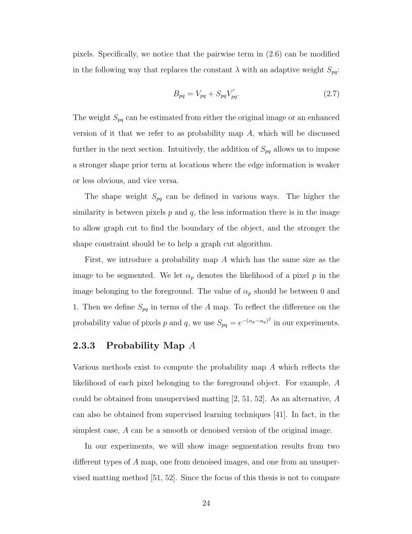
2.2 Statistical results comparing the star shape method [85]. Re-

sults with adaptive shape prior method (ASP) by using the de-

noised images as Spq are shown in the last column. Very similar

results were obtained by applying the matting maps as Spq. . . 34

3.1 Accuracy comparison between our shape classification method

and three other competing methods in terms of identifying split/no-

split cases. . . . . . . . . . . . . . . . . . . . . . . . . . . . . . 50

3.2 Probability of correct detection (PCD) for four image sets. We

compare our bottleneck detection method (BN) with watershed

method (WS), Kumar’s rule based method (RB) and Farhan’s

improved method (IM) in the table. . . . . . . . . . . . . . . . 57

3.3 Overall accuracy for four image sets. We compare our bottle-

neck detection method (BN) with watershed method (WS), Ku-

mar’s rule based method (RB) and Farhan’s improved method

(IM) in the table. . . . . . . . . . . . . . . . . . . . . . . . . . 57

5.1 Interactive tools, the corresponding reasons for the tools and

detailed actions for the tools in the proposed interactive seg-

mentation system . . . . . . . . . . . . . . . . . . . . . . . . . 88

5.2 Summary of the interactive tools and their corresponding meth-

ods for the proposed interactive segmentation system . . . . . 89

5.3 Accuracy improvement on oil sand images for the complete sys-

tem with four different kinds of initial segmentation algorithms 96

5.4 Score improvement on oil sand images for the complete system

with four different kind of initial segmentation algorithms . . . 96

5.5 Accuracy and score improvement on leukocyte images for the

complete system . . . . . . . . . . . . . . . . . . . . . . . . . . 100

List of Figures

1.1 An example of oil sand images from oil sand mining industry

is shown in (a), its segmentation result from a state-of-the-art

automatic segmentation algorithm using deep neural networks

[53] is shown in (b) and its desired output is shown in (c) . . . 3

1.2 The illustration of an interactive image segmentation system,

which includes the input image, the user, the computational

segmentation algorithm(s) with some prior knowledge, and the

user interface. . . . . . . . . . . . . . . . . . . . . . . . . . . 5

2.1 Example of graph cut on a graph. In this graph, the two cir-

cles represent the two terminal vertices (source and sink). The

squares donate all the other vertices. The thick red edges link

each terminal to the other vertices, and the thin black edges

join the non-terminal vertices. The green dashed lines represent

a cut found which separates the vertices into two sets. The total

cost of this cut equals the sum of all the edge weights on all the

black dashed edges. . . . . . . . . . . . . . . . . . . . . . . . . 20

2.2 Examples of test images and their corresponding probability

maps A. From (a) to (d), the images are ore fragment image,

bladder image, star fish image and image of an excavation shovel

tooth. The top row shows the original images, the middle row

shows the corresponding probability maps from denoised im-

ages, while the bottom row shows the corresponding probability

maps from an unsupervised matting method [52]. . . . . . . . 25

2.3 Results from Freedman et al.’s shape template based method

[32]. Column (a) shows the original images. Columns (b)-(d)

show segmentation results from Freeman and Zhang’s original

shape template method with λ = 0.2, 0.5 and 0.8. Columns (e)

and (f) show segmentation results from our adaptive shape prior

applied to Freedman and Zhang’s shape prior method. Column

(e) uses denoised images as the probability maps A. Column

(f) uses matting maps as the probability maps. . . . . . . . . 33

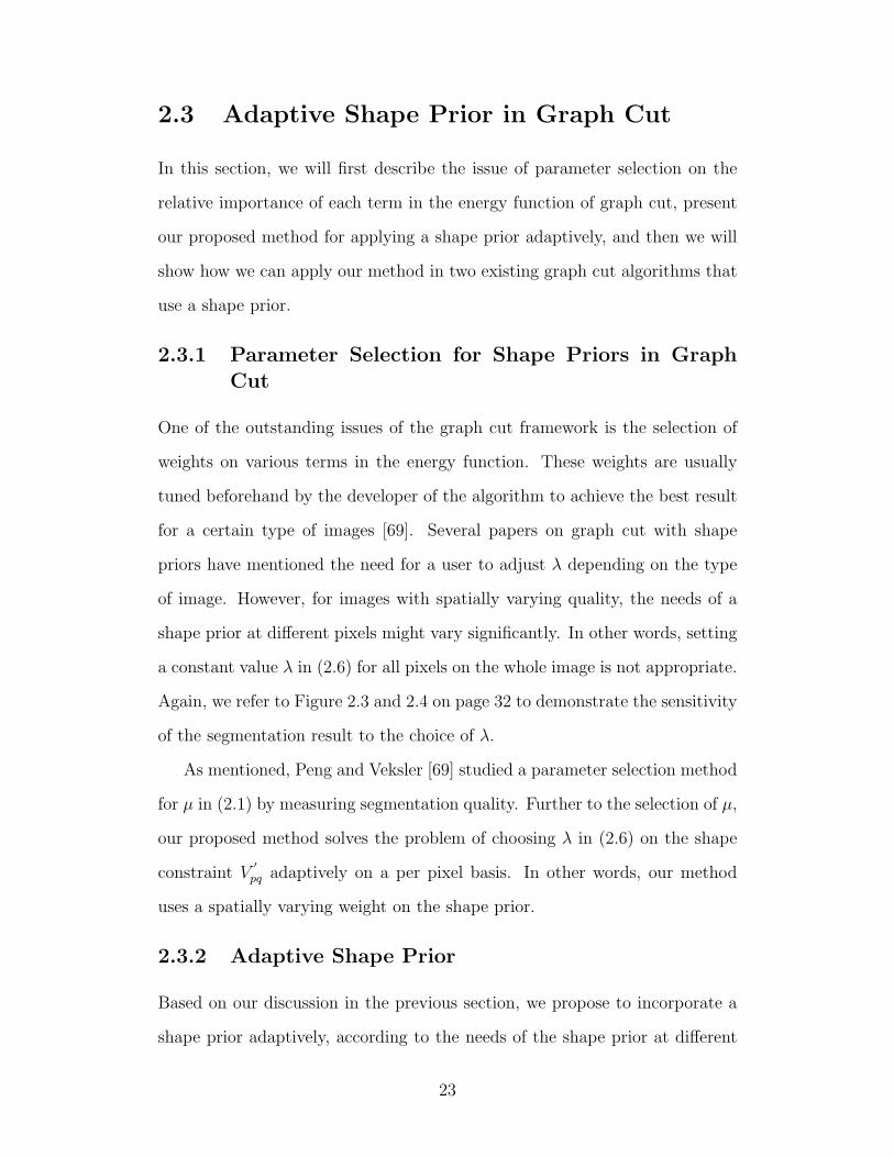
2.4 Results from the star shape prior method [85]. Column (a)

shows the original images. Columns (b)-(d) show segmentation

results from the original star shape prior method with λ = 0.2,

0.5 and 0.8. Columns (e) and (f) show segmentation results from

our adaptive shape prior applied to Veksler’s star shape prior

method. Column (e) uses denoised images as the probability

maps A. Column (f) uses matting maps as the probability maps. 34

3.1 Visual comparison on the detection of splitting points. The top,

middle and bottom rows show the results from classic concavity

based method, which can find only one concavity point; the

results from [8] and [48], which are not always the correct points;

and the results using our proposed bottleneck detection. The

detected splitting points are shown in red circles on the black

contour of the clumps. . . . . . . . . . . . . . . . . . . . . . . 42

3.2 Flowchart of the online phase in the proposed clump splitting

algorithm. . . . . . . . . . . . . . . . . . . . . . . . . . . . . 44

3.3 Examples of a pair of points found via the bottleneck rule. The

red crosses indicate points A∗ and B∗ located at the bottleneck

positions of the white contour. . . . . . . . . . . . . . . . . . . 46

3.4 Example of the local image patch I (the rectangle area high-

lighted). It is determined by the pair of points A∗ and B∗ found

from the previous step. . . . . . . . . . . . . . . . . . . . . . . 48

3.5 Visual results for clump splitting. The first row shows the orig-

inal segmentation, the second row shows the splitting results

from watershed algorithm (WS), the third row shows the split-

ting results from Kumar’s concavity based method (RB) [48],

the fourth row shows the results from the improved method (IM)

[30] and the last row shows our results (BN). Column (a) and

(b) are oil sands, column (c) is yeast cell, column (d) is blood

cell, column (e) and (f) are curvalaria cells. We only show one

example for yeast cell and blood cell because their shapes are

very similar. . . . . . . . . . . . . . . . . . . . . . . . . . . . . 53

3.6 Visual results for multiple splitting cases. Row 2 through 5 show the orig-

inal segmentation, the splitting results from watershed algorithm (WS),

the splitting results from Kumar’s concavity based method (RB) [48], the

results from the improved method (IM) [30] and our results (BN), respec-

tively. Column (a) and (b) are oil sands, and column (c) and (d) are yeast

cells. WS and our BN work better than the competing RB and IM meth-

ods. In addition, WS could produce comparable results to ours only if the

stopping criterion is carefully tuned, to avoid over or under-segmentation. 54

3.7 Visual comparison between a straight cut and our weighted

shortest path cut. The top, middle and bottom rows show

the original images with the segmented boundary, the split-

ting results using bottleneck detection with straight cut, and

the splitting results using our weighted shortest path cut. The

segmented boundaries are shown in green. Column (a), (b), (c)

and (d) are from oil sand images, yeast cell images, blood cell

images and curvalaria cell images respectively. . . . . . . . . . 55

3.8 An example on how PCD and accuracy are calculated. (a)

shows the input to the splitting algorithm while (b) shows the

output. There are in total 15 connected components in (a), in

which 5 of them are clumps. In (b), 1 out of the 5 clumps is

correctly split, while 11 out of the 15 connected components

are correct. Therefore, we have PCD = 1/5, and accuracy =

11/15. This shows that a high accuracy (11/15) does not guar-

antee a high PCD (1/5), especially in images where the major-

ity connected components are not clumps. . . . . . . . . . . . 56

4.1 Example of landmarks on the contour of an airway on an airway

image. On the airway, the white diamonds around crosses are

mathematical landmarks, and the red crosses only are pseudo

landmarks. . . . . . . . . . . . . . . . . . . . . . . . . . . . . . 64

4.2 Flowchart of the proposed shape PCA algorithm, with exam-

ples on oil sand image segmentations. The left column in the

figure shows the training steps, with training shapes extracted

from manually labeled segmentation. The right column shows

the testing steps with incorrectly segmented objects in the ini-

tial segmentation. The red boundary on the last image on the

right column represents the improved segmentation after our

proposed shape PCA method. . . . . . . . . . . . . . . . . . 76

4.3 An example of visual results of how segmentations have been

improved after performing global and local shape PCA methods

on oil sand images. (a), (b) and (c) are global shape PCA results

with the selections of 3, 5 and 10 PCs while (d), (e) and (f) are

local shape PCA results with the selections of 3, 5 and 10 PCs.

The location within the green dashed box shows an example

where local and global shape PCA perform differently. . . . . 79

4.4 Statistical results of accuracy with both global and local shape

PCA methods on oil sand images. . . . . . . . . . . . . . . . 80

4.5 Statistical results of score with both global and local shape PCA

methods on oil sand images. . . . . . . . . . . . . . . . . . . 81

5.1 The general flowchart of our proposed interactive image seg-

mentation system. . . . . . . . . . . . . . . . . . . . . . . . . 88

5.2 An example of the user interface for the proposed interactive

segmentation system. This example demonstrates the segmen-

tation of an oil sand image with the initial segmentation results

displayed in green boundaries of the segmented objects on top

of the original input oil sand image. . . . . . . . . . . . . . . 92

5.3 An example of the visual results on oil sand image to compare

the original image (a), the corresponding initial segmentation

result from [53] (b) and the final result (c). . . . . . . . . . . . 95

5.4 Improvement on pixel accuracy generated by each of the five

tools for oil sand images . . . . . . . . . . . . . . . . . . . . . 97

5.5 Improvement on object score generated by each of the five tools

for oil sand images . . . . . . . . . . . . . . . . . . . . . . . . 98

5.6 An example of the visual results on leukocyte image to compare

the original image (a), the corresponding initial segmentation

result from [73] (b) and the final result (c). . . . . . . . . . . . 99

5.7 Improvement on pixel accuracy generated by each of the five

tools for leukocyte images . . . . . . . . . . . . . . . . . . . . 101

5.8 Improvement on object score generated by each of the five tools

for leukocyte images . . . . . . . . . . . . . . . . . . . . . . . 101

5.9 Usability study on the proposed segmentation system in terms

of action per object, i.e., the total number of mouse clicks each

object needs in the images. NN, logGabor, OSA and Otsu repre-

sent that the initial segmentation is obtained from a neural net-

work based method [53], a ground truth decomposition method

via Gabor filter [54], the OSA method [4], and Otsu’s method

[68] for oil sand images, respectively. Boost represents that the

initial segmentation for leukocyte images are obtained from a

boosting method [73]. . . . . . . . . . . . . . . . . . . . . . . 102

Chapter 1

Introduction

1

1.1 Problem Motivation and Formulation

In digital image processing, image segmentation is generally an important part

of image analysis. Image segmentation refers to the process of subdividing

an image into its constituent parts or objects [33]. In other words, image

segmentation subdivides an image into different parts at a level depending on

the problem to be solved, i.e. the purpose after image segmentation.

Automatic image segmentation is challenging. While it is normally easy

and fast for humans to segment objects from an image, it is difficult for com-

puters to perform this task automatically. Some automatic segmentation algo-

rithms have achieved great success in certain applications. However, for appli-

cations such as oil sand mining images, medical imaging, etc., where the image

quality is limited by acquisition, image level information such as image inten-

sity is usually not enough for any segmentation algorithm to obtain desired

segmentation results. Few automatic segmentation algorithms are completely

reliable and robust. Figure 1.1 shows an example of oil sand images from oil

sand mining industry in (a), its segmentation result from a state-of-the-art au-

tomatic segmentation algorithm using deep neural networks [53] in (b) and its

desired output in (c). We can see that even with the state-of-the-art automatic

segmentation algorithm, the result shown in (b) still contains obvious segmen-

tation mistakes involving over-segmentation, under-segmentation and incor-

rectly segmented object boundaries. In this dissertation, under-segmentation

refers to segmentation mistakes in which the total number of pixels labeled

as foreground in the segmentation result is more than the total number of ex-

pected foreground pixels in the ground truth image, while over-segmentation

refers to segmentation mistakes in which the total number of pixels labeled

as foreground in the result is less than the total number of pixels expected as

foreground pixels.

2

(a)

(b)

(c)

Figure 1.1: An example of oil sand images from oil sand mining industry isshown in (a), its segmentation result from a state-of-the-art automatic seg-mentation algorithm using deep neural networks [53] is shown in (b) and itsdesired output is shown in (c)

Therefore, image segmentation algorithms should take advantage of prior

knowledge to ensure the success in practical and challenging applications.

Prior knowledge is discovered to be of great effect on image segmentation

algorithms. Prior knowledge describes what is expected in an image. In gen-

eral, prior knowledge comes in two ways: from human knowledge, such as user

interaction at various levels, and from the common properties of the objects

of interest, such as shape. User interaction is a part of many segmentation

procedures in practice. The interactions are needed to correct or bootstrap an

3

image segmentation algorithm. In general, an interactive segmentation sys-

tem can be illustrated in Fig 1.2. In such an interactive segmentation system,

the input is typically an image to be segmented. With the help of some prior

knowledge, the computational methods generate an initial segmentation of the

input image. After that, the user judges the results generated and provides

feedback interactively to the system. The system then interprets the user’s

intention and improves the segmentation accordingly until the user is satisfied

with the output. Although there are existing work in interactive segmentation,

user interaction can still be very time-consuming and the user’s intention may

not be correctly interpreted. On the other hand, prior knowledge is available

in various image segmentation applications. A segmentation algorithm can

make use of prior knowledge such as shape, texture, etc., which are common

object features, to obtain what is expected in an image.

The primary focus of this dissertation is therefore, to improve image seg-

mentation by shape-guided algorithms within an interactive segmentation frame-

work which requires minimal user interaction. Shape information which is

the key to ensure successful segmentation is embedded in each of the devel-

oped segmentation algorithms, throughout the whole segmentation procedure.

User interaction is utilized to judge what types of segmentation algorithms are

needed, initialize appropriate segmentation positions, choose proper parame-

ters for the algorithms, etc. As subsequent chapters will demonstrate, shape

priors and user interaction can be utilized in segmenting challenging images.

1.2 User Interaction in Interactive Image Seg-

mentation

Interactive image segmentation, as opposed to fully automatic one, means

the process of partitioning an image into its constituent parts or objects with

the help of user interaction. While automatic image segmentation algorithms

4

Figure 1.2: The illustration of an interactive image segmentation system,which includes the input image, the user, the computational segmentationalgorithm(s) with some prior knowledge, and the user interface.

have been difficult in many applications, interactive image segmentation has

become more and more popular. Although some existing work differentiates

between interactive segmentation and semi-automatic segmentation [36] in the

way that interactive segmentation involves the user in both the initialization

and the post-processing stages of the segmentation process iteratively, while

semi-automatic segmentation only involves the user in the initialization stage,

this dissertation unifies these two terms and refers to interactive segmentation

as any segmentation which requires some kind of user input.

A variety of interactive segmentation algorithms have been proposed in

recent decades. In general, different interaction strategies influence the seg-

mentation results in different manners. The success of an interactive segmen-

tation system depends on the combination of the type of user input, how the

input is interpreted as the feedback to the segmentation algorithms, and how

the feedback is applied in the context of the interactive segmentation process.

5

In the rest of this section, we will give a comprehensive review of interactive

image segmentation algorithms.

1.2.1 Initialization in Interactive Segmentation

The initialization for image segmentation refers to the procedure for setting

an initial starting point such as proper segmentation positions on an image,

proper values for parameters in the segmentation algorithms, etc. As men-

tioned, despite the efforts, few fully automatic segmentation algorithms are

completely reliable and robust due to noisy image qualities, object occlusions,

etc. Therefore, user interaction in the initialization stage is the first and crucial

step in deciding the success of a segmentation task.

Initialization interaction can be generally categorized by the way of the user

interaction: seeding, such as snake and active contour based methods [42]; la-

beling foreground and background pixels with strokes, such as the graph cut

methods [16, 71] and watershed methods [62]; region of interest, such as bound-

ing box method [50]; boundary tracking and boundary editing, such as livewire

[63] and lazy snapping [56]. A combination of these types of interactions also

exist in the literature [14, 55, 96, 51, 90, 57].

Although snake and active contour based methods [42] are classic tools in

image segmentation, they are sensitive to the positions of the seeds. With

seeding followed by energy minimization, they are also not flexible and inter-

active enough when repeated user editings are required to achieve a satisfying

result. Livewire methods [63], on the other hand, allow objects of interest to

be extracted via mouse tracings. Although these methods achieve improve-

ment on the accuracy of object boundaries, the amount of human interaction

is intensive. More recently, graph cut methods [16, 71, 46] have achieved suc-

cess, because they not only are efficient and globally optimal, but also allow

one to incorporate user interaction easily, such as labeling the background

6

and foreground pixels with strokes. Besides seeding, specifying foreground

or background pixels, etc., more recent interactive segmentation algorithms

have incorporated user interactions in the form of combining initialization,

boundary editing and boundary tracing [64, 56, 67, 58, 10]. Even though

some of these methods claim to be easy in image segmentation and boundary

refinement, the amount of user interaction is tedious. Besides, it is easy to

lose direct control from the user, i.e., the user’s intention cannot always be

correctly interpreted in the interaction procedure.

1.2.2 Post-processing in Interactive Segmentation

Besides initialization, post-processing is also a critical step after the segmen-

tation algorithms are performed. Post-processing allows the user to adjust

the segmentation results to become more suitable for different purposes, etc.

State-of-the-art post-processing techniques include methods such as mathe-

matical morphology, merging small adjacent regions, filtering small objects,

filtering badly shaped objects, filling holes, etc. [34, 5, 94, 11] While blindly

applying automatic post-processing methods might not achieve desirable re-

sults, manually tuning the parameters for a specific application or manually

tracing the boundary of the desired object is time-consuming and not generally

applicable.

In the literature, Olabarriaga [66] has proposed a human computer inter-

active framework to tackle the segmentation of medical images with human

interaction in the post-processing steps. This framework makes strong as-

sumptions that the user is capable of identifying the needs for post-processing

and providing the proposed computational methods prompt feedback to cor-

rect the result. However, they apply similar computational methods for all

post-processing cases, which are not generally applicable. Sarigul [75] has pre-

sented a system for refinement and analysis of segmented CT/MRI images. In

7

their system, a post-processing method is proposed and applied to CT/MRI

images. The system is developed based on rules such as region property, size,

etc. Although the system claims to observe the human interaction and apply

corresponding automated techniques to develop its own refinement rules, the

post-processing operations proposed are insufficient for segmentation mistakes.

1.2.3 Summary

In summary, most existing research on interactive image segmentation involves

user interaction in either the initialization, boundary editing/tracing or post-

processing steps. While user initializations are not sufficient to generate desir-

able results on challenging images, algorithms with boundary tracing are very

time-consuming. Although some post-processing methods have been proposed

to tackle mistakes made by existing segmentation algorithms, these proposed

methods are sometimes unable to interpret the user’s intention correctly, in-

sufficient and not generally applicable.

This motivates the research of this dissertation to developed an interactive

image segmentation system which both reduce the amount of user interaction

and better interprets the user’s intention. Based on the observations that

there are a finite number of segmentation mistakes from existing segmentation

algorithms and most mistakes are still confined to part of the desired object

of interest, we will propose an interactive segmentation framework by the

types of mistakes made by existing segmentation algorithms. We will conclude

that there are commonly five types of mistakes made by any segmentation

algorithms. Subsequently, five types of interactive tools are needed to deal

with each of the failure cases. The overall goal is to take advantage of minimal

amount of user interaction which can be correctly interpreted for the user’s

intention, to benefit interactive image segmentation. The details of this system

will be presented in Chapter 5.

8

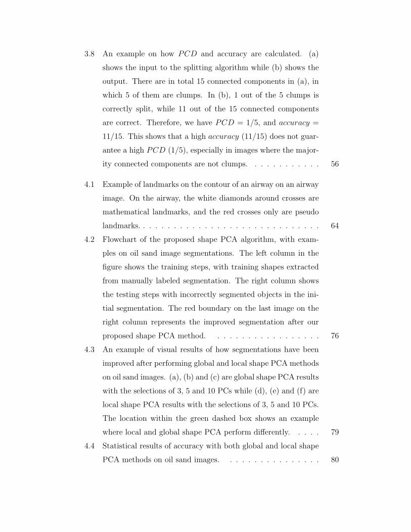
1.3 Shape Priors in Image Segmentation

After obtaining different types of user interaction, corresponding segmenta-

tion algorithms are needed to perform the segmentation tasks. While some

segmentation algorithms tend to analyze images by using pure low level in-

formation such as edge information, some other strategies tend to use prior

knowledge about what is expected to be segmented from the image. Such

prior knowledge usually reflects the common properties of the desired objects.

Shape priors are one of the most obvious and important common features in a

big amount of image analysis task. Therefore, the second focus of this disser-

tation is to develop shape-guided segmentation algorithms for different types

of interactive image segmentation. In the following section, we will present

some reviews on existing shape-guided segmentation algorithms based on the

types and purposes of interactive segmentation, i.e., generating the segmen-

tation with shape priors, solving certain types of under-segmentation issues

caused by object fusion by clump splitting, and refining final object boundary.

1.3.1 Shape Priors in Graph Cut

Shape priors have been incorporated in various ways in image segmentation.

If an object of a certain shape is expected as the output of a segmentation

algorithm, a shape constraint can be imposed on the shape of a foreground

object. Most existing popular shape based methods incorporate shape infor-

mation into a specific image segmentation algorithm, such as active contour,

graph cut, etc. After incorporating shape information, the segmentation prob-

lems can then be formulated in terms of energy minimization. Some energy

minimization problems can be formulated further to the max-flow/min-cut

problem in a graph, which represents one of the most popular and successful

interactive segmentation algorithms: graph cut [16].

9

Shape priors in graph cut have also been developed in a number of ways.

The shape prior term is usually defined in the energy function to penalize

the discrepancy between the segmented shape and the expected shape. Some

methods express this shape prior term using a shape template [101, 61, 32, 47],

while others regulate it as a more flexible constraint [85, 25]. These shape

priors have made graph cut segmentation even more successful in challenging

data sets.

However, one of the issues with shape prior methods is the selection of the

weight on the shape term in the energy function. The weight is usually tuned

beforehand to achieve the best result for a certain type of images. Several

existing works have mentioned the need to adjust the weight on the shape

term depending on the type of images. Even within the same type of images,

the needs of a shape prior at different pixels might vary significantly due to

noise and intensity inhomogeneities. Therefore, setting a constant weight for

the shape prior for all pixels on the whole image is not appropriate. This leads

to our proposed adaptive shape prior (ASP) method, which combines image

intensity information and shape information adaptively, based on the different

needs for the shape prior at different locations of the image. The details on

the ASP method will be described in Chapter 2.

1.3.2 Shape Priors in Clump Splitting

When performing segmentation of an image, multiple objects of interest can

cluster into clumps. Especially for images with heavily touching or overlap-

ping objects, such cases could seriously affect the overall success of the image

analysis task. Existing clump splitting methods can be generally categorized

into morphological methods [33, 35, 60, 72, 83], watershed methods [13], model

based approaches [39, 6, 59], and concavity based analysis [97, 92]. Almost

all the methods in the literature assume binary images, discard the original

10

intensity information and only work on object shape by, for example, finding

dominant or concavity points on the boundary of the binary segmentation.

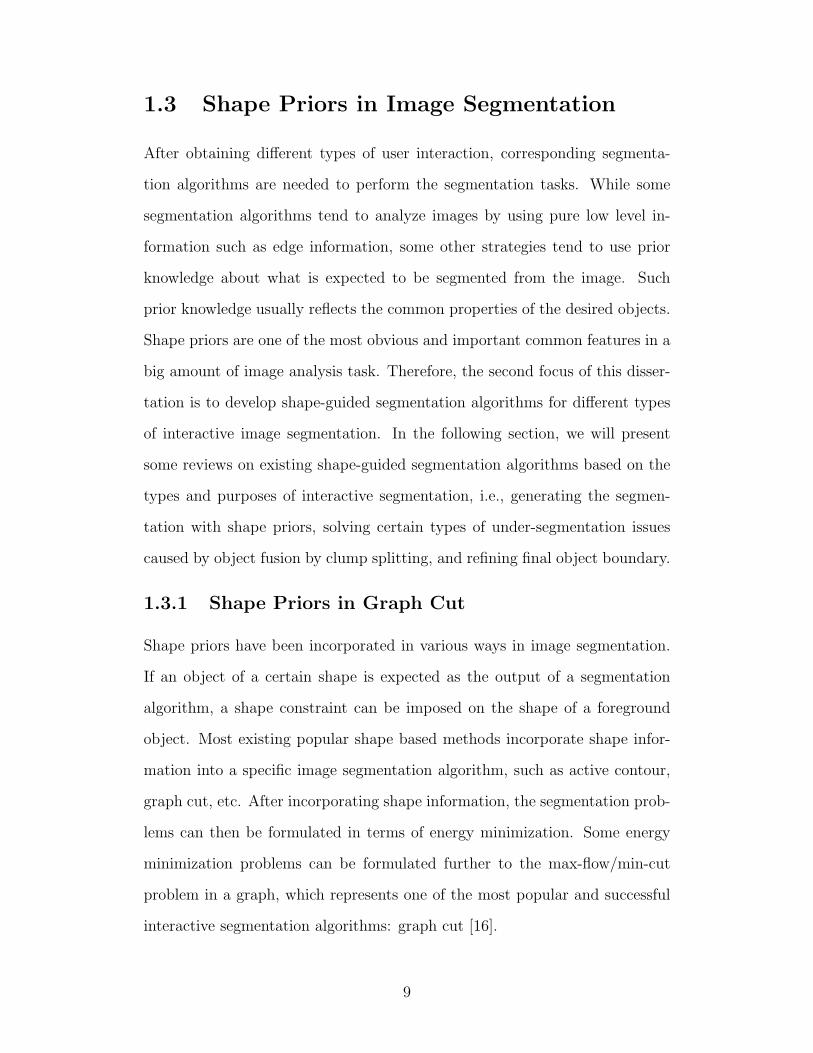
Although concavity analysis offers an intuitive way of splitting and is so

far the most popular technique in clump splitting, the procedure of finding the

splitting points and split lines is very parameter-dependent. Concavity based

methods also suffer from other limitation mentioned in Chapter 3. Therefore,

we will present a novel clump splitting method via bottleneck detection, which

takes advantage of the bottleneck positions on the clumps effectively and over-

comes the drawbacks mentioned above. The details on this method will be

described in Chapter 3.

1.3.3 Shape Priors in Boundary Refinement

At the final stage of the segmentation task, shape priors are also vital parts in

refining the boundary of the incorrectly segmented objects. Especially when

intensity information is weak or missing, statistical shape information plays an

important role. Statistical shape analysis describes the geometrical properties

statistically from a set of similar shapes. In the last two decades, model-based

segmentation has been successful in shape based image analysis. By matching

a statistical model which contains shape information about the expected shape

in an image, the segmentation algorithm can perform image segmentation

effectively.

One of the problems with current statistical shape models is that when in-

tensity information is very inadequate or missing, statistical models developed

from statistical shape analysis such as active shape model have difficulties

converging to the correct segmentation. Therefore, we focus on improving

the segmentation boundary when image intensity information is inadequate

or missing. In Chapter 4 we will describe the proposed shape PCA method,

which works by taking advantage of statistical shape information only, which

11

is not directly available from the image, to improve image segmentation in

boundary refinement.

1.4 Contributions

This dissertation introduces novel shape-guided algorithms for interactive im-

age segmentation. We propose three shape-guided algorithms for different

stages of the segmentation process: initial segmentation, clump splitting and

boundary refinement. To integrate these shape-guided algorithms, a compre-

hensive interactive segmentation system is developed which efficiently incor-

porates user interaction. Specifically, the user interaction takes place in a

scenario where the segmentation results are progressively refined by a combi-

nation of these shape-guided methods. The major contributions of this Ph.D.

thesis are:

• Adaptive shape prior (ASP) method. An adaptive shape prior

method is proposed for incorporating shape priors into the graph cut

based segmentation framework to eliminate incorrect cases in previous

approaches in which the parameters for the shape prior have to be tuned

to fit the image. The adaptive shape prior works by adding the shape

term in the energy function based on a probability map, which is straight-

forward to calculate and does not add much additional cost to the al-

gorithm. With the help of the probability map which can be utilized to

reflect the different needs of the shape prior at different locations of the

image, the ASP method combines information from both image inten-

sity and shape level adaptively. The ASP method can be easily applied

to various types of graph cut segmentation algorithms with shape pri-

ors, such as Freedman et al.’s graph cut method, and star shape prior

method.

12

• Clump splitting method via bottleneck detection. The clump

splitting method solves a very common and critical type of segmenta-

tion mistake: under-segmentation due to object fusions. In most existing

clump splitting methods, the objects to be split into are expected to have

roughly convex shape. The proposed clump splitting method therefore

focuses on clumps with their splitting points occurring at bottleneck

positions of the binary clump. It aims at finding splitting points via

bottleneck detection, and obtaining a cutting line with the help of find-

ing connected pixels between splitting points which minimize an energy

function. To help with multiple splitting cases, a shape classification

based method is also proposed to decide whether to split a connected

component iteratively.

• Shape PCA method. In order to refine the boundary of the incor-

rectly segmented objects in the final stage of the image segmentation

task, the shape PCA method takes advantage of statistical shape level

information, which is not directly available from image level, and refines

the shape of the incorrectly segmented object with the first few principal

components, which presumably represent the true shape of the object.

The local Shape PCAmethod is also proposed to compare with the global

shape PCA method. As long as the incorrectly segmented portions of

the object boundary can be localized correctly, either automatically or

manually, local shape PCA can be easily applied to perform boundary

refinement.

• A shape-guided interactive segmentation system. To integrate

all of the shape-guided algorithms proposed in this dissertation together

with minimal user input, a novel comprehensive shape-guided interac-

tive segmentation system is developed. The proposed system includes

13

five decisive tools which intuitively reflect user’s intention: object ad-

dition, object deletion, clump splitting, object merging, and boundary

refinement. These five decisive tools are developed based on common

cases of failure from any segmentation algorithms. From observation,

most image segmentation tasks can be handled by one or a combination

of these five tools. By combining all the shape-guided algorithms pro-

posed in this dissertation, this interactive segmentation system can be

constructed into a highly effective and efficient interactive object seg-

mentation system with minimal user input.

1.5 Dissertation Organization

This dissertation is organized as follows. Chapter 2 first reviews different

shape priors in graph cut image segmentation, followed by the description of

the adaptive shape prior method, which is the first contribution of this thesis.

Clump splitting in image segmentation is reviewed in Chapter 3 followed by

the description on the proposed splitting method via bottleneck detection.

Chapter 4 presents the background on statistical shape analysis, followed by

the third contribution of this dissertation, namely the shape PCA method.

Chapter 5 describes the comprehensive interactive image segmentation system

we proposed in order to integrate all of the proposed shape-guided algorithms,

followed by detailed experimental results. Finally, conclusions and future work

are presented in Chapter 6.

14

Chapter 2

Image Segmentation viaAdaptive Shape Prior

15

This chapter presents the first contribution of this dissertation, namely the

adaptive shape prior (ASP) method. The adaptive shape prior method com-

bines information from both image level and shape level adaptively, based on

the different needs of a shape prior at different locations of the image. This

chapter will first review some background on graph cut and shape priors in

graph cut segmentation. The ASP method will then be described in details

with experimental results demonstrating its effectiveness.

2.1 Introduction

Image segmentation has always been an important and challenging task in

computer vision. Since Boykov and Jolly [16] introduced the application of

the graph cut algorithm into image segmentation, graph cut has become one

of the leading approaches in image segmentation in the last decade, because

it not only allows one to incorporate user interaction, but also is an efficient

algorithm.

More recently, in order to handle noisy images or images with object occlu-

sions effectively, new methods have been developed in the graph cut segmenta-

tion framework to exploit shape priors. Freedman and Zhang proposed to in-

corporate shape priors in graph cut segmentation by matching the segmented

curve with a shape template [32]. Veksler has showed how to implement a

shape prior for objects defined as star shaped [85]. Das et al. presented a

similar idea to incorporate shape priors for shapes defined as compact [25].

In addition, some research activities focus on one or two particular types of

objects with particular shapes [79, 47], some on incorporating multiple shape

priors into one image [86], and yet some on shape representation and general

shape constraints [24, 50].

One of the problematic issues of the graph cut framework is the selection

of weights on the various terms in the energy function. These weights are

16

usually tuned beforehand by the developer of the algorithm to achieve the

best result for a certain type of images [69]. For example, Peng and Veksler

[69] designed a parameter selection method by measuring segmentation qual-

ity based on different features of the segmentation. They ran graph cut for

different parameter values and chose the parameters which produced segmen-

tation of the highest quality. However, their method only targets issues of

selecting the parameters between the data term and the boundary term in

the energy function, while setting a constant weight on the shape prior. For

images corrupted by significant noise and intensity inhomogeneities, the needs

for a shape prior at different pixels are different in general. Therefore, setting

a constant weight on the shape prior term for all pixels may not be appropri-

ate. As an example, columns (b) to (d) in Figure 2.3 and 2.4 on page 32 show

examples where different parameter settings for the shape prior can lead to

very different segmentation results.

To solve the issue described above, we propose to impose shape constraints

selectively, by applying the shape prior adaptively in graph cut. To determine

the need for the shape prior at each pixel, we derive a shape weight term based

on image intensity. The intuition behind this is that if a pair of neighboring

pixels appear similar, there should be a higher weight for the shape constraint

in the energy function to compensate for the weak or missing edge information.

In this way our method gives flexibility in applying a shape prior, and helps

obtaining a segmentation result that better matches with the shape prior. As

will be seen in this chapter, this weight on the shape constraint can be easily

calculated without much additional computational cost.

Song et al. [80] proposed an adaptive framework for segmentation of brain

tumors in MRI images within an iterative scheme. They incorporated a shape

atlas of probabilistic priors into the graph cut energy function by combining

it with the image intensity distribution. However, the “adaptive” idea focuses

17

on the data term D in (2.1) only [80]. Furthermore, the performance of their

method relies a lot on the accuracy of the atlas, and several parameters, such

as the weight λ between the data and boundary terms, as well as the scale σ

for calculating the neighborhood links [80].

In another study, Bar-Yosef et al. [9] proposed a variational method for

model based segmentation with an adaptive shape prior, with the help of a

shape confidence map. Their prior confidence map was defined to select a

shape model among many shape models, with the maximum confidence at

each pixel to reflect the reliability of the shape prior at each pixel. The prior

confidence map then determines if the segmentation algorithm should follow

the shape prior or not at each pixel location. However, their method only

focuses on the variational framework with many shape prior models, and has

only been applied in one specific application.

In contrast to the previous work, our proposed method tackles adaptive

shape prior from a different angle. The weight on the shape constraint is

obtained from the available image level information, and it reflects how much

each pixel needs the shape prior to help with image segmentation. In other

words, we measure the need for the shape prior between a pair of pixels, instead

of the reliability of the shape prior.

This chapter is organized as follows. In Section 2.2 we present the back-

ground on the graph cut segmentation with shape priors in a unified way to

combine the boundary and shape term in the energy function. Then we first

describe the issue of parameter selection on the relative importance of each

term in graph cut, then present our proposed method for adaptive shape pri-

ors and give examples of applying it in some existing graph cut methods with

shape priors. Finally we provide the experimental results to demonstrate the

generality and superior performance of our approach.

18

2.2 Graph Cut Image Segmentation

This section presents the background on the graph cut segmentation with

shape priors. We will first explain the background on graph cut in terms of

graph theory and the max-flow/min-cut optimization. Then the application

of graph cut algorithm with shape priors on image segmentation will be pre-

sented in a unified way to combine the boundary and shape term in the energy

function.

2.2.1 Graph Cut

Many segmentation problems can be formulated in terms of energy minimiza-

tion. Such energy minimization problems can be further formulated into a

maximum flow problem in a graph. Under most formulations of such prob-

lems, the minimum energy solution corresponds to the maximum a posteriori

estimate of a solution. The term “graph cut” is applied specifically to those

models which employ a max-flow/min-cut optimization.

Let G = ⟨V, E⟩ be a weighted graph where V is the set of vertices and E

represents the set of edges. V has two distinguished vertices called a source

and a sink. A cut C ⊂ E is a set of edges such that the terminals are separated

in the induced graph G(C) = ⟨V, E − C⟩. In addition, no proper subset of C

separates the terminals in G(C). The cost of the cut C thus equals the sum

of its edge weights.

The min-cut problem focuses on finding the cut with minimum cost. Ac-

cording to [46], this can be solved by computing the maximum flow between

the terminals (source and sink). The worst case complexity is low-order poly-

nomial, although the running time in practice for the graphs is nearly linear

[84].

Figure 2.1 demonstrate an example of such a graph. In Figure 2.1, the

19

two circles represent the two terminal vertices (source and sink). The squares

donate all the other vertices. The thick red edges link each terminal to the

other vertices, and the thin black edges join the non-terminal vertices. The

green dashed lines represent a cut found which separates the vertices into two

sets. The total cost of this cut equals the sum of all the edge weights on all

the black dashed edges.

Figure 2.1: Example of graph cut on a graph. In this graph, the two circlesrepresent the two terminal vertices (source and sink). The squares donate allthe other vertices. The thick red edges link each terminal to the other vertices,and the thin black edges join the non-terminal vertices. The green dashed linesrepresent a cut found which separates the vertices into two sets. The totalcost of this cut equals the sum of all the edge weights on all the black dashededges.

2.2.2 Graph Cut Energy Function

Graph cut segmentation achieves an optimal solution by minimizing such an

energy function via the max-flow/min-cut algorithm:

E(F ) = µD(F ) +B(F ) (2.1)

20

where F = (f1, . . . , fp, . . . , fn) represents a binary vector whose component fp

specifies the assignment of background or foreground to pixel p in an arbitrary

set of data elements P in an image I. The data term D represents the cost of

labeling F according to the image level information, and the boundary term

B denotes the cost of labeling F according to same prior knowledge, such as

discontinuity on the boundary. µ is a non-negative coefficient which specifies a

relative importance between the boundary term B and the data term D [16].

To be more specific, (2.1) is usually written as:

E = µ∑p∈P

Dp(fp) +∑

{p,q}∈N :fp =fq

Bpq(fp, fq) (2.2)

where N is the set of neighboring pixels on the image I, and fp represents the

label assigned to pixel p. The particular forms for Dp(fp) and Bpq(fp, fq) are

discussed in the following sections.

2.2.3 Region Term

The region term Dp assumes that the penalties for assigning pixel p to “fore-

ground” or “background” are given. One example of defining the region term

Dp is to apply the negative log-likelihood model, which is originally motivated

by the MAP-Markov Random Field formulation [16].

Dp(“obj”) = − lnPr(Ip|“obj”) (2.3)

Dp(“bkg”) = − lnPr(Ip|“bkg”) (2.4)

where “obj” and “bkg” represent object and background respectively.

2.2.4 Boundary Term

In graph cut, the boundary term Bpq is a penalty term for the discontinuity

between a pixel pair p and q. For graph cut without shape priors, Bpq = Vpq.

21

One example of defining Vpq is to penalize the neighboring pixel pairs with

high intensity contrast:

Vpq = e(−(Ip−Iq)

2

2σ2 ) · 1

dist(p, q)(2.5)

where Ip represents the image intensity of pixel p, σ is a constant and dist(p, q)

is usually calculated as the Euclidean distance between pixels p and q [16].

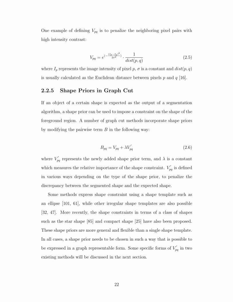
2.2.5 Shape Priors in Graph Cut

If an object of a certain shape is expected as the output of a segmentation

algorithm, a shape prior can be used to impose a constraint on the shape of the

foreground region. A number of graph cut methods incorporate shape priors

by modifying the pairwise term B in the following way:

Bpq = Vpq + λV′

pq (2.6)

where V′pq represents the newly added shape prior term, and λ is a constant

which measures the relative importance of the shape constraint. V′pq is defined

in various ways depending on the type of the shape prior, to penalize the

discrepancy between the segmented shape and the expected shape.

Some methods express shape constraint using a shape template such as

an ellipse [101, 61], while other irregular shape templates are also possible

[32, 47]. More recently, the shape constraints in terms of a class of shapes

such as the star shape [85] and compact shape [25] have also been proposed.

These shape priors are more general and flexible than a single shape template.

In all cases, a shape prior needs to be chosen in such a way that is possible to

be expressed in a graph representable form. Some specific forms of V′pq in two

existing methods will be discussed in the next section.

22

2.3 Adaptive Shape Prior in Graph Cut

In this section, we will first describe the issue of parameter selection on the

relative importance of each term in the energy function of graph cut, present

our proposed method for applying a shape prior adaptively, and then we will

show how we can apply our method in two existing graph cut algorithms that

use a shape prior.

2.3.1 Parameter Selection for Shape Priors in GraphCut

One of the outstanding issues of the graph cut framework is the selection of

weights on various terms in the energy function. These weights are usually

tuned beforehand by the developer of the algorithm to achieve the best result

for a certain type of images [69]. Several papers on graph cut with shape

priors have mentioned the need for a user to adjust λ depending on the type

of image. However, for images with spatially varying quality, the needs of a

shape prior at different pixels might vary significantly. In other words, setting

a constant value λ in (2.6) for all pixels on the whole image is not appropriate.

Again, we refer to Figure 2.3 and 2.4 on page 32 to demonstrate the sensitivity

of the segmentation result to the choice of λ.

As mentioned, Peng and Veksler [69] studied a parameter selection method

for µ in (2.1) by measuring segmentation quality. Further to the selection of µ,

our proposed method solves the problem of choosing λ in (2.6) on the shape

constraint V′pq adaptively on a per pixel basis. In other words, our method

uses a spatially varying weight on the shape prior.

2.3.2 Adaptive Shape Prior

Based on our discussion in the previous section, we propose to incorporate a

shape prior adaptively, according to the needs of the shape prior at different

23

pixels. Specifically, we notice that the pairwise term in (2.6) can be modified

in the following way that replaces the constant λ with an adaptive weight Spq:

Bpq = Vpq + SpqV′pq. (2.7)

The weight Spq can be estimated from either the original image or an enhanced

version of it that we refer to as probability map A, which will be discussed

further in the next section. Intuitively, the addition of Spq allows us to impose

a stronger shape prior term at locations where the edge information is weaker

or less obvious, and vice versa.

The shape weight Spq can be defined in various ways. The higher the

similarity is between pixels p and q, the less information there is in the image

to allow graph cut to find the boundary of the object, and the stronger the

shape constraint should be to help a graph cut algorithm.

First, we introduce a probability map A which has the same size as the

image to be segmented. We let αp denotes the likelihood of a pixel p in the

image belonging to the foreground. The value of αp should be between 0 and

1. Then we define Spq in terms of the A map. To reflect the difference on the

probability value of pixels p and q, we use Spq = e−(αp−αq)2 in our experiments.

2.3.3 Probability Map A

Various methods exist to compute the probability map A which reflects the

likelihood of each pixel belonging to the foreground object. For example, A

could be obtained from unsupervised matting [2, 51, 52]. As an alternative, A

can also be obtained from supervised learning techniques [41]. In fact, in the

simplest case, A can be a smooth or denoised version of the original image.

In our experiments, we will show image segmentation results from two

different types of A map, one from denoised images, and one from an unsuper-

vised matting method [51, 52]. Since the focus of this thesis is not to compare

24

the performance of unsupervised and supervised methods for computing A, we

only discuss experiments that use unsupervised methods. In our experiments,

the denoised images are generated by applying a Gaussian filter on the original

images, and matting images are generated from an existing matting method

[51, 52].

Examples of the original images and their enhanced versions serving as the

probability maps are shown in Figure 2.2. The first row shows the original

images, and the second and third rows show the corresponding probability

maps by denoising and matting [52]. To demonstrate the generality of our

method, our experiments include images in four different application domains:

(a) ore images in mining, (b) shovel tooth images from an excavation shovel,

(c) bladder images in medical applications and (d) star fish images.

Figure 2.2: Examples of test images and their corresponding probability mapsA. From (a) to (d), the images are ore fragment image, bladder image, starfish image and image of an excavation shovel tooth. The top row shows theoriginal images, the middle row shows the corresponding probability maps fromdenoised images, while the bottom row shows the corresponding probabilitymaps from an unsupervised matting method [52].

25

2.3.4 Adaptive Shape Template Method

Freedman and Zhang introduced the idea of incorporating a shape template

in the form of level set to graph cut [32]. Their method begins with the

assumption that the shape prior is a single fixed template [32]. In order to

incorporate the shape prior, they modified the original energy function of graph

cut by the shape term in Equation (2.6) as:

V′

pq = ϕ

(p+ q

2

)(2.8)

where ϕ is a regular unsigned distance function whose zero level set corre-

sponds to the shape template curve c. By adding this shape energy term V′pq,

minimization of the graph cut energy function encourages the object boundary

to be aligned with the zero level set [32].

To be more detailed, after adding the shape energy term V′pq, the energy

function for Freeman and Zhang’s shape template method can be written as:

E(f) = µ∑

p∈P Dp(fp) +∑

(p,q)∈N :fp =fqVpq(fp, fq)+

λ∑

{p,q}∈N :fp =fqϕ(p+q2

).

(2.9)

A drawback of Freeman and Zhang’s method is the requirement of object-

template alignment through a variety of transformations which are computa-

tionally expensive. Another more relevant limitation is the difficulty in choos-

ing a proper λ, which is a common problem for existing graph cut methods

with shape priors.

Following our proposed adaptive shape prior pairwise term in (2.7), we can

redefine the pairwise term in the energy function (2.9) to be adaptive as in

(2.7). That is, the energy function (2.9) for Freedman and Zhang’s method

can be redefined as:

E(f) = µ∑

p∈P Dp(fp) +∑

(p,q)∈N :fp =fqVpq(fp, fq)+∑

{p,q}∈N :fp =fqSpqϕ

(p+q2

).

(2.10)

26

2.3.5 Adaptive Star Shape Method

A more recent graph cut method with a generic shape prior is the star shape

prior method [85]. The star shape prior is not specific to any particular shape,

but rather defines a class of shapes. With the assumption that a center of the

object is known, the star shape prior method adds a shape constraint to the

graph cut energy function as described below.

Consider a center of the star shape is denoted as c. Let 1 and 0 be the

object label and the background label, respectively. For an object to be a star

shape, for any point p inside the object, every single point q on a straight line

connecting c and p must also be inside the object. This implies that if p is

assigned label 1, then every point between point c and p is also assigned 1.

With the assumption that q is between c and p, the star shape method defines

the following pairwise shape constraint term V′pq:

V′

pq(fp, fq) =

0 if fp = fq,∞ if fp = 1 and fq = 0,β if fp = 0 and fq = 1

(2.11)

where β is a weight constant.

To be more detailed, after adding the shape energy term V′pq, the energy

function for the star shape method can be written as:

E(f) = µ∑

p∈P Dp(fp) +∑

(p,q)∈N :fp =fqVpq(fp, fq)+

λ∑

(p,q)∈N :fp =fqV

′pq(fp, fq)

(2.12)

where V′pq is a shape energy term defined by (2.11).

Similar to other shape prior methods in graph cut segmentation, the star

shape method still has the limitation with parameter selection for different

terms in the energy function. As discussed in [85], β needs to be chosen

appropriately by the user in order to obtain good segmentation results. It is

obvious that λ and β are relative weights, and the problem of selecting them

remains.

27

Following similar procedure as for the shape template method, we can

redefine the pairwise term in the energy function (2.12) to be adaptive as in

(2.7). That is, the energy function (2.12) can be redefined as:

E(f) = µ∑

p∈P Dp(fp) +∑

(p,q)∈N :fp =fqVpq(fp, fq)+∑

(p,q)∈N :fp =fqSpqV

′pq(fp, fq).

(2.13)

2.3.6 Optimality of the New Energy Function

A function E is graph-representable if there exists a graph G = (V, E) with

terminals s and t and a subset of vertices V0 ⊂ V − {s, t} such that, for any

configuration f1, . . . , fn, the value of the energy E(f1, . . . , fn) is equal to a

constant plus the cost of the mininum cut among all cuts [46]. To be more

detailed, if we define the class F 2 energy functions to be written as a sum of

functions of up to two binary variables at a time [46], i.e.,

E(f1, . . . , fn) =∑i

Ei(fi) +∑i<j

Eij(fi, fj), (2.14)

then E is graph-representable if and only if each term Eij satisfies the following

inequality:

Eij(0, 0) + Eij(1, 1) ≤ Eij(0, 1) + Eij(1, 0). (2.15)

Functions which satisfy the condition of (2.15) is called regular.

If an energy function E is graph-representable by a graph G, it is possible

to find the exact minimum of E in polynomial time by computing the min-

cut on G [46]. Therefore, as long as an energy function satisfies (2.15), a

graph can be constructed and a global optimized solution can be obtained via

max-flow/min-cut algorithm.

In (2.10) and (2.13), the Vpq term is defined the same as in (2.5). The

difference lies in the shape term V′pq. For both (2.10) and (2.13), we have

28

V (0, 0) = 0 and V (1, 1) = 0. As well we have V′(0, 0) = 0 and V

′(1, 1) = 0. On

the other hand, the energy function E is defined to be nonnegative. Therefore

V (0, 1) + V (1, 0) ≥ 0 and V′(0, 1) + V

′(1, 0) ≥ 0. Since Spq is nonnegative,

and in our experiments β from (2.11) is nonnegative, SpqV′pq is nonnegative

as well. This shows that the new energy functions in (2.10) and (2.13) are

graph-representable. Therefore, we can construct a graph according to [46]

and obtain optimized solutions for (2.10) and (2.13) via max-flow/min-cut

algorithm.

2.4 Experiments

In order to evaluate the segmentation results from the experiments, different

evaluation metrics can be applied. In this section, we will first describe three

different evaluation metrics which will be used in this thesis. Some of these

metrics will be used for evaluating the results in this chapter, while some others

will be used for evaluating results in some other chapters. After describing the

evaluation metrics, we will then present the experimental results from our

adaptive shape prior method.

2.4.1 Evaluation Metrics

To evaluate the image segmentation performance quantitatively, several eval-

uation metrics are used in this dissertation. Supervised evaluation is the most

widely used evaluation method in image research. It computes the difference

between the ground truth and the segmentation result using a given evaluation

metric. In this thesis, we apply supervised evaluation methods which compare

the segmented results with the ground truth images with three different met-

rics: pixel accuracy, labeling score and Jaccard index.

For convenience, TP , TN , FP and FN stand for the number of samples

(e.g., the number of pixels or the number of objects) being labeled as true

29

positive, true negative, false positive, and false negative.

Pixel accuracy is defined as

TP + TN

TP + TN + FP + FN(2.16)

Pixel Accuracy is a pixel level criterion which commonly measures the per-

centage of correctly labeled pixels.

Labeling score is defined as

L = min(S(A,B), S(B,A)) (2.17)

with

S(A,B) =m∑j

n∑i

|Aj ∩Bi||Aj ∪Bi|

Bi∪|Aj∩Bi|=∅

Bi

Aj∪j

Aj

(2.18)

where Aj is a connected component in image A and Bi is a connected com-

ponent in image B. This labeling score is based on [70]. It is a form of local

intersection-over-union whereby both errors at the pixel level and object level

are penalized. In contrast to pixel accuracy, label score not only takes the pixel

labeling error into account, but also penalizes over-segmentation and under-

segmentation on the object level.

Jaccard index is defined as

TP

TP + FP + FN(2.19)

Jaccard index is the ratio of intersection and union of the segmented region

and ground truth region.

30

2.4.2 Experimental Results

To validate our proposed shape prior method, we have run experiments on

two graph cut methods with shape priors. We use a MATLAB wrapper with

the C++ max-flow code by Boykov and Kolmogorov [45]. When comparing

our proposed method to Freedman and Zhang’s shape template method [32],

the shape template is introduced in the same way, i.e., we assume an aligned

template as the shape prior. The aligned shape templates for each image are

exactly the same for both Freedman and Zhang’s method and our method.

As mentioned in [32], the key assumption of Freeman and Zhang’s method is

that, based on the user input, the shape template can be well aligned with the

image using the Procrustes Method [27]. Details on the Procrustes Method

are described in the later chapter of this thesis on Page 65. Given the aligned

template, the distance function can be easily computed via scaling, as the

input to the graph cut energy function. It is also mentioned that the rigid

transformation computed via the Procrustes Method will not be extremely

accurate [32]; however the algorithm is robust in the situation in which the

template is not exactly accurate. When comparing our method to the original

star shape prior method [85], we also perform our experiments based on exactly

the same user initialization to specify a center of the object to be segmented.

We perform our experiments with two different types of probability map A,

one obtained by denoising, and the other by an unsupervised matting method

[51, 52]. The denoised images are generated from applying a Gaussian filter

on the original images. After obtaining the probability map A, the probabil-

ity map is combined with the shape prior from either Freedman’s method or

the star shape prior method, and finally the corresponding energy function is

minimized via graph cut.

Figures 2.3 and 2.4 show the comparison results of our adaptive method

31

to the shape template method [32] and the star shape prior method [85],

respectively. In both figures, the original images are shown in column (a), and

results obtained by the competing methods are shown in columns (b) to (d)

with different values of λ. Our results are shown in columns (e) and (f). The

difference is that, the results shown in column (e) uses denoised images as the

probability map A, while the results shown in column (f) utilizes matting [52].

Table 2.1 and 2.2 show the statistical results. To evaluate the performance

of the algorithms quantitatively, we apply two popular evaluation metrics:

Jaccard index [40] and pixel accuracy.

In total, our experiments included 20 oil sand images, 46 tooth images,

15 bladder images and 10 starfish images. The last two columns in the ta-

bles demonstrate the superior performance of our method over the competing

methods. The highlight columns show the best performance in each row. It

is clear that our method obtains better segmentation results most of the time

without the need to optimize with regard to λ, while the two competing meth-

ods both need to tune the parameter λ.

When comparing columns (e) and (f) in Figure 2.3 and 2.4, we obtain

almost the same segmentation results even though we use different techniques

for obtaining Spq. This shows that our method is flexible in terms of how

A is generated. Since we are not interested in picking the best method for

computing A, comparison among various types of A is not further examined

in our study.

2.5 Summary

We have proposed an adaptive method for incorporating shape priors into

the graph cut based segmentation framework to eliminate incorrect cases in

previous approaches in which parameters had to be tuned to fit the image.

Adaptive shape prior works by adding the shape term in the energy function

32

Figure 2.3: Results from Freedman et al.’s shape template based method [32].Column (a) shows the original images. Columns (b)-(d) show segmentationresults from Freeman and Zhang’s original shape template method with λ =0.2, 0.5 and 0.8. Columns (e) and (f) show segmentation results from ouradaptive shape prior applied to Freedman and Zhang’s shape prior method.Column (e) uses denoised images as the probability maps A. Column (f) usesmatting maps as the probability maps.

Table 2.1: Statistical results comparing Freedman et al.’s shape templatemethod [32]. Results with adaptive shape prior method (ASP) by using thedenoised images as Spq are shown in the last column. Very similar results wereobtained by applying the matting maps as Spq.

33

Figure 2.4: Results from the star shape prior method [85]. Column (a) showsthe original images. Columns (b)-(d) show segmentation results from theoriginal star shape prior method with λ = 0.2, 0.5 and 0.8. Columns (e)and (f) show segmentation results from our adaptive shape prior applied toVeksler’s star shape prior method. Column (e) uses denoised images as theprobability maps A. Column (f) uses matting maps as the probability maps.

Table 2.2: Statistical results comparing the star shape method [85]. Resultswith adaptive shape prior method (ASP) by using the denoised images as Spq

are shown in the last column. Very similar results were obtained by applyingthe matting maps as Spq.

34

based on a probability map. We have shown that the proposed method can

be easily applied to various types of graph cut based image segmentation

algorithms with shape priors, such as Freedman et al.’s graph cut method

with shape template, and the star shape prior method. Although we need an

extra step to obtain the probability map A, this step is straightforward and

does not add much additional cost to the graph cut segmentation. In Chapter

5 we will describe how to integrate the ASP method proposed in this Chapter

to an interactive segmentation framework.

35

Chapter 3

Clump Splitting via BottleneckDetection

36

In this chapter we will investigate the clump splitting method, which solves

a common and critical mistake by existing image segmentation: under-seg-

mentation due to object fusion. Especially, we focus on clumps with their

splitting points occurring at bottleneck positions. That is, the objects to be

split into are expected to have roughly a convex shape. This is a common case

in clump splitting and various clump splitting methods have been developed to

deal with this case. This chapter will first present a comprehensive review on

existing clump splitting methods, followed by the description of the proposed

clump splitting method via bottleneck detection, the second contribution of

this dissertation. Experimental results will also be presented to demonstrate

the superior performance of this proposed method.

3.1 Introduction

When performing segmentation of an image in different domains, multiple

objects of interest tend to cluster into clumps in the image. Generally, clumps

are formed due to either touching or overlapping objects, especially when

object density is high in the image or if the objects in the image are close to

each other. In such cases, clump splitting is required to divide a segmented

region into two or more parts or portions. In applications in which the sizes

and shapes of the objects in the image need to be accurately determined,

the splitting of a clumped object into constituent objects must be performed

for optimal segmentation performance. Although a human operator may be

able to detect the constituent objects of interest based on prior knowledge,

perception of texture and structure of the original image, it still remains a

challenge for a computer algorithm to handle this automatically.

Generally, separating clumps using image analysis is not easy. Even in cases

where the segmentation of the image between foreground and background is

easily achieved because of high contrast between them, the segmentation often

37

fails to separate the individual objects, which form clumps because of a very

high degree of resemblance among the objects in a clump. Therefore, effective

and efficient clump splitting methods are needed to resolve under-segmented

objects.

3.2 Review of Clump Splitting Methods

Existing clump splitting methods can be categorized into mathematical mor-

phology based methods [33], watershed based techniques [13], model based

approaches [39, 6, 59], concavity based analysis [97, 92], etc. Almost all the

methods found in the literature assume that the images are binarized and

discard the original intensity information [29].

Morphological methods are quite simple and widely used in image analy-

sis tasks. Many of these methods are using basic morphological operations,

such as erosion, dilation, opening and closing [35, 60, 72, 83]. However, these

methods are generally not accurate when the clumps are heavily clustered.

For example, one difficulty with morphology-based methods is that they may

completely remove an object of interest in a clump.

Watershed based methods [13] are well known segmentation techniques,

which can potentially serve as clump splitting methods. Watershed based

methods split a clump based on the intensity surface of the image. For the

marker based watershed method, the first step involves the identification of

the markers to control the number of objects in the image. Once the markers

are obtained, the watershed algorithm is applied with the constraint that the

only regional minima are markers. Then the watershed lines obtained are

consequently the split lines for the clumps. However, markers are difficult to

determine in general. As a result, for objects which vary in size and shape,

watershed tends to over-segment the object of interest and, for objects which

heavily overlap, watershed tends to under-split them.

38

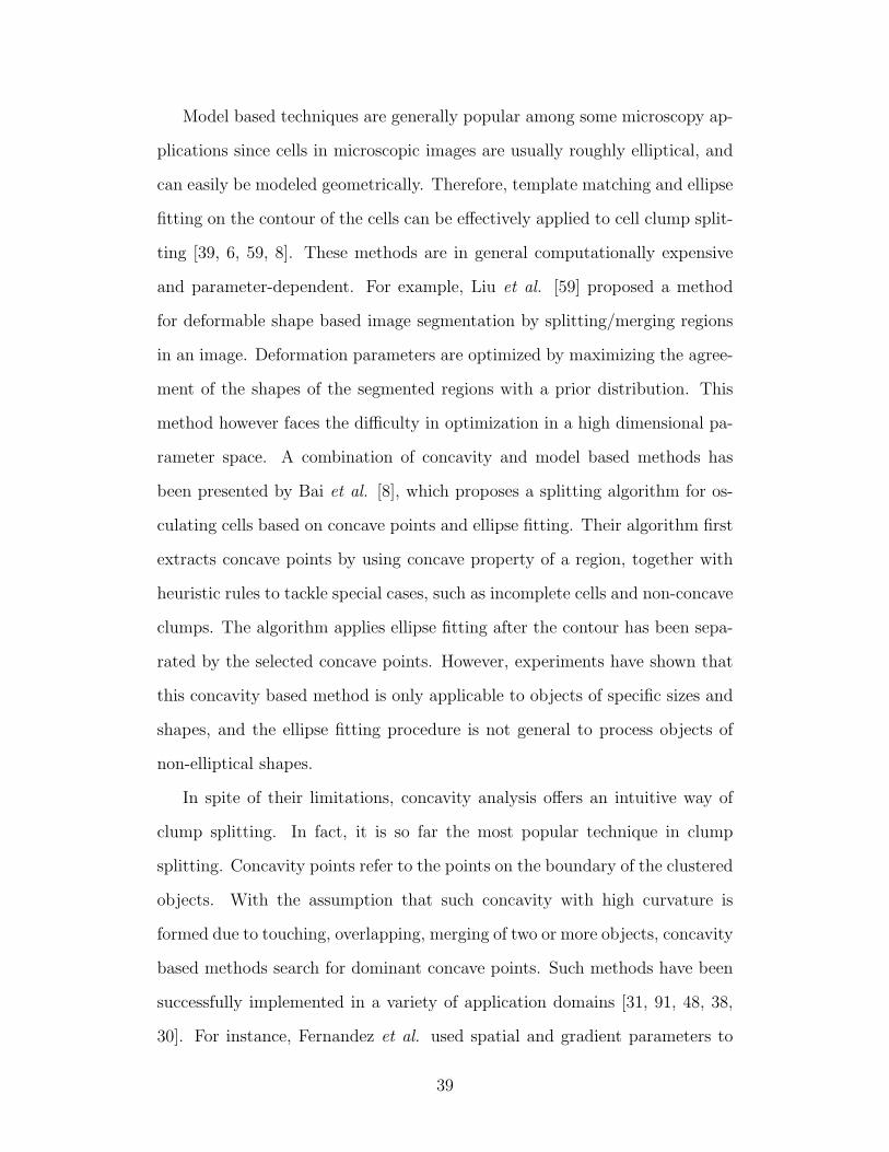
Model based techniques are generally popular among some microscopy ap-

plications since cells in microscopic images are usually roughly elliptical, and

can easily be modeled geometrically. Therefore, template matching and ellipse

fitting on the contour of the cells can be effectively applied to cell clump split-

ting [39, 6, 59, 8]. These methods are in general computationally expensive

and parameter-dependent. For example, Liu et al. [59] proposed a method

for deformable shape based image segmentation by splitting/merging regions

in an image. Deformation parameters are optimized by maximizing the agree-

ment of the shapes of the segmented regions with a prior distribution. This

method however faces the difficulty in optimization in a high dimensional pa-

rameter space. A combination of concavity and model based methods has

been presented by Bai et al. [8], which proposes a splitting algorithm for os-

culating cells based on concave points and ellipse fitting. Their algorithm first

extracts concave points by using concave property of a region, together with

heuristic rules to tackle special cases, such as incomplete cells and non-concave

clumps. The algorithm applies ellipse fitting after the contour has been sepa-

rated by the selected concave points. However, experiments have shown that

this concavity based method is only applicable to objects of specific sizes and

shapes, and the ellipse fitting procedure is not general to process objects of

non-elliptical shapes.

In spite of their limitations, concavity analysis offers an intuitive way of

clump splitting. In fact, it is so far the most popular technique in clump

splitting. Concavity points refer to the points on the boundary of the clustered

objects. With the assumption that such concavity with high curvature is

formed due to touching, overlapping, merging of two or more objects, concavity

based methods search for dominant concave points. Such methods have been

successfully implemented in a variety of application domains [31, 91, 48, 38,

30]. For instance, Fernandez et al. used spatial and gradient parameters to

39

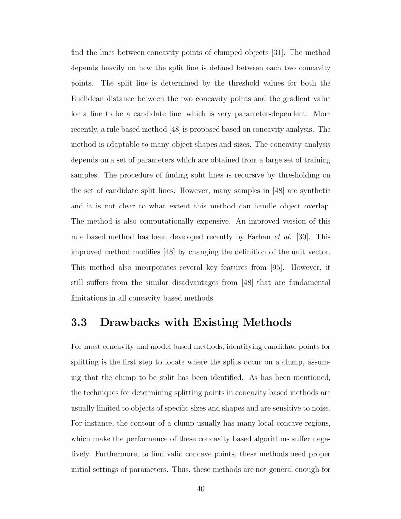
find the lines between concavity points of clumped objects [31]. The method

depends heavily on how the split line is defined between each two concavity

points. The split line is determined by the threshold values for both the

Euclidean distance between the two concavity points and the gradient value

for a line to be a candidate line, which is very parameter-dependent. More

recently, a rule based method [48] is proposed based on concavity analysis. The

method is adaptable to many object shapes and sizes. The concavity analysis

depends on a set of parameters which are obtained from a large set of training

samples. The procedure of finding split lines is recursive by thresholding on

the set of candidate split lines. However, many samples in [48] are synthetic

and it is not clear to what extent this method can handle object overlap.

The method is also computationally expensive. An improved version of this

rule based method has been developed recently by Farhan et al. [30]. This

improved method modifies [48] by changing the definition of the unit vector.

This method also incorporates several key features from [95]. However, it

still suffers from the similar disadvantages from [48] that are fundamental

limitations in all concavity based methods.

3.3 Drawbacks with Existing Methods

For most concavity and model based methods, identifying candidate points for

splitting is the first step to locate where the splits occur on a clump, assum-

ing that the clump to be split has been identified. As has been mentioned,

the techniques for determining splitting points in concavity based methods are

usually limited to objects of specific sizes and shapes and are sensitive to noise.

For instance, the contour of a clump usually has many local concave regions,

which make the performance of these concavity based algorithms suffer nega-

tively. Furthermore, to find valid concave points, these methods need proper

initial settings of parameters. Thus, these methods are not general enough for

40

clump splitting. In addition, as will be shown in this study, concavity points

are not always the best candidate points for splitting. Although Bai et al. [8]

proposed an extra step by adding points which are not concave points for split-

ting, this extra step is not always accurate and efficient, due to its assumption

that the objects are similar in both shape and size.

To demonstrate this issue, in Figure 3.1, columns (a) - (d) show four differ-

ent clumps. The red circles on the contours represent points found for splitting.

The first row shows the results from a classical concavity based method, which

can only find one concave point, because the second splitting point is not a

concave point. The second row shows the results from more recent concavity

based methods such as [8] and [48], which can find the second splitting point

through some rules. Unfortunately, since these rules normally assume that the

size of the two splitting candidates should be almost the same size, the second

points found are not necessarily the correct splitting points. The third row

show the results of our method based on bottleneck detection, which correctly

identifies a pair of splitting points in each of the cases. We will discuss the

details of our bottleneck detection method in Section 3.4.2.

To join each pair of selected splitting points, almost all the methods found

in the literature assume that the images are binarized and discard the original

intensity information [29]. Some splitting algorithms blindly join two selected

points with the shortest Euclidean distance. Some other splitting methods

apply the short cut rule [78], that is, if boundary points can be joined in more

than one way, the short cut rule prefers the shortest cut. However, these

methods may yield inaccurate segmentations. For an application where seg-

mentation accuracy is very important, blindly finding the shortest Euclidean

cut between the selected split points may not be optimal. From our observa-

tion, existing intensity information from the original image could be helpful

in obtaining a more accurate boundary than a straight line joining the pair of

41

(a) (b) (c) (d)

Figure 3.1: Visual comparison on the detection of splitting points. The top,middle and bottom rows show the results from classic concavity based method,which can find only one concavity point; the results from [8] and [48], which arenot always the correct points; and the results using our proposed bottleneckdetection. The detected splitting points are shown in red circles on the blackcontour of the clumps.

selected points. We refer to Figure 3.7 on page 55 to demonstrate this issue

in our experimental result section.

Another problematic issue with clump splitting is to decide whether a con-

nected component is a clump, and if it is, how many times it needs to be split.

While morphology and watershed based methods are parameter-dependent to

produce the number of splits, model and concavity based methods generally

decide the number of splits at the same time when the candidate split lines are

selected. When the best split lines are selected, the number of splits is decided

simultaneously. Various methods are proposed for this selection process. For

instance, Kumar et al. [48] applied a linear SVM classifier to determine the

best split line with concavity based features called the measure of split. This

classification has significantly improved the results for correct number of splits.

Farhan [29] applied Delaunay triangulation to list all candidate split lines, and

then made use of saliency, alignment and vector directional features to form a

42

cost function to select the best split lines. Once the split lines are selected, the

number of splits is also determined. However, most of these concavity based

methods are quite parameter-dependent in order to set the rules for selecting

the best split lines, and they still suffer from the limitation of concavity based

splitting methods as we mentioned in the beginning of this section.

3.4 Clump Splitting via Bottleneck Detection

To overcome these drawbacks mentioned in Section 3.3, we propose a novel

clump splitting method based on bottleneck detection and shape classifica-

tion. In contrast to most existing methods which detect splitting points first,

and then decide whether to split a connected component at these split points

afterwards, in our proposed method, we first decide whether to split a con-

nected component via a shape classification procedure and, if positive, apply

the proposed bottleneck detection to split the clump. Admittedly that in an

interactive segmentation framework, the decision of whether to split a con-

nected component can be made by the user interactively, we propose such a

method through shape classification as an option for the user.

Specifically, our proposed method contains two phases: offline and online.

A shape classifier is trained offline and then applied online iteratively. The

online phase consists of three steps as summarized by the flowchart in Figure

3.2. For the first step, we apply the shape classifier to decide whether to

split a connected component, with the help of a set of shape features. For

the second step, we focus on clumps with their splitting points occurring at

bottleneck positions. The only assumption made is that the objects to be split

into have roughly a convex shape. Based on our survey, this is a common

assumption in clump splitting. After locating the bottleneck positions, in the

third step, we find an optimal split curve between the selected points, based on

minimizing an image energy which corresponds to finding a connecting curve

43

that visually best splits the constituent objects of interest. Each time a new

connected component is generated from splitting, it will go through the shape

classification step again until no more splitting is found to be necessary.

Figure 3.2: Flowchart of the online phase in the proposed clump splittingalgorithm.

3.4.1 Shape Classification

This section describes the first step of our proposed method: shape classifi-

cation. This step is applied at the beginning of each iteration to determine

if a connected region should be split. Shape classification is a natural way to

determine if a split is necessary [65]. It is our general observation that, shape

features such as solidity and convexity are good application-specific features

to classify connected regions into splitting and no-splitting cases. Therefore,

the input to the shape classifier can be visualized as a matrix having the same

number of columns as the shape features we extract. Each row of the ma-

trix corresponds to a connected component. For each application, we build a

specific shape classifier based on shape features.

Different learning algorithms can be applied for shape classification based

44

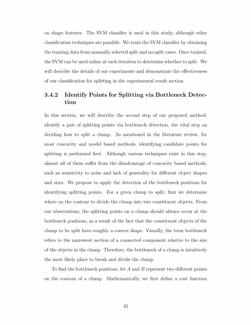
on shape features. The SVM classifier is used in this study, although other

classification techniques are possible. We train the SVM classifier by obtaining

the training data from manually selected split and no-split cases. Once trained,

the SVM can be used online at each iteration to determine whether to split. We

will describe the details of our experiments and demonstrate the effectiveness

of our classification for splitting in the experimental result section.

3.4.2 Identify Points for Splitting via Bottleneck Detec-tion

In this section, we will describe the second step of our proposed method:

identify a pair of splitting points via bottleneck detection, the vital step on

deciding how to split a clump. As mentioned in the literature review, for

most concavity and model based methods, identifying candidate points for

splitting is performed first. Although various techniques exist in this step,

almost all of them suffer from the disadvantage of concavity based methods,

such as sensitivity to noise and lack of generality for different object shapes

and sizes. We propose to apply the detection of the bottleneck positions for

identifying splitting points. For a given clump to split, first we determine

where on the contour to divide the clump into two constituent objects. From

our observations, the splitting points on a clump should always occur at the

bottleneck positions, as a result of the fact that the constituent objects of the

clump to be split have roughly a convex shape. Visually, the term bottleneck

refers to the narrowest section of a connected component relative to the size

of the objects in the clump. Therefore, the bottleneck of a clump is intuitively

the most likely place to break and divide the clump.

To find the bottleneck positions, let A and B represent two different points

on the contour of a clump. Mathematically, we first define a cost function

45

between points A and B as:

Es(A,B) =dist(A,B)

min {length(A,B), length(B,A)}(3.1)

where dist(A,B) represents the Euclidean distance between points A and B

inside the clump, length(A,B) denotes the clockwise length from point A to

B on the boundary of the clump, min {length(A,B), length(B,A)} represents

the smaller value between the two lengths. Here, we assume that for any

clump, the boundary should be one closed curve. Then, we denote by A∗

and B∗ the positions of the bottleneck on the contour where the cost Es is

minimized:

(A∗, B∗) = argminA,B

Es(A,B). (3.2)

Figure 3.3: Examples of a pair of points found via the bottleneck rule. Thered crosses indicate points A∗ and B∗ located at the bottleneck positions ofthe white contour.

Figure 3.3 shows a visual example of points A∗ and B∗ found via (3.2).

Again, we refer to Figure 3.1 to show some simple experiments to demon-

strate the advantage of the bottleneck method over the traditional concavity

point based methods and rule-based methods [48, 8]. We can see that our

bottleneck-based method works for situations when points for splitting in-

clude non-concave points, or when concave points with very high concavity

value are not the optimal candidate locations for splitting. Although [8] and

[39] proposed an extra step by adding points which are not concave points for

splitting, these extra steps are not always accurate and efficient, as shown in

the second row of Figure 3.1.

46

Even though we only find a pair of splitting points at one bottleneck, our

method can be extended easily to finding multiple pairs of points for splitting.

We have addressed the determination of the number of constituent objects in a

clump in Section 3.4.1 via shape classification. For objects which are classified

as split cases via shape classifier, the splitting algorithm will continue to work

iteratively via bottleneck detection.

3.4.3 Cut Between Selected Points via Weighted Short-est Path

As mentioned, almost all the methods found in the literature assume that the

images are binarized and discard the original intensity information. However,

from our observation, intensity information can sometimes be helpful in ob-

taining a more accurate object boundary. We refer to Figure 3.7 on page 55

to demonstrate this in our experiments. Therefore, we propose to connect the

pair of points found in the bottleneck detection step by the weighted shortest

path, to be described next. We will also show in the experiments that the

proposed method not only makes use of helpful edge information, but also can

work in a way similar to the existing methods when edge information is not

evident.

To begin with, we crop as the region of interest a small local image patch

I from the original image, around the two selected splitting points A∗ and B∗.

The size of the image patch I is defined to be proportional to the object size.

Figure 3.4 shows an example on how I (the highlighted rectangle) is formed,

from A∗ and B∗ found from Figure 3.3. We can see clearly that in this case

there exists some useful intensity information which can help in finding the

accurate splitting curve.

Intuitively, our goal is to find the strongest edge that connects the two

splitting points in the local image patch I. This leads to the following energy

47

Figure 3.4: Example of the local image patch I (the rectangle area highlighted).It is determined by the pair of points A∗ and B∗ found from the previous step.

function based on edge strength:

e(I) =

(∣∣∣∣ ∂∂xI∣∣∣∣+ ∣∣∣∣ ∂∂yI

∣∣∣∣) . (3.3)

Given such an energy function, finding a path between points A∗ and B∗

that maximizes the energy function corresponds to finding a connecting curve

that visually best splits the constituent objects of interest. This is under the

assumption that the constituent objects have a noticeable edge in between

them. Formally, we define a cut c to be a path connecting A∗ and B∗ on

I, with either a 4- or 8-pixel connectivity. We then define the cost of cut c

between points A∗ and B∗ to be E(c) =∑L

i=1 1/e(I(ci)), where ci represents

the position of a pixel at location i on the cut, and L is the length of c.

Therefore, an optimal cut c∗ minimizes cut cost E(c), i.e.:

c∗ = argminc

E(c) = argminc

L∑i=1

1

e(I(ci)). (3.4)

Interestingly, minimizing E(c) is equivalent to finding the weighted shortest

path between points A∗ and B∗ on I. In our implementation, we apply the

Dijkstra algorithm [26] to solve this shortest path problem.

Energy function (3.3) could also be written in different ways [7], as long as

it captures the edge information from the original image. In our experiments,

we only used gradient-based edge strength defined in (3.3). It is also obvious

that when edge information is not adequate, the cut between points A∗ and

48

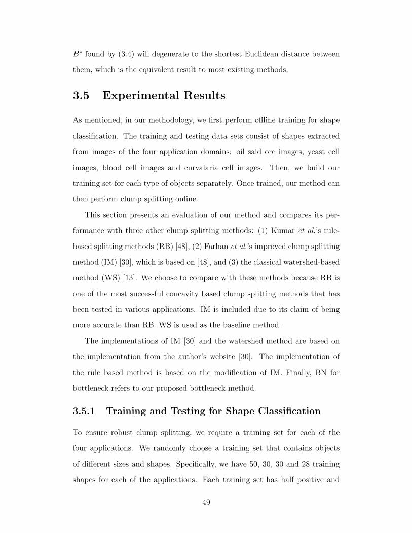
B∗ found by (3.4) will degenerate to the shortest Euclidean distance between

them, which is the equivalent result to most existing methods.

3.5 Experimental Results

As mentioned, in our methodology, we first perform offline training for shape

classification. The training and testing data sets consist of shapes extracted

from images of the four application domains: oil said ore images, yeast cell

images, blood cell images and curvalaria cell images. Then, we build our

training set for each type of objects separately. Once trained, our method can

then perform clump splitting online.

This section presents an evaluation of our method and compares its per-

formance with three other clump splitting methods: (1) Kumar et al.’s rule-

based splitting methods (RB) [48], (2) Farhan et al.’s improved clump splitting

method (IM) [30], which is based on [48], and (3) the classical watershed-based

method (WS) [13]. We choose to compare with these methods because RB is

one of the most successful concavity based clump splitting methods that has

been tested in various applications. IM is included due to its claim of being

more accurate than RB. WS is used as the baseline method.

The implementations of IM [30] and the watershed method are based on

the implementation from the author’s website [30]. The implementation of

the rule based method is based on the modification of IM. Finally, BN for

bottleneck refers to our proposed bottleneck method.

3.5.1 Training and Testing for Shape Classification

To ensure robust clump splitting, we require a training set for each of the

four applications. We randomly choose a training set that contains objects

of different sizes and shapes. Specifically, we have 50, 30, 30 and 28 training

shapes for each of the applications. Each training set has half positive and

49

half negative shapes (split/no-split cases). For testing, we have 649, 120, 257

and 50 testing objects for each of the applications.

It should be pointed out that, for each of the four types of images, we

build a specific shape classifier based on shape features of solidity, convexity,

eccentricity, area and variance on radius vectors. These features are used as the

inputs to an SVM classifier. In our experiments, we used the libsvm package

[17] for implementation.

We compare the accuracy from our shape classification to three other clump

splitting methods in Table 3.1. Accuracy is defined as the total number of cor-

rectly labeled connected components as split/no-split cases over the total num-

ber of connected components in the testing data set. The details of evaluation

metrics are described in Section 2.4.1 on page 29.

The results in Table 3.1 show that our shape classification method achieves

a much better accuracy in all image sets. Especially for the segmentations of

oil sand images, our method achieve much better accuracy due to very different

shapes and sizes in oil sand objects compare to cell objects. We will also show

in the next section that our method outperforms the competing methods in

the splitting point detection step as well, which makes the overall performance

even better in Table 3.2 and Table 3.3.

Table 3.1: Accuracy comparison between our shape classification method andthree other competing methods in terms of identifying split/no-split cases.

Image set WS [13] RB [48] IM [30] Our method

Oil sands 64% 66% 68% 86%Yeast cells 88% 81% 81% 90%Blood cells 87% 88% 88% 90%

Curvalaria cells 72% 86% 88% 88%

50

3.5.2 Implementation of Clump Splitting

After shape classification, connected components which are determined to be

clumps will go through the second and third steps of our method: splitting

via bottleneck detection and cutting between the detected points. Each time

when new objects are generated as the result of splitting, they will go through

the shape classification step again until no more new clumps are found, as

described in Figure 3.2. In this section, we will demonstrate some visual and

quantitative results and compare our results with three competing methods.

3.5.2.1 Visual Results

Visual results are shown in Figure 3.5, where the first row shows six input

clumps, the second to fourth rows show the splitting results from the three

competing methods, and the fifth row shows the results from our method. We

can see that our bottleneck-based method works for situations when points

for splitting include non-concave points, or when concave points with very

high concavity values are not the optimal candidate positions for splitting. It

is also clear that IM (row 4) tends to over-split. This is because IM takes

multiple points in one concavity region to avoid under-segmentation. In the

case of watershed (WS, row 2), over-split occurs some times and under-split

some other times. For cases when objects heavily overlap, watershed tends to

under-split. Another significant difference between our method and the rest of

the methods is shown in column (d), where while the other methods can only

split clumps based on points on the contour of the clump, our method can

successfully split connected components with other points inside the original

clump, which is possible for heavily overlapped clumps.

Another group of visual results are shown in Figure 3.6 to demonstrate the

effectiveness on multiple splitting cases only. We show the examples only from

the applications of oil sand ore images and yeast images because the multi-

51

ple splitting cases are more complicated in these two applications, in which

existing concavity based methods easily fail. Similarly, we can see that our

bottleneck-based method works for situations when points for splitting include

non-concave points, or when concave points with very high concavity values

are not the optimal candidate positions for splitting. Our shape classification

step helps in stopping the splitting procedure so that the algorithm does not

over-split the clumps.

Figure 3.7 demonstrates the advantage of our method in connecting bot-

tleneck positions. Row 1 shows four example input images, row 2 shows the

cuts of these clumps with a straight line, and row 3 shows the cuts by our

method which exploits image intensity information. Clearly, available edge in-

formation is helpful for accurate clump splitting, compared to connecting two

points with the shortest Euclidean distance. Especially for column (b), in the

third row, with edge based splitting, one newly split component has a more

obvious bottleneck shape than the results from the other methods and leads

to the next split successfully, while in the second row, a straight cut misleads

the next split and results in a cut that prevents the next clump splitting from

happening. For clumps in which edge information is missing between objects,

our split algorithm then provides a straight cut between each pair of splitting

points.

3.5.2.2 Quantitative Results

The overall performance of the clump splitting is evaluated quantitatively

using two metrics: (1) the overall accuracy, as defined in Section 2.4.1 on

page 29 ; (2) the probability of correct detection (PCD), which is defined as

the percentage of correctly split clumps [8], i.e., the number of correctly split

clumps divided by the total number of clumps that need to be split. Formally,

let C stands for the total number of correctly split clumps and T stands for

52

(a) (b) (c) (d) (e) (f)

Figure 3.5: Visual results for clump splitting. The first row shows the originalsegmentation, the second row shows the splitting results from watershed algo-rithm (WS), the third row shows the splitting results from Kumar’s concavitybased method (RB) [48], the fourth row shows the results from the improvedmethod (IM) [30] and the last row shows our results (BN). Column (a) and(b) are oil sands, column (c) is yeast cell, column (d) is blood cell, column(e) and (f) are curvalaria cells. We only show one example for yeast cell andblood cell because their shapes are very similar.

53

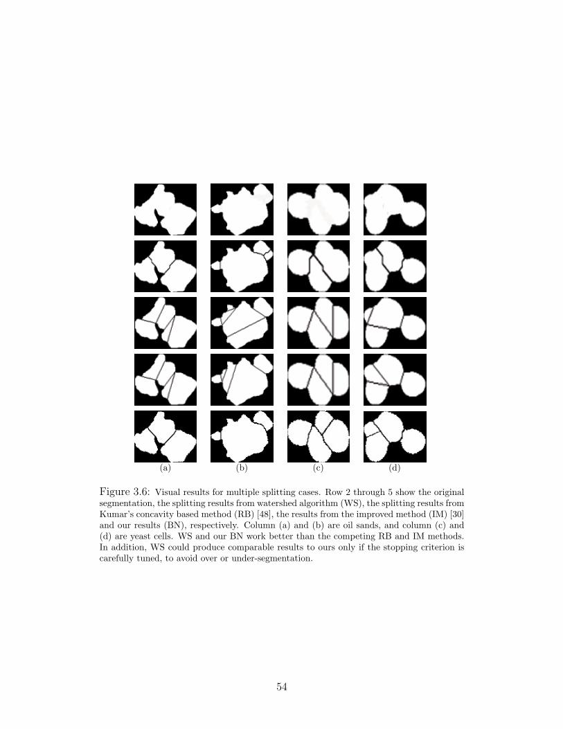
(a) (b) (c) (d)

Figure 3.6: Visual results for multiple splitting cases. Row 2 through 5 show the originalsegmentation, the splitting results from watershed algorithm (WS), the splitting results fromKumar’s concavity based method (RB) [48], the results from the improved method (IM) [30]and our results (BN), respectively. Column (a) and (b) are oil sands, and column (c) and(d) are yeast cells. WS and our BN work better than the competing RB and IM methods.In addition, WS could produce comparable results to ours only if the stopping criterion iscarefully tuned, to avoid over or under-segmentation.

54

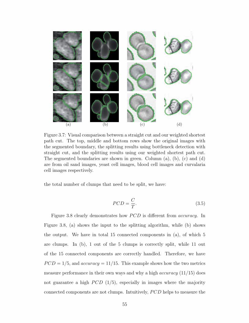
(a) (b) (c) (d)

Figure 3.7: Visual comparison between a straight cut and our weighted shortestpath cut. The top, middle and bottom rows show the original images withthe segmented boundary, the splitting results using bottleneck detection withstraight cut, and the splitting results using our weighted shortest path cut.The segmented boundaries are shown in green. Column (a), (b), (c) and (d)are from oil sand images, yeast cell images, blood cell images and curvalariacell images respectively.

the total number of clumps that need to be split, we have:

PCD =C

T. (3.5)

Figure 3.8 clearly demonstrates how PCD is different from accuracy. In

Figure 3.8, (a) shows the input to the splitting algorithm, while (b) shows

the output. We have in total 15 connected components in (a), of which 5

are clumps. In (b), 1 out of the 5 clumps is correctly split, while 11 out

of the 15 connected components are correctly handled. Therefore, we have

PCD = 1/5, and accuracy = 11/15. This example shows how the two metrics

measure performance in their own ways and why a high accuracy (11/15) does

not guarantee a high PCD (1/5), especially in images where the majority

connected components are not clumps. Intuitively, PCD helps to measure the

55

(a) (b)

Figure 3.8: An example on how PCD and accuracy are calculated. (a) showsthe input to the splitting algorithm while (b) shows the output. There arein total 15 connected components in (a), in which 5 of them are clumps. In(b), 1 out of the 5 clumps is correctly split, while 11 out of the 15 connectedcomponents are correct. Therefore, we have PCD = 1/5, and accuracy =11/15. This shows that a high accuracy (11/15) does not guarantee a highPCD (1/5), especially in images where the majority connected componentsare not clumps.

effectiveness of the splitting step only, while accuracy helps to measure the

effectiveness of the whole algorithm including shape classification.

The results in terms of PCD and the overall accuracy are presented in

Table 3.2 and Table 3.3, respectively. From both tables, we can see that in

most application domains BN obtains significantly higher accuracies and PCDs

than the competing methods. This is mostly because our method does not

begin with locating concave points and then evaluating all of them in order

to find the splitting points, but rather we find one pair of points that best

represent the bottleneck positions of the component. Therefore, our method

has a great advantage in splitting cases in which one or both of the points

are not necessarily concave points, or are not concave points with the highest

concavity value.

In addition, when comparing the results between Table 3.2 and Table 3.3,

we can see that results of PCD reflect more on how accurately the clumps are

split, which affects the overall performance of each method. When we compare

Table 3.3 with Table 3.1, we can see that our method (BN) reaches a much

56

better performance when compared with the competing methods, especially

in the oil sand, yeast cell and curvalaria cell data sets. In many cases, BN

succeeds while the other methods generally fail when clumps with multiple

objects heavily overlap. Compared with RB and IM, BN does not determine

the number of splits by evaluating all pairs of split points and split lines,

which are local measurements, but rather by considering the clump shape

globally. Our shape classification method also has an advantage in terms of its

flexibility to deal with various types of object classes expected in the clump

splitting applications.

Table 3.2: Probability of correct detection (PCD) for four image sets. Wecompare our bottleneck detection method (BN) with watershed method (WS),Kumar’s rule based method (RB) and Farhan’s improved method (IM) in thetable.

Image set WS [13] RB [48] IM [30] BN

Oil sands 22% 36% 39% 83%Blood cells 70% 54% 56% 72%Yeast cells 48% 61% 74% 83%

Curvularia cells 32% 58% 47% 60%

Table 3.3: Overall accuracy for four image sets. We compare our bottleneckdetection method (BN) with watershed method (WS), Kumar’s rule basedmethod (RB) and Farhan’s improved method (IM) in the table.

Image set WS [13] RB [48] IM [30] BN

Oil sands 60% 59% 62% 86%Yeast cells 58% 56% 60% 80%Blood cells 86% 86% 87% 87%

Curvalaria cells 47% 62% 66% 70%

57

3.6 Summary

In this chapter we have proposed a novel framework to perform clump split-

ting. The proposed method consists of three steps: (1) decide whether to split

a candidate connected component by shape classification; (2) find a pair of

points for clump splitting and (3) join the pair of selected points. In the first

step, an application-specific shape classifier is applied to determine whether a

connected component should be split. In the second step, a pair of points for

splitting is detected using an application-independent bottleneck rule, under

the assumption that the desired objects have roughly a convex shape. We

acknowledge that clump splitting in general is a research topic of broad in-

terest in image processing where this assumption may not hold, and that our

proposed algorithm should not be considered as general for splitting objects of

arbitrary shape. In the third step, the selected splitting points for step two are

joined by finding the optimal splitting line between them, based on minimizing

an image energy, again in an application-independent manner. The shape clas-

sifier is built offline via various shape features extracted from training shapes

in each application and a support vector machine.

The proposed method has several advantages over existing methods. First,

our method is not parameter-dependent on finding candidate points for split-

ting, unlike most existing methods, especially concavity based methods, which

are highly parameter-dependent. Our method is global and always finds the

bottleneck of a clump, which gives the best positions for splitting a convex-

shaped clump. Second, our method avoids dealing with special situations in

which splitting points are not concave. In these cases, almost all existing meth-

ods need to add extra points according to the heuristic rules and constraints.

Our method, on the other hand, avoids this issue by finding the optimal pair

of points, instead of one point at a time. Furthermore, our method takes in-

58

tensity information into account in localizing the cut between splitting points

and finds a more accurate cut than the straight-line cut that directly joins the

splitting points. Finally, the proposed method makes use of shape classifica-

tion to determine which connected components are clumps and the number

of splits for each clump, and it is therefore more flexible than model based

methods. We have validated our method in four different application domains

and have shown its better robustness and accuracy in clump splitting than the

state-of-the-art algorithms for this important problem in image segmentation.

The proposed clump splitting method can be easily incorporated in an

interactive segmentation framework. Admittedly in an interactive segmenta-

tion framework, the decision of whether to split a connected component can

be made by the user interactively, our proposed shape classification method

can also help in automated segmentation applications. In Chapter 5 we will

describe how to integrate this clump splitting method into an interactive seg-

mentation framework.

59

Chapter 4

Boundary Refinement via ShapePCA Method

60

This chapter presents the third contribution of this dissertation, namely the

shape PCA method. In order to refine the boundary of the incorrectly seg-

mented objects at the final stage of an image segmentation task, the shape

PCA method takes advantage of statistical shape information and refines the

shape of an incorrectly segmented object with the first few principal compo-

nents, which presumably represent the true shape of the object. This chapter

will first review some background on statistical shape analysis, focusing on

two dimensional shape representation, shape alignment and some existing sta-

tistical shape models. Then, principal component analysis (PCA) and our

proposed shape PCA method will be described followed by experimental re-

sults validating its effectiveness.

4.1 Introduction

Shapes are one of the basic and important visual features used to describe

image content. The shape of an object is a geometrical description of such an

object in a certain dimensional space, as determined by the object’s external

boundary. Mathematicians define shape as “all the geometrical information

that remains when location, scale and rotational effects are filtered out from

an object” [27]. In other words, a shape is not dependent on geometrical

transformations such as translation, scaling and rotation. Shapes can often be

described by basic geometry primitives such as points, lines, curves, etc.

Shape analysis is a difficult task in computer vision. When a three dimen-

sional object in the real world is projected onto a two dimensional plane, one

dimension of the shape information is lost. A shape extracted from digital

images is generally the projected 3-D object on a 2-D plane. What is worse,

the shapes we obtained from an digital image are often corrupted with noise,

occlusion, distortion, etc.

Statistical shape analysis is a geometrical analysis from a set of shapes

61

via statistical measures, to describe the geometrical properties among similar

shapes. Statistical shape analysis is now widely used to represent and analyze

various shapes. Before describing our proposed shape PCA method in Section

4.3, we will first present some preliminaries and existing methods in statistical

shape analysis.

4.2 Statistical Shape Analysis

4.2.1 Shape Representation

One of the first steps after collecting a set of shapes is to apply a proper shape

representation scheme for further statistical analysis. Shapes are generally

represented by effective and important shape features based on the boundary

of the shape, or both shape boundary and interior content of the shape. In

this dissertation, only two dimensional objects are considered. It is generally

assumed that the 2D information is sufficient for a reasonable characterization

of shapes [43].

There are different description techniques for categorizing shapes. Some

categorize them into contour-based and region-based methods [99]. This cate-

gorization is based on whether the shape features are extracted from the con-

tour of the shape only, or from the whole shape region. Under each class, dif-

ferent methods can be categorized further into structural approaches or global

approaches. This sub-class is based on whether the shape is represented as a

whole or represented by sub segments/sections of the shape. These approaches

can be even further distinguished into space domain or transform domain.

Another way of categorizing shape representation techniques is to divide

them into functional approaches, set theory approaches, and point/landmark

approaches, each of which is based on how shapes are described mathemati-

cally [43]. The functional methods describe shapes in terms of contour func-

62

tion, radius vector function, support function, width function, tangent-angle

function, etc. The set theory approaches, on the other hand, represent shapes

in terms of simple geometrical parameters such as area, perimeter, convex hull,

area-perimeter ratio, different roundness ratios, convexity ratio, etc. The third

types of techniques, which are one of the most commonly used techniques in

shape representation, describe shapes by a set of points which usually lie on

the contour of the shapes and are defined by some geometrical properties or

have a certain physical meaning. Such methods are also called landmark based

techniques.

In statistical shape analysis, one of the most popular shape representation

methods is to locate a finite number of coordinate points which are called

landmarks on the contour of a shape. A landmark is defined as a point of

correspondence on each object that matches between and within a group of

similar objects [27]. Landmarks are sometimes also called vertices, control

points, dominant points, nodes, markers, etc. Given a set of similar shapes in

a computer vision task, for each shape, a set of landmark points are extracted

using one or a combination of shape representation techniques. The extracted

landmark points must be consistent from one shape to another.

There are generally three types of landmarks: anatomical landmarks, math-

ematical landmarks and pseudo landmarks. An anatomical landmark is a point

assigned by an expert that corresponds between organisms in some biologically

meaningful way [27]. For example, the corners on the contour of an eye or

the joint point between two lungs are anatomical landmarks. Mathematical

landmarks are points located on an object which corresponds to some mathe-

matical or geometrical property of the shape. For example, dominant points

which are found on the high curvature positions on a contour of a shape are

mathematical landmarks. Pseudo landmarks are constructed points located

between anatomical or mathematical landmarks. Figure 4.1 shows an exam-

63

ple of landmarks located on the contour of an airway on an airway image. On

the airway, the white diamonds around crosses are mathematical landmarks,

and the red crosses only are pseudo landmarks.

Figure 4.1: Example of landmarks on the contour of an airway on an airwayimage. On the airway, the white diamonds around crosses are mathematicallandmarks, and the red crosses only are pseudo landmarks.

4.2.2 Shape Alignment

Finding a meaningful correspondence between two or more than two shapes is

a fundamental step before shape analysis can be properly performed. In such

a task, the goal is to find an explicit relationship between a group of similar

shapes. Finding such a matching involves searching through all possible shape

alignments [12]. Shape alignment is one of the solutions for shape matching by

performing transformation search. In statistical shape analysis, finding align-

ment between shapes is formulated as an optimization problem over matched

landmarks. In this section, we will introduce two basic and popular shape

alignment techniques: Procrustes analysis [27] and congealing [49].

64

4.2.2.1 Procrustes Analysis

The most popular method to align shapes in statistical shape analysis is the

generalized Procrustes alignment (GPA) [27]. The standard Procrustes match

minimizes the mean squared distance between two shapes. To align a group

of shapes to their mean shape, this procedure runs iteratively, resulting in the

generalized Procrustes alignment (GPA) [37, 81]. In the following sections we

will describe Procrustes distance and GPA.

Procrustes Distance

The Procrustes distance [27, 28, 15, 21] is a type of shape metric that requires

two aligned shapes to have one-to-one point correspondence. The alignment

process involves four steps as follows.

1. Compute the centroid of each of the shapes.

2. Normalize the two shapes to have the same size.

3. Align the two shapes at the centroids with regard to their positions.

4. Align the shapes with regard to their orientations.

After performing the four steps above, the squared Procrustes distance

between two shapes A and B is simply the sum of the squared point distances.

Let the landmark coordinates for shape A and B be A = (xAi, yAi), and

B = (xBi, yBi), i = 1...n, where n represents the total number of landmarks

on the border of each shape. The squared Procrustes distance between shape

A and B is therefore:

P 2d =

n∑i=1

[(xAi − xBi)2 + (yAi − yBi)

2]. (4.1)

Generalized Procrustes Alignment

To align a group of shapes to their mean shape, the standard Procrustes match

procedure run iteratively, resulting in the generalized Procrustes alignment.

65

The following iterative approach describes the generalized Procrustes analysis

procedure [81].

1. Choose an initial estimate of the mean shape (e.g. the first shape in the

set).

2. Align all the remaining shapes to the mean shape.

3. Re-estimate of the mean from the aligned shapes.

4. If the estimated mean has changed return to step 2.

When the mean shape does not change significantly within an iteration, the

above procedure converges.

4.2.2.2 Congealing

Among existing shape alignment methods, congealing is a flexible nonparamet-

ric data-driven framework for the joint alignment of a set of shapes. Congealing

has been successfully applied to the joint alignment of binary, gray scale and

color images [49].

Congealing is defined with respect to a set of transformations. For the

purpose of shape alignment, congealing is applied by taking a set of images and

transforming them according to a continuous set of allowable transformations

to make them more similar, according to the measure of similarity. It works

by parameterizing the set of transformations composing of x-translation, y-

translation, rotation, x-scale, y-scale, x-shear and y-shear. Thus, given a

parameter vector v = (tx, ty, θ, sx, sy, hx, hy), a transformation matrix U is

formed by:

U = F (tx, ty, θ, sx, sy, hx, hy)

=

1 0 tx0 1 ty0 0 1

cos θ − sin θ 0sin θ cos θ 00 0 1

esx 0 0

0 esy 00 0 1

1 hx 00 1 00 0 1

1 0 0hy 1 00 0 1

66

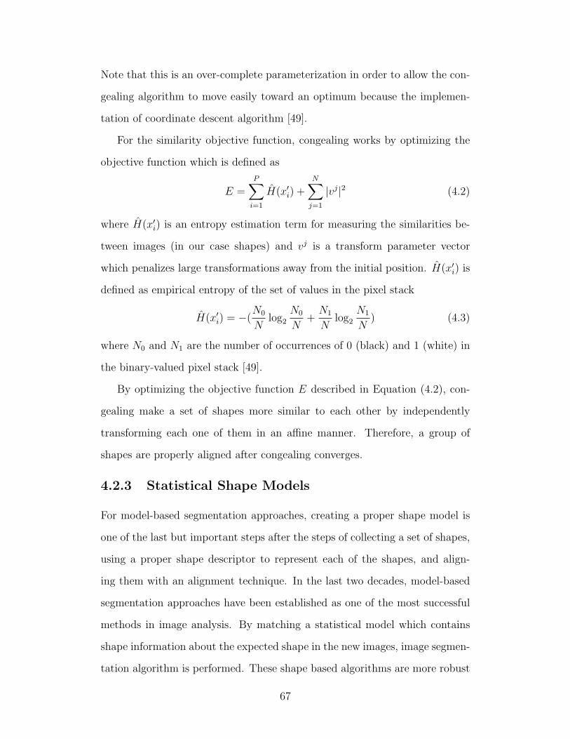
Note that this is an over-complete parameterization in order to allow the con-

gealing algorithm to move easily toward an optimum because the implemen-

tation of coordinate descent algorithm [49].

For the similarity objective function, congealing works by optimizing the

objective function which is defined as

E =P∑i=1

H(x′i) +

N∑j=1

|vj|2 (4.2)

where H(x′i) is an entropy estimation term for measuring the similarities be-

tween images (in our case shapes) and vj is a transform parameter vector

which penalizes large transformations away from the initial position. H(x′i) is

defined as empirical entropy of the set of values in the pixel stack

H(x′i) = −(

N0

Nlog2

N0

N+

N1

Nlog2

N1

N) (4.3)

where N0 and N1 are the number of occurrences of 0 (black) and 1 (white) in

the binary-valued pixel stack [49].

By optimizing the objective function E described in Equation (4.2), con-

gealing make a set of shapes more similar to each other by independently

transforming each one of them in an affine manner. Therefore, a group of

shapes are properly aligned after congealing converges.

4.2.3 Statistical Shape Models

For model-based segmentation approaches, creating a proper shape model is

one of the last but important steps after the steps of collecting a set of shapes,

using a proper shape descriptor to represent each of the shapes, and align-

ing them with an alignment technique. In the last two decades, model-based

segmentation approaches have been established as one of the most successful

methods in image analysis. By matching a statistical model which contains

shape information about the expected shape in the new images, image segmen-

tation algorithm is performed. These shape based algorithms are more robust

67

compare to algorithms which only segment an image based on image inten-

sity information. Considering the variability of the objects of similar shapes,

information about shape variations can be included in a shape model. Statis-

tical shape model is such an approach to collect statistical shape information

including shape variations via a number of sample shapes.

Constructing a statistical shape model basically consists of extracting the

mean shape and a number of modes of variation from a collection of samples.

Due to the dominant role and simplicity in landmark-based representation, we

concentrate on landmark-based models in this section. Given a set of such

examples, we first align them into a common Euclidean coordinate system

using shape alignment techniques such as GPA or congealing. Once aligned,

different statistical shape models can be applied. In the following section,

some background on principal component analysis (PCA) will be presented,

followed by the description of Active Shape Model.

4.2.3.1 PCA and Related Work

Principal Component Analysis (PCA) [44] is a standard method in a variety

of applications to find out inherent data structure. It refers to a mathematical

procedure that applies orthogonal transformation to convert a set of originally

possibly correlated variables to a set linearly uncorrelated variables. The lin-

early uncorrelated variables are defined as principal components. The principal

components represent the major directions of variability in the dataset and are

described by the eigenvectors. The orthogonal transformation generates prin-

cipal components in such a way that the first principal component has the

highest variance.

Principal Component Analysis (PCA) has been used widely in the liter-

ature for modeling shape variations for traditional statistical shape analysis.

Cootes et al. [23] introduced the Active Shape Model (ASM). On the other

68

hand, Active Appearance Model (AAM) is introduced as a generative model

that can synthesize images similar to those in the training set [20]. Typically,

AAM is used for image interpretation and syndissertation applications. Using

a set of training images, both shape and texture of the object of interest are

modeled. Therefore, image interpretation tasks can easily fit a new unseen

image into the model.

Moreover, Cootes et al. [22] developed PCA in the tangent space for sta-

tistical shape analysis. They [23, 22, 19] applied PCA and built a point dis-

tribution model (PDM) to describe the variability in shape, which is a model

for shape and uses Procrustes residuals. Based on this two-dimensional for-

mulation of shape PCA, Wang et al. [93] proposed an approach for boundary

detection where shape priors and edge information of the input image are in-

corporated. However, these methods encounter difficulties for cases when edge

information is weak, or when objects have occlusions. To deal with these situ-

ations when edge information is very weak or totally missing, we propose the

shape PCA method in Section 4.3. Before getting into the details of our shape

PCA method, we will give some related background on a specific statistical

shape model: active shape model.

4.2.3.2 Active Shape Model

Cootes et al. introduced the Active Shape Model (ASM), which is a deformable

model that globally constrains the deformation of a shape to valid instances of

the object of interest [23]. The shape constraint normally improves the model

and provides better segmentation. The ASM algorithm consists of three major

steps: (i) generating Point Distribution Model (PDM), (ii) generating Local

Appearance Model (LAM), and (iii) model search procedure. We will describe

each of the major steps briefly in this section.

69

Point Distribution Model

The point distribution model (PDM) is a model for representing the mean ge-

ometry of the shape and some statistical modes of geometric variation inferred

from a set of training shapes. It is the first and most crucial step for the ASM

algorithm.

Let the contour of an object be represented by a fixed number of labeled

landmarks pi = (xi, yi), i = 1...n. Prior to modeling the shape variations in the

training set, we assume that they are already aligned with respect to transla-

tion, rotation and scaling via a shape alignment method. Non-rigid variations

are then modeled by using the PDM. PDM uses principal component analysis

(PCA) to capture the second-order statistics in the training set. The PDM

represents a shape as a mean shape plus a weighted sum of basic functions

defined as the eigenvectors of the covariance matrix. Formally, the mean shape

is defined as:

x =1

N

N∑i=1

xi. (4.4)

where N stands for the number of shapes and xi denotes the ith shape. The

covariance matrix is

S =1

N − 1

N∑i=1

(xi − x)(xi − x)T . (4.5)

The eigenvector φk and eigenvalues λk of S are therefore computed as:

Sφk = λkφk. (4.6)

Since the matrix of the eigenvectors ϕ = [φ1φ2...φN ] represents the modes

of variations of the shapes, normally the variations in the training set can be

described by a small number of modes. Therefore, a good estimation of the

shape can be obtained by retaining the eigenvectors φi that correspond to the

t largest eigenvalues:

x = x+ ϕb (4.7)

70

where ϕ = [φ1φ2...φN ] and b is a t dimensional vector given by

b = ϕT (x− x). (4.8)

The vector b defines a set of parameters of a deformable model [18].

PDM can be extended to any arbitrary number of dimensions, but is typ-

ically used in two dimensional image and three dimensional volume applica-

tions.

Local Appearance Model

During the training phase of constructing ASM, a local appearance profile is

constructed for every landmark point on the contour. The main idea is to

examine the image level information in a region on the original image around

each landmark throughout the training set. Given a training set of Np images,

the local appearance profile is constructed as follows. Assuming we are dealing

with gray scale images, for every landmark point j in the image i of the training

set, a gray level profile gij is extracted, of length np pixels, centered around

the landmark point. Here the actual gray level profile from the image is not

used, but its normalized derivative. This gives invariance to the offsets and

uniform scaling of the gray levels.

Therefore, the gray level profile of the landmark j in the image i is a vector

of np intensity values:

gij = [gij0gij1 . . . gijnp−1]T (4.9)

and the normalized derivative of the gray level profile is

yij =dgij∑np−2

k=0 |dgijk|(4.10)

where dgij = [gij1 − gij0, gij2 − gij1, . . . , gijNp−1 − gijNp−2]T .

Now the mean of the normalized derivative profiles of each landmark through-

out the training set can be calculated. For each landmark j, the mean profile

71

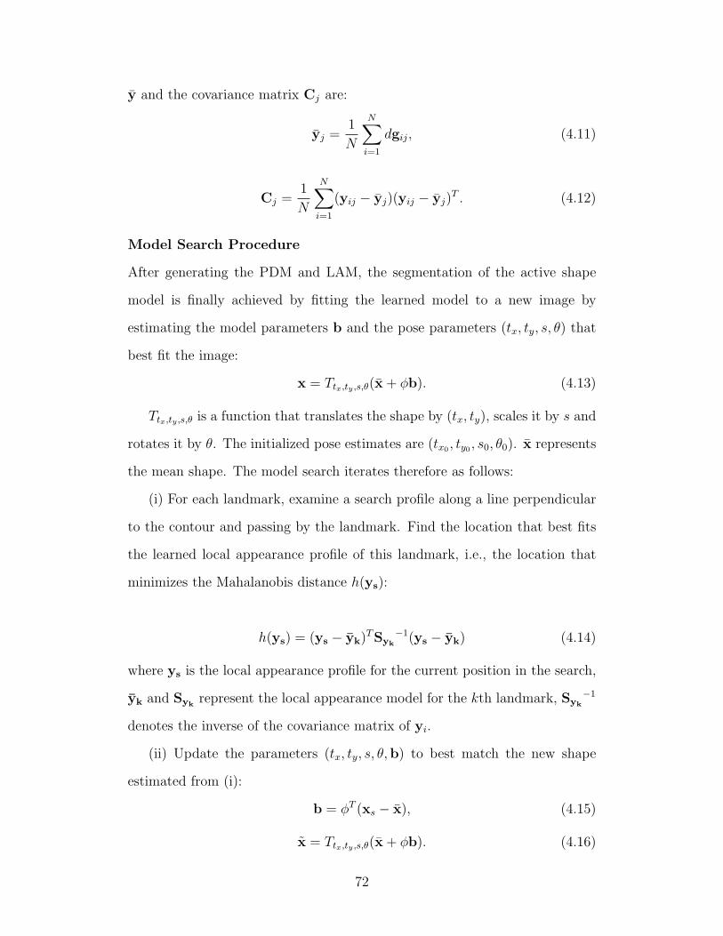
y and the covariance matrix Cj are:

yj =1

N

N∑i=1

dgij, (4.11)

Cj =1

N

N∑i=1

(yij − yj)(yij − yj)T . (4.12)

Model Search Procedure

After generating the PDM and LAM, the segmentation of the active shape

model is finally achieved by fitting the learned model to a new image by

estimating the model parameters b and the pose parameters (tx, ty, s, θ) that

best fit the image:

x = Ttx,ty ,s,θ(x+ ϕb). (4.13)

Ttx,ty ,s,θ is a function that translates the shape by (tx, ty), scales it by s and

rotates it by θ. The initialized pose estimates are (tx0 , ty0 , s0, θ0). x represents

the mean shape. The model search iterates therefore as follows:

(i) For each landmark, examine a search profile along a line perpendicular

to the contour and passing by the landmark. Find the location that best fits

the learned local appearance profile of this landmark, i.e., the location that

minimizes the Mahalanobis distance h(ys):

h(ys) = (ys − yk)TSyk

−1(ys − yk) (4.14)

where ys is the local appearance profile for the current position in the search,

yk and Sykrepresent the local appearance model for the kth landmark, Syk

−1

denotes the inverse of the covariance matrix of yi.

(ii) Update the parameters (tx, ty, s, θ,b) to best match the new shape

estimated from (i):

b = ϕT (xs − x), (4.15)

x = Ttx,ty ,s,θ(x+ ϕb). (4.16)

72

4.3 Boundary Refinement via Shape PCA

One problem with current statistical models is that when image level informa-

tion is inadequate or missing, the statistical models have difficulties converging

to the correct segmentation. On the other hand, in an interactive segmentation

scenario, when the user can tell that the image level information is inadequate

or missing, so that existing statistical shape model based methods will have dif-

ficulties, a different method based only on statistical shape information should

be applied to avoid such difficulties. Our proposed shape PCA method is de-

veloped with such motivation. Our shape PCA method is capable of not only

refining the boundary of the desired object, but also improving the efficiency

of the segmentation procedure by avoiding the model search procedure.

4.3.1 Shape PCA Projection

As mentioned, previous shape PCA methods in image segmentation incor-

porate statistical shape information as a prior term in the deformable shape

model and iteratively achieve convergence in a segmentation process. Our

method, on the other hand, exploits the assumption that the major princi-

pal components (PCs) represent the true shape and the residual error from

shape PCA represents segmentation errors and thus should be removed in

order to obtain satisfying segmentation results. The geometric shape infor-

mation is represented using landmarks on the contour of the shape, based on

two dimensional formulation. Shape PCA is subsequently applied to extract

relevant information, under the assumption that a correctly segmented shape

should be similar to those previously seen in the training set.

To be more detailed, the shape PCA method consists of a training phase

and a testing phase. For both the training and the testing phase, we first

convert the geometric shapes into a numerical representation. Since we choose

73

landmark based representation in our experiments, this procedure is typically

done by identifying or placing landmarks along the shape boundary. To illus-

trate it in a simple way, in our experiments, we evenly place a fixed number of

landmarks along the boundary of the aligned shape, which is done in a similar

way in existing work such as [23]. Here we assume that all the shapes are

aligned already, by either procrustes analysis or congealing.

In the training phase, given m aligned shapes, each of which with a set

of n landmarks, we can calculate the mean shape and the covariance matrix.

Each of the aligned shapes can be represented as:

Li = [xi(1), xi(2), . . . , xi(n), yi(1), yi(2), . . . , yi(n)]T (4.17)

where i = 1, ...,m, xi(k) and yi(k) denote the x and y coordinates of the kth

landmark position in the two dimensional Euclidean space. After performing

PCA on the aligned shapes in the training set, we let PCj represent the jth

principal component.

In the testing phase, when a new testing shape comes which needs bound-

ary refinement, in order to reconstruct a new shape, we can perform PCA

projection by using only a selected number of the principal components. The-

oretically, the first few largest eigenvectors usually describe the most significant

modes of variations of the shapes which belong to the same category. We can

therefore reconstruct a new shape in the reprojection process by not using

the rest of the PCs which presumably mostly represent unwanted parts of the

shapes. Following this assumption, we have

Lgi =

∑j∈SPCA

(PCj · wj) (4.18)

where Lgi = [x′

i(1), x′i(2), . . . , x

′i(n), y

′i(1), y

′i(2), . . . , y

′i(n)]

T represents the re-

constructed shape, SPCA is a subset of {1, . . . ,m}, which represents the indices

of selected principal components, and wj = PCTj Li.

74

4.3.2 Algorithm for Shape PCA

As mentioned, the proposed shape PCA algorithm consists of two parts, train-

ing (left column of Figure 4.2) and testing (right column of Figure 4.2). The

training part where PCA is performed to learn object shapes consists of the

following steps:

1. Obtain training shapes. This can be done from a collection of ground

truth images which are manually labeled by experts.

2. Align all the extracted shapes. Before shape alignment, the same

number of landmarks are placed evenly on the perimeter of each of the

aligned training shapes. Then the alignment can be done by different

shape alignment methods. In our experiments we choose congealing

(see Section 4.2.2.2) because it is efficient and optimal, although similar

results could be obtained by Generalized Procrustes Alignment.

3. Perform principal component analysis on the training shapes.

To apply the extracted shape information from the training phase online, im-

provement for a given incorrectly segmented object consists of the following

steps (we call them testing steps):

1. Shape alignment. This step performs similar landmark interpolation

and shape alignment procedures as in the training phase.

2. Shape PCA projection. In this step, we choose a fixed number of

principal components and perform PCA projection on the testing shape,

which is the incorrectly segmented object.

3. Obtain the segmentation results. In order to obtain the final image

segmentation result, the inverse procedure for the aligned shape should

be performed, such as scaling, rotation, etc.

75

Figure 4.2: Flowchart of the proposed shape PCA algorithm, with examples onoil sand image segmentations. The left column in the figure shows the trainingsteps, with training shapes extracted from manually labeled segmentation.The right column shows the testing steps with incorrectly segmented objectsin the initial segmentation. The red boundary on the last image on the rightcolumn represents the improved segmentation after our proposed shape PCAmethod.

76

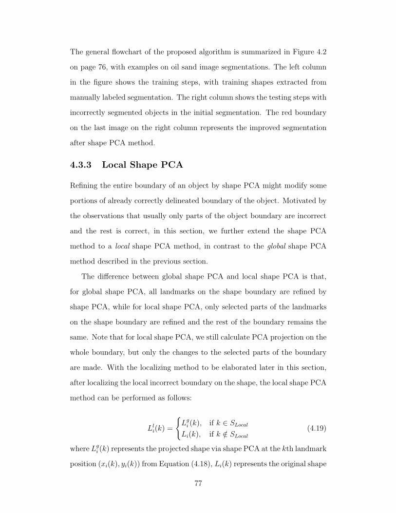
The general flowchart of the proposed algorithm is summarized in Figure 4.2

on page 76, with examples on oil sand image segmentations. The left column

in the figure shows the training steps, with training shapes extracted from

manually labeled segmentation. The right column shows the testing steps with

incorrectly segmented objects in the initial segmentation. The red boundary

on the last image on the right column represents the improved segmentation

after shape PCA method.

4.3.3 Local Shape PCA

Refining the entire boundary of an object by shape PCA might modify some

portions of already correctly delineated boundary of the object. Motivated by

the observations that usually only parts of the object boundary are incorrect

and the rest is correct, in this section, we further extend the shape PCA

method to a local shape PCA method, in contrast to the global shape PCA

method described in the previous section.

The difference between global shape PCA and local shape PCA is that,

for global shape PCA, all landmarks on the shape boundary are refined by

shape PCA, while for local shape PCA, only selected parts of the landmarks

on the shape boundary are refined and the rest of the boundary remains the

same. Note that for local shape PCA, we still calculate PCA projection on the

whole boundary, but only the changes to the selected parts of the boundary

are made. With the localizing method to be elaborated later in this section,

after localizing the local incorrect boundary on the shape, the local shape PCA

method can be performed as follows:

Lli(k) =

{Lg

i (k), if k ∈ SLocal

Li(k), if k /∈ SLocal

(4.19)

where Lgi (k) represents the projected shape via shape PCA at the kth landmark

position (xi(k), yi(k)) from Equation (4.18), Li(k) represents the original shape

77

at landmark position k, SLocal is the selected local sections of the boundary

that need to be fixed, expressed as a subset of {1, . . . n}.

To identify sections of the object boundary that should be improved or

refined via shape PCA, we observe that in applications such as oil sand images

and cell images, empirically there is a strong correlation between incorrect

boundary delineation and frequent change in the polarity of the curvature.

This change can be captured with the help of the radius-vector function [82]

associated with the object boundary. Therefore, in order to localize inaccurate

boundary, we focus on detecting local boundary with high variances of radius-

vector function and select them as SLocal to perform local shape PCA.

To be more specific, after landmarks are placed evenly on the perimeter of

the shape, we pick an arbitrary point O that is interior to the shape, and calcu-

late the distances or radii from O to the landmarks. For a section of the bound-

ary to be considered inaccurate or incorrect, the variance of the radii within

that section must exceed a certain threshold, which is application-dependent.

This calculation is then performed to all landmarks, and the sections which

need to be corrected can then be identified and assigned to SLocal in Equation

(4.19).

4.4 Experimental results

The shape PCA method has been implemented and tested on oil sand images

[88]. Our experiment uses a set of nine oil sand images to validate the proposed

approach for boundary refinment. The nine images are first segmented by

human experts to establish ground truth. They are then sent to a watershed-

based segmentation algorithm [53] to generate machine-segmented images, to

be corrected by our shape PCA algorithm. The first ground truth image is

used for training to obtain the PCs of expected shapes, and the remaining

eight are used for testing.

78

When shape PCA is performed on the eight testing images, the number

of principal components varies from one to the maximum number of principal

components (74 in our experiments). We perform shape PCA for both global

and local shape PCA and compare the statistical and visual results.

Figure 4.3 shows an example of visual results of how segmentations have

been improved after performing shape PCA method on oil sand images. In

Figure 4.3, (a), (b) and (c) are global shape PCA results with the selections

of 3, 5 and 10 PCs while (d), (e) and (f) are local shape PCA results with the

selections of 3, 5 and 10 PCs. The location within the green dashed box shows

an example where local and global shape PCA perform differently. Figure

4.4 and Figure 4.5 show the statistical results of accuracy and score from

both global and local shape PCA methods on oil sand images. The details of

evaluation metrics are described in Section 2.4.1 on page 29

Figure 4.3: An example of visual results of how segmentations have beenimproved after performing global and local shape PCA methods on oil sandimages. (a), (b) and (c) are global shape PCA results with the selections of3, 5 and 10 PCs while (d), (e) and (f) are local shape PCA results with theselections of 3, 5 and 10 PCs. The location within the green dashed box showsan example where local and global shape PCA perform differently.

From both statistical and visual results, we can see that performing shape

79

Figure 4.4: Statistical results of accuracy with both global and local shapePCA methods on oil sand images.

80

PCA as a boundary refinement step improves the final segmentation results, at

both the pixel level and object level, when the number of principal components

is properly chosen. In particular, local shape PCA produces a better and more

stable performance than global shape PCA in general, as long as the incorrectly

segmented sections of the object boundary can be correctly identified.

Figure 4.5: Statistical results of score with both global and local shape PCAmethods on oil sand images.

Our experimental results are based on the application of oil sand image seg-

mentations. However, because we make few assumptions, except that ground

truth images are available and objects of interest share common shape char-

acteristics, the proposed algorithm is not limited to this application. It could

be easily applied to applications such as blood cell image segmentations, etc.

As long as the incorrectly segmented sections of the boundary can be localized

correctly, either automatically or manually, our shape PCA method can be

utilized into the boundary refinement procedure in an segmentation task.

81

4.5 Summary

This chapter focuses on the last step of an image segmentation task: boundary

refinement. We start approaching boundary refinement by statistical shape

analysis. After reviewing some preliminaries and background on statistical

shape analysis, the shape PCA method is proposed in this chapter. The shape

PCA method takes advantage of shape information which is not directly avail-

able from image level. In the boundary refinement process, the shape PCA

method refines the 0boundary of an object by using the first few principal

components which presumably represent the true shape of the object. The

local shape PCA method is also proposed to be compared with the global

shape PCA method. As long as the incorrectly segmented portions of the

object boundary can be localized correctly, either automatically or manually,

local shape PCA can be easily applied to perform boundary refinement for

incorrectly segmented objects. In Chapter 5 we will describe how to integrate

the shape PCA method to an interactive segmentation system.

82

Chapter 5

An Interactive ImageSegmentation System

83

This chapter introduces a comprehensive framework for interactive image seg-

mentation, as an example to integrate the shape-guided segmentation algo-

rithms developed in this dissertation. This interactive segmentation frame-

work is composed of five tools, which are developed based on common cases

of incorrect segmentations from any segmentation algorithms. From observa-

tion, most image segmentation tasks can be handled by a combination of these

five actions. When combining all the shape-guided segmentation algorithms

we proposed in the previous chapters, adaptive shape prior (ASP) method,

clump splitting method via bottleneck detection, and shape PCA method,

this interactive segmentation framework can be constructed into a highly ef-

fective and efficient interactive object segmentation system with minimal user

input.

5.1 Purpose of User Interaction

As mentioned, user interaction is very crucial for obtaining desired segmen-

tation results. As a general rule from the existing research, the purpose of

interaction is to combine the expertise of a human operator and the power of

a segmentation algorithm to obtain the desired delineation of the object in the

image in an efficient manner [66]. Figure 1.2 has already demonstrated the

general process of an interactive segmentation and where user interaction can

be applied. The major assumption for this interaction process is that the user

who is interacting should have a correct and clear vision of the desired segmen-

tation result. The user should also be able to judge what types of dedicated

segmentation algorithms are needed. Guiding the segmentation algorithm to

find and improve correct segmentation results in an efficient way is also the

user’s role in the interactive segmentation process.

In an interactive scenario, the purpose of the user interaction can be sum-

marized in the following ways:

84

1. To judge whether the segmentation result is correct.

2. To choose a function/option to perform a dedicated segmentation algo-

rithm.

3. To initialize a starting position on the image for the segmentation algo-

rithm.

4. To set/change parameter values for the segmentation algorithm.

5. To compose/modify the primitive results obtained from a segmentation

algorithm.

Combinations of these purposes in user interaction can be found in several pre-

vious works [16, 42, 71, 50, 10]. Ideally, an effective and efficient interactive

segmentation system should serve as much a combination of the purposes de-

scribed above as possible, i.e., a simple mouse click can both judge whether the

result obtained is correct and to choose a segmentation algorithm to perform

the task.

5.2 Types of User Interaction

Besides the purposes of user interaction, we should also be aware of the com-

mon existing types of interaction between the user and the computer in image

processing. These common types of user interaction exist in tasks such as

image segmentation, image editing, image post-processing, etc. A good in-

teractive system should design simple and effective interactions which require

minimal user input. One way of categorizing the types of user interaction in

image segmentation are listed as following:

1. Point. For example, a single mouse click or multiple clicks to add or

delete seeds in segmentation algorithms such as snake and active contour

models [42].

85

2. Line. For example, a stroke to specify labeling pixels for foreground or

background in the graph cut algorithm [16].

3. Area. For example, a couple of clicks to specify the region of interest in

the grabcut algorithm [71].

4. Volume. For example, for three-dimensional structure segmentation,

multiple mouse clicks can define the volume of interest.

5.3 Common Segmentation Mistakes

Segmentation algorithms fail when the object in the image deviates too much

from the ideal appearance covered by the segmentation model [66]. On the

other hand, it is important to note that, in a lot of cases, segmentation mis-

takes are still confined to part of the desired object of interest. Based on

this observation, in this chapter, we will develop a comprehensive interactive

image segmentation framework based on common segmentation mistakes. We

observe that there are a finite number of cases of failure, which correspond

to the finite number of tools needed in the interactive segmentation system.

To sum up, most existing segmentation algorithms are bounded to fail in the

following situations:

1. When an object of interest should be segmented but is missing, an ad-

dition action is needed to add such an object.

2. When an object should not be there but is included in the segmentation

result, a deletion action is needed to remove it.

3. When the segmentation algorithm under-segments the objects due to

object fusion, a splitting action is needed to split two or more than two

connected components.

86

4. When the segmentation algorithm over-segments the object of interest

into multiple objects, a merging action is needed to merge two or more

disconnected objects.

5. When the visual evidence is too low, or there is too much noise from

the image, or there is misleading visual evidence, etc., a boundary

refinement action is needed to refine/edit the incorrectly segmented

portions of the object.

Although there are no universal rules of the types of mistakes of all possible

segmentation algorithms, from observations, most segmentation algorithms are

bounded to make similar mistakes as stated above. Interestingly, splitting

and deletion actions deal with under-segmentation misktaes, while merg-

ing and addition actions deal with over-segmentation mistakes. Boundary

refinement can deal with both under- and over-segmentation.

5.4 An Interactive Segmentation System based

on Common Segmentation Mistakes

In an interactive segmentation system, the interactive tools available to the

user must be powerful and intuitive, and allow efficient interaction. Depending

on the purpose of user interaction, the corresponding tool should be specific

for the action that the user wants to perform. It is inefficient to design one

universal editing tool as it will display nonspecific performance, because each

of the mistakes described in Section 5.3 leads to a different type of algorithm

or method.

Since we have concluded that there are commonly five types of segmenta-

tion mistakes, subsequently, five types of tools are needed to deal with each of

the mistakes: addition, deletion, splitting, merging and boundary refinement.

For each interactive tool, a corresponding method will be designated. Table

87

5.1 gives a summary of the different types of segmentation mistakes and the

corresponding actions proposed. Figure 5.1 presents a general flowchart of our

proposed interactive image segmentation system.

Table 5.1: Interactive tools, the corresponding reasons for the tools and de-tailed actions for the tools in the proposed interactive segmentation system

Tools Reasons Actions

Addition Object of interest is missing Add an object of interestDeletion Segmented object should be removed Remove an objectSplitting Under-segmentation Split one object into two,

or more than two, objectsMerging Over-segmentation Merge two, or more than

two, disconnected objectsBoundary Visual evidence is low, misleading Refine the boundary to aRefinement visual evidence, etc. more desired segmentation

Figure 5.1: The general flowchart of our proposed interactive image segmen-tation system.

88

For each of the five cases in the proposed framework, we apply either one

of the shape-guided algorithms we described in the previous chapters, or an

interactive method. For addition, the adaptive shape prior method described

in Chapter 2 can be utilized. For deletion, the user can interactively select

each unwanted object or a whole region in which unwanted objects are. For

splitting, the clump splitting method via bottleneck detection described in

Chapter 3 can be applied. For merging, we design an interactive way to let the

user select adjacent objects to be merged by joining the touching boundaries

between them. Finally, boundary refinement can be achieved by the shape

PCA method presented in Chapter 4.

Table 5.2 provides a summary of each of the interactive tools and their cor-

responding methods described in this dissertation. The proposed framework

is an example to integrate all the proposed shape-guided algorithms in this

dissertation. On the other hand, this proposed system is not constrained by

these shape-guided segmentation algorithms. It is flexible and should easily

integrate other types of segmentation algorithms.

Table 5.2: Summary of the interactive tools and their corresponding methodsfor the proposed interactive segmentation system

Tools Methods

Addition Adaptive Shape PriorDeletion Interactive Object DeletionSplitting Clump Splitting via Bottleneck DetectionMerging Interactive Objects MergingBoundary Refinement Shape PCA

5.5 Experimental Results

This section presents the details of the proposed interactive segmentation sys-

tem and the extensive experimental evaluation of the system, focusing on the

89

image segmentation performance and the system usability study. The seg-

mentation performance is evaluated both quantitatively and visually, and the

usability study is performed in terms of action per object.

5.5.1 Experiment Details

5.5.1.1 System Interface

The proposed interactive segmentation system has been designed and imple-

mented. Figure 5.2 on page 92 shows an example of the user interface devel-

oped as an illustration of how this system works, in which an example on oil

sand image segmentation is displayed. In this example, once the user selects

to open an input image from (1), the selected image will be loaded and dis-

played in the image window at (2) on the user interface. To obtain the initial

segmentation result for this image, the user can either choose an existing seg-

mentation algorithm among the methods listed in (3), or select an image of

the saved segmentation result from previous work from (1). In this example,

the four segmentation algorithms listed in (3) are examples of segmentation

algorithms we applied in our experiments for generating the initial segmen-

tation results. Once the initial segmentation result of the selected image is

obtained, this result is displayed in green boundaries of the segmented objects

on top of the original image, as shown in Figure 5.2.

When the user starts to visually judge the initial segmentation results, the

system provides different ways for the user to interactively select the desired

segmentation tools. To begin with, there are some basic image processing tools

available listed in (4), based on the users’ feedback. These tools include some

automatic image post-processing functions such as filling holes, shape filters,

etc. Furthermore, the five major interactive tools proposed in this system

are available at position (6) to (10). By selecting these tools, the user can

easily choose any of the five proposed interactive tools at any stage of the

90

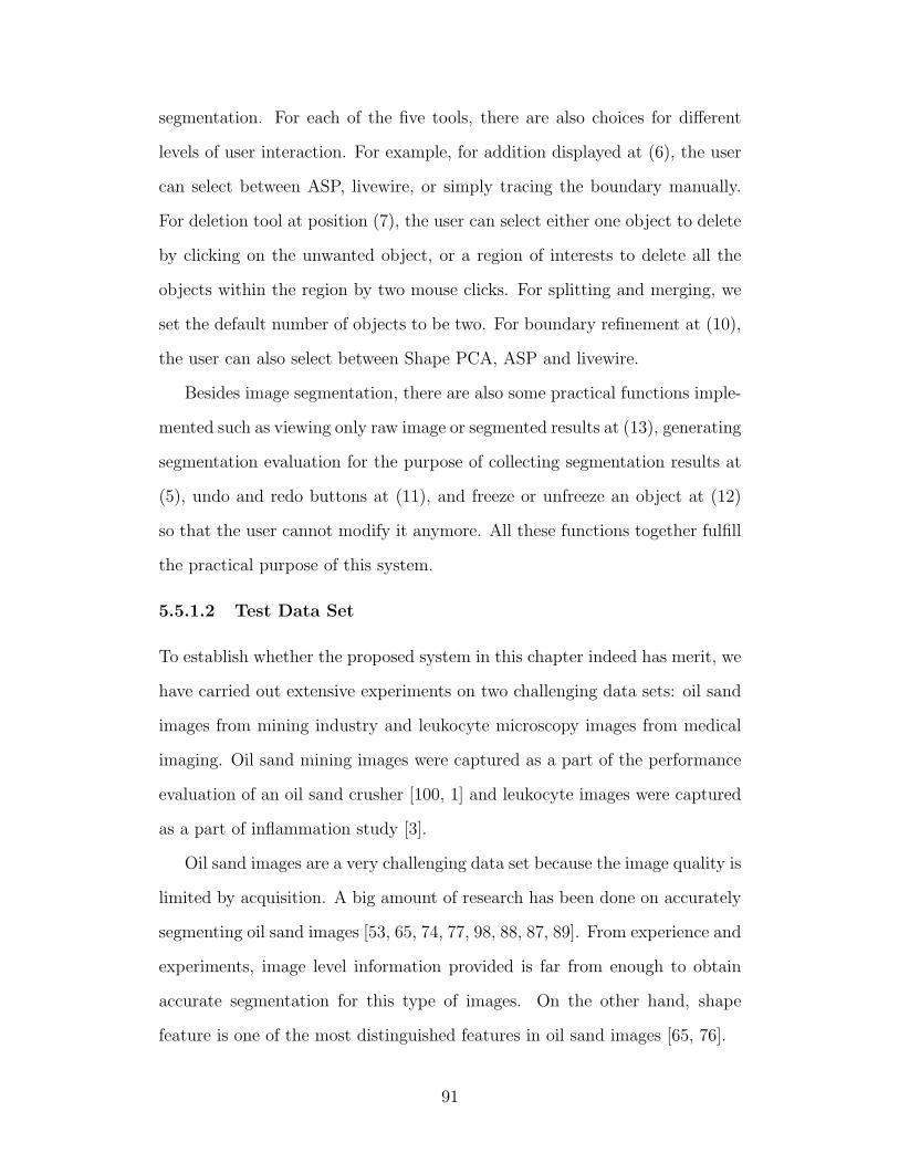
segmentation. For each of the five tools, there are also choices for different

levels of user interaction. For example, for addition displayed at (6), the user

can select between ASP, livewire, or simply tracing the boundary manually.

For deletion tool at position (7), the user can select either one object to delete

by clicking on the unwanted object, or a region of interests to delete all the

objects within the region by two mouse clicks. For splitting and merging, we

set the default number of objects to be two. For boundary refinement at (10),

the user can also select between Shape PCA, ASP and livewire.

Besides image segmentation, there are also some practical functions imple-

mented such as viewing only raw image or segmented results at (13), generating

segmentation evaluation for the purpose of collecting segmentation results at

(5), undo and redo buttons at (11), and freeze or unfreeze an object at (12)

so that the user cannot modify it anymore. All these functions together fulfill

the practical purpose of this system.

5.5.1.2 Test Data Set

To establish whether the proposed system in this chapter indeed has merit, we

have carried out extensive experiments on two challenging data sets: oil sand

images from mining industry and leukocyte microscopy images from medical

imaging. Oil sand mining images were captured as a part of the performance

evaluation of an oil sand crusher [100, 1] and leukocyte images were captured

as a part of inflammation study [3].

Oil sand images are a very challenging data set because the image quality is

limited by acquisition. A big amount of research has been done on accurately

segmenting oil sand images [53, 65, 74, 77, 98, 88, 87, 89]. From experience and

experiments, image level information provided is far from enough to obtain

accurate segmentation for this type of images. On the other hand, shape

feature is one of the most distinguished features in oil sand images [65, 76].

91

Figure 5.2: An example of the user interface for the proposed interactivesegmentation system. This example demonstrates the segmentation of an oilsand image with the initial segmentation results displayed in green boundariesof the segmented objects on top of the original input oil sand image.

92

Furthermore, to demonstrate the general applicability of this research, we

have also applied our interactive segmentation system on the leukocyte images.

Leukocyte plays an important role in the study of inflammation [3]. Typical

leukocyte studies on leukocyte images require segmenting and tracking leuko-

cyte. Several challenges exist in automatic delineation of leukocyte microscopy

images, which are described in [73].

5.5.2 Segmentation Evaluation

Different experiments were performed on both oil sand images and leukocyte

images to evaluate the segmentation improvement. We carried out experiments

of both performing all tools on the images, and performing only one tool on

the images each time. Image segmentation performance is usually evaluated

both quantitatively and visually. Although visual evaluation by humans is

very intuitive and straightforward, it is sometimes subjective. Quantitative

evaluation is on the other hand more objective. In both data sets, manual

segmentation results from experts are defined as our ground truth images. In

our evaluation, we compute the difference between the ground truth and the

segmentation result using evaluation metric such as pixel accuracy and object

score. The rest of this section describes the details of each of the experiments

and the corresponding evaluation results visually and quantitatively.

Experiment 1: applying the complete system to oil sand images

In this experiment, the complete interactive system of all five tools is applied

when necessary to the oil sand images. We choose this group of images because

they are the same data set studied thoroughly in the previous work on oil sand

image segmentation [53, 54].

In this experiment, we have applied four types of different segmentation

algorithms to generate the initial segmentation results, as a starting point of

93

the test data set. This is to test whether our system is dependent on a certain

type of segmentation algorithm. The four initial types of segmentation algo-

rithms are a deep neural network based method (NN) from [53], ground truth

decomposition method via Gabor filter (logGabor) from [54], OSA method

(OSA) [4] and Otsu’s method (Otsu) [68].

An example of the visual results is shown in Figure 5.3 which demonstrates

the segmentation improvement visually. It shows the original oil sand image in

(a), the corresponding initial segmentation result from a neural network based

segmentation algorithm (NN) [53] in (b) and the final result after applying

our segmentation system on (b) in (c). We can see that with the help of the

five tools, the segmentation quality has been significantly improved in the final

result.

Table 5.3 and Table 5.4 show the quantitative results on the improvement

of pixel accuracy and object score respectively, after applying our complete

system to the test data set of oil sand images. From both accuracy and score

improvement, it is clear that the proposed system has improved the segmen-

tation quality on both pixel and object level. Since each of the initial segmen-

tation results obtained from the four different segmentation algorithms has

obtained segmentation improvements by using our system, this shows that the

improvement from our system is independent of the initial segmentation algo-

rithm. Furthermore, it is also interesting to see that a segmentation algorithm

which performs worse initially, such as OSA or logGabor method, benefits

more from the system in terms of accuracy and score improvement. This is

because such a method makes more mistakes in the initial segmentation stage

and thus provides the system with more opportunities to improve.

In addition, when comparing the pixel accuracy improvement with the

object score improvement, the quantitative improvement on the object scores

is in general higher than the pixel level accuracies. This is because the object

94

(a)

(b)

(c)

Figure 5.3: An example of the visual results on oil sand image to compare theoriginal image (a), the corresponding initial segmentation result from [53] (b)and the final result (c).

level score takes into account and penalizes under- and over-segmentation more

than pixel level accuracy [70]. Since tools such as splitting and merging target

at under- and over-segmentation problems, the segmentation improvement on

the object level could be significant while the improvement on pixel accuracy

level could be subtle.

Experiment 2: applying each of the five tools independently to oil

sand images

Besides applying the complete system to oil sand images, each of the five tools

95

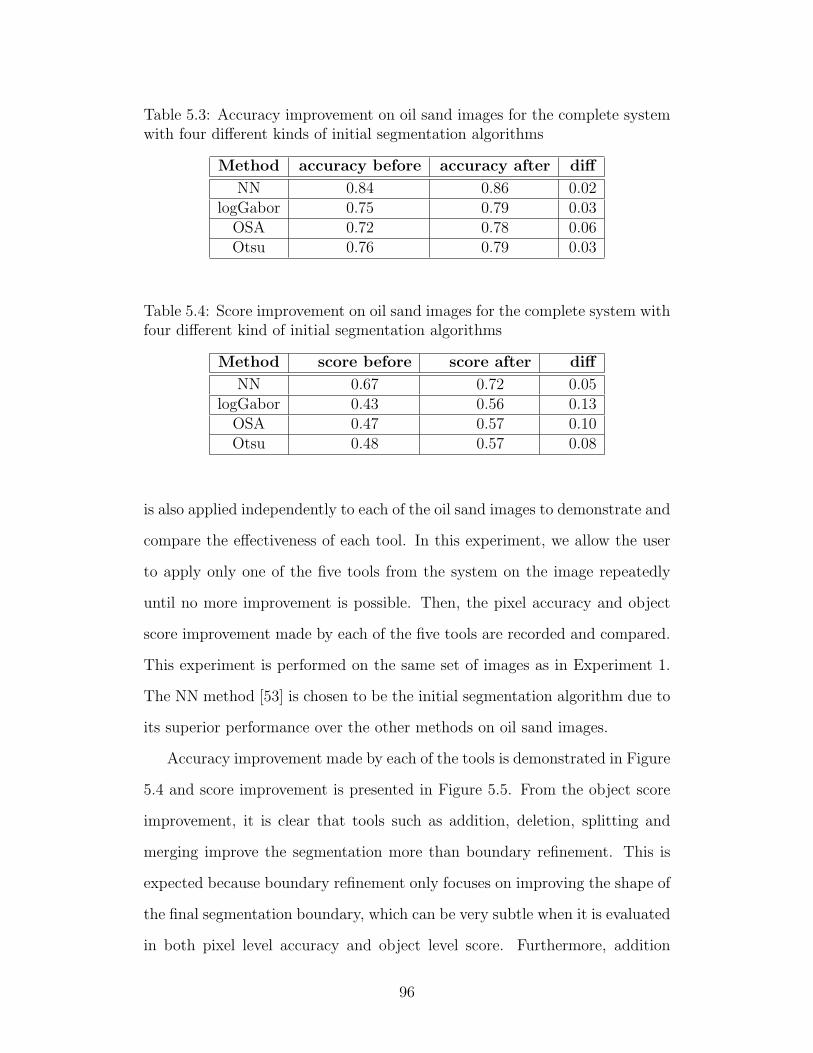
Table 5.3: Accuracy improvement on oil sand images for the complete systemwith four different kinds of initial segmentation algorithms

Method accuracy before accuracy after diff

NN 0.84 0.86 0.02logGabor 0.75 0.79 0.03OSA 0.72 0.78 0.06Otsu 0.76 0.79 0.03

Table 5.4: Score improvement on oil sand images for the complete system withfour different kind of initial segmentation algorithms

Method score before score after diff

NN 0.67 0.72 0.05logGabor 0.43 0.56 0.13OSA 0.47 0.57 0.10Otsu 0.48 0.57 0.08

is also applied independently to each of the oil sand images to demonstrate and

compare the effectiveness of each tool. In this experiment, we allow the user

to apply only one of the five tools from the system on the image repeatedly

until no more improvement is possible. Then, the pixel accuracy and object

score improvement made by each of the five tools are recorded and compared.

This experiment is performed on the same set of images as in Experiment 1.

The NN method [53] is chosen to be the initial segmentation algorithm due to

its superior performance over the other methods on oil sand images.

Accuracy improvement made by each of the tools is demonstrated in Figure

5.4 and score improvement is presented in Figure 5.5. From the object score

improvement, it is clear that tools such as addition, deletion, splitting and

merging improve the segmentation more than boundary refinement. This is

expected because boundary refinement only focuses on improving the shape of

the final segmentation boundary, which can be very subtle when it is evaluated

in both pixel level accuracy and object level score. Furthermore, addition

96

improves both accuracy and score the most due to the fact that adding an

object affects the total number of pixels and objects more than the other

tools.

Another interesting observation is that simply combining the improvement

made by all the tools does not equal to the overall improvement made by the

complete system described in Experiment 1. This is because that some of the

segmentation improvements should be made when combining two or more than

two of the tools in the system, instead of only applying one of the tools. For

example, an under-segmented clump might need to be split first, then some

of the objects that result from the split should be merged with some other

objects to obtain the final result.

Figure 5.4: Improvement on pixel accuracy generated by each of the five toolsfor oil sand images

Experiment 3: applying the complete system to leukocyte images

To further demonstrate the general applicability of the proposed system, sim-

ilar to Experiment 1, the system was also applied to the segmentation of

leukocyte images. The same procedure in Experiment 1 is followed for ap-

plying all necessary tools of the complete system to leukocyte images. The

leukocyte image data set consists of nine images from a previous study in [73].

97

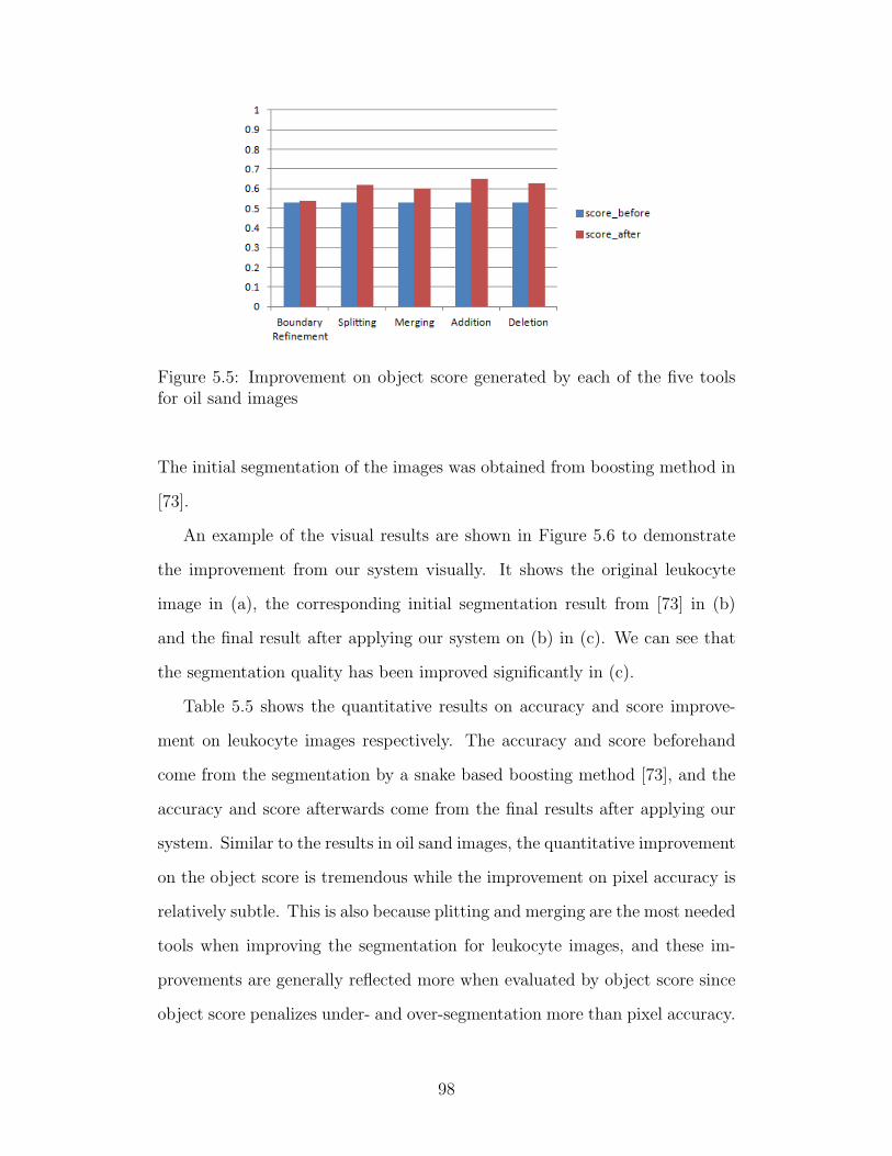
Figure 5.5: Improvement on object score generated by each of the five toolsfor oil sand images

The initial segmentation of the images was obtained from boosting method in

[73].

An example of the visual results are shown in Figure 5.6 to demonstrate

the improvement from our system visually. It shows the original leukocyte

image in (a), the corresponding initial segmentation result from [73] in (b)

and the final result after applying our system on (b) in (c). We can see that

the segmentation quality has been improved significantly in (c).

Table 5.5 shows the quantitative results on accuracy and score improve-

ment on leukocyte images respectively. The accuracy and score beforehand

come from the segmentation by a snake based boosting method [73], and the

accuracy and score afterwards come from the final results after applying our

system. Similar to the results in oil sand images, the quantitative improvement

on the object score is tremendous while the improvement on pixel accuracy is

relatively subtle. This is also because plitting and merging are the most needed

tools when improving the segmentation for leukocyte images, and these im-

provements are generally reflected more when evaluated by object score since

object score penalizes under- and over-segmentation more than pixel accuracy.

98

(a)

(b)

(c)

Figure 5.6: An example of the visual results on leukocyte image to comparethe original image (a), the corresponding initial segmentation result from [73](b) and the final result (c).

Experiment 4: applying each of the five tools independently to leuko-

cyte images

Similar to Experiment 2, besides applying the complete system to leukocyte

images, each of the five tools is also applied independently to leukocyte images

99

Table 5.5: Accuracy and score improvement on leukocyte images for the com-plete system

accuracy before accuracy after diff

0.95 0.98 0.03

score before score after diff

0.51 0.67 0.16

to demonstrate and compare the effectiveness of each tool. This experiment

is performed on the same set of images as in Experiment 3.

Improvement made by each of the tools is demonstrated in Figure 5.7

for pixel accuracy and Figure 5.8 for object score. Both figures show that

addition, deletion and splitting improve the segmentation more than the other

tools. Especially from Figure 5.8, it is clear that addition and splitting have

improved the object level score the most.

In addition, when comparing the results from Experiment 4 to results from

Experiment 2, it is also interesting to notice that the performance on each of

the five tools is application dependent. Since different applications encounter

different segmentation mistakes, each of the five tools can be either applied

independently or combined together to achieve the best improvement for the

specific application.

5.5.3 Usability Study

Usability study is an important step for an interactive segmentation system.

Various ways of usability studies exist for interactive segmentation algorithms.

Lazy snapping [56] conducts its usability study based on criteria such as ease

of use, time spent and user feedback. For evaluating selection accuracy over

time, edge-respecting brushes method [67] studies user experience by giving the

users a specific amount of time, instructing them to achieve as much accuracy

as possible within that time and then comparing the user’s results to average

100

Figure 5.7: Improvement on pixel accuracy generated by each of the five toolsfor leukocyte images

Figure 5.8: Improvement on object score generated by each of the five toolsfor leukocyte images

ground truth results. To evaluate the usability and efficiency of our proposed

interactive system, we did the following evaluations in quantitative measures,

which are common usability measures that exist in the literature.

Experiment 5: Action per object

To evaluate the amount of user interaction needed from the user, we have

performed a usability study to record the total number of objects per image

and the total number of actions (mouse clicks) performed by the user. The

101

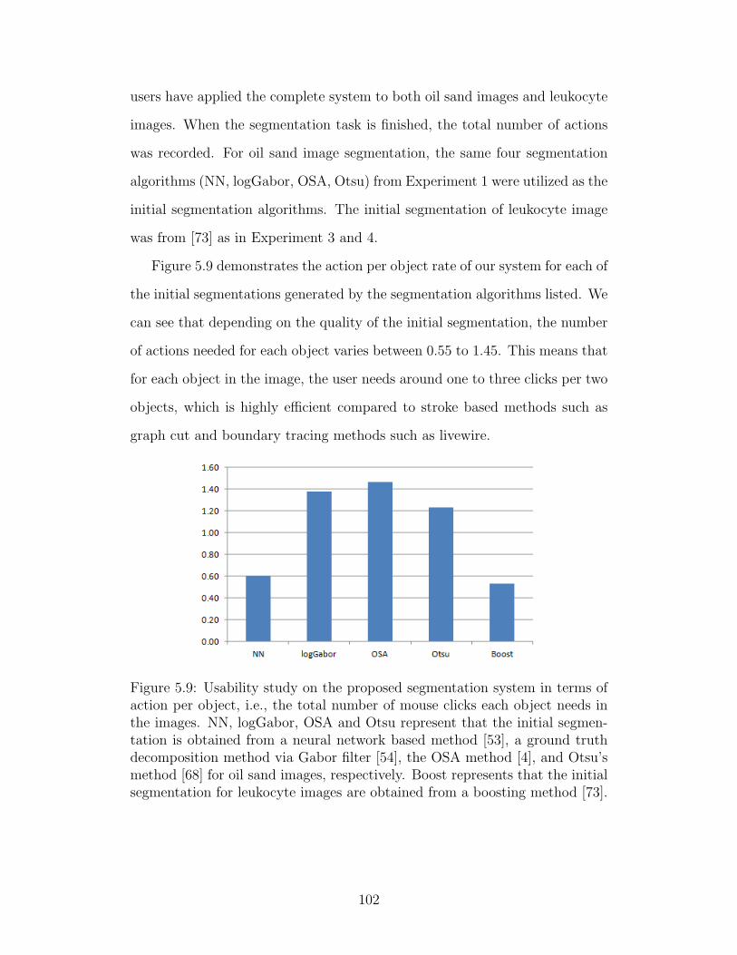
users have applied the complete system to both oil sand images and leukocyte

images. When the segmentation task is finished, the total number of actions

was recorded. For oil sand image segmentation, the same four segmentation

algorithms (NN, logGabor, OSA, Otsu) from Experiment 1 were utilized as the

initial segmentation algorithms. The initial segmentation of leukocyte image

was from [73] as in Experiment 3 and 4.

Figure 5.9 demonstrates the action per object rate of our system for each of

the initial segmentations generated by the segmentation algorithms listed. We

can see that depending on the quality of the initial segmentation, the number

of actions needed for each object varies between 0.55 to 1.45. This means that

for each object in the image, the user needs around one to three clicks per two

objects, which is highly efficient compared to stroke based methods such as

graph cut and boundary tracing methods such as livewire.

Figure 5.9: Usability study on the proposed segmentation system in terms ofaction per object, i.e., the total number of mouse clicks each object needs inthe images. NN, logGabor, OSA and Otsu represent that the initial segmen-tation is obtained from a neural network based method [53], a ground truthdecomposition method via Gabor filter [54], the OSA method [4], and Otsu’smethod [68] for oil sand images, respectively. Boost represents that the initialsegmentation for leukocyte images are obtained from a boosting method [73].

102

5.6 Summary

The chapter has proposed a novel and comprehensive interactive image seg-

mentation system as an example to integrate the proposed shape-guided al-

gorithms in the previous chapters. This proposed segmentation system is

developed based on the observation that common cases of failure from seg-

mentation algorithms can be categorized in five basic types, each of which

needs a corresponding segmentation algorithm. Therefore, five different de-

cisive tools which intuitively reflect user’s intention are developed: addition,

deletion, splitting, merging and boundary refinement. From observation, most

image segmentation tasks can be handled by one or a combination of these

five tools.

By combining them, a state-of-the-art shape-guided interactive segmenta-

tion system can be constructed which is capable of extracting high quality

foreground objects from an image effectively and efficiently with only one or

two mouse clicks per object. Experimental results from both segmentation

quality evaluation and user study have shown the effectiveness and efficiency

of this system.

103

Chapter 6

Conclusions

104

6.1 Conclusions

This dissertation focuses on improving image segmentation with the combina-

tion of shape-guided segmentation algorithms and minimal user interaction.

Starting with an image, the initial segmentation is achieved with some seg-

mentation algorithms. Then, to deal with certain types of under- and over-

segmentation mistakes, clump splitting and merging are required on top of

the initial segmentation. Finally, boundary refinement is needed to finalize

the shape of the segmentation results. For each types of different interactive

segmentation, shape information is utilized to guide the segmentation algo-

rithms.

The segmentation can be first achieved by the proposed adaptive shape

prior method (ASP) in the graph cut framework. The ASP method is pro-

posed to incorporate shape priors adaptively, depending on the need of the

shape prior at each pixel on the image. The ASP method eliminates mistakes

from previous approaches in which parameters had to be tuned to fit the image.

It works by adding the shape term in the energy function based on a proba-

bility map, which can be obtained by, for example, image enhancement and is

therefore straightforward, automatic and with little extra computational cost

to the algorithm. We have shown that ASP can be easily applied to various

types of graph cut based segmentation algorithms with shape priors, such as

shape template and star shape method.

To deal with under-segmentation such as clump splitting, the bottleneck

detection method is proposed to take advantage of shape information on the

bottleneck of a clump. The proposed method consists of three steps and has

several advantages over existing methods. First, our method is not parameter-

dependent on finding candidate points for splitting, unlike most existing meth-

ods, especially concavity based methods, which are highly parameter-dependent.

105

Second, our method avoids dealing with special situations in which the split-

ting points are not concave, in which almost all existing methods need to add

extra points according to the heuristic rules and constraints. Furthermore, our

method takes intensity information into account in localizing the cut between

splitting points and finds a more accurate cut than the straight-line cut that

directly joins the splitting points. Finally, the proposed shape classification

method determines the number of splits for each clump, which is more flexible

than model based methods.

Subsequently, in order to refine the incorrectly segmented portions of the

object boundary obtained from previous steps, the shape PCA method is de-

veloped to utilize statistical shape information when image level information

is inadequate or missing. The shape PCA method takes advantage of shape

information which is not directly available from image level and improves the

object boundary using the first few selected principal components which pre-

sumably represents the true shape of the object. A local shape PCA method

is also proposed in contrast to the global shape PCA method. As long as the

incorrectly segmented portions of the object boundary can be localized cor-

rectly, either automatically or manually, local shape PCA can be easily applied

to perform boundary refinement.

Finally, as an example to integrate these proposed shape-guided algorithms

together, a comprehensive interactive segmentation system is developed which

is composed of five different decisive tools that intuitively reflect the intention

of the user: addition, deletion, splitting, merging and boundary refinement.

From observations, most image segmentation tasks can be handled by one or

a combination of these five tools. Specifically, the user interaction takes place

in a scenario where the segmentation results are progressively refined by a

combination of the shape-guided methods proposed in this dissertation. By

combining them, a state-of-the-art shape-guided interactive segmentation sys-

106

tem can be constructed which is capable of extracting high quality foreground

objects from images effectively and efficiently with minimal amount of user

input.

6.2 Future Work

The potential future research for shape-guided interactive segmentation can

be identified as follows:

• Incorporating the adaptive shape prior into energy functions other than

graph cut. So far we have proposed and successfully incorporated shape

priors adaptively into the graph cut based energy functions. While graph

cut is one of the most successful interactive segmentation algorithms in

recent decades, other types of energy functions based on level set are

also widely used in automatic image segmentation. Further research are

needed to determine the generality and capability of the adaptive shape

prior idea, e.g., if it is possible to incorporate this idea into level set based

energy functions. Another direction is to examine whether more types

of shapes can be incorporated into the adaptive shape prior segmenta-

tion framework, either graph cut or level set based framework. While

we have seen that the current method is relatively robust compared to

other existing shape prior methods, it will be interesting to see whether

this robustness holds in the case of greater variations in shapes and im-

ages, and if not, how the algorithm maybe modified to account for these

changes.

• Selecting the number of principal components for the shape PCA method

adaptively. Currently, the number of principal components selected in

the shape PCA method is determined based on our observation and

experience from the experiments for certain types of applications. How-

107

ever, we notice that ideally, for different types of image applications

with different shapes, there will be different number of principal compo-

nents needed to perform the shape PCA method and achieve the best

result. Even for different objects within the same application, the need

for the number of principal components might also vary because some

object shapes are better segmented in the initial segmentation than oth-

ers. Therefore, we would like to explore the possibility of determining

the number of principal components needed for obtaining the true shape

of the object more adaptively.

• Interactive merging. So far the proposed interactive merging method de-

veloped in our interactive segmentation system is a simple and straight-

forward method which only works for merging adjacent objects that

touch each other. Our method simply eliminates the touching boundary

of the objects and merges the selected pieces into one. In the future

work, we would like to explore possible shape-guided segmentation algo-

rithms to not only find the merging boundary of the objects under some

shape guidance, but also merge objects which are not directly adjacent

to each other.

• Applying reinforcement learning (RL) to the proposed segmentation sys-

tem. Based on the observation that similar mistakes are often made

repetitively in the same application and the same interactive tool is often

selected for such type of mistakes to perform the segmentation, apply-

ing RL to incrementally learn and eventually automate this interactive

procedure is a natural continuation of this PhD dissertation. The RL

applied to this proposed segmentation system should learn from the user

interaction incrementally, and eventually performs the selection of the

tools with little need of user interaction. RL has the nature of learning

108

both offline and online, and can continuously learn and adapt to the

updated environment while the user performs the task. This is useful in

an interactive segmentation task.

109

Bibliography

[1] Issue: Canadians want responsible development of the oil sand, 2007.

Sustainability Report.

[2] Image matting. http://www.computervisiononline.com/node/238, Jan-

uary 2012. Internet access.

[3] Inflammation: The leukocyte adhesion cascade.

http://bme.virginia.edu/ley, January 2012. Internet access.

[4] OSA. http://webdocs.cs.ualberta.ca/ cims/research/projects.html, Jan-

uary 2012. Internet access.

[5] Agilent Technologies Inc. Post processing pico image software for agi-

lent afm systems. Internet: cp.literature.agilent.com/litweb/pdf/5989-

7596EN.pdf, November 2007. Datasheet.

[6] S. Araki, N. Yokoya, H. Iwasa, and H. Takemura. A new splitting active

contour model based on crossing detection. In Proceedings of the Second

Asian Conference on Computer Vision, volume II, pages 346–350, 1995.

[7] S. Avidan and A. Shamir. Seam carving for content-aware image resizing.

ACM Transactions on Graphics, 26(3):10, 2007.

[8] X. Bai, C. Sun, and F. Zhou. Splitting touching cells based on concave

points and ellipse fitting. Pattern Recognition, 42(11):2434–2446, 2009.

110

[9] I. Bar-Yosef, A. Mokeichev, K. Kedem, I. Dinstein, and U. Ehrlich.

Adaptive shape prior for recognition and variational segmentation of

degraded historical characters. In Pattern Recognition, volume 42, pages

3348–3354, 2009.

[10] W. A. Barrett and A. S. Cheney. Object-based image editing. In 29th

Annual Conference on Computer Graphics and Interactive Technique,

pages 777–784, 2002.

[11] O. Basset and C. Cachard. Ultrasound image post-processing - applica-

tion to segmentation. Physics for medical imaging applications, 240:227–

239, 2007.

[12] A. C. Berg. Shape Matching and Object Recognition. PhD thesis, U. C.

Berkeley, December 2005.

[13] S. Beucher and C. Lantuejoul. Use of watersheds in contour detection.

In Proceedings of the International Worksscla hop on Image Processing,

Real-Time Edge and Motion Detection/Estimation, pages 17–21, 1979.

[14] A. Blake, C. Rother, M. Brown, P. Perez, and P. Torr. Interactive image

segmentation using an adaptive GMMRF model. In Proceedings of the

European Conference in Computer Vision, pages 428–441, 2004.

[15] F. L. Boostein. Landmark methods for forms without landmarks: lo-

calizing group differences in outline shape. Medical Image Analysis,

1(3):225–244, 1997.

[16] Y. Y. Boykov and M.-P. Jolly. Interactive graph cuts for optimal bound-

ary and region segmentation of objects in N-D images. In Proceedings

Eighth IEEE International Conference on Computer Vision, volume 1,

pages 105–112, 2001.

111

[17] C. C. Chang and C. J. Lin. LIBSVM: A library for support vector

machines. Internet: www.csie.ntu.edu.tw/ cjlin/libsvm, 2011. Software.

[18] T. Cootes and C. Taylor. Statistical models of appearance for computer

vision, February 2012. Internet access.

[19] T. F. Cootes, G. J. Edwards, and C. J. Taylor. Active appearance

models. In Proceedings of the 5th European Conference on Computer

Vision, volume 2, pages 484–498, 1998.

[20] T. F. Cootes, G. J. Edwards, and C. J. Taylor. Active appearance

models. IEEE Trans. on Pattern Analysis and Machine Intelligence,

2001.

[21] T. F. Cootes and C. J. Taylor. Statistical models of appearance for

computer vision. Internet: http://www.isbe.man.ac.uk/ bim/,, October

2001. Technical Resport.

[22] T. F. Cootes, C. J. Taylor, D. H. Cooper, and J. Graham. Training

models of shape from sets of examples. In British Machine Vision Con-

ference, pages 9–18, 1992.

[23] T. F. Cootes, C. J. Taylor, D. H. Cooper, and J. Graham. Active shape

models - their training and application. Computer Vision and Image

Understanding, 61:38–59, 1995.

[24] D. Cremers, T. Kohlberger, and C. Schnorr. Nonlinear shape statistics

in mumford-shah based segmentation. In IEEE European Conference on

Computer Vision, pages 93–108, 2002.

[25] P. Das, O. Veskler, V. Zavadsky, and Y. Boykov. Semiautomatic seg-

mentation with compact shape prior. In Image and Vision Computing,

volume 27, pages 206–219, 2009.

112

[26] E. W. Dijkstra. A note on two problems in connexion with graphs.

Numerische Mathematik, 1:269–271, 1959.

[27] I. L. Dryden and K. V. Mardia. Statistical Shape Analysis. John Wiley

& Sons, Chichester, 1 edition, September 1998.

[28] N. Duta, A. K. Jain, and M.-P. Dubuisson-Jolly. Learning 2d shape mod-

els. In Proceedings Conf. on Computer Vision and Pattern Recognition,

volume 2, pages 8–14, 1999.

[29] M. Farhan. Automated clump splitting for biological cell segmentation

in microscopy using image analysis. Master’s thesis, Tampere University

of Technology, Finland, November 2009.

[30] M. Farhan, O. Yli-Harja, and A. Niemisto. An improved clump splitting

method for convex objects. In International Workshop on Computational

Systems Biology, pages 35–38, 2010.

[31] G. Fernandez, M. Kunt, and J.-P. Zryd. A new plant cell image segmen-

tation algorithm. In International Conference of Image Analysis and

Processing, pages 229–234, 1995.

[32] D. Freedman and T. Zhang. Interactive graph cut based segmentation

with shape priors. In Computer Vision and Pattern Recognition, pages

755–762, 2005.

[33] R. C. Gonzalez and R. E. Woods. Digital Image Processing. Prentice

Hall, 2 edition, January 2002.

[34] O. Gormeza and H. H. Yilmazb. Image post-processing in dental prac-

tice. European Journal of Dentistry, 3(4):343–347, October 2009.

113

[35] X. C. He and N. H. C. Yung. An efficient segmentation algorithm based

on mathematical morphology and improved watershed. Intelligent Com-

puting in Signal Processing and Pattern Recognition, 345:689–695, 2006.

[36] F. Heckel, O. Konrad, H. K. Hahn, and H.-O. Peitgen. Interactive 3d

medical image segmentation with energy-minimizing implicit functions.

Computers & Graphics.

[37] T. Heimann and H.-P. Meinzer. Statistical shape models for 3d medical

image segmentation: A review. Leitfaden der angewandten Informatik.

[38] D. M. Hobson, R. M. Carter, and Y. Yan. Rule based concave curvature

segmentation for touching rice grains in binary digital images. In IEEE

Instrumentation and Measurement Technology Conference, pages 1685–

1689, May 2009.

[39] H. Ip and R. Yu. Recursive splitting of active contours in multiple clump

segmentation. Electronics Letters, 32(17):1564–1566, August 1996.

[40] P. Jaccard. etude comparative de la distribution florale dans une por-

tion des alpes et des jura. Bulletin del la Societe Vaudoise des Sciences

Naturelles, 37:547–579, 1901.

[41] V. Jain and H. S. Seung. Natural image denoising with convolutional

networks. In Advanceds in Neural Information Processing Systems, 2008.

[42] M. Kass, A. Witkin, and D. Terzopoulos. Snakes: Active contour models.

International Journal on Computer Vision, 1(4):321–331, 1987.

[43] V. Kindratenko. Development and Application of Image Analysis Tech-

niques for Identification and Classification of Microscopic Particles. PhD

thesis, University of Antwerp, Belgium, 1997.

114

[44] M. Kirby. Geometric Data nalysis: An Empirical Approach to Dimen-

sionality Reduction and the Study of Patterns. John Wiley & Sons, New

York, 2001.

[45] V. Kolmogorov and R. Zabih. Multi-camera scene reconstruction via

graph cuts. In European Conference on Computer Vision, pages 82–96,

2002.

[46] V. Kolmogorov and R. Zabih. What energy functions can be minimized

via graph cuts. IEEE Transactions on Pattern Analysis and Machine

Intelligence, 26(2):65–81, 2004.

[47] M. Kumar, P. Torr, and A. Zisserman. Obj cut. In IEEE Conference on

Computer Vision and Pattern Recognition, pages 18–25, 2005.

[48] S. Kumar, S. H. Ong, S. Ranganath, T. C. Ong, and F. T. Chew. A

rule-based approach for robust clump splitting. Pattern Recognition,

39(6):1088–1098, June 2006.

[49] E. G. Learned-Miller. Data driven image models through continuous

joint alignment. In IEEE Transactions on Pattern Analysis and Machine

Intelligence, volume 28, 2006.

[50] V. Lempitsky, P. Kohli, C. Rother, and T. Sharp. Image segmenta-

tion with a bounding box prior. In IEEE International Conference on

Computer Vision, pages 277–284, 2009.

[51] A. Levin, D. Lischinski, and Y. Weiss. A closed-form solution to natural

image matting. IEEE Transactions on Pattern Analysis and Machine

Intelligence, 30:228–242, 2008.

115

[52] A. Levin, A. Rav-Acha, and D. Lischinski. Spectral matting. In IEEE

Transactions on Pattern Analysis and Machine Intelligence, volume 30,

pages 1699–1712, 2008.

[53] I. Levner. Data Driven Object Segmentation. PhD thesis, Department

of Computing Science, University of Alberta, 2008.

[54] I. Levner, R. Greiner, and H. Zhang. Supervised image segmentation

via ground truth decomposition. In IEEE International Conference on

Image Processing, pages 737–740, 2008.

[55] Y. Li, J. Sun, and H.-Y. Shum. Video object cut and paste. In SIG-

GRAPH 2005, pages 595–600, 2004.

[56] Y. Li, J. Sun, C.-K. Tang, and H.-Y. Shum. Lazy snapping. In SIG-

GRAPH 2004, volume 23, pages 303–308, 2004.

[57] D. Liu, Y. Xiong, L. Shapiro, and K. Pulli. Robust interactive image seg-

mentation with automatic boundary refinement. In IEEE International

Conference on Image Processing, 2010.

[58] J. Liu, J. Sun, and H.-Y. Shum. Paint selection. In SIGGRAPH ’09:

ACM SIGGRAPH 2009 papers, 2009.

[59] L. Liu and S. Sclaroff. Shape-guided split and merge of image regions. In

IWVF-4: Proceedings of the Fourth International Workshop on Visual

Form, pages 367–377. Springer-Verlag, 2001.

[60] N. Lu and X. Ke. A segmentation method based on gray-scale mor-

phological filter and watershed algorithm for touching objects image.

In International Conference on Fuzzy Systems and Knowledge Delivery,

pages 474–478, 2007.

116

[61] J. Malcolm, Y. Rathi, and A. Tannenbaum. Graph cut segmentation

with nonlinear shape priors. In Proceedings of the Fourteenth IEEE

International Conference on Image Processing, volume 4, pages 365–368,

2007.

[62] F. Meyer and S. Beucher. Morphological segmentation. Journal of Visual

Communication and Image Representation, 1(1):21–46, 1990.

[63] E. N. Mortensen and W. A. Barrett. Intelligent scissors for image compo-

sition. In Computer Graphics, SIGGRAPH Proceedings, pages 191–198,

1995.

[64] E. N. Mortensen and W. A. Barrett. Interactive segmentation with in-

telligent scissors. In Graphical Models and Image Processing, volume 60,

pages 349–384, 1998.

[65] D. P. Mukherjee, Y. Potapovich, I. Levner, and H. Zhang. Ore image

segmentation by learning image and shape features. Pattern Recognition

Letters, 30(6):615–622, April 2009.

[66] S. D. Olabarriaga. Human-Computer Interaction for the Segmentation

of Medical Images. PhD thesis, University of Amsterdam, 1999.

[67] D. R. Olsen, Jr. and M. K. Harris. Edge-respecting brushes. In Proceed-

ings of the 21st annual ACM symposium on User interface software and

technology, pages 171–180, 2008.

[68] N. Otsu. A threshold selection method from gray-level histogram. IEEE

Transaction on Systems Man. Cyber, pages 62–66, 1979.

[69] B. Peng and O. Veksler. Parameter selection for graph cut based image

segmentation. In British Machine Vision Conference, 2008.

117

[70] M. Polak, H. Zhang, and M. Pi. An evaluation metric for image segmen-

tation of multiple objects. Image and Vision Computing, 27(8):1223–

1227, July 2009.

[71] C. Rother, V. Kolmogorov, and A. Blake. GrabCut: Interactive fore-

ground extraction using iterated graph cuts. ACM Transactions on

Graphics, 23:309–314, 2004.

[72] C. D. Ruberto, A. Dempster, S. Khan, and B. Jarra. Segmentation of

blood images using morphological operators. In International Conference

on Pattern Recognition, pages 397–400, 2000.

[73] B. N. Saha. The Evolution of Snake toward Automation for Multiple

Blob-Object Segmentation. PhD thesis, Department of Computing Sci-

ence, University of Alberta, 2011.

[74] B. N. Saha, N. Ray, and H. Zhang. Snake validation: A PCA-based

outlier detection method. IEEE Signal Processing Letters, 16(6):549–

552, June 2009.

[75] E. Sarigul. Interactive Machine Learning for Refinement and Analysis of

Segmented CT/MRI Images. PhD thesis, Virginia Polytechnic Institute

and State University, September 2004.

[76] J. Shi. Adaptive local threshold with shape information and its appli-

cation to oil sand image segmentation. Master’s Thesis, University of

Alberta, 2010.

[77] J. Shi, H. Zhang, and N. Ray. Solidity based local threshold for oil sand

image segmentation. In 16th IEEE International Conference on Image

Processing, pages 2385–2388, November 2009.

118

[78] M. Singh, G. D. Seyranian, and D. D. Hoffman. Parsing silhouettes:

The short-cut rule. Perception and Psychophysics, 61:636–660, 1999.

[79] G. Slabaugh and G. Unal. Graph cuts segmentation using an elliptical

shape prior. In International Conference on Image Processing, volume 2,

2005.

[80] Z. Song, N. Tustison, B. Avants, and J. Gee. Adaptive graph cuts with

tissue priors for brain MRI segmentation. In IEEE International Sym-

posium on Biomedical Imaging, 2006.

[81] M. B. Stegmann and D. D. Gomez. A brief introduction to statistical

shape analysis, March 2002.

[82] D. Stoyan and H. Stoyan. Fractals, Random Shapes and Point Fields:

Methods of Geometrical Statistics. John Wiley & Sons, Chichester,

September 1994.

[83] N. Sweeney and B. Sweeney. Efficient segmentation of cellular images

using gradient-based methods and simple morphological filters. In En-

gineering in Medicine and Biology Society, pages 880–882, 1997.

[84] O. Veksler. Efficient Graph-based Energy Minimization Methods in Com-

puter Vision. PhD thesis, Cornell University, 1999.

[85] O. Veskler. Star shape prior for graph-cut image segmentation. In IEEE

European Conference on Computer Vision, pages 454–467, 2008.

[86] N. Vu and B. Manjunath. Shape prior segmentation of multiple objects

with graph cuts. In IEEE Conference on Computer Vision and Pattern

Recognition, pages 1–8, 2008.

[87] H. Wang and H. Zhang. Adaptive shape prior in graph cut segmentation.

In IEEE International Conference on Image Processing, September 2010.

119

[88] H. Wang and H. Zhang. Improving image segmentation via shape PCA

reconstruction. In IEEE International Conference on Acoustics, Speech

and Signal Processing, March 2010.

[89] H. Wang, H. Zhang, and N. Ray. Clump splitting via bottleneck detec-

tion and shape classification. Pattern Recognition, January 2012.

[90] J. Wang, M. Agrawala, and M. F. Cohen. Soft scissors: an interac-

tive tool for realtime high quality matting. In SIGGRAPH ’07: ACM

SIGGRAPH 2007 papers, New York, NY, USA, 2007. ACM.

[91] W. Wang and H. Sung. Cell cluster image segmentation on form analy-

sis. In International Conference of Natural Computation, pages 833–836,

2007.

[92] W. X. Wang. Binary image segmentation of aggregates based on polygo-

nal approximation and classification of concavities. Pattern Recognition,

31(10):1503–1524, 1998.

[93] Y. Wang and L. H. Staib. Boundary finding with correspondence using

statistical shape models. In IEEE Conference on Computer Vision and

Pattern Recognition, pages 338–345, 1998.

[94] T. P. Weldon. Removal of image segmentation boundary errors using an

N-ary morphological operator. In SoutheastCon, 2007, pages 509–513,

2007.

[95] Q. Wen, H. Chang, and B. Parvin. A delaunay triangulation approach

for segmenting clumps of nuclei. In IEEE International Symposium on

Biomedical Imaging, pages 9–12, 2009.

120

[96] Q. Yang, C. Wang, X. Tang, M. Chen, and Z. Ye. Progressive cut: an

image cutout algorithm that models user intentions. IEEE Multimedia,

14(3):55–66, 2007.

[97] T. T. E. Yeo, X. C. Jin, S. H. H. Ong, and R. S. Jayasooriah.

Clump splitting through concavity analysis. Pattern Recognition Let-

ters, 15(10):1013–1018, October 1994.

[98] A. Zadorozny. Contrast enhancement of oil sand images using morpho-

logical scale space. Master’s Thesis, University of Alberta, 2006.

[99] D. Zhang and G. Lu. Review of shape representation and description

techniques. Pattern Recognition, 37:1–19, 2004.

[100] H. Zhang. Image processing for the oil sands mining industry. IEEE

Signal Processing Magazine, 25:198–200, November 2008.

[101] J. Zhu-Jacquot. Graph cuts segmentation with geometric shape priors for

medical images. In Proceedings of the 2008 IEEE Southwest Symposium

on Image Analysis and Interpretation, pages 109–112, Washington, DC,

USA, 2008. IEEE Computer Society.

121