Unit Root Tests in Three-Regime SETAR Models∗

George KapetaniosDepartment of Economics, Queen Mary, University of London

Yongcheol ShinSchool of Economics, University of Edinburgh

This Version, November 2003

Abstract

This paper proposes a simple testing procedure to distinguish a unit root processfrom a globally stationary three-regime self-exciting threshold autoregressive process.Following the threshold cointegration literature we assume that the process follows therandom walk in the corridor regime, and therefore we propose that the null of a unit rootbe tested by the Wald statistic for the joint significance of autoregressive parametersin both lower and upper regimes. We establish that when threshold parameters areknown, the suggested Wald test has a well-defined asymptotic null distribution freeof nuisance parameters. In the general case where threshold parameters are unknowna priori, we consider the three most commonly used summary statistics - average,exponential average and supremum. Assuming that the grid set for thresholds canbe selected such that the corridor regime be of finite width both under the null andunder the alternative, we can establish both stochastic equicontinuity and uniformconvergence of the aforementioned summary statistics. Monte Carlo evidence clearlyindicates that the proposed tests are more powerful than the Dickey-Fuller test thatignores the threshold nature under the alternative. We illustrate the usefulness of ourproposed tests by examining stationarity of bilateral real exchange rates for the G7countries.

JEL Classification: C12, C13, C32.Key Words: Self-exciting Threshold Autoregressive Models, Unit Roots, Globally Station-ary Processes, Threshold Cointegration, Monte Carlo Simulations, Real Exchange Rates,Transactions Costs, Dread of Depreciation.

∗We are grateful to Frederique Bec, In Choi, James Davidson, Juan Dolado, Jayasri Dutta, EmmanuelGuerre, Inmoo Kim, Bruce Hansen, Taewhan Kim, Gary Koop, Stephen Leybourne, Paul Newbold, PeterPhillips, Pentti Saikkonen, Myunghwan Seo, Andy Snell, Rob Taylor and the seminar participants at theEconometric Study Group, Bristol 2001, Sungkunkwan University, University of Edinburgh, University ofNottingham, and the 57th ESEM Conference, Venice, Italy, 2002 for their helpful comments on an earlierversion of this paper. Partial financial support from the ESRC (grant No. R000223399) is also gratefullyacknowledged. The usual disclaimer applies.

1 Introduction

There has been increasing concern in econometrics that the information revealed by theanalysis of a linear model in a single time series may be insufficient to give definitive inferenceon important hypotheses. In particular, the power of tests such as the Dickey-Fuller (1979,hereafter DF) unit root test or the Engle-Granger (1987) test for cointegration has beencalled into question. At the same time the stability of estimated parameters over the sorts oftime horizons required to invoke the guidance of asymptotics in linear models has also comeunder suspicion. As a response to these problems, attention is turning to nonlinear dynamicsto improve estimation and inference. Theoretical models of nonlinear adjustments have beenproposed earlier by Hicks (1950) and others in the context of business cycle analysis. Also inthe context of asset markets, the extent of arbitrage trading in response to return differentialsis limited by the level of transaction costs. These costs may lead to a nonlinear relationshipbetween the level of arbitrage activity and the size of the return differentials. Therefore,the level of arbitrage trading and hence the speed with which the returns differential revertstowards zero are an increasing function of the size of the returns differential itself. Sercu et al.(1995) and Michael et al. (1997) develop the theory suggesting that the larger the deviationfrom the purchasing power parity (PPP), the stronger the tendency for real exchange ratesto move back to equilibrium. Some progress has already been made in other respects aswell and now the applied macro time-series literature abounds with cases where departingfrom linearity has yielded significant gains in both prediction and inference. See for exampleKoop et al. (1996), Pesaran and Potter (1997), Kapetanios (1999), Taylor (2001), Ioannideset al. (2003) and Kapetanios et al. (2003a,b).In particular, Balke and Fomby (1997) have popularised a joint analysis of nonstationarity

and nonlinearity in the context of threshold cointegration. The threshold cointegratingprocess is defined as a globally stationary process such that it might follow a unit root inthe middle regime, but it is dampened in outer regimes. Importantly, they have shown viaMonte Carlo experiments that the power of the DF unit root tests falls dramatically withthreshold parameters of a three-regime threshold autoregressive (TAR) model. Since then,there have been a few studies to address the joint issues of nonstationarity and nonlinearity,but mostly using univariate two regime TAR models. The first line of research follows theself-exciting TAR (SETAR) modelling approach where the lagged dependent variable is usedas the transition variable. Enders and Granger (1998) have proposed an F-test for the nullhypothesis of a unit root against an alternative of a stationary two-regime TAR process.Contrary to expectations, however, their simulation results show that the suggested F testis less powerful than the DF test that ignores the threshold nature under the alternative.See Berben and van Dijk (1999) for an extension.There has also been an alternative line of studies in a two-regime TAR model. Caner and

Hansen (2001) have considered tests for threshold nonlinearity when the underlying univari-ate process follows a unit root, then developed unit root tests when threshold nonlinearityis either present or absent. See also Gonzalez and Gonzalo (1998) and Shin and Lee (2001).This approach is critically different from the aforementioned SETAR-based approach; it al-lows only for the case where transition variables are stationary. Thus, the possibility ofusing the lagged dependent variable as the transition variable is excluded since it becomes

[1]

nonstationary under the null. In this regard, this approach might be of reduced interest inthe current case where we wish to analyse the global stationarity of the underlying long-runrelationships such as PPP.To bridge the two areas of nonstationarity and nonlinearity in the context of the threshold

cointegration, we consider a more general three regime SETAR model. Unlike the previousstudies using the two step-based approach proposed by Balke and Fomby (1997) and Lo andZivot (2001), this paper aims to provide a direct test that would have more power againstthe alternative of globally stationary three regime SETAR processes. For further economicand econometric backgrounds in favor of three regime TAR models see Anderson (1997), Becet al. (2001), Taylor (2001), Dutta and Leon (2002) and Bec et al. (2002).Following the threshold cointegration literature, we impose that the processes follow a

unit root in the corridor regime and thus propose that the null hypothesis of a (linear)unit root against the alternative of globally stationary three regime SETAR process betested by the Wald test for the joint significance of autoregressive parameters under bothlower and upper regimes. We establish that when threshold parameters are known, thesuggested Wald test does have a well-defined asymptotic null distribution free of nuisanceparameters. Moreover, in the special case where autoregressive parameters under both outerregimes are symmetric, the null of a unit root can now be tested by the Wald test for thesignificance of the common autoregressive parameter, and its asymptotic null distribution isshown to be equivalent to the distribution of the squared DF t-statistic. In the general casewhere threshold parameters are unknown a priori, this kind of test suffers from the well-known Davies (1987) problem since threshold parameters are not identified under the null.Following Hansen (1996), we consider the three most commonly used summary statistics -average, exponential average and supremum - over a grid set of possible threshold values.Under the maintained assumption that the corridor regime will be inactive, we do not needto estimate any parameter in the middle regime. This observation leads us to assume thatthe grid set for unknown thresholds can be selected such that the corridor regime be offinite width both under the null and under the alternative. Given this assumption, we canestablish first stochastic equicontinuity of the Wald statistic and then uniform convergenceof the aforementioned summary statistics.The small sample performance of our suggested tests is compared to that of the DF test

via Monte Carlo experiments. We find that both average and exponential average tests havereasonably correct size, but the supremum test tends to display significant size distortions insmal samples. As expected, both average and exponential average tests eventually dominatethe power of the DF test as the threshold band widens. We illustrate the usefulness of ourproposed tests by examining the stationarity of bilateral real exchange rates for the G7 coun-tries (excluding France). In sum, our proposed (asymmetry) Wald tests reject the null threetimes out of five cases, while the DF test rejects the null only once. Given some support forthe SETAR alternative, we estimate SETAR models and find that autoregressive parametersin outer regimes are significantly negative in all cases except for Canada. More interestingly,the speed of mean or range reversion is faster in the lower regime (depreciation) than in theupper regime (appreciation) for Germany, Italy and Japan. This raises further issue thatempirical evidence may be available to bolster the hypothesis of asymmetric foreign exchangemarket interventions that countries may choose to resist depreciations more vigorously than

[2]

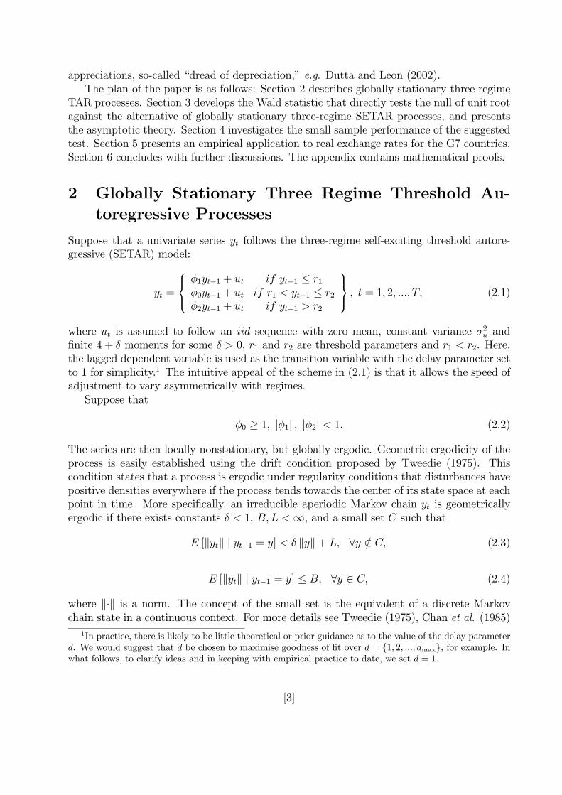
appreciations, so-called “dread of depreciation,” e.g. Dutta and Leon (2002).The plan of the paper is as follows: Section 2 describes globally stationary three-regime

TAR processes. Section 3 develops the Wald statistic that directly tests the null of unit rootagainst the alternative of globally stationary three-regime SETAR processes, and presentsthe asymptotic theory. Section 4 investigates the small sample performance of the suggestedtest. Section 5 presents an empirical application to real exchange rates for the G7 countries.Section 6 concludes with further discussions. The appendix contains mathematical proofs.

2 Globally Stationary Three Regime Threshold Au-

toregressive Processes

Suppose that a univariate series yt follows the three-regime self-exciting threshold autore-gressive (SETAR) model:

yt =

⎧⎪⎨⎪⎩φ1yt−1 + ut if yt−1 ≤ r1φ0yt−1 + ut if r1 < yt−1 ≤ r2φ2yt−1 + ut if yt−1 > r2

⎫⎪⎬⎪⎭ , t = 1, 2, ..., T, (2.1)

where ut is assumed to follow an iid sequence with zero mean, constant variance σ2u andfinite 4 + δ moments for some δ > 0, r1 and r2 are threshold parameters and r1 < r2. Here,the lagged dependent variable is used as the transition variable with the delay parameter setto 1 for simplicity.1 The intuitive appeal of the scheme in (2.1) is that it allows the speed ofadjustment to vary asymmetrically with regimes.Suppose that

φ0 ≥ 1, |φ1| , |φ2| < 1. (2.2)

The series are then locally nonstationary, but globally ergodic. Geometric ergodicity of theprocess is easily established using the drift condition proposed by Tweedie (1975). Thiscondition states that a process is ergodic under regularity conditions that disturbances havepositive densities everywhere if the process tends towards the center of its state space at eachpoint in time. More specifically, an irreducible aperiodic Markov chain yt is geometricallyergodic if there exists constants δ < 1, B,L <∞, and a small set C such that

E [kytk | yt−1 = y] < δ kyk+ L, ∀y /∈ C, (2.3)

E [kytk | yt−1 = y] ≤ B, ∀y ∈ C, (2.4)

where k·k is a norm. The concept of the small set is the equivalent of a discrete Markovchain state in a continuous context. For more details see Tweedie (1975), Chan et al. (1985)

1In practice, there is likely to be little theoretical or prior guidance as to the value of the delay parameterd. We would suggest that d be chosen to maximise goodness of fit over d = {1, 2, ..., dmax}, for example. Inwhat follows, to clarify ideas and in keeping with empirical practice to date, we set d = 1.

[3]

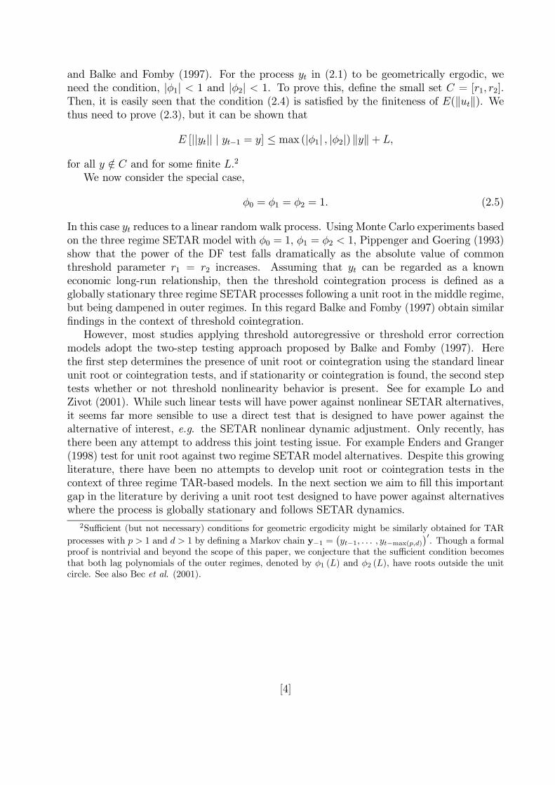
and Balke and Fomby (1997). For the process yt in (2.1) to be geometrically ergodic, weneed the condition, |φ1| < 1 and |φ2| < 1. To prove this, define the small set C = [r1, r2].Then, it is easily seen that the condition (2.4) is satisfied by the finiteness of E(kutk). Wethus need to prove (2.3), but it can be shown that

E [||yt|| | yt−1 = y] ≤ max (|φ1| , |φ2|) kyk+ L,

for all y /∈ C and for some finite L.2We now consider the special case,

φ0 = φ1 = φ2 = 1. (2.5)

In this case yt reduces to a linear random walk process. Using Monte Carlo experiments basedon the three regime SETAR model with φ0 = 1, φ1 = φ2 < 1, Pippenger and Goering (1993)show that the power of the DF test falls dramatically as the absolute value of commonthreshold parameter r1 = r2 increases. Assuming that yt can be regarded as a knowneconomic long-run relationship, then the threshold cointegration process is defined as aglobally stationary three regime SETAR processes following a unit root in the middle regime,but being dampened in outer regimes. In this regard Balke and Fomby (1997) obtain similarfindings in the context of threshold cointegration.However, most studies applying threshold autoregressive or threshold error correction

models adopt the two-step testing approach proposed by Balke and Fomby (1997). Herethe first step determines the presence of unit root or cointegration using the standard linearunit root or cointegration tests, and if stationarity or cointegration is found, the second steptests whether or not threshold nonlinearity behavior is present. See for example Lo andZivot (2001). While such linear tests will have power against nonlinear SETAR alternatives,it seems far more sensible to use a direct test that is designed to have power against thealternative of interest, e.g. the SETAR nonlinear dynamic adjustment. Only recently, hasthere been any attempt to address this joint testing issue. For example Enders and Granger(1998) test for unit root against two regime SETAR model alternatives. Despite this growingliterature, there have been no attempts to develop unit root or cointegration tests in thecontext of three regime TAR-based models. In the next section we aim to fill this importantgap in the literature by deriving a unit root test designed to have power against alternativeswhere the process is globally stationary and follows SETAR dynamics.

2Sufficient (but not necessary) conditions for geometric ergodicity might be similarly obtained for TAR

processes with p > 1 and d > 1 by defining a Markov chain y−1 =¡yt−1, . . . , yt−max(p,d)

¢0. Though a formal

proof is nontrivial and beyond the scope of this paper, we conjecture that the sufficient condition becomesthat both lag polynomials of the outer regimes, denoted by φ1 (L) and φ2 (L), have roots outside the unitcircle. See also Bec et al. (2001).

[4]

3 Testing the Null of a Unit Root Against the Al-

ternative of Globally Stationary Three-Regime TAR

Process

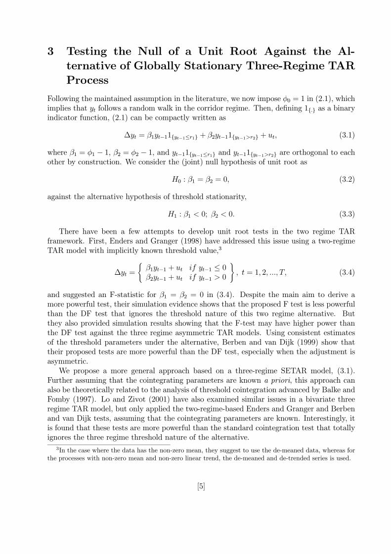
Following the maintained assumption in the literature, we now impose φ0 = 1 in (2.1), whichimplies that yt follows a random walk in the corridor regime. Then, defining 1{.} as a binaryindicator function, (2.1) can be compactly written as

∆yt = β1yt−11{yt−1≤r1} + β2yt−11{yt−1>r2} + ut, (3.1)

where β1 = φ1 − 1, β2 = φ2 − 1, and yt−11{yt−1≤r1} and yt−11{yt−1>r2} are orthogonal to eachother by construction. We consider the (joint) null hypothesis of unit root as

H0 : β1 = β2 = 0, (3.2)

against the alternative hypothesis of threshold stationarity,

H1 : β1 < 0; β2 < 0. (3.3)

There have been a few attempts to develop unit root tests in the two regime TARframework. First, Enders and Granger (1998) have addressed this issue using a two-regimeTAR model with implicitly known threshold value,3

∆yt =

(β1yt−1 + ut if yt−1 ≤ 0β2yt−1 + ut if yt−1 > 0

), t = 1, 2, ..., T, (3.4)

and suggested an F-statistic for β1 = β2 = 0 in (3.4). Despite the main aim to derive amore powerful test, their simulation evidence shows that the proposed F test is less powerfulthan the DF test that ignores the threshold nature of this two regime alternative. Butthey also provided simulation results showing that the F-test may have higher power thanthe DF test against the three regime asymmetric TAR models. Using consistent estimatesof the threshold parameters under the alternative, Berben and van Dijk (1999) show thattheir proposed tests are more powerful than the DF test, especially when the adjustment isasymmetric.We propose a more general approach based on a three-regime SETAR model, (3.1).

Further assuming that the cointegrating parameters are known a priori, this approach canalso be theoretically related to the analysis of threshold cointegration advanced by Balke andFomby (1997). Lo and Zivot (2001) have also examined similar issues in a bivariate threeregime TAR model, but only applied the two-regime-based Enders and Granger and Berbenand van Dijk tests, assuming that the cointegrating parameters are known. Interestingly, itis found that these tests are more powerful than the standard cointegration test that totallyignores the three regime threshold nature of the alternative.

3In the case where the data has the non-zero mean, they suggest to use the de-meaned data, whereas forthe processes with non-zero mean and non-zero linear trend, the de-meaned and de-trended series is used.

[5]

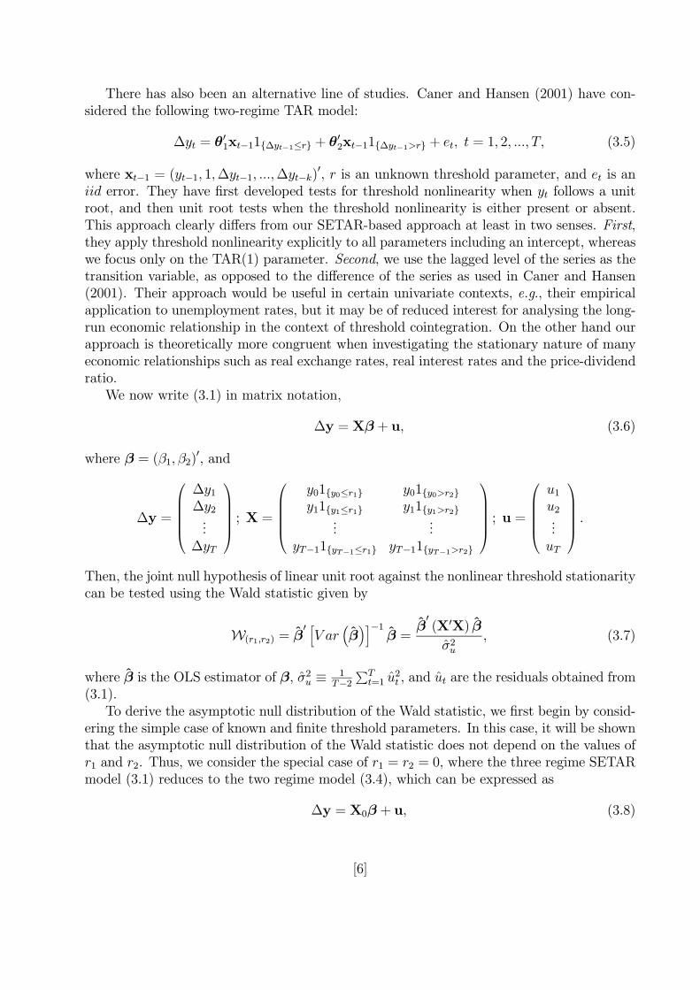
There has also been an alternative line of studies. Caner and Hansen (2001) have con-sidered the following two-regime TAR model:

∆yt = θ01xt−11{∆yt−1≤r} + θ02xt−11{∆yt−1>r} + et, t = 1, 2, ..., T, (3.5)

where xt−1 = (yt−1, 1,∆yt−1, ...,∆yt−k)0, r is an unknown threshold parameter, and et is an

iid error. They have first developed tests for threshold nonlinearity when yt follows a unitroot, and then unit root tests when the threshold nonlinearity is either present or absent.This approach clearly differs from our SETAR-based approach at least in two senses. First,they apply threshold nonlinearity explicitly to all parameters including an intercept, whereaswe focus only on the TAR(1) parameter. Second, we use the lagged level of the series as thetransition variable, as opposed to the difference of the series as used in Caner and Hansen(2001). Their approach would be useful in certain univariate contexts, e.g., their empiricalapplication to unemployment rates, but it may be of reduced interest for analysing the long-run economic relationship in the context of threshold cointegration. On the other hand ourapproach is theoretically more congruent when investigating the stationary nature of manyeconomic relationships such as real exchange rates, real interest rates and the price-dividendratio.We now write (3.1) in matrix notation,

∆y = Xβ + u, (3.6)

where β = (β1, β2)0, and

∆y =

⎛⎜⎜⎜⎜⎝∆y1∆y2...

∆yT

⎞⎟⎟⎟⎟⎠ ; X =⎛⎜⎜⎜⎜⎝

y01{y0≤r1} y01{y0>r2}y11{y1≤r1} y11{y1>r2}

......

yT−11{yT−1≤r1} yT−11{yT−1>r2}

⎞⎟⎟⎟⎟⎠ ; u =⎛⎜⎜⎜⎜⎝u1u2...uT

⎞⎟⎟⎟⎟⎠ .

Then, the joint null hypothesis of linear unit root against the nonlinear threshold stationaritycan be tested using the Wald statistic given by

W(r1,r2) = β0 hV ar

³β´i−1

β =β0(X0X) β

σ2u, (3.7)

where β is the OLS estimator of β, σ2u ≡ 1T−2

PTt=1 u

2t , and ut are the residuals obtained from

(3.1).To derive the asymptotic null distribution of the Wald statistic, we first begin by consid-

ering the simple case of known and finite threshold parameters. In this case, it will be shownthat the asymptotic null distribution of the Wald statistic does not depend on the values ofr1 and r2. Thus, we consider the special case of r1 = r2 = 0, where the three regime SETARmodel (3.1) reduces to the two regime model (3.4), which can be expressed as

∆y = X0β + u, (3.8)

[6]

where

X =

⎛⎜⎜⎜⎜⎝y01{y0≤0} y01{y0>0}y11{y1≤0} y11{y1>0}

......

yT−11{yT−1≤0} yT−11{yT−1>0}

⎞⎟⎟⎟⎟⎠ .The Wald statistic testing for β = 0 in (3.8) is given by

W(0) =β0(X0

0X0) β

σ2u, (3.9)

where β is the OLS estimator of β, σ2u ≡ 1T−2

PTt=1 u

2t , and ut are the residuals obtained from

(3.4).

Theorem 3.1 Consider the two-regime SETAR model (3.8). Then, the Wald statistic test-ing for β = 0, defined by (3.9), has the following asymptotic null distribution:

W(0) ⇒

nR 10 1{W (s)≤0}W (s)dW (s)

o2R 10 1{W (s)≤0}W (s)2ds

+

nR 10 1{W (s)>0}W (s)dW (s)

o2R 10 1{W (s)>0}W (s)2ds

, (3.10)

where W (s) is a standard Brownian motion defined on s ∈ [0, 1].

This result is exactly the same as obtained for the F-test considered by Enders andGranger (1998), i.e. F =W(0)/2. This result is of limited use, but the next theorem showsthat the limiting null distribution of the statisticW(r1,r2) is in fact equivalent to that ofW(0).

Theorem 3.2 Assuming that r1 and r2 are finite and given, and under the null hypothesisβ1 = β2 = 0, the W(r1,r2) statistic defined in (3.7) weakly converges to W(0). Furthermore,under the alternative hypothesis β1 < 0 and β2 < 0, W(r1,r2) diverges to infinity.

This (null) distributional invariance is due to the well-established fact that the unit rootprocess stays within the (fixed) corridor regime for a proportion of time which goes to zeroat rate T−1/2, e.g., Feller (1957).Asymptotic results are so far derived under the simplifying assumption that threshold

parameters are known, and we now consider a general case with unknown threshold parame-ters. In such a case it is well-established that this test suffers from the Davies (1987) problemsince unknown threshold parameters are not identified under the null. Most solutions to thisproblem involve integrating out unidentified parameters from the test statistics. This isusually achieved by calculating test statistics over a grid set of possible values of thresh-old parameters, r1 and r2, and then constructing the summary statistics. For stationaryTAR models this problem has been studied in Tong (1990) and Hansen (1996). We considerthe three most commonly used statistics: the supremum, the average and the exponentialaverage of the Wald statistic defined respectively by

Wsup = supi∈ΓW(i)(r1,r2)

, Wavg =1

#Γ

#ΓXi=1

W(i)(r1,r2)

, Wexp =1

#Γ

#ΓXi=1

exp

⎛⎝W(i)(r1,r2)

2

⎞⎠ ,(3.11)

[7]

whereW(i)(r1,r2)

is the Wald statistic obtained from the i-th point of the threshold parametersgrid set, Γ and #Γ is the number of elements of Γ.Unlike the stationary TAR models, the selection of the grid of threshold parameters

needs more attention. The threshold parameters r1 and r2 usually take on the values in theinterval (r1, r2) ∈ Γ = [rmin, rmax] where rmin and rmax are picked so that Pr (yt−1 < rmin) =π1 > 0 and Pr (yt−1 > rmax) = π2 < 1. The particular choice for π1 and π2 is somewhatarbitrary, and in practice must be guided by the consideration that each regime needs tohave sufficient observations to identify the underlying regression parameters. If we wereto select the set Γ using the conventional quantile-based approach under which thresholdparameters diverge under the null of a unit root and are bounded under the alternative, thenthe above asymptotic results will not hold.However, since our approach assumes that the coefficient on the lagged dependent vari-

able is set to zero in the corridor regime (r1 ≤ yt−1 < r2), we can assign arbitrarily smallsamples (relative to total sample) to the corridor regime since we do not need to estimateany parameters in the corridor regime. Notice also that the threshold parameters exist onlyunder the alternative hypothesis in which the process is stationary and therefore boundedin probability. In this case only a finite grid search will be meaningful for further estima-tion. For a discussion on the construction of the grid in stationary threshold models thatsupport our approach, see Tong (1990) and Chan (1993). This observation leads us to makean assumption that the grid for unknown threshold parameters should be selected such thatthe selected corridor regime be of finite width both under the null and under the alterna-tive. Under this restriction, we can further establish that the theoretical results obtained inTheorems 3.1 and 3.2 do hold in the more general case with unknown threshold parametersas shown below. Noticing that a random walk process will stay within a corridor regime offinite width for Op

³√T´periods only, then setting π1 = π− c/T δ and π2 = π+ c/T δ, where

π is the sample quantile corresponding to zero and δ ≥ 1/2, guarantees that the grid set willbe of finite width under the null hypothesis.4 In practice, c can be chosen so as to give areasonable coverage of each regime in samples of sizes usually encountered. For example, forT = 100 and δ = 1/2, c can be set to 3 to give a 60% coverage of the sample for the grid.Recently, in a similar context, Bec et al. (2002) develop an adaptive consistent unit root

tests based on the symmetric three regime TAR model and propose an adaptive choice of thegrid set which restricts the grid to remain bounded under the null (as we do) but unboundedunder the alternative.5 Unlike our approach, they do not impose that the autoregressivecoefficient in the corridor regime is known in (3.1). Since the value of the autoregressiveparameter of the corridor regime is likely to lie close to zero even under the alternative, esti-

4Further restrictions on the limits of the grid in the form of a minimum difference between the upperand lower bound may also be placed to guarantee that the grid width does not tend to zero asymptoticallyunder the alternative hypothesis. For example, estimate a AR(1) model and obtain a consistent estimateof σ2 under the null. We then use this and an assumed AR coefficient, say 0.99, to obtain the standarddeviation of the process implied by a linear AR(1) model. This measure of spread can then be used to fixthe minimum width of the thresholds grid.

5The assumption of an unbounded grid under the alternative made in Bec et al. (2002) does not seem toboost the power of the tests as also reported in their simulations. Since the threshold can meaningfully onlytake finite values under the alternative as the process is stationary, the likelihood of the model (and also thetest statistic) is maximised only for finite thresholds.

[8]

mating this additional parameter and testing its (joint) significance will lead to a loss of thepower of the test. Further, our approach not to estimate the inactive corridor regime sim-plifies considerably the asymptotic analysis. Finally, the symmetry assumption is sometimestoo restrictive, see the discussion of the empirical section.The pointwise convergence obtained in Theorem 3.2 is not sufficient for establishing

uniform convergence of the supremum, the average and the exponential average of the Waldstatistic. In addition, we need to prove the stochastic equicontinuity of W(i)

(r1,r2)over the set

Γ. For a definition of stochastic equicontinuity see for example Davidson (1994, p. 336).

Theorem 3.3 Assuming that the grid set Γ is of finite width, the Wald statistic W(i)(r1,r2)

isweakly stochastically equicontinuous, namely, ∀² there exists δ > 0 such that

limsupT→∞

Pr

"supr∈Γ

supr0∈S(r,δ)

¯W(i)r −W

(i)r0

¯≥ ²

#< ², (3.12)

where W(i)r is the Wald statistic obtained from the i-th point of Γ, r = (r1, r2), r

0 = (r01, r02)

and S (r, δ) is a sphere of radius δ centered around r.

Combining the stochastic equicontinuity established in Theorem 3.3 with pointwise con-vergence of W(i)

(r1,r2)to W(i)

(0) established in Theorem 3.2 we now establish the uniform con-

vergence of Wsup and Wavg to W(0) and of Wexp to exp³W(0)/2

´.

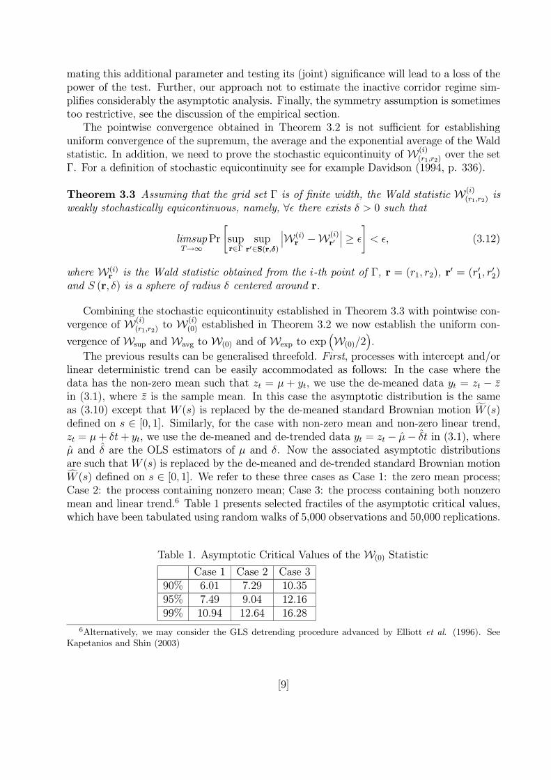
The previous results can be generalised threefold. First, processes with intercept and/orlinear deterministic trend can be easily accommodated as follows: In the case where thedata has the non-zero mean such that zt = µ + yt, we use the de-meaned data yt = zt − zin (3.1), where z is the sample mean. In this case the asymptotic distribution is the sameas (3.10) except that W (s) is replaced by the de-meaned standard Brownian motion fW (s)defined on s ∈ [0, 1]. Similarly, for the case with non-zero mean and non-zero linear trend,zt = µ+ δt+ yt, we use the de-meaned and de-trended data yt = zt − µ− δt in (3.1), whereµ and δ are the OLS estimators of µ and δ. Now the associated asymptotic distributionsare such that W (s) is replaced by the de-meaned and de-trended standard Brownian motioncW (s) defined on s ∈ [0, 1]. We refer to these three cases as Case 1: the zero mean process;Case 2: the process containing nonzero mean; Case 3: the process containing both nonzeromean and linear trend.6 Table 1 presents selected fractiles of the asymptotic critical values,which have been tabulated using random walks of 5,000 observations and 50,000 replications.

Table 1. Asymptotic Critical Values of the W(0) Statistic

Case 1 Case 2 Case 390% 6.01 7.29 10.3595% 7.49 9.04 12.1699% 10.94 12.64 16.28

6Alternatively, we may consider the GLS detrending procedure advanced by Elliott et al. (1996). SeeKapetanios and Shin (2003)

[9]

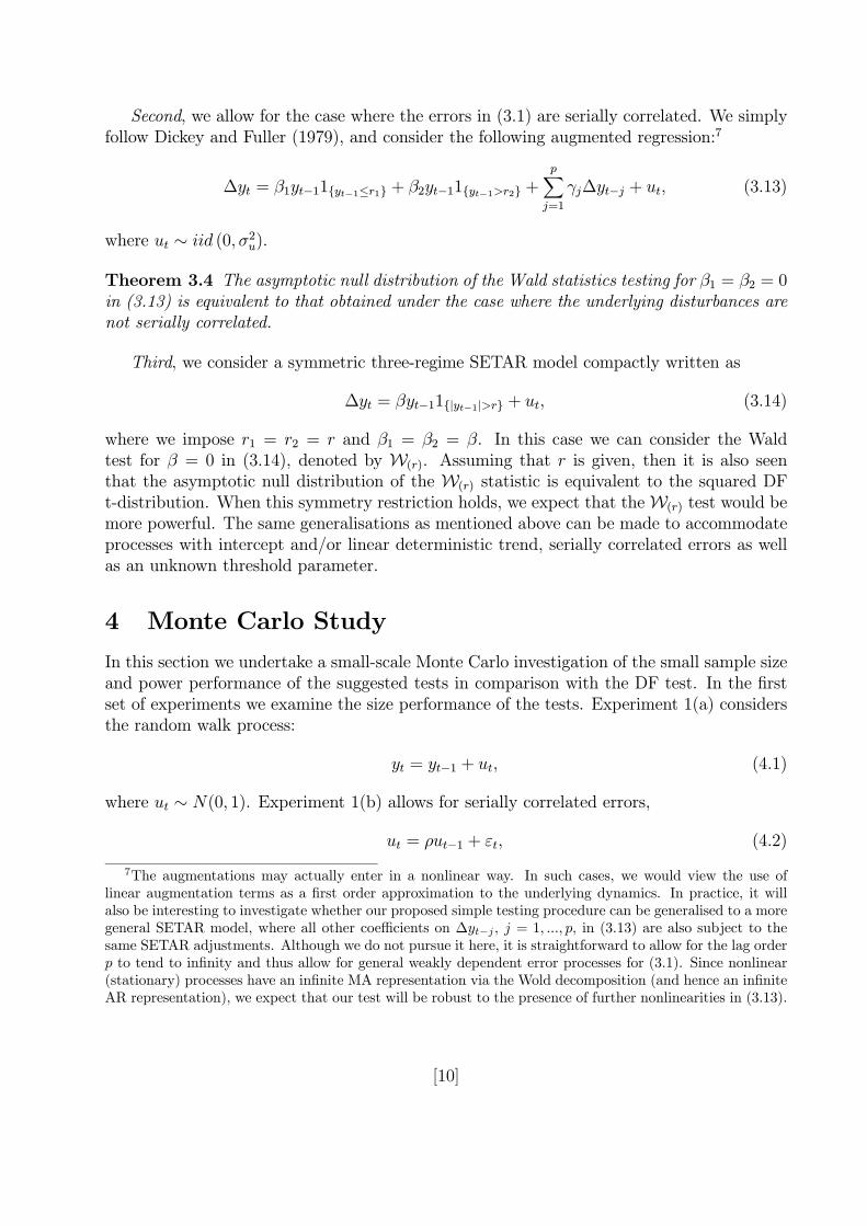
Second, we allow for the case where the errors in (3.1) are serially correlated. We simplyfollow Dickey and Fuller (1979), and consider the following augmented regression:7

∆yt = β1yt−11{yt−1≤r1} + β2yt−11{yt−1>r2} +pXj=1

γj∆yt−j + ut, (3.13)

where ut ∼ iid (0,σ2u).

Theorem 3.4 The asymptotic null distribution of the Wald statistics testing for β1 = β2 = 0in (3.13) is equivalent to that obtained under the case where the underlying disturbances arenot serially correlated.

Third, we consider a symmetric three-regime SETAR model compactly written as

∆yt = βyt−11{|yt−1|>r} + ut, (3.14)

where we impose r1 = r2 = r and β1 = β2 = β. In this case we can consider the Waldtest for β = 0 in (3.14), denoted by W(r). Assuming that r is given, then it is also seenthat the asymptotic null distribution of the W(r) statistic is equivalent to the squared DFt-distribution. When this symmetry restriction holds, we expect that theW(r) test would bemore powerful. The same generalisations as mentioned above can be made to accommodateprocesses with intercept and/or linear deterministic trend, serially correlated errors as wellas an unknown threshold parameter.

4 Monte Carlo Study

In this section we undertake a small-scale Monte Carlo investigation of the small sample sizeand power performance of the suggested tests in comparison with the DF test. In the firstset of experiments we examine the size performance of the tests. Experiment 1(a) considersthe random walk process:

yt = yt−1 + ut, (4.1)

where ut ∼ N(0, 1). Experiment 1(b) allows for serially correlated errors,

ut = ρut−1 + εt, (4.2)

7The augmentations may actually enter in a nonlinear way. In such cases, we would view the use oflinear augmentation terms as a first order approximation to the underlying dynamics. In practice, it willalso be interesting to investigate whether our proposed simple testing procedure can be generalised to a moregeneral SETAR model, where all other coefficients on ∆yt−j , j = 1, ..., p, in (3.13) are also subject to thesame SETAR adjustments. Although we do not pursue it here, it is straightforward to allow for the lag orderp to tend to infinity and thus allow for general weakly dependent error processes for (3.1). Since nonlinear(stationary) processes have an infinite MA representation via the Wold decomposition (and hence an infiniteAR representation), we expect that our test will be robust to the presence of further nonlinearities in (3.13).

[10]

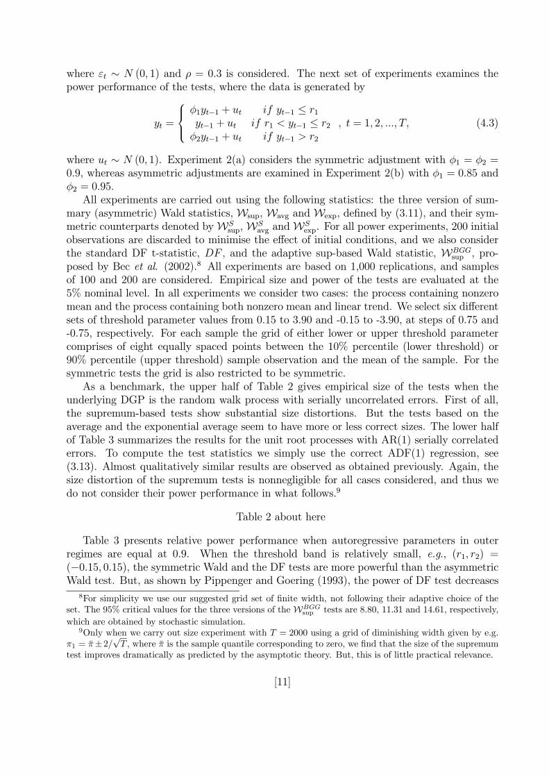
where εt ∼ N (0, 1) and ρ = 0.3 is considered. The next set of experiments examines thepower performance of the tests, where the data is generated by

yt =

⎧⎪⎨⎪⎩φ1yt−1 + ut if yt−1 ≤ r1yt−1 + ut if r1 < yt−1 ≤ r2φ2yt−1 + ut if yt−1 > r2

, t = 1, 2, ..., T, (4.3)

where ut ∼ N (0, 1). Experiment 2(a) considers the symmetric adjustment with φ1 = φ2 =0.9, whereas asymmetric adjustments are examined in Experiment 2(b) with φ1 = 0.85 andφ2 = 0.95.All experiments are carried out using the following statistics: the three version of sum-

mary (asymmetric) Wald statistics, Wsup, Wavg and Wexp, defined by (3.11), and their sym-metric counterparts denoted byWS

sup,WSavg andWS

exp. For all power experiments, 200 initialobservations are discarded to minimise the effect of initial conditions, and we also considerthe standard DF t-statistic, DF , and the adaptive sup-based Wald statistic, WBGG

sup , pro-posed by Bec et al. (2002).8 All experiments are based on 1,000 replications, and samplesof 100 and 200 are considered. Empirical size and power of the tests are evaluated at the5% nominal level. In all experiments we consider two cases: the process containing nonzeromean and the process containing both nonzero mean and linear trend. We select six differentsets of threshold parameter values from 0.15 to 3.90 and -0.15 to -3.90, at steps of 0.75 and-0.75, respectively. For each sample the grid of either lower or upper threshold parametercomprises of eight equally spaced points between the 10% percentile (lower threshold) or90% percentile (upper threshold) sample observation and the mean of the sample. For thesymmetric tests the grid is also restricted to be symmetric.As a benchmark, the upper half of Table 2 gives empirical size of the tests when the

underlying DGP is the random walk process with serially uncorrelated errors. First of all,the supremum-based tests show substantial size distortions. But the tests based on theaverage and the exponential average seem to have more or less correct sizes. The lower halfof Table 3 summarizes the results for the unit root processes with AR(1) serially correlatederrors. To compute the test statistics we simply use the correct ADF(1) regression, see(3.13). Almost qualitatively similar results are observed as obtained previously. Again, thesize distortion of the supremum tests is nonnegligible for all cases considered, and thus wedo not consider their power performance in what follows.9

Table 2 about here

Table 3 presents relative power performance when autoregressive parameters in outerregimes are equal at 0.9. When the threshold band is relatively small, e.g., (r1, r2) =(−0.15, 0.15), the symmetric Wald and the DF tests are more powerful than the asymmetricWald test. But, as shown by Pippenger and Goering (1993), the power of DF test decreases

8For simplicity we use our suggested grid set of finite width, not following their adaptive choice of theset. The 95% critical values for the three versions of the WBGG

sup tests are 8.80, 11.31 and 14.61, respectively,

which are obtained by stochastic simulation.9Only when we carry out size experiment with T = 2000 using a grid of diminishing width given by e.g.

π1 = π±2/√T , where π is the sample quantile corresponding to zero, we find that the size of the supremum

test improves dramatically as predicted by the asymptotic theory. But, this is of little practical relevance.

[11]

monotonically with the threshold values. On the other hand, the decrease in power of oursuggested tests is much slower especially for the exponential average test, and the power ofour tests eventually dominate the DF test as the threshold band gets wider. For example,looking at the demeaned processes with (r1, r2) = (−3.15, 3.15) and T = 200, we find thatthe powers of the Wexp, Wavg, WS

exp, WSavg and DF tests are 0.772, 0.681, 0.737, 0.648 and

0.544, respectively. Despite our expectation that the symmetric Wald test is more powerfulthan the asymmetric one in this set-up, the overall powers of both tests are comparable.

Table 3 about here

Table 4 gives the results for asymmetric threshold autoregressive parameters set to 0.85and 0.95, respectively. We find that all the tests are less powerful now than obtained inthe symmetric case. The power loss is less significant for our suggested tests as the corridorregime widens, since the power loss of the DF test is faster. Also as expected, the asymmetricWald test is now more powerful than the symmetric test as the threshold band gets larger.

Table 4 about here

Overall results suggest that both average and exponential average statistics have rea-sonably correct size and good power. Since the exponential average test seems to be morepowerful, we recommend to use the exponential average tests in practice.10 On the otherhand, the power of the WBGG

sup test is significantly lower than even the DF test for almostall experiments considered. As expected, the test proposed by Bec et al. (2002) does notperform well when the grid set of the thresholds are bounded under the alternative.11

5 Empirical Application to G7 Real Exchange Rates

Exchange rates affect both the relative price of goods and the return differential on assets.The first effect dictates purchasing power parity (PPP) and the second dictates uncoveredinterest parity, which are central to the study of international economics. However, atleast for advanced economies, deviations form PPP are highly persistent and a substantialbody of evidence suggests that the real exchange rate, measuring deviation from PPP, areindistinguishable from nonstationary time series. In this section we apply our proposedtests and examine whether the real exchange rates follow unit root processes. Since the realexchange rate embodies the long-run purchasing power parity relationship between nominalexchange rates, domestic and foreign prices, this test can be regarded as the univariate-basedtest for threshold cointegration, assuming that the cointegrating parameters are known. Forthe underlying theoretical background see Sercu et al. (1995), Balke and Fomby (1997),Michael et al. (1997), and Taylor (2001).

10Empirical results in the next section also seem to be consistent with this finding.11Similar results are also found in Bec et al. (2002) when the grid set is chosen using the conventional

quantile-based approach. But we note in passing that their test is designed to be more powerful under theadaptive choice of the grid set in which the upper bound tends to infinity under the alternative.

[12]

Quarterly data on US real exchange rates for the G7 countries were collected coveringthe period 1960Q1 to 2000Q4.12 Following the Monte Carlo findings we consider only theaverage and the exponential average of both asymmetric and symmetric Wald tests, jointlywith the DF tests. In practice, the number of augmentations in (3.13) must be selectedprior to the test to accommodate possible serially correlated errors. We could propose thatstandard model selection criteria be used for this purpose because under the null of a linearmodel, the properties of these criteria are well understood at least in linear models, e.g.,Ng and Perron (1995). Here we choose four augmentations for the underlying regression aswe have quarterly observations. Since all real exchange rates seem to be trending over thewhole sample period, we use the detrended version of the tests. To construct the thresholdparameter grid, we set the grid of either lower or upper threshold parameter comprises ofeight equally spaced points between the 10% quantile (lower threshold) or 90% quantile(upper threshold) and the mean of the sample as described in the previous section.Table 5 below presents the unit root test results. In sum, the DF test fails to reject

the null hypothesis of a unit root for any of countries at the 5% significance level. On theother hand, our proposed asymmetry Wald tests reject the null three times out of five cases,namely for Germany, and Japan real exchange rates at the 5% significance level, and furtherfor Italy at the 10% level, whereas the symmetry Wald test rejects the null two times forGermany and Japan at the 5% significance level.

Table 5 abouthere

Given the strength of evidence against the null and some support for the SETAR alter-native we also obtain estimates of both asymmetric and symmetric SETAR autoregressiveparameters in outer regimes along with the estimates of corresponding threshold parameters.The estimation results are also reported in Table 5. Although we cannot interpret the t-statistic as a significance test, we refer to it as “significant” if an asymptotic 95% confidenceinterval around the estimate excludes zero. We see that β1 and β2 in asymmetric SETARmodels and β in symmetric SETAR models are “significant” in all cases except for Canada.These are consistent with similar findings by Michael et al. (1997) that nonlinear meanreversion (or more precisely range reversion) arising from fixed costs of transactions costs incurrency markets is present for several industrial countries. Another interesting finding isthat the speed of mean reversion is faster in the lower regime than in the upper regime forGermany, Italy and Japan. As high values of real exchange rates are defined as appreciationand vice versa, this implies that the data periods dominated by extreme depreciation maydisplay substantially faster reversion towards their underlying equilibrium range than thosecharacterised by extreme appreciation. This raises the issue that empirical evidence maybe available to bolster the (alternative) hypothesis of asymmetric foreign exchange marketinterventions that countries may choose to resist depreciations more vigorously than appre-ciations, so-called “dread of depreciation,” see Dutta and Leon (2002) for further details.This result clearly highlights the need for tests that are designed to deal with asymmetricSETAR models.

12The data have been obtained from the IFS database. Real exchange rates are calculated using thewholesale price index. But, the full data for France are not available, so we drop the French case.

[13]

6 Concluding Remarks

The investigation of nonstationarity in conjunction with the threshold autoregressive mod-elling has recently attracted attention in econometric study. It is clear that misclassifying astable nonlinear process as nonstationary can be misleading both in impulse response andforecasting analysis. In this paper we have proposed unit root tests that are designed to havepower against globally stationary three regime SETAR processes. Our proposed tests areshown to have better power than the DF test that ignores the three regime SETAR natureof the alternative. Although our tests are based on a univariate model, we have illustratedthat it can also be used as a test of linear lack of cointegration against nonlinear thresholdcointegration, assuming that the process under investigation can be regarded as a linearcombination of the nonstationary variables with known cointegrating parameters.There are further research issues. First, it might be possible to find an alternative testing

procedure based on an arranged regression along similar lines to Tsay (1998) and Berbenand van Dijk (1999), which is likely to boost the power of the tests. Second, a more generalTAR(p) model could be adopted where all the parameters including intercepts are alsosubject to the same nonlinear scheme as in Caner and Hansen (2001). Finally, although ourtest is univariate, it could be extended to establish the existence of cointegrating equilibriumrelationship such as those conjectured to govern real exchange rates. Recently, Kapetanios etal. (2003b) propose testing procedures to detect the presence of a cointegrating relationshipthat follows a globally stationary smooth transition autoregressive process in a nonlinearerror correction model with an application to price-dividend relationship. In this regard,a cointegration test based on an error correction model subject to SETAR nonlinearity iscurrently under investigation.

[14]

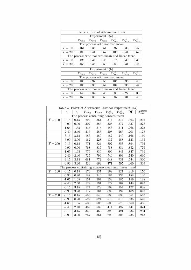
Table 2. Size of Alternative TestsExperiment 1(a)

Wsup Wavg Wexp WSsup WS

avg WSexp

The process with nonzero meanT = 100 .161 .035 .051 .097 .033 .047T = 200 .183 .041 .057 .108 .041 .052The process with nonzero mean and linear trend

T = 100 .125 .034 .045 .078 .030 .039T = 200 .153 .036 .050 .089 .031 .044

Experiment 1(b)Wsup Wavg Wexp WS

sup WSavg WS

exp

The process with nonzero meanT = 100 .186 .037 .053 .105 .036 .048T = 200 .186 .036 .054 .104 .036 .047The process with nonzero mean and linear trend

T = 100 .140 .032 .046 .083 .027 .038T = 200 .150 .033 .050 .087 .031 .040

Table 3: Power of Alternative Tests for Experiment 2(a)r1 r2 Wavg Wexp WS

avg WSexp DF WBGG

sup

The process containing nonzero meanT = 100 -0.15 0.15 .299 .361 .314 .374 .363 .295

-0.90 0.90 .302 .385 .328 .377 .337 .278-1.65 1.65 .235 .315 .253 .311 .266 .223-2.40 2.40 .215 .283 .208 .266 .201 .178-3.15 3.15 .186 .280 .182 .240 .166 .160-3.90 3.90 .162 .228 .137 .188 .123 .135

T = 200 -0.15 0.15 .771 .824 .802 .853 .894 .792-0.90 0.90 .768 .815 .788 .834 .852 .779-1.65 1.65 .779 .830 .809 .847 .847 .739-2.40 2.40 .725 .799 .740 .803 .740 .630-3.15 3.15 .681 .772 .648 .737 .544 .500-3.90 3.90 .526 .663 .471 .595 .360 .309

The process containing nonzero mean and linear trendT = 100 -0.15 0.15 .176 .237 .168 .227 .216 .150

-0.90 0.90 .182 .246 .184 .234 .188 .146-1.65 1.65 .157 .204 .139 .185 .159 .128-2.40 2.40 .129 .191 .122 .167 .148 .092-3.15 3.15 .124 .178 .109 .154 .127 .088-3.90 3.90 .117 .164 .098 .139 .103 .092

T = 200 -0.15 0.15 .553 .643 .530 .638 .651 .567-0.90 0.90 .529 .624 .518 .616 .635 .528-1.65 1.65 .506 .605 .500 .576 .560 .498-2.40 2.40 .439 .539 .414 .497 .441 .374-3.15 3.15 .355 .469 .329 .421 .334 .294-3.90 3.90 .267 .361 .220 .306 .235 .213

[15]

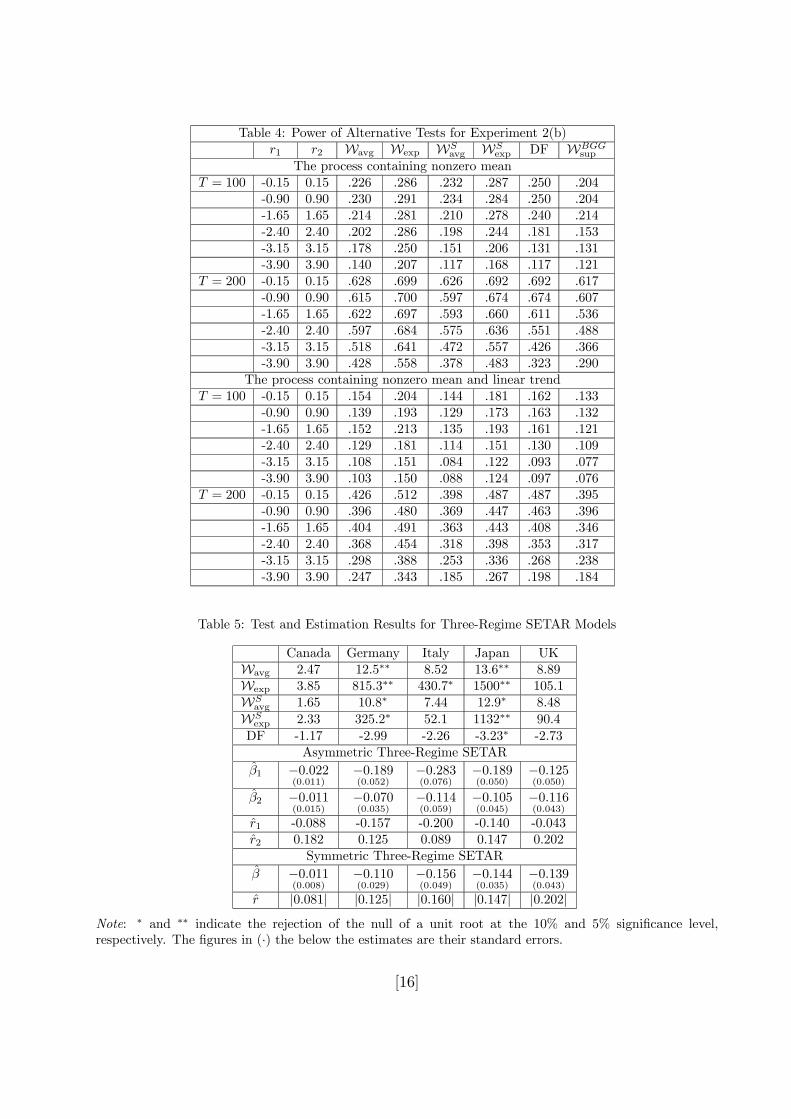
Table 4: Power of Alternative Tests for Experiment 2(b)r1 r2 Wavg Wexp WS

avg WSexp DF WBGG

sup

The process containing nonzero meanT = 100 -0.15 0.15 .226 .286 .232 .287 .250 .204

-0.90 0.90 .230 .291 .234 .284 .250 .204-1.65 1.65 .214 .281 .210 .278 .240 .214-2.40 2.40 .202 .286 .198 .244 .181 .153-3.15 3.15 .178 .250 .151 .206 .131 .131-3.90 3.90 .140 .207 .117 .168 .117 .121

T = 200 -0.15 0.15 .628 .699 .626 .692 .692 .617-0.90 0.90 .615 .700 .597 .674 .674 .607-1.65 1.65 .622 .697 .593 .660 .611 .536-2.40 2.40 .597 .684 .575 .636 .551 .488-3.15 3.15 .518 .641 .472 .557 .426 .366-3.90 3.90 .428 .558 .378 .483 .323 .290

The process containing nonzero mean and linear trendT = 100 -0.15 0.15 .154 .204 .144 .181 .162 .133

-0.90 0.90 .139 .193 .129 .173 .163 .132-1.65 1.65 .152 .213 .135 .193 .161 .121-2.40 2.40 .129 .181 .114 .151 .130 .109-3.15 3.15 .108 .151 .084 .122 .093 .077-3.90 3.90 .103 .150 .088 .124 .097 .076

T = 200 -0.15 0.15 .426 .512 .398 .487 .487 .395-0.90 0.90 .396 .480 .369 .447 .463 .396-1.65 1.65 .404 .491 .363 .443 .408 .346-2.40 2.40 .368 .454 .318 .398 .353 .317-3.15 3.15 .298 .388 .253 .336 .268 .238-3.90 3.90 .247 .343 .185 .267 .198 .184

Table 5: Test and Estimation Results for Three-Regime SETAR Models

Canada Germany Italy Japan UKWavg 2.47 12.5∗∗ 8.52 13.6∗∗ 8.89Wexp 3.85 815.3∗∗ 430.7∗ 1500∗∗ 105.1WSavg 1.65 10.8∗ 7.44 12.9∗ 8.48

WSexp 2.33 325.2∗ 52.1 1132∗∗ 90.4

DF -1.17 -2.99 -2.26 -3.23∗ -2.73Asymmetric Three-Regime SETAR

β1 −0.022(0.011)

−0.189(0.052)

−0.283(0.076)

−0.189(0.050)

−0.125(0.050)

β2 −0.011(0.015)

−0.070(0.035)

−0.114(0.059)

−0.105(0.045)

−0.116(0.043)

r1 -0.088 -0.157 -0.200 -0.140 -0.043r2 0.182 0.125 0.089 0.147 0.202

Symmetric Three-Regime SETAR

β −0.011(0.008)

−0.110(0.029)

−0.156(0.049)

−0.144(0.035)

−0.139(0.043)

r |0.081| |0.125| |0.160| |0.147| |0.202|

Note: ∗ and ∗∗ indicate the rejection of the null of a unit root at the 10% and 5% significance level,respectively. The figures in (·) the below the estimates are their standard errors.

[16]

A Appendix

A.1 Proof of Theorem 3.1

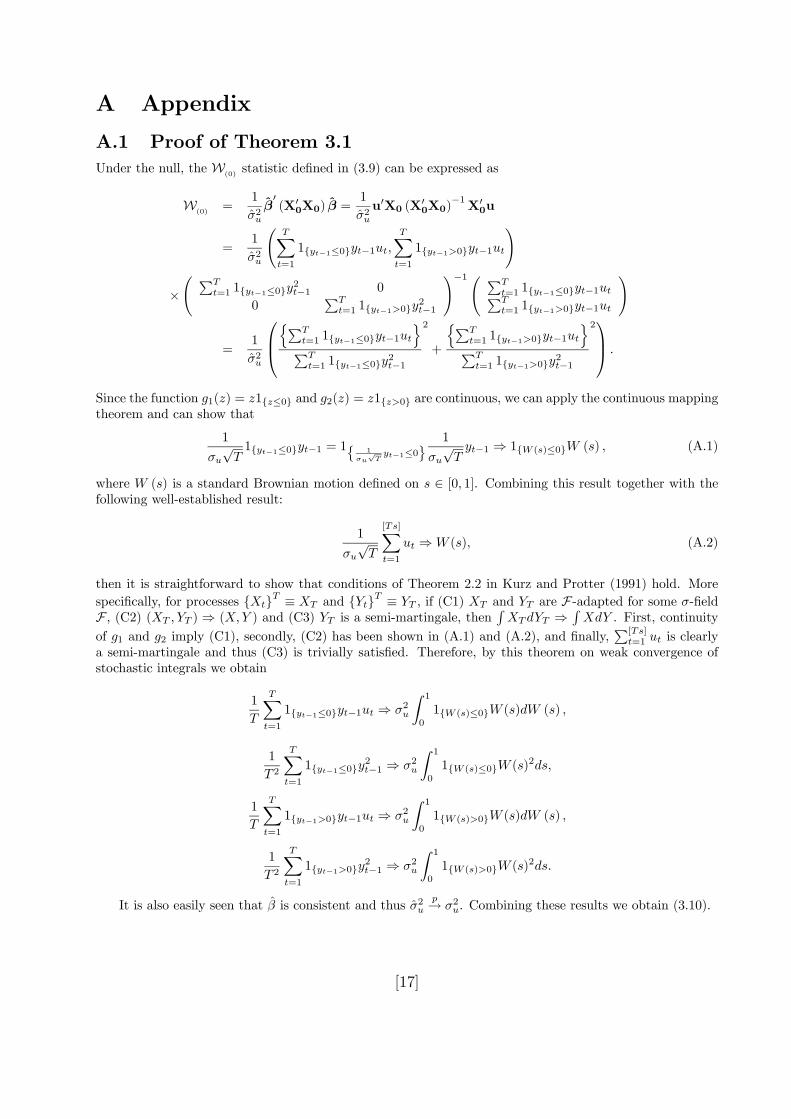
Under the null, the W(0)statistic defined in (3.9) can be expressed as

W(0)

=1

σ2uβ0(X0

0X0) β =1

σ2uu0X0 (X

00X0)

−1X00u

=1

σ2u

ÃTXt=1

1{yt−1≤0}yt−1ut,TXt=1

1{yt−1>0}yt−1ut

!

×à PT

t=1 1{yt−1≤0}y2t−1 0

0PTt=1 1{yt−1>0}y

2t−1

!−1Ã PTt=1 1{yt−1≤0}yt−1utPTt=1 1{yt−1>0}yt−1ut

!

=1

σ2u

⎛⎜⎝nPT

t=1 1{yt−1≤0}yt−1uto

PTt=1 1{yt−1≤0}y

2t−1

2

+

nPTt=1 1{yt−1>0}yt−1ut

oPT

t=1 1{yt−1>0}y2t−1

2⎞⎟⎠ .

Since the function g1(z) = z1{z≤0} and g2(z) = z1{z>0} are continuous, we can apply the continuous mappingtheorem and can show that

1

σu√T1{yt−1≤0}yt−1 = 1

©1

σu√Tyt−1≤0

ª 1

σu√Tyt−1 ⇒ 1{W (s)≤0}W (s) , (A.1)

where W (s) is a standard Brownian motion defined on s ∈ [0, 1]. Combining this result together with thefollowing well-established result:

1

σu√T

[Ts]Xt=1

ut ⇒W (s), (A.2)

then it is straightforward to show that conditions of Theorem 2.2 in Kurz and Protter (1991) hold. More

specifically, for processes {Xt}T ≡ XT and {Yt}T ≡ YT , if (C1) XT and YT are F-adapted for some σ-fieldF , (C2) (XT , YT ) ⇒ (X,Y ) and (C3) YT is a semi-martingale, then

RXTdYT ⇒

RXdY . First, continuity

of g1 and g2 imply (C1), secondly, (C2) has been shown in (A.1) and (A.2), and finally,P[Ts]t=1 ut is clearly

a semi-martingale and thus (C3) is trivially satisfied. Therefore, by this theorem on weak convergence ofstochastic integrals we obtain

1

T

TXt=1

1{yt−1≤0}yt−1ut ⇒ σ2u

Z 1

0

1{W (s)≤0}W (s)dW (s) ,

1

T 2

TXt=1

1{yt−1≤0}y2t−1 ⇒ σ2u

Z 1

0

1{W (s)≤0}W (s)2ds,

1

T

TXt=1

1{yt−1>0}yt−1ut ⇒ σ2u

Z 1

0

1{W (s)>0}W (s)dW (s) ,

1

T 2

TXt=1

1{yt−1>0}y2t−1 ⇒ σ2u

Z 1

0

1{W (s)>0}W (s)2ds.

It is also easily seen that β is consistent and thus σ2up→ σ2u. Combining these results we obtain (3.10).

[17]

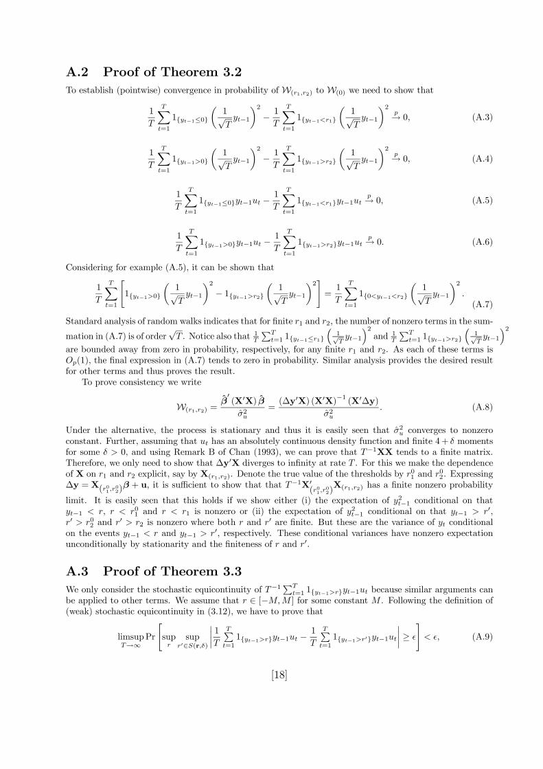
A.2 Proof of Theorem 3.2

To establish (pointwise) convergence in probability of W(r1,r2) to W(0) we need to show that

1

T

TXt=1

1{yt−1≤0}

µ1√Tyt−1

¶2− 1

T

TXt=1

1{yt−1<r1}

µ1√Tyt−1

¶2p→ 0, (A.3)

1

T

TXt=1

1{yt−1>0}

µ1√Tyt−1

¶2− 1

T

TXt=1

1{yt−1>r2}

µ1√Tyt−1

¶2p→ 0, (A.4)

1

T

TXt=1

1{yt−1≤0}yt−1ut −1

T

TXt=1

1{yt−1<r1}yt−1utp→ 0, (A.5)

1

T

TXt=1

1{yt−1>0}yt−1ut −1

T

TXt=1

1{yt−1>r2}yt−1utp→ 0. (A.6)

Considering for example (A.5), it can be shown that

1

T

TXt=1

"1{yt−1>0}

µ1√Tyt−1

¶2− 1{yt−1>r2}

µ1√Tyt−1

¶2#=1

T

TXt=1

1{0<yt−1<r2}

µ1√Tyt−1

¶2.(A.7)

Standard analysis of random walks indicates that for finite r1 and r2, the number of nonzero terms in the sum-

mation in (A.7) is of order√T . Notice also that 1T

PTt=1 1{yt−1≤r1}

³1√Tyt−1

´2and 1

T

PTt=1 1{yt−1>r2}

³1√Tyt−1

´2are bounded away from zero in probability, respectively, for any finite r1 and r2. As each of these terms isOp(1), the final expression in (A.7) tends to zero in probability. Similar analysis provides the desired resultfor other terms and thus proves the result.

To prove consistency we write

W(r1,r2) =β0(X0X) β

σ2u=(∆y0X) (X0X)−1 (X0∆y)

σ2u. (A.8)

Under the alternative, the process is stationary and thus it is easily seen that σ2u converges to nonzeroconstant. Further, assuming that ut has an absolutely continuous density function and finite 4+ δ momentsfor some δ > 0, and using Remark B of Chan (1993), we can prove that T−1XX tends to a finite matrix.Therefore, we only need to show that ∆y0X diverges to infinity at rate T . For this we make the dependenceof X on r1 and r2 explicit, say by X(r1,r2). Denote the true value of the thresholds by r

01 and r

02. Expressing

∆y = X(r01,r02)β + u, it is sufficient to show that that T−1X0

(r01,r02)X(r1,r2) has a finite nonzero probability

limit. It is easily seen that this holds if we show either (i) the expectation of y2t−1 conditional on thatyt−1 < r, r < r01 and r < r1 is nonzero or (ii) the expectation of y

2t−1 conditional on that yt−1 > r0,

r0 > r02 and r0 > r2 is nonzero where both r and r

0 are finite. But these are the variance of yt conditionalon the events yt−1 < r and yt−1 > r0, respectively. These conditional variances have nonzero expectationunconditionally by stationarity and the finiteness of r and r0.

A.3 Proof of Theorem 3.3

We only consider the stochastic equicontinuity of T−1PTt=1 1{yt−1>r}yt−1ut because similar arguments can

be applied to other terms. We assume that r ∈ [−M,M ] for some constant M . Following the definition of(weak) stochastic equicontinuity in (3.12), we have to prove that

limsupT→∞

Pr

"supr

supr0∈S(r,δ)

¯1

T

TPt=11{yt−1>r}yt−1ut −

1

T

TPt=11{yt−1>r0}yt−1ut

¯≥ ²#< ², (A.9)

[18]

where S (r, δ) is a sphere of radius δ centred at r. Assuming without loss of generality that r0 < r, then theprobability in (A.9) can be written as

limsupT→∞

Pr

"supr

supr0∈S(r,δ)

¯1

T

TPt=11{r0≤yt−1≤r}yt−1ut

¯≥ ²#

≤ limsupT→∞

Pr

"supr

supr0∈S(r,δ)

1

T

TPt=1

¯1{r0≤yt−1≤r}ut

¯|yt−1| ≥ ²

#. (A.10)

A standard result in random walk theory (see e.g., Feller, 1957) is that a random walk crosses zero Oa.s.(√T )

times. This implies that a random walk lies within a corridor of finite width for Oa.s(√T ) periods. Therefore,

1{r0≤yt−1≤r} will take unity at mosthc√Tiperiods for some fixed constant c, where [.] denotes integer part,

and zero otherwise.13 Therefore, onlyhc√Titerms in the summation in (A.10) are non-zero. In the cases

where these terms are non zero, |yt−1| can be at most M . Taking the supremum over r and r0 inside thesummation in (A.10), it is easily seen that (A.10) holds if

limsupT→∞

Pr

⎡⎣MT

[c√T ]P

i=1|uti | ≥ ²

⎤⎦ < ², (A.11)

where ti denotes the subsequence of periods when the process lies within the finite corridor band. This issmaller than

limsupT→∞

Pr

⎡⎣MT

[c√T ]P

i=1{|uti |−E (|uti |)}+

M

T

[c√T ]P

i=1E (|uti |) ≥ ²

⎤⎦ . (A.12)

By the finiteness of the second moment of ut,MT

P[c√T ]i=1 E (|uti |) tends to zero. Hence, we concentrate on

limsupT→∞

Pr

⎡⎣MT

[c√T ]P

i=1{|uti |−E (|uti |)} ≥ ²

⎤⎦ . (A.13)

But by the law of large numbers, and using the assumption that ut’s are iid, we have

limsupT→∞

Pr

⎡⎣P[c√T ]i=1 {|uti |−E (|uti |)}cT 1/2

≥ ²

⎤⎦ = 0, (A.14)

As the normalisation M/T in (A.13) is smaller than the normalisation 1/T 1/2 needed for (A.14) to hold,hence (A.13) holds, which proves (A.9). Alternatively, using the law of the iterated logarithm (e.g., Davidson,1994, p. 408), it can also be shown that

limsupT→∞

P[c√T ]i=1 {|uti |−E (|uti |)}T 1/4 ln(ln(T 1/2))

= c1,

where c1 is a constant a.s. Since the normalisation M/T in (A.13) is smaller than the normalisation1/T 1/4 ln(ln(T 1/2)) needed for the above result to hold, hence this will also prove the following strongequicontinuity condition:

Pr

"limsupT→∞

supr

supr0∈S(r,δ)

¯1

T

TPt=11{yt−1>r}yt−1ut −

1

T

TPt=11{yt−1>r0}yt−1ut

¯≥ ²#= 0.

13A standard result in random walk theory is that a random walk crosses zero Oa.s.(√T ) times. This

implies that a random walk lies within a corridor of finite width for Oa.s(√T ) periods. See Feller (1957).

[19]

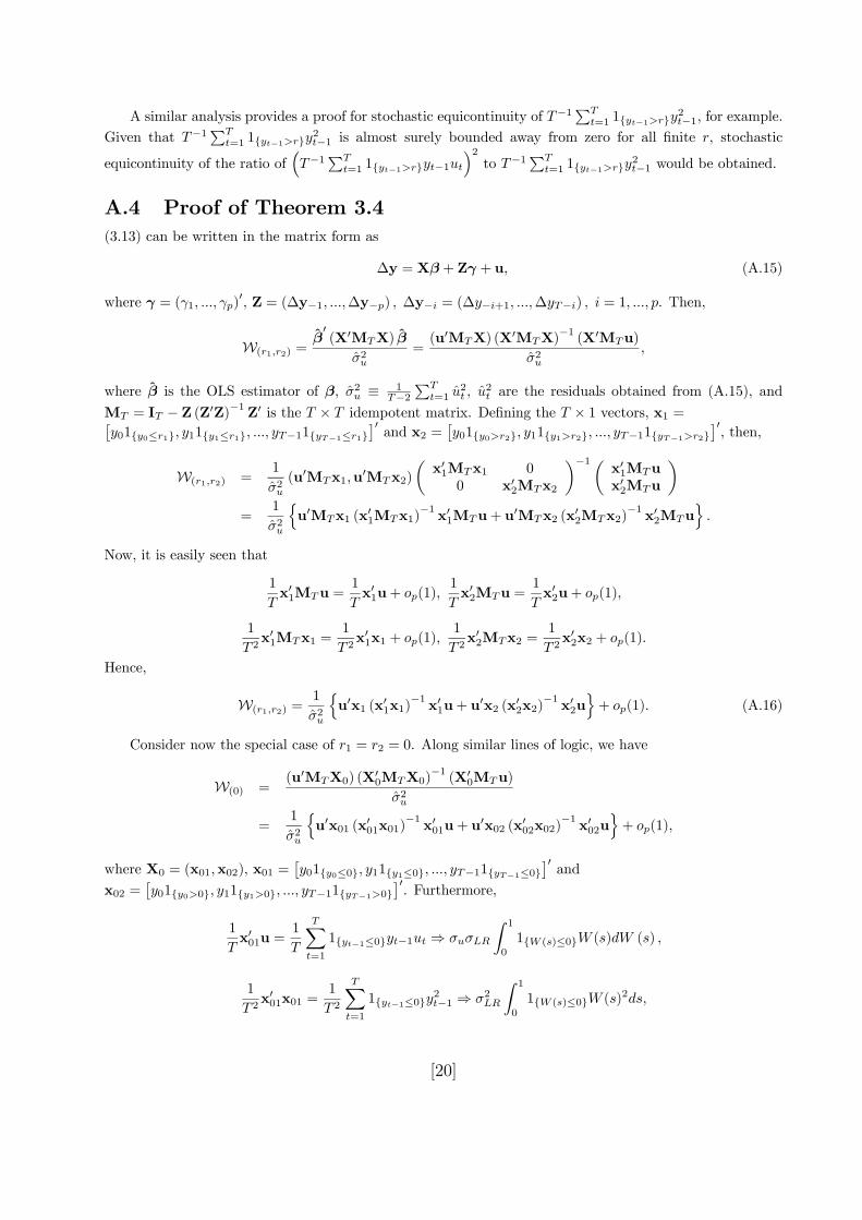
A similar analysis provides a proof for stochastic equicontinuity of T−1PTt=1 1{yt−1>r}y

2t−1, for example.

Given that T−1PTt=1 1{yt−1>r}y

2t−1 is almost surely bounded away from zero for all finite r, stochastic

equicontinuity of the ratio of³T−1

PTt=1 1{yt−1>r}yt−1ut

´2to T−1

PTt=1 1{yt−1>r}y

2t−1 would be obtained.

A.4 Proof of Theorem 3.4

(3.13) can be written in the matrix form as

∆y = Xβ + Zγ + u, (A.15)

where γ = (γ1, ..., γp)0, Z = (∆y−1, ...,∆y−p) , ∆y−i = (∆y−i+1, ...,∆yT−i) , i = 1, ..., p. Then,

W(r1,r2) =β0(X0MTX) β

σ2u=(u0MTX) (X

0MTX)−1(X0MTu)

σ2u,

where β is the OLS estimator of β, σ2u ≡ 1T−2

PTt=1 u

2t , u

2t are the residuals obtained from (A.15), and

MT = IT − Z (Z0Z)−1 Z0 is the T × T idempotent matrix. Defining the T × 1 vectors, x1 =£y01{y0≤r1}, y11{y1≤r1}, ..., yT−11{yT−1≤r1}

¤0and x2 =

£y01{y0>r2}, y11{y1>r2}, ..., yT−11{yT−1>r2}

¤0, then,

W(r1,r2) =1

σ2u(u0MTx1,u

0MTx2)

µx01MTx1 0

0 x02MTx2

¶−1µx01MTux02MTu

¶=

1

σ2u

nu0MTx1 (x

01MTx1)

−1x01MTu+ u

0MTx2 (x02MTx2)

−1x02MTu

o.

Now, it is easily seen that

1

Tx01MTu =

1

Tx01u+ op(1),

1

Tx02MTu =

1

Tx02u+ op(1),

1

T 2x01MTx1 =

1

T 2x01x1 + op(1),

1

T 2x02MTx2 =

1

T 2x02x2 + op(1).

Hence,

W(r1,r2) =1

σ2u

nu0x1 (x

01x1)

−1x01u+ u

0x2 (x02x2)

−1x02u

o+ op(1). (A.16)

Consider now the special case of r1 = r2 = 0. Along similar lines of logic, we have

W(0) =(u0MTX0) (X

00MTX0)

−1(X0

0MTu)

σ2u

=1

σ2u

nu0x01 (x

001x01)

−1x001u+ u

0x02 (x002x02)

−1x002u

o+ op(1),

where X0 = (x01,x02), x01 =£y01{y0≤0}, y11{y1≤0}, ..., yT−11{yT−1≤0}

¤0and

x02 =£y01{y0>0}, y11{y1>0}, ..., yT−11{yT−1>0}

¤0. Furthermore,

1

Tx001u =

1

T

TXt=1

1{yt−1≤0}yt−1ut ⇒ σuσLR

Z 1

0

1{W (s)≤0}W (s)dW (s) ,

1

T 2x001x01 =

1

T 2

TXt=1

1{yt−1≤0}y2t−1 ⇒ σ2LR

Z 1

0

1{W (s)≤0}W (s)2ds,

[20]

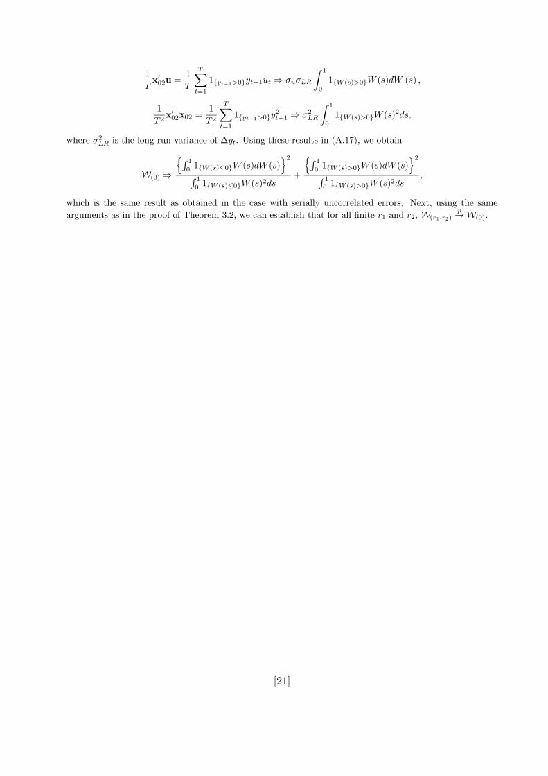
1

Tx002u =

1

T

TXt=1

1{yt−1>0}yt−1ut ⇒ σuσLR

Z 1

0

1{W (s)>0}W (s)dW (s) ,

1

T 2x002x02 =

1

T 2

TXt=1

1{yt−1>0}y2t−1 ⇒ σ2LR

Z 1

0

1{W (s)>0}W (s)2ds,

where σ2LR is the long-run variance of ∆yt. Using these results in (A.17), we obtain

W(0) ⇒

nR 101{W (s)≤0}W (s)dW (s)

o2R 101{W (s)≤0}W (s)2ds

+

nR 101{W (s)>0}W (s)dW (s)

o2R 101{W (s)>0}W (s)2ds

,

which is the same result as obtained in the case with serially uncorrelated errors. Next, using the same

arguments as in the proof of Theorem 3.2, we can establish that for all finite r1 and r2, W(r1,r2)p→W(0).

[21]

References

[1] Anderson, H. (1997) Transactions costs and non-Linear adjustment towards equilibrium in the UStreasury bill market. Oxford Bulletin of Economics and Statistics 59, 465-84.

[2] Bec, F., Salem, M. B. and Carrasco, M. (2001) Tests of unit-root versus threshold specification with anapplication to the PPP. Unpublished manuscript, University of Rochester.

[3] Bec. F., Guay, A. and Guerre, E. (2002) Adaptive consistent unit root tests based on autoregressivethreshold model. Unpublished manuscript, Universite Paris 6.

[4] Balke, N. S. and Fomby, T.B. (1997) Threshold cointegration. International Economic Review 38, 627-45.

[5] Berben, R. and van Dijk, D. (1999) Unit root tests and asymmetric adjustment: a reassessment.Unpublished manuscript, Erasmus University Rotterdam.

[6] Caner, M. and Hansen, B. E. (2001) Threshold autoregression with a unit root. Econometrica 69,1555-96.

[7] Chan, K.S. (1993) Consistency and limiting distribution of the least squares estimator of a thresholdautoregressive model. Annals of Statistics 21, 520-33.

[8] Chan, K.S., Petrucelli, J.D., Tong, H. and Woolford, S. W. (1985) A multiple threshold AR(1) model.Journal of Applied Probability 22, 267-79.

[9] Davidson J. (1994) Stochastic Limit Theory. Oxford University Press: Oxford.

[10] Davies, R. B. (1987) Hypothesis testing when a nuisance parameter is present under the alternative.Biometrika 74, 33-43.

[11] Dickey, D. A. and Fuller, W. A. (1979) Distribution of the estimators for autoregressive time series witha unit root. Journal of the American Statistical Association 74, 427-31.

[12] Dutta, J. and Leon, H. (2002) Dread of depreciation: measuring real exchange rate interventions.Unpublished manuscript, University of Birmingham.

[13] Elliot, B. E., Rothenberg, T. J. and Stock, J. H. (1996) Efficient tests of the unit root hypothesis.Econometrica 64, 813—836.

[14] Enders, W. and Granger, C. W. J. (1998) Unit root test and asymmetric adjustment with an exampleusing the term structure of interest rates. Journal of Business and Economic Statistics 16, 304-11.

[15] Engle, R. and Granger, C. W. J. (1987) Cointegration and error correction: representation, estimationand testing. Econometrica 55, 251-76.

[16] Feller, W. (1957) An Introduction to Probability Theory and its Applications. Wiley: New York.

[17] Gonzalez, M. and Gonzalo, J. (1998) Threshold unit root models. Universidad Carlos III de Madrid,Discussion Paper.

[18] Hansen, B. E. (1996) Inference when a nuisance parameter is not identified under the null hypothesis.Econometrica 64, 414—30.

[19] Hicks, J. R. (1950) A Contribution to the Theory of the Trade Cycle. Oxford University Press: Oxford.

[20] Ioannides, C., Peel, D. and Peel, M. (2003) The time series properties of financial ratios: revisited.Forthcoming in Journal of Business, Finance and Accounting.

[21] Kapetanios, G. (1999) Essays on the Econometric Analysis of Threshold Models. Unpublished Ph.D.Thesis, University of Cambridge.

[22] Kapetanios, G. and Shin, Y. (2003) GLS detrending-based unit root tests in nonlinear STAR andSETAR framework. Unpublished manuscript, University of Edinburgh.

[22]

[23] Kapetanios, G., Shin, Y. and Snell, A. (2003a) Testing for a unit root in the nonlinear STAR framework.Journal of Econometrics 112, 359-79.

[24] Kapetanios, G., Shin, Y. and Snell, A. (2003b) Testing for cointegration in nonlinear STAR errorcorrection models. Unpublished manuscript, University of Edinburgh.

[25] Koop, G., Pesaran, M. H. and Potter, S. M. (1996) Impulse response analysis in nonlinear multivariatemodels. Journal of Econometrics 74, 119-47.

[26] Kurtz, T. G. and Protter, P. (1992) Weak limit theorems for stochastic integrals and stochastic differenceequations. Annals of Probability 19, 1035-70.

[27] Lo, M. C. and Zivot, E. (2001) Threshold cointegration and nonlinear adjustment to the law of oneprice. Macroeconomic Dynamics 5, 533-576.

[28] Michael, P., Nobay, R. A. and Peel, D. A. (1997) Transactions costs and nonlinear adjustment in realexchange rates: an empirical investigation. Journal of Political Economy 105, 862-79.

[29] Ng, S. and Perron, P. (1995) Unit root tests in ARMA models with data-dependent methods for theselection of the truncation lag. Journal of the American Statistical Association 90, 268-81.

[30] Pesaran, M.H. and Potter, S. M. (1997) A floor and ceiling model of US output. Journal of EconomicDynamics and Control 21, 661-95.

[31] Pippenger, M. K. and Goering, G. E. (1993) A note on the empirical power of unit root tests underthreshold processes. Oxford Bulletin of Economics and Statistics 55, 473-81.

[32] Sercu, P., Uppal, R. and van Hulle, C. (1995) The exchange rate in the presence of transaction costs:implications for tests of purchasing power parity. Journal of Finance 50, 1309-19.

[33] Shin, D. W. and Lee, O. (2001) Test for asymmetry in possibly nonstationary time series data. Journalof Business and Economic Statistics 19, 233-44.

[34] Tong, H. (1990) Nonlinear Time Series: A Dynamical System Approach. Oxford University Press:Oxford.

[35] Taylor, A. (2001) Potential pitfalls for the PPP puzzle? Sampling and specification biases in meanreversion tests of the LOOP. Econometrica 69, 473-98.

[36] Tsay, R. S. (1998) Testing and modelling multivariate threshold models. Journal of the AmericanStatistical Association 94, 1188-1202.

[37] Tweedie, R. L. (1975) Sufficient conditions for ergodicity and recurrence of Markov on a general statespace. Stochastic Processes Appl. 3, 385-403.

[23]