UNIT -1 BASICS OF MANAGERIAL ECNOMICS LESSON 5
352
UNIT -1 BASICS OF MANAGERIAL ECNOMICS LESSON 5- Tools and Technique of Decision Making So this is the last lesson of this Unit i.e. Unit – 1. After doing this lesson you will be able to know the various tools and techniques of decision making. How these tools and technique are useful for managers in making the right decision. But before knowing the tools and technique of decision making can you answer some of my questions: • Is decision making a process? • Are there any particular steps required for decision making? • Is decision making depends on the condition or situations? • What are the various conditions affecting decision making? o.k. Fine, tell me why decision making is required? t. See we all know we have unlimited wants, and the means to satisfy those wants are very limited. We have to make choices. We cannot have whatever we want. We have to make preferences amongst our choices. And we will prefer those thing first which is most needed. Therefore our choice depends on our need. What we need the most is to be chosen firs Factors influencing managerial decision:
-
Upload
khangminh22 -
Category
Documents
-
view
3 -
download
0
Transcript of UNIT -1 BASICS OF MANAGERIAL ECNOMICS LESSON 5

UNIT -1 BASICS OF MANAGERIAL ECNOMICS LESSON 5- Tools and Technique of Decision Making So this is the last lesson of this Unit i.e. Unit – 1. After doing this lesson you will be able to know the various tools and techniques of decision making. How these tools and technique are useful for managers in making the right decision. But before knowing the tools and technique of decision making can you answer some of my questions:
• Is decision making a process? • Are there any particular steps required for decision making? • Is decision making depends on the condition or situations? • What are the various conditions affecting decision making?
o.k. Fine, tell me why decision making is required?
t.
See we all know we have unlimited wants, and the means to satisfy those wants are very limited. We have to make choices. We cannot have whatever we want. We have to make preferences amongst our choices. And we will prefer those thing first which is most needed. Therefore our choice depends on our need. What we need the most is to be chosen firs
Factors influencing managerial decision:

Now its clear that managerial decision making is influenced not only by economics but also by several other significant considerations. While economic analysis contributes a great deal to problem solving in an enterprises it is important to remember that three other variable also influences the choices and decision made by the managers. These are as follows: Human and behavioral considerations Technological forces Environmental factors. Steps in decision making: there are certain things which are to be taken into account while making decisions. No matter what’s the size of the problem but like every thing decision making should also be in certain steps. Following are the various steps in decision making:
• Establish objectives • Specify the decision problem • Identify the alternatives • Evaluate alternatives • Select the best alternatives • Implement the decision • Monitor the performance
Business decision making is essentially a process of selecting the best out of alternative opportunities open to the firm. The above steps put managers analytical ability to test and determine the appropriateness and validity of decisions in the modern business world. Modern business conditions are changing so fast and becoming so competitive and complex that personal business sense, intuition and experience alone are not sufficient to make appropriate business decisions. It is in this area of decision making that economic theories and tools of economic analysis contribute a great deal. Application of economic tools:

For e.g. A firm plans to launch a new product for which close substitutes are available in the market. One method of deciding whether or not to launch the product is to obtain the services of the business consultants or to seek expert opinions. If the matter has to be decided by the managers of the firms, two areas which they need to know:
• Production related issues • Sales prospects and problems
Basic economic tools in managerial economics for decision making: Economic theory offers a variety of concepts and analytical tools which can be of considerable assistance to the managers in his decision making practice. These tools are helpful for managers in solving their business related problems. These tools are taken as guide in making decision. Following are the basic economic tools for decision making:
1) Opportunity cost 2) Incremental principle 3) Principle of the time perspective 4) Discounting principle 5) Equi-marginal principle
1) Opportunity cost principle: By the opportunity cost of a decision is meant the sacrifice of alternatives required by that decision. For e.g. a) The opportunity cost of the funds employed in one’s own business is the interest
that could be earned on those funds if they have been employed in other ventures. b) The opportunity cost of using a machine to produce one product is the earnings
forgone which would have been possible from other products. c) The opportunity cost of holding Rs. 1000as cash in hand for one year is the 10%
rate of interest, which would have been earned had the money been kept as fixed deposit in bank.

Its clear now that opportunity cost requires ascertainment of sacrifices. If a decision involves no sacrifices, its opportunity cost is nil. For decision making opportunity costs are the only relevant costs. 2) Incremental principle: It is related to the marginal cost and marginal revenues, for economic theory. Incremental concept involves estimating the impact of decision alternatives on costs and revenue, emphasizing the changes in total cost and total revenue resulting from changes in prices, products, procedures, investments or whatever may be at stake in the decisions. The two basic components of incremental reasoning are
1) Incremental cost 2) Incremental Revenue
The incremental principle may be stated as under : “ A decision is obviously a profitable one if –
a) it increases revenue more than costs b) it decreases some costs to a greater extent than it increases others c) it increases some revenues more than it decreases others and d) it reduces cost more than revenues”
3) Principle of Time Perspective
Managerial economists are also concerned with the short run and the long run effects of decisions on revenues as well as costs. The very important problem in decision making is to maintain the right balance between the long run and short run considerations. For example,(illustration) Suppose there is a firm with a temporary idle capacity. An order for 5000 units comes to management’s attention. The customer is willing to pay Rs 4/- unit or Rs.20000/- for the whole lot but not more. The short run incremental cost(ignoring the fixed cost) is only Rs.3/-. There fore the contribution to overhead and profit is Rs.1/- per unit (Rs.5000/- for the lot) Analysis: From the above example the following long run repercussion of the order is to be taken into account :
1) If the management commits itself with too much of business at lower price or with a small contribution it will not have sufficient capacity to take up business with higher contribution.
2) If the other customers come to know about this low price, they may demand a similar low price. Such customers may complain of being treated unfairly and feel discriminated against.
In the above example it is therefore important to give due consideration to the time perspectives. “ a decision should take into account both the short run and long run effects on revenues and costs and maintain the right balance between long run and short run perspective”.
4) Discounting Principle : One of the fundamental ideas in Economics is that a rupee tomorrow is worth less than a rupee today. Suppose a person is offered a choice to make between a gift of Rs.100/- today or Rs.100/- next year. Naturally he will chose Rs.100/- today. This is true for two reasons-
i) the future is uncertain and there may be uncertainty in getting Rs. 100/- if the present opportunity is not availed of
ii) 2) even if he is sure to receive the gift in future, today’s Rs.100/- can be invested so as to earn interest say as 8% so that one year after Rs.100/- will become 108
5) Equi - marginal Principle: This principle deals with the allocation of an available resource among the alternative activities. According to this principle, an input should be so allocated that the value added by the last unit is the same in all cases. This generalization is called the equi-marginal principle. Suppose, a firm has 100 units of labor at its disposal. The firm is engaged in four activities which need labors services, viz, A,B,C and D. it can enhance any one of these activities by adding more labor but only at the cost of other activities. FURTHER READINGS:
1) MANAGERIAL ECONOMICS : By: R.L VARSHNEY K.L MAHESHWARI 2) MANAGERIAL ECONOMICS : By: H. CRAIG PETERSON W. CRIS LEWIS
UNIT -1
BASICS OF MANAGERIAL ECONOMICS
LESSON – 2 CONCEPT OF ECONOMICS IN DECISION MAKING
What do you mean by decision making?
Well decision making is not something which is
related to managers only or which is related to corporate world, but it is something which
is related to everybody’s life. Whether a person is working or non working, irrespective
of his/her field decision making is important to everyone.
You need to make decision irrespective of the
work you are doing. As a student also you have to take so many decisions.
Suppose at a particular point of time you want to go for a movie, and at the same point of
you want to go for shopping then what you will do. You can’t do two things at the same
point of time. You have to decide what to first and what to do next.
Therefore decision making can be called as choosing the right option from the given one.
To decide is to choose. Whether to do this or to do that is what decision making.
Meaning of decision making:
Decision making is the most important function of business
managers. Decision making is the central objective of Managerial Economics.
Decision making may be defined as the process of selecting the suitable action from
among several alternative courses of action.
The problem of decision making arises whenever a number of alternatives are available.
Such as :
What should be the price of the product?
What should be the size of the plant to be installed?
How many workers should be employed?
What kind of training should be imparted to them?
What is the optimal level of inventories of finished products, raw material, spare parts,

etc.?
Therefore we can say that the problem of decision making arises due to the scarcity of
resources. We have unlimited wants and the means to satisfy those wants are limited,
with the satisfaction of one want, another arises, and here arises the problem of decision
making.
While performing his function manager has to take a lot of decisions in conformity with
the goal of the firm. Most of the decisions are taken under the condition of uncertainty,
and involves risks.
The main reasons behind uncertainty and risks are uncertain behavior of the market
forces which are as follows:
The demand and supply
Changing business environment
Government policies
External influence on the domestic market
Social and political changes
Economic problem:
Meaning of Economic problem:
To know the meaning of the term economic problem we
have to put together the four characteristics i.e.
Human wants are unlimited.
Human wants vary in their intensity.
The means or resources are relatively limited.
There are alternative uses of the limited resources.
Therefore economic problem can be called as the problem related to the unlimited wants
with limited resources. Problem arises due to this unlimited wants only. Resources used
to satisfy one want cannot be used to satisfy the other want – it means that every man
begins to face the problem of economizing his means.

The problem of economy is how to use the relatively limited resources with alternative
uses in the face of unlimited wants.
Every try to use his/her limited resources with alternative uses so that he gets the
maximum satisfaction out of his limited resources. Everyone tries to satisfy those wants
which are most urgent or intense and then those wants slightly less urgent and so on thus
sacrificing the satisfaction of those wants which lower on the scale of preference for
which he may not have resources.
This is known as the problem of economy--- how to make the maximum use of limited
resources.
The sources of Economic problem:
Resource sand scarcity:
This is the main source of the economic problem. we have limited
resources and the means to satisfy those resources are very limited.
Here the resources of the society consists not only of the free gifts of the nature such as
land, forests and minerals, but also of human capacity both mental and physical and of all
sorts of man-made aids to further production, such as tools, machinery, building etc.
These resources can be divided into three main groups:
1. All those free gifts of nature, such as land, forests, minerals, etc. are commonly
called as natural resources and known to economists as LAND.
2. All human resources, mental and physical, both inherited and acquired, which
economists call LABOUR.
3. All those man-made aids to further production, such as tools, machinery, plants
and equipments, including everything man-made which is not consumed for its
own sake but is used in the process of making other goods and services, and
which is known to economists as CAPITAL.
Economics help us in economizing our means. It helps us in understanding the problem
and making the right decision so that its helpful for the organization for its further

planning.
Managerial economic is concerned with decision making at the firm level.
Decision making problems faced by business firms:
• To identify the alternative courses of action of achieving given objectives.
• To select the course of action that achieves the objectives in the economically
most efficient way.
• To implement the selected course of action in a right way to achieve the business
objectives.
The prime function of management is Decision making and forward planning. Forward
planning goes hand in hand with decision making. Forward planning means establishing
plans for the future.

UNIT -1 BASICS OF MANAGERIAL ECONOMICS LESSON 4- Relationship between managerial economic, economic, and other subjects After studying this lesson you will be able to distinguish managerial economics with its related subjects. Managerial economic is not something which is related to economics only, but there are other areas also to which managerial economic is related. Other related subjects of managerial economics are:
• Economics • Mathematics • Statistics • Accounting • Operation Research • Computers • Management Before knowing the relationship between managerial economics and other related fields it is customary to divide economics into “positive” and “normative” economics. Economists make a distinction between positive and normative that closely parallels popper’s line of demarcation. Positive economics: It deals with description and explanation of economic behavior,
Economics and Managerial economics. Managerial economics draws on positive economics by utilizing the relevant theories as a basis for prescribing choices. A positive statement is a statement about what is and which contains no indication of approval or disapproval. It’s not like that positive statement is always right, positive statement can be wrong. Positive statement is a statement about what exists. Normative economics: It is concerned with prescription or what ought to be done. In normative economics, it is inevitable that value judgment are made as to what should and what should not be done. Managerial economics is a part of normative economics as its focus is more on prescribing choice and action and less on explaining what has happened. It expresses a judgment about whether a situation is desirable or undesirable. The primary task of Managerial economics is to fit relevant data to this framework of logical analysis so as to reach valid conclusion as a basis for action.

Another branch of economics which is normative like managerial is public policies analysis which is concerned with the problems of managing the government of a country. Economic and managerial economic: Economics contributes a great deal towards the performance of managerial duties and responsibilities. Just as the biology contributes to the medical profession and physics to engineering, economics contributes to the managerial profession. All other qualifications being same, managers with working knowledge of economics can perform their function more efficiently than those without it. What is the basic function of the managers of the business? As you all know that the basic function of the manager of the firm is to achieve the organizational objectives to the maximum possible extent with the limited resources placed at their disposal. Economics contributes a lot to the managerial economics. Mathematics and managerial economics: Mathematics in ME has an important role to play. Businessmen deal primarily with concepts that are essentially quantitative in nature e.g. demand, price, cost, wages etc. The use of mathematical logic I the analysis of economic variable provides not only clarity of concepts but also a logical and systematical framework. Statistics and managerial economics: Statistical tools are a great aid in business decision making. Statistical techniques are used in collecting processing and analyzing business data, testing and validity of economics laws with the real economic phenomenon before they are applied to business analysis. The statistical tools for e.g. theory of probability, forecasting techniques, and regression analysis help the decision makers in predicting the future course of economic events and probable outcome of their business decision. Statistics is important to managerial economics in several ways. ME calls for marshalling of quantitative data and reaching useful measures of appropriate relationship involves in decision making. Let me explain it through an example: In order to base its price decision on demand and cost consideration, a firm should have statistically derived or calculated demand and cost function. Operation research and managerial economics:

It’s an inter-disciplinary solution finding techniques. It combines economics, mathematics, and statistics to build models for solving specific business problems. Linear programming and goal programming are two widely used OR in business decision making. It has influenced ME through its new concepts and model for dealing with risks. Though economic theory has always recognized these factors to decision making in the real world, the frame work for taking them into account in the context of actual problem has been operationalised. The significant relationship between ME and OR can be highlighted with reference to certain important problems of ME which are solved with the help of OR techniques, like allocation problem, competitive problem, waiting line problem, and inventory problem. Management theory and managerial economics: As the definition of management says that it’s an art of getting things done through others. Bet now a day we can define management as doing right things, at the right time, with the help of right people so that organizational goals can be achieved. Management theory helps a lot in making decisions. ME has also been influenced by the developments in the management theory. The central concept in the theory of firm in micro economic is the maximization of profits. ME should take note of changes concepts of managerial principles, concepts, and changing view of enterprises goals. Accounting and managerial economics: There exits a very close link between ME and the concepts and practices of accounting. Accounting data and statement constitute the language of business. Gone are the days when accounting was treated as just bookkeeping. Now its far more behind bookkeeping. Cost and revenue information and their classification are influenced considerably by the accounting profession. As a student of MBA you should be familiar with generation, interpretation, and use of accounting data. The focus of accounting within the enterprise is fast changing from the concept of bookkeeping to that of managerial decision making. Mathematic is closely related to ME. Certain mathematical tools such as logarithm and exponential, vectors, determinants and matrix algebra and calculus etc. Computers and managerial economics: You all know that today’s age is known as computer age. Everyone of us are totally dependent on computers. This computers have effected eachone of us in every field. Managers also have to depend on computers for decision making. Computer helps a lot in decision making. Through computers data are presented in such a nice manner that its really very easy to take decisions. There are so many sites which help us in giving knowledge of various things, and in a way helps us in updating our knowledge.

Conclusions: Managerial Economics is closely related to various subjects i.e. Economics, mathematics, statistics, accountings. Computers etc. a trained managerial economist integrates concepts and methods from all these subjects bringing them to bear on business problem of a firm. In particular all these subjects are getting closed to Managerial Economics and there appears to be trends towards their integration.

Introduction:
Economic Issues

The Economic Problem
• Economic problems
– production and consumption
– scarcity: the central economic problem
• Macroeconomic issues
– growth
– unemployment
– inflation
– balance of trade deficits
– cyclical fluctuations

The Economic Problem
• Microeconomic issues
– choices:
• what
• how
• for whom
– the concept of opportunity cost
– rational decision making
• weighing up marginal costs and marginal benefits
– the social implications of choice

The Economic Problem
• The production possibility curve
– what the curve shows

0
1
2
3
4
5
6
7
8
0 1 2 3 4 5 6 7 8Units of clothing (millions)
Un
its o
f fo
od
(m
illio
ns)
Units of food Units of clothing
(millions) (millions)
8m 0.0
7m 2.2m
6m 4.0m
5m 5.0m
4m 5.6m
3m 6.0m
2m 6.4m
1m 6.7m
0 7.0m
A production possibility curve

0
1
2
3
4
5
6
7
8
0 1 2 3 4 5 6 7 8Units of clothing (millions)
Un
its o
f fo
od
(m
illio
ns)
Units of food Units of clothing
(millions) (millions)
a 8m 0.0
7m 2.2m
6m 4.0m
5m 5.0m
4m 5.6m
3m 6.0m
2m 6.4m
1m 6.7m
0 7.0m
a
A production possibility curve

0
1
2
3
4
5
6
7
8
0 1 2 3 4 5 6 7 8Units of clothing (millions)
Un
its o
f fo
od
(m
illio
ns)
Units of food Units of clothing
(millions) (millions)
8m 0.0
b 7m 2.2m
6m 4.0m
5m 5.0m
4m 5.6m
3m 6.0m
2m 6.4m
1m 6.7m
0 7.0m
b
A production possibility curve

0
1
2
3
4
5
6
7
8
0 1 2 3 4 5 6 7 8Units of clothing (millions)
Un
its o
f fo
od
(m
illio
ns)
Units of food Units of clothing
(millions) (millions)
8m 0.0
7m 2.2m
c 6m 4.0m
5m 5.0m
4m 5.6m
3m 6.0m
2m 6.4m
1m 6.7m
0 7.0m
c
A production possibility curve

0
1
2
3
4
5
6
7
8
0 1 2 3 4 5 6 7 8Units of clothing (millions)
Un
its o
f fo
od
(m
illio
ns)
Units of food Units of clothing
(millions) (millions)
8m 0.0
7m 2.2m
6m 4.0m
5m 5.0m
4m 5.6m
3m 6.0m
2m 6.4m
1m 6.7m
0 7.0m
A production possibility curve

0
1
2
3
4
5
6
7
8
0 1 2 3 4 5 6 7 8Units of clothing (millions)
Un
its o
f fo
od
(m
illio
ns)
A production possibility curve

0
1
2
3
4
5
6
7
8
0 1 2 3 4 5 6 7 8Units of clothing (millions)
Un
its o
f fo
od
(m
illio
ns)
x
A production possibility curve
w

The Economic Problem
• The production possibility curve
– what the curve shows
– microeconomics and the p.p. curve:

The Economic Problem
• The production possibility curve
– what the curve shows
– microeconomics and the p.p. curve:
• choices and opportunity cost

The Economic Problem
• The production possibility curve
– what the curve shows
– microeconomics and the p.p. curve:
• choices and opportunity cost
• increasing opportunity cost

Units of clothing (millions)
Un
its o
f fo
od
(m
illio
ns)
Increasing opportunity costs
x
y
0
1
2
3
4
5
6
7
8
0 1 2 3 4 5 6 7 8
1
1
z 1
2

The Economic Problem
• The production possibility curve
– what the curve shows
– microeconomics and the p.p. curve:
• choices and opportunity cost
• increasing opportunity cost
– macroeconomics and the p.p. curve:

The Economic Problem
• The production possibility curve
– what the curve shows
– microeconomics and the p.p. curve:
• choices and opportunity cost
• increasing opportunity cost
– macroeconomics and the p.p. curve:
• production within the curve

v
x
y
O
Making a fuller use of resources F
oo
d
Clothing
Production inside the production possibility curve

The Economic Problem
• The production possibility curve
– what the curve shows
– microeconomics and the p.p. curve:
• choices and opportunity cost
• increasing opportunity cost
– macroeconomics and the p.p. curve:
• production within the curve
• shifts in the curve

O
Growth in potential output F
oo
d
Clothing
Now

O
Fo
od
Clothing
Now
Growth in potential output
5 years’ time

O
Fo
od
Clothing
Growth in potential and actual output

O
Fo
od
Clothing
Growth in potential and actual output
x
y

The Economic Problem
• The circular flow of income
– firms and households

The circular flow of goods and incomes

The Economic Problem
• The circular flow of income
– firms and households
– goods markets
• real flows: goods and services

The circular flow of goods and incomes

The circular flow of goods and incomes
Goods and services

The Economic Problem
• The circular flow of income
– firms and households
– goods markets
• real flows: goods and services
• money flows: consumer expenditure

The circular flow of goods and incomes
Goods and services
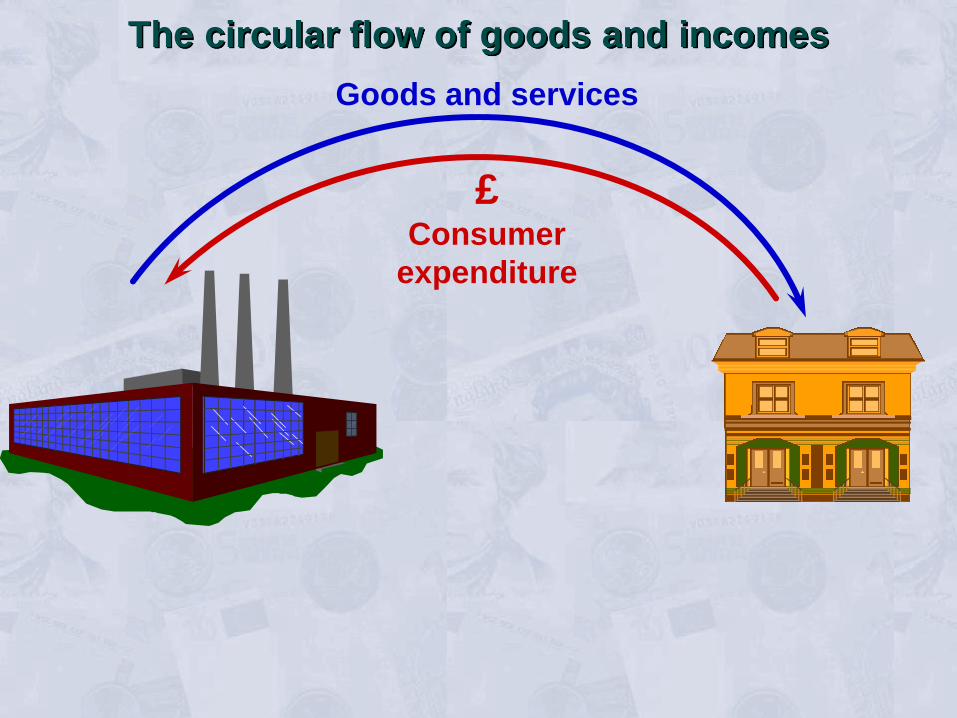
Goods and services
£ Consumer
expenditure
The circular flow of goods and incomes

The Economic Problem
• The circular flow of income
– firms and households
– goods markets
• real flows: goods and services
• money flows: consumer expenditure
– factor markets

The Economic Problem
• The circular flow of income
– firms and households
– goods markets
• real flows: goods and services
• money flows: consumer expenditure
– factor markets
• real flows: services of labour and other factors

Goods and services
£ Consumer
expenditure
The circular flow of goods and incomes

Goods and services
£ Consumer
expenditure
Services of factors of production (labour, etc)
The circular flow of goods and incomes

The Economic Problem
• The circular flow of income
– firms and households
– goods markets
• real flows: goods and services
• money flows: consumer expenditure
– factor markets
• real flows: services of labour and other factors
• money flows: wages and other incomes

Goods and services
£ Consumer
expenditure
Services of factors of production (labour, etc)
The circular flow of goods and incomes

Goods and services
£ Consumer
expenditure
Wages, rent
dividends, etc.
£
Services of factors of production (labour, etc)
The circular flow of goods and incomes

The Economic Problem
• The circular flow of income (cont.)
– macroeconomic issues
• the size of total flows
– microeconomic issues
• individual markets
• choices within goods and factor markets

UNIT -1 BASICS OF MANAGERIAL ECONOMICS LESSON 4- Relationship between managerial economic, economic, and other subjects After studying this lesson you will be able to distinguish managerial economics with its related subjects. Managerial economic is not something which is related to economics only, but there are other areas also to which managerial economic is related. Other related subjects of managerial economics are:
• Economics • Mathematics • Statistics • Accounting • Operation Research • Computers • Management Before knowing the relationship between managerial economics and other related fields it is customary to divide economics into “positive” and “normative” economics. Economists make a distinction between positive and normative that closely parallels popper’s line of demarcation. Positive economics: It deals with description and explanation of economic behavior,
Economics and Managerial economics. Managerial economics draws on positive economics by utilizing the relevant theories as a basis for prescribing choices. A positive statement is a statement about what is and which contains no indication of approval or disapproval. It’s not like that positive statement is always right, positive statement can be wrong. Positive statement is a statement about what exists. Normative economics: It is concerned with prescription or what ought to be done. In normative economics, it is inevitable that value judgment are made as to what should and what should not be done. Managerial economics is a part of normative economics as its focus is more on prescribing choice and action and less on explaining what has happened. It expresses a judgment about whether a situation is desirable or undesirable. The primary task of Managerial economics is to fit relevant data to this framework of logical analysis so as to reach valid conclusion as a basis for action.

Another branch of economics which is normative like managerial is public policies analysis which is concerned with the problems of managing the government of a country. Economic and managerial economic: Economics contributes a great deal towards the performance of managerial duties and responsibilities. Just as the biology contributes to the medical profession and physics to engineering, economics contributes to the managerial profession. All other qualifications being same, managers with working knowledge of economics can perform their function more efficiently than those without it. What is the basic function of the managers of the business? As you all know that the basic function of the manager of the firm is to achieve the organizational objectives to the maximum possible extent with the limited resources placed at their disposal. Economics contributes a lot to the managerial economics. Mathematics and managerial economics: Mathematics in ME has an important role to play. Businessmen deal primarily with concepts that are essentially quantitative in nature e.g. demand, price, cost, wages etc. The use of mathematical logic I the analysis of economic variable provides not only clarity of concepts but also a logical and systematical framework. Statistics and managerial economics: Statistical tools are a great aid in business decision making. Statistical techniques are used in collecting processing and analyzing business data, testing and validity of economics laws with the real economic phenomenon before they are applied to business analysis. The statistical tools for e.g. theory of probability, forecasting techniques, and regression analysis help the decision makers in predicting the future course of economic events and probable outcome of their business decision. Statistics is important to managerial economics in several ways. ME calls for marshalling of quantitative data and reaching useful measures of appropriate relationship involves in decision making. Let me explain it through an example: In order to base its price decision on demand and cost consideration, a firm should have statistically derived or calculated demand and cost function. Operation research and managerial economics:

It’s an inter-disciplinary solution finding techniques. It combines economics, mathematics, and statistics to build models for solving specific business problems. Linear programming and goal programming are two widely used OR in business decision making. It has influenced ME through its new concepts and model for dealing with risks. Though economic theory has always recognized these factors to decision making in the real world, the frame work for taking them into account in the context of actual problem has been operationalised. The significant relationship between ME and OR can be highlighted with reference to certain important problems of ME which are solved with the help of OR techniques, like allocation problem, competitive problem, waiting line problem, and inventory problem. Management theory and managerial economics: As the definition of management says that it’s an art of getting things done through others. Bet now a day we can define management as doing right things, at the right time, with the help of right people so that organizational goals can be achieved. Management theory helps a lot in making decisions. ME has also been influenced by the developments in the management theory. The central concept in the theory of firm in micro economic is the maximization of profits. ME should take note of changes concepts of managerial principles, concepts, and changing view of enterprises goals. Accounting and managerial economics: There exits a very close link between ME and the concepts and practices of accounting. Accounting data and statement constitute the language of business. Gone are the days when accounting was treated as just bookkeeping. Now its far more behind bookkeeping. Cost and revenue information and their classification are influenced considerably by the accounting profession. As a student of MBA you should be familiar with generation, interpretation, and use of accounting data. The focus of accounting within the enterprise is fast changing from the concept of bookkeeping to that of managerial decision making. Mathematic is closely related to ME. Certain mathematical tools such as logarithm and exponential, vectors, determinants and matrix algebra and calculus etc. Computers and managerial economics: You all know that today’s age is known as computer age. Everyone of us are totally dependent on computers. This computers have effected eachone of us in every field. Managers also have to depend on computers for decision making. Computer helps a lot in decision making. Through computers data are presented in such a nice manner that its really very easy to take decisions. There are so many sites which help us in giving knowledge of various things, and in a way helps us in updating our knowledge.

Conclusions: Managerial Economics is closely related to various subjects i.e. Economics, mathematics, statistics, accountings. Computers etc. a trained managerial economist integrates concepts and methods from all these subjects bringing them to bear on business problem of a firm. In particular all these subjects are getting closed to Managerial Economics and there appears to be trends towards their integration.

UNIT 1 SCOPE OF MANAGERIAL Microbes
ECONOMICS
Objectives
After studying this unit, you should be able to:
.. understand the nature and scope of managerial economics;
.. familiarize yourself with economic terminology;
.. develop some insight into economic issues;
.. acquire some information about economic institutions;
.. understand the concept of trade-offs or policy options facing society today.
Structure
1.1 Introduction
1.2 Fundamental Nature of Managerial Economics
1.3 Scope of Managerial Economics
1.4 Appropriate Definitions
1.5 Managerial Economics and other Disciplines
1.6 Economic Analysis
1.7 Basic Characteristics: Decision-Making
1.8 Summary
1.9 Self-Assessment Questions
1.10 Further Readings
1.1 INTRODUCTION
For most purposes economics can be divided into two broad categories,
microeconomics and macroeconomics. Macroeconomics as the name suggests is
the study of the overall economy and its aggregates such as Gross National
Product, Inflation, Unemployment, Exports, Imports, Taxation Policy etc.
Macroeconomics addresses questions about changes in investment, government
spending, employment, prices, exchange rate of the rupee and so on. Importantly,
only aggregate levels of these variables are considered in the study of
macroeconomics. But hidden in the aggregate data are changes in output of a
number of individual firms, the consumption decision of consumers like you, and the
changes in the prices of particular goods and services.
Although macroeconomic issues are important and occupy the time of media and
command the attention of the newspapers, micro aspects of the economy are also
important and often are of more direct application to the day to day problems facing
a manager. Microeconomics deals with individual actors in the economy such as
firms and individuals. Managerial economics can be thought of as applied
microeconomics and its focus is on the interaction of firms and individuals in
markets.
When you read a newspaper or switch on a television, you hear economic
terminology used with increasing regularity. For a manager, some of these
economic terms are of direct relevance and therefore it is essential to not only
understand them but also apply them in relevant situations. For example, GDP
growth rate could impact the product a manager is marketing, change in money
Introduction to Managerial
Economics
supply by the RBI could impact inflation and affect the demand for your product,

fiscal deficit could affect interest rates and therefore investment spending by a
manager etc. The focus of managerial economics is on how the firm reacts to
changes in the economic environment in which it operates and how it predicts these
changes and devises the best possible strategies to achieve the objectives that
underlie its existence.
The economy is the institutional structure through which individuals and firms in a
society coordinate their desires. Economics is the study of how human beings in a
society go about achieving their wants and desires. It is also defined as the study of
allocation of scarce resources to satisfy individual wants or desires. The latter is
perhaps the best way to broadly define the study of economics in general. The
emphasis is on allocation of scarce resources across competing ends. You should
recognize that human wants are unlimited and therefore choice is necessary.
Choices necessarily involve trade-offs. For example, if you wish to acquire an
MBA degree, you must take time off to devote to study. Your time has many uses
and when you devote more time to study you are allocating it to a particular use in
order to achieve your goal. Economics would be a most uninteresting subject if
resources were unlimited and no trade offs were involved in decision making.
There are many general insights economists have gained into how the economy
functions. Economic theory ties together economists’ terminology and knowledge
about economic institutions. An economic institution is a physical or mental
structure that significantly influences economic decisions. Corporations,
governments, markets are all economic institutions. Similarly cultural norms are the
standards people use when they determine whether a particular activity or
behaviour is acceptable. For example, Hindus avoid meat and fish on Tuesdays.
This has an economic dimension as it has a direct impact on the sale of these items
on Tuesdays. Further, economic policy is the action usually taken by the
government, to influence economic events. And finally, economic reasoning helps in
thinking like an economist. Economists analyse questions and issues on the basis of
trade-offs i.e. they compare the cost and the benefits of every issue and make
decisions based on those costs and benefits.
The market is perhaps the single most important and complex institution in our
economy. A market is not necessarily a physical location, but a description of any
state that involves exchange. The exchange could be instantaneous or it could be
over time i.e. exchange which is agreed today but where the transaction takes
place, say after 3 months. You will learn in this course the myriad functions that
markets perform, most significantly bringing buyers and sellers together. Markets
could be competitive or monopolistic, with a large number of firms or a small
number of firms, with free entry and exit or government licensing restricting entry
of firms and so on. The major point is that firms operate in different types of
markets and use the well-established principles of managerial economics to improve
profitability. Managerial economics draws on economic analysis for such concepts
as cost, demand, profit and competition. It attempts to bridge the gap between the
purely analytical problems that intrigue many economic theorists and the day-to-day
decisions that managers must face. It offers powerful tools and approaches for
managerial policy-making. It will be relevant to present here several examples
illustrating the problems that managerial economics can help to address. These also

explain how managerial economics is an integral part of business. Demand, supply,
cost, production, market, competition, price etc. are important concepts in real
business decisions.
7
1.2 FUNDAMENTAL NATURE OF MANAGERIAL
ECONOMICS
A close relationship between management and economics has led to the
development of managerial economics. Management is the guidance, leadership
and control of the efforts of a group of people towards some common objective.
While this description does inform about the purpose or function of management, it
tells us little about the nature of the management process. Koontz and O’Donell
define management as the creation and maintenance of an internal environment in
an enterprise where individuals, working together in groups, can perform efficiently
and effectively towards the attainment of group goals. Thus, management is –
.. Coordination
.. An activity or an ongoing process
.. A purposive process
.. An art of getting things done by other people.
On the other hand, economics as stated above is engaged in analysing and providing
answers to manifestations of the most fundamental problem of scarcity. Scarcity of
resources results from two fundamental facts of life:
.. Human wants are virtually unlimited and insatiable, and
.. Economic resources to satisfy these human demands are limited.
Thus, we cannot have everything we want; we must make choices broadly in
regard to the following:
.. What to produce?
.. How to produce? and
.. For whom to produce?
These three choice problems have become the three central issues of an economy
as shown in figure 1.1. Economics has developed several concepts and analytical
tools to deal with the question of allocation of scarce resources among competing
ends. The non-trivial problem that needs to be addressed is how an economy
through its various institutions solves or answers the three crucial questions posed
above. There are three ways by which this can be achieved. One, entirely by the
market mechanism, two, entirely by the government or finally, and more reasonably,
by a combination of the first two approaches. Realistically all economies employ the
last option, but the relative roles of the market and government vary across
countries. For example, in India the market has started playing a more important
role in the economy while the government has begun to withdraw form certain
activities. Thus, the market mechanism is gaining importance. A similar change is
happening all over the world, including in China. But there are economies such as
Myanmar and Cuba where the government still plays an overwhelming part in
solving the resource allocation problem. Essentially, the market is supposed to guide
resources to their most efficient use. For example if the salaries earned by MBA
degree holders continue to rise, there will be more and more students wanting to
earn the degree and more and more institutes wanting to provide such degrees to

take advantage of this opportunity. The government may not force this to happen, it
will happen on its own through the market mechanism. The government, if anything,
could provide a regulatory function to ensure quality and consumer protection.
According to the central deduction of economic theory, under certain conditions,
markets allocate resources efficiently. ‘Efficiency’ has a special meaning in this
context. The theory says that markets will produce an outcome such that, given the
economy’s scarce resources, it is impossible to make anybody better-off without
making somebody else worse-off.
Scope of Managerial
Economics
Introduction to Managerial
Economics
8
Figure 1.1: Three Choice Problems of an Economy
SCARCIT Y
Unlimited Choice Limited Resources
What do produce? How to produce? For whom to produce?
In rich countries, markets are too familiar to attract attention. Yet, a certain awe is
appropriate. Let us take an incident where Soviet planners visited a vegetable
market in London during the early days of perestroika, they were impressed to find
no queues, shortages, or mountains of spoiled and unwanted vegetables. They took
their hosts aside and said: “We understand, you have to say it’s all done by supply
and demand. But can’t you tell us what’s really going on? Where are your planners
and what are their methods?”
The essence of the market mechanism is indeed captured by the supply-anddemand
diagram that you will become familiar with in Block 4. At the place where
the curves intersect, a price is set such that demand equals supply. There, and only
there, the benefit from consuming one more unit exactly matches the cost of
producing it. If output were less, the benefit from consuming more would exceed
the cost of producing it. If output were higher, the cost of producing the extra units
would exceed the extra benefits. So the point where supply equals demand is
“efficient”.
However, the conditions for market efficiency are extremely demanding—far too
demanding ever to be met in the real world. The theory requires “perfect
competition”: there must be many buyers and sellers; goods from competing
suppliers must be indistinguishable; buyers and sellers must be fully informed; and
markets must be complete—that is, there must be markets not just for bread here
and now, but for bread in any state of the world. (What is the price today for a loaf
to be delivered in Timbuktu on the second Tuesday in December 2014 if it rains?)
In other words, market failure is pervasive. It comes in four main varieties:
Monopoly: By reducing his sales, a monopolist can drive up the price of his good.
His sales will fall but his profits will rise. Consumption and production are less than
the efficient amount, causing a deadweight loss in welfare.
Public goods: Some goods cannot be supplied by markets. If you refuse to pay for
a new coat, the seller will refuse to supply you. If you refuse to pay for national
defence, the “good” cannot easily be withheld. You might be tempted to let others

pay. The same reasoning applies to other “non-excludable” goods such as law and
order, clean air, and so on. Since private sellers cannot expect to recover the costs
of producing such goods, they will fail to supply them.
Externalities: Making some goods causes pollution: the cost is borne by people
with no say in deciding how much to produce. Consuming some goods (education,
anti-lock brakes) spreads benefits beyond the buyer; again, this will be ignored
What to produce ?
9
when the market decides how much to produce. In the case of “good” externalities,
markets will supply too little; in the case of “bads”, too much.
Information: In some ways a special kind of externality, this deserves to be
mentioned separately because of the emphasis placed upon it in recent economic
theory. To see why information matters, consider the market for used cars. A
buyer, lacking reliable information, may see the price as providing clues about a
car’s condition. This puts sellers in a quandary: if they cut prices, they may only
convince people that their cars are rubbish.
The labour market, many economists believe, is another such ‘market for lemons’.
This may help to explain why it is so difficult for the unemployed to price
themselves into work.
When markets fail, there is a case for intervention. But two questions need to be
answered first. How much does market failure matter in practice? And can
governments put the failure right? Markets often correct their own failures. In other
cases, an apparent failure does nobody any harm. In general, market failure matters
less in practice than is often supposed.
Monopoly, for instance, may seem to preclude an efficient market. This is wrong.
The mere fact of monopoly does not establish that any economic harm is being
done. If a monopoly is protected from would-be competitors by high barriers to
entry, it can raise its prices and earn excessive profits. If that happens, the
monopoly is undeniably harmful. But if barriers to entry are low, lack of actual (as
opposed to potential) competitors does not prove that the monopoly is damaging: the
threat of competition may be enough to make it behave as though it were a
competitive firm. Many economists would accept that Microsoft, for instance, is a
near-monopolist in some parts of the personal-computer software business–yet
would argue that the firm is doing no harm to consumers because its markets
remain highly contestable. Because of that persistent threat of competition, the
company prices its products keenly. In this and in other ways it behaves as though it
were a smaller firm in a competitive market.
Even on economic grounds (never mind other considerations), there is no tidy
answer to the question of where the boundary between state i.e. governments and
market should lie. Markets do fail because of monopoly, public goods, externalities,
lack of information and for other reasons. But, more than critics allow, markets find
ways to mitigate the harm–and that is a task at which governments have often been
strikingly unsuccessful. All in all, a strong presumption in favour of markets seems
wise. This is not because classical economic theory says so, but because
experience seems to agree. And as stated above, the real world seems to be
moving in the direction of placing more reliance on markets than on governments.

1.3 SCOPE OF MANAGERIAL ECONOMICS
From the point of view of a firm, managerial economics, may be defined as
economics applied to “problems of choice” or alternatives and allocation of scarce
resources by the firms. Thus managerial economics is the study of allocation of
resources available to a firm or a unit of management among the activities of that
unit. Managerial economics is concerned with the application of economic concepts
and analysis to the problem of formulating rational managerial decisions. There are
four groups of problem in both decisions-making and forward planning.
Resource Allocation: Scare resources have to be used with utmost efficiency to
get optimal results. These include production programming and problem of
transportation etc. How does resource allocation take place within a firm?
Scope of Managerial
Economics
Introduction to Managerial
Economics
10
Naturally, a manager decides how to allocate resources to their respective uses
within the firm, while as stated above, the resource allocation decision outside the
firm is primarily done through the market. Thus, one important insight you can draw
about the firm is that within it resources are guided by the manager in a manner
that achieves the objectives of the firm. More will be said about this in Unit 2.
Inventory and queuing problem: Inventory problems involve decisions about
holding of optimal levels of stocks of raw materials and finished goods over a
period. These decisions are taken by considering demand and supply conditions.
Queuing problems involve decisions about installation of additional machines or
hiring of extra labour in order to balance the business lost by not undertaking these
activities.
Pricing Problem: Fixing prices for the products of the firm is an important
decision-making process. Pricing problems involve decisions regarding various
methods of prices to be adopted.
Investment Problem: Forward planning involves investment problems. These are
problems of allocating scarce resources over time. For example, investing in new
plants, how much to invest, sources of funds, etc.
Study of managerial economics essentially involves the analysis of certain major
subjects like:
.. The business firm and its objectives
.. Demand analysis, estimation and forecasting
.. Production and Cost analysis
.. Pricing theory and policies
.. Profit analysis with special reference to break-even point
.. Capital budgeting for investment decisions
.. Competition.
Demand analysis and forecasting help a manager in the earliest stage in choosing
the product and in planning output levels. A study of demand elasticity goes a long
way in helping the firm to fix prices for its products. The theory of cost also forms
an essential part of this subject. Estimation is necessary for making output

variations with fixed plants or for the purpose of new investments in the same line
of production or in a different venture. The firm works for profits and optimal or
near maximum profits depend upon accurate price decisions. Theories regarding
price determination under various market conditions enable the firm to solve the
price fixation problems. Control of costs, proper pricing policies, break-even
analysis, alternative profit policies are some of the important techniques in profit
planning for the firm which has to work under conditions of uncertainty. Thus
managerial economics tries to find out which course is likely to be the best for the
firm under a given set of conditions.
1.4 APPROPRIATE DEFINITIONS
According to McNair and Meriam, “Managerial economics is the use of economic
modes of thought to analyse business situations.” According to Prof. Evan J
Douglas, ‘Managerial economics’ is concerned with the application of economic
principles and methodologies to the decision making process within the firm or
organisation under the conditions of uncertainty”. Spencer and Siegelman define it
as “The integration of economic theory with business practices for the purpose of
facilitating decision making and forward planning by management.” According to
11
Hailstones and Rothwel, “Managerial economics is the application of economic
theory and analysis to practice of business firms and other institutions.” A common
thread runs through all these descriptions of managerial economics which is using a
framework of analysis to arrive at informed decisions to maximize the firm’s
objectives, often in an environment of uncertainty. It is important to recognize that
decisions taken while employing a framework of analysis are likely to be more
successful than decisions that are knee jerk or gut feel decisions.
Activity 1
a) Development of managerial economics is the result of close interrelationship
between management and economics. Discuss.
......................................................................................................................
......................................................................................................................
......................................................................................................................
......................................................................................................................
b) Which statement is true of the basic economic problem?
(i) The problem will exist as long as resources are limited and desires are
unlimited.
(ii) The problem exists only in less developed countries.
(iii) The problem will disappear as production expands.
(iv) The advancement of technology will cause the problem to disappear.
c) Why is decision making by any management truly economic in nature?
......................................................................................................................
......................................................................................................................
......................................................................................................................
......................................................................................................................
1.5 MANAGERIAL ECONOMICS AND OTHER
DISCIPLINES
Managerial economics is linked with various other fields of study like–

Microeconomic Theory: As stated in the introduction, the roots of managerial
economics spring from micro-economic theory. Price theory, demand concepts and
theories of market structure are few elements of micro economics used by
managerial economists. It has an applied bias as it applies economic theories in
order to solve real world problems of enterprises.
Macroeconomic Theory: This field has little relevance for managerial economics
but at least one part of it is incorporated in managerial economics i.e. national
income forecasting. The latter could be an important aid to business condition
analysis, which in turn could be a valuable input for forecasting the demand for
specific product groups.
Operations Research: This field is used in managerial economics to find out the
best of all possibilities. Linear programming is a great aid in decision making in
business and industry as it can help in solving problems like determination of
facilities on machine scheduling, distribution of commodities and optimum product
mix etc.
Scope of Managerial
Economics
Introduction to Managerial
Economics
12
Theory of Decision Making: Decision theory has been developed to deal with
problems of choice or decision making under uncertainty, where the applicability of
figures required for the utility calculus are not available. Economic theory is based on
assumptions of a single goal whereas decision theory breaks new grounds by
recognizing multiplicity of goals and persuasiveness of uncertainty in the real world
of management.
Statistics: Statistics helps in empirical testing of theory. With its help, better
decisions relating to demand and cost functions, production, sales or distribution are
taken. Managerial economics is heavily dependent on statistical methods.
Management Theory and Accounting: Maximisation of profit has been
regarded as a central concept in the theory of the firm in microeconomics. In
recent years, organisation theorists have talked about “satisficing” instead of
“maximising” as an objective of the enterprise. Accounting data and statements
constitute the language of business. In fact the link is so close that “managerial
accounting” has developed as a separate and specialized field in itself.
1.6 ECONOMIC ANALYSIS
Economic activity is the constant effort to match ends to means because of
scarcity of resources. The optimal economic activity is to maximise the attainment
of ends, the means and their scarcities or to minimise the use of resources, given
the ends and their priorities.
Decision making by management is truly economic in nature because it involves
choices among a set of alternatives - alternative courses of action. The optimal
decision making is an act of optimal economic choice, considering objectives and
constraints. This justifies an evaluation of managerial decisions through concepts,
precepts, tools and techniques of economic analysis of the following types:
Micro and Macro Analysis: In micro-analysis the problem of choice is focused

on single individual entities like a consumer, a producer, a market etc. Macro
analysis deals with the problem in totality like national income, general price level
etc.
Partial and General Equilibrium Analysis: To attain the state of stable
equilibrium, the economic problem may be analysed part by part - one at a time -
assuming “other things remaining the same.” This is partial equilibrium analysis. In
general equilibrium analysis the assumption of “given” or “other things remaining
equal” may be relaxed and interdependence or interactions among variables may
be allowed.
Static, Comparative Static and Dynamic Analysis: This is in reference to time
dimension. A problem may be analysed
- allowing no change at a point of time (static)
- allowing once for all change at a point of time (comparative static)
- allowing successive changes over a period of time (dynamic).
Positive and Normative Analysis: In positive economic analysis, the problem is
analyzed in objective terms based on principles and theories. In normative
economic analysis, the problem is analyzed based on value judgement (norms). In
simple terms, positive analysis is ‘what it is’ and normative analysis is ‘what it
should be.’ For example, CEOs in private Indian enterprises earn 15 times as much
as the lowest paid employee is a positive statement, a description of what is. A
normative statement would be that CEOs should be paid 4-5 times the lowest paid
employee.
13
Activity 2
a) The major groups of problems in decision making are:
(i)
(ii)
(iii)
(iv)
b) The 3 choice problems of an economy are:
(i)
(ii)
(iii)
The problems arise due to................................................................................
c) Name the kind of economic analysis that is appropriate for each of the following:
(i) The ONGC has expansion plans ...............................................................
(ii) The NTC is making loss ..........................................................................
(iii) The textile industry is facing recession ......................................................
(iv) The population growth in India is alarming .................................................
(v) There is a bearish trend in the stock market ..............................................
1.7 BASIC CHARACTERISTICS: DECISION-MAKING
Managerial Economics serves as ‘a link between traditional economics and the
decision making sciences’ for business decision making.
The best way to get acquainted with managerial economics and decision making is
to come face to face with real world decision problems.
Tata’s Vision 2000

Presently there are about 87 firms in the Tata empire. As many as 16 recorded
losses in 1995-96. The Tata’s companies that are in the limelight are TISCO,
TELCO, ACC, Tata Exports and Tata Chemicals.
Contribution of bottom – In terms of turnover : 35% of total of group.
20 companies – In terms of net profit : 0.2% of total sales of group.
– In terms of assets & net worth <1% of total sales of
group.
The question is – Do such non-performers warrant an existence or
will the group be better off if it could hive off the
divisions, or else amalgamate them with other
existing units.
On the three basic – Last two companies are way below the group as a
indications whole; providing 4.2% return on shareholders;
1.9% return on capital employed.
Keeping these figures in mind, Tata’s planned refocusing exercises like
.. Divestment - mergers
.. Amalgamations - takeovers.
.. To create a learner and suggestive group with an estimated turn- over of
Rs. 1,10,000 crore by 2000.
Scope of Managerial
Economics
Introduction to Managerial
Economics
14
.. From being production-led to being consumer and market-led; being up in top
three in every segment.
Tata’s “Vision 2000” is a group. Why not give someone else a chance to run your
business more efficiently if you cannot do so? It makes better economic as well as
business sense. But then, the ball is in the court of Tata’s. The What and How to
do is their prerogative.
The basic characteristics of managerial economics can now be enumerated as:
.. It is concerned with “decision making of an economic nature.”
.. It is “micro-economic” in character.
.. It largely uses that body of economic concepts and principles, which is known
as “theory of the firm.”
.. It is “goal oriented and prescriptive”
.. Managerial economics is both “conceptual and metrical”. It includes theory with
measurement.
Figure 1.2: Decision-Making
Managerial economics should be thought of as applied microeconomics, which
focuses on the behavior of the individual actors on the economic stage; firms and
individuals.
Figure 1.3: Basic Characteristics
Management Decision Problems
Economic Theory
Microeconomics

Macroeconomics
Decision Science
Mathematical Economics
Managerial Economics
Application of economic theory &
decision tools to solve
managerial decision problems
Optimal Solution to Managerial
Decision Problems
Decision-
Problem
Traditional
Economics
Managerial
Economics
Decision Sciences
(Tools and Techniques
of Analysis)
Optimal Solution
to Business
Problems
15
1.8 SUMMARY
Managerial economics is used by firms to improve their profitability. It is the
economics applied to problems of choices and allocation of scarce resources by the
firms. It refers to the application of economic theory and the tools of analysis of
decision science to examine how an organisation can achieve its objective most
efficiently. Managerial decisions are evaluated through concepts, tools and
techniques of economic analysis of various types. It is linked with various fields of
study.
1.9 SELF-ASSESSMENT QUESTIONS
1. Discuss the nature and scope of managerial economics.
2. “Managerial economics is the integration of economic theory with business
practice for the purpose of facilitating decision-making and forward planning by
manager”. Explain and comment.
3. Define scarcity and opportunity cost. What role do these two concepts play in
the making of management decisions?
4. Managerial economics is often said to help the business student integrate the
knowledge gained in other courses. How is this integration accomplished?
5. Compare and contrast microeconomics with macroeconomics. Although
managerial economics is based primarily on microeconomics, explain why it is
also important for managers to understand macroeconomics.
6. Justify that managerial economics is economics applied in decision-making.
7. What is the role of managerial economics in preparing managers?
8. How is managerial economics related to different disciplines?
1.10 FURTHER READINGS

Haynes, W.W., Managerial Economics: Analysis and Cases, Business
Publications, Inc., Texas, Ch. 1.
Adhikary, M., Managerial Economics, Khosla Publishers: Delhi, Ch. 1.
Baumol, William, J., Economic Theory and Operations Analysis, Prentice-Hall of
India Pvt. Ltd., New Delhi.
Scope of Managerial

The Law of Demand and the Demand Curve
We begin with demand because demand is usually easier to understand from our personal
experiences. We are all consumers and we all demand goods and services. Demand is derived from
consumers' tastes and preferences, and it is bound by income. In other words, given a limited
income (whether it be $30,000 or $5 million), the consumer must decide what goods and services to
purchase. Within his budget, the consumer will purchase those goods and services that he likes best.
Each consumer will purchase different things because
individual preferences and incomes differ.
The law of demand holds that other things equal, as
the price of a good or service rises, its quantity
demanded falls. The reverse is also true: as the price
of a good or service falls, its quantity demanded
increases. This law is a simple, common sense
principle. Think of your trips to the grocery store.
When the price of orange juice rises, for example, you
buy less of it. When that item is on sale, you purchase
more of it. This is all that we mean by the law of
demand.
Table 1 lists the monthly quantity of rental videos demanded by
an individual given several different prices. If the rental price is
$5, the consumer rents 10 videos per month. If the price falls to
$4, the quantity demanded increases to 20 videos, and so on. The
figure titled "Demand Curve" plots the inverse relationship
between price and quantity demanded.
A demand curve is a graphical depiction of the law of demand. We plot price on the vertical
axis and quantity demanded on the horizontal axis. As the figure illustrates, the demand curve
has a negative slope, consistent with the law of demand.
TABLE 1
Demand for Videos
Price Quantity Demanded
$5 10
$4 20
$3 30
$2 40
$1 50
The Law of Supply and the Supply Curve

Supply is slightly more difficult to understand because
most of us have little direct experience on the supply
side of the market. Supply is derived from a producer's
desire to maximize profits. When the price of a product
rises, the supplier has an incentive to increase
production because he can justify higher costs to
produce the product, increasing the potential to earn
larger profits. Profit is the difference between revenues
and costs. If the producer can raise the price and sell the
same number of goods while holding costs constant,
then profits increase.
The law of supply holds that other things equal, as the price of a
good rises, its quantity supplied will rise, and vice versa. Table 2
lists the quantity supplied of rental videos for various prices. At $5,
the producer has an incentive to supply 50 videos. If the price falls
to $4 quantity supplied falls to 40, and so on. The figure titled
"Supply Curve" plots this positive relationship between price and
quantity supplied.
A supply curve is a graphical depiction of a supply schedule plotting price on the vertical axis
and quantity supplied on the horizontal axis. The supply curve is upward-sloping, reflecting
the law of supply.
TABLE 2
Supply of Videos
Price Quantity Supplied
$5 50
$4 40
$3 30
$2 20
$1 10
Equilibrium: Determination of Price and Quantity
What price should the seller set and how many videos will be rented per month? The seller could
legally set any price she wished; however, market forces penalize her for making poor choices.

Suppose, for example, that the seller prices each video at $20. Odds are good that few videos will be
rented. On the other hand, the seller may set a price of $1 per video. Consumers will certainly rent
more videos with this low price, so much so that the store is likely to run out of videos. Through trial
and error or good judgement, the store owner will eventually settle on a price that equates the
forces of supply and demand.
In economics, an equilibrium is a situation in which:
there is no inherent tendency to change, quantity demanded equals quantity supplied, and the market just clears.
At the market equilibrium, every consumer who wishes to purchase the product at the market price
is able to do so, and the supplier is not left with any unwanted inventory. As Table 3 and the figure
titled "Equilibrium" demonstrate, equilibrium in the video example occurs at a price of $3 and a
quantity of 30 videos.
TABLE 3
Video Market Equilibrium
Price Quantity
Demanded
Quantity
Supplied
$5 10 50
$4 20 40
$3 30 30
$2 40 20
$1 50 10

Suppose that the video store owner charges $2 per video rental. The result is a shortage. A
shortage occurs when quantity demanded exceeds quantity supplied. At a price of $2,
quantity supplied is 20 videos but quantity demanded is 40 videos. Some consumers who
wish to rent videos are unable to do so. A shortage implies the market price is too low.
Shortages are common in socialist economies because low prices for common staples such as
food and energy are set by the government. Rather than pay higher prices, people are forced
to wait in long lines to purchase the desired goods and services.
A surplus occurs when quantity supplied exceeds quantity demanded. With a rental price of
$4, quantity supplied is 40 videos but quantity demanded is only 20 videos. A surplus of 20
videos exists. A surplus implies the market price is too high.
Perhaps more often than not, markets are not exactly in equilibrium. Minor surpluses and
shortages are common in a market economy. A stroll through most malls at the end of the
clothing season reveals the excess clothing inventory that many stores carry. How do they
manage this situation? By lowering prices. Lower prices reduce the incentive for stores to
carry the clothes while simultaneously increasing the incentive for consumers to purchase the
clothes. The important point is that even though a market may not be in perfect equilibrium, it
tends to gravitate towards equilibrium over time. This fact makes markets stable most of the
time such that persistent surpluses and shortages are uncommon and self-correcting.
Persistent and severe shortages and surpluses do occur in the U.S. economy every now and
then. At the end of 1998, for example, the supply of hogs in the U.S. markets was so much
greater than demand that the price of hogs fell from about $50 per hundredweight to $13 per
hundredweight. Many farmers were so badly hurt by that experience that they left the hog
market completely--a painful but self-correcting force. In the late 1970s the relative shortage
of gasoline resulted in long lines at the gas pumps. The shortages lasted for a couple years
until oil producers stepped up production and consumers learned to use fuel more efficiently.
A Shift versus a Movement Along a Demand
Curve
It is essential to distinguish between a movement
along a demand curve and a shift in the demand
curve. A change in price results in a movement along
a fixed demand curve. This is also referred to as a
change in quantity demanded. For example, an
increase in video rental prices from $3 to $4 reduces
quantity demanded from 30 units to 20 units. This
price change results in a movement along a given
demand curve. A change in any other variable that
influences quantity demanded produces a shift in the demand curve or a change in demand.
The terminology is subtle but extremely important. The majority of the confusion that
students have with supply and demand concepts involves understanding the differences
between shifts and movements along curves.

Suppose that incomes in a community rise
because a factory is able to give employees
overtime pay. The higher incomes prompt
people to rent more videos. For the same rental
price, quantity demanded is now higher than
before. Table 4 and the figure titled "Shift in
the Demand Curve" represent that scenario. As
incomes rise, the quantity demanded for videos
priced at $4 goes from 20 (point A) to 40
(point A'). Similarly, the quantity demanded
for videos priced at $3 rises from 30 to 50. The
entire demand curve shifts to the right.
A shift in the demand curve changes the equilibrium position. As illustrated in the figure
titled "Equilibrium After a Demand Curve Shift" the shift in the demand curve moves the
market equilibrium from point A to point B, resulting in a higher price (from $3 to $4) and
higher quantity (from 30 to 40 units). Note that if the demand curve shifted to the left, both
the equilibrium price and quantity would decline.
TABLE 4
Change in Demand for
Videos after Incomes Rise
Price Initial Quantity
Demanded
New Quantity
Demanded
Quantity
Supplied
$5 10 30 50
$4 20 40 40
$3 30 50 30
$2 40 60 20
$1 50 70 10
Factors that Shift the Demand Curve
We list and explain four factors that can shift a demand curve:
1. Change in consumer incomes: As the previous video rental example demonstrated, an increase in income shifts the demand curve to the right. Because a consumer's demand for goods and services is constrained by income, higher income levels relax somewhat that constraint, allowing the consumer to purchase more products. Correspondingly, a decrease in income shifts the demand curve to the left. When the economy enters a recession and more people become unemployed, the demand for many goods and services shifts to the left.
2. Population change: An increase in population shifts the demand curve to the right. Imagine a college town bookstore in which most students return home for the summer. Demand for books shifts to the left while the students are away. When they return, however, demand for books increases even if the prices are unchanged. As another example, many communities are experiencing "urban sprawl" where the metropolitan boundaries are pushed ever wider by new housing developments. Demand for gasoline in these new communities increases with population. Alternatively, demand for gasoline falls in areas with declining populations.

3. Consumer preferences: If the preference for a particular good increases, the demand curve for that good shifts to the right. Fads provide excellent examples of changing consumer preferences. Each Christmas season some new toy catches the fancy of kids, and parents scramble to purchase the product before it is sold out. A few years ago, "Tickle Me Elmo" dolls were the rage. In the year 2000 the toy of choice was a scooter. For a given price of a scooter, the demand curve shifts to the right as more consumers decide that they wish to purchase that product for their children. Of course, demand curves can shift leftward just as quickly. When fads end suppliers often find themselves with a glut of merchandise that they discount heavily to sell.
4. Prices of related goods: If prices of related goods change, the demand curve for the original good can change as well. Related goods can either be substitutes or complements.
o Substitutes are goods that can be consumed in place of one another. If the price of a substitute increases, the demand curve for the original good shifts to the right. For example, if the price of Pepsi rises, the demand curve for Coke shifts to the right. Conversely, if the price of a substitute decreases, the demand curve for the original good shifts to the left. Given that chicken and fish are substitutes, if the price of fish falls, the demand curve for chicken shifts to the left.
o Complements are goods that are normally consumed together. Hamburgers and french fries are complements. If the price of a complement increases, the demand curve for the original good shifts to the left. For example, if McDonalds raises the price of its Big Mac, the demand for french fries shifts to the left because fewer people walk in the door to buy the Big Mac. In contrast, If the price of a complement decreases, the demand curve for the original good shifts to the right. If, for example, the price of computers falls, then the demand curve for computer software shifts to the right.
A Shift versus a Movement Along a Supply
Curve
As with demand curves, it is essential to distinguish
between a movement along a given supply curve
and a shift in a supply curve. A change in price
results in a movement along a fixed supply curve.
This is also referred to as a change in quantity
supplied. For example, if the rental price of videos
rises from $3 to $4, quantity supplied increases
from 30 to 40 units. A change in any other variable
that influences quantity supplied produces a shift in
the supply curve or a change in supply.
TABLE 5
Change in Supply due to an

Suppose for example that the video store
purchases its videos from Hollywood Inc.
but Hollywood Inc. just increased its prices.
Now the video rental store has to pay more
to purchase the videos that it makes available
to customers. For a given rental price of
videos, the video store has to reduce the
quantity of videos it supplies. For the same
price, quantity supplied will be lower than
before. Table 5 and the figure titled "Shift in
the Supply Curve" show this scenario.
Initially at a price of $4, quantity supplied
was 40 (point A). After the leftward shift of
the supply curve, at the same price of $4,
quantity supplied is only 20 units (point A').
Equilibrium price and quantity change after a shift in the supply curve. The figure titled
"Equilibrium After a Supply Curve Shift" plots the new equilibrium after the leftward shift of
the supply curve. The equilibrium moves from point A to point B, resulting in a higher price
(from $3 to $4) and lower quantity (from 30 to 20). Conversely, a rightward shift of the
supply curve reduces the equilibrium price and increases the equilibrium quantity.
Increase in Video Costs
Price Quantity
Demanded
Initial Quantity
Supplied
New Quantity
Supplied
$5 10 50 30
$4 20 40 20
$3 30 30 10
$2 40 20 0
$1 50 10 0
Factors that Shift the Supply Curve
We list and explain three factors that shift a supply curve:
1. Change in input costs: An increase in input costs shifts the supply curve to the left. A supplier combines raw materials, capital, and labor to produce the output. If a furniture maker has to pay more for lumber, then her profits decline, all else equal. The less attractive profit opportunities force the producer to cut output. Alternatively, car manufacturer may have to pay higher labor costs. The higher labor input costs reduces profits, all else equal. For a given price of a car, the manufacturer may trim output, shifting the supply curve to the left. Conversely, if input costs decline, firms respond by increasing output. The furniture manufacturer may increase production if lumber costs fall. Additionally, chicken farmers may boost chicken output if feed costs decline. The reduction in feed costs shifts the supply curve for chicken to the right.
2. Increase in technology: An increase in technology shifts the supply curve to the right. A narrow definition of technology is a cost-reducing innovation. Technological progress allows firms to produce a given item at a lower cost. Computer prices, for example, have declined radically as technology has improved, lowering their cost of production. Advances in communications technology have lowered the telecommunications costs over time. With the advancement of technology, the supply curve for goods and services shifts to the right.

3. Change in size of the industry: If the size of an industry grows, the supply curve shifts to the right. In short, as more firms enter a given industry, output increases even as the price remains steady. The fast-food industry, for example, exploded in the latter half of the twentieth century as more and more fast food chains entered the market. Additionally, on-line stock trading has increased as more firms have begun delivering that service. Conversely, the supply curve shifts to the left as the size of an industry shrinks. For example, the supply of manual typewriters declined dramatically in the 1990s as the number of producers dwindled.
Government Regulation of the Market: Price Ceilings and Floors
Sometimes the market equilibrium outcome is perceived by certain groups or individuals to be unfair
or unjust. Societal values may dictate that the market
outcome be altered. Government can intervene in
markets in any number of ways, including the banning of
the production and consumption of certain goods and
services entirely. Government can also regulate heavily
industries such as banking that it deems too sensitive to
be left alone. We focus on two methods of government
intervention: price ceilings and price floors.
A price ceiling is a legal maximum that can be charged for a good. The ceiling is shown by a
horizontal line at the ceiling price which--to be effective--is set below the equilibrium price.
The figure titled "Price Ceiling" illustrates a ceiling at $2. At a price of $2 quantity demanded
is 40 units and quantity supplied is 20 units. The result is a shortage in which quantity
demanded exceeds quantity supplied.
Common examples of markets with price ceilings are apartment rentals and credit cards.
Some municipalities such as Santa Monica, California impose maximum rents that can be
charged for given apartments. For example, a ceiling of $1,000 per month might be set on
two-bedroom apartments. In addition, some states have usury laws where interest rates are
prevented from rising beyond a certain level. Credit card issuers in those states cannot charge
interest rates above the ceiling.
Are these price ceiling justified? It depends. Equity is a subjective concept. Invariably, price
ceilings help some groups and hurt others. For example, caps on apartment rents help tenants
who pay below-market rents but hurt landlords and other prospective tenants who are shut out
of the market due to the shortage. Santa Monica is plagued with buildings that landlords
abandoned because the buildings became unprofitable to operate. Hence, the total supply of
apartments in Santa Monica is lower than it otherwise would be.

Intervention in markets should not be taken lightly
because often serious by-products emerge. With
apartment price ceilings, underground markets often
appear in which landlords and tenants agree to the
"official" contract rate but tenants agree to make
additional side payments. In addition, if landlords
cannot set prices, they begin to adjust the quality of
their apartments, letting them fall into disrepair.
Some tenants end up living in unkempt conditions
and are afraid to report the landlord because they
may find themselves homeless if the landlord quits
renting the apartment.
A price floor is a legal minimum that can be charged for a good. The floor, as shown in the
figure titled "Price Floor," is represented by a horizontal line. To be effective, the floor must
be set above the equilibrium price. In the figure the floor is set at $4. Quantity demanded is
20 units and quantity supplied is 40 units. The result of the floor is a surplus of 20 units.
Common examples of price floors are found in agricultural markets such as sugar, wheat and
milk. The minimum wage is also a price floor because it sets a minimum dollar amount that
employers can pay employees.
As with price ceilings, the same tradeoff occurs between equity and efficiency with price
floors. Some groups benefit while others lose. In the case of the minimum wage, those who
are able to find the higher paying jobs benefit. Employers who must pay higher wages lose
along with those in the labor force who cannot find jobs because wages are too high.
Agricultural price floors benefit farmers at the expense of consumers. Nevertheless, society
has thus far deemed the benefits received from the price floors to be worth the costs.
Paradoxes Resolved
We now have the tools necessary to explain more fully some of the paradoxes presented at the
beginning of the chapter. Why do school teachers earn $30,000 per year while some star athletes
earn $18 million per year? Although differences in demand are important, the salary differentials are
driven primarily by differences in the supply curves of the two markets. The number of excellent
school teachers in the U.S. is quite high. To teach at most grade schools and high schools, one must
attend college and typically earn a degree and an education certificate. Thousands of students take
such a track in life. In contrast, star athletes are extremely rare. Home run hitters in baseball such as
Babe Ruth, Mark McGwire and Barry Bonds only come along so often. Likewise, talented basketball
players such as Michael Jordan and Moses Malone are rare. The incredibly small supply of such
superstars, coupled with a high demand for their services, allows them to command enormous
salaries. Is it fair that teachers are paid such dismal salaries relative to the athletes? Many teachers
may not think so, but again, fairness is a relative concept.
A couple that purchases diamond engagement rings for one another are undoubtedly shocked
by the high prices of diamonds. The same couple can stop at a water fountain and take drinks

of water for free. Married couples can survive without diamond rings--water is essential.
What accounts, then, for the high relative price for diamonds? Supply and demand factors
both play important roles in this example. In most parts of the world, diamonds are in far
shorter supply than drinking water. Consumers also value a diamond more than a glass of
water under normal circumstances. The relatively small supply and the relatively high
demand for diamonds drive their prices high relative to water.
Let's carry this paradox one step further. Suppose that the married couple somehow becomes
stranded in the desert with no water to be found. A man approaches carrying a large jug of
water. He offers to trade the water for the diamond rings. Does the couple make the
exchange. Why or why not?
5.1 The Price Elasticity of Demand
The price elasticity of demand is a measure of the extent to which the quantity demanded
of a good changes when the price of the good changes and all other influences on buyers’
plans remain the same.
A. Percentage Change in Price
1. The midpoint method uses the average of the initial price and new price in the denominator
when calculating a percentage change. Because the average price is the same between
two prices regardless of whether the price falls or rises, the percentage change in price
calculated by the midpoint method is the same for a price rise and a price fall.
a. Using the midpoint formula, the percentage change in price equals
.100×
2÷price Initial + priceNew
price Initial priceNew
B. Percentage Change in Quantity Demanded
Use the midpoint method when calculating the percentage change in quantity.
.100
2quantity Initial quantity New
quantity Initial quantity New
1. Minus Sign
Because a change in price causes an opposite change in quantity demanded, for the price
elasticity of demand we focus on the magnitude of the change by using the absolute value.
C. Elastic and Inelastic Demand
The price elasticity of demand falls into three categories:
1. Elastic demand—when the percentage change in the quantity demanded exceeds the
percentage change in price (which means the elasticity is greater than 1).
2. Unit elastic demand—when the percentage change in the quantity demanded equals the
percentage change in price (which means the elasticity equals 1).
3. Inelastic demand—when the percentage change in the quantity demanded is less than
the percentage change in price (which means the elasticity is less than 1).
4. There are two extreme cases:
a. Perfectly elastic demand—when the quantity demanded changes by a very large
percentage in response to an almost zero percentage change in price.
b. Perfectly inelastic demand—when the quantity demanded remains constant as the
price changes.
D. Influences on the Price Elasticity of Demand
1. Substitution Effect

If good substitutes are readily available, demand is elastic. If good substitutes are hard to
find, demand is inelastic.
2. Three factors determine how easy substitutes are to find:
a. Luxury versus necessity—there are few substitutes for necessities (so demand is price
inelastic) and there are many substitutes for luxuries (so demand is price elastic).
b. Narrowness of definition—the more narrowly defined the good is, the more elastic its
demand. The more broadly defined the good, the less elastic its demand.
c. Time elapsed since price change—the longer the time that has passed since the price
change, the more elastic is demand.
3. Income Effects
The larger the proportion of income spent on the good, the more elastic is demand
because a price change has a large, noticeable impact on the budget. The smaller the
proportion of income spent on the good, the less elastic is demand.
E. Computing the Price Elasticity of Demand
1. The formula used to calculate the price elasticity of demand is:
. price in change Percentage
demandedquantity in change Percentage =demand of elasticity Price
a. If the price elasticity of demand is greater than 1 (the numerator is larger than the
denominator), demand is elastic.
b. If the price elasticity of demand is equal to 1 (the numerator equals the denominator),
demand is unit elastic.
c. If the price elasticity of demand is less than 1 (the numerator is less than the
denominator), demand is inelastic.
2. Slope and elasticity
The slope of a demand curve measures the responsiveness of quantity demanded to a
change in price, but it is not a units-free measure of this responsiveness and cannot be
used to compare the demand curves of different goods.
3. A units-free measure
The percentage change in price and the percentage change in quantity demanded (the
denominator and numerator of the elasticity formula) are independent of the units of
measurement. As a result, the elasticity formula produces a units-free measure of
responsiveness.
F. Elasticity Along a Linear Demand Curve
Along a straight-line demand curve, the slope is constant, but the elasticity changes.
1. At the midpoint of a linear demand curve, the elasticity equals 1 and demand is unit elastic.
2. Above the midpoint of a linear demand curve, elasticity is greater than 1 and demand is
elastic.
3. Below the midpoint of a linear demand curve, elasticity is less than 1 and demand is
inelastic.
G. Total Revenue and Price Elasticity of Demand
1. Total revenue from the sale of a good equals (the price of the good) (the quantity of the
good sold).
2. The total revenue test is a method of estimating the price elasticity of demand because
the impact of a change in price on total revenue depends on the elasticity of demand.
a. If elasticity is greater than 1, an increase in price decreases total revenue. Price and
total revenue change in opposite directions.
b. If elasticity equals 1, an increase in price does not change total revenue.
c. If elasticity is less than 1, an increase in price increases total revenue. Price and total
revenue change in the same direction.
H. Your Expenditure and Your Elasticity of Demand
When the price of a good increases, your expenditure on that good depends on the elasticity
of your demand for that good.
a. If your demand is elastic, your expenditure on the good decreases when the price rises.
b. If your demand is unit elastic, your expenditure on the good does not change when the
price rises.
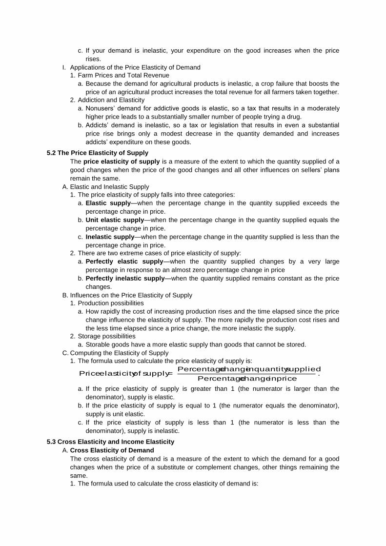
c. If your demand is inelastic, your expenditure on the good increases when the price
rises.
I. Applications of the Price Elasticity of Demand
1. Farm Prices and Total Revenue
a. Because the demand for agricultural products is inelastic, a crop failure that boosts the
price of an agricultural product increases the total revenue for all farmers taken together.
2. Addiction and Elasticity
a. Nonusers’ demand for addictive goods is elastic, so a tax that results in a moderately
higher price leads to a substantially smaller number of people trying a drug.
b. Addicts’ demand is inelastic, so a tax or legislation that results in even a substantial
price rise brings only a modest decrease in the quantity demanded and increases
addicts’ expenditure on these goods.
5.2 The Price Elasticity of Supply
The price elasticity of supply is a measure of the extent to which the quantity supplied of a
good changes when the price of the good changes and all other influences on sellers’ plans
remain the same.
A. Elastic and Inelastic Supply
1. The price elasticity of supply falls into three categories:
a. Elastic supply—when the percentage change in the quantity supplied exceeds the
percentage change in price.
b. Unit elastic supply—when the percentage change in the quantity supplied equals the
percentage change in price.
c. Inelastic supply—when the percentage change in the quantity supplied is less than the
percentage change in price.
2. There are two extreme cases of price elasticity of supply:
a. Perfectly elastic supply—when the quantity supplied changes by a very large
percentage in response to an almost zero percentage change in price
b. Perfectly inelastic supply—when the quantity supplied remains constant as the price
changes.
B. Influences on the Price Elasticity of Supply
1. Production possibilities
a. How rapidly the cost of increasing production rises and the time elapsed since the price
change influence the elasticity of supply. The more rapidly the production cost rises and
the less time elapsed since a price change, the more inelastic the supply.
2. Storage possibilities
a. Storable goods have a more elastic supply than goods that cannot be stored.
C. Computing the Elasticity of Supply
1. The formula used to calculate the price elasticity of supply is:
. price in change Percentage
suppliedquantity in change Percentage =supply of elasticity Price
a. If the price elasticity of supply is greater than 1 (the numerator is larger than the
denominator), supply is elastic.
b. If the price elasticity of supply is equal to 1 (the numerator equals the denominator),
supply is unit elastic.
c. If the price elasticity of supply is less than 1 (the numerator is less than the
denominator), supply is inelastic.
5.3 Cross Elasticity and Income Elasticity
A. Cross Elasticity of Demand
The cross elasticity of demand is a measure of the extent to which the demand for a good
changes when the price of a substitute or complement changes, other things remaining the
same.
1. The formula used to calculate the cross elasticity of demand is:

.
scomplementor ssubstitute its of
one of price in change Percentage
gooda of demandedquantity in change Percentage = demand of elasticity Cross
2. The cross elasticity of demand for a substitute is positive.
3. The cross elasticity of demand for a complement is negative.
B. Income Elasticity of Demand
The income elasticity of demand is a measure of the extent to which the demand for a good
changes when income changes, other things remaining the same.
1. The formula used to calculate the income elasticity of demand is:
. income in change Percentage
demandedquantity in change Percentage = demand of elasticity Income
2. For a normal good, the income elasticity of demand is positive.
3. When the income elasticity of demand is greater than 1, demand is income elastic. 4.
When the income elasticity of demand is between zero and 1, demand is income
inelastic.
5. For an inferior good, the income elasticity of demand is less than 0.

Lesson-21
Applications of the Theory of Production
Production The creation of any good or service that has an economic value either to consumers or to other producers is called the production. Production analysis focuses on the efficient use of inputs to create outputs. The process involves all the activities associated with providing goods and services. Managerial Questions Managerial questions are as follows: 1. Whether to produce or shut down? 2. How much to produce? 3. What input combination to use? 4. What type of technology to use? Examples
• Physical processing or manufacturing of material goods • Production of transportation services • Production of legal advice • Production of education • Production of invention (R&D) • Production of bank loans
Production Function The production function relates the output of a firm to the amount of inputs, especially capital and labor. It can also be defined as a schedule (table, equation) showing the maximum amount of output that can be produced from any specified set of inputs, given the existing technology or “state of the art.” In short, the production function is a catalog of various possibilities of output. Q = f (X,Y) or (K,L) It is important to keep in mind that the production function describes technology, not economic behavior. A firm may maximize its profits given its production function but generally takes the

production function as a given element of that problem. In specialized long-run models, a firm may choose its capital investments to choose among various production technologies. Economic Efficiency The production function incorporates the technically efficient method of production. Here, the latest technological processes are used. When the economists use production functions, they assume that the maximum level of output is obtained from any given combination of inputs. It means, they assume that production is technically efficient. When producers are faced with input prices, the problem is not technical but economic efficiency. How to produce a given amount of output at the lowest possible cost? To be economically efficient, a producer should determine the combination of inputs that solves this problem. What is technical inefficiency? If, for example, an alternative process can produce the same amount of output using less of one or more inputs and the same amount of all others, the first process is technically inefficient. If, however, the second process uses less of some inputs but more of others, the economically efficient method of producing a given level of output depends on the prices of the inputs. One might cost less but actually be less technically efficient. Classifying Inputs
1. Fixed Input A fixed input is one that is required in the production process. The amount of the fixed input employed is constant over a given period of time regardless of the quantity of output produced.
2. Variable Input It is the one whose quantity employed in the production process is varied, depending on the desired quantity of output to be produced.
Time Frames
1. Short-run It is a period of time in which one or more of the inputs are fixed.
2. Very Short-run It is a period of time in which all resources are fixed.

3. Long-run It is a time period which is long enough so that all resources can be varied.
Example of Ore Mining Output = tons or ore mined Capital (horsepower) Labor 250 500 750 1,000 1,250 1,500 1,750 2,0001 1 3 6 10 16 16 16 132 2 6 10 24 29 29 44 443 4 16 29 44 55 55 55 504 6 29 44 55 58 60 60 555 16 43 55 60 61 62 62 606 29 55 60 62 63 63 63 627 44 58 62 63 64 64 64 648 50 60 62 63 64 65 65 659 55 59 61 63 64 65 66 6610 52 56 59 62 64 65 66 67

Labor Output MP ∆Q ÷ ∆X
AP (Q ÷ X)
Elasticity MP ÷ AP
0 0 1 6 +6 6 1.02 16 +10 8 1.253 29 +13 9.67 1.344 44 +15 11 1.365 55 +11 11 1.06 60 +5 10 .507 62 +2 8.86 .238 62 0 7.75 0.09 61 -1 6.78 -.15
10 59 -2 5.90 -.34 Returns to Scale It is the relation between output and variation in all inputs taken together. Returns to Factor It is the relation between output and variation in only one of the inputs employed.

Total Product It is the total output that results from employing a specific quantity of resources in a production system. Marginal Product It is the incremental change in total output that can be produced by the use of one more unit of the variable input in the production process. It can also be defined as the change in output associated with a unit change in one input factor, holding the other inputs constant. ∆Q-- Change brought about by a change in ∆X units of the variable input and Y remains fixed
MPx = ∆Q∆X
Or, in continuous terms:
MPx = ∂Q∂X
Average Product
APx = QX
It is the ratio of the total output to the amount of the variable input used in producing the output. Production Elasticity The percentage change in output results from a given percentage change in the amount of the variable input X employed in the production process is called production elasticity. In this case, Y remains constant. It can also be defined as the percentage change in output associated with a one percent change in all inputs.
Ex = %∆Q%∆X
= ∆Q/Q∆X/X
By rearranging terms:

= ∆Q/∆X
Q/X
= MPxAPx
Law of Diminishing Marginal Returns It is a principle stating that as more and more of a variable input is combined with a fixed input in short-run production, the marginal product of the variable input eventually declines. This is the economic principle underlying the analysis of short-run production for a firm. Among a host of other things, it offers an explanation for the upward-sloping market supply curve. The law of diminishing marginal returns helps us to understand supply. The law of supply and the upward-sloping supply curve indicate that a firm needs to receive higher prices to produce and sell larger quantities. This observation is easily verified by reviewing the slope of the marginal product curve. As the number of units of the variable input increases with other inputs held constant, there exists a point beyond which the marginal product of the variable input declines. It should be noted that it is not a mathematical theorem. It is empirical assertion. The concepts of total and marginal product and the Law of Diminishing Returns to a factor are important to identify efficient as opposed to inefficient input combinations. Determining the Optimal Use of the Variable Input With one of the inputs (Y) fixed in the short-run, a producer should determine the optimal quantity of the variable input (X) to employ in the production process. This is a study of Marginal Revenue Product (MRP) and Marginal Factor Cost (MFC). One can say that this is a study about the role of revenue and cost in the production system. 1. MRP It is the change in total revenue resulting from a unit change in a variable input. In this case, all other inputs remain unchanged. Marginal revenue product is found by dividing the change in total revenue by the change in the variable input. This is also termed as the value of the marginal product. Marginal revenue product is a key component for understanding the demand for productive inputs, i.e. factor demand. It can be defined as the amount that an additional unit of the variable input adds to the total revenue. It can also be defined as the economic value of a marginal unit of a particular input factor when used in the production of a specific product.

MRP = ∆TR∆X
Where ∆TR is the change in total revenue associated with the given change (∆X) in the variable input. MRPx is equal to the marginal product of (MPx) times the marginal revenue (MRQ) resulting from the increase in output obtained. MRP = MPx . MRQ Example
Units TP MP MR at $5 1 3 3 $15 2 7 4 20 3 10 3 15 4 12 2 10 5 13 1 5
If the addition of one more laborer to a workforce would result in the production of two incremental units of a product than can be sold for $5, the MP of labor is 2 and its MRP is $10 (2 x $5). 2. Marginal Factor Cost (MFC) MFC is the amount that an additional unit of the variable input adds to the total cost.
MFC = ∆TC∆X
Optimal Input Level Given the marginal revenue product and marginal factor cost, one can compute the optimal amount of the variable input for using it in the production process. An economic activity should be expanded as long as the marginal benefits exceed the marginal costs. The optimal point occurs at the point where the marginal benefits are equal to the marginal costs. MRPx = MFCx

Single Input System Profit maximization requires production at a level where the marginal revenue is equal to the marginal cost. Because the only variable in the system is input L, the marginal cost of production is as follows:
MC = ∆TC
∆Output
MC = PL
MPL
Since marginal revenue should be equal to the marginal cost at the profit-maximizing level, MRQ can be substituted for MCQ
MRQ = PL
MPL
Solving for PL yields: PL = MRQ x MPL or PL = MRPL A profit-maximizing firm always employs an input upto the point where its marginal revenue product equals its cost. It should be noted that if MRPL> PL, labor usage should be expanded. And if MRPL < PL, labor usage should be cutback. Refer to the ore-mining example: 1. The firm can employ as much labor as it needs by paying workers $50 per period (the labor market is considered perfectly competitive). 2. The firm can sell all the ore it can produce at a price of $10 per ton. MRP = MFC = $50 3. In a case of less than six workers, MRP > MFC and the addition of more workers will increase revenue. Beyond six, the opposite is true.
Labor Total Prod. MP of TR or P • MR MRP MFC

Input Tons of Ore
Labor Q ∆∆TRQ
MP•MR
0 0 0 1 6 6 60 10 60 502 16 10 160 10 100 503 29 13 290 10 130 504 44 15 440 10 150 505 55 11 550 10 110 506 60 5 600 10 50 507 62 2 620 10 20 508 62 0 620 10 0 50 The Production Function with Two Variable Inputs In the ore-mining example, assume that both capital and labor are now variable. 1. Production Isoquant A production isoquant is either a geometric curve or an algebraic function representing all the various combinations of the two inputs that can be used in producing a given level of output. It can also be defined as a curve (a locus of points) showing all possible combinations of inputs physically capable of producing a given fixed level of output. 2. Marginal Rate of Technical Substitution It is the rate at which one input may be substituted for another input in the production process. It can also be defined as the rate at which one input is substituted for another along an isoquant. The rate of change of one variable with respect to another variable is given by the slope of a curve relating the two variables. Thus, the rate of change of input Y with respect to X, i.e. the rate at which Y may be substituted for X in the production process is given by the slope of the curve relating Y to X. This is the slope of the isoquant. Since the slope is negative and one wishes to express the substitution rate as a positive quantity, a negative sign is attached to the slope.
MRTS = Y1 - Y2X1 - X2
= ∆Y∆X
For example, in the example of ore mining, moving from 3 to 4 workers yields the MRTS of 250 (horsepower).
MRTS = - 750-500
3-4 = 250

For every unit of labor, added 250 horsepower may be discharged without changing the total output. It should be noted that one can show the MRTS equal to the ratio of the marginal products of X and Y.
∆Y = ∆Q
MPY
And
∆X = ∆Q
MPX
Substituting these in above yields,
MRTS = MPXMPY
The Optimal Combination of Inputs A firm should make two input choice decisions which are as follows: 1. Choose the input combination that yields the maximum level of output possible with a given level of expenditure. 2. Choose the input combination that leads to the lowest cost of producing a given level of output. This occurs when, in any constrained optimization problem, one chooses the level of each activity whereby the marginal benefits from the last unit of each activity per dollar cost of the activity are equal. This is known as the equimarginal criterion.
MPXCX
= MPYCY
-or-
MPXPX
= MPYPY
The optimal combination of inputs in either the cost-minimization or output-maximization problem is a function of the relative prices of the inputs. One can also say that a policy that is cost-effective should arrange things so that the marginal value of emissions is equalized across all sources. This is known as the “equimarginal criterion.” Changes in Input Prices

Assume that a firm is taking out its production process with the most cost minimizing combination of labor and capital. This is an efficient operation. As we know that:
MPXCX
= MPYCY
Suppose, the price of input X rises while the price of input Y is unchanged and the original combination of inputs MPX and MPY are unchanged. At the original combinations, the increase in CX makes:
MPXCX
< MPYCY
Substitution Effect If a firm wishes to produce the same level of output, it will increase Y and decrease X as it moves along the isoquant. If the input-price ratio changes, a firm moves ahead toward the input that becomes relatively less expensive and away form the input that becomes relatively more expensive. In the case of labor and capital, if wages/interest increases or decreases, K/L increases or decreases at each level of output. This change in the K/L ratio is called the substitution effect. Isoquant and Isocost Combinations Optimal input proportions can be found graphically for a two-input, single-output system by adding a budget line or isocost curve (a line of constant costs) in the diagram of production isoquants. Each point on a budget line represents some combination of inputs (X and Y) whose cost equals constant expenditure.

Figure 4.1
The expansion path is the optimal input combination for increasing output. It should be noted that the proportion in which the inputs are combined need not to be same for all levels of output. The expansion path shows how factor proportions change when output changes with the factor-price ratio held constant. The Decision Making Principle To minimize the cost (expenditure) of producing a given level of output with fixed input prices, a producer should combine inputs in such quantities that the marginal rate of technical substitution of capital and labor is equal to the input ratio, i.e. the price of labor to the price of capital. Returns to Scale A production theory also offers a means for analyzing the effects on output of changes in the scale of production. An increase in the scale of production consists of a simultaneous proportionate increase in all the inputs used in the production process. The proportionate increase in the output of the production process that results from the given proportionate increase in all the inputs is defined as the physical returns to scale.
εQ = %∆Q%∆X =
∂Q∂X •
XQ
Where εQ > 1 increasing εQ = 1 constant εQ < 1 decreasing

1. Increasing-- In this case, output goes up proportionately more than the increase in input usage.
2. Constant-- In this case, output goes up by the same proportion as the increase in input usage. 3. Decreasing-- In this case, output goes up proportionately less than the increase in input usage. Estimation of Production Function One of the more common approaches utilizes the Cobb Douglas production function method. Q = αLβ1Kβ2 Where 1. Both inputs are required to create output 2. MRTS will diminish as required by production theory Logarithmic Specification Ln Q = Ln α + β1LnL + β2LnK Elasticity of Production
EL = MPLAPL
Where MPL = αβ1Lβ1-1Kβ2 and,
APL = αLβ1Kβ2
L = αLβ1-1Kβ2
Thus,
EL = αβ1Lβ1-1Kβ2
αLβ1-1Kβ2 = β1
The exponents- returns to scale 1. Increasing-- β1 + β2 > 1 2. Constant-- β1 + β2 = 1 3. Decreasing-- β1 + β2 < 1 Example

Q = 1.01 0.75 K 0.25 Q-- An index of physical volume of manufacturing L-- An index of the average number of employed wage earners only (i.e. salaried employees, officials and working proprietors were excluded) K-- An index of the value of plants, buildings, tools and machinery reduced to dollars of constant purchasing power The sum of the exponents were restricted to one. (Constant returns to scale) Further Studies by Cobb and Douglas Q = .84 L0.63 K0.30 A one percent increase in labor input results in about a 2/3 percent increase in output and a one percent increase in capital input results in approximately a 1/3 percent increase in output. The sum of the exponents is slightly less than one. It seems to indicate the presence of decreasing returns to scale. However, the sum is not significantly different from 1.0. Hence, it really confirms constant returns to scale. A Three Variable Model
Q = αLpβ1Ln
β2 Kβ3
Where Q-- The value added by production plants over 18 industries Ln -- Non-production work-years
Lp -- Production work-hours
K-- Gross book values of depreciable and depletable assets Empirical Estimation of a Production Function for a Major League Baseball by CE. Zech as published in the American Economist In an attempt to quantify the factors that contribute to the team’s success, a Cobb-Douglas production function was developed using data from the 26 major league baseball teams in 1977. Output (Q) was measured by team victories. Inputs from five different categories were included in the model which are as follows: • Hitting-- batting average and power (home runs) • Running-- stolen base record • Defense-- fielding percentage and total chances accepted • Pitching-- earned run average (ERA) and strikeouts-to-walks ratio

• Coaching-- Lifetime won-lost record and number of years spent managing in the major leagues
• Dummy-- NL = 0, AL = 1

Variable Eq. 1 Eq. 2 Eq. 3 Eq. 4 Constant .017 .018 .010 .008 Dummy -.002 -.003 .004 .003 B avg. 2.017 1.986 1.969 1.927 Homeruns .229 .299 .208 .215 Stolen Bases .119 .120 .110 .112 Strikeouts/Walks .343 .355 .324 .334 TotField Chances 1.235 1.200 Field % 5.62 5.96 Mngr.W/L -.003 -.004 Mngr. Years -.004 -.004 R2 .789 .790 .773 .774
Findings
1. Hitting average contributes almost six times as much as pitching to a team’s success. Contradict traditional wisdom?
2. Homeruns contribute about twice as much as stolen bases to a team’s success. 3. Coaching skills are not significant in any of the regression equations. 4. Defensive skills are not significant in any of the regression equations. 5. The sum of the statistically significant variables in each of the four equations range from
2.588 to 2.709. Because these are all greater than 1.0, the baseball production functions exhibit increasing returns to scale.

Lesson-22
Cost Analysis-I
Introduction to Cost
We can look at the business firm from at least two points of view: productivity, inputs, and outputs or outputs and costs. In advanced microeconomics, these two points of view are called "duals." They are equally valid, but they point up different things. They are also opposites from a certain point of view-- the higher the productivity, the lower the costs. By looking at the firm from the point of view of costs, we shift our perspective somewhat, and gain a much more direct understanding of supply.
We also look more directly at the difference between the long and short run. In the short run, we have two major categories of costs:
• Fixed Costs • Variable Costs
In the long run, however, all costs are variable. Thus, we must study costs under two quite different headings. Costs will vary quite differently in the long run and in the short.
Fixed and Variable Cost
Variable costs are costs that can be varied flexibly as conditions change. In the John Bates Clark model of the firm, labor costs are the variable costs. Fixed costs are the costs of the investment goods used by the firm, on the idea that these reflect a long-term commitment that can be recovered only by wearing them out in the production of goods and services for sale.
The idea here is that labor is a much more flexible resource than capital investment. People can change from one task to another flexibly (whether within the same firm or in a new job at another firm), while machinery tends to be designed for a very specific use. If it isn't used for that purpose, it can't produce anything at all. Thus, capital investment is much more of a commitment than hiring is. In the eighteen hundreds, when John Bates Clark was writing, this was pretty clearly true.
Over the past century, education and experience have become more important for labor, and have made labor more specialized. Increasing automatic control has made some machinery more flexible. So the differences between capital and labor are less than they once were, but all the same, it seems labor is still relatively more flexible than capital. It is this relative difference in flexibility that is expressed by the simplified distinction of long and short run.
Of course, productivity and costs are inversely related, so the variable costs will change as the productivity of labor changes.

Here is a picture of the fixed costs (FC), variable costs (VC) and the total of both kinds of costs (TC) for the productivity example in the last unit:
Figure 22.1
Output produced is measured toward the right on the horizontal axis. The cost numbers are on the vertical axis. Notice that the variable and total cost curves are parallel, since the distance between them is a constant number -- the fixed cost.
Opportunity Cost
Connection between the distinctions of fixed vs. variable costs and opportunity costs
In economics, all costs are included whether or not they correspond to money payments. If we have opportunity costs with no corresponding money payments, they are called implicit costs. The implicit costs (as well as the money costs) are included in the cost analysis.
There is some correlation between implicit costs and fixed or variable costs, but this correlation will be different in such different kinds of firms as
A factory owned by an Absentee Investor
This is the easiest case to understand. All of the labor costs to the absentee investor are money costs, including the manager's salary. If the investor has borrowed some of the money he invested in the factory, then there are some money costs of the capital invested -- interest on the loan. However, we must consider the opportunity cost of invested capital as well. The investor's own money that he has used to buy the factory is money that she could have invested in some other business. The return she could have gotten on another investment is the opportunity cost of her own funds invested in the business. This is an implicit cost, and in this case the implicit cost is part of the cost of capital and probably a fixed cost.

A "Mom-and-Pop" Store
A "mom-and-pop" store (family proprietorship or partnership) is a store in which family members are self-employed and supply most of the labor. Typically, "Mom" and "Pop" don't pay themselves a salary -- they just take money from the till when they need it, since it is their property anyway. As a result, there are no money costs for their labor. But their labor has an opportunity cost -- the salary or wages they could make working similar hours in some other business -- and so, in this case, the implicit costs include a large component of variable labor costs.
A large Modern Corporation
The corporation has relatively few implicit costs, but generally will have some. All labor costs will be expressed in money terms (though benefits and bonuses have to be included), since the shareholders don't supply labor to the corporation as "Mom and Pop" do in a family proprietorship. It will pay interest to bondholders and dividends to shareholders. But the dividends aren't really a cost item -- they include profits distributed to the shareholders. Moreover, the typical corporation will retain some profits and invest them within the business, a "plowback" investment. Conversely, shareholders may take a large part of their payout in appreciation of the stock value and plowback investment is one reason for the appreciation.
Thus we would say that the corporation has a net equity value, that is, that the corporation "owns" a certain amount of capital that it invests in its own business (very much like the absentee owner in the first example). This capital has an opportunity cost, and that opportunity cost is an implicit cost. The stockholders, who own the corporation, ultimately receive (as dividends or appreciation) both the opportunity cost of the equity capital and any profit left over after it is taken out.
Unit Cost
Costs may be more meaningful if they are expressed on a per-unit basis, as averages per unit of output. In this way, we again distinguish
Average Fixed Cost (AFC)
This is the quotient of fixed cost divided by output. In the numerical example we are using, when output is 4020 (in the table) fixed cost is 80000, so AFC is 80000/4020=19.9
Average Variable Cost (AVC)
This is the quotient of average cost divided by output. In the example, at an output of 4020 the variable cost is 350000, giving AVC of 350000/4020=87.06.
Average Total Cost (ATC or AC)

This is the quotient of total cost divided by output. In the example, with 4020 of output total cost is 430000, so AC is 430000/4020 = 106.96 = 87.06+19.90.
Here are the average, average variable, and average fixed costs for our example firm.
Table 22.1
Q AC AFC AVC
945 138 85 53
1780 101 45 56
2505 92 32 60
3120 90 26 64
3625 91 22 69
4020 95 20 75
4305 100 19 81
4480 107 18 89
4545 117 18 99 Here are the average cost (AC), average variable cost (AVC) and average fixed cost (AFC) in a diagram. This is a good representative of the way that economists believe firm costs vary in the short run.
Figure 22.2
Notice how the average fixed costs decline as the fixed costs are "spread over more units of output." For large outputs, however, average variable costs rise pretty steeply. The idea is that with a limited capital plant and thus limited productive capacity -- in the short run

-- costs would rise much more than proportionately to output as output goes beyond "capacity." The average total cost, dominated by fixed costs for small output, declines at first, but as output increases, fixed costs become less important for the total cost and variable costs become more important, and so, after reaching a minimum, average total cost begins to rise more and more steeply.
Marginal Cost
As before, we want to focus particularly on the marginal variation. In this case, of course, it is marginal cost. Marginal cost is defined as
As usual, Q stands for (quantity of) output and C for cost, so Q stands for the change in output, while C stands for the change in cost. As usual, marginal cost can be interpreted as the additional cost of producing just one more ("marginal") unit of output.
Let's have a numerical example of the Marginal Cost definition to help make it clear. Total cost is 280000 for an output of 3120, and it is 33000 for an output of 3625. So we have
and
so that
for a marginal cost of $99.01 for the next unit produced. As usual, this is an approximation, and the smaller the change in output we use, the better the approximation is.
Here is the marginal cost for our example firm, along with output and average cost.

Table 22.2
Output AverageCost Marginal
Cost
0 0
9.45
945 137.57
52.91
1780 101.12
59.88
2505 91.82
68.97
3120 89.74
81.30
3625 91.03
99.01
4020 94.53
126.58
4305 99.88
175.44
4480 107.14
285.71
4545 116.61 769.23
Here is a picture of marginal cost for our example firm, together with average cost as output varies.

Figure 22.3
As before, the distance to the right on the horizontal axis measures the output produced. The average and marginal costs are on the vertical axis. Average cost is shown by the curve in yellow, and marginal cost in red. Notice how the marginal cost rises to cross average cost at its lowest point.
Maximization of Profit and Cost
We can now give another rule for the maximization of profits. The new rule is really just the same rule as we saw before, only now we state it in terms of price and costs. It is the equimarginal principle in yet another form.
The question is: "I want to maximize profits. How much output should I sell, at the given price?"
The answer is: increase output until
p = MC
The point is illustrated by the following table, which extends the marginal cost table in an earlier page to show the price and the profits for the example firm.
Table 22.3
Output AverageCost price profit Marginal
Cost
0 0 9.45
100 0

945 137.57 100 -35503.65
52.91
1780 101.12 100 -1993.60
59.88
2505 91.82 100 20490.90
68.97
3120 89.74 100 32011.20
81.30
3625 91.03 100 32516.25
99.01
4020 94.53 100 21989.40
126.58
4305 99.88 100 516.60
175.44
4480 107.14 100 -31987.20
285.71
4545 116.61 769.23
100 -75492.45
Notice how profits are greatest (at 32516.25) when the marginal cost is almost exactly equal to the price of $100. This occurs at an output of 3625, with marginal cost at 99.01. The profit-maximizing output would be very slightly more than 3625.
Supply and Cost
We have discovered the principle of supply for the individual firm.
Remember: what is supply? It is the relation between the price and the quantity that people want to sell. For an individual firm, that is: the relation between the price and the quantity the firm wants to sell.
So we ask: at a given price, how much will a (profit- maximizing) firm want to sell? The answer: enough so that the price is equal to marginal cost. In other words, the marginal cost curve is the supply curve for the individual firm.
Shutdown Point

As long as the firm produces something, it will maximize its profits by producing "on the marginal cost curve." But it might produce nothing at all. When will the firm shut down?
The answer goes a bit against common sense. The firm will shut down if it cannot cover its variable costs. So long as it can cover the variable costs, it will continue to produce.
This is an application of the opportunity cost principle. Just because fixed costs are fixed, they are not opportunity costs in the short run -- so they are not relevant to the decision to shut down. Even if the company shuts down, it must pay the fixed costs anyway. But the variable costs are avoidable -- they are opportunity costs! So the firm will shut down, as it cannot meet the variable (short run opportunity) costs. But as long as it can pay the variable costs and still have something to apply toward the fixed costs, it is better off continuing to produce.
It is important not to confuse shutdown with bankruptcy. They are two different things. If a company cannot pay its interest and debt payments (usually fixed costs), then it is bankrupt. But that doesn't mean it will shut down. Bankrupt firms are often reorganized under new ownership, and continue to produce-- just because they can cover their variable costs, and so the new owners do better to continue producing than to shut down.
Long Run Cost
Thus far we have not considered the long run in cost theory. We will now think a bit about the long run, using the concept of average cost.
We have defined "the long run" as "a period long enough so that all inputs are variable." This includes, in particular, capital, plant, equipment, and other investments that represent long-term commitments. Thus, here is another way to think of "the long run" it is the perspective of investment planning.
So let's approach it this way: Suppose you were planning to build a new plant-- perhaps to set up a whole new company-- and you know about how much output you will be producing. Then you want to build your plant so as to produce that amount at the lowest possible average cost.
To make it a little simpler we will suppose that you have to pick just one of three plant sizes: small, medium, and large. Here's the way they look in a picture:
Here are the average cost curves for the small (AC1), medium (AC2) and large (AC3) plant sizes:

Figure 22.4
If you produce 1000 units, the small plant size gives the lowest cost. If you produce 3000 units, the medium plant size gives the lowest cost. If you produce 4000 units, the large plant size gives you the lowest cost.
Therefore, the long run average cost (LRAC)-- the lowest average cost for each output range -- is described by the "lower envelope curve," shown by the thick, shaded curve that follows the lowest of the three short run curves in each range.
More realistically, an investment planner will have to choose between many different plant sizes or firm scales of operation, and so the long run average cost curve will be smooth, something like this:

Figure 22.5
As shown, each point on the LRAC corresponds to a point on the SRAC for the plant size or scale of operation that gives the lowest average cost for that scale of operation.
Returns to Scale In our pictures of long run average cost, we see that the cost per unit changes as the scale of operation or output size changes. Here is some terminology to describe the changes: Increasing returns to scale = decreasing cost
Average cost decreases as output increases in the long run Constant returns to scale = constant costs
Average cost is unchanged as output varies in the long run Decreasing returns to scale = increasing costs
Average cost increases as output increases in the long run
Here are pictures of the average cost curves for the three cases:
Increasing returns to scale = decreasing cost
Figure 22.6 Constant returns to scale = constant costs
Figure 22.7 Decreasing returns to scale = increasing costs

Figure 22.8
Increasing Returns to Scale
Economists usually explain "increasing returns to scale" by indivisibility. That is, some methods of production can only work on a large scale-- either because they require large-scale machinery, or because (getting back to Adam Smith, here) they require a great deal of division of labor. Since these large-scale methods cannot be divided up to produce small amounts of output, it is necessary to use less productive methods to produce the smaller amounts. Thus, costs increase less than in proportion to output-- and average costs decline as output increases.
Increasing Returns to Scale is also known as "economies of scale" and as "decreasing costs." All three phrases mean exactly the same.
Constant Returns to Scale
We would expect to observe constant returns where the typical firm (or industry) consists of a large number of units doing pretty much the same thing, so that output can be expanded or contracted by increasing or decreasing the number of units. In the days before computer controls, machinery was a good example. Essentially, one machinist used one machine tool to do a series of operations to produce one item of a specific kind -- and to double the output you had to double the number of machinists and machine tools.
Constant Returns to Scale is also known as "constant costs." Both phrases mean exactly the same.
Decreasing Returns to Scale
Decreasing returns to scale are associated with problems of management of large, multi-unit firms. Again with think of a firm in which production takes place by a large number of units doing pretty much the same thing -- but the different units need to be coordinated by a central management. The management faces a trade-off. If they don't spend much on management, the coordination will be poor, leading to waste of resources, and higher cost. If they do spend a lot on management, that will raise costs in itself. The idea is that the bigger the output is, the more units there are, and the worse this trade-off becomes -- so the costs rise either way.

Decreasing Returns to Scale is also known as "diseconomies of scale" and as "increasing costs." All three phrases mean exactly the same.
In our examples, the LRAC is (more or less roughly) u-shaped, like this:
Figure 22.9
The idea is that:
• for small outputs, indivisibilities predominate, and so long run average cost declines with increasing output
• for intermediate outputs, operations can be expanded roughly proportionately, while tendencies to increasing and decreasing costs -- if any -- offset one another.
• for large outputs, the problems of management predominate, and so long run average cost increases with increasing output.
That's reasonable -- but we should recall that it is pretty much a guess, and may or may not apply in a particular case!
Summary
By thinking in terms of cost, rather than productivity, we gain several points of understanding of supply:
• While total and average cost concepts have their uses, the most important in the short run is marginal cost.
• To maximize profits, the firm will increase output to the point where marginal cost equals a given price.
• Therefore, the marginal cost curve is itself the supply curve, in the short run. • The firm will shut down, however, if it cannot cover its variable cost. • We may think of the long run as a perspective of investment planning. • Long run average cost is the "lower envelope" of all the short run average cost
curves for different plant or firm sizes. • We may observe increasing costs, decreasing costs, or constant costs as output
increases, in the long run -- or all three, depending on output.

Lesson-23
Cost Analysis-II Explicit Costs and Implicit Costs Economists have classified types of costs as explicit (accounting) costs, and implicit costs. Explicit costs are out of pocket, obvious kinds of costs, e.g., expenses on books, tuition, as, etc. Implicit costs are not really expenses you incur, but involve income or values you are giving up by not doing something that you could have chosen to do. For instance, if you decide to go to school full time instead of working a $20,000 job, you are giving up earning $20,000. This is your implicit cost. Sample problem: Suppose you are running a small business and incur the following expenses: labor = $80,000; raw materials = 30,000; finance charges on a loan = $3,000. You are not paying explicit rent, because you own the building you are operating in. If you would rent it out, however, you could be earning $12,000. You also estimate your own time to be worth $25,000. What are your expenses?
Accounting vs. Economic Costs Accountants have been primarily concerned with measuring costs for financial reporting purposes. As a result, they define and measure cost by the historical outlay of funds that takes place in the exchange or transformation of a resource. Economists have been mainly concerned with measuring costs for decision-making purposes. The objective is to determine the present and future costs (or resources) associated with various alternative courses of action. In calculating the cost to the firm of producing a given quantity of output, economists include some additional costs that are typically not reflected in financial reports. • Explicit cost are considered by both groups • Implicit costs are considered by economists:
a. Opportunity cost of time b. Opportunity cost of capital
Economic Profit = Tot Rev - Exp Cost - Imp Cost Accounting versus Economic Profits

To calculate accounting and economic profits we need to know the company’s total revenue. Let’s suppose it is $140,000. Then, accounting profits are: total revenue minus explicit costs or: $140,000 - $113,000 = $27,000. Economic profits are: total revenue minus total economic costs or; $140,000 - $150,000 = -$10,000 (i.e. a loss of $10,000). The above firm reaps a positive accounting profit; but the negative economic profit indicates that from an economic point of view, the owner should discontinue the operation. Total and Per Unit Costs Seven cost functions, which we will discuss, are:
1. Total Variable Cost (TVC) – The cost of all variable resources. Examples: Cost of labor, materials, office supplies.
2. Total Fixed Cost (TFC) – The cost of all fixed inputs. Examples: Cost
of the building, large pieces of machinery, certain taxes
3. Total Cost (TC) – This is the sum of TVC and TFC.
4. Average Variable Cost (AVC) – This is variable cost per product.
5. Average Fixed Cost (AFC) – This is fixed cost per product.
6. Average Total Cost (ATC) – This is total cost per product.
7. Marginal Cost (MC) – This is the cost of producing an additional unit of the product
Cost Calculations
Using the above abbreviations and Q for the quantity of output: ATC = TC/Q AFC = TFC/Q AVC = TVC/Q MC = change in TC/change in Q

Example: Let’s suppose you are making 50 bottles of wine each week. You know that your fixed costs add up to $300, and your variable costs amount to $900. You also know that if you were to make extra 5 bottles, your total cost would rise by $60. What is your total cost; average total cost; average total cost; average variable cost; average fixed cost; and marginal cost? Answer: Total cost = $300 + $900 = $1200 ATC = $1200/50 = $24 AVC = $900/50 = $18 AFC = $300/50 = $6 MC = $60/5 = $12 A table with cost data might show the following:
• Ore Mining Example-- Cost Data
Q L VC FC TC AFC AVC ATC MC 0 0 0 150 150 150 0 150 6 1 50 150 200 25.00 8.33 33.33 8.33 16 2 100 150 250 9.38 6.25 15.63 5.00 29 3 150 150 300 5.17 5.17 10.34 3.85 44 4 200 150 350 3.41 4.55 7.95 3.33 55 5 250 150 400 2.73 4.55 7.27 4.55 60 6 300 150 450 2.50 5.00 7.50 10.00 62 7 350 150 500 2.42 5.65 8.06 25.00 62 8 400 150 550 2.42 6.45 8.87 ERR 61 9 450 150 600 2.46 7.38 9.84 -50.00 59 10 500 150 650 2.54 8.47 11.02 -25.00
a. Rent of the ore-mining equipment = $0.20 per horsepower (750 x 0.20 =
$150) b. Cost of each worker employed is $50 per period.
1. TC = FC + VC
2. AFC = FCQ
3. AVC = VCQ
4. ATC = TCQ or AFC + AVC

5. MC = ∆TVC
∆Q , note the following
TVC = a + bQ, where
b = ∆TVC
∆Q = MC
6. Cost Elasticity ε = %∆TC%∆Q =
∆TC∆Q .
QTC
ε < 1 increasing returns to scale ε = 1 constant ε > 1 decreasing
1. Cubic Form (with Quadratic MC):
Cubic-- Assumes that both marginal cost and average variable cost functions have U-shapes.

F o r R e f e r e n c eo n ly
VC = a + bQ - cQ2 + dQ3 a > 0, b < 0, and c > 0 Thus, MC is U-shaped MC = b -2cQ + 3dQ2 Example: FC = $100 TVC = 60Q - 3Q2 + 0.10Q3 then we know, TC = 100 + 60Q - 3Q2 + 0.10Q3
AFC = 100Q
AVC = 60 - 3Q + 0.10Q2 Note: AVC reaches a min at
Qm = - b2c or
AVC = MC
ATC = 100Q + 60 - 3Q + 0.10Q2
MC = d(VC)
dQ = 60 - 6Q + 0.30Q2

2. Cost Curves Fig. 1
Fig. 2
The curves above show typical shapes of a firm’s total cost, total variable cost and total fixed cost curves. Total fixed cost is constant at $50 for all levels of production. Total cost and total variable cost increase with higher levels of output. Note that total fixed cost and total variable cost always add to total cost. Relationship of TFC, TVC, and TC
TFC is constant and unaffected by output level TVC is always increasing; increasing at a decreasing rate first and
then at an increasing rate TC has same shape as TVC; but higher by the vertical distance
equal to TFC

Note: These characteristics based on “typical” production function; shapes of cost curves depend on characteristics of the underlying production function. Average and Marginal cost curves
• AFC – always declining but at a decreasing rate • ATC and AVC – U-shaped; declining at first, reaching a minimum, and
then increasing at higher output levels • Vertical diff. bet. ATC and AVC is the AFC (changes with output level) • ATC and AVC have minimum points at different output levels • MC – generally increasing; with a “typical” production function, MC
decreases over a short range before starting to increase • MC hits AVC and ATC at its minimum points - as long as marginal is
below average, average is decreasing (and vice-versa)
3. Short-Run Cost Functions In addition to measuring the costs of producing a given quantity of output, economists are also concerned with determining the behavior of costs as output is varied over a range of possible values. The behavior of costs is expressed in terms of a cost function.
4. Total Cost Function Total Cost = sum of all costs; FC + TVC
5. Long-Run Cost Functions The long-run cost function is obtained directly from the production function by finding the expansion path. Remember, the expansion path for a production process consists of the combinations of inputs X and Y for each level of Q that satisfy the optimality criterion:
MPC
x
x =
MPC
y
y
Over the long-run planning horizon, the firm can choose the combination of inputs that minimizes the cost of producing a desired level of output. Using the existing production methods and technology, the firm can choose:
• The plant size, • Types and sizes of equipment, • Labor skills, and • Raw materials

that, when combined, yield the lowest cost of producing the desired amount of output. The long-run average cost function (LAC) consists of the lower boundary (envelope) of all the short-run cost curves.
The relationship between LTC, LMC, and LAC is as follows-- The long-run cost function is obtained directly from the production function by first finding the expansion path for the given production process. The expansion path for a production process consists of the combinations of inputs X and Y for each level of output Q that satisfy the optimality criterion developed earlier. Recall we derived the condition that the MRTS between two inputs must be equal to the ratio of the unit costs of the two inputs for a given input combination to be an optimal solution to either the output-maximization or cost-minimization problem.
MRTS = CxCy
Graphically, the optimal input combination occurred at the point where the production isoquant was tangent to the isocost line.

Note:
LAC = LTC
Q and LMC = ∆LTC
∆Q
6. The Long Run Average Cost Curve
The long-run average cost curve is derived from a number of short-run average cost curves. For each fixed plant size (short run), you look at the lowest costs for that size plant. These bottom portions of the different short run cost curves make up the long run average cost curve.
A firm’s long run average cost curve is the “envelope” of many short run average cost curves. All inputs are variable and the firm has the choice of building or changing to a

variety of plant or facility sizes. A small operation (SRAC1), which wants to produce 300 Units, will have average costs of $26. A larger one, which produces 700 units, can produce each product for $17 (economies of scale). When the firm gets too large (SRAC6), average costs rise to $20 (diseconomies of scale).
7. Increasing, Decreasing, and Constant Returns to Scale Note that increasing returns to scale is closely associated with the concept economies of scale (the downward sloping part of the long run average total cost curve.) Decreasing returns to scale relates to diseconomies of scale (the upward part of the curve). Increasing returns to scale occurs when a firm increases its inputs, and a more than proportionate increase in production results. For example, one year a firm employs 200 workers and 50 machines and produces 1000 products. A year later it increases the number of workers to 40 0and the machines to 100 (inputs doubled) and the output rises to a level of 2500 (more than doubled). Increasing returns to scale is often accompanied by decreasing long run average costs (economies of scale). A firm which gets bigger may experience this because of increased specialization, more efficient use of large pieces of machinery (for example, use of assembly lines), volume discounts, etc. Decreasing returns to scale happens when the firm’s output rises by less than the percentage increases in inputs. In the last example, had the firm’s output risen to 1500, we would experience decreasing returns to scale. Decreasing returns to scale can be associated with rising long run average costs (diseconomies of scale). An organization may become too big, thus creating too many layers of management, too many departments, and too much red tape. This lead to a lack of communications, inefficiency, and delays in decision-making. Constant returns to scale occurs when the firm’s output rises proportionate to the increase in inputs. What would output have to be for this to take place?
8. Marginal Utility
Marginal utility is the additional satisfaction one gets from consuming one more item of a good or service. Satisfaction is measured in utils (use your imagination). Let’s say that you are about to eat a pizza consisting of 6 slices. The first piece might give you 140 utils of satisfaction (you were starving!). The second slice, your hunger somewhat satisfied after the first, yields you only 60 utils. The third’s down to 20 utils and a possible fourth, if forced upon you, could produce negative additional utils (your total would drop.)
9. The Law of Diminishing Marginal Utility

Referring back to the example in the previous objective, you can see that the marginal utility declines as the person consumes more slices. This is typical of almost all (beer and other substances known to be harmful to body and soul may be sole exceptions…) consumption: the more you have of something the less the additional unit is worth to you. This phenomenon explains why if you are shopping in a supermarket you only buy a limited quantity of goods. As the marginal utility of, for example, the fifth orange declines, you may decide that this orange is not worth your additional expense.
10. Application of Cost Concepts Profit-maximizing rules (Short-run) If price or MR > min. ATC (or TR>TC), produce output where MR =MC If min AVC < price or MR < min. ATC (or TVC < TR < TC), produce where MR = MC; But will incur a loss between zero and TFC (loss minimized) If price or MR < min ATC, do not produce and loss will equal TFC Profit-maximizing rules (Long-run) If price or MR > ATC, produce where MR=MC If price or MR < ATC, stop production and sell fixed assets
11. Isoquants and the Producer's equilibrium
When producing a good or service, how do suppliers determine the quantity of factors to hire? Below, we work through an example where a representative producer answers this question.
Let’s begin by making some assumptions. First, we shall assume that our producer chooses varying amounts of two factors, capital (K) and labor (L). Each factor was a price that does not vary with output. That is, the price of each unit of labor (w) and the price of each unit of capital (r) are assumed constant. We’ll further assume that w = $10 and r = $50. We can use this information to determine the producer’s total cost. We call the total cost equation an isocost line (it’s similar to a budget constraint).
The producer’s isocost line is:
10L + 50K = TC (1)
The producer’s production function is assumed to take the following form:
q = (KL)0.5 (2)

Our producer’s first step is to decide how much output to produce. Suppose that quantity is 1000 units of output. In order to produce those 1000 units of output, our producer must get a combination of L and K that makes (2) equal to 1000. Implicitly, this means that we must find a particular isoquant.
Set (2) equal to 1000 units of output, and solve for K. Doing so, we get the following equation for a specific isoquant (one of many possible isoquants):
K = 1,000,000/L (2a)
For any given value of L, (2a) gives us a corresponding value for K. Graphing these values, with K on the vertical axis and L on the horizontal axis, we obtain the blue line on the graph below. Each point on this curve is represented as a combination of K and L that yields an output level of 1000 units. Therefore, as we move along this isoquant output is constant (much like the fact that utility is constant as we move along an indifference curve).
How much K and L should the producer hire? The answer is that our choice must exist somewhere on this isoquant. If each possible choice must lie on this isoquant, then our basis for choosing one "best" combination should be to choose the least cost combination. Let’s experiment with some different possibilities, by plugging values for L and K into the isocost equation above. Each combination should yield output of 1000 units. Several combinations, and their specific total cost are given as follows:
L K TC
1,000 1,000 60,000
5,000 200 60,000
10,000 100 105,000

100 10,000 501,000
Now, the firm’s goal is to produce 1000 units at the lowest possible TC. The lowest total cost on the table is $60,000, so we can start there. There are two choices which yield this total cost. They are represented below as B1 and B2.
Is there a lower cost combination of L and K available? Yes, we can produce at a total cost of $52,500 by employing either 250 units of K and 4000 units of L, or 800 units of K and 1250 units of L. This appears on the graph below.
The second isocost, where TC = $52,500, rests below the former isocost, where TC = $60,000. If we continue to find lower and lower levels of total cost that provide us with 1000 units of output, then we will clearly reach lower and lower points on the isoquant. Eventually, we can find a level of total cost that involves a tangency between the isocost and isoquant. This is pictured below at point A.

In addition to being the lowest cost combination of L and K that produces 1000 units of output, pt. A involves a tangency point between the isoquant and isocost. That is, the slopes of these curves at pt. A are equal. The slope of the isocost is w/r, or –1/5. The slope of the isoquant is the ratio of the marginal products, MPL/MPK, which is given as the marginal rate of technical substitution (MRTS). Using calculus, it is possible to derive the MRTS as –K/L. Point A satisfies the condition that K/L = 1/5.
We can solve for K* and L* at pt. A, using (1), (2a) and the fact that, at pt. A, K/L = 1/5. First, substitute (2a) into (1) and the equation K/L = 1/5. We're left with:
10L + 50(1,000,000/L) = TC and (1,000,000/L)/L = 1/5
Solve the second equation for L, substitute that result into the first equation to get the lowest value for TC (TC*).
TC* = $44,721.36
Once you have TC*, you can substitute this value into the isocost equation above (10L + 50,000,000/L = TC) and then solve for L* (rounded to the nearest whole number).
L* = 2,236
Going back to (1), we can substitute in L* and TC*, to get K*.
K* = 447
12. Economies of Scale Declining long-run average costs over the lower part of the possible outputs are usually attributed to economies of scale. Economies of scale occur over the range of the long-run

cost function which corresponds to increasing returns to scale of the production function. Where do economies of scale come from? 1. Plant Economies
Specialization in the use of labor and capital Indivisible nature of many types of capital equipment Purchase price of different sizes of equipment
2. Firm Economies
Materials procurement / quantity discounts Economies in raising funds (capital procurement) Sales promotion Technological innovation Management
13. Glossary of terms
1. Cost-- The sacrifice incurred whenever an exchange or transformation of
resources takes place. 2. Sunk cost-- A cost incurred regardless of the alternative action chosen in a
decision-making problem. 3. Cost function-- A mathematical model, schedule, or graph that shows the cost
(such as total, average, or marginal cost) of producing various quantities of output.
4. Opportunity cost-- The value of a resource in its next best alternative use. Opportunity cost represents the return or compensation hat must be foregone as the result of the decision to employ the resource in a given economic activity.
5. Marginal cost-- The incremental increase in total cost that results from a one-unit increase in output.
6. Cost elasticity-- A measure that indicates the percentage change in total costs associated with a 1-percent change in output.
7. Economies of Scale: Declining long-run average costs as the level of output for the firm (or production plant) is increased. The decline in costs is generally attributed to production or marketing advantages.
8. Diseconomies of scale-- Rising long-run average costs as the level of output is increased.
9. Minimum efficient scale-- The output level at which long run average costs are first minimized.
10. Capacity-- The output level at which short-run average costs are minimized. 11. Operating leverage-- The use of assets having fixed costs (e.g. depreciation) in an
effort to increase expected returns.

Lesson-24
Economies of Scale
Economies of scale can be of two kinds-- internal economies and external economies. Internal economies of scale are those which arise from the firm increasing its plant size. On the other hand, external economies arise outside the firm-from improvement (or, deterioration) in the environment in which the firm operates. The economies external to the firm may be realized from actions of other firms in the same or in another industry. While the internal economies of scale relate only to the long run and determine the shape of the long-run cost curve, the external economies affect the position of the long-run cost curves.
Internal Economies
Internal economies are given in a summary form in the figure given later in the chapter, where these are categorized into real and pecuniary economies. Real economies arise when the quantity of inputs used for a given level of output decreases. While pecuniary economics are those savings in expenses, which accrue to the firm in the nature of relatively, lower prices paid for inputs and lower costs of distribution. These savings arise due to bulk buying and selling by the growing firm.
Real Economies of Scale
Real economies are of four kinds:
a. Production economies b. Marketing economies c. Managerial economies d. Transport and storage economies
a) Production Economies
Production economies arise from
(a) Labor (b) Fixed capital (c) Inventory requirements of the firm.
These are as follows:
Labor economies-- Labor economies arise because of the following factors:

(ii) Division of labor economies-- Larger output allows division of labor, which reduces cost by increasing specialization, by saving time (otherwise lost in passing from one operation to another), and providing good conditions for inventions of a great number of machines.
(iii) Cumulative volume economies-- The technical personnel engaged in production tend to acquire significant experience from large-scale production. This 'cumulative volume' experience helps in higher productivity and, therefore, reduced costs
Technical economies-- These are associated with fixed capital, which includes machinery and equipment. Such economies arise because of the following:
(iv) Specialized equipment. The production methods become more mechanized as the output scale increases. This would imply more specialized capital equipment and lower variable costs.
(v) Indivisibility. The machinery and equipment generally have the property of indivisibility, which means that equipment is available only in minimum sizes or in definite ranges of size. When output is increased from zero to the maximum capacity level of the machine, the same machine and equipment are used. As a result the cost of machine is shared between more and more units of output. In short, as the output is increased, the machinery and equipment comes to be utilized more intensively and consequently the cost of production per unit declines.
(vi) Integration of processes. The large size firms enjoy economies of large machines. Integration of processes occurs where one large automatic transfer or numerically controlled machine can carry out a series of consecutive processes, saving labor cost and time required to set up the work on each of a series of successive specialized machines.
(vii) Economies of increased dimensions for many types of equipment both initial and running costs increase less rapidly than capacity (e.g., tanks, blast furnaces and other static and mobile containers). These result in economies of increased dimensions. Any container whose external dimensions are doubled has its volume increased eight times, but the area of its surface walls would have increased only four times. This reduces material costs and, where appropriate, heat loss and surface, air and water resistance per unit.
(viii) Economies in set-up costs. The larger the scale of output, the

more a multipurpose machinery is left to one set-up and, therefore, set-up costs of general purpose machines reduce.
(ix) Economies of overhead costs. Obviously, the larger the scale of output, the lower the unit costs of initial fixed expenses which are need for a new business or a new product.
II. Inventory economies. Role of inventories is to meet the random changes in the input and output sides of the operations of the firm. It has been found that the input as well as output inventories increase at a rate lower than that of increase in output. These economies arise due to the phenomenon of massed resources.
b) Marketing Economies. These economies arise because: I. The advertising expenditure is generally found to have increased less than
proportionately with scale. Consequently, larger the output, smaller the advertising cost per unit. Similar situation prevails in case of other types of selling activities.
II. The development and adoption of new models and designs involve considerable expenses in R&D. The larger the output, more thinly this R&D expenditure spreads over output.
c) Managerial Economies. Managerial economies arise because: I. Larger the firms, greater are the opportunities for the division of managerial
tasks. The division of managerial tasks helps managers to specialize in their own areas of responsibility, thus leading to greater efficiency.
II. Teamwork experience. By working in a team, the managers of large firms tend to acquire a more comprehensive outlook as well as a quicker and better decision-making ability.
III. In a large firm, with decentralization in decision-making, the delay in the flow of information is reduced, thereby increasing the efficiency of management.
IV. Modern managerial and organizational techniques. Large firms provide opportunities for the introduction of modern managerial techniques and organizational restructuring. These help the management to increase efficiency.
d) Transport and Storage Economies. Storage costs obviously fall with the increase in the size of output, as it provides the economies of increased dimensions (discussed already). The transportation costs, on the other hand, involve an L-shaped average cost curve-transport unit costs falling up to the point of the full capacity and remaining constant thereafter.
Pecuniary Economies of Scale
These economies include the discounts that a firm can obtain due to its large size. These discounts may be in the nature of:
i. Lower raw material price due to bulk buying. ii. Lower cost of capital, as banks usually place greater faith in the large firms and,
therefore, charge lower rate of interest.

iii. Offers of lower rates for advertising to large firms because of their large-scale advertising.
iv. Lower transportation rates due to bulk transportation. v. In case the large firm is able to attain a size to gain monopolistic power or is
able to create an image of prestige to be associated with the firm it may be in a position to save on labor costs by paying lower wages and salaries.
External Economies
Like internal economies, external economies also help in cutting down production costs. With the expansion of an industry, certain specialized firms also come up for working up the by-products and waste materials. Similarly, with the expansion of the industry, certain specialized units may come up for supplying raw material, tools, etc., to the firms in the industry. Moreover, they can combine together to undertake research, etc., whose benefit will accrue to all the firms in the industry. Thus, a firm benefits from expansion of the industry as a whole. These benefits are external to the firm, in the sense that these arise not because of any effort on the part of the firm but accrue to it due to expansion of industry as a whole. In this sense these economies are external to the firm. All these external economies help in reducing production costs.


Diseconomies of Scale
When a firm continues to expand its size, a stage comes when diminishing returns to scale set in. As a firm expands beyond a level, it encounters growing diseconomies. These diseconomies more than cancel out the economies of large-scale production and cause average costs of production to start rising. Let us discuss in detail reasons for such a phenomenon.
Technical factors are unlikely to produce diseconomies of scale. If inefficiencies arise as a result of over large plant size then they can be avoided by replicating units of plant of a smaller size. In fact, technical factors are more likely to 'limit' the sources of scale economies than to act as a source of diseconomies.
When diseconomies of scale arise they are more likely to be associated with the human and behavioral problems of managing a large enterprise. Let us understand this with the he1p of a highly simplified organization chart or a managerial hierarchy given in figure below. Both Vijay and Ashok (who may, for example, be the divisional managers) are responsible to Ram. If Vijay wants to communicate with Ashok he must follow the formal chain of command and pass his message through Ram, whose function is coordination. This will be a time-consuming process involving red-tapism but, given a large organization with a large number of managers, such indirect coordination may be the only practical method of communicating while avoiding disorganization and chaos.
RAM
Vijay Ashok
Now, if the firm grows further, then another layer of management must be inserted between Ram, Vijay and Ashok. This increases the chain of command and Vijay, in order to communicate with Ram, must pass his message through an intermediary. This increases the costs of communication and also introduces the problems of possible message distortion and misinterpretation with corresponding implications for organizational efficiency.
These arguments can be well explained with the help of Williamson's concept of 'control loss '. The decisions taken by a top executive must be based on information passed across a series of hierarchical levels. In turn, the instructions based on this information must be transmitted down through these successive stages. This transmission results in a serial reproduction loss or distortion, of both the information and instructions. This may occur even when the individuals forming the hierarchy have identical objectives. Increases in the scale of the hierarchy result in reduction of the quality of the information reaching the top coordinator and of the instructions passed down by him to lower-level personnel.

Moreover, since the capacity of the top administrator for assimilating information and issuing instruction is limited he can, after a point, only cope with an expansion of the hierarchy by sacrificing some of the details provided before the expansion. Thus, the quantity of information received and transmitted per unit of output will be less after expansion than before it. This is known as 'control loss'. As a result it can be argued that operating units will not adhere as closely to the top administrator's objectives of cost minimization as they did before the expansion.
Secondly, there is the problem of morale and motivation of both management and labor force. It is often argued that due to lack of personal touch the spirit in a large firm is less than that in a small firm. The labor force is more closely identified with small firm and this results in improved productivity and greater overall loyalty to the organization. Moreover, since management of a large firm may feel more secure they may become sluggish and develop lack of enterprise. This sluggishness is- absent in managers of small firms who see the generally present threat of being put out of business
In short, we may say that decreasing returns to scale will become operative when management becomes a problem. This problem is more serious in agriculture than in industry: as their operations expand the law of decreasing returns becomes operative earlier in agriculture than in industry
Economies/Diseconomies of Scale Fig – 17.2 AC 0 ES CRS DES Q

• ES: range of output encompassing economies of scale (decreasing unit costs; [includes increasing returns to scale])
• CRS: range of output encompassing constant returns to scale (constant unit costs)
• DES: range of output encompassing diseconomies of scale (increasing unit costs;
[includes decreasing returns to scale])
The Concept of Learning Curve
The learning curve analysis is based on the assumption that workers improve with practice, so the per unit cost of additional output declines. The reduction in cost due to this learning process is known as the learning curve effect, where learning curve graphically depicts the relationship- between labor cost and additional units of output.
Learning curve is measured in terms of percentage fall in marginal labor cost when output doubles. The table presents data for an "80 per cent" learning curve. Each time output doubles, the cost of producing this additional output decreases to 80 per cent of the previous level. This implies 10 per cent reduction in addition to cost.
The pattern of reduction in factor cost is based on the following formula:
Lx=k. X"
where
x = production unit
Lx= units of labor hours for producing xth unit.
k = cost to produce first unit.
n = log slope/log 2, where slope equals the rate at which cost of producing additional unit declines,
In a similar way we can find cumulative labor hours.
Table 17.1: Measurement of Learning Curve
(Wage rate = Rs. 10 per hour)
Output unit Labor hours Cumulative Cumulative Cost of Cumulative Labor hours Average Labor hours Average labor
Labor hours = Col. 2 x Rs. 10 Cost

= Col. 3 -+- col. 1 = Co/. 4 x Rs.
10 (1) (2) (3) (4) (5) (6) 1 2,000 2,000 2,000.0 20,000 20,000 2 1,600 3,600 1,800.0 16,000 18,000 4 1,280 6,284 1,558.5 12,800 15,585 8 1,024 10,692 1,336.5 10,240 13,365 16 820 17,840 1,115.0 8,200 11,150 32 650 29,357 917.4 6,500 9,174 64 530 47,849 747.6 5,300 7,476
With the help of cols 1 and 5 in Table 17.1, we can plot the learning curve (Fig. 17.2).
The learning curve is expressed in terms of marginal labor cost. The average cost as expressed by cumulative average labor cost is also seen declining (col. 6, Table 17.6), showing the impact of improving efficiency of labor with practice.
25
Unit 20
Labor 15
Cost 10
(Rs. 000) 5
0
8 16 32
Cumulative output (units)
Economies of Scope
While discussing the law of variable proportions and economies of scale, it was implicitly assumed that the firm produces only one product. In modem-day business we frequently encounter firms (like Hindustan Lever, P&G, Nestle, etc.), which produce more than one product. It has been observed that a multi-product firm often experiences economies or diseconomies of scope. If a single firm producing multiple products can together produce them cheaper compared to a situation where each product is produced by a separate firm, we say that the economies of scope exist in such a case. For example, if firm A produces 100 units of X and 500 units of Y per month at the total cost of Rs.1, 00,000. While, on the other hand, suppose X and Y were produced by two separate firms: the cost of

producing 100X by firm B being Rs.25, 000 and the cost of producing 500r by firm C being Rs.90, 000. Firm A then experiences economies of scope because its cost of producing both goods X and r together is Rs.1, 00,000, which is less than the cost of producing them separately (Rs.25, 000 + Rs.90, 000 = Rs. l, 15,000). This difference in the cost of producing goods jointly by a firm and producing them separately by separate firms can be used to measure the degree of economies of scope.
Degree of economies of scope = TC(Q,) + TC(Q2) - Tc(QI + Q2)
Tc(QI + Q2)
where, TC (QI) = total cost of producing QI units of good 1 only;
TC (Q2) = total cost of producing Q2 units of good 2 only;
TC (QI +Q2) = total cost of producing goods I and 2 jointly; producing QI units of goods 1 and Q2 units of goods 2.
Thus, in the case of Firm A in example above, the degree of economies of scope equals
Rs. 25, 000 + Rs. 90, 000 - Rs.l, 00, 000 - 0.15
Rs.l, 00, 000
If the degree of economies of scope is positive it implies that economies of scope exist. When this measure becomes negative, it means that producing goods separately is cheaper than producing them together.
The main reasons for the existence of economies of scope are:
i. In case a firm produces several products, it is very likely that many of them use common production facilities and inputs. For example, a firm producing electrical goods may make use of the same testing or assembly line facilities for geysers, food-warmers, fans, irons, etc.
ii. It happens many a time that the production of one good results in by-products that can be sold by the producer, thereby gaining a cost advantage in the production of the main product. For example, a sugar mill gets molasses as a by-product, which it can sell directly in the market or can use in the production of liquor in its own distillery.
Summary
Economies of Scale
Are the factors that cause average cost to be lower in large-scale operations than in small scale ones

• Specialization with a larger workforce it is possible to divide up the work and recruit and train individuals who exactly match the requirements. They can then become specialists.
• Technical firms benefit from being able to use machinery. Some items are only worthwhile being purchased and used when the fixed costs can be spread over a larger output.
• Purchasing As firms grow they can benefit from being able to buy in bulk.
Diseconomies of Scale
Are the factors that cause costs per unit to increase as the scale of output increases.
• Communication-- In larger organizations people have to be hired to pass on communication, extra bits of paper are used and the message has more opportunity to get distorted as it passes through more layers.
• Co-ordination-- Problems occur as it is much more difficult to coordinate so many people. Empowerment might cause problems. The extra cost of meetings.
• Motivation-- Being part of a larger organization might cause a lack of motivation amongst some employees.
Are bigger firms therefore better?
The answer to that question is obviously 'it depends', as always! Clearly it depends on the opposing effects of the diseconomies and economies of scale. If the diseconomies outweigh the economies then the answer is 'no' and vice-versa. In some cases the small firm has advantages over the larger firm, especially in terms of service, closeness to the market and their ability to exploit niches that will just not be profitable for larger firms to pursue.

Lesson-19
Law of Variable Proportions
Law of Variable Proportions
Law of Variable Proportions is also known as the Law of Diminishing Returns. This law is a generalization which the economists make about the nature of technology which makes possible to combine the same factors of production in a number of different proportions to make the same product. The law states:
When increasing amounts of one factor of production are employed in production along with a fixed amount of some other production factor, after some point, the resulting increases in output of product become smaller and smaller. (That is, first the marginal returns to successive small increases in the variable factor of production turn down and then eventually the overall average returns per unit of the variable input start decreasing.) Since the law assumes that the available quantity of atleast one factor of production is fixed at a given level and that technological knowledge does not change during the relevant period, the Law of Diminishing Returns normally translates into a statement about the short-run choice of production possibilities facing a firm. Since in the longer run it is virtually always possible for a firm to acquire more of the temporarily “fixed” factor-- building an additional factory building, buying additional land, installing additional machines of the same kind, installing newer and more advanced machinery and so on.
A simple example of the working of the Law of Diminishing Returns comes from gardening. A particular twenty by twenty garden plot will produce a certain number of pounds of tomatoes if the gardener just puts in the recommended number of rows and plants per row, waters them appropriately and keeps the weeds pulled. If the gardener varies this approach by adding a pound of fertilizer to the topsoil but otherwise does everything the same, he can increase the number of pounds of tomatoes the garden plot yields by quite a bit. One should notice here the amount of land which is being held fixed or constant. If he adds two pounds of fertilizer rather than just one, probably he can get still more tomatoes per season. But the increase in tomatoes harvested by going from one pound to two pounds of fertilizer is probably smaller than the increase he gets by going from zero pounds to one (diminishing marginal returns). Applying three pounds of fertilizer may still increase the harvest but by only a very little bit over the yield available by using just two pounds. Applying four pounds of fertilizer turns out to be overdoing it, i.e. the garden yields fewer tomatoes than applying only three pounds because the plants begin to suffer damage from root-burn. And five pounds of fertilizer turns out to kill nearly all the plants before they even flower.
Another similar example of diminishing returns in an industrial setting might be a widget factory that features a certain number of square feet of workspace and a certain number of machines inside it. Neither the space available nor the number of machines can be

added to without a long delay for construction or installation, but it is possible to adjust the amount of labor on short notice by working more shifts and/or taking on some extra workers per shift. Adding extra man-hours of labor will increase the number of widgets produced but only within limits. After a certain point, such things as worker fatigue, increasing difficulties in supervising the large work force, more frequent breakdowns by over-utilized machinery, or just plain inefficiency due to overcrowding of the workspace begin to take their toll. The marginal returns to each successive increment of labor input get smaller and smaller and ultimately turn negative.
The Law of Diminishing Returns is significant because it is a part of the basis for the economists’ expectations that a firm’s short-run marginal cost curves will slope upward as the number of units of output increases. And this, in turn, is an important part of the basis for the law of supply’s prediction. According to this law, the number of units of product which a profit-maximizing firm wishes to sell increases as the price obtainable for that product increases.
Production with Two Variable Inputs-- Isoquants
The concept of marginal productivity is central to the economists’ understanding of efficient allocation of resources. For an illustrative example, consider a farmer who has two fields to plant. He can grow a crop of corn on both of them but has a limited amount of labor to allocate between them. Let us say that the farmer can spend 1000 hours of labor on the two fields. If he spends one more hour of labor on the north field, that means he has one hour less to spend on the south field.
Following are the production functions for the two fields:
Labor Input and Output on Two Fields
North Field South Field
labor output labor output
0 0 0 0
100 9500 100 12107
200 18000 200 23429
300 25500 300 33964
400 32000 400 43714
500 37500 500 52679
600 42000 600 60857
700 45500 700 68250
800 48000 800 74858

900 49500 900 80679
1000 50000 1000 85715
Table 2.1
One can visualize the production functions for the two fields. Figure 2.1 shows the production function for the relatively fertile south field with a vertically dashed purple curve and the less fertile north field with a solid green curve. The south field can always produce more with the same amount of labor as compared to the north field.
Figure 2.1 Production functions for two fields
The Problem of Allocation
The farmer’s “allocation problem” is as follows:
How much labor to commit to the north field and how much to the south field?
One “common” approach might be to abandon the infertile north field and allocate the whole 1000 hours of labor to the south field. But a little arithmetic shows that this will not work. Table 2.2 shows the correlated quantities of labor on the two fields and the total output of corn from both fields taken together.
Allocation of Labor and Total Output
on Two Fields
Labor on North Field
Labor on South Field
Total outputin bushels
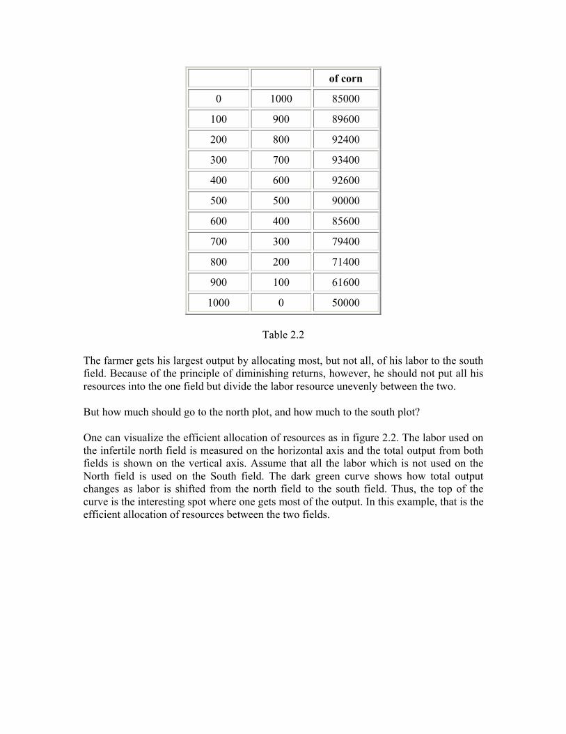
of corn
0 1000 85000
100 900 89600
200 800 92400
300 700 93400
400 600 92600
500 500 90000
600 400 85600
700 300 79400
800 200 71400
900 100 61600
1000 0 50000
Table 2.2
The farmer gets his largest output by allocating most, but not all, of his labor to the south field. Because of the principle of diminishing returns, however, he should not put all his resources into the one field but divide the labor resource unevenly between the two.
But how much should go to the north plot, and how much to the south plot?
One can visualize the efficient allocation of resources as in figure 2.2. The labor used on the infertile north field is measured on the horizontal axis and the total output from both fields is shown on the vertical axis. Assume that all the labor which is not used on the North field is used on the South field. The dark green curve shows how total output changes as labor is shifted from the north field to the south field. Thus, the top of the curve is the interesting spot where one gets most of the output. In this example, that is the efficient allocation of resources between the two fields.

Figure 2.2 Maximum production
It is easy to say that the farmer should put some labor to work on the north field but not much feasible. The vertical orange line shows that the maximum output, i.e. the top of the dark green curve comes when about 300 labor days are allocated to the north field and the rest, 700 labor days, to the south field. And that is right.
It is easy to see where the maximum is in this simple example. But in a more realistic example, in which there could be many more than just two dimensions, it is harder to visualize. One needs a rule that can be applied in more complex, realistic examples, a rule that tells if one has or has not an efficient allocation of resources.
Here comes the economist’s “marginal approach.” The objective is to get to the top of the hill. One can call “the marginal approach” the “bug’s-eye view.” Think of yourself as a bug climbing up that production hill in the picture. How will you know when you are at the top?
Marginal Productivity and Allocation
If you were a bug, you could not see much. Perhaps you could not see to the top of the hill. But you would be able to tell if you were going up, or down, or neither. So you would just keep going as long as you were going up and stop when you were neither going up nor down. That is the way a bug gets to the top of a hill.
If you were a farmer with two fields, it is a little more complicated but the same principle would apply-- take it step by step. However, no matter how much you may be producing, ask yourself, “What would happen if I were to take one worker away from the North Field and put her to work on the South Field? How much less will the North Field produce?” The answer is the marginal productivity of labor on the North Field. “How much more will the South Field produce?” The answer is the marginal productivity of labor on the South Field. So, the move of labor from the North Field will increase production if the marginal productivity on the North Field is less than the marginal

productivity on the South Field. Like the bug, you want to keep moving in that direction as long as production keeps getting greater, i.e. as long as the marginal productivity on the North Field is less than the marginal productivity on the South Field. And you stop when further movement would not get you any higher on the hill, i.e. when the marginal productivities are equal on the two fields.
So, visualize the marginal productivities for these two fields. But this time, do it a slightly different way. Measure the labor used on the infertile north field from left to right on the horizontal axis. Then, what is left is what is available for the north field. So, measure the labor used on the south field from left to right, i.e. from 1000 hours down to zero. The marginal product on the north field is shown with the green line and the marginal product on the south field with the vertical-dashed purple line. One should always remember that the marginal productivity on the south field decreases, as the labor input on the south field gets bigger. So, the marginal productivity on that field increases, as labor used on the field gets smaller.
Figure 2.3 Marginal productivity and efficient allocation
Marginal Productivity
Figure 2.4 shows the most efficient allocation of resources in this case. It is to allocate 300 hours of labor to the north field and 700 hours to the south field, as shown by the vertical red-orange line. For the maximum output, labor is allocated so that the marginal productivity of labor on the north field is equal to the marginal productivity of labor on the south field.

Figure 2.4 Efficient allocation
What happens if the allocation of labor is not 300 to the north field and 700 to the south field?
For example, suppose 200 hours are allocated to the south field and 800 to the north field. This puts us to the left of the orange line and we read off the diagram that the marginal productivity of labor on the north field is 80 bushels of corn while the marginal productivity on the south field is about 62. Remembering the definition of marginal productivity, that means if the farmer spends one additional hour on the north field, he will gain 80 bushels while spending one less on the south field will cost him 62 bushels, leaving a net gain of 18 bushels. What has happened is that spending 800 hours of labor on the south field has pushed the “diminishing returns” on that field so far that it is less productive at the margin than the north field and that will be true anywhere to the left of the orange line. Since, in that range, the marginal productivity on the north field is always greater than the marginal productivity on the south field.
What happens if the allocation is to the right of the most efficient one, i.e. for example, suppose the farmer were to allocate 600 hours to the north field and 400 to the south field?
Looking at the diagram, one may see that the marginal productivity on the north field is 40 while the marginal productivity on the south field is 90. Thus, moving an hour of labor from the north field to the south field will yield a gain of 90-40 = fifty bushels of corn. And the farmer will continue to gain as he moves toward the efficient allocation from the right because, in that range, the marginal product on the south field is always bigger than the marginal product on the north field.
The farmer can gain by reallocating his labor from either side toward the efficient output. Once he has 300 hours of labor on the north field and 700 on the south, the farmer cannot increase his output any further. That is why it is the “efficient” allocation of resources.
Marginal Productivity and the Equimarginal Principle
This is a quite general principle which can be stated as follows:
Rule: When the same product or service is being produced in two or more units of production, in order to get the maximum total output, resources should be allocated among the units of production in such a way that the marginal productivity of each resource is the same in each unit of production.
This example may also be a little clearer example of what we mean by “efficient allocation of resources.” In the example, we have a tiny economy consisting of one farmer and two plots of land. When the marginal productivities on the two plots are equal, this tiny economy has an “efficient allocation of resources.” Ofcourse, real economies are more complex but the principles governing the efficient allocation of resources are the same.
This rule is called as the “Equimarginal Principle.” The idea is to make two things equal “at the margin.” In this case, one has to make the marginal productivity of labor equal to the two fields. It has many applications in economics. In more complicated cases, one will have to generalize the rule carefully. In this example, for instance, you are allocating resources between two fields that produce the same output. When the different areas of production are producing different kinds of goods and services, it will be more complicated. But a version of the Equimarginal Principle will still apply.

Lesson-18
A Firm and its Production

An exchange is a voluntary agreement between two people in which each gives something to the other and gets in return something that he considers of greater value. When John and Jim exchange baseball cards, John gets cards that he considers more valuable than those he gives to Jim. And Jim gets cards that he considers more valuable

than those he gives to John. Unless both sides of the exchange feel that the exchange benefits them, the exchange will not take place. Because both sides get benefit, exchange is, in the terms of game theory, a positive-sum game.
An alternative to interaction by exchange is interaction that involves coercion. With coercion, the actions of one side are not voluntary but forced. If Jim takes baseball cards away from John and threatens to beat him up if he complains, one has interaction based on coercion. Economics focuses almost exclusively on interactions based on exchange and ignores those based on coercion. As a result, it has much more to say about markets than about government which is the primary agent of coercion in society.
People engage in exchange to attain goals. Exchange is not just to take in order to get. People should do things that they do not want to do in order to get things that they desire. The unpleasant part of this process is work and production and the pleasant part is consumption. Work and production are pursued because without them one cannot consume. This division of economic life is illustrated below in what Frank Knight called the “Wheel of Wealth” but which is now more commonly known as “circular flow.”
Figure 1.1
The circular flow diagram divides the economy into two sectors-- one concerned with producing goods and services and the other with consuming them. Resources are converted into goods and services by business and in this transformed state, travel back to consumers. Money flows in the opposite direction. These flows involve two markets in which exchange takes place-- the resource or factor market in which business buys resources and the goods and services market in which business sells goods. Some of the economists define a “factor of production” as the service of some resource. If resources are land, labor and capital, the factors of production are the services of land, labor and capital.
Both the model of supply and demand and consumer choice with utility analysis are key elements of an understanding of exchange economy. However, this group of readings emphasizes the right side of the circular flow diagram, examining the business firm and the constraints or limitations that it has to face in its fight for survival.

Three Fundamental Tasks
The right side of the circular flow diagram shows the three fundamental tasks of all the firms in an exchange economy. These are as follows:
1. A firm should obtain inputs-- Inputs include raw materials, energy, machinery, office space, workers and anything else needed to produce output.
2. A firm should combine or use inputs to produce output-- Output may either be a tangible good such as a pair of shoes or an automobile, or a service such as a haircut or a medical checkup.
3. A firm should sell its output to someone else.
Figure 11.2
A firm that cannot do these three tasks well enough will not survive. When the automobile was developed in the early 20th century, firms that made carriages died because they could no longer do task three, selling their output in an effective manner. Almost all the baskets sold in the United States are imported. Baskets are handmade and no firm in the United States can hire workers at wages lower enough to be able to compete with wages that are acceptable in some other countries. Here is a case in which American firms (or firms in any industrialized nation) have difficulty coping with the first task. The development of the electronics industry is a case in which the second task has changed. New technology allows firms to combine inputs to produce goods that were not possible just a few years ago.
The economic theory of a firm is an analysis of the way a firm should perform the following three tasks to make a profit: (Each task can be described in mathematical or graphical terms)
1. Supply curves of resources-- They indicate how much a firm should pay for the amount of input it wants.
2. The production function-- It tells how much output a firm can produce from a set of inputs.

3. The demand curve for output-- It depends on people’s wants or preferences and tells how much a firm can charge for output.
Each of these mathematical ways of representing the three fundamental tasks can be seen as a constraint or limitation that a firm faces.
A supply-of-resources curve tells at what prices various amounts of a resource can be bought or hired. Though one can view it in a number of ways yet it can also be viewed as a boundary. It tells a firm the minimum it can pay for any amount of a resource. The sellers of resources imposed this boundary on a firm which should buy resources in order to produce. Points to the upper left of a supply curve are attainable whereas those to the lower right are not.
The production function contains information about how much output can be obtained with various quantities of inputs. The production function is often discussed as a relationship between inputs and output, as its name implies. Mathematically, a function is a special sort of relationship. However, it too can be discussed as a boundary. It shows the maximum that can be produced with any combination of resources.
The demand curve can be viewed from a number of perspectives, such as a relationship between price and quantity buyers will buy, as a locus of points of consumer equilibrium, as a measure of marginal benefit to a buyer, or as a boundary. The view that a demand curve represents a boundary that buyers impose on the seller is most useful while developing the theory of a firm. The demand curve limits the amount that sellers can sell at each price. Points to the left of the demand curve are attainable while those to the right are not.
Production and Supply
For investigating the foundations of supply and demand, it is necessary to look at demand and supply as separate headings. Historically, the first stages of the economists’ Reasonable Dialog were focused more on supply. In investigating the foundations of supply, you are investigating the economics of production and that was the central topic for the classical economists.
Adam Smith was very optimistic about the future economic development of the industrializing countries. With increased division of labor leading to higher wages and growing demand, he felt that production could continue to grow. However, Thomas Malthus criticized Smith’s optimism. Malthus spoke for the pessimistic view and, ofcourse, Malthus is best known for his claim that increasing population would lead to poverty. In supporting this idea, Malthus began to study the limits on production. It was this study that has made his work important particularly for Neo-classical economics.
Limits on production stem from limited resources with a given technology. With a given technology, limited quantities of inputs will yield only limited quantities of outputs. The

relationship between the quantities of inputs and the maximum quantities of outputs produced is called the “production function.”
The “production function” is a relationship between quantities of input and quantities of output that tells the greatest output that can be produced with each quantity of input. Malthus did not work out the details but he clearly had this idea in mind as he originated the key concept of diminishing returns.
Diminishing Returns
Malthus is best known for his pessimistic idea that population growth would force incomes down to the subsistence level. Malthus argued that land is a fixed input but the growth of population makes labor a variable input. Malthus proposed a general law of economics which is known as the Law of Diminishing Returns. This law is as follows: When a fixed input is combined in production with a variable input, using a given technology, increases in the quantity of the variable input will eventually depress the productivity of the variable input. Malthus argued that decreasing productivity of labor would depress incomes. And he was right. There is plenty of evidence both observational and statistical that the Law of Diminishing Returns is valid. For example, agricultural economists have carried out experimental tests of the theory. They selected plots of land of identical size and fertility and used different quantities of fertilizer on the different plots. In this example, land was the fixed input and fertilizer the variable input. They found that as the quantity of fertilizer increased, the productivity of fertilizer declined. This is only one of many bits of evidence that the Law of Diminishing Returns is true in general.
On the other hand, in the two hundred years since Malthus wrote, on the whole, population has increased but labor productivity and incomes have not declined. On the whole, they have risen. What seems to have happened is that the technology has improved. Malthus recognized that if technology improved (in agriculture, at least), that might postpone what he saw as the inevitable poverty as a consequence of rising population. Some of the economists and other people believe that the Malthusian prediction will eventually come true. Perhaps, in two hundred years it has not.
But that does not mean the Law of Diminishing Returns is wrong. A law such as this can be true in general but cannot be applied when its assumptions (such as an unchanging technology) are not true. The law is not wrong but just inapplicable to that case.
There are many valid and useful applications of the Law of Diminishing Returns in economics. Two of them are as follows:
• We will use diminishing returns and related concepts to get a better idea of the meaning of the phrase “efficient allocation of resources” and some guidelines for efficiency in that sense

• We will explore how a business firm should direct its production in order to get maximum profits for a better understanding of the economics of supply
The Production Function
Production is the transformation of inputs into outputs. Inputs are the factors of production, i.e. land, labor and capital plus raw materials and business services.
The transformation of inputs into outputs is determined by the technology in use. Limited quantities of inputs will yield only limited quantities of outputs. The relationship between the quantities of inputs and the maximum quantities of outputs produced is called the “production function.”
But how do these outputs change when the input quantities vary? Let us take a look at the following example of a production function:
When most of the people think of fundamental tasks of a firm, the first thing that comes to their minds is that of production. The economists describe this task with the production function which is an abstract way of discussing how a firm gets output from its inputs. It describes, in mathematical terms, the technology available with a firm.
A production function can be represented in a table such as the one given below. In the table 1.1, five units of labor and two of capital can produce 34 units of output. It is, of course, always possible to waste resources and to produce fewer than 34 units with five units of labor and two of capital. But the table 1.1 indicates that no more than 34 can be produced with the technology available. The production function, thus, contains the limitations that technology places on a firm.
A Production Function Labor 5 30 34 37 4 26 30 33 3 21 25 28 2 16 20 23 1 10 13 15 1 2 3 Capital
Table 1.1
The production function can also be illustrated in a graph such as the one given below. The figure 1.1 looks exactly like a graph of indifference curves because the mathematical forms of the production function and the utility function are identical. In one case, inputs

of goods and services combine to produce utility and in the other, inputs of resources combine to produce goods or services. A curved line in the graph shows all the combinations of inputs that can produce a particular quantity of output. These lines are called isoquants. As one moves to the right, one reaches higher levels of production. If one can visualize this as a three-dimensional graph, one can see that the production surface rises increasingly high above the surface of the page. The isoquants indicate a hill. A firm should operate on or below this surface.
Figure 1.1
Marginal Productivity
Productivity, by definition, is a ratio of output to labor input. In most of the statistical discussions of productivity, one refers it to the average productivity of labor as follows:
Average labor productivity is an important concept especially in macroeconomics. In microeconomics, however, focus should be more on the marginal productivity. One can think of the marginal productivity of labor as the additional output as a result of adding one unit of labor with all other inputs held steady and ceteris paribus.
In algebraic terms, an equally correct definition is as follows:
Let us have a numerical example to illustrate the application of the theory. Suppose that:

• When 300 labor-days per week are employed, a firm produces 2505 units of output per week
• When 400 labor-days per week are employed, a firm produces 3120 units of output per week
• It follows that the change in labor input, labor is 100. • It also follows that the change in output, output is 615. • Applying the formula, one may approximate the marginal productivity of labor by
the quotient 615/100 = 6.15.
This result can be interpreted as follows:
Over the range of 300 to 400 man-days of labor per week, each additional worker adds approximately 6.15 units to output.
Ofcourse, if one had more information, one could get a closer approximation. For example, if one had the outputs for 310, 320, ... 390 man-days of labor, one could see how marginal productivity varies within the range 300-400. But one can be sure that the values will be in the neighborhood of 6.15.
Let us extend the numerical example and see how marginal productivity varies over a wide range of labor inputs. Here is a hypothetical example of production with the inputs of land and labor held steady and varying quantities of labor, and the output and average and marginal productivities.
Labor Output Average Productivity Marginal
Productivity
0 0 0
9.45
100 945 9.45
8.35
200 1780 8.90
7.25
300 2505 8.35
6.15
400 3120 7.80
5.05
500 3625 7.25
600 4020 6.70 3.95

2.85
700 4305 6.15
1.75
800 4480 5.60
0.65
900 4545 5.05
-0.45
1000 4500 4.50
Table 1.2
Average and Marginal Productivity
Both average and marginal productivity are important, but for a model of short-run profit-maximizing supply, marginal productivity is the more important.
Following is the average and marginal productivities for the same numerical example. It should be noticed how both average and marginal productivity decrease as the labor input increases. But the marginal productivity declines faster than the average productivity, pulling the average productivity down after it. The downward slope of the marginal productivity line expresses the Law of Diminishing Returns and the downward slope of the average productivity is also a result of the law.
Figure 1.2
Average and marginal productivity

The relationship between average and marginal productivity in the diagram is important in itself. Average and marginal productivity will not always have the same slope. In general, whenever average productivity is greater than marginal productivity, average productivity will slope downward. And whenever, average productivity is less than marginal productivity, average productivity will slope upward. Figure 1.2 does not show any values where average productivity is less but a more complicated example might show and then we would see the second part of the relationship visualized.
To understand the relationship, think as one adds labor input one unit after another, one adds a bit more to output at each step. When the addition is greater than the average, it pulls the average up toward it. When the addition is less than the average, it pulls the average down toward it.
The Law of Diminishing Marginal Productivity
In the discussions of the Law of Diminishing Returns, Malthus did not distinguish between average and marginal productivity. However, in modern economics, one thinks of diminishing returns primarily in terms of marginal, not average, productivity. Thus, the modern statement of Law of Diminishing Returns is as follows: When the technology of production and some of the inputs are held constant and the quantity of a variable input increases continually, the marginal productivity of the variable input will eventually decline. The inputs that are held steady are called the “fixed inputs.” The inputs that are allowed to vary are called the “variable inputs.”
Another way to express the Law of Diminishing Returns is as follows:
As the variable input increases, the output also increases but at a decreasing rate. The marginal productivity of labor is the rate of increase in output as the labor input increases. To say that output increases at a decreasing rate when the variable input increases is another way to say that the marginal productivity declines.
Figure 1.3 shows the relationship between the variable input and the output in the numerical example in the previous table. It should be noticed how the slope gets flatter. As the variable input increases, output increases at a decreasing rate. This is a visualization of the Law of Diminishing Marginal Productivity.

Figure 1.3
Production with Diminishing Returns
There is one rule that seems to hold for all production functions and because it always seems to hold, it is called a law. The Law of Diminishing Returns says that adding more of one input while holding other inputs constant results eventually in smaller and smaller increases in added output. To see the law in the table 1.1, one should follow a column or row. If capital is held constant at two, the marginal output of labor (which economists usually call marginal product of labor) is shown in the table 1.3. The first unit of labor increases production by 13 and as more labor is added, the increase in production gradually falls.
Marginal product is the change in output with the increase of one additional unit of input.
The Marginal Product of Labor Labor Marginal Output First 13 Second 7 Third 5 Fourth 5 Fifth 4
Table 1.3
The Law of Diminishing Returns does not take effect immediately in all production functions. It is possible for the first unit of labor to add only four units of output, the second to add six and the third to add seven. If a production function had this pattern, it would have increasing returns between the first and third worker. The Law of Diminishing Returns says that as one continues to add workers, eventually one will reach a point where increasing returns stop and decreasing returns set in.

The Law of Diminishing Returns is not caused because the first worker has more ability than the second worker and the second is more able than the third. By assumption, all workers are the same. It is not ability that changes but rather the environment into which workers (or any other variable input) are placed. As additional workers are added to a firm with a fixed amount of equipment, the equipment should be stretched over more and more workers. Eventually, the environment becomes less and less favorable to the additional worker. People’s productivity depends not only on their skills and abilities but also on the work environment they are in.
The Law of Diminishing Returns was a central piece of economic theory in the 19th century and accounted for the economists’ gloomy expectations of the future. They saw the amount of land as fixed and the number of people who could work the land as variable. If the number of people expanded, eventually adding one more person would result in very little additional food production. And if population had a tendency to expand rapidly, as economists thought it did, one would predict that (in equilibrium) there would always be some people almost starving. Though history has shown the gloomy expectations wrong, the idea had an influence on the work of Charles Darwin and traces of it still float around today among environmentalists. The second boundary that limits a firm is the demand curve for output.
Demand Curve for Output
Once a firm has produced a product, it has to sell it. The demand curve for output describes the limitations the firm faces in doing this task. The demand curve for output is a constraint on the firm because it gives the maximum price that a firm can charge for each level of production. Thus, if a firm in the figure 1.4 wants to sell 24, it can do so by charging Rs.5 or any price that is lower. It cannot charge Rs.10 and still sell 24 because buyers will not allow it.
Figure 1.4
The demand curve facing a firm depends both on the preferences of consumers and on how well other firms meet those preferences. One can derive a demand curve for an individual from a set of indifference curves showing the individual’s preferences and a

series of budget lines showing changes in price. To get a demand curve for the entire industry, one should add up all the demand curves of individuals. To get the demand curve for eggs, for example, one needs to add up the number of eggs that Smith, Jones and Nelson and all other consumers in the market want at each possible price.
When there is only one firm selling in a market, that firm is a monopolist. The Greek root mono means “one.” The demand curve for the monopolist is the demand curve for the industry. A monopolist is a price searcher or a price maker. It will search along the demand curve for the price-quantity pair that is most profitable. When there is more than one seller, the demand curve that a seller sees is not the same as the demand curve for the industry. The industry demand is split up among sellers. When there are only a few sellers, the sellers will still be price searchers or price makers. These sellers or oligopolists (the Greek root oli means “few”) are price makers because each recognizes that if it wants to sell more, it should lower its price.
However, the demand curve of each oligopolist will be more elastic than the demand curve for the industry as a whole. Suppose, for example, there are two firms in an industry, each produces 50 units of output and the elasticity of the industry demand curve is one. If one firm increases its output by 10% to 55, the industry output increases to 105 which is a 5% increase. Since the price elasticity of demand is one, price should decline by 5%. But for the original firm, a 10% increase in production and a 5% decline in price indicate a price elasticity of two, not one.
As firms get more and more numerous in an industry, the demand curve each sees gets more and more elastic. When there are many sellers in a market, a change of output by any one of them has an insignificant effect on price. To each firm, the demand curve will look perfectly flat. The firm will seem able to sell whatever amount it wants at a fixed price. In this case, each firm is a price maker and sells in a perfectly competitive market. An example of this type of market is the market for wheat. There are many wheat farmers in many countries and none has any noticeable control over the price at which it can sell in the world wheat market.
However, even when there are a great many sellers, each firm may have a downward-sloping demand curve. If buyers expend time and effort to discover prices or the characteristics of the product, they pick a seller and stay with it as long as they find the exchange satisfactory. These downward-sloping demand curves of small sellers are results of the ambiguous definitions of an industry. The products which are produced by most of the firms differ in some way, such as in quality, service or location and from the products of other firms in the industry.
From the viewpoint of a firm, it is not the demand curve but the child of the demand curve, the marginal revenue curve, which is of vital importance. Marginal revenue is the extra revenue which a seller gets when it produces and sells another unit. For the price maker, the marginal revenue curve is the demand curve. For a farmer who can sell corn at Rs.4 a bushel, the extra revenue from selling another bushel is Rs.4. The demand curve for this farmer is flat at Rs.4 and so is his marginal revenue curve.

Table 1.4 illustrates why marginal revenue will be less than price for a price searcher. If a firm charges Rs.3, it can sell one unit and total revenue will be Rs.3. If it sells one more unit, it will be forced to cut price to Rs.2 and total revenue will rise to Rs.4. Selling the extra unit adds only Re.1 to revenue. Although the second unit sold for Rs.2, the firm had to cut the price it was previously receiving for the first unit by Re.1, so the net increase in revenue was only Re.1. By similar logic, selling the third unit reduces total revenue by Re.1, so marginal revenue is Re.1.
Demand and Marginal Revenue Price Quantity Marginal Revenue Rs.3.00 1 . . Rs.1.00 Rs.2.00 2 . . -Rs.1.00 Rs.1.00 3 .
Table 1.4
The previous analysis assumes that a firm can charge only one price. If it charges more than one price, i.e. charge higher prices to those willing and able to pay them and lower prices to others, it can move the marginal revenue curve closer to the demand curve by increasing profits or reducing losses. This pattern of pricing is called price discrimination.
The economists generally assume that a demand curve is fixed but many businesses do not regard it that way. It can vary seasonally with the general level of business activity or with a trend. The demand for turkeys has a pronounced seasonal movement. The demand for automobiles changes during recession. The demand for baby food follows the trends in birth rate.
A business may also be able to move its demand curve through advertising. Advertising may simply give people information, it may change their goals or it may change their perception of the product. For a firm, it does not matter which happens. The result is the same-- good advertising moves the demand curve to the right.
The demand curve can move for other reasons also. If a firm lowers its price and later raises it back to its previous level, it may find that sales at the old price have changed. The lower price may attract new customers who have not tried the product before and who find they like the product enough to stick with it when the old price is restored. Alternatively, some customers may expect prices to be cut again sometime in the future and may decide to postpone its purchase until it happens again. The opposite can happen if a firm temporarily raises price. It may encourage some customers to try substitutes which they may find suit them better than the original product. Or it may encourage the customers to buy more when the price comes down to prepare for any future increase.

A firm may also be able to change its demand curve by changing the characteristics of its product. Finally, many firms sell several products that may be interrelated and any pricing decision on one product will affect not only that product but others also. For example, the prices that General Motors charges for Chevrolets will affect the demand curve for Pontiacs.
The third and final boundary the firm faces is the supply curve for resources.
Supply of Resources
The third task of a firm is to obtain resources needed to produce a product. For each resource, a supply curve shows limitations that a firm faces. These supply curves are based on the preferences of sellers and on the actions of other firms which use the resource.
Because a market demand curve can be derived from utility curves and a budget line, it may seem surprising that a supply curve can also be derived from the same procedure. To see that it can, refer to figure 1.5 which shows indifference curves for income and leisure. Income is desirable because one can obtain other desirable things with it and leisure is desirable because it lets one enjoy his/her income.
Figure 1.5
In today’s world, a greater amount of income needs to be purchased with more work which means less leisure. The tradeoff between leisure and income as shown by the budget line depends on the wage rate. If the wage rate is Rs.10, options open to an individual include 24 hours of leisure and no income or 20 hours of leisure and Rs.40 of income, or 10 hours of leisure and Rs.140 of income.
To get a supply curve for labor, one should see what happens if the wage rate changes. Two wage rates are shown in the figure 1.5. At the higher wage rate, an individual wants less leisure which means he will work more as wages rise, but one could easily draw indifference curves that show the amount of leisure rising as wages rise which means he will work less as wages rise. Higher wages have two effects on the leisure-work decision

and these two effects pull in opposite directions. A higher wage rate increases the benefits of working, causing people to substitute work for leisure. This is called the substitution effect and is caused by changes in the slope of the budget line. Higher wages also increase income and people want more leisure with a higher income. This is called the income effect of a price change and is caused by changes in the distance of the budget line from the origin.
Usually the substitution and income effects reinforce each other but they pull in opposite directions and almost cancel out each other in the case of labor. Most of the economists believe that the market supply curve for labor found by adding up all the supply curves of individuals is close to a horizontal line.
Supply curves for other resources can be obtained in similar ways. The supply curve for capital, for example, depends on decisions of people to consume now or to consume in the future. People who prefer to consume in the future will save and make funds available to finance capital. Their “time preference” determines the shape of indifferent curves. The slope of the budget line depends on the interest rates. The budget line tells how much one can get in the future if one sacrifices consumption now.
Although the market supply curve for labor may be almost vertical yet a few firms see this supply curve. If many other firms are also buying labor, what one firm does may have little effect on the overall market. If a firm is so small in the market that it can see no effects at all on the wage from its hiring decisions, it is a price taker. If it has some effect on wages so that it finds that wages rise when it wants to hire more, the firm is a price maker. The extreme case of a price maker is a monopsonist, i.e. the case of only one buyer in the market. The supply curve for a resource that a monopsonist sees is the same as the market supply curve.
The supply curve for a resource is a constraint or boundary on a firm because it shows the minimum that a firm can pay for a level of the resource. If a firm is a price taker in the resource market, it will face a horizontal supply curve such as that in the figure 1.6. This curve indicates that any number can be bought at P1 with no effect on price. There is no way a firm can attain point “a” even though it might prefer to pay less than P1 because no one will sell at less than P1. Sellers will not sell because of the assumption that there were many other buyers of the resource who will pay P1. Point “c” is possible but a waste of money because the same amount of the resource could be bought for less.

Figure 1.6
If a firm is one of a few buyers or the only buyer of a resource, it may face a supply curve with an upward slope making it a price searcher. It can obtain quantity Q1 if it pays P1 but it should pay more than P1 if it wants quantity Q2.
There are similarities between a supply curve for a resource and a demand curve for output. Both are boundaries and the curve a firm faces may differ from the market curve. The similarity goes further because there is a counterpart for marginal revenue called “marginal resource cost” which measures the extra cost to the firm for hiring one more unit of the resource.
When a firm is a price taker, marginal resource cost is the same as the price of the resource. If a firm can hire as many workers as it wants at Rs.10 per hour, hiring one more hour of labor adds Rs.10 to costs. Marginal resource cost and the supply of labor are both horizontal lines in this case.
When a firm is a price searcher facing an upward-sloping supply curve, the extra cost of hiring another unit of the resource is different from the price of the extra unit. Table 1.5 illustrates the reason for this difference. If a firm wants to buy two units, it cannot pay Re.1 and get two. It should be willing to pay Rs.2 for each. However, the added cost of the second unit is not Rs.2, but Rs.3. This can be shown by comparing the total cost of two units and one unit or Rs.4 less Re.1. The added cost of the second unit is not only the two rupees that should be paid for it but also an added rupee for the first one. By the same logic, the added cost of a third unit is Rs.5.
Computing Marginal Resource Cost
Quantity Price Marginal Resource Cost
1 Rs.1.00 Rs.1.00 2 Rs.2.00 2.00 + 1.00 3 Rs.3.00 3.00+2.00

Table 1.5
The marginal resource cost curve lies above an upward-sloping supply curve because of the assumption that a firm can pay only one price. This is often a realistic assumption. If a firm hires two clerks who do exactly the same work and pays one Rs.4.00 per hour and the other Rs.6.00 per hour, the lower-paid one will be unhappy and may refuse to work for the lower pay. On the other hand, many firms do not publicly disclose their payments to various people and discourage employees from discussing salaries. To the extent that people are unaware of what others are earning, a firm may be able to pay different prices for the same resource, or in an economists’ jargon, to price discriminate. Price discrimination will pull down the MRC curve in the graph closer to, or perhaps even onto, the supply curve.
Figure 1.7
Summary
A business should deal with three constraints or boundaries which are as follows:
1. The demand curve for output 2. The production function 3. Supply curves for inputs
Table 1.6 shows how these concepts are related to the functions of the business and to the marginal concepts that are central in microeconomics.
The Constraints Facing the Firm
Task EconomicConcept
LimitationImposed by
Relationshipbetween
Marginal Concept
Buying inputs
Supply ofresources
Resource owners
Price (money)and amountof resource
Marginal resource cost
Producing Production Technology Inputs and Marginal

output function output product Selling output
Demand curve Customers Output and
price (money)Marginal revenue
Table 1.6
The importance of these three constraints can be seen in a product that no firm can produce at a profit. Any one of three changes, if large enough, can change the situation and make a profit possible. The cost of the inputs may drop in enough price to make a product profitable. Technology may also improve enough to make the product profitable. People may also increase the amount they are willing to pay for the product enough so that it is profitable. These three changes are changes in the supply-of-resources curves, the production function and the demand curve respectively.
Application
Diminishing returns plays an important part in the efficient allocation of resources. For efficiency, ofcourse, one wants to give more resources to the use in which they are more productive. But as one gives more resources to a particular use, one will observe diminishing returns whose use will become less productive. That may sound frustrating but, infact, it leads to a very important principle which one can apply to the problem of efficient allocation of resources.

Chapter-17
Theory of Production After reading this lesson, you would be able to:
1. Define production function, isoquants, marginal product, price discrimination, monopsonist and the all-or-nothing demand curve.
2. Define increasing, decreasing and constant returns to scale. 3. Distinguish between income and substitution effects. 4. Distinguish between an individual buyer’s demand curve and the industry
demand, and between industry demand and the demand curve facing an individual seller.
5. Compute marginal revenue from the demand curve of the seller when that demand curve is given in the form of a table.
6. Compute marginal resource cost from the supply curve of the buyer when supply curve is given in the form of a table.
7. Explain why marginal resource cost equals price for a buyer who is a price taker. 8. Explain why marginal revenue equals price for a seller who is a price taker, and
why marginal revenue is less than price for a seller who is a price maker. 9. Explain what the law of diminishing returns is and under what conditions it holds. 10. Explain why the demand curve, the supply curve for resources and the production
function can be treated as boundaries. Though economists are interested in many cases of unintended consequences yet the unintended consequences that involve businessmen seeking their own gain have been at the heart of economic analysis. Smith noted that, “It is not from the benevolence of the butcher, the brewer, or the baker, that we expect our dinner, but from their regard to their own interests. We address ourselves, not to their humanity but to their self love, and never talk to them of our necessities but of their advantages.” Since Smith, a great deal of intellectual effort has gone into exploring the question that under what conditions the interests of society will be served by businessmen seeking to make a profit. This question is, infact, the core of microeconomics. The reading selections present background material to this exploration by explaining a large number of technical terms that economists use and also by looking at a few of the simplifying assumptions they generally invoke.

Slide 1 Overview
I. Production Analysis– Total Product, Marginal Product, Average Product– Isoquants– Isocosts– Cost Minimization
II. Cost Analysis– Total Cost, Variable Cost, Fixed Costs– Cubic Cost Function– Cost Relations
III. Multi-Product Cost Functions
___________________________________ ___________________________________ ___________________________________ ___________________________________ ___________________________________ ___________________________________ ___________________________________
Slide 2 Production Analysis
• Production Function– Q = F(K,L)– The maximum amount of output that can
be produced with K units of capital and L units of labor
• Short-Run vs. Long-Run Decisions• Fixed vs. Variable Inputs
___________________________________ ___________________________________ ___________________________________ ___________________________________ ___________________________________ ___________________________________ ___________________________________
Slide 3 Production functions
Example-- Calvin has expanded his operation. Taking his lemonade profits, he has integrated upstream, buying the local supplier of lemonade cups. His engineer (former management consultant Hobbes) has given Calvin a table of output and input combinations which is as follows:
labor0 5 10 15 20 25 30 35 40
capital 0 0 0 0 0 0 0 0 0 05 0 20 46 73 101 129 156 182 20610 0 31 70 111 150 188 223 255 28415 0 40 90 140 187 231 269 302 32920 0 49 107 164 217 263 302 333 35625 0 56 122 185 241 289 327 354 37030 0 63 135 203 262 310 345 366 37435 0 69 148 220 280 327 358 373 37040 0 75 159 234 295 340 366 373 36045 0 80 169 247 309 351 372 370 34550 0 86 179 259 320 359 374 363 32555 0 91 188 270 331 365 373 352 30160 0 96 197 281 339 370 370 338 274
___________________________________ ___________________________________ ___________________________________ ___________________________________ ___________________________________ ___________________________________ ___________________________________

Slide 4
0 5 10 15 20 25 30 35 400
15
300
50
100
150
200
250
300
350
400
output
labor
capital
Production with IRS and DRS ranges
350-400300-350250-300200-250150-200100-15050-1000-50
The red line marks the totalproduct of capital for a givenquantity of labor (30 units)
A mapping of the production data
___________________________________ ___________________________________ ___________________________________ ___________________________________ ___________________________________ ___________________________________ ___________________________________
Slide 5
0 5 10 15 20 25 30 35 4005101520
25303540
0102030405060708090100
110
120
130
140
150
160
170
180
190
200
210
220
230
240
250
260
270
280
290
300
310
320
330
340
350
360
370
380
labor
capital
Production with IRS and DRS ranges370-380
360-370
350-360
340-350
330-340
320-330
310-320
300-310
290-300
280-290
270-280
260-270
250-260
240-250
230-240
220-230
210-220
200-210
190-200
The colored bands mark inputcombinations for a given level ofoutput. These are called isoquants.
A view from the top -- isoquants
___________________________________ ___________________________________ ___________________________________ ___________________________________ ___________________________________ ___________________________________ ___________________________________
Slide 6 Mathematical relationshipsThe production function relates output to inputs
The marginal product relates changes in output to changes in one input by holding the other constant
The total product of labor is the relationship between labor input and quantity output, given capital
0,
),(
>∂∂
∂∂=
Kf
Lf
LKfQ
LQ
locallyLfMPL
∆∆
=
∂∂
= )(
),( KLfTPL =
___________________________________ ___________________________________ ___________________________________ ___________________________________ ___________________________________ ___________________________________ ___________________________________

Slide 7 Total Product
• Cobb-Douglas Production Function• Example-- Q = F(K,L) = K.5 L.5
– K is fixed at 16 units – Short run production function:
Q = (16).5 L.5 = 4 L.5
– Production when 100 units of labor are usedQ = 4 (100).5 = 4(10) = 40 units
___________________________________ ___________________________________ ___________________________________ ___________________________________ ___________________________________ ___________________________________ ___________________________________
Slide 8 Marginal Product of Labor
• MPL = ∆Q/∆L• Measures the output produced by the last
worker• Slope of the production function
___________________________________ ___________________________________ ___________________________________ ___________________________________ ___________________________________ ___________________________________ ___________________________________
Slide 9 Average Product of Labor
• APL = Q/L• Measures the output of an “average” worker
___________________________________ ___________________________________ ___________________________________ ___________________________________ ___________________________________ ___________________________________ ___________________________________

Slide 10
Q
L
Q=F(K,L)
IncreasingMarginalReturns
DiminishingMarginalReturns
NegativeMarginalReturns
MP
AP
Stages of Production
___________________________________ ___________________________________ ___________________________________ ___________________________________ ___________________________________ ___________________________________ ___________________________________
Slide 11 With Lemonade, we have a similar pattern
The Labor Product Function
0
50100
150200
250
300350
400
0 20 40 60 80
Labor
Outp
ut
Average and marginal product
0
2
4
6
8
10
12
0 20 40 60 80
Labor
MPL &
APL
APL MPL
`
___________________________________ ___________________________________ ___________________________________ ___________________________________ ___________________________________ ___________________________________ ___________________________________
Slide 12 Time framesTo maximize profit when only labor is variable, there is a need to set MRP=wage rate
To break even, one needs to set ARP=wage rateAverage and marginal product
0
2
4
6
8
10
12
0 20 40 60 80
Labor
MPL
& A
PL
APL MPL
`
Profit maximizing point
Break-even point
Here, assume P=1,and w=8
___________________________________ ___________________________________ ___________________________________ ___________________________________ ___________________________________ ___________________________________ ___________________________________

Slide 13 Isoquant
• The combinations of inputs (K, L) that yield the producer the same level of output
• The shape of an isoquant reflects the ease with which a producer can substitute among inputs while maintaining the same level of output L
___________________________________ ___________________________________ ___________________________________ ___________________________________ ___________________________________ ___________________________________ ___________________________________
Slide 14
0 5 10 15 20 25 30 35 4005101520
25303540
0102030405060708090100
110
120
130
140
150
160
170
180
190
200
210
220
230
240
250
260
270
280
290
300
310
320
330
340
350
360
370
380
labor
capital
Production with IRS and DRS ranges370-380
360-370
350-360
340-350
330-340
320-330
310-320
300-310
290-300
280-290
270-280
260-270
250-260
240-250
230-240
220-230
210-220
200-210
190-200
The colored bands mark inputcombinations for a given level ofoutput. These are called isoquants.
A view from the top -- isoquants
___________________________________ ___________________________________ ___________________________________ ___________________________________ ___________________________________ ___________________________________ ___________________________________
Slide 15 Linear Isoquants
• Capital and labor are perfect substitutes
Q3Q2Q1
Increasing Output
L
K
___________________________________ ___________________________________ ___________________________________ ___________________________________ ___________________________________ ___________________________________ ___________________________________

Slide 16 Leontief Isoquants
• Capital and labor are perfect complements
• Capital and labor are used in fixed-proportions
Q3Q2
Q1
K
Increasing Output
___________________________________ ___________________________________ ___________________________________ ___________________________________ ___________________________________ ___________________________________ ___________________________________
Slide 17 Cobb-Douglas Isoquants
• Inputs are not perfectly substitutable
• Diminishing marginal rate of technical substitution
• Most of the production processes have isoquants of this shape
Q1
Q2
Q3
K
L
Increasing Output
___________________________________ ___________________________________ ___________________________________ ___________________________________ ___________________________________ ___________________________________ ___________________________________
Slide 18 Isocost• The combinations of
inputs that cost the producer the same amount of money
• For given input prices, isocosts farther from the origin are associated with higher costs
• Changes in input prices change the slope of the isocost line
K
LC1C0
L
KNew isocost line for a decrease in the wage (price of labor)
___________________________________ ___________________________________ ___________________________________ ___________________________________ ___________________________________ ___________________________________ ___________________________________

Slide 19 Cost Minimization
• Marginal product per dollar spent should be equal for all inputs
• Expressed differentlyr
MPw
MP KL =
rwMRTSKL =
___________________________________ ___________________________________ ___________________________________ ___________________________________ ___________________________________ ___________________________________ ___________________________________
Slide 20 Cost Minimization
Q
L
K
Point of Cost Minimization
Slope of Isocost=
Slope of Isoquant
___________________________________ ___________________________________ ___________________________________ ___________________________________ ___________________________________ ___________________________________ ___________________________________
Slide 21 Cost Analysis
• Types of Costs– Fixed costs (FC)– Variable costs (VC)– Total costs (TC)– Sunk costs
___________________________________ ___________________________________ ___________________________________ ___________________________________ ___________________________________ ___________________________________ ___________________________________

Slide 22 Total and Variable CostsC(Q)-- Minimum total cost of producing alternative levels of output:
C(Q) = VC + FC
VC(Q)-- Costs that vary with output
FC-- Costs that do not vary with output
$
Q
C(Q) = VC + FC
VC(Q)
FC
___________________________________ ___________________________________ ___________________________________ ___________________________________ ___________________________________ ___________________________________ ___________________________________
Slide 23 Fixed and Sunk Costs
FC: Costs that do not change as output changes
Sunk Cost: A cost that is forever lost after it has been paid
$
Q
FC
C(Q) = VC + FC
VC(Q)
___________________________________ ___________________________________ ___________________________________ ___________________________________ ___________________________________ ___________________________________ ___________________________________
Slide 24 Some DefinitionsAverage Total Cost
ATC = AVC + AFCATC = C(Q)/Q
Average Variable CostAVC = VC(Q)/Q
Average Fixed CostAFC = FC/Q
Marginal CostMC = ∆C/∆Q
$
Q
ATC
AVC
AFC
MC
___________________________________ ___________________________________ ___________________________________ ___________________________________ ___________________________________ ___________________________________ ___________________________________

Slide 25 Fixed Cost
$
Q
ATC
AVC
MC
ATC
AVC
Q0
AFC Fixed Cost
Q0×(ATC-AVC)
= Q0× AFC
= Q0×(FC/ Q0)
= FC
___________________________________ ___________________________________ ___________________________________ ___________________________________ ___________________________________ ___________________________________ ___________________________________
Slide 26 Variable Cost
$
Q
ATC
AVC
MC
AVCVariable Cost
Q0
Q0×AVC
= Q0×[VC(Q0)/ Q0]
= VC(Q0)
___________________________________ ___________________________________ ___________________________________ ___________________________________ ___________________________________ ___________________________________ ___________________________________
Slide 27
$
Q
ATC
AVC
MC
ATC
Total Cost
Q0
Q0×ATC
= Q0×[C(Q0)/ Q0]
= C(Q0)
Total Cost
___________________________________ ___________________________________ ___________________________________ ___________________________________ ___________________________________ ___________________________________ ___________________________________

Slide 28 Economies of Scale
LRAC
$
Output
Economiesof Scale
Diseconomiesof Scale
___________________________________ ___________________________________ ___________________________________ ___________________________________ ___________________________________ ___________________________________ ___________________________________
Slide 29
If average costs fall with output, the marginal cost is less than average cost. A measure of this is the cost disadvantage ratio:
Declining average costs reflect economies of scale.
Economies of scale
ACMCACCDR −
=
___________________________________ ___________________________________ ___________________________________ ___________________________________ ___________________________________ ___________________________________ ___________________________________
Slide 30
0 5 10 15 20 25 30 35 400
15
300
50
100
150
200
250
300
350
400
output
labor
capital
Production with IRS and DRS ranges
350-400300-350250-300200-250150-200100-15050-1000-50
In our example, we have regions of falling and rising AC
IRS range
DRS range
___________________________________ ___________________________________ ___________________________________ ___________________________________ ___________________________________ ___________________________________ ___________________________________

Slide 31 An Example
– Total Cost-- C(Q) = 10 + Q + Q2
– Variable cost function:VC(Q) = Q + Q2
– Variable cost of producing 2 units:VC(2) = 2 + (2)2 = 6
– Fixed costs:FC = 10
– Marginal cost function:MC(Q) = 1 + 2Q
– Marginal cost of producing 2 units:MC(2) = 1 + 2(2) = 5
___________________________________ ___________________________________ ___________________________________ ___________________________________ ___________________________________ ___________________________________ ___________________________________
Slide 32 Multi-Product Cost Function
• C(Q1, Q2): Cost of producing two outputs jointly
___________________________________ ___________________________________ ___________________________________ ___________________________________ ___________________________________ ___________________________________ ___________________________________
Slide 33
• Scope economies imply that joint production costs are lower than separate costs
• This means integrated production is more cost efficient
It is measured as follows:
Economies of scope
),(),()()(
21
2121
QQTCQQTCQTCQTCS −+
=
___________________________________ ___________________________________ ___________________________________ ___________________________________ ___________________________________ ___________________________________ ___________________________________

Slide 34 Economies of Scope
• C(Q1, Q2) < C(Q1, 0) + C(0, Q2)• It is cheaper to produce the two outputs
jointly instead of separatelyExamples
___________________________________ ___________________________________ ___________________________________ ___________________________________ ___________________________________ ___________________________________ ___________________________________
Slide 35 Cost Complementarities
• The marginal cost of producing good 1 declines as more of good two is produced:
∆MC1/∆Q2 < 0.
Examples
___________________________________ ___________________________________ ___________________________________ ___________________________________ ___________________________________ ___________________________________ ___________________________________
Slide 36 A Numerical Example
• C(Q1, Q2) = 90 - 2Q1Q2 + (Q1 )2 + (Q2 )2
• Cost ComplementaritySince a = -2 < 0MC1(Q1, Q2) = -2Q2 + 2Q1
• Economies of scopeSince 90 > -2Q1Q2
• Implications for merger
___________________________________ ___________________________________ ___________________________________ ___________________________________ ___________________________________ ___________________________________ ___________________________________

Slide 37 Relevant cost componentsAccounting costs often reflect historical cost. In addition, they are incompleteRelevant costs for maximization of profits are both explicit costs and implicit costs (i.e. the cost of lost opportunities or the opportunity cost of a project)Economic profit is then any return net of explicit and implicit costsCosts include sunk costs (past costs that can no longer be affected) and also incremental costsMarginal costs are a special case of incremental costsIn the short-run, one makes decisions vis-à-vis variable costs
___________________________________ ___________________________________ ___________________________________ ___________________________________ ___________________________________ ___________________________________ ___________________________________
Slide 38 • Firms are highly leveraged when fixed costs are a
high relative to variable costs
• High leverage means profit will rise(fall) faster in upswings(downswings)
• This can be measured by the profit elasticity
Operating Leverage
TFCAVCPQAVCPQQ
dQdE
−−−
=⋅=)(
)(π
ππ
___________________________________ ___________________________________ ___________________________________ ___________________________________ ___________________________________ ___________________________________ ___________________________________

Lesson-20
Theory of the Firm
For developing the supply and demand approach to economics, the economists first worked out the basis of the demand curve. By treating the demand for a product or service as a rational decision by a (primarily) self-interested individual or family, the economists were able to understand the relation of the demand for one product or service to the demands for other products and services and to many other forms of economic activity. It was natural to apply the same approach to supply. As a first step, one needs to think about the decision-makers in supplying goods and services and what a “rational decision” to supply goods and services would mean. In economics, this is often called the “theory of the firm.” A firm is a unit that does business on its own account. Firm is from the Italian word, firma, a signature and the idea is that a firm can commit itself to a contract. Thus, a firm is the decision-maker in supplying goods and services.
There are three main kinds of firms in modern market economies which are as follows:
Proprietorships A proprietorship (or proprietary business) is a business owned by an individual known as the “proprietor.” Many “mom and pop stores” and other “mom and pop” businesses are proprietorships. Some of the proprietorships are too small even to employ a person full time. Craftsmen, such as plumbers and painters, may have “day jobs” and work as self-employed proprietors part time after hours. The computer programmers and others may also do that. At the other extreme, some proprietary businesses employ many hundreds of workers in a wide range of specializations. In a proprietorship, a proprietor is almost always the decision-maker for the business. Partnerships A partnership is a business jointly owned by two or more persons. In most of the partnerships, each partner is legally liable for debts and agreements made by any partner. Ofcourse, this requires a great deal of trust and thus, partners generally know one another well enough to have that sort of trust. Family partnerships are very common for that very reason. There are now a few “limited partnerships” in which some of the partners are protected from legal liability for the agreements made by others, beyond some limits. In many cases, one partner is designated as the managing partner and is the main decision-maker for the business. Corporations A corporation has two characteristics that distinguish it from most of the proprietorships and partnerships which are as follows:

• Limited liability • Anonymous ownership
Limited liability means that the owner of shares in a corporation cannot lose more than a certain amount if the company fails. Usually, an amount is the money paid to buy the shares. Anonymous ownership means that the owner of the shares can sell them without getting the permission of anyone other than the buyer. By contrast, in most of the partnerships, no single partner can sell without getting the agreement of the other partners. In such a case, the continuing partners will, ofcourse, want to know about the new partner. And he will not be an “anonymous owner.” In a typical corporation, the shareholders formally elect a board of directors who, in turn, select the officers of the company. One of these officers, often called the “president,” will be the principal decision-maker for the firm but he will be expected to make decisions in the interest of the shareholders.
While there are millions of proprietorships, typically very small, the biggest businesses are corporate and corporations are particularly important because of their size.
Objectives
Malthus did not have firms in mind when he formulated the law of diminishing returns. But this law has applications which Malthus did not envision. In the Reasonable Dialog of economics in the nineteenth century, the development of these ideas was a bit indirect. In circa eighteen-seventies, the economists were rethinking the theory of consumer demand. They applied a version of “diminishing returns” and the Equimarginal Principle to determine how a consumer would divide his/her spending among different consumer goods. That worked pretty well and, therefore, some other economists, especially the American economist, John Bates Clark, tried using the same approach in the theory of the firm. These innovations were the beginning of neoclassical economics.
By following the neoclassical approach, one may interpret “rational decisions to supply goods and services” to mean decisions that maximize something. What does a supplier maximize? The operations of a firm will, ofcourse, depend on its objectives. One of the objectives that all the three kinds of firms share is profits and it seems that profits are the primary objective in most of the cases. We will follow the neoclassical tradition by assuming that the firms aim at maximizing their profits.
There are two reasons for this assumption which are as follows:
1. Despite the growing importance of non-profit organizations and the frequent calls for corporate social responsibility, profits still seem to be the most important single objective of producers in our market economy. Thus, it is the right place to start.
2. A good deal of the controversy in the Reasonable Dialog of economics has centered on the implications of profit motivation. Is it true, as Adam Smith held, that the “invisible

hand” leads profit-seeking businessmen to promote the general good? To assess that question, one needs to understand the implications of profit maximization.
Profit
Profit is defined as revenue minus cost. However, one needs to be a little careful in interpreting that. Remember, the economists understand cost as opportunity cost, i.e. the value of the opportunity given up. Thus, when we say that businesses maximize profit, it is important to include all costs whether they are expressed in money terms or not.
For example, a cab-driver, the self-employed proprietor of an independent cab service, says, “I’m making a ‘profit,’ but I can’t take home enough to support my family, so I’m going to have to close down and get a job.” The proprietor is ignoring the opportunity cost of his own labor. When those opportunity costs are taken into account, one will find that he is not really making a profit after all.
Let us say that the cab driver makes $500 a week driving his cab, after taking out all the expenses (gasoline, maintenance, etc). Suppose, he can get a wage (including tips) of $800 driving for someone else with hours no longer and about the same conditions otherwise. Then, $800 is the opportunity cost of his labor. After deducting the opportunity cost from his $500 net as an independent cabbie, he is actually losing $300 per week.
This is one of the most important reasons for using the opportunity cost concept. It helps us to understand the circumstances that lead people to get into and out of business.
Because the accountants traditionally considered only money costs, the net of money revenue minus money cost is called “accounting profit.” Actually, modern accountants are well aware of opportunity cost and use the concept for special purposes. The economist’s concept is sometimes called as “economic profit.” If there will be some doubt as to which concept of profit one means, one will sometimes use the terms “economic profit” or “accounting profit” to make it clear which is intended.
The John Bates Clark Model
Like any other unit, a firm is also limited by the technology available. Thus, it can increase its outputs only by increasing its inputs. As usual, this will be expressed by a production function. The output that a firm can produce depends on the land, labor and capital the firm puts to work.
In formulating the neoclassical theory of a firm, John Bates Clark took over the classical categories of land, labor and capital and simplified them in two ways. These are as follows:
1. He assumed that all labor is homogenous-- One labor hour is a perfect substitute for any other labor hour.

2. He ignored the distinction between land and capital, grouping together both kinds of non-human inputs under the general term “capital.” And he assumed that this broadened “capital” is homogenous.
Ofcourse, the simplifying assumptions are not true. John Bates Clark’s conception of a firm is highly simplified, like a map at a very large scale. In more advanced economics, one can get rid of the simplifying assumptions and deal with a much more realistic “map” of a business firm.
In the John Bates Clark model, there are some important differences between labor and capital and they relate to the long and short-run.
Short and Long-Run
A key distinction between the short and long-run is as follows:
Some inputs can be varied flexibly in a relatively short period of time. One conventionally thinks of labor and raw materials as “variable inputs” in this sense. Other inputs require a commitment over a longer period of time. Capital goods are thought of as “fixed inputs” in this sense. A capital good represents a relatively large expenditure at a particular time with the expectation that the investment will be repaid and any profit paid by producing goods and services for sale over the useful life of the capital good. In this sense, a capital investment is a long-term commitment. So, capital is thought of as being variable only in the long-run but fixed in the short-run.
Thus, one can distinguish between the short-run and the long-run as follows:
In the perspective of the short-run, the number and equipment of firms operating in each industry is fixed. In the perspective of the long-run, all inputs are variable and firms can come into existence or cease to exist. So, the number of firms is also variable.
Assumptions
The John Bates Clark model of a firm is very simple. Think of a business that uses two inputs, homogenous labor and homogenous capital and produces a single homogenous kind of output. The output could be a product or service but, in any case, it is measured in physical (not money) units such as bushels of wheat, tons of steel or minutes of local telephone calls. In the short-run, in addition, the capital input is treated as a given “fixed input.” Also, one can identify the price of labor with the wage in the John Bates Clark model. In a modern business firm, one has to include benefits as well as take-home wages. The technical term for the total of wages and benefits is “employee compensation.”
The two more simplifying assumptions are as follows:
• The price of output is a given constant

• The wage (the price of labor per labor hour) is a given constant
By putting all of them together, just two kinds of input and one kind of output, one kind of output fixed in the short-run and given output price and wage, it seems to be a lot of simplifying assumptions and it is. But these are actually not arbitrary simplifying assumptions. They are the assumptions that fit best into many applications and the starting point for still others.
Once, you have simplified your conception of the firm to this extent, nothing much is left for the director of a firm to decide.
The Firm’s Decision
In the short-run, there are only two things that are not given in the John Bates Clark model of the firm. These two things are as follows:
• Output produced • Labor (variable) input
And that is not actually two decisions but just one, since labor input and output are linked by the “production function.” Either the output is decided and the labor input will have to be just enough to produce that output or the labor input is decided and the output is whatever that quantity of labor can produce. Thus, a firm’s objective is to choose the labor input and corresponding output that will maximize profit.
Let us continue with the numerical example given in a previous lesson. Suppose, a firm is producing with the production function as shown there in the short-run. Also presume that the price of the output is $100 and the wage per labor-week is $500. How much labor the firm would use and how much output it would produce in order to maximize profits?
The relationship between labor input and profits is as follows:

Figure 3.1 Labor input and profits In the figure 3.1, the green curve shows the profits rising and then falling and the labor input increases. Ofcourse, the eventual fall-off of profits is a result of “diminishing returns” and the problem a firm faces is to balance “diminishing returns” against the demand for the product. The objective is to get to the top of the profit hill. One can see that this means hiring something in the range of four to five hundred workers for the week. But just how many?
The way to approach this problem is to take a bug’s-eye view. Think of yourself as a bug climbing up that profit hill. How will you know when you are at the top?
The Marginal Approach
The bug’s-eye view is the marginal approach. However, much labor is being employed at any given time, the really relevant question is, “Suppose one more unit of labor is hired, will profits be increased or decreased?” “If one unit of labor is eliminated, will profits increase or decrease?” In other words, what does one additional labor unit add to profits? What would elimination of one labor unit subtract from profits?
We can break that question down. Profit is the difference of revenue minus cost. Ask, “What does one additional labor unit add to cost? What does one additional labor unit add to revenue?”
The first question is relatively easy. What one additional labor unit will add to cost is the wage paid to recruit the one additional unit.
The second question is a little trickier. It is easier to answer a related question, “What does one additional labor unit add to production?” By definition, that is the marginal product. The marginal product of labor is defined as the additional output as a result of increasing the labor input by one unit. But we need a measurement that is comparable with revenue and profits, i.e. a measurement in money terms. Since the price is given, the measurement we need is the “value of the marginal product.”
Value of the Marginal Product (VMP) The value of the marginal product of an input is the increase in the money value of a firm’s output when it adds one more unit of the input, keeping the quantities of other inputs fixed. One can say that an input’s marginal benefit is the value of its marginal product.
For the purpose of reviewing, add one more unit to the labor input.
Increase in revenue = Value of marginal productIncrease in cost = Wage

1. What will one additional labor unit add to profits?
The VMP minus the wage.
2. What will the elimination of one labor unit add to profits?
The wage minus the VMP of labor.
And, in either case, the “addition to profits” may be a negative number-- either building up the workforce or cutting it down can drag down profits rather than increasing them.
So, by again taking the bug’s-eye view, one may ask “Is the VMP greater than the wage or less?” If greater, increase the labor input because it will increase profits by the difference, i.e. VMP-wage. If less, cut the labor input because it will increase profits by the difference, i.e. wage-VMP. One should continue doing this until the answer is “neither.” Then, there will be no further scope to increase profits by changing the labor input as the stage of maximum profits would already have been achieved.
Let us go back to the numerical example from a previous lesson. Assume that the price of output is $100 per unit and the wage is $500. In figure 3.2, the VMP is $100*MP.
Figure 3.2
Suppose, the firm begins by using just 200 units of labor as shown by the orange line. The manager asks herself, “If I were to increase the labor input to 201, it would increase both costs and revenue but by how much?”
The VMP is 850. So, an additional worker will add $850 to revenue. Since the wage is $500, the additional worker will add just $500 to cost for a net gain of $350. It is a good idea to “upsize” and add one more worker.

On the other hand, suppose the firm is using 800 units of labor as shown by the other orange line. The manager asks herself, “If I were to cut the labor input to 799, it would cut both costs and revenue but by how much?”
The VMP is 200. So, the additional worker will add just $200 to revenues. Since the wage is $500, the additional worker will add just $500 to cost for a net loss of $300. It is the time to “downsize” and cut the labor force.
In each case, there is an unrealized potential. The amount of unrealized potential is the difference between the VMP and the wage. The firm’s profit potential will not be 100% realized until the VMP is equal to the wage. That is again according to the “Equimarginal Principle.”
The Equimarginal Principle
By taking the marginal approach, i.e. the bug’s-eye view, we have discovered the diagnostic rule for maximum profits. The way to maximize profits is to hire enough labor so that
VMP=wage,
where p is the price of output and VMP = p*MP, i.e. the marginal productivity of labor in money terms.
This is another instance of the Equimarginal Principle. According to its rule, profits are not maximized until the labor input is adjusted so that the marginal product in labor, in dollar terms, is equal to the wage. Since the wage is the amount that the additional (marginal) unit of labor adds to cost, one could think of the wage as the “marginal cost” of labor and express the rule as “value of marginal product of labor equal to marginal cost.”
Profit Maximization
In the numerical example, assume that the price of output is $100 per unit and the wage is $500 per worker per period. Then, the p*MP, wage and profits will be as follows:
Labor Wage AccountingProfit Marginal
Productivity p*MP
0 500 0
100 9.45 945
500 44500

8.35 835
200 500 78000
7.25 725
300 500 100500
6.15 615
400 500 112000
5.05 505
500 500 112500
3.95 395
600 500 102000
2.85 285
700 500 80500
1.75 175
800 500 48000
0.65 65
900 500 4500
-0.45 -55
1000
500 -50000
Table 3.1
In the table 3.1, the transition from 400 to 500 units of labor gives p*MP=505 which is near to the VMP=wage. And this is the highest profit. So, the profit-maximizing labor force is about 500 units.
Following is the figure of the profit maximizing hiring in this example:

Figure 3.3 Maximizing profit
Figure 3.3 suggests that the exact amount is a bit less than 500 units of labor. The exact number is 454.54545454545 ... units of labor-- a repeating decimal fraction.
The shaded area between the VMP curve and the price (wage) line should be noticed. In the figure 3.3, the area of the shaded triangle is the total amount of payments for profits, interest and rent, i.e. everything that the firm pays out for factors of production other than labor. The rectangular area below the wage line and left of the labor=454. The line represents the wage bill. Thus, the John Bates Clark model provides a visualization of the division of income between labor and property.
Figure 3.3 can also be used to understand why VMP=wage is the diagnostic that tells us the profit is at a maximum. Suppose, the labor input is less than 500. It is 200. Then, an additional labor-day of labor will add about 7.8 units to output and about $780 to the firm’s sales revenue. But it will only $500 to the firm’s costs, adding roughly $220 to profits. So, it is profitable to increase the labor input from 200, or by the same reasoning, from any labor input less than $500.
This difference between the VMP and the wage is the increase or decrease in profits from adding or subtracting one unit of labor. It is sometimes called the marginal profit. The absolute value of the marginal profits is a measure of unrealized potential profits. This is the reason why a businessman wants to adjust the labor input so that VMP-wage=0.
Suppose the labor input is 800 labor-days per week. If the firm “downsizes” to 799 labor-days, it will reduce its output by just about 1.2 units and its sales revenue by about $120. But, it will reduce its labor cost by $500 and increase its profits by about $380. Thus, a movement toward the VMP=wage again increases profits by realizing some unrealized potential profit.
The formula VMP=wage is a diagnostic for maximum profits because it tells that there is no further potential to increase the profits by adjusting the labor input or marginal profit is zero.

The marginal productivity rule is the key to maximization of profits in the short-run. But now, let us take a look at the long-run perspective.
Increasing Returns to Scale and the Long-run
In microeconomics, diminishing returns is a short-run thing. In the long-run, all inputs can be increased or decreased in proportions. A reduction in the marginal productivity of labor due to an increase in the labor input can be offset by increasing the tools and equipment the workers have to work with. How will that come out on net?
In the long-run, there can be three possible cases which are as follows:
1. Decreasing returns to scale-- If an increase in all the inputs in the same proportion k leads to an increase of output in a proportion less than k, there are decreasing returns to scale. For example, if the inputs to a dairy farm have increased (cows, land, barns, feed, labor etc) by 50% and milk output by only 40%, there are decreasing returns to scale in dairy farming. This is also known as the “diseconomies of scale,” since production is less cheap when the scale is larger. 2. Constant returns to scale-- If an increase in all the inputs in the same proportion k leads to an increase in output in the same proportion k, there are constant returns to scale. For example, if the number of machinists and machine tools have increased by 50% each and the number of standard pieces produced by 50%, there are constant returns in machinery production. 3. Increasing returns to scale-- If an increase in all the inputs in the same proportion k leads to an increase of output of a proportion greater than k, there are increasing returns to scale. For example, if the inputs to a software engineering firm have increased by 50% and output by 60%, there are increasing returns to scale in software engineering. This might occur because in the larger workforce, some of the programmers can concentrate more on particular kinds of programming and get better at them. This is also known as the “economies of scale,” since production is cheaper when the scale is larger.
In introductory economics, these long-run tendencies are usually discussed in the context of cost analysis rather than marginal productivity analysis. However, increasing returns to scale, in particular, creates some complications for the application of marginal productivity thinking. Thus, there may be something to gain by exploring how increasing returns to scale goes well with marginal productivity. To keep it as simple as possible, let us consider a numerical example of a two-person labor market and a fictitious product that is produced with increasing returns to scale. The economists often like to talk about the production of “widgets,” therefore, this fictitious industry is the widget-tying industry.
Example of production with increasing returns to scale is as follows:

Assumptions
Since this is a long-run analysis, there is no fixed input. Indeed, for simplicity, there is only one input. Labor is the only input and is variable.
There are three people in a small economy. These three people are as follows:
• Bob (worker) • John (worker) • Gordon, an entrepreneur-- He organizes a business if and only if it is profitable to
do so
Quantum of the work they perform is as follows:
• Bob can alone produce output worth 2000 per week • Bob’s opportunity cost is 2100 per week • John can alone produce 2000 per week • John’s opportunity cost is 2800 per week
If Bob and John work together, they can produce 5500 per week. Suppose, for example, Gordon sets up a widget-tying business and hires Bob and, later, John to do the work. This is an example of “increasing returns to scale,” since input increases by 100% when the second worker is hired and output increases by 175% as a result.
The output would increase more than in proportion to inputs because of the following reasons:
1. Simply having four hands may increase productivity as the two men can simultaneously do different parts of the job.
2. Each may concentrate on some part of the work, getting better at it with more practice but leaving the other part to the other worker who also gains practice and skill in that part. (These were the kinds of advantages Adam Smith particularly stressed)
3. Each may concentrate on the tasks for which he has a greater inborn talent.
It should be noticed that the two-person widget-tying operation uses resources with an opportunity cost of 2800+2100=4900 and produces output worth 5500 for a net increase in production of 600. Evidently, it is a good thing that such a team be organized.
The Dark Side of the Force
Increasing returns to scale are a powerful force for increasing productivity but the problem of organizing them efficiently is “the dark side of the force.” According to the above-mentioned example, an enterprise that yields a net gain of 600 to society cannot be organized without producing a loss. The market system cannot take advantage of the potentiality for gain through division of labor and increasing returns to scale in this case.

This possibility was discovered by an early 20th century British economist, Arthur Charles Pigou. Despite after 80 years of discussion, this analysis is not at all widely understood, even among professional economists. Pigou thought it might be a good idea for the government to subsidize enterprises with increasing returns to scale. In this case, a subsidy of 150 would make the widget-tying enterprise profitable and produce a gain of 600 in national product.
There may be another solution. Since the widget-tying enterprise adds 600 to national output but loses atleast 100, what happens to the difference of 700? Then, Bob will get it. Bob is paid atleast 2800 but his opportunity cost is only 2100, accounting for the difference of 700. Suppose, Bob and John were not paid the same wage and each was paid his opportunity cost plus 100. Then, the wage bill would be 2200+3000=5200 and Gordon would finish with a profit of 300. Thus, wage discrimination may make it possible for the widget-tying enterprise to exist when it cannot exist so long as each worker is paid the same wage for the same work.
Although the conclusions are surprising and controversial yet the number of people support them. Some people believe that each person should be paid according to her or his contribution and interpret “marginal productivity” as a person’s contribution. However, this may impossible when there are increasing returns to scale as there may not be enough output to pay everyone on that basis. Some people also say that each person ought to be paid in proportion to her or his contribution, so that people are paid equally for the same work. That, too, may be impossible.
Discrimination or subsidy may be necessary to allow some socially useful activities to exist. There may be no simple system of payment (such as, supply and demand or equal pay for equal work) that will allow a socially useful enterprise with increasing returns to scale to exist.
This is the reason for the existence of organizations. If there were no increasing returns to scale, there would be a little reason for any business to employ more than one person. There would instead have an economy consisting of self-employed individuals like a yeoman agricultural system. Instead, there would be an economic system consisting in part of large, complicated organizations with internal arrangements and payments systems that have little to do with contributions or marginal productivity and may be discriminatory. From an abstract point of view, they may waste resources by not paying at the marginal productivity. But the benefits of increasing returns to scale are so large that even falling for short of potential efficiency, they can still be very productive.
People naturally avoid complexity and organizations sometimes try to set up simple, market-like internal payment and fund transfer systems. They do it with a hope that this will increase efficiency. But this can fail badly in the context of increasing returns to scale.
One can refer to an experience at Drexel. A few years ago, we went over to “revenue centered budgeting.” The idea was to let the colleges retain a high proportion of the

revenue they produce through tuition, grants, contracts and so on. We felt that this would give the deans and college faculties more “incentives” to set up new programs and initiatives. However, it was not possible to let the colleges keep 100%, since some money was needed to run shared services like the computer center, student-life activities and the library, not to mention the salaries of high administrators. But it could not be made to work. If the proportion kept by the colleges was high enough to make it profitable for them to set up new programs and initiatives, there was not enough for the purposes of the central administration. If the proportion taken by the central administration was enough to do its job, the colleges were losing money on their new programs and initiatives. So, Drexel moved away from “revenue centered budgeting” in practice, although there is still some work being done to work out a “revenue centered budgeting” system that will work.
Following is a prediction based on the theory of increasing returns to scale:
A revenue-centered budgeting system probably can be made to work, but it will be just as complex and frustrating than the centralized budgeting traditionally has been. That complexity and frustration (and large organizations) are the price which one pays for the benefits of increasing returns to scale.
Summary
The concept of marginal productivity and the Law of Diminishing Returns play a central roles in both the efficient allocation of resources in general and in profit maximization in the John Bates Clark model of the business firm.
The John Bates Clark model and the principle of diminishing marginal productivity provide a good start on a theory of the firm and of supply. In applying the marginal approach and the Equimarginal Principle to profit maximization, it extends the understanding of the principles of efficient resource allocation. Some key points of the lesson are as follows:
• The distinction between marginal productivity and average productivity • The “Law of Diminishing Marginal Productivity” • The rule for division of a resource between two units producing the same product,
i.e. equal marginal productivities • The diagnostic formula, i.e. VMP=wage, that tells us the input and output are
adjusted to maximize profits in the business firm in the short-run • In the long-run, there may be increasing, decreasing, or constant returns to scale • Increasing returns to scale complicates things somewhat for the marginal
productivity approach

Lesson-23
Cost Analysis-II Explicit Costs and Implicit Costs Economists have classified types of costs as explicit (accounting) costs, and implicit costs. Explicit costs are out of pocket, obvious kinds of costs, e.g., expenses on books, tuition, as, etc. Implicit costs are not really expenses you incur, but involve income or values you are giving up by not doing something that you could have chosen to do. For instance, if you decide to go to school full time instead of working a $20,000 job, you are giving up earning $20,000. This is your implicit cost. Sample problem: Suppose you are running a small business and incur the following expenses: labor = $80,000; raw materials = 30,000; finance charges on a loan = $3,000. You are not paying explicit rent, because you own the building you are operating in. If you would rent it out, however, you could be earning $12,000. You also estimate your own time to be worth $25,000. What are your expenses?
Accounting vs. Economic Costs Accountants have been primarily concerned with measuring costs for financial reporting purposes. As a result, they define and measure cost by the historical outlay of funds that takes place in the exchange or transformation of a resource. Economists have been mainly concerned with measuring costs for decision-making purposes. The objective is to determine the present and future costs (or resources) associated with various alternative courses of action. In calculating the cost to the firm of producing a given quantity of output, economists include some additional costs that are typically not reflected in financial reports. • Explicit cost are considered by both groups • Implicit costs are considered by economists:
a. Opportunity cost of time b. Opportunity cost of capital
Economic Profit = Tot Rev - Exp Cost - Imp Cost Accounting versus Economic Profits

To calculate accounting and economic profits we need to know the company’s total revenue. Let’s suppose it is $140,000. Then, accounting profits are: total revenue minus explicit costs or: $140,000 - $113,000 = $27,000. Economic profits are: total revenue minus total economic costs or; $140,000 - $150,000 = -$10,000 (i.e. a loss of $10,000). The above firm reaps a positive accounting profit; but the negative economic profit indicates that from an economic point of view, the owner should discontinue the operation. Total and Per Unit Costs Seven cost functions, which we will discuss, are:
1. Total Variable Cost (TVC) – The cost of all variable resources. Examples: Cost of labor, materials, office supplies.
2. Total Fixed Cost (TFC) – The cost of all fixed inputs. Examples: Cost
of the building, large pieces of machinery, certain taxes
3. Total Cost (TC) – This is the sum of TVC and TFC.
4. Average Variable Cost (AVC) – This is variable cost per product.
5. Average Fixed Cost (AFC) – This is fixed cost per product.
6. Average Total Cost (ATC) – This is total cost per product.
7. Marginal Cost (MC) – This is the cost of producing an additional unit of the product
Cost Calculations
Using the above abbreviations and Q for the quantity of output: ATC = TC/Q AFC = TFC/Q AVC = TVC/Q MC = change in TC/change in Q

Example: Let’s suppose you are making 50 bottles of wine each week. You know that your fixed costs add up to $300, and your variable costs amount to $900. You also know that if you were to make extra 5 bottles, your total cost would rise by $60. What is your total cost; average total cost; average total cost; average variable cost; average fixed cost; and marginal cost? Answer: Total cost = $300 + $900 = $1200 ATC = $1200/50 = $24 AVC = $900/50 = $18 AFC = $300/50 = $6 MC = $60/5 = $12 A table with cost data might show the following:
• Ore Mining Example-- Cost Data
Q L VC FC TC AFC AVC ATC MC 0 0 0 150 150 150 0 150 6 1 50 150 200 25.00 8.33 33.33 8.33 16 2 100 150 250 9.38 6.25 15.63 5.00 29 3 150 150 300 5.17 5.17 10.34 3.85 44 4 200 150 350 3.41 4.55 7.95 3.33 55 5 250 150 400 2.73 4.55 7.27 4.55 60 6 300 150 450 2.50 5.00 7.50 10.00 62 7 350 150 500 2.42 5.65 8.06 25.00 62 8 400 150 550 2.42 6.45 8.87 ERR 61 9 450 150 600 2.46 7.38 9.84 -50.00 59 10 500 150 650 2.54 8.47 11.02 -25.00
a. Rent of the ore-mining equipment = $0.20 per horsepower (750 x 0.20 =
$150) b. Cost of each worker employed is $50 per period.
1. TC = FC + VC
2. AFC = FCQ
3. AVC = VCQ
4. ATC = TCQ or AFC + AVC

5. MC = ∆TVC
∆Q , note the following
TVC = a + bQ, where
b = ∆TVC
∆Q = MC
6. Cost Elasticity ε = %∆TC%∆Q =
∆TC∆Q .
QTC
ε < 1 increasing returns to scale ε = 1 constant ε > 1 decreasing
1. Cubic Form (with Quadratic MC):
Cubic-- Assumes that both marginal cost and average variable cost functions have U-shapes.

F o r R e f e r e n c eo n ly
VC = a + bQ - cQ2 + dQ3 a > 0, b < 0, and c > 0 Thus, MC is U-shaped MC = b -2cQ + 3dQ2 Example: FC = $100 TVC = 60Q - 3Q2 + 0.10Q3 then we know, TC = 100 + 60Q - 3Q2 + 0.10Q3
AFC = 100Q
AVC = 60 - 3Q + 0.10Q2 Note: AVC reaches a min at
Qm = - b2c or
AVC = MC
ATC = 100Q + 60 - 3Q + 0.10Q2
MC = d(VC)
dQ = 60 - 6Q + 0.30Q2

2. Cost Curves Fig. 1
Fig. 2
The curves above show typical shapes of a firm’s total cost, total variable cost and total fixed cost curves. Total fixed cost is constant at $50 for all levels of production. Total cost and total variable cost increase with higher levels of output. Note that total fixed cost and total variable cost always add to total cost. Relationship of TFC, TVC, and TC
TFC is constant and unaffected by output level TVC is always increasing; increasing at a decreasing rate first and
then at an increasing rate TC has same shape as TVC; but higher by the vertical distance
equal to TFC

Note: These characteristics based on “typical” production function; shapes of cost curves depend on characteristics of the underlying production function. Average and Marginal cost curves
• AFC – always declining but at a decreasing rate • ATC and AVC – U-shaped; declining at first, reaching a minimum, and
then increasing at higher output levels • Vertical diff. bet. ATC and AVC is the AFC (changes with output level) • ATC and AVC have minimum points at different output levels • MC – generally increasing; with a “typical” production function, MC
decreases over a short range before starting to increase • MC hits AVC and ATC at its minimum points - as long as marginal is
below average, average is decreasing (and vice-versa)
3. Short-Run Cost Functions In addition to measuring the costs of producing a given quantity of output, economists are also concerned with determining the behavior of costs as output is varied over a range of possible values. The behavior of costs is expressed in terms of a cost function.
4. Total Cost Function Total Cost = sum of all costs; FC + TVC
5. Long-Run Cost Functions The long-run cost function is obtained directly from the production function by finding the expansion path. Remember, the expansion path for a production process consists of the combinations of inputs X and Y for each level of Q that satisfy the optimality criterion:
MPC
x
x =
MPC
y
y
Over the long-run planning horizon, the firm can choose the combination of inputs that minimizes the cost of producing a desired level of output. Using the existing production methods and technology, the firm can choose:
• The plant size, • Types and sizes of equipment, • Labor skills, and • Raw materials

that, when combined, yield the lowest cost of producing the desired amount of output. The long-run average cost function (LAC) consists of the lower boundary (envelope) of all the short-run cost curves.
The relationship between LTC, LMC, and LAC is as follows-- The long-run cost function is obtained directly from the production function by first finding the expansion path for the given production process. The expansion path for a production process consists of the combinations of inputs X and Y for each level of output Q that satisfy the optimality criterion developed earlier. Recall we derived the condition that the MRTS between two inputs must be equal to the ratio of the unit costs of the two inputs for a given input combination to be an optimal solution to either the output-maximization or cost-minimization problem.
MRTS = CxCy
Graphically, the optimal input combination occurred at the point where the production isoquant was tangent to the isocost line.

Note:
LAC = LTC
Q and LMC = ∆LTC
∆Q
6. The Long Run Average Cost Curve
The long-run average cost curve is derived from a number of short-run average cost curves. For each fixed plant size (short run), you look at the lowest costs for that size plant. These bottom portions of the different short run cost curves make up the long run average cost curve.
A firm’s long run average cost curve is the “envelope” of many short run average cost curves. All inputs are variable and the firm has the choice of building or changing to a

variety of plant or facility sizes. A small operation (SRAC1), which wants to produce 300 Units, will have average costs of $26. A larger one, which produces 700 units, can produce each product for $17 (economies of scale). When the firm gets too large (SRAC6), average costs rise to $20 (diseconomies of scale).
7. Increasing, Decreasing, and Constant Returns to Scale Note that increasing returns to scale is closely associated with the concept economies of scale (the downward sloping part of the long run average total cost curve.) Decreasing returns to scale relates to diseconomies of scale (the upward part of the curve). Increasing returns to scale occurs when a firm increases its inputs, and a more than proportionate increase in production results. For example, one year a firm employs 200 workers and 50 machines and produces 1000 products. A year later it increases the number of workers to 40 0and the machines to 100 (inputs doubled) and the output rises to a level of 2500 (more than doubled). Increasing returns to scale is often accompanied by decreasing long run average costs (economies of scale). A firm which gets bigger may experience this because of increased specialization, more efficient use of large pieces of machinery (for example, use of assembly lines), volume discounts, etc. Decreasing returns to scale happens when the firm’s output rises by less than the percentage increases in inputs. In the last example, had the firm’s output risen to 1500, we would experience decreasing returns to scale. Decreasing returns to scale can be associated with rising long run average costs (diseconomies of scale). An organization may become too big, thus creating too many layers of management, too many departments, and too much red tape. This lead to a lack of communications, inefficiency, and delays in decision-making. Constant returns to scale occurs when the firm’s output rises proportionate to the increase in inputs. What would output have to be for this to take place?
8. Marginal Utility
Marginal utility is the additional satisfaction one gets from consuming one more item of a good or service. Satisfaction is measured in utils (use your imagination). Let’s say that you are about to eat a pizza consisting of 6 slices. The first piece might give you 140 utils of satisfaction (you were starving!). The second slice, your hunger somewhat satisfied after the first, yields you only 60 utils. The third’s down to 20 utils and a possible fourth, if forced upon you, could produce negative additional utils (your total would drop.)
9. The Law of Diminishing Marginal Utility

Referring back to the example in the previous objective, you can see that the marginal utility declines as the person consumes more slices. This is typical of almost all (beer and other substances known to be harmful to body and soul may be sole exceptions…) consumption: the more you have of something the less the additional unit is worth to you. This phenomenon explains why if you are shopping in a supermarket you only buy a limited quantity of goods. As the marginal utility of, for example, the fifth orange declines, you may decide that this orange is not worth your additional expense.
10. Application of Cost Concepts Profit-maximizing rules (Short-run) If price or MR > min. ATC (or TR>TC), produce output where MR =MC If min AVC < price or MR < min. ATC (or TVC < TR < TC), produce where MR = MC; But will incur a loss between zero and TFC (loss minimized) If price or MR < min ATC, do not produce and loss will equal TFC Profit-maximizing rules (Long-run) If price or MR > ATC, produce where MR=MC If price or MR < ATC, stop production and sell fixed assets
11. Isoquants and the Producer's equilibrium
When producing a good or service, how do suppliers determine the quantity of factors to hire? Below, we work through an example where a representative producer answers this question.
Let’s begin by making some assumptions. First, we shall assume that our producer chooses varying amounts of two factors, capital (K) and labor (L). Each factor was a price that does not vary with output. That is, the price of each unit of labor (w) and the price of each unit of capital (r) are assumed constant. We’ll further assume that w = $10 and r = $50. We can use this information to determine the producer’s total cost. We call the total cost equation an isocost line (it’s similar to a budget constraint).
The producer’s isocost line is:
10L + 50K = TC (1)
The producer’s production function is assumed to take the following form:
q = (KL)0.5 (2)

Our producer’s first step is to decide how much output to produce. Suppose that quantity is 1000 units of output. In order to produce those 1000 units of output, our producer must get a combination of L and K that makes (2) equal to 1000. Implicitly, this means that we must find a particular isoquant.
Set (2) equal to 1000 units of output, and solve for K. Doing so, we get the following equation for a specific isoquant (one of many possible isoquants):
K = 1,000,000/L (2a)
For any given value of L, (2a) gives us a corresponding value for K. Graphing these values, with K on the vertical axis and L on the horizontal axis, we obtain the blue line on the graph below. Each point on this curve is represented as a combination of K and L that yields an output level of 1000 units. Therefore, as we move along this isoquant output is constant (much like the fact that utility is constant as we move along an indifference curve).
How much K and L should the producer hire? The answer is that our choice must exist somewhere on this isoquant. If each possible choice must lie on this isoquant, then our basis for choosing one "best" combination should be to choose the least cost combination. Let’s experiment with some different possibilities, by plugging values for L and K into the isocost equation above. Each combination should yield output of 1000 units. Several combinations, and their specific total cost are given as follows:
L K TC
1,000 1,000 60,000
5,000 200 60,000
10,000 100 105,000

100 10,000 501,000
Now, the firm’s goal is to produce 1000 units at the lowest possible TC. The lowest total cost on the table is $60,000, so we can start there. There are two choices which yield this total cost. They are represented below as B1 and B2.
Is there a lower cost combination of L and K available? Yes, we can produce at a total cost of $52,500 by employing either 250 units of K and 4000 units of L, or 800 units of K and 1250 units of L. This appears on the graph below.
The second isocost, where TC = $52,500, rests below the former isocost, where TC = $60,000. If we continue to find lower and lower levels of total cost that provide us with 1000 units of output, then we will clearly reach lower and lower points on the isoquant. Eventually, we can find a level of total cost that involves a tangency between the isocost and isoquant. This is pictured below at point A.

In addition to being the lowest cost combination of L and K that produces 1000 units of output, pt. A involves a tangency point between the isoquant and isocost. That is, the slopes of these curves at pt. A are equal. The slope of the isocost is w/r, or –1/5. The slope of the isoquant is the ratio of the marginal products, MPL/MPK, which is given as the marginal rate of technical substitution (MRTS). Using calculus, it is possible to derive the MRTS as –K/L. Point A satisfies the condition that K/L = 1/5.
We can solve for K* and L* at pt. A, using (1), (2a) and the fact that, at pt. A, K/L = 1/5. First, substitute (2a) into (1) and the equation K/L = 1/5. We're left with:
10L + 50(1,000,000/L) = TC and (1,000,000/L)/L = 1/5
Solve the second equation for L, substitute that result into the first equation to get the lowest value for TC (TC*).
TC* = $44,721.36
Once you have TC*, you can substitute this value into the isocost equation above (10L + 50,000,000/L = TC) and then solve for L* (rounded to the nearest whole number).
L* = 2,236
Going back to (1), we can substitute in L* and TC*, to get K*.
K* = 447
12. Economies of Scale Declining long-run average costs over the lower part of the possible outputs are usually attributed to economies of scale. Economies of scale occur over the range of the long-run

cost function which corresponds to increasing returns to scale of the production function. Where do economies of scale come from? 1. Plant Economies
Specialization in the use of labor and capital Indivisible nature of many types of capital equipment Purchase price of different sizes of equipment
2. Firm Economies
Materials procurement / quantity discounts Economies in raising funds (capital procurement) Sales promotion Technological innovation Management
13. Glossary of terms
1. Cost-- The sacrifice incurred whenever an exchange or transformation of
resources takes place. 2. Sunk cost-- A cost incurred regardless of the alternative action chosen in a
decision-making problem. 3. Cost function-- A mathematical model, schedule, or graph that shows the cost
(such as total, average, or marginal cost) of producing various quantities of output.
4. Opportunity cost-- The value of a resource in its next best alternative use. Opportunity cost represents the return or compensation hat must be foregone as the result of the decision to employ the resource in a given economic activity.
5. Marginal cost-- The incremental increase in total cost that results from a one-unit increase in output.
6. Cost elasticity-- A measure that indicates the percentage change in total costs associated with a 1-percent change in output.
7. Economies of Scale: Declining long-run average costs as the level of output for the firm (or production plant) is increased. The decline in costs is generally attributed to production or marketing advantages.
8. Diseconomies of scale-- Rising long-run average costs as the level of output is increased.
9. Minimum efficient scale-- The output level at which long run average costs are first minimized.
10. Capacity-- The output level at which short-run average costs are minimized. 11. Operating leverage-- The use of assets having fixed costs (e.g. depreciation) in an
effort to increase expected returns.

Chapter-27
Market Structure and Competition—Introduction
We have discussed that the theory of supply and demand is a theory of price in competitive markets. In this lesson, we will discuss how the supply curve is determined by price competition and profit maximization.
We can now study what economists call "industrial organization," i.e. the study of industries, including their organization and structure, how they conduct business, how they respond to change and evolve, and how efficiently they perform.
Economists believe all these things are interrelated, so this is sometimes called a structure/conduct/performance approach.
Slide 1
Market Structures
___________________________________ ___________________________________ ___________________________________ ___________________________________ ___________________________________ ___________________________________ ___________________________________

Slide 2
Market Structures
• Type of market structure influences how a firm behaves:–Pricing–Supply–Barriers to Entry–Efficiency–Competition
___________________________________ ___________________________________ ___________________________________ ___________________________________ ___________________________________ ___________________________________ ___________________________________
Slide 3
Market Structures
• Degree of competition in the industry
• High levels of competition-- Perfect Competition
• Limited Competition-- Monopoly• Degrees of competition in between
___________________________________ ___________________________________ ___________________________________ ___________________________________ ___________________________________ ___________________________________ ___________________________________
Slide 4
Market Structure
• Determinants of market structure–Freedom of entry and exit–Nature of the product-- homogenous
(identical), differentiated?–Control over supply/output–Control over price–Barriers to entry
___________________________________ ___________________________________ ___________________________________ ___________________________________ ___________________________________ ___________________________________ ___________________________________

Slide 5
Market Structure
•Perfect Competition:– Free entry and exit to industry– Homogenous product-- identical, so no
consumer preference– Large number of buyers and sellers-- no
individual seller can influence price– Sellers are price takers-- have to accept the
market price– Perfect information available to buyers and
sellers
___________________________________ ___________________________________ ___________________________________ ___________________________________ ___________________________________ ___________________________________ ___________________________________
Slide 6 Market Structure
• Examples of perfect competition:–Financial markets-- stock
exchange, currency markets, bond markets?
–Agriculture?• To what extent?
___________________________________ ___________________________________ ___________________________________ ___________________________________ ___________________________________ ___________________________________ ___________________________________
Slide 7
Market Structure
Advantages of Perfect Competition:• High degree of competition helps
allocate resources to most efficient use• Price = Marginal Costs• Normal profit made in the long run• Firms operate at maximum efficiency• Consumers benefit
___________________________________ ___________________________________ ___________________________________ ___________________________________ ___________________________________ ___________________________________ ___________________________________

Slide 8
Market Structure
• What happens in a competitive environment?– New idea?-- firm makes short-term
abnormal profit– Other firms enter the industry to take
advantage of abnormal profit– Supply increases, price falls– Long run-- normal profit made– Choice for consumer– Price sufficient for normal profit to be made
but no more
___________________________________ ___________________________________ ___________________________________ ___________________________________ ___________________________________ ___________________________________ ___________________________________
Slide 9
Market Structure
• Imperfect or Monopolistic Competition– Many buyers and sellers– Products differentiated– Relatively free entry and exit– Each firm may have a tiny ‘monopoly’
because of the differentiation in their product
– Firm has some control over price– Examples: Restaurants, professions--
solicitors etc., building firms-- plasterers, plumbers etc.
___________________________________ ___________________________________ ___________________________________ ___________________________________ ___________________________________ ___________________________________ ___________________________________
Slide 10
Market Structure
• Oligopoly-- Competition amongst the few– Industry dominated by small number of large firms– Many firms may make up the industry– High barriers to entry– Products could be highly differentiated-- branding or
homogenous– Non-price competition– Price stability within the market-- kinked demand
curve?– Potential for collusion?– Abnormal profits– High degree of interdependence between firms
___________________________________ ___________________________________ ___________________________________ ___________________________________ ___________________________________ ___________________________________ ___________________________________

Slide 11 Market Structure
• Examples of OligopolisticStructures:–Supermarkets–Banking Industry–Chemicals–Oil–Medicinal drugs–Broadcasting
___________________________________ ___________________________________ ___________________________________ ___________________________________ ___________________________________ ___________________________________ ___________________________________
Slide 12 Market Structure
Measuring Oligopoly:• Concentration ratio-- the proportion
of market share accounted for by top 10 number of firms:– E.g., 5 firm concentration ratio of 80%--
means top 5 five firms account for 80% of market share
– 3 firm CR of 72%-- means top 3 firms account for 72% of market share
___________________________________ ___________________________________ ___________________________________ ___________________________________ ___________________________________ ___________________________________ ___________________________________
Slide 13 Market Structure
Duopoly:• Industry dominated by two large
firms• Possibility of price leader
emerging-- rival will follow price leader’s pricing decisions
• High barriers to entry• Abnormal profits likely
___________________________________ ___________________________________ ___________________________________ ___________________________________ ___________________________________ ___________________________________ ___________________________________

Slide 14 Market Structure
Monopoly:• Pure monopoly-- industry is the
firm• Actual monopoly-- where firm has
>25% market share• Natural Monopoly-- high fixed
costs-- gas, electricity, water, telecommunications, rail
___________________________________ ___________________________________ ___________________________________ ___________________________________ ___________________________________ ___________________________________ ___________________________________
Slide 15 Market Structure
• Monopoly:–High barriers to entry–Firm controls price or output/supply–Abnormal profits in long run–Possibility of price discrimination–Consumer choice limited–Prices in excess of MC
___________________________________ ___________________________________ ___________________________________ ___________________________________ ___________________________________ ___________________________________ ___________________________________
Slide 16 Market Structure
Advantages and disadvantages of monopoly:
• Advantages:– May be appropriate if natural monopoly– Encourages R&D– Encourages Innovation– Development of some products not likely
without some guarantee of monopoly in production
– Economies of Scale can be gained--consumer may benefit
___________________________________ ___________________________________ ___________________________________ ___________________________________ ___________________________________ ___________________________________ ___________________________________

Slide 17 Market Structure
• Disadvantages:–Exploitation of consumer-- higher
prices–Potential for supply to be limited--
less choice–Potential for inefficiency:
X-inefficiency-- complacency over controls on costs
___________________________________ ___________________________________ ___________________________________ ___________________________________ ___________________________________ ___________________________________ ___________________________________
Slide 18 Market Structure
Kinked Demand CurvePrice
Quantity
D = elastic
D = Inelastic
£5
100
Kinked D Curve
___________________________________ ___________________________________ ___________________________________ ___________________________________ ___________________________________ ___________________________________ ___________________________________

Lesson-28
Perfect Competition
Economists in general recognize four major types of market structures (plus a larger number of subtypes):
• Perfect Competition • Monopoly • Oligopoly • Monopolistic competition
Market
A market consists of all the (potential) buyers and sellers of a particular good or service. For a market to exist, though, these potential buyers and sellers must have some way to communicate offers to buy and sell with one another. One possibility for them is to come together and yell at one another (as at the New York Stock Exchange). In traditional societies, craftsmen in a particular trade may all be located on the same street so that customers know where to go to buy.
Of course, many modern markets make use of a wide range of electronic communication methods, as do NASDAQ and the international currency markets.
Thus, it is natural to identify a market with the place where traders come together (as in the case of a stock market) or the means by which they communicate. But the market consists of the people willing to buy and sell.
Perfect Competition

What many economists call "p competition" is an idealized structure of an industry in which price competition is dominant-- in fact, the only form of competition possible. The terminology "perfect competition" is quite common but not quite universal. The term "pure competition" is also sometimes used. In this lesson, we will use the term "p-competition," where “p” stands for perfect, pure or price, whichever you may like.
A p-competitive structure is defined by four characteristics. For an industry to have a p-competitive structure, it must have all four of these characteristics, which are as follows:
• Many buyers and sellers • A homogenous product • Sufficient knowledge • Free entry
These all are characteristics that favor price competition.
Many Buyers and Sellers
The idea is that the sellers and buyers are small relative to the size of the market, so that no one of them can "fix the price." If there are "many small sellers," it makes it much harder for any seller or group of sellers to "rig the price." Similarly, if there are "many small buyers," there is little opportunity for buyers to "rig the price" in their own favor.
Each seller reasons as follows-- "If I try to charge a price above the market price, my customers will know that they can get a better price from my competitors. My own share of the market is so small that all of my customers will be able to buy what they want from the competition-- and I won't have any customers left!" Thus, the seller treats the price as being given and determined by "the forces of the market" independently of his/her own output.
How many sellers should be there and how small? There is no absolute answer to that question, but there must be enough number of sellers. They must each be small enough

that each regards the price as being determined by the market, so that none of the sellers sees any opportunity to push the price up by cutting back on his or her output.
Similarly, there should be enough number of buyers. Each should be small enough that each one treats the price as being determined by the market and beyond his or her own ability to influence.
These conditions encourage the buyers and sellers in the market not to try to control the price but instead to compete against one another whenever quantity supplied differs from quantity demanded. This drives the price toward the equilibrium of supply and demand.
Homogeneity
If the product (or service) of one seller differed significantly from that of another seller, then each seller would probably be able to retain at least some of the customers, even at a very high price. These would be the customers who just prefer this seller's product (or service) to that of someone else. The assumption of homogenous products serves to rule that out.
But this assumption should not be taken too literally. No two potatoes are exactly alike. We are not assuming that the goods are alike-- only that the goods produced by one supplier are good substitutes for those offered by another seller. Thus, the potatoes don't need to be just alike, provided that, on average, Farmer Jones' potatoes are just as good as Farmer Green's.
This is especially important with respect to services. It would be hard to prove that two haircuts are just alike. But so long as the haircuts supplied by one barber are substitutable for the haircuts supplied by another-- and their conversation is about equally amusing-- then the "homogenous products" assumption is fulfilled.
"Homogenous products" means all suppliers sell products that are perfect substitutes. If different sellers sold different products, then customers might be reluctant to switch suppliers when one supplier raises the price. They might stick with the supplier even at

the higher price. This is because even at the higher price, they like the product of that firm more than the product of any other firm. By ruling this out, the homogeneity of products encourages price competition.
Knowledge
Some versions of the "perfectly competitive" structure include "perfect knowledge" as one of its characteristics. But, of course, "perfect knowledge" never exists in reality.
Perfect information is little less clear than the other assumptions-- we can hardly assume that people know everything there is to know. In practice, what is important is that each buyer and seller knows all about his or her opportunities to make deals. That is, he or she knows the terms on which other market participants will buy and sell. A seller would assume that his or her customers would know if the competition were selling more cheaply. If the customers did not know that they had alternatives, then even a very small seller might get away with pushing the price up, without losing many customers. Thus, the "perfect information" assumption complements the other assumptions. The assumptions that there are many small buyers and many small sellers, and the assumption of free entry, all mean that buyers and sellers have many alternatives of potential buyers and sellers to choose among. The assumption of sufficient information says that they know what those alternatives are.
Traders need to know quite a bit to compete effectively in markets. They need to know the terms on which other people are offering goods and services, or offering to buy, and the quality of the goods and services offered. They also need to know enough about costs to judge whether the trade is profitable or not. This is what is called "sufficient knowledge."
Free Entry
You must be remembering Adam Smith's concept of the "natural price"-- when the price of beer is high, so that brewing is especially profitable, people will enter the brewing trade and their competition with the established breweries will force the price down toward the "natural" price. As Smith was aware, in the long run the entry of new competition-- or the exit of unprofitable firms from the industry, to go into other trades--

is one of the most important aspects of competition. It is, thus, one of the four characteristics of the p-competitive structure.
Free entry means that new companies can set up in business to compete with established companies whenever the new competitors feel that the profits are high enough to justify the investment. This is, first and foremost, a legal condition. That is, in a "perfectly competitive" market, there are no government restrictions on the entry of new competition. This legal status is often called by the French phrase "laissez faire," meaning "let them make (whatever they want to make for sale)." But it could also be a practical condition. For example, if no one could set up in business without enormous capital investments, that might prove an effective limit on the entry of new competition. This is true especially if, for some reason, the capital cannot be raised by borrowing or issuing shares.
Let us sum up the four characteristics of p-competition:
1. Many small sellers-- The more the sellers, the more substitutes the consumer has. 2. Homogenous products-- When the product is homogenous, then the substitutes are
"perfect substitutes." 3. Sufficient knowledge-- When customers know the prices offered by other sellers, they
will be better able to switch, increasing elasticity further. 4. Free entry-- In the long run, companies may even enter the market to provide still
more substitutes.
Other Market Forms
The other three market structure models can be defined in terms of the ways in which they deviate from the characteristics of p-competition.
In a “monopoly,” there is just one seller of a good or service for which there is no close substitute.
In an “oligopoly,” there are two or more, but only a few firms.

In “monopolistic competition,” the products are not homogenous but are "differentiated."
We do not have a standard model for "insufficient knowledge," but, at least in some cases, that seems to work similarly to "product differentiation."
The Competitive Firm
The next step is to explore the operation of a firm in a p-competitive industry. To be specific, what does the demand curve for the individual firm look like?
The individual firm's demand curve is different from that of the industry, and is more elastic. This is because substitutes increase elasticity. The customer of the firm has many good substitutes for that firm's output, namely, the output of other firms in the industry.
Firm Demand in P-Competition
Since a p-competitive structure is an idealization of these tendencies, we say that the demand curve for a p-competitive firm is infinitely elastic.
In fact, the demand curve for a p-competitive firm is a horizontal line corresponding to the going price.
And that makes sense because the price in a p-competitive market is determined by supply and demand, and not by the seller or the buyer. Conversely, so far as the seller or the buyer is concerned, the price must be a given, since it is determined by supply and demand. The seller has no control over the price. To say that the seller has no control over the price is to say that the price is given-- a constant, horizontal line-- from the point of view of the seller.

Economists sometimes express this by saying that the price is "parametric," meaning that while it may change from time to time, it does not change in response to the firm's output decision.
Firm Supply and Demand
All of our examples of profit maximization to date are based on the assumption of given prices. Thus, we already know that the supply curve of a p-competitive firm is the firm's marginal cost curve.
Thus, marginal cost = price is the same as quantity supplied = quantity demanded for the individual firm.
When marginal cost = price for each firm in the industry, we have quantity supplied = quantity demanded in the industry as a whole.
Figure 18.1
In the Figure 18.1, q, s and d refer to output, supply and demand from the point of view of the individual firm, respectively, and S, D and Q are for the industry as a whole. Cost and supply curves and demand curves are also shown. Price (per unit sold) is the same from all points of view.

Profits and Entry
In the picture shown above, the firm is making an "economic profit." All costs, explicit and implicit, are included in the firm's average cost curve. In particular, average cost includes the opportunity cost of capital investment. So, another way of putting it is that investors in this industry are making more than their best alternative investment in any other industry.
These profit opportunities will attract new firms into the industry. With "free entry," the (short run) supply curve of the industry shifts to the right, causing the price to drop until the economic profits are eliminated.
This process of entry and price change is known as the "long run equilibrium process," and it continues until "long run equilibrium" is attained. The following figure shows the firm and industry in "long run equilibrium."
Figure 18.2
The new price, quantity, firm demand and short run supply are indicated by primes-- p', q', Q', d', S'. At a slightly lower price, the individual firm is lower on the MC curve and produces a little less. But, since there are more firms in the industry, the industry as a whole produces more.
P-Competitive Equilibrium as an Ideal

Figure 18.3
In the long run equilibrium of a p-competitive industry, each firm chooses the plant and equipment and productive capacity that gives the lowest average cost overall. This is shown by the Figure 18.3.
To see what this means, we might ask the following hypothetical questions:
1. If an industry is to produce a certain amount of output, how should the output be divided among the different firms?
2. More specifically, how many firms should share that production assignment?
If there are many firms, then each will be producing at a very small scale. They will not be taking advantage of the economies of scale, and cost per unit will be high. On the other hand, if there are very few firms, each will be producing on a very large scale, and suffering from diseconomies of scale. So, again, unit costs would be high. It would be best to balance the disadvantages of too large scale against the disadvantages of too small scale. It would be ideal to have just enough firms in the industry so that each is at the bottom of its average cost curve. The total cost of producing that output is then at a minimum.
What we see is that the equilibrium in a p-competitive industry does just that. That is one reason why economists often think of p-competition as an ideal.
The assumption is that the long run average cost curve is u-shaped, as shown in the figure. There may be some industries for which it is not true, and the argument would not be applicable to those industries.

Points about Long Run Equilibrium
We have seen that profits will lead to the entry of new firms into a p-competitive industry. This also works in the opposite direction-- if firms in the industry were taking losses, supply in the industry will decrease. Firms in the industry might continue to produce in the short run despite the losses. Remember that a profit-maximizing firm will continue to produce in the short run, as long as it can cover its variable costs. However, in the long run, firms will drop out of the industry if they continue to lose money. Thus, the supply curve of the unprofitable industry will shift to the left. But that, in turn, means prices will rise, and the long run equilibrium comes where the price is equal to average cost, as shown in Figure 18.2.
This could apply to any economic activity to which there is "free entry." Economic profits-- profits over and above the opportunity cost of capital-- will attract new entrants. Returns less than the opportunity cost of capital will cause firms to get out of the industry. This will continue until the return on capital in that activity is the same as the opportunity cost of invested capital, i.e. until profits are zero.
We might call this principle as "the entry principle." It says that in the long run, with free entry, returns to invested capital in an industry are just enough to offset the opportunity cost. When there are economic profits or losses, entry into the industry or exit of firms from it will shift the industry supply until economic profits are zero.
Long Run Supply
We can use these principles to explore the long run supply curve of the industry. Remember that in the short run, the capital plant and productive capacity of the industry is given, and the industry is made up of a certain group of firms. But in the long run, all of these things are variable. By definition, capital plant is variable in the long run-- in fact, all inputs are variable. And the number and identity of the firms in the industry is variable. As we have just seen, economic profits will bring more firms into the group, and losses will result in the exit of firms. Alfred Marshall expressed this by saying that a competitive industry is like a forest, and the firms are like the trees. A forest does not grow by having bigger trees, but by having more trees. And similarly, a competitive industry grows or shrinks primarily by having more or fewer firms.

Let us consider a simple case. The simplifying assumptions are as follows:
1. All firms have identical cost curves. 2. The cost curves are u-shaped as shown in Figure 18. 3. 3. The cost curves remain stationary as the number of firms in the industry changes.
Now, let us look at the Figure 18.4. We start out in long run equilibrium with 10,000 firms producing a total output of Q1. Short run supply and demand curves are not shown. The average and marginal cost curves shown represent approximately those for the 10,000th firm with respect to its contribution to industry output, after the other 9,999 firms have produced their parts. (These cost curves are very exaggerated. Drawn to scale, they would be invisible).
Figure 18.4
Now suppose that there is an increase in demand (not shown) and the price rises above pe. The existing 10,000 firms will enjoy economic profits. These profits will attract new firms. So, the number of firms in the industry will grow, shifting the short run industry supply (not shown) to the right, and, thus, depressing the price back toward pe. When will these new entries stop? The answer is only when economic profits are back to zero. We suppose, for this example, that this happens when there are 15,000 firms in the industry, producing Q2 of output. As the (exaggerated) cost curves for the 15,000th firm show, the price will be back at pe.
What this example shows us is that the long run supply curve in this case is a horizontal line corresponding to the bottom of the average cost curve of a firm in the industry.

We have been thinking of supply curves as being upward sloping. But as we noted, there are some exceptions. In the long run, supply may or may not be upward sloping.
Long Run Supply Curve
For each industry output, the long run supply curve shows the lowest price at which that output can be produced, so that the price covers all costs including the opportunity cost of invested capital.
Thus, the long run supply curve is a boundary-- the boundary between profitable and unprofitable prices, given industry output. On simplifying assumptions, we conclude the following:
1. All firms have identical cost curves. 2. The cost curves are u-shaped. 3. The cost curves remain stationary as the number of firms in the industry changes.
The Long Run Supply (LRS) curve is a horizontal line. In economics, this special case is known as a constant-cost industry, for reasons that are probably obvious. But these simplifying assumptions cannot always be applied. Assumption 3 is the tricky one. For example, agricultural industries would clearly be exceptions to it.
Suppose, for example, that the demand for wheat increases, so wheat farming becomes profitable. Then, more farmers switch from producing other crops to producing wheat. But that increases the demand for the best wheat land, so the rental cost of that land increases. New firms will have to pay the higher rental cost or make use of land that is less well suited to producing wheat. Either way, the new firms will have higher costs. Thus, the cost curves will shift upward as the number of wheat farms increases, and the new long run equilibrium price will be higher. Agricultural industries are not constant cost industries, but increasing cost industries.

For an increasing cost industry, the long run supply curve is upward sloping. Some economists believe there are also decreasing-cost industries, with downward-sloping long run supply curves.
Example of Long Run Supply in a Constant-Cost Industry-- Computer Software
We are not sure that computer software is a constant-cost industry. One reason is that computer programs are not identical, so we would have to measure the output of the industry in some uniform units. Perhaps, to a rough approximation, the output can be measured in lines of code. Of course, not all lines are equal-- some lines are wasted and some are inspired. But this measure may work fine on average, and, in fact, businessmen do use lines of code as a measure of programmer output.
Let us assume, for the sake of the example, that software output can be measured on average by lines of code and that the industry is a constant-cost industry. The example is illustrated by Figure 18.5.
Figure 18.5

In the figure, the long run supply of computer software is the gray line LRS. At the beginning, we have long run equilibrium at pe and Q1. Demand is D1 and short run supply is S1.
Now, a breakthrough in computer hardware, a complementary good, increases the usefulness of computer software, and so does the increase in the demand for software. (The invention of desktop computers clearly had this effect.) In the short run, the price of computer software rises to pt with Q2 lines of software produced. At this price, software is a profitable industry-- the price is above the long run supply curve, which, by definition, is the boundary between profitable and unprofitable prices. Thus, there will be entry into the software industry (and more programmers and software engineers will be trained, an investment in human capital) so that the short run supply curve shifts to the right. The shift continues until the new long run equilibrium is reached at price pe and production Q3 with short run supply S2.
This two-stage adjustment process is the characteristic of industries characterized by free entry and supply-and-demand pricing.
Summary
The conduct and performance of an industry will depend to some extent on its structure. Among four major types of structures recognized by economists, we have focused on the p-competitive-- sometimes called perfectly or purely competitive-- structure as the one corresponding most closely to the supply and demand model. This structure can be described by four basic characteristics:
• Many buyers and sellers • A homogenous product • Sufficient knowledge • Free entry
All of these characteristics push an industry toward predominant price competition. So p-competitive could also stand for "price-competitive." In the short run, the p-competitive industry's supply curve is its marginal cost curve. In the long run, entry of new firms and exit of firms already in the industry will lead to a price corresponding to average cost, inclusive of the opportunity costs of capital and other resources. In other words, there are

no "economic" profits. We have also found that the p-competitive model defines a kind of ideal in which rational self-interest leads to an allocation of resources in which given quantities of outputs are produced by enterprises of an efficient cost-minimizing scale. This remarkable finding is one modern counterpart to Adam Smith's conception of the "invisible hand."

Lesson-29
Monopoly
We have seen that p-competition has some remarkable results. It defines an ideal market structure in two senses: 1. In p-competition, price competition dominates all other forms of competition and
forces the price to the supply-and-demand equilibrium. 2. At that price and the corresponding output, marginal benefit is equal to marginal cost,
so the allocation of resources is efficient, i.e. net benefits are maximized.
But it seems unlikely that all industries are p-competitive, even approximately. We expect to find p-competition in industries that (among other characteristics) have many small sellers. But we observed some industries (Cable TV, for example) in which there is only one seller in a particular local market, and other industries in a whole spectrum from one to few to many sellers. P-competition is the many-small-sellers extreme of that spectrum.
Now we consider the opposite extreme-- a monopoly. By definition, a monopoly is the only seller of a product for which there is no close substitute. It is an industry in which there is only one firm, or conversely, a firm that has the whole industry to itself.
Causes of Monopoly
Most economists regard monopoly as an exceptional case in a modern economy. In an economy populated by alert profit-seekers, it seems that any profitable monopoly would quickly attract competitors. For a monopoly to be stable, there must be some "barrier to entry." The assumption of free entry into the industry should not apply. Thus, we ask what might create the exception, what might "cause" a monopoly, and what the "barrier to entry" might be.
Following are some of the causes of monopoly:

• Patents and other forms of intellectual property • Control of an input resource • Government • Decreasing cost • Crime
Patents and Other Forms of Intellectual Property
Patent law is designed to increase the incentive to invent new methods of production and new goods. The inventor is granted a temporary monopoly on the use of the invention. The idea behind this is that the patent makes the invention more profitable, during the term of the patent, and that these profits encourage inventors. So, it increases the rate of technical progress.
For example, the Polaroid Company owns the basic patents on instant cameras. When the Kodak Company produced instant cameras in competition with Polaroid, a court found that this violated Polaroid's patent rights. As a result, Kodak had to cease and desist, and pay a penalty to Polaroid.
Other forms of "intellectual property" include copyrights on books and works of art such as trademarks and trade secrets. Copyrights and trademarks probably do not create monopolies in and of themselves. There may be close substitutes for copyrighted books, and close or even perfect substitutes can be offered for trademarked goods, provided they do not falsify the trademark. However, it is possible that trade secrets might create monopolies. The formula for Coca Cola, for example, is a trade secret. While Coca Cola probably is not a monopoly, this is a matter of degree-- it is a distinctive product. Whether other colas are close substitutes or not, we leave to your own judgment.
Control of an Input Resource
Products which require a natural resource input may be monopolized if one supplier can get control of all known supplies of the natural resource. For example, at one time all the known supplies of nickel were controlled by a single company. Aluminum ore too was, at one time, controlled by a single supplier.

Government Grants of Monopoly
Monopolies can be created by legislation. Historically, this has been an important source of monopolies as, for example, a monarch might grant a monopoly of wine to a favorite. In the modern world, governments may still encourage monopoly in many countries of the world, though this seems less common as time goes on.
Decreasing Costs
Monopolies can come about because there are decreasing costs (increasing returns to scale) in the long run. In such a case, the long run average cost slopes downward, as shown in the:
Figure 29.1
Increasing Returns to Scale In such a case, the largest producer can undersell the rest and still make a bigger profit. Therefore, in an industry in which there are increasing returns to scale, we would not be surprised to find a monopoly in the absence of any other causes. Such a case is called a "natural monopoly."
Crime
While economists usually limit themselves to the discussion of legal activities, it is clear that criminal coercion can prevent competition and create monopolies. This is probably most common in activities that are anyway illegal, such as gambling, which often seem to be local monopolies.

Once established in illegal activities, criminals may use their profits and means of coercion to monopolize businesses that are legal, in principle, such as small scale lending. A possible example is the so-called "loan sharking." The "loan shark" makes risky loans, which is legal in itself, but limits his risk by using the threat of violence (which is not legal) to limit the risk and assure that the loan and interest are paid. High interest rates will be charged, and these may be illegal. When there is a high risk of default, loans will be supplied only at very high interest rates, legal or not. But, if the loan shark uses coercive threats to maintain a monopoly of these risky loans, the rate of interest may be even higher than the risk of default requires, because of a monopoly mark-up.
Monopoly Demand
The demand curve for a monopoly is different from that of a p-competitive firm.
In p-competitive industry, we have to distinguish between the industry demand and the demand for the output of an individual firm, which are quite different. As we can recall, the p-competitive firm has a horizontal demand curve. If there are two or more firms in an industry, we have to distinguish between the industry demand and the firm demand. But in a monopoly-- an industry with only one firm-- there is no such distinction.
The demand curve for the monopoly is the demand curve for the industry-- since the monopoly controls the output of the entire industry-- and the industry demand curve is downward sloping. So, the monopoly's demand curve is downward sloping. This means that the monopoly can push the price up by limiting output. If the monopoly cuts back on its output, it can move up the industry demand curve to a higher price.
To illustrate what this means, let us "tell a story" about monopoly. In this story, the monopoly will be created by legislation.
The story begins with a competitive industry consisting of many firms. As usual, we will call it the "widget" industry. Economists often use the word "widget" meaning "some small good or service, not specific." (This came from a 1950's musical comedy-- "How to Succeed in Business Without Really Trying.") You would not be far off if you think of it as a small manufactured good.

We will need to make a few simplifying assumptions.
Assumption-- Each firm operates under constant costs in the long run. We recall that with constant costs in the long run, each firm's long run average cost is a horizontal line. We need two more facts about constant costs in the long run, and one more assumption.
Fact-- With constant long run costs, the firm's long run marginal cost is also a horizontal line, identical with the LRAC curve.
Assumption-- The firm cost curves remain the same as the number of firms in the industry increases.
Fact-- When the assumption is true, the long run average cost, marginal cost and supply curve of the industry are also the same horizontal line.
With these assumptions, the competitive industry's supply curve is a horizontal line. The discussion would be a little more complex in general, allowing for more complicated supply curves, but the overall results would be the same.
The following figure shows long run supply and demand under these assumptions. In the figure, it is assumed that the constant average cost for the widget industry is $40 per unit. So, the long run supply curve is the horizontal red line at $40, while the industry demand is the downward sloping green line.

Figure 29.2 As we can see, the long run equilibrium output for the widget industry is 21,000 units of output at a price of $40. Here, in Table 29.1, the numbers for the example are given.
Table 29.1
Price Quantity
100 097 100094 200089 400083 600077 800071 1000066 1200060 1400054 1600049 1800043 2000037 2200031 2400026 26000

20 2800014 30000
The national legislature passes a law limiting competition in the widget industry. All the small firms in the industry are consolidated into one large corporation. The owners of the old competitive firms are issued shares in the corporation proportionate to their ownership in the old firms. The corporation is now the only firm allowed to supply the widget industry.
The board of directors of the widget industry now meet to consider their policy, and they aim at maximizing profits. How will they go about this?
In general, the logic of monopoly profit maximization is very much like the logic of the other "maximization" questions we have dealt with. We will use the marginal cost, marginal benefit logic to solve it.
But it is different from the p-competitive firm, because the price is no longer fixed, from the point of view of the monopoly.
Of course, the monopoly will charge "all the market will bear," i.e. it will choose a price and output on the demand curve. But that does not tell us much. Starting at the competitive equilibrium price of $40, the monopoly will raise its price to increase its profits, but its quantity sold will drop with each price increase. Eventually, its profits will begin to decline because the lost sales offset the higher prices. How far up will the monopoly push the price?
To solve this problem, we need to go through one more concept-- marginal revenue.
Marginal Revenue
We can define marginal revenue by the following formula:

Where R is revenue (i.e. price times quantity sold) and Q is the quantity sold. As usual, this is an approximative formula, and the smaller the change in Q, the better the approximation. We can interpret marginal revenue as (approximately) the increase in total revenue as a result of selling one more unit of output. Here is an example of the calculation of the approximation-- suppose output increases from 10,000 to 11,000 and revenue increases from 7,54,286 to 7,14,286. Then, we have the following equation:
Thus, between 10,000 and 11,000 units of output, the marginal revenue is approximately $40.
Monopoly, P-Competition and Marginal Revenue
Here is a difference between monopoly and p-competition. For the p-competitive firm, the marginal revenue is the same as the price, since each unit sold will add the price to revenue. For the monopoly, it is different. In order to sell one more unit, the monopoly has to drop its price a bit. The additional unit sold will add something to revenue, but the cut in price will decrease the revenue from the units the monopoly could have sold at the old price without cutting. So, the net addition to revenue will be less than the price at which the additional unit is sold. It could even be negative-- the lost revenue from the price cut could be more than the price for which the additional unit is sold.
For example, suppose the monopoly is selling 11,000 widgets at $69 each. This gives a total revenue of $759,000. In order to increase sales to 13,000 widgets, the monopoly has to reduce its price to $63. The price of $63 applies to the first 11,000 units as well as the remaining 2000-- all units of output are sold at the same market price. So, 11,000 units at $63 per unit yields only $693,000. This is more than made up by the $126,000 earned from selling 2000 more units at $63, leaving a total revenue of $819,000-- an increase in

revenue relative to the $759,000 the monopoly started with. But this increase is not in proportion to the additional sales.
Example of Marginal Revenue
The following is a table of the output, price and marginal revenue with regard to the numerical example discussed in this lesson. Notice that the marginal revenue drops much faster than the price, and in fact, it is negative when the price is $40 or more.
Table 29.2
Output Price Marginal Revenue
0 097
1000 9789
3000 9177
5000 8666
7000 8054
9000 7443
11000 6931
13000 6320
15000 579
17000 513
19000 46 -14
Demand and Marginal Revenue
The following figure of demand and marginal revenue for the example is based on the data in the previous table. Demand is shown as the dark green line, and marginal revenue as the light green line.

Figure 29.3
Monopoly Profit Maximization
The rule for monopoly profit maximization is as follows:
MR = MC
The rule says that the monopoly should increase output up to the level where the marginal cost curve intersects the marginal revenue curve, in order to maximize its profits. The price charged is the corresponding price on the demand curve. Notice that this is a two-stage analysis:
1. At the first stage, the marginal cost, shown in red, and the marginal revenue, shown in light green, determine the output. Profit maximizing output is the output at which they intersect, shown by the gold line.
2. At the second stage, the output and the demand curve determine the price. Trace up the vertical gold line to the dark green demand curve, and that is the profit-maximizing price.
The figure is a little more complex:

Figure 29.4
The output that corresponds to maximum profits is Q', which is 10,500 widgets, and the monopoly price is $70 per widget.
Monopoly Output Restriction
In the figure, the monopoly maximizes its profits by selling Q'.
Now, let us get back to our story. You may recall that the widget industry had been monopolized by an act of the legislature. Before it was monopolized, it had sold 21,000 units at a price of $40-- to the right where demand crosses the marginal cost line. Now, we see the monopoly selling much less. In fact, it will sell just half what the competitive industry sold-- 10,500 units at a price of $70.
(It will not be this simple as a rule. Remember, we have made a lot of simplifying assumptions to get here. What we can be sure of in general is that a profit-maximizing monopoly will sell less than the supply-demand output, at a higher price).
Monopoly Profits

In the example, the widget industry started out in long run equilibrium with zero economic profits. Once the monopoly cuts back to its long run equilibrium at a higher price, it will have positive economic profits. In the Figure 29.5 below, profits are shown by the shaded blue area. The amount of monopoly profit in this example is $30 (the markup over $40 of cost per unit) times 10,500 widgets sold, or $315,000.
Figure 29.5
Monopoly Inefficiency
The restriction of output by the monopoly is inefficient. This inefficiency is shown in the following figure:

Figure 29.6 We can explain the inefficiency of monopoly by using the concept of consumers' surplus with the help of the figure. There are three areas-- the lightly shaded area above the profit rectangle, the lightly shaded area to its right, and the profit rectangle itself. Before the industry is monopolized, consumers buy 21,000 widgets at $40 per widget and their consumers' surplus is the sum of the three areas. After the monopolization, the consumers buy 11,500 widgets at $70, and their consumers' surplus is the area of the upper triangle.
Let us add up the benefits of monopolization. After monopolization, the net benefits from widget production have two components-- the profit rectangle plus the upper consumers' surplus triangle. But the opportunity cost of monopolization is the consumers' surplus the consumers would have enjoyed if they had continued to buy at $40-- the sum of the three areas. Thus, the benefits of monopolization are less than the costs, and the difference-- the excess cost-- is measured by the area of the (red) triangle to the right.
This loss of consumers' surplus is called the "deadweight loss" (meaning the monopoly profits are not enough to offset it) or the "welfare triangle." It is a measure of the waste due to monopoly restriction of output. In this example, it is half of the monopoly profits.
Complications in the Theory of Monopoly
But there are still some complications we have not taken account of. So far, we have been assuming that the monopoly has the same cost conditions that a competitive industry would have. The complications arise when the monopoly and a competitive industry cannot have the same cost conditions. This could happen for two reasons.

1. The monopoly, lacking the spur of competition, wastes resources so that its cost
curves are above those of a competitive industry. The term for this is "X-Inefficiency." This is a deviation from the neoclassical assumption of absolute rationality, but perhaps a very important realistic deviation. A good deal of observational evidence suggests that different firms can have quite different costs, in what seems to be the same circumstances. Competition, driving prices down, will tend to eliminate this problem by eliminating the high-cost firms. In the absence of any competition at all, costs would be higher than they would be in a competitive industry. There is some evidence that this is true.
2. There are economies of scale, so the monopoly, operating on a larger scale, can achieve lower costs. This is the case of natural monopoly.
"Natural" Monopoly
"Natural" monopoly creates a dilemma for neoclassical economics and (perhaps) for market economies.
The following figure is an example of "natural" monopoly. The example assumes that there is one indivisible cost. But once it is paid, the firm can produce an unlimited amount at a constant marginal cost. Thus, the long run marginal cost is horizontal, but the long run average cost is downward sloping.
Figure 29.7

The dilemma is that output Q1, where MC = price, is still the efficient output. But at that output, the monopoly cannot cover its total costs. On the other hand, a profit-maximizing monopoly will produce much less, at Q3, which covers costs but is inefficient.
In different countries and at different times, governments have dealt with this problem in three primary ways:
• Government Ownership • Regulation • Deregulation
Government Ownership
Government ownership has been a common response outside the United States, and there are cases of municipal ownership in the US.
Government ownership could, in principle, solve the problem. This is because the government could operate the monopoly efficiently, charging a price equal to marginal cost, and cover the losses out of tax revenues.
In practice, however, government monopolies usually seem to have been operated as "cash cows" for the government, and that is not a solution to the problem of high monopoly prices. It has been quite common around the world, for example, for public telephone monopolies to raise the price of telephone service to pay the deficit of the postal system. Poor telephone service at a high price is the predictable result.
In recent years, many of these government monopolies have been privatized.
Regulation

In the United States, for most of the 20th century, the most common response has been regulation. In this system, a private monopoly is recognized and protected as such on the condition that it keeps its price down below the profit-maximizing level. The monopoly would be allowed to earn a "fair rate of return."
Over the years, this was more and more interpreted as meaning that the monopoly would operate at Q2 where the price just covers average cost. This is less efficient than Q1 but better than Q3. However, there are some other complications that led economists and regulators to question this interpretation by the 1960s. In recent years, the trend has been away from regulation.
Deregulation
Natural monopolies are complex businesses with different lines of business and different cost conditions. Here, changing technology may change the cost curves, making more competition possible. The telephone industry provides some examples. The Bell monopoly of the 1970s offered both long distance and local service as well as some other lines of business. Microwave technology and other technical developments were making it possible for smaller firms to compete with Bell in long distance service. But, so long as Bell remained under "natural monopoly" regulations, all its lines of business were interdependent and had to be regulated in complicated ways.
This led some economists to argue that even in natural monopoly conditions, it is best to rely more on market forces and less on government. Under the influence of those economists, US natural monopolies have increasingly been "deregulated." This began with the Jimmy Carter Administration (1977-80) and has been continued since by all administrations, whether Republican or Democratic.
Deregulation has not meant that all regulations were eliminated, but their scope has been cut back a great deal. At a minimum, the companies have had more freedom to set their own prices, while in most cases they are no longer protected from new competition.
Deregulation as Market-Based Regulation

It is not clear that "deregulation" has really reduced the scope of regulation of "natural monopolies." In practice, what emerged in the 1990s might be better described as market-based regulation. The nature of the regulations has changed in ways that are designed to encourage rather than restrict price competition.
This is illustrated by a recent court decision. Michael Weinstein, a columnist for the New York Times, writes (January 28, 1999, p C2) that the Supreme Court in January upheld Federal Communications Commission regulations that had been challenged by the local telephone service providers in some parts of the United States. The regulations were designed to encourage new companies to enter the local markets to compete with the Bell Telephone Companies and other local service providers. Free entry, remember, is a key characteristic of price-competitive markets. "The problem was that no company was in a position to provide local service using only its own equipment. Entrants would need to use, at least initially, some or all of the Bell network, including wires into homes, switching equipment and operator services," writes Weinstein. He quotes Gene Kimmelman, a Consumers' Union representative, as saying that the FCC had imposed "smart rules that compel the Bell companies to compete on fair terms with their rivals." The rules required that the local providers lease their physical facilities to the new entrants and limit the price they can charge. "... under the commission's rules, the Baby Bells would charge enough to cover legitimate costs-- the costs of a low-cost provider-- and not one penny more." Similar rules have been imposed on local providers of electrical power in some areas, including the Philadelphia region.
The local service providers had argued that they should not be forced to help their competitors by allowing them to use the physical facilities which are the property not of the new entrants, but of the established local providers. They argued that this was against the spirit of deregulation and perhaps against the constitutional protection of private property. However, the FCC argued that a failure to require the local providers to rent their facilities at a controlled price "posed the danger that the Bells would exploit the 1996 act to dominate telecommunications markets, making a mockery of Congress' will."
Once again, we see the dilemma of natural monopoly. It may be that the new sort of regulations, designed to make the telecommunications and other "public utility" markets function more like price-competitive markets, will be more effective in the long run than the old sort that tolerated the monopoly so long as it did not raise the price too high. But the idea that we can get rid of regulation and rely on the spontaneous forces of competition seems as far away as ever.

Summary
Monopoly provides an important example of an exception to the Fundamental Principle of Microeconomics in that there is not enough competition to push the price down to the supply-demand level. Indeed, there is only one seller.
We have seen that a profit-maximizing monopoly will involve in the following:
• Produce less than a comparable p-competitive industry • Charge a higher price • This output restriction is inefficient
However, if there are economies of scale, p-competition may simply not be possible. The extreme case of "natural monopoly" leaves us with a choice of the least of three evils:
• Public ownership • Regulation • Deregulation

Lesson-30
Imperfect Competition
We have identified p-competition as an ideal, in the sense that the p-competitive structure encourages strong price competition. This, in turn, leads to price and output at the supply-and-demand equilibrium levels. In appropriate circumstances, the supply-and-demand equilibrium is efficient, as the Fundamental Principle of Microeconomics points out.
For an industry to have a p-competitive structure, it must have all four of these characteristics:
• Many buyers and sellers • A homogenous product • Sufficient knowledge • Free entry
Some industries, such as financial service industries and many agricultural industries, seem to approximate the p-competitive structure nearly enough. So, there is little doubt that the p-competitive theory can be applied to them. A few industries are equally clearly exceptions to which the p-competitive theory cannot be applied like the monopolies. There seem to be a considerable number of industries that do not clearly fit either extreme. The discussion of these cases in the 1920's and 1930's led to a classification of industries and markets into four major types:
• Perfect Competition • Monopoly • Oligopoly • Monopolistic Competition
"Oligopoly" and "monopolistic competition" are often lumped together as "imperfect competition."

The following table illustrates the four characteristics of "pure competition" and how the four market forms differ.
Sellers Product Knowledge Entry
Pure Competition Many Homogenous Sufficient Free
Monopoly One ? ? None
Oligopoly Few ? ? None or limited
Monopolistic Competition Many Differentiated ? Free
Forms of Imperfect Competition
The two recognized forms of imperfect competition are defined by the ways in which they deviate from the four characteristics of p-competitive markets. Oligopoly The term "oligopoly" comes from Greek roots meaning "few sellers," and that is the way oligopoly differs both from p-competition and monopoly-- there is more than one seller, but not "very many." Of course, this is a vague conception-- the vagueness is unavoidable in the use of the relative term "few"-- and economists have debated on the exact boundaries between "few" and "many.” For the small number of sellers to be stable, there presumably must be some "barriers to entry" of new competitors. Monopolistic Competition In monopolistic competition, the products sold by the different firms in the industry group are not homogenous but differentiated. Thus, each firm has a "monopoly" of its own product. But it is not a true monopoly because the differentiated products are "close substitutes." Once again, we have a certain vagueness here-- how close is a "close substitute?" But once again, the vagueness is in the facts, and not in the discussion-- the products of real firms may be more or less close substitutes in different cases. For monopolistic competition, however, entry is free.
All of this vagueness is a bother. But it should be kept in mind that these are broad umbrella terms, each of which includes a range of possibilities, and that may overlap to some extent. For example, some oligopolies sell differentiated products.

Implications of Imperfect Competition
The main significance of the four characteristics of p-competitive structure is that they are conducive to price competition. When these characteristics are missing, we may see the following:
• Increased non-price competition • Decreased price competition
Other Forms of Competition
In these other two market structures, which together are often called "imperfectly competitive" structures, there may just be less competition, or there may be other forms of competition, like "non-price competition."
Non-price competition includes the following:
• Competition in the characteristics of the good
- Differentiation - Quality competition
• Advertising
- Informational - Persuasive
Product Differentiation
Products are differentiated when the products of different companies are not perfect substitutes. Instead, “every company has a monopoly of its own product." Nevertheless, companies may compete by changing the characteristics of the product they sell. The idea

is not necessarily to make a better product than the competitor, but a product which is just different-- to appeal to a different "market niche."
Again, economists (on the whole) regard this form of competition as a mixed bag. They give the following arguments:
1. It increases variety, thus increasing the range of consumer choice. 2. It divides up the market, leading to higher prices and costs.
According to the traditional ideas on "imperfect competition" developed in the first half of the twentieth century, this form of competition is especially common in "monopolistic competition." In fact, it is a part of the definition of monopolistic competition. But it is also observed in many oligopolies.
Competition in Quality
In some industries, there is cutthroat competition to introduce a product which is superior to rival products. This form of competition has a good reputation, but it can certainly be overdone and may be overrated.
Competition in quality lends itself to "horse races" in which only the winner gets any profit at all. Recent research indicates that these "winner take all" competitions tend to lead to over-investment and waste of resources. The constant upgrading of computer software may be an example. In any event, too much of a good thing, i.e. spending too much on a good thing, can always change it into a bad thing.
On the other hand, quality improvement makes consumers better off in an obvious and probably major way. So, competition in quality is at worst a mixed bag.
Informational Advertising

In a p-competitive market, there is no advertising. This is because there is no need to advertise. The firm can sell its profit-maximizing output at the market price, so why should it spend on advertising? But in the real world, advertising is a very important competitive strategy.
When the aim of advertising is to give people information about the availability, characteristics and prices of goods, we call it "informational advertising." This sort of advertising increases the consumer's range of choice and may improve the quality of the decisions consumers make. It can also contribute to the effectiveness of price competition, so (in some markets) it may complement price competition and bring the market closer to the supply-and-demand outcome than it otherwise would be.
The purpose of cutting your price is to attract more customers, after all. If nobody knows about the price cut, it will be less effective, so why bother? Conversely, an advertised price cut can be the most powerful form of price competition.
Some "professional ethics" laws have prohibited physicians and lawyers from advertising, on the grounds that such advertising would be inconsistent with professionalism. In recent years, as part of the trend toward increased reliance on markets in modern economies, those laws have been repealed in some jurisdictions. The repeal does seem to lead to increased price competition.
All the same, like other forms of non-price competition, economists regard informational advertising as something of a mixed bag. They say the following things:
1. It gives people information they might lack. 2. It can be overdone, spending too much on advertising and driving prices up.
Persuasive Advertising
The purpose of persuasive advertising is to shift the utility functions of the customers, and thus, to shift their demand curves in favor of the good being advertised. Since we

judge consumers' benefits in terms of given consumer utility functions, it is hard to say if consumers benefit or lose. So, persuasive advertising looks like spending money without making consumers any better off, and many economists regard this as a negative.
We expect that both forms of advertising will be especially common in oligopolies and whenever products are differentiated, as in monopolistic competition. Monopolies too may find it profitable to advertise.
Summary
While the various forms of non-price competition seems to be a mixed bag-- some good, and some bad consequences-- many economists feel that, on the whole, more competition in all these categories tends to be better than less competition. This is especially likely where the competition results in an increased range of consumer choice. Common sense tells us that choices "keep the suppliers honest." On the other hand, economic theory tells us that even when the suppliers are as honest as they could be, more choices can make people better off, but never worse off. So, non-price competition, even though it has costs, can have pretty substantial benefits that more than balance them.
Let us go through a very interesting example of garbage pickup. Garbage pickup is a rather interesting industry, in the sense that we can find just about all forms of economic organization in this field.
1. Government organization-- In many localities, the garbage is hauled by public employees.
2. Privatization-- There are a considerable number of communities in which garbage is hauled by private monopolies under a contract with the government.
3. Free competition-- You must have seen some people picking up garbage from roadside.
4. Autarky-- Autarky means each person must provide the service for himself or herself, and there are rural areas in which there is indeed no garbage pickup service at all.

UNIT III : ANALYSIS OF FINANCIAL STATEMENTS
_______________________________________________________________________
1. INTRODUCTION:
After the preparation of the Financial Statements, they are analysed by the businesses
for the purpose of analyzing the performance of the company in relation to various
aspects such as – the profitability, liquidity, etc. This analysis is highly useful for
understanding the effect of the various policies made and also for projecting future
performance and financial condition. This aids the management in effective decision
making.
2. LEARNING OBJECTIVES
After going through this chapter, the reader is expected to –
1. Understand what is meant by Financial Statement Analysis
2. Identify the objectives of Financial Statement Analysis
3. Understand the various types of financial analysis
4. Understand and analyse the various tools and techniques of Financial
Statement Analysis
5. Understand how to prepare and interpret Comparative and Common size
Financial Statements and Trend analysis
6. Understand the concept of Ratio anlaysis, its respective merits, demerits and
the various classifications of ratios etc
7. Understand the concept of Funds Flow Analysis – its merits, demerits,
meaning of the work fund, movement of funds, etc and also preparation of
Funds Flow Analysis
8. Understand the concept of Cash Flow Analysis – its merits, demerits,
distinction between Cash Flow and Funds Flow concepts, Preparation of Cash
Flow Analysis etc
3. FINANCIAL STATEMENT ANALYSIS
The analysis of financial statement is an important aid to financial analysis. Because, in
spite of the limitations of traditional financial statements, they provide some extremely
useful information to the extent the balance sheet mirrors the financial position on a
particular date in terms of the structure of the assets, liabilities and owners’ equity, and so
on and the profit and loss account shows the results of operations during a certain period
of time in terms of the revenues obtained and the cost incurred during the year. Thus, the UNIT II : ACCOUNTING MECHANICS
____________________________________________________________________

1. INTRODUCTION
The financial accounting has evolved over the no of years into a specialized profession. The process
of accounting starts with recording in the Journal, preparing ledger accounts, prepare trial balance
and final accounts and at the end of this process, the financial statements are circulated to the
stakeholders and shareholders. Proper pricing and valuation of inventory and adoption and
maintenance of sound depreciation policy also contribute to maximize the earnings of the concern.
2. LEARNING OBJECTIVES
After going through this chapter, the reader is expected to –
1. Understand the accounting cycle that is followed by all the businesses 2. Understand the basic records that every business maintains 3. Understand when revenue is recognized 4. Understand the concept of inventory pricing and valuation 5. Understand how depreciation is calculated and what are the various methods available for
calculating for depreciation.
3. BASIC RECORDS
The American Institute of certified public accountants (AICPA) defined accounting as
“Accounting is the art of recording classifying and summarizing in a significant manner and
in terms of money transactions and events which are in part at least of a financial character
and interpreting the results thereof”.
From the above definition the accounting process is very clear. This process of recording the
transactions in appropriate books, classifying the various accounts and summarizing in the form of
various financial statements and communicating them to all stock holders and stake holders is
known as the accounting cycle.

Accounting Cycle
Transaction
!
Recording in either Journal or subsidiary books as the case may be
!
Periodically classifying the various transactions into ledger accounts
!
Preparation of trial balance
!
Preparation of Trading Account
!
Preparation of Profit and Loss Account
!
Preparation of Balance Sheet
!
Circulating the Financial statement to the Stock holders and Stake holders
Journal is known as the original book of entry. It is a book in which a transaction is recorded for the
first time in the form of a journal entry. Whenever a transaction happens it is immediately recorded
in the journal.

Ledger is a book where various transactions are grouped and classified into several ledger accounts.
The closing balances of these accounts give the input for the preparation of trial balance. Ledger
accounts are prepared periodically according to the need.
After ledger accounts are prepared, a statement showing the arithmetic accuracy of the recording of
information is prepared with the help of closing balances of ledger accounts. This statement is
known as a trial balance. This is usually prepared before the preparation of final accounts. The
matching of debit and credit column totals implies that the recording is accurate.
Once the trial balance is prepared, the next step is preparation of financial statements. The first
statement to be prepared is trading account, which shows the gross profit made by the concern for
the accounting year.
After preparing the trading account, every business has to prepare the profit and loss account which
shows the net profit earned by the company during the current year.
The last statement as the Balance sheet is prepared to show the financial position of the business on
any given day, usually the last day of the financial year. This statement shows the closing balances
of various assets and liabilities of the business.
4. PREPARATION OF FINANCIAL STATEMENTS
Every business has to prepare its own financial statements at the end of each accounting year.
Financial statements are the statements that show the operational results of a business for a given
period and also give the financial position of a concern on a given date. The financial statements
prepared by a manufacturing firm include – Manufacturing account, Trading account, Profit and Loss

account and Balance sheet. The financial statements prepared by a trading firm include – the
Trading account, Profit and loss account and Balance sheet
Trading account is a statement that is prepared for a period of one year. It shows all manufacturing
or factory expenses on the debit side and shows sales revenue and closing stock on the credit side.
The expenses are matched against the revenues and the result may be Gross profit or Gross Loss.
This is carried forward to the Profit & Loss account.
Profit and Loss account is the second statement that is prepared by all the businesses after the
trading account. This account shows all expenses other than manufacturing expenses, (office and
administration expenses, selling and distribution expenses) and both operating and non-operating
losses on its debit side. It shows all incomes and gains, both operating and non-operating on its
credit side. The matching of both expenses & losses with the incomes & gains gives the operational
results for the year. Usually all businesses follow the mercantile system of accounting (accrual
system) while preparing their final accounts. When expenses are less than the incomes, the
resulting figure is known as Net profit and if the expenses are more than the incomes, then it will
result in Net Loss. This net profit or net loss is carried forward to the Balance sheet to be adjusted
against the capital.
Balance sheet is a statement showing the financial position of a business on a given date, which is
usually the last day of the financial year / accounting year. This statement shows the balances of all
liabilities it owes to the outsiders on the debit side and the balances of assets on the credit side of
the statement. All outstanding expenses which belong to the current year but have not yet been
paid will be shown on the liabilities and all expenses which are paid for the future period are shown
on the credit side of the statement. Similarly, all incomes which belong to the current year, but
have not yet been received will be shown on the credit side of the statement and all incomes which
belong to the future but have already been received in advance are shown on the debit side of the
statement. The general rule is that both the sides must be the same, showing that every debit has
an
While preparing the final accounts, all the adjustments which have not been made to the balances
must be adjusted.
Illustration

The following trial balance is extracted from the books of Mr.Pillai on 31.03.2002
PARTICULARS DEBIT (Rs) CREDIT (Rs)
Furniture & Fittings 640 -
Motor Vehicles 6,250 -
Buildings 7,500 -
Capital - 12,500
Bad debts 125 -
Provision for doubtful debts - 200
Sundry debtors & Creditors 3,800 2,500
Stock as on 1.4.2002 3,460 -
Purchases and Sales 5,415 15,540
Bank Overdraft - 2,850
Sales & Purchase returns’ 200 125
Advertising 450 -
Interest on Bank overdraft 118 -
Commission - 375
Cash 650 -
Taxes & Insurance premium 782
General expenses 1,250 -
Salaries 3,300 -
TOTAL 34,000 34,000
Adjustments:

1) Stock on hand on 31.3.2002 Rs.3,250 2) Depreciate Buildings @5% pa, Furniture @ 10% pa, Motor Vehicles @ 20% pa 3) Rs.85 is due for interest on bank overdraft 4) Salaries Rs.300 and taxes Rs.200 are outstanding 5) Insurance premium amounting to Rs.100 is prepaid 6) One third of the commission received is in respect of work to be done next year 7) Write off a further sum of Rs.100 as bad debts from debtors and create provision for
doubtful debts @ 5% on debtors Prepare a trading and Profit & Loss account and Balance sheet of the company.
Solution:
Trading and P&L account for the year ended 31st March 2002
Particulars Amount Particulars Amount
To opening stock
To purchases 5475
Less: returns 125
To Gross profit
3460
5350
9690
By Sales 15,450
Less: returns 200
By closing stock
15,250
3,250
To baddebts 125
(+)Further baddebts
Written off 100
(+)5% provision for
doubtful debts 185
410
(-)old provision for
doubtful debts 200
210
By Gross profit
By Commission 375
(-)received in advance 125
9690
250

To advertising
To interest on Bank
Overdraft 118
(+)outstanding 85
To general expenses
To salaries 3300
(+)outstanding 300
To taxes & insurance 782
(+)outstanding taxes 200
982
(-)Prepaid insurance
premium 100
To depreciation:
Buildings @ 5% 375
Furniture @ 10% 64
Motor vehicles @ 20% 1250
To Net profit
450
203
1250
3600
882
1689
1656
9940 9940

Balance sheet of Mr.Pillai as at 31st March 2002
Liabilities Amount Assets Amount
Capital 12500
(+)Net profit 1656
Sundry creditors
Bank overdraft
Outstanding salaries
Outstanding taxes
Outstanding interest on
bank overdraft
Commission received in
advance
14156
2500
2850
300
200
85
125
Furniture & fixtures 640
(-) depreciation 64
Motor vehicles 6250
(-) depreciation 1250
Buildings 7500
(-) depreciation 375
Sundry debtors 3800
(-)baddebts writtenoff 100
3700
(-)5% new provision 185
Cash
Closing stock
Prepaid insurance premium
576
5000
7125
3515
650
3250
100
20,216 20,216
Illustration 2
From the following Trial Balance of Evergreen and Company Limited, prepare Trading,
Profit and Loss Account and Balance Sheet.

Trial Balance as on 31-12-1995:
Rs. Rs.
Cash in Hand 2,400
Purchases 2,40,000
Stock as on 1-1-95 70,000
Debtors 1,00,000
Plant & Machinery 1,20,000
Furniture 30,000
Bills Receivable 40,000
Rent & Taxes 20,000
Wages 32,000
Salaries 37,600
Capital 2,00,000
Bills Payable 44,000
Creditors 48,000
Sales 4,00,000
------------ ------------
6,92,000 6,92,000
------------ ------------
Adjustments:
(1) Closing inventory as on 31-12-1995 : Rs. 50,000
(2) Outstanding wages : Rs. 5,000
(3) Depreciation on Plant & Machinery at 10% Furniture at 5%
Solution:

Trading and P&L account for the year ended 31st March 2002
Particulars Amount Particulars Amount
To opening stock
To purchases
To Wages 32,000
Add: outstanding 5,000
To Gross profit
70,000
2,40,000
37,000
1,03,000
By Sales
By closing stock
4,00,000
50,000
To depreciation:
Plant & Machinery
Furniture
To Rent & Taxes
To salaries
To Net profit
12,000
1,500
20,000
37,600
31,900
By Gross profit
1,03,000
1,03,000 1,03,000
Balance sheet as at 31st March 2002
Liabilities Amount Assets Amount
Capital 2,00,000
(+)Net profit 31900
Sundry creditors
Outstanding Wages
Bills payable
2,31,900
48,000
5,000
44,000
Cash in hand
Debtors
Plant & Mach 1,20,000
Less Dep 12,000
Furniture 30,000
2,400
1,00,000
1,08,000

Less Dep 1,500
Bills receivable
Closing stock
28,500
40,000
50,000
3,28,900 3,28,900
5. REVENUE RECOGNITION & MEASUREMENT
Under accrual system of accounting revenues from the sale of merchandise are considered to be
earned in the accounting year in which the ownership of goods passes from the seller to the buyer.
As a result even though cash for the sale may not be collected until the following period, the
revenue is recognized as being earned at the time of sale. Usually the physical delivery of goods
occurs at the same time as the sale of the goods.
Sales revenue is regarded as earned if the following conditions are satisfied.
1) The seller has passed the legal ownership of the goods to the buyer 2) The selling price of the goods has been established 3) The buyer has paid the purchase price of the goods or it is certain that he will pay the
price. If any of these conditions are not fulfilled revenue cannot be recorded.
6. MATCHIING REVENUES AND EXPNSES
During the process of preparing the trading and profit loss account, the relevant expenses and
revenues are matched to arrive at the operating results of the business i.e. profit or loss. Expenses
may be categorized as manufacturing expenses, office and administration expenses and selling &
distribution expenses. Revenues may arise from sale of products and services or from sale of fixed
assets and income from investments. In trading account the manufacturing expenses are matched
against the sales and closing stock to arrive at the gross profit or loss. In profit and loss account the
office administration expenses, selling & distribution expenses along with other non-operating
expenses or less are matched against the operating and non-operating incomes arising out of the

business. This results in net profit or net loss. Usually the mercantile system of accounting is
adopted while preparing the financial statements. All the receivables and payables are considered
and shown in the appropriate statements provided they belong to the current year.
7. INVENTORY PRICING AND VALUATION
Inventories refers to unsold goods purchased or manufactured. According to the Accounting
Standard :2 (Revised), inventories are assets :
(a) held for sale in the ordinary course of business ; (b) in the process of production for such sale or (c) in the form of materials or supplies to be consumed in the production process of in
the rendering of services.
Thus, the term inventory include stock of (i) finished goods (ii) work-in-progress and (iii) raw
materials and components. In case of a trading concern, inventory primarily consists of finished
goods while in case of a manufacturing concern, inventory consists of raw materials, components,
stores, work-in-process and finished goods.
Objectives of inventory valuation
1) Determination of income 2) Determination of financial position
Inventory Systems :
1) Periodic inventory system :
Under this system the merchandise inventory account is updated only periodically,
after a physical count has been made. Usually, the physical count takes place at the
end of the accounting period. Many departmental stores use this system
2) Perpetual inventory system :

Perpetual inventory system has been defined as ‘ a system of record maintained by
the controlling department, which reflects physical movement of stocks and their
current balances i.e. it is technique of controlling stock by maintaining stock records,
such as bin card in stores and stores ledger in accounts, in such a manner that the
stock balance is available at any point of time (perpetually)’. Under this system
stores ledger is recorded after each transaction of receipt, issue or transfer. This
facilitates regular stock verification physically which obviates the stoppage of work
for stock taking.
The success of perpetual inventory system depends on (1) maintenance of bin cards
and stores ledger up-to-date (2) reconciliation of quantity balance as shown by bin
cards with that in stores ledger (3) continuous verification of physical stock with bin
card quantity (4) reconciliation of discrepancies arising out of physical verification,
as well as comparison with stores ledger (5) remedial action to remove the cause of
discrepancies (6) correction of stock records.
Methods of valuation of inventories or Pricing Issues of Material :
Materials issued from stores should be valued at the rate they are carried in stock. The various
methods for pricing material issues from stores are classified as follows :
1) Specific identification method
This method is applicable to materials purchased for a particular job, order or
process, and identified when received either in stores or in the shop floor directly.
Such materials are usually non-standard and actual cost is charged to the
job/order/process concern. No question of difference arises out of such pricing.
2) First in First Out (FIFO)
This method assumes that materials are used in the order in which they are received
in stores (chronologically). Hence the price of the first lot is charged to all issues till
the stock losts. As a result closing stock will be valued at latest purchase price.

This method is useful in the slow moving or less frequently used materials of bulk
items and high unit costs.
3) Last In First Out (LIFO)
This method assumes that the last receipt of stock is issued first. Hence issues are
priced at current prices, while stock remains at historical cost. This method is useful
under the inflationary conditions of the market.
This method is useful for materials used less frequently and under inflationary
conditions.
4) Highest in First Out (HIFO)
Under this method issues are valued at their highest price i.e. costliest items are
issued at first, and inventory is kept at lowest possible prices. Thus a secret reserve
is created by undervaluing stock. This method is complicated to administer if there
are numerous purchases within a short period.
This method is mainly used for monopoly products or cost plus contracts.
5) Base Stock Method
This method assumes that a minimum stock is always carried at original cost. The
issues are priced using one of the conventional method like FIFO, LIFO, etc, at actual
costs.
This method will be suitable for tanning, smelting, oil refineries, etc. which use basic
raw materials like hides, non-ferrous metal, and crude oil for their products.

6) Next In First Out (NIFO)
Under this method issues are valued at the price expected the next purchase i.e.
price of material which has been ordered but not yet received. Problem may arise if
the price ruling at the time of supply defers from the purchase order price. However
this method attempts to value issues at nearest to current market prices.
7) Weighted Average Price Method
This method gives due importance to quantities received also. Issue prices are
calculated at average cost price of materials in hand i.e. by dividing the value of
materials in stock by the quantities in stock. Weighted average price remains the
same till the next issue is received. Thus issue prices are derived at the time of
receipt and not at the time of issues.
This method is suitable where wide fluctuation of prices occur as it evens out prices
over the accounting period.
8. NET REALISATION VALUE :
According to International Accounting Standard 2 (IAS 2) the Net realizable value means “ the
estimated selling price in the ordinary course of business less costs of completion and less costs
necessarily to be incurred in order to make the sale”.
Under this method, Inventories are to valued at cost or net realizable value whichever is less.
9. FIXED ASSETS AND DPERECIATION ACCOUNTING

Fixed Assets :
Fixed assets refer to the various tangible and intangible assets used in the business for producing
and selling the products or rendering services to the customers. Fixed assets are characterized by
their long term investment in the business.
Depreciation :
Depreciation is a permanent, continuing and gradual shrinkage in the book value of a fixed asset due
to use, wear and tear, obsolescence or effluxion of time.
Characteristics of Depreciation :
1) It refers to the fall or shrinkage in the true value of an asset 2) It refers to a fall in the book value of asset, which may or may not be equal to the
market value or the cost price of the asset. 3) The fall in the book value in a slow and gradual process
Need for providing Depreciation :
1) To ascertain the profits 2) To show the assets at their proper value 3) To create funds for replacement of assets 4) Provision of depreciation is a statutory need u/s 205 of the Indian Companies Act, 1956. 5) To spread over the cost of the fixed asset 6) To show correct financial position 7) To compute tax liability 8) To determine product cost for managerial decision making
Distinction between depreciation, depletion and amortization :
Depreciation is calculated on fixed, physical and tangible assets.
Depletion refers to the physical exhaustion of natural resources

Amortization refers to writing -off of long term assets or intangible assets. Such as leaseholds, copy
rights, etc.
Causes of Depreciation :
1) Physical deterioration (wear & tear) (erosion, rust, rot and decay) 2) Economic factors (obsolescence & inadequacy) 3) Time factors – (eg. Intangible fixed assets such as patent rights) 4) Depletion
Computation of Depreciation :
1) Depreciation base 2) Useful/Economic life 3) Depreciation method
Methods of Depreication :
1) Fixed installment or Straight line method 2) Diminishing balance or Written down value method 3) Sum of digits method 4) Annuity method 5) Depreciation fund/Sinking fund method 6) Insurance policy method 7) Revaluation method 8) Activity method (i) Production unit method (ii) Machine Hour rate method (iii) Service
unit (hrs) method (iv) Depletion’s method.
Illustration

1. A van was bought for Rs.1,86,000 on 1st Jan 2002. Extra partitions and a new counter were fitted
to make use of it as a traveling shop. The additional cost was Rs.18,000. Repairs during the year
amounted to Rs.2,000. The van was depreciated on its capital cost @ 15%. Pa. show the asset
account on 31st Dec 2002
Solution:
Van account
Date Particulars Amount Date Particulars Amount
1st
Jan
2002
To Bank
(1,86,000 +
18,000)
2,04,000 31st
Dec
2002
By Dep @ 15%
By Bal.c/d
30,600
1,73,400
2,04,000 2,04,000
10. INTANGIBLE ASSETS
Intangible assets refers to those assets which cannot be seen or touched, such as goodwill. They do
not generate goods or services directly. They reflect the rights of the firm and includes patent rights,
copy rights, trade marks and goodwill.
SUMMARY
The financial accounting has evolved over the no of years into a specialized profession. The process
of accounting starts with recording in the Journal, preparing ledger accounts, prepare trial balance
and final accounts and at the end of this process, the financial statements are circulated to the
stakeholders and shareholders. Proper pricing and valuation of inventory and adoption and
maintenance of sound depreciation policy also contribute to maximize the earnings of the concern.

This process of recording the transactions in appropriate books, classifying the various accounts and
summarizing in the form of various financial statements and communicating them to all stock
holders and stake holders is known as the accounting cycle.
Every business has to prepare its own financial statements at the end of each accounting year.
Financial statements are the statements that show the operational results of a business for a given
period and also give the financial position of a concern on a given date. The financial statements
prepared by a manufacturing firm include – Manufacturing account, Trading account, Profit and Loss
account and Balance sheet. The financial statements prepared by a trading firm include – the
Trading account, Profit and loss account and Balance sheet
Under accrual system of accounting revenues from the sale of merchandise are considered to be
earned in the accounting year in which the ownership of goods passes from the seller to the buyer.
As a result even though cash for the sale may not be collected until the following period, the
revenue is recognized as being earned at the time of sale. Usually the physical delivery of goods
occurs at the same time as the sale of the goods.
Sales revenue is regarded as earned if the following conditions are satisfied. – i) The seller has
passed the legal ownership of the goods to the buyer, ii) The selling price of the goods has been
established, iii) The buyer has paid the purchase price of the goods or it is certain that he will pay
the price. If any of these conditions are not fulfilled revenue cannot be recorded.
The term inventory include stock of (i) finished goods (ii) work-in-progress and (iii) raw materials and
components. In case of a trading concern, inventory primarily consists of finished goods while in
case of a manufacturing concern, inventory consists of raw materials, components, stores, work-in-
process and finished goods.
There are two main objectives to inventory valuation. They are – i) Determination of income, ii)
Determination of financial position

There are two inventory systems. They are – i) periodic inventory system and ii) Perpetual
inventory system.
The various methods of valuation of inventories or pricing issues of material are – i) Specific
identification method , ii) FIFO, iii) LIFO, iv) HIFO, v) Base Stock Method, vi) Next In First Out
(NIFO), vii) Weighted Average Price Method
Depreciation is a permanent, continuing and gradual shrinkage in the book value of a fixed asset due
to use, wear and tear, obsolescence or effluxion of time.
Short Questions
1. What is an accounting cycle? 2. Explain the meaning of the term ‘Journal’ and state its significance 3. What is a ledger? 4. What is a trial balance? 5. What are final accounts? 6. When sales revenue is recognized? 7. What do you mean by inventory valuation? 8. Define fixed assets 9. What is depreciation? 10. Distinguish between depreciation, depletion and amortisation 11. What are intangible assets? 12. Define budget and budgetary control 13. Explain the various objectives of depreciation. 14. Distinguish between a master budget and a functional budget
Long Questions
1. Define financial accounting. Explain the process of accounting cycle in depth with an illustration 2. Mention the various adjustments to be made while preparing the final accounts 3. What is inventory? Explain the various methods of issuing material issues 4. Define depreciation. What are the various methods of calculating depreciation? 5. Explain the concept of budgeting and budgetary control. What are the essentials of an
effective budgetary control system? 6. Explain the concept of budgetary control. What are its merits and demerits. How do you classify
budgets?

Exercises
1. The following are the balances extracted from Nalan on 31-12-1998
Rs.
Capital 30,000
Drawings 5,000
Furniture & Fittngs 2,600
Bank Overdraft 4,200
Creditors 13,800
Business Premises 20,000
Sales Returns 2,000
Discounts (Debtors) 1,600
Discounts (Creditors) 2,000
Taxes & Insurance 2,000
Stock on 1-1-1998 22,000
Debtors 18,000
Rent from tenants 1,000
Purchases 1,10,000
Sales 1,50,000
General expenses 4,000
Salaries 9,000
Commission (Debtors) 2,200
Carriage on purchases 1,800
Bad debts written off 800

Adjustments
(1) Stock on hand 31-12-1998 : Rs. 20,060
(2) Write off depreciation Business premises : Rs. 300, Furniture & fittings : Rs. 250
(3) Make provision for 5% on debtors for doubtful debts.
(4) Allow interest on capital at 5%.
(5) Carry forward Rs. 200 for unexpired insurance.
2. From the following Trial Balance of KRISHNAN as at 31-12-1987, you are required to prepare a
Trading, Profit and Loss account for the year ended 31-12-1987 and Balance Sheet as at that date
after making necessary adjustments.
Rs. Rs.
Capital 80,000
Drawings 6,000
Plant & Machinery (Balance on 1-1-87) 20,000
Plant & Machinery (Additional on 1-7-87) 5,000
Stock on 1-1-87 15,000
Purchases 82,000
Returns Inwards 1,000
Sundry debtors 20,000
Furniture & Fixtures 5,000
Freight & Duty 2,000
Carriage Outwards 500
Rent, Rates & taxes 4,600
Printing & Stationery 800
Trading expenses 400

Sundry Creditors 10,000
Discounts 800
Sales 1,20,000
Return Outwards 2,000
Posting & telegraph 800
Provision for debtors 400
Subrent for premises upto 30-6-87 1,200
Insurance charges 700
Salaries & Wages 21,300
Cash in hand 6,200
Cash in Bank 20,500
---------------- ----------------
2,13,400 2,13,400
--------------- ----------------
Adjustments:
(1) Stock on 31-12-87 : Rs. 14,600 (2) Write off Rs. 600 as bad debts (3) Provision for doubtful debts is to be maintained at 5% on debtors (4) Create a provision for discount on debtors & reserves fro discount on creditors at 2% (5) Provision for depreciation on Furniture and fixtures is at 5% per annum and Plant &
Machinery at 20% per annum (6) Insurance prepaid was Rs. 100
A fire occurred on 25th December 1987 in the godown and stock of the value of Rs. 5,000 was
destroyed. It was fully insured and insurance company admitted the claim in full
3. the following Trial Balance of LOVMOON Ltd. And other particulars given, prepare Trading, Profit
and Loss account and Balance Sheet for the year ended 31-12-1995.
Rs. Rs.

Prepaid expenses 1,000 Share Capital 10,00,000
Balance at Bank 1,76,000 Sundry Creditors 2,32,000
Motor Vehicles 1,48,000 Sales 31,60,000
Sundry Debtors 2,96,000 Provision for
Printing & Stationery 6,600 doubtful debts 5,000
Purchases 24,00,000 General reserve 2,00,000
Opening Stock 2,40,000 Last Year P&L
Bad debts 11,400 A/c Balance 1,24,000
Freehold premises
At cost 8,00,000
Repairs to premises 47,600
Mgr.’s Remuneration 20,000
Wages & Salaries 2,29,000
Motor & Delivery exp. 99,000
Administration exp. 1,31,400
Rates & taxes 15,000
Goodwill 1,00,000
----------------- ------------------
47,21,000 47,21,000
---------------- ------------------
Adjustment:
(1) Stock on hand 31-12-95 : Rs. 2,80,000 (2) Depreciation on Motor vehicles : Rs. 74,000 (3) Sundry creditors include a claim for damages : Rs. 20,000 made last year. This was settled
during this year for Rs. 15,100 (4) Unpaid wages : Rs. 1,600 (5) Rates paid in advance : Rs. 3,000 (6) Provision for bad debts is to be reduced to Rs. 3,500 (7) The item of repairs to premises includes Rs. 20,000 for a new structure

(8) Stock of stationery on hand : Rs. 2,200
4. A company purchased a second hand machine on 1st Jan 2000 for Rs.37,000 and
immediately spent Rs.2,000 on its repairs and Rs.1,000 on its installation. On 1st July 2001,
it purchased another machine for Rs.10,000 and on 1st July 2002, it sold off the first machine
purchased in 2000 at Rs.28,000. on the same date, it purchased machinery for Rs.25,000.
The second machine purchased for Rs.10,000 was sold off on 1st July 2003 for Rs.2000.
Depreciation was annually on 31st December provided on machinery @ 10% on the original
cost. In 2001, however, the co changed the method of providing depreciation and adopted the
Written down value method, the rate of depreciation being 15%. Give the machinery account
for the 4 years commencing from 1st January 2000.
TEXT BOOKS FOR THE CHAPTER:
1. S.N.Maheshwari, S.K.Maheshwari, “Accounting for Management”, Vikas
Publishing House Pvt. Ltd, 2006
2. M.A.Sahaf, “Management Accounting – Principles & Practice”, Vikas Publishing
House Pvt. Ltd, 2006
3. M.Y.Khan & P.K.Jain, “Management Accounting”, Tata Mcgraw Hill Publishing
company Ltd, 2007
4. Jawaharlal, “Advanced management accounting”, S.Chand & co ltd, 2003
REFERENCES FOR THE CHAPTER:
1. R.S.N.Pillai & Bagavathi, “Management Accounting”, S.Chand & Co. Ltd, New Delhi, 2004
2. O.S.Gupta, Pankaj Kothari, “Accounting for Managers”, Frank Bros. Pvt. Ltd, New
Delhi, 2004
UNIT I : FINANCIAL ACCOUNTING _______________________________________________________________________
1.1 INTRODUCTION:
Accounting has been termed as the language of business. The basic function of accounting thus is to communicate the operating
results of the business to the stake holders and share holders of a business.
1.2 LEARNING OBJECTIVES

After going through this chapter, the reader is expected to –
1. Understand what accounting is, does and how its different branches serve the purpose of providing information to the needy
2. Know the various users of accounting information 3. Identify the objectives of financial statements 4. Understand the various functions and limitations of financial accounting 5. Understand the generally accepted accounting principles (GAAP) which governs the
preparation of financial statements of a concern 6. Understand the various financial statements such as – balance sheet and its related
concepts, profit and loss account and its related concepts etc 7. Develop an idea about the concepts of inflation accounting and human resources
accounting
1.3. DEFINITION OF ACCOUNTING:
The American Institute of certified public accountants (AICPA) defined accounting
as “Accounting is the art of recording classifying and summarizing in a significant
manner and in terms of money transactions and events which are in part at least of a
financial character and interpreting the results thereof”.
1.4. OBJECTIVES OF FINANCIAL STATEMENTS
The basic objective of financial statements according to AICPA is ‘to provide qualitative financial information about the business enterprise that is useful to statement users, particularly owners and creditors in making economic decisions. Apart from this the other
important objectives are :
1) To provide information about the economic activities of the enterprise to several external groups who, otherwise have no access to such information.
2) To provide useful information to investors and creditors in taking decisions relating to investment and lending.
3) To provide information to potential investors in evaluating the earning power of the enterprise.
4) To provide economic information to the owners to judge the management on its stewardship of the resources of the enterprise and the achievements of the corporate objectives.
5) To provide information which enables the investors to compare the performance with similar other undertakings and take appropriate decisions regarding retention or disinvestments of their holdings.
6) To provide information regarding accounting policies and contingent liabilities of the enterprise as these have a barring in predicting, comparing and evaluating the earning power of the enterprise.
1.5. FUNCTIONS OF FINANCIAL ACCOUNTING :
1. Keeping systematic records

2 Protecting the properties of the business 3 Communicating the results to the stake holders of the business 4 Meeting the legal requirements
1.6. LIMITATIONS OF FINANCIAL ACCOUNTING :
1. Only transactions which can be measured in terms of money can be recorded in the books of accounts. Events however important they may be to the business do not find a place in the accounts if they can not be measured in terms of money.
2. According to the cost concept assets are recorded at the cost at which they are acquired and therefore ignore the changes in values of assets brought about by changing value of money and market factors.
3. There is conflict between one accounting principle and another. For example, current assets are valued on the basis of cost or market price whichever is less according to the principle of conservatism. Therefore in one year cost basis may be taken, whereas in another year market price may be taken. This principle contravenes the principle of consistency.
4. The balance sheet is largely the result of the personal judgement of the accountant with regard to the adoption of accounting policies and as such objectivity factor is lost.
5. Financial accounting can be understood only by persons who have accounting knowledge.
6. Inter firm comparison and comparative study of two periods is not possible under this system as required past information cannot be made available.
7. Financial accounting does not indicate the cost behaviour, therefore cost control cannot be adopted.
1.7. COST ACCOUNTING
DEFINITION: According to the Institute of Cost and Works Accountants (ICWA), London, Cost
accounting is “ the process of accounting for costs from the point at which expenditure is
incurred or committed to the establishment of its ultimate relationship with cost centers and
cost units. In its widest usage it embraces the preparation of statistical data, the application
of cost control methods and the ascertainment of the profitability of activities carried out or
planned.”
1.8. OBJECTIVES OF COST ACCOUNTING :
1) to aid in the development of long range plans by providing cost data that acts as a basis for projecting data for planning.

2) To ensure efficient cost control by communicating essential data costs at regular intervals and thus minimize the cost of manufacturing.
3) Determine cost of products or activities, which is useful in the determination of selling price or quotation.
4) To identify profitability of each product, process, department etc of the business 5) To provide management with information in connection with various operational
problems by comparing the actual cost with standard cost, which reveals the discrepancies or variances.
1.9. LIMITATIONS OF COST ACCOUNTING
Cost Accounting like other branches of accountancy is not an exact science but is an art
which was developed through theories and accounting practices based on reasoning and
commonsense. These practices are dynamic and evolving. Hence, it lacks a uniform
procedure applicable to all the industries across. It has to be customized for each industry,
company etc.
1.10. MANAGEMENT ACCOUNTING
DEFINITION : According to M.A.Sahaf Management Accounting is “ a system for gathering,
summarizing, reporting and interpreting accounting data and other financial information primarily
for the internal needs of the management. It is designed to assist internal management in the
efficient formulation, execution and appraisal of business plans.”
Management Accounting covers not only the use of financial data and a part of costing theory but
extends beyond. It scope covers
1. Financial accounting 2. Cost accounting 3. Financial statement analysis 4. Budgeting 5. Inflation accounting 6. Management reporting 7. Quantitative techniques 8. Tax accounting 9. Internal audit 10. Office services
1.11. FUNCTIONS OF MANAGEMENT ACCOUNTING :
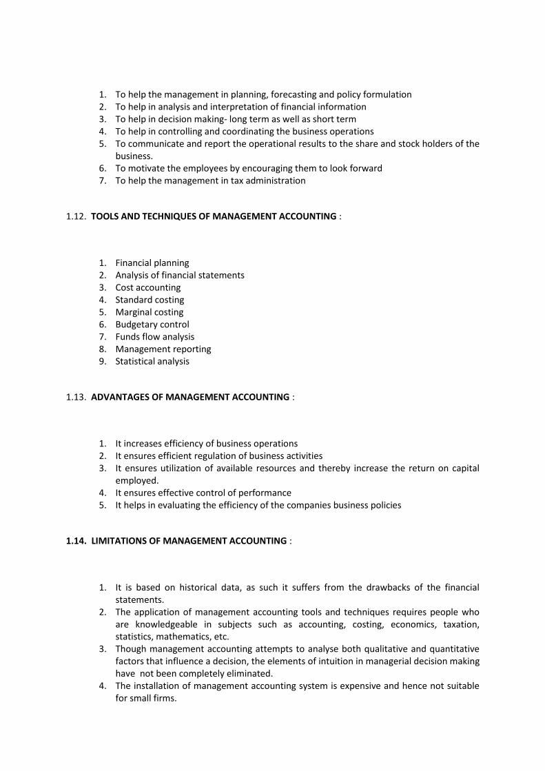
1. To help the management in planning, forecasting and policy formulation 2. To help in analysis and interpretation of financial information 3. To help in decision making- long term as well as short term 4. To help in controlling and coordinating the business operations 5. To communicate and report the operational results to the share and stock holders of the
business. 6. To motivate the employees by encouraging them to look forward 7. To help the management in tax administration
1.12. TOOLS AND TECHNIQUES OF MANAGEMENT ACCOUNTING :
1. Financial planning 2. Analysis of financial statements 3. Cost accounting 4. Standard costing 5. Marginal costing 6. Budgetary control 7. Funds flow analysis 8. Management reporting 9. Statistical analysis
1.13. ADVANTAGES OF MANAGEMENT ACCOUNTING :
1. It increases efficiency of business operations 2. It ensures efficient regulation of business activities 3. It ensures utilization of available resources and thereby increase the return on capital
employed. 4. It ensures effective control of performance 5. It helps in evaluating the efficiency of the companies business policies
1.14. LIMITATIONS OF MANAGEMENT ACCOUNTING :
1. It is based on historical data, as such it suffers from the drawbacks of the financial statements.
2. The application of management accounting tools and techniques requires people who are knowledgeable in subjects such as accounting, costing, economics, taxation, statistics, mathematics, etc.
3. Though management accounting attempts to analyse both qualitative and quantitative factors that influence a decision, the elements of intuition in managerial decision making have not been completely eliminated.
4. The installation of management accounting system is expensive and hence not suitable for small firms.

1.15. USERS OF FINANCIAL ACCOUNTS
Many people use financial statements for varied purposes. The table below summarises the
main user groups and provides examples of their areas of interest in accounts:
User Interest in / Use of Accounting Information
Investors Investors are concerned about risk and return in relation to their
investments. They require information to decide whether they should
continue to invest in a business. They also need to be able to assess
whether a business will be able to pay dividends, and to measure the
performance of the business' management overall. The key accounting
information for an investor is therefore:
- Information about growth - sales, volumes
- Profitability (profit margins, overall level of profit)
- Investment (amounts invested, assets owned)
- Business value (share price)
- Comparative information of competitors
Lenders Banks and loan stockholders who lend money to a business require
information that helps them determined whether loans and interest will be
paid when due. The key accounting information for lenders is therefore:
- Cash flow
- Security of assets against which the lending may be secured
- Investment requirements in the business
Creditors Suppliers and trade creditors requirement information that helps them
understand and assess the short-term liquidity of a business. Is the business
able to pay short-term debt when it falls due? Creditors will, therefore, be
looking for information on:
- Cash flow
- Management of working capital
- Payment policy
Debtors Customers and trade debtors require information about the ability of the
business to survive and prosper. As customers of the company's products,
they have a long-term interest in the company's range of products and
services. They may even be dependent on the business for certain products
or services. Customer will be particularly interested in:
- Sales growth
- New product development
- Investment in the business (e.g. production capacity)

Employees Employees (and organisations that represent them - e.g. trade unions) require
information about the stability and continuing profitability of the business. They
are crucially interested in information about employment prospects and the
maintenance of pension funding and retirement benefits. They are also likely to
interested in the pay and benefits obtained by senior management!. Employees
will, therefore look for information on:
- Revenue and profit growth
- Levels of investment in the business
- Overall employment data (numbers employed, wage and salary costs)
- Status and valuation of company pension schemes / levels of company pension
contributions
Government There are many government agencies and departments that are interested in
accounting information. Local government needs information to levy local taxes
and rates. Various regulatory agencies need information to support decisions
about takeovers and grants, for example.
Analysts Investment analysts are an important user group - specifically for companies
quoted on a stock exchange. They require very detailed financial and other
information in order to analyse the competitive performance of a business and
its sector. Much of this is provided by the detailed accounting disclosures that
are required by authorities. However, additional accounting information is
usually provided to analysts via informal company briefings and interviews.
Public at large Interest groups, formed by various groups of individuals who have a specific
interest in the activities and performance of businesses, will also require
accounting information.
1.16. ACCOUNTANCY PRINCIPLES (GAAP – GENERALLY ACCEPTED
ACCOUNTING PRINCIPLES)
Accounting principles, rules of conduct and action are described by various terms such as
concepts, conventions, tenets, assumptions, axioms, postulates, etc.
1.16.1. Accounting concepts
The term ‘Concept’ is used to mean necessary assumptions and ideas which are fundamental
to accounting practice. The various accounting concepts are as follows:
Business Entity concept : For accounting purposes, the proprietor of an entreprise is always considered to be separate and distinct from the business which he/she controls
Dual aspect concept : Every business transaction involves two aspects – a receipt and a payment. i.e, every debit has an equal and corresponding credit. The dual aspect concept is expressed as : Capital + Liabilities = Assets. This is known as ‘the accouting equation’.

Going concern concept :Under this assumption, the entreprise is normally viewed as a going concern. It is assumed that the entreprise has neither the intention nor the necessity of liquidation of of curtailing materially the scale of its operations. That is why assets are valued on the basis of going concern concept and are depreciated on the basis of expected life rather than on the basis of market value.
Accounting period concept : ‘Accounting year’ is the period of 12 months for which accounts are to be prepared under the Companies Act and Banking Regulation Act.
Money measurement concept : In accounting, every event or transaction which can be expressed in terms of money is recorded in the books of accounts. This concept doesnot record any fact or happening, however important it is to the business, in the books of accounts if it cannot be expressed in terms of money. And as per this concept, a transaction is recorded at its money value on the date of occurance and the subsequent changes in the money value are conveniently ignored.
Historical Cost concept : The underlying idea of cost concept is – I) asset is recorded at the price paid to acquire it, that is, at cost and ii) this cost is the basis for all subsequent accounting for the asset. Fixed assets are shown in the books of accounts at cost less depreciation. Current assets are periodically valued at cost price or market price whichever is less.
Revenue recognition concept : In accounting, ‘revenue’ is the gross inflow of cash, receivables or other considerations arising in the course of an enterprise from the sale of goods, from the rendering of services and from the holding of assets. In the case of revenue, the important question is at what stage, the transaction should be recognised and recorded.
Periodic matching of cost and revenue concept : After the revenue recognition, all costs, incurred in earning that revenue should be charged against that revenue in order to determine the net income of the business.
Verifiable objective evidence concept : As per this concept, all accounting must be based on objective evidence. I.e, the transactions should be supported by verifiable documents.
Accrual concept : Under this concept, revenue recognition and costs for the relevant period, depends on their realisation and not on actual receipt or payment. In relation to revenue, the accounts should exclude amounts relating to subsequent period and provide for revenue recognised, but not received in cash. Like wise, in relation to costs, provide for costs incurred but not paid and exclude costs paid for subsequent period.
1.16.2. Accounting conventions
The term ‘convention’ is used to signify customs or traditions as a guide to the preparation of
accounting statements. The various accounting conventions are as follows.
Convention of disclosure : This convention implies that accounts must be honestly prepared and all material information must be disclosed therein. The term ‘disclosure’ implies that there is to be a sufficient disclosure of information which is of material interest to proprietors, present and potential creditors and investors. This concept also applies to events occuring after the balance sheet date and the date on which the financial statements are authorised for issue, which are likely to have a substantial influence on the earnings and financial position of the enterprise. Their non-disclosure would affect the ability of the users of such statements to make proper evaluations and decisions.

Convention of materiality : As per this convention, financial statements should disclose all items which are material enough to effect evaluations or decisions. The American Accounting Association (AAA) defines ‘ materiality’ as “an item should be regarded as material if there is reason to believe that knowledge of it would influence the decision of informed investor”. Unimportant items can be either left out or merged with other items. Sometimes, items are shown as footnotes or in parentheses according to their relative importance.
Convention of consistency : Consistency, as used in accounting means that persistant application of the same accounting procedures or method by a given firm from one time period to the next so that the financial statements of different periods can be compared meaningfully. This convention thus implies that in order to enable the management to draw important and meaningful conclusions of performance over a period or between different firms, accounting practices should remain unchanged for a fairly long time.
Convention of conservatism : According to this convention, the accountant should be conservative in his/her approach in his estimated, opinions and selection of procedure. In accounting, conservatism refers to the early recognition of unfavourable events. For instance, all possible and expected losses must be provided for. But on the other hand, gains and other financial benefits should not be provided for unless they are realised. In other words, ‘anticipate no profit and provide for all possible losses’.
1.17. PROFIT AND LOSS ACCOUNT AND RELATED CONCEPTS:
The starting point in understanding the profit and loss account is to be clear about the meaning of
"profit". Profit is the reward for taking risk. Profit has an important role in allocating resources
(land, labour, capital and enterprise). Put simply, falling profits signal that resources should be taken
out of that business and put into another one; rising profits signal that resources should be moved
into this business. The main task of accounts, therefore, is to monitor and measure profits. Profit =
Revenues less Costs. So monitoring profit also means monitoring and measuring revenues and
costs. There are two parts to this:-
1) Recording financial data. This is the ‘book-keeping’ part of accounting.
2) Measuring the result. This is the ‘financial’ part of accounting.
Profits are ‘spent’ in three ways.
1) Retained for future investment and growth.
2) Returned to owners eg a ‘dividend’.
3) Paid as tax.
1.17.1. Components of Profit and Loss Account
The Profit & Loss Account aims to monitor profit. It has three parts.

1) The Trading Account: This records the money in (revenue) and out (costs) of the business as a
result of the business’ ‘trading’ ie buying and selling. This might be buying raw materials and selling
finished goods; it might be buying goods wholesale and selling them retail. The figure at the end of
this section is the Gross Profit.
2) The Profit and Loss Account : This starts with the Gross Profit and adds to it any further costs and
revenues, including overheads. These further costs and revenues which may be in the nature of
other operating, administrative, selling and distribution expenses. This account also includes
expenses which are from any other activities not directly related to trading (non-operating). An
example is interest on investments. Thus, profit and loss account contains all other expenses and
losses, incomes and gains of the business for the accounting year for which financial statements are
being prepared. In this process, it follows the mercantile basis of accounting (i.e, it takes into
account all paid and payable expenses, and received and receivable receipts). The net result of
profit and loss account is called as net profit. The main feature of profit and loss account is that it
takes into account all expenses and incomes that belong to the current accounting year and excludes
those expenses and incomes that belong either to the previous period or the future period.
3) The Appropriation Account. This shows how the profit is ‘appropriated’ or divided between the
three uses mentioned above.
1.17.2. INTRODUCTION TO THE TRADING ACCOUNT:
A Trading account is a statement prepared by a firm to ascertain its trading results for the
accounting year. Just like Profit & Loss account, it is also prepared for the year ending. It takes into
account the various trading expenses (usually all direct expenses) and incomes. The net result will
be either trading / gross profit or gross loss. In case of a manufacturing concern, it will prepare an
additional statement called a manufacturing account. A manufacturing account is prepared by a
manufacturer to ascertain the cost of goods manufactured during the current accounting year.
1.17.3. FORMAT OF MANUFACTURING ACCOUNT:
Manufacturing account of ABC. Ltd for the year ending…..
PARTICULARS AMOUNT PARTICULARS AMOUNT
To work-in-process (opening) By Closing stock

To Raw material consumed:
Opening stock
Add: Purchase of raw material
Less: Closing stock of Raw
material
To Direct or productive wages
To Factory overhead:
Power and Fuel
Factory rent
Carriage inwards
Octroi. etc
Raw materials
Work-in-process
By Cost of production transferred
to Profit & Loss account
TOTAL TOTAL
1.17.4. FORMAT OF TRADING ACCOUNT
Trading account of ABC. Ltd for the year ending…..
PARTICULARS AMOUNT PARTICULARS AMOUNT
To Opening stock
To Purchases
To Direct or productive wages
To wages and salaries
To Power and Fuel
To Factory rent
To Carriage inwards
To Octroi. etc
To Gross profit transferred to
Profit & Loss account
By Closing stock
By Sales
By Gross Loss transferred to
Profit & Loss account

TOTAL TOTAL
1.17.5. Uses of the Profit and Loss Account.
1) The main use is to monitor and measure profit. This assumes that the information recording is
accurate. Significant problems can arise if the information is inaccurate, either through
incompetence or deliberate fraud.
2) Once the profit (loss) has been accurately calculated, this can then be used for comparison or
judging how well the business is doing compared to itself in the past, compared to the managers’
plans and compared to other businesses.
1.17.6. The format of a typical profit and loss account is as follows:
PARTICULARS AMOUNT PARTICULARS AMOUNT
To Gross loss b/d
To Salaries
To Salaries and wages
To Rent
To Commission
To Advertisement
To Bad debts
To Discount allowed
To Reserve for bad debts
To Reserve for doubtful debts
To Reserve for discount on
debtors
To Freight/ carriage outwards
To loss on sale of fixed assets
By Gross profit b/d
By interest received
By rent received
By commission received
By bad debts recovered
By Reserve for discount on
creditors
By discount received
By gain on sale of fixed assets
By net loss transferred to capital
account

To uninsured loss due to fire
To interest on capital
To manger’s commission
To transfers to reserve accounts
To net profit transferred to
capital account
TOTAL TOTAL
1.18. THE BALANCE SHEET AND RELATED CONCEPTS:
According to Howard, a Balance sheet may be defined as – ‘a statement which reports the values
owned by the enterprise and the claims of the creditors and owners against these properties’.
The Balance sheet is a statement that is prepared usually on the last day of the accounting year,
showing the financial position of the concern as on that date. It comprises of a list of assets,
liabilities and capital. An asset is any right or thing that is owned by a business. Assets include land,
buildings, equipment and anything else a business owns that can be given a value in money terms
for the purpose of financial reporting. To acquire its assets, a business may have to obtain money
from various sources in addition to its owners (shareholders) or from retained profits. The various
amounts of money owed by a business are called its liabilities. To provide additional information to
the user, assets and liabilities are usually classified in the balance sheet as:
- Current: those due to be repaid (Current liabilities) or converted into cash within 12 months of the
balance sheet date(Current Assets).
- Long-term: those due to be repaid (Long term liabilities) or converted into cash more than
12 months after the balance sheet date (Fixed Assets).
1.18.1. Fixed Assets
A further classification other than long-term or current is also used for assets. A "fixed asset" is an
asset which is intended to be of a permanent nature and which is used by the business to provide
the capability to conduct its trade. Examples of "tangible fixed assets" include plant & machinery,
land & buildings and motor vehicles. "Intangible fixed assets" may include goodwill, patents,

trademarks and brands - although they may only be included if they have been "acquired".
Investments in other companies which are intended to be held for the long-term can also be shown
under the fixed asset heading.
1.18.2. Capital
As well as borrowing from banks and other sources, all companies receive finance from their
owners. This money is generally available for the life of the business and is normally only repaid
when the company is "wound up". To distinguish between the liabilities owed to third parties and to
the business owners, the latter is referred to as the "capital" or "equity capital" of the company. In
addition, undistributed profits are re-invested in company assets (such as stocks, equipment and the
bank balance). Although these "retained profits" may be available for distribution to shareholders -
and may be paid out as dividends as a future date - they are added to the equity capital of the
business in arriving at the total "equity shareholders' funds".
At any time, therefore, the capital of a business is equal to the assets (usually cash) received from
the shareholders plus any profits made by the company through trading that remain undistributed
1.18.3. The basic functions of a balance sheet are:
1. It gives the financial position of a company on any given date 2. It gives the liquidity picture of the concern 3. It gives the solvency position of the concern
1.18.4. The basic components of a balance sheet are:
LIABILITIES ASSETS
1. Net Worth 2. Non-current liabilities / long term
liabilities 3. Current liabilities
1. Fixed assets 2. Intangible assets 3. Current assets 4. Deferred expenditure 5. Other assets

1.18.5. Pro-forma of a Balance sheet is as follows:
Balance sheet of ABC Ltd as on 31st December 2005
LIABILITIES AMOUNT
(Rs)
ASSETS AMOUNT
(Rs)
Capital
Add: Net profit for the period
Further capital introduced
Interest on capital
Less: Drawings
Interest on drawings
Net loss for the period Loans
Other long term borrowings
Sundry creditors
Bills / Notes payable
Outstanding expenses
Incomes received in advance etc
Fixed assets
Land & Buildings
Plant & Machinery
Equipment
Furniture & Fixtures
Investments:
Current assets:
Sundry debtors
Closing stock
Bills / Notes receivable
Prepaid expenses
Outstanding incomes
Cash in hand
Cash at bank etc
TOTAL LIABILITIES TOTAL ASSETS
1.18.6. COMMON ADJUSTMENTS AFFECTING THE PREPARATION OF BALANCE SHEET ARE:
1. Income received in advance: Income received in respect of which service has not been
rendered is known as income received in advance. In order to calculate the exact profit or less made during the year, such income should not be taken in to account while preparing profit and loss account. Hence this amount must be deducted from the respective income account in the profit and loss account and must be treated as a liability in the balance sheet. The adjustment entry is

Income account Dr.
To income received in advance.
2. Closing stock : Closing stock appears on the credit side of trading account and assets side of balance sheet if it is given in the adjustments. If it is given in the trial balance it will appear only on the assets side of the balance sheet. The entry passed is
Closing Stock A/c Dr.
To Trading Account.
3. Outstanding expenses : Outstanding expenses refer to those expenses which have become due during the accounting period for which financial statements are being prepared, but not yet have been paid. Such expenses if given in the adjustments, should be added to the respective expenditure account on the debit side of profit and loss account and must be shown as liabilities in the balance sheet. If such expenses are given in the trial balance they should be recorded only on the liability side of the balance sheet. The journal entry to be passed is
Respective Expenditure A/c Dr.
To Outstanding Expenditure
4. Pre-paid expenses : They are those expenses which have been paid in advance. They are also known as un-expired expenses. If given in adjustments, they should be deducted from the respective expenditure account on the debit side of the profit and loss account and must be shown on the asset side of the balance sheet. If given in the trial balance, they must be shown only on the asset side of the balance sheet. The adjustment entry is
Pre-paid expenditure A/c Dr.
To Respective Expenditure
5. Outstanding or accrued income : This is the income which has been earned during the current accounting year and has become due but not yet received by the firm. If given in the adjustments, it must be added to the respective income account on the credit side of the profit and loss account and must be shown on the assets side of the balance sheet. But if given in the trial balance, it must be shown only on the asset side of the balance sheet. The entry is

Outstanding/Accrued Income A/c Dr.
To Respective Income
6. Depreciation : It is a reduction in the value of the asset due to wear and tear, lapse of time, obsolescence, exhaustion and accident. It is charged on fixed assets of the business. If given in the adjustments, it must be shown on the debit side of the profit and loss account and must be deducted from the respective asset account in the balance sheet. If given in the trial balance, it must be shown only on the debit side of the profit and loss account. The entry is
Depreciation A/c Dr.
To Respective Fixed Asset
7. Bad Debts : They represent that portion of credit sales (debtors) that had become bad due to the inability of the debtor to repay the amount. It is a loss to the business and gain to the debtor. This is a real loss to the business and as such must be deducted from the debtors before deducting any reserves created on debtors. If given in the adjustments it must be shown on the debit side of the profit and loss account and must be deducted from the debtors account on the asset side of the balance sheet. If given in the trial balance this amount must be shown only in the profit and loss account. The entry is
Bad debts A/c Dr.
To Debtor’s personal account
8. Provision for bad debts : This represents a provision made by the business for any potential bad debts. It is charged to the profit and loss account debit side and must be deducted from the debtors after deducting the bad debts if any on the asset side of the balance sheet, if given in the adjustments. If given in the trial balance, it must be considered only in preparing the profit and loss account. The entry is
Profit and loss A/c Dr.
To Provision for bad debts

9. Provision for doubtful debts : This represents a provision made by the business for any potential doubtful debts. If given in the adjustments, it must be charged to the profit and loss account debit side and must be deducted from the debtors after deducting the bad debts (if any) and reserve for bad debts on the asset side of the balance sheet. If given in the trial balance, it must be considered only in preparing the profit and loss account. The entry is
Profit and loss A/c Dr.
To Provision for doubtful debts
10. Provision for doubtful debts : This represents a provision made by the business for any potential discount to be allowed to the debtors. If given in the adjustments, it must be charged to the profit and loss account debit side and must be deducted from the debtors after deducting the bad debts (if any), reserve for bad debts (if any) and reserve for doubtful debts (if any) on the asset side of the balance sheet. If given in the trial balance, it must be considered only in preparing the profit and loss account. The entry is
Profit and loss A/c Dr.
To Provision for discount on debtors
11. Reserve for discount on creditors: This represents a provision made by the business for any potential discount to be allowed by the creditors of the business. If given in the adjustments, it must be charged to the profit and loss account credit side and must be deducted from the creditors on the liabilities side of the balance sheet. If given in the trial balance, it must be considered only in preparing the profit and loss account. The entry is
Reserve for discount on creditors A/c Dr
To Profit and Loss A/c
12. Interest on capital: This is the return the owners of the business will get for investing in the business. Usually it is paid or added to the capital at a fixed percentage. If given in the adjustments, it is shown on the debit side of the profit and loss account and is usually added to the capital account on the liabilities side of the balance sheet. If given in the trial balance, it must be shown on the debit side of profit and loss account. The entries are :
Profit and Loss A/c
To Interest on capital

Interest on capital A/c Dr
To capital A/c
13. Interest on Drawings: Drawings represents the withdrawals made by the owners during the accounting year either in the form of stock, cash or withdrawal from bank for personal use. They must be deducted from the capital account on the liabilities side of the balance sheet. Sometimes, firms charge interest on such drawings made by the owners to discourage them from withdrawing their investment. Usually it is levied as a fixed percentage. It is an income to the business and a loss to the owner. Hence, if given in the adjustments, it must be shown on the credit side of the profit and loss account and deducted from the capital in the balance sheet. If given in the trial balance, it must be shown only in the profit and loss account. The respective entries are:
Interest on Drawings A/c Dr
To Profit and loss A/c
Interest on Drawings A/c Dr
To capital A/c
1.19. POINTS TO BE REMEMBERED WHILE PREPARING THE FINANCIAL
STATEMENTS:
1. Items given in the trial balance must be shown only once as it is assumed that they are
already adjusted once 2. Items given in the adjustments must be accounted for twice. 3. Any difference in the trial balance must be transferred to suspense account. If the balance is
short on the debit side, the difference must be shown on the asset side of the balance sheet and if the balance is short on the credit side, it must be shown on the liabilities side of the balance sheet.
4. Wherever required, working notes must be maintained for accuracy and clarity. 5. Some of the adjustments are unique, such as distribution of free samples. They are to be
treated case by case.
1.20 INTRODUCTION TO INFLATION ACCOUNTING
Assessing a company's performance after adjusting for the effects of inflation is the general meaning
of inflation accounting. And it involves the adoption of definitions of costs, revenue, profit and loss
that are fully inflation-adjusted.

1.20.1 DEFINITION OF INFLATION ACCOUNTING
According to M.A.Sahaf, Inflation accounting is an accounting technique which aims to
record business transactions at current values and to neutralize the impact of changes in the
price on the business transaction.
1.20.2 REASONS FOR DISCREPENCIES IN ACCOUNTS DUE TO ADOPTION OF
HISTORICAL COST ACCOUNTS
1. Recording of fixed assets at their historical costs 2. Recording of inventory at historical cost instead of current cost 3. Recording of other assets and liabilities without taking into account their current values
1.20.3 ISSUES IN INFLATION ACCOUNTING
1. ADJUSTEMENT OF HISTORIC COST DATA: In the early days of inflation accounting development, business houses often used to debate whether the historic cost data should be adjusted for inflation induced price level changes or not. But, later they started to follow it all the same while preparing their financial statements.
2. ADJUSTMENT ITEMS: While adjusting items for inflation, there are 2 approaches one can take – 1) covering the adjustment of all financial items, 2) covering the adjustment of only those items that have direct impact on financial results
3. USE OF INDEX NO: The opinion of experts is varied on the use of index numbers for adjusting the financial accounts. They can either use general purchasing power index or specific index number. Mostly the use of general purchasing power index is recommended as (a) it replaces the monetary unit of measurement which ceases to be stable during the changing price level (b) it provides the uniform standard of measurement for comparing diverse resources (c) it can be used for restating assets as well as shareholders capital (d) it communicates information regarding utilization of funds and profits gained to the proprietors
1.20.4 TECHNIQUES OF INFLATION ACCOUNTING
The most important techniques developed by professional institutes and accountants to deal
with inflationary conditions are (1) Current purchasing power – [CPP], (2) Replacement cost
accounting method [RCA], (3) Current value accounting method [CVA] and (4) Current cost
accounting method [CCA].
1. Current Purchasing Power [CPP] : This is a very popular method among professional institutes. Under this system the business keeps its accounts maintained under financial accounting system {i.e. conventional historical cost basis}. Then at the end of the account

period supplementary statements must be prepared showing all the items of financial statements in terms of the value of a rupee to which they relate. These supplementary statements indicate the changes in the financial conditions of the concern during the financial period as a result of changes in the purchasing power of a rupee. For this purpose general price index is used.
2. Replacement cost accounting method [RCA] : This method attempts to resolve financial reporting problems that arise during the periods of rapidly changing prices. It states that firms should create fixed asset replacement provision in the Profit and loss account which is adequate to meet the requirements. Thus the charges to profit and loss account are governed by the replacement cost of each item rather than the depreciation cost. This concept requires that the reported amount of expenses are to be measured at the time of asset expiration. Further all the non-monetary items must be reported at the respective replacement cost as on the balance sheet date.
3. Current value accounting method [CVA] : Under this method all items of balance sheet are shown at current values. According to this method, the net assets at the beginning and at the end of the accounting period are ascertained and difference is implied to be profit or loss for the period. It attempts to reflect economic reality to the preparation of financial statements by using current values for reporting various items in the balance sheet.
4. Current cost accounting method [CCA] : This method had been suggested as a base for financial reporting by Sandiland Committee appointed by the British Committee in 1973 to solve the problem of price level changes. The Committee reported that CPP may be used along with either historical cost or value accounting.
1.20.5 ADVANTAGES OF INFLATION ACCOUNTING
1. It reflects an accurate picture of the profitability of the concern as it matches its current revenues with its current costs. It keeps that capital intact as it does not allow payment of dividend and taxes out of capital.
2. It enables a comparative study of the profitability of various concerns set up at different periods.
3. As depreciation is charged on current value of assets, it is easier for the concern to replace the assets.
4. By providing accurate financial information to the various interested parties, it discharges the social obligation of the business.
5. It enables the company to realize a realistic price for its shares in the investment market.
1.20.6 DIS-ADVANTAGES OF INFLATION ACCOUNTING

1. It is a complicated, confusing and time consuming process as it requires lot of work. 2. The adjusted financial statements are difficult to be understood, analyzed and interpreted
by a common man. If proper conversion method is not adopted the information provided may be inaccurate.
3. Income Tax Act of 1961 does not recognize the depreciation charged on current value of fixed assets. Hence it is not suitable for tax purposes.
4. During inflation profits are overstated as lower depreciation is charged to fixed assets.
1.21 INTRODUCTION TO HUMAN RESOURCE ACCOUNTING
The concept of HR accounting was not known to the world till the early 60’s. During this period,
few experts like Hermanson, Hekimian, Jones and Rensis Likert had recognised HR as assets just like
any other tangible or intangible assets.
1.21.1 DEFINITION OF HUMAN RESOURCE ACCOUNTING (HRA)
The term ‘HR Accounting’ implies accounting for Human resources – namely, the
knowledgeable, trained and loyal employees who participate in the earning process and total
assets. Different authors have defined HR Accounting in different terms. According to the
American Accounting Association (1973), HR Accounting is ‘the process of identifying and
measuring data about human resources and communicating the information to interested
parties’. In the words of Stephen Knauf – HR Accounting is ‘the measurement and
quantification of human organization inputs, such as recruiting, training, experience and
commitment’.
Thus, HR Accounting had been defined by many authors in different ways. In essence, it
represents a systematic attempt to assess the value of human resource of an organization.
1.21.2 THE PROCESS OF HRA
The process of HR Accounting includes – identification and measurement or quantification of human
resource in an organization and its reflection in its annual reports or financial statements.
1.21.3 THE OBJECTIVES OF HRA
The objectives of HR accounting are:

1. To provide relevant information about the human resource to the management and aid in its decision making
2. To help management in evaluating the performance of its personnel and calculate its return on investment
3. To help the management in planning and controlling the various functions or activities related with its human resource such as – man power planning, recruiting, training and retirement etc.
1.21.4 ADVANTAGES OF HRA
The various advantages a firm can enjoy by establishing HR Accounting are as follows:
1. Its adoption acts as a motivating factor for the employees of the concern as it is reflected in its financial statements
2. It helps the management in identifying and controlling several problems related with human resources
3. It enables the management in efficiently using its man power by providing quantified information about its HR
4. By considering HR as an asset in its financial statements, it provides a measure of profitability
5. It helps the investors or potential investors in assessing the true value of a firm by providing realistic information about its HR
1.21.5 DISADVANTAGES OF HRA
At the same time, a firm may also face certain limitations in implementing HRA such as :
1. HR as an asset cannot be owned by any firm. 2. Quantification of HR value is subjective in nature and there is no common valuation model
existing which can be used across the industries or by all the companies in the same industry 3. As its establishment and implementation involves huge cost, it may not suit small firms 4. The concept of HRA is not recognized by tax authorities and has only academic value 5. There is no objective procedure to be followed in the valuation of the HR, hence
comparative analysis may not be possible, and even if possible, may not be reliable
1.21.6 TECHNIQUES OF VALUATION OF HR
There are around eight techniques for valuation of HR. They are as follows :

1. Historical cost Method: This method was developed by Rensis Likert and his associates and was adopted by R.G.Barry corporation, Ohio, Colombia, USA, in 1968. This method involves capitalization of the costs incurred on HR related activities such as – recruitment, selection, placement, training and learning etc, and amortized over the expected length of services of the employees. The un expired cost represents the firm’s investment in HR. In case an employee leaves the organization before the expiry of the expected services’ life period, the firm shall write off the entire amount of un expired cost against the revenue of the period during which he or she leaves.
2. Replacement Cost Method: This method was initially developed by Hekimian and Jones. According to this method, a firm’s HR value is its replacement cost. According to Flamholtz, this replacement cost may be – i) individual replacement cost – which refers to the cost of replacing an employee with an equivalent substitute in terms of skill, ability and knowledge and ii) positional replacement cost – which refers to the cost of replacing the set of services expected to be rendered by an employee at the respective positions he holds and will hold at present and in future. Thus, the HR value will appear in the financial statements at its replacement cost.
3. Opportunity cost method: This method has been suggested by Hekimian and Jones and refers to the valuation of HR on the basis of an employee’s value in alternative uses, i.e, opportunity cost. This cost refers to the price other divisions are willing to pay for the service of an employee working in another division of an organization.
4. Capitalisation of Salary method: This method had been proposed by Baruch Lev and Aba Schwartz in terms of economic value of HR. According to them, the salaries payable to employees during their stay with the organization may be used in valuing the HR of an organization. Thus the value of HR is the present value of future earnings of homogeneous group of employees..
5. Economic valuation method: This values the HR of an organization by considering the present worth of the employees’ future service expected to be derived during their stay with the organization. Under this method, the valuation of HR involves 3 steps – 1) estimation of employee’s future services, 2) multiply step 1 by the employee’s rate of pay and 3) Multiply step 2 by the rate of return on investment. This would give the present worth of employee’s service.
6. Return on efforts employed method: Under this method, HR valuation is done on the basis of the quantifying the efforts made by the individuals for the organizational benefits by taking into account factors such as –positions an employee holds, degree of excellence employee achieves, and the experience of the employee.
7. Adjusted discounted future wages method: This model has been developed by Roger.H.Hermanson. Under this method, HR valuation is done on the basis of relative efficiency of an organization in the industry. This model capitalizes the extra profit a firm earns over and above that of the industry expectations. As such, this model involves 4 steps – 1) estimation of 5 years (succeeding) wages and salaries payable to different levels of

employees 2) finding out the present value of such estimated amount at the normal rate of return of the industry, 3) determining the average efficiency ratio (the co’s average rate of return for the past 5 yrs)/ Industry’s average rate of return for the past 5 yrs) for 5 years, 4) finding out the present value of future services of the co’s Hr by multiplying the discount value (as in 2nd step) by the firm’s efficiency ratio (as calculated in 3rd step)
8. Reward valuation method: This model has been developed by Flamholtz and is commonly known as – the stochastic rewards valuation model. It values the HR of a concern on the basis of an employee’s value to an organization at various service states (roles) that he is expected to occupy during the span of his working life with the organization. This model involves – estimation of an employee’s expected service life, identifying the set of service roles he may occupy during his service life, estimating the value derived by an organization at a particular service state of a person for the specified time period, estimating the probability that a person will occupy at possible mutually exclusive service state at specified future times, quantifying the total services derived by the organization from all its employees, and discounting the total value thus arrived at to its present value at a pre determined rate.
SUMMARY
The American Institute of certified public accountants (AICPA) defined accounting
as “Accounting is the art of recording classifying and summarizing in a significant
manner and in terms of money transactions and events which are in part at least of a
financial character and interpreting the results thereof”.
Basically, the financial statements provide quantitative data about the performance of
an organization to the users, thereby helping in their decision making.
The various functions of accounting include keeping systematic records of the
business, protecting the properties of a business, meeting the legal requirements and
communicating the operating results to the interested parties
Inherently, financial accounting suffers from some limitations such as – recording of
monetary transactions alone, conflict between the various accounting concepts and
conventions such as for ex. – convention of conservatism and convention of
consistency regarding recording of assets, personal bias of the accountant in the
accounting treatment of certain items, the need for expertise on the part of the users
etc
Cost accounting is designed as the process of accounting for costs from the point at
which expenditure is incurred or committed to the establishment of its ultimate
relationship with cost centers and cost units. In its widest usage it embraces the
preparation of statistical data, the application of cost control methods and the
ascertainment of the profitability of activities carried out or planned.”
Mainly, Cost accounting deals with providing cost data to the management for
internal decision making purpose.
As Cost accounting is not a science but an art, and is still developing, it lacks a
uniform procedure which can be applied by all types of business. It can only be
customized by the firm which is adopting it Management Accounting is defined as a system for gathering, summarizing, reporting and
interpreting accounting data and other financial information primarily for the internal needs

of the management. It is designed to assist internal management in the efficient formulation, execution and appraisal of business plans.”
The scope of Management accounting covers many areas of finance such as – financial accounting, Cost accounting, Financial Statement Analysis, Budgeting, Inflation accounting, Management reporting, Quantitative techniques, Tax accounting, Internal audit etc
The basic functions of Management accounting include helping the management in
decision making
The various tools of Management accounting include – financial planning, Analysis
of financial statements, Cost accounting, Standard costing, Marginal costing,
Budgetary control, Funds flow analysis, Management reporting, Statistical analysis
etc
The adoption of Management accounting ensures – efficiency in business operations,
regulation of business operations, utilization of resources etc
But, as Management is based on financial statements, it suffers from all the
drawbacks of the financial statements.
Many categories of people use financial statements for varied uses. Some of them are
– investors, lenders, creditors, debtors, employees, government, analysts, public at
large etc
There are several principles and practices followed by businesses in recording their
information. These principles and practices are widely known as – GAAP (Generally
Accepted Accounting Principles). The adoption of these enables adoption of common
practices in accounting by all the businesses.
The FINAL accounts or Financial statements are prepared by all the businesses at the
end of their accounting year. They include – a Trading account, Profit & Loss
account and a Balance sheet. If it is a manufacturing concern, the list includes the
preparation of a manufacturing account also A Trading account is a statement prepared by a firm to ascertain its trading results for the
accounting year. A manufacturing account is prepared by a manufacturer to ascertain the cost of goods manufactured during the current accounting year.
A Profit & Loss account is a statement that is prepared for the accounting period by taking into account the various trading expenses and incomes. The main feature of profit and loss account is that it takes into account all expenses and incomes that belong to the current accounting year and excludes those expenses and incomes that belong either to the previous period or the future period.
A Balance sheet is a statement that is prepared on the last day of the accounting
period by taking stock of the various assets and liabilities of a business. It reflects the
financial position of a concern. There are various items that need to be adjusted while
preparing the final accounts
Inflation accounting has been defined as an accounting technique which aims to
record business transactions at current values and to neutralize the impact of changes
in the price on the business transaction
Accounting transactions which are recorded on the basis of historical cost basis do not
reflect the true performance of the concern and also may not help it in realistic
decision making. Hence, inflation accounting need to be adopted by businesses.
There are around 4 techniques in which it can be done. They include - (1) Current
purchasing power – [CPP], (2) Replacement cost accounting method [RCA], (3)
Current value accounting method [CVA] and (4) Current cost accounting method
[CCA]. But adoption of this is rather complicated, expensive, and the income tax Act
does not recognize it.

HR Accounting has been defined as the process of identifying and measuring data
about human resources and communicating the information to interested parties.
The process of HR Accounting includes – identification and measurement or
quantification of human resource in an organization and its reflection in its annual
reports or financial statements
HRA aims at recognizing the value of human factor in the organization and thus, help
the organization in achieving its objectives by motivating its work force, increasing its
efficiency, helping in measuring the profitability of a concern etc.
The basic limitation of HRA is that HR as an asset cannot be owned by anyone. And
quantification of HR is highly subjective in nature. It also is expensive and is not
recognized by Tax authorities
There are around 8 methods of HR valuation in practice. They include – Historical
Cost Method, Replacement Cost Method, Opportunity Cost Method, Capitalization of
Salary Method, Economic Valuation Method, Return on Efforts Employed Method,
Adjusted Discounted Future Wages Method and Reward Valuation Method.
TEST YOUR KNOWLEDGE
Short Questions:
1. Define Accounting. What are its functions and limitations? 2. What are the objectives of financial statements? 3. Define cost accountancy. What are its objectives and limitations? 4. What is Management accounting? What are its functions, advantages and disadvantages? 5. What are the various tools and techniques of Management accounting? 6. Why is Accounting regarded as an aid to management? 7. Explain any three of the accounting concepts 8. What are final accounts? What purpose do they serve? 9. Briefly explain the concept of inflation accounting. What are its merits and demerits? 10. “Accounts ignore inflation and inflation makes a mockery of them.” Explain. 11. Explain the concept of HRA. What are its objectives? 12. Discuss the significance of HRA in the modern business
Long Questions:
1. Distinguish between financial, cost and management accounting 2. State the persons who will be interested in accounting information 3. Discuss briefly the accounting concepts and conventions 4. Differentiate between (i) outstanding expenses and prepaid expenses (ii) Outstanding
income and incomes received in advance (iii) interest on capital and interest on drawings 5. Write short notes on – (i) manufacturing account (ii) trading account (iii) profit and loss
account and (iv) balance sheet. 6. Explain the various adjustments affecting the preparation of a balance sheet.

7. Discuss the various methods of accounting for price level changes. 8. Explain the various methods of HR valuation
TEXT BOOKS FOR THE CHAPTER:
5. S.N.Maheshwari, S.K.Maheshwari, “Accounting for Management”, Vikas Publishing House Pvt. Ltd, 2006
6. M.A.Sahaf, “Management Accounting – Principles & Practice”, Vikas Publishing House Pvt. Ltd, 2006
7. M.Y.Khan & P.K.Jain, “Management Accounting”, Tata Mcgraw Hill Publishing company Ltd, 2004
REFERENCES FOR THE CHAPTER:
2. R.S.N.Pillai & Bagavathi, “Management Accounting”, S.Chand & Co. Ltd, New Delhi, 2004 3. O.S.Gupta, Pankaj Kothari, “Accounting for Managers”, Frank Bros. Pvt. Ltd, New Delhi,
2004.
Capital B udgeting
Unit Structure:
1. Introduction
2. Learning Objectives
3. Section title
3.1 Capital Projects
3.2 Significance of capital budgeting
3.3 Appraisal of capital projects
3.4 Requisites for appraisal of capital projects
3.5 Methods used for projects appraisal
a) Payback period (PB) method
b) Accounting Rate of Return (ARR) method

c) Net present value (NPV) method
d) Internal rate of return (IRR) method
3.6 Decision tree approach
3.7 Capital Asset pricing model (CAPM)
3.8 Simulation analysis
3.9 Sensitivity analysis
3.10 Risk analysis in the case of single project
3.11 Risk – Return analysis for multi projects
3.12 Have you understand questions
3.13 Summary
3.14 Exercises
3.15 References

INVESTMENT DECISIONS
(CAPITAL BUDGETING)
In this unit you will learn capital projects, significance of capital
budgeting, appraisal techniques of capital projects, under conditions of
certainty, risk and uncertainty, etc.
1. INTRODUCTION
Capital budgeting is budgeting for capital projects. The exercise
involves ascertaining I estimating cash inflows and outflows, matching the
cash inflows with the outflows appropriately and evaluation of the
desirability of the project.
2. LEARNING OBJECTIVES:
After reading this lesson you will be conversant with:
The nature of investment decision
Scanning and identification of investment opportunities
Criteria for preliminary screening
Prepare each flow projections for projects
Assessing the financial viability of projects using the various
appraisal criteria.
3.1 CAPITAL PROJECTS

Businesses invest in capita] projects of different nature. These
capital projects involve investment in physical assets, as opposed to
financial assets like shares, bonds or funds. Capital projects necessarily
involve processing! manufacturing service works. These require
investments with a longer time horizon. The initial investment is heavy in
fixed assets and investment in permanent working capital is also heavy.
The benefits from the projects last for few to many years.
Capital projects may be new ones, expansion of existing ones,
diversification of existing ones, renovation or rehabilitation of infirm
ones, R&D activities, or captive service projects. An enterprise may put up
a new subsidiary, increase stake in existing subsidiary or acquire a
running firm. All these are considered capital projects.
Capital projects involve huge outlay and last for years. Hence these
are riskier than investments in financial assets. Capital projects have
technological dimension and environmental dimension. So, careful
analysis is needed. Decisions once taken cannot be reversed in respect of
capital projects. So, “listen before leaping” and “think before jumping”
are the caveats needed. Thorough evaluation of costs and benefits is
needed.
3.2 SIGNIFICANCE OF CAPITAL BUDGETING
Every business has to commit funds in fixed assets and permanent
working capital. The type of fixed assets that a firm owns influences i) the
pattern of its cost (i.e. high or low fixed cost per unit given a certain

volume of production), ii) the minimum price the firm has to charge per
unit of product, iii) the break-even position of the company, iv) the
operating leverage of the business and so on. These are all very vital
issues shaping the profitability and risk complexion of the business.
Hence the significance of the capital budgeting.
Capital budgeting is significant because it deals with right kind of
evaluation of projects. A project must be scientifically evaluated, so that
no undue favour or dis-favour is shown to a project. A good project must
not be rejected and a bad project must not be selected. Hence the
significance of capital budgeting.
Capital investment proposals involve i) longer gestation period, ii).
huge capital outlay, iii) technological considerations needing
technological forecasting, iv) environmental issues too, which require the
extension of the scope of evaluation to go beyond economic costs and
benefits, v) irreversible decision once get committed, vi) considerable
peep into the future which is normally very difficult, vii) measuring of and
dealing with project risks which is a daunting task in deed and so on. All
these make capital budgeting a significant task.
Capital budgeting involves capital rationing. That is the available
funds must be allocated to competing projects in the order of project
potentials. Usually, the indivisibility of project poses the problem of
capital rationing because required funds and available funds may not be
the same. A slightly high return projects involving higher outlay may have

to be skipped to choose one with slightly lower return but requiring less
outlay. This type of trade-off has to be skillfully made.
The building blocks of capital budgeting exercise are mostly
estimates of price and variable cost per unit output, quantity of output
that can be sold, the tax rate, the cost of capital, the useful life of the
project, etc. over a period of years. A clear system of forecasting is
needed. Hence the significance of capital budgeting.
What should be the discount rate? Should it be the pre-tax overall
cost of capital? Or the post-tax overall cost of capital? The choice is very
crucial making capital budgeting exercises significant ones.
Finally, which is the appropriate method of evaluation of projects.
There is a dozen or more methods. The choice of method is important.
And different methods might rank projects differently leading to a
confined picture of project desirability ranks. A dear thinking is needed so
that confusion is not descending on the choice of projects. Hence the
significance of capita) budgeting.
3.3 APPRAISAL OF CAPITAL PROJECTS
Appraisal means examination and evaluation. Capital projects need
to be thoroughly appraised as to costs and benefits.
The costs of capital projects include the initial investment at the
inception of the project. Initial investment made in Land, building,
machinery, plant, equipment, furniture, fixtures, etc. generally, gives the
installed capacity. Investment in these fixed assets is one time. Further a

one-time investment in working capital is needed in the beginning, which
is filly salvaged at the end of the life of the project.
Against this find committed returns in the form of net cash earnings
are expected. Net cash earnings sales variable cast -a-Fixed cost
(including depreciation, Tax + Depreciation. These are computed as
follows. Let ‘P’ stand for price per unit, ‘V’ for variable cost per unit, ‘Q’
for quantity produced & sold, ‘F’ stand to total fixed expenses exclusive of
Depreciation, ‘0’ stand to depreciation on fixed assets, ‘I’ for interest on
borrowed capital id ‘T’ for tax rate).
Then cash earnings = [(P-V)Q-F-D-I](1-T)+D
These cash earnings have to be estimated through out the
economic life of the investment. That is, all the variables in the equation
have to be forecast well over a period of years.
Now that, we have the benefits from the investment estimated, the
same may be compared with costs of the capital project and ‘netted’ 1
find out whether costs exceed benefits or benefits exceed costs. This
process of estimation of costs and benefits and comparison of the same is
call& appraisal. Payback period, accounting rate of return, net present
value, rate of return, decision free technique, sensitivity analysis,
simulation and capital asset pricing model (CAPM) are certain methods of
appraisal.
3.4 REQUISITES FOR APPRAISAL OF CAPITAL PROJECTS

The computation of profit after tax and cash flow relevant in
evaluation of projects. Hence this is presented here as a prelude better
understanding the whole process.
Say in fixed assets at time zero, you are investing Rs.20 lakhs. You
have estimated the following for the next 4 years.
With this information we can estimate profit after tax for the business.
For that, apart the given variable expenses and fixed expenses, depreciation of
the fixed assets has to be considered. The annual value depreciation is given by
the cost of fixed assets divided by number of years of life. In our case the figure
comes to Rs. 20,00,000/4 = Rs.5 lakhs.
The calculations are given in three stages, viz. computation of profit
before tax (PBT), profit after tax (PAT) and cash flow.
The profit before tax (PBT) for a period is given by: (selling price per unit
- variable cost per unit) * (No. of units sold) - Fixed expenses - Depreciation. So,
for the 5t yew PBT = (200-100) (30000) - 12,00,000 - 5,00,000 = 30,00,000 -
47,00,000 = 13,00,000. Table gives the working and results.

Table
Profit after tax (PAT) for the different years is obtained by subtracting
tax from the PBT.
Profit after tax = PAT = PBT (1-Tax Rate). So, for the first year PAT =
13,00,000 (1-30%) = 13,00,000 (0.7) = 9,10,000. Similarly for the other years
the profit figures can be obtained as in table 4.2.
Cash-flow from business is equal to PAT plus depreciation. Table 4.3 gives cash
flow from business.
Table

3.5 METHODS USED FOR PROJECTS APPRAISAL
A. PAYBACK PERIOD (PBP) METHOD
Pay back period refers to the number of years one has to wait back the
capital invested in fixed assets in the beginning. For this we have to g cash flow
from business.
We have invested Rs. 20,00,000 at time zero. After one year a sum of
Rs.14,10,000 is returned. By next year a sum of Rs. 19,70,000 is returned. But
we have to get back only Rs. 5,90,000 (i.e 20,00,000 - 14,10,000). So, in the
second we have to wait only for part of the year to get back Rs. 5,90,000. The
part of the year = 5.90,000/ 19,70,000 = 0.30 I hat is, pay back period is 1.30
years or 1 year, 3 months and 19 days.
In general pay-back period is given by ‘n’ in the equation
.01
ICFn
t
t
where ‘t’ 1 to n, I = initial investment, CF = cash flow at time ‘t’ and
t = time measured in years.

Normally business as want projects that have lease pay back period,
because the invested money is got back very soon. As future is risky, earlier
one gets back the money invested the better for him. Some businesses fix a
maximum limit on pay back period. This is the cut-off pay back period, serving
as the decision criterion. Accordingly a pay back period ceiling of 3 years
means, only projects with payback period equal to or less than 3 years will be
accepted.
Merits of payback period
1. It is cash flow based which is a definite concept
2. Liquidity aspect is taken care of well
3. Risky projects are avoided by going for low gestation period projects
4. It is simple, common sense oriented
Demerits of payback period
1. Time value of money is not considered as earnings of all years are simply
added together
2. Explicit consideration for risk is not involved
3. Post-payback period profitability is ignored totally.
B. ACCOUNTING RATE OF RETURN (ARR) METHOD
Here the accounting rate of return (ARR) is calculated. it is also called
average rate of return. To compute ARR average annual profit is calculated
From the PBT for different years (as in table 4.1) average annual PBT can
calculated.

The average annual PBT = Total PBT I No. of years
AAPBT = 46,00,000/4
= 11,50,000
ARR = AAPBT / Investment
= 11,50,000/20,00,000 = 0.574 = 57.4%
The denominator can be average investment, i.e., (original value plus
terminal value)/2. Here it is 10 lakhs. Then the ARR will be Rs.1
1,50,000/Rs.l0,00,000 = 1.148 or 114. 8%.
ARR can also be computed on the basis of PAT. The Average Annual
PAT /Original investment.
Average Annual PAT = Total PAT/ No. of years
= 31,00,000 / 4 = 7,75,000
So, ARR = 7,75,000 / 20,00,00 = 0.3875 = 38.75%
The denominator can be the average investment, instead of investment,
then AR.R is = Rs.7,75,000 / Rs. 10,00,000=0.775 or 77.5%.
Merits of ARR
i. It is simple, common sense oriented
ii. Profits of all years taken into account
Demerits of ARR
i. Time value of money is not considered

ii. Risk involved in the project is not considered
iii. Annual average profits might be same for different projects but accrual
of profits might differ having significant implications on risk and liquidity
iv. The ARR has several variants and that it lacks uniform understanding.
A minimum ARR is fixed as the benchmark rate or cut-off rate. The
estimated ARR for an investment must be equal to or more than this
benchmark or cut off rate so that the investment or project is chosen.
C. NET PRESENT VALUE (NPV) METHOD
Net present value is computed given the original investment. annual
cash flows (PAT + Depreciation) and required rate of return which is “al to the
cost of capital. Given these, NPV is calculated as follows
n
t
t
T kCFINPV1
)1/(
I = Original or initial investment
CFt = annual cash flows
K = cost of capital and
t= time measured in years.
For the problem we have done under the pay back period method we
can get the NPV, taking k = say 10% or 0.1. Then the
NPV= -I + CF1 /(1+k)1 + CF2 /(1+k)2 + CF3 I(1+k)3 + CF4(l+k)4
= -20,00,000+14, l0,000/l.l+19,70000/112+l 1,60,000/1.13+

5,60,000/1.14
= -20,00,000 + 14,10,000x0.909 + 19,70,000xO.826 +
11,60,000xO.751 + 5,60,000xO.683
= - 20,00,000 + 12,81,818 + 16,28,099 + 8,71,525 + 3,79,042
= - 20,00,000 + 41,60,484 = Rs. 21,60,484
If it is required thatk= 10%, 11%, 12%and 13% respectivelyfo year 1 through
year 4, the formula is written as follows.
NPV = -I+CFt/(l+kt)t
= - I + CF1 / (1+k1)1 + CF2 / (l+k2)2 + CF3 /(1+k3)3 + CF4/(1+k4)4
In the above example
NPV = -20,00,000+14,10,000/1.1+19,70,000/1.112+1 1,60,000/1. 123+
5,60,000/1.13
= -20,00,000+14, 10,000xO. 909+19, 70,000 x O.8 17+1
1,60,000xO.712+5,60,000 xO.635
= - 20,00,000 + 40,49,482 = Rs. 20,49,482
If the NPV = 0’ or greater than zero, the project can be taken. In case
there are several mutually exclusive projects with NPV >0, we will select the
one with highest NPV. In the case of mutually inclusive projects you first take
up the one with highest NPV, next the project with next highest NPV, a so on
as long as your find for investments lasts. The factor “k” need not be same for

all projects. It can be high for projects whose cash flows suffer greater
fluctuations due to risk, and lower for projects with lower fluctuation.
D. INTERNAL RATE OF RETURN (IRR) METHOD
Internal Rate of Return (IRR) is the value of ‘k” in the equation, I + Z CF /
(l+k)t = 0. In other words, IRR is that value of “k” for which aggregated
discounted value of cash flows from the project is equal to original investment
in the project. When manually computed, “k” i.e., IRR is got through and error
and if need be, adopting a soil of interpolation. Suppose for a particular value
oft -I +E CF1 I (l+k)t >0, we have to use a higher ‘k’ in our t trial and if the value
is <0, a lower ‘k’ has to employed next time. Then you can interpolate k. The
value of ‘k’ thus got is the IRR. For the project in question alt under NPV), the
IRR is worked out as follows;
If we take, k = 50%, then, I CF1 / (l+k)t comes to 22,69,877 i.e.,
14,10,000/1.5 + 19,70,000/1.52 + l1,60,000/l.5 + 5,60,000/1.5j. This is higher
the ‘I’ by.2,69,877. So, ‘k’ is enhanced to 60%. Then 14,10,000/1.6 +
19,70,000/1.62 + 1l,60,00O/1.6 + 5,60,000/l.6, i.e., I CF1 / (1+k comes to
Rs.20,19,433. This is marginally higher than ‘I’. So, we have to still try at higher
discount rate, say 61%. The PV comes to Rs.19,97,083. Now, we can take the
interpolated value as the IRR, which is between 60% and 61%.
IRR = 60% + [(20,19,433 - 20,00,000)/(20,19,423 - 19,97,083)] X
(61% - 60%)
= 60%+[ 19433 122350]X 1%60% +0.869% = 60.869%
If the computed 11W is equal to or greater than cost of capital, the
project will be selected. Otherwise, it is rejected. For mutually exclusive

projects, project with highest 11W, subject to it being equal to or greater than
cost of capital, will be chosen. For mutually inclusive projects, you start taking
up first the project with highest IRR, next, the next highest IRR project and so
on subject to (i) the IRR is greater than or equal to cost of capital and (ii) you
have investible find.
3.6 DECISION TREE APPROACH
Decision tree approach is a versatile tools used for decision making
under conditions of risk. The features of this approach are: (1) it takes into
account the results of all expected outcomes, (ii) it is suitable where decisions
are to be made in sequential parts - that is, if this has happened already, what
will happen next and what decision has to follow, (iii) every possible outcome
is weighed using joint probability model and expected outcome worked out,
(iv) a tree-form pictorial presentation of all possible outcomes is presented
here and hence the term decision-tree is used. An example will make
understanding easier.
An entrepreneur is interested in a project, say introduction of a fashion
product for which a 2 year market span is foreseen, after which the product
turns fade and that within the two years all money invested must be realised
back in full. The project costs Rs. 4,00,000 at the time of inception.
During 1st year, three possible market outcomes are foreseen. Low
penetration, moderate penetration and high penetration are the three
outcomes, whose probability values, respectively, are 0.3, (i.e., 30% chance),
0.4 and 03 and the cash flows after tax under the three possible outcomes are
respectively estimated to be Rs. 1,60,000, Rs. 2,20,000 and Rs. 3,0.0,000.

The level of penetration during the 2 year is influenced by level of
penetration in the first year. The probability values of different penetration
levels in the 2 year given the level of penetration in the 1 year and respective
cash flows are estimated as follows;
How do you read the above table? It is very simple. if low penetration
resulted in 1 year, low presentation in 2” year with probability of 0.2 and cash
flow of Rs.80,000, moderate penetration in 2 year with probability of 0.6 and
cash flow of Rs.2,00,000 and high penetration in 2” year with probability of 0.2
and cash flow of Rs.3,00,000 are possible. Similarly you can follow for other
cases.
Combining 1 and 2°’ year penetration levels together, 9 outcomes
possible. These are:
S.No 1styear
penetration
2ndyear
penetration
1styear
cash flow
1st year
proba-
bility (P1)
2nd year
cash flow
2nd year
proba-
bility (P2)
joint
probability
(P1xP2)
1 Low Low 160000 .3 80000 .2 0.06

S.No 1styear
penetration
2ndyear
penetration
1styear
cash flow
1st year
proba-
bility (P1)
2nd year
cash flow
2nd year
proba-
bility (P2)
joint
probability
(P1xP2)
2 Low Moderate 160000 .3 200000 .6 0.18
3 Low High 160000 .3 300000 .2 0.06
4 Moderate Low 220000 .4 260000 .3 0.12
5 Moderate Moderate 220000 .4 300000 .4 0.16
6 Moderate High 220000 .4 320000 .3 0.12
7 High Low 300000 .3 320000 .1 0.03
8 High Moderate 300000 .3 400000 .8 0.24
9 High High 300000 .3 480000 .1 0.03
At this stage, we may go for present value evaluation of these set of
outcomes. And this is done below. For this we requite a discounting rate. Let
us take a I 00% discount rate. Then the present value of Rs. I receivable at 1st
year end is Rs.0.909 (i.e. 1/1.1) and at 2”1 year end is Rs.0.826 (i.e., 1/1.12).
Now the present values of the 9 cash flow streams can be worked out. These
values, the NPV relevant to each stream (i.e., the aggregate of the present
value of the two cash flows of each stream minus investment Rs.4,00,000),
joint probability (i.e., product of probabilities of the two cash flows of each
stream) and expected value of NPV (i.e., joint probability times NPV of each
stream) are given below in table 4.5.
S. PV of 1st PV of 2nd PV of both NPV of each joint Expected

No year flow year flow year flows stream prob. NPV
(1) (2) (3) (4)=(2)+(3) (5)=(4)-
400000
(6) (7)=(5)(6)
1 145440 50080 195520 -204480 0.06 -12269
2 145440 165200 310640 -89360 0.18 -16085
3 145440 247800 393240 -6760 0.06 -403
4 199980 214760 414740 14740 0.12 1709
5 199980 247800 447780 47780 0.16 7645
6 199980 264320 464300 64300 0.12 7716
7 272700 264320 537120 137130 0.03 4111
8 272700 330400 603100 203100 0.24 48744
9 272700 346920 619620 219620 0.03 6889
Total 1.00 47395
The expected NPV of the project is negative at Rs.12269, if low
penetration prevailed both in the 1st and 2nd year and this has probability of 6
out of 100 or .06. The expected NPV is negative at Rs.16085, if low penetration
in 1st year and moderate penetration in 2nd year prevailed and the probability
of this happening is 18%. S.No.8 tells that NPV of Rs.48744 with probability of
24% is possible when high penetration in first year and moderate penetration
in the 2 year result. The expected NPV of the project is the aggregate of the
expected NPV of the different streams = Rs.47395. Since, it is positive, the
project may be taken up.

3.7 CAPITAL ASSET PRICING MODEL (CAPM)
Capital Asset Pricing Model (CAPM) is one of the premier methods of
evaluation of capital investment proposals. CAPM gives a mechanism by which
the required rate of return for a diversified portfolio of projects can be
calculated given the risk. According to CAPM the required rate of return
comprised of two parts: first, a rise-free rate of return and second a risk
premium for the amount of systematic risk of the portfolio. The formula is:
Required rate of return = Rf + (Rm -Rf) Bi, when
R1- risk free rate of return
Rm- return on market portfolio
Bi- Beta or risk coefficient of the evaluated portfolio given market portfolio
beta = 1
CAPM, therefore, gives a risk-return relationship for portfolio of
projects.
CAM technique for evaluating capital projects
Just we have to calculate the required rate of return for the capital
project given its beta coefficient, risk free return and market return. Then get
the estimated return for the project. If the estimated return for the project is
greater than or equal to the required rate of return accept the project.
Otherwise reject the project.
The risk-free return is the rate of return obtainable on risk free
investments, Like investment in government bonds.

The market rate of return is the grand average rate of return obtainable
on market representative portfolio. A surrogate for this can be return of
representative market indices like NASDAG, DOW JONES INDUSTRIAL, S&P 500,
BSE SENSEX (India), and the like.
Beta of the project -covariance between returns of the project and the
chosen market portfolio divided by variance of the return on the market
portfolio. The returns referred to here can be historical or future expected or
both. So, given the returns (expected or actual) of the market portfolio over a
period of time and those of the capital project over the same time horizon as
above, beta of the project can be calculated. The formula is:
Beta= Z(Rm-MRm)(Ri-MRi)/ (Rm-MRm)2
When Rm = returns on market portfolio over times
MRm = mean return on market portfolio
Ri = returns on the capital project over times
MRm = mean return of the capital project
Suppose the following are the Rm and Ri for 5 years given in rows (i) and
(ii) below. Beta is computed based on the above formula as given in the rest of
the rows below:

MRm = 60/5 12 and
MRi = 70/5 = 14
β=Beta = (Rm-MRm)(Ri-MRi)/ (Rm-MRm)2
=436/320= 1365
Let Rf=8%
Required rate of return = Rf + (MRm — MRi) β
= 8%+(12%-8%)l.3625
=8%+5.45%= 13.45%
The mean R, = 14%. So, the actual or expected return is greater than the
required return. This project can be accepted.
CAPM assumes perfect capital market, free flow of information,
homogenous risk-return expectations of investors, that diversification
thoroughly reduces the unsystematic risk, existence of representative market
portfolio and so on.

3.8 SIMULATION ANALYSIS
When uncertainly haunts in the estimation of variables in a capital
budgeting exercise, simulation technique may be used with respect to a few of
the variables, taking the other variables at their best estimates.
We know that P, V, F, Q, T, K, I, D and N are the important variables. (P -
Price per unit of output, V -. Variable cost per unit of output, F - Fixed cost of
operation, Q - Quantity of output, T - Tax rate, K - Discount rate or cost of
capital, I - Original investment, D - Annual depreciation and N - Number of
years of the project’s life).
Suppose in a project, P, V, F, Q, N and I arc fairly predictable but & and
‘T’ are playing truant. In such cases, the K and T will be dealt through
simulation while others take given values.
Suppose that P = Rs.300/unit, V = Rs. 150/unit, F = l5,00,000/p.a,
Q = 2O,000/p.a, N = 3 years and I = Rs.18,00,000. Then rural profit before tax =
[(P-V)Q] - F - D = [(300-I 50)*200001 - 15,00.000 - 000 = Rs. 9,00,000/p.a.
The profit after tax and hence cash flow cannot be computed as tax rate,
T is not predictable. Further as ‘k’ is not predictable, present value cannot he
computed as well. So, we use simulation here.
Simulation process gives a probability distribution to each of the truant
playing variables. Let the probability distribution for ‘T’ and ‘K’ be follows:

Next, we construct cumulative probability and assign number ranges, as
follows separately for T and K. Two digit random n ranges are used. We start
with 00 and end with 99, thus using 100 numbers. For the different values of
the variable in question, as many number random number as are equal by the
probability values of respective values used. Thus, for variable T, 20% of
random numbers aggregated for its first 30% and 50% of random number for
its next value 35% and 40%.
For the first value of the unpredictable variable, we assign random
number 00 to 19. For the second value was assign random numbers 20—69
and for the third value 70 - 99 are assigned. Similarly for the variable ‘K’
random numbers are assigned. These are given in the above table 4.6.
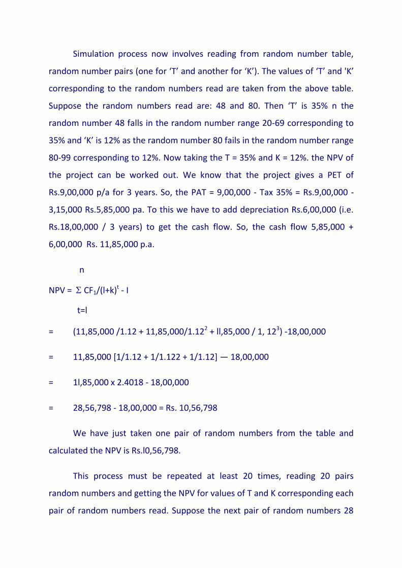
Simulation process now involves reading from random number table,
random number pairs (one for ‘T’ and another for ‘K’). The values of ‘T’ and 'K’
corresponding to the random numbers read are taken from the above table.
Suppose the random numbers read are: 48 and 80. Then ‘T’ is 35% n the
random number 48 falls in the random number range 20-69 corresponding to
35% and ‘K’ is 12% as the random number 80 fails in the random number range
80-99 corresponding to 12%. Now taking the T = 35% and K = 12%. the NPV of
the project can be worked out. We know that the project gives a PET of
Rs.9,00,000 p/a for 3 years. So, the PAT = 9,00,000 - Tax 35% = Rs.9,00,000 -
3,15,000 Rs.5,85,000 pa. To this we have to add depreciation Rs.6,00,000 (i.e.
Rs.18,00,000 / 3 years) to get the cash flow. So, the cash flow 5,85,000 +
6,00,000 Rs. 11,85,000 p.a.
n
NPV = CF1/(l+k)t - I
t=l
= (11,85,000 /1.12 + 11,85,000/1.122 + ll,85,000 / 1, 123) -18,00,000
= 11,85,000 [1/1.12 + 1/1.122 + 1/1.12] — 18,00,000
= 1l,85,000 x 2.4018 - 18,00,000
= 28,56,798 - 18,00,000 = Rs. 10,56,798
We have just taken one pair of random numbers from the table and
calculated the NPV is Rs.l0,56,798.
This process must be repeated at least 20 times, reading 20 pairs
random numbers and getting the NPV for values of T and K corresponding each
pair of random numbers read. Suppose the next pair of random numbers 28

and 49: Corresponding ‘T’ = 35% and ‘K’ = 11%. Then the PAT = PBT - T =
9,00,000 - 3,15,000 = 5,85,000. The cash flow = 5,85,000 ÷ 6,00,000 = Rs.
11,85,000.
n
NPV = CF1/(l+k)t - I
t=l
= (11,85,000/1.11 + 11,85,000 /1.112+11,85,000/1.113) - 18,00,000
= (10,67,598 + 9,6 1,773 + 8,66,462) — 18,00,000
= 28,95,803 — 18,00,000 = Rs.10,95,803
Similarly the NPV for other simulations be obtained. NPVs may be
averaged and if the same is positive the project may h
3.9 SENSITIVITY ANALYSIS
Sensitivity analysis attempts to study the level of sensitivity project
worth, say the NPV, for changes in a key influencing factor, keeping influence
of all other influencing factors at constant level.
Sensitivity analysis presumes uncertainty of the values of al or some of
the influencing factors. For such factors, the range of their values and most
likely values are given. Other factors take constant values.
We know that NPV of a project is influenced by P, V, Q, F, 1, N, 0, T and
K. Let F, 1, N, D and K are constant at Rs.15,00,000, Rs.18,00,000, 3 years,
Rs.6,00,000 and 15% P, V, Q and T are hence the uncertain variables. Let their
range of values and most likely values be as follows:

P: Rs.200-Rs.350; Most Likely value Rs.300
V Rs.100-Rs.250; Most Likely value Rs..150
Q: 15000-22000; Most Likely value 20,000
T: 30%-40%; Most Likely value 35%
Suppose we want to study the sensitivity of NW with respect to ‘T’. then
other uncertain variables, namely,?, V and Q will be assigned their most likely
values. Needless to say, the variables taking constant values will take their
fixed values. The variable T’ will be taking different values within the range of
its values for each such values of T, the NPV will be worked out and sensitivity
of the NPV to that factor is analysed. Accordingly, for our purpose: I = Rs.
18,00,000, N = 3 years, D = Rs.6,00,000, F = Rs.15,00,000, k = 15%. P, V and Q
at their most likely values: Rs.300, Rs. 150 and 20,000 units. ‘T’ shall take
different values within its range, say 30%, 32.5%, 35%, 37.5% and 40%. For
each of these 5 values of T, NPV will be worked out and sensitivity of NW
analysed.
First let T be 30%. The annual cash flow is:
= [(P-V)Q - F - D ] ( J-T) + D
= [(300-150)20000— 15,00,000 — 6,00,000] (1-30%) + 6,00,000
= [30,00,000 — 21,00,000] (0.70) + 6,00,000
= 9,00,000(0.70) ÷ 6,00,000
= Rs. 12,30,000 pa
NPV = (12,30,000 / 1.15 + 12,30,000/1.152 + 12,30,000 / l.153) - 18,00,000

= 28,08,369 — 18,00,000 Rs. 10,08,369
Let T be 32.5%. The annual cash flow is:
= [(P-V) Q - F - D] (I-D) +D
= [(300-150)20000— 15,00,000 — 6,00,000] (1-32.5%) + 6,00,000
= [30,00,000 — 21,00,000] (0.675) + 6,00,000
= 9,00,000(0.675) + 6,00,000
= Rs. 12,07,500 p.a
NPV = (12,07,500/1.15 + 12,07,500/1.152 + 12,07,500/1.153) - 18,00,000
= 27,56,994 - 18,00,000 = Rs. 9,56,994
Let T be 35% The annual cash flow is:
= [(P-V)Q - F - D] (I-D) +D
= [(300-150) 20000— 15,00,000 — 6,00,000] (1-35%) + 6,00,000
= [30,00,000 — 21,00,000] (0.65) ÷ 6,00,000
= 9,00,000(0.65) + 6,00,000
= Rs. 11,85,000 p.a
NPV = (11,85,000/1.15 + 11,85,000/1.152 + 11,85,000/1.15)— 18,00,000
= 27,05,622 - 18,00,000 = Rs. 9,05,622
Let T be 37.5%. The annual cash flow is:
= [(P-V)Q - F - D] (I-D) +D

= [(300-150) 20000 — 15,00,000 — 6,00,O0’’] (1-37.5%) + 6,00,000
NPV = (l2,30,000 15 + 12,30,000/1.152 + 12,30,000/l.l5)— 18,00,000
= 28,08,369 — 18,00,000 Rs. 10,08,369
Let T be 32%. The annual cash flow is:
= [(P-V)Q - F - D] (I-D) +D
= [(300-150)20000— 15,00,000 — 6,00,000] (1-32.5%) + 6,00,000
= [30,00,000 — 21,00,000] (0.675) + 6,00,000
= 9,00,000(0.675) + 6,00,000
= Rs. 12,07,500 p.a
NPV = (12,07,500/1.15 + 12,07,500/1.1 2 + 12,07,500/1.15) — 18,00,000
= 27,56,994 - 18,00,000 = Rs. 9,56,994
Let T be 35% The annual cash flow is:
= [(P-V)Q - F - D] (I-D) +D
= [(300-150) 20000— 15,00,000 — 6,00,000] (1-35%) + 6,00,000
= [30,00,000 — 21,00,000] (0.65) ÷ 6,00,000
= 9,00,000(0.65) + 6,00,000
= Rs. 11,85,000 p.a
NPV = (11,85,000/1.15 + 11,85,000/1.152 + 11,85,000/1.15)— 18,00,000
= 27,05,622 - 18,00,000 = Rs. 9,05,622

Let T be 37.5%. The annual cash flow is:
= [(P-V)Q - F - D] (I-D) +D
= [(300-150) 20000 — 15,00,000 — 6,00,O0’’] (1-37.5%) + 6,00,000
= [30,00,000—21,00,000] (0.625) + 6,00,000
= Rs. 11,62,500 p.a
NPV = (11,62,500/1.15 + 11,62,500/1.152 + 1 1,62,500/1.153)— 18,00,000 =
26,54,249 - 18,00,000 = Rs. 8,54,249
= [30,00,000 - 21,00,000] (0.60) + 6,00,000
= 9,00,000 (0.60) + 6,00,000
= Rs. 11,40,000 p.a
NPV = (1l,40,000/1.1541l,40,000/1.152+l1,40,000/l.153)_18,00,000
= 26,02,876 - 18,00,000 = Rs. 8,02,876
You might have noted that as T rises, npv falls.
Rate of change in NPV for a given change in T.
When T rises to 32.5% (i.e. (0.325) from 30% (i.e. 0.3) NPV falls to
Rs.9,56,994 from Rs.10,08,369.
Rate of change = ./
/
TT
NPVNPV
61.00.0833
0.0509-
0.025/0.3
3.6951375/1008-

When T rises to 35% (i.e. (0.35) from 32.5% (i.e. 0.325) NPV falls to
Rs.9,05,622 from Rs.9,56,994.
Rate of change = ./
/
TT
NPVNPV
698.00.07692
0.05368-
.025/0.325
9451372/9569-
When T rises to 37.5% from 35% NPV falls to Rs.8,54,249 from Rs.
9,05,622
Rate of change = ./
/
TT
NPVNPV
794.00.0714
0.0567-
0.025/0.35
2251373/9056-
When T rises to 40% from 37.5% NPV falls to Rs.3,02,816 falls to Rs.
8,02,816 from Rs. 8,54,249
Rate of change = ./
/
TT
NPVNPV

9015.00.0667
0.0601-
50.025/0.37
4951373/8542-
The rate of MI in NT’V is rising with the rise tax rate. Hence NPV is highly
negatively sensitive with tax rate.
We can study the sensitivity of NPV to ‘T’ in the form of a graph, taking
NPV on the y-axis and Ton the x axis also.
We can do the sensitivity analysis of NPV with respect to another
uncertain variable, say ‘P’ keeping V, Q and T at their most likely values, other
variables at their fixed values and changing the value of P within its given range
of values. Similarly, we can do the sensitivity analysis of NPV with respect to V,
keeping P. Q and T at their most likely values, other variables at their fixed
values and changing the value of V within its given range of values. So, also we
can replicate the sensitivity with respect to ‘Q’.
Now of the 4 uncertain variables, namely, P, V, Q and T, with respect to
which the NPV is most sensitive can be seen. Knowledge of the same will help
monitoring the project with respect to those variables very ably. Hence the
utility of sensitivity analysis.
Illustration 4.1
A firm is currently using a machine purchased two years ago for
Rs.l4,00,000. It has further 5 years of life. It is considering replacing of the
machine with a new one which will cost Rs.28,00,000 cost of installation
Rs.2,00,000. Increase in working capital is Rs.4,00,000. The profits before tax
and depreciation are as follows for the two machines:

Year 1 2 3 4 5
Current
machine (Rs)
6,00,000 6,00,000 6,00,000 6,00,000 6,00,000
New
machine (Rs)
10,00,000 12,00,000 14,00,000 18,00,000 20,00,000
The firm adopts fixed installment method of depreciation. Tax rate and
capital gain tax is 10% on inflation un-adjusted capital gain.
Is it desirable to replace the current machine by the new one, taking the
resale value of old machine at Rs. 16,00,000 at present and using, PBP, ARR,
NPV and IRR? (For NPV method take 10% as discount rate, for ARR shod cutoff
rate is 15% and for PBP method cutoff period is 3.5 years).
Solution
First we have to calculate the size of investment needed. This includes,
purchase cost of new machine, cost of installation and working capital addition
needed, reduced by net sale proceeds (after capital gain tax) of old machine.
The old machine’s original cost = 000,00,14.Rs
Depreciation for the past 2 years
@ Rs.2,00,000 [14,00,000 + life 7 years] 000,00,10.
000,00,4.
Rs
Rs

It is sold for 000,00,6.
000,00,16.
Rs
Rs
Total Gain
This gain has two components, capital gain and revenue Capital gain =
Rs. Sale value - original cost = Rs.16,00,000 - Rs.14,00,000 = Rs.2,00,000.
Revenue gain Total gain-capital gain Rs.6,00,000 - Rs.4,00,000 = Rs.2,00,000.
Tax on revenue gain = Rs.4,00,000 x 40% = Rs.1,60,000. Tax on capital gain =
200000 x 10% = 20,000. Therefore, after adjustment, net sales proceeds of old
machine = Rs. 16,00,000 - Rs.20,00,000 - Rs.1,60,000 = Rs. 14,20,000. Now we
can compute net investment at time zero, i.e. at beginning as follows:
Cost of new machine = Rs. 28,00,000
Add installation cost = Rs. 2,00,000
Cost of machine = Rs. 30,00,000
Add. AddI. Working capital = Rs. 4,00,000
Rs. 34,00,000
Less net saLe proceeds of old machine = Rs. 14,20,000
Net investment Rs. 19,80,000
Now we have to calculate change or increment in cash flow because of
the firm going for replacement of old machine by new one. For this purpose,
what is the cash flow from new machine and what would be the cash flow

from old machine had the firm continued with that must be computed. The
difference of former over the latter is the change in cash flow.
Illustration 4.2
A company brought a machine 2 years earlier at a cost of Rs.60,000 and
estimated useful life of 12 years in all. Its current market price is Rs.25,000. The
management considers replacing this machine with a new one, life 10 years,
price Rs. 1,00,000. The new machine can produce 15 units more per hour. The
annual operating hours are 1000 both for new and old machines. Selling price
per unit is Rs.3. The new machine will involve add!. Material cost by Rs.6,000
and labour by RS.6,000 p.a. But savings in cost of consumable stores of Rs.1000
and repairs of Rs.l000 p.a. will result. The corporate tax rate is 40%. Advice on
the replacement assuming additional working capital of Rs.10000 introduced

now, can be redeemed at 10 years later, cost of capital as 10% and SLM of
depreciation, using NPV method.
Solution
1) Computation cash outflow at present
Cash of new machine : Rs. 1,00,000
Add: Addl. Working capital : Rs. 10,000 1,10,000
Less: Sales value of old machine
Tax shield on loss of old
Machine (book value — Market value) x
tax rate [(50000-25000) x 40%] : Rs. 10,000 35,000
-----------
75,000
ii) Computation of Add!. Gross income
Addl. Production per annum = Hours of operation x Addl. Output
= 1000 x 15 = 15,000
Addl. Gross income per annum = Addl. Production p.a x unit price
= 15,000 x Rs.3 = Rs.45,000
From 1 year to 10th year, Rs.45,000 addl. Income is thus predicted.


ii) Cash Flow Computation
Details Year 1 to 9 Year 10
Addl. Gross Income 45000 45000
Add. Savings in consumable stores &
repairs
2000 2000
47000 47000
Less: Addl. Materials & Labour cost 12000 12000
PBD & T 35000 35000
Addl. Depreciation ( 10000 - 5000 ) 5000 5000
PBT 30000 30000
Less Tax @ 40% 12000 12000
PAT 18000 18000
Addl. Depreciation 5000 5000
Add: Working Capital Recovery - 10000
Cash Flow 23000 33000
NPV = CF1/(l+k)t + CF10 / ( 1+ k )10- I

t=l
Since uniform cash flow is found throughout l to 91h years, the NPV formulates
can be slightly modified as:
NPV = [ACF 1 / (I+k)t +CF10 X 1 ( 1+k)10 ] - I
= 23000 [ l / 1.1 + 1 / 1.12 + ………1 / 1.19 ] + 33000 x 1 / 1.110 - 75000
= (23000 x 5.759) + (33000 x 0.386) — 75000
= 145195 - 75000 = Rs. 70195
The replacement is advised
Illustration 4.3
A company has 3 investment proposals. The expected PV of cash flows
and the amount of investment needed are as below:
Project Investment PV of cash flows
1. Rs. 2.00 lakhs Rs. 2.90 lakhs
2 Rs. 1.15 lakhs Rs. 1.85 lakhs
3 Rs. 2.70 lakhs Rs. 4.00 lakhs
If projects I and 2 are jointly taken, there will be no economics or
diseconomies. If projects 1 and 3 are undertaken, economics result in
investment and combined investment will be Rs.4.4 lakhs. If 2 and 3 are

combined, combined PV of cash flow will be Rs.6.2 lakhs. If all the 3 projects
are combined, all the above economics will result but diseconomy in the form c
additional investment of Rs. 1.25 lakhs will be needed. Find which project
projects be taken.
Solution
Projects Invt. Needed PV of cash flows NPV
1 2,00,000 2,90,000 90,000
2 1,15,000 1,85,000 70,000
3 2,70,000 4,00,000 1,30,000
1&2 3,15,000 4,75,000 1,60,000
1&3 4,40,000 6,90,000 2,50,000
2&3 3,85,000 6,20,000 2,35,000
1,2&3 6,80,000 9,10,000 2,30,000
Projects I & 3 will be chosen as NPV is higher
3.10 RISK ANALYSIS IN THE CASE OF SINGLE PROJECT
Project risk refers to fluctuation in its payback period, ARR, IRR, NPV. or
so. Higher the fluctuation, higher is the risk and vice versa. Let us take NPV
based risk.

If NPV from year to year fluctuate, there is risk. This can be measured
through standard deviation of the NPV figures. Suppose the expected NPV of a
project is Rs. 18 lakhs, and std. deviation of Rs.6 lakhs. The coefficient of
variation C.V is given by sM. deviation divided by NPV.
C.V = Rs.6,00,000 / Rs 18,00,000=0.33.
3.11 RISK RETURN ANALYSIS FOR MULTI PROJECTS
When multiple projects are considered together, what is the overall risk
of all projects put together? Is it the aggregate average of std. deviation of NPV
of all projects? No, it is not. Then what? Now another variable has to be
brought to the scene. That is the correlation coefficient between NPVs of pairs
of projects. When two projects are considered together, the variation in the
combined NPV is influenced by the extent of correlation between NPVs of the
projects in question. A high correlation results in high risk and vice versa. So,
the risk of all projects put together in the form of combined std. deviation is
given by the formula:
2/1
jiijp p
where,
p = combined portfolio std. deviation
Pij = correlation between NPVs of pairs of projects
i, j = std. deviation of iin and jth projects, i.e., any pair of projects taken at a
time.

Three projects have their std. deviations as follows: Rs.4000, Rs.6000
and Rs.10000. The correlation coefficients are l&2 0.6, 1&3 0.78 and 2&3 : -0.5.
What is the overall std. deviation of the portfolio of projects?
p = [Pij i j ] ½ = [1
2+22+3
2+2P1212+2P2323+2P1313] ½
= [40002 + 60002 + 100002 + 2x0.6x4000x6000 -i- 2x0.78x6000xl0000 +
2x(-0. 5)xl 0000x4000] ½
= [16000000+36000000+ 100000000+28800000+93600000-400000000] ½
= [234400000] ½ = Rs. 15,310
What is the return from these multiple projects? This is simple. It is the
aggregate NPVs. Suppose the three projects have NPVs of Rs.16,000, Rs.20,000
and Rs.44,000. The combined NPV = 16000 + 20000 + 44000 = Rs.80000.
The combined coefficient of variation = combined std. deviation I
combined NPV = Rs.15340/Rs.80000 = 0.19 = 19% If we take the correlation
factor unadjusted figures of combined std. deviation and combined NPVs, the
coefficient of variation would have been: 20000/80000 = 0.25 = 25%. The
correlation factor has resulted in reducing overall portfolio risk from 25% to
19%. This results essentially when there is low degree of correlation among the
projects. More so if there is higher negative correlation among the projects.
Illustration
Three projects involve an outlay of Rs.2,00,000, Rs.3,00,000 and
Rs.5,00,000 respectively. The estimated return from the projects are 14%, 16%
and 20%. The std. deviation of returns are 5%, 10% and 10%. The correlation

coefficients are 1&2 : 0.4, 2&3 : 0.6 and 1&3 : 0.2. Find the portfolio return and
risk
Solution
The portfolio or combined return is simply the weighted return of the
projects. This is given by: wi Ri where wi - is the weight (0.2, 0.3 and 0.5 for
the three projects respectively) and Ri - is the respective project return.
Portfolio return = (wi Ri
= 0.2x14% + 0.3x16% + 0.5x20%
= 2.8% + 4.8% -‘-10% = 176%
( p = Portfolio risk = [(wi wj pij (i (j]112
= [wlwl(l(1 + w2w2(2(2 + w3w3(3(3 + 2w1w2(12 (1(2 +
2w2w3(23 (2(3 + 2w1w3(13 (1(3]1/2
Putting the given values, we get that,
p, = [0.2+0.9+2.5+2A+18+2] ½
= [26] ½ = 5.099%
3.12 HAVE YOU UNDERSTOOD QUESTIONS
1. Bring out the meaning and significance of capital projects.
2. Calculate pay-back period, ARR, NPV (at k=10%) and IRR given
3.13 SUMMARY

Capital budgeting essentially involves evaluation of the worth of capital
investment proposals based on estimates of cash inflows and outflows, it is
scientific exercise and uses several techniques. PBP, ARR, NPV and IRR are
certainty techniques. CAPM, sensitivity analysis, simulation analysis, decision
tree technique etc. are techniques of evaluation used under conditions of risk
and uncertainty. CAPM technique can be used for single as well as a portfolio
of projects. For a portfolio of projects, over all return (in NPV or IRR mode) and
overall risk (in the form of std. deviation of NPV or IRR) can be computed to
judge the efficiency of the portfolio.
3.14 EXERCISES
1. Calculate pay-back period, ARR, NPV (at k=10%) and IRR given
Years 1 2 3 4
PBT (Lakhs
Rs.) 40 45 50 55
Tax Rate 40% 40% 5% 35%
2. Using decision tree approach find the expected NPV of the project givi the
following cash flows:
Time zero Time 1 Time 2
-10 lakhs 6 lakhs p. (.6) 4 lakhs p. (.6)
5 lakhsP. (.4)

10 lakhsP. (.4) 6 lakhs p. (.4)
2 lakhs p. (.6)
The cost of capital is 10%
P = Probability
3. For two mutually exclusive projects the projected cash flows are:
Period Project A Project B
Time zero (outflow) Rs.2,20,000 Rs.2,70,000
1 to 7 years (inflow each year) Rs. 60,000 Rs. 70,000
using IRR method, find the better of the two (an annuity of the 1 for 7 years
has a present value of Rs.3.92, R&3.81, R4.3.91 and Rs. 3.60 at 17%, 18%, 19%
and 20%).
4. Machine A costs Rs. 10,00,000 payab1 immediately, while Machine B
costing Rs. 12,00,000 can be paid Rs.6,00,000 down and balance 1 year hence.
The cash flow from the machines are:
Year 1 2 3 4 5
A (Rs. in lakhs) 2 6 4 3 2
B( Rs.in lakhs) Nil 6 6 8 Nil
At 7% discount rate which is better by NPV?

5. Texas filaments ltd has the following figures for its expansion plan,
involving a capital outlay of Rs.5 crs.
Year 1 2 3 4
Unit selling price (Rs.) 7.0 10.0 12.0 15.0
Addi. Sales quantity (Crs) 0.9 0.95 1 1.05
Unit variaNe cost (Rs) 4.0 5.0 6.5 8.0
Tax Rate 30% 30% 35% 35%
Find the PBP and APR of the expansion project.
6. A project has an equity beta of 1.2 and debt beta zero and is a have a debt -
equity ratio of 3:7. Given risk free rate of return of 10% and market return oil
18%, Find the required return for the project per CAPM.
The P, V, Q, F, 1, T and K of a project are as follows:
P = Rs.300; Investment I = Its. 20,00,000; N = 4 years, K = 10%, T = 30% fixed
cost (excluding depreciation) = Rs. 15,00,000. The quantity of sales (a) is a
sensitive factor with the range 12,000 to 20,000 with most likely value 17000.
similarly, variable cost, V, is a sensitive factor with range Rs.130 to Rs.180, with
most likely value of Rs.160 per unit perform sensitivity analysis w.r.t quantity
and variable cost
7. A project's cash flow, life and discount rate have the following probability
distribution.

Cash Flow Prob. Life Prob. Dis. Rate Prob.
Rs. 5 Crs 20 2 .25 9% 0.22
Rs. 8 Crs .72 3 .45 10% .66
Rs. 10 Crs .08 4 .30 12% 12
Perform simulation of PV of cash flow for five runs taking the following random
number sets: i) 12, 18, 82; ii) 70, 38, 48; iii) 78, 02, 49; iv) 22, 18,79; v) 65, 92,
36. 11 the project outlay is Rs. 18 crs, find the expected NPV of the project.
3.15 REFERENCES:
1. Financial Management and Policy - Van Home
2. Financial Decision Making — Hampton
3. Management of Finance - Weston and Brigham
4. Financial Management - P.Chandra