Managerial economics updated

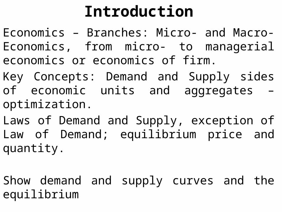
IntroductionEconomics – Branches: Micro- and Macro-Economics, from micro- to managerial economics or economics of firm.Key Concepts: Demand and Supply sides of economic units and aggregates – optimization.Laws of Demand and Supply, exception of Law of Demand; equilibrium price and quantity.

Show demand and supply curves and the equilibrium

Issues and Importance of Study of Managerial Economics

Managerial Economics is “the application of economics to the real business activities so as to get desired business results” in a fiercely competitive environment where thousands of rivals plan strategies to get control of the market.

Important Issues: Production, cost and organization of firms in market place.Topics studied: • Law of demand and elasticity of demand• Demand forecasting• Production theory – returns to scale, technology, cost, revenue and profit• Objectives of firms• Determination of prices– methods, cartels, groups, leadership• Tools to judge economic efficiency – break-even analysis, linear programming, game theory etc• Micro planning – project, capital budgeting, cost benefit analysis, public investment criteria regarding turnkey projects• Business environment and social welfare.

Where do Principles of Micro-economics fit in managerial decision making?

The primary activities of decision making are:• Finding occasions for making decisions• Identifying possible courses of action• Evaluating the revenues and costs associated with each course of action• Choosing the course that best meets the goals and objective of the firm, which is maximizing the wealth of a firm PV of net cash flows or PV (π) and

PV (π) = π1/(1+r) + π2/(1+r)2 + π3/(1+r)

3 + …….+ πn/(1+r)

n Where, πn is the profit in year n in current prices and r is an appropriate discount rate for converting future value into present value.

Constraints to Decision MakingConstraints in managerial decision making involve:

• Legal - including environmental laws, laws relating to women’s/child rights, provisions inconsistent with generally accepted standards of behavior

• Contractual – bind the firm because of some prir agreements

• Financial – maximize production subject to the budgeted amount

• Technological considerations – set physical limit on capacity/volume of production

Circular Flow of Economic Activities

Payment for goods/service

Payment for Goods/ServicesProduct Market

Goods and Services

Goods and Services

Households

Economic Resources

Firms

Income

Factor Market Factor Payments

Economic Resources

Demand AnalysisIndividual and Market demand: Definition/explanation.Illustration: Max, a graduating senior has accumulated an impressive file of tests during his college career. He plans to sell the collection to three prospective buyers, whose demand equations are: Q1 = 30 – 1P, Q2 = 22.5 – 0.75P, and Q3 = 37.5 – 1.25P, where, Q1, Q2 and Q3 are quantity demanded by the three buyers. Calculate (a) the demand equation for Max’s tests (b) how many more tests he can sell for each one-dollar decrease in price, (c) the charge to sell his entire collection if he has a file of 60 tests and (d) the quantity demanded by each of the three buyers at this price

(a) Market demand Qm = Q1+ Q2 + Q3 =30 – 1P + 22.5 – 0.75P + 37.5 – 1.25P = 90 – 3P

(b) The equation shows that an 1 dollar decrease in price will increase the quantity demanded by 3 tests

(c) To sell the entire set of collections, i.e., Qm = 60, Qm = 90 – 3P or, 60 = 90 – 3p, which makes P = 10 and (d) at price P = 10, Q1 = 30 – 10 = 20 tests; Q2 = 22.5 – 0.75 x10 = 15 tests and Q3 = 37.5 – 1.25 x 10 = 25 tests

Demand, Supply and Equilibrium

Demand Function Qd = a + bP, where b<0 and

Qs = c + dP, where d >0At equilibrium, Qd = Qs => a + bP = c + dP

Which implies Pe = c – a/b – d

and Qe= a + b (c – a/b – d)Specific case: Qd = 14 – 2P and Qs = 2 + 4P

At equilibrium, Qd =Qs => 14 – 2P = 2 + 4P

Solving the equations, we get Pe = 2 and Qe=10 units

Theory of CostsInvolves three important/basic areas of managerial economics:

• Resource allocation decisions;• Decisions on expanding product line;• Decisions on capital investment; there are

other areas, too.Cost has different meaning. Traditional definition tends to focus on explicit and historical dimension of costs. The economic approach emphasizes opportunity cost and includes both explicit and implicit costs.

Explicit and Implicit Cost: Explicit cost are those costs that involve an actual payment to other parties, while implicit cost represents the value of foregone opportunities but do not involve actual cash payments. If an input is purchased at some price but its price is later changed, the traditional approach makes the cost estimates based on the purchase price while the economic approach does it on the basis of the present market price.

Sunk cost – Expenditures made in the past or to be made in future against contractual arrangement. Example: cost of inventory, future rental payments on a warehouse (as part of long-term lease)

Theory of CostsNormal Profit: If all opportunity costs (according to the norms demanded by the concept of economic approach) are accounted for, the cost estimate should include normal payment for all inputs, including managerial and entrepreneurial skills and capital supplied by the owners of the firm. The cost includes a normal rate of profit, which refers to profit in excess of these normal returns and considering this, normal economic profit is determined by revenues less all economic costs. Often normal returns to entrepreneurial skills and capital supplied by the owners are not included as costs in the income statement.

Marginal and Incremental Cost: Marginal cost refers to the change in total cost associated with a one-unit change in output, while incremental cost refers to the total additional cost of implementing a managerial decision, such as adding a new product line, acquiring a major competitor, developing an in-house legal staff. Marginal cost is in fact a subcategory of incremental cost.

Opportunity Cost of a product or a factor of production is what must be given up to acquire that product or factor and in general, the opportunity cost of any decision is the value of the next best alternative that must be forgone. The manager who hires an additional secretary may have to forego hiring an additional clerk in the shipping department.

Fixed Cost, Variable Cost and Marginal CostCapital

Labor Input

Output Rate

TFC AFC TVC AVC Total Cost

Marginal Cost

10 0 0 1000 ─ 0 ─ 1000 ─10 2 1 1000 100

0200 200 1200 200

10 3.67 2 1000 500 367 184 1367 16710 5.1 3 1000 333 510 170 1510 14310 6.77 4 1000 250 677 169 1677 16710 8.77 5 1000 200 877 175 1877 20010 11.2

76 1000 167 1127 188 2127 250

10 14.60

7 1000 143 1460 208 2460 333

10 24.60

8 1000 125 2460 307 3460 1000

Draw curves for TFC, TVC, TC, MC, AC, AVC by using the above data; MC, AC and AVC first decline, reach a minimum and then shift upwards; short-run cost curves are U-shaped, long-run cost curves are flatter.

Costs and the Concept of Profit-1

Total cost (TC), fixed cost (FC), variable cost (VC), average cost (c/q), marginal cost (Δc/Δq; m in y = mx + c) accounting cost, explicit cost, implicit cost, economic cost (explicit + implicit cost),opportunity cost; revenue and break-even analysis

Calculation of Economic Profit Econ. Profit =Sales $90,000 Revues minus all Less: Cost of goods sold $40,000 relevant costs,

Gross profit $50,000 both explicit andLess: Advertising $10,000 implicit Depreciation $10,000 Utilities $3,000 Property Tax $2,000 Misc. expenses $5,000

$30,000Net Accounting Profit $20,000Less: Implicit Costs Return on own capital invested $10,000 Opportunity cost ($5000 x 12) $60,000$70,000

Net Economic Profit $50,000─[Net accounting profit – implicit costs]

Costs and the Concept of Profit-2Suppose that you are a good dressmaker. You have 4 yards of a material purchased for Tk 200 per yard a few years ago. You have the options for (a) selling it now @Tk 1200 per yard and (b) using it in making dress that may sell for Tk 7200. The making of the dress would require 4 hours of your labor, which you can sell elsewhere for Tk 800 per hour. Decide whether you should make the dress or sell the material.

Soln: Revenue from sale of dress made Tk 7200Less: cost of the material 4 x 1200 = 48004 hors of labor 4 x 800 = 3200

Tk 8000(net) Economic Profit Tk.– 800

Alternatively, if the material is soldRevenue Tk 1200 x 4yds = Tk 4800Less: Cost of material (at historic price) 4 x 200 = Tk 800 Profit = 4800 – 800 = Tk 4000

Clearly, making dress is not profitable

Cost, Revenue, Profit and Firm’s Equilibrium-1Total cost function C = 1000 + 10q – 0.9q2 + 0.04q3

MC = dc/dq = 10 – 1.8q + 0.12q2 Total variable cost = Total cost – fixed cost = 10q – 0.9q2 + 0.04q3

AVC = TVC/q = 10 – 0.9q + 0.04q2

Profit π = Revenue – Cost = pq – (FC + q.AVC)Or, π + FC = q(p – AVC) => q = (FC + π)/(p – AVC)

This gives the rate of output necessary to generate a certain amount of profit π

At break-even the π = 0 and therefore, the break-even volume of output is qBE = FC/(p – AVC)

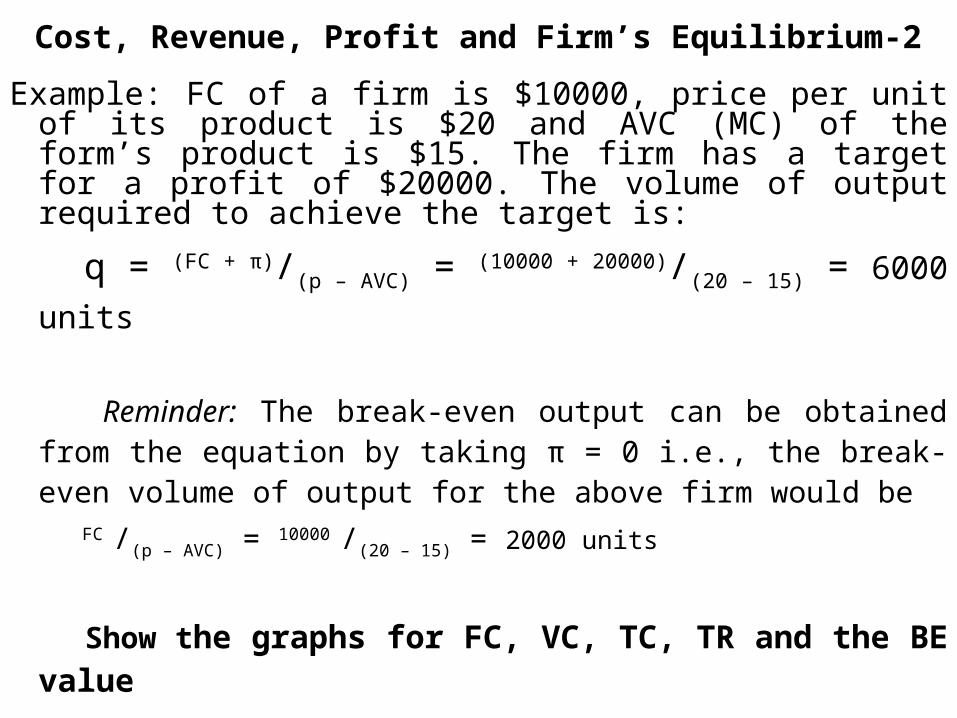
Cost, Revenue, Profit and Firm’s Equilibrium-2Example: FC of a firm is $10000, price per unit of its product is $20 and AVC (MC) of the form’s product is $15. The firm has a target for a profit of $20000. The volume of output required to achieve the target is:

q = (FC + π)/(p – AVC) = (10000 + 20000)/(20 – 15) = 6000 units

Reminder: The break-even output can be obtained from the equation by taking π = 0 i.e., the break-even volume of output for the above firm would be

FC /(p – AVC) = 10000 /(20 – 15) = 2000 units

Show the graphs for FC, VC, TC, TR and the BE value

Finding minimum average variable costTC = 1000 + 10Q – 0.9Q2 + 0.04Q3, Find the rate of output that

results in minimum average variable cost.Solution: dMC = --- (TC) = 10 – 1.8Q + 0.12Q2 dQ TVC = 10Q – 0.9Q2 + 0.04Q3 and AVC = 10 – 0.9Q + 0.04Q2

AVC will be minimum at the point of intersection of the MC and AVC curves and therefore, for AVC to be minimum, AVC = MC

or, 10 – 0.9Q + 0.04Q2 = 10 – 1.8Q + 0.12Q2

solving which we get Q = 0, 0r 11.25 i.e, the average variable cost will be minimum when the out is 11.25

units. Alternative Solution: Minimize the AVC function i.e., find the value of Q for which AVC is minimum.

Optimization of a Firm’s OutputFollowing are the cost and revenue functions for a firm:

TC = 50 + 4q and TR = 20q ─ q2; Calculate

the volume of output for which profit would be maximum.Profit π = (20q ─ q2) − (50 + 4q) = 16q – q2 – 50dπ/dq = 16 – 2q dπ/dq = 0 => 16 – 2q => q = 8 ………(i) and d/dq(dπ/dq )= – 2 < 0 ...……(ii)

Conditions (i) and (ii) indicate that the firm will have

maximum profit if the output is 8 units and the profit at

output 8 is: π8 = 16q – q2 – 50 = 16x8 – 82 – 50 = 30 units

Alternatively,MC = dc/dq = 4 and MR = dπ/dq = 20 – 2q and For πmax MC = MR => 4 = 20 – 2q i.e., q = 8 implying that profit is maximum when q = 8 units.

Consumer BehaviorConsumer’s equilibrium (maximization of satisfaction)

Utility (total and marginal, and Marginal Utility Theory

to explain consumer’s equilibrium: First explain: TU and MU Schedule; Then, the three important postulates: a.MU diminishes; b.TU is maximum when MU is zero, andc.Consumer is in equilibrium when MU = 0

Indifference Curve Theory: indifference, indifferenceschedule and curve, properties of indifference curve, budget line, consumer’s equilibrium on the indifference curve, shifts in consumer’s equilibriumbased on changes in price and income (PCC and ICC)

Elasticity of DemandElasticity = measure for response in demand to change in price and income; price, income, cross and substitution elasticityPrice elasticity of demand ep =(proportionate change in quantity demanded of a product X) ÷ (proportionate change in price of the product x) ep = ─(Δq/q)÷ (Δp/p ) = ─ (dq/dp). p/q The price of a product changes from tk 10 per unit to Tk 12 and because of this, the quantity demanded changes from 10 units to 7 units. The ep stands at ─ 1.5, this means that the increase in price by 1% would cause a reduction in demand by 1.5%.

Let the demand equation is Qd = 100 – 4p i.e., the demand at price $10 is 100 – 4x10 = 60 units and the ep = ─ (dq/dp). p/q or, – 4. 10/60 = ─ 0.67

Price Elasticity of DemandDeterminants of ep Availability of substitutes – products having good substitutes have high ep

Proportion of income spent – demand tends to be inelastic for goods and services that account for only a small proportion of total expenditure (demand for salt)

Time period – demands are usually elastic in the long term than in the short run; people have preference in maintaining the standards in consumption once achieved and consumers adjust expenditures in the long run.

ep<–1, the demand is elastic (luxury goods), if price increases, consumers spend less, revenues of sellers decrease

ep = –1, unitary elastic, revenues of sellers remain unchanged

–1< ep<0, demand is inelastic (everyday necessities), revenues of sellers increase, even with increase in price

Income Elasticity of Demand Income elasticity of demand ei =(proportionate change in quantity demanded of a product X) ÷ (proportionate change in income of the consumer buying it)ei = (Δq/q)÷ (ΔI/I ) = (dq/dI). I/q Let the demand equation is Qd = 50,000 + 5I. If someone’s income(I) is Tk 10,500, Qd = 50,000 + 5x10,500 = 102,500; and ei = (dq/dI). I/q = 5. 10,500/50,000 = 0.512

This means that the an 1% increase in income causes 0.512% increase in the quantity of a product (for which the ei = 0.512) consumed.Income elasticity is usually positive. But take the case of hot dogs (in the US) – it is a food for low income group of people. But if the income of this group of people increases, they usually give up hot dogs and switch to other types of meat. Therefore, income elasticity of hot dogs may be negative. Use of the concept of elasticity: pricing, targeting of products for different market segments

Income elasticity: Engel’s Law

Percentage of income spent on food decreases as income increases – Ernst Engel, Germany

Implication: • Farmers may not prosper as much as people in other occupations during the periods of economic prosperity;

• Food expenditures do not keep pace with increases in GDP;

• Farm incomes may not increase as rapidly as incomes in general

Cross Elasticity of DemandThe responsiveness of quantity demanded of a product X to change in the price of another (usually, a substitute or complementary) product Yec =(proportionate change in quantity demanded of a product X) ÷ (proportionate change in price of another product Y)ec = (Δqx/qx)÷ (Δpy/py ) = (dqx/dpy)÷ (py/qx ) A fall in price of a product Y increases demand for its complementary product XReduction in price of a product Y decreases demand for its substitute product X; however, cross elasticity is not reciprocal i.e., ec for coffee is not the same as ec for tea, tastes of consumers, their incomes, price of some other products matter.Exercise: the demand for X in terms of the price for y is given by qx = 100 + 0.5 py; calculate ec Soln: ec = (dqx/dpy)÷ (py/qx ) = (150 – 125)/(100 - 50)÷ (50 + 100)/(125 + 150) = 0.27; Note: (py/qx ) should be calculated as

the ratio of ranges

Elasticity: ProblemThe demand for (Qx) for books of a publishing company is determined as Qx = 12000 – 5000Px + 5I + 500Pc, where Px = price charged for the company’s books I = per capita income of the buyers Pc= price of the books of competing publishers

Determine the effect ofa.increase in price of the company’s books on

its revenuesb.rising incomes of the buyers on the sale of

the company’s booksc.rise in prices of the books of the competing

publishers on the demand for the company’s books

Assume that the initial values of Px, I, and Pc are $5, $10,000 and $6 respectively

Solution to Elasticity: Problema. Effect of increase in price of the company’s books on its revenues

The effect of increase in price can be assessed by computing price elasticity of demand. Substituting the initial values of I and Pc in the demand equation,

Qx = 12000 – 5000Px + 5(10000)I + 500(6) = 65000 – 5000Px

The value of dq/dp for the given demand equation is:

dQx/dPx = d/dPx (65000 – 5000Px)= – 5000; and p/q = Px/Qx

where Px = $5 and Qx= 65000 – 5000Px = 65000 – 5000(6) = 40000

Now, ep = ─ (dq/dp). p/q and for the given demand equation ep = ─ 5000 . 5/40000 = ─ 0.625 [dq/dp= dQx/dPx = ─ 5000, and p/q = Px/Qx where Px = $5 and Qx= 40000]. The value of ep = ─ 0.625 i.e., – 1 < ep < 0 implies that the company’s books are price inelastic and raising the price of its books will increase the total revenue

Solution to Elasticity: Problemb. Income elasticity ei = dQx/dI . I/QThe demand function is: Qx = 12000 – 5000Px + 5I + 500Pc

dQx/dI = 5, and at income I = 10,000 quantity demanded Qx = 40,000 , which means that the

income elasticity ei = dQx/dI . I/Q= 5. 10000/40000 = 1.25

We find that income elasticity ei > 1. this implies that the company’s books belong to luxury goods. Since with increase in income buyers tend to buy more of luxury goods, during the period of rising incomes, the sale of the company’s books will increase.

Solution to Elasticity: Problem

c. The demand function is: Qx = 12000 – 5000Px + 5I + 500Pc

And the cross elasticity ec = dQx/dPy . Py/QxThe Pc in the demand curve is equivalent to Py of the cross

elasticity and ec = dQx/dPy.Py/Qx = 500. 6/4000 = 0.075

[since dQx/dPy = dQx/dPc = 500]

This implies that a 1% increase in the price of the books of competing publishers would result in a 0.075% increase in the demand for the company’s books.

Regression EquationSimple regression – relationship between two variables

Y = a + bX, where Y may be production cost and X output.

Y = dependent variable, X = independent variable,

a = intercept on y- axis and in the given case, fixed cost

b = slope of the cost function, variable cost per unit or marginal cost; the function may be compared with the equation y = mx + c

Problem: Formulate the regression equation and predict the cost of producing 20 units of the product

Show freehand plotting of the costAt the different levels of output and Draw the straight line cruisingThrough the points.

PRODUCTION PERIOD

TOTAL COST ($Y)

TOTAL OUTPUT (X)

1 100 02 150 53 160 84 240 105 230 156 370 237 410 25

Regression Equation: Soln of the ProblemCost (Yt)

Output (Xt)

Yt – Yav

Xt – Xav

(Xt – Xav )2

(Xt – Xav)(Yt – Yav )

100 0 ─ 137.14

─ 12.29

151.04 1685.45

150 5 ─ 87.14

─ 7.29 53.14 635.25

160 8 ─ 77.14

─ 4.29 18.40 330.93

240 10 ─ 2.86 ─ 2.29 5.24 ─ 6.55230 15 ─ 7.14 2.71 7.34 ─ 19.35370 23 132.86 10.71 114.70 1422.93410 25 172.86 12.71 161.54 2197.05

Yav =237.14

Xav = 12.29

Σ(Xt – Xav )2= 511.40

Σ(Xt – Xav)(Yt – Yav )= 6245.71

The regression equation is: Y = a + bX, where, b = Σ(Xt – Xav)(Yt – Yav ) ÷ Σ(Xt – Xav )2 = 6245.71 ÷ 511.40 = 12.21; a = Yav – bXav = 237.14 – (12.21)(12.29) = 87.08The equation therefore, is Y = 87.08 + 12.21XAdd: talk about R2 – the coefficient of determination (proportion of the dependent variable explained by the regression , value of it varies between 0 and 1; when the value of R2 is higher it means that the regression fits the data very well.

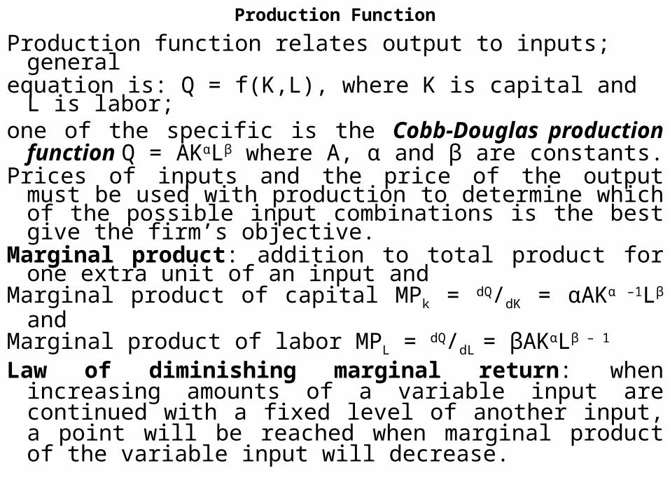
Production FunctionProduction function relates output to inputs; general

equation is: Q = f(K,L), where K is capital and L is labor;

one of the specific is the Cobb-Douglas production function Q = AKαLβ where A, α and β are constants.

Prices of inputs and the price of the output must be used with production to determine which of the possible input combinations is the best give the firm’s objective.

Marginal product: addition to total product for one extra unit of an input and

Marginal product of capital MPk = dQ/dK = αAKα –1Lβ and

Marginal product of labor MPL = dQ/dL = βAKαLβ – 1 Law of diminishing marginal return: when increasing amounts of a variable input are continued with a fixed level of another input, a point will be reached when marginal product of the variable input will decrease.

Matrix of Inputs (capital and labor) and Output CAPITAL↓

8 283 400 490 565 632 693 748 8007 265 374 458 529 592 648 700 7486 245 346 424 490 548 600 648 6935 224 316 387 447 500 548 592 6324 200 283 346 400 447 490 529 5653 173 245 300 346 387 424 458 4902 141 200 245 283 316 346 374 4001 100 141 173 200 224 245 265 283

Labor→ 1 2 3 4 5 6 7 8

•If 4 units of capital and 2 units of labor are used, the maximum production will be 283 units; if K = 8 and L = 2, the output Q = 400 units , and the like.•There is a substitutability between the factors of production; there are varying ways to produce a particular rate of output by using different combinations of inputs•245 units can be output can be produced by using any of the combinations - K = 6 and L = 1, K = 3 and L = 2, K = 2 and L = 3 or K = 1 and L = 6•A firm can use a labor intensive or a capital intensive process (e.g., 6 units of capital and 1 unit of labor or 1 unit of capital and 6 units of labor to produce the same output.

Total, Average and Marginal ProductsTen equally skilled and diligent workers are ready to work in a factory equipped with machines and ready stock of materials. As workers add in, the output increases and figures on the number of workers, total product, average product and marginal product can be shown as under:

Av. Product (AP)= average output per unit and AP = TP/L,TP = Total productL = No of workersMarginal Product (MP)= change in outputAssociated with one-Unit change in workersMP = ΔQ/ΔL,Q = amount of output.

No of Workers

Total Product

Av. Product

Marginal Product

0 0 − −1 2 2 22 5 2.5 33 9 3 44 14 3.5 55 22 4.4 86 40 6.7 187 57 8.1 178 63 7.9 69 64 7.1 110 63 6.3 − 1

Total Output

Total Output (Q)

Rate of labor input (L)

Average and Marginal Product

Marginal product

Average product

Rate of labor input

Producer’s EquilibriumOutput at which a producer is most satisfied, usually, a level at which the firm has the maximum profit, which can be attained either by minimizing costs or maximizing sales. Minimizing costs: use Isoquant and budget line - manufacturer may use two factors of production and a number of different combinations of the factors can yield the same amount of output. The curve representing these combinations is called the iso-quant/equal product curve/product indifference curve. The producer may choose any of these combinations but his decision on which combination he would pick depends on the prices of the factors and his budget that may be shown by his budget line/isocosts (also known as price line or outlay line).

Isoquant

Budget Line

Producer’s Equilibrium: Minimizing costsIsoquant (also known as product indifference curves or equal product curves) and isocost (also known as price line or outlay line) curves are used to determine efficient input rate combination for given production rates. All points on the isoquant represent the combination of inputs that produce the same amount of output. Isoquants generally slope downward, are convex to the origin and do not intersect each other.

Marginal Rate of Technical Substitution of X for Y is the number of units of factor Y, which can be replaced by one unit of factor X, quantity of output remaining the same. Thus, MRTSxy = Δy/Δx

The MRTSxy generally diminishes as the quantity of X is increased relative to quantity of Y (quantity of output remaining unchanged). This is called the law of diminishing marginal rate of substitution.

Producer’s Equilibrium: Maximizing RevenueUse Production Possibility curve and Iso-Revenue Line:

Production Possibility Curve represents what assortment of goods and services an economy can produce with the resources and techniques at its disposal. Increase in the resources at the disposal of the firm would take it to a higher production possibility curve.

The question is: which of the various combinations the firm will decide to produce? The answer is: the combination that is shown at the point of tangency with the iso-revenue line. Production possibility curves move upwards or downwards in a way that they remain parallel to each other. Iso-revenue lines also do the same. Their movements, along with the shifts of the points of tangency, determine the output expansion path.

Production possibilities

Good X (thousands) Good Y (thousands)

A 0 15B 1 14C 2 12D 3 9E 4 5F 5 0

Producer’s EquilibriumThe manufacturer has a fixed amount of resources and he can produce different combination of two goods that may be produced by the same amount of resources. The curve drawn by plotting the points showing such combinations is called production possibility curve and the manufacturer can choose any of these combinations.

But the manufacturers choice will be determined by the market prices of the goods and he will chose the combination that gives him the maximum revenue. The curve that shows the different combinations of two goods that can give the same amount of revenue is called the iso-revenue curve.

Production Iso-revenue

possibility curve curve

Returns to ScaleQ = f(K,L), if both inputs are changed by some factor λ output may change to some factor h, which may be equal to λ, more than λ or less than λ. Now consider the case hQ = f(λk, λL), where λ = 2 i.e., both the inputs are doubled. In such case, the Cobb-Douglas production function Q = AKαLβ may look like

hQ = A(2K)α(2L)β = 2α + β(AKαLβ) = 2α + β(Q) => h = 2α + βThe equation h = 2α + β is derived from a production function that uses both factors K and L increased by 2 times and the equation shows that if both factors of production are increased by 2 times, the output increases by this increases 2α + β times.

If the proportion in which the output increases is the same as the proportion of increase of the inputs i.e., if h = 2 then α + β = 1

This is a situation when we have constant returns to scale. Similarly, if h > 2, α + β > 1, it is a situation, when we have increasing returns to scale and if h < 2, α + β < 1, it is a situation, when we have decreasing returns to scale. Thus in case of constant returns to scale, the function Q = AKαLβ may be written as Q = AKαL1 – α

Returns to Scale: Matrix of Inputs and Output CAPITAL↓

8 283 400 490 565 632 693 748 8007 265 374 458 529 592 648 700 7486 245 346 424 490 548 600 648 6935 224 316 387 447 500 548 592 6324 200 283 346 400 447 490 529 5653 173 245 300 346 387 424 458 4902 141 200 245 283 316 346 374 4001 100 141 173 200 224 245 265 283

Labor→ 1 2 3 4 5 6 7 8

• The table indicates that there is a substitutability between the factors of production. The firm can use a capital-intensive production process or a labour intensive one. • Now, if inputs rates are doubled, the output also doubles e.g., K = 1, L = 4 q = 200 and K = 2, L = 8 q = 400, this is a case of constant returns to scale. Returns to scale means change in output because of proportionate change in inputs.• In reality, output may increase more (or less) than in proportion to changes in inputs. Also output may change because of change in one input while the other inputs remains constant. In such case, the change in the output rate is referred to as returns to factor. •The output table does not allow for determination of the profit maximizing output or the best way to produce some specified rate of output.

Production with one variable input Assumes that the rate of input of one factor of production is fixed (the period of production is not long enough to change the input rate of that factor). The question is: how to determine the optimal (profit maximizing) rate of employment of the variable factor?

Say, of the two input labour and capital, capital is fixed. In that case, the principle to be followed to optimize the level of employment of labour is that the additional units of labour be hired until the marginal revenue product of labour (MRPL) equals the wage rate (w). MRP is defined as marginal revenue times marginal product, which is in fact, the value of the extra unit of labour. Thus the optimizing condition is MRPL = w

Similarly, if labour input is fixed, the capital stock would be varied and the capital would be employed until the marginal revenue product of capital equals the price of capital (r) i.e., MRPK = r

Now, MRPL = MR.MPL; but MR = ΔTR/ΔQ and MPL = ΔQ/ΔL or, MRPL = ΔTR/ΔQ .ΔQ/ΔL = ΔTR/ΔL = d/dL(TR)

ProblemThe production function of Global Electronics is Q = 2K0.5L0.5 and the marginal product function for labour and capital are given by

MPL = d/dL(Q) = 2. ½.2K0.5L0.5 = √K/√L, and MPK = d/dK(Q) = 2. ½.2K0.5L0.5 = √L/√KAssume that the capital stock is fixed at 9 units (K = 9). if the price of output (P) is $6 per unit, and wage is $2 per unit, determine the optimal (profit maximizing) rate of labour to be hired. What labour rate is optimal if the wage rate is increased to $3 units?

Solution:First, determine the MRPL assuming that K is fixed at 9. Note that P = MRMRPL = MR.MPL = P. MPL = P.√K/√L, = 18/√LFor optimizing, MRPL = w or, 18/√L = 2 which means, L = 81 i.e, 18 units of labour should be employedIf the wage rate increases to $3, the profit maximizing condition would be 18/√L = 3 implying that L = 36

The example shows that as the price of labour increases, the firm demands less labour i.e., the labour demand curve is downward sloping.

Production with two variable inputsIf both capital and labour are variable, there may be three ways for efficient resource allocation in production:

maximize production for a given dollar outlay on labour and capital (production possibility curve);

minimize the dollar outlay on labour and capital inputs necessary to produce a specified rate of output (MPa/Pa = MPb/Pb = MPc/Pc = ............ = MPn/Pn, where MPa, MPb, ...., MPn, are marginal product of the factors A, B .....,N and Pa, Pb, ....,Pn are the prices of these factors); If MPa/Pa > MPb/Pb it is advantageous for the entrepreneur to employ more of the favtor A than of factor B. He will employ more of one factor and less of the other till the ‘proportionality rule’ is satisfied.

produce the output rate that maximizes profit (in this case, for each input, the marginal revenue product will equal the input prices).

Laws of Returns and Returns to Scale There are three laws of returns: Law of diminishing, increasing and constant returns. However, they are only three aspects of one law viz., the law of variable proportions. According to law of diminishing returns applicable in agriculture “successive application of labour and capital to a given area of land must ultimately, other things remaining the same, yield a less than proportionate increase in produce”. An industry is subject to law of increasing returns if extra investment in the industry is followed by more than proportionate returns i.e., the marginal product increases (with lowering of marginal cost). This may happen by specialization of machinery and labour. The Law of constant returns says that increased investment of the labour and capital results in a proportionate increase in output and whatever the output or scale of production, the cost per unit remains unaltered. Returns to Scale refers to the effect of doubling, trebling, quadrupling and so on of all the inputs on the output of the product, a situation when all the productive forces are increased or decreased simultaneously in the same ratio. Laws of return and returns to scale are not the same thing: Laws of returns refer to situations when some factors may be increased or decreased and at least one factor remains unchanged, while returns to scale refers to a situation when all factors change simultaneously in a given proportion.

Economies of ScaleEconomies of Scale: If the scale changes (to a large proportion) economies take place because of lowering unit costs or increased productivity as a result of specialization of labour and inventory. There may be diseconomies, too. For example, transportation cost may go high, wage rates may be increased (due to increased demand of labour for the large scale industry) etc.

Economies of scale may be understood as the benefits obtained because of increase in the size of the firm/output. Why do increasing returns to scale occur?

• Use of technologies that are cost-efficient at high levels of production

• Specialization of labor• Economies in inventoriesWhen do decreasing returns to scale occur?When firms grow so large that the management cannot effectively manage (for example, increase in costs of gathering, organizing, transportation, reviewing information etc)

Economies of ScopeEconomies of scope: firms often find that even without increasing the scale, per unit costs are lower when two or more products are produced (because of use of idle/temporarily ‘surplus’ capacity) Economies of Scope: large-scale firms will have excess capacity that can be used to produce other products with little or no increase in capital costs; Other firms may take advantage of their unique skills or comparative advantage in marketing to develop products that are complementary with the firm’s existing product (e.g., Fisons develops a market for its toiletry products, industries producing other cosmetics get easier ways to promote their products in the market that are developed for Fisons toiletries. Other industries can use the retail outlets selling Fisons products).

Economies of large-scale production• Efficient use of capital equipment; • Economy of specialized labour (through division of labour); • Better utilization/greater specialization in management;• Economies of buying and selling; Economies of overhead charges; • Economy in rent; Experiments and research• Advertisement and salesmanship; • Utilization of by-products; • Meeting adversity; • Cheap creditDiseconomies of scaleOver-worked management; Individual tastes ignored; No personal element; Possibility of depression; Dependence on foreign markets; cut-throat competition; International complications and war; Lack of adaptability.

Internal and External EconomiesTechnical economies (large size, linkage process, superior techniques, increased specialization); • Managerial economies (functional specialization and delegation of routine and detailed matters to subordinates); • Commercial economies (bargaining advantage of large firms in purchase deals, procurement of credit etc); • Financial economies (large firms can borrow more, and on more favourable terms);• Riskbearing economies (large firm can spread risk and even eliminate them). External • Economies of concentration (arising out of availability of skilled worker, provision of better transport and credit, advantage of localized industries etc);• Economies of information (publication of trade journals, dissemination of research etc);• Economies of disintegration (splitting of some processes for taking up by specialist firms).

Theory of ProductionProduction: Transformation of inputs into outputs. inputs are what a firm buys (i.e., productive resources) and outputs are what it sells (i.e., goods and services). Production is defined as creation of utility and more precisely, creation/addition of value.

Production is creation of utility and utility created may be of three types:

• Form utility – (physical change/transformation of one set of goods into another

• Place utility – transportation of goods/services to place of use

• Time utility – keeping in store till required.The theory of production studies • factors of production and their organization, • the laws of production that govern the relations between inputs and outputs, and among others,

• the theory of population (because population supplies labour, the most important factor of production).

Theory of Production: Importance

The theory of production • plays an important role in the theory of relative prices,

• helps in analyzing relations between costs and volumes of outputs,

• tells how manufacturers combine various inputs to optimize the production of output,

• provides a base for the theory of demand of firms for productive resources and thus, the prices to be fixed for the factors of production, which implies that

• the theory of production has a great relevance to the theory of distribution.

Factors of ProductionLand, Labour, Capital and Organization

Land: All natural resources (useful and scarce, actually and potentially), which yield an income or have exchange value. Land has features that have bearing on rent:

• Land is nature’s gift to man• Land is permanent (original and indestructible)• Land lacks mobility in geographical sense• Land is fixed in quantity (land has no supply price i.e., supply of land remains the same, no matter whether there is any change in price)

• Land provides infinite variation in degrees of fertility; No two pieces of land are alike.

LabourLabour: Any work whether manual or mental, which is undertaken for a monetary consideration. Peculiarities of labour that have bearing on its price i.e., wage:

• Labour is inseparable from the labourer himself

• Labourer has to sell his labour in person • Labour does not last (it is perishable, it has no reserve price whether one sells or holds it for some time)

• Labourer has very weak bargaining power• Changes in price of labour react rather curiously on its supply (fall in price i.e., wage below a certain point may increase the supply of labour; some members of the family who did not work before, may start seeking job).

Efficiency of LabourFactors that determine efficiency of Labour –racial qualities–climatic conditions–education (general and technical)–personal qualities (physique, mental alertness, intelligence, resourcefulness, initiative, and above all, integrity)

–industrial organization and equipment

–factory environment–working hours–fair and prompt payment–social and political factors

Division of labourSimple – also called functional division of labour, is the division by major occupations (carpenters, blacksmiths, weavers etc)

Complex – No group of workers makes a complete article; the making of an article is split into a number of processes and sub-processes which are carried out by separate groups of people.

Territorial – locations specializing in different trade or product

Advantages:Increase in productivity; increase in dexterity and skill; facilitating inventions; introduction of machinery; saving in time, tools and implements; diversity in employment; promotion of large-scale production.

Disadvantages:Monotony; retardation of human development; loss of skill, risk of unemployment; industry dehumanized (under division of labour, many people combine to produce an article and “everybody’s business becomes nobody’s business”, the workers lose all sense of responsibility and pride in their work and thus the industry is dehumanized)

CapitalCapital: That part of man’s wealth which is used in producing further wealth or which yields income. Capital is not a primary or original factor of production; it is ‘produced means of production, often referred to as dead labour. The term capital is generally used for capital goods such as plant, machinery, tools, accessories, stocks of raw material, goods in process, and fuel. Land is not regarded as capital because, it is a free gift of nature and it is permanent i.e, it has no mobility, while capital is perishable and mobile.

Capital formationincrease in stock of real capital in a country and it involves making of more capital goods such as machinery, tools, factories, transport equipment, materials, electricity etc, which are all used for further production of goods. Capital formation essentially requires savings, which must be invested in order to have new capital goods.

Capital Formation: stages/componentsThe three stages of the process of capital formation are:• Creation of savings by individuals or households – the level of savings in a country depends upon the power to save and will to save. The power to save is a function of the average level of income and the distribution of national income. savings at the household level may be voluntary and forced. Besides households, other important agents of savings are the business and enterprises and the government.• Mobilization of savings – transfer of savings from households to businessmen for investment; development of capital market.• Investment of savings in real capital – The primary factor that determines the level of investment is the size of the market; other important factors are inducement to invest, marginal efficiency of capital, and the rate of interest (prospective yield).An important component of capital is foreign capital (foreign savings) that comprises – direct private investments,– loans or grants by foreign governments, and – loans or grants by international agencies.Capital formation may take place also through deficit financing, which is newly created money and this usually takes place by deliberate allocation of expenditure in excess of incomes.

Organization/Enterprise

Organization/Enterprise: two main functions of this factor of production are

(a)organizing; and (b)risk taking/uncertainty bearing.

Entrepreneurs initiate business, mobilize productive resources, take financial responsibility of enterprises and play the role of investors

Another important function of entrepreneur: innovation and initiatives of invention

Managerial economics updated

Documents

Transcript of Managerial economics updated