PMFIE- Managerial Economics Course Material - MEASI ...
89
Prepared by Dr S G BALAJI, MBA, PGDIB, M.Phil, Ph.D. Associate professor- Academic and R&D MEASI Institute of Management, Royapettah, Chennai-14. PMFIE- Managerial Economics Course Material Prepared By Dr. S.G. BALAJI, M.B.A., PGDIB., M.Phil., Ph.D. Associate Professor - Academic and Re3search & Development MEASI Institute of Management, Royapettah, Chennai – 14 MEASI INSTITUTE OF MANAGEMENT CHENNAI-14 Approved by All India Council of Technical Education and Affiliated to the University of Madras, ISO 9001:2015 Certified Institute
-
Upload
khangminh22 -
Category
Documents
-
view
2 -
download
0
Transcript of PMFIE- Managerial Economics Course Material - MEASI ...

Prepared by Dr S G BALAJI, MBA, PGDIB, M.Phil, Ph.D. Associate professor- Academic and R&D
MEASI Institute of Management, Royapettah, Chennai-14.
PMFIE- Managerial Economics
Course Material
Prepared By
Dr. S.G. BALAJI, M.B.A., PGDIB., M.Phil., Ph.D.
Associate Professor - Academic and Re3search & Development
MEASI Institute of Management, Royapettah, Chennai – 14
MEASI INSTITUTE OF MANAGEMENT
CHENNAI-14 Approved by All India Council of Technical Education and
Affiliated to the University of Madras, ISO 9001:2015 Certified Institute

Prepared by Dr S G BALAJI, MBA, PGDIB, M.Phil, Ph.D. Associate professor- Academic and R&D
MEASI Institute of Management, Royapettah, Chennai-14.
VISION & MISSION STATEMENTS
VISION;
• To emerge as the most preferred Business School with Global recognition by producing most
competent ethical managers, entrepreneurs and researchers through quality education.
MISSION;
• Knowledge through quality teaching learning process; To enable the students to meet the
challenges of the fast challenging global business environment through quality teaching learning
process.
• Managerial Competencies with Industry institute interface; To impart conceptual and practical
skills for meeting managerial competencies required in competitive environment with the help of
effective industry institute interface.
• Continuous Improvement with the state of art infrastructure facilities; To aid the students in
achieving their full potential by enhancing their learning experience with the state of art infrastructure
and facilities.
• Values and Ethics; To inculcate value based education through professional ethics, human values
and societal responsibilities.
PROGRAMME EDUCATIONAL OBJECTIVES (PEOs)
PEO 1; Placement; To equip the students with requisite knowledge skills and right attitude
necessary to get placed as efficient managers in corporate companies.
PEO 2; Entrepreneur; To create effective entrepreneurs by enhancing their critical thinking,
problem solving and decision-making skill.
PEO 3; Research and Development; To make sustained efforts for holistic development of
the students by encouraging them towards research and development.
PEO4; Contribution to Society; To produce proficient professionals with strong integrity to
contribute to society.
MEASI INSTITUTE OF MANAGEMENT
CHENNAI-14 Approved by All India Council of Technical Education and
Affiliated to the University of Madras, ISO 9001:2015 Certified Institute

Prepared by Dr S G BALAJI, MBA, PGDIB, M.Phil, Ph.D. Associate professor- Academic and R&D
MEASI Institute of Management, Royapettah, Chennai-14.
Program Outcome;
PO1; Problem Solving Skill; Apply knowledge of management theories and practices to
solve business problems.
PO2; Decision Making Skill; Foster analytical and critical thinking abilities for data-based decision
making.
PO3; Ethical Value; Ability to develop value based leadership ability.
PO4; Communication Skill; Ability to understand, analyze and communicate global,
economic, legal and ethical aspects of business.
PO5; Individual and Leadership Skill; Ability to lead themselves and others in the achievement
of organizational goals, contributing effectively to a team environment.
PO6; Employability Skill; Foster and enhance employability skills through subject knowledge.
PO7; Entrepreneurial Skill; Equipped with skills and competencies to become an entrepreneur.
PO8; Contribution to community; Succeed in career endeavors and contribute significantly to the community.
MEASI INSTITUTE OF MANAGEMENT
CHENNAI-14 Approved by All India Council of Technical Education and
Affiliated to the University of Madras, ISO 9001:2015 Certified Institute
Prepared by Dr S G BALAJI, MBA, PGDIB, M.Phil, Ph.D. Associate professor- Academic and R&D
MEASI Institute of Management, Royapettah, Chennai-14.
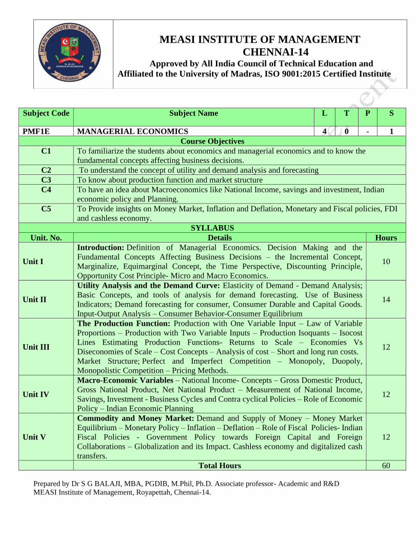
Subject Code Subject Name L T P S
PMF1E MANAGERIAL ECONOMICS 4 0 - 1
Course Objectives
C1 To familiarize the students about economics and managerial economics and to know the
fundamental concepts affecting business decisions.
C2 To understand the concept of utility and demand analysis and forecasting
C3 To know about production function and market structure
C4 To have an idea about Macroeconomics like National Income, savings and investment, Indian
economic policy and Planning.
C5 To Provide insights on Money Market, Inflation and Deflation, Monetary and Fiscal policies, FDI
and cashless economy.
SYLLABUS
Unit. No. Details Hours
Unit I
Introduction: Definition of Managerial Economics. Decision Making and the
Fundamental Concepts Affecting Business Decisions – the Incremental Concept,
Marginalize, Equimarginal Concept, the Time Perspective, Discounting Principle,
Opportunity Cost Principle- Micro and Macro Economics.
10
Unit II
Utility Analysis and the Demand Curve: Elasticity of Demand - Demand Analysis;
Basic Concepts, and tools of analysis for demand forecasting. Use of Business
Indicators; Demand forecasting for consumer, Consumer Durable and Capital Goods.
Input-Output Analysis – Consumer Behavior-Consumer Equilibrium
14
Unit III
The Production Function: Production with One Variable Input – Law of Variable
Proportions – Production with Two Variable Inputs – Production Isoquants – Isocost
Lines Estimating Production Functions- Returns to Scale – Economies Vs
Diseconomies of Scale – Cost Concepts – Analysis of cost – Short and long run costs.
Market Structure; Perfect and Imperfect Competition – Monopoly, Duopoly,
Monopolistic Competition – Pricing Methods.
12
Unit IV
Macro-Economic Variables – National Income- Concepts – Gross Domestic Product,
Gross National Product, Net National Product – Measurement of National Income,
Savings, Investment - Business Cycles and Contra cyclical Policies – Role of Economic
Policy – Indian Economic Planning
12
Unit V
Commodity and Money Market: Demand and Supply of Money – Money Market
Equilibrium – Monetary Policy – Inflation – Deflation – Role of Fiscal Policies- Indian
Fiscal Policies - Government Policy towards Foreign Capital and Foreign
Collaborations – Globalization and its Impact. Cashless economy and digitalized cash
transfers.
12
Total Hours 60
MEASI INSTITUTE OF MANAGEMENT
CHENNAI-14 Approved by All India Council of Technical Education and
Affiliated to the University of Madras, ISO 9001:2015 Certified Institute

Prepared by Dr S G BALAJI, MBA, PGDIB, M.Phil, Ph.D. Associate professor- Academic and R&D
MEASI Institute of Management, Royapettah, Chennai-14.
Reference Books
1. Damodaran, S., Managerial Economics, 2nd Edition, Oxford University Press, 2011.
2. Dwivedi, D.N., Managerial Economics, Vikas Publishing House, 2011.
3. Hirschey, M., Managerial Economics; An Integrative Approach, South Western, 2010.

Prepared by Dr S G BALAJI, MBA, PGDIB, M.Phil, Ph.D. Associate professor- Academic and R&D
MEASI Institute of Management, Royapettah, Chennai-14.
MEASI INSTITUTE OF MANAGEMENT
CHENNAI-14 Approved by All India Council of Technical Education and
Affiliated to the University of Madras, ISO 9001:2015 Certified Institute
4. Keat, P.G., Young, P. and Banerjee, S., Managerial Economics; Economics Tools for Today’s
Decision Makers, 6th Edition, Pearson, 2010.
5. Salvatore, D. and Srivastava, R., Managerial Economics; Principles and Worldwide Applications,
7thEdition, Oxford University Press, 2012.
6. Thomas, C.R., Maurice, C. and Sarkar, S., Managerial Economics, 9th Edition, Tata McGraw-Hill
Education Pvt. Ltd., 2010.
E-Sources
1. http://pearsoned.co.in/prc/book/paul-g-keat-managerial-economics-economic-tools-todays-
decision-makers6e-6/9788131733530
2. http://pearsoned.co.in/prc/book/h-craig-petersen-managerial-economics-4e-4/9788177583861
3. http://www.onlinevideolecture.com/mba-programs/kmpetrov/managerial
economics/?courseid=4207
4. http://ocw.mit.edu/courses/economics/
5. https://www.slideshare.net/dvy92010/nature-and-scope-of-managerial-economics-76225857
Assessment Tools Used
1. Assignments 6. Group Discussion
2. Internal Assessment Tests 7. Class room Exercises
3. Model Exams 8. Quiz
4. Seminars 9. Practical problems
5. Case studies 10. Synetics
Content Beyond Syllabus
1. Relationship of Managerial Economics with other disciplines
2. Difference between Micro and Macroeconomics
3. Discussions about current changes and developments in the Indian Economy like Demonetization
and GST, Digital economic transactions in digital India
Additional Reference Books
1. Managerial Economics; Craig H. Petersen, W. Chris Lewis and Sudhir K. Jain, Pearson
Education, 5th Ed., 2008.
2. Managerial Economics – Foundations of Business Analysis and Strategy; Christopher R. Thomas
and S. Charles Maurice, McGraw Hills, 10th Ed., 2011.
3. Managerial Economics - Economic Tool for Today’s Decision Makers; Paul G. Keat, Philip K.
Y. Young and Sreejata Banerjee, Pearson Education, 6th Ed., 2013.

Prepared by Dr S G BALAJI, MBA, PGDIB, M.Phil, Ph.D. Associate professor- Academic and R&D
MEASI Institute of Management, Royapettah, Chennai-14.
MEASI INSTITUTE OF MANAGEMENT
CHENNAI-14 Approved by All India Council of Technical Education and
Affiliated to the University of Madras, ISO 9001:2015 Certified Institute
Course Outcomes
CO No. On completion of this course successfully the students will; Program Outcomes
C105.1 Be able to understand the basic concepts of managerial economics that
helps the firm in decision making process.
PO2, PO4
C105.2 Be familiar about the Basic concepts of Demand, Supply and
Equilibrium and their determinants.
PO4, PO6, PO7
C105.3 Have better idea and understanding about production function and
market structure
PO6, PO7
C105.4 Have better insights about macroeconomics concepts like National
income, Savings and Investment, Indian Economic Policy and planning
PO8
C105.5
Possess better knowledge about Money market, Monetary and Fiscal
policy, inflation and deflation, FDI and globalization and Cashless
economy and digitalized cash transfers.
PO7
Prepared by Dr S G BALAJI, MBA, PGDIB, M.Phil, Ph.D. Associate professor- Academic and R&D
MEASI Institute of Management, Royapettah, Chennai-14.
MEASI INSTITUTE OF MANAGEMENT
CHENNAI-14 Approved by All India Council of Technical Education and
Affiliated to the University of Madras, ISO 9001:2015 Certified Institute
UNIT – I - INTRODUCTION Introduction: Definition of Managerial Economics. Decision Making and the Fundamental
Concepts Affecting Business Decisions – the Incremental Concept, Marginalism, Equimarginal
Concept, the Time Perspective, Discounting Principle, Opportunity Cost Principle- Micro and
Macro Economics.
INTRODUCTION:
People have limited number of needs which must be satisfied if they are to survive as human
beings. Some are material needs, some are psychological needs and some others are emotional
needs. People’s needs are limited; however, no one would choose to live at the level of basic human
needs if they want to enjoy a better standard of living. This is because human wants (desire for the
consumption of goods and services) are unlimited. It doesn’t matter whether a person belongs to
the middle class in India or is the richest individual in the World, he or she wants always something
more. For example bigger a house, more friends, more salary etc., Therefore the basic economic
problem is that the resources are limited but wants are unlimited which forces us to make choices.
Economics is the study of this allocation of resources, the choices that are made by economic
agents. An economy is a system which attempts to solve this basic economic problem. There are
different types of economies; household economy, local economy, national economy and
international economy but all economies face the same problem. The major economic problems
are (i) what to produce? (ii) How to produce? (iii) When to produce and (iv) For whom to produce?
Economics is the study of how individuals and societies choose to use the scarce resources that
nature and the previous generation have provided. The world’s resources are limited and scarce.
The resources which are not scarce are called free goods. Resources which are scarce are called
economic goods.
WHY STUDY ECONOMICS?
A good grasp of economics is vital for managerial decision making, for designing and
understanding public policy, and to appreciate how an economy functions. The students need to
know how economics can help us to understand what goes on in the world and how it can be used
as a practical tool for decision making. Managers and CEO’s of large corporate
bodies, managers of small companies, nonprofit organizations, service centers etc., cannot succeed
in business without a clear understanding of how market forces create both opportunities and
constraints for business enterprises.
Prepared by Dr S G BALAJI, MBA, PGDIB, M.Phil, Ph.D. Associate professor- Academic and R&D
MEASI Institute of Management, Royapettah, Chennai-14.
MEASI INSTITUTE OF MANAGEMENT
CHENNAI-14 Approved by All India Council of Technical Education and
Affiliated to the University of Madras, ISO 9001:2015 Certified Institute
REASONS FOR STUDYING ECONOMICS:
➢ It is a study of society and as such is extremely important.
➢ It trains the mind and enables one to think systematically about the problems of business
and wealth.
➢ From a study of the subject it is possible to predict economic
➢ trends with some precision.
➢ It helps one to choose from various economic alternatives.
Economics is the science of making decisions in the presence of scarce resources. Resources are
simply anything used to produce a good or service to achieve a goal. Economic decisions involve
the allocation of scarce resources so as to best meet the managerial goal. The nature of managerial
decision varies depending on the goals of the manager.
A Manager is a person who directs resources to achieve a stated goal and he/she has the
responsibility for his/her own actions as well as for the actions of individuals, machines and other
inputs under the manager’s control.
MANAGERIAL ECONOMICS:
Managerial economics is the study of how scarce resources are directed most efficiently to
achieve managerial goals. It is a valuable tool for analyzing business situations to take better
decisions.
DEFINITION:
Prof. Evan J Douglas defines Managerial Economics as “Managerial Economics is concerned with
the application of economic principles and methodologies to the decision making process within
the firm or organization under the conditions of uncertainty”
According to Milton H Spencer and Louis Siegelman “Managerial Economics is the integration of
economic theory with business practices for the purpose of facilitating decision making and
forward planning by management”
According to Mc Nair and Miriam, ‘Managerial Economics consists of the use of economic modes
of thoughts to analyze business situations’.

Prepared by Dr S G BALAJI, MBA, PGDIB, M.Phil, Ph.D. Associate professor- Academic and R&D
MEASI Institute of Management, Royapettah, Chennai-14.
MEASI INSTITUTE OF MANAGEMENT
CHENNAI-14 Approved by All India Council of Technical Education and
Affiliated to the University of Madras, ISO 9001:2015 Certified Institute
NATURE AND SCOPE OF MANAGERIAL ECONOMICS:
I. Managerial Economics – is it positive or normative?
Economics is divided into two categories (i) positive economics and (ii) Normative Economics,
analysis the strength of business organization.
II. Area of study
Demand analysis and Forecasting:
- Accurate estimation of demand by analysis the forces acting on demand of the product produced
by the firm forms the vital issue in taking effective decision at the firm level.
Cost and production analysis: In decision making, cost estimates are essential. Production
planning, profit planning etc
. Pricing decisions, policies and practices: Pricing forms the core of managerial economics.
The success of failure of a firm mainly depends on accurate price decisions to effectively compete
in the market.
Profit management: All business enterprises are profit-making institutions. The success or
failure of a firm is measured only in terms of profit it has made and the percentage of dividend it has
declared.
Capital Management: Capital management is the most troublesome and also ticklish problem
from the management of a business involving high-level decisions. Capital management deals with
planning and control of capital expenditure, cost of capital, rate of return and selection of project,
ect.
Linear programming and theory of Games:
Linear programming and theory of games have come to be regarded as part of managerial
economics recently, as there is a trend towards integration of managerial economics and operations
research.
III. Profits: the central concepts in managerial Economics
Profits are the primary measures of the success of any business. It is the acid test of the economic
strength of the firm. Economic theory makes a fundamental assumption that maximizing profit is
the basic aim of every firm. Profit maximization continuous to be the objective of the firm and the
study of firm in managerial economics has centered round the concepts of profit.
IV. Optimization
This aims at optimizing a given objective. The aim of linear programming is to aid the process of
optimization and choice. Optimization is basic to managerial economics in decision-making.
V. Relationship of managerial economics with other Disciplines.
Managerial economics is closely related to other subjects like microeconomic theory,
macroeconomic theory, mathematics, statistics, accounting, and decision-making and operation
research
Prepared by Dr S G BALAJI, MBA, PGDIB, M.Phil, Ph.D. Associate professor- Academic and R&D
MEASI Institute of Management, Royapettah, Chennai-14.
MEASI INSTITUTE OF MANAGEMENT
CHENNAI-14 Approved by All India Council of Technical Education and
Affiliated to the University of Madras, ISO 9001:2015 Certified Institute
FUNDAMENTAL CONCEPTS IN MANAGERIAL ECONOMICS THAT AID DECISION
MAKING
Economic theory offers a variety of concepts and analytical tools which can be of considerable
assistance to the managers in his decision making practice. These tools are helpful for managers
in solving their business related problems. These tools are taken as guide in making decision.
Following are the basic economic tools that aid for decision making:
1. Opportunity cost
2. Incremental principle
3. Principle of the time perspective
4. Discounting principle
5. Equi-marginal principle
1. Opportunity Cost Principle
By the opportunity cost of a decision is meant the sacrifice of alternatives required by that
decision. For e.g.
1. The opportunity cost of the funds employed in one’s own business is the interest that
could be earned on those funds if they have been employed in other ventures.
2. The opportunity cost of using a machine to produce one product is the earnings forgone
which would have been possible from other products.
3. The opportunity cost of holding Rs. 1000as cash in hand for one year is the 10% rate of
interest, which would have been earned had the money been kept as fixed deposit in bank.
Its clear now that opportunity cost requires ascertainment of sacrifices. If a decision involves no
sacrifices, its opportunity cost is nil. For decision making opportunity costs are the only relevant
costs.
2. Incremental Principle
It is related to the marginal cost and marginal revenues, for economic theory. Incremental concept
involves estimating the impact of decision alternatives on costs and revenue, emphasizing the
changes in total cost and total revenue resulting from changes in prices, products, procedures,
investments or whatever may be at stake in the decisions.
The two basic components of incremental reasoning are
1. Incremental cost
2. Incremental Revenue
Prepared by Dr S G BALAJI, MBA, PGDIB, M.Phil, Ph.D. Associate professor- Academic and R&D
MEASI Institute of Management, Royapettah, Chennai-14.
The incremental principle may be stated as under:
“A decision is obviously a profitable one if –
• it increases revenue more than costs
• it decreases some costs to a greater extent than it increases others
• it increases some revenues more than it decreases others and
• it reduces cost more than revenues
3. Principle of Time Perspective
Managerial economists are also concerned with the short run and the long run effects of decisions
on revenues as well as costs. The very important problem in decision making is to maintain the
right balance between the long run and short run considerations.
For example; Suppose there is a firm with a temporary idle capacity. An order for 5000 units comes
to management’s attention. The customer is willing to pay Rs 4/- unit or Rs.20000/- for the whole
lot but not more. The short run incremental cost(ignoring the fixed cost) is only Rs.3/-. There fore
the contribution to overhead and profit is Rs.1/- per unit (Rs.5000/- for the lot)
Analysis:
From the above example the following long run repercussion of the order is to be taken into
account:
1. If the management commits itself with too much of business at lower price or with a small
contribution it will not have sufficient capacity to take up business with higher contribution.
2. If the other customers come to know about this low price, they may demand a similar low
price. Such customers may complain of being treated unfairly and feel discriminated against.
In the above example it is therefore important to give due consideration to the time perspectives.
“a decision should take into account both the short run and long run effects on revenues and costs
and maintain the right balance between long run and short run perspect
MEASI INSTITUTE OF MANAGEMENT
CHENNAI-14 Approved by All India Council of Technical Education and
Affiliated to the University of Madras, ISO 9001:2015 Certified Institute
Prepared by Dr S G BALAJI, MBA, PGDIB, M.Phil, Ph.D. Associate professor- Academic and R&D
MEASI Institute of Management, Royapettah, Chennai-14.
MEASI INSTITUTE OF MANAGEMENT
CHENNAI-14 Approved by All India Council of Technical Education and
Affiliated to the University of Madras, ISO 9001:2015 Certified Institute
4. Discounting Principle
One of the fundamental ideas in Economics is that a rupee tomorrow is worth less than a rupee
today. Suppose a person is offered a choice to make between a gift of Rs.100/- today or Rs.100/-
next year. Naturally he will chose Rs.100/- today. This is true for two reasons-
1. The future is uncertain and there may be uncertainty in getting Rs. 100/- if the present
opportunity is not availed of
2. Even if he is sure to receive the gift in future, today’s Rs.100/- can be invested so as to
earn interest say as 8% so that one year after Rs.100/- will become 108
5. Equi – Marginal Principle
This principle deals with the allocation of an available resource among the alternative activities.
According to this principle, an input should be so allocated that the value added by the last unit is
the same in all cases. This generalization is called the equi-marginal principle.
Suppose, a firm has 100 units of labor at its disposal. The firm is engaged in four activities which
need labors services, viz, A,B,C and D. it can enhance any one of these activities by adding more
labor but only at the cost of other activities.
THE MICRO AND MACRO ECONOMICS:
Economic analysis is of two types (a) Micro economic analysis and (b) Macro economic analysis
a) Definition of Micro economics:
According to E. Boulding, “Micro economics is the study of particular firm, particular
household, individual price, wage, income, industry, and particular commodity.”
In the words of Leftwitch, “Micro economics is concerned with the economic activities of such
economic units as consumers, resource owners and business firms.”
• ‘Micro’ is a Greek word means ‘small’.
• Micro economic theory studies the behaviour of individual decision-making units such as
consumers’ resource owners, business firms, individual households, wages of workers, etc.
Prepared by Dr S G BALAJI, MBA, PGDIB, M.Phil, Ph.D. Associate professor- Academic and R&D
MEASI Institute of Management, Royapettah, Chennai-14.
• It studies the flow of economic resources or factors of production from the resource owners
to business firms and the flow of goods and services from the business firms to households. It
studies the composition of such flows and how the prices of goods and services in the flow are
determined.
• In this analysis economists pick up a small unit and observe the details of its operation.
• It provides analytical tools for the study of the behaviour of market mechanism.
• It is also called as Price theory and
• It is also called as Partial Equilibrium analysis.
Importance of Micro economics:
• Micro economics occupies a very important place in the study of economic theory.
• It has both theoretical and practical importance.
• It explains the functioning of a free enterprise economy.
• It tells how millions of consumers and producers in an economy take decisions about the
allocation of productive resources among millions of goods and services.
• It explains how through market mechanism goods and services produced in the community are
distributed.
• It explains the determination of the relative prices of the various products and productive
services.
• It helps in the formulation of economic policies calculated to promote efficiency in production
and the welfare of the masses.
Limitations of Micro economics:
• It cannot give an idea of the functioning of the economy as a whole. An individual industry may
be flourishing, where as the economy as a whole may be languishing.
• It assumes full employment which is a rare phenomenon, at any rate in the capitalist world.
Therefore it is an unrealistic assumption.
b) Definition of Macro economics:
According to E. Boulding “Macro economics deals not with individual quantities as such but
with aggregates of these quantities, not with individual income but with national income not with
individual prices but with price levels, not with individual outputs but with national output.”
According to Gardner Ackely, “Macro economics concerns with such variables as the aggregate
volume of the output of an economy, with the extent to which its resources are employed, with
MEASI INSTITUTE OF MANAGEMENT
CHENNAI-14 Approved by All India Council of Technical Education and
Affiliated to the University of Madras, ISO 9001:2015 Certified Institute
Prepared by Dr S G BALAJI, MBA, PGDIB, M.Phil, Ph.D. Associate professor- Academic and R&D
MEASI Institute of Management, Royapettah, Chennai-14.
MEASI INSTITUTE OF MANAGEMENT
CHENNAI-14 Approved by All India Council of Technical Education and
Affiliated to the University of Madras, ISO 9001:2015 Certified Institute
the size of national income and with the general price level.”
• Macro economics is the obverse of microeconomics.
• It is the study of economic system as a whole.
• It studies not one economic unit like a firm or an industry but the whole economic system.
• Therefore it deals with totals or aggregates national income output and employment, total
consumption, saving and investment and the genera level of prices.
• It is also called as Income theory and
• It is also called as aggregative economics
Importance of Macro economics:
• It helps in understanding the functioning of a complicated economic system
• It gives a bird’s eye view of the economic world
• For the formulation of useful economic policies for the nation macro economics is of the utmost
significance.
• It is far more fruitful to regulate aggregate employment and national income and to work out a
national wage policy
• It occupies most important place in economic theory in its pursuit of the solution of urgent
economic problems.
Limitations of Macro economics:
• Individual is ignored altogether. It is individual welfare which is the main aim of economics.
• It overlooks individual differences. Say the general price level may be stable, but the price of
food grains may have gone spelling ruin to the poo
Prepared by Dr S G BALAJI, MBA, PGDIB, M.Phil, Ph.D. Associate professor- Academic and R&D
MEASI Institute of Management, Royapettah, Chennai-14.
MEASI INSTITUTE OF MANAGEMENT
CHENNAI-14 Approved by All India Council of Technical Education and
Affiliated to the University of Madras, ISO 9001:2015 Certified Institute
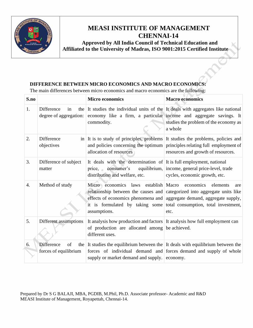
DIFFERENCE BETWEEN MICRO ECONOMICS AND MACRO ECONOMICS:
The main differences between micro economics and macro economics are the following:
S.no Micro economics Macro economics
1. Difference in the
degree of aggregation:
It studies the individual units of the
economy like a firm, a particular
commodity.
It deals with aggregates like national
income and aggregate savings. It
studies the problem of the economy as
a whole
2. Difference in
objectives
It is to study of principles, problems
and policies concerning the optimum
allocation of resources
It studies the problems, policies and
principles relating full employment of
resources and growth of resources.
3. Difference of subject
matter
It deals with the determination of
price, consumer’s equilibrium,
distribution and welfare, etc.
It is full employment, national
income, general price-level, trade
cycles, economic growth, etc.
4. Method of study Micro economics laws establish
relationship between the causes and
effects of economics phenomena and
it is formulated by taking some
assumptions.
Macro economics elements are
categorized into aggregate units like
aggregate demand, aggregate supply,
total consumption, total investment,
etc.
5. Different assumptions It analysis how production and factors
of production are allocated among
different uses.
It analysis how full employment can
be achieved.
6. Difference of the
forces of equilibrium
It studies the equilibrium between the
forces of individual demand and
supply or market demand and supply.
It deals with equilibrium between the
forces demand and supply of whole
economy.
Prepared by Dr S G BALAJI, MBA, PGDIB, M.Phil, Ph.D. Associate professor- Academic and R&D
MEASI Institute of Management, Royapettah, Chennai-14.
MEASI INSTITUTE OF MANAGEMENT
CHENNAI-14 Approved by All India Council of Technical Education and
Affiliated to the University of Madras, ISO 9001:2015 Certified Institute
UNIT-II - UTILITY ANALYSIS AND THE DEMAND CURVE Utility Analysis and the Demand Curve: Elasticity of Demand - Demand Analysis: Basic Concepts,
and tools of analysis for demand forecasting. Use of Business Indicators: Demand forecasting for
consumer, Consumer Durable and Capital Goods. Input-Output Analysis – Consumer Behavior-
Consumer Equilibrium
BASIC CONCEPTS OF UTILITY ANALYSIS:
MEANING OF UTILITY:
The want satisfying power of a commodity is called utility. It is a quality possessed by a
commodity or service to satisfy human wants. Utility can also be defined as value-in-use of a
commodity because the satisfaction which we get from the consumption of a commodity is its
value-in-use.
TYPES OF UTILITY:
Utility may take any of the following forms:
(1) Form Utility:
When utility is created and or added by changing the shape or form of goods, it is form utility.
When a carpenter makes a table out of wood, he adds to the utility of wood by converting it into a
more useful commodity like furniture. He has created form utility.
(2) Place Utility:
When the furniture is taken from the factory to the shop for sale, it leads to place utility. This is
because it is transported from a place where it has no buyers to a place where it fetches a price.
(3) Time Utility:
When a farmer stores his wheat after harvesting for a few months and sells it when its price rises,
he has created time utility and added to the value of wheat.
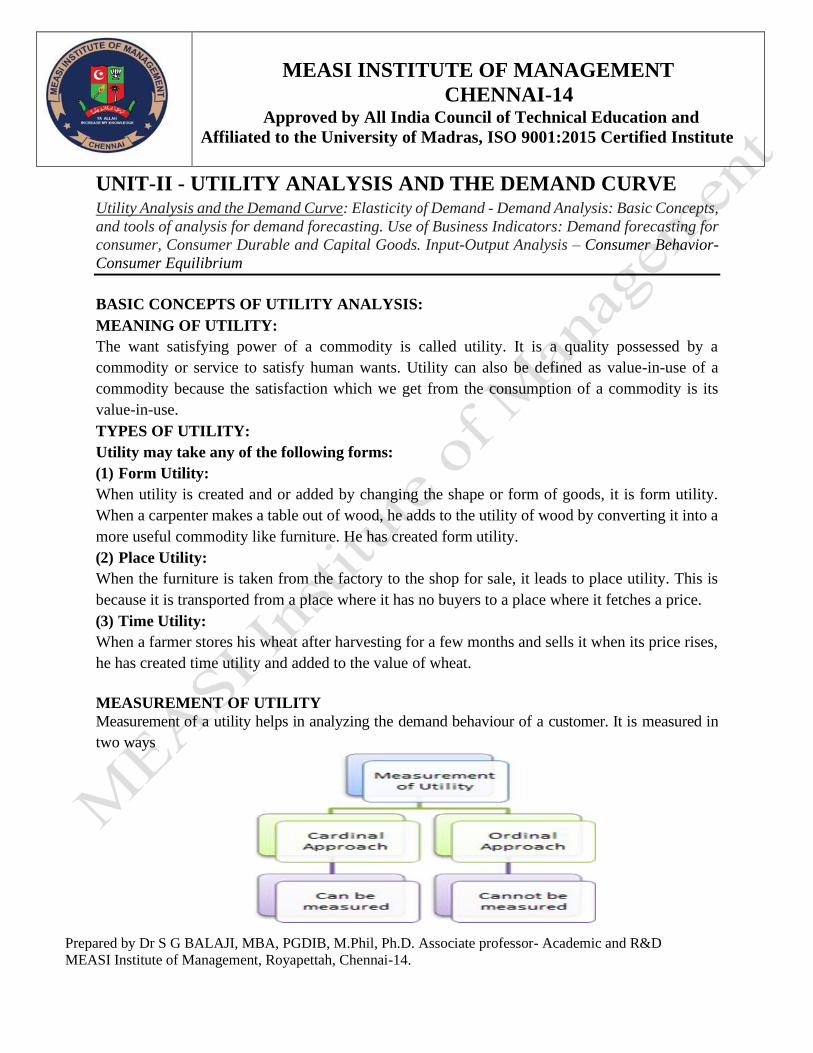
MEASUREMENT OF UTILITY
Measurement of a utility helps in analyzing the demand behaviour of a customer. It is measured in
two ways

Prepared by Dr S G BALAJI, MBA, PGDIB, M.Phil, Ph.D. Associate professor- Academic and R&D
MEASI Institute of Management, Royapettah, Chennai-14.
MEASI INSTITUTE OF MANAGEMENT
CHENNAI-14 Approved by All India Council of Technical Education and
Affiliated to the University of Madras, ISO 9001:2015 Certified Institute
Cardinal Approach
In this approach, one believes that it is measurable. One can express his or her satisfaction in cardinal
numbers i.e., the quantitative numbers such as 1, 2, 3, and so on. It tells the preference of a customer
in cardinal measurement. It is measured in utils.
Limitation of Cardinal Approach
• In the real world, one cannot always measure utility.
• One cannot add different types of satisfaction from different goods.
• For measuring it, it is assumed that utility of consumption of one good is independent of that of another.
• It does not analyze the effect of a change in the price
Ordinal Approach
In this approach, one believes that it is comparable. One can express his or her satisfaction in ranking.
One can compare commodities and give them certain ranks like first, second, tenth, etc. It shows the
order of preference. An ordinal approach is a qualitative approach to measuring a utility.
Limitation of Ordinal Approach
• It assumes that there are only two goods or two baskets of goods. It is not always true.
• Assigning a numerical value to a concept of utility is not easy.
• The consumer’s choice is expected to be either transitive or consistent. It is always not possible.
TYPES OF UTILITY CONCEPTS:
We Measure utility in units called utils. It is useful analytically to distinguish between the
two utility concepts
1. Total Utility: The Sum of total satisfaction which a consumer receives by consuming the various
units of the commodity.
2. Marginal Utility: Marginal utility refers to the utility of one unit of commodity or one more
unit of the commodity. It is the extra satisfaction or additional satisfaction we get by consuming
one more unit of the commodity.
Prepared by Dr S G BALAJI, MBA, PGDIB, M.Phil, Ph.D. Associate professor- Academic and R&D
MEASI Institute of Management, Royapettah, Chennai-14.
MEASI INSTITUTE OF MANAGEMENT
CHENNAI-14 Approved by All India Council of Technical Education and
Affiliated to the University of Madras, ISO 9001:2015 Certified Institute
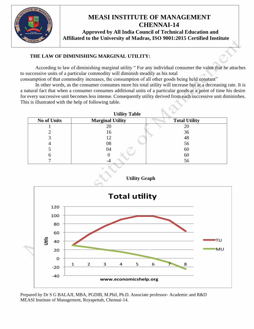
THE LAW OF DIMINISHING MARGINAL UTILITY:
According to law of diminishing marginal utility “ For any individual consumer the value that he attaches
to successive units of a particular commodity will diminish steadily as his total
consumption of that commodity increases, the consumption of all other goods being held constant”
In other words, as the consumer consumes more his total utility will increase but at a decreasing rate. It is
a natural fact that when a consumer consumes additional units of a particular goods at a point of time his desire
for every successive unit becomes less intense. Consequently utility derived from each successive unit diminishes.
This is illustrated with the help of following table.
Utility Table
No of Units Marginal Utility Total Utility
1 20 20
2 16 36
3 12 48
4 08 56
5 04 60
6 0 60
7 -4 56
Utility Graph

Prepared by Dr S G BALAJI, MBA, PGDIB, M.Phil, Ph.D. Associate professor- Academic and R&D
MEASI Institute of Management, Royapettah, Chennai-14.
MEASI INSTITUTE OF MANAGEMENT
CHENNAI-14 Approved by All India Council of Technical Education and
Affiliated to the University of Madras, ISO 9001:2015 Certified Institute
DEMAND ANALYSIS:
Introduction:
The concepts of demand and supply are useful for explaining what is happening in the
market place. Every market transaction involves an exchange and many exchanges are undertaken
in a single day. The circular flow of economic activity explains clearly that every day there are a
number of exchanges taking place among the four major sectors mentioned earlier.
A market is a place where we buy and sell goods and services. A buyer demands goods and
services from the market and the sellers supply the goods in the market. In economics, demand is
“the quantity of goods and services that will be bought for a given price over a period of time”.
For example if 10 Lakhs laptops are purchased in India during a year at an average price of
Rs.25000/- then we can say that the annual demand for laptops is 10 Lakhs units at the rate of
25,000/-.
This chapter describes demand and supply which is the driving force behind a market
economy. This is one of the most important managerial factors because it assists the managers in
predicting changes in production and input prices. The manager can take better decisions regarding
the kind of product to be produced, the quantity, the cost of the product and its selling price. Let
us understand the concept of demand and its importance in decision making.
DEMAND:
Demand means the ability and willingness to buy a specific quantity of a commodity at the
prevailing price in a given period of time. Therefore, demand for a commodity implies the desire
to acquire it, willingness and the ability to pay for it.
DETERMINANTS OF DEMAND:
There are various factors affecting the demand for a commodity. They are:
1. Price of the good:
The price of a commodity is an important determinant of demand. Price and demand are
inversely related. Higher the price less is the demand and vice versa.
2. Price of related goods:
The price of related goods like substitutes and complementary goods also affect the demand. In
the case of substitutes, rise in price of one commodity lead to increase in demand for its substitute.
In the case of complementary goods, fall in the price of one commodity lead to rise in demand for
both the goods.
Prepared by Dr S G BALAJI, MBA, PGDIB, M.Phil, Ph.D. Associate professor- Academic and R&D
MEASI Institute of Management, Royapettah, Chennai-14.
MEASI INSTITUTE OF MANAGEMENT
CHENNAI-14 Approved by All India Council of Technical Education and
Affiliated to the University of Madras, ISO 9001:2015 Certified Institute
3. Consumer’s Income:
This is directly related to demand. A change inthe income of the consumer significantly influences
his demand for most commodities. If the disposable income increases, demand will be more.
4. Taste, preference, fashions and habits:
These are very effective factors affecting demand for a commodity. When there is a change in
taste, habits or preferences of the consumer, his demand will change. Fashions and customs in
society determine many of our demands.
5. Population:
If the size of the population is more, demand for goods will be more . The market demand for a
commodity substantially changes when there is change in the total population.
6. Money Circulation:
More the money in circulation, higher the demand and vice versa.
7. Value of money:
The value of money determines the demand for a commodity in the market. When there is a rise
or fall in the value of money there may be changes in the relative prices of different goods and
their demand.
8. Weather Condition:
Weather is also an important factor that determines the demand for certain goods.
9. Advertisement and Salesmanship: If the advertisement is very attractive for a commodity,
demand will be more. Similarly if the salesmanship and publicity is effective then the demand for
the commodity will be more.
10. Consumer’s future price expectation: If the consumers expect that there will be a rise in
prices in future, he may buy more at the present price and so his demand increases.
11. Government policy (taxation): High taxes will increase the price and reduce demand, while
low taxes will reduce the price and extend the demand.
12. Credit facilities: Depending on the availability of credit facilities the demand for
commodities will change. More the facilities higher the demand.
13. Multiplicity of uses of goods: if the commodity has multiple uses then the demand will be
more than if the commodity is used for a single purpose.

Prepared by Dr S G BALAJI, MBA, PGDIB, M.Phil, Ph.D. Associate professor- Academic and R&D
MEASI Institute of Management, Royapettah, Chennai-14.
MEASI INSTITUTE OF MANAGEMENT
CHENNAI-14 Approved by All India Council of Technical Education and
Affiliated to the University of Madras, ISO 9001:2015 Certified Institute
DEMAND FUNCTION, DEMAND SCHEDULE, DEMAND CURVE:
DEMAND FUNCTION is a function that describe how much of a commodity will be purchased
at the prevailing prices of that commodity and related commodities, alternative income levels, and
alternative values of other variables affecting demand.
Price is not the only factor which determines the level of demand for a good. Other important
factor is income. The rise in income will lead to an increase in demand for a normal commodity.
A few goods are named as inferior goods for which the demand will fall, when income rises.
Another important factor which influences the demand for a good is the price of other goods. Other
factors which affect the demand for a good apart from the above mentioned factors are:
Changes in Population
Changes in Fashion
Changes in Taste
Changes in Advertising
A change in demand occurs when one or more of the determinants of demand change and it is
expressed in the following equation.
Qd X = f (Px, Pr, Y, T, Ey, Ep, Adv….)
Where, Qd X = quantity demanded of good ‘X’
Px = the price of good X
Pr = the price of a related good
Y = income level of the consumer
T = taste and preference of the consumers
Ey = expected income
Ep = expected price
Adv = advertisement cost
The above mentioned demand function expresses the relationship between the demand and other
factors. The quantity demanded of commodity X varies according to the price of commodity (Px),
income (Y), the price of a related commodity (Pr), taste and preference of the consumers (T),
expected income (Ey) and advertisement cost(Adv) spent by the organization.
Prepared by Dr S G BALAJI, MBA, PGDIB, M.Phil, Ph.D. Associate professor- Academic and R&D
MEASI Institute of Management, Royapettah, Chennai-14.
MEASI INSTITUTE OF MANAGEMENT
CHENNAI-14 Approved by All India Council of Technical Education and
Affiliated to the University of Madras, ISO 9001:2015 Certified Institute
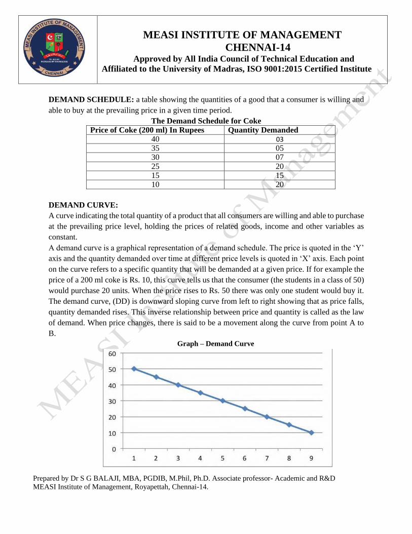
DEMAND SCHEDULE: a table showing the quantities of a good that a consumer is willing and
able to buy at the prevailing price in a given time period.
The Demand Schedule for Coke
Price of Coke (200 ml) In Rupees Quantity Demanded
40 03 35 05 30 07 25 20 15 15 10 20
DEMAND CURVE:
A curve indicating the total quantity of a product that all consumers are willing and able to purchase
at the prevailing price level, holding the prices of related goods, income and other variables as
constant.
A demand curve is a graphical representation of a demand schedule. The price is quoted in the ‘Y’
axis and the quantity demanded over time at different price levels is quoted in ‘X’ axis. Each point
on the curve refers to a specific quantity that will be demanded at a given price. If for example the
price of a 200 ml coke is Rs. 10, this curve tells us that the consumer (the students in a class of 50)
would purchase 20 units. When the price rises to Rs. 50 there was only one student would buy it.
The demand curve, (DD) is downward sloping curve from left to right showing that as price falls,
quantity demanded rises. This inverse relationship between price and quantity is called as the law
of demand. When price changes, there is said to be a movement along the curve from point A to
B.
Graph – Demand Curve
Prepared by Dr S G BALAJI, MBA, PGDIB, M.Phil, Ph.D. Associate professor- Academic and R&D
MEASI Institute of Management, Royapettah, Chennai-14.
MEASI INSTITUTE OF MANAGEMENT
CHENNAI-14 Approved by All India Council of Technical Education and
Affiliated to the University of Madras, ISO 9001:2015 Certified Institute
DEMAND DISTINCTIONS: TYPES OF DEMAND
Demand may be defined as the quantity of goods or services desired by an individual, backed by
the ability and willingness to pay.
TYPES OF DEMAND:
1. Direct and indirect demand: (or) Producers’ goods and consumers’ goods: demand for
goods that are directly used for consumption by the ultimate consumer is known as direct demand
(example: Demand for T shirts). On the other hand demand for goods that are used by producers
for producing goods and services. (example: Demand for cotton by a textile mill)
2. Derived demand and autonomous demand: when a produce derives its usage from the use of
some primary product it is known as derived demand. (example: demand for tyres derived from
demand for car) Autonomous demand is the demand for a product that can be independently used.
(example: demand for a washing machine)
3. Durable and non durable goods demand: durable goods are those that can be used more than
once, over a period of time (example: Microwave oven) Non durable goods can be used only once
(example: Band-aid)
4. Firm and industry demand: firm demand is the demand for the product of a particular firm.
(example: Dove soap) The demand for the product of a particular industry is industry demand
(example: demand for steel in India )
5. Total market and market segment demand: a particular segment of the markets demand is
called as segment demand (example: demand for laptops by engineering students) the sum total of
the demand for laptops by various segments in India is the total market demand. (example: demand
for laptops in India)
6. Short run and long run demand: short run demand refers to demand with its immediate
reaction to price changes and income fluctuations. Long run demand is that which will ultimately
exist as a result of the changes in pricing, promotion or product improvement after market
adjustment withsufficient time.
7. Joint demand and Composite demand: when two goods are demanded in conjunction with one
another at the same time to satisfy a single want, it is called as joint or complementary demand.
(example: demand for petroland two wheelers) A composite demand is one in which a good is
wanted for several different uses. ( example: demand for iron rods for various purposes)
8. Price demand, income demand and cross demand: demand for commodities by the consumers
at alternative prices are called as price demand. Quantity demanded by the consumers at
alternative levels of income is income demand. Cross demand refers to the quantity demanded of
commodity ‘X’ at a price of a related commodity ‘Y’ which may be a substitute or
complementary to X.

Prepared by Dr S G BALAJI, MBA, PGDIB, M.Phil, Ph.D. Associate professor- Academic and R&D
MEASI Institute of Management, Royapettah, Chennai-14.
MEASI INSTITUTE OF MANAGEMENT
CHENNAI-14 Approved by All India Council of Technical Education and
Affiliated to the University of Madras, ISO 9001:2015 Certified Institute
Price Demand: The ability and willingness to buy specific quantities of a good at the prevailing
price in a given time period.
Income Demand: The ability and willingness to buy a commodity at the available income in a
given period of time.
Market Demand: The total quantity of a good or service that people are willing and able to buy
at prevailing prices in a given time period. It is the sum of individual demands.
Cross Demand: The ability and willingness to buy a commodity or service at the prevailing price
of the related commodity i.e. substitutes or complementary products. For example, people buy
more of wheat when the price of rice increases.
EXCEPTIONAL DEMAND CURVE OR PERVERSE DEMAND CURVE OR
EXCEPTION TO THE LAW OF DEMAND:
The demand curve slopes from left to right upward if despite the increase in price of the
commodity, people tend to buy more due to reasons like fear of shortages or it may be an absolutely
essential good.
The law of demand does not apply in every case and situation. The circumstances when the law of
demand becomes ineffective are known as exceptions of the law. Some of these important
exceptions are as under.
1. Giffen Goods:
Some special varieties of inferior goods are termed as Giffen goods. Cheaper varieties millets like
bajra, cheaper vegetables like potato etc come under this category. Sir Robert Giffen of Ireland
first observed that people used to spend more of their income on inferior goods like potato and less
of their income on meat. After purchasing potato the staple food, they did not have staple food
potato surplus to buy meat. So the rise in price of potato compelled people to buy more potato and
thus raised the demand for potato. This is against the law of demand. This is also known as Giffen
paradox.
2. Conspicuous Consumption / Veblen Effect:
This exception to the law of demand is associated with the doctrine propounded by Thorsten
Veblen. A few goods like diamonds etc are purchased by the rich and wealthy sections of society.
The prices of these goods are so high that they are beyond the reach of the common man. The
higher the price of the diamond, the higher its prestige value. So when price of these goods falls,
the consumers think that the prestige value of these goods comes down. So quantity demanded of
these goods falls with fall in their price. So the law of demand does not hold good here.

Prepared by Dr S G BALAJI, MBA, PGDIB, M.Phil, Ph.D. Associate professor- Academic and R&D
MEASI Institute of Management, Royapettah, Chennai-14.
MEASI INSTITUTE OF MANAGEMENT
CHENNAI-14 Approved by All India Council of Technical Education and
Affiliated to the University of Madras, ISO 9001:2015 Certified Institute
3. Conspicuous Necessities:
Certain things become the necessities of modern life. So we have to purchase them despite their
high price. The demand for T.V. sets, automobiles and refrigerators etc. has not gone down in spite
of the increase in their price. These things have become the symbol of status. So they are purchased
despite their rising price.
4. Ignorance:
A consumer’s ignorance is another factor that at times induces him to purchase more of the
commodity at a higher price. This is especially true, when the consumer believes that a high- priced
and branded commodity is better in quality than a low-priced one.
5. Emergencies:
During emergencies like war, famine etc, households behave in an abnormal way. Households
accentuate scarcities and induce further price rise by making increased purchases even at higher
prices because of the apprehension that they may not be available. . On the other hand during
depression, , fall in prices is not a sufficient condition for consumers to demand more if they are
needed.
6. Future Changes In Prices:
Households also act as speculators. When the prices are rising households tend to purchase large
quantities of the commodity out of the apprehension that prices may still go up. When prices are
expected to fall further, they wait to buy goods in future at still lower prices. So quantity demanded
falls when prices are falling.
7. Change In Fashion:
A change in fashion and tastes affects the market for a commodity. When a digital camera replaces
a normal manual camera, no amount of reduction in the price of the latter is sufficient to clear the
stocks. Digital cameras on the other hand, will have more customers even though its price may be
going up. The law of demand becomes ineffective.
8. Demonstration Effect:
It refers to a tendency of low income groups to imitate the consumption pattern of high income
groups. They will buy a commodity to imitate the consumption of their neighbors even if they do
not have the purchasing power.
9. Snob Effect:
Some buyers have a desire to own unusual or unique products to show that they are different from
others. In this situation even when the price rises the demand for the commodity will be more.
10. Speculative Goods/ Outdated Goods/ Seasonal Goods:
Speculative goods such as shares do not follow the law of demand. Whenever the prices rise,

Prepared by Dr S G BALAJI, MBA, PGDIB, M.Phil, Ph.D. Associate professor- Academic and R&D
MEASI Institute of Management, Royapettah, Chennai-14.
MEASI INSTITUTE OF MANAGEMENT
CHENNAI-14 Approved by All India Council of Technical Education and
Affiliated to the University of Madras, ISO 9001:2015 Certified Institute
The traders expect the prices to rise further so they buy more. Goods that go out of use due to
advancement in the underlying technology are called outdated goods. The demand for such goods
does not rise even with fall in prices
11. Seasonal Goods:
Goods which are not used during the off-season (seasonal goods) will also be subject to similar
demand behaviour.
12. Goods in Short Supply:
Goods that are available in limited quantity or whose future availability is uncertain also violate
the law of demand.
ELASTICITY OF DEMAND:
In economics, the term elasticity means a proportionate (percentage) change in one variable
relative to a proportionate (percentage) change in another variable. The quantity demanded of a
good is affected by changes in the price of the good, changes in price of other goods, changes in
income and changes in other factors. Elasticity is a measure of just how much of the quantity
demanded will be affected due to a change in price or income.
Elasticity of Demand is a technical term used by economists to describe the degree of
responsiveness of the demand for a commodity due to a fall in its price. A fall in price leads to an
increase in quantity demanded and vice versa.
The elasticity of demand may be as follows:
1. Price Elasticity of demand
2. Income Elasticity of demand
3. Cross Elasticity of demand
4. Advertising Elasticity of demand
1. PRICE ELASTICITY
The response of the consumers to a change in the price of a commodity is measured by the price
elasticity of the commodity demand. The responsiveness of changes in quantity demanded due to
changes in price is referred to as price elasticity of demand. The price elasticity of demand is
measured by dividing the percentage change in quantity demanded by the percentage change in
price.

Prepared by Dr S G BALAJI, MBA, PGDIB, M.Phil, Ph.D. Associate professor- Academic and R&D
MEASI Institute of Management, Royapettah, Chennai-14.
MEASI INSTITUTE OF MANAGEMENT
CHENNAI-14 Approved by All India Council of Technical Education and
Affiliated to the University of Madras, ISO 9001:2015 Certified Institute
Price Elasticity = Proportionate change in the Quantity Demanded / Proportionate change in price
Percentage change in quantity demanded
=
Percentage change in price
ΔQ / Q 10
= --------- = ------ = 0.5
ΔP / P 20
ΔQ = change in quantity demanded
ΔP = change in price
P = price
Q = quantity demanded
For example:
Quantity demanded is 20 units at a price of Rs.500. When there is a fall in price to Rs. 400 it results
in a rise in demand to 32 units. Therefore the change in quantity demanded is12 units resulting
from the change in price of Rs.100.
The Price Elasticity of Demand is = 500 / 20 x 12/100 = 3
TYPES OF PRICE ELASTICITY:
Price elasticity of demand is generally classified into the following categories.
1. Perfectly elastic demand
2. Perfectly inelastic demand
3. Unit elasticity of demand
4. Relatively elastic demand
5. Relatively inelastic demand
Type Numerical Expression Description Shape of curve
Perfectly Elastic ∞ Infinity Horizontal
Perfectly Inelastic o Zero Vertical
Unit Elasticity 1 One Rectangle Hyperbola
Relatively Elastic ≥ 1 More than one Flat
Relatively Inelastic ≤ 1 Less than one Steep

Prepared by Dr S G BALAJI, MBA, PGDIB, M.Phil, Ph.D. Associate professor- Academic and R&D
MEASI Institute of Management, Royapettah, Chennai-14.
MEASI INSTITUTE OF MANAGEMENT
CHENNAI-14 Approved by All India Council of Technical Education and
Affiliated to the University of Madras, ISO 9001:2015 Certified Institute
1. Perfectly Elastic Demand (Ed = ∞) a small change in price will change the quantity demanded
by an infinite amount.
2. Perfectly Inelastic Demand (Ed = 0) the quantity demanded does not change regardless of
the percentage change in price.
3. Unit Elasticity of Demand (Ed =1) the percentage change in quantity demanded is the same as
the percentage change in price that caused it.

Prepared by Dr S G BALAJI, MBA, PGDIB, M.Phil, Ph.D. Associate professor- Academic and R&D
MEASI Institute of Management, Royapettah, Chennai-14.
MEASI INSTITUTE OF MANAGEMENT
CHENNAI-14 Approved by All India Council of Technical Education and
Affiliated to the University of Madras, ISO 9001:2015 Certified Institute
4. Relatively Elastic Demand (Ed >1) a small percentage change in price leading to a larger
change in Quantity demanded.
5. Relatively Inelastic Demand (Ed < 1) a change in price leads to a smaller percentage change
in quantity demanded.

Prepared by Dr S G BALAJI, MBA, PGDIB, M.Phil, Ph.D. Associate professor- Academic and R&D
MEASI Institute of Management, Royapettah, Chennai-14.
MEASI INSTITUTE OF MANAGEMENT
CHENNAI-14 Approved by All India Council of Technical Education and
Affiliated to the University of Madras, ISO 9001:2015 Certified Institute
2. INCOME ELASTICITY OF DEMAND:
Income elasticity of demand for a commodity shows the extent to which a consumer
demand for a commodity changes as a result of changes in his income.
Percentage change in quantity demanded of Goods X
Income elasticity =
Percentage change in Income of the Consumers
Qx Y = ÷
Qx Y
Where
Qx = Quantity demanded of X
Y = Income level of consumer
TYPES OF INCOME ELASTICITY OF DEMAND:
1. High Income elasticity
2. Unitary Income elasticity
3. Low Income elasticity
4. Zero Income elasticity
5. Negative Income elasticity
6.
1. High Income Elasticity ( Ei > 1) : The change in income increases the demand for
that commodity more than the change in the income

Prepared by Dr S G BALAJI, MBA, PGDIB, M.Phil, Ph.D. Associate professor- Academic and R&D
MEASI Institute of Management, Royapettah, Chennai-14.
MEASI INSTITUTE OF MANAGEMENT
CHENNAI-14 Approved by All India Council of Technical Education and
Affiliated to the University of Madras, ISO 9001:2015 Certified Institute
2. Unitary Income Elasticity ( Ei = 1) : The change in income leads to the same
percentage of change in the demand for the good.
3. Low Income Elasticity ( Ei < 1): The change in income increases the demand for the
commodity but at a lesser percentage than the change in the Income.
Prepared by Dr S G BALAJI, MBA, PGDIB, M.Phil, Ph.D. Associate professor- Academic and R&D
MEASI Institute of Management, Royapettah, Chennai-14.
MEASI INSTITUTE OF MANAGEMENT
CHENNAI-14 Approved by All India Council of Technical Education and
Affiliated to the University of Madras, ISO 9001:2015 Certified Institute
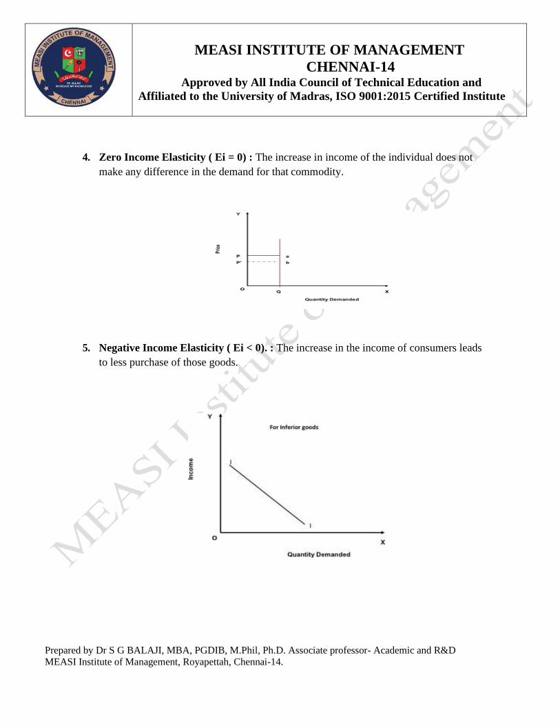
4. Zero Income Elasticity ( Ei = 0) : The increase in income of the individual does not
make any difference in the demand for that commodity.
5. Negative Income Elasticity ( Ei < 0). : The increase in the income of consumers leads
to less purchase of those goods.
Prepared by Dr S G BALAJI, MBA, PGDIB, M.Phil, Ph.D. Associate professor- Academic and R&D
MEASI Institute of Management, Royapettah, Chennai-14.
MEASI INSTITUTE OF MANAGEMENT
CHENNAI-14 Approved by All India Council of Technical Education and
Affiliated to the University of Madras, ISO 9001:2015 Certified Institute
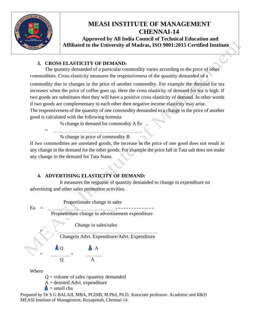
3. CROSS ELASTICITY OF DEMAND:
The quantity demanded of a particular commodity varies according to the price of other
commodities. Cross elasticity measures the responsiveness of the quantity demanded of a
commodity due to changes in the price of another commodity. For example the demand for tea
increases when the price of coffee goes up. Here the cross elasticity of demand for tea is high. If
two goods are substitutes then they will have a positive cross elasticity of demand. In other words
if two goods are complementary to each other then negative income elasticity may arise.
The responsiveness of the quantity of one commodity demanded to a change in the price of another
good is calculated with the following formula.
% change in demand for commodity A Ec
=
% change in price of commodity B
If two commodities are unrelated goods, the increase in the price of one good does not result in
any change in the demand for the other goods. For example the price fall in Tata salt does not make
any change in the demand for Tata Nano.
4. ADVERTISING ELASTICITY OF DEMAND:
It measures the response of quantity demanded to change in expenditure on
advertising and other sales promotion activities.
Proportionate change in sales
Ea =
Proportionate change in advertisement expenditure
Change in sales/sales
=
Changein Advt. Expenditure/Advt. Expenditure
Q A
= ÷
Q A
Where Q = volume of sales /quantity demanded
A = denoted Advt. expenditure
= small cha
Prepared by Dr S G BALAJI, MBA, PGDIB, M.Phil, Ph.D. Associate professor- Academic and R&D
MEASI Institute of Management, Royapettah, Chennai-14.
DEMAND FORECASTING:
A Forecast is an estimate of future situation. Forecasting demand denotes an estimation
of the level of demand of the product at a future period under a given circumstances.
STEPS INVOLVED IN DEMAND FORECASTING:
Step 1: Identification of objective
Step 2: Determining the nature of goods under consideration.
Step3: Selecting proper method of forecasting
Step4: Interpretation of results.
DETERMINANTS FOR DEMAND FORECAST:
Goods can be broadly classified into three categories:
1. Durable Consumer goods
2. Non-durable consumer goods,
3. Capital goods.
1. Consumer Durable goods:
The demand for consumer durables fall into two categories
▪ Replacement demand
▪ New Demand
Forecasting has to made separately for both. The special difficulties in forecasting
in case of consumer durables are as follows.
i. Changes in size and characteristics of population
ii. Saturation limit of the market
iii.Existing stock of the goods
iv. Replacement demand Vs new demand
v. Income level of consumers
vi. Consumer credit outstanding
vii. Taste & scales of preferences of consumers.
2. Non – durable consumer goods:
Non- durable consumer goods are those which can be used only once. Demand for
such goods is basically influenced by the following factors.
i. Purchasing power of the consumer
ii. Price of the commodity
iii. Population and its characteristics.
MEASI INSTITUTE OF MANAGEMENT
CHENNAI-14 Approved by All India Council of Technical Education and
Affiliated to the University of Madras, ISO 9001:2015 Certified Institute

Prepared by Dr S G BALAJI, MBA, PGDIB, M.Phil, Ph.D. Associate professor- Academic and R&D
MEASI Institute of Management, Royapettah, Chennai-14.
MEASI INSTITUTE OF MANAGEMENT
CHENNAI-14 Approved by All India Council of Technical Education and
Affiliated to the University of Madras, ISO 9001:2015 Certified Institute
3. Capital Goods:
Capital goods are also called as producers goods. Capital goods are defined as those
goods which help in further production of goods. Capital goods includes machinery,
equipment’s, tools etc. The demand for a capital goods is a derived demand. More over
demand for capital goods is of two kinds.
i. Replacement demand
ii. New demand.
METHODS/TECHNIQUES OF DEMAND FORECASTING:
Several methods are employed for forecasting demand all of them can be classified under
two categories namely survey method and statistical method.
1. Survey Method:
Survey method is one of the most common and direct methods of forecasting demand in
the short term. This method encompasses the future purchase plans of consumers and their
intentions. In this method, an organization conducts surveys with consumers to determine the
demand for their existing products and services and anticipate the future demand accordingly.

Prepared by Dr S G BALAJI, MBA, PGDIB, M.Phil, Ph.D. Associate professor- Academic and R&D
MEASI Institute of Management, Royapettah, Chennai-14.
MEASI INSTITUTE OF MANAGEMENT
CHENNAI-14 Approved by All India Council of Technical Education and
Affiliated to the University of Madras, ISO 9001:2015 Certified Institute
a) Experts’ Opinion Poll:
Refers to a method in which experts are requested to provide their opinion about the product.
Generally, in an organization, sales representatives act as experts who can assess the demand for
the product in different areas, regions, or cities.
Sales representatives are in close touch with consumers; therefore, they are well aware of the
consumers’ future purchase plans, their reactions to market change, and their perceptions for other
competing products. They provide an approximate estimate of the demand for the organization’s
products. This method is quite simple and less expensive.
b) Market Experiment Method:
Involves collecting necessary information regarding the current and future demand for a product.
This method carries out the studies and experiments on consumer behavior under actual market
conditions. In this method, some areas of markets are selected with similar features, such as
population, income levels, cultural background, and tastes of consumers.
The market experiments are carried out with the help of changing prices and expenditure, so that
the resultant changes in the demand are recorded. These results help in forecasting future demand.
c) Delphi Method:
Refers to a group decision-making technique of forecasting demand. In this method, questions are
individually asked from a group of experts to obtain their opinions on demand for products in
future. These questions are repeatedly asked until a consensus is obtained.
In addition, in this method, each expert is provided information regarding the estimates made by
other experts in the group, so that he/she can revise his/her estimates with respect to others’
estimates. In this way, the forecasts are cross checked among experts to reach more accurate
decision making.
Ever expert is allowed to react or provide suggestions on others’ estimates. However, the names
of experts are kept anonymous while exchanging estimates among experts to facilitate fair
judgment and reduce halo effect.
The main advantage of this method is that it is time and cost effective as a number of experts are
approached in a short time without spending on other resources. However, this method may lead
to subjective decision making
Prepared by Dr S G BALAJI, MBA, PGDIB, M.Phil, Ph.D. Associate professor- Academic and R&D
MEASI Institute of Management, Royapettah, Chennai-14.
MEASI INSTITUTE OF MANAGEMENT
CHENNAI-14 Approved by All India Council of Technical Education and
Affiliated to the University of Madras, ISO 9001:2015 Certified Institute
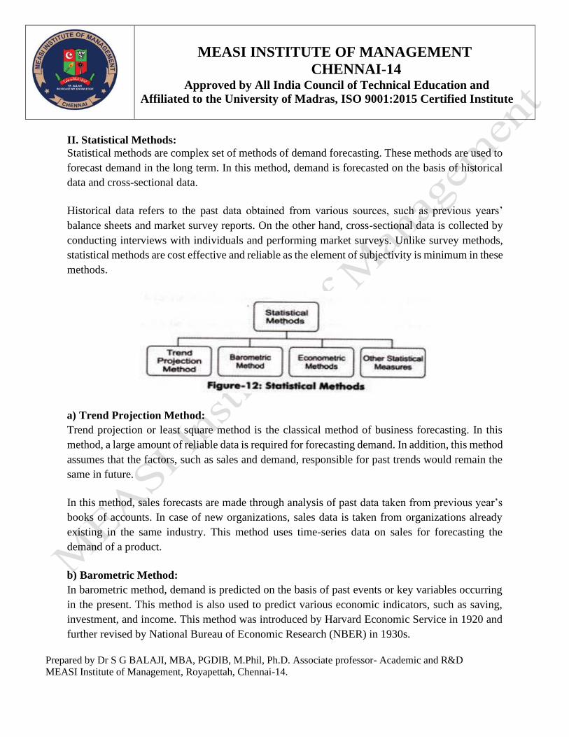
II. Statistical Methods:
Statistical methods are complex set of methods of demand forecasting. These methods are used to
forecast demand in the long term. In this method, demand is forecasted on the basis of historical
data and cross-sectional data.
Historical data refers to the past data obtained from various sources, such as previous years’
balance sheets and market survey reports. On the other hand, cross-sectional data is collected by
conducting interviews with individuals and performing market surveys. Unlike survey methods,
statistical methods are cost effective and reliable as the element of subjectivity is minimum in these
methods.
a) Trend Projection Method:
Trend projection or least square method is the classical method of business forecasting. In this
method, a large amount of reliable data is required for forecasting demand. In addition, this method
assumes that the factors, such as sales and demand, responsible for past trends would remain the
same in future.
In this method, sales forecasts are made through analysis of past data taken from previous year’s
books of accounts. In case of new organizations, sales data is taken from organizations already
existing in the same industry. This method uses time-series data on sales for forecasting the
demand of a product.
b) Barometric Method:
In barometric method, demand is predicted on the basis of past events or key variables occurring
in the present. This method is also used to predict various economic indicators, such as saving,
investment, and income. This method was introduced by Harvard Economic Service in 1920 and
further revised by National Bureau of Economic Research (NBER) in 1930s.
Prepared by Dr S G BALAJI, MBA, PGDIB, M.Phil, Ph.D. Associate professor- Academic and R&D
MEASI Institute of Management, Royapettah, Chennai-14.
MEASI INSTITUTE OF MANAGEMENT
CHENNAI-14 Approved by All India Council of Technical Education and
Affiliated to the University of Madras, ISO 9001:2015 Certified Institute
This technique helps in determining the general trend of business activities. For example, suppose
government allots land to the XYZ society for constructing buildings. This indicates that there
would be high demand for cement, bricks, and steel.
The main advantage of this method is that it is applicable even in the absence of past data.
However, this method is not applicable in case of new products. In addition, it loses its applicability
when there is no time lag between economic indicator and demand.
c) Econometric Methods:
Econometric methods combine statistical tools with economic theories for forecasting. The
forecasts made by this method are very reliable than any other method. An econometric model
consists of two types of methods namely, regression model and simultaneous equations model
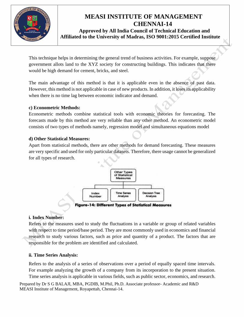
d) Other Statistical Measures:
Apart from statistical methods, there are other methods for demand forecasting. These measures
are very specific and used for only particular datasets. Therefore, there usage cannot be generalized
for all types of research.
i. Index Number:
Refers to the measures used to study the fluctuations in a variable or group of related variables
with respect to time period/base period. They are most commonly used in economics and financial
research to study various factors, such as price and quantity of a product. The factors that are
responsible for the problem are identified and calculated.
ii. Time Series Analysis:
Refers to the analysis of a series of observations over a period of equally spaced time intervals.
For example analyzing the growth of a company from its incorporation to the present situation.
Time series analysis is applicable in various fields, such as public sector, economics, and research.

Prepared by Dr S G BALAJI, MBA, PGDIB, M.Phil, Ph.D. Associate professor- Academic and R&D
MEASI Institute of Management, Royapettah, Chennai-14.
MEASI INSTITUTE OF MANAGEMENT
CHENNAI-14 Approved by All India Council of Technical Education and
Affiliated to the University of Madras, ISO 9001:2015 Certified Institute
iii. Decision Tree Analysis:
Refers to the model that is used to take decision in an organization. In the decision tree analysis, a
tree-type structure is drawn to decide the best solution for a problem. In this analysis, we first find
out different options that we can apply to solve a particular problem.
After that, we can find out the outcome of each option. These options/decisions are connected with
a square node while the outcomes are demonstrated with a circle node. The flow of a decision tree
should be from left to right.
FORECASTING DEMAND FOR NEW PRODUCTS:
Demand forecasting for the new products requires special skill and techniques as they are
new products and no previous data will be available about their sales. The method or techniques
should be carefully tailored for the product. Joel Dean makes six possible approaches towards
forecasting of new products. They are as follows:
1. The Evolutionary approach in forecasting demand
The principle behind this approach is that the demand for a new product is only an outgrowth
and evolution of the existing product. It means that the demand conditions of the existing product
should be taken into account while accessing the demand for the product.
Examples: Color TV sets from black and white TV sets; Left-side steering cars from right-side
steering cars, etc. But this approach is useful only when the new product is very close to the old
existing product.
2. Substitute approach in forecasting demand
By this the new product is analyzed as a substitute for the old existing product or service.
3. Growth curve approach in forecasting demand
The estimates of rate of growth and ultimate level of demand for the new product will be
established on the basis of some growth patterns of an already established product.
For example, the average sales of Talcum powder will give an idea as to how a new cosmetic
will be received in the market.
4. Opinion Poll approach in forecasting demand
Under this, the demand for the new product will be estimated by making direct enquiries from the
ultimate consumers. This is done by sample survey method. But, this is a very complicated process
as there will be problems of sampling, probing the real intentions of the consumers, etc..

Prepared by Dr S G BALAJI, MBA, PGDIB, M.Phil, Ph.D. Associate professor- Academic and R&D
MEASI Institute of Management, Royapettah, Chennai-14.
MEASI INSTITUTE OF MANAGEMENT
CHENNAI-14 Approved by All India Council of Technical Education and
Affiliated to the University of Madras, ISO 9001:2015 Certified Institute
5. Sales Experience approach in forecasting demand
According to Sales experience approach method, samples of new products shall be offered in a
sample market to forecast demand. This is done through distributive channels like departmental
stores or cooperative society, etc., or by direct mailing. Total demand is predicted on the basis of
the sample market. But, the difficulty in this lies in determining the allowance to make for the
immaturity of the sample market and full-fledged market.
6. Vicarious approach in forecasting demand
Through vicarious approach method, the reaction of the customer towards new product can be
found out indirectly through the specialized dealers who are able to judge the needs, tastes and
preferences of customers.
The dealers being the link between the producer and the ultimate consumers, will be able to know
how the customers will receive the new product.
THE FEATURES / CRITERIA OF A GOOD DEMAND FORECASTING METHOD:
We studied about different methods of forecasting. Some are costly methods, a few are
cheap methods. Some methods are flexible and some requires skill. Therefore there is a problem
of choosing the best method for a particular demand situation. The following are the criteria for
selecting a good forecasting they are
1. Accuracy:
Accuracy denotes near to actual demand. A firm should forecast its demand very close to the actual
market demand so that required quantities could be made available for the market. Inaccurate
forecast may cost huge to the firm. It may create over or under production. Forecast should be
explicit. For example, there would be an increase in sales in the next year than the current is not a
good forecast but there would be an increase in sales by 20% in the next year is an accurate
forecast.
2. Longevity or Durability:
Demand forecast generally takes huge time, money and planning. Since a forecast takes a lot of
time and money, it should be usable for longer span of time or multiple years. A forecast for short
span of time may not be effective for the organization.
3. Flexibility or Scale-ability:
A demand forecast should be flexible and adaptable to any kind of changes. Now a days there is a
rapid change in the tastes and preferences of consumers. This affects the demand for different
products up to a great extent. Therefore, the demand forecasts made by a firm should be able to
reflect those changes accordingly. Apart from this, a business firm, while making forecasts, should
consider various business risks that may take place in the future.

Prepared by Dr S G BALAJI, MBA, PGDIB, M.Phil, Ph.D. Associate professor- Academic and R&D
MEASI Institute of Management, Royapettah, Chennai-14.
MEASI INSTITUTE OF MANAGEMENT
CHENNAI-14 Approved by All India Council of Technical Education and
Affiliated to the University of Madras, ISO 9001:2015 Certified Institute
4. Acceptability and Simplicity:
Acceptability is one of the most important criterions of a good demand forecasting method. That
means a forecast should be acceptable to all. It should also be as simple as possible. A business
firm should forecast its market demand by using simple and easy methods so that the organizations
do not face any complexities. However, some companies generally prefer advanced statistical
methods, which may prove difficult and complex.
5. Availability:
A good a good demand forecasting method should have adequate and up-to-date data available.
The forecasts should be done in timely manner so that necessary arrangements could be made
related to the market demand. Data should be available to the decision makers at all time.
6. Plausibility and Possibility:
It denotes that the demand forecasts should be reasonable, so that they are easily understood by
individuals who will use it. Again, it should have the quality of application in the changing business
conditions.
7. Economy:
A good demand forecasting method should have a relationship with costs and benefits. It should
be economically effective. The forecasting should be made in such a way that the costs do not
exceed the benefits that will be derived from it. Costs should be less and benefits should be high.
8. Yielding quick results:
A good demand forecasting method should yield quick result rather than taking longer period to
respond. It should match with the changing business environment.
9. Maintenance of timeliness:
It should take care of timelines. Data should be available to users as and when requires so that
decision making does not hamper.

Prepared by Dr S G BALAJI, MBA, PGDIB, M.Phil, Ph.D. Associate professor- Academic and R&D
MEASI Institute of Management, Royapettah, Chennai-14.
MEASI INSTITUTE OF MANAGEMENT
CHENNAI-14 Approved by All India Council of Technical Education and
Affiliated to the University of Madras, ISO 9001:2015 Certified Institute
INPUT-OUTPUT ANALYSIS:
Introduction:
Input –output analysis is a technique of studying the production structure of an economy.
Input-output analysis seeks to analyze inter industry relationship in order to understand the
interdependences and complexities of the system and to find the demand and supply for maintain
balance between each of industry. The input-output analysis is also known as inter industry flow
analysis.
Methods or Procedure of Input-Output Analysis:
The method or procedure to be adopted in input/output analysis consists of several steps.
The first step is to preparation of the input-output table it is also called an Transaction Matrix.
Secondly after preparing transaction matrix we have to compute technical coefficients. Thirdly
we have to obtain required equations and solving them. Finally some work has to be done towards
substitution.
1. Preparation of Input-Output Table:
For the preparation of input-output table all the firms in the country or the economy have
to be grouped under different sectors conveniently. After having distinguished the sectors and also
the firms under each sector we have to construct a transaction scheme showing how much each
sector buys from each sector in a given year.
Input-Output Table (in million Rs.)
From Sector To Sector Consumer Total
Agriculture Industry Services
Agriculture
2.00
4.50
0.40
3.10
10.00
Industry 4.00 12.00 2.00 32.00 50.00
Services 0.40 6.00 3.60 30.00 40.00
The input- output table cited above shows how much each of the sectors bought from the
other sectors and how much they delivered to various sectors in a given year. From the table we
understand that the annual value of agricultural output was Rs.10million and out of this 2million
worth of output went to agriculture itself (i.e.) the farmers purchased 2 million worth of output
from farmers. Agricultural production worth of Rs.4.50 million was delivered to industry and
Rs.0.40 million worth of output was delivered to services. The consumers are directly purchased
from the farmers Rs.3.10 million worth of products.

Prepared by Dr S G BALAJI, MBA, PGDIB, M.Phil, Ph.D. Associate professor- Academic and R&D
MEASI Institute of Management, Royapettah, Chennai-14.
MEASI INSTITUTE OF MANAGEMENT
CHENNAI-14 Approved by All India Council of Technical Education and
Affiliated to the University of Madras, ISO 9001:2015 Certified Institute
From this table we came to know that total production of industrial sectors was Rs.50
million worth and out of this it has delivered Rs.4 million worth of output to agriculture, Rs.12
million worth has gone to industry itself and Rs.2 million worth to service sector. In Industry sector
had delivered Rs.32million worth of output to consumers directly. The total production of service
sector Rs.40million worth and out of this Rs.3.60 million had gone to service itself and the rest
had gone to agriculture, industry and consumers.
The table reveals that consumers had made total purchases worth Rs.65.10 million from
the three sectors (3.10 +32.00+30.00)
Based on the above table the transaction matrix is to be prepared.
Transaction Matrix (in million Rs)
From Sector To Sector Consumer Total
Agriculture Industry Services
Agriculture
2.00
4.50
0.40
3.10
10.00
Industry 4.00 12.00 2.00 32.00 50.00
Services 0.40 6.00 3.60 30.00 40.00
Primary Input 3.60 27.50 34.00 ---- 65.10
Total 10.00 50.00 40.00 65.10 ----
In the above stated simplified transaction matrix we find that total sector income or primary
input equals Rs.65.10 million (3.60+27.50+34.00=65.10).which is just enough to pay for the total
consumption.
2. Computation of Technical Co- efficient:
The Second step in the analysis is the computation of technical co-efficient. This is also
known as input co-efficient which play a vital role in the analysis. This is computed as follows.
From the table of transaction matrix we know that the total production of agricultural sector
is worth Rs.10 million. To produce this 10 million worth of products the agricultural sector has to
make an input of Rs.2 million from its own sector, Rs.4million from industrial sector and Rs.0.40
million from service sector. In other words to produce Rs.1 million worth of output in the
agricultural sector it has to make an input of Rs.0.2 million received from its own sector, Rs.0.4
million from industrial sector and Rs.0.04 million from service sector. In the same manner we shall
consider the other two sectors.

Prepared by Dr S G BALAJI, MBA, PGDIB, M.Phil, Ph.D. Associate professor- Academic and R&D
MEASI Institute of Management, Royapettah, Chennai-14.
MEASI INSTITUTE OF MANAGEMENT
CHENNAI-14 Approved by All India Council of Technical Education and
Affiliated to the University of Madras, ISO 9001:2015 Certified Institute
The input co-efficients or technical co-efficients which are tabulated below are
Input (or) Technical Co-efficients Table
From Sector To Sector
Agriculture Industry Service
Agriculture 0.20 0.09 0.01
Industry 0.40 0.24 0.05
Service 0.04 0.12 0.09
The significance of the nine ratios obtained in the above table is that a unit of output of a
sector technically requires a certain given and fixed percentage input from each of the sector. This
denotes that the input will have to be increased proportionately with level of output.
3. Obtaining Equations and solving them:
Obtaining equations and solving them. After having obtained the technical co-efficients
with the help of input-output table. Certain equations have to be obtained for solving them
simultaneously. Let us denote the total agricultural production Rs.10 millions as X and total
industrial production as Y. The total service sector production may be denoted as Z. From this we
have to calculate the equations.
Thus we get the equation as R.H.S = L.H.S
X= 0.2x+0.09y+0.01z+3.10
1X= 0.2x+0.09y+0.01z =3.10
= 0.08x -0.09y-0.01z =3.10 1
(1x-0.2)
In the same manner with the help of Second row we get
Y= 0.40x+0.24y+0.05z+32.00
1Y-0.40x+0.76y-0.05z=32 2
(1y-0.24)
In the same manner with the help of Third row we get
Z= 0.04x+0.12y+0.09z+30.00
1Z- 0.04x-0.12y+0.91z= 30 3
(1z-0.09)
Solving equations 1&2&3 we get the following values
X = 10;
Y = 50;
Z = 40 ;

Prepared by Dr S G BALAJI, MBA, PGDIB, M.Phil, Ph.D. Associate professor- Academic and R&D
MEASI Institute of Management, Royapettah, Chennai-14.
4. Work in Substitution:
Forming transaction mix table and working out equations with several unknowns requires
the help of computer and knowledge of advanced mathematics suppose we desire to know what
will happen if the consumer demand for agriculture rises by 15% while there demand for industry
and services remain the same. Then we have to form another set of three equations with 3
unknowns. Thus the no. of linear equations will go on increase with so much number of unknowns
and therefore the process is reduced to a mere exercise in substitution. In the three equations 1,2,3
above we find that on the right hand side the equations given consumer demand for agriculture,
Industry and services respectively. We give the following symbols as follows.
Cx for consumer demand for agriculture Production
Cy for consumer demand for Industrial Production
Cz for consumer demand for services.
On this basis, equations (i), (ii), (iii) will be written as
0.8x-0.09y-0.1z = Cx
-0.4x+0.76y-0.05z = Cy
-0.04x-0.12y+0.91z = Cz
We can solve this set of equations for X, Y and Z and obtain equation 4,5,6. Now for any
amount of Cx, Cy, and Cz. We can determine how much should be produced in each of this sector.
Thus the problem has been reduced to an exercise in substitution.
CONSUMER BEHAVIOUR:
Consumer behavior refers to the study of consumer while engaged in the process of
consumption.
CONSUMER EQUILIBRIUM:
Consumer is in equilibrium when he or she is consuming the best possible combination of
two goods with the given amount of income.
At point b, and e, the consumer will have a lesser satisfaction at IC3 with the same
amount of income.
Consumer equilibrium is reached when indifference carve tangent with budget line which
represents best combination of two goods with limited income as point C.
MEASI INSTITUTE OF MANAGEMENT
CHENNAI-14 Approved by All India Council of Technical Education and
Affiliated to the University of Madras, ISO 9001:2015 Certified Institute

Prepared by Dr S G BALAJI, MBA, PGDIB, M.Phil, Ph.D. Associate professor- Academic and R&D
MEASI Institute of Management, Royapettah, Chennai-14.
UNIT – III - PRODUCTION FUNCTION AND MARKET STRUCTURE
The Production Function: Production with One Variable Input – Law of Variable Proportions –
Production with Two Variable Inputs – Production Isoquants – Isocost Lines Estimating
Production Functions- Returns to Scale – Economies Vs Diseconomies of Scale – Cost Concepts
– Analysis of cost – Short and long run costs.
Market Structure: Perfect and Imperfect Competition – Monopoly, Duopoly, Monopolistic
Competition – Pricing Methods.
THE PRODUCTION FUNCTION:
INTRODUCTION:
Production is an important economic activity which satisfies the wants and needs of the people.
Production function brings out the relationship between inputs used and the resulting output. A
firm is an entity that combines and processes resources in order to produce output that will satisfy
the consumer’s needs. The firm has to decide as to how much to produce and how much input
factors (labour and capital) to employ to produce efficiently. This chapter helps to understand the
set of conditions for efficient production of an organization.
FACTORS OF PRODUCTION include resource inputs used to produce goods and services.
Economist categorise input factors into four major categories such as land, labour, capital and
organization.
Land: Land is heterogeneous in nature. The supply of land is fixed and it is a permanent factor
of production but it is productive only with the application of capital and labour.
Labour: The supply of labour is inelastic in nature but it differs in productivity and efficiency
and it can be improved.
Capital: is a man made factor and is mobile but the supply is elastic.
Organization: the organization plans, , supervises, organizes and controls the business activity
and also takes risks.
MEASI INSTITUTE OF MANAGEMENT
CHENNAI-14 Approved by All India Council of Technical Education and
Affiliated to the University of Madras, ISO 9001:2015 Certified Institute

Prepared by Dr S G BALAJI, MBA, PGDIB, M.Phil, Ph.D. Associate professor- Academic and R&D
MEASI Institute of Management, Royapettah, Chennai-14.
MEASI INSTITUTE OF MANAGEMENT
CHENNAI-14 Approved by All India Council of Technical Education and
Affiliated to the University of Madras, ISO 9001:2015 Certified Institute
PRODUCTION FUNCTION
Production function indicates the maximum amount of commodity ‘X’ to be produced from
various combinations of input factors. It decides on the maximum output to be produced from a
given level of input, and how much minimum input can be used to get the desired level of output.
The production function assumes that the state of technology is fixed. If there is a change in
technology then there would be change in production function.
Q = f (Land, Labour, Capital, Organization)
Q = f (L, L, C, O)
The production manager’s responsibility is that of identifying the right combination of inputs for
the decided quantity of output. As a manager ,he has to know the price of the input factors and the
budget allocation of the organization. The major objective of any business organization is
maximizing the output with minimum cost. To achieve the maximum output the firm has to utilize
the input factors efficiently. In the long run, without increasing the fixed factors it is not possible
to achieve the goal. Therefore it is necessary to understand the relationship between the input and
output in any production process in the short and long run.
ASSUMPTIONS OF PRODUCTION FUNCTION:
Production function is based on the following assumptions:
i. Production function is related to a specified period of time.
ii. The state of technology remains constant during that period of time.
iii. The factors of production are divisible into most viable units.
iv. The substitution of one factor input for the other is limited.
v. The firm is using the most efficient technique available in production.
PRODUCTION THEORY:
Production theory plays an important role in making decisions pertaining to organization
and management of a production process of a business firm.
Production theory covers the following aspects:
i. Production with one variable input (or) Law of variable proportions.
ii. Production with Two variable inputs (or) Isoquants
iii. Production with all variable inputs (or) Returns to scale
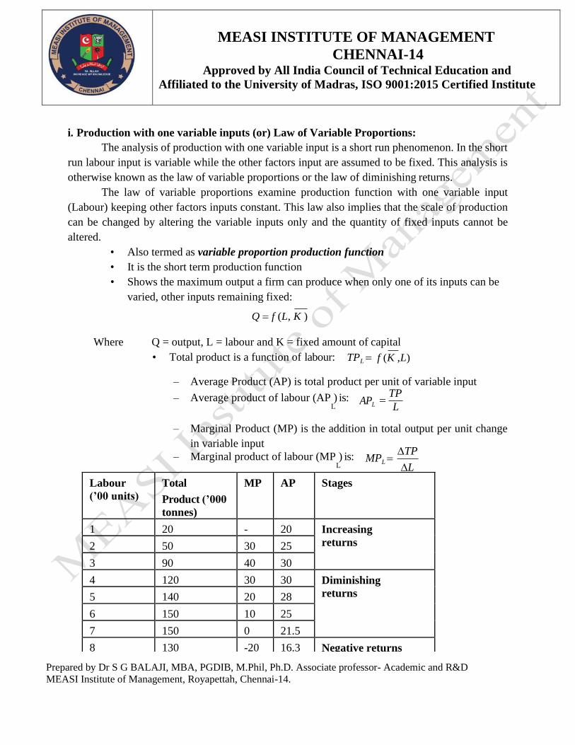
Prepared by Dr S G BALAJI, MBA, PGDIB, M.Phil, Ph.D. Associate professor- Academic and R&D
MEASI Institute of Management, Royapettah, Chennai-14.
i. Production with one variable inputs (or) Law of Variable Proportions:
The analysis of production with one variable input is a short run phenomenon. In the short
run labour input is variable while the other factors input are assumed to be fixed. This analysis is
otherwise known as the law of variable proportions or the law of diminishing returns.
The law of variable proportions examine production function with one variable input
(Labour) keeping other factors inputs constant. This law also implies that the scale of production
can be changed by altering the variable inputs only and the quantity of fixed inputs cannot be
altered.
• Also termed as variable proportion production function
• It is the short term production function
• Shows the maximum output a firm can produce when only one of its inputs can be
varied, other inputs remaining fixed:
Q = f (L, K )
Where Q = output, L = labour and K = fixed amount of capital
• Total product is a function of labour: TPL =
f (K ,L)
– Average Product (AP) is total product per unit of variable input
– Average product of labour (AP ) is: L
APL = TP
L
– Marginal Product (MP) is the addition in total output per unit change
in variable input
– Marginal product of labour (MP ) is: L
MPL =
TP
L
MEASI INSTITUTE OF MANAGEMENT
CHENNAI-14 Approved by All India Council of Technical Education and
Affiliated to the University of Madras, ISO 9001:2015 Certified Institute
Labour
(’00 units)
Total
Product (’000
tonnes)
MP AP Stages
1 20 - 20 Increasing
returns 2 50 30 25
3 90 40 30
4 120 30 30 Diminishing
returns 5 140 20 28
6 150 10 25
7 150 0 21.5
8 130 -20 16.3 Negative returns
9 100 -30 11.1

Prepared by Dr S G BALAJI, MBA, PGDIB, M.Phil, Ph.D. Associate professor- Academic and R&D
MEASI Institute of Management, Royapettah, Chennai-14.
MEASI INSTITUTE OF MANAGEMENT
CHENNAI-14 Approved by All India Council of Technical Education and
Affiliated to the University of Madras, ISO 9001:2015 Certified Institute
• As the quantity of the variable factor is increased with other fixed factors, MP and AP of
the variable factor will eventually decline.
• Therefore law of variable proportions is also called as law of diminishing marginal
returns.
ii. Production with Two Variable inputs (or) Isoquants:
The analysis of production with two variable inputs is a long run phenomenon. In
the long run both the inputs (i.e) labour and capital are potentially variable. Production with two
variable inputs can be examined by means of a family or isoquants or isoproduct curves or equal
product curves or production indifference curves.
An isoquant is defined as the various combinations of two inputs (labour & capital)
in the existing state of technology to produce a given level of output.
• All inputs are variable in long run and only two inputs are used
• Firm has the opportunity to select that combination of inputs which maximizes
returns
• Curves showing such production function are called isoquants or iso-product
curves.
An isoquant is the locus of all technically efficient combinations of two inputs for producing a given level of
output Represented as: Q = f (L, K )
Ou
tpu
t

Prepared by Dr S G BALAJI, MBA, PGDIB, M.Phil, Ph.D. Associate professor- Academic and R&D
MEASI Institute of Management, Royapettah, Chennai-14.
MEASI INSTITUTE OF MANAGEMENT
CHENNAI-14 Approved by All India Council of Technical Education and
Affiliated to the University of Madras, ISO 9001:2015 Certified Institute
Capital (Rs.
crore)
Labour (’00
units)
40 6
28 7
18 8
12 9
8 10
45
40
35
30
25
20
15
10
5
0
6 7 8 9 10
Labour ('00 units)
iii. Production with all variable inputs (or) Returns to Scale:
The analysis of production with all variable inputs is a long run phenomenon. In the long
run all the productive inputs are variable. The firm should therefore consider the best way to
increase the output. Output can be increased in this case by changing the scale of operation by
increasing all the productive inputs proportionately. This is generally referred to as returns to scale.
Returns to Scale is of three important stages
i. Constant Returns to scale
ii. Increasing Returns to scale
iii. Decreasing returns to scale.
Returns to Scale show the degree by which the level of output changes in response to a given
change in all the inputs in a production system.
Cap
ital (R
s. C
ro
re)
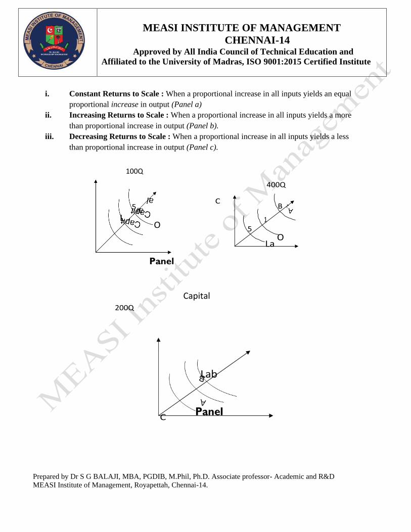
Prepared by Dr S G BALAJI, MBA, PGDIB, M.Phil, Ph.D. Associate professor- Academic and R&D
MEASI Institute of Management, Royapettah, Chennai-14.
MEASI INSTITUTE OF MANAGEMENT
CHENNAI-14 Approved by All India Council of Technical Education and
Affiliated to the University of Madras, ISO 9001:2015 Certified Institute
i. Constant Returns to Scale : When a proportional increase in all inputs yields an equal
proportional increase in output (Panel a)
ii. Increasing Returns to Scale : When a proportional increase in all inputs yields a more
than proportional increase in output (Panel b).
iii. Decreasing Returns to Scale : When a proportional increase in all inputs yields a less
than proportional increase in output (Panel c).
100Q 400Q
C
Panel
200Q
Capital

Prepared by Dr S G BALAJI, MBA, PGDIB, M.Phil, Ph.D. Associate professor- Academic and R&D
MEASI Institute of Management, Royapettah, Chennai-14.
ECONOMIES OF SCALE:
Economies of scale means a fall in average cost of production due to growth in the size of the
industry within which a firm operates.
Factors Causing Economies Of Scale:
There are various factors influencing the economies of scale of an organization. They are
generally classified in to two categories as Internal factors and External factors.
Internal Factors:
1. Labour economies: if the labour force of a firm is specialized in a specific skill then the
organization can achieve economies of scale due to higher labour productivity.
2. Technical economies: with the use of advanced technology they can produce large quantities
with quality which reduces their cost of production.
3. Managerial economies: the managerial skills of an organization will be advantageous to
achieve economies of scale in various business activities.
4. Marketing economies: use of various marketing strategies will help in achieving economies
of scale.
5. Vertical integration: if there is vertical integration then there will be efficient use of raw
material due to internal factor flow.
6. Financial economies: the firm’s financial soundness and past record of financial transactions
will help them to get financial facilities easily.
7. Economies of risk spreading: having variety of products and diversification will help them to
spread their risk and reduce losses.
8. Economies of scale in purchase: when the organization purchases raw material in bulk
reduces the transportation cost and maintains uniform quality.
MEASI INSTITUTE OF MANAGEMENT
CHENNAI-14 Approved by All India Council of Technical Education and
Affiliated to the University of Madras, ISO 9001:2015 Certified Institute

Prepared by Dr S G BALAJI, MBA, PGDIB, M.Phil, Ph.D. Associate professor- Academic and R&D
MEASI Institute of Management, Royapettah, Chennai-14.
MEASI INSTITUTE OF MANAGEMENT
CHENNAI-14 Approved by All India Council of Technical Education and
Affiliated to the University of Madras, ISO 9001:2015 Certified Institute
External Factors:
1. Better repair and maintenance facilities: When the machinery and equipments are repaired
and maintained, then the production process never gets affected.
2. Research and Development: research facilities will provide opportunities to introduce new
products and process methods.
3. Training and Development: continuous training and development of skills in the managerial,
production level will achieve economies of scale.
4. Economies of location: the plant location plays a major role in cutting down the cost of
materials, transport and other expenses.
5. Economies of Information Technology: advanced Information technology provides timely
accurate information for better decision making and for better services.
6. Economies of by-products: Organizations can increase the economies of scale by minimizing
waste and can be environmental responsible by using the by- products of the organization.
DISECONOMIES OF SCALE:
Arises due to managerial problems. If the size of the business becomes too large, then it becomes
difficult for management to control the organizational activities therefore diseconomies of scale
arise.
Graph – Economies of Scale and Diseconomies of scale
Factors Causing Diseconomies Of Scale:
1. Labour union: continuous labour problem and dissatisfaction can lead to diseconomies of
scale.
2. Poor team work: Poor performance of the team leads to diseconomies of scale.

Prepared by Dr S G BALAJI, MBA, PGDIB, M.Phil, Ph.D. Associate professor- Academic and R&D
MEASI Institute of Management, Royapettah, Chennai-14.
MEASI INSTITUTE OF MANAGEMENT
CHENNAI-14 Approved by All India Council of Technical Education and
Affiliated to the University of Madras, ISO 9001:2015 Certified Institute
3. Lack of co-ordination: lack of coordination among the work force has a major role to play in
causing diseconomies of scale.
4. Difficulty in fund raising: difficulties in fund raising reduce the scale of operation.
5. Difficulty in decision making: the managerial inability, delay in decision making is also a
factor that determines the economies of scale.
6. Scarcity of Resources: raw material availability determines the purchase and price. Therefore
there is a possibility of facing diseconomies in firms.
7. Increased risk: growing risk factors can cause diseconomies of scale in an organization. It is
essential to reduce the same.
COST CONCEPTS:
MEANING OF COST:
The term cost simply means cost of production. It is the total of all cost incurred by a
business firm in its production process.
COST DETERMINANTS
The cost of production of goods and services depends on various input factors used by the
organization and it differs from firm to firm. The major cost determinants are:
1. Level of output: The cost of production varies according to the quantum of output. If the size
of production is large then the cost of production will also be more.
2. Price of input factors: A rise in the cost of input factors will increase the total cost of
production.
3. Productivities of factors of production: When the productivity of the input factors is high
then the cost of production will fall.
4. Size of plant: The cost of production will be low in large plants due to mass production with
mechanization.
5. Output stability: The overall cost of production is low when the output is stable over a period
of time.
6. Lot size: Larger the size of production per batch then the cost of production will come down
because the organizations enjoy economies of scale.
7. Laws of returns: The cost of production will increase if the law of diminishing returns
applies in the firm.
8. Levels of capacity utilization: Higher the capacity utilization, lower the cost of production
9. Time period: In the long run cost of production will be stable.
10. Technology: When the organization follows advanced technology in their process then the
cost of production will be low.

Prepared by Dr S G BALAJI, MBA, PGDIB, M.Phil, Ph.D. Associate professor- Academic and R&D
MEASI Institute of Management, Royapettah, Chennai-14.
MEASI INSTITUTE OF MANAGEMENT
CHENNAI-14 Approved by All India Council of Technical Education and
Affiliated to the University of Madras, ISO 9001:2015 Certified Institute
11. : over a period of time the experience in production process will help the firm to reduce cost
of production.
12. Process of range of products: Higher the range of products produced, lower the cost of
production.
13. Supply chain and logistics: Better the logistics and supply chain, lower the cost of
production.
14. Government incentives: If the government provides incentives on input factors then the cost
of production will be low.
TYPES OF COSTS:
There are various classifications of costs based on the nature and the purpose of calculation. But
in economics and for accounting purpose the following are the important cost concepts.
Actual cost/ Outlay cost/ Absolute cost / Accounting cost: The cost or expenditure which a firm
incurs for producing or acquiring a good or service. (Eg. Raw material cost)
Opportunity cost: The revenue which could have been earned by employing that good or service
in some other alternative uses. (Eg. A land owned by the firm does not pay rent. Thus a rent is an
income forgone by not letting it out)
Sunk cost: Are retrospective (past) costs that have already been incurred and cannot be recovered.
Historical cost: The price paid for a plant originally at the time of purchase.
Replacement cost: The price that would have to be paid currently for acquiring the same plant.
Incremental cost: Is the addition to costs resulting from a change in the nature of level of
business activity. Change in cost caused by a given managerial decision.
Explicit cost: Cost actually paid by the firm. If the factors of production are hired or rented then
it is an explicit cost.
Implicit cost: If the factors of production are owned by a firm then its cost is implicit cost.
Book cost: Costs which do not involve any cash payments but a provision is made in the books
of accounts in order to include them in the profit and loss account to take tax advantages.
Social cost: Total cost incurred by the society on account of production of a good or service.
Transaction cost: The cost associated with the exchange of goods and services.
Controllable cost: Costs which can be controllable by the executives are called as controllable
cost.
Shut down cost: Cost incurred if the firm temporarily stops its operation. These can be saved by
continuing business.
Economic costs are related to future. They play a vital role in business decisions as the costs
considered in decision - making are usually future costs. They are similar in nature to that of
incremental, imputed explicit and opportunity costs.
Prepared by Dr S G BALAJI, MBA, PGDIB, M.Phil, Ph.D. Associate professor- Academic and R&D
MEASI Institute of Management, Royapettah, Chennai-14.
MEASI INSTITUTE OF MANAGEMENT
CHENNAI-14 Approved by All India Council of Technical Education and
Affiliated to the University of Madras, ISO 9001:2015 Certified Institute
Fixed cost: Some inputs are used over a period of time for producing more than one batch of
goods. The costs incurred in these are called fixed cost. For example amount spent on purchase of
equipment, machinery, land and building.
Variable cost: When output has increased the firm spends more on these items. For example the
money spent on labour wages, raw material and electricity usage. Variable costs vary according to
the output. In the long run all costs become variable.
Total cost: The market value of all resources used to produce a good or service.
Total Fixed cost: Cost of production remains constant whatever the level of output.
Total Variable cost: Cost of production varies with output.
Average cost: Total cost divided by the level of output.
Average variable cost: Variable cost divided by the level of output.
Average fixed cost: Total fixed cost divided by the level of output.
Marginal cost: Cost of producing an extra unit of output.
COST FUNCTION (COST – OUTPUT RELATIONSHIP):
Cost function simply express the functional relationship between cost and output. This
function can be written as
C = f (Q,T,pf,K)
Where C= Total Cost
Q= Level of output
T= Technology
Pf= Prices of factors
K= Fixed factor
TYPES OF COST FUNCTION:
The cost function can broadly be classified into
1. The Short run cost function (or) Short Run cost-output Relationship
2. The Long run cost function (or) Long Run cost-output Relationship
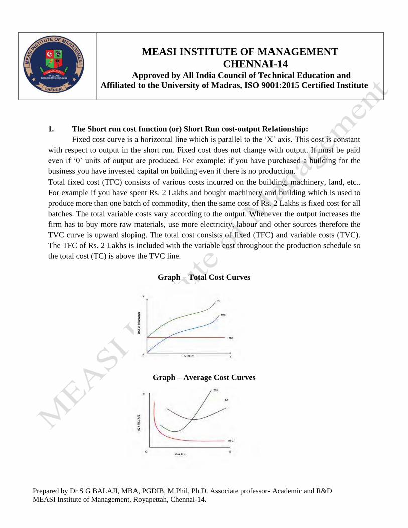
Prepared by Dr S G BALAJI, MBA, PGDIB, M.Phil, Ph.D. Associate professor- Academic and R&D
MEASI Institute of Management, Royapettah, Chennai-14.
MEASI INSTITUTE OF MANAGEMENT
CHENNAI-14 Approved by All India Council of Technical Education and
Affiliated to the University of Madras, ISO 9001:2015 Certified Institute
1. The Short run cost function (or) Short Run cost-output Relationship:
Fixed cost curve is a horizontal line which is parallel to the ‘X’ axis. This cost is constant
with respect to output in the short run. Fixed cost does not change with output. It must be paid
even if ‘0’ units of output are produced. For example: if you have purchased a building for the
business you have invested capital on building even if there is no production.
Total fixed cost (TFC) consists of various costs incurred on the building, machinery, land, etc..
For example if you have spent Rs. 2 Lakhs and bought machinery and building which is used to
produce more than one batch of commodity, then the same cost of Rs. 2 Lakhs is fixed cost for all
batches. The total variable costs vary according to the output. Whenever the output increases the
firm has to buy more raw materials, use more electricity, labour and other sources therefore the
TVC curve is upward sloping. The total cost consists of fixed (TFC) and variable costs (TVC).
The TFC of Rs. 2 Lakhs is included with the variable cost throughout the production schedule so
the total cost (TC) is above the TVC line.
Graph – Total Cost Curves
Graph – Average Cost Curves
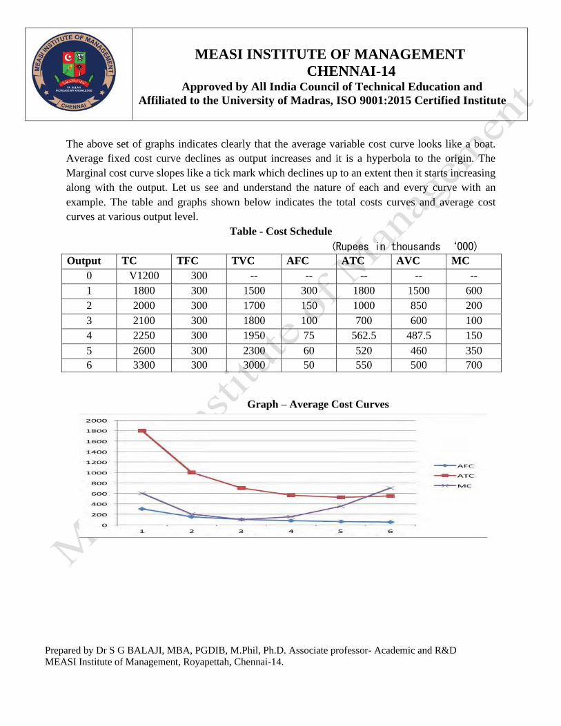
Prepared by Dr S G BALAJI, MBA, PGDIB, M.Phil, Ph.D. Associate professor- Academic and R&D
MEASI Institute of Management, Royapettah, Chennai-14.
MEASI INSTITUTE OF MANAGEMENT
CHENNAI-14 Approved by All India Council of Technical Education and
Affiliated to the University of Madras, ISO 9001:2015 Certified Institute
The above set of graphs indicates clearly that the average variable cost curve looks like a boat.
Average fixed cost curve declines as output increases and it is a hyperbola to the origin. The
Marginal cost curve slopes like a tick mark which declines up to an extent then it starts increasing
along with the output. Let us see and understand the nature of each and every curve with an
example. The table and graphs shown below indicates the total costs curves and average cost
curves at various output level.
Table - Cost Schedule
(Rupees in thousands ‘000)
Output TC TFC TVC AFC ATC AVC MC
0 V1200 300 -- -- -- -- --
1 1800 300 1500 300 1800 1500 600
2 2000 300 1700 150 1000 850 200
3 2100 300 1800 100 700 600 100
4 2250 300 1950 75 562.5 487.5 150
5 2600 300 2300 60 520 460 350
6 3300 300 3000 50 550 500 700
Graph – Average Cost Curves
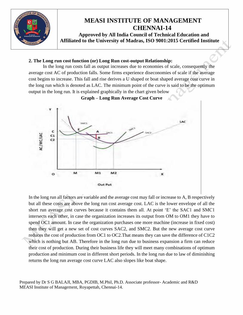
Prepared by Dr S G BALAJI, MBA, PGDIB, M.Phil, Ph.D. Associate professor- Academic and R&D
MEASI Institute of Management, Royapettah, Chennai-14.
MEASI INSTITUTE OF MANAGEMENT
CHENNAI-14 Approved by All India Council of Technical Education and
Affiliated to the University of Madras, ISO 9001:2015 Certified Institute
2. The Long run cost function (or) Long Run cost-output Relationship:
In the long run costs fall as output increases due to economies of scale, consequently the
average cost AC of production falls. Some firms experience diseconomies of scale if the average
cost begins to increase. This fall and rise derives a U shaped or boat shaped average cost curve in
the long run which is denoted as LAC. The minimum point of the curve is said to be the optimum
output in the long run. It is explained graphically in the chart given below
Graph – Long Run Average Cost Curve
In the long run all factors are variable and the average cost may fall or increase to A, B respectively
but all these costs are above the long run cost average cost. LAC is the lower envelope of all the
short run average cost curves because it contains them all. At point ‘E’ the SAC1 and SMC1
intersects each other, in case the organization increases its output from OM to OM1 they have to
spend OC1 amount. In case the organization purchases one more machine (increase in fixed cost)
then they will get a new set of cost curves SAC2, and SMC2. But the new average cost curve
reduces the cost of production from OC1 to OC2.That means they can save the difference of C1C2
which is nothing but AB. Therefore in the long run due to business expansion a firm can reduce
their cost of production. During their business life they will meet many combinations of optimum
production and minimum cost in different short periods. In the long run due to law of diminishing
returns the long run average cost curve LAC also slopes like boat shape.

Prepared by Dr S G BALAJI, MBA, PGDIB, M.Phil, Ph.D. Associate professor- Academic and R&D
MEASI Institute of Management, Royapettah, Chennai-14.
MEASI INSTITUTE OF MANAGEMENT
CHENNAI-14 Approved by All India Council of Technical Education and
Affiliated to the University of Madras, ISO 9001:2015 Certified Institute
COST CONTROL:
Cost control means the regulation of the cost of operating a business firm. It is an efficient
tool of management of the firm.
TECHNIQUES OF COST CONTROL:
Cost control is exercised through the following techniques.
i. Budgetary control
ii. Standard Costing
iii. Inventory Control
iv. Ratio Analysis
v. Value Analysis
vi. Work Study.
1. Budgetary Control: Budgetary control is a system in which there is constant checking &
evaluation of actual results compared with the budget goals.
2. Standard Costing: Standard costing is defined as the preparation and use of standard cost
their comparison with actual cost.
3. Inventory control: This technique is also adopted to reduce investment in inventory & to
avoid obselence losses.
4. Ratio Analysis: Ratio is a yard stick which provide a measure of relationship between the
two figures compared. The ratio may be expressed in percentage terms.
5. Value Analysis: It is a technique of cost control which studies cost in relation to product
design.
6. Work Study: The work study techniques of cost control involves systematic collection of
work data and critical evaluation of the existing and proposed methods of undertaking the
work.
MARKET STRUCTURE:
Products are priced under different market situations based on certain conditions which
vary from market to market. This will in turn depends upon the degree of competition in the
product market. The market situations may be classified as:
i. Perfect Competitions
ii. Monopoly
iii. Monopolistic Competitions
iv. Oligopoly
vii. Duopoly etc
Prepared by Dr S G BALAJI, MBA, PGDIB, M.Phil, Ph.D. Associate professor- Academic and R&D
MEASI Institute of Management, Royapettah, Chennai-14.
MEASI INSTITUTE OF MANAGEMENT
CHENNAI-14 Approved by All India Council of Technical Education and
Affiliated to the University of Madras, ISO 9001:2015 Certified Institute
I. Perfect Competitions:
Perfect Competition is a market situation in which there are large number of buyers and
sellers engaged in buying & selling homogeneous products respectively without any artificial
restrictions.
Features:
• Large number of buyers and sellers
• Existence of homogeneous products
• Free entry & exit of firms,
• Perfect mobility of factors of production
• Perfect knowledge about the market conditions
• No existence of transport cost.
II. Monopoly:
Monopoly is a market situation in which there is only one seller who controls total
market supply of products which has no close substituted products.
Features:
• There is single producer or seller of a product
• A complete absence of competition
• There is no close substitute for the products
• There is complete control over the market supply
• There is prevention of entry of new firms in the long run.
III. Monopolistic Competition:
It is a real market situation which lies in between two extreme market situations namely.
Perfect competition & monopoly. It is a market situation in which there are many buyers and
sellers of differentiated products engaged in buying & selling close but not perfect substitute
products.
Features:
• There are many buyers and sellers
• Product being sold are differentiated or homogeneous in character
• There is free entry or exit of firms
• The Goal of the firm is profit maximization
• Prices of factors of production and technology are given
Prepared by Dr S G BALAJI, MBA, PGDIB, M.Phil, Ph.D. Associate professor- Academic and R&D
MEASI Institute of Management, Royapettah, Chennai-14.
MEASI INSTITUTE OF MANAGEMENT
CHENNAI-14 Approved by All India Council of Technical Education and
Affiliated to the University of Madras, ISO 9001:2015 Certified Institute
IV. Oligopoly:
Oligopoly is a market situation in which there are few sellers engaged in selling their
homogeneous or differentiated products.
Features:
• There are few sellers selling either homogeneous or differentiated products
• There is high degree interdependence on the part of the firm.
• There is a high degree of cross elasticity of demand
• There is price rigidity
V. Duopoly:
Duopoly is a market situation in which there are two sellers of a product.
PRICING POLICY:
Pricing policy plays a dominant role in the overall policy of a business firm formulating
pricing policies and setting the price are important aspects of managerial decision making. If the
price is set too high the seller may not find enough customers to buy his product. If the price is too
low the seller may not able to cover his cost. Thus, setting an appropriate price is essential for
every business firm.
Objectives:
1. Maximization of profits for the entire product line.
2. Promotion of long run welfare of the firm
3. Adoption of prices to fit competitive situation
4. Flexibility to vary prices to meet changes
5. Stabilization of prices and the profit margin.
6. Adoption of the systematic methods of pricing new products
PRICING METHODS:
The pricing methods can be broadly classified into two parts:
1. Cost Oriented Pricing Method
2. Market Oriented Pricing Method

Prepared by Dr S G BALAJI, MBA, PGDIB, M.Phil, Ph.D. Associate professor- Academic and R&D
MEASI Institute of Management, Royapettah, Chennai-14.
MEASI INSTITUTE OF MANAGEMENT
CHENNAI-14 Approved by All India Council of Technical Education and
Affiliated to the University of Madras, ISO 9001:2015 Certified Institute
1. Cost-Oriented Pricing Method: Many firms consider the Cost of Production as a base for
calculating the price of the finished goods. Cost-oriented pricing method covers the following
ways of pricing:
▪ Cost-Plus Pricing: It is one of the simplest pricing method wherein the manufacturer
calculates the cost of production incurred and add a certain percentage of markup to it to
realize the selling price. The markup is the percentage of profit calculated on total cost i.e.
fixed and variable cost.
E.g. If the Cost of Production of product-A is Rs 500 with a markup of 25% on total cost,
the selling price will be calculated as Selling Price= cost of production + Cost of
Production XMarkup Percentage/100 Selling
Price=500+500X0.25=625
Thus, a firm earns a profit of Rs 125 (Profit=Selling price- Cost price)
▪ Markup pricing- This pricing method is the variation of cost plus pricing wherein the
percentage of markup is calculated on the selling price.E.g. If the unit cost of a chocolate is
Rs 16 and producer wants to earn the markup of 20% on sales then mark up price will be:
Markup Price= Unit Cost/ 1-desired return on sales
Markup Price= 16/1-0.20 = 20
Thus, the producer will charge Rs 20 for one chocolate and will earn a profit of Rs 4 per
unit

Prepared by Dr S G BALAJI, MBA, PGDIB, M.Phil, Ph.D. Associate professor- Academic and R&D
MEASI Institute of Management, Royapettah, Chennai-14.
MEASI INSTITUTE OF MANAGEMENT
CHENNAI-14 Approved by All India Council of Technical Education and
Affiliated to the University of Madras, ISO 9001:2015 Certified Institute
▪ Target-Return pricing– In this kind of pricing method the firm set the price to yield a
required Rate of Return on Investment (ROI) from the sale of goods and services.E.g. If soap
manufacturer invested Rs 1,00,000 in the business and expects 20% ROI i.e. Rs 20,000, the
target return price is given by:
Target return price= Unit Cost + (Desired Return x capital invested)/ unit salesTarget
Return Price=16 + (0.20 x 100000)/5000Target Return Price= Rs 20
Thus, Manufacturer will earn 20% ROI provided that unit cost and sale unit is accurate. In
case the sales do not reach 50,000 units then the manufacturer should prepare the break- even
chart wherein different ROI’s can be calculated at different sales unit.
2. Market-Oriented Pricing Method: Under this method price is calculated on the basis of market
conditions. Following are the methods under this group:
▪ Perceived-Value Pricing: In this pricing method, the manufacturer decides the price on
the basis of customer’s perception of the goods and services taking into consideration all
the elements such as advertising, promotional tools, additional benefits, product quality,
the channel of distribution, etc. that influence the customer’s perception.
E.g. Customer buy Sony products despite less price products available in the market, this
is because Sony company follows the perceived pricing policy wherein the customer is
willing to pay extra for better quality and durability of the product.
▪ Value Pricing: Under this pricing method companies design the low priced products and
maintain the high-quality offering. Here the prices are not kept low, but the product is re-
engineered to reduce the cost of production and maintain the quality simultaneously.
E.g. Tata Nano is the best example of value pricing, despite several Tata cars, the company
designed a car with necessary features at a low price and lived up to its quality.
▪ Going-Rate Pricing- In this pricing method, the firms consider the competitor’s price as
a base in determining the price of its own offerings. Generally, the prices are more or less
same as that of the competitor and the price war gets over among the firms.
E.g. In Oligopolistic Industry such as steel, paper, fertilizer, etc. the price charged is same.
▪ Auction Type pricing: This type of pricing method is growing popular with the more
usage of internet. Several online sites such as eBay, Quikr, OLX, etc. provides a platform
to customers where they buy or sell the commodities.
▪ Differential Pricing: This pricing method is adopted when different prices have to be
charged from the different group of customers. The prices can also vary with respect to
time, area, and product form.
E.g. The best example of differential pricing is Mineral Water. The price of Mineral Water
varies in hotels, railway stations, retail stores.

Prepared by Dr S G BALAJI, MBA, PGDIB, M.Phil, Ph.D. Associate professor- Academic and R&D
MEASI Institute of Management, Royapettah, Chennai-14.
MEASI INSTITUTE OF MANAGEMENT
CHENNAI-14 Approved by All India Council of Technical Education and
Affiliated to the University of Madras, ISO 9001:2015 Certified Institute
UNIT – IV - MACRO ECONOMIC VARIABLES
Macro Economic Variables – National Income- Concepts – Gross Domestic Product, Gross
National Product, Net National Product – Measurement of National Income, Savings, Investment
- Business Cycles and Contracyclical Policies – Role of Economic Policy – Indian Economic
Planning
NATIONAL INCOME:
National income gives information about the nation’s productive capacity and economic
strength. National income study will reveal the extent of utilization of countries resources and
extent of unemployment. Before getting into discussions of national income in detail. We should
understand some of the concepts & terms.
1. Wealth & Income
2. Stock and Flow
3. Circular flow of Income and goods
CONCEPTS OF NATIONAL INCOME:
The purpose of national income accounting is to obtain some measure of the performance
of the aggregate economy. The major concepts used in the national income calculation are Gross
Domestic Product (GDP), Gross National Product (GNP), Net National Product (NNP), personal
income and Disposable income.
Gross Domestic Product is the total market value of all final goods and services currently
produced within the domestic territory of a country in a year. It measures the market value of
annual output of goods and services currently produced and counted only once to avoid double
counting. It includes only final goods and services. It includes the value of goods and services
produced within the domestic territory of a country by nationals and non nationals.
Gross National Product is the market value of all final goods and ervices produced in a year.
GNP includes net factor income from abroad.
GNP = GDP + Net factor income from abroad (income received by Indian’s abroad – income
paid to foreign nationals working in India)

Prepared by Dr S G BALAJI, MBA, PGDIB, M.Phil, Ph.D. Associate professor- Academic and R&D
MEASI Institute of Management, Royapettah, Chennai-14.
MEASI INSTITUTE OF MANAGEMENT
CHENNAI-14 Approved by All India Council of Technical Education and
Affiliated to the University of Madras, ISO 9001:2015 Certified Institute
Net National Product at market price is the market value of allfinal goods and services after
providing for depreciation.
NNP = GNP – Depreciation
Depreciation means fall in the value of fixed capital due to wear and tear.
NNP at factor cost is called as National Income:
National income is the sum of the wages, rent, interest and profits paid to factors for their
contribution to the production of goods and services in a year.
Nnp = Nnp (Market Price) – Indirect Tax + Subsidies
Personal income (PI) is the sum of all incomes earned by all individuals / households during a
given year. Certain incomes are received but not earned such as old age pension etc.,
PI = NI – Social Security Contribution – Corporate Income Tax –
Undistributed Corporate Profits + Transfer Payments.
Disposable income is calculated by deducting the personal taxes like income tax, personal
property tax from the personal income (PI).
Disposable Income = Personal Income – Personal Taxes =Consumption + Saving
APPROACHES TO CALCULATE NATIONAL INCOME:
The Income Approach:
The income of individuals from employment and business, the profits of the firms and public sector
earnings are taken into consideration.
National Income is the income of individuals + self employment + profits of firms and public
corporate bodies + rent + interest (transfer payments, scholarships, pensions are not included) this
includes the sum of the income earned by individuals from various input factors such as rent of
land, wages and salaries of employees, interest on capital, profits of entrepreneurs and income of
self employed people. This method indicates the income distribution among various income groups
of people.
Prepared by Dr S G BALAJI, MBA, PGDIB, M.Phil, Ph.D. Associate professor- Academic and R&D
MEASI Institute of Management, Royapettah, Chennai-14.
MEASI INSTITUTE OF MANAGEMENT
CHENNAI-14 Approved by All India Council of Technical Education and
Affiliated to the University of Madras, ISO 9001:2015 Certified Institute
The Expenditure Approach:
In this approach national income is calculated by using the expenditure of individuals, private,
government and foreign sectors. i.e. the sum of all the expenditure made on goods and services
during a year. i.e.
National Income = Expenditure Of Individuals + Govt. + Private Firms + Foreigners
GDP = C + I + G + (X-M)
Where,
C = expenditure on consumer goods and services by individuals and households
I = expenditure by private business enterprises on capital goods
G = government expenditure on goods and services (government purchase)
X-M = exports – imports
The Output Approach:
In this approach we measure the value of output produced by firms and other organization in a
particular time period. i.e. the National Income = income from agriculture + fishery + forestry +
construction + transportation + manufacturing + tourism + water + energy …
GDP at Market Price + Subsidies –Taxes
GNP at Factor Cost + Net Income From Abroad
FACTORS DETERMINING NATIONAL INCOME:
1. Quantity of goods and services produced by the country. Higher the quantity of production,
higher shall be the national income.
2. Quality of products and services produced in the country will also determine the national
income of a country.
3. Innovation of more technical skills will improve the productivity which will reflect on national
income of the country.
4. Political stability strengthens the national income of an economy.
DIFFICULTIES IN THE CALCULATION OF NATIONAL INCOME:
1. Any income earned abroad have to be included
2. To avoid double counting, value added method should be considered
3. Services rendered free of charges are not to be included
4. Capital gains, transfer payments are not to be included
5. Changes in price level will also affect the calculation
6. Value of military services will not be taken into consideration

Prepared by Dr S G BALAJI, MBA, PGDIB, M.Phil, Ph.D. Associate professor- Academic and R&D
MEASI Institute of Management, Royapettah, Chennai-14.
MEASI INSTITUTE OF MANAGEMENT
CHENNAI-14 Approved by All India Council of Technical Education and
Affiliated to the University of Madras, ISO 9001:2015 Certified Institute
PROBLEMS IN MEASURING NATIONAL INCOME IN INDIA:
1. Non monetized sector: there are number of sectors in which the wages and salaries are
provided in kind, not in monetary measures.
2. Illiteracy: due to higher illiteracy rate the results may be biased.
3. Lack of occupational specification: we have difficulty in classifying the nature of the job
existing in India.
4. Unorganized productive activities: people involved in unorganized productive activities are
not fully covered in the calculation of national income.
5. Lack of adequate statistical data: Inadequate data leads to approximation of the calculation.
6. Self-consumption: Farm products kept for self-consumption are not considered for the
national income calculation.
7. Unpaid Services: services of house wives are not reckoned as national income.
BUSINESS CYCLE (OR) TRADE CYCLE:
During the course of last two centuries many industrial economists of the world have made
tremendous progress and many backward agricultural countries have turned into the biggest
industrial nations of the world. The economic activity of a nation will have its periodic up’s and
down’s and they play an important part in determining the long run trend.
The study of this up’s and down’s is called the study of business cycle (or) trade cycle (or)
Industrial fluctuations.
Definition:
R A Gordon defined business cycle as consisting of “recurring alteration of expansion and
contraction in aggregate economic activity, the alternating movements in each direction being self-
reinforcing and prevailing virtually all parts of the economy”.
PHASES OF BUSINESS CYCLE:
Business cycle is characterized by different phases called the
• Expansion or Boom
• Peak
• Contraction
• Depression

Prepared by Dr S G BALAJI, MBA, PGDIB, M.Phil, Ph.D. Associate professor- Academic and R&D
MEASI Institute of Management, Royapettah, Chennai-14.
MEASI INSTITUTE OF MANAGEMENT
CHENNAI-14 Approved by All India Council of Technical Education and
Affiliated to the University of Madras, ISO 9001:2015 Certified Institute
1] Expansion or Boom
This phase is characterized by an increase in output and employment. There is also an increase in the
demand in the market, capital expenditure, sales and subsequently an increase in income and profits.
This cycle will continue till there is hundred percent utilization of available resources. And the
production level will be at the maximum capacity. The unemployment rates will be zero with the
exception of voluntary unemployment and frictional or structural employment (which is temporary).
In this phase both the prices and cost increase at a somewhat faster rate. But generally, the public
enjoy prosperity and a higher standard of living. The growth rate will eventually deaccelerate as the
economy approaches its peak.
2] Peak
As the name suggests this is the highest point of all the phases of business cycles. At this point the
output is maximum, and the involuntary unemployment is basically zero. As the economy goes
through expansion, inputs become rarer. Their demands increase and so does their prices. This leads
to an increase in the price of consumer goods as well.
Income does not see a proportional increase. So consumers have to review their expenses and cut back
on their consumption. Aggregate demand in the market will stagnate. This will mark the end of the
expansion phase. The growth of the economy stabilizes at the peak for a short period. Then it goes in
the reverse direction.

Prepared by Dr S G BALAJI, MBA, PGDIB, M.Phil, Ph.D. Associate professor- Academic and R&D
MEASI Institute of Management, Royapettah, Chennai-14.
MEASI INSTITUTE OF MANAGEMENT
CHENNAI-14 Approved by All India Council of Technical Education and
Affiliated to the University of Madras, ISO 9001:2015 Certified Institute
3] Contraction
At the peak of an economy, demand is stagnant. Then very soon, demand starts falling in certain
sections of the economy. This is the start of the contraction phase of the trade cycle, which is the
opposite of the expansion phase.
Even the investment levels and employment levels decrease along with the demand. Now there is a
mismatch between demand and supply in the market. Once producers become aware of the shift in
the economy they start disinvesting, scaling back operations, canceling orders for goods and labor etc.
This will start a domino effect. Now producers of capital goods and raw materials will also start
canceling orders and holding off investment.
At this turning point in the economy, the prices of the goods also fall. Income levels decreases which
decrease consumer spending as well. The outlook about the economy is pessimistic and we will see
a contraction in economic activities across all sectors. We call this phase recession
4] Depression
Depression is the lowest of the phases of business cycles. It is a severe form of recession. In this
phase, we will see a negative growth rate in the economy. There is a continuous decrease in demand.
The companies that cannot dispose of their stocks keep reducing the prices. Some companies will be
forced to shut down due to mounting losses. This will adversely affect employment rates.
The capital and money market also suffer greatly. The interest rate is at its lowest. After this phase,
the economy will recover by additional investments, and the business cycle will continue.
ECONOMIC POLICY
An economic policy is a course of action that is intended to influence or control the behavior of
the economy. Economic policies are typically implemented and administered by the government.
Examples of economic policies include decisions made about government spending and taxation,
about the redistribution of income from rich to poor, and about the supply of money. The
effectiveness of economic policies can be assessed in one of two ways, known as
positive and normative economics.
Goals of economic policy:
The goals of economic policy consist of value judgments about what economic policy should
strive to achieve and therefore fall under the heading of normative economics. While there is much
disagreement about the appropriate goals of economic policy, several appear to have wide,
although not universal, acceptance. These widely accepted goals include:
Prepared by Dr S G BALAJI, MBA, PGDIB, M.Phil, Ph.D. Associate professor- Academic and R&D
MEASI Institute of Management, Royapettah, Chennai-14.
MEASI INSTITUTE OF MANAGEMENT
CHENNAI-14 Approved by All India Council of Technical Education and
Affiliated to the University of Madras, ISO 9001:2015 Certified Institute
1. Economic growth: Economic growth means that the incomes of all consumers and firms
(after accounting for inflation) are increasing over time.
2. Full employment: The goal of full employment is that every member of the labor force
who wants to work is able to find work.
3. Price stability: The goal of price stability is to prevent increases in the general price level
known as inflation, as well as decreases in the general price level known as deflation.
INDIAN ECONOMIC PLANNING:
Planning is a continuous process that involves choices and decision making about
allocation of available resources with the objective of achieving effective and efficient utilisation
and growth of these resources. In India, planning is done both at the center as well as the state
level. Economic planning is done by the central authority after a complete survey of the economic
situation. The policy objectives are designed based on the future development goals of the country.
In India, until 2014, planning was the responsibility of the National Planning Commission that was
established on March 15, 1950. The first five-year plan was prepared by the Planning Commission
for the period 1951-56. The first Prime Minister of India, Pandit Jawaharlal Nehru was the first
chairman of the Planning Commission. The Prime Minister was always the ex- officio chairman
of the Planning Commission. The Deputy Chairman who was nominated by commission held the
rank of a cabinet minister.
In 2014, the government led by Prime Minister Narendra Modi dissolved the Planning Commission
and replaced it by the think tank called NITI Aayog. NITI here, stands for National Institution for
Transforming India.
Objectives of Planning:
Planning plays a very significant role especially in a developing country like India.
The following are some of the objectives of economic planning in India:
1. Economic Growth and Development:
Every five-year plan had a growth target that had to be achieved by the end of the planning period.
In order to bring about an improvement in standard of living of the people, the per capita income
has to rise. A rise in per capita income is necessary to overcome the problems of poverty and its
effects.

Prepared by Dr S G BALAJI, MBA, PGDIB, M.Phil, Ph.D. Associate professor- Academic and R&D
MEASI Institute of Management, Royapettah, Chennai-14.
MEASI INSTITUTE OF MANAGEMENT
CHENNAI-14 Approved by All India Council of Technical Education and
Affiliated to the University of Madras, ISO 9001:2015 Certified Institute
2. Increase in Employment:
The developing economies generally suffer from open unemployment and disguised
unemployment. India is no exception to it. Slow growth of the agricultural sector and lack of
investments in the industrial sector are major causes for high levels of unemployment in the
country. Measures have been taken in every five- year plan to create employment opportunities,
thereby, increasing labor productivity.
3. Increase in Investment:
Economic growth cannot be achieved unless adequate investments are made to bring about an
increase in output capacity. Investments help in creating employment opportunities. One of the
objectives of planning is, thus, to push up the rate of investment to ensure smooth flow of capital
to various sectors of the economy.
4. Social Justice and Equity:
The five-year plans also focused on reducing inequalities in the distribution of income in order to
ensure social justice. Prevalence of inequalities in the economy results in exploitation of the poor
wherein the rich become richer and the poor become poorer.
5. Balanced Regional Development:
In India, there exists a wide gap in the development of different states and regions. While Gujarat,
Tamil Nadu, Maharashtra etc., enjoy high levels of development, there are states like Bihar,
Odisha, Nagaland etc., which remain backward. Planning aims at bringing about a balanced
regional development by diverting more resources to the poor and backward regions.
6. Modernisation:
Modernisation refers to a shift in the composition of output, innovation and advancement in
technology. Modernisation helps an economy to advance at a faster pace and compete with the
developed nations of the world. The objective of planning is to encourage and incentivise
investments into various sectors of the economy, especially the industrial sector, to help them adopt
new technologies and thus, increase efficiency.

Prepared by Dr S G BALAJI, MBA, PGDIB, M.Phil, Ph.D. Associate professor- Academic and R&D
MEASI Institute of Management, Royapettah, Chennai-14.
MEASI INSTITUTE OF MANAGEMENT
CHENNAI-14 Approved by All India Council of Technical Education and
Affiliated to the University of Madras, ISO 9001:2015 Certified Institute
UNIT – V - COMMODITY AND MONEY MARKET
Commodity and Money Market: Demand and Supply of Money – Money Market Equilibrium –
Monetary Policy – Inflation – Deflation – Role of Fiscal Policies- Indian Fiscal Policies -
Government Policy towards Foreign Capital and Foreign Collaborations – Globalization and its
Impact. Cashless economy and digitalized cash transfers.
MONEY MARKET:
The term ‘money’ is something that people generally accept as a payment for goods and
services. It is also used to pay off debts
Money is defined as anything that acts as a medium of exchange.
FUNCTIONS OF MONEY:
The functions of money can be studied under the following heads • Medium of Exchange:
– the most convenient medium of exchange. – all the things which have utility are available in exchange for money. – Under barter system where goods (or services) are exchanged for goods
(or services) dual coincidence of wants is the basis for exchange. • Measure of Value:
– Provides a common denominator to all types of goods and services. • Store of Value:
– Can be saved for future with convenience, whereas other goods can be saved for a limited time period only.
DEMAND FOR MONEY:
• Keynes has identified three motives to hold money
– Transaction Motive:
• Consumers need money to meet their day to day needs,
• producers need money to make investments.
– Precautionary Motive:
• To cover for unforeseen events such as sickness, accidents and losses, money is kept as
precaution for contingency.
– Speculative Motive:
• For making gains from speculation on future value of bonds and securities.
• Money may be demanded as a flow (transaction motive) as well as a stock (precautionary
motive).
• Money as a flow is that which is in circulation.
• Total money supply at any point of time consists of money in circulation as well as in stock (in
various forms of savings and deposits).
SUPPLY FOR MONEY:
In India the RBI is responsible for money supply and control. It maintains a separate
issue department for this purpose and keeps it distinct from the Banking department

Prepared by Dr S G BALAJI, MBA, PGDIB, M.Phil, Ph.D. Associate professor- Academic and R&D
MEASI Institute of Management, Royapettah, Chennai-14.
MEASI INSTITUTE OF MANAGEMENT
CHENNAI-14 Approved by All India Council of Technical Education and
Affiliated to the University of Madras, ISO 9001:2015 Certified Institute
EQUILIBRIUM IN THE MONEY MARKET:
Equilibrium in the money market takes place when the quantity of money demanded is
equal to the quantity supplied. Here's what this equilibrium looks like.
Now that we have a model to work with, we can begin to visualize what happens when
money demand increases or decreases, or when the money supply is increased or decreased by
the Federal Reserve. Let's look first at an example of money demand changing and then see what
happens when the supply of money changes instead
Suppose that the economy is doing very well and real GDP increases this year by 5%.
The higher that income is the more of their wealth people choose to hold in the form of money,
so this leads to an increase in the demand for money.
On the other hand, if the economy experiences a recession, income could fall below their
previous level from a previous year. A decrease in income throughout the economy would cause
a leftward shift in the money demand curve, and result in a lower interest rate, from r1 to r2.
MONETARY POLICY:
Monetary policy is an important economic tool which is used to attain many
macroeconomic goals. Monetary policy regulates the supply of money and availability of credit in
the economy. It deals with both the lending and borrowing rates of interest of commercial banks.
It aims to maintain price stability, full employment and economic growth. Reserve
Bank of India (RBI) is responsible for formulating and implementing monetary policy of India. It
was announced twice a year (slack season and busy season) but now once in a year. It refers to the
credit control measures adopted by the central bank of a country.
The efforts of monetary authorities to increase the benefits of existing monetary system
and to reduce the disabilities in the process of economic development and growth can be called
the monetary policy of the country.

Prepared by Dr S G BALAJI, MBA, PGDIB, M.Phil, Ph.D. Associate professor- Academic and R&D
MEASI Institute of Management, Royapettah, Chennai-14.
MEASI INSTITUTE OF MANAGEMENT
CHENNAI-14 Approved by All India Council of Technical Education and
Affiliated to the University of Madras, ISO 9001:2015 Certified Institute
OBJECTIVES OF MONETARY POLICY OF INDIA:
1. To achieve Price stability
2. To attain Exchange rate stability
3. To avoid the negative impacts of business cycle
4. To experience full employment position
INSTRUMENTS:
The major instruments used to achieve the above said objectives are
Bank rate: The rate of interest charged by the RBI against the commercial bank borrowings. If
RBI increases the bank rate from 2% to 3% then the commercial banks rate of interests will go up
from for example 7% to 10% which in turn reduce the public borrowings due to higher interests
and minimize the money circulation in the country.
Reserve ratio: CRR (Cash Reserve Ratio), SLR (statutory Liquidity Ratio) the RBI insist on
commercial banks to keep a certain percentage as reserve in their hands for ensuring liquidity and
regulating credit. The RBI can increase the CRR from 3% to 15%. In case when the RBI increases
CRR from 10% to 12% then the availability of money in the hands of banks will come down. Thus
the credit creating capacity of the commercial banks will be reduced and money supply in the
market also will be regulated.
Open market operation: RBI selling the government securities to the public. In that case instead
of having money in the hands the public will receive certificates for a fixed time period and they
will receive interest against the same. But the money circulation among the public will be reduced.
Margin requirements: Margin requirement for mortgaging against the loans will be increased to
reduce to credit and it will be reduced to increase the credit flow.
Credit rationing: The loans and advances are provided only for production purpose and for
essential activities to cut down the money in circulation.
Moral suasion: RBI controls the commercial banks for creating loans and advances by persuasion
through issue of circular.
Direct actions: Sometimes RBI takes direct action against the credit created by the banks in
contravention of the RBI guide line to overcome the inflationary situation.
Prepared by Dr S G BALAJI, MBA, PGDIB, M.Phil, Ph.D. Associate professor- Academic and R&D
MEASI Institute of Management, Royapettah, Chennai-14.
MEASI INSTITUTE OF MANAGEMENT
CHENNAI-14 Approved by All India Council of Technical Education and
Affiliated to the University of Madras, ISO 9001:2015 Certified Institute
LIMITATIONS OF MONETARY POLICY:
1. Monetary policy operates in a broad front
2. Success and failure depends on the banking system of the country
3. It has Institutional restrictions
4. Unorganized money market does not support the monetary policy
5. Existence of non monetized sector also defies RBI’s regulation
6. It is not very effective in overcoming depression.
MONETARY POLICY AND ECONOMIC DEVELOPMENT:
1. Economic development needs the support of credit planning
2. Improving the efficiency of banking system
3. Decide interest rates
4. Public debt management
Monetary policy refers to various decisions and measures of the monetary authorities, state
and central bank, influencing money supply and credit situation in the monetary system as a whole
with a view to full fill certain macro economic goals. It deals with the cost of credit and the
availability of credit. Monetary policy is the attempt by the government or its agent, the central
bank, to manipulate monetary variables such as the rate of interest or the money supply to achieve
policy goals.
INFLATION:
Inflation is an economic condition in which the aggregate prices are always increasing in
a country. The value of money is falling. Inflation is nothing but too much of money chasing too
few goods. For example in Zimbabwe the inflationary rate is too high as more than 1000 % and
in turn they require bag full of money for a meal. And the value of their currency is very low in
the market. Inflation means not only sustainable rise in the price of the goods and services, but
the value of the currency falls in the market and the supply of money in circulation is more.
Deflation is the opposite of inflation. It is a state of disequilibrium in which a contraction
of purchasing power tends to cause or is the effect of a decline of the price level.
TYPES OF INFLATION
1. ON THE BASIS OF SPEED:
1. Creeping inflation: the inflationary rate is less than 2% that means prices are increasing
gradually.
2. Walking inflation: the inflationary rate of a country is around 5% little more than creeping.

Prepared by Dr S G BALAJI, MBA, PGDIB, M.Phil, Ph.D. Associate professor- Academic and R&D
MEASI Institute of Management, Royapettah, Chennai-14.
MEASI INSTITUTE OF MANAGEMENT
CHENNAI-14 Approved by All India Council of Technical Education and
Affiliated to the University of Madras, ISO 9001:2015 Certified Institute
3. Running inflation: the rate of growth in prices are more i.e. the inflation is growing at the
rate of 10%.
4. Galloping inflation: higher growth rate compared to the earlier stages i.e. the change is
around 25%.
The major four types of inflation is depicted graphically in the following graph. ‘X’ axis
denotes the year and ‘Y’ axis for rise in price level. Based on the elasticity and slope we can
understand over a period of time sustainable inflationary situation leads to higher level of inflation
in the economy.
Graph – Types Of Inflation
2. ON THE BASIS OF INDUCEMENT:
1. Deficit induced: the deficit in the balance of payments of the country or fiscal deficit is the
reasons for inflation. The value of the currency is falling due to the above mentioned reasons.
2. Wage induced: due to higher wages and salaries the money supply in the country increases
leading to inflation.
3. Profit induced: higher the profit the organizations earn, they tend to share with their
stakeholders which induces the money supply and reduces the value of money.
4. Scarcity induced: the raw material and other input factor scarcity (for example petrol) may induce
the price hike in the market.
5. Currency induced: the value of currency fluctuates due to various internal and external forces.
6. Sectoral inflation: a particular sector of a country may be the reason for economic growth or
money supply. (for example in India the growth in service sector particularly IT)

Prepared by Dr S G BALAJI, MBA, PGDIB, M.Phil, Ph.D. Associate professor- Academic and R&D
MEASI Institute of Management, Royapettah, Chennai-14.
MEASI INSTITUTE OF MANAGEMENT
CHENNAI-14 Approved by All India Council of Technical Education and
Affiliated to the University of Madras, ISO 9001:2015 Certified Institute
7. Foreign trade induced: if the country has unfavorable balance of payments, that means the
country’s exports are less than the imports, then we need more of foreign currency to make
payments to the exporters ultimately this increases the demand for other currencies in the market.
8. War time, Post war, Peace time: During war period the government expenditure on various
amenities will induce the inflation and the production, availability of the commodities will be low
which leads to price hike. To settle down the economy after war or natural calamities the
government spending will be more.
3. ON THE BASIS OF EXTENT OF COVERAGE:
Based on the coverage, economists classify the inflation as open and repressed; Comprehensive
and sporadic.
EFFECTS OF INFLATION ON VARIOUS ECONOMIC ACTIVITIES OF THE
COUNTRY:
On Producers: Producers will earn more profit due to higher prices.
On debtors and creditors: Creditors will be happy to receive more returns on their lending.
On wage and salary earners: Wage holders will struggle to purchase the goods and services.
On fixed income group: Income is fixed but the value of the currency is falling and prices are
increasing therefore it is difficult to manage the normal life. i.e. they are affected.
On investors: Investors will receive more returns on their investments.
On farmers: Farmers will suffer.
On social, moral and political effects: Due to money supply and higher the cash in hand the
social, moral values are declining in the society with political disturbances.
Demand Pull Inflation:
Inflation will result if there is too much spending when compared to output. Aggregate demand is
greater than aggregate supply which leads to price hike and inflation. An increase in aggregate
demand when the economy is at less than full employment level will result in an increase
in both price and output. If the economy is at full employment then the demand will increase which
leads to inflation.
Cost Push Inflation:
Inflation is caused by change in the supply side of the economy, it increases cost of production,
prices and inflation. Initially increase in costs leads to a chain of wage increases which leads to
increase in demand and cost.
Prepared by Dr S G BALAJI, MBA, PGDIB, M.Phil, Ph.D. Associate professor- Academic and R&D
MEASI Institute of Management, Royapettah, Chennai-14.
MEASI INSTITUTE OF MANAGEMENT
CHENNAI-14 Approved by All India Council of Technical Education and
Affiliated to the University of Madras, ISO 9001:2015 Certified Institute
METHODS OF CONTROLLING INFLATION
Control Of Inflation:
It is clear that the inflationary situation in the long run is not going to help the economy to grow.
Therefore the Government has to take many steps to overcome this problem. The given list of
measures was taken through monetary and fiscal policy of our country and is explained in detail
in the following chapters.
1. Monetary measures : to control inflation are:
• Bank rate
• Open market operations
• Higher reserve ratio
• Consumer credit control
• Higher margin requirements
2. Fiscal measures:
• Regulating to Government expenditure
• Taxation
• Public borrowing
• Debt management
• Over valuation of home currency
3. Others:
• Wage policy
• Price control measures and rationing the essential supplies
• Moral suasion
ANTI INFLATIONARY MEASURES:
The two important tools of macro level economic policy are monetary policy and fiscal policy.
The monetary policy regulates the supply of money and availability of credit in the economy. It
deals with both the lending and borrowing rates of interest for commercial banks. These two tools
are used to control inflation and mitigate its severity.
Monetary measures: Since too much money is the fundamental problem in the economy, the
central banking authorities use various instruments to reduce the money supply and credit.
Fiscal measures: By adopting suitable measures in taxation, public expenditure and borrowing,
the government can curb inflation. The following chapter discusses these two measures in detail.

Prepared by Dr S G BALAJI, MBA, PGDIB, M.Phil, Ph.D. Associate professor- Academic and R&D
MEASI Institute of Management, Royapettah, Chennai-14.
MEASI INSTITUTE OF MANAGEMENT
CHENNAI-14 Approved by All India Council of Technical Education and
Affiliated to the University of Madras, ISO 9001:2015 Certified Institute
DEFLATION:
According to Paul Einzing, “ Deflation is a state of disequilibrium in which contraction
of purchasing power tends to cause or is the effect of a decline of the price level”
Deflation can be caused by multiple factors:
1. Structural changes in capital markets
When different companies selling similar goods or services compete, there is a tendency to lower
prices to have an edge over the competition.
2. Increased productivity
Innovation and technology enable increased production efficiency which leads to lower prices of
goods and services. Some innovations affect the productivity of certain industries and impact the
entire economy.
3. Decrease in supply of currency
The decrease in the supply of currency will decrease the prices of goods and services to make it
affordable to people.
EFFECTS OF DEFLATION:
Deflation may have the following impacts on an economy:
1. Reduction in Business Revenues
In an economy faced with deflation, businesses must drastically reduce the prices of their
products or services to stay profitable. As reducing in prices take place, revenues begin to drop.
2. Lowered Wages and Layoffs
When revenues begin to drop, businesses need to find means to reduce their expenses to meet
objectives. One way is by reducing wages and cutting jobs. This adversely affects the economy
as consumers would now have less to spend.
FISCAL POLICY:
Fiscal policy is defined as the conscious attempt of the government to achieve certain
macro economic goals of policy by altering the volume and pattern of its revenue and
expenditures and the balance between them. The major economic goals of fiscal policy are to
maintain a high average level of employment and business activity, to minimize fluctuations in
employment activity, prevent inflation and to produce and promote economic growth.
The fiscal policy is used to control inflation through making deliberate changes in
government revenue and expenditure to influence the level of output and prices. It is a budgetary
policy. Fiscal policy is the use of government taxes and spending to alter macroeconomic outcomes
of the country. During the great depression of the 1930s people were out of work, they were unable
to buy goods and services therefore government had to increase, to regulate macroeconomic values
and money supply.
Prepared by Dr S G BALAJI, MBA, PGDIB, M.Phil, Ph.D. Associate professor- Academic and R&D
MEASI Institute of Management, Royapettah, Chennai-14.
MEASI INSTITUTE OF MANAGEMENT
CHENNAI-14 Approved by All India Council of Technical Education and
Affiliated to the University of Madras, ISO 9001:2015 Certified Institute
The use of government spending and taxes to adjust aggregate demand is the essence of
fiscal policy. The simplest solution to the demand shortfall would be to increase government
spending. The government increases it’s spending through construction of tanks, schools,
highways. This increased spending is a fiscal stimulus. Economic stability is a macro goal of the
fiscal policy of a country whether developed or developing. By economic stabilization it means;
controlling recession or depression and price stability
OBJECTIVES OF FISCAL POLICY:
1. To maintain economic stability in the country
2. To bring Price stability
3. To achieve full employment
4. To provide social justice
5. To promote export and introduce import substitution
6. To mobilize more public revenue
7. To reallocate available resources
8. To achieve balanced regional growth.
INSTRUMENTS OF FISCAL POLICY:
The major instruments to be used to control inflation and to achieve the above said objectives are
(i) Taxation
(ii) Public borrowings
(iii) Deficit financing.
Fiscal policy deals with the government expenditure and its composition. Government
expenditures are classified into two categories as capital expenditure and consumption
expenditure. The spending on construction of road, dams and others are called as capital
expenditure. Government expenditure on consumption of goods and services are called as
consumption expenditure. The interest paid by the government against the borrowings or national
debt is called as interest payment. Governments’ transfer of money from one sector to other is
called Transfer of payments.
Prepared by Dr S G BALAJI, MBA, PGDIB, M.Phil, Ph.D. Associate professor- Academic and R&D
MEASI Institute of Management, Royapettah, Chennai-14.
MEASI INSTITUTE OF MANAGEMENT
CHENNAI-14 Approved by All India Council of Technical Education and
Affiliated to the University of Madras, ISO 9001:2015 Certified Institute
GOVERNMENT POLICY TOWARDS FOREIGN CAPITAL AND FOREIGN
COLLABORATIONS:
FOREIGN DIRECT INVESTMENT:
Foreign capital plays a vital role in the industrialization and economic development of a
country, as it forms one of the essential determinants of economic growth of developing
countries. Over the past two decades many countries around the world have experienced
substantial growth in their economies with even faster growth in international transactions,
especially in the form of Foreign Direct Investment (FDI). The share of FDI in the world GDP
has grown fivefold.
FDI refers to the net inflows of investments to acquire a lasting management interest
(10% or more of voting stock) in an enterprise operating in an economy other than that of the
investor.
FDI = Equity capital + reinvestment of earnings + short term capital + long term capital.
FDI is classified as inward FDI and outward FDI. It can be a loan, collaboration or
borrowing. The major investors in FDI are individual, group, private and public entity.
NEED FOR FDI IN INDIA:
As India is a developing country, capital has been one of the scarce resources that are usually
required for economic development. Capital is limited and there are many issues such as Health,
poverty, employment, education, research and development, technology obsolesce, global
competition. The flow of FDI in India from across the world will help in acquiring the funds at
cheaper cost, better technology, employment generation, and upgraded technology transfer,
scope for more trade, linkages and spillovers to domestic firms. The following arguments are
advanced in favor of foreign capital
Sustaining a high level of investment: As all the under-developed and the developing countries
want to industrialize and develop themselves, therefore it becomes necessary to raise the level to
investment substantially. Due to poverty and low GDP the saving are low. Therefore there is a
need to fill the gap between income and savings through foreign direct investments.
Technological gap: In Indian scenario we need technical assistance from foreign source for
provision if expert services, training of Indian personnel and educational, research and training
institutions in the industry. It only comes through private foreign investment or foreign
collaborations.
Exploitation of natural resources: in India we have abundant natural resources such as coal,
iron and steel but to extract the resources we require foreign collaboration.

Prepared by Dr S G BALAJI, MBA, PGDIB, M.Phil, Ph.D. Associate professor- Academic and R&D
MEASI Institute of Management, Royapettah, Chennai-14.
MEASI INSTITUTE OF MANAGEMENT
CHENNAI-14 Approved by All India Council of Technical Education and
Affiliated to the University of Madras, ISO 9001:2015 Certified Institute
Understanding the initial risk: In developing countries as capital is a scare resource, the risk of
investments in new ventures or projects for industrialization is high. Therefore foreign capital helps
in these investments which require high risk.
Development of basic infrastructure: In the recent years foreign financial institutions and
government of advanced countries have made substantial capital available to the under developed
countries. FDI will help in developing the infrastructure by establishing firm’s different parts of
the country.
Improvement in the balance of payments position: The inflow FDI will help in improving the
balance of payment. Firms which feel that the goods produced in India will have a low cost, will
produce the goods and export the same to other country. This helps in increasing the exports.
Foreign firm’s helps in increasing the competition: Foreign firms have always come up with better
technology, process, and innovations comparing with the domestic firms. They develop a
completion in which the domestic firms will perform better it survive in the market.
DETERMINANTS OF FDI
The determinant varies from one country to another due their unique characteristics and
opportunities for the potential investors. In specific the determinants of FDI in India are:
Stable Policies: India’s stable economic and socio policies have attracted investors across border.
Economic factors: Different economic factors encourage inward FDI. These include interest
loans, tax breaks, grants, subsidies and the removal of restrictions and limitation.
Cheap and skilled labour: There is abundant labor available in India in terms of skilled and
unskilled human resources. Foreign investors will to take advantage of the difference in the cost
of labor as we have cheap and skilled labors.
Basic infrastructure: India though is a developing country, it has developed special economic
zone where there have focused to build required infrastructure.
Unexplored markets: In India there is large scope for the investors because there is a large section
of markets have not explored or unutilized.
Availability of natural resources: India has large volume of natural resources such as coal, iron
ore, Natural gas etc. If natural resources are available they can be used in production process or
for extraction of mines by the foreign investors.
ADVANTAGES OF FDI TO THE HOST COUNTRY:
1. Availability of scarce factors of production
2. Improves the balance of payments
3. Building of economic and social infrastructure
4. Fostering the economic linkage

Prepared by Dr S G BALAJI, MBA, PGDIB, M.Phil, Ph.D. Associate professor- Academic and R&D
MEASI Institute of Management, Royapettah, Chennai-14.
MEASI INSTITUTE OF MANAGEMENT
CHENNAI-14 Approved by All India Council of Technical Education and
Affiliated to the University of Madras, ISO 9001:2015 Certified Institute
5. Strengthening of the government budget.
DISADVANTAGES TO HOST COUNTRY:
1. Balance of payment depends on improvement of technology
2. Employment of expatriates
3. Unhealthy competition
4. Cultural and political issues
ADVANTAGES OF FDI TO HOME COUNTRY:
1. Improves the availability of raw material
2. Improves the Balance of payments of the country
3. It creates more Employment
4. Creates more Revenue
5. Builds Political relations
6. Gets better investment opportunity.
DISADVANTAGES TO HOME COUNTRY:
1. Too much Exploitation of factors of production
2. Conflict with the government of host country.
GLOBALIZATION AND ITS IMPACT:
GLOBALIZATION:
Globalization means integrating the domestic economy with the world economy, moving towards
a new world economic order which leads to integrated financial markets and trade. Globalization
improves the effective allocation of resources and expenditure of a country along with economic
growth. Globalization has helped developed countries more than the developing countries.
Globalization has completely transformed the way Indian business used to operate.
Globalization is a process of integration of the world into one market by removal of all the
political, geographical trade and business barriers among nations. Indian businesses should
formulate the following strategies to overcome the challenges posed by globalization.
1. Behavioral strategy: continuous up gradation of skills, knowledge and technology of Human
Resource is important for empowerment. Efforts should be made to develop a comprehensive
version of managerial strategy which helps to improve the decision making skills and problem
solving skills of the managers.

Prepared by Dr S G BALAJI, MBA, PGDIB, M.Phil, Ph.D. Associate professor- Academic and R&D
MEASI Institute of Management, Royapettah, Chennai-14.
MEASI INSTITUTE OF MANAGEMENT
CHENNAI-14 Approved by All India Council of Technical Education and
Affiliated to the University of Madras, ISO 9001:2015 Certified Institute
2. Operational strategy: producing quality products and maintaining the international quality is
essential in the globalised market. Organizations must use various methods like TQM, JIT, Kaizen
and others to improve the operational efficiency. Therefore organizations should plan a gradual
transition in technological up gradation.
3. Marketing strategy: to maximize customer satisfaction, to render better services, and to
introduce e-marketing, net marketing etc., Various marketing strategies should be followed to
improve retail environment.
4. Investment for growing FDI: Due consideration should be given to the exchange rate, other
risks like political risk and economic risk.
5. Governance: the business situation changed dramatically over the last few years. Quality is
important for sustainable development in this competitive environment. Business opportunities
are more with tough competition. Therefore good governance will maximize the value of
shareholders wealth.
6. Risk management strategy: international business is complex in nature and it leads to various
types of risks. Which can be managed by insurance, letter of credit, joint ventures, but the top
management should consider broader business strategies to define and overcome these risks.
EFFECTS OF GLOBALIZATION ON INDIAN ECONOMY
1. India’s share in the world export have increased from .53% (1950) to 1 % (2005)
2. Foreign exchange reserves had increased to $180billion (2007)
3. Export growth has increased to a maximum of 20 percent per annum.
4. Current account deficit of 3% has reduced to 1.1%.
Reduction in external debt crisis from 8 billion in 1990 to $3billion in 2006
BENEFITS TO CONSUMERS: Consumers were able to get large variety of goods with
improved quality at a reasonable price.
GLOBALIZING - WORLD EVIDENCE:
1. Expanding Trade
2. Increasing capital flow
3. Rising tourism and migration
4. Linking of farthest corners of the world by new technology.
Prepared by Dr S G BALAJI, MBA, PGDIB, M.Phil, Ph.D. Associate professor- Academic and R&D
MEASI Institute of Management, Royapettah, Chennai-14.
MEASI INSTITUTE OF MANAGEMENT
CHENNAI-14 Approved by All India Council of Technical Education and
Affiliated to the University of Madras, ISO 9001:2015 Certified Institute
FORCES OF GLOBALIZATION:
1. Revolutionary changes have taken place in the field of Information technology.
2. Advancement in travel and transportation
3. Liberalization of trade regimes
4. Emergence of trading blocs
UPSHOT OF GLOBALIZATION:
1. Unprecedented economic growth
2. Multi-locational manufacturing
3. Surge in international trade
4. Explosive growth in capital movements
5. Increase in labour movement
6. Emergence of cultural commonalities
THE WAY FORWARD:
1. Build on your strength
2. Develop a global force
3. Achieve excellence in areas of one’s comparative advantage
4. Build up an effective regulatory system
5. Develop a good social security network
Thus we can conclude by saying that globalization is progressing well world over,
whether we like it or not it is bringing together different nations as one. We can see the evidence
in the Indian economy. Government of India has also taken many steps towards globalization
which has its own merits and demerits. It is evident that India has potential to face the situation.
This is the macroeconomic environment prevailing in India as well as in other parts of the world.

Prepared by Dr S G BALAJI, MBA, PGDIB, M.Phil, Ph.D. Associate professor- Academic and R&D
MEASI Institute of Management, Royapettah, Chennai-14.
MEASI INSTITUTE OF MANAGEMENT
CHENNAI-14 Approved by All India Council of Technical Education and
Affiliated to the University of Madras, ISO 9001:2015 Certified Institute
CASHLESS ECONOMY AND DIGITALIZED CASH TRANSFERS:
WHAT IS CASHLESS ECONOMY?
A Cashless Economy is an economy in which all types of transactions are carried out through
digital means. It includes e-banking (Mobile banking or banking through computers), debit and
credit cards, card-swipe or point of sales (POS) machines and digital wallets.
DIGITALIZED CASH TRANSFERS:
• Payment banks
• Electronic Fund Transfer Systems
• Mobile Wallets
• Internet Banking
• Banking cards
• Banks pre-paid cards
• Point of sale
• Mobile Banking
CHALLENGES IN INDIA MAKING A CASHLESS ECONOMY:
There are a number of obstacles in making India a cashless economy. Some of them are as
under:-
• Currency denominated economy:
• Transactions are mainly in cash:
• ATM use is mainly for cash withdrawals and not for settling online transactions
• Limited availability of point of sale terminals. (POS machines)
• Mobile Internet penetration remains weak in rural India
ADVANTAGES OF GOING CASHLESS:
• Convenience
• Discounts
• Tracking spends
• Budget discipline
• Lower risk
• Small Gains

Prepared by Dr S G BALAJI, MBA, PGDIB, M.Phil, Ph.D. Associate professor- Academic and R&D
MEASI Institute of Management, Royapettah, Chennai-14.
MEASI INSTITUTE OF MANAGEMENT
CHENNAI-14 Approved by All India Council of Technical Education and
Affiliated to the University of Madras, ISO 9001:2015 Certified Institute
DISADVANTAGES OF CASHLESS ECONOMY:
• Higher risk of identity theft
• Losing phone
• Difficult for tech-unsavy
• Overspending