Managerial Economics - Accord University
534
-
Upload
khangminh22 -
Category
Documents
-
view
0 -
download
0
Transcript of Managerial Economics - Accord University


MANAGERIALECONOMICS
[FOR MMS MUMBAI UNIVERSITY]
D. M. MITHANI, M.A., Ph.D.,
Professor EmeritusL.J. Institute of Management, Ahmedabad.
Professor,College of Business,
Norths University of Malaysia.
Formerly ReaderDepartment of Commerce,
University of Mumbai,Mumbai.
First Edition: 2010
MUMBAI NEW DELHI NAGPUR BENGALURU HYDERABAD CHENNAI PUNE LUCKNOW AHMEDABAD ERNAKULAM BHUBANESWAR INDORE KOLKATA

© Author
No part of this publication may be reproduced, stored in a retrieval system, or transmitted in any form or by any means,electronic, mechanical, photocopying, recording and/or otherwise without the prior written permission of the publishers.
Published by : Mrs. Meena Pandey for Himalaya Publishing House Pvt. Ltd.,“Ramdoot”, Dr. Bhalerao Marg, Girgaon, Mumbai - 400 004.Phone: .022-2386 01 70/2386 38 63, Fax: 022-2387 71 78Email: [email protected] Website: www.himpub.com
Branch Offices
New Delhi : “Pooja Apartments”, 4-B, Murari Lal Street, Ansari Road, Darya Ganj,New Delhi - 110 002. Phone: 011-23270392/23278631, Fax: 011-23256286
Nagpur : Kundanlal Chandak Industrial Estate, Ghat Road, Nagpur - 440 018.Phone: 0712-2738731/3296733, Telefax: 0712-2721215
Bengaluru : No. 16/1 (Old 12/1), 1st Floor, Next to Hotel Highlands, Madhava Nagar,Race Course Road, Bengaluru - 560 001.Phone: 080-22281541/22385461, Telefax: 080-22286611
Hyderabad : No. 3-4-184, Lingampally, Besides Raghavendra Swamy Matham,Kachiguda, Hyderabad - 500 027.Phone: 040-27560041/27550139, Mobile: 09848130433
Chennai : No. 85/50, Bazullah Road, T. Nagar, Chennai - 600 017.Phone: 044-28344020/32463737/42124860
Pune : First Floor, "Laksha" Apartment, No. 527, Mehunpura, Shaniwarpeth(Near Prabhat Theatre), Pune - 411 030.Phone: 020-24496323/24496333
Lucknow : Jai Baba Bhavan, Church Road, Near Manas Complex andDr. Awasthi Clinic, Aliganj, Lucknow - 226 024. Phone: 0522-2339329,Mobile:- 09305302158/09415349385/09389593752
Ahmedabad : 114, “SHAIL”, 1st Floor, Opp. Madhu Sudan House,C.G.Road, Navrang Pura, Ahmedabad - 380 009.Phone: 079-26560126, Mobile: 09327324149/09314679413
Ernakulam : 39/104 A, Lakshmi Apartment, Karikkamuri Cross Rd., Ernakulam,Cochin – 622011, Kerala.Phone: 0484-2378012/2378016, Mobile: 09344199799
Bhubaneswar : 5 Station Square, Bhubaneswar (Orissa) - 751 001.Mobile: 09861046007, E-mail: [email protected]
Indore : Kesardeep Avenue Extension, 73, Narayan Bagh, Flat No. 302,IIIrd Floor, Near Humpty Dumpty School, Narayan Bagh,Indore 452 007(M.P.) Mobile: 09301386468
Kolkata : 108/4, Beliaghata Main Road, Near ID Hospital, Opp. SBI Bank,Kolkata - 700 010, Mobile: 09910440956
DTP by : HPH Editorial Office, Bhandup (Rajani Tambe)
Printed by : Prabhat Book Binders, Mumbai
First Edition : 2010

Preface
This book explores Managerial Economics for the understanding and application ofeconomic analysis in the process of business decision-making by the managers. Understandingof economics as an applied science in management is crucial for the decision-makers inbusiness tasks, such as correct pricing and marketing decisions and resource allocation as wellas business forecasting and planning.
The book offers an exploration of managerial economic concepts, principles and toolsof analysis with illustration and cases on practical consideration as an outcome of over fourdecades long teaching and writing experience of the author in India and abroad.
The volume is especially designed to cater to the syllabus of MANAGERIAL ECONOMICSprescribed by the Mumbai University for the MMS Course, (w.e.f. academic year 2010–2011).The book is research-based on the guidelines indicated in the syllabus. In covering the topicsof the syllabus, a synthetic approach is made by filling up the gaps in the logical developmentof the subject for a better understanding by the Indian students. The text will be equally usefulto the teaching fraternity as well. The book can also be fruitfully used by the students ofmanagement discipline in other Universities in India and abroad.
The author is grateful to Dr. Shirhhalti, Director general of Oriental Institute ofManagement, Vashi, Prof. Timojit Roy, H.K. Institute of (HKMR) Management and Research,(Mumbai), Prof. G.H. Hamlani, and Shri Wasim Javed Khan, Managing Director of HKMR,Mumbai, Prof. Mukul Mukerjee, Oriental Institute of Management, Vashi for their valuablesuggestion and interaction with the author on the subject.
Mumbai, 9 March, 2010 D. M. MITHANI

Syllabus
(a) The Meaning, Scope and Methods of Management Economics
(b) Economics Concepts Relevant to Business, Demand and Supply, Production,Distribution, Consumption and Consumption Function, Cost, Price, Competition,Monopoly, Profit, Optimisation Margin and Average, Elasticity Micro and MacroAnalysis.
(c) Demand Analysis and Business Forecasting Market Structures, FactorsInfluencing Demand Elasticities and Demand Levels Demand Analysis forVarious Products and Situations, Determinants of Demand Durable and Non-Durable Goods Long Run and Short Run Demand and Autonomous DemandIndustry and Firm Demand.
(d) Cost and Production Analysis, Cost Concepts, Short Term and Long Term, CostOutput Relationship, Cost of Multiple Products Economies of Scale ProductionFunctions Cost and Profit Forecasting Break-even Analysis.
(e) Market Analysis, Competition, Kinds of Competitive Situations, Oligopoly andMonopoly, Measuring Concentration of Economics Power.
(f) Pricing Decisions, Policies and Practices, Pricing and Output Decisions underPerfect and Imperfect Competition, Oligopoly and Monopoly, Pricing Methods,Products Line Pricing, Specific Pricing Problem, Price Dissemination, PriceForecasting.
(g) Profit Management, Role of Profit in the Economy, Nature and Measurementof Profit, Profit Policies, or Profit, Maximisation, Profits and Control, ProfitPlanning and Control.
(h) Capital Budgeting, Demand for Capital, Supply of Capital, Capital RelationingCost of Capital Appraising of Profitability of a Project, Risk and Uncertainty,Economics and Probability Analysis.
(i) Macro Economics and Business, Business Cycle and Business Policies, EconomicIndication, Forecasting for Business, Input-output Analysis.

ContentsUNIT – 1 : THE MEANING OF MANAGERIAL ECONOMICS
Chapter 1 The Meaning, Scope and Methods of Managerial Economics 3 – 23
– Meaning of Managerial Economics
– The Salient Features and Significance of ManagerialEconomics
– Managerial Economics: Normative or Positive
– Scope of Managerial Economics
– Scientific Method of Economic Analysis in the ManagerialDecision-making
– Basic Assumptions in Economic Models and Analysis
– Time Perspective
– Discounting Principle
UNIT – 2 : ECONOMIC CONCEPTS RELEVANT TO BUSINESSChapter 2 Economic Concepts 27 – 44
– Demand
– Supply
– Production
– Distribution
– Consumption
– Consumption Function
– Cost
– Price
– Competition
– Monopoly
– Profit
– Margin and Average
– Otimisation
– Elasticity
– Firm and Industry
Chapter 3 Macro and Micro Analysis 45 – 53
– Micro and Macroeconomics
– Distinction between Micro and Macroeconomics
– The Subject-matter and the Scope of Microeconomics

– Importance and Uses of Microeconomics
– Limitations of Microeconomics
– Importance of Macroeconomics
– Limitations of Macroeconomics
UNIT – 3 : DEMAND ANALYSIS AND BUSINESS FORECASTING
Chapter 4 Market Structures 57 – 67
– Meaning of Market
– Product and Factor Markets
– Classification of Market Structures
– Markets based on Time Element
– Types of Market Structures formed by the Nature ofCompetition
– Perfect Competition
– Monopoly
– Types of Monopoly
– Imperfect Competition
– Market Economy Paradigm
Chapter 5 Demand Analysis 68 – 103
– Introduction
– Individual Demand and Market Demand
– Determinants of Demand
– Demand Function
– Demand Schedule
– The Demand Curve
– The Law of Demand
– Exceptions to the Law of Demand or Exceptional DemandCurve (Upward Sloping Demand Curve)
– Change in Quantity Demanded Versus Change in Demand
– Reasons for Change (Increase or Decrease) in Demand
– Demand Distinctions: Types of Demand
– Network Externalities in Market Demand
– Practical Problems
Chapter 6 Elasticities and Demand Levels 104 – 141
– The Concept of Elasticity of Demand
– Price Elasticity of Demand

– Types of Price Elasticity
– Measurement of Price Elasticity
– Proof of the Geometric Method
– ARC Elasticity of Demand
– Factors Influencing Elasticity of Demand
– Income Elasticity of Demand
– Types of Income Elasticity
– Applications of Income Elasticity
– Cross Elasticity of Demand
– Advertising or Promotional Elasticity of Demand
– Practical Applications
– Application Problem: A Hypothetical Case Study
Chapter 7 Demand Estimation: Analysis for Various Products 142 – 168and Situations
– Estimating the Demand Function
– Major Steps in Demand Estimation
– Functional Forms in Estimation
– Properties of Empirical Results
– Demand Function Illustration/Problem
– Hypothetical Cases of Demand Estimation
– A Review of Select Case Studies on Demand Estimation
Chapter 8 Demand Analysis in Business Forecasting 169 – 193
– The Meaning of Demand Forecasting
– The Significance of Demand Forecasting in Business
– Short-term and Long-term Forecasting
– General Approach to Demand Forecasting
– The Sources of Data Collection for Business Forecasting
– Market Survey/Studies
– Statistical Method of Forecasting Demand
– Consumption Level Method
– Trend Projections
– Criteria of a Good Forecasting Method
– Sales Growth Trend Analysis
– Business Forecasting Function: Some Reflections on PracticalConsiderations
– Choosing a Forecasting Model
– Business Forecasting: Summing Up

UNIT – 4 : COST AND PRODUCTION ANALYSIS
Chapter 9 Cost: Concepts and Cost-Output Relationship 197 – 237
– Introduction
– Real Cost
– Opportunity Cost or Alternative Cost
– Money Cost
– Accounting and Economic Costs
– Fixed and Variable Costs
– Types of Production Cost and their Measurement
– Short-run Total Costs Schedule of a Firm
– TFC, TVC and TC Curves
– Short-run Per Unit Cost
– Explanation of the U-shape of ATC Curve
– Marginal Cost Curve (MC Curve)
– The Relationship Between Marginal Cost and Average Cost
– Empirical Cost Functions
– Characteristics of Long-run Costs
– Economies of Scale and the LAC
– Technological Change and Long-run Cost
– Long-run Marginal Cost Curve (LMC)
– Estimation of Long-run Cost Function
– Cost Elasticity
– Minimum Efficient Scale
– Cost Leadership
Chapter 10 Economies of Scale and Scope 238 – 264
– Large-scale of Production
– The Size of Firm and Industry
– Economies of Scale
– Forms of Internal Economies
– Forms of External Economies
– Diseconomies as Limits to Large-scale Production
– Scale Economies Index
– X-efficiency
– Managers Per Operative Ratio (MOR)
– Economies of Scope
– The Learning Curve
– A Case Study: Costs Matter

Chapter 11 Production Function 265 – 300
– Introduction
– The Concept of Production Function
– Time Element and Production Functions
– Cobb-Douglas Production Function
– Laws of Production
– The Law of Diminishing Marginal Returns
– The Law of Variable Proportions
– The Laws of Returns to Scale: The Traditional Approach
– Estimation of Production Functions
– Cobb-Douglas Production Function
– Measurement of AP and MP
– Empirical Illustrations
– Output Elasticity
– Production Function through Iso-quant Curve
– Properties of Iso-quant
– Economic Region
– Least-cost Factor Combination: Producer’s Equilibrium
– Returns to Scale Explained through Iso-quants
– Technical Change
Chapter 12 Cost and Profit Forecasting: Break-Even Analysis 301 – 314
– The Meaning of Break-even Analysis (BEA)
– The Break-even Chart
– Formula Method for Determining BEP
– Assumptions of Break-even Analysis
– Limitations of BEA
– Usefulness of BEA
– Practical Problem
– Cost Control
– Techniques of Cost Control
– Areas of Cost Control
UNIT – 5 : MARKET ANALYSIS
Chapter 13 Market Analysis: Price Determination 317 – 331
– Market Economy
– Price Determination Under Perfect Competition
– Significance of Time Element
– Market Price and Normal Price
– Changes in Equilibrium Price
UNIT – 6 : PRICING DECISIONS
Chapter 14 Price and Output Decision Under Perfect Competition 335 – 354
– Introduction
– Short-run Equilibrium of the Competitive Firm
– The Nature of Equilibrium Under Cost Differences BetweenFirms
– The Short-run Supply Curve of the Firm and Industry
– The Short Period Equilibrium of the Industry
– Long-run Equilibrium of the Firm
– Equilibrium of the Industry in the Long-run
– Long-run Equilibrium of the Firms Under HeterogeneousConditions
Chapter 15 Monopoly: Pricing and Output Decision 355 – 378
– Meaning of Monopoly
– Absolute and Limited Monopoly
– Measures of Monopoly Power
– Sources of Monopoly Power: What Makes a Monopoly?
– Monopoly Equilibrium in the Short-run: How a MonopolistDetermines Price and Output
– Long-run Monopoly Equilibrium
– Comparison of Perfect Competition and Monopoly
– Misconceptions about Monopoly Pricing and Profit
Chapter 16 Monopoly: Price Discrimination 379 – 398
– Meaning of Price Discrimination
– Forms of Price Discrimination
– Degrees of Price Discrimination
– The Ingredients for Discriminating Monopoly: ConditionsEssential for Price Discrimination
– When is Price Discrimination Profitable?
– Profit Maximisation: Pricing and Output Equilibrium UnderDiscriminating Monopoly
– Dumping
– Economic Effects of Price Discrimination
– Social Justification of Price Discrimination

Chapter 17 Monopolistic Competition Pricing under Imperfect 399 – 419
Competition
– Introduction
– The Concept of Monopolistic Competition
– Characteristics of Monopolistic Competition
– Equilibrium Output and Price Determination of a FirmUnder Monopolistic Competition
– Product Differentiation: Basis and Objectives
– Objectives of Product Differentiation
– Product Differentiation: A Facet of Non-price Competition
– Quantitative Measures of Product Differentiation
Chapter 18 Oligopoly 420 – 430
– Meaning of Oligopoly
– Kinked Demand Curve
– Kinked Demand Curve Theory of Oligopoly Prices
– Pattern of Behaviour in Oligopolistic Markets
– Market Share
– Concentration Ratio
– Game Theory and Oligopoly
Chapter 19 Pricing Methods 431 – 457
– Introduction: General Philosophy
– Objectives of Pricing Policy
– Factors Involved in Pricing Policy
– Pricing Methods
– Administered Price
– Major Issues of the Policy of Price Control/AdministeredPrices
– Export Pricing
– Transfer Pricing
– Multi-product Pricing
– Predatory Pricing
– Price Matching
– Skimming Pricing
– Penetration Pricing
– Product Line Pricing
– Multiple Pricing
– Loss Leader Pricing

– Premium Pricing
– Optimal Product Pricing
– Odd/Even Pricing
– Specific Pricing Problem: Practical Aspects
– Price Dissemination
– Price Forecasting
UNIT – 7 : PROFIT MANAGEMENT
Chapter 20 Profit Management 461 – 472
– Introduction
– Role of Profit in the Economy
– Nature and Measurement of Profit
– Nature of Profit
– Sources of Profit
– Risk and Uncertainty
– Profit Policy: Profit Restraint
– Problems in Profit Policy
– Criteria for Acceptable Profit or Rate of Return on Investment
– Profit Planning
Chapter 21 Profit Maximisation 473 – 483
– Meaning of Profit Maximisation
– The Marginal Cost-marginal Revenue Equality Approach
– MC = MR Approach in Reality
– An Estimation Problem
UNIT – 8 : CAPITAL BUDGETING
Chapter 22 Capital Budgeting 487 – 499
– Introduction
– Meaning and Significance of Project Planning
– The Problem and Difficulties of Project Planning
– Stages of Project Planning
– Investment Criteria
– Decision-making Rules

UNIT – 9 : MACROECONOMICS AND BUSINESS
Chapter 23 Business Cycles and Business Policies 503 – 524
– Introduction
– Features of Business Cycle
– Phases of Business Cycle
– Economic Indication
– Advertising Budget Product Policy and Business Cycles –A Managerial Insight
– Economic Indication and Forecasting for Business
Chapter 24 Input output Analysis 525 – 532
– Introduction
– Assumptions in Input-output Analysis
– The Transactions Matrix
+– A General Formulation of Input-output Model

Unit IThe Meaning of Managerial Economics

The Meaning, Scopeand Methods of
Managerial Economics
1CHAPTER
1. MEANING OF MANAGERIAL ECONOMICS
In management studies, the terms ‘Business Economics’ and ‘Managerial Economics’ areoften synonyms. Both the terms, however, involve ‘economics’ as a basic discipline useful forcertain functional areas of business management.
Economics is the study of men as they live, behave, move and think in the ordinarybusiness of life. Economics in essence pertains to an understanding of life’s principalpreoccupation. It is a religion of the day-in living for the want satisfying activity. Economics,as a social science, studies human behaviour as a relationship between numerous wants andscarce means having alternative uses.
Economics is a logic of choice. It teaches the art of rational decision-making, ineconomising behaviour to deal with the problem of scarcity. Economics is of significant usein modern business, as decision-making is the core of business, and success in businessdepends on right decisions. A firm or business unit faces the problem of decision-making inthe course of alternative actions, in view of the constraint set by given resources, which arerelatively scarce.
Managerial economics is essentially applied economics in the field of business management.It is the economics of business or managerial decisions. It pertains to all economic aspectsof managerial decision making.
Managerial economics, in particular, is the study of allocation of resources available toa business firm or an organisation. Business or managerial economics is fundamentallyconcerned with the art of economising, i.e., making rational choices to yield maximum returnout of minimum resources and efforts, by making the best selection among alternative coursesof action.

Managerial Economics4
Managerial economics, in the true sense, is the integration of economic principles withbusiness management practices. The subject-matter of business economics apparently pertainsto economic analysis that can be helpful in solving business problems, policy and planning.But, one cannot make good use of economic theory in business practices unless one mastersthe basic contents, principles and logic of economics.
Managerial economics is an evolutionary science, it is a journey with continuing understandingand application of economic knowledge — theories, models, concepts and categories indealing with the emerging business/managerial situations and problems in a dynamic economy.
Managerial economics is pragmatic. It is concerned with analytical tools and techniquesof economics that are useful for decision-making in business. Managerial economics is,however, not a branch of economic theory but a separate discipline by itself, having its ownselection of economic principles and methods. In essence, managerial economics rests on theedifice of economics. Knowledge of economics is certainly useful to business people.Businessmen/business managers must know the fundamentals of economics and economictheories for a meaningful analysis of business situations.
Decision-making is the crucial aspect of dealing with business problems. Decision becomesessential since business problems would usually imply a basic question: What is the alternativecourse of action? For instance, business/managerial decisions: Should an electronic goodsmanufacturer cut the price of its best selling television set in response to a rival company’slaunching of a new model? Should a commercial bank go for Internet banking? Should apublisher offer more trade discount in response to a new competitors’ entry into the marketof educational books? Should a pharmaceutical firm undertake a promising but costly R&Dprogramme? What tender should a construction company submit to get a road constructioncontract from the municipal corporation in a city? These are all economic decision-makingissues in essence. A sensible economic analysis in each case is required in determining
alternative course of action and making the best choice.
It would be an economic choice — the rational choice towards optimisation. Tounderstand and appreciate business decision-making, in actual practice, therefore a soundknowledge of tools of economics is warranted. A course in managerial economics thusprovides an understanding of the framework and economic tools needed by managers/businessmen as an aid to better business decision-making.
Managerial Economics: An Integration of Economics, Decision Science andBusiness Management
Managerial economics is a specialised discipline of management studies which dealswith application of economic theory and techniques to business management. Managerialeconomics is evolved by establishing links on integration between economic theory anddecision sciences (tools and methods of analysis) along with business management in theoryand practice — for the optimal solution to business/managerial decision problems. This means,managerial economics pertains to the overlapping area of economics along with the tools ofdecision sciences such as mathematical economics, statistics and econometrics as applied tobusiness management problems. The idea is presented in a nutshell through Figure 1.1.

The Meaning, Scope and Methods of Managerial Economics 5
Fig. 1.1: The Nature of Managerial Economics
Managerial economics is confined only to a part of business management. It is primarilyaddressed to the analysis of economising aspects of business problems and decision-makingby a business firm or an organisation. It is not directly concerned with the managerialproblems and actions involving implementation, control, conflict resolution and othermanagement strategies in day-to-day operations of the business. (Mote, et al.: 1963)
Managerial economics draws heavily on traditional economics, as well as decisionscience in analysing the business problems and the impact of alternative courses of action onthe efficient allocation of resources or optimisation.
Managerial economics is however, not a branch of economic theory but a separatediscipline by itself having its own selection of economic principles and methods. In essence,managerial economics rests on the edifice of economics. Knowledge of economics is certainlyuseful to business people. Businessmen/business managers must know the fundamentals ofeconomics and economic theories for a meaningful analysis of business situation.
Managerial economics is, by and large, the application of knowledge of economicconcepts, methods and tools of analysis to the managerial/business decision-making process,involved within the firm or organisation in conducting the business or productive activity.The relation of managerial economics to economic theory is somewhat like that of medicineto biology.
In short, managerial economics deals with the application of economic principles andmethodologies to the decision-making process, within the firm under the given situation. Itseeks to establish rules and principles to facilitate the attainment of the chosen economicgoals of business management, such as minimisation of costs, maximisation of revenues andprofits, and so on. It follows that certain economic theories are directly useful in businessanalysis and practice of decision-making as well as forward planning of management. Managerialeconomics deals with this kind of knowledge and principles. It is a collection of thosemethods/analytical techniques that have direct application to business management.
In economic theory, mostly a single goal is assumed for the sake of simplicity andconvenience of analysis. For example, it is assumed that a rational consumer aims at themaximisation of utility or a firm’s objective is to maximise its profit. Economic theory is thusbased on ceteris paribus, i.e., given conditions with certainty of actions or events, or withinthe framework of axioms.
Business Managementin Theory and Practice:
Decisions, Problems
TraditionalEconomics and
Tools andTechniques of
Decision Sciences
ManagerialEconomics

Managerial Economics6
In business decision-making, however, the real situation tends to be quite differentfrom theoretical assumptions. Actually,
• there are multiple goals in running a business;
• there is lack of certainty due to dynamic changes;
• the element of uncertainty may create disappointment in the realisation of businessexpectations.
As a result, economic theory cannot provide clear-cut solutions to business problems.Nonetheless, economic theory does help in arriving at a better decision. But, there may bea number of obstacles and weaknesses of economic analysis in an actual decision-makingexercise.
There exists a wide gap between theory and actual business in practice. In economictheory, for instance, the firm — decision-maker — identifies profit maximising output byequating marginal revenue with marginal cost. But, in actual practice, this may not bepossible to attain due to resource constraints. In this case, the business decision should bemade with the help of linear programming for optimisation. Again, economic theory of firmassumes ‘profit maximisation’ to be the sole objective. It disregards the businessman’s ‘psychicincome’ and such other aims in running a business. In practice, prices are set by the firmsin view of some standard mark-up on costs, rather than following the behavioural rule ofequating marginal cost with marginal revenue.
Managerial economics, thus, attempts to bridge the gap between the purely analyticalproblems dealt with in economic theory and decisions problems faced in real business. Itseeks to provide powerful tools of analysis and reasoning approaches for managerial/businesspolicy-making.
Decision-making is an art as well as science. Many managerial decisions are addressed in aroutine manner. Rules of thumb or the tried-and-true decision rules are, however, invalidatedby the changes in routine situations. Dynamic changes in business situations need that decisionsare to be addressed in a proactive manner. In proactive decision-making, many alternativeshave to be explored; conditions and assumptions have to be reviewed and structured in aperspective manner. Managerial economics offers an understanding of business and economicperspectives, jargons, tools, technique and tactics that will facilitate manager’s development
as a proactive decision-maker — a decision-maker who addresses dynamic business situationsin a critical, comprehensive and careful manner, right in time, using formal analytical toolsand skills that are guided by the knowledge, judgement, experience and intuition.
2. THE SALIENT FEATURES AND SIGNIFICANCE OF MANAGERIAL ECONOMICS
Following are the main characteristic features of Managerial Economics as a specialiseddiscipline:

The Meaning, Scope and Methods of Managerial Economics 7
• It involves an application of economic theory — especially, microeconomic analysisto practical problem solving in real business life. It is essentially appliedmicroeconomics.
• It is a science as well as art facilitating better managerial discipline. It explores andenhances economic mindfulness and awareness of business problems and managerialdecisions.
• It is concerned with firm’s behaviour in optimal allocation of resources. It providestools to help in identifying the best course among the alternatives and competingactivities in any productive sector whether private or public.
Managerial economics incorporates elements of both micro and macroeconomics dealingwith management problems in arriving at optimal decisions. It uses analytical tools ofmathematical economics and econometrics with two main approaches to economicmethodology involving ‘descriptive’ as well as ‘prescriptive’ models. Descriptive models aredata based in describing and exploring economic relationships of reality in simplified abstractsense. Prescriptive models are the optimising models to guide the decision makers about themost efficient way of realising the set goal. Often, descriptive models provide a building blockfor developing optimising models in solving the managerial or business problems. For example,a descriptive model explains and predicts the general behaviour of price movements. It mayserve as a base for constructing an optimising model for profit maximisation goal of the firm.In a prescriptive model, the set of alternative strategies towards attainment of the objectivefunction in operation terms within specified constraints may be derived with the help ofdescriptive models in background.
Managerial economics differs from traditional economics in one important respect thatit is directly concerned in dealing with real people in real business situations. Furthermore,unlike the present trend of modern economics, which is leaning towards sophisticatedtheoretical, mathematical and complicated econometrics models, managerial economics isconcerned more about behaviour on the practical side. Policy executives have to respond tobehavioural approach of managerial economics for a better understanding of the day-to-dayeconomy at micro and macro levels in sharpening their logic of choice. Needless to say thatchoice is the core of all business problems in general including economic decision-making.The choice has to be professional, efficient and effective. Managerial economics becomesmore meaningful when co-ordinated with other discipline of management with a broaderknowledge, techniques/methods, dogmas and theories involved — using sharp common sensein practical decision making. The significance of managerial economics is to be traced in thedevelopment of business/corporate planning and policy decisions — which are firmly basedon a closely argued analysis of all relevant data, evidence and past experience, presentoutcomes and future expectations. Managerial economics has a pivotal place in allied businessdisciplines concerned into the arena of decision-making. Managerial economics as an appliedeconomic science deals/helps in analysing the firm’s markets, industry trends and macroforces which are directly relevant to the concerned business activity. Knowledge of managerialeconomics is of great help in seeking maximisation of the firm’s efficiency through theanalysis of its operations and their interaction with the external environment. It also guidesmanagement by interpretation of that environment in terms, which are relevant to the conduct

Managerial Economics8
of the concerned business activity and action. Managerial economics provides necessary skillsin furtherance of business goals and functions. It is fundamentally concerned with theinteraction between the internal operations of the business firm and the business and economicenvironment: such as marketing, business development, government business policies,government liaison, investment climate and finance affected by the macro-economic behaviourand policies of the government. It is truly an applied economic science — a discipline usefulin pursuit of objectives as well as efficient functioning and performance of a business firm —especially, in a corporate system. Indeed, managerial economics is basically concerned withmicro rather than macro area of economic analysis, which is directly relevant to the practicalbusiness-economic decision-making. Managerial economics, in short, deals directly withbusiness realities and realisations.
Managerial economics deals with a thorough analysis of key elements involved in thebusiness decision-making. For example, if a business manager wants to enlarge his firm’sproducts’ share in the market, knowledge of managerial economics will help him in determiningthe size and dimensions of the market with a better understanding of its competitive structure.Further, the technique of economic analysis will assist him in designing the course of actionas well as measuring the effectiveness of the decision arrived at. Economists, in general, areusually asked to comment on, to support or criticise, or to provide solutions for alliedeconomic-oriented business problems in various industries, trade and commerce.
Managerial economics helps the manager to understand the intricacies of the businessproblems which make the problem-solving easier and quicker, arrive at correct and appropriatedecisions, improve the quality of such decisions, and so on. A major contribution of managerialeconomics to management pertains to its guidance for economising/optimisation andidentification of key variables in the business decision-making process.
Most managerial decisions are made under conditions of varying degrees of uncertaintyabout the future. To reduce this element of uncertainty, it is essential to have homework ofresearch/investigation on the problem-solving before the action is undertaken. For example,if a businessman when decides to adopt a new variety of product in his product mix, it wouldpay him a rich dividend if he conducts some market research in advance to ascertain thecustomer needs, their likings, and the possibility of the market acceptance of the new productenvisaged. The process of such business research involves some common steps such as: (i)problem definition, (ii) research design, (iii) data collection, (iv) data analysis and (v)interpretation of results. Knowledge of managerial economics coupled with managementscience and statistical techniques will be of great help to a manager in understanding,interpretation and evaluation of quantified variables pertaining to market and business economy.Modern business decision-making is more fact-based, evidence-based and as such has greaterdegree of validity and reliability.
Ostensibly, knowledge of managerial economics is a boon to a manager/businessman/entrepreneur. In these days of competition and dynamism, it is inevitable for a manager/businessman to specialise in his business, management as well as economics of business (i.e.,managerial economics) to determine and realise the competitive advantage of the firm andthe concerned industry to win. Modern businessman never believes in sheer luck. He bangson skilful management and appropriate timely economic decision-making. This art is facilitatedby the science of managerial economics.

The Meaning, Scope and Methods of Managerial Economics 9
Managerial economics deals with practical business problems relating to production,pricing and sale. These problems are theoretically analysed by traditional economics. Forconceptual understanding and analysis of relevant business problems, we need to resort toeconomics theory. For further data-based analysis on practical side, we make use of tools andtechniques of decision sciences such as statistics and econometrics Statistics shown how tocollect, summarise and analyse data. Econometrics technique are useful in tracing empiricalrelationships. For example, how much to produce is a business decision. This can be arrivedat through demand analysis. For this we may construct a statistical; and econometric; andeconometric demand function and its estimation gives up a quantitative insight for appropriatedecision.
3. MANAGERIAL ECONOMICS: NORMATIVE OR POSITIVE
Economics studies economic activities of mankind without reference to their ethicalsignificance. Economic activities may be good or bad but so long as they involve the use oflimited resources to satisfy many wants, they constitute a part and parcel of economics. Thisraises a further question, viz., does economics study activities, as they ought to? It involvessaying whether economics is a positive science, which studies things as they are. For example,Physics, Chemistry and other positive sciences do not suggest how things should work, butstudy things as they actually work or behave. Normative sciences study things, as they oughtto. Ethics, for example, is a normative science. It tells us how we should behave. As a matterof fact, the positive sciences simply describe, while the normative sciences simply prescribe.
Positive Economics explains the economic phenomenon as: What is, what was and what willbe. Normative Economics prescribes what it ought to be.
Whether economics is a positive science or a normative science is a controversialquestion. According to economists like Professors Marshall and Pigou, the ultimate object ofthe study of any science is to contribute to human welfare. According to these economists,economics should be a normative science. It should be able to suggest policy measure to thepoliticians. It should be able to prescribe guidelines for the conduct of economic activities.Economists have to be both tool makers and tool users. It means that not only economistsshould build up the economic theory but also, at the same time, they should provide policymeasures.
According to Prof. Robbins, however, economics is a positive science. Science is, afterall, a search for truth and, therefore, economics should study the truth as it is and not as itought to be. This is because when we say that this ought to be like this, we presume that ourpoint of view is correct. When we express opinions, our own value enters into our consideration.In the study of a problem at a given point of time, not only economic considerations but alsomany other considerations, such as ethical, political, etc., must be considered. It is afterweighing the relative importance of these various factors that a policy decision is to be taken.There are, therefore, bound to be differences in respect of policy prescription and it is,therefore, better to keep away from areas which are controversial and study the facts as theyare.

Managerial Economics10
Obviously, Prof. Robbins’s point of view is not accepted by many. His critics say thatthe view that science is for science’s sake should be discarded, as we discard the view thatart is for art’s sake. Science is, no doubt, a search for truth but it is equally important todetermine which is a significant truth, i.e., significant from the point of view of the bettermentof life.
We must strike a balance between these two extreme views. The main function ofeconomics, as Lord Keynes has said, is not to provide a body of settled conclusions immediatelyapplicable in policy. It provides a method, or a technique of thinking, which enables itspossessor to draw correct conclusions. It means that those who know economics can makeintelligent analyses of economic problems, and point out their whys and wherefors. Thismight provide them some guidelines for the conduct of economic affairs. Thus, economistscan give directional advice and then leave the decision taking function to the supreme bosses.The main task of an economist is not to stand in the forefront of attack (i.e., to provide policy)but to stand behind the lines, in order to provide the armoury of knowledge, i.e., to indicatethe implications of the various policy measures.
Managerial economics is a blending of pure or positive science with applied or normativescience. It is positive when it is confined to statements about causes and effects and tofunctional relations of economic variables. It is normative when it involves norms and standards,mixing them with cause-effect analysis.
Normative approach in managerial economics has ethical considerations and involvesvalue judgements based on philosophical, cultural and religious positions of the community.One cannot disregard the normative functions of managerial economics, though the disciplinemay be treated primarily as a positive science. If business economic studies are completelydetached from all normative significance, the significance of managerial economics itself willnot be more than a purely formal technique of reasoning, algebra of choice. Essentially,managerial economics is a logic of rational choice and a science for the betterment ofbusiness management, which cannot and should not refrain from essential value judgements.
The value judgements and normative aspect and counselling in managerial economicsstudies can never be dispensed with altogether. As an applied social science, managerialeconomics is firmly rooted in the realm of social values and problems; hence, it cannot beand should not be made a pure value free science. Managerial economics is something morethan a science, a science calling not only for systematic thinking but for human sympathy,imagination and in an unusual degree for the saving grace of commonsense in businessculture. Cultural values and religious sentiments of the people coin the business ethics, whichgoverns the managerial decision-making in designing the production pattern and planning ofthe business in a country. Islamic culture, for instance, approves only the ‘Halal’ productsprescribed in the light of Hadith and Sunnah. Similarly, the Hinduism or Buddhism followersmay not approve products originating from the killings of animals. A modern multinationalbusiness firm has to abide by such norms in determining its business policy and expansionin different regions. Likewise, in entertainment business, a film producer needs to judge thesocial impact of the movie. So, the publishers must see that their publications should notcause damage to the social values or degrade morality. Media managers also bear similarresponsibilities and so on. Furthermore, in industrial pursuit, environmental abuses need tobe minimized and ecological balance has to be maintained.

The Meaning, Scope and Methods of Managerial Economics 11
Managerial economists should seek to understand and examine not only what is happeningin the business field; they should also seek to devise or guide in formulating and choosingalternative policies that may influence the course of business events for the betterment of thesociety at large.
Economists DifferOften economists have appeared to have differences of opinions on the solutions to
given problems and their advise to the policy-makers. They disagree on several issues anddiagnosis.
This happens, because economic policy-making is a blending of positive and normativeapproaches.
Secondly, economists may disagree on the ground of different economic theories andtheir axioms in analysing the working of an economy.
Thirdly, economists may disagree on the incorporated variances and their significancein the economic models constructed for empirical investigations. Disagreement may be onthe ground of sample size and methodology.
Fourthly, economist may have disagreements on the pricing norms and suggestions.They may differ on the value judgements.
Often, in the course of public policies, therefore, economists be different and argue foras against on certain measures and values. In the matter of public expenditure, for instance,there are differing views about the percentage of allocations on defence and development.
Likewise, economists have no common agreement whether interest rates showed arehigh or low or zero for the financial sector growth and its impact on the real economicgrowth in the country.
Same way, in trade policy their views differ on free trade and protection devices. As aresult, often the policy-makers get confused by receiving conflicting devices from differentground of economists and the public policy issue tends to became controversial.
For instances, the monetarists argue that the money matter the must and inflation is amonetary phenomenon. The fiscalists, on the other hand, used that money does not matterand inflation is caused by the inflationary gap when aggregate demand exceeds the aggregatesupply.
Hence, solution lies in the fiscal management of aggregate demand. Whereas, to supplyside economists the solution implies the supply management. Nonetheless, the study ofeconomics has its significance. Managers get a better insight about the working of the economyby learning the principles of economics, economics theories, dogmas and mode of analysisthat will be of at most significance in the course of business and managerial decision-making.
4. SCOPE OF MANAGERIAL ECONOMICS
Business economics, in the true sense, is the integration of economic principles withbusiness practice. The subject-matter of business economics, as such, should pertain to economic

Managerial Economics12
analysis that can be helpful in solving business problems, policy and planning. But, onecannot make good use of economic theory in business practices unless he masters the basiccontents, principles, and logic of economics. Business economics is pragmatic. It is concernedwith analytical tools that are useful for decision-making in business.
Managerial economics is an evolving science. It is a newly developing subject with thepopularity of management studies. Hence, there is no demarcation or any uniform pattern ofits subject-matter and scope.
Business economics has picked-up relevant concepts, techniques, tools and theoriesfrom micro and macroeconomics applicable to business issues and problems of decision-making.
Following are the core topics of managerial economics:
• Demand Function and Estimation
• Demand Elasticity
• Demand Forecasting
• Production Function and Laws
• Cost Analysis
• Pricing and Output Determination in different market structures such as perfectcompetition, monopoly, oligopoly and monopolistic competition
• Pricing Policies and Practices in Real Business
• Profit Planning and Management
• Project Planning and Management
• Project Planning
• Capital Budgeting and Management
• Break-even Analysis
• Linear Programming
• Game Theory
• Government and Business.
The scope of business economics is usually restricted to the understanding of the businessbehaviour and problems of a firm at a micro level in the context of the prevailing businessenvironment.
The methodology of business economics involves microeconomic analysis in analysingthe behaviour and problems of the business unit in particular.
• Microeconomic analysis is understand the business environment in the economy.
Business economics is a science as well as art. Further, it is positive as well as normativescience. As a positive science, it deals with empirical studies of business phenomenon such

The Meaning, Scope and Methods of Managerial Economics 13
as demand cost, production, etc. As a normative science, it discusses policy objectives andbusiness practices with a critical approach and suggest for the socially desirable course ofbusiness actions.
Following are the main characteristic features of business economics as a specialised discipline:
• It involves on application of economics theory – especially microeconomics analysis topractical problem solving in real business life. It is essentially applied microeconomics. It isa science and facilitating better managerial discipline.
• It is concerned with firm’s between in optimal allocation of resources. It provides toolsto help identify the best source among the alternatives and competing activities in anyproductive sector whether private or public.
Managerial economic incorporate elements of both micro and macroeconomics dealingwith management problems in achieving at optimal decisions. It uses analytical tools atmathematical with two main approaches to economic methodology involving descriptive aswell as prescriptive models. Descriptive models are data based in describing and exploringeconomic relationships of reality in simplified abstract sense. Prescriptive models are theoptimising models to guide the decision-makers above the most efficient way of realising theset goal. Often, descriptive models provide a building block for developing optimising modelsin solving the managerial on business problems. For example, a descriptive model explainand predicts the general behaviour of price movement It may serve as a base for constructingan optimising model for profit maximisation goal of the firm. The set of alternative strategiestowards attainment of the objective function in operation terms within specified constraints,in prescriptive model, may be derived with the help of descriptive models in background.
Uses/Objectives of Managerial EconomicsManagerial economics is pragmatic. It is concerned with analytical tools that are useful
for decision-making in business.
In short, business economics essentially implies the application of economic principlesand methodologies to the decision-making process within the firm under the conditions ofuncertainty.
Managerial economics is a selection from the tool box of economic priciples, methodsand analysis applied to business management and decision-making.
It follows, thus, that economic theories are very useful in business analysis and practicefor decision-making and forward planning by management.
Managerial economics may be useful in the following respects:
l It makes problem-solving easy in business;
l It improves the quality and preciseness of decisions;
l It helps in arriving at quick and appropriate decisions.

Managerial Economics14
Business economics is applicable to several areas of business and management in practice,such as production management, inventory management, marketing management, financemanagement, human resource and knowledge management.
KnowledgeManagement
Production andInventory
Management
StrategicManagement
Human ResourcesManagement
MarketingManagement
BusinessEconomics:Theory and
Policy Issues
FinancialManagement
Fig. 1.2: Application Areas of Managerial Economics in Business Decision-making
The application of Managerial economics in business decisions, problems and alliedareas of management are pinpointed in Fig. 1.2.
5. SCIENTIFIC METHOD OF ECONOMIC ANALYSIS IN THE MANAGE RIAL DECISION-MAKING
Economics is an applied social science. In studying human economic behaviour in thesociety, it adopts a scientific approach. In understanding and examining the economic lifeand problem of the people, an economist behaves like a scientist because of the scientificmethod involved in the study.
The Scientific MethodThe scientific method implies an analytical approach in the study of a phenomenon. The
economist while studying man’s economic behaviour and the associated problem. The man’seconomic behaviour on the whole pertains to the want-satisfying activity against using theavailable limited on scarce resources.
In economic analysis, therefore observation are made first and the hypothesis is formed.Then, data are collected for testing the hypothesis. When, the hypothesis is proved and thenthe outcome is generalised as economic theory. Time and again, the theory is tested andevaluated by further observation and empirical investigation. Unlike, natural science, thereis no laboratory experimentation. But the whole society, economy on the world at large is

The Meaning, Scope and Methods of Managerial Economics 15
considered as a working lab in practice. Episodes in the economic life are analysed andeconomic theory is formed. Or, the existing economic theories are evaluated further in thelight of new episodes occurring time-to-time in economic society.
Modern economic life is dynamic and one’s behaviour governed by human mind is notcertain. This keeps economics as a social science little less than perfect with permanency ofthe theory in its universal application.
Managerial economists tend to rely on the scientific research method in building andempirically testing business-oriented economic models. This scientific approach consists ofthe following steps:
Defining the problem
Formulation of the hypothesis
Abstraction for the model building
Data collection
Testing the hypothesis
Deduction based on data analysis
Evaluating the test results
Conclusion for decisions
Defining the ProblemThe starting point of business economic investigation/research and analysis is the statement
of the problem to be solved in the concerned business. The problem needs to be clearlydefined by isolating the exact business phenomenon of economic interest and application. Itinvolves framing the relevant questions to be explored in specific terms. In general, thedefining of problem helps the manager/analyst in shaping the nature, course and direction ofthe business research.
Indeed, the problem needs to be defined in view of the goals and the constraints.
Out of several business goals, a specific goal is selected to determine the problem andthe constraints are identified in the way of fulfilment.
ConstraintsIn reality, firms may encounter several constraints in its business operations, such as:
Availability of required inputs in required proportions.
Quality standards of labour and the productivity. Different workers have differentattitude to their work and the proficiency may differ. All labour units are not alikein performance of their tasks.
Production capacity of the organisation in short and long run.
Managerial talents.

Managerial Economics16
Government regulations.
Taxation.
Warehousing and logistic facilities.
Business capital funds.
State of technology.
Provision of company’s hardware and software.
Quantum of information and knowledge acquisition, management and utilisation.
Corporate culture of the company.
Diversity of human resource and its mode of utilisation.
Formulation of HypothesisA hypothesis in a business enquiry is a tentative/largerly untested explanation of the
behaviour, assumption about the course of behavioural tendency and discovering the cause-effect relationships among the governing factors/variables of the concerned businessphenomenon. In managerial economic analysis, hypothesis are formed to identify pattern ofeconomic behaviour and discover the business variables’ economic relationship with a viewto test the proposition and shed new lights on the issues and, thus, draw inferences fordecision-making.
Abstraction/Model BuildingAbstraction and model building were essential in framing up the enquiry to a manageable
proportion by eliminating complexities and unnecessary or insignificant details. The processinvolves distillation and restrictions for choosing variables and selecting relevant informations.The investigation problem is much simplified through appropriate model building based onabstraction of reality by simplifying assumptions.
In practical business studies, thus, assumptions and identifications are utilised to simplifyand highlight the essential features of the events, situation and behavioural relationship foran easy investigation, analysis, inference and quick decision-making. As such, out of manygoals in hand, only a few major ones or sometimes a single one is being selected at a timein a business decision-making based on scientific economic enquiry. For instance, profitmaximisation is identified as a basic goal in studying a firm’s business behaviour. Similarly,in tracing the cause effect relationships among some major overriding variables, even froma practical business viewpoint, it is customary to assume that all other relevant factors whichare not of any primary concern are constant in the model constructed for an enquiry. Theabstract or axioms in the business economic model should, however, be reasonably representingthe real world phenomena.
Data CollectionAs per the model specification of the variables such as price, demand, sales, advertising
expenditure, and so on relevant data have to be collected. Data may be time series, cross-sectional or pooled.

The Meaning, Scope and Methods of Managerial Economics 17
Time series data are based on the time movement and historical records.
y = f(t) where y = a micro or macro economic quantity and t = time element whichmay be a year, quarter, month, week or day.
Cross-sectional data are based on the relationship of dependent variable with otherelements such as geographical place, firms, etc. Say, for instance, data on profits of differentbanks in a given year constitute cross-sectional data.
Pooled data are the mix of time and other elements. For example, yearly profits ofdifferent banks during a certain period, say over a decade.
Testing the HypothesisThe hypothesis need to be verified on empirical basis by using the relevant data.
Furthermore, the significance of statistical coefficient should be determined. For further details,read Appendix 2.1.
Deduction based on Data AnalysisIf properly formulated hypothesis indicates not only cause effect relationship, but also
serves as the basis for predictions on empirical results. Predictions, forecasts or conclusionsare derived from logical deductive reasoning. (Thompson and Formly, 1993, p. 5). Say, forexample, if we find a significant positive correlation between advertising expenditure andsales volume of a firm, we may conclude that for further expansion of sales the firm shouldincrease its advertising expenditure.
Evaluating the Test ResultsWhen real world events confirm a hypothesis — (cause-effect relationship) — it is accepted.
This, however, does not, mean that the hypothesis is proved. What it simply means is thatthe investigated events have failed to disprove the hypothesis. Hypothesis can only be tested;it can never be proved. The empirical results of the hypothesis researched can only be tested/evaluated by examining its predictions in the light of experimental and observational facts(Beveridge, 1957, p. 118).
A hypothesis is rejected when observed facts contradict its prediction. A hypothesiswhen successfully survives a number of tests, it acquires the status of a theory.
Conclusion for DecisionsWhen a hypothesis is accepted — having passed various statistical tests, it can be useful
for making inferences or drawing conclusions about a business situation for decision-making.
Interpretation and inference making from empirical results for the future course of actionis an art and the success of decision depends on the skill of the manager or the decision-maker.

Managerial Economics18
Chart 1.1
Theoretical Real BusinessBusiness World World
Hypothesis: Relationships among Observations/actual behaviourthe business and economic variables and concern of actions: Facts
Empirical measures:
Predictions: Hypothesis Testing
Decision-making
Model Building
Chart 1.1 outlines the scientific approach to managerial economic research/analysis insolving a business problem. It involves a bridging between theory and real business world.
The significance of economic models and micro-macro analysis lies in the logical framework created
by them for the decision-making process in business management. Managerial economics, thus, becomes
useful as it makes the task of successful business management easier through characterisation of business
behaviour with a scientific blending of economic theory and business experience in practice.
As any decision tool, analysis and techniques of managerial economics, however, mustbe used with discretion.
6. BASIC ASSUMPTIONS IN ECONOMIC MODELS AND ANALYSIS
Economists usually construct models for analysing economic behaviour and problems inview. An economic model is a set of assumptions about economic variables and theirrelationships concerning certain aspects of economic reality. In essence, an economic modelis an abstract of economic reality. It is constructed to simplify the complexities of reality inorder to comprehend the interactions of forces operating in an economy.
Economic models are constructed by using logic and mathematics for deductingimplications on the basis of assumptions. In short, economists develop and use theoreticalmodels as aides to understanding economic complexities, with simplifying assumptions.
Ceteris Paribus Assumption
In analysing problems and business situation such as markets, demand, competition,price and cost strategies and so on, managerial economics make use of economic and

The Meaning, Scope and Methods of Managerial Economics 19
econometric models as an abstraction or realty. Eventually, these model tends to be less thanperfectly realistic. This is simply because, the models are constructed with a focus on particularaspect or issue of the business or managerial economic problem assuming all other thingsbeing equal the typical ceteris paribus assumptions.
Ceteris paribus is always taken for granted in constructing most of economic models. Infact, laws and hypothesis of economics are always stated with the qualifying phrase: “otherthings being equal”, i.e., ceteris paribus assumption.
Ceteris paribus is a Latin phrase meaning “all other things remaining the same” or “allrelevant factors being equal or unchanged.” The term is used frequently as an axiom in theanalysis of a variety of economic phenomena. For example, in price theory the analysis ofa price change is carried under ceteris paribus assumption regarding the market behaviour.It is assumed, for instance, that only demand changes, supply and determinants of supplyremaining unchanged. Thus, it is inferred that when demand rises, supply being constant,price rises.
Economic inferences based on ceteris paribus axiom models are logically sharp, butmany times irrelevant for the practice. Ceteris paribus implies static model which is unsuitablefor application to a dynamic situation. In reality, we usually find dynamism. Thus, statictheoretical models have least practical relevance, they are good for theoretical understandingonly. A large part of micro economics based on ceteris paribus assumption suffers from suchlimitation.
Modern economics is a more positive economics in nature, which provides “a systemof generalisations that can be used to make correct predictions about the consequences of anychange in circumstances.” Economics, thus, becomes an objective science when its dogmasare based on a number of explicit and implicit assumptions. Professor Friedman mentions thefollowing three interrelated, positive roles of assumptions in an economic theory: “(a) Theyare often an economical mode of describing or presenting a theory; (b) they sometimesfacilitate an indirect test of a hypothesis by its implications; (c) they are sometimes a convenientmeans of specifying the conditions under which the theory is expected to be valid.”
The basic assumptions in economics may be broadly classified into three categories:psychological, structural and institutional.
Psychological AssumptionsSince economics is a science concerned with human behaviour, certain psychological
assumptions, some of which may even be tacitly made, are basic to the inferences drawn andexplanations furnished, relating to varied economic phenomena. In economic analysis, it isbasically assumed that the behaviour of an economic man, whether he is a consumer or aproducer or an agent of production, is normal and that he is a rational person. Thus, in everyeconomic analysis, it is explicitly or tacitly assumed that decision-taking units in the economicsystem such as consumers, factors or firms, behave in a rational manner. Their behaviour istreated as rational when it is confined to some specific well-defined motivation. Thus, invarious economic theories, we always find that a rational consumer is seeking maximisationof his total satisfaction in his purchases. He is, thus, assumed to behave to pursue this total

Managerial Economics20
of utility maximisation. And, we have laws of economics, like the law of equi-marginal utility,which explain how such a goal is attained by the consumer. Similarly, in analysing a firm’sbehaviour, economists usually assume that the firm is rational and seeking maximisation oftotal profits in its business.
The assumption of rationality in the behaviour of an economic entity is a psychologicalassumption. It also implies consistency in the choice and behaviour of the economic manconcerned. It is thus assumed, for instance, that the tastes, habits and preference of theconsumer remain unchanged, while examining the demand behaviour.
Structural AssumptionsEconomics is the study of economic activities. Economic activities are basically confined
to the exploitation of productive resources: natural, human and manmade, for the satisfactionof the multiple human wants. In constructing an economic model, to study the working ofa particular phenomenon or in selling an economic dogma, certain implicit assumptionsabout the related structural issues involved about the nature of physical structure, or thetopography of a region, the climatic conditions, or the biological limitations of humanresources, are to be made. These are the many implied structural assumptions in the analysisof an economic phenomenon. For instance, in studying agricultural economics, it is implicitlyassumed as a fact that all lands are not capable of being used for all kinds of crops in allseasons. In industrial activity, on the other hand, it is assumed that the biological factor limitsthe labour supply of an individual worker. Thus, a firm cannot double the working hours ofthe workers in order to double its output. Workers get tired once their normal capacity isexhausted. It is a biological fact. Again, it also involves a psychological factor that workersoften prefer leisure to work, once their income rises to a certain point.
Institutional AssumptionsMan is a socio-political animal, his behaviour is influenced by the social, political and
economic institutions of the time. Thus, in analysing his economic behaviour, we have tomake assumptions about the social, political and economic institutions surrounding him.Institutional assumptions are specifically related to the type of economic system and itspolitical setting. For instance, if the behaviour is studied in a capitalist economic system, wehave to assume that there is least government control and that the market mechanism has astrategic role in arriving at economic decisions. If, on the other hand, a socialist economicsystem is considered, the complete control of the government on economic resources, anda centralised comprehensive planning are automatically implied. Similarly, in a mixed economy,the strategic role of the public sector and the relative scope of the private sector, have to beclearly defined. Needless to say, economic dogmas and economic policies should be formulatedwithin the constraints of the psychological, structural and institutional assumptions. Evidently,a meaningful scientific theory is based on the selection of some ‘crucial’ assumptions whichare specific to understand a particular class of phenomena. Indeed, there can be more thanone set of assumptions, in terms of which an economic theory may be set forth. Accordingto Friedman, “The choice among such alternative assumptions is made on the grounds of theresulting economy, clarity and precision in presenting the hypothesis; their capacity to bringindirect evidence to bear on the validity of the hypothesis; by suggesting some of its implications

The Meaning, Scope and Methods of Managerial Economics 21
that can be readily checked with observation or by bringing out its connection with otherhypothesis dealing with related phenomena and similar considerations.”
Above all, in modern economic analysis, it is being assumed that the pattern of regularbehaviour of economic entities is reasonably stable — at least in the short-run, and it is themost fundamental feature of an operational economic proposition.
7. TIME PERSPECTIVE
Economists widely used the concepts of functional time periods, short-run and long-runin their analysis. This time perspective of short and long period is also important in businessdecision-making. Especially, the entrepreneur or business manager has to review the long-range effects on costs and revenues of decisions. “The really important problem in decision-making is to maintain, the right balance between the long-run, short-run, and intermediate-run perspectives.” (Haynes, Mote, Paul: 1971).
Time is an important factor in business decision-making. A timely decision is alwayseffective and rewarding, if appropriate.
Usually, decisions for the future actions are based on the past observations. A foreseeablefuture outcome is generally the extension of the course of action and the results obtained inthe relevant past period in the business trend analysis.
In business decisions, in relation to time-period, thus, there are short-term and long-termperspectives.
Short-term time perspectives are based on the short-run analysis of the business data andperformance. Usually, from trade cycles’ point of view, seasonal fluctuations in the businessare observed and decisions are carried to deal with the changing circumstance in the courseof business within a short period. For instance, a banker would also find it necessary tomaintain a high quantum of cash flow as liquidity to honour the demand for depositswithdrawals in the first week of every month, as people have to pay out their monthly billsand meet necessary expenses of a high order. During Diwali season, fireworks producers/sellers have to keep a larger stock than otherwise.
By and large, inventory management is based on short-term perspectives. A bus companyhas to manage extra tyres; a bookseller keeps high stock only before and initial month ofschool/college semester beginning. Guides-books are stored more in quantity when examinationperiod, October/April is near. It involves short-term business planning to maintain businessroutine with the given business size.
In long-run, the perception is towards growth, development and expansion. It is relatedto the long-run business planning for progress. In this regard, external influencing factors arealso considered. For instance, when an airline assumes that business is expanding and it hasincreased flights due to increasing number of travellers in the years to follow on account ofrising income level and economic growth rates, it has to order extra aircrafts for replacementand for additional flights, it is a long-term perspective.

Managerial Economics22
For a successful business and just-in-time strategy, a manager has to decide the timeperspective of business options and actions well in advance and implement at an appropriatetime. He should avoid unwise decision on time perspectives. For example, a long-runpreparation of sweets by a sweet shop is obviously not a wise decision.
The market demand for education when projected on a short-run basis by a universityis an unwise decision. It should go for a long-term projection and long-term growth planning.
8. DISCOUNTING PRINCIPLE
A present gain is valued more than a future gain. Thus, in investment decision-making,discounting of future value with the present one is very essential. The following formula isuseful in this regard:
)(l iAV+
=
where, V= present value, A = annuity or returns expected during a year, i = currentrate of interest.
To illustrate the formula, suppose A = 110 and i = 10% or 1/10, we can ascertain thepresent value of Rs. 110 one year after as:
1001.1110
0.11110
==+
=V
In business decision-making process, thus, the discounting principle may be stated as: “Ifa decision affects costs and revenues at future dates, it is necessary to discount those costs andrevenues to present values before a valid comparison of alternatives is possible.”
Case Study
Decision-making — A Mini Case [Hypothetical]: Method ofManagerial Economics
Pioneer Automobiles projected an increasing demand for their cars in the country by 20 per cent per
annum. Currently, all their 10 plants are fully in operation up to their maximum capacity. The firm intends
to expand its output with an objective of earning more profits. The management has two options to choose
for expanding the output:
(1) Strategy one: S1: Construct two new additional plants.
(2) Strategy two: S2: A rival firm, Prestige Automobiles, is in financial trouble and wishes to sell outits two plants in the vicinity of the pioneer. Buy this and modify.
Decision-making Process1. Objective: Increase in Profit (P)
2. Analysis: Work out relative cost and profit analysis in the case of these two strategies:
PS1 and PS2

The Meaning, Scope and Methods of Managerial Economics 23
3. Decision Rules:
When,
(i) PS1 > PS2
Choose S1
(ii) PS1 = PS2
Choose S1
(iii) PS1 < PS2
Choose S2.
MODEL QUESTIONS
1. What is managerial economics?
2. “Managerial economics is an integration of economic theory, decision science andbusiness management.” Comment.
3. Discuss the salient features and significance of managerial economics.
4. Is managerial economics a positive or normative science?
5. Explain and illustrate the stages in the process of managerial decision-making.
6. Write explanatory notes on:
(a) The nature of managerial economics.
(b) The scope of a managerial economist.
(c) Significance of managerial economics.
7. Explain the scientific method of managerial economic analysis.
Unit IIEconomic Concepts Relevant to Business

Economic Concepts2
CHAPTER
In this chapter, some fundamental economic concepts relevant to business have beendiscussed.
1. DEMAND
Ordinarily, by demand is meant the desire or want for something. In economics, however,demand means much more than that. The economics meaning of demand refers the effectivedemand, i.e., the amount the buyers are willing to purchase at a given price and over a givenperiod of time. From managerial economic’s point of view, thus, the concept of demand maybe looked upon as follows:
1. Demand is the Desire or Want Backed up by Money. Demand means effective desireor want for a commodity, which is backed up by the ability (i.e., money or purchasingpower) and willingness to pay for it.
Obviously, to a businessman, a buyer’s wish for the product without possessing moneyto buy it or unwillingness to pay a given price for it will not constitute a demand for it. Forinstance, a pauper’s wish for a Maruti car will not constitute its potential market demand, ashe has no ability to pay for it. Likewise, a miser’s desire for the same, how rich he may be,will not become an effective demand when he is unlikely to spend the money for thefulfilment of that desire.
In short:
Demand = Desire + Ability to pay (i.e., Money or Purchasing Power) + Will to spend
2. Demand is Always Related to Price and Time. Demand is not an absolute term. Itis a relative concept. Demand for a commodity should always have a reference to price andtime. For instance, an economist would say that the demand for grapes by a household, ata price of Rs. 40 per kg, is 10 kilograms per week.
Managerial Economics28
Economists always mention the amount of demand for a commodity with reference toa particular price and specific time period, such as per day, per week, per month or per year.‘They are not concerned over with a single isolated purchase, but with a continuous flow ofpurchase.’ In economics studies, therefore, demand is expressed ‘as so much per period oftime — one million oranges per day, say, or seven million oranges per week, or 365 millionper year’ (Ibid., p. 47).
We may, thus, define demand as follows:
Definition of Demand. The demand for a product refers to the amount of it which will bebought per unit of time at a particular price.
3. Demand may be Viewed Ex-Ante or Ex-Post. Demand for a commodity may beviewed as ex-ante, i.e., intended demand or ex-post, i.e., what is already purchased. Theformer denotes potential demand, while the latter refers to the actual amount purchased.
2. SUPPLY
In economics, supply during a given period of time means the quantities of goods whichare offered for sale at particular prices. Thus, the supply of a commodity may be defined asthe amount of that commodity which the sellers (or producers) are able and willing to offerfor sale at a particular price during a certain period of time.
Supply is a relative term. It is always referred to in relation to price and time. Astatement of supply without reference to price and time conveys no economic sense. Forinstance, a statement such as ‘the supply of milk is 500 litres’ is meaningless in economicanalysis. One must say, ‘the supply at such and such a price and during a specific period.’Hence, the above statement becomes meaningful if it is said ‘at the price of Rs. 20 per litre,a dairy farm’s daily supply of milk is 500 litres.’ Here, both price and time are referred towith the quantity of milk supplied.
Secondly, supply is what the seller is able and willing to offer for sale. The ability of aseller to supply a commodity, however, depends on the stock available with him. Thus, stockis the determinant of supply. Similarly, another determining factor is the will of the seller. Aseller’s willingness to supply a commodity, however, depends on the difference between thereservation price and the prevailing market price or the price which is offered by the buyerfor that commodity. If the ruling market price is greater than the seller’s reservation price, he(the seller) is willing to sell more. But at a price below the reservation price, the seller refusesto sell. In short, supply always means supply at a given price. At different prices, the supplymay be different. Normally, the higher the price, the greater the supply and vice versa.
3. PRODUCTION
Production is an outcome of economic activity. Its purpose is the satisfaction of wants– collective or individual. Production is meant for changing the form or arrangement ofmatter by man, in order to create further utility and make it more useful for satisfying humanwants. Consumption is not possible without production.

Economic Concepts 29
Production means the process of transforming the factors of production such as land, labourand capital into goods and services. It is the process by which the input of factors ofproduction results in the output economic goods.
Production eventually means creation of utilities such as form utility, place utility andtime utility. It implies creation of additional utilities by changing form, place and time.
production by changing form: Manufacturing activities lead to the creation of formutility. For example, changing of cotton into cloth or of wood into furniture is the productionby creating form utility.
Production by changing place: Activities relating to the change of place of commodities,i.e., bringing apples from Simla to Bombay, is also regarded as production, as there iscreation of place utility.
Production by changing time: Supplying the goods at a time when they are needed mostis the production by creating time utility. Traders, for instance, keep stocks of goods for saleat a proper time to satisfy the buyers’ needs when the demand rises considerably. Preservingfruits in cold storages and supplying them during off season, is production by creating timeutility. The utility of stored grain and grass increases during the pre-monsoon period and inthe event of a famine or scarcity. This is also production.
As a matter of fact, creation of place utility and time utility may be described as“distributive services” or “exchange activities.” Thus, production includes transportation, tradingand commerce, together with industry and agriculture. Therefore, all productive economicactivities are the process of production of material goods. Non-material goods resulting fromdirect services of doctors, lawyers, teachers, dancers, musicians, actors, etc., are also regardedas production.
According to J.R. Hicks, ‘any activity towards the satisfaction of other people’s wantsthrough exchange’ is production. Value (in use) of the commodity produced is also increasedbecause its utility has increased. Hence, production is also the creation of values.
Features of ProductionThe concept of production would be still clearer, if we notice the following features of
economic production or productive activity.
1. Wider Term: “Production” is a wider term which relates to both goods and servicesproduced in different sectors of the economy – agriculture, mining and quarrying,manufacturing, trading, transport and communication, banking and other professional serviceslike those of doctors, lawyers, teachers, etc.
2. Creation of Value: Production implies creation of economic goods having exchangevalues. Production process, thus, results in the creation of value, measurable in terms ofmoney (i.e., price).
3. Transformation of Resources: ”Production” refers to transformation of productiveresources (inputs) into marketable goods and services (outputs). The term “inputs” or “productiveresources” means factors of production. Thus, production is the result of combined efforts ofthe various factors of production – land, labour, capital and enterprise.

Managerial Economics30
4. Complete Process: Production is the complete process in the creation of economicgoods to satisfy consumers’ wants. Thus, production implies all processes necessary, say, frommanufacturing to marketing, to bring goods into the hands of the consumers.
5. Flow over a Period of Time: Production is a flow concept. Thus, productive activityis measured as a rate of output per unit of time period, e.g., 1000 TV sets produced permonth by an electronic firm.
Firm as a Producing Unit
The firm is a producing unit. It is a business unit which undertakes production activity.The firm buys and coordinates the services of productive factors such as land, labour andcapital along with its organisation for producing a commodity and sells it in the market tothe households.
The firm is controlled by the entrepreneur who undertakes major decisions such as:
• What to produce
• Where to produce
• How and how much to produce
• Whom to sell and at what price
The firm hires factors of production and pays them remuneration to compensate for theirproductive services.
In short, the firm organises the business and bears risks. Thus, a firm, i.e., the entrepreneuror a businessman as the owner/controller of the firm earns profits as the reward.
Firm owns/organises a plant. It may be a factor/plant as a production plant containingshed, machineries, equipments etc. A plant is a place arrangement for a production process.Whereas firm is a decision-making unit.
4. DISTRIBUTION
In a modern economy, the production of goods and services is a joint operation. Allgroups of factors of production, viz., land, labour, capital, and enterprise, are combinedtogether in productive activity. Productive activity is thus the result of the joint efforts of thesefour factors of production which work collectively to produce wealth. These factors need tobe paid or rewarded for their services for producing wealth, and hence the problem ofdistribution follows. Distribution thus refers to the sharing of the wealth that is producedamong the different factors of production.
The wealth that is produced by the people is distributed in the following forms: (i) rentas share of land, (ii) wages as remuneration for labour, (iii) interest as return on capital, and(iv) profit as reward of enterprise. Distribution thus implies the division of national incomeamongst the different classes: landlords, labourers, capitalists and entrepreneurs. It is throughdistribution of production that different individuals in the community receive their income.

Economic Concepts 31
Thus, distribution is an economical method by which the real wealth, collectively producedby the agents of production, is divided or distributed among them.
Functional Distribution vs. Personal DistributionIn economics, the term ‘distribution’ has at least two connotations: (i) functional
distribution, and (ii) personal distribution. Functional distribution refers to the distinct shareof national income received by the people, as agents of production per unit of time, asreward for the unique functions rendered by them through their productive services. Theseshares are commonly described as wages, rent, interest, and profits. Briefly, thus, functionaldistribution relates to the share of the factors of production in the form of rent, wages, interestand profits in the aggregate production. It is a macro concept.
Personal distribution, on the other hand, is a micro concept. It refers to a given amountof wealth and income received by individuals in society through their economic efforts, i.e.,individual’s personal earnings of income through various sources. The concept of equalityand inequality of income distribution and social justice is basically concerned with thepersonal distribution of income. Taxation measures are designed to influence personaldistribution of income and wealth in a community.
The theory of distribution deals with functional distribution and not with personaldistribution of income. It seeks to explain the principles governing the determination of factorrewards — rent, wages, interest and profits — i.e., how prices of the factors of production areset. Needless to say, rent is the price of land. Wage is the price of labour. Interest is the priceof capital, and profit of enterprise. The theory of distribution thus states how the product isfunctionally distributed among the cooperating factors in the process of production.
The theory of distribution does not explain what is the income of each and everyindividual in the community, and why it is so much. It just explains how labour, as a whole,or as a class, as a factor of production, would receive its share of national income, and asalso the other factors of production.
5. CONSUMPTION
Consumption is the action of consumer for using the satisfaction of given wants.Consumption, however, does not imply the using up or the destruction of goods. In theconsumption process, there is destruction of utility. Its end result is the satisfaction of want.
In the consumption of perishable goods, however, with the destruction of utility, thegood is also used up or literally consumed. It vanishes or disappears in the process ofconsumption, e.g., when we drink milk or tea, eat banana or biscuits, they are also destroyedtogether with the destruction of utility for satisfying our thirst or hunger. Whereas in the caseof durable goods, though their utility is destroyed, goods remain in existence. The depreciationof such goods is slow, so the same goods go on satisfying our wants again and again. Theirutility remains till they become old and deteriorate or break down. Thus, a car in use doesnot disappear and if well maintained may not even deteriorate perceptibly. But in the realconsumption process, we definitely exhaust its utility, though gradually, by using its servicesin a steady flow over its life time.

Managerial Economics32
Further, wealth and not capital is consumed by the consumers for satisfying wants, e.g.,when we travel by a railway, we directly consume railway’s services and not the rail-carriageor engine. Engine or train compartment is just a capital for facilitating railway services. At themost, this is regarded as indirect consumption.
Briefly, thus, consumption is the using up of utility, directly or indirectly, when we cometo satisfy our wants.
Importance of Consumption1. Consumption is the beginning and end of economic activity. Wants are satisfied
through the consumption of goods. And, wants are the starting point of economicactivity. Thus, the desire for consumption comes before production. Producersproduce goods because there is want, there is consumption. And every economiceffort results in the production of goods and services. This production is ultimatelyconsumed for the satisfaction of wants.
2. Production and consumption are associated with each other. Without production,consumption is not possible; without consumption, production is useless.
3. In a market-oriented economy, consumption behaviour of the consumer and theirdemand pattern determine the mode of production.
Household as a Consuming Unit
In a market economy, households and firms are the major economic entity. Microeconomic theory deals with their behaviour in particular.
The household refers to a basic consuming unit. A household may be defined as anindividual or a group of individuals in a family under one roof who undertake decisionsregarding consumption for the satisfaction of their numerous wants.
In macroeconomics, thus, a household is a consumer. It seeks to describe consumerbehaviour in demand theory.
The behaviour of household is important because it constitutes demand for a commodity.The market demand is composed by the aggregate of individual demand.
A Consumer is sovereign in a market economy. He chooses his wants and buys goodsaccordingly to satisfy them. Consumer’s preference is thus very important in determining thepattern of demand as well as the forms of production in a market. Since a consumer has manywants against his limited income, he has to make a rational choice.
Scale of PreferenceScale of preference means the arrangement of wants and the relative preference of goods
in accordance with the degree of intensity or urgency of different wants. We have to arrangeour wants according to our scale of preference because our means to satisfy our wants arelimited. It is because our wants are of varying importance and that they can be arranged onour scale of preference so that choice is possible. A man will give the highest order of priority

Economic Concepts 33
of preference to some wants and put other wants in a descending order of preference. Thisordering of wants is called the scale of preference.
Every consumer has his unique scale of preference. It is obvious that the scale ofpreference will differ from individual to individual, from time to time and from place toplace. Today, we might prefer to coffee and after some time, we might prefer coffee to tea.
Human beings may be conscious or unconscious, rational or irrational, consistent orinconsistent in preparing a scale of preference.
6. CONSUMPTION FUNCTION
Consumption expenditure is the major constituent of aggregate demand in an economy.The level of a community’s expenditure on consumption is determined by a multitude offactors such as, household income, tastes and preferences, current and expected prices,expected future income, holding of liquid assets, interest rates, debts, real wealth, advertisingand sales propaganda, taxation, inflation and the availability of goods. Keynes, however,assumed that in the short-run, real consumer spending is primarily determined by current realpersonal disposable income (that is, gross personal income minus personal tax liabilities).Prof. Hansen remarks that “income is singled out as the main determined of consumption justas in the case of the familiar demand wave, price is singled out as the primary determinantof the quantity taken.”
In specific terms, Keynes held that current consumption depends upon current disposalincome. A rise in income leads to a rise in consumption and vice versa. The empiricalconsumption income relationship is represented by the consumption function.
The consumption function or propensity to consume is nothing but an expression of anempirical income-consumption relationship. In technical terms, Keynes postulates that ceterisparibus consumption is a function of income.
Algebraically, the relationship between consumption as a dependent variable and totalreal income as the independent variable is expressed as:
C= f (Y); f > 0
Fundamental idea of Keynesian economics is that an increased level of employment canonly be achieved and maintained by an increased level of expenditure on either consumptionor investment or both.
In short, effective demand which determines the level of employment in an economyis determined by the size of aggregate demand expenditure or the aggregate demand function,which is composed of consumption and investment functions.
The consumption function appears to be a significant factor determining the level ofeffective demand in an economy. Consumption function, or the propensity to consume,denotes the consumption demand in the aggregate demand of the community, which dependson the size of income and the share that is spent on consumption goods. The propensity toconsume is a schedule showing the various amounts of consumption corresponding to differentlevels of income. Thus, by consumption function, we mean a schedule of functional relationship,indicating how consumption reacts to income variations. Keynes, on the basis of a fundamental

Managerial Economics34
psychological law, observed that as income increases, consumption also increases, but lessproportionately. Secondly, he also states that the propensity to consume is relatively stable inthe short-run, and, therefore, the amount of community consumption varies in a regularmanner with aggregate income. Since consumption increases less than income, there isalways a widening gap between income and consumption as income expands. Keynes, thus,argues that in order to sustain the level of income and employment in the economy, investmentdemand should be increased because consumption demand is relatively a stable componentof the aggregate “effective demand”.
7. COST
Production is the outcome of the transformation process under by employing variousresource-inputs together. These resources comprising land, labour, capital and entrepreneurare called factors production. To secure a regular supply of these factor units, a firm compensatethe factor owners in the for of payment of rent, wages, and profits. From the factor owners’point of view, rent, wages, and profit are incomes but to the firms they are costs. The volumeof that a firm produces depends upon the costs of the factors and the price the firm is likelyto get the output. These considerations also determine the profitability of a producedcommodity. The cost of production good depends on the number of factor units necessaryto produce level of output and the prevailing prices of the factor units. The number of factorunits required in turn depends on the technique of production the efficiency of factor units.As such, the cost of production is jointly determined by the technique of production adopted,the organisational efficiency of entrepreneurs and the productive efficiency of factors andtheir prices, along with the rate of output and size of plant.
There are different viewpoints on the cost concepts. We shall review some of them asfollows.
Outlay Cost and Opportunity CostOutlay cost refers to the actual financial expenditure of the firm. It is recorded in the
firm’s books of account. For instance, payment of wages, interest, cost of raw materials, costof machineries, etc. are the actual or outlay costs.
Opportunity cost, on the other hand, is a notional idea. It is not the actual expenditureincurred by the firm. It is measured in terms of the opportunity lost. It represents sacrificedalternatives. Opportunity cost may be measured in terms of profits from the next best alternativeventure that are foregone by the firm by using the available resources for a particular business.
Usually, the opportunity cost of investing owned capital fund in the business is measuredin terms of the current interest rate, as the businessman could have lent this money insteadof investing in business earned interest thereon. Thus, interest is the sacrifice of investingowned business capital. It is its opportunity cost. It is just a notional idea which does notappear in the books of account.
Thus, the opportunity cost is measured in terms of the forgone benefits from the nextbest alternative use of a given resource.

Economic Concepts 35
Definition: The opportunity cost of a given economic resource is the forgone benefits from the next
best alternative use of that resource.
In other words, the opportunity cost of producing certain commodity is the value of theother commodity that the resource used in its production could have produced instead.
It should be noted that opportunity cost of anything is just the next best alternative (themost valuable other commodity) forgone in the use of productive resources and not allalternative possible uses.
8. PRICE
“Price” refers to the amount of money which must be exchanged for one unit ofcommodity. In other words, price is the value of a commodity determined in money terms.
Price is the money measurement of the exchange value of a commodity, e.g., price ofan apple may be Rs. 2/-, the price of an orange may be Re. 1/- and so on.
Relative prices of two goods reflect their real ratio of values-in-exchange, e.g., the priceof apple Rs. 2 and orange Re. 1 means that 1 apple = 2 oranges.
The price of a commodity is determined by the interaction of its demand and supply.
Thus, price depends on two factors: (i) utility and (ii) cost of production. Apart fromutility, basically a high cost of production would imply a higher price of the commodity andvice versa.
Distinctions between Value and PriceConceptually, value and price may be distinguished as under:
(1) Value is a real concept. Price is a money concept.
(2) Value is a relative term. The exchange value of one commodity is measured in termsof another commodity, e.g., 1 Kilo Rice = 2 Kilos Wheat.
Price is an absolute term. Price is the exchange value of a unit of a good or servicemeasured in absolute terms through money, e.g., the price of 1 kilo rice is Rs. 6.
(3) Value is expressed as the ratio of exchanges between two commodities. Thus, thevalue of one commodity is related to the value of another commodity in terms of each other.It involves comparison, e.g., 1 Kg. Rice = 2 Kgs. Wheat. Alternatively, it means 1 Kg. Wheat= ½ Kg. Rice.
Price is just related to the money value of a commodity.
(4) Value can relate to any quantity of goods, such as 10 Kgs.Rice = 20 Kgs. Wheat.
Price is always determined per unit of a commodity.
(5) Value of goods cannot rise or fall together in general. When the exchange value ofone commodity rises, that of another related commodity must necessarily fall, e.g., take 1

Managerial Economics36
apple = 2 oranges. Now, if the exchange value of apples rises in terms of oranges, then 1apple = 4 oranges, which means a decline in the exchange value of oranges in terms ofapples as 1 orange = ¼ apple now, as against 1 orange = ½ apple previously.
Thus, the two values move in opposite directions.
In short, all values cannot change in a uniform manner simultaneously, because valueis a relative term and it is the ratio of exchange.
On the other hand, prices of all goods can rise or fall together. It is possible that theprices of pins, pens, pencils, apples, bananas, oranges and thousands of other commoditiesmay increase or decrease at a time.
Thus, there can be a general fall or rise in prices because price is an absolute termexpressed in money.
Economists, however, refer to the value theory as the price theory as price is a monetaryequivalent of the exchange value of a commodity.
9. COMPETITION
Business managers are always concerned with the competition in markets. Degree ofcompetition in the market crucially affects the business strategies, policies and profits of thebusiness firm. Competitive framework is pivotal in determining the business goals and modeof actions to be undertaken by the operating firms.
In modern times, the competitiveness of the market is actually determined by the individualseller (firm)’s power to influence market price [Lipsey and Chrystal (2004) Economics, OxfordUniversity Press, New York]. The market trends to the more competitive, when a firm willnow no power as less power to influence the market supply and price. Apparently, when thefirm posses a high degree of power to influence the market in the matter of supply and price,the market turns out to the less competitive.
By and large, the nature of competition as the competitiveness of the market is conditionalby the number of sellers (firms) existing in the market. As a matter of fact, larger the numberof firms in existence competition tends to the high. Fewer the number of sellers, competitiontends to the less.
When there are many firms and each having zero degree of market power, the markettends to the perfectly competitive. For example, farmers in India selling their farm output suchas rice have no power to influence the market price for their produce independently, so theagrarian market thought to be highly competitive and the price is solely determined by theinteraction of the forces of demand and supply in the market.
Zero degree of market power implies perfect competition in the market. In this regard,economists usually mention perfectly competitive market existing in some cases such as stockexchange market and agricultural output market.

Economic Concepts 37
Pure and Perfect CompetitionA distinction is often made between pure competition and perfect competition. But this
distinction is more a matter of degree than of kind. For a market to be purely competitive,three fundamental conditions must prevail. These are: (i) a large number of buyers and sellers;(ii) homogeneity of product and (iii) free entry or exit of firms. For the market to be perfectlycompetitive, four additional conditions must be fulfilled, viz., (a) perfect knowledge of market,(b) perfect mobility of factors of production, (c) absolute government non-intervention, and(d) no transport cost difference.
Incidentally, the term “perfect competition” is traditionally used by the British economistswhile discussing the price theory. American economists, however, prefer to construct a “purecompetition” market model, realistically assuming that additional conditions for perfectcompetition, such as perfect mobility of labour, perfect knowledge of market, etc., may notbe attainable.
Perfect competition in fact is just a concept, a suggestive norm or an ideal for the marketstructure. Pure competition substantiates the norm of perfect competition without fully attainingit.
10. MONOPOLY
Monopoly is the other extreme form of market situation. Pure monopoly is just theopposite of perfect or pure competition. Monopoly is the antithesis of competition. Undermonopoly, a seller has the capacity to influence the price of this product for the sole supplierin the market.
If the firm is a single seller, there is a pure absolute monopoly. The degree of monopolypower tends to the less with the increase in the number of sellers in the market.
Pure monopoly is a market condition in which there is only one seller. He controls theentire market supply of a product. Because there is no rival producing a close substitute, themonopoly firm itself is an industry, so its output constitutes the total market supply.
In a monopoly market, the seller (the monopolist) is faced by a large number of competingbuyers. But, being the sole supplier, the monopolist has a strong hold over price determination.He usually tries to set the price and output of his product entirely in his own interests of profitmaximisation.
11. PROFIT
Profit is the price of entrepreneurship.
Profit is the reward earned by an entrepreneur for his contribution to the process ofproduction. In a capitalist system, profit is the primary measure of success of a business firm.
An entrepreneur is entitled to receive profits for his basic entrepreneurial functions, viz.,(i) the organisation of business, and (ii) bearing of business risks. Profit may be defined as thesurplus of revenue over the cost of production.

Managerial Economics38
In symbolic terms: π = TR − TC (where, π = Profit, TR = Total revenue, and TC = Totalcost)
Characteristics of ProfitProfit is the earning of an entrepreneur. It differs from other factor rewards like rent,
wages and interest, on account of the following peculiarities:
(1) Profit is a residual reward. Profit is received by the entrepreneur as a residual surplus,which is left over after meeting all the business expenses from the sales receipts.
(2) Profit is not contractual. Unlike rent, wages and interest, profit is not a predeterminedcontractual payment. Therefore, it is not an explicit cost.
(3) Profit is the end result of business. Other factor rewards such as rent, wages andinterest are received by their agents during the process of production. Profit is realised by theentrepreneur only after the completion of business, i.e., after completing the sales and meetingall the expenses.
(4) Profit is not a fixed income. All other factor incomes such as rent, wages and interestare predetermined and fixed. Profit being a residual income cannot be fixed in a predeterminedmanner.
(5) Profit is uncertain and fluctuating. Unlike other factor prices, profit is not a certainreward of entrepreneurship. It varies from time to time. It is conditioned by business prosperity.Profits may be high during a period of prosperity. Profits decline during a recession. Theremay be even losses during a depression.
Thus, while other factor incomes are generally stable over a period of time, profit iswidely fluctuating.
(6) Profit can also be negative. All other factor rewards such as rent, wages and interestare always positive. Profit is not always positive. It can also be negative such as when anentrepreneur suffers a loss in the business.
(7) Profit is not determined through a formal factor market. All other factor prices aredetermined in a formal factor market. For instance, rent is determined in the land market,wages in the labour market and interest in the capital market. There is no such formalentrepreneurial market for determination of profit.
(8) Profit is a dynamic concept. Profit depends on many factors such as enterpreneur’sorganisational ability, changes in market demand and supply conditions, element of monopolypower, innovation such as production of new items, discovery of new markets, new modesof advertising and sales propaganda, etc., and many other dynamic changes in the economy.
Accounting and Economic Interpretation of Profit
The term “profit” has different connotations in the accounting sense and in the economicsense.
In the accounting sense, when the total cost is subtracted from the total revenue or totalsales receipts of the firm, the residual is termed as “profit.”
Economic Concepts 39
Profit = Total Revenue − Total Cost
In the economic sense also, profit is measured in the same fashion. But conceptually,there is a sharp difference in its measurement. There is a distinction between accounting andeconomic definition of costs.
In accounting practice, when the total cost is measured, only explicit costs, i.e., contractualpayments made to different factor inputs by the firm, are considered. These include wages,salaries, expenses on raw materials, fuel and power, rent and interest. To these inputs, costsof depreciation charges are also added.
In the economic sense, when the total costs are measured, we include explicit as wellas implicit costs. Implicit costs refer to costs which are to be deemed and imputed as costswhen a firm uses its own capital for which obviously, no interest is payable to anybody.Similarly, the entrepreneur provides managerial service for which he does not receive anyremuneration by way of salary. For such functional work rendered by the entrepreneur,therefore, we find implicit wage, implicit interest, and implicit rent included in the cost ofproduction. Thus, in the economic sense:
Profit = Total Revenue − Total explicit and implicit costs
In this way, in the economic sense, profit is looked upon as a surplus, i.e., a surplus ofa firm’s total receipts over its total costs (explicit plus implicit).
Gross Profit and Net ProfitIn ordinary parlance, profit actually means gross profit. It is the surplus of total revenue
over total money expenditure incurred by a firm during the production process. Gross profit,thus, includes many items of input, service and other miscellaneous costs. So it cannot beregarded as profit in the real sense. Thus, though profit is a residual income, the whole ofit is not pure economic profit which is a return for the risk-bearing function of the entrepreneur.
Gross profit includes the following items:
1. Imputed Costs. Imputed costs like maintenance and depreciation charges. To arriveat net profit, these are to be deducted from the gross profit.
2. Implicit Returns. Implicit returns, such as implicit rent, implicit wages, and implicitinterest for the factors — land, labour and capital — owned and supplied by the entrepreneurhimself. In many business firms, the entrepreneur uses his own land, invests his own capital,and also he himself works as manager.
3. Normal Profit. Normal profit is also the implicit cost of entrepreneurial input. It isthe imputed minimum return for the entrepreneur’s organisational function.
4. Non-entrepreneurial profit. It includes windfall gains, monopoly gains, etc., whichaccrue to the entrepreneur as a result of change in events and market imperfections. Thisprofit element is not related to entrepreneurial ability in the strict sense.
5. Net Profit. It is the pure economic profit earned by the entrepreneur for his servicesand efficiency.

Managerial Economics40
In short:
Gross Profit = Net Profit + implicit rent + implicit wages + implicit interest +normal profit + depreciation and maintenance charges + non-entrepreneurial profit.
Thus, it follows that:
Net Profit = Gross Profit — (implicit rent + implicit wages + implicit interest +normal profits + depreciation and maintenance charges + non-entrepreneurial profit)
Indeed,Net Profit = Economic profit or pure business profit.
12. MARGIN AND AVERAGE
The concept of margin is fundamentally used in economic thinking and arriving at theright rational decision.
In economic science, that the terms like marginal utility, marginal buyer, marginal cost,marginal revenue, etc., are used in a pivotal sense.
Margin refers to the last in the total or an extra into the total. For example, if buyer buysfour apples then 4th apple is taken as marginal. Likewise, in a given total of 4 apples, whenan addition is made by one more apple, this extra one is considered a margin.
In measuring the cost, therefore, the addition made to total cost by cost of producingan extra unit of the product is considered as marginal cost. In a given total units of a product,thus, the marginal cost is measured as follows:
MCn = TCn – TCn-1
Where, n = number of units
MC = Marginal Cost
TC = Total Cost
n – 1 = the last unit into the total
Similar formula is used to measure the marginal utility in the product purchased by aconsumer.
MUn = TUn – TUn-1
Where, MU = Marginal Utility
TU = Total Utility
Average
Average refers to total value divided by the number of items. Thus, average cost (AC),for instance, is measured as:

Economic Concepts 41
Q
TCAC = ,
Where TC= Total Cost,
Q= Total quantity of output.
13. OTIMISATION
The equi-marginal principle is fundamental in economic analysis. It is very significantin determining optimal condition in resource allocation. According to the equi-marginalprinciple, a factor input should be employed in different activities in such a proportion thatits value of marginal product is equal (or the same) in all the uses, so that optimum level isreached. In symbolic terms, for instance:
(VMPL)a = (VMPL)b = (VMPL)c.
(Here, VMPL refers to the value of marginal product of labour; a, b, c are three activities.)
The equi-marginal principle is greatly useful in investment decisions and in the allocationof research expenditures.
Application of equi-marginal principle in the business or managerial activity is illustrated,as under:
Multi-Plant Firm: Cost Minimisation
MC1 = MC2 = MC3 =… = MCn
[Where, MC refers to the marginal cost in plant 1, 2, 3,… n (number of plants)]
Multi-Market Territories: Sales Revenue Maximisation
MR1 = MR2 = MR3 =… = MRn
[Where, MR refers to the marginal revenue in market territory 1, 2, 3,…n (numberof territories)]
Multi-Product Firm: Profit Maximisation
MPF1 = MPF2 = MPF3 =… = MPFn
[Where, MPF refers to the marginal profit earned in product 1, 2, 3,…n (numberproduct)]
A manager has to either maximise or minimise an outcome. It is referred to as optimisationtechnique. Techniques and tools of optimisation involve finding the value of an independentor determining business variable that would result into maximisation of the value of thedependent variable. For example, a competitor firm has to determine the level of output (Q),at a given price, that would maximise its profit. As a rule, thus, the firm tends to equate itsmarginal cost with marginal revenue resulting into maximisation of total profit.
Likewise, labour cost is minimised when the marginal product of labour is equated withthe wage rate paid. Thus:

Managerial Economics42
W = MPL.
Where, W = wage rate
MPL = marginal product of labour
Rule of Maximisation
As a rule, total profit (Ð) of a firm is maximised when the difference between its totalrevenue (TR) and total cost (TC), thus; (TR – TC) is maximum.
Since, profit function is ∠ = TR – TC, in order to maximise profit (Ð) we have tomaximise total revenue (TR) and minimise total cost (TC).
For further details, see chapter on Theory of Profit Maximisation.
Total revenue is maximised, when marginal revenue is zero.
TR = PQ
Where, P= Price and
Q = Quantity of output.
Let, a praise function be:
P = 600 – 6Q
By substitution,
PQ = (600 – 6Q) Q
∴ TR = 600Q – 6Q2
To find Q maximising TR, using first derivative in calculus, thus:
dQ
dTR = 600 – 12Q
If we set above equation to zero, then:
600 –12Q = 0
∴ –12Q = –600
∴ Q = 50
This suggests that when Q = 50, total revenue (TR) is maximum.
Substituting Q = 50 in the equation TR = 600Q – 6Q2
∴ TR = 600 (50) – 6 (50)2
∴ TR = 30,000 – 15,000
= 15,000
If we change Q by 1 unit more or less, the total revenue will decline in this case.
Check:

Economic Concepts 43
If Q= 51
TR = 600(51) – 6(51)2
= 30,600 – 15,606
= 14.994
If Q= 49
TR = 600(49) – 6(49)2
= 29,400-14,406
= 14,994
It follows that only when Q = 50 in this case, TR is maximised.
14. ELASTICITY
Term elasticity refers to degree of responsiveness of a dependent variable to the changein determining variable in an economic function. For example, in a given demand function:
D = f (P) for a product,
Where, D= demand, P= price and f denotes functional relation. Suppose, price (P)increases by 10; where, demand rises by 20%, it implies that demand is highly respondingto the change in price.
Concept of elasticity is widely used in managerial decision-making.
15. FIRM AND INDUSTRY
Firm and industry are the basic concepts in price theory. In economics, the terms ‘firm’and ‘industry’ connote some special meanings than what is understood in common parlance.
FirmFirm refers to a business unit — an enterprise undertaking the production of a commodity.
In economic theory, the term firm connotes a particular production unit. It symbolises a unitof control over a group of factors of production coordinated for the purpose of producinga commodity.
A firm may be a small one or a very large one. The term ‘small firm’ refers to a singleplant, factory, business or retailing unit, which has small capital investment, producing smallquantities of a product per unit of time. On the other hand, a large firm is one which hasa number of plants under a complex managerial organisation, with a diversity of financialcapital investments, which may produce a wide variety of products and in large quantitiesper unit of time.
Managerial Economics44
IndustryThe term industry refers to a group of firms engaged in the production of a specific
commodity, including its close substitutes. Thus, an industry is a set of firms producinghomogeneous goods. Here, the term ‘homogeneity’ implies similarity of productive activity,results, and satisfaction of similar wants by similar kinds of goods. Thus, there are firms, whichare engaged in the same type of production. All these firms together constitute the industry.A firm’s production plant has a specific location. An industry is spread over a wide region.
In short, a firm is an individual productive unit. An industry is a set of all such firms,big or small, engaged in identical productive activity. In fact, grouping all the firms, big andsmall, according to the most prominent characteristics that they have in common constitutesan industry. In this way, an industry may be considered just a classification of a number offirms having common characteristics in regard to the production activity.
MODEL QUESTIONS
1. Define the following concepts:
(a) Demand
(b) Supply
(c) Production
(d) Distribution
2. Write explanatory note on:
(a) Consumption
(b) Consumption Function
(c) Cost
(d) Price
(e) Competition
(f) Monopoly
3. What is profit? What are its characteristics?
4. Explain the techniques of optimisation.

Macro and MicroAnalysis
3CHAPTER
1. MICRO AND MACROECONOMICS
Microeconomics and macroeconomics are the two major branches of modern economictheory. The terms “microeconomics” and “macroeconomics” were originated by Ragnar Firschin 1933. The prefixes “micro” and “macro” have been derived from the Greek words Mikrosand Makros which mean “small” and “large”, respectively. In other words, “micro” meansindividualistic and “macro” means aggregative.
Meaning of MicroeconomicsMicro means a small part. Microeconomics, is thus, the branch of economics which is
concerned with the analysis of the behaviour of the individual (specific or particular) economicunits or variables, such as an individual consumer or a producer or the price of a particularcommodity, etc. Microeconomics, as Boulding puts, “is the study of particular firms, particularhouseholds, individual prices, wages, incomes, individual industries, particular commodities.”Essentially, microeconomics is a study of particular economic organisms (consumers, producers,etc.) and their interactions, and of particular economic quantities (prices, wages, income, etc.)and their determination.
In figurative terms, microeconomics consists of observing the economy through amicroscope, as it were, to see how the millions of cells in the body economic, i.e., millionsof consumers, producers, etc., act and react in the course of working of the whole economicorganism. In other words, microeconomics is useful in understanding a firm’s view of somevery specific components of an economic system.
Microeconomics basically deals with individual decision-making and the problem ofresource allocation. It examines, in particular, as to how individual consumers and producersbehave and how their behaviours interact. This helps us in understanding how an economic

Managerial Economics46
process determines which goods should be produced, who will produce them, how they willbe produced and how they will be distributed. Microeconomics, as such, examines theallocation of resources in certain situations involving individuals, groups and society as awhole. But its approach is always specific or non-aggregate.
Microeconomic theory is often called the ‘price theory’ or ‘value theory’ because it isprimarily concerned with determination of relative prices of different goods. The subject-matter of microeconomics fundamentally covers the following areas: (i) Theory of Value, i.e.,‘Product Pricing’ and ‘Factor Pricing’, and (ii) Theory of Economic Welfare.
Meaning of Macroeconomics“Macro” means large or aggregate (total). Macroeconomics is, thus, a branch of economics
which deals with the aggregate behaviour of the economy as a whole. Macroeconomics isessentially an aggregate economics. It makes a study of the economic system in general.Macroeconomics perceives the overall dimensions of economic affairs of a country. It looksat the total size, shape and functioning of the economy as a whole, rather than working ofarticulation or dimensions of the individual parts. To use Marshall’s metaphorical language,macroeconomics views the forest as a whole, independently of the individual trees composingit.
Microeconomics did refer to aggregates like market demand, market supply, industry,etc., but these are not considered in relation to the economy as a whole. On the other hand,macroeconomics concerns itself with aggregates relating to the economy as a whole. Inmacroeconomics, economic phenomena are studied in their aggregate size, shape andbehaviour. Macroeconomics is, in fact, a study of very large, economy-wide aggregate variableslike national income, total savings, total consumption, total investment, money supply, pricelevels, unemployment, economic growth rate, etc.
2. DISTINCTION BETWEEN MICRO AND MACROECONOMICS
Broadly speaking, microeconomic analysis is individualistic, whereas macroeconomicanalysis is aggregative. In essence, thus, microeconomics deals with the part (individual) unitswhile macroeconomics deals with the whole (all units taken together) of the economy. Sinceboth approaches tend to provide an insight or understanding into the working of an economicsystem, both are interrelated. Hence, the differences between microeconomics andmacroeconomics are bound to be more or less of a degree rather than of kind.
For analytical reasons, however, microeconomics and macroeconomics may bedistinguished on the following counts:
Difference in NatureMicroeconomics is the study of the behaviour of the individual units, in particular,
consumers, firms and resource owners (factors of production), rather than aggregates.Macroeconomics, on the other hand, is the study of the behaviour of the economy as awhole.

Macro and Micro Analysis 47
Difference in MethodologyIndividualistic and aggregative. Microeconomics is individualistic, whereas
macroeconomics is aggregative in the methodological approach.
Traditional economic analysis, especially that followed by the neoclassical economists,was largely confined to the study of individual aspects of economic behaviour activities,problems, experiences — and the equilibrium process of an economic activity, isolated fromthe general set-up. Again, the results of such analysis were averaged out and generalised bytraditional economists to explain the aggregative behaviour of the system as a whole. Moderneconomists, including Keynes, however, realised the inadequacy of such an analysis andargued that such generalisation of individual behaviour cannot just be a summation ofindividual activities. A community’s economic behaviour has its own distinctive modes andcourses. It is, therefore, wrong to extend micro-level study to understand macro-level aggregativeworking of the economy as a whole.
Obviously, as the overall macroeconomic system is highly synchronised and interconnectedin nature, no one part of the system can be considered in isolation from the others. A separatebranch of study was needed to comprehend the aggregative economic relations.Macroeconomics was consequently developed to describe the typical nature of aggregateeconomic behaviour as distinct from isolated individual activities. Microeconomics, of course,did refer to aggregates like market demand, market supply, industry, etc., but these were notconsidered in relation to the economy as a whole. On the other hand, macroeconomicsconcerns itself with aggregates relating to the economy as a whole. In macroeconomics,economic phenomena are studied in their aggregate size, shape and behaviour.
Difference in Economic VariablesMicro quantities and Macro quantities. Microeconomics is concerned with the behaviour
of micro variables or micro quantities such as individual demand, supply, particular commodityprices, wages, individual industries, etc.
Macroeconomics is, however, concerned with the behaviour of macro variables ormacro quantities such as national income, price levels, national output, total investment, totalconsumption, total savings in the economy, etc. In short, microeconomics deals with theindividual incomes and output, whereas macroeconomics deals with the national income andnational output.
Difference in the Field of InterestMicroeconomic theories and macroeconomic theories. Microeconomics primarily deals
with the problems of pricing and income distribution. It seeks to explain the determinationof relative prices of particular commodities in the product markets. It is also concerned withthe determination of factor pricing such as rent, wages, interest and profit and in turn, thetheory of income distribution.
Macroeconomics, on the other hand, pertains to the problems of the size of nationalincome, economic growth and the general price level.

Managerial Economics48
Difference in Outlook and ScopeIn fact, both microeconomics and macroeconomics deal with the phenomena of
aggregation. However, from the point of view of scope, the concept of aggregation inmicroeconomics is different from that of aggregation in macroeconomics.
In macroeconomics, usually, behavioural elements of units with homogeneouscharacteristics are aggregated. For example, the concept of ‘industry’ in microeconomics isan aggregate concept. Industry refers to a set of all firms producing homogeneous goods takentogether. Similarly, market is the aggregate concept. Likewise, market demand is measured asthe summation of all individual consumer’s demand for a given product in the market. Also,market supply is the aggregate of the production supplied by individual firms. As such,microeconomics, however, never uses aggregates relating to the economy-wide total. Itsscope is limited.
Macroeconomics, on the other hand, uses aggregates which relate to the entire economyor to a large sector of the economy and when it considers industrial output, it refers to thewhole of output produced by the industrial sector and similarly, agricultural output for theentire agricultural sector. These are sub-aggregates constituting the economy’s total output.Likewise, when macroeconomists talk of aggregate demand, they refer to the demand for allproducts by all households taken together for the economy as a whole. Thus, aggregatedemand covers all market demands.
In short, macroeconomics always considers aggregates as economy-wide total. Its scope is totalor much wider than the partial scope of the microeconomics in using the concept of aggregates.
Demarcation in Areas of StudyTheory of value and theory of economic welfare are the major areas covered in
microeconomics. The theory of value includes pricing and distribution, i.e., product pricingand factor pricing.
On the other hand, income and employment theory and monetary theory are the coretopics of macroeconomics. In a broad sense, public finance, growth and international tradeare also included in the fields of macroeconomics.
3. THE SUBJECT-MATTER AND THE SCOPE OF MICROECONOMICS
Microeconomics is basically concerned with market behaviour and allocation of resources.It, thus, seeks to examine the fundamental questions of economic analysis, such as:
What goods shall be produced out of the given resources and in what quantities?
Who will produce them and how?
How these goods shall be valued or priced in the exchange process?
To whom and how the wealth so produced shall be distributed?
How efficiently are the resources allocated for production and consumption in theeconomic society?

Macro and Micro Analysis 49
The subject-matter of microeconomics is, thus, confined to the following major fields:
Pricing;
Distribution; and
Welfare.
PricingA major part of microeconomic theory is confined to the price theory. Microeconomics
assumes the total quantity of resources available in an economic society as given and seeksto explain how these shall be allocated to the production of particular goods for the satisfactionof chosen wants. In a free market economy, the allocation of resources is based on therelative prices and profitability of different goods. As such, to explain the allocation ofresources, microeconomics seeks to explain the pricing phenomenon.
Price theory explains how the price of a particular commodity is determined in thecommodity market. For in-depth analysis of price determination, it contains:
Theory of demand of the analysis of consumer behaviour.
Theory of production and cost or the analysis of producer behaviour.
Theory of product pricing or price determination under different market structures.
DistributionDistribution is an equally important branch of microeconomics. The theory of distribution
basically deals with factor pricing. It seeks to explain how rewards of the individual factorsof production such as land, labour, capital and enterprise are determined for their productivecontribution. In other words, it is concerned with the phenomena of rent, wages, interest andprofits, as the respective rewards of these four categories of factors, viz., land, labour, capitaland enterprise.
Since demand and supply of each of these factors are characteristically different, thereare separate theories to explain rent, wages, interest and profits. Thus, distribution fieldincludes, general theory of distribution, theories of rent, theories of wages, theories of interestand theories of profits.
WelfareWelfare economics is an important branch of microeconomics as it seeks to explain how
efficient is the allocation of resources so determined. It seeks to explain under what conditionsthe efficiency in production, efficiency in distribution and overall economic efficiency, i.e.,the efficiency in the direction of production are attainable.
The theory of economic welfare explains how an individual consumer maximises hissatisfaction when production efficiency is achieved by allocation of resources or reallocationof resources in such a way as to maximise output from a limited set of input.

Managerial Economics50
Along with individual economic welfare, welfare economics is also confined to thesocial welfare. Social welfare is based on overall economic efficiency of the system. Whenmaximum individual wants are satisfied at the best possible or optimum level by a productionpattern through efficient allocation of resources, overall economic efficiency or ‘Paretooptimality’ condition is reached. Conditions of overall economic efficiency, i.e., Paretooptimality conditions, are of great help in raising the standard of living of the population andmaximisation of social welfare. The subject-matter and scope of microeconomics may be thuspinpointed as in Chart 3.1 given below:
Chart 3.1
Microeconomics
Theory Theory Theory General Theoriesof of of Theory of ofDemand Production Pricing Distribution
Pricing Distribution Welfare(Theory of Value) (Factor Pricing) (Welfare Economics)
Rent Wages Interest Profits
4. IMPORTANCE AND USES OF MICROECONOMICS
Microeconomics has great theoretical and practical significance.
It explains price determination and the allocation of resources. It provides anunderstanding of the working of market mechanism in a capitalist/free enterpriseeconomy.
It has direct relevance in business decision-making. The knowledge of price theoryhas its own significance in practical business decision-making. It is useful to abusinessman in determining the price policy. It guides him in attainment of maximumproductivity through optimum allocation of his given resources. It teaches him theanalysis of the costs of production and estimation of the demand for his product.
It serves as a guide for business/production planning. Tools of microeconomics areuseful in preparing the expansion plan of a business. It is also helpful in investmentdecision taking by the firm.
It serves as a basis for prediction. Microeconomic theory is useful to make conditionalpredictions. Demand forecasting, for instance, rests on microeconomic principles ofdemand.

Macro and Micro Analysis 51
It teaches the art of economising. Microeconomic principles deal with theeconomising of scarce resources and show how to use them efficiently so as to gainmaximum out of minimum. Microeconomic law, like the law of substitution, showshow a consumer can maximise his satisfaction by equating the ratios of marginalutilities to the prices of different goods which he buys. Likewise, there is optimumutilisation of the factors of production when their marginal products become unequal.
It is useful in determination of economic policies of the government. For instance,in determining a tax policy the government can know the effect and incidence ofa particular tax through microeconomic tools and then judge its rationality anddesirability. It also provides the principle for determining the price policy for thepublic enterprise. Similarly, the nature of price control administered prices, andsuch other policy issues can be determined on the basis of relevant microeconomicanalysis.
It serves as the basis for welfare economics. Microeconomics examines the subjectivesatisfaction that individuals derive from consuming goods and services and fromenjoying leisure. It also suggests how to eliminate wastages and have optimisationof resources so as to fetch maximum social welfare which is the underlying goal ofwelfare economics.
It explains the phenomena of international trade. Microeconomic theories explainmany aspects of international trade such as the emergence, nature and gains ofinternational trade, determination of exchange rate, impact of tariffs on prices, etc.
5. LIMITATIONS OF MICROECONOMICS
Despite being a significant major branch of economic science and its immense usefulnessin explaining economic behaviour of the individual economic units, microeconomics hasinherent limitations as follows:
Concept of marginalism. Microeconomic theories are based on the principle ofmarginalism. Marginal changes are assumed in the relevant phenomena. Marginalchange refers to the addition of just a single unit more. Thus, these are concepts likemarginal utility, marginal cost, marginal product, marginal revenue, etc. It, thus,refers to a bit by bit change in the total variation. The theories, thus, imply equilibriumconditions in terms of margin, such as a consumer equating marginal utility withprice for the maximisation of total satisfaction, a producer equating marginal costwith marginal revenue for maximisation of profits, etc. In practice, however, it isvery difficult to realise this marginal approach.
Unrealistic assumption of full employment and over simplification. The entiremicroeconomics is based on the assumption of full employment even in a short-termanalysis, which is unrealistic. By assuming full employment, microeconomic theorieshave over simplified the conditions of reality.
Pure capitalist model. Microeconomic theories assume laissez-faire policy and pure-capitalism in their behaviouristic models. Today there is no pure capitalism, so mostof the microeconomic theories have no significant relevance to practice.

Managerial Economics52
Incomplete explanation and misleading generalisation. Microeconomics studiesspecific economic units separately from the rest of the whole economy. It, thus,explains only a part and not the whole of working of an economic system.Microeconomics, thus, does not furnish a complete explanation of the wholephenomenon. Again, application of deductive method in generalisation from particularbehaviour is often misleading. What is true for an individual may not be true for theentire system.
In fact, the classical economists had made the same mistake in stating that when eachindividual saves, everyone of them would become wealthy so the society tends to be rich andwealthy. Here they failed to realise the paradox of thrift caused by deficiency of aggregatedemand and consequently falling level of income.
To recapitulate, in a nutshell, microeconomics has certain inherent limitations:
Most of the microeconomic theories are abstract.
Most of the microeconomic theories are static — based on ceteris paribus, i.e.,assuming “other things being equal.”
Microeconomics unrealistically assumes ‘laissez-faire’ policy and pure capitalism.
Microeconomics studies only parts and not the whole of the economic system. Thus,it cannot explain the functioning of the economy at large.
By assuming independence of wants and production in the system, microeconomicshas failed to consider their ‘dependence effect’ on economic welfare.
Microeconomics misleads when one tries to generalise from the individual behaviour.It is improper to portray the character and behaviour of aggregate, simply bygeneralising from character and behaviour of the individual components.
Microeconomics in dealing with macroeconomic system unrealistically assumes fullemployment.
6. IMPORTANCE OF MACROECONOMICS
Macroeconomics has its unique importance:
It explains the working of the economic system as a whole.
It examines the aggregate behaviour of the macroeconomic entities like firms,households and the government.
Its knowledge is indispensable for the policy-makers for formulating macroeconomicpolicies such as monetary policy, fiscal policy, industrial policy, exchange control,income policy, etc.
It is very useful to the planner for preparing economic plans for the country’sdevelopment.

Macro and Micro Analysis 53
It is helpful in international comparison. For example, microeconomic data likenational income, consumption, saving-income ratio, etc., are required for acomparative study of different countries.
It explains economic dynamism and intricate interrelationships among macroeconomicvariables, such as price level, income, output and employment.
Its study facilitates overall purposes of control and prediction.
7. LIMITATIONS OF MACROECONOMICS
Macroeconomics has certain limitations.
It ignores, individual behaviour altogether.
It has a tendency to excessive generalisation. Thus, analysing in aggregate terms, itpays least attention to the differences involved in the constituents.
It is not easy to get correct and complete measures of economic aggregates. Thus,macroeconomic analysis lacks precision in actual practice.
Macroeconomic predictions are not fully reliable when they are based on incompleteinformation or inaccurate measures. National income, price index number, etc., areonly rough indicators.
Often macro-level policies may not produce the same results at micro-levels.
The manager or businessman should be aware of the changing economic policies atnational, international and global levels. In most countries, a shift is taking place from stateintervention to a freer market economy. Macroeconomic policies such as monetary, fiscal,industrial and trade policies are now oriented more to stable and sustainable economicgrowth and development with human face rather than being just anti-cyclical in nature.Knowledge of macroeconomics in this respect is essential for an effective manager.
For macroeconomic events and policy regimes have important implications for business.Liberalised economic policies are seeking to inspire market economy by being more supportive,pro-business and innovative in many countries today. Business enterprises should perform andprogress in the new environment by grabbing the opportunities at all level through suchawareness.
MODEL QUESTIONS
1. Define microeconomics.
2. Distinguish between microeconomics and macroeconomics.
3. What is the subject-matter of microeconomics?
4. Trace the significance of microeconomics.
5. What are the limitations of microeconomics?

Managerial Economics54

Unit IIIDemand Analysis and Business Forecasting

Market Structures4
CHAPTER
1. MEANING OF MARKET
Ordinarily, a market is understood as a place where commodities are bought and soldat retail or wholesale prices. Thus, a marketplace is thought to be a place consisting of anumber of big and small shops, stalls and even hawkers selling various types of goods.
In economics, however, the term “market” does not refer to a particular place as suchbut it refers to a market for a commodity or commodities. Thus, economists speak of, say,a wheat market, a tea market, a gold market and so on.
Definition. An arrangement whereby buyers and sellers come in close contact with each otherdirectly or indirectly to sell and buy goods is described as market.
It follows that for the existence of a market, buyers and sellers need not personally meeteach other at a particular place. They may contact each other by any means such as telephoneor telex.
Thus, the term “market” is used in economics in a typical and a specialised sense:
It does not refer only to a fixed location. It refers to the whole area of operation ofdemand and supply.
It refers to the conditions and commercial relationships facilitating transactionsbetween buyers and sellers. Thus, a market signifies any arrangement in which thesale and purchase of goods take place.
Thus, to create a market for a commodity, what we need is only a group of potentialsellers and potential buyers; they may be at different places.
Markets may be physically identifiable, e.g., the cutlery market in Mumbai situatedat Jumma Masjid Street or one which is identified in a general sense, without any

Managerial Economics58
reference to a particular commodity, such as the labour market, the stock market,etc.
Existence of different prices for a specific commodity means existence of differentmarkets.
2. PRODUCT AND FACTOR MARKETS
Analytically, markets may be categorised into: (i) product market, and (ii) factor market.
A ‘product market’ or ‘commodity market’ refers to an arrangement in effecting buyingand selling of commodities. In fact, each commodity has its market. We, thus, speak of thecotton market, the wheat market, the rice market, the gold market, the tea market, the clothmarket, the automobile market, the tyre market, the fish market, the cutlery market, thetimber market and so on. Markets for precious metals such as gold and silver are called thebullion exchanges or bullion markets. Markets for capital change such as government securitiesbonds, shares, etc., are called the stock exchanges, while markets for commodities are calledproduce exchanges.
Similarly, there are factor markets in which factors of production such as land, labourand capital are transacted. There are, thus, markets called labour market, land market, andcapital market. The households or the consumers are the buyers in the product markets. Theirdemand is the direct demand for the consumption of goods.
The firms or the producers are the buyers in the factor markets. Their demand forproductive resources or factors of production is a derived demand. In the product market, thecommodity price of a specific commodity is determined individually in the concernedcommodity market by the interaction of demand for and supply of the commodity. Theproduct market facilitates exchange of goods in the society. Factor prices such as rent of land,wages of labour and interest for capital are determined in the factor markets as the price ofeach factor is determined by the interaction between its demand and supply in its respectivemarket. Factor markets, in essence, facilitate distribution of income, in the form of rents,wages, interest and profits.
3. CLASSIFICATION OF MARKET STRUCTURES
The market is a set of conditions in which buyers and sellers come in contact for thepurpose of exchange. The market situations vary in their structure. Different market structuresaffect the behaviour of buyers and sellers (firms). Further, different prices and trade volumesare influenced by different market structures. Again, all kinds of markets are not equallyefficient in the exploitation of resources, and consumers welfare also varies accordingly.Hence, the different aspects of the pricing process should be analysed in relation to thedifferent types of markets.
Markets may be classified on the basis of different criteria, such as geographical spaceor area, time element and the nature of competition.
Chart 4.1 pinpoints the classification of different types of market structures.

Market Structures 59
Chart 4.1 Different Types of Market Structures
CLASSIFICATION OF MARKETS
AREA WISE TIME ELEMENT COMPETITION
LOCAL VERY SHORT PERIOD PERFECTMARKETS MARKET COMPETITION
REGIONAL SHORT PERIODMONOPOLY
MARKETS MARKET
NATIONAL LONG PERIODOLIGOPOLYMARKETS MARKET
WORLD VERY LONG PERIOD MONOPOLISTIC
MARKETS MARKET COMPETITION
In view of the space element, or the geographical area covered by the market, we mayenlist the following types of markets:
Local Markets,
Regional Markets,
National Markets, and
World Markets.
Local Markets Markets pertaining to local areas are called local markets. When commodities are
bought and sold at one place or in one locality only, they have local markets. Local markethas a narrow geographical coverage. It is confined to a particular village, town or city only.Retail trading has a local market only. Perishable goods like milk, vegetables, fruits, etc., aremostly sold in local markets. Tailoring shops, dispensaries, restaurants, coaching classes, etc.,are confined to the local markets. Goods supplied only in local markets are usually producedon a small scale.
Regional MarketsThere are regional markets when goods are sold within a particular region only. For
example, most of the films produced in regional languages in India have their regional

Managerial Economics60
markets only. Similarly, textbooks sanctioned by the Maharashtra State SSC Board have aregional market.
National MarketsWhen goods are demanded and sold on a nationwide scale, there is a national market.
The goods produced by large scale industries tend to have national markets. A large numberof items such as TV sets, cars, scooters, fans, vanaspati ghee, cosmetic products, etc., producedby big companies have national markets. A good network of transport and communicationand banking facilities help in promoting national markets.
World MarketsWhen goods are traded internationally, there exist world markets or international markets.
In international markets, goods are exchanged between buyers and sellers from differentcountries. In the world market transactions, we use the terms “exports” and “imports” ofgoods.
Multinational corporations have world markets for their products. Similarly, export businessis confined to the world market. Incidentally, on geographical or spatial consideration, tradeand markets may also be broadly classified into: (i) domestic or internal, and (ii) international.We shall, thus, distinguish between internal trade and international trade.
4. MARKETS BASED ON TIME ELEMENT
Time element to the functional or operational time period pertaining to productionprocesses and market forces at work. The time element may be distinguished by the followingfunctional time periods of varying durations, namely:
market period,
short period,
long period, and
very long period or secular time.
Considering these time periods, markets may be distinguished as: (1) Very short periodmarket, (2) Short period market, (3) Long period market, and (4) Very long period market.
Very Short Period MarketThe market for a commodity during the market period is referred to as “the very short
period market.” On functional basis, the market period is regarded as a very short time periodduring which it is physically impossible to change the stock of a commodity even by a singleunit further. The basic characteristic of a very short period (or market period) market is thatin this market it is not possible to make any adjustments in the supply to the changingdemand conditions.
In a very short period market, the equilibrium price of a commodity is referred to as the“market price” which is established by the intersection of market period demand and marketperiod supply.

Market Structures 61
Short Period MarketThe market of a commodity during short period is referred to as “the short period
market.” The short period is a functional time period during which it is possible for a firmto expand output of a commodity to some extent by changing the variable inputs such aslabour, raw materials, etc., under its fixed plant size. Thus, the firm is in a position to makesome adjustment in the supply in the changing demand conditions. In the short periodmarket, the equilibrium price is established by the intersection of short period demand andshort period supply.
Long Period MarketThe market for a commodity in the long period is referred to as “the long period
market.” The long period refers to a functional time period which is sufficient to permitchanges in the scale of production to a firm by changing its plant size. In the long periodmarket, the firm is in a position to make better and sufficiently well and even full adjustmentsin supply in the changing demand conditions. In the long period market, the equilibriumprice of a commodity is established by the interaction of long period demand and long periodsupply. It is referred to as the normal price.
Very Long Period MarketThe market for a commodity in the very long period is referred to as “the very long
period market.” The very long period market is a secular time period which runs over a seriesof decades. During such a very long functional time period, dynamic changes take place indemand and supply situations. There can be perfect adjustment between demand and supplyin the secular period. Thus, secular equilibrium is determined between demand and supplyin the secular period. However, the secular period is of little theoretical significance onaccount of the too long period involved in its operation.
5. TYPE OF MARKET STRUCTURES FORMED BY THE NATURE OFCOMPETITION
Traditionally, the nature of competition is adopted as the fundamental criterion fordistinguishing different types of market structures. The degree of competition may vary amongthe sellers as well as the buyers in different market situations. Usually, the market structuresare classified in accordance with the nature of competition among the sellers. The nature ofcompetition among the sellers is viewed on the basis of two major aspects: (1) The numberof firms in the market; and (2) The characteristics of products, such as whether the productsare homogeneous or differentiated. Individual seller’s control over the market supply and hishold on price determination basically depend upon these two factors.
On the selling side or supply side of the market, the following types of market structuresare commonly distinguished: (1) Perfect competition; (2) Monopoly; (3) Oligopoly; and (4)Monopolistic competition.
In examining market structures on the supply side, we shall basically confine our attentionto the two extremes of the market situations, namely: (i) perfect competition; and (ii) monopoly.

Managerial Economics62
Other forms of market such as oligopoly and monopolistic competition fall in between thesetwo extremes. Oligopoly and monopolistic competition are the market situations characterisedby imperfect competition.
6. PERFECT COMPETITION
Perfect competition refers to the market structures where competition among the sellersand buyers prevails in its most perfect form. In the perfectly competitive market, a singlemarket price prevails for the commodity, which is determined by the forces of total demandand total supply in the market. Under perfect competition, every participant (whether a selleror a buyer) is a price-taker. Everyone has to accept the prevailing market price as individuallyno one is in a position to influence it.
Conditions or Characteristics of Perfect CompetitionThe following conditions must exist for a market structure to be perfectly competitive.
These are also the distinct features or distinguishing marks of perfect competition:
Large Number of Sellers. A perfectly competitive market structure is basically formedby a large number of actual and potential firms and sellers. Their number is sufficientlylarge and as the size of each firm is relatively small, so the individual seller’s orfirm’s supply is just a fraction of the market supply. Consequently, any variation inindividual supply has a negligible effect on the total supply. Thus, an individual firmor seller cannot exert any influence on the ruling market price. In a perfectlycompetitive market, thus, a firm is a price-taker.
Large Number of Buyers. There are a very large number of actual and potentialbuyers so that each individual buyer’s demand constitutes just a fraction of the totalmarket demand. Hence, no individual buyer is in a position to exert his influenceon the prevailing price of the product. From the above two conditions, it followsthat though an individual buyer or seller cannot affect the price, all firms togetheror all buyers together can change the market supply or demand as a whole, so thatthe market price will be affected.
Product Homogeneity. The commodity supplied by each firm in a perfectlycompetitive market is homogeneous. That means, the product of each seller isvirtually standardised, i.e., there is no identification of the product of each seller, asthere is no product differentiation. Since each firm produces an identical product,their products can be readily substituted for each other. Hence, the buyer has nospecific preference to buy from a particular seller only. He purchase from anyparticular seller is a matter of chance and not of choice, on account of thehomogeneity of goods.
Free Entry and Exit of Firms. There is free entry of new firms into the market. Thereis no legal, technological, economic, financial or any other barrier to their entry.Similarly, existing firms are free to quit the market. Thus, the mobility of firmsensures that whenever there is scope in the business, new entry will take place andcompetition will remain always stiff. Due to the natural stiffness of competition,inefficient firms would have to eventually quit the industry.

Market Structures 63
Perfect Knowledge of Market Conditions. Perfect competition requires that all thebuyers and sellers must possess perfect knowledge about the existing market conditions,especially regarding the market price, quantities and sources of supply. When thereis such perfect knowledge, no buyer could be charged a price different from themarket price. Similarly, no seller would unnecessarily lose by selling at a lower pricethan the prevailing market price. This way, perfect knowledge ensures transactionsat a uniform price.
Perfect Mobility of Factors of Production. A necessary assumption of perfectcompetition is that factors of production are perfectly mobile. Perfect mobility offactors alone can ensure easy entry or exit of the firms. Again it also ensures that thefactor costs are the same for all firms.
Government Non-intervention. Perfect competition also implies that there is nogovernment intervention in the working of market economy. That is to say, there areno tariffs, subsidies, rationing of goods, control on supply of raw materials, licensingpolicy or other government interference. Government non-intervention is essentialto permit free entry of firms and for automatic adjustment of demand and supplythrough the market mechanism.
Absence of Transport Costs Element. It is essential that competitive position of nofirm is adversely affected by the transport cost differences. It is thus assumed thatthere is absence of transport cost as all firms are closer to the market or there is equaltransport cost faced by all, as all firms are supposed to be equally faraway from themarket.
7. MONOPOLY
Monopoly is the other extreme form of market situation. Pure monopoly is just theopposite of perfect or pure competition. Pure monopoly is a market structure in which thereis only one seller. He controls the entire market supply of a product. Because, there is no rivalproducing a close substitute, the monopoly firm itself is an industry, so its output constitutesthe total market supply. In a monopoly market, the seller (the monopolist) is faced with alarge number of competing buyers. But, being the sole supplier, the monopolist has a stronghold over price determination. He usually tries to set the price and output of his productentirely in his own interests of profit maximisation.
Features of MonopolyThe following are the main characteristics of a pure monopoly market:
There exists only one seller but there are many buyers.
The monopoly firm is the industry.
There are many entry barriers such as natural, economic, technological or legal,which do not allow competitors to enter the market. The monopolist has, therefore,complete hold over the market supply and price determination.

Managerial Economics64
A monopoly firm is a “price-maker.” In a monopoly market, the price is solelydetermined at the discretion of the monopolist, since he has control over the marketsupply.
There are no closely competitive substitutes for the product of the monopolist. Sothe buyers have no alternative or choice. They have to either buy the product fromthe monopolist or go without it.
Monopoly is a complete negation of competition.
Since a monopolist has a complete control over the market supply in the absenceof a close or remote substitute for his product, he can fix the price as well as quantityof output to be sold in the market. Though a monopolist is a price-maker, he hasno unlimited power to charge a high price for his product in the market. This isbecause, he cannot disregard demand situation in the market. If buyers refuse to buyat a very high price, he has to keep a lower price. He will produce that level ofoutput which maximises the profits and charge only that price at which he is in aposition to dispose of his entire output. Thus, the monopolist sets price for hisproduct in relation to the demand position, and not just fix any price he likes.
8. TYPES OF MONOPOLY
The following are the important types of monopoly:
Pure Monopoly and Imperfect MonopolyPure monopoly means a single firm which controls the supply of a commodity which
has no substitutes, not even a remote one. It possesses absolute monopoly power. Such amonopoly is very rare. Imperfect monopoly means a limited degree of monopoly. It refers toa single firm which produces a commodity having no close substitutes. The degree of monopolyis less than perfect in this case and it relates to the availability of a close substitute. In practice,there are many cases of such imperfect monopoly. Pure monopoly is a complete negation ofcompetition. Imperfect monopoly, however, does not totally rule out the possibility ofcompetition. It implies a threat of competition from the rivals producing remote substitutes.Hence, imperfect monopoly lacks absolute monopoly power in deciding price and outputpolicy. Pure monopoly is referred to as absolute monopoly, while imperfect monopoly isreferred to as limited or relative monopoly.
Legal, Natural, Technological and Joint MonopoliesOn the basis of the sources of deriving monopoly power, monopolies may be classified
as: (i) legal, (ii) natural, (iii) technological, and (iv) joint. Legal monopolies emerge on accountof legal provisions like patents, trade marks, copyrights, etc. The law forbids the potentialcompetitors to imitate the design and form of products registered under the given brandnames, patents or trade marks. Natural advantages like good location, old-age establishment,involvement of huge investment, business reputation, etc., confer natural monopolies onmany firms. Technological expertise, economies of large scale and efficiency of superiorcapital use and the process of mechanisation, etc., confer technological monopolies to big

Market Structures 65
firms. Through business combinations like trusts, cartels, syndicates, etc., some firms mayunite in a group and acquire joint monopolies in the market.
Simple Monopoly and Discriminating Monopoly A simple monopoly firm charges a uniform price for its product to all the buyers. A
discriminating monopoly firm charges different prices for the same product to different buyers.A simple monopoly operates in a single market. A discriminating monopoly operates in morethan one market.
Private Monopoly and Public or Social MonopolyConsidering the nature of ownership, monopolies may be grouped into: (i) private
monopolies, and (ii) public or social monopolies. When an individual or a private bodycontrols a monopoly firm, it is regarded as a private monopoly. When production is solelyowned, controlled and operated by the state, it is regarded as a social or public monopoly.Public monopolies are confined to nationalised industries.
9. IMPERFECT COMPETITION
Theoretically, perfect competition is the simplest market situation assumed by theeconomists. Modern economists like Mrs. Joan Robinson and Prof. Chamberlin have, however,challenged the very concept of perfect competition. They regard it as a totally unrealisticmodel, something imaginary, without any relation whatsoever to economic reality. Allconditions of perfect competition do not exist simultaneously. So, in reality there is imperfectrather than perfect competition.
In reality competition is never perfect. So, there is imperfect competition when perfectform of competition among the sellers and the buyers does not exist. This happens as thenumber of firms may be small or products may be differentiated by different sellers in actualpractice. Similarly, there is no pure monopoly in reality. Imperfect competition covers allother forms of market structures ranging from highly competitive to less competitive in nature.Traditionally, oligopoly and monopolistic competition are categorised as the most realisticforms of market structures under imperfect competition.
OligopolyOligopoly refers to the market structure where there are a few sellers (more than two
but not too many) in a given line of production. Fellner defines oligopoly as “competitionamong the few.” In an oligopolistic market, firms may be producing either a homogeneousproduct or may have product differentiation in a given line of production. The oligopolymodel fits well in such industries as automobile, manufacturing of electrical appliances, etc.,in our country. Following are the distinguishing features of an oligopolistic market:
There are a few sellers supplying either homogeneous products or differentiatedproducts.
Firms have a high degree of interdependence in their business policies in fixing priceand determining output.

Managerial Economics66
Firms under oligopoly have always the fear of retaliation by rivals.
Competition is of a unique type in an oligopolistic market. Here, each oligopolistfaces competition, and has to wage a constant struggle against his rivals.
Advertising and selling costs have strategic importance to oligopolist firms.
Monopolistic CompetitionMonopolistic competition refers to the market structure in which there are a large
number of firms producing similar but not identical products. Monopolistic competition is ablend of monopoly and competition. Monopolistic competition is similar to perfect competitionin that it has a large number of sellers, but its dissimilarities lie in its product differentiation.In perfect competition, goods are identical or homogeneous, while in monopolistic competition,products are differentiated through trade marks, brand names, etc. For example, in the softdrink market, products are distinguished by brand names such as Thums-Up, Limca, GoldSpot, etc. Product differentiation confers a degree of monopoly to each seller in a marketunder monopolistic competition. Thus, in such a market, many monopolists compete witheach other on the selling side. There are a large number of buyers too. But each buyer haspreference for a particular seller or a brand of the product in the market. For instance, asmoker may prefer Panama brand cigarettes to Wills.
Following are the major characteristics of monopolistic competition:
There are a large number of sellers.
There are a large number of buyers.
There is product differentiation. Each seller tries to distinguish his product from therest.
Each seller resorts to advertising and sales promotion efforts. Thus, selling costs area unique feature of monopolistic competition.
Monopolistic competition has two aspects: (i) price competition, i.e., sellers competein price determination, and (ii) non-price competition, i.e., sellers compete throughproduct improvements and advertising sales promotion efforts.
10. MARKET ECONOMY PARADIGM
A firm’s business performance in terms of price, output and profit strategy is governedby its behaviour in the given/changing market structure. The market economy paradigm inFigure 4.1 below shows that the market structure is crucial in determining the businessbehaviour/course of decision-making and action of the firm, which in turn determines thevarious aspects of business performance of the firm in a market economy.
Market Business Business
Structure Behaviour Performance
Fig. 4.1: Market Economy Paradigm

Market Structures 67
MODEL QUESTIONS
1. Distinguish between:
(a) Perfect competition and monopoly.
(b) Product market and factor market.
2. What do you mean by the term “market” in economics?
3. Explain the different types of market structures.
4. Write short notes on:
(a) Types of monopoly.
(b) Oligopoly.
(c) Monopolistic competition.
(d) Sources of monopoly.
(e) Market Economy Paradigm.
5. Perfect competition, monopoly, monopolistic competition and oligopoly are thetypes of market structures considered in economic analysis.
Which of these types would you relate to the following markets?
(i) Foodgrains: Rice and Wheat, (ii) Stock market, (iii) Market for bus transport inNew Delhi, (iv) Passenger Cars, (v) Petrol, (vi) Confectionery, (vii) Fireworks, (viii)Cigarettes, (ix) Market for liquor in Goa, (x) Branded fastfood in Mumbai.

Demand Analysis5
CHAPTER
1. INTRODUCTION
The success of a business largely depends on sales. Sales depend on market demandbehaviour. Market demand analysis is a core topic in managerial economics, for it seeks tosearch out and measures the determinants of demand, thus, forces governing sales of aproduct.
Market demand analysis serves the following managerial purposes:
It is an important technique for sales forecasting with a sound base and greateraccuracy.
It provides a guideline for demand manipulation through advertising and salespromotion programmes.
It shows direction to product planning and product improvement.
It is useful in determining the sales quotas and appraisal of performance of thepersonnel in sales department.
It is an anchor for the pricing policy.
It indicates the size of the market for given product and the market share of theconcerned firm.
It, thus, reflects the scope of business expansion and competitive position of the firmin market trend.
For these reasons, demand analysis is essential for successful production planning andbusiness expansion in managerial decision-making.

Demand Analysis 69
We shall, therefore, learn the basic concept, law and theory of demand to understandconsumer behaviour first, and then discuss the main ideas about demand elasticity, demandestimation and demand forecasting as applied in business decision-making.
2. INDIVIDUAL DEMAND AND MARKET DEMAND
Consumer demand for a product may be viewed at two levels: (i) Individual demand,and (ii) Market demand.
Individual demand refers to the demand for a commodity from the individual point ofview. The quantity of a product consumer would buy at a given price over a given periodof time is his individual demand for that particular product. Individual demand is consideredfrom one person’s point of view or from that of a family or household’s point of view.Individual demand is a single consuming entity’s demand.
Market demand for a product, on the other hand, refers to the total demand of all thebuyers, taken together. Market demand is an aggregate of the quantities of a product demandedby all the individual buyers at a given price over a given period of time.
Market demand function is the sum total of individual demand function. It is derived byaggregating all individual buyer’s demand function in the market.
Market demand is more important from the business point of view. Sales depend on themarket demand. Business policy and planning are based on the market demand. Prices aredetermined on the basis of market demand for the product. In a competitive market, interactionbetween total or market demand and market supply determine the equilibrium price. Undermonopoly also, the seller has to determine the price of his product with due considerationto the position of market demand. He simply cannot determine any high price, disregardingthe market demand for the product.
Usually, under market mechanism, resources would be automatically channelled inproducing those goods which have a greater intensity of market demand and consequently,higher prices and more profitability. Market demand, thus, serves as a guidepost to producersin adjusting their supplies in a market economy.
3. DETERMINANTS OF DEMAND
Demand for a commodity depends on a number of factors. Several factors may affectthe individual demand for a product. Likewise, the market demand for a product is influencedby many factors. We shall identify some of the major determinants of demand as under:
Factors Influencing Individual DemandAn individual’s demand for a commodity is generally determined by such factors as:
Price of the Products. Usually, price is a basic consideration in determining thedemand for a commodity. Normally, a larger quantity is demanded at a lower pricethan at a higher price.

Managerial Economics70
Income. A buyer’s income determines his/her purchasing capacity. Income is,therefore, an important determinant of demand. Obviously, with the increase inincome one can buy more goods. Rich consumers usually demand more and moregoods than poor customers. Demand for luxuries and expensive goods is related toincome.
Tastes, Habits and Preferences. Demand for many goods depends on the person’stastes, habits and preferences. Demand for several products like ice-cream, chocolates,beverages and so on depends on individual’s tastes. Demand for tea, betel, cigarettes,tobacco, etc., is matter of habits.
People with different tastes and habits have different preferences for different goods.A strict vegetarian will have no demand for meat at any price, whereas a non-vegetarian who has liking for chicken may demand it even at high price. Similar isthe case with demand for cigarettes by non-smokers and smokers.
Relative Prices of Other Goods — Substitute and Complementary Products. Howmuch the consumer would like to buy of a given commodity, however, also dependson the relative prices of other related goods such as substitute or complementarygoods to a commodity.
When a want can be satisfied by alternative similar goods, they are called substitutes.For example, peas and beans, groundnut oil and til oil, tea and coffee, jowar andbajra, etc., are substitutes of each other. The demand for a commodity depends onthe relative price of its substitutes. If the substitutes are relatively costly, then therewill be more demand for this commodity at a given price than in case of itssubstitutes are relatively cheaper.
Similarly, the demand for a commodity is also affected by its complementary product.In order to satisfy a given want, two or more goods are needed in combination,these goods are referred to as complementary goods. For example, car and petrol,pen and ink, tea and sugar, shoes and socks, sarees and blouses, gun and bullets,etc., are complementary to each other. Complementary goods are always in jointdemand. If a given commodity is a complementary product, its demand will berelatively high when its related commodity’s price is lower than otherwise. Or, whenthe price of one commodity decreases, the demand for its complementary productwill tend to increase and vice versa. For example, a fall in the price of cars will leadto an increase in the market demand for petrol.
Consumer’s Expectation. A consumer’s expectation about the future changes in theprices of a given commodity also may affect its demand. When he expects its pricesto fall in future, he will tend to buy less at the present prevailing low price. Similarly,if he expects its price to rise in future, he will tend to buy more at present.
Advertisement Effect. In modern times, the preferences of a consumer can be alteredby advertisement and sales propaganda, albeit to a certain extent only. In fact,demand for many products like toothpaste, toilet soap, washing powder, processedfoods, etc., is partially caused by the advertisement effect in a modern man’s life.

Demand Analysis 71
Factors Influencing Market DemandThe market demand for a commodity originates and is affected by the form and change
in the general demand pattern of the community of the people at large. The following factorsaffect the common demand pattern for a product in the market.
Price of the Product. At a low market price, market demand for the product tendsto be high and vice versa.
Distribution of Income and Wealth in the Community. If there is equal distributionof income and wealth, the market demand for many products of commonconsumption tends to be greater than in the case of unequal distribution.
Community’s Common Habits and Scale of Preferences. The market demand for aproduct is greatly influenced by the scale of preferences of the buyers in general. Forexample, when a large section of population shifts its preferences from vegetarianfoods to non-vegetarian foods, the demand for the former will tend to decrease andthat for the latter will increase.
General Standards of Living and Spending Habits of the People. When people ingeneral adopt a high standard of living and are ready to spend more, demand formany comforts and luxury items will tend to be higher than otherwise.
Number of Buyers in the Market and the Growth of Population. The size of marketdemand for a product obviously depends on the number of buyers in the market.A large number of buyers will usually constitute a large demand and vice versa. Assuch, growth of population over a period of time tends to imply a rising demandfor essential goods and services in general.
Age Structure and Sex Ratio of the Population. Age structure of population determinesmarket demand for many products in a relative sense. If the population pyramid ofa country is broadbased with a large proportion of juvenile population, then themarket demand for toys, school bags etc., i.e., goods and services required bychildren will be much higher than the market demand for goods needed by theelderly people. Similarly, sex ratio has its impact on demand for many goods. Anadverse sex ratio, i.e., females exceeding males in number (or, males exceedingfemales as in Mumbai) would mean a greater demand for goods required by thefemale population than by the male population (or the reverse).
Future Expectations. If buyers in general expect that prices of a commodity will risein future, then present market demand would be more as most of them would liketo hoard the commodity. The reverse happens if a fall in the future prices is expected.
Level of Taxation and Tax Structure. A progressively high tax rate would generallymean a low demand for goods in general and vice versa. But, a highly taxedcommodity will have a relatively lower demand than an untaxed commodity — ifthat happens to be a remote substitute.
Inventions and Innovations. Introduction of new goods or substitutes as a result ofinventions and innovations in a dynamic modern economy tends to adversely affect

Managerial Economics72
the demand for the existing products, which as a result of innovations, definitelybecome obsolete. For example, the advent of electronic calculators has made addingmachine obsolete.
Fashions. Market demand for many products is affected by changing fashions. Forexample, demand for commodities like jeans, salwar-kameej, etc., is based on currentfashions.
Climate or Weather Conditions. Demand for certain products is determined byclimatic or weather conditions. For example, in summer, there is a greater demandfor cold drinks, fans, coolers, etc. Similarly, demand for umbrellas and raincoats isseasonal.
Customs. Demand for certain goods is determined by social customs, festivals, etc.For example, during Dipawali days, there is a greater demand for sweets and crackers,and during Christmas, cakes are more in demand.
Advertisement and Sales Propaganda. Market demand for many products in thepresent day is influenced by the sellers’ efforts through advertisements and salespropaganda. Demand is manipulated through sales promotion. When these factorschange, the general demand pattern will be affected, causing a change in the marketdemand as a whole. Of course, there is always a limit.
4. DEMAND FUNCTION
In demand analysis, one should recognise that at any point in time the quantity of agiven product (good or service) that will be purchased by the consumers depends on anumber of key variables or determinants. In technical jargon, it is stated in terms of demandfunction for the given product. A demand function in mathematical terms expresses thefunctional relationship between the demand for the product and its various determiningvariables.
In composing the demand function for a product, therefore, one should identify andenlist the most important factors (key variables) which affect its demand. To suggest a few,such as:
The ‘own price’ of the product itself (P)
The price of the substitute and complementary goods (Ps or Pc)
The level of disposable income (Yd) with the buyers (i.e., income left after directtaxes)
Change in the buyers’ taste and preferences (T)
The advertisement effect measured through the level of advertising expenditure (A)
Changes in population number or the number of the buyers (N).
Demand Analysis 73
Using the symbolic notations, we may express the demand function, as follows:
Dx = f (Px, Ps, Pc, Yd, T, A, N, u)
Here, we assumed commodity X; hence, Dx represents the amount demanded for thecommodity X and Px refers to the price of X. Further, u is incorporated to recognise ‘other’unspecified/unknown determinants of the demand for commodity X.
The symbolic notations in stating the demand function are arbitrarily chosen and thereis no hard and fast rule in their regard. Sometimes, even, X1, X2, X3…. Xn, etc., are used todenote the determining variables. In symbolic terms, thus, the demand function can also bestated as under:
Qd = f (P,X1,X2…Xn)
Where, Qd = quantity demanded
P = price
X1, X2…Xn = other demand determinants
For easy comprehension, however, it is preferable to use alphabets easily connoting theparticular factors, such as T is used for taste, Ps for price of substitute, A for advertising effectand so on.
In reality, the demand function is a complex phenomenon. Utmost care is thus neededin identification of the key determinants. Beside theoretical knowledge, long practicalexperience, correct perception and common sense play an important role in arriving at anappropriate demand function for a given product.
In economic theory, however, a very simple statement of demand function is adopted,assigning all other determining variables, except the own price of the product, to be constant.An over-simplified and the most commonly stated demand function is, thus:
Dx = f (Px)
which connotes that the demand for commodity X is the function of its price. The traditionaldemand theory deals with this demand function specifically.
It must be noted that by demand function, economists mean the entire functionalrelationship, i.e., the whole range of price-quantity relationship, and not just the amountdemanded at a given price per unit of time. In other words, the statement, ‘the amountdemanded is a function of price’ implies that for each possible price there is a differentquantity demanded.
To put it differently, demand function for a commodity relates to the entire demandschedule, which shows the varying amounts purchased at alternative prices over a given timeof period.

Managerial Economics74
5. DEMAND SCHEDULE
A tabular statement of price/quantity relationship is called the demand schedule. Itrelates the amount the consumer is willing to buy corresponding to each conceivable pricefor that given commodity, per unit of time. There are, thus, two types of demand schedule:(i) the individual’s demand schedule, and (ii) the market demand schedule.
Individual Demand ScheduleA below list showing the quantities of a commodity that will be purchased by an
individual at each alternative conceivable price in a given period of time (say per day, perweek, per month or per annum) is referred to as an individual demand schedule. Table 5.1illustrates a hypothetical (purely imaginary) demand schedule of an individual consumer, sayMr. X for mangoes.
Table 5.1: Individual Demand Schedule
Price of Mangoes Amount Demanded per Week(Rs. per kg) (Quantities in kg)
80 2
70 4
60 6
50 10
40 16
The demand schedule has the following characteristics:
The demand schedule does not indicate any changes in demand by the individualconcerned, but merely expresses his present behaviour in purchasing the commodityat alternative prices.
It shows only the variation in demand at varying prices.
It seeks to illustrate the principle that more of a commodity is demanded at a lowerprice than at a higher one. In fact, most of the demand schedules show an inverserelationship between price and quantity demanded.
Market Demand ScheduleThe demand side of the market is represented by the demand schedule. It is tabular
statement narrating the quantities of a commodity demanded in aggregate by all the buyersin the market at different prices over a given period of time. A market demand schedule, thus,represents the total market demand at various prices. Theoretically, the demand schedule ofall individual consumers of a commodity can be complied and combined to form a compositedemand schedule, representing the total demand for the commodity at various alternative prices.The derivation of market demand from individual demand schedules is illustrated in Table 5.2.Here is it is assumed that the market is composed only of three buyers, A, B and C.

Demand Analysis 75
Table 5.2: A Market Demand Schedule (Hypothetical Data)
Price (in Rs.) Units of Commodity X Demand per Day by Total or Market Demand
Individuals
A + B + C =
4 1 1 3 5
3 2 3 5 10
2 3 5 7 15
1 5 9 10 24
Apparently, the market demand schedule is constructed by the horizontal additions ofquantities at various prices related in the individual demand schedules. It follows that likeindividual demand schedule, the market demand schedule also depicts an inverse relationshipbetween price and quantity demanded.
In general, the demand schedule (whether of an individual or of a market) denotes aninverse functional relationship between price and quantity demanded. That is to say, whenthe price rises, demand tends to fall and vice versa. It refers to the general tendency of theconsumers that more will be bought at low prices and less will be bought at high prices. Thistendency is described as the fundamental law of demand.
Market demand function serves as the basis for knowing the revenue consequences of alternativeoutput and pricing policies of the firm.
Demand Equation and Demand ScheduleA linear demand function may be stated as follows:
D = a – bP
where, D stands for the amount demanded, a is constant parameter signifying initial demandirrespective of the price. Similarly, b is a constant parameter which represents a functionalrelationship between the price (P) and demand (D), b having a minus sign denotes a negativefunction. It implies that the demand for a commodity is a decreasing function of its price. Infact, b measures the slope of the demand curve. Indeed, b suggests that the demand curveis downward sloping.
We may, now illustrate a demand equation and the computation of demand schedule,assuming estimated demand functions, as:
Dx = 20 – 2Px
Where, Dx = Amount demanded for the commodity X
Px = Price of X
Suppose, the given prices per unit of the commodity X are: Rs. 1, 2, 3, 4 and 5alternatively. In relation to these prices, a demand schedule may be constructed as in Table5.3.

Managerial Economics76
Table 5.3: Demand Schedule for Commodity X
Price per Unit UnitsRs. Demanded
(Px) (Dx)
1 18
2 16
3 14
4 12
5 10
When, this schedule of Table 5.3, is represented graphically, a linear (straight-line)demand curve is drawn, as in Figure 5.1.
6. THE DEMAND CURVE
A demand curve is a graphical presentation of a demand schedule. When price quantityinformation of a demand schedule is plotted on the graph, a demand curve is drawn.Demand curve thus depicts the picture of the data contained in the demand schedule. Itrelates the amount the consumer is willing to buy at each alternative conceivable price forthe commodity over a given period of time.
Customarily, the price variable is represented on the y-axis and the demand variable onthe x-axis. Figure 5.1 illustrates the demand curve based on the data contained in Table 5.1.
In Figure 5.1, the quantity demanded is measured on the horizontal axis (x-axis) and theprice is measured on the vertical axis (y-axis). Corresponding to the price-quantity relationsgiven in the demand schedule (Table 5.3) related points are obtained on the graph. Thesepoints are joined and the smooth curve DD is drawn, which is called the demand curve.
The demand curve has a negative slope. It slopes downwards from left to right, representingan inverse relationship between price and demand. Figure 5.1 however, represents an individualdemand curve. Likewise, by plotting the market demand schedule graphically, the marketdemand curve may be drawn.

Demand Analysis 77
Fig. 5.1: Demand Curve
Derivation of Market Demand CurveThe market demand curve is derived by the horizontal summation of individual demand
curves for a given product. Figure 5.2 illustrates this. Figure 5.2 is drawn by plotting the datacontained in Table 5.2.
Y(Px)
5
4
3
2
1
O10 12 14 16 18 (Dx)
X
Dx = 20 – 2Px
QUANTITY
PRIC
E
Fig. 5.2: Derivation of Market Demand Curve
It may be observed that the slope of the market demand curve is an average of the slopesof individual demand curves. Essentially, the market demand curve too has a downward slopeindicating inverse price-quantity relationship.
Characteristics of a Typical Demand CurveIt is interesting to note certain characteristics of a typical demand curve. These are as
under:
The demand curve is drawn by joining the loci of points representing alternativeamounts of the commodity demanded by the consumer per period of time at allrelevant prices.
1
2
3
4
Y
X
D(A)
O
1
2
3
4
Y
X
D(Market)O
1
2
3
4
Y
X
D( C)
O
1
2
3
4
Y
X
D(B)
O
A’s DEMAND B’s DEMAND C’s DEMAND TOTAL DEMAND
2 2 2 54 4 4 106 6 6 158 8 8 2010 10 10 25
QUANTITY
PR
ICE

Managerial Economics78
Usually, a demand curve has a negative slope, which reflects the inverse relationshipbetween price and quantity demanded. It thus shows that demand contracts with arise in price, and when the price falls, there is an expansion of demand.
A particular point on the demand curve depicts specifically a single price-quantityrelation. The entire range of the demand curve relates to a complete functionalrelationship between price and demand. The demand curve as a whole, and not itsparticular point, reflects the demand behaviour of the consumer in relation to allpossible alternative price variation.
A demand curve may be linear or non-linear. This depends on the data obtained incompiling the demand schedule. When the demand curve turns out to be a straight-line, it is called a linear demand curve. A non-linear demand curve has a curvature.
In theoretical discussion, economists often draw a diagram of demand curve with algebraicinterpretation in a general sense rather than an arithmetical demonstration of any particulardemand schedule. Such a demand curve is meant to describe only a behavioural tendencyrather than looking for the measurement of an exact empirical relationship in a numericalsense between price and quantity demanded. A diagrammatic presentation of demand curveis shown in Figure 5.3.
Fig. 5.3: A Linear Demand Curve
Figure 5.3 is a linear demand curve. It shows that at a higher price OP1, demand isOQ1. At a lower price, OP2 a large quantity is demanded. It must be noted that no scale orexact numerical measurement of x-axis or y-axis is mentioned in this diagram. It is purelyinterpreted in algebraic sense, visualised geometrically. Of course, one can also give numericalvalues to OP1, OP2, OQ1, OQ2, etc., and have a cardinal interpretation as well.
Figure 5.3 represents a straight-line demand curve, which is called a linear demandcurve. Its slope is negative but constant. That means, there is the same proportionate inverserelationship between the price and quantity demanded at each stage or at each point on thedemand curve. A demand curve is said to be non-linear when it is not a straight-line or itis, literally, with a curvature in slope. Figure 5.2 represents the cases of non-linear demandcurves. Here, the market demand curve shows disproportionate functional relationship betweenprice and quantities at various points.
QUANTITY
PR
ICE

Demand Analysis 79
7. THE LAW OF DEMAND
The law of demand describes the general tendency of consumers’ behaviour in demandinga commodity in relation to the changes in its price. The law of demand expresses the natureof functional relationship between two variables of the demand relation, viz., the price andthe quantity demanded. It simply states that demand varies inversely to changes in price. Thenature of this inverse relationship stressed by the law of demand which forms one of the bestknown and most significant laws in economics.
Statement of the Law of Demand. Ceteris paribus, the higher the price of a commodity, thesmaller is the quantity demanded and lower the price, larger the quantity demanded.
In other words, the demand for a commodity extends (i.e., the demand rises) as the pricefalls and contracts (i.e., demand falls) as the price rises. Or briefly stated, the law of demandstresses that, other things remaining unchanged, demand varies inversely with price.
The conventional law of demand, however, relates to the much simplified demandfunction:
D = f (P)
where, D represents demand, P the price and f, connotes a functional relationship. It, however,assumes that other determinants of demand are constant, and only price is the variable andinfluencing factor. The relation between price and quantity of demand is usually an inverseor negative relation, indicating a larger quantity demanded at a lower price and smallerquantity demanded at a higher price.
Explanation of the Law of Demand
From the view point of Managerial Economics, the law of demand should be referredto the market demand. The law of demand can be illustrated with the help of a marketdemand schedule, i.e., as the price of a commodity decreases the corresponding quantitydemanded for that commodity increases and vice versa.
Table 5.4: A Market Demand Schedule (Imaginary Data)
Price of Commodity X Quantity Demanded (in Rs.) (Units Per week)
5 100
4 200
3 300
2 400
1 500
Table 5.4 represents a hypothetical demand schedule for commodity X. We can readfrom this table that with a fall in price at each stage demand tends to rise. There is an inverserelationship between price and the quantity demanded. Usually, economists draw a demandcurve to give a pictorial presentation of the law demand. When the data of Table 5.4 areplotted graphically, a demand curve is drawn as shown in Figure 5.4.

Managerial Economics80
Fig. 5.4: Demand Curve
In Figure 5.4, DD is a downward sloping demand curve indicating an inverse relationshipbetween price and demand. Demand curve is a very convenient means of further economicsanalysis. From the given market demand curve one can easily locate the market demand fora product at a given price. Further, the demand curve geometrically represents the mathematicaldemand functions:
Dx = f (Px).
Assumptions Underlying the Law of DemandThe above stated law of demand is conditional. It is based on certain conditions as
given. It is, therefore, always stated with the ‘other things being equal.’ It relates to the changein price variable only, assuming other determinants of demand to be constant. The law ofdemand is, thus, based on the following ceteris paribus assumptions:
No change in consumer’s income. Throughout the operation of the law, theconsumer’s income should remain the same. If the level of a buyer’s income changes,he may buy more even at a higher price, invalidating the law of demand.
No change in consumer’s preferences. The consumer’s taste, habits and preferencesshould remain constant.
No change in the fashion. If the commodity concerned goes out the fashion, a buyermay not buy more of it even at a substantial price of reduction.
No change in the price of related goods. Prices of other goods like substitutes andsupportive, i.e., complementary or jointly demanded products remain unchanged.If the prices of other related goods change, the consumer’s preferences would changewhich may invalidate the law of demand.
No expectation of future price changes or shortages. The law requires that the givenprice change for the commodity is a normal one and has no speculative consideration.That is to say, the buyers do not expect any shortages in the supply of the commodity
Y
XDx
(Px)PR
ICE
DX=f(Px)
5
4
3
2
1
100 200 300 400 500DEMAND FOR COMMODITY X (in units per week)
O
D
D

Demand Analysis 81
in the market and consequent future changes in the prices. The given price changeis assumed to be final at a time.
No change in size, age composition and sex ratio of the population. For the operationof the law in respect of total market demand, it is essential that the number of buyersand their preferences should remain constant. This necessitates that the size ofpopulation as well as the age structure and sex ratio of the population should remainthe same throughout the operation of the law. Otherwise, if population changes,there will be additional buyers in the market, so the total market demand may notcontract with a rise in price.
No change in the range of goods available to the consumers. This implies that thereis no innovation and arrival of new varieties of product in the market which maydistort consumer’s preferences.
No change in the distribution of income and wealth of the community. There isno redistribution of incomes either, so that the levels of income of the consumersremain the same.
No change in government policy. The level of taxation and fiscal policy of thegovernment remains the same throughout the operation of the law. Otherwise,changes in income-tax, for instance, may cause changes in consumer’s income orcommodity taxes (sales tax or excise duties) and may lead to distortion in consumer’spreferences.
No change in weather conditions. It is assumed that the climatic and weatherconditions are unchanged in affecting the demand for certain goods like woollenclothes, umbrella, etc.
In short, the law of demand presumes that except for the price of the product, all otherdeterminants of its demand are unchanged. Apparently, the validity of the law of demand orthe inference about inverse relationship between price and demand depends on the existenceof these conditions or assumption.9
8. EXCEPTIONS TO THE LAW OF DEMAND OR EXCEPTIONALDEMAND CURVE (UPWARD SLOPING DEMAND CURVE)
It is almost a universal phenomenon of the law of demand that when the price falls, thedemand extends and it contracts when the price rises. But sometimes, it may be observed,though, of course, very rarely, that with a fall in price, demand also falls and with a rise inprice, demand also rises. This is a paradoxical situation or a situation which apparently iscontrary to the law of demand. Cases in which this tendency is observed are referred to asexceptions to the general law of demand. The demand curve for such cases will be typicallyunusual. It will be upward sloping demand curve as shown in Figure 5.5. It is described asan exceptional demand curve.
In Figure 5.5, DD is the demand curve which slopes upward from left to right. It appearsthat when OP1, is the price, OQ1 is the demand and when the price rises to OP2, demandalso extends to OQ2. It represents a direct functional relationship between price and demand.

Managerial Economics82
Fig. 5.5: Exceptions Demand Curve: Upward Sloping Demand Curve
Such upward sloping demand curves are unusual and quite contradictory to the law ofdemand as they represent the phenomenon that ‘more will be demanded at a higher priceand vice versa.’ The upward sloping demand curve thus, refers to the exceptions to the lawof demand. There are a few such exceptional cases, which may be categorised as follows:
Giffen goods. In the case of certain inferior goods called Giffen goods (named afterSir Robert Giffen), when the price falls, quite often less quantity will be purchasedthan before because of the negative income effect and people’s increasing preferencefor a superior commodity with the rise in their real income. Probably, a fewappropriate examples of inferior goods may be listed, such as staple foodstuffs likecheap potatoes, cheap bread, pucca rice, vegetable ghee, etc., as against superiorcommodities like good potatoes, cake, basmati rice and pure ghee.
Articles of snob appeal. Sometimes, certain commodities are demanded just becausethey happen to be expensive or prestige goods, and have a ‘snob appeal.’ Theysatisfy the aristocratic desire to preserve exclusiveness for unique goods. These aregenerally ostentatious articles, and purchased by the fewer rich people or using themas ‘status symbol.’ It is observed that, when prices of such articles like, say diamonds,rise their demand also rises. Similarly, Rolls Royce cars are another outstandingillustration.
Speculation. When people speculate about changes in the price of a commodity inthe future, they may not act according to the law of demand at the present pricesay, when people are convinced that the price of a particular commodity will risestill further, they will not contract their demand with the given price rise: on thecontrary, they may purchase more for the purpose of hoarding. In the stock exchangemarket, some people tend to buy more shares when their prices are rising, in thehope that the rising trend would continue, so they can make a good fortune infuture.
Consumer’s psychological bias or illusion. When the consumer is wrongly biasedagainst the quality of a commodity with the price change, he may contract this

Demand Analysis 83
demand with a fall in price. Some sophisticated consumers do not buy when thereis stock clearance sale at reduced prices, thinking that the goods may be of badquality.
9. CHANGE IN QUANTITY DEMANDED VERSUS CHANGE IN DEMANDIn economic analysis, the technical jargon ‘changes in quantity demanded’ and ‘changes
in demand’ altogether have different meanings.
The phrase ‘changes in quantity demanded’ relates to the law of demand. It refers to thechanges in the quantities purchased by the consumer on account of the changes in price. Wemay say that the quantity demanded of a commodity increases when its price increases. But,it is incorrect to say that demand decreases when price increases or demand increases whenprice decreases. For ‘increase and decrease’ in demand, refers to changes in demand causedby the changes in various other determinants of demand, price remaining unchanged.
The movement along the demand curve measures changes in quantity demanded inrelation to changes in price, while changes in demand are reflected through shifts in demandcurve. The phrase ‘changes in quantity demanded’ essentially implies variation in demandreferring to ‘extension’ or ‘contraction’ of demand which are quite distinct from the term‘increase’ or ‘decrease’ in demand.
Extension and Contraction of DemandA variation in demand implies ‘extension’ or ‘contraction’ of demand. When with a fall
in price more of a commodity is bought, there is an extension of demand. Similarly, whena lesser quantity is demanded with a rise in price, there is a contraction of demand. In short,demand extends when the price falls and it contracts when the price rises. The terms ‘extension’and ‘contraction’ are technically used in stating the law of demand.
The terms ‘extension’ and ‘contraction’ of demand should, however, be distinguishedfrom ‘increase’ or ‘decrease’ in demand. The former is used for indicating variation indemand, while the latter for denoting changes in demand. Variation in demand is theconnotation of the law of demand. It expresses a functional relationship between demand andprice. A change in demand due to a change in price is called extension or contraction.Extension and contraction, relates to the same demand curve. A change in demand due tocauses other than price is called increase and decrease in demand.
In graphical exposition, ‘extension’ or ‘ contraction’ of demand is shown by the movementalong the demand curve. A downward movement from one point to another on the samedemand curve implies extension of demand, for instance, movement from a to b in Figure5.6. It suggests that when the price reduces from OP to OP1, demand extends from OQ toOQ1, while an upward movement from one point to another on the same demand curveimplies contraction of demand, e.g., movement from a to c in the figure. It suggests that whenprice rises from OP to OP2, demand contracts from OQ to OQ2.
In short, a change in the quantity demanded in response to a change in price is explainedby the term ’extension’ or ‘contraction’ of demand. Further, extension or contraction impliesa movement on the same demand curve. It, thus, signifies that the demand schedule remainsthe same.
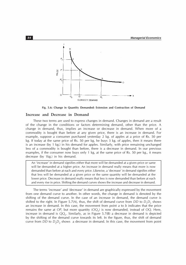
Managerial Economics84
Fig. 5.6: Change in Quantity Demanded: Extension and Contraction of Demand
Increase and Decrease in DemandThese two terms are used to express changes in demand. Changes in demand are a result
of the change in the conditions or factors determining demand, other than the price. Achange in demand, thus, implies an increase or decrease in demand. When more of acommodity is bought than before at any given price, there is an increase in demand. Forexample, suppose a consumer purchased yesterday 2 kg. of apples at a price of Rs. 50 perkg. If today at the same price of Rs. 50 per kg, he buys 3 kg. of apples, then it means thereis an increase (by 1 kg.) in his demand for apples. Similarly, with price remaining unchangedless of a commodity is bought than before, there is a decrease in demand. In our previousexamples, if the consumer now buys only 1 kg, at the same price of Rs. 50 per kg., it meansdecrease (by 1kg.) in his demand.
An ‘increase’ in demand signifies either that more will be demanded at a given price or samewill be demanded at a higher price. An increase in demand really means that more is nowdemanded than before at each and every price. Likewise, a ‘decrease’ in demand signifies eitherthat less will be demanded at a given price or the same quantity will be demanded at thelower price. Decrease in demand really means that less is now demanded than before at eachand every rise in price. Shifting the demand curves shows the increase and decrease in demand.
The terms ‘increase’ and ‘decrease’ in demand are graphically expressed by the movementfrom one demand curve to another. In other words, the change in demand is denoted by theshifting of the demand curve. In the case of an increase in demand, the demand curve isshifted to the right. In Figure 5.7(A), thus, the shift of demand curve from DD to D1D1 showsan increase in demand. In this case, the movement from point a to b indicates that the priceremains the same at OP, but more quantity (OQ1) is now demanded, instead of OQ. Here,increase in demand is QQ1. Similarly, as in Figure 5.7(B) a decrease in demand is depictedby the shifting of the demand curve towards its left. In the figure, thus, the shift of demandcurve from DD to D2D2 shows a decrease in demand. In this case, the movement from point

Demand Analysis 85
a to c indicates that the price remains the same at OP, but less quantity QQ2 is nowdemanded than before. Here, decrease in demand is QQ2.
PR
ICE
PR
ICE
a b C aPP
Fig. 5.7: Increase in Demand (A) and Decrease in Demand (B)
In short, a change in the quantity demanded due to change in the overall pattern ofdemand results in an increase or decrease in demand. For a change in demand, the changein factors other than price is responsible.
10. REASONS FOR CHANGE (INCREASE OR DECREASE) IN DEMAND
A change in demand occurs when the basic conditions of demand change. An alterationin the demand pattern (increase or decrease in demand) is caused by many kinds of changes.Some of the important changes are:
Changes in income. A change in the income of the consumer significantly influenceshis demand for most commodities. The demand for superior commodities in generaland for comforts and luxury articles increases with a rise in the consumer’s income.Similarly, overall demand generally decreases with a fall in income. In estimatingdemand function for commodities such as cars, for instance, changes in gross nationalproduct (GNP) or per capita real income is considered as crucial factors by theresearchers in general.
Changes in taste, habits and preference. When there is a change in taste, habits orpreference of the consumer, his demand will change. For instance, when a persongives up his smoking habit, this demand for cigarettes decreases.
Change in fashions and customs. Fashions and customs of our society determinemany of our demands. When these change, demands also change.
Change in the distribution of wealth. Through fiscal measures, government canreduce inequality of income and wealth and bring about a just distribution ofwealth, consequently the demand pattern may change in a dynamic welfare society.Welfare programes like free medical aid, free education, pension schemes, etc., raisethe purchasing power of the poorer sections of the community and their standardof living, so the overall demand pattern may change.

Managerial Economics86
Change in substitutes. Changes in the supply of substitutes, change in their prices,the development of new and better quality substitutes certainly affect the demandfor the given product. For instance, introduction of ballpoint pens has caused a fallin the demand for fountain pens.
Change in demand of position complementary goods. When there is a change inthe demand conditions of a complementary good (which is jointly demanded), therewill be side effects on demand. For instance, a change in the demand for shoes willautomatically bring about a similar change in the demand for shoe laces.
Change in population. The market demand for a commodity substantially changeswhen there is change in the total population or change in its age or sex composition.For instance, if the birth rate is high in a country, more toys and chocolates will bedemanded. But when the birth rate is substantially reduced through overall familyplanning efforts, their demand will decrease. Similarly, if the sex ratio of the countrychanges and if females outnumber males, demand for skirts will increase and thatfor shirts will decrease.
Advertisement and publicity persuasion. A clever and persistent advertisement andpublicity programmes by the producers affects consumer’s preference and causesalteration in the demand for products. Generally, demand for patent medicines andtoilet articles is very much determined by salesmanship and publicity. Often achange in demand for a new brand of the article in question, or the changed versionof the former one (e.g., when Charminar cigarettes became Gold (Char Minar) itcauses a spurt in sales.
The Case of US Snack Cake Industry
In the US snack cake industry with a decline in the health-consciousness trend, bakeriesresponded by reducing the number of low-calories/low-fat products in 1993. Again in 1994, underthe impact of the Nutrition Labelling and Education laws, the buyers’ preference shifted to morehealth-prone foods. The producers responded to this demand change and supplied low andreduced fat-varieties of products. The Figure 5.8 below represents this phenomenon of the shiftingmarket-demand.
Fig. 5.8: Demand for Low-Calorie/Low-Fat Products of the US Snack Cake Industry
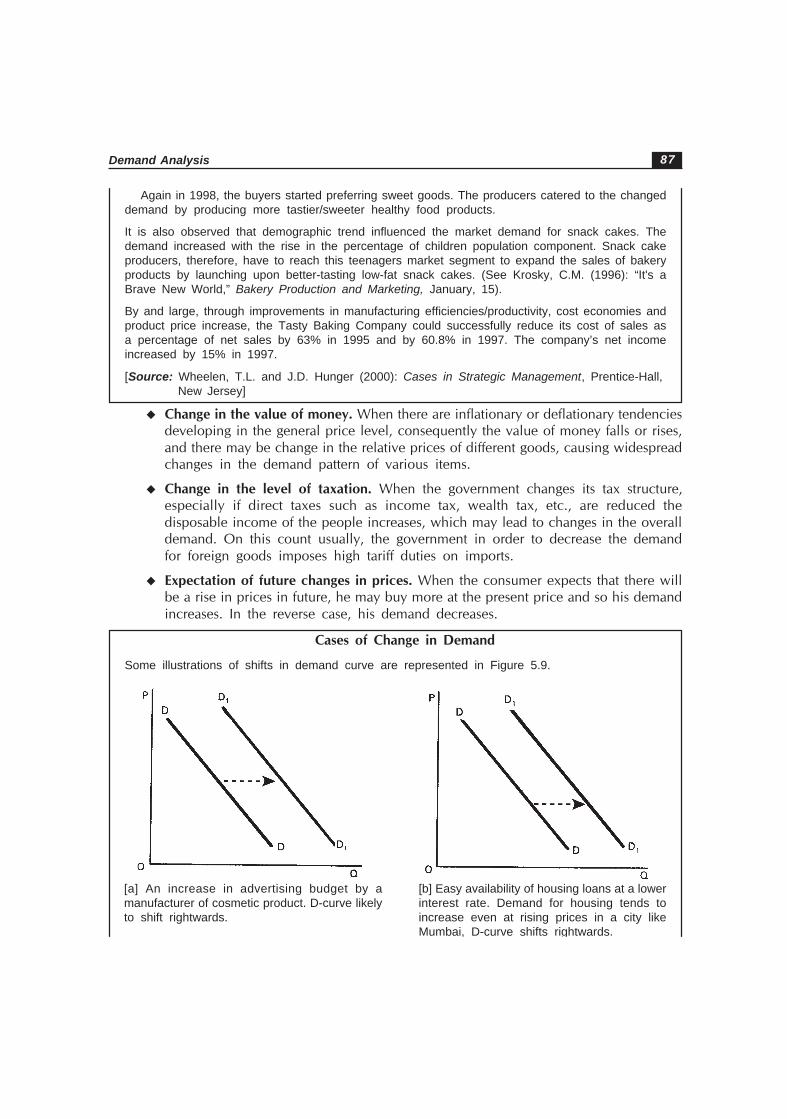
Demand Analysis 87
Again in 1998, the buyers started preferring sweet goods. The producers catered to the changeddemand by producing more tastier/sweeter healthy food products.
It is also observed that demographic trend influenced the market demand for snack cakes. Thedemand increased with the rise in the percentage of children population component. Snack cakeproducers, therefore, have to reach this teenagers market segment to expand the sales of bakeryproducts by launching upon better-tasting low-fat snack cakes. (See Krosky, C.M. (1996): “It's aBrave New World,” Bakery Production and Marketing, January, 15).
By and large, through improvements in manufacturing efficiencies/productivity, cost economies andproduct price increase, the Tasty Baking Company could successfully reduce its cost of sales asa percentage of net sales by 63% in 1995 and by 60.8% in 1997. The company’s net incomeincreased by 15% in 1997.
[Source: Wheelen, T.L. and J.D. Hunger (2000): Cases in Strategic Management, Prentice-Hall, New Jersey]
Change in the value of money. When there are inflationary or deflationary tendenciesdeveloping in the general price level, consequently the value of money falls or rises,and there may be change in the relative prices of different goods, causing widespreadchanges in the demand pattern of various items.
Change in the level of taxation. When the government changes its tax structure,especially if direct taxes such as income tax, wealth tax, etc., are reduced thedisposable income of the people increases, which may lead to changes in the overalldemand. On this count usually, the government in order to decrease the demandfor foreign goods imposes high tariff duties on imports.
Expectation of future changes in prices. When the consumer expects that there willbe a rise in prices in future, he may buy more at the present price and so his demandincreases. In the reverse case, his demand decreases.
Cases of Change in Demand
Some illustrations of shifts in demand curve are represented in Figure 5.9.
[a] An increase in advertising budget by amanufacturer of cosmetic product. D-curve likelyto shift rightwards.
[b] Easy availability of housing loans at a lowerinterest rate. Demand for housing tends toincrease even at rising prices in a city likeMumbai, D-curve shifts rightwards.

Managerial Economics88
[c] Recession in the economy leading todecline in consumer’s incomes. D-curvefor consumption goods will tend to shiftleftwards.
[d] Government’s proposal for the cut inincome tax rates causing rise in disposalincomes of the people. Market D-curve forgoods may shift rightwards.
Fig. 5.9: Cases of Shifts in Demand Curves
11. DEMAND DISTINCTIONS: TYPES OF DEMAND
The demand behaviour of the buyer or consumer differs with different types of demand.From managerial business economic’s point of view, thus, we may distinguish the followingimportant types of demand:
1. Demand for Consumer’s Goods and Producer’s Goods;
2. Demand for Perishable Goods and Durable Goods;
3. Autonomous Demand and Company Demand;
4. Industry Demand and Long-run Demand;
5. Short-run Demand and Company Demand;
6. Joint Demand and Composite Demand; and
7. Price Demand, Income Demand, and Cross Demand.
Demand for Consumers’ Goods and Producers’ Goods
Commodities may be divided into two sub-groups: (i) consumer goods, and (ii) producergoods.
Goods and services demanded by consumers for the direct satisfaction of theirwants, i.e., consumption purpose are referred to as consumer goods, e.g., food,clothes, house, services of a lawyer, doctor, teacher, cobbler, housemaid, etc. Goodswhich are demanded by producers in the process of production are referred to asproducer goods or capital goods, e.g., tools and equipments, machinery, raw materials,factory buildings, offices, etc.

Demand Analysis 89
Demand for consumer goods is direct or autonomous. Demand for producer goodsis derived. It is based on the demand for the output.
Demand for customer goods depend on its marginal utility. Demand for producergoods depends on its marginal productivity or the marginal revenue products.
Since marginal utility curves are usually negatively sloping, the demand curves forconsumer goods are negatively sloping.
Similarly, the producer goods too have negatively sloping demand curves because themarginal productivity or marginal revenue product curves are also negatively sloping.
Dean (1976), assigned the following reasons for explaining the distinctive demandbehaviour for producer goods in the economy:
The buyers of producer goods are professionals. They are usually experts. They areless likely to be influenced by sales promotion activities.
The producers buyers are more sensitive to factor price differences and substitutes.Thus, the demand for capital labour and other products tends to be elastic.
The motives of the producers buyers are purely economic. They buy capital goodson account of profit prospects.
Their demand being derived from consumption demand, there are frequent andviolent fluctuations in it.
The distinction between some capital goods and consumption goods is, however, arbitrary.It is based on who buys the goods and why. For example, a refrigerator purchased by thehouseholds is regarded as the consumer goods, while if it is purchased by a hotel it isconsidered to be the producer goods. Further, economic motive alone is not always kept inmind by the producers buyers. For instance, while buying the office furniture quite oftencostly items are ordered to maintain prestige rather than to see the economy of purchases.As Joel Dean (1976, p. 148) mentions, ‘There are thousands of incidental needs on anybusiness that are simply not worth the cost of scientific purchase planning.’
Demand for Perishable Goods and Durable Goods
From durability point of view, goods in general may be sub-divided into: (i) perishablegoods, and (ii) durable goods.
Perishable goods have no durability. That is, they cannot be stored for a long time.,e.g., milk, eggs, fish, vegetables, etc. Durable goods last long, whereas perishablegoods perish soon. Durable goods are storable for a long period, e.g., house furniture,car, clothes, etc.
Use of non-durable goods or perishable goods gives one short service. Durablegoods, on the other hand, can be used for several years.
There are durable and perishable consumption goods, e.g., vegetables, fish, etc., areperishable consumption goods, while TV set, car, etc., are durable consumption

Managerial Economics90
goods. Similarly, there are durable and non-durable capital goods, e.g., factory-plant, machinery, etc., are durable capital goods, while raw material, power, etc.,are non-durable capital goods. Durable physical capital assets are referred to as fixedcapital. Non-durable capital, which has one-time use only in the process of production,is called working or circulating capital. Fixed capital remains a fixed input componentin the short period, while working capital is a variable capital input all the time.
Capital assets are referred to as fixed capital. Non-durable capital, which has one-time use only in the process of production, is called working or circulating capital.Fixed capital remains a fixed input component in the short period, while workingcapital is a variable capital input all the time.
Perishable goods have more elastic demand. Durable goods have less elastic demandin the short run. Their demand tends to be more elastic in the long run.
The demand for perishable goods is always immediate. Demand for durable goodsis postponable.
The existing conditions of style, convenience and the income of the buyers usuallygovern the demand for non-durable goods.
Demand for durable goods depends on current trends, the state of optimism, the rateof obsolescence, lifetime of the product, improvement in product design, apart from pricesand incomes and such other considerations.
Demand for durable goods is more volatile in relation to business condition. Hence,demand analysis of durable goods is a complex phenomenon. Storability, postponability,replacement and expansion are the interrelated problems involved in determining the demandfor durable goods. (See Dean: 1976, p. 148).
Total demand for durable goods is composed of new demand as well as replacement requirement.Thus: D = Dn + Dr,
where, D = total demand for durable goods, Dn = new demand and Dr = replacementdemand. Dn and Dr are influenced by different factors.
The new demand or expansion demand (Dn) for durable goods is determined by a number offactors such as:
prices
buyers’ incomes
cost of maintenance
operating costs
resale value in future
price changes
product improvement

Demand Analysis 91
price concessions on outdated models
obsolescence rate, etc.
All these need to be included in the demand functions for the durable goods.
The replacement demand (Dr) for durable goods depends on:
the degree of postponability
expected shortages
rate of obsolescence caused by technological advancement and innovations
physical determination
financial exigencies
urge for renovation
cultural lags
rivalry of alternative investment
competition in the market, etc.
Autonomous Demand and Derived Demand
Spontaneous demand for goods, which is based on an urge to satisfy some wants directlyis called autonomous demand. Demand for consumer goods is autonomous. It is a finaldemand. It is a direct demand.
When the demand for a product depends on the demand for some other commoditiesit is called derived demand. ‘When demand for a product is tied to the purchase of someparent product, its demand is called derived.’ (Dean: 1976, p.150)
In many cases derived demand of the dependent product is owing to its being acomponent part of the main product, e.g., demand for doors derived from demand forhouses, or demand for bulbs derived from demand for lamps. Similarly, demand for antennasis derived from the demand for TV sets.
In many cases, demand for dependent product is caused by complementary consumption,e.g., demand for sugar emerges from the demand for tea. Demand for all capital goods isderived.
In modern days, however, it is rare to see demand for goods to be wholly-independentof all others. In fact, mostly demands are derived demand, e.g., even so-called autonomousdemand for a car by a household is derived from the demand for transport service. There isa thin line of demarcation between autonomous demand and derived demand. The distinctionbetween the two types of demand is rather arbitrary and a matter of degree.
Generally, derived demand is less price elastic than autonomous demand, e.g., thedemand for paints for automobiles is much inelastic as even a large percentage change in theprice of paints carries insignificant impact on the total cost of producing automobiles.

Managerial Economics92
The concept of derived demand facilitates demand forecasting very easy, especially inthose cases where dependent and parent products are used in fixed proportions and there isa definite time lead in the parent product’s demand.
Industry Demand and Firm or Company Demand
A firm is a business unit. Industry is the group of closely competitive firms. Industrydemand refers to the total demand for the commodity produced by a particular industry, e.g.,total demand for cars in India is the demand for automobile industry’s output in aggregateand essentially represents the market demand. Firm or company demands relate to the marketdemand for the firm’s output.
In demand analysis, thus, it should be noted that within the industry, the products of onecompany or firm can be substituted for another owing to their similarities. Company or firm’sdemand, therefore, is fairly elastic. A basic relationship of a firm’s demand and industry ormarket demand is established by the market structure whether perfect competition, monopoly,or monopolistic competition. In a perfectly competitive market, the degree of substitutabilitybeing perfect owing to homogeneity of goods of the different firms, the firms or companydemand for the product tends to be perfectly elastic. So, the demand curve becomes horizontalstraight-line.
If there is product differentiation and monopolistic competition among the firms, thenthe demand curve for the individual firm will be downward sloping. Industry’s demand curveas a whole is downward sloping indicating inverse price quantity relationship. In case ofmonopoly, the firm itself is industry, so its demand is identical with the industry demand.
Figure 5.10 illustrates demand conditions of industry and company.
Fig. 5.10: Industry and Company Demand
Further industry demand may be classified customer groupwise, e.g., cement demandedby the builders, individual households, housing boards and government departments.
A business economist or the business manager has to see the share of company demandin the industry demand. For undertaking sales forecasting, therefore, it is essential to project

Demand Analysis 93
industry demand first and then given projection for the growth of company’s demand inrelation to the company’s share in total demand and the possible growth of the rivals in thebusiness.
Short-run Demand and Long-run Demand
Though there is no clear demarcation between the short-run and long-run demand, thedistinction is useful for solving many decision-making problems. Especially, demand elasticitydiffers with time. In specific terms:
‘Short-run demand refers to existing demand with its immediate reaction to price changes,income fluctuation, etc., whereas long-run demand is that which will ultimately exist as aresult of the changes in pricing, promotion, or product improvement, after enough time isallowed to let the market adjust itself to the new situation.’ (Dean: 1976, p. 150)
The short-run elasticity of industry demand is usually less than the long-run elasticityowing to many reasons, such as:
cultural lags in information and experience;
capital investment required of buyers to shift consumption patterns;
time adjustment involved, e.g., it takes time to change consumption habits, timeneeded to arrange for the finance, etc.
Figure 5.11 illustrates the long-run and short-run demand curves for an industry.
Fig. 5.11: Short-run and Long-run Demand
Joint Demand and Composite Demand
Demands for most of the commodities in real life are independent of each other. Butthere are several commodities the demands for which are interrelated. Interrelation in demandmakes markets for physically different goods interlinked and interdependent. Broadly, twotypes of interrelationships exist in demand for such commodities.

Managerial Economics94
Joint or complementary demand. When two goods are demanded in conjunction withone another at the same time to satisfy a single want, they are said to be joint or complementarydemand. Examples are pens and ink, cars and petrol, bread and butter, coffee, sugar andmilk, pipes and pipe tobacco and so on. In such cases, a change in demand for one commodityleads to a change in demand for the other in the same direction and often in the sameproportion. Commodities so related are termed as complementary goods.
Composite demand. A commodity is said to be in composite demand when it is wantedfor several different uses. Steel is needed for manufacturing cars, building, construction ofrailways, etc. Households, factories, railways, chemical industries, etc., demand coal. Woolis required in clothing, carpet manufacturing and in several other industries. Similarly, electricityalso has a composite demand as it is used for lighting, cooking, TV, radio and many otherelectrical appliances by a household. Likewise, sugar is another illustration of compositedemand. Sugar is needed for a variety of purposes ranging from the manufacture of sweets,toffees to preservatives, etc. A change in demand for the commodity by one user will affectits supplies to others and will bring about a change in its price and hence alter its demandpattern.
Price Demand, Income Demand and Cross DemandPrice demand refers to the various quantities of a product purchased by the consumer
at alternative prices. In price demand, the demand function is based on the single price. Thus:
D = f (p)
where, D refers to demand, f shows functional relationship and p denotes price of theproduct.
Usually, price demand function has inverse functional relationship between the priceand the demand. The law of demand pertains to the customer behaviour regarding pricedemand.
Income demand refers to the various quantities of a commodity demanded by theconsumer at alternative levels of his changing money income. In income demand, the demandfunction is based on the income variable: (M). Thus:
D = f (M)
The income demand function is usually a direct function. It indicates that demandextends with the rise in income and vice versa.
Cross demand refers to the various quantities of a commodity (say, X) purchased by theconsumer in relation to changes in the price of a related commodity (say, Y – which maybe either a substitute or a complementary product).
Cross demand function may be stated as follows:
Dx = f (Py)
where, Dx = the demand for commodity X and Py = the price of commodity Y.

Demand Analysis 95
12. NETWORK EXTERNALITIES IN MARKET DEMAND
Theoretically, in earlier discussion (Section 3.3) it is assumed that individual demandsfor the product are independent, therefore, we desire market demand function/curve bysimply summing individual buyers’ demands. In reality, however, these may be interdependenceof demand, i.e., an individual demand may be depending on the demands of the otherpeople in the case of some goods. This situation is described as ‘network externalities’ whichmay be positive or negative in effect.
Economists have identified two such network externalities:
Bandwagon Effect
Snob Effect or Veblen Effect.
The Bandwagon Effect
In today’s life, demand for certain goods seems to be determined basically not by theirusefulness or utility but mostly on account of bandwagon effect or demonstration effect. Thus,demand in such cases is influenced by the consumption of pace setters or trend setters (suchas filmstars, models, group leaders, even friends and neighbours) in the community. Thatmeans demand of an individual is conditioned by the consumption of others; hence, the pricebecomes a minor consideration in this case.
Owing the bandwagon effect, the market demand curve trends to shift upward, asdepicted in Figure 5.12.
In Figure 5.12 the initial demand curve DD is based on utility of the product. In thiscase, a price cut leads to a slight expansion of demand. In the diagram, for instance, PP1 pricereduction implies QQ1 increase in quantity demanded, in the absence of bandwagon effect.In the presence of bandwagon effect, however, the demand curve shifts upward, suggestingan increase in demand. In our illustration, it is DD, thus, Q1Q2 increase in demand ismeasured on account of the bandwagon effect.
Fig. 5.12: Bandwagon Effect: The Demand Curve Shifts to the Right

Managerial Economics96
In short, the bandwagon effect on market demand for a product is the result of thebuyer’s desire to be in style or fashion — that is, to have it because others have it. Demandfor jeans and other fashionable clothes, for instance, is caused by the bandwagon effect.
For selling the clothes, therefore, marketing approach is to create a bandwagon effect.Likewise, in the case of children’s toys such as Barbie dolls demand arises on account of thebandwagon effect. In advertising and marketing of many products, therefore, the object is tobuild up a bandwagon effect. Bandwagon effect leads to the manipulation of the marketdemand. It shifts the demand curve to the right as shown in Figure 5.12. Use of modernmedia such as TV, Movies, Fashion Shows and so on in advertising strategies are meant toproduce such bandwagon or demonstration effect to manipulate market demand.
The bandwagon effect is essentially associated with stylishness, craze or fads of thepeople as greater and greater number of people want to use a product due to demonstrationeffect influencing on their desire through advertising media.The craze for compact disc (CD)songs albums of pop music is a good example of bandwagon effect that implies a positivenetwork externality on market demand for the product. The bandwagon effect will be strongerwhen the intrinsic value of the product is also high. In the case of personal computer (PC),for instance, when more and more people tend to own it because of its usefulness, moresoftware will be written and supplied at cheaper rates, then the PCs worth tends to rise furtherand so its demand too will shift. A price reduction due to large-scale production of PCs mayfurther include more buyers to buy the computer. In this way, the bandwagon effect mayhave its significance in determining the pricing strategy of the business firm in such products.(See, Pindyck and Rubinfeld: 1995, pp. 119-120).
The Snob Effect: Veblen Effect
The snob effect refers to the desire of a person (usually the rich one) to own exclusiveor unique product — called snob good or ‘Veblen good.’ It serves as a status symbol. Whenonly a few people could own a snob good, its demand tends to be high among the affluentgroup. Designer clothes and other products such as Rolls Royce cars, Ray Ban goggles, afancy restaurant, an antique, a rare painting, etc., are prestige goods and because of theirsnob value, the seller has to restrict the supply of such snob appeal goods. In marketing andadvertising strategies of such exclusive type of goods, demand has to be made effective bycreating a snob effect.
Rich buyer’s choices are usually governed by the snob appeal. The snob effect is alsoreferred to as Veblen effect. For the snobbish goods are described as Veblen goods (namedafter Thorstein Veblen). The Veblen effect is associated with the goods of conspicuousconsumption or ostantatious articles used by the affluent people. Thorstein Veblen argued thatthe affluent class in the society has a tendency to demonstrate their superiority of ‘high class’by spending on frivolous goods and services — super luxury items — such as diamonds, five-star hotels, palatial buildings, etc. When price of such luxuries rise, their snob appeal isenhanced, so their demand shifts upward. With the fall in the prices of such goods their snobappeal diminishes, causing a downward shift in their demand from the affluent section.
Network externality of snob effect, however, is negative. A snob good loses its prestigewhen it no longer remains exclusive and becomes a commonly used product. Though the

Demand Analysis 97
market demand for such a commodity, when its price falls tend to rise, the individual demandof the snobbish buyer of the product will fall. That means, when a prestige good loses its snobvalue, its market demand from the snobbish buyers will decrease with the fall in its price; andthe demand may be added up from the new common buyers. Maruti car in India, in thebeginning, for instance, has gained status symbol among the richer sections of the societycould have lost its snob appeal with the large expansion in its output.
In forming business strategies, such Veblen effect of snob appeal is gainfully exploitedin certain cases. Airlines, for instance, keep a much high ticket fare for the business class incomparison to ‘economy class.’ Similarly, in 5-star hotels deluxe rooms are much higherpriced as compared to the standard rooms.
Land values in posh locality tend to be much higher than those of dwellings by theordinary people. For instance, the land price in Malabar Hill in Mumbai is much more thanin Marol and a construction company must be well aware of such facts in execution of itsbusiness prospects.
Veblen Effect Paradox
In certain branded goods such as Ray Ban or Levis products, i.e., exclusive or designerproducts there exists an inherent paradox. Initially, these goods are meant to serve the Vebleneffect. At high prices, there is a limited but high demand from the richer section of the buyers.When these goods are produced in a large quantity, their prices will fall. It will carry a massappeal to upper middle income groups. So their demand will expand. But a further increasein output will lead to further price reduction. At this price, however, the demand will tendto fall on account of the loss of exclusivity. The brand would lose its significance below thisprice and the product would be purchased on account of its functional utility.
The demand curve for the branded or designer products, i.e., Veblen Goods (jeans,goggles, etc.), is ‘Z’ shape (assuming linearity for convenience) as shown in Figure 5.13.
PRIC
E
Fig. 5.13: The Market Demand Curve for Veblen Effect Product

Managerial Economics98
In figure 5.13, the demand curve DD has changing slopes at a and b points. At priceP1, demand is Q1. When price is lowered to P2, demand is Q2. A further reduction of priceto P3, leads to a fall in demand as the brand loses its exclusivity appeal. After that, the productdemand is determined just by its functional utility. In case of Veblen paradox, thus, pricingthe Veblen product is an art under the situation of ‘Z’ shape demand curve. Traditional pricetheory does not provide any clue when the demand curve contains both rising and fallingsegments. Stretched ‘Z’ shaped demand curve implies that at very high price, the marketdemand is limited but less elastic. When price is reduced, demand expands, as per the lawof demand. But, beyond a limit, a further fall in price leads to contraction in market demand.And, when the branded goods lose their exclusivity appeal, these goods have to compete withunbranded goods in the market. Such unbranded goods are then disposed of in shoppingcentres and supermarkets at very high discounts to attract common buyers. (See Prager: 1993,pp. 126-127).
The network externalities play a significant role in influencing the market demand for certainproducts such as computers, CD players, fax machines, handphones, etc. A positive networkexternality causes an upward shift in the market demand curve. The producers may experiencea rapid growth in demand for such products, because of the bandwagon effect a positivenetwork externality for quite a long time till the saturation point is reached.
13. PRACTICAL PROBLEMS
Practical problems in the context market demand function are illustrated as follows:
P:1. The demand function for beer in a city Qd = 400 – 4P
Where Qd = the quantity demanded of beer (in ’000 bottles per week)
P = the price of beer per bottle
(a) Construct a demand curve assuming price Rs. 10, 12, 15, 20 and 25 per bottle.
(b) At what price would demand be zero?
(c) If the producer want to sell 3,80,000 bottles per week, what price should it charge?
Solution:P = 10 : Qd = 400 – 4 × 10 = 360
P = 12 : Qd = 400 – 4 × 12 = 352
P = 15 : Qd = 400 – 4 × 15 = 340
P = 20 : Qd = 400 – 4 × 20 = 320
P = 25 : Qd = 400 – 4 × 25 = 300
With suitable scale plot this data on a graph such as shown in Fig. 5.14.

Demand Analysis 99
Fig. 5.14
Scale: y-axis: 2cm = 10
(Note: For convenience, there is the scale from origin on x-axis).
DD is the linear demand curve derived on the basis of the given function and given thealternative price.
In the equation: Qd = 400 – 4P, let us put Qd = 0
400 – 4P = 0
By manipulation: 4P = 400
P = 400/4 = 100
That is to say, at price Rs.100 per bottle, the demand for beer will be zero.
In the given demand equation:
Qd = 400 – 4P
Let Qd = 380
380 = 400 – UP
By manipulation:
4P = 400 – 380 = 20
P = 20/4 = 5
That is to say, the given demand function suggests that the producer should fix the priceat Rs. 5 per bottle in order to sell 3,80,000 bottles per week.
P: 2. Truett and Truett (1980), stated the following demand function for a brand X ofmicrowave ovens:
Qx = f(Px, Pz, Nw, Y, A)
Where, Qx = quantity demanded per year for brand X of microwave ovens in a city.
Px = price of X Brand

Managerial Economics100
Pz = Price of Z Brand
Nw = Number of working women
Y = Mean annual household income
A = Annual advertising expenditure
Assuming hypothetical data, we may state the demand estimation as under:
Qx = 11,93,200 – 100Px + 20Pz + 0.002Nw + 1.8Y + 0.3A
On this basis, given that:
Px = Rs. 8,000
Pz = Rs. 9,000
Nw = 8,00,000 in a city
Y = Rs. 1,00,000
A = Rs. 60,000
We can estimate the demand for X Brand microwave oven as follows:
Qx = 26,500 – (100 × 8,000) + (20 × 9,000) + (0.002 × 8,00,000) + (1.8 × 1,00,000) + (0.3 × 60,000)
= 26,500 – (8,00,000 + 1,80,000 + 1,600 + 1,80,000 + 1,800)
= 11,93,200 – 11,634,000
= 29,800
Ans.: 29,800 microwave ovens of X Brand are purchased annually in this city.
P: 3. Raj Kumar & Co., the cabinet-maker has estimated the following demand functionfor the steel cabinets produced by them:
Qd = 1,500 - 0.03P + 0.09AE
Where, Qd = quantity demanded of steel cabinets
P = average price of the steel cabinet
AE = the firm’s advertising expenditure.
All data are on a quarterly basis. The firm currently spends Rs. 10,000 per quarter onadvertising.
State the demand curve equation for the price-demand relationship. Give graphicalrepresentation assuming price variable values to be Rs. 10,000, Rs. 9,000, Rs. 8,000, Rs.7,000, and Rs. 6,000.

Demand Analysis 101
Solution: Substituting the value for AE variable in the above equation, we have simplified price-
demand equation as follows:
Qd = 1,500 + 900 – 0.03P
Thus:
P1 = Rs. 10,000 Q1 = 2,400 – 0.03 × 10,000 = 2,400 – 300 = 2,100
P2 = Rs. 9,000 Q2 = 2,400 – 0.03 × 9,000 = 2,400 – 270 = 2,130
P3 = Rs. 8,000 Q3 = 2,400 – 0.03 × 8,000 = 2,400 – 240 = 2,160
P4 = Rs. 7,000 Q4 = 2,400 – 0.03 × 7,000 = 2,400 – 210 = 2,190
P5 = Rs. 6,000 Q5 = 2,400 – 0.03 × 6,000 = 2,400 – 180 = 2,200.
[Plot price and quantity values on a graph]
MODEL QUESTIONS
1. Explain the important determinants of demand.
2. (a) What is meant by Demand Function, Demand Schedule and Demand Curve?
(b) Explain how market demand is derived from individual demand.
3. What do you understand by a shift in demand curve? Enumerate three possiblereasons for such shift.
4. Four of the following five events might reasonably be responsible in shifting thedemand curve for coffee to a new position. Point out the one which would not shiftthe demand curve and why?
(a) A fall in the price of tea.
(b) An increase in the money income of the consumers.
(c) A widespread advertisement campaign undertaken by the producers of coffee.
(d) A change in the habit of the consumers.
(e) A rise in price of coffee.
5. Over the years, the demand for textiles in India has grown inspite of rising prices.How would you reconcile this fact with the law of demand?
6. (a) State and explain the law of demand.
(b) Are there any exceptions to the law of demand?
7. Distinguish between:
(a) Industry demand and consumer demand.
(b) Individual demand and market demand.

Managerial Economics102
(iii) Increase in demand and extension of demand.
(vi) Decrease in demand and contraction of demand.
(v) Variation in demand and change in demand.
(vi) Demand schedule and demand curve.
(vii) Usual demand curve and exceptional demand curve.
8. Do you agree with the following statements? Give reasons.
(a) There are some exceptions to the law of demand.
(b) There are no exceptions to the law of demand.
(c) When the price of petrol rises, the demand for cars decreases.
(d) Demand is a relative term.
(e) Price is the sole determinant of demand.
(f) Demand curve can never have an upward slope.
(g) All desires become demand.
9. Explain and illustrate Veblen goods paradox.
10. Discuss the Bandwagon effect and Snob effect on market demand behaviour.
11. A producer of a Veblen good wishes to expand the supply and lower the price witha view to attract more buyers. What can be the outcome?
12. Draw and explain the market demand curve for the following quotation from TheWall Street Journal (March, 1987). “While many (baby boomers) might help fuel theinitial success of a new ice-cream or fashion, many stop buying when one of theseproducts becomes too commonplace.” (Quoted by Ponger 1993: p. 131).
13. What is the significance of demand analysis to a manager?
14. Analyse the import on the market demand for cosmetics under the following situations:
(a) A change in the sex ratio of the population increasing the females against malesin number.
(b) A general price rise in consumer product by 10 per cent.
(c) An increase in excise duties on cosmetics.
15. Specify the demand functions for the following:
(1) Gasoline
(2) Chicken
In each case, explain your choice of the variables included.

Demand Analysis 103
16. (a) What are the determinants of market demand for consumption goods in general?
(b) Write demand function (in mathematical terms) for:
(i) Pizza, and (ii) Fish
17. Identify the major influencing factors to the market demand for
(a) Ice-cream
(b) Sugar
(c) Ballpen
(d) Designer jeans.
18. The price of gold increases. Will this affect the demand for gold? How?
19. Is there any difference of expression between ‘a rise in demand’ and ‘an increase indemand’ for Godrej Hair Dye in Mumbai market.
Problems[1] Construct a demand schedule for a product X for alternative prices Re. 1, Rs. 2, Rs.3,
Rs. 4 and Rs. 5 given its demand function: Dx = 90 – 2Px. Draw the demand curvefor the same? What is its mathematical attribute?
[Dx: 88, 86, 84, 82, 80 Dx = f(Px) DxPx
∆∆ <0]
[2] The demand curve for commodity X is represented by Qx = 1,60,000 – 1,000 Px.
Construct the demand schedule assuming initial price to be Rs. 100 and consequentincrease by Rs. 10 up to Rs. 150. Plot the demand curve.
[3] Suppose the demand function for Komal butter in a town is estimated to be:
Qd = 600 – 5P
Where, Qd is the quantity demanded of butter (in ’000 kgs per week) and P standsfor the price.
(a) Estimate at what price, demand would be zero.
(b) Draw a demand curve, at alternative prices: Rs. 25, Rs. 35, Rs. 50, Rs. 60 andRs. 80 per kg.
(c) What is the statistical characteristics of this demand curve?

Elasticities andDemand Levels
6CHAPTER
1. THE CONCEPT OF ELASTICITY OF DEMAND
Demand usually varies with price. But the extent of variation is not uniform in all cases.In some cases, the variation is extremely wide; in some others, it may just be nominal. Thatmeans sometimes demand is greatly responsive to changes in price; at other times, it may notbe so responsive. The economists, to measure this responsiveness or the extent of variation,use the term “elasticity.” In measuring the elasticity of demand, two variables are considered:(i) demand, and (ii) the determinant of demand. For measuring the elasticity coefficient, thus,a ratio is made of the two variables.
demandoftdeterminaninchangePercentage
demandedquantityinchangePercentageDemandofElasticity =
The term ‘elasticity of demand’, when used without qualifications, is commonly referredto as price elasticity of demand. This is a loose interpretation of the term. In a strict logicalsense, however, the concept of elasticity of demand should measure the responsiveness ofdemand for a commodity to changes in the variables confined to its demand function. Thereare, thus, as many kinds of elasticity of demand as its determinants. In view of its majordeterminants, however, economists usually consider three important kinds of elasticities ofdemand:
Price elasticity
Income elasticity of demand
Cross price elasticity of demand or just cross elasticity.

Elasticities and Demand Levels 105
2. PRICE ELASTICITY OF DEMAND
The extent of response of demand for a commodity to a given change in price, otherdemand determinants remaining constant, is termed as the price elasticity of demand. Theprice elasticity of demand may, thus, be defined as the ratio of the relative change in demandand price variables.
The coefficient of price elasticity (e) is measured as:
Since the relative change of variables can be measured either in terms of percentagechange or proportional change, the price elasticity coefficient can be measured alternativelyas:
priceinchangealProportionThe
demandedquantityinchangealProportionThee =
Representing it in symbols, the price elasticity formula can be stated as:
e = ∆P/P
∆Q/Q Alternatively e =
∆P
P
Q
∆Q×
Or, by rearranging: e = QP
QP
∆Q×
where; Q = the original demand (say Q1)
P = the original price (say P1)
∆ Q = the change in demand. It is measured as the difference between the new
demand (say Q2) and the old demand (Q1). Thus,∆ (Q = Q2 – Q1.
∆ P = the change in price. It is measured as the difference between the new price
P2 and the old price (say P1). Thus, ∆ P = P2 – P1.
The above formula, in fact, relates to point price elasticity of demand, that is, thecoefficient signifies very small or marginal changes only. To illustrate the use of the formula,suppose the following information is available from a demand schedule:
Price of Apples Quantity Demanded(Rs.) (Kgs.)
20 (P1) 100 (Q1)
21 (P2) 96 (Q2)
priceinchangepercentageThe
demandedquantityinpercentageThee =

Managerial Economics106
Thus,
∆ P = P2 – P1 = 21 – 20 = 1, and P = P1 = 20
∆ Q = Q2 – Q1 = 96 – 100 = – 4, and Q = Q1 = 100
(Here, minus signs are ignored).
Elasticity of demand
e = 0.85
4
1
20
100
4
∆P
P.
Q
∆Q−==×
−=
Owing to inverse price-demand relationship, the coefficient of price elasticity of demandis, usually, negative. Customarily, however, economists report it as a positive number, referringto its absolute value for the sake of convenient comparison and analysis. Hence, its signs areignored. This means, in above illustration the elasticity of demand is less than one.
Using the above formula, the numerical coefficient of price elasticity can be measuredfrom any such given data. Apparently, depending upon the magnitudes and proportionalchanges involved in data on demand and prices, one may obtain various numerical valuesof coefficient of price elasticity, ranging from zero to infinity.
When price elasticity coefficient is greater than unity (e > 1), the commodity is said tobe price elastic. If it is less than unity (e < 1), the product is considered to be price inelastic.This knowledge is very useful in determining pricing policy and other business decisions.
3. TYPES OF PRICE ELASTICITY
Marshall has suggested a three-fold classification of types of price elasticity of demand,viewing the numerical coefficient of price elasticity in terms of unity or 1. Since the numericalcoefficient (e) values range between zero and infinity, in terms of unity we may say eithere is equal to, greater than or less than 1. Marshall’s classification is as follows:
Unit elasticity of demand (e = 1)
Elastic demand (e > 1), i.e., elasticity is greater than unity.
Inelastic demand (e < 1), i.e., elasticity is less than unity.
Marshall treats unit elasticity as normal or standard elasticity and all economists commonlyhold the same notion. By elastic demand, we mean that demands respond greatly or relativelymore to a price change. It, however, does not imply that the consumers are fully responsiveto a price change. What it means simply is this that a relatively large change in demand iscaused by a smaller changes in price. Similarly, inelastic demand does not mean that demandis totally insensitive. It only means that the relative change in demand is less than that ofprice. It means demand responds to a lesser extent only. Modern economists have elaboratedthe Marshallian classification further and stated five kinds of price elasticity as under:

Elasticities and Demand Levels 107
Perfectly elastic demand;
Perfectly inelastic demand;
Relatively elastic demand;
Unitary inelastic demand; and
Relatively inelastic demand.
Perfectly Elastic DemandAn endless demand at the given price is the case of perfectly elastic demand. When
demand is perfectly elastic, with a slight or infinitely small rise in the price of a commodity,the consumer stops buying it. The numerical coefficient or perfectly elastic demand is infinity(e = a).
In a broad sense, the shape of demand curve is significant in ascertaining the elasticityof demand. In the case of perfectly elastic demand, the demand curve will be a horizontalstraightline. Thus, the demand curve in Figure 6.1(A) implies that at the ruling price of OP,the demand is infinite, while a slight rise in price would mean zero demand.
1A E
D
P1
PPL
P1
P1
P2
e - 0
Y Y YY
X X M2 M1 M2 X M1 M2
e = I0 - 0
D
QUANTITY DEMAND PER UNIT OF FIVE
Y
Fig. 6.1: Types of Price Elasticity of Demand
Figure 6.1(A) indicates that at price OP a person would buy as much of the givencommodity as can be obtained, i.e., an infinite quantity, and that even at a slightly raisedprice he would buy nothing. While, it is assumed that when price is lowered, the demandcurve shifts down at this price — the demand curve remaining horizontal. Perfectly elasticdemand is a case of theoretical extremity. It is hardly encountered in practice.
Perfectly Inelastic Demand
When the demand for a commodity shows no response at all to a change in price, thatis to say, whatever change in price, the demand remains the same, it is called a perfectlyinelastic demand. Perfectly inelastic demand has, thus, zero elasticity (e = 0). In this case,the demand curve would be a straight vertical line as in Figure 6.1(B). Figure 6.1(B) indicates
(A) (C)(B) (D) (E)

Managerial Economics108
that whether the price moves from OP2 to OP1 or OP3, the quantity demanded remains thesame, OM only. Perfect inelasticity is again a theoretical consideration rather than a verypractical phenomenon. However, a commodity of absolute necessity like salt seems to haveperfectly inelastic demand for most consumers.
Relatively Elastic Demand
When the proportion of change in the quantity demanded is greater than that of price,the demand is said to be relatively elastic. The numerical value of relatively elastic demandlies between one and infinity. Thus, what Marshall called elasticity greater than unity ofdemand is again referred to as “relatively elastic” demand or “more elastic” demand. Arelatively elastic demand will be represented by a gradually sloping, i.e., rather a flatter,demand curve as shown in Figure 6.1(C). In Figure 6.1(C) when the price falls from OP1 toOP2 the demand rises to OM2 which is relatively large in proportion to the change in price
P
∆P
Q
∆O> ; hence, elasticity is greater than one. It is a more realistic concept as many commodities
have such higher elastic demand.
Relatively Inelastic Demand
When the proportion of change in the quantity demanded is less than that of price, thedemand is considered to be relatively inelastic. The numerical value of relatively inelasticdemand lies between zero and one. Hence, the concept “relatively inelastic” or “less elastic”demand is the same as what Marshall presented by a rapidly sloping, i.e., rather a steeper,demand curve as shown in Figure 6.1(D). In Figure 6.1(D) when the price falls by P1 P2, thedemand is extended just by M1M2 which is relatively very less in proportion to the change
in price P
∆PQ
∆O< ; hence, elasticity is less than one. This is also a very realistic concept.
Unitary Elastic Demand
When the proportion of change in demand is exactly the same as the change in price,the demand is said to be unitary elastic. The numerical value of unitary elastic demand isexactly 1. It is just the same as that of elastic demand, the demand curve would be arectangular hyperbolar curve, as shown in Figure 6.1(E). In Figure 6.1(E) when the price fallsby P1 P2, the demand is extended by M1 M2 which is in the same proportion to change in
price
>P
∆P
Q
∆O hence, elasticity is equal to unity. This is a theoretical norm, which helps to
distinguish between elastic and inelastic demand in general.
The different kinds of price elasticity of demand discussed above can be summarised asin the following table:

Elasticities and Demand Levels 109
Table 6.1: Price Elasticity of Demand
Numerical Terminology DescriptionValue
e = a Perfectly (or infinitely) elastic Consumers have infinite demand at aparticular price and none at all at aneven slightly higher than this given price.
e = 0 Perfectly (or completely) inelastic Demand remains unchanged, whateverbe the change in price.
e > 1 Relatively elastic Quantity demanded changes by a largerpercentage than does price.
e < 1 Relatively inelastic Quantity demanded changes by asmaller percentage than does price.
e = 1 Unitary elastic Quantity demanded changes by exactlythe same percentage as does price.
It should be noted that various demand curves drawn in Figure 6.1 are based on thesame scale. If these are not drawn on the same scale, it will be erroneous to make assertionsabout their relative elasticities. Because, it is quite likely that the same demand schedules mayhave curves with different slopes when the scales along the x-axis are different. It is only whenscales are the same, will the two demand curves have different slopes representing differentdemand schedules. Even then, just by looking at the demand curves, we cannot infer preciselyanything about elasticities over different price ranges on each curve without some calculations.If two demand curves are drawn on the same scale and we consider the same price rangein each case, then only can we assert that a flatter demand curve represents a greater elasticityof demand than a steeper demand curve.
Indeed, in a broad sense, the elasticity of demand for a commodity depends on thedemand schedule or demand function and hence on the shape of the demand curve for thatcommodity. To recapitulate again, on a given scale, the different slopes of demand curverelating to price elasticity can be compared as in Figure 6.2.
In Figure 6.2 (A), the demand curve D1 represents perfectly elastic demand. D2 representsperfectly inelastic demand. Similarly, in Fig. 6.2 (B), unitary elastic demand is represented bythe curves D4 and D5 respectively.

Managerial Economics110
Fig. 6.2: Slopes of Demand Curve
4. MEASUREMENT OF PRICE ELASTICITY
There are three different methods of measuring price elasticity of demand:
Ratio method to measure coefficient of price elasticity;
Total revenue method; and
Point method.
The Ratio MethodOf these, the calculation of coefficient of price elasticity by ratio method has been
already discussed in the previous section using the formula:
e = ∆P
P
Q
∆Q×
It is also known as percentage method, when we measure the ratio as:
e = %∆∆
%∆∆
Where, %∆ Q = percentage change in demand.
%∆ P = percentage change in price.
Total Revenue (or Total Outlay) MethodMarshall suggested that the easiest way of ascertaining whether or not demand is elastic
is to examine the change in total outlay of the consumer or total revenue of the sellercorresponding to change in price of the product.

Elasticities and Demand Levels 111
Total Revenue (or Total Outlay) = Price × (Quantity Purchased or sold)
According to this method:
When with a change in price, the total revenue (TR) remains unchanged, demand is unitelastic (e = 1). The total remains constant in the case of unit elastic demand, because thedemand changes in the same proportion as the price. This has been illustrated in Table 6.2.
When with a rise in price, the total revenue falls or with a fall in price, the totalrevenue rises, elasticity of demand is greater than unity. This happens because theproportion of change in demand is relatively greater than that of price. In short,when the price and total outlay move in opposite directions, demand is relativelyelastic (See Table 6.2).
When with a rise in price, the total revenue also rises and with a fall in price, thetotal revenue falls, elasticity of demand is less than unity. This happens because theproportion of change in demand is relatively less than the proportion of change inprice. Briefly, thus, when the price and total outlay move in the same direction,demand is relatively inelastic (Table 6.2).
Table 6.2: Total Outlay Method
Price Quantity Total Elasticity
Rs. (Units) Revenue (TR) of Demand (e)
Original 2 10 20 —
1. Change 4 5 20 e = 1
1 20 20 (unit)
2. Change 4 4 16 e > 1
1 24 24 (elastic)
3. Change 4 6 24 e < 1
1 16 16 (inelastic)
We may now summarise the total outlay method as follows:
Table 6.3: Total Revenue Method
Price Total Revenue (TR) Type of Elasticity (e)
1. Increases Constant e =1
Decreases Constant (Unitary)
2. Increases Decreases e > 1
Decreases Increases (Relatively elastic)
3. Increases Increases e < 1
Decreases Decreases (Relatively inelastic)
Figure 6.3 represents the relationship between total outlay (or total revenue) and theprice elasticity of demand. In Figure 6.3, Panel (A) represents an upward sloping total revenue

Managerial Economics112
curve (T1R) indicating that when price rises from P1 to P2 total outlay (or total revenue) risesfrom R1 to R2. It shows how the demand is relatively inelastic (e < 1).
Panel (B) represents a vertical straight-line total revenue curve (T2R). Here, total revenueremains unchanged (OR), whether price changes from P1 to P2 or vice versa. It means thatthe demand is unitary elastic (e = 1).
Panel (C) represents a downward sloping total revenue curve (T3R). So, with the rise inprice from P1 to P2, total revenue decreases from R1 to R2. It means that the demand isrelatively elastic (e > 1).
Thus, from the behaviour of total outlay or total revenue, we can infer the kind of priceelasticity of demand. Likewise, from a given price elasticity, we can conclude about thenature of change in the consumer’s total outlay or seller’s total revenue. In the case of unitaryelastic demand, with any change in price, total revenue remains unaltered. But when thereis elastic demand, the total revenue is expected to move in the opposite direction of thechange in price, while in the case of inelastic demand, the total revenue would change inthe same direction as of the price change.
TOTAL REVENUE
(A) (B) (C)
Y
O
R
a
R1
b
PR
ICE P1
P2
T1
R2X
B<1 Y
O
R
aP1
P2
R X
e=1
b
T2Y
O
R
P1
P2
X
e>1
T3
R1R2
Fig. 6.3: Total Outlay (Revenue) and Elasticity of Demand
Behavioural relationships between price changes, elasticity, and total revenue may besummarised as under:
Table 6.4: Price Changes, Elasticity and Total Revenue
Change in Change in Total Revenue When:
Price e < 1 e > 1 e = 1
Rise Rise Fall No Change
Fall Fall Rise No Change

Elasticities and Demand Levels 113
The total revenue method of measuring elasticity is, however, less exact. It can indicateonly the class of elasticity, but not its exact numerical value, we have to resort to the formulamethod or the point method. However, the economic significance of total outlay or totalrevenue method is that it shows more directly what happens to the total outlay or revenueas a practical guide for determining a price policy and its effect on demand and revenue.
However, the total revenue method gives the value of elasticity as equal to one, greaterthan one and less than one. It does not give correctly the numerical value of elasticity andtherefore, the second method, i.e., formula method is used.
Point Elasticity Method or the Geometric Method
Marshall also suggested another method called the point elasticity method or geometricalmethod for measuring price elasticity at a point on the demand curve.
The simplest way of explaining the point method is to consider a linear (straight-line)demand curve. Let the straight-line demand curve be extended to meet the two axes, as inFigure 6.4. When a point is plotted on the demand curve like point P in Figure 6.4, it dividesthe curve into two segments. The point elasticity is, thus, measured by the ratio of the lowersegment of the curve below the given point to the upper segment of the curve above thepoint.
Fig. 6.4: Point Method
For brevity, we may again put that:
pointtheabovecurvedemandtheofsegmentUpper
pointgiventhebelowcurvetheofsegmentLowerElasticityintPo =
or, to remember through symbols, we may put as:
e = U
L
where, e stands for point elasticity, L stand for lower segment, and U for the uppersegment.

Managerial Economics114
In Figure 6.4, AB is the straight-line demand curve and P is a given point. Thus, PB isthe lower segment and PA the upper segment.
∴e = U
L =
PA
PB
If after the actual measurement of the two parts of the demand curve, we find that PB= 3 cms and PA = 2 cms, then elasticity at point P is 3/2
= 1.5.
This measure is called a ‘point’ elasticity measurement because it effectively measureselasticity at a point on the demand curve assuming infinitely small changes in price andquantity variables.
5. PROOF OF THE GEOMETRIC METHOD
The above stated geometrical ratio of point method of measuring elasticity of demandcan be proved as under:
Let us consider a straight-line demand curve AB which intercepts the two axes (See Fig.6.5). Point P is given. Another point P1 is taken so closely to denote just a marginal change.(In Fig. 6.5, however, the distance between P and P1
is shown as significant only for the sakeof analysis which should actually be interpreted as a difference of only a point and not asegment).
Fig. 6.5: Geometric Proof
Point elasticity formulation is e=U
L. Thus, we have to prove that point elasticity is
e = PA
PB
A
M
M1
P
P1
R

Elasticities and Demand Levels 115
At points P and P1 in the diagram, we get the following particulars:
1. The initial price (P) is OM;
2. The initial demand (Q) is OQ;
3. The change in price (DP) is MM1; and
4. The change in demand (DQ) is QQ1.
Since price elasticity of demand is defined as a ratio of the proportional change inquantity demanded to the proportional change in price, the formula for measuring elasticitycoefficient is:
e =∆P
P
Q
∆Q×
Substituting the given geometrical particulars in the formula, we get
e = 1
1
MM
OM
OQ
OQ×
By interchange:
e =OQ
OM
MM
1
1 ×
Now, let us plot point R at the intersection point of lines PQ and M1P1. It can be seenthat:
QQ1 =RP and MM1 = PR
e =OQ
OM
RP
RP1 ×
Now, in ∆ s PRP1 and PQB
∠PRP1 = ∠PQB (both being right angles)
∠RPP1 = ∠QPB (common angle for both the triangles)
∠PP1R = ∠PBQ
Since all angles are equal for both the triangles, they are similar,
∠PRP1 = ∠PQB5
Their corresponding sides are proportional.
Ratio of their corresponding sides are equal.

Managerial Economics116
PQ
QB
PR
RP1 =
However, PQ = OM
∴ OM
QB
PQ
QB
PR
RP1 ==
OQ
OBe
OQ
OM
OM
OBe =∴×=∴ …(3)
Now, OQ = MP
MP
OBe =∴
Taking QB as a base, we have ∆ PQB and with MP as a base, we have ∆ AMP. In ∆ s
AMP and PQB
∠AMP = ∠PQB (both right angles)
∠MPA = ∠QBP (as per the Pythagoras theorem).
∆ MAP = ∠QPB
∴ ∆ AMP and PQB are similar.
∴ Their corresponding sides are proportional.
PA
PB
AM
PQ
MP
QB==∴
PA
PBe =∴
Since PB is the lower segment and PA the upper one of the demand curves, the theoremis proved that point-elasticity on a linear demand curve is measured by the ratio of lowersegment to the upper segment of the demand curve at the point.
If, however, the demand curve is non-linear, then draw a tangent at the given point,extending it to intercept both the axes (See Figure 6.6).

Elasticities and Demand Levels 117
Fig. 6.6: Point Elasticity
Point elasticity is, thus, measured by the ratio of the lower part of the tangent below thegiven point to the upper part of the tangent above the point.
Then, elasticity at point P in Figure 6.6 can be measured as: PA
PB
Important Observations in Point MethodRegarding point elasticity measurement, it must be noted that, Point elasticity is different
at different points on a given demand curve. This can be proved in two ways. First, by makinguse of the geometrical formula e = L/U, we may measure the price elasticity at differentpoints of given demand curve as shown in Figure 6.7. It goes without saying that on anystraight-line demand curve, price elasticity will be different at different points, since a demandcurve represents a demand schedule and demand schedule has different elasticities at variousalternative prices.
Fig. 6.7: Point Elasticities
We can prove this theorem in another way on the basis of treatment followed byProfessor Lipsey. In Figure 6.7, point P, being exactly in middle, e = 1. Between A and Pany point taken will show e > 1. Between P and B any point taken will show e < 1. Atpoint A, e = ∞, at point B, e = 0.
P
AD
D1
A
M
M1 P
P1
P2
e=1
e>1
e =
e<1
e=0
8

Managerial Economics118
We may, thus, conclude that if
L = U: PB = PA : e = 1
L > U: P1B > P1A : e > 1
L < U: PaB < P2A : e < 1
U = 0: PB = 0 : e = Ο
L = 0: PA = 0 : e = ∞
Since,
e = ∆P
P
Q
∆Q× by interchange,
=
Q
P
∆P
∆Qe
As such, elasticity measurement is split into two ratios:
DQ/DP, the ratio of change in quantity demanded to a change in price, it isdetermined by the slope of demand curve.
P/Q denotes price-quantity ratio. It depends on the position of the point on thedemand curve at which we want to measure the degree of elasticity.
Evidently in the case of a straight-line demand curve, the slope remains constant. Butwhen the position of point varies as P1, P2, etc., the price quantity relations change whichaffect elasticity. From an analysis of Figure 6.7 it follows that, as we move downward onthe straight-line demand curve, the elasticity varies from infinity (∞) on the price axis tozero on the quantity axis. This is because, slopes at all the point are identical due to achange in the position of the P points, the price-quantity ratio P/Q varies. On the price axis(y-axis) Q = 0.
∴ P/Q = ∞. As we move downward, P decreases and Q increases.
∴ P/Q tends to fall, so elasticity tends to fall.
On quantity (x-axis ), P = 0, P/Q = 0, e = 0.
While in the case of a non-linear demand curve (See Figure 6.8), it will be seen that not
only the position of point P/Q relationship varies, but the slopes ∆ O/∆ P also changes at
different points. As the tangent drawn on the curve tends to be flatter at each point movingdownward on the demand curve, the ratio (PB/PA) tends to decrease PB/PA PB1 > PA1 >PB2 /PA2. Thus, elasticity decreases which means point elasticity decreases as we movedownwards on the demand curve, whether it is linear or non-linear.

Elasticities and Demand Levels 119
Fig. 6.8: Point Elasticity
Two parallel straight-line demand curves having identical slopes, do nothave same elasticities at a given price
In Figure 6.9, D1D1 and D2D2 are two parallel linear demand curves. At price OM, weget points P1 and P2 on the respective demand curves. Since D1D1/D2D2, their slopes, as theratio; ∆Q/∆P are the same at P1 and P2. However, elasticity is determined by two factors:slope and price-quantity ratio.
Fig. 6.9: Parallel Demand Curves and Price Elasticity
At
P1 :1OQ
OM
Q
P= ; at P2 :
2OQ
OM
Q
P=
Since
OQ2 < OQ1 21 OQ
OM
OQ
OM<
The degree of price elasticity is at P1 higher than at P2. Thus, elasticities of two paralleldemand curves at the same price are unequal. Again, the demand curve which is closer to
Y
O
M
D1
D2
Q2Q1 D2D1
X
AD
D1
P
P1
P2
A1
A2
B1 B2B

Managerial Economics120
the origin has a higher price elasticity at each price than the curve which is away from theorigin.
It also follows, thus, that as the linear demand curve shifts towards its right (away fromthe origin), at each price, elasticity of demand will tend to be less than before. And, if it shiftstowards the origin, at each price on new demand curve, elasticity will be higher than before.This means, an increase in demand tends to lower the elasticity and a decrease in demandraises price elasticity.
Two intersecting linear demand curves have unequal price elasticities at the point ofintersection.
In Figure 6.10, D1D1 and D2D2 are two straight-line demand curves which cross at pointP. At point P thus, P/Q = OM /OQ is the same for both the demand curves. But, here theslopes of two curves differ, hence, the ratio ∆Q/∆P is not equal for both the curves. D2D2is a flatter curve. Hence, in the case of D2D2 at point P, the price elasticity coefficient is largerthan that of D1D1.
Fig. 6.10: Intersecting Demand Curves and Elasticity
Though the slope of demand curve is significant in determining price elasticity, it shouldnot be confused with elasiticity coefficient. The slope, i.e., steepness of the curve, alone willnot indicate the degree of price elasticity. But, the position of point, so the price quantityrelation P/Q, is equally significant in measuring the elasticity coefficient. Thus, elasticitycoefficient is affected by the multiplication of two ratios; P/Q and DQ/DP. In the case of thehyperbola demand curve, the product of both these ratios remain unchanged (being equalto throughout the range of the curve) as we move from one point to the other. So priceelaticity remains constant and equal to unity throughout the curve. Hence, in the case of thehyperbola demand curve, price elasticity does not vary between different points.
6. ARC ELASTICITY OF DEMAND
To calculate a price elasticity over some portion of the demand curve rather than at apoint, the concept of arc elasticity of demand is used (See Figure 6.11).
Y
O
R
M
X
P
D1Q D2
D1
D2
PR
ICE

Elasticities and Demand Levels 121
In Figure 6.11, point elasticity is measured at a point (say ‘a’) on the demand curve. Arcelasticity is measured on a range of demand curve, say between ‘a and b.’ The formula forarc elasticity measurement is:
21
21arc
PPe
++
×=∆P∆Q
where,
P1 = original price,
P2 = new price,
Q1 = original quantity demand,
Q2 = new demand,
∆ P = P2 – P1; ∆ Q = Q2 – Q1
For all theoretical purpose, however, point elasticity rather than arc elasticity is commonlyused. However, in practical consideration of decision-making, it is better to use arc elasticitymeasure, when the price change is more than 5%.
Illustration:
Suppose, initially P1 = 10 and Q1 = 100. Now, P2 = 12 and Q2 = 90. Then,
∆ Q = 90 – 100 = – 10
∆ P = 12 – 10 = 2
0.5790100
1210
2
10earc −=
++
×−
=
Let us take another example: Initial price is Rs. 100 and 1,000 units are demanded. Newprice is Rs. 120 and 800 units are demanded. Thus:
P1 = Rs. 100 Q1 = 1,000
P2 = Rs. 120 Q2 = 800
∆ P = Rs. 20 ∆ Q = – 200
(P)
O (O)
D
D2
P1
P2
Q2Q1
D
a
b
Point elasticity
Arc elasticity
Fig. 6.11: Point vs. Arc Elasticity

Managerial Economics122
I: Point elasticity at P1 is measured as:
120
100
1000
200
P
P
Q
Qe −=×
−=
∆×
∆=
II: Point elasticity at P2 is measured as:
1.520
120
800
200
P
P
Q
Qe −=×=
∆×
∆=
In this case, a problem arises about how to classify demand elasticity. Is the demandunitary elastic or more elastic? Arc elasticity solves this dilemma.
III: Arc elasticity is measured as:
1.2220.1222108001000
120100
20
200
2Q1Q
2P1P
P
Qarce −=×=
+
+
−=
+
+
∆
∆=
It suggests that the elasticity of demand is greater than unity. It should be noted that arcelasticity tends to be in the middle of two point elasticities in consideration.
7. FACTORS INFLUENCING ELASTICITY OF DEMAND
When the demand for a commodity is elastic or inelastic will depend on a variety offactors. The major factors affecting elasticity of demand are:
Nature of commodity. According to the nature of satisfaction the goods give, theymay be classified into luxury, comfort or necessary goods. In general, luxury andcomfort goods are price elastic, while necessary goods are price inelastic. Thus, forexample, the demand for foodgrains, cloth, salt, etc., is generally inelastic while thatfor radio, furniture, car, etc., is elastic.
Availability of substitutes. Where there exists a close substitute in the relevant pricerange, its demand will tend to be elastic. But in respect of commodities having nosubstitutes, their demand will be somewhat inelastic. Thus, for example, demand forsalt, potatoes, onions, etc., is highly inelastic as there are no close or effectivesubstitutes for these commodities. On the other hand, commodities like tea, coffeeor beverages such as Thums-Up, Mangola, Gold Spot, Fanta, Sosyo, etc., having awide range of substitutes, have a more elastic demand in general.
Number of uses. Single use goods will have generally less elastic demand as comparedto multi-use goods, e.g., for commodities like coal or electricity having a compositedemand, elasticity is relatively high. With the fall in price, these commodities maybe demanded increasingly for various uses. It may be elastic in some of the uses, andmay be inelastic in some other uses, e.g., coal is used by the railways and consumersas fuel. But the former’s demand is inelastic as compared to the latter’s. Technically,thus, the demand for a multi-use commodity in those uses where marginal utility ishigh, will be inelastic while in those uses where the marginal utility is low, thedemand will be elastic.

Elasticities and Demand Levels 123
Consumer’s income. Generally, larger the income, the demand for overall commoditiestends to be relatively inelastic. The demand pattern of a millionaire is rarely affectedeven by significant price changes. Similarly, the redistribution of income in favourof low-income people may tend to make demand for some goods relatively elastic.
Height of price and range of price change. There are certain goods like costly luxuryitems or bulky goods such as refrigerators, TV sets, etc., which are highly priced ingeneral. In their case, a small change in price will have a insignificant effect on theirdemand. Their demand will, therefore, be inelastic. However, if the price change islarge enough, then their demand will be elastic. Similarly, there are perishablegoods like potatoes and onions, etc., which are relatively low priced and bought inbulk, so a small variation in their prices will not have much effect on their demand,hence, their demand tends to be inelastic.
Proportion of expenditure. Items that constitute a smaller amount of expenditure ina consumer’s family budget tend to have a relatively inelastic demand, e.g., acinegoer who sees a film every fortnight is not likely to give it up when the ticketrates are raised. But one who sees a film every alternate day, perhaps may cut downhis number of films. So, is the case with matches, sugar, kerosene, etc. Thus, cheapor small, expensive or large expenditure items tend to have more demand inelasticitythan expensive or large expenditure items.
Durability of the commodity. In the case of durable goods, the demand generallytends to be inelastic in the short-run, e.g., furniture, bicycle, radio, etc. In the caseof perishable commodities, on the other hand, demand is relatively elastic, e.g.,milk, vegetables, etc.
Habit. There are certain articles which have a demand on account of habit and inthese cases, elasticity is less than unity, e.g., cigarettes to a smoker have inelasticdemand.
Complementary goods. Goods which are jointly demanded have less elasticity, e.g.,ink, petrol have inelastic demand for this reason.
Time. In the short period, demand in general will be less elastic, while in the longperiod, it becomes more elastic. This is because it takes sometime for the news ofa price change to become known to all the buyers. Consumers may expect a furtherchange, so they may not react to an immediate change in price. People are reluctantto change their habits all of a sudden. When durable goods are worn out, these aredemanded more. Demand for certain commodities may be postponed for sometime,but in the long run, it has to be satisfied.
Recurrence of demand. If the demand for a commodity is of a recurring nature, itsprice elasticity is higher than that of a commodity which is purchased only once.For instance, bicycles, taperecorders, transistors, etc., are purchased only once, hence,their price elasticity will be less. But, the demand for fast food items such as pizza,burger, etc., would be more price elastic.
Possibility of postponement. When the demand for a product is postponable, it willtend to be price elastic. In the case of consumption goods which are urgently andimmediately required, their demand will be inelastic.

Managerial Economics124
Price Elasticity of Demand for Food Items
The Annual Report of the National Food Survey Committee has estimated the price elasticity of demand
for various food items for the period 1984-89 in the UK Table 6.5 represents a classification of demand
elasticity of selected items from this Report. Demand for potatoes, vegetables and chicken tend to be
inelastic. Whereas, the demands for the food items like cheese, carass meat and frozen peas, appear to
be price elastic in the UK markets. In other countries also, a similar nature of demand elasticities of such
items is quite probable.
Table 6.5: The Price Elasticity of Demand for Select Food Items
Elasticity of Demand Inelastic Demand
e > 1 e < 1
Cheese: e = 1. 20 Bread: e = 0. 09
Carass Meat: e = 1. 37 Milk: e = 0. 19
Frozen Peas: e = 1. 12 Sugar: e = 0. 24
Potatoes: e = 0. 21 Vegetables: e = 0. 27
Chicken: e = 0. 13
Source: Annual Report of the National Food Survey Commitee, MAFF, 1989, Table 6.2.
Price Elasticities of Demand for Automobiles
Reviewing certain case studies on demand elasticities for automobiles available in the existing literature,
some interesting findings have been observed:
There is a marked a high cross-elasticity of demand between new and old cars. When price of new
cars come down, the demand for second hand cars tend to decrease. When price of second hand
better condition cars go down, the market demand for new cars is adversely affected.
The price elasticity of demand for new cars is greater than unity, but the coefficient varies between
1.1 to 1.4. That means, by lowering the price in small business a dealer cannot expect much
improvement in the sales revenue.
According to a study in 19831 the price elasticity of specific models in some cases has tended to
be very high. For example, in case of Ford Mustang it was estimated at 8.4 and for Impala it was
estimated to be 14.8.
A study in 19952 observede price elasticity coefficient between 5 to 6.7 in the case oflow-to- medium priced automobiles, whereas for high priced cars it was 3 to 4. Hence, thecompetitors/dealers find high cross-elasticities of demand in the segmented car markets.

Elasticities and Demand Levels 125
References:
1. Irvine F.O. Jr (1983): ‘Demand Equation for Individual New Car Models Estimated Using Transaction
Price with Implication for Regulatory Issues,’ Southern Economic Journals, 49, pp. 764-782.
2. Berry S. J. Levensohn and A. Parker (1995): ‘Automobile Price in Market Equilibrium,’ Econometrica,
63rd, 4 July, pp. 841-891.
Classification of Price Elasticity of Demand: Recapitalisation
In economic analysis, usually, the possible degrees/coefficient values of the price elasticity of demand
are divided in terms of unity (i.e.,1) into five general categories:
Unitary elastic demand: e = 1
Elastic demand: e > 1
Inelastic demand: e < 1
Perfectly elastic demand: e = ∞
Perfectly inelatic demand: e = 0
The last two categories are theoretical extremes and rarely found in pratice. Table 6.6 below summarily
provides the classification of price elasticity of demand.
Table 6.6: Classification of Price Elasticity of Demand
Degree of Price Elasticity (e) Types of Price Elasticity of Demand
(1) e = 1 Unitary Elastic
(2) e > 1 Elastic
(3) e < 1 Inelastic
(4) e = ∞ Perfectly Elastic
(5) e = 0 Perfectly Inelastic
8. INCOME ELASTICITY OF DEMAND
Income is a major determinant of demand for a number of goods. We may have anincome demand function thus:
D = f (M)
Where, M refers to the money income of the buyer.
It suggests that the demand may change due to a change in the consumer’s income,other factors remaining constant. The concept of income elasticity is, thus, introduced toascertain the extent of such change. The income elasticity of demand measures the degreeof responsiveness of demand for a good to changes in the consumer’s income.

Managerial Economics126
Definition: The income elasticity is defined as a ratio percentage or proportional change in thequantity demanded to the percentage or proportional change in income.
Income elasticity coefficient is, thus, measured by the following formula:
incomeinchangePercentage
demandedquantityinchangePercentageelasticityIncome =
Symbolically,
%∆∆
%∆∆em =
Where, %∆ Q signifies the percentage change in demand, and %∆ M the percentage
change in income.
Q
M.
∆M
∆Qor
∆M
M
Q
∆Qem ×=
Where,
∆ Q = change in demand
Q = initial demand
M = initial income
∆ M = change in income
9. TYPES OF INCOME ELASTICITY
Income elasticity on the basis of its coefficient (em), may thus be classified as under:
Unitary income elasticity of demand; (em = 1);
Income elasticity of demand greater than unity; (em > 1);
Income elasticity of demand less than unity; (em < 1);
Zero income elasticity of demand; (em = 0); and
Negative income elasticity of demand. (em < 0);
Unitary Income ElasticityWhen the percentage change in demand is equal to the percentage change in income,
the demand is unitary income elastic. Thus, em = 1.
The demand curve representing income demand function D = f(M) will have an upwardslope, and will be at 45° angle, as shown in Fig. 6.12 curve D1.

Elasticities and Demand Levels 127
Income Elasticity Greater than UnityWhen the percentage change in quantity demanded is greater than the percentage
change in income, the income elasticity of demand is greater than unity. Thus, em > 1. Thedemand curve will be flatter as D2 in this case.
Income Elasticity Less than UnityWhen the percentage change in demand is less than the percentage change in price, the
income elasticity of demand is less than unity. Thus, em < 1. The demand curve in this casewill be steeper like D3 in Figure 6.12.
Y
ODEMAND
X
D2
D3
D4D5
Em<0
Em=
0
Em<1
Em=1
450
INC
OM
E
Fig. 6.12: Income Elasticity of Demand
Zero Income Elasticity When the income change in any direction or in any proportion but carries no effect
on demand, so that the quantity demanded remains unchanged, it is referred to as zeroincome elasticity of demand. Thus, em = 0. The demand curve in this case is a vertical linelike D4 in Figure 6.12.
Negative Income ElasticityWhen an increase in income causes a decrease in the demand for a commodity, the
demand is said to be negative income elastic. The income elasticity coefficient, em < 0. Thedemand curve in this case will be downward sloping like D5 in Figure 6.12. Only in the caseof a few exceptional inferior goods like jowar and bajra in India and margarine in the USA,do we find income elasticity.
Income elasticity is generally positive, as there is a positive correlation between incomeand demand. Other things remaining the same, with an increase in income, there will be anincrease in demand and vice versa. Sometimes, however, negative income elasticity is alsoobserved. Especially, in the case of Giffen goods and certain kinds of inferior goods, incomeelasticity is negative. That is to say, when with a rise in income the consumer buys less ofa commodity, then there is negative income effect. But in most cases, the amount demanded

Managerial Economics128
increases with a rise in the consumer’s income and decreases with a fall in income. Thus,income elasticity, which is a numerical expression of income effect on demand, is found tobe positive in the case of most commodities.
Income elasticity of demand depends upon per capita income and the prevailing standardof living of a community. In industrially advanced countries of the West, with high livingstandards, the elasticity of demand for home appliances and gadgets, cars, new house, etc.,is usually very high. Comparatively, for necessaries such as potatoes, salt, bread, incomeelasticity of demand is quite low.
A high positive income elasticity of demand may be found in many food items in India,because people here are already living on a subsistence level and they are underfed. So, witha rise in income, they would buy, first, more of food products on account of their highmarginal propensity to consume. Even ordinary comfort goods will also have a high positiveincome elasticity of demand in India, as our standard of living is very low.
The income elasticity helps us in classifying the commodities. The following points maybe stated in this regard:
When income elasticity (em) is positive, the commodity is of a normal type.
When income elasticity (em) is negative, the commodity is inferior. For instance,cereals like jowar, bajra, etc., are inferior goods, so their income elasticity is negative.
If income elasticity coefficient is positive and greater than one (em > 1), thecommodity is a luxury. For example, the demand for TV sets, cars, etc., is highlyincome elastic.
If income elasticity coefficient is positive but less than unity (em < 1 ), the commodityis an essential one, e.g., the demand for foodgrains is income elastic.
If income elasticity coefficient is zero (em = 0), the commodity is neutral. Forinstance, consumption of commodities like salt, matchbox, etc., has zero incomeelasticity.
10. APPLICATIONS OF INCOME ELASTICITY
K.K. Seo points out that income elasticity of demand is applicable to many planning andstrategy problems, such as:
Long-term business planning. In the long-run, demand for comforts and luxurygoods may tend to be highly income elastic. Hence, prospects for long-run growthin sales for these goods are very bright. The firm can plan out its business accordingly.
Market strategy. Income elasticity of demand is helpful in developing market strategies.
Housing development strategies. On the basis of income elasticity, housingdevelopment requirement can be predicted and construction work can be effectivelylaunched upon.

Elasticities and Demand Levels 129
Combined Effects of Elasticities of Demand
Price effect and income effect together on the demand for a product can be captured through
combined effects of price and income elasticities of demand by using the following equation:
Q2 = Q1 [1 + ep (%DP) + em (%DM)]
Where,
Q1 = initial (current period) quantity demanded
Q2 = estimated demand quantity in relation to changes in price and income
P = price
M = income
ep = price elasticity at demand
em = income elasticity of demand
Illustration
[1] Panavision, a TV manufacturing company, is planning to increase the price of its television sets
by 10 per cent next year. The Economic Report of the country has forecasted rise in per capita income
by 5% during this period. Panavision economic adviser has estimated price elasticity for the TV set at
-1.4 and income elasticity at 2.2. The Panavision currently sells 50,000 TV sets. Give the forecast for the
sales. Is it advisable to raise the price of TV sets as has been decided in this case when each TV set is
currently priced at Rs. 10,000?
Solution:
Given particulars:
ep = –1.4; em = 2.2
Q1 = 50,000
%DP = 10% %DM = 5%
Q2 = 50,000 [1 + (–1.4)(0.10) + (2.2) (0.05)]
= 50,000 × 0.97 = 48,500.
It follows that positive income effect in this case is more than offset by the negative price effect. As
such, sales would be expected to decline to 48,500.
At initial price of Rs. 10,000 annual total revenue of the firm is Rs. 50 lakh. When the price is raised
to Rs. 11,000; then 48,500 TV sets are expected to be sold. This would fetch total revenue of Rs. 53.35
lakh. As such, the company is going to gain and should, therefore, proceed by its decision.
[2] A number of empirical studies of automobile demand in a country have observed that the price
elasticity is approximately –1.2 and the income elasticity is +2.8. The current sales amount to 8 lakh units.
If the price rises by 10% and income rises 5% next year, how many cars are expected to be sold?
Ans: In this case, price effect on price elasticity (ep) –1.2% and income effect on income elasticity (em)
is +2.8%.
%DQ = ep × DP + em × %DM
= –1.2 × 10% + 2.8 × 5%
= 1.02
Demand for automobiles = Qa = (1.02) × 8 lakh = 8.16 lakh cars.

Managerial Economics130
11. CROSS ELASTICITY OF DEMAND
In arriving at the price elasticity of demand, one takes into account the change indemand due to a change in the price of the same commodity. In cross elasticity of demand,we take into account the change in the price of commodity Y and its effects on the demandfor commodity X. The concept of cross elasticity is important in the case of commoditieswhich are substitutes and complementary. Tea and coffee are substitutes for each other, penand ink, car and petrol are complementary goods.
Definition: The cross elasticity demand refers to the degree of responsiveness of demand fora commodity to a given change in the price of some related commodity.
The cross elasticity of demand between any two goods X and Y is measured by dividingthe proportionate change in the quantity demanded of X by the proportionate change in theprice of Y. Thus:
YofPriceinchangepercentageorateProportion
XforDemandinchangepercentageorateProportionDemandofElasticityCross =
Symbolically,
x
x
y
x
x
xxyc
Q
P
∆P
∆Q
Q
∆Qeore ×÷=
ec or exy = cross elasticity of demand – (demand for X in relation to the price of Y)
∆ Qx = change in quantity demanded for commodity X
Qx = initial demand for X
Py = initial price of commodity Y
∆ Py = change in the price of commodity Y (Preferably d instead of
∆ is used to represent a point change.)
The cross elasticity of demand measures the extent to which products are substitute orcomplementary. A positive cross elasticity of demand indicates that the two products inconsideration are substitutes, since an increase/decrease in the price of one causes an increase/decrease in the quantity demand of the other.
A negative cross elasticity of demand indicates that the two products in considerationare complementary to each other, since an increase/decrease in the price of one leads to acontraction/extension in demand for the other.

Elasticities and Demand Levels 131
Illustration.
To illustrate the use of the formula, let us take data from Table 6.7.
Table 6.7: Monthly Demand of a Household
Commodity Original Change
Price Quantity Price Quality
(Rs.) (Units) (Rs.) (Units)
Tea 3 50 3 60
Coffee 4 30 5 20
Bread 2 80 2 90
Butter 75 30* 6 40*
(*Butter 50 gram packets)
Solution
From Table 6.7, we may take data for tea and coffee and measure the coefficientof price cross elasticity as under:
Let X = tea, Y = coffee,
Qx = 50, ∆ Qx = 60 – 50 = 10.
Py = 4, ∆ Py = 5 – 4 = 1.
0.84/5501
410
Q∆P
P∆Qe
xy
yxxy ==
××
==
Now, let X = bread, Y = butter, then:
Qx = 80, ∆ Qx = 10
Py = 7, ∆ Py = –1
0.888
7
801
710
Q∆P
P∆Qe
xy
yxxy −=
−=
×−×
==
Thus, the numerical coefficient of cross elasticity of demand may be either positive ornegative. Substitute goods have positive, price elasticity of demand. Jointly demanded orcomplementary products have negative price cross elasticity of demand.
A higher coefficient of cross elasticity obviously means a higher degree of substitutabilityor complementarity between two goods X and Y. Two unrelated goods have zero crosselasticity. Fig. 6.13 graphically illustrates the cross elasticity of demand.
When the demand function like Dx = f (Py) is plotted graphically, it will take differentpositions as per the price cross elasticity, as shown in Figure 6.13. It will have an upwardslope like D1 if X is a substitute of Y. It will have a downward slope like D2, if X is a

Managerial Economics132
complementary to Y. It will be a vertical line (D3) if X is unrelated to Y. So any change inthe price of Y has no effect on the demand for X.
The nature of the goods relative to their uses mainly determines the cross elasticity ofdemand. The cross elasticity tends to be high when two goods satisfy the same wants equallywell.
Fig. 6.13: Cross Elasticity
One should be rational in approach with a common sense that cross price elasticityshould not be worked out in the case of totally unrelated goods. For example, change in theprice of razor blade and the demand for petrol.
Application of Cross Elasticity of Demand in Transport System
The concept of cross price elasticity of demand can be useful in determining competitive price strategy
and policy in the alternative rival modes of services, such as rail-road services. Cross elasticity, here is taken
as a measure of the effect of a change in the fares on the demand for the rail service, and vice versa. To
illustrate the point, let us consider a hypothetical case study.
The cross elasticity of demand for a train service from station A to B is the rate of change in the number
of train tickets sold on that route in relation to the percentage change in the price of bus service for the
same route. If the bus company reduced its fare from Rs. 40 to Rs.35, and the following data are observed:
Fare (Rs.) Daily No. of Passengers
Rail Bus Rail Bus(Ordinary Class)
1. Before fare change 45 40 500 200
2. After fare change 45 35 400 300
Percentage change 0 –12.5% –20% 50%
Cross elasticity is:
1.612.5%–
–20%
ServiceBusin%P
ServiceRailin%QeC ===
Such a high cross elasticity reflects that the market demand is greatly responsive to thecompetitive price variation.

Elasticities and Demand Levels 133
Selected cross price elasticities of demand are presented in Table 6.8.
Table 6.8: Selected Cross-Price Elasticities of Demand in the USA
Demand for Effect of Price on exy
(x) (y)
Coffee Tea 0.15
Butter Margarine 1.53
Electricity Natural Gas 0.50
Source: Nelson (1995): Microeconomics: Theory, Issues, Applications, Dryden Press, NewYork, p. 220.
12. ADVERTISING OR PROMOTIONAL ELASTICITY OF DEMAND
In case of several products, the market demand is influenced through advertisement orpromotional efforts. The demand function in this case may be stated as:
Qx = f (A)
where,
Qx = Demand for the product x measured through the quantity sold in the market.
A = Advertisement expenditure of the firm.
The degree of responsiveness of demand to changes in advertising or promotional elasticityof demand, (eA) measured, thus:
eexpenditurentadvertiseminchangeateproportionorPercentage
salesinchangeateproportionorPercentagee A =
In symbolic terms,
eA = %%
QA
∆∆
Alternatively,
CA =
∆∆QA
AQ
where, Q = Quantity of sales, and
A = Amount of advertisement expenditure.
Illustration
At initial advertisement expenditure of Rs. 50,000 the demand for a firm’s product is80,000 units. When the advertisement budget is increased to Rs. 60,000 the sales volumeincreased to 90,000 units.

Managerial Economics134
The advertising elasticity of demand is measured, thus:
A1 = Rs. 50,000 A2 = Rs. 60,000
Q1 = Rs. 80,000 Q2 = Rs. 90,000
∆ A = Rs. 10,000 ∆ Q = Rs. 10,000
∆Q∆A
∆A∆Q
eA ×=
0.6380,000
50,000
10,000
10,000=×=
In particular, point elasticity is used when the price-quantity changes are infinitesimallysmall — (assuming that a small price change is indicated by a virtual point on the demandcurve). When there is a substantial price change, a discrete movement is observed. In thiscase, arc elasticity is preferable. For all practical purposes, when price change is over 5 percent, it is better to use arc elasticity measurement to capture a more realistic idea of demandelasticity.
Arc Advertising Elasticity
The arc advertising elasticity is measured as:
+
+
=
2Q1Q
2A1A
A
QarcAe
∆∆
In the above example,
0.6590,00080,000
60,00050,000
10,000
10,000arcAe =
+
+×=
13. PRACTICAL APPLICATIONS
The concept of elasticity of demand has a wide range of practical application in economicsand business.
To BusinessmenIn decision-making, the concept of elasticity of demand is of utmost practical use, for
while taking decision for pricing policy, the businessman has to know the likely effect of pricechanges on the demand for his product in the market. He has to consider, for instance,whether a lowering of price will cause an expansion in the demand for his product, and ifso to what extent and thus to what extent his total revenue would rise fetching what amount

Elasticities and Demand Levels 135
of profit. This he can know easily if he has an idea about the demand elasticity for hisproduct. Most businessmen consciously or unconsciously know by intuition something aboutthe elasticity of demand for their product while making a price decision. Several, however,do not pay any attention to the price elasticity of demand and make the wrong decisions, sosuffer heavy losses. In scientific management decision-making, thus, one has to try to form asprecise an idea as possible of the degree of elasticity of demand, for it is a convenient short-hand way of expressing the effects of price change on the demand for a product.
By knowing the type of elasticity of demand, it is easy to know whether a price cut isbetter or a price rise for increasing the sales, total revenue and the profit. When the demandfor the product is found unitary elastic, price change is ineffective in bringing more totalrevenue, so unless the cost is changed it is not worthwhile to change the price.
In case of demand elasticity being more than unity, a price cut would lead to anincrease in sales more than proportionately, so the total revenue will rise: hence in such acase, a price cut policy would be more appropriate.
On the other hand, if the product has inelastic demand, by raising a price, no significantdecrease in sales will be effected, so the total revenue and the profit would rise. Hence, insuch cases, a price rise policy would be appropriate.
In short, for elastic demand a businessman would be better off by charging a low priceand in case of inelastic demand, by putting a high price for the commodity, the businesswould be profitable.
Particularly, a monopolist will be greatly influenced by the degree of price elasticity forhis goods, so that he will have a rational price discrimination policy. That is he will chargedifferent prices in different markets. The B.E.S.T., for example, charges different rates for theconsumption of electricity, depending on the use to which it is put.
Illustration: Practical Application
In practice, the price variations and differentials in several businesses such as hotels, airlines, ferries,
coaches, time-to-time, reflect differences in the level of demand, particularly the varying elasticity of
demand at different times such as peak seasons and off-seasons over a year. A telephone company also
decides its rate structure into peak rate, standard rate, discount rate, etc., at different times of the day. For
example, during working day 8.00 a.m. to 7.00 p.m. peak rate is charged on calls, while lower or discount
rates are charged during night hours. On public holidays, discount rate is charged. In all such cases,
pricing is based on demand consideration rather than the cost element.
Likewise, the knowledge of income elasticity is important to certain producers in theirdemand and sales forecasting and planning business expansion. For instance, the demand forTV sets is highly income elastic, so when per capita income or income level of a class ofconsumers is found to be rising, TV manufacturers can expect a greater sale even at slightlyhigher prices.
Similarly, cross elasticity helps certain businessmen to mould their business policies. Forinstance, edible oil producers may find that the demand for oil increases when the price ofghee rises. Likewise, sugar in relation to changes in the price of gur. Similarly, demand forraincoats is bound to multiply considerably in the face of a rise in the prices of umbrellasand vice versa.

Managerial Economics136
To the Government and Finance MinisterIn determining fiscal policy also, the concept of elasticity of demand is very important
to the government. The finance minister has to consider the elasticity of demand whileselecting commodities for taxation. Tax imposition on commodities for getting a substantialrevenue becomes worthwhile only if the taxed goods have an inelastic demand. Otherwise,if the demand is more elastic, it will contract very much with a rise in price as a result ofadded taxation (like sales tax or excise duty), hence, the total revenue yield would not bemuch. That is why, generally taxes are levied on commodities like kerosene, matches, cigarettes,sugar, etc., which have an inelastic demand.
In International TradeThe concept is also useful in formulating export and import policies of a country.
Further, in determining terms in the sphere of international trade, the relative elasticities ofdemand for commodities in the two countries are very important.
To Policy-MakersIn economic analysis, the concept is useful in solving the mystery of how farmers may
remain poor despite a bumper crop. Since agricultural products, particularly foodgrains, haveinelastic demand, when there is a bumper crop it can be sold only by cutting prices substantially.Hence, the total income of farmers will be lower in spite of a bigger crop.
To Trade UnionistsThe concept of price elasticity is useful to trade unions in wage bargaining. The union
leaders, when they find that demands for their industry’s product is fairly elastic, will ask fora higher wage to workers and use the producer to cut the price and increase sales which willcompensate for his loss in total profit.
In this way, the concept of demand is of a great practical significance to businessmen,economists, farmers, trade unions and government policy-makers.
14. APPLICATION PROBLEM: A HYPOTHETICAL CASE STUDY
Adam, the owner of Ever-Joy Ice Cream Centre, near University Campus, was also a part-time student of management studies in a Commerce College. After having studied the theoryof price elasticity of demand, he thought that the demand for ice cream should be priceelastic. For an experiment he announced special-reduced price for the Ever-Joy Ice CreamCone in the second week of August 2001 under the ‘54th Independence Anniversary Week.’He observed the following sales outcome.
Adam worked out price elasticity coefficient in this case to be:
2.51000
5
1
500
Q
P
∆P∆Q
e =×=×=

Elasticities and Demand Levels 137
Table 6.9: Sales Data for Ever-Joy Ice Cream Cone
August Price Total Sales Total Sales Revenue
Regular
Ist Week Rs. 5 1,000 Rs. 5,000
Special
2nd Week Rs. 4 1,500 Rs. 6,000
Finding demand elasticity to be much above unity, he inferred that the price reductionled the total sales revenue to increase. This outcome encouraged him to reduce the price inOctober on a permanent basis to Rs. 4.50. To his utter surprise he found that his averageweekly sales revenue rather declined to Rs. 4,770.
What happened? Though the average weekly demand had risen to 1,060 with the pricereduction, the sales revenue declined. Because, this time the degree of price elasticity is:
0.61000
5
0.5
60e =×= which turns out to be less than unity. Adam got puzzled. How did
the demand suddenly become price inelastic? Why? What went wrong?
Adam’s approach to price policy was purely theoretical, assuming all other things beingequal. He did not care to look at other factors influencing the demand for ice-cream, suchas possibilities like winter, climatic adverse effects, similar price war by the rivals’ shops inthe area.
Besides, Adam offered a 20% price reduction temporarily in August only for a week, somost buyers responded to take the advantage and probably the rival did not retaliate knowingit a short-term phenomenon at that time. Furthermore, now when the buyers realised thatprice-reduction in October is permanent, they did not react much on the buying-spree. In theprevious case of price reduction, the buyers expected that in future — after the celebrationweek is over — price will go back to the original level, therefore, they purchased more. Thisphenomenon of further expectations was also not taken into accounting determining the laterprice-reduction policy. In short, the business decision of Adam was misled by overestimationof price elasticity from the very short-term data in a special situation rather than resorting todemand estimation based on the long-term sales data under normal circumstances.
From Adam’s experience, we should learn one important lesson that any judgementbased on a partial view may not always be good. Besides, reality widely differs from theory.Real life is never so simple as depicted in theory. Managerial decision-making in practice is,therefore, more of an art than science.

Managerial Economics138
A Mini-Case: VCD Rentals
According to a Chamber of Commerce study in Mumbai’s VCD-rental market, the price elasticity of
demand for VCD rentals is 0.7. A 10% rise in rentals implies a decline the demand for VCDs on rentals
by 7%. That means, the demand for VCD’s on rentals is inelastic. Based on this information, the owner
of Andheri Music Stores, a B.Com. graduate, increased the rentals by 25% in order to enhance its total
revenue. Contrary to his expectations, the store’s total revenue decreased, in consequence. What is the
mystery?
Well, there is no mystery. It is a matter of simple economic behaviour of the customers. The study
reported the measure of elasticity by assuming: if all VCD rental stores in Mumbai increased their prices
by 10%, the market-demand will drop by 7%. But, in an isolated case, when the particular seller only
charges a high price, the customers can easily shift to the other competitors in the vicinity. Then, the
individual concerned seller loses his sales. In this case, the demand facing an individual seller tends to
be elastic, though as a whole market demand for the product is inelastic. As such, the increase in price
by an individual seller causes a decrease in his total sales revenue. The Andheri Music Store, obviously,
experienced a decline in its total revenue, owing to its isolated action.
MODEL QUESTIONS
1. (a) What is elasticity of demand?
(b) On what factors does elasticity of demand depend?
2. (a) Explain the concept of cross elasticity of demand.
(b) Indicate its usefulness in the classification of market situations.
(c) What are its limitations?
3. (a) Distinguish between price elasticity, income elasticity and cross elasticity of demand.
(b) On a straight-line demand curve, select any point ‘p’ and give a geometrical proof of measurement of elasticity at this point.
(c) When the price of commodity X was Rs. 10 per unit, people consumed 3,000 units. With a fall in price to Rs. 9, they consumed 3,150 units. State the formula and measure the elasticity of demand for X.
4. What is point elasticity of demand? How is it measured?
5. (a) Define cross elasticity of demand.
(b) Would you except the cross elasticity of demand to be positive, negative or zero for each of the following pairs of products:
(i) Kelvinator and Godrej refrigerators.
(ii) Tables and chairs,
(iii) Maruti car and railway tickets.
What general rule can you give to base your answers?

Elasticities and Demand Levels 139
6. Explain the concept of cross elasticity of demand. How would you measure suchelasticity?
7. Define cross elasticity of demand and state its formula. How does such elasticitydiffer in case substitutes and complementary goods?
Problems1. Calculate price elasticity of demand for different years from the following data:
Year Percentage Change Percentage Changein Price in Quantity
1981 5.0 –3.2
1982 –2.5 5.6
1983 Zero 1.2
1984 6.5 –2.5
2. Investigating the demand for textile in a country X, a researcher observed that thedemand for textiles tend to rise by 1.5 per cent with one per cent decrease in theprices of textiles; with the rise in one per cent of per capita GDP, the demand fortextiles rise by 0.45 per cent and when food prices increased by one per cent, thedemand for textiles contracts by 0.93 per cent.
(a) Identify the type of demand elasticities in this case and define them.
(b) Which type of elasticity the textile mills should consider significant for businessdevelopment?
(c) How much rise in sales is expected during a festival season by offering 20 percent discount by textile mills showrooms?
3. Oldfield and Tyler in the TRRL study (1981) measured mean fare demand elasticitiesfor rail travel between London and several other stations up to a distance of 120kilometres, as under:
Season Cheap FullTicket Day Fare Fare
I Class: – 0.20 – 0.11 – 0.13
II Class: – 0.56 – 0.50 0.20
Give your comment in this context.
[Hints:
The low elasticity for full fare travel and Ist class passenger may be attributed to thelarge element of business travel.
The relatively high elasticity of demand for cheap day tickets is due to its highoptional nature.
Class season ticket has higher elasticity than that of the Ist class because of poor andricher income groups of passengers.]

Managerial Economics140
4. The Serpell Report (1983) on Railway finances in England, for instance, measuredprice elasticity of demand for rail services on some routes to be fairly inelastic(– 0.15); hence, suggested fares rise of 40 per cent for London commuters. In thiscase, workout the revenue effect if fare is raised from £-10 to £-14 and daily 1,000passengers are travelling on this route. Should the authorities accept this suggestion?Give your comment.
[Hints:
e = %%∆∆
QP
∴ – 0.15 =∆Q
40% ∴ ∆Q = 6%
TR = P.Q
Initially: TR = 10 × 1000 = £ 10,000
DQ = 6%
∴ with the rise in fare new Q = 940
∴ At new price £ 14
TR= 14 × 940 = £ 13,160
Comment: Since demand is fairly inelastic, with the increase in fare, its revenue effect ispositive and substantially high; therefor e, the railway authorities should accept the suggestionmade by the Serpell Report.]
5. Suppose the sales for bicycles in Pune at various prices are as follows:
Price of a Bicycle (Rs.) Quantity Demand per Month
(’000 of bicycle)
500 25
700 22
1,000 15
Calculate the Arc price elasticity of demand between:
(i) Price Rs. 500 and Rs. 1,000
(ii) Price Rs. 500 and Rs. 700
(iii) Price Rs. 1,000 and Rs. 700.
6. A firm increases its advertising expenditure from Rs. 60,000 to Rs. 75,000. Its salesincrease by 20% from the initial volume of 90,000 units. Measure the promotionalelasticity of demand.
7. Assume that the average price of a new model of Maruti car in Mumbai is Rs.4,60,000and 90,000 cars are sold at this price in a year. If the price elasticity of demand for

Elasticities and Demand Levels 141
new cars is 1.7 what will be the effect on annual sales when the average price ofthis new model declines to Rs. 4,15,000.
8. A firm increased its advertising expenditure from Rs. 1,20,000 to Rs. 1,60,000 lastyear. This year its sales increased by 40% from the initial volume of 80,000 units.Measure the promotional elasticity of demand.
Project Work
In the context of demand elasticity:
Review the phone call charges — Rate structure of MTNL and Tata Indicom.
Review the tariffs of Taj, Hilton, Orchid, Leela and Hayyat.
Review the airfare seasonwise of Air India, Jet Airways.

Demand Estimation:Analysis for Various
Products andSituations
7CHAPTER
1. ESTIMATING THE DEMAND FUNCTION
For all practical purposes, a business firm may seek to estimate the demand function forits product. In the process an attempt is made to quantify the relationship between thedemand for a product and its determinant variables, such as price, national income, i.e.,Gross National Product (GNP) or Gross Domestic Product (GDP), advertising expenditure,price of substitute and complements, population, etc. The demand estimation is a first stepto demand forecasting. Demand estimation can be useful in certain business decision-making.For example:
Knowledge about market demand is vital for the business manager in creating price, sales andoutput strategies against dynamic changes in the determinants of demand.
Several business decisions in this regard can be aided by information and empirical measuresregarding consumer demand behaviour, such as demand function and elasticity of demand.
A computer dealer would like to know the implications of a reduction in exciseduties, lower prices and rising GNP on the demand for personal computers.
A cigarette manufacturer may be interested in knowing the impact of increase inexcise duties on cigarettes on its sales.
An electricity company (such as Dabhol Power Company) while planning to constructa new power station should know the likely growth of demand for electricity overthe decade of time.
An electronics manufacturer might be interested in estimating changing proportionof demand for domestic and imported electronic items when the import policy ofthe government is liberalised.

Demand Estimation: Analysis for Various Products and Situations 143
A firm would like to know how much would its sales decline when the rivalproducer reduces the price.
An automobile manufacturer wants to know how much increase in his sales of carsis possible by advertising more.
2. MAJOR STEPS IN DEMAND ESTIMATION
The following are the major steps involved in estimating the demand function for aproduct:
Specification of the demand function
Adopting the form of demand function
Choice of statistical technique
Data collection
Empirical process
Result reporting
Interpretation
Evaluation.
Specification of the Demand Function
Identify the determinant variables of the demand for the given product. State the demandfunction in econometric terms. For example, a demand function of general form may bestated as under:
Qx = b0 + b1Px + b2Y + b3Ps + b4Pc + b5Z + u
Where:
Qx = quantity demanded of product X
Px = price of X
Y = income or GDP
Ps = price of substitute
Pc = price of complement
Z = any other determinant variable
u = error term representing random or unspecified factors.
In empirical measurement of a demand function one should notice that all thedeterminants might not be directly or readily quantifiable. Attributes or qualitative variablessuch as race, religion, sex, strikes, government policy, urban-rural, etc., may need to bequantified by constructing artificial variables called ‘dummy’ or ‘binary’ variables. Dummy

Managerial Economics144
variables may take on values of 0 or 1, where 0 indicating the absence of an attribute and1 indicating the presence of that attribute. For example, 1 may show that a person is a maleand 0 implies a female.
Adopting the Form of Demand FunctionAfter specification the functional form of demand function is to be decided: whether it
will be linear, quadratic, log-linear, double-log, etc.,
Choice of Statistical TechniqueFor computation choose the appropriate statistical technique: regression analysis,
descriptive statistics, etc. Ordinarily least square method is a widely adopted technique indemand estimation.
Data CollectionCollect the required data for the variables identified in the demand function.
Regression and correlation analysis are basically used for the empirical measurement ofrelationship/the degree of association of determinant variables to demand.
Empirical Process: Estimation of the Parameters of the Demand ModelDerive the parameter values (beta: ‘b’ coefficients) for the each variable by running the
regression equation. A suitable computer software programe such as SAS or SPSS may be usedfor this.
Result ReportingThe empirical results: value of parameters and other statistical characteristics and test
details such as R2, D-W test, standard errors or t-values should be reported in a systematicorder. Often parameters (‘b’ coefficients) are reported as short-term and long-term elasticities,using log-linear model.
InterpretationThe empirical findings may be interpreted for the decision-making purpose.
EvaluationThe empirical results should be evaluated and cross-checked by means of market surveys,
customer interviews, marketing tests, and expert manager’s opinions.
3. FUNCTIONAL FORMS IN ESTIMATION
Usually, demand functions are estimated through regression methods in either of thefollowing functional forms: (i) linear function and (ii) double-log function.

Demand Estimation: Analysis for Various Products and Situations 145
Linear Function Form
(a) Simple Regression (Two Variables) ModelDx = b0 + bl Px + u
where, Dx = Quantity demanded of commodity x
Px = Price of commodity x
u = Unknown determinant of demand/mis-specification/error terms
b0 and bl are the intercept and slope coefficients, respectively. These are unknown parametervalues which need to be estimated on the basis of some dates which may be time series orcross-sectional data. Usually, time series data about demand are obtained through salesrecords over a period of time and the demand function is estimated for a concerned firm orindustry, for the use in managerial/business decision-making. When time element is to bedenoted for the empirical demand function, it is stated as follows:
Dxt = b0 + bl Pxt + ut
When a linear function is represented graphically it shows a straight-line, usuallydownward sloping as in Figure 7.1.
The coefficients in the linear demand function (for that matter any linear function)represent the multiplier value.
Suppose, we have an estimated demand function for shirts in a Departmental Store asfollows:
Q = 300 – 1.5 P
(Note: Mathematically, one is free to choose any notation in stating a function. Here,instead of D we have preferred to use Q for the quantity demanded. One can even write Dsor Qs to represent the demand for shirt. For price P, one can even put X. A suitable notationshould be used, what it represents need to be specified.)
Fig. 7.1: The Linear Demand Function

Managerial Economics146
The above equation (3) indicates that when the price falls by Rupee 1, other things beingunchanged, the demand for shirts rises by 1.5 units. In other words, 1.5 is the demandmultiplier value for the change in demand corresponding to a unit change in price.
The intercept coefficient (b0) is 300. It represents the demand owing to other factorswhich is constant assuming other determinants (other than price) are given.
Furthermore, demand quantity from such a demand function can be estimated in relationto a given price. In the above illustration, at price Rs. 90, the demand for shirt is estimatedto be:
Q = 300 – 1.5 (90)
= 300 – 135 = 165 shirts
Now, suppose the price is raised to Rs. 100. Then, the demand would be:
Q = 300 – 1.5 (100)
= 300 – 150 = 150 shirts
The minus sign of coefficient for the price variable, thus, implies a contraction ofdemand with the rise in price. Evidently, it shows an inverse relationship of demand withprice. Hence, a fall in price would imply a rise in demand.
(b) Multiple Regression (Many Variables) ModelDx =b0 + blPx + b2M + U
Where,
M is an additional variable to the price variable (P) in the earlier case. M refers to the moneyincome.
Suppose, in our illustration, the demand function for shirts is estimated to be:
Q = 200 – 1.2P + 0.7M
This suggests that when the price rises by Rupee 1 the demand falls by 1.2 units. Thecoefficient of income variable M, however, has +ve sign which implies that when incomerises by a Rupee, the demand for shirts increases by 0.7 units, assuming price and otherdeterminants remaining unchanged.
In empirical demand estimation, thus, one can go on adding more and more variables(determinants) into the demand function, and each coefficient (parameter value) to eachvariable (determinant) should be interpreted on the basis of its algebraic sign. When thedemand model is appropriately formed, the signs to each explanatory variable (determinant)will be correctly found in estimation, as per the theoretically expected relationship/logicallytrue behaviour as per the reality.
To work out elasticity of demand from such a liner function, one needs to adoptmathematical method of elasticity formula based on: slope X point.

Demand Estimation: Analysis for Various Products and Situations 147
Thus:
The price elasticity of demand is measured as:
ep = bl
PQ
where, bl is slope coefficient relating to the price variable.
Similarly, income elasticity of demand is measured as:
em = b2
MQ
In the above examples, for instance, with respect to equation (4)
ep = 1.590165
= 0.82
Whereas in the case of equation (6):
Q = 200 – 1.2P + 0.7M
We can workout the demand elasticities at a given price and given income, as under:
Suppose:
P = 100, assuming M = 0
Q = 200 – 1.2 (100) = 200 – 120 = 80
ep = 1.2 10080
= 1.5
Suppose:
M = 1000, assuming P = 0
Q = 200 + 0.7 (1000) = 200 + 700 = 900
em = 0.7 1000900
= 0.78
Double-Log or Log-Linear FormTo capture demand elasticities directly, the demand function in empirical estimation is
expressed in double-log or log-linear or constant elasticity form as follows:
Log Qd = b0 + b1
P for two variables are in the case of multivariables:
Log Dx = b0 + b1 log Px + u
Here, b1 coefficient directly represents the price elasticity of demand.

Managerial Economics148
For example, if an estimated demand function is reported as under:
Log Dx = 10.3 – 2.4 Log Px
Then, price elasticity of demand is 2.4 as suggested by b1 coefficient. It means that whenprice rises by 1%, the demand for x falls by 2.4%.
In case of multiple regression model thus:
Log Dx = 5.2 – 1.33 Log Px + 0.92 Log M + 0.85 Log Py
(Where Px = price of substitute/complementary product.
Price elasticity of demand is 1.33
Income-elasticity of demand is 0.92.
and cross elasticity of demand is 0.85)
It should be noted that +ve sign to the variable Py implies that the commodity Y is asubstitute for commodity X. A negative (–) sign would in this case suggest Y to be complementaryproduct.
4. PROPERTIES OF EMPIRICAL RESULTS
In empirical studies usually regression equation is measured by adopting Ordinary LeastSquare (OLS) method in estimating the demand function. Normally, the estimated demandfunction in a case study is reported with the following details:
Parameters. Demand equation with estimated values of parameters coefficients suchas b1, b2, etc.
Coefficient of determination. The R2 indicates the degree of fitness of the regression,i.e., how good or well the sample regression line fit the data. sometimes R–2 is alsoused. It refers to adjusted R2. A high value of R2, which is nearer to 0.99, or 1.0indicates that the fit is very good. In fact, the value of R2 implies the extent to whichthe variation in explanatory variable can explain the variation in dependent variable.For instance, in a demand function:
Dx = 30 – 1.5Px;
R2 = 0.876
Implies that 88 per cent cases of change in demand are explained by the change ofprice in the given set of data on the basis of which the demand function is estimated.
Usually the higher value of R2, the estimated equation is regarded to be a better oneon the goodness of it.
Test of Significance. It is conducted through t-test. t-statistics are generally reportedin parenthesis below the parameter coefficients, such as b0, b1, etc., estimated t-values indicate the statistical significance of the particular coefficient at 1%, 5% or10% level of significance (or 99% or 90% of probability confidence internal). A highvalue (above 2 as a rule of thumb at 5% level of significance) of estimated t implies

Demand Estimation: Analysis for Various Products and Situations 149
that the particular variable is statistically significant in the model. A lower valuewould mean that it is statistically insignificant or less influential as a determinant.The estimated t-value is usually compared with critical t-value obtained from thestudent t-distribution table. When estimated t > critical t, it is statistically significant,otherwise not.
All these above-mentioned statistical econometric characteristics are automaticallymeasured and reported in computer software programes for estimating the regressionequation. The manager needs to learn the art of interpretation and develop his logicof choice decision-making power through grasping this technique.
Some case studies, illustration and problem regarding the empirical demand functionand their significance in managerial decision-making discussed below, would be useful inbetter understanding the practical application of demand analysis.
5. DEMAND FUNCTION ILLUSTRATION/PROBLEM
The demand function for beer in a city is:
Qd = 400 – 4P
Where,
Qd = the quality demand of beer (in ’000 bottles per week).
P = the price of beer per bottle.
Construct a demand curve assuming price Rs. 10, 12, 15, 20 and 25 per bottle.
Solution:
(a) P = 10 : Qd = 400 – 4 × 10 = 360
(b) P = 12 : Qd = 400 – 4 × 12 = 352
(c) P = 15 : Qd = 400 – 4 × 15 = 340
(d) P = 20 : Qd = 400 – 4 × 20 = 320
(e) P = 25 : Qd = 400 – 4 × 25 = 300
With a suitable scale plot this data on a graph.
Such as:

Managerial Economics150
Fig. 7.2: The Demand Function for Beer
Scale : Y-axis : 2cm = 10
X-axis : 1cm = 10
(Note: For convenience there is a break in the scale from origin on X-axis).
DD is the linear demand curve derived on the basis of the given function and given the alternative price.
Demand Curve EquationRaj Kumar & Co. the cabinetmaker has estimated the following demand function for the
steel cabinets produced by them:
Qd = 1,500 – 0.03P + 0.09AE
Where,
Qd = quantity demanded of steel cabinets
P = average price of the steel cabinet
AE = the firm’s advertising expenditure.
All data are on a quarterly basis. The firm currently spends Rs. 10,000 per quarter onadvertising.
State the demand curve equation for the price-demand relationship. Give graphicalrepresentation assuming price variable values to be Rs. 10,000, Rs. 9,000, Rs. 8,000, Rs.7,000,and Rs. 6,000.
Solution:
Substituting the value for AE variable in the above equation, we have simplified price-demand equation as follows:
Qd = 1,500 + 900 – 0.03P
Thus:
P1 = Rs. 10,000 Q1 = 2,400 – 0.03 × 10,000 = 2,400 – 300 = 2,100
P2 = Rs. 9,000 Q2 = 2,400 – 0.03 × 9,000 = 2,400 – 270 = 2,130

Demand Estimation: Analysis for Various Products and Situations 151
P3 = Rs. 8,000 Q3 = 2,400 – 0.03 × 8,000 = 2,400 – 240 = 2,160
P4 = Rs. 7,000 Q4 = 2,400 – 0.03 × 7,000 = 2,400 – 210 = 2,190
P5 = Rs. 6,000 Q5 = 2,400 – 0.03 × 6,000 = 2,400 – 180 = 2,200
Case Study: Demand for Sweet Potatoes in the US
Using data for the period 1949-1972, Schrionper and Mathia (1975) estimated the demand forsweet potatoes in the United States as follows:
Ds = 7,609 – 1606 Ps + 479 Pw + 59 PN + 947 PCI – 271 t
Where,
Ds = the Quantity of sweet potatoes sold annually per 1,000 hundred weight (cwt) in the country.
Ps = the farm price of sweet potatoes per cmt. (real-dollar price)
PN = the population number – two-yearly moving average, in millions
PCI= the real per capita personal disposable income (’000 USA).
Pw = the real dollar price of white potatoes per cwt.
t = time trend (t = 1 for 1949…up to t = 24 for 1972).
The Managerial Interpretation:
For each one dollar increase in the price of sweet potatoes (Ps), its demand contractsby 1,606 annually.
For each one dollar increase in the real price of white potatoes the substitution effectcauses the annual demand for sweet potatoes to rise by 479, but it falls by 271 witheach passing year (as per the coefficients of time trend variable t).
For each population number increases by one million the demand for sweet potatoesincreases by 59.
For each increase in per capita real income by US $1,000, the demand for sweet potatoesincreases by 947.
Given the actual values of the determinants for the year 1972, as under:
PN = 208.78, PCI = 3.19, Pw = 2.41 and t = 24, we can obtain the price-demandfunction as follows:
Ds = 7,609 – 1,606Ps + 479 (2.41) + 59 (208.78) + 947 (3.19) – 271 (24)
= 7,609 – 1,606Ps + 1,149.6 + 12,318.02 + 3,020.93 – 6,504
= 17,594 – 1,606Ps
At Ps = 5 US $ per 9’000 cwt in 1972, total demand is:
Ds = 17,594 – 1,606 (5) = 9,564
Price elasticity of demand in this case is worked out as:

Managerial Economics152
ep = b (P/Q)
= 1,606 (5/9,564)
= 0.84
This suggests the demand for sweet potatoes to be price inelastic. Elasticity is less than unity.
6. HYPOTHETICAL CASES OF DEMAND ESTIMATION
Demand Function for Passenger CarsAn automobile firm specified the following linear demand function (Dc) for the domestic
car market:
Dc = b0 + b1 Pc + b2 Yd + b3 Pm + b4 MIG + b5 Ri + u
where, the terms b0 ………..b5 are the parameters of the demand function/equation — whichare to be estimated on the basis of the sample data.
Pc = Average price of the new domestic cars (measured in ’0000)
Yd = Disposable per capita income (in Rs.)
Pm = Average price for the imported cars (in Rs.)
MIG = The number of people in the middle income group.
Ri = Average rate (%) of interest charged by the banks on car loans.
The demand function is estimated by collecting time series data on yearly basis, asunder:
Dc = –21 – 0.000003 Pc + 0.000002 Yd + 0.000004 Pm + 0.0005 MIG –0.63 Ri
R2 = 0.95
(Here, Dc is measured in ’000 units).
Managerial InterpretationR2 = 0.95 suggests that the fit is good, indicating that 95% of the total variation in
demand for domestic cars can be explained by the variations in the specified determinants.
Intercept coefficient — 21 has no economic meaning.
Parameter values estimated implies that:
The demand for domestic cars falls by 0.000003 units (i.e., 0.03) cars for eachincrease in its price by Rupee 1.
The demand increases by 0.000002 units (i.e., 0.02 cars) with each Rupee 1 increaseof the disposable per capita income.

Demand Estimation: Analysis for Various Products and Situations 153
The demand for domestic car increases by 0.00004 units (i.e., 0.04 cars) with everyRupee 1 rise in the price of imported cars.
With every additional million persons in the middle income group in urban areas,the demand for domestic cars increases by 0.0005 units (i.e., 50 cars).
With each 1% increase in the interest rates on car loans, the demand for cardecreases by 0.63 units (i.e., 6,300 cars).
To measure the total annual demand for the domestic cars, thus, each parameter in theabove demand equation is to be multiplied by the given value of the related determinant andthe product is summed up.
Suppose:
Pc = Rs. 1,25,000
Yd = Rs. 13,000
Pm = Rs. 2,10,000
MIG = 2,00,000 in a city
Ri = 10%
Thus, Dc = – 21 – (0.000003 × 125,000) + (0.000002 × 13,000) + (0.000004×2,10,000) + (0.005 × 2,0,000) – (0.63 × 0.10) = 973.191
Thus, Annual demand for domestic cars estimated to be 97,319 passenger cars.
Demand Function for CheeseSuppose a market survey has identified the multi-variate demand function for Amul
Cheese in Mumbai, as follows:
Qx = 2 – 5Px + 6Py – 15Pz + 0.001 Yd
Where,
Qx = Annual consumption per family of Amul Cheese, in kgs
Pc = Price per kg of Amul Cheese
Py = Price per kg of Vijaya Cheese
Pz = Price per kg of Britannia Bread
Yd = Median annual family disposable income.
Managerial InterpretationThe parameters of the above stated demand equation show the effect of each upon the
overall demand when all other determinants (variables) are kept constant, as follows:
Intercept value 2 indicates autonomous demand for cheese — irrespective of theinfluence of the identified determinants.

Managerial Economics154
5Px indicates that a Re. 1 increase in the price of Amul Cheese will lead to 5 kgdecrease in its annual demand per family.
6Py indicates that a Re. 1 increase in the price of Vijaya Cheese (substitute product)will cause a 6 kg increase in demand for Amul Cheese.
–15 Pz implies that a Re. 1 increase in the price of Britannia Bread (complementaryproduct) will lead to 15 kg decrease in the demand for Amul Cheese.
0.001 Yd suggest that a Rs.1,000 increase in median family disposable income willlead to a one kg increase in demand for Amul Cheese.
Let,
Px = Rs. 100
Py = Rs. 90
Pz = Rs. 5
Yd = Rs. 50,000
then, we may workout the demand/sales of Amul Cheese as:
Qx = 2 – (5 × 100) + (6 × 90) – (15 × 5) + (0.001 × 50,000)
= 2 – 500 + 540 – 75 + 50
= 63
that is to say, the annual demand on expected sale of Amul Cheese is 63 kg per family.
If we take the demand (Qx) as a function of price (Px), other things being equal, we mayestimate
Qx = (2 + 540 – 75 + 50) – 5Px
Qx = 517 – 5Px
At price, Px = Rs. 100, the demand for Amul Cheese is measured to be:
Qx = 570 – 5(100) = 17 kg
If Amul Cheese price is raised by 2 per cent, the demand would be:
Qx = 517 – 5(102) = 7 kg
Demand Function in Decision-making
Demand function for the educational books published by the Himalaya Publishing House(HPH) is estimated as under:
Qa = 20000 – 50Pa + 60Pb + 0.5PCI
Where, Pa = the average price charged for the educational books by the HPH
Pb = the average price charged by the rival publishers.
PCI=per capita income of the average buyers:
Given that Pa = Rs. 100, Pb = Rs. 110, and PCI = Rs. 15,000.

Demand Estimation: Analysis for Various Products and Situations 155
In this situation, the manager of the HPH seeks to determine:
(a) The effect of price increase on the total revenue;
(b) The probable impact of lowering prices by rival publishers; and
(c) The effect of rising per capita income on the sales volume.
Solution:
(a) To assume the effect of a price rise on total revenue in this case, the manager has tocompute the price elasticity of demand. The demand function is simplified, thus:
Qa = 20,000 + 110(60) + 0.5(15,000) – 50Pa
Qa = 34,100 – 50Pa
∴ Qa = 34,100 – 5,000 = 29,100
Since ︲50=∆∆
=a
aPQb
=×
∆∆
=∴a
a
a
a
a
aQPbe
QP
PQe or
= –50 × 100/29,100 = – 0.17
Decision: The demand for educational books being inelastic (0.17): (e < 1), total revenuewould increase with the increase in price.
(b) To know the effect of rival publishers’ pricing policy, the manager should workout cross-price elasticity of demand:
=×
∆∆
=∴a
bc
a
b
b
ac Q
PbeQP
PQe or
In this case: DQa/DPb = 60, at Pb = 110 and Qa = 29100
∴ ec = 60 × 110/29100 = 0.23
The cross price elasticity coefficient 0.23 suggests that a 10% decrease in the price of rivalpublishers’ books would result in a 2.3% decrease in demand for HPH books and vice versa.
(c) To trace the impact of change in income, the manager should workout income elasticity of demand, thus:
=×
∆∆
=∴a
ma
am Q
mbeQm
mQe or
Here, slope coefficient (b):
mQa∆∆
= 0.5

Managerial Economics156
At given per capita income =15,000, Qa = 29,100
∴ em = 0.5 × 15,000/29,100 = 0.26
Since em < 1, the educational books are a necessary good. Demand being income inelastic,when income rises by 10%, the rise in demand for the HPH books will be less than proportionate— only 2.6%.
7. A REVIEW OF SELECT CASE STUDIES ON DEMAND ESTIMATION
A manager needs to recognise important determinants of demand for his firm’s productas well as the total market demand. Some of the determining variables such as price, salespromotion policy, i.e., advertisement expenditure, quality of product are to an extentcontrollable by the firm. Quantitative estimates of demand function, thus, provide a scientificbase to managerial decision-making in business. Below a few selected case studies availablefrom the literature are reviewed briefly, so as to provide some idea of actual demand analysisin practice.
In empirical measurement of a demand function one should notice that all thedeterminants may not be directly or readily quantifiable. Attributes or qualitative variablessuch as race, religion, sex, strikes, government policy, urban-rural, etc., may need to bequantified by constructing artificial variables called ‘dummy’ or ‘binary’ variables which maytake on values of 0 or 1, where 0 indicating the absence of an attribute and 1 indicating thepresence of that attribute. For example, 1 may show that a person is a male and 0 impliesa female.
Case Study 1: Demand Function for Chicken
The demand function for chicken in the United States for the period 1960 to 1992 isestimated by Gujarati (1992) as under:
Log Y = 2.033 + 0.452 log X2 – 0.372 log X3
t = (17.597) (18.284) (–5.864)
R2 = 0.98
Where Y = per capita consumption of chicken (Lbs.)
X2 = the real disposable in come per capita
X3 = the real retail price (in cents) of chicken per pound.
As seen from the R2, the model is a good fit explaining 98 per cent of variation independent variable by the determinant variables. The parameter coefficients are also significantas estimated t-values are high. The demand equation suggests that income elasticity of demandfor chicken in the US is 0.45, which is less than unity. Thus, demand is inelastic to incomevariable. Similarly, the price elasticity of demand for chicken in the US is less than unity(0.37).

Demand Estimation: Analysis for Various Products and Situations 157
What can we say about business implication of such a demand function?
Demand for chicken being price inelastic, an increase in price of chicken will lead toincrease in the sales revenue. Similarly, a decrease in price of chicken will lead to decreasein the sales revenue. If average growth rate of per capita income in the country is 3 per cent,demand for chicken will rise annually by 1.2 per cent only.
An increase in the number of poultry farms and the growth of their size leading to anincrease in the supply of chicken in the market would cause a decrease in the market priceof chicken leading to a fall in sales revenue of each seller and a decline in their profit margin.This means there is no large scope for the new entrants in the poultry farming business, unlessthere is an export market for chicken, through growth of frozen chicken processing industryexploited and expanded.
Case Study 2: The Demand for Air Travel
Cigliano (1980) estimated the price and income elasticities for Airline Travel in theNorth Atlantic Market on the basis of 1965-1978 data. He worked out the demand functionfor air travel between the US and Europe as under:
Log Qt = 2.74 – 1.25 log Pt +1.91 log GNPt
(–5.07) (7.29)
R–2 = 0.97
Where,
Q = number of passengers (in ’000) on planes run by the International Air TransportAssociation (IATA).
P = average annual air fair between New York and London.
GNP = gross national product of the U.S.
t = time element (yearly basis)
(Parentheses represent t-stastics value.)
Managerial Interpretation
The coefficient of determination: R– 2 = 0.97 suggests that the model is a good fit
explaining 97% of the variations. T-stastics values being high imply that price and incomevariable (parameter coefficients) are significant in carrying their influence on demand behaviour.This being double-log function, the price and income elasticities are directly captured fromthe slope parameters. As such, price elasticity of demand for air travel in this sector is 1.25and income elasticity of demand is 1.91. This means, with a 10% rise in air fare, the traveldemand falls by 12.5 per cent and vice versa. On the other hand if GNP of the countryincreases by 10% the demand increases by 19.1%. This also suggests that the air travel is aluxury and price elastic. Hence, during off-season when flights are going almost half-emptyat regular price, a lower off-season price would benefit the air lines increasing their salesrevenues without increasing their operational expenses.

Managerial Economics158
In this investigation, Cigliano also observed great difference of price elasticities fordifferent classes of air-travel, such as economy DW-class 1.83 and business class/1st class 0.45.This justifies price discrimination, i.e., charging much higher fare to the business class andlower fare to the economy class passengers in order to maximise sales revenue and profits bythe airlines.
Case Study 3: Imports Demand Function
Patra and Ranjan (1992) have developed the following import demand for select sectorsof India:
QM = f (GDPfc, Pm, DWP, DP, RFA)
Where,
QM = Quantity of imports
GDPfc = Gross domestic product at factor cost
Pm = Unit value of imports
DWP = Domestic wholesale price
DP = Domestic production
RFA = Real foreign assets
In log-linear form, this demand function can be expressed as:
Log Qm = b0 + b1 log GDPfc + b2 log Pm + b3 log DWP + b4 log DP+ log RFA.
Using 1970-71 to 1988-89 data for the India’s imports, Patra and Ranjan (1992) haveestimated the aggregate price elasticity of imports to be –0.42 and aggregate income elasticityof imports to 1.57, suggesting that India’s imports are price inelastic and income elastic. Thisimplies that even if import prices due to fall in exchange rates (external value) of rupee orrising prices in the world economy, India’s imports are less likely to decline significantly.Besides, economic growth rate when accelerates and the country income is rising, importswill also rise. This means, imports have a good scope for business under globalising liberalisedIndian economy in recent years.
Case Study 4: Demand Function for Handloom Textiles in Kolkata
Dasgupta (1996) estimated a demand function for Handloom Textiles in Kolkata in theyear 1987-88 based on cross-sectional data from households obtained through two stagesystematic random sampling method. On theoretical plane, the following model of demandfunction for handlooms was formulated:
Log PCEH = b0 + b1PHC + b2PMC +b3FI + b4IG + b5TI + b6EDU + b7OC + b8MT
Where,
PCEH = Per capita household expenditure on handloom
PHC = Price per meter of handloom cloth

Demand Estimation: Analysis for Various Products and Situations 159
PMC = Price per meter of mill cloth
FI = Family income
IG = Income group of the household (whether low income, middle income or highincome)
TI = Total individuals in the household
EDU = Level of education of the householder (whether primary, secondary or universitylevel)
OC = Occupation of the householder
MT = mother tongue of the householder
Price and family income and number of individuals in a household are quantitativevariables, other determinants are qualitative. The effect of qualitative variables is taken intoconsiderations by dummy variables.
A prior expected sign of the PHC variable is positive while that in the case of PMCshould be negative. Positive signs are also expected in the case of family income and economicgroup. Negative sign is expected in the case of TI.
The log-linear model was fitted to the data of handloom buyers through the step writemethod with household per capita expenditure on handloom or dependent variable. Theauthor has reported the final equation showing that in the log form the household per capitaexpenditure on handloom is positively related with price of Handloom (PHC), Universityeducation of head of household (EDU) and affluence of household (IGH) and negativelyrelated to total number of members in the household (TI).
Log PCEH = 1.6926 + 0.0216 PHC + 0.1366 EDU + 0.2877 IGH – 0.0982 TI
(20.242) (13.494) (2.460) (3.824) (–5.635)
R2 = 0.6264
(Figures in the parenthesis refer to t-statistics.)
Where,
PCEH = Per capita expenditure on handloom in each household
PHC = Average price of handloom clothing
EDU = Dummy variable for education of head of household — university level
(1 = University degree, 0 = otherwise)
GH = Income group – high level
Dummy variable for income group
(1 = high, 0 = otherwise)
TI = Total number of members in a household.

Managerial Economics160
Managerial InterpretationThe above stated demand function may be interpreted as follows:
Other things being given, a one rupee increase in the handloom cloth price leads to2.16 per cent rise in per capita expenditure on handloom. With every unit rise in householdsize the per capita expenditure falls by 9.82 per cent. The price is, however, the leastimportant variable in deciding the per head amount of expenditure on handloom; the averageprice of handloom cloth has the smallest coefficient. On the other hand, the affluence of thehousehold is the most important variable in deciding per capita expenditure, thus, demandfor handloom followed by the university education of the head of household.
This suggests that non-price factors are more important than the price in determining thedemand for handloom textiles in Kolkata. Handloom is more in demand with the improvedeconomic status (higher income level) among the residents in the city. Weavers should,therefore, be encouraged to cater to the needs of the wealthier section and highly-educatedpeople in the city.
The author thus, suggests that Bengal handloom industry for its betterment should shiftits focus and expand the market in this segment (i.e., educated high income group of buyers),catering to their special needs and choice. With this kind of approach it can hope to surviveand counter the attacks from the mill sector in textile markets. This will also help in improvingthe earnings and welfare of the weaver clan in the city.
Case Study 5: Demand Function for Automobiles
Using the US data for 1921-1953, Chow (1957) estimated the following demand functionfor new automobiles in the country.
Qd = 0.075 – 0.231 St–1 – 0.0201 Pt + 0.0117 Ydt
(0.047) (0.0026) (0.0011)
R2 = 0.86
Where, Qd = the annual purchase of new automobiles per capita
St–1 = the stock of automobiles per capita at the end of the previous year
Pt = the price of automobiles relative to the consumer price index (CPI)
Ydt = per capita disposable income at constant prices
Managerial InterpretationThe model fit is good as revealed by the high R2. It explains 86 per cent of the
variations. Further, the long-run price and income elasticities of demand for new automobiles,at average values, are worked out to be –0.63 and 3.0, respectively.
This result suggests that the demand for new automobiles is price inelastic, whereas itis highly income elastic.

Demand Estimation: Analysis for Various Products and Situations 161
Case Study 6: Demand Function for Tobacco
Koutsoyiannis (1963) identified the following demand function in general for Tobacco:
D = aMbPcπdNkert
where,
D = Quantity of tobacco demanded
M = Money Income
P = Price of Tobacco goods
π = Index of prices of other goods
N = Adult population number
e = Base of natural logarithms
t = Time element — years
The above equation is related in double-log form, thus:
Log D = log a + b log M + c log P + d log π + k log N + rt log e
Further, parameters b, c, d and k represent constant elasticities. That means the elasticitiesof demand for tobacco with respect to income, price of tobacco, price of other goods andpopulation number are taken as constant over time.
Moreover, the trend takes two forms of a constant rate of change per unit of time.
Taking data for the period 1950-1959, Koutsoyiannis estimated the following demandfunction for the USA.
Log D = log – 11.84419 – 0.93726 log P + 0.33698 log M + 2.18760 log N
(–2.13) (–5.63) (1.18) (3.20)
R–2= 0.722 DW = 1.134
(Parentheses represent t-statistics)
The equation suggests that demand for tobacco is price inelastic. It is highly elastic withnumber of people. That means, tobacco consumption is influenced mainly by changes in thenumber of smokers in the country with increasing population.
Similarly, a demand function for tobacco is also measured for Australia during 1950-1959 and reported as under:
Log D = log –32.48263 – 0.36186 log P + 0.42580 log M + 0.042323 log t
(–2.54) (–3.43) (0.81) (2.08)
R2 = 0.971
DW =1.445
This equation also suggests price and income inelasticities of demand for tobacco. Infact, t-test shows that income is insignificant variable in this case.

Managerial Economics162
Case Study 7: Demand Function for Cigarettes in India
Dholakia (1996) estimated the demand function for cigarettes in India based on data forthe period 1982-83 to 1994-95 as follows:
DC = 23782 – 20.239 PC + 138.390 PB – 347.61 N + 39.712 CPI + 1.703 Yd
(5.61) (–3.73) (3.66) (–4.34) (2.78) (1.65)
R2 = 0.8727 F = 9.60
(Parantheses represent t-value at 5 per cent level of significance).
Where, DC = demand for cigarettes
PC = price of cigarettes (in Rs. per 1,000)
PB = price of Biris (in Rs. per 1,000)
N = population number
CPI = consumer price index
Yd = real per capita disposal income (in Rs.)
Managerial InterpretationThe above stated estimated function suggests that the data fits well since R = 0.8727.
Demand curve for cigarettes in relation to its price has a negative slope (since PC’s coefficientvalue is negative: –20.239).
Further, t-test suggest that price is also a significant determinant. The positive sign ofcoefficient for Biris, as equation further shows that disposable income has a positive influenceon the demand for cigarettes. But, the income variable is insignificant as implied by the lowvalue of t-statistics.
In short, the above demand function implies that demand for cigarettes in India is highlyprice elastic but relatively less income elastic. Dholakia also compares price elasticity ofdemand for cigarettes in India with that of the United States as measured by Gary Becker(1994). Gary Becker estimated the US price elasticity of demand for cigarettes to –0.4 in theshort-run and –0.75 in the long-run. This suggests demand for cigarettes in the US to be priceinelastic. Again, thus in India it is estimated to be highly elastic (at around –2). Dholakiaargues that this difference is obvious, since cigarettes form only 16 per cent of the totalconsumption of tobacco in India, whereas in the US, it is the main form of tobaccoconsumption.
In India’s case, therefore, when government tends to impose high taxes on cigarettes forrevenue consideration, it may not be a paying proposition, as contrary to common beliefcigarettes are not price inlastic in India, so when demand contracts in a greater proposition,revenues may not rise so sharply, and in all probability of decline in revenue from increasedexcise in cigarettes. This is a matter of detailed investigation through further research. Dholakia,however, observes that only 12 per cent of the tobacco users who consume cigarettes contributealmost 87 per cent of the excise revenue from the tobacco estate. This means incidence oftax on cigarettes is very high compared to other use of tobacco. Dholakia, therefore, infers

Demand Estimation: Analysis for Various Products and Situations 163
the need to bring down the excise rates on cigarettes for the growth and exports potential ofthe Indian cigarettes industry. Incidentally, Gary Becker had also argued for a case againstraising tax rates beyond its optimal limit on the cigarettes on the US, despite its priceinelasticity beyond 95 cents (the optimal limit) on cigarettes, the tax revenue will tend todecline from this item.
Case Study 8: Demand Functions for Pizza
The Market Research Consultants of India at Mumbai compiled the data on sales (Q),price (P), advertising expenditure (A) and disposable income (Y) per households for the SardarPizza Ltd’s 20 outlets in Maharashtra. A multiplicating demand model in double log-linearform [Log Q = b0 + b1 Log P + b2 Log A + b3 Log Y] was estimated. The computer-resultsare obtained as under:
Predictor Coefficient t-Ratio
Constant – 12.6481 – 4.24
Log P – 0.6802 – 3.36
Log A 1.2944 9.19
Log Y 1.1567 3.18
R2 = 98.9%
Rq = 94.5% F static = 63.86
(a) Write the result in a suitable equation form, stating the demand model for empiricalinvestigation.
(b) Indicate whether the demand for Pizza is price elastic, income elastic and advertisingelastic. What are its policy implications for increasing the sales.
(c) Is the model a good fit? How?
Solutions
(a) Demand Model for Empirical Estimation:
Log Q = b0 + b1 Log P + b2 Log A + b3 Log Y
Estimated demand function:Log Q = – 12.6481 – 0.6802 Log P + 1.2944 Log A + 1.1567 log Y
(–4.24) (–3.36) (9.19) (3.18)
(Parenthesis represent t-statistics.)
(b) Double-log model beta coefficients capture demand elasticities directly.

Managerial Economics164
Thus,
Price elasticity = 0.68
Advertising elasticity= 1.29
Income elasticity = 1.16
It follows that the demand for Pizza in this case is price inelastic (e < 1), while it isadvertising and income elastic (e > 1). Advertising elasticity is higher than income elasticity.
In business policy, therefore, the firm should resort to more advertising to increase itssales.
(c) The model is a good fit. It explains almost 99% of variations in the dependentvariable demand for pizza caused by the charges in the determinants (price, advertising andincome).
Mini Case: Southwest Airlines CEO’s Business View on Demand for Air-Travel
Usually air-travel is considered to be luxury for the comman people. The CEO of SouthwestAirline, Herb Kelleher, long time back in 1972, held the view contrary to the belief that theair-travels are meant mostly for the well-to-do people and executive class rather.
Kelleher sought to make air travels affordable and accessible to ordinary people.
The U.S. Civil Aeronautic Board (CAB) had prescribed regulations for all inter-state fares forairlines in the USA. The Southwest Airline came out as inter-states airlines with a bargain fare
in Texas, covering Dallas, Huston and San Antonio. Only one-class seatings were providedwithout any frills services. Simple cash receipts and reasonable plastic boarding passes wereused for the cost economy. The consumers responded remarketably well to the low price air-travel.
Jet Blue a new airline, in 2000 entered into the US air travel market. It also followed theSouthwest business model, but with a larger aircraft. Within two-year time, it had 27 AirbusA320 planes for the travel network covering 19 cities.
Recently in Malaysia, as against well established and government supported Malaysia Airlines
(MAS), the new private Airline company called Air Asia, came out on the Southwest model,offering budget fare in selected centres and gradually extended up to Bangkok, in Thailand andJakarta, Surabaya and other destinations in Indonesia. Air Asia’s advertising slogan is – ‘NowEvery One Can Fly.’
Demand Chain Management
Often Supply Chain Management (SCM) is looked upon as a core component of globalcompetitiveness, usually undermining the significance of Demand Chain Management (DCM).However, DCM can also be a source of core competitiveness of a global firm. For instance,retailers like Seven-Eleven of Japan and Longs Drug Stores of the United States have gainedmuch through Demand Chain Management (DCM).

Demand Estimation: Analysis for Various Products and Situations 165
Demand knowledge is utterly important. The firm should know who are the customers for itsproducts, what are their preferences, how do they make their purchases, where do they go forshopping, how frequent they order, what are their buying capacities and so on. DCM relatesto gathering and using market demand information to respond to actual customer needs quicklyand accurately by driving a replenishment system for the just-in-time of the reliable deliveryof goods and services to customers.
Seven-Eleven Japan (SEJ)’s business consists convenience store chain numbering to more than8,200 store in Japan. Retail stores of the SEJ are linked with the central headquarters through
an Integrated Service Digital Network (ISDN). The firm collects demand information throughpoint-of-sale data and analyses them region-wise, product-wise, and time-wise. The informationis made available to all stage and suppliers for the effective Demand Chain Management.
Similarly, Longs Drug Stores in the United State uses DCM for the cost effective inventorymanagement. The firm is using the NON-STOP solutions technology involving state-of-the-artmethodology for optimisation of demand chain activities involving forecasting, inventorycontrol, material handling, transportation and warehousing.
In short, DCM — the smart use of demand data — is crucial as the key to continuing successin modern business.
(Source: Han L. Lee and S. Whang (2001): “Demand Chain Excellence: The Tale of Two Retailers”, Supply Chain Management Review, March, pp. 21-26)
Case Study: Pricing Admission in a Tourist Spot: Kankaria Carnival at Maninagar inAhmedabad
Ahmedabad is a capital city of Gujarat. It is now also clarified and characterised to be Mega-City in the Urbanisation development of the State.
Kankaria Talao (Lake) is a famous tourist spot in Ahmedabad. The government authorities havedeveloped this place of recreation for the public with a carnival of zoo, children park withgames and so on. Assume that you are an advisor to the Governing Board of the Kakaria Talao.The Governing Board is seeking your advice and suggestions to increase its revenue at this spotto adequately meet the maintenance costs.
Presently, the Admission Rate for Adult is Rs. 10 and for child under 11 years is Rs. 5.
The Chairman of the Governing Board has asked you to determine a suitable admission pricestrategy to improve the revenue from this source.
• What do you think?
• Would you suggest a rise in price of admission?
• Or a cut in price?
• Give reason.
• Prepare a brief report.

Managerial Economics166
Hints:
• For a proper perception of the situation you need to collect details from the daily officerecords about the admission flows on weekdays and weekends and other public holidaysand the number of adults and children visitors and the amount of revenue received byselling the admission tickets.
• Prepare a time-series of detail for two groups: (I.) Holidays (II.) Weekdays pertaining tothe four variables:
• Admission Price Adult (PA)
• Admission Price Child (PC)
• Adult Revenue (AR)
• Child Revenue (CR)
• Take double-log model equations
Hints: Log AR (t) = bo + bi Log PA(t) … (1)
Where,
AR= Adult Revenue
PA= Admission price adult
t= time element
Hints: Log CR(t) = bo + bi Log PC(t) ... (2)
Where,
CR = Child Revenue
PC = Admission price child
• In each equation as above, Hints represents the price elasticity coefficient.
• Workout these models for both the groups: Adult and child and for week-day andholidays.
• Obtain the value of Hints from regressions result in each case.
• Compare the elasticity coefficients in each case.
• If elasticity coefficients suggest that demand is more prices inelastic on holidays then raisethe admission rates for adult and child, say from Rs. 10 to Rs. 12 and Rs. 5 to Rs. 6.

Demand Estimation: Analysis for Various Products and Situations 167
If elasticity coefficient shows that demand is highly price elastic, then better to reduce theadmission price.
• Think of giving conventional admission price on weekdays to attract more people.
• Likewise, obtain data about the carnival items: Boating, zoo, etc., and workout demandelasticity and give suggestion about price strategy.
• For sake of practice and assignment, the student may workout the models with someimaginary data, produce result, give interpretation and write a professional report onconsultancy.
MODEL QUESTIONS
1. Describe major steps involved in estimating the demand function for a product?
2. Illustrate citing hypothetical case study how demand function is useful in decision-making.
Problems1. A Japanese firm developed a new compact camera. After one year, the following
demand function is estimated:
Qx = – 190.14 – 1.05 Px + 3.62 Yd + 1.88 Py + 3.98 A
(32.11) (0.18) (1.92) (0.63) (1.25)
R2 = 0.94
(Parentheses represent the standard errors of the coefficients)
Where,
Qx = The quantity demanded in thousands, Px = The price per unit in Rs.,Yd = Per capita disposable income in Rs., Py = The price of competitive brandof camera, A = The monthly advertising budget
The camera is currently sold at Rs. 2,000. The current values of the other variablesare Yd = Rs. 20,000 per month.
Interpret the demand function
(i) Estimate the current monthly demand
(ii) Work out price, income and cross elasticities
(iii) Calculate promotional elasticity of demand
(iv) Forecast the change in demand if the price of the camera in lowered to Rs. 1,800
2. Sawant Footwear has estimated the demand function for its ‘Hero’ shoes as under:
Qx = 250.68 – 410.31Pa + 1.24Y + 240.23Pb
(150.11) (0.47) (65.58)

Managerial Economics168
Where,
Qx = Quantity demanded per month, Pa = The price of Hero Shoes, Y = Per capitaincome (GDP), Pb = The price of competitor’s shoes, R2 = 0.933
Figures in the parentheses are the standard errors of the coefficients
The current (1988) values of the determinants are:
Pa = Rs. 279.99 Pb = Rs. 274.99
GDP per capita = Rs. 15,000
1. Estimate the current demand for the Hero shoes.
2. Workout price elasticity of demand for the Hero shoes.
3. Workout cost elasticity of demand for the Hero shoes.
4. If GDP per capita income is expected to be Rs. 20,000 by the year 2000, predictthe sales of Hero shoes.
3. Suppose the demand function for Amul butter in a town is estimated to be:
Qd = 600 – 5P
Where Qd is the quantity demand of butter (in, 000 kgs. per week) and P stands forthe price.
(a) Estimate at what price demand would be zero? [Rs. 120]
(b) Draw a demand curve, at alternative price: Rs. 25, Rs. 35, Rs. 50, Rs. 60, andRs. 80 per kg. [475, 425, 350, 300, 200]
(c) What is the statistical characteristic of these demand curves? [downward sloping]
4. Investigating the demand for textile in a country X, a researcher observed that thedemand for textiles tends to rise by 1.5 per cent with one per cent decrease in theprices of textiles; with the rise in one per cent of per capita GDP, the demand fortextiles rises by 0.45 per cent and when food prices increase by one per cent thedemand for textiles contract by 0.93 per cent.
(a) Identify the types of demand elasticity in this case and define them.
(b) Which type of elasticity the textile mills should consider significant for the businessdevelopment?
(c) How much rise in sales is expected, during a festival season by offering 20 percent discount by textile mills show rooms?
5. Give your managerial comments on the following. Demand function for cigarettesin country X.
Qd = 2.033 – 0.633 log P + 1.987 log PN + 1.123 log PCI
(– 3.711) (2.855) (1.235)

Demand Analysis inBusiness Forecasting
8CHAPTER
1. THE MEANING OF DEMAND FORECASTING
In modern business, production is often made in anticipation of demand. Anticipationof demand implies demand forecasting. Forecasting means expectations about the futurecourse of development. The future is uncertain. But, not entirely so. Hence, one can hopefullypredict the future event and reasonably gain. Demand forecasting means expectation aboutthe future course of the market demand for a product. Demand forecasting is based on thestatistical data about past behaviour and empirical relationships of the demand determinants.
Demand forecasting is not a speculative exercise into the unknown. It is essentially a reasonablejudgement of future probabilities of the market events based on scientific background. Demandforecasting is an estimate of the future demand. It cannot be hundred per cent precise. But,it gives a reliable approximation regarding the possible outcome, with a reasonable accuracy.It is based on the mathematical laws of probability.
Demand forecasting may be undertaken at the following levels:
Micro level. It refers to the demand forecasting by the individual business firm forestimating the demand for its product.
Industry level. It refers to the demand estimate for the product of the industry as awhole. It is undertaken by an Industrial or Trade Association. It relates to the marketdemand as a whole.
Macro level. It refers to the aggregate demand for the industrial output by the nationas a whole. It is based on the national income or aggregate expenditure of thecountry. Country’s consumption function provides an estimate for the demand

Managerial Economics170
forecasting at macro level. Consumption function refers to the functional relationshipbetween the disposable income1 and consumption. It shows the propensity toconsume or different levels of consumption expenditure by the community at thevarying levels of income. With the growth of national income, consumptionexpenditure increases, as such, overall demand for goods and services in generalmay tend to rise.
2. THE SIGNIFICANCE OF DEMAND FORECASTING IN BUSINESS
Demand forecasting is very essential in the course of business decision-making. Itssignificance may be traced as under:
Production Planning. Demand forecasting is a prerequisite for the production planningof a business firm. Expansion of output of the firm should be based on the estimatesof likely demand, otherwise there may be overproduction and consequent lossesmay have to be faced.
Sales Forecasting. Sales forecasting is based on the demand forecasting. Promotionalefforts of the firm should be based on sales forecasting.
Control of Business. For controlling the business on a sound footing, it is essentialto have a well conceived budgeting of costs and profits that is based on the forecastof annual demand/sales and prices.
Inventory Control. A satisfactory control of business inventories, raw materials,intermediate goods, semi-finished product, finished product, spare parts, etc., requiressatisfactory estimates of the future requirements which can be traced through demandforecasting.
Growth and Long-term Investment Programmes. Demand forecasting is necessaryfor determining the growth rate of the firm and its long-term investment programmesand planning.
Stability. Stability in production and employment over a period of time can bemade effective by the management in the light of the suitable forecasting aboutmarket demand and other business variables and smoothening of the businessoperations through counter-cyclical and seasonally adjusted business programmes.
Economic Planning and Policy-Making. Demand forecasting at macro level for thenation as a whole is of a great help to the planners and policy-makers for a betterplanning and rational allocation of the country’s productional resources. Thegovernment can determine its import and export policies in view of the long-termdemand forecasting for various goods in the country.
1. Disposable income refers to net income after deduction of tax.

Demand Analysis in Business Forecasting 171
3. SHORT-TERM AND LONG-TERM FORECASTING
For business decision-making purposes, a firm may undertake short-term and long-termforecasting of demand and other variables.
Short-term ForecastingShort-term forecasting normally relates to a period not exceeding a year. Some writers
like Professor E. J. Douglas (1994) prefers to use the term demand estimation for short-termdemand forecasting. To him demand estimation refers to the determination of the volume ofcurrent demand for a firm’s product, for a short period say over a month or a year.
Short-term forecasts relate to the day-to-day particulars which are concerned with tacticaldecisions under the given resource constraints; as in the short-run, the available resources,scale of operations, etc., are fixed or unalterable, by and large. In short-term forecasting, afirm is primarily concerned with the optimum ulitisation of its existing production capacity.
Short-term forecasting may serve the following purposes:
Evolving a Sales Policy. A short-term demand forecasting is useful in evolving asuitable sales policy in view of the seasonal variation of demand and so as to avoidthe problem of short supply or overproduction of the firm’s products in the market.
Determining Price Policy. Short-term sales forecasting will help the firm indetermination of a suitable price policy to clear off the stocks during off-season, andto take advantage in the peak season.
Evolving a Purchase Policy. In view of the short-term forecasting of material prices,a firm can evolve a rational purchase policy for buying raw materials and controlits inventory stocks with a greater economy.
Fixation of Sales Targets. Demand and sales forecasting in the short-term helps thebusiness firm in setting sales targets and for establishing controls over the business.It is no use fixing high sales targets, when sales forecasting reveals a decline in aquarter.
Determining Short-term Financial Planning. A firm’s short-term financial policy andplanning can be suitably determined on the basis of short-term demand forecasting.A firm’s need for cash depends on its production and sales. Without sales forecasting,a rational financial planning is not possible.
Long-term ForecastingLong-term forecasting refers to the forecasts prepared for long period during which the
firm’s scale of operations or the production capacity may be expanded or reduced.
Long-term forecasts are normally for the periods exceeding a year, usually 3-5 years oreven a decade or more. Functionally, the long periods which permit alternations in the scaleof production differ from industry to industry and firm to firm.

Managerial Economics172
A long-term forecasting relates to those informations which are vital for undertakingstrategic decisions of the business pertaining to its expansion or contraction over a period oftime.
In business decision-making, long-term forecasting may serve the following purposes:
Business Planning. Long-term forecasting is of great assistance to long-term businessplanning. Long-term demand potential will provide the required guidelines forplanning of a new business unit or for the expansion of the existing one. Capitalbudgeting by a firm is based on the long-term demand forecasting.
Manpower Planning. It is essential to determine long-term sales forecast for anappropriate manpower planning by the firm in view of its long-term growth andprogress of the business.
Long-term Financial Planning. Finance is the kingpin of the modern business. Inview of the long-term demand and sales forecasting and the production planning,it becomes easier for the firm to determine its long-term financial planning andprogrammes for raising the funds from the capital market.
In this way, long-term forecasting may have several important implications for long-termplanning of a business firm.
4. GENERAL APPROACH TO DEMAND FORECASTING
Following Professors Haynes, Mote and Paul (1970), we may spell out the importantsteps in dealing with any demand forecasting problem as under:
Specification of Objectives. Identify and clearly lay down the objectives of forecasting,whether it is short-term forecasts, forecasts of market shares or a general industryforecast.
Identification of Demand Determinants. Ascertain the determining variables of thedemand function for the product.
There are three important categories of goods, viz., consumers’ durable goods, consumers’non-durable goods, and capital goods. Demand determinants of these categories are alsodifferent.
Demand for non-durable consumers’ goods is largely affected by the factors like price(P), disposable personal income (y) and demographic characteristics (D) of the country. Thus,the demand function for customers’ non-durables can be identified as:
Qd = f (P, y, D)
where, Qd refers to the quantity demanded.
For durable goods, total market demand is composed of new owner demand andreplacement demand. Consumer credit facilities also play an important role in determiningsuch demand. Recently, the payment facilities introduced by the car producers/dealers haveaugmented the demand for cars in India.

Demand Analysis in Business Forecasting 173
For estimating the demand for capital goods, we have to consider the growth prospectsof the present product as well as the capital-output ratio.
Choice of Methods of Forecasting. Another step is to select suitable methods offorecasting in view of the objectives, availability of data, etc. Business indicators mayserve the purpose for short-term forecast. Regression analysis is essential for the long-term forecast.
Interpretation. Once the data are collected and statistical estimates are made, theirimplications are to be judged for policy-making. Interpretation of demand/salesforecasting is an art. It is very significant for business decision-making.
Normally, forecasts are made on annual basis. They are also subdivided monthwise orweekwise for further analysis.
5. THE SOURCES OF DATA COLLECTION FOR BUSINESS FORECASTING
Through a market research, a variety of informations — qualitative and quantitative,called “data” have to be collected prior to the estimation of demand function and businessforecasting. These informations may be pertaining to various aspects of the market anddemand, such as effective demand in the past and present, nature of product, types ofconsumer — whether domestic consumers or industrial consumers, age, sex and income ofthe consumers and their attitude, preferences, tastes, habits, etc., price quotations in the retailand wholesale markets, market territories — whether urban, rural, local, national, internationalor global, nature of market structure on the basis of the degree of competition, methods usedfor sales promotion, e.g., advertising, free samples, discounts, window display, and so on, aswell as the expenditures so incurred or involved.
Primary and Secondary DataThe marker research may be based on two types of sources of data collection, viz.,
primary sources and secondary sources, providing primary data and secondary data, respectively.
Primary data or informations are original in character which are collected for the firsttime for the purpose of analysis. Primary data are raw data and require statistical processing.
Secondary data or informations are those which are obtained from someone else’srecords. These data are already in existence in the recorded or published forms. Secondarydata are like finished products since they have been processed statistically in some form orthe other.
In a market research for the demand analysis, a beginning may be made with thecollection of secondary data, which would provide clues for further inquiry.
Secondary Sources of DataThere are ample secondary sources for collecting the required information for market
and demand analysis. The main source of such data are:

Managerial Economics174
Official publications of the Central, State and Local governments, such as Plandocuments, Census of India, Statistical Abstracts of the Indian Union, Annual Surveyof Industries, Annual Bulletin of Statistics of Exports and Imports, Monthly Studies ofProduction of Selected Industries, Economic Survey, National Sample Survey Reports,etc.
Trade and technical or economic journals and publications like the Economic andPolitical Weekly, Indian Economic Journal, Stock Exchange Directory, Basic Statisticsand other informations supplied by the Centre for Monitoring Indian Economy, etc.
Official publications like the Reserve Bank of India, e.g., Annual Report on Currencyand Finance, Monthly Bulletin of Reserve Bank of India, etc.
Official publications of international bodies like the IMF, UNO, World Bank, etc.
Market reports and trade bulletins published by stock exchange, trader associations,large business houses, chambers of commerce, etc.
Publications brought out by research institutions, universities, associations, etc.
Unpublished data such as firm’s accountbooks showing data about sales, profits, etc.
Secondary data should not be taken at their face value and are never to be usedblindly. A careful and searching inquiry must be made as to the meaning andlimitations of these data as well as their adoptability and relevance for the purposeof the present investigation. However, it must be emphasised that governmentpublications and reports, surveys, etc., as also parliamentary papers, are most authentic.In India, we have a veritable treasure of such data.
Primary Sources/MethodsSecondary informations may not be sufficient for a meaningful and accurate market
research. It is to be supported and supplemental by the primary data. Further, many a time,secondary data may not be available, or may not be suitable for a particular type of marketand demand analysis. Then, there is no alternative, but to resort to the primary sources of datacollection.
For demand forecasting purposes, usually, two primary methods are resorted to:
Market Survey/Studies or the Survey method; and
Market Experimentation.
6. MARKET SURVEY/STUDIES
The market survey is the most direct approach to demand forecasting in the short run.It may be a sample survey or a census inquiry.
A census market inquiry means the inquiry of the entire universe or population, i.e.,covering all units or items involved in the total market field. It may be adopted in capitalgoods market where number of buyer-firms is limited. In most of consumer goods items,however, it would be a costly affair and time consuming also.

Demand Analysis in Business Forecasting 175
In large cases, therefore, market survey is essentially a sample survey. In the same survey,only a few items are selected from the given field and their details are obtained. From thesample data, however, statistical inferences are drawn for the entire population (i.e., totalityof all units of the field under consideration).
For the purpose of demand analysis, the market surveys may be conducted to obtain one ormore of the following types of information:
Total market demand.
Increase in demand.
Firm’s share in the market demand.
Consumers’ income levels.
Elasticities of demand in relation to price and income change.
Consumers’ motives.
Consumers’ preferences, habits, tastes, etc.
Consumers’ intentions and expectations.
Consumers’ reactions towards product improvement.
Consumers’ attitudes towards substitutes and complementary products.
Impact of sales promotion effort on demand.
Social status of buyers.
Buyers’ age, sex and educational level.
Impact of government policies on the market behaviour.
There are two variants of the survey method:
(i) the consumer survey; and
(ii) the survey of sales forces or the collective opinion.
The Consumer Survey
A sample survey of the consumers may be undertaken questioning them about what theyare planning or intending to buy. A questionnaire may be prepared in this regard. This maybe mailed to the consumers. Or, it may be sent through enumerators (i.e., field investigators).
In the questionnaire, the respondents (the consumers) may be asked for their reactionsto hypothetical changes in demand determinants such as price, income, prices of substitutes,advertising, etc.
The informations collected through questionnaires are to be thoroughly scrutinised andedited to check inconsistencies, inaccuracy and incorrectness of the data supplied. These datamay be classified and tabulated for systematic presentation and analysis.
Sometime, personal observations or the personal interview method may also be adoptedto collect informations when there is a small sample size of consumer survey.

Managerial Economics176
On the basis of the data/informations collected in the consumer survey, the managerialeconomist can construct important demand relationships, such as, price-demand, income-demand, advertisement expenditure-demand, cross demand, etc.
There are certain drawbacks of the consumer survey method. These are:
1. This method is expensive.
2. It is time consuming.
3. It is likely that the consumers may not be able to give correct answers and may notalso cooperate in providing the answers.
4. Information obtained through consumer survey is likely to be limited or incomplete.
5. The success of this method also depends on the designing of questionnaire. An ill-drafted questionnaire may lead to distortions in the answer and unreliable information.
6. Cheating on the part of enumerators may also vitiate the results of the survey.
Nonetheless, the consumer surveys made through personal interview, observation orquestionnaire method, are essential for knowing consumer expectations regarding futureprices, income, inflation, and product improvement having impact on their demand functions.Changes in tastes and preferences can be detected only through consumer survey.
Consumer survey is useful for knowing the demand for new products where no past salesdata are available. It is also useful in the case of industrial products, engineering goods,consumer durables, housing, etc., where buyers usually plan their purchases much in advance.
In short, the consumer survey method is useful for obtaining short-term forecasts basedon people’s intentions/expectations. Consumer survey is useful for knowing the demand fornew products where no past sales data are available. It is also useful in the case of industrialproducts, engineering goods, consumer durables, housing, etc., where buyers usually plantheir purchases much in advance.
The Collective OpinionIt is also referred to as salesforce polling and experts’ opinion survey. Under this method,
the salesmen have to report to the head office their estimates of expectations of sales in theirterritories. Such information can also be obtained from the retailers and wholesalers by thecompany. By aggregating these forecasts a generalisation on an average is made, which is alsobased on the value judgement and collective wisdom of top sales executives, marketingmanager, business/managerial economists all together. Sometimes even experts’ opinion isobtained from the dealers, distributors, suppliers or from the executives of the trade associations,or marketing consultants.
The opinion method is cheaper and easy to handle. It is less time consuming also. Itsmain drawback, however, is that it is subjective and subject to a high element of bias of thereporting agency.
The opinion method is based on the value judgement of the salesmen. It can be usedfor forecasting the sales for new products. It is also regarded as “hunch” method of business

Demand Analysis in Business Forecasting 177
forecasting since it is based on the hunches of experts. Its main drawback is that it is subjective.Its accuracy depends on the intelligence of the reporting salesman. It cannot be relied uponfor long-term business planning.
Delphi MethodOlaf Helmer originated the Delphi method in the late 1940s. Delphi method is used for
conducting opinion poll or survey. Under this method, a group of experts are repeatedlyquestioned for their opinions or comments on some issues and their agreements anddisagreements are clearly identified. It is a time-saving device. It can be effectively used forthe heterogeneous group of experts with different backgrounds. Its major drawback is that itpresupposes that its conductors are objective in approach and possess great thinking abilityand power of reasoning.
Market Experimentation
Sometimes market experiments may be conducted to make certain specific observations.
There may be two types of market experimentation: (1) experimentation in laboratory,and (2) test marketing.
Experimentation in LaboratoryIt is also referred to as the consumer clinic method. In this method, a consumer clinic
or small laboratory is formed by creating an artificial market situation. To study consumerreaction to a change in demand variables, in the controlled conditions of the consumerclinic, the selected consumers are given a small amount of money and asked to buy certainitems. The consumer behaviour in the clinic is thus observed and inferences are drawn.
It is expensive and time consuming method. The stimulated market situation may not befully representing the actual market situation.
Test MarketingIn this method, a market experiment is performed under actual market conditions. First,
a choice of the market for experiments is made and is segregated from the rest. The businessfirm then conducts the experiment in this market, under controlled conditions, by varyingone or more of demand determinants like price, advertisement, packaging, etc. Consumerbehaviour in the market is then observed and recorded. This may help in assessing the effectsof changes in the determining variable on the consumer demands for the product.
Unlike consumer survey, in the case of market experiments, demand is estimated on thebasis of actual purchases (and not intentions or expectations) of the consumer under the givenor partially known conditions.
To ensure valid results, it is necessary that market experiments be conducted on sufficientlylarge-scale.

Managerial Economics178
The following are the major drawbacks of market testing experimentation:
It is a very expensive method.
It is also quite a risky method, as experiments may be reacted upon by the consumersas well as dealers. There are all possibilities that the consumer may be driven awayby price increase in the segmented market subject to experimentation.
It is also difficult to plan market experimentation under heterogeneous market conditions.
Further, when experiments are directly conducted in the field or market and not in theconsumer clinic or laboratory, it is difficult to derive even one price elasticity of demand fromthe observations made, as other relevant demand determinants are also likely to change alongwith the price change.
In fact, survey and experimentation methods at the most give arc rather than pointelasticities. Hence, coefficients in demand functions are not obtainable under these methods.These methods are, thus, not directly useful for prediction purposes.
Direct market experimentation are, however, very significant to provide best guidancefor pricing the new product in the absence of statistical data. These are also useful indetermining a suitable marketing strategy by verifying the results of statistical studies.
Market experimentations are, often conducted in advanced countries like the UnitedStates. In India, however, a market experimentation is hardly tried.
7. STATISTICAL METHODS OF FORECASTING DEMAND
Once market demand data are collected by the market survey or from the sales recordsof the firm, demand forecasting can be possible from such information.
There are various methods adopted to estimate potential demand. Some people do relyon personal judgement and experience. Some depend on statistical techniques. Statisticalmethods are, obviously, more scientific against crude value judgement used to estimate futuredemand.
It is, however, dangerous to rely solely either on value judgement or regard statisticalcalculations to be hundred per cent perfect. One must take a mid-way by combining statisticalresults with the value judgement. Again, different statistical forecasting methods are notmutually exclusive. They are to be used in combination for accuracy and cross-checkingpurposes.
For forecasting purposes, it is essential to estimate the structural form and parameters ofthe demand function empirically. In modern times, however, for demand forecasting purpose,statistical methods are preferred and commonly adopted. They are economical as well asmore reliable.
In statistical analysis, economists usually resort to two types of data for demand estimation:(i) time series data and (ii) cross-sectional data.

Demand Analysis in Business Forecasting 179
Time Series DataTime series data refer to data collected over a period of time recording historical
changes in price, income, and other relevant variables influencing demand for a commodity.Time series analysis relate to the determination of change in a variable in relation to time.Usually, trend projections are important in this regard.
Cross-sectional DataCross-sectional analysis is undertaken to determine the effects of changes in determining
variables like price, income, etc., on the demand for a commodity, at a point of time.
In time series analysis, for instance, for measuring income elasticity of demand, a salesincome relationship may be established from the historical data and their past variations. Incross-sectional analysis, however, different levels of sales among different income groups maybe compared at a specific point of time. The income elasticity is then estimated on the basesof differences so measured.
Sometimes, pooled data are also used. Pooled data implies a combination of time andcross-sectional data.
The important demand forecasting methods are:
Consumption Level Method.
Trend Projection Method.
Regression Analysis and Econometric Method.
8. CONSUMPTION LEVEL METHOD
Consumption level demand may be estimated on the basis of the coefficients of incomeelasticity and price elasticity of demand.
Viewing, projected income level and income elasticity of demand relationship, demandforecasting may be made as under:
D* = D (1+ M*.em)
where, D* = Projected per capita demand
D = Per capita demand
M* = Projected relative/percentage change in per capita income
em = Income elasticity of demand
Illustration: Suppose, the income elasticity of demand for chocolates is 3. In the year1995, per capita income is $ 500 and per capita annual demand for chocolates is 10 millionin a city. It is expected that in the year 2000 per capita income will be increased by 20 percent. Then, the projected per capita demand for chocolates in 2000 will be:
Managerial Economics180
D* = (10) (1 + 0.5 × 3)
= 10 × 2.5 = 25
Similarly, price elasticity coefficient can be an easy method of demand estimation inview of the change in price, as follows:
D* = D (1 + P*.e)
where, D* = Projected demand
D = Present demand
P* = expected relative or percentage change in price
e = Price elasticity of demand.
Illustration: Present markets demand for commodity X is 2,000 kg. at Rs. 10 per kg. Itsprice-elasticity is 2. Suppose, if price declines to Rs. 5, then expected change in demand is:
D* = (2,000) (1 + 0.5 × 2)
= 4,000
9. TREND PROJECTIONS
A time series analysis of sales data over a period of time is considered to serve as a goodguide for sales or demand forecasting.
For long-term demand forecasting, trend is computed from the time based demand functiondata.
Trends refer to the long-term persistent movement of data in one direction — upwardor downward.
There are two important methods used for trend projections: (i) the method as movingaverages, (ii) the least square method.
The Method of Moving AveragesA moving average forecast is based on the average of a certain number of most recent
periods. One can select the number of months or years or other period units in the movingaverage according to how far back the data is relevant to future observations.
Under this method either 3-yearly, 4-yearly or 5-yearly, etc., moving average is calculated.First, moving total of the values in group of years (3, 4 or 5) is calculated, each time givingup the first preceding year from the group. Then, it is divided by the number of years in thegroup. This is evident from the following illustration:

Demand Analysis in Business Forecasting 181
Year Demand 3-Yearly Moving 3-Yearly Moving
(’000) Total Average (Trend) (’000)
1991 10 — —
1992 12 36 12
1993 14 42 14
1994 16 45 15
1995 15 51 17
1996 20 54 18
1997 19 60 20
1998 21 — —
The moving average (trend) so obtained is plotted on a graph and from graphicalpresentation forecasting is projected through the extension of the curve for the years ahead,measured on the x-axis.
The method of least squares is more scientific as compared to the method of movingaverages. It uses the straight-line equation Y = a + bX, to fit the trend to the data.
Regression Analysis and Econometric Model BuildingMost commonly for demand forecasting purposes, the parameters of the demand function
are estimated with regression analysis. In demand regression, equations relevant variableshave to be included with practical considerations and relevant data have to be obtained. Toillustrate the point, we may cite a few examples: (i) Personal disposable income towardsdemand for consumer product, (ii) Agricultural or farm incomes towards demand for theagricultural equipments, fertilisers, etc., (iii) Construction contracts for demand towards buildingmaterial such as cement, bricks, steel, tiles, etc., and (iv) Automobile registry over a periodtowards demand for car spare parts, petrol, etc.
Collecting such informations, demand parameters may be computed with the help ofregression analysis.
Econometric models are very useful in this regard. Econometric models identify functionalrelationship between variables.
To illustrate such an econometric model in practice, Professors Haynes, Mote and Paul(1970) used the following equation for predicting the demand for passenger transport in alarge city in India:
Y = 2.9 + 0.57X
where, Y = average number (lakh) of passengers carried per day in the city
X = mid-year population estimate (lakh) for the city.

Managerial Economics182
Thus, to predict the demand for passenger transport (Y) for 1990, we have to put thevalue of mid-year population estimate for 1990 (i.e., X).
Suppose, X = 100 lakh (for 1990)
Then, Y = –2.9 + 5.7(100)
= –2.9 + 57 = 54.1 lakh
There are various limitations to regression analysis of economic indicator. First of all, itis not easy to locate an appropriate economic indicator for demand forecasting of a particularproduct. Secondly, it is inapplicable for the new product as no past data are available in thiscase. However, the method is useful when there are time lags involved in demand data.
PRACTICAL PROBLEMS
P: 1. A departmental store conducted a study of the demand for men’s shirts. It foundthat the average daily demand (D) in terms of price (P) is given by the equation:
D = 700 - 5 P
(i) How many shirts per day can the store expect to sell at a price of Rs. 100 per shirt?
(ii) If the store wants to sell 100 shirts per day, what price should it charge?
(iii) What is the highest price anyone would be willing to pay?
Solution:
(i) D = 700 – 5P
Since P = 100
∴ D = 700 – 5 (100) = 700 – 500 = 200 Ans. 200 Shirts
(ii) 100 – 700 = 5P
∴ 5P = 700 – 100
∴ 5P = 700 – 100
∴ P =6005 = 120 Ans. Rs. 120 Price
(iii) D = 700 – 5P
Here D = 1
∴ 1 = 700 – 5P
∴5P = 700 – 1
∴ P =6995
= 139.8 Ans. 139.80

Demand Analysis in Business Forecasting 183
P: 2. The annual sales of a company are as follows:
Year: 1991 1992 1993 1994 1995
Sales: 45 56 58 46 75 (Rs. 1,000)
Using the method of least squares, fit a straight-line trend and estimate the annual salesof 1987.
Solution:
Year Sales (1990 = 0) Estimated Trendtime-dev. Y = 45 + 5X
y x x2 xy (Rs. ’000)
1991 45 1 1 45 56
1992 56 1 1 112 55
1993 78 3 9 234 60
1994 46 4 16 184 65
1995 75 5 25 375 70
n = 5 Σx = 300 Σx = 15 Σx2 = 55 Σxy — 950
Take normal equations:
Σy = n.a. + bΣx ... (1)
Σxy = aΣx + bΣx2 ... (2)
Substituting the computed values, we have:
300 = 5a + 15b ... (3)
950 = 15a + 55b ... (4)
For solving them, thus:
Let us multiply equation (3) with 5
∴ 950 = 15a + 45b
Thus, 950 = 15a + 55b
– 900 = – 15a – 45b
50 = 10b
∴b = 5010 = 5.
In 300 = 5a + 15b, substituting b = 5
Thus, 300 = 5a + 15 × 5
∴5a = 300 – 75
∴300 = 5a + 75

Managerial Economics184
∴5a = 225
∴ a =2255
= 45
Now, straight-line equation is: Y = a + bX
∴ Y – 45 + 5X
∴ Y 1981 + 45 + 5 (1) = 50
Y 1982 = 45 + 5 (2) = 55
Y 1983 = 45 + 5 (3) = 60
Y 1984 = 45 + 5 (4) = 65
Y 1984 = 45 + 5 (5) = 70
Forecast for the year 1987
Y 1987 = 45 + 5 (7) = 80 ∴ Rs. 80,000
P: 3 In order to predict the demand for passenger transport in Hyderabad, the followingequation was used:
Y = –2.9 + 0.57X
The population is estimated to be 1,85,000 on January 1, 1977. Find out the demandfor passenger transport.
Solution:Y = –2.9 + 0.57 (1,85,000)
= –2.9 + 1,054,500
= 1,954,497
Ans. The demand for passenger transport is 1,954,497.
10. CRITERIA OF A GOOD FORECASTING METHOD
Joel Dean (1976) lays down the following criteria of a good forecasting method:
Accuracy. Forecast should be accurate as far as possible. Its accuracy must be judgedby examining the past forecasts in the light of the present situation.
Plausibility. It implies management’s understanding of the method used for forecasting.It is essential for a correct interpretation of the results.
Simplicity. A simpler method is always more comprehensive than a complicatedone.
Economy. It should involve lesser costs as far as possible. Its costs must be comparedagainst the benefits of forecasts.
Quickness. It should yield quick results. A time consuming method may delay thedecision-making process.

Demand Analysis in Business Forecasting 185
Flexibility. Not only the forecast is to be maintained up to date, there should bepossibility of changes to be incorporated in the relationships entailed in forecastprocedure, time-to-time.
Demand Function for Oil and Demand Forecasting
Prof. Dermot Gately (1986) presented a model for the demand function for oil as follows:
D(t) = b0 + b1M(t) + b2 P(t) + b3 D(t – 1)
Where, D = demand for oil; M = income; P = price; t = time element – current year; andt –1 = previous year.
Applying lagged double log model of demand function towards time series data for the period1950-1982, Gately estimated the demand for oil in the UK as under:
LnDt = – 3.83 + 0.81 LnMt – 0.15 LnPt + 0.72 LnDt – 1
It follows that, current income has positive effect on demand for oil. Oil price carries anegative effect.
Forecasting Demand for Oil in 2000
Suppose daily demand for oil in the UK in 1999 is 2.1 million barrels and predicted incomeof the country for 2000 is pound sterling 110 billion. Current oil price in 2000 is poundsterling 30 per barrel. On the basis of this information, the demand for oil for 2000 isestimated as under:
LnD(2000) = – 3.83 = 0.81 Ln 11000000000 – 0.15 Ln 30 + 0.72 Ln 2100000
LnD(2000) = Ln 7.3786
By anti-log:
D(2000) = 2.39 million barrels per day
11. SALES GROWTH TREND ANALYSIS
For this analysis, a constant period by period percentage overtime is assumed. On thebasis of annual compounding, the constant annual rate of sales growth model is stated as:
St = S0(1 + G )t
where,
S = sales annuity (value/volume)
G = constant annual growth rate
0 = current period
t = time element

Managerial Economics186
Log model in this case is: log St = log S0 + log (1 + G)t
For example:
Using a firm’s sales data for 10 years, the following result is obtained:
log St = log 1.78 + log 0.21t
∴ St = (Anti-log 1.78) × (Anti-log 0.21)t
12. BUSINESS FORECASTING FUNCTION: SOME REFLECTIONS ON PRACTICAL CONSIDERATIONS
Significance of ForecastingIn modern management, forecasts serve as the base for many business decisions and
action plans.
Often, a forecast tends to provide a reasonable base upon which strategies and goals ofa business firm can be established. A manager should know the market and sales forecastingrelevant to the concerned business as well as the factors leading to the forecasts — whichultimately are to be played on in the decision-making and action plans.
Market and sales forecasting is actually a process which involves predicting consumerbehaviour, understanding channel activities relating to a business, the comparative andcompetitive environment and advantages and, above all the concerned products.
Forecasting PhilosophyForecasting philosophy can have several dimensions. According to Gordon-Rich (1997),
the following four facets of the forecasting philosophy are crucial:
Shipment is urged by consumption.
Market is always dynamic.
Forecast axioms are more important.
A single forecast should link all planning activities.
Shipment FunctionConsumption impels shipment. As such, shipments of a product are a function of retail
sell. A conceptual formula in this context may be used as:
S = (RM × BS) + (RI)
where,
S = shipments
RM = retail market
BS = brand share
RI = the change in retail inventories

Demand Analysis in Business Forecasting 187
This consumption view of the market can be used in a simple formula of consumptionmodel, as mentioned below in Table 8.1, to explain forecasts to the management of a firm.
Table 8.1: The Consumption Model
(a) (b) (c) (d) (e)Market Change Market Change Retail Change Retail Shipment Change size (%) share (%) market (%) inventory (units) (%)Year (unit) (%) (units) change
(units)
(1) (2) (3) (4) (5) (6) (7) (8) (9) (10)
1998 1000 — 48.0 — 480 — 0 480 —
1999 1100 10.0 49.0 2.0 539 12.3 16 555 15.6
2000 1210 11.0 51.0 4.1 617 14.5 13 630 13.5
In this consumption model, percentage change over price year for the size of market,market share, retail consumption and shipments provides a simple but useful cross validationforecast to serve as the base for decision-making. The management can look upon the keyfactors which influence sales and the assumptions involved that can be manipulated throughaction plans.
Market size and its growth serve as the foundation stone of the business forecasting.Different statistical models may be used and evaluated to determine the market size of aproduct.
A firm can manipulate its market share in several ways such as: through advertising,product improvement, pricing, discount policy, distribution strategies and so on.
A different job is to identify the degree of share change that can be achieved throughmarketing activity historically, and forecasted in practice. So also, it is not an easy task toestimate the changes in retail inventories. If this is not accurately measured shipments cannotbe precisely forecasted, since shipments are measured as the net consumption resulted afterthe retail inventory change, (Gordon-Rich, 1997, p. 4).
Dynamic Condition of the MarketA modern business cannot be steady because the markets are never steady. Consumer
behaviour, thus, always demands a change over a period of time. The marketing channelsare, therefore, dynamically changing. In this context, demand forecasting serves as the basisof sales forecasting. This requires a correct signification and estimation of market demandfunction for a given product.
Forecast AxiomsIt is the forecast axioms rather than the estimates which are more important for the
management decisions. In shipment forecasting model, illustrated above, dynamics such asmarket growth and share goals tend to be more important in the decision-making. Withoutmarket parameters one cannot evaluate a forecast for a reasonable decision-making.

Managerial Economics188
Single Forecast ApproachIn coordinated business planning activities such as marketing, finance and production
the same forecast should serve the base.
Forecasting Data and Model BuildingForecasting has to be obtained from various sources: order bookings, shipments records,
cash registers of the retailers, market surveys conducted by the specialised organisations andso on.
The market research team of the firm plays an important role. They may also provideinformation on advertising effectiveness, brand awareness and consumer usage studies alongwith other relevant data (Gordon-Rich, 1997, p. 6).
The business research teams on practical consideration needs to construct and evaluatea multitude of forecasting models such as judgemental, time series and causal models.Judgemental forecasting involves qualitative and quantitative methods. Time series forecastingrequires historical data — choice is to be made from several time series models such asseasonal decomposition, least-squares, moving averages, Box-Jenkins and ARIMAs. Causalmodels have to be developed for the forecasts of explanatory variables. Linear and non-linearmultiple regressions may be used in this context.
What is required is that forecasting models should be reliably explaining market factorsusing similar methodologies relating to business decisions. The management is ultimatelyinterested in the action plan generated from the forecasting process rather than sophisticationof methodologies and diagnostic approach used to generate a forecast: the decision-makers“steer the corporate ship using the information given by the forecasting company, therebyadjusting the forecast to meet objectives.” (Gordon-Rich, 1997, p. 7).
13. CHOOSING A FORECASTING MODEL
There are three kinds of forecasting models conceived:
Time Series Model
Cause-and-effect Model
Judgemental Model
Time Series Model refers to data based on time element such as daily, weekly, monthly,quarterly, or yearly data also called as historical data. The time series model of demandforecasting in mathematical terms may be specified as:
Dt = f(t), or
St = f(t)
Where, D = demand quantity
S = sales volume or value
t = time period

Demand Analysis in Business Forecasting 189
In statistical analysis of time series, trend is usually worked out to prepare a forecast. Theforecast is based on the assumption that the past data (trend) pattern will follow into thefuture.
Cause-and-Effect Model. In this case, a demand function is specified with its concerneddeterminants. The model reflects that there is a cause and there is an effect. For example, itmay be observed that sales depend on advertising expenses on a product. In this case,demand model would be:
Dx = f(A)
where, Dx = demand for product x
A = advertising expenditure of the firm
Usually, a policy variable such as advertising expenditure at micro level is used for salesforecasting of the concerned product by the firm. Sometimes, uncontrollable or non-policyvariable is also used as a determinant for forecasting the future demand in the market ingeneral to know the business prospects in a growing economy. For example:
Dx = f(GNP, Px)
where, GNP = gross national product of the country
Px = price of product x
For forecasting telecommunications demand, for instance, price and income are themost commonly used explanatory variables. This kind of econometric modelling for forecastassumes that relationship between demand/sales and the determinant (independent variable)is significant and stable.
Data for this kind of model may be historical, cross-sectional or pooled. Regression ismostly preferred in business forecasting in practice.
Judgemental Model. It is used in the absence of inapplicability of historical data. Forexample, in the case of new product or fad items. A survey technique is used to collectinformation from the relevant and reliable sources and inferences are made through judgement.Important judgemental models include Analog, Bayesian, Delphi and Pert techniques.
No single model ever can serve all purposes and all situations in practical business. Rightchoice of model is essential for a correct/reliable forecasting. For choosing a right/appropriatemodel, one should consider:
Objective
Data characteristics
Forecast horizon
Analysis

Managerial Economics190
ObjectiveObjective of forecast is the prime deciding factor in choosing a right type of forecasting
model. For instance, policy decision-making is the object of forecasting then the modelshould be specified with the controllable policy variable as the determinant and regressionmay be used. That is to say, cause-and-effect model would be appropriate in the case offorecasting sales based on advertising when policy decision is required for an amount ofadvertising budget in future.
Data CharacteristicsQuantum and pattern of business data are important in knowing its characteristic fitness
for forecasting purpose. The pattern of data can be known through its graphical presentation.If the curve is smooth and consistent, time series/regression model would be appropriate.Sometimes, in time series extreme values have to be adjusted by dampening the high valuesand inflating the low values for normal consideration.
In adopting regression models usually in business data linear regression techniques arepreferred. Business data are often subject to seasonal variation. This must be accounted forin the case of short-term forecasting. Besides, cause-and-effect relationship of data should becarefully traced and examined. The functional relationship involved should be strong andstable. The forecasting should not be based on spurious correlation between the forecastvariables. The correlation should be theoretically supported.
Forecast HorizonIn forecasting, accurate time horizon is important. Short-term forecasting is usually more
accurate than the long-term projection. Regression models are more appropriate in short-termforecasting. Trend analysis is better for the long-term projection of data.
AnalysisAnalysis reveals useful information such as forecasting errors that can improve forecasts.
If the forecast appears to be consistently above or below the actual, one needs to upgradeor dampen the forecasts accordingly. Expertise and experience both are required for a correctchoice of forecasting model.
Concluding RemarksForecasting is not an easy task. There is no universally applicable model. Forecaster
should seek to fit a model correctly to a situation and not the other way round. Quite oftensimple model proves to be better and more appropriate than the sophisticated model in realbusiness. Models need to be revised from time-to-time to cope with dynamic changes.
In an industry which is subject to frequent and significant trend changes thus, having nostable historical forecasting methods such as time series and econometric modelling havebecome less accurate. Developments of new or advanced forecasting techniques are requiredto cope up with the dynamism of the new millennium.

Demand Analysis in Business Forecasting 191
A Mini Case: China’s Demand Pattern and Unilever’s Business Approach
In recent years, Unilever China in its business strategy responded very closely to the complexneeds of the consumers in China. The Chinese consumers have typical preferences with typicaltastes and local needs. Modern buyers have also become quality conscious. By studying thedemand pattern in the Chinese economy, the Unilever developed a portfolio of brands of itsproducts — considering traditional Chinese outlook and trend of technological improvementsin the country. With its joint ventures and large-scale consolidation in 1999, the company’sbrand folio contained a ‘mix’ of global and local brands. Dove, Lux, Lipton and Ponds are
the global brands of the Unilever promoted and managed in China by the local professionals.Unilever’s expertise and resources are extended to the development of local brands such asHazeline and Lao Cai Soy Sauce. In short, the Unilever China sought to balance the globaland local market segments in satisfying the distinct demand composition of the consumers.
14. BUSINESS FORECASTING: SUMMING UP
A right choice of forecasting method is essential for a business manager. There is nosingle method or solution that can work in all cases. Appropriateness of the business forecastingprocess and method depends on these goal, constraints and capabilities.
Business forecasting involves major steps such as:
• Identification and formulation of problem.
• Goals decisions
• Constraints consideration
• Data collection through samples within a domain
• Data Manipulation
• Workable Forecasting Model building
• Evaluation of the model
• Actual forecast: Model exemption.
• Evaluation of the resulting outcome.
Business forecasting is facilitated by the ‘Computer Forecasting Packages’:
(i) Statistical Packages – for, time series analysis, regression analysis, etc. and
(ii) Forecasting packages available for direct application.
Minitab, SAS and SPSS are the popular sophisticated packages available in the market.Forecast-X, Crystal Ball Predictor and Tulpak add-in are also available for comprehensiveforecasting purposes.
The main purpose of business forecasting is to predict by reducing the range of uncertaintyin the course of decision and action undertaken by the manager.
In big concern, there is a special cell run by the staff for business/demand forecastingpurpose. Marketing managers are greatly helped by the demand forecasting.

Managerial Economics192
MODEL QUESTIONS
1. What are the important methods of demand forecasting?
2. Spell out the general approach to demand forecasting?
3. What are the criteria of a good forecasting method?
4. Examine the ‘Trend Projection’ method and collective opinion method of demandforecasting.
5. (a) Discuss the utility of demand forecasting.
(b) What are the criteria of a good forecasting method?
6. Write notes on:
(a) Market Survey
(b) Market Experiments
(c) Secondary Sources
7. Distinguish between:
(a) Short-term and long-term demand forecasting (or demand estimation and demandforecasting)
(b) Market survey and experiments
8. What is the significance of demand forecasting in business decisions? Critically examinethe various methods of demand forecasting.
9. How would you approach to demand/sales forecasting in the following cases?
(a) Samsung 29” TV set in Mumbai.
(b) Health Resort Scheme in Bangalore.
(c) Shares of Infosys (an IT organisation)
(d) Exports of Diamond.
(e) Bajaj Scooters in Delhi.
Problems1. The price per purchase and the market share of Monkey Brand Cigarettes in a region
are obtained as under:
Price (Paise) 82 80 78 76 74 72 70
Market Percentage share 5 7 10 15 20 25 30
Establish a linear demand function on the basis of this information.
What demand do you expect at price paise 60?
2. Given data:
Year 1990 1991 1992 1993 1994 1995 1996
Sales 10 12 15 18 24 25 30
Project the sales in future for the year 1999.

Demand Analysis in Business Forecasting 193
3. By the method of least squares, compute trends values:
Year 1981 1982 1983 1984 1985
Sales 50 62 78 48 74
(Rs. in lakh)
4. Forecast the annual sales for 1988.
Project the trends of sales for the next three years:
Years Sales (Rs. in lakh)
1981 120
1982 140
1983 150
1984 170
1985 190
5. The following series show the sales of fertilisers in A.P. during 1980-85.
Years Sales (Rs. in lakh)
1980 83
1981 92
1982 71
1983 90
1984 169
1985 200
Using the method of least squares, find the trend values and estimate the sales forthe year 1986.
Using the following demand equation:
Y = –3.2 + 0.62x
estimate the demand for road transport in 1985, if the population is 2,044,000 ina city.
6. Project the trend of sales for the next four years
Year 1995 1996 1997 1998 1999
Sales 120 140 130 145 160
(in Rs. ’00000)
7. Using the method of least squares, estimate demand for the years 2000 and 20001.
Year 1995 1996 1997 1998 1999
Sales of water pumps: 91 99 95 101 120

Managerial Economics194

Unit IVCost and Production Analysis

Cost: Concepts andCost-OutputRelationship
9CHAPTER
1. INTRODUCTION
In managerial economics, cost is normally considered from the producer’s or firm’spoint of view. In producing a commodity (or service), a firm has to employ an aggregate ofvarious factors of production such as land, labour, capital and entrepreneurship. These factorsare to be compensated by the firm for their efforts or contribution made in producing thecommodity. This compensation (usually in terms of factor price) is the cost. Thus, the cost ofproduction of a commodity is the aggregate of price paid for the factors of production usedin producing that commodity. Cost of production, therefore, denotes the value of the factorsof production employed. In short, thus, the value of inputs required in the production of agood determines its cost of output. The term “cost” has various concepts. These are: (i) RealCost; (ii) Opportunity Cost; and (iii) Money Cost.
2. REAL COST
The term “real cost of production” refers to the physical quantities of various factors usedin producing a commodity. For example, real cost of a table is composed of a carpenter’slabour, two cubic feet of wood, a dozen of nails, half a bottle of varnish paint, depreciationof carpenter’s tools, etc., which go into the making of the table. Real cost, thus, signifies theaggregate of real productive resources absorbed in the production of a commodity (or aservice).
Definition. The real cost of production of a commodity refers to the exertion of labour,sacrifice involved in the abstinence from present consumption by the savers to supply capital,and social effects of pollution, congestion, and environmental distortions.

Managerial Economics198
In a much philosophical way, Marshall (1920), describes “real cost” as follows: “Theproduction of a commodity generally requires many different kinds of labour and the use ofcapital in many forms. The exertions of all the different kinds of labour that are directly orindirectly involved in making it together with the abstinences or rather the waiting requiredfor saving the capital used in making it — all these efforts and sacrifices together will be calledthe real cost of production of commodity.”
According to Marshall, thus, the real cost of production signifies toils, troubles, sacrificeon account of loss of consumption for savings, social effects of pollution caused by factorysmoke, automobiles, etc.
Evidently, the concept of real cost is an abstract idea. Its exact measurement is notpossible.
3. OPPORTUNITY COST OR ALTERNATIVE COST
Since the real production cost cannot be measured in an absolute sense, the concept ofopportunity cost is evolved to measure it in an objective sense. The concept of opportunitycost is based on the scarcity and versatility (alternative applicabilities) characteristics ofproductive resources. It is the most fundamental concept in economics.
It is a known economic fact that our wants are multiple, while our resources are scarcebut capable of alternative uses. So, the problem of choice is involved. We have to choosethe use of a given resource for a particular purpose out of its alternative applicabilities. Whenwe choose the resource in one use to have one commodity for satisfying a particular want,it is obvious that its other use as some other commodity that can be produced by it cannotbe available simultaneously. This means, the second alternative use of the resources (oranother commodity) is to be sacrificed to have the resource employed in one particular way,i.e., to get a particular commodity because the same resource cannot be employed in twoways at the same time. Apparently, the employment of factors in producing a commodityalways involves the loss of opportunity of production of some other commodity. The sacrificeor loss of alternative use of a given resource is termed as “opportunity cost.”
Thus, the opportunity cost is measured in terms of the forgone benefits from the nextbest alternative use of a given resource. In other words, the opportunity cost of producing acertain commodity is the value of the other commodity that the resources used in its productioncould have produced instead. It should be noted that opportunity cost of anything is just thenext best alternative (the most valuable other commodity) foregone in the use of productiveresources and not all alternative possible uses.
The real cost of production of something using a given resource in an objective sense is thebenefit foregone (or opportunity lost) of some other thing by not using that resource in its bestalternative use. Some economists, therefore, describe it as alternative cost of production. “Thealternative or opportunity cost of one unit of product A is the amount of product B that hasbeen sacrificed by allocating the resources to produce A rather than B.”

Cost: Concepts and Cost-Output Relationship 199
Importance of the Concept of Opportunity Cost
The concept of opportunity cost has a great economic significance.
Determination of Relative Prices of Goods. The concept of opportunity cost isuseful in explaining the determination of relative prices of different goods. Forinstance, if the same group of factors can produce either one car or six scooters, thenthe price of one car will tend to be at least six times more than that of one scooter.
Determination of Normal Remuneration to a Factor. The opportunity cost sets thevalue of a productive factor for its best alternative use. It implies that if a productivefactor is to be retained in its next best alternative use, it must be compensated foror paid at least what it can earn from its next best alternative use. For instance, ifa college professor can get an alternative employment in a bank as an officer at asalary of Rs. 20,000 per month, the college has to pay at least Rs. 20,000 salary toretain him in the college.
Decision-making and Efficient Resource Allocation. The concept of opportunity costis essential in rational decision-making by the producer. This can be explained withthe help of an example. Suppose, a producer in the automobile industry has todecide as to whether he should produce motor cars or scooters out of his givenresources. He can arrive at a rational decision by measuring the opportunity costsof producing cars and scooters and making a comparison with the prevailing marketprices of these goods. Suppose, opportunity cost of 1 motor car is 6 scooters. Theprice of scooter is Rs. 30,000, while the price of car is Rs. 2,00,000. In this case,it is worthwhile to produce cars rather than scooters. Because, if he produces 6scooters, he will get only Rs. 1,80,000, whereas a car fetches him Rs. 2,00,000, thatis, Rs. 20,000 more. This would also mean an efficient resource allocation. Likewise,a factor agent or owner will decide about the use of the economic resources in thatoccupation where its opportunity cost is high. For instance, if an Economics Professorcan get a job in a bank as an economist on a monthly salary of Rs. 20,000 againstRs. 12,000 in a college, then it is quite likely that he would resign from the collegeand join the bank. It would also mean a more efficient use of his knowledge andtalent. It follows that a resource will always tend to move or will be used in anoccupation where it has a high opportunity cost. Thus, the concept of opportunitycost serves as a useful economic tool in analysing optimum resource allocation andrational decision-making.
4. MONEY COST
Cost of production measured in terms of money is called the money cost.
“Money cost” is the monetary expenditure on inputs of various kinds — raw materials,labour, etc., required for the output. It is the money spent on purchasing the different unitsof factors of production needed for producing a commodity. Money cost is, obviously thepayment made for the factors in terms of money. Money cost is the outlay cost, i.e., actualfinancial expenditure of the firm.

Managerial Economics200
Explicit and Implicit Costs
While analysing total money costs, the economists speak of explicit and implicit moneycosts. To determine total costs, they include both explicit as well as implicit money costs.
Definition. Explicit costs are direct contractual monetary payments incurred through markettransactions.
Explicit costs refer to the actual money outlay or out of pocket expenditure of the firmto buy or hire the productive resources it needs in the process of production. It is referredto as out-of-pocket costs.
The following items of a firm’s expenditure are explicit money costs:
Costs of raw materials;
Wages and salaries;
Power charges;
Rent of business or factory premises;
Interest payments of capital invested;
Insurance premiums;
Taxes like property tax, duties, licence fees, etc.;
Miscellaneous business expenses like marketing and advertising expenses (sellingcosts), transport cost, etc.
The above list of items included in money cost is an explicit payment made by the firm.These are recorded expenditures during the process of production. It is, thus, known asaccounting cost or explicit money costs, as these are actual monetary expenditures incurredby the firm.
To an economist, however, this is not enough for consideration. In the economic sense,there are certain costs which are implicit in nature, such as when there is an imputed valueof goods and services used by the firm, but no direct payment is made for such use. Thus,from an economist’s point of view, apart from explicit costs, there are implicit money costs(which are generally not considered by the accountant unless some special provision is madefor it).
Definition. Implicit costs are the opportunity costs of the use of factors which a firm doesnot buy or hire but already owns.
Implicit costs are not directly incurred by the firm through market transactions, butnevertheless are to be reckoned in the measurement of total money costs of production. Theseare to be imputed or estimated on the bases of the opportunity costs, i.e., from what thefactors owned by the firm itself could earn in their next best alternative employment.
Implicit money costs are imputed payment which are not directly or actually paid outby the firm as no contractual disbursement is fixed for them. Such implicit money costs arisewhen the firm or entrepreneur supplies certain factors owned by himself. For instance, the

Cost: Concepts and Cost-Output Relationship 201
entrepreneur may have his own land in production, for which no rent is to be paid in theactual sense. But this, however, is to be reckoned as a cost, assuming that if the entrepreneurhad rented this land to somebody, he would have definitely earned some rent. Hence, suchrent is to be imputed and regarded as implicit money cost. Thus, implicit money costs areas follows:
Wages of labour rendered by the entrepreneur himself.
Interest on capital supplied by him.
Rent of land and premises belonging to the entrepreneur himself and used in hisproduction.
Normal returns (profits) of entrepreneur, a compensation needed for his managementand organisational activity.
These items are to be valued at current market rates for estimating the implicit moneycost. These are implicit money costs, because these go to the entrepreneur himself. These areself-recipient payments. And they are, in practice, unrecorded expenditure of production.Implicit costs, unlike out-of-pocket costs, do not require current cash expenditures. As such,they are also referred to as book costs. In economic analysis, however, we need to determinetotal money costs as both are composed of explicit and implicit expenses. For, the distinctionbetween explicit and implicit money costs is important in analysing the concept of profit. Inthe accounting sense, profit is calculated as the residual of total sales receipts minus total costs(in an explicit sense). In the economic sense, however, normal profit is included in total costof production which consists of explicit and implicit expenses all taken together. Underimplicit costs, normal profit — a return to the entrepreneur management function — isincluded.
But in the economic sense, real business or economic profit is the surplus of totalrevenue over total economic cost.
Economic cost = Accounting costs (or explicit cost) + Implicit cost.
Money cost is also regarded as the supply price of the factors needed for producing acommodity. To some economists, thus, the money cost of production of a commodity is themoney fund required to induce the factors of production to be allocated to this production,rather than to seek employment in alternate uses.
5. ACCOUNTING AND ECONOMIC COSTS
An economist’s idea of cost of production differs from that of an accountant. Ineconomics, the cost of production consists of remuneration to all the factors of production,viz., wages to labour, rent to land, interest to capital and normal profits to the entrepreneur.An accountant on the other hand would include in the cost of production only the cashpayments to the factors of production, made by the entrepreneur, for the services renderedby these factors in the productive process. These cash payments are called the explicit costs.Thus, an accountant will include only explicit costs in his cost calculations. Thus, theaccountant’s concept of cost includes wage, interest and rent payment but not the profits

Managerial Economics202
made by the entrepreneur because no entrepreneur even makes cash payment to himself. Incommon practice also, we do not tend to regard profits as part of a firm’s cost of production.But in economic theory, however, normal profits form a part of business firm’s cost ofproduction.
Again in the calculation of normal profits which are in economics part of a firm’s cost,implicit costs must be included. Implicit costs are totally disregarded by an accountant. Thesecosts include rent on land owned by the entrepreneur himself since he would have receivedrent on his land if he had rented it out to someone. Similarly, implicit costs also includewages of management. If the entrepreneur had worked as a manager elsewhere, he wouldhave received wages. So, these wages must also form a part of a firm’s cost of production.Thirdly, an entrepreneur might have invested his own capital in his business. Had he lent outthis capital to someone, he would have received interest on it. So the interest on entrepreneur’sown capital must also be included in cost calculations. All these are implicit costs and whilean economist takes them into consideration in his cost calculations, an accountant does not.
In sum, while an accountant includes only explicit costs in his cost calculations, aneconomist includes in it explicit and implicit costs.
6. FIXED AND VARIABLE COSTS
(Prime and Supplementary Costs)It may be recalled that the short-run period refers to the time interval during which some
factor units cannot be adjusted. The factors of production which cannot be adjusted duringthe short period are together referred to as plant and include capital equipment, top managerialpersonnel and minimum of subordinate staff such as watch and ward, maintenance technicians,etc. In other words, short period is the period during which the plant of a firm cannot bechanged.
The short-run cost function relates to the short-run production function. A short-runproduction function Q = f (a, b, c, d...n), stated in general, implies two sets of inputcomponent: (i) fixed inputs, and (ii) variable inputs. Thus, factors of production employed,in the short run, are classified as fixed factors and variable factors.
Fixed factors are unalterable. These factors are, for instance, machineries, factory building,managerial staff, etc., which remain unchanged over a period of time. Variable factors arelabour, raw materials, power, etc., the inputs or which are varied to vary the output in theshort run.
Since costs refer to the prices paid to the factors of production, prices paid for fixedfactors and those paid for variable factors are termed as fixed costs and variable costsrespectively.
Fixed Costs (Or Supplementary Costs)Fixed costs are the amount spent by the firm on fixed inputs in the short-run. Fixed costs
are, thus, those costs which remain constant, irrespective of the level of output. These costs

Cost: Concepts and Cost-Output Relationship 203
remain unchanged even if the output of the firm is nil. Fixed costs, therefore, are known as“supplementary costs” or “overhead costs.”
Definition. Fixed costs are those costs that are incurred as a result of the use of fixed factorinputs. They remain fixed at any level of output in the short-run.
Fixed costs, in the short-run, remain fixed because the firm does not change its size andamount of fixed factors employed. Fixed or supplementary costs usually include:
Payments of rent for building.
Interest paid on capital.
Insurance premiums.
Depreciation and maintenance allowances.
Administrative expenses — salaries of managerial and office staff, etc.
Property and business taxes, licence fees, etc.
These costs are overhead costs in the sense that they are to be incurred even if the firmis shut down temporarily and the current production may be nil. Further, they do not changeas the output increases. Thus, fixed costs are also referred to as “unavoidable contractualcosts” which occur even if there is no output. In brief, the costs incurred on the business plantare called fixed costs.
Fixed costs may be classified into two categories: (i) Recurrent, and (ii) Allocable.
Recurrent fixed costs are those which give rise to cash output as certain explicit paymentslike rent, interest on capital, general insurance premiums, salaries of permanent irreduciblestaff, etc., are to be made at a regular time-interval by the firm. The allocable fixed costs referto implicit money costs like depreciation charges which involve no direct cash outlays butare to be reckoned on the basis of time rather than usage.
Variable Costs (Or Prime Costs)
Variable costs are those costs that are incurred on variable factors. These costs varydirectly with the level of output. In other words, variable costs are those costs which risewhen output expands and fall when output contracts. When output is nil, they are reducedto zero.
Definition. Variable costs are those costs that are incurred by the firm as a result of the useof variable factor inputs. They are dependent upon the level of output.
Variable costs are frequently referred to as direct costs or prime costs. Briefly, variablecosts or prime costs represent all those costs which can be altered in the short-run as theoutput alters. These are regarded as “avoidable contractual costs” (when output is nil).
The short-run variable costs include:
Prices of raw materials,
Wages of labour,

Managerial Economics204
Fuel and power charges,
Excise duties, sales tax,
Transport expenditure, etc.
Besides, user costs are included in variable costs for analytical purposes. User cost is thedepreciation caused by the actual use of capital assets like machinery. It is linked with therate of output.
Variable costs may be classified into: (i) fully variable costs, and (ii) semi-variable costs.The former vary more or less at the same rate of output, e.g., cost of raw materials, power,etc. Semi-variable costs are, however, those costs which do not change with output, but theywill be completely eliminated when output is nil.
The distinction between prime costs (variable costs) and supplementary costs (fixed costs) is, however,
not always significant. In fact, the difference between fixed and variable costs is meaningful and relevant
only in the short period. In the long run, all costs are variable because all factors of production become
adjustable in the long run. In the short period, only those costs are variable which are incurred on the
factors which are adjustable in the short period. In the short run, however, the distinction between prime
and supplementary costs is very significant because it influences the average cost behaviour of the product
of the firm. Thus, it has a significant bearing on the theory of firm. In specific terms, the significance of
making this distinction between fixed and variable costs is that in the short period a firm must cover at
least its variable or prime costs if it is to continue in production. Even if a firm is closed down, it will have
to incur fixed or supplementary costs. The firm will suffer no great loss in continuing production if it can
cover at least its variable costs under the prevailing price.
7. TYPES OF PRODUCTION COSTS AND THEIR MEASUREMENT
In economic analysis, the following types of costs are considered in studying cost dataof a firm:
Total Cost (TC),
Total Fixed Cost (TFC),
Total Variable Cost (TVC),
Average Fixed Cost (AFC),
Average Variable Cost (AVC),
Average Total Cost (ATC), and
Marginal Cost (MC).
Total Cost (TC)Total cost is the aggregate of expenditures incurred by the firm in producing a given
level of output. Total cost is measured in relation to the production function by multiplyingfactor prices with their quantities.

Cost: Concepts and Cost-Output Relationship 205
If the production function is: Q = f (a, b, c...n), then total cost is TC = f (Q) whichmeans total cost varies with output.
For measuring the total cost of a given level of output, thus, we have to aggregate theproduct of factor quantities multiplied by their respective prices.
Conceptually, total cost includes all kinds of money costs, explicit as well as implicit.Thus, normal profit is also included in total cost. Normal profit is an implicit cost. It is anormal reward made to the entrepreneur for his organisational services. It is just a minimumpayment essential to retain the entrepreneur in a given line of production. If this normalreturn is not realised by the entrepreneur in the long-run, he will stop his present businessand will shift his resources to some other industry.
Now, an entrepreneur himself being the paymaster, he cannot pay himself, so he treatsnormal profit as implicit costs and adds to the total cost.
In the short-run, total cost may be bifurcated into total fixed cost and total variable cost.Thus, total cost may be viewed as the sum of total fixed cost and total variable cost at eachlevel of output. Symbolically, TC = TFC + TVC.
Total Fixed Cost (TFC)Total fixed cost corresponds to fixed inputs in the short-run production function. It is
obtained by summing up the product of quantities of the fixed factors multiplied by theirrespective unit prices. TFC remains the same at all levels of output in the short run.
Suppose a small furniture shop proprietor starts his business by hiring a shop at amonthly rent of Rs. 1,000 borrowing Rs. 50,000 from a bank at an interest rate of 10% andbuys capital equipment worth Rs. 2,000. Then his monthly total fixed cost is estimated to be:
Rs. 1,000 + Rs. 2,000 + Rs. 500 = Rs. 3,500(Rent) (Equipment cost) (Monthly interest on the loan)
Total Variable Cost (TVC)Corresponding to variable inputs in the short-run production, is the total variable cost.
It is obtained by summing up the product of quantities of input multiplied by their prices.
Again, TVC = F(Q) which means, total variable cost is an increasing function of output.
Suppose, in our illustration of the furniture shop proprietor, if he were to start with theproduction of chairs he employs a carpenter on a wage of Rs. 200 per chair. He buys woodworth Rs. 2,000 rexine sheets worth Rs. 1,500, spends Rs. 400 for other requirements toproduce 3 chairs. Then his total variable cost for producing 3 chairs is measured as Rs. 2,000(wood price) + Rs. 1,500 (rexine cost) + Rs. 400 (allied cost) + Rs. 600 (labour charges) Rs.4,500.
Average Fixed Cost (AFC)Average fixed cost is total fixed cost divided by total units of output.
QTFCAFC = ,

Managerial Economics206
where Q stands for the number of units of the product.
Thus, average fixed costs is the fixed cost per unit of output.
In the above example, thus, when TFC = Rs. 3,500 and Q = 3.
1,166.67Rs.3
3,500AFC ==∴
Average Variable Cost (AVC)
Average variable cost is total variable cost divided by total units of output.
Q
TVCAVC =∴ where, AVC means average variable cost
Thus, average variable cost is variable cost per unit of output. In the above example,TVC = Rs. 4,500 for Q = 3
1,500 Rs.3
4,500AVC ==∴
Average Total Cost (ATC)
Average total cost or average cost is total cost divided by total units of output. Thus:
Q
TCACorATC =
In the short run, since
TC = TFC + TVC
(TVC/Q)(TFC/Q)Q
TVCTFC
Q
TCATC +=
+==
Since = Q
TFC= AFC and
Q
TVC= AVC,
∴ ATC = AFC + AVC.
Hence, average total cost can be computed simply by adding average fixed cost andaverage variable cost at each level of output. To take the above example, thus:
ATC = Rs. 1,166.67 + Rs. 1,500 = Rs. 2,666.67 per chair.
Marginal Cost (MC)The marginal cost is also a per unit cost of production. It is the addition made to the
total cost by producing one more unit of output. Symbolically, MCn = TCn – TCn – 1, thatis, the marginal cost of the nth unit of output is the total cost of producing n units minus thetotal cost of producing n – 1 (i.e., one less in the total) units of output.

Cost: Concepts and Cost-Output Relationship 207
Suppose, the total cost of producing 4 chairs (i.e., n = 4) is Rs. 10,000 while that for3 chairs (i.e., n – 1 is Rs. 8,000. Marginal cost of producing the 4th chair, therefore, worksout as under:
MC4 = TC4 – TC3 = Rs. 10,000 – Rs. 8,000 = Rs. 2,000.
Definition. Marginal cost is the cost of producing an extra unit of output.
In other words, marginal cost may be defined as the change in total cost associated witha one unit change in output. It is also an “extra-unit cost” or incremental cost, as it measuresthe amount by which total cost increases when output is expanded by one unit. It can alsobe calculated by dividing the change in total cost by the one unit change in output.
Symbolically, thus, Q∆∆TC
MC1
= where, D denote change in output assumed to change by
1 unit only.
Therefore, output change is denoted by D1.
It must be remembered that marginal cost is the cost of producing an additional unit ofoutput and not of average product. It indicates the change in total cost of producing anadditional unit.
8. SHORT-RUN TOTAL COSTS SCHEDULE OF A FIRM
Functionally, the cost behaviour, i.e., cost-output relationship, is observed in the shortrun as well as long-run. We have, thus, short-run cost function which states cost-outputrelationship or the behaviour of costs under a given scale of output in the short-run. Similarly,there is the long-run cost function which states cost-output relationship or the behaviour ofcosts with the changing scale of output in the long run. The short-run and long-run costfunctions are important for a firm to consider the price or equilibrium level of outputdetermination.
Cost function of a firm can be expressed statistically as cost schedule or graphically inthe form of a cost curve. A cost schedule is a statement of variations in costs resulting fromvariations in the level of output. It shows the response of costs to changes in output. Costschedules depend upon the length of the time interval. So they vary from short period to longperiod.
Short-run Total CostsTo examine the cost behaviour in the short-run, we may begin our analysis with
consideration of the following three total cost concepts:
Total Fixed Cost (TFC). It is the cost pertaining to all fixed inputs like machinery,etc., at any given level of output.
Total Variable Cost (TVC). It is the cost pertaining to all variable inputs like rawmaterials, etc., at any given level of output.

Managerial Economics208
Total Cost (TC). It is the cost pertaining to the entire factor inputs at any given levelof output. It is the total cost of production derived by aggregating total fixed andvariable costs together.
Thus, TC = TFC + TVC.
Table 9.1 contains a much simplified hypothetical production schedule with total costsof an illustrative firm. Data in the table show the behaviour of TFC, TVC and TC in the short-run.
The data are based on the following assumptions:
Labour and capital are the two factor inputs.
Labour is the variable factor.
Capital is the fixed factor.
Price of labour is Rs. 10 per unit. Price of capital is Rs. 25 per unit.
Since 4 units of capital are used as fixed factors, the total fixed cost (TFC), Rs. 100remains constant throughout (See column 4 in Table 9.1).
The total variable cost (TVC) varies with the variation in labour units (See column5).
Column 6 measures the total cost. It is TFC and TVC at all levels of output.
Table 9.1: The Short-run Total Costs Schedule of a Firm (Hypothetical Data)
Units of Capital Units of Labour Total Product TFC TVC TC(Fixed Factor) (Variable Factor) (TP) (Rs.) (Rs.) (Rs.)
(1) (2) (3) (4) (5) (6)
4 0 0 100 — 100
4 1 2 100 10 110
4 2 5 100 20 120
4 3 10 100 30 130
4 4 15 100 40 140
4 5 18 100 50 150
4 6 20 100 60 160
4 7 21 100 70 170
Behaviour of Total CostsExamining cost schedules in Table 9.1, we may observe the following interesting points
about the behaviour of various total costs:
TFC remains constant at all levels of output. It is the same even when the outputis nil. Fixed costs are thus independent of output.
TVC varies with the output. It is nil when there is no output. Variable costs are, thus,direct costs of the output.

Cost: Concepts and Cost-Output Relationship 209
TVC does not change in the same proportion. Initially, it is increasing at a decreasingrate, but after a point, it increases at an increasing rate. This is due to the operationof the law of variable proportions or non-proportional output, which suggests thatinitially to obtain a given amount of output relatively, variations in factors areneeded in less proportion, but after a point when the diminishing phase operates,variable factors, are to be employed in a greater proportion to increase the same‘level’ of output.
TC varies in the same proportion as the TVC. Thus, in the short period, the changesin total cost are entirely due to changes in the total variable costs, as fixed costs, theother component of total costs, remain constant.
9. TFC, TVC AND TC CURVES
Total cost curves are derived by plotting the total cost schedules graphically. The costcurves depict cost output behaviour of the firm in an explicit manner. In Figure 9.1 we,however, presented generalised smooth out types of total fixed, total variable and total costcurves to explain the short-run cost behaviour from the constant.
A careful observation of Figure 9.1 reveals the following important characteristics of costbehaviour:
Fig. 9.1: Short-run Total Cost Curves
The TFC curve is horizontal indicating constant total fixed cost at each output level. TheTVC curve rises at a decreasing rate up to a point and at an increasing rate thereafter. Itreflects the operation of the law of diminishing returns. TC is drawn by vertical adding upof TFC and TVC.
The Curve TFC is the Curve of Total Fixed Costs. It is a straight horizontal line,parallel to the X-axis, denoting characteristics of fixed costs at all levels of output.
The Curve TVC Represents Total Variable Costs. It reflects a typical behaviour oftotal variable costs, as it initially rises gradually, but eventually becomes steeper
Y
XO

Managerial Economics210
denoting a sharp rise in total variable costs. The upward rising total variable costsare related to the size of the output.
The Curve TC Represents Total Costs. It is derived by vertically adding up TVC andTFC curves. It is easy to see that the shape of TC is largely influenced by the shapeof TVC. When the TVC curve becomes steeper, TC also becomes steeper. Further,the vertical distance between TVC curve and TC curve is equal to TFC and isconstant throughout because TFC is constant. Evidently, the vertical distance betweenTVC and TC curves represents the amount of total fixed costs.
10. SHORT-RUN PER UNIT COST
Per unit cost is the average cost. It refers to the cost per unit of output.
Following are the four important per unit costs in which a firm is always interested inthe short period:
Average Fixed Cost = Total Fixed Cost, Output (AFC = TFC/Q)
Average Variable Cost = Output
Cost Variable Total, Output (AVC = TVC/Q)
Average Total Cost = Average Fixed Cost + Average Variable Cost (ATC = AFC + AVC).
Marginal Cost = (Total cost associated with a certain quantity of output)
Alternatively (Total cost associated with the quantity of output of one less)
Marginal Cost = Change in Total Cost ¸ One Unit Change in Output (MC = DTC/ DQ)
It must be noted that abbreviations TVC, TFC, TC, AFC, AVC, ATC and MC respectively,are frequently used by economists to represent total variable cost, total fixed cost, total cost,average fixed cost, average variable cost, average total cost and marginal cost. Hence, as wehave also used these abbreviations in the following sections so often without qualifications,the reader should memorize the connotations of these abbreviations.
The computation of AFC, AVC, ATC and MC has been illustrated in Table 9.2. Here, wehave purposely taken some new data (rather than repeating those from Table 9.1) for takingthe product variation unit-wise and without going into the details of factor components andfactor prices, in order to make the computation simple and straightforward.
From the cost schedules given in Table 9.2, it is apparent that costs per unit are derivedfrom the total costs. It is obvious that the firm will have four short period categories of unitcosts: (i) Average Fixed Cost (AFC), (ii) Average Variable Cost (AVC), (iii) Average Total Cost(ATC), (iv) Marginal Cost (MC).

Cost: Concepts and Cost-Output Relationship 211
Table 9.2: Output, Total Costs and Average or Unit Costs of a Firm (HypotheticalData)
T(Q) TFC TVC TC AFC
Q
TFCAVC
Q
TVCATC
Q
TCMC
(1) (2) (3) (4) (5) (6) (7) (8)
0 100 0 100 — — — —
1 100 25 125 100 25 125 25(125–100)
2 100 40 140 50 20 70 15(140–125)
3 100 50 150 33.3 16.6 50 10(150–140)
4 100 60 160 25 15 40 10(160–150)
5 100 80 180 20 16 36 20(180–160)
6 100 110 210 16.3 18.3 35 30(210–180)
7 100 150 250 14.2 21.4 35.7 40(250–210)
8 100 300 400 12.5 37.5 50 150(400–250)
9 100 500 600 11.1 55.6 66.7 200(600–400)
10 100 900 1000 10 90 100 400(1000–600)
Analysing the various cost data, economists have generalised the following characteristic features:
AFC decreases as the output increases. Since the total fixed costs remain the same, average fixed
costs decline continuously. It is the outcome of “spreading the overhead over more units.” Since
AFC = TFC/Q, it is the pure arithmetical result that the numerator remaining unchanged, the
increasing denomination causes a diminishing product. TFC thus spreads over each unit of output
with an increase in output (Q). Hence, AFC diminishes continuously.
AVC first decreases and then increases as the output increases.
ATC decreases initially. It remains constant at a point for a while, but then goes on increasing as
output increases.
Marginal Cost (MC) decreases initially but then increases as the output is increased.
The MC is determined by the rate of increase in the total variable cost (TVC). In the beginning, for
the very first unit, thus average variable cost and marginal cost are the same (because AVC = TVC
for the first unit).
When the average cost is minimum, MC = AC.
11. THE BEHAVIOUR OF SHORT-RUN AVERAGE COST CURVES
The behaviour patterns and relations of short-run unit costs become more explicit whenwe plot the cost data on a graph and draw the respective cost curves.

Managerial Economics212
Figure 9.2, however, depicts a generalised form of cost behaviour in the short-run. Here,the cost curves are drawn as the idealised or smoothed out versions of the cost data.
Figure 9.2 illustrates four short period cost curves, namely:
AFC curve,
AVC curve,
ATC curve, and
MC curve.
A curve representing such data is always a rectangular hyperbola. Hence, the AFC curveis a rectangular hyperbola. It, thus, implies that any point on the curve gives the same totalcost as the product of multiplication of average fixed cost by the units of output. This propertyof the curve signifies the fact that total fixed cost is constant throughout. A curve representingsuch data is always a rectangular hyperbola. Hence, the AFC curve is a rectangular hyperbola.It, thus, implies that any point on the curve gives the same total cost as the product ofmultiplication of average fixed cost by the units of output. This property of the curve signifiesthe fact that total fixed cost is constant throughout.
Fig. 9.2: Short-run Average Cost Curves
The AFC curve is rectangular hyperbola curve indicating that overheads costs are spreadout when output is increased. The AVC is a U-shaped curve indicating that AVC initially fallsand then rises with increased output. It reflects the law of diminishing returns. ATC curve isviewed as the sum of the AFC and AVC curves. The ATC curve is U-shaped. MC curve is alsoU-shaped. It is derived from the TVC curve. Average Variable Cost Curve (AVC Curve).
The average variable cost generally declines in the initial stages as the firm expands andapproaches the optimum level of output. After the plant capacity output is reached, theaverage variable cost begins to rise sharply. Thus, usually, the average variable cost curvedeclines initially, reaches the minimum and then goes on rising. The AVC curve is, thus,slightly U-shaped, indicating that as the output increases initially, the average variable cost

Cost: Concepts and Cost-Output Relationship 213
is decreasing, then it remains constant for a while and again starts increasing. There are, thus,three phases of AVC curve: (i) decreasing phase, (ii) constant phase, and (iii) increasing phase.These stages in the AVC curves correspond to the stages of increasing, constant and decreasingaverage product (returns to the variable factors) underlying the law of variable proportions.
Average Total Cost Curve (ATC Curve)
Since the average total cost is the sum of average fixed and average variable costs, theATC curve is also a vertical summation of the AFC and AVC curves. Hence, the curve ATCis derived by the superimposition of the AVC curve over the AFC curve. As such, the ATCcurve is U-shaped, indicating that if the output of the firm is increased, initially the averagetotal cost decreases up to a point, then it remains constant for a while and thereafter, it startsrising.
12. EXPLANATION OF THE U-SHAPE OF ATC CURVE
The reasons why the ATC curve is U-shaped are not far to seek. Since, ATC = AFC +ATC, it follows that the behaviour of the ATC curve is determined by the AVC curve and AFCcurve. The AFC curve is a rectangular hyperbola, which implies that the average fixed costdiminishes continuously as output expands. In the initial stage, the AVC curve also slopesdownward. As such, in the beginning the ATC curve tends to fall when output expands. Ata certain point, however, the AVC starts rising, so the AVC curve has a positive slope, yet theATC curve continues to fall. This is due to the predominant influence of the falling AFC curve.Since the falling effect of AFC curve is stronger than the rising effect of AVC curve at this stage,the net effect causes ATC to fall. But, as the output expands further to a higher level, the AVCcurve tends to rise sharply due to the operation of the law of diminishing returns. Now, therising effect of AVC being predominant, it more than discounts the falling effect of AFC curve,so the net effect is that the ATC starts rising. Indeed, at the point where that rise of AVCexactly nullifies the fall of AFC, the balancing effect causes ATC to remain constant first andthen when the rising effect of AVC becomes more pronounced the ATC starts rising. As suchthe overall ATC curve assumes U-shape. The falling path of ATC is largely due to the fallingAFC curve, while its rising path is largely influenced by the rising AVC curve. It may be notedthat the distance between ATC and AVC curve becomes narrow as the curves move upward.This is a clear indication of the increasing influence of AVC on ATC in the later stage. In thisway, the slopes of the ATC curve, initially negative and thereafter positive, reflect the combinedinfluence of fixed and variable cost curves. The economic reason underlying the U-shape ofthe average cost curve is that there is greater importance of fixed costs in any firm till thenormal capacity is exhausted and the normal point or the point of least cost combination ofvarious factors (fixed and variable) is reached. The average cost, therefore, declines in thebeginning. But once the normal output of the plant is reached, more and more variablefactors are to be employed due to the diminishing returns so that the variable cost risessharply to increase the output further which outweighs the effect of falling average fixedcost so that the ATC starts moving with AVC. In fact, the combination of increasing anddiminishing marginal product makes the AVC curve U-shaped. This is how the ATC curveassumes U-shape in the short-run period.

Managerial Economics214
Again, as we have already seen, the ATC curve is the reciprocal of the AP curve. TheAP curve is formed by the operation of the law of diminishing returns in the short-run. Theoccurrence of non-proportional output is basically due to the indivisibility of fixed factors andimperfect substitutability between fixed and variable factors.
13. MARGINAL COST CURVE (MC CURVE)
The marginal cost curve also assumes U-shape indicating that in the beginning, themarginal cost declines as output expands, thereafter, it remains constant for a while and thenstarts rising upward.
Marginal cost is the rate of change in total costs when output is increased by one unit.In a geometrical sense, marginal cost at any output is the slope of the total cost curve at thecorresponding point.
Apparently, the slope of the MC curve also reflects the law of diminishing returns.
In the short run, the marginal cost is dependent of fixed cost and is directly related tothe variable cost. Hence, the MC curve can also be derived from the TVC curve. In fact, theTC and TVC curves have an identical slope at each level of output, because TC curve isderived just by shifting TVC curve at TFC level. Thus, MC can be derived from the TVC curveand AVC curve is also derived from the TVC curve. However, MC will not be the same asAVC. As a matter of fact, AVC curve and MC curve are the reflection and the consequenceof the law of non-proportional output operating in the short-run.
Thus, the AVC curve is exactly the reverse of AP, whereas MC curve is exactly the reverseof MP curve.
14. THE RELATIONSHIP BETWEEN MARGINAL COST AND AVERAGE ~ COST
Focusing their attention on average and marginal costs data, economists have observeda unique relationship between the two as follows:
When AC is minimum, the MC is equal to AC. Thus, MC curve must intersect at theminimum point of ATC curve.
When AC is falling, MC is also falling initially, after a point MC may start rising butAC continues to fall. However, AC is greater than MC (AC > MC). Hence, ultimatelyat a point both costs will be equal. Thus, when MC and AC are failing, MC curvelies below the AC curve.
Once MC is equal to AC, then as the output increases AC will start rising and MCcontinues to rise further but now MC will be greater than AC. Therefore, when boththe costs are rising, MC curve will always lie above the AC curve.
The above stated relationship is easy to see through geometry of AC and MC curves, asshown in Figure 9.3.

Cost: Concepts and Cost-Output Relationship 215
It can be seen that:
Initially, both MC and AC curves are sloping downward. When AC curve is fallingMC curve lies below it.
When AC curve is rising, after the point of intersection, MC curve lies above it.
It follows thus that when MC is less than AC, it exerts a downward pull on the ACcurve. When MC is more than AC it exerts an upward pull on the AC curve.Consequently, MC must equal AC, while AC is at the minimum. Hence, MC curveintersects at the lowest point of AC curve. It may be recalled that MC curve alsointersects the lowest point of AVC curve. Thus, it is a significant mathematicalproperty of MC curve that it always cuts both the AVC and ATC curves at theirminimum points.
In Figure 9.3, thus, MC curve crosses the AC curve at point P. At this point P, for OQlevel of output the average cost is PQ which is the minimum.
Fig. 9.3: Relationship between AC and MC
The MC curve intersects the AC curve at its minimum point from below.
It should be noted that no such relationship can ever be traced between the MC curveand the AFC curve simply because by definition, the MC curve is independent.
Further, the area underlying the MC curve is equal to the total variable cost of a givenoutput.
In fact, the point on each average cost curve measures the average cost but the areaunderlying them denote total costs as under:
Total, area underlying the AFC curve measures the total fixed cost.
The area underlying the AVC curve measures the total variable cost.
The area underlying the MC curve measures the total variable cost.
The area underlying the ATC curve measures the total cost.

Managerial Economics216
Finally, the MC curve is important because it is the cost concept relevant to rationaldecision-making. It has greater significance in determining the equilibrium of the firm. In fact,the increasing MC due to diminishing returns sets a limit to the expansion of a firm duringthe period. Further, it is the MC curve which acts on the supply curve of the firm.
From the above discussion of cost behaviour, we may conclude that short run averagecost curves (AVC, ATC and MC curves) are U-shaped, except the AFC curve, which is anasymptotic and downward sloping curve.
ESTIMATION OF COST FUNCTIONS
Cost-output functional relationship is expressed by the cost function. Thus:
TC = f(Q)
Where,
TC = total cost
Q = output quantity
In mathematical terms, there are three variants of cost function:
Linear
Quadratic, and
Cubic
Linear Cost FunctionA linear short-run cost function is stated as:
TC = a + bQ
Where,
a and b are constant parameters, a is intercept, b is slope coefficient. Here, ‘a’ representstotal fixed cost and ‘bQ’ represents total variable cost. Thus:
Q
a
Q
TFCAFC ==
bQ
TTCAFC ==
bQ
a
Q
bQa
Q
TCATC +=
+==
bdQ
dTCMC ==

Cost: Concepts and Cost-Output Relationship 217
When plotted graphically linear cost function depicts TC, AC and MC curves as illustratedin Fig. 9.4.
Fig. 9.4: Linear Cost Function
Illustration:
TC = 100 + 0.5Q
∴TFC = 100
TVC = 0.5Q
At Q = 10
TVC = 0.5 × 10 = 5
TC = 100 + 5 = 105
10.50.510
100b
Q
aAC =+=+=
MC = b = 0.5
Quadratic Cost FunctionTC = a + bQ + cQ 2
In this case:
AC = Qa
+ b + cQ
2cQbMC +=
Graphical representation as in Fig. 9.5.

Managerial Economics218
Fig. 9.5: Quadratic Cost Function
Quadratic cost function indicates only law of diminishing returns.
Illustration:
TC = 100 + 60Q + 3Q2
AFC = Q
a=
Q
100
AC = Q
100 + 60+ 3Q
MC = 60 + 6Q
If Q = 10, then
AFC = Q
100 + 60 + 30 = 100
MC = 60 + 60 = 120
Cubic Cost FunctionTC = a + bQ – cQ2 + dQ3
Alternatively, one can also write:
TC = b0 + b1Q – b2Q2 + b3Q3
(or may choose any symbolic notation)
AC =aQ + b – cQ + dQ 2
MC = b – 2cQ + 3dQ 2

Cost: Concepts and Cost-Output Relationship 219
When plotted graphically, cost lines are as illustrated in Fig. 9.6.
Fig. 9.6: Cubic Cost Function
Illustration:
TC = 100 + 60Q – 5Q2 + 0.7Q3
∴AFC = Q
100
AC =Q
100+ 60 – 5Q + 0.7Q 2
AVC =60 – 5Q + 0.7Q 2
MC= 60 – 10Q + 2.1Q 2
If Q =10, then
AC = 10 + 60 – 50 + 70 = 90
AVC = 60 – 50 + 70 = 80
MC = 60 – 100 + 210 = 170
Case Study
A case in service sector, hospitals play a central role in providing health services. Francisco (1970)
made a study of the cost curves for short-term (in the sense of the average length of stay of a patient in
the hospital — not to be confused with short-run behaviour) in general hospitals. Using data of about 4,710
hospitals obtained from the American Hospital Association annual survey for 1966 and reported the
following estimate:
CO
ST
OUTPUT
Q
100

Managerial Economics220
AC = 46 – 0.25U + 0.98F + 10.62D
(0.014) (0.063) (0.46)
R2 = 0.23
Where, AC = The average cost per patient day.
U = The percentage occupancy or utilisation rate.
F = Facilities and services unweighted index.
D = Urban dummy variable.
The fit is poor as R2 is very low, so the model is explaining only 23% of variations. Nonetheless,
the results suggest that utilisation (–0.250) is a significant factor in lowering the average cost. On the
other hand, facilities and services (+0.98 F) if increased AC will go up.
16. EMPIRICAL COST FUNCTIONS
The cost functions of business firms in reality from actual cost output data can beestimated by using certain statistical econometric techniques. Below certain empirical costfunctions have been reviewed for the benefit of the reader.
Case 1: Cost Function of a Hosiery MillJoel Dean (1941) estimated the total cost behaviour of a hosiery knitting mill in the US
by fitting a simple regression equation of the form: TC = b1 + b2 to the data, thus:
TC = 2,953.59 + 1.998Q(6,109.83)
where,
TC = total cost in dollars
Q = output in dozens of pairs(parenthesis represent the standard error of estimate)
For producing 1,000 dozen pairs, therefore, the total cost is worked out as:
TC = 2,935.59 + 1.998 (1,000)
= 4,933.59 dollars
Average cost is measured as: Q
TCAC =
AC = 1.998 + Q
2935.59

Cost: Concepts and Cost-Output Relationship 221
Hence, average cost in this case, for producing 1,000 dozen pairs is:
AC = 1.998 + 1000
2935.59 = 4.93 dollars
Case 2: A Road Passenger Transport Firm's Cost FunctionJack Johnson (1960) estimated the cost function of a road passenger transport firm in the
U.K., by dividing the firm's expenses into six major groups: (i) vehicle operating expenses(national insurance of drivers and conductors, gasoline, fuel oil, tyres and lubricants), (ii)maintenance (i.e., expenditure of labour consisting wages, clothing and materials) anddepreciation of vehicles and equipment, (iii) other traffic (i.e., the wages of traffic staff, buscleaning costs, (iv) maintenance and tickets, tolls, insurance, etc., renewal of structures, (v)vehicle licences, and (vi) general expenses.
Johnson estimated the firm's total cost function as:
TC = 0.6558 + 0.4433 Q
where,
TC = total cost (measured in tens of thousands of British pounds)
Q = car miles (in million)
Average cost in this case measured as:
Q
0.65580.4433AC +=
Thus,
For a car miles (Q) 4 million:
TC = 0.6558 + 0.4433 (4)
= 2.429
Hence, total cost is £ 24,290
Average cost is,
4
0.65580.4433AC +=
= 0.60725
Hence, average cost is £6,072.50

Managerial Economics222
Comment:
Following Dean’s approach, several empirical studies in manufacturing sector have measured cost-
output relationship as linear. Linear cost function implies that total cost curve is an upward sloping straight-
line and the marginal cost curve tends to be horizontal straight-line.
In some studies cubic cost function is also worked out. For instance, Nordin (1947) measured light
fuel cost curve for the electric light and power plant as follows:
Y = 16.68 + 0.125 x + 0.00439 x2
[For details, see Nordin, J.A. (1947): ‘Note on a Light Plant’ Cost Curves’ Econometrics, July pp. 231-
35].
In short, linearity suggests constant marginal cost; while non-linearity suggest rising marginal cost in
estimation. In practice, therefore, manager should use his rational judgement in selecting the approach
to estimation. The linear model is simple, though it may not be exact to reality. It is, however, an
approximation. Non-linear function is more accurate. One should see that there is no large error that
destroys the usefulness of the estimation.
17. CHARACTERISTICS OF LONG-RUN COSTS
The long-run period is long enough to enable a firm to vary all its factor inputs. In thelong-run, a firm is not tied to a particular plant capacity. It can move from one plant capacityto another whenever it is obliged to do so in the light of changes in demand for its products.
The firm can expand its plant in order to meet the long-term increase in demand orreduce plant capacity if there is a drop in demand.
In the long-run, thus, there are only the variable costs or direct costs as total cost. Thereis no dichotomy of total cost into fixed and variable costs as we see in the short-run analysis.
In the long-run, when we examine the unit cost of a firm, we come across only theaverage marginal costs. Hence, we have only to study the shape and relationships of thelong-run average cost curve and the long-run marginal cost curve.
As a matter of fact, the long-run is a ‘planning horizon.’ All economic activity actuallyoperates in the short-run, the long-run is only a perspective view for the future course ofaction. Thus, an economic entity — entrepreneur or consumer — can plan his course ofaction in the long-run, but in the real course of operation chooses actually numerous aspectsof the short-run. This means, the long-run comprises all possible short-run situations fromwhich a choice is made for the actual course of operation.
In reality, thus, the long-run consists of perspective planning for the expansion of thefirm; hence, it involves various short-run adjustments visualised over a period of time.
Derivation of the LAC CurveMethodologically, the long-run average cost curve (LAC) is the envelope of the various
short run average cost curves. It is drawn as tangent to the SACs as depicted in Figure 9.7.

Cost: Concepts and Cost-Output Relationship 223
In Figure 9.7, the LAC is derived as tangent to SAC1, SAC2 and SAC3. The MC is, thus,a flatter U-shaped curve.
Q1Q2 Q3
OUTPUT
CO
ST
Fig. 9.7: Derivation of the LAC Curve
Features of the LAC Curve
Following are the main features of the LAC curve:
Tangent Curve. By joining the loci of various plant curves relating to differentoperational short-run phases, the LAC curve is drawn as a tangent curve.
The LAC approximates a smooth curve, if the plant sizes can be varied by infinitely smallcapacities and there are numerous short-run average cost curves to each of which the MC isa tangent. In other words, the long-run average cost curve is the locus of all these points oftangency (See Fig. 9.7 and 9.8).
Envelope Curve. The LAC curve is also referred to as the ‘envelope curve’, becauseit is the envelope of a group of short-run average cost curves appropriate to differentlevels of output.
In Figure 9.8, the LAC curve is enveloping or tangential to a number of plant sizes andthe related SACs.
In Figure 9.8 the LAC curve is drawn on the basis of three possible plant sizes. This isa much simplified assumption. Normally, however, the firm may come across with a choiceamong a large variety of plants. Thus, more realistically, the LAC is to be drawn with referenceto a large number of possible plant sizes, as shown in Figure 9.8.

Managerial Economics224
Fig. 9.8: The LAC Curve drawn from Many Plant Sizes
Planning Curve. LAC curve is regarded as the long-run planning device, as it denotesthe least unit cost of producing each possible level output and the size of the plantin relation to the LAC curve. A rational entrepreneur would select the optimum scaleof plant. The optimum scale of plant is that plant size at which a SAC is tangent tothe LAC, such that both the curves have the minimum point of tangency.
M
OUTPUT PER UNIT OF TIME
AVE
RA
GE
CO
ST
Fig. 9.9: The LMC and the LAC curves
In Fig. 9.9, at OQ2 level of output, SAC is tangent to LAC at both the minimum points.Thus, OQ2 is regarded as the optimum scale of output, as it has the minimum per unit cost.It should be noted that, there will be only one such point on the LAC curve to which a SACcurve is tangent as well as both have the minimum points at the point of tangency. And assuch this particular SAC phase is regarded as the most efficient one. All other SAC curves aretangent to the LAC but at the point of tangency neither LAC nor SAC curve has the minimumpoint. In fact, at all these points SAC curves are either rising nor falling, showing a higher cost.

Cost: Concepts and Cost-Output Relationship 225
Anyway, the optimum scale of plant will inevitably be adopted in the long-run by thefirm under perfect competition. But the firms under monopoly and monopolistic competitionare less likely to select the optimum plant size.
Minimum Cost Combinations. Since LAC is derived as the tangent to various SACcurves under consideration, the cost levels be presented by the LAC curve for differentlevels of output reflect minimum cost combinations of resource inputs to be adoptedby the firm at each long-run level of output.
Flatter U-Shaped. The LAC curve is less U-shaped or rather dish-shaped. This meansthat in the beginning it gradually slopes downwards and then, after reaching acertain point, it gradually begins to slope upwards. This implies that in the long-runwhen the firm adopts a larger scale of output, its long-run average cost in thebeginning tends to decrease. At a certain point, it remains constant, and then rises.This behaviour of long-run average costs is attributed to the operation of laws ofreturns to scale. Increasing returns in the beginning cause decreasing costs, constantreturns, constant costs, and then decreasing returns, increasing costs.
18. ECONOMIES OF SCALE AND THE LAC
The LAC curve is the mirror image of the returns to the scale in the long-run.
It is apparent that since returns to the scale are based on the internal economies anddiseconomies of scale, the long-run average cost curve traces these economies of scale. As amatter of fact, increasing returns to scale can be largely traced to the economies whichbecome available to a firm when it expands its scale of operations. As a result of theseeconomies, the firm enjoys a number of cost advantages and return in terms of total output.Thus, economies of scale explain the falling segment of the LAC curve. This shows that thedeclining average cost of output in the long-run is due to economies of large-scale enjoyedby the firm.
Increasing LAC is attributed to the diseconomies of scale after a certain point of furtherexpansion.
In short, economies and diseconomies of large scale play a significant role in determiningthe shape of the LAC curve. Again the structure of an industry is also affected by the costconsideration which is conditioned by the economies and diseconomies of scale. Of themany determinants of the number and size of firms in an industry, the cost consideration andrelevant economies and diseconomies are a significant determining factor.
Increasing average costs in the long run, attributed to the growing diseconomies of scale,set a limit to the further expansion of the firm.
Economies and diseconomies of scale reflect upon the behaviour of the LAC curve.Analytically speaking the downward slope of the LAC curve may be attributed to the internaleconomies of scale. Similarly, the upward slope of the LAC curve is caused by the internaldiseconomies of scale. And, the horizontal slope of the LAC curve may be explained in termsof the balance between internal economies and diseconomies (See Fig. 9.10).

Managerial Economics226
Fig. 9.10: Internal Economies — Diseconomies and the LAC curve
Internal economies cause LAC curve to fall. It remains constant when economies equaldiseconomies of scale. Net diseconomies cause LAC to rise.
In short, the internal economies and diseconomies have their significance in determiningthe shape of the LAC curve of a firm. However, the shift in the LAC curve may be attributedto the external economies and diseconomies. External economies reflect in reducing theoverall cost function of the firm. Thus, a downward shift in the LAC may be caused byexternal economies as shown in Fig. 9.11.
In Figure 9.10, ABCD is the LAC curve. Its AB portion — the downward slope — issubject to the internal economies. Its BC portion — the horizontal slope — is due to thebalance between economies and diseconomies. Its CD portion — the upward slope — issubject to internal diseconomies.
In Figure 9.11, the original LAC1 curve shifts downwards as LAC2 on account of externaleconomies.
Similarly, an upward shift in the LAC curve may be attributed to the external diseconomies,as shown in Figure 9.12.
A
B C
D
LAC
A
ECONOMIES
LAC1
EXTERNAL
LAC2
Fig. 9.11: The Effect of External Economies on the LAC Curve
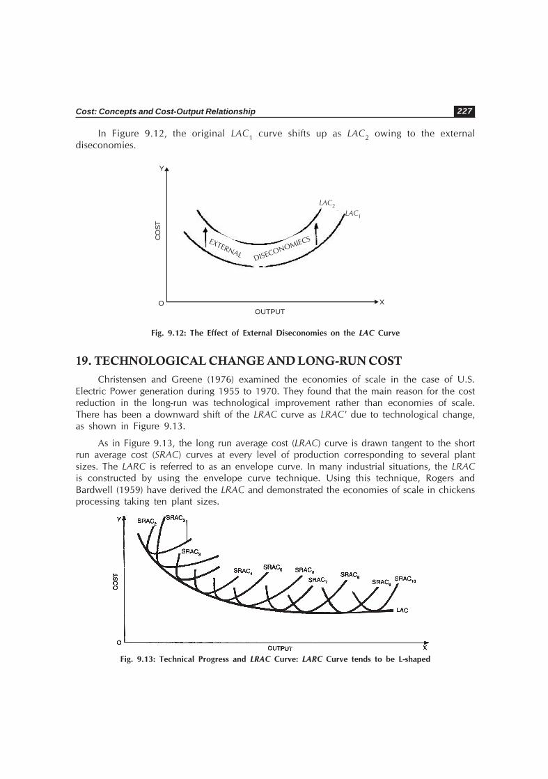
Cost: Concepts and Cost-Output Relationship 227
In Figure 9.12, the original LAC1 curve shifts up as LAC2 owing to the externaldiseconomies.
OUTPUTO
Y
X
CO
ST
Fig. 9.12: The Effect of External Diseconomies on the LAC Curve
19. TECHNOLOGICAL CHANGE AND LONG-RUN COST
Christensen and Greene (1976) examined the economies of scale in the case of U.S.Electric Power generation during 1955 to 1970. They found that the main reason for the costreduction in the long-run was technological improvement rather than economies of scale.There has been a downward shift of the LRAC curve as LRAC' due to technological change,as shown in Figure 9.13.
As in Figure 9.13, the long run average cost (LRAC) curve is drawn tangent to the shortrun average cost (SRAC) curves at every level of production corresponding to several plantsizes. The LARC is referred to as an envelope curve. In many industrial situations, the LRACis constructed by using the envelope curve technique. Using this technique, Rogers andBardwell (1959) have derived the LRAC and demonstrated the economies of scale in chickensprocessing taking ten plant sizes.
Fig. 9.13: Technical Progress and LRAC Curve: LARC Curve tends to be L-shaped
EXTERNALDISECONOMIECS
LAC1
LAC2

Managerial Economics228
and their SRAC to SRAC2 respectively into account. Their study depict a gradually downwardsloping LRAC (as in Figure 9.14) indicating the economic benefit of the large-scale output ofbroilers at the New Hampshire Agricultural Experiment Station (See Rogers G.B. and E.T.Bardwell: 1959).
The LRAC curve implies that average processing cost of chicken is reducing with therising scale of output per hour (on account of economies of scale).
When China’s demand for import of wheat from the US is expected to increase in the years to follow,
on the one hand, and the US farmers may shift their land use to alternative crops, on the other hand,
the supply of wheat in the US market may decline. Consequently, the flour prices may tend to rise which
may lead to an increase in costs of bakery products. This may result in rise in prices of bakery goods.
To determine its impact on future demand then the bakeries should estimate the price elasticity of demand
for their products. Usually, demand for common bakery items will be inelastic; hence, there is less chance
of severe impact on this industry. It is also observed that the innovative gesture helps the firm in capturing
a better market. Tasty Baking Company in the United States, for instance, automated the production
systems at its Hunting Park plant which cut its product operations time significantly from 12 hours to 45
minutes. By 1990, it renovated and upgraded production process further. In 1989, for instance, it
introduced 3.5 megawalt cogeneration system to minimise the use of petroleum-based products which
become more cost effective. In 1995, it acquired Ducth Mill Baking Company and expanded its product
lines as well as distribution. It also used a special film developed by Mobil to maintain the freshness of
the products for a longer time without using preservatives. This implied a higher cost. This was, however,
compensated by the rising sales. In 1997, the Tasty, Baking Company upgraded its use of computer
technology in operating performance.
In practice, LRAC is more common than the theoretical LRAC curve, as in Figure 9.14.
Fig. 9.14: Typical LARC Curve
20. LONG-RUN MARGINAL COST CURVE (LMC)
Like the short-run marginal cost curve, the long-run marginal cost curve is also derivedfrom the slope of total cost curve at the various points relating to the given output each time.

Cost: Concepts and Cost-Output Relationship 229
The shape of LMC curve has also a flatter U-shape, indicating that initially as output expandsin the long-run with the increasing scale of production tends to decline. At a certain stage,however LMC tends to increase. The behaviour of the curve is shown in Figure 9.15.
Fig. 9.15: Derivation of LAC Curve
In Figure 9.15, the LAC refers to the long-run average cost curve. And the LMC refersto the long-run marginal cost curve.
From Figure 9.15, the relationship between LAC and LMC may be traced as follows:
When LAC curve decreases, LMC curve also decreases and LMC < LAC.
At a certain stage, LMC tends to rise, though LAC continues to fall. Indeed, LMC isstill less than LAC.
When LAC is the minimum, LMC-LAC. Thus, the LMC curve intersects, at the lowestpoint of the LAC curve.
Thereafter both the LAC and LMC curves slope upwards. Now LMC > LAC. So, theLMC curve lies above the LAC curve.
21. ESTIMATION OF LONG-RUN COST FUNCTION
In long run, there is no fixed cost component, all are variable costs. Thus:
TC = bQ – cQ2 + dQ3
Example:
TC = 160Q – 20Q2 + 1.2Q3
AC = 160 – 20Q + 1.2Q2
MC= 160 – 40Q + 3.6Q2

Managerial Economics230
In the above illustrated cost function, put the given value of Q and estimate the costfunction for each output (Q) level.
Problem: Illustration
TC = 250Q – 10Q 2 + 2Q 3
Estimate TC, MC and AC if output is 100 units.
Solution:
(1) TC = (250 × 100) – (10 × 100 × 100) + (2 × 100 × 100 × 100)
= 25,000 – 1,00,000 + 20,00,000
= 19,25,000.
(2) MC = 250 – 20Q + 6Q2
= 250 – (20 × 100) + (6 × 100 × 100)
= 250 – 2,000 + 60,000
= 58,250
(3) AC = 250 – 10Q + 2Q2
= 250 – (10 × 100) + (2 × 100 × 100) = 19,250
Case Study Estimation
Gupta (1968) estimated the long-run cost functions (LAC) for selectmanufacturing industries in India, as follows:
Cement
LAC = 65.6 +Q
5622 + 0.005Q
Chemicals
LAC = 73.9 – 0.0002Q
Cotton Textiles
LAC = 89.7 + Q
273
Iron and Steel
LAC = 92.6 – 0.003Q
Paper
LAC = 73.6 + Q
963
Sugar
LAC = 85.0 +Q
124 + 0.001Q
22. COST ELASTICITY
Cost elasticity refers to the ratio percentage change in total cost in relation to a 1%change in output. Thus:

Cost: Concepts and Cost-Output Relationship 231
e cost = % DTC
% DQ
where, % DQ = 1%
Proportionate cost elasticity:
e cost = TCQ
ΔQTC Δ
×
where, TC = Total cost
Q = Quantity of output
e cost = 1
implies constant AC (zero economies of scale/constant return of scale)
e cost < 1
implies decreasing AC (economies of scale/increasing return of scale)
e cost > 1
implies increasing AC (diseconomies of scale/decreasing returns to scale)
23. MINIMUM EFFICIENT SCALE
The minimum efficient scale (MES) of production corresponds to the minimum long-runATC. To find MES, using calculus method, take the first derivative of the LRAC function andset the results equal to zero, and solve for Q.
Illustration:
A firm’s long-run total cost (LRTC) function is:
LRTC = 5,005Q – 6Q2 + 0.005 Q3
(i) Measure the average cost in the long-run
(ii) Find minimum efficient scale (MES) of production.
Solution:
(i) Long-run Average Cost:
QLRACLRAC =
∴∴∴∴∴ QQQLRAC
32 0.0055,000 +−=
6
= 5,000 – 6Q + 0.005Q3

Managerial Economics232
(ii) Minimum Efficient Scale:
00.016 =+−= QdQ
dLRAC
∴ ∴ ∴ ∴ ∴ Q = 600
The minimum efficient scale of production is 600 units.
24. COST LEADERSHIP
The concept of cost leadership is coined by Michael Porter as an element of businessstrategy towards competitive advantage. Fundamentally, cost leadership implies the lowestcost of operation in the business by the firm. It reflects the scale and soul efficiency of thefirm. By and large, cost leadership is a business strategy of doing the business at the lowestpossible cost in a market. It is the outcome of the learning curve effect caused by cumulativeexperience in handling the business by the cost leadership firm. In Aviation industry inMalaysia, for instance, Air-Asia has turned out as the successful low-cost yet profit-makingairline. Air-Asia supplies the air travel flights operations that are basic in serving the need ofthe people with no-frills product. Air-Asia operation is at a relatively much lower cost andthe flights are made available to large number of customer base. For this, the firm is alwaysinnovative in searching the ways of cost reductions and also making more money. Itspromotional strategy is quite appealing it the air travellers.
Cost leadership position in the industry is acquired by a competitive firm through:
Cost control measures
Avoiding wastages
Better supervision on the workers
Access to cheaper source of capital and required finance. Financial management atlow-cost.
Focus on quantitative targets for the business expansion while ensuring that the costis maintained at the minimum level.
Dell, for instance, in computer industry is identified as the cost lender. Similarly, Wal-Mart has earned its cost leadership reputation in retail trade. Wal-Mart could achieve thisowing to the various innovative methods adopted in the process of cost-reduction and remainingmuch ahead of its competitors.
Porter argues that there are two generic level strategies found in the modern business:
Product differentiation
Cost leadership
In a certain markets, such as commodity market, there is no much choice left except costleadership for the operating firm.
Cost: Concepts and Cost-Output Relationship 233
In fact, cost leadership strategy is adopted by the firm in order to generate competitiveadvantage by creating more economic value at the lowest costs in comparison to thecompetitors.
Cost leadership, however, is not a synonym of low price. Though, it is quite likely thatthe lowest priced can be charged by the cost leader firm and still can make a higher profit.
Sources of Cost LeadershipTo develop cost leadership business strategy, it’s essential for the managers to understand
the fundamentals of cost analysis.
The following are the major sources of cost advantage to be realised under the costleadership strategy in business:
Economies of ScaleCost economy arising due to fixed overhead costs, when level of output increases
Reaching to a level of minimum efficient scale much earlier than the competingfirms in the market
Learning Curve EffectThis is the outcome of cumulative experience gained by the expanding firms operatingin different market territories.
InternationalisationThe firm that expands business in overseas markets gaining more experience incomparison to firms confined to the domestic business only.
Technological Acquisition and ImprovementIn these days of K-economy, the firm can hope to bring down costs through acquisitionand improvements of the available technology. Extensive and effective use ofinformation technology is remarkable in this context.
Access to Low Cost InputsThe firm that can acquire the required business resources at a lower price incomparison to the rivals can easily come out with cost leadership business strategyin the market. Wal-Mart, for instance, manage its provisions for its stores at lowercosts through its efficient distribution centres besides its locational advantages.
Knowledge ManagementThe firm needs to acquire knowledge of cost minimisation and effectively use it todevelop its cost competitive edge in the market.

Managerial Economics234
Cost Conscious Organisational CultureThe industrial organisation of the firm has to be efficiency-driven and always be costconscious. The organisational culture has to be focused on cost-effectiveness inbusiness operations. Wal-Mart, for example, has succeeded well in this direction.
According to Hooley et. al. (2004)1, Cost leadership business strategy yields competitiveadvantage for the firm in the market by conferring the value of return on investment owningto the neutralising effect on the competitive threats of five forces indicated by Porter, suchas:
Threat of New Entry
Threat of Rivalry
Threat of Substitutes
Threat of Suppliers
Threat of Buyers.
Source: Hooley, Saunders and Piery (2004). Marketing Strategy and Competitive Positioning,Prentice-Hall.
MODEL QUESTIONS
1. Distinguish between:
(a) Prime costs and supplementary costs.
(b) Explicit costs and Implicit costs.
(c) Real cost and opportunity cost.
2. Explain briefly the following concepts:
(a) Opportunity Cost.
(b) Money Cost.
(c) Real Cost.
(d) Marginal Cost.
(e) Average Fixed Cost.
(f) Average Variable Cost.
3. (a) What is meant by opportunity cost?
(b) What is its economic significance?
4. Do you agree with the following statements? Give reasons.
(a) The distinction between prime and supplementary cost is invalid in the long run.
(b) In the short run, there is a distinction between fixed and variable costs.

Cost: Concepts and Cost-Output Relationship 235
(c) Opportunity cost is a useful concept in decision-making and efficient allocationof resources.
(d) Economists consider only explicit costs of production.
(e) Marginal cost is an incremental cost.
5. Write notes on:
(a) Opportunity Cost.
(b) Prime and Supplementary Costs.
6. Explain briefly the following statements:
(a) Marginal fixed cost tends to be zero in the short run.
(b) Marginal costs are variable costs.
(c) Marginal cost is independent of the fixed cost.
(d) The marginal cost curve intersects the average cost curve.
(e) When MC is zero, TC is maximum, while AC is minimum.
(f) Fixed costs are independent of the level of output.
(g) AVC initially falls, thereafter rises.
(h) The shape of the LAC curve is determined by economies of scale.
(i) The AFC curve is symptotic to the axes.
(j) MC is given by the slope of either the TC or the TUC curve.
7. What are the relations between returns to scale and the long run average cost ?
8. Why is short run average cost curve U-shaped ?
9. Explain the concepts of average fixed cost, average variable cost, average cost andmarginal cost and show their interrelationship.
10. Discuss the cost output relationship in the long run.
11. Mention the salient features of the long run average cost curve. What is its significancein managerial decision-making.
12. Why, in practice, the LAC curve is likely to be L-shaped?
Problems1. From the following data, measure the Total Cost, Average Cost and Marginal Cost.
Manufacturer of X product X incurred fixed costs of Rs. 300/-:
Variable cost: 500 640 720 740 800 900
Output unit: 1 2 3 4 5 6
[Hints: 1. Add Rs. 300 fixed to variable costs at all stages to final total cost.
Thus, Total Cost = 500 + 300 = 800, 640 + 300 = 940 etc.]
Total Cost

Managerial Economics236
2. Average Cost = etc.4.7,200
9408;
100
800:Thus
Produced Units of No.
Cost Total==
3. Marginal cost is addition to total cost 50, 140, 80, 20, 60, 100.
2. Estimate average and marginal cost from the following cost function:
TC = 150Q – 8Q2 + 3Q3
3. Explain the concepts of average fixed cost, average variable cost, average total costand marginal cost. Show their interrelationship through cost functions anddiagrammatic presentation.
4. Explain the laws of returns to scale.
5. Complete the following table:
Units of Output TFC TVC TC MC AC
1. 20 30
2. 45
3. 70
4. 95
5. 150
6. 220
6. You are given the following short run cost function:
TC: 100 + 60Q + 3Q2 + 0.1Q3
Measure Marginal Cost and Average Cost, if Q = 1000.
7. Based on your knowledge of the definition of the various measures of short run cost,complete the following table:
Q TC TFC TVC AC AFC AVC MC
0 1200 — — X X X X
1 — — — 265 — — —
2 — — 204 — — — —
3 — — — 161 — — —
4 — — — — — — 86
5 — — 525 — — — —
6 — — — 120 — — —
7 — — — — — 97
8 — — 768 — — — —
9 — — — — — 97 —
10 — — — — — — 127

Cost: Concepts and Cost-Output Relationship 237
8. On the basis of the following cost function:
TC = 100 + 60Q + 3Q2
(i) Compute the average cost, and marginal cost.
(ii) Indicate the point at which diminishing returns occur.
9. TC = 600Q – 20Q2 + 1.2Q3
On the basis of above cost function calculate the long run average cost and marginalcost. Plot them graphically.
10. Estimate average and marginal cost from the following cost function:
TC = 150Q – 8Q2 + 3Q3

Economies of Scaleand Scope
10CHAPTER
1. LARG-SCALE OF PRODUCTION
The scale of production means the size of the production unit of a firm or a businessestablishment. The scale of production can vary from very small to very large, depending onthe quantity of output per unit of time of the firm. Thus, the scale of production positivelyvaries with the size of the firm.
Large-scale production refers to the production of a commodity on a large-scale, witha large plant size firm. Large-scale production or output requires large-scale input, i.e., theuse of the efforts of the factors of production on a large-scale. On the other hand, productionof a commodity with a small plant size firm will have the production of a commodity on asmall scale.
Motives Behind Large-scale Production
A notable feature of production in the modern industrial economy is that productiontakes place on a large-scale. The growing large-scale of production in the modern economyis due to the expansion of large firms producing commodities. The principal motives leadingto the expansion of the size of a firm are:
Desire for Economy. Generally, a large-scale of output is more economical.
Desire for Large Profit. Business on a large-scale certainly yields more profits.
Desire for Economic Power and Prestige. A large firm can command and control alarge section of the business in general and has a high reputation in the market.
Desire for Increase of Demand. When the demand for a product increases and thesize of its market expands, the firm will have to increase its scale of production to

Economies of Scale and Scope 239
adjust its supply to demand. Alternatively, by increasing the scale of output and byresorting to greater specialisation and division of labour, the firm can increase itsproductivity as a whole and lower its cost of production so that it can supply moreat a lower price as a result of which the demand for its product increases.
Desire for Self-Defence in a Competitive Market. Owing to cut-throat competitionin business, the firm may be forced to enlarge its scale of production for its verysurvival.
2. THE SIZE OF FIRM AND INDUSTRY
Production in modern economy is carried on by a large number of firms of differenttypes and sizes. The firm may be defined as an independently administered enterprise — abusiness unit, whether a sole proprietor, partnership, or a joint stock company — producing
a particular commodity. All such firms taken together constitute the industry. Thus, an industryis composed of all the firms — individual business units producing similar commodities. Forexample, Sony is a firm, Samsung is also a firm producing electronic goods. Likewise, thereare several electronic goods manufacturers in India. All of them together constitute theelectronic industry.
A firm or a business establishment may be large or small. Usually, the size of anestablishment is measured by the value of its output or by the number of labourers it employs,or by the amount and value of its fixed capital such as buildings, plant and equipment. Thesize of a firm increases when it uses more and more of capital, labour and other factors ofproduction.
An industry may consist of both large and small firms at a time. Like firms, the size of
an industry also may be large or small. The size of an industry depends on the size of firmsit constitutes and their number. Thus, the size of an industry increases when:
There is an increase in the number of firms in it; or
There is an increase in the size of firms comprising it.
3. ECONOMIES OF SCALE
Large scale production is economical in the sense that the cost of production is low. Thelow cost is a result of what is called “economies of scale.”
The concept “economies of scale” may be viewed in two senses: broad and narrow.
Definition. In a broad sense, anything which serves to minimise average cost of productionin the long-run as the scale of output increases is referred to as “economies of scale.” It ismeasured in money terms.
In a narrow sense, however, the term ‘economies of scale’ relates to the characteristics ofthe production process by which average productivity is enhanced with the expanding scale ofoutput. Real economies are measured in physical terms. Increasing returns to scale are caused bythese real economies.

Managerial Economics240
The economies of scale may be classified as: (i) internal economies, and (ii) externaleconomies.
Internal Economies
Internal economies are those economies which are open to an individual firm when itssize expands. They emerge within the firm itself as its scale of production increases. Internaleconomies in the scale of its output cannot be realised unless the firm increases its output,i.e., expands its size. Thus, internal economies are the function of the size of a firm. Theseare solely enjoyable by the firm itself when its scale of production increases, independentlyof the actions of other firms.
External Economies
External economies are those economies which are shared by all the firms in an industryor in a group of industries when their size expands. They are available to all firms fromoutside, irrespective of their size and scale of production. They are the result of the growthand expansion of any particular industry or a group of industries as a whole. Thus, externaleconomies are the function of the size of the industry. They are not confined to one or twofirms, but shared by all the firms (irrespective of their size) in an industry when its sizeexpands. Thus, external economies can never be monopolised by any one firm in an industry.
In fact, external economies arise mainly due to the localisation of industries. Thus,external economies are enjoyed by a firm when some other firms grow larger; these arise asa result of the cost reducing effects of expansion and growth elsewhere.
Briefly, thus, economies of size of a firm are “internal economies” and those of the sizeof industry are “external economies.”
In pecuniary sense, both internal and external economies imply cost reduction. It is,however, difficult to draw a line of demarcation between internal and external economiesbecause of their overlapping nature. When the size of a firm increases, it enjoys internaleconomies, but its expanding size also causes the growth of industry which, in turn, leads tosome external economies. External economies, in turn, reduce the cost of productionsimultaneously with the cost economies caused by the increasing scale of output in the firm.In practice, internal and external economies arise in an overlapping or interwoven manner,so the distinction between the two cannot be easily measured from a given cost function ofa firm.
4. FORMS OF INTERNAL ECONOMIES
The principal types of internal economies of scale can broadly be grouped under sixheadings: labour, technical, managerial, marketing, financial and risk-spreading.
Labour Economies
Increased division of labour is a major source of labour economies. The extent ofdivision of labour is preconditioned by the scale of output. As output increases and the labour

Economies of Scale and Scope 241
force grows, a more and more complex division of labour with a greater degree of specialisation,with all its advantages, may become possible. Moreover, a large firm can attract more efficientlabour, as it can offer a wide vertical mobility, better prospects of promotion, as a result ofincreasing specialisation in the production processes. As such, the skill, efficiency andproductivity of labour as a whole in such large firms rise, reducing the cost per unit of output.
Technical EconomiesTechnical economies refer to reductions in the cost of the manufacturing process itself.
These relate to the methods and techniques of production, specially to the nature and formsof capital employed.
Following Prof. Cairncross, we may classify the various kinds of technical economies asfollows:
Economies of Superior Technique. As a firm expands, it can use superior techniquesand capital goods. A small firm cannot install a high quality machine or other capitalgoods which a big firm can. Small firms generally make increasing use of ordinarymachines operated by hand while large firms make a synchronised application ofbig automatic machines worked by steam or electricity. Such automatic machinesare quicker and more efficient, and their output is large as compared to the ordinarymachines. Thus, for instance, an automatic loom is more economical than ahandloom. But a village weaver cannot afford to have an automatic loom, whicha textile mill obviously can. Similarly, a rotary printing press, linotype machine, etc.,are more economical than hand composing. But a small job printer cannot affordto have such big machines which only a well-established newspaper organisationlike “The Times of India” can.
Economies of Increased Dimension. Certain technical economies may becomeavailable just on account of increased dimensions. This is purely a mechanicaladvantage of using large machines. Large pieces of equipment are relatively moreeconomical than smaller ones and usually there is an optimal minimum to the sizeof any piece of equipment. The reason for this lies in the laws of physical universewhich govern the rate of increase of the various properties of inanimate bodies withan increase in their size. For example, as we increase the size of a cube, its surfaceincreases by the square of its sides, whereas its inner capacity rises by the cube ofits sides. Thus, the carrying capacity of a ship increases in proportion to the cubeof its dimensions. As such, a big ship is more economical than a small one, becausea big ship can be run by a crew of sailors just as large as required for a small one.Similarly, a double decker bus is more economical than a single decker. For onlyone driver is needed, whether it is a double decker or a single decker bus. Similarly,a big lorry does not need more drivers than a small station wagon, and so on.Moreover, the size of a unit of machine can usually be doubled without doublinglabour and other material costs.
Economies of Linked Process. A large plant usually enjoys the advantage of thelinking of processes, i.e., by arranging production activities in a continuous sequencewithout any loss of time. Prof. Cairncross points out, “There is generally saving in

Managerial Economics242
time and saving in transport costs, since two departments of the same factory arecloser together than two separate factories.” For the same reason, processes of editingand printing of newspapers are generally carried out in the same premises.
Similarly, in the iron and steel industry, the main production stages like melting ironore into pig iron, converting pig iron into mild steel, rolling steel into sheet plate,etc., are linked together to avoid waste of power, heating process, etc., and, thus,to achieve economies.
Economies in Power. Large units of machines and their continuous running by alarge firm are often more economical in their power consumption as compared toa small machine.
Economies of By-products. Large firms can make a more economical use of theirraw materials. A large firm can avoid waste of its raw materials, which it caneconomically use for manufacturing certain by-products. Large chemical companiesare, for instance, constantly developing new varieties of by-products in this way.Similarly, cane pulp and molasses of big sugar factories can be effectively used bythe paper industry and liquor distilleries.
Economies of Continuation. Technical economy is also realised due to long runcontinuation of the process of production. For instance, in the printing press industry,there is an apparent economy to be realised by printing more copies of a composedsheet. Thus, if composing and printing cost of 1,000 copies per page is Rs. 12, for2,000 copies it would cost only Rs. 14, that is, just Rs. 2 more for the extra 1,000copies, because the same sheet plate which is composed once will remain in use forprinting extra copies. Hence, there is only additional printing cost involved, whilethe composing cost remains the same.
Managerial EconomiesAs a result of the indivisibility of managerial factors, the cost per unit of management
will fall as output increases, thus, with the increasing scale of output, greater managerialeconomies are enjoyed by an expanding firm. For a good manager can organise a largeoutput with the same efficiency as he can organise a small output. And his remunerationnormally remains the same whether the output is large or small. Morever, a large firm canhire a first-rate manager by paying a handsome salary, so its overall administration will bemore efficient as well as economical. An entrepreneur can delegate some of his functions totrained and specialised personnel in his various departments and can get better and moreefficient productive management with scientific business administration. But economies inmanagement can be realised only when production is on a large scale. A small producercannot afford to have all such personnel with knowledge of scientific business administration.
Marketing EconomiesMarketing economies are economies of buying (of raw materials) and selling (goods
produced). A large firm can generally buy more cheaply than a small one, because it canpurchase its raw materials on a large scale at a low cost (paying wholesale price). Further,

Economies of Scale and Scope 243
a big firm also employs purchasing experts to purchase the required raw materials moreeconomically and in time.
Similarly, on the sales side, a big firm can reap advantages of large scale marketing.Selling is generally less expensive per unit when large quantities are distributed, because aselling organisation should be of an optimum size whatever be the volume of sales handled.
Financial EconomiesIn financial matters, a large firm has relatively greater advantages than a smaller one.
Usually, it has a wider reputation and greater influence in the money market. Big firms areusually regarded less risky by investors, hence, they may be willing to lend capital to suchfirms even at a lower rate of interest than to small firms. Thus, the cost of obtaining creditand capital is lower to a large concern than to a smaller one. Further, big firms can easilyraise their capital by issuing shares and debentures. The shares of a big concern number inmillions and are held by thousands of people. But a small firm having no recognition in thecapital market cannot command such capital.
It can only raise a modest capital from the personal resources or loans from relatives ora bank or from moneylenders. And it cannot procure money from the general public byoffering shares for sale on the stock exchange. Briefly, thus, the important financial advantageenjoyed by a large firm is the existence of a ready market for its shares and its soundreputation in the capital market.
Risk-Minimising EconomiesA large firm by producing a wide range of products is in a position to eliminate or
minimise business risks by spreading them over. Risk-spreading advantages are sought by abig firm in the following ways:
By Diversification of Output. As a big firm can produce a number of items and indifferent varieties, the loss in one can be compensated by gain in others, e.g., GodrejSoaps Ltd. is producing soap, talcum powder, shaving cream, etc., various types ofcosmetic products and thereby spreading its business risks.
By Diversification of Market. When a product is produced on a large-scale, it canhave an extended market throughout the country so that the danger of fluctuationsin demand is reduced to the minimum. Thus, demand for nationwide popularproduct is more stable than a locally supplied article.
By Diversification of Sources of Supply as well as of Process of Manufacturing. Ina large firm, there are less chances of disruption of output as a result of scarcity ofraw materials or break down of a particular process.
5. FORMS OF EXTERNAL ECONOMIES
By external economies we mean gains accruing to all the firms in an industry from thegrowth of that industry. External economies are enjoyable by all the firms in the industry,irrespective of their size. External economies are, in essence, the advantages of localisation.

Managerial Economics244
An industry expands when the number of firms increases or their size expands in a particularregion; thus, localisation of industry takes place and all the advantages of localisation accrueto firms in that industry.
The chief types of external economies are: (1) Economies of localisation; (2) Economiesof information; (3) Economies of disintegration; and (4) Economies of by-products.
Economies of LocalisationWhen a number of firms are located in one place, all of them derive mutual advantages
through the training of skilled labour, provision of better transport facilities, stimulation ofimprovements, etc. These are in fact the benefits of localisation. Concentration of a particularindustry in one area, in course of time, results in the development of conditions helpful tothe industry. And all the firms in that area reap mutual benefits. Moreover, when there is anincreasing concentration of firms, arrangement can be made for repairs and maintenance andspecial services required by the industry. The cost of production is thereby reduced.
Economies of Information or Technical and Market IntelligenceA large and growing industry can bring out trade and technical publications to which
every firm can have access. Producers are, thus, saved from independent research which isvery costly. In a large industry, research work is done jointly. There can be a researchassociation of the industry as a whole. And each firm enjoys the benefits of research. Statistical,technical and other market information becomes more readily available to all firms in agrowing industry. As such when the industry progresses, the cost of production falls.
Economies of Vertical DisintegrationThe growth of industry will make it possible to split up production and some subsidiary
jobs can be left to be done more efficiently by specialised firms. New subsidiary industriesmay grow up to serve the needs of the main industry, e.g., in the textile industry, the colourmanufacturing process may be taken up by a specialised chemical firm and the mills may getbetter products at low cost. When a particular process is split up and performed on a largescale by a specialised firm, it can yield all the internal economies of large scale production.Hence, all firms in the industry will be able to get this process done at a lower cost insteadof attempting to meet their own needs by carrying it out themselves on a small scale at a highcost. But the subsidiary industry or specialised firm in a particular process may spring up onlywhen the industry is large enough to support it.
Economies of By-productsA large industry can make use of waste materials for manufacturing by-products. The
firm using it can flourish when waste material available in the industry is converted intoby-products. For example, in a sugar factory belt, sugarcane pulp can be used by the papermill in producing paper. Sugar factory will get some return for the sugarcane pulp by sellingit to the paper mill in the vicinity. This means an indirect economy in cost.

Economies of Scale and Scope 245
A Case Study of New Zealand
Electricity Distribution: Economies of Scale
Gills and Wyatt (1993) observed ‘L’ shape average cost curve using a translog cost model to estimate
economies of scale in electricity distribution in New Zealand. Their case study is based on 60 Electricity
Supply Authorities (ESAs) in the country. The ESAs are statutorily obliged to supply electricity and are price
takers in the bulk purchase of electricity from the Electricity Corporation of New Zealand (ECNZ). Their
study is based on cross-section data for the 1986-87 financial year. To estimate the economies of scale
they considered that cost, rather than production, is a better measure as the firms usually intends cost
minimization. They described the following cost model for the firms in the electricity industry:
TC = f (Y, P, I)
Where,
TC = total cost,
Y = output,
P = a vector of n input prices, and
I = a vector of an additional industry-specific variables.
The model assumes that output and input prices are exogenous. Further, for a given technology, firms
adjust input levels so as to minimise costs of production scale economies is defined in terms of the
relationship between cost and output along the expansion path. That means, with given input prices and
industry-specific variables, costs minimised at each level of output. It is defined as the ratio of average to
marginal costs, thus:
SCALE = (Dlog C/(Dlog Y)–1
If SCALE >1 implies economies of scale, SCALE <1 implies diseconomies.
For empirical consideration, input prices are defined as follows:
The prices of labour and other inputs are the associated expenditures divided by the number of
employees.
1. Price of capital inputs were measured — (a) total capital value/circuit kilometres of distribution line;
(b) the value of capital/the combined amount of circuit kilometres of distribution line plus KVA
transformer capacity; and (c) a constant capital price across ESAs, and
2. The price of electricity purchased — alternatively measured: (a) total electricity cost divided by total
electricity purchased and generated (cents/kWh); (b) constant values of 2.8084 cents/kWh for South
Island ESAs and 3.4318 cents/kWh for North Island ESAs in order to consider the average energy
components in the wholesale electricity tariff. Besides, they include five industry-specific variables
including load factor and density and three dummy variables for the type of ESA, ESA location and
regional (urban, rural) consideration.
Their results show that there are significant scale economies in New Zealand Electricity Distribution
and the average cost (AC) move implied by their estimated Translog Model is L-shape as shown in Figure
10.1.

Managerial Economics246
Fig. 10.1
6. DISECONOMIES AS LIMITS TO LARGE-SCALE PRODUCTION
Beyond a particular limit, however, certain disadvantages of large-scale productionemerge. When there is an expansion of the firm beyond an optimum limit, the very internaland external economies turn out to be diseconomies. These diseconomies, by raising theaverage cost of production, act as a limiting factor on the further expansion of the firm. Sinceeconomies of large-scale are not available beyond a certain point, a firm cannot expand itssize indefinitely.
Generally, the following factors of diseconomies of scale limit the size of a firm:
Difficulties of ManagementAs a firm expands, complexities and problems of management increase. Thus, after a
point, the manager finds it difficult to control the whole production organisation. Theentrepreneur and management will not be able to maintain contact with each other andcheck on all the departments of a very large concern. The problem of supervision becomescomplex and intractable, thus leading to increasing possibilities of mistakes andmismanagement. All these prove to be uneconomical, for the defects in organisation will leadto waste and result in rising average costs.
Difficulties of CoordinationThe tasks of organisation and coordination become progressively more and more difficult
with the increasing size of the firm. The management of the firm will gradually face numerousproblems of decision-making and organisation. It may, therefore, not find enough time to givecareful thought to individual problems. Decisions so taken in a hurry result in inefficiencyand increase in the cost of goods.
Difficulties in Decision-makingA large firm cannot take quick decisions and make quick changes as and when they are
needed, for it has to consult various departments for making any decisions and so urgentmatters requiring timely decisions are inevitably delayed. This may sometimes cause loss tothe firm.

Economies of Scale and Scope 247
Increased RisksAs the scale of production increases, investment also increases, so too the risks of
business. The larger the output, obviously the greater will be the loss. To bear greater risksis an important limitation to the expansion of the size of a firm from an error of judgementor misfortune in business. Therefore, unwillingness to bear greater risks is an importantlimitation to the expansion of the size of a firm.
Labour DiseconomiesExtreme division of labour with a growing scale of output results in lack of initiative and
drive in the executive personnel. Thus, a large firm becomes more impersonal and contactbetween management and workers becomes less. As such there are more chances of occurrenceof grievances, and industrial disputes which prove to be costly to the large firm.
Scarcity of Factor SuppliesDue to the increase in the concentration of firms in a particular locality, each firm will
find scarcity of available factors. Hence, competition among firms in purchasing labour, rawmaterials, etc., will result in increased factor prices. Thus, extreme concentration of externaleconomies becomes a sort of diseconomy in the form of high factor prices.
Financial DifficultiesA big concern needs huge capital which cannot always be easily obtainable. Hence, the
difficulty in obtaining sufficient capital frequently prevents the further expansion of suchfirms.
Marketing DiseconomiesWhen the industry expands and the firm grows, competition in the market tends to
become stiff. Thus, firms under monopolistic competition (which is the most realistic marketsituation in many lines of production) will have to undertake extensive advertising and salespromotion efforts and expenditure which ultimately lead to higher costs.
7. SCALE ECONOMIES INDEX
Scale Economies Index (SEI) is a measurement to trace the relationship between cost andeconomics of scale.
SEI = (1 – COE) 100
Where,
SEI = Scale Economics Index
EC = Cost-Output Elasticity
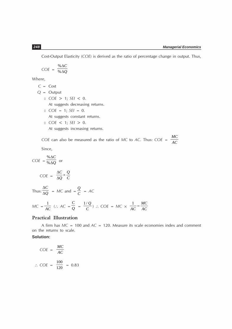
Managerial Economics248
Cost-Output Elasticity (COE) is derived as the ratio of percentage change in output. Thus,
COE = %%∆∆
CQ
Where,
C = Cost
Q = Output
l COE > 1; SEI < 0.
At suggests decreasing returns.
l COE = 1; SEI = 0.
At suggests constant returns.
l COE < 1; SEI > 0.
At suggests increasing returns.
COE can also be measured as the ratio of MC to AC. Thus: COE = MCAC
Since,
COE =%%∆∆
CQ or
COE =∆∆
CQ
QC
×
Thus: QC
∆∆
= MC and = CQ
= AC
MC =1
AC (∴ AC =CQ =
1 / QC ) ∴ COE = MC × AC
MCAC
=1
Practical IllustrationA firm has MC = 100 and AC = 120. Measure its scale economies index and comment
on the returns to scale.
Solution:
COE =MCAC
∴ COE =100120 = 0.83

Economies of Scale and Scope 249
Scale economies index:
SEI = 1 – COE
∴ SEI = 1 – 0.83 = 0.17
Since SEI is positive, the firm is operating under the increasing returns to scale.
8. X-EFFICIENCY
Cost economy is the major goal of a business firm. Efficiency in production implies costeconomy. An efficient firm will tend to experience a lower cost function. When efficiencyimproves, cost function of the firm tends to shift downwards. In practice, a major way of costreduction is seen through minimisation of the wastage of resources. More wastage implieshigher costs. Low wastage means low costs. X-efficiency refers to the phenomenon of thefirm’s ability to monitor and control the production unit to minimize the wastage of resources.X-efficiency is a function of management to reduce or minimize the waste of resources inoperations. New managerial approaches such as ‘Six Sigma Methodology’ [as adopted byMotorola, General Electrics (GE) and many other organisations] are essentially meant towardsattainment of X-efficiency (i.e. waste minimisation as well as zero defect level) of the businessfirm.
9. MANAGERS PER OPERATIVE RATIO (MOR)
Empirical evidences usually show that unit costs tend to decrease with the increasingscale of output, thus, supporting the hypothesis of economies of scale. The empirical evidenceof diseconomies of scale may not be easy to detect on account of changing state of technology.Existence of managerial diseconomies, however, can be inferred by comparing the ‘managersper operative ratios’ (MORs) in different organisations with different sizes. It is observed thatthe larger the firm the great number of managerial staff relative to the number of employeesis an indication of possible managerial diseconomies. Table 10.1 presents such MORs.
Table 10.1: The Managers per Operative by Firm Size
Firm Size Managers per(No. of Employees) Operative (MOR) Ratio
1-100 0.39
100-200 0.42
200-500 0.44
500-700 0.47
700-1500 0.51
1500-2500 0.60
2500-3000 0.67
Business Monitor (1988), suggests that with bigger firms the number of managerial/officestaff (administrative, technical and clerical) is higher in a relative sense than with the smallersize firms. A bigger firm is top heavy (Dunnett; 1992, p. 51).

Managerial Economics250
10. ECONOMIES OF SCOPE
In business parlance, the concept of economies of scope is often used somewhat differentlythan the concept of economies of scale. It refers to the reduction in unit cost realised whenthe firm produces two or more products jointly rather than separately. That is to say, a multi-product firm often experiences economies of scope leading to the lowering of costs.
Economies of scope exist when a firm produces two products together under the sameproduction facilities as against producing them under separate facilities. It is reflected in thelesser cost or cost economy. Thus:
TC(Qx, Qy) < TC(Qx, 0) + TC (0, Qy)
where, TC = total cost, Qx= output quantity of product X and Qy= output quantity of product Y.
For example, it may prove to be less expensive or more economical, for Phillips toproduce TV set and DVD Players by more intensively utilising a single assembly plant thanto produce these goods at two separate, less intensively used, plants. The economy of scopeis thus realised by avoiding duplication of the factor inputs in certain ways under a jointoperation as compared to separate operations.
In short, economies of score is attributed to the multi-product cost function. themultiproduct cost function of a firm refer to the cost of producing a given quantity of twoof more products simultaneously (Say Q1 units of output of product X and Q2 units ofproduct Y) under the same process of plants operations, assuming all factor-inputs are usedoptimally (Efficiently). Today, one may come across several multi-product firms domesticallyas well as internationally. HalvaH Packard (HP), for examples, produces computer as well asprinters of various types. So is the case with International Business Machines (IBM) Inc.Likewise, Honda produces both cars and motorbikes, and so on.
Empirical Illustration: Economies of Scope
A firm’s total cost function is:
TC = 200 – Qx Qy + Qx2 + Qy
2
where Qx and Qy represent the number of units of product x and y, respectively.
Question: Do economies of scope exist, when the firm produces 2 units of x and 4 unitsof y?
Solution:
TC (Qx, Qy) < TC (Qx, 0) + TC (0, Qy)
TC (Qx, Qy) = 200 – (2) (4) + (2)2 + (4)2
= 200 – 8 + 4 + 16 = 212
TC(Qx, 0) = 200 – Qx(0) + Qx2 + (0)2
= 200 + Qx2 = 200 + (2)2 = 204
TC (0, Qy) = 200 – (0)Qy + (0)2 + (Qy)2
= 200 + Qy2 = 200 + (4)2 = 216

Economies of Scale and Scope 251
Since:
(212) < (204 + 216)
It follows that economies of scope exist in this case.
Degree of Economies of ScopeThe degree of economies of scope can be measured in terms of the difference in the
costs of production jointly and separately. The following formula is used to measure thedegree of economies of scope.
)BnAn(TC
)BnAn(TC)Bn(TC)An(TCDES
+
+−+=
Where,
DES = degree of economies of scope.
TC(An) = total cost of producing An units of product A separately
TC(Bn) = total cost of producing Bn units of product B separately
TC(An+Bn) = total cost of producing products A and B jointly, i.e., producing Anunits of product A and Bn units of product B together.
Illustration
To illustrate the application of the above formula, let us assume that when a firmproduces two goods A and B jointly: 10 units of A and 20 units of B per day its total costis Rs. 1,500. On the other hand, when A and B products are separately produced by twoindividual firms, total cost of producing 10 units of A by firm No. 1 is Rs. 8,000, and thatby firm No. 2 is Rs. 12,000 for producing 20 units of B.
In this case:
TC (A10) = Rs. 8,000
TC (B20) = Rs. 12,000
TC (A10 + B20) = Rs. 15,000
33.0000,15
000,15–000,12000,8DES =
+=
A positive value of DES indicates existence of economies of scope. A negative value ofDES implies diseconomies of scope. Diseconomies of scope or negative DES suggests that itis better or more economical to produce two goods separately than jointly.
The economies of scope, has a close relationship with the economies of scale. A multi-product firm
usually tends to have a scale of operation than a single product firm. So, the former reaps the benefits
of the economies of scale. This may be attributed to the fact that a multi-product firm uses common
infrastructure such as business office, factory plant, vehicles, managerial staff, etc. Furthermore, a

Managerial Economics252
multi-product firm can reap the economy of by-product under the economies of scope. For instance,
a sugar factory can use its molasses — (by-product) for producing liquor by starting its own distillery
units.
In practice, Motorola may be cited as a multi-product firm — producing two-way radios, cellular
phones, pagers, semi-conductors and other electronic gadgets — experiencing economies of scope
and economies of scale to the limit.
Cost ComplementarityIn multi-cost function, cost complementary exists. Its refers to the decrease in the marginal
cost of producing one type of product, in the joint production operations with the increasein the other complementary products. Suppose, in the case of cost function:
TC (Qx,Qy) for producing X and Y by the multi-produced firm we take, MC ( Qx,Qy)as the marginal cost of producing X.
Then,
Cost complementary is traced, when: dMCx ( Qx, Qy) < 0 d Qy
It follows that when dQy is increased by 1 unit, the marginal costs of producing X (byone unit, more) decreases.
Illustration:
To illustrate then point, let us assume a multi-product firm’s costs function to be:
TC = 200 – 0.4 x QX QY + (Qx)2 + (Qy)2
Suppose, the firm produces 1 units of product X and 3 units of product Y.
The presence of cost complementarity is indicated as:
‘Beta’ coefficiency “b” –0.4 represent the marginal cost. Thus –0.4 being negative, inthis case suggests cost complementarity.
11. THE LEARNING CURVE
The cost structure of a long established or a global firm tends to be influenced by thebusiness experience as well as learning effects. The managers/operators of the firm andemployees may be able to carry on their functions more efficiently due to the increasedexperience and learning. The time involved in completing the tasks will tend to reduce as theworkers have become accustomed to the jobs and easily carry on the routine work withoutcausing wastages. Usually, experienced people perform well. Fig. 10.2 indicates the firm’sunit cost reduction of total cumulative output resulting on account of learning/experienceeffect.
The learning curve initially has a steeper slope, but then it becomes flatter indicating thatit would be increasingly harder to realise cost advantage once most of the learning opportunitiesare already exploited.

Economies of Scale and Scope 253
Fig. 10.2: The Learning Curve
Experience is the best teacher in business. Over a time when a firm accumulates itsbusiness experience it may tend to improve its production/organisation methods with improvedknowledge and experience of management and labour used in the production process. Thefirm’s learning experience would pay in terms of cost reduction. In long-run, these tends tothe downward shifts in the average cost curves of the firm on account of learning on experiencehere it should be effect that improves productive efficiency of the firm in its operations overtime. This is depicted in Figure 10.3.
The long-run average cost curve shifts downward in each time period t0, t1, and t2,correspondingly as LACt0, LACt1 and LACt2.
The downward shift of LAC is parallel for the learning by experience enhances the firm’sefficiency at all levels of production.
Fig. 10.3: Learning Effect on LAC
Learning Curve
Y
X Total Cumulative Output (Q)
0
Unit Cost (AC)

Managerial Economics254
Learning EffectAt managerial level, the learning effect manifests in several ways of experience factor,
such as:
l Perfection and precision reached due to constant practice of managerial decision-making.
l Finding more efficient production and business procedure.
l Knowing better ways to use tools and equipments.
l On account of familiarisation with the production activity it becomes easy and quickto give required instructions to workers in handling the jobs, thus, reducing wastefrom defects and disruptions.
l Right placement of right people.
l Better co-ordination and control.
l Improved operation sequences facilitating more skilful movements of workers incompleting the assigned jobs with proven integration.
l Better quality control methods leading to lesser rejection and re-doing of the jobprocess.
l Better project management and time scheduling taught by experience enables tohave more time-savings and less chances of disruption in the integrated stages ofproduction process.
Learning effect is different from the scale economy effect. Learning curve effect is seenassuming periodic scale of output, technology projection, and input prices being constant.The learning effect is measured as the difference between actual average costs and estimatedaverage costs. It implies saving in costs. In a technical way, economies of scale are measuredthrough the given LAC as a change in level of output per time period. The learning effect ismeasured by the shift in the LAC with respect to cumulative output change.
Empirically, the learning or experience effect rate can be measured by using the formula:
LER = 1 1
0−
ACtACt × 100
Where,
LER = Learning effect rate
ACt0 = Average cost in initial period (t0) increment
ACt1 = Average cost in next period (t1) increment.
Incidentally, the ratio ACt1/ACt0 is referred to as “experience factor.”

Economies of Scale and Scope 255
Illustration
Suppose a firm develops a new PC model in 1995 with an average costs of Rs. 30,000per unit. In 1996, however, its average costs declined to Rs. 24,000 when other things beinggiven and output is doubled. This may be simply attributed to learning effect. The learningeffect rate (LER) in this case is worked out, thus:
LER =24,000130,000
−
× 100
= 20%
If we project to double the output again in 1998, the existence of learning effect wouldimply the reduction in average costs further by 20%. That is, to Rs. 19,200 (i.e., by Rs. 4,800less which is 20% of Rs. 24,000).
The learning curve effect is usually measured in terms of the percentage decrease inadditional cost with respect to a 100 per cent increase in output each time (i.e., cumulativeoutput is doubled each time). A numerical example of learning curve is presented by the datain Table 10.2, assuming a “20 per cent” learning effect rate, so that as per the experiencefactor the labour cost of production each time tends to be 80 per cent of the previous levelwith doubling of cumulative output each time in this case.
Table 10.2: Learning Curve Data
Unit of Output Unit of Cumulative Cumulative Cumulative Unit Labour Average
Cost Labour Hours Labour Hours Average Labour Cost Labour
(Q) (C) (CC) Hour (CC’) (AC) (AC’)
col. 3 ÷ col 1 col. 2 × Rs. 10 col. 4 × Rs. 10
1 2 3 4 5 6
1 100 100 100 1000 1000
2 80 180 90 800 900
4 64 244 61 640 610
8 51 295 37 510 370
16 41 336 21 410 210
Note: Figures have been rounded off @ wage rate is given as Rs. 10 per hour.
In the above schedule, reduction is measured in real terms (i.e., labour hours) andassuming wage rate at Rs. 10 per labour hour the money cost is worked out.
The learning curve (LC) reflects the percentage decline in average cost (unit labour cost)as total cumulative output increases by 100 per cent (or doubled) each time.
Learning curve effect is observed in several industries — ranging from aircraftmanufacturing, ship building, oil refineries, power plants to semi-conductor memorychipproduction and its rate varies between 20% to 30%.

Managerial Economics256
The knowledge of learning effect rate is useful to a manager in production cost forecastingand pricing strategies. For instance, Texas Instruments in the US adopted an aggressive pricestrategy in view of the learning curve effect. It is important in determining the firm’s competitiveadvantage in the market and assuming its dominant position.
Learning effect is to be realised by the firm through integrated information system andzeal for improvement with gaining of experience. Team work, incentives and total qualitymanagement are crucial in this regard. Learning effect benefit is enjoyable by the firm or atthe most industry specific, but cannot be considered to be economy wide, because thephenomenon is important in new industries producing undifferentiated products but manysectors of the economy rarely fit into this pattern.
11.9.2 Learning Curve Hypothesis
Nonetheless, the learning curve has its strategic importance in those industries whereexperience factor has its marked influence — for the learning process implies an improvementin production efficiency and quality of output at no additional cost. This may enhance thefirm’s competitive advantage and enable it to acquire and maintain leadership or dominatingposition in the concerned market by increasing its market share, time and again.
Needless to say that skilful management is required to capture the learning curve as apart of corporate strategy of a modern business firm in the development of new products,such as semi-conductor, generic drugs, etc. Using experience factor skilfully in improvingproductivity and establishing cost price reduction strategy is oft-noted attribute of the Japanesestyle of management. (K.K. Seo: 1991, p. 378). Similarly, Texas Instruments, today’s bigbusiness firm in chip production in earlier stages of its growth, had well documented thelearning curve in adopting an aggressive price strategy — by keeping unit prices very low witha view to expand its cumulative output very fast and capture the advantage of experiencefactor successfully in order to acquire a greater market share and dominance in computerindustry. (See, Salvatore: 1996, p. 291).
Mathematically, the following formula serves the purpose of determining the pattern of cost reduction
of the learning curve.
AC = aQb
Where,
AC = average factor/input cost for producing xth unit of a product
a = average cost for producing the first unit of output
b = shore parameter coefficient which is negative.
The above quadratic equation can be expressed by translating it as a linear function in terms of double
log form, Thus:
Log AC = log a + b log Q
The parameters a and b can be estimated by using regression method on time series data pertaining
to average cost and cumulative output.

Economies of Scale and Scope 257
Illustration:
Suppose in a case study, the following estimates are obtained for a and b parameters of the above
given cost function:
Log AC = 5 – 0.5 log Q
If we take, Q = 20
Log AC = 5 – 0.5 log 20
(Log AC = 5 – 0.5 (1.3010)
= 5 – 0.6506
= 4.3495
Antilog of 4.3495 is
Therefore, the average input cost of 20th unit of output is Rs. 22,370.
In an analogous way, we can determine AC for different output Units (Q), with the given cost function.
The learning curve hypothesis is also proved by Liberaman (1984)’s study of 37 ChemicalProcessing Units. Cost reductions (5.5 per cent per annum) observed by the industry wereattributed to the learning effect of the growth of cumulative industry output and investmentin improved capital equipment. The study revealed that the average cost declined by 27 percent each time corresponding to doubling of cumulative output. This learning effect hadexceeded the 11 per cent reduction caused by the economies of scale.
A successful modern business firm has a tendency to expand in size. An enterprise may grow for
a variety of reasons.
The main motives for its growth are:
l Gaining the economies of large-scale of output.
l Acquiring larger market share, thus, dominance or leadership in the market with a degree of
monopoly power.
l Diversification of products with a view to minimize risks. For example, Imperial Tobacco Company
is producing more than 60 types of products ranging from cigarettes to cardboard cartons. (Fuller
1997: pp. 64). It is also referred to as lateral integration.
Internal Expansion. There are several approaches to expand the size of the firm internally, such as:
l Increasing the output with a larger scale of current production field.
l Exploiting new market territories.
l Producing different varieties and types of the goods — i.e., diversification of products.
External Expansion. The business firm can also expand its size externally through merger or acquisition.
Under the merger, two firms join together as a single business unit. The mergered firms lose their one.
Sometimes a smaller or weaker commercial bank is merged with a bigger or stronger bank to avoid
liquidation and acquire sustainability.
Acquisition implies take-over. A firm may take over the plants of another firm. For example, a holding
company may be formed to acquire a controlling interest in other firms. The taken over firm, tends
to retain its separate identity. Its main policy decisions are, however, governed by the holding
company.

Managerial Economics258
Under the merger or acquisition, a firm grows either by horizontal or vertical integration. Horizontal
integration implies the merging of two firms engaged in the same stage of production. Merger of two
commercial banks or two cotton textile mills under a single control implies horizontal integration.
Vertical integration implies mergers of two firms operating at different stages of production. There is
backward vertical integration when a firm joins another firm which is at an earlier stage of process
of production. For example, a textile mill acquires a weaving firm. There is a forward vertical
integration when a firm acquires another firm at a later stage of production process. For example, an
automobile manufacturing company acquiring a chain of dealership networks run by another firm.
There is a conglomerate merger when two firms join together but their products are not directly
related. For example, merger of the Imperial Tobacco Company and United Biscuits Company in
1986 is a case of conglomerate merger.
Vertical integration is undertaken with a view to ensure security and enhance efficiency. Efficiency
may result in cost reductions on account of administrative or managerial economies, technical or
engineering economies, financial and marketing economies achievable in an integrated business firm.
Similarly, Irwin and Klenow (1994), have observed the significance of learning curve inthe semi-conductor industry. The industry was measured to have learning rates around 20 percent on an average. That means, a 10 per cent increase in cumulative production in the semi-conductor industry could lead to a 2 per cent reduction in cost.
12. A CASE STUDY: COSTS MATTER
These days airlines are becoming more competitive. Due to distinct business strategiesadopted by the airlines, in many countries, two competitive market segments have preciselyemerged:
(i) the traditional full-service airlines and
(ii) the ‘no-frills service’ [Budget] airlines.
Main Features of Full-Service Airlinesl They offer varieties of services to different classes of the passengers such as First Class
Business/Executive Class, one economy class.
l These are relatively high-cost airlines
l They resort to price discrimination policy: Higher fares are charged to business classand low fares to the economy class.
l They operate domestically as well as internationally.
l They operate on different kinds of aircraft.
l They have a wide network.
l They are more resourceful.
l They have a long establishment with huge investment.
l They have large staff.

Economies of Scale and Scope 259
l They compete on providing better and improved services to the passengers. Forexample, Singapore Airlines has earned worldwide reputation for its better servicesand customer case.
l Though these airlines may enjoy a degree of economies of scale, after a point, theydo experience a rising operating costs due to rising factor costs an other relatedcauses.
l Some Airlines provide extra facilities, such as ‘business lounges’ which imply additionalcosts.
l To encourage customer loyalty they resort to free milage scheme to frequent flyers.Provision of free tickets, thus, implies extra costs and no revenue.
Main Features of ‘No-frills’ Budget Airlinesl Budget Airlines are specifically ‘Low-cost Airlines’ meant to provide airline services
at the lowest possible cost.
l These airlines are ‘no-frills’ airlines which tend to compete with traditional fullservice airlines by seeking core competency through cost minimisation at the bottomlevel.
l These ‘low-cost airlines’ usually operate only on one kind of aircraft, e.g., Airbus orBoeing 737.
l They have single class only.
l They offer common standardised treatment to all the passengers.
l They do not serve any drinks or meals. It is a cost saving device on food items aswell as crew for the services.
l They may sell some food items at a high price and make some money.
l Usually they do not provide seat allocation. Passengers can choose any vacant seat.
l By not providing normal forms of tickets they economise further.
l Unlike 20 kg. norm for the luggage, these airlines mostly permit 15 kg. Any excessluggage weight is charged heavily to make additional revenue.
l These airlines operate on point-to-point routes. Services transfer of luggage is notprovided. It saves their operational costs further.
l They often use low traffic, secondary airport and save costs.
l They book a large part of tickets on Internet thus, economise on ticketing staff andtravel agents’ commission.
l To augment their business revenue, some low-cost airlines also offer ancillary productssuch as holiday tour packages, hotel bookings etc.
l They do not offer any extra facilities such as lounges; hence, no such additionalcosts.

Managerial Economics260
l Relatively, they operate with much less staff than the traditional airlines.
l They seek to minimise costs and maximise revenue through faster turnaround of theaircrafts.
Fig. 10.4: Comparative Cost Functions
Figure 10.4 theoretically portrays the relative cost functions differential of these twocategories of the airlines.
In Fig. 10.4, one can see that Budget Airline has a lower cost function (B) than theTraditional Airline Cost function (A).
In the United States, the Southwest Airlines was the pioneer of the concept of low-costairline services. Recently in Malaysia, Air Asia has come up as a budget airline on the sameground.
Discussion and Concluding RemarksThe main lesson of the above discussion is that cost is one of the important factors from
which budget airlines such as Southwest, Air Asia, etc. derive their competitive advantage andbusiness core competency in the highly competitive Airline industry today. The budget airlinescan keep its low fares by maintaining costs at the minimum level and faster turnaround ofthe aircrafts. It is observed that in the United States, the low-cost airlines tend to havecaptured atleast one-third of the market share in airline industry.
Some of the pioneers low-cost airlines have acquired dominant position in this segmentof the market. e.g., Southwest in the United States. However, with the entry of several low-cost competitors gradually the dominating position of the lending airline is being threatened.For instance, in the United States, Jet Blue, Air Tran and Song have appeared as a toughcompetitors to the Southwest.
Another phenomenon is that in recent years, the ‘cost-function gap’ between the freeservice airlines and budget-airline is becoming borrower. On the one hand, there is a risingcost pressures owing to rising fuel prices, competition compelling to deviate from no frillsapproach, providing television sets, etc. In short, low-cost airlines may gradually be movingon rising costs. On the other hand, full-service: high-cost airlines are seeking cost economy.They slowly cut down their services range, thus, save on expenses.
C
A
B
AC
AC
O Q
Traditional Air Line
Budget Air Line

Economies of Scale and Scope 261
Ultimate result of such a trend on cost functions can be captured as in Fig. 10.5.
Fig. 10.5: Changing Trends of Cost Functions
In Fig. 10.5, a persistent competitive trend on cost function is seen. For Budget Airlines,the cost function is seen. For Budget Airlines, the cost function is shifting upward from B toB’. In case of traditional airline, the cost function is shifting from A to A’.
The ‘costgap’ between A’ and B’ is much narrower than between A and B. How cana budget-line retain its success in this situation? Answer is not so simple in practice. But, wemay suggest: Stick to providing best services at the lowest fares.
QUESTIONS FOR DISCUSSION
1. Indicate the main features of a traditional airline service.
2. Indicate the main features of a budget airline service.
3. Show diagrammatically the cost differentials between the full-service airline and low-cost airline.
4. Can you suggest that an airline can have a ‘mix’ of traditional and low-cost approach:
Mini Case Study: High Costs Problem of Delta Airlines
I Introduction
Delta Airlines is one of the biggest airlines in the United States of America.
The airline industry in the USA has witnessed a severe decline in the post September 11, 2001period. The Delta also experienced a downward trend in its business revenue against rising costsand consequently negative business income yield. Refer to data in Table 10.3.
Table 10.3: Delta Business — Financial Data
(US$) Million
Year end Revenue Costs Income Yield
December (TR) (TC) Before Tax
2001 13879 15743 – 1864
2002 13035 15307 – 2002
2003 13303 14492 – 1189
Source: www.hoovers.com

Managerial Economics262
In mid-2004, Delta had the biggest quarter loss of US$ 2 billion. Delta’s CEO, Grinstein, chalked out
a Restructuring Plan in order to set the things right for its business and restoring profitability by 2006.
Analysis of Delta’s Major Problem
Analysts observed that Delta’s main problem was rising costs against falling yields. Like other major
airlines in the US, Delta too had very high operational costs. The company’s bloated cost structure and
high cost of labour are the root of the problem.
• Deltas’s labour cost — as a percentage of operational cost in 2004 was estimated to be 43.4%.
Against this Jet-Blue had 30.9% and America West 27.3%. [See, Boyd Group/ASRC Inc.
www.sfgate.com and Exhibit V in Regani S. and Dutta S. (2005): ‘Problems at Delta Airlines,’ Case
Folio: February - www.icfaipress.org for more details]
• Delta’s contribution to pension funds was one of the main reason for high labour cost, as in 2004
many of its pilots opted for early retirement. Delta’s 50% of revenue was siphoned-off in salary
payments. Besides, perquisites and benefits to the employees claimed on its revenue.
• Rising prices of fuel was another critical cost factor. In 2003, fuel prices were US $26 a barrel, it
jumped to US $31 in 2003, and further to US $47 in 2004.
• Delta being an oldest airline it also carried the burden of high legacy costs’ such as pensions, free
flight passes, etc. New Airlines have a competitive edge against this as they do not carry such
liabilities.
• The low-cost airlines such as South-West, Jet-Blue, etc., posed another threat of competition.
• Delta’s work culture is more rigid. It stresses more on confirmity. It gives no flexibility to the
employees. It resulted into lower productivity. New competitive airlines are found to be more
flexible and informal.
• Delta did not establish strong relations with its partners: travel agents. Travel agents charged high
booking charges.
The Delta Solution: Cornerstones of Restructuring Plan
The ‘Delta Solution’ aimed at improving its business performance with the following key initiatives:
• Updating and upgrading customer products and services, including cabins and online functionality.
• Adding more flights.
• Reducing congestion.
• Elimination of 6000-7000 jobs in next 18 months.
• Lowering management overhead costs by 15%.
• Reducing pay and park benefits.
• Employee reward program.
• Profit sharing.
• Performance-based incentive payouts.
• Profit-sharing and performance-related pay scheme implied lowering of labour cost burden.
• Restructuring of over 50% of the airline’s operations.
Economies of Scale and Scope 263
• Improvements in services, fleet and networks to eliminate operational inefficiencies and enhance
productivity.
• Calling to work harder for less.
• Elimination of unnecessary costs.
• Creation of fun culture. Delta launched ‘Song’ — a new low-cost subsidiary as budget-airline.
QUESTIONS FOR DISCUSSION
1. Trace the major problems of Delta Airline in 2004.
2. Indicate cornerstones of Delta Solution.
3. Do you think ‘Song’ can succeed?
4. What lessons can you draw for Air-India from the Delta’s experience?
To Decision-makingo Scale economies are ubiquitous. Scale economy effects can exist in all kinds of business
activities: production, marketing, distribution as well as R&D.
o Cost economy is a boon to the firms operating and expanding on a large-scale of production.
o Scale Economies Index (SEI) = 100 [1 = EC]
EC = %%∆
∆
C
Q
EC = MC
AC
o Increasing returns caused by the economies of scale tend to imply decreasing cost condition.
o Increasing cost is the result of diseconomies of scale.
o Technological change is essential to avoid the situation of increasing costs.
o Learning through experience is a common tradition in business.
MODEL QUESTIONS
1. What is meant by economies of scale? Give examples.
2. What are the types of internal economies?
3. What are the major types of external economies?
4. Write brief notes on:
(a) Diseconomies.
(b) Internal Economies.
(c) External Economies.

Managerial Economics264
5. Distinguish between:
(a) Internal economies and external economies.
(b) Labour economies and managerial economies.
(c) Economies of disintegration and economies of by-products.
(d) Marketing economies and financial economies.
6. Are the following statements true or false? Give reasons.
(a) Economies of scale persist limitlessly.
(b) Managerial economies arise when the scale of output expands.
(c) Technical economies emerge when the size of firm expands.
(d) A large firm can reap the advantages of financial and marketing economies.
(e) A reasonable concentration is beneficial to the existing firms.
(f) It is difficult to draw a line of demarcation between internal and external economiesof scale in a firm’s cost function.
(g) Internal and external economies are overlapping.
7. (a) What is meant by internal and external economies of scale?
(b) Discuss various types of internal economies available to a firm.
8. Discuss the economies of scale into an expanding software firm in Bangalore.
Problems1. Total cost of producing 10 X is Rs. 75,000 and that of 20 Y is Rs. 95,000 separately.
If both are produced jointly then the cost is Rs. 1,60,000. Workout the degree ofeconomies of scope in this case.
2. In a case study, the cost function is estimated as follows:
Log AC = 150 – 0.6 log Q
Measure the average input cost of 50th unit of output.
3. If MC = 900, AC = 1,100, measure the scale economy index and give yourmanagerial comment.
Project Work
Write a brief cse study of Indian Airlines/Air India, especially focussing on the cost structure. Collect
relevant information from the airlines annual reports or website or from the head office. Would you
recommend Air India to adopt a low-cost budget airline model.

Production Functions11
CHAPTER
1. INTRODUCTION
Production implies provision of goods and services, often described as ‘commodities.’In technical sense, production is the transformation of resources into commodities overtimeand/or space. To put it simply, production is the act of converting or transforming input intooutput. The act of production is technically carried out by a firm. A firm is a business unitwhich undertakes the activity of transforming inputs into outputs of goods and services. In theproduction process, a firm combines various inputs in different quantities and proportions toproduce different levels of outputs. Production is a flow concept. It is measured as a rate ofoutput per unit of time.
2. THE CONCEPT OF PRODUCTION FUNCTION
The rate of output of a commodity functionally depends on the quantity of inputs usedper unit of time. The technological-physical relationship between inputs and outputs is referredto as the production function. Basically, production function is an engineering concept, butit is widely used in business economics for studying production behaviour. “The productionfunction is the name given to the relationship between rates of input of productive servicesand the rate of output of product. It is the economist’s summary of technical knowledge”(Stigler, 1966: p. 136).
Definition. A production function refers to the functional relationship, under the giventechnology, between physical rates of input and output of a firm, per unit of time.
The concept of production function is a summarised description of technologicalpossibilities. It shows for a given technique of production output that can be obtained fromvarious levels of factor inputs.

Managerial Economics266
Westbrook and Tybout (1993: p. 87) states that “the relationship between input andoutput flows in manufacturing is determined by the technology employed and by the economicbehaviour of the producers.”
Algebraic Statement of Production FunctionIn algebraic terms, the production function may be written as:
Q = f(a, b, c, d, … , n, T–)
Q represents the physical quantity of output (commodity produced) per unit of time.
f denotes functional relationship. a, b, c, d, n represent the quantities of various inputs(productive factors) per employed time period. T– refers to the prevailing state of technologyor ‘know-how.’
The bar (–) is placed on T– just to indicate that technology is assumed to be constant.
The expression implies that the output or the quantity (Q) of the product depends onthe quantities, a, b, c, d, n of the various inputs used with the given state of technology inthe production process per period of time. Often economists present a simple productionfunction, assuming a two-factor model, as under:
Qx = f (K, L)
where, Qx is the rate of output of commodity X per unit of time. K refers the units ofcapital used per unit of time, and L is the labour units employed per unit of time. Theproduction function can be expressed in terms of a mathematical equation, a table, orgeometric curves specifying the maximum output that can be obtained for the givencombination of factor inputs.
Attributes of Production FunctionFor a clear understanding of the concept of production function, its following attributes
should be carefully noted:
Flow Concept. A production function is a flow concept. It relates to the flow ofinputs and the resulting flows of output of a commodity during a period of time.Here, time is taken to be functional or operational time period.
Physical Concept. A production function is a technical relationship between inputsand outputs expressed in physical terms and not in terms of a monetary unit, suchas rupee or dollar.
State of Technology and Inputs. It implies that the production of a firm depends onthe state of technology and inputs. Technology refers to the sum total of knowledgeof the means and methods of producing goods and services. It is the society’sknowledge concerning the industrial and agricultural arts. It includes methods oforganisation and techniques of production. Input refers to anything that is used bythe firm in the process of production. Thus, inputs include every type of productiveresource — land, labour, capital, etc., also time and human energy as well asknowledge which are employed by the firm for producing a commodity. The set offactor inputs in a production function has the following important characteristics.

Production Functions 267
Inputs (a, b, c, d...n) are complementary in nature as their combined productiveservices are transformed into production of a specific commodity.
Some inputs are substitutes to one another. Thus, for example, if a and b aresubstitutable factors, a may be increased instead of b. The a is fixed while b isvariable at a time. In practice, however, factors like labour and capital, are notperfectly substitutable, but there may be sufficiently high degree of substitutability.
Some inputs may be specific. Particularly, highly specialised factors are of specificuse, as they have least degree of substitutability.
Factors Combination for the Maximum Output. The concept of a production functionin economic analysis is viewed to indicate something more than just a technicalrelationship. It is taken to be the technical relationship showing the maximumoutput that can be produced by a specific set of combination of factor inputs. Fromthe economic point of view, the rational firm is interested not in all the numerouspossible levels of output corresponding to the different combinations of factor inputs,but only that combination which yields maximum output.
Short-run and Long-run Production Function. Fixity or variability of factors dependson the functional time period under consideration. On functional criteria, there areshort period and long period. Correspondingly, we have a short-run and long-runproduction functions. Short-run production function pertains to the given scale ofproduction. Long-run production function pertains to the changing scale of production.
3. TIME ELEMENT AND PRODUCTION FUNCTIONS
The functional relationship between changes in input and consequent changes in outputdepends on the time element short-run and long-run time periods. This time element consideredhere is the functional or operational time period.
The Short-runThe term “short-run” is defined as a period of time over which the inputs of some factors
of production cannot be varied. Factors which cannot be altered in the short-run are calledfixed factors. Thus, by definition, in the short period, some factors are fixed and some arevariable. Elements of capital such as plant, machinery and equipment are generally fixed inthe short-run. But a fixed factor can also be land or the manager or administrative staff. Inthe short period, thus, the output is produced with a given scale of production, i.e., the sizeof plant or firm remaining unchanged.
Again, short-run production implies a restricted set of choices open to the firm onaccount of inelasticity of fixed factors. Hence, in the short-run period, output can be variedonly by varying the variable factors combined with the given set of fixed factor inputs.
Short-run Production FunctionBy definition, in the short period, the production function includes fixed and variable
components of inputs. At least one significant factor is fixed over the short period. Algebraically,thus, short-run production function may be stated as under:

Managerial Economics268
Q,= f(a/p0, c0,... n0, T)
where, stroke (/) divides between variable and fixed components. Subscript 0 at the top is usedto denote fixed factors. Thus, a, b, c are quantities of fixed factors. Technology (T–) is, obviously,held constant.
The Long-runThe term “long-run” is defined as a period of time long enough to permit variations in
the inputs of all factors of production employed by a firm. In other words, the long periodis such a time period over which all factors become variable. Thus, there is no distinctionbetween fixed and variable factors in the long-run, as all factors become variable factors.Adjustment between factors can be easily brought about in the long-run. The size of plantwhich is usually fixed in the short period can be varied in the long-run; hence, the scale ofproduction can be varied only in the long-run. Thus, in the long-run, there is a full scope foradjustment between factors in the production process.
Long-run (normal period) is associated with the change in the scale of production,assuming the basic technology of production to be constant. Again, the long-run being relatedto operational time involved in altering the fixed factors (of short period), does not correspondto a specific period of time.
Long-run Production FunctionIn the long-run, the firm operates with the changing scale of output and its size as a
whole is varied. Thus, long-run production can be stated as under:
Q = f(a, b, c, ……, n, T)
It is evident that there is no dichotomy of inputs in the long-run, as all factors aredenoted as variable components in production. However, for analytical convenience, T, thestate of technology, is held constant.
There is no fixity or uniformity in the duration of the short-run or the long-run period. Theduration varies from industry to industry. In industries like steel or heavy electricals, the capitalequipment used is complex and sophisticated. Several years are taken to erect their plants. Asudden rise in demand for their products can be met only by the more intensive use of their
existing plant capacities. In other industries such as light machine tools, electrical goods, etc.,capital equipment is simple. It can be manufactured and installed in a few months only. Forsuch industries, the long period is of a few months. A demand for their products can be metby expanding plant capacity within a short time, say, about a couple of months.
4. COBB-DOUGLAS PRODUCTION FUNCTION
C.W. Cobb, and P.H. Douglas made a statistical inquiry into some manufacturing industriesin America and other countries to trace the empirical relations between changes in physicalinputs and the resulting output. From their studies, a generalised form of production functionwith two variable inputs, viz., labour and capital, has been evolved which is as follows:
Q = a [LbK 1–b]

Production Functions 269
where, Q is the quantity of output, L and K stand for the quantities of labour and capital,respectively while a and b are positive constants.
The above stated production function is a linear and homogeneous function of degree,one which establishes constant returns to the scale.
5. LAWS OF PRODUCTION
Production process involves the transformation of all inputs into output. In productionfunction, we study different combinations of inputs producing various quantities of outputunder different technical conditions. The production function expresses such relationshipbetween inputs and outputs. The production function has been explained by differenteconomists in different ways to formulate laws relating to the relationship between inputs andoutputs. These can be studied in the following ways:
1. Output can be produced by keeping one factor or some factors fixed while otherfactors are varied. This is the traditional production function which held sway overthe economist’s mind for well over two centuries. The law of diminishing marginalreturns is based upon this type of production function, which was originally explainedby British classical economists like Thomas Robert Malthus, David Ricardo and JohnStuart Mill. It was refined and elaborated at the hands of Alfred Marshall, leaders ofthe Neoclassical school.
2. Another type of production function is one in which only one factor is variablewhile other factors are kept constant. Prof. Benham explained this type of productionfunction which has been described as the law of variable proportions. This isconsidered as the modem version of the law of diminishing marginal returns.
3. In another type of production function, the quantities of every input in the combinationof inputs can be varied to produce different quantities of output. This is known asthe law of returns to scale. Since it is not possible to change the scale of operationsin a short period, the law of returns to scale is associated with the long periodproduction process.
6. THE LAW OF DIMINISHING MARGINAL RETURNS
The law of diminishing marginal returns was originally explained by the classicaleconomists with reference to agriculture. It was studied in relation to the land which was keptconstant while other factors were increased. The output did not increase proportionately. Itis the experience of every farmer that the output of land cannot be doubled by doubling thelabour and capital on a given piece of land. If this is possible all the foodgrains required forthe entire world population could have been produced only on one piece of land by increasingthe variable factors. As this is not possible on a given piece of land, additional land is broughtunder the plough. Marshall stated this law as follows:
“An increase in capital and labour applied in the cultivation of land causes in generala less than proportionate increase in the amount of produce raised, unless it happens tocoincide with an improvement in the arts of agriculture.”

Managerial Economics270
In the initial stages of cultivation of a given piece of land, perhaps due to undercultivationof land, when additional units of capital and labour are invested, additional output may bemore than proportionate. But after a certain extent when the land is cultivated with somemore investment, the additional output will be less than proportionate under all normalcircumstances, unless some improvements take place in the methods or techniques ofcultivation.
Although the law was originally explained in connection with land and agriculture, itis not peculiar to land only. It is applicable in all fields of production like industry, mining,fishing, house construction, etc., along with agriculture. In agriculture, it is applicable in bothintensive and extensive cultivation of land. In the case of intensive cultivation, when additionalinvestment is made on a given piece of land, the marginal returns would diminish. Even inthe case of extensive cultivation when additional land is brought under cultivation, marginalreturns would diminish when the additional land is of inferior grade. David Ricardo explainedthis in his famous theory “The Ricardian Theory of Rent” which is based upon the spirit ofthis law. Similarly, Malthusian theory of population explained by the famous classical economistT.R. Malthus, made use of the essence of this law in explaining the changes in food productionin any country.
The law is applicable in mining and fishing. As the depth of a mine increases, theadditional quantity of mineral per unit of investment may decrease after a certain point ofproduction. The cost of production of raw material may increase due to diminishing marginalreturns.
7. THE LAW OF VARIABLE PROPORTIONS
This is the modem version of the law of diminishing marginal returns. Under this law,it is assumed that only one factor of production is variable while other factors are fixed. Aswe increase the quantity of variable factor while keeping other factors constant, the outputof variable factor may increase more than proportionately in the initial stages of productionbut finally it will not increase proportionately. Prof. Benham states the law as follows:
“As the proportion of one factor in a combination of factors is increased after a point,the average and marginal production of that factor will diminish.”
The conditions underlying the law are as follows:
Only one factor is varied and all other factors should remain constant.
The scale of output is unchanged, and the production plant or the size efficiency ofthe firm remain constant.
The technique of production does not change.
All units of the factor input varied are homogeneous, i.e., all the units have identicalcharacteristics and equal efficiencies.
Under such circumstances, the physical relationship between input (variable factorproportions) and output is described by the Law of Variable Factor Proportion or the Law ofNon-Proportional Output.

Production Functions 271
The law of non-proportional output states that in the short-run, the returns variablefactors will be more than proportionate initially, and after a point, returns will be less thanproportionate. This is what the law describes about the behaviour in total output resultingfrom increased application of variable factors to fixed factors.
The law of variable proportions is based upon the fact that all factors of productioncannot be substituted for one another. And it is a noted economic fact that “the elasticity ofsubstitution between different factors is not infinite.”
We shall once again state the law more elaborately thus: “In the short-run, as the amountof variable factors increases, other things remaining equal, output (or the returns to the factorsvaried) will increase more than proportionately to the amount of variable inputs in thebeginning, that it may increase in the same proportion and ultimately it will increase lessproportionately.”
To clarify the relationship further, we may adopt the following measurements of product:
Total Product (TP). Total number of units of output produced per unit of time byall factor inputs is referred to as total product. In the short run however, the totaloutput obviously increases with an increase in the variable factor input. Thus, TP =F(QVF), where TP denotes total produce and QVF denotes the quantity of thevariable factor.
Average Product (AP). The average product refers to the total product per unit of agiven variable factor. Thus, by dividing the total product by the quantity of thevariable factor, we get average product. Symbolically:
QVF
TPAP =
Suppose, the total product of a commodity is 400 units per day with 25 workersemployed, then:
AP = 400/25 = 16 units per worker.
Marginal Product (MP). Owing to the addition of a unit to a variable factor, all otherfactors being held constant, the addition realised in the total product is technicallyreferred to as the marginal product. In formalised terms, the marginal product maybe defined thus: (MPn = TPn – TPn–1,) where, MPn stands for the marginal productwhen n units of a variable factor are employed. TP refers to total output and refersto the number of units of variable factor employed (n = QVF).
Suppose, when 26 workers are employed, the total product is increased to 440 unitsfrom 400 units but when 25 workers are employed, the marginal product of the twenty-sixthworkers is measured as:
MP = TP26 – Tp25 = 440 – 400 = 40 units.
It may be stated that the marginal product is the rate of measuring the change in thetotal product in relation to a unit-wise change in the employment of the variable factor. Thus,in mathematical terms:

Managerial Economics272
∆QVF
∆TPMP =
This ratio is, in fact, termed as ‘incremental product.’
In graphical terms, in terms of calculus, however, the marginal product is defined as MP= dTP/dVF where d = a unit change measured by the derivative of the related variable.
Statement. Using the concept of marginal product, the law may be stated as follows:
During the short period, under the given state of technology and other conditions remaining
unchanged, with the given fixed factors, when the units of a variable factor are increased inthe production function in order to increase the total product, the total product initially mayrise at an increasing rate and, after a point, it tends to increase at a decreasing rate becausethe marginal product of the variable factor in the beginning may tend to rise but eventuallytends to diminish.
To illustrate the working of this law, let us take a hypothetical production schedule ofa firm as given in Table 11.1.
Table 11.1: Production Schedule
Units of Total Average Marginal
Variable Input Product (TP) Product Product (MP)
(Labour) (n) (AP) (TPn) (TPn – TPn–1)
1 20 20 20
2 50 25 30 Stage I
3 90 30 40
4 120 30 30
5 135 27 15
6 144 24 9 Stage II
7 147 21 3
8 148 18.5 1
9 148 16.4 0
10 145 14.5 – 3 Stage III
It is assumed that the amount of fixed factors, land and capital, is given and heldconstant throughout. To this, labour — the variable factor — is added unit-wise in order toincrease the production of commodity X. The rate of technology remains unchanged. Theinput output relationship is thus observed in Table 11.1.
From Table 11.1, we may note the following interesting points:
The law of diminishing returns becomes evident in the marginal product column.Initially, the marginal product of the variable input (labour) rises. The total productrises at an increasing rate (= marginal product). Average product also rises. This isanalytically described as the stage of increasing returns (Stage I).

Production Functions 273
Reaching a certain point (in our illustration when the 4th unit of labour is employed)the marginal product begins to diminish. Thus, the rate of increase in the totalproduct slows down. This is the stage of diminishing returns (Stage II).
When the average product is maximum, the marginal product is equal to the averageproduct. In our illustration, when the 4th labour unit is employed, the averageproduct is 30 and the marginal product is also 30.
As the marginal product tends to diminish, it ultimately becomes zero and negativethereafter (Stage III).
When the marginal product becomes zero, the total product is the maximum. In ourillustration 148 is the highest amount of total product, when the marginal productis zero when 9 units of labour are employed. Further, when the marginal productbecomes negative, the total product begins to decline in the same proportion. Eventhough the average product is decreasing at this stage, it remains positive up to acertain point.
These points would be more explicit when the given production schedule is plottedgraphically. We represent a graphic illustration of the product curves and the law of diminishingreturns in its generalised form, as in Figure 11.1, so that smooth curves are drawn.
UNIT OF THE VARIABLE FACTOR
Fig. 11.1: The Product Curves
In Figure 11.1, the X-axis measures the units of a variable factor employed, the Y-axismeasures the output. The total produce curve (TP) shows a similar information about thebehaviour or total output as in the production schedule in Table 11.1. The total productcurve has an upward slope up to point b, and then it moves downward. However, the slopeof TP curve changes at each point. The curve (TP), however, becomes steeper up to pointn2. After this point, TP curve’s slope becomes negative.
Evidently, TP moves through three stages: (i) the first stage of increase in the rate of totaloutput; (ii) the second stage of a decrease the increase in the rate of total output; (iii) the thirdstage of decline in total output.
Managerial Economics274
These three stages are: basically confined to the behaviour of the marginal product. Themarginal product is rising, diminishing and eventually it becomes negative. Hence, the marginalproduct curve MP has an ‘upside down’ U shape. That means the MP curve is rising upwardup to a point and then it falls downward. The rate of change of slope of the TP curve hasa bearing to the formation of the MP curve, When the MP curve intercepts at point n2 onthe X-axis, it corresponds to point b on the TP curve, which signifies that when MP = 0, TP= maximum. Again, the declining part of the TP curve is in proportion to the negative partof MP curve.
Further, stages I and II pertaining to increasing and diminishing returns are regarded asrational or practicable phases in the production process. Stage III of negative returns is,however, considered as the irrational phase of production. Nevertheless, it is quite likely thata firm lacking perfect knowledge may be operating in this stage. In agriculture, this may bevery common. For instance, evidences of overcrowding of broilers and layers in poultry farmshave been recorded by some economists.
Explanation of the StagesThe operation of the law of diminishing returns in three stages is attributed to two
fundamental characteristics of factors of production:
(i) Indivisibility of certain fixed factors, and
(ii) Imperfect substitutability between factors.
Indivisibility of fixed factors implies that initially when a smaller quantity of variablefactor inputs are employed along with a given set of factors, there is a bit of disproportionalitybetween the two sets of factor components. On technical grounds, thus, the fixed factors arenot very effectively exploited. For instance, a factor like machinery, on account of its lumpiness,will be grossly underutilised when only a very few units of a variable input like labour areapplied.
Increasing ReturnsWhen the employment of variable inputs increased, a combination of fixed and variable
factors tends to be nearer the optimum. Thus, when the short run production function isadjusted to optimisation, the resulting output tends to be in greater proportion to the increasein the variable factor units. This phenomenon is also attributable to certain internal economies*such as managerial and technical economies as the productive services of indivisible factorslike manager and machines will be used more efficiently when greater inputs of variablefactors like labour and raw materials are applied. In short, the stage of increasing marginalproduct of the variable factor is due to the greater inefficiency in the use of certain divisiblefixed factors when larger units of the variable factors are combined with them. For example,a set of machines may require a minimum number of workers for its full and efficientoperation. So, when the number of workers is increased, the machine is brought into efficientrunning, hence, the marginal product of die workers increases steeply. Similarly, an increasein the units of variable factors like labour may lead to a better utilisation of their services onaccount of growing specialisation.

Production Functions 275
It must be noted that increasing returns in the short run will be noticeable only if fixedfactors are indivisible, while the variable factors are obtainable in very small units. In somelines of production, however, the firm may not visualise a stage of increasing returns veryclearly if the variable factor units are not obtainable small units, say, for instance, a workercannot be hired for less than a day or a month. Similarly, if the fixed factor units are notperfectly divisible into small units, it is difficult to achieve increasing returns.
Diminishing Returns The reason for diminishing returns is not far to seek. As in the short period, fixed factors
cannot be changed, the firm seeks to increase output by employing more and more units ofvariable factors, thereby trying to substitute fixed factors by variable factors. But due toimperfect substitutability of factors, when the fixed factor is overutilised, there emerge internaldiseconomies, and the diminishing returns (decrease in marginal product) follow. The marginalproduct decreases because a given quantity of fixed factors, is combined with larger andlarger amounts of variable factors. So, there is disproportionality of factor inputs in the crucialfactor causing diminishing returns. Indeed, the nature of the production function determinesthe exact course of output behaviour in the short run. If the fixed factors involved are of verybig size and indivisible, on technical grounds, being unadaptable to the factors with a smallamount of variable input, the marginal product of the variable input will initially rise sharply,and it will decline also very fast soon after the required units of variable factors are employedfor their efficient use.
Negative ReturnsStage III is the stage of negative returns, when the input of a variable factor is much
excessive in relation to the fixed components in the production function. For instance, anexcessive use of chemical fertilisers on a farm may eventually spoil the farm output. Similarly,say, overstaffing of salesmen in a departmental store may create a situation that may hampereach other while attending to the customers, hence the sales may tend to decline. In sucha case, sales could be increased effectively just by reducing the number of salesmen in theshop.
Stage III of negative returns is obviously an irrational stage. Similarly, stage I is alsoirrational from the profitability point of view. Stage II is the only rational stage of productionin the short run. It is the area of operation in which the firm can maximise its profits.
Assumptions of the Law of DMRIt must be noted that the law of diminishing marginal returns (DMR) or the law of
variable factor proportions is valid only in those situations in which factor proportions arevariable, i.e., in situations where some factors are increased in a quantity relative to thequantities of other factors. If all factor inputs are variable in the same proportion, the law ofdiminishing returns will not operate.
* The term ‘internal economies’ is used here in a very loose sense, because actually the term is associated with increasein the size of a firm and increasing scale of output.

Managerial Economics276
The law of diminishing returns holds good, subject to the following two conditions:
1. A given technology is used throughout the process of production and it remainsunchanged. Whatever change takes place in the proportion of factor inputs is withinthe scope of available methods and techniques.
2. The law assumes that the units of different factor inputs are perfectly homogeneous.Every unit of a factor input is of equal efficiency and, therefore, interchangeablewith any other factor input in the production function.
The classical economists held the view that the law of diminishing returns operatedwidely in the field of agriculture. Usually, therefore, the working of the law is illustrated withland produce in most textbooks. However, the law holds equally true in the case of industrialsector too. Marshall, in fact, stressed the universal applicability of this law. It is applicable inmanufacturing, fisheries, mining, trading, commerce, transport and even services. Whereverone factor input is varied and other factors are held constant, the law will ultimately tend tooperate, if the basic technology is not changed. In industries, quick improvement in technologymay postpone its operation from time-to-time. But, if conditions remain unchanged, the stageof diminishing returns occurs sooner or later.
Significance of the LawThe economic significance of the law of non-proportional output is obvious. It is useful
to businessmen in their short-run production planning at the micro-level. A careful producerwill not move into the third stage of negative returns. Rationally, the ideal combination offactor proportion (fixed plus variable inputs) will be when the average product is at itsmaximum and it is the maximum cost combination of factors. Moreover, the law implies thatwhen, under the given technology, the stage of diminishing returns takes place, we shouldchange the technology to avoid its occurrence.
8. THE LAWS OF RETURNS TO SCALE: THE TRADITIONAL APPROACH
Adjustment among different factors can be brought about in the long period. Thus, allfactors become variable in the long-run. That means, in the long-run, the size of a firm canbe expanded as the scale of production is enhanced. Economists use the phrase “returns toscale” to describe the output behaviour in the long-run in relation to the variations in factorinputs.
In the short-run, thus, we have returns to variable factor. In the long-run, we havereturns to scale. The long run production function Q = f(a1, b1, c1, ...n, T) implies that allcomponents of inputs are varied to increase production.
We may, thus, state the principle of returns to scale as follows:

Production Functions 277
Fig. 11.2: Returns to Scale
Statement. “As a firm in the long run increases the quantities of all factors employed, otherthings being equal, the output may rise initially at a more rapid rate than the rate of increasein inputs, then output may increase in the same proportion of input, and ultimately, outputincreases less proportionately.”
Assumptions. The law, however, assumes that:
1. Technique of production is unchanged.
2. All units of factors are homogeneous.
3. Returns are measured in physical terms.
There are three phases of returns in the long run which may be separately described as:(1) the law of increasing returns; (2) the law of constant returns; and (3) the law of decreasingreturns.
Let us briefly describe these laws.
The Law of Increasing Returns
The law of increasing returns describes increasing returns to scale. There are increasingreturns to scale when a given percentage increase in input will lead to a greater relativepercentage increase in the resultant output.
Algebraically,F
∆FQ
∆Q> ,
Where Q
Q∆ = Proportionate change in output and
F
∆F = Proportionate change in inputs (factors).
UNITS OF FACTOR INPUTS

Managerial Economics278
The production function coefficient (PFC) in the long run is, thus, measured by the ratioof the proportionate change in output to a given proportionate change in input. In symbolicterms:
PFC F)/F(∆Q)/Q(∆
= or ∆FF
Q
∆Q×=
If PFC > 1, it means increasing returns to scale.
Diagrammatically, the law of increasing returns may be represented as in Fig. 11.2. InFig. 11.2(A), the curve IR is an upward sloping curve denoting increasing returns to scale. Theincreasing returns to scale are attributed to the realisation of internal economies of scale suchas labour economies, managerial economies, technical economies, etc., with the expansionof the size of the firm.
Marshall explains increasing returns in terms of ‘increased efficiency’ of labour andcapital in the improved organisation with the expanding scale of output and employment offactor input. It is referred to as ‘the economy of organisation’ in the earlier stages of expansion.
In short, increasing returns may be attributed to improvements in large scale operation,division of labour, use of sophisticated machinery, better technology, etc. Thus, increasingreturns to scale are due to indivisibilities and economies of scale and technologicaladvancement.
The Law of Constant Returns
The process of increasing returns to scale, however, cannot go on forever. It may befollowed by constant returns to scale. As the firm continues to expand its scale of operations,it gradually exhausts the economies responsible for the increasing returns. Then, the constantreturns may occur. There are constant returns to scale when a given percentage increase ininputs leads to the same percentage increase in output.
Algebraically, F
∆FQ
∆Q= . It implies that the doubling of factor inputs doubles the output.
Thus, PFC = 1 under constant returns to scale.
Diagrammatically, the law of constant returns may be represented as in Figure 11.2(B).
In Figure 11.2(B), the curve CR is a horizontal straight-line depicting constant returns toscale. The operation of the law of constant returns to scale implies that the effect of internaleconomies emerging in certain factors is neutralised by internal economies that may result insome other factors, so that the output increases in the same proportion as input. It must benoted that constant returns to scale are relevant only for the time periods in which adjustmentof all factors is possible.
According to Marshall, the law of constant returns tends to operate when the actions ofthe laws of increasing returns and decreasing returns are balanced out; or in other words,economies and diseconomies of scale are exactly in balance over a range of output.

Production Functions 279
Constant returns to scale are quite often assumed in economic theoretical models forsimplification. Such an assumption is based on the following conditions:
1. All factors are homogeneous.
2. All factors are perfectly substitutable.
3. All factors are infinitely divisible.
4. The supply of all factors is perfectly elastic at the given prices.
The Law of Decreasing Returns
As the firm expands, it may encounter growing diseconomies of the factors employed.As such when powerful diseconomies are met by feeble economies of certain factors, decreasingreturns to scale set in. There are decreasing returns to scale when the percentage increase inoutput is less than the percentage increase in input.
Algebraically, F
∆FQ
∆Q< . Thus, PFC < 1 under decreasing returns to scale.
Diagrammatically, the law of decreasing returns may be presented as in Figure 11.2(C).
In Figure 11.2 (C), the curve DR is a downward sloping curve denoting decreasingreturns to scale.
Decreasing returns to scale are usually attributed to increased problems of organisationand complexities of large-scale management which may be physically very difficult to handle.
Economists generally consider the following causes for the decreasing returns to scale:
1. Though all physical factor inputs are increased proportionately, organisation andmanagement as a factor cannot be increased in equal proportion.
2. Business risk increases more than proportionately when the scale of production isenhanced. An entrepreneurial efficiency has its own physical limitations.
3. When scale of production increases beyond a limit, growing diseconomies oflarge-scale production set in.
4. The increasing difficulties of managing a big enterprise. The problem of supervisionand coordination becomes complex and intractable in a large-scale of production.A very large enterprise may become unwieldy to manage.
5. Imperfect substitutability of factors of production causes diseconomies resulting in adeclining marginal output.
9. ESTIMATION OF PRODUCTION FUNCTIONS
On operational basics, there are two kinds of production functions:
• Short-run production function
• Long-run production function

Managerial Economics280
In a simplified economic model, short run production function is stated as follows:
Q= f (V, F)
Where,
Q= The quantity of resulting output
f = Function of
V = Variable factor input quantity
F = Fixed factor input quantity
In long-run, since all factors tend to be variable, the long-run production function isstated as:
Q = f (V)
For empirical measurement various mathematical relationships such as linear, quadratic,cubic, and power are used as the availability or data and the purpose of inquiry. As such,there are following five types of linear and non-linear models of production functions appliedin empirical studies:
Linear Production Function
Quadratic Production Function
Cubic Production Function
Power Production Function
Cobb-Douglas Production Function.
Liner Production FunctionA much simple linear production function for the short run is stated as:
Q = b0 + b1V
If variable factor V is taken to be labour (L), then it can also be stated as:
Q = b0 + b1L
The linear equation represents straight-line for the production curve, when the productionfunction is plotted on a graph.
(I) NEAR PRODUCTION FUNCTION (II) QUADRATIC PRODUCTION FUNCTIONFig. 11.3: Production Functions

Production Functions 281
The value of “b0” intercept parameter in short run production function refers to the fixedfactor input quantity. “b1” is the slope coefficient. It represents the marginal product (MP) thevariable factor.
It being constant also represents the average product (AP). As such, AP = MP when MPis constant. In such a case, the marginal and average product curves are horizontal straighter-lines, which tend to coincide. See Figure 11.3. Panel (I).
Quadratic Production FunctionIt is stated as follows:
Q = b0 + b1 V – b2 V2
This equation measures downward slopes of the AP and AP curves. See, Figure 11.3,panel (B). It is useful to know the quantum of diminishing returns.
Cubic Production FunctionIt is stated as:
Q = b0 + b1 V + b2 V2 – b3 V3
This function highlights the operation of the law of non-proportional returns to thevariable factors. When its estimated value is presented graphically, it shows initially themarginal product (MP) curve is rising and then falling. It also shows that the MP curveintercepts the AP curve at its maximun point. See Figure 11.4.
Fig. 11.4: Cubic Production Function’s Graph
It is obviously a non-linear form.
Power Function
It is stated as follows:
Q = a V
Where, a is the constant parameter and b is the power. When it is expressed in logarithmicterms, it is transformed into linear function:
Log Q = log a + b log V

Managerial Economics282
10. COBB-DOUGLAS PRODUCTION FUNCTION
The above stated forms of production functions considered only a single variable factorat a time. To be more realistic in approach, Cobb-Douglas production function considers twovariable factor inputs. Thus:
Q = f (L, K, F)
Where,
L = Labour
K = Capital
F = Refers to fixed factor component of input.
For empirical measurement, the Cobb-Douglas production function is presented withpower terms as:
Q = aLb Kc
Q = Total output
L = Labour units-input
K = Capital units-input
Stated in double log form it is transformed into a linear function:
Log Q = log a + b log L + c log K
It is widely used in empirical research on production. In estimating regression of a Cobb-Douglas production, it showed transformed into a linear form by using double-log terms.
Data to estimate production function can be obtained from relevant sources such ascompany records and accounts on employment, purchases, output, etc. For using regressionmethods, time series or cross-sectional data may be collected.
11. MEASUREMENT OF AP AND MP
In short-run production function, we ignore b0 value given for fixed factor. And, focuson variable factor’s parameters: b1, b2 and b3. In long run function, there is no fixed factorsparameter.
Linear function:
Q = 100 + 4L
Ignore 100, i.e., b0
APL = Q/L = 4L/L = 4
MPL = dQ/dL = b1 = 4

Production Functions 283
Quadratic function:
Q = 100 + 20L – 3L2
AP = Q/L = (20L – 3L2)/L
= 20 – 3L
MP = dQ/dL = 20 – 6L
Suppose, L = 3
Then, APL = 20 – 3L = 20 – (3 × 3) = 6
MPL = 20 – 6L = 20 – (6 × 3) = 2
Cubic function:
Q = 50L + 8L2 – 2L3
Therefore, AP = Q/L = (50L + 8L2 – 2L3) / L
= 50 + 8L – 2L2
MP = dQ/dL = 50 + 16L – 6L2
Power function:
Q = aLb Kc
(Here, L = labour units, K = capital units)
APL = Q/L
MPL = b(Q/L)
APK = Q/K
MPK = c(Q/K)
Suppose,
Q = 1.3 L0.7 K 0..3
If L = 120, K = 60
Q = 1.3 (120)0.7 (60)0.3
= 1.3 × 28.5 × 3.4 = 126
APL = Q/L = 126/120 = 1.05
APK = Q/K = Q/K = 126/60 = 2.1
MPL = 0.7 × 1.05 = 0.74
MPK = 0.3 × 2.1 = 0.63

Managerial Economics284
12. EMPIRICAL ILLUSTRATIONS
Below some empirical measures of some cases of short-run production are given:
Case 1: Agricultural Production Function
Q = 200 + 4L
Where, L = Labour units
If L = 100 units, then:
Q = 200 + 4 (100) = 600
Suppose, labour inputs is increased in agricultural operation by 2 per unit.
Therefore, L = 102 units.
So, Q1= 200 + 4 (102)
= 608
Q1/Q = 608/600 = 1.013
It follows that, there is 1.3% increase in output against 2% increase in labour input. Thisimplies diminishing returns to scale.
Case 2: Mumbai Garage has estimated the following Production Function for Car-wash Service
Q = 6L – 0.5L2
Q = Number of car washes per hour
L = Number of workers
Price per car wash is Rs. 50. Hourly wage rate paid to the workers is Rs. 40.
Using this information, prepare a production schedule measuring total product (TP),average product (AP), average and marginal revenue product and advice the firm how manyworkers should it employ in this case.
In this case, we assume employment of the number of workers adding one worker eachtime into the production function and work on the resulting total product (Q). Thereafter, MP,AP, MRP and ARP to be measured, as in Table 11.2.
AP = TP/Q
MP = TPn – TPn–1
MRP= MP × Price
ARP = AP × Price

Production Functions 285
Table 10.2: Production Schedule of Car Washes
No. of Total Product Marginal Average MRP ARPWorkers (TP) Product Product (Rs.) (Rs.)
(L) Q = 6L – 0.5L2 (MP) (AP)
1 6 – 0.5 = 5.5 5.5 5.5 275 275
2 12 – 2 =10.0 4.5 5.0 225 250
3 18 – 4.5 =13.5 3.5 4.5 175 225
4 24 – 8 =16.0 2.5 4.0 125 200
5 30 – 12.5 =17.5 1.5 3.5 75 175
6 36 – 18 = 18.0 0.5 3.0 30 150
7 42 – 24.5 = 17.5 – 0.5 2.5 – 25 125
The production schedule shows that there is operation of the law of diminishing marginalproduct with the increase in the number of workers. The marginal product of each additionalworker tends to decline, whereas the garage has to pay the wage at a constant rate. Theproduction theory suggests that the firm should compare MRP of workers with the wage rate(W). It should employ additional workers till MRP is greater than wage rate.
An equilibrium as near equilibrium position is reached when MRP = W or MRP W. Inthis case, when five workers are employed MRP = Rs. 75 which is higher by closer to wagerate Rs. 40. If the sixth worker is employed MRP = Rs. 30, which is less than the wage rate(W) Rs. 40. Therefore, the sixth worker should not be employed under the present businesscondition.
Case 3:
A researcher estimated Cobb-Douglas production function for soft drinks industry bycollecting information on number of workers and plant size for the 25 soft drink bottlingplants in a country.
He applied the following function:
Q = aLb Kc
where,
Q = Soft drinks bottles
L = Number of workers
K = Plants size
By transformation into double log form:
Log Q = log a + b log L + c log K
The result of estimation:
Log Q = log 1.36 + 0.64 log L + 0.33 log K

Managerial Economics286
Anti-log of log 1.36 = 18.21
Therefore, Q = 18.21 L0.64 K0.32
It is observed that both inputs in this case exhibit decreasing marginal product sinceeach power coefficient is less than 1.
Case 4:
Moroney (1967) used the following form of Cobb-Douglas production function forapplication in US manufacturing
Log V: log I´ + b1 log X1 + b2 log X2 + b3 log X3 + e
where,
V = output measure
I´ and the bs are parameter efficients to the estimated
X1 = capital
X2 = production workers
X3 = non-production workers
e = random variable
13. OUTPUT ELASTICITY
Output elasticity is defined as the ratio of the percentage change in quantity producedto the percentage change in factor input. Thus:
eQ = ∆F%
∆Q%
where, eQ = output elasticity
Q = quantity of product
F = quantity of factors employed.
Output elasticity (eQ) is greater than 1, when (%DQ ) > (%F)
It suggests increasing returns to scale.
Output elasticity (eQ) is equal to 1, when (%DQ) = (%DF). It suggests constant returnsto scale.
Output elasticity (eQ) is less than 1, when (%DQ) < (%DF). It suggests decreasing returnsto scale.

Production Functions 287
Returns to Scale in Chilean Manufacturing Industries
Westbrook and Tybout (1993) for estimating returns to scale in Chilean Manufacturing Industries used
a simple Cobb-Douglas production function for a particular industry:
Yit = aLit + bKit + eit
Here, i = the firm subscript
t = the time element
Y = the logarithm of real value added
L = the logarithm of labour (measured in efficiency units)
K = the logarithm of the true capital stock
e = an error term
Using Chilean Panel data for the period 1979-86, the authors have reported the various estimates in
their study.
It is interesting to note the following Cobb-Douglas production functions in their estimations.
(1) Textiles
Y = L0.51 K0.30
Return to Scale: 0.81
(2) Furniture
Y = L0.40 K0.77
Returns to Scale: 1.17
(3) Bakeries
Y = L0.78 K0.34
Return to Scale: 1.12
(4) Plastic
Y = L0.99 K0.02
Returns to scale: 1.01
Lessons to Policy-Makers
• Increases in safe cause improvements in efficiency.
• There are productivity gains associated with policies that promote business in an industry.
• Mexico’s dramatic trade liberalisation was associated with modest increases in scale efficiency.
• External returns to scale can be derived from information spillovers, infrastructure, induced expansionof the intermediate goods menu, or other forces.
• Positive correlation between size and profitability need not constitute a case for anti-trust activity.
[For details refer to Westbranch M.D. and J.R. Tybout (1993). Estimating Returns to Scale with Large,
Imperfect Panels: an Application to Chilean Manufacturing Industries”. The World Bank, Economic Review,
Vol. 7, No. 1, January 1993.

Managerial Economics288
14. PRODUCTION FUNCTION THROUGH ISO-QUANT CURVE
In the long-run, as all factors are variable, the firm has a wider choice of adoptingproductive techniques and factor proportions, in relation to employed technology. Again, thebasic characteristic of productive resources is that they are substitutable, though imperfectly,by another one to a certain extent. Thus, in a given production function, the variability ofdifferent factor inputs also implies their substitutability. In fact, one factor can be substitutedfor another in a particular manner; so that a constant level of output may be maintained. Toelucidate the point, let us assume a production function with two variable inputs, say, labour(L), and capital (K); thus: Q = F (L, K).
Now, the firm can combine labour and capital in different proportions and can maintainspecified level of output; say, 10 units of output of a product X, under the prevailing stateof technology and given organisational ability of the entrepreneur units of labour (L) andcapital (K) may combine alternatively, as follows:
2L + 9K
3L + 6K
4L + 4K
5L + 3K
The first combination implies greater use of capital and less of labour to have a givenlevel of output (say 10 units of X as we assumed). In this factor combination, we have relativecapital intensity, while even by the last combination, by using more labour and less capitalwe can produce the same level of output. We have illustrated only four alternative combinationsof labour and capital. However, there can be innumerable such combinations for producingthe same quantity of output. If we plot all these combinations graphically and join the lociof their points, we derive a curve, as shown in Figure 11.5.
Equal Product Curve (Iso-Quant)The equal product curve is also called production iso-quant. (Iso-quant means equal
quantity). The concept of production iso-quant is, thus, similar to the concept of indifferencecurve. It represents all these combinations of two-factor inputs which produce a given quantityof product. Unlike an indifference curve, the equal product curve, however, signifies adefinite measurable quantity of output, so the units of output can be labelled to the given iso-quant. In Figure 11.5 (A) thus, we have labelled IQ curve as X 10, as it represents 10 unitsof commodity X.
Iso-quant measures a quantum of production resulting from alternative combination oftwo variable inputs. Iso-quant map represents a set of iso-quants describing production functionof a firm. A higher iso-quant represents a larger quantity of output than the lower one.
Like an indifference map, we can have an iso-quant map or production map showing aset of iso-quants, each iso-quant representing a specified volume of output. See Figure 11.5 (B).

Production Functions 289
Fig. 11.5: Equal Product Curves
Difference Between Equal Product Curve and Indifference Curve
Equal product curves, however, may be distinguished from indifference curves as follows:
• Indifference curves indicate level of satisfaction. Equal product curves indicate quantityof output.
Indifference curves relate to combinations between two commodities. Equal productcurves relate to combinations between two factors of production.
Indifference curves cannot be easily labelled as there is no numerical measurementof the satisfaction involved. Equal product curves can be easily labelled as physicalunits of output represented by it are measurable.
On indifference map, between higher and lower indifference curve, the extent ofdifference in the satisfaction is not quantifiable. On equal product map, we canmeasure the exact difference between the output represented by one iso-quant andthe other iso-quant. Thus, unlike indifference maps and their levels of satisfaction,the size of physical output at various points on equal product maps are quantifiableand comparable.
15. PROPERTIES OF ISO-QUANT
Following are the important properties (characteristic features) of iso-quants:
Iso-quants have a negative slope. This means that in order to maintain a given levelof output, when the amount of one factor input is increased that of the other mustbe decreased. At each point on a iso-quant term, we get factor combination whichproduces the same level of output.
Iso-quants are convex to origin. The slope of the iso-quant measures, the marginalrate of technical substitution of one factor input (say labour) for the other factorinput (say, capital).
Y
O X
Y
O XLABOUR (L) LABOUR (L)
X10
IQ IQ2IQ1
Iq3
X10
X20
X30

Managerial Economics290
Symbolically,
MRTSLK = DK/DL
where, AIRTSLK = the marginal rate of technical substitution of factor L (labour) for factor K (capital)
DK = Change in capital, and
DL = Change in labour
The marginal rate of technical substitution measures the rate of reduction in one factorfor an additional unit of another factor in the combination. This is just sufficient to producethe same quantity of output. The convexity of iso-quant suggests that MRTS is diminishingwhich means that as quantities of one factor labour is increased, the less of another factorcapital will be given up, if output level is to be kept constant.
Elasticity of factor substitution (EFS) is measured as follows:
LKMRTS%
L
K%
EFS∆
∆
=
Iso-quants do not intersect. This is necessary because by definition each iso-quantrepresents a specific quantum of output. Therefore, if two iso-quants intersect eachother it would involve logical contradiction as a particular iso-quant at a time maybe representing a small as well as a large quantity of output. To avoid such logicalcontradiction, care is taken that no two or more iso-quants (equal product curves)should cut each other.
Iso-quants do not intercept either axis. If an iso-quant is touching the x-axis, it meansoutput is possible even by using a factor (e.g., labour alone without using capital).But, this is unrealistic from the production function point of view. Both (labour andcapital) are essential in some proportion to produce a commodity. Similarly, if aniso-quant touches y-axis, that is only capital, can produce output. This is unrealistic.
The iso-quant is an oval shape curve. It must be noted that one iso-quant may havea positive upward slope at its ends, when with relatively small amount of a factor,relatively large amount of another factor is combined, in such a manner that themarginal productivity of this abundant factor tends to be negative and as suchresulting in a decline in a total output. In such cases, the end portions of the curvesare regarded as uneconomical.
16. ECONOMIC REGION
The economic region of the iso-quant is determined by drawing tangents to the curvesparallel to the two axes, and the points of tangency indicate zero marginal productivity ofthe abundant factor. See Figure 11.6.

Production Functions 291
Fig. 11.6: Economic Region
a1 and b1 are tangency points on 1Q1. Similarly, a2 and b2 points are on 1Q2. Thus,points a1, a2, a3, etc., represent zero marginal productivities of capital. While, b1, b2, b3,etc., represent zero marginal productivities of labour. Joining these points, we derive ‘ridgelines.’ The economic region is constrained by these ridge lines.
Isocost LineThe concept of isocost line is similar to budget line discussed in the theory of consumer
demand in chapter 4 section 4.8.
Isocost line is a graphical device — a line showing all of the combinations of the twofactors (say, labour and capital) that can be purchased for a given expenditure outlay by thefirm.
To draw an isocost line, we require the information about unit prices of the two factorsand total outlay. Suppose total outlay is Rs. 100. Labour cost is Rs. 10 per unit. Capital costis Rs. 30 per unit. Some alternative factor combinations are assumed as follows:
Combination Capital (K) Labour (L)
A 3 1
B 2 4
C 1 7
Plotting these values on a graph, joining the loci of points a, b, and c we have to drawthe isocost line as shown in Fig. 11.7.
ECONOMIC REGION

Managerial Economics292
Fig. 11.7: Isocost Line
In Fig. 11.7, AB represents the Isocost line.
The Isocost line AB is derived by joining the loci of points a, b, a and c representingalternative factor combinations.
4
3
2
1
01 2 3 4 5 6 7 8 B X
A
a
b
c
UNIT OF LABOUR (L)
ISOCOST LINE
Y
X
UNIT OF LABOUR (L)
A
A1
A2
B B1 B2
Fig. 11.8: Isocost Line
When outlay is increased, price of factors remaining unchanged factor combination willchange with more quantities of factors being purchased. For each increase in total outlay,thus, the isocost lines will be different and shifted upward. Prices of factors remaining unchanged,the isocost lines will have parallel shifts as demonstrated in Figure 11.8.
AB, A1B1, A2B2 are the cost lines. They are drawn with parallel shifts to reflect alternativelevels of firm’s outlays on factors when their prices are unchanged.
The slopes of isocost line vary when factor prices vary. Fig. 11.9 clarifies this point.

Production Functions 293
Fig. 11.9: Changes in shapes of isocost lines
AB, A1B and AB1 are alternative cost lines corresponding to varying factor prices.
In Figure 11.9, AB is the original isocost line. Total outlay remaining the same, whencapital price is lowered, labour price remaining unchanged, the new isocost line A1B isdrawn. Similarly, B1A represents new isocost line when labour price is reduced, capital pricebeing unchanged.
It follows that the slope of the isocost line depends on the ratio of the prices of two givenfactors.
17. LEAST-COST FACTOR COMBINATION: PRODUCER’S EQUILIBRIUM
Equal product curves indicate various possibilities of combining two factors. A rationalfirm is, however, interested in selecting an optimum combination, which yields maximumbenefit or production, i.e., the firm is interested in least-cost combination of factors.
The least-cost combination of factors can be determined by comparing a productionmap in relation to a given cost line. The cost line is determined by the ratio of prices of twofactors, assuming a given investment fund with the firm and given prices of factors. The firm’soutlay is then translated into real terms through the factor price ratio. The cost line is the costconstraint (the firm’s budget). In our illustration, the slope of cost line measures.
PK
PL (where, PL = price of labour, PK = price of capital).
Point of tangency between cost line and the iso-quant determines producer’s equilibrium.
Fig. 11.10 (A) shows superimposition of production map on cost line AB. At point a,the iso-quant JQ1 interests the cost line. If the firm moves to point b, it gets more outputrepresented by IQ2. Similarly, point e give IQ3. IQ3 is the highest attainable iso-quant inrelation to the given line. Fig. 11.10 (B) refers to the equilibrium position: cost line is atangent to the iso-quant at point e.
X
UNIT OF LABOUR (L)
A
A1
B B1

Managerial Economics294
Fig. 11.10: Least-Cost Combination
18. RETURNS TO SCALE EXPLAINED THROUGH ISQ-QUANTS
Laws of returns to scale can be explained with the help of equal product curves or iso-quants.
Assuming that a rational firm tries to produce each quantum of output at the leastpossible costs, we may draw various alternatives.
OZ is the scale line. It shows different quantities of output at minimum costs.
Equilibrium points at which different cost lines or firm’s budget lines are tangent todifferent equal product curves as shown in Figure 11.11.
X
Y
A
a
N B
M
B
X
Y
A a
B
M
A
b
e
cd IQ1
IQ2
X
UNIT OF LABOUR (L)
M2
M3
N1N2
M1
IQ1
IQ2
N3
IQ3
Fig. 11.11: Scale Line
In Fig. 11.11, factor-price or cost lines M1N1, M2N2, etc., are tangent to iso-quants atpoints A, B, C, and so on. Joining the loci of these points, scale line OZ is drawn. It indicatesthe manner in which the firm adjusts the scale of operation of output in relation to eachrelative factor price consideration. It is, therefore, also described as the expansion path of the

Production Functions 295
concerned firm. Scale line, in fact, represents alterations in factor combinations and therespective equilibrium of the firm. It shows different quantities of output produced by the firmat minimum costs under the situation of two variable factor inputs with their fixed price ratio.
The nature of scale line is affected by two factors: (i) returns to scale, and (ii) constancyor variability in factor proportions, i.e., the nature of production functions. The returns to thescale can be shown on an iso-quant map as in Fig. 11.12.
X
UNIT OF LABOUR (L)
N1N2
IQ1
IQ2
N3
IQ3
IQ4
IQ5
IQ6
Iq7
10
2040
50
60
80
70
Fig. 11.12: Returns to Scale
Figure 11.12 shows that initially there are increasing returns with an increase in outlayon factors as there is a narrowing distance between successive iso-quants in the beginning:AB> BC> CD. After point D, the distance between successive iso-quants remains the same.Thus:
CD = DE, which means constant returns to scale. Finally, after point B there is operationof the law of decreasing return. The distance between successive iso-quants tend to getwidened. Thus,
EF < FG.
The narrowing distance between successive IQs suggests increasing returns to scale. Thewidening distance suggests decreasing returns.

Managerial Economics296
19. TECHNICAL CHANGE
Sometimes, technical change is analysed and estimated in production function. Thetechnical change may embody with improvement in factor efficiency. It is embodied withfactor inputs. There is disembodied technical change when a shift in production functionovertime resulting into improved efficiency in combining factor inputs. It is disembodiedsince it is not embodied in factor inputs, but it is the result of reorganisation or renovationin activities.
Intrilligator (1965) estimated, using Cobb-Douglas model, a production functionincorporating both embodied and disembodied technical change for aggregate U.S.manufacturing output for the period 1929-1958. In doing this exercise he considered varioustime series for labour input, involving alternative adjustments: (i) in the effectiveness of thelabour force, and (ii) for the changes in working hours, education and age, sex ratios of theworkers. In the case of capital input, he considered alternative rates of embodied technicalchange and improvements in the technical efficiencies.
He reported the following best estimate:
Q = 0.869 e 0.0167t L0.862t K 0.138
(0.0026) (0.044)
R2 = 0.993 DW = 2.159
(parentheses refer to S.E.)
where, L = labour inputs of unchanging quality, and
K = capital inputs for embodied technical change of 4% annually.
In this model R 2 = 0.99 suggesting that fit is very good. DW test rules on the possibilityof auto-correlation. the estimate suggests that disembodied technical change (e) is 1.67%annually, whereas technical change embodied in capital amount is mentioned to be 4%. Notechnical change is embodied in labour.
Solved ProblemThe short run production function of a hosiery mill is:
Qx = 12L + 6L² – 0.1L³
where, Qx = daily output of banians
L = the number of workers employed
(i) How many workers are employed when the average output of banians is maximised?
(ii) How many workers are employed when the marginal output of banians is maximised?
(iii) If the daily wage rate is Rs. 30 and the selling price of banian is Rs. 40 per piece,how many banians should be produced to maximise profits in this business?

Production Functions 297
Solution:
(i) From the production function Qx = 12L + 6L² – 0.1L³ derive Qx/L as follows:
L
0.2L–6L
dL
L)/(Qxd 2
=
APL (i.e., Qx/L) = 12 + 6L – 0.1L²
First derivative of the function is obtained as:
= 6 – 0.2L
Assuming:
6 – 0.2L = 0
we have, L = 2.06
= 30
Answer: When APL is maximised, 30 workers are employed.
(ii) From the production funtion take:
dLdQ
= 1L + 12L – 0.3L²
Take second derivative:
dLdQ
= 12 – 0.6L
Therefore, setting second derivative, as follows:
Setting 0Ld
xd2
2
=
thus:
12 – 0.6L = 0
therefore, L = 6.012
= 20
Answer: When MPL are maximised, 20 workers are employed.
(iii) The profit maximising condition is:
VMP = P × MPP = W
therefore, MPP = W/P
= 12 + 12L – 0.3L² = 12

Managerial Economics298
therefore, 0.3L = 12
L = 40
Here, APP >MPP when L > 30.
If L = 40,
Qx = 12L + 6L² – 0.1L³
Therefore, Qx = (12 × 40) + (6 × 40 × 40) – (0.1 × 40 × 40 × 40)
= 3,680
Answer: Profits are maximised when 3,680 banians are produced.
MODEL QUESTIONS
1. Write notes on:
(a) Production Function.
(b) The Laws of Returns to Scale.
(c) Equal Product Curves.
(d) Producer’s Equilibrium.
2. (a) What is iso-quant?
(b) What are the properties of iso-quants?
3. Define the following:
(a) Production function.
(b) Iso-quant.
4. State whether the following statements are true or false giving reasons in brief:
(i) The iso-quants are concave to the origin.
(ii) Two iso-quants can intersect each other.
[Hints: (i) False, (ii) False]
5. What is a production function? How does a long run production function differ froma short-run production function?
6. Explain the laws of returns to scale. Describe them using the Iso-quants.
7. Explain the difference between a short-run and long-run production function. Citeone example of this difference in a business situation.
8. Explain the concepts of average product and marginal product of a variable factor.Show their behavioural relationship giving a hypothetical production schedule anddiagrammatic representation.

Production Functions 299
Problems1. If, short-run production function is:
Q = 30L + 4L2 – 0.6L3
Where, Q = Quantity or output per weeks
L = Number of workers
Estimate average and marginal productivity when 6 workers are employed.
2. If Q = 1.01L0.75 K0.25
Estimate TP, average and marginal products of labour and capital when 10 workersare employed with 4 machines.
3. Following data relate to the amount of tuna that could be caught with different crewsizes.
No. of Fishermen 3 4 5 6 7 8 0
Daily Tuna Catch (Kg.) 300 450 590 665 700 725 710
(i) Determine the point at which diminishing returns occur.
(ii) Indicate the points that delineate the three stages of production.
(iii) If the market price of tuna is Rs. 13.5 per kg. determine how many fishermenshould the company use if the daily wage rate is Rs. 100.
4. The owner of a car wash measures the following short-run production function:
Q = 6L – 0.5L2
where Q = no. of car washes per hour
L = no. of workers
(i) Generate a schedule showing total product, average product, and marginal product.
(ii) Plot this schedule on a graph.
(iii) If the price of car wash is Rs. 15, how many workers should the owner employif he pays hourly wage rate Rs. 6 to each workers?
(iv) Suppose he gets students to work in the evening at Rs. 4 per hour. Should heemploy more workers then?
5. Cobb-Douglas production function is adopted by the consulting firm for estimatingproduction function of bus service in a city:
Q = b0Lb1Kb2
where, Q = Output in millions of passenger miles L = Labour input in working hours,
K = Capital input in bus transit hours.

Managerial Economics300
Regression results:
b0 = 1.3, b1 = 0.27, b2 = 0.75
State Cobb-Douglas estimated production function in this case.
6. Diamond Foot Ware (DFW) is a producer of gents’ shoes. The following Cobb-Douglas production function has been estimated for its new brand of shoes called‘Executives’.
Q = 10 K0.6 L0.7
where, Q is total output (hundreds of pairs), K is capital input (hundreds of machie-hours), L is labour input (hundreds of labour hours). In the year 2003, DFW spentRs. 20 lakh on factor inputs for the production of new brand shoes. The unit pricesof K and L are Rs. 200 and Rs. 100. The firm allocated 10 lakh on each of thesetwo factor inputs. How many pairs of the ‘Executive’ shoes did DFW produce?
[Hints: 5,000200
10,00,000K == machine-hours
10,00,000100
10,00,000L == man-hours
Q = 10(50)0.6 (100)0.7
In log model:
Q = log 10 + 0.6 log 50 + 0.7 log 100]

Cost and ProfitForecasting: Break-
even Analysis
12CHAPTER
1. THE MEANING OF BREAK-EVEN ANALYSIS (BEA)
The break-even analysis (BEA) has considerable significance for economic research,business decision-making, company management, investment analysis and public policy.
The BEA is an important technique to trace the relationship between costs, revenue andprofits at the varying levels of output or sales.
As Joel Dean (1976) puts it, the BEA presents flexible projections of the impact of thevolume of output upon cost, revenue and profits. As such, it provides an important bridgebetween business behaviour and economic theory of the firm.
In BEA, the break-even point is located at that level of output or sales at which the netincome or profit is zero. At this point, total cost is equal to total revenue. Hence, the break-even point is the no-profit-no-loss zone.
However, the object of the BEA is not just to determine the break-even point (BEP), butto understand the functional relationship among cost, revenue and the rate of output.
The BEA is essentially related to cost and profit forecasting exercise conducted in businessdecision making.
2. THE BREAK-EVEN CHART
In recent years, the break-even charts have been widely used by business economists,company executives, investment analysts, government agencies and even trade unions.
A break-even chart (BEC) is a group of the short-run relation of total cost and of totalrevenue to the rate of output and sales.
The BEC graphically shows cost and revenue relation to the volume of output. It thusdepicts profit output relationship. Hence, the BEC is also called profit group.

Managerial Economics302
Fig. 12.1: The Break-even Chart
Figure 12.1 illustrates a typical break-even chart.
In Figure 12.1, the volume of output is measured along the X-axis; cost and revenue aremeasured along the Y-axis.
For the sake of simplicity, assuming constant factors, a linear revenue function is drawn.Similarly, a linear total cost function is assumed. It is composed of the fixed cost which isrepresented by the horizontal curve (TFC) on the chart. The variable cost function is alsoassumed to change linearly in a constant proportion to the change in output rate.
In the chart, the break-even point (B) is the point at which total revenue equals totalcost, so net profit is zero at OQ level of output.
The area between the TR curve and TC curve depicts the profit function. It follows thatthe firm incurs loss, when it produces output below OQ level. OQ level of output is at break-even point of no profit, no loss. When it expands further output, it makes profit.
The break-even chart is an excellent instrument panel for guidance of the businessmanager or businessman in determining the profitable output and controlling the business.
An Alternative Form of the Break-Even ChartSometimes, an alternative form of the break-even chart is drawn by starting with the
variable cost function from the horizontal axis and then adding total fixed cost to determinethe total cost function or curve, as shown in Figure 12.2.
TOTA
L C
OS
T , T
OTA
L R
EV
EN
UE
BREAK-EVENPOINT
FIXED COST
TR
TC
TVC
OUTPUT(SALES)O X
Y
B
Q
VARIABLE COST
LOSS

Cost and Profit Forecasting: Break-even Analysis 303
TOTA
L C
OS T
, TO
TAL
RE
VE
NU
EBREAK-EVENPOINT
FIXEDCOST
TR
TC
TVC
OUTPUT(SALES)O X
Y
B
Q
VARIABLE COST
CO
NTR
IBU
TIO
N
LOSS
Fig. 12.2: The Break-even Chart (Alternative Form)
We get similar information in Figure 12.2, as in the traditional Figure 12.1. However,this alternative form of BEC is better for providing a ready reference to the contribution tofixed (overhead) cost and profits.
3. FORMULA METHOD FOR DETERMINIG BEP
There are two ways of determining the break-even point (BEP) by means of a formula.It can be determined either in terms of physical units of output or in terms of sales value ofthe output, i.e., in money terms.
BREAK-EVEN ANALYSIS OF THE PC-BUILD, INC.
In a case study prepared by Remey and Timmons, the break-even chart of the PC-Build, Inc. (a
manufacturing firm in the personal computer kit industry) is reported, as follows:
The firm intended to offer three main products, viz: B2000 Basic kit, SX3000 Super Kit, and SX4000
Deluxe kit priced at $699, $899 and $1500, respectively.
800,000700,000600,000500,000400,000300,000
200,000
100,000
O100 200 300 400 500 600 700 800
Y
X
TOTAL REVENUESTOTAL COSTS
FIXED COSTS
UNITS PRODUCED
DO
LLAR
S
The BEA Chart (Fig. 12.3) suggests that the firm reaches the break-even point at 521 units of product-sales
mix.
Fig. 12.3

Managerial Economics304
BEP in Terms of Physical UnitsViewing in terms of per unit cost and revenue, the break-even point (BEP) is located at
that level of output at which the price or average revenue (AR) is equal to the average cost(AC). Thus, the selling price should cover the average variable cost (AVC) in full as well asa part of the fixed cost. The price of the excess other (AVC) is regarded as contribution marginper unit, which contributes towards the fixed cost. Thus, the BEP is spotted at a point wherea sufficient number of units of output are produced so that its total contribution marginbecomes equal to the total fixed cost. Hence, we may give the formula as under:
BEP =TFC
P AVC−
where,
BEP = the break-even point
TFC = the total fixed cost
P = the selling price
AVC = the average variable cost
Obviously, P–AVC measures the contribution margin per unit.
The following examples illustrate the application of the formula:
Example 1. Given the following total cost and total revenue functions, determine thebreak-even point:
TC = 48 + 10Q
TR = 50Q
(Here, Q is the units of output sold).
Solution: From these linear cost functions, we have
Total Fixed Cost (TFC) = 48
Average Variable Cost (AVC) = 10 per unit
Since TR = P.Q
TR = 50Q
implies Rs. 50 as the selling price (P)
The formula for measuring BEP is
BEP =TFC
P AV−
BEP =480
50 1048040−
= = 12 units.

Cost and Profit Forecasting: Break-even Analysis 305
Answer: Break-even point is reached when 12 points are produced and sold. Because,when 12 units are produced, TC = 480 + Rs. 120 = Rs. 600 and TR = 50 × 12 = Rs. 600.
Thus, TR = TC, so no profit, no loss. Net profit is zero. Hence, the break-even point.
BEP in Terms of Sales Value
When the firm is a multi-product firm, the BEP is to be measured in terms of sales value,by expressing the contribution margin as a ratio to sales. Thus,
BEP = RatioonContributi
CostFixedTotal
Here, the contribution ratio is measured as:
Contribution Ratio (CR) = TR
TVC–TR
The following example illustrates the application of the formula:
Example 2. A firm incurs fixed cost of Rs. 4,000 and variable cost of Rs. 10,000 andits total sales receipts are Rs. 15,000. Determine the break-even point.
Solution:
CR =TR
TVC–TR
= 3
1
15,000
1,000–15,000=
BEP = 1
34,000
/
4,000
31
×==
CR
TFC=12,000
Answer: The break-even point is reached when the firm’s sales value is Rs. 12,000. AtRs. 12,000 sales value, there is no profit, no loss. Because, variable cost at sales value ofRs. 12,000 is
8,0003
12,0002=
×
TC = Rs. 8,000 + Rs. 4,000 = Rs. 12,000 is equal to TR = Rs. 12,000.

Managerial Economics306
4. ASSUMPTIONS OF BREAK-EVEN ANALYSIS
The validity of the BEA is conditioned by a number of assumptions as follows:
1. The cost function and the revenue function are linear.
2. The total cost is divided into fixed and variable costs.
3. The selling price is constant.
4. The volume of sales and the volume of production are identical.
5. Average and marginal productivity of factors are constant.
6. The product-mix is stable in the case of a multi-product firm.
7. Factor price is constant.
In practice, all these assumptions are unlikely to be fulfilled.
5. LIMITATIONS OF BEA
The break-even analysis has certain major limitations as follows:
l It is static. In the BEA, everything is assumed to be constant. This implies a staticcondition. It is not suited to a dynamic situation.
l It is unrealistic. It is based on many assumptions which do not hold good inpractice. Linearity of cost and revenue function are true only for a limited range ofoutput.
l It has many shortcomings. The BEA regards profit as a function of output only. Itfails to consider the impact of technological change, better management, division oflabour, improved productivity and such other factors influencing profits.
l Its scope is limited to the short-run only. The SEA is not an effective tool for along-run analysis.
l It assumes horizontal demand curve with the given price of the product. But thisis not so in the case of a monopoly firm.
l It is difficult to handle selling costs in the BEA. Selling costs do not vary withoutput. They manipulate sales and affect the volume of output.
l The traditional BEA is very simple. It makes no provision for corporate income-tax,etc.
Despite these limitations, however, the BEA serves some useful purpose in businessdecision making. The BEA provides a rough guideline for the alternative possibilities andarriving at a better decision. Of course, the BEA is not a perfect substitute for judgement ofcommonsense and intuition possessed by the businessman. But, it can be a good supplementto the value judgement and logical deductions made with commonsense.

Cost and Profit Forecasting: Break-even Analysis 307
6. USEFULNESS OF BEA
The BEA is particularly useful for decision-making in regard to pricing, cost control,product-mix, channels of distribution, etc.
l The BEA provides microscopic view of the profit structure of the firm.
l Empirical cost functions required in BEA can be of great help for cost control inbusiness.
l The BEA when it provides a flexible set of projections of costs and revenue underexpected future conditions can serve the purpose of profit prediction and becomesa tool for profit making.
l The BEA can be used for determining the ‘safety margin’ regarding the extent towhich the firm can permit a decline in sales without causing losses.
Safety Margin = 100×Sales
BEP–Sales
l The BEA can be useful in determining the target profit sales volume.
Target Sales Volume =Margin onContributi
Profit Target–TFC
l It is useful in arriving at make or buy decision.
In short, BEA is highly significant in business decision-making pertaining to pricingpolicy, sales projection, capital budgeting, etc. However, the technique is to be used cautiously.
7. PRACTICAL PROBLEM
A small firm incurs fixed expenses amounting to Rs. 12,000. Its variable cost of productX is Rs. 5 per unit. Its selling price is Rs. 8. Determine its break-even quantity (BEQ) and safetymargin for the sales of 5000 units.
Solution:
(i) BEQ = AVC–P
TFC
= 4,0005–8
12,000=
(ii) Safety Margin = 100Sales
BEQ–Sales×
= 20%1005000
4000–5000=×

Managerial Economics308
Interpretation of the Result
P : 1. BEQ or BEP 4000 units of product X in this case implies that the firm would nothave any loss or profit of selling this level of output at Rs. 8. In other words, this is a zeroprofit output level, because:
π = TR — TC
Solution:
In this case,
TR = P.Q = 8 × 4,000 = 32,000
TC = TFC + TVC
= 12,000 + 5 × 4000 = 32,000
∴ π = 32,000 – 32,000 = 0
Answer: Furthermore, the safety margin 20% in this case suggests that the firm can affordto reduce its sales of product X upto 20 per cent of the present sales value of 5000 units (i.e.,20% of Rs. 40,000) before incurring any loss.
P : 2. A firm starts its business with fixed expenses of Rs. 60,000 to produce commodityX. Its variable cost is Rs. 2 per unit. Prevailing market price of the product is Rs. 6. How muchshould the firm produce to earn profit of Rs. 20,000 at this price?
Solution:
In this case we have to determine target profit sales volume (TPS) by using the formula:
TPS = MarginonContributi
Profit Target–TFC
Contribution Margin = Price – AVC
= 6 – 2 = Rs. 4
∴ TPS = 10,0004
40,000
4
20,000–60,000==
Answer: The firm should produce 10,000 units of X to earn targeted profit of Rs. 20,000per unit of time.
A Hypothetical Case of Cost Volume Profit Analysis (CVPA)
Break-even Analysis (BEA) is essentially cost volume profit analysis (CVPA). It is an analyticaltechnique for tracing relationships among key business variables such as costs, revenues andprofits at different output levels. Needless to say that BEA chart is a basic CVPA chart. CVPA isuseful for analysing a decision-making problem. Let us assume a hypothetical case of a publisherfor publishing a textbook on Business Economics. Following particulars are available.

Cost and Profit Forecasting: Break-even Analysis 309
COST GROUP: Amount
I. Fixed costs: (Rs.)
Editing charges 10,000
Artist: Design/Diagram charges 15,000
Typesetting charges 25,000
Total Fixed Costs (TFC) 50,000
II. Variable cost items (per copy):
Paper costs 10
Printing charges 20
Binding costs 2
Salesman commission 3
Administrative overhead 10
Wholesaler’s discount 15
Author’s royalties 10
Total Variable Cost (AVC): 70
List Price (P): 85
Price contribution in this case is: P – AVC = 85 – 70 = 15
Break Even quantity is estimated as:
QBE = TFC/(P – AVC) = 50,000/(85 – 70) = 3333 copies.
The publisher should evaluate the size of the total market on the basis of number of students aspotential buyers, other books in competition and other determinants.
If it is observed that the book cannot reach this break-even point within a reasonable time limit (sayone year), the business decision should be made for cutting down the costs of production byreducing the number of diagrams, number of pages, author’s royalties with convincing negotiationsand so on. Suppose a 20% cut is effectuated, then:
TFC = 40,000, AVC = 56
Now price is also reduced to Rs. 80 to be more competitive. In this case:
QBE = 40,000/(80 – 56) =1667 copies
If in one year the firm is expecting to sell at least 25000 copies and prints accordingly, its profitestimate is:
Profit = TR – TC
TR = 2500 x 80 = Rs.200,000
TC = TFC + TVC = 50000 + (56 × 2500) = Rs.190,000
Profit = 200,000 – 190,000 = 10,000
Author in this case may get total royalty, assuming Rs. 8 per copy: 500 × 8 = Rs. 20,000

Managerial Economics310
P : 3. A manufacturer buys certain components for producing X at Rs. 20 per unit. Ifhe has to make these components it would require a fixed cost Rs. 15,000 and averagevariable cost Rs. 5. His present requirement is 1000 units of these components.
Advise him whether he should make or by them, if he intends to double the output.
Solution:
In this case, we need to measure the BEP of the components
Thus:
BEP = AVC–P
TFC
Here, for P we have to take the purchase price.
∴ BEP = 10015
15,000
2–20
15,000==
Answer: At 1000 units requirement, it makes no difference whether the firm buys ormakes the components. But, when requirement increases, it is profitable to make thecomponents.
8. COST CONTROL
Profit maximisation is the major objective of a business firm. Even if profit is notmaximised, in the long-run, the firm must be able to earn sustained profits.
Profit depends on the positive difference between the selling price and unit cost ofoutput. When the price is determined by the market forces, the firm at a given price of theproduct can enjoy profits by minimising its cost of production. Cost control is thus essentialfor the cost minimisation.
Cost control implies a search for carrying the production in economic ways. It entailsa programme of continuous improvement in cost standards. According to Prof. J. Batty, costcontrol refers to “the comparison of actual and standard costs and then taking action on anyvariations which have arisen.”
A planned programme of cost reduction is essential for the effective cost control. Itshould be noted that cost control is not cost reduction. Cost control implies efforts to be madefor achieving a target or goal or cost minimisation. Cost reduction means the actual achievementin reducing the cost. It is the real and permanent reduction in the unit costs of productionachieved by reducing the expenditure and/or by raising the productivity. In cost reductions,standards are always challenged for further improvement. In cost control, however, standardsare accepted as they are fixed and not challenged over a period of time. Thus, cost control,in practice, lacks dynamic approach.
For improving its profitability and competitiveness, however, the firm must resort to costcontrol.
Cost and Profit Forecasting: Break-even Analysis 311
It helps it in actual cost reduction and the lowering of price. In a high cost economyof India, therefore, cost control is very important for the industries.
In cost control activity, two important rules have great significance: (i) Keeping costsdown is always easier than bringing them down and (ii) when business conditions are good,lesser efforts are involved in cost control than under bad business situation.
There should be a consortium approach, i.e., all concerned, such as executives, foremen,supervisors and workers, should join hands to achieve a common goal of cost minimisation.
For controlling costs, it is not sufficient to have actual cost information. Though it relatesto past performance, it does not show whether this performance was satisfactory or not. Assuch, the management has to lay down some cost standard norms for evaluation of the actualcost and measure its deviation from the norms. The planning and control function should beintegrated with the estimated cost standards under given efficient working of the firm.
9. TECHNIQUES OF COST CONTROL
There are two methods of cost control, viz., (i) budgetary control, and (ii) standardcosting,
Budgetary Control
The budgetary control relates to the cost of running different production departments inthe factory or company. To control factory overhead costs, preparation of flexible budgets isof great use. Flexible or variable budgets serve as a basis for determining anticipated costs atvarious levels of production processes, viz., selling and distribution costs, warehousing andtransport costs, administration costs, accounts department’s costs, labour and factory overheadcosts, etc.
Similarly, capital expenditure budget is to be prepared covering a detailed plannedexpenditure on plant, machinery, tools, etc. Further, the company’s cash budget must beprepared for the entire business organisation.
Finally, a master budget is to be prepared by aggregating departmental budgets. Themaster budget should reconcile the conflicts between the departmental budgets. The masterbudget should also incorporate a planned profit and cost account and the annual balancesheet.
When the period of budget commences, actual cost data should be collected andcompared with the budgetary data for effecting cost control in a proper way.
Standard Costing
Standard costing is devised to form standards of performance for producing commodities.Standards serve as the norms or goals which are to be attained in actual cost performance.They also serve for evaluating the actual cost data and their deviation from the set norms.Statistical technique of variance is useful in this regard.

Managerial Economics312
The major objective of setting standard costs is to induce cost consciousness in the firm’soperation.
Standard costing implies estimate of what a product ought to cost reasonably, during afuture period, under the efficient working of the firm.
Standard costing is formed by collecting all kinds of information like material costs,labour costs, overhead costs, selling costs, etc., from various sources.
After preparing the standard costs, actual cost data are collected on monthly basis andcompared. Any deviation or variance of actual data from the standard costs may be attributedto factors like: (i) higher material prices; (ii) excess use of materials; (iii) low productivity oflabour; (iv) higher wages; (v) less output than what is planned; (vi) high overhead charges;etc.
Standard costing can trace these causes and which department is responsible for highcost can be easily located.
10. AREAS OF COST CONTROL
In cost controlling efforts the following important areas may be carefully tackled:
l Cost of materials. For minimising the material cost buying should be done withproper care. A bulk purchase of materials at wholesale rates would imply aconsiderable savings in this regard.
Use of materials can be economised and made more efficient through Research andDevelopment (R&D).
Through inventory controls, material costs may be reduced further. Packaging costsof materials should be minimised by reusing the containers, etc.
l Labour costs. Labour costs can be economised by improving the labour productivitythrough training, automation devices, etc. Through proper co-ordination in differentjob processes, wastage or labour-time can be minimised, which indirectly reducesthe labour cost per unit of output. A sound HRM policy (to be a good employer)can be effective in causing better industrial harmony and workers’ dedication. Earlyretirement offers, such as Voluntary Retirement Schemes (VRS) are also regarded asan effort of labour cost reduction approach in the corporate and public sectorenterprises.
l Overhead costs. Overhead expenses of the firm can be minimised by propermaintenance of machinery, tools and equivalent, avoiding wastage of electricity,fuel, etc., proper checks costs can be saved by reduction of clerical and accountingwork. Checking the misuse of telephones can save upon telephone bills. Saving intransport costs is possible by taking advantage of full-load of bigger vehicles orwagon loads. Outsourcing is the best method of cost minimisation in many areas ofproductive activity.
l Selling costs. Selling costs can be minimised by training of salesmen, propersupervision in the sales department, selecting cheaper or better media of effectiveadvertisements, etc.

Cost and Profit Forecasting: Break-even Analysis 313
To Decision-making
o The break-even analysis is a guide post to firm’s economic performance andexpansion.
o Break-even point indicates zero profit position which is the start marching pointtowards profitability of the business venture.
o Break-even point is determined when total revenue equates total cost. At this point,Marginal cost = marginal revenue; however, the marginal cost is falling.
MODEL QUESTIONS
1. (a) What is break-even analysis?
(b) What are the assumptions underlying break-even analysis?
(c) What are the limitations of break-even analysis?
2. Explain and illustrate break-even chart. Point out the usefulness of break-even analysis.
3. (a) What is the difference between cost control and cost reduction?
(b) What are the techniques of cost control?
4. Explain the concept of break-even point. What are its assumptions? Using hypotheticalfigures, determine break-even points in terms of physical units.
5. Discuss the importance of cost control in relation to profit planning with specificreference to the major areas of cost control and tools of such control.
Problems1. Explain the term “Break-even Analysis” and discuss its usefulness. Calculate the
break-even point from the following data:
Sales : 550 units
Sales Receipts: Rs. 28,875
Total Fixed Costs : Rs. 16,000
Total Variable Costs : Rs. 11,000
2. Explain the nature of break-even analysis. Given the following functions, find thebreak-even point:
Total Cost = l00 + 5X
Total Revenue = 10Y where X is the quantity sold.
[Hints: The reader should note that here ‘X’ is used, whereas in the text ‘we have used ‘Q’ as thenotation for the quantity.]
3. A firm purchases ball bearings at Rs. 12. Its monthly requirement is 1000 units. Ifit decides to make, its fixed cost would be Rs. 18,000 and variable cost Rs. 5 perunit. What is your advice?

Managerial Economics314
4. The Sardar Manmohan Singh (SMS) Pvt. Ltd. has been manufacturing track suits forathletes. Currently its output is around 75% of its rated capacity of 20,000 units peryear. Atal Exports Pvt. Ltd., has approved the sample and has offered to buy 5,000units at a special price of Rs. 1,500 per suit, whereas the company’s normal priceis Rs. 2,100. The Company’s cost function is analysed as under:
Per unit Costs Rs.— Labour 250
— Material 820
— Administration variable cost 130
— Fixed cost 400
1,600
Decision Problems:
A. Should the SMS accept the offer?
B. As a consultant, what is your advice if the Atal Exporters offers to buy 10,000 units.

Unit VMarket Analysis

Market Analysis:Price
Determination
13CHAPTER
1. MARKET ECONOMY
In a market economy pricing is basically conditioned by the market structure. There aremany different market structures. Perfect competition is a very important type of marketstructure assumed by the classical and neo-classical economists as a theoretical model.
The market is a set of conditions in which buyers and sellers come in contact for thepurpose of exchange. The market situations vary in their structure. Different market structuresaffect the behaviour of buyers and sellers (firms). Further, different prices and trade volumesare influenced by different market structures. Again, all kinds of markets are not equallyefficient in the exploitation of resources and consumers’ welfare also varies accordingly.Hence, the aspects of pricing process should be analysed in relation to the different types ofmarket.
A market economy is the framework in which exchange is mediated through marketswhere prices play a decisive role through interaction of the forces of demand and supply.
Pure and Perfect CompetitionA distinction is often made between pure competition and perfect competition. But this
distinction is more a matter of degree and not of kind. For a market to be purely competitive,three fundamental conditions must prevail. These are: (i) a large number of buyers and sellers;(ii) a homogeneity of product, and (iii) the free entry or exit of firms. For the market to beperfectly competitive, four additional conditions must be fulfilled, viz., (a) perfect knowledgeof market, (b) perfect mobility of factors of production, (c) absolute government non-intervention,and (d) no transport cost difference.
Incidentally, the term ‘perfect competition’ is traditionally used by the British economistswhile discussing the price theory. American economists, however, prefer to construct a “pure

Managerial Economics318
competition” market model, realistically assuming that additional conditions for perfectcompetition, such as perfect mobility of labour, perfect knowledge, etc., may not be attainable.
Perfect competition, in fact, is just a concept, a suggestive norm or ideal for the marketstructure. Pure competition substantiates the norms of perfect competition without fully attainingit.
Perfect Competition in PracticePerfect competition is an ‘ideal concept’ of market rather than an actual market reality.
By and large, the perfect competition model fits into the market for farm products. Forinstance, in the markets for rice, wheat, cotton, jowar and other foodgrains, fruits, vegetables,eggs, milk, etc., there is a large number of buyers and sellers and for all practical purposes,the products are physically identical. But, outside of agriculture, perfect competition is a rarephenomenon. In fact, in present day economics, the competitive market is becoming less andless realistic even in agricultural products.
Imperfect CompetitionTheoretically, perfect competition is the simplest market situation assumed by the
economists. Modern economists like Mrs. Joan Robinson and Prof. Chamberlin have, however,challenged the very concept of perfect competition. They regard it as a totally unrealisticmodel, something imagined without any contact whatsoever with economic reality. Allconditions of perfect competition do not exist simultaneously. So, in reality there is imperfectcompetition rather than perfect one.
In reality, competition is never perfect. So, there is imperfect competition when perfectform of competition among the sellers and the buyers fails to exist. This happens as thenumber of firms may be small or products may be differentiated by different sellers in actualpractice. Similarly, there is no pure monopoly in reality.
Imperfect competition covers all other forms of market structures ranging from highlycompetitive to less competitive in nature. Traditionally, oligopoly and monopolistic competitionare categorised as the most realistic forms of market structures under imperfect competition.
Theoretical Importance of the Perfect Competitive Market ModelDespite perfect competition being regarded as not a very realistic phenomenon, the
beginning of economic analysis is usually made with the competitive market model for thefollowing reasons:
It is a simple and convenient form of market structure to understand.
It is also a near abstraction of the market economy when capitalism ruled supreme.
It provides us a clear insight into how a market economy works.
It helps us to form a clear perception of the basic principles governing the functioningof the market economy.
It serves as a first step in understanding the nature of more complex forms of marketstructures.

Market Analysis: Price Determination 319
It is regarded as an ideal form of market on normative grounds.
In fact, perfect competition is honoured for its perfect efficiency and optimumallocation of resources. It leads to such rational price determination at which totaldemand supply are in the long run optimally adjusted.
It provides a standard to judge the economic efficiency and welfare implication ofless competitive types of markets.
Competitive markets are not totally absent. Such markets are still found in someareas, e.g., foodgrain markets in our country are highly competitive.
Perfect competition, though a limiting and much simplified model of market structurein theory, is a very useful concept for studying the laws of markets as well as for understandingthe mechanics of business decision-making in practice.
2. PRICE DETERMINATION UNDER PERFECT COMPETITION
In a market, the exchange value of a product expressed in terms of money is calledprice. In a market economy, the equilibrium price is determined by the market forces.
Under perfect competition, there is a single ruling market price — the equilibrium price,determined by the interaction of forces of total demand (of all the buyers) and total supply(of all the sellers) in the market.
Thus, both the market or equilibrium price and the volume of production in a marketunder perfect competition are determined by the intersection of total demand and totalsupply. To elucidate the prices of intersection, let us consider hypothetical data on marketdemand for and market supply of wheat, as in Table 13.1.
Table 13.1: Market Demand and Supply Schedules for Wheat
Possible Price Total Demand Total Supply Pressure on(Rs. per kg.) (kg. per week) (kg. per week) Price
20 1,000 10,000 Downward
19 3,000 8,000 Downward
18 4,000 6,000 Downward
17 5,000 5,000 Neutral
16 7,000 4,000 Upward
15 10,000 2,000 Upward
Comparing the market demand and supply position at alternative possible prices, wefind that when the price is Rs. 20, supply of wheat is 10,000 kg., but demand for wheat isonly 1,000 kg. Hence, 9,000 kg. of wheat supply remains unsold. This would bring adownward pressure on price, as the seller would compete and the force will push down theprice. When the price falls to Rs. 19, demand rises to 3,000 kg., while the supply willcontract to 8,000 kg. Still the supply is in excess of demand. Thus, the surplus of the supplycauses a further downward pressure on price. Eventually, the price will tend to fall. Thisprocess continues till the price settles at Rs. 17 per kg. at which the same amount (5,000 kg.)

Managerial Economics320
is demanded as well as supplied. This is termed as equilibrium price. Equilibrium price is themarket clearing price. In this price, market demand tends to be equal to the maket supply.
If, however, we begin from a low price (Rs. 15 per kg.), we find that the demand(10,000 kg.) exceeds the supply (2,000 kg.). Thus, there is a shortage at Rs. 15 per kg. Thiscauses an upward pressure on the price, so the price will tend to move up. When the pricerises, the demand contracts and the supply expands. This process continues till the equilibriumprice is reached, at which the demand becomes equal to the supply. At equilibrium price,there is neutral pressure of demand and supply forces as both are equal in quantity. Ingeneral, a pictorial depiction of price is determined at the intersection point of the demandcurve and the supply curve.
In Figure 13.1, PM is the equilibrium price, at which OM is the quantity demanded aswell as supplied. At point P, the demand curve intersects the supply curve. To understand theprocess of equilibrium, suppose the price is not at the equilibrium point. Now, if the priceis higher than the equilibrium price, as OP1, then at this price the supply is P1b, while thedemand is P1a. Thus, there is a surplus amounting to ab. That is to say, more is offered forsale than what the people are willing to buy at the prevailing price. Hence, to clear the stockof unsold output, the competing sellers will be induced to reduce the price. Eventually, adownward movement and adjustment, as shown by the downward pointed arrows, willbegin, which would lead to: (i) the contraction of supply, as the firms will be prompted toreduce their resources in the industry, and (ii) the expansion of demand, as the marginalbuyers* and other potential buyers will be attracted to buy in the market and old buyers alsomay be induced to buy more at the falling price. Similarly, if the price is below the equilibriumlevel, the demand tends to exceed the supply.
* Marginal buyers are those who are on the margin of doubt and dilemma as to whether to buy this commodity ata given price or not, because marginal utility is estimated by them to be exactly equal to the price.
Fig. 13.1: Market Price Determination
At OP2 price, for instance, the demand is P2d, while the supply is P2c. Thus, there isa shortfall of supply amounting to cd. That is to say, buyers want to purchase more than whatis available in the market at the prevailing price. This induces the competing buyers to bidup the price. So, an upward push and adjustment will develop as shown by the arrows

Market Analysis: Price Determination 321
pointed upwards. Thus, the demand contracts as marginal buyers will be driven away fromthe market and some buyers will buy less than before. On the other hand, the supply expandsas the existing firms will increase their output to which new firms will also add their output.Evidently, when the price is set at an equilibrium point at which the demand curve intersectsthe supply curve, shortages and surpluses, disappear, hence there is perfect adjustment betweendemand and supply under the given conditions. So long as demand and supply positions areunchanged, the ruling equilibrium price will prolong over a period of time.
3. SIGNIFICANCE OF TIME ELEMENT
The element of time occupies a pivotal place in the Marshallian theory of value. Accordingto the traditional value theory, the forces of demand and supply determine the price. Theposition of supply is greatly influenced by the element of time taken into consideration. Here,time refers to the operational time period pertaining to economic action and force at work.Functionally, the supply of a commodity relates to this operational time involved regardingadaptation of firms in their production activity. Supply is thus adjusted in relation to thechanging demand in view of the time span given for such adjustment.
According to Marshall, the time element may be distinguished by the following threetime periods of varying durations, namely: (i) market period, (ii) short period, and (iii) longperiod. Price determination, in view of this time span, may be conceived as market periodprice, short period price and long period price.
Market Period PriceThe market period is a very short period. During this period, it is practically impossible
to alter output or increase stock. Thus, supply of the commodity tends to be perfectly inelastic.During the market period, potential supply (the stock) and actual supply tend to be identical.Thus, the market period or for brevity, the market price, is determined by the interaction ofmarket period demand and supply as shown in Figure 13.2.
In panel (A) of Figure 13.2, the SS supply curve is a vertical straight-line, representingperfectly inelastic supply. DD is the demand curve.
(A) (B)
Fig. 13.2: Market Period Price

Managerial Economics322
In Figure 13.2 (A), the intersection between demand curve (DD) and supply curve (SS)determines the equilibrium price OP at which demand is equal to supply (OQ).
Supply being fixed during the market period, the equilibrium price — the market periodprice — tends to be solely governed by the changes in demand condition. Evidently asdemand increases, the market price rises correspondingly and when demand decreases, theprice also decreases to that extent. The point is clarified in panel (B) of Figure 13.2. A shiftin the demand curve from DD to D1D1 means an increase in demand, along with which thenew equilibrium price rises from OP to OP1. Similarly, if there is a decrease in demand aspresented by the curve D2 D2, the new price is also set at OP2 level.
Short Period PriceThe short period is that functional time period during which the size of the firm and the
scale of production remain unchanged. Hence, during the short period, the stock of a givencommodity can be increased only to a limited extent. As such the supply curves of theexisting firms will tend to be relatively inelastic. Therefore, the supply curve of industry orthe market will also be relatively inelastic.
The short period price is determined by interaction of the forces of short-run demandand supply. In graphical terms, the short period equilibrium price is determined at the pointof intersection between the short-run demand curve and short-run supply curve as shown inFig. 13.3.
In Figure 13.3, SS is the short-run market demand curve which has a steeper slope,indicating relatively inelastic supply (es < 1). DD is the short-run market demand curve. OPis the equilibrium price, at which OQ is the quantity demanded as well as supplied.
Indeed, in short-run price determination also, demand forces tend to have greater impactas compared to the supply force. Thus, when the short-run demand increases, there is somevariation in supply in the process of adjustment, but adjustment tends to be imperfect andmuch less than the market requirement. Short period price is also referred to as sub-normalprice.
Fig. 13.3: Market Period Price

Market Analysis: Price Determination 323
Long Period PriceLong period is the sufficient functional time period during which the firm can change
its size and the scale of production. Thus, in the long-run, therefore, the supply curve of anindustry tends to become relatively elastic.
Consequently, interaction between long-run supply and demand determines the long-periodequilibrium price. Graphically, the long run price is determined at the point of intersectionbetween the long-run demand and supply curves, as shown in Fig. 13.4.
Fig. 13.4: Long Period Price
In Figure 13.4, SS is the long-run supply curve which is a flatter curve, indicatingrelatively elastic supply (es > 1). DD is the long run demand curve which is also more elastic.OP is the equilibrium price at which OQ is demand as well as supply.
In the long-run, as compared to the demand force, the supply force becomes a dominantfactor in determining the equilibrium price. The long-run price is also described as normalprice.
Concluding RemarksThe Marshallian time analysis suggests that the degree of elasticity of supply tends to vary
in relation to time. The supply tends to be relatively inelastic in the short-run and relativelyelastic in the long-run. Again, in the short period, the utility of the commodity concerned hasgreater significance in the determination of its value (i.e., value in exchange or price). In thelong-run, the supply factor bears greater influence upon the equilibrium price determination.The supply factor is based on the cost element. Thus, in the long-run, cost consideration hasgreater significance in the determination of value. In fine, we may quote Marshall: “Actualvalue at any time, the market value as it is often called, is often influenced by passing eventsand causes whose action is fitful and short-lived than by those which work persistently. Butin long periods, these fitful and irregular causes, in a large measure, efface one another’sinfluence so that in the long-run, persistent causes dominate values completely.”

Managerial Economics324
4. MARKET PRICE AND NORMAL PRICE
A distinction is often made between market price and normal price. The followingpoints may be enumerated in this regard:
Market price, in its strict sense, refers to the market period price. It is the equilibriumprice determined by the interaction of day-to-day demand and supply. Normal price, on theother hand, refers to the long period price. It is the equilibrium price determined by theforces of long run demand and supply.
Fig. 13.5: Market Price and Normal Price
In Figure 13.5, the curve MPS refers to the market period supply. The market periodprice OP is determined corresponding to DD demand curve. When demand curve shifts toD1D1, supply is adjusted (up to OQ1) in the long-run, so the normal price is determined asOPn corresponding to the intersection point between the LRS curve and the D1D1 curve.
In the case of market price, the supply tends to be fixed and perfectly inelastic. Thus,the demand factor has a greater influence in effecting a change in the equilibriummarket price. While in the case of normal price, the supply tends to be fairly elastic,so it has relatively a greater impact in setting an equilibrium price.
Market price is a fluctuating phenomenon. It represents unstable equilibrium positionsof demand and supply. Normal price, on the other hand, is a stable phenomenon.It represents stable equilibrium conditions of demand and supply. In short, marketprice is a temporary equilibrium price, while the long-run or normal price is apermanent equilibrium price under a given situation.
Market price is affected by changes in the short-run force of demand determinants.Normal price is affected by long-run dynamic forces of demand and supplydeterminants such as population growth, technological advancement, territorialexpansion, innovation, changes in habits and preferences of consumers, pace ofeconomic development, etc.

Market Analysis: Price Determination 325
Though the market price is continually fluctuating, it is related to the normal price.It tends to oscillate around the normal price and tends to be equal to it butmomentarily. The relationship between market normal price may be describeddiagrammatically as in Fig. 13.6.
It may be seen that, from time to time, the market price tends to oscillate it, moves upand down around the normal price. That is, sometimes, it is higher than the normal price,at other times, it may be lower than the normal price.
Fig. 13.6: Market Price and Normal Price Relationship
It must be noted that market price and normal price are eventually determined by therespective forces of demand and supply in the related periods — the market period (very shortperiod) and the long period. One should never think of the normal price as an average ofthe market prices taken over a period of time.
Though the market price and the normal price are closely related, they have no statisticalrelationship; their relationship is functional, based on the time element. Market price representsthe very short period equality between demand and supply. Normal price represents long runequality between demand and supply. However, market price is a reality, whereas the normalprice is a myth. This is because the actual action and market behaviour of sellers and buyersare always seen in the very short period in the day-to-day transactions, whereas the longperiod is just an analytical concept.
Long run may be imagined but cannot be experienced in real life, whereas very shortperiod is always actually being lived and experienced.
The laws of equilibrium economics do not rule the real business world. Usually, tradingis taking place at disequilibria prices.
5. CHANGES IN EQUILIBRIUM PRICE
An equilibrium price is one at which demand and supply tend to be equal to each other.It thus follows that any change in the demand condition or the supply condition or asimultaneous change in the conditions of both demand and supply would imply acorresponding change in the equilibrium price.
Changes in demand may take place due to changes in the determinants of demand suchas population, fashion, income of consumers, tastes, habits and preferences of consumers,price of substitutes, introduction of new goods, taxation level, etc. Similarly, changes in

Managerial Economics326
supply may be effected on account of changes in factor prices and cost conditions, techniqueof production, innovation, fiscal policy of the government, weather conditions in the case ofagricultural and agro-based products, etc.
We may examine the various possible cases of changes in demand and supply and theequilibrium price as follows:
1. Assuming supply to be fixed, demand increases or decreases.
2. Assuming demand to be fixed, supply increases or decreases.
3. Supply and demand both increase or decrease in the same proportion.
4. Supply and demand both increase, but supply increases in a greater proportion thandemand.
5. Supply and demand both increase, but demand increases in a greater proportionthan supply.
6. Supply and demand both decrease, but supply decreases in a greater proportionthan demand.
7. Supply and demand both decrease, but demand decreases in a greater proportionthan supply.
8. Supply increases while demand decreases.
9. Supply decreases while demand increases.
Case 1: Supply being constant, when demand increases, the equilibrium price in acompetitive market tends to rise. Similarly, a decrease in demand implies a fall in price. Thegraphical illustration in Figure 13.7 makes the point clear.
Fig. 13.7: Changes in Demand and Price
In Figure 13.7, the original equilibrium price is PQ corresponding to the original demandcurve DD and the supply curve SS. When demand curve shifts to D1D1, representing an

Market Analysis: Price Determination 327
increase in demand, the equilibrium price rises to P1 Q1, at which more quantity of (OQ1)is demanded and supplied. Similarly, when the demand curve shifts to D2D2, representing adecrease in supply, the new equilibrium price is set at P2 Q2 which is lower than the originalprice.
Case 2: Demand being constant, when supply increases, the equilibrium price tends tofall. When supply decreases, the price tends to rise. This is illustrated in Fig. 13.8.
Fig. 13.8: Changes in Supply and the Price
In Figure 13.8, original price is PQ. When the supply curve shifts to S1S1, depicting anincrease in supply, the price falls to P1Q1. Similarly, when the supply curve shifts to S2S2,representing a decrease in supply, the price rises to P2Q2.
Case 3: When supply and demand increase or decrease in the same proportion, theequilibrium price remains unchanged. This is illustrated in Figure 13.9.
Fig. 13.9: Proportionate Change in the Demand and Supply

Managerial Economics328
In Panel (A) of Figure 13.9, the original price is PQ but as demand and supply curvesshift to D1 D1 and S1S1 representing an increase in equal proportion the new equilibriumprice is P1Q1 which is of the same height as the original price PQ. It means at the same pricemore is bought and sold. Similarly, when demand and supply decrease in equal proportion,less is bought and sold at the original price level as shown in panel (B) in Figure 13.9.
Case 4: When supply increases in a greater proportion than the increase in demand, theequilibrium price tends to fall. In Figure 13.10 the original price is PQ. The new equilibriumprice is P1Q1 which is lesser than the original price PQ but more amount (OQ1) is boughtand sold at this lower price.
Case 5: When demand increase in a greater proportion than the increase in supply, theequilibrium price rises as shown in Figure 13.11.
Fig. 13.10: Supply Increase exceeding theDemand Increase
Fig. 13.11: Demand Increase exceeding the SupplyIncrease
The new equilibrium price tends to be P1Q1 as a result of shifts in the supply anddemand curves.
Case 6: When supply decreases in greater proportion than the decrease in demand, thenew equilibrium price tends to rise. In Figure 13.12, the new equilibrium price P1 Q1 isgreater than the original price PQ.
Case 7: When demand decreases in a greater proportion than supply, the equilibriumprice falls In Figure 13.13, the new equilibrium price is P1Q1 at which less amount isdemanded as well as supplied than before. Indeed P1Q1 < PQ.

Market Analysis: Price Determination 329
Case 8: When supply increases, while demand decreases, the market price or equilibriumprice decreases to a greater extent.
Fig. 13.13: Demand Decrease exceeding theSupply Increase
Fig. 13.12: Supply Decrease exceeding theDemand Decreases
A Case Study: Price Ceiling
In a free market economy, market prices tend more toward equilibrium positions, such that market
supply tends to be equal to the market demand. Often in case of certain essential goods in short supply,
e.g., gasoline, oil, sugar, cement, even public transport and so on often people tend to feel that the market
price is unduly high. A democratic government may relent to this public opinion and impose a legal price
ceiling for the product.
Fig. 13.14: Effect of Price Ceiling
When the price ceiling is imposed by the government buying or selling of that product for more than
this price is regarded as illegal and punishable offence.
What happens to the course of market behaviour under price ceiling? The situation can be explained
the help of the Figure 13.14.
Figure 13.14, say refers to a product such as gas. In this case the equilibrium price P is the result of
interaction between demand (D) and supply (S) curves. Q is the equilibrium quantity of demand and
supply in the market at this price P.

Managerial Economics330
Suppose, assuming P to be unduly high, the government prescribes a ceiling price P–. At this price
allowing market forces to operate, demand tends to be at point a, i.e., rising up to Q2. On the other hand,
the supply tends to contract at point b, i.e., falling up to Q1. This results into a wider gap between demand
and supply, causing frustration among the buyers that everybody will not be able to get the product since
it is sold on the basis of first come first serve till the stock lasts. This may induce long queues and waits
— causing waste of human energy and time — implying non-price cost. This may also lead to favouritism
and black marketing. The dealers may supply to their friends and relations without waiting in queues or
to the others who are ready to pay a premium price.
A cut in price creates a disincentive effect on the supplier of gas. It leads to reduction in production.
This implies wastage of resources under the resulting less utilised or excess capacity. A classic example
of this situation was noticed in case of price-controlled gasoline in the United States in 1979. The
economists at the U.S. Department of Energy estimated the non-price cost of obtaining gasoline in terms
of lost time to be around the $200 million per month during the 1979 gas shortage (Roanoke Times and
World News, July 5, 1979). Disguised price increase of blackmarketing is a common feature of price
control observed in many cases in Indian economy from time to time.
What is the solution to such problem? The solution lies in long-term policy of encouraging the
increases in output and supply of such scarce products rather than resorting to price control. In short-
term, the government should adopt a process of supply management in the economy by means of
additional imports to the domestic supply to maintain the stable equilibrium price when there is a
temporary increase in demand.
Fig. 13.15: The Impact of Supply Management
In Figure 13.15, P is equilibrium price corresponding to D and S curves. When demand during festive
season increases the demand curve shifts to D1. In the normal course, the price would rise to P1. But, if
the government manages to increase the market supply to S1 by means of imports of the product, the new
equilibrium interaction point b between demand (D1) and supply (S1) curves establishes equilibrium market
price P — that was at the original level.
MODEL QUESTIONS
1. Discuss competitive equilibrium price with reference to time element.
2. Discuss the efforts of changes in demand and supply on equilibrium market price.

Market Analysis: Price Determination 331
3. Distinguish between market price and normal price.
4. Explain the case of price-controlled gasoline in the American economy in 1979.
5. Explain the effect of government intervention in market price behaviour.
6. What is the solution to avoid black marketing of essential goods in short supply?
7. Residential Flats’ prices in Mumbai are determined by the market forces. Givingreasons, trace the probable effect on the flat prices of the following:
(a) When banks decrease interest charges in the housing loans.
(b) Cement prices and other building material costs rise.
(c) Recession in the economy
8. Explain, using diagrams, the probable effect on equilibrium price and quantity in themarket for Cocoa beans, under the following situation:
(a) A drought in the cocoa-producing regions.
(b) An increase in effective advertising expenditure undertaken by the Cadbury.
Problem1. In recent years, Bangalore is characterised as the Sillicon Valley of India. In the last
few years, the commercial and residential real estate markets in Bangalore reachedrecord high price levels. Are these markets related? Explain.
[Hints: Marshallian cross and show demand shifts]
Project Work
Collect data on share prices index and trading in Bombay Stock Exchange.
[Refer to current issues of The Economic Times]

Unit VIPricing Decisions

Price and OutputDecision Under
Perfect Competition
14CHAPTER
1. INTRODUCTION
Perfect competition meaning an extremely high degree of competition is an ideal marketstructure model in economic theory. Though basically, it is an abstract idea which is notsubject to empirical verification, a perfectly competitive market model to an economist is likefrictionless model to a physicist.
Under perfectly competitive market model, firm refers to an individual/single businessunit, and industry means collective set of all the business units/firms producing identicalgoods.
The Motive of a Competitive FirmIt is assumed that the business motive of all the firms under perfect competition is profit
maximisation. Each firm seeks to maximise its profits and no other goals are pursued.
Under these assumptions, we shall proceed to analyse the equilibrium of the firm andthe industry in the short run and in the long run in a perfectly competitive market.
A firm under perfect competition is a price-taker. It accepts the prevailing market priceand divide only about the quantum of output that maximises its profit.
2. SHORT-RUN EQUILIBRIUM OF THE COMPETITIVE FIRM
In the present analysis, the term ‘competitive firm’ is used to mean that the firm isoperating under conditions of perfect competition. In a perfectly competitive market:
There is a sufficiently large number of firms producing and selling the product. Thus,no individual firm alone can influence the market price.

Managerial Economics336
There is a large number of buyers so that no single buyer can affect the market.
The products of all firms are homogeneous (identical).
There is free entry or exit of firms in the industry.
Both the sellers and buyers have perfect knowledge, i.e., full informations about themarket conditions and the prevailing prices. This means there is no ignorance thatdistorts competition.
There is perfect mobility of factors of production.
There is no government intervention. The market forces are allowed to operatefreely.
Under this situation of a competitive market, only a single market price is ruling for theproduct. The competitive firm is, thus, a price-taker. It has a perfectly elastic demand for itsproduct, so it can sell whatever is produced at a given price.
Since the firm has to accept the market determined price for the product, it can decideonly about the quantity of the product.
The firm decides only about the equilibrium level of output. Under the sole objectiveof profit maximisation, thus, the firm will produce that level of output which maximises itsprofits.
The behavioural rule of profit maximisation is to equate marginal revenue with marginalcost.
Profit is maximised when MC = MR. Obviously, then, how much a competitive firmwill produce in the short period depends on its short run marginal cost and the prevailingmarket price (since, under perfect competition, Price = MR in the short-run).
Short-run is a functional or operational time period during which the firm cannotchange its size, as certain fixed factors and the plant cannot be altered. So, the firm producesmore only with the help of variable inputs along with the given fixed factor inputs.
To determine the equilibrium level of output at a given price in the short-run, the firmcompares its short-run marginal cost (SMC) with the short run marginal revenue (SMR) of theproduct.
The short run marginal revenue (SMR) of the firm depends on the price of the product.The competitive price is a market determined phenomenon. The short-run equilibrium priceis determined in the market by the intersection of the short period demand and short periodsupply curves, as shown in Fig. 14.1.

Price and Output Decision Under Perfect Competition 337
Fig. 14.1: Short-run Profit Maximisation
In the short run, the competitive firm maximises its profits by choosing an output (OQ) at
which its SMC = SMR. PEAB measures the profits.
At this short-run price, the firm obtains its revenue functions from the demand curve forits products. From the firm’s point of view, the demand for the product is perfectly elastic.Thus, at the short period market price, OP in our illustration (Fig. 14.1), the demand curveSRD is a horizontal straight-line, corresponding to which the short-run average revenue (SAR)and the short-run marginal revenue (SMR) are depicted.
Along with this, the short-run average cost (SAC) and short-run marginal cost (SMC) aredrawn for comparison. The equilibrium point is determined by the intersection of the SMCcurve from below, so that SMC = SMR.
In Figure 14.1, E is the equilibrium point, at which the SMC curve intersects the SMRcurve from below.
Consequently, OQ is the equilibrium level of output determined by the firm in theshort-run. Since areas under the respective average revenue and cost curve measure totalrevenue and total costs, the differences between the two show profit. The shaded area PEABrepresents the maximised profits.
Further Analysis of the Short-run Equilibrium of the FirmWhen the firm attains a short-run equilibrium position, it does not necessarily imply that
it makes excess or supernormal profits (as shown in Fig. 14.2). Its profitability position dependson the conditions of average revenue (i.e., the price) and the level of the average costfunctions in the short-run equilibrium. Thus,
1. When Price (or AR) > AC, there is excess profit.
2. When AR = AC, only normal profit is yielded.
3. When AR (or Price) < AC, losses occur.
PRIC
E, C
OST
, REV
ENU
E

Managerial Economics338
Fig 14.2: Short-run Unstable Equilibria of a Competitive Firm
When price is P1, equilibrium position E1, P1 = AVC, thus, loss is P1 E1F1L1. Price P2 andcorresponding equilibrium E2 implies only normal profit, because P2 = ATC. Price P3 > ATC,suggests excess profit P3 E3 AB.
Again, the short-run equilibrium price is also not stable. With the changing conditionsof demand and supply in the short-run, the short period market price varies. The firm has toadjust its output level in relation to the changing prices.
These points become explicitly clear when the process of equilibrium of a competitivefirm is analysed graphically (or diagrammatically). For doing so, the individual firm’s demandcurve (or the average revenue curve) is to be set against its short-run cost curve as in Figure14.2.
In Fig. 14.2, prices P1, P2, P3, etc., are alternatively market determined short-run industryprices in different short-run demand and supply situations. The firm accepts them alternativelyto determine the equilibrium output. With the corresponding revenue functions, such, AR1= MR1, AR1 = MR2, etc., the short-run per unit cost functions: MC, ATC, AVC, are compared.
It may be recalled that a competitive firm will have a set of four per unit cost curvesin the short-run, viz., AFC, AVC, ATC and MC curves.* The firm under perfect competitionhas a perfectly elastic demand for its product, hence its demand or the average revenue curveis a horizontal straight-line at a given price. All these curves are set in one diagram (Fig. 14.2).It must be noted that the MC curve in the figure has the shape of an “umbrella handle.” Thisis because only the rising path of MC curve is important in deciding the equilibrium point,hence, the falling path of the curve has been eliminated. Similarly, the AFC curve is quiteoften eliminated from the equilibrium diagram, because it has no significant role to play inthe equilibrium process in the short run. Because fixed costs do not vary with output, the firmin the short-run will not be very anxious to recover them immediately. This is not also
PRIC
E, C
OST
, REV
ENU
E
* This time we have chosen not to use prefix S to denote short run to the notations of the respectivecost curves.

Price and Output Decision Under Perfect Competition 339
possible in the initial stage, as plant installation costs (fixed costs) are generally very high. Thefirm’s short-run output is, thus, influenced solely be variable costs. The firm has to recoverits variable costs or the current business expenses for its survival. Further the MC curveintersects at the lowest point of the AVC and ATC curves.
From the diagram, the following analytical points become explicit:
Loss. If the market price of the commodity is less than the short-run average totalcosts at all possible output levels, there will be losses rather than profits to the firm.In our illustration (Fig. 14.2), when the market price is OP1, the firm with the givencost condition would be at equilibrium at point E, and will produce OQ1 level ofoutput. At this level, though MR = MC, the firm does not get any profit. On thecontrary, it incurs some losses as price (or AR) = AVC only. But its AC (or ATC) curvelies above its AR curve. Hence, the firm is not able to cover its full costs by the priceat which it sells its output. At point E1 the equilibrium condition MR = MC issatisfied but the firm’s total revenue is OP1E1Q1 (the area underlying the firm’sdemand curve) at price OP1. It is just equal to the firm’s total variable costs (whichis also OP1E1M1, the area underlying the AVC curve). For, at point E1, price OP1= AR1 = AVC. Apparently, the firm’s total fixed costs of producing OQ1 level ofoutput remain uncovered. This is the maximum net loss to the firm as it cannotrecover some part of its fixed costs at the given price (of course, with the given costcondition). The firm will be ready to suffer this loss and continue in business in thehope that business conditions (the market price) may improve at some future date.Thus, so long as the firm is able to recover its current business expenses, technicallytermed “variable costs”, in the short-run, it will continue to be in the industry.
Normal Profit. When the price is equal to average total costs in the short-run, thefirm gets only normal profits. In our illustration when the price is OP2, the firm isin equilibrium at point E2 at which MR = MC. At this point, Price = AR = AC. Thus,the firm’s total revenue of producing OQ2 level of output is equal to its total costsince the AC curve is tangent to AR curve at point E2, the underlying area OP2 E2Q2 is common for both. At this price, the firm produces that level of output whichgives him the total revenue which just equals its total costs; hence, the firm yieldsonly normal profit. The demand curve (AR) is tangent to the AC curve. Therefore,TR = TC. This is called the “break-even point.” At this point, the firm is not ableto maximise its real business profit, but it only gets a maximum normal profit, whichis just sufficient for the firm to be in business.
Excess Profit. When the short-run market price is above the short-run average totalcosts, the firm makes excess (or supernormal) profits. In our illustration, when theprice is OP3, the equilibrium point is E3 for the firm and the firm produces OQ3level of output. At this point, MR = MC, but AR > AC, therefore, the firm gets excessprofit (profit which is in excess of normal profit). In the diagram, the total revenueis OP3 E3 Q3 for producing OQ3 output, and its total costs is OQ3 BA. The differencebetween the two is represented by the shaded area which denotes excess profit.

Managerial Economics340
Shut-down Point
If the market price for the product is below minimum average variable costs, such asOPx in our illustration, the firm will cease to produce, if this appears to be not just atemporary phenomenon. When the price is less than the average variable cost, it will neithercover fixed costs nor a part of the variable costs. Then the firm can minimise losses up to totalfixed costs only by not producing. It is therefore, regarded as the shut down point.
Shut-Down Point Estimation
Shut-Down Point (SDP) =onContributiUnitPer
CostFixedAvoidable
Avoidable Fixed Cost = Total Fixed Cost – [Unavoidable Fixed cost + Additional cost of shut down]
Per Unit Contribution = Price – Average Variable Cost
Example,
A manufacturer of product X when produces 1,00,000 units under its normal capacity of the plant
in a year detects the following particulars:
(a) Raw material costs : Rs. 11.50 per unit
(b) Variable overheads costs: Rs. 3.50 per unit
(c) Labour costs: Rs. 5.00 per unit
(d) Fixed overheads costs: Rs. 10.00 per unit
(e) Variable marketing/Selling costs: Re. 1 per unit
In the next three months, the firm can produce only 16,000 units and sell at the prevailing market
price Rs. 30 per unit.
It is observed that if this plant is shut-down the fixed manufacturing costs can be reduced to Rs. 60,000
for the quarter. However, additional cost of plant shut down estimated to be Rs. 10,000.
Estimate the shut down point and give managerial decision as to whether the plant should be shut down
for three months.
Solution:
Average Variable Cost (AVC)
Rs. 11.50 + Rs. 3.50 + Rs. 5.00 + Rs. 1.00 = Rs. 21
Per Unit Contribution = Rs. 70 (Price) – Rs. 21 (AVC) = Rs. 9
Total contribution on 15,000 units:
15,000 × Rs. 9 = Rs. 1,35,000
Total fixed cost for 3 months
100,000 × Rs. 10 = 3/12 = Rs. 2,50,000
Avoidable fixed cost for the period (3 months in this case)
[Total Fixed Cost Rs. 2,50,000] – [Unavoidable fixed cost (Rs. 60,000) + Additional cost
shut down (Rs. 10,000)] = Rs. 1,80,000

Price and Output Decision Under Perfect Competition 341
Estimation of SDP:
Shut Down Point = onContributiUnitPer
CostFixedAvoidable
1,80,000
9 = 20,000 units.
Estimation of Loss in operation:
Total Fixed costs for 3 months: Rs. 2,50,000
Less: Total contribution on 15,000 units (x Rs. 9): Rs. 35,000
∴ Loss expected: Rs. 1,15,000
Estimation of shut down loss:
Unavoidable Fixed Cost: Rs. 60,000
Plus: Additional cost of shut down:Rs. 10,000
Total Loss on shut down: Rs. 70,000
Ans: In this case, the shut down point is 20,000 units. When the plant continues in operation, under
the prevailing situation, the expected loss amounts to Rs. 1,15,000 which is far in excess of total loss
on shut down estimated to be Rs. 70,000. It is, therefore, advisable that the managerial decision
should be in favour of shut down of the plant for 3 months. Under this decision, the management
minimises its loss from Rs. 1,15,000 (in operation) to Rs. 70,000 (when there is shut down).
It follows that in the short period, a competitive firm can be in equilibrium at various pointE1, E2, E3, etc., depending on the industry or market price and the costs condition of the firm.These are temporary equilibrium points. Thus, in the short run, the firm has unstable equilibrium,because the subnormal price is also unstable. At these various unstable equilibrium points, thoughMR = MC, the firm gets excess profits at some point, normal profit at some other, or even incurslosses at some others.
To summarise the analysis:
1. The firm in the short-run has temporary equilibrium.
2. The firm is at equilibrium in the short run, when the short run marginal cost is equal to the marginal
revenue at the given short run equilibrium price.
3. The firm gets maximum normal profits when the price is equal to the firm’s average total costs.
4. The firm yields maximum excess profits when the market price is higher than the firm’s average
total costs.
5. A maximum loss is incurred by the firm when the price is just equal to the average variable costs.
The loss is equal to the total fixed cost. The loss is minimised when the price is less than the average
total costs but above the average variable cost.
6. If the price is very low, being less than the average variable costs, the firm stops production
altogether.

Managerial Economics342
3. THE NATURE OF EQUILIBRIUM UNDER COST DIFFERENCES BETWEEN FIRMS
In the above analysis of equilibrium of the firm, we have assumed that all the firms inthe industry have identical costs condition. This is possible under two assumptions: (i) thereis perfect competition in the factor market so that there are identical factor prices, and (ii)all factors (including entrepreneurs) are homogeneous, i.e., all units of all factors are equallyalike to all the firms.
Under these assumptions, one firm represents the cost for all firms in the industry. But,if we relax the second condition of homogeneity, there are costs differences, so the natureof the equilibrium will vary from firm to firm.
In relaxing the homogeneity condition of factors, we may consider two possibilities:
All Factors Except Entrepreneurs are Homogeneous
That is, entrepreneurial skill is assumed to vary from firm to firm. As such, the costconditions of different firms tend to differ on account of the difference in organisational skills.A firm controlled by the most efficient entrepreneur will be producing at lower costs ofproduction due to better productivity under good organisation than the firm which iscontrolled by a relatively inefficient entrepreneur. Evidently, per unit cost curves of the firms
managed by efficient entrepreneurs will be at a lower level, while those of the firms run byinefficient entrepreneurs will be at a higher level. The degree of differences in the costsconditions will depend on the differences on the entrepreneur skills.
The nature of the short run equilibrium in this sort of situation can be expressed as inFigure 14.3.
PR
ICE
, C
OS
T,
RE
VE
NU
EP
RIC
E,
CO
ST
, R
EV
EN
UE
PR
ICE
, C
OS
T,
RE
VE
NU
EP
RIC
E,
CO
ST
, R
EV
EN
UE
Fig. 14.3: Heterogeneous Firms’ Equilibrium Positions

Price and Output Decision Under Perfect Competition 343
Firm A earns excess profit. Firm B earns normal profit. Firm C incurs bearable loss PE3FL,since the price covers variable cost plus a part of its fixed cost. Firm D finds loss unbearableas it fails to recover even running expenses (variable costs) of the business.
Figure 14.3 represents cases of four types of firms. Firm A is assumed to be organisedby the most efficient entrepreneur. During the short period, at OP market price, this firmattains equilibrium by producing OQ1 level of output. Because of costs of lower level, it earnsPE1BC amount of supernormal profit. Firm B is assumed to be controlled by the entrepreneurwho is relatively less efficient than that of firm A. At the same OP market price, thus, the firmB produces OQ2 equilibrium level of output. At equilibrium point E2 the firm’s MC = MR= AR = AC. It, thus, earns normal profit only. Firm C is assumed to be managed by a stillless efficient entrepreneur. It produces OQ3 level of output at the price OP. At E3 equilibriumpoint, the firm’s MC = MR, but AR is less than AC and more than AVC. The firm, thus, coversits variable costs and a part of fixed costs, too. The firm C remains in the business despite thelosses incurred. But the firm D which is managed by a very inefficient entrepreneur has arelatively higher cost level. The firm, thus, finds that at OP ruling market price, the revenuecurve is much below the AVC curve. Thus, the firm fails to cover even its current businessexpenses. The losses are much and the only way out is to close down. The firm D will, thus,quit the industry even in the short-run.
In short, we may conclude that under heterogeneity of entrepreneurship, cost conditionsdiffer, so at the ruling market price though firms reach an equilibrium point by equation MRand MC, their profitability differs. Some firms which are controlled by most efficiententrepreneurs would earn supernormal profit, while other firms, controlled by somewhat lessefficient entrepreneurs, get only normal profits. Some other firms, controlled by still inefficiententrepreneurs, might incur losses. Some might get subnormal profits while some might getzero normal profit, and some might minimise the losses by recovering a part of fixed costs.And, firms which are managed by totally inefficient entrepreneurs incur heavy losses. Ultimately,they have to shut down their business if they fail to improve or if the same market situationpersists for long.
All Factors are Heterogeneous
When all factors and their units are heterogeneous, the productivity gaps between thefirms will be wider. Consequently, their cost differences will tend to be even bigger than whatwe have assumed in the cases of heterogeneous entrepreneurship.
Hence, the same Fig. 14.3 can be interpreted to explain the nature of equilibrium witha large degree of differences between the different firms’ costs and profits conditions. Thus,the firms which employ more efficient factors of production will have lower costs and moreprofits — supernormal profits. Less productive firms due to inefficiency of factors will earn justnormal profits. Some firms will earn only subnormal profits and some zero normal profits,while firms having very inefficient factors of production will incur heavier losses and will tendto quit the industry.

Managerial Economics344
4. THE SHORT-RUN SUPPLY CURVE OF THE FIRM AND INDUSTRY
From the equilibrium output levels, it is easy to derive the supply curve of the firm andindustry.
Short-run Supply Curve of a FirmUnder perfect competition, the firm supplies what it produces at a given market price.
It produces that level of output at which MR = MC. Thus, firm’s supply curve can be derivedfrom its equilibrium points, i.e., the points of intersection of its MC curve with alternativedemand curves at different prices. To illustrate the point, let us reconsider the diagram offirm’s equilibrium as in Figure 14.4.
In Figure 14.4, SS supply curve is derived from SMC curve.
Fig. 14.4: Derivation of Firm’s Supply Curve
The perfectly competitive firm’s supply curve is that segment of its MC curve which lies above its AVC curve
It is easy to see from the figure that at various prices, different amounts of equilibriumoutput are produced by the firm. Whatever is produced is supplied at the given price,because the demand is perfectly elastic for the firm’s output. Hence, the equilibrium pointsE1, E2, E3 become the points of supply curve and joining them we get the SS supply curve,as shown in the parallel diagram. The result may be summarised in Table 14.1.
Table 14.1: Relation Between Price and Output Produced/Supplied
Price Equilibrium Output AmountProduced Supplied
OP1 OQ1 OQ1
OP2 OQ2 OQ2
OP3 OQ3 OQ3
It, thus, follows that the supply curve so derived is an usual upward sloping supplycurve, indicating that the supply expands with the rise in prices and vice versa.

Price and Output Decision Under Perfect Competition 345
The supply curve so derived is in fact just nothing but the reproduction of the marginalcost curve (as E1, E2, E3, etc., points being common for both).
It must be noted that only the rising path of MC can serve as the supply curve of thefirm while the falling path cannot, for the obvious reason of its being insignificant in equilibriumprocess. The supply curve of the firm in the short-run, however, is that portion of the marginalcost curve that lies above the average variable cost curve. The MC curve lying below the AVCcurve cannot be regarded as the supply curve because at this point, the firm stops productionaltogether (as has been seen in the analysis in the previous section). Supply, thus contractsto zero at any price below AVC. The firm produces either at a loss or profit at any point asper the given price, where the short-run MC curve equals the price only when the price isabove AVC.
In short, a competitive firm’s marginal cost curve above the AVC curve is its supplycurve in the short-run.
The Short-run Supply Curve of the Industry
The total market of the industry’s supply is the aggregate of all individual sellers’ (orfirms’) supply at the prevailing price. Since the individual firm’s supply curve is representedby its marginal cost curve, it follows that the supply of the industry is based on the costs ofthe firms. In market price determination, therefore, when the supply has a significant role inthe short period, the cost element becomes important. At each possible price, firm A, firmB, etc., produce equilibrium output as per the equality of MC with price. When all factorsare homogeneous, all the firms under perfect competition will have identical cost conditions.Then the shape of MC curves for each firm will be similar. By horizontal summation of thesecurves, the supply curve of the industry is derived. This has been illustrated in Figure 14.5.
It will be seen that the slopes of these curves are identical. Indeed, industry’s supplycurve represents larger quantities than those of firms. But if entrepreneurs are heterogeneous,all other factors being identical, the cost condition of the different firms will be differentaccording to their differing entrepreneurial ability. In this case, the slope and position of theMC curve will be different for the different individual firms as has been illustrated in Figure14.5.
It can be seen that firm B has much lower costs as compared to A. The industry supplycurve is the superimposition of these curves. One thing, however, remains true, that theindustry supply curve is also an upward sloping curve implying that industry expands itssupply only at a rising price and contracts it at a falling price.

Managerial Economics346
Fig. 14.5: Derivation of Industry’s Supply Curve
5. THE SHORT PERIOD EQUILIBRIUM OF THE INDUSTRYAn industry is in equilibrium in the short-run when there is no tendency for its total
output to expand or contract, i.e., the output of the industry is steady. When the followingthree conditions are satisfied, an industry will be in equilibrium in the short-run:
1. The individual firms comprising the industry have no tendency to vary their output.This means, when each individual firm produces output at which is MR = MC, atthe prevailing price, no existing firm will vary its output. In other words, all theexisting firms must be producing an equilibrium level of output.
2. It is not necessary that each firm in the industry should be earning normal profitsin the short-run. Some firms may be earning normal profits, some supernormalprofits, or even some may be incurring losses depending on their cost functions. Thismeans, firms making supernormal profits and maximum losses can co-exist alongwith the short-run equilibrium of the industry.
3. The short period market price and its determining factors, viz., short period demandand short period supply, are in equilibrium. When the total quantity demanded isequal to total quantity supplied, at the equilibrium short-run market price, the marketis cleared, so there is no reason for the market price to change in the short-run. Thus,

Price and Output Decision Under Perfect Competition 347
the market and all the firms in the industry attain short-run equilibrium at this price(See Fig. 14.6).
Fig. 14.6: Short-run Equilibrium of Industry and Firm
In short-run, industry equilibrium is determined by the number of firms and their equilibriumoutput. Intersection of short-run demand and supply curves of the market, determine short-runprice OP and corresponding OQ output. Individual firms determine their equilibrium outputin view of SMC = SMR.
In Figure 14.6 (Panel A), curve SS represents short-run industry supply and DD representsshort-run industry demand. Both the curves intersect at E determining OP as the short-runequilibrium price, at which OQ is the quantity demanded equal to the quantity supplied inthe entire market.
At this price, industry is in equilibrium. The firms are also in equilibrium by equatingMR with MC. But, they may be making profits or losses as in Figure 14.6 panels B and Crespectively.
6. LONG-RUN EQUILIBRIUM OF THE FIRM
For attaining equilibrium, the same principle of equalising MR with MC is applied in thelong-run. Thus, the firm has to set its long-run costs with the price and revenues.
In the long-run, since the firm can adjust its output by changing the scales of plant, thelong-run average cost curve is disc-shaped. But the competitive firm’s demand curve beingperfectly elastic at the given long-run market price, the LMR (= LAR) curve would be ahorizontal straight-line. The firm would produce that level of output at which LMR = LMC,so that its profits are maximised. In other words, in the long-run, the firm adjusts its outputand the scales of its plant so as to equate long-run marginal costs with price. As Prof. Lipsey(2000, p. 250) remarks, entry into and exit of firms from the industry is the key to long-runequilibrium under perfect competition. The process of long-run equilibrium of a competitivefirm has been illustrated in Fig. 14.7.

Managerial Economics348
Fig. 14.7: The Process of Long-run Equilibrium
In long-run, market price is determined by intersection of long-run demand and supplycurves. Corresponding to P1, P2, P3 prices, E1, E2 and E3 equilibrium positions are shown toexplain the process of attaining long-run equilibrium by the competitive firm.
Figure 14.7 graphically depicts the process of long run equilibrium adjustment in theoutput produced by typical firm in relation to the alternative long-run market prices.
In Figure 14.7, panel (A) represents the market demand and industry’s supply positionof a given product in the long-run; panel (B) represents a given firm’s LAC and LMR at variousP1, P, etc. The firm is a price-taker and the market price in the long-run (the normal price)is determined by the intersection of the demand curve DD and supply curve SS of theindustry. Initially, suppose S1 S1 is the supply curve which intersects the DD curve so that OP1is the equilibrium price. At this price, the firm gets LMR1 curves which intersect the LMCcurve at point E1.The firm produces OQ1 of output. At this point, the firm gets excess profits,since LAR > LAC. The amount of excess profit earned is denoted by the shaded area P1E1AB.As such, some new firms are attracted to the business. Because when a firm in the long-rungets pure excess profit, it means that relatively there is a small number of firms in the industryas compared to industry’s total demand for the product. Further, the long-run provides ampletime for the producers in other industries to enter this industry which appears to be moreprofitable. Mobility of firms from one industry to another is possible under perfect competition,as perfect mobility of all factors is assumed to be an essential condition of a competitivemarket. When the new firms enter the industry under consideration, the supply of the industryincreases so that the supply curve shifts to the right. Then the long run equilibrium price willobviously decline with the increase in supply, the demand being unchanged. With the fallin price, the firm contracts its output also, and obviously its excess profits will decline. Butstill the firms may yield some excess profit. This continues to provide an attraction to newproducers to enter the industry. When more new firms enter, the supply curve shifts furtherdownwards to the right. Now the supply curve may become SS; when it intersects thedemand curve DD, OP price is obtained. The firm readjusts its output with the falling priceat OP. Now, the firm produces OQ level of output, at which LMR = LMC. But at this pointLAC = Price.
CO
ST
, RE
VE
NU
E
PR
ICE

Price and Output Decision Under Perfect Competition 349
Hence, the firm gets only the normal profit. The attraction for the new firm now ceases.Further, if the supply curve would have shifted further to S2S2, then the price would havebeen OP2. Then, the firm would have attained a temporary equilibrium point E2. But the firmat this point incurs losses. The firm in the long-run must cover its full costs and should getnormal profit. If it cannot, it has to quit the industry. When some firms, due to excessivesupply in the industry, find it difficult to carry on, they may quit as their plants wear out, orshift to another industry. If this happens, then the supply curve starts shifting to the left,showing a decrease in supply. When it moves back to SS, the equilibrium normal price OPis obtained. At this price, the firm produces equilibrium output, which gives just normalprofits. At this position, the firm will find itself in a stable condition and will not change itsoutput any further in the long-run. Thus, under perfect competition, long-run equilibrium isattained when the number of firms is so adjusted that an individual firm can get neither excessprofit nor suffer any loss, but only normal profit. This occurs at a point where the long-runequilibrium price is equal to minimum LAC.
The long-run full equilibrium position of a typical representative firm is, therefore,redrawn explicitly in Figure 14.8.
Fig. 14.8: Long-run Full Equilibrium
In long-run, price = LAR = LMR = LMC = LAC. Therefore, only normal profit. PanelB shows P = LMC = LMR = LAC = SAC = SMC.
In Fig. 14.8 Panel A, the firm earns just normal profit under the full equilibrium conditionsof the long-run, thus: P = LAR =LMR = LAC = LMC. Similarly, Fig. 14.8 Panel B shows thatlong-run price = LMC = LMR = LAC = SAC = SMC.
The firm in the long-run has a permanent single equilibrium point, where:
Price = LMR = LMC = LAC.
Since the LMC intersects LAC at the minimum point, LMC = LMR = Price, is possibleonly if the firm operates at the minimum point of the AC curve in the long-run, i.e., whenit produces the least cost output. A firm in the long-run must operate at this minimum point.

Managerial Economics350
It cannot afford to operate at any other point on the LAC curve. Given the normal equilibriumprice, if it operates at the higher point of AC, it incurs unbearable losses in the long-run andit has to quit the industry. Therefore, under perfect competition, in the long-run, it mustoperate at the minimum point of average cost for its survival. In the long-run, a firm’s profitis just normal.
The condition of a long-run equilibrium of a competitive firm can be summarised thus:
1. LMC = LMC, i.e., profit is maximised.
2. Price (AR) = LAC, therefore, normal profits.
3. LMR = LAR (Price), implying that the firm is a price-taker or the output of theindividual firm cannot influence the price.
4. LMC = LAC, i.e., the firm is operating at a minimum average cost.
The last condition indicates that, under perfect competition, all firms in the long periodmust operate at their most efficient level of output so that AC is at the minimum. If this isso, the resources are utilised in an optimum way.
Finally, the existence of long-run equilibrium condition of a firm means that short-runequilibrium also exists simultaneously, because the long-run is composed of a series ofshort-run phases.
Thus, when a firm is in long run equilibrium, it must be in short-run equilibrium as well,but not vice versa. To be able to produce its equilibrium output at the lowest point of LAC,a firm has to build a plant associated with the short-run average cost curve (SAC) which hasthe same lowest point as that of LAC. Short-run marginal cost (SMC) curve should intersectat the lowest point of SAC curve. This has been illustrated in Fig. 14.8, Panel B.
Thus, when a firm is in long-run equilibrium.
Price = LMC = LMR = LAC = SAC = SMC.
In the long-run, industry automatically attains equilibrium when all the firms attainequilibrium.
7. EQUILIBRIUM OF THE INDUSTRY IN THE LONG-RUN
The equilibrium in a perfectly competitive industry is established under the followingconditions:
1. Industry being a collection of firms, for an industry to be a long-run equilibrium,apparently all the existing firms in the industry must be producing an equilibriumlevel of output by equating the long-run marginal cost with the long-run marginalrevenue: (LMC = LMR). Aggregate of their output constitutes the total supply of theindustry.
2. The number of firms in the industry must be stable. There should be no entry of anew firm. Neither there is exit of any from the existing ones. This requires that allthe existing firms must be earning normal profits. This happens when all the firmshave Price or LAR = LAC.

Price and Output Decision Under Perfect Competition 351
Unless all the firms are earning just the normal profits, industry will not attain astable equilibrium in the long-run. Because, if some firms are earning excess profits,it would encourage new entrants in the industry which will lead to changes in theindustry supply and market prices in the long-run. Thus, it is essential that all thefirms must earn normal profits in the long-run so that the industry attains an equilibriumposition.
3. The long equilibrium price is established so that total quantities demanded andsupplied in the long-run are equal and the market is cleared off. The long-runequilibrium of the industry is portrayed in Figure 14.9.
In Figure 14.9 the long-run price OP is determined by the intersection of the long-runsupply curve S and demand curve D. At this price, the firm’s equilibrium is determined byequating LMR = LMC. Thus, OM is the equilibrium output of the firm in the long-run. Thereis a full equilibrium position: Price = LAR = LMR = LAC = LMC. As such, the firm enjoysjust normal profits.
Fig. 14.9: Industry’s and Firm’s Equilibrium in the Long-run
Long-run equilibrium: Price = LAR = LAC = LMR = LMC.
It follows that, when all the firms are in equilibrium, and all of them earn normal profits,or their number being stable, the market supply position becomes stable in the long-run andunder the given demand condition (D in Figure 14.9 Panel A), the long-run equilibrium price(OP) is established making industry in the long-run equilibrium. The firms under homogeneityconditions are identical — having identical cost functions so they must be operating at theminimum point of LAC (See Figure 14.9 Panel B). Those firms which are inefficient so thattheir cost functions are at a higher level, i.e., LAC price, have to quit the industry in thelong-run as they fail to earn normal profits and losses are not sustainable by them.
To sum up, industry and firm’s equilibrium conditions in the long-run are Long-runEquilibrium Price = LAR = LAC = LMR = LMC.

Managerial Economics352
8. LONG-RUN EQUILIBRIUM OF THE FIRMS UNDER HETEROGENEOUS CONDITIONS
In the above analysis, we have assumed that all factors of production are homogeneousfor all firms, so all of them have identical cost conditions. But, in reality, we may find thatall factors are not homogeneous. Under heterogeneous conditions of factors, the cost conditionswill differ from firm to firm. Hence, the nature of equilibrium will not be identical for all thefirms.
Now, if we assume that entrepreneurs are not homogeneous, but all other factors arehomogeneous, then, in the long-run, we can have two categories of firms: (i) intramarginalfirms, and (ii) marginal firms. Intramarginal units are those which are controlled by the mostefficient entrepreneurs, so that their costs of production are lower than those of other firms.At the long run normal price, it is quite likely that these firms may be earning some supernormalprofit. The case of intramarginal firms is thus represented in Figure 14.10.
In Figure 14.10 Panel A, it will be seen that at price OP, the Firm A, produces moreefficiently at a lower cost, is in a position to earn supernormal profit, represented by theshaded rectangle area: PE1, MN. Evidently, intramarginal firms will earn different degrees ofsupernormal profit, depending on the level of their AC and MC cost curves.
Similarly, Figure 14.10 Panel B represents the case of a marginal firm. Firm B is assumedto be less efficiently managed as compared to A. It is just efficient enough to stay in theindustry by earning a normal profit.
PR
ICE
, CO
ST
, RE
VE
NU
E
Fig. 14.10: Equilibrium Position of Intramarginal and Marginal Firms
In the long-run, intramarginal firm earns excess profit, while the marginal firm earns only normal profit.
A marginal firm earning a just normal profit in the long-run is on the margin of profitability.Being on the margin of profitability, if any price below OP in long-run takes place, the firmwill fail to earn normal profit and it will have to shut-down. Intramarginal firms are free fromsuch danger. A possibility may be considered that if there is any entry of new firms whichare equally or more efficient than firms like firm A, there will be keen competition in themarket. This will cause a decline in the long-run equilibrium price. Then, intramarginal firms

Price and Output Decision Under Perfect Competition 353
may start earning only normal profits and consequently may become marginal, while marginalfirms like firm ‘B’ have to quit the industry.
The gist of the discussion is that even in the long run under equilibrium conditions ofthe firms and industry, it is possible that at least some firms (the intramarginal firms) may tendto earn supernormal profits. This is due to heterogeneity of organisational skill. The sameanalysis is obviously extended with greater degree of cost differences when all factors areheterogeneous.
Mini Case Study: College Canteen
Mr. Patel runs a canteen in a college in Navrang Pura. This college is opposite to the Gujarat University
Campus side entrance for the lecture halls. This college is a degree college having busy lecture schedules
beginning right from morning till evening up to 4:00 p.m.
Patel Canteen has seating accommodation for 100 customers at a time during morning 8:00 to 10:00,
lunch hour 12:00 to 2:00 the flow of teachers and students as customers is continuous and all seats are
in full turnover.
After 4:30, there are only a few customers. Yet, Mr. Patel keeps the canteen open up to 6:30 p.m.
During these odd hours, a few customers always do come for the snacks and tea. These are the
postgraduate students coming from the nearby Gujarat University, as they have evening classes 6:00 p.m.
on wards.
Now, the question is should Mr. Patel continue to keep the canteen open during 4:30 p.m. to 6:30
p.m. or shut-down.
In his decision-making, Mr. Patel should consider his cost-function and business revenues from the
canteen at these odd hours.
When he looks upon the fixed costs elements of canteen business – such as the rent, tables, chairs,
utensils, plates, kitchen facilities, etc., tend to remain unchanged whether runs it up to 4:00 p.m. or up
to 6:30 p.m. Only what he has to consider is the variable costs pertaining to electricity, gas, food materials,
etc. Even canteen workers wages is semi-variable, so it remains almost fixed like. In short, Mr. Patel should
consider that during these hours of operations, least he should get minimum revenue at least that should
cover up his running expenses (i.e., variable costs). So, that there is no loss on running costs. And, he
may be hopefully expecting some days more customers at these add hours of business, so that revenue
may exceed the total costs and add into his profits. A rational businessman always looks to the opportunities
of making some profit in doing the business.
Suppose, he observes that Monday to Fridays he tends to cover up his running expenses but on
Saturdays, his revenue is below the variable cost. For, usually there are very few customers when there
are no evening lectures in weekend. He, thus, decides to close the canteen by 4:30 p.m. on Saturdays.
Same logic of decision-making is applied in running the canteen during summer holidays. He may shut
it down afternoon onwards.
In holiday resorts also, the similar decision is made by the owners. Resorts are open for the business
only during the period when business revenue is at least equal to the variable costs. During rainy seasons,
a holiday resort in the area of heavy rain may be closed for the month of July and August.
In place like Goa, to make-up for the situation of lower business, the resorts may be offering high
concessional rates to attract the common tourist of high demand elasticity.

Managerial Economics354
MODEL QUESTIONS
1. Analyse carefully the conditions of equilibrium of an individual firm under perfectcompetition both in the short-run and the long-run periods. Illustrate your answerwith diagrams.
2. Explain how an individual firm attains equilibrium in the short and the long periodsunder conditions of perfect competition.
3. Show how an individual firm will attain equilibrium under perfect competition inthe short-run period in the following situations:
(a) When all factors are homogeneous;
(b) When entrepreneurs are heterogeneous, and all other factors homogeneous.
4. (a) Derive the short-run industry supply curve with the help of cost curves of a firm under perfect competition.
(b) Do all firms always get normal profit under perfect competition?
5. Explain the following statements:
(a) Price can be substituted for marginal revenue in the MR = MC condition of afirm’s equilibrium, when an industry is purely competitive.
(b) A competitive firm must look to average variable cost in determining whether ornot to produce in the short-run.
(c) That segment of a firm’s MC curve which lies above its AVC curve constitutes theshort run supply curve for the firm under perfect competition.
(d) Under perfect competition, a firm’s average revenue and marginal revenue areequal for all levels of sales.
(e) Perfect competition does not imply rivalry of the firms.
(f) The supply curve of a competition industry is the horizontal sum of the marginalcost curves of all the constituent firms.
(g) A competitive firm is in long-run equilibrium only when it is producing at theminimum point of its LAC curve.
6. What are the necessary and sufficient conditions for equilibrium of a firm underperfect competition?

Monopoly: Pricing andOutput Decision
15CHAPTER
1. MEANING OF MONOPOLY
Monopoly is a form of market structure in which a single seller or firm has control overthe entire market supply, as there are no close substitutes for his products and there arebarriers to the entry of rival producers. This sole seller in the market is called ‘monopolist.’
Features of MonopolyThe characteristic features of a monopoly firm are:
Single firm. The monopolist is the single producer in the market. Thus, undermonopoly firm and industry are identical.
No substitute. There are no closely competitive substitutes for the product. So thebuyers have no alternative or choice. They have either to buy the product or gowithout it.
Anti-thesis of competition. Being a single source of supply, monopoly is a completenegation of competition.
Price-maker. A monopolist is a price-maker and not a price-taker. In fact, his pricefixing power is absolute. He is in a position to fix the price for the product as helikes. He can vary the price from buyer to buyer. Thus, in a competitive industry,there is single ruling price, while in a monopoly, there may be price differentials.
Downward sloping supply curve. A monopoly firm itself being the industry, it facesa downward sloping demand curve for its product. That means it cannot sell moreoutput unless the price is lowered.

Managerial Economics356
Entry barriers. A pure monopolist has no immediate rivals due to certain barriers toentry in the field. There are legal, technological, economic or natural obstacles,which may block the entry of new firms.
Price-cum-output determination. Since a monopolist has a complete control overthe market supply in the absence of a close or remote substitute for his product, hecan fix the price as well as quantity of output to be sold in the market.
Though a monopolist is a price-maker, he has no unlimited power to charge a high pricefor his product in the market. This is because, he cannot disregard demand situation in themarket. If buyers refuse to buy at a very high price, he has to keep a lower price. He willproduce that level of output which maximises the profits and charge only that price at whichhe is in a position to dispose of his entire output. Thus, a monopolist sets price for hisproduction in relation to the demand position, and not just fix up any price he likes.
2. ABSOLUTE AND LIMITED MONOPOLY
A distinction needs to be made between absolute and limited monopoly. In a very strictsense, an absolute or pure monopoly refers to a form of market which is controlled by asingle producer who is in a position to charge any price for his product, and the highest pricehe can charge may be to the extent of the entire income of the buyers. Chamberlin thus putsthat, for absolute monopoly power, the firm must have control over the supply of all goodsand services in the country as a whole. Such type of pure monopoly, however, can neverexist. In a rather relaxed sense, however, we may define an absolute monopoly as the onein which the sole seller has full control over the market supply of a product which has nosubstitute, not even a remote one. This means that pure monopoly is a complete negation ofcompetition. As there are no immediate rivals, the monopolist can freely adopt his own pricepolicy. According to Triffin, “pure monopoly is that where the cross elasticity of demand ofthe monopolist’s product is zero.” Such pure monopoly is merely a theoretical concept. It isa rare phenomenon in reality. For, a commodity is bound to have a substitute, though it maybe a very remote one. For instance, a stereo recordplayer is a remote substitute for televisionas a means of entertainment. Again, in a wider sense, all goods and services are remotesubstitutes for a given product as they compete for consumer’s allocation of income. Inpractice, therefore we cannot come across pure monopoly. It, thus, remains merely a theoreticalconcept.
In reality, we find a limited monopoly or a relative monopoly. Relative monopoly isdefined in various ways. Professor Lerner, for instance, compares the demand curve faced byan individual competitive producer with that faced by the monopolist. To a competitive firm,a demand for its product is perfectly elastic, while to a monopoly firm, it is inelastic. Accordingto Lerner, thus, the degree of inelasticity of demand measures the relative degree of monopolypower enjoyed by the firm. Chamberlin, however, defines relative monopoly from the pointof view of supply. He observes that relative monopoly exists when the supply of a productis concentrated in the hands of one or a few producers. For all practical purposes, we may,however, put that a monopolist in the real world has a limited degree of monopoly poweras he is the producer controlling the market supply of a particular product which has no closesubstitutes. As there are no close substitutes, the cross elasticity of demand between a

Monopoly: Pricing and Output Decision 357
monopolist’s product and other products is very low. Nevertheless, a monopoly implies athreat of competition, even from a remote substitute. In a limited monopoly, of course, arelatively high or low degree of monopoly power depends on the closeness or remoteness ofthe substitute for a given product. Further, so long as new entries are prevented in the fieldof production, a high relative degree of monopoly power is secured by the monopolist. Inshort, the lesser the degree of competition, the greater is the degree of monopoly powerenjoyed by the monopoly firm. Some economists, however, prefer to use the term ‘simplemonopoly’ instead of ‘limited monopoly.’ Simple monopoly implies absence of close substitutes.But it does not mean absence of competition, as it has to face competition from remotesubstitutes.
In short, a simple monopoly means a single seller controlling the market supply of aproduct that lacks close substitutes. Hence, there are no immediate rivals to a simple monopolistbut his degree of monopoly power is not absolute, as the possibility of competition at anytime is not completely ruled out. For instance, in the beginning, the Tata Iron and SteelCompany Ltd. (TISCO), had a very high degree of monopoly in the supply of steel and alliedproducts, but now it faces competition from Indian Iron and Steel Company (IISCO) andMysore Iron and Steel company as well as from the steel plants of Bhilai, Bokaro, Durgapurand Rourkela. Besides, there is Vishakapatnam Steel Plant of Rashtriya Ispat Nigam Ltd. (RINL)established in 1992. There are other players in the private sector, such as Essar, Mukand,Lloyds, Jindal, Nippon Denro Ispat Ltd., Mahindra Ugine Steel Company Ltd., FACOR, MardiaSteel Ltd. TISCOs monopoly power is now, to an extent, due to its quality and some buyers’specific preferences.
Whether monopoly exists in pure form or not, the theory of monopoly serves as animportant tool for analysing the problems of pricing, output and resource allocation in themarket structures and actual production activity. In fact, some industries, especially publicutilities, have a high degree of relative monopoly power, so they approximate to puremonopoly. Again, in a market, a dominant firm controlling almost 75 to 80 per cent of thetotal market can very well be fitted to the pure monopoly market model. Furthermore,principles of pure monopoly would serve as a stepping stone to deal with the more realisticphenomenon, like monopolistic competition, with greater ease.
3. MEASURES OF MONOPOLY POWER
In practice, no monopolist possesses absolute power. Thus, a pure monopoly does notand cannot exist in a market economy. There is always a partial or limited monopoly in anyfield. Monopoly power is expressed in charging a high price much above the cost by restrictingoutput to earn a high level of supernormal or net profit.
Economists have suggested various methods of measuring the degree of monopoly power.The important measures are: (i) Traditional measure, (ii) Lerner’s measure, and (iii) Triffin’smeasure.
Traditional MeasureA monopolist is a price-maker, but his price fixation is conditioned by the elasticity of
demand. When the demand is inelastic, he can charge a high price without losing much sale

Managerial Economics358
and can earn maximum net monopoly profit. The degree of monopoly power varies inverselywith demand elasticity. Under perfect competition, since a firm’s demand curve is perfectlyelastic, the degree of monopoly power is zero. In a monopoly market, if the demand for thefirm’s product is inelastic, a larger degree of monopoly power is obtained to that extent.Complete inelasticity of demand obviously implies unlimited degree of monopoly power toa single seller in the market.
Lerner’s MeasureAccording to Lerner, the difference between the price charged by the monopolist, and
his marginal cost serves as the best measure of the degree of monopoly power. He deviseda formula to measure the degree of monopoly power, called Lerner’s Index, as follows:
DMP = P – MC/P
where, DMP stands for the index or degree of monopoly power, P stands for the price, andMC refers to the marginal cost.
Under perfect competition, P = MC
∴ DMP = 0.
Under monopoly, P > MC. ∴ DMP > O. DMP depends on P – MC.
The index of monopoly power is greater than zero but less than unity. It cannot be equalto unity, because MC cannot be zero for any product.
Again, Lerner’s formula looks like the inverse of the formula for the elasticity of demand.This can be seen as under:
In monopoly equilibrium, MR = MC.... by substitution:
DMP = P – MR/P
Since, MR = P (e–1/e) (this has been proved earlier in Chapter 13), by substitution:
DMP = P – P(e – 1/e) / P =1/e
It, thus, follows that the degree of monopoly power varies inversely with the elasticityof demand.
However, Lerner’s index does not measure anything beyond the effectiveness of existingsubstitutes. It does not consider potential substitutes. It also cannot measure non-pricecompetition in cases of product differentiation. In fact, the real degree of monopoly powercan never be measured through a single index.
Triffin’s MeasureTriffin suggested the cross elasticity of demand between products as a measure of monopoly
power. The cross elasticity of demand between any two goods, X and Y, measures the effectupon the demand or sales of X on account of a change in the price of Y. Thus,

Monopoly: Pricing and Output Decision 359
exy =∆
∆Qx
QxPyPy
×
Triffin states that when the price of cross elasticity of demand between the product ofone firm and of all other firms is zero, it implies that other firms’ products are not substitutesfor the product of this firm. The reciprocal of cross elasticity would thus be infinity, indicatingabsolute monopoly power.
In short, Triffin prefers to use the inverse of price cross elasticity of demand rather thanthe price elasticity of demand (as used by Lerner). He mentions that, to a pure monopoly firm,the cross elasticity demand for its product is zero, therefore:
DMP =1
exy = 10 = ∝. This implies an absolute monopoly power.
Monopoly and Monopoly PowerA distinction between monopoly and monopoly power should be carefully noted. A
pure or perfect monopolist possesses absolute monopoly power. But, one need not be a puremonopolist to possess a degree of monopoly power. Monopoly power implies ability to setthe price. Even small producers like tailors, beauty parlours, medical practitioners, etc., dopossess a degree of monopoly power, though individually they have no control over theentire market, but they are price-makers rather than price-takers. Different grades or degreesof monopoly power exist in reality.
4. SOURCES OF MONOPOLY POWER: WHAT MAKES A MONOPOLY?
There are several conditions which may form an entry barrier to give rise to monopolypower to a firm. The main sources of monopoly power are:
Natural SourceIn many cases natural sources create a monopolistic position, which are described as
‘natural monopolies.’ In certain circumstances where competition is inconvenient or may notbe workable, automatically a firm may acquire monopoly power. For instance, in the caseof public utilities like telephone service or water supply, bus transport, electricity, etc., thesupply by more than one firm is basically inconvenient and relatively costly to consumers.Hence, monopoly is preferred in such cases. Thus, all public utility services, in general, tendto become natural monopolies. Government, thus, grants them exclusive franchise but subjectsthem to certain regulations to prevent abuses of monopoly power.
Similarly, in many professional services, natural talent and skill bestow monopoly onsome individuals. For instance, a surgeon who is highly skilled and popular can charge higherfees than others in the field, as he has the monopoly of his skill. The same is the case witha lawyer, a singer, or an actor.
Another natural factor is location. Even in an imperfect market, sellers of homogeneousproducts may have a distinct monopoly position on account of locational advantage. For

Managerial Economics360
example, each petrol pump or a departmental store has its own location privilege andposition, bestowing some degree of monopoly to the firm concerned.
So also, limited size of the market and huge capital needs may confer natural monopolyon the existing firm. If the size of the market is small and technologically superior hugecapital investment is required in producing a commodity, such as in electricity, it will notpermit the existence of more than a single large plant, thereby conferring monopoly on theexisting firm.
The exclusive ownership of a key resource by a single firm simply leads to monopoly.De Beers, the South African diamond company is a classic example of such monopoly. DeBeers has the control over 80% of the world’s diamond supply.
Exclusive Possession of Technical KnowledgeExclusive knowledge of techniques of production also bestows monopoly to a firm. If
the firm alone possesses the technical know-how about the production of a commodity, entryof rivals in the market is not possible, then the firm automatically acquires monopoly position.
Exclusive Ownership of Raw Materials Sometimes, monopoly is acquired through the sole ownership or control of essential
raw materials by a firm, as it would be an effective barrier to the entry of other firms in thefield. Right to private property thus serves as a means to achieve monopoly power. Forinstance, De Beers Company of South Africa has the monopoly in molybdenum supplies asmost of the world’s diamond mines are owned by it.
Legal SourcesLegislative enactments regarding patents and copyrights, trade marks, etc., grant monopoly
to the privileged firms, and such legal provision obstructs the entry of potential competitorsin the field. Under such legal privileges, by using trade marks and trade names, producerstry to differentiate their products from those of other manufacturers and try to secure consumers’patronage and thereby acquire some degree of monopoly power. Similarly, when a patentright or copyright is granted to a firm, it tends to bestow monopoly on the domestic producersby restricting foreign competition in the home market. Licensing requirements in certainindustries also tend to create a monopolistic position for those producers who are fortunateenough to get such licences as others are legally forbidden to undertake similar industrialactivity. Thus, monopolies created through legal privileges are termed “legal monopolies” or“government granted monopolies.”
Economies of Large ScaleBig and old firms enjoy economies of large-scale on technological grounds by employing
complex capital. Consequently, they have low cost of production and are able to supplygoods at low prices which obstructs new entrants in the business. In this way, such firms maytend to hold a degree of monopoly power.

Monopoly: Pricing and Output Decision 361
Business ReputationBusiness reputation of long standing firms possesses a degree of monopoly power. They
are always in an advantageous position in comparison to new adolescent rivals. Mature firmshave little financial difficulties, nor do they require extra efforts to build up a clientele. Thisalso confers an element of monopoly on such a firm.
Business CombinesThrough business combines, like the formation of cartels, syndicates, trusts, pools or
holding companies, joint monopolies are created by big business houses to capture economicpower and position. Business combinations are made to eliminate competition among thegroup and to acquire a degree of monopoly power, as well as to curb rivals and to blockadethe entry of new potential competitors by aggressive and unfair tactics like productdisparagement, rock bottom price cutting, hiring away of strategic personnel of rivals, etc.Monopoly acquired through such cartel or trust formations is socially least desirable. Hence,many enlightened governments have passed anti-monopoly legislations. For example, theSherman Anti-trust Act of 1883 passed in the U.S.A. is a glaring example in this regard. InIndia, the Monopolies and Restrictive Trade Practices (MRTP) Act, 1969, sought to deal withthe concentration of economic power and check the growth of monopolies. It was repealedin 2002. In December 2002, Competition Act, 2002 has been passed to regulate combinations.
Creation of Artificial Barriers to New CompetitionThe existing firm may resort to tactics like limit pricing policy, heavy advertising,
continuous product differentiation, etc., thereby reducing the scope of new entry andcompetition, ultimately to establish its monopolistic position in the market.
In view of the effective entry barriers, monopolies may be grouped into : (i) those havingno fear of competition, and (ii) those having a constant fear of competition. When a monopolistis armed with some effective and strong entry barriers in his field, he is least worried aboutany potential rivals, so he will devise his price-output policy so as to take full advantage ofhis special position and earn maximum net profit. If, however, a monopolist is not well-armedagainst rivals, he will be under the threat of competition, consequently, he will decide hisoutput policy to safeguard his monopoly position first rather than maximising his profits. Inthis regard, Professor Machlup considered that a monopolist of the first category is confidentand with a secured optimistic attitude, while the second category of monopolist lacks confidenceand holds a pessimistic view about his business prospect.
5. MONOPOLY EQUILIBRIUM IN THE SHORT-RUN: HOW A MONOPO- LIST DETERMINES PRICE AND OUTPUT
To examine the equilibrium price and output determination of a monopoly firm or themonopolist, we may begin with the construction of a perfect monopoly market model underthe following assumptions:
There is only a single seller or firm in the market facing many buyers.
The entire market supply is controlled by the firm, as there are no close substitutesfor its product.

Managerial Economics362
There are entry barriers. So, competition from the rivals is not possible.
The demand curve for the firm’s product is downward sloping. It is known to thefirm; so average and marginal revenues for different quantities of output are measurableat alternative prices.
The monopoly firm itself being the industry is the price-maker.
The firm attempts to maximise its profits.
In such a situation, the monopolist has to make two decisions: (i) to determine the pricefor his product, and (ii) to determine the equilibrium/optimum level of output.
In view of the downward sloping demand curve, however, these two decisions of themonopolist are interdependent. If he decides one, the other is just implied.
Thus, he cannot determine both the price and output separately. Either he can decidea price on the given demand curve and sell the amount demanded by the buyers in themarket. Alternatively, he can determine the level of output and has to set the price as per thedemand condition. Thus, the monopolist cannot have independent decisions about both theprice and the quantity of output. He can either decide the quantity or the price, but not bothas per his choice.
The monopolist is, however, interested in profit maximisation, so he follows the behaviouralrule of equating the marginal cost with the marginal revenue, by which the profit is maximised.
The monopolist, thus, maximises his short-run profits, when he produces that level ofoutput at which
The short-run marginal cost is equal to the short-run marginal revenue (SMC = SMR).
The marginal cost is rising.
In graphical terms, the crucial conditions for the short-run monopoly equilibrium are,thus,
The intersection point between the SMC and SMR curves.
The SMC curve cuts the SMR curve from below. In other words, the shape of theSMC curve at the point of intersection.
Once the equilibrium or optimum level of output is decided by the monopolist, theprice is to be set in relation to the demand position. The monopolist cannot determine priceindependently of the market demand.
A monopoly firm equates its MC with MR and determines equilibrium output. Price isdetermined in view of demand or average revenue curve.

Monopoly: Pricing and Output Decision 363
Fig. 15.1: Short-run Monopoly Equilibrium
The point is made clear in Figure 15.1. In Figure 15.1, the equilibrium point B isdetermined by the intersection of the SMR curve and the SMC curve, so that SMC = SMR.Thus, OM equilibrium output is produced by the firm. The firm can sell this output only atprice OP. The price is determined by drawing a perpendicular AQ which intercepts thedemand curve (SAR curve) at point A. In this illustration, monopoly profit is PABC for outputOQ at price OP.
Evidently, once the output is decided, the price is determined correspondingly in relationto the given demand curve. Alternatively, if the monopolist fixes the price, the output willbe determined accordingly. But, for profit maximisation, he adopts the rationale of equatingMC with MR and the process of adjustment is easily described graphically. Anyway, thougha pure monopolist has full control over the market supply, he cannot determine priceindependently of the market demand for his product. Thus, when equilibrium output isdecided at the point of equality between MC and MR, the price is automatically determinedin relation to the demand for the product. In our illustration, the monopolist will not chargea price higher than OP, because if he does so, he will not be able to sell OM output. Hewould not like to lower the price either because that will reduce his maximum profit. Thus,when OP price is charged and OM output is sold, the monopolist obtains a maximum profit,which is represented by the shaded rectangle PABC. This is termed as monopoly profit andit is over and above the normal profit, which is already estimated in the total costs of the firm.Another important point that must be observed in the diagram is that the monopolist is inequilibrium on the elastic segment of his demand curve (the AR curve). Secondly, the monopolyequilibrium output is determined at the falling path of the AC curve, which means that themonopolist restricts output before producing it at the optimum level of minimum average costin order to maximise his profit.
PR
ICE
, C
OS
T,
RE
VE
NU
E

Managerial Economics364
Illustration: Monopoly Price-Output DecisionsA monopoly firm’s demand and cost functions are as under:
Q = 100 – P
TC = 100 – 10Q + 20Q2
where, Q =demand in 10,000 units, P = Price, and TC = Total cost
By manipulation, the demand equation is:
P = 100 – Q
∴ TR =P.Q = 100Q – Q2
∴ MR = 100 – 2Q and, MC = –10 + 40Q
Applying profit maximisation rule (MC = MR):
– 10 + 40Q = 100 – 2Q
∴ 42Q =110\Q = 2.62 = 26,200 units.
A Rule Of Thumb For Monopoly Pricing
In practice, the monopolist may have a limited knowledge of the AR and MR curves, many also knowthe MC over a limited output range only. For all practical purposes, therefore, the following formulamay be used to determine price directly as a mark-up over marginal cost:
++=
e11MCP
where,
P = PriceMC = Marginal cost e = Elasticity of demand
Example. Suppose, the price elasticity of demand for the monopolist product is 0.3 and the marginalcost is Rs.10 per unit of output, then,
33.1433.4103.0
1110 =+=++=
P
Mark-up here is 4.33If demand elasticity is 1.3, then mark-up is 1.77. Hence, the price is determined at Rs. 11.77.
Mark-up is high when demand is less elastic and vice versa.
6. LONG-RUN MONOPOLY EQUILIBRIUM
In the long-run, the monopolist can change the scale of his output in response to along- run change in demand. This is the case with a competitive firm also. But whatdistinguishes monopoly from pure competition is that the entry of new firms being ruledout, excess profits (supernormal profits) are possible even in the long-run. Again, the long-run

Monopoly: Pricing and Output Decision 365
demand curve for a monopoly product is relatively inelastic as compared to the industrydemand for a competitive product, whereas a competitive firm’s demand curve is perfectlyelastic.
As a rule, a monopoly firm will attain a long-run equilibrium, determined by theequality of long-run marginal cost (LMC) and the marginal revenue, so that the profit ismaximised. In making long-run production adjustment, the monopolist may have to considereither of the possible courses. First, in the short-run, he was producing under loss, and nowhe finds that the plant size to be developed in the long-run cannot overcome that loss andthere are no chances of earning even a normal profit. So it is better to wind up the business.In technical terms, when the LAC curve is assumed to lie above the demand curve, the firmhas to shut down further production in the long-run. Secondly, if the firm is earning someprofit in the short-run (and normally a monopoly firm does), it has to determine the mostprofitable long-run plant size and correspondingly different price and output. This has beenillustrated in Figure 15.2.
Fig. 15.2: Long-run Monopoly Equilibrium
In Figure 15.2, curve D is the demand curve as well as the average revenue of amonopoly firm. LAC and LMC are the long-run average and marginal cost curves. LAC is anenvelope to various SAC curves. Now, if we start with the initial period, in SAC1 phase, themonopolist produces OQ1 output and charges P1A1 price and P1A1B1C1 profit is earned. Inthe long-run, he expands his output. He seeks to adopt a suitable plant size in the long-runso that a large profit is reaped, which is the maximum in the long run conditions. Forequating LMC with LMR at the intersection point E of their respective curves OQ2 level ofoutput is thus produced. This is made possible by adopting plant size represented by SAC2.P2Q2 is the price determined. Since the price or the average revenue P2Q2 exceeds A2Q2long-run average cost, pure monopoly profit is earned, which is represented by the shadedrectangle P2A2B2C2.
Long-run monopoly equilibrium is determined at a point E at which LMC curve intersectsLMR curve.
PR
ICE
, C
OS
T,
RE
VE
NU
E

Managerial Economics366
With the long run adjustment of output, both optional short run and long run marginalcosts are equal to the marginal revenue. The optional plant size here refers to that short runphase wherein the short run average total cost curve (SAC2 in our illustration) is tangent tothe long run average curve (LAG) at the point A2 that corresponds to the long run equilibriumoutput (OQ2). Obviously, then the profit obtained amounting to P2A2B2C2 is definitely greaterthan the profit P1A1B1C1, obtained from the previous plant size (SAC1). Figure 15.2 portraysshifting equilibrium of the monopolist from the short run to the long run.
It follows that in the long run also, the monopolist can earn a high excess profit. Thisis because of absence of rivals. In fact, a monopolist reaps a high monopoly profit by reasonof his power to restrict output and to equate MC with MR and with AR or price. If he wereto produce more, he will have to lower the price so that his excess profit would dwindle.He can restrict output because of absence of rivals. Thus, it has been said that the monopolistmakes a monopoly profit for not producing. The above analysis of Figure 15.2 also impliesthat a monopolist does not produce goods but produces profits. Indeed, a monopolist’s powerto make profit is limited by the demand conditions, cost situation and the nature of entrybarriers.
The Classic Case of De Beers’ Monopoly in Diamond Business
De Beers, a South African mining group is a classic case of monopoly in diamond extraction. Itresorted to capture its monopoly in the world diamond market through advertising strategy ofpopularising diamonds as precious prestige goods among the gem stones. De Beers has establisheda Central selling organisation which controls more than 80 per cent of the diamond business of theworld. The company has its eye on emerging new market territories including China — as the world’sbiggest single market.
De Beers’ monthly pricing strategy implies continuous rise in the value of diamonds with its managementof control over the market supply. When there is a slack in market condition it withholds the stockat an appropriate time. The company supplements its supply control with demand manipulation tomaintain a high level of diamond prices.
The company, however, observes that the diamond market in the new millennium is facing someserious problems. The main problems pertain to the oversupply of diamonds, falling prices andreduced profitability. Recently, big countries like Russia and America have dumped their stocks inthe world diamond market that has caused reduced prices and lower profits to the Diamond King.The company had undertaken certain strategic measures to deal with the situation, such as:
Purchase of surplus gems to hoard them (worth over $4 billion).
Control over its mine operations and output.
Negotiations with Russia.
The company is, however, worried on account of the discovery of new rich diamond mines inAustralia and Canada. This may lead to an increase of diamond supply with adverse consequenceson price and profitability of diamond industry as well as company’s business and monopolisticposition in future.
On the other hand, the Western market appears to be at the point of saturity. There is only a rayof hope by exploiting the Asian markets to sustain the growth of diamond industry (Mitchelson andMann: 1995).

Monopoly: Pricing and Output Decision 367
7. COMPARISON OF PERFECT COMPETITION AND MONOPOLY
Following Koutsoyiannis, we may adopt the following methodological scheme for thecomparison of two market models, such as perfect competition and monopoly.
Objectives of the firm.
Assumptions regarding the market conditions.
Behavioural Rules of the firm.
Basic magnitude of the long run market equilibrium, viz., (i) price, (ii) output, (iii) profit,and (iv) capacity utilisation.
Comparison of Objectives of the FirmTheoretically, both types of firms, whether competitive or monopolistic, are seeking
profit maximisation. However, a monopolist is in a somewhat better position to maximise hisprofits than a competitive producer. He may also strive to acquire more market power, inpractice.
Comparison of Assumptions Regarding Market ConditionsAssumptions of the competitive and monopoly market models sharply differ from each
other as follows:
Number of Sellers. In a perfectly competitive market, there is a large number ofsellers. In a monopolistic market, there is only a single seller.
Control over Market Supply. A competitive firm has no control over the marketsupply. Its action is insignificant in the market because its individual supply is justa fraction of the total market supply. A monopolist, on the other hand, has fullcontrol over the market supply.
Industry. In a competitive model, many firms producing homogeneous productsconstitute an industry.
In a monopolistic market, the monopolistic firm is itself the industry.
Entry Conditions. Perfect competition is characterised by the free entry and exit ofthe firms. There are no entry-barriers. In a monopolistic market, entry of rivals isblocked.
Degree of Knowledge. Perfect knowledge about market conditions is assumed onthe part of participants in both market structures — perfect competition and monopoly.
Comparison of Behavioural Rules of the FirmA competitive firm is a price-taker. A monopolistic firm is a price-maker.
The demand curve confronted by a competitive firm for its product is perfectlyelastic. It is a horizontal straight-line. It implies that the firm can sell any amount ofoutput at the ruling market price. While the demand curve confronted by a monopolist

Managerial Economics368
is relatively inelastic. It is a downward sloping curve. It suggests that the monopolistcan sell more only by lowering price.
To a competitive firm, price is given in the market. So at that price, the average andmarginal revenue will be the same. Hence, AR and MR curves coincide and arerepresented through the demand curve which is horizontal straight-line. In the caseof monopoly, the downward sloping demand curve represents the AR curve. TheMR curve also slopes downwards, but it lies below the AR curve. If it is linear, thenit lies at half the distance between the price axis and the demand curve.
It follows that a major difference between a competitive equilibrium and a monopolyequilibrium is that whilst in the case of the former, the MC curve of the firm mustbe rising at or near the equilibrium level of output, in the case of the latter this isnot essential. A monopoly firm can attain equilibrium under any state of returns toscale or cost conditions, whether constant, rising or falling. The fundamental conditionof monopoly equilibrium that must be satisfied is MC = MR, and the MC curve mustintersect the MR curve from below (yet it need not necessarily be rising).
Monopoly Equilibrium Under Different Costs ConditionsA detailed observation of monopoly equilibrium under different conditions of returns to
scale and corresponding cost behaviour is made through diagrams, as in Figure 15.3.
Rising Costs. In some industries there are diminishing returns or increasing costs. Thesituation is described in Figure 15.3(A). The average cost and the marginal costcurves are rising upward. The equilibrium output is OQ. Correspondingly, PQ is theprice set. The shaded rectangle PABC shows the excess monopoly profit. It may benoted that, in this case, the monopolist would not like to expand his output. Thus,by restricting output, he can charge a very high price and earn supernormal profit.Briefly, under conditions of diminishing returns or increasing costs, the monopolyprice tends to be much higher than the competitive price.
Constant Costs. Some industries may work under conditions of constant costs. In thatcase, marginal and average costs remain constant. Thus, the MC and AC curvescoincide in a horizontal straight-line. This condition is incompatible with a competitivefirm’s equilibrium because a horizontal straight-line will represent AC, MC, MR andAR together; so there cannot be any intersection point representing an equilibriumposition. A monopolist, however, can be at equilibrium in this case, as shown inFigure 15.3.
Panel A represents rising costs condition. Panel B portrays constant costs. Panel C showsdecreasing costs condition. Corresponding monopoly equilibrium positions are easilycomparable in this diagram.
Here, the equilibrium output is OQ and the monopoly price is PQ. The monopoly profitis PABC, the shaded rectangle. It may be noticed that the level of output in such a case doesnot affect the average cost of production; so the monopolist is not concerned with the sizeof production. Hence, the cost condition being constant remains a neutral factor. The monopolyprice is, therefore, primarily determined by the position of demand.

Monopoly: Pricing and Output Decision 369
Decreasing Costs. Some lines of production may be operating under conditions ofincreasing returns or decreasing average and marginal costs. Falling cost conditionsare incompatible with perfect competition. But monopoly equilibrium is possibleeven under such a condition.
Indeed, a firm with a falling MC curve can never remain only a small supplier ofthe total market output. It increases its output to exploit fully the economies of largescale production. Eventually, it continues to expand and increase profits till itcompletely dominates the market. In Figure 15.3(C), the monopoly equilibrium isdepicted by falling average and marginal costs. Equilibrium output is OQ, monopolyprice is PQ and monopoly profit is PARC. It must be noticed that the MC curve cutsthe MR curve from below, yet at equilibrium output, it continues to fall.
Fig. 15.3: Monopoly Equilibrium Under Different Cost Conditions
If, however, the MC curve falls more rapidly than the MR curve, then there is nochance of any intersection between the two and in such a case equilibrium is not possible.Thus, the situation in which the MC curve is steeper than the MR curve and lies muchbelow the MR curve is incompatible with monopoly equilibrium. This is, however, a rarity.But, in the long-run, the MC curve tends to fall more swiftly than the MR curve.
Comparison of Long-run Market EquilibriumTo compare between the long-run equilibria of the perfectly competitive firm and the
monopolistic firm, we may refer to the following idealised diagrams (as in Fig. 15.4 Panel Aand B).
In these figures, we have not mentioned prefix ‘L’ to denote ‘long-run’ to the cost andrevenue functions, just for the sake of convenience in exposition of the analysis.
Relationship between Price and MC. Comparing the long-run equilibrium conditions ofthe two models, we find that though the fundamental rule of profit maximisation is the same,i.e., equating MC with MR, the characteristic difference lies with respect to price or average
PR
ICE
, C
OS
T,
RE
VE
NU
E

Managerial Economics370
revenue and MC. In perfect competition, price = AR = MR; thus, at equilibrium output,MC = price. In monopoly, on the other hand MR < AR or price at all levels of output;at equilibrium point, thus, MC = MR, but it will be less than price. Briefly, thus, undercompetition, price = MC, under monopoly price > MC.
Panel A represents competitive firm’s equilibrium. Panel B represents monopoly firm’sequilibrium. Monopoly price PM is higher than competitive price OP. Competitive outputOQ is more than monopoly output OM. Competitive firm gets normal profit. Monopoly firmmakes monopoly profit PABC.
Mrs. Joan Robinson specifies an empirical relationship between the monopoly price andMC as follows:
Price = MC × e
e − 1
Where, e stands for the price elasticity of demand.
This means, the exact level of monopoly price will depend upon the relative strengthof the elasticity of demand and the marginal cost. Greater the inelasticity of the demand curve(steeper the slope of the curve), the higher the monopoly price.
Fig. 15.4: Comparison between Equilibrium Positions Under Competition and Monopoly
Monopoly equilibrium is, however, always set in the elastic segment of the demandcurve. This is because, under monopoly equilibrium, since MR = MC, we have:
P or A = MR × ( )e
e− 1
Alternatively:
MR = AR e
e( )−1
PR
ICE
, C
OS
T,
RE
VE
NU
E
PR
ICE
, C
OS
T,
RE
VE
NU
E

Monopoly: Pricing and Output Decision 371
Thus,
(a) When e > 1; MR is positive.
(b) When e = 1; MR is zero.
(c) When e < 1; MR is negative.
In Fig. 15.5, MR is zero at point B, corresponding to which point A in the demand curvemeasures e = 1.
Any equilibrium point (E) of the monopoly firm will lie between P and B, but not at B,that is, on the positive side of the MR curve, which lies in the PA segment of the demandcurve which is relatively elastic (e > 1).
Since any point on or beyond B is also ruled out under monopoly equilibrium, it followsthat the demand curve or AR curve cannot cut the X-axis though the MR curve can. Because,inelastic segment of the demand curve between A and D implies negative MR, with whichpositive MC curve cannot intersect, and the MC can never be negative. Evidently, the followingtwo conditions are proved under monopoly equilibrium:
(i) The demand curve (or AR curve) of the monopolist cannot cut the X-axis, thoughthe MR curve may.
(ii) The equilibrium condition of the monopolist, i.e., MR = MC occurs in the elasticsegment of the demand curve.
Fig. 15.5: Monopoly AR & MR and Equilibrium
It should be noted that the price set by a monopolist is not equated to MC but standsabove it and determined in relation to the demand curve. In monopoly, MC associates costand quantity, not price and quantity. Thus, though the marginal cost curve plays an importantrole in determining equilibrium output, unlike in a competitive firm, in case of monopoly,it does not function as the supply curve. The supply curve is related to the price and output.In a competitive model, the firm equates price and MC because, Price = MR. So, the MC
PR
ICE
, C
OS
T,
RE
VE
NU
E

Managerial Economics372
curve is directly associated with equilibrium price and output; hence, it functions as thesupply curve as well. While in the case of a monopoly firm, the MC curve is not directlyassociated with price and output, but only with output, while price is based on the demandcurve (or the average revenue curve). As such, analytically speaking, the MC curve of amonopoly firm cannot be just reproduced as the supply curve.
Output and Cost Conditions. Monopoly price is often associated with an output theaverage cost of which is still falling. Often the MC curve cuts the MR curve to theleft of the lowest point of the AC curve. The chief reason for this restriction of outputis that as output increases the unit revenue or the price falls, and marginal revenuedrops below this declining price, whereas marginal cost is likely to mount. Incidentally,under perfect competition, it pays a firm to expand production when the averagecost is falling in as much as the price and marginal revenue both stay as high fora large output as for a small output. But, in a monopoly it does not pay to expandoutput to a great extent as price and MR tend to fall, while MC tends to rise thoughAC may be falling.
Magnitudes of Price and Output. Usually, the monopoly price tends to be higherwhile the monopoly output smaller than that under perfect competition. A directcomparison of price and output under monopoly and competition is, however,difficult because a competitive firm is just a part of the industry as a whole, whilea monopoly firm is an industry by itself. In a much simplified way, however, underspecial assumptions, such a comparison may be made as shown in Figure 15.6.
Monopoly price P2M2 > Competitive Price PlM1.
Monopoly output OM2 < Competitive output OM1.
In Fig. 15.6, DD and SS are the industry’s demand and supply curves in a competitivemarket. The market price P1M1 is determined by the intersection of the DD and SS curves.The industry’s equilibrium output is OM1. Now, let us assume that all the firms in this industrycombine together by forming a cartel and acquire a monopolistic position in the market. Itis also assumed that all the firms have identical cost conditions and the business combinationdoes not result in any extra economies of scale. Hence, the SS curve of the industry nowfunctions as the MC curve for the cartel. A cartel being a monopoly institution, it will not setits equilibrium output at which MC = MR. In relation to the demand curve DD (which, inturn, is the AR curve), the MR curve is drawn, which is intersected by the MC curve at pointB. Corresponding to this point B, OM2 output is determined and P2M2 price is charged. Itis easy to see that P2M2 > P1M1 (P2M2 is monopoly price while P1M1 is competitive price).Again, OM2 < OM1 (OM2 is monopoly output while OM1 is competitive output).
It follows that, price is higher and output less under monopoly market than in a competitivemarket. From the social and consumer point of view, competition seems to be less advantageousthan monopoly in normal circumstances.
Profit. In a perfect normal equilibrium condition of a firm under competition, in thelong run only normal profit is realised. In the case of a monopoly, excess monopolyprofit can be earned even in the long-run. In fact, the positive difference betweenprice and MC in a monopoly gives excess profit. In short, under perfect competition

Monopoly: Pricing and Output Decision 373
normally there is no possibility of abnormal profits in the long-run, while amonopolistic firm can earn abnormal profits in the long-run.
Fig. 15.6: Monopoly and Competitive Price and Output
Capacity Utilisation. In the long-run, when the competitive firm gets only normalprofit, it operates at the minimum point of the LAC curve. Hence, the competitivefirm tends to be of optimum size. The normal capacity of a competitive firm is fullyexhausted in the long-run. A monopoly firm, on the other hand, attains equilibriumat the falling path of the AC curve, which means it does not utilise its plant capacityto the full extent. The ‘excess capacity’ in the monopoly firm, thus, causes it to beof less than optimum size.
Monopoly vs. CompetitionUnder the assumption of a linear (constant) cost function, the following model demonstrates
the monopoly and competitive price output differences.
Pm = Monopoly price;
Qm = Monopoly output;
Pc = Competitive price;
Qc = Competitive output;
CAB = Consumer surplus/welfare
On Figure 15.7, monopoly price (Pm) is higher than the competitive price (Pc). While,monopoly output (Qm) is less than the competitive output (Qc). Monopoly in the market asagainst the competition, therefore, implies a low level of consumer surplus/welfare, representedby the shaded triangle CAB. This suggests that with a shift from monopoly to a competitivemarket situation, the consumer surplus/welfare gain is improved to the extent of CAB. It is alsoimplied that there is allocation inefficiency of resource use under monopoly situation as
PR
ICE
, C
OS
T,
RE
VE
NU
E

Managerial Economics374
output is restricted up to Qm. Changing to competition means increase in output up to Qcunder the same given resource availability — which means a more efficient allocation/use ofthe productive resources. In short, monopoly market situation indicates misallocation ofresources, whereas competitive market situation indicates optimum allocation/use of resources.It is, therefore, required that the government’s role is to intervene in the functioning of marketin order to check the growth of monopoly and encourage/facilitate competition in the marketeconomy, thus to uplift the welfare contour of the national economic society.
8. MISCONCEPTIONS ABOUT MONOPOLY PRICING AND PROFITS
It is commonly alleged that a monopolist can always charge a very high price and earnhigh profits because he has control over the market supply and is a price-maker. This is reallynot so. A monopolist cannot determine price on the basis of his supply alone. He has toconsider the demand aspect as well. In fact, the monopoly price is determined by the relativestrength of the forces of demand and supply. Again, while determining the equilibrium priceand output, the monopolist is interested in maximum sales because he wants to maximisetotal profits and not unit profits. So, if the demand is slack, he will have to set a low pricecorresponding to profit maximising condition: MC = MR. Again, it is also erroneous to takeit for granted that the monopolist’s price is always higher than the competitive price. It, infact, depends on various considerations. If the demand is highly inelastic, while the supplyis under conditions of increasing costs, then the monopolist will restrict output in order toproduce at a lower cost and earn a higher profit. Under these circumstances, obviously, themonopoly price will be very high compared to the competitive price. For example, privatemonopoly is socially harmful in respect of production and sale of essential agriculturalcommodities like foodgrains for which the demand is highly inelastic while the supply isunder increasing costs on account of the law of diminishing returns operating on land.
Fig. 15.7: Monopoly/Competitive Model
If, on the other hand, the demand is highly inelastic, but the supply is under increasingreturns or decreasing costs condition, the monopoly price would tend to be nearer the

Monopoly: Pricing and Output Decision 375
competitive price. In such cases, monopoly can be socially tolerated. For instance, in producingcomforts and luxury items, if a private monopolist invests huge capital, thereby enjoying theeconomies of scale so that he may supply goods at a low price at a competitive rate, then,such monopoly can be tolerated. Again, when there is a very limited market for a producta monopolist can supply it at a lower price on account of its low cost of production due tolarge-scale economies than what is feasible in a competitive market by a large number offirms producing the goods on a small-scale. The competitive market price in such a case willtend to be high because though P = AC, under competition, the AC itself tends to be highdue to lack of economies of scale and the small scale of production adopted by each firm.If, however, there is a monopoly which has to cater to the entire market; it would resort toa large scale production. Hence, the output will be produced at a much lower cost, so evenif the monopolist sets a higher price than AC for the sake of high profit, it may relatively turnout to be lower than that of the competitive firm.
Similarly, it is also incorrect to say that the monopolist can always earn abnormally highmonopoly profit due to his advantageous position in the market. In many cases, demand andcost situation may not be very favourable to the monopolist, so that he cannot make profits.In the long-run, the monopolist may be under the threat of new entry in his line of production,so that he may resort to price limit which gives him a lower profit but not a high maximumprofit. Potential competition, thus, serves as a significant constraint on the behaviour of themonopolist. Again, in some cases, the demand situation may be such that the demand curveor the average revenue curve in the long run may be just tangent to the LAC curve. In thiscase, the monopolist would earn only a normal profit (See Fig. 15.8 to understand thesituation).
Since PM price = LAC, monopoly firm earns only normal profit.
In Figure 15.8, the monopolist decides an equilibrium output OM, and charges PMprice. Since the AR curve is tangent to the LAC curve at point P, Price = Average Revenue= Average Cost. Hence, the monopolist simply earns a normal profit.
The only difference between such normal profit monopoly equilibrium and competitiveequilibrium is that the monopolist is producing at less than optimum size, i.e., at a higheraverage cost, while a competitive firm, earning normal profit, would be producing at aminimum average cost, i.e., it has an optimum size. In other words, under monopoly,eventhough there is just a normal profit earned, there is unutilised capacity of the plant andresources, while in a competitive firm’s equilibrium, the normal capacity is fully utilised.
Anyway, it can be concluded from the above discussion that the monopolist cannotalways earn high monopoly profits. Again, the monopolist in the long-run should earn at leastnormal profits, otherwise he cannot survive. A monopolist finding the cost situation muchabove the demand consideration in the long-run has no alternative but to wind up hisbusiness.

Managerial Economics376
Fig. 15.8: Normal Profit Monopoly Equilibrium
Monopoly Equilibrium with a LossA monopolist may be operating at a loss in the short-run. Short-run monopoly equilibrium
with a loss is illustrated in Figure 15.9.
Fig. 15.9: Loss-making Monopoly Firm’s Equilibrium
In Figure 15.9, equilibrium point E is determined by the intersection of MR curve withSMC curve. Producing OQ equilibrium output, which is to be sold at OP price, the firmincurs loss AR per unit for failing to recover full average cost. Area PABC measures total loss.
PABC measures the loss.
PR
ICE
, C
OS
T,
RE
VE
NU
EP
RIC
E,
CO
ST
, R
EV
EN
UE

Monopoly: Pricing and Output Decision 377
In the long-run, when the monopolist finds that the demand condition is such that hecannot cover up long-run average cost, nor is it possible to lower the cost function, he quits.Figure 15.10 represents such a case of a quitting monopolist.
LAC is above LAR, therefore, unbearable loss.P
RIC
E,
CO
ST
, R
EV
EN
UE
Fig. 15.10: Long Run Loss: Monopolist Quits
In Figure 15.10, LAC, curve is above LAR curve, therefore, any equilibrium position,such as E, suggests that there is a permanent loss to the firm, so it must quit.
Monopoly in Sporting Industry
Recently monopoly elements in sports have emerged as lucrative business and become a sensitiveissue in the West and other parts of the world, as there tends to be monopolistic deals betweensporting organisations and broadcasting corporations. In many cases, monopoly in sports is abusedby the sporting authorities by using their control and rights in charging exorbitant price for thebroadcasts of the games on TV For instance, the English Premier League charged about $1 billionto the BSkyB for the rights to broadcast a fraction of its matches via satellite in Britain. Likewise, theNational Football League (NFL) in the USA asked for about $15 billion for broadcasting its matcheson American TV networks. It is a matter of fact that the NFL managed price discrimination tactics toapportion rights among several broadcasters to maximise its profits.
To regulate such monopoly power of the purveyors of sport, it is suggested that the governmentintervention is socially desirable. Julian Le Grand and Bill Hew, both of the London School ofEconomics have recommended that a government agency should control the prices broadcasterscharge viewers, so that broadcasting fees paid for the sport rights would hold down (See, Economist,London, 17 Feb. 98, p. 82).
But, this is not a simple proposition to put into practice, for the viewers do not pay the prices directly.They pay indirectly: through taxes to finance the government owned broadcasting through additionaladvertisement time, and high adverisement expenditure included in products they buy, high subscriptionfees for cable or satellite channels, and so on.
Another solution lies in encouraging competition among the sporting teams in each popular game.
Anti-trust authorities have to make some concrete efforts in this direction.

Managerial Economics378
MODEL QUESTIONS
1. Define monopoly. How does a firm attain equilibrium under monopoly?
2. What is monopoly? How does a monopoly firm attain equilibrium under differentcost conditions?
3. Define Monopoly. How is monopoly price determined?
4. (a) What are the sources of monopoly power?
(b) Describe the major types of monopoly.
(c) What are the measures of monopoly power?
5. Compare Perfect Competition models with Monopoly models of market structures.
6. Examine the following statements:
(a) A monopolist seeks to earn a maximum unit profit.
(b) Pure monopoly is far from frequent.
(c) The monopolist is a price-maker; the competitive producer is a price-taker.
(d) Monopoly price is always higher than the competitive price.
(e) A monopolist never earns normal profits.
(f) Under monopoly, price is higher and output is restricted.
7. Compare the long-run equilibrium of a firm in a perfectly competititve and amonopolistic market.
8. “Monopoly price need not necessarily be high.” Examine this statement theoreticallyand indicate some cases in practice.
Problems1. If Qx = 60 – Px
TC = 60 – 6Q + 12Q2
Q = demand in million
P = price
TC = Total cost
Determine monopoly firm’s output.
2. A monopoly firm has the following:
Cost function: TCx = 1000 – 100Qx + 200Qx2
Demand function: Dx = 1000 – Px. Determine its profit maximising quantity.

Monopoly: PriceDiscrimination
16CHAPTER
1. MEANING OF PRICE DISCRIMINATION
A monopoly firm which adopts the policy of price discrimination is referred to as adiscriminating monopoly. Price discrimination implies the act of selling the output of thesame product at different prices in different markets or to different buyers.
In a broad sense, price discrimination occurs in two ways: (i) by charging different pricesfor the same product, and (ii) by not setting prices of different varieties of products or differentproducts in relation to their cost differences. In the theory of discriminating monopolies,however, for the sake of simplicity and convenience, the meaning of price discrimination isbasically confined to the former notion, i.e., charging of different prices for the same productto different buyers or in different markets. Indeed, the conclusion arrived at from this simplevariation of price discrimination can be extended to a more complicated version.
2. FORMS OF PRICE DISCRIMINATION
Price discrimination may take many forms and guises. The common forms of pricediscrimination may be stated as under:
Personal discrimination. Generally, depending upon the economic status of buyers,different prices may be charged to different buyers in providing similar services. Forexample, a surgeon may charge a high operation fee to a rich patient and a lowerfee to a poor one. Similarly, lawyers may charge different fees to different types ofclients depending on theirincome status. A teacher also discriminates between richand poor students as regards his private tuition fees.
Age discrimination. Price discrimination may be based on the basis of age of thebuyers. Usually, buyers are grouped into children and adults. Thus, for instance, a

Managerial Economics380
barber may charge lower rates for children’s haircuts than those for adults. In railwaysand bus transport services, it is a commonly adopted form of price discriminationthat persons below 12 years of age are charged at half the rates.
Sex discrimination. In selling certain goods, producers may discriminate betweenmale and female buyers by charging low prices to females. For instance, a tourorganising firm may provide seats to ladies at concessional rates. In certain cinemahouses in small towns, a Zenana show may be arranged at concessional rates forladies only.
Locational or territorial discrimination. When a monopolist charges different pricesin different markets located at different places, it is called locational or geographicaldiscrimination. For instance, a film producer may sell distribution rights to differentfilm distributors in different territories at different prices. Similarly, a firm maydiscriminate between domestic markets and export markets for its products.
Size discrimination. On the basis of size or quantity of the product, different pricesmay be charged. For instance, an economy size toothpaste tube is relatively cheaperthan a small size tube. Similarly, a product is sold in the retail market at a higherprice than in the wholesale market by the producer.
Quality variation discrimination. On the basis of some qualitative differences, differentprices may be charged for the same product. For instance, a publisher may sell adeluxe edition of the same book at a higher price than its paperback edition. Qualityvariation may be in the form of material used, the nature of packing, colour, style,etc. Thus, jellies packed in tins are sold at a lower price than in bottles. A tailorcharges higher stitching charges for a safari bush shirt than for an ordinary shirt. Aparticular print or colour saree may be priced higher than other sarees of the samecloth.
Special service or comforts. Price discrimination may also be resorted to on the basisof special facilities or comforts. Railways, for instance, charge different fares for thefirst class and second class travel. Similarly, cinema houses keep different admissionrates for stalls, upper stalls, dress circle and balcony. Likewise, restaurants chargedifferent rates for special rooms and general tables. In a hospital also, charges forspecial wards and general wards are different.
Following Prof. Watson we may summarise the Basis of Price Discrimination asfollows:
Main Classes Basis of Discrimination Illustrations
1. Product: (a) Quality Better quality, higher prices; e.g., deluxe modelsof TV Sets.
(b) Labels Higher prices for labelled or branded productsand lower prices for unbranded products like videocassettes, etc.
(c) Size Large-size — higher price.
(d) Time Off-season rates, excursion rates in transport.

Monopoly: Price Discrimination 381
2. Personal: Income Doctor’s fees.
3. Group: (i) Age Children’s fare.
(ii) Sex Concessional rates to ladies in tours.
(iii) Military status Lower admission charge for men in uniform.
(iv) Location Zone prices. Lower export prices.
(v) Status of buyers Concessions to students.
(vi) Use of product Electricity charges for domestic use and commercialuse.
Use discrimination. Sometimes, depending on the kind of use of the product, differentrates may be charged. For instance, an electricity distribution company may chargelow rates for domestic consumption of electricity while still lower rates for industrialuse as compared to the higher rates for light and fan.
Time discrimination. On the basis of the time of service, different rates may becharged. For instance, cinema houses charge lower rates of admission for morningand matinee shows than for regular shows. Similarly, the telephone company chargeshalf-rates for trunk-calls at night.
Nature of commodity discrimination. Sometimes, because of the nature of acommodity, price discrimination may be made, for instance, freight charges by therailways are different for coal and iron for the same distance.
3. DEGREES OF PRICE DISCRIMINATION
The extent and mode of price discrimination depend on circumstances. Professor Pigou,however, distinguishes between three degrees of price discrimination, viz.: (i) first degreeprice discrimination, (ii) second-degree price discrimination, and (iii) third-degree pricediscrimination.
First Degree Price DiscriminationIt is the extreme case of price discrimination. Under this, the monopolist charges different
prices to different buyers for each different unit of the same product. The price charged foreach unit, in each buyer’s case, is set in accordance with the marginal utility the buyerestimates and thus at what maximum price he is willing to pay for it. Under first degree pricediscrimination, the entire consumer’s surplus of the buyer is converted into monopolist revenueand profits. Here, the demand curve itself becomes the MR curve of the monopolist (See Fig.16.1). Mrs. Joan Robinson describes this as ‘perfect discrimination.’ It is possible only whenbuyers are few so that each one can be dealt with individually and the monopolist fullyknows what maximum they would pay for each unit of his product. This being a rarephenomenon, the discrimination of first degree is almost a rarity.

Managerial Economics382
Fig. 16.1: Perfect Price Discrimination: (First Degree)
Perfect Price DiscriminationFirst degree price discrimination may better be called perfect price discrimination.
When a monopolist can charge each buyer the highest price that he/she is willing topay, the price discrimination is perfect. Figure 16.1 illustrates perfect price discriminationtheoretically through a diagrammatic model.
The monopoly firm equates its supply curve with demand curve and produces OQequilibrium level of output. The firm charges each buyer a price which he is willing to paythe most highest say, he may be charging Rs. 19 to a buyer which he is willing to pay utmost.He charges Rs. 9 to a buyer who is willing to pay only up to Rs. 9 for the unit and so on.When the price is charged to each buyer in accordance with what he is willing to pay utmost,there is no consumer surplus left with any buyer. In other words, the entire consumer surplusis converted into producer surplus. The producer surplus is shown as PSE in this diagram.Under perfect price discrimination, thus the monopolist maximises its profit to this extent.
There are two major problems encountered in resorting to perfect price discrimination.First, the monopolist should know perfectly well as to how much maximum price a buyeris willing to pay. This the buyer may not intend to reveal correctly. Second, there should beno possibility of reselling.
In practice, these conditions cannot be met perfectly well. Often, therefore, pricediscrimination tends to be imperfect. It may be of a second degree or third degree pricediscrimination.
Second-Degree Price DiscriminationUnder this category of price discrimination, the monopolist sells blocks of output at
different prices. Here, the possible maximum price is charged for some given minimum blockof output purchased by the buyer and then the additional blocks are sold at successivelylower prices. However, the units in a particular block will be uniformly priced.

Monopoly: Price Discrimination 383
Thus, when first degree price discrimination is a case of unit wise differing prices, thesecond degree price discrimination is a case of block wise differing prices. In the seconddegree price discrimination, the monopolist captures a part of the consumer’s surplus and notthe whole of it. In each group or market, the marginal buyers, of course, do not get anyconsumer’s surplus, as the price is equal to what they are prepared to pay, while intramarginalbuyers receive some consumer’s surplus for what they have been asked to pay is actually lessthan what they are willing to pay for the commodity. This sort of price discrimination isfeasible when the total market for the product is very wide, with a large number of buyershaving different tastes, different incomes, and different conditions, so that subdivisions of themarket or groups of buyers can be easily made.
Thus, in the case of public utilities, like supply of electricity, telephone services, gasservices, rail and bus transport services, etc., the services are given in blocks of small units,such as kilowatt hours of electricity, minutes of telephoning, cubic feet of gas, kilometres ofdistance, etc., that can be easily measured, recorded and billed. A graphical illustration ofsecond degree price discrimination is given in Figure 16.3.
Fig. 16.2: Price Discrimination(First Degree)
Fig. 16.3: Price Discrimination(Second Degree)
In Figure 16.3, DD is the market demand curve for electricity in a region. Say, themonopolist produces output OQ3, which can be sold at OP3 uniform price. Then, the totalrevenue of the monopolist would be: OP3 GQ3. Instead, if price discrimination is adopted,total revenue can be enhanced. The market demand may be divided into say three groups.Their limits are represented by points A, B, and C. Thus, OQ1 amount may be sold in thefirst group (I) at OP1, Q1 Q2 amount is sold in group II at OP2 price, and Q2Q3 is sold togroup III at OP3 price. Thus, under price discrimination the total revenue of the monopolistbecomes the sum of the three rectangles: OP1AQ1 + Q1 EBQ2 +Q2FCQ3 area OP1 AEBFCQ3,which is obviously greater than OP3GQ3.

Managerial Economics384
Third Degree Price Discrimination
Third degree price discrimination is the most common type of monopolist pricediscrimination in which the firm divides its total output into many submarkets and setsdifferent prices for its product in each market in relation to the demand elasticities. The thirddegree price discrimination, thus, crucially differs from the second degree one in one respectthat in the latter case, the price tends to be minimum as per the marginal utility of themarginal buyers, while in the case of the former, price depends on the allocation of outputand the related demand elasticities in each market. For allocations of output, the monopolistwould follow the principle of equi-marginal revenue, i.e., total output in each market willbe distributed for sale in such a way that from each market, the resulting marginal revenueshould be equal, so that the revenue is the maximum. Different prices are charged in differentmarket, but in each market, buyers are treated equally.
Figure 16.4 represents the case of third degree price discrimination. Two markets aretaken into account. Demand curves for Market I and Market II are D1 and D2, respectively.D1 is less elastic and D2 is more elastic demand curve. When the monopoly firm producesQ1Q2 total output, it distributes OQ1 amount in Market I and OQ2 in Market II. OP1 priceis set in Market I and OP2 price in Market II.
Fig. 16.4: Third Degree Price Discrimination
OP1 is a higher price charged in Market I having less elastic demand for the productthan OP2 price charged in Market II (having more elastic demand). In this way, however,marginal revenues from both markets are equated (M1Q1 = M2Q2).
The theory of discriminating monopoly is usually confined to the third degree pricediscrimination which is a very practicable method. For theoretical details, refer to Figure16.6.

Monopoly: Price Discrimination 385
Price Discrimination StrategyThird degree price discrimination strategy is also referred to as group pricing or zone
pricing. In this strategy, markets are separated into different groups and zones of the buyersand different price are charged to the groups in relation to their demand elasticities. The zonehaving inelastic demand for the product is charged higher price, and the zone having moreelastic demand for the product is charged a lower price.
Further, a price discrimination strategy called ‘versioning’ is becaming popular in manybusinesses today. Different versions of a product to different groups of buyers are offered atdifferent prices catering to their varying needs and desires. For example, DVD version andVCD version of same movie is offered by the music company and the DVD copy is sold ata higher price than the VCD copy.
‘Bundling’ is another method of price discrimination. Items of multiple products arebundled together in a package. Package deal is made cheaper than the total prices of individualitems sold. For example, a T.V. set is separately charged at Rs. 25,000 and the DVD playerat Rs. 8,000. But, in a package deal of bundling the price may be quoted as Rs. 30,000.
‘Two-layers Pricing’ is also a mode of price discrimination adopted by some organisationsin order to enhance their profits, especially in Travel Resorts or Health Clubs. For example,a fixed membership or admission fee is charged to the consumers for the right is enter or buya product and then in addition variable prices for the different units of the products orservices purchased by them.
Another form of third degree price discrimination is ‘Promotional Coupons Sales’. Underthis system, those buyers who attach coupons or vouchers are charged a discounted lowerprice than the customers who buy at regular prices. Time to time, some organisations, Pizza-Hut, for instance, advertises promotional sales coupons on some dates in a newspaper. Like-wise, budget airlines, such as Air-Asia in Malaysia and Thailand offer different blocks of lowerprices for travel during different periods on the same routes and destinations to the on-linesbuyers. Early birds – customers grabs the advantage of the lower prices, while others haveto pay higher prices for the same services.
CannibalisationUnder discriminating monopoly, sometimes there is a chance of cannibalisation occurring
when the sales of low-priced segmented product demand may cause a decline in the demandfor the high-price segmented product. For example, high-income group families occupyingstandard rooms in hotels, thus, quite likely that in off-seasons, the demand for standard roomsrises, while that for deluxe rooms declines. That is to say, the sales of standard rooms havecannibalise the demand for deluxe rooms. Likewise, the sales of promotional discount-priceshirts may cannibalise the demand for the new arrival shirts.
Cannibalisation may take place when the seller has no power to discriminate directlyby perfectly separating the buyer segments in the market. The monopolist, thus, chooses torely on a direct segment discrimination based on the product.

Managerial Economics386
Cannibalisation, however, can be mitigated in various ways:
Choose the product design reflecting an equivalent degradation of low-priced productand upgradation of high-priced product. That means, products are differented muchalong with price discrimination. Of course, then there is no pure price discriminationbased on the homogeneity of products.
Introduce multiple discrimination product variables. In a package of restrictedeconomy class fares, the airline, for instance, may put several conditions to avoidcannibalisation of the demand at normal fares.
Make demand-supply adjustment. In promotional low fares ticketing, the airlines,may limit its range for instance much lower than the normal fare ticket provision.Budget airlines are practing this kind of pricing strategy to do away with the problemof cannibalisation of demand under segmented price discrimination.
4. THE INGREDIENTS FOR DISCRIMINATING MONOPOLY: CONDITIONS ESSENTIAL FOR PRICE DISCRIMINATION
The following are the essential conditions enabling the firm to resort to price discrimination:
Monopoly. Monopoly is a prerequisite of price discrimination. Undoubtedly, pricediscrimination is incompatible with perfect competition, because, as there are manysellers selling a homogeneous product, if one seller quotes a higher price to a groupof buyers, who know the ruling market price, it is quite likely that they will go toother sellers. Under a monopoly, price discrimination is possible because eventhough different buyers would know that they are differently charged, they have noalternative source of buying the product. Monopoly is a necessary but a sufficientcondition to engage in price discrimination. Other ingredients for price discriminationare as follows:
Segmentation of the market. The monopolist should be in a position to segment themarket by classifying the buyers into separate groups. When total market is dividedinto submarkets, each submarket acquires a separate identity so that one submarkethas no connection with the others. Again, consumers have no inclination to movefrom a high priced market to a low priced one, either due to ignorance or absenceof inertia.
Apparent product differentiation. Through artificial differences in the same product,such as differences in packing, brand name, etc., an apparent product differentiationmay be created, so that it can be sold to the poor and the rich consumers at differentprices. Price discrimination, with product differentiation, is tolerated by buyers.
Buyers’ illusion. When consumers have an irrational attitude that high priced goodsare always highly qualitative, a monopolist can resort to price discrimination.Obviously, there is hardly any difference in viewing a film from the last row of thestalls and from the front row in the upper stall seats, yet a purchaser of an upperstall seat derives greater pleasure or place utility of occupying a high priced seat.

Monopoly: Price Discrimination 387
Prevention of resale or re-exchange of goods. Goods of discriminating monopoly,sold in different markets, should not be re-exchangeable between buyers of a lowpriced market and a high priced market. Wide geographical distance, high cost oftransport, national frontiers (in case of internationally traded goods) and tariffs,effectively prevent re-exchange.
Non-transferability characteristics of goods. There are some goods which, by theirvery nature, are non-transferable between one buyer and another. In direct personalservices, therefore, price discrimination is easily resorted to because of this non-transferability characteristic. Obviously, a poor person cannot go on behalf of therich to get medical treatment from a doctor. Similarly, haircuts, private tuitions, etc.,are non-transferable services by their very nature.
Let-go attitude of buyers. When price differences between two markets are verysmall, the consumers do not think it worthwhile to consider such discrimination. Forinstance, in the distribution of Dalda Vanaspati (cooking medium), there is a zonalprice differential which is a marginal one, so that we hardly pay any attention tosuch differences of 5 to 10 paise per kilogram in different zones.
Legal sanction. When, in some cases, price discrimination is legally sanctioned, thetransfer of use of the produce is legally prohibited in order to make it effective. Forinstance, if electricity, for domestic purposes is used for commercial purposes, thecustomer is liable to penalties.
5. WHEN IS PRICE DISCRIMINATION PROFITABLE?
Even though circumstances may favour price discrimination, it may not be alwaysprofitable for the monopolist. Price discrimination is possible when there are different separatemarkets. But, the profitability aspect of price discrimination basically depends on the natureof elasticity of demand in these markets. Thus, the basic conditions of profitable pricediscrimination are:
1. Elasticity of demand differs in each market.
2. The cost-differential of supplying output in different markets should not be large inrelation to the price-differential based on elasticity-differential.
Indeed, the elasticity-differential in different markets is a very vital condition. If thedegrees of elasticity of demand at each price in different markets have the same numericalcoefficient, price discrimination cannot be profitably adopted. Thus, markets with identicalelasticities of demand will be treated as one by the monopolist from the price policy pointof view. Because, in order to maximise profit, the monopolist follows the rule of equatingmarginal cost with marginal revenue. When the monopolist considers separate markets, hetakes the combined marginal revenue (CMR) by aggregating the marginal revenue of differentmarkets and distributes equilibrium total output in different markets so that marginal revenuesin each market are the same.
Now, if the monopolist faces iso-elastic demand curves in two markets, he will not resortto price discrimination, because he finds that it cannot improve upon his total revenue; so

Managerial Economics388
it cannot add to his profits. When at a single price, elasticities of demand are equal in twomarkets, their average revenue are equal, so their marginal revenues too are equal. This isapparent from the formula:
MR = P (e – 1) /e
Now, when P and e are the same in two markets, it follows that MR in the two marketsis the same. Hence, if any amount of output is transferred from one market to the other anddifferent prices are charged, the aggregate total revenue from the two markets will remain thesame as before. This means, that the gain realised in one market is lost in the other. Hence,the purpose of price discrimination, i.e., to maximise profit, is not served. The monopolyprofit, whether in simple monopoly or discriminating monopoly in this situation, remains thesame. So, the monopolist will not resort to price discrimination and displease his buyers forno material gain.
It follows that if elasticities of demand in two markets at a single monopoly price aredifferent, it would be profitable to adopt price discrimination. Because when elasticity differsin two markets at a given price, the marginal revenue in the two markets will not be identical.To clarify the point, let us assume two markets I and II, and the single monopoly price Rs. 10;say, elasticity of demand in market I, e1 = 2, while in market II, e2 = 4.
Thus,
In market I, MR1 =
−
=
−
=2
1210
1e
eP = 5
While, in market II, MR2 = 10
−
414
= 7.5
Again, MR is high in market II, having a higher elasticity of demand. Hence, if outputis transferred from the low elasticity market to the high elasticity one, marginal gain will bemore than marginal loss. For instance, if one more unit is sold in market II, the gain will beRs. 7.50 while the loss in market I is Rs. 5. Hence, net gain is Rs. 2.50. But on account ofthe downward sloping demand curve, the price will have to be lowered in market II in orderto sell more.
Suppose the price is lowered to Rs. 9. Then, MR2 = 9 × ( 4 – 1)/4 = 6.75.
Correspondingly, due to lesser output supplied in market I, the price may rise there, tosay Rs. 11. Then, MR1 = 11 × (2–1)/ 2 = 5.50. This means, by resorting to pricediscrimination, MR of inelastic demand market is also improved, and consequent rise inaverage and total revenue leads to a rise in total profit.
It may, therefore, be concluded that price discrimination is a profitable proposition toa monopolist only when he deals with different markets with different elasticities of demand.

Monopoly: Price Discrimination 389
6. PROFIT MAXIMISATION: PRICING AND OUTPUT EQUILIBRIUM UNDER DISCRIMINATING MONOPOLY
Assuming a third degree price discrimination, the price discriminating monopolist hasto decide:
1. the total output to be produced;
2. the distribution of the supply of output in different markets, i.e., how much to sellin each market with a view to maximising profits.
3. the prices of the product in different markets.
The behavioural equilibrium conditions in this regard are:
(a) To determine total output, the monopolist should equate marginal cost (MC) withthe combined marginal revenue (SMR) of different markets.
(b) To maximise profits, the total output in different markets will be distributed in sucha way that marginal revenue in each market is the same.
(c) Prices in different markets will be decided in relation to the quantity of outputallocated for the sale and the position of the demand curve. As a rule, a higher pricewill be quoted in the market with inelastic demand, and a lower one in the marketwith elastic demand. Obviously, lesser quantity will be supplied to the inelasticdemand market and larger amount to the elastic demand market. Indeed, onceallocation of output is decided, price determination in each market automaticallyfollows directly from the demand curve.
The ModelTo explain the equilibrium conditions of the price discriminating monopolist, we may
assume a simple model for the graphical analysis as follows:
1. The monopolist is facing two separate markets I and II.
2. The demand for the product in the market I is relatively inelastic (i.e., ed1 < 1)
3. The demand for the product in the market II is relatively elastic, i.e., ed2 > 1.
4. The firm’s per unit revenue functions/curves are evident from the respective demandcurves of the two markets, as such, by aggregating them the combined revenuecurves are also obtainable as shown in Fig. 16.5. D1 represents the demand curveof market I, which is relatively inelastic. AR1 and MR1 are the respective average andmarginal revenue curves of the market I. In market II, demand curve D2 is relativelyelastic. AR2 and MR2 are its average and marginal revenue curves. SMR representsthe combined marginal revenue curve. ΣMR = MR1 + MR2. The MC curve representsthe marginal cost of output.
5. The firm’s cost conditions are known.
6. The rationale of price discrimination is the maximisation of total profits. Under theseassumptions, comparing the per unit costs and revenue conditions, the equilibrium

Managerial Economics390
level of output can be reached by the monopolist when the MC is equal to thecombined marginal revenue curve Σ MR, as shown in Figure 16.5.
y
xO Q1 Q2 Q
D2
MR1MR2
MR
D2
ACMC
TE
A2
T2
M2
T1
M1MK
P2
P1
B CA1
Fig. 16.5: Equilibrium Under Third Degree Price Discrimination
Note: EMR is drawn by superimposition of MR2 curve to MR1 curve at point C.
Total output OQ, where MC = S MR.
Market I: OP1 price, OQ1 output. P1A1 T1K profit.
Market II: OP2 price, OQ2 output. P2A2 T2K profit.
As shown in Fig. 16.5, equilibrium point is determined where the MC curve intersectsS MR curve, so at this point, marginal cost equates with aggregate marginal revenue (MC = MR.)It is the profit maximising equilibrium condition. Thus, OQ is the equilibrium output. Themonopolist now allocates this OQ output in such a way that MR1 = MR2. To determine this,a horizontal line ME parallel to the X-axis is drawn. The line ME crosses the MR1 curve atpoint M1 and MR2 curve at point M2. Correspondingly, OQ1 and OQ2 quantities of outputare determined for allocation in these two markets, respectively. When OQ1 is allocated tomarket I, in relation to its demand curve D1, OP1 price is obtained. Similarly, when OQ2 isto be sold in market II, OP2 price is set to capture this much demand in market II. It is easyto see that MR1 for OQ1 output is M1Q1 = OM, MR2 for OQ2 output is M2 = OM. Again,OQ1 + OQ2 = OQ and SMR for OQ is EQ = OM. Therefore, SMR = MR1 = MR2.
In short, OQ is the total output determined, where MC = MR. Of the total OQ outputproduced, OQ1 is supplied to market I and sold at price OP1. The rest OQ2 is supplied tomarket II and sold at price OP2. It can be seen that OP1 > OP2, while OQ1 < OQ2.Demand is inelastic in market I, so the price charged is high and amount supplied is less.Demand being more elastic in market II, a large quantity is supplied and the price chargedis low.
In our illustration, the discriminating monopolist’s profit maximisation is measured asunder:
Profit = TR – TC

Monopoly: Price Discrimination 391
In market I: Total Revenue obtained from sale of OQ1 output at OP2 price is measured
by the area OP1A1Q1. Similarly, total cost of producing OQ1
output is measured as OKT1Q1.
In market II: Total Revenue obtained from sale of OQ2 output at OP2
price is measuredas OP2A2Q2
. Similarly, total cost of producing OQ1 output measured as OKT2Q2
.
Price earned from market I is, thus:
Profit (I) = OP1A1Q1 — OKT1 Q1
= P1A1T1 K
Similarly, profit earned from market II is:
Profit (II) = OP2A2Q2 — OKTQ2
= P2A2T2K
∴ Total Proft = Profit (I) + Profit (II) P1A1T1K + P2A2T2K
Alternative DiagramAn alternative diagrammatical exposition is presented through Figure 16.6.
In Fig. 16.6, Panel (a) represents the conditions of Market I. D1 represents its demandcurve, which is relatively inelastic. AR1 and MR1 are the respective average and marginalrevenue curves of the market I. Panel (b) represents market II. Its demand curve is D2 whichis relatively elastic. AR2 and MR2 are its average and marginal revenue curves. Panel (c)represents the condition of aggregate market of the monopoly firm. CMR represents thecombined marginal revenue curve.
(a)
MARKET I(b)
MARKET II
(c)
AGGREGATE MARKET
Fig. 16.6: Price Distribution
CMR = MR1 + MR2. The MC curve represents the marginal cost of output. At point E,the MC curve intersects SMR curve, so at this point, MC = CMR, it is the profit maximisingequilibrium condition. Thus, OQ is the equilibrium output. The monopolist now allocatesthis OQ output in such a way that MR1 = MR2. To determine this, a horizontal line AEparallel to the x-axis is drawn. The line AE crosses the MR1 curve at point a and MR2 curveat point b. Correspondingly, OQ1 and OQ2 quantities of output are determined for allocation

Managerial Economics392
in these two markets, respectively. When OQ1 is allocated to Market I, in relation to itsdemand curve AR1, P1Q1 price is obtained. Similarly, when OQ2 is to be sold in Market II,P2Q2 can be the price to have this much demand in Market II. It is easy to see that MR1 forOQ2 output is aQ1 = OA, MR2 for OQ2 output is bQ2 = OA. Again, OQ1 + OQ2 = OQand, CMR for OQ is EQ = OA. ∴ CMR = MR1 = MR2.
In short, OQ is the total output determined, where MC = CMR. It gives total profitshown by the areas between the CMR curve and the MC curve. Thus, shaded area KBEFmeasures total profit. Of the total OQ output produced, OQ1 is supplied to Market I and soldat price P1Q1. The rest OQ2 is supplied to Market II and sold at price P2Q2. It can be seenthat P1Q1 > P2Q2, while OQ1 < OQ2. Demand is inelastic in Market I, so the price chargedis high and amount supplied is less. Demand being more elastic in Market II, a large quantityis supplied and the price charged is low.
In the above analysis, we have assumed monopoly position of the firm in both themarkets. Sometimes, however, the monopolist may face two markets one of which is amonopoly market and the other a perfect competition one. Such a situation is observed inthe case of a firm dealing with the export market as well as the domestic market. Now, if insuch a case the firm adopts price discrimination, it is called ‘dumping.’
7. DUMPING
The practice of discriminatory monopoly pricing in the area of foreign trade is describedas “dumping.” It implies different prices in the domestic and foreign markets. Haberler definesdumping as “the sale of a good abroad at a price which is lower than the selling price of thesame good at the same time circumstances at home, taking account of differences in transportcosts.” Under dumping, a producer possessing monopoly in the domestic market for hisproduct, charges a high price to the domestic buyers and sells it at a low competitive pricein foreign markets. A reverse of dumping is a situation in which a producer charges a lowdomestic price and a high foreign price for his product. The rationale behind dumping is thatit enables the exporter to compete in the foreign market and capture the market by sellingat a low price, even sometimes below cost and to make up the deficiency in sales revenueby charging high prices to the home buyers (taking advantage of monopoly power in thehome market). In fact, the higher domestic price serves to subsidise a segment of foreignprice, which considerably helps to promote exports. Export earnings may, however, be madeavailable to promote the growth of home industries, which otherwise would not have beenpossible. Moreover, by resorting to dumping when the producer is able to widen the size offoreign markets for his product, his investment risks are minimised and when he has to launchlarge-scale production, he can reap the economies of large-scale, resulting in cost minimisation.Eventually, in the long run, it may become possible for him to sell goods at a cheaper pricein the domestic market as well.
Thus, dumping, in essence, implies price discrimination. The success of internationalprice discrimination, however, depends on the following conditions:
1. The producer must possess a degree monopoly power at least in the home market.
2. There must be clearly defined separate markets. In international trade, markets areclearly differentiated into home and foreign markets. In fact, in international trade,markets are separated by space, differences in customs, languages, currencies, etc.

Monopoly: Price Discrimination 393
3. It should not be possible for the buyers to re-sell the goods from a cheaper marketto the dearer one. In foreign trade, of course, the distance transport cost element andthe customs prevent this tendency.
4. Price discrimination is profitable only when two different markets have differentelasticities of demand. It is meaningless to resort to price discrimination if twoseparate markets have identical demand curves, because under such conditions, thetotal receipts will not be affected by shifting to a uniform price policy.
Microtheorists presume that price discrimination, or dumping, maximises the total profitof exporters. According to microeconomic analysis, a monopolist, in order to maximise profit,will try to equate combined marginal revenue of the two markets with the marginal cost ofhis product. As Stigler puts, under dumping, the producer chooses that level of output atwhich marginal revenue in the home market as well as foreign market taken together is setequal to marginal cost, and the price is related to marginal revenue by the equation:MR = P (e–1)/e , where e is the elasticity of demand, different prices will be set for boththe markets to derive maximum profits.
The condition of equilibrium in the case of dumping is depicted diagrammatically inFig. 16.7.
Fig. 16.7: Dumping
In Figure 16.7, it is assumed that the firm is selling its product in two markets: (i) homemarket, and (ii) foreign market. In the home market, the firm has a monopoly. In the foreignmarket, it has to face perfect competition. The demand curve for the firm’s product in thehome market is, thus, downward sloping. ARh and MRh are the average and the marginalrevenue curves relating to the home market.
The firm is a price-maker in the home market. In the foreign market, however, due toperfect competition, the firm has to sell at the ruling price. OPf is assumed to be the priceprevailing in the foreign market. At that price, the firm’s demand curve is assumed to be

Managerial Economics394
perfectly elastic. Therefore, AR = MRf represents the identical average and marginal revenuecurve of the firm relating to the foreign market. By superimposing MR curve on MRf curve,we derive the combined marginal revenue curve abc (the bold curve).
To determine equilibrium output in aggregate, the firm compares MC with combinedMR. In the figure, the MC curve intersects the SMR curve (abc) at point E. Correspondingly,OQ level of output is determined. The firm has to distribute this OQ output between thehome market and the foreign market. It will be distributed in such a way that MRh = MRf= MC. At point b on the combined MR curve, MRf = MRh. That is, bM is the identicalmarginal revenue in both markets, EQ is combined revenue. Here, bM = EQ. Consideringthis point b, OM is supplied in the home market. The home market price is determined inrelation to the demand curve. Thus, the price OPh is determined for the home market. Forthe foreign market, the price OPf is already given. At this given price the firm sells MQ outputin the foreign market. Thus, OM domestic sale + MQ export = OQ total output. The pricecharged in the home market OPh is higher than the export price OPf; which is a competitiverate.
In this case of dumping, maximum profit is yielded as follows:
(a) Profit from the home market, when OM output is sold at OPh price:
Profit= Total Revenue – Total Cost
= (OPhDM – OKGM)
= PhDGK
(b) Profit from the foreign market, when MQ output is sold at OPf price:
Profit = Total Revenue – Total Cost
= MbEQ – MGFQ
= GbEF
Total profit from both markets: PhDGK + GbEF.
In short, three conditions are necessary for equilibrium under price discrimination(including dumping):
1. There must be at least two separate markets, with different elasticities of demand.
2. Marginal revenues from all markets should be the same. Thus, MR1 = MR2 = ...= MR~. (n stands for the number of separate markets).
3. Marginal revenue of all markets must be equal to the marginal cost of producingentire output. Thus, MR1 = MR2 = .... MRn = MC.

Monopoly: Price Discrimination 395
8. ECONOMIC EFFECTS OF PRICE DISCRIMINATION
The following are the major economic effects of price discrimination:
1. According to Mrs. Robinson, total output under price discrimination tends to belarger than the output under a simple monopoly with a uniform price policy.
2. Total profits of the discriminating monopolist will be higher than that of the simplemonopolist, because price discrimination at least partially helps the monopolist inconverting the consumer’s surplus into a profit.
3. Price discrimination helps in increasing the sales and the output, as such, larger scaleof production and minimisation of costs.
4. Socially justified price discrimination under which the poor buyers are chargedlower prices, helps in improving the economic welfare of the community at large.
5. With the widening of the size of market in the case of dumping, the exporting firmcan reap the advantage of the economies of large-scale plant size in operation.
6. Price discrimination of the first and second degrees obstruct the maximisation ofutility by a consumer.
7. Price discrimination leads to inefficient allocation of resources in a market economy.
8. Price discrimination can also be inequitable when the richer consumers are benefitedat the cost of the poor.
9. SOCIAL JUSTIFICATION OF PRICE DISCRIMINATION
Price discrimination is often condemned but not all price discrimination, for, whethera particular price discrimination is good or bad, and has social justification or not, is to bedecided on the basis of various economic and normative considerations. In fact, the impactof price discrimination tends to differ significantly in different cases. So each case must beproperly evaluated to arrive at a rational conclusion.
Doctors usually resort to price discrimination by scaling fees to the income of patients.
The discriminating monopoly model is valid for understanding the pricing policy of medical services —
as charging what the traffic will bear. Doctors tend to justify this policy for understanding the pricing policy
of medical services — as charging what the traffic will bear. Doctors tend to justify this policy for
undertaking medical charities to help the poor patients. Kessel (1985), pp. 315, however, argues that “if
there were mere competition among doctors in the sale of medical services, i.e., if doctors were individually
free to pursue their self-interest, there would be less discrimination in the pricing of medical services.”
(p. 305)
In general, however, it may be laid down that there are certain cases and circumstancesin which price discrimination can be justified and socially desirable on welfare grounds.Especially, it is the motive behind price discrimination that is important. In those cases whereprice discrimination implies larger production than that in a simple monopoly, society maybe benefited in certain ways such as: (i) more wants are satisfied, (ii) average cost of production

Managerial Economics396
may be lowered on account of larger output and economies of scale, (iii) more employmentby this discriminating monopolist, and (iv) relatively lower discriminatory prices than a singlemonopoly price. All these lead to greater economic welfare. Hence, such a discriminatingmonopoly has social justification. In some cases, it is an utmost social desirability to havediscrimination for the availability of certain products or services. There may be cases in whichno output will be made available if price discrimination is not followed either in theory orin practice. In technical language, if the average cost curve of a particular product is muchabove its demand or average revenue curve throughout its range, one price system will notat all be profitable. But, if price discrimination is adopted by subdividing the market aggregate,marginal revenue will be such that at least a small segment will tend to lie above the averagecost curve, so that some profit is realised from one market which would compensate for theloss incurred in another, hence, the monopolist would be encouraged to produce output.Mrs. Robinson thus says that, “It may happen, for instance, that a railway would not be built,or a country doctor would not set up in practice, if discrimination were forbidden.” Indeed,doctors in private discriminate between rich and poor patients. They justify discrimination onthe ground that although they collect only nominal fees from poor patients, their actual costof service is very high. They, thus, recover this loss by charging high fees to rich patients whocan afford to pay. If uniform fees were to be charged, they would be certainly too high forthe low income group people, and so their services would be beyond their reach. Similarly,railways find their economic way only through price discrimination. The operating cost is justa fraction of the total cost of the railways, but if all traffic is to be charged on the basis ofthe ‘cost of service’ principle, certain types of traffic may not exist at all, then there will beunderutilisation of the capacities, so that railways will find it difficult to cover more traffic.They would, therefore, resort to discrimination in freight rate for different types of goods suchas coal, milk, iron, clothes, cattle and grass. They also charge the lowest class passengerscomparatively lesser than the better and highest class.
To Decision-makingo When a monopolist resorts to price discrimination, it is called discriminating monopoly.
o Price discrimination is the act of selling the same product at different prices to differentbuyers.
o Price discrimination is possible only under monopoly. It is incompatible with perfectcompetition.
o Separate markets and differences of elasticity of demand markets are the essentialconditions of price discrimination. In markets with iso-elastic demand curves, pricediscrimination cannot be a profitable phenomenon.
o To maximise profits, the discriminating monopolist equates marginal cost with aggregatemarginal revenue and determines equilibrium output at that point.
o The total output so produced is allocated to different markets, in such a way that marginalrevenue in each market is the same and equal to the marginal cost of total output.
o Prices in each market are decided in relation to the demand curves and their elasticities.As a rule, the market with inelastic demand is charged a high price and the market withelastic demand a low price.

Monopoly: Price Discrimination 397
o Dumping is a special case of price discrimination. Under dumping, the monopolist hasa monopoly in the home market, but has to face keen competition in the foreign market.Thus, he supplies a large output in the foreign market at competitive price and restrictssupply in the domestic market and sets a higher price to make-up for his profits.
o Price discrimination is socially desirable only if it leads to some net social benefits.
Price discrimination may, therefore, be justified in those cases where the average revenueof the monopolist does not exceed the average utility to consumers. If, however, averagerevenue is greater than average cost, the monopolist does earn a profit. But his profit can onlybe justified if it is confined to maintaining the efficiency of the plant.
Price discrimination, however, does not receive social and moral justification under thefollowing circumstances:
1. If price discrimination is solely motivated for maximisation of personal profit bytaking undue advantage of group of buyers, inelastic demand position and artificiallysubdividing the market.
2. When price discrimination is resorted to in favour of rich consumers, it can proveto be a worst social evil. Similarly, when the net social benefit of price discriminationis negligible or zero, then also it lacks social justification.
3. When a case like dumping is resorted to in order to eliminate competition andacquire monopoly power in a wider market, it has no social justification. Because,here for the individual benefit of the firm, home buyers are exploited. When thereis no social gain there can be no social justification. Only normal dumping isjustified on the economic ground of market extension and economies of scaleswhich ultimately prove to be socially beneficial.
MODEL QUESTIONS
1. (a) What is discriminating monopoly?
(b) What are the degrees of price discrimination?
2. (a) What is price discrimination?
(b) Under what conditions is it possible and profitable?
3. (a) When is price discrimination possible?
(b) Explain how a discriminating monopolist would distribute his total output among different markets.
4. (a) What are the essential conditions for the practice of price discrimination?
(b) Show how the discriminating monopolist will distribute his total output between the monopolistic home market and perfectly competitive world market?
5. What is price discrimination? When is it possible? Is discriminating monopoly sociallypreferable to a simple monopoly?

Managerial Economics398
6. Explain the conditions in which profits will be maximised by a discriminatingmonopolist when:
(a) there is monopoly in the domestic market and perfect competition in the exportmarket, and
(b) monopoly in both markets.
7. Explain fully the conditions which should be fulfilled if a discriminating monopolistis to be in equilibrium. Illustrate your answer with diagrams.
8. Write notes on:
(a) Degrees of Price Discrimination.
(b) Justification for Price Discrimination.
(c) Discriminating Monopoly.
(d) Dumping.
9. (a) What is Price Discrimination?
(b) When is it possible?
(c) Explain p rice discrimination under dumping.

MonopolisticCompetition Pricing
Under ImperfectCompetition
17CHAPTER
1. INTRODUCTION
According to Chamberlin, the traditional value theory contains a curious mixture,confusion and separation of the ideas of perfect competition from pure monopoly. However,neither perfect competition nor pure monopoly are realistic phenomena. Indeed, puremonopoly can hardly exist because there are remote substitutes, or other substitutes thesupply of which cannot be controlled by a particular monopolist. Similarly, perfect competitionhas certain pre requisites, all of which can even practically exist, at a time. Chamberlin thusobserves that, in practice, there is a group of monopolists in every line of production competingwith each other. This may be described as monopolistic competition.
Under imperfect market conditions, monopolistic/oligopolistic rather than perfectcompetition tend to emerge. In a growing market economy, firms tend to acquire marketpower through diversification, mergers and vertical integration, product differentiation,innovations and advertising.
2. THE CONCEPT OF MONOPOLISTIC COMPETITION
Monopolistic competition refers to the market organisation in which there is keencompetition, but neither perfect nor pure, among a group of a large number of small producersor suppliers having some degree of monopoly power because of their differential products.Thus, monopolistic competition is a mixture of competition and a certain degree of monopolypower. In other words, a market with a blending of monopoly and competition is describedas monopolistic competition. It is a hybrid of monopoly and competition — thus, monopolisticcompetition.

Managerial Economics400
Monopolistic competition is commonly found in many fields, especially in retail trade, in theservice industries, and in some branches of manufacturing. In the manufacturing field, thegarment industry, shoemaking, cosmetic products, furniture manufacturing, etc., monopolisticcompetition is common. In the distribution field (retail business), monopolistic competitionprevails in such trades as cloth stores, chemist and drug stores, electrical appliances stores, liquorstores, grocery stores, gasoline stations, etc., located in close proximity to one another. Similarly,service trades like barber’s saloons, beauty parlours, laundries, and even coaching classes and
restaurants in a city like Mumbai tend to have monopolistically competitive markets.
3. CHARACTERISITCS OF MONOPOLISTIC COMPETITION
Monopolistic competition, as the term suggests, entails the attributes of both monopolyand competition:
The following are the main features of monopolistic competition:
Large Number of Sellers. A market organisation characterised by monopolisticcompetition must have a sufficiently large number of sellers or firms selling closelyrelated, but not identical products. The large number of firms, in the same line ofproduction, leads to competition. Since there is no homogeneity of goods supplied,competition tends to be impure but keen. The number of firms being relatively large,there are less chances of collusion of business combines to eliminate competitionand to rig prices.
Another impact of large number is that a relatively small percentage of the totalmarket is shared by individual firms. Thus, an individual firm’s supply is just a smallpart of the total supply so that it has a very limited degree of control over the marketprice. Once an equilibrium price is set in a particular line of production, the newentrant has to follow it, though not strictly, but in the vicinity of that range. However,in determining the course of its own price and production policy, each firm canafford to ignore the rival’s reaction. Because as there is a large number of firms, theimpact of one firm’s action upon all other rivals will tend to be too insignificant tocause any reaction among rivals. To elucidate the point, suppose there are about 51producers in a particular line of production, so that each one controls 1/5th part ofthe total market. Now, if one producer increases his sale by about 13 per centthrough price reduction, each of the rivals may experience a decline in his sales justby 0.2 per cent which will be treated as insignificant. Hence, a firm is not a pricetaker under monopolistic competition. It can adopt an independent price andproduction policy. This is what distinguishes monopolistic competition from perfectcompetition. The firm’s independence, under monopolistic competition, is attributedto the degree of product differentiation it adopts.
Product Differentiation. Monopolistic competition is essentially competition withdifferentiated products. It is the most distinguishing feature of monopolistic competitionthat the product of each seller is branded and identified. Unlike perfect competition,thus; there is no homogeneity of product. Through product differentiation, eachseller acquires a limited degree of monopoly power.

Monopolistic Competition Pricing Under Imperfect Competition 401
Large Number of Buyers. There are a large number of buyers in this type of market.However, each buyer has a preference for a specific brand of the product. He, thus,becomes a patron of a particular seller. Unlike perfect competition, here buying isby choice and not by chance.
Free Entry. Under monopolistic competition, there are no entry barriers. Firms canenter or quit freely. This makes competition stiff because of the close substitutesproduced by the new entrants with their own brand names.
Selling Costs. Selling costs are a unique feature of monopolistic competition. Sinceproducts are differentiated and may be varied from time-to-time, advertising andother forms of sales promotion become an integral part in marketing the goods.Outlays incurred on this account are termed as selling costs. Selling costs are, thus,costs which are meant for sales promotion. This distinguishes it sharply from purecompetition. In pure or perfect competition, there is no need to advertise productsand undertake sales promotion efforts because the goods are homogeneous and eachfirm experiences a perfectly elastic demand curve so that it can sell as much as itlikes at the ruling price. Under monopolistic competition, products are differentiatedand these differences are made known to buyers through advertisement and othermeans of sales promotion. Again, selling efforts are needed to cause a shift indemand for the product and to capture a wider market. The demand curve facedby each firm under monopolistic competition is downward sloping. Hence, at agiven price, if more quantity of a good is to be sold, an upward shift in the demandcurve is essential. This upward shift, or increase in demand for product, is achievedby a firm through advertisement and sales promotion effort, i.e., by increasing sellingcosts. Briefly, advertising and selling costs which are incompatible with perfectcompetition due to homogeneity of goods become an integral part of monopolisticcompetition due to product differentiation.
Two-Dimensional Competition. Monopolistic competition has two facets: (a) pricecompetition, and (b) non-price competition. In this kind of market, the firms competewith each other on the price issue. They also compete on non-price issues to expandtheir sale. Non-price competition is in terms of product variation and selling costsincurred by each seller to capture his share in the market.
The Group. Chamberlin introduced the concept of group to replace the traditionalconcept of industry in the theory of value. Industry refers to a collection of firmsproducing a homogeneous commodity. The term ‘industry’ is in perfect tune withpure or perfect competition. It is also conducive to a monopoly market, as a monopolyfirm itself is the industry. But the term is not in harmony with monopolisticcompetition. Monopolistic competition is characterised by product differentiation.Firms, under monopolistic competition produce similar but not identical goods.Therefore, we cannot conceive of an industry in the monopolistically competitivemarket. It is ridiculous to talk of the furniture industry, bicycle industry, automobileindustry, etc., in an analytical sense. This is because, on account of productdifferentiation, the product of each firm is identifiable and, in a sense, therefore,each firm is an industry in itself, just like a monopoly firm.

Managerial Economics402
In reality, the major companies control a large number of products — domestic as wellas international — over the wide spectrum of industrial economy. There are a variety ofproduct groups (rather than traditional concept of industry), such as:
Automobiles
Textiles
Footwear
Soap
Food and Beverages
Drugs and Chemicals
Confectionery
Cosmetics
Paper
In short, since there is no homogeneity of products sold by all the sellers in themonopolistically competitive market, we cannot think of industry as conceived by Marshall.Chamberlin, therefore, introduced the concept of group. A group is a cluster of firms producingvery related but differentiated products. Thus, when product differentiation is a prominentfeature of the market, the collection of firms that produce similar varieties of product havinga high negative cross elasticity of demand is referred to as ‘group’ or ‘product group.’Chamberlin assumed the ‘group’ to be open that is, there is unrestricted entry of new firmsinto the groups till it reaches complete equilibrium.
4. EQUILIBRIUM OUTPUT AND PRICE DETERMINATION OF A FIRM UNDER MONOPOLISTIC COMPETITION
A firm under monopolistic competition is a price-maker. Thus, unlike perfect competition,there is a pricing problem. The firm has to determine a suitable price for its product whichyields a maximum total profit. Assuming a given variety of product and constant sellingoutlays, when price is considered as the only variable factor, the short-run analysis of priceadjustment by an individual firm under monopolistic competition, more or less, entails thesame features like that of price-output determination under pure monopoly. In the long-run,however, a major difference is noticeable in the equilibrium process and position due to achange in demand conditions and other factors associated with the process of groupequilibrium.
The Short-run EquilibriumTo explain the process of individual equilibrium, we assume that all other producers are
in equilibrium with respect to their prices, varieties of products, and sales outlays. We furtherassume that the firm which we have taken in our consideration has also a given variety ofproduct and constant sales expenditure. Hence, there is only the problem of price and outputdetermination.
Electronics
Computers
Heavy Chemicals
Cement
Electrical machinery
Non-electrical machinery
Metals and Metal products
Coalas and Coffee
Construction.

Monopolistic Competition Pricing Under Imperfect Competition 403
In the short-run, the firm can adopt an independent price policy, with least considerationfor the varieties produced and prices charged by other producers. The firm being rational indetermining the price for a given product will seek to maximise total profits.
Since the quality of product is assumed to be given, we have a definite demand schedulefor it. Again as the product is differentiated, the demand curve is downward sloping. Thedemand curve or the sales curve of the firm in a monopolistically competitive market is,however, much more elastic than that of a firm in a pure monopoly. This is so because thereis a large number of competitors selling similar products as close substitutes, whereas in thecase of pure monopoly, there is absence of competition. The precise shape and degree ofelasticity contained in the demand curve of a firm under monopolistic competition, however,depends on two factors: (i) the number of firms in the group, and (ii) the extent of productdifferentiation. If, however, the group has a large number of firms and if the productdifferentiation is relatively weak, the demand curve of each firm will be highly elastic. If,however, the group is relatively small and the product differentiation is prominently significant,then the demand curve of each firm will tend to be less elastic.
Knowing the demand curve, which is the sales curve of the firm for a given product,we can easily derive its marginal revenue curve. The demand curve itself is the averagerevenue curve, which is downward sloping curve for a firm in a monopolistically competitivemarket. The marginal revenue curve also slopes downward and lies below the averagerevenue curve.
In order to maximise its total profits or minimise its losses in the short-run, the firmproduces that level of output at which marginal cost is equal to marginal revenue (i.e., MC= MR). Thus, equilibrium output is determined at the point of intersection of the MC curveand the MR curve as shown in Figure 17.1.
Fig. 17.1: Short-run Equilibrium of a Monopolistically Competitive Firm
In Figure 17.1, we have assumed the case of a representative firm with hypothetical costand revenue data in a monopolistically competitive market. For the sake of simplicity, it isthus assumed that: (i) demand conditions, and (ii) cost conditions are identical for all the firmsin the group. These assumptions, in fact, are the bold assumptions made by Chamberlin in

Managerial Economics404
his theory of monopolistic competition and its characteristic, i.e., diversity of group underproduct differentiation. No doubt, these assumptions very much simplify our model, but theyare not altogether unrealistic. In the case of retail shops such as provision stores or chemistshops, etc; standardised products will tend to have more or less identical demand and costconditions, as their product differentiation is confined to only locational differences.
Equilibrium point E is determined where, SMC = SMR. OP price. OQ output. PABCis profit.
In Figure 17.1, we see that the firm attains equilibrium when OQ output is producedat which SMR = SMC. In relation to the given demand curve (SAR curve), the firm will setOP price to sell OQ output. The firm as such earns supernormal profits to the tune of PABC.Such profits in the short-run are possible when there are not enough rivals who sell closelycompetitive substitutes to compete these profits away.
The Long-run EquilibriumWhen firms in the short-run earn supernormal profits in a monopolistically competitive
market, some new firms will be attracted to enter the business, as the group pertaining to theindustry is open. On account of rivals’ entry, the demand curve faced by the typical firm willshift to the origin and it will also tend to be more elastic, as its share in the total market isreduced due to competition from an increasing number of close substitutes. Gradually, in thelong-run, when the firm’s demand curve (AR curve) becomes tangent to its average curve, thefirm earns only normal profits. The situation is depicted in Figure 17.2.
As shown in Figure 17.2 in the long-run, the firm produces OQ level of output, at whichLMC = LMR, (EQ). At this equilibrium output, the LMR curve is tangent to the LAC curve atpoint P. Thus, PQ, is the price which is equal to the average cost. Apparently, OQPA is thetotal revenue as well as total cost, so the firm earns only normal profit in the long run. Existingcompetitors in the market in the long-run will be producing similar products, and theireconomic profits will be competed away. Thus, in the absence of long-run profits, there isan incentive to the entry of new firms. Furthermore, it can also be noticed that when a typicalfirm attains equilibrium and determines the price (= AC), by producing OQ level of outputas shown in Figure 17.2, it is just breaking even. Since the LAR curve is tangent to the LACcurve at point P, which is attainable only by producing OQ level of output, any output lessthan that implies that AR < AC, indicating a loss. So also, any output more than OQ meansP < AC and a loss.
Fig. 17.2: Long-run Equilibrium of a Monopolistically Competitive Firm

Monopolistic Competition Pricing Under Imperfect Competition 405
At E, LMC = LMR. Further, PQ Price = LAR. Only normal profit.
It should be noted that monopolistic competition implies severe competition betweena large number of firms producing close substitute products. Hence, this market situation ismore similar to perfect competition than monopoly. In a monopolistic group, owing to theunrestricted entry of new firms, abnormal profits are usually competed away in the long-run,and firms will always seek to realise pure economic profits once again by advertising andinnovation in products or processes. Consequently, firms will resort to non-price competition,i.e., competition in product variation as well as by increasing their advertising expenditure(selling costs).
5. PRODUCT DIFFERENTIATION: BASIS AND OBJECTIVES
Product differentiation is a unique feature of monopolistic competition.
Basis of Product DifferentiationThere are many ways of making products different from one another. Branding is the
most common and essenial aspect of unique identification of product. Analytically,differentiation may be classified into two types: (i) quality and characteristics of the productitself, and (ii) conditions relating to the sale of the product.
Product differentiation relating to quality and characteristics of the product can have awide dimension, implying real as well as spurious or imaginary differences. Products ofdifferent firms may have real or physical differences in their functional features — the modeof use and operations, etc.; size, design and style, strength and durability, differences in thequality of materials, chemical composition, workmanship, cost of inputs, etc. There may beimaginary or spurious differences relating to trade marks and brand names (e.g., aspirinproducts like Aspro, Anacin, Avedan, etc.), colour and packing, etc. Advertising claims andsales propaganda are also some of the spurious differences which may influence the mindsof buyers of products of different sellers.
Branding is Rewarding
Under monopolistic competition, branding is often rewarding. A brand is something — extra satisfaction
due to confidence or trust about the quality of the product — that is bought by a consumer.
Branding is a power marketing concept which is timeless. Branding is extensively used by the
producers such as Coca-Cola, Pepsi, UnilLever, Rado, Citizen, and so on. A brand has characteristics and
association — an identifiable product, service person or place: say, a brand can be a name of a place
like London or Hong Kong, a film star like Shah Rukh Khan, a musical brand like Spice Girls, the name
of the firm itself such as Citibank, or a special name given to the product such as Pepsi Cola, and so on
— to which the consumer perceives relevant unique added value to the product.
Branding is a creation of an integrated marketing communication programme or marketing activity
“mix” of strategic devices involving seven Ps: product, price, place, promotion, process, projection,
physical evidence and prestige in today’s competitive business environment.
Product differentiation may be due to the conditions of sale and marketing. In thisregard, the proximity and prestige of the location of business, the attitude and courteous

Managerial Economics406
approach of the personnel attending to customers, the firm’s own business reputation, buyer’sconfidence, the terms of trade, such as discount and credit, acceptance of returned goods,and guarantee of service and repairs, etc., are the important aspects of product differentiation.
Product differentiation, thus, may range from strong to weak, which influences theconsumer’s psychology and preference or choice. In any event, product differentiation, whetherreal or spurious, identifies the seller and confers on him a degree of monopoly power whichhe can exploit well to capture a segment of the market.
6. OBJECTIVES OF PRODUCT DIFFERENTIATION
Product differentiation has two dimensions: (i) product differentiation as a point of time,and (ii) product development or quality variation over a period of time. Product differentiationat a point of time aims at identifying the product of the seller from the product of rivals. Butover a long period of time, when the sellers resort to product competition, each one adoptsquality variation of improvement in the product. The purpose of product development is inquality variation. The product is adjusted more sensitively to the tastes and preferences ofconsumers, which would ensure their strong patronage. Instances of product developmentundertaken by Indian producers, from time to time, are not uncommon. For instance, forbetter results, T.V. manufacturers are making technical improvements in their sets. In electricalappliances, furniture, garments, etc., also, material, design, styles, etc., are varied for bettermentof the products. Even in textbooks and other books, when new editions are brought out, thereis some improvement in the quality. By resorting to product improvement and giving a newbrand name to it, the producer hopes to have a more inelastic demand for his product as wellas a demand curve further up and to the right of origin. So, he can charge a higher pricethan what was charged for the old variety, without losing patronage. This is possible becausehe then enjoys greater attachment of the consumers to this product. If he charges the sameprice and improves his product, his sales are bound to multiply. That is how when producersresort to quality variation and product differentiation in a monopolistically competitive market,the phenomenon of product competition takes place.
7. PRODUCT DIFFERENTIATION: A FACET OF NON-PRICE COMPETITION
In a monopolistic group, when a firm resorts to non-price competition, it undertakesquality variations. Qualitative changes in the product imply adapting the product to the latentdemand of prospective buyers. It means moulding a variant of the product item that makesa greater and wider appeal to the consumers. Indeed one variant of the product may commandthe loyalty of more buyers than another one. When a quality improvement of product isbrought about in relation to the materials used, the workmanship or to the service, etc., thefirm benefits from altogether a new demand for its product than what it had for its previousproduct. This is because the quality variation conforms to the tastes and preferences of buyers.With improved product and enhanced utility, the producer hopes to face a more inelasticdemand for the product. The demand curve as a result shifts up and to the right with respectto the origin. Apparently, when the producer finds demand for his product or sales curve less

Monopolistic Competition Pricing Under Imperfect Competition 407
elastic due to quality variation, other things being unchanged, he charges a higher price thanbefore, without experiencing any market contraction in the sale of his product, or, if hecontinues to charge the same price, he finds an increase in the demand for his product. Theline of argument is further exposed in Figure 17.3.
Fig. 17.3: Sales Curves with Product Improvement
Demand Curve Da corresponds to variety A, Db to B and Dc to C. Still improved variety C. PC is a demand line.
In Figure 17.3 with different improved varieties A, B, C, etc., of the product, theillustrative firm faces more and more inelastic demands as well as a demand curve furtherup to the right, such as Da, Db, Dc, etc. Remember, here each variant of the product hasits typical demand or sales curve. Hence, the shift from Da to Db is not a shift of the demandcurve but Da and Db are the two different demand (or sales) curves for the two varieties ofthe product, namely, A and B. At a given price OP, we find points A, B, C, etc., on eachdemand curve Da, Db, Dc, etc., showing their respective price-quantity relations.
Besides, product variation involves changes in the cost of production curve. Qualitativeimprovement in the product implies an increase in the cost of production; so the cost curveshifts.
In short, when product variation is undertaken, cost of production changes andsimultaneously, there is an alteration in the demand for it. A peculiar feature of productvariation is that as the product is varied qualitatively rather than quantitatively, a series ofproduct variations, as such cannot be measured along an axis and displayed in a singlediagram. Hence, for each variety of product, a diagram is to be imagined with regard to itscost curve and the relative demand position.

Managerial Economics408
Fig. 17.4: Product Adjustment: Individual Equilibrium
In the product adjustment, the problem of the entrepreneur is to select the “product”whose cost and whose demand are such as will yield the largest total profit at a given price(Chamberlin, 1962: p.78). In other words, a rational producer seeks to choose that variety ofproduct at a given price which yields the maximum total profits. To illustrate the point, letus assume two varieties of product, A and B. In Figure 17.4, the curve AA represents the costcurve for product A and the curve BB represents the cost curve for product B. Assuming afixed price OP for any variety of the product, we have OQ demand for the product A andOQ2 demand for the product B. It should be noted that PL is a fixed price line, but it is nota demand line.
Case of American Pharmaceutical Companies
Measday (1977) observes that in the seventies the big Pharmaceutical companies in America made
full use of exploiting their monopoly power involved in brand and trade marks — which serve as an
important competitive barrier, eventhough free licensing policy is adopted by the government, permitting
manufacturers to enter into the pharmaceutical industry in the case of certain drugs. For instance, over
50 per cent of the market for Chloral Hydrate — an unpatentable drug was shared/controlled by Squibb’s
Noctee Brand and sold at a three to four times higher price into the wholesale market, although a similar
product is supplied cheaply by reliable smaller firms. Likewise, almost 80 per cent of the market for
Meprobamate (a freely licensed patented drug) was controlled only by three brands: Equanil, Miltown and
Meprospan and charged double the prices quoted by other smaller firms.
Elsewhere in the world throughout it is a common experience that branded and generic versions of
the same drugs have wide price differentials. Branded drug producer uses simply the registered trade mark
name, whereas the small generic producer only puts its chemical name, otherwise content-wise there is
no real difference.
In short, in pharmaceutical industry usually trade marks give a wider advantage of monopoly power
to the big producers and make handsome profits. In other industries, probably, no such wide price
differentials between brands are noticeable. Procter and Gamble, for instance, prices its crest toothpaste
much comparable with other brands in the market.

Monopolistic Competition Pricing Under Imperfect Competition 409
An explanation for wider price differential in branded drugs may be attributed to the fact that the
physicians usually prescribe the drug with the brand names and simply they do not have much idea about
the price differentials. Furthermore, there is an illusion that an unbranded drug may be inferior in quality.
The moral of this story in business is that: the key to success lies more in marketing skill, advertising
of the trade marks than just only producing. Approach to market is undoubtedly more important than
manufacturing alone in these days of dynamically moving world.
Source: “The Pharmaceutical Industry” in The Structure of American Industry, Walter Adams (ed.),
New York: Macmillan, pp. 250-284.
It does not imply, in this case, that at a given price there is indefinitely a large demand.Though price is the same, each variety of the product has its typical demand. At point F, thus,there stands a demand curve and at point R, there is a different demand curve implied. Thesedemand curves are not drawn in the diagram just to avoid complexities. Thus, in the processof attaining product equilibrium, the firm cannot move back and forth along the cost curve,say along AA, in order to determine the most profitable output. Rather, the firm has to movefrom one cost curve to another in accordance with the product variation. In order to selecta variety, the firm makes comparisons between costs and demands and the resulting profitsfor all possible varieties and chooses the most profitable one. In our illustration, for productA, the firm’s total revenue at OP price is from OPR (FQ1) while its total cost is OHGQ1.Therefore, the total profit is PFGH. For product B, however, total revenue at OP price isOPRQ2 > and total cost is for OQ2 output OTSQ2. Therefore, the total profit is PRST.Comparing the two it is easy to see that PRST > PFGH. Evidently, the rational firm willchoose B and sell its OQ2 amount at OP price. It may be observed that the for the selectedvariety of the product is not relating to the most C production, i.e., OQ2 is not produced atthe minimum point of average cost curve. Again, the product chosen may not have the lowestcost of product to the cost conditions or its other varieties. For instance, the curve BB, thecurve AA, but its product B which yields a larger profit than that. Moreover, the productchosen may not necessarily be the one which is in demand. Suppose we may take productC into account whose demand is high the cost is also relatively high, the relative profitabilityof C may be less than that of B. In that case, the rational firm will choose product B ratherthan C.
Price and Cost Product VariationSo far we have analysed the equilibrium process of an individual monopolistic
competition, assuming price as constant and product as a variant. Let us now consider boththe factors, price and product, as variable. A rational producer will choose that variety ofproduct and price which yields maximum total profits. To illustrate the point, let us assumethree varieties A, B, and C of a product, demand curves, Da, Db and Dc, as shown in Fig.17.5.

Managerial Economics410
Fig. 17.5: Price-cum-Product Variation: Individual Equilibrium
For product A, equilibrium price and output conditions are P1Q1 and OQ1. Its yieldsprofits (P1FGH. Product B has equilibrium condition of P2Q2 price and OQ2 output whichyields profit for P2RST. Similarly, for product C, equilibrium price is P3Q3 and output is OQ3,which yield profits P3LMN. On comparison, P2 RST > P3LMN > P1FGH. It, thus, follows thatproduct B is the largest profit-yielding variety. So, the producer will select product B andproduce OQ2 quantity and determine the price P2Q2 for it.
8. QUANTITATIVE MEASURES OF PRODUCT DIFFERENTIATION
Product differentiation fundamentally is a qualitative idea. Nevertheless, following Telser(1961), we may state three main approaches to differentiation in quantitative terms on practicalconsideration, as under:
Cross Elasticity Coefficient.
Advertisement Expenditure — Sales Revenue Ratio.
Entropy.
Cross Elasticity CoefficientProduct homogeneity, as in the case of pure competition, implies perfect substitution
between the products supplied by different sellers in the market so that the buyers have nospecific seller only. There is absence of choice element.
Product differentiation, under monopolistic competition on the other hand, suggests lackof such perfect homogeneity since goods are branded with identification of the sellers. Theseproducts, however, have a degree of substitutability. That is to say, if a seller raises price ofhis brand product significantly, buyers may switch over to another brand for the similarproduct supplied by other seller.

Monopolistic Competition Pricing Under Imperfect Competition 411
For this reason, we may consider coefficient of cross elasticity of demand for the crossproducts (branded substitutes) to measure the degree of product differentiation andcorresponding degree of monopoly element implied. The following formula may be used:
CEab 100 = ∆∆
QaPb
PbQa
×
Where,
CEab stands for the cross elasticity of demand for brand a in relation to brand b in thesame line of product supplied by two different firms A and B.
Qa refers to quantity demanded for product/brand a. Pb refers to price of product/brandb. Likewise cross elasticity between ‘a’ and ‘c’ or ‘d’, etc. can be also measured.
Illustration 1
Suppose a market survey in a city X shows that the weekly demand for Sharp 53 cmTV set has increased from Rs. 2,000 to Rs. 2,100. Other things being equal, the price ofToshiba TV set has increased from Rs. 20,000 to Rs. 21,500.
In this case, we may measure the cross elasticity coefficient as follows:
Assuming,
Sharp TV = product a
Toshiba TV = product b
CEab =1001500
20002000
×
= +0.67
In general, cross elasticity coefficient and product differentiation have inverse relationship.A high cross elasticity coefficient implies a lesser degree of product differentiation and viceversa.
This measure can be applied only to the related products which are substitutes in themarket and not to the complementary goods.
Secondly, the cross products should have significant price variations. Marginal pricechange will not reflect much about product differentiation through this measure.
Advertising — Sales Ratio (ASR)
ASR = 100 AESR
Where, AE stands for the advertising expenditure and SR for the sales revenue.

Managerial Economics412
A high ASR implies lesser degree of real product differentiation and vice versa. Usually,in products like cosmetic and drugs it tends to be much higher (around 20 per cent); whilein the case of automobiles it is much lower (around 1 per cent).
A major drawback of this measure is difficulty in obtaining data from the firms. Secondly,an illusionary product differentiation is often created through packing differences rather thanadvertising.
EntropyEntropy is based on randomness. It is a subject measure referring to the consumer’s
loyalty to a particular brand/seller or the product.
The entropic degree lies between zero and unity. When product is homogeneous, theentropic value is zero — for the buyer has no specific preference.
In case of branded goods when products are differentiated, entropic degree will be highup to 1. In case of cigarettes, for instance, a customer has a preference for a particular brandand may stick to it once the habit is formed. So, is the case with toiletries, cosmetics, etc.
The major drawback of this measure is that it is not based on an objective criterion.
There can be other ways of measuring product differentiation, such as productdifferentiation barriers suggesting an element of monopoly power involved. It needs severalinformations and requires high skills on the part of the researcher/observer to come to anyquantitative judgement.
Selling CostsExpenditure incurred by a firm on advertising and sales promotion of its product is
known as selling costs. Thus, selling costs include the following items of expenses:
1. Advertising and publicity expenditure of all sorts.
2. Expenses of sales departments, such as commissions and salaries of sales manager,sales executives and other staff.
3. Margins granted to dealers in order to increase their efforts in favour of particulargoods.
4. Expenses for window displays, demonstration of goods, free distribution of samples,etc.
Economists, however, define selling costs as costs incurred in order to alter the locationor shape of the demand curve or sales curve of a product. The effect of advertising expensesis to shift the demand curve for a given product to the right by making known to theprospective buyers its availability, by describing it, and by suggesting the uses it can be putto. Briefly, the aim of any producer, who incurs advertising expenses, is to sell a larger outputat a given price than what he can sell in absence of these costs.
Under monopolistic competition, often extensive advertising expenditure becomes essentialto highlight the features of product differentiation of the firm’s product from that of rivals.

Monopolistic Competition Pricing Under Imperfect Competition 413
Through a successful advertising campaign, the firm may establish the buyers’ preference,patronage and brand loyal for its product. Thus, render the demand inelastic — so that, it canraise price for augmenting sales revenue and profits.
Sales promotion is based on two important factors: (i) imperfect knowledge on the partof the consumers; and (ii) the possibility of changing their wants through advertising or sellingappeal. Thus, the impact of selling costs on consumer demand depends on these two factors.
To Chamberlin, ignorance of products on the part of the consumer is an importantreason for advertising. Buyers usually are ignorant of the different sellers in a given line ofproduct and the differences in the quality of their products. They are also dimly aware ofrelative prices for similar goods. In this regard, a seller may resort to “informative advertising”,i.e., describing the quality and price of his product and thereby try to influence the shapeand location of the demand curve. By spreading information about the product throughappropriate advertisement, seller’s market may increase, which leads to a shift to the right inthe demand curve for the product. Without advertising, new products or varieties cannotreach the market under monopolistic competition. Indeed, the demand curve will be higherwhen more people are informed about the product through advertising.
There can also be ‘manipulative advertising’, which affects consumer demand by alteringthe wants or preferences of the people.
The Case of Competitive Advertising in Australian Telephone Market
Australia during 1990s witnessed intense non-price competition in the form of war on advertisingcampaign between Optus and Telecom, when the former entered into the Australian marketwith a big bang and challenged the monopoly power of Telecom in 1992. Telecom had toretaliate the move to protect its market share. Consequently, each of them have been incurringnearly $50 million advertising expenditure to capture the stake of $4 billion worth telephonemarket. Newspapers and television had been the large beneficiaries of this advertising bonanza.
Optus tried to attack Telecom and altered consumers’ preference to an extent through itspropaganda about quality of services. Telecom, on the other hand, resorted to price cuts anddiscounts in retaliation. Yet, the intense advertising did pay a rich dividend to Optus, that itcould capture one-tenth of the market. Besides, the entry of other new firms such as GSM hasresulted into further intensification of non-price competition in Australian telecommunicationmarket. (Mitchelson and Mann:1995).
Advertising is a crucial aspect of monopolistic competition because it reinforces customerloyalty by highlighting the attributes of product differentiation and diversity on different firms.
A constantly advertised product becomes more familiar to the general buyers than onewhich is less advertised or not advertised at all in a monopolistically competitive market. Sobuyers generally tend to demand goods or brands with which they are more familiar. As such,demand for the advertised product shifts to the right. Manipulative advertising generatesdemand for the product by its influence on consumer’s psychology, by playing upon humanweakness such as fear, flattery, demonstration effect, so that the consumers’ preference isaltered in favour of the advertised product. Manipulative advertising eventually turns out to

Managerial Economics414
be competitive. Quite often, it consists of false claims about the superiority of the productover that of the rivals. Advertisements for many cosmetic products and pain relief drugs, etc.,appearing in magazines, over radio and TV, etc., are manipulative and competitive ratherthan informative. In practice, however, it is difficult to disentangle information from competitiveadvertising.
Distinction between Selling Costs and Production CostsThe selling costs must be clearly distinguished from the pure cost of production of a
given commodity. Following Chamberlin, we may lay down the significant points of distinctionas under:
Cost of production includes all expenses which must be incurred in order to providethe goods or service, transport it to the buyer, and place it into his hands ready forconsumption. Cost of selling, on the other hand, includes all expenses incurred toobtain a demand, or market, for the product.
Production costs are meant for the creation of utilities which would satisfy the latentdemand of the buyers. Selling costs, on other hand, are meant for the creation andshifting of demand for the product.
Production costs are meant to adapt the product to demand, while selling costs areundertaken to adapt demand to the product. In other words, production costsmanipulate the product, selling costs manipulate demand.
Increase in the costs of production increases the supply of the product. Increase inthe selling costs increases the demand for the product.
Production costs and selling costs exert their effect on prices in different directions.When production costs increase (assuming factor prices as given), the volume ofoutput supplied increases. Hence, in the context of a given demand for a product,its market price tends to fall. While if additional selling costs are incurred, additionaldemand for the product is created which, in turn, causes the market price to rise.
Thus, the distinction between production and selling costs has immense theoreticalsignificance. In classical theory, in the analysis of costs, the element of selling costs wasneglected because selling costs appeared to be inconsistent with perfect competition onaccount of a standardised product and a large number of rivals.
In practice, production costs and selling costs are intermixed throughout the pricesystem. Thus, at no single point can we say that production costs have ended and selling costshave begun. Say for instance, the transport cost cannot always be described as selling cost.Since transport cost enhances the place utility of product, logically, it can be treated asproduction cost along with the cost of manufacturing. Hence, it is difficult in practice toseparate production costs from selling costs.
However, in determining the price, it is obvious that production costs-cum-selling costsmust be covered by the firm if it is to remain in business.

Monopolistic Competition Pricing Under Imperfect Competition 415
Average Selling Cost Curve (ASC)Advertising (synonymous with selling costs) increases the demand for the product. Hence,
increasing selling costs imply increasing sales.
Like production costs, selling costs are also subject to the three sequential stages ofreturns, viz., increasing sales returns, constant and diminishing sales returns. According toChamberlin, in the course of analysis, selling costs, like production costs, can be split up intovarious factors of production, like land, labour and capital that are hired for selling purposein different proportions. “The most efficient Marginal selling cost MSC intersects from belowthe average selling cost ASC as its minimum point combination of factors will always besought for any given total expenditure, and the general laws governing its determination willbe the same for the sales organisation as for the production organisation.” It follows from thisthat, like the average production cost curve, the average selling cost curve is also U-shaped,as depicted in Figure 17.6.
Fig. 17.6: Average and Marginal Selling Costs
In Figure 17.6, the curve ASC, representing average selling cost, is U-shaped. Thisimplies that the selling cost per unit of output initially falls as returns are increasing, reachesthe minimum and then, rises again under diminishing returns. This suggests that, initially,increase in selling costs, leads to a more than proportionate increase in demand for theproduct. Thereafter, demand tends to increase in proportion to increase in total sales outlay.Beyond a certain point, the demand tends to rise less proportionately to the rise in salesoutlay.
The addition made to total selling outlay, for expanding the sale of one extra unit of agiven product, is referred to as the marginal selling cost.
The marginal selling cost curve (MSC) also behaves in a U-shaped manner as shown inFig. 17.6. It, thus, suggests that initially the marginal selling cost declines with the expansionof output and sales. It reaches the minimum, may remain constant for a while and, thereafter,starts rising. The reasons for this sort of behaviour of MSC are the same as has been discussedin the case of ASC.

Managerial Economics416
Concept of the Combined CostIn determining the optimum level of selling outlays, Chamberlin opines that we cannot
draw any conclusion unless the cost of production is also taken into account. Here, heintroduces the concept of combined cost. The aggregate of production costs and selling costsis referred to as combined costs. Thus,
Combined Cost = Production Cost + Selling Cost.
It follows that when as average production cost curve and the average selling cost curveare added together, a combined average cost curve is obtained (See Fig. 17.7).
Fig. 17.7: Combined Costs
In Figure 17.7, the average production cost curve is represented by the curve APC. Theaverage combined cost curve is denoted by ACC. Both the curves are U-shaped, however, therelationship between these two curves is as follows:
The vertical distance between the two curves measures the average selling cost at eachlevel of output. For instance, for OM level of output, CM is the average production cost andBM the average combined cost. Thus, BC is the average selling cost. Again, the area underlyingthe APC curve measures total production cost for a given level of output, while the areabetween the range of ACC and APC curves represents the total selling outlays. The areacorresponding to the distance between ACC and APC curves also measures the total sellingcosts. In the figure, at OM level of output, total production cost is OMCD and the totalcombined cost is OMBA. Therefore, ABCD measures the total selling costs.
Individual Equilibrium: Selling CostsNo doubt, sales expenditure results in an increase in the demand for the firm’s product.
But the question is how much sales expenditure should the firm incur? The optimum salesexpenditure is the one which yields maximum profits. Its determination, however, is anintricate problem because, to a monopolistically competitive firm, selling cost is one of thethree interrelated variables — price, output and selling cost. Thus, in attaining equilibrium,

Monopolistic Competition Pricing Under Imperfect Competition 417
the firm has to actually determine the most profitable output and incorporate relevant salesexpenditure in order to create demand for that output. The firm has, therefore, to determinemaximum profits or net returns, measured as follows:
Net Returns (Profits) = (Price × Output) – (Production Cost + Selling Cost)
Let us assume that product and price are given. The firm has to determine equilibriumoutput with a suitable sales expenditure. It will follow the same marginal rule of profitmaximisation, but because of selling cost, it has to consider the combined cost rather thanproduction cost alone. Thus, by equating marginal combined cost (MMC) with the marginalrevenue (MR), it will determine the most profitable output as well as required selling cost.Since price and product are given, the MR curve tends to be a horizontal line at a fixed price.The process of equilibrium is depicted in Fig. 17.8.
Fig. 17.8: Selling Costs Equilibrium
At E : CMC = MR. OM equilibrium output. RSTV measures selling costs. PESR represents profit.
In Figure 17.8, APC is the average production cost curve, ACC is the combined averagecost (production cost + selling cost) curve. MCC is the marginal combined cost curve. At OPprice, the line PD represents MR = AR. Equilibrium point E is determined by the intersectionof the CMC curve with the MR curve (PD). Thus, OM, the equilibrium level of output isdetermined. To create sufficient demand for OM output, the total selling cost required ismeasured by the area RSTV. Similarly, the maximum profit obtainable is shown by the area.
Intensity of AdvertisingThe advertising sales ratio (ASR) is used to measure the intensity of advertising for a
product. Usually, it is expressed in term of percentage.
The Market Advertising Intensity of a product is measured as the ratio of the advertisingexpenses to the sales revenue. Thus,

Managerial Economics418
MAI(%) = 100(AE/SR)
where,
MAI = the advertising intensity in a market
AE = advertising expenditure
SR = sales revenue
Advertising intensity in UK market of some products is estimated to be as follows:
Vegetables (0.23), TV sets (0.41), Refrigerators (0.75) are the case of low intensity,washing powder (8.0), soaps (14.4). Shampoo (24.8) are the cases of high intensity.
[Source: Advertising Statistics Year Book (1999)].
Usually, high advertising intensity is found in the products sold in oligopolistic ormonopolistic competitive markets, e.g., cosmetics. In the case of innovated products orproducts subject to continual improvements and charges, the advertising intensity tends to behigh.
On the other hand, consumer goods — necessary items such as fruits and vegetables thatare frequently puchased need no more advertising efforts to induce the buyers to make theirchoice.
Advertising intensity tends to be relatively more in case of consumer goods than theproducer goods markets.
A consultancy agency had measured the ASR for certain selected products in the U.K.for 1995, such as: soap (19.5%), shampoo (18.4%), watches (4.2%), books (3.0%), soft drinks(1.2%), Air travel (0.9%) and hairdressing (0.03%). The varying advertising intensity is attributedto the product characteristic and market demands, high traditional goods and new productswill be heavily advertised than standardised products.
The ASR, however, does not indicate the absolute amount of advertising expenditure.Therefore, ASR in case of cars is lower than that of books, advertising on cars claim morespace and time than on books.
MODEL QUESTIONS
1. (a) What are the characteristic features of monopolistic competition?
(b) Show how an individual firm will attain equilibrium under monopolistic competition for a given product, its price and output being allowed to vary, selling costs having been ignored.
2. What are the selling costs? Why are they peculiar to monoplistic competition?
3. What is product differentiation?
4. How much should a competitive monopoly firm spend on advertising? Discuss.
5. How are products differentiated in practice under monopolistic competition?

Monopolistic Competition Pricing Under Imperfect Competition 419
6. Advertising is a necessary evil of modern business. Discuss.
7. Discuss the importance of advertising in the case of a monopolistically compeititvefirm.
8. Would you justify for regulations of market power of monopolistically competitivefirms? Why?
Problems1. Monthly demand for product x of a firm increased from 3,000 units to 3,200 units
when its competitor’s price went up from Rs. 50,000 to Rs. 55,000. Measure thedegree of product differentiation.
2. When monthly advertising expenditure of a firm was Rs. 70,000 its sales revenuewas Rs. 1,80,000. Measure the intensity of advertising.
Project Work and Skill Development
Collect data on advertising expenditure and sales revenue of the firms in Bombay and measure
the coefficients of advertising intensity. Give your comments. Refer to websites.
Collect information on advertising expenses on view films released recently by the Indian film
producers in Mumbai/Delhi/Bangalore and also their collections. Give your comments.

Oligopoly18
CHAPTER
1. MEANING OF OLIGOPOLY
It is a market situation comprising only a few firms in a given line of production. Theirproducts may be standardised or differentiated. The price and output policy of oligopolisticfirms are interdependent. The oligopoly model fits well into such industries as automobile,manufacturing of electrical appliances, etc., in our country.
Feller defines oligopoly as “competition among the few.” In an oligopolistic market, thefirms may be producing either homogeneous products or may be having product differentiationin a given line of production.
The following are the distinguishing features of an oligopolistic market:
Few Sellers. There are a few sellers supplying either homogeneous products ordifferentiated products.
Homogeneous or Distinctive Product. The oligopoly firm may be selling ahomogeneous product. For example, steel/aluminium/copper. These can be a uniqueor distinctive product. For example, automobile-passenger cars.
Blockaded Entry and Exit. Firms in the oligopoly market face strong restrictions onentry or exit.
Imperfect Dissemination of Information. Detailed market informations relating tocost, price and product quality are usually not publicised.
Interdependence. The firms have a high degree of interdependence in their businesspolicies about fixing of price and determination output.
High Cross Elasticities. The firms under oligopoly have a high degree of cross elasticitiesof demand for their products, so there is always a fear of retaliation by rivals. Each

Oligopoly 421
firm consciously considers the possible action and reaction of its competitors whilemaking any change in the price or output.
Advertising. Advertising and selling costs have strategic importance to oligopolyfirms. “It is only under oligopoly that advertising comes fully into its own.” Each firmtries to attract consumers towards its product by incurring excessive expenditure onadvertisements.
Constant Struggle. Competition is of unique type in an oligopolistic market. Here,competition consists of constant struggle of rivals against rivals.
Lack of Uniformity. Lack of uniformity in the size of different oligopolies is also aremarkable characteristic.
Lack of Certainty. Lack of certainty is also an important feature. In oligopolisticcompetition, the firms have two conflicting motives: (i) to remain independent indecision-making, and(ii) to maximise profits, despite the fact that there is a high degree of independenceamong rivals in determining their course of business. To pursue these ends, they actand react to the price output variation of one another in an unending atmosphereof uncertainty.
Price Rigidity. In an oligopolistic market, each firm sticks to its own price. This isbecause, it is in constant fear of retaliation from rivals if it reduces the price. It,therefore, resorts to advertisement competition rather than price cut. Hence, thereis price rigidity in an oligopolistic market.
Kinked Demand Curve: According to Paul Sweezy, firms in an oligopolistic markethave a kinked demand curve for their products.
2. KINKED DEMAND CURVE
The kinked demand curve or the average revenue curve is made of two segments: (i) therelatively elastic demand curve and (ii) relatively inelastic demand curve as shown in Figure18.1.
In Figure 18.1 corresponding to the given price OP, there is a kink at point K on thedemand curve DD. Thus, DK is the elastic segment and KD is the inelastic segment of thecurve. Here, the kink implies an abrupt change in the slope of the demand curve. Before thekink point, the demand curve is flatter, after the kink it becomes steeper.

Managerial Economics422
Fig. 18.1: Kinked Demand CurveAbove the kink at a given price, demand curve is more elastic and blow the kink less elastic.
The kink leads to indeterminateness of the course of demand for the product of the sellerconcerned. He thus, thinks it worthwhile to follow the prevailing price and not to make anychange in it, because raising of price would contract sales as demand tends to be more elasticat this stage. There is also the fear of losing buyers to the rivals who would not raise theirprices. On the other hand, a lowering of price would imply an immediate retaliation fromthe rivals on account of close interdependence of price output movement in the oligopolisticmarket. Hence, the seller will not expect much rise in his sale with price reduction.
3. KINKED DEMAND CURVE THEORY OF OLIGOPOLY PRICES
An important point involved in kinked demand curve is that it accounts for the kinkedaverage revenue curve to the oligopoly firm. The kinked average revenue curve, in turn,implies a discontinuous marginal revenue curve MA-BR (as shown in Fig. 18.2). Thus, thekinky marginal revenue curve explains the phenomenon of price rigidity in the theory ofoligopoly prices.
Fig. 18.2: Discontinuous Marginal Fig. 18.3: Oligopoly Price Rigidity
Revenue Curve
Because of discontinuous marginal revenue curve (MR), there is no change in equilibrium output,eventhough marginal cost changes hence, there is price rigidity. OP does not change.

Oligopoly 423
It is observed that quite often in oligopolistic markets, once a general price level isreached whether by collusion or by price leadership or through some formal agreement, ittends to remain unchanged over a period of time. This price rigidity is on account ofconditions of price interdependence explained by the kinky demand curve. Discontinuity ofthe oligopoly firm’s marginal revenue curve at the point of equilibrium price, the price outputcombination at the kink tends to remain unchanged eventhough marginal cost may change,as shown in Figure 18.3.
In the Fig 18.3, it can be seen that the firm’s marginal cost curve can fluctuate betweenMC1 and MC2 within the range of the gap in the MR curve, without disturbing the equilibriumprice and output position of the firm. Hence, the price remains at the same level OP, andoutput OQ, despite change in the marginal costs.
4. PATTERN OF BEHAVIOUR IN OLIGOPOLISTIC MARKETS
Haynes, Mote and Paul (1970) have enlisted the following important patterns of behaviournormally observed in oligopolistic markets:
Price LeadershipA traditional leader in the oligopoly market announces price changes from time to time
which other competitors follow. The dominant firm may assume the price leadership. Thereis barometric price leadership when a smaller firm tries out a new price, which may or maynot be recognised by the larger firms.
The price leadership of a firm depends on a number of factors, such as:
(a) Dominance in the Market. Dominating position in the market is achieved by the firmwhen it claims a substantial share of the market.
(b) Initiative. When the firm develops a product or a new sales territory.
(c) Aggressive Pricing. When the firm charges lower prices aggressively and captures asizeable market.
(d) Reputation. When the firm acquires reputation for sound pricing policies and accuratedecisions due to its longstanding in the business, the other firms may accept itsleadership.
Price WarsUnder cut-throat competition among the rivals, price wars may emerge in an oligopolistic
market. Under price wars, firms tend to charge prices even below their variable cost. Pricewars are never planned. They occur as a consequence of one firm cutting the prices andothers following suit.
Price Cuts to Weed Out CompetitionA financially strong firm may deliberately resort to price cuts to eliminate competitors
from the market and secure its position.

Managerial Economics424
CollusionBusiness syndicates or trusts may be formed by the competing firms and agree to charge
a uniform price, thereby to eliminate price retaliation or price cut competition. Such businesscollusion implies conversion of an oligopoly into a monopoly. Business collusion is consideredillegal under anti-trust laws, such as the Competition Act, 2002, in India.
Secret Price ConcessionsSometimes, oligopolists may offer secret price concessions for selected buyer instead of
having an open price cut, which is likely to be retaliated by their rivals.
Non-Price CompetitionOwing to the danger of retaliation in price cut competition, the oligopolists may also
resort to non-price competition by competing in sales promotion efforts, advertising, productimprovement, etc. Here, too, the rivals do retaliate.
5. MARKET SHARE
Market share is the percentage of share a firm is able to claim in the total market sales.Thus,
Market share of a firm = Sales of the Firm
Total Market Sales
Market share depends on the size of the firm as well as the size of the market along withthe number of firms in the market. Under pure or perfect competition, an individual firm’smarket share tends to be just fractional.
A Case Study of Oligopoly: Grocery Retailing Trade
Over the years market trade in major cities is turning to become oligopolistic with varying degrees of
concentration. A remarkable feature of urban metropolitan development is the rising share of the supermarket
and corresponding decline of cooperative and independent retailers. Dunnett (1992) illustrated the
phenomenon evidenced from the UK grocery trade during 1961-89. It is observed that supermarket
claimed 29 per cent, cooperatives 11 per cent and independent retailers 60 per cent of the market shares
in grocery retailing in 1961.
In 1981, the market share of the supermarkets increased to 63 per cent, and that of cooperatives to
14 per cent; whereas the share of independent retailers declined to 23 per cent. By 1989, the share of
supermarkets went up to 74 per cent, while that of cooperatives decreased to 11 per cent and that of
independent retailers to 15 per cent. If such a process happens in a city like Mumbai or Delhi in
developing countries like India, it may create an adverse impact on the self-employment situation and
intensity the problem of inequality in the distribution of income.

Oligopoly 425
Oligopoly in US Steel Industry: A Case Study
Truett and Truett (1980) reported an interesting case study of US Steel of price leadership underoligopolistic market structure for the year 1976, reviewing pricing policy comments reportedin The Wall Street Journal. The United States Steel Corporation (USS) has been the dominantfirm in the steel industry and the small firms used to follow its lead. In mid-August 1976,for instance, the USS increased the price of a Class I cold-rolled sheet by 4.5%, i.e., from$ 296 per tonnes to $309 per tonnes. Some small firms were not happy with this meagreincrease to cope with inflation at that time. But, a larger increase was not suited to the USS.
In light of this event, Truett and Truett used the following hypothetical supply function (dueto non-availability of actual data), in order to explain the phenomenon of the dominant firmmodel.
Let,
Industry demand function be:
Qd = 1403 – 2.6P
Where Qd = total market demand for the product (’000 tonnes per month)
P = the market price
Suppose, the supply function of the smaller firms in the industry together is:
Qs = 0.9P + 150
Where, Qs = quantity of the product supplied (’000 tonnes per month)
Assuming Qs = Qd form the above equations (relating to small firm’s supply condition only)
we have:
0.9P + 150 = –2.6P + 1403
∴ 3.5P = 1403 – 150 = 1253
∴ P = $358
which means if the product price is $358 per tonnes, the small firms supply can cover up theentire market.
By subtracting the supply function from the market demand, we can obtain the demand curve
for the USS (QL), the leader firm,
QL = 1403 – 2.6P – [(0.9P) + 150]
QL = 1253 – 3.5P
Assuming price to be $358, total revenue (TRL) and marginal revenue (MRL) for the dominant firm(USS) is worked out as:
TRL = 358QL – 0.2857Q2
∴ MRL = 358 – 0.5714QL
At existing price $ 296 per tonnes, QL = 1253 – 3.5 (296) = 217
∴ MRL = 358 – (0.5714 × 217) = 234
When MC = MR at $260, it follows that MR ($234) tends to be less than MC ($260).

Managerial Economics426
In this case, the firm has to readjust its output and price:
MRL = 260 MCL
∴ MRL = 358 – 0.5714 QL = 260
∴ QL = 171.5 (’000 tonnes per month)
PL = 358 – (0.2857 × 171.5) = $309.
At the price $309, MR = $ 309 which is greater than $260 marginal cost; that is in favour ofthe firm.
This is a simple illustration. In reality, steel industry anywhere is characterised by much morecomplex pricing system. Further, any other giant rival firm in course of time may also take overthe leadership. In 1975, for instance, Armco played the role of leadership in steel industry andwas undercut by the USS (Truett and Truett, 1980, p. 179).
The moral of the story is that in reality price leadership game is a complex phenomenon.Nonetheless, the dominant firm case in oligopoly market does provide an insight about thedemand and cost variables that are relevant for the players in this game.
In a pure monopoly, on the other hand, 100 per cent market share is claimed by thesingle seller, since there is no other competitor.
In oligopoly market, a big leader firm might be claiming a larger share than the followersor smaller firms.
With a price change in oligopolistic market, the market share of a firm may change. Thedegree of responsiveness of the market share of a firm to a change in the price of its productmay be referred as ‘market share elasticity’ (MSE). Thus,
MSE = Percentage change in market share of Firm
Percentage change in price of FirmA
A
Alternatively,
MSE =% of Firm% of Firm
MS AP A
∆∆
where
MS = share,
P = price
D = change
In modern times, advertising expenditure is an important factor in improving the marketshare of a firm under oligopoly. In such a situation, market share elasticity can be measuredas:
MSE = Percentage change in market share of Firm
Percentage change in advertising expenditure of FirmA
A

Oligopoly 427
Collecting relevant data on practical side, researchers can provide useful insight on thesephenomena.
6. CONCENTRATION RATIO
The concentration ratio refers to the extent of market supplied by the number of firmsinvolved.
Hirschey (2004) measured the concentration ratios (CR) for the US industries on thebasis of 1997 Economic Census data. Table 19.1 summarily represents some of these measuresfor the selected industries.
Table 18.1: Concentration Ratios in the US Business
Industry Number of Industry Percentage of Sales Accounted by
Firms Sales Top 4 Firm Top 8 Firm
(US $ millions) (CR4) (CR8)
Soft Drinks 1008 13131 44.7% 55.6%
Footwear 366 4211 27.7% 42.4%
Cement 176 6532 33.5% 52.0%
Telephones 548 38376 54.4% 66.5%
Automobiles 253 205544 88.3% 97.5%
Breakfast Cereal 48 9099 82.9% 93.5%
Source: Hirschey (2004, p. 447)
It follows that automobile industry in the US is having an oligopoly element of highconcentration ratio as top 8 firms claim 98 per cent of the market, though there are 253 firmsin total.
The concentration ratio is measured as under:
CRn =
(n)Total Firms SalesIndustry Sale
100
The CR can range between 0 to 100. However, CR4 and CR8 are common considerations.
If CR4 > 80 means that four firms control over 80 per cent of the total market sales.It is regarded as a high concentration ratio. If CR4 < 20 it implies much lower concentrationratio.
Suppose, the three firms concentration ratio is100 per cent. It means only three firmscontrol the entire market supply, so this oligopoly market or industry is highly concentrated.A 75% five-firm concentration ratio would mean that 75% of the market is covered by thefive big firms in the industry. The market situation is by and large oligopolistic with highconcentration ratio.

Managerial Economics428
The Herfindahl’s Index (HI)
The Herfindahl’s Index is a measure of concentration. It is obtained by squaring andaggregating the market share of each firm. Thus,
HI = (MS1)2 + (MS2)
2 + (MS3)2 + ... (MSN)2
where, MS stands for the ratio of market share of the firm.
1 ... to ... N = the number of firms in the market.
Under pure monopoly, there is a single firm claiming 100% of the market. Hence, inthis case HI = (1.00) = 1.00 or 100%
Illustration: In a duopoly market, firm 1 has 60% share and firm 2 has 40% share, then:
HI = (0.60)2 + (0.40)2
= 0.36 + 0.16 = 0.52 or 52%
Illustration: In an oligopoly market, three firms claim the following shares = 50%, 30%and 20%
HI = (0.50)2 + (0.30)2 + (0.20)2
= 0.25 + 0.09 + 0.04 = 0.38 or 38%
If all firms have equal share of 33.33% then:
HI = 3(0.333)2 = 0.333 or 33.3%
It follows that HI tends to be higher when market is shared unequally than equally bythe competing oligopolists.
A major limitation of the Herfindahl’s Index (HI) is that it does not indicate the degreeof actual and potential competition in the market or suggest the possibility of potentialentrants.
7. GAME THEORY AND OLIGOPOLY
Oligopoly business is just like a game in uncertain situation. Professors Von Neumannand Murgenstern are the originator of game theory applied to the oligopoly problem.
The oligopoly firms in choosing a rational course of action face the problem similar tothat of the players in any game. The players technically resort to game strategies — i.e.,complete sets of plans of action specifying what the player should do during the game. Outof several strategies the player has to make a choice. The same thing applies to the oligopolisticfirm.
An oligopolist firm may came across certain common business strategies in decision-making, such as:
Increase the price
Increase advertising
Improve the product quality.

Oligopoly 429
The firm has to make a suitable selection. While doing so the firm has to consider therepurcussions — rival’s reaction towards a particular business strategy chosen. In businesscompetition, game, the counter-parts/rivals home their own strategies to choose. Hence, thefinal outcome depends on the interaction of strategies adopted by the competitors in theoligopoly market just like a game. In playing a game, the players should anticipate the more/action of the competitors and formulate their own strategy of counteraction. In the same waythe oligopolists decide.
Suppose: There are two oligopoly firms A and B. The problem is to decide whether toincrease the advertisement expenditure or not. A pay-off matrix is to be constructed in twoalternative anticipations:
The rival firm does not increase advertising expenditure. (No retaliation).
The rival firm retaliates. It also increases advertising expenditure.
Considering the outcome of advertising on profit estimated, pay-off matrix is computedin this case as in Table 18.2.
Table 18.2: Pay-off Matrix of the Advertising Game: Profit
(Rs. in million)
B’s strategy Increase Do not Increase
A’s strategy
on Advertising
Increase A B A B
10 5 15 1
Do not increase A B A B
5 6 6 3
It is observed that, when:
A and B both increase advertising expenses. A gets 10 and B gets 5 million profits.
A increases but B does not, A gets profit 15 million, while B gets 1 million.
A does not increase advertising expenditure, but B increases. A gets 5 million, B gets6 million profit.
A and B both do not increase advertising, still A gets 6 million and B gets 3 millionprofit.
A dominant strategy is based on optimum pay-off, irrespective of competitor’s action.
For A, dominant strategy is to increase advertising expenditure.
For B, also dominant strategy is to increase advertising expenditure.
Therefore, from A’s point of view: B will not increase advertising expenditure is highlyuncertain. Similarly, from B’s point of view, A will not increase advertising is highly uncertain.The final outcome is that both tend to advertise.

Managerial Economics430
If both come to an understanding of not to increase advertising expenditure, both wouldgain, but this does not happen so commonly.
The critics, however, argue that the oligopoly game is not a ‘constant sum game’ aspresumed in the theory. Firms in real world may not be fully aware of the rival’s strategies.Watson (1963), thus, concludes that the game theory failed to provide a satisfactory explanationof oligoplistic behaviour in reality.
MODEL QUESTIONS
1. Explain the kinked demand hypothesis of oligopoly market. What is its impact onoligopoly pricing?
2. Describe main features of oligopoly.
3. Discuss the pattern of oligopoly market behaviour.
4. Define oligopoly. Explain how prices and output decisions are made in a oligopolisticmarket.
5. How is market share of a firm determined?

Pricing Methods19
CHAPTER
1. INTRODUCTION: GENERAL PHILOSOPHY
Pricing policy in practice is not completely devoid of pricing theory. There is an economicrationale behind pricing policy and practices.
Pricing is not an easy task. A pricing policy has to be well conceived as there are manypricing problems with practical considerations. The following are the general considerations,involved in formulating a pricing policy by a manufacturer or a firm:
Kind of Market StructurePricing policy is to be set in the light of competitive situation in the market. If the firm
is operating under perfect competition it acts only as price-taker and there is hardly anychoice left. The firm has a pricing problem, when there is imperfect or monopolisticcompetition. Under monopoly, the firm is a price-maker. It has to set its own price policy.Usually, a manufacturing firm today operates under imperfectly competitive market condition,and hence, it has to set its own price policy, as may be feasible. According to Joel Dean, howmuch price discretion a firm has depends on the market conditions, such as:
♦ The number, relative size, and product lines of competitors, i.e., degree of closenessof substitute products supplied by the rivals.
♦ The likelihood of potential competition. This depends on the possibilities of entry ofnew firms in the market and the relative entry barriers.
♦ The stage of consumer acceptance of the product. In other words, degree ofpatronisation of the buyers towards the given product manufactured by the firm.
♦ The degree of potential market segmentation or subdivision and chances of pricediscriminations.

Managerial Economics432
♦ The degree of product differentiation adopted by the concerned firm in comparisonto the rivals in the market.
♦ The opportunities and possibilities for variation in the product service bundle.
♦ The richness of the mixture of service, advertisement and sales propaganda and thereputation of the firm and qualitative improvement in the product bundle.
♦ The cross elasticity of demand provides a unique dividing line between differentiatedproducts and homogeneous products and an idea of the market condition and itsrelative competitiveness. If there is low cross elasticity of demand for the firm’sproduct, it suggests a higher degree of monopoly power and possibility of sellingits product at a high price — at a premium, or even at a discount, without disturbingcompetitors’ prices or sales.
When there is little product differentiation, but there are a few sellers, i.e., there isan oligopoly market, the quantity that the firm can sell at various prices dependsupon the reactions of the rivals to these prices, and it is not easy to predict the rivals’behaviour in an oligopoly market.
Goal of Profit and SalesPricing should normally aim at stimulating profitable combination sales. Sometimes, the
firm may also seek profit maximisation. Sometimes, the firm may want to capture the marketthrough sales maximisation. But, in any case, sales should also be more profit-oriented andnever be loss-oriented, under normal circumstances.
Long Range Welfare of the FirmPrices should be set to promote the long range welfare and well-establishment of the
firm in the market. The firm may seek to discourage entry of the rivals through its low pricepolicy.
FlexibilityPricing policy should be flexible enough to meet the changes in the demand pattern and
market situation.
Business ObjectiveThe firm has to set a clear vision of its business objective such as survival, growth, etc.
Other Miscellaneous ProposalsA firm may also consider certain other proposals in its pricing policy, such as:
♦ Prices should be adapted and individualised in accordance with the diversecompetitive situations encountered by different varieties of products produced bythe firm.

Pricing Methods 433
♦ Provision may be made for a predetermined and systematic method of pricing newproducts which may be introduced by the firm in course of time, under its businessplanning for expansion.
♦ Determination of replacement parts prices form an organised classification of partsby type and manufacture.
♦ Determination of the price discount structure, i.e., price discount differentials fordistribution channels quantity-wise, territory-wise, terms of payment-wise, etc.
♦ Prices have to be viewed in relation to the quality and quantity of the firm’s productand its promotional policies and sales expenditures.
2. OBJECTIVES OF PRICING POLICY
Pricing is not an end in itself. Pricing is a means to an end. Therefore, the firm mustexplicitly lay down its pricing objectives. The firm’s overall objectives serve as guiding principleto pricing. Thus, firm’s business objectives are normally spelled out as the objectives of itsprice policy. Empirical evidences reflect that theoretical goal of profit maximisation is rarelytaken in practice by the business firms in their price policy.
The following are the commonly adopted major pricing objectives of a business firm:
♦ Survival. Basically, in these days of monopolistic competition or dynamic changesand business uncertainties, a firm is always interested in its continued survival first.For the sake of assuring continued existence, generally, a firm is ready to tolerate allkinds of upheaval in product lines, organisational and even personnel changes.
♦ Rate of Growth and Sales Maximisation. A firm may be interested in setting a pricepolicy which will permit a rapid expansion of the firm’s business and its salesmaximisation.
♦ Market Shares. By adopting a price policy the firm may wish to capture a largershare in the market and acquire a dominating leadership position. In oligopolymarket, this is quite common.
♦ Target Return on Investment. The firms may have a predetermined target return oftheir investment, for instance say 10 per cent.
♦ Preventing Competition. In pricing its product, the firm may keep an eye on rival’sentry. So, it may fix up the price such that would prevent competition.
♦ Making Money. Some firms are interested in making a fast buck taking their monopolyadvantage into account and try to sell their goods at premium. Thus, pricing objectivemay be of making money.
♦ Service Motive. A firm may set pricing policy such as to serve the community andimprove its welfare.
♦ Regular Income. Some firms are interested in maintaining regular flow of income,so would set their price policy accordingly.

Managerial Economics434
♦ Price Stabilisation. The firms may be generally interested in keeping their pricesstable within certain range over a period of time, irrespective of marginal changesin demand and costs.
However, the survival of the firm is always the underlying objective in pricing. Inpractice, thus, the following interrelated pricing objectives are commonly held:
— to fulfil a goal rate of return on investment;
— to seek the anticipated rate of growth;
— to improve the market share;
— to stabilise prices and profit margins for the regular flow of income.
3. FACTORS INVOLVED IN PRICING POLICY
The executive’s problems of private pricing policy involves many considerations andright advice from the professional business economist. The following are the important factorsdeserving special attention in determination of a pricing policy of any firm.
♦ Costs;
♦ Demand and Consumer Psychology;
♦ Competition;
♦ Profit; and
♦ Government policy.
CostsCost is an important element in price determination. Cost data serve as the base. Price
has to be along cost. If price is below the cost of production it would mean losses. Thus, costanalysis is important. Along the total costs, average and marginal costs are to be determined.
♦ For business decisions in the short run, direct or variable costs have greater relevance.The firms seek to cover full allocated costs.
♦ Economy in cost is also important for setting a lower price for the product. A highcost of production obviously calls for a higher price.
DemandIn pricing policy, demand can never be overlooked. Rather, demand is more important
for the effective sales. Demand for a firm’s product depends on consumer’s preferences. So,the consumer psychology is very important. Through appropriate advertising and sales campaignconsumers’ psychology can be influenced and their preferences may be altered, thus, demandcan be manipulated.
A low or high price policy is to be set in view of the elasticity of demand. If demandfor the product is highly inelastic, then only rising price policy would be a paying propositionto the businessman.

Pricing Methods 435
Further, in all cases demand is not price elastic. In some cases, especially, consumerdurables, e.g., TV set, car, etc., demand is income elastic. Thus, when income of the buyersrises, the firm can expect to sell more such goods even at high prices.
In case of elastic demand for the goods, a price cut would be beneficial in boosting thesale. However, consumers’ psychology — their anticipation about the price change is alsosignificant. If consumers anticipate a further price cut, then the price cut policy will result inincreasing the sale only marginally in the short-run. But, if they feel that the price cut is final,it will definitely improve the sale to a greater extent.
CompetitionThe nature of pricing policy largely depends on the degree of competition prevailing in
the market. Under perfect competition, there is a uniquely determined ruling price in themarket, also the firm has no scope to design its own price policy. Under monopoly, oligopolyor monopolistic competition, the firm can determine its own price policy.
ProfitsIn determining price policy, profit consideration is also significant. In practice, however,
rarely is there a goal of profit maximisation. Usually, pricing policy is based on the goal ofobtaining a reasonable profit.
Further, most of the businessmen would prefer to hold constant price for their productsrather than going for a price rise on a price cut, as far as possible. Thus, price rigidity maybe the norm of the price policy. But, rigidity does not mean inflexibility. Price fluctuationsdo conform to cost changes.
Government PolicyPricing policy of a firm is also affected by the government policy. If the government
resorts to price control, the firm has to adopt the price as per the formula and ceilingprescribed by the government, then there is little scope to pursue its own pricing. Forinstance, in India we have drug price control, etc.
4. PRICING METHODS
There are four important methods of pricing:
♦ Cost plus or full cost pricing.
♦ Going rate policy.
♦ Pricing for a rate of return.
♦ Administered prices.
Of these factors, Cost, Customers and Competition [3Cs] are crucial in the productpricing. The extent of managerial decision in this regard largely depends on the type ofmarket structure faced by the firm in a market economy. When the firm exists in a competitive

Managerial Economics436
market its role is price-taker, then the pricing decision tends to be a market phenomenon andthe manager has to focus on output policy. Cost factor is an important consideration. Undermonopoly the firm has a greater power of price determination and the course of actiondepends on consumer factor elasticity of demand. Competition is out of question, but costcondition matters. Under monopolistic competition, the firm needs to consider entry or existof competitive firms with product differentiation, while deciding its pricing strategy. Underoligopoly, rivals’ reaction matters most in the determination of the pricing policy.
Cost Plus PricingCost plus pricing is the most commonly adopted method. Under this method cost of a
product is estimated and a margin of some kind of profit is added on the basis of which thepricing is determined. Empirical evidences have shown that a majority of the business firmsusually set prices for their products on the basis of cost plus a fair profit percentage.
Briefly, thus:
Cost plus Pricing = Cost + Fair Profit.
Cost. In cost plus pricing principle in practice, cost refers to full allocated cost. Accordingto Joel Dean (1976), there are, however, three different concepts of the cost component usedin the formula of cost pricing:
♦ Actual cost;
♦ Expected cost; and
♦ Standard cost.
Actual cost refers to historical cost for the latest available period. It covers wage bills,raw material costs, and overhead charges at the then current output rate.
Expected cost means a forecast for the pricing period on the basis of expected prices,output rates and productivity.
Standard cost refers to a normal cost determination at some normal rate of output at agiven level of capacity utilisation and productivity at a normal level.
In practice, usually, the cost base is determined from engineering estimates plus costexperience, historical data and projections.
Fair Profit. By fair profit is usually meant a fixed percentage of profit mark-up. It isarbitrarily determined. Typically, it is determined at 10 per cent in many cases. However, fairprofit mark-up differs from industry to industry and among different firms in the same line ofproduction. These variations are due to many factors, such as:
— differences in turnover rate,
— differences in risks,
— differences in competitive intensity; and
— differences in traditions or customary fixation of profit margin in different businesses.

Pricing Methods 437
Apparently, the ‘fair profit’ in cost plus principle in practical business is fundamentallydifferent from the concept of ‘normal profit’ in economic analysis.
Cost plus pricing is essentially mark-up pricing in practice. It is determined by addinga percentage mark-up to the average variable cost (or marginal cost in monopoly) of theproduct. Thus,
P = AVC + M
where, M = mark-up measured as X% (AVC). It is also referred to as contribution margin.
For example, a firm’s AVC is Rs. 50 and contribution margin (X%) is 10% (thus 0.1 (50)= Rs. 5) ∴ P = 50 + 5 = Rs. 55.
In practice however, cost plus pricing method is regarded as more suitable when theproducers are uncertain about the market demand for their products and would preferstability when rivals’ price strategies are unknown.
Mark-up Price
Mark-up price is expressed in terms of percentage. Either cost price or sale price is takenas the base in determining the mark-up.
♦ Cost Price-based Mark-up = 100
−
icePrCost
upMarkRupee
♦ Sale Price-based Mark-up = 100
Illustration
Cost price of a leather bag = Rs. 1,000
Mark-up decided by the seller = Rs. 200
∴ Selling Price = Rs. 1,200
Mark-up % based on Cost Price = 200/1,000 = 20%
Mark-up % based on Sale Price = 200/1,200 = 16.7%
Given the rupee cost and the desired percentage of mark-up, sales price can be workedby measuring sales mark-up as: 100 – cost-based mark-up.
Illustration
Suppose a retailer buys a produce for Rs. 200 at the wholesale rate. He fixes the cost-based mark-up at 30%
Thus, Sale-price mark-up = 100 – 30 = 70% or 0.7
∴ Sales Price = Rs. 200/0.7 = Rs. 285.71

Managerial Economics438
Usually, mark-ups are calculated on the selling price at each stage of business transactionin a channel of distribution.
The mark-up price can be arrived at by using the formula:
Mark-up Price = )R1(AC−
Where,
AC = average cost
R = expected return (%) on sales (i.e., mark-up)
Illustration:
A garment manufacturer produces 1,000 shirts at the total cost of Rs. 50,000. Theaverage cost is: 5,00,000/1,000 = Rs. 500. If the return on sales is expected 40%. Then,
Mark-up Price = 4.01500−
= 6.0500
= Rs. 833.33.
Shortcomings of the Cost Plus Pricing MethodsThe following are the major drawbacks of the Cost Plus Pricing:
♦ It completely ignores consumer’s preference and demand.
♦ It has thus one sided approach. It takes only costs and firm’s profit margin intoaccount.
♦ It does not take account of the effect of competition.
♦ It ignores rival’s reaction in prescribing a price for the firm’s product.
♦ It over-stresses the precision of allocated costs. In practice, however, cost allocationlacks precision.
♦ Its concept of full cost may not be relevant for the pricing decision.
♦ It ignores the significance of incremental costs in pricing decision.
♦ It, thus, solely considers conventional accounting system, and ignores economictools altogether.
Rate of Return PricingAnother method is that the firms determine the average profit mark-up on costs necessary
to produce a desired rate of return on its investment. Say, for instance, a firm may set its priceof the product in order to get on an average a 12 per cent return on net investment.
Under the rate of return pricing policy, price is determined along a planned rate ofreturn on investment. The rate of return is to be translated into a per cent mark-up as profitmargin on cost. The profit margin is determined on the basis of a normal rate of production.

Pricing Methods 439
The total cost of a year’s normal production is estimated and regarded as standard cost. Then,capital turnover is computed by taking the ratio of invested capital to the annual standardcost. The mark-up percentage of profit margin is obtained by multiplying capital turnover bythe goal rate of return. Thus, if capital turnover (C) is 0.5 and the goal rate of return (R) is12 per cent on invested capital, then,
Mark-up Profit Margin = C × R
= 0.5 × 12 = 16 per cent
This method is essentially cost plus pricing method but an improved one since it buildsprice on cost which is standardised and it develops a profit mark-up related to a rate orreturn.
Going Rate PricingThe going rate pricing is opposite of full cost, or cost plus pricing.
The going rate pricing is not just the phenomenon of perfect competition. It is usuallyhappening in oligopoly and monopolistic competition. The going rate pricing policy meansthat though the firm has the power to fix up its own price for the product, it will not do so,but instead it tries to adjust its own price policy in time with the general pricing structureprevailing in the industry or market.
The going rate pricing is adopted when:
♦ Costs are difficult to measure; and
♦ The firm wants to avoid tension of price rivalry in the market; or
♦ When there is price leadership of a dominant firm in the market.
5. ADMINISTERED PRICE
The term administered prices was introduced by Keynes for the prices charged by amonopolist and therefore, determined by considerations other than marginal cost. A monopolistbeing a price-maker consciously administers the price of his product. He plays a personal partby restricting the output to establish higher price for the product. Unlike competitive prices,thus, administered prices are not determined by the impersonal play of market forces.
Indian economists like L. K. Jha and Malcolm Adiseshiah gave a slightly different meaningof administered prices. According to the Indian economists, an administered price for acommodity is the one which is decided and arbitrarily fixed by the government. It is notallowed to be determined by the free play of market forces of demand and supply. Administeredprices in a market economy are the results of government intervention. They are prescribedby the government rather than determined by the market mechanism. For example, prices ofpetrol, diesel, kerosene and liquid gas are the administered prices in India.
In short, administered prices are the prices which are fixed and enforced by thegovernment.

Managerial Economics440
The following are the major characteristics of administered prices:
♦ They are fixed by the government.
♦ They are statutory, i.e., they are legally enforced by the government.
♦ They are regulatory in nature.
♦ They are meant as corrective measures.
♦ They are the outcome of the price policy of the government.
Need for Administered PricesAdministered prices imply government intervention in the free functioning of the market
mechanism. There are many reasons for the government intervention in the market andfixation of prices in some areas of agricultural and non-agricultural (industrial) sectors. Theneed for administered prices or the prices of the price regulation by the government may bestressed on the following counts:
♦ To correct the imperfections of the market mechanism and lopsidedness in pricestructure of the free enterprise or mixed economy. In reality, the assumptions ofperfect competition do not hold good, so the ‘invisible hands’ of market mechanismfail to provide optimum allocation of resources, nor will it ensure full employmentof available resources or an equitable distribution of income. Thus, the governmentintervention through administered price policy is warranted.
♦ To check the undesirable price rise, of scarce essential consumption of goods andraw materials, especially, when their demand outstrips their supply.
♦ To check the undue price rise of scarcely available essential consumption goods andraw materials, especially, when their demand outstrips their supply.
♦ To provide a relatively stable and assured income to the farmers, in the wake offluctuating land produce on account of changing weather conditions, especially thevagaries of monsoons.
♦ To put a check on high prices charged by the producers under the profit maximisationmotive by taking the advantage of their monopolistic position or growing marketdemand against the slow pace of the growth of market supply.
♦ To provide wage goods and other essential items of mass consumption at lowsubsidised prices to the poor sections of society.
Objectives of Administered PricesThere are many objectives or purposes behind administered prices or the price fixation
by the government. Some of these are:
♦ To protect the interest of the weaker sections of the society. On equity consideration,administered prices are meant to confer benefits to the poor by providing essentialcommodities, especially, food and clothing items at a much lower rates, sometimeseven below the cost of production or lower than the support or procurement price

Pricing Methods 441
paid by the government. The whole purpose is to protect the weaker sections fromexcessive price mark-ups of necessary consumption goods.
♦ To discourage or encourage the consumption or certain commodities. The governmentmay aim at changing the pattern of consumption through administered prices. Byraising the prices of certain commodities, the purpose may be to put a check ontheir consumption. For example, time-to-time the government has been raising theprices of petroleum and petroleum products with a view to curb its increasingconsumption. Likewise, to encourage the consumption of certain commodities, theirprices may be lowered for a certain section of the people. In this regard, the systemof dual pricing is introduced. Under the dual pricing system, there is a levy pricefor the commodity like cement, sugar, etc., which is made available to the poorsection at a lower rate so as to encourage its consumption among the poor.Simultaneously, there is a free market price for the rest of the stock, for which therich buyers pay higher price. In India, for instance, the prices of fertilisers have beendeliberately kept low to induce more consumption/utilisation by the farmers andthereby to improve agricultural productivity.
♦ To mitigate inflation or prevent stagflation. Through price control the governmentmay wish to suppress inflation in the sensitive spots. Price stabilisation is the avowedobjective of administered price policy of the government.
The policy of price control may also aim at countering the stagflation in the economy.Stagflation refers to the phenomenon of high and rising prices accompanied bydeclining productivity, and falling rate of industrial output, i.e., recession. Thus,administered price policy may be designed to avert recession.
♦ To raise public revenue. By raising the administered prices of certain commoditiesunder public monopolies, the government may intend to raise its revenue to meetits increased budgetary expenditure. Administered prices may be considered for therevenue purpose as an alternative to deficit financing or additional taxation in adirect sense. However, arbitrary rise in administered price (much above the cost) ofgoods under public monopolies is, essentially, a tax in disguise.
♦ To ensure the efficient allocation of resources. The administered prices may bedesigned to correct imbalances and distortions in the investment sector of the economythereby to ensure efficient allocation and optimum use of the productive resources.The administered price policy may channelise investment in specific fields. By andlarge, the administered prices are meant to ensure that the free play of marketmechanism does not result in mal-allocation of resources and distortion of therelative price structure.
♦ To promote egalitarian goal. The government may fix up the prices of certaincommodities just to cover up their costs in order to supply them on a no-profit no-loss basis, thereby to improve economic welfare of the masses and fulfil the socialistgoal.
♦ To ensure equitable distribution of scarce goods. An important purpose of theadministered price policy is to ensure equitable distribution of commodities in short

Managerial Economics442
supply according to the needs and requirements of the various consumers, users atreasonable prices. It is also meant to ensure their adequate supply to the prioritysectors.
6. MAJOR ISSUES OF THE POLICY OF PRICE CONTROL/ ADMINISTERED PRICES
Administered prices are the result of the policy of price control resorted to by thegovernment for an efficient management for the economy. Administered prices and/or pricecontrols have to be formulated and implemented within the broad framework of the generaleconomic policy of the government. Compared to other economic policy measures, pricecontrol is a direct measure of achieving certain macroeconomic goals like welfare, equity,and stability.
Nature of Price ControlThe price control may be informal or formal. Under informal price control, the industries/
producers agree to voluntarily regulate the prices consistent within limits suggested by thegovernment. Under formal price control, the prices are statutorily fixed by the governmentwhich is to be accepted by the all concerned. Price control may be total or partial.
Under total price control, the price for the entire stock of output is prescribed, administeredand enforced by the government through a public distribution system and several controlorders/directives. Administered prices of goods supplied by the public monopolies involvetotal price control.
Similarly, drug price control is total in respect of a particular drug produced by theprivate sector. A single price policy or ‘mono pricing’ is implied under total price control ofa commodity.
Under partial price control, the government directly fixes the price for a part of theproduction of a commodity and arranges for its distribution. Rest of the stock is allowed tobe sold in the open market at any price which is determined by the free play of the marketmechanism. Partial control, thus, implies a system of dual pricing.
Dual PricingDual pricing refers to two types of prices for a commodity, viz., (i) controlled price, and
(ii) market price. Controlled price of the product is directly, fixed up by the government fora certain portion of the total output. Its market price is the freely determined market pricefor the remaining quantity of output.
Dual pricing involves the following considerations:
♦ Determining a certain proportion of the output of a commodity which is to beprocured by the government at a fixed rate called levy rate.
♦ Fixing the procurement or levy price.

Pricing Methods 443
♦ Arranging for the distribution of the procured quantity of output to specified categoriesof consumers/users called beneficiaries.
♦ Determining the issue price, i.e., the price payable by the beneficiaries.
♦ Permitting the rest of the stock to be sold by the producers in the open market. Itis referred to as ‘free sale quantity’ which is sold at freely determined market pricethrough market mechanism.
Thus, the major problems associated with dual price system are:
♦ Identification of the commodity to be brought under the system of dual pricing.
♦ Determination of a considerate levy rate or procurement price.
♦ Determination of a reasonable levy price or issue price for the beneficiaries.
♦ Organisation of efficient distribution system.
The following are the main merits of dual pricing:
♦ It is easier and less expensive to administer.
♦ It legitimises the existence of two prices for the product as well as price discriminationamong two groups of buyers.
♦ It permits restricting the benefits of price control to the deserving sections of buyersonly on priority consideration.
♦ It reduces the pressure on the government budget to provide for subsidies andincentives for the production of a particular commodity.
♦ It also obviates the need for higher taxation.
The major drawbacks of dual pricing are as follows:
♦ There is a problem of leakages in administering the system of ‘dual pricing.’ Thisproblem occurs when there is a vast difference between the ‘issue price’ and ‘openmarket price’ of the product. The leakage means transfer of levy quantity for the salein open market by the producers.
♦ It may lead to black marketing.
♦ It may induce/intensify corruption.
♦ It may involve deterioration of quality of the output released for procurement.
♦ It increases the financial burden for the government in organising distribution system.
♦ It may put the government into an embarrassing position when over a period thereis a tremendous expansion of output causing a ‘surplus’ in the economy so that ata time free market price tends to be lower than the levy price.
The Problem of Price Fixation: Cost PlusThe administered prices are fixed on the ‘cost plus’ basis. It, thus, involves the following
considerations on the part of the price fixation authorities:

Managerial Economics444
♦ Computation of the cost of production.
♦ Determination of reasonable return on capital.
Computation of costs is a difficult problem in a country like India where costs widelyvary in different areas and there is paucity of data as well. Then, there is a problem of pricingwhether it is to be based on marginal cost or average cost consideration. In ‘cost plus’ formulathe profit allowance must be made by estimating a reasonable rate of return on capital. Aconsideration is also required for the inter-relationship between input prices and output pricesof farm and industrial sectors. While determining the administered prices of certain goods.Sometimes, a highly fixed raw material prices may cause higher prices for the finishedproducts which may generate inflationary pressures so that the socialist goal of the pricepolicy is vitiated.
7. EXPORT PRICING
Export pricing relates to pricing of products exported by the firm. Its decision is basedin view of international marketing. World market is complex, competitive and sensitive.
In determining the export pricing, the firm should be fully aware of the varied marketstructures and changing business environment for the products in different countries fromtime-to-time.
Product cost is not the only cost for consideration in export pricing. Sales promotioncost is also a crucial factor. Other non-price factors also play significant role in exportmarketing. Delivery cost, and demonstration costs, display discount costs, rivals prices andbusiness policies, qualities of the products and so on need to be considered. For exporters,export marketing strategies rather than price matters much. In a global trading, export pricesare usually decided on the basis of what the traffic can bear. Pricing of goods for exports isoften unrelated to basic output costs or domestic price level.
Economists have suggested marginal cost pricing as the basis of export pricing in adeveloping economy such as India. The marginal pricing criterion is advocated on the followingcounts:
Marginal cost is a direct cost which the firm should recover from export revenue.
It will give a lower price. Low pricing ensures better market acceptance.
It helps in fixing the price at competitive rates.
Profitability of exports need to be measured against direct costs rather than fixedcosts incurred by the exporting firms.
Marginal cost pricing of export goods is determined as follows:
PX = MC + IC
Where, PX = price of export product
MC = marginal cost
IC = incidental export charges.

Pricing Methods 445
For example, MC of an exporting firm is Rs. 100 per unit and incidental chargesincluding normal profit are Rs. 40 then export price is Rs. 140 per unit.
Marginal pricing, however, has following drawbacks:
A lower price setting in a competitive environment by the firm may be contendedas an act of dumping.
A competition among the domestic exporters implies loss of foreign exchange.
It may result into unnecessary price war.
Once a low price is set, it will not be easy to raise it in future.
Sometimes, the country or firm may not have a competitive advantage and the worldprice for the product may be very low. In this case the firm may have to sell the product atbelow cost, (i.e., at loss). In such case, the government has to provide subsidies as incentivesfor export promotion.
In short, there is no standard principle or specific export pricing theory to providestraight guidelines to managerial decision-making on the price front in dealing with internationalmarketing.
Makro: Business Focus
Makro is a Dutch-based retailer company in the global economy. It has about 150 stores around theworld. It has substantial operations with stores in Asian countries such as Malaysia, South Korea,Taiwan and Thailand.
The company operates membership – only warehouse discount retail stores. It supplies a wide rangeof products (nearly 15,000 different items) at near wholesale prices. The company used to economiseits operating costs by reducing advertising expenses, expenses on interior design as well as staff. Thismade it possible to charge low prices in comparison to other rival discount retailers such as Carrefour(French), Wal-Mart (American) and Price Costco (American). Following the Makro’s business strategy,many Asian countries have developed their own version of the warehouse discount store on a smallerscale, for instance, Cash & Carry in Malaysia, or Shinsegae Group’s E-Mart in South Korea. Consumersgenerally benefit with lower prices and scope of wider choices under such retail business system.
There is a great potential for the Makro type of retail stores in Indian metropolitan markets.
8. TRANSFER PRICING
Transfer pricing policy is associated with the multinational corporations (MNCs). Transferpricing refers to intrafirm pricing: the pricing of products transferred from the production orsales unit of a multinational firm in one country to the another unit of the firm in anothernation.
The main motives behind the intrafirm transfer pricing system are:
♦ Maximisation of aggregate profits
♦ Facilitating parent-company control and management spread.

Managerial Economics446
It is observed that often the parent firm’s operating management decides the transferprices. In view of:
♦ the market environment
♦ the nature of the subsidiary firms
♦ the legal structure as well as administrative control and regulations
♦ the government policies
In practice, transfer pricing decisions are usually made through the following alternativearrangements or its mix:
♦ the local production cost plus a standard mark-up.
♦ the most efficient unit’s production cost plus a standard mark-up.
♦ the price negotiations.
Transfer price is adjusted with taxation level of the country.
♦ Low transfer price is quoted in the case of high taxation. To reduce the import dutiesat ad-valorem low transfer price is quoted while shipping to high-tariff nations.
♦ High transfer price is quoted in the case of low taxation.
In high-income tax nations products are over-priced under the transfer price system.
9. MULTI-PRODUCT PRICING
In modern times, most firms resort to produce a variety of products in the interest ofdiversification and risk minimisation. When different varieties of goods are produced on agiven plant and control of management, the cost function tends to be the same for allproducts. But, demand functions for each variety tends to be different. Say, for example, inoil exploration process, crude oil and natural gas may be produced by the firm. In this jointproduct cost is same, but the demand and prices would differ for oil and gas. Likewise, anelectronic manufacturing firm produces television sets of different sizes and demand priceconditions would be different.
Assuming a monopoly model in this case, the product maximizing pricing condition isexplained in Fig. 19.1.

Pricing Methods 447
Fig. 19.1: Multi-product Pricing
In Fig. 19.1, CMR is the combined marginal revenue curve of aggregating MR1 and MR2for product 1 and 2 in the market. Equilibrium point E is determined where CMR = MC. LineE’E pass through points A and B touching marginal revenue curves at MR1 and MR2.correspondingly, quantity OQ1 and OQ2 are determined for product 1 and 2 corresponding todemand curves D1 and D2 prices are determined: OP1 for product 1 and OP2 for product 2.
10. PREDATORY PRICING
It is the practice adopted sometimes by a discriminating monopolist. It refers to charginga price below the average variable cost in a particular market segment with a view toeliminate competitors. In transportation sector in a country, it may so happen that an establishedlarge bus company many charge very low fare, below the average cost, on a certain routewhere there are greater chances of competition by the small operators. The practice iscontinued till they are eliminated. The temporary loss from this market segment is made upby charging a higher fare in some other route where monopoly market power is strong. Inthe United Kingdom, for instance, some large bus operators are accused of such predatorypricing (Sloman, 2007). Predatory pricing, however, is not the same as dumping. Dumpingis the phenomenon of international trade. Dumping focuses on flooding the goods at a lowerprices in the foreign markets. Predatory pricing aims at elimination of the competitors onpreventing the new entries in the market segment, thus, to retain the market power.
11. PRICE MATCHING
The price strategy of the firm in which the offer price advertised by the firm along withan announcement of promise to match with any lower price of a competitor. It is also termedas a low-price guarantee.
MC
Price CMR
E
MR
B
AR (D )2 2
E1
A
P1
O Q Q1 2 Quantity
P2

Managerial Economics448
12. SKIMMING PRICING
Under this pricing strategy, the producer sets up a high price for the product taking thefirst moves advantage in the market before emergence of the competitors. This policy maythe adapted when there are no initial rivals for the distinctive products offered by the sellerin the market. Usually, the innovator initially changes a high price of the products introducedfirst time in the market. For example, a 37" LCD TV when introduced in the Indian marketit was much highly priced exceeding Rs. 1 lakh.
Initially an innovated product is unique in the market, so the innovator changes theprice much above the cost as real market price. It helps him cover up the costs as well asmake a quick profit due to high profit margin. The market normally covered in the beginning.Gradually the price is lowered for a wider distribution. The market price also comes downlater on due to competitors’ imitations.
The skimming price strategy is successful when product is innovated/introduced firsttime, this is a high demand and these are a few competitors in the market.
This strategy is adapted in the initial growth stage of the product life cycle in the marketsituation of high demand against the market supply.
Skimming is just a short-term pricing strategy. It is a paying proposition only when thefirm’s product has inelastic market demand. The gain of high profit margin through highskimming price is short-lived as it encourages the entry of the rivals, thus, supply increasesagainst the demand, eventually price tends to decline, so the profit margin too.
Mini case: DVD Players and Price Skimming
A classical example of skimming pricing is the DVD players introduced in the U.S. market at $500
in the late 1990s.
Gradually, many electronics manufactures started supplying the DVD players. Its price eventually came
down to $100 in the new millennium. Now, Chinese DVD models are sold even much cheaper at less
than $40.
Skimming Pricing implies the practice of ‘skim the cream’. First, high price and then gradually the prices
came down. It goes by the strategy of converting consumer’s surplus into the producer’s profits.
13. PENETRATION PRICING
This pricing strategy is opposite of the skimming pricing. Under this strategy initially lowprices are deliberately set for the products. And, as the markets tend to mature, with theincreasing demand subsequently, the prices are raised.
The idea is behind initial lower price is to get the buyers to try and acquainted with theproducts. Once the buyers accept and appreciate the newly introduced product, the sellermay try to raise the price subsequently when more customers are drawn into the market anda strong demand for the product emerges.
It is an introducing offer price – a low price to stimulate demand. Penetrating pricingpolicy is aiming at penetrating into the market. It is a brand building tactics. It is also intended

Pricing Methods 449
to keep the competitors away. The lower price is set in order to gain a significant marketshare through penetration. Market penetration pricing is successfully adopted by the firmwhen its cost of production is low and price elasticity of demand is high.
14. PRODUCT LINE PRICING
Under this pricing strategy, a range of complementary products are packaged togetherand sold at a price-suggesting a ‘Value Buy’ price. For example, a super market store maymake a package of jams, pancake mix, syrup as a gift box. This box is in an attractive packingand economically prices compared to the aggregate of each items sold separately. Assortedbiscuits box is another example of product line price. Similarly, a package price is offeredfor the range of cosmetic products included in a gift box.
Under this strategy the buyers are induced to purchase a great numbers of products thanotherwise would do so. This increases both they the sales and the profits of the business.
15. MULTIPLE PRICING
Under this strategy discounts are given when the product is purchased in greater quantity.For example, an individual T-shirt is sold at Rs. 250 but 3 T-shirts pack is priced at Rs. 600.
Sales and profit maximising goods are fulfilled under this price strategy. It is strategyinducing the buying in bulk.
16. LOSS LEADER PRICING
Under this strategy, the seller especially, the super-market, restaurants, etc. reduce theprice of one product of large stock at a much lower level even below cost, thus to attractthe customers and expect them eventually to buy other high-priced product too. It is alsoreferred to as decoy pricing.
This pricing strategy is designed to lose customers to the business. The low-pricedproduct is called a loss leader product.
For example, a grocery stage might consider bread as a loss leader product and sell itat a cost price compared to the rival store, and the buyers when buy bread they are also likelyto buy other regular price items sold by the store and eventually a good business is made.Another example is of a cloth store selling shirts and ties; here ties may to the loss leaderproduct.
17. PREMIUM PRICING
This strategy is adapted by the firm for a unique and very quality product supplied inthe market. It carries a prestige value and the buyers are generally from the elite group.
Under this strategy through profit margin is very high, a smaller quantity is being sold.In automobile sector, for instance, Ferrari is a premium car sold at a very high price.

Managerial Economics450
18. OPTIMAL PRODUCT PRICING
Under this pricing strategy, the buyer is induced to pay more for some added-valueon extra feature of the product. In restaurant, for instance, a regular lunch thali is pricedat Rs. 100.
Whereas, special thali is priced at Rs.125 some extra food items are included. Likewise,ice-cream in corn is charged little higher than ice-cream in cup.
19. ODD/EVEN PRICING
Under the odd pricing strategy, price is quoted in decimal point. For example, Batashoes priced at Rs. 99.90, Rs. 119.90, and Rs. 199.90 and likewise to give an impression atlower price. Here, Rs. 99.90 for example, suggests that the price is less than Rs. 100, throughactually the difference is not much. Such price quotations and transactions involve moresmall coins and it becomes a tedious job for the counter cashier and accountants in keepingthe records.
Often even prices are mentioned for the products just to create an impression that theprice is not a significant factor for the products, such as designer goods.
20. SPECIFIC PRICING PROBLEM: PRACTICAL ASPECTS
Pricing is a crucial aspect of any business. In practice, however, it is the most difficulttask to decide a right pricing policy. This is because, on the one hand, the market dictatesprice, and yet, the firm is acting as a price-maker for its own differentiated product. Unlikeother functional areas of management, it is also not easy to pin down the concrete goals andmeasure accurate results in pricing. There is possibility for a trade-off between the level ofprice and the sales volume or the market share (See Figure 19.2). It is, therefore, necessaryto reconcile for an optimum pricing — that is, try to get closer to a better price which canproduce a tremendous effect on the business profitability.
Fig. 19.2: Price-Sales Trade-Off

Pricing Methods 451
Pricing of product is a crucial and complex phenomenon. Right pricing decision is not an easy task.
By managing better pricing, more profits can be realised. If the goal is to increase the sales volume a
lowering of price is required. If the goal is to increase profits margin, an increase in price is suggested.
Marn and Rusiello (1992:85), for example, empirically measured that for the 2,463 companies in the
compustat aggregate, a 1 per cent increase in price realisation — assuming a steady unit sales volume
— implied an improvement of profit margin by around 11 per cent on an average.
Dolan (1995:174) suggests that for improving the firm’s pricing capability, the decision-makers should
have their focus on the process rather than on the outcome. Examine all the considerations that play a
role in determining the proper price rather than just asking what should the price be. Several interrelated
issues need to be carefully and consistently managed to arrive at right pricing for the product in a
monopoly blended competitive market.
A successful pricing policy complements the firm’s marketing strategy. It gives a message — the
marketing ideology — of the firm to the buyers. The pricing policy for Swatch watches is a classic example
on this point (See Taylor, 1993).
In Figure 19.2, PS curve represents price-sales volume (or market share) trade-off. A highsales volume corresponds with low price and vice versa. Assuming equilibrium price (P) asper the market forces of demand and supply, the differentiated product’s ‘right’ price needto be decided in the vicinity — within the range diagrammatically expressed by the circle.
Strategy Towards Better PricingFor instance, let customers know that the company is friendly and easy to deal with and
it follows one price/fixed price policy, hence, there is no scope for negotiations. Furthermore,the company’s product is not just affordable, it is approachable.
The pricing process in reality involves a coordination of several dimensions andparticipants: such as cost estimation by the accounting department, pricing strategy formedby the marketing department, utility orientation conveyed by the sales department, supply oroutput capacity determined by the production department, capital budgeting process of thefinance department and so on.
Usually, firms determine the cost and add profit mark-up in setting the price.
Donald (1995) enlists the following major steps to better pricing:
Mini case: Pricing Policies: New Strategies
In these days of intense competitive business situation, firms in general are more concernedwith the approximate pricing policies for their products. Especially, in retail business inmodern times, new strategies like ‘everyday low pricing,’ ‘yield management’ and ‘pricematching’ have evolved in practice.
• Everyday low pricing:
In the American markets, retailers such as Montgomery Ward, Sears and Wal-Mart to mentiona few among others, have introduced the strategy of ‘Everyday Low Pricing’. Similarly, TESCOin Thailand and Malaysia tends to follow this kind of strategy.

Managerial Economics452
Reduction in advertising expenses is assumed to be the major gain of this pricing strategy. Inthe retail business of general merchandise, the firm such as Wal-Mart Stores¹ has succeededvery well in everyday low pricing strategy on account of its customer focus as well as highlyefficient distribution system and cost controlling measure in shipping and inventories.
•Yield management:
Under the ‘yield management’ strategy the firm charges the price in accordance with thedemand fluctuations in the market. When demand is seen to be increasing, the price is raised.When the demand slacks, the price is quickly lowered to arrest the declining business yield.For this, the firm has to keep a continuous track on market situation: demand trend and thesales trends. Hotels and Airlines usually follow this strategy by keeping a track record ofconsumer demand, its segmentations over a period of time. A market demand differentials isseen among the tourists and executive customers of hotels and airlines.
•Price matching:
Firms may set offer prices occasionally to match with competitive market prices. In practice,however, it is observed that few buyers take the advantage of such offers. Those who do nottake advantage belong to a segment of the market with greater willingness to pay more;eventually, they pay up high prices.
1. For details of Wal-Mart’s success story refer to Vance S.S. and R.V. Scolt (1997). Wal-Mart:A History of Sam Walton’s Retails Phenomenon, New York: Twayne Publisher.
♦ Assess the ‘Value of Product’ from customer’s angle.
[Glaxo, for instance, introduced its Zantac ulcer medication in the American marketin 1983 emphasising its perceived value to the customer. It sold the drug at a 50per cent premium over Tagamet — the rival product and within a short span of timeacquired market leadership.]
♦ Customise the products and discriminate prices for different segments of the markets/buyers.
[Polaroid Corporation, for instance, followed this principle when it introduced itsSX-70 instant photograph camera. In the beginning, Polaroid priced the SX-70 forthe dealers at $120 per camera and the ultimate buyers had to pay around $200.Later on, to capture the wider market, it reduced the price almost by 50 per cent.Most software manufacturers also adopt the similar strategy.]
♦ Assess price elasticities of demand.
[Higher price policy suits well when demand is highly inelastic. Low price policypays a rich dividend when demand is highly elastic.]
♦ Create an optimal price structure.
[This helps in determining a rational quantity discounts policy of the firm.]
♦ Relate the Pricing Policy to the rivals’ reaction/retaliation.
[Pricing in a modern business is just like a game of chess. Competitors are likely toreact to a firm’s price cut through non-price competition such as advertising or

Pricing Methods 453
product improvement or the marketing mix: price cut + advertising + productvariation.]
♦ Assess the buyers’ emotional reaction on long-term basis.
[The negative reaction of the majority of buyers who feel that the price is unfair canbe devastating for business in the long-run.]
♦ Undertake revenue vs. cost analysis.
[Profitability goal is to be realised through such an analysis.]
An effective rational pricing process is to be gradually evolved and cannot be justcreated or implemented overnight (Donald 1995:183).
21. PRICE DISSEMINATION
Price dissemination refers to information on prices of products prevailing in variousmarkets is made widely available to the market participants, especially the suppliers. Theconcept is largely adopted regarding market intelligence in the agricultural sector. When thegovernment agency undertakes price dissemination policy and programme by spreading themarket knowledge above prevailing commodity prices to the farm producers, the farmerswould be able to get better price for their output by supplying their output by choosing themarket which pays higher price.
The Planning Commission of India in the Ninth Plan have identified the disseminationof futures prices of agricultural commodities by the Forward Markets Commission under thePrice Dissemination Project.
On May 2010, under the 11th Five year plan, the Price Dissemination Project fordissemination of prices of agricultural commodities to the farmers is given a new focus andthrust by the Government of India.
The Price Dissemination Project (PDP) envisages display of spot and futures marketprices of agricultural goods in the local language on a real time basis on electronic priceticker boards planned at various centres under the AGMARKNET project. The project isimplemented by the Forward Markets Commission in association with the four NationalExchanges in India, such as: MCX, NCDEX, NMCE and ICEX and AGMARKNET. Physicalmarket prices of important Mandis and futures market prices to the be displayed on the priceticker boards. The main features of the PDP are:
♦ Focus on dissemination of prices of locally produced/traded agricultural commodities.
♦ Display of information in the local language.
♦ Real time basis.
There are some 183 ticker boards installed in various Mandies in 14 states of thecountry. This is intended to help all stakeholders in the agricultural sector to take advantageof informal decision on production – cropping are acreage, marketing and sourcing as wellas hedging against price risks. With this Indian farmers will have enhanced bargaining powerand can’t fetch better price for their produce. They will be benefited in taking correct

Managerial Economics454
cropping decisions and post harvesting market decisions for the future prices quoted at theExchanges are meant to provide useful inputs to them for decision-making during pre-sourcingand post-harvest periods of cultivation.
Price dissemination implies that information and knowledge about prices in the marketsis a power to help gainful decision-making. The PDP in India is envisaged to empower thefarm-producers with price information and to ensure that they can get the right and betterprice for their produce. The success of PDP depends on further initiatives and education ofthe farmers on this aspect. It is aurged that all the commodity market stakeholders includingtraders have to ensure that the interests of the farmers should be served better for the sustainableagricultural activity and business in the agrarian sector.
22. PRICE FORECASTING
Price forecasting is a complex phenomenon. Its complexity is attributed to the complexitiesof modern market structures. In a regulated/controlled market by the government such as ina command economy, price forecasting is virtually based on cost forecasting. In a free orcompetitive market economy, however, price forecasting is quite distinct from just costforecasting.
Cost forecasting is a matter of cost function.
Price forecasting is primarily a matter of demand function with an element of uncertainty.A manager in a dynamic competitive market must try to understand the uncertainties relatingto the demand position and market behaviour in reality. The results of forecasting models aremathematically based on quantitative parameters often may not prove correct predictabilitywhen the conditions and constraints are drastically and suddenly changing in a dynamiceconomy. Business growth and markets do not move in linearity on order. As such, priceforecasting which is intimately related to demand forecasting tends to be a complex andfluctuating phenomenon.
Nonetheless, price forecasting is essential in the conduct of a modern business becauseprofitability of the business venture is directly related to the prices in the market.
Industrialists, traders, investors need to have some idea about price behaviour in thecurrent behaviour in the current as well as future. For this, price forecasting is necessary.Market economy is inherently subject to trade cycles and economic fluctuations are associatedwith price fluctuations that are not perfectly predictable in all the cases all times. Priceforecasting based on historical data may turn out to be less correctly predictable or probabilityof outcomes may not remain the same in the long-run.
In business planning, therefore, long-term price forecasting for the short-run phasesinvolved may not be accurate. The concept of normal price has some sense and applicationbut what is assumed and predictable through forecasting models may lack certainty.
Often, managers are looking towards forward curves of their business growth for thepurpose of price forecasting. The forward curve business model are essentially derived withforward prices determined on the bases of alternative courses of demand and supply interactionin the markets for the given product. This may help to an extent in knowing the market pricevolatility and prescribing policies towards risks management.

Pricing Methods 455
Certainly, “an educated forecast based on fundamentals of supply and demand is betterthan no forecast at all”. (Ku Anne, Platts Energy Business and Technology, May 2002).
In a modern business, thus, price forecasts are widely used as the basis for input,inventory management and project finance. Since most markets in today’s global arena arevolatile and uncertain, therefore, no linear progress can ever be assumed.
The business managers used to adopt a range of quantitative and qualitative tools indeploying various forecasting models for short, medium and long period considerations.
In price forecasting models, transactibility, liquidity and effective demand in future areimplicitly assumed. The model may involve spot-price forecasting that is , how much peoplewill be ready to pay for the product in the future course of market. In practice, however,short-term price and business forecasts tend to be a matter of common sense and observationsof the market situation rather than models. A ‘Bania Buddhi’ – (high common senseunderstanding and intution about the market behaviour such as that possessed by DhirubhaiAmbani) is required for the successful businessman in the long-term, that is essential to avoidand overcome pitfalls and risks in reality rarely captured in the historical analysis of thebusiness forecasting models. Only a ‘bania buddhi’ captures well about the understanding ofthe interaction between the various products, location markets, regional and territorial system-wide reliability, pricing and business policies can ensure success in the operations and outcomesof the business.
Nonetheless, the importance of modeling approach in the course of modern businesscannot be undermined. Econometric models have their scientific stands and utility over justintuitive decisions. Along with scientifically based forecasts of empirical business-price-profit-forecasting models, the businessman has to be precautionary against uncertainties caused bynature and human behaviour. As such, price expectations should be blended with elementsof uncertainty and unpredictable risks.
To overcome biases and market emotions, however, price and business forecasts musttake a long-term view of economic fundamentals and market parameters into consideration.Every forecasts need to be checked, validated and monitored by the risks manager. A CEOshould see that the business in-house price forecasts must work in coordination with riskmanagement department in order to get their model assumptions validated and can makemore reliable forecasts.
Even a comparison with forecasts suggested by consultancy firm can be helpful andcapturing the complexities of real market behaviour and arriving at a better judgementaldecisions.
Some organisations rely on outsourcing for producing price forecasting models fortheir business purpose. Commercially developed models do have some benefits of costeconomy and expertised job. Price forecasting models constructed by the consultancy firmsare data-intensive and sophisticated in approach. Even then, model risks cannot be denied.
Elementary Price Forecasting ModelAn elementary price forecasting model can be cited as under:
Px = f(Dx, Sx)

Managerial Economics456
Where,
Px = Market price for product X
Dx = Market demand for product X
Sx = Market supply of product X
This economic model may be restated in econometric terms, as under:
Px = b0 + b1 Dx + b2 Sx + u
b0, b1, b2 are unknown parameters. It refers to the error terms – uncertainty elements.
In double-log form, it may be restated as:
Log Px = b0 +b1 log Dx + b2 log Sx + u
This model can be elaborated taking market determinants of demand and supply of theproduct to capture the reality and greater reliability of price forecasting.
For practical purpose, collect historical data for price, demand and supply of productX over a given period of time. Run the regression and obtain the parameter values.
A Case Study: Illustration
Gupta R., A. Katurdi and S.M. Miller (2003) in a case study on housing prices forecasting in the U.S.
used Bayesian and classical models to forecast housing prices in 20 US states. Their approach considered
common factors in a Factor-Augmented Vector Autoregressive (FAVAR) or Factor-Augmented Bayesian
Vector Autoregressive (FABVAR) models or Bayesian shrinkage in a large-scale Bayesian Vector Autoregressive
(LBVAR) models for the period 1976-1994 as the in-sample plus 1995-2003 as the out-of-sample horizon
data and compared the forecast performance of the alternative models.
Housing prices forecasts are useful in forecasting inflation and output. Housing investments refer to
volatile component of demand and explain wealth effects on consumption.
The forecast of housing price inflation can enable policy-makers to understand the future course of
macroeconomic behaviour and arrive at policy decisions.
Income (y), interest rates (R), Construction Costs (CC), Wage rate (W), Sock Prices (SP), industrial output
(IO), Consumer Confidence Index (CI) among other determinants are taken into consideration for eromicy
price (PH) forecasting, thus:
PH = f (Y, R, CC, W, SP, IQ, CI)
It is translated to empirical model as:
Log PH = b0 + b1 Y + b2 R + b3 CC, b4 W, b5 SP, b6 IO, b7 (CI) + u
MODEL QUESTIONS
1. What are the objectives of pricing policy?
2. Explain the method of cost-plus pricing. What are its limitations?
3. Discuss the major factors involved in pricing policy.

Pricing Methods 457
4. Describe the important pricing methods.
5. Write notes on:
(i) Cost-plus pricing (ii) Administered prices (iii) Price Discrimination
(iv) Skimming pricing (v) Penetrting pricing (vi) Loss leader pricing
(vii) Price Dissemination (viii) Price Forecasting
6. Perfect competition, monopoly, monopolistic competition and oligopoly are thetypes of market structures considered in economic analysis. Which of these typeswould you relate to the following markets?
(i) Foodgrains: Rice and Wheat (ii) Stock market
(iii) Market for bus transport in Mumbai (iv) Passenger Cars
(v) Petrol (vi) Confectionery
(vii) Fireworks (viii) Cigarettes
(ix) Market for ice cream in Delhi (x) Branded fast food in Mumbai
(xi) Software in Bangalore.

Unit VIIProfit Management

Profit Management20
CHAPTER
1. INTRODUCTION
A business firm is always profit motivated. Profit seeking is the motive force of anybusiness undertaking. Market economy is, thus, profit-oriented. Thus, the classical economistshave regarded profit maximisation as the sole objective of the business firm in a capitalisteconomy. In economic theory, the basic assumption is that though a rational firm seeks tomaximise profit, profit seeking is not the only objective of a business. In reality, profit is notan end in itself. For the survival of the business, of course, depends on the firm’s ability toearn some profit so as to keep it alive, which may not be or need not be the maximum.
Even from an egalitarian point of view, profit is not a sinful act. Reasonable profit is therighteous reward of the entrepreneur for his entrepreneurial and organisational activity. Assuch, a rational profit policy and planning is important for a modern business firm.
2. ROLE OF PROFIT IN THE ECONOMY
Profit is a crucial earning expected in a business. Profitability is an index of the successof business in an economy. Though, in reality, business organisations rarely avoided theobjective of profit maximisation, they do expect and try for a high level of profit.
A reasonably high level of profit is essential to play its positive role in the marketeconomy as well as the economy as whole, on various counts:
Shareholders’ BenefitProfit is the reward for shareholders. Shareholders receive high dividends when profit
is high.

Managerial Economics462
High Business Reputation
High dividends paid from high profit improves the image of the company in sharemarket. Ambani; Tata, Birla and such other large business houses have earned their businessreputation because of their organisation’s high profitability.
High Capacity to do R&D
When substantial profit is earned by a company is earned by a company it is enabledto put more funds to reinvest in its Research and Development (R&D) programme. This makesit possible to acquire, improve and adopt better technology and enhance the efficiency scaleof the firm.
Prudency Against Risks
Part of profit may be retained as reserve funds that may provide a cushion to the firmfor risk-bearing and self-innovance in bad times of economic down-turn.
Ploughing Back for Growth
A high profit earnings enable the firm to invest further using own resources for theexpansion and growth of the business. Retained profits would become an important sourceof internal finance to launch upon new capital investment projects and business enlargement.
Corporate Tax Revenue
When companies earn more profit, the government receives high yields from profit=tax.
Business Sustainability
A profit-making organisation can deal with cyclical ups and down of the business morecomfort ability and remain in a sustained position in the dynamic market of the moderntimes.
Better Employment
A firm earning better profits can offer better employments, such as bonus, recreationfacilities, high increments, etc. to the staff employed in its organisation.
Virtuous Cycle
There is a virtual cycle of risks and profit management in a dynamic earning. Anenterprise expects to earn high returns from high risks involving ventures. When high profitsare earned the firm gains more confidence and has capacity to bear further high risks andearn more profits.
Market Signals
Super normal profits earned by the firms imply business potentiality of growth in adynamic market economy. It indicates serve of entry for the new firms in a competitivesituation.

Profit Management 463
Resource AllocationUsually, the rate of returns expected in the channels of business guide the producers to
allocate their business resources into the production activity. For instance, if profit range ishigh in two wheeler than in car manufacturing, the automobile firm may shift its focus fromcar to two wheeler vehicles production. In plant, profit diverts scare business resources toflow where returns are expected to the be high and better. This would mean optimisation ofresource allocation to meet business goals in a better way.
By and large, profit has a positive role to play in a dynamic market economy. Profit isa legitimate earnings of Genuine entrepreneurship in serving the community through want-fulfilfying activity rather than market spemation. Hence, lowest risk-taking business communitydeserves respect and dignity in a free economic society.
3. NATURE AND MEASUREMENT OF PROFIT
In accountancy terms; Profit = Total Business Revenue – Total Explicit Business Expenditure
In practice, profitability measurement of a business for view needs to gaze a cash flowprojection at least for two years of starting a new business. Besides, profitability depends onthe costs of the investment in business undertaking. That refers to how much and in whatways the business funds have been raised. The entrepreneur when brings the own moneyto invest its opportunity cost is to measured in terms of the prevailing interest rate on anaverage. A firm’s business fund earning depends on the debt-equity ratio. If it borrows morethrough institutional finance costs and liabilities are greater than that raised through equityin shares.
Financial management is a crucial part in the measurement of profit earning.
Next comes, how the firms incurs its business expenditure. A high overhead cost reducesbusiness profitability level. Profit depends on difference between current revenue and currentbusiness expenses. As such, break-even analysis is important in estimating the profitabilityaspect of a business venture.
Ultimately, price is the main factor. A high price and high demand can accure a betterreturn against controlled costs. Pricing depends on the market situation and the firm’s marketinfluencing power. An element of monopoly through innovation and uniqueness of operationcan fetch a better price to the firm than otherwise. Competitive situation has also its role. Ina highly competitive market the firm can earn only normal profit. To earn super-normalprofit, the firm showed also the super-normal genuinely.
4. NATURE OF PROFIT
Profit is the earning of an entrepreneur. To the economist, the most significant pointabout profit is that it is a residual income.
However, the term ‘profit’ has different connotations in the accounting sense and in theeconomic sense.

Managerial Economics464
In the accounting sense, when total cost is subtracted from total revenue or total salesreceipts of the firm, the residual is termed as profit.
Thus, Profit = Total Revenue – Total Cost.
In the accounting sense also, profit is measured in the same fashion. But conceptually,there is a sharp difference in its measurement.
In the accounting sense practice, when total cost is measured, only explicit costs, i.e.,contractual payments made to different factor inputs by the firm are considered. Theseinclude wages, salaries, expenses on raw materials, fuel and power, rents, and interest. Tothese inputs, cost of depreciation charges are added.
In the economic sense, when the total costs are measured, we include explicit as wellas implicit costs. Implicit costs refer to costs which are to be deemed and imputed as costswhen a firm uses its own capital, for which obviously no interest is payable to anybody.Similarly, the entrepreneur provides managerial service for which he does not receive anyremuneration by way of salary. In a true economic sense, therefore, implicit and explicit rentsare included in the cost of production. Hence,
Profit = Total Revenue – Total explicit and implicit costs.
Professors Savage and Small, therefore, define profit as “what remains of the firm’srevenue after all inputs have been paid.”1 In this way, in the economic sense, profit is lookedupon as a surplus, i.e., a surplus of a firm’s total receipts over its total costs (explicit plusimplicit).
Profit is the return to entrepreneurial ability. However, a minimum sum essential toretain the entrepreneur in a given line of production is termed as ‘normal profit’. This normalprofit is treated as a part of the cost of production. Hence, normal profit is not true economicprofit. In the true economic sense, profit, i.e., economic or pure profit, is the total revenueleft after all costs – explicit, including normal profit – are paid. In this sense, economic profitsare residual. Thus, when economists talk of profits, they always mean economic or purebusiness profit, which is in excess of normal profit.
Another important feature of profit is that, being a residual income, it may even benegative. Negative profit is called loss. When total cost exceeds total revenue, there is lossor negative profit. It is only the entrepreneur who has to suffer a negative reward.
5. SOURCES OF PROFIT
Sources of economic profit are many. There exists a lack of agreement among economistsabout the true sources of profit and the proper functions of the entrepreneur. Differenteconomists have emphasised different sources of profit. For instance, in the view of J. B.Clark, the origin of profit is attributed to a dynamic economy. It is held that in a purelycompetitive, static economy, pure profits tend to be zero. Since there is perfect generalequilibrium in the economy, so in each cases, price = average cost, only normal profit is
1.Savage, C.I. and Small, J.R. Introduction to Marginal Economics, p.22.

Profit Management 465
yielded. But it is only dynamic changes like change in demand, technological advancement,etc., which cause the emergence of pure profit in a modern dynamic economy. ProfessorSchumpeter, on the other hand, emphasises innovation as the fundamental source of profit.Hawley considers risk-bearing as the source of profit, while F. H. Knight traces profit touncertainty. Mrs. Robinson, Professors Chamberlin and Kalecki, however, opine that profit isdetermined by the degree of monopoly power enjoyed by the entrepreneur in the market forhis product. Professor Keirstead, therefore, summarises all these sources of profit in thefollowing words: “Profits may come to exist as a result of monopoly or monoposony as areward for innovation, as a reward for the correct estimate of uncertain factors, either particularto the industry or general to the whole economy.”
6. RISK AND UNCERTAINTY
Risk and uncertainty-bearing is the modern view for justification of profit.
In the history of economic ideas, there are two stages in the development of such anidea:
1. The risk-bearing theory of profit, and
2. The uncertainty-bearing theory of profit.
The former was presented by Hawley which had many shortcomings. Prof. Knight madean improvement over it and presented a refined version called ‘uncertainty-bearing’ theory.
The Risk-Bearing and ProfitThe classical and neoclassical economists did recognise that risk is inherent in any
business. J.S. Mill, for instance, mentioned about the hazard or risk of enterprise. Marshallalso regarded risk-bearing as a unique function of the entrepreneur. But, it was Prof. Hawleywho categorically attributed profit to the compensation payable to the entrepreneur for hisrisk-bearing function.
To Professor Hawley, since the entrepreneur undertakes the risks of the business, he isentitled to receive profit as his reward. In fact, the chance to make a profit induces businessmento run the risk of loss. If there is no hope for substantial profit, no one will be willing to riskmoney by investing it in a business.
Profits are commensurate with risks. The more risky the business, the higher is theexpected profit rate. Professor Holland has empirically investigated the rate of profit oncapitalisation earned by business firms, with a view to discovering whether the spectrum ofprofit rates of business can be explained by the risk factor. He concludes: “The riskier theindustry or firm the higher its profit rate.” But, he also warns that this is a tentative finding;therefore, much remains to be refined and tested in depth.
The following criticisms have been levelled against the risk theory:
1. There can be no functional relationship between risk and profit. Those who undertakehigh risks in certain business may not necessarily earn high profits.

Managerial Economics466
2. To some critics, like Carve, profit is based not on the entrepreneur’s ability toundertake the risks of business, but rather on his capability of risk-avoidance.
3. The theory disregards many other factors attributable to profit and just concentrateson risks.
The Uncertainty-Bearing and ProfitIt is a refined and improved version of Hawley’s risk-bearing theory, propounded by
Prof. Knight.
According to Prof. Knight, profit is the reward to the entrepreneur for uncertainty-bearing.
Profit is earned by the entrepreneur when he is capable of making successful decisionsabout the business under conditions of uncertainty owing to dynamic changes.
Knight defines pure profit as “the difference between the returns actually realised by theentrepreneur and the competitive rate of interest on high-class gilt-edged securities.” Accordingto Knight, pure profits are linked with uncertainty and risk-bearing. He, however, classifiesrisk into: (i) insurable risks, and (ii) non-insurable risks. Of the many risks involved in thebusiness, some risks are predictable because they are certain and hence are insurable. Forinstance, fire, theft, flood accident, etc., are risks in business, but these can be insured. Thus,business loss arising out of such risks are covered by insurance. Hence, in a modern economy,insurable risks are not the real risks attributed to entrepreneurial functions.
True entrepreneurship lies in bearing non-insurable risks and uncertainties. Unforeseeablerisks are non-insurable. According to Stonier and Hague,2 the difference between insurableand non-insurable risks lies in the fact that there is a possibility of statistical prediction of theprobability of some events while there are certain events whose probability of occurrencecannot be predicted statistically. For instance, the probability of fire or accident, in general,can be estimated quite precisely by statisticians. Hence, the insurance companies calculatethe risk and offer insurance policies at premiums which cover the amount of claims theymight have to pay. So, the insurance company does not bear the actual risk. Similarly,entrepreneurs avoid risks by insuring against them. Again, the insurance premiums paid bythem are treated as costs of production, which are covered in the price of the product. Thus,it follows that profit cannot be the reward for such insurable risks. But there are risks whichare uncertain and incalculable. Such risks being unpredictable, no insurance company wouldbe willing to cover them. Such non-insurable risks are:
1. Demand Fluctuations: In a dynamic economy, changes in demand for a product mayresult from a change in the size and age structure of the population, change in fashion,change in distribution of income, etc. When demand fluctuates, the firm’s revenue alsochanges. There cannot be insurance against these changes. A sudden decrease in demandmay cause a great loss to a firm; but such losses are non-insurable.
2. Trade Cycles: In a capitalist economy, prosperity and depression are two major facetsof modern business. During prosperity, a handsome profit may be reaped. But, during a
2. Stonier and Hague (4th edition) op. cit., p. 359.

Profit Management 467
depression, there is overall contraction of economic activities, leading to a sudden rapiddecrease in demand for goods and resources, causing widespread losses. Recession anddepression lack periodicity, hence alterations in the revenue and cost conditions of firms,influenced by such phenomena, cannot be predicted nor can they be insured against.
3. Technological Changes: When technology advances, a firm has to adopt a newtechnology to retain its competitive strength. And technology has a direct bearing on the costof production. Discarding old techniques, etc., leads to a loss which cannot be insuredagainst.
4. Competition: Most of the markets are monopolistically competitive and there are nostrong barriers to entry. Entry of new firms means a cut in the existing market share possessedby old firms. Competition from new rivals, then leads to a fall in price and diminution ofprofit. But, there cannot be any insurance against the risks of competition. Again, no one canpredict when exactly a new firm will enter the market and what will be its competitivestrength.
5. Structural Changes: In a dynamic economy, there are constant changes in consumertastes, income, prices of substitutes, population growth, advertising, etc. These structuralfactors may continually alter the sales of firms, so that a high degree of uncertainty aboutbusiness is created, which is not insurable.
6. Changes in Government Policies: Government’s economic policies — industrial, fiscaland monetary, etc., — are always uncertain and unpredictable. Changes in government’seconomic policies widely affect business situations; for instance, when high taxes are imposedon certain goods, people’s preferences may alter, so sales of such goods may decline. Ifgovernment relaxes its import policy, producers of import substitutes will face keen foreigncompetition, and may also experience a decline in their sales. Similarly, changes in licensingpolicy may alter the degree of monopoly power and sales position of many existing firms.Again, when, say, the Reserve Bank adopts a tight money policy by raising the bank andinterest rates, cost conditions of many firms and their expansion project may be adverselyaffected.
7. Outbreak of War: War affects business in a very uncertain manner — yet, nobody canpredict a war.
All these risks are uncertain and unforeseeable, and so are uninsurable. It is the mainfunction of the entrepreneur to bear all such uncertainties of business. These uncertainties aredistinct from risk, which is predictable and insurable. They coincide with risk which isunpredictable and uninsurable. Thus, all true profit is an exclusive reward to the entrepreneurfor making business decisions for his firm under unpredictable, uncertain dynamic economicconditions.
In short, Knight’s theory implies that:
1. Profit is the reward for uncertainty-bearing.
2. The unmeasurable risks are termed as uncertainty. These unmeasurable risks are truehazards of business.
3. Pure profit is, however, a temporal and unfixed reward. It is tuned to uncertainty.Once the unforeseen circumstances become known, necessary adjustment would bepossible. Then, pure profit disappears.

Managerial Economics468
Criticisms
1. Knight’s theory has been criticised on the following counts:
2. In fact, it is business ability rather than atmosphere of uncertainty which leads to ahigh reward of profit.
3. Knight fails to distinguish between ownership and control in modern joint stockcompanies, where shareholders are the owners but business control is in the handsof salaried managers. The concept of profit and entrepreneurial function in suchcases is not suitably exposed by the theory.
4. The theory does not suit well to expose the phenomenon of monopoly profit, whenthere is least uncertainty involved in a monopoly business.
5. Above all, the uncertainty element cannot be quantified to impute profit.
To sum up: “The modern theory of profit regards the entrepreneur’s contribution to theprocess of production as that of bearing non-insurable risks and uncertainties.”3
Concluding RemarksPure profits are the reward for bearing risks and uncertainties. In a purely competitive
market of a static economy, where the risk of uncertainty is absent, in the long-run, whenindustry attains equilibrium, there exists no pure profit.
Since there is no uncertainty about the future and the entrepreneur has to repeat thesame process of production without any risk, there is no profit in the true sense, i.e., profitas residual income. There is no residual surplus because price = average cost, and themarginal revenue product of entrepreneurship tends to be zero.4
It follows that in the long-run, in a static economy, there is only normal profit. Theremay be other implicit profit such as wages of management, when an entrepreneur himselfrenders the services in place of a manager, to conduct the business affairs. Again, there maybe implicit interest to be earned by the entrepreneur for his own capital invested in thebusiness. All these elements, though residual incomes as surplus or revenue over the explicitcost of the firm, should not be regarded as pure profits because these are not earned asreward for risk-taking. Pure profits are earned as the reward for the entrepreneurial functionof uncertainty-bearing. Ours is a dynamic world having a high degree of uncertainty andprovides a source of earning pure profits even in the long-run.
The Innovation and ProfitSchumpeter deemed profit as the reward for enterprise and innovation. In his view, the
entrepreneur initiates innovation in the business and when he succeeds, he earns profit as hisreward. Schumpeter emphasised this function of the entrepreneur to distinguish him from thebureaucratic executive or the manager, who simply runs an established business in a steadymanner. Innovation and growth of a firm are the real job of the entrepreneur. As an innovator,the entrepreneur pursues new activities. Innovation means commercial application of newscientific inventions and discoveries. An innovator is, therefore, a businessman with a vision,
3. Ibid., p. 359.4. Ibid., p. 367

Profit Management 469
originality and is bold enough to bear high risks involved in undertaking a new business. Theinnovator is not himself a scientist, but he successfully introduces new inventions on acommercial basis. To explain the phenomenon, we may refer to an example given bySamuelson. The scientific theory of radio wave was the brain wave of Maxwell. It wasexperimented upon by Hertz, and its commercial profitable use was carried out by Marconiand Sarnoff, who are the innovators in radio manufacturing.
Innovation is always purposeful. It is sought for altering cost and revenue data in aprofitable manner. There are, thus, two types of innovation: (i) product innovation, and (ii)market innovation. Under product innovations, there are technical improvements, changes inthe method of production and changes in the method of organisation and operation, etc., allof which affect the cost and quality of the product. When cost minimisation techniques areintroduced by the firm, it can yield, at least temporarily, a high rate of profit.
Under market innovations, there are changes influencing the market demand for thefirm’s products. Discovery and exploitation of new market territory, introducing a new varietyof product and product improvement, new modes of advertising and sales propaganda, etc.,may be regarded as market innovations.
Any form of innovation leads to a profit. It is described as innovational profit. Innovationalprofit is not the attribute of a particular factor unit such as monopoly profit. It is uncertainand unpredictable. It is temporary in nature. An innovator who is a pioneer of the businesswould earn innovational profit till other firms successfully imitate him and compete for it ona large scale. Thus, innovational profits disappear when similar products enter the market. Butonce innovational profit is competed away by rivals and imitators, the pioneer may searchfor another innovation. So, again, he tends to earn innovational profit. In this way, innovationalprofit appears and reappears. So, these innovational profits exist continually in a modernprogressive business.
Since there is a high element of uncertainty involved in innovational profit on accountof imitation, new inventions, etc., we can say that innovation, as a source of profit, is nothingbut a special case of risk and uncertainty-bearing.
In fact, Schumpeter’s innovation theory of profit is a functional theory. Essentially,innovation implies uncertainty. Innovators earn uncertainty-induced profits. But, Knight’suncertainty theory of profit has wider connotation than Schumpeter’s innovation theory, foruncertainty is involved in all business making, even when it is not concerned with innovation.The entrepreneur, thus, earns profits not only for innovation but also for bearing non-insurablerisks and uncertainties in business activity.
7. PROFIT POLICY: PROFIT RESTRAINT
In practice, firms rarely seek to maximise profits. Most firms have many goals of primaryimportance other than profit. Instead of maximisation of profit, thus, the firms are interestedin putting a limit on their profits. There are several reasons for limiting or controlling profits.
Maintaining Business GoodwillA policy of limiting profit may be followed by a firm in order to win appreciation of
consumers and earn business reputation and maintain business goodwill in the market. Bykeeping a low profit margin, the firm may create a good impression on the consumers and
Managerial Economics470
enjoy their patronage. Thus, in an inflationary situation, by restricting the profit margin, thefirm may be in a position to maintain a stable price for its product which will definitely fetchconsumers’ appreciation. Further, keeping a high profit margin and higher prices may alsoinvolve the danger of consumer resentment. To avoid this, it is considered a wise policy tokeep a low profit margin and maintain business goodwill.
Wage ConsiderationIf the firm maintains high profits, trade unions will demand high wages, which may
inflate costs and further complicate the management problem. Thus, to avoid such happeningsand to maintain good labour relations profit control is imperative.
Avoiding High Taxation and Government’s InterventionHigh profits may attract high taxation. Again, high profits may be taken as an index of
monopoly power which may attract government’s attention and investigation and its eventualcontrol. The government may, through price control, regulation of profit, intervene, etc., sothe firm may consider it to be a wise policy to aim at less than possible maximum profits.
Avoiding RiskThe risk element tends to be high under profit maximisation. Thus, to minimise risk, it
is imperative not to go in for maximisation of profits but be satisfied with a reasonableprofitability of the business venture.
Obstructing Potential CompetitionHigh profitability of the business may attract new competitors to enter the field and
share the market. Thus, only a fair profit may be earned by the concerned firm to discouragenew entry in its production line. As Joel Dean (1976) puts it: “Competitors can invade themarket as soon as they discover its profitability, find ways to shift the patents, and make thenecessary development outlays in production design, production plant, technique and marketpenetration.” For this reason, a firm may not want to show profit earnings in the business butdepict a gloomy picture so that newcomers are discouraged from entering the market.
Goal of Domination and Leadership in the MarketIf the firm aims to dominate the market and acquire leadership, it may seek to maximise
sales and capture the market rather than maximise its profits.
Enlightened Self-interest of SurvivalThe firm in its own interest, for survival, would limit its profits and try to see that its
existence becomes permanent in the market so that it can earn a regular flow of businessincome in the long term. It also implies considerations to prevent loss instead of maximumreturn.
Idealism and Service MotivationA firm may adopt an idealistic approach and service motivation, so that it will not go
in for profit maximisation and instead would like to serve the nation in a reasonable manner.

Profit Management 471
The firm’s idea may be to provide more employment with better wages. It may look into thewelfare of its workers more than the self-interest of profit maximisation. A businessman withphilanthropic ideas and attitudes always tends to control the profits of his organisation.
Liquidity PreferenceFor a comfortable position in the business liquidity, i.e., possession of cash is very
important. Liquidity of the firm also depends upon the positive ratio of current assets tocurrent liabilities.
Especially, in banking business greater emphasis is placed on liquidity rather thanprofitability. A bank arranges its assets in the ascending order of liquidity and descendingorder of profitability.
8. PROBLEMS IN PROFIT POLICY
Though a firm may seek to pursue many other objectives than profit; profit does becomea part of the game. Usually, the firm does make budgeting for obtaining a planned rate ofprofit and would certainly try to improve its profit performance overtime, though it may notaim at profit maximisation. In practice, a firm seeks to earn a target rate of return on itsinvestment. It, thus, encounters two major problems in determining its profit policy.
What should be the reasonable rate of profit?
How to determine it?
Thus, the basic problem of profit policy is to determine a profit standard through thetarget rate of return on investment.
9. CRITERIA FOR ACCEPTABLE PROFIT OR RATE OF RETURN ON INVESTMENT
Various criteria may be applied to determine the rate of return on investment and decidethe most acceptable rate of profit. These may be enlisted as follows:
Competitive rates of profits.
Historical profit rate.
Sufficient earning to protect the equity.
Plough-back of profit rate.
Competitive Rates of Profit: The firm in its profit policy may consider the rates of profitsearned by other firms in the same industry of the rates prevailing in other related industriesin similar economic business conditions.
Historical Profit Rate: The firm may look into its past earnings in normal times anddetermine the planned rate of return for the future course of operation. The firm has toexamine the impact of historical rate of profit on equity capital in the past, dividends toshareholders and the degree of competence in the market.

Managerial Economics472
Sufficient Earning to Protect the Equity: The rate of return on investment should adequatelyprotect the interest of the present shareholders, so that it has no problem in raising new equitycapital for further expansion.
Plough-back of Profit Rate: The rate of return may be such that it can adequatelyfinance growth through internal resources, i.e., by plough-back of profit.
10. PROFIT PLANNING
In modern business, profit earning is not an easy task. Profitability and success of thebusiness depends on the firm’s accurate business planning and operation. Profit planning isessential in the wake of many constraints, limitations and uncertainties of modern businessconditions. Profit planning is an art as well as science. It is the sign of a good business, whichcan make profit consistent with myriad of risk elements encountered and this is only possiblewith an appropriate profit planning.
To earn profit one has to face risks and one who deals with risks successfully canmake profit.
To deal with the risks and to avoid losses one has to plan. It is the essence of profitplanning.
Profit planning is an integral part of business policy and planning, Profit policy isprogrammed through profit planning. Profit planning gives a concrete shape to the profitpolicy of the firm. Profit policy is an ideal. Profit planning is a time-bound action to fulfil thisideal.
Profit is the difference between total sales revenue and total cost of production. Thus,in profit planning, to regulate the profit, sales volume and input quantity (or cost of production)are to be manipulated. In modern business, profits are, thus, controlled by adopting manysophisticated techniques such as break-even analysis, cost control, profit volume analysis andlinear programming.
MODEL QUESTIONS
1. Why do firms put a limit on their profits?
2. (a) Define profits.
(b) What are the main sources of profit?
3. “Profits are a reward for risks and uncertainty-bearing.” Discuss.
4. Explain the dynamic theory of profit.

Policies on ProfitMaximisation
21CHAPTER
1. MEANING OF PROFIT MAXIMISATION
In determining the equilibrium of a firm, it is assumed that the firm aims at maximisationof its profits. This assumption is fundamental to the analysis of the behaviour of a firm whoseentrepreneur is assumed to act rationally. It is, therefore, necessary to define clearly themeaning of profit maximisation.
Profit in the ordinary sense is understood as the excess of the firm’s total revenue of salesproceeds of a given output over its cost of production. Symbolically,
p = R – C
where, p = profit,
R = total revenue, and
C = total cost
when R > C, then R – C is a positive value; it is called profit. If, however, R < C, thenR – C is negative, it is called loss. This is the interpretation of the term profit in the accountingsense. But when an economist calculates total cost, he includes all explicit as well as implicitcosts. Economists have, therefore, two distinct notions of profit: (i) normal profit, and (ii)supernormal profit.
Normal ProfitIt refers to that amount of earnings which is just sufficient to induce the firm to stay in
the industry. Normal profit is, thus, the minimum reasonable level of profit which theentrepreneur must get in the long-run, so that he is induced to continue the employment ofhis resources in its present form.

Managerial Economics474
Normal profit is the opportunity cost of entrepreneurship. It is equivalent to the transferearnings of the entrepreneur. That means, if the entrepreneur fails to earn the normal rate ofprofit in the long-run, he will close down the operation of his firm and quit the industry inorder to shift his resources elsewhere.
Normal profit is considered as the least possible reward which in the long-run must beearned by the entrepreneur, as compensation for his organisational services as well as forbearing the insurable business risks.
Normal profit is always regarded as a part of factor costs. Since entrepreneurial serviceis a factor of production, the price paid for it is the normal profit and it is to be incorporatedwhile calculating the total cost. Of course, normal profit is the implicit money cost. Thus, inthe economic sense, when the total cost (C) is measured, it also covers the normal profit ofthe firm. As such, when R = C, ordinarily it will be inferred that there is no profit. In theeconomic sense, though we may say, there is no pure business profit, but there is normalprofit, which is already embedded in the total cost.
It must be remembered that the entrepreneur desires a fixed amount as normal profit,which is independent of the output. So, normal profit as a factor cost is a fixed implicit costelement.
Evidently, when output expands, total normal profit like TFC gets spread over the rangeof output. This has a bearing on the shape of the average cost curve (AC), as shown in Figure21.1
Following Stonier and Hague (1966), in Figure 21.1, we have drawn two AC curves, oneexcluding normal profit-cost element (AC) and another by including it (AC + NP). It may beobserved that as we move from left to right, the vertical distance between AC and AC + NPcurves tend to become narrow in a steady manner. This implies that as output increases,normal profit per unit of output, diminishes. However, the total normal profit at all levels ofoutput remains the same. Geometrically, thus, when output is OA, the average normal profitis QR. When output rises to OB, the average normal profit diminishes to VW. Total normalprofit is PQRS in the former case and TVWZ in the latter case. However, PQRS = TVWZ.
Normal profit is measured by the difference between AC + NP and AC curves.
In economic theory, thus, whenever the average cost curve is drawn, the normal profitas the factor cost element of a fixed nature is always included; hence, ATC curve means AC+ NP curve.

Policies on Profit Maximisation 475
Fig. 21.1: Normal Profit and AC Curve
A theoretical importance of the concept of normal profit is for determining the industry’sequilibrium. When only normal profit is earned by the existing firms, there will be no newentry in the competitive market or the industry.
Supernormal ProfitProfits in excess of normal profit are considered as supernormal. Since normal profit is
included in the cost of production, supernormal profit is obtained when total revenue exceedstotal costs (i.e., TR > TC). It is also called pure business profit or “excess profit.”
Supernormal profit depends on the demand conditions in the business, which are uncertainand unpredictable. Thus, supernormal profit is the reward for bearing uncertainties andunpredictable risks of business. Sometimes, in a competitive market, supernormal profit is alsoearned due to extraordinary efficiency on the part of the entrepreneur.
When the existing firms earn supernormal profit, new entries will be attracted to theindustry, so the equilibrium of the industry is threatened.
Incidentally, when TR > TC, such that only a part of normal profit is earned by the firm,it is called subnormal profit. Subnormal profit is the profit below the normal profit earnedwhen total revenue covers up explicit costs fully and a part of implicit cost of entrepreneurialservices.
Profit MaximisationFrom the above analysis, it follows that an entrepreneur’s income consists of two elements:
normal profits and surplus of total revenue over total cost, which is termed as residualincome. Normal profits are the minimum income which the entrepreneur must receive if heis to continue to remain in his line of production. They are a part of the costs, and in pursuingthe objective of profit maximisation, the entrepreneur does not aim at maximising normalprofits. What he aims at maximising is the residual income, i.e., the difference between thetotal revenue and the total cost, which is known as ‘supernormal profit.’

Managerial Economics476
A firm is said to be in equilibrium when it has no inclination to expand or to contractits output. The firm will reach such a state when it maximises its residual profits. Residualprofits are the difference between total revenue and total cost. The firm will, therefore, reachequilibrium when it maximises the difference between its total revenue and total cost.
The behavioural rule of profit maximisation or the equilibrium output of the firm isexplained by the Marginal Revenue-Marginal Cost equality approach (MR: MC Approach).
2. THE MARGINAL COST-MARGINAL REVENUE EQUALITY APPROACH
An informative and useful method of determining a firm’s equilibrium output is thecomparison of Marginal Cost (MC) with Marginal Revenue (MR) at each successive unit ofoutput, instead to Total Revenue (TR) and Total Cost (TC).
The marginal cost-marginal revenue (MR : MC) approach clearly shows the behaviouralrole of profit maximisation by using price as an explicit variable.
Essentially, the MC : MR approach is the corollary of the TC : TR approach.
According to the TR : TC approach, at equilibrium or profit maximising level of output,
the slope of TR curve = slope of TC curve. The slope of TR curve, i.e., Q∆
TR∆ TR is the
marginal revenue (MR); and the slope of the TC curve, i.e., ∆Q
∆TC is the marginal cost (MC).
This means, MR = MC.
Hence, the profit maximising condition may be stated as the rate of output at which thedifference between TR and TC is the greatest, or the point at which MR = MC.
Let us consider a much simplified case study of a hypothetical firm under perfectcompetition. Assuming the prevailing market price to be Rs. 10 per unit, its revenue, and costdata are presented in Table 21.1.
Table 21.1: Revenue, Cost and Profit of a Hypothetical Competitive Firm
Market Units of Total Total Profit Marginal MarginalPrice Output Revenue Cost (+) or Revenue Cost
(Rs.) per Sold (Rs.) (Rs.) Loss (–) (Rs.) (Rs.)Unit (P) (Q) (TR = PQ) (TC) = (TR–TC) (MR) (MC)
10 0 0 10 – 10 0 0
10 1 10 16 – 6 10 > 6
10 2 20 20 0 10 > 4
10 3 30 21 + 9 10 > 1
10 4 40 22 + 18 10 > 1

Policies on Profit Maximisation 477
10 5 50 25 + 25 10 > 3
10 6 60 30 + 30 10 > 5
10 7 70 37 + 33 10 > 7
10 8 80 47 + 33 10 = 10
10 9 90 61 + 29 10 < 14
10 10 100 81 + 19 10 < 20
According to the marginal revenue and marginal cost approach, the equality betweenthe marginal revenue (MR) and the marginal cost (MC) of the firm is the condition of profitmaximising output as well as the equilibrium of the firm. This suggests that a firm will go onexpanding its output as long as every additional unit produced adds more to its total revenuesthan what it adds to its total costs. The firm will not produce a unit which adds more to itstotal costs than what it adds to its total revenues, obviously because this would put the firmto a loss. In other words, the firm will be increasing its profits by expanding its output to thelevel at which the marginal revenue just equals the marginal cost. It will be disadvantageousfor the firm to produce an output of less than this level or more than this level, because thenits total residual profits will be less than maximum.
A firm will be in equilibrium when it produces a level of output at which the marginalcost is equal to the marginal revenue. This point is made clear in Table 21.1. Examine the MRand MC columns in this table. A comparison of the two columns show that when MR > MC,it is advantageous for the firm to produce more, as additional output sold adds to its total profit.The firm gets maximum total profit of Rs. 33 when 8 units are produced. At this stage, MR= MC: Rs. 10. A further expansion implies MC exceeding MR, so there is loss and reductionin total profit achieved before. Thus, a firm will stick to a production of 8 units per periodof time under the given conditions. The marginal approach thus gives a determinate solution,irrespective of the nature of data, whether discrete or continuous.
Thus, the equilibrium point is the intersection point of the MR curve and the MC curve,as shown in Figure 21.2.
Fig. 21.2: Behavioural Rule of Profit Maximisation

Managerial Economics478
In Figure 21.2, MR is the marginal revenue curve and MC is the marginal cost curve.MC intersects MR from below at point E. At this point B, MC = MR, when the OQ of outputis produced. OQ is the equilibrium output, yielding maximum profits. Diagrammatically, thearea underlying the MR curve measures the total revenue of the output and the area underlyingthe MC curve measures the total costs. The difference between TR and TC is thus measuredby the area AGEF, which is the profit area. The area is obtained when the firm produces OQlevel of output at which MR = MC and the profits appear to be maximum. Supposing thefirm is producing less, say, up to OQ1, then by increasing output further, the firm is in aposition to add to its total profit, measured by the area FGE, because MR > MC.
Profit is maximised when MR = MC. Thus, equilibrium point is determined where MCcurve intersects MR curve from below.
The addition to total profit is possible until MR = MC. The firm will profit by increasingits output so long as its MR > MC. Once MR = MC, further production means MC > MR.As shown in the diagram, when the firm produces OQ units of output MC > MR, i.e., lossamounting to the area EST. Apparently, to produce up to OQ2 level of output is not a payingproposition for the firm and it will find it advantageous to reduce the level of output backto OQ. Thus, the point at which MR = MC is the maximum profit position; it is the equilibriumpoint. Again, for the firm under perfect competition MR = Price. Thus, either P = MC orMR = MC can be regarded as the equilibrium condition in the case of a competitive firm.
Essential ConditionsEquating marginal cost with marginal revenue is the behavioural rule of profit
maximisation. A rational entrepreneur, as such, will fix his output so as to equate marginalrevenue with marginal cost in any market situation, purely competitive, less competitive ornon-competitive (monopoly). In graphical terms, the equilibrium point is set at the point ofintersection between the MC curve and the MR curve.
The equality of marginal revenue and marginal cost is the first-order rule and necessarycondition of profit maximisation. But, it is not by itself sufficient to assure a firm’s equilibriumor profit maximisation. The second order and significant condition is that at an equilibriumpoint, the MC curve should intersect the MR curve from below and not from above. Thisimplies that after the equality between MR and MC, the marginal cost must be increasing withfurther output. Prof. Samuelson (1985), calls it the ‘best-profit point.’
If the MC curve cuts the MR curve from above, the intersection point is not an equilibriumpoint by yielding the maximum profit, because then beyond this equality point, MC wouldbe less than MR and it would be profitable for the firm to expand its output.
In Fig. 21.2 (A) and (B), A and E are two intersection points at which MR = MC. Butpoint A is not the profit maximising position. It is rather the break-even point. When a firmexpands its product further from OB, it can yield residual profits. Thus, at point E, once againMR = MC, at which the firm maximises its profits. A further expansion of output puts the firmin loss, since after point E, MC > MR. Therefore, when the MC curve is U-shaped at the pointof equilibrium, it must intersect the MR curve from below, and not from above, to maximisethe profit. In other words, the true equilibrium point is one at which the MC curve cuts theMR curve from below and after that it is not possible for it to be less than the MR curve.

Policies on Profit Maximisation 479
To sum up, the firm’s equilibrium or profit maximisation conditions are:
First Order Condition: MR = MC. Graphically, it is the point of intersection of theMC curve and the MR curve.
Second Order Condition: MC must be rising with further expansion of output.Graphically, the MC curve must intersect the MR curve from below.
Profit Maximisation Problem: A Hypothetical Case Study
A practical significance of marginal analysis is highlighted by the following hypothetical business
problem on profit-maximisation. Sai Baba Plastic Works is a small firm producing buttons. It is seeking
profit maximisation. At the prevailing market price, say Rs. 12 per box it can sell as many buttons as it
produces. It has, however, a limited capacity of a single manufacturing plant. It is operating at full capacity
on all working days, except Sundays. If it has to work on Sunday, the firm has to pay overtime (double)
wage rates to the workers. As such, the marginal costs of production on weekdays remain constant, but
tend to be higher on Sundays.
Suppose, the firm gets a contract from ‘Big Boss’ a garment producing firm to supply the buttons with
its brand name and ready to pay Rs. 18 per box for weekly order of 1,000 boxes. The firm’s full capacity
daily output is 1,000 boxes, which it can sell at Rs. 12 per box in the market. The firm’s weekly fixed
costs amount to Rs. 1,000 (rent + interest + insurance). Variable costs is Rs. 10 per box (raw materials
Rs. 5 + labour cost Rs. 5).
Assuming no cost difference between ordinary and brand name imposed buttons, what should be the
output determination by the firm? Should the firm produce more by working on Sundays?
The rational decision can be guided by the marginal approach of profit maximisation rule suggested
by the economic theory.
In this case, the marginal costs (MC) remain constant at Rs.10 for the normal working days —Monday
to Saturday. On Sunday, however, the MC tends to be Rs. 15 per box. (Rs. 5 raw materials costs and
Rs. 10 labour cost).
The rational approach to the business lies in doing the most cost effective activity first on MC
consideration of the supply side; while the most revenue enhancing output should be sold first looking
to the demand side.
As such, the firm should produce brand name buttons first to cater to the high-priced order at Rs.18.
Thereafter, decision should be made on whether it is worthwhile to work on Sunday to produce ordinary
buttons.
In this case, the marginal revenue initially for six days tend to be higher than the marginal cost.
(Monday: MR = Rs. 20 > MC = Rs. 10, other five days Tuesday through Saturday MR = Rs. 12 >
MC = Rs. 10). But, on Sunday the marginal cost (Rs. 15) tends to be higher than the marginal revenue
(Rs. 10); therefore, on Sunday the firm should not work.
The two alternative situations in this case can be reviewed as under:

Managerial Economics480
[1] The firm operates on 6 days: Monday to Saturday.
Day Output (Q) Price (P) Total Revenue Total Variable
(TVC) (TR) Cost
Monday 1000* 18 18,000 10,000
Tuesday 1000 12 12,000 10,000
Wednesday 1000 12 12,000 10,000
Thursday 1000 12 12,000 10,000
Friday 1000 12 12,000 10,000
Saturday 1000 12 12,000 10,000
Weekly Total 78,000 60,000
*with brand-name
In this case
∴∴∴∴∴ Total Cost = TFC + TVC
= 1,000 + 60,000 = Rs.61,000
p = TR – TC
∴∴∴∴∴ p = 78,000 – 61,000 = Rs.17,000 per week
[2] The firm operates on 7 days including Sunday
For Monday to Saturday total revenue and total cost should remain the same.
On Sunday variable cost per box is Rs. 15, therefore, total variable cost for 1,000 boxes:
15 × 1,000 = Rs.15,000
Against this, total revenue is Rs. 12,000. Hence, there is a loss by Rs. 3,000.
Alternatively speaking, profits when the firm operates for 7 days will be measured as:
TR = Rs.78,000 (Monday to Saturday output sold) + Rs.12,000 (Sunday’s out-sold)
= Rs. 90,000
TVC = Rs. 60,000 (Monday to Saturday) + Rs.15,000 = Rs.75,000
TC = Rs.1,000 (TFC) + Rs.75,000 = Rs.76,000
p = TR – TC
∴∴∴∴∴ p = 90,000 – 76,000 = 14,000
It follows that when the firm operates for 6 working days its weekly profit is Rs. 17,000 but it tends
to be less (at Rs. 14,000) when it works on Sunday as well. The right decision, therefore, is: do not
operate on Sunday. The weekly equilibrium output, therefore, will be 60,000 boxes of buttons.

Policies on Profit Maximisation 481
3. MC = MR APPROACH IN REALITY
Economic theory implies that decision-making for profit maximization goal of the firmis simple enough: it is achieved when marginal cost and marginal revenue become equal.Does this mean that, in reality, the business firms do measure the marginal costs and marginalrevenues and determine their output level? In actual practice, most business firms are, however,unaware of these economic concepts. Though economic theory is logical in suggesting MC= MR approach to profit maximisation, it does not describe in reality the problem whichactually works for the profit making decision of the business firm in the real world.
Nonetheless, one should not jump to conclude that economic theories are totallyunrealistic and have no applicable use. In defence of economic theory in this regard one maysay that theory is generally never intended to be descriptively realistic. It is the view held bythe neo-classical school of thought. The fruitfulness of the theory is to be evaluated by andlarge, by the accuracy of its conditional predictions — under the framework of its model. Forinstance, if price and quantity vary in accordance with the adjustment process implied by thetheory then one should accept the model to the useful in explaining the real behaviour. Itfollows that even though business firms really are not aware of the concepts and estimatesof marginal costs and revenues, in practice, they still behave in accordance to the principleas if they are aware of it. Further, the theory assumes profit maximisation goal in explainingfirm equilibrium, but in practice whether profit is really maximised or not is of as muchimportance as the fall — that profit serves as an incentive to produce and a firm does producetill some profit is available and obviously will cease to produce more when it is not profitable.
Business decisions, by and large are, profit-oriented in practice. In this context, explicit,ignorance of the businessmen about marginal costs and revenues carries not much importance,when his behaviour actually establishes the fact as suggested by the theory in an impliedway. The crucial point is that business firms do assume that a particular course of action onlycan help in having maximum profit (or, at least better profitability of the venture — whichmay be considered as a sort of profit maximisation in a loose sense of reality). Such behaviourof business towards profit maximisation is explained in theoretical terms as equating MC withMR.
Optimal Pricing Policy
In revenue analysis, the following simple direct relation between price (P), price elasticity or demand
(ep) and marginal revenue (MR) is detected:
MR = P (1+ 1/ep)
Profit maximising condition is:
MC = MR
MC = P (1+1/ep)
The profit maximising or optimal price is obtained, thus,
P = MC/( 1+1/ep)

Managerial Economics482
Illustration
For product X, price elasticity is estimated to be – 2.5. The marginal cost of producing X is Rs. 30.
Determine the optimal price in this case.
Solution:
Given particulars:
MC = 30
ep = – 2.5
∴ π = 30/(1+ 1/– 2.5)
= 30/(1 – 0.4) = 30/0.6 = Rs. 50
When marginal cost is Rs. 30, but ep is – 1.25, then,
π = 30/( 1 + 1/ – 1.25) = 30/0.2 = Rs. 150
4. AN ESTIMATION PROBLEM
Hypothetical firm data are given as under:
(i) P = 10 – 0.3Q
(ii) TC = 6 + 4Q + 0.7Q2
where,
P = price, Q = output and TC = total cost
Determine profit maximising output level, also price, a total revenue, total cost andprofit at this optimum level.
Solution:
Let π = profit
π = (TR) – (TC)
TR = P.Q
∴ TR = Q(10 – 0.3Q)
= 10Q – 0.3Q2
∴ π = (10Q – 0.3Q2) – (6 + 4Q + 0.7Q2)
= 10Q – 0.3Q2 – 6 – 4Q – 0.7Q2
= 6Q – Q2 – 6
To maximise profit, we require
0=π
dQd
∴ dQπd
= 6 – 2Q = 0
∴ 2Q = 6 ∴ Q = 3

Policies on Profit Maximisation 483
Price:
P = 10 – 0.3Q
∴ P = 10 – 0.3 × 3 = 9.1
TR = PQ = 9.1 × 3 = 27.3
TC = 6 + (4 × 3) + (0.7 × 0.3 × 0.3)
= 18.063
π = 273 – 18.063 = 9.24
MODEL QUESTIONS
1. Explain and illustrate the MC = MR approach to profit maximisation.
2. Is the theory of profit maximisation logically perfect?
3. What is meant by normal profit?
4. Do firms really equate their marginal cost with marginal revenue in practice?
Problems1. Determine profit maximising output, when:
P = 20 – 0.6Q
TC = 12 + 8Q + 1.4Q2
2. Determine Firm’s equilibrium level of output under:
TC = 6 + 4Q + 0.7Q2
TR = 10Q – 0.3Q2
How much is the profit earned?

Managerial Economics484

Unit VIIICapital Budgeting

Capital Budgeting22
CHAPTER
1. INTRODUCTION
Project planning is the main and most practical branch of Managerial Economics.
A project refers to a scheme for investing resources. A project, thus, implies capitalproject or capital investment. It is also referred to as capital expenditure.
Capital expenditure decision is always there and important in any business or for anyorganisation. For example, a bank is planning to install a computer system for its operationalwork, a printing press is considering to adopt desktop printing technology, the Central Railwayis thinking to extend the Harbour line trains up to Borivali; and so on pertaining to a capitalexpenditure decision, thus, involving project planning.
There are capital projects that generates returns for a longer time, usually more than ayear. New operation plants, factory buildings, company’s transport vehicles are the examplesof capital projects. Capital projects involve capital (long-term) investment.
Basic Characteristics of a Project
Following are the characteristic features of a project:
l It involves a current and near future outlay of funds called ‘capital expenditure.’
l It is non-routine.
l It is non-repetitive.
l It is one-off undertaking.
l It is discrete with time, financial and technical goals.
l It is essentially a long-term phenomenon.

Managerial Economics488
l It considers a flow of benefits (monetary as well as non-monetary) to be yielded infuture.
2. MEANING AND SIGNIFICANCE OF PROJECT PLANNING
Project planning is essentially a long term planning of proposed capital outlays on ascheme. It relates to long-term investment decisions.
Project planning implies a process of conceiving, generating, evaluating and selectingthe most profitable investment proposal or project. It involves a plan for the investment offunds. It deals with major issues like:
l The process of determining the worthiness of investment projects in consideration.
l The anticipated rate of returns from these projects.
l The cost of capital.
l The availability of capital funds, the amounts of which can be allocated by the firm.
Project planning is a means for:
l Organising the work of the project.
l Deciding who does what, when, how and where.
l Determining the resources required.
l Allocating the given resources on a time-phased basis.
l Assigning and defining responsibilities of the different departments involved in theprocess.
l Integrating and co-ordinating the entire process.
l Controlling the whole scheme.
l Estimating the time for the completion of the project.
Need for Project PlanningProject planning or capital expenditure planning is of the utmost significance to any
organisation, for several reasons:
l Capital expenditure decisions have long term effects. They provide the frameworkfor the course of future actions and performance.
l Huge outlays are involved in a project. So, utmost care is needed. It requires capitalbudgeting.
l Capital expenditure decisions once taken are not easily reversible. This is because,the capital expenditure once incurred cannot be withdrawn without incurring heavylosses — as there may be scrapping of the capital equipment. Thus, project planningis essential to avoid a wrong capital investment decision.

Capital Budgeting 489
l The investment on capital assets is sunk which influences the conduct of businessover a long period of time.
l Long-term investment decisions involve a higher degree of risk and uncertainty.Therefore, it should be carefully done through project planning.
l Project planning involves capital budgeting to avoid losses.
l Project planning helps in achieving control as well as flexibility over the business inthe long run.
l It can assure optimal utilisation of the project planning or planning capital expenditure(on fixed assets) is to direct the flow of capital funds into specific uses and manageit with a view to earn maximum returns on investment.
l It serves as an index of the firm’s performance in business and reveals its anomalies,if any.
3. THE PROBLEM AND DIFFICULTIES OF PROJECT PLANNING
A business cannot survive unless it makes a profit. Profit provides an incentive and alsoserves as a guide in project planning.
The fundamental problem of project planning is choosing from among alternativeinvestment opportunities in consideration. A rational choice would be to select the mostprofitable investment projects from the given set.
This is not an easy task. It involves various considerations and prerequisites on practicalside.
Further, there are many difficulties associated with the taking of capital expendituredecisions. To mention a few of them:
l There is a problem of measuring the costs and benefits involved in a particularproject. Especially, intangible benefits and costs are difficult to measure.
l Even tangible benefits accruing in future cannot be measured with certainty due todynamic nature of the economy.
l When costs and benefits in money terms are measured over a period of time,comparison is not valid under inflationary conditions. For, during inflation, thevalue of rupee does not remain the same.
l Inadequate information due to lack of statistical records may also pose a problem.Incomplete information would mean incomplete analysis, which does not help inderiving reliable and relevant conclusions.
l Budgetary limits and considerable expenses required in collection of data are alsoa major problem in the project planning exercise. A small firm, therefore, finds itdifficult to undertake capital budgeting/project planning worth the name.
l In practice, thus, the project planning is not at all simple. It involves manycomplexities. Hard thinking, research, careful planning and huge expenditure arerequired in finding suitable investment projects and arriving at a rational decision.

Managerial Economics490
4. STAGES OF PROJECT PLANNING
Project planning is a complex process. It consists of several stages from conceiving anddeciding about an investment project to its implementation, operation and evaluation. Themajor steps involved in a systematic project planning may be, thus, split out as under:
l Search for new investment proposals.
l Project classification.
l Analysis of costs and benefits:
(i) Estimating cash flows.
(ii) Computing the cost of capital.
l Measurement of investment worth.
l Feasibility study.
l Decision-making: selection.
l Implementation.
l Performance review.
Search for New Investment ProposalsThe Project Planning process begins with the creating of new ideas of investment proposals.
The management has to discover the new investment opportunities which are to be comparedfor deciding the most profitable investments.
Regarding this project, a businessman has to identify investment opportunities from theenormously vast field. This is not an easy task. As Prof. Prasanna Chandra (1987, p. 31) putsit: “Identification of investment opportunities calls for understanding the environment inwhich one operates, sensitivity to emerging investment possibilities, imaginative analysis of avariety of factors, some tangible and some intangible, and a modicum of luck.”
Following Prasanna Chandra (1987:31), we may suggest that a businessman while searching for
investment proposals should have the following considerations:
l Acquaintance with governmental regulatory framework such as industrial policy, the Competition
Act, 2002, Export Import policies, Corporate taxation and incentives, etc.
l Analysis of the performance of the existing industries especially, an examination of their profitability
and capacity utilisation aspects would indicate the scope for further investment in the field.
l Many project ideas can be detected from the analysis of input output framework of different
industries as well as trends of exports and imports in the country. Likewise, a careful study of the
government’s plan outlays and guidelines to industries issued by the government from time to time
can be of great help in searching the new investment proposals.
l Among other things, a knowledge of commercial geography, investigation of local materials and
resources, a study of economic and social trends for tracing the determinants of demand for

Capital Budgeting 491
various goods/services, awareness of new technological advancements, participation in trade and
industrial fairs at national and international levels, a zeal for modification, adaptation, renovation,
etc., can immensely benefit the prospective entrepreneur in his project planning.
In short, the firm’s R&D Department must constantly search out new products, improvements in the
qualities of the existing products, marketing, organisational, technological and other innovations.
Project ClassificationIn Project planning, usually projects are classified into the following categories, for a
careful capital expenditure analysis:
l Replacement for maintenance. Capital investment needed for replacing the worn-out or damaged equipments and machineries.
l Replacement for cost reduction. Investment pertaining to replacing old obsoleteequipment by new equipment under the process of modernisation.
l Expansion of existing products. Investment required for increasing the output of theexisting products.
l Expansion of existing markets. Investment pertaining to expansion of distributionalchannels of the existing markets.
l Innovations. Investment necessitated for innovations, such as producing a new product,exploiting new market territories, improvement in organisational methods, etc.
l Environmental investments. Investments required to deal with problems like safetydevices, labour agreements, factory environment, etc.
l Others. All others which are not covered by the above stated categories.
Quite often, the last two categories of investment are dealt with separately from regularcapital budgeting owing to the complexities involved in their evaluation. (Hirschey and Pappas,1998, p. 495).
Analysis of Costs and Benefits
In financial terms, an investment project is viewed as a stream of costs and benefits. Theanalysis of costs and benefits of a capital expenditure involves: (i) estimating cash flows, and(ii) computing the cost of capital.
l Estimating cash flows: The estimation of cash flows associated with investmentprojects is a significant but very complicated step in the process of capital budgetingor project planning. The management has to forecast changes in cash flows whichmay emerge from each investment project. Cash flows refer to changes in revenuesand costs of capital.
The estimation of cash flows in capital expenditure planning is not an easy job. Itinvolves the search for obtaining information from accounting as well as engineering data.There are also many techniques and methodologies used in cash flow analysis. A suitablemethod is to be selected which is a very difficult task.

Managerial Economics492
In cash flow analysis, a number of key variables and their relationships are to beexamined. Cash flows should be constructed on an incremental basis and after tax basis.Depreciations are to be excluded from the cash flows.
l Computing the cost of capital: The project planning also involves a method ofcomputing the cost of capital which will consider the availability of funds at thefirm’s disposal.
The Measurement of Investment WorthThen follows the measurement of investment worth in the project planning process. It
requires to find a common denominator into which all investment inputs on expected cash/profits flows be converted. Such a common denominator is essential for comparison andranking of different investment proposals. When the future profit flows occur at differentpoints for different investment projects, no direct comparison would be possible; therefore,it is necessary to convert the flows into comparable common units. The criteria for measuringinvestment worth are based on the discounting principle.
Feasibility StudyIt is necessary to examine the feasibility of the identified project.
The feasibility study requires a preliminary project analysis regarding the financial,marketing, technical and economic aspects of the project. It helps in determining the viabilityof the project. The feasibility study implies a detailed analysis about costs, means of financing,location, technology to be used, requirement and availability of factor inputs, demandpotentiality, sales revenue expected, profitability etc.
A feasibility report is thus a part and parcel of the project planning, serving as a guidefor decision-making.
Decision MakingAfter ranking different investment proposals in terms of their relative profitability and
feasibility criteria, the next step is to choose, i.e., to decide about the project to be undertakenfor execution.
Selection of suitable project to meet the objective in consideration is an importantaspect of project planning.
ImplementationFor implementation of the selected investment proposal for an industry it needs to be
formulated into a concrete project. It involves many aspects such as designing of the plant,choice of machineries and equipment, construction of the plant building and installation ofmachineries, arrangement for other requirements, training of the staff and ultimatelycommissioning of the plant.

Capital Budgeting 493
Performance ReviewPerformance review is the post-completion audit of the working of the project in
execution. There is the need for continuous monitoring of the projects, (while being executed).When this is not done there is inevitably over-run and disaster. It implies a systematic reviewof the results of capital expenditure. Under performance review of the project, its actualoperation is evaluated in comparison with the projected ideas.
The performance review is useful in preventing future cases of over-optimism, over-expansion, imbalances and such other business problems in long-term planning. It, thus, helpsin arriving at cautious decision making in the future, for proper planning and control of theactivities of a project.
5. INVESTMENT CRITERIA
The measurement of ‘investment worth’ is a very important aspect of project planning.For appraising the relative worth or profitability of alternative investment proposals, severalcriteria have been proposed. Of these, the most commonly adopted investment criteria are:
l Payback Period Method,
l Discounted Present Value Method, and
l Internal Rate of Return.
Payback Period MethodThe payback period method, also called payout period method, is a very simple and
commonly used method of project evaluation.
It is a non-discounting criterion. The payback period method measures the length oftime required to recover the original investment outlay from the annual cash inflow expectedfrom the investment project. Thus:
Payback Period = Initial Investment Outlay
Annual Cash Inflow
For example, if an investment project requires an outlay of Rs. 1,00,000 and results inthe cash inflow of Rs. 20,000 per annum, its payback period is: 1,00,000 ÷ 20,000 = 5 years.
When there are several investment proposals, the payout period of each will be calculatedand they would be ranked. Those projects will be preferred which yield quick results, i.e.,which have a shorter payback period.
In this criterion, usually some years may be specified as the maximum acceptablepayback period (PBP). Suppose x years are accepted as worth considering, whereas projectshaving PBP > x years are rejected.
Example. Projects A, B, C, D, E and F involve initial cash outlays of Rs. 5 lakhs, 4 lakhs,6 lakhs, 7 lakhs, 6 lakhs and 6 lakhs, respectively. Project A generates a constant annual cash

Managerial Economics494
inflow of Rs. 1 lakh, project B generates 50 thousand, C generates 1.5 lakhs, D generates 70thousand, E generates 2 lakhs, F generates 1 lakh, respectively. Which is the most desirableproject on the basis of the payback period criterion? Adopting 5 years as the maximumacceptable payback period, which projects are worth considering?
Solution: We shall first measure the payback period (PBP) of each project as follows:
Project A’s PBP =51 = 5 years
Project B’s PBP =4
0.5 = 8 years
Project C’s PBP =6
1.5 = 4 years
Project D’s PBP =7
0.7 = 10 years
Project E’s PBP =62 = 3 years
Project F’s PBP =61 = 6 years
Thus: (i) On the basis of the payback period criterion, Project E is the most desirable one.
(ii) Adopting 5 years as the maximum acceptable payback period, Project A, C andE are deemed worthwhile.
If annual cash inflows are not constant we have to sum up the annuities and see whenit becomes equal to the initial outlay. The following example clarifies the point.
Example. Projects A and B involve cash outlays of Rs. 5,00,000 each. Project generatescash inflows of Rs. 1,00,000, Rs. 1,15,000, Rs. 1,25,000, Rs. 1,60,000, Rs. 2,00,000 inthe first, second, third, fourth and fifth years, respectively. Whereas, project B generatesRs. 1,40,000, 1,60,000, 2,00,000, 1,70,000 and 1,00,000, respectively.
On the basis of payback period criterion, which project will be chosen?
Solution:
Year Cash-flow of Cumulative Cash-flow of Cumulative
Project A Sum Project B Sum
0 5,00,000 — – 5,00,000 —
1 1,00,000 1,00,000 1,40,000 1,40,000
2 1,15,000 2,15,000 1,60,000 3,00,000

Capital Budgeting 495
3 1,25,000 3,40,000 2,00,000 5,00,000
4 1,60,000 5,00,000 1,70,000 6,70,000
5 2,00,000 7,00,000 1,00,000 7,70,000
From the columns of cumulative sum, we can see that project A takes 4 years, whileproject B takes 3 years to recover the initial cash outlay of Rs. 5,00,000. Therefore, on thebasis of PBP criterion, project B will be chosen.
Merits. Following are the major advantages of the payback period criterion:
l It is simple and easy to calculate.
l It eases the problem of liquidity of the firm by stressing quick recovery.
l It favours less risky projects which generate higher rates of returns in the earlier yearsthan those which have high gestation period.
Drawbacks. Following are major limitations of the PBP criterion.
l It does not consider profitability of the project.
l It ignores changes in cash flows.
l It disregards the time value of money. It simply adds up annuities without appropriatediscounting. This means there is a violation of the basic rule of financial analysis.
l It overemphasises the liquidity aspect of a project.
l It does not consider other objectives of the firm, such as scales maximisation, etc.
l It does not pay attention to cash inflows after the payback period. There may be aproject generating better rates of returns after the PBP which might have beenrejected under this criterion. To illustrate the point: suppose there are two projectsA and B generating annual returns as under:
Year Project A Project B
0 50,000 50,000
1 30,000 20,000
2 20,000 25,000
3 10,000 20,000
4 5,000 15,000
As per the PBP method, project A is preferred because it takes only 2 years for recoverywhile project B takes more than 2 years. But, if we see post PBP returns, in third and fourthyears, project B yields Rs. 20,000 and Rs. 15,000 as against Rs. 10,000 and Rs. 5,000 in thecase of A. Even then, B is rejected.
Despite such drawbacks, the PBP criterion is widely adopted in practice, for the followingreasons:

Managerial Economics496
l It is the most suitable criterion when the firm is in urgent need of cash and wantsimmediate liquidity.
l It is a quasi-break-even point analysis.
l The payback period is somewhat reciprocal for the internal rate of return when aproject is of long duration and yielding a constant annuity.
l It reveals information regarding the rate at which the risks and uncertainty associatedwith a project can be resolved. (Chandra, p. 235)
Discounted Present Value MethodThe discounted present value of a project is measured by taking a discounted sum of
the stream of net income (the cash-flows) during the expected life time of the project.
Thus:
DPV = 31 2
2 31 1 1 1n
nR RR R+ + +...+
( +c) ( + c) ( + c) ( + c)
where DPV = discounted present value
R = annual return
n = life of the project
c = discount rate. Here, interest rate or cost of capital is taken as the discount rate.
Having measured the DPV, the net present value (NPV) is calculated as under:
NPV = DPV – I
(where, I stands for the initial investment outlay of the project).
Illustration. Initial investment expenditure of firm is Rs. 55,000,00. Its discounted presentvalue is Rs. 50,000,00. Then:
NPV = Rs. 60,000,00 – Rs. 55,000,00 = Rs. 5,000,00. Hence, the project is acceptable.
For choosing the project on this criterion, the decision rate is:
1. If NPV is positive, the project is acceptable.
2. If NPV is negative, the project is to be rejected.
3. If NPV is zero, there is indifference position in the choice.
Merits. This method has the following advantages:
l It takes into account the complete income stream during the life time of theproject.
l It reckons the time value of money.

Capital Budgeting 497
l It is possible to estimate and compare combined NPV of two or more projectsassociated in packages of investment proposals.
Limitations. Following are its major limitations:
l It is grossly affected by the different discount rates. Thus, in one situation if a projectis preferred on account of positive NPV, it may be rejected if higher discount rateis taken and NPV turns out to be negative.
l It is an absolute measure. It may, therefore, not be very meaningful to thoseentrepreneurs who want to consider the rate of return on their investments.
Internal Rate of ReturnThis method of evaluating a project is based on the technique of discounting cash flow.
It is similar to the Keynesian concept of marginal efficiency of capital.
The internal rate of return is the rate of return or the discount rate which equates thediscounted present value of its expected future marginal yields with the investment cost ofproject. In symbolic terms:
Rr
Rr
Rrn
n1 2
21 1 1( ) ( )....
( )++
++ +
+ = I
where,R = expected annual cash flow.
I = investment cost of project.
n = life time of the project.
r = internal rate of return.
In economic sense, the internal rate of return (IRR) may mean either: (i) the rate of returnon the unrecovered investment balance in the project, or (ii) the rate of return earned on theinitial investment made in the project. According to Prof. Prasanna Chandra (1987, p. 251),the first interpretation of IRR is more realistic.
Meritsl It recognises the time value of money.
l It deals with the whole range of the annual returns earned during the life time ofthe project.
l It provides a meaningful consideration to the entrepreneurs in their decision makingprocess.
Limitationsl The IRR criterion makes no distinction between lending and borrowing.
l There may not be a unique IRR in a project. There may be multiple rates of return.Then, it becomes a very complex phenomenon.

Managerial Economics498
l It is not a suitable method for ranking the projects having substantially differentinvestment costs.
6. DECISION-MAKING RULES
General rules in arriving at a rational capital expenditure decision are:
l Equate benefits and rate of return.
l Equate efforts and costs of capital funds.
l Appraise all investment proposals within the limits of available funds.
l Rank the projects.
l Select those projects in which rate of return exceeds the cost of capital.
The decision rules in project planning are not just pertaining to the profitability rankingorder of the projects. In reality, many more considerations are involved in actual practice.
l Urgency. The businessman has to see the urgency of the project. Many timesprofitability aspects are disregarded when there is an emergency situation arising fora particular type of investment outlay. For example, when a machinery breaksdown, it requires immediate repairs which cannot be postponed for buying a vehiclefor the factory.
l Certainty of income. A project yielding low but certain income may be preferredat a time against a high income yielding project with great uncertainty.
l Intangible factors. Business reputations, psychic income, effect of a project on theemployees’ morale, etc., may be weighed high against mere profitability consideration.Entrepreneur’s liking and temperament are also equally important in the selection ofa project.
l Budgeting constraints. A project may be highly profitable, but may have to berejected if it involves a high initial cost which is beyond the financial capacity ofthe firm.
Indeed, project planning is an art, and there cannot be a straight or readymade solutionto it in any field.
MODEL QUESTIONS
1. (a) What is meant by project?
(b) What are its main features?
2. Give the meaning and significance of project planning.
3. What are the problems and difficulties associated with project planning?
4. Describe the stages or phases of project planning.
5. Briefly explain the major investment appraisal criteria.

Capital Budgeting 499
6. Explain the following investment criteria for the evaluation of projects:
(a) Payback period method
(b) Discounted present value method
(c) Internal rate of return.
7. Explain the payback period method of appraising capital expenditure projects. Whatare its merits and demerits?
Problems1. XYZ Co. has got up to Rs. 20,000 to invest. The following proposals are under consideration:
Project Initial Outlay Annual Cash Flow Life(Rs.) (Rs.) (Years)
A 10,000 2,500 5
B 8,000 2,600 7
C 4,000 1,000 15
D 10,000 2,400 15
E 5,000 1,125 15
F 6,000 2,400 6
(a) Rank these projects in the order of their desirability under the payback period method.
(b) Which projects would you recommend?
2. A firm’s initial investment is Rs. 60,000,00 on a project. Its discounted present value is Rs. 58,000,00.Is this project acceptable? Why?
3. Krishna Corporation seeks to invest Rs. 20,00,000. The following investment proposals are underconsideration. The cost of capital for their firm is estimated to be 15%.
Project Initial outlay Annual Cash Flow Life of Project
Rs. Rs. (Years)
A 1,00,000 2,50,000 10
B 7,00,000 2,00,000 8
C 3,00,000 60,000 20
D 5,00,000 1,50,000 10
E 5,00,000 1,20,000 2-0
Using Payback method, determine a right choice.
Project Work
Review case studies or collect informations on Project Planning and Capital Budgeting of some
Industrial Houses like Ambani, Tata and Birla.

Managerial Economics500

Unit IXMacroeconomics and Business

Business Cyclesand Business
Policies
23CHAPTER
1. INTRODUCTION
The economic progress of capitalist countries has been marked by periodical and frequentfluctuations in the tempo of economic activity in investments, in output, in income and inemployment. These economies are constantly experiencing such changes. The dynamic forcesoperating in the capital economy create various kinds of business or economic fluctuations.Some are abrupt, isolated and discontinuous. Some are continuous, lasting for long periodsof time in the same direction while some are rhythmic and recurring in nature. Thus, accordingto their typical characteristics, fluctuations or movements in economic activity are commonlyclassified as: (1) secular trends; (2) seasonal fluctuations; (3) cyclical fluctuations; and (4) randomfluctuations. However, among these, cyclical fluctuations have attracted the major attention ofeconomists, as they create significant disturbances in the functioning of the economic systemand their causation is not easily perceived.
Cyclical FluctuationsCyclical fluctuations are wave-like changes in economic activity characterised by recurring
phases of expansion and contraction.
These oscillating movements take the shape of waves from peak to trough and fromtrough to peak as illustrated in Fig. 23.1. One complete period of such oscillation is calleda cycle. Cycles have a free rhythm and are irregular. But they exhibit a recognised patternof recurrent expansions and contractions.
2. FEATURES OF A BUSINESS CYCLE
The term “business cycle” or “trade cycle” in economics refers to the wave-like fluctuationsin the aggregate economic activity, particularly in employment, output and income. In other

Managerial Economics504
words, trade cycles are ups and downs in economic activity. A trade cycle is defined invarious ways by different economists. For instance, Mitchell defined a trade cycle as afluctuation in aggregate economic activity. According to Haberler, “The business cycle in thegeneral sense may be defined as an alternation of periods of prosperity and depression, ofgood and bad trade.”
The business cycle refers to the cyclical variation in economic activity. Economic activityis empirically captured in terms of the rate of growth of gross domestic product (GDP), percapita income, level of employment, inflation rate and interest rates – referred to as macro-economic variables. These variables are not constant, but fluctuate over time.
Fig. 23.1: Cyclical Fluctuations
The following features in a trade cycle are worth noting:
(i) A trade cycle is a wave-like movement.
(ii) Cyclical fluctuations are recurrent in nature.
(iii) Expansion and contraction in a trade cycle are cumulative in effect.
(iv) Trade cycles are all-pervading in their impact.
(v) A trade cycle is characterised by the presence of a crisis, i.e., the peak and the trough are not
symmetrical, that is to say, the downward movement is more sudden and violent than the change from
downward to upward.
(vi) Though cycles differ in timing and amplitude, they have a common pattern of phases which are
sequential in nature.
3. PHASES OF A BUSINESS CYCLE
A business cycle is commonly divided into four well-defined and inter-related recurringphases:
l Prosperity phase — expansion or the upswing.
l Recessionary phase — a turn from prosperity to depression (or upper turning point).
l Depressionary phase — contraction or downswing.

Business Cycles and Business Policies 505
l Revival or recovery phase — the turn from depression to prosperity (or lower turningpoint).
The above four phases of a trade cycle are shown in Fig. 23.2. These phases arerecurrent and follow a regular sequence. This means that when prosperity ends, recessionstarts; depression follows recession; recovery follows depression; prosperity comes after recoveryand in turn gives way to recession. Thus, each phase always appears when the immediatelypreceding phase has run its course. It should be remembered that no phase has any definiteperiodicity or time interval.
Fig. 23.2: The Phases of a Trade Cycle
Prosperity PhaseHaberler defines prosperity as “a state of affairs in which the real income consumed, real
income produced and level of employment are high or rising and there are no idle resourcesor unemployed workers or very few of either.”
As Haberler points out, the characteristic features of prosperity are (i) a high level ofoutput and trade, (ii) a high level of effective demand; (iii) a high level of employment andincome; (iv) a high marginal efficiency of capital; (v) a price inflation; (vi) arising structureof interest rate; (vii) a large expansion of bank credit; (viii) overall business optimism, and (ix)tendency of the economy to operate at almost full capacity along its production possibilityfrontier.
In the expansionary phase of the business cycle, following events occur:
l Income level tends to rise.
l Unemployment rate declines.
l Industrial growth rate accelerates.
l Actual output level exceeds the potential output level.
l Investment increases.
l Investors become optimistic and more enthusiastic.
l Consumption tends to rise.

Managerial Economics506
l Consumer demand for goods and services in the market tend to increase, even at therising prices.
l Prices tend to rise and provide greater incentives for business expansion.
l Interest rates rise.
l Share price index tends to rise.
l Bullish tendency spreads.
l Foreign portfolio as well as direct investments (FD) capital inflows — tend to increasein an open economy.
l Money supply increases.
l There is a risk of ‘over-heating’ of the economy.
In Indian context, cyclical variations essentially refer to the growth rates of economicactivity and not so to the level of economic activity. That is to say, the growth rates fluctuateeven through the Indian economy in growing continuously. [See the Economics Times, 2003]*
The prosperity phase comes to an end when the forces favouring expansion becomeprogressively weak. Bottlenecks begin to appear at the peak of prosperity. In fact, the profit-inflation and over-optimism which increase the tempo, carry with them the seeds of self-destruction. In view of high profits and business optimism, entrepreneurs invest more andexpand further. But scarcity of resources, particularly, the shortage of raw materials andlabour, causes bottlenecks and business calculations go wrong. Hence, entrepreneurs becomeover-cautious and the peak of prosperity and their over-optimism pave the way to over-pessimism. Thus, prosperity digs its own grave.
Recessionary PhaseWhen prosperity ends, the recession begins. Recession relates to a turning point rather
than a phase. It lasts relatively for a shorter period of time. It marks the point at which theforces that make for contraction finally win over the forces of expansion. Liquidation in thestock market, repayment of bank loans and the decline of prices are its outward symptoms.The stock market is the first to experience the downfall as there will be sudden and violentchanges in the prevailing atmosphere. During a recession, businessmen lose confidence.Everyone feels pessimistic about the future profitability of investment. Hence, investment willbe drastically curtailed and production of capital goods industries will fall.
During the recessionary phase, the banking system and the people in general try to attaingreater liquidity. Therefore, credit sharply contracts. Business expansion stops, orders arecancelled and workers are laid off. There is a general drive to contract the scale of operations,leading to increase in unemployment; thus, income throughout the economy falls. Reducedincome causes a decrease in aggregate expenditure and thus, the general demand falls, inturn, prices, profit and business decline.
* Economic Times (2003): Economics for Managers, CD Rom, Times Multimedia India, Mumbai.
In India the Economic Times (ET), in collaboration with the National Council for Applied Economic Research (NCAER),constructs a business confidence index (BCI) for the country, on the basis of a survey of the business sentiment andpublishes on a quarterly basis in the Economic Times.

Business Cycles and Business Policies 507
Depressionary PhaseDuring a depression, the most deplorable conditions prevail in the economy. Real
income consumed, real income produced and the rate of employment fall or reach subnormallevels due to idle resources and capacity.
As Haberler points out, the characteristic features of a depression are the reverse ofprosperity: (i) shrinkage in the volume of output, trade and transactions; (ii) rise in the levelof unemployment; (iii) price deflation; (iv) fall in the aggregate income of the community(especially wages and profits); (v) fall in the structure of interest rates; (vi) curtailment inconsumption expenditure and reduction in the level of effective demand; (vii) collapse of themarginal efficiency of capital and decline in the investment demand function; (viii) contractionof bank credit, etc.
In short, a depressionary period is characterised by an overall curtailment of aggregateeconomic activity and its bottom. Thus, depression and prosperity differ in degree rather thanin kind. In the former economic activity is at its trough, while in the latter, economic activityis at its peak.
However, a depression cannot be regarded as a permanent feature of an economy. Infact, the very forces which cause the depression are themselves self-defeating. For during adepression, businessmen postpone replacement of their plant and machinery and consumerspostpone the purchase of durable goods. Hence, the need for replacement and the purchaseof durable goods gradually accumulate. Hence, after a period of time, there will be amoderate increase in the purchase of durable goods on the consumer’s part and replacementof plant and machinery on the part of producers. This will call for an increase in production,in turn leading to an increase in employment, income and aggregate effective demand. Bankswill be anxious to expand credit by reducing the rate of interest. Gradually, pessimismvanishes and optimism develops and economic activity once again gathers momentum thus,a stage of recovery sets in.
Recovery PhaseThe revival or recovery phase refers to the lower turning point at which an economy
undergoes change from depression to prosperity. With an improvement in demand for capitalgoods, recovery sets in. When the demand for consumption goods rises or when the capitalstock increases, the demand for capital goods will rise and new investment will be induced.Such induced investment will cause a rise in employment and income. The increased incomein turn will lead to a rise in consumption which will push up the demand further which inturns leads to a rise in prices, profits, further investment, employment and income. Once theexpansionary movement starts, this is how it gathers momentum. During the revival period,level of employment output and income slowly and steadily improve. Stock markets becomemore sensitive during this period. A bullish atmosphere will prevail on the stock exchanges.An increase in stock prices favours expansion and hastens revival. The expectations of theentrepreneurs improve and business optimism leads to the stimulation of developmentinvestment. The wave of recovery, once initiated, begins to feed upon itself. Thus, during arecessionary period, the expansionary process will be self-reinforcing and if it is continued forsome time, the economy will find itself in a position of rising level income output and

Managerial Economics508
employment. When this happens, revival slowly emerges into prosperity and the cycle repeatsitself.
A business cycle is a complex phenomenon which embraces the entire economic system.It can scarcely be traced to any single cause. Normally, a business cycle is caused andconditioned by a number of factors, both exogenous and endogenous. A brief review ofimportant trade cycle theories has been attempted in the following sections.
4. ECONOMIC INDICATION
A business cycle is a complex phenomenon which embraces the entire economic system.It can scarcely be traced to any single cause. Normally, a business cycle is caused andconditioned by a number of factors, both exogenous and endogenous. Exogenous forces arethose which are external to the economic system, e.g., war, innovation, population movement,territorial development, etc. These are temporary shocks.
Endogenous factors are integral to the economic structure. They are the forces whichoperate from within the economic system. As such, they include economic variables like thevolume of bank credit, liquidity preference behaviour, the price level, interest rate, theelasticity of supply of production factors, marginal propensity to consume, marginal efficiencyof capital, etc. These factors are primarily responsible for the periodic wave-like movements— the cycles. (Hamberg, D.: Business Cycles.)
Various theories have been expounded by different economists to explain the causes ofa trade cycle, the symptoms of which are alternating periods of prosperity and depression.Different explanations have been advanced stressing one or a few factors at a time.
Thus, in order to get a comprehensive idea of such a complex phenomenon, it becomesnecessary for us to review certain important explanations provided by eminent trade cycletheorists.
The twentieth century economists, however, became more conscious about the need tostudy the cyclical fluctuations. Although between 1900 and 1930, a large number of economistsstudied and explained the business cycles, they kept the business cycle theory outside theframework of general economic theory. The general economic theory continued to operateunder assumption of full employment, whereas business cycle theories were propounded toexplain why the economy generates fluctuations in employment and output. It was Keyneswho in his book General Theory of Employment, Interest and Money published in 1936, triedto integrate these two sets of economic doctrines by discarding the assumption of fullemployment.
Monetary PhenomenonR.G. Hawtrey describes the trade cycle as a purely monetary phenomenon, in this sense
that all changes in the level of economic activity are nothing but reflections of changes inthe flow of money.
Thus, he holds firmly the view that the causes of cyclical fluctuations were to be foundonly in those factors that produce expansions and contractions in the flow of money —

Business Cycles and Business Policies 509
money supply. Hence, the ultimate cause of economic fluctuations lies in the monetarysystem.
According to Hawtrey, the main factor affecting the flow of money — money supply —is the credit creation by the banking system. To him, changes in income and spending arecaused by changes in the volume of bank credit. The real causes of the trade cycle can betraced to variations in effective demand which occur due to changes in bank credit. Therefore,“the trade cycle is a monetary phenomenon, because general demand is itself a monetaryphenomenon.”
He points out that it is the rate of progress of credit development that determines theextent and duration of the cycle, thus, “when credit movements are accelerated, the periodof the cycle is shortened.” This implies that if credit facilities do not exist, fluctuation doesnot occur. So, by controlling credit, one can control fluctuations in the economic activity.
He further maintains that although the rate of progress of cycles may be influenced bynon-monetary causes, these factors operate indirectly and through the medium of the creditmovement. For example, a non-monetary factor such as optimism in a particular industry canaffect activity directly, but it cannot exert a general influence on industry unless optimism isallowed to reflect itself through monetary changes, i.e., through increased borrowing. Onthese grounds, Hawtrey regarded trade cycle as a purely monetary phenomenon.
The gist of Hawtrey’s theory is that the inherent instability in bank credit causes changesin the flow of money which in effect leads to cyclical variations. An economic expansion iscaused by the expansion of bank credit and the economic crisis occurs no sooner the creditcreation is stopped by the banking system; thus, a contraction of credit leads to a depression.
The Monetary Sequence of a Trade CycleBasically, Hawtrey’s theory dwells upon the following postulates:
(1) The consumers’ income is the aggregate of money income=national income orcommunity’s income in general.
(2) The consumers’ outlay is the aggregate of money spendings on consumption andinvestment.
(3) The consumers’ total outlay constitutes community’s aggregate effective demand forreal goods and services. Thus, general demand is a monetary demand.
(4) The wholesalers or traders have strategic position in the economy. They are extremelysensitive in their stock hoarding business to the changes in the rate of interest.
(5) The changes in the flow of money are usually caused by the unstable nature of bankcredit. Hence, bank credit has a unique significance in Hawtrey’s cyclical model.
According to Hawtrey, changes in business activity are due primarily to variations ineffective demand or consumers’ outlay. It is the total money income that determines consumers’outlay. The stability of the whole economic system follows from the establishment of monetaryequilibrium. Under monetary equilibrium:

Managerial Economics510
(i) consumers’ outlay = consumers’ income;
(ii) consumption = production;
(iii) cash balances of consumers and traders remain unchanged;
(iv) bank credit flow is steady;
(v) market rate of interest = the profit rate;
(vi) wages (as money costs) and prices on the whole are equal (this means normal profitmargin and the normal rate of productive activity); and
(vii) there is no net export or import of gold.
Hawtrey contends that such a monetary equilibrium situation is one of extremely delicatebalance, which can be easily dislocated by any number of causes and when disturbed, tendsto move into a transitional period of cumulative disequilibrium. He emphasised that primarilyit is unstable nature of the credit system in the economy that causes changes in the flow ofmoney and disturbs the monetary equilibrium. In this connection he feels that the discountrate or interest rate exerts a great influence.
The Expansion PhaseA typical expansion phase, according to Hawtrey, might proceed along the following
lines.
The expansion phase of the trade cycle is brought about by an increase of credit andlasts so long as the credit expansion goes on. A credit expansion is brought about by banksthrough the easing of lending conditions along with a reduction in the discount rate, therebyreducing the costs of credit.
By lowering their lending rates, banks stimulate borrowing. Such a reduction in theinterest rate is a great stimulus to wholesalers (or traders). According to Hawtrey, traders arein a strategic position as they tend to carry their large stocks primarily with borrowed money.Moreover, traders usually mark their profits as fraction of the value of a large turnover ofgoods. Hence, a small change in the interest rate affects their profits to a disproportionatelylarge extent. Thus, they are very sensitive to change in the rate of interest.
Traders are induced to increase their stocks — inventories— when the interest rate falls.Hence, they give large order to the producers; the increased orders of traders causes theproducers to raise their level of production and employment. This in turn leads to an increasein income and monetary demand. “Thus the whole amount of the funds created by the bankis received as income, whether profits, wages, rents, salaries, or interest, by those engaged inproducing the commodities.”(Hawtrey, 1970, p. 90) Evidently, the increased production leadsto an expansion of consumers income and outlay.
This means increased demand for goods in general, and traders find their stocksdiminishing. These result in further orders to producers, a further increase in productiveactivity, in consumers’ income and outlay, and in demand, and a further depletion of stocks.Increased activity means increased demand, and increased demand means increased activity.This leads to a cumulative expansion, set up, fed and propelled by the continuous expansionof bank credit.

Business Cycles and Business Policies 511
Hawtrey further states: “Productive activity cannot grow without limit. As the cumulativeprocess carries one industry after another to the limit of productive capacity, producers beginto quote higher and higher prices.” (Hawtrey, 1970, p. 162). Thus, when prices rise, tradershave a further incentive to borrow and hold more stocks in view of the rising profits. Therising prices operate in the same way as falling interest rates and the spiral of cumulativeexpansion is accelerated further. This means that there are three important factors whichinfluence credit expansion by banks. These are: (i) the rate of interest charged by the banks;(ii) traders’ expectations about the price behaviour; and (iii) the actual magnitude of theirsales. The rate of interest is determined by the banks. Traders’ expectations depend on generalbusiness conditions and their psychology. Actual magnitude of sales depend on the net effectof the first two upon the consumers’ outlay. In short, “Optimism encourages borrowing,borrowing accelerates sales, and sales accelerate optimism.” (Hawtrey, 1970, p. 347)
Financial Crisis (Recession)According to Hawtrey, prosperity comes to an end when credit expansion ends.
As banks go on increasing credit, their cash funds deplete and they are forced to curtailcredit and raise interest rates in order to discourage the demand for new loans. Due to theshortage of gold reserves, the central bank — as lender of the last resort — has to set a limiton the accommodation to commercial banks. Eventually, the central bank will start contractingcredit by raising the bank rate. Thus, the drain of cash from the banking system ultimatelyresults in an acute shortage of bank ‘reserve’, so that the banks not only refuse to lend anymore, but actually are compelled to contract. It is interesting to note that in Hawtrey’s viewa drain upon the cash reserves of the banking system is caused by the public. For a rise inconsumers’ income generally would lead to an increase in the cash holding (unspent margins)by the public. This happens when the wages rise and consequently wage-earners’ demand forcash rises. Thus, what ultimately limits the expansion of credit is the absorption of money incirculation, mainly by wage earning classes.
Moreover, under the international gold standard, if expansion is taking place rapidly ina country, it will lose gold to other countries due to excessive imports. Eventually, the centralbank will have to adopt a restrictive policy.
Contraction Phase (Depression)The recessionary phase merges with depression due to the growing shortages of credit.
The contraction of credit exerts a deflationary pressure on prices and profits and on consumers’income and outlay. High rare of interest charged by banks discourages traders to hold largestocks and their demand for credit decreases. Prices start falling, profits also drop. Accordingly,traders further reduce stocks and stop ordering goods. Producers in turn will curtail outputand employment. The income of the factors of production will decline. When consumers’income and outlay decrease, effective demand decreases, stocks and output decrease, pricesfall, profits fall and so on-a cumulative downswing develops.
In a nutshell, it is the contraction of effective demand reflected in reduced outlay byconsumers and increased holding of cash balances in view of a large credit curb that causesa vicious circle of deflation leading to severe depression.

Managerial Economics512
RecoveryDuring a depression, as traders experience slackening in the demand for their goods,
they will try to dispose of goods at whatever low price they get and repay bank’s loans. Whenloans are liquidated, money gradually flows from circulation into the reserves of bank. Asdepression continues, banks will have more and more idle funds. The credit creating capacityof banks increases and in order to stimulate borrowing, banks lower the interest rate. Traderswill now be stimulated to increase their inventories and the whole process of expansion willbe once again set in motion. The central bank now helps by lowering the bank rate and adoptopen market purchases of securities so that cash is pumped into banks improving theirlendable resources. And when the purchase of securities is carried far enough, the newmoney will find an outlet. Hawtrey believes that the ordinary measures of monetary instrumentssuch as bank rate policy and open market operations may help in bringing about a revival.
In Hawtrey’s view, this cyclical behaviour is fundamentally a monetary phenomenon.He does not deny that non-monetary causes (such as invention, discovery, bumper crops, etc.)may affect productive activity but he feels that their effects will be synchronised only withmonetary effects. Non-monetary causes have no periodicity; the periodicity that appears intrade cycles is due to monetary effects, and it can be surmounted by an appropriate bankingpolicy. According to Hawtrey, it is only the inherent instability of bank credit that causesfluctuations in business and turn them into rhythmic changes. Abolish the instability of bankcredit by an appropriate bank policy and the trade cycles will disappear.
A Critical AppraisalNo doubt, Hawtrey’s theory is perfectly logical in its basic concept of a self-generating
cycle of cumulative process of expansion and contraction. One of the most striking featuresof Hawtrey’s theory is his explanation of the period of a cycle, i.e., his explanation of theturning points of expansion and contraction.
Hawtrey, in his analysis, however, exaggerates the significance of wholesalers, ignoringthe capital goods industries and all other sectors of the economy.
Some critics have pointed out that monetary inflation and deflation are not causes, asHawtrey expounds, but the result of trade cycles. In fact, credit expansion follows businessexpansion, and once it takes place, it would accelerate business activity. So monetary deflationis preceded by business contraction.
The role of bank credit in the economic system is over-emphasised by Hawtrey. It is truethat finance is the backbone of business and bank credit plays an important role in it, butit does not mean that banks are always the leaders of economic activity.
Hawtrey asserts that changes in the flow of money are the sole and adequate cause ofeconomic fluctuations. But, a trade cycle, being a complex phenomenon, cannot be attributedto a single cause. There are various non-monetary endogenous and exogenous factors, besidesmonetary factors which influence economic activity. Thus, it is incorrect to say that tradecycles are a purely monetary phenomenon.

Business Cycles and Business Policies 513
Monetary Over-investmentThe gist of the monetary over-investment theory is that the working of the monetary
system brings about over-investment in the economy, causing crises and depressions. The bestknown exponent of this theory is the Austrian economist, F.A. Hayek. Broadly speaking,Hayek’s theory centres on the analysis of equilibrium between production of capital goodsand consumption goods. When the structure of production is in equilibrium, production ofcapital goods and consumption goods takes place in exactly the same proportion as thedistribution of monetary demand by consumers between consumption and saving. It impliesthat the productive resources are distributed between production of capital goods andconsumption goods in the same proportion as the saving and expenditure on consumptiongoods. According to Hayek, cyclical fluctuations are the result of the shortening and lengtheningof the process of production that are brought about by an expansion in money supply,causing the market rate of interest to fall below the natural or equilibrium rate of interest. Afall in interest rate leads to changes in the structure of production.
Thus, in Hayek’s analysis, the failure of the banking system to keep the supply of moneyneutral causes trade cycles. And, therefore, the correct remedy to end trade cycles is to havea “neutral money policy”. To achieve this, Hayek suggests that the money supply be keptconstant under normal conditions and necessary changes be made only to offset changes inthe velocity of money circulation or to adjust monetary supply to the changes in transactionsdemand for money.
Hayek’s theory is based on the assumption that the full utilisation of investment in thecapital goods sector would reduce the resources used in the production of consumer goods.But in a situation in which resources are primarily utilised, investment and consumption arecomplementary rather than competitive. Thus, the fundamental assumption of the theory isincorrect as resources are never fully employed.
Moreover, Hayek’s theory wrongly assumes that the increasing demand for consumergoods causes a shortening of the process of production and hence a decline in the capitalgoods investment. He fails to see that increase in consumption demand may mean a highermarginal efficiency of capital which in turn will stimulate investment rather than retard it. Thetheory does not, however, explain the major phases of cyclical process, particularly thecontraction phase. Therefore, Hayek’s theory, like Hawtrey’s over-emphasises the monetarycause of disturbances and underestimates the effects of other non-monetary factors which areequally responsible for cyclical fluctuations.
Non-monetary Over-investmentTo some extent, this theory like Hayek’s also postulates that an excessive amount of
investment causes a boom, and over-investment ultimately leads to a depression. UnlikeHayek, however, the exponents of this theory do not lay too much emphasis on the role ofmonetary factors. They regard the monetary system as a part of the response mechanism inthe process of a trade cycle, but not as a causative factor. According to this theory, tradecycles are caused by real capital (investment goods) rather than money.

Managerial Economics514
Under-consumption (or Over-saving)According to another group of economists like Malthus, Sismondi, Marx and Hobson,
the root cause of a trade cycle is over-saving or under-consumption which is due to theexisting unequal distribution of wealth in the community. Among the under-consumptiontheorists, Hobson’s analysis of the trade cycle in noteworthy. The central idea of Hobson’stheory is that during the course of economic prosperity, profiteers share a larger part ofincreased income than the wage-earners. Thus, relatively, inequality of income in the communityincreases. The large-income recipients, however, will consume only a portion of their incomeand save the rest. Thus, saving in the economy will increase. Hobson explains that the undueexercise of the habit of saving would not enrich the community but would impoverish it,because such large amount of saving gives rise to a greater volume of capital formation whichin turn produces larger quantities of consumption goods. But, in view of the increasinginequality of income and rising saving, the amount of consumption taking place in theeconomy will not be sufficient to lift all the goods brought to the market, and a decline setsin. Thus, a boom cannot last long because of the limitations of the community’s power ofconsumption on account of inequalities of income. In short, the originating cause of depressionis under-consumption.
The Psychological FactorCertain economists like J.S. Mill, Beveridge and Pigou have expounded a theory of trade
cycles which emphasises the importance of psychological factors. Pigou presents a completeexplanation of a trade cycle by combining psychological factors with economic influences.In his view the core of industrial fluctuations (i.e., trade cycles) may be found in the wavesof “over-optimism” and “over-pessimism” in the business community leading to the tendencyof the heavy goods industries to expand and contract by a greater amount in relation to theconsumer goods industries. According to Pigou, the psychological errors of optimism andpessimism give rise to a trend of business fluctuations in a pervasive manner. Business optimismand pessimism are interacting forces, for one the business community realises that it has madean error of optimism, it then tries to correct it by commiting errors of pessimism. Eventually,thus, each phase of the cycle generates, in turn, a state of psychology which sets in motionthe forces which cause a reversal of the prevailing situation, which again in the process willcause another reversal and so on. Consequently, a wavelike movement in economic activityoccurs.
The Innovation TheoryThe innovation theory of a trade cycle is propounded by J.A. Schumpeter. He regards
innovations as the originating cause of trade cycles. The term “innovation” should not beconfused with inventions. Inventions, in ordinary parlance, are discoveries of scientific novelties.Innovation is the application of such inventions to actual production (i.e., exploiting them).It is innovations that are subject to cyclical fluctuations, not inventions. Innovation, thus, ineconomics means the commercial application of inventions like new techniques of production,new methods of organisation, novel products, etc.
Schumpeter regards trade cycles as the offspring of economic progress in a capitalistsociety. Cyclical fluctuations are inherent in the economic process of industrial production.

Business Cycles and Business Policies 515
When there are internal changes taking place on account of innovation, the developmentprocess begins. Schumpeter classifies innovation into five categories as follows:
(i) Introduction of new type of goods.
(ii) Introduction of new methods of production.
(iii) Opening of new markets.
(iv) Discovering of new sources of raw materials.
(v) Change in the organisation of an industry, like the creation of a monopoly, trust, orcartel or breaking up of a monopoly, cartel, etc.
Innovation, however, does not arise spontaneously. It must be actively promoted bysome agency in the economic system. Such an agent, according to Schumpeter, is an“entrepreneur”, entrepreneurs are innovators.
To carry out his innovative function, the entrepreneur needs two things. First, he musthave the technical knowledge to produce new products or new services. Second, since theintroduction of innovation presupposes the diversion of the means of production from theexisting to new channels, the entrepreneur must also possess the power of disposal over thefactors of production. The necessary command over the productive factor is provided by themonetary factor in the form of credit. The entrepreneur secures funds for his project not fromsaving out of his own income but from the borrowings from the bank or financial institution.
Thus, money capital and bank credit play a significant role in the Schumpeterian theory.According to Schumpeter, credit is important only insofar as the innovation is concerned inthe context of a progressing economy, and only if the innovator requires credit to carry onhis function, i.e., innovative activity. In the absence of innovation, in a circular flow ofmoney economy, where Say’s Law of Market operates in toto, no credit is required.
The strategic factors in the Schumpeterian theory are, thus, (i) innovations and (ii)entrepreneurs. Innovations brought about by entrepreneurs disturb the circular flow of stationaryeconomy, so the development is a dynamic, discontinuous, cyclical process. Schumpeterattributes the swarm-like appearance of entrepreneurs to the cyclical nature of economicprogress. In his view, the cyclical upswing starts when entrepreneurs start investing in thecommercial applications of their innovative ideas. This may start gradually when a fewleading entrepreneurs with drive come into the field. But once these few innovators havedemonstrated the profitability of their ventures, others will imitate and follow suit. With a fewleaders smoothening the path, the original innovators are soon followed by a swarm-likeappearance of entrepreneurial activity. Schumpeter assumes that innovating activity is helpedby the banking systems’ readiness to give credit. The “swarm-like” appearance of entrepreneurialactivity naturally raises the volume of investment which in turn raises income, employmentand output. Thus, the prosperity phase gathers momentum and the economy moves up, awayfrom the neighbourhood of equilibrium.
In short, the clustering of innovations creates a discontinuous disturbance in the economy.It will lead to an overwhelming outflow of new products when all these innovations arebeginning to have their full effect. When the market is flooded with new products, their pricesfall and profit margins decline. On the other hand, the credit-financed innovations bid up thefactor prices and so the costs of production rise.
Managerial Economics516
New innovations will now cease. Hence, prosperity will end and recession begins. Atthis stage, credit deflation also ensues with the persistent tendency of new firms to utilise thesales receipts of their new products to repay their bank loans. This tends to put the old firmsin a difficult position of readjustment and adaptation. For, when credit deflation sets in, theflow of money stream into the economy will slacken hence the demand for revenues of theold firms, making their position still more awkward; so the recession is aggravated further.Schumpeter describes this process as “auto-deflation” implying thereby that commercial banksplay only a passive role in the process.
The recession in the economic system is caused by the stoppage of innovations and theslackening of entrepreneurial activity. He stresses that innovations halt not because there islack of inventions, but because the economic environmnet is not favourable for furtherinnovation. When there is overproduction in the prosperity period, general prices decline,reducing the profit margins. The disappearance of profit margins of new investment makesinnovations financially unattractive.
Further, during an economic crisis, expectations are dampened under conditions ofuncertainty. Since the clustering of innovations in the prosperity period had led the economyto a very disequilibrated state, all values and estimates in the system change now. This makesthe accurate planning of new investments extremely difficult. So, the economic situation sodeveloped acts as a deterrent to the planning and formation of new enterprises.
However, Schumpeter’s theory of trade cycles is imperfect. It suffers from many drawbackssuch as:
(i) His theory is highly institutional: it requires the existence of a typical institutionalframework of society for its validity. He considers entrepreneurs as mere innovators.Further, he overemphasises the role of the entrepreneur, thereby creating a verystrong personal element in the path of industrial progress.
(ii) Schumpeter artributes trade cycles to the phenomenon of innovations only. But, thetrade cycle being a complex phenomenon cannot be attributed to a single factoralone.
(iii) Schumpeter unrealistically assumes that innovations are financed solely by means ofbank credit. They must be financed out of voluntary savings. Moreover, majorinnovations generally require long-term credit, whereas the banking system usuallygrants only short-term loans.
Marginal Efficiency of CapitalKeynes never enunciated an exclusive trade cycle theory. Nevertheless, he made a
significant contribution to it. According to him, a trade cycle occurs due to the fluctuationsin the rate of changes in the marginal efficiency of capital. In his own words, “The trade cycleis best regarded as being occasioned by a cyclical change in the marginal efficiency ofcapital, though complicated and often aggravated by associated changes in the other significantshort-period variables of the economic system.”
A broad idea of Keynes’s theory may be visualised in the following lines: the expansionphase of the cycle is occasioned by a high value of marginal efficiency of capital, a rapid

Business Cycles and Business Policies 517
increase in the rate of investment would take place. Thus, employment and income wouldalso increase. Through the multiplier effect, there would be multiple increase in income inrelation to each increment in new investment outlay. Thus, a cumulative rising trend occursduring the expansionary phase. In this period, businessmen are optimistic about the future,expecting higher and higher profits. Therefore, business activity progressively expands. Theprocess of cumulative economic expansion, thus, goes on and on till the peak level of boomis reached.
As expansion enters the boom stage, certain economic forces come into operation whichtend to lower the marginal efficiency of capital due to two reasons. First, as more built upin the capital goods investment occurs, the supply prices of the capital assets increase. Thishappens because the cost of production of new capital assets increases as shortages andbottlenecks of materials and labour develop during the course of expansion. Second, theyields or returns on the capital assets tend to fall below the expectation level as more andmore capital goods are built up (which lead to increased competition and falling prices). Boththese factors will combine to depress the marginal efficiency of capital. Businessmen arealways very sensitive to a decline in the marginal efficiency of capital and will adjust theiractivities accordingly — hence, a decline in investment.
Thus, according to Keynes, the collapse of the marginal efficiency of capital is apredominant cause of the crisis. The collapse of the marginal efficiency of capital beingsudden, the change from an upward to a downward tendency takes place suddenly (thedown-turn, i.e., a crisis, is always, therefore, sharp), and in this respect, it differs from thelower turning-point (revival) which occurs imperceptible (the up-turn is, thus, rather flatter).
Just as contraction is due to the collapse of the marginal efficiency of capital, so alsoa revival takes place only when the marginal efficiency of capital gradually recovers from itslow level. In contrast to the fall in the marginal efficiency of capital, which is sudden, itsrecovery takes time. The time necessary for recovery of the marginal efficiency of capital isdetermined by the durability of capital assets and the carrying costs of surplus stocks whichlargely influence the period of their liquidation.
Prof. Hansen summarises in a scholarly fashion the essentials of Keynes’s discussion ofa trade cycle as follows:
(1) Fluctuation in the rate of investment constitute a cycle.
(2) Fluctuations in the marginal efficiency of capital cause fluctuations in the rate ofinvestment. Thus, the primary factor responsible for trade cycle is the marginalefficiency of capital.
(3) Fluctuations in the rate of interest, though having a significant role to play usuallyreinforce and supplement the primary factors (i.e., changes in the marginal efficiencyof capital).
(4) Fluctuations in the marginal efficiency of capital are mainly due to: (i) changes inthe prospective yield of capital assets, and (ii) changes in the supply price.
(5) At the peak of the boom, the prospective yields decline due to growing abundance(and, therefore, lower marginal productivity) of capital goods. This being an objectivefact, it in turn induces a wave of pessimistic expectations (a psychological factor).

Managerial Economics518
(6) In the absence of fiscal policy, a variable rate of interest may be useful as a meansto stabilise the cycle.
Keynes, however, preferred the maintenance of a low rate of interest in conjunctionwith other more radical measures like fiscal policy to regularise the cycle.
The real contribution of Keynes’s theory of employment to the trade cycle analysis liesin the explanation of turning points of the cycle. Prior to his general theory, an explanationof the lower and upper turning points was perhaps the most difficult task of the trade cycleanalysis. Most trade cycle theories usually conceived of some limiting factors like bottlenecks,limits to credit expansion, etc., as an explanation for the turning points of the cycle. AfterKeynes’s theory, however, such an explanation lost its importance. Keynes provided theexplanation of the turning points by introducing the concept of consumption function, whichindicates that the marginal propensity to consume being less than unity, the expenditure onconsumption goods does not increase in proportion to the increase in income. Thisautomatically sets a limit to the expansion of the output of consumption goods and may leadto over-production during the boom period. This fact alone reacts upon the marginal efficiencyof capital which tends to decline at the peak of the boom.
However, Keynes’s theory of trade cycles is criticised on many grounds. It has been saidthat his theory fails to provide a proper explanation of the phenomenon; it also does notexplain why the change in the rate of interest occurs in such a way as to produce theobserved variations in the rate of investment. Moreover, in Keynes’s opinion, the marginalefficiency of capital depends on the psychology of the entrepreneurs, and psychological shiftscause fluctuations in the marginal efficiency of capital. But Keynes neglected the real factorsunderlying these psychological shifts in explaining the crisis Prof. Hazlitt, however, criticisesKeynes for attributing the down-turn to a “sudden collapse in the marginal efficiency ofcapital.” According to Hazlitt, the term “marginal efficiency of capital” is very vague andambiguous.
Multiplier and Acceleration InteractionProf. Hicks tries to provide a more adequate explanation of trade cycles by combining
the multiplier and acceleration principles. According to him, “the theory of acceleration andthe theory of multiplier are the two sides of the theory of fluctuations, just as the theory ofdemand and the theory of supply are the two sides of the theory of value.”
In the Hicksian model, the following concepts play an important role.
(1) The warranted rate of growth.
(2) Induced and autonomous investment.
(3) The multiplier and the accelerator.
The warranted rate of growth is defined as the rate of growth which will sustain itselfin congruity with the equilibrium of saving and investment. Thus, when real investment inan economy is in line with real saving, the economy is said to be growing at a warrantedrate of growth. According to Hicks, the interaction of the multiplier and the acceleratorcauses economic flucuations around the warranted rate of growth.

Business Cycles and Business Policies 519
Hicks considers two types of investments viz., autonomous and induced. Autonomousinvestment is that which is independent of changes in the level of output (income). That isto say, it is not a function of the changes in the level of output. Thus, autonomous investmentis not related to the growth of the economy. According to Hicks, “public investment, investmentwhich occurs in direct response to inventions, and much of the ‘long-range’ investment whichis only expected to pay for itself over a long-period — all of these can be regarded asautonomous investment.” He assumes that investment increases at a regular rate so that itremains in progressive equilibrium if it were not disturbed by extraneous forces.
On the other hand, induced investment is that which depends on changes in the levelof output (income). Thus, it is a function of the economy’s growth rate. This induced investmentis central to Hicks’s theory of cycles, for the operation of the acceleration principle, a keyfactor depends on it. An increase in output (consequent upon a permanent increase indemand) from one period to the next causes a “hump” in investment, i.e., expansion ofcapital stock (induced investment) which, then, interacts through the multiplier. This is Hick’saccelerator.
According to Hicks, an expansionary phase starts in the economy when there is anautonomous increase in investment due to exogenous factors like technological improvements,territorial developments or population changes. This new autonomous investment will generatean enlarged amount of income, once again under the multiplier effect. Likewise, a supercumulative process of income generation and investment expansion based on the “interactionof the multiplier and the accelerator” will be encountered in a free economy. It is interestingto note that economists use the term “leverage effect” to denote the full enlarged rise inincome that occurs as a result of autonomous investment, and the combined multiplier-accelerator leverage is termed as the “super-multiplier”.
According to Hicks, the process of interaction of the multiplier and accelerator willcontinue to operate till the expansion of economic activity (measured in terms of income andemployment) reaches the “full employment ceiling point” of the economy. In other words,the upper limit to the expansion of income and employment is determined by the level offull employment in the economy. In a dynamic economy, however, there will be an expandingor rising ceiling and, therefore, it takes much longer time than in a static society to reach theceiling point; but once the ceiling point is reached, the cycle will undergo a downwardmovement.
After the upper turning point has been reached, a surplus capacity appears, and therefore,investment declines. With each decline in investment, due to the backward operation of themultiplier, income and consumption expenditure fall further. In Hicks’s view, there is amarked asymmetry in one respect between the upswing that takes place after the lowerturning point and the downswing that follows the upper turning point. During the upswing,an increase in consumption induces an increase in additional investment in capital goods sothat there is a positive acceleration effect operating together with the multiplier effect. On theother hand, during a contractionary phase, the accelerator effect becomes inoperative becauseinvestment cannot fall below zero and disinvestment cannot exceed the replacementrequirements. Disinvestment in fixed capital can only take place only by a cessation of grossinvestment, thus, the adjustment of fixed capital to a decline in the level of output and

Managerial Economics520
income takes place only by a slow process of wearing out, and hence, must take considerabletime. Once this condition is reached, a further fall in output can induce no further disinvestmentin fixed capital, at least not immediately. Thus, during the downswing, the extent to whichthe decline in investment can be carried is not determined according to the acceleratorrelation (as it is determined during the upswing) but by the magnitude of excess capacity.During the downswing, the place of the accelerator is taken by something which behavesquite differently — something which can best be treated as a downward adjustment inautonomous investment.
Hicks’s view that while the upswing is the result of the combined action of multiplierand accelerator, the downswing is largely a product of the multiplier alone, the acceleratorremaining in operative for the most part. Hicks describes it as a “mere ghost” of what it wasin the boom. He gives two reasons for this:
(1) The reduction of fixed capital can take place only by the process of its wearing out.Thus, it is only the rate of depreciation of capital goods and not the accelerator ratio that candetermine the reduction of the capital assets.
(2) The working capital may also be prevented from declining in the proportion suggestedby the acceleration coefficient. Businessmen may hold back their stocks rather than sell themat a loss.
In Hicks’s opinion, since the induced investment tends to be negative during a depression,the lower turning point or recovery is initiated solely by the operation of the autonomousinvestment.
During a depressionary phase, there is some production, but much below the economy’sproduction possibility frontier in terms of the existing capital stock. However, during theprocess of production, equipment tends to depreciate and maintain the plant capacity, theworn out capital assets have to be replaced. This is provided for out of existing surplus plantcapacity. Therefore, at the end of each time period, the excess or surplus plant capacity isless than what it was at the beginning of this period. Ultimately, all the excess plant capacitywill be used up. And, provision for further replacement of worn-out capital has to be madeby fresh investment. The need to replace the worn-out equipment acts as a stimulant to theeconomy during a depression. During a depression, thus, a stage is reached when the amountof disinvestment turns out to be less than the amount of autonomous investment so that therewill be an increase in the net investment expenditure. And once there is an increase in netinvestment, income, output and expenditure tend to increase in a multiplier fashion withwhich the accelerator also will join hands. Thus, the interaction to the multiplier and acceleratorwill lead to a cumulative expansion in the economy. And the cycle will move on the pathof prosperity.
In Hicks’s opinion, the analysis of the upper turning point of a cycle is not so easy.However, he provides an explanation of the upper turning point by adopting the concept ofnatural rate of growth as developed by Prof. Harrod. According to Harrod, the natural rateof growth is one which is permitted under the constraint of the increase in population, capitalaccumulation, development of technology and the given work-leisure preference pattern. Thisis the production ceiling beyond which the economy cannot afford to expand.

Business Cycles and Business Policies 521
According to Hicks, cycles have weak endings and strong endings. Cycles with weakendings are called free cycles and cycles with strong endings are called constrained cycles.A free cycle with a weak ending takes place when the interaction between the multiplier andthe accelerator is not very strong so that economy moves along the path of production ceilingset by the natural rate of growth. In such a cycle, the upper turning point occurs. A constrainedcycle, a cycle with a strong ending, takes place when the interaction between the multiplierand the accelerator is strong enough to lead the economy along the path of expansion untilthe restraint determined by the production ceiling is reached. The course of the expansionphase is constrained by the production ceiling set by the natural rate of growth. No furtherexpansion beyond this ceiling is possible. And when the production ceiling is reached, theexpanding force of the multiplier and the accelerator becomes inadequate for the expansionto continue any longer; the most that the expansion path can do is to creep along to theceiling. But Hicks opines that the economy cannot do so for more than a very limited time,because, “when the path has countered the ceiling, it must (after a little while) bounce offfrom it, and begin to move in a downward direction” According to Hicks, this downwardmovement is inevitable because initial burst of autonomous investment is supposed to beshort-lived at this point, the upper turning point is finally and fully reached.
In spite of its various merits, the Hicksian theory of trade cycle suffers from the followingweaknesses. Its fundamental shortcoming is that Hicks assumes a fixed value of the multiplierduring the fixed phases of the cycles. Here he seems to follow Keynes blindly, regarding thestable consumption function. Empirical studies of modern economists, however, reveal thatthe marginal propensity to consume is not constant in relation to the cyclical changes inincome. As the economy passes from one cyclical phase to another, the multiplier changes.
Kaldor points out that the vulnerable point of the Hicksian theory is the use of the crudeand misleading acceleration principle. This principle assumes that investment generated bya change in output is some coefficient of the change of output that is independent of theabsolute size of the change. In reality, however, the rate of expansion of firms conforms totheir financial resources, and they cannot take advantage of the large investment opportunitiesduring the prosperity phase as assumed by Hicks. The Hicksian explanation of the phenomenonof trade cycles was highly mechanical and in the real world, movements do not take placeso mechanically as has been depicted by Hicks. Therefore, Hicks’s theory is regarded asinadequate as it fails to stress the psychological forces arising from future uncertainty andexpectations which play an important part in the dynamic capitalist economy.
It follows that opinions differ widely about the cause of cycles. According to a large andinfluential school of thought, trade cycles are mainly due to unwarranted credit expansion.A trade cycle is thus regarded solely as a monetary phenomenon. On the other hand, amajority of economists give various non-monetary, rather than monetary, factors as the realcause of trade cycles. Some like Schumpeter assert that fluctuations in innovative activity arethe main causes of cycles. Some stress on psychological factors like waves of optimism andpessimism which cause oscillations in business activity. Some attribute cycles to over-investment.To some others, it is due to over-saving; to others it is due to lack of savings. Some opinethat it is the mischief of the varying rates of interest, and some to the varying rate of profits.Economists like Keynes explain that it is due to fluctuations in the marginal efficiency ofcapital, while economists like Hicks and Samuelson regard it as being due to interactions of

Managerial Economics522
the multiplier and the accelerator. However, a large majority of economists are agreed uponthe fact that the changes in investment are the most important of the factors causing tradecycles.
In fact, however, modern economists tend to describe the trade cycle as a cycle ofinvestment activity. The consumption function being regarded more or less as a stablephenomenon in the short run, the most variable factor in the economy is investment, whichis fluctuating and volatile to a degree, causing cyclical variation. Thus, variations in investmenttogether with variations in induced consumption are the sources of a trade cycle.
Many Economists have agreed upon this point. But as to why fluctuations occur in theinvestment activity is again a controversial point. Various explanations have been advancedon this point. To some economists, it is because of an excessive tendency to save, while tosome others, it is due to bursts of invention; some, on the other hand, regard it as phenomenonof excessive accretion to equipment during the period of gestation. Some call it the result ofincreased profits in a period of rising prices. Economists like Hicks consider it the effect ofthe accelerator and the multiplier and the interaction of both, while Keynes and Hansenregard it as a consequence of fluctuations in the marginal efficiency of capital. Haberler,however, suggests that although there is no common agreement on the determinants of theupper and lower turning points of a cycle, there seems to be considerable harmony in thevarious operations and explanations about the nature of cumulative process of expansion andcontraction.
We may conclude that trade cycles being a complex phenomenon are caused andconditioned by various factors — monetary, non-monetary, exogenous and endogenous —and it is not easy to attribute it to any one single factor. Different cycles at different times arecaused by different factors. Every cycle in the economic history of a country is to be analysedindividually. Thus, we cannot draw generalisations from a particular factor as the fundamentalcause of trade cycles. Thus, the trade cycle may be regarded as an unsolved riddle.
5. ADVERTISING BUDGET PRODUCT POLICY AND BUSINESS CYCLES — A MANAGERIAL INSIGHT
An understanding of cyclical trends in the economy is useful for the managers in decidingthe course of advertising expenses, time to time.
1. During recessionary situation, the firms need to increase advertising expenditure forinducing the buyers to spend more on articles of comforts and luxuries that havehigh income elasticity of demand.
2. During property period the firms need to increase advertising expenditure on thosegoods which have high advertising elasticity, so that sales increase and businessprofits multiply. Advertising expenditure helps in manipulating demand in favour ofthe company’s product. In oligopoly market or even under monopolistic competition,it works. Further, an increasing scale of advertising during good business period,helps in achieving cost economy too.

Business Cycles and Business Policies 523
3. The firm can launch value-for-money brands products during slump period. This isbecause under tight money situation, the consumer would appreciate and welcomereasonably priced utility oriented new products.
6. ECONOMIC INDICATION AND FORECASTING FOR BUSINESS
For the successful and risk-managed business, the manager should understand the cyclicalbehaviour – phases and magnitudes of trade cycles in the markets and global economy.
A prosperity phase indicate the period of business expansion. It should be properlyviewed to adopt expanding business planning for growth.
When crisis occurs, in the economic downturn, appropriate measures should be takento minimise the losses of the firm.
The manager must watch and look for the micro benefits from the macro measures ofthe government stimulus policy and programme.
A business forecasting is to be envisaged for the growth and control of the business inthe light of the business cycles occurring in to the domestic and global markets.
Waves of business optimism and pessimism should be clearly understood on the roadmap of the economic path and the course of business.
Project management and inventory management in the course of business should beimplemented in light of cyclical trends and associated business forecasting.
During recession, the firm has to remain patient and bearish in its approach when thereis a wave business pessimism, but should not go to the extreme of business shut-downcondition. Bear the losses and continue with optimistic view of betterment in future and takethe advantage when the opportunities are emerging. Be bullish at the bottom of bearishtendency during recession. Be courageous. Be rational rather than remaining emotional whenthere is a bad business situation. Find out the ways to improve. Be creative. Be innovative.Be positive.
Often stock prices and exchange market indices are taken to judge the economic situationand business prospects. But, it is equally true that wise and timely macro-economic policiesof the government can rescue the business. Therefore, business manager has to understandthe implications of macro policies – such as monetary policy, interest rates, fiscal policy –tax-cut and government expenditure, debt scenario and budget deficits – on the businessbehaviour along with business forecasting.
Business forecasting based on historical data and past experience is a ex-post phenomenon,whereas macro policies are ex-ante in approach. An understanding of both with a businesspolicy-mix would be a paying proposition.
To Decision-makingo Market economy is inherently unstable. It is characterised with cyclical variations.
o A business cycle contains business expansion and business contraction.

Managerial Economics524
o Each business cycle is a historical entity by itself.
o Economic crisis refers to sudden end of the peak of prosperity. It is followed by businessdownturn.
o A firm’s advertising budget should be co-ordinated with cyclical trends.
MODEL QUESTIONS
1. What is a trade cycle? Describe the various phases of a trade cycle.
2. What are business cycles? Explain how they are caused?
3. Why cyclical fluctuations occur in income and price?
4. Discuss the view that the business cycle is a purely monetary phenomenon.
5. Examine the role played by:
(a) Innovation,
(b) Change in investment,
(c) Money in a trade cycle.
6. Critically examine Keynes’s explanation of the trade cycles.
7. State and critically discuss Hicks’s theory of trade cycles.

Input-outputAnalysis
24CHAPTER
1. INTRODUCTION
Modern economic activities are interdependent. Economic system as such may be viewedas a set of industries having mutual inter-relationship. The relationship exists in the buyingprocess of some industries as input, the output of some other industries and selling theiroutput to other industries in the framework of economic organisation.
Let us consider a very simple economy as our model, having only two industries:“manufacturing” and “agriculture.” These two industries sell a portion of their products tohouseholds and a portion to one another as raw material. For instance, “agriculture” may sellfruits directly to consumers, but also sell them to “manufacturing” for jam making. In the firstcase, fruits constitute part of what is called “final output.” In the second case, the “output”cannot be called “final” because it is used as “input” of “manufacturing” contributing to themanufacture of jam which is a “final output” of the manufacturing industry. Similarly,“manufacturing” sector may sell D.D.T. and other insecticides to households for killing bed-bugs but also supply insecticides to “agriculture” for pest and insect control in which D.D.T.and other insecticides serve as “input.” The technique, which enables us to capture detailedpicture of such interdependent economic activities is known as “inter-industry” or “Input-output” analysis.
Prof. W.W. Leontief was a pioneer in the field of input-output analysis. He has devisedthe matrix form of representation for analysing the complicated web of inter-industry relationor dependence. Input-output analysis, in fact, analyses the interdependence of the economicorganisation. It exposes the pattern of movements of intermediary goods between variousindustries.

Managerial Economics526
The main objects of input-output analysis are:
lllll Comprehension. To have a complete comprehensive and concise account of whatis happening in the economy.
lllll Reflecting the nature of interdependence. To know inter-industry output relationship.This would enable the planners in deciding which sector is strategic for the economyhow much is to be allocated in this and other sectors. In particular, the input-outputtable may be used to determine the requirements of capital, skilled labour, foreignexchange, fuel, power and the other factors for the whole of any given plan or forany particularproject within the plan.
lllll Testing device. Moreover, input-output analysis is of great help in testing the internalconsistency of a programme or plan with a view to locate and remove bottlenecks.
lllll Prediction. To predict the gross output needed in the various sectors of economicactivities in order to achieve an objective like say maximum profit, maximum growthrate, optimal level of employment, maximum savings, etc.
lllll Tool of analysis. As a tool of economic analysis it provides a deep insight in preparingeconomic policies — for economic forecasting in developed countries and foreconomic planning or programming in developing nations.
The main sources of information which may be used in construction of input-outputtables consist of the accounts of business activities. This information is obtained through thecensus of production. Additional information may also be received from the governmentbudgets and other records.
2. ASSUMPTIONS IN INPUT-OUTPUT ANALYSIS
For analytical simplification, a number of assumptions are usually made in input-outputanalysis. The important ones are as follows:
lllll There is a single primary input.
lllll A single homogeneous product is turned out by each industry. Here, a single productmay sometimes, be taken as a composite product made of several items in fixedproportions.
lllll A typical industry in the system sells inputs to other industries, to consumers,government and foreign countries. Obviously, the sales to consumers, governmentand exports do not go as input. These are just sales. However, the final demand issupposed to be from consumers only.
lllll Input-output relations are always linear. Hence, direct proportionality is assumed.
lllll Technical co-efficients in the production process being constant, there is constantreturns to scale.
lllll A firm achieves equilibrium when its total input = total output. Inventories willeither be accumulated or exhausted when input is more than output or otherwise.

Input-output Analysis 527
lllll The nature of input-output relation is purely technical. It does not reflect any marketequilibrium conditions.
lllll The input-output analysis is ex-post static analysis of the data obtained.
lllll Inter-industry transactions are measured in terms of money rather than physicalunits. This is simply because money is a convenient and universal unit used formeasuring and totalling inputs and outputs of different industries.
3. THE TRANSACTION MATRIX
An input-output analysis is based upon the construction of the transaction matrix. Matrixrefers to a set of row and columns. A transaction matrix represents, usually in monetary orsometimes in quantitative terms, all the transactions of an economic system. These economictransactions are visualised as the web of inter-industry transactions in the form of output ofeach industry as distributed among: (a) the invertor’s sector to different industries as intermediarygoods or raw materials and (b) the final demand sector, in which the demand for its produceis directly from consumers intended for consumption only.
According to Leontieff, an input-output matrix may be set up either in the open orclosed form. In the closed system the final demand is not considered separately. For transactionsof household sector are taken into consideration, as an industry. The open system is preferredby many. This is because under this along with other sectors or industries we have anadditional sector with additional input which is not an output of any other industry. It is aprimary input. Labour is such an additional input. Further, the final demand is separatelytreated in an open system.
Below a single open Leontieff matrix has been illustrated. We assume only two sectors:(i) agriculture, and (ii) industry and the consumers to represent final demand.
Table 24.1: Matrix I
(Rs. in billion)
Output Inter-industry Final Demand Total Output
Input Agriculture Industry Sector (Consumers) (Sales)
Agriculture 4 4 2 10
Industry 4 8 8 20
Consumers’ Primary Input 2 8 — 10
Total Input (Cost) 10 20 10 40
It can be seen that, each row in this table presents the balancing equation of the outputof an industry from the sales point of view and each column indicates the input of an industryfrom the purchase point of view.

Managerial Economics528
By reading row thus:
Value of input of industry = Value of sales to agriculture
+ Value of sales to industry
+ Value of final sales to consumers
= Rs. 4 + 8+ 8 = 20 billion
Similarly, by reading the column thus:
Value of input of industry = Value of purchase from agriculture
+ Value of purchase from industry
+ Value of purchase from the consuming sector
= Rs. 4 + 8 + 8 = 20 billion
Some information can be obtained for other sectors — agriculture and consumer.
Thus, total value of output of agriculture is Rs. 10 billion.
In case of household or consumer sector, however we may find that it sells nothing toitself. But it has primary input labour to be sold to agriculture and industry at Rs. 2 and8 billion, respectively = Rs. 10 billion total which is in fact the sum of wages and salariesearned by the household sector.
From an input-output table we can easily measure:
Technical coefficient of a sector or industry = outputtotals)sector'(orsIndustry'
inputs)sector'(orsIndustry'
For matrix 1, thus we can calculate the following technical coefficients.
Table. 24.2
(Rs. in billion)
Agriculture Industry
Agriculture4
10 = 0.420
4 = 0.2
Industry4
10= 0.4
20
8 = 0.4
Primary input2010
= 0.220
8 = 0.4
The technical coefficients represent the linear relationship between the input and outputof each industry or sector. Besides, a technical coefficient indicates the number of units ofan industry’s output required as input by a given industry to produce one unit of output,therefore, it is also described as marginal input coefficient of production.

Input-output Analysis 529
Since they represent technological relations, technical coefficients are calculated regardingproduction only. They are obviously not calculated for final demand or consumer’s sector.
The technical coefficients are usually formated through a matrix. For instance, in caseof two industries the technology matrix may be written as:
x11 x12
X = x12 x12
1 –x11 –x21 1–x12 – x22
Thus, using the data from Table 31.1 we have
Agriculture 0.4 0.2
X = Industry 0.4 0.4
Primary input 0.2 0.4
For:
x11 = 0.4 x12 = 0.2 x21 = 0.4 x22 = 0.6
Thus:
1 – x11 – x12 = 1 – 0.4 – 0.4 = 0.3
1 – x12 – x22 = 1 – 0.2 – 0.4 = 0.4
We may now write equations of supply side and demand side as follows:
If we put a = agriculture
b = industry
c = primary input or labour
Then, supply side equation is:
a = 0.4 + 0.4b + 0.2 a; b = 0.2a + 0.4b + 0.4a
(Take aggregate column-wise technological matrix coefficients).
Similarly, for the demand side we have to add value of final demand from consumertogether with internal use and use by other sectors for each sector. Thus:
a = 0.4a + 0.2b + 100 and b = 0. 4a + 0.4b + 400
(Take aggregate row-wise technological matrix co-efficients and row-wise final demandfrom the input-output matrix).
We thus, get two simultaneous equations on demand side with two unknowns A and I.By solving them, we can find the value of A and I. Thus:
a = 4a + 0.2b + 2; b = 0.4a + 0.4b + 8
∴ 0.6a – 0.2b = 2; – 0.4a + 0.6b = 8,
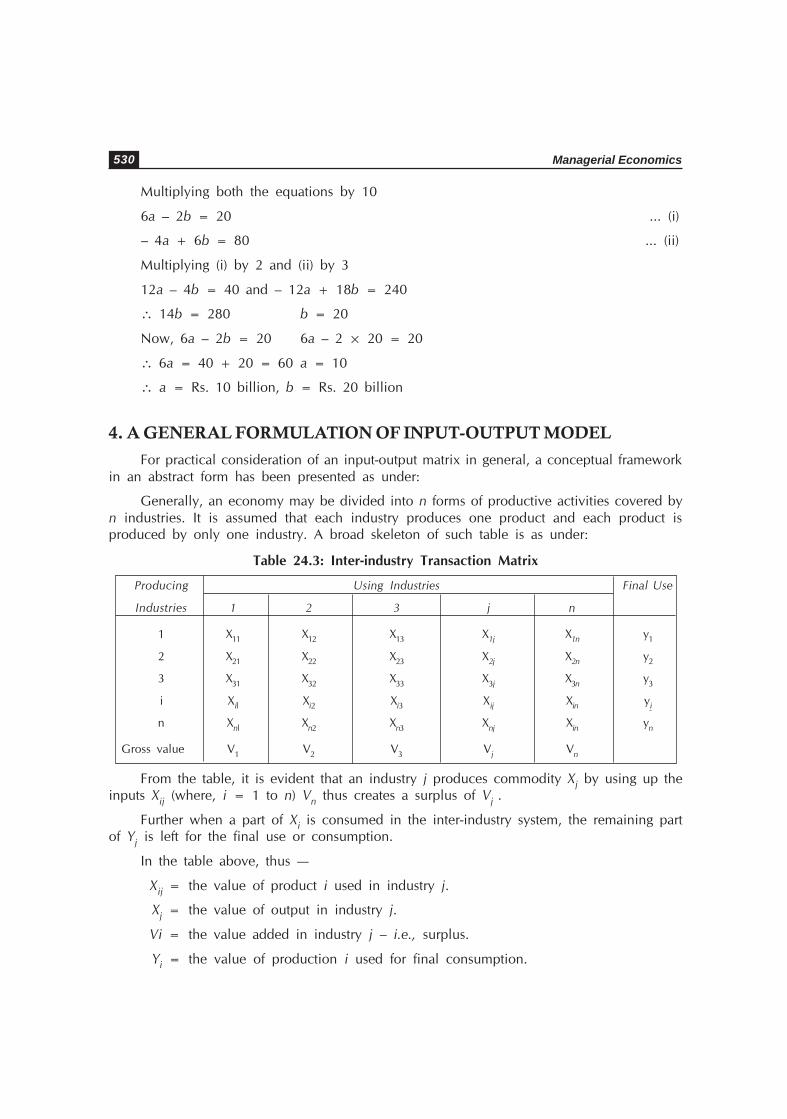
Managerial Economics530
Multiplying both the equations by 10
6a – 2b = 20 ... (i)
– 4a + 6b = 80 ... (ii)
Multiplying (i) by 2 and (ii) by 3
12a – 4b = 40 and – 12a + 18b = 240
∴ 14b = 280 b = 20
Now, 6a – 2b = 20 6a – 2 × 20 = 20
∴ 6a = 40 + 20 = 60 a = 10
∴ a = Rs. 10 billion, b = Rs. 20 billion
4. A GENERAL FORMULATION OF INPUT-OUTPUT MODEL
For practical consideration of an input-output matrix in general, a conceptual frameworkin an abstract form has been presented as under:
Generally, an economy may be divided into n forms of productive activities covered byn industries. It is assumed that each industry produces one product and each product isproduced by only one industry. A broad skeleton of such table is as under:
Table 24.3: Inter-industry Transaction Matrix
From the table, it is evident that an industry j produces commodity Xj by using up theinputs Xij (where, i = 1 to n) Vn thus creates a surplus of Vj .
Further when a part of Xi is consumed in the inter-industry system, the remaining partof Yj is left for the final use or consumption.
In the table above, thus —
Xij = the value of product i used in industry j.
Xj = the value of output in industry j.
Vi = the value added in industry j – i.e., surplus.
Yi = the value of production i used for final consumption.
Producing Using Industries Final Use
Industries 1 2 3 j n
1 X11 X12 X13 X1j X1n y1
2 X21 X22 X23 X2j X2n y2
3 X31 X32 X33 X3j X3n y3
i Xil Xi2 Xi3 Xij Xin yi
n Xnl Xn2 Xn3 Xnj Xin yn
Gross value V1 V2 V3 Vj Vn

Input-output Analysis 531
The above table can be split further. In particular, there is a tradition to break up thefinal use column into five components:
[i] Private consumption (p); [ii] Public consumption (G); [iii] Exports (E); [iv] Grossinvestment (Ig) and [v] Net addition to stock, i.e., capital formation (Ik). It constitutes thedemand side (D) of the economy. To this, for an economy, a supply side column (s) is alsoadded which is composed of two elements [1] output (O) and [2] imports (M).
Table 24.4: A Comprehensive Sectoral Accounts Matrix
The sectoral accounts displayed in Table 31.4 reveal the following balances:
1. Total supply equals to total demand:
X1 + Mi = (X11 + X12 + ... + Xin) + (Ci + Igi + Iki + Ei)
∴ Xi = (X11 + X12 + ... Xin + Ci + Igi + Iki + Ei) – Mi
Here i = 1to n and Mi stands for the value of product i imported.
Thus:
Xn + Mn = Sj
n
=1 Xnj + Cn + Ign + Ikn + Rn
2. Production equals cost plus surplus.
Xj = X1j + ... + Xnj + Vj
l Problem of product-mix. There is the problem of product-mix when a particularsector produces a variety of products. Here, the difficulty arises of classifying inputs.A solution to this problem is that: an input should be treated as originating from thesector which produces it to a major extent.
l Improper records. Collection of data on wages and salaries, depreciation etc. alsoposes many practical difficulties due to lack of proper records, indifference of people,and inefficiency of statistical staff in a backward country.
Similarly, the row of value added by manu-facture is decomposed into: [i] wages andsalaries (w), [ii] depreciation (d) and [iii] the remaining surplus (s).
Thus, a table giving a completely consistent system of sectoral accounts may be drawnas shown in Table 24.4.
Here,
C = Consumption in private and public sector (P + G).
Ig = Gross investment.
Producing Final Use (D)
Sector Using Sector Demand Component (Supply)
1 2 i n (P + G) Ig Ik E M O
= C

Managerial Economics532
Ik = Net addition to stock of capital.
E = Export.
O = Output gross domestic product.
w = Wages.
b = Depreciation.
s = Surplus.
The construction of such a table is based on the following assumptions:
(i) There is uniqueness of sector and commodity.
(ii) There is constant return to the scale.
(iii) For valuation, prices are stated either in producer’s price or purchaser’s price andall information about prices is made in uniform prices.
However, for many purposes, a table in producer’s price is superior to that in a purchaser’sprice. For, a table based on purchaser’s price is likely to be a loss table. But in a country likeIndia, where any kind of information on distributive margin is so inadequate, purchaser’sstatements seem to be better. Thus, there are hardly two to three tables of Indian sectoralaccount stated in producer’s prices. Mostly, these tables are found in terms of purchaser’sprices.
To Decision-makingo Technical coefficient of an industry is measured by the ratio of Industry Input to Industry
Output.
o In a closed input-output matrix, the final demand is not treated separately.
o In an open input-output matrix, the final demand is considered separately.
MODEL QUESTIONS
1. State the assumptions in input-output analysis.
2. Explain and illustrate the transaction matrix.