Transportation Research Part A 44 (2010) 642–659

Contents lists available at ScienceDirect

Transportation Research Part A

journal homepage: www.elsevier .com/locate / t ra

Unintended environmental impacts of nighttime freight logistics activities

Nakul Sathaye *, Robert Harley, Samer MadanatInstitute of Transportation Studies, University of California, 109 McLaughlin Hall, Berkeley, CA 94720-1720, United States

a r t i c l e i n f o

Article history:Received 13 October 2009Received in revised form 23 March 2010Accepted 24 April 2010

Keywords:City logisticsOff-peakNighttime operationsTruck trafficFreight policyAtmospheric dispersion

0965-8564/$ - see front matter � 2010 Elsevier Ltddoi:10.1016/j.tra.2010.04.005

* Corresponding author. Tel.: +1 510 520 9175; faE-mail address: nsathaye@berkeley.edu (N. Sath

1 Although noise is an important concern, the term

a b s t r a c t

In recent years, the reduction of freight vehicle trips during peak hours has been a commonpolicy goal. To this end, policies have been implemented to shift logistics operations tonighttime hours. The purpose of such policies has generally been to mitigate congestionand environmental impacts. However, the atmospheric boundary layer is generally morestable during the night than the day. Consequently, shifting logistics operations to thenight may increase 24-h average concentrations of diesel exhaust pollutants in many loca-tions. This paper presents realistic scenarios for two California cities, which provide dieselexhaust concentration and human intake estimates after temporal redistributions of dailylogistics operations. Estimates are made for multiple redistribution patterns, includingfrom 07:00–19:00 to 19:00–07:00, similar to daytime congestion charging polices, andfrom 03:00–18:00 to 18:00–03:00, corresponding to the PierPASS program at the portsof Los Angeles and Long Beach. Results for these two redistribution scenarios indicate that24-h average exhaust concentrations would increase at most locations in California, anddaily human intake is likely to worsen or be unimproved at best. These results are shownto be worse for inland than coastal settings, due to differences in meteorology. Traffic con-gestion effects are considered, using a new graphical method, which depicts how off-peakpolicies can be environmentally improving or damaging, depending on traffic speeds andmeteorology.

� 2010 Elsevier Ltd. All rights reserved.

1. Introduction

Policies for shifting freight logistics operations away from highly impacting times and locations are receiving increasedattention from policy makers and analysts (Eliasson et al., 2009; Giuliano and O’Brien, 2007; Hensher and Puckett, 2007;Holguin-Veras and Cetin, 2009; Holguin-Veras et al., 2006; Olszewski and Xie, 2005; Quak and de Koster, 2009; Sathayeet al., 2006). Of course, such policies are not new, as records indicate their implementation as early as 2000 years ago(Holguin-Veras, 2008). Despite the important drawback of increased noise near residences, presently, the policy of shiftinglogistics operations to the night is becoming more widely accepted and promoted. The conventional wisdom is that off-peakpolicies are beneficial for transportation systems and the environment.1

Off-peak policies are being implemented to induce more efficient utilization of transportation infrastructure in manylocations around the world. For instance, nighttime delivery programs have been implemented with much success in manyEuropean cities (Geroliminis and Daganzo, 2005). A delivery program in Barcelona shows that logistics operations can beconducted at night without creating a detrimental noise problem (Forkert and Eichhorn, 2008). This city has also devotedlanes of some of its main boulevards to delivery operations during off-peak hours (Dablanc, 2007). The Port Authority ofNew York has implemented a time of day pricing initiative to incentivize off-peak operations (Holguin-Veras et al., 2006).

. All rights reserved.

x: +1 510 642 1246.aye).

environment will not account for noise in this paper.

N. Sathaye et al. / Transportation Research Part A 44 (2010) 642–659 643

In addition, consideration for off-peak policies is not limited to the urban scale. The passage of state legislation in Californiaencourages port terminals to extend service hours to nights and weekends (Giuliano and O’Brien, 2007).

These implementations are generally supported by studies which indicate that off-peak policies, and especially shifts tonight, can reduce traffic congestion and emissions (Browne et al., 2006; McKinnon, 2003; OECD, 2003). However, some pre-vious studies have found that environmental impacts may increase. For example, in Southern California it has been shownthat emissions can increase due to the circumvention of peak-period truck restrictions by the use of smaller vehicles (Camp-bell, 1995). Research on logistics in the Netherlands indicates that restrictions by time windows and vehicle type can in-crease emissions associated with deliveries (Quak and de Koster, 2009). Two previous studies use concepts ofatmospheric science, which will be a focus of this paper, to show that exhaust concentrations can increase as a result ofoff-peak operations. One study provides estimates of the change in pollutant concentrations resulting from trucks, pointingout the potential problems resulting from off-peak policies (Panis and Beckx, 2007). An experimental study in Southern Cal-ifornia shows that pollutant concentrations, resulting from aggregate traffic, can be higher during pre-sunrise than daylighthours, despite lower total traffic levels (Hu et al., 2009). Such analyses have taken steps towards investigating the environ-mental impacts of off-peak policies, which are becoming increasingly important as the detrimental health impacts of dieselexhaust (DE) are apparent (California Air Resources Board, 1998; Lloyd and Cackette, 2001; US Environmental ProtectionAgency, 2002). However, current analyses of off-peak policies still generally neglect to incorporate a comprehensive assess-ment of environmental impacts.

A complete environmental assessment of city-logistics policies would involve the following steps:

1. Assessment of adaptations by logistics operators.2. Assessment of the effects on traffic congestion.3. Assessment of the effects on tailpipe emissions from passenger and freight logistics vehicles (and possibly life-cycle

emissions).4. Assessment of resulting pollutant concentrations through atmospheric modeling.5. Estimation of environmental impacts (e.g. human intake).

Adjustments can be made to this general framework such as iterative prediction of logistics adaptations and traffic con-gestion. However, the general framework is valid for almost any city logistics policy. Many studies, including those men-tioned above, focus on the first two steps, with a fair number adding the tailpipe emissions component of the third(Campbell, 1995; Giuliano and O’Brien, 2007; Quak and de Koster, 2007, 2009). We additionally note the possibility thatlife-cycle emissions may be sensitive to certain policies (Facanha and Horvath, 2006; Sathaye et al., 2010). Although thefourth and fifth steps are often neglected, some studies do focus on making detailed impact assessments (Kinney et al.,2000; Wu et al., 2009). However, generalized values for monetary impact per emissions are more commonly used in policyanalyses (Holguin-Veras and Cetin, 2009; Janic, 2007; Ubillos, 2008). Analysis approaches which account for only specificassessment steps or which use generalized values can be useful for deriving some insights, however results can be mislead-ing due to the spatial and temporal variation of environmental impacts and the subtleties of transportation systems. There-fore, significant questions can remain about the usefulness and accuracy of these conclusions.

In this paper, we focus on concepts relating to the fourth and fifth steps, which have been studied in depth through thefields of atmospheric (McElroy, 2002; Seinfeld and Pandis, 1997) and environmental science (Bennett et al., 2002; Marshallet al., 2005). An important aspect of atmospheric physics for this paper is the concept of stability, which describes the degreeof vertical mixing that occurs in the atmospheric boundary layer (ABL). A more unstable ABL allows for increased vertical dis-persion and decreased concentration of pollutants. One of the primary contributors to the instability of the ABL is solar heating(Ahrens, 2003). Heating causes an increase in temperature and decrease in density of parcels of air at the Earth’s surface. Con-sequently these parcels rise through surrounding air which is more dense, causing pollutants to be dispersed to higher alti-tudes. Pasquill stability classes have been the most widely used scheme for categorizing stability for several decades (Pasquill,1961). Although recently developed dispersion models have begun to use more detailed methods, the majority of models stilluse these classes and they provide a useful descriptive tool. An updated usage of Pasquill stability classes clearly indicates thatdaytime atmospheric instability increases with the level of solar radiation, and that the nighttime stability class is never lessthan that of daytime (Mohan and Siddiqui, 1998). Although the degree of influence of this phenomenon may vary, the ubiq-uitous effect of solar heating over the Earth’s land masses makes it relevant for the majority of metropolitan areas.

We investigate this phenomenon and its influence on DE concentrations and human intake associated with nighttimemetropolitan logistics policies. In Section 2, scenarios are presented for two locations in California, contrasting the extentto which estimated DE concentrations and human intake are affected by local meteorology. In Section 3, a new graphical toolis presented, which can describe environmental impacts, while accounting for various possible traffic states and associatedemission factors. Section 5 concludes the paper.

2. Influence of local meteorology on diesel exhaust concentrations

Diesel particulate matter (DPM) concentrations resulting from truck DE are quantified at two locations under hypothet-ical scenarios in which truck trips are shifted out of peak hours. The locations are in California in the vicinity of Interstate 880

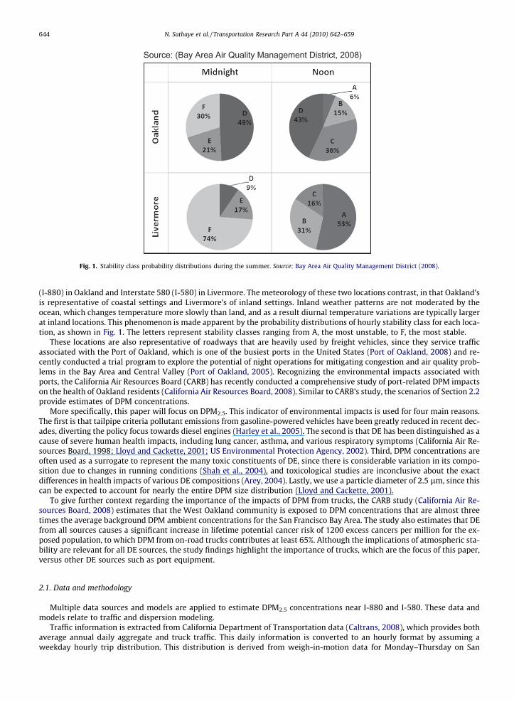
Source: (Bay Area Air Quality Management District, 2008)

Fig. 1. Stability class probability distributions during the summer. Source: Bay Area Air Quality Management District (2008).

644 N. Sathaye et al. / Transportation Research Part A 44 (2010) 642–659

(I-880) in Oakland and Interstate 580 (I-580) in Livermore. The meteorology of these two locations contrast, in that Oakland’sis representative of coastal settings and Livermore’s of inland settings. Inland weather patterns are not moderated by theocean, which changes temperature more slowly than land, and as a result diurnal temperature variations are typically largerat inland locations. This phenomenon is made apparent by the probability distributions of hourly stability class for each loca-tion, as shown in Fig. 1. The letters represent stability classes ranging from A, the most unstable, to F, the most stable.

These locations are also representative of roadways that are heavily used by freight vehicles, since they service trafficassociated with the Port of Oakland, which is one of the busiest ports in the United States (Port of Oakland, 2008) and re-cently conducted a trial program to explore the potential of night operations for mitigating congestion and air quality prob-lems in the Bay Area and Central Valley (Port of Oakland, 2005). Recognizing the environmental impacts associated withports, the California Air Resources Board (CARB) has recently conducted a comprehensive study of port-related DPM impactson the health of Oakland residents (California Air Resources Board, 2008). Similar to CARB’s study, the scenarios of Section 2.2provide estimates of DPM concentrations.

More specifically, this paper will focus on DPM2.5. This indicator of environmental impacts is used for four main reasons.The first is that tailpipe criteria pollutant emissions from gasoline-powered vehicles have been greatly reduced in recent dec-ades, diverting the policy focus towards diesel engines (Harley et al., 2005). The second is that DE has been distinguished as acause of severe human health impacts, including lung cancer, asthma, and various respiratory symptoms (California Air Re-sources Board, 1998; Lloyd and Cackette, 2001; US Environmental Protection Agency, 2002). Third, DPM concentrations areoften used as a surrogate to represent the many toxic constituents of DE, since there is considerable variation in its compo-sition due to changes in running conditions (Shah et al., 2004), and toxicological studies are inconclusive about the exactdifferences in health impacts of various DE compositions (Arey, 2004). Lastly, we use a particle diameter of 2.5 lm, since thiscan be expected to account for nearly the entire DPM size distribution (Lloyd and Cackette, 2001).

To give further context regarding the importance of the impacts of DPM from trucks, the CARB study (California Air Re-sources Board, 2008) estimates that the West Oakland community is exposed to DPM concentrations that are almost threetimes the average background DPM ambient concentrations for the San Francisco Bay Area. The study also estimates that DEfrom all sources causes a significant increase in lifetime potential cancer risk of 1200 excess cancers per million for the ex-posed population, to which DPM from on-road trucks contributes at least 65%. Although the implications of atmospheric sta-bility are relevant for all DE sources, the study findings highlight the importance of trucks, which are the focus of this paper,versus other DE sources such as port equipment.

2.1. Data and methodology

Multiple data sources and models are applied to estimate DPM2.5 concentrations near I-880 and I-580. These data andmodels relate to traffic and dispersion modeling.

Traffic information is extracted from California Department of Transportation data (Caltrans, 2008), which provides bothaverage annual daily aggregate and truck traffic. This daily information is converted to an hourly format by assuming aweekday hourly trip distribution. This distribution is derived from weigh-in-motion data for Monday–Thursday on San

N. Sathaye et al. / Transportation Research Part A 44 (2010) 642–659 645

Francisco Bay Area highways and has been used in previous research (Dreher and Harley, 1998). Composite PM2.5 emissionfactors, accounting for both trucks and other vehicles, are estimated using EMFAC2007 (California Air Resources Board, 2006)and the distribution of truck flows by axle class as specified in the Caltrans data. The formula for the estimation of compositeDPM2.5 emission factors for a specific location and hour of the day is shown in Eq. (A.1) in Appendix A. We note that all PM2.5

emitted from trucks is assumed to come from diesel engines, since gasoline-powered trucks make a negligible contribution.This is justified, since gasoline-powered trucks are relatively uncommon and have much lower PM2.5 emission factors. Theemission factors also vary by hourly average speeds, which are extracted from the PeMS database (PeMS, 2008). However,this has only a minor effect in the two scenarios considered in this paper, since hourly average speeds do not fall below64 km/h. Traffic speeds are considered further in Section 3.

Values for the composite DPM2.5 emission factor and hourly vehicle trips are then applied in the Caltrans line source dis-persion model, Caline4 (Benson, 1984, 1992), to estimate concentrations at various receptor locations. Additional inputs toCaline4, such as aerodynamic surface roughness and hourly meteorology variables are extracted from meteorological data(Bay Area Air Quality Management District, 2008). The meteorological variables extracted are wind direction, wind speed,atmospheric stability class, standard deviation of wind direction and temperature. The mixing height is estimated accordingto the formula suggested by Benson (1984). All roadway geometry variables such as widths, lengths and locations of bridgesare determined by use of Google Earth (Google, 2008a).

Concentrations of DPM2.5 depend on emission factors, atmospheric stability, wind direction and wind speed. In accor-dance with the literature, the expected concentration is calculated based on a joint distribution of the three meteorologicalvariables (Pfafflin and Ziegler, 2006). This allows for the estimation of a seasonal average based on a joint probability massfunction (pmf) which is derived from the meteorological data. The pmf is created by categorizing wind speeds into 15 bins,each having an interval of 1 m/s and wind directions into 24 bins each having an interval of 15�. Stability is categorizedaccording to the six Pasquill classes. For each combination of these three variables, Caline4 is applied to estimate the

Fig. 2. I-880 and receptor locations 1–4 in Oakland. Source: Google (2008b).

646 N. Sathaye et al. / Transportation Research Part A 44 (2010) 642–659

concentration (Conch) for a given hour and receptor location. Subsequently, Eq. (A.2) is used to calculate the expected con-centration (E[Conch]) for each hour and receptor location.

The contribution of the DPM2.5 concentration made by trucks is then calculated by multiplying E[Conch] by the fraction oftotal emissions released by trucks (TCh) during hour h. We note that Caline4 output Conch values vary linearly with the inputcomposite emission factor (Benson, 1984), so the value used for the car emission factor has no effect as long as TCh is mod-ified appropriately.

The 24-h average DPM2.5 concentration (E[Conc24]) is then calculated according to Eq. (A.3). E[Conc24] allows for compar-ison of the effects of shifting logistics operations from peak periods to the night.

Although E[Conc24] provides a basis for understanding the effects associated with off-peak operations, several additionalfactors influence health impacts (Marshall et al., 2006). In particular, hourly variations in breathing rates and time spent in-side buildings (indoors) are likely to have significant impact. Values from previous studies are used for hourly breathing rates(Marshall, 2005) and fraction of time spent indoors (Klepeis et al., 2001). Based on previous estimates, we assume that theindoor exposure concentration is 2/3 of outdoor ambient concentrations (Lloyd and Cackette, 2001; Marshall et al., 2006). Eq.(A.4) is used to estimate 24-h average pollutant intake (E[Intake24]) for an individual remaining at a single receptor through-out the day, with the assumption that all of his time is spent either indoors or outdoors.

2.2. Results

Figs. 3 and 4 display estimates for E[Conc24] and E[Intake24] respectively, in Oakland for summer and winter at the recep-tor locations shown in Fig. 2. Figs. 5–7 present analogous information for Livermore. To allow for comparison, the results areproduced for six different cases of daily truck trip distribution. These cases will be referred to alphabetically as cases a–f.Case a represents the status quo, which is based on the previously mentioned hourly truck trip distribution (Dreher and Har-ley, 1998). Case b is based on a 24-h uniform hourly distribution of truck trips. For cases c–f, the same total number of trucktrips are shifted out of peak periods, but the times of the assumed peak and off-peak periods differ. Accordingly, a differentpercent of trips is removed from the peak hours for each case (and this percent is uniform across peak hours for each case).Moreover, trips are assumed to be uniformly added to the off-peak hours. The percent of trips shifted, and peak and off-peaktimes are displayed in the Figs. 3, 4, 6 and 7.

0 0.2 0.4 0.6 0.8

4

3

2

1

4

3

2

1

PM2.5 concentration (µg/m3)

Rece

ptor

num

ber

a: Status Quo

b: Uniform

c: 07:00-19:00 to 19:00-07:00 (29% of trips shifted)

d: 03:00-18:00 to 18:00-03:00 (26% of trips shifted)

e: 03:00-0:900 to 18:00-03:00 (100% of trips shifted)

f: 03:00-0:900 to 18:00-22:00 (100% of trips shifted)

Summer

Winter

Fig. 3. Estimated DPM2.5 concentrations in Oakland.

0 0.05 0.1 0.15 0.2 0.25

4

3

2

1

4

3

2

1

PM2.5 intake (μg/hr)

Rece

ptor

num

ber

a: Status Quo

b: Uniform

c: 07:00-19:00 to 19:00-07:00 (29% of trips shifted)

d: 03:00-18:00 to 18:00-03:00 (26% of trips shifted)

e: 03:00-0:900 to 18:00-03:00 (100% of trips shifted)

f: 03:00-0:900 to 18:00-22:00 (100% of trips shifted)

Summer

Winter

Fig. 4. Estimated individual DPM2.5 intake in Oakland.

Fig. 5. I-580 and receptor locations 1–3 in Livermore. Source: Google (2008b).

N. Sathaye et al. / Transportation Research Part A 44 (2010) 642–659 647

0 0.2 0.4 0.6 0.8

3

2

1

3

2

1

PM2.5 concentration (µg/m3)

Rece

ptor

num

ber

a: Status Quo

b: Uniform

c: 07:00-19:00 to 19:00-07:00 (29% of trips shifted)

d: 03:00-18:00 to 18:00-03:00 (26% of trips shifted)

e: 03:00-0:900 to 18:00-03:00 (100% of trips shifted)

f: 03:00-0:900 to 18:00-22:00 (100% of trips shifted)

Summer

Winter

Fig. 6. Estimated DPM2.5 concentrations in Livermore.

648 N. Sathaye et al. / Transportation Research Part A 44 (2010) 642–659

The receptor locations shown in Figs. 2 and 5 are distributed to capture some of the potential variations in pollutant con-centrations in residential neighborhoods due to wind direction and distance from the roadway. The only exception is recep-tor 4 in Fig. 2, which is located to show how the effects of wind direction vary across seasons and potential influences on thehealth of port workers. The prevailing wind direction in Oakland is from the west, primarily because of the bay-breeze effect;however southwesterly winds are frequent, especially during the winter due to the Hayward Gap (Bay Area Air Quality Man-agement District, 2010). Wind direction in the Livermore Valley is more variable and is generally highly dependent on localconditions. In the case of the data used for this study, the prevailing wind direction is generally from the west during thesummer and the northeast during winter. The distance from each receptor to the nearest point on the highway is also shownin Figs. 2 and 5.

For the remainder of Section 2 we will refer to the percent changes in E[Conc24] and E[Intake24] for various cases versuscase a, to draw comparisons relative to the status quo. Case c represents a situation in which truck trips are shifted out ofdaytime hours, similarly for examples to the congestion charging schemes in London (Transport for London, 2009) andStockholm (Daunfeldt et al., 2009). Results for case c, as shown in Figs. 3 and 6, indicate that nighttime logistics operationscause significantly larger relative increases in E[Conc24] at receptor locations in Livermore than in Oakland, in accordancewith the variations in stability class shown in Fig. 1. In addition, the changes during the summer are larger due to greaterdiurnal variation in prevailing meteorology. This results from increased solar heating during summer, when there are moredaylight hours and more intense sunlight during the day. The effect of wind direction is also notable, as the prevailing winddirection is from the southwest instead of northwest for a much higher fraction of the time during the night than the day inOakland. Although concentrations at receptor 4 are generally low, the diurnal change in wind pattern results in a larger per-cent change in E[Conc24] at receptor 4 than the other receptors, since this intersection lies directly to the northwest of I-880.This fraction is also much greater during the winter than the summer. Case c, as shown in Figs. 4 and 7, reveals that a shift oftruck trips away from daytime hours does not generally improve E[Intake24] in Oakland, and is likely to worsen E[Intake24] inLivermore. These results are commensurate with the E[Conc24] increases shown in Figs. 3 and 6.

Case d applies the peak and off-peak times currently utilized in the PierPASS system at the ports of Los Angeles and LongBeach (PierPASS, 2009). As can be seen in Figs. 3 and 6, E[Conc24] for case d is generally less than that for case c, since case dshifts trips out of pre-dawn hours, when the ABL is very stable, and also the off-peak period begins slightly earlier, when theABL is relatively unstable. However E[Conc24] for case d is greater than that for case a. Figs. 4 and 7 show that E[Intake24] for

0 0.05 0.1 0.15 0.2 0.25

3

2

1

3

2

1

PM2.5 intake (μg/hr)

Rece

ptor

num

ber

a: Status Quo

b: Uniform

c: 07:00-19:00 to 19:00-07:00 (29% of trips shifted)

d: 03:00-18:00 to 18:00-03:00 (26% of trips shifted)

e: 03:00-0:900 to 18:00-03:00 (100% of trips shifted)

f: 03:00-0:900 to 18:00-22:00 (100% of trips shifted)

Summer

Winter

Fig. 7. Estimated individual DPM2.5 intake in Livermore.

N. Sathaye et al. / Transportation Research Part A 44 (2010) 642–659 649

cases a and d is comparable in Oakland, whereas E[Intake24] for case d is consistently higher than for case a in Livermore.These results indicate that the hours utilized in PierPASS are not likely to reduce DE concentrations and may worsen humanintake in many locations.

Cases e and f utilize alternative times for peak and off-peak periods to show what types of policies are more likely to ame-liorate impacts. Case e removes trips from pre-dawn hours and the morning commute period, and shifts them to the currentPierPASS off-peak period. This results in comparable or lesser values of E[Conc24] and E[Intake24]. These results differ fromcase d, since trips are not shifted away from the late morning and afternoon, when the ABL is unstable. Case f is the sameas case e, except that the off-peak period to which truck trips are shifted ends at 22:00, corresponding to the decrease inport drayage activity after this time (BST Associates, 2008). The sharp drop in activity is associated with the 22:00–23:00break taken by longshoremen. Although breathing rates are higher during the evening than the night, the results for casef generally indicate that there is a further reduction in E[Conc24] and E[Intake24] versus case e, since truck trips are shiftedto earlier hours, when the ABL is less stable. Therefore, a focus on shifting off-peak operations to the evening instead ofthe night may allow both reduced health impacts and better utilization of labor.

In order to get a sense of the magnitude of the health implications of these results, we may compare E[Intake24] againstthose found in previous research. The mean DPM2.5 intake for California’s South Coast Air Basin has been estimated to bearound 2 lg/h (Marshall et al., 2006), which is likely of similar order of magnitude to that in the San Francisco Bay Area.Therefore, comparing this estimate with the results in Figs. 4 and 7, the highways in the scenario locations are contributingsignificantly to excess DPM2.5 intake measured at the receptor locations. This level of intake is likely to result in a measurableincrease in lung cancer risk for the exposed populations (Marshall, 2005).

3. Accounting for the effects of traffic congestion

In Section 2, we presented multiple scenarios, showing the effects of hourly variations in prevailing meteorology. How-ever, as traffic speeds on the highway segments studied undergo little variation, only cursory investigation of congestion ef-fects was made. As previously mentioned, congestion mitigation is a primary aim of policies for shifting freight trips to off-peak hours. Therefore, in Section 3, we incorporate traffic considerations to provide further analysis of the types of situationsin which unintended environmental impacts are likely to occur.

650 N. Sathaye et al. / Transportation Research Part A 44 (2010) 642–659

The analysis of Section 2 is based on real-world scenarios, whereas in Section 3 we utilize a more conceptual approach, inthat hypothetical examples are used to develop insights. A graphical tool, in the form of a DPM2.5 concentration isopleth dia-gram, is used to analyze the various examples. This type of diagram can be used in future analyses of nighttime logistics pol-icies. We note that this paper does not account for congestion within terminals, for which other mitigation methods such asappointment systems are applicable (Giuliano and O’Brien, 2007). A list of variables used in Section 3 is shown in Table B.1,since they are referred to multiple times in the text.

3.1. Methodology

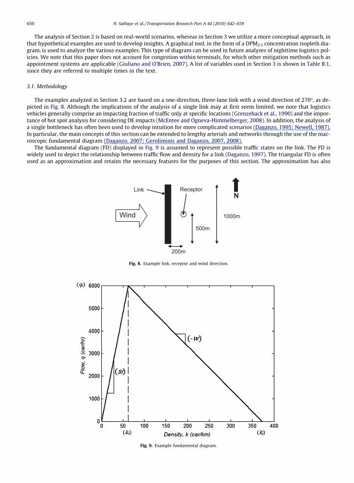
The examples analyzed in Section 3.2 are based on a one-direction, three-lane link with a wind direction of 270�, as de-picted in Fig. 8. Although the implications of the analysis of a single link may at first seem limited, we note that logisticsvehicles generally comprise an impacting fraction of traffic only at specific locations (Grenzeback et al., 1990) and the impor-tance of hot spot analysis for considering DE impacts (McEntee and Ogneva-Himmelberger, 2008). In addition, the analysis ofa single bottleneck has often been used to develop intuition for more complicated scenarios (Daganzo, 1995; Newell, 1987).In particular, the main concepts of this section can be extended to lengthy arterials and networks through the use of the mac-roscopic fundamental diagram (Daganzo, 2007; Geroliminis and Daganzo, 2007, 2008).

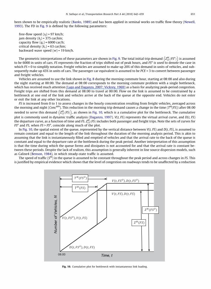
The fundamental diagram (FD) displayed in Fig. 9 is assumed to represent possible traffic states on the link. The FD iswidely used to depict the relationship between traffic flow and density for a link (Daganzo, 1997). The triangular FD is oftenused as an approximation and retains the necessary features for the purposes of this section. The approximation has also

Wind

200m

500m

1000m

ReceptorLinkN

Fig. 8. Example link, receptor and wind direction.

Fig. 9. Example fundamental diagram.

N. Sathaye et al. / Transportation Research Part A 44 (2010) 642–659 651

been shown to be empirically realistic (Banks, 1989) and has been applied in seminal works on traffic flow theory (Newell,1993). The FD in Fig. 9 is defined by the following parameters:

free-flow speed (sf) = 97 km/h;jam density (kj) = 375 car/km;capacity flow (qc) = 6000 car/h;critical density (kc) = 63 car/km;backward wave speed (w) = 19 km/h.

The geometric interpretations of these parameters are shown in Fig. 9. The total initial trip demand ZMCTðFSoÞ

� �is assumed

to be 6000 in units of cars. FS represents the fraction of trips shifted out of peak hours, and FSo is used to denote the case inwhich FS = 0 to simplify notation. Freight vehicles are assumed to make up 20% of this demand in units of vehicles, and sub-sequently make up 43% in units of cars. The passenger car equivalent is assumed to be PCE = 3 to convert between passengerand freight vehicles.

Vehicles are assumed to use the link shown in Fig. 8 during the morning commute hour, starting at 08:00 and also duringthe night starting at 00:00. The demand at 08:00 corresponds to the morning commute problem with a single bottleneck,which has received much attention (Lago and Daganzo, 2007; Vickrey, 1969) as a basis for analyzing peak-period congestion.Freight trips are shifted from this demand at 08:00 to travel at 00:00. Flow on the link is assumed to be constrained by abottleneck at one end of the link and vehicles arrive at the back of the queue at the opposite end. Vehicles do not enteror exit the link at any other locations.

FS is increased from 0 to 1 to assess changes in the hourly concentration resulting from freight vehicles, averaged acrossthe morning and night (ConcMN). This reduction in the morning trip demand causes a change in the time (TM(FS)) after 08:00

needed to serve this demand ZMCTðFSÞ

� �, as shown in Fig. 10, which is a cumulative plot for the bottleneck. The cumulative

plot is commonly used in dynamic traffic analysis (Daganzo, 1997). V(t, FS) represents the virtual arrival curve, and D(t, FS)the departure curve, as a function of time and FS. ZM

CTðFSÞ includes both passenger and freight trips. Note the sets of curves forFSo and FS, when FS > FSo, coincide along much of the plot.

In Fig. 10, the spatial extent of the queue, represented by the vertical distance between V(t, FS) and D(t, FS), is assumed toremain constant and equal to the length of the link throughout the duration of the morning analysis period. This is akin toassuming that the link is instantaneously filled and emptied of vehicles and that the arrival rate to the back of the queue isconstant and equal to the departure rate at the bottleneck during the peak period. Another interpretation of this assumptionis that the time during which the queue forms and dissipates is not accounted for and that the arrival rate is constant be-tween these periods. Despite the lack of realism, this assumption is generally inherent in line source dispersion models, suchas Caline4 (Benson, 1984), in which steady-state traffic is assumed.

The speed of traffic (SM) in the queue is assumed to be constant throughout the peak period and across changes in FS. Thisis justified by empirical evidence which shows that the level of congestion on roadways tends to be unaffected by a reduction

Fig. 10. Cumulative plot for bottleneck with instantaneous link loading.

652 N. Sathaye et al. / Transportation Research Part A 44 (2010) 642–659

in trip demand, although the length of the peak period may be reduced (Small, 1992). The nighttime traffic speed (SN) is as-sumed to be equal to sf and the time to service night truck demand (TN(FS)) is used analogously to the use of TM(FS). Theassumptions inherent in this setup simplify the development of the examples in Section 3.2 without hindering their purpose.Further investigation, related to the implications of relaxing traffic assumptions, can be found in a previous report (Sathayeet al., 2009) which depicts the implications of a shortened peak period and associated decreasing marginal benefits.

3.2. Results

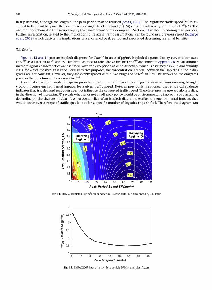
Figs. 11, 13 and 14 present isopleth diagrams for ConcMN in units of lg/m3. Isopleth diagrams display curves of constantConcMN as a function of SM and FS. The formulas used to calculate values for ConcMN are shown in Appendix B. Mean summermeteorological characteristics are assumed, with the exceptions of wind direction, which is assumed as 270�, and stabilityclass, for which the median is used. For illustrative purposes, the concentration intervals between the isopleths in these dia-grams are not constant. However, they are evenly spaced within two ranges of ConcMN values. The arrows on the diagramspoint in the direction of decreasing ConcMN.

A vertical slice of an isopleth diagram provides a description of how shifting logistics vehicles from morning to nightwould influence environmental impacts for a given traffic speed. Note, as previously mentioned, that empirical evidenceindicates that trip demand reduction does not influence the congested traffic speed. Therefore, moving upward along a slice,in the direction of increasing FS, reveals whether or not an off-peak policy would be environmentally improving or damaging,depending on the changes in ConcMN. A horizontal slice of an isopleth diagram describes the environmental impacts thatwould occur over a range of traffic speeds, but for a specific number of logistics trips shifted. Therefore the diagram can

Trip

Fra

ctio

n Sh

ifted

, FS

0.60.45

0.290.23

0.21

0.2

0.18

0.17

0.16

0.14

8 15 25 35 45 55 65 75 85 950

0.1

0.2

0.3

0.4

0.5

0.6

0.7

0.8

0.9

1

Peak-Period Speed,SM (km/hr)

Improving Regime (I)

Damaging Regime (D)

Fig. 11. DPM2.5 isopleths (lg/m3) for summer in Oakland with free-flow speed, sf = 97 km/h.

0

0.5

1

1.5

2

2.5

3

PM2.

5 Em

issi

ons

(g/k

m)

Vehicle Speed (km/hr)8 15 25 35 45 55 65 85 95

Fig. 12. EMFAC2007 heavy–heavy-duty vehicle DPM2.5 emission factors.

Trip

Fra

ctio

n Sh

ifted

, FS

0.650.48

0.31

0.2

0.18

0.17

0.17

0.16

0.15

0.15

8 15 25 35 45 550

0.1

0.2

0.3

0.4

0.5

0.6

0.7

0.8

0.9

1

Peak-Period Speed,SM (km/hr)

Fig. 13. DPM2.5 isopleths (lg/m3) for summer in Oakland with free-flow speed sf = 64 km/h.

Trip

Fra

ctio

n Sh

ifted

, FS

0.520.46

0.39

0.36

0.32

0.29

0.25

0.21

0.17

8 15 25 35 45 55 65 75 85 950

0.1

0.2

0.3

0.4

0.5

0.6

0.7

0.8

0.9

1

Peak-Period Speed,SM (km/hr)

Fig. 14. DPM2.5 isopleths (lg/m3) for summer in Livermore with free-flow speed, sf = 97 km/h.

N. Sathaye et al. / Transportation Research Part A 44 (2010) 642–659 653

be use to analyze various traffic conditions, for a given meteorological setting. It could also be used to analyze the effects ofan off-peak policy in conjunction with traffic control methods aimed at influencing traffic flows and speeds (Daganzo et al.,2002).

Multiple factors influence the form of isopleth diagrams. The main factors for the examples presented in this paper are SM,SN, and meteorological conditions during morning and night. These factors lead to regimes, characterized by the two arrowsin Figs. 11, 13 and 14. In the lower SM regime (Regime I) off-peak policies improve ConcMN, whereas in the higher SM regime(Regime D), ConcMN increases and environmental damage occurs. Regime D corresponds to the examples of Section 2.2, as thetraffic speeds on those roadways was relatively high. STrans refers to the transition value of SM at which oConcMN/oSM = 0, asshown in Fig. 11.

The reason for the existence of the two regimes is the variation in the morning emission factor (EFM) with respect to SM, asshown in Fig. 12. The variations in the tradeoff between the change in morning average concentration (ConcM) and that of thenight (ConcN) can be attributed to the variations in EFM, since the morning and nighttime meteorological conditions, andnighttime emission factor (EFN) are constant. (EFN is constant, because SN is assumed to be equal to sf; meteorological con-ditions are constant, as previously specified.) Therefore, in the case of low SM and a corresponding high EFN, a shift to thenight results in a reduction in ConcMN, because the number of trips made with high EFN is reduced. Accordingly, the contri-bution of ConcM to ConcMN has decreased more than that of ConcN has increased (the contributions of ConcM and ConcN insteadof their values are considered, because they must be appropriately weighted to directly estimate ConcMN, as the duration ofTM(FS) and TN(FS) differ). To describe the tradeoff in other terms, in Regime I the low SM values cause relatively high morning

654 N. Sathaye et al. / Transportation Research Part A 44 (2010) 642–659

emission factors (EFM); reducing the number of morning trips by shifting trips to the night period outweighs the effects of thestagnant nighttime ABL.

However, EFM decreases with increasing SM, as can be seen in Fig. 12. As SM increases and EFM decreases, the tradeoff be-tween ConcM and ConcN changes, causing improvements in ConcMN with respect to FS to diminish. For high values of SM, thetradeoff is reversed and the effects of the stagnant nighttime ABL outweigh the relatively low values for EFM. The tradeoffreversal occurs at STrans, leading to a regime change from Regime I to D. In Regime D, SM > STrans and ConcMN increases withFS, since the contribution of ConcM decreases less than that of ConcN increases. Note that ConcMN also increases with SM, for SM

greater than about 72 km/h, since EFM increases in this regime, in accordance with Fig. 12. This results in the upside down u-shape of the isopleths around SM = 72 km/h.

Fig. 13 presents the resulting isopleth diagram for the same situation, except that sf is 64 km/h. This lower sf representsthe case of arterials, instead of freeways. The fundamental diagram is accordingly adapted so that qc is reduced, and kc in-creased. As can be seen, STrans is higher than for Fig. 11, because the reduction in sf from 97 km/h to 64 km/h causes a decreasein EFN. This can be seen in the right of Fig. 12. This reduction in EFN makes nighttime freight logistics activities less environ-mentally damaging per trip shifted, than in the case of freeways. Specifically, the increases in ConcN are lower for arterials,whereas the decreases in ConcM are the same for all values of FS and SM

6 64 km/h. Therefore, as SM increases, the increases inConcN do not outweigh the decreases in ConcM, until a higher value of SM is reached, resulting in a higher STrans. This showsthat nighttime policies are more likely to be beneficial for cases in which SN is lower, such as arterials.

Fig. 14 shows the isopleth diagram for summer conditions in Livermore. In comparison with Fig. 11, a shift to nighttimeoperations by logistics vehicles results in greater increases in ConcN, due to greater nighttime stability, whereas the decreasein ConcM is lower for all values of SM and FS. Consequently, the value for STrans is lower for Livermore than Oakland (the trade-off between ConcM and ConcN reverses at a lower SM). Consistent with the higher changes in E[Conc24] values found for Liv-ermore (Fig. 6), these results indicate that unintended environmental impacts are more likely to occur in inland locations inCalifornia.

4. Discussion

In this section, assumptions, sources of uncertainty and pertinent aspects for more detailed analysis in future assessmentsare discussed. These issues are grouped by the latter four steps of the assessment framework presented in Section 1. We notethat although step 1, which involves the assessment of adaptations by logistics operators, is not addressed directly in thispaper, it is likely to be one of the most uncertain aspects and require context-specific analysis. This is due to the nuancesof logistics industry operations and business relationships (Holguin-Veras et al., 2006).

Considering step 2, average values for traffic speeds are straightforwardly used in Section 2, and should not be a greatsource of uncertainty. For Section 3, the average speed of traffic being modeled must be relatively homogeneous withinthe peak and off-peak periods for the isopleth diagram to be meaningful. This should be reasonable for a single bottleneckand has also been identified as a feature of the macroscopic fundamental diagram (Geroliminis and Daganzo, 2008), allowingfor extension of the isopleth diagram to be used for networks. For the analysis of multiple links or networks with inhomo-geneous average speeds, multiple isopleth diagrams can also be used. Of course, this may seem to necessitate the use of aprohibitive number of diagrams; however, as previously mentioned, much of the concern regarding DE impacts is at specificlocations.

Considering step 3, DPM emission factors are a potential source of uncertainty for two main reasons. The first has to dowith whether the EMFAC2007 DPM2.5 emission factors are valid for the area-wide drive cycles they are designed to represent(Lloyd and Cackette, 2001). Although the EMFAC2007 DPM2.5 emission factors are area-wide estimates, they also fall withinthe range of those suggested by multiple empirical studies (Ban-Weiss et al., 2008; Kear and Niemeier, 2006). Therefore, forthe analysis of Section 2, which does not account for speed variations, uncertainties in EMFAC2007 should not affect theimplications of the results. Similarly, the order of magnitude for EMFAC2007 DPM2.5 emission factors is reasonable for Sec-tion 3. However there is a second source of uncertainty for Section 3, which has to do with whether EMFAC2007 DPM2.5

emission factors are appropriate for project-level analysis. At the project level, changes in average traffic speed may not nec-essarily represent changes in time spent idling or spent in high-power transient driving mode, which greatly influence emis-sion factors (Kear and Niemeier, 2006). Nevertheless, the parabolic shape of the DPM2.5 emission factor curve, in whichemission factor is a decreasing function of speed with the exception of very high speeds, should generally be valid for giventraffic control conditions and facility type. This occurs since higher average speeds generally correspond to less time spentidling and in high-power transient driving mode per distance traveled. Therefore, although the exact shape of the isoplethswould differ as a result of minor modifications to the emission factor curve shown in Fig. 12, the general form of the isoplethdiagrams should generally hold. Future applications of the isopleth diagram must ensure that the appropriate relationshipbetween average speed and microscopic traffic phenomena, which influence emissions, is utilized. This will depend on trafficcontrol conditions and facility type, which is a subject of ongoing research (Kear and Niemeier, 2006; Nesamani et al., 2007).

Considering step 4, the dispersion model and assumptions regarding wind direction in Section 3 are potential sources ofuncertainty. Caline4 is a standard model and has been validated for the estimation of pollutant concentrations for severalpollutants; however results are inconclusive for PM2.5 in dense urban areas (Chen et al., 2009). The main reasons for thesemixed results are thought to be street canyon effects and the influence of traffic on atmospheric dispersion. The two scenario

N. Sathaye et al. / Transportation Research Part A 44 (2010) 642–659 655

locations in this paper are residential neighborhoods made up mainly of detached houses. Therefore it is reasonable to as-sume that street canyon effects and the influence of traffic on dispersion patterns do not invalidate the use of Caline4 in thispaper. Future work should utilize appropriate context-specific atmospheric dispersion modeling tools to determine the ex-tent to which atmospheric stability influences DE concentrations in different settings. For Section 3, wind direction is as-sumed constant to derive basic implications; however even if wind direction is realistically accounted for, the generalform of the isopleth diagrams should not differ, since the parabolic emission factor curve and diurnal stability variation willbe present. The only caveat is the extreme case in which STrans becomes very low or high, causing either the improving ordamaging regime to be eliminated from the diagram.

We also note that future policy assessments can also account for DE concentrations resulting from port equipment andother transportation modes, such as maritime vessels. Although different emissions and dispersion models are necessary forsuch DE sources, the implications of atmospheric stability are similar, though generally less impacting on human healthsince they are likely to be further from affected populations (California Air Resources Board, 2008).

Considering step 5, uncertainty regarding DPM2.5 exposure is primarily the result of two main issues. The first has to dowith microenvironments. The methodology of this paper accounts for differences in indoor and outdoor exposure concen-trations, but exposure is likely much higher for people who are in-vehicle near freight traffic, which occurs mainly duringdaytime hours (Marshall et al., 2006). This indicates that estimates of E[Intake24] for cases b–f in Section 2 are biased up-wards versus the population average. However this upward bias may not be that significant, since truck trips avoid commuteperiods when people are most likely to be in-vehicle, truck trips generally only share specific roadways with those of pas-senger, and most of people’s time is spent indoors even during commute hours (Klepeis et al., 2001). The second source ofuncertainty has to do with daily travel patterns, which are also not accounted for in Section 2. The receptor locations are inpredominantly residential neighborhoods, where there are likely to be more people during the night than the day. This indi-cates that estimates of E[Intake24] for cases b–f in Section 2 are biased downwards versus the population average. Althoughthese issues vary across locations and times, we note that a previous study shows that the biases associated with ignoringthe in-vehicle microenvironment and travel patterns largely cancel out for the South Coast Air Basin (Marshall et al., 2006).

Finally, regarding step 5, we consider enhancing the isopleth diagrams to depict DPM intake, rather than concentration.Although STrans is likely to be different versus the concentration isopleth diagrams, the implications of the parabolic emissionfactor curve and atmospheric stability on the form of the isopleths, as discussed in Section 3, should generally still hold. Theonly change is that in some cases intake may not be a parabolic function of speed if traffic control policies, which influencespeed, greatly divert the location of emissions towards higher density populations (e.g. from freeways to on-ramps). As aresult, the form of the isopleths could differ from those shown in Section 3. In this case, multiple isopleth diagrams canbe used if values for STrans are of primary interest. A single diagram can also still be used, although the form of intake isop-leths may not be similar to those for concentrations shown in Section 3. Nevertheless, this issue should not generally negatethe implications of the diagrams in Section 3, since future policy assessments are likely to focus on major roadways and net-works, which will be the dominant source of DE concentrations in the study area.

5. Conclusion

This paper focuses on estimating the change in freight vehicle DE concentrations and human intake as a result of night-time operating policies, indicating that increases in air pollution are likely to result in many metropolitan settings. Althoughthere are many benefits of shifting operations to the nighttime, the results show the importance of carefully assessing theenvironmental impacts of nighttime freight operations. The potential for unintended impacts is shown to be more severe ininland locations during the summer for California, and more generally, locations that exhibit significant diurnal meteorolog-ical variation. However, environmental benefits are likely to occur if off-peak policies are directed at specific time periods,such as the morning commute period. In addition, benefits are more likely to occur for situations with relatively low peak-period traffic speeds, since this corresponds to high peak-period emission factors. The isopleth diagram, developed in thispaper, provides a tool that can be utilized in the future to assess whether or not an off-peak policy is likely to cause envi-ronmental damage. Future policy analyses can incorporate these diagrams to provide a graphical representation of impactsfor decision making. These results highlight the importance of conducting comprehensive assessments of logistics policies inthe future, which account realistically for the complex nature of both transportation and environmental systems.

Acknowledgement

This research was supported by the University of California, Berkeley’s Center for Future Urban Transport (a Volvo Centerof Excellence).

Appendix A. Variables and equations for Section 2

Eqs. (A.1)–(A.4) and the variables in Table A.1 are used in Section 2. For Eq. (A.1), the Caltrans 2-axle and 3-axle classes areassumed to correspond to the EMFAC2007 medium–heavy-duty vehicle class, and the Caltrans 4-axle and 5 or more-axle

Table A.1Variables used for Section 2.

BRh Breathing rate during hour hConc24 24-h average concentration

Conchðsc;wd;ws;�IÞ Concentration at particular receptor location and hour h for stability class sc,wind direction wd, wind speed ws, and a vector of constant inputs �I

EFCT Composite PM2.5 emissions factorec Passenger vehicle PM2.5 emission factoreTn Truck PM2.5 emission factor for axle class denoted by nch Ratio of indoor to outdoor DPM2.5 concentrationIntake24 24-h average intakeN Number of truck axles in highest axle classp(sc, wd, ws) Probability mass functionQTn Hourly trips made by trucks of axle class nQC Hourly trips made by passenger vehiclesSC Set of stability classesTCh Fraction of emissions released by trucks during hour hhh Fraction of time spent outdoors during hour hWD Set of wind direction binsWS Set of wind speed bins

656 N. Sathaye et al. / Transportation Research Part A 44 (2010) 642–659

classes to the EMFAC2007 heavy–heavy-duty class. Cars are included, since traffic flow influences the stability of air over theroadway.

EFCT ¼QC � eC þ

PNn¼2Q Tn � eTn

QC þPN

n¼2Q Tn

ðA:1Þ

E½Conch� ¼X

SC;WD;WS

Conchðsc;wd;ws;�IÞ � pðsc;wd;wsÞ ðA:2Þ

E½Conc24� ¼ 124�X24

h¼1

TCh � E½Conch� ðA:3Þ

E½Intake24� ¼ 124�X24

h¼1

ðch � ð1� hhÞ þ hhÞ � BRh � TCh � E½Conch� ðA:4Þ

Appendix B. Variables and equations for Section 3

The derivation of the formulas used to calculate PM2.5 concentration values for the isopleths diagrams in Section 3.2 canbe seen in Eqs. (B.1)–(B.12). The variables used in Section 3 are shown in Table B.1. Eq. (B.1) is used to compute w based on qc,kj, kc, which are assumed from the FD in Fig. 9.

W ¼ qc

kj � kcðB:1Þ

w is then used along with kc and qc in Eq. (B.2) to calculate Q MCT . SM takes on a range of assumed values, in accordance with the

horizontal axis of the associated isopleth diagram. Therefore, Eq. (B.2) is applied for multiple values of SM to compute theassociated QM

CT values.

QMCT ¼

qc þw� kc

1þw=SM ðB:2Þ

TFVo is then converted to its equivalent in units of cars, TFo, by applying PCE = 3, as shown in

TFo ¼ TFVo � PCETFVo � PCEþ 1� TFVo ðB:3Þ

TFVo is subsequently used to compute Q MT and Q M

C , as shown in Eqs. (B.4) and (B.5). The second case of each equation isused when FS � TFo < 1, representing a situation in which less than 100% of freight trips have been shifted. To maintain thegenerality of the equations, the first case formulas are shown for FS � TFo = 1, since otherwise the denominator could equal 0.

QMT ¼

0 if FS� TFo ¼ 1ð1�FSÞ�TFo

1�FS�TFo � Q MCT otherwise

(ðB:4Þ

QMC ¼

Q MCT if FS� TFo ¼ 1ð1�TFoÞ

1�FS�TFo � QMCT otherwise

(ðB:5Þ

Table B.1Variables used for Section 3.

Conch Caline4 output average PM2.5 concentration for hour hConcY Average PM2.5 concentration during period Y, resulting from logistics vehiclesD(t, FS) Departure curveEFY Composite PM2.5 emission factor during period YeX PM2.5 emission factor for vehicle type XFS Fraction of freight trips shifted to off-peak operationsk Traffic densitykc Traffic critical densitykj Traffic jam densityN Cumulative number of vehiclesO Superscript used to denote original value of variable for FS0 (i.e. where FS = 0)PCE Passenger-car equivalent

QYX

Flow of vehicle type X during period Y

q Traffic flowqc Traffic capacitySTrans Transition MS between improving and damaging traffic speed regimesSY Speed of queued traffic during period Ysf Free-flow traffic speedTY(FS) Duration needed to serve traffic demand during period YTYh Fraction of hour h used to serve trip demand during period Yt TimeTCY Fraction of total traffic PM2.5 emissions made by freight vehicles during period YTFo Fraction of peak-period trip demand comprised of freight vehicles for FS = 0 in units of passenger vehiclesTFVo Fraction of peak-period trip demand comprised of freight vehicles for FS = 0 in units of vehiclesTime Averaging time for PM2.5 concentration estimatesV(t, FS) Virtual arrival curve for all vehiclesw Traffic backward wave speedX

¼C if variable represents passenger vehiclesT if variable represents freight vehiclesCT if variable represents all vehicles

8<:

Y¼

M if variable represents peak periodN if variable represents nightMN if variable represents average peak period and night

8<:

ZYXðFSÞ Trip demand during period Y for vehicle type X

N. Sathaye et al. / Transportation Research Part A 44 (2010) 642–659 657

Q NCT , is assumed to be equal to both qc and Q N

T , since nighttime trip demand by cars is assumed to be 0. This is shown in

Q NT ¼ Q N

CT ¼ qc ðB:6Þ

EFY values for input to Caline4 are then computed as shown in Eq. (B.7). Note that Y is used to save on notation, and indicatesthat the variable is computed for both morning and night.

EFY ¼eT

PCE� Q YT þ eC � Q Y

C

Q YT þ Q Y

C

ðB:7Þ

where Y ¼ M if morningN if night

�:

EFY and the corresponding QYCT are then input into Caline4. TCY is then calculated through the use of Eq. (B.8), to distin-

guish the PM2.5 concentration resulting from freight vehicles, versus that from cars. TCY is later used in Eq. (B.12).

TCY ¼eT

PCE� QYT

eTPCE� QY

T þ eC � Q YC

ðB:8Þ

TM(FS) and TN(FS) are calculated as shown in

TMðFSÞ ¼ ZMCT � ð1� FS� TFoÞ

Q YCT

ðB:9Þ

TNðFSÞ ¼ ZMCT � FS� TFo

QYCT

ðB:10Þ

Caline4 concentration outputs, Conch, which vary with inputs QYCT and EFY, are applied in Eq. (B.12) to estimate the average

concentration, ConcMN, over an assumed averaging period of time (Time). We assume Time = 6 h, since TM(FS) exceeds 4 h forthe slowest travel speed for which Caline4 is applied, 8 km/h, and TN(FS) is always less than 1 h. TYh(FS) represents the frac-tion of an hour, denoted by h, that is used to service trip demand. TYh(FS) is calculated using Eq. (B.11). TYh(FS) is equal to 1 forevery hour except for the last hour of the morning commute and night traffic periods. We note that in the case that the

658 N. Sathaye et al. / Transportation Research Part A 44 (2010) 642–659

duration of either of these periods is less than 1 h, the associated value of TYh(FS) would by default be less than 1 h. Therefore,the first case of Eq. (B.11) is applied when considering the last hour of the morning or night periods, or if they last less than1 h. TYh(FS) can subsequently then be used to assign less weight to these hours as shown in Eq. (B.12). The second case of Eq.(B.11) is used for all other periods.

TYhðFSÞ ¼ TY ðFSÞ � ½TYðFSÞ� if TYðFSÞ ¼ h� s

1 otherwise

(ðB:11Þ

where s ¼ 0 if Y ¼ N8 if Y ¼ M

�h = hour of the day assumed to be represented by an integer (e.g. 08:00 to 09:00 � 8).

Eq. (B.12) is used to calculate ConcMN. The inner summation adds the hourly PM2.5 concentrations resulting from freightvehicles within either the morning or the night period. The outer summation is then used to add across both the morning andnight. The sum is then divided by Time to derive an average concentration, ConcMN.

ConcMN ¼P

Y¼fM;NgPsþ½5þTY ðFSÞ�

h¼s Conch Q YCT ; EFY ;�I

� �� TYhðFSÞ � TCY

TimeðB:12Þ

References

Ahrens, C.D., 2003. Meteorology Today. Brooks/Cole.Arey, J., 2004. A tale of two diesels. Environmental Health Perspectives 112, 812–813.Banks, J., 1989. Freeway speed-flow-concentration relationships: more evidence and interpretations (with discussion and closure). Transportation Research

Record 1225, 53–60.Ban-Weiss, G., McLaughlin, J.P., Harley, R.A., Lunden, M.M., Kirchstetter, T.W., Kean, A.J., Strawa, A.W., Stevenson, E.D., Kendall, G.R., 2008. Long-term

changes in emissions of nitrogen oxides and particulate matter from on-road gasoline and diesel vehicles. Atmospheric Environment 42, 220–232.Bay Area Air Quality Management District. BAAQMD Meteorological Data. <http://www.baaqmd.gov/tec/data/#> (accessed 07.11.08).Bay Area Air Quality Management District. Bay Area Climatology. <http://www.baaqmd.gov/Divisions/Communications-and-Outreach/Air-Quality-in-the-

Bay-Area/Bay-Area-Climatology/Subregions.aspx> (accessed 17.02.10).Bennett, D., McKone, T.E., Evans, J.S., Nazaroff, W.W., Margni, M.D., Jolliet, O., Smith, K.R., 2002. Defining intake fraction. Environmental Science and

Technology 36, 207A–211A.Benson, P.E., 1984. Caline4 – A Dispersion Model For Predicting Pollutant Concentrations Near Roadways. California Department of Transportation.Benson, P.E., 1992. A review of the development and application of the Caline3 and Caline4 models. Atmospheric Environment 26B, 379–390.Browne, M., Allen, J., Anderson, S., Woodburn, A., 2006. Night-Time Delivery Restrictions: A Review. Recent Advances in City Logistics. Elsevier. pp. 245–258.BST Associates, 2008. PierPASS Review: Final Report. Prepared for PierPASS Inc.California Air Resources Board, 1998. Identification of Particulate Emissions from Diesel-Fueled Engines as a Toxic Air Contaminant. <http://

www.arb.ca.gov/regact/diesltac/diesltac.htm> (accessed 01.02.10).California Air Resources Board, 2006. EMFAC2007 v2.3.California Air Resources Board, 2008. West Oakland Study. California Air Resources Board. <http://www.arb.ca.gov/ch/communities/ra/westoakland/

westoakland.htm> (accessed 07.11.08).Caltrans, 2008. 2007 Annual Average Daily Truck Traffic on the California State Highway System. Traffic Data Branch.Campbell, J., 1995. Using small trucks to circumvent large truck restrictions: impacts on truck emissions and performance measures. Transportation

Research Part A 29, 445–458.Chen, H., Bai, S., Eisinger, D., Niemeier, D., Claggett, M., 2009. Predicting near-road PM2.5 concentrations. Transportation Research Record 2123, 26–37.Dablanc, L., 2007. Goods transport in large European cities: difficult to organize, difficult to modernize. Transportation Research Part A 41, 280–285.Daganzo, C.F., 1995. A pareto optimum congestion reduction scheme. Transportation Research Part B 29, 139–154.Daganzo, C.F., 1997. Fundamentals of Transportation and Traffic Operations. Pergamon.Daganzo, C., 2007. Urban gridlock: macroscopic modeling and mitigation approaches. Transportation Research Part B 41, 49–62.Daganzo, C.F., Laval, J., Muñoz, J.C., 2002. Ten Strategies for Freeway Congestion Mitigation with Advanced Technologies. California PATH Research Report.Daunfeldt, S.-O., Rudholm, N., Ramme, U., 2009. Congestion charges and retail revenues: results from the Stockhom road pricing trial. Transportation

Research Part A 43, 306–309.Dreher, D.B., Harley, R.A., 1998. A fuel-based inventory for heavy-duty diesel truck emissions. Journal of the Air and Waste Management Association 48,

352–358.Eliasson, J., Hultkrantz, L., Rosqvist, L., 2009. Stockholm congestion charging trial. Transportation Research Part A 43, 237–310.Facanha, C., Horvath, A., 2006. Environmental assessment of freight transportation in the US. International Journal of Life-Cycle Assessment 11, 229–239.Forkert, S., Eichhorn, C. Innovative Approaches in City Logistics: Inner-City Night Delivery. Niches. <http://www.niches-transport.org/> (accessed 05.11.08).Geroliminis, N., Daganzo, C., 2005. A Review of Green Logistics Schemes Used in Cities around the World. UC Berkeley Center for Future Urban Transport, A

Volvo Center of Excellence.Geroliminis, N., Daganzo, C., 2007. Macroscopic Modeling of Traffic in Cities. Transportation Research Board, 86th Annual Meeting Compendium of Papers.Geroliminis, N., Daganzo, C.F., 2008. Existence of urban-scale macroscopic fundamental diagrams: some experimental findings. Transportation Research

Part B 42, 759–770.Giuliano, G., O’Brien, T., 2007. Reducing port-related truck emissions: the terminal gate appointment system at the Ports of Los Angeles and Long Beach.

Transportation Research Part D 12, 460–473.Google, 2008a. Google Earth 4.3.Google. Google Maps. <http://maps.google.com/maps?hl=en&tab=wl> (accessed 09.11.08).Grenzeback, L.R., Reilly, W.R., Roberts, P.O., Stowers, J.R., 1990. Urban freeway gridlock study: decreasing the effects of large trucks on peak-period urban

freeway congestion. Transportation Research Record 1256, 16–26.Harley, R., Marr, L., Lehner, J., Giddings, S., 2005. Changes in motor vehicle emissions on diurnal to decadal time scales and effects on atmospheric

composition. Environmental Science and Technology 39, 5356–5362.Hensher, D.A., Puckett, S.M., 2007. Congestion and variable user charging as an effective travel demand management instrument. Transportation Research

Part A 41, 615–626.Holguin-Veras, J., 2008. Necessary conditions for off-hour deliveries and the effectiveness of urban freight road pricing and alternative financial policies in

competitive markets. Transportation Research Part A 42, 392–413.Holguin-Veras, J., Cetin, M., 2009. Optimal tolls for multi-class traffic: analytical formulations and policy implications. Transportation Research Part A 43,

445–467.

N. Sathaye et al. / Transportation Research Part A 44 (2010) 642–659 659

Holguin-Veras, J., Wang, Q., Xu, N., Ozbay, K., Cetin, M., Polimeni, J., 2006. The impacts of time of day pricing on the behavior of freight carriers in a congestedurban area: implications to road pricing. Transportation Research Part A 40, 744–766.

Hu, S., Fruin, S., Kozawa, K., Mara, S., Paulson, S.E., Winer, A.M., 2009. A wide area of air pollutant impact downwind of a freeway during pre-sunrise hours.Atmospheric Environment 43, 2541–2549.

Janic, M., 2007. Modelling the full costs of an intermodal and road freight transport network. Transportation Research Part D 12, 33–44.Kear, T., Niemeier, D., 2006. On-road heavy-duty diesel particulate matter emissions modeled using chassis dynamometer data. Environmental Science and

Technology 40, 7828–7833.Kinney, P., Aggarwal, M., Northridge, M., Janssen, N., Shepard, P., 2000. Airborne concentrations of PM2.5 and diesel exhaust particles on Harlem sidewalks:

a community pilot study. Environmental Health Perspectives 108, 213–218.Klepeis, N.E., Nelson, W.C., Ott, W.E., Robinson, J.P., Tsang, A.M., Switzer, P., Behar, J.V., Hern, S.C., Engelmann, W.H., 2001. The National Human Activity

Pattern Survey (NHAPS): a resource for assessing exposure to environmental pollutants. Journal of Exposure Analysis and Environmental Epidemiology11, 231–252.

Lago, A., Daganzo, C.F., 2007. Spillovers, merging traffic and the morning commute. Transportation Research Part B 41, 670–683.Lloyd, A.C., Cackette, T.A., 2001. Diesel engines: environmental impact and control. Journal of the Air and Waste Management Association 51, 809–847.Marshall, J.D., 2005. Inhalation of Vehicle Emissions in Urban Environments. UC Berkeley Energy and Resources Group, PhD Thesis.Marshall, J.D., Teoh, S.-K., Nazaroff, W., 2005. Intake fraction of nonreactive vehicle emissions in US urban areas. Atmospheric Environment 39, 1363–1371.Marshall, J.D., Granvold, P.W., Hoats, A.S., McKone, T.E., Deakin, E., Nazaroff, W.W., 2006. Inhalation intake of ambient air pollution in California’s South

Coast Air Basin. Atmospheric Environment 40, 4381–4392.McElroy, M.B., 2002. The Atmospheric Environment: Effects Of Human Activity. Princeton University Press.McEntee, J.C., Ogneva-Himmelberger, Y., 2008. Diesel particulate matter, lung cancer, and asthma incidences along major traffic corridors in MA, USA: a GIS

analysis. Health and Place 14, 817–828.McKinnon, A., 2003. Logistics and the environment. In: Hensher, D.A., Button, K.J. (Eds.), Handbook of Transport and the Environment. Elsevier, pp. 665–685.Mohan, M., Siddiqui, T.A., 1998. Analysis of various schemes for the estimation of atmospheric stability classification. Atmospheric Environment 32, 3775–

3781.Nesamani, K.S., Chu, L., McNally, M.G., Jayakrishnan, R., 2007. Estimation of vehicular emissions by capturing traffic variations. Atmospheric Environment

41, 2996–3008.Newell, G.F., 1987. The morning commute for nonidentical travelers. Transportation Science 21, 74–88.Newell, G.F., 1993. A simplified theory of kinematic waves in highway traffic, part II: queuing at freeway bottlenecks. Transportation Research Part B 27B,

289–303.OECD, 2003. Delivering the Goods – 21st Century Challenges to Urban Goods Transport.Olszewski, P., Xie, L., 2005. Modeling the effects of road pricing on traffic in Singapore. Transportation Research Part A 39, 755–772.Panis, L.I., Beckx, C., 2007. Trucks driving at night and their effect on local air pollution. In: Proceedings of the European Transport Conference.Pasquill, F., 1961. The estimation of the dispersion of windborne material. The Meteorological Magazine 90, 33–49.PeMS. Freeway Performance Measurement System (PeMS). University of California, Bekeley, California Partners for Advanced Transit and Highways and

California Department of Transportation. <http://pems.eecs.berkeley.edu/> (accessed 07.11.08).Pfafflin, J.R., Ziegler, E.N., 2006. Encyclopedia of Environmental Science and Engineering. CRC Press.PierPASS. PierPASS Releases Revised OffPeak Schedule at the Ports of Los Angeles and Long Beach. <http://www.pierpass.org/press_room/releases/?id=72>

(accessed 25.09.09).Port of Oakland, 2005. Port of Oakland Initiates Night Gates Trial Project. <http://www.portofoakland.com/newsroom/pressrel/view.asp?id=12> (accessed

19.11.08).Port of Oakland. Facts and Figures. Port of Oakland (accessed 07.11.08).Quak, H.J., de Koster, R., 2007. Exploring retailer’s sensitivity to local sustainability policies. Journal of Operations Management 25, 1103–1122.Quak, H.J., de Koster, R., 2009. Delivering goods in urban areas: how to deal with urban policy restrictions and the environment. Transportation Science 43,

211–227.Sathaye, N., Li, Y., Horvath, A., Madanat, S., 2006. The Environmental Impacts of Logistics Systems and Options for Mitigation. Working Paper VWP-2006-4.

UC Berkeley Center for Future Urban Transport, A Volvo Center of Excellence.Sathaye, N., Harley, R., Madanat, S., 2009. Unintended Environmental Impacts of Nighttime Freight Logistics Activities. Working Paper UCB-ITS-VWP-2009-

11. UC Berkeley Center for Future Urban Transport, A Volvo Center of Excellence.Sathaye, N., Horvath, A., Madanat, S., 2010. Unintended impacts of increased truck loads on pavement supply-chain emissions. Transportation Research Part

A 44, 1–15.Seinfeld, J.H., Pandis, S.N., 1997. Atmospheric Chemistry and Physics: From Air Pollution to Climate Change. John Wiley and Sons.Shah, S.D., Cocker III, D.R., Miller, J.W., Norbeck, J.M., 2004. Emission rates of particulate matter and elemental and elemental and organic carbon from in-use

diesel engines. Environmental Science and Technology 38, 2544–2550.Small, K.A., 1992. Trip scheduling in urban transportation analysis. American Economic Review 82, 482–486.Transport for London. Congestion Charging. <http://www.tfl.gov.uk/roadusers/congestioncharging/> (accessed 25.09.09).US Environmental Protection Agency, 2002. Health Assessment Document for Diesel Engine Exhaust. National Center for Environmental Assessment, Office

of Research and Development.Ubillos, J.B., 2008. The costs of urban congestion: estimation of welfare losses arising from congestion of cross-town link roads. Transportation Research Part

A 42, 1098–1108.Vickrey, W.S., 1969. Congestion theory and transport investment. American Economic Review 59, 251–260.Wu, J., Houston, D., Lurmann, F., Ong, P., Winer, A., 2009. Exposure of PM2.5 and EC from diesel and gasoline vehicles in communities near the Ports of Los

Angeles and Long Beach, California. Atmospheric Environment 43, 1962–1971.