Understanding the Links and Interactions between Low ...

Understanding the Links and Interactions between

Low Sanitation and Health Insurance in India

Baseline report∗

May 1, 2015

Orazio Attanasio, Britta Augsburg, Felipe Brugues, Bet Caeyers,Bansi Malde, Borja Perez-Viana

Institute for Fiscal Studies

∗This research was made possible through the generous support of the Strategic Impact EvaluationFund (SIEF). Any errors are the responsibility of the authors.

Contents

1 Executive summary 4

2 Introduction 18

3 Project description 193.1 Project background . . . . . . . . . . . . . . . . . . . . . . . . . . . . . 193.2 Project geographical focus . . . . . . . . . . . . . . . . . . . . . . . . . 213.3 Description of the intervention . . . . . . . . . . . . . . . . . . . . . . 23

3.3.1 Sanitation loans . . . . . . . . . . . . . . . . . . . . . . . . . . . 243.3.2 Sanitation awareness creation activities . . . . . . . . . . . . . . 25

3.4 Intervention objectives . . . . . . . . . . . . . . . . . . . . . . . . . . . 27

4 Evaluation design 304.1 Randomised evaluation approach . . . . . . . . . . . . . . . . . . . . . 304.2 Potential risk factors . . . . . . . . . . . . . . . . . . . . . . . . . . . . 324.3 Sample selection strategy . . . . . . . . . . . . . . . . . . . . . . . . . 34

4.3.1 Selection and randomisation of study GPs . . . . . . . . . . . . 344.3.2 GP segmentation and listing . . . . . . . . . . . . . . . . . . . . 364.3.3 Matching listing dataset to GK clients database . . . . . . . . . 384.3.4 Sample selection and sample size . . . . . . . . . . . . . . . . . 394.3.5 Randomisation of branch order . . . . . . . . . . . . . . . . . . 42

4.4 Instruments for data collection . . . . . . . . . . . . . . . . . . . . . . . 444.4.1 Listing questionnaire . . . . . . . . . . . . . . . . . . . . . . . . 444.4.2 Community (village) questionnaire . . . . . . . . . . . . . . . . 454.4.3 Household questionnaire . . . . . . . . . . . . . . . . . . . . . . 454.4.4 Women questionnaire . . . . . . . . . . . . . . . . . . . . . . . . 464.4.5 Men questionnaire . . . . . . . . . . . . . . . . . . . . . . . . . 474.4.6 Monitoring data and rapid assessments . . . . . . . . . . . . . . 47

4.5 Problems in data collection . . . . . . . . . . . . . . . . . . . . . . . . . 47

5 Findings 505.1 Study population (listing data) . . . . . . . . . . . . . . . . . . . . . . 525.2 Village pro�le (community survey) . . . . . . . . . . . . . . . . . . . . 565.3 Households in study sample (household survey) . . . . . . . . . . . . . 66

5.3.1 General household characteristics . . . . . . . . . . . . . . . . . 665.3.2 Household member characteristics . . . . . . . . . . . . . . . . . 685.3.3 Income generating activities . . . . . . . . . . . . . . . . . . . . 705.3.4 Assets . . . . . . . . . . . . . . . . . . . . . . . . . . . . . . . . 725.3.5 Consumption . . . . . . . . . . . . . . . . . . . . . . . . . . . . 725.3.6 Savings, credit and insurance . . . . . . . . . . . . . . . . . . . 755.3.7 Shocks . . . . . . . . . . . . . . . . . . . . . . . . . . . . . . . . 805.3.8 Sanitation . . . . . . . . . . . . . . . . . . . . . . . . . . . . . . 815.3.9 Water . . . . . . . . . . . . . . . . . . . . . . . . . . . . . . . . 885.3.10 Health care utilisation . . . . . . . . . . . . . . . . . . . . . . . 89

2

5.4 Women versus men in study sample (individual woman and man survey) 935.4.1 Background and status . . . . . . . . . . . . . . . . . . . . . . . 935.4.2 Women empowerment . . . . . . . . . . . . . . . . . . . . . . . 955.4.3 Credit and savings . . . . . . . . . . . . . . . . . . . . . . . . . 975.4.4 Social networks, group membership and political activity . . . . 985.4.5 Sanitation . . . . . . . . . . . . . . . . . . . . . . . . . . . . . . 995.4.6 Personal hygiene . . . . . . . . . . . . . . . . . . . . . . . . . . 1105.4.7 Health . . . . . . . . . . . . . . . . . . . . . . . . . . . . . . . . 111

5.5 Children in study sample (individual woman survey) . . . . . . . . . . 1175.5.1 General characteristics children . . . . . . . . . . . . . . . . . . 1175.5.2 Health . . . . . . . . . . . . . . . . . . . . . . . . . . . . . . . . 1185.5.3 Nutrition . . . . . . . . . . . . . . . . . . . . . . . . . . . . . . 1205.5.4 Hygiene . . . . . . . . . . . . . . . . . . . . . . . . . . . . . . . 1235.5.5 Anthropometrics . . . . . . . . . . . . . . . . . . . . . . . . . . 125

6 Conclusions 127

A Power analysis 130

B More details on the segmentation procedure 131

C More details on the baseline sampling strategy 132

D Details study GPs 134

3

1 Executive summary

This document reports on the baseline data collection for the project titled �Under-standing the Links and Interactions between Low Sanitation and Health Insurance inIndia�, funded through the Strategic Impact Evaluation Fund (SIEF). The overall pur-pose of this project is to shed light on (i) innovative ways of increasing the uptake andusage of safe sanitation practices and (ii) provide evidence on the links and interactionsbetween improved sanitation and health insurance. It does so by studying two distinctbut topically-linked projects: The smaller of these two projects is designed to explorethe potential of providing primary community health insurance for free to communitiesthat reduced open defecation conditional on sustaining this tendency. This componentof the project is still in the development phase and will hence not be covered in thisreport. The second project, which includes a full randomised controlled trial impactevaluation, analyses two variants of an intervention, which in achieving sustainable im-provements in household and community sanitation, aims to improve the health andreduce health expenditures of the poor in rural India � potentially re�ected in lowerhealth care claims volumes.

This report discussed the activities and �ndings of the baseline data collection forthis RCT component. The two overarching aims are (1) to provide an interesting snap-shot of our study population, serving as a useful tool to understand the context in whichthe intervention is taking place, and (2) to formally test whether we see any systematicdi�erences between the treatment and control group prior to the intervention starting.We see this document as an important reference for processes followed, decisions madeand their rationale, and related outcomes for everything relevant to the Impact Evalu-ation (IE) design and hope that it will serve as a useful guide for anyone interested inusing the project's data or understanding the analysis we will undertake going forward.

The ultimate aim of this project component is to use (primary) health insuranceclaims data as an innovative measure for health impacts of sanitation. The study isdesigned to test whether improvements in sanitation lead to lower (primary) healthinsurance claims, and thereby assess the feasibility of underwriting health insurancecontracts based on sanitation ownership.

To answer this question, the �rst step in the project is to assess the e�ectivenessof a sanitation intervention in improving sanitation outcomes. Only if this is achieved,can we go to the next step and measure the impact of improved sanitation on healthinsurance claims. This report focuses on the baseline data collection for the sanitationintervention impact evaluation, which is implemented by the micro�nance institutionGrameen Financial Services Pvt. Ltd. and its NGO arm Navya Disha. These twoorganisations have di�erent focuses, which we explore in the evaluation design, whichincludes two treatment arms and one control group. In the �rst treatment arm, potentialcredit constraints in sanitation uptake are alleviated by providing micro-loans for toiletconstruction. The second treatment arm is exposed to the same �nancial interventionplus awareness creation and other sanitation related activities. These interventions aredescribed in detail in Section 3.3 of this report.

4

Overview of data collection

The study covers two districts in the Indian state of Maharashtra. These districts areLatur and Nanded and are depicted in Figure 1.

Figure 1: Geographical focus of the study

Within these districts, we cover 120 gram panchayats (GPs), the smallest admin-istrative unit by the Government of India. These GPs were identi�ed in collaborationwith our implementing partner based on two dominant criteria: (i) they should fallwithin currently active operational areas and (ii) neither sanitation loans nor healthinsurance products should have been o�ered at any point in time to community mem-bers by our implementing partner. The process of sample identi�cation and subsequentrandomisation to treatment arms is comprehensively described in Section 4.3.

In each GP we then set out to conduct two data collection exercises: a householdlisting and the full baseline survey.

The listing survey started on 14 September 2014 and was completed within a month,on 12 October 2015. As can be seen in Table 1, 38,868 households were interviewedduring the listing exercise, achieving a response rate of 95%. The main reason for non-response was non-availability of households when the survey took place. We discussthis exercise in detail in Section 4.3.2.

The baseline survey (which took place between 24 November 2014 and 26 January2015) targeted a sample of 30 respondents per GP, implying an overall sample size of3,600 households. The achievement is very close to this target, falling just short by 5household interviews (see Table 1). These summary statistics hide an important detailthat signi�cantly complicated data collection activities: our evaluation design makesuse of a strati�ed sampling approach, where households were strati�ed by (i) whether aclient of our implementing partner lives in the household and (ii) whether a child underthe age of two years lives in the household. The main complication was driven bythe fact that, in order to avoid the survey contaminating the study design, the listingsurvey did not explicitly ask the respondent whether or not any household member

5

was a GK client. Instead, the identi�cation of GK households was to be achievedex-post listing, by matching the names of the (only female) clients in the GK clientsdatabase to the names of household members provided during the listing survey. Theprocess and challenges faced are described in Section 4.3.3. Breakdowns on responserate achievements by strata are provided in Section 4.3.

Table 1: Study units, survey instruments and corresponding response rates

Control GK GK + ND Total

Randomisation unit - GPs 41 40 39 120

Data collection activities: Listing

# of HHs visited during listing (total) 14,277 12,830 13,960 41,067# of HHs available for interview (total) 13,482 12,337 13,049 38,868Listing data response rate 94% 96% 94% 95%

Data collection activities: Household survey

# of targeted BL HH respondents 1,230 1,200 1,170 3,600# of achieved BL HH interviews 1,238 1,187 1,170 3,595BL HH survey response rate 101% 99% 100% 99.9%

Data collection activities: Individual survey - male

Male individual interview conducted 1,176 1,146 1,139 3,461†

% of HH interviews with man survey 95% 96% 97% 96%

Data collection activities: Individual survey - female

Female individual interview conducted 1,232 1,179 1,156 3,567†

% of HH interviews with man survey 99% 99% 98% 99%

Data collection activities: Community survey

# of targeted surveys 41 40 39 120# of achieved surveys 40 40 39 119BL HH survey response rate 98% 100% 100% 99.2%†This number excludes observations for which no parent household record is available. 14 such records were excludedfor the female sample and 13 for the male one.

We chose our four di�erent survey instruments during the baseline survey (house-hold, individual - male, individual - female, community) for the following reasons, whichare also outlined in Sections 4.4.3, 4.4.4, 4.4.5, and 4.4.2:

1. Household survey: The household questionnaire, which is described in Section4.4.3, was designed to (a) provide us with information on the baseline levels ofthe outcomes of interest for the study and (b) to collect characteristics of thehousehold that provide a good description of the study population, poverty levelsand wealth, to be used when investigating heterogeneous impacts and to help toimprove power of our impact analysis. The household questionnaire was hence themost extensive module, covering socioeconomic characteristics of the household(assets, income, savings, credit, consumption expenditures), household memberinformation (age, gender, education, etc) and a detailed section on sanitationand hygiene infrastructure, practices and believes. Our main outcomes of interestcovered through this survey instruments can be summarized as follows:

6

(a) Primary Outcomes: Sanitation Uptake, Uptake of safe sanitation, Usageof safe sanitation, health insurance claims;

(b) Secondary Outcomes: Health (diarrhea, child nutritional status), aware-ness about sanitation, changes in perceptions of costs and bene�ts of safesanitation (for the Navya Disha intervention); uptake of credit, awarenessabout health insurance, uptake of health insurance, household income andconsumption (a�ected by credit);

(c) Tertiary outcomes: Productivity, and schooling, among other.

2. Individual woman survey: The woman survey had four key purposes: (i)to collect information on individual sanitation behaviour (one of our primaryoutcomes) reported by the woman herself; (ii) to collect information on individualsanitation preferences and beliefs to understand women's perceptions of the costsand bene�ts of sanitation, and also to identify what they value about it; (iii) tocollect information on child health, child care practices and child nutrition forchildren aged < 5 years and (iv) to collect information on women's status in thehousehold.

3. Individual man survey: The main purpose for the man questionnaire is in linewith points 1 and 2 for the individual woman survey. On the second, sanitationpreferences and perception, this is driven by anecdotal evidence that suggeststhat men and women value sanitation di�erently, and that this explains the slowtake-up rates of sanitation.

4. Community survey: The community survey was designed to collect informa-tion on factors that are expected to facilitate or potentially constrain the uptakeand success of the interventions we study. Accounting for characteristics of theenvironment in which the intervention is implemented will be crucial to assessits success or understand failures. The instrument therefore covers informationon the size, location, access/ connectivity, typical income generating activities,infrastructure, NGOs and services, the political economy, community activities,sources of water, shocks and prices.

Except for the community survey, these instruments were �elded using CAPI method-ology. We describe the process, including piloting, in the respective sections mentionedabove.

IE Design validation Table

As explained in Section 4.1, the evaluation methodology will be based on comparingthe outcomes between the di�erent treatment groups, i.e. control, GK (sanitation loansonly) and 'GK + ND' (sanitation loans + awareness creation). In order to be able toattribute any e�ects to the sanitation interventions, it is imperative that the threegroups being compared are similar in all respects at the outset of the intervention. To

7

test whether randomisation was properly done, we will compare the observable (pre-treatment) characteristics and test that there are no signi�cant di�erences in theirdistribution between the di�erent treatment arms.

Section 5 provides a detailed analysis of data collected during the listing and base-line. The sections focus on providing insight into the study context, while at the sametime validating our IE design. We provide here a few summary tables of the key outcomeand background characteristics.

We present tables showing the average values of di�erent variables for each of thetreatment groups. The key balance test will be based on the statistical joint 'F-test'to test whether overall there are any di�erences between any of the three evaluationgroups. The advantage of this test is that it controls for the fact that we are makingmultiple comparisons, which a normal t-test fails to do. The disadvantage of this testis that if we reject the balance test, i.e. if the test suggests at least one di�erence,we do not know which treatments can be said to be signi�cantly di�erent from eachother. We therefore also show the results of two-way comparisons between control andeach of the treatment groups (as ultimately these will be the comparisons made in theimpact evaluation), to see if any observed di�erences between the means are statisticallysigni�cant at conventional levels. The box presented in Figure 13 in the main body ofthe document explains key statistical concepts that we use in the report.

Before proceeding, note that in all of the tables that follow, we use the following for-mat: The �rst column gives information on which variable is concerned. We then showthe mean for the whole sample (treatment groups and control combined). The followingthree columns show the mean of the control and the treatment groups separately. The�fth column shows the F-statistic of the test of statistical di�erences between any ofthe treatment groups and the second last column shows the associated p-value. Thelast column shows the total number of observations over which the whole sample meanis calculated. Statistical di�erences based on two-way comparisons with the controlgroup, if any, are indicated with asterixes (*).1

General Household Characteristics

Table 2 gives general information on our study households. Our typical study householdis hindu (76%) and consists of 5 household members of which, for almost one in twohouseholds, one member is a child under the age of two years. The vast majority ofhouseholds (93%) are headed by a male, with an average age of 44 years and 6 years ofeducation.

Most households (97%) live in a dwelling they own, which is for 60% of householdsa semi-pucca construction2 and for 23% of households a kucha building.

1Note that throughout, the tests account for clustering of the standard errors at the gram panchayatlevel.

2Pucca stands for �strong�, meaning made of materials like cement, concrete, oven burnt bricks,stone, timber etc. A semi-pucca dwelling has either the walls or the roof but not both, made of puccamaterials.

8

Table 2: General Household Characteristics - SummaryTreatment Status

Whole Sample Control GK GK + ND F-stat P-value N

HH religion: Hinduism 75.8 76.7 72.6 77.9 0.81 0.45 3595(1.634) (2.414) (3.428) (2.481)

Nr of HH members 5.43 5.45 5.36 5.48 0.67 0.51 3595(0.0465) (0.0830) (0.0738) (0.0830)

HHs with children <2 years 43.9 45.2 42.1 44.2 1.33 0.27 3595(0.858) (1.503) (1.276) (1.619)

Nr of children <2 years 0.47 0.49 0.44∗ 0.47 1.84 0.16 3595(0.00962) (0.0166) (0.0147) (0.0179)

Gender HH head (fraction male) 92.5 92.2 92.5 92.9 0.11 0.89 3595(0.566) (0.826) (0.992) (1.115)

Age HH head 44.5 44.1 44.2 45.2 1.37 0.26 3595(0.314) (0.631) (0.485) (0.475)

Years of education HH head 6.02 6.09 6.34 5.63∗ 2.97 0.055∗ 3433(0.115) (0.161) (0.199) (0.219)

Dwelling owned by HH 97.1 96.4 98.0∗∗ 96.8 2.47 0.089∗ 3595(0.353) (0.654) (0.413) (0.699)

Dwelling structure: Semi-pucca house 60.3 61.8 57.4 61.6 1.14 0.32 3595(1.425) (2.327) (2.264) (2.738)

Dwelling structure: Kutcha House 23.4 24.2 21.4 24.5 0.60 0.55 3595(1.317) (2.202) (2.161) (2.441)

HH owns BPL card 13.9 14.3 12.4 15.1 0.73 0.49 3595(0.937) (1.537) (1.653) (1.657)

Note: Standard Errors in parenthesis, clustered at the gram panchayat, * p <0.10, ** p <0.05, *** p <0.01

Source: Household Questionnaire.

Even though almost everyone in the sample holds a government bene�t card (notshown), only 14% own one of the Below Poverty Line (BPL) kind, given only to the poorbelonging to a vulnerable section of the society. Provided that the sanitation subsidyscheme of the SBM government program primarily targets BPL households (see Section3.1), most households in our study sample may not be eligible for government support.This gives space for sanitation loans to potentially play an important role in tackling�nancial barriers to sanitation uptake.

While these and other household characteristics presented in Section 5.3 are forthe large part balanced, we note that some imbalances are presented in this Table.Speci�cally, the F-test suggests a slight imbalance (signi�cant at the 10% level) fordwelling ownership and years of education of the household head. Since both of thesevariables are expected to be determining factors in sanitation uptake decisions, we willhave to ensure that we control for these variables in our impact analysis.

Household Economic Status

The next set of variables presented relate to the households' economic status. Wepresent information on income, consumption expenditures, assets and related to credit,savings and insurance in Table 3.

We start by presenting overall descriptives of the total household income: House-holds in our sample earned in the last year an average of Rs. 60,365 (∼USD 970).3

Employing some back-on-the-envelope calculations indicates that our study households

3This �gure includes two hundred households who report not having received any income (in-kindor in cash) over the last year.

9

live on about US$1.69 per person per day, putting our households slightly above theinternationally accepted poverty line of US$1.25 a day.4

Earnings come to a very large extent from agriculture-related activities, with 48% ofthe sample reporting to receive wages from agricultural labour and 34% deriving incomefrom farming.5 Another important source of income are wages from employment outsidethe agriculture and allied sector, bene�tting 30% of the households sampled. In line withthese occupational patterns we �nd that a signi�cant proportion of households (44%)own agricultural land. The average plot size is 4.6 acres. Amount of land owned is theonly variable of those just discussed which displays some imbalances, with householdsin the GK treatment arm owning slightly more land. However, also this imbalance isonly signi�cant at the 10% level.

We ask households detailed questions on what they spend their earnings on. Basedon some assumptions (all outlined in Section 5.3.5) we can calculate total yearly house-hold expenditures. The mean value of this aggregate measure is Rs. 110,128 (∼USD1,769), almost one third of which is food expenditures (not shown). Note that the to-tal estimated value of these consumables is higher than the reported annual income ofRs.60,365. This discrepancy is primarily driven by the fact that the average householdproduces at home or receives as gifts almost 20% of all food items it consumes.

Table 3: Household Economic Status - SummaryTreatment Status


Total HH income 60365 60365 56257 63158 0.43 0.65 3595(3460.6) (4398.7) (5016.8) (8049.4)

Income source: Wages agriculture 48.1 49.3 46.3 48.7 0.42 0.66 3595(1.459) (2.563) (2.329) (2.653)

Income source: Wages non-agriculture 30.2 28.9 28.9 32.9 0.96 0.39 3593(1.353) (2.240) (2.337) (2.403)

Income source: Business/Farm 34.0 35.5 33.0 33.4 0.31 0.74 3595(1.316) (2.483) (2.123) (2.170)

Agricultural land owned by HH - Acres 4.61 4.44 5.06∗ 4.34 2.37 0.098∗ 1570(0.142) (0.218) (0.259) (0.249)

Total consumption expenditure (last year) 110128 110128 106506 110985 1.23 0.29 3595(1775.9) (3196.1) (2724.2) (3186.5)

HH knows credit source 61.0 61.3 62.6 59.1 0.52 0.60 3593(1.341) (2.046) (2.461) (2.427)

HH taken loan last year 22.0 22.2 18.8 25.1 1.59 0.21 3592(1.491) (2.565) (2.179) (2.866)

Amount outstanding debt 49668 49668 41653 53820 0.71 0.49 792(5536.5) (8291.3) (6090.2) (11681.4)

HH has savings 24.9 25.0 26.2 23.2 0.27 0.77 3593(1.633) (2.680) (2.741) (3.044)

HH has insurance 19.8 17.2 22.0∗∗ 20.3 2.35 0.100∗ 3592(0.968) (1.519) (1.651) (1.779)

HH insurance type: Health 12.0 14.1 8.08∗ 14.3 2.53 0.084∗ 711(1.404) (2.740) (2.008) (2.457)

HH insurance type: RGJAY 8.02 8.45 6.54 9.24 0.44 0.64 711(1.211) (1.966) (2.027) (2.229)



4The calculated value adjusts for the purchasing power parity conversion factor. Without doingso, we get to US$0.76 per person per day. Details are provided in Section 5.3.3

5This category also includes other type of businesses. However, for 94% of the households thisbusiness is a farm (see Table 42).

10

The lower half of Table 3 focusses on �nancial access of our study population. Onecan see that while households are aware of possible credit sources, only 22% have takena loan of more than Rs 500 in the last year. The percentage of households with a loanoutstanding (not shown) is comparable and if they do, the average outstanding amountis Rs.49,668 (∼USD 798), which amounts to a bit more than 80% of the sample averageyearly household income.

Just like income and assets, consumption expenditures are nicely balanced acrosstreatment arms, suggesting that the experimental design was successful in randomlyallocating households of varying income groups to the di�erent samples.

The percentage of households with savings stands with 24% slightly higher thanthose who took credit in the last year. And, �nally, just about 20% of households havesome type of insurance policy. The most common insurance type is life insurance (notshown), held by almost 80% of those with a policy. We show in this summary table theaverage percentages for private health insurance policies and policies under the RajivGandhi Jeevandayee Arogya Yojana (RGJAY) health insurance scheme (sponsored bythe state government of Maharashtra), which are 12% and 8% respectively. We observethat households residing in communities allocated to the GK treatment arm are morelikely to own insurance. While the F-test is signi�cant at the 10% level only, it willbe important to take these baseline values into account in future analysis, particularlywhen getting to the second part of this project where we assess the impact of improvedsanitation on health insurance claims.

Sanitation and Health

The next table (Table 4) provides an overview of sanitation infrastructure and practicesof our study households. As with the two tables presented so far, all variables areconstructed with data collected in the household survey. Hereafter, we will present anumber of indicators collected at the individual level.

We �nd that less than a third of households (31%) own a toilet, out of which 96%are reported to be currently in use. Toilet ownership at baseline (November 2014 -January 2015) is only slightly higher than the 28% coverage that was reported duringthe listing survey that took place two months prior to the baseline survey (see Section5.1). These �gures about existing sanitation facilities were validated through directobservation by the data collection team, which we �nd to be highly correlated (90%)with the self-reported measure. Section 5.3.8 goes into details on the type of toilet,construction materials used as well as other features of the toilet. In general, they areimproved toilets, re�ected in an average value of Rs. 26,527 (∼USD 417), which camepredominantly from the households' own savings. Few households had access or madeuse of external funding to cover the costs of the toilet and only 12% bene�tted fromany type of subsidy.

This reported construction cost is signi�cantly higher than either the sanitationloan o�ered by our implementing partner (Rs. 15,000) or the subsidy provided by thegovernment (Rs. 12,000). These results are suggestive that only those with already themeans to have a toilet built undertook its construction. 6Despite this high cost, only

6Supporting this hypothesis are statistics presented in Raman and Tremolet [2010], which reports

11

13% of households that do not own a toilet think that it is too expensive. At the sametime though, it is clear that �nancial constraint are a major hurdle to uptake: Whenasking the same households (those without a toilet) why they do not own one, thevast majority (83%) responds that they are not able to a�ord a toilet. This is despitethe universal government scheme which subsidises sanitation construction, and henceimplying a role for sanitation loans as considered in this study. Further encouragementfor the intervention under consideration is provided by the fact that more than half ofthose households without a toilet at least theoretically support the idea of taking a loanfor the construction of sanitation facilities.

All of these variables related to sanitation in our study communities are very nicelybalanced. While we see one star on the F-stat for having funded a toilet throughinformal loans, we note that this variable has very little variation, which is likely thedriving force behind this small imbalance.

Table 4: Sanitation, Hygiene and Health - SummaryTreatment Status


HH owns toilet 30.5 28.0 35.1∗ 28.5 1.95 0.15 3595(1.737) (2.788) (2.783) (3.313)

HH's toilet in use 95.5 95.4 96.6 94.3 0.78 0.46 1097(0.835) (1.699) (1.102) (1.572)

Cost of toilet (Rs.) 26527 26527 26684 26610 0.028 0.97 922(712.4) (1433.0) (1044.2) (1224.2)

Source of funding toilet: Savings 87.1 86.5 86.3 88.9 0.32 0.73 1097(1.791) (3.068) (3.557) (2.076)

Source of funding toilet: Loan (formal) 0.27 0.29 0.48 0 1.52 0.22 1097(0.157) (0.283) (0.338) (0)

Source of funding toilet: Loan (informal) 2.01 2.88 0.72∗ 2.70 2.85 0.062∗ 1097(0.484) (1.029) (0.529) (0.915)

HH no toilet: cannot a�ord it 83.1 83.1 83.6 82.6 0.077 0.93 2498(1.100) (1.795) (1.896) (2.019)

HH no toilet: �nd it too expensive 12.6 14.4 12.5 10.9 1.10 0.33 2498(1.000) (1.791) (1.809) (1.524)

HH would borrow to build toilet 54.6 56.7 52.1 54.7 0.88 0.42 2476(1.386) (2.205) (2.679) (2.299)

HH puri�es water 78.4 76.1 82.0∗ 77.4 1.64 0.20 3595(1.561) (2.784) (2.151) (3.018)

HH stores water 63.2 62.6 66.0 61.0 1.03 0.36 3594(1.544) (2.803) (2.304) (2.812)



The last few variables in Table 4 tell us a bit more about hygiene practices of studyhouseholds: 78% report to purify their drinking water, although it is worth noting thatthis is done in a rudimentary manner by �ltering it with a cloth, a method that does noteliminate parasites and bacteria from the water. Further, on average 63% of householdsstore water, which is re�ective of the water access situation and time spent on collectionwater, which we discuss in detail in Section 5.3.9.

on toilet construction costs in three districts of Maharashtra (Chandrapur, Kolhapur and Nashik). Thecosts reported for a typical toilet of a household classi�ed as APL is reported at on average USD332,which is the equivalent of USD373 in December 2014 USD value (the time of our baseline survey).This average hides some variation. The average reported costs in Kolhapur for example is as high asUSD 434 for an average APL toilet, slightly above the average reported by our study households.

12

The next two Tables we discuss show some of the individual sanitation behaviourwe discuss in detail in Section 5.4 of this report.7 Both tables report the same set ofvariables, the di�erence being that responses presented in Table 5 were provided by thefemale and in Table 6 by the male respondent.8 We already discussed above that about30% of households own a private toilet and that the great majority of these are used.Individual sanitation habits reported for those that own a toilet are in line with thesestatistics and so we do not reproduce them here. We show though that the majority ofmale and female respondents report to go for open defecation at a minimum walkingdistance of 5 minutes. The percentage is slightly lower for males (65% versus 70%),who more often defecate closer to their home (unreported in this table). It comes atno surprise that water and soap is rarely available at the site of open defecation. Forhouseholds with toilets, we �nd that more than one third of men (38%) and one quarterof women (27%) report not having access to water at their dwelling. This is in line with�ndings reported above on access to water for sanitation, which only about a third ofhouseholds reported to be piped water into the house and considerable average walkingtimes to collect water (see Section 4.4.2). Of those who do have water available, themajority also seem to have soap (88% for woman and 75% for men), not reported inthis Table.

About one �fth of those going for OD (20% of males and 15% of females) report tobe satis�ed with their OD and the place they frequent.

Table 5: Individual Sanitation, women - SummaryTreatment Status


OD (>5 mins home) 69.5 71.1 65.6 71.7 1.52 0.22 3434(1.654) (2.824) (2.546) (3.111)

Satis�ed with OD (>5 mins home) 15.2 16.6 17.3 11.8 1.26 0.29 2386(1.661) (3.096) (2.882) (2.510)

Hand-washing facility at site - toilet 72.9 80.5 73.7 63.9∗ 1.99 0.14 987(3.353) (4.459) (4.720) (7.152)

Hand-washing facility at site - OD (>5min) 1.45 1.82 0.96 1.51 0.33 0.72 2351(0.504) (1.029) (0.577) (0.890)

Even if HH has toilet, HH members don't use it 22.5 23.9 22.8 20.7 0.22 0.80 3434(2.080) (3.960) (3.550) (3.200)

If people OD, nobody minds as is common habit 26.4 27.7 30.1 21.2 1.67 0.19 3434(2.232) (4.211) (3.770) (3.399)



7We also discuss there reasons for changes in sample sizes that can be observed across variables inthese presented summary tables.

8See Section 4.3.4 for the description of how this selection was done.

13

Table 6: Individual Sanitation, men - SummaryTreatment Status


OD (>5 mins home) 64.8 66.6 60.9 66.8 1.27 0.29 2923(1.877) (3.136) (2.729) (3.762)

Satis�ed with OD (>5 mins home) 20 20.9 21.1 18.0 0.14 0.87 410(2.693) (4.291) (5.166) (4.598)

Hand-washing facility at site - toilet 62.1 64.1 62.3 59.6 0.19 0.83 817(2.940) (4.506) (4.867) (5.768)

Hand-washing facility at site - OD (>5min) 5.07 5.27 5.68 4.27 0.37 0.69 1757(0.698) (1.166) (1.376) (1.082)





We �nally present two variables expressing beliefs about sanitation practices: Forone, we report the interesting �nding that 20-23% of those households that do not owna toilet are of the opinion that even if households have a toilet, household membersdo not necessarily use it. Women are slightly more likely to hold this view. Male andfemale individual respondents are in similar agreement about their belief that nobodyin their community minds about open defecation as this is a common habit (26% ofwomen ascribe to this opinion and 29% of males do).

All of these variables at the individual level are balanced across treatment arms.

We �nally show a set of variables related to self-reported measures of health. Acommon outcome considered in sanitation studies is diarrhea incidence. We ask ourindividual respondents whether they su�ered from diarrhea, using a recall period of 7days. We also ask the female respondents, if they are mothers of children under theage of 2 (slightly more than half of the sample), whether their child had any diarrheawithin that same time period.

As can be seen in Table 7, about 5% of women and children su�ered from diarrhea,and 1% of men.

A considerably larger percentage of household members received any type of med-ical care in the last month (17%) and almost a quarter of households report that ahousehold member was hospitalised for at least one night in the last year. Reasons andother related statistics are presented in Section 5.4.7. As with variables describing thesanitation situation and practices in our study villages, also indicators related to healthdo not display any signi�cant imbalances across the study arms.

14

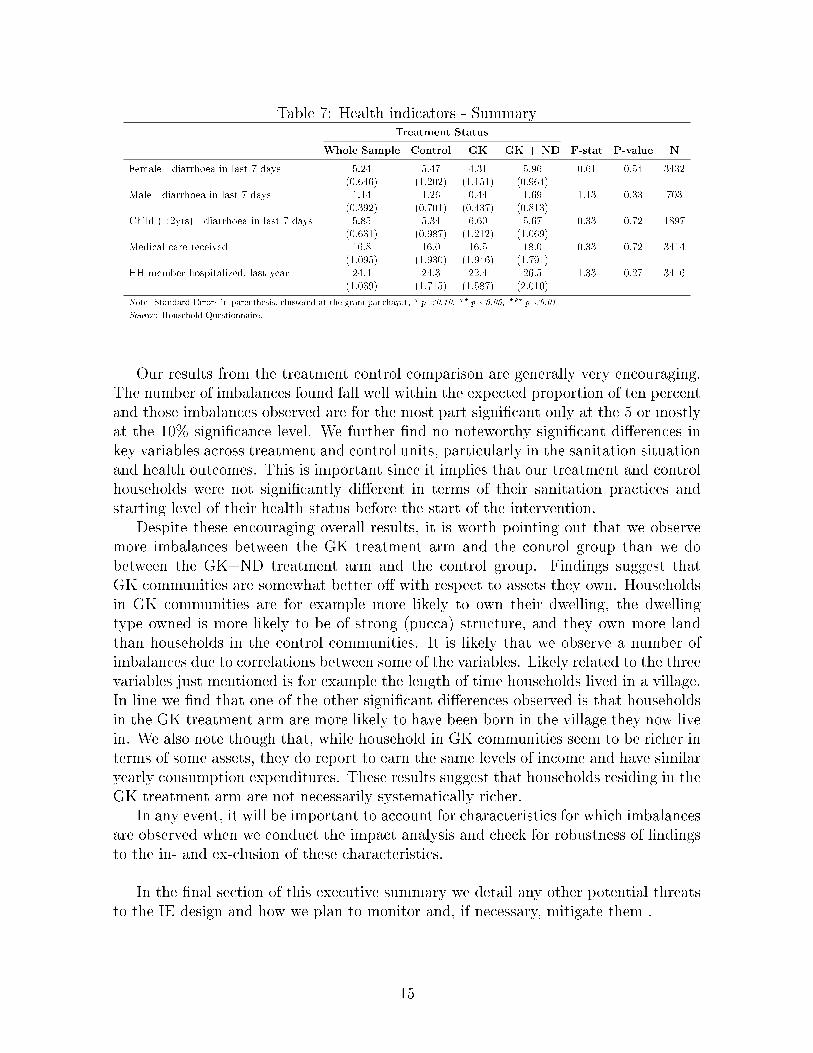
Table 7: Health indicators - SummaryTreatment Status


Female - diarrhoea in last 7 days 5.24 5.47 4.31 5.96 0.61 0.54 3432(0.646) (1.202) (1.151) (0.964)

Male - diarrhoea in last 7 days 1.14 1.26 0.44 1.69 1.13 0.33 703(0.392) (0.701) (0.437) (0.813)

Child (<2yrs) - diarrhoea in last 7 days 5.85 5.34 6.60 5.67 0.33 0.72 1897(0.631) (0.987) (1.212) (1.069)

Medical care received 16.8 16.0 16.5 18.0 0.33 0.72 3414(1.095) (1.930) (1.946) (1.791)

HH member hospitalized, last year 24.4 24.3 22.4 26.5 1.33 0.27 3416(1.039) (1.715) (1.587) (2.010)



Our results from the treatment control comparison are generally very encouraging.The number of imbalances found fall well within the expected proportion of ten percentand those imbalances observed are for the most part signi�cant only at the 5 or mostlyat the 10% signi�cance level. We further �nd no noteworthy signi�cant di�erences inkey variables across treatment and control units, particularly in the sanitation situationand health outcomes. This is important since it implies that our treatment and controlhouseholds were not signi�cantly di�erent in terms of their sanitation practices andstarting level of their health status before the start of the intervention.

Despite these encouraging overall results, it is worth pointing out that we observemore imbalances between the GK treatment arm and the control group than we dobetween the GK+ND treatment arm and the control group. Findings suggest thatGK communities are somewhat better o� with respect to assets they own. Householdsin GK communities are for example more likely to own their dwelling, the dwellingtype owned is more likely to be of strong (pucca) structure, and they own more landthan households in the control communities. It is likely that we observe a number ofimbalances due to correlations between some of the variables. Likely related to the threevariables just mentioned is for example the length of time households lived in a village.In line we �nd that one of the other signi�cant di�erences observed is that householdsin the GK treatment arm are more likely to have been born in the village they now livein. We also note though that, while household in GK communities seem to be richer interms of some assets, they do report to earn the same levels of income and have similaryearly consumption expenditures. These results suggest that households residing in theGK treatment arm are not necessarily systematically richer.

In any event, it will be important to account for characteristics for which imbalancesare observed when we conduct the impact analysis and check for robustness of �ndingsto the in- and ex-clusion of these characteristics.

In the �nal section of this executive summary we detail any other potential threatsto the IE design and how we plan to monitor and, if necessary, mitigate them .

15

Signi�cant risks to IE design

At this stage of the project we perceive that the risks to the IE design are low on thedata collection side: We were able to collect our key indicators satifactorily, and wehave a high response rate to our surveys. We describe data collection problems we facedin Section 4.5, but believe that we were able to solve these in the process in a way thatwould not signi�cantly a�ect our design.

Higher (albeit not 'high') risks are identi�ed with respect to take-up of treatmentand contamination. We present these in Section 4.2 and reproduce here a slightlyshortened version of our �ve potential sources of concern:

1. There could be non-compliance with the randomisation by �eld and/orbranch level sta� of the implementing institutions. To prevent this, the researchteam has visited each of the implementing partner's �eld o�ces to give an in-depth training about the research to all stakeholders involved . Moverover, ourimplementing partner has programmed into their management information systemthat sanitation loan applications from control areas cannot be processed. If thisis tried, head o�ce receives a warning. That means that it is technically notpossible for anyone in the control GPs to receive any sanitation loans from ourimplementing partner. This will also be monitored using GK loan monitoringdata (see Section 4.4.6).

2. Contamination in our design might arise through sanitation information spillingover to neighbouring GPs, which may be control GPs. To be able to account forthis, we will collect information on possible interactions between neighbouringGPs, e.g. common markets, and common branch level GK meetings, characteris-tics of GK branch o�cers, and distances between GPs.

3. Other programs (particularly by the GoI) could intensify their e�orts at improv-ing sanitation infrastructure across study areas and thereby increase sanitationdensity in our control GPs. To some extent, this is not a problem for out evalua-tion design, as long as the government's e�orts are similar across both treatmentand control GPs, and as long as the government does not manage to get toiletsto all of the households in the control group. As described in Section 3.4, theobjective of the intervention is to complement government's e�orts rather thansubstituting for it. In our context - and in fact in most other evaluations ofdevelopment impact - control communities represent cases of �business-as-usual�government activity, rather than �doing nothing� (Ravallion 2008). The impactwe are interested in relates to the contributions of GK and ND's activities in

addition to the government's program. However, if the government scales up itse�orts to the extent that most households in the control group acquire a toilet,the potential for impact from ND and GK is reduced. Even in that case, however,we may still expect there to be an impact on toilet quality rather than toiletownership. Section 3.4 above lists various channels through which we think GKand ND can make a di�erence despite the accelerated e�orts that are being madeby the government. Moreover, the results of the two rapid assessment surveys

16

which will be carried out between baseline and midline will allow us to monitorthis potential risk.

4. In terms of attrition, we anticipate low attrition among GK clients given theirlong-standing relationship with GK. To reduce attrition particularly among non-clients for all surveyed households, we will collect mobile phone numbers of house-hold members and contact details of relatives and friends who are likely to knowof their whereabouts if they move. As will be discussed below, our baseline �nd-ings show that only around 4% of the households in our sample reported to havemigrated in the year prior to the survey. This is consistent with other studies inareas near our study area, which have encountered relatively low attrition rates,driven predominantly by migration (at 3-4%, see for example Mahal et al 2012).Moreover, our baseline results show that more than 97% of all households reportit to be unlikely that they will have moved in a year from now.

5. We might have a threat to our power given unanticipate policy changes by ourimplementing partner which a�ect loan eligibility. Right after the baseline datacollection had taken place, a change was introduced which allows only clients thathave been with the organisation for at least one year to receive a sanitation loan.As we describe in the body of this document, we will monitor this risk using loanuptake data (see Section 4.4.6 for more information). Once the programme hasbeen running for some time, we will be able to judge whether this change is aserious risk to power or not. The planned rapid assessment will additionally helpin this process.

6. There is a possibility that some of the kendras that are part of our study groupclose down between baseline and endline, which would imply a reduction in oure�ective GK sample size. This risk will be followed up very closely by examiningthe GK monitoring data.

7. Finally, we note that there are currently some unde�ned parameters around theimplementation of the (primary) health insurance component, which is crucialfor the second part of the study. The coming months will focus on narrowing downthe necessary steps and putting things for this component in place.

17

2 Introduction

Poor sanitation has obvious implications for public health and provision of safe sanita-tion has thus been recognized to be an indispensable element of disease prevention andprimary health care programs (e.g. the Declaration of Alma-Ata, 1978). Moreover, lackof safe sanitation is acknowledged to a�ect broader outcomes such as productivity andinvestment, which ultimately constrain economic growth (WSP, 2010). Nonetheless,there has been weak overall investment in improving sanitation infrastructure in poorcountries, evident from the fact that the Millennium Development Goal (MDG) onsanitation fell short of its target to halve the 1990 level of proportion of people withoutsustainable access to sanitation by 2015 (WHO-UNICEF, 2014).

Poor sanitation is a particularly important policy issue facing India, which accountsfor over half of the 1.1 billion people worldwide that defecate in the open (WHO-UNICEF, 2014). The Indian Government (GoI) has shown strong commitment toimproving sanitation, establishing the Total Sanitation Campaign in 1999, which wasrevamped in 2012 as the Nirmal Bharat Abhiyan (NBA) policy and most recently inOctober 2014 as the Swachh Bharat Mission (SBM). This policy aims at attaining 100%Open Defecation Free India by 2019 (GoI, 2014). However, despite these e�orts, safesanitation uptake and usage remains low. For instance, the 2011 Indian census reportsthat almost 50% of Indian households do not have access to a private or public latrine.This highlights the need for novel approaches to foster the uptake and sustained usageof safe sanitation in this context.

In light of these challenges, researchers from the Institute for Fiscal Studies, withsupport from the FINISH Society9, teamed up with the Water and Sanitation Program(WSP), Grameen Financial Services Pvt. Ltd. (henceforth referred to by its popularname 'Grameen Koota' of just 'GK') and Navya Disha (ND), to shed light on (i)innovative ways of increasing the uptake and usage of safe sanitation practices and(ii) provide evidence on the links and interactions between improved sanitation andhealth insurance. It does so by studying two distinct but topically-linked projects inrural Maharashtra, India: The smaller of these two projects is designed to explore thepotential of providing primary community health insurance for free to communities thatreduced open defecation conditional on sustaining this tendency. This component ofthe project is still in the development phase and will hence not be covered in this report.The second project, which includes a full randomised controlled trial impact evaluation,analyses two variants of an intervention, which in achieving sustainable improvementsin household and community sanitation, aims to improve the health and reduce healthexpenditures of the poor in rural India � potentially re�ected in lower health care claimsvolumes.

More speci�cally, the interventions o�er on the one hand sanitation loans to membersof women groups which can be used to construct toilets or water connections and on theother hand a package of awareness creating activities - e.g. street plays, wall banners,

9FINISH stands for Financial Inclusion Improves Sanitation and Health and the programme is aresponse to the preventable threats posed by poor sanitation and hygiene. It was launched in 2009as a new approach to improve the health and welfare outcomes of poor households. This approachfocuses on �nancial tools to improve the sanitation situation in both rural and urban areas in India.

18

sanitation and hygiene workshops, etc. The rationale of these interventions is to improvetoilet uptake and usage by i) lifting credit and liquidity constraints faced by poorerhouseholds and ii) improving awareness about the usefulness and cost-e�ectiveness oflow cost safe sanitation. The longer term objective is to improve a wider set of outcomesincluding health, income, etc.

A rigorous impact evaluation, based on a randomised control trial, will evaluate therelative impact of these two interventions over a two-year period. The evaluation designincludes a baseline survey before the intervention, as well as a midline survey after oneyear of the program and an endline survey after two years of the program. The studywill concentrate on 120 GPs in two districts (Latur and Nanded) in rural Maharashtra,India.

This report provides details of the sampling methodology and the baseline datacollection process. It also describes our study population with regard to a wide spectrumof community, household and individual household member characteristics. Whilstdoing so, we test for any systematic di�erences between treatment and control groupswhich could undermine the validity of our randomised evaluation design.

3 Project description

3.1 Project background

According to the most recent Joint Monitoring Program report for Water and Sanita-tion (WHO-UNICEF, 2014), sanitation has signi�cantly improved globally: Sanitationcoverage has increased from 49% in 1990 to 64% in 2012 and open defecation has fallenfrom 24% to 14%, respectively. Behind these average numbers, however, lie stagger-ing disparities across countries. Whereas countries like Ethiopia, Cambodia and Nepalexperienced noteworthy successes, some countries are lacking far behind. As shown inFigure 2, India currently tops the world ranking of the number of people still practic-ing open defecation in 2012 (WHO-UNICEF, 2014). More than half of the 1.1 billionpeople worldwide who practice open defecation live in India, which is more than tentimes the number of any other country. Proportiately, this number amounts to 48% ofthe total Indian population.

Lack of improved sanitation can have disastrous consequences. Recent studies bySpears [2012] and Kumar and Vollmer [2012] suggest that improved sanitation decreasesthe risk of contracting diarrhea and associated infant mortality. Open defecation hasalso been associated with stunting among children and impaired cognitive develop-ment (Pruss-Unstun et al., 2008; Humphrey, 2009; Dangour et al., 2013; Spears, 2013).Moreover, lack of safe sanitation is acknowledged to a�ect broader outcomes such asproductivity and investment, which ultimately constrain economic growth. The Waterand Sanitation program (WSP, 2010) of the World Bank (WB) estimates that poor san-itation costs India US$48 per person per year, the equivalent of 6.4% of the country'sgross domestic product (GDP) annually.

To address these challenges, in 1999 the Government of India (GoI) launched itsambitious Total Sanitation Campaign (TSC), which has been described as the largest

19

Figure 2: Top 10 countries with the highest numbers of people (in millions) practicingopen defecation in 2012

sanitation initiative in the world (Hueso and Bell, 2013). The TSC included communityawareness campaigns, provision of sanitation funds to communities to build sanitationinfrastructure in public places such as schools and hospitals, and provision of small sub-sidies to individual below-poverty-line (BPL) households after they could demonstratehaving constructed their own toilets.

In the year 2003, the TSC introduced the Nirmal Gram Puraskar (NGP) or 'clean vil-lage' award scheme. This scheme o�ers rewards (ranging from US$1,000 to US$10,000,depending on the population size) to local governments that achieve 100 percent opendefecation free status and ensure total sanitation. Since its introduction in 1999, theTSC program has been redesigned twice: once in 2015 to become the Nirmal BharatAbhiyan (NBA) policy and most recently in October 2014 to become the Swachh BharatMission (SBM). In essence, each reform implied an expansion of range rather than aparadigm change, including for example increases in the subsidy amounts.

Studies analysing the e�ectiveness of �nancial incentives for the continued usage ofpreventive health behaviors �nd that though successful in promoting simple behaviorssuch as one-time visits for preventive health checks, there is little supportive evidenceof such incentives generating long-term changes. In the context of sanitation, Spears[2012] shows that the NGP prize in India has been successful in driving sanitationuptake, but little is known about the e�ectiveness of �nancial incentives in promotingsustained sanitation usage. Indeed, available evidence suggests that the NGP prize isnot e�ective in sustaining long term sanitation usage (UNICEF, 2008). Recent �guresfrom the Indian Ministry of Drinking Water and Sanitation 2012 baseline survey showthat 39% of households reported to own toilets, but that two out of 10 of those toiletsare reported to be out of use. Critics argue that the government programs yield poorlyconstructed toilets and that they do not su�ciently address the population's insu�cientdesire to construct, maintain and use toilets. Moreover, in other contexts some haveargued that government subsidies do not always reach the poor (Jenkins and Scott,

20

2007; Jenkins and Sugden, 2006).Possible constraints to health investments in general and toilet adoption and usage

in particular include a lack of information, and credit and liquidity constraints. Forinstance, Pattanayak et al. [2009] provides evidence that the former is an importantconstraint hampering sanitation uptake: Latrine ownership in a rural Indian setting in-creased by 30 per cent on the provision of information, while consistent with the latterconstraint, Tarozzi et al. [2011] �nd in a study in rural Orissa, that uptake of mosquitonets jumped from 2% to 52% when micro-loans were made available for their purchase.The intervention subject to evaluation in this study will relax both of these constraintsby providing information on the bene�ts of safe sanitation and available low cost sani-tation technologies and making available micro-loans for sanitation construction.

The �rst component of our intervention, i.e. the provision of sanitation loans, willbe delivered by Grameen Financial Services Pvt. Ltd., popularly known as GrameenKoota (GK). GK was founded in 1999 as a project of nongovernmental organisationT Muniswamappa Trust and has since become an independent non-banking �nancecompany (NBFC). GK is actively engaged in the micro�nance sector in Karnataka,Maharashtra and Tamil Nadu states and provides a range of �nancial (primarily mi-crocredit and micro insurance) and non-�nancial services to groups of women of age 19to 55 years in rural and semi-urban low income households.10

Grameen Koota provides a wide range of loans, including emergency loans, festivalloans, medical loans, income generating activity loans, etc. Since 2009, GK startedproviding microcredit for the construction of sanitation systems to its clients.

Understanding that providing �nance only is not su�cient to reach high sanitationdensity, and that hygiene promotion also plays an essential role, GK further createdan NGO, the Navya Disha (ND) Trust, which helps its clients understand the bene-�ts of safe sanitation and available toilet technology and infrastructure, the materialsneeded, and procedures for procuring parts, labour, and government approvals. In theintervention subject to evaluation in our study, ND will be in charge of delivering thesanitation awareness creation component.

3.2 Project geographical focus

Our study will concentrate on the south-eastern area of the Maharashtra state, districtsLatur and Nanded (see Figure 3), where GK has branch o�ces. Maharashtra, with itscapital Mumbai, is one of the largest Indian states, counting approximately 100 millionpeople living in almost 44,000 villages (Census, 2011). While this is the second richeststate in the country in terms of per capita income, incidence of poverty remains closeto the national average, implying severe inequalities within the state. According to thelast human development report of Maharashtra (Government of Maharashtra, 2002)�Maharashtra's economy has demonstrated a strong track record of growth and is avisible success story for the rest of the country but its weakness is its uneven distributionof the gains of the growth.�

10As of 2014, GK reported total assets of USD 161 million and a gross loan portfolio of USD 141million outstanding to 543,000 active borrowers (MIX). By February 2015, the number of active clientshad further increased to 863,198 active borrowers.

21

Figure 3: Geographical focus of the study

The study districts Latur and Nanded belong to those areas that have only moder-ately bene�tted from the growth. According to the latest District Level Household andFacility Survey (DLHS-4) collected in 2012-13, these districts face incidences of povertyof on average 35 per cent, only 17% of the households use some type of toilet facilitiesand 40% (77%) of (female) household heads have not attended any school. Access tohealth services is also very poor, with only 13 per cent of villages having a primaryhealth center available in their village and the nearest government hospital being onaverage 63km away.

Figure 4: Location of the 120 study GPs

Within Maharashtra, our study will cover 120 GPs located in Latur and Nandeddistricts, a complete list of which is provided in Appendix D. Figure 4 shows the locationof each of the study GPs, with an indication of their 'treatment' status in the study(this will be discussed in detail in Section 4 below).

22

These GPs were randomly selected from the total list of rural GPs that are servicedby �ve branches of Grameen Koota in Maharashtra (i.e. where they have a clientbase) but where no sanitation loans or health insurance had been provided and no NDactivities had taken place to date. Section 4.3.1 describes the selection of these GPsin more detail. The selected �ve branches lie in administrative blocks Degloor, Udgir,Ahmadpur, Naigaon and Nilanga.

According to the 2012 baseline survey conducted by the Indian Ministry of DrinkingWater and Sanitation (Baseline survey, 2012), on average 27.4% of households in ourstudy GPs reported to have a toilet in 2012. Note that this number hides informationon actual usage of the toilet, which is an additional indicator we will consider in ourstudy.

Note also that the set of GPs in which GK is operational is a result of a carefulselection exercise by GK head quarters (e.g. has to be politically stable, certain numberof women, etc) and can therefore not be considered representative for the state ofMaharashtra.

3.3 Description of the intervention

The �rst year of our study will focus on the evaluation of the relative impact of twovariants of a sanitation intervention:

1. The �rst intervention is the provision of sanitation loans up to Rs. 15,000 toGrameen Koota clients, against an interest rate of 22% per annum over a 2-yearrepayment period. These loans can only be used for the construction of a newtoilet or for repair of an old toilet. In addition, GK o�ers water connections loansof amounts up to Rs. 5,000. Sub-section 3.3.1 discusses further details of theseloans (e.g. loan caps, eligibility criteria, etc).

2. The second intervention, which is a variant of intervention 1, combines the pro-vision of sanitation loans to GK clients with a package of sanitation awarenesscreation activities run by Navya Disha. Education and awareness creation on san-itation issues are targeted to GK sta�, GK members and the broader community.This is done through community-level activities such as theatre plays, wall ban-ners and information sessions for GK clients at their weekly joint liability groupmeetings (see below) and GK branch level workshops. Furthermore, ND and GKengage with the sarpanch to gain support for their activities and to strengthensanitation and hygiene awareness. This is important because the GP plays a piv-otal role in the implementation of the GoI sanitation program, the SBM. Lastly,ND organises mason trainings. Sub-section 3.3.2 provides more details about thespeci�c package of awareness creation activities that will be run by ND in ourstudy area.

23

3.3.1 Sanitation loans

Sanitation loan eligibility criteria

Basically any GK clients is eligible to aply for a sanitation loan. There are no collateralrequirement and the only constraint recentlty (in March 2015) introduced is that aclient needs to have been with GK for more than 1 year to be eligible for this loanproduct. To become a GK client, women must be between the ages of 19 and 55 yearsand form into groups of 5-10 members. Multiple such women groups in a GP are thengrouped together to form a so-called GK kendra. The purpose of the kendra is mainlyfor the management of weekly loan repayments which take place at the GP level (seebelow). Each kendra has a maximum of 30 members.

In order to track loan repayments and loan utilisation, each client is required tohold a GK passbook, in which all loan repayments are registered and the results of loanutilisation checks are kept. Sanitation loans are provided for the construction of a newtoilet or for repair of an old one. GK does not put any restrictions on the type of toiletthe bene�ciary decides to build, except that they advise against single pit technologies.GK and ND sta� (see below) are trained to provide advice on di�erent models, but theultimate choice is left to the client.

GK kendra managers, who are in charge of providing funds and collecting repay-ments on a weekly basis, are instructed to provide a sanitation loan only after the clienthas clearly demonstrated her intention to build a toilet, e.g. by having provided spaceand having digged a pit. The kendra managers are in charge of conducting a series ofloan utilisation checks and to note the results of these checks in the kendra member'spassbook. However, at present no sanctions are imposed in case loans are used for anyother purposes. Lack of reinforcement can have implications for actual loan usage andneeds to be taken into consideration in the analysis of our study.

Sanitation loan caps and costs

Today, GK sanitation loans cover a maximum amount of Rs. 15,000 (which is consid-ered su�cient to build a quality toilet), charging a 22% interest rate per annum at adeclining balance over a 2-year repayment period. This makes sanitation loans rela-tively attractive, as the amount received is higher than any other type of loan providedby GK and the interest rate is lower than those charged for any other loans (typically25%).

In addition to the interest, loan costs include a processing fee of 1.1% of total amountand Rs. 306 life insurance premium. Each client can obtain one sanitation loan only,but clients can take an additional water connection loan of Rs. 5,000. The overall loancap on total loans taken from GK is Rs. 35,000 for new clients and Rs. 40,000 forwomen who have been client for longer than 3 years. The overall loan cap on totalloans from any micro�nance institution in India currently stands at Rs. 100,000.

24

Sanitation loan disbursement and repayment process

The process from sanitation loan application to money disbursement can take any timeup to 4 weeks. Like most of GK's loans, the GK client is required to physically goto the GK branch o�ce for sanitation loan disbursement11. Clients repay the loan ona weekly (Rs. 179) or bi-weekly (Rs. 358) basis during their weekly meetings in thevillage with a GK kendra manager. Loan groups are held jointly liable for repaymentof a loan. That means that if one group member defaults on any loan, no one else inthe loan group can take out a new loan.

3.3.2 Sanitation awareness creation activities

Whereas sanitation loans are targeted at and available only for GK clients, Navya Dishatargets education and awareness creation more widely, i.e. to GK members, GK sta�,GP o�cials and any other residents of the GP community.

First of all, ND organises one-o� GK branch o�ce trainings (one for each ranche),through which GK branch managers and kendra managers receive (i) information aboutND's activities, (ii) get trained about the details of the sanitation loan procedures,(iii) get an awareness training on the importance of hygiene and sanitation (by useof IEC material), (iv) obtain information about the government's SBM scheme, (v)receive a brief introduction to di�erent available sanitation technologies and (vi) receiveawareness creation handouts for distribution in the GP (see Figure 5 for an example ofan IEC handout).

Figure 5: IEC handout

ND sets up separate one-o� trainings but of similar content for GK clients at theirweekly kendra meetings in the GP (one for each kendra). Similarly, they organisemason trainings (one for all masons of 2-3 GPs combined) where again similar materialis covered, but in addition the masons receive an in-door technical training on thedi�erent sanitation technologies (using demonstration material such as a pan and a pintrap and display of demonstration videos). Through an interactive toilet costing session,ND also creates awareness about the actual costs of di�erent sanitation technologies

11Exceptions where loans can be disbursed in the village include emergency loans (Rs. 1,000),festival loans (Rs. 1,000) and medical loans (Rs. 2,000).

25

with the aim of convincing the audience that Rs. 15,000 should be more than su�cientto construct a good quality and sustainable toilet.

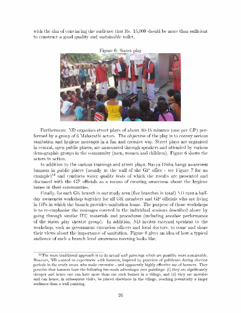
Figure 6: Street play

Furthermore, ND organises street plays of about 30-45 minutes (one per GP) per-formed by a group of 6 Maharathi actors. The objective of the play is to convey serioussanitation and hygiene messages in a fun and creative way. Street plays are organisedin central, open public places, are announced through speakers and attended by variousdemographic groups in the community (men, women and children). Figure 6 shows theactors in action.

In addition to the various trainings and street plays, Navya Disha hangs awarenessbanners in public places (usually at the wall of the GP o�ce - see Figure 7 for anexample)12 and conducts water quality tests of which the results are presented anddiscussed with the GP o�cials as a means of creating awareness about the hygieneissues in their communities.

Finally, for each GK branch in our study area (�ve branches in total) ND runs a half-day awareness workshop together for all GK members and GP o�cials who are livingin GPs in which the branch provides sanitation loans. The purpose of those workshopsis to re-emphasise the messages covered in the individual sessions described above bygoing through similar IEC materials and procedures (including another performanceof the street play theatre group). In addition, ND invites external speakers to theworkshop, such as government extension o�cers and local doctors, to come and sharetheir views about the importance of sanitation. Figure 8 gives an idea of how a typicalaudience of such a branch level awareness meeting looks like.

12The more traditional approach is to do actual wall paintings which are possibly more sustainable.However, ND wanted to experiment with banners, inspired by practices of politicans during electionperiods in the study areas, who make extensive - and apparently highly e�ective use of banners. Theyperceive that banners have the following two main advantages over paintings: (i) they are signi�cantlycheaper and hence one can have more than one such banner in a village, and (ii) they are movableand can hence, in subsequent visits, be placed elsewhere in the village, reaching potentially a largeraudience than a wall painting.

26

Figure 7: Wall banner

Figure 8: Branch level awareness workshop

3.4 Intervention objectives

As described in Section 3.1, the GoI has recently strengthened its sanitation e�ortswith the aim of attaining a 100% Open Defecation Free India by 2019 (GoI, 2015). Thegovernment's large-scale sanitation programs are active throughout India, including inour study area. The purpose of the intervention subject to evaluation in this report isto complement rather than subsitute government's e�orts and should be considered inthat light.

Just like the GoI, the key objectives of GK and ND are, in the �rst instance, toimprove awareness about safe sanitation and to boost toilet construction and usage.Increased access to safe sanitation, in turn, is expected to positively impact on healththrough reduced parasitic/gut infections and reduced illness symptoms such as diar-

27

rhoea. Some studies suggest that health impacts can only be observed if the entirevillage becomes open defecation free (Pearson, 2013). However, so far this evidence issuggestive rather than conclusive. This will be examined more closely as part of thisstudy.

In the longer term, better health of young infants is expected to yield improvedchild growth and development, increased school attendance and increased productiv-ity. Ultimately, improved sanitation practice is expected to yield more stable incomestreams and to reduce intergenerational transmission of poverty. Figure 9 summarisesthe project's short-term and longer-term objectives.

Figure 9: Project objectives

In spite of the government's accelerating e�orts to boost access to sanitation through-out India, we expect there to be a role for GK and ND in assisting the government inthe achievement of their targets, for the following reasons:

• ND activities include the provision of information about the existence of the SBMprogram to villagers and what actions eligible households can take to get accessto the government subsidies

• The government subsidies target speci�c types of households, primarily thoseliving below the poverty line and other marginalised groups. Other demographicgroups in need of �nancial support may reach out to sanitation loans to pay fortoilet construction.

• Government subsidies are disbursed only after the household can demonstratehaving built a toilet. Households in need of money up-front may not be able toconstruct a toilet without �rst acquiring a sanitation loan.

28

• The government subsidy currently stands at Rs. 12,000. Any additional expensesneed to be covered by the households themselves.

• Moreover, an eligible household can reveive a government subsidy only once. Incase a household received a subsidy in the past, when the magnitude of the sub-sidies were much lower, it may still require a loan, for instance to upgrade its oldtoilet.

• Given the magnitude of the scale of India, and the speed at which the SBM pro-gram is being rolled out, this naturally poses a challenge to the e�ciency of theprogram and the accuracy of the monitoring process. WSP (2011) points out thevarious challenges involved with an exponential increase in the number of appli-cants for NGP awards and makes a set of valuable recommendations. In general,we expect there to be some delays in the distribution of government sanitationsubsidies to some eligible households. Although the government subsidies may befree whereas loans come at a cost in the form o�nterest payments, the subsidiesmay be relatively more di�cult to come by whereas the loans are more readilyavailable.

• WSP (2011) notes that experience has shown that there is an inverse relationshipbetween government program scaling up and quality. ND awareness creatingactivities include an emphasis on the importance of high quality and safe toiletsand hence may complement the government's program in terms of improving thequality of the toilets that are being built either through government subsidies orthrough sanitation loans.

29

4 Evaluation design

This evaluation will be based on a 'randomised control trial'. In what follows, we willprovide details on the evaluation design, and highlight how it will enable us to evaluatethe relative impact of each of the two project components described above. We willalso consider potential sources of contamination of the design and discuss the actionswe will take to mitigate those risks.

4.1 Randomised evaluation approach

While our implementing partner GK was already operating in our study area prior tothe start of the project, neither the sanitation loans, nor the ND awareness creationactivities were available to their bene�ciaries nor to the communities their clients areliving in. The interventions analysed in this study have been introduced during thecourse of this project in a manner that both facilitates implementation and allows usto rigorously assess the impact of the interventions. Speci�cally, the interventions havebeen randomly introduced in some of the 120 GPs and not in others.

Randomly providing sanitation services to some (`treatment group') and not toothers (`control group') helps the impact evaluation process as it ensures that prior tothe intervention treatment and control individuals are, on average, statistically the samein terms of observable and unobservable characteristics. In other words, randomisationremoves `selection bias' (i.e. pre-existing di�erences between the treatment and controlgroups, such as di�erent levels of education, that might make one household more likelyto follow hygiene practices than another). In theory, this should ensure that when wecompare the outcomes of treatment and control groups at the end of the intervention,the only di�erence is due to exposure to intervention activities and not due to anyunobserved di�erences between them. It allows one to obtain unbiased e�ects of thetreatment on outcomes of interest.

While the need for randomisation is clear from a methodological point of view,one should also take its ethical implications into account. In particular, during theperiod of the experiment (approximately two years), some areas will be excluded fromthe GK and/or ND sanitation services although they would qualify to be covered inprinciple. Here it should be noted that implementing agencies would not be able to roll-out the programme across all areas of operation within the time of the evaluation. Inpractice, implementing agencies work in phases � covering one area, and then extendingto another and so forth. We simply exploit the existing capacity constraints during theexpansion phase of the programme to de�ne the control groups.13

The interventions were randomised at the GP level (rather than at the householdor individual level), for three key reasons: First, GPs play a key role in implementing

13While GK is theoretically able to roll-out a new loan product in all branches at the same time,experience shows that these are typically not marketed until loan o�cers were trained on the productwhich, in the case of sanitation loans, is done by ND sta�. ND's resource capacity hence basicallyimplies a phased-in approach. However, in the context of this study, the phase-in of loan productswas made more explicit and was, in fact, held back more than originally envisioned, due to delays inevaluation activities.

30

government and state policies related to sanitation; second, because of intra-communityspillovers and feedback e�ects associated with sanitation adoption; and �nally becausethe intervention involves activities open to all GP members (e.g. street plays, engage-ment with the sarpanch, etc). Randomising at the individual or household level wouldtherefore lead to the contamination of the control group, thereby leading to biasedestimates.

Speci�cally, the 120 GPs in our study area (choice of which is described in Section4.3.1 below and the list of GPs included is shown in Appendix ??) were more or lessequally allocated to three evaluation groups:

1. Those that will receive both ND awareness activities and GK sanitation loans(ND + GK);

2. those that will only receive GK sanitation loans (GK); and

3. a control group that will receive no GK or ND services (Control).

The experimental design is summarised in Table 8. The reason why we do not have anequal distribution lies in the fact that randomisation was strati�ed at the level of theGK branch and by GP size (see Section 4.3.1).

Table 8: Evaluation armsControl GK GK + ND Total

41 40 39 120

All 120 GPs (including those in the control group) will continue to receive a standardpackage of services from GK, which includes access to income generating micro-loans,and other loans o�ered by GK. This is important as it implies that our evaluationassesses the impact of providing sanitation activities (through GK and ND) over and

above micro�nance loans for other purposes. This �rst reason for this choice is op-erational: GK (as other MFIs providing sanitation loans) see sanitation loans to baregreater risks than non-income generating activities and hence want to know their clientsbetter before they provide this new loan product (their recent policy change to onlyprovide loans to clients that were with them for at least a year re�ects this concern).The second reason is more important from our evaluation perspective and is that wewould not want sanitation loans to crowd out other investment opportunities (whichcould also a�ect outcomes of interest).

This experimental design will allow us to assess 1) the impact of the provision ofsanitation micro-loans, by comparing the outcomes of the `GK' treatment arm withthe outcomes of the `Control group'; and 2) the additional impact of ND activities bycomparing the outcomes of the households in the `ND + GK' treatment arm with theoutcomes of the households living in the `GK' treatment arm.

Finally, note that a large part of our analysis will be conducted at the individualor household level, and so all estimates will be identi�ed through an intention-to-treatanalysis, based on the initial community-level randomisation, regardless of whether ornot an individual or household actually takes up the intervention (sanitation). Though

31

conservative, this will ensure that estimates are not subject to bias arising from se-lection, i.e. those that choose to build safe sanitation may be di�erent from otherhouseholds in the community. Moreover, all households in treated GPs will receivesome aspect of the intervention (information for all, and credit for some), making theintention-to-treat analysis best suited for our purposes.

We conducted a power analysis to determine our sample size and understand theminimum detectable e�ects we can achieve. For this power analysis, which was doneat the time of writing the proposal, we had to make a number of assumptions, some ofwhich we are now able to re�ne and update with baseline data on our study populationat hand. The key outcome discussed in the power analysis in the submitted proposalwas the number of health insurance claims. We will not be able to update this analysisuntil the health insurance component is implemented. We will therefore update onlythe power analysis related to sanitation uptake. Details are provided in Appendix A.To summarize, the actual baseline mean is higher than was anticipated. The raw ICCis 0.143, which is reduced to 0.105 by taking household characteristics into account.Given this mean and ICC and keeping all other assumptions constant, we will be ableto detect increases of about 10.9-12.3 percentage points. This assumption compareswell with our preferred scenario discussed in the proposal and we conclude that for thetime being, we antitipate that our design will allow us to detect expected minimumimpacts.

4.2 Potential risk factors

There are four potential sources of contamination to the evaluation design that are ofconcern:

1. There could be non-compliance with the randomisation by �eld and/or branchlevel sta� of the implementing institutions. To prevent this, the research teamhas visited each of the GK branches and the ND o�ce to give an in-depth trainingto all stakeholders involved about the research design and the importance of notdoing any sanitation related activities in the control area. Post this training,branches prepared posters listing all communities in which no loans should beprovided, for everyone to see and be reminded of when coming to the o�ce.Picture 10 shows an example. Moverover, GK head o�ce has provided additionalmonitoring of branch sta� and has disabled sanitation loan applications fromcontrol areas in their central management information system. That means thatit is technically not possible for anyone in the control GPs to receive any sanitationloans. This will also be monitored using GK loan monitoring data (see Section4.4.6).

2. Other programs (particularly by the GoI) could intensify their e�orts at improv-ing sanitation infrastructure across study areas and thereby increase sanitationdensity in our control GPs. To some extent, this is not a problem for out evalua-tion design, as long as the government's e�orts are similar across both treatmentand control GPs, and as long as the government does not manage to get toilets

32

Figure 10: Reminder of control GPs in GK branch o�ce

to all of the households in the control group. As described in Section 3.4, theobjective of the intervention is to complement government's e�orts rather thansubstituting for it. In our context - and in fact in most other evaluations ofdevelopment impact - control communities represent cases of �business-as-usual�government activity, rather than �doing nothing� (Ravallion 2008). The impactwe are interested in relates to the contributions of GK and ND's activities in

addition to the government's program. However, if the government scales up itse�orts to the extent that most households in the control group acquire a toilet,the potential for impact from ND and GK is reduced. Even in that case, however,we may still expect there to be an impact on toilet quality rather than toiletownership. Section 3.4 above lists various channels through which we think GKand ND can make a di�erence despite the accelerated e�orts that are being madeby the government. Moreover, we integrated in our design two rapid assessments,approximately 4 and 8 months after the baseline survey. These rapid assessmentswill collect information on sanitation uptake in both control and treatment com-munities, providing us a picture of uptake in both study groups and hence allowingus to monitor this potential risk.

3. Contamination in our design might arise from sanitation information spillingover to neighbouring GPs, which may be control GPs. To be able to accountfor this, we will collect information on possible interactions between neighbouringGPs, e.g. common markets, and common branch level GK meetings, characteris-tics of GK branch o�cers, and distances between GPs. However, in general thisrisk is assessed as low given signi�cant distances between GPs.

4. In terms of attrition, we anticipate low attrition among GK clients given theirlong-standing relationship with GK. To reduce attrition particularly among non-clients for all surveyed households, we will collect mobile phone numbers of house-hold members and contact details of relatives and friends who are likely to knowof their whereabouts if they move. As will be discussed below, our baseline �nd-

33

ings show that only around 4% of the households in our sample reported to havemigrated in the year prior to the survey. This is consistent with other studies inareas near our study area, which have encountered relatively low attrition rates,driven predominantly by migration (at 3-4%, see for example Mahal et al 2012).Moreover, our baseline results show that more than 97% of all households reportit to be unlikely that they will have moved in a year from now.

5. Finally, we note that there are currently some unde�ned parameters around theimplementation of the (primary) health insurance component, which is crucialfor the second part of the study. The coming months will focus on narrowing downthe necessary steps and putting things for this component in place.

In addition to this list of potential contamination concerns, the change in GK's policyin terms of eligibility for loans (allowing only clients who stayed with GK for a year)might reduce our power to detect impacts. We purposely sampled GK client households(details are provided in the following section) but did not take into account how longthey have been with GK. Ideally, we would have liked to sample only amongst clientswho were for at least a year with GK. However, since the policy change happened onlywhen our baseline data collection was already completed, we were not able to take thisinto account. The extent to which this policy change a�ects the study sample is unclearat the moment. Based on loans provided in study areas in February and March of thisyear, we know that roughly 20-30% of sampled clients are with GK for less than oneyear. However, for one, this data does not cover all sampled clients and second, thepolicy is not yet followed strictly (i.e. some of the new clients have already received asanitation loan). We will use GK's loan data, which we expect to receive roughly everytwo months, to monitor this issue closely.

Lastly, there is a possibility that some of the kendras that are part of our studygroup close down between baseline and endline, which would imply a reduction in oure�ective GK sample size. This risk will be followed up very closely by examining theGK monitoring data.

4.3 Sample selection strategy

4.3.1 Selection and randomisation of study GPs

The study took o� by determining the set of 120 GPs to consider as part of the evalua-tion and then to randomly allocate each of these to the three di�erent evaluation arms.This Section provides details on this selection and randomisation process.

The �rst step was to identify the set of feasible study GPs. A feasible study GPwas de�ned as one where (i) GK had operations (i.e. active GK kendra groups) and(ii) where neither sanitation nor health insurance activities had been undertaken byGK in the past. Through interactions with GK, we identi�ed areas where they hadneither sanitation nor health insurance activities ongoing (and did not have them inthe past), but where they were planned (and/or considered feasible) in the near future.During the discussion six blocks (corresponding to branches) within three districts inMaharashtra, namely Solapur (the block of Akkalkot), Nanded (Degloor, Naigaon) and

34

Latur (Ahmedpur, Nilanga, Udgir) were identi�ed. Below it will become clear whylater it was decided to drop district Solapur from the study.

GK does not keep information on the gram panchayat (our unit of randomisation)that the kendra members live in (which corresponds to where the Kendra is registered).This information was however crucial in identifying feasible study GPs (since not allGPs in the operating area of the branches are necessarily covered by GK). The next steptherefore was to get a list of GK kendra groups that GK had in these branches.Withthe list of kendras at hand, kendras were matched to the GPs they were located in.During the process, kendras located in urban areas were excluded (as they would byde�nition not be in a GP and hence not be eligible to become part of the study).Approximately 80% of all kendras were matched to GPs based on their names using2001 census information, and Google (i.e. searching for the Kendra name to see if itwas associated with a village with a di�erent name to the GP name) where possible.The remaining kendras needed to be matched to their GPs with the input from GKbranch sta�.

The �rst list was compiled in November 2012. Due to project delays the list had tobe updated at multiple times before the baseline survey to account for closing of kendras,opening of new kendras and also some matching mistakes were detected (even after thelisting exercise had taken place, which has some implications, as will be explained inSection 4.3.2). Once the list was available, it turned out that there was more than asu�cient number of GPs in just �ve of the six branches. After consultation with allstakeholders in this study, it was decided to drop one branch. This was done for twomain reasons: (i) to ease logistics of data collection and with that reduce data collectioncosts and (ii) to allow GK to start with sanitation activities in the dropped branch14.The selected branch to drop was Akkalkot in Solapur. The �nal list of study brancheswas the following: Degloor, Naigaon, Ahmedpur, Nilanga, and Udgir.

At that stage, the resulting list of feasible GPs included 142 GPs. Since the studydesign only required 120 GPs, this allowed us to additionally drop the largest 5% ofGPs, to reduce the list to 133 GPs. This was useful for two main reasons: (i) it allowedus to reduce the variation of GP size which was quite substantial, and (ii) it againfacilitated data collection logistics, reducing costs. Finally, we randomly seelcted 120GPs out of the list of 133 GPs, conditional on retaining a number of GPs per branchthat was divisible by three (to ensure randomisation across three treatment arms inthe next step). We refer to Table 117 in Appendix D for a list of the �nal set of studyGPs, the administrative blocks in which each of these are located and the GK branchby which there are covered.

The second step was the randomisation of the 120 GPs to one of three evaluationarms (see Section 4.1): Control, GK, GK + ND. Randomisation was strati�ed bybranch and by size of the GP (size in terms of number of households). The reasonfor stratifying by GP size lies in the data collection process which will be described inSection 4.3.2 below. That Section will also explain which GPs were classi�ed as `small'

14The signi�cant project delays implied that GK was only able to start the interventions in studyareas much later than initially envisioned. Dropping one branch was therefore a very welcomed decisionby GK.

35

and which GPs were classi�ed as `large'.15

Table 9 summarises the results of the randomisation to the three evaluation arms,strati�ed by GK branch o�ce and GP size. Table 117 in Appendix D shows for each GPthe evaluation arm that they have been allocated to and provides baseline informationon the number of GK kendras and the number of GK clients living in each of the studyGPs.

Table 9: Random allocation of study GPs to evaluation arms, by branch and size


Ahmadpur Large 2 2 1 5Small 3 2 2 7

Degloor Large 4 4 5 13Small 5 4 5 14

Naigaon Large 5 5 5 15Small 5 5 5 15

Nilanga Large 5 5 4 14Small 4 4 4 12

Udgir Large 5 5 5 15Small 3 4 3 10

Total 41 40 39 120

4.3.2 GP segmentation and listing

An important component of the study design was the implementation of an extensivelisting exercise, the purpose of which was threefold:

• To serve as a sampling frame for the selection of respondents for the baselinesurvey (see Section 4.3.4) - since no up-to-date household level information wasotherwise available. It was important to have a comprehensive and up-to-datesampling frame to ensure we would have a random sample of the whole commu-nity - including households that might have moved in recently, and covering all

15The randomisation process, strati�ed by branch and by GP size, worked as follows: First the GPswere strati�ed into 10 strata: �ve branches and within each branch one stratum for large GPs (morethan 480 households) and one stratum for small GPs (less or equal to 480 households). Randomisationwas done in 2 steps (after drawing a random number for each GP from a uniform distribution): Step 1sorted the data by branch and magnitude of the random number from the highest value to the lowest.Based on this ordering, the �rst N GPs, where N is the largest number of GPs in the stratum that isfully divisible by 3 (e.g. a stratum could have 14 GPs, in which case N would be 12), were assigned insequence to one of the three evaluation arms. For strata where the number of GPs was not divisibleby 3, the `remainder' GPs were randomly allocated in a second step. The idea here was to treat theunallocated units as an additional stratum, and assign them randomly to the evaluation group, butensuring that: (i) no treatment or control group got allocated more than 1 of these units within astratum, and (ii) we randomly chose which treatment group got the extra units. The process is basedon a blog post by McKenzie and Bruhn: http://blogs.worldbank.org/impactevaluations/tools-of-the-trade-doing-strati�ed-randomisation-with-uneven-numbers-in-some-strata

36

marginalised groups (both examples of groups that could be less likely to investinto sanitation);

• To provide us with some important GP level insights of our main outcome variableparticularly (sanitation ownership) at baseline;

• To collect GPS data that allow us, among other: (i) to check that all householdsinterviewed are indeed situated within the selected GPs, (ii) to make it easier toidentify panel households during the follow-up survey, (iii) to calculate distancesbetween neighbourhoods, (iv) to assess for potential spillovers across treatmentarms, (v) to construct social networks measures to assess the role of neighboursin the sanitation uptake, etc.

Based on the assumption that there would be on average 400 households per GP (as perthe 2001 census data and taking population growth into account), the original idea wasto administer a short questionnaire of about �ve minutes and to collect GPS coordinatesof every household in all of the study GPs. However, after we had identi�ed the list ofstudy GPs and updated the population estimates using the latest 2011 census data, itturned out that the actual number of households in the study GPs was much higher, onaverage, around 590, i.e. exceeding the assumption by a considerable amount and withthat exceeding the available budget. Therefore, the following decisions were made:

• Complete listing was done of GPs of size 480 households or smaller;

• In cases where GPs consisted of more than 480 households that were at the sametime spread over more than one village, one village was selected at random forcomplete listing and the other one(s) were excluded from listing;

• GPs consisting of only one village of size greater than 480 households were seg-mented into segments of 120 households and 4 segments were subsequently ran-domly selected for listing purpose, conditional on having at least one segmentwith GK clients (see Appendix B for more details on how segmentation was donein practice);

• The randomisation of GPs to treatment arms took this distinction between `small'and `large' GPs into account (both for fully and only partially listed GPs, see dis-cussion in Section 4.3.1 for details). Speci�cally, GPs (or sampled village withinthe GP in case there was more than one village) that had more than 480 house-holds were classi�ed as being 'large' in the strati�ed randomisation process andthose with less or equal to 480 households were denoted as `small'.

Table 117 in the Appendix shows for each GP the total number of villages it contains,the name of the village within the GP that was sampled for the study, the number ofhouseholds living in that sampled village (i.e. the indicator on the basis of which GPswere strati�ed in the randomisation process) and an indicator for whether or not theGP was segmented during listing.

After completion of the listing exercise, it was discovered that among the 120 GPsthat had originally been sampled for the study - and therefore had been listed - there

37

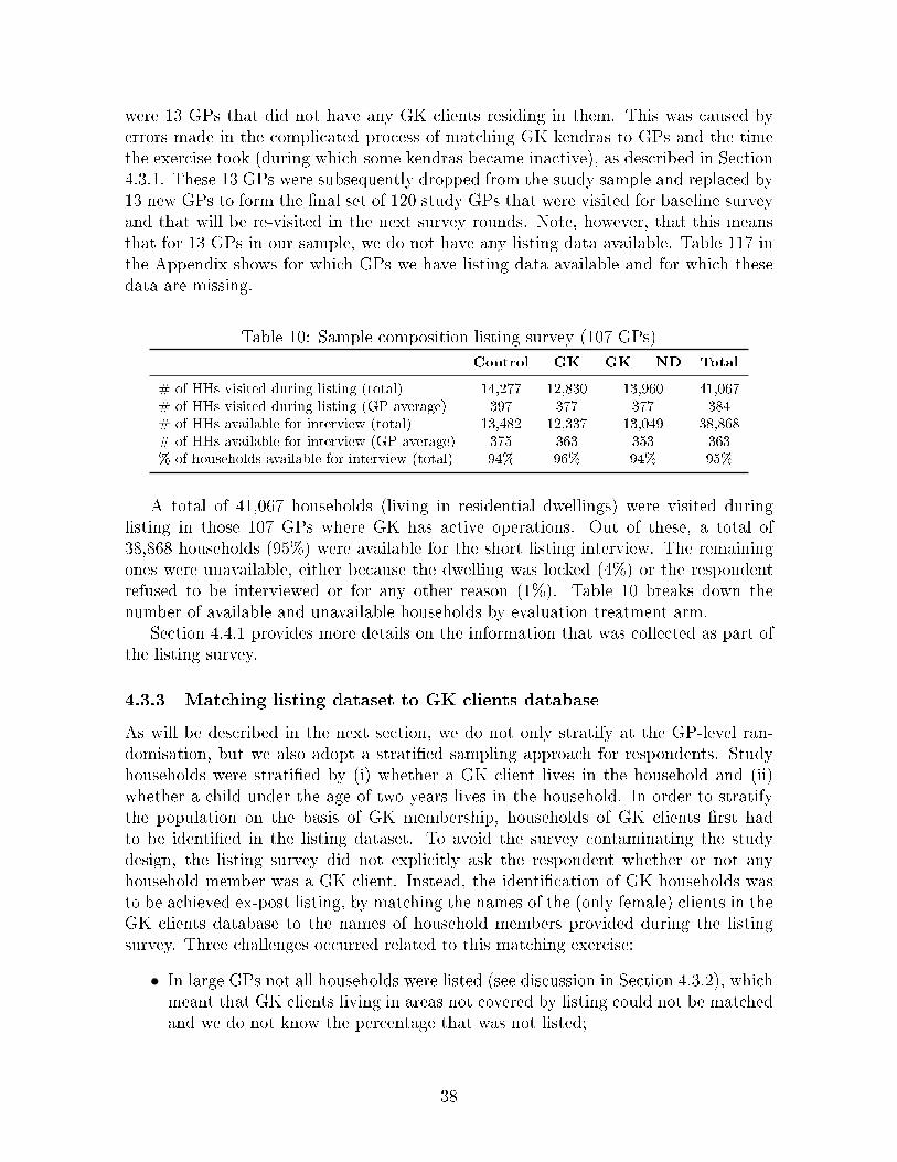
were 13 GPs that did not have any GK clients residing in them. This was caused byerrors made in the complicated process of matching GK kendras to GPs and the timethe exercise took (during which some kendras became inactive), as described in Section4.3.1. These 13 GPs were subsequently dropped from the study sample and replaced by13 new GPs to form the �nal set of 120 study GPs that were visited for baseline surveyand that will be re-visited in the next survey rounds. Note, however, that this meansthat for 13 GPs in our sample, we do not have any listing data available. Table 117 inthe Appendix shows for which GPs we have listing data available and for which thesedata are missing.

Table 10: Sample composition listing survey (107 GPs)


# of HHs visited during listing (total) 14,277 12,830 13,960 41,067# of HHs visited during listing (GP average) 397 377 377 384# of HHs available for interview (total) 13,482 12,337 13,049 38,868# of HHs available for interview (GP average) 375 363 353 363% of households available for interview (total) 94% 96% 94% 95%

A total of 41,067 households (living in residential dwellings) were visited duringlisting in those 107 GPs where GK has active operations. Out of these, a total of38,868 households (95%) were available for the short listing interview. The remainingones were unavailable, either because the dwelling was locked (4%) or the respondentrefused to be interviewed or for any other reason (1%). Table 10 breaks down thenumber of available and unavailable households by evaluation treatment arm.

Section 4.4.1 provides more details on the information that was collected as part ofthe listing survey.

4.3.3 Matching listing dataset to GK clients database

As will be described in the next section, we do not only stratify at the GP-level ran-domisation, but we also adopt a strati�ed sampling approach for respondents. Studyhouseholds were strati�ed by (i) whether a GK client lives in the household and (ii)whether a child under the age of two years lives in the household. In order to stratifythe population on the basis of GK membership, households of GK clients �rst hadto be identi�ed in the listing dataset. To avoid the survey contaminating the studydesign, the listing survey did not explicitly ask the respondent whether or not anyhousehold member was a GK client. Instead, the identi�cation of GK households wasto be achieved ex-post listing, by matching the names of the (only female) clients in theGK clients database to the names of household members provided during the listingsurvey. Three challenges occurred related to this matching exercise:

• In large GPs not all households were listed (see discussion in Section 4.3.2), whichmeant that GK clients living in areas not covered by listing could not be matchedand we do not know the percentage that was not listed;

38

• In the interest of time and costs, the listing survey did not collect informationon the names of all of the household members. It only asked about the name ofthe household head and the name of the spouse of the household head or, in casethere was no spouse, the name of the eldest female member. This meant that incase the GK client was not either the household head or the head's spouse/eldestfemale member in the household, the GK client could not be identi�ed in thelisting dataset (even after using client/spouse's middle names and last names);

• As explained in the previous Section, for 13 out of 120 study GPs we do not havelisting data available. GK clients living in those areas could not be identi�edahead of the start of the baseline survey.

As a result, only half of the GK clients in the study area could be reliably matched tothe listing dataset and the original sampling strategy had to be adjusted. Appendix Cdiscusses the complementary sampling strategies that were adopted in order to circum-vent these problems.

4.3.4 Sample selection and sample size

Household survey

By design, the evaluation included a baseline household survey of a sample of 30 house-holds in each of the 120 study GPs (3600 households in total), strati�ed by (i) whethera GK client lives in the household and (ii) whether a child under the age of two yearsold lives in the household. Originally, based on the information that was available atthe study design phase, the distribution of the sample was planned to be as depicted inFigure 11, i.e. half of the sample being GK client households, the other half non-clienthouseholds and within these interview 8 households with children under the age of 2years and 7 without.

Figure 11: Original sampling strategy per GP

However, as it turned out, in some GPs it was not possible to reach the target numberof available GK households in the stratum of kids less than two years old (i.e. eight).Whereas the sampling strategy for the non-GK group remained the same, the samplingstrategy for the GK group was revised as follows: In case there were not su�cient(i.e. 8) client households with kids less than two years of age, households with kidsless than six years were sampled instead. If still not enough client households fallingin this categor could be identi�ed, then households without kids were over-sampledto obtain a total of 30 sampled households in each GP. To compensate for the lower

39

number of sampled clients with kids in some GPs, in neighbouring GPs a respectivelyhigher number of GK clients with kids was sampled, although always ensuring that aminimum of �ve non-clients with kids was sampled in each of the study GPs.

Further, a total of 14 completed household surveys got lost as a result of a technicalfailure with the electronic survey system (see Section 4.5).

The overall result is that in some GPs there is a shortfall relative to the targetsample size of 30 surveys, whereas in others there is a surplus. Table 118 in AppendixD shows the shortfall/surplus by GP. Given that the survey teams had surveyed a highernumber of households than was required, the net result is a shortfall of 5 households intotal, which is insigni�cant relative to the target sample size of 3600, i.e. 0.001 %. Fornone of the three treatment arms the shortfall/surplus exceeds 1%.

This yields a total sample size of 3,595 in the household survey dataset. Table 11summarises the sample size by stratum (by client/non-client and by kids/no kids) andby treatment arm.

Table 11: Sample composition baseline household survey


Non-GK clients Kids < 2 years old 330 318 314 962(53%) (53%) (54%) (53%)

Kids 2-5 years old 48 34 57 139(8%) (6%) (10%) (8%)

No kids < 6 years old 239 248 213 700(39%) (41%) (36%) (39%)

Total 617 600 584 1801

GK clients Kids < 2 years old 230 182 203 615

(37%) (31%) (35%) (34%)Kids 2-5 years old 120 120 97 337

(19%) (20%) (17%) (19%)No kids < 6 years old 271 285 286 842

(44%) (48%) (49%) (47%)Total 621 587 586 1794

Total 1238 1187 1170 3595

The distribution of the total number of surveys across the di�erent treatment armsis as expected given the number of GPs included in each of the treatment groups.The control group sample has slightly more households than the `GK' and `GK + ND'treatment groups, given that it covers 41 GPs, whereas the other two groups include40 and 39 GPs, respectively. As can be seen from the numbers in brackets in the table,which show the share of each client/non-client stratum within its treatment category,the distribution across treatment arms remains similar when breaking the compositiondown by stratum.

As expected, we observe di�erences (albeit small) in sample composition betweenthe GK and non-GK sub-groups. In the non-GK client group, about 53 % of the sampleof the non-GK group contains households with kids less than two years old and 47%of the sample has households without kids less than two years old. This is very muchin line with the sampling strategy summarised in Figure 11 which targeted for each

40

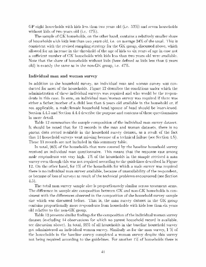
GP eight households with kids less than two years old (i.e. 53%) and seven householdswithout kids of two years old (i.e. 47%).

The sample of GK households, on the other hand, contains a relatively smaller shareof households with kids less than two years old, i.e. on average 34% of the total. This isconsistent with the revised sampling strategy for the GK group, discussed above, whichallowed for an increase in the threshold of the age of kids to six years of age in case nota su�cient number of GK households with kids less than two years old were available.Note that the share of households without kids (here de�ned as kids less than 6 yearsold) is exactly the same as in the non-GK group, i.e. 47%.

Individual man and woman survey

In addition to the household survey, an individual man and woman survey was con-ducted for most of the households. Figure 12 describes the conditions under which theadministration of these individual surveys was required and who would be the respon-dents in this case. In sum, an individual man/woman survey was required if there waseither a father/mother of a child less than 6 years old available in the household or, ifnot applicable, a male/female household head/spouse of head should be interviewed.Section 4.4.5 and Section 4.4.4 describe the purpose and contents of these questionnairesin more detail.

Table 12 summarises the sample composition of the individual man survey dataset.It should be noted that for 13 records in the man and woman datasets, there is noparent data record available in the household survey dataset, as a result of the factthat 14 household surveys went missing because of a technical failure (see Section 4.5).These 13 records are not included in this summary table.

In total, 96% of the households that were covered by the baseline household surveyreceived an individual man questionnaire. This means that the response rate amongmale respondents was very high. 1% of the households in the sample received a mansurvey even though this was not required according to the guidelines described in Figure12. On the other hand, for 1% of the households for which a male survey was requiredthere is no individual man survey available, because of unavailability of the respondent,or because of loss of surveys as result of the technical problems encountered (see Section4.5).

The total man survey sample size is proportionately similar across treatment arms.The di�erence in sample size composition between GK and non-GK households is con-sistent with the di�erences observed in the composition of the household survey samplesize which was discussed before. That is, the man survey dataset in the GK groupcontains proportionally more respondents from households with kids less than six yearsold relative to the non-GK group.

Table 13 presents similar �ndings for the composition of the individual woman surveydataset (excluding 14 observations for which no parent household record is available,see discussion above). In total, 99% of all households in the baseline household surveygot administered an individual woman survey. Similarly as for the man survey, 1 % ofthe households in the baseline survey completed a woman survey despite this surveynot being required according to the guidelines. For another 1% of households there is

41

Figure 12: Respondent woman and man questionnaire

no woman survey data available even though this was required.

Anthropometrics

Finally, the baseline survey took anthropometrics (height and weight) from all childrenup to the age of 2. Table 14 summarises the number and proportion of households forwhich anthropometrics data for both height and weight is available, by GK clients/non-GK clients. Complete anthropometrics were taken in 95% of all households where thiswas required, i.e. those with kids less than to years old. For the remaining 5% ofhouseholds child measurements could not be captured/are not available because of thechild or his/her mother being out of station (4%) or because of other reasons (1%),such as refusals or data getting lost because of the technical issues faced in the �eld(see Section 4.5).

4.3.5 Randomisation of branch order

Finally, we randomised the order in which data collection in each branch was takenplace. While not necessarily high risk, this was to avoid that data collection would be

42

Table 12: Sample composition individual man surveyControl GK GK + ND Total % HHs with

men survey

Non-GK clients Kids < 6 371 352 369 1,092 99%(62%) (60%) (65%) (63%)

No kids < 6 223 233 199 655 94%(38%) (40%) (35%) (37%)

Total 594 585 568 1,747 97%

GK clients Kids < 6 337 298 294 929 98%

(58%) (53%) (52%) (54%)No kids < 6 245 263 277 785 93%

(42%) (47%) (48%) (46%)Total 581 560 570 1,711 95%

Total 1,176 1,146 1,139 3,461 96%

% HHs with man survey 95% 96% 97% 96%

Notes: The numbers in this table exclude 13 observations for which no parent household

record is available.

Table 13: Sample composition individual woman surveyControl GK GK + ND Total % HHs with

woman survey

Non-GK clients Kids < 6 377 350 364 1091 99%(62%) (59%) (63%) (61%)

No kids < 6 236 244 210 690 99%(38%) (41%) (37%) (39%)

Total 613 594 574 1781 99%

GK clients Kids < 6 349 300 298 947 99%

(56%) (51%) (51%) (53%)No kids < 6 270 285 284 839 100%

(44%) (49%) (49%) (47%)Total 619 585 582 1786 99%

Total 1232 1179 1156 3567 99%

%HHs with woman survey 99% 99% 98% 99%

Notes: The numbers in this table exclude 14 observations for which no parent household

record is available.

Table 14: Sample composition anthropometricsControl GK GK + ND Total % HHs (total sample) % sample (with kids)

Non-GK clients 319 305 282 906 50% 94%GK clients 225 168 191 584 33% 95%Total 544 473 473 1490 41% 95%% HHs (total sample) 44% 40% 40% 41%% (HHs sample with kids) 97% 95% 92% 95%

43

done in an order in which for example other programs could be rolled out. One couldthink of government programs that following a speci�c geographic or alphabetical or-dering. The outcome is the following sequence in which baseline survey was conducted:

1. Naigaon

2. Nilanga

3. Udgir

4. Degloor

5. Ahamedpur

4.4 Instruments for data collection

The baseline survey covered �ve di�erent types of surveys (listing questionnaire, com-munity questionnaire, household questionnaire, women questionnaire - including an-thropometrics - and man questionnaire), which were organised and implemented by anexternal survey �rm. The instruments were developed by the research team and re�nedin conjunction with the survey �rm. They were piloted in two stages: First, the paper-versions were tested in the �eld. This took place in two villages in rural Maharashtra,outside our study area16 in the period May 10-13 2014.17 The second piloting focusedon CAPI pre-testing and took place in the period 22-25 September 2014. This testingwas done by the survey �rm exclusively. We refer to the Implementation Report, fordetails about the overall �eld work and quality control procedures, and to the vari-ous �eld training manuals for more information about the instructions provided to theenumerators.

Except for the community questionnaire, all surveys were conducted electronicallyusing PDAs (for listing) or tablets (household, man and woman surveys). The listingsurvey started on 14 September 2014 and was completed within a month, on 12 Oc-tober 2015. The baseline household surveys (community, household, woman and manquestionnaires) took place between 24 November 2014 and 26 January 2015.

4.4.1 Listing questionnaire

The listing exercise was carried out by an external survey �rm using PDAs with in-builtGPS devices. The questionnaire was designed to be brief and cover only names of thehousehold head and spouse, and the eldest female in case the household head was notmarried. These information were used to match GK clients to the listing data. It furthercollected information about children under the age of 2 years for strati�cation purposesand �nally, it asked about the household's caste as well as some basic information onthe households sanitation situation. A more detailed discussion of the purpose andprocedures of this listing excercise is provided above in Section 4.3.2.

16Speci�cally, the PAPI pre-testing took place in two villages (Shindvane and Degaon) in Punedistrict.

17Participants in the training included researchers from the survey �rm, one male and one female�eld supervisor, a representative from WSP India as well as from IFS London.

44

4.4.2 Community (village) questionnaire

The main purpose of this instrument is to collect information on factors that are ex-pected to facilitate or potentially constrain the uptake and success of the interventionswe study. Accounting for characteristics of the environment in which the intervention isimplemented will be crucial to assess its success or understand failures. To that end, thequestionnaire covers information on the village's population (size, caste structure, mainactivities in general and main farming activities in particular, as well as wages for themain activities), transportation links, information on access and distances to speci�cinfrastructure (public services such as schools, police, health services etc, artisans andmasons, and shops), information on te political economy, community activities, sourcesof water and sanitation and waste disposal and �nally shocks experienced and prices ofa list of goods.

This questionnaire focused on one village within the GP. As discussed above, inmost cases this one village would be equivalent to the GP. In remaining ones, thevillage would be picked at random. The information in this questionnaire were collectedfrom relevant, well-informed members of the community. The information could becollected in a group discussion, or on a one-on-one basis with the relevant informants.Community members that were approached include the sarpanch, gram sevak, teacher,talati, anganwadi worker, opinion leader, SHG federation leader, but should also includevillagers that do not have such special posts in the community, and may be from poorerparts of the community.

Due to some logistical problems, one village questionnaire18 (of the GP Dhosni) wasnot yet completed at the time of writing up this baseline report. Completion of thissurvey is scheduled to take place in the next couple of weeks. This report will presentthe community �ndings for 119 villages in 119 GPs.

4.4.3 Household questionnaire

The household questionnaire was designed to provide us with information on the base-line levels of the outcomes of interest for the study: This is very important so as tobe able to assess whether the intervention was e�ective and also how large any e�ectis. Moreover, the baseline level could in some cases be used as a control variable toincrease power of the experiment. The outcomes of interest are as follows:

Primary Outcomes: Sanitation uptake, uptake of safe sanitation, usage of safe san-itation, health insurance claims;

Secondary Outcomes: Health (diarrhea, child nutritional status), awareness aboutsanitation, changes in perceptions of costs and bene�ts of safe sanitation (forthe Navya Disha intervention); Uptake of credit, awareness about health insur-ance, uptake of health insurance, household income and consumption (a�ected bycredit);

Tertiary outcomes: Productivity, schooling, among other.

18Dhosni village in Dhosni GP, Deglur block and Nanded district. This village was allocated to thecontrol group.

45

It should be noted that the secondary and tertiary outcomes allow us to investigatehow the intervention works (i.e. does it follow the channels outlined in the theory ofchange? Which of these channels is most important?), and also impacts on broadersocio-economic outcomes (e.g. productivity and schooling), which are hypothesised tobe a�ected by poor sanitation.

The second major purpose of the household questionnaire is to collect characteris-tics of the household that would provide a good description of the study population,poverty levels and wealth. We will also want to investigate heterogeneous impacts ofthe interventions by some of these variables (e.g. is it only the wealthiest householdsthat take up the loans/build safe sanitation, etc). Finally, some of these variables willbecome covariates in our analysis and help improve the power of the study.

The household questionnaire was hence the most extensive module, covering socio-economic characteristics of the household (assets, income, savings, credit, consumptionexpenditures), household member information (age, gender, education, etc) and a de-tailed section on sanitation and hygiene infrastructure, practices and believes.

Where possible, the head of the household was interviewed, however contributionsfrom other knowledgeable household members were also allowed. At the �rst instancethough, if the household head was not available, the interview was re-scheduled to aconvenient time for the household head. If he or she was not available in the next 2days, another knowledgeable adult household member was interviewed. The interviewtook on average 66 minutes to complete.

4.4.4 Women questionnaire

There are four key reasons for the choice of having a questionnaire administered to awoman in households of our study population, partly in line with reasons describedabove for the household questionnaire:

1. To collect information on individual sanitation behaviour, reported by the womanherself, the former one being one of the key outcome measures in the �rst stageof this experiment;

2. To collect information on individual sanitation preferences and beliefs to under-stand women's perceptions of the costs and bene�ts of sanitation, and also toidentify what they value about it. This set of variables will allow us to identifythe components of the interventions that households are likely to value the most,and thereby are likely to be most e�ective;

3. To collect information on child health, child care practices and child nutrition forchildren aged < 6 years;

4. To collect information on women's status in the household.

The interview was conducted by a female interviewer with a female respondent of thehousehold, selected as described in Section 4.3.4. The interview took on average 32minutes.

46

4.4.5 Men questionnaire

The main purpose for the men questionnaire is in line with points 1 and 2 presentedfor women above. On the second, sanitation preferences and perception, this is drivenby anecdotal evidence that suggests that men and women value sanitation di�erently,and that this explains the slow take-up rates of sanitation.

The interview conducted by a male enumerator with the men (selected as describedin Section 4.3.4), took on average 19 minutes.

4.4.6 Monitoring data and rapid assessments

Finally, emphasis will be placed on monitoring on-going progress and processes of thesanitation intervention. This will be done through two means: First, we will receiveinformation, on an on-going basis (roughly bi-monthly), from GK on the number ofsanitation loans they have provided in study areas. This will inform us about thesanitation uptake among GK clients and will allow us to monitor some of the risksdescribed in Section 4.2.

We will further conduct two rapid assessments (RAs), roughly 4 and 8 months afterimplementation start. These rapid assessments will be done in a similar manner asdone by the GoI when checking OD(F) status of villages. Speci�cally, for the �rst RAwe will select half of the 120 study GPs and will within each of these, interview about30 respondents. These respondents will be di�erent to the baseline respondents, toavoid survey fatigue. The second RA will then concentrate on the remaining 60 GPs.Further details, including the questionnaire to be �elded, are in development at thetime of writing this report.

4.5 Problems in data collection

The previous sections have already touched upon the various problems encounteredduring data collection. This section sums up the main challenges that were faced andthe subsequent decisions that were made to move forward.

1. After selection of the study GPs (see Section 4.3.1), it turned out that the numberof households living in these GPs is signi�cantly higher than what was anticipatedat the project proposal stage (based on the latest census data). Instead of listingall households in all of the study GPs, for large GPs (more than 480 households)it was decided to list only a random sub-set of households. If the GP had morethan one village, one village was randomly sampled. If the sampled village hadmore than 480 households, the village was segmented for listing according to aprocedure described in Section 4.3.2.

2. After completion of the listing exercise, it was discovered that among the 120 GPsthat had originally been sampled for the study - and therefore had been listed -there were 13 GPs that did not have any GK clients residing in them. This wascaused by errors made in the complicated process of matching GK kendras to GPsand the time the exercise took (during which some kendras became inactive), as

47

described in Section 4.3.1. These 13 GPs were subsequently dropped from thestudy sample and replaced by 13 new GPs to form the �nal set of 120 study GPsthat were visited for baseline survey and that will be re-visited in the next surveyrounds. Note, however, that this means that for 13 GPs in our sample, we donot have any listing data available. Table 117 in the Appendix shows for whichGPs we have listing data available and for which these data are missing. Thishad implications for the sampling strategy, which are discussed in Section 4.3.1.

3. Reviewing the listing data, IFS/WSP observed that the GPS readings collectedduring household listing were missing for 26.7% of the households and were du-plicated for 20.2% of the households. This means that for almost half of thehouseholds in the listing dataset we currently do not have accurate GPS coordi-nates available. This issue has been discussed in length with the survey �rm thatwas in charge of collecting these data, who blame poor satellite connectivity asthe main cause for this. The survey �rm has agreed to go back to the �eld tore-capture GPS readings for those households for which these data are missing.This is scheduled to take place in the next few weeks.

4. There was a long delay in the process of obtaining an o�cial support letter fromYasahada for the study. This letter was needed by the survey �eld team as ameans to introduce themselves to the Sarpanch o�ce. The delay in this letteruntil long time after the start of the �eld work meant the �eld teams had a hardtime trying to explain the purpose of their visit to the community o�cials.

5. In some GPs the target number of 8 GK households in the sample with kidsless than 2 years old could not be met. In those incidences, it was decided toincrease the child age threshold for a 'GK household with kid' from 2 years to 6years and, if necessary, to over-sample GK households without kids to obtain thetarget number of 30 GK households per GP. To compensate for the lower numberof sampled clients with kids less than 6 years old in some GPs, in neighbouringGPs a respectively higher number of clients with children less than 6 years old,or if possible less than 2 years old, was sampled, although always ensuring thata minimum of �ve non-clients with kids was sampled in all of the study GPs.Section 4.3.4 discusses this issue in more detail.

6. As a result of some technical problems with the synchronisation of data betweenthe CAPI (Computer-Assisted-Personal-Interviewing) units employed by the sur-vey �rm during data collection and the online server, a (proportionally small)number of completed household/woman/man surveys were lost. This only con-cerns 0.04%, 0.22% and 0.8% of the household/woman/man surveys, respectively,which are too small in number to signi�cantly a�ect the study. Also, the surveyteams completed a higher number of surveys than actually required, which largelycompensates not only for these technical issues but also for those incidences whereeither man and/or woman was unavailable for completion of the individual sur-veys (because of being out of station or refusals). The net shortfall in the numberof surveys comes to 5 household records (0.1%), 23 woman surveys (0.6%) and 44

48

man surveys (1.3%). These missing records are more or less equally distributedacross treatment arms.

49

5 Findings

The data analysis presented in the following sections of this report has two main pur-poses: On the one hand, the data provides a snapshot of our study population andenvironment, serving as a useful tool to understand the context in which the interven-tion is taking place.On the other hand, the analysis allows us to formally test whether we see any systematicdi�erences between the treatment and control group prior to the intervention starting.

As explained in Section 4.1, the evaluation methodology will be based on comparingthe outcomes between the di�erent treatment groups, i.e. 'C' (control), GK (sanitationloans only) and 'GK + ND' (sanitation loans + awareness creation). In order to beable to attribute any e�ects to the sanitation interventions, it is imperative that thethree groups being compared are similar in all respects at the outset of the intervention.Section 4.1 explains that randomisation is the best tool at our disposal for achievingthis; the key is to conduct it properly. To test whether randomisation was properlydone, we will compare the observable (pre-treatment) characteristics and test that thereare no signi�cant di�erences in their distribution between the di�erent treatment arms.If we pass the test, this can be taken as evidence that the samples are balanced in theunobservable dimension as well, given there has been randomisation in the �rst place.

At baseline we can compare variables such as consumption, enterprise, assets andsavings, as well as background characteristics that cannot be changed by the programsuch as age, sex, adult education, and so on. We present tables showing the averagevalues of di�erent variables for each of the treatment groups. The standard way to checkthat the randomisation was successful and that the two sets of data are not signi�cantlydi�erent is the Student's t-test. This t-test compares the means of the treatment andcontrol populations and returns a value known as a p-value, which is a measure of theprobability that an outcome as the one observed is the result of randomly generatingsamples under the assumption that both means are identical. A p-value correspondsto a signi�cance level and we will present in our tables asterixes, indicating signi�cantdi�erences between the treatment groups and the control group at the 10, 5 and 1percent signi�cant level.

Our key balance test will however be based on the statistical joint 'F-test' to testwhether overall there are any di�erences between any of the three evaluation groups.The advantage of this test is that it controls for the fact that we are making multiplecomparisons, which a normal t-test fails to do. For that reason, if we �nd that adi�erence in characteristics passes that test, we conclude that the treatment arms arebalanced. The disadvantage of this test is that if we reject the balance test, i.e. if thetest suggests at least one di�erence, we do not know which treatments can be said to besigni�cantly di�erent from each other. This can be inferred from the results of two-waycomparisons between control and each of the treatment groups just discussed.

50

Figure 13: Guide to technical jargonMagnitude of a di�erence in outcomeIn the �rst instance, we will be interested in the size or magnitude of the di�erencebetween people who receive support (treated group) and people who did not (controlgroup). For instance, imagine that we measure at baseline that the average sampledbene�ciary household earns $50 more than the average control household in our studysample, we would conclude that the magnitude of the di�erence is $50.

Statistical signi�cance and p-valueHowever, when we talk about `signi�cant' or 'insigni�cant' di�erences in this report,we mean di�erences that are `statistically signi�cant' or 'statistically insigni�cant', re-spectively. In the example above, although a di�erence of $50 seems quite large, weremember that this estimated average impact is derived from data on a sample of treat-ment and control households, rather than data on the true population of bene�ciariesand their respective counterfactual values (see discussion in Section 4.1). Given that weonly have one sample available, there is always a possibility that we have been unfor-tunate with our sample and that we happen to have drawn bene�ciaries with relativelyhigh values from a population pool with a true average di�erence of zero. Therefore, it isnecessary to take into consideration the statistical probability of measuring di�erencesof $50 (or more) if there were truly no di�erences in earnings between the treatment andcontrol groups, that is, if in reality the di�erence was zero. This statistical probabilityis usually referred to as the p-value. If the p-value is small, for instance one per cent,this means that the probability of obtaining an estimate of $50 (or more) if the truedi�erence was zero is very small (one per cent) so we can reject the hypothesis thatthere is no di�erence in earnings `at the one per cent signi�cance level'. We would thensay that the result is `signi�cant'. This is di�erent from saying that the magnitudeof the di�erence is large, because magnitude refers to e�ect size, as explained above.Taken together, signi�cance and magnitude help us to interpret the results. In theresults tables below, statistical signi�cance will be indicated with asterisks, with oneasterisk (*) indicating a p-value of less than one per cent, two asterisks (**) indicatinga p-value of less than 5 per cent and three asterisks (***) indicates a p-value of lessthan ten per cent. The higher the p-value, the less con�dent we are that the measureddi�erence re�ects a true di�erence. Values with a p-value of more than ten 10 per centare considered statistically insigni�cant in this report.

Joint Hypothesis Testing and the F-StatisticsIn our study, we deal with two treatment groups and one control group. This presentsan additional concern when comparing the mean results by treatment group. It iscostumary in this setting to run a joint hypothesis test (F-test), which tests for equalityof all means together. This test would detect any of the several possible di�erencesbetween the groups, rather than just comparing one group to another. The disadvantageof this test is that if we reject the balance test, i.e. if the test suggests at least onedi�erence, we do not know which treatments can be said to be signi�cantly di�erentfrom each other. The pairwise tests described above can instead be used for thatpurpose.

51

The box presented in Figure 7 explains some key statistical concepts that we use inorder to accept or reject balance between di�erent groups. In sum, typical balance testsrely on statistical probabilities of observing any di�erences between groups if in realitythere is zero di�erence. If this probability is lower than 10%, then we conclude thatthere is a statistically signi�cant di�erence between groups. However, as the numberof comparisons increases (for instance, if you make comparisons over many variables,which is what we do in this report), it becomes more likely that the groups beingcompared will appear to di�er in terms of at least one attribute. For example, if onetest is performed at the 10% level, there is only a 10% chance of incorrectly concludingthat there is a di�erence even if there is no true di�erence between two groups. However,for 100 comparisons, the expected number of incorrect rejections is 10. We thereforeexpect (and therefore accept) there to be around 1 statistically signi�cant di�erence forevery 10 comparisons we make.

Before proceeding, note that in all of the tables presented below, we use the followingformat: The �rst column gives information on the variable under consideration. Wethen show the mean for the whole sample (treatment groups and control combined).The following three columns show the mean of the control and the treatment groupsseparately. The �fth column shows the F-statistic of the test of statistical di�erencesbetween any of the treatment groups and the second last column shows the associatedp-value. The last column shows the total the number of observations over which thewhole sample mean is calculcated. We also run two-way comparisons between each ofthe treatment groups and the control group. Statistical di�erences with the controlgroup, if any, are indicated with asterixes (*). Note that throughout, the tests accountfor clustering of the standard errors at the gram panchayat level.

We will refer to the sample average when presenting the results, unless the pertreatment group averages are statistically di�erent.

5.1 Study population (listing data)

We start o� by presenting the key characteristics of our study population, based on theinformation that was collected during the listing survey in 107 of our study GPs. Giventhat the respondent to the (quick) listing survey was not necessarily the household heador another knowledgeable member of the household, some answers were set to `don'tknow' leading to missing values. This means that the total number of observations(presented in the last columns of the relevant tables) does not always add up to thetotal number of households in the listing dataset (i.e. 38,868). We note though that thedrops are typically very small as in most cases a household member could be interviewedas we will see shortly.

We provide information on who responded to the listing survey in Table 15. We cansee that 84 percent of the interviews were conducted by the household head, his/herspouse, the son/daughter or son-in-law/daughter-in-law of the head of household. Theother surveys were conducted by other relatives of the household (14%) or non-relatedpersons such as neighbours (3%). The composition in respondent type is very wellbalanced over the treatment arms.

Table 16 presents general demographic information by treatment status, which is

52

Table 15: Respondent to the listing survey (%)Treatment Status

Whole Sample Control GK GK + ND P-value N

Head 33.85 35.40 34.90 31.27∗ 0.154 38848(1.031) (1.517) (2.096) (1.629)

Wife or Husband 32.99 32.02 33.59 33.42 0.835 38848(1.249) (1.842) (2.491) (2.158)

Son or Daughter 12.37 12.99 11.09 12.95 0.193 38848(0.467) (0.836) (0.899) (0.623)

Son-in-Law or Daughter-in-Law 4.50 4.39 4.19 4.90 0.500 38848(0.250) (0.396) (0.477) (0.418)

Grandchild 0.80 0.75 0.86 0.80 0.816 38848(0.0669) (0.112) (0.131) (0.102)

Parent 5.35 5.05 5.01 6.00 0.352 38848(0.309) (0.496) (0.526) (0.559)

Parent-in-Law 0.31 0.18 0.34 0.42∗ 0.098∗ 38848(0.0541) (0.0550) (0.0827) (0.126)

Brother or Sister 3.93 3.70 4.16 3.96 0.767 38848(0.255) (0.408) (0.509) (0.400)

Brother-in-Law or Sister-in-Law 1.27 1.04 1.30 1.47 0.363 38848(0.125) (0.209) (0.213) (0.224)

Niece or Nephew 0.83 0.87 0.62 0.99 0.366 38848(0.114) (0.200) (0.176) (0.208)

Other Relative 1.06 0.91 1.09 1.19 0.633 38848(0.126) (0.186) (0.190) (0.266)

Adopted/Foster/Stepchild 0.07 0.03 0.10 0.08 0.233 38848(0.0217) (0.0139) (0.0580) (0.0307)

Not Related 0.19 0.22 0.24 0.12 0.338 38848(0.0463) (0.0722) (0.113) (0.0383)

Neighbour 2.45 2.41 2.51 2.45 0.990 38848(0.269) (0.495) (0.486) (0.409)

Don't know 0.02 0.05 0.01 0.01 0.417 38848(0.0122) (0.0327) (0.00806) (0.00762)

Note: Standard Errors in parenthesis, clustered at the GP level. *p <0.10, **p <0.05, ***p <0.01

Source: Listing Questionnaire.

balanced across groups. Only 9% of the households interviewed had a female householdhead. The average self-reported age of the household head was about 48 years andthat of the head's spouse was 41 years. Furthermore, the average number of householdmembers is close to 5 and the average number of children under 2 years per householdis 0.18.

53

Table 16: General DemographicsTreatment Status


Female (HH head) 9.17 9.25 9.67 8.61 0.342 38868(0.301) (0.520) (0.512) (0.509)

Age of HH head 47.76 47.92 47.54 47.81 0.842 38589(0.267) (0.467) (0.474) (0.444)

Age of HH head's Spouse 40.98 41.14 40.86 40.94 0.898 34673(0.245) (0.450) (0.416) (0.399)

No. of HH members 4.88 4.91 4.75 4.96 0.341 38817(0.0591) (0.100) (0.123) (0.0740)

No. of children under 2 years 0.18 0.19 0.17 0.18 0.269 38868(0.00444) (0.00735) (0.00866) (0.00652)



Table 17: Caste (%)Treatment Status


Other Backward Class (OBC) 23.53 22.43 25.76 22.55 0.727 38855(1.739) (2.889) (3.641) (2.386)

Special Backward Castes (SBCs) 1.43 1.53 1.61 1.16 0.732 38855(0.265) (0.477) (0.511) (0.386)

Scheduled Castes (SCs) 23.56 24.18 22.40 24.02 0.808 38855(1.091) (1.749) (2.339) (1.533)

Scheduled Tribes (STs) 4.65 4.35 5.43 4.23 0.820 38855(0.711) (0.967) (1.713) (0.903)

Denoti�ed Tribes (DTs) / Vimukta Jati (VJ) 0.86 1.34 0.37 0.82 0.174 38855(0.254) (0.580) (0.103) (0.432)

Nomadic Tribes (NTs) / Bhatkya Jati 10.91 10.70 9.99 12.01 0.719 38855(1.070) (1.958) (1.782) (1.776)

General 34.11 34.63 33.80 33.87 0.978 38855(1.814) (3.008) (3.466) (2.963)

Do not want to reveal 0.27 0.09 0.21 0.52∗ 0.125 38855(0.0913) (0.0384) (0.0931) (0.246)

Don't Know 0.67 0.76 0.43 0.81 0.325 38855(0.148) (0.230) (0.132) (0.344)



In terms of caste composition in our study areas, we can see from Table 17 thatthe most common castes are General (34%), Scheduled Caste (24%), Other BackwardCaste (24%) and Nomadic Tribes (11%), with no signi�cant di�erences between groups.

Moving on to latrine use, Table 18 shows that the majority of households (65%)practice open defecation, while only 29% use any type of toilet (27% at home and2% at a neighbour's, school or community toilet). We �nd a slight imbalance in thepercentage of households going for OD for the GK+ND study group. We note howeverthat this imbalance is only signi�cant at the 10% signi�cance level and the F stat is notsigni�cant. While we are generally not too concerned about imbalances at this level forthe pairwise t-test, given that this is one of our main outcomes, it deserves a bit moreattention.We break down the information on open defecation practices, splitting thesample by households that report to go for OD close to their own and those reporting

54

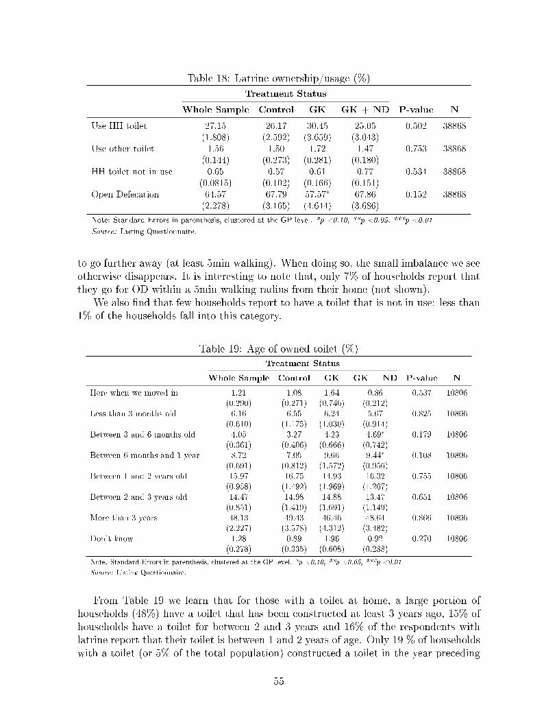
Table 18: Latrine ownership/usage (%)

Treatment Status


Use HH toilet 27.15 26.17 30.45 25.05 0.502 38868(1.808) (2.592) (3.659) (3.043)

Use other toilet 1.56 1.50 1.72 1.47 0.753 38868(0.144) (0.273) (0.281) (0.180)

HH toilet not in use 0.65 0.57 0.61 0.77 0.534 38868(0.0815) (0.102) (0.166) (0.151)

Open Defecation 64.57 67.79 57.57∗ 67.86 0.152 38868(2.278) (3.165) (4.644) (3.686)



to go further away (at least 5min walking). When doing so, the small imbalance we seeotherwise disappears. It is interesting to note that, only 7% of households report thatthey go for OD within a 5min walking radius from their home (not shown).

We also �nd that few households report to have a toilet that is not in use: less than1% of the households fall into this category.

Table 19: Age of owned toilet (%)

Treatment Status


Here when we moved in 1.21 1.08 1.64 0.86 0.537 10806(0.290) (0.271) (0.746) (0.212)

Less than 3 months old 6.16 6.55 6.24 5.67 0.825 10806(0.610) (1.175) (1.030) (0.914)

Between 3 and 6 months old 4.05 3.27 4.23 4.69∗ 0.179 10806(0.361) (0.406) (0.666) (0.742)

Between 6 months and 1 year 8.72 7.05 9.66 9.44∗ 0.108 10806(0.691) (0.812) (1.572) (0.956)

Between 1 and 2 years old 15.97 16.75 14.93 16.32 0.755 10806(0.958) (1.492) (1.969) (1.267)

Between 2 and 3 years old 14.47 14.98 14.88 13.47 0.651 10806(0.851) (1.419) (1.691) (1.149)

More than 3 years 48.13 49.43 46.46 48.64 0.866 10806(2.227) (3.578) (4.312) (3.482)

Don't know 1.28 0.89 1.96 0.92 0.270 10806(0.278) (0.335) (0.608) (0.288)



From Table 19 we learn that for those with a toilet at home, a large portion ofhouseholds (48%) have a toilet that has been constructed at least 3 years ago, 15% ofhouseholds have a toilet for between 2 and 3 years and 16% of the respondents withlatrine report that their toilet is between 1 and 2 years of age. Only 19 % of householdswith a toilet (or 5% of the total population) constructed a toilet in the year preceding

55

the listing survey visit.

5.2 Village pro�le (community survey)

In this section, we discuss the �ndings from the community survey conducted with GPo�cials regarding the characteristics of the village that was sampled for our study. Atthe time of writing this baseline report, the village questionnaire data for one GP werestill pending (see Section 4.4.2). Therefore, this section only presents the informationavailable for 119 GPs.

4.1.1 Demographics

Table 20: General Demographics from Community DataTreatment Status


What is the current population of this village? 3860.78 3660.13 4150.00 3769.95 0.476 0.636 119(309.4) (189.1) (489.6) (607.8)

How many household are in this village? 594.05 618.38 598.35 564.69 0.367 0.703 119(37.03) (33.10) (38.65) (58.04)

Note: Standard Errors in parenthesis, clustered at the block level. *p <0.10, **p <0.05, ***p <0.01

Source: Community Questionnaire.

Table 20 summarises information on the size of the average village in our studysample, which is relatively large: the GP o�cials report an average village populationsize of 594 households and an average of 3,861 residents in the village. This formerestimate is close to the one we used for classi�cation of GPs into small and large groupsfor strati�cation purpose. It was was based on the 2011 census numbers, accounting forpopulation growth, and resulted in an average village size of 605 households. Combinedwith the resident estimate, the community data implies an average household size ofabout 6.5 members. We will see later that this is a slight overestimate: Our listing andhousehold data indicate that the average number of households is about 0.5-1 memberslower. Important for the purpose of this report is that estimates provided by villageo�cials are balanced across treatment arms as is indicated in the Table by large p-valuesin the second to last column.

4.1.2 Economic Activities

Village leaders were asked about the main three economic activities in their respectivevillages and Table 21 presents the �ndings. All respondents report farming and agri-cultural labour. Since there is no variation across villages, the �rst two rows do notprovide any F-stat or P-value. We �nd more variation in the third activity reported:79% of the villages have families involved in daily wage labour (other than agriculture),and 66% have households that are employed in shops. Other activities mentioned wereanimal husbandry (goats and sheeps) and dairy, pottery and other handy crafts as wellas other services.

56

Table 21: Community's engagement in economic activities (%)

Treatment Status


Farming 100.00 100.00 100.00 100.00 . . 119(0) (0) (0) (0)

Agricultural labourer 100.00 100.00 100.00 100.00 . . 119(0) (0) (0) (0)

Daily wage labour 78.99 75.00 75.00 87.18 0.947 0.423 119(3.750) (9.270) (9.410) (8.566)

Goat/Sheep raising 26.89 27.50 30.00 23.08 0.617 0.561 119(4.082) (5.898) (9.972) (9.270)

Dairy 10.92 15.00 12.50 5.13 1.074 0.382 119(2.872) (7.461) (5.629) (3.472)

Shops 65.55 62.50 70.00 64.10 0.386 0.691 119(4.375) (12.63) (10.45) (16.19)

Potters 21.01 22.50 17.50 23.08 0.324 0.731 119(3.750) (6.324) (8.368) (7.148)

Other handicrafts 21.01 17.50 25.00 20.51 0.587 0.576 119(3.750) (3.707) (7.096) (5.639)

Other services 15.97 15.00 10.00 23.08 3.216 0.088∗ 119(3.372) (5.079) (4.916) (7.148)



Respondents were then asked to report on average wages paid in their village for themain three activities. These are presented in Table 22. Average daily wages over thethree main activities in the village are 221 Rs per day for males and 133 Rs per day forfemales, putting female earnings at 60% of those of males. 29 villages (~24%) reportvalues for minors. For this sub-set of villages the average wage reported is Rs. 105 perday per minor. The table also presents the average wages for adult males and femalesfor the two common activities in our study villages, farming and agricultural labour.Farming gives a slightly lower daily wage than the average just presented, namely Rs.215 for males and Rs. 127 for females, and agricultural labour pays again a bit lessat on average Rs. 208 for males and Rs.124 for females. None of these activities andcorresponding wages di�er statistically between treatment and control arms.

In Table 23 we show the major crops, grains and fruit grown by farmers in our studyareas. We can see that our study villages are most homogeneous in terms of the typesof grains they grow, with 92% of villages growing staple dhal and 85% growing Jowar.Also tomatoes are very common with 77% of study villages producing this vegetable.Crops and other grains and fruits show slightly more variation. Still quite common onesto be grown are cotton (56%) sugarcane (50%), groundnut (37%) and okra (59%). TheGK treatment group reports to depend statistically more (at the 5% level) on sugarcanethan the control group - 58 vs 40%, but otherwise the villages are well balanced in termsof the agricultural products.

57

Table 22: Daily WagesTreatment Status


Av. Wage for Males (Top 3 activities) 221.19 220.71 223.42 219.40 0.186 0.833 119(2.902) (4.565) (3.350) (5.910)

Av. Wage for Females (Top 3 activities) 132.54 130.33 139.54 127.61 1.959 0.197 119(2.530) (4.514) (5.719) (4.662)

Av. Wage for Minors (Top 3 activities) 104.94 106.25 102.00 106.67 0.152 0.863 29(4.187) (6.847) (3.405) (9.802)

Avg farming wage for males 214.20 206.50 217.50 218.72 1.278 0.325 119(4.686) (5.726) (6.624) (10.26)

Avg farming wage for females 127.31 123.75 132.00 126.15 1.097 0.375 119(3.077) (3.879) (2.460) (4.603)

Avg wage for male agric. labourers 208.31 208.25 209.49 207.18 0.045 0.956 118(3.219) (5.937) (2.972) (7.504)

Avg wage for female agric. labourers 124.24 123.63 129.74 119.36 1.155 0.358 118(2.737) (4.087) (6.261) (5.080)



Table 23: Main cash crops, grains, fruits and vegetables grown in the community (%)

Treatment Status


Groundnut 36.97 45.00 35.00 30.77∗ 1.814 0.218 119(4.444) (12.97) (12.67) (9.251)

Sugarcane 49.58 40.00 57.50∗∗ 51.28 3.697 0.067∗ 119(4.603) (15.60) (16.95) (20.38)

Cotton 56.30 60.00 57.50 51.28 0.602 0.568 119(4.566) (15.60) (11.96) (21.71)

Turmeric 10.92 15.00 10.00 7.69 0.598 0.570 119(2.872) (8.043) (5.055) (2.460)

Sorghum 8.40 10.00 7.50 7.69 0.157 0.857 119(2.554) (6.530) (2.804) (5.127)

Staple dhal 91.60 95.00 92.50 87.18 1.229 0.337 119(2.554) (3.471) (7.256) (3.289)

Wheat 32.77 37.50 25.00 35.90 3.482 0.076∗ 119(4.321) (9.398) (5.103) (4.489)

Rice 2.52 2.50 0.00 5.13 1.710 0.235 119(1.443) (2.295) (0) (2.749)

Jowar 84.87 77.50 90.00 87.18 1.004 0.404 119(3.298) (9.189) (4.773) (4.492)

Okra 58.82 65.00 47.50 64.10 1.969 0.195 119(4.531) (5.599) (6.091) (5.258)

Cauli�ower 32.77 37.50 37.50 23.08 1.898 0.205 119(4.321) (7.321) (8.765) (5.453)

Tomatoes 77.31 72.50 80.00 79.49 0.375 0.697 119(3.856) (9.828) (6.831) (5.835)



58

4.1.3 Service and Product Availability

We now concentrate on the types of services and products that villages have access to,starting with those relevant for the construction of toilets: Table 24 displays informa-tion on the percentage of villages with access to di�erent artisans and shops in theircommunity. It can be seen that access to some crucial artisans for toilet constructionis provided: 93% report to have a mason and 87% a carpenter. Further 51% have aplumber in their village. Access to materials is on the other hand not provided for themajority of the villages: only one third report to have a concrete block producer, 20%a brick producer and 18% a sanitary hardware store. We see a highly signi�cant im-balance between the GK+ND treatment arm and the control group in terms of accessto carpenters, the treatment group having signi�cantly lower access. As we discussedabove, some imbalances are expected to be found at random, which, given the overallbalancedness seen so far is what we expect to lie behind this imbalance.

Our data provides us with some more information on access, namely distances tothese services in case not available in the village. For communities that do not haveservices discussed in Table 24, the travel distance is as follows: on average 9km toreach a mason, approximately the same to reach a plumber, carpenters, cement blockproducers and sanitary hardware stores are reached within roughly 10km and furthestaway are brick producers with an average distance of 21kilometers. These statistics arenot reported in any Table.

Table 24: Percentage of villages with Artisans available within the villageTreatment Status


Mason 93.28 95.00 92.50 92.31 0.233 0.796 119(2.305) (2.681) (5.579) (4.546)

Plumber 51.26 55.00 60.00 38.46∗ 3.505 0.075∗ 119(4.601) (6.527) (11.45) (9.752)

Carpenter 86.55 90.00 92.50 76.92∗∗∗ 11.024 0.004∗∗∗ 119(3.140) (6.841) (4.435) (7.303)

Cement Block Producer 32.77 32.50 35.00 30.77 0.109 0.898 119(4.321) (4.698) (5.969) (11.86)

Sanitary Hardware Store 17.65 22.50 15.00 15.38 0.625 0.557 119(3.509) (4.971) (3.755) (5.357)

Brick Producer 19.33 22.50 12.50 23.08 2.664 0.123 119(3.635) (5.143) (7.598) (8.378)



Table 25 provides more information on access to construction materials in the vil-lages. In line with the observation from Table 24 we see that availability is quite low:only 17% of villages have cement within their village available, 13% have bricks, and7-7% concrete blocks and rings. We see again only one imbalance for the GK+NDstudy arm.

In terms of village access to health facilities we can see in Table 26 that a bit morethan half of the study communities have access to some type of health facilities. The

59

Table 25: Construction materials available in the village (%)

Treatment Status


Cement 16.81 20.00 20.00 10.26 0.755 0.497 119(3.442) (5.869) (7.032) (4.000)

Brick 13.45 15.00 17.50 7.69 0.819 0.471 119(3.140) (5.346) (7.607) (3.577)

Concrete block 6.72 7.50 10.00 2.56 0.538 0.602 119(2.305) (4.021) (7.012) (2.653)

Concrete ring 8.40 12.50 10.00 2.56∗∗ 2.654 0.124 119(2.554) (4.908) (7.012) (2.653)



di�erent types are displayed in the same table and we can see that about one third ofthe sample has access to a sub-center or ANM (auxiliary nurse-midwife), and about thesame proportion has access to a private clinic. Most unusual to have within the villageis a government hospital (4%). As above we calculate, but don't report, the averagedistances to the service if not located in the village and we learn that, except for thegovernment hospital, which is on average 16km away, all facilities can be reached withinten kilometers at a maximum. We also ask for one-way costs to reach these facilities.These costs, which are balanced across treatment arms, are roughly equivalent to oneRupee per kilometer travelled.

Table 26: Access to health facilities (%)Treatment Status


Access to some health facility 52.94 55.00 62.50 41.03 3.738 0.066∗ 119(4.595) (3.851) (6.215) (8.448)

Sub Centre or ANM 35.29 40.00 37.50 28.21 0.631 0.554 119(4.399) (8.097) (10.31) (7.476)

Primary Health Centre (Phc) 23.53 20.00 25.00 25.64 0.702 0.521 119(3.905) (6.540) (4.751) (5.790)

Community Health Centre 10.92 17.50 7.50∗ 7.69∗∗ 4.447 0.045∗∗ 119(2.872) (3.799) (3.154) (5.016)

Government Hospital 4.20 2.50 5.00 5.13 0.241 0.791 119(1.847) (2.295) (3.195) (3.682)

Private Clinic 32.77 32.50 42.50 23.08 4.436 0.046∗∗ 119(4.321) (6.682) (2.866) (7.531)

Private Hospital/Doctor 27.73 30.00 32.50 20.51 1.252 0.331 119(4.121) (6.593) (7.630) (9.158)



We also present availability of medicines in the villages, which can be seen in Table27. The two medicines we have information on are antibiotics as well as ORS solutions.The latter is available within only just over 40% of the study villages and antibiotics isavailable for less than 30%. We �nd this to be balanced across study arms.

60

Table 27: Medicines available within the village (%)

Treatment Status


ORS solution 41.18 45.00 40.00 38.46 0.107 0.899 119(4.531) (10.68) (5.578) (7.467)

Antibiotics 28.57 22.50 35.00 28.21 1.541 0.266 119(4.159) (6.460) (5.609) (7.195)



The �nal set of services we consider are NGOs and GP level committees focusedon those related to water, sanitation and education. These are presented in Table28. It is relevant to highlight that while the presence of projects from NGOs focusingon water is about 26%, only 2.5% of villages are subject to NGOs o�ering sanitationrelated services. Most villages have on the other hand established a Health, Sanitationand Nutrition committee (ranging from 85% to 97% of communities across treatmentarms). It is worth nothing that the data reports statistically signi�cant di�erencesbetween the groups both from the pairwise t-tests and the F test, at the 1% level.Speci�cally, the GK + ND treatment group reports lower community organization intopics of Health, Sanitation and Nutrition, (69.23% vs 92.68% from the control group).To the extent that previous existence of Sanitation Committee or Health Centres relateswith community views on sanitation or health, our estimates on sanitation and healthinsurance take-up will (likely) be biased downwards. We can however account for thisinformation in our analysis to avoid biased impact �ndings.

Table 28: NGO and Village committeesTreatment Status


NGO undertaking water projects 26.05 27.50 25.00 25.64 0.037 0.964 119(4.040) (12.22) (10.29) (9.935)

NGO undertaking sanitation projects 2.52 2.50 2.50 2.56 0.000 1.000 119(1.443) (2.295) (2.271) (2.653)

Village Health, Sanitation and Nutrition Committee 84.87 92.50 92.50 69.23∗∗∗ 49.405 0.000∗∗∗ 119(3.298) (4.772) (4.882) (4.876)

Village Water committee/association 92.44 92.50 95.00 89.74 0.555 0.592 119(2.434) (3.753) (3.405) (5.533)



4.1.4 Finance and Insurance Services

We next review the �nancial services available in the villages (Table 29). According toour data, (micro)�nance services are not widely available in our study villages: onlyabout 7% have a micro�nance institution o�ering credit. Interestingly, almost all ofthe villages (8 out of 9 villages that report to have access to an MFI in the village)report that the MFI o�ers loans for sanitation and/or home improvement purposes.

61

Table 29: Availability of Financial Services AvailabilityTreatment Status


Bank 21.85 25.00 30.00 10.26 5.306 0.030∗∗ 119(3.804) (7.156) (5.477) (4.847)

Micro�nance Institution 6.72 5.00 12.50 2.56 1.215 0.341 119(2.305) (2.681) (5.929) (2.354)

Life Insurance - government 60.50 55.00 62.50 64.10 0.585 0.577 119(4.500) (7.329) (8.961) (8.991)

Health Insurance - government 20.17 15.00 22.50 23.08 0.915 0.435 119(3.694) (8.000) (7.261) (10.73)

Crop Insurance - government 17.65 17.50 17.50 17.95 0.007 0.993 119(3.509) (7.326) (5.702) (7.741)

Life Insurance - private 34.45 37.50 32.50 33.33 0.106 0.900 119(4.375) (13.94) (5.823) (9.703)

Health Insurance - private 14.29 17.50 15.00 10.26 1.031 0.395 119(3.221) (7.741) (7.514) (7.130)

Crop Insurance - private 14.29 20.00 12.50 10.26 1.444 0.286 119(3.221) (8.563) (7.366) (5.533)



Unfortunately, we did not ask this separately, so cannot say whether it is the homeimprovements and/or sanitation loans that are o�ered.

Of further interest in the context of this research study (particularly the longer-term objective), is the availability and access to insurance products. The most commonproduct available is life insurance, with 60% of villages reporting access to this productfrom the government and about 35% from private insurance companies. Also availableis health insurance, with 20% of villages reporting coverage from government providersand 14% from private ones. Similar access proportions are reported for crop insurance.All these are balanced across treatment arms. We �nd one imbalance in the accessto banks, for which the access proportion is on average 20%, but is observed to besigni�cantly lower for our GK+ND treatment arm.

4.1.5 Community Life

Before embarking into our �nal and main community variables of interest (sanitation,water and waste disposal), let's review brie�y the general community life of our studyGPs. This is of interest since some of the activities conducted by ND target communitiesand one might believe that these would be more e�cient in communities which arealready active in their communal life. We show in Table 30 that our study GPs seem tohave a strong community life, with 91.67% of GPs holding religious activities, 90.83%political activities and 89.17% social activities happening. We �nd this to be balancedacross treatment arms.

62

Table 30: Community-wide Activities from Community Data

Treatment Status


Religious activities 92.44 92.50 92.50 92.31 0.001 0.999 119(2.434) (4.432) (3.469) (4.546)

Political activities 91.60 92.50 92.50 89.74 0.478 0.635 119(2.554) (4.432) (3.757) (3.164)

Social activities 89.08 90.00 90.00 87.18 0.129 0.880 119(2.872) (3.051) (3.979) (5.079)



4.1.6 Sanitation

We now embark on describing the sanitation situation in the villages, as inferred fromthe community questionnaire.

Table 31 shows that, congruent with �ndings we will present below on the listingand household data, open defecation is widespread practice with 70% of GPs statingthat it is either very common or common for their community members to openlydefecate. The most commonly reported places where people practice open defecationare: in the �eld �eld (68%), along the roadside (58%), in woods/forests (28%), andalong the river/lake (19%). Regretfully, as increasingly highlighted in the media, ODis not perceived to be safe for women. In line, we �nd that, on average, 24% of villagesreport that the OD places frequented are not safe for women. In addition, on average30% of these OD places for women are reported to be exposed. These practices arestatistically the same across our treatment and control groups.

Table 31: Community Sanitation PracticesTreatment Status


Open defecation (very) common 70.59 67.50 72.50 71.79 0.237 0.794 119(4.195) (9.196) (5.098) (6.483)

OD - �eld 68.07 75.00 70.00 58.97 1.319 0.314 119(4.292) (3.608) (7.322) (9.150)

OD - roadside 57.98 57.50 60.00 56.41 0.091 0.914 119(4.544) (15.70) (14.36) (12.07)

OD - woods/forest 28.57 25.00 35.00 25.64 0.627 0.556 119(4.159) (9.270) (14.15) (7.681)

OD - river/lake 19.33 17.50 20.00 20.51 0.160 0.854 119(3.635) (7.420) (10.90) (9.480)

OD - railway line 3.36 7.50 0.00 2.56 1.154 0.358 119(1.659) (4.985) (0) (2.354)

OD - other 10.08 12.50 7.50 10.26 0.819 0.471 119(2.772) (5.571) (3.757) (4.962)

Are the places safe for women? 24.37 22.50 20.00 30.77 0.744 0.502 119(3.952) (5.956) (6.412) (6.286)

Are the places for women exposed? 30.25 25.00 30.00 35.90 0.623 0.558 119(4.229) (13.27) (5.349) (2.986)



63

We also collected information on the sanitation facilities available at schools in theGPs. Table 32 shows our �ndings for government and private primary schools. Ourdata shows that GPs have on average one government-run primary school, and thatthese are generally well equipped with respect to sanitation infrastructure: 96% of theschools have sanitation facilities, 87% have sanitation facilities (supposedly workingand accessible) speci�c for children and 83% have such sanitation facilities speci�c forgirls. Privately run primary schools are much less prominent in our study vilages withon average one school per ten GPs. The sanitation infrastructure is reported to beconsiderably worse with on average ten percentage points lower availability than ingovernment run schools. A similar overall pattern holds for middle schools, albeit withmuch lower average number of government middle schools available (0.36 per GP). We�nd no imbalances across study arms.

Table 32: Community Schools and Sanitation InfrastructureTreatment Status


No. Primary- government 0.99 1.00 1.00 0.97 0.918 0.363 119(0.00840) (0) (0) (0.0265)

San. Facilities: Primary- government 95.76 97.50 95.00 94.74 1.833 0.215 118(1.862) (2.512) (4.838) (4.083)

San. Facilities for children: Primary- government 87.29 92.50 82.50 86.84 1.437 0.287 118(3.080) (5.089) (8.512) (6.045)

San. Facilities for girls: Primary- government 83.90 87.50 82.50 81.58 0.338 0.722 118(3.398) (5.571) (8.512) (7.953)

No. Primary- private/aided 0.13 0.20 0.10 0.10 1.225 0.338 119(0.0314) (0.0511) (0.0506) (0.0316)

San. Facilities: Primary- private/aided 87.50 87.50 75.00 100.00 0.929 0.454 16(8.539) (9.682) (25.62) (0)

San. Facilities for children: Primary- private/aided 68.75 75.00 75.00 50.00 0.588 0.590 16(11.97) (13.69) (25.62) (27.39)

San. Facilities for girls: Primary- private/aided 62.50 62.50 75.00 50.00 0.223 0.808 16(12.50) (11.86) (25.62) (27.39)



The �nal community level sanitation related variables we discuss relate to sanitationcampaigns and activities that took place the year previous to the baseline survey. Ascan be seen in Table 33, 28% of villages report for some activities to have taken placeand this number is balanced across treatment groups. Most common are street plays,which 75% of those villages that had any activities report. Village meetings are alsoquite common (44%). Less frequently reported are �lm showings (17%), wall paintings(11%) and �yer distributions (2%).

4.1.7 Water Sources & Garbage Disposal

We �nally turn to present information on village access to water source and practicesrelated to garbage disposal.

Table 34 shows the results on water sources. We �nd that only 57% of GPs reportto provide access to piped water to all or most of their households, making it the mostcommonly used source of water for drinking and cooking purpose. In line with this,88% of villages report that their households get drinking water piped into their homeor yard. Other reported sources include public handpumps (52%), tubewell or borewell

64

Table 33: Sanitation-related Activities from Community DataTreatment Status


Sanitation-related activities 37.82 37.50 37.50 38.46 0.014 0.987 119(4.464) (8.215) (11.20) (7.977)

Street Plays 75.56 80.00 80.00 66.67 1.164 0.374 45(6.479) (7.621) (11.88) (9.601)

Film Showings 17.78 20.00 26.67 6.67 0.928 0.445 45(5.764) (11.88) (10.50) (6.405)

Village Meetings 44.44 40.00 46.67 46.67 0.677 0.543 45(7.491) (11.34) (11.68) (11.97)

Flyer Distribution 2.22 6.67 0.00 0.00 0.773 0.413 45(2.222) (7.406) (0) (0)

Wall Paintings 11.11 20.00 13.33 0.00 2.139 0.199 45(4.738) (13.51) (8.614) (0)



(47%), public taps (42%), and protected dug wells (37%). We �nd statistical di�erencesbetween groups in usage of handpumps and public taps. In particular, we �nd that theGK group has lower access on both relative to the control only for the former signi�cantat the 5% signi�cance level though.

Table 34: Water Sources from Community DataTreatment Status


Do most HHs have access to piped water? 57.14 52.50 62.50 56.41 0.331 0.726 119(4.556) (8.724) (10.81) (11.00)

HHs drink from Piped water into dwelling yard/plot 88.24 85.00 87.50 92.31 0.858 0.456 119(2.966) (4.651) (7.003) (3.577)

HHs drink from Public tap/stand pipe 41.18 45.00 27.50∗ 51.28 2.091 0.180 119(4.531) (7.877) (7.702) (9.077)

HHs drink from Tubewell or borewell 46.22 45.00 55.00 38.46 2.441 0.142 119(4.590) (10.75) (9.268) (3.765)

HHs drink from Handpump 51.26 57.50 40.00∗∗ 56.41 3.138 0.093∗ 119(4.601) (6.733) (6.055) (7.808)

HHs drink from Dug well - protected 36.97 32.50 42.50 35.90 0.443 0.656 119(4.444) (7.605) (8.450) (7.185)



Our survey also collected information on general garbage disposal habits. Whilewe have information on both short-term (daily) and longer-term basis, we present hereonly the former, noting that the habits do not di�er greatly by this distinction. We�nd that the most common means of disposing of garbage in the study area is to simplyleave (55%) or bury (45%) it on the own land. Another quite common practice is toburn the garbage on own land (36%) or somewhere else (22%), or people simply throwit in the street (35%). This practice shows the only imbalance signi�cant at the 5%signi�cance level, indicating that communities allocated to the GK treatment arm areless likely to throw their daily rubbish into the street.

65

Table 35: Garbage Disposal from Community DataTreatment Status


Daily: Throw it away in waste baskets - trucks pick it up 8.40 10.00 7.50 7.69 0.153 0.860 119(2.554) (5.737) (3.469) (4.420)

Daily: Burn on their own land 36.13 42.50 32.50 33.33 1.446 0.285 119(4.422) (7.786) (8.471) (7.429)

Daily: Burn somewhere else 21.85 15.00 35.00∗ 15.38 2.310 0.155 119(3.804) (5.960) (8.831) (4.311)

Daily: Leave it on their own land 55.46 55.00 57.50 53.85 0.185 0.834 119(4.575) (5.024) (4.701) (2.563)

Daily: Throw it into the street / drainage 35.29 37.50 27.50∗∗ 41.03 4.568 0.043∗∗ 119(4.399) (5.082) (5.491) (13.35)

Daily: Bury it on own land 45.38 50.00 47.50 38.46 0.892 0.443 119(4.583) (7.217) (6.968) (9.279)

Daily: Bury it somewhere else 20.17 20.00 27.50 12.82 1.710 0.235 119(3.694) (6.952) (6.342) (4.696)

Daily: Village garbage pit 21.01 25.00 15.00 23.08 1.277 0.325 119(3.750) (6.387) (8.006) (6.743)



5.3 Households in study sample (household survey)

In this section, we present summary descriptive statistics for key demographic, socio-economic, hygiene, health, and child development variables.

5.3.1 General household characteristics

Table 36 provides information on household's religion, primary activity and living sta-tus. The majority of households in our sample profess Hinduism (76%), the dominantreligion in India, followed by Islam (14%) and Buddhism (10.5%).We can see from thelast column, that there is no signi�cant di�erence between these proportions betweenthe treatment and control areas. For example in the control area, 76% of the sampledeclares to be Hindu, wheras this number stands at 72% for the GK treatment groupand 78% for the `GK + ND' group.

The overwhelming majority of households are engaged primarily in agricultural ac-tivities (77%). Of these, almost half are cultivators and the rest derive their livelihoodsfrom doing labour for others (29%) or allied agricultural activities (11%).19 The re-maining households rely on other kind of waged employment (17%) or self-employment(4%) to sustain their households.

Barely 4% of the households report any members having migrated in the last year.Even though almost everyone in the sample holds a government bene�t card, only

14% own one of the Below Poverty Line (BPL) kind, given only to the poor belonging toa vulnerable section of the society. Provided that the sanitation subsidy scheme of theSBM government program primarily targets BPL households (see Section 3.1), mosthouseholds in our study sample may not be eligible for government support. This givesspace for sanitation loans to potentially play an important role in tackling �nancialbarriers to sanitation uptake.

19Activities like dairy farming, poultry farming, bee-keeping, �sheries etc. are de�ned as belongingto the allied agriculture category.

66

Table 36: General household characteristicsTreatment Status


HH religion: Hinduism 75.8 76.7 72.6 77.9 0.81 0.45 3595(1.634) (2.414) (3.428) (2.481)

HH religion: Islam 13.7 12.4 15.9 12.7 0.43 0.65 3595(1.500) (2.218) (3.248) (2.162)

HH religion: Jainism 0.056 0 0.17 0 2.09 0.15 3595(0.0392) (0) (0.117) (0)

HH religion: Buddhism 10.5 10.8 11.3 9.32 0.43 0.65 3595(0.934) (1.557) (1.794) (1.465)

Primary activity HH: Cultivator 37.1 35.9 36.2 39.1 0.59 0.56 3595(1.248) (2.135) (1.979) (2.322)

Primary activity HH: Agriculture wage labour 28.9 29.2 27.1 30.3 0.42 0.66 3595(1.383) (2.242) (2.463) (2.465)

Primary activity HH: Allied agriculture 10.9 11.2 12.6 8.89 1.74 0.18 3595(0.839) (1.450) (1.503) (1.337)

Primary activity HH: Waged employment 16.8 17.9 16.3 16.2 0.34 0.71 3595(0.952) (1.599) (1.527) (1.804)

Primary activity HH: Self-employment 4.09 3.47 4.63 4.19 1.02 0.36 3595(0.396) (0.519) (0.642) (0.857)

Primary activity HH: Other 1.72 1.62 2.44 1.11 1.93 0.15 3595(0.282) (0.429) (0.654) (0.280)

HH members have migrated last year 4.28 3.39 3.71 5.81∗ 1.86 0.16 3595(0.516) (0.687) (0.832) (1.080)

HH owns BPL card 13.9 14.3 12.4 15.1 0.73 0.49 3595(0.937) (1.537) (1.653) (1.657)

HH owns goverment card 98.9 98.8 98.7 99.3 1.35 0.26 3594(0.176) (0.276) (0.370) (0.248)



We next describe some general characteristics about the dwellings where the house-holds in our sample reside (Table 37).

Almost all the sampled households live in a dwelling they own (97%). Statisticallysigni�cant di�erences in ownership status are found among treatment groups due tothe slightly larger mean recorded for the GK sub-sample. In magnitude, however, thedi�erence is relatively small (1.6 percentage points). Similarly, the GK group presentsa larger proportion of households with a pucca house20 than the other groups, i.e.21% compared to an overall sample average of 16%. Most households (60%) possess asemi-pucca house, which has either the walls or the roof but not both, made of puccamaterials. The ownership of this kind of house is balanced across treatment status.This is also the case for the materials of the �oor, with the sole exception of tiled �oors,which are more commonly found in the dwellings of the GK group (a result directlyrelated to the higher prevalence of pucca houses within this group). Given that semi-pucca (60%) and kutcha (23%) houses are the most common ones in our sample, itcomes as no surprise that earth or mud (42%) and cement (27%) �oors are the mostusual ones. Firewood is used by 88% of the households as fuel for cooking, whilst mosthouses (92%) have electricity as their source of lighting.

20These are houses whose major portion of walls and roof are made of pucca (�strong�) materials,like cement, concrete, oven burnt bricks, stone, timber etc.

67

Table 37: Characteristics HH dwellingTreatment Status


Owned by HH member 97.1 96.4 98.0∗∗ 96.8 2.47 0.089∗ 3595(0.353) (0.654) (0.413) (0.699)

Dwelling structure: Pucca House 16.3 14.0 21.2∗∗∗ 13.8 5.69 0.0044∗∗∗ 3595(0.976) (1.330) (1.927) (1.490)

Dwelling structure: Semi-pucca house 60.3 61.8 57.4 61.6 1.14 0.32 3595(1.425) (2.327) (2.264) (2.738)

Dwelling structure: Kutcha House 23.4 24.2 21.4 24.5 0.60 0.55 3595(1.317) (2.202) (2.161) (2.441)

Material �oor: Mud/clay/earth 42.1 43.0 38.7 44.6 1.34 0.26 3595(1.538) (2.474) (2.545) (2.881)

Material �oor: Cement 27.3 25.6 27.9 28.4 0.41 0.67 3595(1.323) (2.297) (2.127) (2.413)

Material �oor: Tiles 5.34 5.25 6.82 3.93 3.22 0.043∗∗ 3595(0.492) (0.870) (0.903) (0.702)

Material �oor: Other 30.7 31.4 33.4 27.0 1.39 0.25 3595(1.668) (2.909) (2.969) (2.671)

Cooking fuel: Lpg, biogas, kerosene or other 12.1 11.1 15.0∗ 10.3 2.01 0.14 3595(0.923) (1.294) (1.947) (1.395)

Cooking fuel: Firewood 87.9 88.9 85.0∗ 89.7 2.01 0.14 3595(0.923) (1.294) (1.947) (1.395)

Lighting fuel: Kerosene lamps, candles... 7.48 6.70 6.66 9.15 1.60 0.21 3595(0.615) (1.055) (0.857) (1.209)

Lighting fuel: Electricity 92.5 93.3 93.3 90.9 1.60 0.21 3595(0.615) (1.055) (0.857) (1.209)



5.3.2 Household member characteristics

We now turn to the sampled households and their members. Table 38 shows the generalcomposition of these household units. The average household in our sample has morethan �ve members, of which almost three are male. The sampling strategy of the studytargeted a disproportionately high number of households with kids less than 2 years, afeature corroborated by the actual data. The estimated proportion of households withvery young children is similar for all groups, with an overall sample average of 44%.The number of two year olds is slightly above one for those households who have them,whereas the number of children below �ve is closer to two. Our average study householdhas close to one young child. Conditional on having a young child, households havetypically almost two.

In Table 39 and Table 40 some general information about the household head andspouse is displayed. The great majority of heads of households in the sample are male(93%). They are on average 44 years of age, are married and have received closeto six years of formal education, yet 30% of them are illiterate. By contrast, their(predominantly female) spouses are some �ve years younger, less educated and haveacquired a lower level of literacy (about 50% report being illiterate). Here, we observesigni�cant di�erences in baseline education and literacy levels : Both the household headand spouse in the `GK + ND' group seem to have lower educational status comparedto their counterparts in the control group and the GK group. Given the consistency ofthis pattern across the various educational outcomes, we will need to control for thisduring the endline analysis. We at the same time note that only one of the imbalances

68

Table 38: Household compositionTreatment Status


Nr of HH members 5.43 5.45 5.36 5.48 0.67 0.51 3595(0.0465) (0.0830) (0.0738) (0.0830)

Nr of male HH members 2.77 2.75 2.77 2.78 0.15 0.86 3595(0.0252) (0.0450) (0.0351) (0.0492)

Nr of female HH members 2.66 2.70 2.59∗ 2.69 1.62 0.20 3595(0.0289) (0.0460) (0.0517) (0.0502)

HHs with children <2 years 46.7 48.5 45.3∗ 46.3 1.41 0.25 3595(0.848) (1.382) (1.290) (1.677)

Nr of children <2 years 0.56 0.59 0.54 0.55 1.27 0.28 3595(0.0129) (0.0211) (0.0215) (0.0239)

HHs with children <5 years 57.1 58.8 55.1∗ 57.4 1.89 0.16 3595(0.865) (1.423) (1.299) (1.700)

Nr of children <5 years 0.95 0.98 0.91∗ 0.95 1.65 0.20 3595(0.0173) (0.0259) (0.0309) (0.0323)

Nr of children 6-14 years 0.78 0.78 0.78 0.79 0.035 0.97 3595(0.0182) (0.0288) (0.0317) (0.0339)

Nr of elderly (>64 years) 0.28 0.28 0.28 0.27 0.12 0.89 3595(0.00933) (0.0182) (0.0120) (0.0173)



observed is signi�cant at the 5% level.

Table 39: Information on the household headTreatment Status


Gender HH head (fraction male) 92.5 92.2 92.5 92.9 0.11 0.89 3595(0.566) (0.826) (0.992) (1.115)

Age HH head 44.5 44.1 44.2 45.2 1.37 0.26 3595(0.314) (0.631) (0.485) (0.475)

Marital status HH head 92.4 91.6 92.8 92.6 0.58 0.56 3595(0.511) (0.902) (0.798) (0.936)

Years of education HH head 6.02 6.09 6.34 5.63∗ 2.97 0.055∗ 3433(0.115) (0.161) (0.199) (0.219)

Head able to read 67.0 67.4 69.6 63.8 3.07 0.050∗ 3595(0.983) (1.638) (1.562) (1.770)

Head able to write 70.7 71.6 73.4 66.8∗ 3.08 0.050∗∗ 3595(1.045) (1.431) (1.766) (2.044)



69

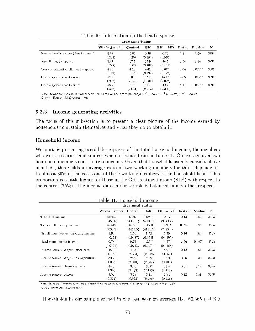
Table 40: Information on the head's spouseTreatment Status


Gender head's spouse (fraction male) 0.67 0.80 0.46 0.75 0.51 0.60 3291(0.221) (0.298) (0.193) (0.570)

Age HH head's spouse 38.1 37.7 37.9 38.7 0.98 0.38 3291(0.299) (0.577) (0.467) (0.487)

Years of education HH head's spouse 4.09 4.18 4.41 3.67∗ 3.64 0.029∗∗ 3081(0.113) (0.173) (0.197) (0.199)

Head's spouse able to read 49.9 50.6 53.7 45.1∗ 4.63 0.012∗∗ 3291(1.232) (2.148) (1.931) (2.072)

Head's spouse able to write 53.9 54.3 57.7 49.7 3.11 0.048∗∗ 3291(1.312) (2.074) (2.214) (2.336)



5.3.3 Income generating activities

The focus of this subsection is to present a clear picture of the income earned byhouseholds to sustain themselves and what they do to obtain it.

Household income

We start by presenting overall descriptives of the total household income, the memberswho work to earn it and sources where it comes from in Table 41. On average over twohousehold members contribute to income. Given that households usually consists of �vemembers, this yields an average ratio of two working members for three dependents.In almost 80% of the cases one of these working members is the household head. Thisproportion is a little higher for those in the GK treatment group (81%) with respect tothe control (75%). The income data in our sample is balanced in any other respect.

Table 41: Household incomeTreatment Status


Total HH income 60365 60365 56257 63158 0.43 0.65 3595(3460.6) (4398.7) (5016.8) (8049.4)

Typical HH yearly income 64746 64746 64590 65833 0.024 0.98 3595(4002.1) (4463.5) (8111.5) (7820.8)

Nr HH members contributing income 1.69 1.66 1.72 1.70 0.46 0.63 3595(0.0278) (0.0487) (0.0541) (0.0395)

Head contributing income 0.78 0.75 0.81∗∗ 0.77 2.76 0.067∗ 3595(0.0111) (0.0215) (0.0174) (0.0168)

Income source: Wages agriculture 48.1 49.3 46.3 48.7 0.42 0.66 3595(1.459) (2.563) (2.329) (2.653)

Income source: Wages non-agriculture 30.2 28.9 28.9 32.9 0.96 0.39 3593(1.353) (2.240) (2.337) (2.403)

Income source: Business/Farm 34.0 35.5 33.0 33.4 0.31 0.74 3595(1.316) (2.483) (2.123) (2.170)

Income source: Others 3.01 3.07 3.21 2.74 0.22 0.81 3590(0.321) (0.632) (0.496) (0.518)



Households in our sample earned in the last year on average Rs. 60,365 (∼USD

70

970)21. This �gure includes two hundred households who report not having receivedany income (in-kind or in cash) over the last year. Employing the sub-sample whoreported positive yearly earnings, back of the envelope calculations indicate that theaverage household in the sampled area lives on $2.8 per day. Recalling that eachhousehold has on average 5.43 members, it translates into barely $0.52 per personper day. Even excluding children, i.e. members of less than 15 years of age, fromthis estimation the daily income per adult amounts to only $0.76 per person per day,far below the internationally recognised poverty line of US$ 1.25 per person per day.We can make this comparison more meaningful by adjusting for the purchasing powerparity conversion factor. This factor is the number of Rupees required to buy the sameamount of goods and services in the local market as a US$ would buy in the UnitedStates. Adjusting for this, the average household member has access to US$ 1.69 perday, placing our study population slightly above the international poverty line.22

The typical yearly income reported by the respondents was slightly higher, reachingRs. 64,746 (∼USD 1,039) for the whole sample.

Our study households' earnings come to a very large extent from agriculture-relatedactivities, with 48.1% of the sample reporting receiving wages for agricultural labourand 34% deriving income from the farm.23 Another important source of income arewages from employment outside the agriculture and allied sector, bene�tting 30% ofthe households sampled.

Table 42: Household businessTreatment Status


HH owns business 31.1 32.4 30.0 30.9 0.28 0.76 3595(1.308) (2.437) (2.108) (2.196)

Primary activity business: Farm 94.3 95.0 94.1 93.6 0.19 0.83 1119(0.937) (1.461) (1.656) (1.774)

Primary activity business: Shop/restaurant 4.92 4.99 3.93 5.80 0.69 0.50 1119(0.681) (1.210) (1.017) (1.254)

Primary activity business: Other 3.49 3.49 3.37 3.59 0.011 0.99 1119(0.603) (1.006) (1.052) (1.078)

Nr of workers in HH business 5.79 6.20 5.74 5.40 1.16 0.32 1119(0.232) (0.342) (0.435) (0.409)

Enterprise expenses last year 34717 34717 35858 33344 0.16 0.85 1118(2654.6) (6249.8) (3128.1) (3169.6)

Enterprise revenue last year 63860 63860 60160 52579∗ 1.76 0.18 1119(5172.7) (11559.6) (6308.5) (6487.1)



Household business

From Table 42 we learn that 31% of households own a business, which for the majorityof them is a farm, and for the rest is generally a shop or restaurant. These businesses

21Exchange rate are derived from http://www.imf.org/external/np/�n/data/param_rms_mth.aspx22The PPP conversion is based on PPP conversion factors available on

http://data.worldbank.org/indicator/PA.NUS.PPPC.RF.23This category also includes other type of businesses. However, for 94% of the households this

business is a farm (see Table 42).

71

employ an average of almost six people under normal circumstances, the majority ofthem household members, which outnumber non-members two to one. These enterprisesprovide a good pro�t margin, averaging almost Rs. 30,000 annually (∼USD 482), about47% over the revenue.

5.3.4 Assets

This section provides some insight into the wealth of households in terms of their assets.First we provide an overview of the ownership of assets that can be found in ruralhouseholds (Table 43). Control and treatment groups do not display any signi�cantdi�erence with respect to asset ownership, with the sole exception of four-wheeledmotor vehicles which seem to be more common among households in the GK group.However, given the clear and consistent balance in terms of income and in terms of allof the other assets in the list we are not concerned that this one particular di�erencewill in�uence the study.

We see in Table 44 that close to half of the households hold some land (other thanthe land the dwelling is built on, if applicable), have some furniture (typically chairsand tables, or beds), television and some jewellery. Phones and electric appliances arecommon possessions among households in our sample. Other important assets held byhouseholds are cattle (26%) and bicycles (29%).

Those who own land, possess on average 3 and 4.6 acres of non- and agriculturalland, respectively, the value of the latter being close to half a million rupees (∼USD8030). Land tenure is signi�cantly higher for the GK group than for the control group,elbeit only at the 10 percentage point signi�cance level. The value of the dwellingamounts to almost two hundred thousand rupees (∼USD 3212) with no signi�cantdi�erences across groups24.

5.3.5 Consumption

We next turn to consumption expenditures of the households. The statistics presentedin Table 45 correspond to three aggregated consumption categories: food consumption,other non-durable and durable goods. These measures are generated with informationcollected from a wide range of items. With regard to the household expenditure on food,consumption for 21 di�erent items was employed to come up with this aggregate, whichrepresents the value of annual consumption of all of these food items, including homegrown food or items obtained as gifts in addition to goods purchased on the market. Themean value of this aggregate measure in a year is Rs. 63,797 (∼USD 1,025), excludingalcohol and tobacco, where we make the assumption that the reported expendituresfrom the last week are representative for the whole year.25

In order to obtain an estimate of total consumption one has to add other spendingcategories like services and non-food consumables, which represent Rs.1,666 (∼USD 27)

24Two outliers for the value of the dwelling and eight values for the total value of land owned werereplaced by their respective GP median values.

25Outliers in consumption values have been replaced by the sample median .

72

Table 43: Household asset ownershipTreatment Status


HH assets: Land 44.5 44.4 43.1 46.1 0.36 0.70 3590(1.449) (2.498) (2.364) (2.637)

HH assets: Bycicle 28.5 28.0 30.5 26.9 0.36 0.70 3593(1.793) (3.001) (2.925) (3.359)

HH assets: Motorcycle 16.6 16.2 18.5 15.3 1.47 0.23 3593(0.756) (1.214) (1.433) (1.227)

HH assets: Four wheeler 1.14 0.73 1.86∗∗ 0.85 3.26 0.042∗∗ 3593(0.184) (0.244) (0.382) (0.290)

HH assets: Chairs/tables 49.9 49.0 52.2 48.4 0.42 0.66 3593(1.830) (3.197) (3.241) (3.020)

HH assets: Beds 37.2 35.5 41.4 34.9 1.37 0.26 3593(1.797) (2.854) (3.087) (3.303)

HH assets: Cupboard 32.2 31.7 33.8 31.0 0.34 0.71 3593(1.360) (2.116) (2.647) (2.267)

HH assets: Other furniture 7.32 5.98 9.11 6.92 1.13 0.33 3593(0.846) (1.330) (1.629) (1.380)

HH assets: Refrigerator 6.04 5.74 7.00 5.38 1.07 0.35 3593(0.477) (0.852) (0.877) (0.710)

HH assets: TV 54.5 56.9 55.9 50.4∗ 1.70 0.19 3593(1.473) (2.442) (2.216) (2.845)

HH assets: Radio 4.15 4.60 4.22 3.59 0.36 0.70 3593(0.462) (0.637) (0.675) (1.036)

HH assets: Phone 84.1 85.1 83.2 84.1 0.51 0.60 3593(0.767) (1.199) (1.406) (1.363)

HH assets: Electric appliances 73.4 73.3 75.8 71.3 1.15 0.32 3593(1.292) (2.391) (1.975) (2.252)

HH assets: Steel/glass plates 85.5 85.9 86.0 84.6 0.100 0.91 3593(1.387) (2.421) (2.202) (2.565)

HH assets: Jewellery 57.3 56.8 58.8 56.4 0.13 0.88 3593(2.108) (3.612) (3.646) (3.685)

HH assets: Cattle 26.5 27.1 26.1 26.3 0.064 0.94 3593(1.172) (1.927) (2.238) (1.908)

HH assets: Goats/Sheep 4.90 4.12 5.32 5.30 0.88 0.42 3593(0.448) (0.694) (0.768) (0.851)

HH assets: Chickens 5.26 4.52 5.06 6.24 0.59 0.55 3593(0.616) (0.853) (0.970) (1.324)

HH assets: Agricultural equipment 14.0 12.2 14.9 15.1 0.95 0.39 3593(0.975) (1.655) (1.712) (1.662)

HH assets: Other 33.4 31.7 35.2 33.2 0.66 0.52 3593(1.227) (1.982) (2.241) (2.117)



73

Table 44: Household assets valueTreatment Status


Agricultural land owned by HH - Acres 4.61 4.44 5.06∗ 4.34 2.37 0.098∗ 1570(0.142) (0.218) (0.259) (0.249)

Non-agricultural land owned by HH - Acres 3.01 2.37 3.92∗ 3.20 1.79 0.18 107(0.357) (0.239) (0.876) (0.805)

Value land owned (Rs.) 471665 471665 465354 469825 0.32 0.72 3595(7925.6) (13997.0) (10532.9) (16013.9)

Value main dwelling (Rs.) 184458 184458 197518 181426 0.62 0.54 3595(8138.1) (12163.3) (16389.1) (13296.6)

Value representative assets (Rs.) 672351 672351 676745 668455 0.046 0.95 3595(11442.0) (20136.8) (18188.2) (20994.5)



Table 45: Household consumptionTreatment Status


Food consumption (last year) 63797 63797 61286∗ 64956 1.81 0.17 3595(1010.2) (1750.0) (1494.9) (1907.4)

Nondurable consumption expenditure (past month) 1666 1666 1691 1649 0.039 0.96 3595(64.73) (106.6) (106.1) (123.4)

Durable consumption expenditure (last year) 26008 26008 24621 25889 0.74 0.48 3595(937.6) (1804.5) (1470.3) (1531.1)

Total consumption expenditure (last year) 110128 110128 106506 110985 1.23 0.29 3595(1775.9) (3196.1) (2724.2) (3186.5)



monthly for the typical household. Durable goods consumption, in turn, is reported tobe in the region of twenty-six thousand rupees annually (∼USD 418).

Overall, the grand total for the value of household consumption is an estimated Rs.110,128 (∼USD 1,769), almost one third of which are food expenditures. Note that thetotal estimated value of these consumables is higher than the reported annual incomeof Rs.60,365 that we discussed above. The average household in our dataset, however,produces at home or receives as gifts almost 20% of all food items it consumes.

Just like income and assets, consumption expenditures are nicely balanced acrosstreatment arms, suggesting that the experimental design was successful in randomlyallocating households of varying income groups to the di�erent samples.

74

5.3.6 Savings, credit and insurance

In this section we look at the �nancial transactions of the household, namely, at thesavings at their disposal, their credit history and the insurance policies that they mayhold.

Savings

Table 46 shows that 25% of households have savings, averaging thirty-�ve thousandrupees (∼USD 562) for those who have them. The vast majority of these householdsemploy formal �nancial institutions like banks as their vehicle for saving.

Table 46: Household savingsTreatment Status


HH has savings 24.9 25.0 26.2 23.2 0.27 0.77 3593(1.633) (2.680) (2.741) (3.044)

Amount savings (Rs.) 35095 35095 40461 29571 1.47 0.23 893(2725.7) (4398.9) (5466.9) (3475.0)



Credit

Households are asked about their credit access and borrowing activities for both smallamounts (less than Rs 500) and larger amounts (Rs 500 and above). This distinctionwas made as small amounts of borrowing are typically non-negligible in rurual India, butrarely reported when asking about household debts. We start by discussing responsesto small amounts of credit, followed by the larger ones.

From Table 47 we can see that 61% of households state to know a source wherethey can turn to in case they need to borrow less than Rs. 500.. The main source forthis type of credit are friends (72%) and relatives (53%), followed at great distance bymoneylenders (15%) and more formal institutions like banks (12%). It is worth notingthat almost nobody in our sample mentions micro�nance institutions as a viable sourceof such small amounts. However as we will see shortly, MFIs are also not a prominentsource for larger amounts in our study area. Borrowing from friends appears to beless common in the control group that in our treatment groups by a small margin. Inany other respect, credit statistics are shown to be balanced across treatments in thesample.

The above table describes just potential borrowing and sources of credit for house-holds, actual borrowing of small amounts was much less common among householdsthan their knowledge of sources may suggest. As we can see in Table 48 only 21% ofthem took any loan of less than Rs. 500 (∼USD 8) in the last month. As expectedthere is a high correlation between known sources and actual lenders, and most of thesesmall loans were taken from friends (68%) and relatives (23%), with any other sources

75

Table 47: Household credit sources (<Rs.500)Treatment Status


HH knows credit source 61.0 61.3 62.6 59.1 0.52 0.60 3593(1.341) (2.046) (2.461) (2.427)

Sources of borrowing: Bank 11.8 12.3 11.2 11.8 0.087 0.92 2193(1.015) (2.041) (1.717) (1.394)

Sources of borrowing: Micro�nance inst. 0.41 0.13 0.67∗ 0.43 1.78 0.17 2193(0.132) (0.131) (0.287) (0.240)

Sources of borrowing: SHG 6.29 7.64 5.12 6.07 0.48 0.62 2193(1.033) (1.930) (1.696) (1.690)

Sources of borrowing: Moneylender 15.3 15.4 16.6 13.9 0.33 0.72 2193(1.361) (2.292) (2.469) (2.268)

Sources of borrowing: Relative 52.7 52.0 53.1 53.0 0.032 0.97 2193(1.880) (3.363) (3.262) (3.116)

Sources of borrowing: Friend 71.8 66.7 75.1∗∗ 73.8∗ 2.74 0.068∗ 2193(1.619) (2.714) (2.846) (2.643)

Sources of borrowing: Work 11.4 10.9 11.3 11.8 0.045 0.96 2193(1.179) (2.144) (1.800) (2.164)



playing a very marginal role. The total amount borrowed adding up all loans by thosewho took any is less than a thousand rupees (∼USD 16), of which 65% is still owed onaverage. 80% of the household who borrowed in the last month are still indebted.

Table 48: Household borrowing (<Rs.500)Treatment Status


HH taken loan last month 20.8 21.3 17.0 24.3 2.89 0.059∗ 2193(1.380) (2.597) (1.820) (2.567)

HH borrowed from: Bank 2.19 1.85 3.97 1.19 1.22 0.30 456(0.659) (1.024) (1.570) (0.824)

HH borrowed from: Moneylender 7.24 7.41 10.3 4.76 1.51 0.23 456(1.258) (2.103) (2.910) (1.637)

HH borrowed from: Relative 23.0 22.2 23.8 23.2 0.043 0.96 456(2.139) (3.933) (3.820) (3.348)

HH borrowed from: Friend 67.8 68.5 61.9 71.4 1.24 0.29 456(2.395) (3.898) (4.739) (3.776)

Amount borrowed last month 729.8 670.1 669.1 832.7 0.54 0.58 455(67.78) (82.72) (114.6) (140.9)

HH has debt outstanding 79.6 79.4 80 79.5 0.0034 1.00 451(3.058) (5.492) (5.728) (4.734)

Amount outstanding debt 470.1 407.1 496.3 511.1 0.55 0.58 451(52.56) (58.46) (119.5) (94.44)



Given that the GK intervention in this study aims at promoting the construction ofsanitation systems through the provision of credit, households were asked about theirknowledge of credit sources for the speci�c purposes addressed by the intervention priorto its implementation. About half of the sample was asked about whether they knowof any institution that provides loans for housing improvements, whereas the other halfof the sample was asked about whether they know of any institution that provides

76

loans for educational purposes (neither of which are loans that were provided by GKprior to the intervention). The results reveal a general lack of awareness of any sourcesavailable for getting a loan with the purpose of making house improvements (only 7%know of any institution for this purpose, which includes toilet construction), or forfunding education (less than 5%). Even among those who are aware of any source offunding, micro�nance institutions are relatively unheard of, just 10% and 6% of thesehouseholds know of a micro�nance institution that disburses loans for improving thehouse or furthering education, respectively, within these tiny sub-samples.

Table 49: Knowledge of sources speci�c purposeTreatment Status


HH knows credit source for housing improvements 7.13 6.75 7.13 7.53 0.11 0.89 1780(0.705) (1.138) (1.339) (1.181)

HH knows MFI for housing loan 10.2 12.2 11.9 6.82 0.44 0.65 127(3.019) (6.555) (5.022) (3.799)

HH knows credit source for building toilet 43.3 43.9 42.9 43.2 0.0084 0.99 127(4.176) (5.363) (6.203) (9.227)

HH knows MFI for toilet loan 3.64 5.56 5.56 0 1.11 0.34 55(2.485) (5.518) (4.880) (0)

HH knows credit source for education 4.47 3.17 4.87 5.46 1.39 0.25 1812(0.628) (0.991) (1.210) (1.015)

HH knows MFI for education loan 6.17 10 3.45 6.25 0.48 0.62 81(2.636) (5.718) (3.517) (4.316)



With regard to credit sources for large amounts (over Rs. 500), they are reportedlyknown by only half of the sample. Nevertheless, households tend to turn to similarcredit sources as for smaller amounts with only two exceptions of note, both banksand moneylenders are considerably more often mentioned for larger amounts of credit:23% and 28% of credit aware households would seek funding from these two sourcesrespectively. Micro�nance institutions continue to be a negligible source of borrowingin our sample area.

Information was also collected about the credit history during the last year fromhouseholds whose borrowing exceeded �ve hundred rupees. According to our �ndingsreported Table 51, 22% of households got indebted at some point during the year,93% of whom have still outstanding debts. Both the amount borrowed (sum of thethree most recent loans) and still owed are close to �fty thousand rupees, suggestingthat probably the wealthiest households in the sample are responsible for most of theborrowing recorded. Only a meagre 2% of households took a loan for building a toilet,health expenses and purchase of agricultural inputs are the most frequent reasons forhouseholds to get into debt.

77

Table 50: Household credit sources (>Rs.500)Treatment Status


HH knows source to borrow from 52.2 53.7 52.4 50.3 0.44 0.64 3593(1.475) (2.146) (2.606) (2.871)

Sources of borrowing: Bank 23.1 22.0 23.7 23.9 0.22 0.81 1875(1.386) (2.394) (2.671) (2.024)

Sources of borrowing: Micro�nance inst. 1.60 1.35 1.77 1.70 0.26 0.77 1875(0.266) (0.408) (0.489) (0.480)

Sources of borrowing: SHG 7.95 10.4 7.09 6.11 1.14 0.32 1875(1.189) (2.167) (1.947) (1.946)

Sources of borrowing: Moneylender 28.2 28.6 30.3 25.7 0.61 0.55 1874(1.703) (2.895) (2.804) (3.094)

Sources of borrowing: Relative 57.2 55.8 56.4 59.8 0.31 0.73 1875(2.318) (4.162) (4.117) (3.671)

Sources of borrowing: Friend 66.0 62.0 68.1 68.4 1.34 0.27 1875(1.892) (3.111) (3.484) (3.078)

Sources of borrowing: Work 12.7 12.9 12.7 12.6 0.0074 0.99 1875(1.227) (2.145) (2.074) (2.148)



Table 51: Household borrowing (>Rs.500)Treatment Status


HH taken loan last year 22.0 22.2 18.8 25.1 1.59 0.21 3592(1.491) (2.565) (2.179) (2.866)

Amount borrowed last year 45998 45998 39561 47498 0.90 0.41 792(3821.1) (8191.3) (4473.8) (5870.3)

HH has debt outstanding 93.1 93.8 93.3 92.2 0.14 0.87 792(1.264) (1.917) (2.085) (2.405)

Amount outstanding debt 49668 49668 41653 53820 0.71 0.49 792(5536.5) (8291.3) (6090.2) (11681.4)

HH took loan for building toilet 2.02 2.18 2.24 1.70 0.12 0.89 792(0.509) (0.873) (0.948) (0.839)



Insurance

Finally, we look at whether households have insurance and if so, of which type. As wecan see in Table 52, 20% of households have taken an insurance policy in the sampledarea. Among them, the most common insurance type is life insurance, held by almost80% of those with a policy. Other types of insurance bought are crop insurance (19%)and health insurance (12%). Of this latter group almost 80% are participants of theRajiv Gandhi Jeevandayee Arogya Yojana (RGJAY) health insurance scheme sponsoredby the state government of Maharashtra; the program's main objective is to improvemedical access for both Below Poverty Line (BPL) and Above Poverty Line (APL)families.

78

Table 52: Household insuranceTreatment Status


HH has insurance 19.8 17.2 22.0∗∗ 20.3 2.35 0.100∗ 3592(0.968) (1.519) (1.651) (1.779)

HH insurance type: Crop 19.0 19.7 18.5 18.9 0.050 0.95 711(1.686) (2.762) (2.925) (2.991)

HH insurance type: Weather 1.97 0.47 1.54 3.78 1.55 0.22 711(0.816) (0.461) (0.893) (2.156)

HH insurance type: Life 79.3 74.2 85∗∗ 77.7 2.77 0.067∗ 711(1.963) (4.522) (2.775) (2.768)

HH insurance type: Health 12.0 14.1 8.08∗ 14.3 2.53 0.084∗ 711(1.404) (2.740) (2.008) (2.457)

HH insurance type: Vehicle 7.17 4.69 9.23∗ 7.14 1.82 0.17 711(1.006) (1.417) (2.015) (1.456)

HH insurance type: Livestock 0.56 0.94 0.38 0.42 0.30 0.74 711(0.272) (0.634) (0.373) (0.407)

HH insurance type: Other 1.97 2.82 1.93 1.26 0.62 0.54 710(0.610) (1.229) (1.130) (0.724)

HH has RGJAY 8.02 8.45 6.54 9.24 0.44 0.64 711(1.211) (1.966) (2.027) (2.229)



79

5.3.7 Shocks

We now turn to negative shocks experienced by the households over the last year.Results are displayed in Table 53.

The most common shock su�ered by households was bad harvest, which reportedlya�ected 35% of the households. It is interesting to put this �nding in context with ourincome �gures above, where we show that housholds had on average a lower incomethan their typical earnings. It is possible that these bad harvests played a role, given thelarge proportion of households who earn their livelihoods primarily in the agriculturalsector. The occurrence of all other shocks was substantially less frequent, for example,the death of a household member only hit 3% of the sample. We see imbalances acrossour treatment arms in the occurance of shocks but note that these imbalances are likelydriven by the low occurance of relevant shocks. Bad harvests on the other hand, whichis a shock more likely to occur for households of our sample, is on the other handbalanced across arms.

Table 53: Shocks and risksTreatment Status


Unexpected job loss 2.15 2.75 1.10∗ 2.57 3.40 0.037∗∗ 3586(0.357) (0.772) (0.349) (0.608)

Robbery/ Theft 0.39 0.49 0.084∗∗ 0.60 4.04 0.020∗∗ 3583(0.0985) (0.185) (0.0838) (0.205)

Bad harvest 35.1 35.1 34.5 35.6 0.056 0.95 3589(1.388) (2.525) (2.202) (2.456)

Death HH member 3.01 3.08 2.03 3.93 3.06 0.050∗ 3586(0.362) (0.689) (0.414) (0.691)



80

5.3.8 Sanitation

In this section, we provide an overview of the sanitation facilities of the household, themotivation for constructing them or not and the way they are �nanced.

Table 54: Toilet ownership

Treatment Status


HH owns toilet 30.5 28.0 35.1∗ 28.5 1.95 0.15 3595(1.737) (2.788) (2.783) (3.313)

HH's toilet in use 95.5 95.4 96.6 94.3 0.78 0.46 1097(0.835) (1.699) (1.102) (1.572)



Table 54 gives a broad picture of the sanitation situation in our sample area. Lessthan a third of households (31%) own a toilet, out of which 96% are reported to becurrently in use. Toilet ownership at baseline (November 2014 - January 2015) isonly slightly higher than the 28% coverage that was reported during the listing surveythat took place two months prior to the baseline survey (see Section 5.1). These �guresabout existing sanitation facilities were validated through direct observation by the datacollection team, who observed and con�rmed that 29% of households had, indeed, atoilet. This observed measure is highly correlated (90%) with the self-reported measure.

Table 55: Toilet typeTreatment Status


Flush/pour �ush to - piped sewer system 2.37 2.88 2.16 2.10 0.17 0.84 1097(0.575) (1.119) (0.967) (0.867)

Flush/pour �ush to -septic tank 24.2 22.5 23.3 27.0 0.67 0.51 1097(1.890) (3.466) (3.381) (2.692)

Flush/pour �ush to - pit latrine 26.0 31.1 23.0 24.3 1.58 0.21 1097(2.064) (3.447) (3.542) (3.354)

Ventilated improved pit latrine (vip) 16.0 15.0 16.8 16.2 0.12 0.89 1097(1.587) (2.701) (2.650) (2.884)

Pit latrine with slab 24.6 19.6 27.6 26.1 1.25 0.29 1097(2.142) (3.922) (3.605) (3.351)

Composting toilet 5.01 7.49 5.04 2.40 1.74 0.18 1097(1.220) (3.069) (1.561) (1.172)



As seen in Table 55 �ush or pour �ush toilets are the kind most commonly ownedby households, accounting for more than half of the existing ones. These toilets arecharacterised by having a water seal that prevents the passage of �ies and odours. Acomparatively smaller but still numerous group of households (42%) possess dry-typetoilets, namely, improved pit latrines either ventilated (16%) or with a slab (25%).

The location of the toilet (Table 56) is for all of those households reporting tohave one within or in the immediate vicinity of the dwelling, with the latter being themost common occurrence (85%). These results are backed by the interviewer's direct

81

Table 56: Toilet locationTreatment Status


Location toilet: In dwelling 14.1 14.4 13.9 14.1 0.012 0.99 1097(1.322) (2.530) (1.971) (2.437)

Location toilet: Attached dwelling 42.1 44.7 41.5 40.2 0.39 0.68 1097(1.993) (3.666) (3.058) (3.696)

Location toilet: In compound 42.8 40.9 42.9 44.4 0.26 0.77 1097(1.826) (3.252) (2.552) (3.808)

Location toilet: 10 mins walking 0.73 0 1.44∗∗ 0.60 3.85 0.024∗∗ 1097(0.275) (0) (0.605) (0.419)



Table 57: Pit/septic tank characteristicsTreatment Status


Material pit/tank: Brick 72.2 71.2 72.9 72.4 0.064 0.94 1097(2.103) (3.706) (3.069) (4.281)

Material pit/tank: Stone 2.19 1.44 3.84 0.90 1.97 0.14 1097(0.605) (0.593) (1.408) (0.499)

Material pit/tank: Cement rings 17.3 18.7 15.6 18.0 0.31 0.74 1097(1.816) (3.633) (2.601) (3.327)

Material pit/tank: Other permanent materials 7.84 8.65 7.67 7.21 0.077 0.93 1097(1.487) (2.883) (2.471) (2.290)

Material covering pit/tank: Cement 98.0 98.3 98.3 97.3 0.40 0.67 1097(0.550) (0.618) (1.088) (0.970)

Material covering pit/tank: Other 1.82 1.44 1.44 2.70 0.66 0.52 1097(0.542) (0.579) (1.067) (0.970)



observations, which yield the same conclusions. The GK group is 1 percentage pointmore likely than the control group to have to walk for 10 minutes to reach its owntoilet. This di�erence is statistically signi�cant at the 5% level but given the smallproportion of households this response option is relevant to we do not consider this ofgreat concern.

The toilet's pit or septic tank is usually made of brick (72% of the cases) with cementrings as a distant second. In contrast, the super structure covering the pit or tank isalmost invariably constructed with cement (Table 57).

For an overwhelming majority of households (96%) the pit has never reached ismaximum capacity, this �nding seems indicative of the relative novelty of the sanitationfacilities in the area. For 15 of the 39 households whose pit or tank �lled up, this tookmore than 5 years to occur (see Table 58), however, for a third of the household the pitneeded to be emptied after just one to two years. These factual results come in markedcontrast with the time that households who have never had a �lled pit expect this tohappen, the tendency here is to consider that the pit would take longer to become fullthan what the actual results suggest.

Most toilet owners (79%) in the sample plan to empty the pit when it �lls up andcontinue to use it, yet only a minority of them (16%) would rather opt/be able to usea second pit instead of emptying the full one. Very few others would consider other

82

Table 58: Pit/tank �lledTreatment Status


Pit/septic tank �lled up 3.62 3.77 3.90 3.10 0.16 0.86 1078(0.733) (1.657) (1.001) (1.095)

Pit/tank �lled up in: One year or less 7.69 0 12.5 10 1.61 0.22 39(4.382) (0) (8.113) (9.873)

Pit/tank �lled up in: 1-2 years 33.3 53.8 18.8∗ 30 1.63 0.22 39(9.924) (14.23) (12.68) (18.39)

Pit/tank �lled up in: 2-3 years 7.69 15.4 6.25 0 1.50 0.24 39(4.261) (10.81) (5.846) (0)

Pit/tank �lled up in: 4-5 years 12.8 7.69 18.8 10 0.34 0.71 39(5.791) (8.039) (10.49) (9.873)

Pit/tank �lled up in: More than 5 years 38.5 23.1 43.8 50 1.07 0.36 39(9.257) (10.01) (15.55) (19.05)

Pit/tank expected to �ll up in: One year or less 4.54 5.69 3.49 4.64 0.74 0.48 1058(0.763) (1.360) (1.201) (1.398)

Pit/tank expected to �ll up in: 2-3 years 11.1 14.1 8.73∗ 10.8 1.73 0.18 1058(1.225) (2.382) (1.624) (2.331)

Pit/tank expected to �ll up in: 4-5 years 13.2 14.7 13.2 11.8 0.38 0.69 1058(1.333) (2.769) (2.069) (2.000)

Pit/tank expected to �ll up in: More than 5 years 57.6 49.4 62.6∗∗ 59.8∗ 2.79 0.065∗ 1058(2.325) (4.631) (3.206) (3.517)

Pit/tank expected to �ll up in: Don't know 13.6 16.2 12.0 13.0 1.05 0.35 1058(1.208) (2.265) (1.887) (1.943)

When pit/tank full: Use second pit 16.1 17.6 14.1 17.1 0.52 0.59 1097(1.692) (3.879) (2.184) (2.554)

When pit/tank full: Empty it 78.5 76.9 81.8 76.0 1.44 0.24 1097(1.743) (3.752) (2.372) (2.733)

When pit/tank full: Use someone else's toilet 0.36 0.29 0 0.90 1.45 0.24 1097(0.221) (0.283) (0) (0.659)

When pit/tank full: OD 1.73 2.59 1.68 0.90∗ 1.44 0.24 1097(0.500) (0.896) (1.011) (0.484)

When pit/tank full: Other 0.18 0 0.24 0.30 1.02 0.36 1097(0.128) (0) (0.236) (0.298)



alternatives, like turning to open defecation.

83

Table 59: Construction and funding toiletTreatment Status


Who constructed toilet-Self/Other family member 11.3 13.1 6.97∗∗ 14.8 6.22 0.0027∗∗∗ 1091(1.134) (2.172) (1.356) (2.050)

Who constructed toilet-Self/Other family member with help 0.37 0.29 0.24 0.60 0.29 0.75 1091(0.181) (0.287) (0.239) (0.421)

Who constructed toilet-Hired labour 11.6 7.56 13.2∗ 13.9∗ 2.30 0.10 1091(1.453) (2.133) (2.290) (2.801)

Who constructed toilet-Mason 92.4 91.6 93.8 91.5 0.90 0.41 1091(0.865) (1.706) (1.116) (1.674)

Who constructed toilet-Arranged dwelling owner 0.37 0.29 0.48 0.30 0.11 0.90 1091(0.181) (0.285) (0.336) (0.299)

Who constructed toilet-Goverment o�cial 1.19 1.16 1.92 0.30 1.18 0.31 1091(0.594) (0.714) (1.381) (0.299)

Who constructed toilet-NGO workers 0.46 0 1.20 0 1.68 0.20 1091(0.370) (0) (0.926) (0)

Cost of toilet (Rs.) 26527 26527 26684 26610 0.028 0.97 922(712.4) (1433.0) (1044.2) (1224.2)

Source of funding toilet: Savings 87.1 86.5 86.3 88.9 0.32 0.73 1097(1.791) (3.068) (3.557) (2.076)

Source of funding toilet: Loan (formal) 0.27 0.29 0.48 0 1.52 0.22 1097(0.157) (0.283) (0.338) (0)

Source of funding toilet: Loan (informal) 2.01 2.88 0.72∗ 2.70 2.85 0.062∗ 1097(0.484) (1.029) (0.529) (0.915)

Source of funding toilet: Subsidy 11.8 11.5 12.9 10.5 0.13 0.88 1097(1.981) (2.562) (4.329) (2.373)

Source of funding toilet: Transfers 4.74 5.19 3.84 5.41 0.53 0.59 1097(0.693) (1.230) (1.129) (1.225)

Source of funding toilet: Other 0.27 0.58 0 0.30 1.54 0.22 1097(0.156) (0.409) (0) (0.287)



In the vast majority of cases (92%) the toilet was built by masons hired for thisspeci�c purpose, only 11% of households took the task upon themselves or hired un-specialised labour to complete the job as displayed in Table 59. The average cost ofthe toilet was reportedly of approximately Rs. 26,000 (∼USD 417), which came pre-dominantly from the household's own savings. This amount is signi�cantly higher thaneither the sanitation loan o�ered by GK (Rs. 15,000) or the subsidy provided by thegovernment (Rs. 12,000). Few households had access or made use of external fund-ing to cover the costs of the toilet and only 12% bene�tted from any type of subsidy.These results are suggestive that only those with already the means to have a toiletbuilt undertook its construction. Supporting this hypothesis are statistics presented inRaman and Tremolet [2010], which reports on toilet construction costs in three districtsof Maharashtra (Chandrapur, Kolhapur and Nashik). The costs reported for a typicaltoilet of a household classi�ed as APL is reported at on average USD332, which is theequivalent of USD373 in December 2014 USD value (the time of our baseline survey).This average hides some variation. The average reported costs in Kolhapur for exampleis as high as USD 434 for an average APL toilet, slightly above the average reportedby our study households.

84

Table 60: Motivation building toiletTreatment Status


More convenience 65.0 65.1 63.3 67.0 0.30 0.74 1097(1.798) (2.388) (3.208) (3.472)

Female members in the household wanted one 78.0 76.1 79.6 78.1 0.32 0.73 1097(1.728) (3.536) (2.684) (2.671)

Health improvement 51.5 47.8 55.4 50.5 1.18 0.31 1097(2.051) (3.476) (3.578) (3.346)

People in village had one 9.75 9.80 10.1 9.31 0.043 0.96 1097(1.045) (1.800) (1.683) (1.973)

Imposed by someone in village 3.46 4.03 3.60 2.70 0.38 0.68 1097(0.706) (1.127) (1.349) (1.071)

Usage of toilets elsewhere 2.10 3.17 1.44 1.80 0.70 0.50 1097(0.560) (1.238) (0.801) (0.828)

Physical problems with OD 13.1 12.1 14.1 12.9 0.17 0.84 1097(1.505) (2.455) (2.476) (2.861)

Di�culties in �nding alternatives 2.73 2.31 2.16 3.90 0.49 0.61 1097(0.651) (0.918) (0.726) (1.614)

So not embarrassed with guests 3.92 4.32 4.32 3.00 0.44 0.65 1097(0.712) (1.035) (1.381) (1.133)

Status in the village 7.29 6.05 6.71 9.31 0.62 0.54 1097(1.123) (1.724) (1.716) (2.411)

Better hygiene 17.3 16.1 17.3 18.6 0.14 0.87 1097(1.730) (2.837) (2.570) (3.671)

Greater safety 12.9 12.4 12.7 13.5 0.048 0.95 1097(1.472) (2.585) (2.417) (2.678)

Financial support from government 4.83 2.88 5.76 5.71 1.45 0.24 1097(1.001) (0.989) (1.777) (2.087)

Other �nancial support 0.46 0.58 0.24 0.60 0.44 0.65 1097(0.200) (0.401) (0.241) (0.404)

Owner/Landlord decided 1.00 0.86 0.72 1.50 0.56 0.57 1097(0.312) (0.495) (0.524) (0.578)

Government o�cial decided 0.64 0.29 0.96 0.60 0.37 0.69 1097(0.386) (0.284) (0.912) (0.419)

NGO employee or other decided 0.36 0 0.96 0 1.84 0.18 1097(0.282) (0) (0.706) (0)

Other 0.27 0.29 0.24 0.30 0.015 0.98 1097(0.157) (0.286) (0.238) (0.298)



From Table 60 we can see that 78% of respondents cite the in�uence of female house-hold members as one of the main motivations leading to the decision of constructinga toilet. This is closely followed by the convenience of having access readily to a sani-tation facility when it belongs to the household, mentioned by 65% of the sub-samplewith a toilet. A third reason brought forward by half of the respondents is the perceivedimprovement in health that a toilet could bring. Other reasons stated are general issues(e.g. safety or physical problems) with other defecation alternatives (25%), the wish ofbetter hygiene (17%), or social repercussions (11%) appear to be important as well butare less often cited.

85

Table 61 provides information on households that used to have a toilet but to notanymore, which is less the 1% of our study households. The main reason why they donot have it anymore is that is became unusable.

Table 61: Household does not own toilet anymoreTreatment Status


HH had toilet 0.80 1.01 0.91 0.48 1.13 0.33 2498(0.176) (0.304) (0.362) (0.233)

Reason no longer toilet: Became unusable 60 88.9 42.9∗∗ 25∗∗ 4.43 0.027∗∗ 20(10.68) (10.76) (16.24) (22.24)

Reason no longer toilet: Never used it 15 0 14.3 50∗ 2.17 0.14 20(8.275) (0) (13.91) (25.69)

Reason no longer toilet: Was in previous home 5 0 14.3 0 0.94 0.34 20(5.020) (0) (13.91) (0)

Reason no longer toilet: Other 20 11.1 28.6 25 0.45 0.64 20(8.718) (10.76) (14.83) (22.24)



When asking households without a toilet about the reasons for the same we �nd thatthe main obstacle for building a toilet stated by those households is lack of �nancialresources (83%). This can be seen in Table 62. Limited space availability comes secondbut it is only argued by 17% of the households, and other reasons seem not to havemuch weight in preventing households from building a sanitation facility. These �ndingsare supportive to the rationale behind the GK intervention, which aims to relax thehouseholds �nancial constraints and to lead to a sizeable increase in toilet adoption.

86

Table 62: Reasons for not owning a toiletTreatment Status


No need 4.36 3.37 4.68 5.14 1.10 0.34 2498(0.541) (0.764) (0.850) (1.126)

I cannot a�ord it 83.1 83.1 83.6 82.6 0.077 0.93 2498(1.100) (1.795) (1.896) (2.019)

I �nd it too expensive 12.6 14.4 12.5 10.9 1.10 0.33 2498(1.000) (1.791) (1.809) (1.524)

No space 17.1 17.4 17.3 16.7 0.033 0.97 2497(1.133) (1.728) (2.041) (2.120)

Had not the time to construct one 11.6 11.1 12.3 11.6 0.15 0.86 2498(0.952) (1.530) (1.604) (1.793)

Toilet shouldn't be close to house 0.76 0.67 1.04 0.60 0.52 0.60 2498(0.199) (0.377) (0.334) (0.307)

Never thought about it 8.89 9.54 8.57 8.48 0.14 0.87 2498(0.872) (1.646) (1.371) (1.444)

Religious and cultural reasons 0.080 0 0.26 0 2.14 0.15 2498(0.0562) (0) (0.178) (0)

Not everybody in HH wants it 0.44 0.22 0.39 0.72 1.29 0.28 2498(0.127) (0.157) (0.217) (0.264)

No one else I know has one 1.04 1.12 0.78 1.19 0.37 0.69 2498(0.231) (0.439) (0.340) (0.398)

Open defecation is seen as better 0.68 0.45 0.78 0.84 0.69 0.50 2498(0.165) (0.214) (0.351) (0.294)

Lack of info what toilet to build 1.68 1.01 2.08 2.03 1.50 0.23 2498(0.343) (0.370) (0.634) (0.727)

I dont know how to get a toilet 2.64 2.02 2.34 3.58 0.95 0.39 2498(0.480) (0.813) (0.792) (0.866)

Stay in rented house 0.64 0.45 0.26 1.19 1.35 0.26 2498(0.219) (0.269) (0.178) (0.552)

Can use neighbour's 0.20 0.34 0.13 0.12 0.51 0.60 2498(0.0886) (0.191) (0.129) (0.119)

Other 2.00 1.23 1.95 2.87∗ 1.67 0.19 2498(0.392) (0.436) (0.748) (0.804)



Conforming with the above results, 62% claim that they would not be able to coverthe cost of building a toilet even if they wanted to. Table 63 provides information on theremaining 38% of households. These households state a relatively wide set of potentialsources for funds for construction of a toilet: 40% state they would take a formal loan,43% an informal one, 48% report they could get subsidy, and 41% report they coulduse transfers from family or friends. Lastly, the majority of the households without atoilet (55%) would be willing to borrow for covering the expenditures of constructingone, another important result justifying the approach of the present intervention.

87

Table 63: Potential for building toiletTreatment Status


HH able to fund toilet 37.7 36.1 36.7 40.1 0.73 0.48 2486(1.486) (2.127) (2.942) (2.657)

Formal loan for building toilet 39.4 39.7 39.4 38.9 0.016 0.98 2170(1.783) (2.863) (3.127) (3.271)

Informal loan for building toilet 43.2 45.7 42.1 41.6 0.47 0.63 2191(1.991) (3.105) (3.062) (3.994)

Subsidy for building toilet 48.3 51.7 48.9 44.2 0.81 0.45 2178(2.321) (4.182) (3.356) (4.225)

Transfers for building toilet 41.4 40.7 42.8 40.7 0.092 0.91 2350(2.267) (3.777) (4.198) (3.828)

HH would borrow to build toilet 54.6 56.7 52.1 54.7 0.88 0.42 2476(1.386) (2.205) (2.679) (2.299)



5.3.9 Water

The survey also collected information on the household access to water for drinking,cooking and sanitation purposes. A summary of it is presented below. As it can beinferred from the hypothesis tests carried out, treatment and control groups do notdi�er in any respect in terms of their access to water.

From the �gures in Table 64 we learn that the main sources of water for cooking anddrinking are piped water into the dwelling (31%), public tap or pipe (25%), tubewellor borewell (23%), handpump (21%) and dug well (15%). This multiplicity of sourcesis due to the fact that not all houses have water all year round from the same source(for example, 21% of household rely on a di�erent source for the dry season) or at leastcannot get enough water from it. Consequently, people in the area need to turn toseveral sources to ensure a continuous supply of water in the house.

Only 38% of the household have access to water in their own dwelling. For the rest,the source is located an average of 142 metres from the household residence, takinghousehold members about 20 minutes to reach the source, collect water and returnhome. This action needs to be performed on average eleven times a day to maintainthe supply of water that the household requires. Very likely for this reason and otherproblems related to the di�culties in accessing water, a large proportion of households(63%) store it at home as shown in Table 65.

An equally large number of households pay for drinking and cooking water bothin the wet and dry seasons (about 65% in both cases). In spite of almost 80% ofthe household purifying the water for own consumption, this is done in a rudimentarymanner by �ltering it with a cloth, a method that does not eliminate parasites andbacteria from the water.

As seen in Table 66, the water used for sanitation needs comes from very similarsources as the consumed water, however, collecting it is much more laborious. Keepingthe household water supply takes considerably more trips and longer time, especially,during the dry season when household members need to spend close to an hour in theprocess.

88

Table 64: Water cooking and drinkingTreatment Status


Water source: Piped water into dwelling 30.8 31.7 31.6 29.0 0.16 0.85 3595(2.345) (4.385) (4.069) (3.638)

Water source: Public tap/stand pipe 25.1 26.4 25.7 23.0 0.36 0.70 3595(1.912) (2.946) (3.903) (2.984)

Water source: Tubewell or borewell 22.5 20.0 22.3 25.4 0.75 0.47 3595(1.715) (2.500) (2.658) (3.622)

Water source: Handpump 21.3 21.5 19.3 23.1 0.31 0.73 3595(2.091) (3.907) (3.231) (3.639)

Water source: Protected dug well 14.7 13.5 13.8 16.8 0.42 0.66 3595(1.591) (2.846) (2.607) (2.773)

HH has water all year from a source 82.6 83.0 82.3 82.4 0.020 0.98 3594(1.677) (2.908) (2.761) (3.040)

HH has water in own dwelling/yard 38.3 38.4 38.3 38.3 0.00013 1.00 3594(2.303) (4.343) (3.901) (3.643)

Distance water source (mtrs) 141.7 140.8 129.6 154.4 0.80 0.45 2729(7.790) (12.28) (12.08) (15.53)

Distance water source (mins) 20.5 21.8 20.6 19.0∗ 1.80 0.17 2729(0.605) (1.192) (0.906) (0.952)

Trips per day water source 11.6 12.2 11.5 10.9∗ 1.44 0.24 2729(0.318) (0.532) (0.580) (0.515)

Other water source dry season 20.9 18.3 23.4∗ 21.1 1.45 0.24 3594(1.266) (2.009) (2.257) (2.236)



5.3.10 Health care utilisation

The �nal section focussing on the household as a whole concerns health care utilisationby all its members.

Our statistics in Table 67 indicate that 17% of the households had at least one mem-ber receiving medical attention in the last month which did not require hospitalisation.The mean number of times this happened within this period was 1.46. The main causefor visiting a health facility or being visited by a health worker the last time were di-gestive problems (38%), followed by respiratory problems (31%), other unde�ned typesof pain or medical reasons account for most of the remaining causes.

The average total amount incurred by households in need of this kind of health careduring the last month26 is of Rs. 4,444 (∼USD 71), a large cost given the levels ofincome seen earlier.

26The survey enquired about the last three visits in the past month and only three householdsreported as many visits, thus, the above can be readily understood as a measure of total cost ofoutpatient care for our sampled households in a given month.

89

Table 65: Purifying and paying for waterTreatment Status


HH stores water 63.2 62.6 66.0 61.0 1.03 0.36 3594(1.544) (2.803) (2.304) (2.812)

HH pays for water wet season 65.8 63.5 66.2 67.9 0.53 0.59 3592(1.710) (3.256) (2.786) (2.736)

HH pays for water dry season 64.6 62.8 64.9 66.2 0.34 0.72 3593(1.671) (3.213) (2.649) (2.726)

HH puri�es water 78.4 76.1 82.0∗ 77.4 1.64 0.20 3595(1.561) (2.784) (2.151) (3.018)

Puri�cation method: Filtering w/ cloth 95.3 94.7 95.1 96.2 0.85 0.43 2820(0.578) (1.058) (1.109) (0.750)

Puri�cation method: Water �lter 4.50 4.46 5.24 3.76 0.58 0.56 2820(0.599) (1.107) (1.121) (0.819)



Table 67: Outpatient medical careTreatment Status


Medical care received 16.7 15.7 16.6 17.9 0.33 0.72 3574(1.099) (1.921) (1.965) (1.797)

Nr of visits HH 1.46 1.53 1.46 1.40 0.29 0.75 392(0.0856) (0.150) (0.181) (0.0937)

Reason med. care: Digestive Problems 38.0 44.8 35.3 34.1 1.46 0.24 405(2.763) (4.950) (4.329) (4.756)

Reason med. care: Respiratory problems 31.4 36.6 28.6 29.0 0.90 0.41 405(2.801) (4.842) (4.109) (5.300)

Reason med. care: Preventive medical exam/check-up 9.63 10.4 10.5 7.97 0.33 0.72 405(1.543) (2.683) (2.856) (2.380)

Reason med. care: Skin problems 3.46 3.73 3.01 3.62 0.076 0.93 405(0.836) (1.579) (1.347) (1.419)

Reason med. care: Other acute pain 12.3 12.7 10.5 13.8 0.39 0.68 405(1.652) (3.176) (2.436) (2.897)

Reason med. care: Other medical problem 21.0 14.9 22.6 25.4∗ 1.94 0.15 405(2.605) (4.000) (5.676) (3.543)

Cost of outpatient care 4444 4444 3843 4513 0.26 0.77 403(729.3) (1897.8) (819.3) (727.8)



In the last year 25% of households in our sample sought inpatient medical care(Table 68), although this was a relatively infrequent event for most of them, with thenumber of admissions averaging little above one. The main reason for being admittedinto a hospital, clinic or other health centre was some type of illness, typically a�ectingthe digestive system. The incidence of digestive problems seems to be higher for theGK+ND group at a 10 % signi�cance level, but this is the only case of unbalancedesnessamong the health care utilisation data. As expected, the cost of having householdmembers hospitalised is markedly higher than receiving outpatient care and amountsto more than �fteen thousand rupees (∼USD 240), a serious blow to the economy ofour average household in our study area.

90

Table 66: Water for sanitationTreatment Status


Dry season: Piped water into dwelling 23.2 24.3 22.3 23.1 0.082 0.92 3594(1.976) (3.968) (3.164) (2.977)

Dry season: Public tap/stand pipe 18.7 19.7 20.7 15.6 1.05 0.35 3594(1.617) (2.468) (3.313) (2.473)

Dry season: Tubewell or borewell 20.4 19.1 20.3 22.0 0.29 0.75 3594(1.527) (2.225) (2.534) (3.120)

Dry season: Handpump 18.3 18.7 16.1 20 0.44 0.64 3594(1.800) (3.159) (2.659) (3.453)

Dry season: Protected dug well 15.7 15.6 16.4 15.3 0.045 0.96 3594(1.505) (2.669) (2.609) (2.526)

Wet season: Piped water into dwelling 31.7 32.6 30.4 31.9 0.078 0.92 3594(2.253) (4.275) (3.838) (3.493)

Wet season: Public tap/stand pipe 21.6 23.3 22.5 18.8 0.87 0.42 3594(1.642) (2.647) (3.275) (2.494)

Wet season: Tubewell or borewell 18.4 17.0 18.5 19.7 0.29 0.75 3594(1.486) (2.190) (2.346) (3.114)

Wet season: Handpump 15.8 15.8 15.1 16.4 0.053 0.95 3594(1.731) (3.217) (2.732) (3.000)

Wet season: Protected dug well 10.3 9.45 10.3 11.2 0.16 0.85 3594(1.258) (2.206) (2.156) (2.161)

Distance (mins): Dry season 55.9 57.8 53.7 56.1 0.078 0.92 3594(4.360) (8.037) (6.607) (7.874)

Distance (mins): Wet season 38.5 38.7 35.9 41.1 0.28 0.76 3594(2.875) (4.877) (4.721) (5.291)

Trips per day: Dry season 15.5 16.3 14.9 15.2 0.98 0.38 3073(0.423) (0.709) (0.738) (0.730)

Trips per day: Wet season 12.4 13.2 12.0 12.0 1.56 0.21 2873(0.323) (0.538) (0.598) (0.517)



Table 68: Inpatient medical careTreatment Status


Hospitalisation HH member 24.5 24.2 22.6 26.7 1.28 0.28 3577(1.051) (1.783) (1.583) (2.010)

Nr of admissions HH 1.21 1.22 1.21 1.21 0.048 0.95 877(0.0315) (0.0458) (0.0764) (0.0408)

Reason hosp.: Illness (digestive problems) 32.7 30.1 29.7 37.8∗ 2.68 0.073∗ 877(1.721) (3.176) (2.807) (2.711)

Reason hosp.: Illness (other) 39.6 41.8 41.0 36.2 0.78 0.46 877(1.949) (3.504) (3.034) (3.442)

Reason hosp.: Accident 3.42 3.68 3.38 3.21 0.061 0.94 877(0.571) (0.987) (1.038) (0.945)

Reason hosp.: Physical aggression (violence) 3.99 3.34 4.51 4.17 0.31 0.73 877(0.750) (0.955) (1.199) (1.593)

Reason hosp.: Surgery 7.07 6.69 4.14 9.94 3.00 0.054∗ 877(1.004) (1.412) (1.183) (2.166)

Reason hosp.: Medical analysis or studies 1.14 0.33 1.88 1.28 1.82 0.17 877(0.382) (0.324) (0.957) (0.616)

Reason hosp.: Other 7.18 7.69 6.77 7.05 0.076 0.93 877(1.029) (1.663) (1.784) (1.864)

Cost of inpatient care 15974 15974 12619∗ 15807 2.20 0.11 877(1347.8) (2918.8) (1556.6) (1943.7)



91

During the survey participants without a toilet were asked to predict qualitativelythe change in their health expenditures under the hypothetical scenario that they owneda toilet (Table 69). Whereas most households consider that they would see a reductionin their health expenditures (45%) as a result of having a sanitation facility available,many believe that they would not appreciate any variation in their medical care costs(25%), or that these may even rise (15%).

Table 69: Hypothetical health costsTreatment Status


We would spend more 14.6 15.4 16.0 12.5 0.58 0.56 2497(1.562) (2.911) (3.036) (2.051)

We would spend less 44.5 43.4 45.8 44.6 0.072 0.93 2497(2.388) (4.194) (4.519) (3.691)

We would spend the same 25.2 24.4 24.4 26.8 0.52 0.60 2497(1.102) (1.808) (2.019) (1.901)



92

5.4 Women versus men in study sample (individual woman andman survey)

In this section we look at and compare information collected from an individualadultwoman and man of the household, who were either the mother/father of a child lessthan 6 years old (preferrably the youngest child), or the head/spouse of head of thehousehold. We refer to Figure 12 in Section 4.3.4 for more details on the respondentselection process.

Several questions (not all) were asked of both man and woman in the individualsurveys, which allows for a comparison. However, if the respondent of the individualman questionnaire was the same as for the household survey, several sections of theman questionnaire were skipped to avoid survey fatigue. Where possible, responsesfrom the household survey were used in order to compare the male responses to thefemale responses, but this was not always possible. As a result, the sample size for malerespondent is considerably reduced for some variables.

Given that the main use of these individual data will involve making intra-householdcomparisons, we will present the baseline results of the sample restricted to those house-holds for which we have data at all levels: household level, individual man and womanlevel. This reduces the individual survey sample size to 3,434 respondents (a 5% dropfrom the total).

5.4.1 Background and status

We �rst look at the background and the status of the interviewed woman and menin the household presenting information about their age, education and that of theirparents (if available) in Table 70 for women and Table 71 for men.

Table 70: Background and status womenTreatment Status


Age of respondent 30.7 30.1 30.9∗ 31.0∗ 1.96 0.14 3433(0.206) (0.363) (0.288) (0.394)

Years of schooling 5.90 6.00 6.16 5.54 2.40 0.095∗ 3297(0.119) (0.192) (0.196) (0.214)

Years of schooling father 2.35 2.36 2.31 2.39 0.052 0.95 3059(0.0874) (0.115) (0.164) (0.175)

Years of schooling mother 0.71 0.65 0.79 0.69 0.82 0.44 3015(0.0456) (0.0550) (0.0961) (0.0815)

Living in village all her life 8.07 7.69 7.91 8.61 0.21 0.81 3434(0.567) (0.895) (0.886) (1.147)


Source: Woman Questionnaire.

Female respondents, presumably with young children, are little over 30 years of ageand have received around 6 years of formal education. The parents of the interviewedwomen tend to be signi�cantly less educated than their daughter, especially the mothers,who are mostly illiterate (86%) and received on average less than one year of schooling.The majority of women come from a di�erent village than the one where they currently

93

Table 71: Background and status menTreatment Status


Age of respondent 43.4 43.0 43.6 43.5 0.29 0.75 3430(0.306) (0.569) (0.475) (0.536)

Years of schooling 7.66 7.70 8.02 7.24 3.31 0.040∗∗ 3341(0.122) (0.189) (0.179) (0.244)

Years of schooling father 3.37 3.20 3.76 3.18 1.11 0.33 659(0.179) (0.317) (0.324) (0.271)

Years of schooling mother 1.14 1.20 1.18 1.02 0.20 0.82 633(0.126) (0.221) (0.199) (0.230)

Living in village all his life 97.6 96.2 99.1∗∗ 97.5 2.54 0.084∗ 703(0.587) (1.323) (0.595) (0.953)


Source: Man Questionnaire.

live, most likely as a result of moving into their husband's home after getting married.In line, almost half of the women in our sample live with their in-laws, whereas littlemore than 1% share a roof with their own parents (Table 72).

Table 72: General information female respondentTreatment Status


Married 99.1 99.2 98.3 99.6 1.60 0.21 3434(0.331) (0.602) (0.754) (0.169)

Age when married 17.7 17.7 17.8 17.7 1.03 0.36 3366(0.0502) (0.0784) (0.0893) (0.0909)

Arranged marriage 98.9 98.4 99.3 99.0 1.19 0.31 3402(0.261) (0.458) (0.290) (0.556)

Sanitation facilities mattered 75.0 73.0 75.6 76.5 0.19 0.82 3402(2.256) (4.119) (3.595) (3.958)

Dowry paid 72.9 76.0 70.8 71.8 1.91 0.15 3391(1.253) (1.816) (2.700) (1.800)

Living with in-laws 45.1 46.2 44.1 45.0 0.24 0.79 3434(1.213) (2.178) (2.193) (1.903)

Living with parents 1.11 1.11 0.70 1.51 1.96 0.15 3434(0.183) (0.351) (0.253) (0.323)



Male respondents are considerably older than their female counterparts with almost40 years of age and are also signi�cantly more educated, having little less than 8 yearsof schooling. To some extent, this higher education level also extends to their parents,although illiteracy is still predominant among them. Unlike our female respondents,almost the entirety of our male sample has always lived in the same village where theywere born. This is especially true for members of the GK treatment group, who havea signi�cantly higher proportion of permanent residents>

As expected given the selection criteria for the respondents to the women question-naire, 99% of respondents are married. Their marriages took place when they wereyoung, about 18 years old, in an arranged ceremony (99%), which typically involved

94

the payment of a dowry (73%). A large proportion of women (75%) reported that,when they were looking for a husband, it mattered whether their husband could o�erthem a home with sanitation facilities.

5.4.2 Women empowerment

We next describe how the most important decisions in the household are taken and towhat extent women are involved in these matters. In Table 73 we show the averageproportion of women who have a say in some key aspects of the household life as pertheir own perspective. 67% of our female respondents report being able to decide bythemselves or jointly with their husbands about having another child, 68% can in�uencewhether the child goes to the doctor and 61% take part in deciding whether to sendthe children to school. With regard to monetary matters and employment, the womenin our sample seem to have less power to decide, and approximately only half of themreport involvement in deciding whether they work, what they do with the money theyearn and whether the household should make a signi�cant household purchase.

Table 73: Women's involvement decision making in the household: Women's perspectiveTreatment Status


Having another child 66.7 69.3 61.9∗ 68.7 1.64 0.20 3434(1.745) (2.669) (3.487) (2.717)

Taking children to doctor 68.2 68.4 67.5 68.7 0.078 0.93 3434(1.164) (1.781) (2.340) (1.893)

Children schooling 61.2 61.9 59.8 62.0 0.22 0.80 3434(1.340) (2.019) (2.793) (2.063)

Money earned 54.4 56.8 52.9 53.4 1.05 0.35 3434(1.329) (1.882) (2.504) (2.426)

Buying large HH item 56.9 57.4 57.1 56.2 0.067 0.93 3434(1.347) (2.097) (2.496) (2.392)

Working 52.6 53.4 51.4 52.8 0.16 0.85 3434(1.426) (2.254) (2.789) (2.325)



It is interesting to compare women's reported power of their degree of intra-householddecision making with what their husband's give them credit for. Such information isshown in Table 74. Men a�rm, to a greater extent than their own spouses (82% versus67%), that the latter's opinion count when it comes to deciding about adding anothermember to the family. This trend is however reversed for the rest of the decision areas.According to the results, 61% of men think that their wives' views regarding childrenmedical needs matter; Only 23% and 32% of men report that their spouse has a anysay on whether they should work and what to do with their earnings, respectively, and34% consult their spouses when considering to buy an expensive household item.

95

Table 74: Women's involvement decision making in the household: Men's perspectiveTreatment Status


Having another child 81.5 79.1 81.9 83.5 0.46 0.63 703(1.822) (3.669) (2.774) (2.861)

Taking children to doctor 61.5 58.6 65.6 60.3 0.75 0.47 703(2.459) (3.990) (4.345) (4.350)

Children schooling 50.4 48.1 56.4 46.8 1.32 0.27 703(2.685) (4.231) (4.375) (5.040)

Money earned 32.4 27.2 38.8∗∗ 31.6 2.02 0.14 703(2.440) (3.693) (4.413) (4.335)

Buying large HH item 33.7 33.5 36.1 31.6 0.25 0.78 703(2.414) (3.471) (4.476) (4.504)

Working 23.5 21.8 25.6 23.2 0.18 0.84 703(2.613) (3.757) (5.100) (4.653)



Lastly, Table 75 presents an overview of di�erent indicators attempting to capturethe extent of women's degree of autonomy. Most women (about 80%) feel free to visitneighbours, the temple or fetch water on their own. The majority of them (66%) alsofeel permitted to visit unaccompanied friends and relatives within the village wherethey live, but only 45% feel permitted to do so outside the village. Visiting the localmarket or going to the doctor unaccompanied is only allowed to only 44% and 47% ofwomen, respectively. Their control over money is also rather limited, with just abouthalf of the sample being able to decide about buying basic personal items (e.g. clothesand medicines) and food by themselves. Whereas 15% of women in the sampled areaare part of a lending group, only 59% of them claim being able to participate in thedecision of borrowing from the group.

96

Table 75: Women's autonomyTreatment Status


Go alone: local market 44.2 47.5 43.9 41.1 1.33 0.27 3317(1.630) (2.575) (2.757) (3.040)

Go alone: Health centre/doctor 46.9 50.7 46.6 43.3 1.28 0.28 3363(1.895) (3.037) (3.233) (3.461)

Go alone: Visit neighbours 79.4 81.8 77.4 78.8 0.95 0.39 3394(1.373) (2.126) (2.729) (2.200)

Go alone: Visit friends/relatives in village 66.2 69.9 64.4 64.2 1.42 0.24 3388(1.705) (2.451) (2.841) (3.438)

Go alone: Visit friends/relatives out village 44.6 47.4 45.4 40.9 0.98 0.38 3376(1.950) (3.317) (3.301) (3.425)

Go alone: The Shrine / Mosque / Temple 76.2 78.3 74.0 76.2 0.90 0.41 3390(1.294) (1.956) (2.576) (2.121)

Go alone: Collect water 82.9 84.2 81.8 82.8 0.30 0.74 3328(1.232) (1.962) (2.595) (1.733)

Control money: Fruits or Vegetables 50.7 52.7 49.0 50.5 0.34 0.71 3226(1.885) (3.158) (3.325) (3.279)

Control money: Other food items 47.2 48.8 45.9 46.9 0.25 0.78 3232(1.729) (2.898) (3.074) (2.990)

Control money: Clothes for yourself 51.9 54.1 50.7 50.9 0.27 0.76 3262(2.134) (3.711) (3.652) (3.685)

Control money: Medicine for yourself 49.9 51.6 50.0 48.2 0.16 0.85 3260(2.368) (4.192) (3.899) (4.166)

Control money: Toiletries for yourself 62.0 64.8 60.8 60.2 0.33 0.72 3270(2.456) (4.416) (4.234) (4.040)

Control money: Clothes and medicine for your kids 45.5 47.3 44.3 44.9 0.19 0.83 3243(2.101) (3.754) (3.277) (3.822)

Member of lending group 14.8 14.5 14.1 15.6 0.16 0.85 3434(1.040) (1.635) (1.693) (2.055)

Decision loan lending group 59.4 58.8 64.6 55.1 0.84 0.43 507(3.022) (4.595) (4.669) (6.039)



5.4.3 Credit and savings

In this section we look at the individual credit history and savings of the man and womaninterviewed. Given the comprehensive overview of the household �nances provided inthe corresponding subsections of the household part of this report, we only enquireabout whether each member has savings and borrowed money last year. The answerto these questions are presented in Table 76. 14% of women have savings that theyconsider their own, not at the disposal of the rest of the family. By contrast, 26% ofthe male respondents have accumulated some money that they they consider their own.Whereas we learnt from the household level survey results that 20% of the householdsreported to have taken a loan, here we observe that 6% of respondents - both manand woman - report to have taken a loan for themselves in the last 12 months. Thediscrepancy with the household survey is likely driven by the fact that the individualquestionnaire is not necessarily administered to the household head, who is most likelyin the household to take credit, loans that would count towards the reported borrowingpercentage in the household survey.

97

Table 76: Savings and credit man and womenTreatment Status


Woman: Has savings 14.0 13.7 15.5 12.9 0.58 0.56 3434(0.987) (1.667) (1.808) (1.615)

Woman: Taken loan last year 6.29 5.90 6.94 6.04 0.28 0.76 3434(0.619) (1.202) (1.065) (0.907)

Man: Has savings 26.0 25.5 26.0 26.6 0.021 0.98 703(2.080) (3.558) (3.483) (3.749)

Man: Taken loan last year 6.83 6.69 7.49 6.33 0.11 0.90 703(1.101) (2.163) (1.857) (1.665)



5.4.4 Social networks, group membership and political activity

As part of the survey administered to male respondents, we enquired about their po-litical a�liations and the degree of their political involvement. Table 77 shows thatwhile our respondents are rarely members of any community group themselves (only2% belong to one, usually a religious or social group), they seem to be heavily engagedin community politics. Almost without exception, respondents voted in the last LokSabha election, and, at the more local level, 56% of them participated in a meetingcalled by the gram panchayat within the last year.

Table 77: Group membership and political activityTreatment Status


Member of group 4.69 4.19 4.92 4.97 0.13 0.88 3434(0.615) (1.326) (0.822) (0.960)

Voted Lok Sabha election 98.0 97.9 98.7 97.6 1.14 0.32 3434(0.324) (0.498) (0.461) (0.690)

Attended meeting called by GP 56.1 53.8 59.8 55.0 0.95 0.39 3434(1.847) (3.514) (3.228) (2.685)



We also asked about social networks of our male respondents, and by extension hishousehold. Speci�cally, we ask whether they knew anyone outside their household whocould come and help them to make house improvements for free. As far as sanitationis considered a home improvement, this social network hence tells us something aboutrelationships that may help the household in the construction of a toilet (Table 78).We �nd that this does not seem to be the case for 98% of the sample. On the otherhand, a majority of the respondents (53%) seem to have someone to whom they canresort to if in need of borrowing Rs. 1000 urgently.

98

Table 78: Social networksTreatment Status


Help dwelling improvements 2.39 2.48 1.93 2.75 0.46 0.63 3434(0.368) (0.641) (0.570) (0.690)

Borrowing Rs. 1000 readily 53.1 53.9 51.2 54.0 0.31 0.73 3434(1.694) (2.917) (2.712) (3.145)



5.4.5 Sanitation

In this section, we provide a comprehensive overview of the men and women's practices,expectations, perceived bene�ts and beliefs related to sanitation

Sanitation practices

The sanitation practices of our respondents are summarised in Tables 79 and 80. 29%of women report typically using their own toilet to defecate, however, the most commonlocation used among them is an open area more than �ve minutes from their residence(70%). These practices are mirrored by men, of which 65% usually go for OD more than�ve minutes from their home. We do however in addition �nd a larger percentage of menperforming OD near their residence (7%) than women (2%). Almost everyone reportto be content with possessing a private toilet for doing their needs, whereas less than20% of the respondents are happy with the open areas where they typically defecate.The large majority of women (82%) feel unsafe visiting these places, particularly whenthey are far from home. Despite the low levels of satisfaction the open locations areperceived su�ciently comfortable for about 32% of women and 44% of men. Otherlocations (such as neighbour's toilet or community toilet) are little used in our sampleand are not reported here.27

27The statistics in these tables do not present any signi�cant di�erences across treatment arms withonly two exceptions which have very small sample sizes. Balancedness among the di�erent treatmentgroups also holds for the rest of the data on sanitation practices.

99

Table 79: OD practice, satisfaction, comfort and safety: WomenTreatment Status


Own toilet 28.9 26.8 33.4∗ 26.4 1.98 0.14 3434(1.716) (2.878) (2.629) (3.257)

OD (close home) 2.04 2.22 1.23∗ 2.66 2.29 0.11 3434(0.316) (0.461) (0.372) (0.729)

OD (>5 mins home) 69.5 71.1 65.6 71.7 1.52 0.22 3434(1.654) (2.824) (2.546) (3.111)

Satis�ed with Own toilet 93.6 93.3 92.9 94.9 0.33 0.72 991(1.202) (2.134) (2.196) (1.718)

Satis�ed with OD (>5 mins home) 15.2 16.6 17.3 11.8 1.26 0.29 2386(1.661) (3.096) (2.882) (2.510)

Comfortable visiting Own toilet 98.9 99.4 98.7 98.7 0.59 0.55 991(0.350) (0.444) (0.669) (0.628)

Comfortable visiting OD (>5 mins home) 32.2 32.2 29.5 34.8 0.76 0.47 2373(1.876) (3.537) (3.095) (2.993)

Safe visiting Own toilet 98.8 99.7 98.4 98.3 2.15 0.12 991(0.389) (0.315) (0.706) (0.849)

Safe visiting OD (>5 mins home) 18.8 18.1 17.5 20.7 0.42 0.66 2386(1.584) (2.762) (3.050) (2.371)



Table 80: OD practice, satisfaction, comfort and safety: MenTreatment Status


Own toilet 29.0 26.1 33.7∗ 27.2 1.91 0.15 2923(1.880) (3.032) (2.856) (3.721)

OD (>5 mins home) 64.8 66.6 60.9 66.8 1.27 0.29 2923(1.877) (3.136) (2.729) (3.762)

Satis�ed with Own toilet 88.8 87.3 88.5 90.4 0.087 0.92 241(3.051) (5.331) (5.377) (5.032)

Satis�ed with OD (>5 mins home) 20 20.9 21.1 18.0 0.14 0.87 410(2.693) (4.291) (5.166) (4.598)

Comfortable visiting Own toilet 91.1 87.3 88.1 97.5∗ 2.45 0.093∗ 235(2.662) (5.235) (4.970) (2.519)

Comfortable visiting OD (close home) 43.5 54.2 41.7 33.3∗ 1.47 0.24 69(5.623) (9.861) (9.952) (6.833)

Comfortable visiting OD (>5 mins home) 47.4 44.1 54.8 44.7 0.95 0.39 390(3.747) (7.153) (5.993) (5.756)



It comes at no surprise that water and soap is rarely available at the site of opendefecation (Tables 81 and 82). For households with toilets, we �nd that more than onethird of men (38%) and one quarter of women (27%) report not having access to waterat their dwelling. This is in line with �ndings reported above on access to water forsanitation, with only about a third of households reporting to have piped water intothe house and having to undertake considerable average walking times to collect water.Of those who do have water available, the majority also seem to have soap (88% forwoman and 75% for men). In spite of these di�culties to �nd water and soap at thesite of defecation, the vast majority of men (91%) and women (83%) claim to alwayswash their hands after defecating, and usually with soap and water, 87% of men and83% of women.

100

Table 81: Washing hands: WomenTreatment Status


Water washing hands at site Own toilet 72.9 80.5 73.7 63.9∗ 1.99 0.14 987(3.353) (4.459) (4.720) (7.152)

Water washing hands at site OD (>5 mins home) 1.45 1.82 0.96 1.51 0.33 0.72 2351(0.504) (1.029) (0.577) (0.890)

Soap at site Own toilet 88.0 90.3 91.0 81.1 1.30 0.28 826(2.115) (2.657) (2.415) (5.719)

Soap at site OD (>5 mins home) 5.81 4.94 11.9∗ 2.05∗∗ 4.75 0.011∗∗ 775(1.339) (1.190) (3.921) (0.723)

Hand washing: Never 0.73 0.60 0.88 0.71 0.24 0.79 3434(0.165) (0.238) (0.327) (0.287)

Hand washing: Sometimes 5.74 6.07 4.66 6.48 0.64 0.53 3434(0.726) (1.319) (1.129) (1.293)

Hand washing: Most of the time 9.64 9.06 11.3 8.53 0.31 0.73 3434(1.510) (2.628) (2.843) (2.324)

Hand washing: Always 83.9 84.3 83.1 84.3 0.051 0.95 3434(1.742) (3.431) (2.931) (2.594)

Hand washing manner: Soap and water 82.6 83.3 82.9 81.7 0.16 0.85 3434(1.245) (2.113) (2.271) (2.067)

Hand washing manner: Ash and water 8.12 7.86 8.35 8.17 0.032 0.97 3434(0.791) (1.436) (1.262) (1.402)

Hand washing manner: Water only 7.28 6.92 6.41 8.53 0.50 0.61 3434(0.848) (1.335) (1.335) (1.690)

Hand washing manner: Wipe in soil 1.11 1.20 1.49 0.62 1.11 0.33 3434(0.287) (0.527) (0.608) (0.277)

Hand washing manner: Wipe in cloth 0.61 0.51 0.62 0.71 0.077 0.93 3434(0.223) (0.316) (0.433) (0.400)

Wash hands before cooking 99.6 99.7 99.6 99.6 0.22 0.80 3427(0.120) (0.143) (0.258) (0.211)



Table 82: Washing hands: MenTreatment Status


Water washing hands at site Own toilet 62.1 64.1 62.3 59.6 0.19 0.83 817(2.940) (4.506) (4.867) (5.768)

Water washing hands at site OD (>5 mins home) 5.07 5.27 5.68 4.27 0.37 0.69 1757(0.698) (1.166) (1.376) (1.082)

Soap at site Own toilet 75.4 67.6 76.3 82.1 1.28 0.28 211(3.719) (6.975) (5.752) (5.660)

Soap at site OD (>5 mins home) 4.10 0.99 9.46∗ 3.23 2.02 0.14 268(1.542) (0.998) (4.350) (2.437)

Hand washing: Never 0.14 0.20 0.10 0.11 0.18 0.84 2923(0.0680) (0.138) (0.103) (0.106)

Hand washing: Sometimes 3.73 3.27 3.69 4.26 0.51 0.60 2923(0.443) (0.614) (0.894) (0.768)

Hand washing: Most of the time 5.30 5.15 6.36 4.37 0.55 0.58 2923(0.818) (1.516) (1.536) (1.118)

Hand washing: Always 90.8 91.3 89.8 91.3 0.20 0.82 2923(1.008) (1.746) (1.987) (1.436)

Hand washing manner: Soap and water 87.0 88.7 88.9 83.5 1.29 0.28 702(1.532) (2.376) (2.550) (2.775)

Hand washing manner: Ash and water 4.70 4.60 3.10 6.33 1.20 0.31 702(0.876) (1.324) (1.040) (1.933)

Hand washing manner: Water only 8.26 6.69 7.96 10.1 0.78 0.46 702(1.208) (1.801) (2.268) (2.081)



101

Regarding the location where people in the area usually go to urinate (Tables 83 and84), the proportion of women using their own toilet is almost identical as for defecation(29%), yet it is some ten percentage points lower for men The majority of men (55%)and a sizeable proportion of women (30%) opt to use a private bathroom enclosure(without toilet) to urinate. Urinating in an open area is still relatively common forwomen (42%) and men (30%). The comfort associated with urinating in the open palesin comparison with that provided by private urination sites, especially in the case ofwomen, who report feeling comfortable using a private toilet in more than 90%28 of thecases compared to less than 40% for open urination.

Table 83: Urination location: WomenTreatment Status


Own toilet 28.8 27.5 32.6 26.3 1.43 0.24 3434(1.690) (2.814) (2.620) (3.233)

Open area (close home) 37.7 35.7 35.0 42.4 0.97 0.38 3434(2.327) (3.896) (3.815) (4.265)

Open area (>5 mins home) 4.14 5.13 2.72 4.53 2.08 0.13 3434(0.644) (1.451) (0.478) (1.118)

Own bathroom/bathing enclosure 30.5 31.5 31.1 28.9 0.16 0.85 3434(2.088) (3.843) (3.416) (3.546)


Comfortable visiting Open area (close home) 38.8 33.4 36.1 45.7 1.50 0.23 1264(3.100) (5.553) (4.923) (5.196)

Comfortable visiting Open area (>5 mins home) 32.6 32.2 35.5 31.4 0.046 0.95 141(4.878) (6.985) (11.02) (8.219)

Comfortable visiting Own bathroom/bathing enclosure 91.7 92.4 89.0 93.8 0.88 0.42 1046(1.368) (1.558) (3.296) (1.632)



Table 84: Urination location: MenTreatment Status


Own toilet 17.1 13.9 20.2∗∗ 17.5 2.83 0.063∗ 2923(1.246) (1.675) (2.126) (2.497)

Open area (close home) 20.5 22.5 16.8∗ 22.1 2.25 0.11 2923(1.288) (2.361) (1.997) (2.214)

Open area (>5 mins home) 9.48 8.91 9.64 9.91 0.16 0.85 2923(0.739) (1.299) (1.212) (1.327)

Own bathroom/bathing enclosure 54.5 55.7 55.0 52.6 0.49 0.61 2923(1.334) (2.455) (2.056) (2.373)


Comfortable visiting Open area (close home) 59.5 57.9 66.5 55.7 1.42 0.25 565(2.902) (4.758) (4.544) (5.293)

Comfortable visiting Open area (>5 mins home) 46.3 46.1 42.4 50 0.27 0.76 281(4.233) (7.081) (6.881) (7.656)

Comfortable visiting Own bathroom/bathing enclosure 73.4 73.8 75.1 70.9 0.21 0.81 1588(2.591) (4.360) (3.954) (5.114)



28Which however still leaves almost 10% of women feel uncomfortable using the own toilet.

102

As can be seen in tables 85 and 86, there is a much greater variety in bathinglocations than places used for defecation. The typical bathing site for the majority ofrespondents is a closed bathroom, located either inside the house (as for 28% of womenand 35% of men) or outside (22% and 27%, respectively). Indoor closed bathrooms seemto be signi�cantly more common among female members of the GK group with respectto the other groups, as indicated by the low p-values registered for theequal means test.The same applies to the percentage of men who bathe in a shielded structure outsidethe house, which is less common among respondents of the GK treatment area (6%)and more so for those in the control group (14%). For all other bathing locations thedescriptives are statistically equivalent for all groups.

Table 85: Bathing location: WomenTreatment Status


Closed bathroom inside house 27.9 24.0 34.4∗∗ 25.5 3.21 0.044∗∗ 3434(1.739) (2.667) (3.333) (2.753)

Bathroom enclosure inside the house 11.8 11.8 11.3 12.3 0.087 0.92 3434(0.839) (1.206) (1.410) (1.711)

Part of a room inside house 3.96 4.87 3.16 3.82 0.57 0.57 3434(0.643) (1.195) (1.069) (1.043)

Closed bathroom outside house 21.7 22.3 20.7 22.0 0.079 0.92 3434(1.722) (2.487) (3.183) (3.247)

Bathroom enclosure outside house 10.3 11.5 9.05 10.3 0.94 0.39 3434(0.763) (1.317) (1.161) (1.446)

Shielded structure outside house 17.2 18.2 15.6 17.7 0.42 0.66 3434(1.251) (2.139) (2.174) (2.164)

Space outside house not enclosed 2.30 2.74 1.58 2.58 1.13 0.33 3434(0.348) (0.540) (0.601) (0.648)

Open bathing space outside house 5.68 5.73 4.75 6.57 0.68 0.51 3434(0.711) (1.338) (0.809) (1.434)



Table 86: Bathing location: MenTreatment Status


Closed bathroom inside house 34.9 33.5 35.7 35.4 0.084 0.92 703(2.400) (4.141) (4.384) (3.941)

Bathroom enclosure inside the house 20.1 16.7 22.9 20.7 0.94 0.39 703(1.960) (2.765) (3.883) (3.457)

Part of a room inside house 2.70 2.51 3.08 2.53 0.077 0.93 703(0.687) (1.258) (1.159) (1.137)

Closed bathroom outside house 27.0 25.1 29.1 27.0 0.22 0.80 703(2.611) (4.013) (4.378) (5.066)

Bathroom enclosure outside house 7.97 7.95 6.17 9.70 0.74 0.48 703(1.228) (2.165) (1.747) (2.381)

Shielded structure outside house 8.96 13.8 5.73∗∗ 7.17∗ 2.87 0.061∗ 703(1.406) (2.938) (1.664) (2.165)

Space outside house not enclosed 2.28 2.09 2.20 2.53 0.051 0.95 703(0.582) (0.841) (1.059) (1.109)

Open bathing space outside house 2.70 2.09 2.20 3.80 0.53 0.59 703(0.703) (1.235) (0.909) (1.407)



103

Sanitation expectations, beliefs and perceived bene�ts

This subsection attempts to shed light on the perceptions and beliefs that people in thearea hold about sanitation. The aim is to unravel possible reasons for why ownershipof sanitation facilities is not more widespread in our study area.

Figure 14: Toilet Types

We start by examining respondents' price and duration expectations for three dif-ferent types of toilets, ranging from the most basic to a more sophisticated installation.A visual representation of the three type of toilets was shown to respondents and ishere replicated in Figure 14. These types were further described before asking questionsrelated to them: Toilet type 1 is a simple toilet, with a hole dug out to be a pit (no lin-ing) and a simple structure that ensures that one cannot be seen by others when usingit. This structure could be made of plastic sheets, palm leave or other locally availablematerials. The second kind of toilet is one with a lined single pit, and a structure thatprovides privacy and protects from the elements. Finally, the third option is a toiletdisplaying a twin pit toilet with a pucca super-structure (i.e. walls, roof, door), whichensures privacy. This toilet can be locked and has a vent-pipe for aeration; The lattertoilet is often interpreted by people in that area as being a sceptic tank (and thereforethis picture was also described to them as such), even though in practice it is not.

Respondents were shown these pictures and asked to estimate the minimum andmaximum cost of each toilet type in turn, their answers are summarised in Tables 87and 88. Both men and women consider that the most basic type of toilet ranges fromabout seven thousand (∼USD 112) to nine thousand rupees (∼USD 145). The moreadvanced second option is considered to imply a substantial jump in prices in the mindof our respondents, costing a minimum of Rs. 20,000 (∼USD 312) and a maximum ofabout Rs. 26,000 (∼USD 430). The price of the third and highest quality installationmore than doubles with respect to the second type. Respondents reckon that thiskind of toilet is worth at least Rs. 43,000 (∼USD 691) and that its cost can reachup to Rs. 52,000 (∼USD 835). While both genders report relatively similar costs, it

104

is worth noting that women report throughout slightly lower estimates than men. Ingeneral though, it is fair to say that, independent of the gender, respondents believethat building a toilet requires large �nancial commitments, which can be a di�cultobstacle to overcome judging by what we have learned so far about income levels andaccess to �nance for people in our study area.

Table 87: Expected cost and duration of toilets: WomenTreatment Status


Min. cost: Toilet type 1 6331 6331 6345 6591 0.65 0.53 3434(185.4) (294.0) (298.8) (362.7)



Max. cost: Toilet type 1 8544 8544 8585 8924 0.82 0.44 3434(249.4) (388.3) (394.2) (498.7)



Min. duration: Toilet type 1 5.27 5.07 5.34 5.41 0.45 0.64 3434(0.168) (0.248) (0.327) (0.291)



Max. duration: Toilet type 1 7.17 6.80 7.29 7.42 0.82 0.44 3434(0.232) (0.323) (0.455) (0.413)





105

Table 88: Expected cost and duration of toilets: MenTreatment Status




Min. cost: Toilet type 3 43704 43704 42295∗ 43402 1.65 0.20 3434(800.9) (1052.0) (1395.8) (1633.9)



Max. cost: Toilet type 3 52058 52058 50067∗∗ 51898 2.35 0.100∗ 3434(895.3) (1146.6) (1527.8) (1854.3)









The costs estimated by respondents stand in stark contrast with the calculationsdone by the government and the GK micro�nance institute, who believe that a decentquality two pit toilet technology can be constructed at a costs of at most Rs. 12,000-15,000. This suggests that there is widespread misperception among the populationabout the actual costs of making sanitation investments. One of the objectives of theND intervention in our study is to better inform the people in this regard.

The average estimated time that the household can use the toilet without any has-sle (repair or having pit �ll up) raises substantially from the �rst to the last type oftoilet. While toilet type 1 is expected to last no more than seven years, the secondone is expected be in service for at least sixteen years and up to twenty according toparticipants. Lastly, the third installation is estimated to be operational a minimum ofthree times the years of the most basic toilet, and could last over 40 years.

Although women estimated costs slightly lower than men, they tend to be moreoptimistic than men regarding the longevity of the toilets. No signi�cant di�erencesare observed in the expectations of the di�erent treatment groups.

We now turn to the beliefs held about sanitation by people in our study area.Tables 89 and 90 depict whether respondents agree (or strongly agree) with a widearray of statements. Responses for men and women are fairly similar, and no signi�cantdi�erences are found across the treatment groups. The great majority of the peopleinterviewed (close to 90%) consider that only poor people struggle to �nd the funding

106

for constructing a toilet, and more than 60% agree with the notion that such �nancialbarriers a�ect the whole of the community. There is widespread support (∼65%) to theidea that sanitation is the responsibility of the government.

Table 89: Beliefs about sanitation: WomenTreatment Status


Sanitation responsibility of government 69.0 70.9 65.2 71.0 0.73 0.48 3434(2.128) (3.641) (4.098) (3.185)

All community members struggle to fund building toilet 59.4 61.2 54.6 62.5 1.39 0.25 3434(2.159) (3.822) (3.541) (3.709)

Only poor members struggle to fund building toilet 88.4 89.0 85.9 90.1 0.45 0.64 3434(1.825) (3.150) (3.507) (2.738)


Even if HH has toilet, men don't use it 22.9 24.7 23.0 21.0 0.27 0.77 3434(2.047) (4.010) (3.345) (3.149)

Even if HH has toilet, children don't use it 20.6 21.4 22.0 18.4 0.31 0.73 3434(2.151) (4.169) (3.634) (3.256)

Even if HH has toilet, older HH members don't use it 21.6 23.2 22.6 19.1 0.38 0.69 3434(2.172) (4.182) (3.607) (3.378)

If HH has toilet, neighbours will come to use it 16.5 16.2 18.2 15.1 0.23 0.79 3434(1.973) (3.731) (3.450) (2.990)

If neighbours don't use toilet, more likely I fall sick 67.5 63.0 68.6 71.0∗ 1.82 0.17 3434(1.724) (3.044) (2.495) (3.186)

If neighbours use toilet, environment I live cleaner 76.2 72.9 78.5 77.2 0.92 0.40 3434(1.734) (3.236) (2.651) (2.990)

Acceptable to OD as ancestors did it 21.0 23.4 23.5 15.9 1.71 0.19 3434(2.113) (3.917) (3.800) (3.034)




Table 90: Beliefs about sanitation: MenTreatment Status


Sanitation responsibility of government 63.1 66.8 60.0∗ 62.4 2.06 0.13 3434(1.537) (2.143) (2.656) (3.014)

All community members struggle to fund building toilet 64.2 67.4 60.5∗ 64.6 1.66 0.19 3434(1.615) (2.604) (2.812) (2.851)

Only poor members struggle to fund building toilet 91.4 94.4 90.8∗ 88.9∗∗∗ 4.39 0.014∗∗ 3434(0.875) (0.979) (1.527) (1.823)


Even if HH has toilet, men don't use it 20.9 23.1 16.6 23.0 0.97 0.38 3434(2.344) (4.532) (3.504) (3.960)

Even if HH has toilet, children don't use it 17.8 20.5 12.1 20.7 2.05 0.13 3434(2.235) (4.306) (2.999) (3.996)

Even if HH has toilet, older HH members don't use it 18.3 20.8 13.5 20.6 1.41 0.25 3434(2.209) (4.244) (3.169) (3.840)

If HH has toilet, neighbours will come to use it 15.4 18.7 11.2 16.3 1.46 0.24 3434(1.955) (3.654) (2.916) (3.403)

If neighbours don't use toilet, more likely I fall sick 74.9 73.2 75.7 75.7 0.23 0.80 3434(1.678) (3.089) (3.023) (2.529)

If neighbours use toilet, environment I live cleaner 85.1 82.4 86.1 87.0 1.00 0.37 3434(1.400) (2.616) (2.402) (2.133)

Acceptable to OD as ancestors did it 26.6 25.3 24.9 29.6 0.94 0.39 3434(1.427) (2.053) (2.382) (2.870)




Under the scenario hypothetical for many - that the household owns a toilet- one

107

Table 91: Toilet construction responsibility: WomenTreatment Status


Every HH should be responsible own toilet 17.1 13.3 19.6∗∗ 18.6 2.88 0.060∗ 3434(1.352) (1.649) (2.375) (2.774)

Government should provide toilets for all 37.3 36.3 39.4 36.3 0.32 0.73 3434(1.766) (3.377) (3.301) (2.326)

Government should just support the poor 31.6 34.3 27.4 33.0 1.25 0.29 3434(1.888) (3.450) (3.232) (2.990)

Gram Panchayat should be responsible 13.7 16.1 13.2 11.9 0.97 0.38 3434(1.206) (2.357) (1.939) (1.852)

Other should be responsible 0.17 0 0.35 0.18 1.34 0.27 3434(0.108) (0) (0.274) (0.176)



Table 92: Toilet construction responsibility: MenTreatment Status


Every HH should be responsible own toilet 32.9 31.5 34.9 32.4 0.43 0.65 3434(1.665) (2.342) (2.779) (3.431)

Government should provide toilets for all 29.8 31.1 28.8 29.3 0.33 0.72 3434(1.246) (2.063) (2.205) (2.187)

Government should just support the poor 30.8 29.9 32.2 30.5 0.19 0.83 3434(1.580) (2.476) (2.839) (2.883)

Gram Panchayat should be responsible 6.32 7.18 4.13 7.64 1.09 0.34 3434(1.157) (2.114) (1.635) (2.165)

Other should be responsible 0.029 0.085 0 0 1.01 0.32 3434(0.0291) (0.0849) (0) (0)



out of �ve respondents reports that household members will not use it. Importantly,almost 30% of people still hold the view that open defecation is justi�ed on the groundsthat it is commonly practiced and/or that it was done by past generations. Mostrespondents (over 70%) are however aware that improved sanitation practices by theneighbours would reduce the incidence of disease su�ered by their own household andwould improve their living environment.

Consistent with what we observed above, Tables 91 and 92 about the question ofwho should be responsible for the construction of toilets show that more than 60%of respondents believe that the government should take the lead in this e�ort, eithersupporting only the poor or every household without a toilet. Interestingly, a largerproportion of men (32%) than women (17%) think that households should in fact beultimately responsible for building their own toilets.

Finally, Tables 93 and 94 examine the bene�ts that our respondents consider a toiletmay bring. Almost every man and woman interviewed agree that a toilet would maketheir family happier and healthier, enable household members to work more, improvethe social status of the family, save them time in doing their needs and make womenin the household feel safer. Note, however, that over one quarter of the respondentsthink that having a toilet has some negative implications, such as unhealthy smells,less physical exercise, less time to socialise with others and/or negative health impacts.

108

Importantly, over 60% of the women (compared to only 44% of men) state that havinga toilet means that the family has to spend more time fetching water.

Table 93: Bene�ts of sanitation: WomenTreatment Status


Family will be happier 94.9 95.5 95.4 93.9 0.41 0.66 3434(0.704) (0.993) (0.971) (1.594)

Family will be healthier 94.0 95.0 93.8 93.3 0.49 0.61 3434(0.749) (1.001) (1.173) (1.639)

HH members able to work more 94.2 94.8 94.8 93.0 0.72 0.49 3434(0.627) (0.791) (0.996) (1.384)

Family less embarrassed when family and friends come 93.7 94.1 94.2 92.6 0.44 0.64 3434(0.671) (0.939) (1.006) (1.471)

Family less embarrassed when guests from outside visit 93.4 94.0 94.0 92.2 0.60 0.55 3434(0.693) (0.985) (1.022) (1.517)

Women in family safer 96.0 96.0 96.1 95.7 0.028 0.97 3434(0.623) (0.866) (1.017) (1.321)

Family will save time 94.3 95.4 93.8 93.5 0.91 0.40 3434(0.663) (0.898) (1.181) (1.317)

Toilets are unhealthy because they stink 25.0 23.2 27.4 24.3 0.88 0.42 3434(1.318) (2.352) (2.301) (2.143)

Family members will get less exercise 36.4 35.9 42.0 31.3 1.69 0.19 3434(2.419) (4.175) (4.118) (4.109)

Family members will miss out spending time w/others 35.5 33.7 40.9 32.0 1.69 0.19 3434(2.147) (3.709) (3.571) (3.734)

Family members might get sick more easily 26.4 24.1 31.3 23.9 1.58 0.21 3434(1.921) (3.321) (3.411) (3.113)

Family will have to spend more time fetching water 62.5 60.3 67.3 59.9 1.83 0.16 3434(1.891) (3.397) (2.932) (3.318)



Table 94: Bene�ts of sanitation: MenTreatment Status


Family will be happier 94.6 94.5 93.8 95.4 0.41 0.67 3434(0.724) (1.316) (1.308) (1.107)

Family will be healthier 93.0 92.9 92.6 93.4 0.082 0.92 3434(0.860) (1.569) (1.502) (1.380)

HH members able to work more 91.8 92.3 91.6 91.4 0.099 0.91 3434(0.932) (1.425) (1.478) (1.911)

Family less embarrassed when family and friends come 91.3 92.8 91.3 89.8 0.68 0.51 3434(1.022) (1.582) (1.537) (2.125)

Family less embarrassed when guests from outside visit 91.2 92.6 90.3 90.7 0.61 0.54 3434(0.982) (1.520) (1.682) (1.875)

Women in family safer 95.1 94.8 95.4 95.0 0.089 0.92 3434(0.683) (1.244) (0.972) (1.304)

Family will save time 93.4 93.0 93.7 93.7 0.082 0.92 3434(0.818) (1.381) (1.334) (1.530)

Toilets are unhealthy because they stink 17.3 16.2 15.7 20.0 1.23 0.30 3434(1.176) (1.900) (1.918) (2.206)

Family members will get less exercise 26.1 25.4 24.2 28.9 0.73 0.49 3434(1.686) (2.984) (2.852) (2.855)

Family members will miss out spending time w/others 25.4 24.3 23.9 28.1 0.59 0.55 3434(1.729) (2.835) (3.104) (2.990)

Family members might get sick more easily 21.0 20 19.4 23.5 1.07 0.35 3434(1.210) (1.828) (2.178) (2.203)

Family will have to spend more time fetching water 44.2 43.8 45.1 43.8 0.044 0.96 3434(1.894) (2.966) (3.651) (3.191)



109

5.4.6 Personal hygiene

In addition to the detailed information about their sanitation practices, women indi-vidually interviewed by female interviewers were also enquired about their intimatehygiene practices. Their answers are summarised in Table 95. Most of the 80% of fe-male respondents who still menstruate use a cloth to prevent the bloodstains associatedwith the period from becoming apparent (82%) . Only 15% use a sanitary napkin. Themajority of the women dispose of their protection by burning it (60%) and/or wash andre-use it (60%). Ten percent still simply throw it away into the environment.

Table 95: Personal hygiene womenTreatment Status


Gets menstruation 80.4 82.2 80.8 78.2∗ 1.55 0.22 3434(0.944) (1.444) (1.583) (1.810)

Use cloth 82.4 81.3 82.4 83.6 0.21 0.81 2762(1.408) (2.557) (2.097) (2.614)

Use cotton 9.12 10.5 9.02 7.73 0.29 0.75 2762(1.399) (2.512) (2.093) (2.607)

Use sanitary napkin 14.8 14.4 15.5 14.3 0.11 0.90 2762(1.022) (1.332) (2.323) (1.499)

Disposal: throw it in toilet pit 2.24 2.60 2.72 1.36 1.40 0.25 2762(0.407) (0.695) (0.803) (0.561)

Disposal: throw it in �eld 0.80 1.14 0.33∗∗ 0.91 3.14 0.047∗∗ 2762(0.178) (0.293) (0.183) (0.403)

Disposal: throw it away along other rubbish 10.2 9.56 13.2 7.95 1.69 0.19 2762(1.132) (1.737) (2.410) (1.478)

Disposal: burn it 59.9 64.3 57.4∗∗ 57.7∗ 2.74 0.069∗ 2762(1.398) (2.407) (2.180) (2.486)

Disposal: wash and re-use it 59.5 58.1 56.8 63.9 0.89 0.41 2762(2.290) (4.080) (3.527) (4.148)



110

5.4.7 Health

The focus of this section is on individuals' health condition and the problems thatwomen face when seeking treatment, and evaluate their awareness of the causes ofdiarrhoea and how to prevent it.

Health condition

Starting with the perception of the sampled participants about their own health inTables 96 and 97, we see that most people consider themselves to be in good health(about 60%), or at least have fair health (approx. 27%). This is not only similar betweenmen and women, but also across groups by treatment status. We observe a statisticallysigni�cance di�erence in the proportion of women reporting to be in extremely poorhealth but in terms of magnitude this di�erence is very small (less than 0.26 percentagepoints).

Table 96: Health condition: WomenTreatment Status


Extremely poor health 0.17 0.26 0∗ 0.27 3.22 0.043∗∗ 3434(0.0697) (0.143) (0) (0.149)

Poor health 3.38 3.50 2.99 3.64 0.28 0.76 3434(0.400) (0.719) (0.607) (0.741)

Fair health 27.9 26.8 31.5 25.5 1.23 0.30 3434(1.524) (2.164) (3.119) (2.471)

Good health 60.9 62.6 57.6 62.7 0.88 0.42 3434(1.661) (2.404) (3.383) (2.703)

Very good health 6.90 6.50 7.03 7.19 0.090 0.91 3434(0.739) (1.192) (1.409) (1.230)

Excellent health 0.67 0.43 0.88 0.71 0.82 0.44 3434(0.166) (0.179) (0.343) (0.314)



111

Table 97: Health condition: MenTreatment Status


Extremely poor health 0.31 0.099 0.41 0.43 1.74 0.18 2923(0.0988) (0.0981) (0.196) (0.201)

Poor health 1.92 2.38 1.44 1.92 1.14 0.32 2923(0.261) (0.559) (0.339) (0.405)

Fair health 27.3 26.1 26.6 29.4 0.38 0.69 2923(1.599) (2.604) (2.658) (3.041)

Good health 58.0 60.8 56.8 56.2 0.86 0.43 2923(1.641) (2.519) (2.921) (3.052)

Very good health 9.61 8.81 10.8 9.28 0.28 0.76 2923(1.101) (1.687) (2.057) (1.961)

Excellent health 2.84 1.78 4∗ 2.77 1.64 0.20 2923(0.504) (0.595) (1.142) (0.763)



Having said that, almost a quarter of the women interviewed su�ered from stomachache or fever in the last four weeks, close to 18% had been coughing during the period,and around 15% experienced fatigue or shakiness. Our restricted sub-sample of men,likely younger than the overall sample, seem not to have undergone any kind of sicknessin the last month other than perhaps a fever, reported by 8% of them.

Table 98: Su�ered from disease: WomenTreatment Status


Stomach ache 22.5 21.3 23.6 22.8 0.25 0.78 3433(1.365) (2.514) (2.213) (2.329)

Nausea/vomiting 8.54 9.32 7.21 9.07 0.65 0.52 3432(0.895) (1.721) (1.305) (1.559)

Diarrhoea 5.24 5.47 4.31 5.96 0.61 0.54 3432(0.646) (1.202) (1.151) (0.964)

Cough 17.6 18.4 18.2 16.2 0.67 0.51 3431(0.994) (1.898) (1.907) (1.219)

Fever 26.9 26.9 28.1 25.7 0.32 0.73 3430(1.237) (2.012) (2.406) (1.965)

Toothache 7.96 7.95 8.17 7.75 0.030 0.97 3430(0.693) (1.190) (1.198) (1.213)

A burning feeling during urination 5.89 5.81 6.50 5.34 0.31 0.73 3431(0.604) (1.040) (1.074) (1.012)

Frequent and intense urge to urinate 4.98 5.21 4.75 4.98 0.042 0.96 3432(0.693) (1.355) (0.939) (1.255)

Fatigue or shakiness 14.5 17.2 13.2 12.9 0.77 0.46 3430(1.429) (2.986) (2.028) (2.210)

A bad smelling genital discharge 5.21 6.67 4.92 4 0.37 0.69 3433(1.167) (2.520) (1.519) (1.826)

Genital itching 5.13 5.81 4.75 4.80 0.093 0.91 3432(1.045) (2.153) (1.447) (1.727)



112

Table 99: Su�ered from disease: MenTreatment Status


Stomach ache 5.12 4.18 3.52 7.59 1.04 0.36 703(1.077) (1.275) (1.716) (2.376)

Nausea/vomiting 1.14 1.67 0.88 0.84 0.42 0.66 703(0.389) (0.783) (0.623) (0.578)

Diarrhoea 1.14 1.26 0.44 1.69 1.13 0.33 703(0.392) (0.701) (0.437) (0.813)

Cough 3.56 2.93 2.64 5.06 0.96 0.38 703(0.782) (1.346) (1.219) (1.392)

Fever 7.54 6.69 7.49 8.44 0.21 0.81 703(1.137) (1.623) (2.040) (2.187)

Toothache 0.85 0.84 1.32 0.42 0.64 0.53 703(0.333) (0.567) (0.718) (0.407)



113

Problems getting medical treatment

We have seen above how women struggle to have their voice heard when it comes toimportant households decisions. These problems extend to the domain of health care aswell. The majority (59%) of women �nd it di�cult to cover the distance to the healthprovider, in line with about half of the sample not having access to any health facilitywithin their village (reported in Section 4.4.2) And that is only if they get permissionto make the visit (a challenge for 41% of them) and gather the money to meet the costsof the treatment, which is reported to be no easy task for more than half of the sample.Additional barriers arise from the limitations posed by the health care system in ourstudy area, which in the eyes of our female respondents is usually understa�ed (68%),especially with female health workers who can make the visit more comfortable, andundersupply of drugs (70%).

Table 100: Problems in getting medical treatmentTreatment Status


Getting permission 40.5 34.6 46.6∗ 40.4 1.47 0.23 3434(2.857) (4.721) (5.144) (4.810)

Getting money for treatment 52.9 47.5 59.1∗ 52.4 1.44 0.24 3434(2.838) (4.819) (4.833) (4.937)

Distance to health facility 59.2 53.9 63.9 60.0 1.21 0.30 3434(2.680) (4.542) (4.594) (4.679)

Transport issues 62.4 56.7 65.1 65.5 1.23 0.30 3434(2.658) (4.470) (4.712) (4.500)

Finding someone to go with you 52.1 50.1 53.3 53.1 0.14 0.87 3434(2.706) (4.749) (4.977) (4.281)

Concern no female health provider 63.4 60.3 64.3 65.7 0.51 0.60 3434(2.384) (3.885) (4.432) (4.016)

Concern no health provider 68.2 66.3 68.7 69.6 0.23 0.80 3434(2.131) (3.543) (3.886) (3.623)

Concern no drugs available 70.4 68.0 71.4 72.0 0.42 0.66 3434(1.998) (3.175) (3.781) (3.379)



114

Health knowledge

To conclude this subsection, we assess the understanding of women about what themain causes of diarrhoea in children are (Table 101) and how it can be prevented(Table 102). 80% of women correctly state that water can carry diseases, implying that2 out of 10 women are not aware that water can carry diseases. They see dirty water(60%), eating food gone bad (about 50%) and an unbalanced diet (47%) as the maincarriers of diarrhoea. A lower proportion of respondents mention poor hygiene, in theform of not washing one hands (37%), open defecation (22%), unwashed food (29%) ordirtiness of the residence (20%), as responsible for children contracting the disease.

Table 101: Health knowledge: Causes diarrhoeaTreatment Status


Thinks water can carry diseases 79.8 78.5 80.3 80.7 0.34 0.72 3433(1.158) (2.098) (2.124) (1.749)

Dirty water 60.3 57.7 59.4 64.0 0.79 0.46 3433(2.174) (3.432) (3.953) (3.833)

Eating spoiled food 54.3 55.6 51.6 55.6 0.29 0.75 3433(2.421) (3.921) (4.228) (4.391)

Eating food touched by �ies 47.3 45.6 48.2 48.2 0.14 0.87 3433(2.322) (4.195) (4.238) (3.571)

An unbalanced diet 46.9 50.9 46.1 43.6∗∗ 2.07 0.13 3433(1.584) (2.553) (2.929) (2.628)

Not washing one's hands 33.6 33.7 33.2 33.8 0.013 0.99 3433(1.783) (3.117) (3.099) (3.042)

Teething/New teeth arriving 32.1 35.4 31.4 29.5 0.90 0.41 3433(1.736) (3.269) (2.572) (3.058)

Exposure to the sun 11.7 12.2 11.3 11.5 0.045 0.96 3433(1.223) (2.218) (2.063) (2.057)

Certain types of vaccinations 9.26 11.2 9.41 7.10 0.82 0.44 3433(1.314) (2.822) (1.892) (1.881)

Unwashed food 28.8 26.2 31.4 28.8 0.94 0.39 3433(1.608) (2.724) (2.678) (2.903)

Changing weather 31.5 30.6 31.8 32.0 0.037 0.96 3433(2.267) (3.984) (3.974) (3.807)

Mother's milk 5.83 5.64 4.93 6.93 0.74 0.48 3433(0.677) (1.165) (1.055) (1.264)

Bottle feeding 9.50 9.32 9.85 9.33 0.033 0.97 3433(0.967) (1.606) (1.703) (1.718)

Eating raw food 21.5 21.7 22.9 19.9 0.21 0.81 3433(1.933) (3.450) (3.415) (3.141)

Using dirty toilets 14.7 12.7 16.3 15.1 0.52 0.60 3433(1.414) (2.427) (2.647) (2.221)

Open defecation 21.8 17.9 22.3 25.4∗∗ 2.00 0.14 3433(1.719) (2.606) (3.408) (2.754)

Dirtiness of house 19.5 18.5 17.9 22.1 0.75 0.47 3433(1.553) (2.470) (2.939) (2.597)

Dirtiness of neighbours/area 7.25 5.38 6.86 9.59∗∗ 1.99 0.14 3433(0.894) (1.364) (1.591) (1.615)



Regarding the ways in which children can be prevented from having diarrhoea,most importantly, our respondents cite good personal hygiene (66%) and practices, like

115

hand washing (50%) and protecting the food (54%) and water (57%) consumed, as keyelements.

Table 102: Health knowledge: Prevention diarrhoeaTreatment Status


Protect environment 35.1 32.8 31.3 41.3∗ 2.78 0.066∗ 3433(1.817) (2.761) (3.074) (3.344)

Protect food 54.4 54.1 53.0 56.1 0.14 0.87 3433(2.407) (4.041) (4.357) (4.093)

Protect water 56.7 56.4 54.0 59.7 0.91 0.41 3433(1.662) (2.559) (3.036) (2.952)

Good personal hygiene 65.9 63.2 66.2 68.5 0.76 0.47 3433(1.804) (3.323) (3.277) (2.641)

Wash hands before eating 49.9 50.6 50.1 48.9 0.056 0.95 3433(2.220) (3.739) (4.227) (3.526)

Wash hands before cooking 43.6 42.2 44.0 44.8 0.096 0.91 3433(2.525) (4.281) (4.784) (4.014)

Wash hands before serving 36.2 34.4 39.3 34.9 0.36 0.70 3433(2.484) (4.218) (4.650) (3.983)

Wash hands after defecation 44.1 43.1 44.2 45.1 0.072 0.93 3433(2.228) (3.968) (3.972) (3.614)

Wash hands after removing faeces 21.4 22.2 24.0 17.9 0.96 0.39 3433(1.973) (3.612) (3.591) (2.907)

Eat less 7.25 8.29 7.04 6.39 0.34 0.71 3433(0.923) (1.886) (1.512) (1.316)

Sterilise drinking water 41.0 39.0 42.9 41.1 0.32 0.73 3433(2.076) (3.651) (3.336) (3.760)

Avoid raw fruit 10.9 11.6 10.6 10.6 0.077 0.93 3433(1.241) (2.296) (1.877) (2.240)

Cow dung on the �oor 8.30 8.38 8.09 8.44 0.012 0.99 3433(1.001) (1.808) (1.652) (1.731)

Causes diarrhoea: Nothing, it's God's will 1.46 1.97 1.23 1.15 0.63 0.54 3433(0.296) (0.616) (0.404) (0.478)

Avoid spicy food 20.0 21.9 21.1 17.1 0.76 0.47 3433(1.891) (3.622) (3.425) (2.612)



116

5.5 Children in study sample (individual woman survey)

Children are possibly the members of the household who stand more to gain fromimproved sanitation since they are more vulnerable to disease and also are more severelya�ected by it, which is why we dedicated a set of questions focuses on young childrenin the household. Our examination of this elicited information completes our analysisof data collected through household and individual level questionnaires. We provide anoverview of the child's health, how it is fed, the manner its hygiene is dealt with for theyoungest child bore by the interviewee, and anthropometrics for all children below twoyears of age.

5.5.1 General characteristics children

We begin by summarising the pro�le of the female respondent in terms of her fertility(Table 103). The proportion of women with children less than six years of age is 54%,and on average they currently have only one child. Only 44% of the female respondentshave babies younger than 2 years. The age of the youngest child is about 19 monthson average and 55% of them are boys. There is a slight imbalance in the fraction ofhouseholds with young children and in their number, which echoes the �nding fromthe household data where the same occurs. Women in the treatment group GK havesigni�cantly fewer children and in a lesser proportion in statistical terms, however, thedi�erences in practice are only of a maximum of four percentage points among groups.As it has been consistently the case with the rest of the data, the descriptives forchildren are for the most part statistically equivalent for the three comparison groupswith very few exceptions to note.

Table 103: Children in the householdTreatment Status


Children <6 years 54.3 56.6 52.0∗∗ 54.2 2.66 0.074∗ 3567(0.921) (1.408) (1.400) (1.876)

Nr children <6 years 0.85 0.88 0.80∗∗ 0.87 2.81 0.064∗ 3567(0.0162) (0.0219) (0.0270) (0.0333)

Babies(<2 years) 43.9 45.4 42.1∗ 44.1 1.43 0.24 3567(0.871) (1.501) (1.304) (1.657)

Nr babies(<2 years) 0.49 0.50 0.47 0.49 0.55 0.58 3567(0.0113) (0.0197) (0.0204) (0.0179)

Age child (months) 18.6 18.0 18.7 19.1 0.68 0.51 1936(0.393) (0.627) (0.662) (0.741)

Gender youngest child (fraction male) 55.3 55.2 58.2 52.4 1.97 0.14 1936(1.169) (1.770) (1.905) (2.272)



117

5.5.2 Health

Most women with children believe that their youngest o�spring are as healthy as anyother child of his/her age (60%) or for 33% of respondents even healthier than av-erage (Table 104). As seen in Table 105, almost all children have received the BCGvaccine against tuberculosis, the three doses against polio and the DPT to avoid infec-tion by diphtheria, pertussis or tetanus. The proportion of vaccinated children dropsagainst measles, and almost none of them have been administered any of the doses ofthe pentavalent vaccine (which provides additional protection against hepatitis B anddiphtheria).

Table 104: Child health statusTreatment Status


Healthier 32.5 32.6 31.5 33.5 0.10 0.90 1936(1.869) (3.195) (3.325) (3.173)

Same health level 59.8 58.0 62.3 59.4 0.47 0.63 1936(1.885) (3.183) (3.275) (3.298)

Less healthy 7.39 9.04 5.87∗ 7.03 1.81 0.17 1936(0.681) (1.262) (1.088) (1.082)



Table 105: Child vaccinationTreatment Status


BCG, 1st dose at zero months 99.0 99.0 99.0 98.9 0.035 0.97 1930(0.233) (0.410) (0.368) (0.424)

POLIO, doses 1-3 at 1.5-3.5 months 97.2 97.0 98.0 96.6 1.59 0.21 1929(0.384) (0.742) (0.523) (0.660)

DPT, doses 1-3 90.7 89.7 91.6 91.0 0.51 0.60 1921(0.801) (1.339) (1.392) (1.421)

MEASLES, 1 dose 70.3 68.6 70.3 72.2 0.62 0.54 1923(1.322) (2.444) (2.153) (2.153)

Pentavalent, 1 dose 0.17 0.17 0.18 0.17 0.0025 1.00 1726(0.0993) (0.164) (0.181) (0.172)



118

According to the descriptives in Table 106 not less than 1 out of 4 children ineach of our three study groups su�ered from fever in the last 7 days. One out of tenof the children had had periods of vomiting and 6% of the kids had had diarrhoea.These �ndings bear witness to how vulnerable children are to disease in the study area.Diarrheic children had to endure it for close to four days out of the seven in the week,and 80% of their mothers sought advice about how to treat their condition.

Table 106: Child diseasesTreatment Status


Vomiting 12.9 15.2 12.3 11.1 0.72 0.49 1931(1.421) (3.055) (2.177) (1.692)

Fever 24.9 26.4 25.9 22.3 0.67 0.51 1931(1.677) (3.200) (2.726) (2.587)

Skin rashes 3.68 5.60 3.61 1.60∗∗ 2.89 0.060∗ 1930(0.827) (1.773) (1.485) (0.539)

Itching sores on feet and legs 3.11 3.88 3.11 2.24 0.72 0.49 1930(0.600) (1.224) (1.022) (0.737)

Indigestion 4.04 3.45 4.75 4.01 0.31 0.73 1930(0.629) (1.034) (1.263) (0.953)

Stomach Pain 4.05 3.88 4.10 4.17 0.024 0.98 1928(0.618) (1.080) (1.317) (0.733)

Unusual tiredness 2.75 3.59 2.62 1.93 0.81 0.45 1929(0.547) (1.187) (0.819) (0.646)

Unusually paleness 2.85 3.16 3.11 2.25 0.36 0.70 1929(0.574) (1.124) (1.044) (0.724)

Diarrhoea 5.86 5.19 6.72 5.78 0.49 0.61 1927(0.626) (0.964) (1.212) (1.061)

Nr of days diarrhoea last week 3.71 3.53 3.71 3.89 0.34 0.71 113(0.169) (0.343) (0.254) (0.274)

Sought advice diarrhoea 79.6 69.4 85.4 83.3 1.17 0.32 113(4.435) (8.425) (6.982) (6.794)



119

5.5.3 Nutrition

Table 107 starts by showing the fraction of two-year olds who are currently breastfed,which accounts for 88% of the sample. The remainder were fed with their mother'smilk in the past but not anymore. Children typically drink plain water (79%), andwatery items, like dal or rice water. 24% of them are also given other types of milk,such as, tinned or animal milk. Commercially produced liquids are hardly consumedby children in the area of study, with little more than 5% of mothers feeding them totheir babies.

Table 107: Child nutrition: LiquidsTreatment Status


Not breastfed anymore 11.3 9.78 12.6 11.9 0.38 0.68 1527(1.405) (2.360) (2.218) (2.670)

Currently breastfed 88.2 89.7 87.2 87.5 0.31 0.73 1527(1.414) (2.399) (2.239) (2.660)

Never breastfed 0.46 0.54 0.21 0.60 0.71 0.49 1527(0.168) (0.300) (0.208) (0.334)

Plain Water 78.8 78.0 81.8 76.9 1.28 0.28 1521(1.371) (2.347) (2.112) (2.534)

Commercially produced infant formula 5.07 5.81 4.61 4.67 0.26 0.77 1520(0.697) (1.428) (1.117) (0.933)

Watery items (e.g Dal/Rice water) 52.7 51.7 57.0 49.6 1.97 0.14 1520(1.451) (1.980) (2.799) (2.672)

Tinned/powdered/animal milk 23.7 24.5 22.0 24.5 0.25 0.78 1521(1.752) (3.104) (2.741) (3.168)

Juice or juice drinks 5.14 7.27 3.14 4.68 1.06 0.35 1518(1.358) (2.718) (1.066) (2.630)

Butter milk/beaten curd 5.07 6.38 3.77 4.88 0.63 0.54 1518(1.179) (1.914) (1.324) (2.619)

Any other liquids 57.6 46.7 72.7 57.1 0.70 0.51 33(10.21) (14.27) (15.90) (22.86)



The diet of the children in our sample (Table 108) seems to be dominated by somespeci�c items, like grains (e.g. bread, roti, chapati, rice, kitchdi, noodles) consumed by63% of them, any kind of milk (38%), leafy vegetables (18%) and fruit (15%). Abouthalf of them also get to eat biscuits and other sweets

120

Table 108: Child nutrition: FoodTreatment Status


Any commercially forti�ed baby food 9.62 9.07 11.6 8.35 0.83 0.44 1517(1.024) (1.700) (2.014) (1.569)

Any bread/rice/roti/other food from grains 63.0 63.9 64 61.2 0.27 0.77 1518(1.751) (2.682) (3.278) (3.156)

Any pumpkin, carrots, or sweet potatoes 6.19 7.08 5.26 6.10 0.27 0.77 1518(1.245) (2.106) (1.369) (2.717)

Any white potatoes, white yams, cassava 6.65 6.72 7.16 6.10 0.069 0.93 1518(1.273) (2.405) (1.535) (2.444)

Any dark green, leafy vegetables 18.1 19.1 17.3 17.7 0.14 0.87 1518(1.514) (2.567) (2.261) (2.952)

Any mangoes/papayas/cantaloupe/jackfruit 6.06 6.17 7.16 4.88 0.41 0.66 1518(1.103) (2.057) (1.514) (2.021)

Any other fruits or vegetables 15.0 14.2 15.8 15.0 0.17 0.85 1517(1.255) (2.013) (1.939) (2.518)

Is the child non-vegetarian 3.16 4 3.16 2.24 1.14 0.32 1517(0.537) (1.038) (1.017) (0.625)

Any meat 1.45 2.00 1.26 1.02 0.59 0.55 1516(0.364) (0.739) (0.568) (0.514)

Any eggs 1.25 1.45 1.26 1.02 0.15 0.87 1518(0.339) (0.650) (0.569) (0.512)

Any fresh or dried �sh or shell�sh 0.73 0.91 0.63 0.61 0.11 0.89 1516(0.264) (0.529) (0.352) (0.443)

Any pulses/lentils/beans or other legumes 4.48 4.54 5.89 3.05 1.12 0.33 1518(0.803) (1.424) (1.475) (1.223)

Any nuts or foods made from nuts 9.29 9.09 10.7 8.13 0.42 0.66 1517(1.222) (2.206) (1.958) (2.119)

Any milk 37.6 38.5 37.7 36.6 0.063 0.94 1518(2.135) (3.748) (3.437) (3.829)

Any cheese, yoghurt or other milk products 11.7 11.3 13.3 10.6 0.19 0.83 1518(1.906) (3.344) (3.222) (3.292)

Any food made with oil, fat, ghee or butter 15.6 15.8 17.7 13.4 0.34 0.71 1518(2.188) (3.929) (3.576) (3.727)

Any biscuits or other sweets 54.3 52.1 54.9 56.1 0.53 0.59 1518(1.662) (2.631) (2.670) (3.295)

Any other solid or semi-solid food 13.1 16.7 13.9 8.13∗∗ 2.55 0.082∗ 1517(1.747) (3.350) (2.999) (2.334)



We also asked mothers of the youngest children about their care and feeding practiceswhen the child contracts diarrhoea (Tables 109 and 110). Their answers reveal thatcontrarily to the usual medical advise, children drink commonly the same (37%) or evenless (40%), instead of drinking more to rehydrate the loss of liquids.In a similar way,they eat less (39%) or about the same (37%).

121

Table 109: Diarrhoea: DrinkingTreatment Status


Child drank: Much less 1.00 0.58 0.83 1.64 1.18 0.31 1902(0.288) (0.351) (0.533) (0.591)

Child drank: Somewhat less 40.5 41.9 40.2 39.1 0.15 0.86 1902(2.188) (3.715) (4.062) (3.560)

Child drank: About the same 36.9 35.8 41.2 33.9 0.79 0.45 1902(2.445) (3.951) (4.233) (4.415)

Child drank: More 0.53 0.44 0∗ 1.15 5.83 0.0038∗∗∗ 1902(0.159) (0.242) (0) (0.395)

Child drank: Nothing to drink 5.99 5.53 6.13 6.38 0.058 0.94 1902(1.109) (1.580) (2.055) (2.146)

Child drank: Not Applicable 13.0 14.1 9.44 15.2 1.85 0.16 1902(1.448) (2.460) (1.963) (2.854)

Child drank: Don't know 2.10 1.60 2.15 2.62 0.33 0.72 1902(0.514) (0.689) (0.820) (1.129)



Table 110: Diarrhoea: FoodTreatment Status


Child ate: Much less 1.00 0.87 1.16 0.98 0.095 0.91 1902(0.270) (0.330) (0.574) (0.497)

Child ate: Somewhat less 38.9 38.9 39.2 38.6 0.0071 0.99 1902(2.124) (3.722) (4.045) (3.195)

Child ate: About the same 37.1 34.5 41.9 35.4 1.35 0.26 1902(2.024) (3.338) (3.528) (3.513)

Child ate: More 2.05 3.49 2.15 0.33∗ 2.17 0.12 1902(0.827) (1.810) (1.518) (0.228)

Child ate: Nothing to eat 1.79 1.89 1.16 2.29 0.99 0.38 1902(0.355) (0.576) (0.477) (0.743)

Child ate: Not Applicable 16.4 18.5 11.8∗∗ 18.7 2.68 0.073∗ 1902(1.525) (2.559) (2.220) (2.922)

Child ate: Don't know 2.73 1.89 2.65 3.76 0.79 0.46 1902(0.609) (0.760) (1.043) (1.311)



122

5.5.4 Hygiene

Following the pattern of the rest of the survey, which has elicited comprehensive infor-mation about sanitation through all its survey instruments, mothers of children below�ve were asked in detail about how they dealt with their child's hygiene.

Table 111 informs us about the type of diaper used by children and how theirmothers handle them. The majority of children (55%) wear cloth nappies to retainstools, as opposed to cotton (18%) or disposable diapers (2%), and 24% do not wearanything. 84% of those mothers using cloth nappies usually wash them with soap (in83% of the cases) and (or) water. This water is typically thrown away along with otherrubbish (46%) or rinsed into a drain (37%).

Table 111: Child hygiene: DiaperTreatment Status


Cloth nappy 54.6 55.6 54.4 53.7 0.058 0.94 1903(2.379) (4.289) (4.257) (3.702)

Cotton nappy 18.8 16.2 23.5 17.0 1.39 0.25 1903(1.874) (3.000) (3.574) (3.059)

Disposable nappy/diaper 1.84 2.47 2.48 0.49∗ 3.50 0.033∗∗ 1903(0.504) (1.080) (0.918) (0.272)

Nothing 24.8 25.8 19.7 28.6 1.42 0.25 1903(2.329) (4.167) (3.696) (4.055)

Washed nappy: Water 70.6 69.4 70.2 72.6 0.11 0.90 1039(2.961) (4.852) (5.475) (5.080)

Washed nappy: Soap / soap powder 83.9 84.0 86.6 81.1 0.53 0.59 1039(2.099) (3.284) (3.264) (4.304)

Washed nappy: Bleaching powder 6.06 3.66 11.2∗ 3.66 2.08 0.13 1039(1.405) (1.459) (3.548) (1.647)

Washed nappy: Other 0.19 0.26 0.30 0 1.01 0.37 1039(0.136) (0.262) (0.300) (0)

Disposal water: Thrown toilet pit 10.6 9.69 12.5 9.76 0.51 0.60 1039(1.179) (1.915) (2.383) (1.768)

Disposal water: Thrown in �eld 0.67 0.79 0∗ 1.22 3.11 0.048∗∗ 1039(0.280) (0.434) (0) (0.710)

Disposal water: Thrown along other rubbish 46.0 45.8 44.7 47.6 0.079 0.92 1039(3.160) (5.837) (5.231) (5.108)

Disposal water: Rinsed into drain/ditch 37.1 36.9 35.9 38.4 0.075 0.93 1039(2.783) (4.999) (4.728) (4.603)

Disposal water: Other 5.68 6.81 6.99 3.05 1.10 0.34 1039(1.615) (3.002) (3.385) (1.274)



Table 112 shows that most of the children under the age of two years (85%) didnot use neither a toilet nor a potty last time they defecated. Lack of toilet use amongbabies is more common in the GK+ND area than in the other two by a non-negligiblemargin.To dispose of the stools mothers threw them in the garbage (43%) or left themin the open (24%). Few took the precaution of having them rinsed into the a drain ortoilet (19%) or burying them (20%). The stools were handled with a cloth or leaves41% of the times, 38% used scrap material for the purpose and 24% just took themwith their hands to remove them.

After the child defecates, Table 113 tells us that the mother cleaned the child'sbottom almost always. After doing this the majority - but not all - of our respondentsreported to wash their hands every time, with soap (73%) or at least water (26%).

123

Table 112: Child hygiene: DefecationTreatment Status


Child used toilet or latrine 5.68 5.39 5.45 6.22 0.14 0.87 1903(0.692) (1.170) (1.132) (1.277)

Child used child potty 9.56 15.3 8.43∗ 4.26∗∗∗ 5.60 0.0047∗∗∗ 1903(1.501) (2.964) (2.532) (1.563)

Child did not use toilet/latrine/potty 84.8 79.3 86.1 89.5∗∗∗ 3.50 0.033∗∗ 1903(1.654) (3.286) (2.707) (2.027)

Disp stools: Child used toilet or latrine 4.78 5.09 4.46 4.75 0.11 0.90 1903(0.599) (1.000) (0.945) (1.156)

Disp stools: Put/rinsed into toilet or latrine 4.26 5.09 4.79 2.78 1.53 0.22 1903(0.708) (1.382) (1.345) (0.776)

Disp stools: Put/rinsed into drain or ditch 14.8 12.7 16.7 15.2 0.99 0.37 1903(1.308) (1.683) (2.506) (2.571)

Disp stools: Thrown into garage 42.5 43.8 38.3 45.0 1.10 0.34 1903(2.064) (3.438) (3.151) (3.967)

Disp stools: Buried 10.3 10.3 10.4 10.1 0.0021 1.00 1903(1.841) (3.537) (2.898) (2.966)

Disp stools: Left in the open 22.8 22.4 24.8 21.3 0.44 0.65 1903(1.578) (2.624) (2.567) (2.956)

Handling stools: Hands only/bare hands 23.9 23.4 25.6 22.6 0.15 0.86 1903(2.251) (3.856) (4.450) (3.322)

Handling stools: Cloth/paper/leaves 41.1 41.6 39.7 41.9 0.086 0.92 1903(2.346) (4.057) (4.265) (3.839)

Handling stools: Scrap material to scoop feces 38.3 39.4 38.3 36.8 0.12 0.89 1903(2.352) (4.358) (4.267) (3.407)

Handling stools: Did not handle the feces 14.9 14.6 16.2 14.1 0.22 0.80 1903(1.290) (2.053) (2.543) (2.075)

Handling stools: Other 0.42 0 0.83 0.49 1.67 0.19 1903(0.246) (0) (0.681) (0.358)



Table 113: Child hygiene: After defecationTreatment Status


Cleaned bottom 93.3 91.7 95.2 93.3 1.24 0.29 1903(0.931) (1.706) (1.464) (1.551)

No one cleaned child's bottom 4.73 6.40 2.64∗∗ 4.91 2.19 0.12 1903(0.785) (1.465) (1.139) (1.321)

Child cleaned bottom him/herself 1.94 1.89 2.15 1.80 0.068 0.93 1903(0.399) (0.719) (0.785) (0.530)

Washed hands after the cleaning 99.0 98.8 99.0 99.2 0.16 0.85 1902(0.268) (0.510) (0.498) (0.350)

Wash hands: Soap 72.9 70.7 80.6 67.7 2.49 0.087∗ 1883(2.813) (5.054) (3.685) (5.254)

Wash hands: Water 26.2 28.3 18.2 31.7 2.67 0.073∗ 1883(2.809) (5.074) (3.674) (5.207)



124

5.5.5 Anthropometrics

In this section we present objective measures with the aim of assessing the health andnutritional status of children under two years of age. In order to construct these indiceswe collected anthropometric data for the child's weight and height employing Secascales and following World Health Organisation (WHO) recommendations. Generaldescriptives for all the children who could be measured by enumerators (in some casesbelonging to the same household and having the same mothers) appear in Table 114.On average these infants are a bit over 1 year old (13.5 months of age), they weigh8 kilograms and are 72 centimetres tall. Table 114 also contains information on threeimportant measures to evaluate the health and nutritional state of the child populationin our sample, these are:

• Weight for age (Underweight). This is probably the most common assessment ofchild nutrition status. It represents a suitable combination of both linear growthand body proportion and thus can be used for the diagnosis of underweight chil-dren.

• Weight for height (Wasting). This is a measure of current body mass. It isgenerally seen as a measure of acute or short-term inadequate nutrition and/orpoor health status. It is the best index to use to re�ect wasting malnutrition,when it is di�cult to determine the exact ages of the children being measured.

• Height for age (Stunting). This is a measure of linear growth. Stunting refersto shortness. A de�cit in height for age is generally assumed to indicate exposureto an unhealthy environment, such as poor nutrition, unhygienic environment ordisease in the past and hence captures long-term, cumulative e�ects.

More speci�cally, we look at the z-scores of these measures. A z-score describes howmuch a point (such as the weight for height for a speci�c child) deviates from a referencepoint. The reference point is in this case the WHO Child Growth Standards. Detailson these standards and how they were constructed can be found in WHO MulticentreGrowth Reference Study Group (2006,2007).29 Looking at the summary statistics of thez-scores of the variables has two purposes. First, we can simultaneously look at whetherthe sample is balanced between treatments and control with respect to these measures.Second, the summary statistics give us an idea of the nutritional status of the samplepopulation we are considering. With regard to the former aim, we do not �nd anyimbalances among the z-scores for the three groups. Furthermore, considering also thehypotheses tests carried out in Table 115, this extends to all the anthropometric dataand derived indices, leading us to conclude that children are statistically similar acrossgroups in anthropometric terms. We will also employ the z-scores to draw conclusionsabout how healthy infants are in the sample area. As we can see, the mean of thedistributions for weight for age as well as weight for height are below zero. This implies

29Following the guidelines of these studies, we removed those observations deemed extreme (i.e.biologically implausible) and, therefore likely a byproduct of measurement error, using their establishedcriteria before estimating the z-scores.

125

that in our sample most children are a�ected by health and nutrition problems to acertain extent. We continue investigating this below.

Table 114: AnthropometricsTreatment Status


Age (months) 13.5 13.4 13.5 13.4 0.055 0.95 1449(0.195) (0.322) (0.317) (0.375)

Weight (kg) 8.12 8.05 8.19 8.13 0.40 0.67 1449(0.0628) (0.107) (0.105) (0.112)

Height (in cm) 72.3 72.0 72.7 72.2 0.69 0.50 1449(0.266) (0.482) (0.385) (0.483)

Body Mass Index (BMI) 15.4 15.3 15.4 15.5 0.46 0.63 1449(0.0738) (0.115) (0.129) (0.139)

Weight-for-height z-score -0.89 -0.93 -0.95 -0.79 0.85 0.43 1449(0.0550) (0.0827) (0.108) (0.0944)

BMI for age z-score -0.81 -0.86 -0.85 -0.71 0.71 0.49 1449(0.0569) (0.0890) (0.108) (0.0977)

Height-for-age z-score -1.24 -1.30 -1.17 -1.24 0.32 0.73 1449(0.0668) (0.118) (0.112) (0.113)

Weight-for-age z-score -1.34 -1.41 -1.33 -1.26 0.99 0.37 1449(0.0437) (0.0715) (0.0818) (0.0717)



Table 115 displays the relevant descriptives. Prevalence based reporting is doneusing a cut-o� point, which is consistent with clinical screening. Prevalence of malnu-trition (measured by weight for age) is for example the percentage of children in theage range of our infants (0 to 2 years) whose weight for age measure is more than twostandard deviations below the median of the international reference population for thesame age group. For the measure weight for age, the WHO Global Database on ChildGrowth and Malnutrition uses values of less than three standard deviations below thenorm (<-3SD) as severe undernutrition and a value of less than two standard devia-tions below the norm (<-2SD) as low weight for age. Values of less than two standarddeviations for height for age and weight for age are considered as moderate to severe.

Knowing this, we can now scrutinise the data and conclude that the messages con-veyed by the z-scores statistics are con�rmed by the prevalence data. 20% of childrenin our sample are moderately to severely undernourished, and almost 9% su�er fromsevere undernutrition. The seemingly poor health situation of infants on our study areais further backed by the high incidence of low height-for-age in the sample, with 18%of the children moderately stunted and as many as 14% severely so. Consistently withthis, a similar proportion of children are wasted or severely wasted.

126

Table 115: Prevalence variablesTreatment Status


Underweight (-3 SD <weight-for-age <-2 SD) 19.9 22.3 18.5 18.6 1.09 0.34 1449(1.223) (2.075) (2.181) (1.985)

Severely underweight (weight-for-age <-3 SD) 8.90 10.1 9.47 6.93∗ 1.70 0.19 1449(0.851) (1.190) (1.866) (1.319)

Stunted (-3 SD <length-for-age<-2 SD) 18.2 18.8 18.9 16.7 0.40 0.67 1449(1.222) (2.178) (2.187) (1.912)

Severely stunted (length-for-age <-3 SD) 14.3 15.6 13.4 13.6 0.35 0.70 1449(1.190) (1.989) (1.853) (2.297)

Wasted (-3 SD <weight-for-height <-2 SD) 15.3 15.6 16.3 14.1 0.34 0.72 1449(1.097) (1.766) (1.954) (1.974)

Severely wasted (weight-for-height <-3 SD) 7.18 7.32 8.37 5.84 1.03 0.36 1449(0.751) (1.224) (1.612) (0.993)



6 Conclusions

This report discussed the activities and �ndings of the baseline data collection forthis RCT component of the project titled �Understanding the Links and Interactionsbetween Low Sanitation and Health Insurance in India�, funded through the StrategicImpact Evaluation Fund (SIEF).

We provided an overview of data collection activities, including a description ofchallenges faced and how they were met. We have further shown formal tests comparingall important characteristics collected at baseline, across treatments and control. Thisis an important exercise since it allows us to see whether, indeed, the randomisationwas successful at creating three groups (two treatment and one control) that appearsimilar on all dimensions. The only di�erence between these groups will then be thattreatment arms are eligible for and do receive the intervention.

Our results from the treatment versus control comparison are generally very en-couraging. The number of imbalances found fall well within the expected proportionof ten percent and those imbalances observed are for the most part signi�cant onlyat the 5 or mostly at the 10% signi�cance level. We further �nd no noteworthy sig-ni�cant di�erences in key variables across treatment and control units, particularly inthe sanitation situation and health outcomes. This is important since it implies thatour treatment and control households were not signi�cantly di�erent in terms of theirsanitation practices and starting level of their health status before the start of theintervention.

Despite these encouraging overall results, it is worth pointing out that we observemore imbalances between the GK treatment arm and the control group than we dobetween the GK+ND treatment arm and the control group. Findings suggest that GKcommunities are somewhat better o� with respect to some assets they own. Householdsin GK communities are for example more likely to own their dwelling, the dwellingtype owned is more likely to be of strong (pucca) structure, and they own more landthan households in the control communitis. It is likely that we observe a number ofimbalances due to correlations between some of the variables. Likely related to the threevariables just mentioned is for example the length of time households lived in a village.

127

In line we �nd that one of the other signi�cant di�erences observed is that householdsin the GK treatment arm are more likely to have been born in the village they nowlive in. We also note though that, while households in GK communities seem to bericher in terms of some assets, they do report to earn the same levels of income andhave similar yearly consumption expenditures. These results suggest that householdsresiding in the GK treatment arm are not necessarily systematically richer.

In any event, it will be important to account for characteristics for which imbalancesare observed when we conduct the impact analysis and check for robustness of �ndingsto the in- and ex-clusion of these characteristics.

References

A.D. Dangour, L. Watson, O. Cumming, S. Boisson, and et al. Che, Y. Interventions toimprove water quality and supply, sanitation and hygiene practices, and their e�ectson the nutritional status of children. Cochrane Database Syst Rev 8: CD009382.,2013.

GoI. Swach bharat mission (gramin) guidelines, 2014. URL http://www.mdws.gov.

in/sites/upload_files/ddws/files/pdf/SwachBharatGuidlines.pdf.

WHO Multicentre Growth Reference Study Group. Who child growth standards:Length/height-for-age, weight-for-age, weight-for-length, weight-for-height and bodymass index-for-age: Methods and development., 2006.

WHO Multicentre Growth Reference Study Group. Child growth standards: Headcircumference-for-age, arm circumference-for-age, triceps skinfold-for-age and sub-scapular skinfold-for-age: Methods and development. 2007.

A. Hueso and B. Bell. An untold story of policy failure: the total sanitation campaignin india. Water Policy, 15(1001-17), 2013.

JH Humphrey. Child undernutrition, tropical enteropathy, toilets, and handwashing.Lancet, 374:1032�1035, 2009.

M.W. Jenkins and B. Scott. Behavioral indicators of household decision-making anddemand for sanitation and potential gains from social marketing in ghana. Soc. Sci.Med., 64(12):2427�2442, 2007.

M.W. Jenkins and Sugden. Rethinking sanitation: Lessons and innovations for sustain-ability in the new millennium., 2006.

S. Kumar and S. Vollmer. Does access to improved sanitation reduce childhood diarrheain rural india. Health Economics, 2012.

S.K. Pattanayak, J.C. Yang, K.L. Dickinson, C. Poulos, S.R. Patil, R.K. Mallick, J.L.Blitstein, and P. Praharaj. Shame or subsidy revisited: social mobilization for sani-tation in orissa, india., 2009.

128

http://www.mdws.gov.in/sites/upload_files/ddws/files/pdf/SwachBharatGuidlines.pdf

http://www.mdws.gov.in/sites/upload_files/ddws/files/pdf/SwachBharatGuidlines.pdf

A. Pruss-Unstun, R. Bos, F. Gore, and J. Bartram. Safer water, better health: costs,bene�ts and sustainability of interventions to protect and promote health., 2008.

R. Raman and S. Tremolet. Financing on-site sanitation for the poor: A six coun-try comparative review and analysis, 2010. URL http://www-wds.worldbank.

org/external/default/WDSContentServer/WDSP/IB/2010/10/07/000333038_

20101007004230/Rendered/PDF/569430WP0finan101public10BOX353742B.pdf.

D. Spears. E�ects of rural sanitation on infant mortality and human capital: Evidencefrom india's total sanitation campaign, 2012.

D. Spears. The nutritional value of toilets: How much international vari-ation in child height can sanitation explain? RICE Working Pa-

per, 2013. URL http://riceinstitute.org/wordpress/wpcontent/uploads/

downloads/2013/07/Spearsheight-and-sanitation-6-2013.pdf.

A. Tarozzi, A. Mahajan, B. Blackburn, D. Kopf, L. Krishnan, and J. Yoong. Micro-loans, bednets and malaria: Evidence from a randomized control trial in orissa (in-dia)., 2011.

UNICEF. Impact assessment of nirmal gram puraskar awarded panchayats: Finalreport, 2008.

WSP (Water and Sanitation Program). The economic impacts of inedequate sanitationin india, 2010. URL http://www.zaragoza.es/contenidos/medioambiente/onu/

765-eng.pdf.

WHO-UNICEF. Progress on drinking water and sanitation, 2014. URL http://www.

unicef.org/media/files/JMP_2014_Update.pdf.

129

http://www-wds.worldbank.org/external/default/WDSContentServer/WDSP/IB/2010/10/07/000333038_20101007004230/Rendered/PDF/569430WP0finan101public10BOX353742B.pdf



http://riceinstitute.org/wordpress/wpcontent/uploads/downloads/2013/07/Spearsheight-and-sanitation-6-2013.pdf

http://riceinstitute.org/wordpress/wpcontent/uploads/downloads/2013/07/Spearsheight-and-sanitation-6-2013.pdf

http://www.zaragoza.es/contenidos/medioambiente/onu/765-eng.pdf

http://www.zaragoza.es/contenidos/medioambiente/onu/765-eng.pdf

http://www.unicef.org/media/files/JMP_2014_Update.pdf

http://www.unicef.org/media/files/JMP_2014_Update.pdf

A Power analysis

The key outcome discussed in the power analysis in the submitted proposal was thenumber of health insurance claims. We will not be able to update this analysis untilthe health insurance component is implemented. We will therefore discuss here onlythe power analysis related to sanitation uptake.

The exact variable we consider is the percentage of households owning a toilet. Wewill use the same approach as followed for and presented in the proposal, computingminimum detectable e�ects (MDEs) for a power of 0.8 and 0.9, and a signi�cance levelof 0.05, assuming two-sided t-tests and a sample of 80 communities (40 treatment and40 control) and 30 interviewed households within each community. At the time ofproposal-writing, we assumed a baseline sanitation uptake of 0.15 percent. Since wehad only indicative information for the intra-cluster correlation (ICC) of the outcome,we presented three scenarios, one with an ICC of 0, one with an ICC of 0.15 andthe third with an ICC of 0.3. The MDEs we calculated under these assumptions are>5.7 percentage points (ppt), 11-13ppt and 15-18 ppt for the respective ICCs. Thesenumbers can be seen in Table 116 (columns 1a, 1b, and 1c).

Table 116: Updated power analysis - sanitation uptake

(1a) (1b) (1c) (2) (3) (4)

Proposal Full GK Non-

Assumption: sample clients clients

1 2 3

Sample size 2,400 2,400 2,400 2,400 1,200 1,200Clusters 80 80 80 80 80 80Power 0.8-0.9 0.8-0.9 0.8-0.9 0.8-0.9 0.8-0.9 0.8-0.9

Mean of control BL 0.15 0.15 0.15 0.28 0.245 0.316ICC - raw outcome 0 0.15 0.3 0.143 0.173 0.147ICC - residual 0.105 0.116 0.096

MDE (with lowest ICC) - ppt >5.7 11-13 15-18 10.9-12.3 12.0-14.3 12.0-14.0

Notes: The Table shows statistics for the power analysis, repeating numbers presented in

the proposal (columns "Proposal", under three di�erent scenarios) and showing updated

numbers for di�erent samples: The full sample, GK client households only, and Non-client

households only. 'ICC' stands for Intra-Cluster-Correlation, 'ICC - raw outcome' refers

to the ICC calcuated on the original baseline data, 'ICC - residual' refers to the ICC

calculated based on the residual of a regression of the outcome on a number of household-

level characteristics. 'MDE' stands for minimum detectable e�ect.

With the baseline data at hand we are able to re�ne this analysis, being able tocalculate the actual baseline mean of our outcome variable of interest in the studyarea, and calculating the ICC. We present two ICCs, one calculated on the raw data,the second calculated on the residual of a regression of the outcome on a number ofhousehold characteristics30. We use this latter ICC in the calculation of MDEs, as it

30The household characteristics used in the regression analysis are the household's religion, caste,

130

is a more precise measure, increasing our power. The updated mean that relates tothe numbers presented in the proposal can be seen in column (2) of Table 116. Theactual baseline mean is higher than was anticipated, namely 28% of households own atoilet in the study area. The raw ICC is 0.143, which is reduced to 0.105 by takinghousehold characteristics into account. Given this mean and ICC and keeping all otherassumptions constant, we will be able to detect increases of about 10.9-12.3 percentagepoints. This assumption compares well with our preferred scenario discussed in theproposal.

Table 116 presents two additional scenarios: One where we look only at the sampleof GK clients and the other where we look at non-clients only. It is worth noting thatthe changes we are able to detect for these sub-samples are about 1-2 percentage pointslarger than those using the whole sample, which is driven by the reduced sample size.For the �nal analysis, we will calculate weights that allow us to make use of the fullsample, accounting for the fact that we have two distinct sub-sample groups.

We further note that we will also be able to pool the two treatment arms and therebyincreasing our sample size (and hence power). Under this scenario we have 80 treatmentcommunities and 40 control. With this increased sample size, the MDEs we are ableto detect decrease by roughly 1-2 percentage points. However, we note an importantcaveat: The two treatments are likely to have di�erential impacts, which would implydi�erent variances in our two treatment samples, which would change the exact MDEwe are able to detect.

B More details on the segmentation procedure

The household listing exercise involved preparing up-to-date location and layout sketchmaps (each of which are available), assigning and marking a number to each structurein the GP, recording addresses of these structures, identifying residential structures,and then listing the names of heads of households and collecting other information (ifrequired). Two di�erent procedures were followed for segmentation, depending on thetype of the sampled village:

1. Segmentation using notional segments (most common approach):

• Step 1 - On the �rst day of a listing exercise in a particular GP, the �eld teamreached the village, conducted a transect walk and identi�ed the boundariesof the village (including the hamlets, which is a sub-division of the village).This exercise was done with the help of knowledgeable persons in the village,which included Panchayat Secretary members/ teachers and others.

• Step 2 � After identi�cation of the village boundary, the supervisor prepareda rough layout map of the village by marking the directions as north, south,

household composition, gender, marital status, age, main activity and education level of the householdhead, ownership status of the dwelling as well as some indicators about the dwelling such as materialsof the �oor and also the cooking material used by the household, and whether the households owns abene�t card or not.

131

east and west. While preparing the layout map, the supervisor again tookhelp from local knowledgeable persons to identify di�erent physical features(hillock, water body, stream), road network and important landmarks in thevillage.

• Step 3 � After preparing the layout map, the supervisor requested communitymembers/knowledgeable persons in the village to advise them on how tosegment the village in equal parts (based on latest available population data& growth rate).

• Step 4 � After the segments were drawn on the map and the boundary/startpoint and end point of each segment were identi�ed, the team went back tothe �eld once again to con�rm the segment and to identify more landmarks.

• Step 5 � Once the team identi�ed all segments with all identi�cation details,sample segments got selected by following a simple random sampling method,conditional on having at least one segment with a GK kendra located in it(this information was provided by the GK o�ce).

2. Segmentation using natural segments: In case of densely populated large villageswith number of hamlets located outside the main village, an alternative methodfor segmentation was followed. In this case, segmentation makes use of the nat-ural layout of the village (internal road network) and all segments may not benecessarily of same size. For such villages, the �eld team also conducted a transectwalk and discussed with various knowledgeable persons in the village, identifyingthe segment based on the normal spread of the village. For example, in caseof a village with 700 households, there might have been six segments with thefollowing number of households: 200, 150, 150, 100, 50 and 50. In such case asystematic random sampling technique was followed to identify the study seg-ments and e�ort were made to select the required number of segments so that theapproximate number of households required for listing matches with the selectionof clusters.

We refer to the training manual of the listing survey for more details on the segmentationprocedure.

C More details on the baseline sampling strategy

Strategy followed in listed GPs

Sampling non-GK clients

For 107 out of the 120 sampled GPs we have listing data available which we could useto sample 15 households of non-GK clients, strati�ed by whether or not the householdhad kids less than 2 years old. Speci�cally, we randomly sampled 15 households (plus8 back-up households) from the listed population excluding those clients which weresuccessfully matched to GK clients. Given the fact that we did not manage to match all

132

clients, it is possible that some of the households in the pool from which we sampled non-client households actually have client members, and if we were unlucky it is possible thatwe sampled those. We do not expect this to have happened too often (given the smallnumber of clients in the village relative to the village size) and if it happened we expectthis to have happened as (un-)frequently in the control group as in the treatment group.This is something we can verify after (re-)matching households from the baseline surveyto the GK client database, using the detailed information provided in the householdroster. This exercise will take some time and had not yet been completed at the timeof writing up this baseline report.

Sampling GK clients

Given imperfect matching of the GK clients to the listing data, an alternative samplingapproach was adopted for the sampling of GK clients. In particular, the survey teamstook a list of all GK clients (matched and unmatched) living in a particular GP to theGP o�ce, where they met with GP o�cials and anganwadi workers31 in order to obtaindetails about the GK clients (without knowing that these were GK clients). Speci�cally,they collected information about (i) whether or not there were any kids below 2 yearsold or 5 years old living in the household of the client and (ii) about the location of thehousehold. This information was pre-populated for those GK clients which had beensuccessfully matched to the listing data.

The names on the list were sorted in a random order, such that after all informationwas collected the �eld supervisor could use the list to randomly sample GK clientsby stratum (kids/no kids), starting from the top of the list and going down until therequired number of clients in each stratum was reached. In GPs with more than 2kendras the list started with listing, in a random order, all clients of two randomlysampled GPs. After this, the list continued with listing the clients of the remainingkendras in the GP (again in a random order). In segmented GPs and/or in GPs withmore than one village and with more than 1 kendra, kendras with zero matches werelisted at the end of the list (giving priority to kendras which are more likely to belocated in the segmented/listed areas).

Strategy followed in non-listed GPs

In the 13 study GPs that were added to the study sample only after listing had takenplace, the procedure for the selection of households of GK clients was exactly the sameas described in the previous Section. That is, the supervisor identi�ed respondentsof client households following a randomised list of clients after consultation with GPo�cials and anganwadi workers.

However, given that no listing data were available for these 13 GPs, we could notfollow the same sampling procedure as the one we followed in the 107 originally selectedGPs for the selection of non-GK client households. Instead, the survey teams followedthe following procedure for the selection of non-GK clients in those GPs:

31Anganwadi workers are local welfare o�cers who provide child related health care and educationalservices to households in their communities, with the aim of combatting child malnutrition

133

• They �rst prepared a rough map of the GP in line with the maps prepared for allthe original set of GPs when these were visited for listing (see Appendix B). In casethere were more than 480 households in a GP (or sampled village within the GP),the GP was segmented. When doing the segmentation, the survey teams followedexactly the sample procedure as the one followed when segmenting villages forlisting (see Appendix B).

• In small GPs (less than or equal to 480 households), the GP was divided in 4notional clusters. Each of these four clusters was further divided into two sub-clusters to cover either households with kids or households without kids. Theallocation of each sub-cluster to the kids/no kids stratum was done at random.In each sub-cluster, the total number of households was divided by the requiredsample to arrive at an interval. The team covered every nth household startingfrom the north west point of the cluster. The starting household was selectedusing a computer generated random number. Thus, in each sub-cluster aroundtwo households, either with or without kids, was covered. In case there was nota su�cient number of households in a particular stratum (kids/no kids) availablein a sub-cluster designated for that particular stratum, households belonging tothat stratum were randomly sampled in sub-clusters that had originally beendesignated to the other stratum.

• In bigger GP (more than 480 households) notional segments of 120 householdseach were made and four segments were selected using a systematic random sam-pling procedure. The total sample of 15 sample households was divided equallyin these four selected segments. Within each segment a similar procedure wasfollowed to select households as that followed within a cluster in the smaller GP.

D Details study GPs

134

Table 117: Baseline details of study GPs

District Branch Block GP Treatment # villages Sampled village # HHs Listing Segmented # kendras # clients % toilet % OD

Latur Ahmadpur Ahmadpur Andhori GK 1 Andhori 992 Yes Yes 1 34 31% 49%

Latur Ahmadpur Ahmadpur Belur GK + ND 1 Belur 352 Yes No 1 32 41% 42%

Latur Ahmadpur Ahmadpur Chilkha Control 1 Chilkha 213 Yes No 1 34 10% 78%

Latur Ahmadpur Ahmadpur Dhalegaon GK 1 Dhalegaon 690 Yes Yes 1 28 40% 46%

Latur Ahmadpur Ahmadpur Hadolti GK + ND 1 Hadolti 1637 Yes Yes 4 139 33% 48%

Latur Ahmadpur Ahmadpur Hipparga Kajal Control 1 Hipparga Kajal 448 Yes No 1 41 32% 64%

Latur Ahmadpur Ahmadpur Kingaon Control 1 Kingaon 2265 No N/A 5 141 N/A N/A

Latur Ahmadpur Ahmadpur Lanji GK 2 Lanji 328 Yes No 1 30 35% 63%

Latur Ahmadpur Ahmadpur Sangavi (Su) GK + ND 2 Sangavi (Sunegaon) 381 No N/A 1 38 N/A N/A

Latur Ahmadpur Ahmadpur Tembhurni GK 1 Tembhurni 257 Yes No 2 40 23% 68%

Latur Ahmadpur Ahmadpur Thodga Control 1 Thodga 563 Yes No 3 77 6% 76%

Latur Ahmadpur Ahmadpur Vilegaon Control 2 Vilegaon 396 No N/A 1 31 N/A N/A

Latur Nilanga Nilanga Ambulga Vi Control 4 Ambulga 342 Yes No 1 22 7% 74%

Latur Nilanga Nilanga Ansarwada GK + ND 1 Ansarwada 600 Yes No 2 57 33% 56%

Latur Nilanga Nilanga Dapka GK + ND 2 Dapka 1054 No N/A 2 70 N/A N/A

Latur Nilanga Nilanga Dhanora Control 2 Dhanora 405 Yes No 2 51 30% 59%

Latur Nilanga Nilanga Hadga Control 1 Hadga 570 Yes Yes 1 28 38% 52%

Latur Nilanga Nilanga Halgara GK 2 Halgara 1344 Yes Yes 5 103 26% 67%

Latur Nilanga Nilanga Handral GK + ND 1 Handral 129 Yes Yes 1 40 52% 23%

Latur Nilanga Nilanga Hanmantwadi Ab GK 1 Hanmantwadi Ab 480 No N/A 1 27 N/A N/A

Latur Nilanga Nilanga Harijawalga GK 2 Harijawalga 374 No N/A 1 40 N/A N/A

Latur Nilanga Nilanga Jajnoor GK + ND 1 Jajnoor 453 Yes No 2 53 17% 73%

Latur Nilanga Nilanga Jau GK 1 Jau 227 Yes No 1 36 58% 36%

Latur Nilanga Nilanga Jewari GK + ND 3 Jewari 320 Yes No 1 25 10% 71%

Latur Nilanga Nilanga Kelgaon GK + ND 1 Kelgaon 868 Yes Yes 4 133 18% 73%

Latur Nilanga Ausa Kharosa Control 1 Kharosa 1246 Yes Yes 4 119 14% 82%

Latur Nilanga Nilanga Kokalgaon GK 1 Kokalgaon 691 Yes Yes 1 25 18% 56%

Latur Nilanga Nilanga Lambota Control 1 Lambota 742 Yes Yes 1 39 22% 73%

Latur Nilanga Nilanga Madansuri GK 1 Madansuri 972 Yes Yes 2 58 25% 27%

Latur Nilanga Nilanga Makni Control 1 Makni 466 Yes No 1 47 35% 50%

Latur Nilanga Nilanga Manathpur GK + ND 1 Palapur 180 Yes No 2 58 10% 73%

Latur Nilanga Nilanga Nanand Control 1 Nanand 860 Yes Yes 1 40 12% 83%

Latur Nilanga Nilanga Nitur Control 6 Nitur 1445 Yes Yes 4 95 16% 80%

Latur Nilanga Nilanga Sarwadi GK 1 Sarwadi 673 Yes Yes 1 43 84% 6%

Latur Nilanga Nilanga Sindhkhed GK 1 Sindhkhed 421 Yes No 1 45 15% 73%

Latur Nilanga Nilanga Umarga H GK + ND 1 Umarga H 545 Yes No 1 23 22% 69%

Latur Nilanga Deoni Walandi GK 1 Walandi 1026 Yes Yes 3 85 35% 60%

Latur Nilanga Nilanga Yelnoor Control 1 Yelnoor 447 Yes No 1 45 10% 81%

Latur Udgir Udgir Banshelki GK 1 Banshelki 486 No N/A 1 32 N/A N/A

Latur Udgir Udgir Bhakaskheda Control 1 Bhakaskheda 499 Yes No 1 25 63% 23%

Latur Udgir Udgir Chandegaon GK 1 Chandegaon 311 Yes No 1 20 22% 60%

Latur Udgir Udgir Dawangaon GK + ND 1 Dawangaon 525 Yes No 1 30 25% 45%

Latur Udgir Udgir Dewarjan GK + ND 3 Dewarjan 931 Yes Yes 1 39 25% 55%

Latur Udgir Udgir Ekurga Road Control 1 Ekurga Road 335 Yes No 1 20 31% 25%

Latur Udgir Deoni Hanchanal GK 1 Hanchanal 293 Yes No 1 19 27% 65%

Latur Udgir Udgir Kallur GK + ND 1 Kallur 345 Yes No 1 27 46% 15%

Latur Udgir Deoni Kamalwadi GK 1 Kamalwadi 286 Yes No 2 46 26% 66%

Latur Udgir Udgir Karkheli GK + ND 1 Karkheli 263 Yes No 1 26 46% 18%

Latur Udgir Udgir Kiniyalladevi GK + ND 1 Kiniyalladevi 486 Yes No 1 23 32% 33%

Latur Udgir Udgir Kumtha Kh Control 1 Kumtha Kh 659 Yes Yes 1 37 31% 38%

Latur Udgir Udgir Lohara Control 1 Lohara 1283 Yes Yes 2 67 21% 53%

Latur Udgir Udgir Loni GK 1 Loni 765 No N/A 5 134 N/A N/A

Latur Udgir Udgir Malkapur GK 1 Malkapur 1059 Yes Yes 2 55 67% 17%

Latur Udgir Udgir Nagalgaon GK 4 Nagalgaon 677 Yes Yes 3 100 33% 30%

Latur Udgir Udgir Nalgir GK + ND 2 Nalgir 985 Yes Yes 3 84 27% 35%

Latur Udgir Udgir Netragaon GK + ND 1 Netragaon 225 Yes No 1 25 21% 40%

Latur Udgir Udgir Nideban GK + ND 1 Nideban 1024 Yes Yes 2 53 65% 14%

135

Baseline details of study GPs - continued

District Branch Block GP Treatment # villages Sampled village # HHs Listing Segmented # kendras # clients % toilet % ODLatur Udgir Udgir Pimpari Control 1 Pimpari 335 Yes No 1 30 49% 34%

Latur Udgir Udgir Shekapur Control 1 Shekapur 377 Yes No 1 26 64% 24%

Latur Udgir Udgir Shelhal GK 1 Shelhal 467 Yes No 1 29 55% 20%

Latur Udgir Udgir Shirol Control 1 Shirol 548 Yes No 1 23 27% 62%

Latur Udgir Udgir Somnathpur Control 1 Somnathpur 1061 Yes Yes 1 29 34% 59%

Latur Udgir Udgir Wadhona (Bk) GK 1 Wadhawana (Bk) 1713 No N/A 3 68 N/A N/A

Nanded Degloor Degloor Achegaon GK + ND 1 Achegaon 279 Yes No 1 26 26% 70%

Nanded Degloor Degloor Alur GK + ND 1 Alur 587 Yes No 1 29 15% 81%

Nanded Degloor Degloor Amdapur GK 1 Amdapur 169 Yes No 1 17 14% 81%

Nanded Degloor Degloor Bagantakli GK 1 Bagantakli 266 Yes No 1 35 35% 54%

Nanded Degloor Degloor Bhayegaon GK 1 Bhayegaon 235 Yes No 2 45 18% 81%

Nanded Degloor Degloor Borgaon Control 1 Borgaon 160 Yes No 1 19 14% 82%

Nanded Degloor Degloor Davangir GK + ND 1 Davangir 338 Yes No 1 26 10% 89%

Nanded Degloor Degloor Dhosni Control 1 Dhosni 228 Yes No 1 17 8% 32%

Nanded Degloor Mukhed Gojegaon GK 1 Gojegaon 712 Yes Yes 1 35 14% 85%

Nanded Degloor Degloor Hanegaon Control 2 Hanegaon 1336 Yes Yes 2 31 7% 35%

Nanded Degloor Degloor Hottal Control 1 Hottal 359 Yes Yes 1 29 21% 38%

Nanded Degloor Mukhed Jahur GK 1 Jahur 738 Yes Yes 2 41 9% 86%

Nanded Degloor Degloor Karegaon GK + ND 2 Karegaon 196 Yes No 1 18 22% 26%

Nanded Degloor Degloor Khanapur GK 1 Khanapur 1204 Yes Yes 2 37 15% 20%

Nanded Degloor Degloor Kini GK + ND 2 Kini 412 Yes No 1 18 8% 28%

Nanded Degloor Degloor Kushawadi GK 1 Kushawadi 277 Yes No 1 41 21% 20%

Nanded Degloor Degloor Loni GK + ND 3 Loni 778 Yes Yes 3 85 7% 88%

Nanded Degloor Degloor Malegaon (M) Control 1 Malegaon (M) 557 No N/A 2 41 N/A N/A

Nanded Degloor Degloor Markhel Control 1 Markhel 1217 Yes Yes 3 88 13% 32%

Nanded Degloor Degloor Martoli Control 1 Martoli 379 Yes No 2 52 13% 84%

Nanded Degloor Mukhed Mukramabad GK + ND 1 Mukramabad 1652 Yes Yes 2 59 15% 83%

Nanded Degloor Degloor Narangal Bk Control 1 Narangal Bk 708 Yes Yes 2 40 22% 69%

Nanded Degloor Degloor Shahapur GK 2 Shahapur 1432 Yes Yes 1 37 31% 58%

Nanded Degloor Mukhed Undri Pd GK + ND 1 Undri Pd 509 Yes No 1 19 7% 89%

Nanded Degloor Degloor Walag GK + ND 1 Walag 529 Yes No 3 74 21% 69%

Nanded Degloor Degloor Wazarga GK + ND 1 Wazarga 251 Yes No 1 15 14% 82%

Nanded Degloor Degloor Zari Control 2 Zari 414 Yes No 1 26 14% 76%

Nanded Naigaon Biloli Arjapur Control 1 Arjapur 432 Yes No 1 27 22% 52%

Nanded Naigaon Biloli Belkoni Bk GK + ND 1 Belkoni Bk 567 Yes Yes 1 23 19% 57%

Nanded Naigaon Naigaon Betakbiloli GK + ND 1 Betakbiloli 494 Yes No 1 20 6% 85%

Nanded Naigaon Naigaon Bhopala GK + ND 1 Bhopala 423 Yes No 1 20 10% 75%

Nanded Naigaon Biloli Bijur GK 1 Bijur 230 Yes No 1 15 10% 64%

Nanded Naigaon Biloli Chinchala Control 1 Chinchala 377 No N/A 1 38 N/A N/A

Nanded Naigaon Naigaon Degaon GK 1 Degaon 826 Yes Yes 1 32 18% 71%

Nanded Naigaon Naigaon Gadga Control 1 Gadga 664 Yes Yes 1 19 19% 59%

Nanded Naigaon Naigaon Ghungrala GK 1 Ghungrala 524 Yes No 1 34 19% 66%

Nanded Naigaon Naigaon Kahala Bk GK + ND 1 Kahala Bk 438 Yes No 3 124 19% 68%

Nanded Naigaon Naigaon Kandala GK + ND 1 Kandala 377 Yes No 4 116 6% 77%

Nanded Naigaon Biloli Kasrali Control 3 Kasrali 1121 Yes Yes 5 127 24% 55%

Nanded Naigaon Naigaon Khairgaon Control 1 Khairgaon 390 Yes No 3 93 16% 77%

Nanded Naigaon Biloli Kinhala GK + ND 1 Kinhala 438 Yes No 1 30 16% 40%

Nanded Naigaon Biloli Kolheborgaon GK + ND 1 Kolheborgaon 573 Yes No 3 67 12% 48%

Nanded Naigaon Naigaon Krushnur Control 1 Krushnur 916 Yes Yes 2 45 18% 69%

Nanded Naigaon Naigaon Kuntur GK + ND 1 Kuntur 1342 Yes Yes 3 82 16% 76%

Nanded Naigaon Biloli Lohgaon GK + ND 1 Lohgaon 1106 Yes Yes 2 70 19% 60%

Nanded Naigaon Naigaon Manjaram GK 2 Manjaram 1232 Yes Yes 4 102 12% 78%

Nanded Naigaon Loha Martala Control 1 Martala 547 No N/A 2 60 N/A N/A

Nanded Naigaon Naigaon Narsi GK 1 Narsi 2190 Yes Yes 13 366 17% 78%

Nanded Naigaon Naigaon Palasgaon Control 2 Palasgaon 383 Yes No 1 29 14% 70%

Nanded Naigaon Naigaon Pimpalgaon GK + ND 1 Pimpalgaon 357 Yes No 3 54 12% 72%

Nanded Naigaon Biloli Ramtirth GK 1 Ramtirth 551 Yes No 1 29 7% 29%

136

Baseline details of study GPs - continued

District Branch Block GP Treatment # villages Sampled village # HHs Listing Segmented # kendras # clients % toilet % ODNanded Naigaon Mukhed Salgara Kh GK 1 Salgara Kh 404 No N/A 2 50 N/A N/A

Nanded Naigaon Naigaon Sawarkhed Control 1 Sawarkhed 435 Yes No 2 35 10% 76%

Nanded Naigaon Naigaon Somthana GK 1 Somthana 476 Yes No 1 29 19% 67%

Nanded Naigaon Naigaon Talbid GK 1 Talbid 159 Yes No 1 13 29% 59%

Nanded Naigaon Biloli Talni GK 1 Talni 399 Yes No 1 29 25% 22%

Nanded Naigaon Mukhed Umardari Control 1 Umardari 516 Yes No 2 57 20% 72%

137

Table 118: Sample size and composition (by GP)

Actual sample size Sample shortfall/surplusDistrict Branch Block GP Treatment Total GK clients non-GK clients Total GK clients non-GK clientsLatur Ahmadpur Ahmadpur Andhori GK 36 20 16 6 5 1Latur Ahmadpur Ahmadpur Belur GK + ND 30 15 15 0 0 0Latur Ahmadpur Ahmadpur Chilkha Control 32 16 16 2 1 1Latur Ahmadpur Ahmadpur Dhalegaon GK 30 15 15 0 0 0Latur Ahmadpur Ahmadpur Hadolti GK + ND 30 15 15 0 0 0Latur Ahmadpur Ahmadpur Hipparga Kajal Control 32 16 16 2 1 1Latur Ahmadpur Ahmadpur Kingaon Control 29 15 14 -1 0 -1Latur Ahmadpur Ahmadpur Lanji GK 29 14 15 -1 -1 0Latur Ahmadpur Ahmadpur Sangavi (Su) GK + ND 30 15 15 0 0 0Latur Ahmadpur Ahmadpur Tembhurni GK 30 15 15 0 0 0Latur Ahmadpur Ahmadpur Thodga Control 30 15 15 0 0 0Latur Ahmadpur Ahmadpur Vilegaon Control 32 15 17 2 0 2Latur Nilanga Nilanga Ambulga Vi Control 30 15 15 0 0 0Latur Nilanga Nilanga Ansarwada GK + ND 31 16 15 1 1 0Latur Nilanga Nilanga Dapka GK + ND 32 17 15 2 2 0Latur Nilanga Nilanga Dhanora Control 34 19 15 4 4 0Latur Nilanga Nilanga Ekurga Road Control 30 15 15 0 0 0Latur Nilanga Nilanga Hadga Control 30 15 15 0 0 0Latur Nilanga Nilanga Halgara GK 30 15 15 0 0 0Latur Nilanga Nilanga Handral GK + ND 29 14 15 -1 -1 0Latur Nilanga Nilanga Hanmantwadi Ab GK 24 9 15 -6 -6 0Latur Nilanga Nilanga Harijawalga GK 30 15 15 0 0 0Latur Nilanga Nilanga Jajnoor GK + ND 30 15 15 0 0 0Latur Nilanga Nilanga Jau GK 30 15 15 0 0 0Latur Nilanga Nilanga Jewari GK + ND 30 15 15 0 0 0Latur Nilanga Nilanga Kelgaon GK + ND 28 15 13 -2 0 -2Latur Nilanga Ausa Kharosa Control 30 15 15 0 0 0Latur Nilanga Nilanga Kokalgaon GK 30 15 15 0 0 0Latur Nilanga Nilanga Lambota Control 30 15 15 0 0 0Latur Nilanga Nilanga Madansuri GK 30 15 15 0 0 0Latur Nilanga Nilanga Makni Control 30 15 15 0 0 0Latur Nilanga Nilanga Mannathpur GK + ND 30 15 15 0 0 0Latur Nilanga Nilanga Nanand Control 30 15 15 0 0 0Latur Nilanga Nilanga Nitur Control 28 15 13 -2 0 -2Latur Nilanga Nilanga Sarwadi GK 30 15 15 0 0 0Latur Nilanga Nilanga Sindhkhed GK 28 13 15 -2 -2 0Latur Nilanga Nilanga Umarga H GK + ND 30 15 15 0 0 0Latur Nilanga Deoni Walandi GK 30 15 15 0 0 0Latur Nilanga Nilanga Yelnoor Control 30 15 15 0 0 0Latur Udgir Udgir Banshelki GK 30 15 15 0 0 0

138

Sample size and composition (by GP) - continued

Actual sample size Sample shortfall/surplusDistrict Branch Block GP Treatment Total GK clients non-GK clients Total GK clients non-GK clientsLatur Udgir Udgir Bhakaskheda Control 30 15 15 0 0 0Latur Udgir Udgir Chandegaon GK 30 15 15 0 0 0Latur Udgir Udgir Dawangaon GK + ND 30 15 15 0 0 0Latur Udgir Udgir Dewarjan GK + ND 30 15 15 0 0 0Latur Udgir Deoni Hanchanal GK 30 15 15 0 0 0Latur Udgir Udgir Kallur GK + ND 30 15 15 0 0 0Latur Udgir Deoni Kamalwadi GK 30 15 15 0 0 0Latur Udgir Udgir Karkheli GK + ND 30 15 15 0 0 0Latur Udgir Udgir Kiniyalladevi GK + ND 30 15 15 0 0 0Latur Udgir Udgir Kumtha Kh Control 30 15 15 0 0 0Latur Udgir Udgir Lohara Control 30 15 15 0 0 0Latur Udgir Udgir Loni GK 30 15 15 0 0 0Latur Udgir Udgir Malkapur GK 30 15 15 0 0 0Latur Udgir Udgir Nagalgaon GK 30 15 15 0 0 0Latur Udgir Udgir Nalgir GK + ND 29 15 14 -1 0 -1Latur Udgir Udgir Netragaon GK + ND 30 15 15 0 0 0Latur Udgir Udgir Nideban GK + ND 30 15 15 0 0 0Latur Udgir Udgir Pimpari Control 30 15 15 0 0 0Latur Udgir Udgir Shekapur Control 30 15 15 0 0 0Latur Udgir Udgir Shelhal GK 30 15 15 0 0 0Latur Udgir Udgir Shirol Control 30 15 15 0 0 0Latur Udgir Udgir Somnathpur Control 30 15 15 0 0 0Latur Udgir Udgir Wadhona (Bk) GK 30 15 15 0 0 0Nanded Degloor Deglur Achegaon GK + ND 30 15 15 0 0 0Nanded Degloor Deglur Alur GK + ND 30 15 15 0 0 0Nanded Degloor Deglur Amdapur GK 30 15 15 0 0 0Nanded Degloor Deglur Bagantakli GK 29 15 14 -1 0 -1Nanded Degloor Deglur Bhayegaon GK 30 15 15 0 0 0Nanded Degloor Deglur Borgaon Control 30 15 15 0 0 0Nanded Degloor Deglur Davangir GK + ND 30 15 15 0 0 0Nanded Degloor Deglur Dhosni Control 30 15 15 0 0 0Nanded Degloor Mukhed Gojegaon GK 30 15 15 0 0 0Nanded Degloor Deglur Hanegaon Control 30 15 15 0 0 0Nanded Degloor Deglur Hottal Control 30 15 15 0 0 0Nanded Degloor Mukhed Jahur GK 30 15 15 0 0 0Nanded Degloor Deglur Karegaon GK + ND 30 15 15 0 0 0Nanded Degloor Deglur Khanapur GK 30 15 15 0 0 0Nanded Degloor Deglur Kini GK + ND 30 15 15 0 0 0Nanded Degloor Deglur Kushawadi GK 30 15 15 0 0 0Nanded Degloor Deglur Loni GK + ND 30 15 15 0 0 0

139


Actual sample size Sample shortfall/surplusDistrict Branch Block GP Treatment Total GK clients non-GK clients Total GK clients non-GK clientsNanded Degloor Deglur Malegaon (M) Control 30 15 15 0 0 0Nanded Degloor Deglur Markhel Control 31 15 16 1 0 1Nanded Degloor Deglur Martoli Control 30 15 15 0 0 0Nanded Degloor Mukhed Mukramabad GK + ND 30 15 15 0 0 0Nanded Degloor Deglur Narangal Bk Control 30 15 15 0 0 0Nanded Degloor Deglur Shahapur GK 30 15 15 0 0 0Nanded Degloor Mukhed Undri Pd GK + ND 30 15 15 0 0 0Nanded Degloor Deglur Walag GK + ND 30 15 15 0 0 0Nanded Degloor Deglur Wazarga GK + ND 30 15 15 0 0 0Nanded Degloor Deglur Zari Control 30 15 15 0 0 0Nanded Naigaon Biloli Arjapur Control 30 15 15 0 0 0Nanded Naigaon Biloli Belkoni Bk GK + ND 30 15 15 0 0 0Nanded Naigaon Naigaon Betakbiloli GK + ND 30 15 15 0 0 0Nanded Naigaon Naigaon Bhopala GK + ND 25 10 15 -5 -5 0Nanded Naigaon Biloli Bijur GK 26 11 15 -4 -4 0Nanded Naigaon Biloli Chinchala Control 15 15 0 0 0 0Nanded Naigaon Naigaon Degaon GK 30 15 15 0 0 0Nanded Naigaon Naigaon Gadga Control 30 15 15 0 0 0Nanded Naigaon Naigaon Ghungrala GK 31 15 16 1 0 1Nanded Naigaon Naigaon Kahala Bk GK + ND 37 20 17 7 5 2Nanded Naigaon Naigaon Kahala Kh Control 15 0 15 0 0 0Nanded Naigaon Naigaon Kandala GK + ND 30 15 15 0 0 0Nanded Naigaon Biloli Kasrali Control 30 15 15 0 0 0Nanded Naigaon Naigaon Khairgaon Control 30 15 15 0 0 0Nanded Naigaon Biloli Kinhala GK + ND 30 15 15 0 0 0Nanded Naigaon Biloli Kolheborgaon GK + ND 30 15 15 0 0 0Nanded Naigaon Naigaon Krushnur Control 30 15 15 0 0 0Nanded Naigaon Naigaon Kuntur GK + ND 30 15 15 0 0 0Nanded Naigaon Biloli Lohgaon GK + ND 29 14 15 -1 -1 0Nanded Naigaon Naigaon Manjaram GK 28 14 14 -2 -1 -1Nanded Naigaon loha Martala Control 30 15 15 0 0 0Nanded Naigaon Naigaon Narsi GK 30 15 15 0 0 0Nanded Naigaon Naigaon Palasgaon Control 30 15 15 0 0 0Nanded Naigaon Naigaon Pimpalgaon GK + ND 30 15 15 0 0 0Nanded Naigaon Biloli Ramtirth GK 30 15 15 0 0 0Nanded Naigaon Mukhed Salgara Kh GK 30 15 15 0 0 0Nanded Naigaon Naigaon Sawarkhed Control 30 15 15 0 0 0Nanded Naigaon Naigaon Somthana GK 30 15 15 0 0 0Nanded Naigaon Naigaon Talbid GK 27 12 15 -3 -3 0Nanded Naigaon Biloli Talni GK 29 14 15 -1 -1 0

140


Actual sample size Sample shortfall/surplusDistrict Branch Block GP Treatment Total GK clients non-GK clients Total GK clients non-GK clientsNanded Naigaon Mukhed Umardari Control 30 15 15 0 0 0

TOTALS 3595 1794 1801 -5 -6 1

141

Understanding the Links and Interactions between Low ...

Documents

Transcript of Understanding the Links and Interactions between Low ...