Understanding mass transport mechanisms in oxygen ...
239
University College London Department of Chemical Engineering Bernhard Tjaden Understanding mass transport mechanisms in oxygen transport membrane porous support layers: correlating 3D image-based modelling with diffusion measurements Supervisor: Dr. Paul Shearing Co-Supervisor: Dr. Dan Brett Industrial Supervisor: Dr. Jonathan Lane Thesis submitted for fulfilment of the degree of Doctor of Philosophy 2016
-
Upload
khangminh22 -
Category
Documents
-
view
1 -
download
0
Transcript of Understanding mass transport mechanisms in oxygen ...
University College London
Department of Chemical Engineering
Bernhard Tjaden
Understanding mass transport mechanisms in
oxygen transport membrane porous support
layers: correlating 3D image-based modelling
with diffusion measurements
Supervisor: Dr. Paul Shearing
Co-Supervisor: Dr. Dan Brett
Industrial Supervisor: Dr. Jonathan Lane
Thesis submitted for fulfilment of the degree of
Doctor of Philosophy
2016

ii

iii
Declaration
I, Bernhard Tjaden, confirm that the work presented in this thesis is my own. Where information
has been derived from other sources, I confirm that this has been indicated in the thesis.
Bernhard Tjaden

iv
Acknowledgments
Firstly, I want to express my gratitude towards Paul, Dan and Jonathan, my supervisors of this
project: without them, I would not be in this situation of having had to answer question on what
I have accomplished since I started working for and being paid by them. Over the past three
years working with them, I learned as much as never before and their motivation and guidance
saw me through any difficulties.
Secondly, to all my colleagues in the department: thank you for always helping me patiently and
for all the advice you gave me. Leon, Vidal, Erik, Dami, James and Rhod were the first ones to
welcome me in the EIL and made me feel a part of the group. Tom (Mason) and Jay always
assisted me during my laboratory work, be it ordering gases or designing and building my test
rig. I am grateful to Donal and Tom, who worked with me closely in the office as well as in the
gym, to nourish body and mind in equal measures. Also, I want to acknowledge the entire UCELL
team, together with whom I participated in some memorable events, including muddy Wales and
vernal Cambridge. Also, thank you to all my colleagues from outside of UCL: first and foremost
Sam and Antonio from Imperial College who were always happy to discuss our research.
Finally, I want to thank my family, girlfriend Melanie and closest friends Stephan and Paul, who
accompanied me throughout my path. Without them I would not have been able to gather these
experiences.
Thank you all!
Bernhard Tjaden
London, 26.09.2016
v
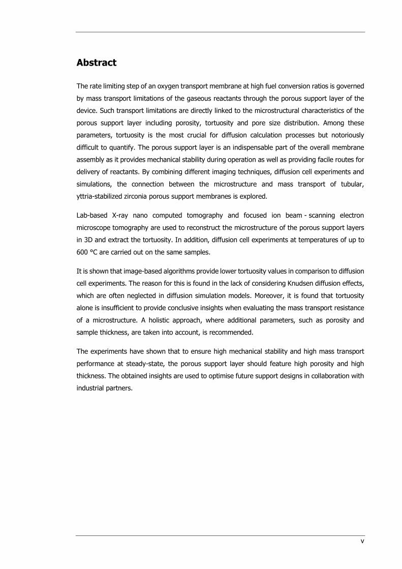
Abstract
The rate limiting step of an oxygen transport membrane at high fuel conversion ratios is governed
by mass transport limitations of the gaseous reactants through the porous support layer of the
device. Such transport limitations are directly linked to the microstructural characteristics of the
porous support layer including porosity, tortuosity and pore size distribution. Among these
parameters, tortuosity is the most crucial for diffusion calculation processes but notoriously
difficult to quantify. The porous support layer is an indispensable part of the overall membrane
assembly as it provides mechanical stability during operation as well as providing facile routes for
delivery of reactants. By combining different imaging techniques, diffusion cell experiments and
simulations, the connection between the microstructure and mass transport of tubular,
yttria-stabilized zirconia porous support membranes is explored.
Lab-based X-ray nano computed tomography and focused ion beam - scanning electron
microscope tomography are used to reconstruct the microstructure of the porous support layers
in 3D and extract the tortuosity. In addition, diffusion cell experiments at temperatures of up to
600 °C are carried out on the same samples.
It is shown that image-based algorithms provide lower tortuosity values in comparison to diffusion
cell experiments. The reason for this is found in the lack of considering Knudsen diffusion effects,
which are often neglected in diffusion simulation models. Moreover, it is found that tortuosity
alone is insufficient to provide conclusive insights when evaluating the mass transport resistance
of a microstructure. A holistic approach, where additional parameters, such as porosity and
sample thickness, are taken into account, is recommended.
The experiments have shown that to ensure high mechanical stability and high mass transport
performance at steady-state, the porous support layer should feature high porosity and high
thickness. The obtained insights are used to optimise future support designs in collaboration with
industrial partners.

vi
vii
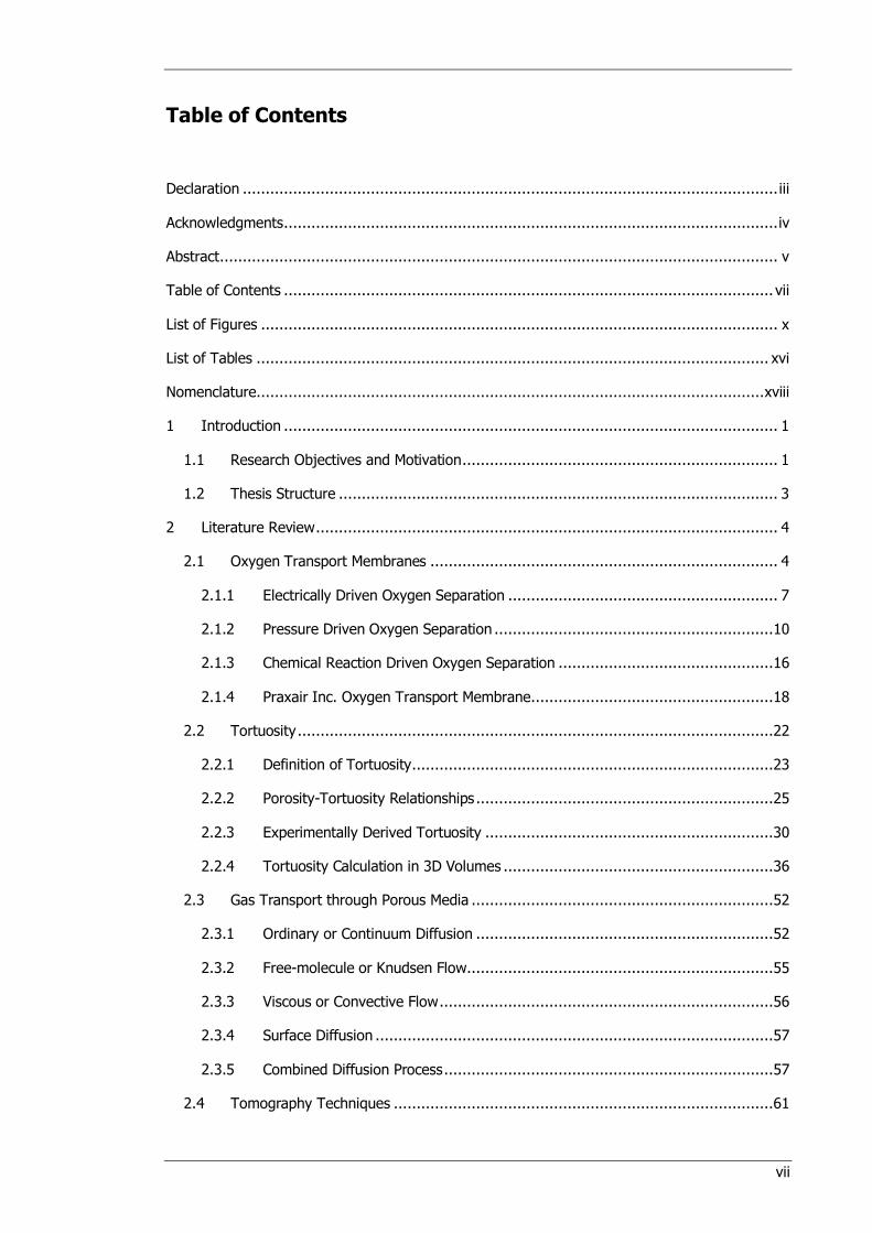
Table of Contents
Declaration ..................................................................................................................... iii
Acknowledgments ............................................................................................................ iv
Abstract .......................................................................................................................... v
Table of Contents ........................................................................................................... vii
List of Figures ................................................................................................................. x
List of Tables ................................................................................................................ xvi
Nomenclature ............................................................................................................... xviii
1 Introduction ............................................................................................................ 1
1.1 Research Objectives and Motivation ..................................................................... 1
1.2 Thesis Structure ................................................................................................ 3
2 Literature Review ..................................................................................................... 4
2.1 Oxygen Transport Membranes ............................................................................ 4
2.1.1 Electrically Driven Oxygen Separation ........................................................... 7
2.1.2 Pressure Driven Oxygen Separation .............................................................10
2.1.3 Chemical Reaction Driven Oxygen Separation ...............................................16
2.1.4 Praxair Inc. Oxygen Transport Membrane .....................................................18
2.2 Tortuosity ........................................................................................................22
2.2.1 Definition of Tortuosity ...............................................................................23
2.2.2 Porosity-Tortuosity Relationships .................................................................25
2.2.3 Experimentally Derived Tortuosity ...............................................................30
2.2.4 Tortuosity Calculation in 3D Volumes ...........................................................36
2.3 Gas Transport through Porous Media ..................................................................52
2.3.1 Ordinary or Continuum Diffusion .................................................................52
2.3.2 Free-molecule or Knudsen Flow ...................................................................55
2.3.3 Viscous or Convective Flow .........................................................................56
2.3.4 Surface Diffusion .......................................................................................57
2.3.5 Combined Diffusion Process ........................................................................57
2.4 Tomography Techniques ...................................................................................61
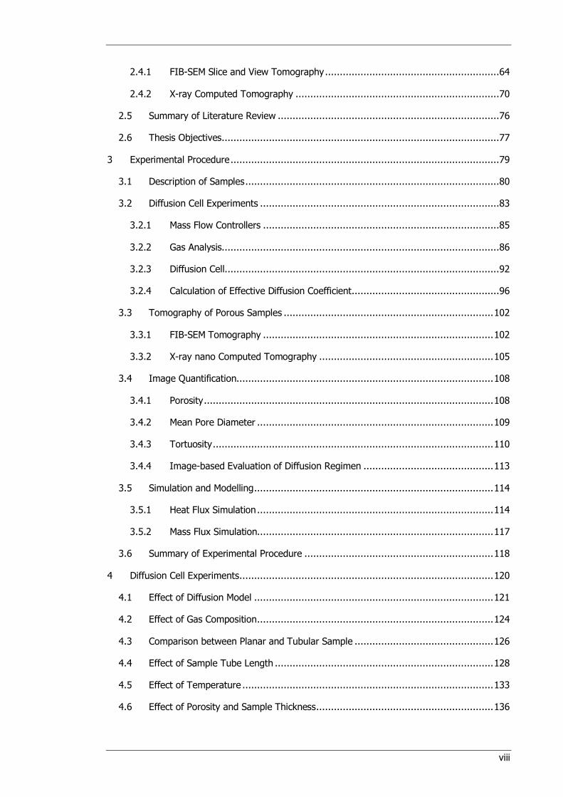
viii
2.4.1 FIB-SEM Slice and View Tomography ...........................................................64
2.4.2 X-ray Computed Tomography .....................................................................70
2.5 Summary of Literature Review ...........................................................................76
2.6 Thesis Objectives ..............................................................................................77
3 Experimental Procedure ...........................................................................................79
3.1 Description of Samples ......................................................................................80
3.2 Diffusion Cell Experiments .................................................................................83
3.2.1 Mass Flow Controllers ................................................................................85
3.2.2 Gas Analysis..............................................................................................86
3.2.3 Diffusion Cell.............................................................................................92
3.2.4 Calculation of Effective Diffusion Coefficient..................................................96
3.3 Tomography of Porous Samples ....................................................................... 102
3.3.1 FIB-SEM Tomography .............................................................................. 102
3.3.2 X-ray nano Computed Tomography ........................................................... 105
3.4 Image Quantification....................................................................................... 108
3.4.1 Porosity .................................................................................................. 108
3.4.2 Mean Pore Diameter ................................................................................ 109
3.4.3 Tortuosity ............................................................................................... 110
3.4.4 Image-based Evaluation of Diffusion Regimen ............................................ 113
3.5 Simulation and Modelling ................................................................................. 114
3.5.1 Heat Flux Simulation ................................................................................ 114
3.5.2 Mass Flux Simulation................................................................................ 117
3.6 Summary of Experimental Procedure ................................................................ 118
4 Diffusion Cell Experiments ...................................................................................... 120
4.1 Effect of Diffusion Model ................................................................................. 121
4.2 Effect of Gas Composition ................................................................................ 124
4.3 Comparison between Planar and Tubular Sample ............................................... 126
4.4 Effect of Sample Tube Length .......................................................................... 128
4.5 Effect of Temperature ..................................................................................... 133
4.6 Effect of Porosity and Sample Thickness ............................................................ 136
ix
4.7 Conclusions of Diffusion Cell Experiments .......................................................... 138
5 Image Analysis and Quantification .......................................................................... 140
5.1 Evaluation of Imaging Specifications ................................................................. 140
5.2 Comparison between FIB-SEM and X-ray nano CT .............................................. 143
5.3 Comparison between Planar and Tubular Sample ............................................... 148
5.4 Image-based Tortuosity for 2.4th Generation Porous Support Layers ..................... 151
5.5 Image-based Evaluation of Diffusion Regime ..................................................... 159
5.6 Artificial Opening and Closing of Sample Volumes ............................................... 166
5.7 Conclusions of Image Analysis and Quantification ............................................... 172
6 Simulation and Modelling ....................................................................................... 173
6.1 Sensitivity Analysis of Meshing Parameters ........................................................ 173
6.2 Comparison between Heat and Mass Flux Simulation .......................................... 176
6.3 Comparison of Calculated Tortuosity Values ....................................................... 179
6.4 Conclusions of Simulation and Modelling ........................................................... 181
7 Conclusions and Future Work ................................................................................. 182
7.1 Conlusions ..................................................................................................... 182
7.2 Future Work ................................................................................................... 186
7.2.1 Transient Diffusion Cell Experiments .......................................................... 186
7.2.2 Effect of Aging and Degradation on Microstructure ...................................... 187
7.2.3 Current Measurement Experiment ............................................................. 188
7.2.4 Effect of Tube Length and Arrangement on Diffusive Mass Transport ............ 189
7.3 Dissemination ................................................................................................ 190
7.3.1 Peer-reviewed Publications ....................................................................... 190
7.3.2 Co-Authored Peer-reviewed Publications .................................................... 190
7.3.3 Conference Attendance ............................................................................ 191
8 Bibliography ......................................................................................................... 193
9 Appendices............................................................................................................... I
Appendix A Mass Balance over Diffusion Cell ............................................................... II
Appendix B MATLab Script ........................................................................................ V
x
List of Figures
Figure 2-1: Oxygen generating techniques using ceramic membranes. Reproduced with
permission from Elsevier [10]. ........................................................................................... 6
Figure 2-2: Oxygen ion transport membrane configurations using a pure ionic conductor (A), a
perovskite mixed conductor (B) and a dual-phase mixed conductor (C). Reproduced with
permission from the Royal Society of Chemistry [11]. .......................................................... 7
Figure 2-3: Cross section of membrane structure showing SDC electrolyte, BSCF + SDC electrode
and BSCF + SDC + Ag current distributor. Reproduced with permission from Elsevier [16]. ...... 9
Figure 2-4: Five step pressure driven oxygen generation through a MIEC membrane. .............11
Figure 2-5: Schematic of simplified oxygen separation membrane with dense, ionic conducting
electrolyte and external electronic circuit. Reproduced with permission from the Royal Society of
Chemistry [11]. ..............................................................................................................14
Figure 2-6: MIEC membrane layout with 4 μm thin LSCF-layer. Reproduced with permission from
Elsevier [32]. .................................................................................................................16
Figure 2-7: Tubular reaction driven oxygen separation reactor for methane reforming.
Reproduced with permission from Elsevier [33]. .................................................................18
Figure 2-8: Working principle of OTM for CH4 to syngas conversion. .....................................20
Figure 2-9: Representation of tortuosity in porous medium. .................................................23
Figure 2-10: Comparison of Bruggeman exponents and scaling parameters for different battery
layers referenced in Table 2-3. .........................................................................................28
Figure 2-11: Wicke Kallenbach (A) and Graham (B) diffusion cell setup. Reproduced with
permission from Elsevier [111]. ........................................................................................31
Figure 2-12: Comparison of experimentally and image-based tortuosity values at different
temperatures and for varying H2 concentrations in N2. Reproduced with permission from Elsevier
[113].............................................................................................................................34
Figure 2-13: Geometric tortuosity histogram achieved by FMM for all three phases of a SOFC
cathode. Reproduced with permission from John Wiley and Sons [145]. ...............................37
Figure 2-14: Geometric tortuosity distribution of the pore-phase of the LiCoO2 battery cathode of
yz (A), xz (B) and xy (C) planes. Reproduced with permission from Elsevier [147]. .................38
Figure 2-15: Representative volume element analysis of the tortuosity factor for the pore and
LSCF-phase of an SOFC cathode as function of electrode thickness. Reproduced with permission
from Elsevier [174]. ........................................................................................................43
Figure 2-16: Temperature distribution across the porous-phase of an YSZ porous support
membrane of an oxygen transport membrane. ...................................................................44
Figure 2-17: Electric analogy for combining diffusion phenomena. Adapted from [38].............57
Figure 2-18: Sectioning of a 3D structure by a 2D plane for stereology. Reproduced with
permission from Springer [101]. .......................................................................................62
xi
Figure 2-19: Tomography techniques as function of image resolution and sample volume.
Reproduced with permission from Cambridge University Press [205]. ...................................62
Figure 2-20: Relationship between sample size and microstructural parameter. Reproduced with
permission from John Wiley and Sons [187].......................................................................63
Figure 2-21: Electron generation via SEM imaging: secondary electrons (SE1) generated by the
incident beam B; backscattered electrons (BSE) escaping the sample while generating additional
secondary electrons (SE2). Reproduced with permission from Springer [207]. ........................65
Figure 2-22: SEM image showing the phase-contrast between nickel (bright), YSZ (grey) and pore
(black) of an SOFC anode by using a low accelerating voltage of 1 kV. Reproduced with permission
from Elsevier [208]. ........................................................................................................66
Figure 2-23: Working principle of FIB-SEM tomography. Reproduced with permission from Elsevier
[206].............................................................................................................................67
Figure 2-24: Lift-out sample preparation of Ni-YSZ SOFC electrode. Reproduced with permission
from Elsevier [209]. ........................................................................................................68
Figure 2-25: Working principle of filtered back projection algorithm where the same sample was
reconstructed using an increasing number of projections. ....................................................71
Figure 2-26: Change of greyscale histogram of reconstructions as function of increasing number
of projections .................................................................................................................72
Figure 2-27: Detailed 3D reconstruction of an SOFC anode at 200 °C (A) and 700 °C (B).
Reproduced with permission under a Creative Commons license [220]. .................................75
Figure 2-28: Combination of absorption-contrast (A) and phase-contrast (B) imaging of a
lithium-ion battery electrode to enhance contrast (C) and facilitate quantification algorithms.
Reproduced with permission under a Creative Commons license [224]. .................................75
Figure 3-1: Experimental validation circle of this project where diffusion cell experiments,
tomography techniques and simulation and modelling are applied. .......................................79
Figure 3-2: EDX data on complete OTM assembly for each layer. .........................................81
Figure 3-3: Setup of diffusion cell test rig. .........................................................................84
Figure 3-4: Calibration curves for MFCs correlating the set flow rate with the measured flow rate
in the Gilibrator. .............................................................................................................85
Figure 3-5: GC calibration curve for N2-CH4 which collates area of the chromatograms with the
associated gas mole fraction. ...........................................................................................88
Figure 3-6: Diffusion fluxes for the CH4-N2 binary gas mixture measured in the GC using different
carrier gases (Ar, H2 and He) for the same experiment as function of concentration gradient Δy.
....................................................................................................................................89
Figure 3-7: In-operando gas measurement of CO2-N2 gas mixture using the MS.....................91
Figure 3-8: CO2 values on N2 side of the membrane for the CO2-N2 gas mixture measured using
the GC and the MS for two tubular current generation porous support samples. ....................92
Figure 3-9: Wicke Kallenbach diffusion cell and sample mounting for planar samples. .............93
Figure 3-10: Build-up (A) and working principle (B) of tubular diffusion cell. ..........................95

xii
Figure 3-11: Tubular sample sealing and mounting mechanism for experiments < 300 °C using a
high temperature O-ring (A), for temperatures > 300 °C sealed with Ceramabond (B) using
O-rings cut out of Thermiculite (C); mounted sample with a ~ 20 cm long extension tube to
ensure that the sample is in the centre of the furnace (D). ..................................................95
Figure 3-12: Flowchart showing the methodology of diffusion cell experiments. .....................96
Figure 3-13: Diffusion cell model for mass balance calculation. ............................................97
Figure 3-14: Deviation of simulated diffusion fluxes of a H2-N2 binary gas mixture from Graham's
law (cf. equation (3-9)) as function of pressure gradient between gas inlet and outlet. ......... 102
Figure 3-15: Sample preparation of 2nd generation tubular membranes (cf. Table 3-1) for SEM
imaging showing samples encapsulated in epoxy resin before (A) and after polishing (B) after
gold sputtering (C). ....................................................................................................... 103
Figure 3-16: Laser milled U-trench in tubular porous support sample. ................................. 104
Figure 3-17: First (A) and last (B) SEM image of FIB-SEM slice and view tomography. .......... 105
Figure 3-18: Operating principle of an X-ray nano CT system showing the optical components
used to achieve a monochromatic beam. ......................................................................... 106
Figure 3-19: Sample mounted on top of a sewing needle. ................................................. 107
Figure 3-20: Illustration of sample volume growing algorithm for microstructural RVE analysis.
.................................................................................................................................. 109
Figure 3-21: Fast marching method across the porous phase of a binary sample (A) running in
x-dimension (B) and y-dimension (C). ............................................................................. 111
Figure 3-22: Illustration of the pore centroid method calculation approach which measures the
distance d(n) of the centres of mass between two 2D image slices. ..................................... 112
Figure 3-23: Results of the TauFactor solver by Cooper [151] running across the pore phase of a
porous sample showing the binary image map, the initial, linear concentration distribution and
the concentration distribution at steady-state. .................................................................. 113
Figure 3-24: StarCCM+ meshing procedure showing the imported solid phase surface mesh (A)
around which a cube (B) is snapped and Boolean subtracted to produce the porous phase (C);
then, a surface mesh (D) and ultimately, a volume mesh (E) are generated for the heat flux
simulation. ................................................................................................................... 115
Figure 4-1: Comparison of tortuosity values for sample 100% TZ3YSB K at ambient temperature
using Fick's law (A) and the equimass model (B) with and without Knudsen diffusion, respectively.
.................................................................................................................................. 122
Figure 4-2: Comparison of tortuosity values for sample 100% TZ3YSB K calculated via Fick's law,
equimass model and dusty gas model both including Knudsen diffusion. ............................. 124
Figure 4-3: Effect of injected fuel gas composition on measured fuel gas concentrations on the
N2 side of sample 100% TZ3YSB K (A) and on calculated tortuosity at ambient temperature (B).
.................................................................................................................................. 125
Figure 4-4: Comparison of achieved tortuosity values between the planar and tubular sample at
ambient temperature using the DGM for calculations. ....................................................... 126
xiii
Figure 4-5: Consistency check of tubular diffusion cell experiments repeating the same experiment
at different dates using sample PS 2310 1360C. ............................................................... 127
Figure 4-6: The effect of tube length of sample PS 2.4 30.0% on tortuosity. ....................... 129
Figure 4-7: Comparison of achieved tortuosity values between the planar and tubular sample at
ambient temperature for different sample tube lengths. .................................................... 130
Figure 4-8: Effect of gas volume flow rate on the tortuosity (A), fuel gas concentration on N2 side
of the membrane (B) and the diffusive flux (C) of sample PS 2.4 22.6%. ............................ 131
Figure 4-9: OTM reactor tube arrangement: OTM tubes are positioned perpendicular to the air
gas flow and scaled-out in tube length and number of tubes. Concentration fluctuations are
expected along the tube as well as in direction of the gas flow inside the OTM reactor. ........ 132
Figure 4-10: Diffusion fluxes of CH4, CO2 and CO as function of temperature for all four 2.4th
generation samples. ...................................................................................................... 134
Figure 4-11: Tortuosity values calculated via the dusty gas model for each gas species as function
of temperature for each gas species and sample as function of temperature. ...................... 135
Figure 4-12: Average tortuosity values for each sample calculated after the FM, EM and DGM (A)
and fraction between the minimum and maximum tortuosity value for each sample across all
temperatures and gas mixtures as a function of applied diffusion model (B). ....................... 136
Figure 4-13: Comparison of resistance factor (cf. equation (3-8)) and effective diffusivity (cf.
chapter 2.2.1) using average tortuosity values at ambient temperature based in Fick's law
including Knudsen......................................................................................................... 138
Figure 5-1: Comparison of magnifications on complete OTM (A) and porous support X-ray scans
(B and C). .................................................................................................................... 141
Figure 5-2: Comparing of absorption and phase-contrast imaging mode showing radiographs (A)
and image slices (B). ..................................................................................................... 142
Figure 5-3: SEM image of the porous cathode layer of the complete OTM sample at high
accelerating voltage of 30 kV revealing solid structures beneath the sample surface. ............ 143
Figure 5-4: Reconstructed volumes and raw 2D image slices of sample 100% TZ3YSB K using
X-ray nano CT (A,C) and FIB-SEM tomography (B,D). ....................................................... 145
Figure 5-5: 2D porosity development along each axis and RVE analysis of porosity for X-ray nano
CT (A,C) and FIB-SEM tomography (B,D) reconstructions of sample 100% TZ3YSB K. .......... 146
Figure 5-6: Tortuosity τ calculated via heat flux simulation and FMM for the X-ray nano CT (A)
and the FIB-SEM tomography sample (B); RVE analysis for τc for both samples using the fast
marching method (C,D). ................................................................................................ 147
Figure 5-7: Comparison of pore size histogram of sample 100% TZ3YSB K imaged using X-ray
nano CT (A) and FIB-SEM tomography (B), sample PS 2310 1360C imaged using X-ray nano CT
(C) and PS 1909 1360C imaged using X-ray nano CT (D). ................................................. 149
Figure 5-8: Comparison of directional tortuosity values calculated via the Laplace euqation solver
for the planar and tubular samples. ................................................................................ 151
Figure 5-9: Cropped sample volumes of 2.4th generation porous support layers. .................. 153

xiv
Figure 5-10: Pore size distribution of pore diameters dP for all reconstructed 2.4th generation
porous support volumes. ............................................................................................... 154
Figure 5-11: Directional tortuosity calculated via the Laplace equation solver for all reconstructed
2.4th generation porous support volumes. ........................................................................ 155
Figure 5-12: 2D porosity development along the x-, y-, and z-axes for all reconstructed 2.4th
generation porous support volumes. ............................................................................... 156
Figure 5-13: 2D pore diameter development along the x-, y-, and z-axes for all reconstructed
2.4th generation porous support volumes. ........................................................................ 157
Figure 5-14: RVE analysis for all 2.4th generation porous support sample cubes and cuboids using
the Laplace solver and the FMM. .................................................................................... 158
Figure 5-15: Comparison of image-based tortuosity calculation approaches for all eight current
generation porous support sample volumes. .................................................................... 159
Figure 5-16: Effect of temperature T (with dP=0.78 μm) (A) and mean pore diameter dP (with
T=1,000 °C) (B) on diffusion coefficients. ........................................................................ 160
Figure 5-17: Visualisation of pore diameter (dP) distribution of porous samples PS 2.4 30.0% (A)
and PS 2.4 22.6% (B) based on the BoneJ calculation plugin in ImageJ. ............................. 161
Figure 5-18: Distribution of Knudsen number Kn in samples PS 2.4 30.0% (A,B) and PS 2.4 22.6%
(C,D) for CH4 at 600°C (A,C) and 1000°C (B,D). ............................................................... 162
Figure 5-19: Histogram of Knudsen numbers using the mean free path of CH4 for samples
PS 2.4 30.0% (A) and PS 2.4 22.6% (B) at varying temperatures. ...................................... 163
Figure 5-20: Distribution of the binary diffusion coefficient DCH4,N2 (A,B), Knudsen diffusion
coefficient DK,CH4 (C,D) and effective diffusion coefficient DCH4 (E,F) in samples PS 2.4 30.0% (left)
and PS 2.4 22.6% (right) at 1,000°C............................................................................... 165
Figure 5-21: Change of segmented porous phase of sample PS 2.4 22.6% by gradually opening
the solid phase until the porosity is equal to the porosity of sample PS 2.4 30.0%; the sample
framed with a red square is sample PS 2.4 30.0%. ........................................................... 167
Figure 5-22: Change of segmented porous phase of sample PS 2.4 30.0% by gradually closing
the solid phase until the porosity is equal to the porosity of sample PS 2.4 22.6%; the sample
framed with a red square is sample PS 2.4 22.6%. ........................................................... 168
Figure 5-23: Tortuosity along each axis calculated by the Laplace equation solver for each volume
of the opening and closing procedure.............................................................................. 169
Figure 5-24: Pore connectivity, mean pore diameter dP and porosity ε for each volume of the
opening and closing procedure. ...................................................................................... 170
Figure 5-25: Cumulative pore size distribution for each volume of the opening and closing
procedure. ................................................................................................................... 170
Figure 5-26: Comparison of pore size distribution histograms of the initial PS 2.4 30.0% and
PS 2.4 22.6 % volumes with sample volumes Closing 5 and Opening 6. .............................. 171
Figure 6-1: Tortuosity values based on heat flux simulation as function of surface smoothing
extent in Avizo and mesh base size in StarCCM+. ............................................................. 174
xv
Figure 6-2: Comparison of characteristic tortuosity values calculated via the mass flux simulation
using Fick's law without Knudsen diffusion expressions at ambient temperature................... 175
Figure 6-3: Comparison of simulated mass flows across the x-axis of the sample cube PS 2.4 30.0%
for different gases calculated via Fick’s law and Fick’s law including Knudsen diffusion.......... 176
Figure 6-4: Directional tortuosity values of the sample cube PS 2.4 30.0% for different gases
using Fick’s law and Fick’s law including Knudsen diffusion (A) and the development of directional
tortuosity as function of temperature (B). ........................................................................ 177
Figure 6-5: Comparison of directional tortuosity values for the current generation porous support
membranes calculated via the Laplace equation solver, heat flux simulation and mass flux
simulation. ................................................................................................................... 178
Figure 6-6: Comparison of characteristic tortuosity values for geometric and flux-based tortuosity
calculation approaches as function of porosity. ................................................................. 180
Figure 6-7: Comparison of geometric, simulation and experimental based tortuosity values for all
four current generation porous support membranes. ........................................................ 180
Figure 7-1: List of experimental and image-based tortuosity values for all analysed porous support
samples. ...................................................................................................................... 185
Figure 7-2: Real-time gas measurement of H2 tracer experiment in MS measuring the time
between H2 injection and detection to evaluate the effect of membrane thickness on diffusion
phenomena. ................................................................................................................. 186
Figure 7-3: Complete OTM scan, where internal cracks and holes are highlighted in red and blue.
.................................................................................................................................. 187
Figure 7-4: Complete OTM tube cap showing holes (blue) around the tube (red) inside the glass
sealing. ....................................................................................................................... 188
Figure 7-5: Characteristic tortuosity values for image based algorithms, resistance measurements
and diffusion experiments. ............................................................................................. 189
Figure 9-1: Diffusion cell model for mass balance calculation ................................................ II
xvi
List of Tables
Table 2-1: Air separation processes for oxygen generation [8]. ............................................. 5
Table 2-2: List of materials used for first generation oxygen ion transport membrane [37]. .....21
Table 2-3: Comparison of Bruggeman exponent and scaling parameter for battery layers fitted to
experimental results. .......................................................................................................27
Table 2-4: Tortuosity values for pore, Ni and YSZ-phase of an SOFC anode calculated using the
random walk method and LBM [134]. ...............................................................................42
Table 2-5: Tortuosity values for graphite and pore-phase using the random walk method and
finite volume method [169]..............................................................................................42
Table 2-6: Comparison of tortuosity values along each dimension for pore-phases of porous
membranes calculated using flux-based algorithms. ............................................................47
Table 2-7: Comparison of tortuosity values along each dimension for pore-phases of porous
membranes calculated using flux-based algorithms (continued). ..........................................48
Table 2-8: Comparison of tortuosity values along each dimension for pore-phases of porous
membranes calculated using flux-based algorithms (continued). ..........................................49
Table 2-9: Comparison of tortuosity values along each dimension for pore-phases of porous
membranes calculated using geometric-based algorithms. ...................................................50
Table 2-10: Comparison of tortuosity values along each dimension for pore-phases of porous
membranes calculated using geometric-based algorithms (continued). .................................51
Table 3-1: Sample description of 2nd generation tubular porous support membrane and complete
OTM. .............................................................................................................................80
Table 3-2: Sample description of planar porous support membrane. .....................................82
Table 3-3: Sample description of 2.4th generation tubular porous support membranes. ...........82
Table 3-4: Summary detailing experimental analyses carried out for each sample. .................83
Table 3-5: Gas chromatograph specifications. ....................................................................87
Table 3-6: Input parameters for 1D DGM model to verify the assumption of neglecting viscous
flux contribution during diffusion cell experiments. ........................................................... 101
Table 3-7: Collision diameters of selected gases used to calculate the mean free path and the
binary diffusion coefficient via equation (2-20). ................................................................ 114
Table 4-1: Mean pore diameter dP, porosity ε and membrane thickness δ for 2.4th generation
porous support samples. ............................................................................................... 128
Table 4-2: Comparison of porous support layer properties including the resistance factor and the
effective diffusivity based on diffusion cell experiments at ambient temperature. ................. 137
Table 5-1: FIB-SEM tomography specifications of sample 100% TZ3YSB K. ......................... 144
Table 5-2: X-ray nano CT specifications of sample 100% TZ3YSB K. ................................... 144
Table 5-3: Comparison of porosity ε and mean pore diameter dP of planar porous support sample
100% TZ3YSB K calculated via FIB-SEM and X-ray nano CT. ............................................. 145

xvii
Table 5-4: Comparison of characteristic tortuosity τc for heat flux and FMM with empirical
tortuosity correlations of sample 100% TZ3YSB K............................................................. 148
Table 5-5: Comparison of pixel size, cube side length s, porosity ε and mean pore diameter dP of
tubular samples PS 2310 1360C and PS 1909 1360C. ........................................................ 148
Table 5-6: X-ray nano CT specifications of 2.4th generation of porous support membrane samples.
.................................................................................................................................. 152
Table 5-7: Tomography-based mean pore diameter dP and porosity ε for the cube and cuboid
volume of each 2.4th generation porous support sample. ................................................... 152
Table 5-8: Calculated mean free paths calculated after equation (2-22) using rigid sphere
diameters from Table 3-7 for selected gases at varying temperatures. ................................ 162
Table 5-9: Average Knudsen numbers calculated based on the mean pore diameter and mean
free path of CH4 for samples PS 2.4 30.0% and PS 2.4 22.6%. .......................................... 164
Table 5-10: Effective diffusion coefficient DCH4 calculated based on the binary diffusion coefficient
DCH4,N2 and Knudsen diffusion coefficient DK,CH4. ............................................................... 166
Table 6-1: Comparison of porosity calculated via pixel counting in Avizo and after volume meshing
in StarCCM+ and COMSOL. ............................................................................................ 175
xviii
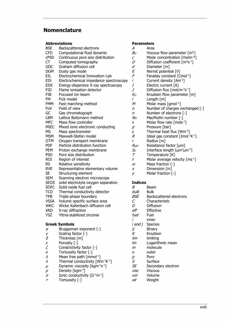
Nomenclature
Abbreviations Parameters BSE Backscattered electrons A Area CFD Computational fluid dynamic BO Viscous flow parameter [m²] cPSD Continuous pore size distribution c Molar concentration [molm-³] CT Computed tomography D Diffusion coefficient [m²s-1] GDC Graham diffusion cell d Diameter [m] DGM Dusty gas mode E Nernst potential [V] EIL Electrochemical Innovation Lab F Faraday constant [Cmol-1] EIS Electrochemical impedance spectroscopy i Current density [Am-2] EDX Energy-dispersive X-ray spectroscopy I Electric current [A] FID Flame ionisation detector J Diffusion flux [mol/m-2s-1] FIB Focused ion beam KO Knudsen flow parameter [m] FM Fick model l Length [m] FMM Fast marching method M Molar mass [gmol-1] FoV Field of view n Number of charges exchanged [-] GC Gas chromatograph n Number of electrons [-] LBM Lattice Boltzmann method NM MacMullin number [-] MFC Mass flow controller �� Molar flow rate [mols-1] MIEC Mixed ionic-electronic conducting p Pressure [bar] MS Mass spectrometer �� Thermal heat flux [Wm-2] MSM Maxwell-Stefan model R Ideal gas constant [Jmol-1K-1] OTM Oxygen transport membrane r Radius [m] PDF Particle distribution function Rdiff Resistance factor [μm] PEM Proton exchange membrane SV Interface length [μm2μm-3] PSD Pore size distribution T Temperature [K] ROI Region of interest �� Molar average velocity [ms-1] RS Relative sensitivity w Mass fraction [-] RVE Representative elementary volume x Dimension [m] SE Structuring element y Molar fraction [-]
SEM Scanning electron microscope SEOS solid electrolyte oxygen separation Indices SOFC Solid oxide fuel cell B Beam TCD Thermal conductivity detector bulk Bulk TPB Triple-phase boundary BSE Backscattered electrons VSSA Volume specific surface area C Characteristic WKC Wicke Kallenbach diffusion cell D Diffusion
XRD X-ray diffraction eff Effective YSZ Yttria-stabilized zirconia fuel Fuel i inner Greek Symbols i and j Species α Bruggeman exponent [-] ij Binary γ Scaling factor [-] K Knudsen δ Thickness [m] lim limiting
ε Porosity [-] lm Logarithmic mean ζ Constrictivity factor [-] m molecule κ Tortuosity factor [-] o outer λ Mean free path [mmol-1] p Pore λ Thermal conductivity [Wm-1K-1] S Surface μ Dynamic viscosity [kgm-1s-1] SE Secondary electron ρ Density [kgm-3] visc Viscous
σ Ionic conductivity [Ω-1m-1] vol Volume τ Tortuosity [-] wt Weight
Chapter 1: Introduction
1
1 Introduction
Oxygen transport membranes (OTMs) are used to extract oxygen out of air via an electrochemical
process at high temperatures. In this way, pure oxygen can be produced for a wide range of
energy-related applications at a fraction of cost and energy demand compared to current
technologies. The OTM analysed in this project is used for the combined oxygen separation and
subsequent reformation of natural gas into a nitrogen free synthetic gas consisting of CO and H2
only. The advantages of combining an air separation membrane and gas reforming reactor into
a single step include the reduced cost and complexity of the system. Praxair Inc., the industrial
partner of this project, aims to use this technology in natural gas locations to directly produce a
liquid fuel on-site for easier transportation. In general, the produced synthetic gas can be used
for a variety of applications such as chemical processing, liquid fuel production and energy supply
purposes in steam or gas cycle power plants. Any kind of application integrated with OTMs is
easily enhanced by carbon capture and sequestration techniques due to the absence of nitrogen
in the gas stream. This makes the application of OTMs a viable solution for tackling the current
energy and climate crisis [1].
To accelerate commercialisation and ensure safety and resilience in long-term operation, a much
improved understanding of the underlying material microstructure is required. In particular, the
porous support layers, which are commonly applied on the anode side of the membrane, are of
vital importance to ensure mechanical stability of the overall membrane assembly. However, such
layers contribute to mass transport limitations at high fuel conversion ratios. In collaboration with
Praxair Inc., this project focuses on the complex interplay between microstructural parameters of
and gaseous mass transport phenomena within the porous support layer of OTMs to minimize
the mass transport resistance of such porous layers while ensuring high mechanical stability
during operation.
1.1 Research Objectives and Motivation
The operating principle of an OTM is similar to a solid oxide fuel cell (SOFC), which is why the
advent of OTMs is closely related to the development of new materials and fabrication methods
in the field of SOFCs. In essence, an OTM is an internally short circuited SOFC and consists of
three layers:
A porous cathode where oxygen is reduced.
A porous anode where the reduced oxygen is oxidised and, in the configuration analysed
here, where CH4 reforming reactions take place.
And a dense electrolyte layer, which conducts oxygen ions from the cathode to the anode
and electrons from the anode back to the cathode to close the circuit.
Chapter 1: Introduction
2
Due to the similarities between SOFCs and OTMs, the rate limiting steps at high fuel conversion
rates are identical, with the microstructure of the porous support layer acting as a resistance for
gaseous diffusion mechanisms and limits the performance of the device. These limitations are
governed by the microstructural characteristics of the porous support layer such as tortuosity,
porosity and mean pore diameter.
Additionally, a porous support layer is common, and is commonly placed on the anode side of the
membrane for mechanical stability. Such porous support layers can be several orders of
magnitude thicker than the functional electrode and electrolyte layers [2]. The mechanical
strength of the overall membrane assembly can be adjusted by altering either the porosity or the
thickness of the porous support layer [3]. Such, modifications, however, can influence the mass
transport behaviour and, hence, the performance of the OTM.
As a result, this project aims to extract the microstructural parameters and effective transport
properties for a range of different porous support layers of OTMs using image and
simulation-based techniques. The results are then correlated with diffusion cell experiments to
verify the suitability of computer algorithms in this field of application. Special attention will be
paid to the tortuosity of the membrane, since it is not uniformly defined and calculated in the
electrochemical community and thus, remains notoriously difficult to quantify.
X-ray nano computed tomography (X-ray nano CT) and the focused ion beam (FIB) - scanning
electron microscope (SEM) slice and view technique are employed to extract the 3D volumes of
the porous support samples. These volumes are then further processed in MATLab, Avizo Fire 8,
StarCCM+ and COMSOL software packages to determine the gas transport resistance of the
microstructures. Diffusion cell experiments are carried out in parallel on the same samples using
a Wicke Kallenbach type diffusion cell. The diffusion cell test rig allows the measurement of gas
diffusing processes through planar and tubular samples via gas chromatography. Different
diffusion models (Fick’s law, the equimass diffusion model and the dusty gas model) are applied
to extract the microstructural characteristics and to compare the level of consistency between the
diffusion experiments and computational calculation algorithms.
The samples analysed in this project are provided by Praxair Inc. The supplied samples differed
in manufacturing conditions, porosity, thickness and date of production. The aforementioned
techniques are applied on the whole range of samples to obtain thorough conclusions about the
effect of the varied manufacturing and structural parameters on the performance.
Chapter 1: Introduction
3
1.2 Thesis Structure
This thesis is divided into several chapters to address the above research objectives:
The literature review in chapter 2 introduces different operating principles of oxygen transport
membranes, microstructural characteristics, gas diffusion mechanisms and image analysis
techniques; here, the need for understanding the correlation between microstructural parameters
and gaseous mass transport is highlighted.
Chapter 3 explains the applied methodology which aims at correlating data obtained via
tomography, simulation and diffusion cell experiments with each other and analyse diffusive mass
transport under varying conditions.
Chapters 4 through 6 summarise, compare and interpret the results acquired by applying the
experimental methods; each of the different chapters focuses on a specific analysis technique.
Comparisons and conclusions are drawn from the result chapters and presented in chapter 7; the
experiences gained directly feed into the planning of further research plans and are reported back
to Praxair Inc. to improve and optimize the design of the porous support layer. Moreover, an
outlook on future work is given by detailing several ideas for continuing experiments and analysis
techniques.
Chapter 2: Literature Review
4
2 Literature Review
This chapter summarises the fundamentals and most recent developments in the research areas
connected to this project. The mechanics and physics behind the operation of oxygen transport
membranes include electrochemistry, material science and transport phenomena. Additionally,
the scope of this project spans from microstructural level in the nanometre-scale to cell level
when operating the diffusion test rig. Therefore, this section is divided into four major parts:
1. The different working principles of oxygen transport membranes including electrically,
pressure and chemical reaction driven oxygen separation, are explained.
2. Microstructural parameters, which are of paramount importance in the field of mass
transport phenomena, are introduced, focusing on the tortuosity τ.
3. Gas transport mechanisms are elaborated, highlighting different types of diffusion and
how they interact with each other.
4. Finally, X-ray computed tomography and the FIB-SEM slice and view method are
described.
2.1 Oxygen Transport Membranes
Oxygen is one of the most produced and consumed industrial chemicals in the world. The majority
of the biggest industrial sectors e.g. the pulp and paper, metallurgy or chemical industry, use O2
for a wide range of chemical and technical processes, which make it a highly demanded
commodity. In addition, oxygen is used in smaller scale applications as well, including medical
applications, waste water treatment, welding and fish farming, to name but a few [4]. Moreover,
the need for oxygen is expected to increase over the coming years due to the need of reducing
carbon emissions: for carbon capture and sequestration technologies to be successful, the
exhaust gas stream of a plant has to be cleaned of any constituent but CO2. The pure carbon
dioxide can then be sequestered for storage or for utilisation. One way to achieve this is to
combust conventional fuels with pure O2 (i.e. oxyfuel combustion) which results in an exhaust
gas consisting only of CO2 and H2O. Here, the water vapour is then easily removed, resulting in
a CO2 stream of high purity. Also, gasification with pure oxygen provides a valuable, nitrogen free
synthetic gas, which forms an intermediate component for subsequent liquid fuel, chemical or
energy conversion processes [5].
At present, there are three main techniques for separating oxygen from air, which can be broadly
divided into cryogenic and non-cryogenic technologies [6, 7]: cryogenic distillation, adsorption
and membrane technologies. Among these, the latter two fall under the non-cryogenic technology
category.
Chapter 2: Literature Review
5
Cryogenic distillation is used when large amounts of oxygen in the range of 100 tO2/day are
required. For this, air is liquefied by cooling it down to a temperature of around - 185 °C.
Afterwards, the liquid air is distilled and separated according to the boiling points of each
constituent. This technology is widely applied, mature and the produced oxygen stream features
high purity of > 99 vol%. However, it is also an energy intensive and complex technology and,
when integrated in a power plant, consumes around 15 % of the power plant electricity output
[6].
Non-cryogenic techniques are employed for small to medium oxygen production capacities (cf.
Table 2-1). In pressure swing adsorption, sorbents (mainly zeolites), in combination with high
pressure, adsorb nitrogen from air, producing an oxygen enriched stream. To regenerate the
sorbents, the pressure is decreased, which reduces the equilibrium of nitrogen adsorption on the
sorbents and releases nitrogen to the atmosphere. For continuous oxygen production, several
vessels, which operate under adsorption and desorption mode alternatingly, are connected in
parallel.
Air separation using polymeric membrane technologies offers a much lower energy demand
compared to the previous options. This is achieved by applying a molecular sieve, letting only
permeable gases traverse through the membrane. Oxygen is diffusing through such a membrane
due to an imposed pressure gradient over the separation layer. Yet, only low oxygen purities of
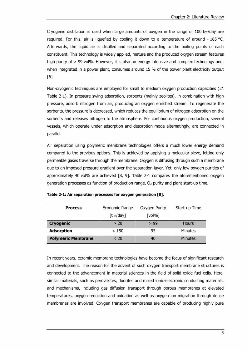
approximately 40 vol% are achieved [8, 9]. Table 2-1 compares the aforementioned oxygen
generation processes as function of production range, O2 purity and plant start-up time.
Table 2-1: Air separation processes for oxygen generation [8].
Process Economic Range
[tO2/day]
Oxygen Purity
[vol%]
Start-up Time
Cryogenic > 20 > 99 Hours
Adsorption < 150 95 Minutes
Polymeric Membrane < 20 40 Minutes
In recent years, ceramic membrane technologies have become the focus of significant research
and development. The reason for the advent of such oxygen transport membrane structures is
connected to the advancement in material sciences in the field of solid oxide fuel cells. Here,
similar materials, such as perovskites, fluorites and mixed ionic-electronic conducting materials,
and mechanisms, including gas diffusion transport through porous membranes at elevated
temperatures, oxygen reduction and oxidation as well as oxygen ion migration through dense
membranes are involved. Oxygen transport membranes are capable of producing highly pure
Chapter 2: Literature Review
6
oxygen from air at elevated temperatures at a fraction of the energy demand compared to the
aforementioned air separation processes [9].
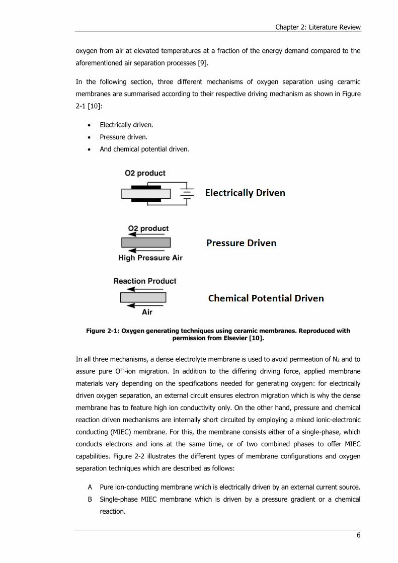
In the following section, three different mechanisms of oxygen separation using ceramic
membranes are summarised according to their respective driving mechanism as shown in Figure
2-1 [10]:
Electrically driven.
Pressure driven.
And chemical potential driven.
Figure 2-1: Oxygen generating techniques using ceramic membranes. Reproduced with permission from Elsevier [10].
In all three mechanisms, a dense electrolyte membrane is used to avoid permeation of N2 and to
assure pure O2--ion migration. In addition to the differing driving force, applied membrane
materials vary depending on the specifications needed for generating oxygen: for electrically
driven oxygen separation, an external circuit ensures electron migration which is why the dense
membrane has to feature high ion conductivity only. On the other hand, pressure and chemical
reaction driven mechanisms are internally short circuited by employing a mixed ionic-electronic
conducting (MIEC) membrane. For this, the membrane consists either of a single-phase, which
conducts electrons and ions at the same time, or of two combined phases to offer MIEC
capabilities. Figure 2-2 illustrates the different types of membrane configurations and oxygen
separation techniques which are described as follows:
A Pure ion-conducting membrane which is electrically driven by an external current source.
B Single-phase MIEC membrane which is driven by a pressure gradient or a chemical
reaction.

Chapter 2: Literature Review
7
C Dual-phase MIEC membrane which is driven by a pressure gradient or a chemical reaction.
The following sections present the differences between the above membrane structures in more
detail.
Figure 2-2: Oxygen ion transport membrane configurations using a pure ionic conductor (A), a perovskite mixed conductor (B) and a dual-phase mixed conductor (C). Reproduced with
permission from the Royal Society of Chemistry [11].
2.1.1 Electrically Driven Oxygen Separation
In the electrically driven oxygen separation configuration, oxygen is produced out of an oxygen
rich flow by applying an electric potential across the separating membrane. Oxygen molecules
are reduced to oxygen ions on the cathode side of the cell and migrate through the dense cell
layer. On the permeate (anode) side of the cell, the reverse process takes place, in which oxygen
ions recombine to O2 while releasing electrons via electrochemical oxidation. The free electrons
then travel back to compensate the electron consumption for oxygen reduction on the cathode
side and thus, completing the overall electron circuit.
In this case, the process layout is similar to solid oxide electrolysis cell operation, as the electric
potential is applied externally. The flow rate of generated oxygen is a direct function of the applied
electric current to the cell and is calculated using Faraday’s 1st law of electrolysis:
��𝑂2 =𝐼
𝑛𝐹 (2-1)
In which the following are defined:
��𝑂2 oxygen molar flow rate [mols-1] I applied electric current [A] n number of charges exchanged [-] F Faraday constant [Cmol-1]
Hence, the amount of produced oxygen can be directly regulated by the electric current. Another
analogy between OTMs, electrolysers and fuel cells is the employment of the Nernst equation
shown in equation (2-2) to determine the needed potential across the dense membrane to drive
the reaction. The Nernst potential is a result of the concentration gradient between the pure
A B C
Chapter 2: Literature Review
8
oxygen side and the air side of the membrane. This potential has to be overcome by the external
circuit to extract oxygen from the air side and transport it against the concentration gradient to
the pure oxygen side. Moreover, polarisation losses, including activation, concentration and ohmic
losses, have to be included when calculating the required potential [12, 13].
𝐸 =𝑅𝑇
𝑛𝐹 ln (
𝑝𝑂2′
𝑝𝑂2′′) (2-2)
In which the following are defined:
E Nernst potential [V] R ideal gas constant [Jmol-1K-1) T temperature [K] n number of charges exchanged [-] F Faraday constant [Cmol-1] 𝑝𝑂2′ , 𝑝𝑂2′′ oxygen partial pressure on either side of membrane, respectively [Pa]
In addition, the electrically driven oxygen separation method is capable of producing pure oxygen
gas at elevated pressure. This makes the implementation of an additional gas compressor in the
system unnecessary in comparison to pressure and reaction driven oxygen generators (cf.
chapters 2.1.2 and 2.1.3).
Oxygen reduction at the surface of and oxygen ion migration within the dense separation
membrane is analogous to reactions taking place in SOFCs. Hence, similar materials are applied
in either device. Fluorite structures were amongst the first oxygen ion conductors investigated as
electrolytes for SOFCs [14]. The aim of identifying and manufacturing a suitable oxygen ion
conductor is to achieve an ionic conductivity of > 1 mScm-1 at operating conditions [15]. Several
different fluorite type oxides, such as ceria (CeO2) with different dopants, have been analysed in
the field of electrically driven oxygen separation.
Samarium doped ceria (Sm0.2Ce0.8O1.9, SDC), widely serves as material for dense electrolytes due
to its high ionic conductivity. A membrane assembly achieving a stable area-specific resistance
(ASR) of 0.0122 Ωcm² at 2.34 Acm-2 for a period of 900 min at 700 °C was manufactured by
Zhou et al. [16] by placing an SDC electrolyte between two electrodes made from a mixture of
Ba0.5Sr0.5Co0.8Fe0.2O3−δ (BSCF) and SDC. In addition, a porous layer of BSCF (49 wt%), SDC
(21 wt%) and Ag (30 wt%) was placed on top of both BSCF+SDC electrode layers. Here, the
BSCF+SDC and the BSCF+SDC+Ag were applied for different purposes: the first layer of
BSCF+SDC acted as catalyst for the oxygen reduction on the cathode side and oxygen ion
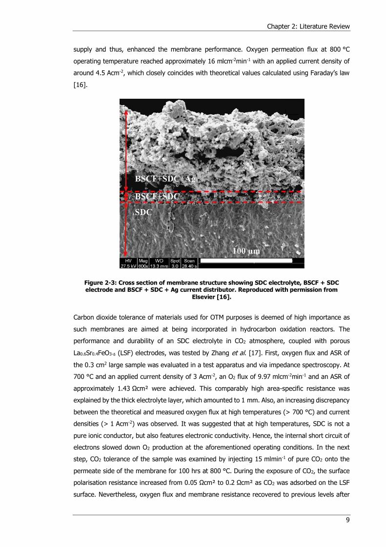
oxidation on anode side, while the BSCF+SDC+Ag-layer served as current distributor. Figure 2-3
shows the cross section of the membrane assembly taken with a scanning electron microscope,
where the electrolyte and the two electrode layers are visible. The positive role of Ag in the porous
layer was highlighted as it increased the amount of adsorbed oxygen, ensured good electron
Chapter 2: Literature Review
9
supply and thus, enhanced the membrane performance. Oxygen permeation flux at 800 °C
operating temperature reached approximately 16 mlcm-2min-1 with an applied current density of
around 4.5 Acm-2, which closely coincides with theoretical values calculated using Faraday’s law
[16].
Figure 2-3: Cross section of membrane structure showing SDC electrolyte, BSCF + SDC electrode and BSCF + SDC + Ag current distributor. Reproduced with permission from
Elsevier [16].
Carbon dioxide tolerance of materials used for OTM purposes is deemed of high importance as
such membranes are aimed at being incorporated in hydrocarbon oxidation reactors. The
performance and durability of an SDC electrolyte in CO2 atmosphere, coupled with porous
La0.6Sr0.4FeO3-δ (LSF) electrodes, was tested by Zhang et al. [17]. First, oxygen flux and ASR of
the 0.3 cm2 large sample was evaluated in a test apparatus and via impedance spectroscopy. At
700 °C and an applied current density of 3 Acm-2, an O2 flux of 9.97 mlcm-2min-1 and an ASR of
approximately 1.43 Ωcm² were achieved. This comparably high area-specific resistance was
explained by the thick electrolyte layer, which amounted to 1 mm. Also, an increasing discrepancy
between the theoretical and measured oxygen flux at high temperatures (> 700 °C) and current
densities (> 1 Acm-2) was observed. It was suggested that at high temperatures, SDC is not a
pure ionic conductor, but also features electronic conductivity. Hence, the internal short circuit of
electrons slowed down O2 production at the aforementioned operating conditions. In the next
step, CO2 tolerance of the sample was examined by injecting 15 mlmin-1 of pure CO2 onto the
permeate side of the membrane for 100 hrs at 800 °C. During the exposure of CO2, the surface
polarisation resistance increased from 0.05 Ωcm² to 0.2 Ωcm² as CO2 was adsorbed on the LSF
surface. Nevertheless, oxygen flux and membrane resistance recovered to previous levels after
Chapter 2: Literature Review
10
the CO2 experiment. Additionally, energy-dispersive X-ray spectroscopy (EDX) and X-ray
diffraction (XRD) analysis as well as scanning electron microscopy (SEM) of the membrane before
and after exposure to pure CO2 revealed that there was no structural change in the membrane
and no carbon was detected on the surface [17].
Aside from samarium, gadolinia is also used as a ceria dopant (gadolinia doped ceria, CGO) for
dense, ionic conducting electrolyte production. Yadav et al. [13] focused on testing novel
electrode materials with the aim of enhancing kinetics for oxygen reduction and oxidation,
respectively. For this, two composite electrodes consisting of PrBaCo2O5+x (PBCO) with CGO and
NdBaCo2O5+x (NBCO) with CGO were produced. In either case, the fraction of both materials
amounted to 50 wt%. The performance of both electrode assemblies in combination with the
dense CGO separation layer was evaluated using gas chromatography and AC impedance
spectroscopy. The highest observed oxygen molar flux was achieved when using PBCO-CGO
electrodes with a thickness of 550 μm. Here, the molar flux amounted to 2.48 ×10⁻⁶ molcm-2s-1
at 800 °C at an applied voltage of 1 V while using 100 cm3min-1 of helium as sweep gas.
Impedance spectroscopy revealed an area-specific resistance of 0.21 Ωcm² and an activation
energy of 107 kJmol-1 at 650 °C for the PBCO-CGO electrode, respectively. The authors suggest
that the investigated materials offer excellent oxygen reduction reaction kinetics due to the lower
ASR values of the novel electrode materials compared to ASR values presented in [18]. However,
the authors also stated that the overall membrane performance would benefit from a thinner
electrolyte [13].
Losses within the membrane layers, however, are only a small part when considering an overall
oxygen transport membrane reactor which includes balance of plant equipment. Meixner et al.
[19] presented a three cell stack, solid electrolyte oxygen separation (SEOS) unit, which was
tested for over 6,500 hrs during which a stable ASR of 0.6 Ωcm² was achieved. They used an
undisclosed rare-earth doped ceria, using gadolinia and samaria as dopants, as their electrolyte
material which performed stably for the whole test duration. Additionally, a complete oxygen
generator including balance of plant equipment was engineered as a proof of concept. The
authors highlighted that the only moving part in such a system is the air mover to supply fresh
air to the SEOS stack [19].
Currently, electric driven oxygen generation devices are commercially available from several
different companies. One example is the StarGen™ Ultra-High Purity Oxygen Generator from
Praxair Inc. [20]. Here, tubular membranes are applied to provide pure oxygen for laboratory
scale applications and on demand O2 supply.
2.1.2 Pressure Driven Oxygen Separation
As the name of this separation process indicates, the driving force for oxygen generation is a bulk
pressure gradient across the dense electrolyte layer. In addition, an inert sweep gas, such as He,
Chapter 2: Literature Review
11
continuously removes permeated O2 from the surface to maintain an oxygen partial pressure
gradient across the membrane. By applying a mixed ionic-electronic conducting membrane, no
external power source is necessary compared to electrically driven oxygen separation. Ionic and
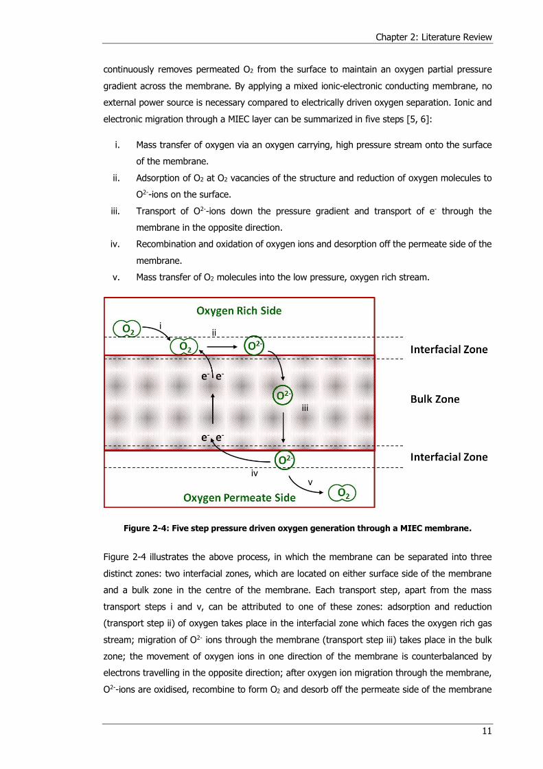
electronic migration through a MIEC layer can be summarized in five steps [5, 6]:
i. Mass transfer of oxygen via an oxygen carrying, high pressure stream onto the surface
of the membrane.
ii. Adsorption of O2 at O2 vacancies of the structure and reduction of oxygen molecules to
O2--ions on the surface.
iii. Transport of O2--ions down the pressure gradient and transport of e- through the
membrane in the opposite direction.
iv. Recombination and oxidation of oxygen ions and desorption off the permeate side of the
membrane.
v. Mass transfer of O2 molecules into the low pressure, oxygen rich stream.
Figure 2-4: Five step pressure driven oxygen generation through a MIEC membrane.
Figure 2-4 illustrates the above process, in which the membrane can be separated into three
distinct zones: two interfacial zones, which are located on either surface side of the membrane
and a bulk zone in the centre of the membrane. Each transport step, apart from the mass
transport steps i and v, can be attributed to one of these zones: adsorption and reduction
(transport step ii) of oxygen takes place in the interfacial zone which faces the oxygen rich gas
stream; migration of O2- ions through the membrane (transport step iii) takes place in the bulk
zone; the movement of oxygen ions in one direction of the membrane is counterbalanced by
electrons travelling in the opposite direction; after oxygen ion migration through the membrane,
O2--ions are oxidised, recombine to form O2 and desorb off the permeate side of the membrane
i ii
iii
iv v
Chapter 2: Literature Review
12
in the interfacial zone (transport step iv); transport steps i and v feature the mass transport of
gas streams in the channels adjacent to either side of the MIEC membrane.
The rate of oxygen generation is limited by the largest resistance encountered in one of these
three zones: transport resistance in the interfacial zones is governed by surface kinetics while
transport resistance in the bulk zone is governed by charge transfer resistance of ions and
electrons through the membrane, respectively. By thinning the bulk zone, bulk diffusion resistance
can be reduced to such a level, that it is of equal magnitude as the resistance in the interfacial
zones. The thickness, at which bulk resistance and surface resistance are equal, is called
characteristic thickness δc, which is calculated using equation (2-3) [21–24].
𝛿𝑐 =𝐷𝑖𝑖∗
𝑘𝑆 (2-3)
In which the following are defined:
δc characteristic thickness [m] Dii* oxygen ion diffusion coefficient [m2s-1]
kS surface exchange coefficient [ms-1]
For MIEC membrane manufacturing purposes, the characteristic thickness is of high significance
as it is not advantageous to produce membranes thinner than δc (thus, shifting the rate limiting
step of oxygen ion migration towards surface exchange reactions) unless the surface exchange
coefficient kS is increased at the same time. Otherwise, the oxygen generation will be limited by
surface exchange reactions and would not benefit from a thinner layer [22].
In cases where the oxygen flux is limited by the bulk resistance, the resulting amount of oxygen
flow rate is depending on the pressure gradient applied across the membrane and calculated
using the Wagner equation:
𝐽𝑂2 =𝜎𝑖𝑅𝑇
4𝛿𝑛2𝐹2 ln (
𝑝𝑂2′
𝑝𝑂2′′ ) (2-4)
In which the following are defined:
JO2 O2 flow rate [molm-²s-1] σi ionic conductivity [Ω-1m-1] R ideal gas constant [Jmol-1K-1] T Temperature [K] δ thickness of membrane [m] n number of charges exchanged [-] F Faraday constant [Cmol-1] 𝑝𝑂2′ , 𝑝𝑂2′′ O2 partial pressure on feed and permeate side of membrane [Pa]
Chapter 2: Literature Review
13
If the oxygen flux through a membrane is linearly dependent on the O2 partial pressure gradient
across the membrane, the rate limiting step is dominated by bulk diffusion according to the
Wagner equation [25].
As indicated above, only certain membrane materials offer the characteristics needed for pressure
driven oxygen separation, such as high electronic and ionic conductivity, high oxygen vacancy
density in the lattice, low activation energy for O2--migration and fast surface kinetics associated
with oxygen reduction. For this purpose, predominantly perovskite type materials have been
investigated [26], as they offer high stability at elevated operating temperatures and ensure high
selectivity of species which can migrate through the membrane [5, 6, 15, 24, 27, 28]. However,
most perovskite membranes contain alkaline earth ions in their lattice structure, which form
carbonate depositions in the presence of CO2. This leads to an immediate cessation of oxygen
permeation [29]. As a result, recent developments have focused on dual-phase membrane
materials, which increase ionic and electronic conductivity as well as CO2 tolerance and
mechanical and chemical stability [25].
In a dual-phase membrane, the oxygen generation flux is limited by the lower conductivity of
either ionic or electronic conducting phase at the operating temperature. The overall membrane
conductivity is maximised by combining an ionic and an electronic conducting material in the
correct ratios. Luo et al. [26] investigated the appropriate ratios by combining Fe2O3 (FO) and
Ce0.9Gd0.1O2-δ (CGO) as CO2 tolerant MIEC membrane: the authors tested a variety of
compositions of FO and CGO and concluded, that a matrix of 40 wt% FO and 60 wt% CGO in the
electrolyte featured highest oxygen permeation flux of 0.18 mlcm-²min-1 at 1,000 °C. In this
configuration, electronic conductivity of the Fe2O3-phase and ionic conductivity of the
Ce0.9Gd0.1O2-δ-phase were almost equal amounting to ~ 0.16 Scm-1. An even further increase in
oxygen permeation flux to 0.20 mlcm-²min-1 was measured after the air side of the membrane
was covered with a porous layer of La0.6Sr0.4CoO3-δ (LSC). The authors mentioned that due to the
porous layer coated on the air side of the membrane, surface area for oxygen reduction reaction
is increased, resulting in a reduction of surface exchange resistance. Moreover, the effect of
increased sintering temperature (from 1,300 °C to 1,350 °C) on oxygen permeation was analysed:
higher sintering temperatures resulted in increased grain size of both phases, inducing an
interruption of percolation of the FO network in the membrane and thus, blocking the electron
transport and consequently oxygen generation. Furthermore, the oxygen flux through the
membrane stayed constant when pure CO2 was used as sweep gas. The authors attributed the
chemical stability of the membrane to the absence of alkali earth metal elements in the crystal
structure [26].
Similar oxygen generation fluxes were achieved in subsequent experiments, where a comparison
between different manufacturing techniques was presented [29]. 40 wt% NiFe2O4 (NFO) and
60 wt% Ce0.9Gd0.1O2-δ (CGO) powders were mixed and membranes were prepared using three
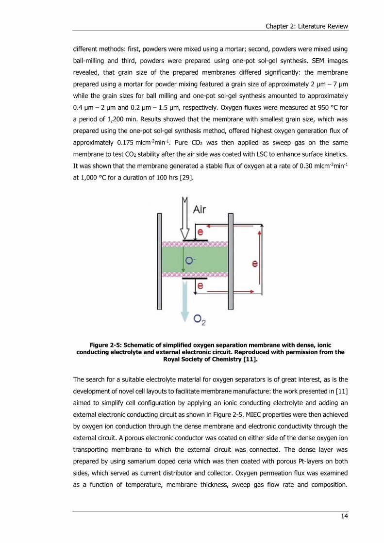
Chapter 2: Literature Review
14
different methods: first, powders were mixed using a mortar; second, powders were mixed using
ball-milling and third, powders were prepared using one-pot sol-gel synthesis. SEM images
revealed, that grain size of the prepared membranes differed significantly: the membrane
prepared using a mortar for powder mixing featured a grain size of approximately 2 μm – 7 μm
while the grain sizes for ball milling and one-pot sol-gel synthesis amounted to approximately
0.4 μm – 2 μm and 0.2 μm – 1.5 μm, respectively. Oxygen fluxes were measured at 950 °C for
a period of 1,200 min. Results showed that the membrane with smallest grain size, which was
prepared using the one-pot sol-gel synthesis method, offered highest oxygen generation flux of
approximately 0.175 mlcm-2min-1. Pure CO2 was then applied as sweep gas on the same
membrane to test CO2 stability after the air side was coated with LSC to enhance surface kinetics.
It was shown that the membrane generated a stable flux of oxygen at a rate of 0.30 mlcm-2min-1
at 1,000 °C for a duration of 100 hrs [29].
Figure 2-5: Schematic of simplified oxygen separation membrane with dense, ionic conducting electrolyte and external electronic circuit. Reproduced with permission from the
Royal Society of Chemistry [11].
The search for a suitable electrolyte material for oxygen separators is of great interest, as is the
development of novel cell layouts to facilitate membrane manufacture: the work presented in [11]
aimed to simplify cell configuration by applying an ionic conducting electrolyte and adding an
external electronic conducting circuit as shown in Figure 2-5. MIEC properties were then achieved
by oxygen ion conduction through the dense membrane and electronic conductivity through the
external circuit. A porous electronic conductor was coated on either side of the dense oxygen ion
transporting membrane to which the external circuit was connected. The dense layer was
prepared by using samarium doped ceria which was then coated with porous Pt-layers on both
sides, which served as current distributor and collector. Oxygen permeation flux was examined
as a function of temperature, membrane thickness, sweep gas flow rate and composition.
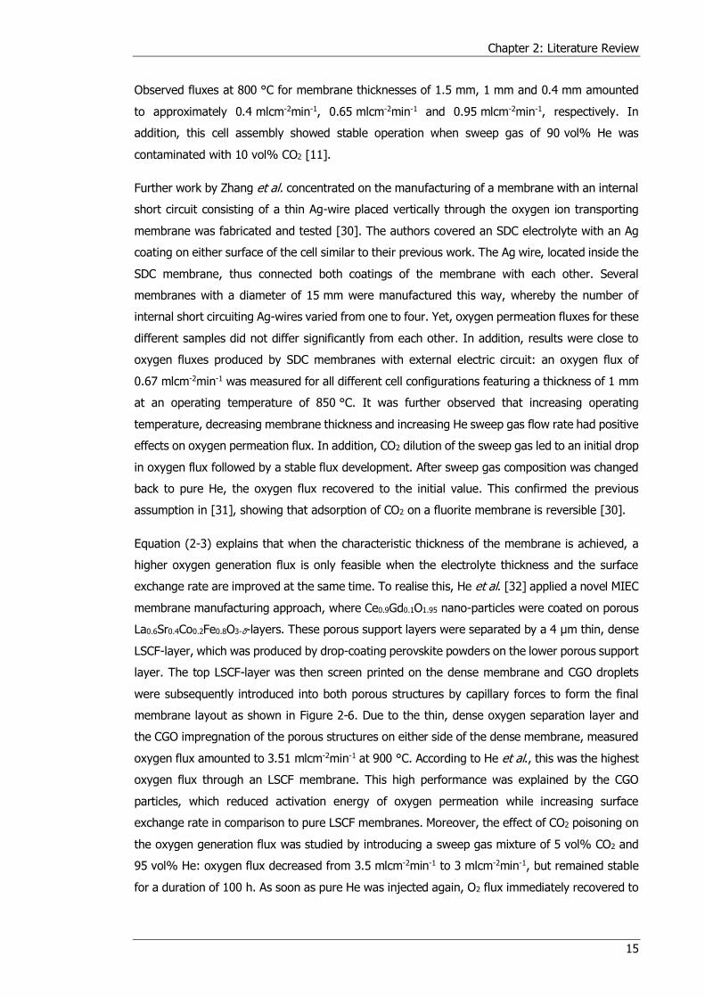
Chapter 2: Literature Review
15
Observed fluxes at 800 °C for membrane thicknesses of 1.5 mm, 1 mm and 0.4 mm amounted
to approximately 0.4 mlcm-2min-1, 0.65 mlcm-2min-1 and 0.95 mlcm-2min-1, respectively. In
addition, this cell assembly showed stable operation when sweep gas of 90 vol% He was
contaminated with 10 vol% CO2 [11].
Further work by Zhang et al. concentrated on the manufacturing of a membrane with an internal
short circuit consisting of a thin Ag-wire placed vertically through the oxygen ion transporting
membrane was fabricated and tested [30]. The authors covered an SDC electrolyte with an Ag
coating on either surface of the cell similar to their previous work. The Ag wire, located inside the
SDC membrane, thus connected both coatings of the membrane with each other. Several
membranes with a diameter of 15 mm were manufactured this way, whereby the number of
internal short circuiting Ag-wires varied from one to four. Yet, oxygen permeation fluxes for these
different samples did not differ significantly from each other. In addition, results were close to
oxygen fluxes produced by SDC membranes with external electric circuit: an oxygen flux of
0.67 mlcm-2min-1 was measured for all different cell configurations featuring a thickness of 1 mm
at an operating temperature of 850 °C. It was further observed that increasing operating
temperature, decreasing membrane thickness and increasing He sweep gas flow rate had positive
effects on oxygen permeation flux. In addition, CO2 dilution of the sweep gas led to an initial drop
in oxygen flux followed by a stable flux development. After sweep gas composition was changed
back to pure He, the oxygen flux recovered to the initial value. This confirmed the previous
assumption in [31], showing that adsorption of CO2 on a fluorite membrane is reversible [30].
Equation (2-3) explains that when the characteristic thickness of the membrane is achieved, a
higher oxygen generation flux is only feasible when the electrolyte thickness and the surface
exchange rate are improved at the same time. To realise this, He et al. [32] applied a novel MIEC
membrane manufacturing approach, where Ce0.9Gd0.1O1.95 nano-particles were coated on porous
La0.6Sr0.4Co0.2Fe0.8O3-δ-layers. These porous support layers were separated by a 4 μm thin, dense
LSCF-layer, which was produced by drop-coating perovskite powders on the lower porous support
layer. The top LSCF-layer was then screen printed on the dense membrane and CGO droplets
were subsequently introduced into both porous structures by capillary forces to form the final
membrane layout as shown in Figure 2-6. Due to the thin, dense oxygen separation layer and
the CGO impregnation of the porous structures on either side of the dense membrane, measured
oxygen flux amounted to 3.51 mlcm-2min-1 at 900 °C. According to He et al., this was the highest
oxygen flux through an LSCF membrane. This high performance was explained by the CGO
particles, which reduced activation energy of oxygen permeation while increasing surface
exchange rate in comparison to pure LSCF membranes. Moreover, the effect of CO2 poisoning on
the oxygen generation flux was studied by introducing a sweep gas mixture of 5 vol% CO2 and
95 vol% He: oxygen flux decreased from 3.5 mlcm-2min-1 to 3 mlcm-2min-1, but remained stable
for a duration of 100 h. As soon as pure He was injected again, O2 flux immediately recovered to
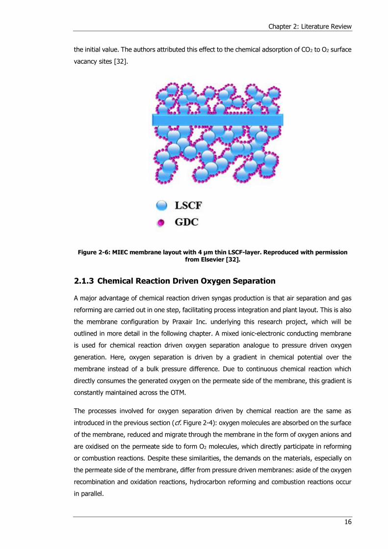
Chapter 2: Literature Review
16
the initial value. The authors attributed this effect to the chemical adsorption of CO2 to O2 surface
vacancy sites [32].
Figure 2-6: MIEC membrane layout with 4 μm thin LSCF-layer. Reproduced with permission from Elsevier [32].
2.1.3 Chemical Reaction Driven Oxygen Separation
A major advantage of chemical reaction driven syngas production is that air separation and gas
reforming are carried out in one step, facilitating process integration and plant layout. This is also
the membrane configuration by Praxair Inc. underlying this research project, which will be
outlined in more detail in the following chapter. A mixed ionic-electronic conducting membrane
is used for chemical reaction driven oxygen separation analogue to pressure driven oxygen
generation. Here, oxygen separation is driven by a gradient in chemical potential over the
membrane instead of a bulk pressure difference. Due to continuous chemical reaction which
directly consumes the generated oxygen on the permeate side of the membrane, this gradient is
constantly maintained across the OTM.
The processes involved for oxygen separation driven by chemical reaction are the same as
introduced in the previous section (cf. Figure 2-4): oxygen molecules are absorbed on the surface
of the membrane, reduced and migrate through the membrane in the form of oxygen anions and
are oxidised on the permeate side to form O2 molecules, which directly participate in reforming
or combustion reactions. Despite these similarities, the demands on the materials, especially on
the permeate side of the membrane, differ from pressure driven membranes: aside of the oxygen
recombination and oxidation reactions, hydrocarbon reforming and combustion reactions occur
in parallel.
Chapter 2: Literature Review
17
This makes the selection of the electrode and electrolyte material, which can cater for these
requirements, crucial. A planar, 0.5 mm thick dual-phase MIEC membrane consisting of 60 wt%
Ce0.8Gd0.2O1.9 (CGO) and 40 wt% Gd0.2Sr0.8FeO3-δ (GSF) was successfully applied by Zhu and Yang
[25] for direct partial oxidation of methane. Here, CGO served as ion conductor and GSF as ion
and electron conductor. The reasoning behind combining a pure ion conductor with a MIEC
material as dense layer was to ensure high ionic conductivity of the composite membrane: when
combining a pure ionic and pure electronic conductor to achieve MIEC properties, ionic
conductivity proves to be low as the electronic conducting phase blocks oxygen ion conduction.
This can be avoided when both phases are ionically conducting. A layer of LSC was coated on the
air side, while LiLaNiO/γ-Al2O3 was applied as catalyst for partial oxidation of methane on the
permeate side of the membrane. First, oxygen flux without syngas production was measured,
reaching 0.8 mlcm-2min-1 at 950 °C. When 6 mlmin-1 of pure methane was introduced at the
permeate side of the membrane, oxygen flux increased to approximately 5.2 mlcm-2min-1 at
950 °C, producing synthetic gas with a CH4 conversion rate of 99 %vol [25].
A different membrane architecture was chosen in [33], where a single-phase MIEC membrane
was manufactured and examined under syngas production operation. The tubular membrane
consisted of a dense La0.8Sr0.2Fe0.7Ga0.3O3-δ (LSFG) layer coated with La0.8Sr0.2Fe0.7Ga0.3O3-δ (LSFN)
as porous catalyst for CH4 reformation. The overall thickness of the membrane amounted to
~ 0.7 mm so that no additional support layer was necessary. The tubular sample was capped off
on one end to fit into the experimental setup depicted in Figure 2-7. While the inner side was fed
with air at atmospheric pressure, methane was injected and reformed in the porous catalyst layer
under a pressure of 0.3 MPa. To avoid carbon deposition on the membrane, a steam to carbon
ratio close to unity was maintained at an operating temperature of 900 °C. Experiments were
carried out over a period of 142 h and measurements showed, that analysed parameters were
largely dependent on the contact time of feed gas on the membrane: a change in feed contact
time (calculated by dividing the volume of the reactor by the volume flow rate of the feed gas)
between 13 s and 35 s caused variations in oxygen flux between 0.9 Nm3m-²h-1 and
0.5 Nm3m-²h-1, methane conversion rate between 74 vol% and 90 vol% and CO selectivity
between 50 vol% and 20 vol%, respectively. SEM analysis of the surface of the catalyst layer
showed that the microstructure of the membrane was affected by the experiments: spherical
agglomerates disappeared from the layer and the layer showed higher densification, which might
induce cracks. Also, images of the cross section of the membrane revealed the formation of a
1 μm to 5 μm thick Sr-rich coating between the LSFG and LSFN layer. However, the authors
concluded that the formation of such a layer did not affect the performance of the membrane
[33].
Chapter 2: Literature Review
18
Figure 2-7: Tubular reaction driven oxygen separation reactor for methane reforming. Reproduced with permission from Elsevier [33].
To match thermal and chemical expansions and thus, avoid formation of cracks and pinholes
during operation of methane reforming, Araki et al. [34] suggested to use a single component
for preparing an OTM membrane assembly, consisting of a porous support layer, a buffer layer
and a dense layer. For this purpose, Ca0.8Sr0.2Ti0.7Fe0.3O3-δ (CTO) was chosen where each layer
was manufactured through a distinct method: the solid-state reaction method, the citrate method
and the supercritical hydrothermal synthesis method were used for preparing the porous support,
the buffer and the dense oxygen separation layer. As a catalyst for methane reforming, a film of
Ni/CTO was coated on the support side of the one-component ceramic membrane-reactor, while
the surface of the dense layer on the air side of the membrane was covered with LSC. During
experimental operation at decreasing temperatures from 950 °C to 800 °C, CO selectivity
increased from 90 % to almost 100 %, while CH4 conversion rate decreased from approximately
90 % to < 30 %. Likewise, oxygen permeation rate decreased from 11.8 mmolcm-²h-1 to
2 mmolcm-²h-1. The authors stated that due to the decrease in O2 generation flux, oxidation of
CO into CO2 was suppressed which, in turn, resulted in an increasing CO selectivity [34]. Even
though it was reasoned that the use of only one component for preparing the different layers of
the OTM avoids damage to the membrane caused by different thermal and chemical expansion
coefficients of constituents, no post mortem analysis was carried out to verify this claim.
2.1.4 Praxair Inc. Oxygen Transport Membrane
Praxair Inc. is a global chemical gas supplier with origin in the United States of America. The
company is involved in the research and development of OTMs for oxygen generation in small

Chapter 2: Literature Review
19
and large scale applications ranging from laboratory implementations to power plant operations.
One commercial example for such a product is the StarGen™ Ultra-High Purity Oxygen Generator
[20]: here, ceramic tubes are used to electrically separate oxygen from air for local O2 production.
The main area of application is in small scale oxygen supply in the range of 1 lmin-1 to 2 lmin-1
such as laboratories or other analysis and research facilities. Recently, their research efforts in
the field of OTMs has expanded towards chemical reaction driven oxygen separation and its
integration in conventional power plant systems to CH4 into a N2 free synthetic gas. For this type
of OTM configuration, Praxair Inc. envisages three application stages [35]:
1. Near term application of OTM for auto thermal syngas production.
2. Intermediate term application of OTM for partial oxidation of fuel.
3. Long-term application of OTM in boilers for direct process heating and power plant
operation.
Syngas production using an OTM as indicated under point 1 aims at producing synthetic gas from
methane for liquid fuel production. One possible application for this could be the conversion of
natural gas resources at remote locations into liquid form for easier transportation and is currently
the main driver for this research project.
The operating principle of an OTM converting CH4 into syngas as explained in [35] is depicted in
Figure 2-8 and can be summarised as follows:
CH4 mixed with reforming agents such as steam diffuses through the porous support
towards the porous anode layer.
Pure O2, H2O and CH4 react within the anode layer to form synthetic gas consisting of
pure CO and H2.
CO and H2 diffuse away from the anode layer and are released from the porous support.
On the cathode side of the membrane, air is diffusing through the porous layer to reach
the mixed ionic-electronic conducting membrane.
O2 is reduced to O2--ions, which migrate through the dense MIEC layer.
On the anode side, O2--ions are oxidised to directly participate in the reforming reactions,
while electrons traverse back through the MIEC layer towards the cathode layer, closing
the electron cycle.
Oxygen depleted air leaves the porous cathode layer.
Operating temperature of the membrane lies at approximately 1,000 °C and operating
pressure on the anode side lies between 7 bar to 25 bar.
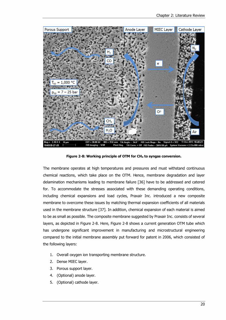
Chapter 2: Literature Review
20
Figure 2-8: Working principle of OTM for CH4 to syngas conversion.
The membrane operates at high temperatures and pressures and must withstand continuous
chemical reactions, which take place on the OTM. Hence, membrane degradation and layer
delamination mechanisms leading to membrane failure [36] have to be addressed and catered
for. To accommodate the stresses associated with these demanding operating conditions,
including chemical expansions and load cycles, Praxair Inc. introduced a new composite
membrane to overcome these issues by matching thermal expansion coefficients of all materials
used in the membrane structure [37]. In addition, chemical expansion of each material is aimed
to be as small as possible. The composite membrane suggested by Praxair Inc. consists of several
layers, as depicted in Figure 2-8. Here, Figure 2-8 shows a current generation OTM tube which
has undergone significant improvement in manufacturing and microstructural engineering
compared to the initial membrane assembly put forward for patent in 2006, which consisted of
the following layers:
1. Overall oxygen ion transporting membrane structure.
2. Dense MIEC layer.
3. Porous support layer.
4. (Optional) anode layer.
5. (Optional) cathode layer.
Chapter 2: Literature Review
21
As outlined above, the dense layer was used to transport oxygen ions in one direction and
electrons into the opposite, thereby separating oxygen from an oxygen rich feed gas stream,
such as air. This layer was fabricated as thin as possible to reduce resistance to ionic and
electronic transport, which made the use of a porous support layer indispensable to provide
mechanical stability. Applications of this membrane were planned in direct oxyfuel combustion or
syngas production and an optional intermediate layer was integrated to enhance surface area for
these reactions. In the same way, the optional surface exchange layer enhanced surface
exchange rate of the dense layer by increasing the surface area.
The composition and thickness of each layer varies, as can be seen by the difference in
microstructure in Figure 2-8. Table 2-2 summarises chemical composition, thickness δ, mean pore
diameter dp and porosity ε of each layer of the first generation membrane, where exact
specifications were not disclosed for every layer. It is visible, that all layers, except the porous
support layer, consisted of a dual-phase for ionic and electronic conduction. These dual-phase
layers preferably consisted of 50 vol% of either phase [37]. The membrane can be produced
either as planar or tubular cell. In recent publications on the application of OTM for oxyfuel
combustion and syngas generation by Praxair Inc. and in this research project, tubular cells were
deployed due to higher mechanical stability [1, 20, 35].
Table 2-2: List of materials used for first generation oxygen ion transport membrane [37].
Layer Composition δ
[µm]
dp
[µm]
ε
[-]
2 Electronic-phase (La0.825Sr0.175)0.97Cr0.76Mn0.225V0.025O3-δ
- - Ionic-phase Zr0.89Sc0.1Y0.01O2-δ
3 Porous Support Zr0.97Y0.03O2-δ 1 mm –
2.5 mm 2 - 5 0.4 – 0.6
4 Electronic-phase La0.8Sr0.2FeO3-δ
20 – 60 0.1 - 0.5 0.4 - 0.6 Ionic-phase Zr0.89Sc0.1Y0.01O2-δ
5 Electronic-phase
10 - 25 0.1 – 0.5 0.4 – 0.6 Ionic-phase
Research by Praxair Inc. revealed that mass transport resistance through the porous support
layer becomes rate limiting with increasing fuel conversion ratios as summarised in [1]. High fuel
conversion ratios can’t be avoided when aiming at completely reforming the fuel gases in an OTM
reactor. Microstructural characteristics of porous structures e.g. tortuosity, porosity and pore size
distribution, play a vital role in quantifying gaseous mass transport resistance [38–40]. At the
same time, the mechanical stability of OTMs during operation is ensured by the support layer.
With regards to the functional electrode and electrolyte layers, such porous support layers can

Chapter 2: Literature Review
22
be several orders of magnitude thicker [2]. These findings highlight the need to better understand
the interaction between the microstructure of the porous support layer and diffusive mass
transport, which forms the basis of the research need for this thesis.
2.2 Tortuosity
The previous sections mention that the dense oxygen separation layer of an OTM is manufactured
as thin as possible to maximise oxygen flux. This makes a porous support layer indispensable to
ensure the mechanical stability of the overall membrane assembly. Yet, diffusion of gases though
porous media is, among other factors such as temperature and gas composition, substantially
influenced by the microstructure of the porous membrane.
The importance of the effect of the microstructural characteristics including porosity, tortuosity
and pore size distribution on the performance of electrochemical devices has been widely
demonstrated [41, 42]. As a consequence, studies using microstructural analysis techniques [43]
are crucial for understanding and optimising such vital parameters. Among these, tortuosity plays
an essential role in mass transport limiting operating regimes and concentration polarisation
resistance [44, 45]. This is valid for batteries, fuel cells and oxygen transport membranes alike.
Here tortuosity, in combination with porosity, is used to relate the effective transport properties
of diffusion and electric or ionic conductivity to its respective bulk property. Moreover, both
parameters are applied to determine the Knudsen flow parameter KO and the viscous flow
parameter BO as outlined in section 2.3. As such, tortuosity is an integral parameter in modelling
and quantifying fuel cell [46] and battery [47] behaviour. In addition, tortuosity serves as an
input parameter in Newman-type models of battery performance [48] and the Adler-Lane-Steele
model for electrode kinetics [49].
Calculating tortuosity is not trivial, which is why a wealth of tortuosity calculation methods have
been developed, not only in the electrochemical community, but across many fields of research
(optics, magnetism, geology, medicine, etc.), each with associated definitions and areas of
application [50, 51].
Because of the limited application of tortuosity experiments in OTMs, literature from the wider
field of porous materials in electrochemical devices are reviewed. Due to the importance of
tortuosity and the multitude of calculation approaches, the following sections review the use of
tortuosity and various tortuosity calculation methods in the field of electrochemistry. These
methods can differ considerably from each other in terms of calculation approach and data
preparation techniques. The findings presented below have been submitted for peer-reviewed
publication [52].
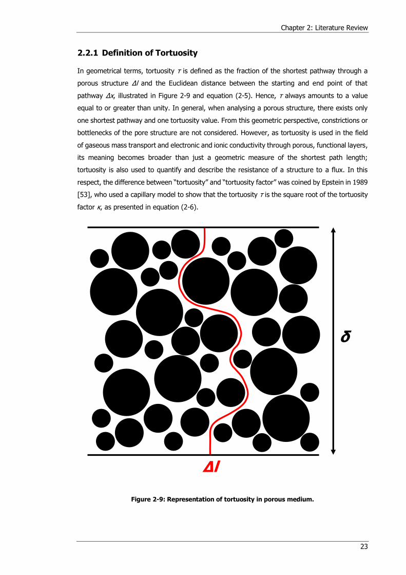
Chapter 2: Literature Review
23
2.2.1 Definition of Tortuosity
In geometrical terms, tortuosity τ is defined as the fraction of the shortest pathway through a
porous structure Δl and the Euclidean distance between the starting and end point of that
pathway Δx, illustrated in Figure 2-9 and equation (2-5). Hence, τ always amounts to a value
equal to or greater than unity. In general, when analysing a porous structure, there exists only
one shortest pathway and one tortuosity value. From this geometric perspective, constrictions or
bottlenecks of the pore structure are not considered. However, as tortuosity is used in the field
of gaseous mass transport and electronic and ionic conductivity through porous, functional layers,
its meaning becomes broader than just a geometric measure of the shortest path length;
tortuosity is also used to quantify and describe the resistance of a structure to a flux. In this
respect, the difference between “tortuosity” and “tortuosity factor” was coined by Epstein in 1989
[53], who used a capillary model to show that the tortuosity τ is the square root of the tortuosity
factor κ, as presented in equation (2-6).
Figure 2-9: Representation of tortuosity in porous medium.
Δl
δ
Chapter 2: Literature Review
24
𝜏 =∆𝑙
𝛿 (2-5)
𝜅 = 𝜏2 (2-6)
In which the following are defined:
τ tortuosity [-] Δl actual diffusion path [m] δ thickness of medium [m] κ tortuosity factor [-]
The tortuosity factor accounts for both the additional path length and its change in velocity of a
species when migrating through a porous structure. Epstein then applied this derivation in the
field of diffusion, where the tortuosity factor is used to calculate the effective diffusion coefficient
Deff based on the bulk diffusion coefficient Dbulk, shown in equation (2-7), which is also valid for
ionic and electronic conductivity.
𝐷𝑒𝑓𝑓 =휀
𝜅𝐷𝑏𝑢𝑙𝑘 =
휀
𝜏2𝐷𝑏𝑢𝑙𝑘 (2-7)
𝐷𝑒𝑓𝑓 =휀휁
𝜏𝐷𝑏𝑢𝑙𝑘 (2-8)
In which the following are defined:
Deff effective diffusion coefficient [m2s-1] ε porosity [-] κ tortuosity factor [-] Dbulk bulk diffusion coefficient [m2s-1] τ tortuosity [-] ζ constrictivity factor [-]
Yet, the theory behind the tortuosity factor is controversial, especially in the field of diffusive
mass transport: van Brakel and Heertjes [54], for example, defined a constrictivity factor δ to
account for the variation in pore diameter along the diffusion pathway, which is included in
calculating the effective transport property via equation (2-8).
This constrictivity factor was later adopted by Holzer et al. [55] who stated that the
implementation of τ2 was used to explain high values of experimentally derived tortuosities.
Consequently, the authors differentiated between two types of tortuosity [55, 56]:
1. That, which is acquired by indirect calculations-based on experimental data τexp.
2. And that, which is determined via geometric algorithms from reconstructed 3D volumes
τgeo.
Chapter 2: Literature Review
25
Additionally, when analysing diffusive mass transport problems, depending on the diffusion
mechanism taking place through a porous medium (ordinary diffusion, Knudsen diffusion and/or
viscous flow) [39] and on the gases involved [57], different tortuosity values may dominate: not
all molecules will be affected by the microstructure to the same extent when migrating through
such a layer. The inherent difference of the mean free path between each gaseous species leads
to different Knudsen numbers (cf. chapter 2.3.5) and thus, different diffusion pathways for
different species at different temperatures, gas compositions and transport regimes. It can thus
be inferred, that a different tortuosity value is dominating for each species and each transport
regime.
Moreover, in experimental approaches, tortuosity is not always presented explicitly, but is rather
combined with porosity into a “diffusibility” [58, 59] or “effective relative diffusivity” [60, 61] value
expressed as 𝜏2
. Additionally, in the field of battery research, tortuosity is contained in the
MacMullin number NM, which relates the bulk conductivity of the electrolyte σbulk to the effective
conductivity of the porous electrolyte σeff [62–65]:
𝑁𝑀 =𝜎𝑏𝑢𝑙𝑘𝜎𝑒𝑓𝑓
=𝜏2
휀 (2-9)
In which the following are defined:
NM MacMullin number [-] σbulk bulk conductivity [Sm-1] σeff effective conductivity [Sm-1] ε porosity [-] τ tortuosity [-]
These different definitions and applications of tortuosity cause differences in its interpretation
and calculation approach. For example, geometric-based tortuosity takes only the shortest path
length into account while flux-based values rather account for the path of least resistance. Hence,
the resulting values differ appreciably. These discrepancies are reflected by the vast number of
different tortuosity calculation approaches shown in the following sections.
2.2.2 Porosity-Tortuosity Relationships
Employing a porosity-tortuosity relationship is one of the most fundamental and straightforward
approaches to derive a tortuosity (or effective medium property) of a porous structure. Such
relationships, of theoretical or empirical origin, directly calculate a tortuosity value solely based
on a porosity of a sample.
In the comprehensive work by Shen and Chen [66], a review of past and present correlations is
provided, among which the Bruggeman equation is the most well-known and most widespread
Chapter 2: Literature Review
26
relation in the field of electrochemistry [67]. Equation (2-10) presents the generally used form of
the Bruggeman relationship, where α is the Bruggeman exponent which, in its standard form, is
considered to be 1.5. Recently, the author has provided a translation and explanation of the
mathematical formulation of Bruggeman which is used to derive the widely used model and the
above exponent [68].
τ𝐵𝑟𝑢𝑔𝑔𝑒𝑚𝑎𝑛2 = ε1−𝛼 (2-10)
Whilst the history of the Bruggeman correlation can be traced back to the 1930s, its proliferation
is not notable until the 1950s: Hoogschagen was one of the first to use the Bruggeman and
Maxwell relation [69] (cf. equation (2-11)) to validate experiments, where gas diffusion through
glass spheres was measured. He observed, that values for the labyrinth factor (1
𝜏2) lay between
the Maxwell and Bruggeman correlation, but slightly closer to the latter [58].
𝜏𝑀𝑎𝑥𝑤𝑒𝑙𝑙2 = (
3 − 휀
2) (2-11)
De La Rue and Tobias achieved similar results when measuring the effective conductivity values
of liquid ZnBr2 electrolyte solution. A variety of non-conducting glass spheres of different sizes
were embedded into the electrolyte to achieve different volume fractions. The conductivity as a
function of volume fraction of the embedded phase was evaluated. As was the case in
Hoogschagen’s publication [58], results lay between the Maxwell [69, 70] and Bruggeman relation
[71]. Since then, the Bruggeman equation has become a commonly used method to derive
effective medium properties of porous structures in batteries [72–76] and proton exchange
membrane (PEM) fuel cells [77–86]. Moreover, it has been implemented as a standard addition
to predicting microstructures in electrochemistry models, such as in the COMSOL Multiphysics
modelling software (COMSOL, Inc.) [65].
However, predictions given by the Bruggeman correlation are not always consistent with
experimental results [65, 87]. As a consequence, researchers have adjusted the Bruggeman
equation by altering the exponent α to fit experimental values. Thorat et al. [88] even included
an additional scaling factor γ to correlate the Bruggeman model with their experiments, resulting
in equation (2-12) to be extended to the following form:
τ𝐵𝑟𝑢𝑔𝑔𝑒𝑚𝑎𝑛2 = 𝛾휀1−𝛼 (2-12)
In which the following are defined:
τBruggeman tortuosity calculated via the Bruggeman correlation [-]
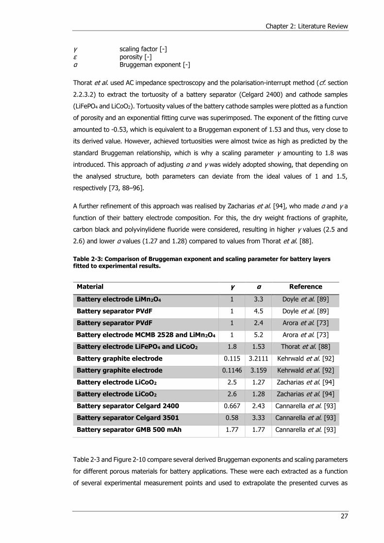
Chapter 2: Literature Review
27
γ scaling factor [-] ε porosity [-] α Bruggeman exponent [-]
Thorat et al. used AC impedance spectroscopy and the polarisation-interrupt method (cf. section
2.2.3.2) to extract the tortuosity of a battery separator (Celgard 2400) and cathode samples
(LiFePO4 and LiCoO2). Tortuosity values of the battery cathode samples were plotted as a function
of porosity and an exponential fitting curve was superimposed. The exponent of the fitting curve
amounted to -0.53, which is equivalent to a Bruggeman exponent of 1.53 and thus, very close to
its derived value. However, achieved tortuosities were almost twice as high as predicted by the
standard Bruggeman relationship, which is why a scaling parameter γ amounting to 1.8 was
introduced. This approach of adjusting α and γ was widely adopted showing, that depending on
the analysed structure, both parameters can deviate from the ideal values of 1 and 1.5,
respectively [73, 88–96].
A further refinement of this approach was realised by Zacharias et al. [94], who made α and γ a
function of their battery electrode composition. For this, the dry weight fractions of graphite,
carbon black and polyvinylidene fluoride were considered, resulting in higher γ values (2.5 and
2.6) and lower α values (1.27 and 1.28) compared to values from Thorat et al. [88].
Table 2-3: Comparison of Bruggeman exponent and scaling parameter for battery layers fitted to experimental results.
Material γ α Reference
Battery electrode LiMn2O4 1 3.3 Doyle et al. [89]
Battery separator PVdF 1 4.5 Doyle et al. [89]
Battery separator PVdF 1 2.4 Arora et al. [73]
Battery electrode MCMB 2528 and LiMn2O4 1 5.2 Arora et al. [73]
Battery electrode LiFePO4 and LiCoO2 1.8 1.53 Thorat et al. [88]
Battery graphite electrode 0.115 3.2111 Kehrwald et al. [92]
Battery graphite electrode 0.1146 3.159 Kehrwald et al. [92]
Battery electrode LiCoO2 2.5 1.27 Zacharias et al. [94]
Battery electrode LiCoO2 2.6 1.28 Zacharias et al. [94]
Battery separator Celgard 2400 0.667 2.43 Cannarella et al. [93]
Battery separator Celgard 3501 0.58 3.33 Cannarella et al. [93]
Battery separator GMB 500 mAh 1.77 1.77 Cannarella et al. [93]
Table 2-3 and Figure 2-10 compare several derived Bruggeman exponents and scaling parameters
for different porous materials for battery applications. These were each extracted as a function
of several experimental measurement points and used to extrapolate the presented curves as
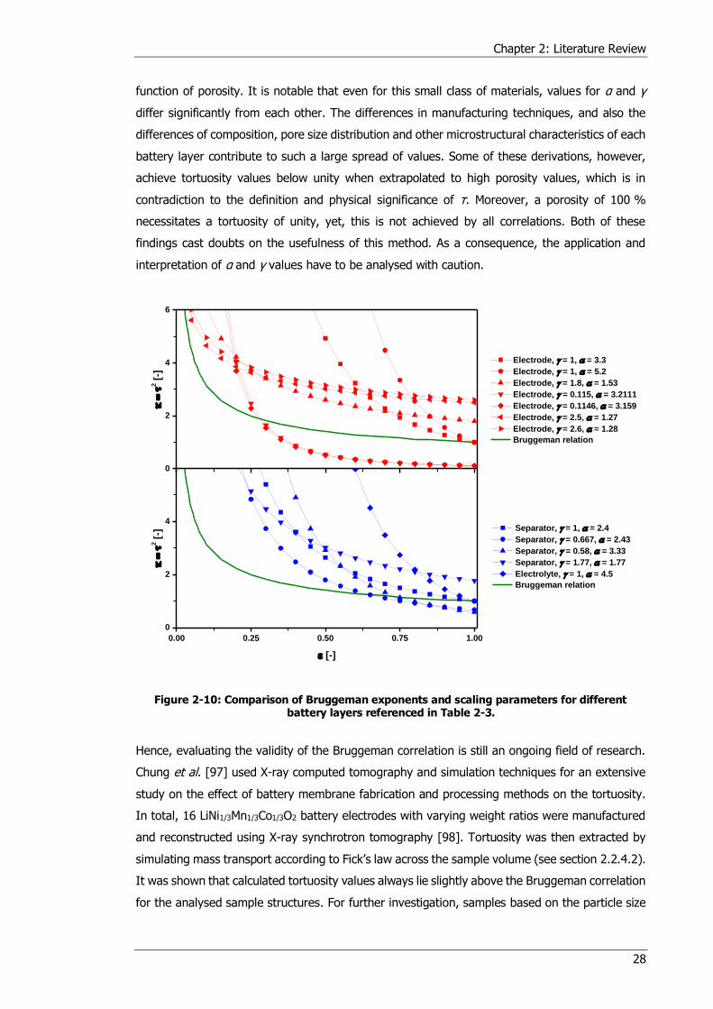
Chapter 2: Literature Review
28
function of porosity. It is notable that even for this small class of materials, values for α and γ
differ significantly from each other. The differences in manufacturing techniques, and also the
differences of composition, pore size distribution and other microstructural characteristics of each
battery layer contribute to such a large spread of values. Some of these derivations, however,
achieve tortuosity values below unity when extrapolated to high porosity values, which is in
contradiction to the definition and physical significance of τ. Moreover, a porosity of 100 %
necessitates a tortuosity of unity, yet, this is not achieved by all correlations. Both of these
findings cast doubts on the usefulness of this method. As a consequence, the application and
interpretation of α and γ values have to be analysed with caution.
Figure 2-10: Comparison of Bruggeman exponents and scaling parameters for different battery layers referenced in Table 2-3.
Hence, evaluating the validity of the Bruggeman correlation is still an ongoing field of research.
Chung et al. [97] used X-ray computed tomography and simulation techniques for an extensive
study on the effect of battery membrane fabrication and processing methods on the tortuosity.
In total, 16 LiNi1/3Mn1/3Co1/3O2 battery electrodes with varying weight ratios were manufactured
and reconstructed using X-ray synchrotron tomography [98]. Tortuosity was then extracted by
simulating mass transport according to Fick’s law across the sample volume (see section 2.2.4.2).
It was shown that calculated tortuosity values always lie slightly above the Bruggeman correlation
for the analysed sample structures. For further investigation, samples based on the particle size
0
2
4
6
0.00 0.25 0.50 0.75 1.00
0
2
4
2 [
-]
Electrode, = 1, = 3.3
Electrode, = 1, = 5.2
Electrode, = 1.8, = 1.53
Electrode, = 0.115, = 3.2111
Electrode, = 0.1146, = 3.159
Electrode, = 2.5, = 1.27
Electrode, = 2.6, = 1.28
Bruggeman relation
2 [
-]
[-]
Separator, = 1, = 2.4
Separator, = 0.667, = 2.43
Separator, = 0.58, = 3.33
Separator, = 1.77, = 1.77
Electrolyte, = 1, = 4.5
Bruggeman relation
Chapter 2: Literature Review
29
distributions of the imaged samples were computer generated, for which the orientation and
particle packing was varied. It was discovered that perfectly ordered particle distributions result
in tortuosities close to the Bruggeman relationship throughout the range of porosity values [97].
However, real structures including OTMs differ significantly from this.
Continuing work in the field of battery research from Wood and co-workers (cf. [95, 97, 98])
culminated in the development of an open source program called BruggemanEstimator [99]. This
program allows the extraction of the Bruggeman exponent α in each dimension of a 3D sample
volume by using two 2D images, namely one top view and one cross-sectional view. The
Bruggeman exponent of the sample is achieved by applying the differential effective medium
approximation method introduced by Bruggeman. In comparison to previously obtained values,
results calculated by the BruggemanEstimator software agreed well with numerical tortuosity
calculation methods [99] and has been recently applied in practise [100]. This approach is similar
to stereological methods which quantify 3D properties based in 2D image slices [101]. The
advantage of stereology is the reduced experimental efforts necessary to extract results. However,
Taiwo et al. [43] recently concluded, that values based on stereological approaches may deviate
appreciably from 3D measurements.
Moreover, a wide range of recent studies report conflicting results on the validity of the
Bruggeman correlation when compared to calculations conducted using tomography techniques.
Conclusions vary substantially as in some instances, simulations agree well with the Bruggeman
correlation [75, 97], while considerable disagreement was observed in other cases [86, 102–104].
The reason for this seems to be sample specific, as heterogeneity and geometry are
characteristics of porous materials that are not accounted for by the Bruggeman correlation. The
aforementioned studies have shown that the characteristic shape of the analysed microstructure
has considerable effects on the validity of the Bruggeman relation: spherical structures, which
follow Bruggeman's initial hypothesis very closely, adhere to the correlation. The correlation,
however, is less suitable for connected solid-phases and complex porous networks.
This is further complicated by the distinctions (or lack thereof) between geometrical and transport
limiting tortuosity [105]. Moreover, porosity-tortuosity relationships provide limited information
in areas, where the analysed sample consists of several layers with different microstructural
features, such as multi-layer battery separators [93]. These combine different properties into a
single separator; i.e. each individual layer exhibits distinct structural properties, and for this
reason, the simplified assumption of a homogenous sample volume made by the Bruggeman
correlation is no longer valid. As a conclusion, it can be stated that porosity-tortuosity
relationships are only applicable and reliable when executed across homogeneous microstructures
which are similar to the microstructure used to derive the respective relationship.
Chapter 2: Literature Review
30
2.2.3 Experimentally Derived Tortuosity
Historically, the lack of detailed geometrical information on complex porous media in 3D has
limited the ability of researchers to extract meaningful data on the tortuosity of a porous body.
In the absence of this information, effective transport properties of porous structures have been
derived experimentally by means of diffusion cell experiments [58, 59, 106–112] and
electrochemical measurements [57, 61, 88, 113].
2.2.3.1 Diffusion Cell Experiments
As reviewed by He et al. [114], diffusion measurement methods in the field of fuel cell research
aim at extracting effective diffusion coefficients of distinct gas mixtures. In these experiments, a
porous sample is mounted between an upper and a lower gas channel where two different gases
are injected. Due to the concentration gradient across the porous material, diffusion of either gas
to the opposite channel is induced. Measuring the concentration of either gas in both streams
allows the calculation of the diffusion fluxes across the membrane via a mass balance over the
cell. The effective diffusion coefficient and in turn, the tortuosity of the sample, are subsequently
derived by applying a suitable diffusion model.
Yet, the applicability of diffusion models for this purpose is dependent on the diffusion mechanism
taking place within the porous medium, including ordinary, Knudsen and/or viscous flow (cf. [38,
39, 115]). The theory behind diffusion models is treated in detail in section 2.3 and the application
of selected models in the experimental section of this project is presented in the methodology
chapter 3.2.4.
In the field of diffusion cell experiments, Wicke Kallenbach cells (WKC) [106] and Graham
diffusion cell (GDC) are applied in practise [111]. Figure 2-11 illustrates the difference and
similarities between both setups. In either diffusion cell, the porous material is placed between
an upper and a lower chamber which are otherwise separated by an impermeable structure. In
the WKC (Figure 2-11A), Gases A and B enter the upper and lower chamber, respectively and
due to porosity of the analysed material, diffusion from either gas to the opposite chamber is
induced. Using a gas chromatograph (GC), concentration levels of either gas in the opposite
stream is determined at the outlets of both chambers. This allows the calculation of effective
molar diffusion flux and derivation of effective binary diffusion coefficient by applying a suitable
diffusion model. When using a GDC (Figure 2-11B), no GC is needed. Here, gases A and B enter
the upper and lower chamber, respectively whereas the exiting stream of the lower compartment
is connected to a digital bubble flow meter. As soon as steady-state conditions are reached, the
valves to and from the lower compartment are closed and the valve to the flow meter is opened.
This way, the effective volumetric diffusion flux for either species is directly readable.

Chapter 2: Literature Review
31
Numbers in Figure 2-11 refer to:
1 Impermeable disc.
2 Porous pellets.
3 Lower chamber.
4 Upper chamber.
5 Valves.
6 Gas chromatograph.
7 Three-way valve.
8 Digital bubble flow meter.
Figure 2-11: Wicke Kallenbach (A) and Graham (B) diffusion cell setup. Reproduced with permission from Elsevier [111].
In [111], a comparison of measurement results between WKC and GDC was carried out using a
set of porous samples with different pore sizes. It was shown, that deviation in effective net
diffusion fluxes between both diffusion cells lay on average below 5 % with only few exceptions.
Even though designs of diffusion cell test apparatus underwent adaptations to fit the specific
experimental layout, similarities with WKCs and GCs are almost always noticeable [114].
Another type of diffusion cell is the Loshmidt cell [116] which has been previously applied by
Zamel et al. [59] in fuel cell research. Here, the authors measured the effective diffusion
A
B
Chapter 2: Literature Review
32
coefficient of an O2-N2 gas mixture migrating through carbon paper, which is commonly applied
as the gas diffusion layer in PEM fuel cells. When increasing the temperature from 25 °C to 80 °C,
the bulk diffusion coefficient of the gas mixture, achieved via a resistance network model based
on Fick’s law, increased from approximately 0.2 cm2s-1 to 0.275 cm2s-1 while the effective diffusion
coefficient increased from approximately 0.05 cm2s-1 to 0.075 cm2s-1. This causes the factor 𝜏2
to
increase by approximately 11.5 % from 0.252 to 0.281. Thus, when considering a constant
porosity value, the tortuosity decreases to the same extent. In addition, the authors compared
the calculated diffusibility values to a set of porosity-tortuosity relationships, among others, the
Bruggeman relation. In all cases, these relationships overestimate the effective diffusion
coefficient.
Compared to the effective diffusion coefficients achieved via diffusion cell experiments, the
tortuosity of a sample serves as an independent microstructural parameter which is, theoretically,
not limited to the applied gas composition and experimental conditions. Hence, the tortuosity
would serve as an ideal comparative value for porous structures. Yet, the direct calculation of
tortuosity based on diffusion measurements [117] is less common. A thorough study of
experimentally calculated tortuosity of fuel cell related porous media has been recently conducted
by Vamvakeros [118]. A range of different gas diffusion layers of PEM fuel cells and a ceramic
interconnect support material of an SOFC underwent a range of diffusion experiments under
varying temperatures and diffusion models. While the SOFC results were comparable to values
found in literature, the PEM featured lower performance compared to similar experiments. Hence,
the conclusion of the author underlined the importance of choosing the correct diffusion model
which is in accordance with the diffusion regime dominating within the sample. As a consequence,
the underlying microstructure has to be investigated carefully to judge whether or not solely
ordinary diffusion or a mixture between ordinary and Knudsen diffusion have to be considered.
2.2.3.2 Electrochemical Experiments
Mass transport limitations play a vital role in electrochemical devices as they are responsible for
concentration polarisation at high current densities. For example, as current densities increase,
the fuel demand in a fuel cell increases linearly, as shown in equation [46]:
��𝑓𝑢𝑒𝑙 =𝑖𝐴
𝑛𝐹 (2-13)
In which the following are defined:
��𝑓𝑢𝑒𝑙 molar flow rate of fuel gas [mols-1]
i current density [Am-2] A membrane area [m2] n equivalent electrons per mole of reactant [-] F Faraday constant [Cmol-1]

Chapter 2: Literature Review
33
The fuel consumption rates at the active sites of a fuel cell are limited by the maximum diffusion
rate of reactant achievable through the porous structures. As introduced in previous sections,
diffusive mass transport and as such, mass transport limitations, are a function of the complex
microstructure of the involved porous membrane layers. Hence, microstructural parameters, such
as tortuosity, are extractable by measuring concentration losses of fuel cells and applying gas
diffusion theory.
In this respect, SOFCs offer the possibility to investigate the effect of fuel gas compositions on
the performance due to their wide fuel flexibility. A thorough study of this topic was presented
by Jiang and Virkar [57]. As the effects of mass transport limitations are dominating under high
current density operations, Jiang and Virkar modified Fick’s law to express the effective diffusion
coefficient as a function of the limiting current density of the fuel cell under specific operating
conditions. The resulting expression is presented in equation (2-14).
𝐷𝑒𝑓𝑓 =𝑖𝑙𝑖𝑚
2𝐹𝑝𝑓𝑢𝑒𝑙0
𝑅𝑇𝛿 −𝑖𝑙𝑖𝑚𝑅𝑇𝛿
𝐴𝑝��𝑓𝑢𝑒𝑙
(2-14)
In which the following are defined:
Deff effective diffusion coefficient [m2s-1] ilim limiting current density [Am-2] F Faraday constant [Cmol-1] 𝑝𝑓𝑢𝑒𝑙0 partial pressure of fuel at the gas inlet [Pa]
R ideal gas constant [Jmol-1K-1] T temperature [K] δ membrane thickness [m] A membrane area [m2]
In their work, the limiting current density was measured experimentally from polarisation curves
for a set of binary and ternary fuel gas mixtures including H2-H2O, CO-CO2, H2-He-H2O, H2-N2-H2O
and H2-CO2-H2O, each under varying concentrations. Tortuosity values were then calculated by
reversing the Bosanquet equation shown in equation (2-28). At 800 °C, the lowest tortuosity
values were achieved for the H2-H2O mixture, which, on average, amounted to 2.23, while the
highest tortuosity values were calculated for the H2-CO2-H2O mixture, amounting to 2.73.
Moreover, in direct comparison between the two binary gas mixtures, it was revealed that fuel
cell performance was higher using H2 as fuel gas rather than CO which, besides the lower
electrochemical activity of CO, was due to the significantly faster diffusion rate of H2. These results
confirm the findings of different tortuosity values for different binary gas mixtures presented in
the previous section.
Brus et al. [113] adopted the same methodology to compare electrochemically derived tortuosity
values with an image-based tortuosity calculation technique, namely the random walk method
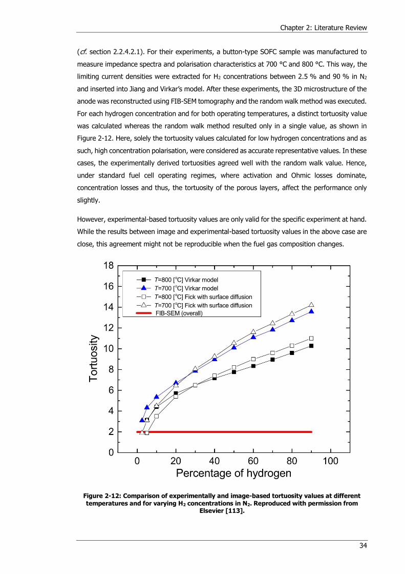
Chapter 2: Literature Review
34
(cf. section 2.2.4.2.1). For their experiments, a button-type SOFC sample was manufactured to
measure impedance spectra and polarisation characteristics at 700 °C and 800 °C. This way, the
limiting current densities were extracted for H2 concentrations between 2.5 % and 90 % in N2
and inserted into Jiang and Virkar’s model. After these experiments, the 3D microstructure of the
anode was reconstructed using FIB-SEM tomography and the random walk method was executed.
For each hydrogen concentration and for both operating temperatures, a distinct tortuosity value
was calculated whereas the random walk method resulted only in a single value, as shown in
Figure 2-12. Here, solely the tortuosity values calculated for low hydrogen concentrations and as
such, high concentration polarisation, were considered as accurate representative values. In these
cases, the experimentally derived tortuosities agreed well with the random walk value. Hence,
under standard fuel cell operating regimes, where activation and Ohmic losses dominate,
concentration losses and thus, the tortuosity of the porous layers, affect the performance only
slightly.
However, experimental-based tortuosity values are only valid for the specific experiment at hand.
While the results between image and experimental-based tortuosity values in the above case are
close, this agreement might not be reproducible when the fuel gas composition changes.
Figure 2-12: Comparison of experimentally and image-based tortuosity values at different temperatures and for varying H2 concentrations in N2. Reproduced with permission from
Elsevier [113].
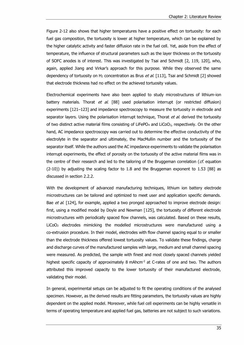
Chapter 2: Literature Review
35
Figure 2-12 also shows that higher temperatures have a positive effect on tortuosity: for each
fuel gas composition, the tortuosity is lower at higher temperature, which can be explained by
the higher catalytic activity and faster diffusion rate in the fuel cell. Yet, aside from the effect of
temperature, the influence of structural parameters such as the layer thickness on the tortuosity
of SOFC anodes is of interest. This was investigated by Tsai and Schmidt [2, 119, 120], who,
again, applied Jiang and Virkar’s approach for this purpose. While they observed the same
dependency of tortuosity on H2 concentration as Brus et al. [113], Tsai and Schmidt [2] showed
that electrode thickness had no effect on the achieved tortuosity values.
Electrochemical experiments have also been applied to study microstructures of lithium-ion
battery materials. Thorat et al. [88] used polarisation interrupt (or restricted diffusion)
experiments [121–123] and impedance spectroscopy to measure the tortuosity in electrode and
separator layers. Using the polarisation interrupt technique, Thorat et al. derived the tortuosity
of two distinct active material films consisting of LiFePO4 and LiCoO2, respectively. On the other
hand, AC impedance spectroscopy was carried out to determine the effective conductivity of the
electrolyte in the separator and ultimately, the MacMullin number and the tortuosity of the
separator itself. While the authors used the AC impedance experiments to validate the polarisation
interrupt experiments, the effect of porosity on the tortuosity of the active material films was in
the centre of their research and led to the tailoring of the Bruggeman correlation (cf. equation
(2-10)) by adjusting the scaling factor to 1.8 and the Bruggeman exponent to 1.53 [88] as
discussed in section 2.2.2.
With the development of advanced manufacturing techniques, lithium ion battery electrode
microstructures can be tailored and optimized to meet user and application specific demands.
Bae et al. [124], for example, applied a two pronged approached to improve electrode design:
first, using a modified model by Doyle and Newman [125], the tortuosity of different electrode
microstructures with periodically spaced flow channels, was calculated. Based on these results,
LiCoO2 electrodes mimicking the modelled microstructures were manufactured using a
co-extrusion procedure. In their model, electrodes with flow channel spacing equal to or smaller
than the electrode thickness offered lowest tortuosity values. To validate these findings, charge
and discharge curves of the manufactured samples with large, medium and small channel spacing
were measured. As predicted, the sample with finest and most closely spaced channels yielded
highest specific capacity of approximately 8 mAhcm-2 at C-rates of one and two. The authors
attributed this improved capacity to the lower tortuosity of their manufactured electrode,
validating their model.
In general, experimental setups can be adjusted to fit the operating conditions of the analysed
specimen. However, as the derived results are fitting parameters, the tortuosity values are highly
dependent on the applied model. Moreover, while fuel cell experiments can be highly versatile in
terms of operating temperature and applied fuel gas, batteries are not subject to such variations.
Chapter 2: Literature Review
36
Hence, it appears to be easier to extract an overall valid tortuosity value for a battery layer than
a fuel cell layer.
2.2.4 Tortuosity Calculation in 3D Volumes
The advent of sophisticated and easily accessible tomography methods has increased the amount
of obtainable data of porous samples which fundamentally changed the perception of
microstructural characterisation in 3D [126]. Focused ion beam–scanning electron microscope
(FIB-SEM) slice and view tomography [127], and X-ray computed tomography (X-ray CT) [128,
129] are among the most prominent methods of reconstructing a sample in three dimensions.
Even though the operation and image acquisition of both methods is radically different as
presented in section 2.4, comparative studies showed that acquired data is identical when the
resolution is the same [130–132].
In recent years, tomographic reconstruction of microstructures in electrochemical devices has
become increasingly widespread, offering the possibility to evaluate vital parameters, such as
triple-phase boundary length in SOFCs [133, 134], connectivity [135], phase distribution [136]
and tortuosity [133, 137] at different length scales [138]. Additionally, the effect of
microstructural parameters on the performance of electrochemical devices has been evaluated
by generating synthetic 3D volumes in-silico [75, 97, 139, 140]. The purpose for this process is
to directly evaluate the effect of specific microstructural variations such as porosity, pore size
distribution, shape or packing orientation of particles on mass transport.
There remains some confusion in the literature regarding the different definitions of tortuosity for
the purpose of image-based modelling: here, we distinguish between two main approaches in
extracting tortuosity:
1. Geometric-based algorithms, which aim to determine the shortest path length through a
porous structure by purely considering geometric aspects.
2. Flux-based algorithms, which mimic mass transport and diffusion behaviour, which is not
taken into consideration in geometric-based algorithms. These methods are further
divided into the following two sub-sections:
a. Voxel-based algorithms that take the extracted dataset and directly execute
tortuosity extraction techniques across the voxel domain of the analysed phase.
b. Mesh-based approaches which rely on generating a volume mesh of the analysed
phase to prepare the sample for computational fluid dynamics (CFD) programs.
It is evident that the increase in development of such techniques correlates with the increasing
accessibility of tomography equipment and high-performance computers.
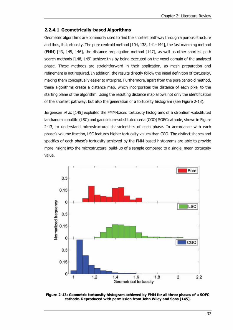
Chapter 2: Literature Review
37
2.2.4.1 Geometrically-based Algorithms
Geometric algorithms are commonly used to find the shortest pathway through a porous structure
and thus, its tortuosity. The pore centroid method [104, 138, 141–144], the fast marching method
(FMM) [43, 145, 146], the distance propagation method [147], as well as other shortest path
search methods [148, 149] achieve this by being executed on the voxel domain of the analysed
phase. These methods are straightforward in their application, as mesh preparation and
refinement is not required. In addition, the results directly follow the initial definition of tortuosity,
making them conceptually easier to interpret. Furthermore, apart from the pore centroid method,
these algorithms create a distance map, which incorporates the distance of each pixel to the
starting plane of the algorithm. Using the resulting distance map allows not only the identification
of the shortest pathway, but also the generation of a tortuosity histogram (see Figure 2-13).
Jørgensen et al. [145] exploited the FMM-based tortuosity histograms of a strontium-substituted
lanthanum cobaltite (LSC) and gadolinium-substituted ceria (CGO) SOFC cathode, shown in Figure
2-13, to understand microstructural characteristics of each phase. In accordance with each
phase’s volume fraction, LSC features higher tortuosity values than CGO. The distinct shapes and
specifics of each phase’s tortuosity achieved by the FMM-based histograms are able to provide
more insight into the microstructural build-up of a sample compared to a single, mean tortuosity
value.
Figure 2-13: Geometric tortuosity histogram achieved by FMM for all three phases of a SOFC cathode. Reproduced with permission from John Wiley and Sons [145].
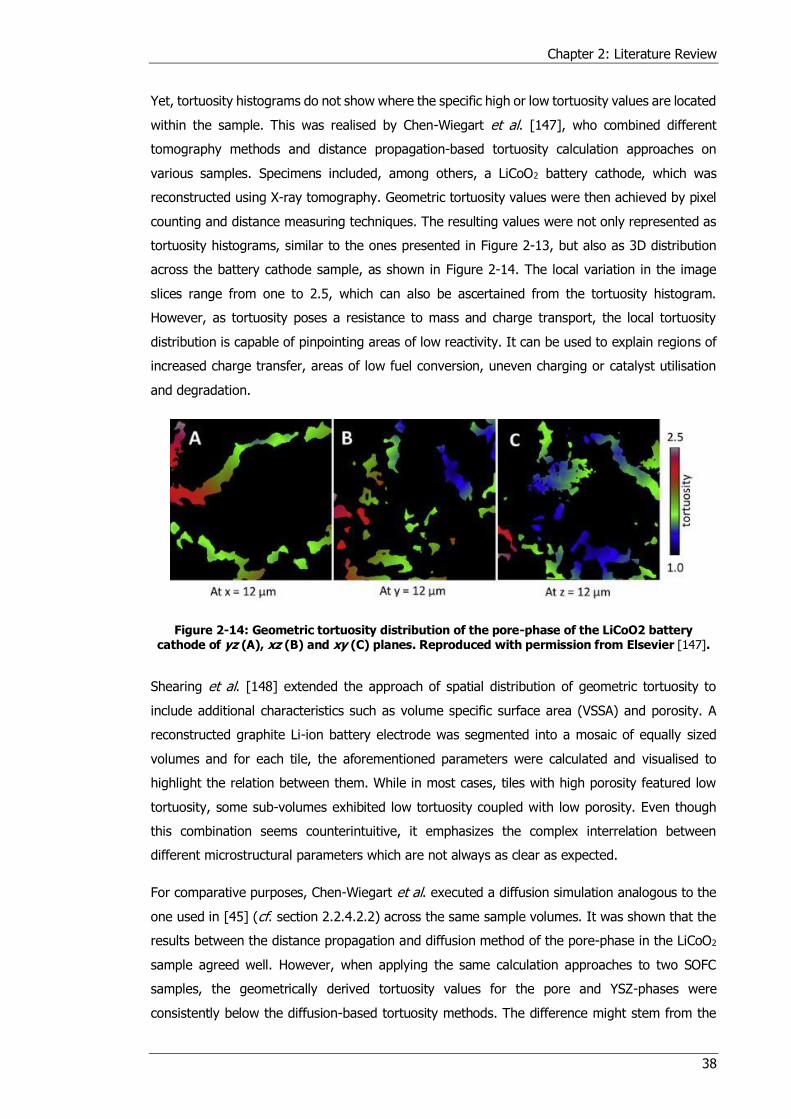
Chapter 2: Literature Review
38
Yet, tortuosity histograms do not show where the specific high or low tortuosity values are located
within the sample. This was realised by Chen-Wiegart et al. [147], who combined different
tomography methods and distance propagation-based tortuosity calculation approaches on
various samples. Specimens included, among others, a LiCoO2 battery cathode, which was
reconstructed using X-ray tomography. Geometric tortuosity values were then achieved by pixel
counting and distance measuring techniques. The resulting values were not only represented as
tortuosity histograms, similar to the ones presented in Figure 2-13, but also as 3D distribution
across the battery cathode sample, as shown in Figure 2-14. The local variation in the image
slices range from one to 2.5, which can also be ascertained from the tortuosity histogram.
However, as tortuosity poses a resistance to mass and charge transport, the local tortuosity
distribution is capable of pinpointing areas of low reactivity. It can be used to explain regions of
increased charge transfer, areas of low fuel conversion, uneven charging or catalyst utilisation
and degradation.
Figure 2-14: Geometric tortuosity distribution of the pore-phase of the LiCoO2 battery cathode of yz (A), xz (B) and xy (C) planes. Reproduced with permission from Elsevier [147].
Shearing et al. [148] extended the approach of spatial distribution of geometric tortuosity to
include additional characteristics such as volume specific surface area (VSSA) and porosity. A
reconstructed graphite Li-ion battery electrode was segmented into a mosaic of equally sized
volumes and for each tile, the aforementioned parameters were calculated and visualised to
highlight the relation between them. While in most cases, tiles with high porosity featured low
tortuosity, some sub-volumes exhibited low tortuosity coupled with low porosity. Even though
this combination seems counterintuitive, it emphasizes the complex interrelation between
different microstructural parameters which are not always as clear as expected.
For comparative purposes, Chen-Wiegart et al. executed a diffusion simulation analogous to the
one used in [45] (cf. section 2.2.4.2.2) across the same sample volumes. It was shown that the
results between the distance propagation and diffusion method of the pore-phase in the LiCoO2
sample agreed well. However, when applying the same calculation approaches to two SOFC
samples, the geometrically derived tortuosity values for the pore and YSZ-phases were
consistently below the diffusion-based tortuosity methods. The difference might stem from the
Chapter 2: Literature Review
39
inherent difference between geometric and diffusion-based considerations: the geometrically
shortest path through a structure is not always the path of least resistance for a flux, owing to
the presence of constrictions and pore necks. Further discussion on the differences of these
considerations is presented in section 2.2.4.2.
In contrast to the aforementioned algorithms, the pore centroid method does not provide a
histogram of tortuosity values or spatial distribution of tortuosity, but rather arrives at one specific
value of tortuosity along each dimension of a sample. The calculation algorithm follows the centre
of mass of a phase of a 2D plane along the third axis of the volume. The length of the pathway
going through each centroid is then calculated and used to determine the tortuosity. Despite its
shortcomings in comparison with the previous algorithms, the pore centroid is a standard option
in image and volume processing programs such as Amira and Avizo (both FEI). As such, it is
easily applied for comparative studies and capable of giving a quick tortuosity estimate.
Cooper et al. used the pore centroid method for comparison reasons when studying an SOFC
[143] and a battery electrode [104]. In [143], the tortuosity of the solid and pore-phase of an
LSCF SOFC cathode was determined by a variety of calculation algorithms, namely heat flux
simulation (cf. sections 2.2.4.2.2 and 3.5.1), Avizo XLab plugin, diffusion simulation, random walk
method (cf. section 2.2.4.2.1) and pore centroid method. These algorithms were executed across
the same sample after imaging at 14 °C and 695 °C using synchrotron X-ray nano CT which have
previously been extracted by Shearing et al. [150]. The pore centroid method produced the lowest
tortuosity values for both phases at both temperatures and closely followed the Bruggeman
relationship. Yet, the flux-based calculation algorithms agreed well with each other as values lay
between the heat flux simulation and the random walk method. The average tortuosity for the
pore-phase amounted to approximately 1.21 in all three dimensions at both temperatures and
lay visibly below the values reported by Gostovic et al. [141] using the same method. Large
variability in homogeneity of a sample significantly affect the results achieved by the pore centroid
method, causing visible fluctuations. In this respect, Cooper [151] pointed out that if the analysed
characteristic feature becomes small compared to the control volume, the centroid of each 2D
plane will tend towards the centre, resulting in a tortuosity of unity which casts doubt on the
applicability of this approach. More detail on the algorithm of the fast marching method and the
pore centroid method are presented in section 3.4.3.
2.2.4.2 Flux-based Algorithms
Even though geometrically-based tortuosity calculation algorithms can extract useful data
concerning the distribution of geometric tortuosity across a sample, these algorithms do not mimic
the flux like behaviour of transport phenomena. For example, small connections consisting only
of one voxel would only contribute a negligible amount to the overall flux of transported species,
while they are fully included in the above calculation methods. As a result, flux-based algorithms
Chapter 2: Literature Review
40
focus on simulating the transport mechanism at hand to extract the tortuosity of a sample. Here,
this method is separated into two parts, namely voxel and mesh-based calculation approaches.
2.2.4.2.1 Voxel-based Calculation Methods
Voxel-based algorithms are directly executed across the voxel domain of the reconstructed
volume. This means that for the methods introduced below, no additional re-tessellation or
re-meshing steps are necessary after the sample has been segmented. In most cases, a binarised
2D image sequence is sufficient to operate the calculation procedure.
One of the first applications of combining X-ray nano tomography with image-based tortuosity
calculation was presented by Izzo et al. [137], where X-ray CT was used to gather microstructural
parameters of a porous SOFC anode, including porosity, tortuosity and pore size distribution. The
authors solved the Laplace equation for diffusive mass transport through the pore-phase of the
electrode as explained in a different publication from the group [152]. Grew et al. [153] applied
the same methodology but extended its application to the solid-phases of a Ni-YSZ SOFC anode.
As effective ionic and electronic conductivity are affected by the tortuous nature of fuel cell
electrode layers (cf. equation (2-7)), tortuosities of solid-phases are equally as important as of
pore-phases. Yet, they were at least a factor of 1.2 higher. Their work was further refined in [154]
by calculating the representative volume element of the pore-phase tortuosity by solving the
Laplace equation using the same method.
Cooper [151] programmed a MATLAB (Mathworks Inc.) Laplace solver called TauFactor [155, 156]
to extract the tortuosity of a two phase segmented 3D tiff stack. The solver then determines the
tortuosity in each dimension for both phases. In [151], Cooper compared the results of the
TauFactor solver to previous work presented in [143], revealing that the solver gives similar
results as the Avizo package XLab Thermo and the heat flux simulation.
Aside from solving the Laplace equation to arrive at the tortuosity of their sample, Izzo et al. [137]
included the lattice Boltzmann method (LBM) [157] to model multi-component gas transport
coupled with an electrochemical model to visualise the H2 distribution in the anode. Due to the
capability to model gaseous, ionic and electronic transport, the LBM became widely applied in
fuel cell research, also with the focus of extracting tortuosity in different phases of a functional
layer [134, 158–163]. For this, the LBM uses the particle distribution function (PDF) 𝑓𝛼𝑃𝐷𝐹𝑖 , which
is a function describing the probability of encountering a particle of a species i at a certain location
xPDF with a certain speed 𝑒𝛼𝑃𝐷𝐹𝑖 at a certain point of time t moving in a certain direction αPDF.
The LBM consists of two steps, namely streaming and collision, which are carried out on each
point of a lattice: during streaming, the particles migrate to adjacent lattice points while during
collision, the interactions between particles at each lattice point governed by the collision term
𝛺𝛼𝑃𝐷𝐹𝑖 are computed. Both steps are collectively expressed by the lattice Boltzmann equation [152,
164]:
Chapter 2: Literature Review
41
𝑓𝛼𝑃𝐷𝐹𝑖 (𝑥𝑃𝐷𝐹 + 𝑒𝛼𝑃𝐷𝐹
𝑖 , 𝑡 + 1) − 𝑓𝛼𝑃𝐷𝐹𝑖 (𝑥𝑃𝐷𝐹 , 𝑡) = 𝛺𝛼𝑃𝐷𝐹
𝑖 (2-15)
Using this approach, Iwai et al. [134] arrived at tortuosity values for each phase in the porous
Ni-YSZ anode by calculating the effective diffusion coefficient and effective ionic as well as
electronic conductivities of the respective phases. The anode sample was reconstructed by
applying FIB-SEM tomography, where the Ni- and YSZ-phases were identified via EDX mapping,
to correlate the correct phase to the respective electron image. Table 2-4 compares the achieved
tortuosity values for all three phases along each dimension using the LBM as well as the random
walk method, which is introduced thereafter. It is evident that the tortuosity values of the
solid-phases are higher compared to the pore-phase, which is identical to findings presented by
Chen-Wiegart et al. [147] using a distance mapping approach. Nevertheless, values for the
pore-phase tortuosity are lower but comparable to values found by Izzo et al. [137]. However,
due to the observed directional anisotropy of the solid-phase tortuosities, Iwai et al. concluded,
that the sample volume was not sufficiently large to present effective ionic and electronic
conductivity values. Vivet et al. [165] achieved similarly high Ni-phase tortuosity values using a
finite difference method. However, due to the higher YSZ fraction in their sample, achieved YSZ
tortuosities lay below the values reported by Iwai et al. [134].
The aforementioned random walk method [70, 134, 166–169] mimics a diffusion process by
distributing a number of non-sorbing particles, so-called “walkers”, across the segmented voxel
phase. The algorithm then starts a time step sequence, where at each step, every walker choses
one neighbouring voxel as its next location. If that neighbouring voxel is of the same phase (e.g.
pore-phase), the walker migrates to that new location. However, if the chosen neighbouring voxel
is of a different phase (e.g. solid-phase), the walker remains at its current location and choses a
different neighbouring voxel at the following time step. By repeating this sequence, the mean
square displacement ⟨𝑟2(𝑡)⟩ of the walkers in the analysed phase is calculated which, in turn, is
used to achieve an effective diffusion coefficient Deff, where Vphase is the volume fraction of the
analysed phase:
𝐷𝑒𝑓𝑓 =𝑉𝑝ℎ𝑎𝑠𝑒6
𝑑⟨𝑟2(𝑡)⟩
𝑑𝑡𝐽𝑖,𝐷 = −𝐷𝑖
∆𝑐𝑖𝛿
(2-16)
Tortuosity is then calculated by comparing the effective diffusion coefficient to the bulk diffusion
coefficient through an empty volume of equal dimensions. The random walk approach was first
formulated in the 1990s [50, 170, 171] and found its way into electrochemistry via Kishimoto et
al. [166], after having been used to extract the tortuosity of porous rocks [172]. However, the
obtained tortuosity is affected by the number of walkers and by the number of time steps chosen
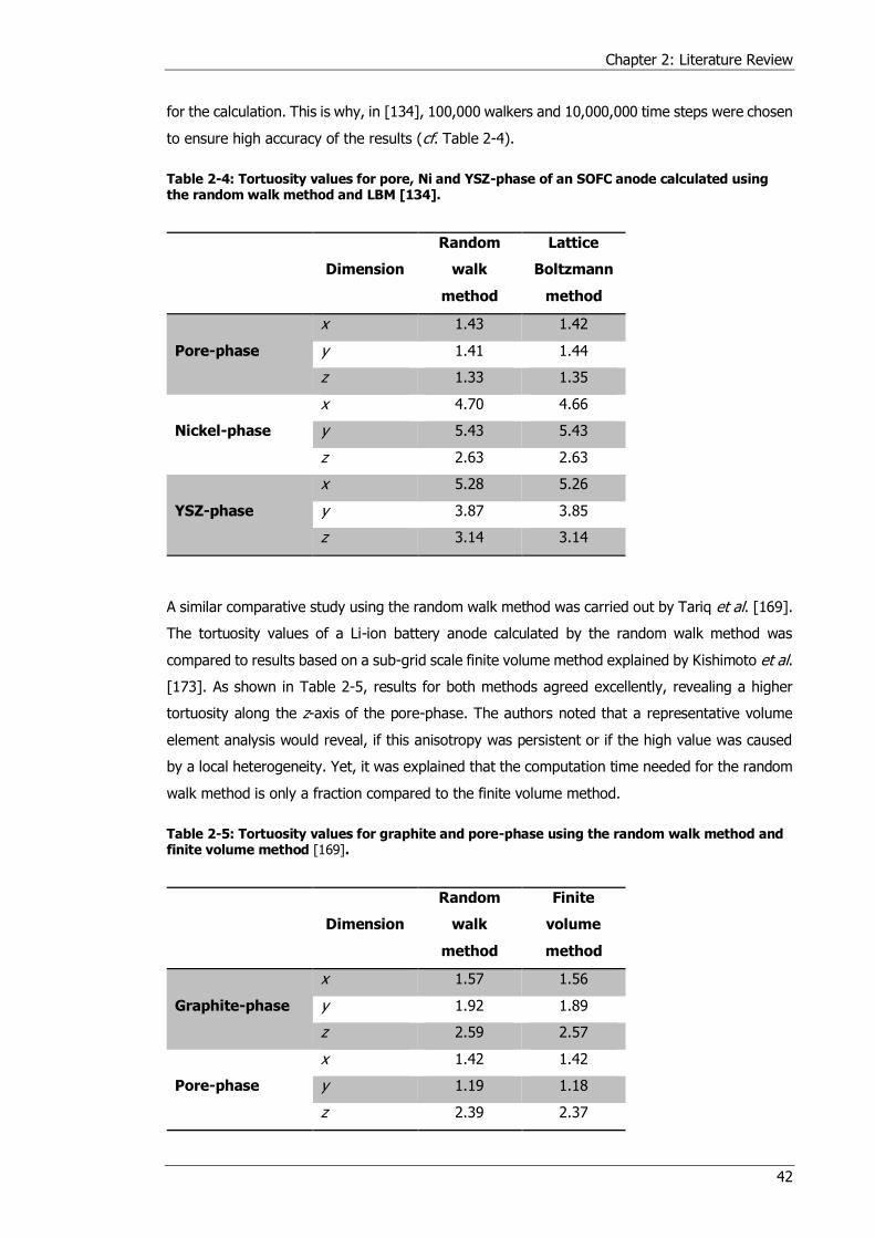
Chapter 2: Literature Review
42
for the calculation. This is why, in [134], 100,000 walkers and 10,000,000 time steps were chosen
to ensure high accuracy of the results (cf. Table 2-4).
Table 2-4: Tortuosity values for pore, Ni and YSZ-phase of an SOFC anode calculated using the random walk method and LBM [134].
Dimension
Random
walk
method
Lattice
Boltzmann
method
Pore-phase
x 1.43 1.42
y 1.41 1.44
z 1.33 1.35
Nickel-phase
x 4.70 4.66
y 5.43 5.43
z 2.63 2.63
YSZ-phase
x 5.28 5.26
y 3.87 3.85
z 3.14 3.14
A similar comparative study using the random walk method was carried out by Tariq et al. [169].
The tortuosity values of a Li-ion battery anode calculated by the random walk method was
compared to results based on a sub-grid scale finite volume method explained by Kishimoto et al.
[173]. As shown in Table 2-5, results for both methods agreed excellently, revealing a higher
tortuosity along the z-axis of the pore-phase. The authors noted that a representative volume
element analysis would reveal, if this anisotropy was persistent or if the high value was caused
by a local heterogeneity. Yet, it was explained that the computation time needed for the random
walk method is only a fraction compared to the finite volume method.
Table 2-5: Tortuosity values for graphite and pore-phase using the random walk method and finite volume method [169].
Dimension
Random
walk
method
Finite
volume
method
Graphite-phase
x 1.57 1.56
y 1.92 1.89
z 2.59 2.57
Pore-phase
x 1.42 1.42
y 1.19 1.18
z 2.39 2.37
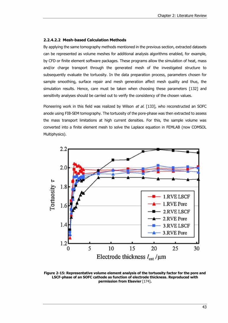
Chapter 2: Literature Review
43
2.2.4.2.2 Mesh-based Calculation Methods
By applying the same tomography methods mentioned in the previous section, extracted datasets
can be represented as volume meshes for additional analysis algorithms enabled, for example,
by CFD or finite element software packages. These programs allow the simulation of heat, mass
and/or charge transport through the generated mesh of the investigated structure to
subsequently evaluate the tortuosity. In the data preparation process, parameters chosen for
sample smoothing, surface repair and mesh generation affect mesh quality and thus, the
simulation results. Hence, care must be taken when choosing these parameters [132] and
sensitivity analyses should be carried out to verify the consistency of the chosen values.
Pioneering work in this field was realized by Wilson et al. [133], who reconstructed an SOFC
anode using FIB-SEM tomography. The tortuosity of the pore-phase was then extracted to assess
the mass transport limitations at high current densities. For this, the sample volume was
converted into a finite element mesh to solve the Laplace equation in FEMLAB (now COMSOL
Multiphysics).
Figure 2-15: Representative volume element analysis of the tortuosity factor for the pore and LSCF-phase of an SOFC cathode as function of electrode thickness. Reproduced with
permission from Elsevier [174].
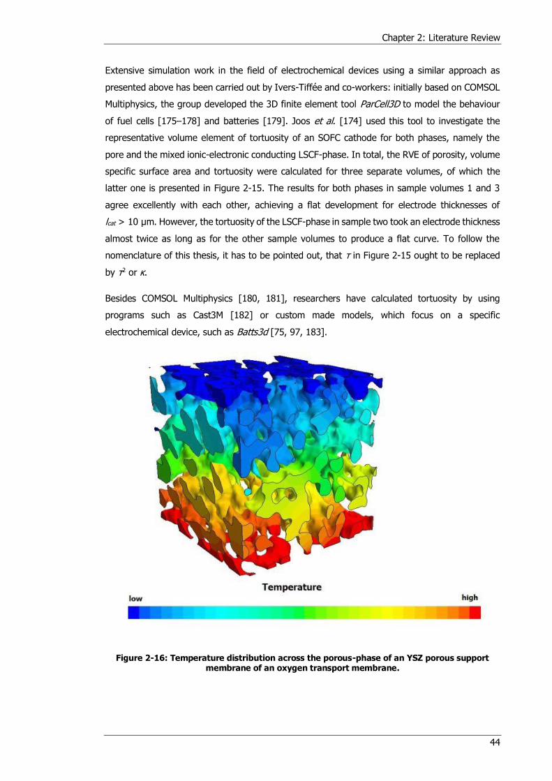
Chapter 2: Literature Review
44
Extensive simulation work in the field of electrochemical devices using a similar approach as
presented above has been carried out by Ivers-Tiffée and co-workers: initially based on COMSOL
Multiphysics, the group developed the 3D finite element tool ParCell3D to model the behaviour
of fuel cells [175–178] and batteries [179]. Joos et al. [174] used this tool to investigate the
representative volume element of tortuosity of an SOFC cathode for both phases, namely the
pore and the mixed ionic-electronic conducting LSCF-phase. In total, the RVE of porosity, volume
specific surface area and tortuosity were calculated for three separate volumes, of which the
latter one is presented in Figure 2-15. The results for both phases in sample volumes 1 and 3
agree excellently with each other, achieving a flat development for electrode thicknesses of
lcat > 10 μm. However, the tortuosity of the LSCF-phase in sample two took an electrode thickness
almost twice as long as for the other sample volumes to produce a flat curve. To follow the
nomenclature of this thesis, it has to be pointed out, that τ in Figure 2-15 ought to be replaced
by τ2 or κ.
Besides COMSOL Multiphysics [180, 181], researchers have calculated tortuosity by using
programs such as Cast3M [182] or custom made models, which focus on a specific
electrochemical device, such as Batts3d [75, 97, 183].
Figure 2-16: Temperature distribution across the porous-phase of an YSZ porous support membrane of an oxygen transport membrane.
Chapter 2: Literature Review
45
In addition to simulating mass and charge transport, the tortuosity is also computable by
exploiting the mathematical similarity between Fourier’s law of heat conduction and Fick’s law of
diffusion shown [132, 138, 184, 185]. By comparing the heat flux through the porous structure
to the heat flux of a dense volume of equal dimensions, the tortuosity is achieved. More details
on this method is presented in section 3.5.1. Cooper et al. [104] scanned a commercially available
LiFePO4 battery cathode using X-ray synchrotron nano CT and investigated the tortuosity of the
pore-phase using heat flux simulation. A cube of 8.8 μm side length was cropped and meshed
using an adaptive polyhedral volume mesh. The heat flux across the porous-phase of the sample
was simulated in StarCCM+ (CD-adapco) resulting in a temperature distribution across the
analysed volume (see Figure 2-16), where the temperature of each mesh element can be
understood as a concentration value of a migrating species.
It is common practise to subdivide a given sample volume into an array of smaller sub-samples
and extract the tortuosity for each individually [92, 174, 186]. Although non-trivial, this approach
allows researchers to extract similar results as tortuosity histograms and tortuosity distribution
maps (cf. section 2.2.4.1) using flux-based methods. This approach reveals the homogeneity or
heterogeneity of a sample, comparable to tortuosity histograms, and pinpoints the locations of
high or low tortuosity. Kehrwald et al. [92] were among the first ones to apply this methodology
on a battery electrode by solving Fick’s law using the program Star-CD (CD-adapco) on a total of
twelve sub-volumes. Local tortuosities showed differences of a factor of three, which might lead
to inefficiencies during charging and discharging of the battery: Li+ ions will avoid areas with
higher tortuosity, but seek areas with low tortuosity, highlighting the need of homogeneous
microstructures in this field to prevent spatial distribution of performance and degradation [186].
In addition, microstructural inhomogeneities might be the cause of failure mechanisms and
material fractures [92].
2.2.4.3 Comparison of Image-based Methods
Table 2-6 through Table 2-10 list pore-phase tortuosity factors and tortuosity values for different
image-based calculation methods along all three axes of the porous samples. Calculation
approaches which take flux-like behaviour into account (cf. Table 2-6 through Table 2-8) arrive
at higher values compared to geometric-based algorithms (cf. Table 2-9 and Table 2-10). It is
thus imperative to distinguish between these two approaches to avoid misinterpretation.
Furthermore, differences in tortuosity values are observed even when analysing the same type
of samples. This can be explained by the chosen imaging resolution; higher resolution uncovers
smaller pore structures and improves pore connectivity. This way, lower tortuosity values are
obtained [138]. Moreover, the size of the sample volume has to be sufficiently large so that
extracted values are representative of the sample bulk [187] (see section 2.4). Hence, the higher
the resolution, and the larger the extracted volume, the more likely the extracted values are
accurate, representative, and not affected by microscopic heterogeneities.
Chapter 2: Literature Review
46
When comparing the work by Wilson et al. [133] and Iwai et al. [134], who analysed the same
type of sample using the same imaging technique achieving similar pixel sizes, no difference in
tortuosities is observed even though Iwai et al. reconstructed a nine times larger sample volume.
Similar findings are revealed when comparing Laurencin et al. [182] and Tjaden et al. [132]. Yet,
this does not contradict the previous statement as homogeneous samples will yield representative
values even for small sample volumes. Also, analysing the same sample type does not necessarily
mean that these are structurally similar.
In addition, the above comparison revealed that different flux-based tortuosity calculation
algorithms yield comparable results, which was also affirmed when executing different algorithms
on the exact same sample [134, 169]. This suggests that the choice of a flux-based computation
algorithm has a smaller effect on the results than sample preparation technique, imaging
parameters and the structure of the sample itself, which includes pore size distribution and
volume fractions of the constituent phases. The interplay between these additional parameters
and the tortuosity is visible when inspecting the work by Wilson et al. [133] and Izzo et al. [137]:
while Izzo et al. presented higher tortuosity values, the porosity of their sample was a factor of
1.5 higher. Hence, the tortuosity itself does not give a full picture of the microstructure and the
performance of the analysed sample, but has to be evaluated with respect to other microstructural
characteristics [42, 148]. Also, care must be taken when applying purely continuum-based models
which do not account for Knudsen diffusion effects, such as the heat flux simulation. Such
simplifications might cause visible differences between experimental and simulation-based results
[132].
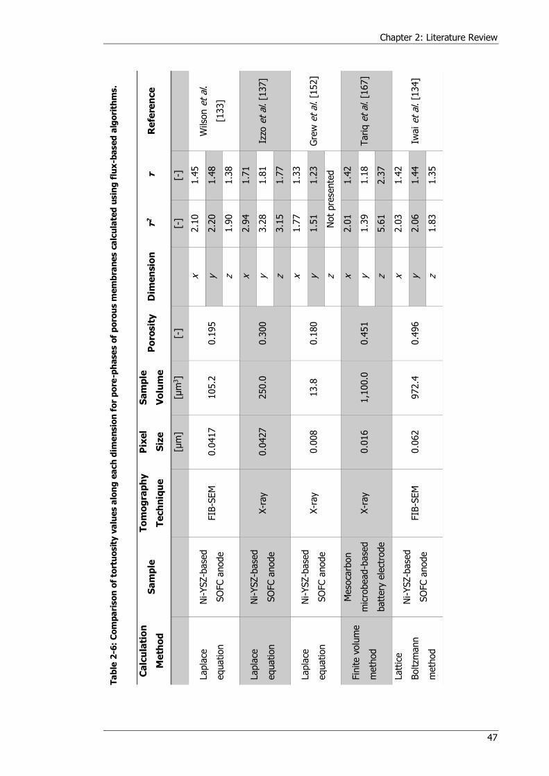
Chapter 2: Literature Review
47
Ta
ble
2-6
: C
om
pa
riso
n o
f to
rtu
osit
y v
alu
es a
lon
g e
ach
dim
en
sio
n f
or
po
re-p
hase
s o
f p
oro
us m
em
bra
nes c
alc
ula
ted
usin
g f
lux
-based
alg
ori
thm
s.
Ca
lcu
lati
on
Me
tho
d
Sa
mp
le
To
mo
gra
ph
y
Te
ch
niq
ue
Pix
el
Siz
e
Sa
mp
le
Vo
lum
e
Po
rosit
y
Dim
en
sio
n
τ2
τ
Re
fere
nce
[μ
m]
[μm
3]
[-]
[-
] [-
]
Lapla
ce
equation
Ni-YSZ-b
ase
d
SO
FC a
node
FIB
-SEM
0.0
417
105.2
0.1
95
x 2.1
0
1.4
5
Wils
on e
t al
.
[133]
y 2.2
0
1.4
8
z 1.9
0
1.3
8
Lapla
ce
equation
Ni-YSZ-b
ase
d
SO
FC a
node
X-r
ay
0.0
427
250.0
0.3
00
x 2.9
4
1.7
1
Izzo
et
al. [1
37]
y 3.2
8
1.8
1
z 3.1
5
1.7
7
Lapla
ce
equation
Ni-YSZ-b
ase
d
SO
FC a
node
X-r
ay
0.0
08
13.8
0.1
80
x 1.7
7
1.3
3
Gre
w e
t al. [
152]
y 1.5
1
1.2
3
z N
ot
pre
sente
d
Fin
ite v
olu
me
meth
od
Meso
carb
on
mic
robead-b
ase
d
batt
ery
ele
ctro
de
X-r
ay
0.0
16
1,1
00.0
0.4
51
x 2.0
1
1.4
2
Tariq e
t al
. [1
67]
y 1.3
9
1.1
8
z 5.6
1
2.3
7
Latt
ice
Boltzm
ann
meth
od
Ni-YSZ-b
ase
d
SO
FC a
node
FIB
-SEM
0.0
62
972.4
0.4
96
x 2.0
3
1.4
2
Iwai et
al. [1
34]
y 2.0
6
1.4
4
z 1.8
3
1.3
5
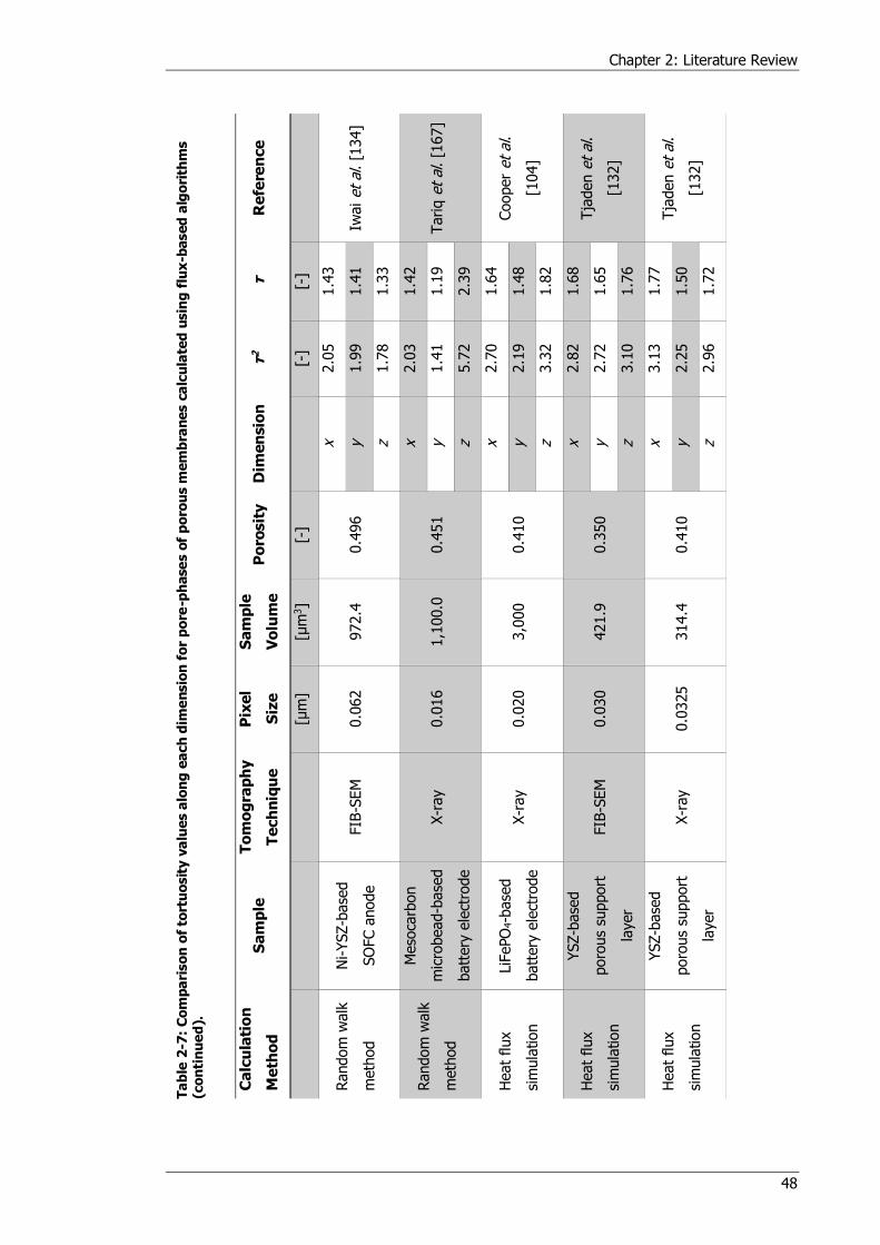
Chapter 2: Literature Review
48
T
ab
le 2
-7:
Co
mp
ari
so
n o
f to
rtu
osit
y v
alu
es a
lon
g e
ach
dim
en
sio
n f
or
po
re-p
hase
s o
f p
oro
us m
em
bra
nes c
alc
ula
ted
usin
g f
lux
-based
alg
ori
thm
s
(co
nti
nu
ed
).
Ca
lcu
lati
on
Me
tho
d
Sa
mp
le
To
mo
gra
ph
y
Te
ch
niq
ue
Pix
el
Siz
e
Sa
mp
le
Vo
lum
e
Po
rosit
y
Dim
en
sio
n
τ2
τ
Re
fere
nce
[μ
m]
[μm
3]
[-]
[-
] [-
]
Random
walk
meth
od
Ni-YSZ-b
ase
d
SO
FC a
node
FIB
-SEM
0.0
62
972.4
0.4
96
x 2.0
5
1.4
3
Iwai et
al. [1
34]
y 1.9
9
1.4
1
z 1.7
8
1.3
3
Random
walk
meth
od
Meso
carb
on
mic
robead-b
ase
d
batt
ery
ele
ctro
de
X-r
ay
0.0
16
1,1
00.0
0.4
51
x 2.0
3
1.4
2
Tariq e
t al
. [1
67]
y 1.4
1
1.1
9
z 5.7
2
2.3
9
Heat
flux
sim
ula
tion
LiF
ePO
4-b
ase
d
batt
ery
ele
ctro
de
X-r
ay
0.0
20
3,0
00
0.4
10
x 2.7
0
1.6
4
Cooper
et
al.
[104]
y 2.1
9
1.4
8
z 3.3
2
1.8
2
Heat
flux
sim
ula
tion
YSZ-b
ase
d
poro
us
support
layer
FIB
-SEM
0.0
30
421.9
0.3
50
x 2.8
2
1.6
8
Tja
den e
t al
.
[132]
y 2.7
2
1.6
5
z 3.1
0
1.7
6
Heat
flux
sim
ula
tion
YSZ-b
ase
d
poro
us
support
layer
X-r
ay
0.0
325
314.4
0.4
10
x 3.1
3
1.7
7
Tja
den e
t al
.
[132]
y 2.2
5
1.5
0
z 2.9
6
1.7
2
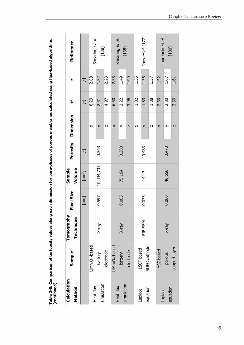
Chapter 2: Literature Review
49
T
ab
le 2
-8:
Co
mp
ari
so
n o
f to
rtu
osit
y v
alu
es a
lon
g e
ach
dim
en
sio
n f
or
po
re-p
hase
s o
f p
oro
us m
em
bra
nes c
alc
ula
ted
usin
g f
lux
-based
alg
ori
thm
s
(co
nti
nu
ed
).
Ca
lcu
lati
on
Me
tho
d
Sa
mp
le
To
mo
gra
ph
y
Te
ch
niq
ue
Pix
el
Siz
e
Sa
mp
le
Vo
lum
e
Po
rosit
y
Dim
en
sio
n
τ2
τ
Re
fere
nce
[μ
m]
[μm
3]
[-]
[-
] [-
]
Heat
flux
sim
ula
tion
LiM
n2O
4-b
ase
d
batt
ery
ele
ctro
de
X-r
ay
0.5
97
10,4
34,7
31
0.3
63
x
8.2
9
2.8
8
Shearing e
t al.
[138]
y
2.3
1
1.5
2
z 4.9
7
2.2
3
Heat
flux
sim
ula
tion
LiM
n2O
4-b
ase
d
batt
ery
ele
ctro
de
X-r
ay
0.0
65
75,1
64
0.3
80
x
6.5
0
2.5
5
Shearing e
t al.
[138]
y
2.2
2
1.4
9
z 3.9
6
1.9
9
Lapla
ce
equation
LSCF-b
ase
d
SO
FC c
ath
ode
FIB
-SEM
0.0
35
144.7
0.4
83
x
1.8
2
1.3
5
Joos
et
al. [1
77]
y
1.8
3
1.3
5
z 1.8
8
1.3
7
Lapla
ce
equation
YSZ-b
ase
d
poro
us
support
layer
X-r
ay
0.0
60
46,6
56
0.4
70
x
2.3
0
1.5
2
Laure
nci
n e
t al.
[180]
y
2.8
0
1.6
7
z 2.6
0
1.6
1
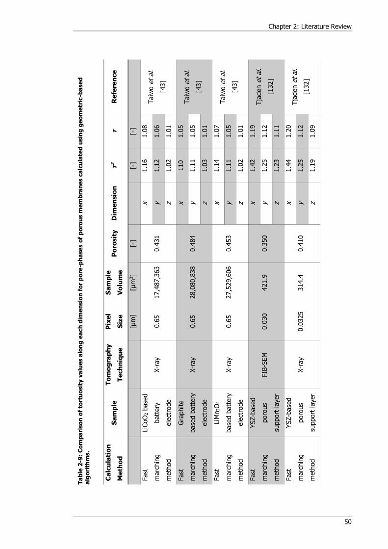
Chapter 2: Literature Review
50
T
ab
le 2
-9:
Co
mp
ari
so
n o
f to
rtu
osit
y v
alu
es a
lon
g e
ach
dim
en
sio
n f
or
po
re-p
hase
s o
f p
oro
us m
em
bra
nes c
alc
ula
ted
usin
g g
eo
me
tric
-base
d
alg
ori
thm
s.
Ca
lcu
lati
on
Me
tho
d
Sa
mp
le
To
mo
gra
ph
y
Te
ch
niq
ue
Pix
el
Siz
e
Sa
mp
le
Vo
lum
e
Po
rosit
y
Dim
en
sio
n
τ2
τ
Re
fere
nce
[μ
m]
[μm
3]
[-]
[-
] [-
]
Fast
marc
hin
g
meth
od
LiC
oO
2 b
ase
d
batt
ery
ele
ctro
de
X-r
ay
0.6
5
17,4
87,3
63
0.4
31
x 1.1
6
1.0
8
Taiw
o e
t al.
[43]
y 1.1
2
1.0
6
z 1.0
2
1.0
1
Fast
marc
hin
g
meth
od
Gra
phite
base
d b
att
ery
ele
ctro
de
X-r
ay
0.6
5
28,0
80,8
38
0.4
84
x 110
1.0
5
Taiw
o e
t al.
[43]
y 1.1
1
1.0
5
z 1.0
3
1.0
1
Fast
marc
hin
g
meth
od
LiM
n2O
4
base
d b
att
ery
ele
ctro
de
X-r
ay
0.6
5
27,5
29,6
06
0.4
53
x 1.1
4
1.0
7
Taiw
o e
t al.
[43]
y 1.1
1
1.0
5
z 1.0
2
1.0
1
Fast
marc
hin
g
meth
od
YSZ-b
ase
d
poro
us
support
layer
FIB
-SEM
0.0
30
421.9
0.3
50
x 1.4
2
1.1
9
Tja
den e
t al
.
[132]
y 1.2
5
1.1
2
z 1.2
3
1.1
1
Fast
marc
hin
g
meth
od
YSZ-b
ase
d
poro
us
support
layer
X-r
ay
0.0
325
314.4
0.4
10
x 1.4
4
1.2
0
Tja
den e
t al
.
[132]
y 1.2
5
1.1
2
z 1.1
9
1.0
9

Chapter 2: Literature Review
51
Ta
ble
2-1
0:
Co
mp
ari
so
n o
f to
rtu
osit
y v
alu
es a
lon
g e
ach
dim
en
sio
n f
or
po
re-p
hase
s o
f p
oro
us m
em
bra
nes c
alc
ula
ted
usin
g g
eo
me
tric
-base
d
alg
ori
thm
s (
co
nti
nu
ed
).
Ca
lcu
lati
on
Me
tho
d
Sa
mp
le
To
mo
gra
ph
y
Te
ch
niq
ue
Pix
el
Siz
e
Sa
mp
le
Vo
lum
e
Po
rosit
y
Dim
en
sio
n
τ2
τ
Re
fere
nce
[μ
m]
[μm
3]
[-]
[-
] [-
]
Pore
Centr
oid
Meth
od
LiF
ePO
4-b
ase
d
batt
ery
ele
ctro
de
X-r
ay
0.0
20
3,0
00
0.4
10
x 1.4
6
1.2
1
Cooper
et
al.
[104]
y 1.4
1
1.1
9
z 1.5
8
1.2
6
Chapter 2: Literature Review
52
2.3 Gas Transport through Porous Media
Hitherto, this literature review discussed microstructural characteristics, especially tortuosity,
while their effect and influence on gas diffusion mechanisms have yet to be presented. In oxygen
transport membranes and other electrochemical devices alike, reactant gases have to diffuse
through the porous support to reach the dense membrane and participate in chemical reactions.
At the same time, product gases have to diffuse away from the dense layer, back into the gas
distribution channel. In either direction, the microstructure of the porous support layer acts as a
resistance to the gases. This behaviour is quantified by applying distinct gas diffusion models,
which have to be selected depending on the dominating diffusion regime [38, 39, 115]. The
following models are introduced in the subsequent sections:
1. Ordinary or continuum diffusion.
2. Free-molecule or Knudsen diffusion.
3. Viscous or convective flow.
4. Surface diffusion.
Even though these transport phenomena are subject to different driving forces and are affected
by gas composition, temperature and pressure in different ways, any kind of combination of these
transport mechanisms can occur at the same time. Hence, the final section of this chapter
analyses combined diffusion models used in literature.
2.3.1 Ordinary or Continuum Diffusion
Under ordinary or continuum diffusion regime, gas molecules move from an area of high
concentration to an area of low concentration. In [115], ordinary diffusion is described by the
migration of helium through silica plate. The plate is impermeable to air which is located on the
top side of the plate while the helium is placed below the plate. Due to its molecular motion and
molecule-molecule collisions, helium molecules traverse through the plate and mix with air on the
opposite side of the plate. After some time, the concentration profile of helium within the silica
plate will tend towards a straight line between the steady-state helium concentrations on either
surface of the plate. Adolf Fick first established a mathematical correlation to describe this
phenomenon, which shows similarities with Fourier’s law of heat conduction [188]:
𝐽𝑖,𝐷 = −𝐷𝑖𝑝
𝑅𝑇
𝑑𝑦𝑖𝑑𝑥
(2-17)
In which the following are defined:
Ji,D diffusion flux [molm-2s-1] Di diffusion coefficient [m2s-1] p pressure [bar]
Chapter 2: Literature Review
53
R ideal gas constant [Jmol-1K-1] T temperature [K] yi molar fraction of species i [-] x dimension [m]
Equation (2-17) is also known as Fick’s first law of diffusion and relates the diffusion flux to the
concentration gradient of a species. The negative sign on the right side of equation (2-17) signifies,
that the gas diffuses “down” the gradient as long as the diffusion coefficient is positive [38]. This
sign convention is valid for all diffusion mechanisms introduced in the following sections.
Here, the diffusion coefficient Di (also known as diffusivity) is applied as a proportionality factor
similar to the thermal conductivity in Fourier’s law of heat conduction. The same correlation is
applied in a binary mixture in which the diffusive fluxes of either species are defined using the
following equations. In this case, the diffusion coefficient Di is replaced by the binary diffusion
coefficients Dij and Dji.
𝐽𝑖,𝐷 = −𝐷𝑖𝑗𝑝
𝑅𝑇
𝑑𝑦𝑖𝑑𝑥
(2-18)
𝐽𝑗,𝐷 = −𝐷𝑗𝑖𝑝
𝑅𝑇
𝑑𝑦𝑖𝑑𝑥
(2-19)
In which species i diffuses in one direction and species j diffuses in the opposite direction, Dij
equals Dji [38, 115] Thus, the sum of the diffusion fluxes Ji + Jj = J amounts to zero. Yet, if
molecular weights of the two, inter-diffusing species differ, a shift in the centre of mass in the
direction of the heavier species is observed. Mason and Malinauskas [38] described this process
using two communicating vessels separated by a porous plate. One vessel is filled with a light
and the other one with a heavy gas. Due to faster molecular motion, the lighter gas will migrate
into the heavier gas vessel quicker which moves the centre of mass towards the heavier gas
vessel. As a result, the pressure will rise in the heavier gas vessel leading to a viscous flow from
the heavier gas vessel towards the lighter gas vessel. Under steady-state, ordinary diffusion
combined with viscous flow make the net flux zero. However, this kind of experimental setup is
not described by laws of pure ordinary diffusion as in equation (2-17) due to the viscous flux
contribution. Consequently, for equalizing pressure in both vessels, the porous plate is replaced
by a movable piston. Due to the pressure difference in both vessels, the piston is moved by the
resulting force which equalises the pressure in both vessels. This way, no viscous flux is observed,
but at the same time, the overall net flux is not zero.
The binary diffusion coefficient used in the above equations is the centrepiece of the ordinary
diffusion theory. To calculate the binary diffusion coefficient Dij, the Chapman-Enskog correlation
is widely applied [115, 189]:
Chapter 2: Literature Review
54
𝐷𝑖𝑗 = −𝐷𝑗𝑖 = 0.0018583√𝑇3 (1
𝑀𝑖
+1
𝑀𝑗)
1
𝑝 𝜎𝑖𝑗2 𝛺𝐷,𝑖𝑗
(2-20)
In which the following are defined:
Dij, Dji binary diffusion coefficient [cm2s-1] T temperature [K] Mi, Mj molar mass [gmol-1] p pressure [bar] σij characteristic diameter of a gas pair [Å] ΩD,ij collision integral [-]
Here, the collision integral ΩD,ij is a function of 𝜅𝑇
𝑖𝑗 in which εij refers to the maximum energy of
attraction between two molecules in Joule and κ refers to the Boltzmann constant. Both, σij and
εij, are stemming from the Lennard-Jones Potential and are used to determine the collision integral
which can be extracted from tables [115].
However, the binary diffusion coefficient calculated in equation (2-20) is not applicable within a
porous membrane as the geometry of the membrane resulting in tortuous and irregularly shaped
migration pathways are not accounted for. As mentioned earlier in the literature review, the
microstructure of a porous layer poses as a resistance to a flux. In diffusion theory, this is
accounted for by reducing the diffusion coefficient according to the membrane’s microstructural
characteristics. The porosity and tortuosity of the porous structure are applied as reduction factors
to calculate effective diffusion coefficient (Dij,eff) as shown in equation (2-21) (cf. section 2.2.1)
[38, 190, 191].
𝐷𝑖𝑗,𝑒𝑓𝑓 =휀
𝜏2𝐷𝑖𝑗 (2-21)
In which the following are defined:
Dij,eff effective binary diffusion coefficient [cm2s-1] Dij binary diffusion coefficient [cm2s-1] ε porosity [-] τ tortuosity [-]
Fick’s law is only applicable provided, that the mean free path of the gas particles is smaller than
the pores. The mean free path describes the path length, a gas molecule travels before it collides
with another gas molecule. In such a case, molecule to molecule collisions dominate while
molecule to wall collisions can be neglected. If, however, the opposite is the case, Knudsen
diffusion is dominating.
Chapter 2: Literature Review
55
2.3.2 Free-molecule or Knudsen Flow
Under free-molecule or Knudsen flow regime, the pore diameter of the porous medium is small
compared to the mean free path of the gas molecules. Consequently, gas molecules collide with
the solid-phase of a membrane more frequently than with another molecule. Hence, in a gas
mixture under Knudsen flow regime, molecules of different species diffuse independently of each
other [38]. Using equation (2-22), the mean free path of a molecule between successive collisions
with another molecule is calculated and can be compared to the pore diameter [115].
𝜆 =1
√2𝜋𝑑𝑚2 𝑐
(2-22)
In which the following are defined:
λ mean free path [mmol-1] dm diameter of molecule [m] c molar concentration [molm-3]
If the criterions for Knudsen diffusion are met, the following set of equations are applied to
calculate the Knudsen flux. First, the molar average velocity �� of the gas has to be calculated
using equation (2-23) [115]. Then, the Knudsen diffusion coefficient, which is a function of the
molar average velocity and the Knudsen flow parameter, is determined. The Knudsen flow
parameter KO accounts for the geometry of the porous structure. In [39, 40], KO amounts to
2
3 𝑟𝑃 𝜏2 for long, straight, cylindrical shaped pores, in which rP is defined as the mean pore
diameter in metres. Together with the molar average velocity, the Knudsen flow parameter
considers the probability of a molecule to hit the wall and to be reflected to the entrance of the
pore before the molecule manages to diffuse through the pore completely. Equation (2-24) shows
the combination of �� and KO to express the Knudsen diffusion coefficient Di,Kn. Finally, the
Knudsen diffusion flux is achieved, analogue to Fick’s law in equation (2-17), by multiplying Di,Kn
with the concentration gradient of the gaseous species across the porous membrane, as shown
in equation (2-25).
�� = √8𝑅𝑇
𝜋𝑀 (2-23)
𝐷𝑖,𝐾 = −𝐾𝑂��𝑖 (2-24)
𝐽𝑖,𝐾𝑛 = −𝐷𝑖,𝐾𝑝
𝑅𝑇
𝑑𝑦𝑖𝑑𝑥
(2-25)
In which the following are defined:
�� molar average velocity [ms-1]
Chapter 2: Literature Review
56
R ideal gas constant [Jmol-1K-1] T temperature [K] Mi molar mass [gmol-1] Di,K Knudsen diffusion coefficient of species i [m2/s-1]
KO Knudsen flow parameter [m] Ji,K Knudsen flux [molm-2s-1] R ideal gas constant [Jmol-1K-1] T temperature [K] yi molar fraction of species i [-] x dimension [m]
2.3.3 Viscous or Convective Flow
Viscous or convective flow is induced by a bulk pressure gradient exerted on a gas. The resulting
gas flow rate is linearly dependent on the pressure gradient. Under viscous flow regime, molecule-
molecule collisions dominate, as is the case with ordinary diffusion mentioned previously.
𝐽𝑣𝑖𝑠𝑐 = −𝑐𝐵𝑂𝜇 𝑑𝑝
𝑑𝑥 (2-26)
In which the following are defined:
Jvisc viscous flux [molm-2s-1] c molar concentration [molm-3] BO viscous flow parameter [m²] µ dynamic viscosity [kgm-1s-1] p pressure [Pa] x dimension [m]
Viscous flow is described by Darcy’s law (see equation (2-26)), where, similar to Knudsen flow,
the viscous flow parameter BO accounts for the geometry of the pore. For a cylindrical pore of
mean pore radius rP, BO amounts to 𝑟𝑃2
8∗𝜏2
[39, 40]. However, in contrast to Knudsen diffusion, a
gas mixture behaves as a single gas as no separation of species is induced under the viscous flux
regime. As a result, the viscous flow of a specific species in a gas mixture is proportional to the
mole fraction in the mixture:
𝐽𝑖,𝑣𝑖𝑠𝑐 = 𝑦𝑖𝐽𝑣𝑖𝑠𝑐 (2-27)
In which the following are defined:
Ji,visc viscous flux of species i [molm-2s-1] yi mole fraction of species i [-] Jvisc viscous flux [molm-2s-1]
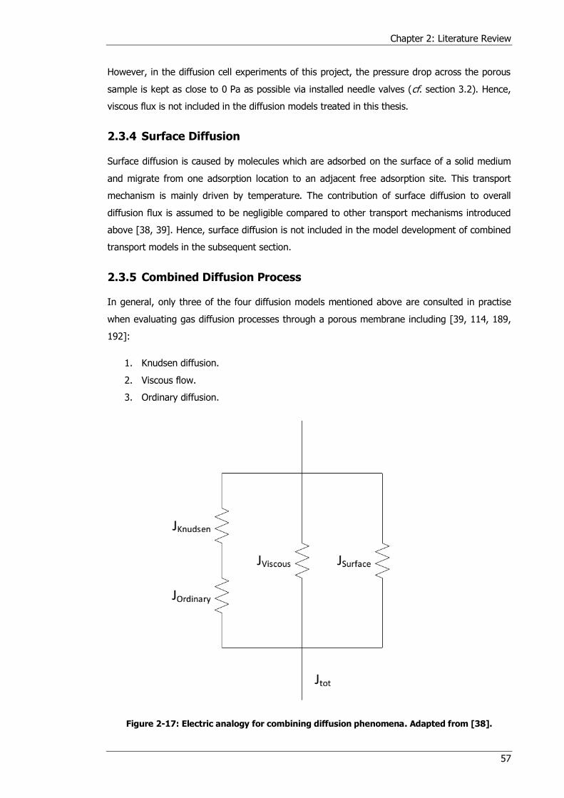
Chapter 2: Literature Review
57
However, in the diffusion cell experiments of this project, the pressure drop across the porous
sample is kept as close to 0 Pa as possible via installed needle valves (cf. section 3.2). Hence,
viscous flux is not included in the diffusion models treated in this thesis.
2.3.4 Surface Diffusion
Surface diffusion is caused by molecules which are adsorbed on the surface of a solid medium
and migrate from one adsorption location to an adjacent free adsorption site. This transport
mechanism is mainly driven by temperature. The contribution of surface diffusion to overall
diffusion flux is assumed to be negligible compared to other transport mechanisms introduced
above [38, 39]. Hence, surface diffusion is not included in the model development of combined
transport models in the subsequent section.
2.3.5 Combined Diffusion Process
In general, only three of the four diffusion models mentioned above are consulted in practise
when evaluating gas diffusion processes through a porous membrane including [39, 114, 189,
192]:
1. Knudsen diffusion.
2. Viscous flow.
3. Ordinary diffusion.
Figure 2-17: Electric analogy for combining diffusion phenomena. Adapted from [38].
Chapter 2: Literature Review
58
In [38], an electric analogy is used to describe the combination of these different transport
phenomena: diffusive fluxes (free and ordinary flow) are in series in one branch and in parallel
to viscous and surface flow, respectively. The total diffusive flux is then the sum of the parallel
diffusive fluxes. Figure 2-17 illustrates this electric analogy.
The previous sections outlined that the Knudsen and ordinary diffusion are driven by a
concentration gradient. However, both fluxes are to a certain extent mutually exclusive due to
their dependence on the mean pore diameter dp and mean free path λ. Hence, the contribution
of either of these two diffusion processes is evaluated by calculating the Knudsen number (Kn),
which is the mean free path of the gas molecules calculated in equation (2-22) divided by the
mean pore diameter of the porous medium [39, 192, 193]:
If Kn > 10, Knudsen flux dominates while ordinary diffusion is negligible.
If Kn < 0.1, ordinary diffusion dominates while Knudsen flux is negligible.
If 0.1 < Kn < 10, both diffusion processes are of equal importance and have to be
accounted.
In the transition region of 0.1 < Kn < 10, ordinary and Knudsen diffusion have to be considered
at the same time. In a binary system, where this is the case, the Knudsen diffusion coefficient
and the binary diffusion coefficient of a species i are hence combined to the effective diffusion
coefficient using the Bosanquet formula [39, 191, 194]. The effective diffusion coefficient 𝐷𝑖𝑒𝑓𝑓
is
then inserted into Fick’s law to establish the Fick model (FM). Both expressions are illustrated in
equations (2-28) and (2-29).
𝐷𝑖,𝑒𝑓𝑓 = (1
휀𝜏2𝐷𝑖𝑗
+1
휀𝜏2𝐷𝑖,𝐾
)
−1
(2-28)
𝐽𝑖,𝐷 = −𝐷𝑖,𝑒𝑓𝑓𝑝
𝑅𝑇
𝑑𝑦𝑖𝑑𝑥
=−𝐷𝑖,𝑒𝑓𝑓𝑅𝑇
𝑑𝑝𝑖𝑑𝑥
(2-29)
In which the following are defined:
Di,eff effective diffusion coefficient of species i [m2s-1] ε porosity [-] τ tortuosity [-] Dij binary diffusion coefficient [m2s-1] Di,K Knudsen diffusion coefficient of species i [m2s-1] Ji,D diffusion flux [mol/(m2∙s)] yi molar fraction of species i [-] x dimension [m] R ideal gas constant [Jmol-1K-1] T temperature [K] pi partial pressure of species I [Pa]
Chapter 2: Literature Review
59
If a pressure gradient adds a viscous flux to an otherwise concentration driven diffusion flux, the
Fick model can be extended by the according expression [189]:
𝐽𝑖,𝐷 = −1
𝑅𝑇 (𝐷𝑖,𝑒𝑓𝑓
𝑑𝑝𝑖𝑑𝑥
+𝐵𝑂𝑐𝑖𝜇
𝑑𝑝
𝑑𝑥) (2-30)
In which the following are defined:
Ji,D diffusion flux [molm-2s-1] Di,eff effective diffusion coefficient of species i [m2s-1] R ideal gas constant [Jmol-1K-1] T temperature [K] pi partial pressure [Pa] BO viscous flow parameter [m2] p pressure [Pa] µ dynamic viscosity [kgm-1s-1] x dimension [m]
This extended Fick model is also referred to as advective diffusive model and linearly combines
Fick’s and Darcy’s law for ordinary diffusion and viscous flow, respectively [50, 114, 189, 192].
Another diffusion model which includes diffusive as well as convective transport is the dusty gas
model (DGM) [38]. The name of the DGM is derived by its main assumption: the porous-phase
of a membrane, through which gases diffuse, is modelled as dust particles in the gas mixture.
These dust particles are motionless which is realised through a mechanical mounting holding the
porous membrane. Equation (2-31) shows the DGM, which is based on the principles of the
different diffusion mechanisms introduced in the previous sections [38].
𝐽𝑖,𝐷𝐷𝑖,𝐾𝑛
+ ∑𝑦𝑗𝐽𝑖,𝐷 − 𝑦𝑖𝐽𝑗,𝐷
𝐷𝑖𝑗,𝑒𝑓𝑓
𝑛
𝑗=1,𝑗≠𝑖
= −𝑝
𝑅𝑇
𝑑𝑦𝑖𝑑𝑥
+𝑦𝑖𝑅𝑇
𝑑𝑝
𝑑𝑥(1 +
𝐵𝑂𝑝
𝜇𝐷𝑖,𝐾𝑛) (2-31)
In which the following are defined:
Ji,D, Jj,D diffusion flux of species i and j [molm-2s-1] Di,Kn Knudsen diffusion coefficient of species i [m2s-1] yi, yj molar fraction of species i and j [-] Dij,eff effective binary diffusion coefficient [m2s-1] R ideal gas constant [Jmol-1K-1)] T temperature [K] p pressure [Pa] x dimension [m] BO viscous flow parameter [m2] µ dynamic viscosity [kgm-1s-1]
The sum in the second term on the left hand side of equation (2-31) is applied to account for a
multicomponent gas mixture. This expression only includes the ordinary diffusion coefficient as
Chapter 2: Literature Review
60
the Knudsen flux the individual gas species migrate independently. The Maxwell-Stefan model
(MSM) uses a similar correlation to account for a multicomponent gas mixture as presented in
the DGM, but neglects Knudsen diffusion. As a result, coefficients related to Knudsen diffusion
drop out of equation (2-31) and result in the following formulation:
∑𝑦 𝐽𝑖,𝐷 − 𝑦𝑖 𝐽𝑗,𝐷
𝐷𝑖𝑗,𝑒𝑓𝑓
𝑛
𝑗=1,𝑗≠𝑖
= −𝑝
𝑅𝑇
𝑑𝑦𝑖𝑑𝑥
(2-32)
The nomenclature in equation (2-32) coincides with equation (2-31). It is visible that complexity
and thus, calculation methods, differ greatly between the above models. As a consequence, the
appropriate model has to be chosen for each individual case. The accuracy of these models has
been discussed [193] and evaluated in literature, predominantly by comparing them to measured
concentration polarisation losses in SOFC anodes [195, 196]: Suwanwarangkul et al. [195]
assessed the accuracy of these three transport models (FM, DGM and MSM) for binary CO-CO2
and H2-H2O as well as ternary H2-H2O-Ar gas mixtures within an SOFC anode. The focus was on
calculating concentration losses in the fuel cell caused by mass transport limitations via the
aforementioned diffusion models and comparing them to measured values. The authors
concluded that for both, binary and ternary gas mixtures, the dusty gas model is recommended
even though numerical solution for this approach is needed [195].
In general, high accuracy between the DGM and experimental results were achieved throughout
the literature, which might be one reason for its widespread use in the field of electrochemistry
[137, 196–199] while the simplicity but lower accuracy of the Fick model was frequently
highlighted.
In these cases, however, tortuosity is usually used as a fitting parameter to tailor calculation
results to measured data. Consequently, when applying diffusion models in reverse to calculate
the tortuosity, the extracted values are highly dependent on the accuracy of the applied model.
However, as authors have mainly aimed at calculating concentration polarisation losses of fuel
cells at high current densities, microstructural parameters, including tortuosity, were frequently
inserted into these models without prior investigation or sensitivity analysis [196–198, 200–202].
Even when combining diffusion cell experiments with the dusty gas model, results are not
completely predictive. One explanation for this is the membrane's morphology, where calculation
parameters, such as BO, KO, ε and τ, are not constant parameters, but rather change along the
diffusion pathways in each dimension [194] and as a function of participating gas mixtures [57].
However, it is only with tomography that such values can be verified and estimated more precisely
to then serve as accurate input parameters for diffusion models. As a result, tomographic
Chapter 2: Literature Review
61
techniques are coupled with diffusion cell experiments in this project to obtain a complete picture
of the effect of microstructural parameters in diffusion processes.
2.4 Tomography Techniques
The development and proliferation of tomography equipment and the associated image-based
modelling tools have provided, for the first time, the capacity to directly extract the geometry of
a sample as a 3D dataset and execute different computation algorithms and determine desired
parameters. In this respect, FIB-SEM tomography and X-ray CT have been mentioned previously
due to their wide application in the field of electrochemistry for microstructural characterisation.
As microstructural properties extend and vary in all three dimensions of a material [203], the aim
of applying such techniques is to reconstruct a three-dimensional volume of the examined sample
and extract geometrical characteristics such as porosity, tortuosity, mean pore diameter and
volumetric distribution of constituents. This allows us to evaluate the effect of different fabrication
methods and processing techniques as well as the effect of operating conditions on the
microstructure of the sample and the device performance.
Historically, the lack of detailed geometrical information regarding the complex microstructure of
porous media in 3D has limited the ability of researchers to extract meaningful data for these
parameters. In absence of this information, stereology has been used for estimating
microstructural characteristics based on features measured by 2D cross sections of the sample
[204]. Elaborate sample preparation and reconstruction techniques are not necessary for this
approach in comparison to tomography, which makes its application straightforward and
timesaving. Stereology provides a set of tools and mathematical correlations to extract 3D
characteristics of a structure based on a 2D image, where images from light as well as electron
microscopes serve as source.
The principle of stereology calculations is shown in Figure 2-18, whereby a 3D sample is sectioned
by a 2D plane. This 2D plane represents the extracted obtained 2D image and forms the basis
for stereological relationships by revealing features such as volumes, surfaces or grain boundaries
of phases present in the 3D sample. However, to avoid misinterpretation of 2D derived
parameters from a single image, a mean value of a set of measurements has to be taken to
estimate the sought-after value with higher accuracy. This sectioning process has to be isotropic,
uniform and random to calculate objective results [101]. Although stereology yields the advantage
of easy implementation compared to tomography techniques, severe errors are expected when
inhomogeneous and anisotropic samples are analysed [43, 204]. This is why stereology is
considered to feature limited means for this project and is thus only used for comparison purposes.
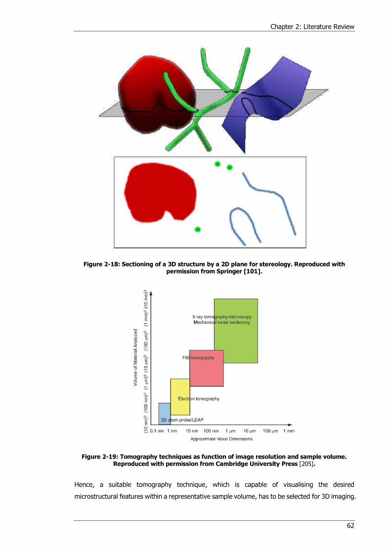
Chapter 2: Literature Review
62
Figure 2-18: Sectioning of a 3D structure by a 2D plane for stereology. Reproduced with permission from Springer [101].
Figure 2-19: Tomography techniques as function of image resolution and sample volume. Reproduced with permission from Cambridge University Press [205].
Hence, a suitable tomography technique, which is capable of visualising the desired
microstructural features within a representative sample volume, has to be selected for 3D imaging.

Chapter 2: Literature Review
63
Figure 2-19 shows the trade-off between voxel size and reconstructed volume: depending on
sample size and pixel/voxel dimensions needed for the analysis, a specific imaging technique is
appropriate. As a result, the chosen imaging technique applied in this project has to meet both
criteria, which is investigated below.
To quantify diffuse mass transport within the pore-phase of the sample, porous features of the
support layer have to be accurately reconstructed. In addition, tracking any structural changes
before, during and after experiments have to be identifiable. As first SEM images of the membrane
showed pores featuring a diameter of < 1 μm (see Figure 2-8), a resolution below this range is
necessary. More precisely, voxel dimensions have to be in the range of tens of nanometres to
analyse and distinguish structural features of that size.
Figure 2-20: Relationship between sample size and microstructural parameter. Reproduced with permission from John Wiley and Sons [187].
The dimensions of the extracted sample volume, however, must also be large enough, so that
extracted parameters are representative across the bulk structure. Here, the concept of the
representative volume element (RVE) is of vital importance to verify the quality of a reconstructed
specimen [187]. Figure 2-20 depicts the relationship between a microstructural parameter n and
the volume of the reconstructed sample L. When gradually increasing the volume while measuring
the same parameter simultaneously, random fluctuations are observed for small volumes (region
I). This behaviour flattens out until a plateau is reached, at which the measured parameter is
independent of the volume size of the sample (region II). However, if the sample volume is
further increased throughout region II, a region of macroscopic heterogeneity (region III) is
entered which, again affects the development of the extracted parameter as a function of
increasing sample volume. The area between region I and region III is referred to as the
RVE
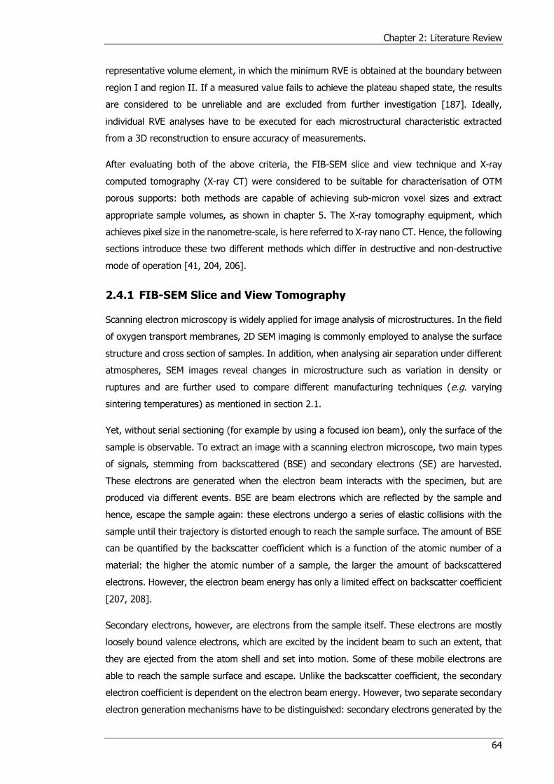
Chapter 2: Literature Review
64
representative volume element, in which the minimum RVE is obtained at the boundary between
region I and region II. If a measured value fails to achieve the plateau shaped state, the results
are considered to be unreliable and are excluded from further investigation [187]. Ideally,
individual RVE analyses have to be executed for each microstructural characteristic extracted
from a 3D reconstruction to ensure accuracy of measurements.
After evaluating both of the above criteria, the FIB-SEM slice and view technique and X-ray
computed tomography (X-ray CT) were considered to be suitable for characterisation of OTM
porous supports: both methods are capable of achieving sub-micron voxel sizes and extract
appropriate sample volumes, as shown in chapter 5. The X-ray tomography equipment, which
achieves pixel size in the nanometre-scale, is here referred to X-ray nano CT. Hence, the following
sections introduce these two different methods which differ in destructive and non-destructive
mode of operation [41, 204, 206].
2.4.1 FIB-SEM Slice and View Tomography
Scanning electron microscopy is widely applied for image analysis of microstructures. In the field
of oxygen transport membranes, 2D SEM imaging is commonly employed to analyse the surface
structure and cross section of samples. In addition, when analysing air separation under different
atmospheres, SEM images reveal changes in microstructure such as variation in density or
ruptures and are further used to compare different manufacturing techniques (e.g. varying
sintering temperatures) as mentioned in section 2.1.
Yet, without serial sectioning (for example by using a focused ion beam), only the surface of the
sample is observable. To extract an image with a scanning electron microscope, two main types
of signals, stemming from backscattered (BSE) and secondary electrons (SE) are harvested.
These electrons are generated when the electron beam interacts with the specimen, but are
produced via different events. BSE are beam electrons which are reflected by the sample and
hence, escape the sample again: these electrons undergo a series of elastic collisions with the
sample until their trajectory is distorted enough to reach the sample surface. The amount of BSE
can be quantified by the backscatter coefficient which is a function of the atomic number of a
material: the higher the atomic number of a sample, the larger the amount of backscattered
electrons. However, the electron beam energy has only a limited effect on backscatter coefficient
[207, 208].
Secondary electrons, however, are electrons from the sample itself. These electrons are mostly
loosely bound valence electrons, which are excited by the incident beam to such an extent, that
they are ejected from the atom shell and set into motion. Some of these mobile electrons are
able to reach the sample surface and escape. Unlike the backscatter coefficient, the secondary
electron coefficient is dependent on the electron beam energy. However, two separate secondary
electron generation mechanisms have to be distinguished: secondary electrons generated by the
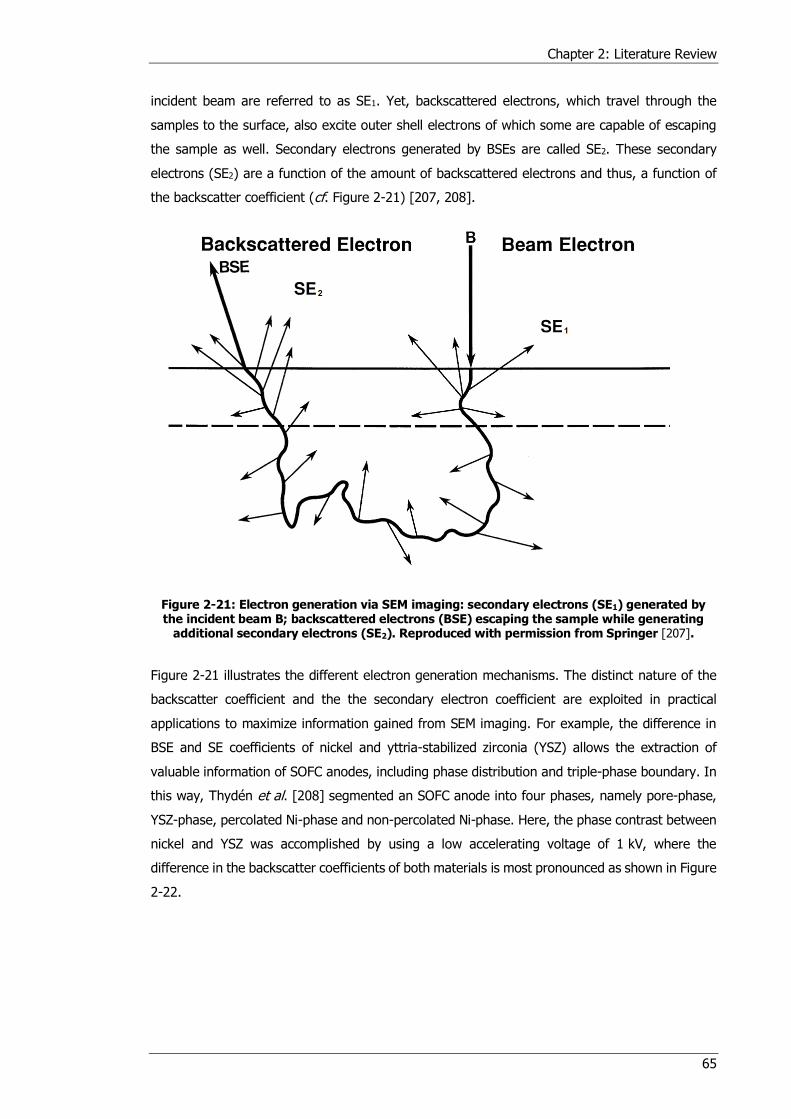
Chapter 2: Literature Review
65
incident beam are referred to as SE1. Yet, backscattered electrons, which travel through the
samples to the surface, also excite outer shell electrons of which some are capable of escaping
the sample as well. Secondary electrons generated by BSEs are called SE2. These secondary
electrons (SE2) are a function of the amount of backscattered electrons and thus, a function of
the backscatter coefficient (cf. Figure 2-21) [207, 208].
Figure 2-21: Electron generation via SEM imaging: secondary electrons (SE1) generated by the incident beam B; backscattered electrons (BSE) escaping the sample while generating
additional secondary electrons (SE2). Reproduced with permission from Springer [207].
Figure 2-21 illustrates the different electron generation mechanisms. The distinct nature of the
backscatter coefficient and the the secondary electron coefficient are exploited in practical
applications to maximize information gained from SEM imaging. For example, the difference in
BSE and SE coefficients of nickel and yttria-stabilized zirconia (YSZ) allows the extraction of
valuable information of SOFC anodes, including phase distribution and triple-phase boundary. In
this way, Thydén et al. [208] segmented an SOFC anode into four phases, namely pore-phase,
YSZ-phase, percolated Ni-phase and non-percolated Ni-phase. Here, the phase contrast between
nickel and YSZ was accomplished by using a low accelerating voltage of 1 kV, where the
difference in the backscatter coefficients of both materials is most pronounced as shown in Figure
2-22.
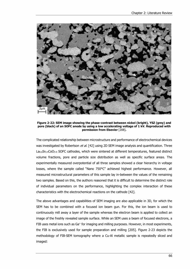
Chapter 2: Literature Review
66
Figure 2-22: SEM image showing the phase-contrast between nickel (bright), YSZ (grey) and pore (black) of an SOFC anode by using a low accelerating voltage of 1 kV. Reproduced with
permission from Elsevier [208].
The complicated relationship between microstructure and performance of electrochemical devices
was investigated by Robertson et al. [42] using 2D SEM image analysis and quantification. Three
La0.6Sr0.4CoO3-δ SOFC cathodes, which were sintered at different temperatures, featured distinct
volume fractions, pore and particle size distribution as well as specific surface areas. The
experimentally measured overpotential of all three samples showed a clear hierarchy in voltage
losses, where the sample called “Nano 750°C” achieved highest performance. However, all
measured microstructural parameters of this sample lay in-between the values of the remaining
two samples. Based on this, the authors reasoned that it is difficult to determine the distinct role
of individual parameters on the performance, highlighting the complex interaction of these
characteristics with the electrochemical reactions on the cathode [42].
The above advantages and capabilities of SEM imaging are also applicable in 3D, for which the
SEM has to be combined with a focused ion beam gun. For this, the ion beam is used to
continuously mill away a layer of the sample whereas the electron beam is applied to collect an
image of the freshly revealed sample surface. While an SEM uses a beam of focused electrons, a
FIB uses metal ions such as Ga+ for imaging and milling purposes. However, in most experiments,
the FIB is exclusively used for sample preparation and milling [205]. Figure 2-23 depicts the
methodology of FIB-SEM tomography where a Cu-Al metallic sample is repeatedly sliced and
imaged:
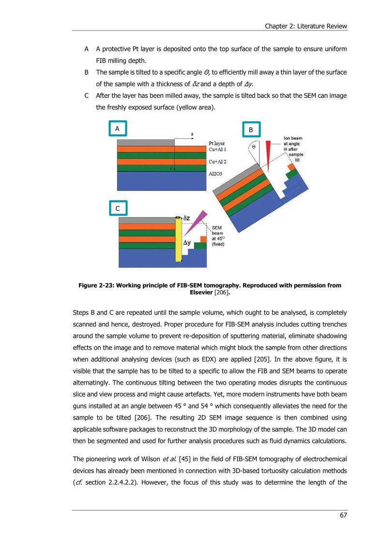
Chapter 2: Literature Review
67
A A protective Pt layer is deposited onto the top surface of the sample to ensure uniform
FIB milling depth.
B The sample is tilted to a specific angle Θ, to efficiently mill away a thin layer of the surface
of the sample with a thickness of δz and a depth of Δy.
C After the layer has been milled away, the sample is tilted back so that the SEM can image
the freshly exposed surface (yellow area).
Figure 2-23: Working principle of FIB-SEM tomography. Reproduced with permission from Elsevier [206].
Steps B and C are repeated until the sample volume, which ought to be analysed, is completely
scanned and hence, destroyed. Proper procedure for FIB-SEM analysis includes cutting trenches
around the sample volume to prevent re-deposition of sputtering material, eliminate shadowing
effects on the image and to remove material which might block the sample from other directions
when additional analysing devices (such as EDX) are applied [205]. In the above figure, it is
visible that the sample has to be tilted to a specific to allow the FIB and SEM beams to operate
alternatingly. The continuous tilting between the two operating modes disrupts the continuous
slice and view process and might cause artefacts. Yet, more modern instruments have both beam
guns installed at an angle between 45 ° and 54 ° which consequently alleviates the need for the
sample to be tilted [206]. The resulting 2D SEM image sequence is then combined using
applicable software packages to reconstruct the 3D morphology of the sample. The 3D model can
then be segmented and used for further analysis procedures such as fluid dynamics calculations.
The pioneering work of Wilson et al. [45] in the field of FIB-SEM tomography of electrochemical
devices has already been mentioned in connection with 3D-based tortuosity calculation methods
(cf. section 2.2.4.2.2). However, the focus of this study was to determine the length of the
A B
C
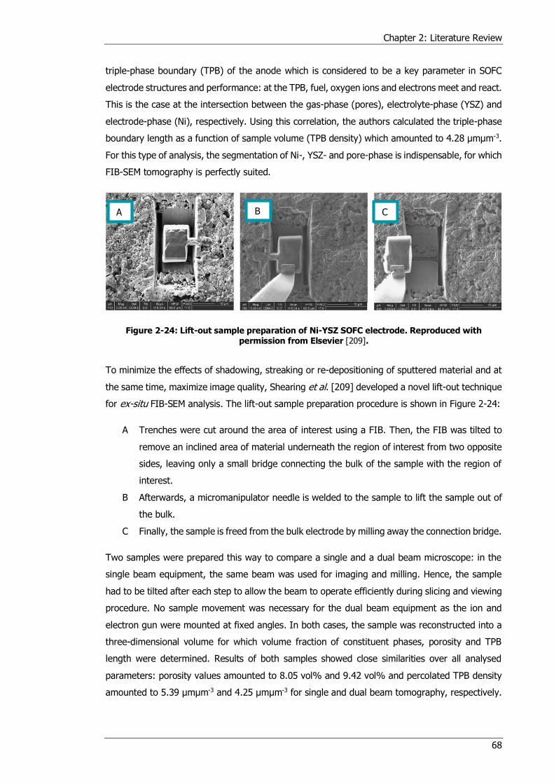
Chapter 2: Literature Review
68
triple-phase boundary (TPB) of the anode which is considered to be a key parameter in SOFC
electrode structures and performance: at the TPB, fuel, oxygen ions and electrons meet and react.
This is the case at the intersection between the gas-phase (pores), electrolyte-phase (YSZ) and
electrode-phase (Ni), respectively. Using this correlation, the authors calculated the triple-phase
boundary length as a function of sample volume (TPB density) which amounted to 4.28 μmμm-3.
For this type of analysis, the segmentation of Ni-, YSZ- and pore-phase is indispensable, for which
FIB-SEM tomography is perfectly suited.
Figure 2-24: Lift-out sample preparation of Ni-YSZ SOFC electrode. Reproduced with permission from Elsevier [209].
To minimize the effects of shadowing, streaking or re-depositioning of sputtered material and at
the same time, maximize image quality, Shearing et al. [209] developed a novel lift-out technique
for ex-situ FIB-SEM analysis. The lift-out sample preparation procedure is shown in Figure 2-24:
A Trenches were cut around the area of interest using a FIB. Then, the FIB was tilted to
remove an inclined area of material underneath the region of interest from two opposite
sides, leaving only a small bridge connecting the bulk of the sample with the region of
interest.
B Afterwards, a micromanipulator needle is welded to the sample to lift the sample out of
the bulk.
C Finally, the sample is freed from the bulk electrode by milling away the connection bridge.
Two samples were prepared this way to compare a single and a dual beam microscope: in the
single beam equipment, the same beam was used for imaging and milling. Hence, the sample
had to be tilted after each step to allow the beam to operate efficiently during slicing and viewing
procedure. No sample movement was necessary for the dual beam equipment as the ion and
electron gun were mounted at fixed angles. In both cases, the sample was reconstructed into a
three-dimensional volume for which volume fraction of constituent phases, porosity and TPB
length were determined. Results of both samples showed close similarities over all analysed
parameters: porosity values amounted to 8.05 vol% and 9.42 vol% and percolated TPB density
amounted to 5.39 μmμm-3 and 4.25 μmμm-3 for single and dual beam tomography, respectively.
A B C
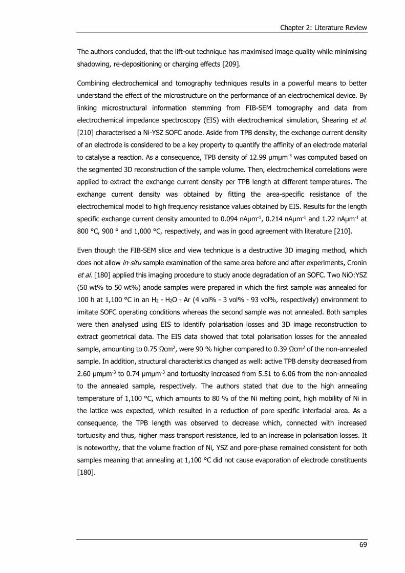
Chapter 2: Literature Review
69
The authors concluded, that the lift-out technique has maximised image quality while minimising
shadowing, re-depositioning or charging effects [209].
Combining electrochemical and tomography techniques results in a powerful means to better
understand the effect of the microstructure on the performance of an electrochemical device. By
linking microstructural information stemming from FIB-SEM tomography and data from
electrochemical impedance spectroscopy (EIS) with electrochemical simulation, Shearing et al.
[210] characterised a Ni-YSZ SOFC anode. Aside from TPB density, the exchange current density
of an electrode is considered to be a key property to quantify the affinity of an electrode material
to catalyse a reaction. As a consequence, TPB density of 12.99 μmμm-3 was computed based on
the segmented 3D reconstruction of the sample volume. Then, electrochemical correlations were
applied to extract the exchange current density per TPB length at different temperatures. The
exchange current density was obtained by fitting the area-specific resistance of the
electrochemical model to high frequency resistance values obtained by EIS. Results for the length
specific exchange current density amounted to 0.094 nAμm-1, 0.214 nAμm-1 and 1.22 nAμm-1 at
800 °C, 900 ° and 1,000 °C, respectively, and was in good agreement with literature [210].
Even though the FIB-SEM slice and view technique is a destructive 3D imaging method, which
does not allow in-situ sample examination of the same area before and after experiments, Cronin
et al. [180] applied this imaging procedure to study anode degradation of an SOFC. Two NiO:YSZ
(50 wt% to 50 wt%) anode samples were prepared in which the first sample was annealed for
100 h at 1,100 °C in an H2 - H2O - Ar (4 vol% - 3 vol% - 93 vol%, respectively) environment to
imitate SOFC operating conditions whereas the second sample was not annealed. Both samples
were then analysed using EIS to identify polarisation losses and 3D image reconstruction to
extract geometrical data. The EIS data showed that total polarisation losses for the annealed
sample, amounting to 0.75 Ωcm2, were 90 % higher compared to 0.39 Ωcm2 of the non-annealed
sample. In addition, structural characteristics changed as well: active TPB density decreased from
2.60 μmμm-3 to 0.74 μmμm-3 and tortuosity increased from 5.51 to 6.06 from the non-annealed
to the annealed sample, respectively. The authors stated that due to the high annealing
temperature of 1,100 °C, which amounts to 80 % of the Ni melting point, high mobility of Ni in
the lattice was expected, which resulted in a reduction of pore specific interfacial area. As a
consequence, the TPB length was observed to decrease which, connected with increased
tortuosity and thus, higher mass transport resistance, led to an increase in polarisation losses. It
is noteworthy, that the volume fraction of Ni, YSZ and pore-phase remained consistent for both
samples meaning that annealing at 1,100 °C did not cause evaporation of electrode constituents
[180].
Chapter 2: Literature Review
70
2.4.2 X-ray Computed Tomography
Destructive imaging methods do not allow comparison of the exact same sample before, during
and after experiments. This is where the advantage of X-ray tomography lies: X-ray CT is a
non-destructive technique allowing in-situ and in-operando tomographic analysis of
microstructural changes of the same sample volume under continuing and varying operating
conditions.
This is achieved by the penetrating nature of the incident X-rays, which are attenuated by
interacting with electrons of the sample. A detector placed behind the specimen then records
transmitted X-rays, which can subsequently be converted into radiograms. For 3D imaging of a
specimen, the sample is rotated around its vertical axis for 180 ° or 360 ° while projections are
collected at discrete angular orientations. Finally, a mathematical algorithm compiles the
sequence of radiograms to form the full 3D structure of the sample volume. In this way, the
sample is not destroyed during imaging, but remains intact for further experiments and additional
analysis methods.
Depending on the density and atomic number of a material along each angular projection, the
intensity of the transmitted photons vary in each image due to absorption and scattering effects.
These effects are combined in the attenuation coefficient, which is a function of the material and
is available for a wide range of elements and mixtures [211, 212]. As a result, each projection
not only contains information about the shape of the sample, but also about the internal
microstructure, which is visualised by recombining all collected images of the scan [213].
The attenuation coefficient of a sample plays an important role for setting up and carrying out
X-ray tomography experiments: the higher the attenuation coefficient, the more X-rays are
attenuated. However, a minimum amount of transmitted photons are necessary to reach the
detector for a good signal-to-noise ratio. Hence, the exposure time for each image has to be
adjusted to meet these specifications. For X-ray generation, two procedures are applied in
practise:
In laboratory scale X-ray devices, a beam of electrons is generated in a filament (the
cathode) which is accelerated towards a metal target (anode) via an applied voltage. By
colliding with the metal target, electrons from the target are temporarily excited to a
higher state. When these excited electrons fall back into their original state, a
characteristic spectrum of X-ray photons combined with a broad-band spectrum referred
to as bremsstrahlung is emitted. Here, the characteristic spectrum of emission lines is
depending on the target material [214].
Synchrotron radiation is generated by accelerating and decelerating charged particles
using electromagnetic fields. This leads to emission of electromagnetic radiation.
Synchrotron generators are typically housed in circular particle accelerators in large,

Chapter 2: Literature Review
71
governmental research facilities. Hence, access to such sources is more limited compared
to laboratory scale X-ray CTs. The advantage in synchrotron-based X-rays lies in the
ability of generating parallel, high brilliance X-ray beams at discrete energy levels of
monochromatic or polychromatic nature. Using finely adjustable X-ray source settings
and optics, chemical and elemental mapping is possible. For example, if a sample consists
of several phases with distinct absorption edges, opacity or transparency of either phase
can be achieved by adjusting the X-ray energy accordingly. In this way, phase-contrast
between different constituents is accomplished by superposing several tomograms taken
at discrete X-ray photon energies. [204, 213–215].
A filtered back projection algorithm is commonly applied to reconstruct the collected images into
a 3D representation of the sample. Figure 2-25 illustrates the working principle of a back
projection algorithm, where the same porous sample was reconstructed with an increasing
number of projections. More projections evidently result in less noise and reveal more details of
the microstructure. Higher image quality aids in subsequent image processing steps such as phase
segmentation.
Figure 2-25: Working principle of filtered back projection algorithm where the same sample was reconstructed using an increasing number of projections.
Figure 2-26 depicts the change in the greyscale histogram of image slices shown in Figure 2-25.
The peaks between the solid and pore phase become more pronounced with a higher number of
projections. This way, threshold segmentation between these two phases is accomplished by
identifying the minimum greyscale value between both peaks. However, the overall scan time
10 Projections 20 Projections 100 Projections
180 Projections 450 Projections 901 Projections

Chapter 2: Literature Review
72
increases linearly with increasing number of projections, which makes the scan more prone to
artefacts such as thermal drifts and vibrations. Hence, a compromise between the exposure time
and the number of projections has to be found to ensure high image quality while keeping the
scan time reasonable.
Figure 2-26: Change of greyscale histogram of reconstructions as function of increasing number of projections
The high importance of quantifying microstructural parameters of electrochemical devices is
reflected by the vast number of publications that apply tomography techniques. One of the first
applications of X-ray tomography in the field of electrochemistry was presented by Izzo et al.,
where microstructural characterisation of a tubular SOFC anode was carried out. Aside from
tortuosity (cf. section 2.2.4.2.1), the pore size distribution and a representative volume element
analysis of porosity were calculated. Not only did the image-based pore size distribution match
well with results from mercury intrusion porosimetry, but the RVE analysis showed, that the
porosity of the sample was independent of sample volume [137].
An SOFC anode was also analysed by Shearing et al. [216] to determine microstructural
characteristics using two different magnifications of an X-ray nano CT system. Pixel size of the
two different magnifications amounted to 32 nm and 65 nm, respectively. To ensure high quality
of tomographic data by exactly fitting the sample to the dimensions of the field of view (FoV) of
the X-ray device, the same lift-out technique as in [209] was used here. Despite the differences
Chapter 2: Literature Review
73
in resolution, porosity of the sample amounted to 8.81 vol% and 9.25 vol% under high and low
magnification, respectively. These results are comparable to the porosity value of the same
sample batch measured in [209], where porosity amounted to 9.42 vol% and was calculated by
using FIB-SEM tomography (see section 2.4.1) [216].
Despite the differences in operating principle between FIB-SEM and X-ray computed tomography,
comparative studies have usually achieved good agreement in calculated data [130, 131, 217].
Even though this is not surprising if the same sample is analysed, small changes in scan setup
can have a visible effect on the results. For example, by changing the accelerating voltage in the
SEM or the number of projections in the X-ray CT system, the image quality is affected. This, in
turn, can have substantial influences on the obtained microstructural features, especially, when
finer structures are investigated.
The validity of results becomes clearer when evaluating the effect of an even wider range of pixel
sizes during microstructural characterisation as presented in [138]. Here, three X-ray instruments
with different pixel sizes were used to characterise the same, commercially available Li-ion battery
cathode:
MicroXCT-200 (pixel size = 597 nm)
Laboratory scale X-ray device at the Henry Moseley X-ray Imaging Facility at the
University of Manchester.
UltraXRM-L200 (pixel size = 65 nm).
Laboratory scale X-ray device at the Henry Moseley X-ray Imaging Facility at the
University of Manchester.
NanoXCT-S100 (pixel size = 15 nm)
Synchrotron X-ray source at the Stanford Synchrotron Radiation Light Source.
Increasing magnification corresponds to a decrease in FoV and thus, volume of the analysed
sample. While porosity (36.3 vol% and 38.0 vol%) and geometric tortuosity (2.0 and 1.9) values
of the MicroXCT-200 and UltraXRM-L200 agreed well with each other, the entire volume of the
NanoXCT-S100 was made up by a single particle. As a consequence, porosity of that sample
volume amounted to 4.5 vol% and as such, tortuosity tended towards infinity. Furthermore, the
obtained geometric tortuosity values were validated by calculating tortuosity using the heat
transfer analogy (cf. sections 2.2.4.2.2 and 3.5.1). Therefore, the samples based on the
MicroXCT-200 and UltraXRM-L200 images were meshed to carry out CFD simulation. It was shown
that average tortuosity (2.21 and 2.01 for the MicroXCT-200 and UltraXRM-L200, respectively)
decreased with increasing image resolution. This trend was consistent with results found via
geometrical calculations stated above. The authors concluded that a higher scan resolution
uncovers smaller pore structures. Hence, the pore connectivity was improved which resulted in
lower tortuosity values [138]. This finding is comparable to the analogy by Mandelbrot, who
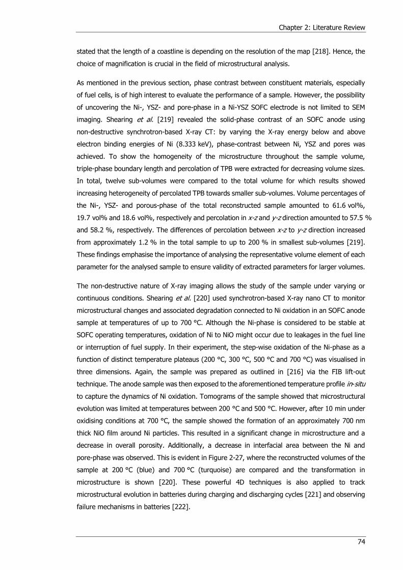
Chapter 2: Literature Review
74
stated that the length of a coastline is depending on the resolution of the map [218]. Hence, the
choice of magnification is crucial in the field of microstructural analysis.
As mentioned in the previous section, phase contrast between constituent materials, especially
of fuel cells, is of high interest to evaluate the performance of a sample. However, the possibility
of uncovering the Ni-, YSZ- and pore-phase in a Ni-YSZ SOFC electrode is not limited to SEM
imaging. Shearing et al. [219] revealed the solid-phase contrast of an SOFC anode using
non-destructive synchrotron-based X-ray CT: by varying the X-ray energy below and above
electron binding energies of Ni (8.333 keV), phase-contrast between Ni, YSZ and pores was
achieved. To show the homogeneity of the microstructure throughout the sample volume,
triple-phase boundary length and percolation of TPB were extracted for decreasing volume sizes.
In total, twelve sub-volumes were compared to the total volume for which results showed
increasing heterogeneity of percolated TPB towards smaller sub-volumes. Volume percentages of
the Ni-, YSZ- and porous-phase of the total reconstructed sample amounted to 61.6 vol%,
19.7 vol% and 18.6 vol%, respectively and percolation in x-z and y-z direction amounted to 57.5 %
and 58.2 %, respectively. The differences of percolation between x-z to y-z direction increased
from approximately 1.2 % in the total sample to up to 200 % in smallest sub-volumes [219].
These findings emphasise the importance of analysing the representative volume element of each
parameter for the analysed sample to ensure validity of extracted parameters for larger volumes.
The non-destructive nature of X-ray imaging allows the study of the sample under varying or
continuous conditions. Shearing et al. [220] used synchrotron-based X-ray nano CT to monitor
microstructural changes and associated degradation connected to Ni oxidation in an SOFC anode
sample at temperatures of up to 700 °C. Although the Ni-phase is considered to be stable at
SOFC operating temperatures, oxidation of Ni to NiO might occur due to leakages in the fuel line
or interruption of fuel supply. In their experiment, the step-wise oxidation of the Ni-phase as a
function of distinct temperature plateaus (200 °C, 300 °C, 500 °C and 700 °C) was visualised in
three dimensions. Again, the sample was prepared as outlined in [216] via the FIB lift-out
technique. The anode sample was then exposed to the aforementioned temperature profile in-situ
to capture the dynamics of Ni oxidation. Tomograms of the sample showed that microstructural
evolution was limited at temperatures between 200 °C and 500 °C. However, after 10 min under
oxidising conditions at 700 °C, the sample showed the formation of an approximately 700 nm
thick NiO film around Ni particles. This resulted in a significant change in microstructure and a
decrease in overall porosity. Additionally, a decrease in interfacial area between the Ni and
pore-phase was observed. This is evident in Figure 2-27, where the reconstructed volumes of the
sample at 200 °C (blue) and 700 °C (turquoise) are compared and the transformation in
microstructure is shown [220]. These powerful 4D techniques is also applied to track
microstructural evolution in batteries during charging and discharging cycles [221] and observing
failure mechanisms in batteries [222].
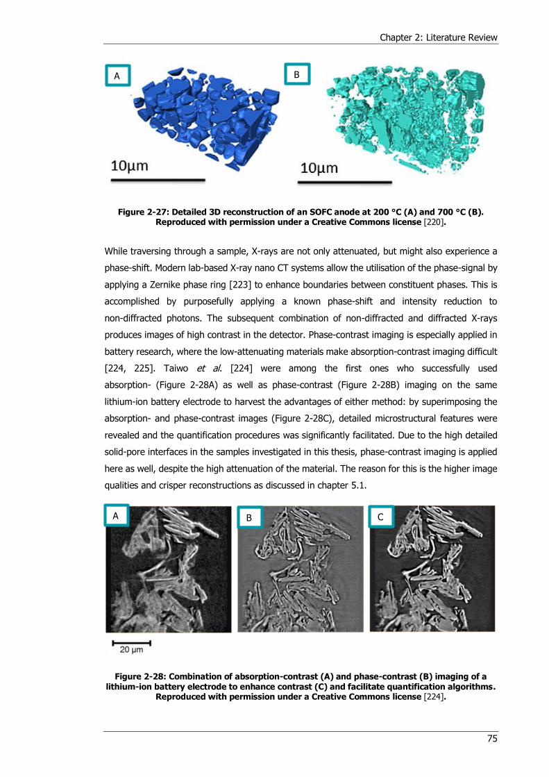
Chapter 2: Literature Review
75
Figure 2-27: Detailed 3D reconstruction of an SOFC anode at 200 °C (A) and 700 °C (B). Reproduced with permission under a Creative Commons license [220].
While traversing through a sample, X-rays are not only attenuated, but might also experience a
phase-shift. Modern lab-based X-ray nano CT systems allow the utilisation of the phase-signal by
applying a Zernike phase ring [223] to enhance boundaries between constituent phases. This is
accomplished by purposefully applying a known phase-shift and intensity reduction to
non-diffracted photons. The subsequent combination of non-diffracted and diffracted X-rays
produces images of high contrast in the detector. Phase-contrast imaging is especially applied in
battery research, where the low-attenuating materials make absorption-contrast imaging difficult
[224, 225]. Taiwo et al. [224] were among the first ones who successfully used
absorption- (Figure 2-28A) as well as phase-contrast (Figure 2-28B) imaging on the same
lithium-ion battery electrode to harvest the advantages of either method: by superimposing the
absorption- and phase-contrast images (Figure 2-28C), detailed microstructural features were
revealed and the quantification procedures was significantly facilitated. Due to the high detailed
solid-pore interfaces in the samples investigated in this thesis, phase-contrast imaging is applied
here as well, despite the high attenuation of the material. The reason for this is the higher image
qualities and crisper reconstructions as discussed in chapter 5.1.
Figure 2-28: Combination of absorption-contrast (A) and phase-contrast (B) imaging of a lithium-ion battery electrode to enhance contrast (C) and facilitate quantification algorithms.
Reproduced with permission under a Creative Commons license [224].
A B
A B C
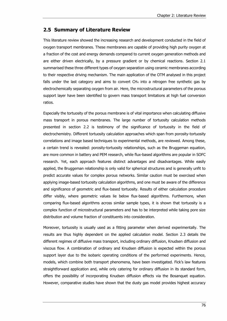
Chapter 2: Literature Review
76
2.5 Summary of Literature Review
This literature review showed the increasing research and development conducted in the field of
oxygen transport membranes. These membranes are capable of providing high purity oxygen at
a fraction of the cost and energy demands compared to current oxygen generation methods and
are either driven electrically, by a pressure gradient or by chemical reactions. Section 2.1
summarised these three different types of oxygen separation using ceramic membranes according
to their respective driving mechanism. The main application of the OTM analysed in this project
falls under the last category and aims to convert CH4 into a nitrogen free synthetic gas by
electrochemically separating oxygen from air. Here, the microstructural parameters of the porous
support layer have been identified to govern mass transport limitations at high fuel conversion
ratios.
Especially the tortuosity of the porous membrane is of vital importance when calculating diffusive
mass transport in porous membranes. The large number of tortuosity calculation methods
presented in section 2.2 is testimony of the significance of tortuosity in the field of
electrochemistry. Different tortuosity calculation approaches which span from porosity-tortuosity
correlations and image based techniques to experimental methods, are reviewed. Among these,
a certain trend is revealed: porosity-tortuosity relationships, such as the Bruggeman equation,
are more common in battery and PEM research, while flux-based algorithms are popular in SOFC
research. Yet, each approach features distinct advantages and disadvantages. While easily
applied, the Bruggeman relationship is only valid for spherical structures and is generally unfit to
predict accurate values for complex porous networks. Similar caution must be exercised when
applying image-based tortuosity calculation algorithms, and one must be aware of the difference
and significance of geometric and flux-based tortuosity. Results of either calculation procedure
differ visibly, where geometric values lie below flux-based algorithms. Furthermore, when
comparing flux-based algorithms across similar sample types, it is shown that tortuosity is a
complex function of microstructural parameters and has to be interpreted while taking pore size
distribution and volume fraction of constituents into consideration.
Moreover, tortuosity is usually used as a fitting parameter when derived experimentally. The
results are thus highly dependent on the applied calculation model. Section 2.3 details the
different regimes of diffusive mass transport, including ordinary diffusion, Knudsen diffusion and
viscous flow. A combination of ordinary and Knudsen diffusion is expected within the porous
support layer due to the isobaric operating conditions of the performed experiments. Hence,
models, which combine both transport phenomena, have been investigated. Fick’s law features
straightforward application and, while only catering for ordinary diffusion in its standard form,
offers the possibility of incorporating Knudsen diffusion effects via the Bosanquet equation.
However, comparative studies have shown that the dusty gas model provides highest accuracy

Chapter 2: Literature Review
77
when comparing calculation with experimental results. This is why the dusty gas model will be
used as a benchmark during the experimental analysis.
In each of these diffusion models, microstructural characteristics are necessary input parameters
for successful calculation. The necessary parameters include porosity and mean pore diameter,
making the tortuosity the only unknown in such calculation procedures. FIB-SEM and X-ray nano
CT have become the standard for microstructural analysis in the field of electrochemistry, as
outlined in section 2.4. Both of these techniques feature distinct advantages and disadvantages
and are routinely applied in practise. Either tomography techniques is capable of reconstructing
representative volumes at high resolutions to determine meaningful values of the desired
parameters.
2.6 Thesis Objectives
The high interest in clean energy systems, in which electrochemical devices are likely to play a
major part in, perpetuates the research activity in the field of oxygen transport membranes.
However, the quantification of microstructural characteristics is of vital importance to better
understand the complex interrelation between performance and membrane microstructure. This
is shown in section 2.1.4, where the rate limiting step at high fuel conversion ratios of the OTM
is found in mass transport limitations in the porous support layer. These limitations are governed
by the underlying microstructural parameters. Here, the interest of Praxair Inc. lies in the
optimisation of the porous support layer of the OTM to provide mechanical stability during
operation coupled with minimal mass transport resistance. By varying the thickness and porosity
of the provided porous support samples, mechanical strength and mass transport resistance are
altered. Thus, the first objective of this thesis is to evaluate the diffusion performance of provided
samples using experimental techniques by applying gas diffusion theory (cf. section 2.3). A
tubular diffusion cell test rig is designed to determine the diffusion behaviour of provided samples
under varying conditions, where the results are presented in chapter 4. The findings of this study
are then used to optimise future designs of porous support layers in collaboration with Praxair
Inc.
At the same time, modern tomography techniques, such as lab-based X-ray CT and FIB-SEM
tomography introduced in section 2.4, allow an unprecedented insight into the nano-scale of a
sample. This has increased the amount of microstructural data extractable for a single sample.
In this field, tortuosity is of high importance, particularly when treating mass transport
phenomena in porous layers. Yet, tortuosity remains an ill-defined parameter in the
electrochemical community, which is notoriously difficult to calculate. Due to these challenges, a
wide range of different methods have been developed in the field of electrochemistry as
highlighted in section 2.2. The determination of tortuosity is dependent on the measurement
approach, where comparisons between different image-based tortuosity calculation models and
Chapter 2: Literature Review
78
between experimental and simulation-based methodologies are limited. Hence, the second
objective of this thesis is to provide a better understanding of the differences in image-based
tortuosity calculation algorithms and to assess the suitability of each method. Chapter 5 presents
the results of tortuosity calculation algorithms, which are executed directly on the voxel domain
of the reconstructed samples. Already here, the difference between geometric and flux-based
tortuosity is shown. Chapter 6 then introduces simulation-based tortuosity algorithms which
model heat and mass flux through the sample. A volume mesh across each analysed sample had
to be generated for this purpose. The tortuosity values calculated in both chapters across the
same samples are then compared to better comprehend the concept of tortuosity in the field of
mass transport.
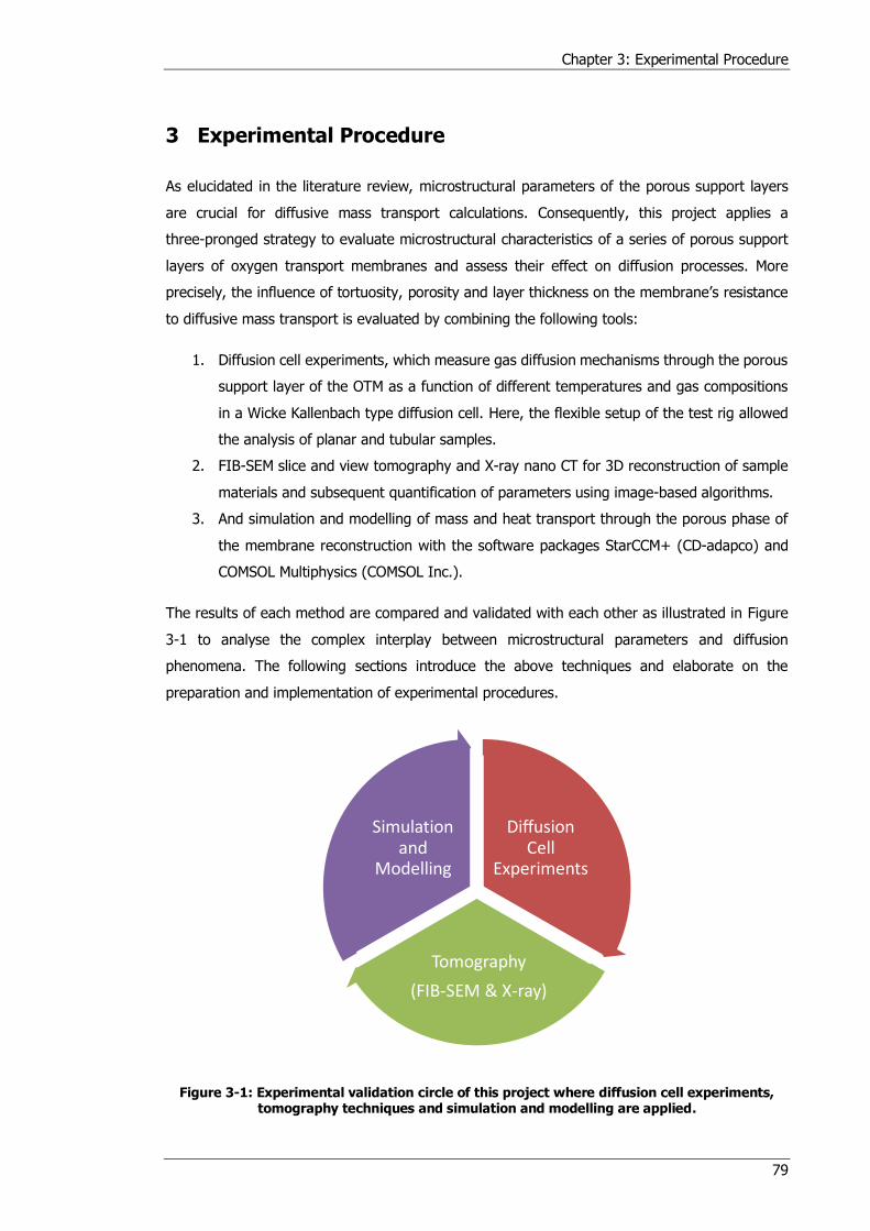
Chapter 3: Experimental Procedure
79
3 Experimental Procedure
As elucidated in the literature review, microstructural parameters of the porous support layers
are crucial for diffusive mass transport calculations. Consequently, this project applies a
three-pronged strategy to evaluate microstructural characteristics of a series of porous support
layers of oxygen transport membranes and assess their effect on diffusion processes. More
precisely, the influence of tortuosity, porosity and layer thickness on the membrane’s resistance
to diffusive mass transport is evaluated by combining the following tools:
1. Diffusion cell experiments, which measure gas diffusion mechanisms through the porous
support layer of the OTM as a function of different temperatures and gas compositions
in a Wicke Kallenbach type diffusion cell. Here, the flexible setup of the test rig allowed
the analysis of planar and tubular samples.
2. FIB-SEM slice and view tomography and X-ray nano CT for 3D reconstruction of sample
materials and subsequent quantification of parameters using image-based algorithms.
3. And simulation and modelling of mass and heat transport through the porous phase of
the membrane reconstruction with the software packages StarCCM+ (CD-adapco) and
COMSOL Multiphysics (COMSOL Inc.).
The results of each method are compared and validated with each other as illustrated in Figure
3-1 to analyse the complex interplay between microstructural parameters and diffusion
phenomena. The following sections introduce the above techniques and elaborate on the
preparation and implementation of experimental procedures.
Figure 3-1: Experimental validation circle of this project where diffusion cell experiments, tomography techniques and simulation and modelling are applied.
Diffusion Cell
Experiments
Tomography
(FIB-SEM & X-ray)
Simulation and
Modelling
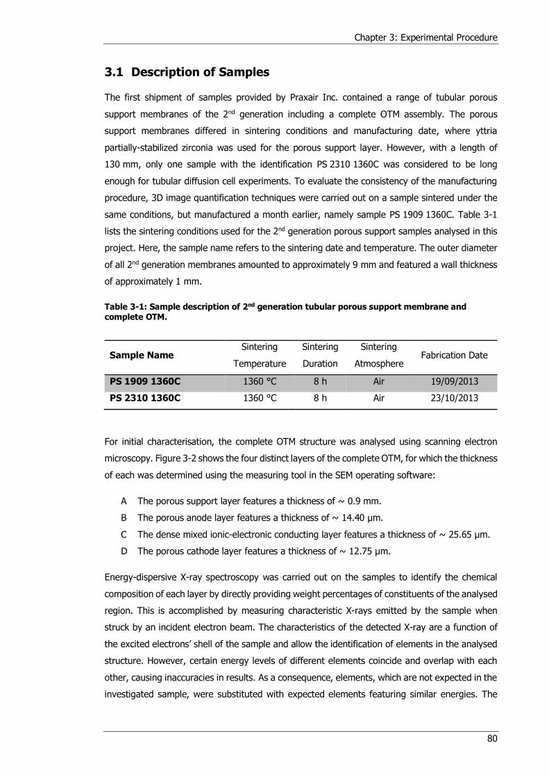
Chapter 3: Experimental Procedure
80
3.1 Description of Samples
The first shipment of samples provided by Praxair Inc. contained a range of tubular porous
support membranes of the 2nd generation including a complete OTM assembly. The porous
support membranes differed in sintering conditions and manufacturing date, where yttria
partially-stabilized zirconia was used for the porous support layer. However, with a length of
130 mm, only one sample with the identification PS 2310 1360C was considered to be long
enough for tubular diffusion cell experiments. To evaluate the consistency of the manufacturing
procedure, 3D image quantification techniques were carried out on a sample sintered under the
same conditions, but manufactured a month earlier, namely sample PS 1909 1360C. Table 3-1
lists the sintering conditions used for the 2nd generation porous support samples analysed in this
project. Here, the sample name refers to the sintering date and temperature. The outer diameter
of all 2nd generation membranes amounted to approximately 9 mm and featured a wall thickness
of approximately 1 mm.
Table 3-1: Sample description of 2nd generation tubular porous support membrane and complete OTM.
Sample Name Sintering
Temperature
Sintering
Duration
Sintering
Atmosphere Fabrication Date
PS 1909 1360C 1360 °C 8 h Air 19/09/2013
PS 2310 1360C 1360 °C 8 h Air 23/10/2013
For initial characterisation, the complete OTM structure was analysed using scanning electron
microscopy. Figure 3-2 shows the four distinct layers of the complete OTM, for which the thickness
of each was determined using the measuring tool in the SEM operating software:
A The porous support layer features a thickness of ~ 0.9 mm.
B The porous anode layer features a thickness of ~ 14.40 μm.
C The dense mixed ionic-electronic conducting layer features a thickness of ~ 25.65 μm.
D The porous cathode layer features a thickness of ~ 12.75 μm.
Energy-dispersive X-ray spectroscopy was carried out on the samples to identify the chemical
composition of each layer by directly providing weight percentages of constituents of the analysed
region. This is accomplished by measuring characteristic X-rays emitted by the sample when
struck by an incident electron beam. The characteristics of the detected X-ray are a function of
the excited electrons’ shell of the sample and allow the identification of elements in the analysed
structure. However, certain energy levels of different elements coincide and overlap with each
other, causing inaccuracies in results. As a consequence, elements, which are not expected in the
investigated sample, were substituted with expected elements featuring similar energies. The
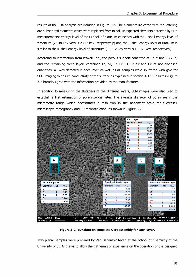
Chapter 3: Experimental Procedure
81
results of the EDX analysis are included in Figure 3-2. The elements indicated with red lettering
are substituted elements which were replaced from initial, unexpected elements detected by EDX
measurements: energy level of the M-shell of platinum coincides with the L-shell energy level of
zirconium (2.048 keV versus 2.042 keV, respectively) and the L-shell energy level of uranium is
similar to the K-shell energy level of strontium (13.612 keV versus 14.163 keV, respectively).
According to information from Praxair Inc., the porous support consisted of Zr, Y and O (YSZ)
and the remaining three layers contained La, Sr, Cr, Fe, O, Zr, Sc and Ce of not disclosed
quantities. Au was detected in each layer as well, as all samples were sputtered with gold for
SEM imaging to ensure conductivity of the surface as explained in section 3.3.1. Results in Figure
3-2 broadly agree with the information provided by the manufacturer.
In addition to measuring the thickness of the different layers, SEM images were also used to
establish a first estimation of pore size diameter. The average diameter of pores lies in the
micrometre range which necessitates a resolution in the nanometre-scale for successful
microscopy, tomography and 3D reconstruction, as shown in Figure 3-2.
Figure 3-2: EDX data on complete OTM assembly for each layer.
Two planar samples were prepared by Zac Dehaney-Steven at the School of Chemistry of the
University of St. Andrews to allow the gathering of experience on the operation of the designed
A B C D

Chapter 3: Experimental Procedure
82
test rig. The same powder and sintering conditions as the 2nd generation Praxair Inc. samples
were used for sample preparation. The only difference was the thickness of the planar samples:
the first one featured a thickness of 0.1 mm and was intended for image analysis while the second
one featured a thickness of 0.5 mm and was intended for diffusion cell experiments. The diameter
of both samples was approximately 16 mm. Table 3-2 summarises the manufacturing parameters
for the planar sample, where the sample name indicates that 100 % Tosoh TZ3YSB 3YSZ powder
was used. The last letter of the sample name is a sequential letter for easier identification.
Table 3-2: Sample description of planar porous support membrane.
Sample Name Sintering
Temperature
Sintering
Duration
Sintering
Atmosphere Fabrication Date
100% TZ3YSB K 1360 °C 8 h Air 16/06/2014
In the course of the project, Praxair Inc. supplied a selection of their latest generation tubular
porous support membranes (generation 2.4). Again, the samples were manufactured at different
sintering temperature as listed in Table 3-3. The focus of experiments with these samples was
on investigating the effect of thickness and porosity on diffusive mass transport. As previously
elaborated, the reasoning behind the variation of these two parameters is to provide the highest
durable and mechanically reliable support layer while keeping gaseous mass transport resistance
at a minimum. The porosity of the samples was varied between 22 vol% and 30 vol% while the
sample thickness was varied between 1 mm and 1.3 mm. The porous support tubes of the 2.4th
generation were cut to feature the same length as sample PS 2310 1360C, namely 130 mm, to
ensure comparability between all tubular samples. The porosity values in Table 3-3 were
calculated by comparing the gravimetrically achieved apparent density of the sample to the
density of the material. These were verified using image quantification techniques afterwards.
The outer diameter of all four samples amounted to approximately 0.9 mm.
Table 3-3: Sample description of 2.4th generation tubular porous support membranes.
Sample Name Sintering
Temperature
Sintering
Duration
Sintering
Atmosphere
Wall
Thickness Porosity
PS 2.4 29.4% 1400 °C 6 h Air 1 mm 29.49 %
PS 2.4 30.0% 1400 °C 6 h Air 1.3 mm 30.03%
PS 2.4 25.1% 1450 °C 6 h Air 1 mm 25.10%
PS 2.4 22.6% 1450 °C 6 h Air 1.3 mm 22.63%
Table 3-4 summarises the experimental procedures carried out for the entirety of analysed
samples. FIB-SEM tomography has only been carried out at the beginning of the project and was
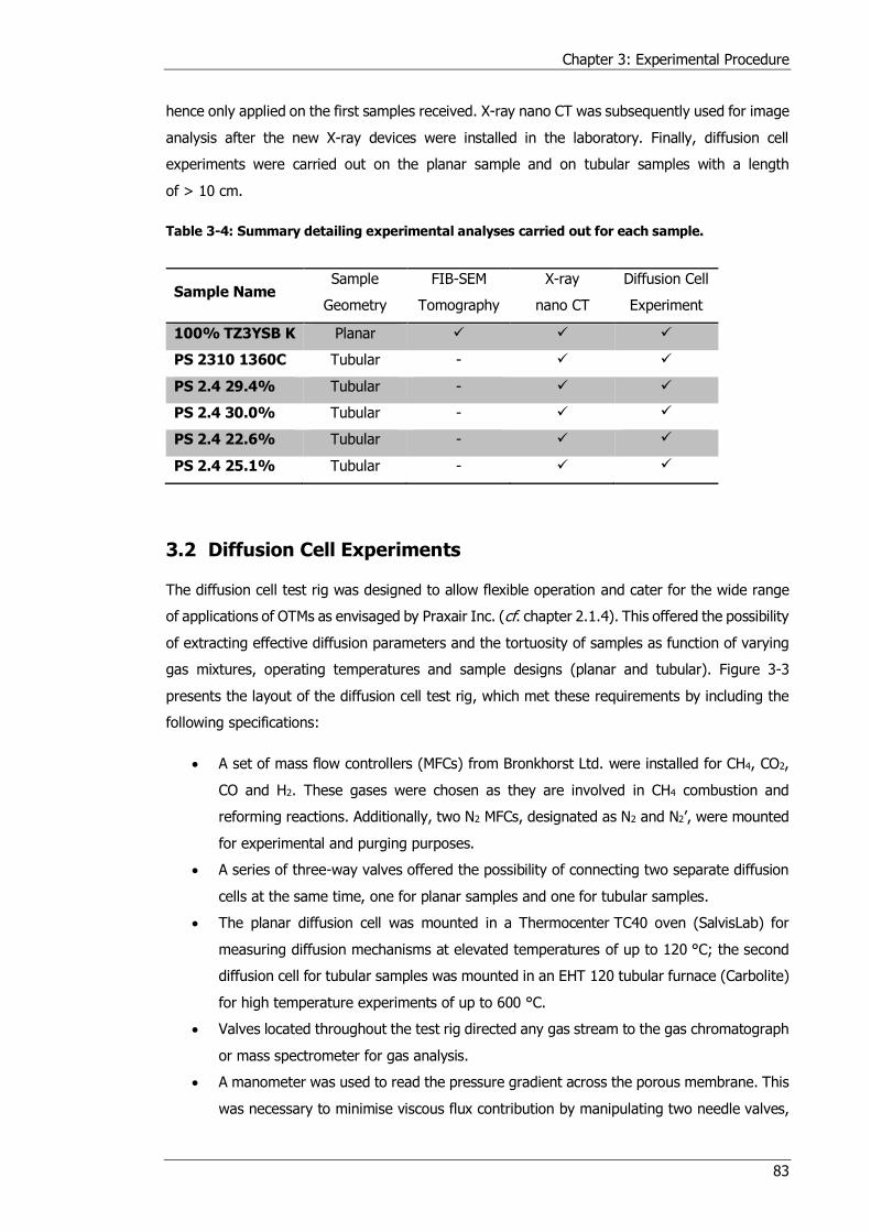
Chapter 3: Experimental Procedure
83
hence only applied on the first samples received. X-ray nano CT was subsequently used for image
analysis after the new X-ray devices were installed in the laboratory. Finally, diffusion cell
experiments were carried out on the planar sample and on tubular samples with a length
of > 10 cm.
Table 3-4: Summary detailing experimental analyses carried out for each sample.
Sample Name Sample
Geometry
FIB-SEM
Tomography
X-ray
nano CT
Diffusion Cell
Experiment
100% TZ3YSB K Planar
PS 2310 1360C Tubular -
PS 2.4 29.4% Tubular -
PS 2.4 30.0% Tubular -
PS 2.4 22.6% Tubular -
PS 2.4 25.1% Tubular -
3.2 Diffusion Cell Experiments
The diffusion cell test rig was designed to allow flexible operation and cater for the wide range
of applications of OTMs as envisaged by Praxair Inc. (cf. chapter 2.1.4). This offered the possibility
of extracting effective diffusion parameters and the tortuosity of samples as function of varying
gas mixtures, operating temperatures and sample designs (planar and tubular). Figure 3-3
presents the layout of the diffusion cell test rig, which met these requirements by including the
following specifications:
A set of mass flow controllers (MFCs) from Bronkhorst Ltd. were installed for CH4, CO2,
CO and H2. These gases were chosen as they are involved in CH4 combustion and
reforming reactions. Additionally, two N2 MFCs, designated as N2 and N2’, were mounted
for experimental and purging purposes.
A series of three-way valves offered the possibility of connecting two separate diffusion
cells at the same time, one for planar samples and one for tubular samples.
The planar diffusion cell was mounted in a Thermocenter TC40 oven (SalvisLab) for
measuring diffusion mechanisms at elevated temperatures of up to 120 °C; the second
diffusion cell for tubular samples was mounted in an EHT 120 tubular furnace (Carbolite)
for high temperature experiments of up to 600 °C.
Valves located throughout the test rig directed any gas stream to the gas chromatograph
or mass spectrometer for gas analysis.
A manometer was used to read the pressure gradient across the porous membrane. This
was necessary to minimise viscous flux contribution by manipulating two needle valves,
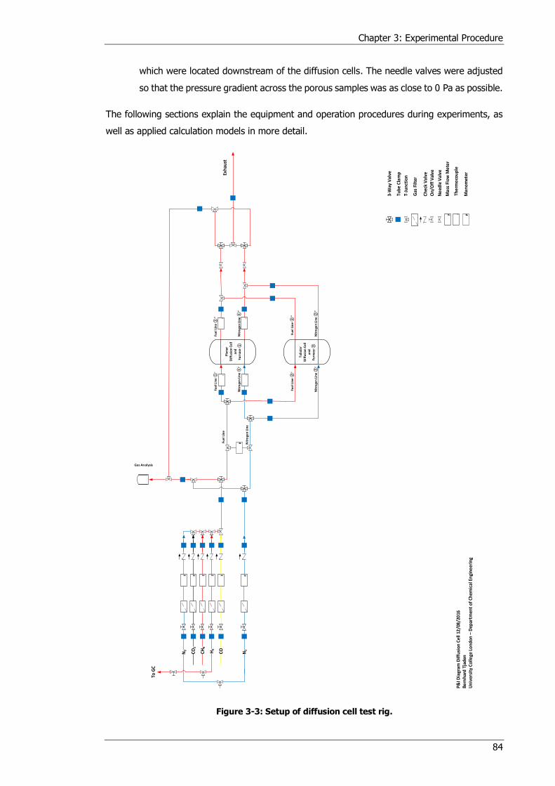
Chapter 3: Experimental Procedure
84
which were located downstream of the diffusion cells. The needle valves were adjusted
so that the pressure gradient across the porous samples was as close to 0 Pa as possible.
The following sections explain the equipment and operation procedures during experiments, as
well as applied calculation models in more detail.
Figure 3-3: Setup of diffusion cell test rig.
On/
Off
Val
ve
Ne
edle
Va
lve
F P
Ma
ss F
low
Me
ter
Ma
no
met
er
P&
I Dia
gram
Dif
fusi
on
Cel
l 12/
08/2
016
Be
rnh
ard
Tja
den
Un
iver
sity
Co
llege
Lo
nd
on
– D
epar
tmen
t o
f C
hem
ical
En
gin
eer
ing
CH
4
CO
F F F
Gas Analysis
F
P
Exh
aust
N2
F
Pla
na
r D
iffu
sio
n C
ell
an
dFu
rna
ce
Fue
l Lin
e
Nit
roge
n L
ine
Fue
l Lin
e
''
Nit
roge
n L
ine
''
Tu
bu
lar
Dif
fusi
on
Ce
lla
nd
Furn
ace
Fue
l Lin
e
'
Nit
roge
n L
ine
'
Fue
l Lin
e
''
Nit
roge
n L
ine
''
Fue
l Lin
e
'
Nit
roge
n L
ine
'
Ch
eck
Va
lve
Gas
Fil
ter
T-Ju
nct
ion
Tub
e C
lam
p
To G
C
N2
3-W
ay V
alve
CO
2F
The
rmo
cou
ple
T
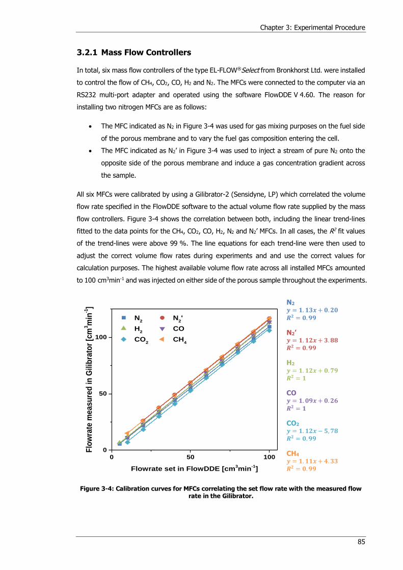
Chapter 3: Experimental Procedure
85
3.2.1 Mass Flow Controllers
In total, six mass flow controllers of the type EL-FLOW®Select from Bronkhorst Ltd. were installed
to control the flow of CH4, CO2, CO, H2 and N2. The MFCs were connected to the computer via an
RS232 multi-port adapter and operated using the software FlowDDE V 4.60. The reason for
installing two nitrogen MFCs are as follows:
The MFC indicated as N2 in Figure 3-4 was used for gas mixing purposes on the fuel side
of the porous membrane and to vary the fuel gas composition entering the cell.
The MFC indicated as N2’ in Figure 3-4 was used to inject a stream of pure N2 onto the
opposite side of the porous membrane and induce a gas concentration gradient across
the sample.
All six MFCs were calibrated by using a Gilibrator-2 (Sensidyne, LP) which correlated the volume
flow rate specified in the FlowDDE software to the actual volume flow rate supplied by the mass
flow controllers. Figure 3-4 shows the correlation between both, including the linear trend-lines
fitted to the data points for the CH4, CO2, CO, H2, N2 and N2’ MFCs. In all cases, the R2 fit values
of the trend-lines were above 99 %. The line equations for each trend-line were then used to
adjust the correct volume flow rates during experiments and and use the correct values for
calculation purposes. The highest available volume flow rate across all installed MFCs amounted
to 100 cm3min-1 and was injected on either side of the porous sample throughout the experiments.
Figure 3-4: Calibration curves for MFCs correlating the set flow rate with the measured flow rate in the Gilibrator.
0 50 1000
50
100
N2
N2'
H2
CO
CO2
CH4
Flo
wra
te m
ea
su
red
in
Gil
ibra
tor
[cm
3m
in-1]
Flowrate set in FlowDDE [cm3min
-1]
N2 𝒚 = 𝟏. 𝟏𝟑𝒙 + 𝟎.𝟐𝟎 𝑹𝟐 = 𝟎.𝟗𝟗
N2’ 𝒚 = 𝟏. 𝟏𝟐𝒙 + 𝟑.𝟖𝟖 𝑹𝟐 = 𝟎.𝟗𝟗
H2 𝒚 = 𝟏. 𝟏𝟐𝒙 + 𝟎.𝟕𝟗 𝑹𝟐 = 𝟏
CO 𝒚 = 𝟏. 𝟎𝟗𝒙 + 𝟎.𝟐𝟔 𝑹𝟐 = 𝟏
CO2 𝒚 = 𝟏. 𝟏𝟐𝒙 − 𝟓,𝟕𝟖 𝑹𝟐 = 𝟎.𝟗𝟗
CH4 𝒚 = 𝟏. 𝟏𝟏𝒙 + 𝟒.𝟑𝟑 𝑹𝟐 = 𝟎.𝟗𝟗

Chapter 3: Experimental Procedure
86
To evaluate the accuracy and consistency of the MFCs, the following test was conducted: a
constant volume flow rate of each MFC was measured by the Gilibrator twelve consecutive times
and the deviations of the minimum and maximum readings were compared to each other. It was
shown that variations between these two extrema lay below 1.6 % for all MFCs. Hence, the high
R2 value of the linear trend-lines in Figure 3-4 and the low fluctuations of the supplied volume
flow rates by the MFCs suggested that the MFCs operated with high accuracy.
3.2.2 Gas Analysis
Gas compositions were measured via two methods to calculate the diffusion flux through the
porous membrane: using a gas chromatograph (GC) and a mass spectrometer (MS). The main
part of the experiments was carried out using the GC while the MS was employed to verify the
measurements. The operating principle and calibration procedure of both techniques are
elaborated here.
3.2.2.1 Gas Chromatograph
A GC-2014 gas chromatograph (Shimadzu Corporation) was used as primary gas analysis
equipment and operated by the software package GCSolutions V 2.30.00. This GC separates the
different gases contained in the sample gas via a CTR I column (Alltech), which is made up of
two cores of different diameters: the inner column of 1/8’’ diameter is packed with a porous
polymer mixture while the outer column of 1/4’’ diameter is filled with an activated molecular
sieve. This special column build-up allows the separation of O2, N2, CH4, CO and CO2 within one
column, perfectly suiting the field of application for the planned experiments.
After the sample gas is separated into its constituents, it is injected into one of two detectors:
either into the flame ionisation detector (FID) or into the thermal conductivity detector (TCD). In
direction comparison, the FID features higher sensitivity, but its application is limited to
hydrocarbons only. However, the TCD is capable of detecting all gaseous compounds and was
thus chosen for this project.
The thermal conductivity detector identifies gas mixtures by comparing the change in resistance
of an electrically heated filament as a function of the injected gas composition. The filament is
heated by a specified electric current of which one side is swept by a carrier gas with high thermal
conductivity and the other side is swept by the sample gas. Due to the difference in thermal
conductivity between the sample gas and the carrier gas, the temperature and thereby the electric
resistance of the filament changes. A chromatogram is then produced by recording the change
in the electric resistances of the two filament parts, identifying the constituents and composition
of the sample gas.
Helium is commonly used as carrier gas due to its high thermal conductivity. However, as thermal
conductivity of He and H2 are close to each other (0.16 Wm-1K-1 and 0.18 Wm-1K-1 at 25 °C and
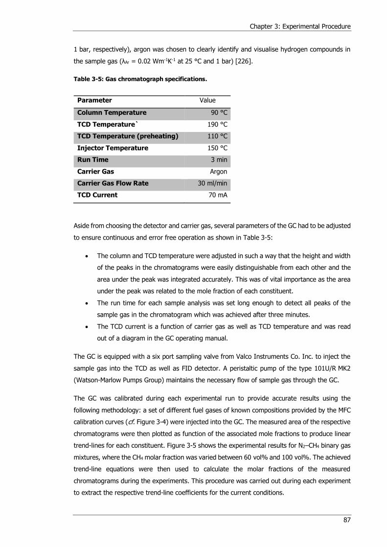
Chapter 3: Experimental Procedure
87
1 bar, respectively), argon was chosen to clearly identify and visualise hydrogen compounds in
the sample gas (λAr = 0.02 Wm-1K-1 at 25 °C and 1 bar) [226].
Table 3-5: Gas chromatograph specifications.
Parameter Value
Column Temperature 90 °C
TCD Temperature` 190 °C
TCD Temperature (preheating) 110 °C
Injector Temperature 150 °C
Run Time 3 min
Carrier Gas Argon
Carrier Gas Flow Rate 30 ml/min
TCD Current 70 mA
Aside from choosing the detector and carrier gas, several parameters of the GC had to be adjusted
to ensure continuous and error free operation as shown in Table 3-5:
The column and TCD temperature were adjusted in such a way that the height and width
of the peaks in the chromatograms were easily distinguishable from each other and the
area under the peak was integrated accurately. This was of vital importance as the area
under the peak was related to the mole fraction of each constituent.
The run time for each sample analysis was set long enough to detect all peaks of the
sample gas in the chromatogram which was achieved after three minutes.
The TCD current is a function of carrier gas as well as TCD temperature and was read
out of a diagram in the GC operating manual.
The GC is equipped with a six port sampling valve from Valco Instruments Co. Inc. to inject the
sample gas into the TCD as well as FID detector. A peristaltic pump of the type 101U/R MK2
(Watson-Marlow Pumps Group) maintains the necessary flow of sample gas through the GC.
The GC was calibrated during each experimental run to provide accurate results using the
following methodology: a set of different fuel gases of known compositions provided by the MFC
calibration curves (cf. Figure 3-4) were injected into the GC. The measured area of the respective
chromatograms were then plotted as function of the associated mole fractions to produce linear
trend-lines for each constituent. Figure 3-5 shows the experimental results for N2–CH4 binary gas
mixtures, where the CH4 molar fraction was varied between 60 vol% and 100 vol%. The achieved
trend-line equations were then used to calculate the molar fractions of the measured
chromatograms during the experiments. This procedure was carried out during each experiment
to extract the respective trend-line coefficients for the current conditions.
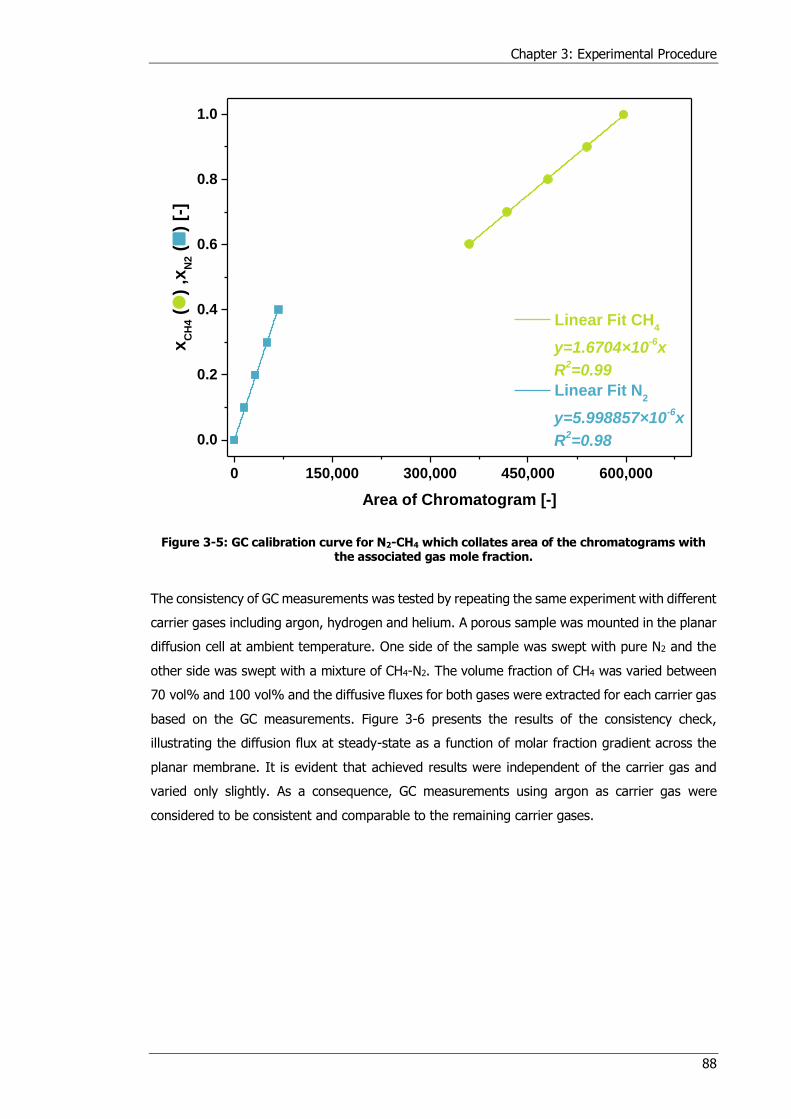
Chapter 3: Experimental Procedure
88
Figure 3-5: GC calibration curve for N2-CH4 which collates area of the chromatograms with the associated gas mole fraction.
The consistency of GC measurements was tested by repeating the same experiment with different
carrier gases including argon, hydrogen and helium. A porous sample was mounted in the planar
diffusion cell at ambient temperature. One side of the sample was swept with pure N2 and the
other side was swept with a mixture of CH4-N2. The volume fraction of CH4 was varied between
70 vol% and 100 vol% and the diffusive fluxes for both gases were extracted for each carrier gas
based on the GC measurements. Figure 3-6 presents the results of the consistency check,
illustrating the diffusion flux at steady-state as a function of molar fraction gradient across the
planar membrane. It is evident that achieved results were independent of the carrier gas and
varied only slightly. As a consequence, GC measurements using argon as carrier gas were
considered to be consistent and comparable to the remaining carrier gases.
0 150,000 300,000 450,000 600,000
0.0
0.2
0.4
0.6
0.8
1.0
Linear Fit CH4
y=1.6704×10⁻⁶x
R2=0.99
Linear Fit N2
y=5.998857×10⁻⁶x
R2=0.98
xC
H4 (
) ,x
N2 (
) [-
]
Area of Chromatogram [-]
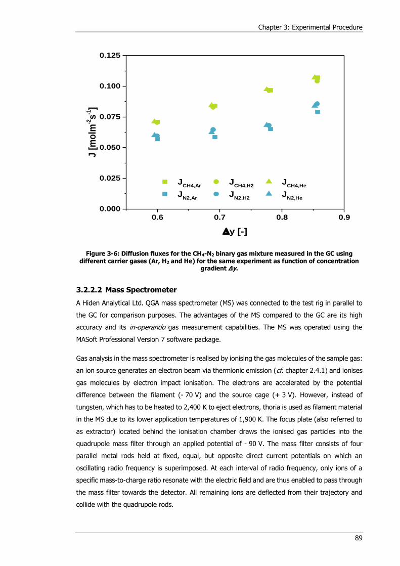
Chapter 3: Experimental Procedure
89
Figure 3-6: Diffusion fluxes for the CH4-N2 binary gas mixture measured in the GC using different carrier gases (Ar, H2 and He) for the same experiment as function of concentration
gradient Δy.
3.2.2.2 Mass Spectrometer
A Hiden Analytical Ltd. QGA mass spectrometer (MS) was connected to the test rig in parallel to
the GC for comparison purposes. The advantages of the MS compared to the GC are its high
accuracy and its in-operando gas measurement capabilities. The MS was operated using the
MASoft Professional Version 7 software package.
Gas analysis in the mass spectrometer is realised by ionising the gas molecules of the sample gas:
an ion source generates an electron beam via thermionic emission (cf. chapter 2.4.1) and ionises
gas molecules by electron impact ionisation. The electrons are accelerated by the potential
difference between the filament (- 70 V) and the source cage (+ 3 V). However, instead of
tungsten, which has to be heated to 2,400 K to eject electrons, thoria is used as filament material
in the MS due to its lower application temperatures of 1,900 K. The focus plate (also referred to
as extractor) located behind the ionisation chamber draws the ionised gas particles into the
quadrupole mass filter through an applied potential of - 90 V. The mass filter consists of four
parallel metal rods held at fixed, equal, but opposite direct current potentials on which an
oscillating radio frequency is superimposed. At each interval of radio frequency, only ions of a
specific mass-to-charge ratio resonate with the electric field and are thus enabled to pass through
the mass filter towards the detector. All remaining ions are deflected from their trajectory and
collide with the quadrupole rods.
0.6 0.7 0.8 0.90.000
0.025
0.050
0.075
0.100
0.125
JCH4,Ar
JCH4,H2
JCH4,He
JN2,Ar
JN2,H2
JN2,He
J [
mo
lm-2s
-1]
y [-]
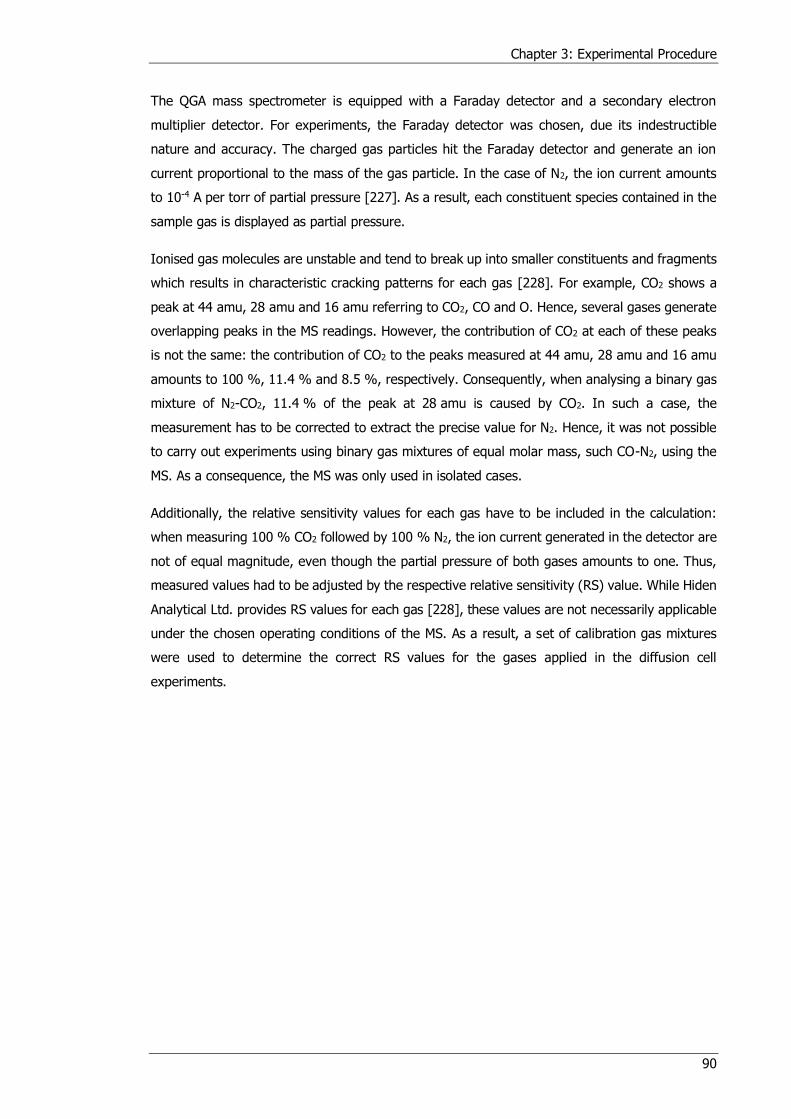
Chapter 3: Experimental Procedure
90
The QGA mass spectrometer is equipped with a Faraday detector and a secondary electron
multiplier detector. For experiments, the Faraday detector was chosen, due its indestructible
nature and accuracy. The charged gas particles hit the Faraday detector and generate an ion
current proportional to the mass of the gas particle. In the case of N2, the ion current amounts
to 10-4 A per torr of partial pressure [227]. As a result, each constituent species contained in the
sample gas is displayed as partial pressure.
Ionised gas molecules are unstable and tend to break up into smaller constituents and fragments
which results in characteristic cracking patterns for each gas [228]. For example, CO2 shows a
peak at 44 amu, 28 amu and 16 amu referring to CO2, CO and O. Hence, several gases generate
overlapping peaks in the MS readings. However, the contribution of CO2 at each of these peaks
is not the same: the contribution of CO2 to the peaks measured at 44 amu, 28 amu and 16 amu
amounts to 100 %, 11.4 % and 8.5 %, respectively. Consequently, when analysing a binary gas
mixture of N2-CO2, 11.4 % of the peak at 28 amu is caused by CO2. In such a case, the
measurement has to be corrected to extract the precise value for N2. Hence, it was not possible
to carry out experiments using binary gas mixtures of equal molar mass, such CO-N2, using the
MS. As a consequence, the MS was only used in isolated cases.
Additionally, the relative sensitivity values for each gas have to be included in the calculation:
when measuring 100 % CO2 followed by 100 % N2, the ion current generated in the detector are
not of equal magnitude, even though the partial pressure of both gases amounts to one. Thus,
measured values had to be adjusted by the respective relative sensitivity (RS) value. While Hiden
Analytical Ltd. provides RS values for each gas [228], these values are not necessarily applicable
under the chosen operating conditions of the MS. As a result, a set of calibration gas mixtures
were used to determine the correct RS values for the gases applied in the diffusion cell
experiments.
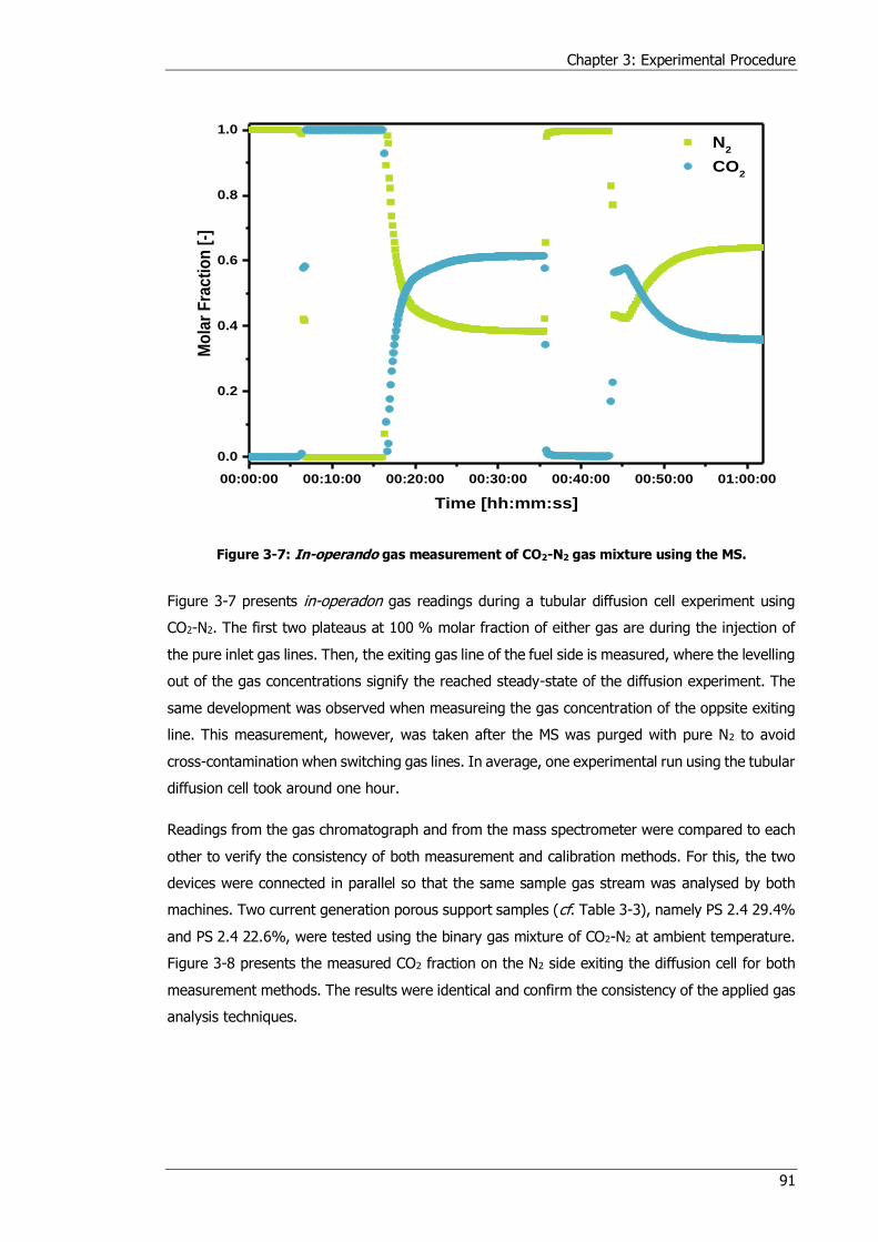
Chapter 3: Experimental Procedure
91
Figure 3-7: In-operando gas measurement of CO2-N2 gas mixture using the MS.
Figure 3-7 presents in-operadon gas readings during a tubular diffusion cell experiment using
CO2-N2. The first two plateaus at 100 % molar fraction of either gas are during the injection of
the pure inlet gas lines. Then, the exiting gas line of the fuel side is measured, where the levelling
out of the gas concentrations signify the reached steady-state of the diffusion experiment. The
same development was observed when measureing the gas concentration of the oppsite exiting
line. This measurement, however, was taken after the MS was purged with pure N2 to avoid
cross-contamination when switching gas lines. In average, one experimental run using the tubular
diffusion cell took around one hour.
Readings from the gas chromatograph and from the mass spectrometer were compared to each
other to verify the consistency of both measurement and calibration methods. For this, the two
devices were connected in parallel so that the same sample gas stream was analysed by both
machines. Two current generation porous support samples (cf. Table 3-3), namely PS 2.4 29.4%
and PS 2.4 22.6%, were tested using the binary gas mixture of CO2-N2 at ambient temperature.
Figure 3-8 presents the measured CO2 fraction on the N2 side exiting the diffusion cell for both
measurement methods. The results were identical and confirm the consistency of the applied gas
analysis techniques.
00:00:00 00:10:00 00:20:00 00:30:00 00:40:00 00:50:00 01:00:00
0.0
0.2
0.4
0.6
0.8
1.0 N
2
CO2
Mo
lar
Fra
cti
on
[-]
Time [hh:mm:ss]
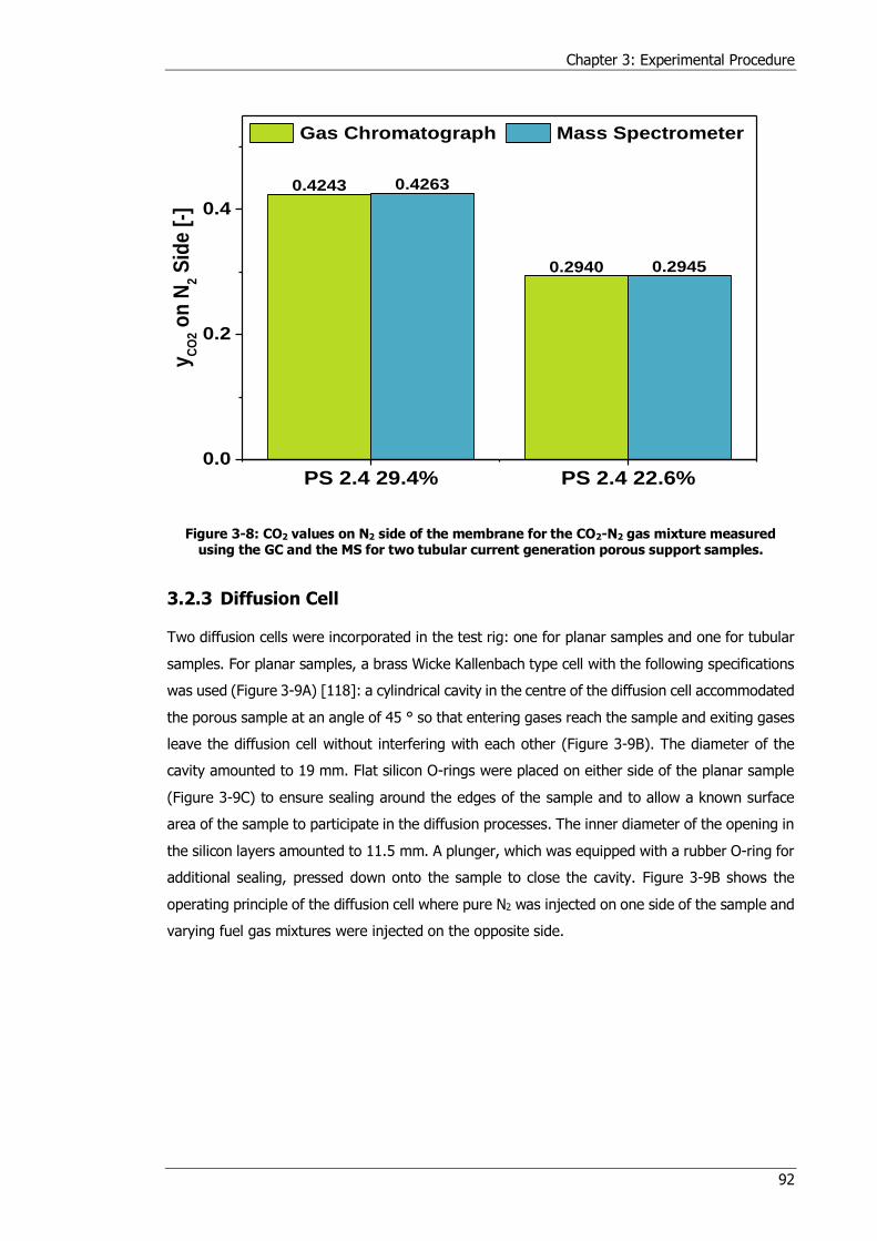
Chapter 3: Experimental Procedure
92
Figure 3-8: CO2 values on N2 side of the membrane for the CO2-N2 gas mixture measured using the GC and the MS for two tubular current generation porous support samples.
3.2.3 Diffusion Cell
Two diffusion cells were incorporated in the test rig: one for planar samples and one for tubular
samples. For planar samples, a brass Wicke Kallenbach type cell with the following specifications
was used (Figure 3-9A) [118]: a cylindrical cavity in the centre of the diffusion cell accommodated
the porous sample at an angle of 45 ° so that entering gases reach the sample and exiting gases
leave the diffusion cell without interfering with each other (Figure 3-9B). The diameter of the
cavity amounted to 19 mm. Flat silicon O-rings were placed on either side of the planar sample
(Figure 3-9C) to ensure sealing around the edges of the sample and to allow a known surface
area of the sample to participate in the diffusion processes. The inner diameter of the opening in
the silicon layers amounted to 11.5 mm. A plunger, which was equipped with a rubber O-ring for
additional sealing, pressed down onto the sample to close the cavity. Figure 3-9B shows the
operating principle of the diffusion cell where pure N2 was injected on one side of the sample and
varying fuel gas mixtures were injected on the opposite side.
0.4243
0.2940
0.4263
0.2945
PS 2.4 29.4% PS 2.4 22.6%0.0
0.2
0.4
yC
O2 o
n N
2 S
ide [
-]
Gas Chromatograph Mass Spectrometer
Chapter 3: Experimental Procedure
93
Figure 3-9: Wicke Kallenbach diffusion cell and sample mounting for planar samples.
The following tests were carried out to check the diffusion cell for leaks and experimental
consistency:
A solid plate was inserted into the place of the porous sample and pure N2 on one side
and pure H2 on the opposite side were injected into the diffusion cell; both exiting gas
lines were analysed to check the system for cross leaking using the GC; chromatograms
showed no traces of H2 in the N2 gas line and vice versa.
Afterwards, the inlet gas lines were swapped for further testing the consistency of the
cell and system arrangement; diffusion cell experiments using a porous sample were then
carried out before and after the gas line swap and the gas chromatograms were
compared to each other; the results were consistent and did not show a change in
measured values before and after the gas line swap.
Finally, the position of the manometer was varied to examine, if the measured pressure
difference across the sample and the subsequently adjusted pressure drop using the
needle valves were independent of the location of the manometer; the manometer was
connected at its standard location, directly before and directly after the diffusion cell;
results showed that the manometer position did not affect the results.
A C
B
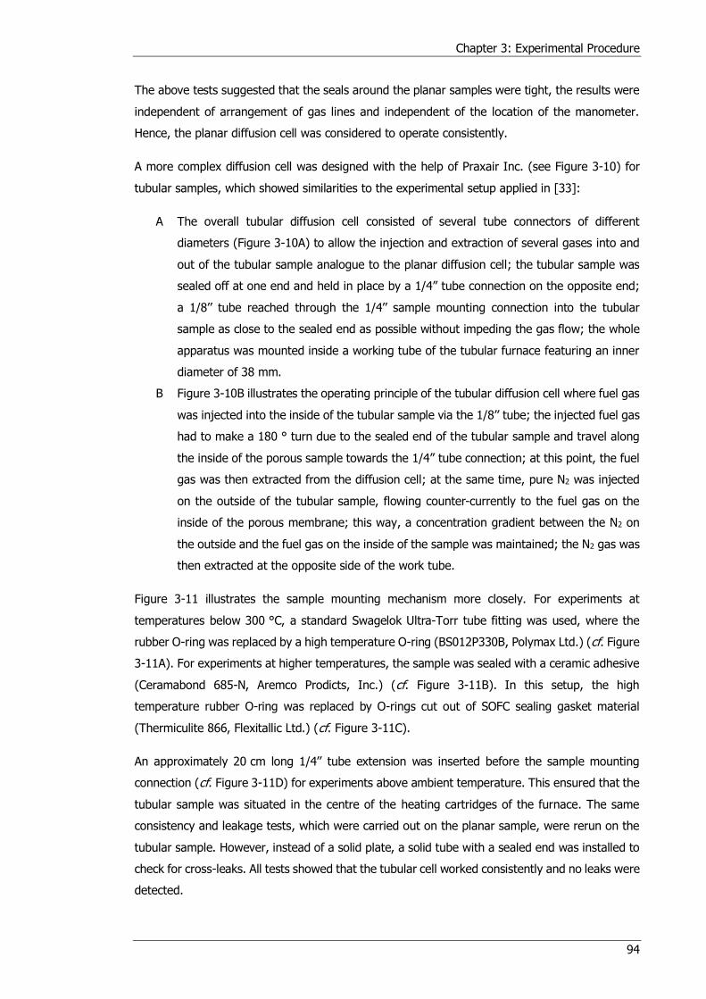
Chapter 3: Experimental Procedure
94
The above tests suggested that the seals around the planar samples were tight, the results were
independent of arrangement of gas lines and independent of the location of the manometer.
Hence, the planar diffusion cell was considered to operate consistently.
A more complex diffusion cell was designed with the help of Praxair Inc. (see Figure 3-10) for
tubular samples, which showed similarities to the experimental setup applied in [33]:
A The overall tubular diffusion cell consisted of several tube connectors of different
diameters (Figure 3-10A) to allow the injection and extraction of several gases into and
out of the tubular sample analogue to the planar diffusion cell; the tubular sample was
sealed off at one end and held in place by a 1/4’’ tube connection on the opposite end;
a 1/8’’ tube reached through the 1/4’’ sample mounting connection into the tubular
sample as close to the sealed end as possible without impeding the gas flow; the whole
apparatus was mounted inside a working tube of the tubular furnace featuring an inner
diameter of 38 mm.
B Figure 3-10B illustrates the operating principle of the tubular diffusion cell where fuel gas
was injected into the inside of the tubular sample via the 1/8’’ tube; the injected fuel gas
had to make a 180 ° turn due to the sealed end of the tubular sample and travel along
the inside of the porous sample towards the 1/4’’ tube connection; at this point, the fuel
gas was then extracted from the diffusion cell; at the same time, pure N2 was injected
on the outside of the tubular sample, flowing counter-currently to the fuel gas on the
inside of the porous membrane; this way, a concentration gradient between the N2 on
the outside and the fuel gas on the inside of the sample was maintained; the N2 gas was
then extracted at the opposite side of the work tube.
Figure 3-11 illustrates the sample mounting mechanism more closely. For experiments at
temperatures below 300 °C, a standard Swagelok Ultra-Torr tube fitting was used, where the
rubber O-ring was replaced by a high temperature O-ring (BS012P330B, Polymax Ltd.) (cf. Figure
3-11A). For experiments at higher temperatures, the sample was sealed with a ceramic adhesive
(Ceramabond 685-N, Aremco Prodicts, Inc.) (cf. Figure 3-11B). In this setup, the high
temperature rubber O-ring was replaced by O-rings cut out of SOFC sealing gasket material
(Thermiculite 866, Flexitallic Ltd.) (cf. Figure 3-11C).
An approximately 20 cm long 1/4’’ tube extension was inserted before the sample mounting
connection (cf. Figure 3-11D) for experiments above ambient temperature. This ensured that the
tubular sample was situated in the centre of the heating cartridges of the furnace. The same
consistency and leakage tests, which were carried out on the planar sample, were rerun on the
tubular sample. However, instead of a solid plate, a solid tube with a sealed end was installed to
check for cross-leaks. All tests showed that the tubular cell worked consistently and no leaks were
detected.
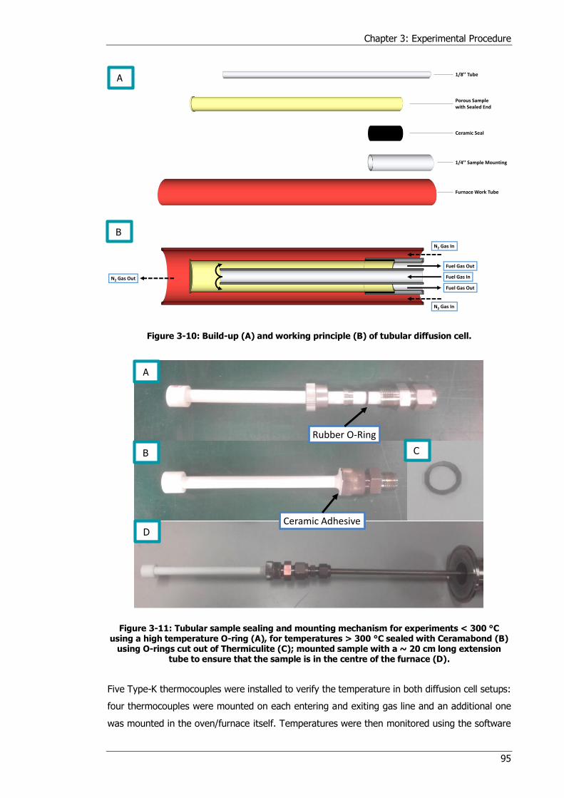
Chapter 3: Experimental Procedure
95
Figure 3-10: Build-up (A) and working principle (B) of tubular diffusion cell.
Figure 3-11: Tubular sample sealing and mounting mechanism for experiments < 300 °C using a high temperature O-ring (A), for temperatures > 300 °C sealed with Ceramabond (B)
using O-rings cut out of Thermiculite (C); mounted sample with a ~ 20 cm long extension tube to ensure that the sample is in the centre of the furnace (D).
Five Type-K thermocouples were installed to verify the temperature in both diffusion cell setups:
four thermocouples were mounted on each entering and exiting gas line and an additional one
was mounted in the oven/furnace itself. Temperatures were then monitored using the software
1/8’’ Tube
Porous Sample with Sealed End
Ceramic Seal
1/4’’ Sample Mounting
Furnace Work Tube
Fuel Gas In
N2 Gas In
N2 Gas Out
Fuel Gas Out
Fuel Gas Out
N2 Gas In
Rubber O-Ring
Ceramic Adhesive
A
B
A
B C
D
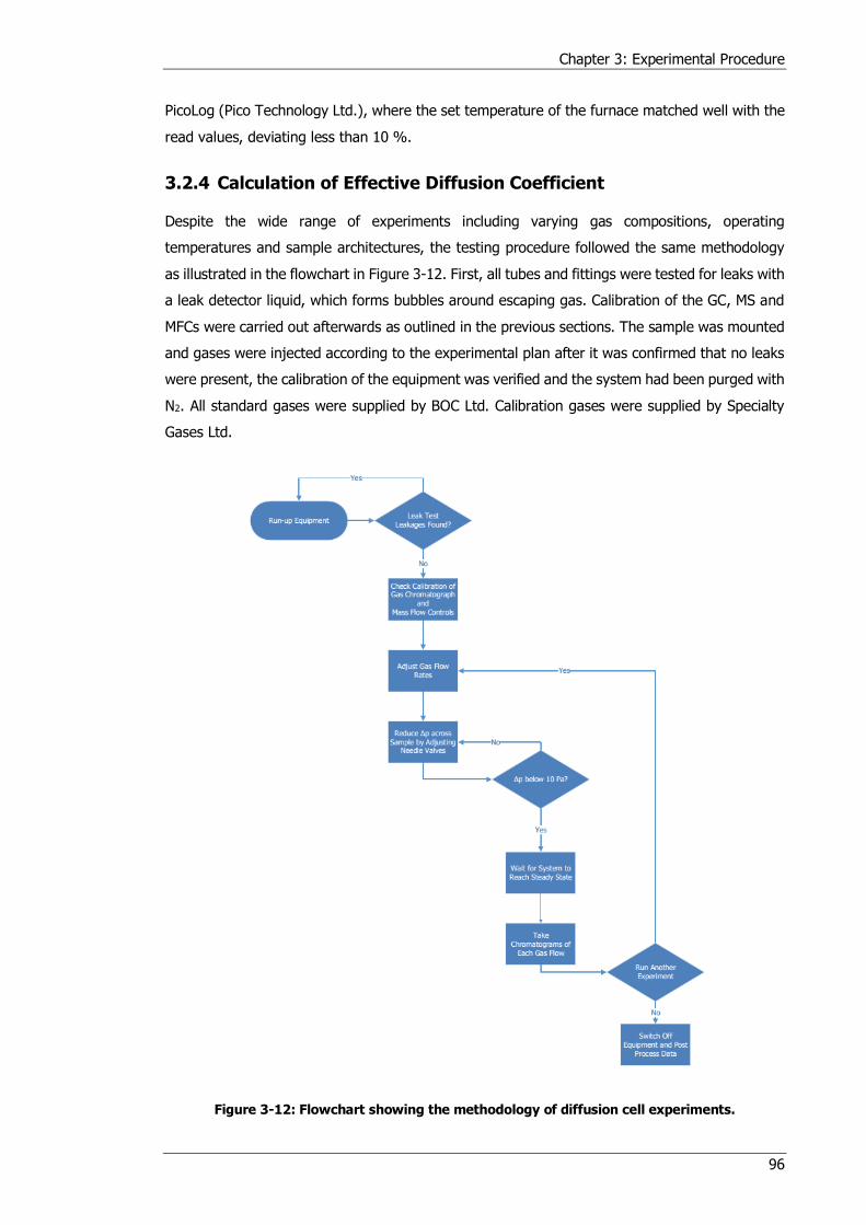
Chapter 3: Experimental Procedure
96
PicoLog (Pico Technology Ltd.), where the set temperature of the furnace matched well with the
read values, deviating less than 10 %.
3.2.4 Calculation of Effective Diffusion Coefficient
Despite the wide range of experiments including varying gas compositions, operating
temperatures and sample architectures, the testing procedure followed the same methodology
as illustrated in the flowchart in Figure 3-12. First, all tubes and fittings were tested for leaks with
a leak detector liquid, which forms bubbles around escaping gas. Calibration of the GC, MS and
MFCs were carried out afterwards as outlined in the previous sections. The sample was mounted
and gases were injected according to the experimental plan after it was confirmed that no leaks
were present, the calibration of the equipment was verified and the system had been purged with
N2. All standard gases were supplied by BOC Ltd. Calibration gases were supplied by Specialty
Gases Ltd.
Figure 3-12: Flowchart showing the methodology of diffusion cell experiments.
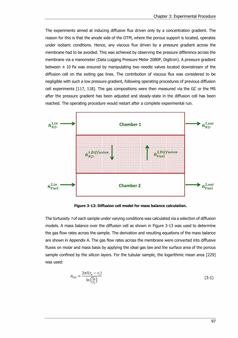
Chapter 3: Experimental Procedure
97
The experiments aimed at inducing diffusive flux driven only by a concentration gradient. The
reason for this is that the anode side of the OTM, where the porous support is located, operates
under isobaric conditions. Hence, any viscous flux driven by a pressure gradient across the
membrane had to be avoided. This was achieved by observing the pressure difference across the
membrane via a manometer (Data Logging Pressure Meter 2080P, Digitron). A pressure gradient
between ± 10 Pa was ensured by manipulating two needle valves located downstream of the
diffusion cell on the exiting gas lines. The contribution of viscous flux was considered to be
negligible with such a low pressure gradient, following operating procedures of previous diffusion
cell experiments [117, 118]. The gas compositions were then measured via the GC or the MS
after the pressure gradient has been adjusted and steady-state in the diffusion cell has been
reached. The operating procedure would restart after a complete experimental run.
Figure 3-13: Diffusion cell model for mass balance calculation.
The tortuosity τ of each sample under varying conditions was calculated via a selection of diffusion
models. A mass balance over the diffusion cell as shown in Figure 3-13 was used to determine
the gas flow rates across the sample. The derivation and resulting equations of the mass balance
are shown in Appendix A. The gas flow rates across the membrane were converted into diffusive
fluxes on molar and mass basis by applying the ideal gas law and the surface area of the porous
sample confined by the silicon layers. For the tubular sample, the logarithmic mean area [229]
was used:
𝐴𝑙𝑚 =2𝜋𝑙(𝑟𝑜 − 𝑟𝑖)
ln (𝑟𝑜𝑟𝑖)
(3-1)
Chamber 1
Chamber 2
𝟐′𝟏,
𝟐,
𝟐′𝟏,
𝟐,
𝟐,
𝟐′𝟏,
Chapter 3: Experimental Procedure
98
In which the following are defined:
Alm logarithmic mean area of sample tube [m2] l sample length [m] rO, ri inner and outer diameter of sample tube [m]
As mentioned above, the diffusive flux was only driven by a concentration gradient by preventing
the development of a pressure gradient across the sample. Consequently, Fick’s first law of
diffusion in the following form was employed as first diffusion model:
𝐽𝑖 = −𝐷𝑖𝑗,𝑒𝑓𝑓𝑝
𝑅𝑇
𝑦𝑖,0 − 𝑦𝑖,𝛿𝛿
(3-2)
In which the following are defined:
Ji diffusion flux [molm-2s-1] Dij,eff effective binary diffusion coefficient [m²s-1] p pressure [Pa] R ideal gas constant [Jmol-1K-1] T temperature [K] yi molar fraction [-] δ thickness [m]
Here, yi,0 and yi,δ refer to the molar fraction of gaseous species i on the two opposite sides of the
membrane. Both were extracted via gas chromatography or mass spectrometry and the porosity
was calculated via tomography. As a consequence, the only unknown parameter in equation (3-2)
is the effective binary diffusion coefficient Dij,eff, which is directly expressible. Hence, the tortuosity
is determined by applying equation (2-21).
Mills [230] criticised the assumption of equimolar diffusion in Fick’s law and developed a new
model. Mills suggested that diffusion follows equimass principles and by converting the molar
fraction gradient in Fick’s first law into a gradient of mass fraction, the governing equation for
equimass diffusion was achieved:
𝐽𝑖 = −𝐷𝑖𝑗,𝑒𝑓𝑓𝑝
𝑅𝑇
𝑀𝑖𝑀𝑗
[𝑤𝑖(𝑀𝑗𝑀𝑖) +𝑀𝑖]
𝑑𝑤𝑖𝑑𝑥
(3-3)
In which the following are defined:
Ji diffusion flux [gm-2s-1] Dij,eff effective binary diffusion coefficient [m²s-1] p pressure [Pa] R ideal gas constant [Jmol-1K-1] T temperature [K] Mi, Mj molar mass [gmol-1] wi mass fraction [-] x dimension [m]
Chapter 3: Experimental Procedure
99
After integrating by using the integration rule ∫1
𝑎 𝑥+𝑏𝑑𝑥 =
1
𝑎𝑙𝑛|𝑎𝑥 + 𝑏|, equation (3-3) takes the
form of equation (3-4):
𝐽𝑖 = −𝐷𝑖𝑗,𝑒𝑓𝑓𝑝
𝑅𝑇𝛿
𝑀𝑖𝑀𝑗
(𝑀𝑗 −𝑀𝑖)ln [
𝑤𝑖,𝛿(𝑀𝑗 −𝑀𝑖) + 𝑀𝑖
𝑤𝑖,0(𝑀𝑗 −𝑀𝑖) +𝑀𝑖
] (3-4)
Again, the tortuosity was determined by applying equation (2-21). The two models do not take
Knudsen diffusion into account. Hence, the Bosanquet equation (equation (2-28)) was employed
on both models. The Bosanquet equation combines the Knudsen diffusion coefficient Di,Kn
calculated via equation (2-24) with the binary diffusion coefficient Dij calculated via equation (2-20)
(cf. chapter 2.3.5). The necessary input parameters of porosity and mean pore diameter were
calculated based on tomographic data as explained in the following chapter. The only remaining
unknown variable in these extended models remained the tortuosity, which was extracted as
before.
In addition, the dusty gas model was applied here as well due to its wide application in literature
and high accuracy (cf. chapter 2.3.5). The DGM is an implicit model [193] as shown in equation
(2-31), which can be simplified and rearranged into an explicit form valid for binary gas mixtures
as presented by Liu et al. [231]:
𝐽𝑖,𝐷 = −𝐷𝑖𝑗,𝑒𝑓𝑓𝐷𝑖,𝐾,𝑒𝑓𝑓
𝐷𝑖𝑗,𝑒𝑓𝑓 + 𝑥𝑖𝐷𝑗,𝐾,𝑒𝑓𝑓 + 𝑥𝑗𝐷𝑖,𝐾,𝑒𝑓𝑓
𝑝
𝑅𝑇
𝑑𝑦𝑖
𝑑𝑥− 𝑐𝑖 [
𝐷𝑖 ,𝐾𝑒𝑓𝑓
𝐷𝑗,𝐾𝑒𝑓𝑓
𝑅𝑇𝑐𝑡𝑜𝑡(𝐷𝑖𝑗,𝑒𝑓𝑓 + 𝑥𝑖𝐷𝑗,𝐾,𝑒𝑓𝑓 + 𝑥𝑗𝐷𝑖,𝐾,𝑒𝑓𝑓)+𝐵𝑂
𝜇]𝑑𝑦𝑖
𝑑𝑥 (3-5)
In which the following are defined:
Ji,D diffusion flux of species i and j [molm-2s-1] Di,K,eff, Dj,K,eff effective Knudsen diffusion coefficient of species i and j [m²s-1] xi, xj molar fraction of species i and j [-] Dij,eff effective binary diffusion coefficient [m²s-1] R ideal gas constant [Jmol-1K-1] T temperature [K] p pressure [Pa] yi molar fraction [-] x dimension [m]
c molar concentration [molm-3] BO viscous flow parameter [m²] µ dynamic viscosity [kgm-1s-1]
Here, the effective Knudsen diffusion coefficients (Di,K,eff, Dj,K,eff) are the Knudsen diffusion
coefficient extended by the term 𝜏2
. The two terms on the right hand side of equation (3-5)
represent the concentration driven (ordinary and Knudsen diffusion) and the pressure driven
(viscous flow) contribution, respectively. As outlined above, the viscous flow term is neglected in
the calculation procedure, resulting in the expression shown in equation (3-6).
Chapter 3: Experimental Procedure
100
𝐽𝑖,𝐷 = −𝐷𝑖𝑗,𝑒𝑓𝑓𝐷𝑖,𝐾,𝑒𝑓𝑓
𝑥𝑖(𝐷𝑗,𝐾,𝑒𝑓𝑓 −𝐷𝑖,𝐾,𝑒𝑓𝑓) + (𝐷𝑖𝑗,𝑒𝑓𝑓 + 𝐷𝑖,𝐾,𝑒𝑓𝑓)
𝑝
𝑅𝑇
𝑑𝑦𝑖𝑑𝑥
(3-6)
Equation (3-7) presents the integrated form of the explicit DGM, where the same integration rule
used for the equimass model was applied here.
𝐽𝑖,𝐷 = −𝑝
𝑅𝑇𝛿
𝐷𝑖𝑗,𝑒𝑓𝑓𝐷𝑖,𝐾,𝑒𝑓𝑓
(𝐷𝑗,𝐾,𝑒𝑓𝑓 − 𝐷𝑖,𝐾,𝑒𝑓𝑓)𝑙𝑛 [
𝑥𝑖,𝛿(𝐷𝑗,𝐾,𝑒𝑓𝑓 −𝐷𝑖,𝐾,𝑒𝑓𝑓) + (𝐷𝑖𝑗,𝑒𝑓𝑓 + 𝐷𝑖,𝐾,𝑒𝑓𝑓)
𝑥𝑖,0(𝐷𝑗,𝐾,𝑒𝑓𝑓 − 𝐷𝑖,𝐾,𝑒𝑓𝑓) + (𝐷𝑖𝑗,𝑒𝑓𝑓 + 𝐷𝑖,𝐾,𝑒𝑓𝑓)] (3-7)
Figure 3-13 shows that two flow rates across the sample are induced during diffusion cell
experiments: one for N2 and one for the fuel gas. As a consequence, τ can be calculated via the
diffusion flux of N2 as well as the diffusion flux of the fuel gas. This results in a distinct tortuosity
value for each flow.
The resistance factor (Rdiff) [225] was then calculated for each sample to provide a more holistic
evaluation of the diffusion resistance. The resistance factor includes the porosity and sample
thickness in addition to the tortuosity as shown in equation (3-8). The resistance factor is of great
use for comparing samples of the 2.4th generation as these samples were manufactured with
different thicknesses and porosities. As a consequence, Rdiff gives a more complete picture of the
effect of microstructural and physical properties on the diffusion behaviour.
𝑅𝑑𝑖𝑓𝑓 =𝜏2𝛿
휀 (3-8)
In which the following are defined:
Rdiff resistance factor [μm] τ tortuosity [-] δ thickness [μm] ε porosity [-]
Finally, Graham’s law was used to verify the consistency of experimental results [39]. The
mathematical expression is shown in equation (3-9) which relates the diffusion fluxes in a binary
gas mixture to the respective molar masses of constituent gases. Graham’s law is not subject to
a chosen diffusion model, but is only based on the gas measurements and the mass balance over
the diffusion cell. As a result, verifying the agreement between the experimental measurements
with Graham’s law was considered to be a powerful tool to evaluate the reliability of the test rig
setup.
𝐽𝑖𝐽𝑗= √
𝑀𝑗𝑀𝑖
(3-9)
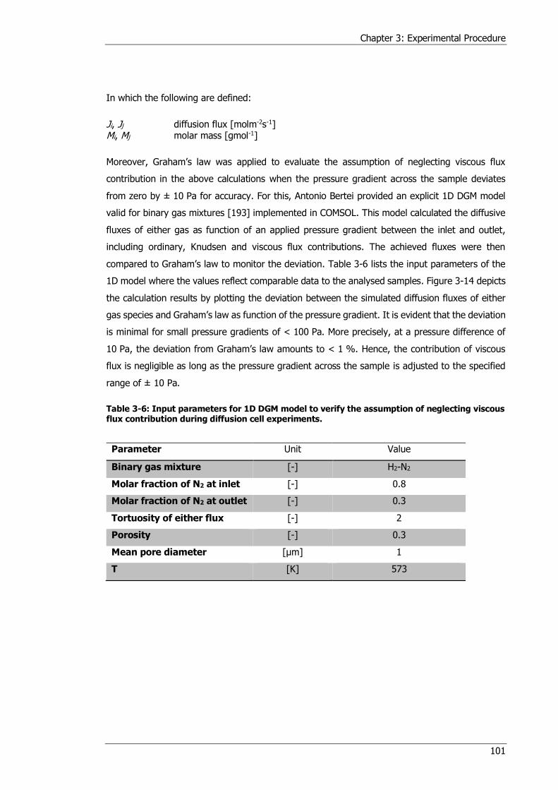
Chapter 3: Experimental Procedure
101
In which the following are defined:
Ji, Jj diffusion flux [molm-2s-1] Mi, Mj molar mass [gmol-1]
Moreover, Graham’s law was applied to evaluate the assumption of neglecting viscous flux
contribution in the above calculations when the pressure gradient across the sample deviates
from zero by ± 10 Pa for accuracy. For this, Antonio Bertei provided an explicit 1D DGM model
valid for binary gas mixtures [193] implemented in COMSOL. This model calculated the diffusive
fluxes of either gas as function of an applied pressure gradient between the inlet and outlet,
including ordinary, Knudsen and viscous flux contributions. The achieved fluxes were then
compared to Graham’s law to monitor the deviation. Table 3-6 lists the input parameters of the
1D model where the values reflect comparable data to the analysed samples. Figure 3-14 depicts
the calculation results by plotting the deviation between the simulated diffusion fluxes of either
gas species and Graham’s law as function of the pressure gradient. It is evident that the deviation
is minimal for small pressure gradients of < 100 Pa. More precisely, at a pressure difference of
10 Pa, the deviation from Graham’s law amounts to < 1 %. Hence, the contribution of viscous
flux is negligible as long as the pressure gradient across the sample is adjusted to the specified
range of ± 10 Pa.
Table 3-6: Input parameters for 1D DGM model to verify the assumption of neglecting viscous flux contribution during diffusion cell experiments.
Parameter Unit Value
Binary gas mixture [-] H2-N2
Molar fraction of N2 at inlet [-] 0.8
Molar fraction of N2 at outlet [-] 0.3
Tortuosity of either flux [-] 2
Porosity [-] 0.3
Mean pore diameter [μm] 1
T [K] 573
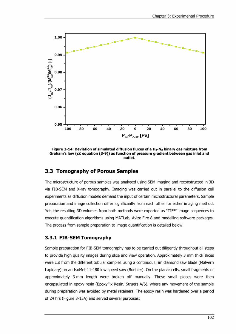
Chapter 3: Experimental Procedure
102
Figure 3-14: Deviation of simulated diffusion fluxes of a H2-N2 binary gas mixture from Graham's law (cf. equation (3-9)) as function of pressure gradient between gas inlet and
outlet.
3.3 Tomography of Porous Samples
The microstructure of porous samples was analysed using SEM imaging and reconstructed in 3D
via FIB-SEM and X-ray tomography. Imaging was carried out in parallel to the diffusion cell
experiments as diffusion models demand the input of certain microstructural parameters. Sample
preparation and image collection differ significantly from each other for either imaging method.
Yet, the resulting 3D volumes from both methods were exported as “TIFF” image sequences to
execute quantification algorithms using MATLab, Avizo Fire 8 and modelling software packages.
The process from sample preparation to image quantification is detailed below.
3.3.1 FIB-SEM Tomography
Sample preparation for FIB-SEM tomography has to be carried out diligently throughout all steps
to provide high quality images during slice and view operation. Approximately 3 mm thick slices
were cut from the different tubular samples using a continuous rim diamond saw blade (Malvern
Lapidary) on an IsoMet 11-180 low speed saw (Buehler). On the planar cells, small fragments of
approximately 3 mm length were broken off manually. These small pieces were then
encapsulated in epoxy resin (EpoxyFix Resin, Struers A/S), where any movement of the sample
during preparation was avoided by metal retainers. The epoxy resin was hardened over a period
of 24 hrs (Figure 3-15A) and served several purposes:
-100 -80 -60 -40 -20 0 20 40 60 80 100
0.95
0.96
0.97
0.98
0.99
1.00
(JH
2/J
N2)/
(M0
.5
N2/M
0.5
H2)
[-]
PIN
-POUT
[Pa]
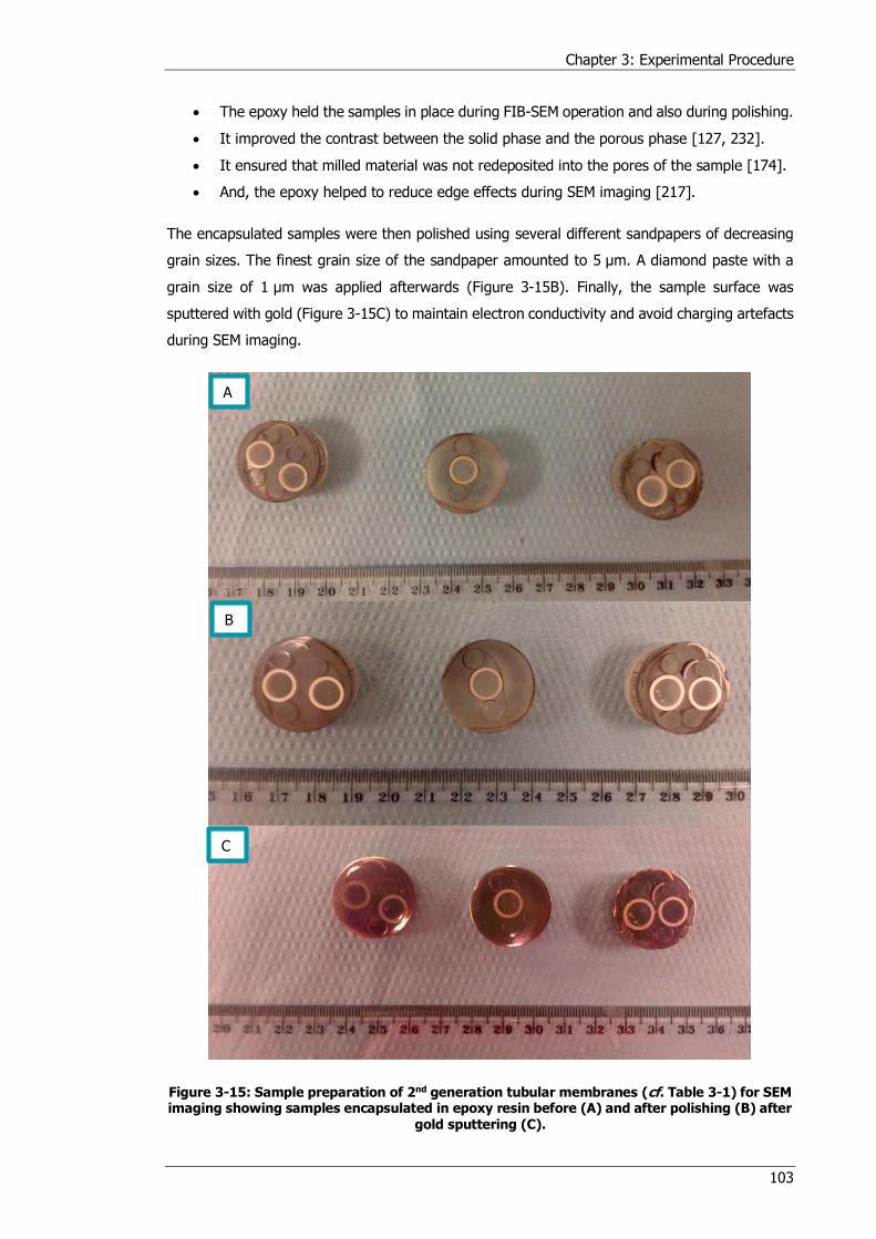
Chapter 3: Experimental Procedure
103
The epoxy held the samples in place during FIB-SEM operation and also during polishing.
It improved the contrast between the solid phase and the porous phase [127, 232].
It ensured that milled material was not redeposited into the pores of the sample [174].
And, the epoxy helped to reduce edge effects during SEM imaging [217].
The encapsulated samples were then polished using several different sandpapers of decreasing
grain sizes. The finest grain size of the sandpaper amounted to 5 μm. A diamond paste with a
grain size of 1 μm was applied afterwards (Figure 3-15B). Finally, the sample surface was
sputtered with gold (Figure 3-15C) to maintain electron conductivity and avoid charging artefacts
during SEM imaging.
Figure 3-15: Sample preparation of 2nd generation tubular membranes (cf. Table 3-1) for SEM imaging showing samples encapsulated in epoxy resin before (A) and after polishing (B) after
gold sputtering (C).
A
B
C
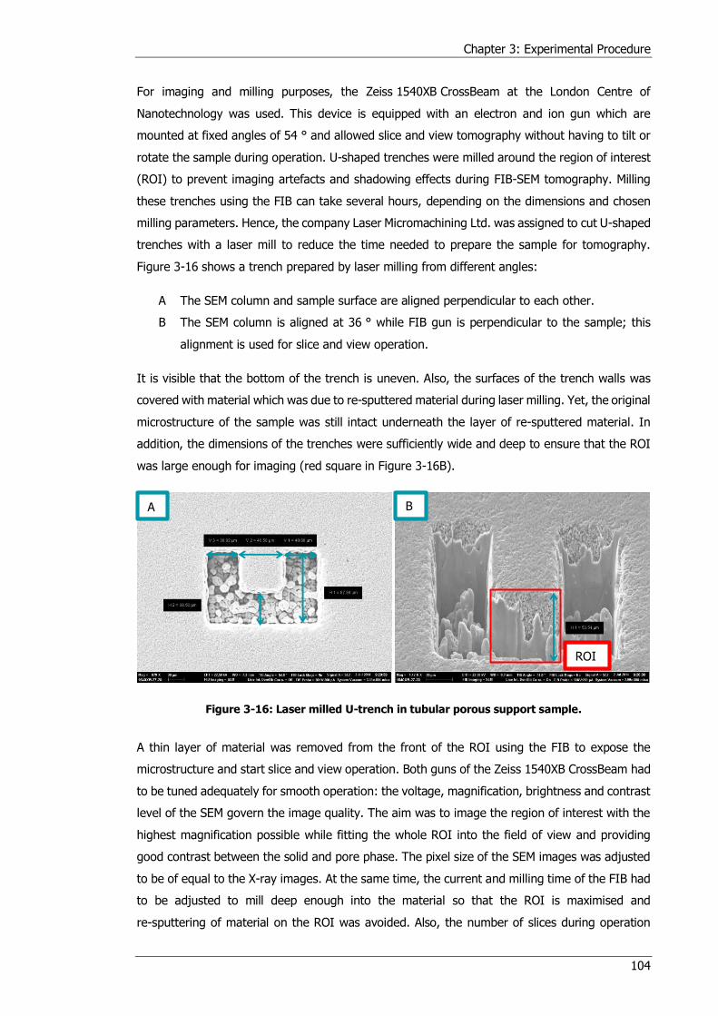
Chapter 3: Experimental Procedure
104
For imaging and milling purposes, the Zeiss 1540XB CrossBeam at the London Centre of
Nanotechnology was used. This device is equipped with an electron and ion gun which are
mounted at fixed angles of 54 ° and allowed slice and view tomography without having to tilt or
rotate the sample during operation. U-shaped trenches were milled around the region of interest
(ROI) to prevent imaging artefacts and shadowing effects during FIB-SEM tomography. Milling
these trenches using the FIB can take several hours, depending on the dimensions and chosen
milling parameters. Hence, the company Laser Micromachining Ltd. was assigned to cut U-shaped
trenches with a laser mill to reduce the time needed to prepare the sample for tomography.
Figure 3-16 shows a trench prepared by laser milling from different angles:
A The SEM column and sample surface are aligned perpendicular to each other.
B The SEM column is aligned at 36 ° while FIB gun is perpendicular to the sample; this
alignment is used for slice and view operation.
It is visible that the bottom of the trench is uneven. Also, the surfaces of the trench walls was
covered with material which was due to re-sputtered material during laser milling. Yet, the original
microstructure of the sample was still intact underneath the layer of re-sputtered material. In
addition, the dimensions of the trenches were sufficiently wide and deep to ensure that the ROI
was large enough for imaging (red square in Figure 3-16B).
Figure 3-16: Laser milled U-trench in tubular porous support sample.
A thin layer of material was removed from the front of the ROI using the FIB to expose the
microstructure and start slice and view operation. Both guns of the Zeiss 1540XB CrossBeam had
to be tuned adequately for smooth operation: the voltage, magnification, brightness and contrast
level of the SEM govern the image quality. The aim was to image the region of interest with the
highest magnification possible while fitting the whole ROI into the field of view and providing
good contrast between the solid and pore phase. The pixel size of the SEM images was adjusted
to be of equal to the X-ray images. At the same time, the current and milling time of the FIB had
to be adjusted to mill deep enough into the material so that the ROI is maximised and
re-sputtering of material on the ROI was avoided. Also, the number of slices during operation
A B
ROI

Chapter 3: Experimental Procedure
105
determined the pixel size along the milling axis and had to be correlated with the pixel size in the
SEM image.
Figure 3-17: First (A) and last (B) SEM image of FIB-SEM slice and view tomography.
The described slice and view method causes the ROI to move upwards during imaging as shown
in Figure 3-17. This can be overcome by manually adjusting the SEM after each image, which is
not practical. Hence, the resulting image sequence had to be processed to account for this shift.
This was done in a custom made MATLab script, which was developed in collaboration with Dr.
Leon Brown and Dami Taiwo at the University College London. The script is presented in Appendix
B and provided a cropped and aligned image sequence of the recorded dataset. The processed
image sequence was subsequently imported into Avizo Fire 8 to segment the solid and pore phase
of the image. Threshold segmentation [233] was considered to be a suitable tool as the samples
consisted only of two phases. These were easily distinguishable from each other due to the clear
distinct grey scale value (cf. Figure 3-17). The segmented sample volumes were exported as
“TIFF” image sequence. These served as basis for subsequent quantification algorithms to
determine microstructural parameters. Furthermore, the surface of the solid phase was extracted
as “ASCII.stl” file for simulation purposes in StarCCM+.
3.3.2 X-ray nano Computed Tomography
The Zeiss Xradia 810 Ultra machines located at the Manchester X-ray Imaging Facility and at the
Electrochemical Innovation Lab (EIL) at University College London were used for X-ray nano CT.
This X-ray device achieves voxel sizes of < 63.1 nm by the use of X-ray focussing optics [126].
This high magnification was necessary to capture all features of the sample microstructure that
affect diffusive mass transport. Yet, high magnification is coupled with a limited field of view
which amounts to < 65 μm in the Zeiss Xradia 810 Ultra.
A B
ROI

Chapter 3: Experimental Procedure
106
Figure 3-18: Operating principle of an X-ray nano CT system showing the optical components used to achieve a monochromatic beam.
The working principle of the nano CT system is depicted in Figure 3-18. The X-rays are generated
by applying a potential of 35 kV between a tungsten filament (cathode) and a chromium target
(anode). The Zeiss Xradia 810 Ultra achieves a quasi-monochromatic beam of 5.4 keV by filtering
out the Bremsstrahlung using the following X-ray optics:
A condenser lens made out of glass focuses the X-ray beams onto the rotating sample.
Furthermore, the condenser lens filters out high energy photons by its specific reflectivity
profile.
Between the condenser and the sample, a pin hole and a beam stopper are located.
These devices allow only beams which interacted with the condenser beforehand, to
reach the sample,
The Fresnel zone plate manufactured from gold uses diffraction to focus the transmitted
X-rays onto the detector. In addition, the diffraction efficiency of the zone plate is highest
for photon energies of 5.4 keV emitted by the target.
A Zernike phase ring is situated behind the Fresnel zone plate to shift the phase of the
X-ray beams during phase-contrast imaging.
Finally, the air gaps between the different optical components filter out low energy X-ray
photons.
Projections are taken and collected at discrete angles while the sample is rotating around its
longitudinal axis. The X-ray projections are recorded in the detector and converted into a visible
X-ray Source
Capillary Condenser
Pinhole
Sample
Fresnel Zone Plate
Zernike Phase Ring
Detector
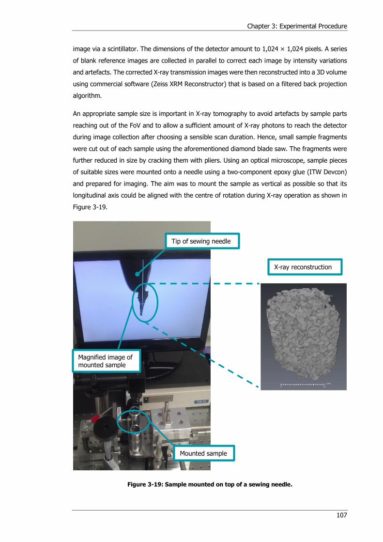
Chapter 3: Experimental Procedure
107
image via a scintillator. The dimensions of the detector amount to 1,024 × 1,024 pixels. A series
of blank reference images are collected in parallel to correct each image by intensity variations
and artefacts. The corrected X-ray transmission images were then reconstructed into a 3D volume
using commercial software (Zeiss XRM Reconstructor) that is based on a filtered back projection
algorithm.
An appropriate sample size is important in X-ray tomography to avoid artefacts by sample parts
reaching out of the FoV and to allow a sufficient amount of X-ray photons to reach the detector
during image collection after choosing a sensible scan duration. Hence, small sample fragments
were cut out of each sample using the aforementioned diamond blade saw. The fragments were
further reduced in size by cracking them with pliers. Using an optical microscope, sample pieces
of suitable sizes were mounted onto a needle using a two-component epoxy glue (ITW Devcon)
and prepared for imaging. The aim was to mount the sample as vertical as possible so that its
longitudinal axis could be aligned with the centre of rotation during X-ray operation as shown in
Figure 3-19.
Figure 3-19: Sample mounted on top of a sewing needle.
Tip of sewing needle
Magnified image of mounted sample
Mounted sample
X-ray reconstruction
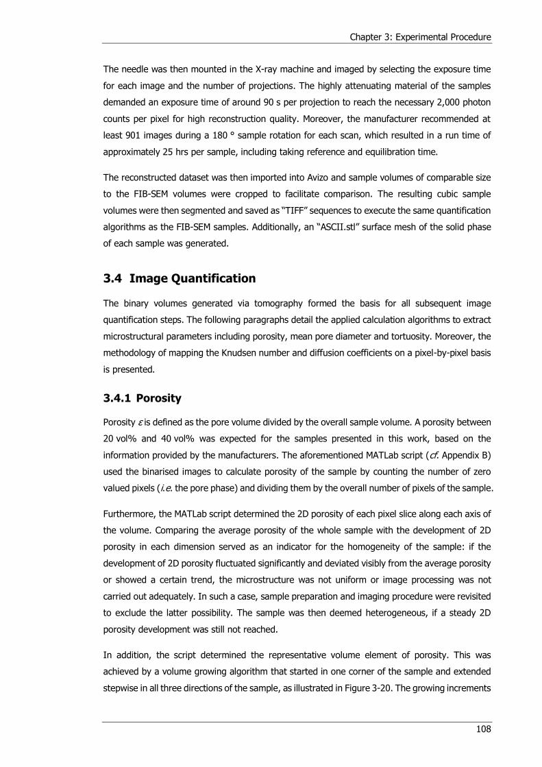
Chapter 3: Experimental Procedure
108
The needle was then mounted in the X-ray machine and imaged by selecting the exposure time
for each image and the number of projections. The highly attenuating material of the samples
demanded an exposure time of around 90 s per projection to reach the necessary 2,000 photon
counts per pixel for high reconstruction quality. Moreover, the manufacturer recommended at
least 901 images during a 180 ° sample rotation for each scan, which resulted in a run time of
approximately 25 hrs per sample, including taking reference and equilibration time.
The reconstructed dataset was then imported into Avizo and sample volumes of comparable size
to the FIB-SEM volumes were cropped to facilitate comparison. The resulting cubic sample
volumes were then segmented and saved as “TIFF” sequences to execute the same quantification
algorithms as the FIB-SEM samples. Additionally, an “ASCII.stl” surface mesh of the solid phase
of each sample was generated.
3.4 Image Quantification
The binary volumes generated via tomography formed the basis for all subsequent image
quantification steps. The following paragraphs detail the applied calculation algorithms to extract
microstructural parameters including porosity, mean pore diameter and tortuosity. Moreover, the
methodology of mapping the Knudsen number and diffusion coefficients on a pixel-by-pixel basis
is presented.
3.4.1 Porosity
Porosity ε is defined as the pore volume divided by the overall sample volume. A porosity between
20 vol% and 40 vol% was expected for the samples presented in this work, based on the
information provided by the manufacturers. The aforementioned MATLab script (cf. Appendix B)
used the binarised images to calculate porosity of the sample by counting the number of zero
valued pixels (i.e. the pore phase) and dividing them by the overall number of pixels of the sample.
Furthermore, the MATLab script determined the 2D porosity of each pixel slice along each axis of
the volume. Comparing the average porosity of the whole sample with the development of 2D
porosity in each dimension served as an indicator for the homogeneity of the sample: if the
development of 2D porosity fluctuated significantly and deviated visibly from the average porosity
or showed a certain trend, the microstructure was not uniform or image processing was not
carried out adequately. In such a case, sample preparation and imaging procedure were revisited
to exclude the latter possibility. The sample was then deemed heterogeneous, if a steady 2D
porosity development was still not reached.
In addition, the script determined the representative volume element of porosity. This was
achieved by a volume growing algorithm that started in one corner of the sample and extended
stepwise in all three directions of the sample, as illustrated in Figure 3-20. The growing increments
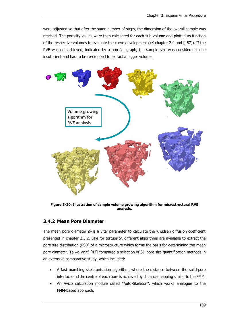
Chapter 3: Experimental Procedure
109
were adjusted so that after the same number of steps, the dimension of the overall sample was
reached. The porosity values were then calculated for each sub-volume and plotted as function
of the respective volumes to evaluate the curve development (cf. chapter 2.4 and [187]). If the
RVE was not achieved, indicated by a non-flat graph, the sample size was considered to be
insufficient and had to be re-cropped to extract a bigger volume.
Figure 3-20: Illustration of sample volume growing algorithm for microstructural RVE analysis.
3.4.2 Mean Pore Diameter
The mean pore diameter dP is a vital parameter to calculate the Knudsen diffusion coefficient
presented in chapter 2.3.2. Like for tortuosity, different algorithms are available to extract the
pore size distribution (PSD) of a microstructure which forms the basis for determining the mean
pore diameter. Taiwo et al. [43] compared a selection of 3D pore size quantification methods in
an extensive comparative study, which included:
A fast marching skeletonisation algorithm, where the distance between the solid-pore
interface and the centre of each pore is achieved by distance mapping similar to the FMM.
An Avizo calculation module called “Auto-Skeleton”, which works analogue to the
FMM-based approach.
Volume growing algorithm for RVE analysis.
Chapter 3: Experimental Procedure
110
A successive morphological opening method, which uses a spherical structural element
of increasing size to determine the volume fraction of pores of a certain diameter.
A continuous pore size distribution method developed by Münch and Holzer [233], which
computes the pore volume fraction that can be filled with a sphere of a certain diameter.
Among these methods, the authors considered the continuous pore size distribution (cPSD)
method from Münch and Holzer the most accurate: unlike the other methods, this algorithm takes
the entirety of the pore network into account and thus, ensures highest precisions. As a
consequence, the cPSD method was applied in this project via an open-source ImageJ plugin
[233] which uses the “TIFF” image sequence as input file.
The cPSD algorithm produces a cumulative pore size distribution chart including the whole range
of pore radii measured in the sample. The raw data of the PSD chart was then used to draw a
pore diameter histogram and calculate the mean pore diameter. However, despite the high
precision of this approach, the orientation or elongation of pores is not provided. For this purpose,
the 2D pore diameter dP,2D of each image slice along each axis of the sample was calculated using
a stereological relation presented in equation (3-10) [101, 234]. The calculation of dP,2D was
implemented in a MATLAB script [225]. Similar to the 2D porosity analysis, the 2D pore diameter
curves along each axis of a sample are an indicator for elongated pores or an accumulation of
constrictions in a certain dimension.
𝑑𝑃,2𝐷 = 4𝑉𝑃𝑆𝑣
(3-10)
In which the following are defined:
dP,2D 2D pore diameter [μm] VP pore volume fraction [-] Sv interface length between the two phases per unit volume [μm2μm-3]
3.4.3 Tortuosity
Due to the importance of tortuosity in the field of electrochemistry, a wide variety of image-based
tortuosity calculation algorithms have been developed. Such algorithms can be broadly
distinguished between geometric and flux-based methods as introduced in chapter 2.2.4. A
selection of image-based tortuosity calculation techniques of either category was applied on the
sample volumes of this project for comparison purposes. The chosen methods are all routinely
applied in the electrochemical community, predominately to evaluate the resistance of a porous
structure to a flux. The algorithms considered here include the fast marching method, the pore
centroid method, the Laplace equation solver and porosity-tortuosity calculation approaches.
These methods were executed directly on the voxel domain of the samples in comparison to the
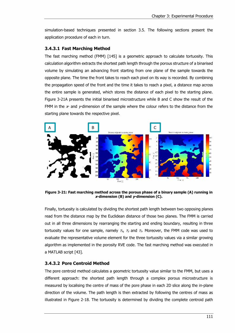
Chapter 3: Experimental Procedure
111
simulation-based techniques presented in section 3.5. The following sections present the
application procedure of each in turn.
3.4.3.1 Fast Marching Method
The fast marching method (FMM) [145] is a geometric approach to calculate tortuosity. This
calculation algorithm extracts the shortest path length through the porous structure of a binarised
volume by simulating an advancing front starting from one plane of the sample towards the
opposite plane. The time the front takes to reach each pixel on its way is recorded. By combining
the propagation speed of the front and the time it takes to reach a pixel, a distance map across
the entire sample is generated, which stores the distance of each pixel to the starting plane.
Figure 3-21A presents the initial binarised microstructure while B and C show the result of the
FMM in the x- and y-dimension of the sample where the colour refers to the distance from the
starting plane towards the respective pixel.
Figure 3-21: Fast marching method across the porous phase of a binary sample (A) running in x-dimension (B) and y-dimension (C).
Finally, tortuosity is calculated by dividing the shortest path length between two opposing planes
read from the distance map by the Euclidean distance of those two planes. The FMM is carried
out in all three dimensions by rearranging the starting and ending boundary, resulting in three
tortuosity values for one sample, namely τx, τy and τz. Moreover, the FMM code was used to
evaluate the representative volume element for the three tortuosity values via a similar growing
algorithm as implemented in the porosity RVE code. The fast marching method was executed in
a MATLAB script [43].
3.4.3.2 Pore Centroid Method
The pore centroid method calculates a geometric tortuosity value similar to the FMM, but uses a
different approach: the shortest path length through a complex porous microstructure is
measured by localising the centre of mass of the pore phase in each 2D slice along the in-plane
direction of the volume. The path length is then extracted by following the centres of mass as
illustrated in Figure 2-18. The tortuosity is determined by dividing the complete centroid path
A B C
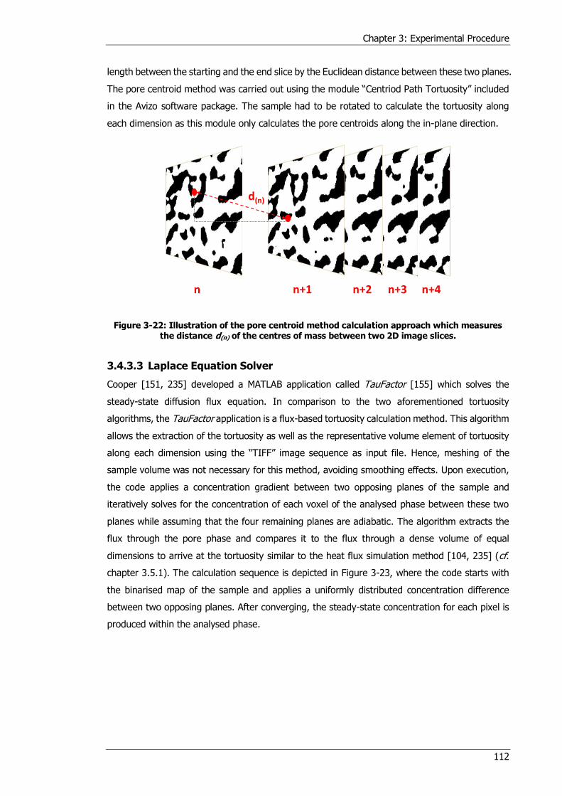
Chapter 3: Experimental Procedure
112
length between the starting and the end slice by the Euclidean distance between these two planes.
The pore centroid method was carried out using the module “Centriod Path Tortuosity” included
in the Avizo software package. The sample had to be rotated to calculate the tortuosity along
each dimension as this module only calculates the pore centroids along the in-plane direction.
Figure 3-22: Illustration of the pore centroid method calculation approach which measures the distance d(n) of the centres of mass between two 2D image slices.
3.4.3.3 Laplace Equation Solver
Cooper [151, 235] developed a MATLAB application called TauFactor [155] which solves the
steady-state diffusion flux equation. In comparison to the two aforementioned tortuosity
algorithms, the TauFactor application is a flux-based tortuosity calculation method. This algorithm
allows the extraction of the tortuosity as well as the representative volume element of tortuosity
along each dimension using the “TIFF” image sequence as input file. Hence, meshing of the
sample volume was not necessary for this method, avoiding smoothing effects. Upon execution,
the code applies a concentration gradient between two opposing planes of the sample and
iteratively solves for the concentration of each voxel of the analysed phase between these two
planes while assuming that the four remaining planes are adiabatic. The algorithm extracts the
flux through the pore phase and compares it to the flux through a dense volume of equal
dimensions to arrive at the tortuosity similar to the heat flux simulation method [104, 235] (cf.
chapter 3.5.1). The calculation sequence is depicted in Figure 3-23, where the code starts with
the binarised map of the sample and applies a uniformly distributed concentration difference
between two opposing planes. After converging, the steady-state concentration for each pixel is
produced within the analysed phase.
d(n)
n n+1 n+2 n+3 n+4
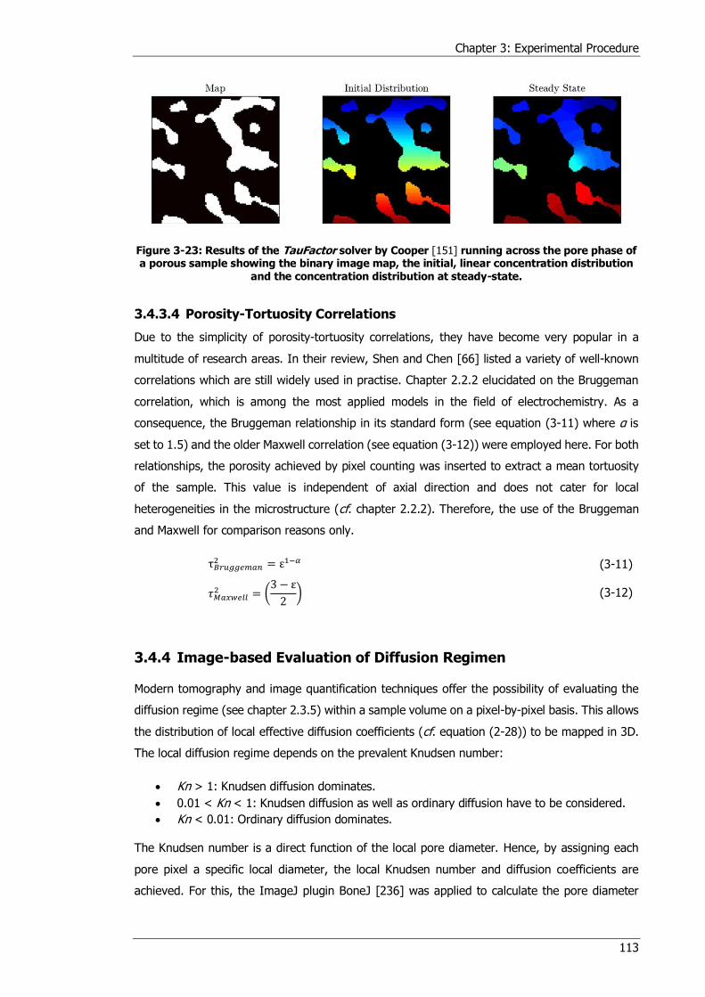
Chapter 3: Experimental Procedure
113
Figure 3-23: Results of the TauFactor solver by Cooper [151] running across the pore phase of a porous sample showing the binary image map, the initial, linear concentration distribution
and the concentration distribution at steady-state.
3.4.3.4 Porosity-Tortuosity Correlations
Due to the simplicity of porosity-tortuosity correlations, they have become very popular in a
multitude of research areas. In their review, Shen and Chen [66] listed a variety of well-known
correlations which are still widely used in practise. Chapter 2.2.2 elucidated on the Bruggeman
correlation, which is among the most applied models in the field of electrochemistry. As a
consequence, the Bruggeman relationship in its standard form (see equation (3-11) where α is
set to 1.5) and the older Maxwell correlation (see equation (3-12)) were employed here. For both
relationships, the porosity achieved by pixel counting was inserted to extract a mean tortuosity
of the sample. This value is independent of axial direction and does not cater for local
heterogeneities in the microstructure (cf. chapter 2.2.2). Therefore, the use of the Bruggeman
and Maxwell for comparison reasons only.
τ𝐵𝑟𝑢𝑔𝑔𝑒𝑚𝑎𝑛2 = ε1−𝛼 (3-11)
𝜏𝑀𝑎𝑥𝑤𝑒𝑙𝑙2 = (
3 − ε
2) (3-12)
3.4.4 Image-based Evaluation of Diffusion Regimen
Modern tomography and image quantification techniques offer the possibility of evaluating the
diffusion regime (see chapter 2.3.5) within a sample volume on a pixel-by-pixel basis. This allows
the distribution of local effective diffusion coefficients (cf. equation (2-28)) to be mapped in 3D.
The local diffusion regime depends on the prevalent Knudsen number:
Kn > 1: Knudsen diffusion dominates.
0.01 < Kn < 1: Knudsen diffusion as well as ordinary diffusion have to be considered.
Kn < 0.01: Ordinary diffusion dominates.
The Knudsen number is a direct function of the local pore diameter. Hence, by assigning each
pore pixel a specific local diameter, the local Knudsen number and diffusion coefficients are
achieved. For this, the ImageJ plugin BoneJ [236] was applied to calculate the pore diameter
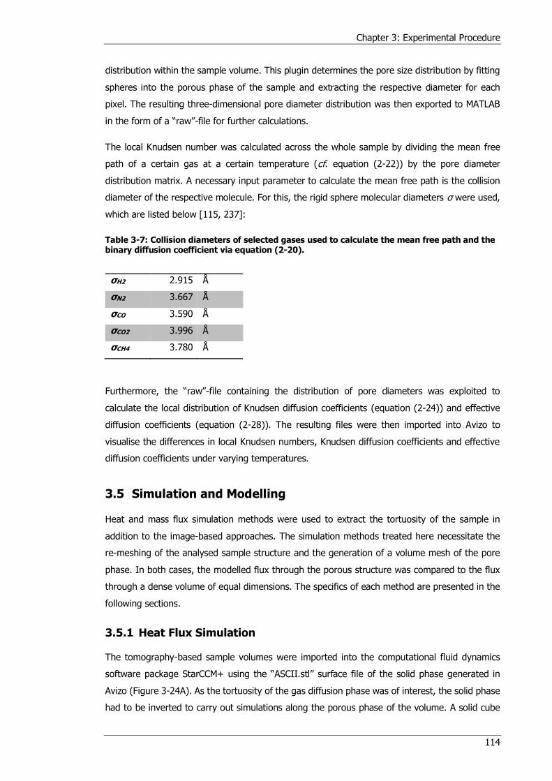
Chapter 3: Experimental Procedure
114
distribution within the sample volume. This plugin determines the pore size distribution by fitting
spheres into the porous phase of the sample and extracting the respective diameter for each
pixel. The resulting three-dimensional pore diameter distribution was then exported to MATLAB
in the form of a “raw”-file for further calculations.
The local Knudsen number was calculated across the whole sample by dividing the mean free
path of a certain gas at a certain temperature (cf. equation (2-22)) by the pore diameter
distribution matrix. A necessary input parameter to calculate the mean free path is the collision
diameter of the respective molecule. For this, the rigid sphere molecular diameters σ were used,
which are listed below [115, 237]:
Table 3-7: Collision diameters of selected gases used to calculate the mean free path and the binary diffusion coefficient via equation (2-20).
σH2 2.915 Å
σN2 3.667 Å
σCO 3.590 Å
σCO2 3.996 Å
σCH4 3.780 Å
Furthermore, the “raw”-file containing the distribution of pore diameters was exploited to
calculate the local distribution of Knudsen diffusion coefficients (equation (2-24)) and effective
diffusion coefficients (equation (2-28)). The resulting files were then imported into Avizo to
visualise the differences in local Knudsen numbers, Knudsen diffusion coefficients and effective
diffusion coefficients under varying temperatures.
3.5 Simulation and Modelling
Heat and mass flux simulation methods were used to extract the tortuosity of the sample in
addition to the image-based approaches. The simulation methods treated here necessitate the
re-meshing of the analysed sample structure and the generation of a volume mesh of the pore
phase. In both cases, the modelled flux through the porous structure was compared to the flux
through a dense volume of equal dimensions. The specifics of each method are presented in the
following sections.
3.5.1 Heat Flux Simulation
The tomography-based sample volumes were imported into the computational fluid dynamics
software package StarCCM+ using the “ASCII.stl” surface file of the solid phase generated in
Avizo (Figure 3-24A). As the tortuosity of the gas diffusion phase was of interest, the solid phase
had to be inverted to carry out simulations along the porous phase of the volume. A solid cube
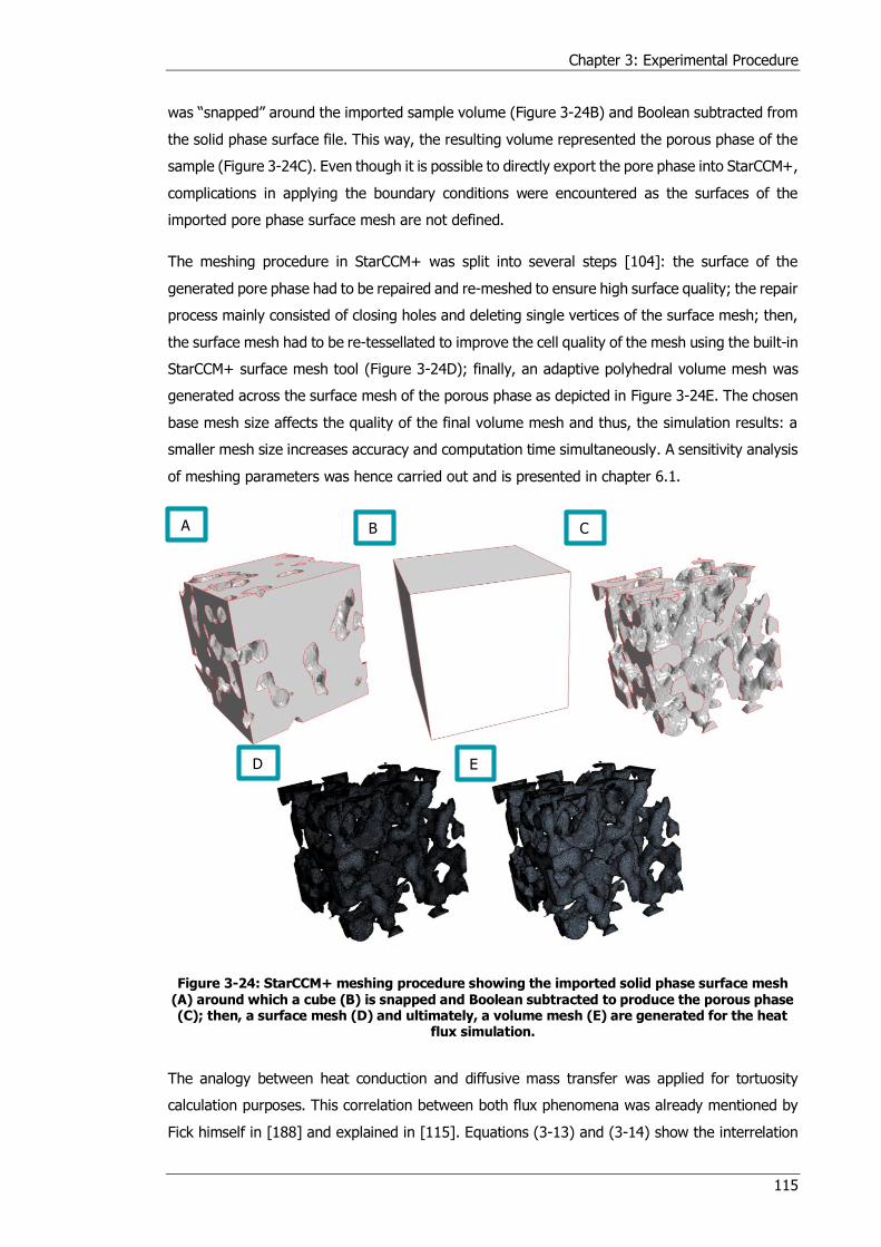
Chapter 3: Experimental Procedure
115
was “snapped” around the imported sample volume (Figure 3-24B) and Boolean subtracted from
the solid phase surface file. This way, the resulting volume represented the porous phase of the
sample (Figure 3-24C). Even though it is possible to directly export the pore phase into StarCCM+,
complications in applying the boundary conditions were encountered as the surfaces of the
imported pore phase surface mesh are not defined.
The meshing procedure in StarCCM+ was split into several steps [104]: the surface of the
generated pore phase had to be repaired and re-meshed to ensure high surface quality; the repair
process mainly consisted of closing holes and deleting single vertices of the surface mesh; then,
the surface mesh had to be re-tessellated to improve the cell quality of the mesh using the built-in
StarCCM+ surface mesh tool (Figure 3-24D); finally, an adaptive polyhedral volume mesh was
generated across the surface mesh of the porous phase as depicted in Figure 3-24E. The chosen
base mesh size affects the quality of the final volume mesh and thus, the simulation results: a
smaller mesh size increases accuracy and computation time simultaneously. A sensitivity analysis
of meshing parameters was hence carried out and is presented in chapter 6.1.
Figure 3-24: StarCCM+ meshing procedure showing the imported solid phase surface mesh (A) around which a cube (B) is snapped and Boolean subtracted to produce the porous phase (C); then, a surface mesh (D) and ultimately, a volume mesh (E) are generated for the heat
flux simulation.
The analogy between heat conduction and diffusive mass transfer was applied for tortuosity
calculation purposes. This correlation between both flux phenomena was already mentioned by
Fick himself in [188] and explained in [115]. Equations (3-13) and (3-14) show the interrelation
A B C
D E
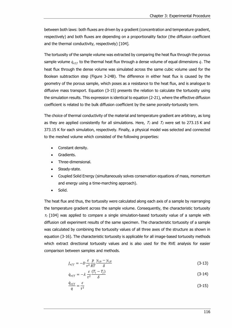
Chapter 3: Experimental Procedure
116
between both laws: both fluxes are driven by a gradient (concentration and temperature gradient,
respectively) and both fluxes are depending on a proportionality factor (the diffusion coefficient
and the thermal conductivity, respectively) [104].
The tortuosity of the sample volume was extracted by comparing the heat flux through the porous
sample volume ��𝑒𝑓𝑓 to the thermal heat flux through a dense volume of equal dimensions ��. The
heat flux through the dense volume was simulated across the same cubic volume used for the
Boolean subtraction step (Figure 3-24B). The difference in either heat flux is caused by the
geometry of the porous sample, which poses as a resistance to the heat flux, and is analogue to
diffusive mass transport. Equation (3-15) presents the relation to calculate the tortuosity using
the simulation results. This expression is identical to equation (2-21), where the effective diffusion
coefficient is related to the bulk diffusion coefficient by the same porosity-tortuosity term.
The choice of thermal conductivity of the material and temperature gradient are arbitrary, as long
as they are applied consistently for all simulations. Here, T1 and T2 were set to 273.15 K and
373.15 K for each simulation, respectively. Finally, a physical model was selected and connected
to the meshed volume which consisted of the following properties:
Constant density.
Gradients.
Three-dimensional.
Steady-state.
Coupled Solid Energy (simultaneously solves conservation equations of mass, momentum
and energy using a time-marching approach).
Solid.
The heat flux and thus, the tortuosity were calculated along each axis of a sample by rearranging
the temperature gradient across the sample volume. Consequently, the characteristic tortuosity
τc [104] was applied to compare a single simulation-based tortuosity value of a sample with
diffusion cell experiment results of the same specimen. The characteristic tortuosity of a sample
was calculated by combining the tortuosity values of all three axes of the structure as shown in
equation (3-16). The characteristic tortuosity is applicable for all image-based tortuosity methods
which extract directional tortuosity values and is also used for the RVE analysis for easier
comparison between samples and methods.
𝐽𝑒𝑓𝑓 = −𝐷휀
𝜏2𝑝
𝑅𝑇
𝑦𝑖,0 − 𝑦𝑖,𝛿𝛿
(3-13)
��𝑒𝑓𝑓 = −𝜆 휀
𝜏2(𝑇𝑖 − 𝑇𝑗)
𝛿 (3-14)
��𝑒𝑓𝑓𝑞
=휀
𝜏2 (3-15)
Chapter 3: Experimental Procedure
117
𝜏𝑐 = 3[(𝜏𝑥−1) + (𝜏𝑦
−1) + (𝜏𝑧−1)]
−1 (3-16)
In which the following are defined:
Jeff effective diffusion flux [mol/(m2∙s)] D diffusion coefficient [m²/s] p pressure [Pa] R ideal gas constant [Jmol-1K-1] T temperature [K]
yi molar fraction [-] ��eff effective thermal heat flux [W/m2] �� thermal heat flux [W/m2] λ thermal conductivity [W/(m∙K)] ε porosity [-] τ tortuosity [-] Ti, Tj temperature [K] δ thickness of membrane [m] τc characteristic tortuosity [-] τx, τy, τz tortuosity in x-, y- and z-dimension [-]
3.5.2 Mass Flux Simulation
The diffusive mass transport of binary gas mixtures through the porous phase was simulated in
COMSOL Multiphysics (COMSOL Inc.). The reconstructed volumes had to be meshed to execute
the appropriate physical calculation models, similar to the heat flux simulation. Although COMSOL
contains a mesh generation module, it was not possible to directly import a surface file or binary
image sequence of the sample and use this as a framework for the volume mesh generation.
Hence, a separate software, namely ScanIP (Simpleware Ltd.), was used for this purpose.
The binary “TIFF” image stack of the cropped samples was imported into ScanIP, where the pore
phase of the sample had to be segmented to create a 3D mask. It is noteworthy that the correct
length-scale of the imported “TIFF” sequence had to be defined to ensure accuracy during the
simulation of Knudsen diffusion. A CFD model was generated based on the 3D mask by choosing
the compound coarseness level of the tetrahedral mesh. The number of mesh elements was
adjusted by varying the coarseness level between - 50 (coarse) and + 50 (fine), comparable to
the base mesh size in StarCCM+. As ScanIP directly generates a volume mesh of the imported
image sequence, no intermediate surface mesh generation or mesh repairing steps had to be
carried out. The effect of the mesh quality on the results is evaluated in chapter 6.1. The
generated volume mesh was then exported as a COMSOL mesh volume with the file format
“mphtxt”.
It is possible to simulate a wide range of different physical, chemical and mechanical phenomena
In COMSOL. The physical model “Transport of Concentrated Species” was selected to simulate
diffusion mechanisms with the 3D structure [238]. This model allows the direct comparison
between Fick’s law and Fick’s law including Knudsen diffusion for different binary gas mixtures.
Chapter 3: Experimental Procedure
118
Knudsen diffusion was included in the model using the Bosanquet equation (see equation (2-28)).
The binary diffusion coefficient and the Knudsen diffusion coefficient had to be inserted into the
software as input parameters as COMSOL’s material library does not contain these coefficients.
Moreover, there was no possibility of calculating the variation in pore diameter on a pixel-by-pixel
basis. Therefore, rather than being able to calculate a local diffusion coefficient as discussed in
chapter 3.4.4, a mean pore diameter and thus, an average effective diffusion coefficient was used
for mass flux simulation.
In addition, a parametric sweep analysis was added to the model, where the temperature was
gradually increased from 298.15 K to 1298.15 K in steps of 100 K. This means that the diffusion
flux of a chosen diffusion model, binary gas mixture and diffusion direction was calculated for the
whole range of temperatures automatically. The equations for calculating the binary and Knudsen
diffusion coefficients were inserted into COMSOL and made a function of the temperature change
in the parametric study to ensure that the coefficients scale with temperature accurately.
The direction of the binary diffusion flux was adjusted by applying a mass fraction of unity and
zero of a chosen gas on two opposite surfaces, respectively. The axis of diffusion was changed
when rearranging the mass fraction gradient across the sample analogue to the heat flux
simulation. Finally, the diffusion flux through the porous phase was compared to the diffusion
flux of a dense cube of equal dimensions by using equation (3-15) to calculate the directional
tortuosity.
3.6 Summary of Experimental Procedure
This chapter presented the applied experimental techniques which were used to quantify the
diffusion resistance of porous support layers. The porous support samples, described in section
3.1, were provided by Praxair Inc. with the purpose of analysing the complex interrelation
between microstructural parameters and diffusive mass transport. More precisely, the effect of
porosity and sample thickness is of interest and reflected by the types of samples provided.
Section 3.2 describes the design of the diffusion cell test rig to measure gas diffusion through the
planar and tubular samples under varying temperature and for different binary gas mixtures. As
diffusion models, Fick’s law and the equimass diffusion model were extended by Knudsen
diffusion expressions via the Bosanquet equation to cater for molecule-wall collisions encountered
in the porous samples. In addition, the more sophisticated dusty gas model was consulted as well
for comparison purposes. However, to fit the specific experimental conditions, the implicit DGM
was converted into an explicit equation and simplified, to include Knudsen and ordinary diffusion
expressions only.
Tomographic datasets of the porous support samples form the basis of subsequent image
quantification and simulation techniques. Hence, section 3.3 elucidates the sample preparation

Chapter 3: Experimental Procedure
119
procedure for FIB-SEM and X-ray nano CT. Image quantification and flux simulation techniques,
which use the reconstructed 3D volumes extracted via both methods to determine microstructural
characteristics, are explained in sections 3.4 and 3.5. Here, the focus is on tortuosity calculation
approaches. A thorough study of the interplay between microstructural characteristics and
diffusion phenomena is provided by combining the conclusions drawn from the diffusion cell
experiments and the image-based quantification algorithms. The results of these different
analysis methods are presented in the following chapters, where chapter 4 through 6 focus on
individual experimental techniques.
Chapter 4: Diffusion Cell Experiments
120
4 Diffusion Cell Experiments
This chapter presents the results of the diffusion cell experiments and is split into several
sub-sections to focus on individual phenomena observed when varying experimental conditions.
The selection of a fitting diffusion model, which accounts for all transport processes encountered
within the analysed sample, was crucial to extract accurate results. Hence, section 4.1 assesses
the suitability of different models to determine the tortuosity of porous support layer samples
using diffusion cell experiments. The planar sample 100% TZ3YSB K was used to compare and
evaluate Fick’s law, the equimass diffusion model and the dusty gas model, introduced in chapter
3.2.4. The planar cell was then further applied to analyse the effect of varying gas composition
on the calculated tortuosity values presented in section 4.2. Binary gas mixtures included CH4-N2,
CO-N2 and CO2-N2 and the mole fractions of the fuel gases were varied between 100 mol% and
70 mol%.
Diffusion cell experiments were started using the planar sample due to its easier implementation
and operating principle. However, the porous support membranes and the OTMs manufactured
and provided by Praxair Inc. were of tubular shape. Hence, the results of the planar sample were
correlated to the results of the tubular sample PS 2310 1360C in section 4.3. Both samples were
manufactured using the same powders and sintering conditions and hence, it was investigated,
if the different diffusion cell layouts resulted in comparable tortuosity values.
The tubular diffusion cell is capable of accommodating sample tubes of different lengths, in
contrast to the restricted sample dimensions fitting into the planar diffusion cell. This is why
section 4.4 analyses the effect of tube length of the current generation tubular porous support
membranes (cf. Table 3-3) on the observed diffusion mechanisms. The outcome of this analysis
feeds back into the design process for scaling future OTM reactors up and out.
The experiments in the above sections were carried out at ambient temperature. Yet, the
operating temperature of the OTM is approximately 1,000 °C (cf. chapter 2.1.4). As a
consequence, the effect of elevated operating temperature of diffusion cell experiments on the
measured transport phenomena was studied in section 4.5 using the current generation porous
support membranes. The temperature was increased to 600 °C in steps of 100 °C and
measurements were taken at each step.
Praxair Inc. aims to improve the mechanical stability and long-term durability of the overall OTM
assembly by adjusting the thickness and porosity of the current porous support layer design.
Section 4.6 investigates the impact of both of these characteristics on the diffusion performance.
This was realised by the sample tubes supplied by Praxair Inc., which differed in thickness,
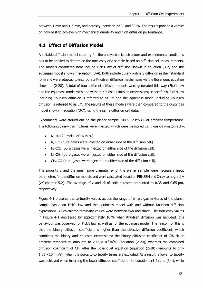
Chapter 4: Diffusion Cell Experiments
121
between 1 mm and 1.3 mm, and porosity, between 22 % and 30 %. The results provide a verdict
on how best to achieve high mechanical durability and high diffusion performance.
4.1 Effect of Diffusion Model
A suitable diffusion model catering for the analysed microstructure and experimental conditions
has to be applied to determine the tortuosity of a sample based on diffusion cell measurements.
The models considered here include Fick’s law of diffusion shown in equation (3-2) and the
equimass model shown in equation (3-4). Both include purely ordinary diffusion in their standard
form and were adapted to incorporate Knudsen diffusion mechanisms via the Bosanquet equation
shown in (2-28). A total of four different diffusion models were generated this way (Fick’s law
and the equimass model with and without Knudsen diffusion expressions). Henceforth, Fick’s law
including Knudsen diffusion is referred to as FM and the equimass model including Knudsen
diffusion is referred to as EM. The results of these models were then compared to the dusty gas
model shown in equation (3-7), using the same diffusion cell data.
Experiments were carried out on the planar sample 100% TZ3YSB K at ambient temperature.
The following binary gas mixtures were injected, which were measured using gas chromatography:
N2-H2 (20 mol% of H2 in N2).
N2-CO (pure gases were injected on either side of the diffusion cell).
N2-CO2 (pure gases were injected on either side of the diffusion cell).
N2-CH4 (pure gases were injected on either side of the diffusion cell).
CH4-CO (pure gases were injected on either side of the diffusion cell).
The porosity ε and the mean pore diameter dP of the planar sample were necessary input
parameters for the diffusion models and were calculated based on FIB-SEM and X-ray tomography
(cf. chapter 5.2). The average of ε and dP of both datasets amounted to 0.38 and 0.65 μm,
respectively.
Figure 4-1 presents the tortuosity values across the range of binary gas mixtures of the planar
sample based on Fick’s law and the equimass model with and without Knudsen diffusion
expressions. All calculated tortuosity values were between two and three. The tortuosity values
in Figure 4-1 decreased by approximately 10 % when Knudsen diffusion was included, this
behaviour was observed for Fick’s law as well as for the equimass model. The reason for this is
that the binary diffusion coefficient is higher than the effective diffusion coefficient, which
combines the binary and Knudsen expressions: the binary diffusion coefficient of CH4-N2 at
ambient temperature amounts to 2.14 ×10⁻⁵ m2s-1 (equation (2-20)) whereas the combined
diffusion coefficient of CH4 after the Bosanquet equation (equation (2-28)) amounts to only
1.85 ×10⁻⁵ m2s-1, when the porosity-tortuosity terms are excluded. As a result, a lower tortuosity
was achieved when inserting the lower diffusion coefficient into equations (3-2) and (3-4), while
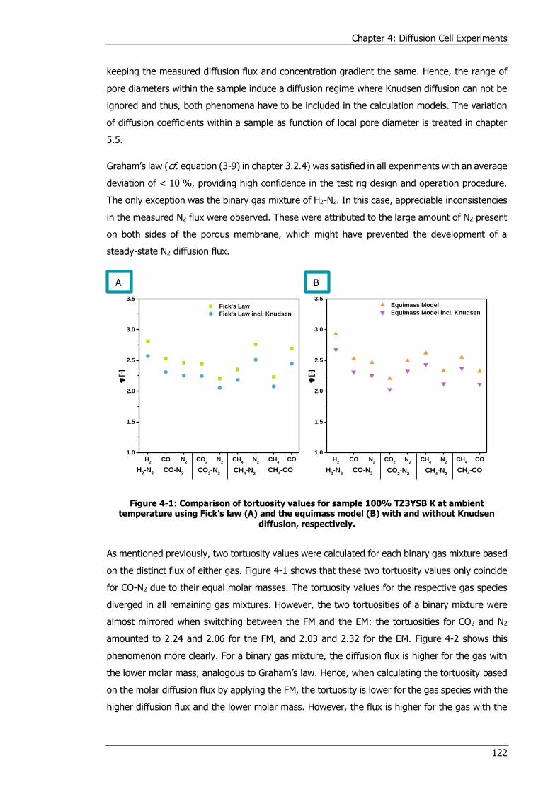
Chapter 4: Diffusion Cell Experiments
122
keeping the measured diffusion flux and concentration gradient the same. Hence, the range of
pore diameters within the sample induce a diffusion regime where Knudsen diffusion can not be
ignored and thus, both phenomena have to be included in the calculation models. The variation
of diffusion coefficients within a sample as function of local pore diameter is treated in chapter
5.5.
Graham’s law (cf. equation (3-9) in chapter 3.2.4) was satisfied in all experiments with an average
deviation of < 10 %, providing high confidence in the test rig design and operation procedure.
The only exception was the binary gas mixture of H2-N2. In this case, appreciable inconsistencies
in the measured N2 flux were observed. These were attributed to the large amount of N2 present
on both sides of the porous membrane, which might have prevented the development of a
steady-state N2 diffusion flux.
Figure 4-1: Comparison of tortuosity values for sample 100% TZ3YSB K at ambient temperature using Fick's law (A) and the equimass model (B) with and without Knudsen
diffusion, respectively.
As mentioned previously, two tortuosity values were calculated for each binary gas mixture based
on the distinct flux of either gas. Figure 4-1 shows that these two tortuosity values only coincide
for CO-N2 due to their equal molar masses. The tortuosity values for the respective gas species
diverged in all remaining gas mixtures. However, the two tortuosities of a binary mixture were
almost mirrored when switching between the FM and the EM: the tortuosities for CO2 and N2
amounted to 2.24 and 2.06 for the FM, and 2.03 and 2.32 for the EM. Figure 4-2 shows this
phenomenon more clearly. For a binary gas mixture, the diffusion flux is higher for the gas with
the lower molar mass, analogous to Graham’s law. Hence, when calculating the tortuosity based
on the molar diffusion flux by applying the FM, the tortuosity is lower for the gas species with the
higher diffusion flux and the lower molar mass. However, the flux is higher for the gas with the
H2
CO N2
CO2
N2
CH4
N2
CH4
CO1.0
1.5
2.0
2.5
3.0
3.5
H2
CO N2
CO2
N2
CH4
N2
CH4
CO1.0
1.5
2.0
2.5
3.0
3.5
Fick's Law
Fick's Law incl. Knudsen
[-
]
H2-N
2CO-N
2CH
4-N
2CH
4-COCO
2-N
2
Equimass Model
Equimass Model incl. Knudsen
[-]
H2-N
2CO-N
2CH
4-N
2CH
4-COCO
2-N
2
A B

Chapter 4: Diffusion Cell Experiments
123
higher molar mass when converting the molar diffusion flux into a mass diffusion flux. The gas
with the higher molar mass featuring the higher mass flux achieves the lower tortuosity when
now applying the EM, resulting in the mirrored tortuosity values.
Even though H2 is the lightest gas, it did not feature the lowest tortuosity in either model. This
seems counterintuitive following the above argument: when applying the FM, the lightest and
smallest gas is expected to diffuse through the porous membrane the easiest. Yet, this was not
shown in the diffusion cell experiments and similar results were presented in [110]. The reason
for the higher tortuosity of H2 compared to all other gases might stem from the larger mean free
path of H2 (cf. chapter 5.5), which results in a larger Knudsen number. This pushes the diffusion
regime closer towards Knudsen diffusion, where molecule-wall collisions dominate. Moreover, the
inconsistencies observed with the N2 flux in the H2-N2 mixture might also affect the H2 flux,
causing additional disparity in the extracted tortuosities. Hence, H2 was not used for subsequent
experiments.
Figure 4-2 introduces the tortuosity values calculated via the dusty gas model according to
equation (3-7) and compares them to the results of the FM and EM. The tortuosity values based
on the DGM were between the FM and EM. The only exception was the H2-based tortuosity, which
was attributed to the above inconsistencies. The dusty gas model provided an almost constant
tortuosity value for the sample across all the analysed gases with tortuosities lying in a narrow
band between 2.2 and 2.3, when disregarding H2. The width of this band increased, however,
when consulting the EM and even more so when analysing the FM. Following the definition of
tortuosity, there is only one shortest pathway through a porous structure and as such, there is
only one distinct tortuosity of a sample. Hence, the results of the DGM adhere to the definition
of tortuosity more closely compared to the other diffusion models. The fraction between the
minimum and maximum tortuosity value across the analysed gas mixtures (excluding H2)
amounted to 0.92, 0.83 and 0.81 for the DGM, the EM and the FM, respectively. One explanation
for this spread might be the simplicity of the latter two models, where previous comparative
studies have shown the higher accuracy of the DGM compared to other diffusion models [195,
196] (cf. chapter 2.3.5). Yet, the average tortuosity values between the three models were almost
identical despite the differences in tortuosity values of individual gases, amounting to 2.3, when
the H2-based results were excluded. It has to be pointed out that the tortuosity values presented
throughout the result chapters of this thesis were rounded to one decimal point.
Based on these results, the dusty gas model was selected to calculate the tortuosity based on
diffusion cell measurements due to the constant tortuosity values achieved across all gas mixtures
as shown in Figure 4-2, which is in good agreement with the definition of tortuosity.
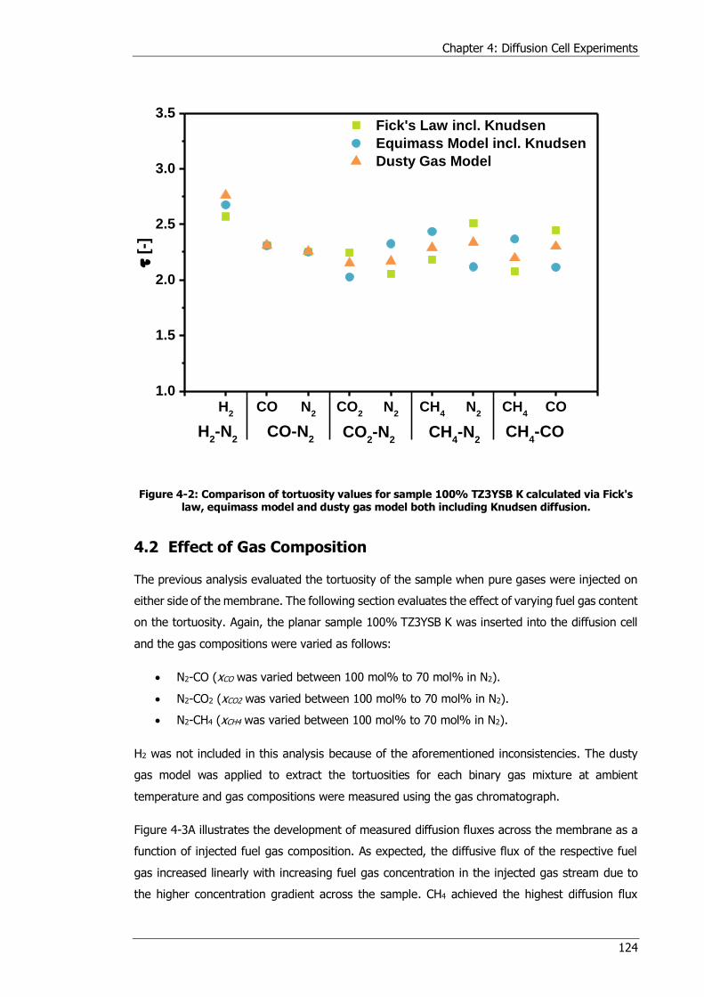
Chapter 4: Diffusion Cell Experiments
124
Figure 4-2: Comparison of tortuosity values for sample 100% TZ3YSB K calculated via Fick's law, equimass model and dusty gas model both including Knudsen diffusion.
4.2 Effect of Gas Composition
The previous analysis evaluated the tortuosity of the sample when pure gases were injected on
either side of the membrane. The following section evaluates the effect of varying fuel gas content
on the tortuosity. Again, the planar sample 100% TZ3YSB K was inserted into the diffusion cell
and the gas compositions were varied as follows:
N2-CO (xCO was varied between 100 mol% to 70 mol% in N2).
N2-CO2 (xCO2 was varied between 100 mol% to 70 mol% in N2).
N2-CH4 (xCH4 was varied between 100 mol% to 70 mol% in N2).
H2 was not included in this analysis because of the aforementioned inconsistencies. The dusty
gas model was applied to extract the tortuosities for each binary gas mixture at ambient
temperature and gas compositions were measured using the gas chromatograph.
Figure 4-3A illustrates the development of measured diffusion fluxes across the membrane as a
function of injected fuel gas composition. As expected, the diffusive flux of the respective fuel
gas increased linearly with increasing fuel gas concentration in the injected gas stream due to
the higher concentration gradient across the sample. CH4 achieved the highest diffusion flux
H2
CO N2
CO2
N2
CH4
N2
CH4
CO1.0
1.5
2.0
2.5
3.0
3.5 Fick's Law incl. Knudsen
Equimass Model incl. Knudsen
Dusty Gas Model
[-
]
H2-N
2CO-N
2CH
4-N
2CH
4-COCO
2-N
2

Chapter 4: Diffusion Cell Experiments
125
among the analysed fuel gases, followed by CO. This behaviour is in accordance with Graham’s
law, where the gas with the lower molar mass features the higher molar diffusion flux. Graham’s
law was followed with a deviation of < 10 % in all but two cases: for yCO = 0.7 and yCH4 = 0.9,
the deviation amounted to < 14 % and < 11 %, respectively. Yet, these slightly higher deviations
are not visible in Figure 4-3A.
Figure 4-3: Effect of injected fuel gas composition on measured fuel gas concentrations on the N2 side of sample 100% TZ3YSB K (A) and on calculated tortuosity at ambient
temperature (B).
Figure 4-3B presents the resulting tortuosity values for each fuel gas as function of the injected
fuel gas concentration. The tortuosity values based on the CO, CH4 and CO2 fluxes remained
almost constant, where the difference between the highest and lowest tortuosity among all three
gases as < 5 %. The experimental error was estimated to lie between ± 10 %, analogous to the
average deviation between the measurements and Graham’s law.
The constant and similar tortuosity values of all gases, which were between 2.1 and 2.4, were in
good agreement with the definition of tortuosity of being a microstructural parameter
independent of varying diffusion conditions. However, the constant development of tortuosity as
a function of fuel gas concentration might only be observable when no chemical reactions are
taking place as the fuel gas concentration affects the operating regime of the OTM. For example,
Brus et al. [113] and Tsai and Schmidt [2] showed that the tortuosity of the anode decreased
with decreasing fuel gas content in an SOFC fuel feed due to the shift towards mass transport
limiting fuel cell operation. Hence, it is expected that the values presented in Figure 4-3B might
be subject to fluctuations during OTM operation.
It can be summarised that no effect of the gas composition on the extracted tortuosity of the
sample was encountered when using the presented diffusion cell experiment methodology.
0.7 0.8 0.9 1.00.04
0.06
0.08
0.10
0.7 0.8 0.9 1.01
2
3
Dif
fusio
n F
lux [
mo
lm-2s
-1]
yCO
(), yCO2
() and yCH4
() in Fuel Line [-]
[-]
yCO
(), yCO2
() and yCH4
() in Fuel Line [-]
B A
Chapter 4: Diffusion Cell Experiments
126
4.3 Comparison between Planar and Tubular Sample
This section compares the diffusion cell experiments of the planar sample 100% TZ3YSB K and
the tubular sample PS 2310 1360C. Both samples were manufactured using the same powders
and sintering conditions (cf. Table 3-1 and Table 3-2). Porosity and mean pore diameter values
for both samples amounted to 0.38 and 0.65 μm for the planar and 0.37 and 0.78 μm (cf. Table
5-5) for the tubular sample.
The DGM was applied to calculate the tortuosity values using the GC for gas measurements.
Experiments for both samples were carried out at ambient temperature, while injecting the
following binary gas mixtures:
N2-CO (pure gases were injected on either side of the diffusion cell).
N2-CO2 (pure gases were injected on either side of the diffusion cell).
N2-CH4 (pure gases were injected on either side of the diffusion cell).
Figure 4-4: Comparison of achieved tortuosity values between the planar and tubular sample at ambient temperature using the DGM for calculations.
Figure 4-4 compares the calculated tortuosity values for each gaseous species of the above binary
gas mixtures for both samples. Graham’s law was followed with a deviation of < 10 % in all
experiments. It is evident that the tortuosity values of the tubular sample were above the values
of the planar sample, where the values for N2-CO were almost identical. Moreover, the fraction
between the minimum and maximum tortuosity value was higher for the tubular sample,
CO N2
CO2
N2
CH4
N2
1.0
1.5
2.0
2.5
3.0
3.5 Planar Sample 100% TZ3YSB K
Tubular Sample PS 2310 1360C
[-
]
CO-N2
CH4-N
2CO
2-N
2
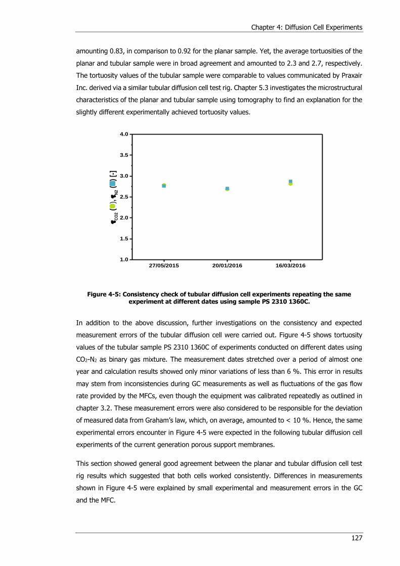
Chapter 4: Diffusion Cell Experiments
127
amounting 0.83, in comparison to 0.92 for the planar sample. Yet, the average tortuosities of the
planar and tubular sample were in broad agreement and amounted to 2.3 and 2.7, respectively.
The tortuosity values of the tubular sample were comparable to values communicated by Praxair
Inc. derived via a similar tubular diffusion cell test rig. Chapter 5.3 investigates the microstructural
characteristics of the planar and tubular sample using tomography to find an explanation for the
slightly different experimentally achieved tortuosity values.
Figure 4-5: Consistency check of tubular diffusion cell experiments repeating the same experiment at different dates using sample PS 2310 1360C.
In addition to the above discussion, further investigations on the consistency and expected
measurement errors of the tubular diffusion cell were carried out. Figure 4-5 shows tortuosity
values of the tubular sample PS 2310 1360C of experiments conducted on different dates using
CO2-N2 as binary gas mixture. The measurement dates stretched over a period of almost one
year and calculation results showed only minor variations of less than 6 %. This error in results
may stem from inconsistencies during GC measurements as well as fluctuations of the gas flow
rate provided by the MFCs, even though the equipment was calibrated repeatedly as outlined in
chapter 3.2. These measurement errors were also considered to be responsible for the deviation
of measured data from Graham’s law, which, on average, amounted to < 10 %. Hence, the same
experimental errors encounter in Figure 4-5 were expected in the following tubular diffusion cell
experiments of the current generation porous support membranes.
This section showed general good agreement between the planar and tubular diffusion cell test
rig results which suggested that both cells worked consistently. Differences in measurements
shown in Figure 4-5 were explained by small experimental and measurement errors in the GC
and the MFC.
27/05/2015 20/01/2016 16/03/20161.0
1.5
2.0
2.5
3.0
3.5
4.0
CO
2 (
),
N2 (
) [-
]

Chapter 4: Diffusion Cell Experiments
128
4.4 Effect of Sample Tube Length
The tubular diffusion cell is capable of testing samples of varying thickness and tube length, while
the planar diffusion cell can only accommodate discs of a certain diameter. Hence, following the
observations from the previous section, the effect of the tube length on the calculated tortuosity
is evaluated here. The current generation sample tubes provided by Praxair Inc. (cf. Table 3-3)
arrived in different lengths. The effect of sample tube length on the tortuosity values was
determined using the sample PS 2.4 30.0%, which was the longest specimen provided by Praxair
Inc. and was shortened several times in the course of this project. The sample featured an initial
length of > 300 mm and was cut down to approximately 250 mm after first experiments to match
the length of the remaining tubular samples of the 2.4th generation. Then, all 2.4th generation
samples were cut to feature the same length as sample PS 2310 1360C (approximately 130 mm).
Finally, samples PS 2.4 30.0% and PS 2.4 22.6% were further reduced in length to approximately
20 mm. Diffusion cell experiments were carried out for each sample length at ambient
temperature.
Table 4-1 presents the microstructural parameters of the porous samples used for calculations:
while the mean pore diameter was based on the tomographic reconstructions (see chapter 5.4),
the porosity values for each sample were taken from Table 3-3. The tortuosity was calculated via
the DGM based on GC measurements.
Table 4-1: Mean pore diameter dP, porosity ε and membrane thickness δ for 2.4th generation porous support samples.
Sample Name dP ε δ
[μm] [-] [mm]
PS 2.4 29.4% 0.71 0.2949 1
PS 2.4 30.0% 0.73 0.3003 1.3
PS 2.4 25.1% 0.65 0.2510 1
PS 2.4 22.6% 0.63 0.2263 1.3

Chapter 4: Diffusion Cell Experiments
129
Figure 4-6: The effect of tube length of sample PS 2.4 30.0% on tortuosity.
Figure 4-6 illustrates the tortuosity of sample PS 2.4 30.0% as function of tube length for CO2-N2
at ambient temperature. It is visible that the calculated tortuosity decreased linearly with
decreasing sample tube length. At a length of 130 mm, the tortuosity values between samples
PS 2.4 30.0% and PS 2310 1360C agreed well with each other. Moreover, at a length of 20 mm,
tortuosity values matched with tortuosities of the planar sample 100% TZ3YSB K. Hence,
excellent agreement in tortuosity values between the planar and tubular sample treated in the
previous section was achieved by reducing the length of sample PS 2310 1360C to 20 mm as
shown in Figure 4-7. The tortuosity values of the tubular sample with a length of 20 mm were
slightly below the values of the planar sample.
The sample length, like the sample thickness (cf. section 4.6), should not affect the tortuosity,
which is in clear contrast to the results presented in Figure 4-6. The extensive void volume of the
used working tube in the tubular furnace might be the explanation for these observations. The
outer diameter of the tubular samples amounted to approximately 10 mm while the furnace
working tube featured an inner diameter of 38 mm and a length of 600 mm. This may have
caused concentration gradient fluctuations and depletion effects downstream of the sample
mounting fitting, which increased with increasing tube length.
0 50 100 150 200 250 300 350
2.5
3.0
3.5
4.0
Sample Tube Length [mm]
CO
2 (
),
N2 (
) [-
]
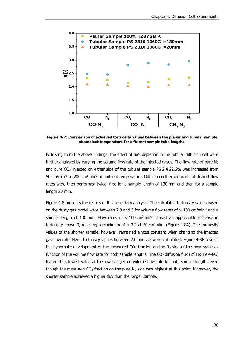
Chapter 4: Diffusion Cell Experiments
130
Figure 4-7: Comparison of achieved tortuosity values between the planar and tubular sample at ambient temperature for different sample tube lengths.
Following from the above findings, the effect of fuel depletion in the tubular diffusion cell were
further analysed by varying the volume flow rate of the injected gases. The flow rate of pure N2
and pure CO2 injected on either side of the tubular sample PS 2.4 22.6% was increased from
50 cm3min-1 to 200 cm3min-1 at ambient temperature. Diffusion cell experiments at distinct flow
rates were then performed twice, first for a sample length of 130 mm and then for a sample
length 20 mm.
Figure 4-8 presents the results of this sensitivity analysis. The calculated tortuosity values based
on the dusty gas model were between 2.8 and 3 for volume flow rates of > 100 cm3min-1 and a
sample length of 130 mm. Flow rates of < 100 cm3min-1 caused an appreciable increase in
tortuosity above 3, reaching a maximum of > 3.2 at 50 cm3min-1 (Figure 4-8A). The tortuosity
values of the shorter sample, however, remained almost constant when changing the injected
gas flow rate. Here, tortuosity values between 2.0 and 2.2 were calculated. Figure 4-8B reveals
the hyperbolic development of the measured CO2 fraction on the N2 side of the membrane as
function of the volume flow rate for both sample lengths. The CO2 diffusion flux (cf. Figure 4-8C)
featured its lowest value at the lowest injected volume flow rate for both sample lengths even
though the measured CO2 fraction on the pure N2 side was highest at this point. Moreover, the
shorter sample achieved a higher flux than the longer sample.
CO N2
CO2
N2
CH4
N2
1.0
1.5
2.0
2.5
3.0
3.5
4.0 Planar Sample 100% TZ3YSB K
Tubular Sample PS 2310 1360C l=130mm
Tubular Sample PS 2310 1360C l=20mm
[-
]
CO-N2
CH4-N
2CO
2-N
2
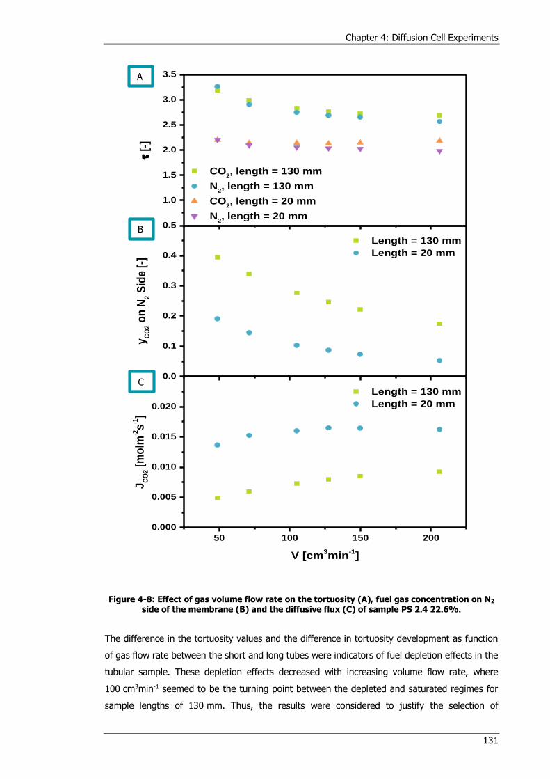
Chapter 4: Diffusion Cell Experiments
131
Figure 4-8: Effect of gas volume flow rate on the tortuosity (A), fuel gas concentration on N2 side of the membrane (B) and the diffusive flux (C) of sample PS 2.4 22.6%.
The difference in the tortuosity values and the difference in tortuosity development as function
of gas flow rate between the short and long tubes were indicators of fuel depletion effects in the
tubular sample. These depletion effects decreased with increasing volume flow rate, where
100 cm3min-1 seemed to be the turning point between the depleted and saturated regimes for
sample lengths of 130 mm. Thus, the results were considered to justify the selection of
0.5
1.0
1.5
2.0
2.5
3.0
3.5
0.0
0.1
0.2
0.3
0.4
50 100 150 200
0.000
0.005
0.010
0.015
0.020
CO2, length = 130 mm
N2, length = 130 mm
CO2, length = 20 mm
N2, length = 20 mm
[-
]
Length = 130 mm
Length = 20 mm
yC
O2 o
n N
2 S
ide
[-]
Length = 130 mm
Length = 20 mm
JC
O2 [
mo
lm-2s
-1]
V [cm3min
-1]
A
B
C
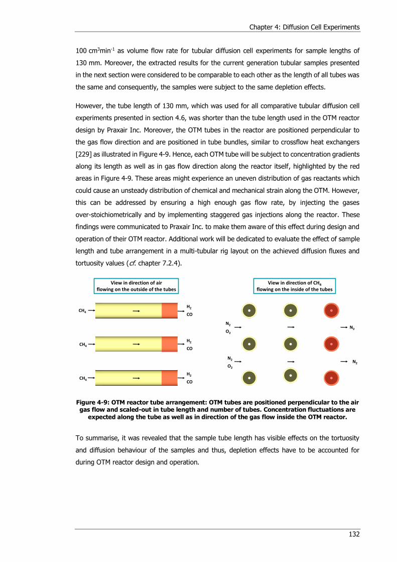
Chapter 4: Diffusion Cell Experiments
132
100 cm3min-1 as volume flow rate for tubular diffusion cell experiments for sample lengths of
130 mm. Moreover, the extracted results for the current generation tubular samples presented
in the next section were considered to be comparable to each other as the length of all tubes was
the same and consequently, the samples were subject to the same depletion effects.
However, the tube length of 130 mm, which was used for all comparative tubular diffusion cell
experiments presented in section 4.6, was shorter than the tube length used in the OTM reactor
design by Praxair Inc. Moreover, the OTM tubes in the reactor are positioned perpendicular to
the gas flow direction and are positioned in tube bundles, similar to crossflow heat exchangers
[229] as illustrated in Figure 4-9. Hence, each OTM tube will be subject to concentration gradients
along its length as well as in gas flow direction along the reactor itself, highlighted by the red
areas in Figure 4-9. These areas might experience an uneven distribution of gas reactants which
could cause an unsteady distribution of chemical and mechanical strain along the OTM. However,
this can be addressed by ensuring a high enough gas flow rate, by injecting the gases
over-stoichiometrically and by implementing staggered gas injections along the reactor. These
findings were communicated to Praxair Inc. to make them aware of this effect during design and
operation of their OTM reactor. Additional work will be dedicated to evaluate the effect of sample
length and tube arrangement in a multi-tubular rig layout on the achieved diffusion fluxes and
tortuosity values (cf. chapter 7.2.4).
Figure 4-9: OTM reactor tube arrangement: OTM tubes are positioned perpendicular to the air gas flow and scaled-out in tube length and number of tubes. Concentration fluctuations are
expected along the tube as well as in direction of the gas flow inside the OTM reactor.
To summarise, it was revealed that the sample tube length has visible effects on the tortuosity
and diffusion behaviour of the samples and thus, depletion effects have to be accounted for
during OTM reactor design and operation.
CH4
CH4
CH4
CO
H2
CO
H2
CO
H2
O2
N2
O2
N2
N2
N2
View in direction of airflowing on the outside of the tubes
View in direction of CH4
flowing on the inside of the tubes
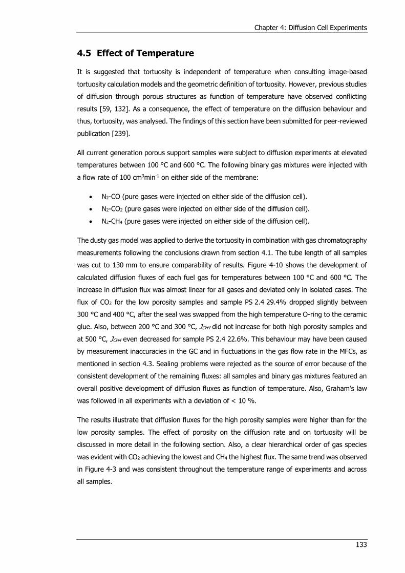
Chapter 4: Diffusion Cell Experiments
133
4.5 Effect of Temperature
It is suggested that tortuosity is independent of temperature when consulting image-based
tortuosity calculation models and the geometric definition of tortuosity. However, previous studies
of diffusion through porous structures as function of temperature have observed conflicting
results [59, 132]. As a consequence, the effect of temperature on the diffusion behaviour and
thus, tortuosity, was analysed. The findings of this section have been submitted for peer-reviewed
publication [239].
All current generation porous support samples were subject to diffusion experiments at elevated
temperatures between 100 °C and 600 °C. The following binary gas mixtures were injected with
a flow rate of 100 cm3min-1 on either side of the membrane:
N2-CO (pure gases were injected on either side of the diffusion cell).
N2-CO2 (pure gases were injected on either side of the diffusion cell).
N2-CH4 (pure gases were injected on either side of the diffusion cell).
The dusty gas model was applied to derive the tortuosity in combination with gas chromatography
measurements following the conclusions drawn from section 4.1. The tube length of all samples
was cut to 130 mm to ensure comparability of results. Figure 4-10 shows the development of
calculated diffusion fluxes of each fuel gas for temperatures between 100 °C and 600 °C. The
increase in diffusion flux was almost linear for all gases and deviated only in isolated cases. The
flux of CO2 for the low porosity samples and sample PS 2.4 29.4% dropped slightly between
300 °C and 400 °C, after the seal was swapped from the high temperature O-ring to the ceramic
glue. Also, between 200 °C and 300 °C, JCH4 did not increase for both high porosity samples and
at 500 °C, JCH4 even decreased for sample PS 2.4 22.6%. This behaviour may have been caused
by measurement inaccuracies in the GC and in fluctuations in the gas flow rate in the MFCs, as
mentioned in section 4.3. Sealing problems were rejected as the source of error because of the
consistent development of the remaining fluxes: all samples and binary gas mixtures featured an
overall positive development of diffusion fluxes as function of temperature. Also, Graham’s law
was followed in all experiments with a deviation of < 10 %.
The results illustrate that diffusion fluxes for the high porosity samples were higher than for the
low porosity samples. The effect of porosity on the diffusion rate and on tortuosity will be
discussed in more detail in the following section. Also, a clear hierarchical order of gas species
was evident with CO2 achieving the lowest and CH4 the highest flux. The same trend was observed
in Figure 4-3 and was consistent throughout the temperature range of experiments and across
all samples.
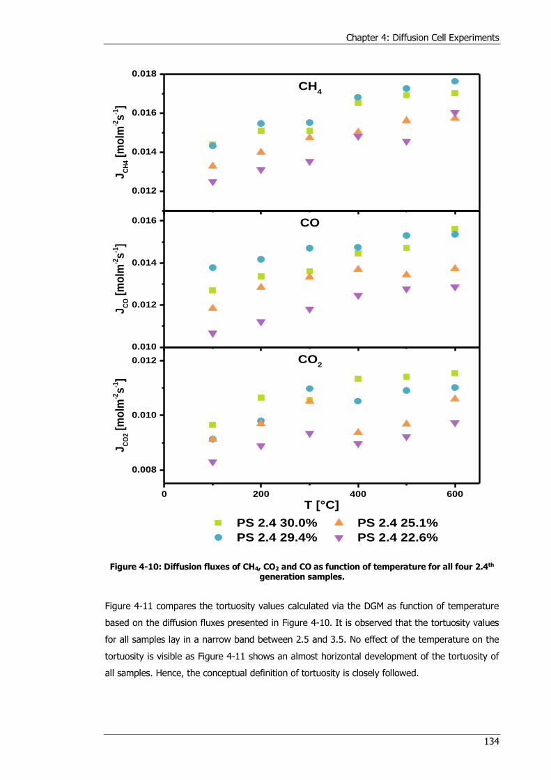
Chapter 4: Diffusion Cell Experiments
134
Figure 4-10: Diffusion fluxes of CH4, CO2 and CO as function of temperature for all four 2.4th generation samples.
Figure 4-11 compares the tortuosity values calculated via the DGM as function of temperature
based on the diffusion fluxes presented in Figure 4-10. It is observed that the tortuosity values
for all samples lay in a narrow band between 2.5 and 3.5. No effect of the temperature on the
tortuosity is visible as Figure 4-11 shows an almost horizontal development of the tortuosity of
all samples. Hence, the conceptual definition of tortuosity is closely followed.
0.012
0.014
0.016
0.018
0 200 400 600
0.008
0.010
0.012
0.010
0.012
0.014
0.016
PS 2.4 30.0% PS 2.4 25.1%
PS 2.4 29.4% PS 2.4 22.6%
JC
H4 [
mo
lm-2s
-1]
CH4
T [°C]
JC
O2 [
mo
lm-2s
-1]
CO2
JC
O [
mo
lm-2s
-1]
CO
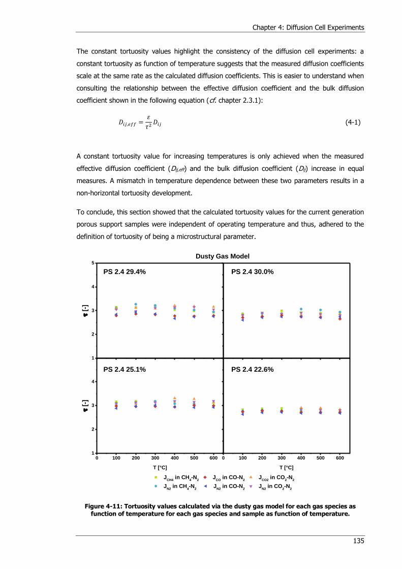
Chapter 4: Diffusion Cell Experiments
135
The constant tortuosity values highlight the consistency of the diffusion cell experiments: a
constant tortuosity as function of temperature suggests that the measured diffusion coefficients
scale at the same rate as the calculated diffusion coefficients. This is easier to understand when
consulting the relationship between the effective diffusion coefficient and the bulk diffusion
coefficient shown in the following equation (cf. chapter 2.3.1):
𝐷𝑖𝑗,𝑒𝑓𝑓 =휀
𝜏2𝐷𝑖𝑗 (4-1)
A constant tortuosity value for increasing temperatures is only achieved when the measured
effective diffusion coefficient (Dij,eff) and the bulk diffusion coefficient (Dij) increase in equal
measures. A mismatch in temperature dependence between these two parameters results in a
non-horizontal tortuosity development.
To conclude, this section showed that the calculated tortuosity values for the current generation
porous support samples were independent of operating temperature and thus, adhered to the
definition of tortuosity of being a microstructural parameter.
Figure 4-11: Tortuosity values calculated via the dusty gas model for each gas species as function of temperature for each gas species and sample as function of temperature.
1
2
3
4
5
0 100 200 300 400 500 6001
2
3
4
0 100 200 300 400 500 600
[
-]
PS 2.4 29.4%
Dusty Gas Model
JCH4
in CH4-N
2 J
CO in CO-N
2 J
CO2 in CO
2-N
2
JN2
in CH4-N
2 J
N2 in CO-N
2 J
N2 in CO
2-N
2
PS 2.4 30.0%
[
-]
T [°C]
PS 2.4 25.1%
T [°C]
PS 2.4 22.6%
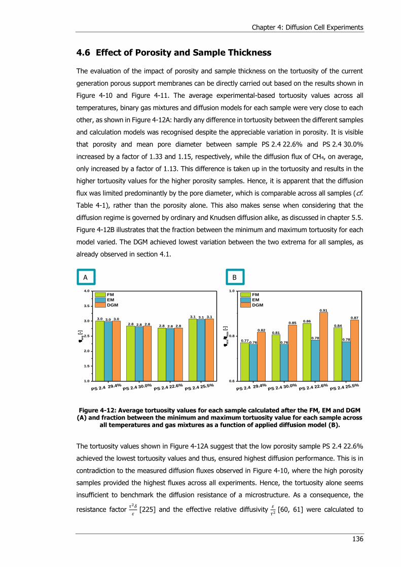
Chapter 4: Diffusion Cell Experiments
136
4.6 Effect of Porosity and Sample Thickness
The evaluation of the impact of porosity and sample thickness on the tortuosity of the current
generation porous support membranes can be directly carried out based on the results shown in
Figure 4-10 and Figure 4-11. The average experimental-based tortuosity values across all
temperatures, binary gas mixtures and diffusion models for each sample were very close to each
other, as shown in Figure 4-12A: hardly any difference in tortuosity between the different samples
and calculation models was recognised despite the appreciable variation in porosity. It is visible
that porosity and mean pore diameter between sample PS 2.4 22.6% and PS 2.4 30.0%
increased by a factor of 1.33 and 1.15, respectively, while the diffusion flux of CH4, on average,
only increased by a factor of 1.13. This difference is taken up in the tortuosity and results in the
higher tortuosity values for the higher porosity samples. Hence, it is apparent that the diffusion
flux was limited predominantly by the pore diameter, which is comparable across all samples (cf.
Table 4-1), rather than the porosity alone. This also makes sense when considering that the
diffusion regime is governed by ordinary and Knudsen diffusion alike, as discussed in chapter 5.5.
Figure 4-12B illustrates that the fraction between the minimum and maximum tortuosity for each
model varied. The DGM achieved lowest variation between the two extrema for all samples, as
already observed in section 4.1.
Figure 4-12: Average tortuosity values for each sample calculated after the FM, EM and DGM (A) and fraction between the minimum and maximum tortuosity value for each sample across
all temperatures and gas mixtures as a function of applied diffusion model (B).
The tortuosity values shown in Figure 4-12A suggest that the low porosity sample PS 2.4 22.6%
achieved the lowest tortuosity values and thus, ensured highest diffusion performance. This is in
contradiction to the measured diffusion fluxes observed in Figure 4-10, where the high porosity
samples provided the highest fluxes across all experiments. Hence, the tortuosity alone seems
insufficient to benchmark the diffusion resistance of a microstructure. As a consequence, the
resistance factor 𝜏2𝛿
[225] and the effective relative diffusivity 𝜏2
[60, 61] were calculated to
0.77
0.81
0.86
0.84
0.76 0.76
0.78 0.78
0.82
0.85
0.91
0.873.0
2.82.8
3.13.0
2.82.8
3.13.0
2.82.8
3.1
PS 2.4 29.4%PS 2.4 30.0%
PS 2.4 22.6%PS 2.4 25.5%
0.6
0.8
1.0
min/
ma
x [
-]
FM
EM
DGM
PS 2.4 29.4%PS 2.4 30.0%
PS 2.4 22.6%PS 2.4 25.5%
1.0
1.5
2.0
2.5
3.0
3.5
4.0
av
g [
-]
FM
EM
DGM
A B
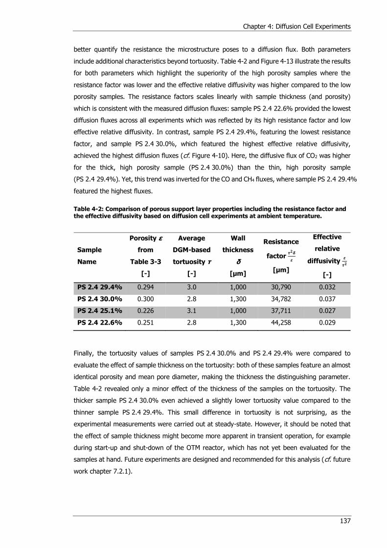
Chapter 4: Diffusion Cell Experiments
137
better quantify the resistance the microstructure poses to a diffusion flux. Both parameters
include additional characteristics beyond tortuosity. Table 4-2 and Figure 4-13 illustrate the results
for both parameters which highlight the superiority of the high porosity samples where the
resistance factor was lower and the effective relative diffusivity was higher compared to the low
porosity samples. The resistance factors scales linearly with sample thickness (and porosity)
which is consistent with the measured diffusion fluxes: sample PS 2.4 22.6% provided the lowest
diffusion fluxes across all experiments which was reflected by its high resistance factor and low
effective relative diffusivity. In contrast, sample PS 2.4 29.4%, featuring the lowest resistance
factor, and sample PS 2.4 30.0%, which featured the highest effective relative diffusivity,
achieved the highest diffusion fluxes (cf. Figure 4-10). Here, the diffusive flux of CO2 was higher
for the thick, high porosity sample (PS 2.4 30.0%) than the thin, high porosity sample
(PS 2.4 29.4%). Yet, this trend was inverted for the CO and CH4 fluxes, where sample PS 2.4 29.4%
featured the highest fluxes.
Table 4-2: Comparison of porous support layer properties including the resistance factor and the effective diffusivity based on diffusion cell experiments at ambient temperature.
Sample
Name
Porosity ε
from
Table 3-3
[-]
Average
DGM-based
tortuosity τ
[-]
Wall
thickness
δ
[μm]
Resistance
factor 𝝉𝟐𝜹
𝜺
[μm]
Effective
relative
diffusivity 𝜺
𝝉𝟐
[-]
PS 2.4 29.4% 0.294 3.0 1,000 30,790 0.032
PS 2.4 30.0% 0.300 2.8 1,300 34,782 0.037
PS 2.4 25.1% 0.226 3.1 1,000 37,711 0.027
PS 2.4 22.6% 0.251 2.8 1,300 44,258 0.029
Finally, the tortuosity values of samples PS 2.4 30.0% and PS 2.4 29.4% were compared to
evaluate the effect of sample thickness on the tortuosity: both of these samples feature an almost
identical porosity and mean pore diameter, making the thickness the distinguishing parameter.
Table 4-2 revealed only a minor effect of the thickness of the samples on the tortuosity. The
thicker sample PS 2.4 30.0% even achieved a slightly lower tortuosity value compared to the
thinner sample PS 2.4 29.4%. This small difference in tortuosity is not surprising, as the
experimental measurements were carried out at steady-state. However, it should be noted that
the effect of sample thickness might become more apparent in transient operation, for example
during start-up and shut-down of the OTM reactor, which has not yet been evaluated for the
samples at hand. Future experiments are designed and recommended for this analysis (cf. future
work chapter 7.2.1).
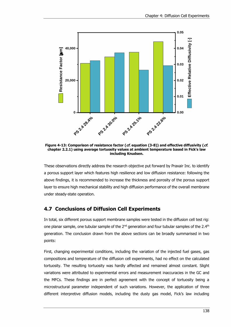
Chapter 4: Diffusion Cell Experiments
138
Figure 4-13: Comparison of resistance factor (cf. equation (3-8)) and effective diffusivity (cf. chapter 2.2.1) using average tortuosity values at ambient temperature based in Fick's law
including Knudsen.
These observations directly address the research objective put forward by Praxair Inc. to identify
a porous support layer which features high resilience and low diffusion resistance: following the
above findings, it is recommended to increase the thickness and porosity of the porous support
layer to ensure high mechanical stability and high diffusion performance of the overall membrane
under steady-state operation.
4.7 Conclusions of Diffusion Cell Experiments
In total, six different porous support membrane samples were tested in the diffusion cell test rig:
one planar sample, one tubular sample of the 2nd generation and four tubular samples of the 2.4th
generation. The conclusion drawn from the above sections can be broadly summarised in two
points:
First, changing experimental conditions, including the variation of the injected fuel gases, gas
compositions and temperature of the diffusion cell experiments, had no effect on the calculated
tortuosity. The resulting tortuosity was hardly affected and remained almost constant. Slight
variations were attributed to experimental errors and measurement inaccuracies in the GC and
the MFCs. These findings are in perfect agreement with the concept of tortuosity being a
microstructural parameter independent of such variations. However, the application of three
different interpretive diffusion models, including the dusty gas model, Fick’s law including
PS 2
.4 2
9.4%
PS 2
.4 3
0.0%
PS 2
.4 2
5.1%
PS 2
.4 2
2.6%
0
20,000
40,000
Re
sis
tan
ce
Fa
cto
r [
m]
0.00
0.01
0.02
0.03
0.04
0.05
Eff
ec
tiv
e R
ela
tiv
e D
iffu
siv
ity
[-]
Chapter 4: Diffusion Cell Experiments
139
Knudsen expressions and the equimass model including Knudsen expressions, resulted in
different tortuosity values for specific gases of each binary gas mixture. Only the dusty gas model
provided a constant tortuosity value under these conditions and thus, was considered to be the
most accurate model, even though average values of the DGM, FM and EM were identical.
Second, a comparative study using a selection of current generation tubular porous support
samples which differed in membrane thickness and porosity showed almost identical tortuosity
values. Theoretically, the sample with the higher porosity should feature a lower tortuosity value.
However, this was not discovered during experiments. The reason for this might be the average
pore diameters of the samples, which were very close to each other and seemed to govern the
flux more than the porosity alone. Yet, the high porosity samples provide a higher diffusion flux
compared to the low porosity samples, which was only reflected when calculating the resistance
factor and the effective relative diffusivity. These parameters take additional microstructural
characteristics into account, including the porosity and sample thickness. Here, the effect of
sample thickness on the diffusion behaviour might become more apparent during transient
operation, for which additional experiments are necessary. Hence, for steady-state operation, a
thicker sample with high porosity combines mechanical stability with good diffusion performance.
Moreover, a comparison between planar and tubular samples, which were manufactured using
the same powders and sintering conditions, resulted in broadly agreeing tortuosity values. The
tortuosity values of the tubular sample were also comparable to values provided by Praxair Inc.
for the same sample calculated via the similar experiments. A linear increase in tortuosity as
function of sample tube length was observed and attributed to depletion effects within the
extensive void volume of the furnace working tube. The findings were reported to Praxair Inc. to
make them aware of such effects during OTM reactor design and operation and future work
should be dedicated to analyse the diffusion behaviour of a multi-tube rig arrangement.
To summarise, the previous sections showed that:
The dusty gas model provided the most accurate tortuosity values which followed the
definition of tortuosity closely.
The gas composition had no effect on the extracted tortuosity of the sample.
The tortuosity of the tubular sample is linearly dependent on the tube length which is
caused by depletion effects within the extensive void volume of the furnace working tube.
The tortuosity was independent of the operating temperature of the diffusion cell test rig.
Porous support layers should feature high thickness and high porosity to ensure high
mechanical stability and good diffusion performance at steady-state.
Chapter 5: Image Analysis and Quantification
140
5 Image Analysis and Quantification
This chapter describes the application of advanced tomography techniques to reveal the complex
microstructure and resolve geometric features affecting the mass transport within the porous
support layer samples. The reconstructed sample volumes formed the framework for subsequent
image quantification algorithms to extract microstructural parameters including the porosity,
tortuosity and pore size distribution, as introduced in chapter 3.4. Here, the porosity and the
mean pore diameter were essential input parameters for the diffusion models applied in the
previous chapter. Moreover, a selection of image-based tortuosity calculation algorithms (cf.
chapter 3.4.3), which are all frequently used in practice, were compared and their suitability for
quantifying diffusive mass transport in porous structures was assessed.
X-ray nano CT using the Zeiss Xradia 810 Ultra and dual beam FIB-SEM slice and view
tomography using the Zeiss 1540XB CrossBeam were applied to reconstruct the planar and
tubular samples for 3D image quantification. The imaging parameters of both techniques were
assessed in section 5.1 to ensure high resolution and image quality. Section 5.2 then compares
the extracted microstructural parameters of the planar sample 100% TZ3YSB K calculated based
via both imaging methods. The reason for this was to verify the consistency of chosen imaging
parameters and image analysis procedures. Section 5.3 relates the microstructural parameters of
the planar sample 100% TZ3YSB K extracted in section 5.2 to the values calculated for the tubular
sample PS 2310 1360C, analogous to chapter 4.3.
FIB-SEM tomography was applied at the beginning of the project, before improved access to the
Zeiss Xradia 810 Ultra nano CT system was established for routine high resolution,
non-destructive 3D imaging. Section 5.4 presents the results of the different image-based
tortuosity calculation algorithms executed on sample reconstructions of the current generation
porous support layers using X-ray nano CT. The local distribution of the diffusion regime on a
pixel-by-pixel basis is then assessed in section 5.5, to address observations made during the
diffusion cell experiments. Finally, section 5.6 applies artificial opening and closing operations on
the sample volumes to mimic different manufacturing techniques without having to manufacture
them individually.
5.1 Evaluation of Imaging Specifications
The choice of imaging parameters during X-ray nano CT has substantial effects on the quality of
the reconstructed volume and thus, on the calculated microstructural data. Figure 5-1 illustrates
the impact of pixel size on the reconstruction of the complete OTM:
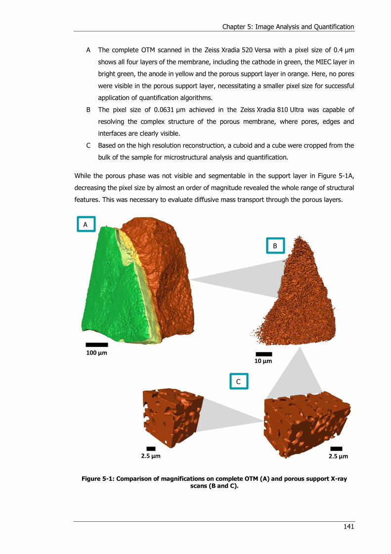
Chapter 5: Image Analysis and Quantification
141
A The complete OTM scanned in the Zeiss Xradia 520 Versa with a pixel size of 0.4 μm
shows all four layers of the membrane, including the cathode in green, the MIEC layer in
bright green, the anode in yellow and the porous support layer in orange. Here, no pores
were visible in the porous support layer, necessitating a smaller pixel size for successful
application of quantification algorithms.
B The pixel size of 0.0631 μm achieved in the Zeiss Xradia 810 Ultra was capable of
resolving the complex structure of the porous membrane, where pores, edges and
interfaces are clearly visible.
C Based on the high resolution reconstruction, a cuboid and a cube were cropped from the
bulk of the sample for microstructural analysis and quantification.
While the porous phase was not visible and segmentable in the support layer in Figure 5-1A,
decreasing the pixel size by almost an order of magnitude revealed the whole range of structural
features. This was necessary to evaluate diffusive mass transport through the porous layers.
Figure 5-1: Comparison of magnifications on complete OTM (A) and porous support X-ray scans (B and C).
100 μm10 μm
2.5 μm2.5 μm
B
C
A
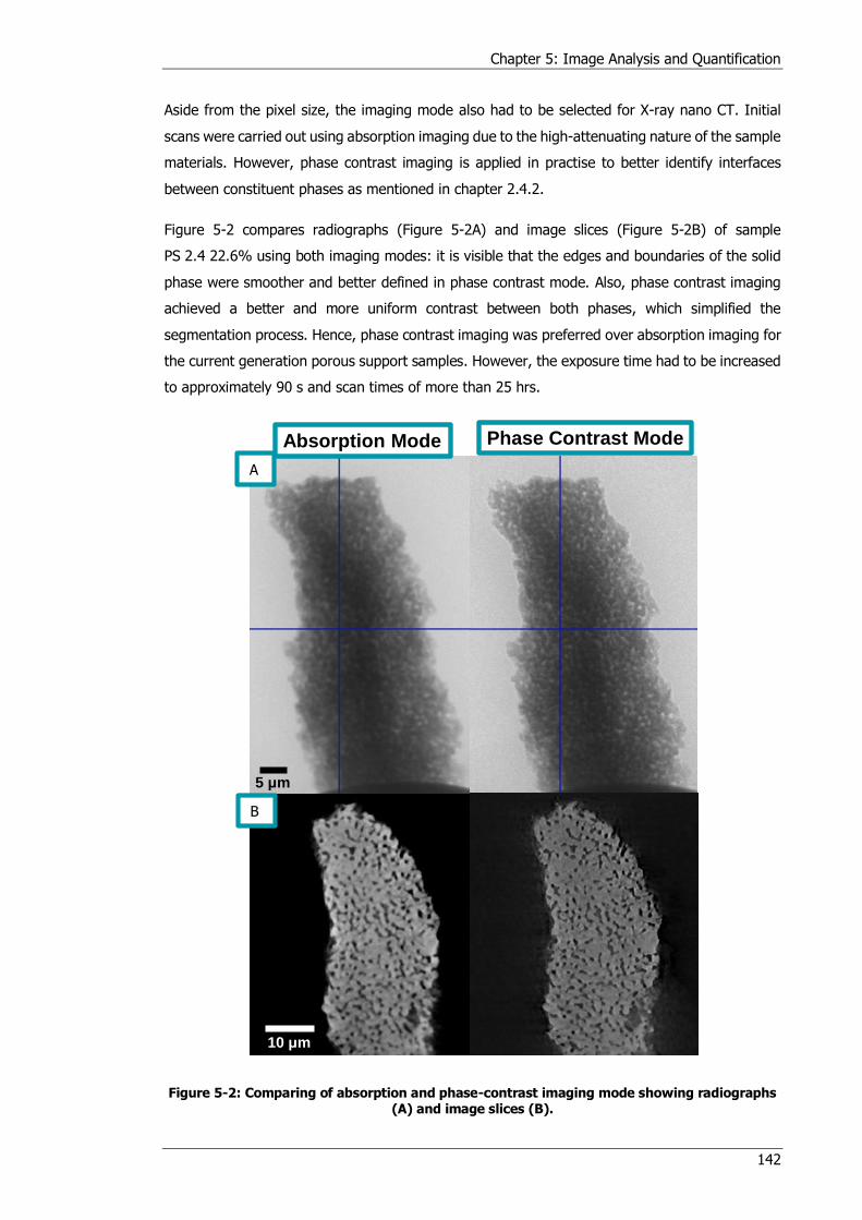
Chapter 5: Image Analysis and Quantification
142
Aside from the pixel size, the imaging mode also had to be selected for X-ray nano CT. Initial
scans were carried out using absorption imaging due to the high-attenuating nature of the sample
materials. However, phase contrast imaging is applied in practise to better identify interfaces
between constituent phases as mentioned in chapter 2.4.2.
Figure 5-2 compares radiographs (Figure 5-2A) and image slices (Figure 5-2B) of sample
PS 2.4 22.6% using both imaging modes: it is visible that the edges and boundaries of the solid
phase were smoother and better defined in phase contrast mode. Also, phase contrast imaging
achieved a better and more uniform contrast between both phases, which simplified the
segmentation process. Hence, phase contrast imaging was preferred over absorption imaging for
the current generation porous support samples. However, the exposure time had to be increased
to approximately 90 s and scan times of more than 25 hrs.
Figure 5-2: Comparing of absorption and phase-contrast imaging mode showing radiographs (A) and image slices (B).
5 μm
Absorption Mode Phase Contrast Mode
10 μm
B
A
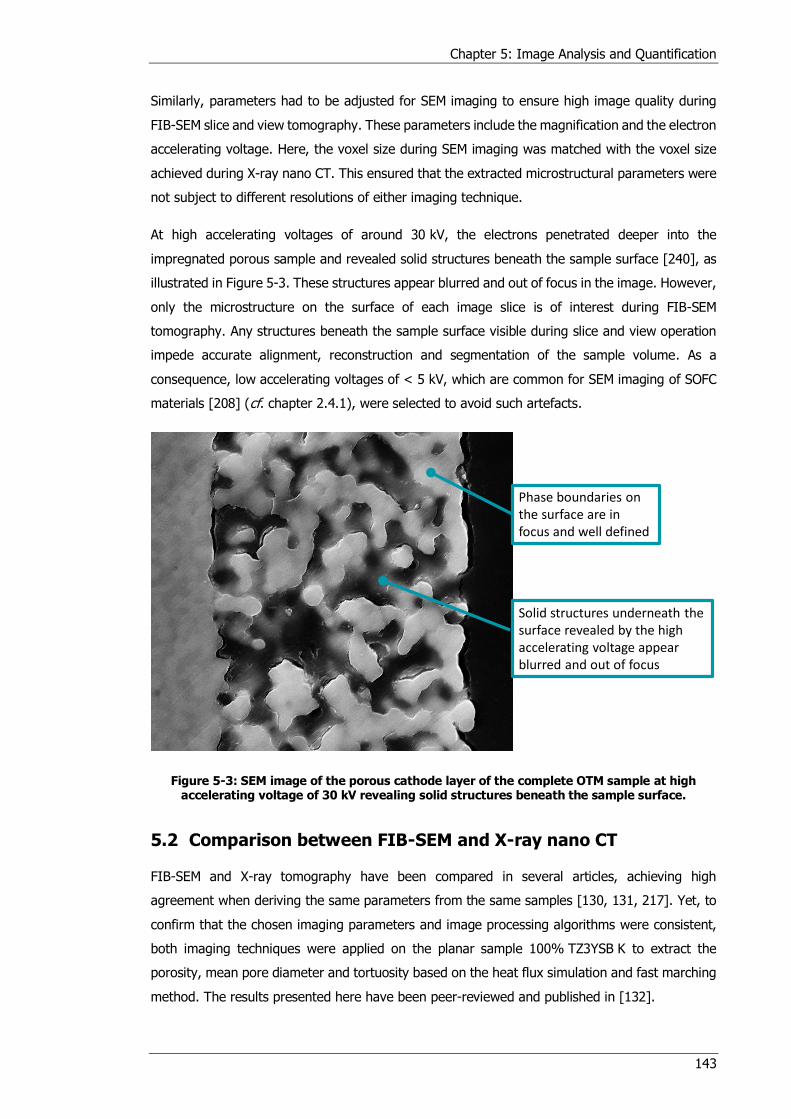
Chapter 5: Image Analysis and Quantification
143
Similarly, parameters had to be adjusted for SEM imaging to ensure high image quality during
FIB-SEM slice and view tomography. These parameters include the magnification and the electron
accelerating voltage. Here, the voxel size during SEM imaging was matched with the voxel size
achieved during X-ray nano CT. This ensured that the extracted microstructural parameters were
not subject to different resolutions of either imaging technique.
At high accelerating voltages of around 30 kV, the electrons penetrated deeper into the
impregnated porous sample and revealed solid structures beneath the sample surface [240], as
illustrated in Figure 5-3. These structures appear blurred and out of focus in the image. However,
only the microstructure on the surface of each image slice is of interest during FIB-SEM
tomography. Any structures beneath the sample surface visible during slice and view operation
impede accurate alignment, reconstruction and segmentation of the sample volume. As a
consequence, low accelerating voltages of < 5 kV, which are common for SEM imaging of SOFC
materials [208] (cf. chapter 2.4.1), were selected to avoid such artefacts.
Figure 5-3: SEM image of the porous cathode layer of the complete OTM sample at high accelerating voltage of 30 kV revealing solid structures beneath the sample surface.
5.2 Comparison between FIB-SEM and X-ray nano CT
FIB-SEM and X-ray tomography have been compared in several articles, achieving high
agreement when deriving the same parameters from the same samples [130, 131, 217]. Yet, to
confirm that the chosen imaging parameters and image processing algorithms were consistent,
both imaging techniques were applied on the planar sample 100% TZ3YSB K to extract the
porosity, mean pore diameter and tortuosity based on the heat flux simulation and fast marching
method. The results presented here have been peer-reviewed and published in [132].
Phase boundaries on the surface are in focus and well defined
Solid structures underneath the surface revealed by the high accelerating voltage appear blurred and out of focus
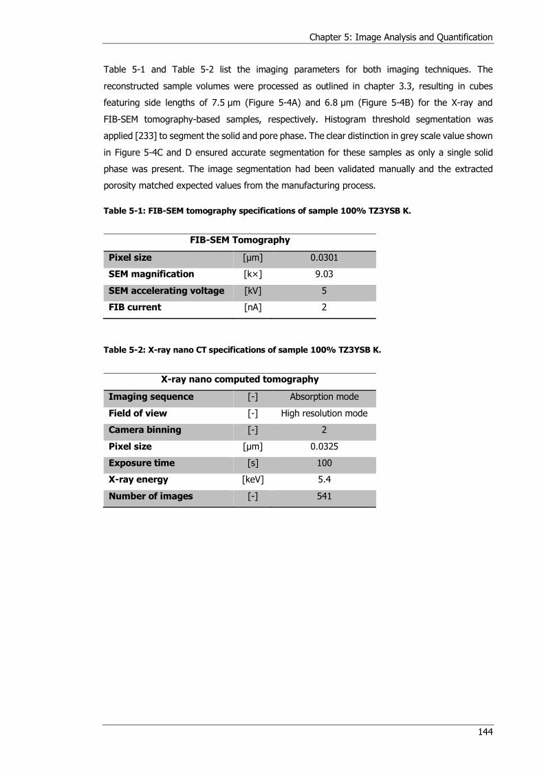
Chapter 5: Image Analysis and Quantification
144
Table 5-1 and Table 5-2 list the imaging parameters for both imaging techniques. The
reconstructed sample volumes were processed as outlined in chapter 3.3, resulting in cubes
featuring side lengths of 7.5 μm (Figure 5-4A) and 6.8 μm (Figure 5-4B) for the X-ray and
FIB-SEM tomography-based samples, respectively. Histogram threshold segmentation was
applied [233] to segment the solid and pore phase. The clear distinction in grey scale value shown
in Figure 5-4C and D ensured accurate segmentation for these samples as only a single solid
phase was present. The image segmentation had been validated manually and the extracted
porosity matched expected values from the manufacturing process.
Table 5-1: FIB-SEM tomography specifications of sample 100% TZ3YSB K.
FIB-SEM Tomography
Pixel size [μm] 0.0301
SEM magnification [k×] 9.03
SEM accelerating voltage [kV] 5
FIB current [nA] 2
Table 5-2: X-ray nano CT specifications of sample 100% TZ3YSB K.
X-ray nano computed tomography
Imaging sequence [-] Absorption mode
Field of view [-] High resolution mode
Camera binning [-] 2
Pixel size [μm] 0.0325
Exposure time [s] 100
X-ray energy [keV] 5.4
Number of images [-] 541
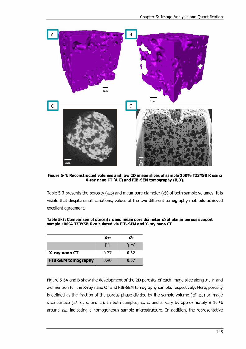
Chapter 5: Image Analysis and Quantification
145
Figure 5-4: Reconstructed volumes and raw 2D image slices of sample 100% TZ3YSB K using X-ray nano CT (A,C) and FIB-SEM tomography (B,D).
Table 5-3 presents the porosity (ε3D) and mean pore diameter (dP) of both sample volumes. It is
visible that despite small variations, values of the two different tomography methods achieved
excellent agreement.
Table 5-3: Comparison of porosity ε and mean pore diameter dP of planar porous support sample 100% TZ3YSB K calculated via FIB-SEM and X-ray nano CT.
ε3D dP
[-] [μm]
X-ray nano CT 0.37 0.62
FIB-SEM tomography 0.40 0.67
Figure 5-5A and B show the development of the 2D porosity of each image slice along x-, y- and
z-dimension for the X-ray nano CT and FIB-SEM tomography sample, respectively. Here, porosity
is defined as the fraction of the porous phase divided by the sample volume (cf. ε3D) or image
slice surface (cf. εx, εy and εz). In both samples, εx, εy and εz vary by approximately ± 10 %
around ε3D, indicating a homogeneous sample microstructure. In addition, the representative
B A
D C
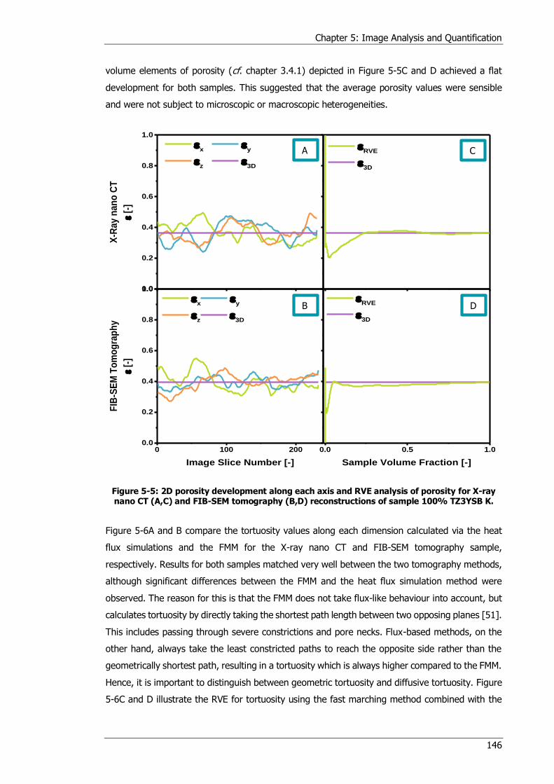
Chapter 5: Image Analysis and Quantification
146
volume elements of porosity (cf. chapter 3.4.1) depicted in Figure 5-5C and D achieved a flat
development for both samples. This suggested that the average porosity values were sensible
and were not subject to microscopic or macroscopic heterogeneities.
Figure 5-5: 2D porosity development along each axis and RVE analysis of porosity for X-ray nano CT (A,C) and FIB-SEM tomography (B,D) reconstructions of sample 100% TZ3YSB K.
Figure 5-6A and B compare the tortuosity values along each dimension calculated via the heat
flux simulations and the FMM for the X-ray nano CT and FIB-SEM tomography sample,
respectively. Results for both samples matched very well between the two tomography methods,
although significant differences between the FMM and the heat flux simulation method were
observed. The reason for this is that the FMM does not take flux-like behaviour into account, but
calculates tortuosity by directly taking the shortest path length between two opposing planes [51].
This includes passing through severe constrictions and pore necks. Flux-based methods, on the
other hand, always take the least constricted paths to reach the opposite side rather than the
geometrically shortest path, resulting in a tortuosity which is always higher compared to the FMM.
Hence, it is important to distinguish between geometric tortuosity and diffusive tortuosity. Figure
5-6C and D illustrate the RVE for tortuosity using the fast marching method combined with the
0.0
0.2
0.4
0.6
0.8
1.0
0 100 2000.0
0.2
0.4
0.6
0.8
1.0
0.0 0.5 1.0
X-R
ay
na
no
CT
[-
]
x
y
z
3D
RVE
3D
RVE
3D
x
y
z
3D
FIB
-SE
M T
om
og
rap
hy
[-
]
Image Slice Number [-] Sample Volume Fraction [-]
C A
D B
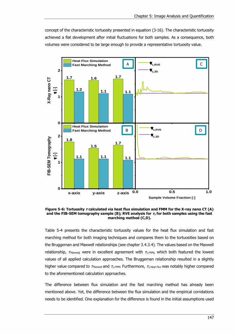
Chapter 5: Image Analysis and Quantification
147
concept of the characteristic tortuosity presented in equation (3-16). The characteristic tortuosity
achieved a flat development after initial fluctuations for both samples. As a consequence, both
volumes were considered to be large enough to provide a representative tortuosity value.
Figure 5-6: Tortuosity τ calculated via heat flux simulation and FMM for the X-ray nano CT (A) and the FIB-SEM tomography sample (B); RVE analysis for τc for both samples using the fast
marching method (C,D).
Table 5-4 presents the characteristic tortuosity values for the heat flux simulation and fast
marching method for both imaging techniques and compares them to the tortuosities based on
the Bruggeman and Maxwell relationships (see chapter 3.4.3.4). The values based on the Maxwell
relationship, τMaxwell, were in excellent agreement with τc,FMM, which both featured the lowest
values of all applied calculation approaches. The Bruggeman relationship resulted in a slightly
higher value compared to τMaxwell and τc,FMM. Furthermore, τc,Heat Flux was notably higher compared
to the aforementioned calculation approaches.
The difference between flux simulation and the fast marching method has already been
mentioned above. Yet, the difference between the flux simulation and the empirical correlations
needs to be identified. One explanation for the difference is found in the initial assumptions used
0.0 0.5 1.0
1.7 1.6 1.7
1.21.1 1.1
1.8
1.51.7
1.1 1.1 1.1
0
1
2
Heat Flux Simulation
Fast Marching Method
X-R
ay n
an
o C
T
[-
]
c,RVE
c,3D
x-axis y-axis z-axis
0
1
2
Heat Flux Simulation
Fast Marching Method
FIB
-SE
M T
om
og
rap
hy
[-
]
Sample Volume Fraction [-]
c,RVE
c,3D
B
A
D
C
Chapter 5: Image Analysis and Quantification
148
by Maxwell and Bruggeman when they established their calculation models: their initial
derivations were based on inserting insulating spheres in a conducting medium and extracting
the effective conductivity of the new, mixed sample as outlined in chapter 2.2.2 and in [68].
However, the analysed microstructure did not contain sphere shaped particles but was rather a
connected, heterogeneous solid structure. Therefore, these correlations were unsuitable for the
microstructures treated here and have to be applied with caution. Hence, the Maxwell and
Bruggeman relationships are only applied for comparison reasons in this thesis.
Table 5-4: Comparison of characteristic tortuosity τc for heat flux and FMM with empirical tortuosity correlations of sample 100% TZ3YSB K.
τc,Heat Flux τc,FMM τBruggeman τMaxwell
[-] [-] [-] [-]
X-ray nano CT 1.66 1.14 1.28 1.15
FIB-SEM tomography 1.65 1.12 1.26 1.14
5.3 Comparison between Planar and Tubular Sample
The comparison between the planar and tubular diffusion cell experiments presented in chapter
4.3 resulted in broadly agreeing tortuosity values: the average tortuosity of the planar sample
(100% TZ3YSB K) amounted to 2.3 while the average tortuosity of the tubular sample
(PS 2310 1360C) amounted to 2.7. X-ray nano CT was thus applied on the tubular sample
PS 2310 1360C and compared to the data of the planar sample summarised in the previous
section to further investigate the reasons for these slight deviations. Moreover, microstructural
data of sample PS 1909 1360C was included in this comparison to evaluate the consistency of
sample manufacturing technique by Praxair Inc.
Table 5-5: Comparison of pixel size, cube side length s, porosity ε and mean pore diameter dP of tubular samples PS 2310 1360C and PS 1909 1360C.
100% TZ3YSB K PS 2310 1360C PS 1909 1360C
Tomography
method [-]
FIB-SEM
Tomography
X-ray
nano CT
X-ray
nano CT
X-ray
nano CT
Pixel size [μm] 0.0301 0.0325 0.0631 0.0325
s [μm] 7.0 7.5 6.3 7.1
ε [-] 0.40 0.37 0.37 0.38
dP [μm] 0.67 0.62 0.78 0.66

Chapter 5: Image Analysis and Quantification
149
The two obtained datasets for the tubular samples were cropped and segmented using the same
methodology as in the previous section. Two cubes with side lengths of 6.3 μm and 7.1 μm were
extracted for sample PS 2310 1360C and PS 1909 1360C, respectively. In theory, all the
microstructural data of the planar and tubular samples should be statistically identical, as the
planar sample was prepared under the same sintering conditions and using the same powders as
the tubular samples. Table 5-5 lists the pixel sizes, side lengths, porosities and mean pore
diameters for all sample volumes. It is visible that porosity of all samples agreed very well with
each other. In addition, the mean pore diameter of both planar sample volumes and the tubular
sample PS 1909 1360C were almost identical. Only the mean pore diameter of sample
PS 2310 1360C was significantly higher.
Figure 5-7: Comparison of pore size histogram of sample 100% TZ3YSB K imaged using X-ray nano CT (A) and FIB-SEM tomography (B), sample PS 2310 1360C imaged using X-ray nano
CT (C) and PS 1909 1360C imaged using X-ray nano CT (D).
Figure 5-7 presents a more detailed analysis of dP by illustrating the pore size distribution
histograms of all samples calculated via the continuous pore size distribution code from [233] (cf.
chapter 3.4.2). Here, the PSDs differed appreciably between the planar and tubular sample. The
planar sample did not feature a clearly developed peak compared to the tubular sample, but
0.00
0.02
0.04
0.06
0.08
Po
re V
olu
me
Fra
cti
n [
-]
100% TZ3YSB K X-ray nano CT PS 2310 1360C X-ray nano CT
0.0 0.5 1.0
0.00
0.02
0.04
0.06
Po
re V
olu
me
Fra
cti
n [
-]
dP [m]
100% TZ3YSB K FIB-SEM Tomography
0.0 0.5 1.0 1.5
dP [m]
PS 1909 1360C X-ray nano CT
A
B
C
D
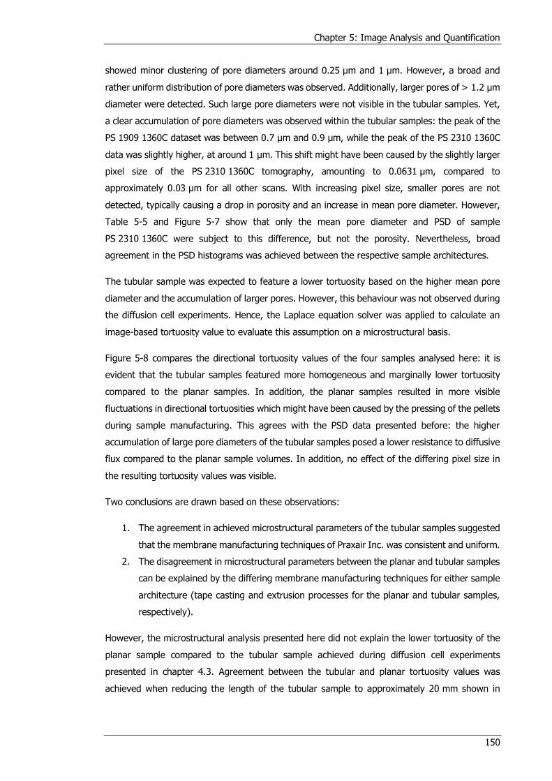
Chapter 5: Image Analysis and Quantification
150
showed minor clustering of pore diameters around 0.25 μm and 1 μm. However, a broad and
rather uniform distribution of pore diameters was observed. Additionally, larger pores of > 1.2 μm
diameter were detected. Such large pore diameters were not visible in the tubular samples. Yet,
a clear accumulation of pore diameters was observed within the tubular samples: the peak of the
PS 1909 1360C dataset was between 0.7 μm and 0.9 μm, while the peak of the PS 2310 1360C
data was slightly higher, at around 1 μm. This shift might have been caused by the slightly larger
pixel size of the PS 2310 1360C tomography, amounting to 0.0631 μm, compared to
approximately 0.03 μm for all other scans. With increasing pixel size, smaller pores are not
detected, typically causing a drop in porosity and an increase in mean pore diameter. However,
Table 5-5 and Figure 5-7 show that only the mean pore diameter and PSD of sample
PS 2310 1360C were subject to this difference, but not the porosity. Nevertheless, broad
agreement in the PSD histograms was achieved between the respective sample architectures.
The tubular sample was expected to feature a lower tortuosity based on the higher mean pore
diameter and the accumulation of larger pores. However, this behaviour was not observed during
the diffusion cell experiments. Hence, the Laplace equation solver was applied to calculate an
image-based tortuosity value to evaluate this assumption on a microstructural basis.
Figure 5-8 compares the directional tortuosity values of the four samples analysed here: it is
evident that the tubular samples featured more homogeneous and marginally lower tortuosity
compared to the planar samples. In addition, the planar samples resulted in more visible
fluctuations in directional tortuosities which might have been caused by the pressing of the pellets
during sample manufacturing. This agrees with the PSD data presented before: the higher
accumulation of large pore diameters of the tubular samples posed a lower resistance to diffusive
flux compared to the planar sample volumes. In addition, no effect of the differing pixel size in
the resulting tortuosity values was visible.
Two conclusions are drawn based on these observations:
1. The agreement in achieved microstructural parameters of the tubular samples suggested
that the membrane manufacturing techniques of Praxair Inc. was consistent and uniform.
2. The disagreement in microstructural parameters between the planar and tubular samples
can be explained by the differing membrane manufacturing techniques for either sample
architecture (tape casting and extrusion processes for the planar and tubular samples,
respectively).
However, the microstructural analysis presented here did not explain the lower tortuosity of the
planar sample compared to the tubular sample achieved during diffusion cell experiments
presented in chapter 4.3. Agreement between the tubular and planar tortuosity values was
achieved when reducing the length of the tubular sample to approximately 20 mm shown in

Chapter 5: Image Analysis and Quantification
151
chapter 4.4, which is significantly shorter than the tubes used by Praxair Inc. in their OTM reactor.
The reason for this were fuel depletion effects observed in the tubular diffusion cell.
Figure 5-8: Comparison of directional tortuosity values calculated via the Laplace euqation solver for the planar and tubular samples.
5.4 Image-based Tortuosity for 2.4th Generation Porous Support
Layers
The same analysis methods presented in the previous sections were applied to the four current
generation tubular porous support samples. The membranes were imaged via X-ray nano CT
using the parameters presented in Table 5-6. Parts of this section have been submitted for
peer-reviewed publication [239].
Two volumes of different dimensions were cropped for each tubular sample to cater for the
difference in membrane thickness: one cuboid sample with the dimensions of
100 × 100 × 200 pixels3 side length (6.31 μm × 6.31 μm × 12.62 μm) and a cubic sample with
100 pixels side length (6.31 μm × 6.31 μm × 6.31 μm) were extracted, which shared the same
1.8
1.9
1.71.7
1.7
1.6
1.71.7
1.8
1.7 1.71.7
100%
TZ3Y
SB K
X-ray
CT
100%
TZ3Y
SB K
FIB
-SEM
PS 2
310
1360
C
PS 1
909
1360
C
1.0
1.5
2.0
x
y
z
[-]
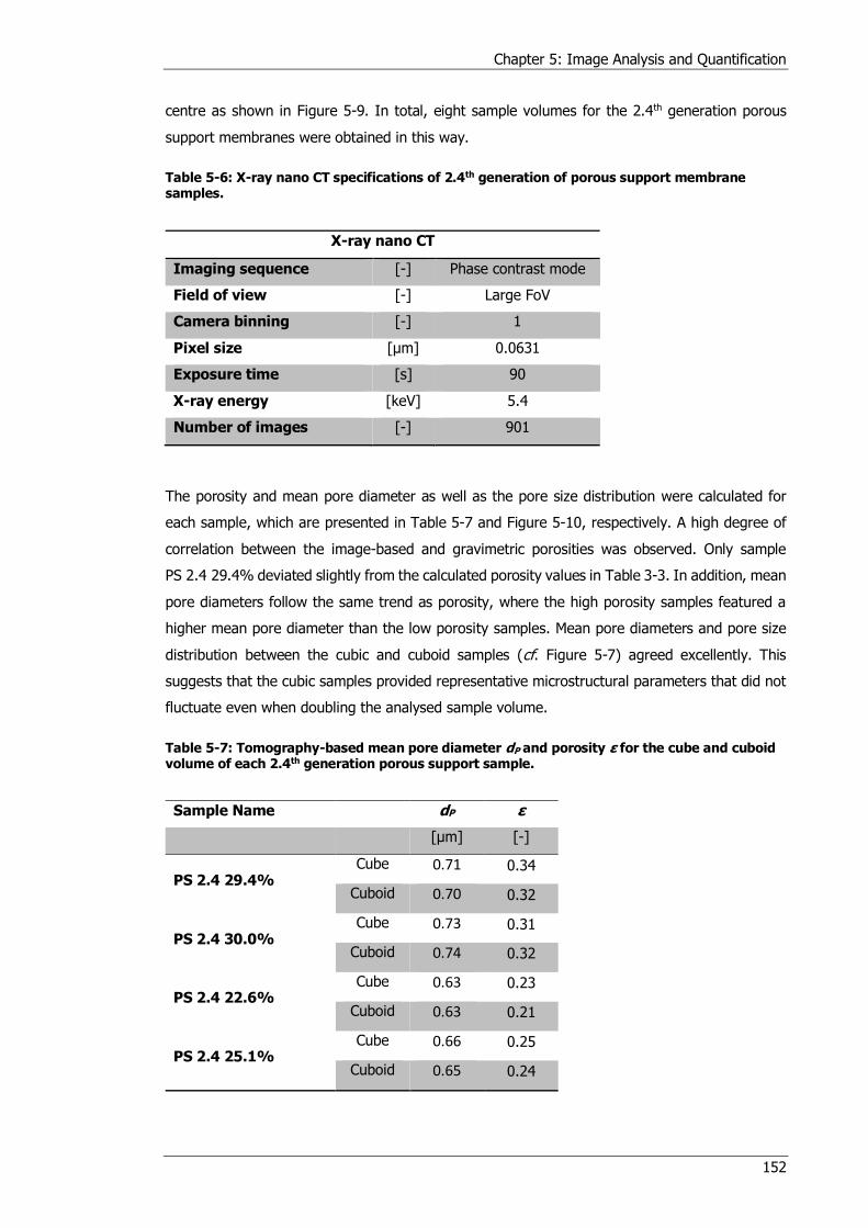
Chapter 5: Image Analysis and Quantification
152
centre as shown in Figure 5-9. In total, eight sample volumes for the 2.4th generation porous
support membranes were obtained in this way.
Table 5-6: X-ray nano CT specifications of 2.4th generation of porous support membrane samples.
X-ray nano CT
Imaging sequence [-] Phase contrast mode
Field of view [-] Large FoV
Camera binning [-] 1
Pixel size [μm] 0.0631
Exposure time [s] 90
X-ray energy [keV] 5.4
Number of images [-] 901
The porosity and mean pore diameter as well as the pore size distribution were calculated for
each sample, which are presented in Table 5-7 and Figure 5-10, respectively. A high degree of
correlation between the image-based and gravimetric porosities was observed. Only sample
PS 2.4 29.4% deviated slightly from the calculated porosity values in Table 3-3. In addition, mean
pore diameters follow the same trend as porosity, where the high porosity samples featured a
higher mean pore diameter than the low porosity samples. Mean pore diameters and pore size
distribution between the cubic and cuboid samples (cf. Figure 5-7) agreed excellently. This
suggests that the cubic samples provided representative microstructural parameters that did not
fluctuate even when doubling the analysed sample volume.
Table 5-7: Tomography-based mean pore diameter dP and porosity ε for the cube and cuboid volume of each 2.4th generation porous support sample.
Sample Name dP ε
[μm] [-]
PS 2.4 29.4% Cube 0.71 0.34
Cuboid 0.70 0.32
PS 2.4 30.0% Cube 0.73 0.31
Cuboid 0.74 0.32
PS 2.4 22.6% Cube 0.63 0.23
Cuboid 0.63 0.21
PS 2.4 25.1% Cube 0.66 0.25
Cuboid 0.65 0.24
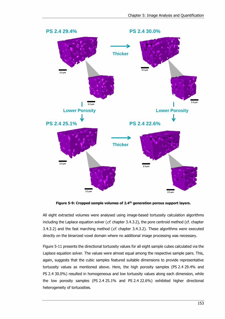
Chapter 5: Image Analysis and Quantification
153
Figure 5-9: Cropped sample volumes of 2.4th generation porous support layers.
All eight extracted volumes were analysed using image-based tortuosity calculation algorithms
including the Laplace equation solver (cf. chapter 3.4.3.2), the pore centroid method (cf. chapter
3.4.3.2) and the fast marching method (cf. chapter 3.4.3.2). These algorithms were executed
directly on the binarized voxel domain where no additional image processing was necessary.
Figure 5-11 presents the directional tortuosity values for all eight sample cubes calculated via the
Laplace equation solver. The values were almost equal among the respective sample pairs. This,
again, suggests that the cubic samples featured suitable dimensions to provide representative
tortuosity values as mentioned above. Here, the high porosity samples (PS 2.4 29.4% and
PS 2.4 30.0%) resulted in homogeneous and low tortuosity values along each dimension, while
the low porosity samples (PS 2.4 25.1% and PS 2.4 22.6%) exhibited higher directional
heterogeneity of tortuosities.
Thicker
Thicker
Lower PorosityLower Porosity
2.5 μm
2.5 μm
2.5 μm
2.5 μm
2.5 μm2.5 μm
2.5 μm 2.5 μm
PS 2.4 29.4% PS 2.4 30.0%
PS 2.4 25.1% PS 2.4 22.6%
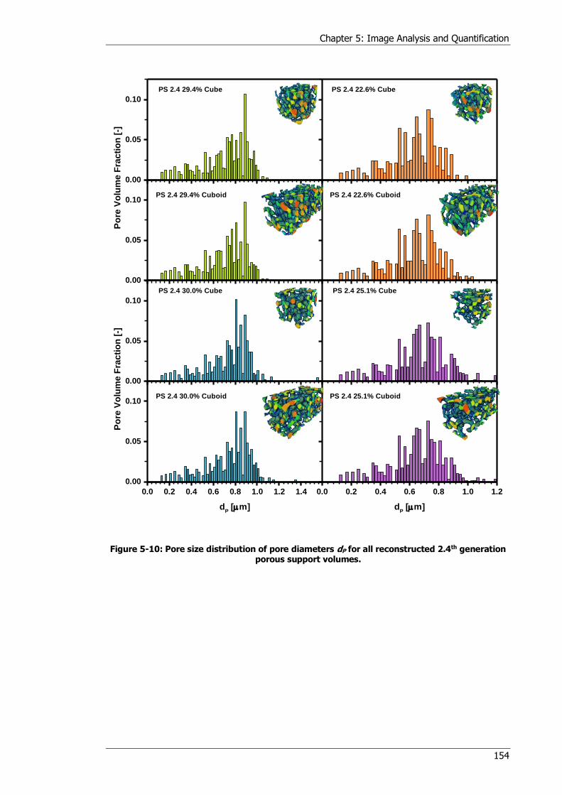
Chapter 5: Image Analysis and Quantification
154
Figure 5-10: Pore size distribution of pore diameters dP for all reconstructed 2.4th generation porous support volumes.
0.00
0.05
0.10
PS 2.4 29.4% Cube
0.00
0.05
0.10
Po
re V
olu
me
Fra
cti
on
[-]
PS 2.4 29.4% Cuboid
PS 2.4 22.6% Cube
PS 2.4 22.6% Cuboid
0.00
0.05
0.10
PS 2.4 30.0% Cube
0.0 0.2 0.4 0.6 0.8 1.0 1.2 1.4
0.00
0.05
0.10
Po
re V
olu
me
Fra
cti
on
[-]
dP [m]
PS 2.4 30.0% Cuboid
PS 2.4 25.1% Cube
0.0 0.2 0.4 0.6 0.8 1.0 1.2
dP [m]
PS 2.4 25.1% Cuboid
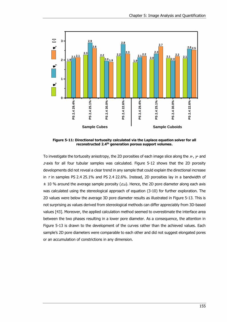
Chapter 5: Image Analysis and Quantification
155
Figure 5-11: Directional tortuosity calculated via the Laplace equation solver for all reconstructed 2.4th generation porous support volumes.
To investigate the tortuosity anisotropy, the 2D porosities of each image slice along the x-, y- and
z-axis for all four tubular samples was calculated. Figure 5-12 shows that the 2D porosity
developments did not reveal a clear trend in any sample that could explain the directional increase
in τ in samples PS 2.4 25.1% and PS 2.4 22.6%. Instead, 2D porosities lay in a bandwidth of
± 10 % around the average sample porosity (ε3D). Hence, the 2D pore diameter along each axis
was calculated using the stereological approach of equation (3-10) for further exploration. The
2D values were below the average 3D pore diameter results as illustrated in Figure 5-13. This is
not surprising as values derived from stereological methods can differ appreciably from 3D-based
values [43]. Moreover, the applied calculation method seemed to overestimate the interface area
between the two phases resulting in a lower pore diameter. As a consequence, the attention in
Figure 5-13 is drawn to the development of the curves rather than the achieved values. Each
sample’s 2D pore diameters were comparable to each other and did not suggest elongated pores
or an accumulation of constrictions in any dimension.
1.9
2.32.2 2.2
1.92.0
2.1 2.12.1
2.9
2.0
2.8
2.1
2.3
2.0
2.6
2.1
2.6
1.9
2.32.2
2.7
2.2
2.5
PS
2.4
29
.4%
PS
2.4
25
.1%
PS
2.4
30
.0%
PS
2.4
22
.6%
PS
2.4
29
.4%
PS
2.4
25
.1%
PS
2.4
30
.0%
PS
2.4
22
.6%
0
1
2
3
Sample Cuboids
x
y
z [
-]
Sample Cubes
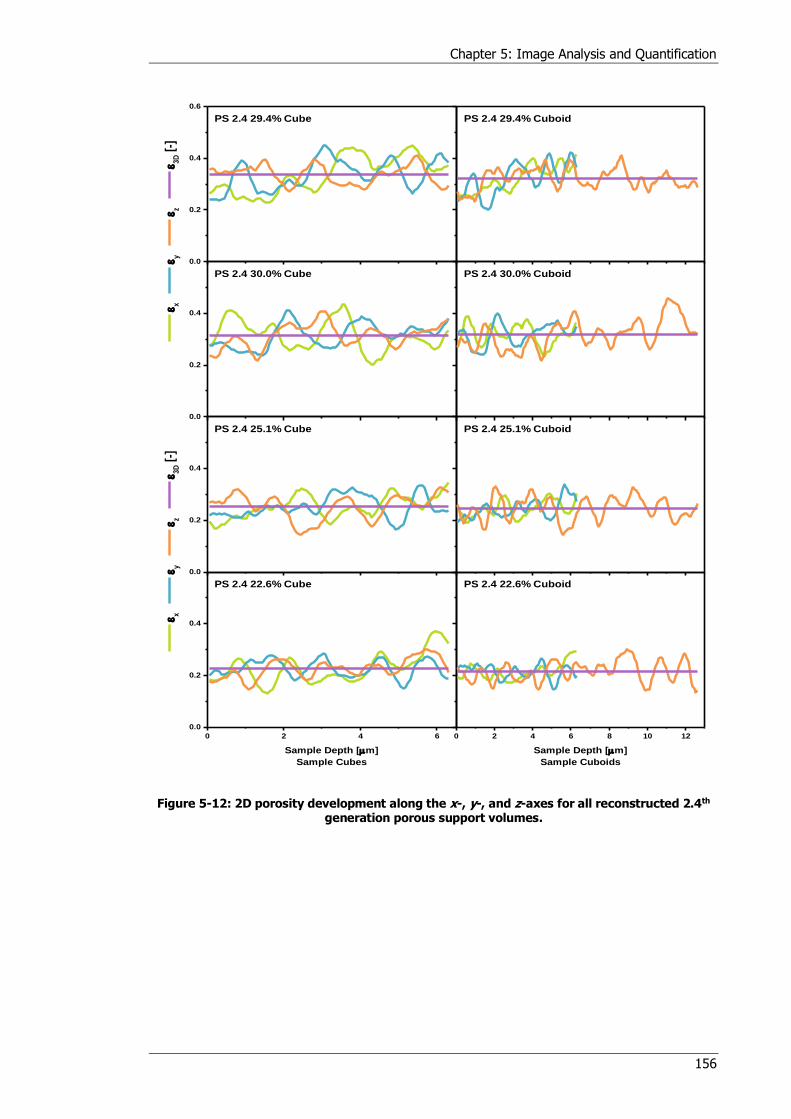
Chapter 5: Image Analysis and Quantification
156
Figure 5-12: 2D porosity development along the x-, y-, and z-axes for all reconstructed 2.4th generation porous support volumes.
0.0
0.2
0.4
0.6
0.0
0.2
0.4
0.0
0.2
0.4
0 2 4 6
0.0
0.2
0.4
0 2 4 6 8 10 12
x
y
z
3D [
-]
PS 2.4 29.4% Cube
x
y
z
3D [
-]
PS 2.4 29.4% Cuboid
PS 2.4 30.0% Cube PS 2.4 30.0% Cuboid
PS 2.4 25.1% Cube PS 2.4 25.1% Cuboid
Sample Depth [m]
Sample Cubes
PS 2.4 22.6% Cube
Sample Depth [m]
Sample Cuboids
PS 2.4 22.6% Cuboid
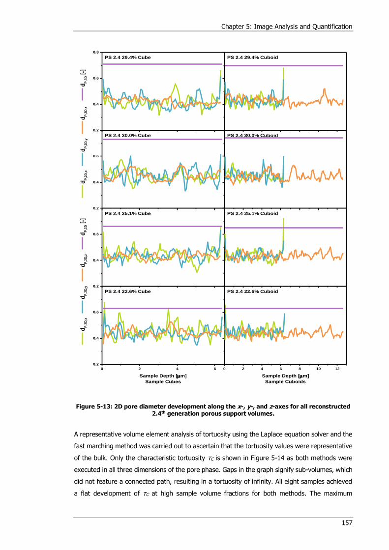
Chapter 5: Image Analysis and Quantification
157
Figure 5-13: 2D pore diameter development along the x-, y-, and z-axes for all reconstructed 2.4th generation porous support volumes.
A representative volume element analysis of tortuosity using the Laplace equation solver and the
fast marching method was carried out to ascertain that the tortuosity values were representative
of the bulk. Only the characteristic tortuosity τC is shown in Figure 5-14 as both methods were
executed in all three dimensions of the pore phase. Gaps in the graph signify sub-volumes, which
did not feature a connected path, resulting in a tortuosity of infinity. All eight samples achieved
a flat development of τC at high sample volume fractions for both methods. The maximum
0.2
0.4
0.6
0.8
0.2
0.4
0.6
0.2
0.4
0.6
0 2 4 6
0.2
0.4
0.6
0 2 4 6 8 10 12
PS 2.4 29.4% Cube PS 2.4 29.4% Cuboid
PS 2.4 30.0% Cube PS 2.4 30.0% Cuboid
PS 2.4 25.1% Cube PS 2.4 25.1% Cuboid
Sample Depth [m]
Sample Cubes
dP
,2D
,x d
P,2
D,y
dP
,2D
,z
dP
,3D [
-]
PS 2.4 22.6% Cube
Sample Depth [m]
Sample Cuboids
dP
,2D
,x d
P,2
D,y
dP
,2D
,z d
P,3
D [
-]
PS 2.4 22.6% Cuboid
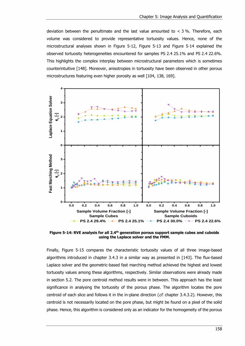
Chapter 5: Image Analysis and Quantification
158
deviation between the penultimate and the last value amounted to < 3 %. Therefore, each
volume was considered to provide representative tortuosity values. Hence, none of the
microstructural analyses shown in Figure 5-12, Figure 5-13 and Figure 5-14 explained the
observed tortuosity heterogeneities encountered for samples PS 2.4 25.1% and PS 2.4 22.6%.
This highlights the complex interplay between microstructural parameters which is sometimes
counterintuitive [148]. Moreover, anisotropies in tortuosity have been observed in other porous
microstructures featuring even higher porosity as well [104, 138, 169].
Figure 5-14: RVE analysis for all 2.4th generation porous support sample cubes and cuboids using the Laplace solver and the FMM.
Finally, Figure 5-15 compares the characteristic tortuosity values of all three image-based
algorithms introduced in chapter 3.4.3 in a similar way as presented in [143]. The flux-based
Laplace solver and the geometric-based fast marching method achieved the highest and lowest
tortuosity values among these algorithms, respectively. Similar observations were already made
in section 5.2. The pore centroid method results were in between. This approach has the least
significance in analysing the tortuosity of the porous phase. The algorithm locates the pore
centroid of each slice and follows it in the in-plane direction (cf. chapter 3.4.3.2). However, this
centroid is not necessarily located on the pore phase, but might be found on a pixel of the solid
phase. Hence, this algorithm is considered only as an indicator for the homogeneity of the porous
0
1
2
3
4
0.0 0.2 0.4 0.6 0.8 1.0
0
1
2
3
0.0 0.2 0.4 0.6 0.8 1.0
La
pla
ce
Eq
uati
on
So
lve
r
C [
-]
PS 2.4 29.4% PS 2.4 25.1% PS 2.4 30.0% PS 2.4 22.6%
Fa
st
Ma
rch
ing
Me
tho
d
C [
-]
Sample Volume Fraction [-]
Sample Cubes
Sample Volume Fraction [-]
Sample Cuboids
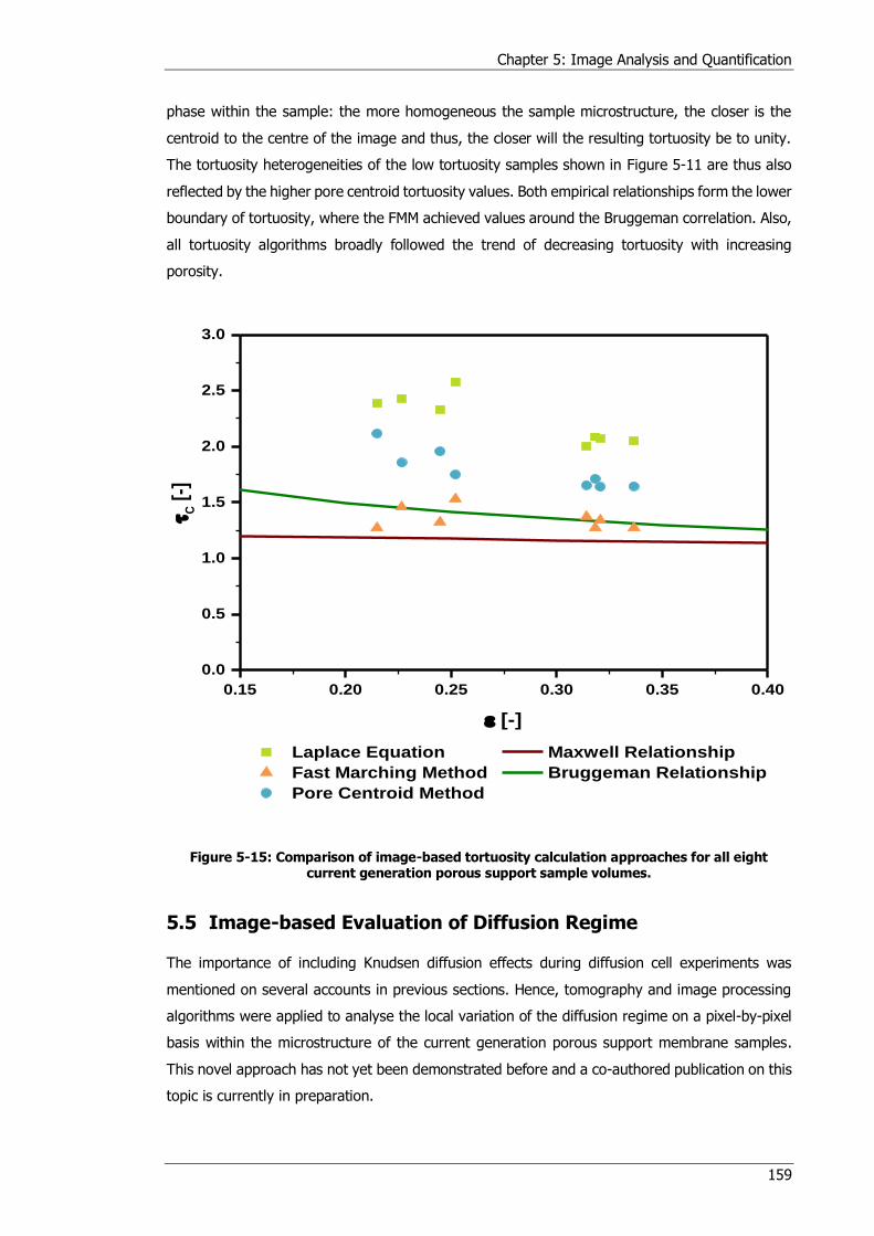
Chapter 5: Image Analysis and Quantification
159
phase within the sample: the more homogeneous the sample microstructure, the closer is the
centroid to the centre of the image and thus, the closer will the resulting tortuosity be to unity.
The tortuosity heterogeneities of the low tortuosity samples shown in Figure 5-11 are thus also
reflected by the higher pore centroid tortuosity values. Both empirical relationships form the lower
boundary of tortuosity, where the FMM achieved values around the Bruggeman correlation. Also,
all tortuosity algorithms broadly followed the trend of decreasing tortuosity with increasing
porosity.
Figure 5-15: Comparison of image-based tortuosity calculation approaches for all eight current generation porous support sample volumes.
5.5 Image-based Evaluation of Diffusion Regime
The importance of including Knudsen diffusion effects during diffusion cell experiments was
mentioned on several accounts in previous sections. Hence, tomography and image processing
algorithms were applied to analyse the local variation of the diffusion regime on a pixel-by-pixel
basis within the microstructure of the current generation porous support membrane samples.
This novel approach has not yet been demonstrated before and a co-authored publication on this
topic is currently in preparation.
0.15 0.20 0.25 0.30 0.35 0.40
0.0
0.5
1.0
1.5
2.0
2.5
3.0
Laplace Equation Maxwell Relationship
Fast Marching Method Bruggeman Relationship
Pore Centroid Method
C [
-]
[-]
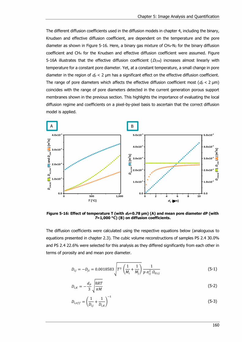
Chapter 5: Image Analysis and Quantification
160
The different diffusion coefficients used in the diffusion models in chapter 4, including the binary,
Knudsen and effective diffusion coefficient, are dependent on the temperature and the pore
diameter as shown in Figure 5-16. Here, a binary gas mixture of CH4-N2 for the binary diffusion
coefficient and CH4 for the Knudsen and effective diffusion coefficient were assumed. Figure
5-16A illustrates that the effective diffusion coefficient (DCH4) increases almost linearly with
temperature for a constant pore diameter. Yet, at a constant temperature, a small change in pore
diameter in the region of dp < 2 μm has a significant effect on the effective diffusion coefficient.
The range of pore diameters which affects the effective diffusion coefficient most (dp < 2 μm)
coincides with the range of pore diameters detected in the current generation porous support
membranes shown in the previous section. This highlights the importance of evaluating the local
diffusion regime and coefficients on a pixel-by-pixel basis to ascertain that the correct diffusion
model is applied.
Figure 5-16: Effect of temperature T (with dP=0.78 μm) (A) and mean pore diameter dP (with T=1,000 °C) (B) on diffusion coefficients.
The diffusion coefficients were calculated using the respective equations below (analoguous to
equations presented in chapter 2.3). The cubic volume reconstructions of samples PS 2.4 30.0%
and PS 2.4 22.6% were selected for this analysis as they differed significantly from each other in
terms of porosity and and mean pore diameter.
𝐷𝑖𝑗 = −𝐷𝑗𝑖 = 0.0018583√𝑇3 (1
𝑀𝑖
+1
𝑀𝑗)
1
𝑝 𝜎𝑖𝑗2 𝛺𝐷,𝑖𝑗
(5-1)
𝐷𝑖,𝐾 = −𝑑𝑃3√8𝑅𝑇
𝜋𝑀 (5-2)
𝐷𝑖,𝑒𝑓𝑓 = (1
𝐷𝑖𝑗+
1
𝐷𝑖,𝐾)
−1
(5-3)
0 500 1,0000.0
1.0x10⁻⁴
2.0x10⁻⁴
3.0x10⁻⁴
4.0x10⁻⁴
0 2 4 6 8 100.0
1.0x10⁻³
2.0x10⁻³
3.0x10⁻³
4.0x10⁻³
5.0x10⁻³
DC
H4,N
2 (
), D
Kn
,CH
4 (
) a
nd
DC
H4 (
) [m
2/s
]
T [°C]
DK
n,C
H4 (
) [m
2/s
]
dP [m]
0.0
1.0x10⁻⁴
2.0x10⁻⁴
3.0x10⁻⁴
4.0x10⁻⁴
5.0x10⁻⁴
DC
H4,N
2 (
), D
CH
4 (
) [m
2/s
]
A B
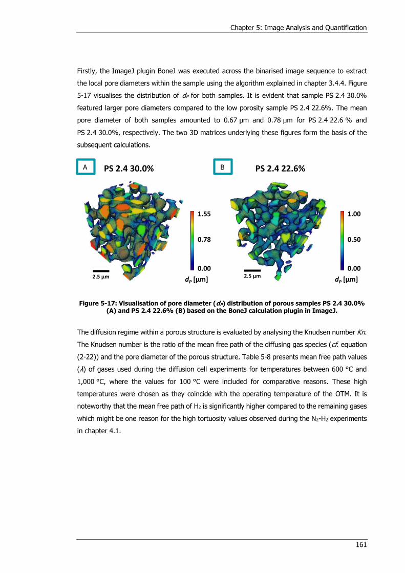
Chapter 5: Image Analysis and Quantification
161
Firstly, the ImageJ plugin BoneJ was executed across the binarised image sequence to extract
the local pore diameters within the sample using the algorithm explained in chapter 3.4.4. Figure
5-17 visualises the distribution of dP for both samples. It is evident that sample PS 2.4 30.0%
featured larger pore diameters compared to the low porosity sample PS 2.4 22.6%. The mean
pore diameter of both samples amounted to 0.67 μm and 0.78 μm for PS 2.4 22.6 % and
PS 2.4 30.0%, respectively. The two 3D matrices underlying these figures form the basis of the
subsequent calculations.
Figure 5-17: Visualisation of pore diameter (dP) distribution of porous samples PS 2.4 30.0% (A) and PS 2.4 22.6% (B) based on the BoneJ calculation plugin in ImageJ.
The diffusion regime within a porous structure is evaluated by analysing the Knudsen number Kn.
The Knudsen number is the ratio of the mean free path of the diffusing gas species (cf. equation
(2-22)) and the pore diameter of the porous structure. Table 5-8 presents mean free path values
(λ) of gases used during the diffusion cell experiments for temperatures between 600 °C and
1,000 °C, where the values for 100 °C were included for comparative reasons. These high
temperatures were chosen as they coincide with the operating temperature of the OTM. It is
noteworthy that the mean free path of H2 is significantly higher compared to the remaining gases
which might be one reason for the high tortuosity values observed during the N2-H2 experiments
in chapter 4.1.
dP [μm]
0.00
1.55
0.78
dP [μm]
0.00
1.00
0.50
PS 2.4 22.6%PS 2.4 30.0%
2.5 μm 2.5 μm
B A
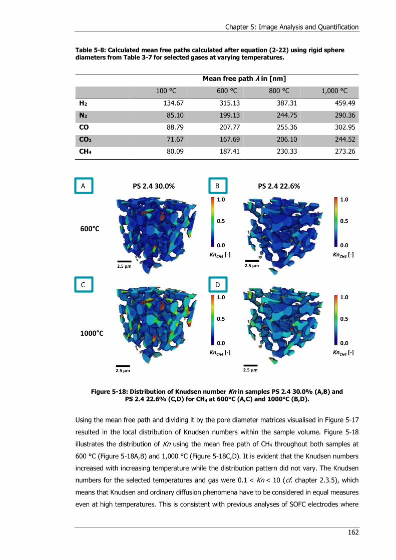
Chapter 5: Image Analysis and Quantification
162
Table 5-8: Calculated mean free paths calculated after equation (2-22) using rigid sphere diameters from Table 3-7 for selected gases at varying temperatures.
Mean free path λ in [nm]
100 °C 600 °C 800 °C 1,000 °C
H2 134.67 315.13 387.31 459.49
N2 85.10 199.13 244.75 290.36
CO 88.79 207.77 255.36 302.95
CO2 71.67 167.69 206.10 244.52
CH4 80.09 187.41 230.33 273.26
Figure 5-18: Distribution of Knudsen number Kn in samples PS 2.4 30.0% (A,B) and PS 2.4 22.6% (C,D) for CH4 at 600°C (A,C) and 1000°C (B,D).
Using the mean free path and dividing it by the pore diameter matrices visualised in Figure 5-17
resulted in the local distribution of Knudsen numbers within the sample volume. Figure 5-18
illustrates the distribution of Kn using the mean free path of CH4 throughout both samples at
600 °C (Figure 5-18A,B) and 1,000 °C (Figure 5-18C,D). It is evident that the Knudsen numbers
increased with increasing temperature while the distribution pattern did not vary. The Knudsen
numbers for the selected temperatures and gas were 0.1 < Kn < 10 (cf. chapter 2.3.5), which
means that Knudsen and ordinary diffusion phenomena have to be considered in equal measures
even at high temperatures. This is consistent with previous analyses of SOFC electrodes where
KnCH4 [-]
0.0
1.0
0.5
KnCH4 [-]
0.0
1.0
0.5
KnCH4 [-]
0.0
1.0
0.5
KnCH4 [-]
0.0
1.0
0.5
600°C
1000°C
PS 2.4 22.6%PS 2.4 30.0%
2.5 μm 2.5 μm
2.5 μm 2.5 μm
B A
D C
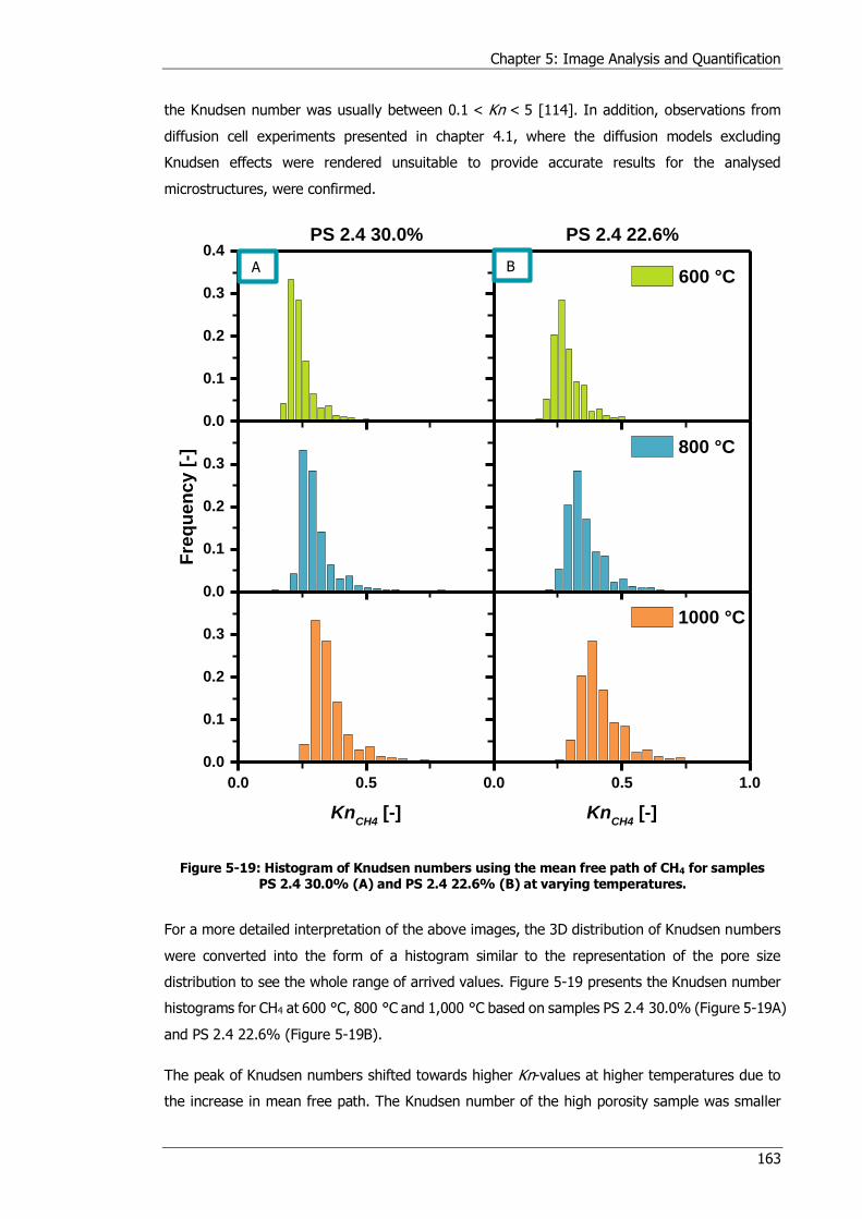
Chapter 5: Image Analysis and Quantification
163
the Knudsen number was usually between 0.1 < Kn < 5 [114]. In addition, observations from
diffusion cell experiments presented in chapter 4.1, where the diffusion models excluding
Knudsen effects were rendered unsuitable to provide accurate results for the analysed
microstructures, were confirmed.
Figure 5-19: Histogram of Knudsen numbers using the mean free path of CH4 for samples PS 2.4 30.0% (A) and PS 2.4 22.6% (B) at varying temperatures.
For a more detailed interpretation of the above images, the 3D distribution of Knudsen numbers
were converted into the form of a histogram similar to the representation of the pore size
distribution to see the whole range of arrived values. Figure 5-19 presents the Knudsen number
histograms for CH4 at 600 °C, 800 °C and 1,000 °C based on samples PS 2.4 30.0% (Figure 5-19A)
and PS 2.4 22.6% (Figure 5-19B).
The peak of Knudsen numbers shifted towards higher Kn-values at higher temperatures due to
the increase in mean free path. The Knudsen number of the high porosity sample was smaller
0.0
0.1
0.2
0.3
0.4PS 2.4 30.0%
0.0
0.1
0.2
0.3
Fre
qu
en
cy
[-]
0.0 0.5
0.0
0.1
0.2
0.3
KnCH4
[-]
600 °C
PS 2.4 22.6%
800 °C
0.0 0.5 1.0
KnCH4
[-]
1000 °C
B A
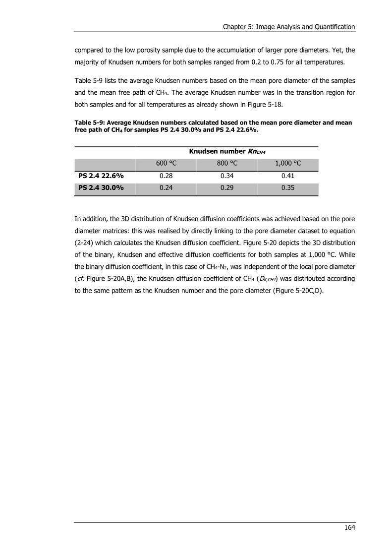
Chapter 5: Image Analysis and Quantification
164
compared to the low porosity sample due to the accumulation of larger pore diameters. Yet, the
majority of Knudsen numbers for both samples ranged from 0.2 to 0.75 for all temperatures.
Table 5-9 lists the average Knudsen numbers based on the mean pore diameter of the samples
and the mean free path of CH4. The average Knudsen number was in the transition region for
both samples and for all temperatures as already shown in Figure 5-18.
Table 5-9: Average Knudsen numbers calculated based on the mean pore diameter and mean free path of CH4 for samples PS 2.4 30.0% and PS 2.4 22.6%.
Knudsen number KnCH4
600 °C 800 °C 1,000 °C
PS 2.4 22.6% 0.28 0.34 0.41
PS 2.4 30.0% 0.24 0.29 0.35
In addition, the 3D distribution of Knudsen diffusion coefficients was achieved based on the pore
diameter matrices: this was realised by directly linking to the pore diameter dataset to equation
(2-24) which calculates the Knudsen diffusion coefficient. Figure 5-20 depicts the 3D distribution
of the binary, Knudsen and effective diffusion coefficients for both samples at 1,000 °C. While
the binary diffusion coefficient, in this case of CH4-N2, was independent of the local pore diameter
(cf. Figure 5-20A,B), the Knudsen diffusion coefficient of CH4 (DK,CH4) was distributed according
to the same pattern as the Knudsen number and the pore diameter (Figure 5-20C,D).

Chapter 5: Image Analysis and Quantification
165
Figure 5-20: Distribution of the binary diffusion coefficient DCH4,N2 (A,B), Knudsen diffusion coefficient DK,CH4 (C,D) and effective diffusion coefficient DCH4 (E,F) in samples PS 2.4 30.0%
(left) and PS 2.4 22.6% (right) at 1,000°C.
The effective diffusion coefficient of CH4 (DCH4) was calculated on a pixel-by-pixel basis by
applying the Bosanquet equation (equation (5-3)) and combining the values of both diffusion
coefficients. Again, the distribution of DCH4 was analogous to the distribution of DK,CH4. Table 5-10
presents average values for DK,CH4 and DCH4 for both samples based on the mean pore diameter.
Hence, fluctuations in the pore diameter within the sample directly scale either parameter.
DCH4 [m2/s]
5×10⁻⁵
1.6×10⁻⁴
1.3×10⁻⁴
DCH4 [m2/s]
5×10⁻⁵
1.6×10⁻⁴
1.3×10⁻⁴
DK,CH4 [m2/s]
6×10⁻⁵
4.0×10⁻⁴
2.0×10⁻⁴
DK,CH4 [m2/s]
6×10⁻⁵
4.0×10⁻⁴
2.0×10⁻⁴
PS 2.4 22.6%PS 2.4 30.0%
2.5 μm 2.5 μm
2.5 μm 2.5 μm
2.5 μm 2.5 μm
DCH4,N2 = 2.6×10⁻⁴ m2/s
B A
D C
F E

Chapter 5: Image Analysis and Quantification
166
Table 5-10: Effective diffusion coefficient DCH4 calculated based on the binary diffusion coefficient DCH4,N2 and Knudsen diffusion coefficient DK,CH4.
Binary diffusion
coefficient
DCH4,N2
Knudsen diffusion
coefficient
DK,CH4
Diffusion
coefficient
DCH4
600 °C 1,000 °C 600 °C 1,000 °C 600 °C 1,000 °C
PS 2.4 22.6% 1.36×10⁻⁴ 2.60×10⁻⁴
2.40×10⁻⁴ 2.90×10⁻⁴ 8.69×10⁻⁵ 1.37×10⁻⁴
PS 2.4 30.0% 2.81×10⁻⁴ 3.39×10⁻⁴ 9.17×10⁻⁵ 1.47×10⁻⁴
The 3D visualisation of DCH4 revealed the significant differences in the value of the diffusion
coefficients throughout the microstructure even though both samples were clearly in the transient
regime. Diffusion coefficients below 1 × 10⁻⁴ m2s-1 and higher than 1.5 × 10⁻⁴ m2s-1 directly affect
the local diffusion flux and deviate visible from the average diffusion coefficients. Nevertheless,
the effect of the local diffusion coefficient on the overall diffusion flux can only be assumed as
the exact flow behaviour of a gas through a porous structure is difficult to predict accurately.
Even though the method presented here calculates a local pore diameter and local diffusion
coefficient, the pore diameter is determined by fitting spheres into the pore phase along the
centre of each channel. Hence, the calculated diffusion coefficients are averaged over the whole
pore diameter. Yet, gas molecules travelling close to the phase boundary might be subject to a
different Knudsen number compared to gas molecules travelling in the centre of the pore. While
for these latter molecules, the presented approach might be accurate, the collision phenomena
of the gas particles close to the phase boundary are not accounted for.
As a conclusion, it can be stated that Knudsen diffusion effects have to be included when
analysing the diffusion performance of the current generation porous support membranes.
Moreover, the consideration of such local variations in image-based computation algorithms
would be desirable to increase the accuracy of results. However, an algorithm capable of including
a local diffusion coefficient for each mesh cell was not available at the time of writing this thesis.
5.6 Artificial Opening and Closing of Sample Volumes
Praxair Inc. produced a series of differently sintered porous support membranes (cf. Table 3-3)
to evaluate the effect of porosity on the diffusion performance of these layers as presented in
chapter 4.6. This time consuming and costly approach would be unnecessary, if image-based
morphological processing techniques were able to mimic these different microstructures artificially.
Hence, this section investigates, how the artificial changes in porosity of a given sample affects
tortuosity and if the generated microstructures are comparable to the microstructures produced
by changing the sintering conditions. This method would open the possibility of estimating the
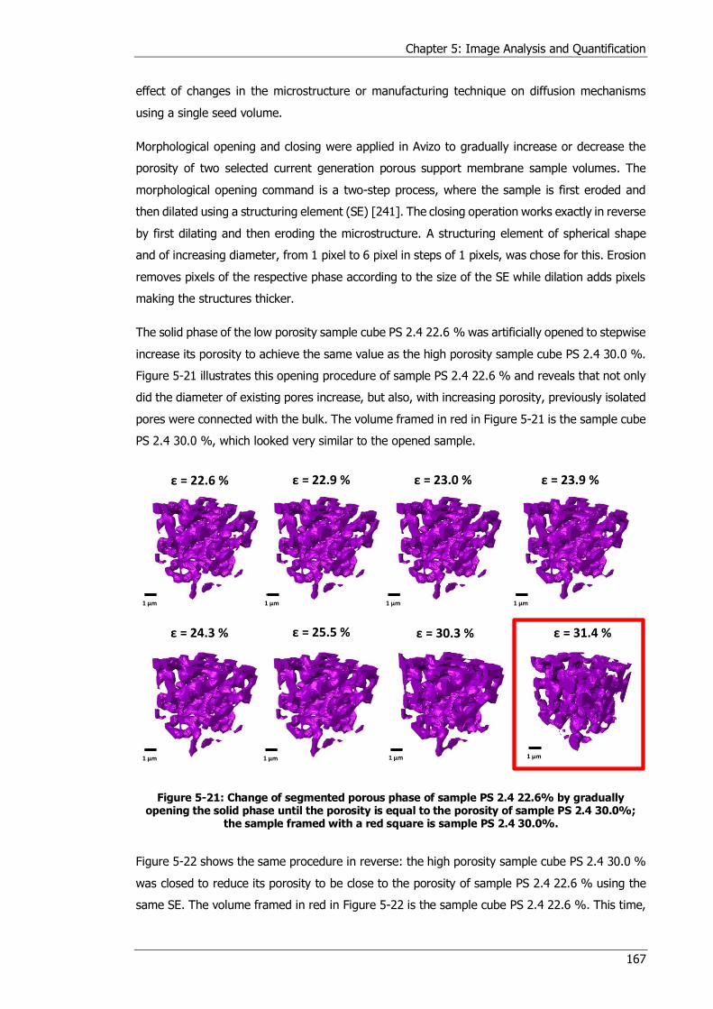
Chapter 5: Image Analysis and Quantification
167
effect of changes in the microstructure or manufacturing technique on diffusion mechanisms
using a single seed volume.
Morphological opening and closing were applied in Avizo to gradually increase or decrease the
porosity of two selected current generation porous support membrane sample volumes. The
morphological opening command is a two-step process, where the sample is first eroded and
then dilated using a structuring element (SE) [241]. The closing operation works exactly in reverse
by first dilating and then eroding the microstructure. A structuring element of spherical shape
and of increasing diameter, from 1 pixel to 6 pixel in steps of 1 pixels, was chose for this. Erosion
removes pixels of the respective phase according to the size of the SE while dilation adds pixels
making the structures thicker.
The solid phase of the low porosity sample cube PS 2.4 22.6 % was artificially opened to stepwise
increase its porosity to achieve the same value as the high porosity sample cube PS 2.4 30.0 %.
Figure 5-21 illustrates this opening procedure of sample PS 2.4 22.6 % and reveals that not only
did the diameter of existing pores increase, but also, with increasing porosity, previously isolated
pores were connected with the bulk. The volume framed in red in Figure 5-21 is the sample cube
PS 2.4 30.0 %, which looked very similar to the opened sample.
Figure 5-21: Change of segmented porous phase of sample PS 2.4 22.6% by gradually opening the solid phase until the porosity is equal to the porosity of sample PS 2.4 30.0%;
the sample framed with a red square is sample PS 2.4 30.0%.
Figure 5-22 shows the same procedure in reverse: the high porosity sample cube PS 2.4 30.0 %
was closed to reduce its porosity to be close to the porosity of sample PS 2.4 22.6 % using the
same SE. The volume framed in red in Figure 5-22 is the sample cube PS 2.4 22.6 %. This time,
ε = 22.6 % ε = 22.9 % ε = 23.0 % ε = 23.9 %
ε = 24.3 % ε = 25.5 % ε = 30.3 %
1 μm
ε = 31.4 %
1 μm 1 μm
1 μm 1 μm 1 μm 1 μm
1 μm
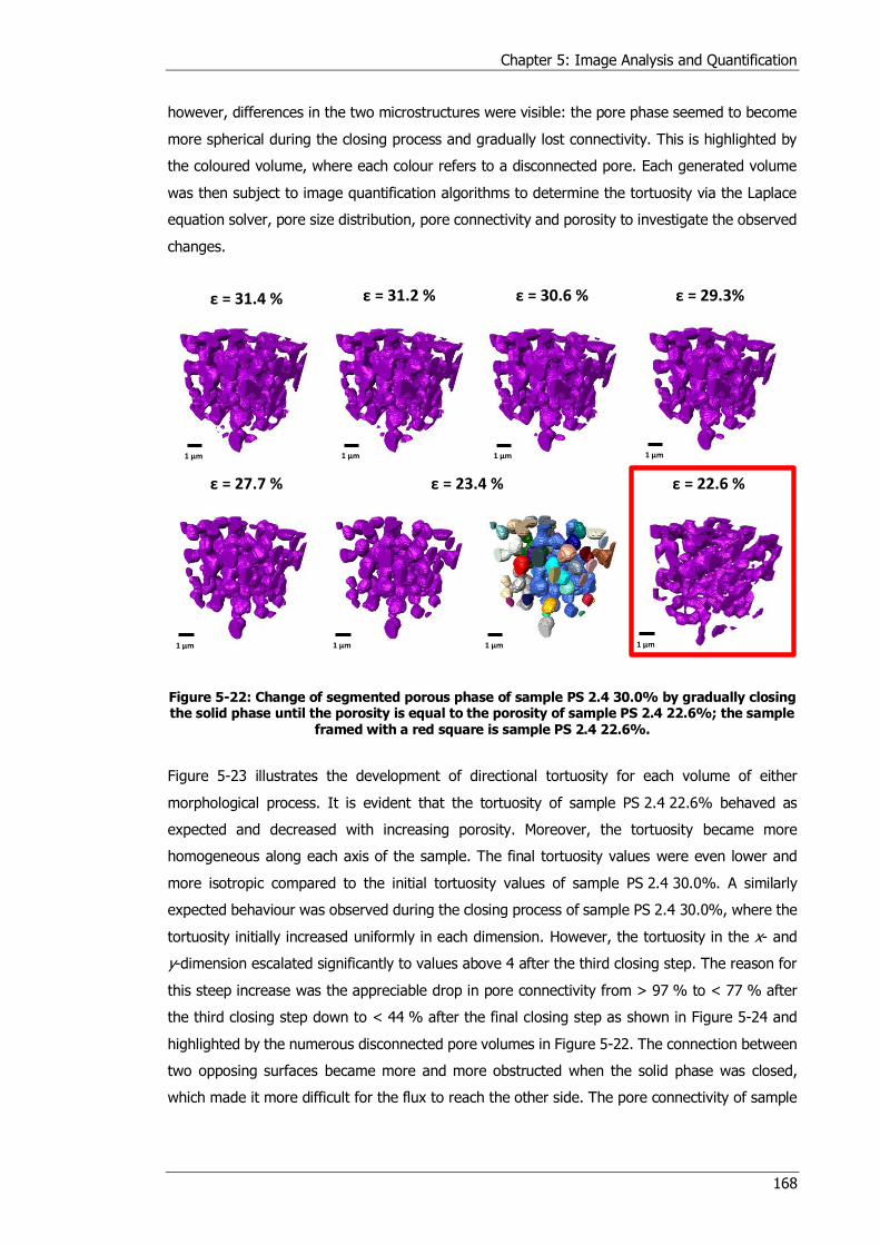
Chapter 5: Image Analysis and Quantification
168
however, differences in the two microstructures were visible: the pore phase seemed to become
more spherical during the closing process and gradually lost connectivity. This is highlighted by
the coloured volume, where each colour refers to a disconnected pore. Each generated volume
was then subject to image quantification algorithms to determine the tortuosity via the Laplace
equation solver, pore size distribution, pore connectivity and porosity to investigate the observed
changes.
Figure 5-22: Change of segmented porous phase of sample PS 2.4 30.0% by gradually closing the solid phase until the porosity is equal to the porosity of sample PS 2.4 22.6%; the sample
framed with a red square is sample PS 2.4 22.6%.
Figure 5-23 illustrates the development of directional tortuosity for each volume of either
morphological process. It is evident that the tortuosity of sample PS 2.4 22.6% behaved as
expected and decreased with increasing porosity. Moreover, the tortuosity became more
homogeneous along each axis of the sample. The final tortuosity values were even lower and
more isotropic compared to the initial tortuosity values of sample PS 2.4 30.0%. A similarly
expected behaviour was observed during the closing process of sample PS 2.4 30.0%, where the
tortuosity initially increased uniformly in each dimension. However, the tortuosity in the x- and
y-dimension escalated significantly to values above 4 after the third closing step. The reason for
this steep increase was the appreciable drop in pore connectivity from > 97 % to < 77 % after
the third closing step down to < 44 % after the final closing step as shown in Figure 5-24 and
highlighted by the numerous disconnected pore volumes in Figure 5-22. The connection between
two opposing surfaces became more and more obstructed when the solid phase was closed,
which made it more difficult for the flux to reach the other side. The pore connectivity of sample
ε = 31.4 % ε = 31.2 % ε = 30.6 %
ε = 27.7 % ε = 23.4 %
ε = 29.3%
ε = 22.6 %
1 μm1 μm1 μm1 μm
1 μm1 μm1 μm1 μm
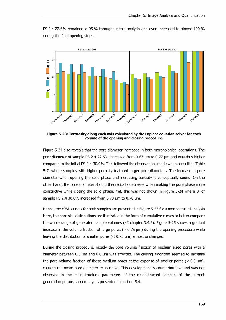
Chapter 5: Image Analysis and Quantification
169
PS 2.4 22.6% remained > 95 % throughout this analysis and even increased to almost 100 %
during the final opening steps.
Figure 5-23: Tortuosity along each axis calculated by the Laplace equation solver for each volume of the opening and closing procedure.
Figure 5-24 also reveals that the pore diameter increased in both morphological operations. The
pore diameter of sample PS 2.4 22.6% increased from 0.63 μm to 0.77 μm and was thus higher
compared to the initial PS 2.4 30.0%. This followed the observations made when consulting Table
5-7, where samples with higher porosity featured larger pore diameters. The increase in pore
diameter when opening the solid phase and increasing porosity is conceptually sound. On the
other hand, the pore diameter should theoretically decrease when making the pore phase more
constrictive while closing the solid phase. Yet, this was not shown in Figure 5-24 where dP of
sample PS 2.4 30.0% increased from 0.73 μm to 0.78 μm.
Hence, the cPSD curves for both samples are presented in Figure 5-25 for a more detailed analysis.
Here, the pore size distributions are illustrated in the form of cumulative curves to better compare
the whole range of generated sample volumes (cf. chapter 3.4.2). Figure 5-25 shows a gradual
increase in the volume fraction of large pores (> 0.75 μm) during the opening procedure while
leaving the distribution of smaller pores (< 0.75 μm) almost unchanged.
During the closing procedure, mostly the pore volume fraction of medium sized pores with a
diameter between 0.5 μm and 0.8 μm was affected. The closing algorithm seemed to increase
the pore volume fraction of these medium pores at the expense of smaller pores (< 0.5 μm),
causing the mean pore diameter to increase. This development is counterintuitive and was not
observed in the microstructural parameters of the reconstructed samples of the current
generation porous support layers presented in section 5.4.
Initi
al Volu
me
Openin
g 1
Openin
g 2
Openin
g 3
Openin
g 4
Openin
g 5
Openin
g 6
0
1
2
3
x
y
z
[-]
PS 2.4 22.6%
Initi
al Volu
me
Clo
sing 1
Clo
sing 2
Clo
sing 3
Clo
sing 4
Clo
sing 5
PS 2.4 30.0%
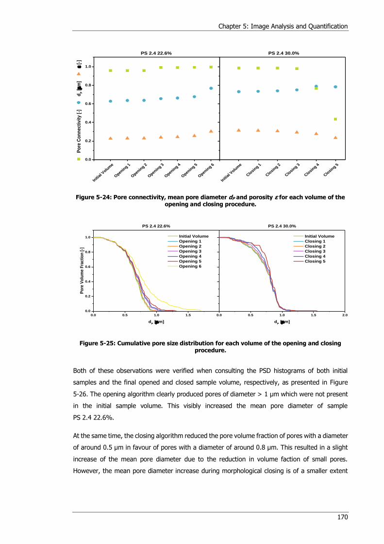
Chapter 5: Image Analysis and Quantification
170
Figure 5-24: Pore connectivity, mean pore diameter dP and porosity ε for each volume of the opening and closing procedure.
Figure 5-25: Cumulative pore size distribution for each volume of the opening and closing procedure.
Both of these observations were verified when consulting the PSD histograms of both initial
samples and the final opened and closed sample volume, respectively, as presented in Figure
5-26. The opening algorithm clearly produced pores of diameter > 1 μm which were not present
in the initial sample volume. This visibly increased the mean pore diameter of sample
PS 2.4 22.6%.
At the same time, the closing algorithm reduced the pore volume fraction of pores with a diameter
of around 0.5 μm in favour of pores with a diameter of around 0.8 μm. This resulted in a slight
increase of the mean pore diameter due to the reduction in volume faction of small pores.
However, the mean pore diameter increase during morphological closing is of a smaller extent
Initi
al Volu
me
Openin
g 1
Openin
g 2
Openin
g 3
Openin
g 4
Openin
g 5
Openin
g 6
0.0
0.2
0.4
0.6
0.8
1.0
Po
re C
on
ne
cti
vit
y [
-] d
P [
m]
[
-]
PS 2.4 22.6% PS 2.4 30.0%
Initi
al Volu
me
Clo
sing 1
Clo
sing 2
Clo
sing 3
Clo
sing 4
Clo
sing 5
0.0 0.5 1.0 1.5
0.0
0.2
0.4
0.6
0.8
1.0
0.0 0.5 1.0 1.5 2.0
Po
re V
olu
me
Fra
cti
on
[-]
dP [m]
Initial Volume
Opening 1
Opening 2
Opening 3
Opening 4
Opening 5
Opening 6
PS 2.4 22.6%
dP [m]
Initial Volume
Closing 1
Closing 2
Closing 3
Closing 4
Closing 5
PS 2.4 30.0%
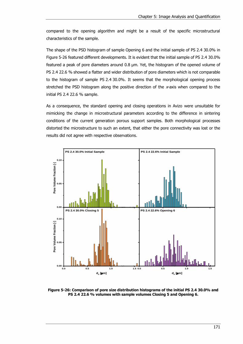
Chapter 5: Image Analysis and Quantification
171
compared to the opening algorithm and might be a result of the specific microstructural
characteristics of the sample.
The shape of the PSD histogram of sample Opening 6 and the initial sample of PS 2.4 30.0% in
Figure 5-26 featured different developments. It is evident that the initial sample of PS 2.4 30.0%
featured a peak of pore diameters around 0.8 μm. Yet, the histogram of the opened volume of
PS 2.4 22.6 % showed a flatter and wider distribution of pore diameters which is not comparable
to the histogram of sample PS 2.4 30.0%. It seems that the morphological opening process
stretched the PSD histogram along the positive direction of the x-axis when compared to the
initial PS 2.4 22.6 % sample.
As a consequence, the standard opening and closing operations in Avizo were unsuitable for
mimicking the change in microstructural parameters according to the difference in sintering
conditions of the current generation porous support samples. Both morphological processes
distorted the microstructure to such an extent, that either the pore connectivity was lost or the
results did not agree with respective observations.
Figure 5-26: Comparison of pore size distribution histograms of the initial PS 2.4 30.0% and PS 2.4 22.6 % volumes with sample volumes Closing 5 and Opening 6.
0.00
0.05
0.10
Po
re V
olu
me
Fra
cti
on
[-]
PS 2.4 30.0% Initial Sample PS 2.4 22.6% Initial Sample
0.0 0.5 1.0 1.5
0.00
0.05
0.10
Po
re V
olu
me
Fra
cti
on
[-]
dP [m]
PS 2.4 30.0% Closing 5
0.0 0.5 1.0 1.5
dP [m]
PS 2.4 22.6% Opening 6

Chapter 5: Image Analysis and Quantification
172
5.7 Conclusions of Image Analysis and Quantification
X-ray nano CT and FIB-SEM tomography proved to be powerful techniques to reconstruct the fine
details of the samples’ microstructures in high resolution. The extracted sample volumes served
as the basis for calculation algorithms, where the focus was on the analysis of the tortuosity of
the current generation porous support membranes. These samples achieved representative
microstructural parameters, including tortuosity, porosity and pore diameter, which were then
compared to examine the effect of sintering conditions. It was shown that the low porosity sample
featured noticeable directional heterogeneity in tortuosity. However, even an extensive
microstructural investigation using stereological relationships and RVE analysis was not able to
pinpoint the reason for this observations, which highlighted the complex interrelation between
porosity, pore size distribution and tortuosity. This correlation of microstructural parameters is
not always straightforward and conceptually sound. The high porosity samples, however, featured
a uniform distribution of directional tortuosity values. Yet, significant differences in tortuosity
values between the geometric and the flux-based calculation algorithms were identified. These
differences were caused by the lack of geometric approaches to account for constrictions and
bottlenecks and only considering the minimal Euclidean distance between two planes. Hence, any
pore connection, even a single pixel, was included in the calculation and thus, the geometric
definition of tortuosity is closely followed. However, a migrating flux is affected by the variation
of pore diameters within the sample and choses the path of least resistance and constriction. As
a consequence, flux-based tortuosity calculation algorithms always resulted in a higher tortuosity
value throughout the above sections. Moreover, porosity-tortuosity algorithms underestimated
tortuosity and proved to be unsuitable for the microstructures analysed in this project.
In addition, image processing algorithms were applied to visualise the distribution of local pore
diameter, Knudsen number and diffusion coefficients within the reconstructed sample volumes.
In this way, the significant variations of diffusion coefficients in all three dimensions of the
samples were highlighted. These variations in pore diameter caused the range of effective
diffusion coefficient to vary by almost a factor of two, which is why Knudsen diffusion expressions
have to be included when analysing the diffusion behaviour within the current generation porous
support membranes. However, to the author’s knowledge, the applied tortuosity and flux
calculation algorithms do not yet include the local variation of pore diameter in their calculation.
Finally, the attempt of artificially mimicking the variation in microstructural characteristics
according to the different sintering conditions used to manufacture the porous support
membranes was not rewarded with success. The standard opening and closing procedures in
Avizo distorted the microstructure in such a way that the results were not comparable to the
original datasets they were supposed to imitate and a more sophisticated “virtual material design”
tool is required, but is beyond the scope of this work.
Chapter 6: Simulation and Modelling
173
6 Simulation and Modelling
Heat flux simulations in StarCCM+ and mass transport simulation in COMSOL were carried out on
X-ray nano CT datasets of the current generation porous support membranes to close the
validation circle as proposed in Figure 3-1. The aim was to extract tortuosity for each sample and
compare it to the tortuosity values calculated via image-based algorithms presented in the
previous chapter. However, the CFD/finite element software packages necessitated the meshing
of the sample volumes. Hence, section 6.1 presents a sensitivity analysis of the chosen meshing
parameters. Only then were the directional tortuosity values calculated based on the heat and
mass fluxes simulated through the meshed pore structures as shown in section 0. Finally, section
6.3 compares the simulation-based tortuosity values to image and experimental-based
tortuosities calculation algorithms and interpret the differences.
6.1 Sensitivity Analysis of Meshing Parameters
Volume meshes of the pore phase for each of the reconstructed 2.4th generation membrane
samples had to be generated to carry out heat and mass flux simulation in StarCCM+ and
COMSOL, respectively. However, computation time and accuracy vary depending on the chosen
meshing parameters. As a consequence, a sensitivity analysis on the effect of the mesh
specifications on the calculated tortuosity was carried out for either simulation software and is
presented here in turn.
The solid phase of all samples was smoothed and exported as “ASCII.stl" surface mesh files from
Avizo into StarCCM+, as outlined in chapter 3.5.1. Then, an adaptive polyhedral volume mesh of
each sample’s pore phase was generated after inverting the imported dataset. The chosen
smoothing extent in Avizo and the chosen base mesh size in StarCCM+ affect the quality of the
final volume mesh and thus, the simulation results. Hence, the smoothing extent was varied
between 1 and 9 and the arbitrary base mesh size was increased from 0.1 to 1 to evaluate their
effect on the achieved tortuosity. The increase in base mesh size caused a decrease of mesh cells
from 600,000 to 8,000. Yet, it has to be noted that the necessary mesh repair steps in StarCCM+
decreased with higher smoothing extent [104].
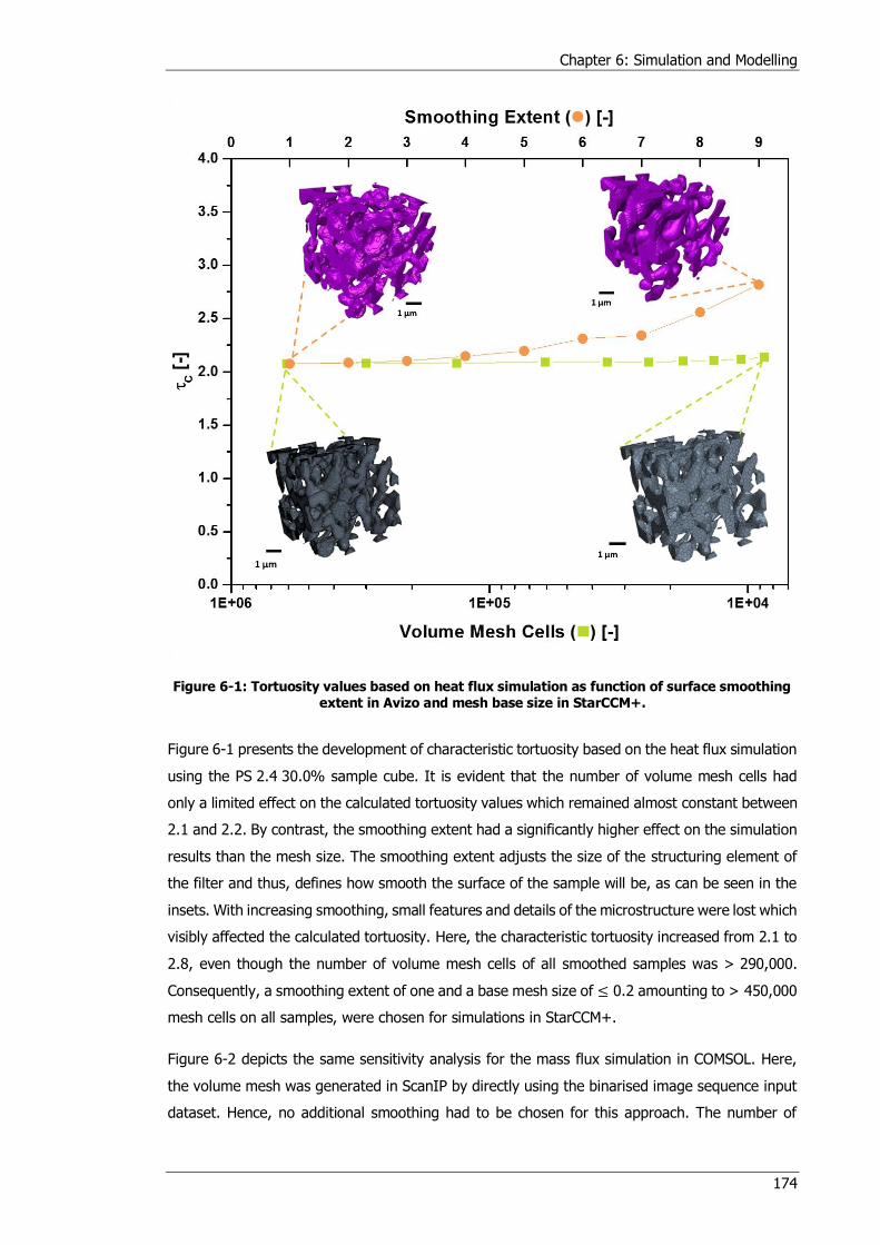
Chapter 6: Simulation and Modelling
174
Figure 6-1: Tortuosity values based on heat flux simulation as function of surface smoothing extent in Avizo and mesh base size in StarCCM+.
Figure 6-1 presents the development of characteristic tortuosity based on the heat flux simulation
using the PS 2.4 30.0% sample cube. It is evident that the number of volume mesh cells had
only a limited effect on the calculated tortuosity values which remained almost constant between
2.1 and 2.2. By contrast, the smoothing extent had a significantly higher effect on the simulation
results than the mesh size. The smoothing extent adjusts the size of the structuring element of
the filter and thus, defines how smooth the surface of the sample will be, as can be seen in the
insets. With increasing smoothing, small features and details of the microstructure were lost which
visibly affected the calculated tortuosity. Here, the characteristic tortuosity increased from 2.1 to
2.8, even though the number of volume mesh cells of all smoothed samples was > 290,000.
Consequently, a smoothing extent of one and a base mesh size of ≤ 0.2 amounting to > 450,000
mesh cells on all samples, were chosen for simulations in StarCCM+.
Figure 6-2 depicts the same sensitivity analysis for the mass flux simulation in COMSOL. Here,
the volume mesh was generated in ScanIP by directly using the binarised image sequence input
dataset. Hence, no additional smoothing had to be chosen for this approach. The number of
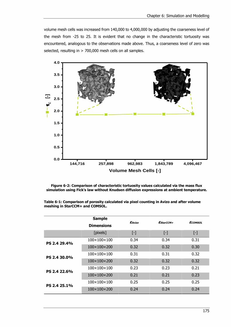
Chapter 6: Simulation and Modelling
175
volume mesh cells was increased from 140,000 to 4,000,000 by adjusting the coarseness level of
the mesh from -25 to 25. It is evident that no change in the characteristic tortuosity was
encountered, analogous to the observations made above. Thus, a coarseness level of zero was
selected, resulting in > 700,000 mesh cells on all samples.
Figure 6-2: Comparison of characteristic tortuosity values calculated via the mass flux simulation using Fick's law without Knudsen diffusion expressions at ambient temperature.
Table 6-1: Comparison of porosity calculated via pixel counting in Avizo and after volume meshing in StarCCM+ and COMSOL.
Sample
Dimensions εAvizo εStarCCM+ εCOMSOL
[pixels] [-] [-] [-]
PS 2.4 29.4% 100×100×100 0.34 0.34 0.31
100×100×200 0.32 0.32 0.30
PS 2.4 30.0% 100×100×100 0.31 0.31 0.32
100×100×200 0.32 0.32 0.32
PS 2.4 22.6% 100×100×100 0.23 0.23 0.21
100×100×200 0.21 0.21 0.23
PS 2.4 25.1% 100×100×100 0.25 0.25 0.25
100×100×200 0.24 0.24 0.24
144,716 257,898 962,983 1,843,789 4,096,467
0.0
0.5
1.0
1.5
2.0
2.5
3.0
3.5
4.0
Volume Mesh Cells [-]
C [
-]
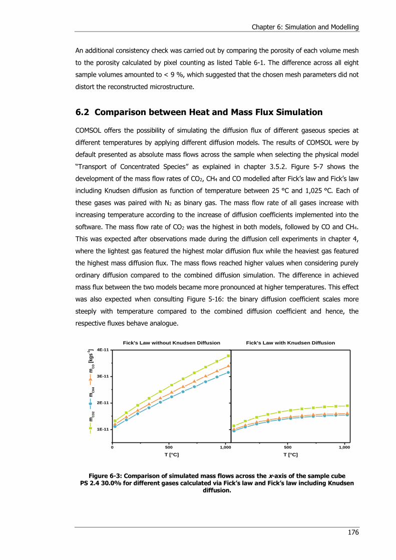
Chapter 6: Simulation and Modelling
176
An additional consistency check was carried out by comparing the porosity of each volume mesh
to the porosity calculated by pixel counting as listed Table 6-1. The difference across all eight
sample volumes amounted to < 9 %, which suggested that the chosen mesh parameters did not
distort the reconstructed microstructure.
6.2 Comparison between Heat and Mass Flux Simulation
COMSOL offers the possibility of simulating the diffusion flux of different gaseous species at
different temperatures by applying different diffusion models. The results of COMSOL were by
default presented as absolute mass flows across the sample when selecting the physical model
“Transport of Concentrated Species” as explained in chapter 3.5.2. Figure 5-7 shows the
development of the mass flow rates of CO2, CH4 and CO modelled after Fick’s law and Fick’s law
including Knudsen diffusion as function of temperature between 25 °C and 1,025 °C. Each of
these gases was paired with N2 as binary gas. The mass flow rate of all gases increase with
increasing temperature according to the increase of diffusion coefficients implemented into the
software. The mass flow rate of CO2 was the highest in both models, followed by CO and CH4.
This was expected after observations made during the diffusion cell experiments in chapter 4,
where the lightest gas featured the highest molar diffusion flux while the heaviest gas featured
the highest mass diffusion flux. The mass flows reached higher values when considering purely
ordinary diffusion compared to the combined diffusion simulation. The difference in achieved
mass flux between the two models became more pronounced at higher temperatures. This effect
was also expected when consulting Figure 5-16: the binary diffusion coefficient scales more
steeply with temperature compared to the combined diffusion coefficient and hence, the
respective fluxes behave analogue.
Figure 6-3: Comparison of simulated mass flows across the x-axis of the sample cube PS 2.4 30.0% for different gases calculated via Fick’s law and Fick’s law including Knudsen
diffusion.
0 500 1,000
1E-11
2E-11
3E-11
4E-11
500 1,000
T [°C]
mC
O2
mC
H4
mC
O [
kg
s-1]
Fick's Law without Knudsen Diffusion
T [°C]
Fick's Law with Knudsen Diffusion
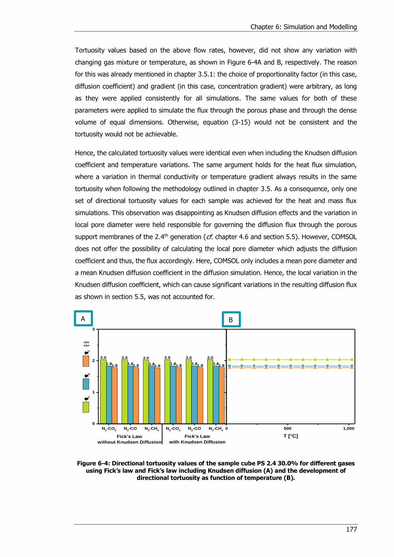
Chapter 6: Simulation and Modelling
177
Tortuosity values based on the above flow rates, however, did not show any variation with
changing gas mixture or temperature, as shown in Figure 6-4A and B, respectively. The reason
for this was already mentioned in chapter 3.5.1: the choice of proportionality factor (in this case,
diffusion coefficient) and gradient (in this case, concentration gradient) were arbitrary, as long
as they were applied consistently for all simulations. The same values for both of these
parameters were applied to simulate the flux through the porous phase and through the dense
volume of equal dimensions. Otherwise, equation (3-15) would not be consistent and the
tortuosity would not be achievable.
Hence, the calculated tortuosity values were identical even when including the Knudsen diffusion
coefficient and temperature variations. The same argument holds for the heat flux simulation,
where a variation in thermal conductivity or temperature gradient always results in the same
tortuosity when following the methodology outlined in chapter 3.5. As a consequence, only one
set of directional tortuosity values for each sample was achieved for the heat and mass flux
simulations. This observation was disappointing as Knudsen diffusion effects and the variation in
local pore diameter were held responsible for governing the diffusion flux through the porous
support membranes of the 2.4th generation (cf. chapter 4.6 and section 5.5). However, COMSOL
does not offer the possibility of calculating the local pore diameter which adjusts the diffusion
coefficient and thus, the flux accordingly. Here, COMSOL only includes a mean pore diameter and
a mean Knudsen diffusion coefficient in the diffusion simulation. Hence, the local variation in the
Knudsen diffusion coefficient, which can cause significant variations in the resulting diffusion flux
as shown in section 5.5, was not accounted for.
Figure 6-4: Directional tortuosity values of the sample cube PS 2.4 30.0% for different gases using Fick’s law and Fick’s law including Knudsen diffusion (A) and the development of
directional tortuosity as function of temperature (B).
0 500 1,000
2.0 2.0 2.0 2.0 2.0 2.0
1.8 1.8 1.8 1.8 1.8 1.81.8 1.8 1.8 1.8 1.8 1.8
N2-CO
2N
2-CO N
2-CH
4N
2-CO
2N
2-CO N
2-CH
4
0
1
2
3
Fick's Law
with Knudsen Diffusion
x
y
z
[-]
Fick's Law
without Knudsen Diffusion
T [°C]
A B
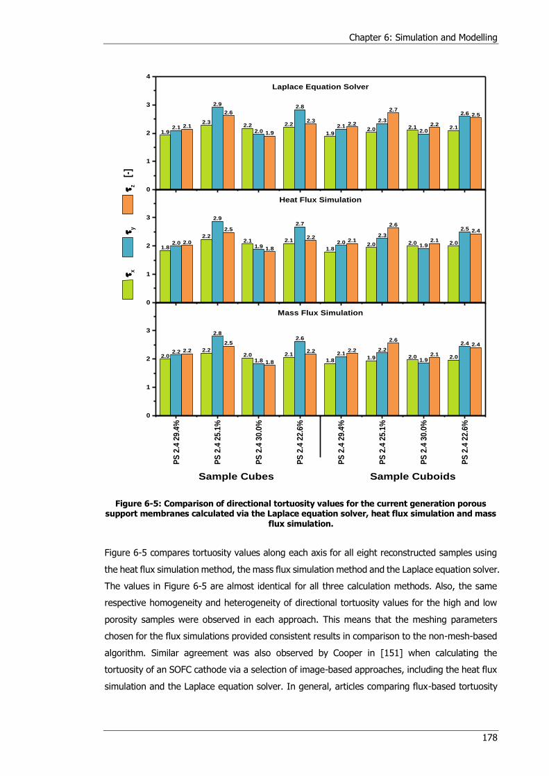
Chapter 6: Simulation and Modelling
178
Figure 6-5: Comparison of directional tortuosity values for the current generation porous support membranes calculated via the Laplace equation solver, heat flux simulation and mass
flux simulation.
Figure 6-5 compares tortuosity values along each axis for all eight reconstructed samples using
the heat flux simulation method, the mass flux simulation method and the Laplace equation solver.
The values in Figure 6-5 are almost identical for all three calculation methods. Also, the same
respective homogeneity and heterogeneity of directional tortuosity values for the high and low
porosity samples were observed in each approach. This means that the meshing parameters
chosen for the flux simulations provided consistent results in comparison to the non-mesh-based
algorithm. Similar agreement was also observed by Cooper in [151] when calculating the
tortuosity of an SOFC cathode via a selection of image-based approaches, including the heat flux
simulation and the Laplace equation solver. In general, articles comparing flux-based tortuosity
1.9
2.32.2 2.2
1.92.0 2.1 2.12.1
2.9
2.0
2.8
2.12.3
2.0
2.6
2.1
2.6
1.9
2.32.2
2.7
2.2
2.5
1.8
2.22.1 2.1
1.82.0 2.0 2.02.0
2.9
1.9
2.7
2.0
2.3
1.9
2.5
2.0
2.5
1.8
2.22.1
2.6
2.1
2.4
2.02.2
2.0 2.11.8
1.9 2.0 2.02.2
2.8
1.8
2.6
2.12.2
1.9
2.4
2.2
2.5
1.8
2.2 2.2
2.6
2.1
2.4
0
1
2
3
4
Laplace Equation Solver
0
1
2
3
Sample Cuboids
x
y
z [
-]
Sample Cubes
Heat Flux Simulation
PS
2.4
29
.4%
PS
2.4
25
.1%
PS
2.4
30
.0%
PS
2.4
22
.6%
PS
2.4
29
.4%
PS
2.4
25
.1%
PS
2.4
30
.0%
PS
2.4
22
.6%
0
1
2
3
Mass Flux Simulation
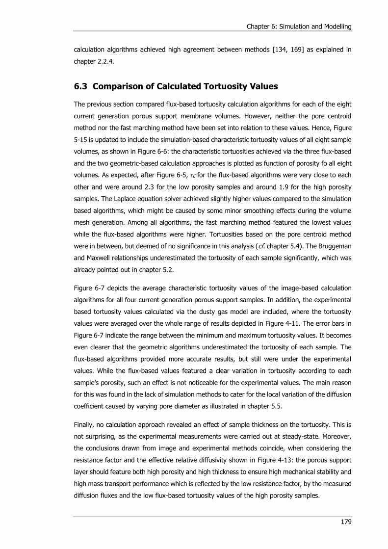
Chapter 6: Simulation and Modelling
179
calculation algorithms achieved high agreement between methods [134, 169] as explained in
chapter 2.2.4.
6.3 Comparison of Calculated Tortuosity Values
The previous section compared flux-based tortuosity calculation algorithms for each of the eight
current generation porous support membrane volumes. However, neither the pore centroid
method nor the fast marching method have been set into relation to these values. Hence, Figure
5-15 is updated to include the simulation-based characteristic tortuosity values of all eight sample
volumes, as shown in Figure 6-6: the characteristic tortuosities achieved via the three flux-based
and the two geometric-based calculation approaches is plotted as function of porosity fo all eight
volumes. As expected, after Figure 6-5, τC for the flux-based algorithms were very close to each
other and were around 2.3 for the low porosity samples and around 1.9 for the high porosity
samples. The Laplace equation solver achieved slightly higher values compared to the simulation
based algorithms, which might be caused by some minor smoothing effects during the volume
mesh generation. Among all algorithms, the fast marching method featured the lowest values
while the flux-based algorithms were higher. Tortuosities based on the pore centroid method
were in between, but deemed of no significance in this analysis (cf. chapter 5.4). The Bruggeman
and Maxwell relationships underestimated the tortuosity of each sample significantly, which was
already pointed out in chapter 5.2.
Figure 6-7 depicts the average characteristic tortuosity values of the image-based calculation
algorithms for all four current generation porous support samples. In addition, the experimental
based tortuosity values calculated via the dusty gas model are included, where the tortuosity
values were averaged over the whole range of results depicted in Figure 4-11. The error bars in
Figure 6-7 indicate the range between the minimum and maximum tortuosity values. It becomes
even clearer that the geometric algorithms underestimated the tortuosity of each sample. The
flux-based algorithms provided more accurate results, but still were under the experimental
values. While the flux-based values featured a clear variation in tortuosity according to each
sample’s porosity, such an effect is not noticeable for the experimental values. The main reason
for this was found in the lack of simulation methods to cater for the local variation of the diffusion
coefficient caused by varying pore diameter as illustrated in chapter 5.5.
Finally, no calculation approach revealed an effect of sample thickness on the tortuosity. This is
not surprising, as the experimental measurements were carried out at steady-state. Moreover,
the conclusions drawn from image and experimental methods coincide, when considering the
resistance factor and the effective relative diffusivity shown in Figure 4-13: the porous support
layer should feature both high porosity and high thickness to ensure high mechanical stability and
high mass transport performance which is reflected by the low resistance factor, by the measured
diffusion fluxes and the low flux-based tortuosity values of the high porosity samples.
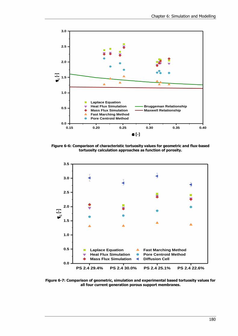
Chapter 6: Simulation and Modelling
180
Figure 6-6: Comparison of characteristic tortuosity values for geometric and flux-based tortuosity calculation approaches as function of porosity.
Figure 6-7: Comparison of geometric, simulation and experimental based tortuosity values for all four current generation porous support membranes.
0.15 0.20 0.25 0.30 0.35 0.40
0.0
0.5
1.0
1.5
2.0
2.5
3.0
Laplace Equation
Heat Flux Simulation Bruggeman Relationship
Mass Flux Simulation Maxwell Relationship
Fast Marching Method
Pore Centroid Method
C [
-]
[-]
PS 2.4 29.4% PS 2.4 30.0% PS 2.4 25.1% PS 2.4 22.6%
0.0
0.5
1.0
1.5
2.0
2.5
3.0
3.5
Laplace Equation Fast Marching Method
Heat Flux Simulation Pore Centroid Method
Mass Flux Simulation Diffusion Cell
C [
-]
Chapter 6: Simulation and Modelling
181
6.4 Conclusions of Simulation and Modelling
This chapter introduced additional methods of deriving tortuosity based on tomography datasets.
However, a volume mesh was necessary to execute these heat and mass flux simulation models.
The quality of the volume mesh directly affects the computation time and the achieved results
which is why a sensitivity analysis was carried out. Yet, only little effect of the number of mesh
elements on the calculated tortuosity were encounter for the heat flux simulation in StarCCM+ as
well as the mass flux simulation in COMSOL. Excellent agreement between the Laplace equation
solver and the flux simulation methods was achieved which suggested, that the chosen meshing
parameters had no effect on the volume and thus, on the calculated values.
A comparison between geometric, flux and experimental-based tortuosity values of the current
generation porous support membranes showed no dependency of the tortuosity on the sample
thickness. However, a clear hierarchy in obtained values was discovered: the geometric
approaches arrived at appreciably lower tortuosity values compared to the flux-based values. At
the same time, the flux-based values were below the experimental-based tortuosities. Moreover,
experimentally derived tortuosities were independent of the porosity in contrast to the
image-based methods. These differences were attributed to the fact that the flux-based
algorithms don’t take varying pore diameters within the sample reconstruction into account. In
spite of this, flux-based algorithms and experimental-based results lead to the same conclusions
concerning the design of the porous support layer when considering the resistance factor and the
effective relative diffusivity: the porous support layer should feature high porosity and thickness
to combine low diffusion resistance with high mechanical stability.
Among the flux-based methods, the Laplace equation solver produced consistent results and is
easiest to execute, as the binarized image sequence is sufficient as input parameter, making the
generation of a volume mesh unnecessary. However, it was clearly shown that the local variation
in pore diameter can have significant effects on the resulting diffusion flux. So far, no simulation
software offered the possibility of including such a calculation. Yet, mesh-based simulation
software packages might become more appropriate if improved models are capable of calculating
the local diffusion coefficient for each mesh cell. This is achievable by calculating the local pore
diameter for each mesh element and then determining the local Knudsen and effective diffusion
coefficients using the same approach as presented in chapter 5.5. The appropriate diffusion
coefficient for each mesh element across the whole porous mesh would be assigned and the
simulation could account for variations in the pore diameter within the sample structure and
determine the resulting diffusion flux accordingly.

Chapter 7: Conclusions and Future Work
182
7 Conclusions and Future Work
7.1 Conlusions
This thesis analysed the diffusion resistance of yttria partially-stabilized zirconia porous support
layers for the application in oxygen transport membranes using image and experimental-based
approaches. The objectives of this thesis were twofold: firstly, to evaluate the diffusion
performance of current generation porous support layers supplied by Praxair Inc. and thus
improving their design of the next generation materials; secondly, to provide a better
understanding of the differences in tortuosity calculation algorithms applied in electrochemistry
and to assess the suitability of each method with regards to diffusion processes. The analysis of
both objectives was interwoven, as tortuosity plays a vital role in evaluating diffusive mass
transport through porous membranes. Experimental, image and simulation-based approaches
have been applied in combination to extract microstructural characteristics relevant for evaluating
the diffusive transport in the porous support layers.
The diffusion cell test rig presented in chapter 4 allowed the examination of planar and tubular
porous support samples under varying conditions. A series of binary gas mixtures, all involved in
the reforming and combustion of CH4, were injected into the diffusion cell to extract the diffusion
flux induced by a concentration gradient across the sample. The tortuosity was then determined
using gas chromatography and appropriate diffusion models. The dusty gas model provided the
most constant tortuosity values across all gas mixtures. No effect on the tortuosity was observed
even under varying gas composition of injected fuel gas mixtures. Moreover, no effect of
temperature or sample thickness on tortuosity was observed at steady-state. This was in perfect
agreement with the definition of tortuosity of being a microstructural parameter and proved the
high accuracy of the dusty gas model. However, experimental results of the current generation
porous support layers showed no effect of porosity on the tortuosity, which is counterintuitive.
The average tortuosity for these four samples was between 2.8 and 3.1. The reason for this might
be the similarity in pore diameters of the samples, which seemed to govern the flux more than
the porosity alone. This makes sense as the diffusion regime expected inside of the porous
samples was in the transition regime, where Knudsen and ordinary diffusion have to be
considered equally. Yet, the measured diffusion fluxes, the calculated resistance factors and the
calculated effective diffusivity values showed that high porosity combined with high membrane
thickness is desired to ensure good mass transport performance and high mechanical stability in
the porous support layer. These observations were consistent for the whole range of analysed
temperatures and gas mixtures and were communicated to Praxair Inc. to optimise the design of
their porous supports.
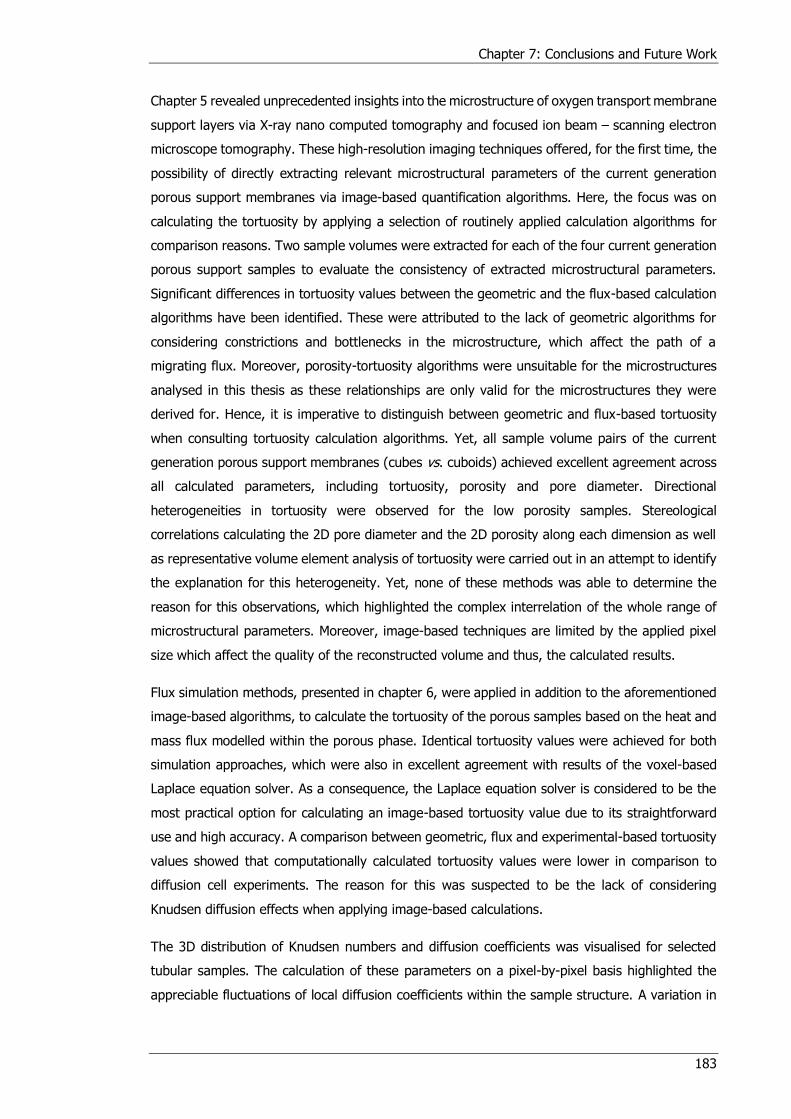
Chapter 7: Conclusions and Future Work
183
Chapter 5 revealed unprecedented insights into the microstructure of oxygen transport membrane
support layers via X-ray nano computed tomography and focused ion beam – scanning electron
microscope tomography. These high-resolution imaging techniques offered, for the first time, the
possibility of directly extracting relevant microstructural parameters of the current generation
porous support membranes via image-based quantification algorithms. Here, the focus was on
calculating the tortuosity by applying a selection of routinely applied calculation algorithms for
comparison reasons. Two sample volumes were extracted for each of the four current generation
porous support samples to evaluate the consistency of extracted microstructural parameters.
Significant differences in tortuosity values between the geometric and the flux-based calculation
algorithms have been identified. These were attributed to the lack of geometric algorithms for
considering constrictions and bottlenecks in the microstructure, which affect the path of a
migrating flux. Moreover, porosity-tortuosity algorithms were unsuitable for the microstructures
analysed in this thesis as these relationships are only valid for the microstructures they were
derived for. Hence, it is imperative to distinguish between geometric and flux-based tortuosity
when consulting tortuosity calculation algorithms. Yet, all sample volume pairs of the current
generation porous support membranes (cubes vs. cuboids) achieved excellent agreement across
all calculated parameters, including tortuosity, porosity and pore diameter. Directional
heterogeneities in tortuosity were observed for the low porosity samples. Stereological
correlations calculating the 2D pore diameter and the 2D porosity along each dimension as well
as representative volume element analysis of tortuosity were carried out in an attempt to identify
the explanation for this heterogeneity. Yet, none of these methods was able to determine the
reason for this observations, which highlighted the complex interrelation of the whole range of
microstructural parameters. Moreover, image-based techniques are limited by the applied pixel
size which affect the quality of the reconstructed volume and thus, the calculated results.
Flux simulation methods, presented in chapter 6, were applied in addition to the aforementioned
image-based algorithms, to calculate the tortuosity of the porous samples based on the heat and
mass flux modelled within the porous phase. Identical tortuosity values were achieved for both
simulation approaches, which were also in excellent agreement with results of the voxel-based
Laplace equation solver. As a consequence, the Laplace equation solver is considered to be the
most practical option for calculating an image-based tortuosity value due to its straightforward
use and high accuracy. A comparison between geometric, flux and experimental-based tortuosity
values showed that computationally calculated tortuosity values were lower in comparison to
diffusion cell experiments. The reason for this was suspected to be the lack of considering
Knudsen diffusion effects when applying image-based calculations.
The 3D distribution of Knudsen numbers and diffusion coefficients was visualised for selected
tubular samples. The calculation of these parameters on a pixel-by-pixel basis highlighted the
appreciable fluctuations of local diffusion coefficients within the sample structure. A variation in
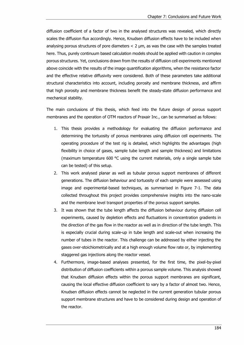
Chapter 7: Conclusions and Future Work
184
diffusion coefficient of a factor of two in the analysed structures was revealed, which directly
scales the diffusion flux accordingly. Hence, Knudsen diffusion effects have to be included when
analysing porous structures of pore diameters < 2 μm, as was the case with the samples treated
here. Thus, purely continuum based calculation models should be applied with caution in complex
porous structures. Yet, conclusions drawn from the results of diffusion cell experiments mentioned
above coincide with the results of the image quantification algorithms, when the resistance factor
and the effective relative diffusivity were considered. Both of these parameters take additional
structural characteristics into account, including porosity and membrane thickness, and affirm
that high porosity and membrane thickness benefit the steady-state diffusion performance and
mechanical stability.
The main conclusions of this thesis, which feed into the future design of porous support
membranes and the operation of OTM reactors of Praxair Inc., can be summarised as follows:
1. This thesis provides a methodology for evaluating the diffusion performance and
determining the tortuosity of porous membranes using diffusion cell experiments. The
operating procedure of the test rig is detailed, which highlights the advantages (high
flexibility in choice of gases, sample tube length and sample thickness) and limitations
(maximum temperature 600 °C using the current materials, only a single sample tube
can be tested) of this setup.
2. This work analysed planar as well as tubular porous support membranes of different
generations. The diffusion behaviour and tortuosity of each sample were assessed using
image and experimental-based techniques, as summarised in Figure 7-1. The data
collected throughout this project provides comprehensive insights into the nano-scale
and the membrane level transport properties of the porous support samples.
3. It was shown that the tube length affects the diffusion behaviour during diffusion cell
experiments, caused by depletion effects and fluctuations in concentration gradients in
the direction of the gas flow in the reactor as well as in direction of the tube length. This
is especially crucial during scale-up in tube length and scale-out when increasing the
number of tubes in the reactor. This challenge can be addressed by either injecting the
gases over-stoichiometrically and at a high enough volume flow rate or, by implementing
staggered gas injections along the reactor vessel.
4. Furthermore, image-based analyses presented, for the first time, the pixel-by-pixel
distribution of diffusion coefficients within a porous sample volume. This analysis showed
that Knudsen diffusion effects within the porous support membranes are significant,
causing the local effective diffusion coefficient to vary by a factor of almost two. Hence,
Knudsen diffusion effects cannot be neglected in the current generation tubular porous
support membrane structures and have to be considered during design and operation of
the reactor.
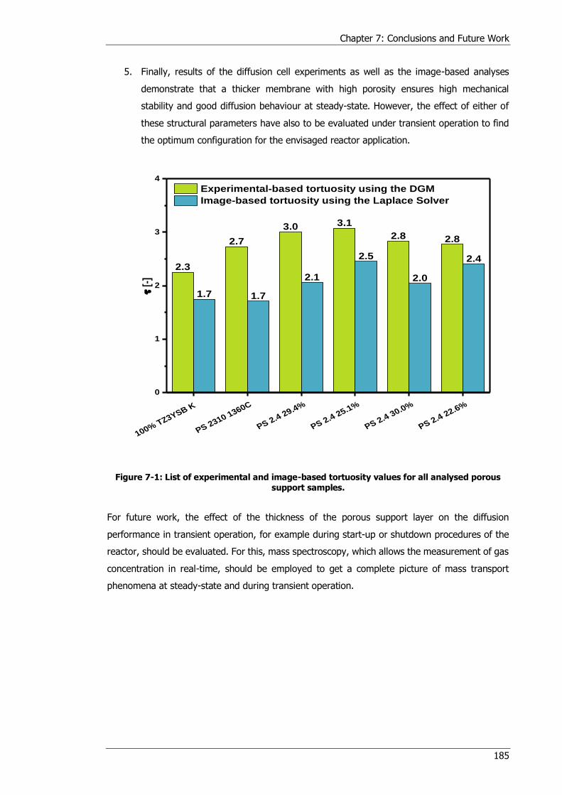
Chapter 7: Conclusions and Future Work
185
5. Finally, results of the diffusion cell experiments as well as the image-based analyses
demonstrate that a thicker membrane with high porosity ensures high mechanical
stability and good diffusion behaviour at steady-state. However, the effect of either of
these structural parameters have also to be evaluated under transient operation to find
the optimum configuration for the envisaged reactor application.
Figure 7-1: List of experimental and image-based tortuosity values for all analysed porous support samples.
For future work, the effect of the thickness of the porous support layer on the diffusion
performance in transient operation, for example during start-up or shutdown procedures of the
reactor, should be evaluated. For this, mass spectroscopy, which allows the measurement of gas
concentration in real-time, should be employed to get a complete picture of mass transport
phenomena at steady-state and during transient operation.
2.3
2.7
3.0 3.1
2.8 2.8
1.7 1.7
2.1
2.5
2.0
2.4
100% TZ3YSB K
PS 2310 1360C
PS 2.4 29.4%
PS 2.4 25.1%
PS 2.4 30.0%
PS 2.4 22.6%
0
1
2
3
4
[-
]
Experimental-based tortuosity using the DGM
Image-based tortuosity using the Laplace Solver
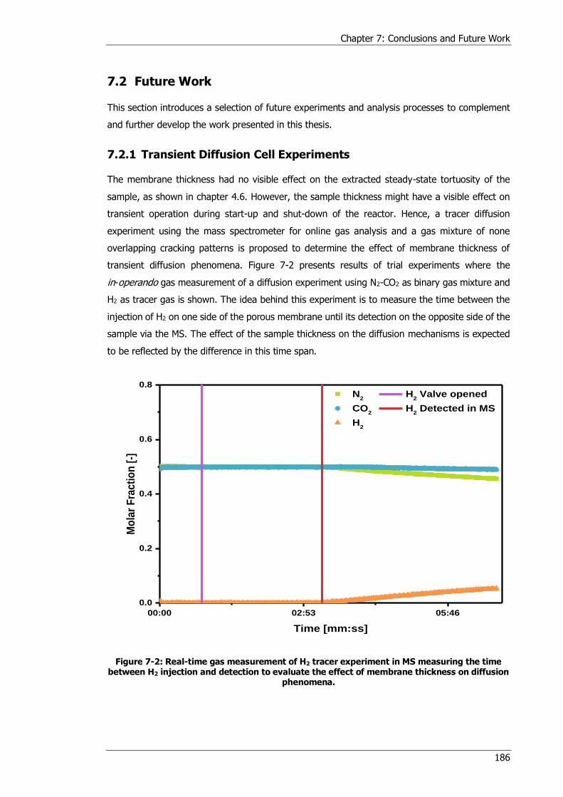
Chapter 7: Conclusions and Future Work
186
7.2 Future Work
This section introduces a selection of future experiments and analysis processes to complement
and further develop the work presented in this thesis.
7.2.1 Transient Diffusion Cell Experiments
The membrane thickness had no visible effect on the extracted steady-state tortuosity of the
sample, as shown in chapter 4.6. However, the sample thickness might have a visible effect on
transient operation during start-up and shut-down of the reactor. Hence, a tracer diffusion
experiment using the mass spectrometer for online gas analysis and a gas mixture of none
overlapping cracking patterns is proposed to determine the effect of membrane thickness of
transient diffusion phenomena. Figure 7-2 presents results of trial experiments where the
in-operando gas measurement of a diffusion experiment using N2-CO2 as binary gas mixture and
H2 as tracer gas is shown. The idea behind this experiment is to measure the time between the
injection of H2 on one side of the porous membrane until its detection on the opposite side of the
sample via the MS. The effect of the sample thickness on the diffusion mechanisms is expected
to be reflected by the difference in this time span.
Figure 7-2: Real-time gas measurement of H2 tracer experiment in MS measuring the time between H2 injection and detection to evaluate the effect of membrane thickness on diffusion
phenomena.
00:00 02:53 05:46
0.0
0.2
0.4
0.6
0.8
N2
H2 Valve opened
CO2
H2 Detected in MS
H2
Mo
lar
Fra
cti
on
[-]
Time [mm:ss]
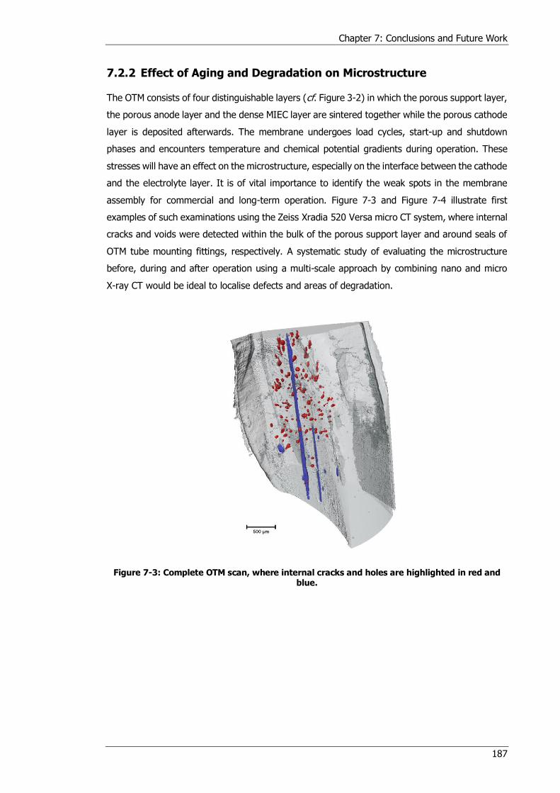
Chapter 7: Conclusions and Future Work
187
7.2.2 Effect of Aging and Degradation on Microstructure
The OTM consists of four distinguishable layers (cf. Figure 3-2) in which the porous support layer,
the porous anode layer and the dense MIEC layer are sintered together while the porous cathode
layer is deposited afterwards. The membrane undergoes load cycles, start-up and shutdown
phases and encounters temperature and chemical potential gradients during operation. These
stresses will have an effect on the microstructure, especially on the interface between the cathode
and the electrolyte layer. It is of vital importance to identify the weak spots in the membrane
assembly for commercial and long-term operation. Figure 7-3 and Figure 7-4 illustrate first
examples of such examinations using the Zeiss Xradia 520 Versa micro CT system, where internal
cracks and voids were detected within the bulk of the porous support layer and around seals of
OTM tube mounting fittings, respectively. A systematic study of evaluating the microstructure
before, during and after operation using a multi-scale approach by combining nano and micro
X-ray CT would be ideal to localise defects and areas of degradation.
Figure 7-3: Complete OTM scan, where internal cracks and holes are highlighted in red and blue.
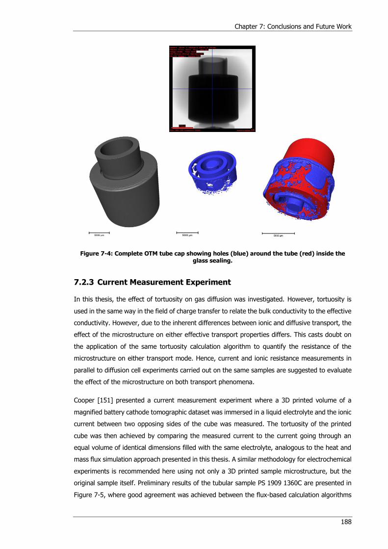
Chapter 7: Conclusions and Future Work
188
Figure 7-4: Complete OTM tube cap showing holes (blue) around the tube (red) inside the glass sealing.
7.2.3 Current Measurement Experiment
In this thesis, the effect of tortuosity on gas diffusion was investigated. However, tortuosity is
used in the same way in the field of charge transfer to relate the bulk conductivity to the effective
conductivity. However, due to the inherent differences between ionic and diffusive transport, the
effect of the microstructure on either effective transport properties differs. This casts doubt on
the application of the same tortuosity calculation algorithm to quantify the resistance of the
microstructure on either transport mode. Hence, current and ionic resistance measurements in
parallel to diffusion cell experiments carried out on the same samples are suggested to evaluate
the effect of the microstructure on both transport phenomena.
Cooper [151] presented a current measurement experiment where a 3D printed volume of a
magnified battery cathode tomographic dataset was immersed in a liquid electrolyte and the ionic
current between two opposing sides of the cube was measured. The tortuosity of the printed
cube was then achieved by comparing the measured current to the current going through an
equal volume of identical dimensions filled with the same electrolyte, analogous to the heat and
mass flux simulation approach presented in this thesis. A similar methodology for electrochemical
experiments is recommended here using not only a 3D printed sample microstructure, but the
original sample itself. Preliminary results of the tubular sample PS 1909 1360C are presented in
Figure 7-5, where good agreement was achieved between the flux-based calculation algorithms
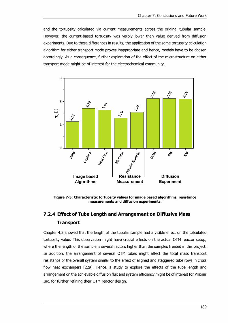
Chapter 7: Conclusions and Future Work
189
and the tortuosity calculated via current measurements across the original tubular sample.
However, the current-based tortuosity was visibly lower than value derived from diffusion
experiments. Due to these differences in results, the application of the same tortuosity calculation
algorithm for either transport mode proves inappropriate and hence, models have to be chosen
accordingly. As a consequence, further exploration of the effect of the microstructure on either
transport mode might be of interest for the electrochemical community.
Figure 7-5: Characteristic tortuosity values for image based algorithms, resistance measurements and diffusion experiments.
7.2.4 Effect of Tube Length and Arrangement on Diffusive Mass
Transport
Chapter 4.3 showed that the length of the tubular sample had a visible effect on the calculated
tortuosity value. This observation might have crucial effects on the actual OTM reactor setup,
where the length of the sample is several factors higher than the samples treated in this project.
In addition, the arrangement of several OTM tubes might affect the total mass transport
resistance of the overall system similar to the effect of aligned and staggered tube rows in cross
flow heat exchangers [229]. Hence, a study to explore the effects of the tube length and
arrangement on the achievable diffusion flux and system efficiency might be of interest for Praxair
Inc. for further refining their OTM reactor design.
1.1
4
1.7
0
1.6
4
1.2
9
1.5
4
2.1
2
2.1
3
2.1
2
FM
M
Lapla
ce
Heat Flu
x
3D
Cube
Tubula
r S
am
ple
DG
M
FM
EM
0
1
2
3
C [
-]
Diffusion
Experiment
Resistance
Measurement
Image based
Algorithms
Chapter 7: Conclusions and Future Work
190
7.3 Dissemination
This section lists first-authored and co-authored peer-reviewed publications as well as attended
conferences, where posters were presented and oral presentations were given.
7.3.1 Peer-reviewed Publications
Tjaden, B., Lane, J., Neville, T.P., Brown, L.D., Mason, T.J., Tan, C., Lounasvuorid, M.M.,
Brett, D.J.L. and Shearing, P.R., “Comparison of Ionic and Diffusive Mass Transport
Resistance in Porous Structures”, ECS Transactions, Submitted.
Tjaden, B., Lane, J., Brett, D.J.L. and Shearing, P.R., “Understanding transport
phenomena in electrochemical energy devices via X ray nano CT”, Journal of Physics:
Conference Series, Submitted.
Tjaden, B., Finegan, D.P., Lane, J., Brett, D.J.L. and Shearing, P.R., “A correlative study
of mass transport resistance in porous oxygen transport membrane supports”, Chemical
Engineering Science, Submitted.
Tjaden, B., Shearing, P.R. and Brett, D.J.L., “Understanding tortuosity in electrochemical
devices: A review of calculation approaches”, International Materials Reviews, Accepted.
Tjaden, B., Cooper, S.J., Brett, D.J.L., Kramer, D. and Shearing, P.R. (Accepted, In Print),
“On the Origin and Application of the Bruggeman Correlation for analysing Transport
Phenomena in Electrochemical Systems”, Current Opinion in Chemical Engineering.
Tjaden, B., Lane, J., Withers, P.J., Bradley, R.S., Brett, D.J.L. and Shearing, P.R., “The
application of 3D imaging techniques, simulation and diffusion experiments to explore
transport properties in porous oxygen transport membrane support materials”, Solid
State Ionics.
7.3.2 Co-Authored Peer-reviewed Publications
Lu, X., Tjaden, B., Bertei, A., Li, T., Li, K., Brett, D.J.L. and Shearing, P.R., “Effect of
Pore Size Distribution on Gas Diffusion Regimes and Mass Transport in an SOFC Anode”,
Chemical Engineering Journal, Submitted.
Bharath, V., Jervis, R., Millichamp, J., Neville, T.P., Mason, T.J., Tjaden, B., Shearing,
P.R., Brown, R., Manos, G. and Brett, D.J.L., “Alkaline Anion Exchange Membrane
Degradation as a Function of Humidity Measured using the Quartz Crystal Microbalance”,
Electrochimica Acta, Submitted.
Finegan, D.P., Cooper, S.J., Tjaden, B., Taiwo, O.O., Gelb, J., Hinds, G., Brett, D.J.L.
and Shearing, P.R. (2016), “Characterising the structural properties of polymer separators
for lithium-ion batteries in 3D using phase contrast X-ray microscopy”, Journal of Power
Sources, Vol. 333, pp. 184–192.
Chapter 7: Conclusions and Future Work
191
Brown, L.D., Abdulaziz, R., Tjaden, B., Inman, D., Brett, D.J.L. and Shearing, P.R.,
“Investigating microstructural evolution during the electroreduction of UO2 to U in LiCl-
KCl eutectic using focused ion beam tomography”, Journal of Nuclear Materials, Vol. 480,
pp. 355–361.
Finegan, D.P., Scheel, M., Tjaden, B., Robinson, J.B., Di Michiel, M., Hinds, G., Brett,
D.J.L. and Shearing, P.R. (2016), “Investigating lithium-ion battery materials during
overcharge-induced thermal runaway: An operando and multi-scale X-ray CT study”,
Physical Chemistry Chemical Physics.
Finegan, D.P., Scheel, M., Robinson, J.B., Tjaden, B., Hunt, I., Mason, T.J., Millichamp,
J., Di Michiel, M., Offer, G.J., Hinds, G., Brett, D.J.L. and Shearing, P.R. (2015), “In-
operando high-speed tomography of lithium-ion batteries during thermal runaway”,
Nature Communications, Vol. 6.
Trogadas, P., Taiwo, O.O., Tjaden, B., Neville, T.P., Yun, S., Parrondo, J., Ramani, V.,
Coppens, M.-C., Brett, D.J.L. and Shearing, P.R. (2014), “X-ray micro-tomography as a
diagnostic tool for the electrode degradation in vanadium redox flow batteries”,
Electrochemistry Communications, Vol. 48 No. 0, pp. 155–159.
7.3.3 Conference Attendance
The Correlative Approach of 3D Imaging Techniques, Simulation and Diffusion Experiments to
Explore Transport Properties in Porous OTM Support Material, oral presentation at the Pacific Rim
Meeting on Electrochemical and Solid-state Science, Honolulu, 2016.
Understanding Transport Phenomena in Electrochemical Energy Devices: A Correlative
Approach, poster and two minutes oral flash presentation at the X-Ray Microscopy
Conference 2016, Oxford, 2016.
The Correlative Approach of 3D Imaging Techniques, Simulation and Diffusion
Experiments to Explore Transport Properties in Porous OTM Support Materials, oral
presentation at the SCI Electrochemistry Postgraduate Conference 2016, London, 2016.
Exploring transport resistance in porous OTM support materials via 3D imaging
techniques, simulation and diffusion experiments, poster presentation at the 20th
International Conference on Solid State Ionics, Keystone, 2015.
Understanding Transport Phenomena in Electrochemical Devices: A Tomographic
Approach in Three and Four Dimensions, oral presentation at the 7th International
Conference on Porous Media & Annual Meeting, Padova, 2015.
Image analysis, simulation and diffusion experiment on 3YSZ porous support layer, poster
presentation at the Science and Technology Facilities Council Early Career Researchers
Conference, 2015.

Chapter 7: Conclusions and Future Work
192
Microstructural Analysis of Porous Support Layer using Diffusion Experiments, Image
Analysis and Simulation, poster presentation at The annual Diamond Synchrotron
Radiation User Meeting, 2014.
Chapter 8: Bibliography
193
8 Bibliography
[1] Rosen, L., Degenstein, N., Shah, M., Wilson, J., Kelly, S., Peck, J. and Christie, M. (2011),
“Development of oxygen transport membranes for coal-based power generation”, 10th
International Conference on Greenhouse Gas Control Technologies, Vol. 4 No. 0, pp.
750–755.
[2] Tsai, C.-L. and Schmidt, H.V. (2011), “Tortuosity in anode-supported proton conductive
solid oxide fuel cell found from current flow rates and dusty-gas model”, Journal of Power
Sources, Vol. 196 No. 2, pp. 692–699.
[3] Kaiser, A., Foghmoes, S.P., Pećanac, G., Malzbender, J., Chatzichristodoulou, C.,
Glasscock, J.A., Ramachandran, D., Ni, D.W., Esposito, V., Søgaard, M. and Hendriksen,
P.V. (2016), “Design and optimization of porous ceramic supports for asymmetric ceria-
based oxygen transport membranes”, Journal of Membrane Science, Vol. 513, pp. 85–94.
[4] Kauranen, P. (2008), “Oxygen Carriers for Energy Efficiency. A Biomimetic Approach”,
VTT, available at:
http://www.spinverse.com/pastevents/nmpfinland2008/files/presentations/thursday_200
8-04-17/Kauranen_NMPFinland2008.pdf (accessed 14 November 2015).
[5] Hashim, S., Mohamed, A. and Bhatia, S. (2010), “Current status of ceramic-based
membranes for oxygen separation from air”, Advances in Colloid and Interface Science,
Vol. 160 1-2, pp. 88–100.
[6] Leo, A., Liu, S. and Costa, J. (2009), “Development of mixed conducting membranes for
clean coal energy delivery”, International Journal of Greenhouse Gas Control, Vol. 3 No.
4, pp. 357–367.
[7] Puig-Arnavat, M., Soprani, S., Sogaard, M., Engelbrecht, K., Ahrenfeldt, J., Henriksen,
U.B. and Hendriksen, P.V. (2013), “Integration of mixed conducting membranes in an
oxygen-steam biomass gasification process”, RSC Advances, Vol. 3 No. 43, pp. 20843–
20854.
[8] Smith, A. and Klosek, J. (2001), “A review of air separation technologies and their
integration with energy conversion processes”, Fuel Processing Technology, Vol. 70 No.
2, pp. 115–134.
[9] Hashim, S., Mohamed, A. and Bhatia, S. (2011), “Oxygen separation from air using
ceramic-based membrane technology for sustainable fuel production and power
generation”, Renewable and Sustainable Energy Reviews, Vol. 15 No. 2, pp. 1284–1293.
[10] Dyer, P., Richards, R., Russek, S. and Taylor, D. (2000), “Ion transport membrane
technology for oxygen separation and syngas production”, Solid State Ionics, Vol. 134 1–
2, pp. 21–33.
Chapter 8: Bibliography
194
[11] Zhang, K., Shao, Z., Li, C. and Liu, S. (2012), “Novel CO2-tolerant ion-transporting
ceramic membranes with an external short circuit for oxygen separation at intermediate
temperatures”, Energy Environ. Sci., Vol. 5 No. 1, pp. 5257–5264.
[12] Singhal, S.C. and Kendall, K. (2003), High-temperature solid oxide fuel cells:
Fundamentals, design, and applicatons, Elsevier Advanced Technology, New York.
[13] Yadav, M., Gong, W. and Jacobson, A.J. (2011), “Electrically driven oxygen separation
through gadolinia-doped ceria using PrBaCo2O5 + x and NdBaCo2O5 + x electrodes”,
Journal of Solid State Electrochemistry, Vol. 15 No. 2, pp. 293-301.
[14] Skinner, S. and Kilner, J. (2003), “Oxygen ion conductors”, Materials Today, Vol. 6 No. 3,
pp. 30–37.
[15] Brett, D.J.L., Atkinson, A., Brandon, N.P. and Skinner, S. (2008), “Intermediate
temperature solid oxide fuel cells”, Chem. Soc. Rev., Vol. 37 No. 8, pp. 1568–1578.
[16] Zhou, W., Shao, Z., Ran, R., Chen, Z., Zeng, P., Gu, H., Jin, W. and Xu, N. (2007), “High
performance electrode for electrochemical oxygen generator cell based on solid
electrolyte ion transport membrane”, Electrochimica Acta, Vol. 52 No. 22, pp. 6297–6303.
[17] Zhang, K., Meng, B., Tan, X., Liu, L., Wang, S. and Liu, S. (2014), “CO2-Tolerant Ceramic
Membrane Driven by Electrical Current for Oxygen Production at Intermediate
Temperatures”, Journal of the American Ceramic Society, Vol. 97 No. 1, pp. 120–126.
[18] Hutchings, K.N., Bai, J., Cutler, R.A., Wilson, M.A. and Taylor, D.M. (2008),
“Electrochemical oxygen separation and compression using planar, cosintered ceramics”,
Solid State Ionics, Vol. 179 11–12, pp. 442–450.
[19] Meixner, L.D., Brengel, D.D., Henderson, B.T., Abrardo, J.M., Wilson, M.A., Taylor, D.M.
and Cutler, R.A. (2002), “Electrochemical Oxygen Separation Using Solid Electrolyte Ion
Transport Membranes”, Journal of The Electrochemical Society, Vol. 149 No. 9, pp. D132.
[20] Praxair Inc. (2013), “StarGen™ Ultra-High Purity Oxygen Generator”, Praxair Inc.,
available at:
http://www.praxair.com/~/media/North%20America/US/Documents/Specification%20Sh
eets%20and%20Brochures/Gases/P10238.ashx (accessed 4 October 2013).
[21] Bouwmeester, H., Kruidhof, H. and Burggraaf, A. (1994), “Importance of the surface
exchange kinetics as rate limiting step in oxygen permeation through mixed-conducting
oxides”, Solid State Ionics, 72, Part 2 No. 0, pp. 185–194.
[22] Steele, B. (1995), “Interfacial reactions associated with ceramic ion transport
membranes”, Interfaces in Ionic Materials, Vol. 75 No. 0, pp. 157–165.
[23] van Doorn, R., Fullarton, I., de Souza, R., Kilner, J., Bouwmeester, H. and Burggraaf, A.
(1997), “Surface oxygen exchange of La0.3Sr0.7CoO3 − δ”, Solid State Ionics, Vol. 96 1–
2, pp. 1–7.
[24] Geffroy, P., Fouletier, J., Richet, N. and Chartier, T. (2013), “Rational selection of MIEC
materials in energy production processes”, Chemical Engineering Science, Vol. 87 No. 0,
pp. 408–433.
Chapter 8: Bibliography
195
[25] Zhu, X. and Yang, W. (2008), “Composite membrane based on ionic conductor and mixed
conductor for oxygen permeation”, AIChE Journal, Vol. 54 No. 3, pp. 665–672.
[26] Luo, H., Jiang, H., Efimov, K., Liang, F., Wang, H. and Caro, J. (2011), “CO2 -Tolerant
Oxygen-Permeable Fe2O3 -Ce0.9Gd0.1O2-δ Dual Phase Membranes”, Industrial &
Engineering Chemistry Research, Vol. 50 No. 23, pp. 13508–13517.
[27] Thursfield, A. and Metcalfe, I. (2004), “The use of dense mixed ionic and electronic
conducting membranes for chemical production”, Journal of Materials Chemistry, Vol. 14
No. 16, pp. 2475–2485.
[28] Sunarso, J., Baumann, S., Serra, J., Meulenberg, W., Liu, S., Lin, Y. and Diniz da Costa, J.
(2008), “Mixed ionic–electronic conducting (MIEC) ceramic-based membranes for oxygen
separation”, Journal of Membrane Science, Vol. 320 1–2, pp. 13–41.
[29] Luo, H., Jiang, H., Efimov, K., Caro, J. and Wang, H. (2011), “Influence of the
preparation methods on the microstructure and oxygen permeability of a CO2-stable dual
phase membrane”, AIChE Journal, Vol. 57 No. 10, pp. 2738–2745.
[30] Zhang, K., Liu, L., Shao, Z., Xu, R., Diniz da Costa, J., Wang, S. and Liu, S. (2013),
“Robust ion-transporting ceramic membrane with an internal short circuit for oxygen
production”, Journal of Materials Chemistry A, Vol. 1 No. 32, p. 9150.
[31] Zhang, K., Zou, Y., Su, C., Shao, Z., Liu, L., Wang, S. and Liu, S. (2013), “CO2 and water
vapor-tolerant yttria stabilized bismuth oxide (YSB) membranes with external short circuit
for oxygen separation with CO2 capture at intermediate temperatures”, Journal of
Membrane Science, Vol. 427 No. 0, pp. 168–175.
[32] He, B., Zhang, K., Ling, Y., Xu, J. and Zhao, L. (2014), “A surface modified
La0.6Sr0.4Co0.2Fe0.8O3−δ ultrathin membrane for highly efficient oxygen separation”,
Journal of Membrane Science, Vol. 464 No. 0, pp. 55–60.
[33] Delbos, C., Lebain, G., Richet, N. and Bertail, C. (2010), “Performances of tubular
La0.8Sr0.2Fe0.7Ga0.3O3−δ mixed conducting membrane reactor for under pressure
methane conversion to syngas”, Catalysis Today, Vol. 156 3–4, pp. 146–152.
[34] Araki, S., Yamamoto, H., Hoshi, Y., Lu, J., Hakuta, Y., Hayashi, H., Ohashi, T., Sato, K.,
Nishioka, M., Inoue, T., Hikazudani, S. and Hamakawa, S. (2012), “Synthesis of
Ca0.8Sr0.2Ti0.7Fe0.3O3−δ thin film membranes and its application to the partial
oxidation of methane”, Solid State Ionics, Vol. 221 No. 0, pp. 43–49.
[35] Lane, J. (2011), Oxygen Transport Membrane (OTM) Development at Praxair, 18th
International Conference on Solid State Ionics, Warsaw.
[36] Bouwmeester, H. (2003), “Dense ceramic membranes for methane conversion”, 5th
International Conference on Catalysis in Membrane Reactors, Vol. 82 1–4, pp. 141–150.
[37] Nagabhushana, N., Lane, J., Christie, G. and van Hassel, B. (2006), Composite Oxygen
Ion Transport Membrane. US Pat. 7,556,676 B2.
[38] Mason, E. and Malinauskas, A. (1983), Gas transport in porous media: The dusty-gas
model, Chemical engineering monographs, Vol. 17, Elsevier, Amsterdam, New York.
Chapter 8: Bibliography
196
[39] Kast, W. and Hohenthanner, C.-R. (2000), “Mass transfer within the gas-phase of porous
media”, International Journal of Heat and Mass Transfer, Vol. 43 No. 5, pp. 807–823.
[40] Nagy, E. (2012), Basic Equations of the Mass Transport through a Membrane Layer, 1st
ed, Elsevier, London.
[41] Shearing, P.R., Brett, D.J.L. and Brandon, N.P. (2013), “Towards intelligent engineering
of SOFC electrodes: a review of advanced microstructural characterisation techniques”,
International Materials Reviews, Vol. 55 No. 6, pp. 347–363.
[42] Robertson, I., Holzer, L., Prestat, M., Münch, B. and Graule, T. (2010), “Effects of particle
and pore sizes, surface area and porosity on the performance of LSC cathodes”,
Proceedings of the 9th European Fuel Cell Forum, pp. 10–83.
[43] Taiwo, O.O., Finegan, D.P., Eastwood, D.S., Fife, J.L., Brown, L.D., Darr, J.A., Lee, P.D.,
Brett, D.J.L. and Shearing, P.R. (2016), “Comparison of three-dimensional analysis and
stereological techniques for quantifying lithium-ion battery electrode microstructures”,
Journal of Microscopy, Vol. 263 No. 3, pp. 280–292.
[44] Virkar, A.V., Chen, J., Tanner, C.W. and Kim, J.-W. (2000), “The role of electrode
microstructure on activation and concentration polarizations in solid oxide fuel cells”,
Solid State Ionics, Vol. 131 1–2, pp. 189–198.
[45] Wilson, J.R. and Barnett, S.A. (2008), “Solid Oxide Fuel Cell Ni–YSZ Anodes: Effect of
Composition on Microstructure and Performance”, Electrochemical and Solid-State
Letters, Vol. 11 No. 10, pp. B181.
[46] Mench, M. (2008), Fuel cell engines, John Wiley & Sons, Hoboken, N.J.
[47] Daniel, C. and Besenhard, J.O. (Eds.) (2011), Handbook of Battery Materials, 2nd,
completely rev. and enlarged ed, Wiley-VCH Verlag GmbH & Co. KGaA, Weinheim.
[48] Newman, J. and Tiedemann, W. (1975), “Porous-electrode theory with battery
applications”, AIChE Journal, Vol. 21 No. 1, pp. 25–41.
[49] Adler, S., Lane, J. and Steele, B. (1996), “Electrode Kinetics of Porous Mixed‐
Conducting Oxygen Electrodes”, Journal of The Electrochemical Society, Vol. 143 No.
11, pp. 3554–3564.
[50] Clennell, B. (1997), “Tortuosity: a guide through the maze”, Geological Society, London,
Special Publications, Vol. 122 No. 1, pp. 299–344.
[51] Ghanbarian, B., Hunt, A.G., Ewing, R.P. and Sahimi, M. (2013), “Tortuosity in Porous
Media: A Critical Review”, Soil Science Society of America Journal, Vol. 77 No. 5, p. 1461.
[52] Tjaden, B., Brett, D.J.L. and Shearing, P.R. (2016), “Tortuosity in electrochemical
devices: a review of calculation approaches”, International Materials Reviews, pp. 1–21.
[53] Epstein, N. (1989), “On tortuosity and the tortuosity factor in flow and diffusion through
porous media”, Chemical Engineering Science, Vol. 44 No. 3, pp. 777–779.
Chapter 8: Bibliography
197
[54] van Brakel, J. and Heertjes, P. (1974), “Analysis of diffusion in macroporous media in
terms of a porosity, a tortuosity and a constrictivity factor”, International Journal of Heat
and Mass Transfer, Vol. 17 No. 9, pp. 1093–1103.
[55] Holzer, L., Wiedenmann, D., Münch, B., Keller, L., Prestat, M., Gasser, P., Robertson, I.
and Grobéty, B. (2013), “The influence of constrictivity on the effective transport
properties of porous layers in electrolysis and fuel cells”, Journal of Materials Science,
Vol. 48 No. 7, pp. 2934-2952.
[56] Wiedenmann, D., Keller, L., Holzer, L., Stojadinović, J., Münch, B., Suarez, L., Fumey, B.,
Hagendorfer, H., Brönnimann, R., Modregger, P., Gorbar, M., Vogt, U.F., Züttel, A., La
Mantia, F., Wepf, R. and Grobéty, B. (2013), “Three-dimensional pore structure and ion
conductivity of porous ceramic diaphragms”, AIChE Journal, Vol. 59 No. 5, pp. 1446–
1457.
[57] Jiang, Y. and Virkar, A.V. (2003), “Fuel Composition and Diluent Effect on Gas Transport
and Performance of Anode-Supported SOFCs”, Journal of The Electrochemical Society,
Vol. 150 No. 7, pp. A942.
[58] Hoogschagen, J. (1955), “Diffusion in Porous Catalysts and Adsorbents”, Ind. Eng.
Chem., Vol. 47 No. 5, pp. 906–912.
[59] Zamel, N., Astrath, N., Li, X., Shen, J., Zhou, J., Astrath, F., Wang, H. and Liu, Z.-S.
(2010), “Experimental measurements of effective diffusion coefficient of oxygen–nitrogen
mixture in PEM fuel cell diffusion media”, Chemical Engineering Science, Vol. 65 No. 2,
pp. 931–937.
[60] Flückiger, R., Freunberger, S.A., Kramer, D., Wokaun, A., Scherer, G.G. and Büchi, F.N.
(2008), “Anisotropic, effective diffusivity of porous gas diffusion layer materials for PEFC”,
Electrochimica Acta, Vol. 54 No. 2, pp. 551–559.
[61] Kramer, D., Freunberger, S.A., Flückiger, R., Schneider, I.A., Wokaun, A., Büchi, F.N. and
Scherer, G.G. (2008), “Electrochemical diffusimetry of fuel cell gas diffusion layers”,
Journal of Electroanalytical Chemistry, Vol. 612 No. 1, pp. 63–77.
[62] MacMullin, R.B. and Muccini, G.A. (1956), “Characteristics of porous beds and structures”,
AIChE Journal, Vol. 2 No. 3, pp. 393–403.
[63] Djian, D., Alloin, F., Martinet, S., Lignier, H. and Sanchez, J.Y. (2007), “Lithium-ion
batteries with high charge rate capacity: Influence of the porous separator”, Journal of
Power Sources, Vol. 172 No. 1, pp. 416–421.
[64] Martínez, M.J., Shimpalee, S. and Van Zee, J.W. (2009), “Measurement of MacMullin
Numbers for PEMFC Gas-Diffusion Media”, Journal of The Electrochemical Society, Vol.
156 No. 1, pp. B80.
[65] Landesfeind, J., Hattendorff, J., Ehrl, A., Wall, W.A. and Gasteiger, H.A. (2016),
“Tortuosity Determination of Battery Electrodes and Separators by Impedance
Spectroscopy”, Journal of The Electrochemical Society, Vol. 163 No. 7, pp. A1373.
Chapter 8: Bibliography
198
[66] Shen, L. and Chen, Z. (2007), “Critical review of the impact of tortuosity on diffusion”,
Chemical Engineering Science, Vol. 62 No. 14, pp. 3748–3755.
[67] Bruggeman, D.A.G. (1935), “Berechnung verschiedener physikalischer Konstanten von
heterogenen Substanzen. I. Dielektrizitätskonstanten und Leitfähigkeiten der Mischkörper
aus isotropen Substanzen”, Annalen der Physik, Vol. 416 No. 7, pp. 636–664.
[68] Tjaden, B., Cooper, S.J., Brett, D.J.L., Kramer, D. and Shearing, P.R. (2016), “On the
origin and application of the Bruggeman correlation for analysing transport phenomena in
electrochemical systems”, Current Opinion in Chemical Engineering, Vol. 12, pp. 44–51.
[69] Maxwell, J. (1873), A treatise on electricity and magnetism, Vol. 1, Clarendon press,
Oxford.
[70] Chueh, C.C., Bertei, A., Pharoah, J.G. and Nicolella, C. (2014), “Effective conductivity in
random porous media with convex and non-convex porosity”, International Journal of
Heat and Mass Transfer, Vol. 71 No. 0, pp. 183–188.
[71] Rue, R. and Tobias, C. (1959), “On the Conductivity of Dispersions”, Journal of The
Electrochemical Society, Vol. 106 No. 9, pp. 827–833.
[72] Fuller, T.F., Doyle, M. and Newman, J. (1994), “Simulation and Optimization of the Dual
Lithium Ion Insertion Cell”, Journal of The Electrochemical Society, Vol. 141 No. 1, pp. 1–
10.
[73] Arora, P., Doyle, M., Gozdz, A.S., White, R.E. and Newman, J. (2000), “Comparison
between computer simulations and experimental data for high-rate discharges of plastic
lithium-ion batteries”, Journal of Power Sources, Vol. 88 No. 2, pp. 219–231.
[74] Doyle, M. and Newman, J. (1995), “The use of mathematical modeling in the design of
lithium/polymer battery systems”, Electrochimica Acta, Vol. 40 13–14, pp. 2191–2196.
[75] Vijayaraghavan, B., Ely, D.R., Chiang, Y.-M., García-García, R. and García, E.R. (2012),
“An Analytical Method to Determine Tortuosity in Rechargeable Battery Electrodes”,
Journal of The Electrochemical Society, Vol. 159 No. 5, pp. A548.
[76] Miranda, D., Costa, C.M., Almeida, A.M. and Lanceros-Méndez, S. (2015), “Modeling
separator membranes physical characteristics for optimized lithium ion battery
performance”, Solid State Ionics, Vol. 278, pp. 78–84.
[77] Bernardi, D.M. and Verbrugge, M.W. (1991), “Mathematical model of a gas diffusion
electrode bonded to a polymer electrolyte”, AIChE Journal, Vol. 37 No. 8, pp. 1151–1163.
[78] Lin, G., He, W. and van Nguyen, T. (2004), “Modeling Liquid Water Effects in the Gas
Diffusion and Catalyst Layers of the Cathode of a PEM Fuel Cell”, Journal of The
Electrochemical Society, Vol. 151 No. 12, pp. A1999.
[79] Pharoah, J.G., Karan, K. and Sun, W. (2006), “On effective transport coefficients in PEM
fuel cell electrodes: Anisotropy of the porous transport layers”, Journal of Power Sources,
Vol. 161 No. 1, pp. 214–224.
Chapter 8: Bibliography
199
[80] Das, P.K., Li, X. and Liu, Z.-S. (2010), “Effective transport coefficients in PEM fuel cell
catalyst and gas diffusion layers: Beyond Bruggeman approximation”, Applied Energy,
Vol. 87 No. 9, pp. 2785–2796.
[81] Marquis, J. and Coppens, M.-O. (2013), “Achieving ultra-high platinum utilization via
optimization of PEM fuel cell cathode catalyst layer microstructure”, Chemical Engineering
Science, Vol. 102, pp. 151–162.
[82] Pant, L.M., Mitra, S.K. and Secanell, M. (2013), “A generalized mathematical model to
study gas transport in PEMFC porous media”, International Journal of Heat and Mass
Transfer, Vol. 58 1–2, pp. 70–79.
[83] Chaudhary, S., Sachan, V.K. and Bhattacharya, P.K. (2014), “Two dimensional modelling
of water uptake in proton exchange membrane fuel cell”, International Journal of
Hydrogen Energy, Vol. 39 No. 31, pp. 17802–17818.
[84] Xing, L., Liu, X., Alaje, T., Kumar, R., Mamlouk, M. and Scott, K. (2014), “A two-phase
flow and non-isothermal agglomerate model for a proton exchange membrane (PEM) fuel
cell”, Energy, Vol. 73, pp. 618–634.
[85] Xing, L., Mamlouk, M., Kumar, R. and Scott, K. (2014), “Numerical investigation of the
optimal Nafion® ionomer content in cathode catalyst layer: An agglomerate two-phase
flow modelling”, International Journal of Hydrogen Energy, Vol. 39 No. 17, pp. 9087–
9104.
[86] Wu, W. and Jiang, F. (2014), “Microstructure reconstruction and characterization of
PEMFC electrodes”, International Journal of Hydrogen Energy, Vol. 39 No. 28, pp. 15894–
15906.
[87] DuBeshter, T., Sinha, P.K., Sakars, A., Fly, G.W. and Jorne, J. (2014), “Measurement of
Tortuosity and Porosity of Porous Battery Electrodes”, Journal of The Electrochemical
Society, Vol. 161 No. 4, pp. A599.
[88] Thorat, I., Stephenson, D.E., Zacharias, N., Zaghib, K., Harb, J. and Wheeler, D.R.
(2009), “Quantifying tortuosity in porous Li-ion battery materials”, Journal of Power
Sources, Vol. 188 No. 2, pp. 592–600.
[89] Doyle, M., Newman, J., Gozdz, A.S., Schmutz, C.N. and Tarascon, J.-M. (1996),
“Comparison of Modeling Predictions with Experimental Data from Plastic Lithium Ion
Cells”, Journal of The Electrochemical Society, Vol. 143 No. 6, pp. 1890–1903.
[90] Patel, K.K., Paulsen, J.M. and Desilvestro, J. (2003), “Numerical simulation of porous
networks in relation to battery electrodes and separators”, Journal of Power Sources, Vol.
122 No. 2, pp. 144–152.
[91] Arora, P. and Zhang, Z. (2004), “Battery Separators”, Chem. Rev., Vol. 104 No. 10, pp.
4419–4462.
[92] Kehrwald, D., Shearing, P.R., Brandon, N.P., Sinha, P.K. and Harris, S.J. (2011), “Local
Tortuosity Inhomogeneities in a Lithium Battery Composite Electrode”, Journal of The
Electrochemical Society, Vol. 158 No. 12, pp. A1393-A1399.
Chapter 8: Bibliography
200
[93] Cannarella, J. and Arnold, C.B. (2013), “Ion transport restriction in mechanically strained
separator membranes”, Journal of Power Sources, Vol. 226, pp. 149–155.
[94] Zacharias, N.A., Nevers, D.R., Skelton, C., Knackstedt, K., Stephenson, D.E. and Wheeler,
D.R. (2013), “Direct Measurements of Effective Ionic Transport in Porous Li-Ion
Electrodes”, Journal of The Electrochemical Society, Vol. 160 No. 2, pp. A306.
[95] Ebner, M., Chung, D.-W., García, E.R., Wood, V., Ebner, M., Chung, D.-W. and Wood, V.
(2014), “Tortuosity Anisotropy in Lithium-Ion Battery Electrodes”, Advanced Energy
Materials, Vol. 4 No. 5, pp. n/a.
[96] Vadakkepatt, A., Trembacki, B., Mathur, S.R. and Murthy, J.Y. (2016), “Bruggeman's
Exponents for Effective Thermal Conductivity of Lithium-Ion Battery Electrodes”, Journal
of The Electrochemical Society, Vol. 163 No. 2, pp. A119.
[97] Chung, D.-W., Ebner, M., Ely, D.R., Wood, V. and García, E.R. (2013), “Validity of the
Bruggeman relation for porous electrodes”, Modelling and Simulation in Materials Science
and Engineering, Vol. 21 No. 7, p. 74009.
[98] Ebner, E., Geldmacher, F., Marone, F., Stampanoni, M. and Wood, V. (2013), “X-Ray
Tomography of Porous, Transition Metal Oxide Based Lithium Ion Battery Electrodes”,
Advanced Energy Materials, Vol. 3 No. 7, pp. 845–850.
[99] Ebner, M. and Wood, V. (2015), “Tool for Tortuosity Estimation in Lithium Ion Battery
Porous Electrodes”, Journal of The Electrochemical Society, Vol. 162 No. 2, pp. A3064.
[100] Lagadec, M.F., Ebner, M., Zahn, R. and Wood, V. (2016), “Communication—Technique
for Visualization and Quantification of Lithium-Ion Battery Separator Microstructure”,
Journal of The Electrochemical Society, Vol. 163 No. 6, pp. A992.
[101] Russ, J. and DeHoff, R.T. (2000), Practical Stereology, 2nd ed, Kluwer Academic/Plenum,
New York, London.
[102] Stephenson, D.E., Hartman, E.M., Harb, J.N. and Wheeler, D.R. (2007), “Modeling of
Particle-Particle Interactions in Porous Cathodes for Lithium-Ion Batteries”, Journal of The
Electrochemical Society, Vol. 154 No. 12, pp. A1146.
[103] Gupta, A., Seo, J.H., Zhang, X., Du, W., Sastry, A.M. and Shyy, W. (2011), “Effective
Transport Properties of LiMn2O4 Electrode via Particle-Scale Modeling”, Journal of The
Electrochemical Society, Vol. 158 No. 5, pp. A487.
[104] Cooper, S.J., Eastwood, D.S., Gelb, J., Damblanc, G., Brett, D.J.L., Bradley, R.S., Withers,
P.J., Lee, P.D., Marquis, A.J., Brandon, N.P. and Shearing, P.R. (2014), “Image based
modelling of microstructural heterogeneity in LiFePO4 electrodes for Li-ion batteries”,
Journal of Power Sources, Vol. 247, pp. 1033–1039.
[105] Zhang, Y., Chen, Y., Yan, M. and Chen, F. (2015), “New formulas for the tortuosity factor
of electrochemically conducting channels”, Electrochemistry Communications, Vol. 60, pp.
52–55.
[106] Wicke, E. and Kallenbach, R. (1941), “Die Oberflächendiffusion von Kohlendioxyd in
aktiven Kohlen”, Kolloid-Zeitschrift, Vol. 97 No. 2, pp. 135-151.
Chapter 8: Bibliography
201
[107] Evans, R.B., Watson, G.M. and Truitt, J. (1962), “Interdiffusion of Gases in a Low
Permeability Graphite at Uniform Pressure”, Journal of Applied Physics, Vol. 33 No. 9, pp.
2682–2688.
[108] Evans, R.B., Watson, G.M. and Truitt, J. (1963), “Interdiffusion of Gases in a Low‐
Permeability Graphite. II. Influence of Pressure Gradients”, Journal of Applied Physics,
Vol. 34 No. 7, pp. 2020–2026.
[109] Bardakci, T. and King, F.G. (1992), “Measurements of argon, nitrogen and carbon dioxide
diffusion through random assemblies of small spheres”, Gas Separation & Purification,
Vol. 6 No. 1, pp. 43–48.
[110] Williford, R.E., Chick, L.A., Maupin, G.D., Simner, S.P. and Stevenson, J.W. (2003),
“Diffusion Limitations in the Porous Anodes of SOFCs”, Journal of The Electrochemical
Society, Vol. 150 No. 8, pp. A1067.
[111] Soukup, K., Schneider, P. and Šolcová, O. (2008), “Comparison of Wicke–Kallenbach and
Graham's diffusion cells for obtaining transport characteristics of porous solids”, Chemical
Engineering Science, Vol. 63 No. 4, pp. 1003–1011.
[112] Salejova, G., Grof, Z., Solcova, O., Schneider, P. and Kosek, J. (2011), “Strategy for
predicting effective transport properties of complex porous structures”, Computers &
Chemical Engineering, Vol. 35 No. 2, pp. 200–211.
[113] Brus, G., Miyawaki, K., Iwai, H., Saito, M. and Yoshida, H. (2014), “Tortuosity of an SOFC
anode estimated from saturation currents and a mass transport model in comparison with
a real micro-structure”, Solid State Ionics, Vol. 265, pp. 13–21.
[114] He, W., Zou, J., Wang, B., Vilayurganapathy, S., Zhou, M., Lin, X., Zhang, K., Lin, J., Xu,
P. and Dickerson, J. (2013), “Gas transport in porous electrodes of solid oxide fuel cells:
A review on diffusion and diffusivity measurement”, Journal of Power Sources, Vol. 237
No. 0, pp. 64–73.
[115] Bird, R.B., Stewart, W.E. and Lightfoot, E.N. (2002), Transport phenomena, 2nd, Wiley
international ed, J. Wiley, New York.
[116] Loschmidt, J. (1870), “Experimental-Untersuchungen über die Diffusion von Gasen ohne
poröse Scheidewände I”, Sitzungsbericht der Kaiserlichen Akademie der Wissenschaften
Wien, Vol. 61, pp. 367–380.
[117] Kalyvas, C. (2003), “The Impact of Diffusion on Solid Oxide Fuel Cell Anode
Performance”, Ph.D. Thesis, Department of Chemical Engineering and Chemical
Technology, Imperial College of Science, Technology and Medicine, London.
[118] Vamvakeros, A. (2013), “Measuring Tortuosity in Porous Media”, M.Sc. Thesis, University
College London, London.
[119] Schmidt, H.V. and Tsai, C.-L. (2008), “Anode-pore tortuosity in solid oxide fuel cells
found from gas and current flow rates”, Journal of Power Sources, Vol. 180 No. 1, pp.
253–264.
Chapter 8: Bibliography
202
[120] Schmidt, H.V., Tsai, C.-L. and Lediaev, L. (2009), “Determination of Anode-Pore
Tortuosity from Gas and Current Flow Rates in SOFCs”, in Advances in Solid Oxide Fuel
Cells III: Ceramic and Engineering Science Proceedings, Volume 28, Issue 4, John Wiley
& Sons, Inc, pp. 127–140.
[121] Harned, H.S. and French, D.M. (1945), “A Conductance Method For The Determination Of
The Diffusion Coefficients Of Electrolytes”, Annals of the New York Academy of Sciences,
Vol. 46 5 The Diffusion, pp. 267–284.
[122] Newman, J. and Chapman, T.W. (1973), “Restricted diffusion in binary solutions”, AIChE
Journal, Vol. 19 No. 2, pp. 343–348.
[123] Stewart, S.G. and Newman, J. (2008), “The Use of UV/vis Absorption to Measure
Diffusion Coefficients in LiPF6 Electrolytic Solutions”, Journal of The Electrochemical
Society, Vol. 155 No. 1, pp. F13.
[124] Bae, C.-J., Erdonmez, C.K., Halloran, J.W. and Chiang, Y.-M. (2013), “Design of Battery
Electrodes with Dual-Scale Porosity to Minimize Tortuosity and Maximize Performance”,
Advanced Materials, Vol. 25 No. 9, pp. 1254–1258.
[125] Doyle, M. and Newman, J. (1997), “Analysis of capacity–rate data for lithium batteries
using simplified models of the discharge process”, Journal of Applied Electrochemistry,
Vol. 27 No. 7, pp. 846–856.
[126] Shearing, P.R., Eastwood, D.S., Bradley, R.S., Gelb, J., Cooper, S.J., Tariq, F., Brett,
D.J.L., Brandon, N.P., Withers, P.J. and Lee, P.D. (2013), “Exploring electrochemical
devices using X-ray microscopy: 3D microstructure of batteries and fuel cells”, Microscopy
and Analysis, Vol. 27 No. 2, pp. 19–22.
[127] Cantoni, M. and Holzer, L. (2014), “Advances in 3D focused ion beam tomography”, MRS
Bulletin, Vol. 39 No. 04, pp. 354–360.
[128] Stock, S.R. (2013), “Recent advances in X-ray microtomography applied to materials”,
International Materials Reviews, Vol. 53 No. 3, pp. 129–181.
[129] Maire, E. and Withers, P.J. (2014), “Quantitative X-ray tomography”, International
Materials Reviews, Vol. 59 No. 1, pp. 1–43.
[130] Nelson, G.J., Harris, W.M., Lombardo, J.J., Izzo, J.R., Chiu, W.K.S., Tanasini, P., Cantoni,
M., van Herle, J., Comninellis, C., Andrews, J., Liu, Y., Pianetta, P. and Chu, Y. (2011),
“Comparison of X-ray Nanotomography and FIB-SEM in Quantifying the Composite
LSM/YSZ SOFC Cathode Microstructure”, ECS Transactions, Vol. 35 No. 1, pp. 2417–
2421.
[131] Shearing, P.R., Gelb, J. and Brandon, N.P. (2009), “Characterization of SOFC Electrode
Microstructure Using Nano-Scale X-ray Computed Tomography and Focused Ion Beam
Techniques: a Comparative Study”, ECS Transactions, Vol. 19 No. 17, pp. 51–57.
[132] Tjaden, B., Lane, J., Withers, P.J., Bradley, R.S., Brett, D.J.L. and Shearing, P.R. (2016),
“The application of 3D imaging techniques, simulation and diffusion experiments to
Chapter 8: Bibliography
203
explore transport properties in porous oxygen transport membrane support materials”,
Solid State Ionics, Vol. 288, pp. 315–321.
[133] Wilson, J., Kobsiriphat, W., Mendoza, R., Chen, H., Hiller, J., Miller, D., Thornton, K.,
Voorhees, P., Adler, S. and Barnett, S. (2006), “Three-dimensional reconstruction of a
solid-oxide fuel-cell anode”, Nature Materials, Vol. 5 No. 7, pp. 541–544.
[134] Iwai, H., Shikazono, N., Matsui, T., Teshima, H., Kishimoto, M., Kishida, R., Hayashi, D.,
Matsuzaki, K., Kanno, D., Saito, M., Muroyama, H., Eguchi, K., Kasagi, N. and Yoshida, H.
(2010), “Quantification of SOFC anode microstructure based on dual beam FIB-SEM
technique”, Journal of Power Sources, Vol. 195 No. 4, pp. 955–961.
[135] Chen-Wiegart, Y., Cronin, S., Yuan, Q., Yakal-Kremski, K., Barnett, S. and Wang, J.
(2012), “3D Non-destructive morphological analysis of a solid oxide fuel cell anode using
full-field X-ray nano-tomography”, Journal of Power Sources, Vol. 218 No. 0, pp. 348–
351.
[136] Vivet, N., Chupin, S., Estrade, E., Richard, A., Bonnamy, S., Rochais, D. and Bruneton, E.
(2011), “Effect of Ni content in SOFC Ni-YSZ cermets: A three-dimensional study by FIB-
SEM tomography”, Journal of Power Sources, Vol. 196 No. 23, pp. 9989–9997.
[137] Izzo, J.R., Joshi, A., Grew, K., Chiu, W.K.S., Tkachuk, A., Wang, S. and Yun, W. (2008),
“Non-destructive Reconstruction and Analysis of Solid Oxide Fuel Cell Anodes using X-ray
Computed Tomography at sub-50 nm Resolution”, ECS Transactions, Vol. 13 No. 6, pp.
1–11.
[138] Shearing, P.R., Brandon, N.P., Gelb, J., Bradley, R.S., Withers, P.J., Marquis, A.J.,
Cooper, S.J. and Harris, S.J. (2012), “Multi Length Scale Microstructural Investigations of
a Commercially Available Li-Ion Battery Electrode”, Journal of The Electrochemical
Society, Vol. 159 No. 7, pp. A1023.
[139] Zalc, J.M., Reyes, S.C. and Iglesia, E. (2004), “The effects of diffusion mechanism and
void structure on transport rates and tortuosity factors in complex porous structures”,
Chemical Engineering Science, Vol. 59 No. 14, pp. 2947–2960.
[140] Zhang, Y., Xia, C. and Ni, M. (2012), “Simulation of sintering kinetics and microstructure
evolution of composite solid oxide fuel cells electrodes”, International Journal of
Hydrogen Energy, Vol. 37 No. 4, pp. 3392–3402.
[141] Gostovic, D., Smith, J.R., Kundinger, D., Jones, K.S. and Wachsman, E.D. (2007), “Three-
Dimensional Reconstruction of Porous LSCF Cathodes”, Electrochemical and Solid-State
Letters, Vol. 10 No. 12, pp. B214.
[142] Smith, J.R., Chen, A., Gostovic, D., Hickey, D., Kundinger, D., Duncan, K.L., DeHoff, R.T.,
Jones, K.S. and Wachsman, E.D. (2009), “Evaluation of the relationship between cathode
microstructure and electrochemical behavior for SOFCs”, Solid State Ionics, Vol. 180 No.
1, pp. 90–98.
Chapter 8: Bibliography
204
[143] Cooper, S.J., Kishimoto, M., Tariq, F., Bradley, R.S., Marquis, A.J., Brandon, N.P., Kilner,
J.A. and Shearing, P.R. (2013), “Microstructural Analysis of an LSCF Cathode Using In
Situ Tomography and Simulation”, ECS Transactions, Vol. 57 No. 1, pp. 2671–2678.
[144] Chen, Z., Wang, X., Giuliani, F. and Atkinson, A. (2015), “Microstructural characteristics
and elastic modulus of porous solids”, Acta Materialia, Vol. 89, pp. 268–277.
[145] Jørgensen, P.S., Hansen, K.V., Larsen, R. and Bowen, J.R. (2011), “Geometrical
characterization of interconnected phase networks in three dimensions”, Journal of
Microscopy, Vol. 244 No. 1, pp. 45–58.
[146] Jørgensen, P.S., Ebbehøj, S.L. and Hauch, A. (2015), “Triple phase boundary specific
pathway analysis for quantitative characterization of solid oxide cell electrode
microstructure”, Journal of Power Sources, Vol. 279, pp. 686–693.
[147] Chen-Wiegart, Y., DeMike, R., Erdonmez, C., Thornton, K., Barnett, S. and Wang, J.
(2014), “Tortuosity Characterization of 3D Microstructure at Nano-scale for Energy
Storage and Conversion Materials”, Journal of Power Sources, Vol. 249 No. 0, pp. 349–
356.
[148] Shearing, P.R., Howard, L.E., Jørgensen, P.S., Brandon, N.P. and Harris, S.J. (2010),
“Characterization of the 3-dimensional microstructure of a graphite negative electrode
from a Li-ion battery”, Electrochemistry Communications, Vol. 12 No. 3, pp. 374–377.
[149] Çeçen, A., Wargo, E.A., Hanna, A.C., Turner, D.M., Kalidindi, S.R. and Kumbur, E.C.
(2012), “3-D Microstructure Analysis of Fuel Cell Materials: Spatial Distributions of
Tortuosity, Void Size and Diffusivity”, Journal of The Electrochemical Society, Vol. 159 No.
3, pp. B299.
[150] Shearing, P.R., Bradley, R.S., Gelb, J., Lee, S., Atkinson, A., Withers, P.J. and Brandon,
N.P. (2011), “Using Synchrotron X-Ray Nano-CT to Characterize SOFC Electrode
Microstructures in Three-Dimensions at Operating Temperature”, Electrochemical and
Solid-State Letters, Vol. 14 No. 10, pp. B117.
[151] Cooper, S.J. (2015), “Quantifying the Transport Properties of Solid Oxide Fuel Cell
Electrodes”, Ph.D. Thesis, Department of Materials, Imperial College of Science,
Technology and Medicine, London.
[152] Joshi, A.S., Grew, K.N., Izzo, J.R., Peracchio, A.A. and Chiu, W.K.S. (2010), “Lattice
Boltzmann Modeling of Three-Dimensional, Multicomponent Mass Diffusion in a Solid
Oxide Fuel Cell Anode”, Journal of Fuel Cell Science and Technology, Vol. 7 No. 1, p.
11006.
[153] Grew, K.N., Chu, Y.S., Yi, J., Peracchio, A.A., Izzo, J.R., Hwu, Y., Carlo, F. de and Chiu,
W.K.S. (2010), “Nondestructive Nanoscale 3D Elemental Mapping and Analysis of a Solid
Oxide Fuel Cell Anode”, Journal of The Electrochemical Society, Vol. 157 No. 6, pp. B783.
[154] Grew, K.N., Peracchio, A.A., Joshi, A.S., Izzo, J.R. and Chiu, W.K.S. (2010),
“Characterization and analysis methods for the examination of the heterogeneous solid
Chapter 8: Bibliography
205
oxide fuel cell electrode microstructure. Part 1: Volumetric measurements of the
heterogeneous structure”, Journal of Power Sources, Vol. 195 No. 24, pp. 7930–7942.
[155] Cooper, S.J. (2015), “TauFactor. MatLab App for calculating the tortuosity factor of
microstructure”, available at: https://sourceforge.net/projects/taufactor/ (accessed 16
May 2016).
[156] Cooper, S.J., Bertei, A., Shearing, P.R., Kilner, J.A. and Brandon, N.P., “TauFactor: An
open-source application for calculating tortuosity factors from tomographic data”,
SoftwareX.
[157] Sukop, M.C. and Thorne, D.T. (2006), Lattice Boltzmann modeling: An introduction for
geoscientists and engineers, Springer, Berlin, New York.
[158] Hao, L. and Cheng, P. (2009), “Lattice Boltzmann simulations of anisotropic
permeabilities in carbon paper gas diffusion layers”, Journal of Power Sources, Vol. 186
No. 1, pp. 104–114.
[159] Kanno, D., Shikazono, N., Takagi, N., Matsuzaki, K. and Kasagi, N. (2011), “Evaluation of
SOFC anode polarization simulation using three-dimensional microstructures
reconstructed by FIB tomography”, Electrochimica Acta, Vol. 56 No. 11, pp. 4015–4021.
[160] Matsuzaki, K., Shikazono, N. and Kasagi, N. (2011), “Three-dimensional numerical
analysis of mixed ionic and electronic conducting cathode reconstructed by focused ion
beam scanning electron microscope”, Journal of Power Sources, Vol. 196 No. 6, pp.
3073–3082.
[161] Shimura, T., Jiao, Z., Hara, S. and Shikazono, N. (2014), “Quantitative analysis of solid
oxide fuel cell anode microstructure change during redox cycles”, Journal of Power
Sources, Vol. 267, pp. 58–68.
[162] Nabovati, A., Hinebaugh, J., Bazylak, A. and Amon, C.H. (2014), “Effect of porosity
heterogeneity on the permeability and tortuosity of gas diffusion layers in polymer
electrolyte membrane fuel cells”, Journal of Power Sources, Vol. 248, pp. 83–90.
[163] Espinoza, M., Sundén, B., Andersson, M. and Yuan, J. (2015), “Analysis of Porosity and
Tortuosity in a 2D Selected Region of Solid Oxide Fuel Cell Cathode Using the Lattice
Boltzmann Method”, ECS Transactions, Vol. 65 No. 1, pp. 59–73.
[164] Joshi, A.S., Peracchio, A.A., Grew, K.N. and Chiu, W.K.S. (2007), “Lattice Boltzmann
method for multi-component, non-continuum mass diffusion”, Journal of Physics D:
Applied Physics, Vol. 40 No. 23, pp. 7593–7600.
[165] Vivet, N., Chupin, S., Estrade, E., Piquero, T., Pommier, P.L., Rochais, D. and Bruneton,
E. (2011), “3D Microstructural characterization of a solid oxide fuel cell anode
reconstructed by focused ion beam tomography”, Journal of Power Sources, Vol. 196 No.
18, pp. 7541–7549.
[166] Kishimoto, M., Iwai, H., Saito, M. and Yoshida, H. (2009), “Quantitative Evaluation of
Transport Properties of SOFC Porous Anode by Random Walk Process”, ECS Transactions,
Vol. 25 No. 2, pp. 1887–1896.
Chapter 8: Bibliography
206
[167] Kishimoto, M., Iwai, H., Saito, M. and Yoshida, H. (2011), “Quantitative evaluation of
solid oxide fuel cell porous anode microstructure based on focused ion beam and
scanning electron microscope technique and prediction of anode overpotentials”, Journal
of Power Sources, Vol. 196 No. 10, pp. 4555–4563.
[168] Kishimoto, M., Iwai, H., Miyawaki, K., Saito, M. and Yoshida, H. (2013), “Improvement of
the sub-grid-scale model designed for 3D numerical simulation of solid oxide fuel cell
electrodes using an adaptive power index”, Journal of Power Sources, Vol. 223, pp. 268–
276.
[169] Tariq, F., Yufit, V., Kishimoto, M., Shearing, P.R., Menkin, S., Golodnitsky, D., Gelb, J.,
Peled, E. and Brandon, N.P. (2014), “Three-dimensional high resolution X-ray imaging
and quantification of lithium ion battery mesocarbon microbead anodes”, Journal of
Power Sources, Vol. 248, pp. 1014–1020.
[170] Mitra, P.P., Sen, P.N., Schwartz, L.M. and Le Doussal, P. (1992), “Diffusion propagator as
a probe of the structure of porous media”, Physical Review Letters, Vol. 68 No. 24, pp.
3555–3558.
[171] Mitra, P.P., Sen, P.N. and Schwartz, L.M. (1993), “Short-time behavior of the diffusion
coefficient as a geometrical probe of porous media”, Physical Review B, Vol. 47 No. 14,
pp. 8565–8574.
[172] Nakashima, Y. and Kamiya, S. (2007), “Mathematica Programs for the Analysis of Three-
Dimensional Pore Connectivity and Anisotropic Tortuosity of Porous Rocks using X-ray
Computed Tomography Image Data”, Journal of Nuclear Science and Technology, Vol. 44
No. 9, pp. 1233–1247.
[173] Kishimoto, M., Iwai, H., Saito, M. and Yoshida, H. (2012), “Three-Dimensional Simulation
of SOFC Anode Polarization Characteristics Based on Sub-Grid Scale Modeling of
Microstructure”, Journal of The Electrochemical Society, Vol. 159 No. 3, pp. B315.
[174] Joos, J., Ender, M., Carraro, T., Weber, A. and Ivers-Tiffée, E. (2012), “Representative
volume element size for accurate solid oxide fuel cell cathode reconstructions from
focused ion beam tomography data”, Electrochimica Acta, Vol. 82, pp. 268–276.
[175] Rüger, B., Weber, A. and Ivers-Tiffee, E. (2007), “3D-Modelling and Performance
Evaluation of Mixed Conducting (MIEC) Cathodes”, ECS Transactions, Vol. 7 No. 1, pp.
2065–2074.
[176] Rüger, B., Joos, J., Weber, A., Carraro, T. and Ivers-Tiffée, E. (2009), “3D Electrode
Microstructure Reconstruction and Modelling”, ECS Transactions, Vol. 25 No. 2, pp. 1211–
1220.
[177] Joos, J., Carraro, T., Weber, A. and Ivers-Tiffée, E. (2011), “Reconstruction of porous
electrodes by FIB/SEM for detailed microstructure modeling”, Journal of Power Sources,
Vol. 196 No. 17, pp. 7302–7307.
Chapter 8: Bibliography
207
[178] Häffelin, A., Joos, J., Ender, M., Weber, A. and Ivers-Tiffée, E. (2013), “Time-Dependent
3D Impedance Model of Mixed-Conducting Solid Oxide Fuel Cell Cathodes”, Journal of
The Electrochemical Society, Vol. 160 No. 8, pp. F867.
[179] Ender, M., Joos, J., Carraro, T. and Ivers-Tiffée, E. (2011), “Three-dimensional
reconstruction of a composite cathode for lithium-ion cells”, Electrochemistry
Communications, Vol. 13 No. 2, pp. 166–168.
[180] Cronin, S., Wilson, J. and Barnett, S. (2011), “Impact of pore microstructure evolution on
polarization resistance of Ni-Yttria-stabilized zirconia fuel cell anodes”, Journal of Power
Sources, Vol. 196 No. 5, pp. 2640–2643.
[181] Nanjundappa, A., Alavijeh, A.S., El Hannach, M., Harvey, D. and Kjeang, E. (2013), “A
customized framework for 3-D morphological characterization of microporous layers”,
Electrochimica Acta, Vol. 110, pp. 349–357.
[182] Laurencin, J., Quey, R., Delette, G., Suhonen, H., Cloetens, P. and Bleuet, P. (2012),
“Characterisation of Solid Oxide Fuel Cell Ni–8YSZ substrate by synchrotron X-ray nano-
tomography: from 3D reconstruction to microstructure quantification”, Journal of Power
Sources, Vol. 198, pp. 182–189.
[183] Vijayaraghavan, B., Garcia, E. and Chiang, Y.-M. (2011), “Microstructure Modeling of
Rechargeable Lithium-Ion Batteries”, Meeting Abstracts, MA2011-01 No. 10, p. 502.
[184] Trogadas, P., Taiwo, O.O., Tjaden, B., Neville, T.P., Yun, S., Parrondo, J., Ramani, V.,
Coppens, M.-C., Brett, D.J.L. and Shearing, P.R. (2014), “X-ray micro-tomography as a
diagnostic tool for the electrode degradation in vanadium redox flow batteries”,
Electrochemistry Communications, Vol. 48 No. 0, pp. 155–159.
[185] Kashkooli, A.G., Farhad, S., Lee, D.U., Feng, K., Litster, S., Babu, S.K., Zhu, L. and Chen,
Z. (2016), “Multiscale modeling of lithium-ion battery electrodes based on nano-scale X-
ray computed tomography”, Journal of Power Sources, Vol. 307, pp. 496–509.
[186] Harris, S.J. and Lu, P. (2013), “Effects of Inhomogeneities—Nanoscale to Mesoscale—on
the Durability of Li-Ion Batteries”, J. Phys. Chem. C, Vol. 117 No. 13, pp. 6481–6492.
[187] Costanza-Robinson, M.S., Estabrook, B.D. and Fouhey, D.F. (2011), “Representative
elementary volume estimation for porosity, moisture saturation, and air-water interfacial
areas in unsaturated porous media: Data quality implications”, Water Resources
Research, Vol. 47 No. 7, pp. W07513.
[188] Fick, A. (1855), “Ueber Diffusion”, Annalen der Physik, Vol. 170 No. 1, pp. 59–86.
[189] Yuan, J. and Sundén, B. (2014), “On mechanisms and models of multi-component gas
diffusion in porous structures of fuel cell electrodes”, International Journal of Heat and
Mass Transfer, Vol. 69 No. 0, pp. 358–374.
[190] Welty, J., Wicks, C. and Wilson, R. (1984), Fundamentals of momentum, heat, and mass
transfer, 3rd ed, Wiley, New York.
[191] Veldsink, J., van Damme, R., Versteeg, G. and van Swaaij, W. (1995), “The use of the
dusty-gas model for the description of mass transport with chemical reaction in porous
Chapter 8: Bibliography
208
media”, The Chemical Engineering Journal and the Biochemical Engineering Journal, Vol.
57 No. 2, pp. 115–125.
[192] Kong, W., Zhu, H., Fei, Z. and Lin, Z. (2012), “A modified dusty gas model in the form of
a Fick's model for the prediction of multicomponent mass transport in a solid oxide fuel
cell anode”, Journal of Power Sources, Vol. 206 No. 0, pp. 171–178.
[193] Bertei, A. and Nicolella, C. (2015), “Common inconsistencies in modeling gas transport in
porous electrodes: The dusty-gas model and the Fick law”, Journal of Power Sources,
Vol. 279, pp. 133–137.
[194] Beuscher, U. and Gooding, C. (1998), “The permeation of binary gas mixtures through
support structures of composite membranes”, Journal of Membrane Science, Vol. 150 No.
1, pp. 57–73.
[195] Suwanwarangkul, R., Croiset, E., Fowler, M., Douglas, P., Entchev, E. and Douglas, M.
(2003), “Performance comparison of Fick’s, dusty-gas and Stefan–Maxwell models to
predict the concentration overpotential of a SOFC anode”, Journal of Power Sources, Vol.
122 No. 1, pp. 9–18.
[196] Tseronis, K., Kookos, I. and Theodoropoulos, C. (2008), “Modelling mass transport in
solid oxide fuel cell anodes: a case for a multidimensional dusty gas-based model”,
Chemical Engineering Science, Vol. 63 No. 23, pp. 5626–5638.
[197] Vural, Y., Ma, L., Ingham, D. and Pourkashanian, M. (2010), “Comparison of the
multicomponent mass transfer models for the prediction of the concentration
overpotential for solid oxide fuel cell anodes”, Journal of Power Sources, Vol. 195 No. 15,
pp. 4893–4904.
[198] Wang, S., Worek, W. and Minkowycz, W. (2012), “Performance comparison of the mass
transfer models with internal reforming for solid oxide fuel cell anodes”, International
Journal of Heat and Mass Transfer, Vol. 55 15-16, pp. 3933–3945.
[199] Bertei, A., Nucci, B. and Nicolella, C. (2013), “Microstructural modeling for prediction of
transport properties and electrochemical performance in SOFC composite electrodes”,
Chemical Engineering Science, Vol. 101 No. 0, pp. 175–190.
[200] van Hassel, B. (2004), “Oxygen transfer across composite oxygen transport membranes”,
Solid State Ionics, Vol. 174 1–4, pp. 253–260.
[201] Izzo, J.R., Peracchio, A. and Chiu, W.K.S. (2008), “Modeling of gas transport through a
tubular solid oxide fuel cell and the porous anode layer”, Journal of Power Sources, Vol.
176 No. 1, pp. 200–206.
[202] Tjaden, B., Gandiglio, M., Lanzini, A., Santarelli, M. and Järvinen, M. (2014), “Small-Scale
Biogas-SOFC Plant: Technical Analysis and Assessment of Different Fuel Reforming
Options”, Energy Fuels, Vol. 28 No. 6, pp. 4216–4232.
[203] Holm, E. and Duxbury, P. (2006), “Three-dimensional materials science”, Viewpoint set
no. 40: Grain boundary engineering, Vol. 54 No. 6, pp. 1035–1040.
Chapter 8: Bibliography
209
[204] Cocco, A.P., Nelson, G.J., Harris, W.M., Nakajo, A., Myles, T.D., Kiss, A.M., Lombardo,
J.J. and Chiu, W.K.S. (2013), “Three-dimensional microstructural imaging methods for
energy materials”, Physical Chemistry Chemical Physics, Vol. 15 No. 39, pp. 16377–
16407.
[205] Uchic, M.D., Holzer, L., Inkson, B.J., Principe, E.L. and Munroe, P. (2007), “Three-
Dimensional Microstructural Characterization Using Focused Ion Beam Tomography”,
MRS Bulletin, Vol. 32 No. 05, pp. 408–416.
[206] Möbus, G. and Inkson, B.J. (2007), “Nanoscale tomography in materials science”,
Materials Today, Vol. 10 No. 12, pp. 18–25.
[207] Goldstein, J., Newbury, D., Echlin, P., Joy, D., Lyman, C., Lifshin, E., Sawyer, L. and
Michael, J. (2003), Scanning Electron Microscopy and X-ray Microanalysis, 3rd ed,
Springer US, Boston, MA.
[208] Thydén, K., Liu, Y.L. and Bilde-Sørensen, J.B. (2008), “Microstructural characterization of
SOFC Ni–YSZ anode composites by low-voltage scanning electron microscopy”, Solid
State Ionics, Vol. 178 39–40, pp. 1984–1989.
[209] Shearing, P.R., Golbert, J., Chater, R. and Brandon, N.P. (2009), “3D reconstruction of
SOFC anodes using a focused ion beam lift-out technique”, Chemical Engineering
Science, Vol. 64 No. 17, pp. 3928–3933.
[210] Shearing, P.R., Cai, Q., Golbert, J., Yufit, V., Adjiman, C. and Brandon, N.P. (2010),
“Microstructural analysis of a solid oxide fuel cell anode using focused ion beam
techniques coupled with electrochemical simulation”, Journal of Power Sources, Vol. 195
No. 15, pp. 4804–4810.
[211] Hubbell, J.H. (1982), “Photon mass attenuation and energy-absorption coefficients”, The
International Journal of Applied Radiation and Isotopes, Vol. 33 No. 11, pp. 1269–1290.
[212] Hubbell, J.H. and Seltzer, S.M. (2004), “Tables of X-Ray Mass Attenuation Coefficients
and Mass Energy-Absorption Coefficients (version 1.4)”, National Institute of Standards
and Technology, available at: http://www.nist.gov/pml/data/xraycoef/ (accessed 19
August 2016).
[213] Salvo, L., Suéry, M., Marmottant, A., Limodin, N. and Bernard, D. (2010), “3D imaging in
material science: Application of X-ray tomography”, Interactions between radiofrequency
signals and living organisms Interactions entre signaux radiofréquences et vivants, Vol.
11 9–10, pp. 641–649.
[214] Thompson, A., Attwood, D., Gullikson, E., Howells, M., Kortright, J., Robinson, A.,
Underwood, J., Kim, K.-J., Kirz, J., Lindau, I., Pianetta, P., Winick, H., Williams, G. and
Scofield, J. (2009), X-ray Data Booklet, 3rd ed, Lawrence Berkeley National Laboratory.
[215] Banhart, J. (2008), Advanced tomographic methods in materials research and
engineering, Monographs on the physics and chemistry of materials, Oxford University
Press, Oxford, New York.

Chapter 8: Bibliography
210
[216] Shearing, P.R., Gelb, J. and Brandon, N.P. (2010), “X-ray nano computerised tomography
of SOFC electrodes using a focused ion beam sample-preparation technique”, Journal of
the European Ceramic Society, Vol. 30 No. 8, pp. 1809–1814.
[217] Wargo, E.A., Kotaka, T., Tabuchi, Y. and Kumbur, E.C. (2013), “Comparison of focused
ion beam versus nano-scale X-ray computed tomography for resolving 3-D
microstructures of porous fuel cell materials”, Journal of Power Sources, Vol. 241 No. 0,
pp. 608–618.
[218] Mandelbrot, B. (1967), “How Long Is the Coast of Britain? Statistical Self-Similarity and
Fractional Dimension”, Science, Vol. 156 No. 3775, pp. 636–638.
[219] Shearing, P.R., Gelb, J., Yi, J., Lee, W., Drakopolous, M. and Brandon, N.P. (2010),
“Analysis of triple phase contact in Ni–YSZ microstructures using non-destructive X-ray
tomography with synchrotron radiation”, Electrochemistry Communications, Vol. 12 No.
8, pp. 1021–1024.
[220] Shearing, P.R., Bradley, R.S., Gelb, J., Tariq, F., Withers, P.J. and Brandon, N.P. (2012),
“Exploring microstructural changes associated with oxidation in Ni–YSZ SOFC electrodes
using high resolution X-ray computed tomography”, Solid State Ionics, Vol. 216 No. 0,
pp. 69–72.
[221] Taiwo, O.O., Eastwood, D.S., Lee, P.D., Paz-García, J.M., Hall, S.A., Brett, D.J.L. and
Shearing, P.R. (2015), “In-Situ Examination of Microstructural Changes within a Lithium-
Ion Battery Electrode Using Synchrotron X-ray Microtomography”, ECS Transactions, Vol.
69 No. 18, pp. 81–85.
[222] Finegan, D.P., Scheel, M., Robinson, J.B., Tjaden, B., Hunt, I., Mason, T.J., Millichamp,
J., Di Michiel, M., Offer, G.J., Hinds, G., Brett, D.J.L. and Shearing, P.R. (2015), “In-
operando high-speed tomography of lithium-ion batteries during thermal runaway”,
Nature Communications, Vol. 6.
[223] Holzner, C., Feser, M., Vogt, S., Hornberger, B., Baines, S.B. and Jacobsen, C. (2010),
“Zernike phase contrast in scanning microscopy with X-rays”, Nat Phys, Vol. 6 No. 11, pp.
883–887.
[224] Taiwo, O.O., Finegan, D.P., Gelb, J., Holzner, C., Brett, D.J.L. and Shearing, P.R. (2016),
“The use of contrast enhancement techniques in X-ray imaging of lithium–ion battery
electrodes”, Chemical Engineering Science, Vol. 154, pp. 27–33.
[225] Finegan, D.P., Cooper, S.J., Tjaden, B., Taiwo, O.O., Gelb, J., Hinds, G., Brett, D.J.L. and
Shearing, P.R. (2016), “Characterising the structural properties of polymer separators for
lithium-ion batteries in 3D using phase contrast X-ray microscopy”, Journal of Power
Sources, Vol. 333, pp. 184–192.
[226] Shimadzu Corporation, GC-2014 Gas Chromatograph Instruction Manual, Part Number:
221-40609, Kyoto.
[227] Tyrer-Tomkinson, I., MASsoft Professional Version 7: Training Manual, Hiden Analytical
Ltd.
Chapter 8: Bibliography
211
[228] Hiden Analytical Ltd., “Cracking Patterns”, Hiden Analytical Ltd., available at:
http://www.hidenanalytical.com/en/owner-s-area/tech-data/reference/cracking-patterns
(accessed 2 February 2015).
[229] Lienhard IV, J.H. and Lienhard V, J.H. (2008), A heat transfer textbook, 3rd ed,
Phlogiston Press, Cambridge, Massachusetts.
[230] Mills, A.F. (2003), “On steady one-dimensional diffusion in binary ideal gas mixtures”,
International Journal of Heat and Mass Transfer, Vol. 46 No. 13, pp. 2495–2497.
[231] Liu, S., Kong, W. and Lin, Z. (2009), “Three-dimensional modeling of planar solid oxide
fuel cells and the rib design optimization”, Journal of Power Sources, Vol. 194 No. 2, pp.
854–863.
[232] Wiedemann, A., Goldin, G., Barnett, S., Zhu, H. and Kee, R. (2013), “Effects of three-
dimensional cathode microstructure on the performance of lithium-ion battery cathodes”,
Electrochimica Acta, Vol. 88 No. 0, pp. 580–588.
[233] Münch, B. and Holzer, L. (2008), “Contradicting Geometrical Concepts in Pore Size
Analysis Attained with Electron Microscopy and Mercury Intrusion”, Journal of the
American Ceramic Society, Vol. 91 No. 12, pp. 4059–4067.
[234] Exner, H.E. (2004), “Stereology And 3d Microscopy: Useful Alternatives Or Competitors In
The Quantitative Analysis Of Microstructures?”, Image Analysis & Stereology, Vol. 23 No.
2, pp. 73–82.
[235] Finegan, D.P., Scheel, M., Tjaden, B., Robinson, J.B., Di Michiel, M., Hinds, G., Brett,
D.J.L. and Shearing, P.R. (2016), “Investigating lithium-ion battery materials during
overcharge-induced thermal runaway: An operando and multi-scale X-ray CT study”,
Physical Chemistry Chemical Physics.
[236] Dougherty, R. and Kunzelmann, K.-H. (2007), “Computing Local Thickness of 3D
Structures with ImageJ”, Microscopy and Microanalysis, Vol. 13 S02.
[237] He, W., Lu, W. and Dickerson, J.H. (2014), Gas Transport in Solid Oxide Fuel Cells,
Springer International Publishing, Cham.
[238] COMSOL Multiphysics® v. 5.1, COMSOL AB, Stockholm.
[239] Tjaden, B., Finegan, D.P., Lane, J., Brett, D.J.L. and Shearing, P.R., “A correlative study
of mass transport resistance in porous oxygen transport membrane supports”, Chemical
Engineering Science.
[240] Prill, T., Schladitz, K., Jeulin, D., Faessel, M. and Wieser, C. (2013), “Morphological
segmentation of FIB-SEM data of highly porous media”, Journal of Microscopy, Vol. 250
No. 2, pp. 77–87.
[241] Gonzalez, R.C., Woods, R.E. and Eddins, S.L. (2009), Digital Image processing using
MATLAB®, 2nd ed, Gatesmark Publishing, [United States].

Chapter 9: Appendices
I
9 Appendices
Appendix A Mass Balance over Diffusion Cell .................................................................. II
Appendix B MATLab Script ............................................................................................ V
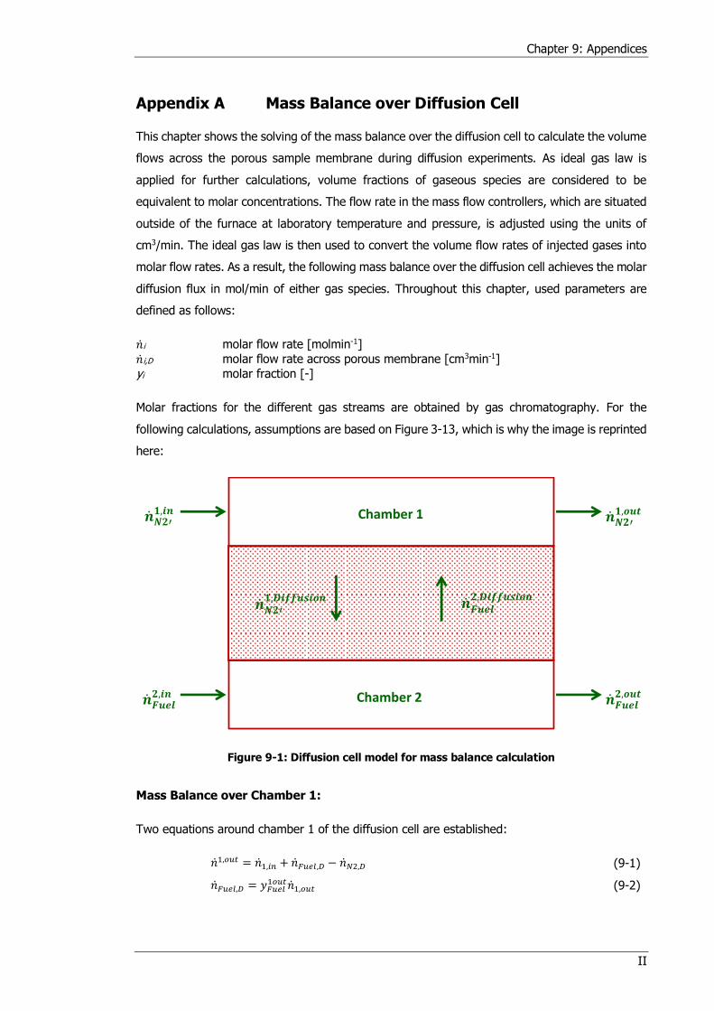
Chapter 9: Appendices
II
Appendix A Mass Balance over Diffusion Cell
This chapter shows the solving of the mass balance over the diffusion cell to calculate the volume
flows across the porous sample membrane during diffusion experiments. As ideal gas law is
applied for further calculations, volume fractions of gaseous species are considered to be
equivalent to molar concentrations. The flow rate in the mass flow controllers, which are situated
outside of the furnace at laboratory temperature and pressure, is adjusted using the units of
cm3/min. The ideal gas law is then used to convert the volume flow rates of injected gases into
molar flow rates. As a result, the following mass balance over the diffusion cell achieves the molar
diffusion flux in mol/min of either gas species. Throughout this chapter, used parameters are
defined as follows:
��i molar flow rate [molmin-1]
��i,D molar flow rate across porous membrane [cm3min-1] yi molar fraction [-]
Molar fractions for the different gas streams are obtained by gas chromatography. For the
following calculations, assumptions are based on Figure 3-13, which is why the image is reprinted
here:
Figure 9-1: Diffusion cell model for mass balance calculation
Mass Balance over Chamber 1:
Two equations around chamber 1 of the diffusion cell are established:
��1,𝑜𝑢𝑡 = ��1,𝑖𝑛 + ��𝐹𝑢𝑒𝑙,𝐷 − ��𝑁2,𝐷 (9-1)
��𝐹𝑢𝑒𝑙,𝐷 = 𝑦𝐹𝑢𝑒𝑙1𝑜𝑢𝑡��1,𝑜𝑢𝑡 (9-2)
Chamber 1
Chamber 2
𝟐′𝟏,
𝟐,
𝟐′𝟏,
𝟐,
𝟐,
𝟐′𝟏,
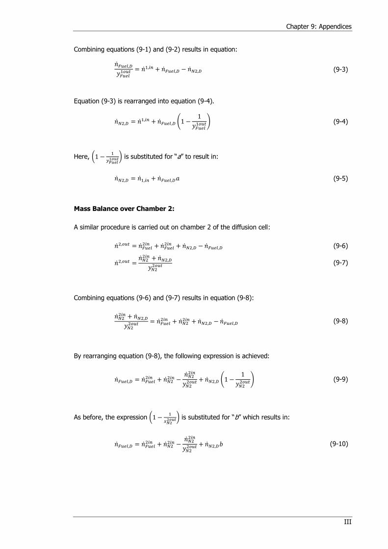
Chapter 9: Appendices
III
Combining equations (9-1) and (9-2) results in equation:
��𝐹𝑢𝑒𝑙,𝐷𝑦𝐹𝑢𝑒𝑙1𝑜𝑢𝑡 = ��1,𝑖𝑛 + ��𝐹𝑢𝑒𝑙,𝐷 − ��𝑁2,𝐷 (9-3)
Equation (9-3) is rearranged into equation (9-4).
��𝑁2,𝐷 = ��1,𝑖𝑛 + ��𝐹𝑢𝑒𝑙,𝐷 (1 −1
𝑦𝐹𝑢𝑒𝑙1𝑜𝑢𝑡) (9-4)
Here, (1 −1
𝑦𝐹𝑢𝑒𝑙1𝑜𝑢𝑡) is substituted for “a” to result in:
��𝑁2,𝐷 = ��1,𝑖𝑛 + ��𝐹𝑢𝑒𝑙,𝐷𝑎 (9-5)
Mass Balance over Chamber 2:
A similar procedure is carried out on chamber 2 of the diffusion cell:
��2,𝑜𝑢𝑡 = ��𝐹𝑢𝑒𝑙2𝑖𝑛 + ��𝐹𝑢𝑒𝑙
2𝑖𝑛 + ��𝑁2,𝐷 − ��𝐹𝑢𝑒𝑙,𝐷 (9-6)
��2,𝑜𝑢𝑡 =��𝑁22𝑖𝑛 + ��𝑁2,𝐷𝑦𝑁22𝑜𝑢𝑡 (9-7)
Combining equations (9-6) and (9-7) results in equation (9-8):
��𝑁22𝑖𝑛 + ��𝑁2,𝐷𝑦𝑁22𝑜𝑢𝑡 = ��𝐹𝑢𝑒𝑙
2𝑖𝑛 + ��𝑁22𝑖𝑛 + ��𝑁2,𝐷 − ��𝐹𝑢𝑒𝑙,𝐷 (9-8)
By rearranging equation (9-8), the following expression is achieved:
��𝐹𝑢𝑒𝑙,𝐷 = ��𝐹𝑢𝑒𝑙2𝑖𝑛 + ��𝑁2
2𝑖𝑛 −��𝑁22𝑖𝑛
𝑦𝑁22𝑜𝑢𝑡 + ��𝑁2,𝐷 (1 −
1
𝑦𝑁22𝑜𝑢𝑡) (9-9)
As before, the expression (1 −1
𝑥𝑁22𝑜𝑢𝑡) is substituted for “b” which results in:
��𝐹𝑢𝑒𝑙,𝐷 = ��𝐹𝑢𝑒𝑙2𝑖𝑛 + ��𝑁2
2𝑖𝑛 −��𝑁22𝑖𝑛
𝑦𝑁22𝑜𝑢𝑡 + ��𝑁2,𝐷𝑏 (9-10)

Chapter 9: Appendices
IV
Volume Flow Rates across Porous Sample
Equations (9-5) and (9-10) are now used to calculate the volume flow rates of N2 and Fuel across
the porous sample as functions of ingoing gas composition and measured gas composition of
exiting gas lines. For ��Fuel,D, equation (9-5) is inserted into equation (9-10) as shown below:
��𝐹𝑢𝑒𝑙,𝐷 =
��𝐹𝑢𝑒𝑙2𝑖𝑛 + ��𝑁2
2𝑖𝑛 −��𝑁22𝑖𝑛
𝑦𝑁22𝑜𝑢𝑡 + ��1,𝑖𝑛𝑏
(1 − 𝑎𝑏)
(9-11)
For ��N2,D, equation (9-10) is inserted into equation (9-5) to express the following equation:
��𝑁2,𝐷 =
��1,𝑖𝑛 + ��𝐹𝑢𝑒𝑙2𝑖𝑛 𝑎 + ��𝑁2
2𝑖𝑛𝑎 −��𝑁22𝑖𝑛
𝑦𝑁22𝑜𝑢𝑡 𝑎
(1 − 𝑎𝑏)
(9-12)
Equations (9-11) and (9-12) are applied to calculate the volume flow rate of N2 and fuel across
the porous membrane as a function of volume flow rate of ingoing gases and gas composition of
exiting gases.
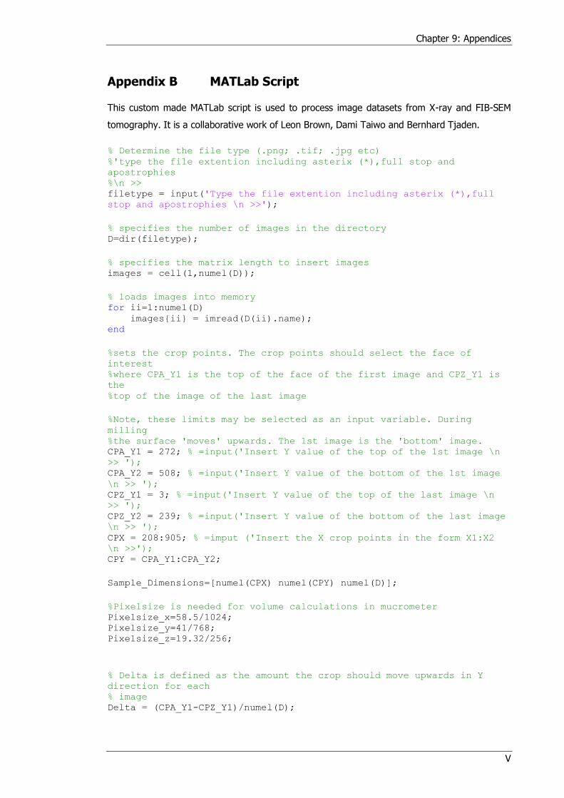
Chapter 9: Appendices
V
Appendix B MATLab Script
This custom made MATLab script is used to process image datasets from X-ray and FIB-SEM
tomography. It is a collaborative work of Leon Brown, Dami Taiwo and Bernhard Tjaden.
% Determine the file type (.png; .tif; .jpg etc) %'type the file extention including asterix (*),full stop and
apostrophies %\n >> filetype = input('Type the file extention including asterix (*),full
stop and apostrophies \n >>');
% specifies the number of images in the directory D=dir(filetype);
% specifies the matrix length to insert images images = cell(1,numel(D));
% loads images into memory for ii=1:numel(D) images{ii} = imread(D(ii).name); end
%sets the crop points. The crop points should select the face of
interest %where CPA_Y1 is the top of the face of the first image and CPZ_Y1 is
the %top of the image of the last image
%Note, these limits may be selected as an input variable. During
milling %the surface 'moves' upwards. The 1st image is the 'bottom' image. CPA_Y1 = 272; % =input('Insert Y value of the top of the 1st image \n
>> '); CPA_Y2 = 508; % =input('Insert Y value of the bottom of the 1st image
\n >> '); CPZ_Y1 = 3; % =input('Insert Y value of the top of the last image \n
>> '); CPZ_Y2 = 239; % =input('Insert Y value of the bottom of the last image
\n >> '); CPX = 208:905; % =imput ('Insert the X crop points in the form X1:X2
\n >>'); CPY = CPA_Y1:CPA_Y2;
Sample_Dimensions=[numel(CPX) numel(CPY) numel(D)];
%Pixelsize is needed for volume calculations in mucrometer Pixelsize_x=58.5/1024; Pixelsize_y=41/768; Pixelsize_z=19.32/256;
% Delta is defined as the amount the crop should move upwards in Y
direction for each % image Delta = (CPA_Y1-CPZ_Y1)/numel(D);

Chapter 9: Appendices
VI
%This crops the images so that the top of the images is always
selected as %the image moves for ii=1:numel(D), croppedimages{ii} = (images{ii}((round((CPA_Y1-
(ii*Delta))):round((CPA_Y2-(ii*Delta)))), CPX)); end
%Test Run
% Uses and applies the command histeq on all cropped images with the
chosen % value for hgram. % hgram has to be chosen in order to increase contrast between solid
and % pore phase.
for ii=1:numel(D), hgram=5; histimages{ii}=histeq(croppedimages{ii},hgram); end
% turn the image into black and white. Change threshold as necessary. BWThreshold=0.5; for ii=1:numel(D), bwimages{ii} = im2bw(histimages{ii}, BWThreshold); end
% Apply median filter to smoothen the image by getting rid of noise
for ii=1:numel(D)
medfilter{ii} = medfilt2(bwimages{ii});
end
%Erodes the image to reduce noise % se is the structural element. STREL may also be used se = [0 1 0;1 1 1;0 1 0];
for ii=1:numel(D),
newimages{ii} = medfilter{ii};
end
for ii=1:numel(D)
CompletedImages{ii} = newimages{ii};
end
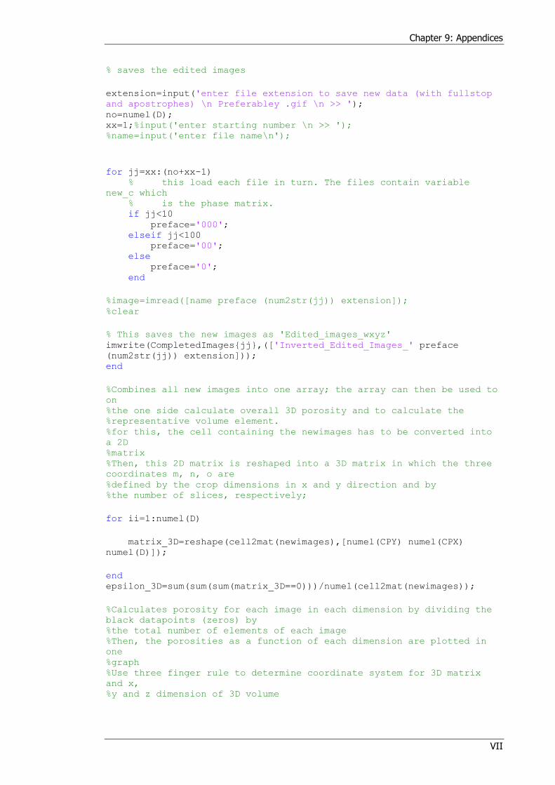
Chapter 9: Appendices
VII
% saves the edited images
extension=input('enter file extension to save new data (with fullstop
and apostrophes) \n Preferabley .gif \n >> '); no=numel(D); xx=1;%input('enter starting number \n >> '); %name=input('enter file name\n');
for jj=xx:(no+xx-1) % this load each file in turn. The files contain variable
new_c which % is the phase matrix. if jj<10 preface='000'; elseif jj<100 preface='00'; else preface='0'; end
%image=imread([name preface (num2str(jj)) extension]); %clear
% This saves the new images as 'Edited_images_wxyz' imwrite(CompletedImages{jj},(['Inverted_Edited_Images_' preface
(num2str(jj)) extension])); end
%Combines all new images into one array; the array can then be used to
on %the one side calculate overall 3D porosity and to calculate the %representative volume element. %for this, the cell containing the newimages has to be converted into
a 2D %matrix %Then, this 2D matrix is reshaped into a 3D matrix in which the three
coordinates m, n, o are %defined by the crop dimensions in x and y direction and by %the number of slices, respectively;
for ii=1:numel(D)
matrix_3D=reshape(cell2mat(newimages),[numel(CPY) numel(CPX)
numel(D)]);
end epsilon_3D=sum(sum(sum(matrix_3D==0)))/numel(cell2mat(newimages));
%Calculates porosity for each image in each dimension by dividing the
black datapoints (zeros) by %the total number of elements of each image %Then, the porosities as a function of each dimension are plotted in
one %graph %Use three finger rule to determine coordinate system for 3D matrix
and x, %y and z dimension of 3D volume
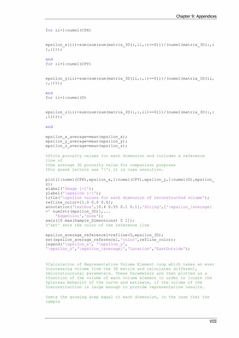
Chapter 9: Appendices
VIII
for ii=1:numel(CPX)
epsilon_x(ii)=sum(sum(sum(matrix_3D(:,ii,:)==0)))/(numel(matrix_3D(:,i
i,:)));
end for ii=1:numel(CPY)
epsilon_y(ii)=sum(sum(sum(matrix_3D(ii,:,:)==0)))/(numel(matrix_3D(ii,
:,:)));
end for ii=1:numel(D)
epsilon_z(ii)=sum(sum(sum(matrix_3D(:,:,ii)==0)))/(numel(matrix_3D(:,:
,ii)));
end
epsilon_x_average=mean(epsilon_x); epsilon_y_average=mean(epsilon_y); epsilon_z_average=mean(epsilon_z);
%Plots porosity values for each dimension and includes a reference
line of %the average 3D porosity value for comparison purposes %For greek letters use '\'; it is case sensitive.
plot(1:numel(CPX),epsilon_x,1:numel(CPY),epsilon_y,1:numel(D),epsilon_
z); xlabel('Image [-]'); ylabel('\epsilon [-]'); title('\epsilon values for each dimension of reconstructed volume'); refline_color=[1.0 0.0 0.6]; annotation('textbox',[0.4 0.55 0.1 0.1],'String',['\epsilon_{average}
=' num2str(epsilon_3D)],... 'EdgeColor','none'); axis([0 max(Sample_Dimensions) 0 1]); %'set' sets the color of the reference line
epsilon_average_reference1=refline(0,epsilon_3D); set(epsilon_average_reference1,'color',refline_color); legend('\epsilon_x', '\epsilon_y',
'\epsilon_z','\epsilon_{average}','Location','EastOutside');
%Calculation of Representative Volume Element loop which takes an ever %increasing volume from the 3D matrix and calculates different, %microstructural parameters. These Parameters are then plotted as a %function of the volume of each volume element in order to locate the %plateau behavior of the curve and estimate, if the volume of the %reconstruction is large enough to provide representative results.
%sets the growing step equal to each dimension, in the case that the
cample
Chapter 9: Appendices
IX
%is not a cube with equal side length. reduction_REV increases the
stepsize %and thus, decrease the number of analysed volumes to decrease
computation time.
reduction_RVE=1/1; Delta_CPX=numel(CPX)/min(Sample_Dimensions)/reduction_RVE; X=Delta_CPX:Delta_CPX:numel(CPX); xx=length(X); Delta_CPY=numel(CPY)/min(Sample_Dimensions)/reduction_RVE; Y=Delta_CPY:Delta_CPY:numel(CPY); yy=length(Y); Delta_D=numel(D)/min(Sample_Dimensions)/reduction_RVE; Z=Delta_D:Delta_D:numel(D); zz=length(Z);
epsilon_RVE=zeros(1,xx);
%for iii=1:xx; % test=iii %end
if(xx~=yy || xx~=zz || yy~=zz) error('The index dimensions are not equal!'); end;
for iii = 1:xx %how many volumes you need
J = zeros(Y(iii),Z(iii),X(iii));
XX = X(iii); YY = Y(iii); ZZ=Z(iii);
J = matrix_3D(1:YY,1:XX,1:ZZ);
epsilon_RVE(iii) = numel(J(J == 0))/numel(J); % Finds
porosity.
fprintf('step = %d \n',iii)
end
%RVE is the analysed volume which increases along the analysis V_grow=X.*Pixelsize_x.*Y.*Pixelsize_y.*Z.*Pixelsize_z; V_grow_pixel=X.*Y.*Z;
%To check, if the RVE loop gives a correct volume in the end, the
volume of %the cube is calculated, using the pixelsize of the reconstruction: Volume_Sample=numel(CPX)*Pixelsize_x*numel(CPY)*Pixelsize_y*numel(D)*P
ixelsize_z;
figure,plot(V_grow,epsilon_RVE,'-o'); xlabel('Analyzed volume [\mum^3]'); ylabel('\epsilon [-]'); title('Representative volume element development for \epsilon'); epsilon_average_reference2=refline(0,epsilon_3D);

Chapter 9: Appendices
X
refline_color=[1.0 0.0 0.6]; set(epsilon_average_reference2,'color',refline_color); axis([0 Volume_Sample 0 1]); annotation('textbox',[0.4 0.65 0.1 0.1],'String',['\epsilon_{average}
= ' num2str(epsilon_3D) ' Sample volume =' num2str(Volume_Sample) '
\mum^3'],'EdgeColor','none'); legend('\epsilon_{RVE}','\epsilon_{average}','Location','EastOutside')
;