Uncertainty in acid deposition modelling and critical load ...
214
R&D Technical ReportTR4-083(5)/1 Uncertainty in acid deposition modelling and critical load assessments R&D Technical Report P4-083(5)/1 J Abbott 1 , G Hayman 1 , K Vincent 1 , S Metcalfe 2 , T Dore 3 , R Skeffington 4 , P Whitehead 4 , D Whyatt 5 , N Passant 1 , M Woodfield 1 1. AEA Technology plc 2. University of Edinburgh 3. Centre for Ecology and Hydrology, Bush 4. Water Resource Associates 5. University of Lancaster
-
Upload
khangminh22 -
Category
Documents
-
view
2 -
download
0
Transcript of Uncertainty in acid deposition modelling and critical load ...
R&D Technical ReportTR4-083(5)/1
Uncertainty in acid deposition modelling and criticalload assessments
R&D Technical Report P4-083(5)/1
J Abbott1, G Hayman1, K Vincent1, S Metcalfe2, T Dore3, RSkeffington4, P Whitehead4, D Whyatt5, N Passant1, M Woodfield1
1. AEA Technology plc2. University of Edinburgh3. Centre for Ecology and Hydrology, Bush4. Water Resource Associates5. University of Lancaster

R&D Technical ReportTR4-083(5)/1 i
Publishing OrganisationEnvironment Agency, Rio House, Waterside Drive, Aztec West, Almondsbury,BRISTOL, BS32 4UD.
Tel: 01454 624400 Fax: 01454 624409Website: www.environment-agency.gov.uk
© Environment Agency 2003 June 2003
ISBN 1 84432 113 4
All rights reserved. No part of this document may be reproduced, stored in a retrieval system,or transmitted, in any form or by any means, electronic, mechanical, photocopying, recordingor otherwise without the prior permission of the Environment Agency.
The views expressed in this document are not necessarily those of the Environment Agency.Its officers, servants or agents accept no liability whatsoever for any loss or damage arisingfrom the interpretation or use of the information, or reliance upon views contained herein.
Dissemination StatusInternal: Released to RegionsExternal: Released to Public Domain
Statement of Use
The research results provide a valuable baseline for critical load assessments of value to IPPCand Habitats Directive assessments. However they are of broader significance in developing afull risk based approach to air quality assessment of processes under Agency regulation.Further work on testing the uncertainty bounds using measurement data has also beencompleted as supplementary work. The results of this aspect of air quality assessment will beincluded within a framework for all air quality assessments following further development.
KeywordsCritical loads, uncertainty, acidification, eutrophication, dynamic models, Monte-Carloanalysis.
Research ContractorThis document was produced under R&D Project P4-083(5) by AEA Technology plc,Culham Science Centre,:Abingdon, Oxfordshire. OX13 3ED.
Tel: 01235 463184
Environment Agency’s Project ManagerThe Environment Agency’s Project Manager for Project P4-083(5) was:Dr Bernard Fisher, National Centre for Risk Analysis and Options Appraisal.

R&D Technical ReportTR4-083(5)/1 ii
EXECUTIVE SUMMARY
The critical loads approach has been developed as an aid to the regulation of acidifyinggas emissions, both within the UK and internationally. The critical load is broadlydefined as the amount of pollutant deposition a part of the environment can toleratewithout harm. Trajectory models such as HARM, TRACK and FRAME have beendeveloped to assess acid deposition to sensitive areas. They use a spatially dis-aggregated emissions inventory and predict deposition at grid squares throughout theUnited Kingdom.
The use of trajectory models and critical loads is now recognised as the acceptedassessment method and is likely to be used to meet the Environment Agency’sobligation under the Habitats Directive. Hence, the Environment Agency would like tohave an understanding of the uncertainties associated with these models and methods.They need to know how robust the models are so that they know to what extent they canrely on them. For example:
1. Are they merely the best cost/time effective guess based on the available evidencebut useful for general policy development?
2. Are they sufficiently robust to form the basis of methods to assess the contributionof specific emissions to deposition, or critical load exceedence?
3. Are they sufficiently robust that they could be relied upon in court as proof of harmto the environment in the event of a breach of an authorisation?
The Environment Agency commissioned this project to get a better understanding of theuncertainties in using trajectory models and the critical loads approach. The aim of theproject was to assess the influence of uncertainty in three main areas:
1. Emission estimates;2. The parameterisation of long range trajectory models;3. The description of critical loads functions.
Consideration of uncertainty also improves understanding of the characteristics ofenvironmental models and avoids treating them as “black boxes”. The report has beenprepared as the result of collaboration. AEA Technology provided the overall projectmanagement, assessed and quantified the uncertainties in model inputs including theuncertainties in emissions, contributed to acid deposition studies and carried out dataanalysis. CEH Edinburgh carried out acid deposition studies using the FRAME model.Edinburgh and Lancaster Universities collaborated on the acid deposition studies, usingthe HARM model, and contributed to the assessment of model input uncertainties.Water Research Associates carried out the literature review of uncertainties in criticalload estimates and the Liphook case study.
The acid deposition models HARM, FRAME and TRACK are all trajectory modelsemploying broadly similar chemical reaction schemes. They have many commonfeatures and might be expected to demonstrate similar behaviour. The model equationscan to some extent be solved analytically. Analytical solutions have been developed aspart of this project and have been used to help identify the critical input parameters,make sensitivity analyses more amenable, and to develop methods of data analysis.
R&D Technical ReportTR4-083(5)/1 iii
The main input parameters included within the models are:
1. Chemical reaction rate constants:2. Dry deposition velocities;3. Wet scavenging coefficients (including enhancement in high rainfall areas);4. Background concentrations of chemical species;5. Wind speed;6. Frequency of winds from each wind direction sector;7. Boundary layer height;8. Emissions;9. Speciation of emitted sulphur dioxide and oxides of nitrogen.
Plausible ranges of these input parameters have been identified based on literaturesurveys, current practice and expert judgement. The uncertainty in some of the inputparameters, such as the rate of reaction of simple gaseous species, is quite small; theuncertainty in other parameters such as the rate of reaction of gases with particulatematter may be quite large, approaching an order of magnitude.
A systematic sensitivity analysis of the uncertainty in the national emissions leads tosome estimates, notably for sulphur and nitrogen oxides, which are substantially lowerthan those which would have been estimated by expert judgement. It is not within thisstudy to explore alternative methodologies, but it is recognised that Monte Carloanalysis is not able to treat uncertainties in processes which are unknown. In additionuncertainties in individual processes are treated as independent variables.
A summary of the sensitivity analyses performed on the models now follows. Theuncertainty in sulphur deposition was investigated by Monte Carlo analysis of theanalytical model with the values of input parameters selected from their plausible rangesusing a single source. The 95th percentile of the predicted deposition rates wasapproximately a factor of 2 times the average value and the 5th percentile wasapproximately half the average value. A first order error analysis of the uncertainty insulphur deposition, in which each of the input variables was changed one variable at atime explained 95% of the overall variance throughout the range of prediction. Themajor contributor to the overall variance of predicted values was the uncertainty in thedry deposition velocity for sulphur dioxide in the vicinity of the receptor. Othersignificant contributors to the variance were the uncertainties in the rate of emission,boundary layer height, wind speed, frequency of the wind direction in the relevantsector and the wet deposition coefficient for sulphur dioxide. At 800 km from thesource, the largest contributors to the variance in the predicted total sulphur depositionrate at receptors are the uncertainties in the dry deposition velocity for sulphur dioxideboth upwind and local to the receptor.
The analytical model was used to compare the performance of Monte Carlo simulationwith that of more limited sampling based on a Latin Square with only 13 model runs.The Latin Square sampling strategy provided a reasonable estimate of the distributionderived from the Monte Carlo analysis in the cumulative probability range between 0.1and 0.9. In both cases, the sulphur deposition distribution function could beapproximated by a log-normal.
R&D Technical ReportTR4-083(5)/1 iv
Monte Carlo analysis of the analytical model for nitrogen deposition was also carriedout. The 95th percentile of the predicted rates of deposition was approximately twice themean value and the 5th percentile was approximately one third of the mean value.Approximately 10-30% of the variance is not explained by first order analysis and isassociated with more complex interactions between parameters. The largest contributorsto the variance in the predicted rates of deposition were the background concentration ofthe hydroxyl radical, the wet deposition of the aerosols, the frequency of the winddirection, the wind speed, the rate constant for the formation of nitrogen pentoxide, therate of emission, and the rate constant for the formation of nitric acid.
Monte Carlo simulations of sulphur, oxidised nitrogen and reduced nitrogen depositionusing the TRACK model, using a 1990 emissions inventory for the UK and threehundred model runs, showed that:1. The 95th percentile of predicted rates of sulphur deposition at a range of sites
throughout the UK (the Secondary Network sites) was typically 1.3 times the meanvalue predicted at each site: the mean was typically around 1.45 times the 5th
percentile.2. The 95th percentile of predicted rates of oxidised nitrogen deposition was typically
around 1.9 times the average: the average was typically around 2 times the 5th
percentile.3. The 95th percentile of predicted rates of reduced nitrogen deposition was typically
around 1.5 times the average: the average is typically around 1.7 times the 5th
percentile.4. The probability distributions of the predicted rates of sulphur, oxidised and reduced
nitrogen deposition were approximately log-normal.
A first order error analysis of the TRACK model in which the input parameters werevaried one variable at a time was also carried out. From this the 5th percentile and 95th
percentile rates of sulphur deposition could be estimated. These were approximately30% greater than those provided by the Monte Carlo analysis. The range of uncertaintyin nitrogen deposition rates were similar to those provided by the Monte Carlo analysis.The estimated 5th percentile rate of reduced nitrogen deposition was similar to thatprovided by the Monte Carlo analysis. The 95th percentile rate of deposition wastypically 50% greater than that provided by the Monte Carlo analysis.
The uncertainty in the estimates made by TRACK of the incremental impact of anadditional 150 kt per annum source of oxides of nitrogen was also investigated usingMonte Carlo analysis. The 95th percentile of the additional oxidised nitrogen depositionwas approximately twice the average value: the 5th percentile was approximately halfthe average value. Comparison of the predictions of the TRACK model with those forthe analytical model showed acceptable agreement, suggesting that the results ofuncertainty analysis for the analytical model are more generally applicable.
The non-linear incremental impact of additional sources was investigated using theTRACK model. Far from the source, the incremental contribution from a 75 kt sourceof oxides of nitrogen was half that for a 150 kt source i.e. the predictions varied linearlywith emission. Closer to the source, the predicted impact showed evidence ofsublinearity: the deposition of oxidised nitrogen associated with a 150 kt source wasonly 1.8 times that for a 75 kt source.
R&D Technical ReportTR4-083(5)/1 v
The uncertainty in predictions of nitrogen deposition made by the HARM model wasinvestigated using a sampling strategy based on a Latin Square. This was based on just12 model runs. The estimated 92nd percentile rates of oxidised and reduced nitrogenwere typically around 1.5 times the mean values: averages were typically around 1.5times the 5th percentiles. The probability distributions of predicted rates of depositionapproximated to log-normal.
First order error analysis of the uncertainty in HARM model predictions of oxidised andreduced nitrogen was also carried out. This provided estimates of oxidised nitrogendeposition similar to those provided by the Latin Square sampling analysis. Estimates ofaverage and 5th percentile rates of reduced nitrogen deposition were similar to thosedetermined by Latin Square sampling: the 95th percentile value was typically 30%greater than that provided by the Latin Square sampling.
A review of the literature on the uncertainty in critical loads has been carried out. Thereview concluded that further work was required to quantify the uncertainty in criticalloads estimates. A case study for Liphook, a forested area in the south of England, wastherefore carried out in order to investigate the uncertainty in the critical load estimate ata well-documented site. The case study involved Monte Carlo simulation, selectinginput values from a plausible range of parameters describing this well-documented site.The coefficients of variation of the variables describing the critical load functionCLminN, CLmaxS and CLmaxN were 22%, 30% and 14 % respectively. The probabilitydistribution of the critical load variables could be approximated by a normaldistribution.
The uncertainty in the prediction of the exceedence of the critical load at the Liphooksite was investigated. Estimates of critical loads sampled from the Liphook Monte Carlosimulation were randomly matched with estimates of the rate of acid depositionsampled from the TRACK Monte Carlo simulation. The simulation indicated that therewas a high probability (>99.9%) that the critical load was exceeded at the site based on1990 emissions. Reducing the rates of deposition to around 40% of that for 1990emissions would reduce the probability of exceedence to around 50%. It would benecessary to reduce acid deposition to approximately 20 % of that predicted from 1990emissions in order to have a high degree of confidence (95%) that the critical load wasnot exceeded at this site. This example suggests that the critical load and depositionmodel methodology can provide an effective tool for emissions reduction policies at theregional scale, but the uncertainties in the assessment of exceedences should be takeninto account
The incremental contribution to sulphur and nitrogen deposition from a large pointsource was considered in relation to the uncertainty in the exceedence at the Liphooksite. For the example considered, the incremental contribution to nitrogen depositionfrom a 150kt per annum emission of NOx 50km away would increase the risk ofexceedence of the critical load by around 1%. The incremental contribution to sulphurdeposition would appear to be greater with a typical increase in the risk of exceedenceof the critical load of approximately 5-10% because of the addition of a major stationarysource. These examples suggest that the impact of large point sources should beexpressed in terms of risk of increasing exceedence. The assessment of sources ofnitrogen oxides should consider the aggregate impact of a number of sources on the riskof exceedence.

R&D Technical ReportTR4-083(5)/1 vi
The assessment of uncertainty carried out in this study does not take account ofmeasured rates of deposition. In practice, the predicted rates of deposition may becompared with observed, or independently estimated rates of deposition at SecondaryNetwork sites throughout the United Kingdom. An integrated assessment approachwould allow the performance of the model at these sites to be taken into account whenestimating the likelihood of exceedence of the critical load at other sites. A simpleprobabilistic method for incorporating measured deposition rates in the assessment ofuncertainty is suggested.
The following conclusions and recommendations are made:
1. The uncertainty in the prediction of rates of deposition resulting from theuncertainty in input parameters may be assessed by Monte Carlo analysis.
2. Latin Square sampling or first order analysis should provide useful estimates of theuncertainty where Monte Carlo analysis is not practical because of the large numberof model runs required. The probability distribution of rate of deposition can usuallybe approximated by a log-normal distribution.
3. The uncertainty in acid deposition models currently used for assessment purposes inthe UK may be broadly described as within a “factor of two”.
4. Analytical deposition models may be used to test Monte Carlo techniques. Their realvalue may arise in their flexibility to optimise input parameters when comparingpredictions against observations, using for example Bayesian Monte-Carlo methods
5. The uncertainty in prediction of critical loads resulting from uncertainties in inputparameters may also be assessed by Monte Carlo analysis.
6. The uncertainty in predicting exceedence of critical loads (deposition minus criticalload) may be obtained by sampling from the probability distributions of thepredicted critical loads and rates of acid deposition.
7. Further investigations should be carried out to integrate measurements of rates ofdeposition into the analysis of uncertainty to counter criticism that only “known”sources of uncertainty have been taken into account.
R&D Technical ReportTR4-083(5)/1 vii
CONTENTS
1 INTRODUCTION 1
1.1 Structure of Report 2
2 ACID DEPOSITION MODEL DESCRIPTIONS 4
2.1 Introduction 4
2.2 HARM - version 11.5 4
2.2 TRACK- version 1.8 5
2.3 FRAME - version 4.2 6
2.4 Analytical models 7
3 ACID DEPOSITION MODEL INPUT PARAMETER UNCERTAINTIES 8
3.1 Introduction 8
3.2 Reaction rate constants 8
3.3 Dry deposition velocities 10
3.4 Wet deposition scavenging coefficients 12
3.5 Background concentrations 14
3.6 Wind speed 14
3.7 Wind direction 16
3.8 Boundary layer height 16
3.9 Emissions 16
3.10 Speciation of emissions 20
4 DEPOSITION MODEL UNCERTAINTIES 21
4.1 Introduction 21
4.2 Sulphate deposition analytical model 22
4.3 Oxidised nitrogen deposition analytical model 29
4.4 TRACK - Baseline predictions 35
R&D Technical ReportTR4-083(5)/1 viii
4.5 TRACK Model - Impact of an additional point source 43
4.6 HARM Model - Baseline predictions 45
4.7 HARM Model - Impact of an additional point source 50
4.8 FRAME 52
5 UNCERTAINTY IN CRITICAL LOADS 55
5.1 Introduction 55
5.2 Uncertainty in critical load function, Liphook case study 57
6 OVERALL UNCERTAINTY IN THE PREDICTION OF CRITICAL LOADEXCEEDENCES 60
6.1 Introduction 60
6.2 Calculation of exceedence 60
6.3 Integration of observed rates of deposition 64
7 CONCLUSIONS AND RECOMMENDATIONS 66
8 REFERENCES 72
R&D Technical ReportTR4-083(5)/1 ix
List of Figures
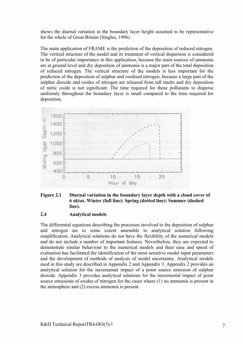
Figure 2.1 Diurnal variation in the boundary layer depth with a cloud cover of 6oktas. Winter (full line): Spring (dotted line): Summer (dashed line). 7
Figure 4.1 Mean, 5th and 95th percentiles of predicted total sulphateconcentrations using the analytical model 23
Figure 4.2 Mean, 5th and 95th percentiles of predicted total sulphur deposition atreceptors using the analytical model 23
Figure 4.3 Mean, 5th and 95th percentiles of predicted distance integrated totalsulphur deposition using the analytical model 24
Figure 4.4 Cumulative contributions to variance in predicted total sulphateconcentration using the analytical model as a function of distance 25
Figure 4.5 Cumulative contribution to variance in predicted total sulphurdeposition at receptor using the analytical model as a function of distance 26
Figure 4.6 Cumulative contribution to variance in predicted “distance integrated”total sulphur deposition using the analytical model as a function of distance 27
Figure 4.7 Comparison of Latin Square sampling estimates of the range of totalsulphate concentrations with Monte Carlo analysis using the analytical model 28
Figure 4.8 Cumulative probability distributions of total sulphate concentration 20km downwind of the source based on Latin Square and Monte Carlosampling of input parameters using the analytical model 29
Figure 4.9 Deposition of oxidised nitrogen for a 1 mole s-1 release, W=10 km, noammonia using the analytical model 32
Figure 4.10 Deposition of oxidised nitrogen for a 1 mole s-1 release, W=10 km,excess ammonia, using the analytical model 32
Figure 4.11 Cumulative probability distribution of predicted nitrogen depositionrates, 200 km downwind of the source using the analytical model 33
Figure 4.12 Contribution to variance in predicted oxidized nitrogen deposition, noammonia case, using the analytical model 34
Figure 4.13 Contribution to variance in predicted oxidized nitrogen deposition,excess ammonia case, using the analytical model 34
Figure 4.14 Predicted sulphur deposition at grid cells containing monitoring sites,TRACK with 1990 emissions: mean, 5th %ile and 95th %ile predictions fromMonte Carlo analysis 37
Figure 4.15 Predicted oxidised nitrogen deposition at grid cells containingmonitoring sites, TRACK with 1990 emissions: mean, 5th %ile and 95th %ilepredictions from Monte Carlo analysis 37
Figure 4.16 Predicted reduced nitrogen deposition at grid cells containingmonitoring sites, TRACK with 1990 emissions: mean, 5th %ile and 95th %ilepredictions from Monte Carlo analysis 38
Figure 4.17 Predicted total (oxidised plus reduced) nitrogen deposition at grid cellscontaining monitoring sites, TRACK with 1990 emissions: mean, 5th %ileand 95th %ile predictions from Monte Carlo analysis 38
Figure 4.18 Predicted total (oxidised, nitrogen, reduced nitrogen and sulphur)deposition at grid cells containing monitoring sites, TRACK with 1990emissions: mean, 5th %ile and 95th %ile predictions from Monte Carloanalysis 39
Figure 4.19 Cumulative probability distribution of sulphur deposition: TRACKmodel, 1990 emissions, Jenny Hurn 39
R&D Technical ReportTR4-083(5)/1 x
Figure 4.20 Cumulative probability distribution of oxidised nitrogen deposition:TRACK model, 1990 emissions, Jenny Hurn 40
Figure 4.21 Cumulative probability distribution of reduced nitrogen deposition:TRACK model, 1990 emissions, Jenny Hurn 40
Figure 4.22 Average, 5 percentile and 95th percentile sulphur deposition predictedusing TRACK, 1990 emissions: Monte Carlo analysis and first order erroranalysis 42
Figure 4.23 Average, 5th percentile and 95th percentile oxidised nitrogen depositionpredicted using TRACK, 1990 emissions: Monte Carlo analysis and firstorder analysis 42
Figure 4.24 Average, 5th percentile and 95th percentile reduced nitrogen depositionpredicted using TRACK, 1990 emissions: Monte Carlo analysis and firstorder analysis 43
Figure 4.25 Incremental contribution to oxidised nitrogen deposition from a pointsource at (5100, 3100) emitting 150 kt oxides of nitrogen per year, TRACKmodel, 1990 base emissions, Monte Carlo analysis. Results from theanalytical model assuming excess ammonia are also shown 44
Figure 4.26 Ratio of contribution to rates of oxidised nitrogen deposition forsources emitting 150 kt and 75 kt per annum of oxides of nitrogen (as NO2):TRACK model 1990 background emissions: source at (5100, 3100) 45
Figure 4.27 Predicted oxidised nitrogen deposition at monitoring sites, HARM with1997 emissions: mean, 8th %ile and 92nd %ile predictions from Latin Squareanalysis. 47
Figure 4.28 Predicted reduced nitrogen deposition at monitoring sites, HARM with1997 emissions: mean, 8th %ile and 92nd % ile predictions from Latin Squareanalysis. 47
Figure 4.29 Cumulative probability distribution of oxidised nitrogen deposition:HARM model, 1997 emissions, Jenny Hurn 48
Figure 4.30 Cumulative probability distribution of reduced nitrogen deposition:HARM model, 1997 emissions, Jenny Hurn 48
Figure 4.31 Average, 5th percentile and 95th percentile oxidised nitrogen depositionpredicted using HARM, 1997 emissions: Latin Square and first order erroranalysis 49
Figure 4.32 Average, 5 percentile and 95th percentile reduced nitrogen depositionpredicted using HARM, 1997 emissions: Latin Square and first order erroranalysis 50
Figure 4.33 Incremental contribution to oxidised nitrogen deposition from a pointsource at (5100,3100) emitting 150 kt oxides of nitrogen per year, HARMmodel, 1997 base emissions, first order analysis 51
Figure 4.34 Predicted reduced nitrogen deposition at monitoring sites, FRAMEwith 1997 emissions: mean, 8th %ile and 92nd %ile predictions from the LatinSquare analysis. 53
Figure 4.35 Cumulative probability distribution of reduced nitrogen deposition:FRAME model, 1997 emissions, Jenny Hurn 53
Figure 5.1 The critical load function. 56Figure 5.2 Cumulative probability distribution of the critical load parameter
CLmaxS for the Liphook site 58Figure 5.3 Cumulative probability distribution of the critical load parameter
CLminN for the Liphook site 59
R&D Technical ReportTR4-083(5)/1 xi
Figure 5.4 Cumulative probability of critical load parameter CLmaxN for theLiphook site 59
Figure 6.1 Cumulative probability distribution of predicted exceedence atLiphook, 1990 emissions. Note the position of exceedence = 0 on the y axis. 61
Figure 6.2 Cumulative probability distribution of predicted exceedence atLiphook, assuming deposition equals half that for 1990 emissions. Note theposition of exceedence = 0 on the y axis. 61
Figure 6.3 Cumulative probability distribution of predicted exceedence atLiphook, deposition 20% of that for 1990 emissions. Note the position ofexceedence = 0 on the y axis. 62
Figure 6.4 Cumulative probability distribution of predicted exceedence atLiphook, deposition 10% of that for 1990 emissions. Note the position ofexceedence = 0 on the y axis. 62
Figure 6.5 Cumulative probability distribution of predicted exceedence atLiphook, deposition 5% of that for 1990 emissions. Note the position ofexceedence = 0 on the y axis. 63
R&D Technical ReportTR4-083(5)/1 xii
List of Tables
Table 3.1 Summary of reaction ratesTable 3.2 Dry deposition velocitiesTable 3.3 Dry deposition velocities used in the HARM, TRACK and FRAME
modelsTable 3.4 Suggested values for the wet scavenging coefficient for 1 mm h-1 rainfall
rateTable 3.5 Wet scavenging coefficients used in HARM, TRACK and FRAMETable 3.6 Representative wind rose used to derive average wind speedTable 3.7 Geostrophic wind data at a number of UK sites.Table 3.8 Frequency of wind in two wind sectors at sites throughout the UKTable 3.9 Results of uncertainty analysis for gaseous pollutants (emissions in
ktonnes) from known sourcesTable 3.10 Comparison of uncertainty in known sources according to expert
judgement and by detailed analysisTable 3.11 Key sources of uncertainty in emissions estimatesTable 4.1 Ranges of input parameters used in Monte Carlo analysis of sulphate
deposition analytical modelTable 4.2 Ranges of input parameters used in Monte Carlo analysis of nitrogen
deposition analytical modelTable 4.3 Input ranges of parameters used in Monte Carlo simulation and first order
error analysis for the TRACK modelTable 4.4 Input ranges of parameters used in Latin Square simulation and first
order error analysis for the HARM modelTable 4.5 HARM modelled UK deposition budgets with and without additional
sourceTable 4.6 Input ranges of parameters used in Latin Square simulation and first
order error analysis for the FRAME modelTable 4.7 Contribution to variance from each of the input parametersTable 5.1 Mean standard deviation and coefficient of variation of the predicted
critical load function parametersTable 6.1 Effect on the standard deviation of exceedence and probability of
exceedence as the rate of deposition is reduced.Table 7.1 Comparison of sampling strategies

R&D Technical ReportTR4-083(5)/1 xiii
APPENDICES
Appendix 1 TRACK, HARM AND FRAME model chemistryAppendix 2 Analytical model for sulphur depositionAppendix 3 Analytical model for nitrogen depositionAppendix 4 Analysis of uncertainty in critical loads: literature reviewAppendix 5 Liphook critical loads case studyAppendix 6 Liphook critical loads case study outputsAppendix 7 Implications of parameter variations for nitrogen deposition
modelled using the HARM model
R&D Technical ReportTR4-083(5)/1 1
1 INTRODUCTION
The Environment Agency is responsible for the protection and management of theenvironment in England and Wales by regulating pollutant releases to land, air andwater. More specifically the Environment Agency has a duty under the EC HabitatsDirective (Council Directive 92/43/EEC on the conservation of natural habitats and ofwild fauna and flora) to review the possible effects of emissions from regulatedprocesses on ecologically sensitive areas. The Directive provides for the creation of anetwork of ecologically sensitive sites throughout Europe, to be known as Natura 2000sites. This network includes SACs (Special Areas of Conservation) for the protection ofnatural habitats of wild fauna and flora other than birds, and SPAs (Special ProtectedAreas) which support wild birds and their habitats. It is the Environment Agency’sresponsibility to review all existing and prospective emissions to assess how a regulatedprocess might affect a Natura 2000 site in England and Wales by 2010. The Agency isinvolved in reviewing existing permissions that could affect existing SPAs and SACs.
The emission of oxides of nitrogen and sulphur from combustion sources in Englandand Wales leads to the deposition of oxidised and reduced nitrogen and sulphur overwide areas. This deposition may lead to the increased acidification of soils and water,particularly in upland areas. Nitrogen deposition may also contribute to theeutrophication of susceptible water bodies.
The critical loads approach has been developed as an aid to the regulation of acidifyinggas emissions, both within the UK and internationally. The critical load is broadlydefined as the amount of pollutant deposition a part of the environment can toleratewithout harm. In the UK straight line trajectory models such as HARM, TRACK andFRAME have been developed to assess acid deposition to sensitive areas. They use aspatially disaggregated emissions inventory and predict deposition at grid squaresthroughout the United Kingdom. The use of straight line trajectory models and criticalloads is now considered to be the standard assessment approach in the UK and is likelyto be used to meet the Environment Agency’s obligation under the Habitats Directive.Hence the Environment Agency would like to have an understanding of theuncertainties associated with these models and assessment methods. The Agency needsto know to what extent it can rely on the methods. For example the questions raisedinclude:
1. Are the models merely the best cost/time effective guess based on the availableevidence, and useful for general policy development?
2. Are they sufficiently accurate to form the basis of methods to assess the contributionof specific emissions to deposition, or to critical load exceedences?
3. Are they sufficiently robust that they could be relied upon in court as evidence ofharm to the environment in the event of a breach of an authorisation.
This project addresses the issues associated with the uncertainties in the use oftrajectory models and the critical loads approach. The aim of the project is to assess theinfluence on uncertainty in three main areas:
1. Emission estimates;

R&D Technical ReportTR4-083(5)/1 2
2. The parameterisation of long range transport models;3. The description of critical loads functions.
There are several sources of uncertainty in models. These include the uncertaintyassociated with:
1. the input parameters;2. the model structure and its spatial and temporal resolution;3. the random nature of some natural processes specifically atmospheric processes.
There appears to be a tendency to neglect uncertainty as our description ofenvironmental interactions becomes more detailed and complex. This study tries toredress the balance. Uncertainty is associated with measurements, but the primaryapproach to estimating uncertainty is to compare modelled predictions with fieldmeasurements. The TRACK, HARM and FRAME model predictions have beencompared with measurements in other studies [e.g. Metcalfe, Whyatt and Derwent,1995; Lee, Kingdon, Jenkin and Garland, 2000; Singles, Sutton and Weston, 1998].There is generally not sufficient measurement data to allow a comprehensiveassessment of uncertainty to be made, but quite good agreement between modelledpredictions and measurements has been achieved by judicious selection of inputparameters.
The deposition models all have many input parameters, some of which are ill-defined orvery uncertain. Consequently, the uncertainty arising from the uncertainty in the inputparameters may be a large component of overall uncertainty. This report addresses theuncertainty associated with only the model input parameters. Uncertainty associatedwith processes erroneously treated or neglected in the models have not beeninvestigated in this study.
A Monte Carlo approach is taken to assess the uncertainty arising from the uncertaintyin model inputs. Predicted rates of acid deposition are not compared with measuredvalues: the empirical assessment of uncertainty is outside the scope of this project. Aprobabilistic method of assessment of overall uncertainty that takes account ofmeasured rates of deposition is suggested as the subject of further work.
AEA Technology Environment have provided the overall management of the project,the assessment of the uncertainty in the emissions estimates and TRACK model output.The University of Edinburgh and the Centre for Ecology and Hydrology at Bushprovided HARM and FRAME model output respectively. Water Research Associatesprovided the uncertainty analysis and critical review of critical loads.
1.1 Structure of Report
Sections 2 to 4 of the report are concerned with the uncertainty in the prediction ofdeposition rates. Section 2 provides a brief description of the main features of themodels HARM, TRACK and FRAME. Section 2 also introduces simple analyticalmodels described in Appendices 2 and 3 for the prediction of acid deposition; theanalytical models provided the basis for understanding the general behaviour of the aciddeposition models and helped in the development of the methods used in theinvestigation

R&D Technical ReportTR4-083(5)/1 3
Section 3 identifies the parameters used in the input to the acid deposition models andthe plausible ranges in these input parameters. Detailed consideration is given to theuncertainty in a key input to the models - the emissions inventory.
Section 4 contains the results of the assessment of the uncertainty in the acid depositionmodel outputs attributable to the uncertainty in the model inputs. Various techniqueshave been used to assess the uncertainty including Monte Carlo simulation, First OrderError analysis using Taylor’s formula and randomised trials using Latin Squaresampling. The performance of the assessment methods is compared.
Section 5 of the report is concerned with the uncertainty in the assessment of criticalloads. It draws upon a literature review of the uncertainty in critical loads prepared aspart of this project and Monte Carlo simulations of critical load assessment for soils in awoodland area at Liphook, Surrey.
Section 6 of the report provides an assessment of the overall uncertainty in theprediction of critical load exceedences. It draws upon the probability distributions forthe deposition and the critical load at a receptor. Monte Carlo simulation is used todevelop the probability distribution of deposition in excess of the critical load.
Section 7 contains conclusions and recommendations.
R&D Technical ReportTR4-083(5)/1 4
2 ACID DEPOSITION MODEL DESCRIPTIONS
2.1 Introduction
Process models of the atmosphere have been widely used to evaluate the impact ofemissions on the environment. These models aim to describe the many different andcomplex chemical and physical processes occurring in the real atmosphere. Processmodels are therefore used
1. to assess the understanding of the processes involved;2. to interpret observations made of the atmosphere;3. to quantify the relative importance of different processes, and4. to assess how the atmospheric system will respond to different emission scenarios.
Lack of knowledge and computational limitations force many simplifications. Theaccuracy and precision of the numerical results obtained and hence, the conclusions thatcan be drawn, depend on many factors:
1. the representation of the atmospheric processes in the model;2. the assumptions and simplifications introduced;3. the quality of the input data.
The models investigated in this study are described in outline below. More detaileddescriptions are available in the references cited. Justification for the assumptions andsimplifications inherent in the numerical models is also provided in the references.
The models considered are all straight line trajectory models and so have many featuresin common. The models differ in their incorporated chemical models, their treatment ofdeposition and of vertical dispersion and the assumed wind fields. The models are notsimulations of actual transport and approximate removal and transformation processes.The main parameters are in some sense composite, idealised representations of actualprocesses. One cannot measure the parameter values explicitly.
Straight-line trajectory models are most widely applied in the United Kingdom. Othermodels formulations, such as the EMEP Lagrangian and Eulerian Acid DepositionModels LADM and MADE50 are also used, but are not considered here. These modelsare examples of cases in which the meteorological description is much more detailed.The changes in the chemical composition of air masses is followed explicitly, ratherthan by considering representative averages. One cannot conclude from this studywhether more complex models would give better predictions.
2.2 HARM - version 11.5
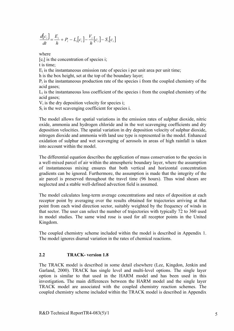
HARM employs a simple trajectory model approach to predict the concentrations andrates of deposition of gases and aerosols containing sulphur and nitrogen over north-west Europe. It is described in more detail by Metcalfe, Whyatt and Derwent(1995).The time development of the trace constituents in a parcel of air advected by a windfield has been represented by the following differential equation:
R&D Technical ReportTR4-083(5)/1 5
[ ] [ ] [ ] [ ]iiii
iiiii cSc
hV
cLPhE
dtcd
−−−+=
where[ci] is the concentration of species i;t is time;Ei is the instantaneous emission rate of species i per unit area per unit time;h is the box height, set at the top of the boundary layer;Pi is the instantaneous production rate of the species i from the coupled chemistry of theacid gases;Li is the instantaneous loss coefficient of the species i from the coupled chemistry of theacid gases;Vi is the dry deposition velocity for species i;Si is the wet scavenging coefficient for species i.
The model allows for spatial variations in the emission rates of sulphur dioxide, nitricoxide, ammonia and hydrogen chloride and in the wet scavenging coefficients and drydeposition velocities. The spatial variation in dry deposition velocity of sulphur dioxide,nitrogen dioxide and ammonia with land use type is represented in the model. Enhancedoxidation of sulphur and wet scavenging of aerosols in areas of high rainfall is takeninto account within the model.
The differential equation describes the application of mass conservation to the species ina well-mixed parcel of air within the atmospheric boundary layer, where the assumptionof instantaneous mixing ensures that both vertical and horizontal concentrationgradients can be ignored. Furthermore, the assumption is made that the integrity of theair parcel is preserved throughout the travel time (96 hours). Thus wind shears areneglected and a stable well-defined advection field is assumed.
The model calculates long-term average concentrations and rates of deposition at eachreceptor point by averaging over the results obtained for trajectories arriving at thatpoint from each wind direction sector, suitably weighted by the frequency of winds inthat sector. The user can select the number of trajectories with typically 72 to 360 usedin model studies. The same wind rose is used for all receptor points in the UnitedKingdom.
The coupled chemistry scheme included within the model is described in Appendix 1.The model ignores diurnal variation in the rates of chemical reactions.
2.2 TRACK- version 1.8
The TRACK model is described in some detail elsewhere (Lee, Kingdon, Jenkin andGarland, 2000). TRACK has single level and multi-level options. The single layeroption is similar to that used in the HARM model and has been used in thisinvestigation. The main differences between the HARM model and the single layerTRACK model are associated with the coupled chemistry reaction schemes. Thecoupled chemistry scheme included within the TRACK model is described in Appendix

R&D Technical ReportTR4-083(5)/1 6
1. The model can take into account the diurnal variation in the rates of chemicalreaction.
The TRACK multi-layer option describes the vertical diffusion of species by the K-theory diffusion equation, based upon Monin-Obukhov similarity theory:
∂∂
∂∂
=∂∂
zcK
ztc
z
where Kz is the eddy diffusivity at height z above the ground.
The eddy diffusivity depends on the atmospheric stability. For neutrally stableatmospheric conditions Kz is calculated from:
−=
hzzuK z 1*κ
where κ is the von Karman constant (0.41) and u* is the friction velocity.
The friction velocity is calculated from:
)/10ln( 0
10* z
uu
κ=
where u10 is the mean wind speed measured 10 m above the ground and z0 is the meanroughness length.
The TRACK model has the facility to model the effects of an additional point source onpredicted concentrations and rates of deposition. The approach taken for the additionalpoint source is slightly different from that used for the other “area” sources. The modelfirst calculates the concentration and rates of deposition at receptors in the absence ofthe additional point source and then performs the calculations with the additional sourcepresent: the incremental contribution from the additional point source is the differencebetween predicted values with and without it. The model allows for the spread of theplume from the point source: it calculates the width of the wind direction sector at thereceptor and applies this dispersion all at once at the source when inputting theemission, as a rate of change of concentration. This is considered to be a reasonableapproximation if the emitted species do not react rapidly.
2.3 FRAME - version 4.2
The FRAME model is similar to the multi-layer TRACK model. It is described in somedetail elsewhere (Singles, Sutton and Weston, 1998). The main differences between theFRAME and multi-layer TRACK model are associated with (1) the chemical reactionscheme, (2) the vertical variation in eddy diffusivity and (3) the inclusion of diurnal andseasonal variation in the boundary layer height. The chemical reaction scheme isdescribed in Appendix 1. The vertical diffusivity is defined as a function of height,atmospheric stability and time of day. It increases linearly with height up to a specifiedheight and then remains at the same value up to the top of the mixing layer. Figure 2.1
R&D Technical ReportTR4-083(5)/1 7
shows the diurnal variation in the boundary layer height assumed to be representativefor the whole of Great Britain (Singles, 1996).
The main application of FRAME is the prediction of the deposition of reduced nitrogen.The vertical structure of the model and its treatment of vertical dispersion is consideredto be of particular importance in this application, because the main sources of ammoniaare at ground level and dry deposition of ammonia is a major part of the total depositionof reduced nitrogen. The vertical structure of the models is less important for theprediction of the deposition of sulphur and oxidised nitrogen, because a large part of thesulphur dioxide and oxides of nitrogen are released from tall stacks and dry depositionof nitric oxide is not significant. The time required for these pollutants to disperseuniformly throughout the boundary layer is small compared to the time required fordeposition.
Figure 2.1 Diurnal variation in the boundary layer depth with a cloud cover of6 oktas. Winter (full line): Spring (dotted line): Summer (dashedline).
2.4 Analytical models
The differential equations describing the processes involved in the deposition of sulphurand nitrogen are to some extent amenable to analytical solution followingsimplification. Analytical solutions do not have the flexibility of the numerical modelsand do not include a number of important features. Nevertheless, they are expected todemonstrate similar behaviour to the numerical models and their ease and speed ofevaluation has facilitated the identification of the most sensitive model input parametersand the development of methods of analysis of model uncertainty. Analytical modelsused in this study are described in Appendix 2 and Appendix 3. Appendix 2 provides ananalytical solution for the incremental impact of a point source emission of sulphurdioxide. Appendix 3 provides analytical solutions for the incremental impact of pointsource emissions of oxides of nitrogen for the cases where (1) no ammonia is present inthe atmosphere and (2) excess ammonia is present.
R&D Technical ReportTR4-083(5)/1 8
3 ACID DEPOSITION MODEL INPUT PARAMETERUNCERTAINTIES
3.1 Introduction
In order to conduct a sensitivity analysis one must consider the range of uncertainty inthe main model parameters. The main input parameters included within the models are:
1. Chemical reaction rate constants:2. Dry deposition velocities;3. Wet scavenging coefficients (including enhancement in high rainfall areas);4. Background concentrations of chemical species;5. Wind speed;6. Frequency of winds from each wind direction sector;7. Boundary layer height;8. Emissions;9. Speciation of emitted sulphur dioxide and oxides of nitrogen.
The ranges of plausible values for the input parameters are assessed in this section andprovide the basis for the baseline model in the uncertainty analysis.
3.2 Reaction rate constants
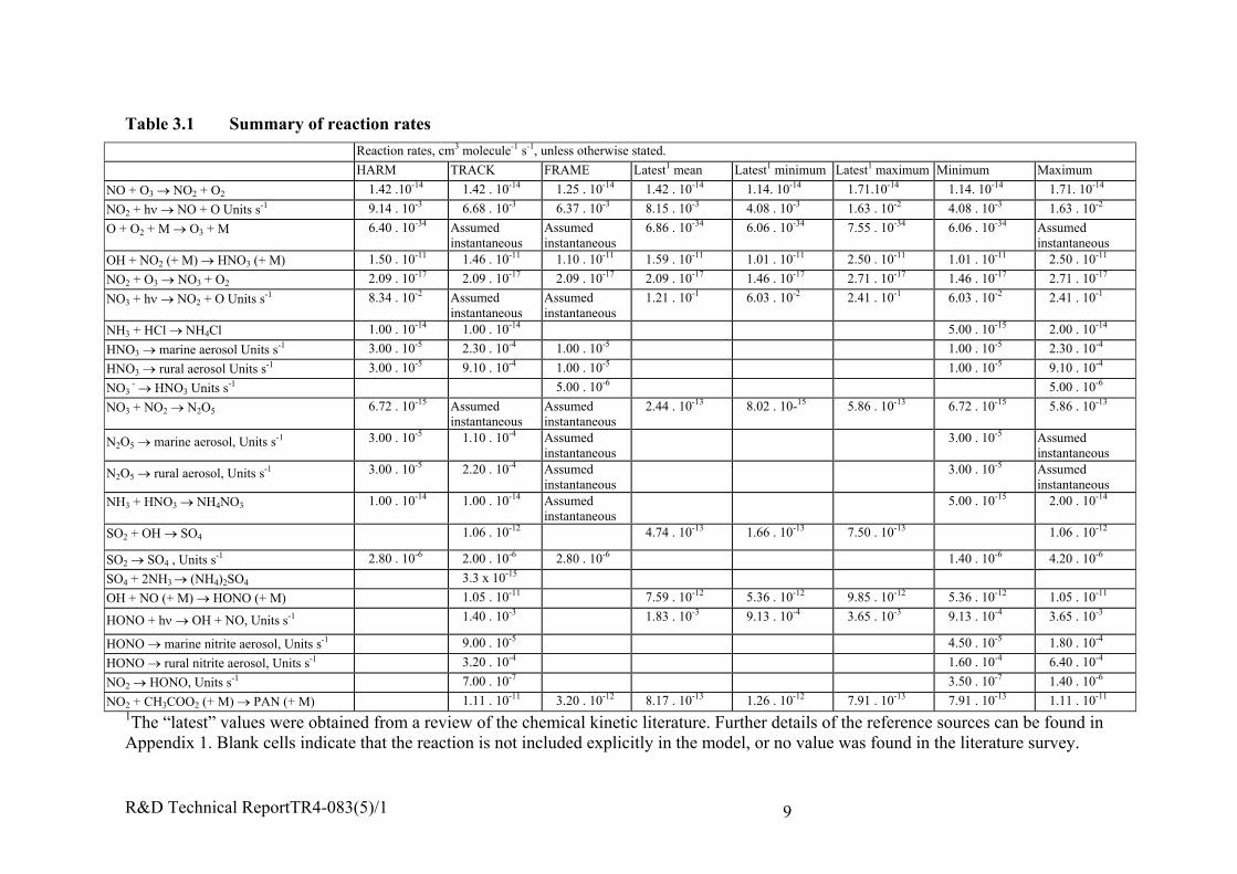
The expressions used to represent the rates of reaction of the species modelled in thethree models are summarised in Appendix 1. The expressions are compared with similarexpressions obtained from recent literature. The expressions have been evaluated fortypical parameters (temperature 283 K, zenith angle 300): the calculated reaction ratesare summarised in Table 3.1. Reaction rate expressions for some reactions in recentliterature have included uncertainty estimates. Table 3.1 includes an assessment of therange of values. The ranges are expressed in terms of the maximum and minimumvalues: these may have been estimated as (1) the mean plus and minus two standarddeviations, (2) the upper and lower bounds of measured values, or (3) best estimatesdepending on the quality of the data. The aim of Table 3.1 is to provide working rangesfor further analysis.
The reactions schemes included within each of the models are incomplete. Many otherpossible reactions are possible between the modelled chemical species and othersubstances in the atmosphere. In some cases, the model reaction schemes represent acomplex chain of reactions by a single reaction. The reaction schemes included in themodels have been selected on the basis of theoretical considerations and practicality.As a subset of the full chemistry they are therefore only representative of main reactiveprocesses and should not be taken to be an exact simulation of atmospheric reactions.The investigation of uncertainties has considered the reaction schemes included withinthe models and has not considered the effects of alternative reaction schemes on thepredicted rates of deposition.
R&D Technical ReportTR4-083(5)/1 9
Table 3.1 Summary of reaction ratesReaction rates, cm3 molecule-1 s-1, unless otherwise stated.HARM TRACK FRAME Latest1 mean Latest1 minimum Latest1 maximum Minimum Maximum
NO + O3 → NO2 + O2 1.42 .10-14 1.42 . 10-14 1.25 . 10-14 1.42 . 10-14 1.14. 10-14 1.71.10-14 1.14. 10-14 1.71. 10-14
NO2 + hν → NO + O Units s-1 9.14 . 10-3 6.68 . 10-3 6.37 . 10-3 8.15 . 10-3 4.08 . 10-3 1.63 . 10-2 4.08 . 10-3 1.63 . 10-2
O + O2 + M → O3 + M 6.40 . 10-34 Assumedinstantaneous
Assumedinstantaneous
6.86 . 10-34 6.06 . 10-34 7.55 . 10-34 6.06 . 10-34 Assumedinstantaneous
OH + NO2 (+ M) → HNO3 (+ M) 1.50 . 10-11 1.46 . 10-11 1.10 . 10-11 1.59 . 10-11 1.01 . 10-11 2.50 . 10-11 1.01 . 10-11 2.50 . 10-11
NO2 + O3 → NO3 + O2 2.09 . 10-17 2.09 . 10-17 2.09 . 10-17 2.09 . 10-17 1.46 . 10-17 2.71 . 10-17 1.46 . 10-17 2.71 . 10-17
NO3 + hν → NO2 + O Units s-1 8.34 . 10-2 Assumedinstantaneous
Assumedinstantaneous
1.21 . 10-1 6.03 . 10-2 2.41 . 10-1 6.03 . 10-2 2.41 . 10-1
NH3 + HCl → NH4Cl 1.00 . 10-14 1.00 . 10-14 5.00 . 10-15 2.00 . 10-14
HNO3 → marine aerosol Units s-1 3.00 . 10-5 2.30 . 10-4 1.00 . 10-5 1.00 . 10-5 2.30 . 10-4
HNO3 → rural aerosol Units s-1 3.00 . 10-5 9.10 . 10-4 1.00 . 10-5 1.00 . 10-5 9.10 . 10-4
NO3 - → HNO3 Units s-1 5.00 . 10-6 5.00 . 10-6
NO3 + NO2 → N2O5 6.72 . 10-15 Assumedinstantaneous
Assumedinstantaneous
2.44 . 10-13 8.02 . 10-15 5.86 . 10-13 6.72 . 10-15 5.86 . 10-13
N2O5 → marine aerosol, Units s-1 3.00 . 10-5 1.10 . 10-4 Assumedinstantaneous
3.00 . 10-5 Assumedinstantaneous
N2O5 → rural aerosol, Units s-1 3.00 . 10-5 2.20 . 10-4 Assumedinstantaneous
3.00 . 10-5 Assumedinstantaneous
NH3 + HNO3 → NH4NO3 1.00 . 10-14 1.00 . 10-14 Assumedinstantaneous
5.00 . 10-15 2.00 . 10-14
SO2 + OH → SO4 1.06 . 10-12 4.74 . 10-13 1.66 . 10-13 7.50 . 10-13 1.06 . 10-12
SO2 → SO4 , Units s-1 2.80 . 10-6 2.00 . 10-6 2.80 . 10-6 1.40 . 10-6 4.20 . 10-6
SO4 + 2NH3 → (NH4)2SO4 3.3 x 10⁻¹⁵
OH + NO (+ M) → HONO (+ M) 1.05 . 10-11 7.59 . 10-12 5.36 . 10-12 9.85 . 10-12 5.36 . 10-12 1.05 . 10-11
HONO + hν → OH + NO, Units s-1 1.40 . 10-3 1.83 . 10-3 9.13 . 10-4 3.65 . 10-3 9.13 . 10-4 3.65 . 10-3
HONO → marine nitrite aerosol, Units s-1 9.00 . 10-5 4.50 . 10-5 1.80 . 10-4
HONO → rural nitrite aerosol, Units s-1 3.20 . 10-4 1.60 . 10-4 6.40 . 10-4
NO2 → HONO, Units s-1 7.00 . 10-7 3.50 . 10-7 1.40 . 10-6
NO2 + CH3COO2 (+ M) → PAN (+ M) 1.11 . 10-11 3.20 . 10-12 8.17 . 10-13 1.26 . 10-12 7.91 . 10-13 7.91 . 10-13 1.11 . 10-11
1The “latest” values were obtained from a review of the chemical kinetic literature. Further details of the reference sources can be found inAppendix 1. Blank cells indicate that the reaction is not included explicitly in the model, or no value was found in the literature survey.
R&D Technical ReportTR4-083(5)/1 10
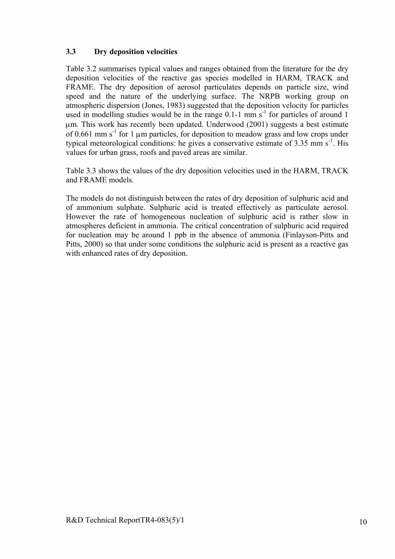
3.3 Dry deposition velocities
Table 3.2 summarises typical values and ranges obtained from the literature for the drydeposition velocities of the reactive gas species modelled in HARM, TRACK andFRAME. The dry deposition of aerosol particulates depends on particle size, windspeed and the nature of the underlying surface. The NRPB working group onatmospheric dispersion (Jones, 1983) suggested that the deposition velocity for particlesused in modelling studies would be in the range 0.1-1 mm s-1 for particles of around 1µm. This work has recently been updated. Underwood (2001) suggests a best estimateof 0.661 mm s-1 for 1 µm particles, for deposition to meadow grass and low crops undertypical meteorological conditions: he gives a conservative estimate of 3.35 mm s-1. Hisvalues for urban grass, roofs and paved areas are similar.
Table 3.3 shows the values of the dry deposition velocities used in the HARM, TRACKand FRAME models.
The models do not distinguish between the rates of dry deposition of sulphuric acid andof ammonium sulphate. Sulphuric acid is treated effectively as particulate aerosol.However the rate of homogeneous nucleation of sulphuric acid is rather slow inatmospheres deficient in ammonia. The critical concentration of sulphuric acid requiredfor nucleation may be around 1 ppb in the absence of ammonia (Finlayson-Pitts andPitts, 2000) so that under some conditions the sulphuric acid is present as a reactive gaswith enhanced rates of dry deposition.

R&D Technical ReportTR4-083(5)/1 11
Table 3.2 Dry deposition velocitiesSPECIES ACID GRASSLAND CALCAREOUS
GRASSLANDHEATHLAND CONIFEROUS
WOODLANDDECIDUOUSWOODLAND
SO2
12±3mms-1 1 8±4 mms-1 1 2±1mms-1 2
7.2±6.5mms-1 310.1mms-1 (Day) 4
6-7.2mms-1 (Seasonal)4
5-11mms-1 5
3-13mms-1 6
6.9-19.2mms-1 26
NO2
1.1-2.4mms-1 7 1mms-1 8 1.5±1.3mms-1 9
1.4±1.1mms-1 9
1-2mms-1 10
HNO3
17-35mms-1 11
25±9mms-1 2776mms-1 12
[10-135mms-1 13,14]6-34mms-1 15
20-100mms-1 16
22-60mms-1 17
NH3
15-20mms-1 18 (pH=3.9) 1-11mms-1 18 19mms-1 19
8.3mms-1 20
11.7mms-1 21
20-30mms-1 22
66mms-1 18
32mms-1 23,24
14-200mms-1 25
References:1. Erisman et al. (1993), Atmos. Environ. 27, 1153-1161 14. Goulding (1998), New Phyt. 139, 49-582. Galbally (1979), Nature 280, 49-50 15. Hanson and Garten (1992), New Phtol. 122, 329-3373. Lorenz and Murphy (1985), Atmos. Environ. 19, 797-802 16. Hanson and Lindberg (1991), Atmos. Environ. 25A, 1615-16344. Finkelstein et al. (2000), J. Geophys. Res. 105, 15365-15377 17. Meyers et al. (1989), B.-Layer Meteorol. 49, 395-4105. Meyers and Baldocchi (1988), Tellus 40B, 270-284 18. Sutton et al. (1993), Q.J.Roy. Met. Soc. 119, 1023-10456. Baldocchi (1988), Atmos. Environ. 22, 869-884 19. Duyzer (1994), J. Geophys. Res. 99, 18757-187637. Hesterberg et al. (1996), Environ. Pollut. 91, 21-34 20. Hansen (1999), Water Air Soil Pollut. 113, 357-3708. Coe and Gallagher (1992), Q. J. Roy. Met. Soc. 118, 767-786 21. Flechard and Fowler (1998), Q.J.Roy. Met. Soc. 124, 759-7919. Rondón et al. (1993), J. Geophys. Res. 98, 5159-5172 22. Duyzer et al. (1994), Atmos. Environ. 28, 1241-125310. Johansson (1987), Tellus 39B, 426-438 23. Duyzer et al. (1992), Environ. Pollut. 75, 3-1311. Müller et al. (1993), Tellus 45B, 346-367 24. Wyers et al. (1992), Environ. Pollut. 75, 25-2812. Sievering et al. (2001), Atmos. Environ. 35, 3851-3859 25. Andersen et al. (1993), Atmos. Environ. 27A, 189-20213. Anderson and Hovmand (1995), Water Air Soil Pollut. 85, 2211-2216 26. Matt et al. (1987), Water Air Soil Pollut. 36, 331-34727. Huebert and Robert (1985) J. Geophys. Res. 90, 2085-209
R&D Technical ReportTR4-083(5)/1 12
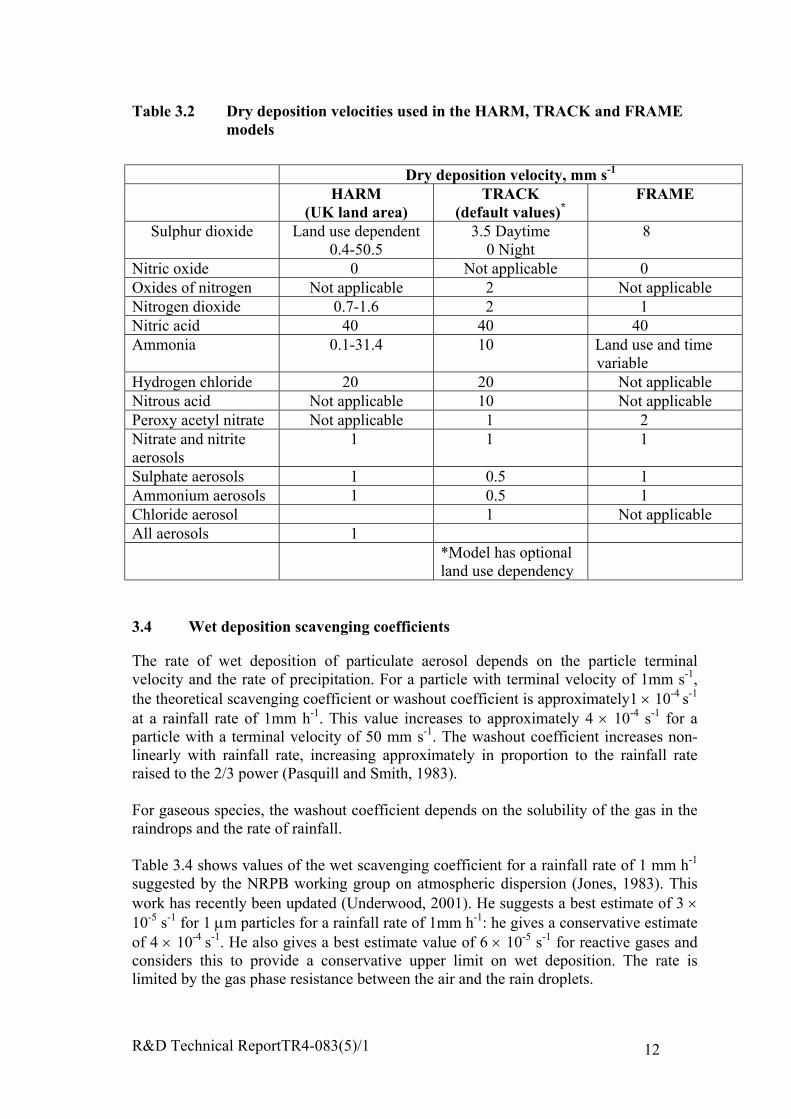
Table 3.2 Dry deposition velocities used in the HARM, TRACK and FRAMEmodels
Dry deposition velocity, mm s-1
HARM(UK land area)
TRACK(default values)*
FRAME
Sulphur dioxide Land use dependent0.4-50.5
3.5 Daytime0 Night
8
Nitric oxide 0 Not applicable 0Oxides of nitrogen Not applicable 2 Not applicableNitrogen dioxide 0.7-1.6 2 1Nitric acid 40 40 40Ammonia 0.1-31.4 10 Land use and time
variableHydrogen chloride 20 20 Not applicableNitrous acid Not applicable 10 Not applicablePeroxy acetyl nitrate Not applicable 1 2Nitrate and nitriteaerosols
1 1 1
Sulphate aerosols 1 0.5 1Ammonium aerosols 1 0.5 1Chloride aerosol 1 Not applicableAll aerosols 1
*Model has optionalland use dependency
3.4 Wet deposition scavenging coefficients
The rate of wet deposition of particulate aerosol depends on the particle terminalvelocity and the rate of precipitation. For a particle with terminal velocity of 1mm s-1,the theoretical scavenging coefficient or washout coefficient is approximately1 × 10-4 s-1
at a rainfall rate of 1mm h-1. This value increases to approximately 4 × 10⁻⁴ s-1 for aparticle with a terminal velocity of 50 mm s-1. The washout coefficient increases non-linearly with rainfall rate, increasing approximately in proportion to the rainfall rateraised to the 2/3 power (Pasquill and Smith, 1983).
For gaseous species, the washout coefficient depends on the solubility of the gas in theraindrops and the rate of rainfall.
Table 3.4 shows values of the wet scavenging coefficient for a rainfall rate of 1 mm h-1
suggested by the NRPB working group on atmospheric dispersion (Jones, 1983). Thiswork has recently been updated (Underwood, 2001). He suggests a best estimate of 3 ×10⁻⁵ s-1 for 1 µm particles for a rainfall rate of 1mm h-1: he gives a conservative estimateof 4 × 10⁻⁴ s-1. He also gives a best estimate value of 6 × 10⁻⁵ s-1 for reactive gases andconsiders this to provide a conservative upper limit on wet deposition. The rate islimited by the gas phase resistance between the air and the rain droplets.
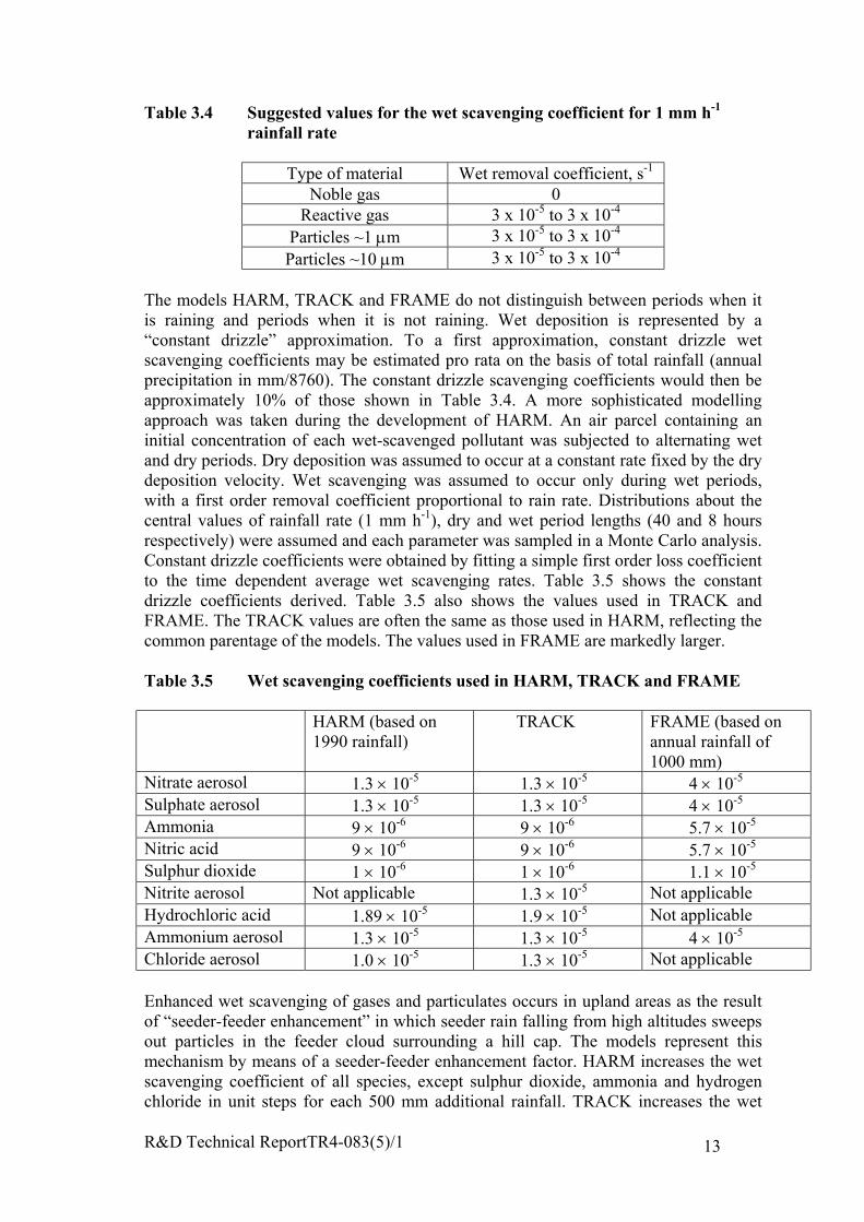
R&D Technical ReportTR4-083(5)/1 13
Table 3.4 Suggested values for the wet scavenging coefficient for 1 mm h-1
rainfall rate
Type of material Wet removal coefficient, s-1
Noble gas 0Reactive gas 3 x 10⁻⁵ to 3 x 10⁻⁴
Particles ~1 µm 3 x 10⁻⁵ to 3 x 10⁻⁴
Particles ~10 µm 3 x 10⁻⁵ to 3 x 10⁻⁴
The models HARM, TRACK and FRAME do not distinguish between periods when itis raining and periods when it is not raining. Wet deposition is represented by a“constant drizzle” approximation. To a first approximation, constant drizzle wetscavenging coefficients may be estimated pro rata on the basis of total rainfall (annualprecipitation in mm/8760). The constant drizzle scavenging coefficients would then beapproximately 10% of those shown in Table 3.4. A more sophisticated modellingapproach was taken during the development of HARM. An air parcel containing aninitial concentration of each wet-scavenged pollutant was subjected to alternating wetand dry periods. Dry deposition was assumed to occur at a constant rate fixed by the drydeposition velocity. Wet scavenging was assumed to occur only during wet periods,with a first order removal coefficient proportional to rain rate. Distributions about thecentral values of rainfall rate (1 mm h-1), dry and wet period lengths (40 and 8 hoursrespectively) were assumed and each parameter was sampled in a Monte Carlo analysis.Constant drizzle coefficients were obtained by fitting a simple first order loss coefficientto the time dependent average wet scavenging rates. Table 3.5 shows the constantdrizzle coefficients derived. Table 3.5 also shows the values used in TRACK andFRAME. The TRACK values are often the same as those used in HARM, reflecting thecommon parentage of the models. The values used in FRAME are markedly larger.
Table 3.5 Wet scavenging coefficients used in HARM, TRACK and FRAME
HARM (based on1990 rainfall)
TRACK FRAME (based onannual rainfall of1000 mm)
Nitrate aerosol 1.3 × 10⁻⁵ 1.3 × 10⁻⁵ 4 × 10⁻⁵
Sulphate aerosol 1.3 × 10⁻⁵ 1.3 × 10⁻⁵ 4 × 10⁻⁵
Ammonia 9 × 10⁻⁶ 9 × 10⁻⁶ 5.7 × 10⁻⁵
Nitric acid 9 × 10⁻⁶ 9 × 10⁻⁶ 5.7 × 10⁻⁵
Sulphur dioxide 1 × 10⁻⁶ 1 × 10⁻⁶ 1.1 × 10⁻⁵
Nitrite aerosol Not applicable 1.3 × 10⁻⁵ Not applicableHydrochloric acid 1.89 × 10⁻⁵ 1.9 × 10⁻⁵ Not applicableAmmonium aerosol 1.3 × 10⁻⁵ 1.3 × 10⁻⁵ 4 × 10⁻⁵
Chloride aerosol 1.0 × 10⁻⁵ 1.3 × 10⁻⁵ Not applicable
Enhanced wet scavenging of gases and particulates occurs in upland areas as the resultof “seeder-feeder enhancement” in which seeder rain falling from high altitudes sweepsout particles in the feeder cloud surrounding a hill cap. The models represent thismechanism by means of a seeder-feeder enhancement factor. HARM increases the wetscavenging coefficient of all species, except sulphur dioxide, ammonia and hydrogenchloride in unit steps for each 500 mm additional rainfall. TRACK increases the wet
R&D Technical ReportTR4-083(5)/1 14
scavenging coefficient of aerosols by a factor of 1 to 3 when the annual rainfall exceedstypically 800 mm. It also has a more sophisticated direction dependent enhancementoption. The rate of sulphur dioxide oxidation is also increased in upland areas in HARMand TRACK. HARM increases the reaction rate in unit steps for each 250mm additionalrainfall. TRACK increases the rate of oxidation by a factor of typically 1.3.
3.5 Background concentrations
The models include an assumption about the initial concentration of ozone. HARMassumes that there is an initial concentration of 30 ppb at the start of the trajectory andthat the ozone is depleted by the reactions that take place. TRACK assumes an initialconcentration of 34 ppb and that ozone depleted by reaction is regenerated with theconcentration being maintained in dynamic equilibrium controlled by an effective drydeposition velocity of 6 mm s-1. FRAME assumes a constant ozone concentration of 30ppb across the model domain.
TRACK also includes reactions involving hydroxyl, nitrate and acetyl peroxy radicals.The concentration fields are taken from the output of a global 3-D model of thetroposphere, STOCHEM. The model can also use invariant radical fields. Defaultvalues are:
OH 1.6 × 10⁶ molecules cm3 (day only);CH3COO2 1.6 × 10⁶ molecules cm3 (day only);NO3 2.5 × 10⁷ molecules cm3 (night only).
3.6 Wind speed
All three models assume a constant geostrophic wind speed that is independent oflocation. HARM and TRACK assume that the wind speed is independent of winddirection. FRAME uses a direction-dependent wind speed. The wind speeds used are:
HARM 10.4 m s-1
TRACK 7.5 m s-1
FRAME 5.62-8.61 m s-1 (direction dependent)
All three models refer to Jones (1981) as the source of the wind speed data used in thederivation of the average wind speed. Table 3.6 shows the source data presented bySingles (1996, p103).
The arithmetic mean of this data is 10.4 m s-1 as used in HARM. Singles (1996) carriedout model runs using the FRAME model for each wind speed/direction class and thencalculated an optimised single value wind speed, for each wind direction, that bestreproduced the combined model predictions for ammonia deposition andconcentrations. The optimised wind speed was direction dependent and was in the range5.62-8.61 m s-1. In earlier work related to the development of the HARM modelDerwent, Dollard and Metcalfe (1988) used the mid-point of the modal wind speedrange (7.5 m s-1).
R&D Technical ReportTR4-083(5)/1 15
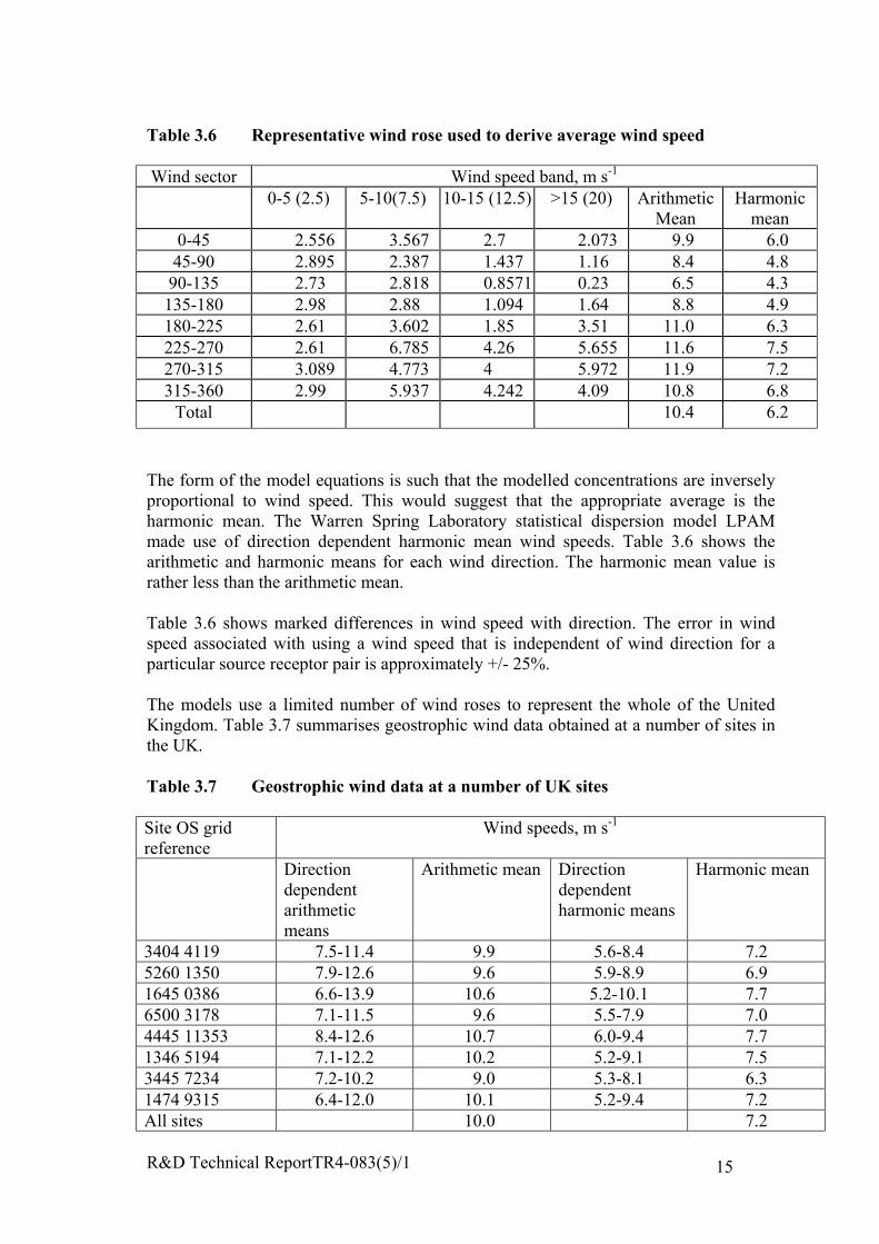
Table 3.6 Representative wind rose used to derive average wind speed
Wind sector Wind speed band, m s-1
0-5 (2.5) 5-10(7.5) 10-15 (12.5) >15 (20) ArithmeticMean
Harmonicmean
0-45 2.556 3.567 2.7 2.073 9.9 6.045-90 2.895 2.387 1.437 1.16 8.4 4.890-135 2.73 2.818 0.8571 0.23 6.5 4.3135-180 2.98 2.88 1.094 1.64 8.8 4.9180-225 2.61 3.602 1.85 3.51 11.0 6.3225-270 2.61 6.785 4.26 5.655 11.6 7.5270-315 3.089 4.773 4 5.972 11.9 7.2315-360 2.99 5.937 4.242 4.09 10.8 6.8
Total 10.4 6.2
The form of the model equations is such that the modelled concentrations are inverselyproportional to wind speed. This would suggest that the appropriate average is theharmonic mean. The Warren Spring Laboratory statistical dispersion model LPAMmade use of direction dependent harmonic mean wind speeds. Table 3.6 shows thearithmetic and harmonic means for each wind direction. The harmonic mean value israther less than the arithmetic mean.
Table 3.6 shows marked differences in wind speed with direction. The error in windspeed associated with using a wind speed that is independent of wind direction for aparticular source receptor pair is approximately +/- 25%.
The models use a limited number of wind roses to represent the whole of the UnitedKingdom. Table 3.7 summarises geostrophic wind data obtained at a number of sites inthe UK.
Table 3.7 Geostrophic wind data at a number of UK sites
Site OS gridreference
Wind speeds, m s-1
Directiondependentarithmeticmeans
Arithmetic mean Directiondependentharmonic means
Harmonic mean
3404 4119 7.5-11.4 9.9 5.6-8.4 7.25260 1350 7.9-12.6 9.6 5.9-8.9 6.91645 0386 6.6-13.9 10.6 5.2-10.1 7.76500 3178 7.1-11.5 9.6 5.5-7.9 7.04445 11353 8.4-12.6 10.7 6.0-9.4 7.71346 5194 7.1-12.2 10.2 5.2-9.1 7.53445 7234 7.2-10.2 9.0 5.3-8.1 6.31474 9315 6.4-12.0 10.1 5.2-9.4 7.2All sites 10.0 7.2
R&D Technical ReportTR4-083(5)/1 16
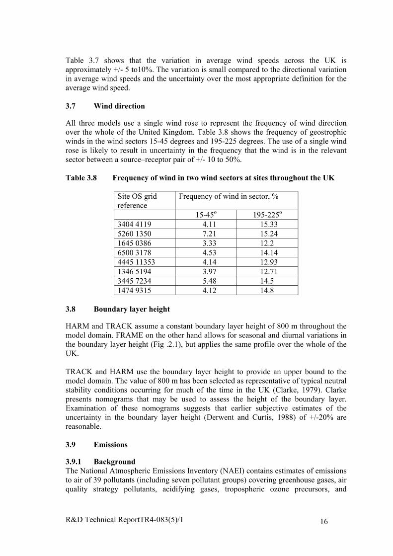
Table 3.7 shows that the variation in average wind speeds across the UK isapproximately +/- 5 to10%. The variation is small compared to the directional variationin average wind speeds and the uncertainty over the most appropriate definition for theaverage wind speed.
3.7 Wind direction
All three models use a single wind rose to represent the frequency of wind directionover the whole of the United Kingdom. Table 3.8 shows the frequency of geostrophicwinds in the wind sectors 15-45 degrees and 195-225 degrees. The use of a single windrose is likely to result in uncertainty in the frequency that the wind is in the relevantsector between a source–receptor pair of +/- 10 to 50%.
Table 3.8 Frequency of wind in two wind sectors at sites throughout the UK
Site OS gridreference
Frequency of wind in sector, %
15-45o 195-225o
3404 4119 4.11 15.335260 1350 7.21 15.241645 0386 3.33 12.26500 3178 4.53 14.144445 11353 4.14 12.931346 5194 3.97 12.713445 7234 5.48 14.51474 9315 4.12 14.8
3.8 Boundary layer height
HARM and TRACK assume a constant boundary layer height of 800 m throughout themodel domain. FRAME on the other hand allows for seasonal and diurnal variations inthe boundary layer height (Fig .2.1), but applies the same profile over the whole of theUK.
TRACK and HARM use the boundary layer height to provide an upper bound to themodel domain. The value of 800 m has been selected as representative of typical neutralstability conditions occurring for much of the time in the UK (Clarke, 1979). Clarkepresents nomograms that may be used to assess the height of the boundary layer.Examination of these nomograms suggests that earlier subjective estimates of theuncertainty in the boundary layer height (Derwent and Curtis, 1988) of +/-20% arereasonable.
3.9 Emissions
3.9.1 BackgroundThe National Atmospheric Emissions Inventory (NAEI) contains estimates of emissionsto air of 39 pollutants (including seven pollutant groups) covering greenhouse gases, airquality strategy pollutants, acidifying gases, tropospheric ozone precursors, and

R&D Technical ReportTR4-083(5)/1 17
hazardous air pollutants. The NAEI is updated each year, with results reported in anannual report (most recently in Goodwin et al, 2001).
Each annual report includes expert judgements of uncertainty in the national emissiontotal for each pollutant. These are intended as ‘ball-park’ estimates of the overalluncertainty in each inventory and are made by the NAEI team member responsible forcompilation of that inventory.
With limited exceptions, these ‘ball-park’ estimates have not changed in recent years,giving the impression that the NAEI has not improved in that period despite theconsiderable research into emission factors carried out. In reality, the inventory is morecomplete, detailed and accurate now than in the past; it is more useful and nationalemission totals are more likely to be accurate. The problem lies in the presentation ofuncertainty, since the current expression of uncertainty is simplistic and lacks rigour inits use of quasi-statistical terminology, and so it is not capable of reflectingimprovement.
As part of the programme of work to maintain the NAEI, a more detailed assessmenthas been made of the uncertainty in the NAEI using software better able to manipulateand display statistical information. This detailed approach provides a more quantitativemeasure of uncertainty.
3.9.2 MethodsQuantitative estimates of the uncertainties in the NAEI have been calculated using adirect simulation approach. This procedure corresponds to the IPCC Tier 2 approachdiscussed in the Good Practice Guidance (IPCC, 2000), as well as the Tier 2 methodproposed in the draft ‘Good Practice Guidance for CLRTAP Emission Inventories’,produced for inclusion in the EMEP/CORINAIR Guidebook on Emission Inventories.The approach, as applied to the UK greenhouse gas inventory, has also been describedin detail by Charles et al (1998).
A brief summary of the method is given below.1. An uncertainty distribution is allocated to each emission factor and each activity
rate. The distributions used were drawn from a limited set of either uniform, normal,triangular, beta, or log-normal distributions. The parameters of the distributions foreach emission factor or activity rate were set either by analysing the available dataon emission factors and activity data, or by expert judgement.
2. A calculation was set up to estimate the emission of each pollutant by samplingindividual data values from each of the emission factor and activity ratedistributions on the basis of probability density and evaluating the resultingemission. Using the software tool @RISK™, this process could be repeated manytimes in order to build up an output distribution of emission estimates, both forindividual sources but also for total UK emissions of each pollutant.
3. The mean value for each emission estimate and the national total was recorded, aswell as the standard deviation and the 95% confidence limits i.e. the emission valuesat the 2.5% cumulative probability and the 97.5% cumulative probability.
4. The process was carried out first using data for 1999, taken from the 1999 version ofthe NAEI (published in Goodwin et al, 2001). The analysis was then extended todata for the year 2000, taken from the 2000 version of the NAEI (report inpreparation) for those pollutants where changes had been made to the methodology
R&D Technical ReportTR4-083(5)/1 18
used to estimate emissions. For this repeat of the analysis it was necessary to re-evaluate the probability distributions used for emission factors and activity rates andmake modifications to the assumptions where appropriate.
5. A key source analysis was undertaken, following the IPCC Tier 2 method (IPCC,2000). The key source analysis identifies the major contributors to inventoryuncertainty.
The method was applied to the known sources of emissions that have been included inthe NAEI: other sources of emission may also contribute to the overall uncertainty inthe emissions estimates, but the contribution has not been quantified.
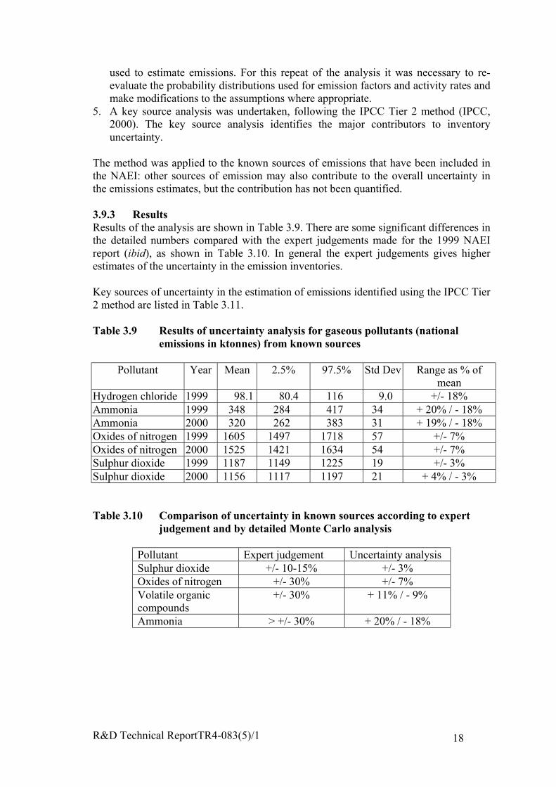
3.9.3 ResultsResults of the analysis are shown in Table 3.9. There are some significant differences inthe detailed numbers compared with the expert judgements made for the 1999 NAEIreport (ibid), as shown in Table 3.10. In general the expert judgements gives higherestimates of the uncertainty in the emission inventories.
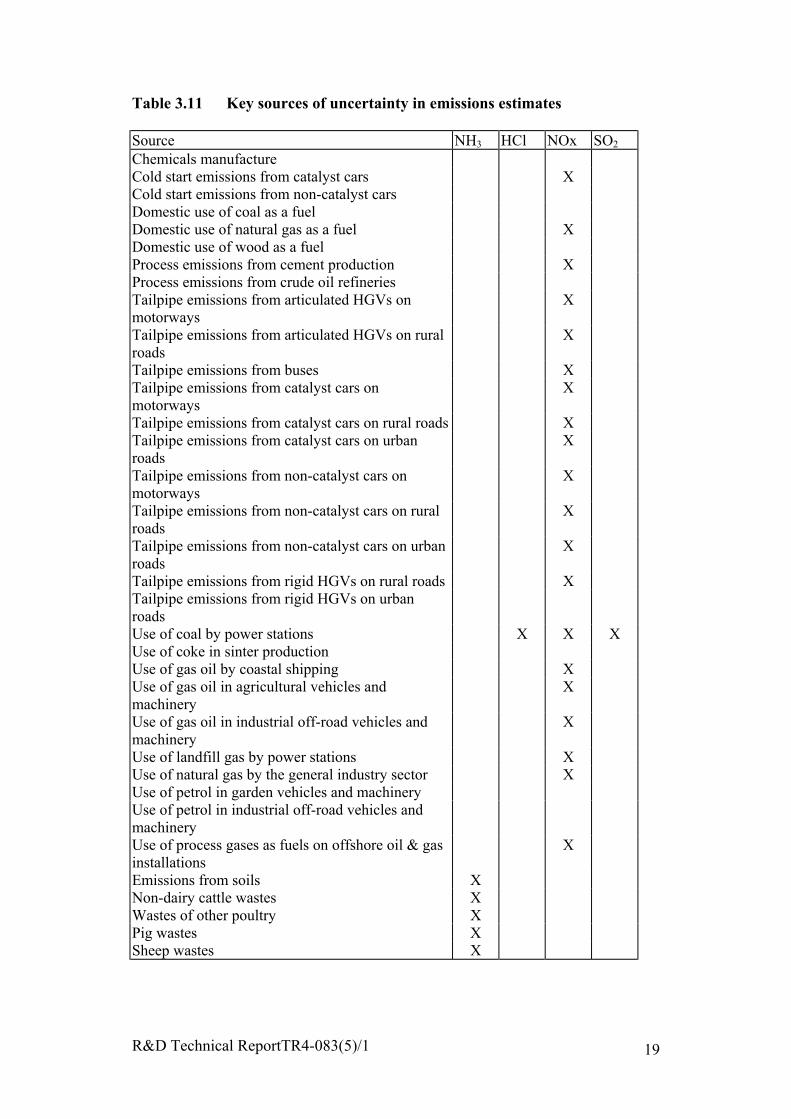
Key sources of uncertainty in the estimation of emissions identified using the IPCC Tier2 method are listed in Table 3.11.
Table 3.9 Results of uncertainty analysis for gaseous pollutants (nationalemissions in ktonnes) from known sources
Pollutant Year Mean 2.5% 97.5% Std Dev Range as % ofmean
Hydrogen chloride 1999 98.1 80.4 116 9.0 +/- 18%Ammonia 1999 348 284 417 34 + 20% / - 18%Ammonia 2000 320 262 383 31 + 19% / - 18%Oxides of nitrogen 1999 1605 1497 1718 57 +/- 7%Oxides of nitrogen 2000 1525 1421 1634 54 +/- 7%Sulphur dioxide 1999 1187 1149 1225 19 +/- 3%Sulphur dioxide 2000 1156 1117 1197 21 + 4% / - 3%
Table 3.10 Comparison of uncertainty in known sources according to expertjudgement and by detailed Monte Carlo analysis
Pollutant Expert judgement Uncertainty analysisSulphur dioxide +/- 10-15% +/- 3%Oxides of nitrogen +/- 30% +/- 7%Volatile organiccompounds
+/- 30% + 11% / - 9%
Ammonia > +/- 30% + 20% / - 18%
R&D Technical ReportTR4-083(5)/1 19
Table 3.11 Key sources of uncertainty in emissions estimates
Source NH3 HCl NOx SO2
Chemicals manufactureCold start emissions from catalyst cars XCold start emissions from non-catalyst carsDomestic use of coal as a fuelDomestic use of natural gas as a fuel XDomestic use of wood as a fuelProcess emissions from cement production XProcess emissions from crude oil refineriesTailpipe emissions from articulated HGVs onmotorways
X
Tailpipe emissions from articulated HGVs on ruralroads
X
Tailpipe emissions from buses XTailpipe emissions from catalyst cars onmotorways
X
Tailpipe emissions from catalyst cars on rural roads XTailpipe emissions from catalyst cars on urbanroads
X
Tailpipe emissions from non-catalyst cars onmotorways
X
Tailpipe emissions from non-catalyst cars on ruralroads
X
Tailpipe emissions from non-catalyst cars on urbanroads
X
Tailpipe emissions from rigid HGVs on rural roads XTailpipe emissions from rigid HGVs on urbanroadsUse of coal by power stations X X XUse of coke in sinter productionUse of gas oil by coastal shipping XUse of gas oil in agricultural vehicles andmachinery
X
Use of gas oil in industrial off-road vehicles andmachinery
X
Use of landfill gas by power stations XUse of natural gas by the general industry sector XUse of petrol in garden vehicles and machineryUse of petrol in industrial off-road vehicles andmachineryUse of process gases as fuels on offshore oil & gasinstallations
X
Emissions from soils XNon-dairy cattle wastes XWastes of other poultry XPig wastes XSheep wastes X
R&D Technical ReportTR4-083(5)/1 20
3.10 Speciation of emissions
The emissions of sulphur from large sources such as power stations are mostly in theform of sulphur dioxide. However, a small part is released as sulphur trioxide, sulphatesor as sulphuric acid. The US EPA report AP42 indicates that approximately 0.7 % of thesulphur in the fuel in bituminous coal combustion is released as sulphur trioxide and asimilar quantity is released as particulate sulphate. For fuel oil combustion, AP42estimates that 1 to 5% is released as sulphur trioxide and a further 1 to 3% is released asparticulate sulphate. TRACK allows for a certain proportion of sulphur dioxide releasedas sulphur trioxide and gaseous and particulate sulphates.
For most fossil fuel combustion systems the major part of the oxides of nitrogenreleased is in the form of nitric oxide. AP42 indicates that the proportion of nitrogendioxide is usually less than 5%. TRACK and FRAME allow for a certain proportion ofthe release to be as nitrogen dioxide.
This systematic sensitivity analysis of the uncertainty in the national emissions leads tosome estimates, notably for sulphur and nitrogen oxides, which are substantially lowerthan those which would have been estimated by expert judgement (see Table 3.10). It isnot within this study to explore alternative methodologies, but it is recognised thatMonte Carlo analysis is not able to treat uncertainties in processes which are unknown.In addition uncertainties in individual processes are treated as independent variables.

R&D Technical ReportTR4-083(5)/1 21
4 DEPOSITION MODEL UNCERTAINTIES
4.1 Introduction
The uncertainty in the predicted deposition resulting from the uncertainty in the inputparameters has been assessed for each of the models in turn. Initial studies were madeusing the analytical models described in Appendices 2 and 3. The initial studies werecarried out to help identify the most important parameters affecting model outputs andto assist in the development of data handling methods. Further investigation was thencarried out using the numerical models TRACK, HARM and FRAME.
The general approach taken in the investigation was to use the models to predict rates ofdeposition for various combinations of input parameter values selected from theplausible range of values identified in Section 3. Three alternative sampling strategieswere employed:
1. Monte Carlo simulation in which the values of all the input parameters wereselected at random from their plausible ranges;
2. First order error analysis in which the input parameters were changed one at a timefrom the baseline value;
3. Sampling based on a Latin Square.
The alternative sampling strategies have been compared.
The sampling strategies employed assume that the input parameters may be sampledindependently of each other. Consideration was given to whether the input parametersmight be strongly correlated. Some parameters (the dry deposition velocities andwashout coefficients of the various aerosol species) were considered likely to bestrongly correlated and were not sampled independently. The remaining parameters maybe correlated slightly, but the effects have not been taken into account.
There are many ways of expressing the uncertainty in model results. The approach takenhere has been to determine the arithmetic mean, and the 5th and 95th percentile values, torepresent the working value and upper and lower bounds for the predicted rates ofdeposition. The data has also been presented in terms of cumulative probabilitydistributions: the cumulative probability distribution is compared with that for anidealised log-normal distribution. (The log-normal distribution was selectedempirically-see Section 4.2.3, for example).
Acid deposition models may be used to predict both the total rates of deposition from allsources and the incremental rate of deposition from a particular source, for example anindividual power station. The uncertainty in both these types of prediction has beenaddressed. The general approach taken was to carry out model runs for the baseline casefirst (i.e. in the absence of the particular source) and then to repeat the model runs withthe additional source for identical sets of input parameters. The effects of linearity of theacid deposition models with respect to the rate of emission of pollutants wereinvestigated by carrying out two sets of model runs with different rates of emissionfrom the additional source.
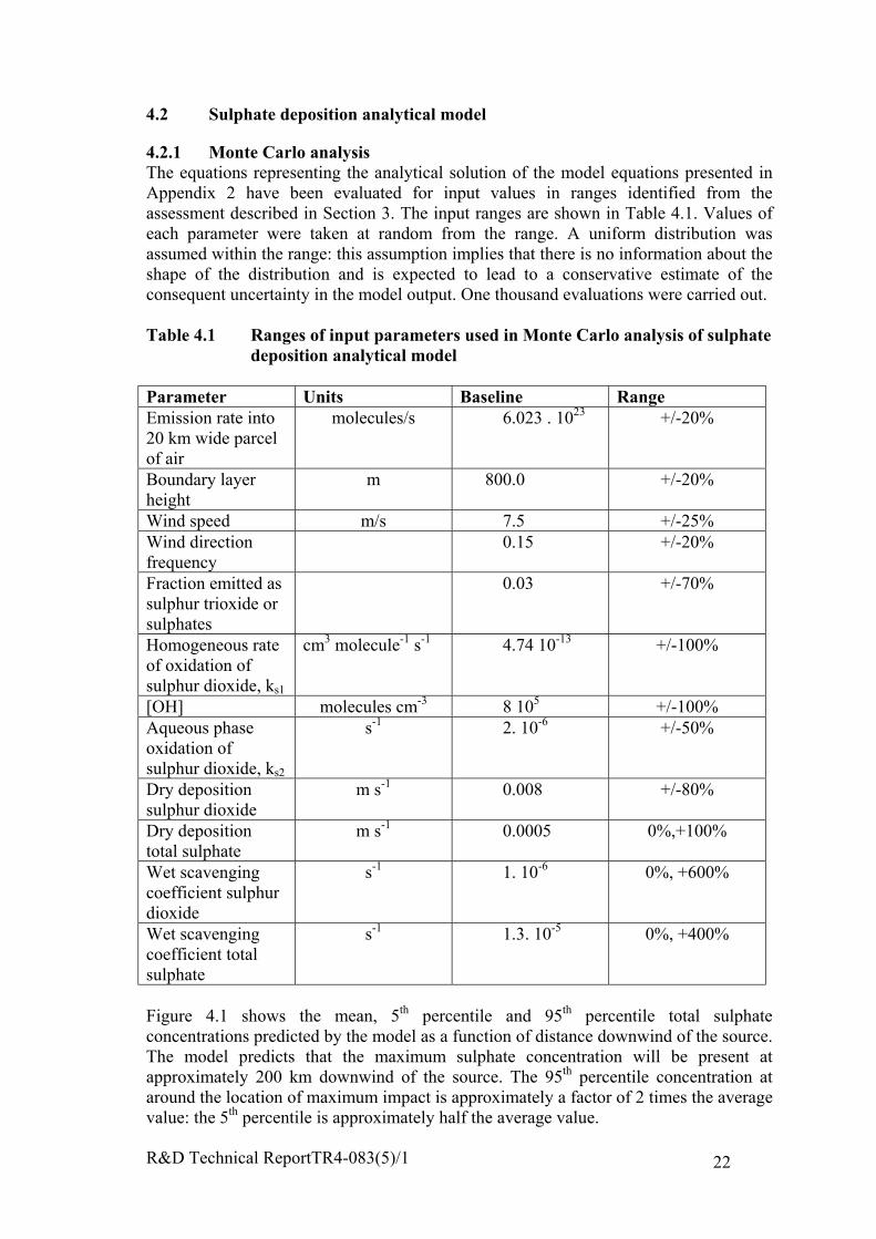
R&D Technical ReportTR4-083(5)/1 22
4.2 Sulphate deposition analytical model
4.2.1 Monte Carlo analysisThe equations representing the analytical solution of the model equations presented inAppendix 2 have been evaluated for input values in ranges identified from theassessment described in Section 3. The input ranges are shown in Table 4.1. Values ofeach parameter were taken at random from the range. A uniform distribution wasassumed within the range: this assumption implies that there is no information about theshape of the distribution and is expected to lead to a conservative estimate of theconsequent uncertainty in the model output. One thousand evaluations were carried out.
Table 4.1 Ranges of input parameters used in Monte Carlo analysis of sulphatedeposition analytical model
Parameter Units Baseline RangeEmission rate into20 km wide parcelof air
molecules/s 6.023 . 1023 +/-20%
Boundary layerheight
m 800.0 +/-20%
Wind speed m/s 7.5 +/-25%Wind directionfrequency
0.15 +/-20%
Fraction emitted assulphur trioxide orsulphates
0.03 +/-70%
Homogeneous rateof oxidation ofsulphur dioxide, ks1
cm3 molecule-1 s-1 4.74 10-13 +/-100%
[OH] molecules cm-3 8 105 +/-100%Aqueous phaseoxidation ofsulphur dioxide, ks2
s-1 2. 10-6 +/-50%
Dry depositionsulphur dioxide
m s-1 0.008 +/-80%
Dry depositiontotal sulphate
m s-1 0.0005 0%,+100%
Wet scavengingcoefficient sulphurdioxide
s-1 1. 10-6 0%, +600%
Wet scavengingcoefficient totalsulphate
s-1 1.3. 10-5 0%, +400%
Figure 4.1 shows the mean, 5th percentile and 95th percentile total sulphateconcentrations predicted by the model as a function of distance downwind of the source.The model predicts that the maximum sulphate concentration will be present atapproximately 200 km downwind of the source. The 95th percentile concentration ataround the location of maximum impact is approximately a factor of 2 times the averagevalue: the 5th percentile is approximately half the average value.

R&D Technical ReportTR4-083(5)/1 23
0.00E+00
1.00E+07
2.00E+07
3.00E+07
4.00E+07
5.00E+07
6.00E+07
7.00E+07
0 500 1000 1500 2000 2500 3000 3500 4000
Distance, km
Tota
l sul
phat
e co
ncet
ratio
n, m
olec
ules
/cm
3
Mean
95th percentile
5th percentile
Figure 4.1 Mean, 5th and 95th percentiles of predicted total sulphateconcentrations using the analytical model
Figure 4.2 shows the mean, 5th percentile and 95th percentile total sulphur depositionrates predicted by the model as a function of distance downwind of the source. Themodel predicts that the maximum sulphur deposition rate will be close to the source.The 95th percentile deposition rate is approximately a factor of 2 times the averagevalue: the 5th percentile is approximately half the average value.
0
1
2
3
4
5
6
7
8
9
0 500 1000 1500 2000 2500 3000 3500 4000
Distance, km
Tota
l sul
phur
dep
ositi
on ra
te, m
oles
Ha-
1 y-
1
Mean
95th percentile
5 th percentile
Figure 4.2 Mean, 5th and 95th percentiles of predicted total sulphur deposition atreceptors using the analytical model
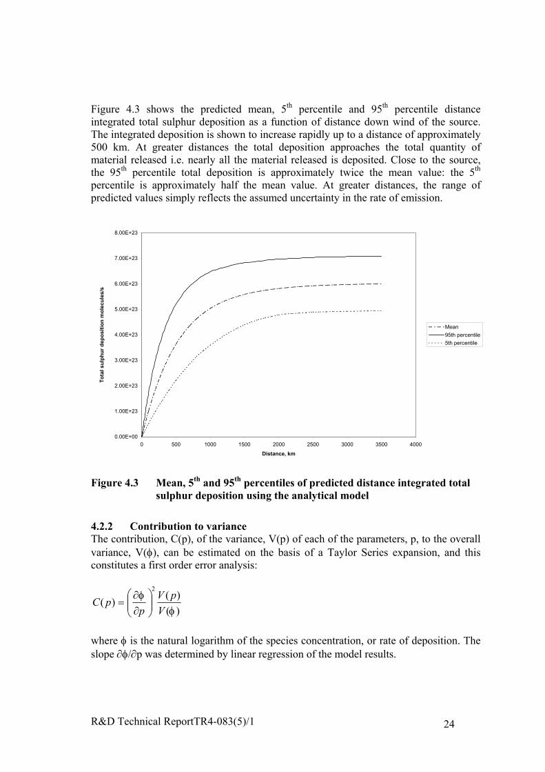
R&D Technical ReportTR4-083(5)/1 24
Figure 4.3 shows the predicted mean, 5th percentile and 95th percentile distanceintegrated total sulphur deposition as a function of distance down wind of the source.The integrated deposition is shown to increase rapidly up to a distance of approximately500 km. At greater distances the total deposition approaches the total quantity ofmaterial released i.e. nearly all the material released is deposited. Close to the source,the 95th percentile total deposition is approximately twice the mean value: the 5th
percentile is approximately half the mean value. At greater distances, the range ofpredicted values simply reflects the assumed uncertainty in the rate of emission.
0.00E+00
1.00E+23
2.00E+23
3.00E+23
4.00E+23
5.00E+23
6.00E+23
7.00E+23
8.00E+23
0 500 1000 1500 2000 2500 3000 3500 4000
Distance, km
Tota
l sul
phur
dep
ositi
on m
olec
ules
/s
Mean
95th percentile
5th percentile
Figure 4.3 Mean, 5th and 95th percentiles of predicted distance integrated totalsulphur deposition using the analytical model
4.2.2 Contribution to varianceThe contribution, C(p), of the variance, V(p) of each of the parameters, p, to the overallvariance, V(φ), can be estimated on the basis of a Taylor Series expansion, and thisconstitutes a first order error analysis:
)()()(
2
φφ
VpV
ppC
∂∂
=
where φ is the natural logarithm of the species concentration, or rate of deposition. Theslope ∂φ/∂p was determined by linear regression of the model results.
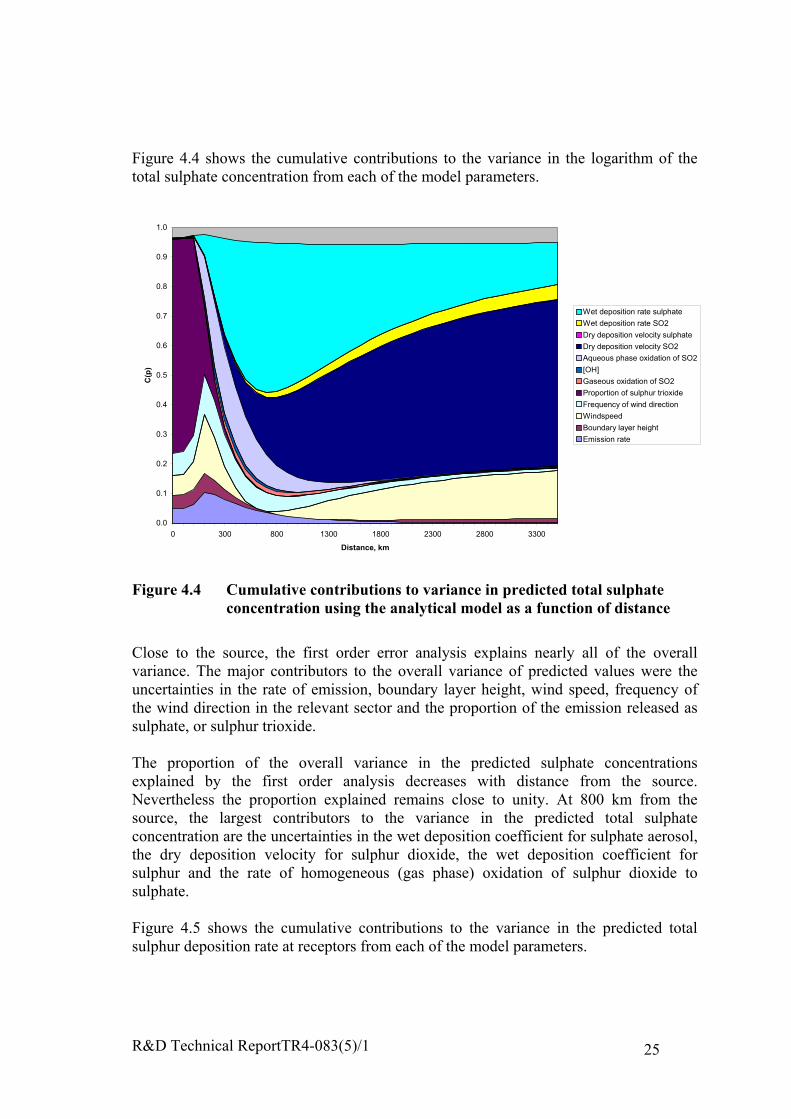
R&D Technical ReportTR4-083(5)/1 25
Figure 4.4 shows the cumulative contributions to the variance in the logarithm of thetotal sulphate concentration from each of the model parameters.
0.0
0.1
0.2
0.3
0.4
0.5
0.6
0.7
0.8
0.9
1.0
0 300 800 1300 1800 2300 2800 3300
Distance, km
C(p
)
Wet deposition rate sulphate
Wet deposition rate SO2
Dry deposition velocity sulphate
Dry deposition velocity SO2
Aqueous phase oxidation of SO2
[OH]
Gaseous oxidation of SO2
Proportion of sulphur trioxide
Frequency of wind direction
Windspeed
Boundary layer height
Emission rate
Figure 4.4 Cumulative contributions to variance in predicted total sulphateconcentration using the analytical model as a function of distance
Close to the source, the first order error analysis explains nearly all of the overallvariance. The major contributors to the overall variance of predicted values were theuncertainties in the rate of emission, boundary layer height, wind speed, frequency ofthe wind direction in the relevant sector and the proportion of the emission released assulphate, or sulphur trioxide.
The proportion of the overall variance in the predicted sulphate concentrationsexplained by the first order analysis decreases with distance from the source.Nevertheless the proportion explained remains close to unity. At 800 km from thesource, the largest contributors to the variance in the predicted total sulphateconcentration are the uncertainties in the wet deposition coefficient for sulphate aerosol,the dry deposition velocity for sulphur dioxide, the wet deposition coefficient forsulphur and the rate of homogeneous (gas phase) oxidation of sulphur dioxide tosulphate.
Figure 4.5 shows the cumulative contributions to the variance in the predicted totalsulphur deposition rate at receptors from each of the model parameters.
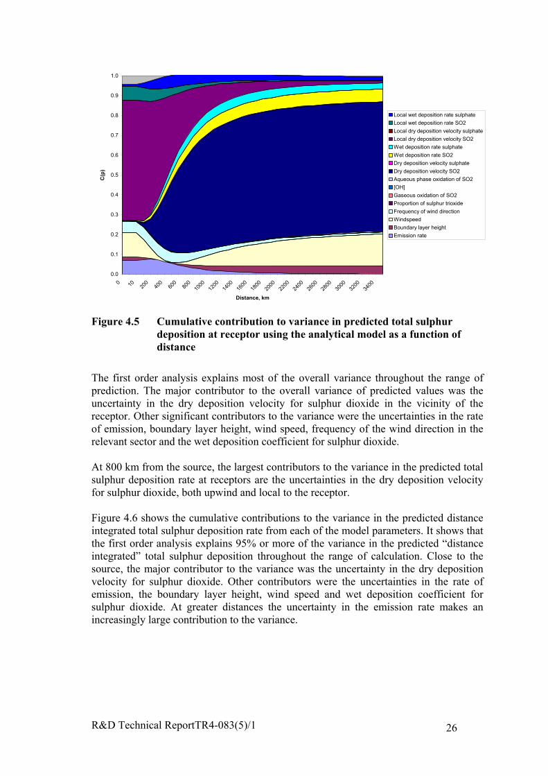
R&D Technical ReportTR4-083(5)/1 26
0.0
0.1
0.2
0.3
0.4
0.5
0.6
0.7
0.8
0.9
1.0
0 10 200
400
600
800
1000
1200
1400
1600
1800
2000
2200
2400
2600
2800
3000
3200
3400
Distance, km
C(p
)
Local wet deposition rate sulphate
Local wet deposition rate SO2
Local dry deposition velocity sulphate
Local dry deposition velocity SO2
Wet deposition rate sulphate
Wet deposition rate SO2
Dry deposition velocity sulphate
Dry deposition velocity SO2
Aqueous phase oxidation of SO2
[OH]
Gaseous oxidation of SO2
Proportion of sulphur trioxide
Frequency of wind direction
Windspeed
Boundary layer height
Emission rate
Figure 4.5 Cumulative contribution to variance in predicted total sulphurdeposition at receptor using the analytical model as a function ofdistance
The first order analysis explains most of the overall variance throughout the range ofprediction. The major contributor to the overall variance of predicted values was theuncertainty in the dry deposition velocity for sulphur dioxide in the vicinity of thereceptor. Other significant contributors to the variance were the uncertainties in the rateof emission, boundary layer height, wind speed, frequency of the wind direction in therelevant sector and the wet deposition coefficient for sulphur dioxide.
At 800 km from the source, the largest contributors to the variance in the predicted totalsulphur deposition rate at receptors are the uncertainties in the dry deposition velocityfor sulphur dioxide, both upwind and local to the receptor.
Figure 4.6 shows the cumulative contributions to the variance in the predicted distanceintegrated total sulphur deposition rate from each of the model parameters. It shows thatthe first order analysis explains 95% or more of the variance in the predicted “distanceintegrated” total sulphur deposition throughout the range of calculation. Close to thesource, the major contributor to the variance was the uncertainty in the dry depositionvelocity for sulphur dioxide. Other contributors were the uncertainties in the rate ofemission, the boundary layer height, wind speed and wet deposition coefficient forsulphur dioxide. At greater distances the uncertainty in the emission rate makes anincreasingly large contribution to the variance.
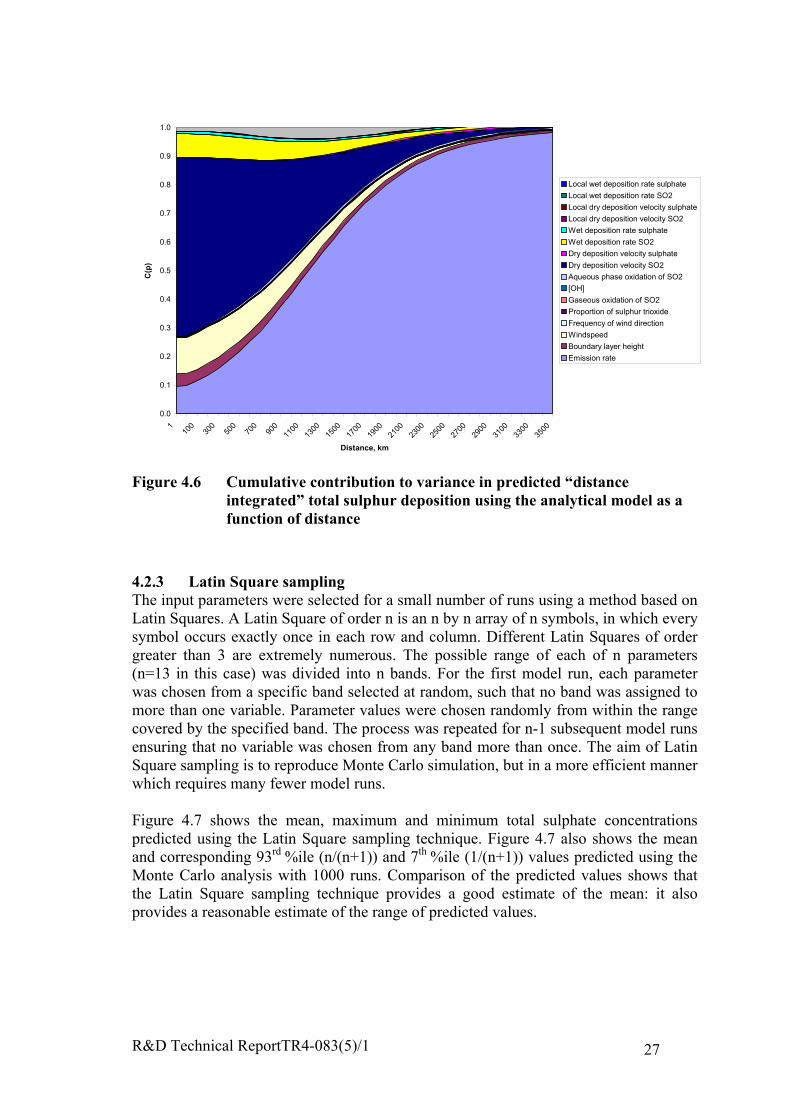
R&D Technical ReportTR4-083(5)/1 27
0.0
0.1
0.2
0.3
0.4
0.5
0.6
0.7
0.8
0.9
1.0
110
030
050
070
090
011
0013
0015
0017
0019
0021
0023
0025
0027
0029
0031
0033
0035
00
Distance, km
C(p
)
Local wet deposition rate sulphate
Local wet deposition rate SO2
Local dry deposition velocity sulphate
Local dry deposition velocity SO2
Wet deposition rate sulphate
Wet deposition rate SO2
Dry deposition velocity sulphate
Dry deposition velocity SO2
Aqueous phase oxidation of SO2
[OH]
Gaseous oxidation of SO2
Proportion of sulphur trioxide
Frequency of wind direction
Windspeed
Boundary layer height
Emission rate
Figure 4.6 Cumulative contribution to variance in predicted “distanceintegrated” total sulphur deposition using the analytical model as afunction of distance
4.2.3 Latin Square samplingThe input parameters were selected for a small number of runs using a method based onLatin Squares. A Latin Square of order n is an n by n array of n symbols, in which everysymbol occurs exactly once in each row and column. Different Latin Squares of ordergreater than 3 are extremely numerous. The possible range of each of n parameters(n=13 in this case) was divided into n bands. For the first model run, each parameterwas chosen from a specific band selected at random, such that no band was assigned tomore than one variable. Parameter values were chosen randomly from within the rangecovered by the specified band. The process was repeated for n-1 subsequent model runsensuring that no variable was chosen from any band more than once. The aim of LatinSquare sampling is to reproduce Monte Carlo simulation, but in a more efficient mannerwhich requires many fewer model runs.
Figure 4.7 shows the mean, maximum and minimum total sulphate concentrationspredicted using the Latin Square sampling technique. Figure 4.7 also shows the meanand corresponding 93rd %ile (n/(n+1)) and 7th %ile (1/(n+1)) values predicted using theMonte Carlo analysis with 1000 runs. Comparison of the predicted values shows thatthe Latin Square sampling technique provides a good estimate of the mean: it alsoprovides a reasonable estimate of the range of predicted values.
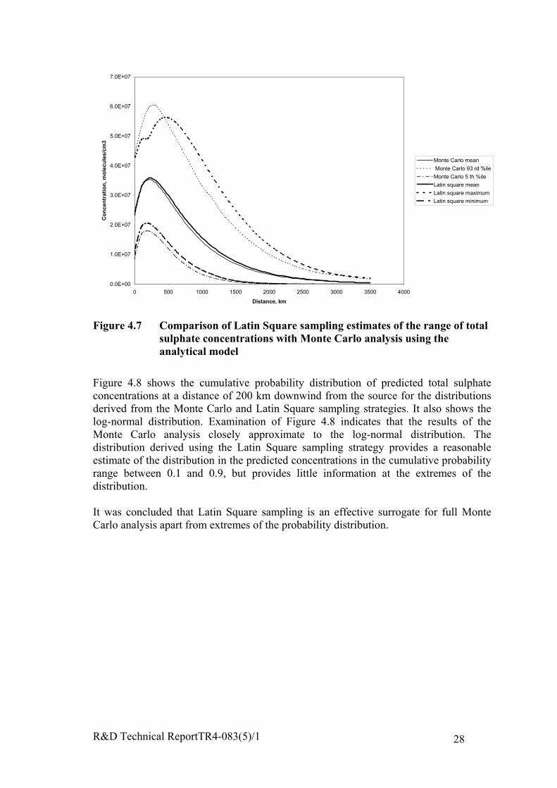
R&D Technical ReportTR4-083(5)/1 28
0.0E+00
1.0E+07
2.0E+07
3.0E+07
4.0E+07
5.0E+07
6.0E+07
7.0E+07
0 500 1000 1500 2000 2500 3000 3500 4000
Distance, km
Con
cent
ratio
n, m
olec
ules
/cm
3
Monte Carlo mean
Monte Carlo 93 rd %ile
Monte Carlo 5 th %ile
Latin square mean
Latin square maximum
Latin square minimum
Figure 4.7 Comparison of Latin Square sampling estimates of the range of totalsulphate concentrations with Monte Carlo analysis using theanalytical model
Figure 4.8 shows the cumulative probability distribution of predicted total sulphateconcentrations at a distance of 200 km downwind from the source for the distributionsderived from the Monte Carlo and Latin Square sampling strategies. It also shows thelog-normal distribution. Examination of Figure 4.8 indicates that the results of theMonte Carlo analysis closely approximate to the log-normal distribution. Thedistribution derived using the Latin Square sampling strategy provides a reasonableestimate of the distribution in the predicted concentrations in the cumulative probabilityrange between 0.1 and 0.9, but provides little information at the extremes of thedistribution.
It was concluded that Latin Square sampling is an effective surrogate for full MonteCarlo analysis apart from extremes of the probability distribution.
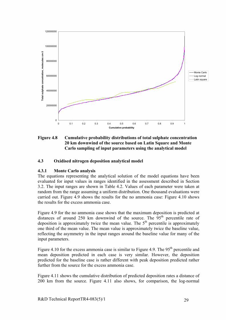
R&D Technical ReportTR4-083(5)/1 29
0
20000000
40000000
60000000
80000000
100000000
120000000
0 0.1 0.2 0.3 0.4 0.5 0.6 0.7 0.8 0.9 1
Cumulative probability
Tota
l sul
phat
e co
ncet
ratio
n, m
olec
ules
cm
-3
Monte Carlo
Log normal
Latin square
Figure 4.8 Cumulative probability distributions of total sulphate concentration20 km downwind of the source based on Latin Square and MonteCarlo sampling of input parameters using the analytical model
4.3 Oxidised nitrogen deposition analytical model
4.3.1 Monte Carlo analysisThe equations representing the analytical solution of the model equations have beenevaluated for input values in ranges identified in the assessment described in Section3.2. The input ranges are shown in Table 4.2. Values of each parameter were taken atrandom from the range assuming a uniform distribution. One thousand evaluations werecarried out. Figure 4.9 shows the results for the no ammonia case: Figure 4.10 showsthe results for the excess ammonia case.
Figure 4.9 for the no ammonia case shows that the maximum deposition is predicted atdistances of around 250 km downwind of the source. The 95th percentile rate ofdeposition is approximately twice the mean value. The 5th percentile is approximatelyone third of the mean value. The mean value is approximately twice the baseline value,reflecting the asymmetry in the input ranges around the baseline value for many of theinput parameters.
Figure 4.10 for the excess ammonia case is similar to Figure 4.9. The 95th percentile andmean deposition predicted in each case is very similar. However, the depositionpredicted for the baseline case is rather different with peak deposition predicted ratherfurther from the source for the excess ammonia case.
Figure 4.11 shows the cumulative distribution of predicted deposition rates a distance of200 km from the source. Figure 4.11 also shows, for comparison, the log-normal

R&D Technical ReportTR4-083(5)/1 30
distribution. It appears from inspection of Figure 4.11 that the log-normal distributionprovides a good representation of the distribution of predicted rates of deposition.
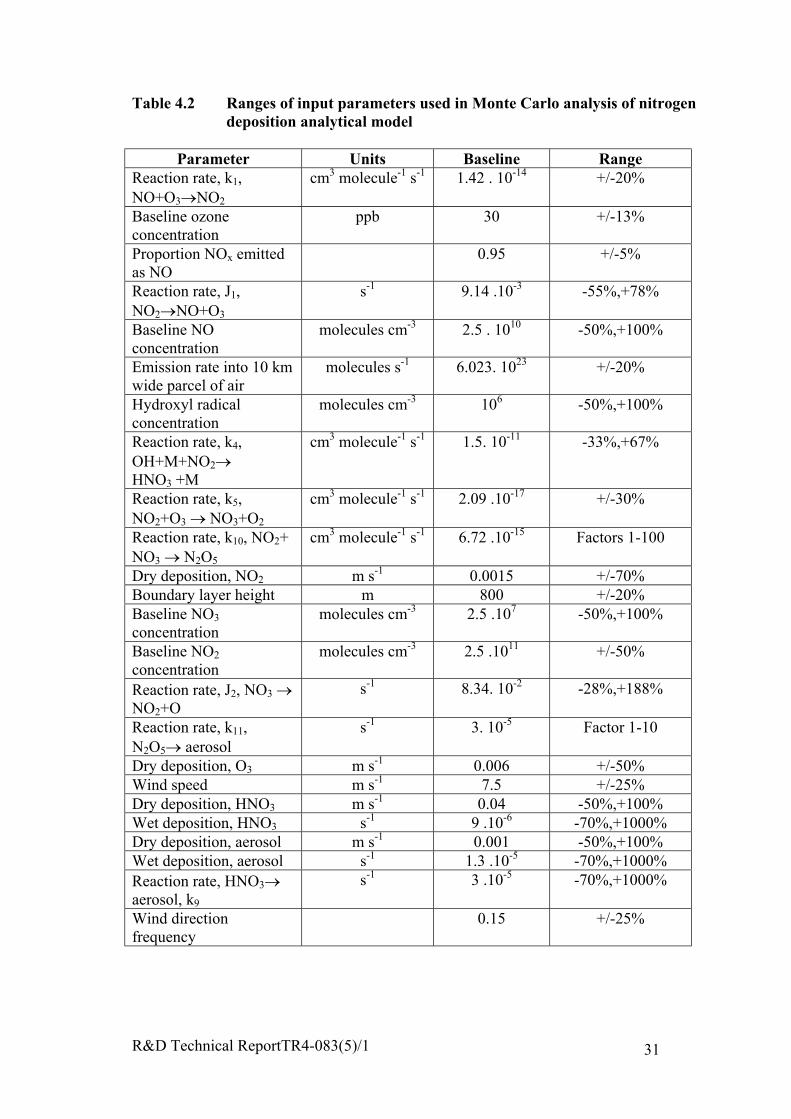
R&D Technical ReportTR4-083(5)/1 31
Table 4.2 Ranges of input parameters used in Monte Carlo analysis of nitrogendeposition analytical model
Parameter Units Baseline RangeReaction rate, k1,NO+O3→NO2
cm3 molecule-1 s-1 1.42 . 10-14 +/-20%
Baseline ozoneconcentration
ppb 30 +/-13%
Proportion NOx emittedas NO
0.95 +/-5%
Reaction rate, J1,NO2→NO+O3
s-1 9.14 .10-3 -55%,+78%
Baseline NOconcentration
molecules cm-3 2.5 . 1010 -50%,+100%
Emission rate into 10 kmwide parcel of air
molecules s-1 6.023. 1023 +/-20%
Hydroxyl radicalconcentration
molecules cm-3 106 -50%,+100%
Reaction rate, k4,OH+M+NO2→HNO3 +M
cm3 molecule-1 s-1 1.5. 10-11 -33%,+67%
Reaction rate, k5,NO2+O3 → NO3+O2
cm3 molecule-1 s-1 2.09 .10-17 +/-30%
Reaction rate, k10, NO2+NO3 → N2O5
cm3 molecule-1 s-1 6.72 .10-15 Factors 1-100
Dry deposition, NO2 m s-1 0.0015 +/-70%Boundary layer height m 800 +/-20%Baseline NO3concentration
molecules cm-3 2.5 .107 -50%,+100%
Baseline NO2concentration
molecules cm-3 2.5 .1011 +/-50%
Reaction rate, J2, NO3 →NO2+O
s-1 8.34. 10-2 -28%,+188%
Reaction rate, k11,N2O5→ aerosol
s-1 3. 10-5 Factor 1-10
Dry deposition, O3 m s-1 0.006 +/-50%Wind speed m s-1 7.5 +/-25%Dry deposition, HNO3 m s-1 0.04 -50%,+100%Wet deposition, HNO3 s-1 9 .10-6 -70%,+1000%Dry deposition, aerosol m s-1 0.001 -50%,+100%Wet deposition, aerosol s-1 1.3 .10-5 -70%,+1000%Reaction rate, HNO3→aerosol, k9
s-1 3 .10-5 -70%,+1000%
Wind directionfrequency
0.15 +/-25%
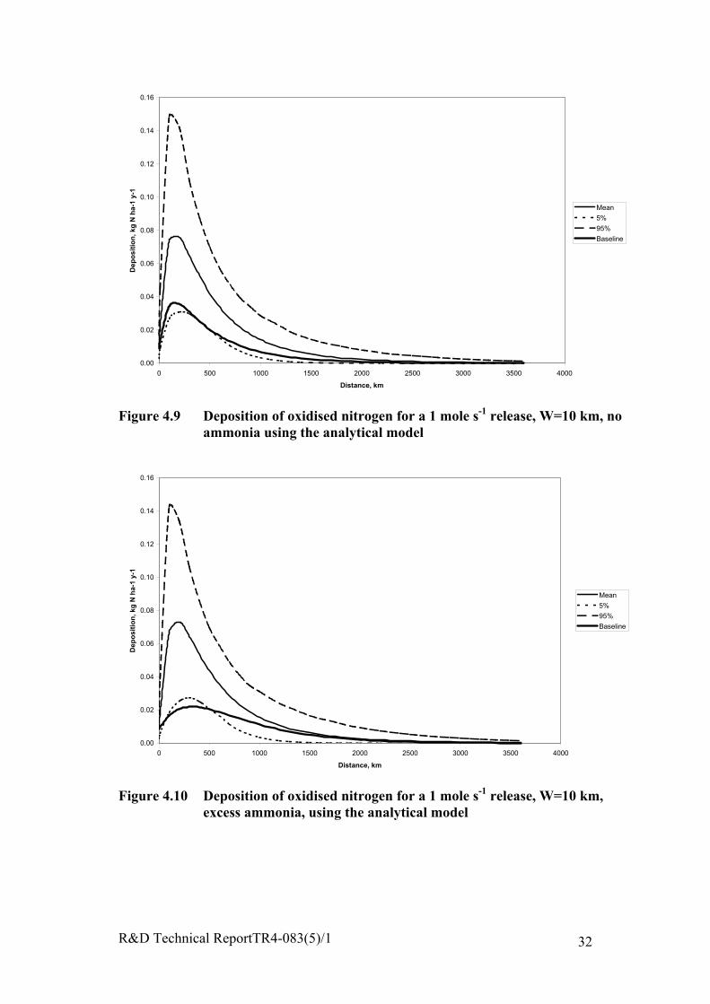
R&D Technical ReportTR4-083(5)/1 32
0.00
0.02
0.04
0.06
0.08
0.10
0.12
0.14
0.16
0 500 1000 1500 2000 2500 3000 3500 4000
Distance, km
Dep
ositi
on, k
g N
ha-
1 y-
1
Mean
5%
95%
Baseline
Figure 4.9 Deposition of oxidised nitrogen for a 1 mole s-1 release, W=10 km, noammonia using the analytical model
0.00
0.02
0.04
0.06
0.08
0.10
0.12
0.14
0.16
0 500 1000 1500 2000 2500 3000 3500 4000
Distance, km
Dep
ositi
on, k
g N
ha-
1 y-
1
Mean
5%
95%
Baseline
Figure 4.10 Deposition of oxidised nitrogen for a 1 mole s-1 release, W=10 km,excess ammonia, using the analytical model
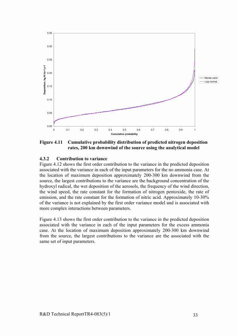
R&D Technical ReportTR4-083(5)/1 33
0.00
0.05
0.10
0.15
0.20
0.25
0.30
0.35
0 0.1 0.2 0.3 0.4 0.5 0.6 0.7 0.8 0.9 1
Cumulative probability
Dep
ositi
on, k
g N
ha-
1 y-
1
Monte carlo
Log normal
Figure 4.11 Cumulative probability distribution of predicted nitrogen depositionrates, 200 km downwind of the source using the analytical model
4.3.2 Contribution to varianceFigure 4.12 shows the first order contribution to the variance in the predicted depositionassociated with the variance in each of the input parameters for the no ammonia case. Atthe location of maximum deposition approximately 200-300 km downwind from thesource, the largest contributions to the variance are the background concentration of thehydroxyl radical, the wet deposition of the aerosols, the frequency of the wind direction,the wind speed, the rate constant for the formation of nitrogen pentoxide, the rate ofemission, and the rate constant for the formation of nitric acid. Approximately 10-30%of the variance is not explained by the first order variance model and is associated withmore complex interactions between parameters.
Figure 4.13 shows the first order contribution to the variance in the predicted depositionassociated with the variance in each of the input parameters for the excess ammoniacase. At the location of maximum deposition approximately 200-300 km downwindfrom the source, the largest contributions to the variance are the associated with thesame set of input parameters.

R&D Technical ReportTR4-083(5)/1 34
0.0
0.1
0.2
0.3
0.4
0.5
0.6
0.7
0.8
0.9
1.0
0 10 100 200 300 400 500 600 700 800 900 1000 1100 1200 1300 1400
Distance, km
C(p
)
Wind direction frequency
k9
Wet deposition rate, aerosols
Dry deposition velocity, aerosols
Wet deposition rate, HNO3
Dry deposition velocity, HNO3
Wind speed
Ozone relaxation rate
k11
j2
Background [NO2]
Background {NO3]
Boundary layer height
Dry deposition velocity, NO2
k10
k5
k4
[OH]
Emission rate
[NO]
J1
Proportion NOx as NO
[O3]
k1
Figure 4.12 Contribution to variance in predicted oxidized nitrogen deposition,no ammonia case, using the analytical model
0.0
0.1
0.2
0.3
0.4
0.5
0.6
0.7
0.8
0.9
1.0
0 10 100 200 300 400 500 600 700 800 900 1000 1100 1200 1300 1400
Distance, km
C(p
)
Wind direction frequency
k9
Wet deposition rate, aerosols
Dry deposition velocity, aerosols
Wet deposition rate, HNO3
Dry deposition velocity, HNO3
Wind speed
Ozone relaxation rate
k11
j2
Background [NO2]
Background {NO3]
Boundary layer height
Dry deposition velocity, NO2
k10
k5
k4
[OH]
Emission rate
[NO]
J1
Proportion NOx as NO
[O3]
k1
Figure 4.13 Contribution to variance in predicted oxidized nitrogen deposition,excess ammonia case, using the analytical model
R&D Technical ReportTR4-083(5)/1 35
4.4 TRACK - Baseline predictions
4.4.1 Monte Carlo simulationThe TRACK model was used to predict sulphur deposition and oxidised and reducednitrogen deposition for the baseline scenario for input parameters in ranges identified inthe assessment described in Section 3. The baseline scenario was based on the 1990emissions inventory for the UK and for the EMEP grid. The input ranges are shown inTable 4.3. Values of each parameter were taken at random from the range assuming auniform distribution. Three hundred model runs were carried out.
Figure 4.14 shows the predicted mean and 5th and 95th percentile rates of sulphurdeposition at grid cells containing Acid Deposition Network sites throughout the UnitedKingdom. The sites include a mixture of sites close to and far from the main sourcesand in upland and lowland areas. The 95th percentile value is typically around 1.3 timesthe average: the average is typically around 1.45 times the 5th percentile. Theuncertainty as a proportion of the mean predicted rate of deposition is affected bydistance from the main sources of emission. The 5th to 95th percentile range decreasesfrom around 80% of the mean at those sites near to the major sources (e.g. Bottesford,Jenny Hurn) to around 40% of the mean at more remote sites (e.g. Goonhilly, Polloch,Strathvaich Dam).
Figure 4.15 shows the predicted mean and 5th and 95th percentile rates of oxidisednitrogen deposition at grid cells containing Acid Deposition Network sites throughoutthe United Kingdom. The 95th percentile value is typically around 1.9 times the average:the average is typically around 2 times the 5th percentile. The uncertainty as a proportionof the mean predicted rate of deposition is affected by distance from the main sources ofemission. The 5th to 95th percentile range tends to increase from around 100% of themean at those sites near to the major sources (e.g. Bottesford, Jenny Hurn) to around250% of the mean at more remote sites (e.g. Goonhilly, Polloch).
Figure 4.16 shows the predicted mean and 5th and 95th percentile rates of reducednitrogen deposition at grid cells containing Acid Deposition Network sites throughoutthe United Kingdom. The 95th percentile value is typically around 1.5 times the average:the average is typically around 1.7 times the 5th percentile. The relationship between theuncertainty as a proportion of the mean predicted rate of deposition and distance fromthe major emission sources is not clear for reduced nitrogen deposition.
Figure 4.17 shows the predicted mean and 5th and 95th percentile rates of total oxidisedand reduced nitrogen deposition at grid cells containing Acid Deposition Network sitesthroughout the United Kingdom. The 95th percentile value is typically around 1.5 timesthe average: the average is typically around 1.5 times the 5th percentile.
Figure 4.18 shows the predicted mean and 5th and 95th percentile rates of total oxidisednitrogen, reduced nitrogen and sulphur deposition at grid cells containing AcidDeposition Network sites throughout the United Kingdom. The 95th percentile value istypically around 1.3 times the average: the average is typically around 1.4 times the 5th
percentile. [Note 1 equivalent (eq) = 16g sulphur or 14 g nitrogen].
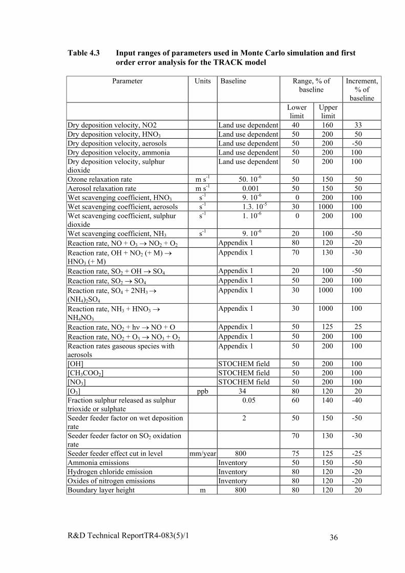
R&D Technical ReportTR4-083(5)/1 36
Table 4.3 Input ranges of parameters used in Monte Carlo simulation and firstorder error analysis for the TRACK model
Parameter Units Baseline Range, % ofbaseline
Increment,% of
baselineLowerlimit
Upperlimit
Dry deposition velocity, NO2 Land use dependent 40 160 33Dry deposition velocity, HNO3 Land use dependent 50 200 50Dry deposition velocity, aerosols Land use dependent 50 200 -50Dry deposition velocity, ammonia Land use dependent 50 200 100Dry deposition velocity, sulphurdioxide
Land use dependent 50 200 100
Ozone relaxation rate m s-1 50. 10-6 50 150 50Aerosol relaxation rate m s-1 0.001 50 150 50Wet scavenging coefficient, HNO3 s-1 9. 10-6 0 200 100Wet scavenging coefficient, aerosols s-1 1.3. 10-5 30 1000 100Wet scavenging coefficient, sulphurdioxide
s-1 1. 10-6 0 200 100
Wet scavenging coefficient, NH3 s-1 9. 10-6 20 100 -50Reaction rate, NO + O3 → NO2 + O2 Appendix 1 80 120 -20Reaction rate, OH + NO2 (+ M) →HNO3 (+ M)
Appendix 1 70 130 -30
Reaction rate, SO2 + OH → SO4 Appendix 1 20 100 -50Reaction rate, SO2 → SO4 Appendix 1 50 200 100Reaction rate, SO4 + 2NH3 →(NH4)2SO4
Appendix 1 30 1000 100
Reaction rate, NH3 + HNO3 →NH4NO3
Appendix 1 30 1000 100
Reaction rate, NO2 + hν → NO + O Appendix 1 50 125 25Reaction rate, NO2 + O3 → NO3 + O2 Appendix 1 50 200 100Reaction rates gaseous species withaerosols
Appendix 1 50 200 100
[OH] STOCHEM field 50 200 100[CH3COO2] STOCHEM field 50 200 100[NO3] STOCHEM field 50 200 100[O3] ppb 34 80 120 20Fraction sulphur released as sulphurtrioxide or sulphate
0.05 60 140 -40
Seeder feeder factor on wet depositionrate
2 50 150 -50
Seeder feeder factor on SO2 oxidationrate
70 130 -30
Seeder feeder effect cut in level mm/year 800 75 125 -25Ammonia emissions Inventory 50 150 -50Hydrogen chloride emission Inventory 80 120 -20Oxides of nitrogen emissions Inventory 80 120 -20Boundary layer height m 800 80 120 20
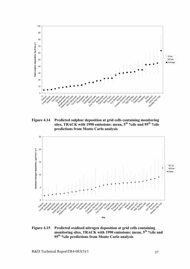
R&D Technical ReportTR4-083(5)/1 37
0
10
20
30
40
50
60
70
80
90
100
0
Polloc
h
Loug
h Nav
ar
Achan
arra
s
Goonh
illy
Glen D
ye
Balquh
idder
Strath
vaich
Dam
Hilsbo
roug
h For
est
Allt a'
Mha
rcad
h
Tycan
ol W
ood
Whit
eadd
er
Loch
Dee
Eskda
lemuir
Bannis
dale
Cow G
reen
Res
.
Redes
dale
Yarne
r Woo
d
Stoke
Fer
ry
Pumlum
on
Llyn
Briann
e
Wob
urn
Presto
n M
ontfo
rd
Llyn
Llyda
w
High M
uffle
s
Compt
on
Flatfo
rd M
ill
Thorg
anby
Driby
Botte
sford
Jenn
y Hur
n
War
dley H
ay C
op
Tota
l sul
phur
dep
ositi
on, k
g S
ha y
-1
5%ile
95%ile
Average
Figure 4.14 Predicted sulphur deposition at grid cells containing monitoringsites, TRACK with 1990 emissions: mean, 5th %ile and 95th %ilepredictions from Monte Carlo analysis
0
5
10
15
20
25
Polloc
h
Loug
h Nav
ar
Achan
arra
s
Balquh
idder
Whit
eadd
er
Strath
vaich
Dam
Allt a'
Mha
rcad
h
Hilsbo
roug
h For
est
Glen D
ye
Eskda
lemuir
Goonh
illy
Redes
dale
Loch
Dee
Tycan
ol W
ood
Presto
n M
ontfo
rd
Llyn
Llyda
w
Cow G
reen
Res
.
Compt
on
Bannis
dale
Thorg
anby
Yarne
r Woo
d
Stoke
Fer
ry
Wob
urn
Botte
sford
Jenn
y Hur
n
High M
uffle
s
Flatfo
rd M
ill
Driby
Llyn
Briann
e
Pumlum
on
War
dley H
ay C
op
Site
Oxi
dise
d ni
trog
en d
epos
ition
, kg
N h
a-1
y-1
5% ile
95%ile
Mean
Figure 4.15 Predicted oxidised nitrogen deposition at grid cells containingmonitoring sites, TRACK with 1990 emissions: mean, 5th %ile and95th %ile predictions from Monte Carlo analysis
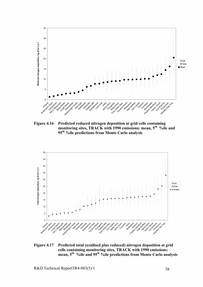
R&D Technical ReportTR4-083(5)/1 38
0
5
10
15
20
25
30
35
Polloc
h
Strath
vaich
Dam
Achan
arra
s
Allt a'
Mha
rcad
h
Balquh
idder
Loug
h Nav
ar
Whit
eadd
er
Hilsbo
roug
h For
est
Glen D
ye
Redes
dale
Goonh
illy
Flatfo
rd M
ill
Eskda
lemuir
Loch
Dee
Driby
Jenn
y Hur
n
Thorg
anby
Stoke
Fer
ry
Cow G
reen
Res
.
Tycan
ol W
ood
Botte
sford
High M
uffle
s
Llyn
Llyda
w
Wob
urn
Compt
on
Bannis
dale
Presto
n M
ontfo
rd
Yarne
r Woo
d
Llyn
Briann
e
Pumlum
on
War
dley H
ay C
op
Red
uced
nitr
ogen
dep
ositi
on, k
g N
ha-
1 y-
1
5%ile
95%ile
Mean
Figure 4.16 Predicted reduced nitrogen deposition at grid cells containingmonitoring sites, TRACK with 1990 emissions: mean, 5th %ile and95th %ile predictions from Monte Carlo analysis
0
5
10
15
20
25
30
35
40
45
50
Polloc
h
Strath
vaich
Dam
Achan
arra
s
Loug
h Nav
ar
Allt a'
Mha
rcad
h
Balquh
idder
Whi
tead
der
Hilsbo
roug
h For
est
Glen D
ye
Redes
dale
Goonh
illy
Eskda
lemuir
Loch
Dee
Tycan
ol W
ood
Thorg
anby
Flatfo
rd M
ill
Cow G
reen
Res
.
Llyn
Llyda
w
Stoke
Fer
ry
Jenn
y Hur
n
Compt
onDrib
y
Botte
sford
Wob
urn
Presto
n M
ontfo
rd
High M
uffle
s
Bannis
dale
Yarne
r Woo
d
Llyn
Briann
e
Pumlum
on
War
dley H
ay C
op
Tota
l nitr
ogen
dep
ositi
on, k
g N
ha-
1 y-
1
5%ile
95%ile
average
Figure 4.17 Predicted total (oxidised plus reduced) nitrogen deposition at gridcells containing monitoring sites, TRACK with 1990 emissions:mean, 5th %ile and 95th %ile predictions from Monte Carlo analysis

R&D Technical ReportTR4-083(5)/1 39
0
1000
2000
3000
4000
5000
6000
7000
8000
9000
Polloc
h
Loug
h Nav
ar
Achan
arra
s
Strath
vaich
Dam
Balquh
idder
Glen D
ye
Allt a'
Mha
rcad
h
Hilsbo
roug
h For
est
Goonh
illy
Whi
tead
der
Tycan
ol W
ood
Eskda
lemuir
Loch
Dee
Redes
dale
Cow G
reen
Res
.
Bannis
dale
Stoke
Fer
ry
Yarne
r Woo
d
Llyn
Llyda
w
Wob
urn
Presto
n M
ontfo
rd
High M
uffle
s
Flatfo
rd M
ill
Compt
on
Pumlum
on
Llyn
Briann
e
Thorg
anby
Driby
Botte
sford
Jenn
y Hur
n
War
dley H
ay C
op
Tota
l dep
ositi
on, e
q ha
-1 y
-1
5th %ile
95th %ile
mean
Figure 4.18 Predicted total (oxidised, nitrogen, reduced nitrogen and sulphur)deposition at grid cells containing monitoring sites, TRACK with1990 emissions: mean, 5th %ile and 95th %ile predictions fromMonte Carlo analysis
Figures 4.19 to 4.21 show the cumulative probability of predicted sulphur, oxidised andreduced nitrogen depositions at the Jenny Hurn site. In each case, the distribution isapproximately log-normal over the 5th to 95th %ile range.
0
10
20
30
40
50
60
70
80
90
100
0 0.1 0.2 0.3 0.4 0.5 0.6 0.7 0.8 0.9 1
Cumulative probability
Tota
l sul
phur
dep
ositi
on, k
g S
ha-1
y-1
Monte carlo
Log normal
Figure 4.19 Cumulative probability distribution of sulphur deposition: TRACKmodel, 1990 emissions, Jenny Hurn

R&D Technical ReportTR4-083(5)/1 40
0
2
4
6
8
10
12
14
16
18
20
0 0.1 0.2 0.3 0.4 0.5 0.6 0.7 0.8 0.9 1
Cumulative probability
Oxi
dise
d ni
trog
en d
epos
ition
, kg
N h
a-1
y-1
Monte Carlo
Log normal
Figure 4.20 Cumulative probability distribution of oxidised nitrogen deposition:TRACK model, 1990 emissions, Jenny Hurn
0
5
10
15
20
25
0 0.1 0.2 0.3 0.4 0.5 0.6 0.7 0.8 0.9 1
Cumulative probability
Red
uced
nitr
ogen
dep
ositi
on, k
g N
ha-
1 y-
1
Monte Carlo
Log normal
Figure 4.21 Cumulative probability distribution of reduced nitrogen deposition:TRACK model, 1990 emissions, Jenny Hurn
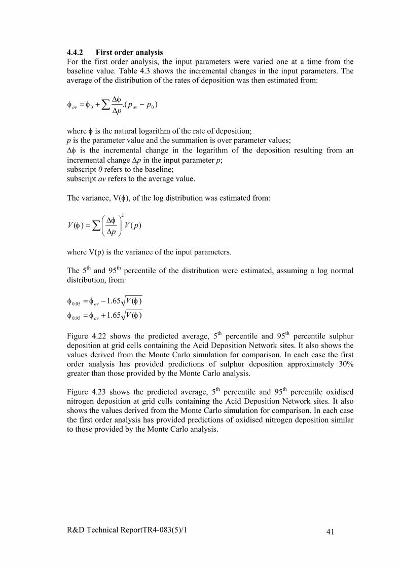
R&D Technical ReportTR4-083(5)/1 41
4.4.2 First order analysisFor the first order analysis, the input parameters were varied one at a time from thebaseline value. Table 4.3 shows the incremental changes in the input parameters. Theaverage of the distribution of the rates of deposition was then estimated from:
).( 00 ppp avav −
∆∆
+= ∑ φφφ
where φ is the natural logarithm of the rate of deposition;p is the parameter value and the summation is over parameter values;∆φ is the incremental change in the logarithm of the deposition resulting from anincremental change ∆p in the input parameter p;subscript 0 refers to the baseline;subscript av refers to the average value.
The variance, V(φ), of the log distribution was estimated from:
∑
∆∆
= )()(2
pVp
V φφ
where V(p) is the variance of the input parameters.
The 5th and 95th percentile of the distribution were estimated, assuming a log normaldistribution, from:
)(65.1
)(65.1
95.0
05.0
φφφ
φφφ
V
V
av
av
+=
−=
Figure 4.22 shows the predicted average, 5th percentile and 95th percentile sulphurdeposition at grid cells containing the Acid Deposition Network sites. It also shows thevalues derived from the Monte Carlo simulation for comparison. In each case the firstorder analysis has provided predictions of sulphur deposition approximately 30%greater than those provided by the Monte Carlo analysis.
Figure 4.23 shows the predicted average, 5th percentile and 95th percentile oxidisednitrogen deposition at grid cells containing the Acid Deposition Network sites. It alsoshows the values derived from the Monte Carlo simulation for comparison. In each casethe first order analysis has provided predictions of oxidised nitrogen deposition similarto those provided by the Monte Carlo analysis.
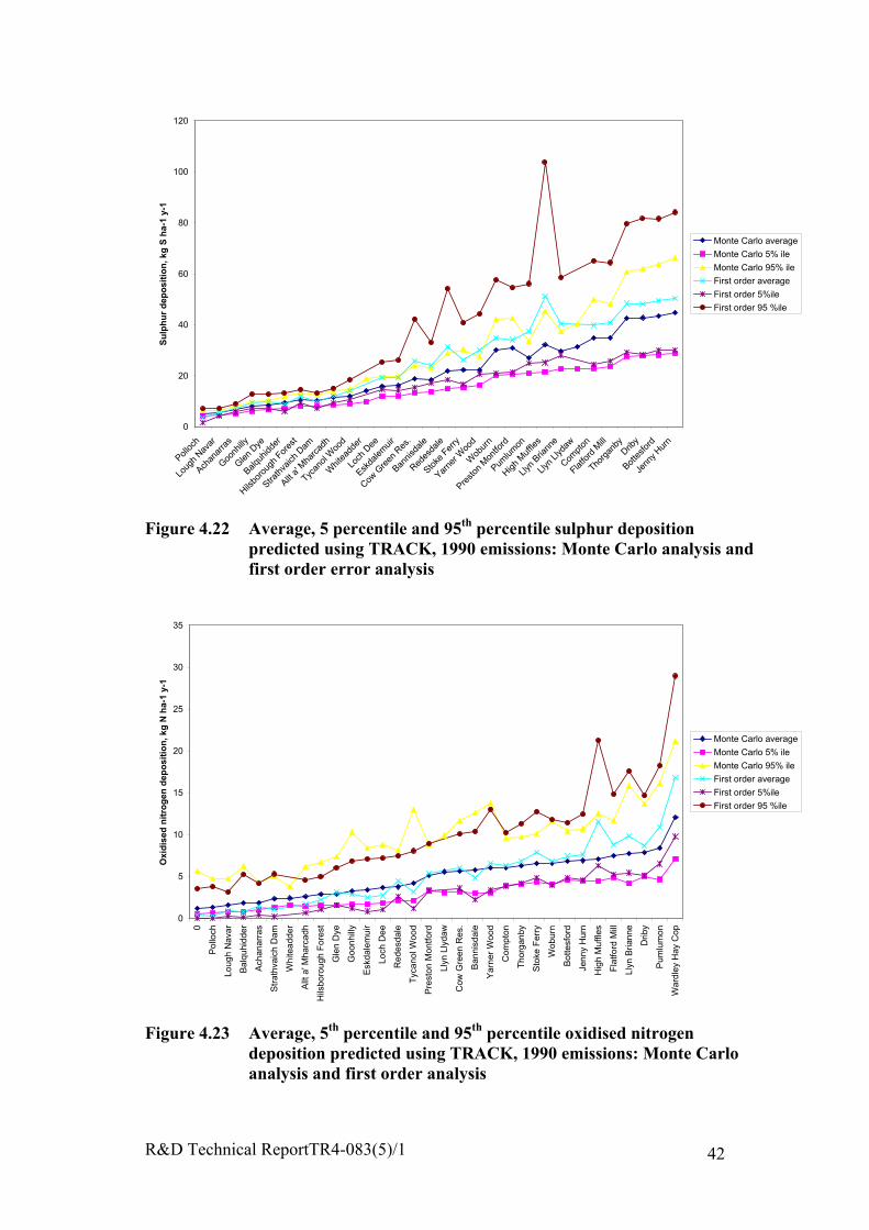
R&D Technical ReportTR4-083(5)/1 42
0
20
40
60
80
100
120
Polloc
h
Loug
h Nav
ar
Achan
arra
s
Goonh
illy
Glen D
ye
Balquh
idder
Hilsbo
roug
h For
est
Strath
vaich
Dam
Allt a'
Mha
rcad
h
Tycan
ol W
ood
Whit
eadd
er
Loch
Dee
Eskda
lemuir
Cow G
reen
Res
.
Bannis
dale
Redes
dale
Stoke
Fer
ry
Yarne
r Woo
d
Wob
urn
Presto
n M
ontfo
rd
Pumlum
on
High M
uffle
s
Llyn
Briann
e
Llyn
Llyda
w
Compt
on
Flatfo
rd M
ill
Thorg
anby
Driby
Botte
sford
Jenn
y Hur
n
Sulp
hur d
epos
ition
, kg
S ha
-1 y
-1
Monte Carlo average
Monte Carlo 5% ile
Monte Carlo 95% ile
First order average
First order 5%ile
First order 95 %ile
Figure 4.22 Average, 5 percentile and 95th percentile sulphur depositionpredicted using TRACK, 1990 emissions: Monte Carlo analysis andfirst order error analysis
0
5
10
15
20
25
30
35
0
Pol
loch
Loug
h N
avar
Bal
quhi
dder
Ach
anar
ras
Str
athv
aich
Dam
Wh
itea
dd
er
Allt
a' M
harc
adh
Hils
boro
ugh
For
est
Gle
n D
ye
Goo
nhill
y
Esk
dale
mui
r
Loch
Dee
Red
esda
le
Tyc
an
ol W
oo
d
Pre
ston
Mon
tford
Llyn
Lly
daw
Cow
Gre
en R
es.
Ban
nisd
ale
Ya
rne
r W
oo
d
Com
pton
Tho
rgan
by
Sto
ke F
erry
Wo
bu
rn
Bot
tesf
ord
Jenn
y H
urn
Hig
h M
uffle
s
Fla
tford
Mill
Llyn
Bria
nne
Drib
y
Pum
lum
on
War
dley
Hay
Cop
Oxi
dise
d ni
trog
en d
epos
ition
, kg
N h
a-1
y-1
Monte Carlo average
Monte Carlo 5% ile
Monte Carlo 95% ile
First order average
First order 5%ile
First order 95 %ile
Figure 4.23 Average, 5th percentile and 95th percentile oxidised nitrogendeposition predicted using TRACK, 1990 emissions: Monte Carloanalysis and first order analysis
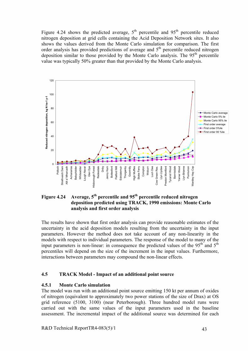
R&D Technical ReportTR4-083(5)/1 43
Figure 4.24 shows the predicted average, 5th percentile and 95th percentile reducednitrogen deposition at grid cells containing the Acid Deposition Network sites. It alsoshows the values derived from the Monte Carlo simulation for comparison. The firstorder analysis has provided predictions of average and 5th percentile reduced nitrogendeposition similar to those provided by the Monte Carlo analysis. The 95th percentilevalue was typically 50% greater than that provided by the Monte Carlo analysis.
0
20
40
60
80
100
120
Pol
loch
Str
athv
aich
Dam
Allt
a' M
harc
adh
Ach
anar
ras
Bal
quhi
dder
Wh
itea
dd
er
Loug
h N
avar
Gle
n D
ye
Hils
boro
ugh
For
est
Red
esda
le
Drib
y
Jenn
y H
urn
Bot
tesf
ord
Fla
tford
Mill
Esk
dale
mui
r
Tho
rgan
by
Goo
nhill
y
Hig
h M
uffle
s
Sto
ke F
erry
Com
pton
Wo
bu
rn
Loch
Dee
Cow
Gre
en R
es.
Llyn
Lly
daw
Pre
ston
Mon
tford
Tyc
an
ol W
oo
d
Ban
nisd
ale
Ya
rne
r W
oo
d
Llyn
Bria
nne
Pum
lum
on
War
dley
Hay
Cop
Red
uced
nitr
ogen
dep
ositi
on, k
g N
ha-
1 y-
1
Monte Carlo average
Monte Carlo 5% ile
Monte Carlo 95% ile
First order average
First order 5%ile
First order 95 %ile
Figure 4.24 Average, 5th percentile and 95th percentile reduced nitrogendeposition predicted using TRACK, 1990 emissions: Monte Carloanalysis and first order analysis
The results have shown that first order analysis can provide reasonable estimates of theuncertainty in the acid deposition models resulting from the uncertainty in the inputparameters. However the method does not take account of any non-linearity in themodels with respect to individual parameters. The response of the model to many of theinput parameters is non-linear: in consequence the predicted values of the 95th and 5th
percentiles will depend on the size of the increment in the input values. Furthermore,interactions between parameters may compound the non-linear effects.
4.5 TRACK Model - Impact of an additional point source
4.5.1 Monte Carlo simulationThe model was run with an additional point source emitting 150 kt per annum of oxidesof nitrogen (equivalent to approximately two power stations of the size of Drax) at OSgrid reference (5100, 3100) (near Peterborough). Three hundred model runs werecarried out with the same values of the input parameters used in the baselineassessment. The incremental impact of the additional source was determined for each

R&D Technical ReportTR4-083(5)/1 44
model run by subtracting the baseline deposition from the total deposition. Theincremental deposition from the source was calculated at receptors on a trajectorypassing through the point source in a direction 330o from north (i.e. towards thenorthwest of Scotland). Figure 4.25 shows the 5th percentile, average and 95th percentileincremental contribution from the source to oxidised nitrogen deposition at increasingdistances from the source. The contribution generally decreases with distance from thesource, although local variations in dry deposition velocity and rainfall have someinfluence on the predicted values. The 95th percentile value is typically approximatelytwice the average value: the 5th percentile is approximately half the average value.
Figure 4.25 also shows for comparison the polar analytical solution from Appendix 3for the excess ammonia case. The input parameters were as for the baseline case inTable 4.2 except that a wind direction frequency of 0.086 was used with a wind sectorsize of 45o corresponding to the wind direction from 135-180o taken from Table 3.6.Although the comparison does not provide a comprehensive test of the analyticalsolution, it does suggest that the analytical solution provides a reasonable surrogate forthe numerical models for the purposes of uncertainty analysis.
0
0.05
0.1
0.15
0.2
0.25
0.3
0.35
0.4
0.45
0.5
3100 4100 5100 6100 7100 8100 9100
Northing, 100m units
Incr
emen
tal
cont
ribut
ion
to o
xidi
sed
nitr
ogen
dep
ositi
on, k
g N
ha-
1 y-
1
Average
5%ile
95%ile
Analytical
Figure 4.25 Incremental contribution to oxidised nitrogen deposition from apoint source at (5100, 3100) emitting 150 kt oxides of nitrogen peryear, TRACK model, 1990 base emissions, Monte Carlo analysis.Results from the analytical model assuming excess ammonia are alsoshown
Model runs were also carried out for a source emission of 75 kt per annum (i.e. half of150 kt). Figure 4.26 shows the 150kt:75 kt ratios of the 5th percentile, average and 95th
percentile rates of deposition. Far from the source, the predicted contribution todeposition from the additional source is approximately proportional to the rate ofemission. Closer to the source, the contribution for the 150 kt emission is around 1.8times that for the 75 kt emission indicating that there is some non-linearity in the
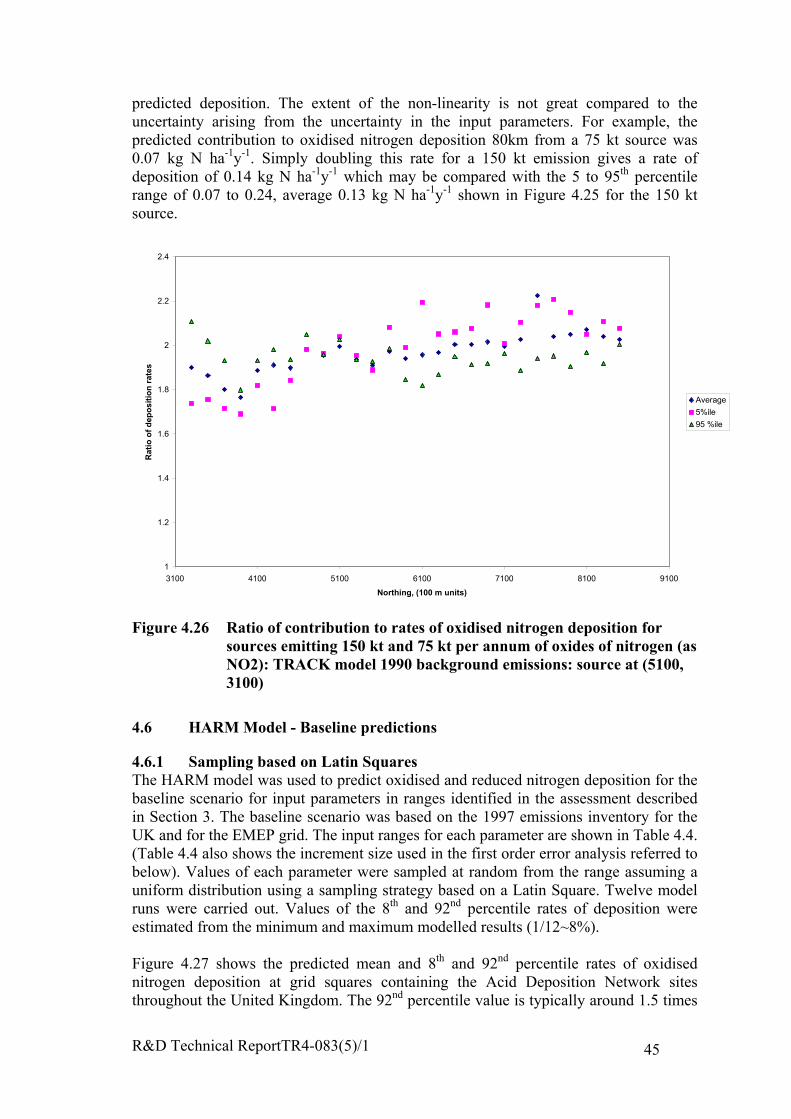
R&D Technical ReportTR4-083(5)/1 45
predicted deposition. The extent of the non-linearity is not great compared to theuncertainty arising from the uncertainty in the input parameters. For example, thepredicted contribution to oxidised nitrogen deposition 80km from a 75 kt source was0.07 kg N ha-1y-1. Simply doubling this rate for a 150 kt emission gives a rate ofdeposition of 0.14 kg N ha-1y-1 which may be compared with the 5 to 95th percentilerange of 0.07 to 0.24, average 0.13 kg N ha-1y-1 shown in Figure 4.25 for the 150 ktsource.
1
1.2
1.4
1.6
1.8
2
2.2
2.4
3100 4100 5100 6100 7100 8100 9100
Northing, (100 m units)
Rat
io o
f dep
ositi
on ra
tes
Average
5%ile
95 %ile
Figure 4.26 Ratio of contribution to rates of oxidised nitrogen deposition forsources emitting 150 kt and 75 kt per annum of oxides of nitrogen (asNO2): TRACK model 1990 background emissions: source at (5100,3100)
4.6 HARM Model - Baseline predictions
4.6.1 Sampling based on Latin SquaresThe HARM model was used to predict oxidised and reduced nitrogen deposition for thebaseline scenario for input parameters in ranges identified in the assessment describedin Section 3. The baseline scenario was based on the 1997 emissions inventory for theUK and for the EMEP grid. The input ranges for each parameter are shown in Table 4.4.(Table 4.4 also shows the increment size used in the first order error analysis referred tobelow). Values of each parameter were sampled at random from the range assuming auniform distribution using a sampling strategy based on a Latin Square. Twelve modelruns were carried out. Values of the 8th and 92nd percentile rates of deposition wereestimated from the minimum and maximum modelled results (1/12~8%).
Figure 4.27 shows the predicted mean and 8th and 92nd percentile rates of oxidisednitrogen deposition at grid squares containing the Acid Deposition Network sitesthroughout the United Kingdom. The 92nd percentile value is typically around 1.5 times
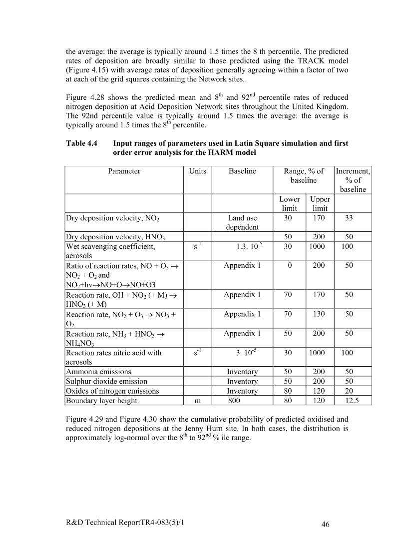
R&D Technical ReportTR4-083(5)/1 46
the average: the average is typically around 1.5 times the 8 th percentile. The predictedrates of deposition are broadly similar to those predicted using the TRACK model(Figure 4.15) with average rates of deposition generally agreeing within a factor of twoat each of the grid squares containing the Network sites.
Figure 4.28 shows the predicted mean and 8th and 92nd percentile rates of reducednitrogen deposition at Acid Deposition Network sites throughout the United Kingdom.The 92nd percentile value is typically around 1.5 times the average: the average istypically around 1.5 times the 8th percentile.
Table 4.4 Input ranges of parameters used in Latin Square simulation and firstorder error analysis for the HARM model
Parameter Units Baseline Range, % ofbaseline
Increment,% of
baselineLowerlimit
Upperlimit
Dry deposition velocity, NO2 Land usedependent
30 170 33
Dry deposition velocity, HNO3 50 200 50Wet scavenging coefficient,aerosols
s-1 1.3. 10-5 30 1000 100
Ratio of reaction rates, NO + O3 →NO2 + O2 andNO2+hv→NO+O→NO+O3
Appendix 1 0 200 50
Reaction rate, OH + NO2 (+ M) →HNO3 (+ M)
Appendix 1 70 170 50
Reaction rate, NO2 + O3 → NO3 +O2
Appendix 1 70 130 50
Reaction rate, NH3 + HNO3 →NH4NO3
Appendix 1 50 200 50
Reaction rates nitric acid withaerosols
s-1 3. 10-5 30 1000 100
Ammonia emissions Inventory 50 200 50Sulphur dioxide emission Inventory 50 200 50Oxides of nitrogen emissions Inventory 80 120 20Boundary layer height m 800 80 120 12.5
Figure 4.29 and Figure 4.30 show the cumulative probability of predicted oxidised andreduced nitrogen depositions at the Jenny Hurn site. In both cases, the distribution isapproximately log-normal over the 8th to 92nd % ile range.
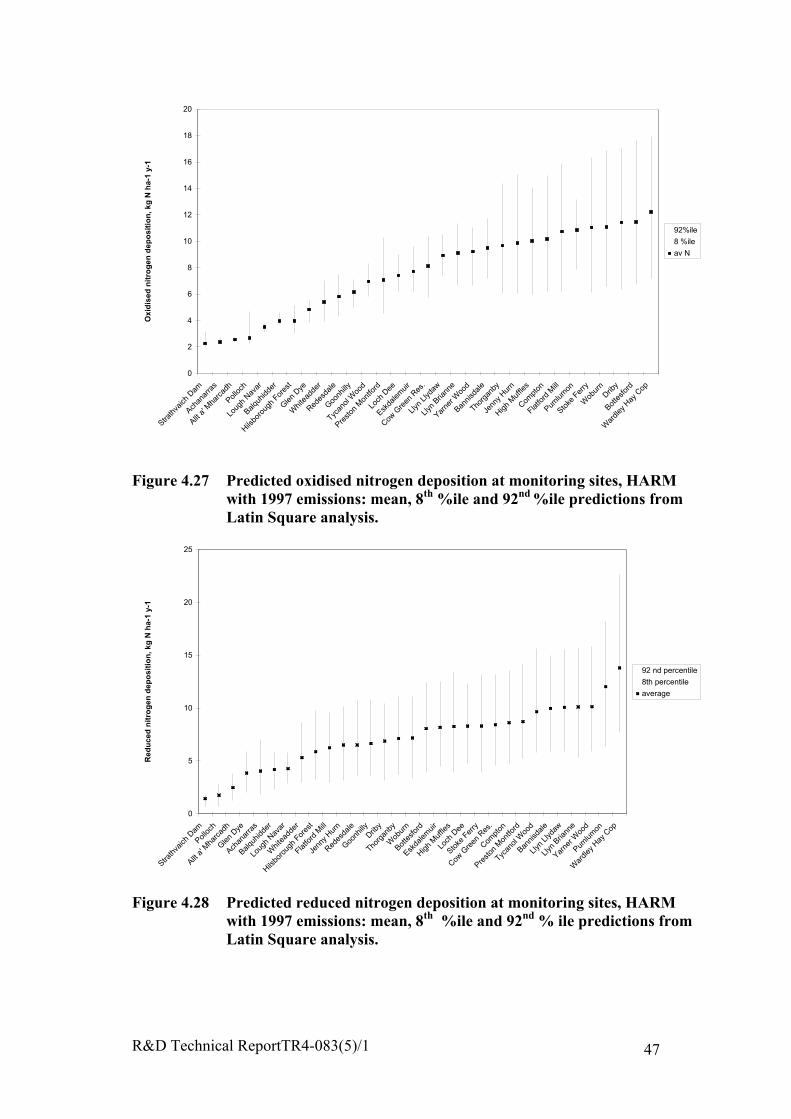
R&D Technical ReportTR4-083(5)/1 47
0
2
4
6
8
10
12
14
16
18
20
Strath
vaich
Dam
Achan
arra
s
Allt a'
Mha
rcad
h
Polloc
h
Loug
h Nav
ar
Balquh
idder
Hilsbo
roug
h For
est
Glen D
ye
Whi
tead
der
Redes
dale
Goonh
illy
Tycan
ol W
ood
Presto
n M
ontfo
rd
Loch
Dee
Eskda
lemuir
Cow G
reen
Res
.
Llyn
Llyda
w
Llyn
Briann
e
Yarne
r Woo
d
Bannis
dale
Thorg
anby
Jenn
y Hur
n
High M
uffle
s
Compt
on
Flatfo
rd M
ill
Pumlum
on
Stoke
Fer
ry
Wob
urn
Driby
Botte
sford
War
dley H
ay C
op
Oxi
dise
d ni
trog
en d
epos
ition
, kg
N h
a-1
y-1
92%ile
8 %ile
av N
Figure 4.27 Predicted oxidised nitrogen deposition at monitoring sites, HARMwith 1997 emissions: mean, 8th %ile and 92nd %ile predictions fromLatin Square analysis.
0
5
10
15
20
25
Strath
vaich
Dam
Polloc
h
Allt a'
Mha
rcad
h
Glen D
ye
Achan
arra
s
Balquh
idder
Loug
h Nav
ar
Whi
tead
der
Hilsbo
roug
h For
est
Flatfo
rd M
ill
Jenn
y Hur
n
Redes
dale
Goonh
illyDrib
y
Thorg
anby
Wob
urn
Botte
sford
Eskda
lemuir
High M
uffle
s
Loch
Dee
Stoke
Fer
ry
Cow G
reen
Res
.
Compt
on
Presto
n M
ontfo
rd
Tycan
ol W
ood
Bannis
dale
Llyn
Llyda
w
Llyn
Briann
e
Yarne
r Woo
d
Pumlum
on
War
dley H
ay C
op
Red
uced
nitr
ogen
dep
ositi
on, k
g N
ha-
1 y-
1
92 nd percentile
8th percentile
average
Figure 4.28 Predicted reduced nitrogen deposition at monitoring sites, HARMwith 1997 emissions: mean, 8th %ile and 92nd % ile predictions fromLatin Square analysis.

R&D Technical ReportTR4-083(5)/1 48
0
2
4
6
8
10
12
14
16
0 0.1 0.2 0.3 0.4 0.5 0.6 0.7 0.8 0.9 1
Cumulative probability
Oxi
dise
d ni
trog
en d
epos
ition
, kg
N h
a-1
y-1
Latin squares
Log normal
Figure 4.29 Cumulative probability distribution of oxidised nitrogen deposition:HARM model, 1997 emissions, Jenny Hurn
0
2
4
6
8
10
12
0 0.1 0.2 0.3 0.4 0.5 0.6 0.7 0.8 0.9 1
Cumulative probability
Red
uced
nitr
ogen
dep
ositi
on, k
g N
ha-
1 y-
1
Latin squares
Log normal
Figure 4.30 Cumulative probability distribution of reduced nitrogen deposition:HARM model, 1997 emissions, Jenny Hurn
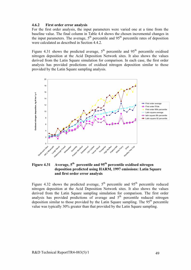
R&D Technical ReportTR4-083(5)/1 49
4.6.2 First order error analysisFor the first order analysis, the input parameters were varied one at a time from thebaseline value. The final column in Table 4.4 shows the chosen incremental changes inthe input parameters. The average, 5th percentile and 95th percentile rates of depositionwere calculated as described in Section 4.4.2.
Figure 4.31 shows the predicted average, 5th percentile and 95th percentile oxidisednitrogen deposition at the Acid Deposition Network sites. It also shows the valuesderived from the Latin Square simulation for comparison. In each case, the first orderanalysis has provided predictions of oxidised nitrogen deposition similar to thoseprovided by the Latin Square sampling analysis.
0
2
4
6
8
10
12
14
16
18
20
Strath
vaich
Dam
Allt a'
Mha
rcad
h
Loug
h Nav
ar
Hilsbo
roug
h For
est
Whit
eadd
er
Goonh
illy
Presto
n M
ontfo
rd
Eskda
lemuir
Llyn
Llyda
w
Yarne
r Woo
d
Thorg
anby
High M
uffle
s
Flatfo
rd M
ill
Stoke
Fer
ryDrib
y
War
dley H
ay C
op
Oxi
dise
d ni
trog
en d
epos
ition
, kg
N h
a-1
y-1
First order average
First order 5%ile
First order 95th percentile
Latin square average
latin square 8th percentile
Latin square 92 percentile
Figure 4.31 Average, 5th percentile and 95th percentile oxidised nitrogendeposition predicted using HARM, 1997 emissions: Latin Squareand first order error analysis
Figure 4.32 shows the predicted average, 5th percentile and 95th percentile reducednitrogen deposition at the Acid Deposition Network sites. It also shows the valuesderived from the Latin Square sampling simulation for comparison. The first orderanalysis has provided predictions of average and 5th percentile reduced nitrogendeposition similar to those provided by the Latin Square sampling. The 95th percentilevalue was typically 30% greater than that provided by the Latin Square sampling.
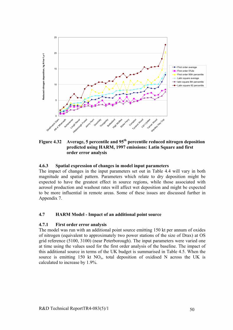
R&D Technical ReportTR4-083(5)/1 50
0
5
10
15
20
25
Strath
vaich
Dam
Allt a'
Mha
rcad
h
Achan
arra
s
Loug
h Nav
ar
Hilsbo
roug
h For
est
Jenn
y Hur
n
Goonh
illy
Thorg
anby
Botte
sford
High M
uffle
s
Stoke
Fer
ry
Compt
on
Tycan
ol W
ood
Llyn
Llyda
w
Yarne
r Woo
d
War
dley H
ay C
op
Red
uced
nitr
ogen
dep
ositi
on, k
g N
ha-
1 y-
1
First order average
First order 5%ile
First order 95th percentile
Latin square average
latin square 8th percentile
Latin square 92 percentile
Figure 4.32 Average, 5 percentile and 95th percentile reduced nitrogen depositionpredicted using HARM, 1997 emissions: Latin Square and firstorder error analysis
4.6.3 Spatial expression of changes in model input parametersThe impact of changes in the input parameters set out in Table 4.4 will vary in bothmagnitude and spatial pattern. Parameters which relate to dry deposition might beexpected to have the greatest effect in source regions, while those associated withaerosol production and washout rates will affect wet deposition and might be expectedto be more influential in remote areas. Some of these issues are discussed further inAppendix 7.
4.7 HARM Model - Impact of an additional point source
4.7.1 First order error analysisThe model was run with an additional point source emitting 150 kt per annum of oxidesof nitrogen (equivalent to approximately two power stations of the size of Drax) at OSgrid reference (5100, 3100) (near Peterborough). The input parameters were varied oneat time using the values used for the first order analysis of the baseline. The impact ofthis additional source in terms of the UK budget is summarised in Table 4.5. When thesource is emitting 150 kt NOx, total deposition of oxidised N across the UK iscalculated to increase by 1.9%.
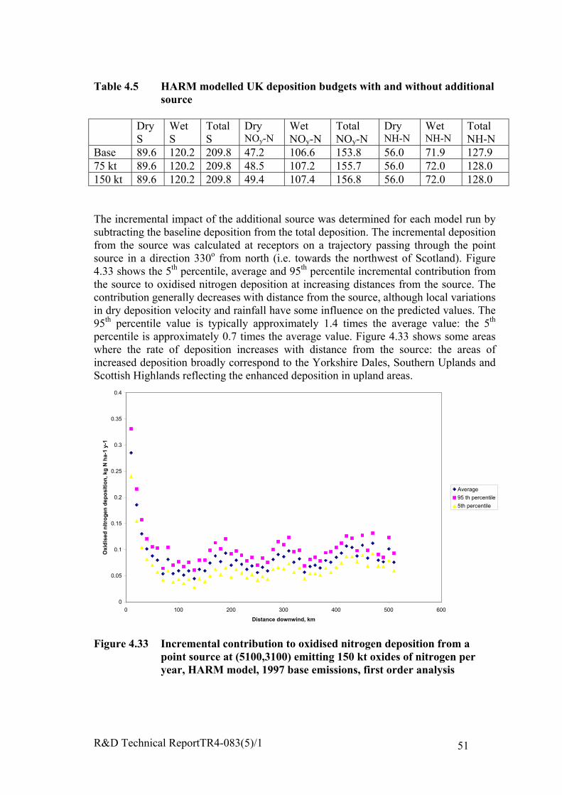
R&D Technical ReportTR4-083(5)/1 51
Table 4.5 HARM modelled UK deposition budgets with and without additionalsource
DryS
WetS
TotalS
DryNOy-N
WetNOy-N
TotalNOy-N
DryNH-N
WetNH-N
TotalNH-N
Base 89.6 120.2 209.8 47.2 106.6 153.8 56.0 71.9 127.975 kt 89.6 120.2 209.8 48.5 107.2 155.7 56.0 72.0 128.0150 kt 89.6 120.2 209.8 49.4 107.4 156.8 56.0 72.0 128.0
The incremental impact of the additional source was determined for each model run bysubtracting the baseline deposition from the total deposition. The incremental depositionfrom the source was calculated at receptors on a trajectory passing through the pointsource in a direction 330o from north (i.e. towards the northwest of Scotland). Figure4.33 shows the 5th percentile, average and 95th percentile incremental contribution fromthe source to oxidised nitrogen deposition at increasing distances from the source. Thecontribution generally decreases with distance from the source, although local variationsin dry deposition velocity and rainfall have some influence on the predicted values. The95th percentile value is typically approximately 1.4 times the average value: the 5th
percentile is approximately 0.7 times the average value. Figure 4.33 shows some areaswhere the rate of deposition increases with distance from the source: the areas ofincreased deposition broadly correspond to the Yorkshire Dales, Southern Uplands andScottish Highlands reflecting the enhanced deposition in upland areas.
0
0.05
0.1
0.15
0.2
0.25
0.3
0.35
0.4
0 100 200 300 400 500 600
Distance downwind, km
Oxi
dise
d ni
trog
en d
epos
ition
, kg
N h
a-1
y-1
Average
95 th percentile
5th percentile
Figure 4.33 Incremental contribution to oxidised nitrogen deposition from apoint source at (5100,3100) emitting 150 kt oxides of nitrogen peryear, HARM model, 1997 base emissions, first order analysis

R&D Technical ReportTR4-083(5)/1 52
4.8 FRAME
4.8.1 Sampling based on Latin SquareThe FRAME model was used to predict reduced nitrogen deposition for the baselinescenario for input parameters in ranges identified in the assessment described in Section3. The baseline scenario was based on the 1997 emissions inventory for the UK and forthe EMEP grid. The input ranges for each parameter are shown in Table 4.6. Values ofeach parameter were sampled at random from the range assuming a uniform distributionusing a sampling strategy based on a randomised Latin Square. Twelve model runs werecarried out with randomised input variables. The model experienced some stabilityproblems when relatively extreme values of the input parameters were used, particularlyfor dry deposition velocities and wet scavenging coefficients. The stability problemswere resolved by reducing the model time step: however, the time required to carry outthe model runs was considered excessive. Consequently all randomised model runswere carried out with these parameters set to their baseline values.
Figure 4.34 shows the predicted mean and 8th and 92nd percentile rates of reducednitrogen deposition at Acid Deposition Network sites throughout the United Kingdom.The mean values are a little larger than those predicted by the TRACK and HARMmodels. The 92nd percentile value is typically around twice the average: the average istypically around twice times the 8th percentile.
Table 4.6 Input ranges of parameters used in the Latin Square simulation andfirst order error analysis for the FRAME model
Parameter Units Baseline Range, % ofbaseline
Increment%
Lowerlimit
Upperlimit
Dry deposition velocity ofammonia
Land use andtime variable 10+ 2000+ 100
Dry deposition of HNO3 mm s-1 40 50+ 200+ 50 Dry deposition aerosols mm s-1 1 0+ 100+ -50Sulphur dioxide emission Inventory 50 200 50Ammonia emissions Inventory 50 200 50Oxides of nitrogen emissions Inventory 80 120 20Ammonium nitrateequilibrium factor
Appendix 1 50 200-50
Vertical dispersion coefficient Default value 50 200 100Boundary layer height m 800 80 120 20Wind speed m s-1 7.5 75 125 10+ Baseline value only used for Latin Square sampling
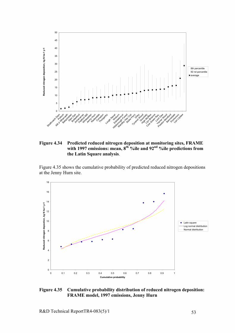
R&D Technical ReportTR4-083(5)/1 53
0
5
10
15
20
25
30
35
40
45
50
Strath
vaich
Dam
Polloc
h
Allt a'
Mha
rcad
h
Balquh
idder
Glen D
ye
Botte
sford
Achan
arra
s
Flatfo
rd M
ill
Whi
tead
der
Jenn
y Hur
n
Redes
dale
Compt
on
Thorg
anby
Loug
h Nav
ar
Wob
urn
Eskda
lemuir
Hilsbo
roug
h For
est
War
dley H
ay C
op
Stoke
Fer
ryDrib
y
Tycan
ol W
ood
Goonh
illy
High M
uffle
s
Llyn
Briann
e
Cow G
reen
Res
.
Loch
Dee
Yarne
r Woo
d
Presto
n M
ontfo
rd
Bannis
dale
Pumlum
on
Llyn
Llyda
w
Red
uced
nitr
ogen
dep
ositi
on, k
g N
ha-
1 y-
1
8th percentile
92 nd percentile
average
Figure 4.34 Predicted reduced nitrogen deposition at monitoring sites, FRAMEwith 1997 emissions: mean, 8th %ile and 92nd %ile predictions fromthe Latin Square analysis.
Figure 4.35 shows the cumulative probability of predicted reduced nitrogen depositionsat the Jenny Hurn site.
0
2
4
6
8
10
12
14
16
18
0 0.1 0.2 0.3 0.4 0.5 0.6 0.7 0.8 0.9 1
Cumulative probability
Red
uced
nitr
ogen
dep
sotio
n, k
g N
ha-
1 y-
1
Latin square
Log normal distribution
Normal distribution
Figure 4.35 Cumulative probability distribution of reduced nitrogen deposition:FRAME model, 1997 emissions, Jenny Hurn
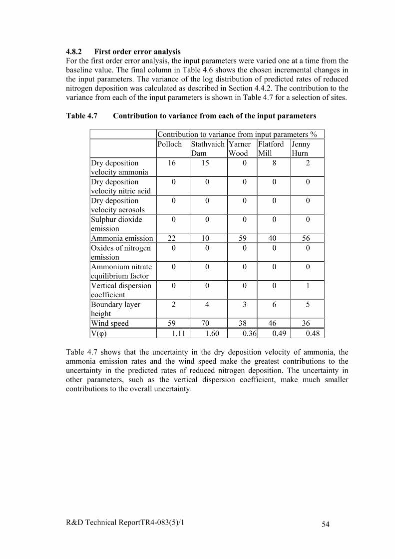
R&D Technical ReportTR4-083(5)/1 54
4.8.2 First order error analysisFor the first order error analysis, the input parameters were varied one at a time from thebaseline value. The final column in Table 4.6 shows the chosen incremental changes inthe input parameters. The variance of the log distribution of predicted rates of reducednitrogen deposition was calculated as described in Section 4.4.2. The contribution to thevariance from each of the input parameters is shown in Table 4.7 for a selection of sites.
Table 4.7 Contribution to variance from each of the input parameters
Contribution to variance from input parameters %Polloch Stathvaich
DamYarnerWood
FlatfordMill
JennyHurn
Dry depositionvelocity ammonia
16 15 0 8 2
Dry depositionvelocity nitric acid
0 0 0 0 0
Dry depositionvelocity aerosols
0 0 0 0 0
Sulphur dioxideemission
0 0 0 0 0
Ammonia emission 22 10 59 40 56Oxides of nitrogenemission
0 0 0 0 0
Ammonium nitrateequilibrium factor
0 0 0 0 0
Vertical dispersioncoefficient
0 0 0 0 1
Boundary layerheight
2 4 3 6 5
Wind speed 59 70 38 46 36V(φ) 1.11 1.60 0.36 0.49 0.48
Table 4.7 shows that the uncertainty in the dry deposition velocity of ammonia, theammonia emission rates and the wind speed make the greatest contributions to theuncertainty in the predicted rates of reduced nitrogen deposition. The uncertainty inother parameters, such as the vertical dispersion coefficient, make much smallercontributions to the overall uncertainty.
R&D Technical ReportTR4-083(5)/1 55
5 UNCERTAINTY IN CRITICAL LOADS
5.1 Introduction
Having undertaken detailed analysis of the likely uncertainties in estimates of aciddeposition over the U.K., it is appropriate to consider the uncertainty in theenvironmental objectives with which the deposition will be compared. The formaldefinition of a critical load is: "a quantitative estimate of an exposure to one or morepollutants below which significant harmful effects on specified sensitive elements of theenvironment do not occur according to present knowledge" (Nilsson and Grennfelt,1988). This definition was elaborated at a workshop at Skokloster in Sweden in 1988,and has been used to develop policy within the UNECE, and more recently the EU, eversince. The underlying notion is that of a threshold: if deposition is below the thresholdthere are no problems; if it is above the threshold, harm is being done to theenvironment. This is the way the concept is explained to policymakers: it thereforeappears to make sense to reduce deposition below the critical load as quickly aspossible, in order to avoid further harm.
But defining "significant harmful effects" for sensitive elements of the environment on aEuropean scale is a formidably difficult task. The natural environment is immenselycomplex, constantly changing, and not well understood. There are millions of species ofanimals, plants and micro-organisms interacting in an inconceivably vast number ofways with each other and with the physical environment. The response of only a few ofthese species to only a few pollutants is known over only a small range of conditions.Even for these, pollutant effects may be modified e.g. by interaction with otherpollutants, or by different physical conditions. Even then, species sometimes havegeographically distinct ecotypes with a different response to pollutants; there isinvariably a range of responses between individuals. Over large areas such as Europe,there are pronounced gradients in physical conditions that change the relativeimportance of ecosystem processes. Even if the response of species or ecosystems topollutants were known with certainty, data on species distribution and physicalcharacteristics of the environment would still need to be known at a fine scale. Thesedifficulties are of course not unique to the critical loads approach: they apply to thesetting of any sort of scientifically-based environmental quality standard. The criticalload approach attempts to overcome them by concentrating on certain species that areknown to be sensitive to pollutant deposition, or chemical substitutes for these, in thehope that this will also protect every other component of the ecosystem. It is clear thenthat the critical load threshold, if there is one, is likely to be very fuzzy.
Appendix 4 is a literature review of the analysis of uncertainty in critical loads. Itcontains a summary of the methods used to estimate critical loads, a description ofprevious uncertainty analyses for critical loads and a discussion of the issues associatedwith the validation of critical loads estimation methods and other factors contributing tothe uncertainty. The aim of Appendix 4 is to summarize current knowledge about theuncertainties entailed in estimating critical loads. Only an outline of critical load
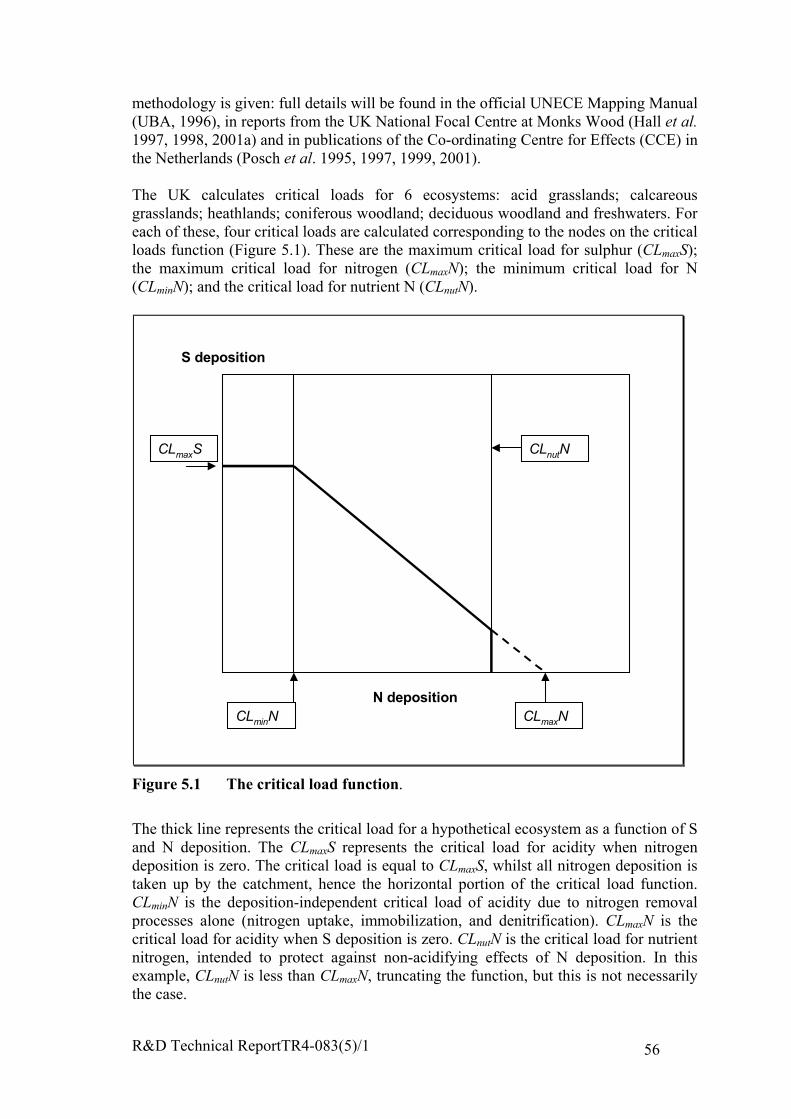
R&D Technical ReportTR4-083(5)/1 56
methodology is given: full details will be found in the official UNECE Mapping Manual(UBA, 1996), in reports from the UK National Focal Centre at Monks Wood (Hall et al.1997, 1998, 2001a) and in publications of the Co-ordinating Centre for Effects (CCE) inthe Netherlands (Posch et al. 1995, 1997, 1999, 2001).
The UK calculates critical loads for 6 ecosystems: acid grasslands; calcareousgrasslands; heathlands; coniferous woodland; deciduous woodland and freshwaters. Foreach of these, four critical loads are calculated corresponding to the nodes on the criticalloads function (Figure 5.1). These are the maximum critical load for sulphur (CLmaxS);the maximum critical load for nitrogen (CLmaxN); the minimum critical load for N(CLminN); and the critical load for nutrient N (CLnutN).
CLmaxNN deposition
S deposition
CLmaxS CLnutN
CLminN
Figure 5.1 The critical load function.
The thick line represents the critical load for a hypothetical ecosystem as a function of Sand N deposition. The CLmaxS represents the critical load for acidity when nitrogendeposition is zero. The critical load is equal to CLmaxS, whilst all nitrogen deposition istaken up by the catchment, hence the horizontal portion of the critical load function.CLminN is the deposition-independent critical load of acidity due to nitrogen removalprocesses alone (nitrogen uptake, immobilization, and denitrification). CLmaxN is thecritical load for acidity when S deposition is zero. CLnutN is the critical load for nutrientnitrogen, intended to protect against non-acidifying effects of N deposition. In thisexample, CLnutN is less than CLmaxN, truncating the function, but this is not necessarilythe case.
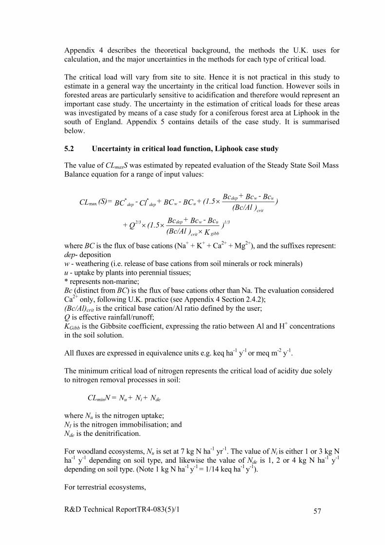
R&D Technical ReportTR4-083(5)/1 57
Appendix 4 describes the theoretical background, the methods the U.K. uses forcalculation, and the major uncertainties in the methods for each type of critical load.
The critical load will vary from site to site. Hence it is not practical in this study toestimate in a general way the uncertainty in the critical load function. However soils inforested areas are particularly sensitive to acidification and therefore would represent animportant case study. The uncertainty in the estimation of critical loads for these areaswas investigated by means of a case study for a coniferous forest area at Liphook in thesouth of England. Appendix 5 contains details of the case study. It is summarisedbelow.
5.2 Uncertainty in critical load function, Liphook case study
The value of CLmaxS was estimated by repeated evaluation of the Steady State Soil MassBalance equation for a range of input values:
where BC is the flux of base cations (Na+ + K+ + Ca2+ + Mg2+), and the suffixes represent:dep- depositionw - weathering (i.e. release of base cations from soil minerals or rock minerals)u - uptake by plants into perennial tissues;* represents non-marine;Bc (distinct from BC) is the flux of base cations other than Na. The evaluation consideredCa2+ only, following U.K. practice (see Appendix 4 Section 2.4.2);(Bc/Al)crit is the critical base cation/Al ratio defined by the user;Q is effective rainfall/runoff;KGibb is the Gibbsite coefficient, expressing the ratio between Al and H+ concentrationsin the soil solution.
All fluxes are expressed in equivalence units e.g. keq ha-1 y-1 or meq m-2 y-1.
The minimum critical load of nitrogen represents the critical load of acidity due solelyto nitrogen removal processes in soil:
CLminN = Nu + Ni + Nde
where Nu is the nitrogen uptake;NI is the nitrogen immobilisation; andNde is the denitrification.
For woodland ecosystems, Nu is set at 7 kg N ha-1 yr-1. The value of Ni is either 1 or 3 kg Nha-1 y-1 depending on soil type, and likewise the value of Nde is 1, 2 or 4 kg N ha-1 y-1
depending on soil type. (Note 1 kg N ha-1 y-1 = 1/14 keq ha-1 y-1).
For terrestrial ecosystems,
)K )(Bc/AlBc - Bc + Bc (1.5 Q +
))(Bc/Al
Bc - Bc + Bc (1.5 + BC - BC + Cl - BC = (S) CL
1/3
gibbcrit
uwdep2/3
crit
uwdepuw
*dep
*dep
×××
×max
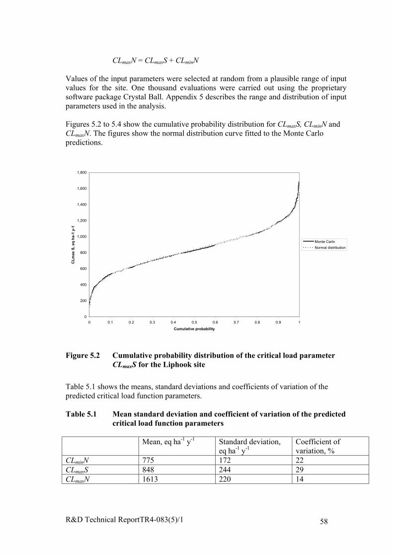
R&D Technical ReportTR4-083(5)/1 58
CLmaxN = CLmaxS + CLminN
Values of the input parameters were selected at random from a plausible range of inputvalues for the site. One thousand evaluations were carried out using the proprietarysoftware package Crystal Ball. Appendix 5 describes the range and distribution of inputparameters used in the analysis.
Figures 5.2 to 5.4 show the cumulative probability distribution for CLmaxS, CLminN andCLmaxN. The figures show the normal distribution curve fitted to the Monte Carlopredictions.
���������������������������������������������������������������������������������������������������������������������������������������
���������������������������������������������������������������������������������������������������������
�������������������������������������������������������������������������������������������������������������������������������������������������������������������������������������������
���������������������������������������������������������������������������������������������������������������������������������������������������������������������������������������������������������������������������
����������������������������������������������������������������������������������������������������������������������������������������������������������������������������������������������������������������������������������������������������������������������������
���������������������������������������������������������������������������������������������������������������������������������������������������������������������������������������������������������������������������������������������������������������������������������������
�����������������������������������������������������������������������������������������������������������������������������������������������������������������������������������������������������������������������������������������������������������������
������������������������������������������������������������������������������������������������������������������������������������������������������������������������������������������������������������������
���������������������������������������������������������������������������������������������������������������������������������������������������������������������
��������������������������������������������������������������������������������������������
������������������������������������������������������
�������������������������������������������������������������
0
200
400
600
800
1,000
1,200
1,400
1,600
1,800
0 0.1 0.2 0.3 0.4 0.5 0.6 0.7 0.8 0.9 1
Cumulative probability
CLm
ax S
, eq
ha-1
y-1
Monte Carlo����������Normal distribution
Figure 5.2 Cumulative probability distribution of the critical load parameterCLmaxS for the Liphook site
Table 5.1 shows the means, standard deviations and coefficients of variation of thepredicted critical load function parameters.
Table 5.1 Mean standard deviation and coefficient of variation of the predictedcritical load function parameters
Mean, eq ha-1 y-1 Standard deviation,eq ha-1 y-1
Coefficient ofvariation, %
CLminN 775 172 22CLmaxS 848 244 29CLmaxN 1613 220 14
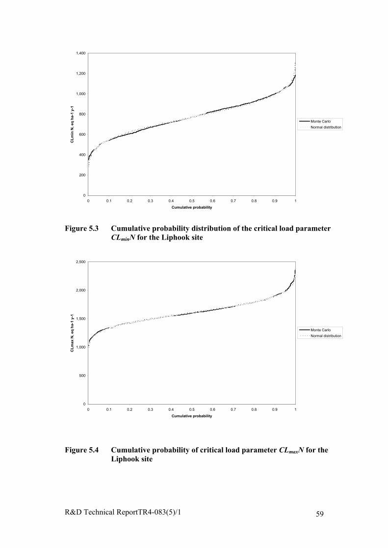
R&D Technical ReportTR4-083(5)/1 59
����������������������������������������������������������������������������������������������������������������������������������������������������������������������
������������������������������������������������������������������������������������������������������������������������������������������������������������
�������������������������������������������������������������������������������������������������������������������������������������������������������������������������������������������������������������������������������������
������������������������������������������������������������������������������������������������������������������������������������������������������������������������������������������������������������������������������������������������������������������������������������������������������
�������������������������������������������������������������������������������������������������������������������������������������������������������������������������������������������������������������������������������������������������������������������������������������������������������������������������������
����������������������������������������������������������������������������������������������������������������������������������������������������������������������������������������������������������������������������������������������������������������������������������������������������
����������������������������������������������������������������������������������������������������������������������������������������������������������������������������������������������������������������������������������
���������������������������������������������������������������������������������������������������������������������������������������������������������������
������������������������������������������������������������������������������������������
����������������������������������������
����������������������������������
0
200
400
600
800
1,000
1,200
1,400
0 0.1 0.2 0.3 0.4 0.5 0.6 0.7 0.8 0.9 1
Cumulative probability
CLm
in N
, eq
ha-1
y-1
Monte Carlo����������
Normal distribution
Figure 5.3 Cumulative probability distribution of the critical load parameterCLminN for the Liphook site
�����������������������������������������������������
������������������������������������������������������������������������������������������������������������
������������������������������������������������������������������������������������������������������������������������������������������������������������������������������������������������������������������������������������
������������������������������������������������������������������������������������������������������������������������������������������������������������������������������������������������������������������������������������������������������������������������������������������������������������������������������������������������������������������������������������������
��������������������������������������������������������������������������������������������������������������������������������������������������������������������������������������������������������������������������������������������������������������������������������������������������������������������������������������������������������������������������������������������������������������������������������������������������������������
�������������������������������������������������������������������������������������������������������������������������������������������������������������������������������������������������������������������������������������������������������������������������������������������������������������������������������������������������������������������������������������������
������������������������������������������������������������������������������������������������������������������������������������������������������������������������������������������������������������������������������
�����������������������������������������������������������������������������������������������������������
��������������������������������������
������������
0
500
1,000
1,500
2,000
2,500
0 0.1 0.2 0.3 0.4 0.5 0.6 0.7 0.8 0.9 1
Cumulative probability
CLm
ax N
, eq
ha-1
y-1
Monte Carlo����������Normal distribution
Figure 5.4 Cumulative probability of critical load parameter CLmaxN for theLiphook site
R&D Technical ReportTR4-083(5)/1 60
6 OVERALL UNCERTAINTY IN THE PREDICTION OFCRITICAL LOAD EXCEEDENCES
6.1 Introduction
The critical load exceedence, the extent to which the deposition exceeds the critical loaddefined by the critical load function, provides a measure of the extent to which the rateof deposition predicted by the acid deposition models exceeds the estimated critical loadat a particular site. It provides an indication of the likely potential for harm caused byacid deposition and the extent to which deposition should be reduced to prevent harm.The overall uncertainty in the exceedence prediction depends on the uncertainty in thepredictions of deposition and the estimates of the critical load. The combined overalluncertainty in exceedence for the case study site at Liphook is investigated in thissection.
6.2 Calculation of exceedence
The exceedence was calculated from:
NCLNNCLSNENCLNSCLSE
depdepdep
depdep
minmax
minmax
when when
≥−+=
<−=
which hold for the special case
CLmaxN = CLmaxS + CLminN
where Sdep is the total wet and dry deposition of sulphur, eq ha-1 y-1, andNdep is the total wet and dry deposition of oxidized and reduced nitrogen, eq ha-1 y-1.
The probability distribution of the exceedence was developed from the probabilitydistributions of the critical loads and the predicted rates of deposition by Monte Carlosimulation. For each of the 1000 joint estimates of CLmaxS, CLminN and CLmaxN (seeSection 5.2) a joint estimate of Sdep and Ndep was sampled at random from the 300randomized TRACK model runs (see Section 4.4.1). Figure 6.1 shows the probabilitydistribution of the predicted exceedence at the Liphook site for the TRACK predictionsusing the 1990 emissions inventory. It shows that the probability that the rate ofdeposition was less than the critical load was less than 0.1% i.e. there is a high degree ofconfidence that the critical load was exceeded.
Consideration was then given to the situation resulting from a reduction in the rates ofdeposition following a global reduction in emissions of sulphur dioxide and oxides ofnitrogen. Figures 6.2 to 6.5 show the cumulative distribution of exceedence forpredicted rates of deposition of 0.5, 0.2, 0.1 and 0.05 times the predicted rates for the1990 emission inventory. Note that the predicted rates of deposition are approximatelylog-normally distributed (see Section 4.4.1).
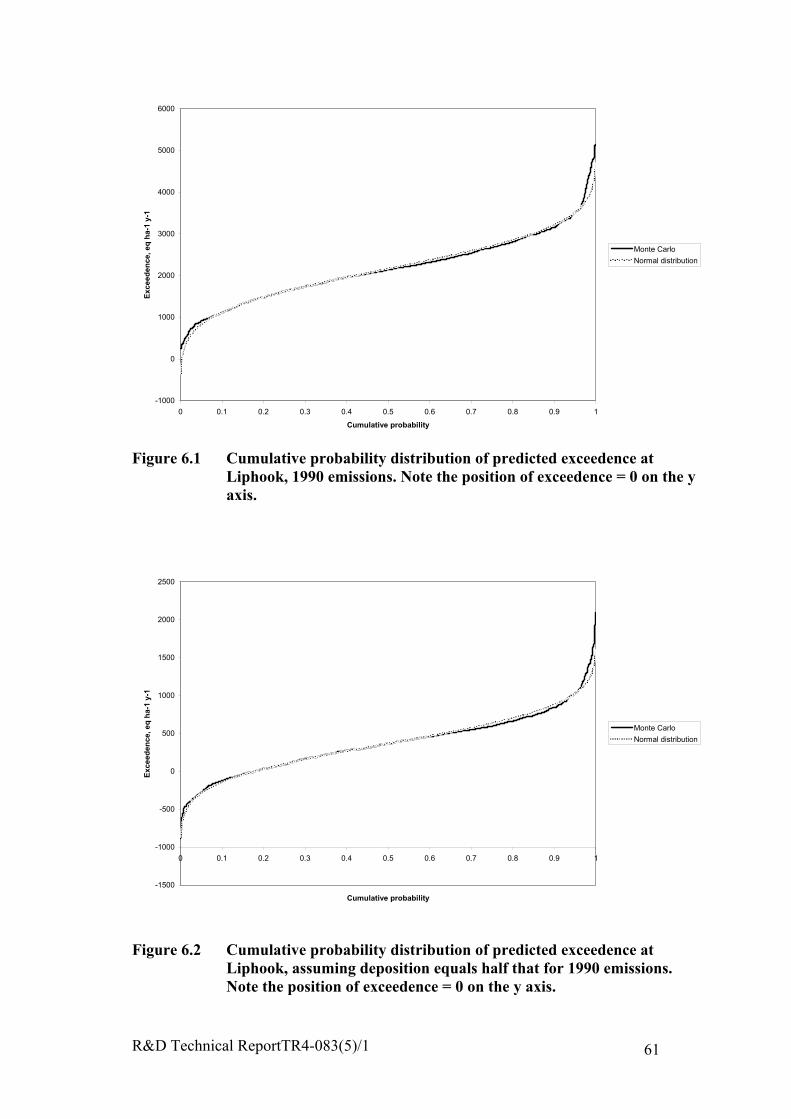
R&D Technical ReportTR4-083(5)/1 61
��������������������������������������������������������������������������������������������������������������������������������������������
������������������������������������������������������������������������������������������������������������������������������������������������������
���������������������������������������������������������������������������������������������������������������������������������������������������������������������������������������������������������������������������
�������������������������������������������������������������������������������������������������������������������������������������������������������������������������������������������������������������������������������������������������������������������������������������������������������������
������������������������������������������������������������������������������������������������������������������������������������������������������������������������������������������������������������������������������������������������������������������������������������������������������������������������������������������������
��������������������������������������������������������������������������������������������������������������������������������������������������������������������������������������������������������������������������������������������������������������������������������������������������������������������������
������������������������������������������������������������������������������������������������������������������������������������������������������������������������������������������������������������������������������������������
����������������������������������������������������������������������������������������������������������������������������������������������������������������
�������������������������������������������������������������������������������������
����������������������������������������������������������������������������������������
-1000
0
1000
2000
3000
4000
5000
6000
0 0.1 0.2 0.3 0.4 0.5 0.6 0.7 0.8 0.9 1
Cumulative probability
Exce
eden
ce, e
q ha
-1 y
-1
Monte Carlo���������
Normal distribution
Figure 6.1 Cumulative probability distribution of predicted exceedence atLiphook, 1990 emissions. Note the position of exceedence = 0 on the yaxis.
�����������������������������������������������
���������������������������������������������������
������������������������������������������������������������������������������������������������������������������������������������
�����������������������������������������������������������������������������������������������������������������������������������������������������������������������������������������������������������������������������
����������������������������������������������������������������������������������������������������������������������������������������������������������������������������������������������������������������������������������������������������������������������������������������������������������������������������������������
�������������������������������������������������������������������������������������������������������������������������������������������������������������������������������������������������������������������������������������������������������������������������������������������������������������������������������������������������������������������������������������������
�����������������������������������������������������������������������������������������������������������������������������������������������������������������������������������������������������������������������������������������������������������������������������������������������������������������������������������������������������
�����������������������������������������������������������������������������������������������������������������������������������������������������������������������������������������������������������������������������������������������
��������������������������������������������������������������������������������������������������������������������������������������������������������
�������������������������������������������������������������
���������������������������������������������������������
-1500
-1000
-500
0
500
1000
1500
2000
2500
0 0.1 0.2 0.3 0.4 0.5 0.6 0.7 0.8 0.9 1
Cumulative probability
Exce
eden
ce, e
q ha
-1 y
-1
Monte Carlo���������Normal distribution
Figure 6.2 Cumulative probability distribution of predicted exceedence atLiphook, assuming deposition equals half that for 1990 emissions.Note the position of exceedence = 0 on the y axis.

R&D Technical ReportTR4-083(5)/1 62
���������������������������������������������������������������������������������������������������
��������������������������������������������������������������������������������������
�������������������������������������������������������������������������������������������������������������������������������������������������������
�����������������������������������������������������������������������������������������������������������������������������������������������������������������������������������������������
�����������������������������������������������������������������������������������������������������������������������������������������������������������������������������������������������������������������������������������������������������������
����������������������������������������������������������������������������������������������������������������������������������������������������������������������������������������������������������������������������������������������������������������������������������������������
��������������������������������������������������������������������������������������������������������������������������������������������������������������������������������������������������������������������������������������������������������������������������������������������
��������������������������������������������������������������������������������������������������������������������������������������������������������������������������������������������������������������������������������������������
�������������������������������������������������������������������������������������������������������������������������������������������������������������������������������������
������������������������������������������������������������������������������������������������������������������������������������
���������������������������������������������������������������������
�������������������������������������������������������������������������������������������
-1400
-1200
-1000
-800
-600
-400
-200
0
200
400
600
0 0.1 0.2 0.3 0.4 0.5 0.6 0.7 0.8 0.9 1
Cumulative probability
Exce
eden
ce, e
q ha
-1 y
-1
Monte Carlo���������Normal distribution
Figure 6.3 Cumulative probability distribution of predicted exceedence atLiphook, deposition 20% of that for 1990 emissions. Note theposition of exceedence = 0 on the y axis.
���������������������������������������������������������������������������������������������������������������������������������������
�������������������������������������������������������������������������������������������������������������������������
��������������������������������������������������������������������������������������������������������������������������������������������������������������������������������������
����������������������������������������������������������������������������������������������������������������������������������������������������������������������������������������������������������������������������������������������
���������������������������������������������������������������������������������������������������������������������������������������������������������������������������������������������������������������������������������������������������������������������������������������������
�����������������������������������������������������������������������������������������������������������������������������������������������������������������������������������������������������������������������������������������������������������������������������������������������������
���������������������������������������������������������������������������������������������������������������������������������������������������������������������������������������������������������������������������������������������������������������������
������������������������������������������������������������������������������������������������������������������������������������������������������������������������������������������������������
������������������������������������������������������������������������������������������������������������������������������������������������������
������������������������������������������������������������������������������������
���������������������������������������������
�����������������������������������������������������
-1600
-1400
-1200
-1000
-800
-600
-400
-200
0
200
400
0 0.1 0.2 0.3 0.4 0.5 0.6 0.7 0.8 0.9 1
Cumulative probability
Exce
eden
ce, e
q ha
-1 y
-1
Monte Carlo������������������Normal distribution
Figure 6.4 Cumulative probability distribution of predicted exceedence atLiphook, deposition 10% of that for 1990 emissions. Note theposition of exceedence = 0 on the y axis.
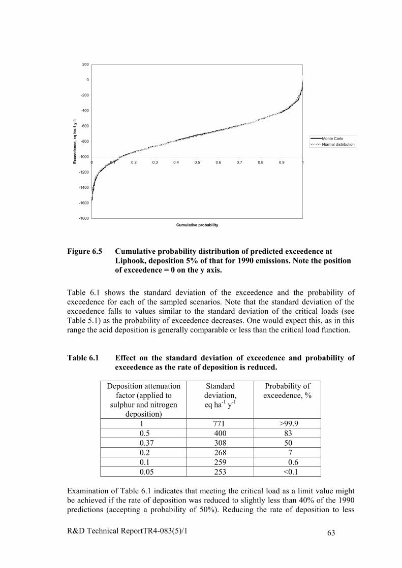
R&D Technical ReportTR4-083(5)/1 63
�����������������������������������������������������������������������������������������������������
��������������������������������������������������������������������������������������������
��������������������������������������������������������������������������������������������������������������������������������������������������������
��������������������������������������������������������������������������������������������������������������������������������������������������������������������������������������������������������������������
��������������������������������������������������������������������������������������������������������������������������������������������������������������������������������������������������������������������������������������������������������������������������������
����������������������������������������������������������������������������������������������������������������������������������������������������������������������������������������������������������������������������������������������������������������������������������������������������������
���������������������������������������������������������������������������������������������������������������������������������������������������������������������������������������������������������������������������������������������������������������������������������������������
������������������������������������������������������������������������������������������������������������������������������������������������������������������������������������������������������������������������������������
���������������������������������������������������������������������������������������������������������������������������������������������������������������������������
��������������������������������������������������������������������������������������������������
��������������������������������������������������
�����������������������������������������������������������������������
-1800
-1600
-1400
-1200
-1000
-800
-600
-400
-200
0
200
0 0.1 0.2 0.3 0.4 0.5 0.6 0.7 0.8 0.9 1
Cumulative probability
Exce
eden
ce, e
q ha
-1 y
-1
Monte Carlo���������Normal distribution
Figure 6.5 Cumulative probability distribution of predicted exceedence atLiphook, deposition 5% of that for 1990 emissions. Note the positionof exceedence = 0 on the y axis.
Table 6.1 shows the standard deviation of the exceedence and the probability ofexceedence for each of the sampled scenarios. Note that the standard deviation of theexceedence falls to values similar to the standard deviation of the critical loads (seeTable 5.1) as the probability of exceedence decreases. One would expect this, as in thisrange the acid deposition is generally comparable or less than the critical load function.
Table 6.1 Effect on the standard deviation of exceedence and probability ofexceedence as the rate of deposition is reduced.
Deposition attenuationfactor (applied to
sulphur and nitrogendeposition)
Standarddeviation,eq ha-1 y-1
Probability ofexceedence, %
1 771 >99.90.5 400 830.37 308 500.2 268 70.1 259 0.60.05 253 <0.1
Examination of Table 6.1 indicates that meeting the critical load as a limit value mightbe achieved if the rate of deposition was reduced to slightly less than 40% of the 1990predictions (accepting a probability of 50%). Reducing the rate of deposition to less
R&D Technical ReportTR4-083(5)/1 64
than 20% of the 1990 predictions would lead to a high degree of confidence (with aprobability of 95%) that the critical load was not exceeded. Table 6.1 shows that therisk of exceeding the critical load at Liphook decreases from very high to very low asthe rate of deposition decreases from 1990 levels to 5% of 1990 levels. This suggeststhat a probabilistic approach to the critical load and regional or national scale depositionmodels can be applied to regional scale emissions policy development.
The effect of an increase in deposition from an additional source on the risk ofexceedence may be assessed as follows. Take for example, a 150 kt per annum emissionof NOx, corresponding to a very large power station. Figure 4.25 for TRACK andFigure 4.33 for HARM indicate that the rate of deposition of oxidised nitrogen 50 kmfrom the source would be of the order of 0.1 kg N ha-1 y-1 or 7 eq ha-1 y-1. Thisincremental increase may be compared with Figures 6.1 to 6.5. The incremental sourcewill increase the risk of exceedence of the critical load by approximately 1% or less ineach case. This example would suggest that the critical load methodology and regionalscale acid deposition models have limited application for assessing the impact ofindividual emission sources of oxides of nitrogen at individual receptor sites, becausethe likely changes in the risk of exceedence are marginal.
For sulphur dioxide, Metcalfe and Whyatt(2000) have predicted the incrementalincrease in sulphur deposition from emissions from Drax power station at receptorsthroughout the UK. Maximum predicted rates of deposition were of the order of 2.25 kgS ha-1 y-1: the predicted rate of deposition at Liphook was approximately 1 kg S ha-1 y-1.These values correspond to 141 eq ha-1 y-1 and 63 eq ha-1 y-1 respectively. Referring toFigs 6.1 to 6.5, this additional deposition will increase the risk of exceedence of thecritical load by approximately 10% and 5 % respectively. This example would suggestthat the critical load methodology and regional scale acid deposition models may bemore useful for assessing the impact of individual emission sources of sulphur dioxide(rather than oxides of nitrogen) at individual receptor sites, because the likely changesin the risk of exceedence appear significant .
6.3 Integration of observed rates of deposition
The above assessment has assumed that the acid deposition model does notoverestimate the rates of deposition. In practice, the predicted rates of deposition maybe compared with observed or independently estimated rates of deposition at SecondaryNetwork sites throughout the United Kingdom. An integrated assessment approachwould allow the performance of the model at these sites to be taken into account whenestimating the likelihood of exceedence of the critical load at other sites. The integrationof observed data with model predictions is outside the scope of this project. However,the following approach is suggested for further investigation. It relies on the assumptionthat exceedence of the critical load at the location of interest is independent of theability of the model to predict rates of deposition at the observation sites.
For each model run, i , with input parameters xij , let the probability pi that the modeldoes not overestimate the observed rate of deposition be:
1+=
nk
p ii

R&D Technical ReportTR4-083(5)/1 65
where ki is the number of sites at which the predicted rate of deposition is less than orequal to the observed rate for the parameter set xij; i equals 1 to n, where n is the numberof sites, and j spans the range of parameters.
Then the overall probability for all m model runs that the model does not overestimatethe observed rate of deposition is:
11
+=∑=
m
p)Not(P
m
ii
Then the joint probability for all m model runs that the critical load is exceeded and themodel does not overestimate the rates of deposition is estimated to be:
11
+=∩∑=
m
p)NotEx(P
m
iiiδ
where δi =0 if the predicted acid deposition is less than or equal to the critical load, andδi =1 otherwise.
Then assuming that exceedence of the critical load is independent of the performance ofthe model at the observation sites, the probability of exceedence is:
)Not(P)NotEx(P)Ex(P ∩
=
While this approach seems inherently reasonable and simple to apply, giving greatestweight to those model runs where exceedence is predicted and the model underestimatesobserved rates of deposition, doubts remain about its statistical rigour.

R&D Technical ReportTR4-083(5)/1 66
7 CONCLUSIONS AND RECOMMENDATIONS
This report has been prepared as the result of successful collaboration between anumber of groups and is a model for further successful co-operation. The aciddeposition models HARM, FRAME and TRACK are simple trajectory modelsemploying broadly similar chemical reaction schemes. They have many commonfeatures and might be expected to demonstrate similar behaviour. The model equationsare to some extent amenable to analytical solution. Analytical solutions have beendeveloped as part of this project and have been used to help identify the critical inputparameters and to develop methods of data analysis.
The main variables in the equations within the models are:
1. Chemical reaction rate constants:2. Dry deposition velocities;3. Wet scavenging coefficients (including enhancement in high rainfall areas) ;4. Background concentrations of chemical species;5. Wind speed;6. Frequency of winds from each wind direction sector;7. Boundary layer height;8. Emissions;9. Speciation of emitted sulphur dioxide and oxides of nitrogen.
Plausible ranges of these input parameters have been identified based on literaturesurveys, current practice and expert judgement. The uncertainty in some of the inputparameters, such as the rate of reaction of simple gaseous species is quite small; theuncertainty in other parameters, such as the rate of reaction of gases with particulatematter may be quite large, approaching an order of magnitude.
A systematic sensitivity analysis of the uncertainty in the national emissions leads tosome estimates, notably for sulphur and nitrogen oxides, which are substantially lowerthan those which would have been estimated by expert judgement. It is not within thisstudy to explore alternative methodologies, but it is recognised that Monte Carloanalysis is not able to treat uncertainties in processes, which are unknown. In additionuncertainties in individual processes are treated as independent variables.
The basis of uncertainty assessment is to make multiple calculations using plausiblerange of parameter values. The uncertainty in sulphur deposition was investigated byMonte Carlo analysis of the analytical model with the values of input parametersselected from their plausible ranges. Maximum rates of sulphur deposition werepredicted close to the source. The 95th percentile of the predicted deposition rates wasapproximately a factor of 2 times the average value and the 5th percentile wasapproximately half the average value.
The analytical model was also used to carry out a first order error analysis of theuncertainty in sulphur deposition, in which each of the input variables was changed onevariable at a time. The first order analysis explained 95% of the overall variance
R&D Technical ReportTR4-083(5)/1 67
throughout the range of prediction. The major contributor to the overall variance ofpredicted values was the uncertainty in the dry deposition velocity for sulphur dioxidein the vicinity of the receptor. Other significant contributors to the variance were theuncertainties in the rate of emission, boundary layer height, wind speed, frequency ofthe wind direction in the relevant sector and the wet deposition coefficient for sulphurdioxide. At 800 km from the source, the largest contributors to the variance in thepredicted total sulphur deposition rate at receptors were the uncertainties in the drydeposition velocity for sulphur dioxide both upwind and local to the receptor.
The analytical model was used to compare the performance of Monte Carlo simulationwith that of more limited sampling based on the use of a Latin Square with only 13model runs. The Latin Square sampling strategy provided a reasonable estimate of thedistribution derived from the Monte Carlo analysis in the cumulative probability rangebetween 0.1 and 0.9, but provided little information at the extremes of the distribution.In both cases, the predicted distribution approximated to log-normal.
Results from the Monte Carlo simulations have possible implications for other studies,particularly those where the number of computer runs is restricted by practicalconsiderations. Table 7.1 summarises the advantages and disadvantages of thealternative sampling strategies in terms of the criteria affecting sensitivity analysis, suchas number of runs and ease of application. These may be important for future studies.
Monte Carlo analysis of the analytical model for nitrogen deposition was also carriedout. The 95th percentile of the predicted rates of deposition was approximately twice themean value and the 5th percentile was approximately one third of the mean value.Approximately 10 to 30% of the variance is not explained by first order analysis and isassociated with more complex interactions between parameters. The largest contributorsto the variance in the predicted rates of deposition were the background concentration ofthe hydroxyl radical, the wet deposition of the aerosols, the frequency of the winddirection, the wind speed, the rate constant for the formation of nitrogen pentoxide, therate of emission, and the rate constant for the formation of nitric acid.
Monte Carlo simulations of sulphur, oxidised nitrogen and reduced nitrogen depositionusing the TRACK model showed that: (a) the 95th percentile of predicted rates ofsulphur deposition at a range of sites throughout the UK (the Secondary Network sites)was typically 1.3 times the mean value predicted at each site: the mean was typicallyaround 1.45 times the 5th percentile, (b) the 95th percentile of predicted rates of oxidisednitrogen deposition was typically around 1.9 times the average: the average wastypically around 2 times the 5th percentile, and (c) the 95th percentile of predicted ratesof reduced nitrogen deposition was typically around 1.5 times the average: the averageis typically around 1.7 times the 5th percentile. The probability distributions of predictedrates of sulphur, oxidised and reduced nitrogen deposition were approximately log-normal.
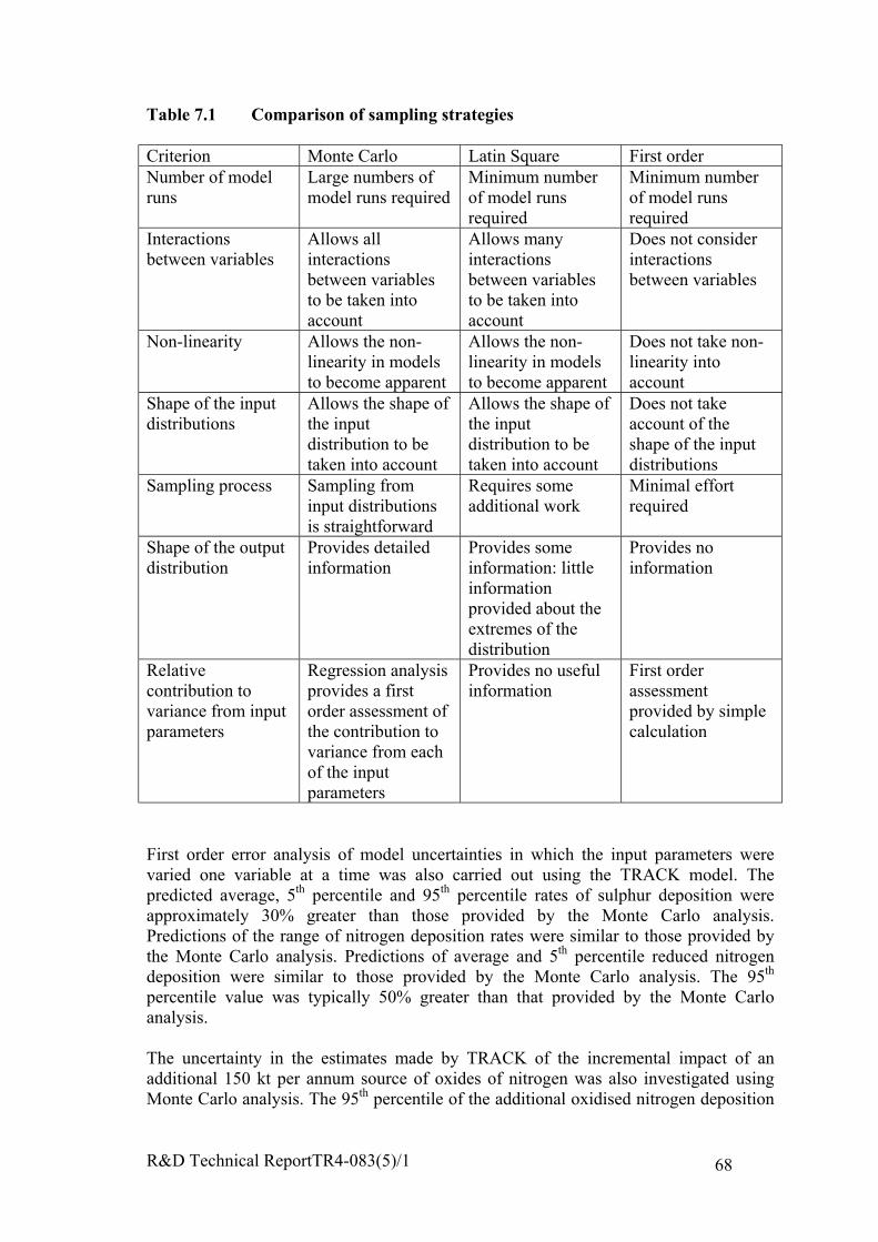
R&D Technical ReportTR4-083(5)/1 68
Table 7.1 Comparison of sampling strategies
Criterion Monte Carlo Latin Square First orderNumber of modelruns
Large numbers ofmodel runs required
Minimum numberof model runsrequired
Minimum numberof model runsrequired
Interactionsbetween variables
Allows allinteractionsbetween variablesto be taken intoaccount
Allows manyinteractionsbetween variablesto be taken intoaccount
Does not considerinteractionsbetween variables
Non-linearity Allows the non-linearity in modelsto become apparent
Allows the non-linearity in modelsto become apparent
Does not take non-linearity intoaccount
Shape of the inputdistributions
Allows the shape ofthe inputdistribution to betaken into account
Allows the shape ofthe inputdistribution to betaken into account
Does not takeaccount of theshape of the inputdistributions
Sampling process Sampling frominput distributionsis straightforward
Requires someadditional work
Minimal effortrequired
Shape of the outputdistribution
Provides detailedinformation
Provides someinformation: littleinformationprovided about theextremes of thedistribution
Provides noinformation
Relativecontribution tovariance from inputparameters
Regression analysisprovides a firstorder assessment ofthe contribution tovariance from eachof the inputparameters
Provides no usefulinformation
First orderassessmentprovided by simplecalculation
First order error analysis of model uncertainties in which the input parameters werevaried one variable at a time was also carried out using the TRACK model. Thepredicted average, 5th percentile and 95th percentile rates of sulphur deposition wereapproximately 30% greater than those provided by the Monte Carlo analysis.Predictions of the range of nitrogen deposition rates were similar to those provided bythe Monte Carlo analysis. Predictions of average and 5th percentile reduced nitrogendeposition were similar to those provided by the Monte Carlo analysis. The 95th
percentile value was typically 50% greater than that provided by the Monte Carloanalysis.
The uncertainty in the estimates made by TRACK of the incremental impact of anadditional 150 kt per annum source of oxides of nitrogen was also investigated usingMonte Carlo analysis. The 95th percentile of the additional oxidised nitrogen deposition

R&D Technical ReportTR4-083(5)/1 69
was approximately twice the average value: the 5th percentile was approximately halfthe average value.
The non-linearity of predictions of the incremental impact of additional sources wasinvestigated using the TRACK model. Far from the source, the incremental contributionfrom a 75 kt source of oxides of nitrogen was half that for a 150 kt source i.e. thepredictions varied linearly with emission. Closer to the source, the predictions wereslightly sublinear: the deposition of oxidised nitrogen associated with a 150 kt sourcewas only 1.8 times that for a 75 kt source.
The uncertainty in predictions of nitrogen deposition made by the HARM model wasinvestigated using a Latin Square sampling strategy. This approach required fewermodel runs than Monte Carlo simulation. The 92nd percentiles of the predicted rates ofoxidised and reduced nitrogen were typically around 1.5 times the mean values:averages were typically around 1.5 times the 8th percentiles. The probabilitydistributions of predicted rates of deposition approximated to log-normal.
First order error analysis of the uncertainty in HARM model predictions of oxidised andreduced nitrogen was also carried out. The first order error analysis provided predictionsof oxidised nitrogen deposition similar to those provided by the Latin Square samplinganalysis. Average and 5th percentile predictions of reduced nitrogen deposition weresimilar to those determined by Latin Square sampling: the 95th percentile value wastypically 30% greater than that provided by the Latin Square sampling.
To balance the uncertainty estimates in the calculation of deposition a review of theliterature on the uncertainty in critical loads was carried out. The review concluded thatfurther work was required to quantify the uncertainty in critical loads estimates. A casestudy for Liphook, a forested area in the south of England, was therefore carried out inorder to investigate the uncertainty in the critical load estimate at a well-documentedsite. The case study involved the standard procedure for estimating the critical load atthis site, but also conducting a Monte Carlo simulation, selecting input values fromplausible ranges for this well-documented site. The coefficients of variation of CLminN,CLmaxS and CLmaxN, the main parameters describing the critical load function at this site,were 22%, 30% and 14 % respectively. The probability distribution of the critical loadsapproximated to a normal distribution.
The uncertainty in the prediction of exceedence of the critical load i.e. deposition minuscritical load, at the Liphook site was investigated. Estimates of critical loads sampledfrom the case study Monte Carlo simulation were randomly matched with estimates ofthe rate of acid deposition sampled from the TRACK Monte Carlo simulation. Thesimulation indicated that there was a high probability (>99.9%) that the critical load wasexceeded at the site based on 1990 emissions. Reducing the rates of deposition toaround 40% of that for 1990 emissions would reduce the probability of exceedence toaround 50%. It would be necessary to reduce acid deposition to approximately 20 % ofthat predicted from 1990 emissions in order to have a high degree of confidence (95%)that the critical load was not exceeded at this site. This example suggests that the criticalload and deposition model methodology could, if required, be adapted to provide aprobabilistic assessment tool for emissions policies at the regional scale, despite theuncertainties in the critical loads function and rates of deposition.

R&D Technical ReportTR4-083(5)/1 70
The incremental contribution to sulphur and nitrogen deposition from a large pointsource was compared to the uncertainty in the exceedence at the Liphook site. For theexample considered, the incremental contribution to nitrogen deposition would increasethe risk of exceedence of the critical load by around 1%. Similarly, the incrementalcontribution to sulphur deposition would increase the risk of exceedence of the criticalload by approximately 10 to 20%. The example suggests that the uncertainties in thecritical load methodology and regional scale deposition models are too large for theimpact of individual sources of oxides of nitrogen at specific receptor sites to beassessed with confidence. The method may be more effective for assessing the impactof sulphur dioxide emissions.
The assessment of uncertainty carried out in this study does not take account ofmeasured rates of deposition. In practice, the predicted rates of deposition may becompared with observed, or independently estimated rates of deposition at SecondaryNetwork sites throughout the United Kingdom. An integrated assessment approachwould allow the comparison of the model estimates with measurements at these sites tobe taken included, improving the reliability of estimates of exceedence of the criticalload at other sites. A probabilistic method for incorporating measured deposition ratesin the assessment of uncertainty is suggested.
The following recommendations are made:
• The uncertainty in the prediction of rates of deposition resulting from theuncertainty in input parameters may be assessed by Monte Carlo analysis.
• Latin Square sampling or first order error analysis should provide usefulestimates of the uncertainty where Monte Carlo analysis is not practicalbecause it would not be practical to make the number model runs Thedistribution of predicted rates of deposition may be approximated by a log-normal distribution.
• The uncertainty in acid deposition models resulting from the uncertainty inthe input parameters may be broadly described as within a “factor of two”.Any estimate could be within a factor of two larger or smaller than the“best” prediction.
• Analytical deposition models may be used to test Monte Carlo techniques.Their real value may arise in their flexibility to optimise input parameterswhen comparing predictions against observations, using for exampleBayesian Monte-Carlo methods.
• The uncertainty in prediction of critical loads resulting from uncertainties ininput parameters may be assessed by Monte Carlo analysis.
• The uncertainty in predicting exceedence of critical loads may be obtainedby sampling from the probability distributions of the predicted critical loadsand rates of acid deposition.
• Further investigations should be carried out to integrate measurements ofrates of deposition into the analysis of uncertainty. The suggestedprobabilistic method would provide a practical means of investigation.
Given the extent of the inaccuracy in assessments of exceedence, which would probablynot be regarded as unexpected by the user community, a number of issues are raisedconcerning the critical loads methodology. The bounds on uncertainty in deposition arecomparable to the bandings associated with critical loads categories. These broadly span
R&D Technical ReportTR4-083(5)/1 71
factors of two, so that the uncertainty in deposition could be interpreted as equivalent toincorrectly assessing the critical load at a site by allocating the site to a wrong category,either one category more or less sensitive.
Estimates of future exceedence, in NEGTAP (2001) for example, suggest that the areaof exceedence of critical loads in the UK exceeds over 71% of sensitive ecosystemsover the period 1995-7, and this is expected to decline to 46% by 2010. Critical loadsfor eutrophication (NEGTAP, 2001) exceeded 25% of the UK with sensitive grasslandsin 1995-7, and 55% of the UK with heathland. These fractions are expected to decline tocirca 20% and 40% respectively in 2010. Reduced ammonia is the main contributor.These predicted fractions are based on estimates using the HARM model for sulphurand nitrogen oxides and the FRAME model for reduced nitrogen. These estimates arebased on ensuring that the “best” estimate of the deposition is less than the “best”estimate of the critical load (or appropriate critical load function). The intention offuture policy measures enacted through the Large Combustion Plant Directive and theGothenburg Protocol is to bring about the emissions reductions producing thesedeclines.
It is apparent that if the exceedence of critical loads is expressed in probabilistic terms,as developed in this study, the estimated improvement as a result of emissionsreductions may be different to those previously forecast, even though the same modelsare applied. The consequence of no longer applying absolute criteria to critical loadexceedences is not part of this study. However some general comments about thebenefits of emissions control can be made. Without absolute criteria, the percentagereduction in area exceeded cannot be used as the measure of improvement.Improvement will still occur as a result of emissions reductions and percentages maystill be one way of summarising the improvement. However an attempt to reduce thefractional area of the country where critical loads are exceeded to a very low percentagewill be sensitive to the way an exceedence is defined in probabilistic terms. Theexample shown in Chapter 6 (Figures 6.1 to 6.2) shows that a decision must be made asto what would be regarded as an acceptably low probability of exceedence,conventionally about 0.05. This probability will never be zero, and as the figures andTable 6.1 show a very low probability of exceedence is very hard to achieve. As thedeposition declines one approaches a region of diminishing returns, if one were torequire a very low probability of exceedence.
The uncertainty in estimates of exceedence also has important implications for thestrategy to be adopted for environmental improvement. Broadly, improvement requiresthe exceedence of critical loads to be minimised. One might therefore expect that ifcritical load exceedence cannot be assessed with great accuracy, as implied by thisstudy, detailed improvements plans based on detailed source reduction plans in specificareas, might not represent a justifiable optimal objective. Instead a more generalstrategy based on national or regional reductions across the board might be all thatcould be justified with any confidence, given the accuracy of the critical loadexceedence estimates.
R&D Technical ReportTR4-083(5)/1 72
8 REFERENCES
Charles, D., Jones, B.M.R., Salway, A.G., Eggleston, H.S. and Milne, R., 1998.Treatment of Uncertainties for National Estimates of Greenhouse Gas Emissions, AEATechnology, Report No AEAT-2688.
Clarke R.H., 1979. A model of the short and medium range dispersion of radionuclidesreleased to the atmosphere. The first report of a working group on atmosphericdispersion. National Radiological Protection Board. NRPB-R91
Derwent R.G., G.J. Dollard and S.E. Metcalfe, 1988. On the nitrogen budget for theUnited Kingdom and Northwest Europe. Q.J.R Meteorol. Soc., 114, 1127-1152.
Derwent R.G. and A.R. Curtis, 1998. Sensitivity and uncertainty analysis of the longrange transport and deposition of nitrogen and sulphur compounds in Europe.: aHowgood application. AERE Report R13284.
Finlayson-Pitts B.J. and J.N. Pitts, 2000. Chemistry of the upper and lower atmosphere.Academic Press.
Goodwin, J.W.L., Salway, A.G., Murrells, T.P., Dore, C.D., Passant, N.R., King, K.R.,Coleman, P.J., Hobson, M.M., Pye, S.T., & Watterson, J.D., 2002. UK Emissions of AirPollutants 1970-1999, AEA Technology plc, Report No. AEAT/ENV/R/0798.
Hall, J. R., 1993. Critical loads mapping at the UK Critical Loads Mapping Centre -data requirements and presentation. In Hornung, M. and Skeffington, R. A. CriticalLoads: Concept and Applications. ITE Report 28, 74-78 London, HMSO
Hall, J., Hornung, M., Freer-Smith, P., Loveland, P., Bradley, I., Langan, S., Dyke, K.,Gascoigne, J., and Bull, K., 1997. Current status of UK critical loads data - December1996 Report to UK Dept of the Environment, Institute of Terrestrial Ecology, MonksWood, Cambs.
Hall, J., Bull, K., Bradley, K., Curtis, C., Freer-Smith, P. H., Hornung, M., Howard, D.,Langan, S., Loveland, P., Reynolds, B., Ulyett, J., and Warr, T., 1998. Status of UKcritical loads and Exceedences January 1998. Part 1 - critical loads and critical loadmaps Report to UK Department of the Environment, Institute of Terrestrial Ecology,Monks Wood, Cambs.
Hall, J., Hornung, M., Kennedy, F., Reynolds, B., Curtis, C., Langan, S., and Fowler, D., 2001a. Status of UK critical loads and Exceedences: Part 1 Critical loads and criticalload maps, update to January 1998 report, CEH, Monks Wood, Cambridge.
Hall, J., Reynolds, B., Aherne, J. and Hornung, M., 2001b. The importance of selectingappropriate criteria for calculating critical loads for terrestrial ecosystems using thesimple mass balance equation. Water, Air and Soil Pollution, Focus, 1, 29-41.
R&D Technical ReportTR4-083(5)/1 73
Hall, J., Hornung, M., Kennedy, F., Langan, S., Reynolds, B. and Aherne, J., 2001c.Investigating the uncertainties in the Simple Mass Balance equation for acidity criticalloads for terrestrial ecosystems. Water, Air and Soil Pollution, Focus, 1, 43-56.
IPCC (Intergovernmental Panel on Climate Change), 2000. Good Practice Guidanceand Uncertainty Management in National Greenhouse Gas Inventories, IPCC.
J.A. Jones, 1983. Models to allow for the effects of coastal sites, plume rise andbuildings on dispersion of radionuclides and guidance on the value of depositionvelocity and washout coefficients. National Radiological Protection Board Fifth Reportof a Working Group on Atmospheric Dispersion. NRPB R157.
D.S. Lee, R.D. Kingdon, M.E. Jenkin and J.A. Garland, 2000. Modelling theatmospheric oxidised and reduced nitrogen budgets for the UK with a Lagrangianmulti-layer long-range transport model. Environmental modelling and assessment, 5,83-104.
S.E. Metcalfe, J.D. Whyatt and R.G. Derwent, 1995. A comparison of model andobserved network estimates of sulphur deposition across Great Britain for 1990 and itslikely source attribution. Q.J.R Meteorol. Soc., 121, 1387-1411.
Metcalfe S.E. and Whyatt J.D., 2000. Linearity of sulphur chemistry in the HARMatmospheric transport and deposition model. Environment Agency R&D TechnicalReport P275.
National Expert Group on Transboundary Air Pollution (NEGTAP), 2001.Transboundary air pollution: Acidification, eutrophication and ground-level ozone inthe U.K. CEH Edinburgh Report ISBN 1 870393 619
Nilsson, J and Grennfelt, P., 1988. Critical loads for sulphur and nitrogen Report1988:15, Nordic Council of Ministers, Copenhagen.
Pasquill F. and F.B. Smith., 1983. Atmospheric diffusion. Third edition. Ellis HorwoodLimited.
Posch, M., de Smet, P. A. M., Hettelingh, J.-P., and Downing, R. J., 1995. Calculationand Mapping of Critical Thresholds in Europe 259101004, RIVM, Bilthoven, TheNetherlands.
Posch, M., Hettelingh, J.-P., de Smet, P. A. M., and Downing, R. J., 1997. Calculationand Mapping of Critical Thresholds in Europe 259101007, RIVM, Bilthoven, TheNetherlands.
Posch, M., de Smet, P. A. M., Hettelingh, J.-P., and Downing, R. J., 1999. Calculationand Mapping of Critical Thresholds in Europe 259101009, RIVM, Bilthoven, TheNetherlands.
Posch, M., de Smet, P. A. M., Hettelingh, J.-P., and Downing, R. J., 2001. Modellingand mapping of critical thresholds in Europe: Status Report 2001, RIVM Report259101010, RIVM, Bilthoven, The Netherlands.
R&D Technical ReportTR4-083(5)/1 74
Posch, M.and Hettelingh, J.-P., 2001. From critical loads to dynamic modelling. InPosch, M., de Smet, P. A. M., Hettelingh, J.-P., and Downing, R. J. Modelling andmapping of critical thresholds in Europe: Status Report 2001. RIVM Report259101010, pp 33-39 RIVM Bilthoven, The Netherlands,.
Salway, A.G., Murrells, T.P., Milne, R., and Ellis, S., 2001. UK Greenhouse GasInventory, 1990 to 1999, AEA Technology plc, Report No. AEAT/ENV/R/0524
R. Singles, 1996. Ph. D. Thesis. University of Edinburgh.
R. Singles, M.A. Sutton and K.J. Weston, 1998. A multi-layer model to describe theatmospheric transport and deposition of ammonia in Great Britain. AtmosphericEnvironment, 32, 393-399.
UBA, 1996. Manual on Methodologies and Criteria for Mapping Critical Levels /Loads and Geographical Areas where they are Exceeded. Texte 71:96,Umweltbundesamt, Berlin.
Underwood B. Y., 2001. Review of deposition velocity and washout coefficient. AEATechnology, Harwell.
US Environmental Protection Agency, 2001. Compilation of air pollution emissionsources. AP42. [www.epa.gov/ttn/chief/ap42/index.html]

R&D Technical Report TR4-083(5)1 Appendix 1-1
Appendices
CONTENTS
Appendix 1 TRACK, HARM and FRAME model chemistryAppendix 2 Analytical Model for sulphur depositionAppendix 3 Analytical model for nitrogen depositionAppendix 4 Analysis of uncertainty in critical loads: literature
reviewAppendix 5 Liphook critical loads case studyAppendix 6 Liphook critical loads case study outputsAppendix 7 Implications of parameter variations for nitrogen
deposition modelled using the HARM model

R&D Technical Report TR4-083(5)/1 Appendix 1-1
1 TRACK, HARM and FRAME model chemistry
CONTENTS
(a) HARM model chemistry(b) TRACK model chemistry(c) FRAME model chemistry(d) Comments on the HARM chemical mechanism(e) Comments on the TRACK chemical mechanism(f) Comments on the FRAME chemical mechanism(g) Notes(h) References
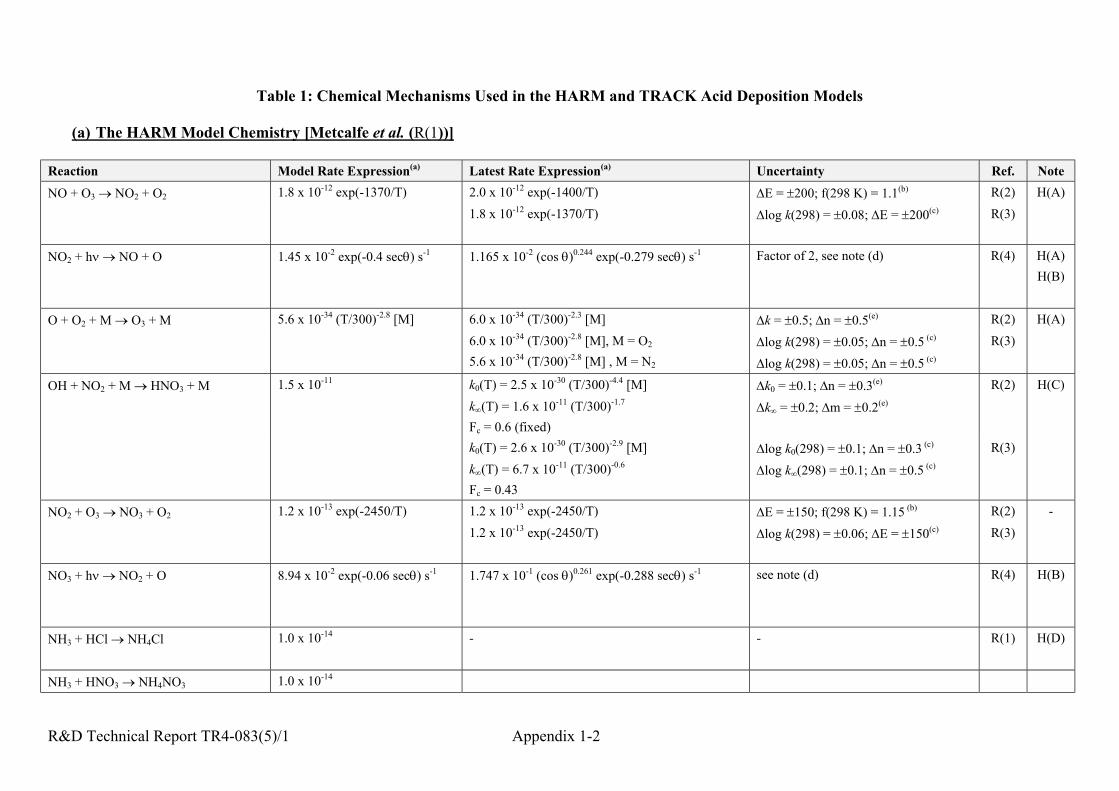
R&D Technical Report TR4-083(5)/1 Appendix 1-2
Table 1: Chemical Mechanisms Used in the HARM and TRACK Acid Deposition Models
(a) The HARM Model Chemistry [Metcalfe et al. (R(1))]
Reaction Model Rate Expression(a) Latest Rate Expression(a) Uncertainty Ref. Note
NO + O3 → NO2 + O2 1.8 x 10⁻¹² exp(-1370/T) 2.0 x 10⁻¹² exp(-1400/T) ∆E = ±200; f(298 K) = 1.1(b) R(2) H(A)1.8 x 10⁻¹² exp(-1370/T) ∆log k(298) = ±0.08; ∆E = ±200(c) R(3)
NO2 + hν → NO + O 1.45 x 10⁻² exp(-0.4 secθ) s-1 1.165 x 10⁻² (cos θ)0.244 exp(-0.279 secθ) s-1 Factor of 2, see note (d) R(4) H(A)H(B)
O + O2 + M → O3 + M 5.6 x 10⁻³⁴ (T/300)-2.8 [M] 6.0 x 10⁻³⁴ (T/300)-2.3 [M] ∆k = ±0.5; ∆n = ±0.5(e) R(2) H(A)6.0 x 10⁻³⁴ (T/300)-2.8 [M], M = O2
5.6 x 10⁻³⁴ (T/300)-2.8 [M] , M = N2
∆log k(298) = ±0.05; ∆n = ±0.5 (c)
∆log k(298) = ±0.05; ∆n = ±0.5 (c)
R(3)
OH + NO2 + M → HNO3 + M 1.5 x 10⁻¹¹ k0(T) = 2.5 x 10⁻³⁰ (T/300)-4.4 [M]k∞(T) = 1.6 x 10⁻¹¹ (T/300)-1.7
Fc = 0.6 (fixed)
∆k0 = ±0.1; ∆n = ±0.3(e)
∆k∞ = ±0.2; ∆m = ±0.2(e)
R(2) H(C)
k0(T) = 2.6 x 10⁻³⁰ (T/300)-2.9 [M]k∞(T) = 6.7 x 10⁻¹¹ (T/300)-0.6
Fc = 0.43
∆log k0(298) = ±0.1; ∆n = ±0.3 (c)
∆log k∞(298) = ±0.1; ∆n = ±0.5 (c)
R(3)
NO2 + O3 → NO3 + O2 1.2 x 10⁻¹³ exp(-2450/T) 1.2 x 10⁻¹³ exp(-2450/T) ∆E = ±150; f(298 K) = 1.15 (b) R(2) -1.2 x 10⁻¹³ exp(-2450/T) ∆log k(298) = ±0.06; ∆E = ±150(c) R(3)
NO3 + hν → NO2 + O 8.94 x 10⁻² exp(-0.06 secθ) s-1 1.747 x 10⁻¹ (cos θ)0.261 exp(-0.288 secθ) s-1 see note (d) R(4) H(B)
NH3 + HCl → NH4Cl 1.0 x 10⁻¹⁴ - - R(1) H(D)
NH3 + HNO3 → NH4NO3 1.0 x 10⁻¹⁴
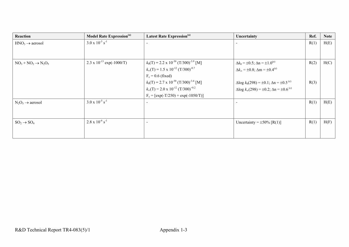
R&D Technical Report TR4-083(5)/1 Appendix 1-3
Reaction Model Rate Expression(a) Latest Rate Expression(a) Uncertainty Ref. Note
HNO3 → aerosol 3.0 x 10⁻⁵ s-1 - - R(1) H(E)
NO3 + NO2 → N2O5 2.3 x 10⁻¹³ exp(-1000/T) k0(T) = 2.2 x 10⁻³⁰ (T/300)-3.9 [M]k∞(T) = 1.5 x 10⁻¹² (T/300)-0.7
Fc = 0.6 (fixed)
∆k0 = ±0.5; ∆n = ±1.0(e)
∆k∞ = ±0.8; ∆m = ±0.4(e)
R(2) H(C)
k0(T) = 2.7 x 10⁻³⁰ (T/300)-3.4 [M]k∞(T) = 2.0 x 10⁻¹² (T/300)+0.2
Fc = [exp(-T/250) + exp(-1050/T)]
∆log k0(298) = ±0.1; ∆n = ±0.5 (c)
∆log k∞(298) = ±0.2; ∆n = ±0.6 (c)
R(3)
N2O5 → aerosol 3.0 x 10⁻⁵ s-1 - - R(1) H(E)
SO2 → SO4 2.8 x 10⁻⁶ s-1 - Uncertainty = ±50% [R(1)] R(1) H(F)
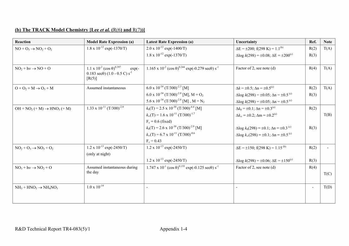
R&D Technical Report TR4-083(5)/1 Appendix 1-4
(b) The TRACK Model Chemistry [Lee et al. (R(6) and R(7))]
Reaction Model Rate Expression (a) Latest Rate Expression (a) Uncertainty Ref. Note
NO + O3 → NO2 + O2 1.8 x 10⁻¹² exp(-1370/T) 2.0 x 10⁻¹² exp(-1400/T) ∆E = ±200; f(298 K) = 1.1(b) R(2) T(A)1.8 x 10⁻¹² exp(-1370/T) ∆log k(298) = ±0.08; ∆E = ±200(c) R(3)
NO2 + hν → NO + O 1.1 x 10⁻² (cos θ)0.397 exp(-0.183 secθ) (1.0 - 0.5 C) s-1
[R(5)]
1.165 x 10⁻² (cos θ)0.244 exp(-0.279 secθ) s-1 Factor of 2, see note (d) R(4) T(A)
O + O2 + M → O3 + M Assumed instantaneous 6.0 x 10⁻³⁴ (T/300)-2.3 [M] ∆k = ±0.5; ∆n = ±0.5(e) R(2) T(A)6.0 x 10⁻³⁴ (T/300)-2.8 [M], M = O2
5.6 x 10⁻³⁴ (T/300)-2.8 [M] , M = N2
∆log k(298) = ±0.05; ∆n = ±0.5 (c)
∆log k(298) = ±0.05; ∆n = ±0.5 (c)
R(3)
OH + NO2 (+ M) → HNO3 (+ M) 1.33 x 10⁻¹¹ (T/300)-2.0 k0(T) = 2.5 x 10⁻³⁰ (T/300)-4.4 [M]k∞(T) = 1.6 x 10⁻¹¹ (T/300)-1.7
Fc = 0.6 (fixed)
∆k0 = ±0.1; ∆n = ±0.3(e)
∆k∞ = ±0.2; ∆m = ±0.2(e)
R(2)T(B)
k0(T) = 2.6 x 10⁻³⁰ (T/300)-2.9 [M]k∞(T) = 6.7 x 10⁻¹¹ (T/300)-0.6
Fc = 0.43
∆log k0(298) = ±0.1; ∆n = ±0.3 (c)
∆log k∞(298) = ±0.1; ∆n = ±0.5 (c)
R(3)
NO2 + O3 → NO3 + O2 1.2 x 10⁻¹³ exp(-2450/T)(only at night)
1.2 x 10⁻¹³ exp(-2450/T) ∆E = ±150; f(298 K) = 1.15 (b) R(2) -
1.2 x 10⁻¹³ exp(-2450/T) ∆log k(298) = ±0.06; ∆E = ±150(c) R(3)
NO3 + hν → NO2 + O Assumed instantaneous duringthe day
1.747 x 10⁻¹ (cos θ)0.155 exp(-0.125 secθ) s-1 Factor of 2, see note (d) R(4)T(C)
NH3 + HNO3 → NH4NO3 1.0 x 10⁻¹⁴ - - - T(D)
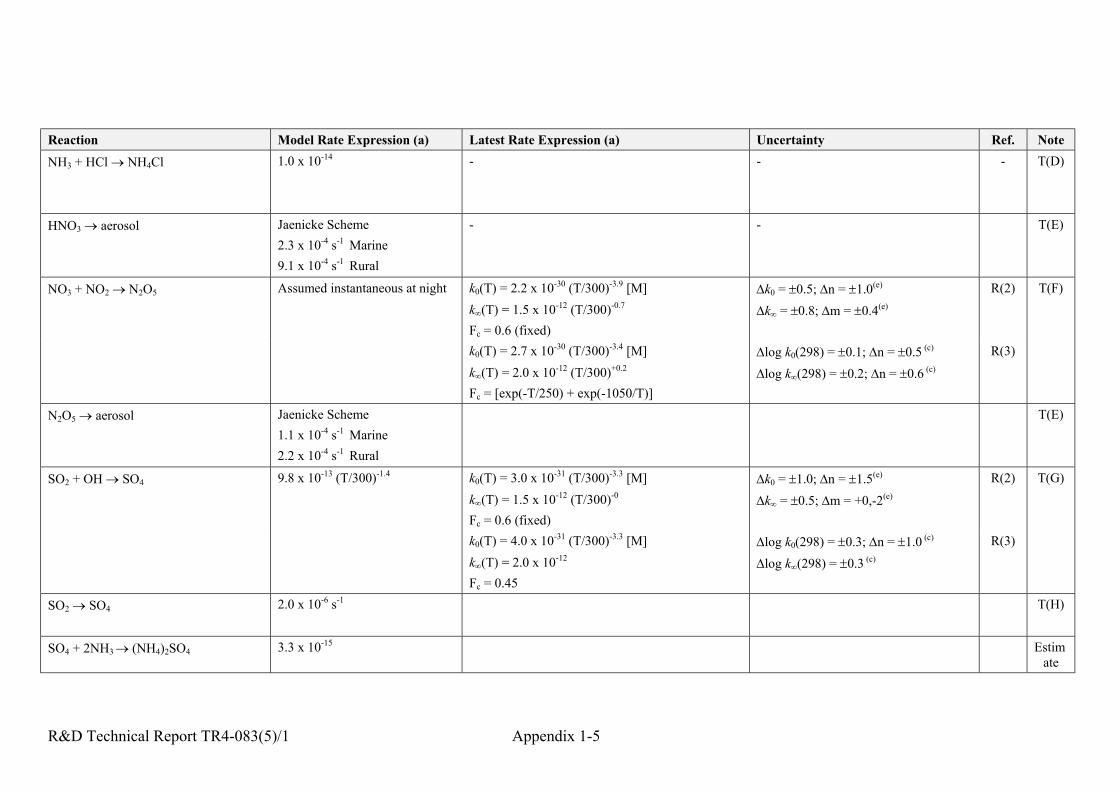
R&D Technical Report TR4-083(5)/1 Appendix 1-5
Reaction Model Rate Expression (a) Latest Rate Expression (a) Uncertainty Ref. Note
NH3 + HCl → NH4Cl 1.0 x 10⁻¹⁴ - - - T(D)
HNO3 → aerosol Jaenicke Scheme2.3 x 10-4 s-1 Marine9.1 x 10-4 s-1 Rural
- - T(E)
NO3 + NO2 → N2O5 Assumed instantaneous at night k0(T) = 2.2 x 10⁻³⁰ (T/300)-3.9 [M]k∞(T) = 1.5 x 10⁻¹² (T/300)-0.7
Fc = 0.6 (fixed)
∆k0 = ±0.5; ∆n = ±1.0(e)
∆k∞ = ±0.8; ∆m = ±0.4(e)
R(2) T(F)
k0(T) = 2.7 x 10⁻³⁰ (T/300)-3.4 [M]k∞(T) = 2.0 x 10⁻¹² (T/300)+0.2
Fc = [exp(-T/250) + exp(-1050/T)]
∆log k0(298) = ±0.1; ∆n = ±0.5 (c)
∆log k∞(298) = ±0.2; ∆n = ±0.6 (c)
R(3)
N2O5 → aerosol Jaenicke Scheme1.1 x 10-4 s-1 Marine2.2 x 10-4 s-1 Rural
T(E)
SO2 + OH → SO4 9.8 x 10⁻¹³ (T/300)-1.4 k0(T) = 3.0 x 10⁻³¹ (T/300)-3.3 [M]k∞(T) = 1.5 x 10⁻¹² (T/300)-0
Fc = 0.6 (fixed)
∆k0 = ±1.0; ∆n = ±1.5(e)
∆k∞ = ±0.5; ∆m = +0,-2(e)
R(2) T(G)
k0(T) = 4.0 x 10⁻³¹ (T/300)-3.3 [M]k∞(T) = 2.0 x 10⁻¹²
Fc = 0.45
∆log k0(298) = ±0.3; ∆n = ±1.0 (c)
∆log k∞(298) = ±0.3 (c)
R(3)
SO2 → SO4 2.0 x 10⁻⁶ s-1 T(H)
SO4 + 2NH3 → (NH4)2SO4 3.3 x 10⁻¹⁵ Estimate
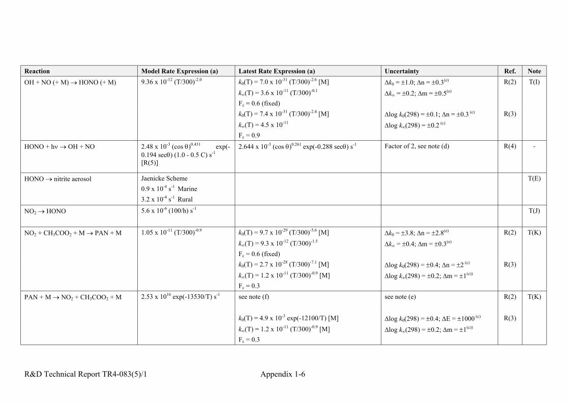
R&D Technical Report TR4-083(5)/1 Appendix 1-6
Reaction Model Rate Expression (a) Latest Rate Expression (a) Uncertainty Ref. Note
OH + NO (+ M) → HONO (+ M) 9.36 x 10⁻¹² (T/300)-2.0 k0(T) = 7.0 x 10⁻³¹ (T/300)-2.6 [M]k∞(T) = 3.6 x 10⁻¹¹ (T/300)-0.1
Fc = 0.6 (fixed)
∆k0 = ±1.0; ∆n = ±0.3(e)
∆k∞ = ±0.2; ∆m = ±0.5(e)
R(2) T(I)
k0(T) = 7.4 x 10⁻³¹ (T/300)-2.4 [M]k∞(T) = 4.5 x 10⁻¹¹
Fc = 0.9
∆log k0(298) = ±0.1; ∆n = ±0.3 (c)
∆log k∞(298) = ±0.2 (c)
R(3)
HONO + hν → OH + NO 2.48 x 10⁻³ (cos θ)0.431 exp(-0.194 secθ) (1.0 - 0.5 C) s-1
[R(5)]
2.644 x 10⁻³ (cos θ)0.261 exp(-0.288 secθ) s-1 Factor of 2, see note (d) R(4) -
HONO → nitrite aerosol Jaenicke Scheme0.9 x 10-4 s-1 Marine3.2 x 10-4 s-1 Rural
T(E)
NO2 → HONO 5.6 x 10⁻⁶ (100/h) s-1 T(J)
NO2 + CH3COO2 + M → PAN + M 1.05 x 10⁻¹¹ (T/300)-0.9 k0(T) = 9.7 x 10⁻²⁹ (T/300)-5.6 [M]k∞(T) = 9.3 x 10⁻¹² (T/300)-1.5
Fc = 0.6 (fixed)
∆k0 = ±3.8; ∆n = ±2.8(e)
∆k∞ = ±0.4; ∆m = ±0.3(e)
R(2) T(K)
k0(T) = 2.7 x 10⁻²⁸ (T/300)-7.1 [M]k∞(T) = 1.2 x 10⁻¹¹ (T/300)-0.9 [M]Fc = 0.3
∆log k0(298) = ±0.4; ∆n = ±2 (c)
∆log k∞(298) = ±0.2; ∆m = ±1(c))
R(3)
PAN + M → NO2 + CH3COO2 + M 2.53 x 10¹⁶ exp(-13530/T) s-1 see note (f) see note (e) R(2) T(K)
k0(T) = 4.9 x 10⁻³ exp(-12100/T) [M]k∞(T) = 1.2 x 10⁻¹¹ (T/300)-0.9 [M]Fc = 0.3
∆log k0(298) = ±0.4; ∆E = ±1000 (c)
∆log k∞(298) = ±0.2; ∆m = ±1(c))
R(3)
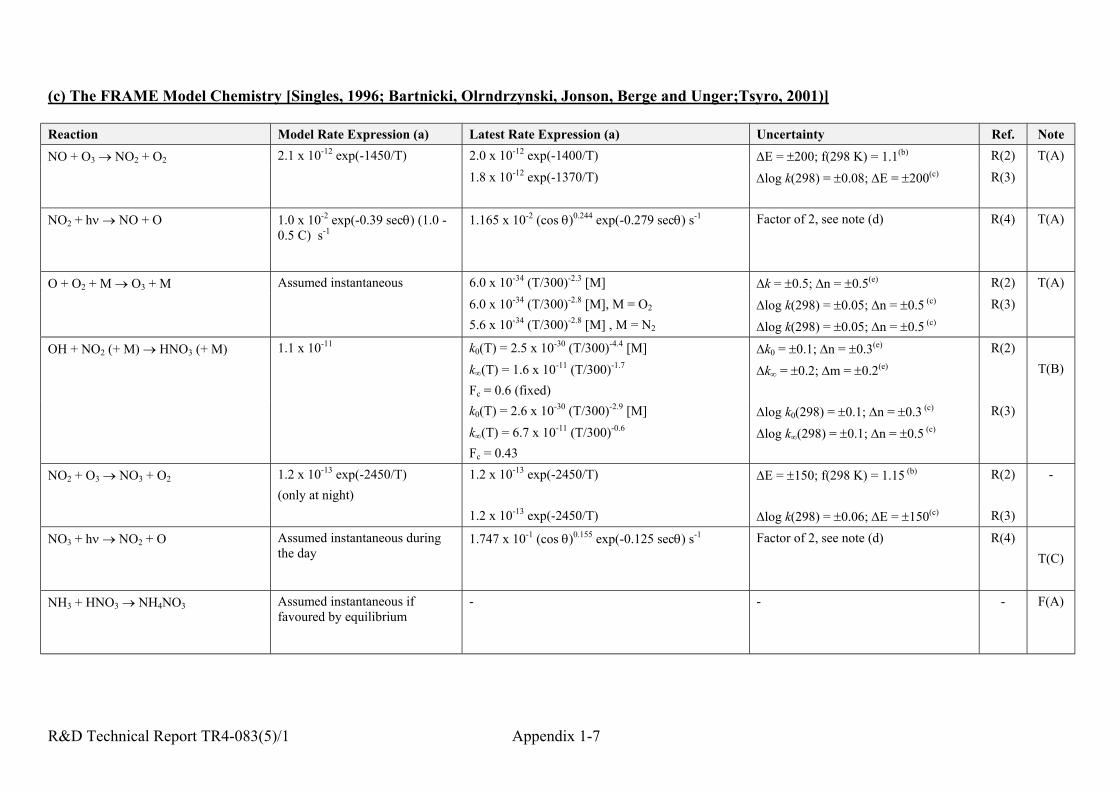
R&D Technical Report TR4-083(5)/1 Appendix 1-7
(c) The FRAME Model Chemistry [Singles, 1996; Bartnicki, Olrndrzynski, Jonson, Berge and Unger;Tsyro, 2001)]
Reaction Model Rate Expression (a) Latest Rate Expression (a) Uncertainty Ref. Note
NO + O3 → NO2 + O2 2.1 x 10⁻¹² exp(-1450/T) 2.0 x 10⁻¹² exp(-1400/T) ∆E = ±200; f(298 K) = 1.1(b) R(2) T(A)1.8 x 10⁻¹² exp(-1370/T) ∆log k(298) = ±0.08; ∆E = ±200(c) R(3)
NO2 + hν → NO + O 1.0 x 10⁻² exp(-0.39 secθ) (1.0 -0.5 C) s-1
1.165 x 10⁻² (cos θ)0.244 exp(-0.279 secθ) s-1 Factor of 2, see note (d) R(4) T(A)
O + O2 + M → O3 + M Assumed instantaneous 6.0 x 10⁻³⁴ (T/300)-2.3 [M] ∆k = ±0.5; ∆n = ±0.5(e) R(2) T(A)6.0 x 10⁻³⁴ (T/300)-2.8 [M], M = O2
5.6 x 10⁻³⁴ (T/300)-2.8 [M] , M = N2
∆log k(298) = ±0.05; ∆n = ±0.5 (c)
∆log k(298) = ±0.05; ∆n = ±0.5 (c)
R(3)
OH + NO2 (+ M) → HNO3 (+ M) 1.1 x 10⁻¹¹ k0(T) = 2.5 x 10⁻³⁰ (T/300)-4.4 [M]k∞(T) = 1.6 x 10⁻¹¹ (T/300)-1.7
Fc = 0.6 (fixed)
∆k0 = ±0.1; ∆n = ±0.3(e)
∆k∞ = ±0.2; ∆m = ±0.2(e)
R(2)T(B)
k0(T) = 2.6 x 10⁻³⁰ (T/300)-2.9 [M]k∞(T) = 6.7 x 10⁻¹¹ (T/300)-0.6
Fc = 0.43
∆log k0(298) = ±0.1; ∆n = ±0.3 (c)
∆log k∞(298) = ±0.1; ∆n = ±0.5 (c)
R(3)
NO2 + O3 → NO3 + O2 1.2 x 10⁻¹³ exp(-2450/T)(only at night)
1.2 x 10⁻¹³ exp(-2450/T) ∆E = ±150; f(298 K) = 1.15 (b) R(2) -
1.2 x 10⁻¹³ exp(-2450/T) ∆log k(298) = ±0.06; ∆E = ±150(c) R(3)
NO3 + hν → NO2 + O Assumed instantaneous duringthe day
1.747 x 10⁻¹ (cos θ)0.155 exp(-0.125 secθ) s-1 Factor of 2, see note (d) R(4)T(C)
NH3 + HNO3 → NH4NO3 Assumed instantaneous iffavoured by equilibrium
- - - F(A)
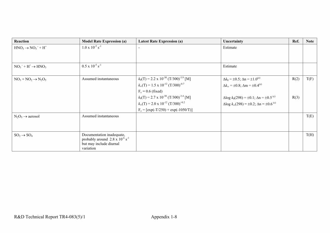
R&D Technical Report TR4-083(5)/1 Appendix 1-8
Reaction Model Rate Expression (a) Latest Rate Expression (a) Uncertainty Ref. Note
HNO3 → NO3 - + H+ 1.0 x 10⁻⁵ s-1 - Estimate
NO3 - + H+ → HNO3 0.5 x 10⁻⁵ s-1 Estimate
NO3 + NO2 → N2O5 Assumed instantaneous k0(T) = 2.2 x 10⁻³⁰ (T/300)-3.9 [M]k∞(T) = 1.5 x 10⁻¹² (T/300)-0.7
Fc = 0.6 (fixed)
∆k0 = ±0.5; ∆n = ±1.0(e)
∆k∞ = ±0.8; ∆m = ±0.4(e)
R(2) T(F)
k0(T) = 2.7 x 10⁻³⁰ (T/300)-3.4 [M]k∞(T) = 2.0 x 10⁻¹² (T/300)+0.2
Fc = [exp(-T/250) + exp(-1050/T)]
∆log k0(298) = ±0.1; ∆n = ±0.5 (c)
∆log k∞(298) = ±0.2; ∆n = ±0.6 (c)
R(3)
N2O5 → aerosol Assumed instantaneous T(E)
SO2 → SO4 Documentation inadequate,probably around 2.8 x 10⁻⁶ s-1
but may include diurnalvariation
T(H)
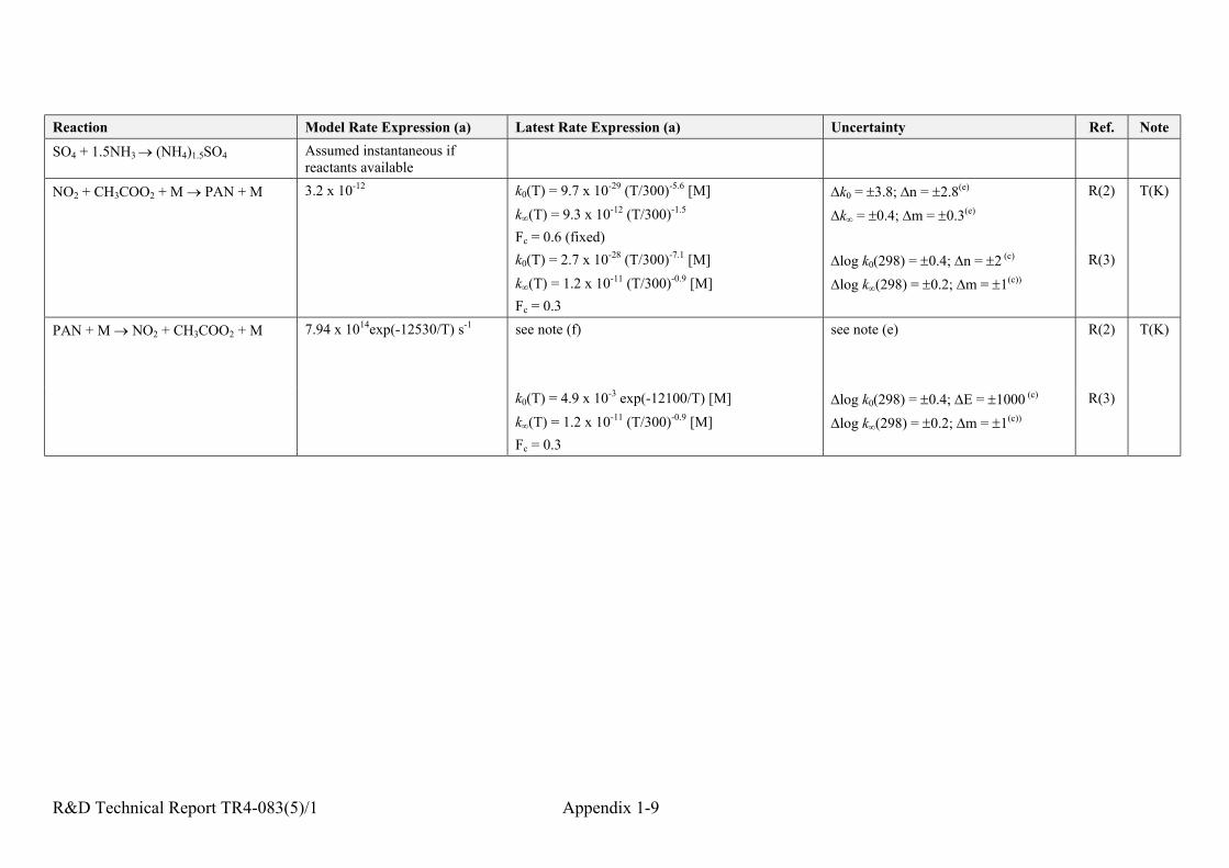
R&D Technical Report TR4-083(5)/1 Appendix 1-9
Reaction Model Rate Expression (a) Latest Rate Expression (a) Uncertainty Ref. Note
SO4 + 1.5NH3 → (NH4)1.5SO4 Assumed instantaneous ifreactants available
NO2 + CH3COO2 + M → PAN + M 3.2 x 10⁻¹² k0(T) = 9.7 x 10⁻²⁹ (T/300)-5.6 [M]k∞(T) = 9.3 x 10⁻¹² (T/300)-1.5
Fc = 0.6 (fixed)
∆k0 = ±3.8; ∆n = ±2.8(e)
∆k∞ = ±0.4; ∆m = ±0.3(e)
R(2) T(K)
k0(T) = 2.7 x 10⁻²⁸ (T/300)-7.1 [M]k∞(T) = 1.2 x 10⁻¹¹ (T/300)-0.9 [M]Fc = 0.3
∆log k0(298) = ±0.4; ∆n = ±2 (c)
∆log k∞(298) = ±0.2; ∆m = ±1(c))
R(3)
PAN + M → NO2 + CH3COO2 + M 7.94 x 10¹⁴exp(-12530/T) s-1 see note (f) see note (e) R(2) T(K)
k0(T) = 4.9 x 10⁻³ exp(-12100/T) [M]k∞(T) = 1.2 x 10⁻¹¹ (T/300)-0.9 [M]Fc = 0.3
∆log k0(298) = ±0.4; ∆E = ±1000 (c)
∆log k∞(298) = ±0.2; ∆m = ±1(c))
R(3)
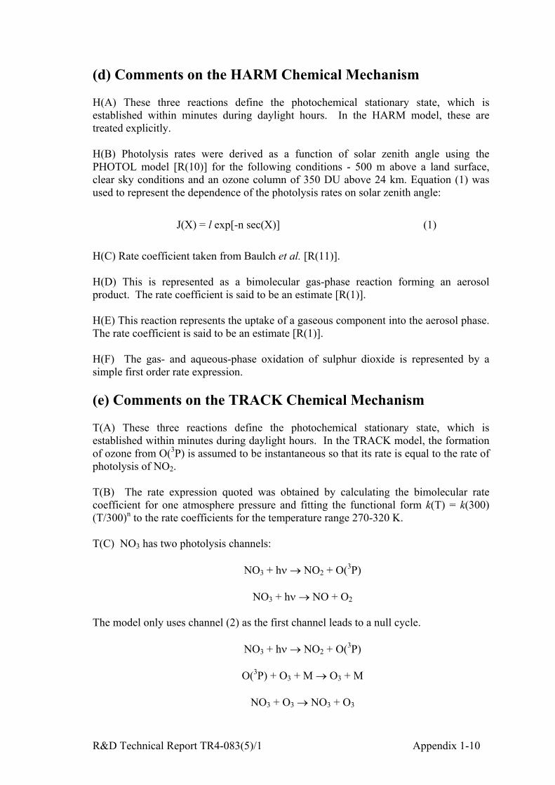
R&D Technical Report TR4-083(5)/1 Appendix 1-10
(d) Comments on the HARM Chemical Mechanism
H(A) These three reactions define the photochemical stationary state, which isestablished within minutes during daylight hours. In the HARM model, these aretreated explicitly.
H(B) Photolysis rates were derived as a function of solar zenith angle using thePHOTOL model [R(10)] for the following conditions - 500 m above a land surface,clear sky conditions and an ozone column of 350 DU above 24 km. Equation (1) wasused to represent the dependence of the photolysis rates on solar zenith angle:
J(Χ) = l exp[-n sec(Χ)] (1)
H(C) Rate coefficient taken from Baulch et al. [R(11)].
H(D) This is represented as a bimolecular gas-phase reaction forming an aerosolproduct. The rate coefficient is said to be an estimate [R(1)].
H(E) This reaction represents the uptake of a gaseous component into the aerosol phase.The rate coefficient is said to be an estimate [R(1)].
H(F) The gas- and aqueous-phase oxidation of sulphur dioxide is represented by asimple first order rate expression.
(e) Comments on the TRACK Chemical Mechanism
T(A) These three reactions define the photochemical stationary state, which isestablished within minutes during daylight hours. In the TRACK model, the formationof ozone from O(3P) is assumed to be instantaneous so that its rate is equal to the rate ofphotolysis of NO2.
T(B) The rate expression quoted was obtained by calculating the bimolecular ratecoefficient for one atmosphere pressure and fitting the functional form k(T) = k(300)(T/300)n to the rate coefficients for the temperature range 270-320 K.
T(C) NO3 has two photolysis channels:
NO3 + hν → NO2 + O(3P)
NO3 + hν → NO + O2
The model only uses channel (2) as the first channel leads to a null cycle.
NO3 + hν → NO2 + O(3P)
O(3P) + O3 + M → O3 + M
NO3 + O3 → NO3 + O3

R&D Technical Report TR4-083(5)/1 Appendix 1-11
Channel (2) can be assumed to be instantaneous as NO3 has a lifetime of seconds duringthe day.
T(D) This is represented as a bimolecular gas-phase reaction forming an aerosolproduct. The rate coefficient is an estimate and is therefore highly uncertain.
T(E) The observed concentrations of nitrate in precipitation are imply that there areother removal processes of gas-phase NOy, in addition to that of HNO3. In particular,NO2, HNO3 and N2O5 may react with seasalt aerosol:
NaCl + 2 NO2 → NaNO3 + ClNO2
NaCl + HNO3 → NaNO3 + HCl
NaCl + N2O5 → NaNO3 + ClNO2
For these reactions, the rate of the first order uptake of the gas on the aerosol surfacehas been treated using the model of Fuchs and Sutugin [R(8)] for typical rural andmarine aerosols. These aerosols have been represented as three log normal distributions,the parameters of which were taken from Jaenicke [R(9)]. The uptake rate depends onthe accommodation coefficient, α, which have been taken from the NASA Evaluation[R(2)] for HNO3 and N2O5.
T(F) This is the only loss process for NO3 at night. The rate limiting step in thesequence
NO2 + O3 → NO3 + O2
NO2 + NO3 + M → N3O5+ M
is the formation of NO3. The rate of formation of N3O5 is equal to the rate of formationof NO3, which explains why this reaction is described as instantaneous.
T(G) This is a simplified representation of the following gas-phase reaction sequence:
OH + SO2 + M → HOSO2 + M
HOSO2 + O2 → SO3 + HO2
SO3 + H2O → H3SO4
The rate expression quoted was obtained by calculating the bimolecular rate coefficientfor one atmosphere pressure and fitting the functional form k(T) = k(300) (T/300)n.
T(H) The aqueous-phase oxidation of sulphur dioxide is presumed to be dominated byits reaction with H2O2 for the pH range typically observed (2-6). The oxidation processis represented as a first order reaction. The value of the rate coefficient has been chosenso that the overall rate coefficient for the gas and aqueous-phase oxidation routes is 2.8

R&D Technical Report TR4-083(5)/1 Appendix 1-12
x 10-6 s-1. The effective gas-phase oxidation rate coefficient is 8 x 10⁻⁷ s-1 for an OHradical concentration of 8 x 10⁵ molecule cm-3.
T(I) The rate expression quoted was obtained by calculating the bimolecular ratecoefficient for one atmosphere pressure and fitting the functional form k(T) = k(300)(T/300)n to the rate coefficients. The pressure dependent rate coefficients were takenfrom the IUPAC Evaluation [R(2)].
T(J) Taken from Harrison et al. [R(11)]. The expression is based about fieldmeasurements of HONO fluxes.
T(K) Rate coefficients used are based on the recommendations of Lightfoot et al.[R(12)], which have been incorporated into the more recent evaluations. Theuncertainty factors are likely to be comparable to those quoted.
(f) Comments on the FRAME Chemical Mechanism
F(A) Ammonium nitrate is formed if :
( )( ) pKNHNHNOHNO ≥++ +− ][][][][ 4333
where Kp is an equilibrium coefficient. The value of Kp is calculated from a semi-empirical expression for solid particulates in dry weather conditions [Stelson andSeinfeld, 1982]:
298ln1.62422078.70ln T
TK rhdrh −−=< where K is in ppm2
The equilibrium constant decreases slowly once the ambient relative humidity exceedthe relative humidity of deliquescence.
2306.123.856)ln( +=T
rhd where rhd is in percent
When the ambient humidity approaches saturation there is a marked decrease in theequilibrium constant.
(g) Notes
(a) Units are cm3 molecule-1 s-1, unless otherwise stated.
(b) The uncertainty factor f(298 K) gives the upper and lower bound (corresponding to~ 1σ) of the rate coefficient at 298 K. The uncertainty factor at other temperatures canbe found using equation (2) (note the absolute value). The upper and lower bounds areobtained by multiplying and dividing the rate coefficient at that temperature by thefactor f(T).
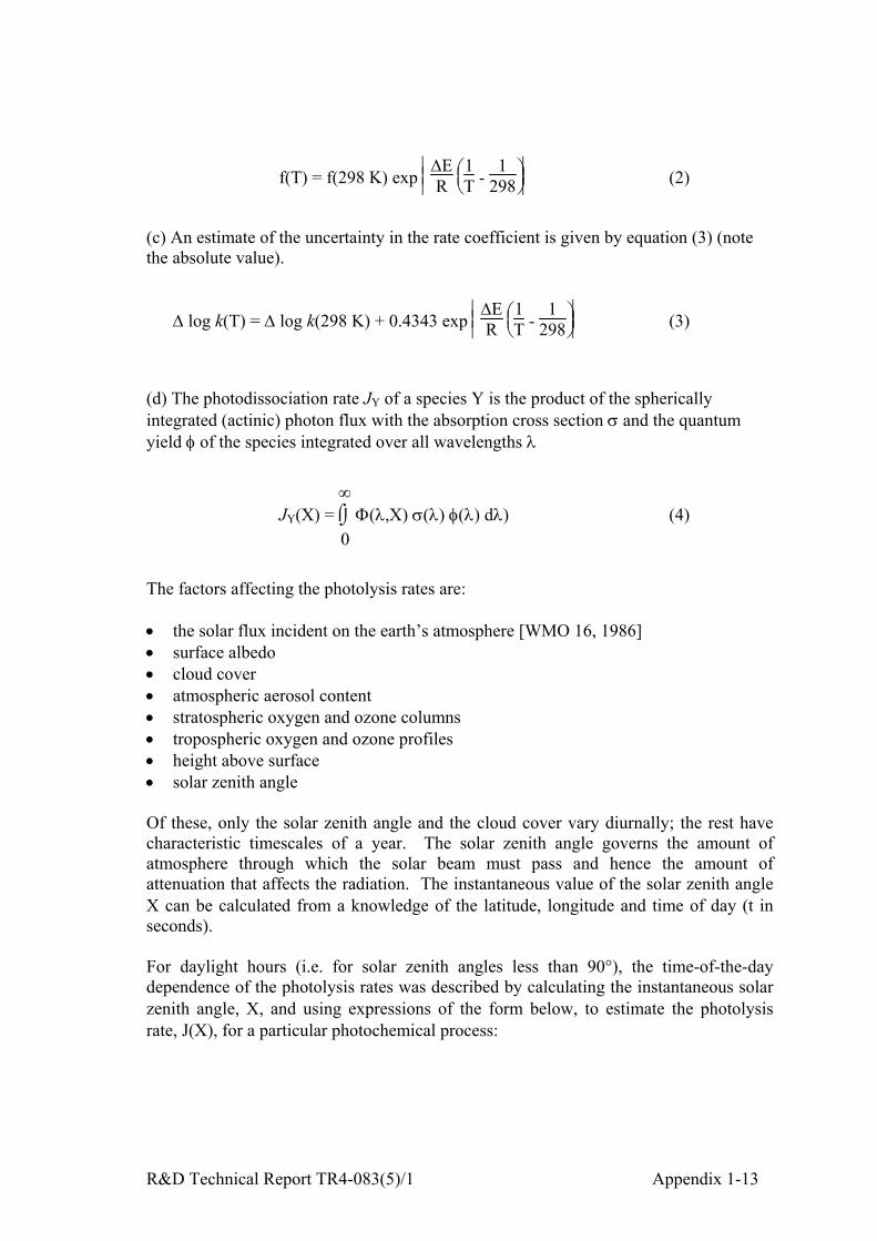
R&D Technical Report TR4-083(5)/1 Appendix 1-13
f(T) = f(298 K) exp
∆E
R
1
T - 1
298 (2)
(c) An estimate of the uncertainty in the rate coefficient is given by equation (3) (notethe absolute value).
∆ log k(T) = ∆ log k(298 K) + 0.4343 exp
∆E
R
1
T - 1
298 (3)
(d) The photodissociation rate JY of a species Y is the product of the sphericallyintegrated (actinic) photon flux with the absorption cross section σ and the quantumyield φ of the species integrated over all wavelengths λ
JY(Χ) = ⌡⌠0
∞ Φ(λ,Χ) σ(λ) φ(λ) dλ) (4)
The factors affecting the photolysis rates are:
• the solar flux incident on the earth’s atmosphere [WMO 16, 1986]• surface albedo• cloud cover• atmospheric aerosol content• stratospheric oxygen and ozone columns• tropospheric oxygen and ozone profiles• height above surface• solar zenith angle
Of these, only the solar zenith angle and the cloud cover vary diurnally; the rest havecharacteristic timescales of a year. The solar zenith angle governs the amount ofatmosphere through which the solar beam must pass and hence the amount ofattenuation that affects the radiation. The instantaneous value of the solar zenith angleΧ can be calculated from a knowledge of the latitude, longitude and time of day (t inseconds).
For daylight hours (i.e. for solar zenith angles less than 90°), the time-of-the-daydependence of the photolysis rates was described by calculating the instantaneous solarzenith angle, Χ, and using expressions of the form below, to estimate the photolysisrate, J(Χ), for a particular photochemical process:
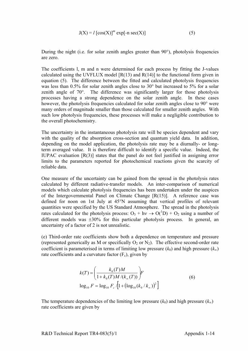
R&D Technical Report TR4-083(5)/1 Appendix 1-14
J(Χ) = l [cos(Χ)]m exp[-n sec(Χ)] (5)
During the night (i.e. for solar zenith angles greater than 90°), photolysis frequenciesare zero.
The coefficients l, m and n were determined for each process by fitting the J-valuescalculated using the UVFLUX model [R(13) and R(14)] to the functional form given inequation (5). The difference between the fitted and calculated photolysis frequencieswas less than 0.5% for solar zenith angles close to 30° but increased to 5% for a solarzenith angle of 70°. The difference was significantly larger for those photolysisprocesses having a strong dependence on the solar zenith angle. In these caseshowever, the photolysis frequencies calculated for solar zenith angles close to 90° weremany orders of magnitude smaller than those calculated for smaller zenith angles. Withsuch low photolysis frequencies, these processes will make a negligible contribution tothe overall photochemistry.
The uncertainty in the instantaneous photolysis rate will be species dependent and varywith the quality of the absorption cross-section and quantum yield data. In addition,depending on the model application, the photolysis rate may be a diurnally- or long-term averaged value. It is therefore difficult to identify a specific value. Indeed, theIUPAC evaluation [R(3)] states that the panel do not feel justified in assigning errorlimits to the parameters reported for photochemical reactions given the scarcity ofreliable data.
One measure of the uncertainty can be gained from the spread in the photolysis ratescalculated by different radiative-transfer models. An inter-comparison of numericalmodels which calculate photolysis frequencies has been undertaken under the auspicesof the Intergovernmental Panel on Climate Change [R(15)]. A reference case wasdefined for noon on 1st July at 45°N assuming that vertical profiles of relevantquantities were specified by the US Standard Atmosphere. The spread in the photolysisrates calculated for the photolysis process: O3 + hν → O(1D) + O2 using a number ofdifferent models was ±30% for this particular photolysis process. In general, anuncertainty of a factor of 2 is not unrealistic.
(e) Third-order rate coefficients show both a dependence on temperature and pressure(represented generically as M or specifically O2 or N2). The effective second-order ratecoefficient is parameterised in terms of limiting low pressure (k0) and high pressure (k∞)rate coefficients and a curvature factor (Fc), given by
( )[ ]20101010
0
0
)/(log1/loglog
))(/()(1)(
)(
∞
∞
+=
+
=
kkFF
FTkMTk
MTkTk
c
(6)
The temperature dependencies of the limiting low pressure (k0) and high pressure (k∞)rate coefficients are given by
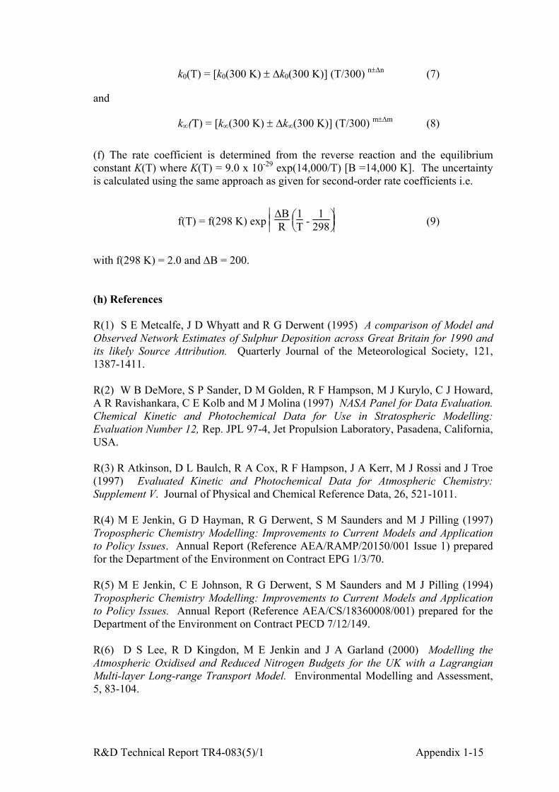
R&D Technical Report TR4-083(5)/1 Appendix 1-15
k0(T) = [k0(300 K) ± ∆k0(300 K)] (T/300) n±∆n (7)
and
k∞(T) = [k∞(300 K) ± ∆k∞(300 K)] (T/300) m±∆m (8)
(f) The rate coefficient is determined from the reverse reaction and the equilibriumconstant K(T) where K(T) = 9.0 x 10⁻²⁹ exp(14,000/T) [B =14,000 K]. The uncertaintyis calculated using the same approach as given for second-order rate coefficients i.e.
f(T) = f(298 K) exp
∆B
R
1
T - 1
298 (9)
with f(298 K) = 2.0 and ∆B = 200.
(h) References
R(1) S E Metcalfe, J D Whyatt and R G Derwent (1995) A comparison of Model andObserved Network Estimates of Sulphur Deposition across Great Britain for 1990 andits likely Source Attribution. Quarterly Journal of the Meteorological Society, 121,1387-1411.
R(2) W B DeMore, S P Sander, D M Golden, R F Hampson, M J Kurylo, C J Howard,A R Ravishankara, C E Kolb and M J Molina (1997) NASA Panel for Data Evaluation.Chemical Kinetic and Photochemical Data for Use in Stratospheric Modelling:Evaluation Number 12, Rep. JPL 97-4, Jet Propulsion Laboratory, Pasadena, California,USA.
R(3) R Atkinson, D L Baulch, R A Cox, R F Hampson, J A Kerr, M J Rossi and J Troe(1997) Evaluated Kinetic and Photochemical Data for Atmospheric Chemistry:Supplement V. Journal of Physical and Chemical Reference Data, 26, 521-1011.
R(4) M E Jenkin, G D Hayman, R G Derwent, S M Saunders and M J Pilling (1997)Tropospheric Chemistry Modelling: Improvements to Current Models and Applicationto Policy Issues. Annual Report (Reference AEA/RAMP/20150/001 Issue 1) preparedfor the Department of the Environment on Contract EPG 1/3/70.
R(5) M E Jenkin, C E Johnson, R G Derwent, S M Saunders and M J Pilling (1994)Tropospheric Chemistry Modelling: Improvements to Current Models and Applicationto Policy Issues. Annual Report (Reference AEA/CS/18360008/001) prepared for theDepartment of the Environment on Contract PECD 7/12/149.
R(6) D S Lee, R D Kingdon, M E Jenkin and J A Garland (2000) Modelling theAtmospheric Oxidised and Reduced Nitrogen Budgets for the UK with a LagrangianMulti-layer Long-range Transport Model. Environmental Modelling and Assessment,5, 83-104.
R&D Technical Report TR4-083(5)/1 Appendix 1-16
R(7) D S Lee, R D Kingdon, M E Jenkin and A Webster (2000) Modelling theContribution of Different Sources of Sulphur to Atmospheric Deposition in the UnitedKingdom. Environmental Modelling and Assessment, 5, 105-118.
R(8) N A Fuchs and A G Sutigin (1971) High-dispersed Aerosols. InternationalReview of Aerosol Physics and Chemistry, 2, 1-60.
R(9) R Jaenicke (1988) Properties of Atmospheric Aerosols in Numerical Data andFunctional Relationships in Science and Technology Landolt-Bornstein New Series, V:Geophysics and Space Research, 4: Meteorology (G. Fischer, ed.) b: Physical andChemical Properties of the Air. 391-457, Springer, Berlin.
R(10) A M Hough (1988) The Calculation of Photolysis Rates for Use in GlobalTropospheric Modelling Studies. AERE Report R-13259, HMSO, London [ISBN 0-7058-1259-6].
R(11) D L Baulch, R Atkinson, R A Cox, R F Hampson, J A Kerr and J Troe (1984)Evaluated Kinetic and Photochemical Data for Atmospheric Chemistry: Supplement II.Journal of Physical and Chemical Reference Data, 13, 1259-1380.
R(11) R M Harrison, J D Peak and G M Collins (1996) The Tropospheric Cycle ofNitrous Acid. Journal of Geophysical Research, 101, 14429-12239.
R(12) P D Lighhtfoot, R A Cox, J N Crowley, M Destriau, G D Hayman, M E Jenkin,G K Moortgat and F Zabel (1992) Organic Peroxy Radicals: Kinetics, Spectroscopyand Tropospheric Chemistry. Atmospheric Environment, 26A, 1805-1964.
R(13) G D Hayman (1997) Effects of Pollution Control on UV Exposure. Final projectreport (AEA\RFIN\22525001\R\ 002 Issue 2) prepared for the Department of Health oncontract 121/6377 (1997).
R(14) G D Hayman, S Espenhahn and J A Garland (1998) Effects of Air PollutionControl on UV Exposure. Project report (AEAT-3937\20467001\001 Issue 1) preparedfor the Department of Health on contract 121/6703.
R(15) IPCC (1995) Climate Change 1994 - Radiative Forcing of Climate Change andan Evaluation of the IPCC IS92 Emission Scenarios. Edited by J T Houghton, L GMeira Filho, J Bruce, H Lee, B A Callendar, E Haites, N Harris and K Maskell,Cambridge University Press: Cambridge, UK.

R&D Technical Report TR4-083(5)/1 Appendix 2-17
2 Analytical model for sulphate deposition
CONTENTS
(a) Introduction(b) Sulphur dioxide oxidation(c) Total sulphate deposition(d) Vertical dispersion(e) Polar co-ordinates(f) Nomenclature
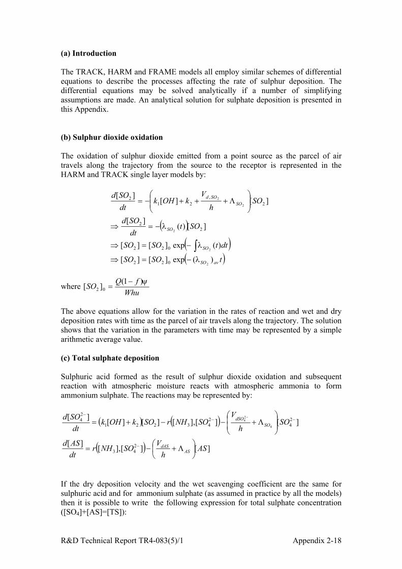
R&D Technical Report TR4-083(5)/1 Appendix 2-18
(a) Introduction
The TRACK, HARM and FRAME models all employ similar schemes of differentialequations to describe the processes affecting the rate of sulphur deposition. Thedifferential equations may be solved analytically if a number of simplifyingassumptions are made. An analytical solution for sulphate deposition is presented inthis Appendix.
(b) Sulphur dioxide oxidation
The oxidation of sulphur dioxide emitted from a point source as the parcel of airtravels along the trajectory from the source to the receptor is represented in theHARM and TRACK single layer models by:
( )( )( )tSOSO
dttSOSO
SOtdtSOd
SOh
VkOHk
dtSOd
avSO
SO
SO
SOSOd
)(exp][][
)(exp][][
][)(][
][][][
2
2
2
2
2
022
022
22
2,
212
λ
λ
λ
−=⇒
−=⇒
−=⇒
Λ+++−=
∫
where Whu
fQSO ψ)1(][ 02−
=
The above equations allow for the variation in the rates of reaction and wet and drydeposition rates with time as the parcel of air travels along the trajectory. The solutionshows that the variation in the parameters with time may be represented by a simplearithmetic average value.
(c) Total sulphate deposition
Sulphuric acid formed as the result of sulphur dioxide oxidation and subsequentreaction with atmospheric moisture reacts with atmospheric ammonia to formammonium sulphate. The reactions may be represented by:
( ) ( )
( ) ][][],[][
][][],[][][][
243
24
243221
24
4
24
ASh
VSONHrdtASd
SOh
VSONHrSOkOHk
dtSOd
ASdAS
SOdSO
Λ+−=
Λ+−−+=
−
−−−
−
If the dry deposition velocity and the wet scavenging coefficient are the same forsulphuric acid and for ammonium sulphate (as assumed in practice by all the models)then it is possible to write the following expression for total sulphate concentration([SO4]+[AS]=[TS]):
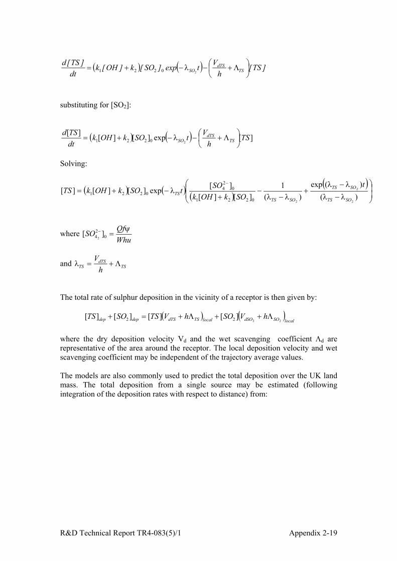
R&D Technical Report TR4-083(5)/1 Appendix 2-19
( ) ( ) ]TS[h
Vtexp]SO[k]OH[kdt
]TS[dTS
dTSSO
+−−+= Λλ
20221
substituting for [SO2]:
Solving:
( ) ( ) ( )( )
−
−+
−−
+−+=
−
)()(exp
)(1
][][][exp][][][
2
2
20221
024
0221SOTS
SOTS
SOTSTS
tSOkOHk
SOtSOkOHkTSλλ
λλ
λλλ
where WhuQfSO ψ
=−0
24 ][
2
and TSdTS
TS hV
Λ+=λ
The total rate of sulphur deposition in the vicinity of a receptor is then given by:
( ) ( )localSOdSOlocalTSdTSdepdep hVSOhVTSSOTS
22][][][][ 22 Λ++Λ+=+
where the dry deposition velocity Vd and the wet scavenging coefficient Λd arerepresentative of the area around the receptor. The local deposition velocity and wetscavenging coefficient may be independent of the trajectory average values.
The models are also commonly used to predict the total deposition over the UK landmass. The total deposition from a single source may be estimated (followingintegration of the deposition rates with respect to distance) from:
( ) ( ) ][exp][][][20221 TS
hVtSOkOHk
dtTSd
TSdTS
SO
Λ+−−+= λ

R&D Technical Report TR4-083(5)/1 Appendix 2-20
( )( )( )
( ) ( )
−−
Λ++
−−
Λ++
−−
−
−−
−+Λ+
=+ −−
)exp(1][
)exp(1][
exp(1exp(1][][][][
2
2
22
2
2
2
0204
02212
uxhVuSO
uxhVuSO
ux
ux
uSOkOHkhVSOTS
SOSOdSO
TSTS
TSdTS
TS
TS
SO
SO
SOTS
TSdTStotaldeptotaldep
SO
λλ
λλ
λ
λ
λ
λ
λλ
(d) Vertical dispersion
TRACK (multi-level mode) and FRAME allow for the dispersion in the verticaldimension of the emitted sulphur dioxide and the reaction products. No allowance ismade for dispersion in the horizontal dimension other than the initial dispersion acrossthe width of the trajectory.
However, in practice, sulphur dioxide emissions from a point source are dispersedthroughout the boundary layer depth within about 6 km, under neutral atmosphericconditions. The initial dispersion of the emission in the vertical dimension ceases tobe important beyond this distance, which is small compared to the range over whichthe models apply. The models all assume a constant trajectory width greater than 5km. The plume from a point source expands in the horizontal dimension at the rate ofapproximately 10% of the distance travelled downwind: the plume will not expand tothe box width until the air parcel has travelled more than 50 km.
At around 7.5 m s-1 wind speed, dispersion in the vertical dimension over the initial 6km corresponds to a mixing time constant of the order of 10-3 s-1 (~7.5/6000). Thisvalue may be compared to the time constant for dry deposition of the most reactivesulphur species, sulphur dioxide (Vd/h) of 10-5 s-1. It is concluded that mixing of thedepositing total sulphate and sulphur dioxide throughout the boundary layer is muchfaster than their rate of depletion by dry deposition and so the concentration gradientaway from the surface will be small. It is therefore unlikely that vertical dispersionwill have a significant effect on the rates of sulphur deposition.
(e) Polar co-ordinates
The analysis presented above has assumed that the pollutant is contained in a parcel ofair of constant width. This follows the general approach taken by the HARM andFRAME models. For a single point source, it is more appropriate to allow for theparcel width to increase with increasing distance from the source to allow forhorizontal dispersion and for statistical variations in wind direction. However, thesulphate deposition equations are linear with respect to the rate of emission and so theaverage rate of deposition at distance x from the source across a wind direction sectortaking account of the increase in sector width may be calculated by putting:
θxW =
in the above equations, where θ is the sector width in radians.

R&D Technical Report TR4-083(5)/1 Appendix 2-21
(f) Nomenclature
Concentrations
[SO2] concentration of sulphur dioxide[SO4
2-] concentration of sulphuric acid[AS] concentration of ammonium sulphate[OH] concentration of OH[TS] concentration of total sulphate = ammonium sulphateplus sulphuric acid
Other parameters
ks1 gas phase reaction rate of sulphur dioxide with OHks2 aqueous phase oxidation rate of sulphur dioxideQ emission rate of sulphur dioxidef proportion of emission as sulphur trioxidex distance downwindW width of trajectoryh boundary layer heightu wind speedVd dry deposition velocityλ characteristic frequencyΛ wet scavenging coefficientΨ frequency of wind in directionθ wind sector angle

R&D Technical Report TR4-083(5)/1 Appendix 3-22
3 Analytical model for nitrogen deposition
The TRACK, HARM and FRAME models all employ similar schemes of differentialequations to describe the processes affecting the rate of nitrogen deposition. Thedifferential equations may be solved analytically if a number of simplifyingassumptions are made. An analytical solution for nitrogen deposition is presented inthis Appendix.
There are however some differences in the reaction schemes employed by theTRACK, HARM and FRAME models. For this analysis, a simplified reaction schemehas been investigated that represents the major features of the reaction schemesemployed in the numerical models,
For the purposes of the analytical assessment, the mass balance of the oxidisednitrogen species has been represented by the following equations. These equationsinvolve some simplification but broadly represent the most significant reactionsconsidered in the acid deposition models.
][]][[][
]][[][]][[][
][]][[][]][[)][]([][
][]][[
][]][[]][[)1(]][[][][
]][[][][
5211231052
2310322353
3232521310333
22310
322352431212
3121
3
2
ONkNONOkdt
ONd
NONOkNOJNOOkdtNOd
NOJONOkNOJONOkOOh
vdtOd
NOh
vNONOk
NOJNOOkNOOHkhEqONOkNOJ
dtNOd
hEqONOkNOJ
dtNOd
dO
dNO
−=
−−=
+−+−−−=
−
−+−−−++−=
+−=
Further reactions then take place involving nitric acid, ammonia, oxidised nitrogenaerosol and ammonium aerosol. The path of these reactions depends on whetherammonia is present. In the absence of ammonia, the mass balance equations for nitricacid and oxidised nitrogen aerosol are:
])[(][][][
])[(][]][[][
395211
339243
3
3
aerNh
vHNOkONkdt
aerNd
HNOh
vHNOkNOOHk
dtHNOd
oxaerdaerox
HNOdHNO
Λ+−+=
Λ+−−=
R&D Technical Report TR4-083(5)/1 Appendix 3-23
If there is excess ammonia present, the nitric acid reacts quickly (effectivelyinstantaneously) with the ammonia to form ammonium aerosol (cf. FRAME). Themass balance equations are then:
])[(]][[][
])[(]][[][
])[(][]][[][
3243
4244
521124
3
3 NHh
vNOOHk
dtNHd
aerNHh
vNOOHkdt
aerNHd
aerNh
vONkNOOHkdt
aerNd
NHdNH
aerdaer
oxaerdaerox
Λ+−−=
Λ+−=
Λ+−+=
The mass balance equations for NO, NO2, NO3, O3 and N2O5 contain non-linearreaction terms. For additional regulated sources, the equations can be linearised aboutthe operating point:
]'[][][ 0 NONONO +=
etc.
where [NO]0 is the baseline concentration and [NO]’ is the contribution from theadditional sources. The mass balance equations may then be written in terms of theincremental change in the concentrations e.g.
hEqONOkNOOkNOJ
dtNOd '
30103121 ]'[][]'[][]'[]'[+−−=
The linearised mass balance equations representing the response to the incrementaladditional source may then be presented in terms of their Laplace transforms(dropping the prime notation for convenience):
( )
( )( )
( ))B( )s](NO[]NO[k)s](NO[]NO[k)s](ON)[s(
)s](O[]NO[k)s](NO[]NO[k]O[k)s](NO)[s(
)s](NO[J)s](NO[]O[kJ)s](NO[]O[k)s](O)[s()A( )s](NO[]NO[kJ
)s](O[]NO[k]NO[k)s](NO[]O[k)s(hE)q()s](NO)[s(
)s](O[]NO[k)s](NO[J)s(hEq)s](NO)[s(
ON
NO
O
NO
NO
302102031052
3025203100353
32203510313
302102
3025010312
30121
52
3
3
21
+=+
+−=+
+−+−=+−
+−++−=+
−+=+
λ
λ
λ
λ
λ
In the absence of ammonia:
)]([)]([)]()[(
)](][[)]()[(
395211
2433
sHNOksONksaerNs
sNOOHksHNOs
oxaerN
HNO
ox+=+
=+
λ
λ
R&D Technical Report TR4-083(5)/1 Appendix 3-24
For excess ammonia:
)](][[)]()[(
)](][[)]()[(
)]([)](][[)]()[(
243
244
521124
3
4
sNOOHksNHs
sNOOHksaerNHs
sONksNOOHksaerNs
NH
aerNH
oxaerNox
−=+
=+
+=+
λ
λ
λ
The characteristic frequencies, λ, are given by:
3
3
3
4
3
3
3
52
3
3
3
2
2
9
11
02102
02501
031003541
031
][
][][
][][][
][
NHdNH
NH
aerdaer
aerNH
aerdaer
aerN
HNOdHNO
HNO
ON
NO
dOO
dNONO
NO
hv
hvh
vh
vk
k
NOkJh
vNOkNOk
hv
NOkOkOHkJ
Ok
ox
Λ+=
Λ+=
Λ+=
Λ++=
=
+=
++=
++++=
=
λ
λ
λ
λ
λ
λ
λ
λ
λ
The use of the Laplace transform method implies that the baseline concentrations[O3]0, [NO]0, [NO3]0 and [NO2]0, dry deposition velocities, wet scavengingcoefficients and reaction rate constants do not change. This is a reasonableapproximation for the purposes of investigating system dynamics and uncertainties.However, in practice these parameters will vary with time and location: these effectscan only be investigated by means of numerical models although the analyticalsolution may be applied piecewise if these parameters do not change rapidly.
The Laplace transform of each species concentration in terms of s may be obtained byalgebraic elimination. In principal, the concentration as a function of time may beobtained as the inverse Laplace transform of the resulting expressions. However, thisis rather tedious. Some simplification follows from frequency-response analysis of theexpression for [NO2](s) and [N2O5](s). The analysis involves substituting s=jω wherej=√(-1) and calculating the amplitude ratio as the modulus of the resulting expression.The analysis is simplified for overdamped systems i.e. where each of thecharacteristic frequencies is real and positive as here. The frequency-responsediagram shows the amplitude ratio plotted against frequency, ω. Fig. A3.1 shows aplot for h[NO2](s)/E(s) for typical parameter values over the range 10-7-2 x 10⁻³ s-1.This range is appropriate for the investigation of regional scale and national scaledeposition corresponding to time scales greater than about 10 minutes up to more than100 hours. System responses that take place over shorter timescales will be damped,
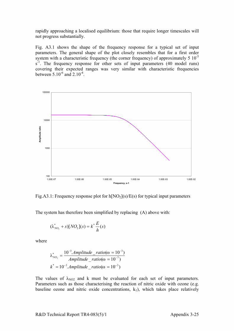
R&D Technical Report TR4-083(5)/1 Appendix 3-25
rapidly approaching a localised equilibrium: those that require longer timescales willnot progress substantially.
Fig. A3.1 shows the shape of the frequency response for a typical set of inputparameters. The general shape of the plot closely resembles that for a first ordersystem with a characteristic frequency (the corner frequency) of approximately 5 10-5
s-1. The frequency response for other sets of input parameters (40 model runs)covering their expected ranges was very similar with characteristic frequenciesbetween 5.10-6 and 2.10-4.
100
1000
10000
100000
1.00E-07 1.00E-06 1.00E-05 1.00E-04 1.00E-03 1.00E-02
Frequency, s-1
Am
plitu
de ra
tio
Fig.A3.1: Frequency response plot for h[NO2](s)/E(s) for typical input parameters
The system has therefore been simplified by replacing (A) above with:
)()]()[( *2
*2
shEksNOsNO =+λ
where
)10(_.10)10(_
)10(_.10
33*
7
33*
2
−−
−
−−
==
==
=
ω
ωω
λ
ratioAmplitudekratioAmplitude
ratioAmplitudeNO
The values of λNO2 and k must be evaluated for each set of input parameters.Parameters such as those characterising the reaction of nitric oxide with ozone (e.g.baseline ozone and nitric oxide concentrations, k1), which takes place relatively
R&D Technical Report TR4-083(5)/1 Appendix 3-26
rapidly, influence the magnitude of λNO2 and k because they determine localisedequilibrium states.
Fig.A3.1 also shows the pseudo-first order amplitude ratio: the amplitude ratio for thepseudo-first order expression is not significantly different from that for (A).
Similarly the right hand side of (B) has been replaced by:
)())]([][)]([][)(( ''3021020310
'' shEksNONOksNONOks =++λ
Substituting into (B) and rearranging gives:
)()]()[)(( **52
**52
shEksONss ON =++ λλ
Species concentrations for a point source were then obtained by inverse Laplacetransforms. For the ammonia absent case:
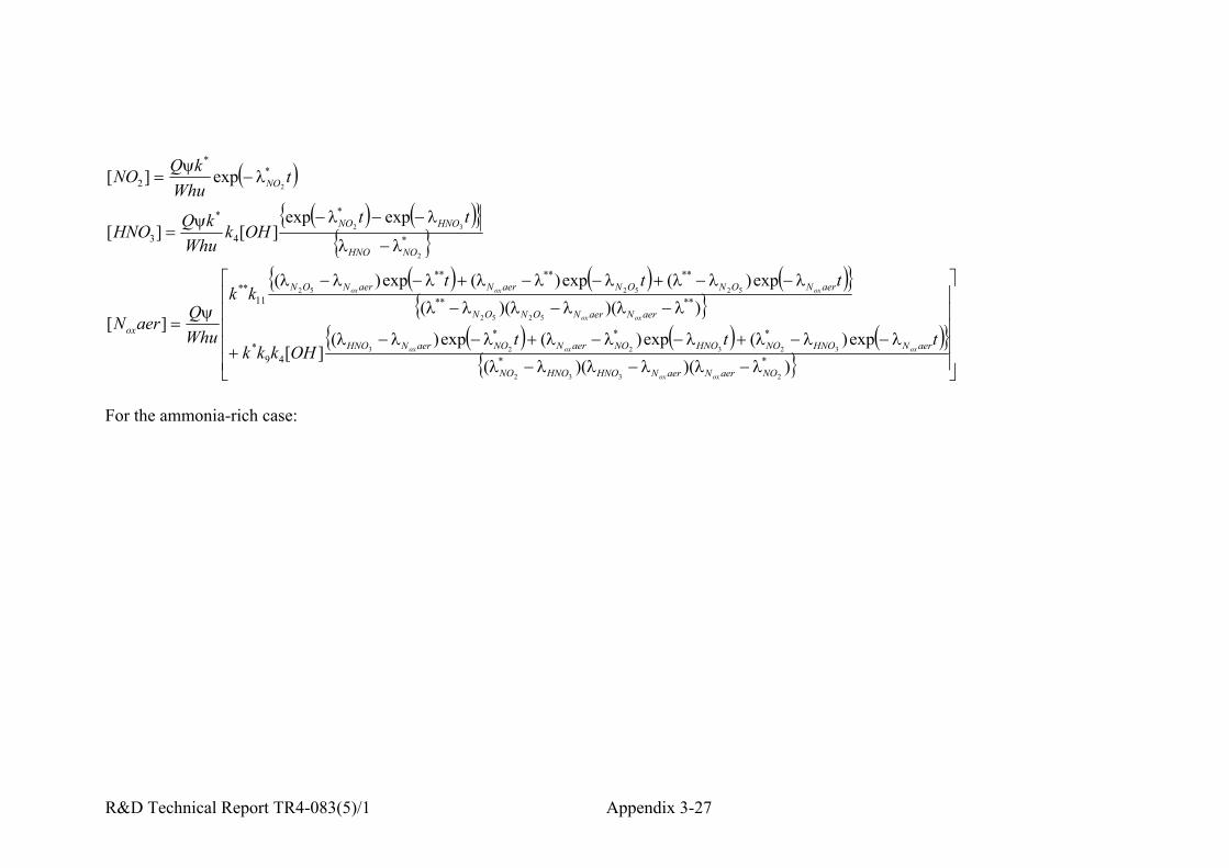
R&D Technical Report TR4-083(5)/1 Appendix 3-27
( )( ) ( ){ }
{ }( ) ( ) ( ){ }{ }
( ) ( ) ( ){ }{ }
−−−
−−+−−+−−+
−−−
−−+−−+−−
=
−
−−−=
−=
))()((exp)(exp)(exp)(
][
))()((exp)(exp)(exp)(
][
expexp][][
exp][
**
***
49*
****
******
11**
*
*
4
*
3
**
2
2332
323223
5252
525252
2
32
2
NOaerNaerNHNOHNONO
aerNHNONOHNONOaerNNOaerNHNO
aerNaerNONON
aerNONONaerNaerNON
ox
NOHNO
HNONO
NO
oxox
oxoxox
oxox
oxoxox
tttOHkkk
tttkk
WhuQaerN
ttOHk
WhukQHNO
tWhu
kQNO
λλλλλλ
λλλλλλλλλ
λλλλλλ
λλλλλλλλλ
ψ
λλ
λλψ
λψ
For the ammonia-rich case:

R&D Technical Report TR4-083(5)/1 Appendix 3-28
( )
( ) ( ) ( ){ }{ }
( ) ( ){ }{ }
( ) ( ){ }{ }
( ) ( ){ }{ }*
*
4*
3
*
*
4*
4
*
*
4*
****
******
11**
**
2
23
32
24
42
2
02
5252
525252
2
expexp][][
expexp][][
expexp][
))()((exp)(exp)(exp)(
][
exp][
NONH
NHNO
NOaerNH
aerNHNO
NOaerN
aerNNO
aerNaerNONON
aerNONONaerNaerNON
ox
NO
ttOHkk
WhuQNH
ttOHkk
WhuQaerNH
ttOHkk
tttkk
WhuQaerN
tWhu
kQNO
ox
x
oxox
oxoxox
λλ
λλψ
λλ
λλψ
λλ
λλ
λλλλλλ
λλλλλλλλλ
ψ
λψ
−
−−−−=
−
−−−=
−
−−−+
−−−
−−+−−+−−
=
−=
The total rate of oxidised nitrogen deposition is then given by ;
( ) ( )hvaerNhvHNOvNOaerNHNONO aerdaeroxHNOdHNOdNOdepoxdepdep Λ++Λ++=++ ][][][][][][332 3232
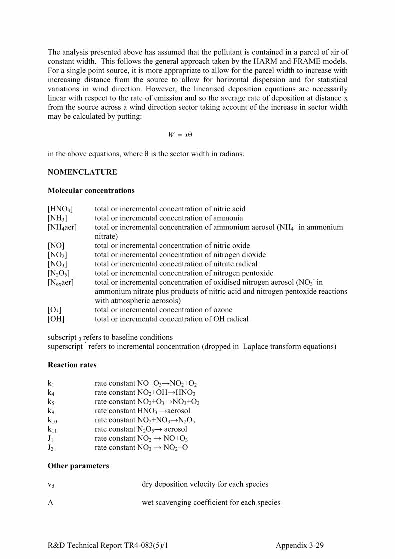
R&D Technical Report TR4-083(5)/1 Appendix 3-29
The analysis presented above has assumed that the pollutant is contained in a parcel of air ofconstant width. This follows the general approach taken by the HARM and FRAME models.For a single point source, it is more appropriate to allow for the parcel width to increase withincreasing distance from the source to allow for horizontal dispersion and for statisticalvariations in wind direction. However, the linearised deposition equations are necessarilylinear with respect to the rate of emission and so the average rate of deposition at distance xfrom the source across a wind direction sector taking account of the increase in sector widthmay be calculated by putting:
θxW =
in the above equations, where θ is the sector width in radians.
NOMENCLATURE
Molecular concentrations
[HNO3] total or incremental concentration of nitric acid[NH3] total or incremental concentration of ammonia[NH4aer] total or incremental concentration of ammonium aerosol (NH4
+ in ammoniumnitrate)
[NO] total or incremental concentration of nitric oxide[NO2] total or incremental concentration of nitrogen dioxide[NO3] total or incremental concentration of nitrate radical[N2O5] total or incremental concentration of nitrogen pentoxide[Noxaer] total or incremental concentration of oxidised nitrogen aerosol (NO3
- inammonium nitrate plus products of nitric acid and nitrogen pentoxide reactionswith atmospheric aerosols)
[O3] total or incremental concentration of ozone[OH] total or incremental concentration of OH radical
subscript 0 refers to baseline conditionssuperscript ‘ refers to incremental concentration (dropped in Laplace transform equations)
Reaction rates
k1 rate constant NO+O3→NO2+O2k4 rate constant NO2+OH→HNO3k5 rate constant NO2+O3→NO3+O2k9 rate constant HNO3 →aerosolk10 rate constant NO2+NO3→N2O5k11 rate constant N2O5→ aerosolJ1 rate constant NO2 → NO+O3J2 rate constant NO3 → NO2+O
Other parameters
vd dry deposition velocity for each species
Λ wet scavenging coefficient for each species

R&D Technical Report TR4-083(5)/1 Appendix 3-30
h boundary layer heightq proportion NOx as NOt timeλ characteristic frequenciesQ rate of emission of NOxW trajectory widthu wind speedψ frequency of wind in trajectory direction

R&D Technical Report TR4-083(5)/1 Appendix 4-i
Appendix 4 Analysis of Uncertainty in Critical Loads:Literature Review
EXECUTIVE SUMMARY
The critical loads approach has been developed as an aid to the regulation of acidifying gasemissions, both within the UK and internationally. The critical load is broadly defined as theamount of pollutant deposition a part of the environment can tolerate without harm. To makeeffective use of the concept, it is important that regulatory agencies understand the limitationsand uncertainties associated with the critical loads approach. This Appendix forms part of alarger report, which is aimed at defining and quantifying the uncertainties involved. The aimof this report is to summarise current knowledge about the uncertainties entailed in estimatingcritical loads themselves.
Each method used for estimating critical loads in the UK is reviewed. For each method, thetheory is outlined; the way it is used in the UK is described; and comments made on theuncertainties involved, quantitatively if possible. The methods covered are: empirical andmass balance critical loads for nutrient nitrogen; empirical and mass balance critical loads forsoil acidity; and for freshwaters the Steady State Water Chemistry Model, the Diatom Model,and the First Order Acid Balance Model. Comments are also made on the derivation of theCritical Loads Function.
Progress in the use of dynamic models for assessment of acidification effects is alsodescribed. Dynamic models are easier to validate than critical load models, fit better witheconomic analyses, and give more realistic impressions to policymakers. They are howevermore demanding of data. In spite of their use of more parameters, there is no real evidencethat they are subject to more uncertainty than orthodox critical load models.
The literature on uncertainty analysis of critical load estimation is reviewed. The uncertaintyof critical load estimates is narrower than what might be intuitively be assumed, coefficientsof variation being typically 25-40%. This may be the result of optimistic assumptions aboutinput data, however, and some methods give wider limits. Sensitivity analyses show that therange of critical loads generated by reasonable changes in some input parameters was >100%of the central value. Considering all input parameters together narrows uncertainty because ofa “compensation of errors” mechanism. Applying different models to the same site andaltering model structures within the limits of theoretical knowledge also generates a widerange of critical load outcomes. There is much uncertainty about uncertainty, and more workis needed to make quantitative estimates.
The steady state nature of critical load models means they are very difficult to validate. Thereis a vague correspondence between critical load exceedence by deposition and areas ofknown damage. The UK’s practice in calculating critical loads is in line with that of otherEuropean countries, which is in any case very varied.

R&D Technical Report TR4-083(5)/1 Appendix 4-ii
The uncertainty in the experimental data behind the two most commonly used critical limits(base cation: aluminium ratios for soils and acid neutralising capacity for waters) is reviewed.Critical limits are effectively the environmental quality standards the critical load is trying toachieve. In both cases the response of the target organisms is probabilistic rather than all-or-nothing. The range between zero and 100% response is very wide, and choice of a criticallimit is largely a matter of choosing the desired degree of precaution or acceptance ofdamage.
Identifying the location of the ecosystem types for which critical loads are calculated is not atrivial task. In the UK, the accuracy of land use identification from satellite data is said to be80-85%, but this is reduced by translation into the categories used for critical loadcalculation.
The methods for aggregation of data from more to less detailed scales pose further problems.For most aggregation methods, this process reduces the area of low critical loads andprobably reduces calculated exceedence. The “average accumulated exceedence” approachprovides a method for using more of the information about exceedence in a given grid square.Other probabilistic methods could be used in the calculation and presentation of critical loads.
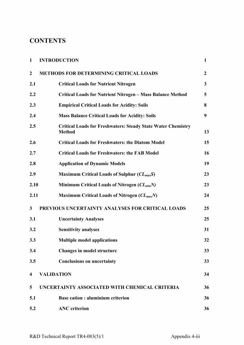
R&D Technical Report TR4-083(5)/1 Appendix 4-iii
CONTENTS
1 INTRODUCTION 1
2 METHODS FOR DETERMINING CRITICAL LOADS 2
2.1 Critical Loads for Nutrient Nitrogen 3
2.2 Critical Loads for Nutrient Nitrogen – Mass Balance Method 5
2.3 Empirical Critical Loads for Acidity: Soils 8
2.4 Mass Balance Critical Loads for Acidity: Soils 9
2.5 Critical Loads for Freshwaters: Steady State Water ChemistryMethod 13
2.6 Critical Loads for Freshwaters: the Diatom Model 15
2.7 Critical Loads for Freshwaters: the FAB Model 16
2.8 Application of Dynamic Models 19
2.9 Maximum Critical Loads of Sulphur (CLmaxS) 23
2.10 Minimum Critical Loads of Nitrogen (CLminN) 23
2.11 Maximum Critical Loads of Nitrogen (CLmaxN) 24
3 PREVIOUS UNCERTAINTY ANALYSES FOR CRITICAL LOADS 25
3.1 Uncertainty Analyses 25
3.2 Sensitivity analyses 31
3.3 Multiple model applications 32
3.4 Changes in model structure 33
3.5 Conclusions on uncertainty 33
4 VALIDATION 34
5 UNCERTAINTY ASSOCIATED WITH CHEMICAL CRITERIA 36
5.1 Base cation : aluminium criterion 36
5.2 ANC criterion 36
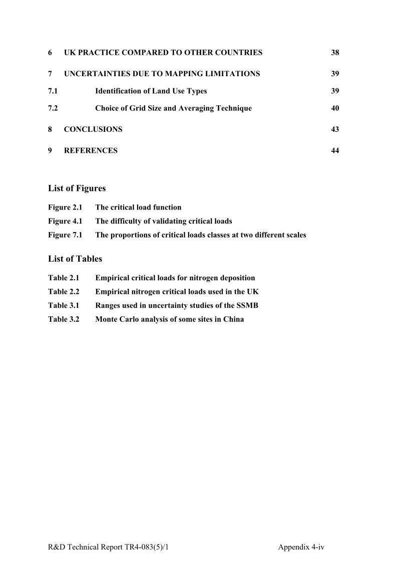
R&D Technical Report TR4-083(5)/1 Appendix 4-iv
6 UK PRACTICE COMPARED TO OTHER COUNTRIES 38
7 UNCERTAINTIES DUE TO MAPPING LIMITATIONS 39
7.1 Identification of Land Use Types 39
7.2 Choice of Grid Size and Averaging Technique 40
8 CONCLUSIONS 43
9 REFERENCES 44
List of Figures
Figure 2.1 The critical load function
Figure 4.1 The difficulty of validating critical loads
Figure 7.1 The proportions of critical loads classes at two different scales
List of Tables
Table 2.1 Empirical critical loads for nitrogen deposition
Table 2.2 Empirical nitrogen critical loads used in the UK
Table 3.1 Ranges used in uncertainty studies of the SSMB
Table 3.2 Monte Carlo analysis of some sites in China
R&D Technical Report TR4-083(5)/1 Appendix 4-1
1 Introduction
The formal definition of a critical load is: "a quantitative estimate of an exposure to oneor more pollutants below which significant harmful effects on specified sensitiveelements of the environment do not occur according to present knowledge" (Nilsson andGrennfelt, 1988). This definition was elaborated at a workshop at Skokloster in Swedenin 1988, and has been used to develop policy within the UNECE, and more recently theEU, ever since. The underlying notion is that of a threshold: if deposition is below thethreshold there are no problems; if it is above the threshold, harm is being done to theenvironment. This is the way the concept is explained to policymakers: it thereforeappears to make sense to reduce deposition below the critical load as quickly aspossible, in order to avoid further harm.
But defining "significant harmful effects" for sensitive elements of the environment on aEuropean scale is a formidably difficult task. The natural environment is immenselycomplex, constantly changing, and not well understood. There are millions of species ofanimals, plants and micro-organisms interacting in an inconceivably vast number ofways with each other and with the physical environment. The response of only a few ofthese species to only a few pollutants is known over only a small range of conditions.Even for these, pollutant effects may be modified e.g. by interaction with otherpollutants, or by different physical conditions. Even then, species sometimes havegeographically distinct ecotypes with a different response to pollutants; there isinvariably a range of responses between individuals. Over large areas such as Europe,there are pronounced gradients in physical conditions, which change the relativeimportance of ecosystem processes. Even if the response of species or ecosystems topollutants were known with certainty, data on species distribution and physicalcharacteristics of the environment would still need to be known at a fine scale. Thesedifficulties are of course not unique to the critical loads approach: they apply to thesetting of any sort of scientifically-based environmental quality standard. The criticalload approach attempts to overcome them by concentrating on certain species, whichare known to be sensitive to pollutant deposition, or chemical substitutes for these, inthe hope that this will also protect every other component of the ecosystem. It is clearthen that the critical load threshold, if there is one, is likely to be very fuzzy.
The aim of this report is to summarise current knowledge about the uncertaintiesentailed in estimating critical loads. Only an outline of critical load methodology can begiven here: full details will be found in the official UNECE Mapping Manual (UBA,1996), in reports from the UK National Focal Centre at Monks Wood (Hall et al. 1997,1998, 2001a) and in publications of the Co-ordinating Centre for Effects (CCE) in theNetherlands (Posch et al. 1995, 1997, 1999, 2001).

R&D Technical Report TR4-083(5)/1 Appendix 4-2
2 Methods for determining critical loads
The UK calculates critical loads for 6 ecosystems: acid grasslands; calcareousgrasslands; heathlands; coniferous woodland; deciduous woodland and freshwaters. Foreach of these, four critical loads are calculated corresponding to the nodes on the criticalloads function (Fig. 2.1). These are the maximum critical load for sulphur (CLmaxS); themaximum critical load for nitrogen (CLmaxN); the minimum critical load for N (CLminN);and the critical load for nutrient N (CLnutN).
CLmaxNN deposition
S deposition
CLmaxS CLnutN
CLminN
Figure 2.1: The critical load function.
The thick line represents the critical load for a hypothetical ecosystem as a function of Sand N deposition. The CLmaxS represents the critical load for acidity when nitrogendeposition is zero. The critical load is equal to CLmaxS whilst all nitrogen deposition istaken up by the catchment, hence the horizontal portion of the critical load function.CLminN is the deposition-independent critical load of acidity due to nitrogen removalprocesses alone (nitrogen uptake, immobilization, and denitrification). CLmaxN is thecritical load for acidity when S deposition is zero. CLnutN is the critical load for nutrientnitrogen, intended to protect against non-acidifying effects of N deposition. In thisexample, CLnutN is less than CLmaxN, truncating the function, but this is not necessarilythe case.
For each type of critical load, the next section describes the theoretical background, themethods the UK uses for calculation, and the major uncertainties in the methods.

R&D Technical Report TR4-083(5)/1 Appendix 4-3
Critical loads for nutrient nitrogen are described first, as they are easier to treat inisolation from the others.
2.1 Critical Loads for Nutrient Nitrogen
The general definition of a critical load was modified somewhat for nitrogen to "aquantitative estimate of an exposure to deposition of nitrogen as NHx and/or NOy belowwhich significant harmful effects in ecosystem structure and function do not occuraccording to present knowledge" (Grennfelt and Thörnelöf, 1988). The addition of theterms "structure" and "function" recognises that ecosystems may be visibly damaged(e.g. by loss of species) or damaged in their capacity to fulfil functions (such asabsorption of N). Deposition of combined nitrogen from the atmosphere has two major,potentially harmful effects: acidification and "eutrophication". Acidification effects aredealt with in conjunction with the acidifying effects of S (see below), but eutrophicationeffects are specific to N and have to be considered separately. Eutrophy (literally "goodnutrition") has acquired connotations of a harmful effect in relation to lakes: in thecontext of N critical loads it means an increase in the N status of an ecosystem to suchan extent that an effect considered to be harmful is likely to appear. The resultingcritical load is the critical load for nutrient nitrogen CLnutN. There are two methods incommon use for estimating the critical load for nutrient nitrogen: the empirical methodand the mass balance method.
2.1.1 Theoretical background – empirical critical loads for nutrient N
The empirical method is based on observations of the N deposition at which changes toecosystem structure and function occur, either in the field or in experiments. The currentofficial values are given by Bobbink et al. (1996) and reproduced in Table 2.1. Anexample of a documented change in ecosystem function is generation of nutrientimbalances in coniferous trees (critical load 10-15 kg N ha-1 y-1); a typical change inecosystem structure is the replacement of heather by grassland in the Netherlands(critical load 15-20 kg N ha-1 y-1). Bobbink et al. (1996) provide estimates of thereliability of each critical load: both the above are regarded as "reliable" (with 2 others -there are 9 rated as "quite reliable" and 6 as "expert judgement" i.e. an informed guess).Absolute values of the critical loads range from 5 kg N ha-1 y-1 (ombrotrophic bogs andarctic heaths) to 35 kg N ha-1 y-1 (calcareous grasslands). Note that there are a numberof different critical loads for the same ecosystem, depending on the ecological effect ofconcern or the characteristics of the ecosystem (e.g. high/low nitrification).
The UNECE Expert Workshop on Chemical Criteria and Critical Limits, held at Yorkin March 2001, proposed a few changes, mostly in a downward direction, and these arealso shown in Table 2.1. There are likely to be more changes, however, resulting from aproposed workshop on empirical nitrogen critical loads in autumn 2002.
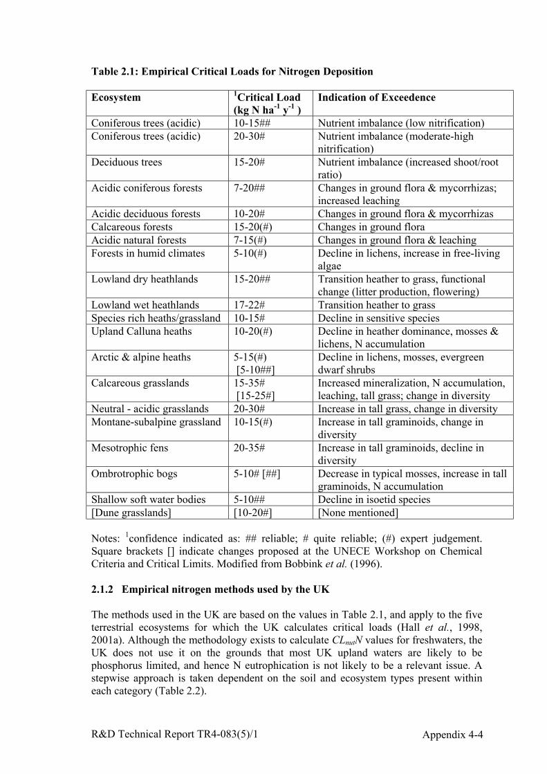
R&D Technical Report TR4-083(5)/1 Appendix 4-4
Table 2.1: Empirical Critical Loads for Nitrogen Deposition
Ecosystem 1Critical Load(kg N ha-1 y-1 )
Indication of Exceedence
Coniferous trees (acidic) 10-15## Nutrient imbalance (low nitrification)Coniferous trees (acidic) 20-30# Nutrient imbalance (moderate-high
nitrification)Deciduous trees 15-20# Nutrient imbalance (increased shoot/root
ratio)Acidic coniferous forests 7-20## Changes in ground flora & mycorrhizas;
increased leachingAcidic deciduous forests 10-20# Changes in ground flora & mycorrhizasCalcareous forests 15-20(#) Changes in ground floraAcidic natural forests 7-15(#) Changes in ground flora & leachingForests in humid climates 5-10(#) Decline in lichens, increase in free-living
algaeLowland dry heathlands 15-20## Transition heather to grass, functional
change (litter production, flowering)Lowland wet heathlands 17-22# Transition heather to grassSpecies rich heaths/grassland 10-15# Decline in sensitive speciesUpland Calluna heaths 10-20(#) Decline in heather dominance, mosses &
lichens, N accumulationArctic & alpine heaths 5-15(#)
[5-10##]Decline in lichens, mosses, evergreendwarf shrubs
Calcareous grasslands 15-35# [15-25#]
Increased mineralization, N accumulation,leaching, tall grass; change in diversity
Neutral - acidic grasslands 20-30# Increase in tall grass, change in diversityMontane-subalpine grassland 10-15(#) Increase in tall graminoids, change in
diversityMesotrophic fens 20-35# Increase in tall graminoids, decline in
diversityOmbrotrophic bogs 5-10# [##] Decrease in typical mosses, increase in tall
graminoids, N accumulationShallow soft water bodies 5-10## Decline in isoetid species[Dune grasslands] [10-20#] [None mentioned]
Notes: 1confidence indicated as: ## reliable; # quite reliable; (#) expert judgement.Square brackets [] indicate changes proposed at the UNECE Workshop on ChemicalCriteria and Critical Limits. Modified from Bobbink et al. (1996).
2.1.2 Empirical nitrogen methods used by the UK
The methods used in the UK are based on the values in Table 2.1, and apply to the fiveterrestrial ecosystems for which the UK calculates critical loads (Hall et al., 1998,2001a). Although the methodology exists to calculate CLnutN values for freshwaters, theUK does not use it on the grounds that most UK upland waters are likely to bephosphorus limited, and hence N eutrophication is not likely to be a relevant issue. Astepwise approach is taken dependent on the soil and ecosystem types present withineach category (Table 2.2).
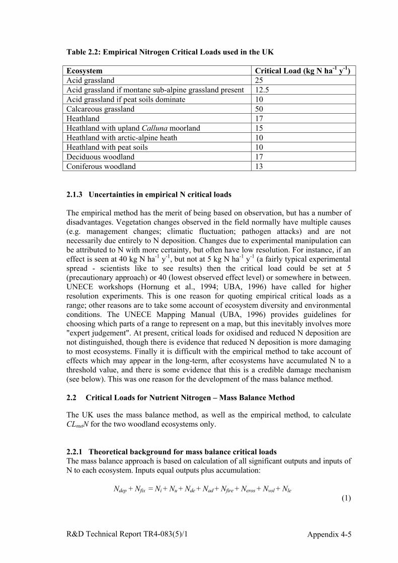
R&D Technical Report TR4-083(5)/1 Appendix 4-5
Table 2.2: Empirical Nitrogen Critical Loads used in the UK
Ecosystem Critical Load (kg N ha-1 y-1)Acid grassland 25Acid grassland if montane sub-alpine grassland present 12.5Acid grassland if peat soils dominate 10Calcareous grassland 50Heathland 17Heathland with upland Calluna moorland 15Heathland with arctic-alpine heath 10Heathland with peat soils 10Deciduous woodland 17Coniferous woodland 13
2.1.3 Uncertainties in empirical N critical loads
The empirical method has the merit of being based on observation, but has a number ofdisadvantages. Vegetation changes observed in the field normally have multiple causes(e.g. management changes; climatic fluctuation; pathogen attacks) and are notnecessarily due entirely to N deposition. Changes due to experimental manipulation canbe attributed to N with more certainty, but often have low resolution. For instance, if aneffect is seen at 40 kg N ha-1 y-1, but not at 5 kg N ha-1 y-1 (a fairly typical experimentalspread - scientists like to see results) then the critical load could be set at 5(precautionary approach) or 40 (lowest observed effect level) or somewhere in between.UNECE workshops (Hornung et al., 1994; UBA, 1996) have called for higherresolution experiments. This is one reason for quoting empirical critical loads as arange; other reasons are to take some account of ecosystem diversity and environmentalconditions. The UNECE Mapping Manual (UBA, 1996) provides guidelines forchoosing which parts of a range to represent on a map, but this inevitably involves more"expert judgement". At present, critical loads for oxidised and reduced N deposition arenot distinguished, though there is evidence that reduced N deposition is more damagingto most ecosystems. Finally it is difficult with the empirical method to take account ofeffects which may appear in the long-term, after ecosystems have accumulated N to athreshold value, and there is some evidence that this is a credible damage mechanism(see below). This was one reason for the development of the mass balance method.
2.2 Critical Loads for Nutrient Nitrogen – Mass Balance Method
The UK uses the mass balance method, as well as the empirical method, to calculateCLnutN for the two woodland ecosystems only.
2.2.1 Theoretical background for mass balance critical loadsThe mass balance approach is based on calculation of all significant outputs and inputs ofN to each ecosystem. Inputs equal outputs plus accumulation:
Ndep + Nfix = Ni + Nu + Nde + Nad + Nfire + Neros + Nvol + Nle(1)
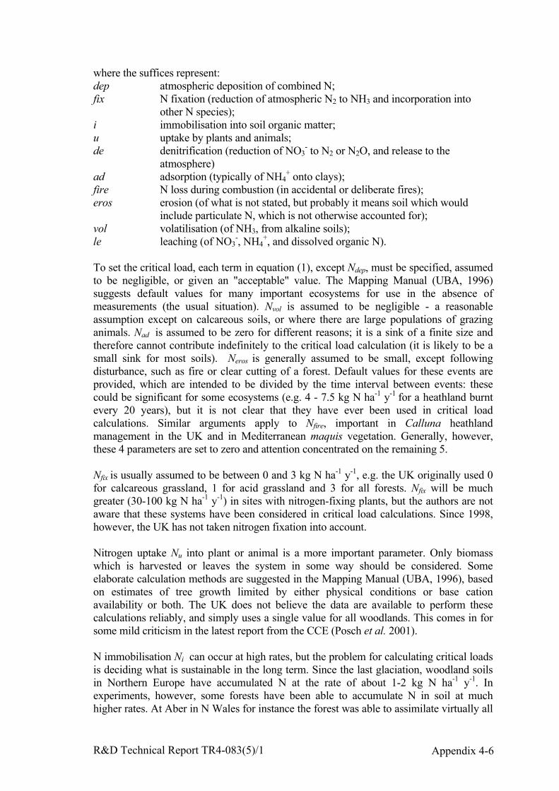
R&D Technical Report TR4-083(5)/1 Appendix 4-6
where the suffices represent:dep atmospheric deposition of combined N;fix N fixation (reduction of atmospheric N2 to NH3 and incorporation into
other N species);i immobilisation into soil organic matter;u uptake by plants and animals;de denitrification (reduction of NO3
- to N2 or N2O, and release to theatmosphere)
ad adsorption (typically of NH4+ onto clays);
fire N loss during combustion (in accidental or deliberate fires);eros erosion (of what is not stated, but probably it means soil which would
include particulate N, which is not otherwise accounted for);vol volatilisation (of NH3, from alkaline soils);le leaching (of NO3
-, NH4+, and dissolved organic N).
To set the critical load, each term in equation (1), except Ndep, must be specified, assumedto be negligible, or given an "acceptable" value. The Mapping Manual (UBA, 1996)suggests default values for many important ecosystems for use in the absence ofmeasurements (the usual situation). Nvol is assumed to be negligible - a reasonableassumption except on calcareous soils, or where there are large populations of grazinganimals. Nad is assumed to be zero for different reasons; it is a sink of a finite size andtherefore cannot contribute indefinitely to the critical load calculation (it is likely to be asmall sink for most soils). Neros is generally assumed to be small, except followingdisturbance, such as fire or clear cutting of a forest. Default values for these events areprovided, which are intended to be divided by the time interval between events: thesecould be significant for some ecosystems (e.g. 4 - 7.5 kg N ha-1 y-1 for a heathland burntevery 20 years), but it is not clear that they have ever been used in critical loadcalculations. Similar arguments apply to Nfire, important in Calluna heathlandmanagement in the UK and in Mediterranean maquis vegetation. Generally, however,these 4 parameters are set to zero and attention concentrated on the remaining 5.
Nfix is usually assumed to be between 0 and 3 kg N ha-1 y-1, e.g. the UK originally used 0for calcareous grassland, 1 for acid grassland and 3 for all forests. Nfix will be muchgreater (30-100 kg N ha-1 y-1) in sites with nitrogen-fixing plants, but the authors are notaware that these systems have been considered in critical load calculations. Since 1998,however, the UK has not taken nitrogen fixation into account.
Nitrogen uptake Nu into plant or animal is a more important parameter. Only biomasswhich is harvested or leaves the system in some way should be considered. Someelaborate calculation methods are suggested in the Mapping Manual (UBA, 1996), basedon estimates of tree growth limited by either physical conditions or base cationavailability or both. The UK does not believe the data are available to perform thesecalculations reliably, and simply uses a single value for all woodlands. This comes in forsome mild criticism in the latest report from the CCE (Posch et al. 2001).
N immobilisation Ni can occur at high rates, but the problem for calculating critical loadsis deciding what is sustainable in the long term. Since the last glaciation, woodland soilsin Northern Europe have accumulated N at the rate of about 1-2 kg N ha-1 y-1. Inexperiments, however, some forests have been able to accumulate N in soil at muchhigher rates. At Aber in N Wales for instance the forest was able to assimilate virtually all
R&D Technical Report TR4-083(5)/1 Appendix 4-7
the experimentally applied input of NH4+ - N at 17.5 kg N ha-1 y-1 for at least 6 years in
spite of being classed as being N saturated, with no obvious deleterious effects.Eventually, however, it is assumed that the C:N ratio of the forest floor would decrease tothe point where N mineralisation and leaching would start to occur. Dynamic models arerequired to assess how long it would take to reach this point. If N deposition increasesproductivity, then C assimilation should also increase, potentially increasing the ability toimmobilise N without decreasing the C:N ratio. The assumption that Ni should be limitedto the historical rate in N-limited systems is thus very much a worst-case assumption. TheMapping Manual recommends 0.5 – 1 kg N ha-1 y-1: the UK uses 1 or 3 kg N ha-1 y-1
depending on soil type.
Denitrification Nde is characteristic of anoxic conditions and thus heavily dependent onsoil type and moisture conditions. It is also dependent on the supply of NO3
- - N, and thuson Ndep. Two methods are suggested in the Mapping Manual (UBA, 1996): the simplestassumes that a constant fraction of the expression (Ndep- Ni - Nu) is denitrified. This isknown as the denitrification fraction fde which varies between 0.1 and 0.8 depending onsoil type. A more complex expression relates denitrification in a non-linear fashion to soilmoisture, temperature and pH, giving a perhaps more realistic curve shape, but on thebasis of a very small amount of experimental data. Again long-term rates are small: 1-3kg N ha-1 y-1 being recommended for forest systems. The UK uses neither of thesemethods: it assumes the rate is 1, 2 or 4 kg N ha-1 y-1 depending on soil type.
The final term to be calculated is Nle. As N leaching is a natural process, and alwaysoccurs even in pristine conditions, an acceptable N leaching Nle(acc) is defined as the rateobserved in similar ecosystems in pristine environments. Recommended values (UBA,1996) range from 0.5 to 4 kg N ha-1 y-1: the UK uses 6 kg N ha-1 y-1.
2.2.2 Nitrogen mass balance methods used by the UK
The UK uses a simplified mass balance equation for the nutrient nitrogen critical loadCLnutN:
CLnutN = Nu + Ni + Nle(acc) + Nde (2)
where Nu is nitrogen uptake;Ni is nitrogen immobilisation;Nle(acc) is the acceptable level of nitrogen leaching;Nde is denitrification.
For both woodland ecosystems, Nu is set at 7 kg N ha-1 y-1, and Nle(acc) at 6 kg N ha-1 y-1.The value of Ni is either 1 or 3 kg N ha-1 y-1 depending on soil type, and likewise the valueof Nde is 1, 2 or 4 kg N ha-1 y-1 depending on soil type. The lower of the empirical andmass balance N critical loads is the value mapped. As the empirical critical load forconiferous woodlands is inevitably lower than the mass balance, this is the value mapped(hence all coniferous woodlands have the same CLnutN value of 13 kg N ha-1 y-1 in theUK). For deciduous woodlands, the UK maps show a mixture of empirical and massbalance values.
R&D Technical Report TR4-083(5)/1 Appendix 4-8
2.2.3 Uncertainties in mass balance N critical loads
Clearly, with much uncertainty over individual terms in equations (1) and (2), the overallresult will also be uncertain. The method has been parameterised with nitrogen-limitednorthern coniferous forests in mind: Nle for instance has a low value, not because of anydeleterious effects of N leaching in the receiving water, but because natural northernforests cycle N very tightly. A higher value for Nle would be ecologically acceptable formore nitrophilous systems. Immobilisation is currently capable of absorbing more N inmost current systems than the default values indicate: the Ni parameter is adjusted to whatmight be the long-term sustainable value. It follows that the mass balance method doesnot necessarily represent the present response of ecosystems, most of which can probablyimmobilise more N without deleterious effects. Only dynamic modelling can estimatewhen deleterious effects might start to appear. The UK has clearly made choices formodels and parameters, which in some cases lie outside the recommended ranges. Thisreflects expert knowledge of UK ecosystems, but is also an indication of uncertainty.
2.3 Empirical Critical Loads for Acidity: Soils
The other nodes on the Critical Load Function are calculated using different models forthe various ecosystems. The models for calculating acidity critical loads are thereforedescribed first, followed by a description of their application to the Critical LoadFunction for the different ecosystems in Sections 2.9 to 2.11. The empirical critical loadfor soils for the UK was the first to be calculated.
2.3.1 Empirical critical loads for acidity for soils: theoretical background
The empirical method of calculating critical loads for forest soils was originallydeveloped at the Skokloster Workshop (Nilsson and Grennfelt, 1988). It is based onassignments of mineral weathering rates to various soil-forming minerals, as mineralweathering is the principal process opposing acidification in terrestrial ecosystems. Theseweathering rates are then modified by site factors, such as slope, soil depth and drainage.The method was modified for use in the UK by Hornung et al. (1995); the originalmineral classifications being changed considerably to take UK conditions into account,especially in relation to lowland clay soils. Soil characteristics were obtained from soilmaps and in underlying databases at the Soil Survey of England and Wales and theMacaulay Land Use Research Institute in Scotland. Results are mapped in classes, whichare intended to give some indication of the uncertainties involved. Class intervals were (inkeq ha-1 y-1): <0.2; 0.2-0.5; 0.5-1.0; 1.0-2.0; and >2.0. These class intervals were chosenunder pressure at the Skokloster Conference (Cresser, 2000), but they have stood the testof time and are widely used. The result (Hornung et al. 1995) is an intuitively satisfyingmap (of course it may be intuitively satisfying because it is based partly on intuition).Nevertheless, the sensitive areas are where they might be expected to be, in the uplands ofthe north and west, and on base poor sandstones in the south.
The UK introduced another innovation: critical loads for peat soils. The Skoklostermethod cannot be applied to these, as they have essentially no weatherable minerals.Cresser and his colleagues (Skiba and Cresser, 1989; Smith et al. 1993) devised a methodwhich is based on laboratory experiments with small peat pellets. From the results ofthese experiments, and a large number of assumptions, they were able to calculate theacid load required to reduce peat in the field by an arbitrary 0.2 pH units. The procedure
R&D Technical Report TR4-083(5)/1 Appendix 4-9
was criticised by Skeffington et al. (1995) and Wilson et al. (1995) on the basis of theirown experiments with peat, but they have yet to come up with a viable alternative.Jenkins and Reynolds (2000) discuss some of the problems, but in the meantime theempirical critical load method devised by Cresser and colleagues is used for UK peats.
2.3.2 Uncertainties in empirical acidity critical loads
The empirical soils method has an element of arbitrariness about it, and depends onexpert knowledge of the mineralogy of UK soils. This is particularly so in England andWales, where mapped soil series do not necessarily have the same mineralogyeverywhere. The modifying factors are also essentially arbitrary. Setting the critical loadequal essentially to the weathering rate implies that it is acceptable for already acidifiedsoils to remain acidified. The fact that the results are reported in classes causes somedifficulties. Similar soils may differ in calculated critical load by a factor of 2 or more,if one is judged to be on one side of a class boundary and the other on the other.Deciding how to represent the class for modelling purposes (e.g. for calculatingexceedence) introduces another arbitrary choice. Should it be the lower bound(precautionary), the central value (moderation) or the upper bound (conservative)? Suchconsiderations led to the mass balance approaches, which are referred to within UNECEas “Level 1” approaches, as opposed to the disparaging epithet “Level 0” applied to theempirical method.
2.4 Mass Balance Critical Loads for Acidity: Soils
2.4.1 Theoretical background to soil mass balance methods
The aim of the acidity mass balance methods is similar to that of the N mass balance: tocalculate all the significant inputs and outputs of acidity, and to link the results to somechemical criterion of "harm" to enable a critical load to be calculated. The mass balancefor S is considered to be:
Sle = Sdep - Sad - Su - Si - Sre - Spr (3)
where the subscripts represent:le leachingdep depositionad adsorption (typically onto sesquioxides or similar soil minerals)u uptake (into plants)i immobilisationre reductionpr precipitation (i.e. as a chemical compound)
For forest soils, uptake, immobilisation, precipitation and reduction of S are consideredto be insignificant. Some of this is arguable: S uptake is perhaps 10% of base cationuptake, and soils which are sufficiently anaerobic to reduce S, are not uncommon in thelandscape as a whole. Sulphate adsorption is an admittedly significant process, butbecause soils are considered to have a finite capacity, it too is ignored, since the systemis assumed to be in steady state. All S leaching is assumed to be SO4
2- (not toounreasonably). Hence the S mass balance reduces simply to:
R&D Technical Report TR4-083(5)/1 Appendix 4-10
SO42-
le = Sdep (4)
A consequence of these assumptions is that the S mass balance does not necessarilyrepresent the behaviour of catchments at the present time. It is very much a worst case,and in the short term (which may be several centuries for strongly sulphate-adsorbingsoils) SO4
2- leaching could be very much less than deposition.
Having obtained mass balances for S and N, these are linked to a definition of "harm"by considering the leaching of Acid Neutralising Capacity (ANC), which requires amass balance of all the other significant ions in the system. This yields:
BCle + NH4+
le - SO42-
le - NO3-le - Cl-
le = ANCle (5)
where:BC base cations (Na+ + K+ + Ca2+ + Mg2+)le leachingANC Acid Neutralising Capacity.All fluxes are expressed in equivalence units e.g. keq ha-1 y-1.
The mass balances expressed by equations (1), (3) and (4) can be combined with otherassumptions to generate the basic mass balance equation (see Posch et al., 1995). Theseassumptions are: (1) chloride inputs equal chloride outputs; (2) base cation sources(deposition and weathering) equal base cation sinks (leaching and uptake); and (3) allleaching from terrestrial catchments is in the form of NO3
-. Substitution then gives:
Sdep + Ndep - BCdep + Cl-dep = BCw - BCu + Ni + Nu + Nde - ANCle (6)
where the symbols represent:BC base cations (Na+ + K+ + Ca2+ + Mg2+)ANC Acid Neutralising Capacitydep depositionle leachingw weathering (i.e. release of base cations from soil minerals)u uptake into plantsi immobilisation in soil organic matterde denitrification.
It is customary to use "non-marine" deposition fluxes in these calculations (symbolisedby *). This makes little difference to the mass balance, as marine (Sdep + Cl-
dep) ≈ marineBCdep. This is the Simple Mass Balance Equation (SMB), so called because it isrecognised that there are a number of simplifying assumptions. It is also known as theSteady State Mass Balance Equation (SSMB). Critical loads for S and N can be derivedfrom this equation, given that values are assigned to all the other parameters and an"acceptable" value of ANCle is defined.
There are several ways of calculating an acceptable ANCle, but by far the most widely-used is the critical base cation : aluminium ratio. This states that the ratio of (K+ + Ca2+
+ Mg2+) to Al in the soil solution should not exceed a certain value (usually 1). Thiscriterion is derived from work on toxicity of Al3+ to tree roots, showing that Ca2+ (andwith rather less certainty Mg2+ and K+) exerts some protection against Al toxicity (see
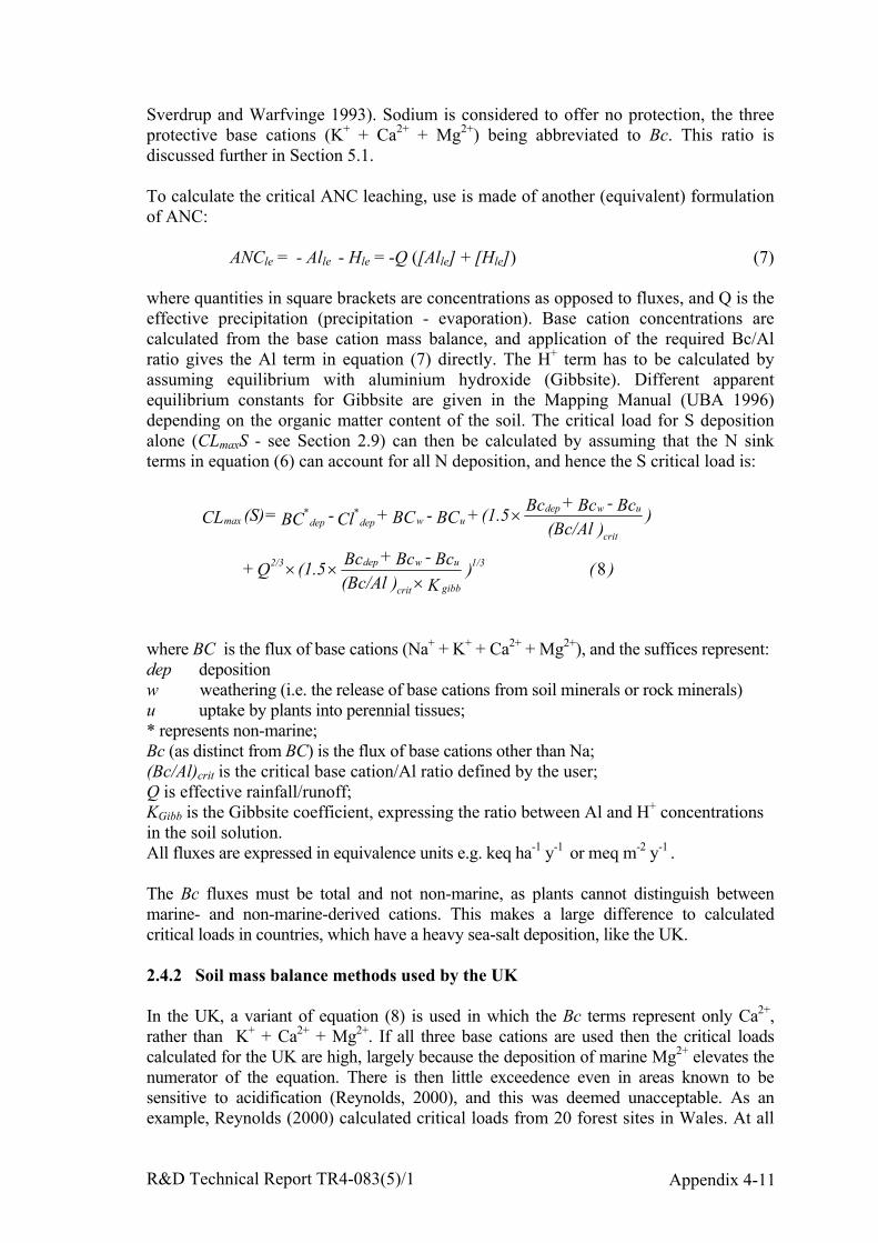
R&D Technical Report TR4-083(5)/1 Appendix 4-11
Sverdrup and Warfvinge 1993). Sodium is considered to offer no protection, the threeprotective base cations (K+ + Ca2+ + Mg2+) being abbreviated to Bc. This ratio isdiscussed further in Section 5.1.
To calculate the critical ANC leaching, use is made of another (equivalent) formulationof ANC:
ANCle = - Alle - Hle = -Q ([Alle] + [Hle]) (7)
where quantities in square brackets are concentrations as opposed to fluxes, and Q is theeffective precipitation (precipitation - evaporation). Base cation concentrations arecalculated from the base cation mass balance, and application of the required Bc/Alratio gives the Al term in equation (7) directly. The H+ term has to be calculated byassuming equilibrium with aluminium hydroxide (Gibbsite). Different apparentequilibrium constants for Gibbsite are given in the Mapping Manual (UBA 1996)depending on the organic matter content of the soil. The critical load for S depositionalone (CLmaxS - see Section 2.9) can then be calculated by assuming that the N sinkterms in equation (6) can account for all N deposition, and hence the S critical load is:
)( )K )(Bc/AlBc - Bc + Bc (1.5 Q +
))(Bc/Al
Bc - Bc + Bc (1.5 + BC - BC + Cl - BC = (S) CL
1/3
gibbcrit
uwdep2/3
crit
uwdepuw
*dep
*depmax
8×
××
×
where BC is the flux of base cations (Na+ + K+ + Ca2+ + Mg2+), and the suffices represent:dep depositionw weathering (i.e. the release of base cations from soil minerals or rock minerals)u uptake by plants into perennial tissues;* represents non-marine;Bc (as distinct from BC) is the flux of base cations other than Na;(Bc/Al)crit is the critical base cation/Al ratio defined by the user;Q is effective rainfall/runoff;KGibb is the Gibbsite coefficient, expressing the ratio between Al and H+ concentrationsin the soil solution.All fluxes are expressed in equivalence units e.g. keq ha-1 y-1 or meq m-2 y-1 .
The Bc fluxes must be total and not non-marine, as plants cannot distinguish betweenmarine- and non-marine-derived cations. This makes a large difference to calculatedcritical loads in countries, which have a heavy sea-salt deposition, like the UK.
2.4.2 Soil mass balance methods used by the UK
In the UK, a variant of equation (8) is used in which the Bc terms represent only Ca2+,rather than K+ + Ca2+ + Mg2+. If all three base cations are used then the critical loadscalculated for the UK are high, largely because the deposition of marine Mg2+ elevates thenumerator of the equation. There is then little exceedence even in areas known to besensitive to acidification (Reynolds, 2000), and this was deemed unacceptable. As anexample, Reynolds (2000) calculated critical loads from 20 forest sites in Wales. At all
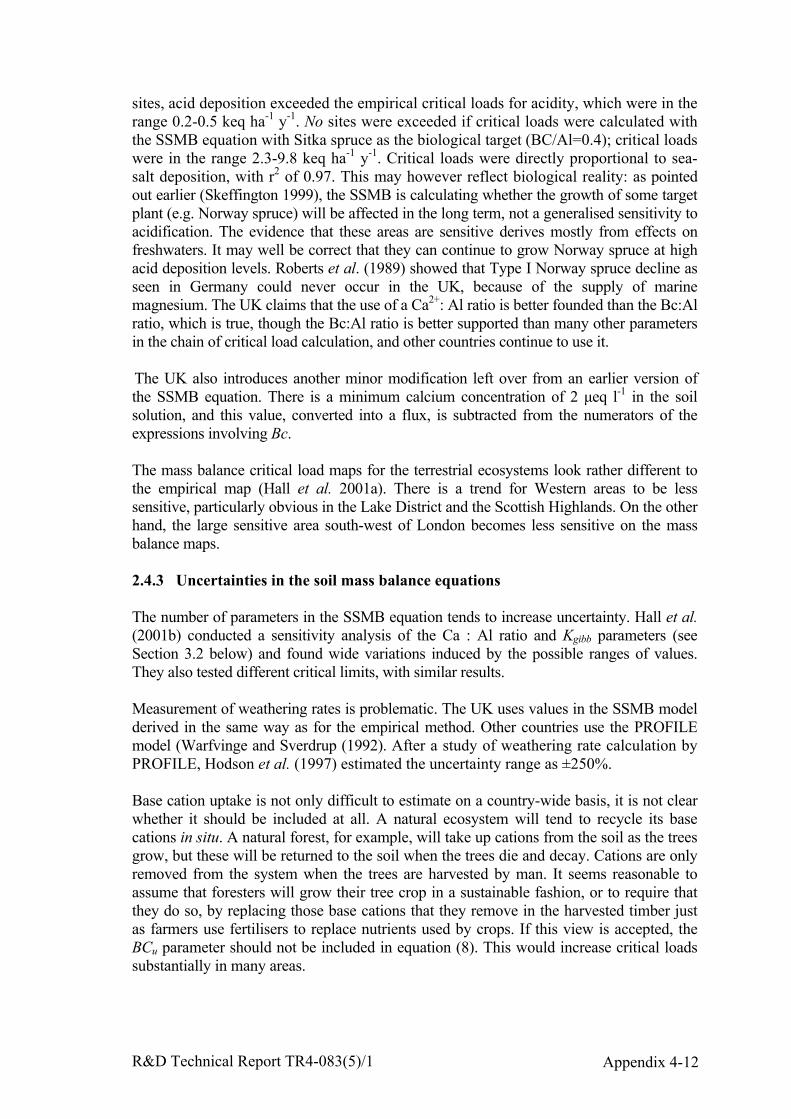
R&D Technical Report TR4-083(5)/1 Appendix 4-12
sites, acid deposition exceeded the empirical critical loads for acidity, which were in therange 0.2-0.5 keq ha-1 y-1. No sites were exceeded if critical loads were calculated withthe SSMB equation with Sitka spruce as the biological target (BC/Al=0.4); critical loadswere in the range 2.3-9.8 keq ha-1 y-1. Critical loads were directly proportional to sea-salt deposition, with r2 of 0.97. This may however reflect biological reality: as pointedout earlier (Skeffington 1999), the SSMB is calculating whether the growth of some targetplant (e.g. Norway spruce) will be affected in the long term, not a generalised sensitivity toacidification. The evidence that these areas are sensitive derives mostly from effects onfreshwaters. It may well be correct that they can continue to grow Norway spruce at highacid deposition levels. Roberts et al. (1989) showed that Type I Norway spruce decline asseen in Germany could never occur in the UK, because of the supply of marinemagnesium. The UK claims that the use of a Ca2+: Al ratio is better founded than the Bc:Alratio, which is true, though the Bc:Al ratio is better supported than many other parametersin the chain of critical load calculation, and other countries continue to use it.
The UK also introduces another minor modification left over from an earlier version ofthe SSMB equation. There is a minimum calcium concentration of 2 µeq l-1 in the soilsolution, and this value, converted into a flux, is subtracted from the numerators of theexpressions involving Bc.
The mass balance critical load maps for the terrestrial ecosystems look rather different tothe empirical map (Hall et al. 2001a). There is a trend for Western areas to be lesssensitive, particularly obvious in the Lake District and the Scottish Highlands. On the otherhand, the large sensitive area south-west of London becomes less sensitive on the massbalance maps.
2.4.3 Uncertainties in the soil mass balance equations
The number of parameters in the SSMB equation tends to increase uncertainty. Hall et al.(2001b) conducted a sensitivity analysis of the Ca : Al ratio and Kgibb parameters (seeSection 3.2 below) and found wide variations induced by the possible ranges of values.They also tested different critical limits, with similar results.
Measurement of weathering rates is problematic. The UK uses values in the SSMB modelderived in the same way as for the empirical method. Other countries use the PROFILEmodel (Warfvinge and Sverdrup (1992). After a study of weathering rate calculation byPROFILE, Hodson et al. (1997) estimated the uncertainty range as ±250%.
Base cation uptake is not only difficult to estimate on a country-wide basis, it is not clearwhether it should be included at all. A natural ecosystem will tend to recycle its basecations in situ. A natural forest, for example, will take up cations from the soil as the treesgrow, but these will be returned to the soil when the trees die and decay. Cations are onlyremoved from the system when the trees are harvested by man. It seems reasonable toassume that foresters will grow their tree crop in a sustainable fashion, or to require thatthey do so, by replacing those base cations that they remove in the harvested timber justas farmers use fertilisers to replace nutrients used by crops. If this view is accepted, theBCu parameter should not be included in equation (8). This would increase critical loadssubstantially in many areas.
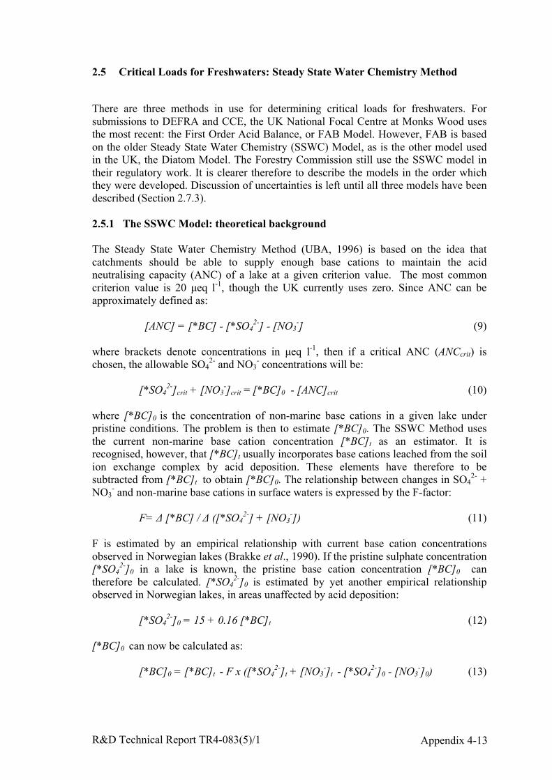
R&D Technical Report TR4-083(5)/1 Appendix 4-13
2.5 Critical Loads for Freshwaters: Steady State Water Chemistry Method
There are three methods in use for determining critical loads for freshwaters. Forsubmissions to DEFRA and CCE, the UK National Focal Centre at Monks Wood usesthe most recent: the First Order Acid Balance, or FAB Model. However, FAB is basedon the older Steady State Water Chemistry (SSWC) Model, as is the other model usedin the UK, the Diatom Model. The Forestry Commission still use the SSWC model intheir regulatory work. It is clearer therefore to describe the models in the order whichthey were developed. Discussion of uncertainties is left until all three models have beendescribed (Section 2.7.3).
2.5.1 The SSWC Model: theoretical background
The Steady State Water Chemistry Method (UBA, 1996) is based on the idea thatcatchments should be able to supply enough base cations to maintain the acidneutralising capacity (ANC) of a lake at a given criterion value. The most commoncriterion value is 20 µeq l-1, though the UK currently uses zero. Since ANC can beapproximately defined as:
[ANC] = [*BC] - [*SO42-] - [NO3
-] (9)
where brackets denote concentrations in µeq l-1, then if a critical ANC (ANCcrit) ischosen, the allowable SO4
2- and NO3- concentrations will be:
[*SO42-]crit + [NO3
-]crit = [*BC]0 - [ANC]crit (10)
where [*BC]0 is the concentration of non-marine base cations in a given lake underpristine conditions. The problem is then to estimate [*BC]0. The SSWC Method usesthe current non-marine base cation concentration [*BC]t as an estimator. It isrecognised, however, that [*BC]t usually incorporates base cations leached from the soilion exchange complex by acid deposition. These elements have therefore to besubtracted from [*BC]t to obtain [*BC]0. The relationship between changes in SO4
2- +NO3
- and non-marine base cations in surface waters is expressed by the F-factor:
F= ∆ [*BC] / ∆ ([*SO42-] + [NO3
-]) (11)
F is estimated by an empirical relationship with current base cation concentrationsobserved in Norwegian lakes (Brakke et al., 1990). If the pristine sulphate concentration[*SO4
2-]0 in a lake is known, the pristine base cation concentration [*BC]0 cantherefore be calculated. [*SO4
2-]0 is estimated by yet another empirical relationshipobserved in Norwegian lakes, in areas unaffected by acid deposition:
[*SO42-]0 = 15 + 0.16 [*BC]t (12)
[*BC]0 can now be calculated as:
[*BC]0 = [*BC]t - F x ([*SO42-]t + [NO3
-]t - [*SO42-]0 - [NO3
-]0) (13)
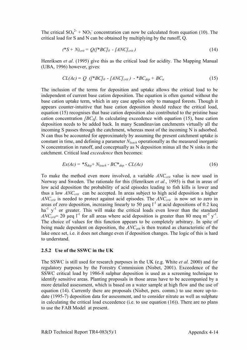
R&D Technical Report TR4-083(5)/1 Appendix 4-14
The critical SO42- + NO3
- concentration can now be calculated from equation (10). Thecritical load for S and N can be obtained by multiplying by the runoff, Q.
(*S + N)crit = Q([*BC]0 - [ANC]crit ) (14)
Henriksen et al. (1995) give this as the critical load for acidity. The Mapping Manual(UBA, 1996) however, gives:
CL(Ac) = Q ([*BC]0 - [ANC]crit ) - *BCdep + BCu (15)
The inclusion of the terms for deposition and uptake allows the critical load to beindependent of current base cation deposition. The equation is often quoted without thebase cation uptake term, which in any case applies only to managed forests. Though itappears counter-intuitive that base cation deposition should reduce the critical load,equation (15) recognises that base cation deposition also contributed to the pristine basecation concentration [BC0]. In calculating exceedence with equation (15), base cationdeposition needs to be added back. In many Scandinavian catchments virtually all theincoming S passes through the catchment, whereas most of the incoming N is adsorbed.N can thus be accounted for approximately by assuming the present catchment uptake isconstant in time, and defining a parameter Nleach operationally as the measured inorganicN concentration in runoff, and conceptually as N deposition minus all the N sinks in thecatchment. Critical load exceedence then becomes:
Ex(Ac) = *Sdep+ Nleach - BC*dep - CL(Ac) (16)
To make the method even more involved, a variable ANCcrit value is now used inNorway and Sweden. The rationale for this (Henriksen et al., 1995) is that in areas oflow acid deposition the probability of acid episodes leading to fish kills is lower andthus a low ANCcrit can be accepted. In areas subject to high acid deposition a higherANCcrit is needed to protect against acid episodes. The ANCcrit is now set to zero inareas of zero deposition, increasing linearly to 50 µeq l-1 at acid depositions of 0.2 keqha-1 y-1 or greater. This will make the critical loads even lower than the standardANCcrit= 20 µeq l-1 for all areas where acid deposition is greater than 80 meq m-2 y-1.The choice of values for this function appears to be completely arbitrary. In spite ofbeing made dependent on deposition, the ANCcrit is then treated as characteristic of thelake once set, i.e. it does not change even if deposition changes. The logic of this is hardto understand.
2.5.2 Use of the SSWC in the UK
The SSWC is still used for research purposes in the UK (e.g. White et al. 2000) and forregulatory purposes by the Forestry Commission (Nisbet, 2001). Exceedence of theSSWC critical load by 1986-8 sulphur deposition is used as a screening technique toidentify sensitive areas. Planting proposals in those areas have to be accompanied by amore detailed assessment, which is based on a water sample at high flow and the use ofequation (14). Currently there are proposals (Nisbet, pers. comm.) to use more up-to-date (1995-7) deposition data for assessment, and to consider nitrate as well as sulphatein calculating the critical load exceedence (i.e. to use equation (16)). There are no plansto use the FAB Model at present.
R&D Technical Report TR4-083(5)/1 Appendix 4-15
2.6 Critical Loads for Freshwaters: the Diatom Model
2.6.1 Diatom model: theoretical background
The Diatom Method is a variant of the SSWC Method, which uses changes in diatompopulations, rather than a critical ANC, as the criterion response. The speciescomposition history of diatom populations in lakes, which is strongly affected by waterchemistry, can be inferred from palaeolimnological studies of sediment cores (e.g.Battarbee et al., 1996). Whether a lake has acidified or not can thus be judged byexamining sediment cores. Battarbee et al. (1996) found that acidified and non-acidifiedlakes can be separated optimally by a relationship between current lake Caconcentration and current S deposition :
[Ca] = 94× *Sdep (17)
where [Ca] is expressed in µeq l-1 and *Sdep in keq ha-1 y-1. Calcium concentration canbe taken as a measure of the neutralising power of the catchment, and hence thisrelationship could be used to set a critical load. However, acid deposition has probablyincreased the [Ca] currently found in lakes. As a rough approximation of the originalneutralising power of the catchment, the original Ca concentration of the lake [Ca2+]*0is estimated in the same way as in the SSWC Method, replacing *BC with *Ca2+ asappropriate. A critical load for S can then be calculated from equation (17). The methodhas been adapted to produce a critical load for acidity in a similar way to the SSWCMethod, by assuming that the current N sinks in the catchment are stable, and that thecatchment adsorbs no S, so that the fraction of nitrogen deposition contributing toacidification aN is:
aN = (*Sdep / Ndep) / (*[SO42-]t / [NO3
-]t ) (18)
If the model is recalibrated using this equation, the Ca:deposition ratio reduces slightly,to 89:1, leaving the critical load for acidity as:
CL(A) = [*Ca2+]0 / 89 (19)
where the critical load is expressed in keq ha-1 y-1, and [*Ca2+]0 in µeq l-1.
Exceedence is defined as:
CL(A)ex= CL(A) - *Sdep - aN Ndep(20)
2.6.2 Use of the Diatom Model in the UK
The Diatom Model is used primarily for research purposes, e.g. Kernan et al. (2001)and Ulyett et al. (2001) used it to calculate critical loads for comparison with catchmentcharacteristics. The parameterisation of the model has not altered since Battarbee et al.(1996).

R&D Technical Report TR4-083(5)/1 Appendix 4-16
2.7 Critical Loads for Freshwaters: the FAB Model
The First Order Acid Balance (FAB) Model is the method of choice for calculatingcritical loads in the UK and continental Europe, partly because it is the only one whichcan be used to generate the critical loads function as it treats S and N independently.Apart from critical loads, it can also be used to predict future sulphate and nitrateconcentrations in surface waters.
2.7.1 The FAB Model: theoretical background
The FAB Method is the aquatic analogue of the SSMB Method, in which an attempt ismade to take into account in-lake processes, which can be very effective in producingalkalinity. As with the SSMB method, a combination of charge balance and mass balanceequations leads to:
*Sdep + Ndep = fNu + (1 - r)(Ni + Nde) + rNret + rSret + *BCle - ANCle (21)
where:dep deposition (all fluxes in acid equivalents ha-1 y -1)f fraction of catchment area which is forestedNu N uptake into forest treesr fraction of catchment area occupied by lakesNi N immobilisation in soil organic matterNde denitrification in the catchment soilsNret in-lake retention of NSret in-lake retention of SBCle leaching of base cations (Na+ + K+ + Ca2+ + Mg2+)ANCle Acid Neutralising Capacity leaching.
Equation (21) differs from that in the Mapping Manual (UBA, 1996) in having non-marine rather than total *Sdep and *BCle, but equation (21) is the correct formulation(Reynolds and Skeffington 1999). It is not clear whether this is universally appreciated.
The soil parameters (N uptake and immobilisation, and denitrification) are estimated asfor the SSMB Model (Section 2.3). Note however that N uptake is only counted if it goesinto forest biomass, as it will then be harvested and removed from the system instead ofrecycled in situ. Immobilisation and denitrification are scaled to the land surface area.
The parameters rNret and rSret model N and S retention by lakes in the catchment. Lakesare powerful generators of alkalinity which can not be ignored when acidification effectsare being considered. The principal processes are S and N reduction in the lake sediments,and the rates of these two processes are estimated as follows. In-lake retention of N isassumed to be proportional to the net input of N i.e. N deposition less immobilisation,uptake and denitrification:
rNret = ρN(Ndep - fNu - (1-r)(Ni + Nde)) (22)
where the factor ρN is modelled by a kinetic equation derived from work on lakes inNorway and sub-arctic Canada:
R&D Technical Report TR4-083(5)/1 Appendix 4-17
ρN = SN / (SN + (Q / r)) (23)
The factor SN is a mass transfer coefficient for N with units of velocity (m y-1).
Sulphur retention is treated in an exactly analogous way:
rSret = ρSSdep (24)
where the factor ρS is modelled by a kinetic equation based on the same lakes:
ρS = SS / (SS + (Q / r)) (25)
where the factor SS is a mass transfer coefficient for S with units of velocity.
The parameters *BCle - ANCle are modelled using exactly the same methods as for theSSWC Model (equations 10-14).
The FAB critical load equation then becomes:
aNCL(N) + aSCL(S) = b1Nu + b2Ni + Q ([*BC]0 - [ANC]crit ) (26)
equivalent to:
aNCL(N) + aSCL(S) = b1Nu + b2Ni + Lcrit (27)
where the coefficients are dimensionless and depend on lake and catchment propertiesalone:
aN = (1-fde(1-r))(1-ρN)aS = 1-ρSb1 = f(1-fde)(1-ρN)b2 = (1-fde)(1-r)(1-ρN)
where ρN and ρS are defined in equations (23) and (25), and fde is the denitrificationfraction, and Lcrit is the critical leaching, defined as Q([*BC]0 - [ANC]crit ). If derivingthese expressions, note that the denitrification fraction is calculated differently forforested and non-forested land.
2.7.2 Use of the FAB Model in the UK
The use and parameterisation of FAB in the UK is described by Curtis et al. (1998,2000). As always, the model has been adapted for British conditions. N uptake isparameterised as a single value of 0.279 keq ha-1 y-1: unlike the value for terrestrialwoodland systems it was not increased to 0.5 keq ha-1 y-1 for 2001. Only coniferousforest uptake of N is counted when calculating freshwater critical loads. Deciduousforest is discounted on the grounds that it is not likely to be harvested (hence removingN from the system), and other ecosystems are not considered at all. This is alsoinconsistent with the methods for terrestrial ecosystems which all includeparameterisation of N uptake.
R&D Technical Report TR4-083(5)/1 Appendix 4-18
Nitrogen immobilisation and denitrification are parameterised as for the terrestrialecosystems, i.e. as fixed values dependent on soil type. The Mapping Manual (UBA,1996) suggests that denitrification should be proportional to deposition (as in thecoefficients of equation (27)) and that the fraction of net N deposition (deposition afterremoval by other sink processes) which is denitrified (fde) should be:
fde = 0.1 + 0.7fpeat (28)
where fpeat is the fraction of peat soils in the catchment. However it was considered thatthis would lead to unrealistically high N removal rates for British upland conditions, upto 30 kg N ha-1 y-1 as opposed to the 1 – 4 kg N ha-1 y-1 actually used. As yetunpublished results from a subsequent research project (the CLAM Project) are said toconfirm the lower values.
Default values are used for the in-lake retention parameters. The UK critical loads areestimated from a single water sample taken, in the autumn or spring of 1992-4, fromwhat was considered to be the most sensitive lake in each 10 km grid square (20 kmgrid square in lowland areas). If no lake was available, a first-order stream was used.The in-lake retention parameters were set to zero if the sample was taken from a stream,although whether this should be so is another topic which is currently being researched.
In the UK, ANCcrit is set to zero, though there are proposals to make it +20 µeq l-1. Thiswould bring the UK into line with some other countries in Europe, but would produceunrealistic critical loads for a proportion of lakes. The current freshwater critical loadmaps produced by the UK contain some errors in that some waters in the South andMidlands have very low critical loads. These are usually lowland waters with anindigenous source of sulphate, which should have been eliminated from the dataset, butwere not owing to an oversight.
2.7.3 Uncertainties in freshwater critical load methods
All three water methods are related, and all are highly empirical. All require theestimation of the pre-industrial base cation concentration through a chain of empiricalequations which are validated with data from the Nordic countries. Where the physicalenvironment differs from that in these countries, the empirical relationships are likely tobe different. Indeed, R. Harriman (pers. communication) has long considered thatequation (12) exaggerates pre-industrial sulphate concentrations in the UK, and uses[*SO4
2-]0 = 7 + 0.05 [*BC]t instead on the basis of measurements in Scottish lochs inrelatively pristine areas. Kämäri et al. (1993) performed an uncertainty analysis on theSSWC Model for lakes in Finland, using Monte Carlo methods. This suggested an overallstandard deviation on the critical load of ±10%. There is also some as yet unpublishedwork in Norway on uncertainties in the SSWC Model.
The assumption that the F-factor (equation (11)) is a constant is not consistent withcurrent biogeochemical knowledge: it should change with the acidification state of thesoil. Henriksen (1995) evaluated the effect of changing F on critical load exceedence. Theeffect was small in Norway, reflecting the sensitivity of Norwegian lakes, but larger inSweden and Finland. For instance, substituting F = 0 in equation (11) reduced exceedencefrom 29.7% in Norwegian lakes to 27.2%, but from 29.6% to 16.4% of Swedish lakes.
R&D Technical Report TR4-083(5)/1 Appendix 4-19
The Diatom Model has the same uncertainties as the SSWC Model except for theuncertainty involved in defining the ANC limit. This is a major advantage of the DiatomModel: there is no constraint to a fixed ANC, and thus some of the individualcharacteristics of lakes are in theory taken into account. However, it uses an additionalempirical relationship, between S deposition and [Ca], which may not be applicableoutside the UK and which may alter with time. Use of the pristine calciumconcentration in equation (19) is precautionary, as the point at which acidification isinitiated will lie somewhere between [*Ca2+]0 and current [Ca2+].
The FAB Model has the same uncertainties as the SSWC Model and a number ofothers. Curtis et al. (2000) discuss some of them. The fraction of the catchment which isforested has to be identified from satellite photographs or other data. Estimates of Nuptake, immobilisation and denitrification have to be provided, usually from defaultvalues. Deposition and runoff data have to be interpolated onto a catchment area fromgrid-based model outputs, which are themselves uncertain. The in-lake retentionparameters are based on data from sub-arctic regions with lower temperatures and henceslower reaction rates than those found in the UK. Rivers are given zero S and Nretention, which in many cases will ignore a significant process. There is also someuncertainty about how to calculate the critical loads function (Sections 2.10 and 2.11).
2.8 Application of Dynamic Models
Dynamic models are not routinely being used to calculate critical loads, although thereis a lot of ongoing work on dynamic modelling in this context both in the UK and inEurope. However dynamic models have the potential to be very useful for regulatorypurposes. In some senses they are more complex than the steady-state models, but theyavoid some of the uncertainties inherent in the latter. Jenkins and Reynolds (2000) haverecently reviewed dynamic models for the assessment of acidification for theEnvironment Agency, and there would be little point in repeating that work here. Theirreport contains a description of the MAGIC Model and a review of some of theuncertainty and validation studies which have been applied to it. There are shorterdescriptions of the SMART and SAFE models. These three models are those likely tobe used for dynamic modelling in UK and European applications. This section thereforeconcentrates on a review of current thinking of how dynamic models might be appliedin a regulatory context.
2.8.1 Advantages of dynamic models
The characteristic of dynamic models is that they calculate the values of environmentalvariables as a function of time. These variables may be chemical values familiar fromthe critical loads methods, such as ANC or Bc : Al ratio. They could also be used togenerate more detailed chemistry, which could be used as input to biological responsemodels. An example might be the use of Al, Ca and pH to predict fish status, or ionexchange models to predict plant growth, as discussed by Jenkins and Reynolds (2000).Though the biological response models introduce additional uncertainty, they focusattention on the ultimate target, the part of the system that public and policymakers arereally interested in. The calculation of ANC is of interest to chemists, but the aim ofpolicy is to protect aquatic organisms.
R&D Technical Report TR4-083(5)/1 Appendix 4-20
As discussed below, dynamic models are easier to validate against measurement datathan steady state critical load models, because they make predictions which should betrue at a certain time. Steady state critical load models are predicting an equilibriumstate which may occur at some future time, possibly centuries hence. Dynamic modelscan make predictions, which come within the time horizon of current policymakers(although the actions necessary to achieve environmental targets within a few years maycome as something of a shock).
In a cost-benefit framework, dynamic models (calculating environmental benefits)interface better with economic models (calculating costs). Economic models aretypically dynamic, at least in the sense that future expenditure is discounted.Schmieman and Van Ierland (1999) provide an example of linked dynamicenvironmental and economic models, which came to the conclusion that the criticalloads approach had provided a sub-optimal solution to the same problem.
Dynamic models escape the uncertainties associated with the damage threshold conceptwhich underlies critical loads. Critical loads as calculated are not really thresholds(Skeffington, 1999) nor do such unequivocal thresholds really exist in the naturalenvironment. The use of dynamic models can obviate the need to define thresholds, andconcentrate attention instead on the response over time of chemical and biologicalentities. The addition of the time dimension adds another choice for the policymaker.This choice may be unwelcome, but gives further scope for balancing costs andbenefits.
2.8.2 Developments in dynamic modelling
Dynamic modelling has been discussed for a long time, but it is now really makingprogress. There are several reasons for this. Firstly, the technology is becomingavailable. Computing power continues to increase, and GIS systems are able totransform and process these data and present the results in the form of maps. Secondly,models (e.g. deposition models) are becoming more sophisticated and can produceoutputs on a finer scale, and environmental data can be obtained on national andEuropean scales. Thirdly, the infrastructure has already been developed under UNECE,and in national critical loads programmes. The people who have developed and runthese programmes can apply their experience to dynamic modelling.
The UNECE Working Group on Effects has set up a Joint Expert Group on dynamicmodelling, which met in October 2000 and November 2001 in Ystad, Sweden. Thelocation is not entirely insignificant, because the meetings were organised and fundedby the Swedish International and National Abatement Strategies for Transboundary AirPollution (ASTA) Programme, which is headed by Jan Nilsson, original promoter of thecritical load concept. The two meeting reports show that real progress is being made.The EU is funding the RECOVER:2010 programme, which is currently modelling theresponse of sensitive waters to reductions of acid deposition in seven Europeancountries, including the UK. Four countries now have fine-scale regional dynamicassessments of the response of soil to deposition reductions. Dynamic models are beingapplied to soils in a subset of the EU/UNECE forest plots. CCE have prepared a draftDynamic Modelling Manual analogous to the Mapping Manual. The USA and Canadaare both developing regional dynamic assessments. The intention is to use dynamic
R&D Technical Report TR4-083(5)/1 Appendix 4-21
models in the reviews of the Gothenburg Protocol and the Emission Ceilings Directivein the middle of the decade, and the structures for doing this are being prepared.
Dynamic model applications to single sites are well established, and a lot of the effortwithin UNECE is being devoted to the problems of applying them on a wider(European) scale. In particular, thought is being given to applying them within theexisting structure of integrated assessment models (Posch and Hettelingh 2001).Dynamic models are too complex and data-demanding to be run within the structure ofthe RAINS Model, which claims to produce cost-optimised solutions to controllingemissions in Europe. It is possible that simplified versions could be used within RAINS,as happened with the EMEP ozone model, though it is not certain that simplifiedversions of the dynamic models, which capture the essentials of their behaviour are infact possible. More realistically, dynamic models could be run to determine target loads,e.g. the maximum deposition which would allow the attainment of a certainenvironmental goal (e.g. ANC concentration) within a given time. These target loadscould be fitted into the existing integrated assessment framework. Another possibility isdescribed by Posch and Hettelingh (2001) as “recovery isolines”, which show recoverytimes as a function of deposition reduction and year of implementation. These could bepre-run and used within a probabilistic optimisation framework as with the GothenburgProtocol. (There is clearly something wrong with this diagram, which implies thatemission reductions in certain years would lead to recovery before the reductions wereimplemented).
Treatment of dynamic models within the UK has no need to be so elaborate. A start hasalready been made on the use of dynamic models to predict acidification status on abroad scale. Jenkins et al. (1997) and Jenkins and Cullen (2001) applied MAGIC to datafrom some of the 22 sites in the UK Acid Waters Monitoring Network. The earlierstudy modelled the effect of the Second Sulphur Protocol to the year 2041. The laterstudy used fewer sites but had the benefit of more data for calibration and a version ofMAGIC with improved N dynamics. It modelled the effect of the Gothenburg Protocolup to 2020. In both cases most sites showed some recovery in ANC, though not alwaysto the UK criterion value of 0 µeq l-1. Up to 2020, best-case and worse-case assumptionsabout nitrate made only minor differences to ANC predictions. Comparing FABpredictions (Curtis et al. 1998) from the same sites, however, indicated that increasingnitrate leaching could make a very large difference indeed to ANC concentrations. Thisstudy illustrates some of the value to be obtained from dynamic modelling: it indicates ageneral pattern of behaviour of sensitive sites, can generate uncertainty bands, andpoints to research directions.
Another style of modelling is to run dynamic models in probabilistic mode. For aregional application, input variables are randomly sampled from defined frequencydistributions based on observed data for the region as a whole. Models are run manytimes, Monte-Carlo fashion, and outputs are in the form of statistical distributions ofparameters for the region as a whole. This approach sacrifices locational informationabout sites within the region, but enables statistical statements to be made about theregion as a whole. The approach is compatible with targets such as “90% of lakeswithin this region should have ANC> 20 µeq l-1 by the year 2020”. An example fromthe UK is a regional model for Wales, which was used by Sefton and Jenkins (1998) toshow that an 80-85% reduction in deposition (based on 1990) would be necessary if95% of acid-sensitive Welsh waters were to achieve ANC > 0 µeq l-1 by the year 2030.
R&D Technical Report TR4-083(5)/1 Appendix 4-22
A heroic attempt at modelling individual sites on a wide scale was that of Evans et al.(1998), who applied MAGIC to 1027 sites in Great Britain using water quality dataderived from the critical loads sample survey, and soil and deposition databases. Sincethis uses a single spot value to represent the annual mean water chemistry, it was to beexpected that there would be some difficulty in calibrating the model at some sites, andthere was, particularly at sites with high sea-salt inputs. Nevertheless satisfactorycalibration was achieved at 698 sites, and the reduction in deposition due to the SecondS Protocol was modelled until 2050. The authors produced some statistics showingregional recovery trends, with some sites still with ANC <0 in 2050, and averagerecovery of ANC compared to the calculated pristine value was about 15-30%,depending on region. The study could have been used for scenario analysis, but theauthors are clearly aware of its limitations and suggest some improvements inmethodology. Nevertheless it demonstrates that meaningful results can be produced bythis approach provided the data are available and a critical approach is adopted.
Water quality modelling usually concentrates on headwater catchments, but very oftenthe important biological resources are lower down in larger streams and rivers. Heremixing of waters from different sources has to be taken into account, and there is spatialconnectivity between catchments, which is not captured on the usual gridded maps.Cooper et al. (2000) devised a procedure for modelling recovery in these catchments byidentifying landscape types, which were assumed to behave as homogenous units, andmixing the waters resulting from modelled changes in the landscape types. Thisprocedure was developed in the Towy catchment in Wales, but it proved possible totransfer it to other UK catchments with varying degrees of success.
2.8.3 Uncertainties in dynamic models
Jenkins and Reynolds (2000) review some uncertainty analyses for dynamic models,and produce error bounds on predictions. In this section, the authors consider thequestion “Are dynamic models more uncertain than orthodox steady-state critical loadmodels?”. There are no quantitative, objective analyses which address this question.The answer will of course depend on which models are chosen for comparison, butsome general statements can be made about the commonly used models.
Dynamic models require more parameters than steady-state models, usually a cause ofgreater uncertainty. Some of the parameters required are the same, weathering rate forinstance, but the dynamic models also require the variation of some parameters overtime, including variation in past centuries and predicted variation in future. Set againstthis, dynamic models are usually calibrated against current conditions, which constrainsthe range of possible outcomes. It is much harder to do this with the steady-statemodels, which inherently predict conditions at some indefinite time in future (seeSection 4). On the other hand there are several examples in which a dynamic model wascalibrated to present conditions in more than one way, leading to very different futurepredictions. But there again there is no need in the dynamic models for the long chain ofempirical relationships used in the freshwater critical load models to estimate pre-industrial base cation concentration. From first principles, all that can be said is thatthere is no evidence that dynamic models are more or less uncertain than the steady-state models. Some quantitative work on this question might be worthwhile.
R&D Technical Report TR4-083(5)/1 Appendix 4-23
2.9 Maximum Critical Loads of Sulphur (CLmaxS)
For terrestrial ecosystems, CLmaxS (Fig. 2.1) is based on the acidity critical load valuesbut also takes into account non-marine base cation and chloride deposition to the soil,and base cation removal from the system:
CLmaxS = CL(A) + *BCdep – *Cldep - BCu (29)
where:CL(A) acidity critical load*BCdep non-marine base cation deposition*Cldep non-marine chloride depositionBCu base cation uptake by vegetation.
For the acid grassland, calcareous grassland and heathland ecosystems, CL(A) is theempirical critical load for soils (Section 2.3). For the deciduous and coniferouswoodland ecosystems CL(A) in equation (29) is the mass balance critical load (equation(8)).
For aquatic ecosystems, CLmaxS is given by:
CLmax(S) = Lcrit / (1-ρS) (30)
where ρS is defined as in equation (25) and Lcrit as in equation (27). This is the criticalload for acid leaching modified by S retention in lakes. Hence for aquatic ecosystems, Sretention is taken into account while base cation deposition is not (at least directly), whilefor terrestrial ecosystems the reverse is the case. The justification for this difference isdebatable.
2.10 Minimum Critical Loads of Nitrogen (CLminN)
The calculation of CLminN for terrestrial ecosystems is closely related to the massbalance model for CLnutN, and similar comments apply. The minimum critical load ofnitrogen represents the critical load of acidity due solely to nitrogen removal processesin soil:
CLminN = Nu+Ni+Nde (31)
where:Nu nitrogen uptakeNi nitrogen immobilisationNde denitrification
This equation applies only if it is assumed that all N deposition which is not taken up,immobilised or denitrified is leached as nitrate. In the UK, Ni and Nde depend solely onsoil type and are restricted to a few discrete values. Immobilisation is either 0.0714 or0.2143 keq ha-1 y-1, and denitrification is either 0.0714, 0.2143 or 0.2857 keq ha-1 y-1.(These are whole numbers when expressed in kg N ha-1 y-1; see Section 2.2.2). The 5terrestrial ecosystems are assumed to have different uptake values. Acid grasslands areassigned a value of 0.0714 keq ha-1 y-1; calcareous grasslands, 0.714 keq ha-1 y-1;
R&D Technical Report TR4-083(5)/1 Appendix 4-24
heathlands, 0.290 keq ha-1 y-1 and deciduous and coniferous woodlands, 0.5 keq ha-1 y-1.Uncertainties are the same as those discussed in relation to the mass balance approachto CLnutN, except that an acceptable leaching does not have to be assumed.
CLminN values for aquatic ecosystems are calculated using the FAB Model (see Section2.7). The formula used in the UK (Curtis et al. 2000) is:
CLminN = fNu + (1-r)(Ni + Nde) (32)
with parameters defined as in equation (21).
This represents the N absorbed by the terrestrial catchment, and differs somewhat fromthe formula in the Mapping Manual (UBA, 1996). N uptake is parameterised as a singlevalue of 0.279 keq ha-1 y-1 and applies only to coniferous forests. Note the value islower than the 0.5 keq ha-1 y-1 used for terrestrial ecosystems.
2.11 Maximum Critical Loads of Nitrogen (CLmaxN)
For terrestrial ecosystems,
CLmaxN = CLmaxS + CLminN (33)
This relationship would not hold if the treatment of denitrification recommended by theMapping Manual (UBA, 1996) were followed, where it is a function of deposition. TheUK’s adoption of a deposition-independent value simplifies the situation.
For aquatic ecosystems, the UK uses the formula, derived from FAB:
CLmaxN = CLminN + Lcrit / (1-ρN) (34)
where values are defined as in equations (23) and (27).
This takes into account the N absorbed by the catchment and the lake, as well as thecritical ANC. This is logical, but as with CLminN it differs from the formula in theMapping Manual.
R&D Technical Report TR4-083(5)/1 Appendix 4-25
3 Previous uncertainty analyses for critical loads
There have been a number of attempts to establish the range of uncertainty of criticalloads in recent years. This may be as a result of pressure from policymakers andindustrial groups concerned about expensive policies being implemented as a result ofcalculations which cannot be trusted. For the latest submission of data to the Co-ordination Centre for Effects (CCE), national centres were asked to include an estimateof uncertainty (though few did).
This section reviews the use of various techniques for estimating uncertainty.
3.1 Uncertainty Analyses
Uncertainty analyses are here defined as studies in which there is a systematic attemptto explore the range of variation in critical loads generated by quantified uncertainty indata inputs and model parameters. Ideally this should include all such inputs andparameters: in practice this is rarely done with complex models, and has never beenattempted for critical loads.
The most frequently utilised technique for uncertainty analysis is Monte Carlosimulation. The data input or model parameter values are sampled from a frequencydistribution. The nature of the distribution reflects knowledge of the particularparameter: it may be known to be approximately normal or log-normal, for instance.More often in ecological modelling there is little or no knowledge of the parameterdistribution, and in these cases a triangular distribution is used where it is felt a centralvalue is more likely, or a uniform distribution if there is no clear information. Thechoice of distribution thus introduces a subjective element into the analysis. Parametervalues are chosen at random from the appropriate distribution, and the model is runmany times, typically hundreds or thousands, with a new set of parameters each time.This generates a distribution of output values. Values can be discarded if they do notmeet a set of criteria, if there is some knowledge or expectation of what the outputvalues ought to be. Otherwise the range and distribution of output values are taken toreflect the uncertainty of the model outputs. Monte Carlo analysis only addresses errorsin data inputs and their propagation through the model, not errors in model structure.Moreover, the simple analysis described above does not preserve the covariancestructure of input parameters (Barkman 1997) i.e. input parameters may be correlatedwith each other. If this is taken into account the uncertainty in the output may increaseor decrease. Simple Monte Carlo simulation is thus a best case approach to uncertaintyanalysis.
The most comprehensive set of uncertainty analyses for critical load models are those ofBarkman and colleagues at the University of Lund, Sweden (Barkman et al. 1995,Barkman 1997, Barkman and Alveteg 2001a,b). These studies consist of an uncertaintyanalysis of the PROFILE Model as used to determine critical loads in Southern Sweden.Critical load determination by PROFILE is in principle the same as by the Steady StateMass Balance Method, PROFILE providing a mechanism for calculating the weatheringrates and some of the nutrient cycling parameters required by the SSMB Model.Barkman used Monte Carlo analysis on two sets of data from forest plots in southernSweden. For the first analysis (Barkman et al. 1995) values were sampled fromtriangular or regular distributions of 30 of the model’s 100 input variables (see
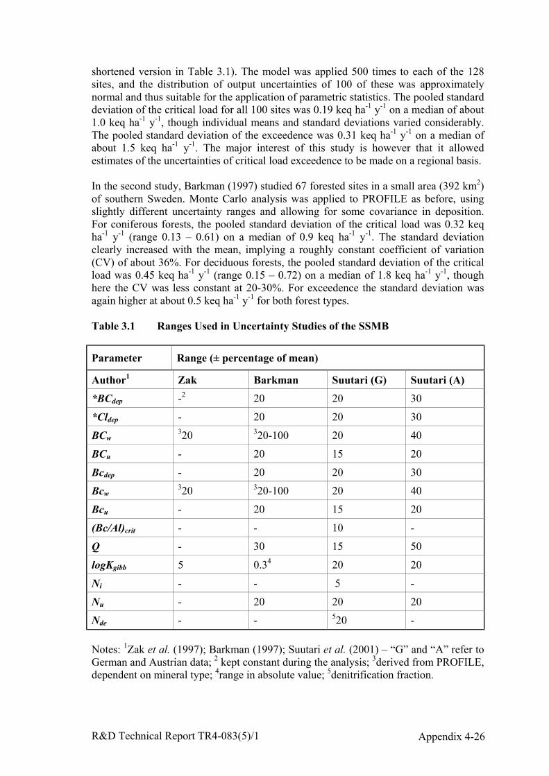
R&D Technical Report TR4-083(5)/1 Appendix 4-26
shortened version in Table 3.1). The model was applied 500 times to each of the 128sites, and the distribution of output uncertainties of 100 of these was approximatelynormal and thus suitable for the application of parametric statistics. The pooled standarddeviation of the critical load for all 100 sites was 0.19 keq ha-1 y-1 on a median of about1.0 keq ha-1 y-1, though individual means and standard deviations varied considerably.The pooled standard deviation of the exceedence was 0.31 keq ha-1 y-1 on a median ofabout 1.5 keq ha-1 y-1. The major interest of this study is however that it allowedestimates of the uncertainties of critical load exceedence to be made on a regional basis.
In the second study, Barkman (1997) studied 67 forested sites in a small area (392 km2)of southern Sweden. Monte Carlo analysis was applied to PROFILE as before, usingslightly different uncertainty ranges and allowing for some covariance in deposition.For coniferous forests, the pooled standard deviation of the critical load was 0.32 keqha-1 y-1 (range 0.13 – 0.61) on a median of 0.9 keq ha-1 y-1. The standard deviationclearly increased with the mean, implying a roughly constant coefficient of variation(CV) of about 36%. For deciduous forests, the pooled standard deviation of the criticalload was 0.45 keq ha-1 y-1 (range 0.15 – 0.72) on a median of 1.8 keq ha-1 y-1, thoughhere the CV was less constant at 20-30%. For exceedence the standard deviation wasagain higher at about 0.5 keq ha-1 y-1 for both forest types.
Table 3.1 Ranges Used in Uncertainty Studies of the SSMB
Parameter Range (± percentage of mean)
Author1 Zak Barkman Suutari (G) Suutari (A)
*BCdep -2 20 20 30
*Cldep - 20 20 30
BCw320 320-100 20 40
BCu - 20 15 20
Bcdep - 20 20 30
Bcw320 320-100 20 40
Bcu - 20 15 20
(Bc/Al)crit - - 10 -
Q - 30 15 50
logKgibb 5 0.34 20 20
Ni - - 5 -
Nu - 20 20 20
Nde - - 520 -
Notes: 1Zak et al. (1997); Barkman (1997); Suutari et al. (2001) – “G” and “A” refer toGerman and Austrian data; 2 kept constant during the analysis; 3derived from PROFILE,dependent on mineral type; 4range in absolute value; 5denitrification fraction.
R&D Technical Report TR4-083(5)/1 Appendix 4-27
Barkman and Alveteg (2001a) investigated the sources of data uncertainty in weatheringrates, critical loads and exceedances for 1883 forest sites in Sweden using Monte Carloanalysis and the PROFILE Model. Monte Carlo analysis was performed on the wholedata set, and compared with a repeated analysis with a subset of input parameters heldconstant. There were six subsets covering atmospheric deposition; stand characteristicssuch as base cation uptake; soil mineral content; soil physical properties; soil solutionchemistry and solution chemistry but including uncertainty in the critical limit. Soilphysical properties were the dominant contributor to uncertainty in weathering rate, butfor critical load and exceedence calculations the major source of uncertainty was thecritical limit i.e. the assumed Bc/Al ratio. This was especially true in the north ofSweden, but in the south, atmospheric deposition and stand characteristics tended to bemost important. The authors suggest that a practical strategy for reducing critical loaduncertainties should concentrate on narrowing uncertainty in deposition and nutrientcycling, because the critical limit is intrinsically difficult to evaluate.
In a related study, Barkman and Alveteg (2001b) considered the effects of uncertaintyon a nationwide critical load assessment. Grouping their site data into 150km EMEPgrid cells, they calculated median and 95% confidence intervals for each grid cell usingMonte Carlo analysis of the individual sites. At 95% confidence, the critical loads ofmost grid cells were not distinguishable – in fact the only significant differences amongthe 35 grid cells were between two cells with low critical loads and two cells with highcritical loads. (In the UK, with its more varied geology, probably no cells would besignificantly different). Re-aggregation onto the EMEP 50km grid made it possible todifferentiate the critical loads on more squares, but even so on 70% of the grid squares itwas uncertain whether the critical load was exceeded, or not within the confidenceintervals calculated.
However Barkman and Alveteg realised that, if uncertainties were not included, the 95-percentile would be a site-specific value (the most sensitive site if there were up to 40sites in the grid square) and hence vulnerable to the random inclusion or omission of asingle site. They argued that since the uncertainty analysis showed that many sites couldin fact be the fifth percentile, it was more robust to construct confidence limits on thepercentiles rather than the individual sites. Since this is an important mechanism fornarrowing confidence intervals on the whole critical load assessment process (seeSuutari et al., 2001, below), and the explanation in Barkman and Alveteg is muchclearer, it is worth quoting exactly how this was done. “…the results from the MonteCarlo simulation are transferred to a matrix with as many columns as there are sites, andas many rows as there are replicate runs. The ordinary cumulative distribution function(CDF) with site-specific uncertainties is created by sorting each column to determinethe median value and the confidence interval for each site….The modified CDF, on theother hand, is created by first sorting each row from low to high, thereby changing theinterpretation of a column from site-specific to percentile-specific values. Each columnis then sorted from low to high to determine the median value and the confidenceinterval for each percentile” (Barkman and Alveteg, 2001b). This modification reducedthe median critical load for all the EMEP 150 squares, and narrowed the confidenceinterval for 90% of them, sometimes considerably. The 95-percentile exceedence wasincreased on all but three of the grid squares, and the confidence intervals of exceedencewere reduced on all squares.
R&D Technical Report TR4-083(5)/1 Appendix 4-28
Zak et al. (1997) and Zak and Beven (1999) also performed an uncertainty analysis ofcritical load estimation using PROFILE, but with very different results. They used atechnique called Generalised Likelihood Uncertainty Estimation (GLUE) which isbased on Monte Carlo techniques and was originally developed to assess the predictivecapability of distributed hydrological models. GLUE recognizes that it is not possible toidentify unequivocally a set of parameters as being optimal for an environmental model.Quite different sets of parameters might be essentially equivalent as simulators of asystem, a concept which they call equifinality. Hence GLUE does not attempt tooptimise on a single set of parameters, but a set of behavioural criteria (not specifiedvery clearly in the papers). Zak et al. (1997) calculated the uncertainty of the criticalload for a small catchment at the Plynlimon research site in mid-Wales. Monte Carlovariation was applied to 10 sets of parameters within the PROFILE model. Distributionswere uniform ± 20%. The best 20% of 60,000 simulations were retained. The mediancritical load was 1.07 keq ha-1 y-1, and the 90% confidence range was 0.27 to 1.87 keqha-1 y-1. This range is similar to the range in the geographical variation in total Sdeposition to the UK (NEGTAP, 2001). A set of 6 field measurements was comparedwith the range of estimates derived from the model: only 3 of the 6 fell within theuncertainty ranges in the simulation. Zak et al. (1997) concluded from this that therewere significant deficiencies in the model structure, or the boundary conditions applied,or both.
Zak and Beven (1999) re-applied the GLUE methodology to critical load estimation byPROFILE at the same catchment but varied a wider range of parameters, and alsoapplied it to a further 4 research catchments. The median and 90% confidence rangealtered a little to 1.20 (0.24 – 1.82) keq ha-1 y-1. Corresponding figures (in keq ha-1 y-1)for the other sites were 0.92 (0.32 – 1.34) for Aber in North Wales; 3.12 (2.60 – 3.58) atUhlirska in the Czech Republic; and 0.80 (0.29 – 1.34) at Fårahall in Sweden. Theofficial critical loads for coniferous forest in the area round Aber were estimated to beabout 2.1 keq ha-1 y-1 in 1998 (quoted in Zak and Beven, 1999), but in the 1.0 to 2.0range in 2001 (Hall et al. 2001a). For the fifth site (Alice Holt Lodge in Hampshire)none of the 60,000 Monte Carlo runs gave an acceptable simulation of the data,showing that PROFILE was inappropriately structured or parameterised for this site.The site has a clay soil, and PROFILE has been observed to give poor results for suchsoils in other studies (e.g. Van der Salm, 2001).
It is perhaps discouraging that such a wide uncertainty range in critical load results fromapplication of fairly narrow uncertainty bands to only about 10% of model parameters,especially given that these are research catchments where many input variables areknown with greater certainty than is generally the case. However, GLUE has beencriticised as a methodology and normally gives wider limits than other such methods.
An interesting Monte Carlo analysis of SSMB critical loads from some sites in Chinawas performed by Larssen et al. (2000). The parameter ranges chosen and resultantcritical loads with 90% confidence intervals are shown in Table 3.2. The critical loadsare very high, partly because of large amounts of base cation deposition. It is notpossible to calculate coefficients of variation from the data presented, but using thestatistic in the bottom row of the table (which will be a little higher than a conventionalCV) the variation ranges from 27 to 50% of the median. Larssen et al. (2000) alsomodelled these sites using the MAGIC model, and using only parameter ranges whichgave acceptable simulations in MAGIC to re-run the Monte Carlo analysis of the SSMB
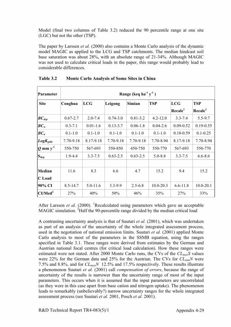
R&D Technical Report TR4-083(5)/1 Appendix 4-29
Model (final two columns of Table 3.2) reduced the 90 percentile range at one site(LGC) but not the other (TSP).
The paper by Larssen et al. (2000) also contains a Monte Carlo analysis of the dynamicmodel MAGIC as applied to the LCG and TSP catchments. The median hindcast soilbase saturation was about 28%, with an absolute range of 21-34%. Although MAGICwas not used to calculate critical loads in the paper, this range would probably lead toconsiderable differences.
Table 3.2 Monte Carlo Analysis of Some Sites in China
Parameter Range (keq ha-1 y-1 )
Site Conghua LCG Leigong Simian TSP LCG
Recalc1
TSP
Recalc1
BCdep 0.67-2.7 2.0-7.4 0.74-3.0 0.81-3.2 4.2-12.0 3.3-7.4 5.5-9.7
BCw 0.3-7.1 0.01-1.6 0.13-3.7 0.06-1.8 0.04-2.6 0.09-0.52 0.19-0.55
BCu 0.1-1.0 0.1-1.0 0.1-1.0 0.1-1.0 0.1-1.0 0.18-0.59 0.1-0.25
LogKgibb 7.70-9.18 8.17-9.18 7.70-9.18 7.70-9.18 7.70-8.94 8.17-9.18 7.70-8.94
Q mm y-1 550-750 567-693 550-850 450-750 550-770 567-693 550-770
Sdep 1.9-4.4 3.3-7.5 0.63-2.5 0.63-2.5 5.0-8.8 3.3-7.5 6.6-8.6
Median
C Load
11.6 8.3 6.6 4.7 15.2 9.4 15.2
90% CI 8.5-14.7 5.0-11.6 3.3-9.9 2.5-6.8 10.0-20.3 6.6-11.8 10.0-20.1
CI/Med2 27% 40% 50% 46% 35% 27% 33%
After Larssen et al. (2000). 1Recalculated using parameters which gave an acceptableMAGIC simulation. 2Half the 90-percentile range divided by the median critical load
A contrasting uncertainty analysis is that of Suutari et al. (2001), which was undertakenas part of an analysis of the uncertainty of the whole integrated assessment process,used in the negotiation of national emission limits. Suutari et al. (2001) applied MonteCarlo analysis to most of the parameters in the SSMB equation, using the rangesspecified in Table 3.1. These ranges were derived from estimates by the German andAustrian national focal centres (for critical load calculation). How these ranges wereestimated were not stated. After 2000 Monte Carlo runs, the CVs of the CLmaxS valueswere 22% for the German data and 25% for the Austrian. The CVs for CLminN were7.5% and 8.8%, and for CLmaxN 12.5% and 17.5% respectively. These results illustratea phenomenon Suutari et al. (2001) call compensation of errors, because the range ofuncertainty of the results is narrower than the uncertainty range of most of the inputparameters. This occurs when it is assumed that the input parameters are uncorrelated(as they were in this case apart from base cation and nitrogen uptake). The phenomenonleads to remarkably (unbelievably?) narrow uncertainty ranges for the whole integratedassessment process (see Suutari et al. 2001, Posch et al. 2001).
R&D Technical Report TR4-083(5)/1 Appendix 4-30
The study by Suutari et al. (2001) illustrates some important questions that need to beasked about such uncertainty analyses. How are the ranges in input variables derived?Though unstated in any of the papers reviewed, the answer appears to be “expertjudgement” i.e. a guess, rather than any objective process. Attempts in the literature toevaluate the uncertainty ranges of some of these parameters tend to result in much widerranges than those used. For instance, Suutari et al. (2001) used an uncertainty of ± 10%for the (Bc/Al)crit parameter (i.e. the range used in the Monte Carlo analysis wasprobably 0.9 to 1.1). Cronan and Grigal (1995) reviewed the use of this indicator, andsuggested that a range of 1.0±50% would give 50% confidence of vegetation damage.Weathering rates provide another example. The German national focal centre estimatedthe range in weathering rates as ±20% and the Austrian ±40%. After a study of theweathering rate calculation by PROFILE, Hodson et al. (1997) estimated theuncertainty range as ±250%. Van der Salm (2001) found the PROFILE modeloverestimated weathering on some Dutch soils by a factor of 7 when not calibrated onlaboratory data, and by a factor of 95 when it was calibrated. A range of ±40% seemssmall compared to these estimates.
Another important question arises when the uncertainty analysis is being applied toanything other than a reasonably homogeneous entity i.e. when there is real variation inthe input parameter, which is due to the varied nature of the thing in question. Forinstance, the unit for critical load calculations on an international level is currently the50 km grid square. A 50 km grid square will typically contain a number of soil types,and weathering rates might easily vary by 2 orders of magnitude – from quartzites tolimestones, say. Is the range term in the Monte Carlo analysis meant to include thisvariation? It clearly does not in the Suutari et al. (2001) study, but probably does in theLarsen et al. (2000) work. Or is the range intended to be the uncertainty for a givenecosystem, and if so how is the uncertainty generated by the variation within the squaretaken into account? The spatial scale of uncertainty analyses needs to be made veryexplicit. Many of the parameters in the SSMB equation will have similar ranges ofnatural variation to that of weathering rate.
The only uncertainty study known to the author performed on freshwater critical loadmodels is that of Kämäri et al. (1993). They performed an uncertainty analysis on theSSWC Model for lakes in Finland, using Monte Carlo methods. This suggested an overallstandard deviation on the critical load of ±10%.
Heywood et al. (2002, in press) studied the influence of uncertainties in S and Ndeposition alone on UK critical load exceedence, using Monte Carlo analysis.Deposition was assumed to vary by ±40%, and S and N were analysed together andseparately. This variation had a considerable, non-linear effect on exceedence with thearea exceeded in the year 2010 varying from +35% and -50% of the deterministic value.Accumulated exceedence (see Section 7.2) varied within wider limits, between +100and –75% of the deterministic value. Although the medians of these distributions werelower than the deterministic values (i.e. a smaller area of exceedence) use of a 95%confidence interval would lead to more pessimistic estimates than those currently usedby policymakers; a 35% increase in area exceeded, for example.
R&D Technical Report TR4-083(5)/1 Appendix 4-31
3.2 Sensitivity analyses
In contrast to uncertainty analyses, sensitivity analyses look at the sensitivity of theoutput variable to changes in one input variable, usually with the others held constant.Sensitivity analyses should be part of an uncertainty analysis, but are more commonthan the latter because they are less technically demanding. Hall et al. (2001b)conducted a limited sensitivity analysis of the SSMB equation as used in the UK.Reducing the (Ca/Al)crit value from 1.5 to 1.0 to 0.5 altered the mean critical load from1.77 to 1.96 to 3.11 keq ha-1 y-1 respectively, and doubled the range between theabsolute maxima and minima. In a parallel investigation, Hall et al. (2001c) investigatedthe effect of altering the Gibbsite equilibrium constant Kgibb on SSMB critical loads.Kgibb governs the relationship between H+ and Al concentrations and thus has a strongeffect on base cation/aluminium ratios. Altering Kgibb through the range recommendedin the Mapping Manual (UBA, 1996) for different soil types altered the mean UKcritical load from 3.2 to 1.8 keq ha-1 y-1. Hall et al. (2001bc) also studied the effect ofusing different critical load criteria on critical loads calculated by the SSMB. Thesecriteria are all used by different European countries (Hall et al. 2001c) as criticalchemical values. The mean value of UK critical loads for coniferous woodland was 1.96keq ha-1 y-1 using (Ca/Al)crit as the criterion, 2.83 keq ha-1 y-1 using a critical Alconcentration of 200 µeq l-1; and 3.17 keq ha-1 y-1 using a critical pH of 4.2. There is noreason why these should be the same, but it highlights the need for a careful choice ofcritical chemical value in relation to the receptor, and some of the reasons for differingcritical loads between European countries. Critical loads derived from a critical pH of4.2 are particularly sensitive to the chosen value of Kgibb, UK mean values varying from1.28 to 20.3 keq ha-1 y-1 when Kgibb was varied over the range of acceptable values (Hallet al. 2001bc).
Wilby (1995) investigated the sensitivity of critical loads to climate change, which hedid by altering the amount of annual runoff assumed in the critical load model (whichwas MAGIC), using observed values for the Beacon Hill Catchment nearLoughborough for each of the 6 years between 1984 and 1990. The calculated criticalload for the wettest year (0.60 keq ha-1 y-1) was almost double that of the driest (0.35keq ha-1 y-1). This is possibly an unusually wide range, as the critical load model used(attainment of a target Al concentration in surface waters) is strongly non-linear, and thecatchment has a low runoff/rainfall ratio compared to most upland catchments.
Thomas and Reynolds (1998) investigated the sensitivity of critical loads as calculatedby the SSMB to changes in all input parameters, using data ranges characteristic of theWelsh uplands. They observed what they called instabilities, regions of the parameterspace where critical loads changed very rapidly in response to small input parameterchanges. Typically these responses were non-linear and occurred just past a zeroresponse threshold. Though not strictly unstable, the critical load response may besurprisingly large if changing a parameter caused one of these regions to be crossed.
Two studies by the Stockholm Environment Institute (Kuylenstierna et al. 2001ab)examined the effects of alternative assumptions about the values of critical loadsderived from measurements of weathering rates and soil parameters, using a low rangeand a high range of twice the value, and similar assumptions about base cationdeposition. Kuylenstierna et al. (2001a) applied this methodology to critical loads andexceedences on a global scale, showing that it made a considerable difference to
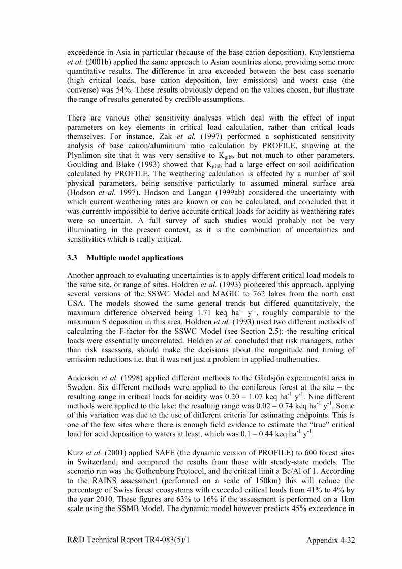
R&D Technical Report TR4-083(5)/1 Appendix 4-32
exceedence in Asia in particular (because of the base cation deposition). Kuylenstiernaet al. (2001b) applied the same approach to Asian countries alone, providing some morequantitative results. The difference in area exceeded between the best case scenario(high critical loads, base cation deposition, low emissions) and worst case (theconverse) was 54%. These results obviously depend on the values chosen, but illustratethe range of results generated by credible assumptions.
There are various other sensitivity analyses which deal with the effect of inputparameters on key elements in critical load calculation, rather than critical loadsthemselves. For instance, Zak et al. (1997) performed a sophisticated sensitivityanalysis of base cation/aluminium ratio calculation by PROFILE, showing at thePlynlimon site that it was very sensitive to Kgibb but not much to other parameters.Goulding and Blake (1993) showed that Kgibb had a large effect on soil acidificationcalculated by PROFILE. The weathering calculation is affected by a number of soilphysical parameters, being sensitive particularly to assumed mineral surface area(Hodson et al. 1997). Hodson and Langan (1999ab) considered the uncertainty withwhich current weathering rates are known or can be calculated, and concluded that itwas currently impossible to derive accurate critical loads for acidity as weathering rateswere so uncertain. A full survey of such studies would probably not be veryilluminating in the present context, as it is the combination of uncertainties andsensitivities which is really critical.
3.3 Multiple model applications
Another approach to evaluating uncertainties is to apply different critical load models tothe same site, or range of sites. Holdren et al. (1993) pioneered this approach, applyingseveral versions of the SSWC Model and MAGIC to 762 lakes from the north eastUSA. The models showed the same general trends but differed quantitatively, themaximum difference observed being 1.71 keq ha-1 y-1, roughly comparable to themaximum S deposition in this area. Holdren et al. (1993) used two different methods ofcalculating the F-factor for the SSWC Model (see Section 2.5): the resulting criticalloads were essentially uncorrelated. Holdren et al. concluded that risk managers, ratherthan risk assessors, should make the decisions about the magnitude and timing ofemission reductions i.e. that it was not just a problem in applied mathematics.
Anderson et al. (1998) applied different methods to the Gårdsjön experimental area inSweden. Six different methods were applied to the coniferous forest at the site – theresulting range in critical loads for acidity was 0.20 – 1.07 keq ha-1 y-1. Nine differentmethods were applied to the lake: the resulting range was 0.02 – 0.74 keq ha-1 y-1. Someof this variation was due to the use of different criteria for estimating endpoints. This isone of the few sites where there is enough field evidence to estimate the “true” criticalload for acid deposition to waters at least, which was 0.1 – 0.44 keq ha-1 y-1.
Kurz et al. (2001) applied SAFE (the dynamic version of PROFILE) to 600 forest sitesin Switzerland, and compared the results from those with steady-state models. Thescenario run was the Gothenburg Protocol, and the critical limit a Bc/Al of 1. Accordingto the RAINS assessment (performed on a scale of 150km) this will reduce thepercentage of Swiss forest ecosystems with exceeded critical loads from 41% to 4% bythe year 2010. These figures are 63% to 16% if the assessment is performed on a 1kmscale using the SSMB Model. The dynamic model however predicts 45% exceedence in
R&D Technical Report TR4-083(5)/1 Appendix 4-33
1995 reducing to only 39% by 2010 and 32% by 2100. The implication is that most ofthese soils will eventually reach the critical limit, but not for a very long time (perhapsmillennia).
3.4 Changes in model structure
Van der Salm and de Vries (2001) investigated the effect of some changes in thestructure of the SSMB to critical loads in The Netherlands. Weathering was made pHdependent. This is theoretically more correct, but means the equation can only be solvediteratively. This modification increased the median critical load from 0.23 keq ha-1 y-1 to0.45 keq ha-1 y-1. The increase was especially marked for clay soils, which acquiredmuch higher (and more credible) weathering rates. The Gibbsite equilibrium wasreplaced by empirically observed relationships between Al and pH differentiated by soiltype. It has long been known that the Gibbsite equilibrium does not describe field datavery well, and modification has often been suggested, but this is the first practicalapplication of this. This modification alone increased the median critical load for forestsoils from 0.27 to 0.39 keq ha-1 y-1. Another criterion was added to the model, so thatsoils were also protected against a reduction in base saturation. This hardly affected themedian critical load in The Netherlands, but decreased its value on the more base richsoils considerably. For instance, the 95-percentile critical load decreased from 15.4 to5.5 keq ha-1 y-1. This study illustrates that theoretically reasonable changes to criticalload model structures can cause very large alterations in critical load.
Tao and Feng (2000ab; 2001) developed a new sensitivity classification, which theyclaimed was more suitable for the sub tropics, and applied it to China. They noted thatalthough some areas were the same, the distribution of sensitivity was very different tothat calculated by the RAINS-ASIA Model, which is based on the SSMB Model.
3.5 Conclusions on uncertainty
It is fair to say that there are conflicting views on the uncertainties which should beattached to critical loads. Some authors (e.g. Hodson and Langan, 1999a,b) believe thatit is impossible to derive critical loads with any useful degree of accuracy, whileestimates of key underlying processes such as weathering rates are so uncertain. Others(e.g. Suutari et al. 2001) derive coefficients of variation of 25% (for CLmaxS) and 10%(for CLminN), probably by underestimating the uncertainty in the input variables.However, compensation of errors and aggregating estimates on a wide spatial scale willreduce uncertainties below what would be expected intuitively. Reasonably objectiveMonte Carlo analyses in areas with good data give CVs in the range of 25-50%. GLUEanalysis gives wider limits. Using alternative but still reasonable models can producelarge differences in critical loads. There is a lot of uncertainty about uncertainties, andmore work is needed to define them objectively.
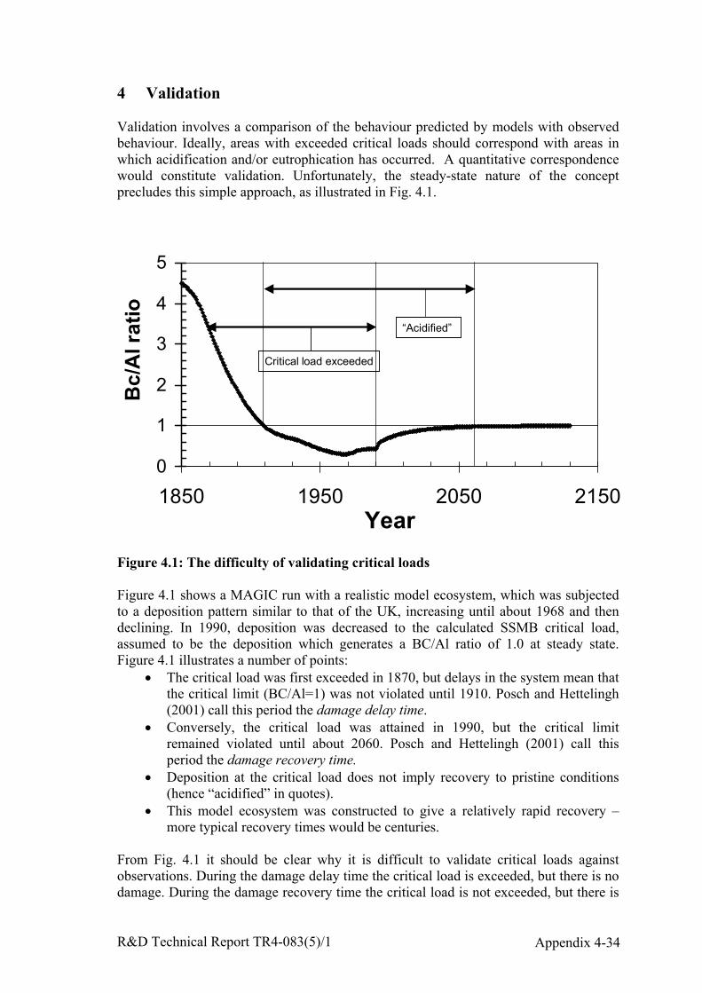
R&D Technical Report TR4-083(5)/1 Appendix 4-34
4 Validation
Validation involves a comparison of the behaviour predicted by models with observedbehaviour. Ideally, areas with exceeded critical loads should correspond with areas inwhich acidification and/or eutrophication has occurred. A quantitative correspondencewould constitute validation. Unfortunately, the steady-state nature of the conceptprecludes this simple approach, as illustrated in Fig. 4.1.
Figure 4.1: The difficulty of validating critical loads
Figure 4.1 shows a MAGIC run with a realistic model ecosystem, which was subjectedto a deposition pattern similar to that of the UK, increasing until about 1968 and thendeclining. In 1990, deposition was decreased to the calculated SSMB critical load,assumed to be the deposition which generates a BC/Al ratio of 1.0 at steady state.Figure 4.1 illustrates a number of points:
• The critical load was first exceeded in 1870, but delays in the system mean thatthe critical limit (BC/Al=1) was not violated until 1910. Posch and Hettelingh(2001) call this period the damage delay time.
• Conversely, the critical load was attained in 1990, but the critical limitremained violated until about 2060. Posch and Hettelingh (2001) call thisperiod the damage recovery time.
• Deposition at the critical load does not imply recovery to pristine conditions(hence “acidified” in quotes).
• This model ecosystem was constructed to give a relatively rapid recovery –more typical recovery times would be centuries.
From Fig. 4.1 it should be clear why it is difficult to validate critical loads againstobservations. During the damage delay time the critical load is exceeded, but there is nodamage. During the damage recovery time the critical load is not exceeded, but there is
0
1
2
3
4
5
1850 1950 2050 2150Year
Bc/
Al r
atio
Critical load exceeded
“Acidified”

R&D Technical Report TR4-083(5)/1 Appendix 4-35
damage. Moreover, the system can be acidifying when the critical load is not exceeded,as in 1850-70, and recovering when the critical load is exceeded, as in 1970-90. Thetime scales of these responses are long compared to the time available for observation.
An example of the difficulty was the Liphook Forest Fumigation Experiment, wheretrees on the same soil (critical load <0.2 keq ha-1 y-1) were subjected to one of three Sdeposition treatments. Deposition in the highest treatment exceeded the critical load bya factor of about 30, but the trees grew perfectly well (McLeod and Skeffington 1995).This does not invalidate the site critical load, however, because it is essentially aprediction that sometime in future tree growth would be affected. Indeed the BC/Alratio at Liphook was well above 1, though decreasing, showing the plots to be in the“damage delay time” stage.
Nevertheless, there is a vague correspondence between critical load exceedence andknown areas of damage, both in the UK and Europe as a whole. To see a quantitativerelationship between critical load exceedence and damage, however, it would benecessary either to make observations for a long time, or choose ecosystems in steadystate. As an example of the former, Reynolds et al. (1998) studied the responses of anumber of manipulated ecosystems in the NITREX Project. These long-term ecosystemexperiments showed responses which were consistent with some calculated critical loadexceedences, in that nitrate leaching was positively correlated with exceedence ofCLnutN.
Southern Norway is somewhere that might be close to steady state in many places,given thin soils, high rainfall, and a long history of relatively high deposition. Henriksenet al. (1999) claimed that there was a good relationship between fish population statusin Norwegian lakes and critical loads exceedence, though the ranges of exceedence forthe fish population categories: “extinct”, “reduced” and “unaffected”, were in fact verysimilar. Nevertheless, they could be statistically distinguished. Southern Norway alsosupplied one of the few instances in which tree defoliation correlated with critical loadexceedence (Nelleman and Frogner 1994). It is hard to find other examples.
Critical loads therefore have some relationship to ecosystem sensitivity, but are neverlikely to be validated quantitatively and unequivocally. This is one of theirdisadvantages compared to dynamic models, which can be used to generate predictions,which can be tested against data on a reasonable timescale.
R&D Technical Report TR4-083(5)/1 Appendix 4-36
5 Uncertainty associated with chemical criteria
The chemical criteria, or critical chemical values, used to determine critical loads arethemselves associated with considerable uncertainties. Most of the criteria have beensubjected to extensive debate, though some of the empirical nutrient nitrogen criticalloads have perhaps not been debated quite as hotly. It is not the intention here to reviewor comment on those debates, but rather to estimate the uncertainties associated with thetwo most commonly used criteria: BC/Al ratio for soils, and ANC for waters.
5.1 Base cation : aluminium criterion
The use of a BC/Al ratio to assess toxicity goes back to the work of Ulrich (1983), andis based on two generally-accepted propositions: that high concentrations of inorganicaluminium are toxic to many plants, and that this toxicity can be alleviated by calcium.The use of certain Bc/Al ratios for individual species derives from a meta analysis bySverdrup and Warfvinge (1993). They plotted growth responses of a number of speciesin experiments against the (Ca + Mg + K) / Al ratio, obtaining a sigmoid curve. A Bc/Alof 1 represented approximately a 20% growth reduction on the mean curve. Of morerelevance to uncertainty analysis, however, is the spread of values. The curve coversfour orders of magnitude in BC/Al ratio, from 0.01 to 100, between 100% growthreduction and no effect. More significantly, the lowest Bc/Al ratio with no growthreduction was 0.6, and the highest with some growth reduction was 20. Given thesensitivity of critical loads to this parameter (Section 3.2) this is a very large range. Thiscovers all species, but the species most investigated (Norway spruce) shows a similarspread.
The use of the Bc/Al ratio has generated an enormous amount of controversy (e.g.Högberg and Jensén, 1994; Løkke et al. 1996) because it is usually uncorrelated withdamage in the field; takes no account of nutrient uptake from the humus layer, where Al islikely to be complexed and not toxic and so on. However, it has proved difficult to devise acritical chemical value which is obviously better. Cronan and Grigal (1995) reviewed over300 papers on the use of the Ca/Al ratio as an indicator of stress in forest ecosystems andconcluded that it was reasonable to use it as a risk parameter. They concluded that a ratiobelow 1.0 indicated a 50% risk of adverse impacts on tree growth and nutrition, a ratiobelow 0.5 indicated a 75% risk, and a ratio below 0.2 almost a 100% risk. The uncertaintyon each of these ratios they estimated to be approximately ±50%. These uncertaintyestimates were arrived at by subjective processes, inevitably in view of the diversity ofexperimental approaches in the papers they reviewed. These estimates are however thebest indication available of the uncertainty to be attached to the Ca/Al ratio. Note thatCronan and Grigal did not review the Bc/Al ratio proposed by Sverdrup and Warfvinge(1993). That is presumably more uncertain still.
5.2 ANC criterion
The use of acid neutralising capacity (ANC) as a criterion to assess damage to aquaticpopulations has also proved controversial. Aquatic organisms should not respond toANC, as it is not a substance but the result of a titration (Skeffington, 1999). It ishowever correlated to the substances that organisms do respond to, particularly H+, Ca2+
and inorganic Al, and provides a convenient surrogate which takes various aspects ofwater chemistry into account, and is relatively easy to measure and calculate. The best

R&D Technical Report TR4-083(5)/1 Appendix 4-37
evidence for determining the appropriate value of ANC to use as a critical limit comesfrom studies in Norway (Lien et al. 1996). These authors were able to correlate the fishand invertebrate status of large numbers of lakes with ANC (and other parameters). Theresults, plotted as cumulative frequency diagrams, give an estimate of the uncertaintydue to natural variation in these waters. For brown trout, for instance, the ANC abovewhich there was no damage to fish populations was about 35 µeq l-1. At an ANCconcentration of 20 µeq l-1 about 10% of populations were reduced. At an ANC of 0 µeql-1 about 50% of populations were reduced, including 15% which were extinct. Allpopulations were reduced, and 75% extinct, at an ANC of –30 µeq l-1. All brown troutwere absent at ANC < -50 µeq l-1. Brown trout was the second most sensitive species,Atlantic salmon being more sensitive but living in rivers rather than lakes. The Norwegiansthus originally chose +20 µeq l-1 ANC as their critical limit, accepting a 10% probability ofdamage but avoiding the setting of unrealistic targets for lakes with naturally low ANC.(Even so, many lakes would naturally have ANC < 20 µeq l-1 in Norway).
It is clear that there is quite a wide range over which a reasonable critical limit could be set,from 0 µeq l-1 accepting approximately 50% damage probability but ensuring no lakes hadan unrealistic target, to +50 µeq l-1 on the precautionary side. This is illustrated by thosecountries which submitted data on freshwater critical loads to the CCE in 2001. Belgiumand Finland used 20 µeq l-1 as their critical limit; Norway used 20-50 µeq l-1 dependingon deposition; Sweden used 20 µeq l-1, where the pre-industrial base cationconcentration [*BC0] was estimated to be less than 25 µeq l-1, and 0.75[*BC0]otherwise, and the UK used 0 µeq l-1. These limits are all based on the same data set ofLien et al. (1996). The Swedish approach is an attempt to avoid the problem of lakeswith naturally low ANC, and appears worth investigating for transfer to the UK.
A further source of uncertainty is the extent to which these limits are transferable to othercountries with different hydrochemical settings, and possibly organisms with differentsensitivities. Ormerod (1993) found relationships between the abundance of variousaquatic organisms and ANC in Wales, although trout populations were not quite extinct inthe ANC –50 to –200 class. The work of Ormerod (1993) and co-workers also shows veryclearly that species richness increases steadily with ANC. There is no threshold or stepchange in toxicity.

R&D Technical Report TR4-083(5)/1 Appendix 4-38
6 UK practice compared to other countries
The methods used for calculating critical loads in the UK differ from those of otherEuropean countries, but then these all differ from each other. Hall et al. (2001c)surveyed the 19 countries submitting data to the CCE in 1999 and discovered they used15 different critical limits and combinations of limits for forest ecosystems. In 2001, thenumber of variants increased, with the Netherlands having the most elaborate systembased both on maintaining a BC/Al ratio and negligible change in soil base andaluminium status. The Mapping Manual (UBA 1996) imposes a certain amount ofstandardisation, but still leaves wide choices of both methods and parameters. Someconcern is expressed in the latest CCE report (Posch et al. 2001) about this, as it mustimpact on the fairness in sharing the burden of emission control between countries ininternational negotiations. To some extent, however, the different methods reflect thedifferent environmental conditions and receptors across Europe, as well as nationalidiosyncrasies.
The UK differs from most countries in using a Ca/Al ratio as the SSMB critical limit forforest ecosystems instead of a Bc/Al ratio, though two other countries do so and twofurther countries use Ca/Al in conjunction with other criteria. It is also unusual, but notunique, in submitting data for heathland and distinguishing between different types ofgrassland. The critical limit used for assessing lake acidification varies betweencountries, as noted in Section 5.2, the UK’s limit being lower than other countries,generating higher critical loads. Otherwise the UK’s methods for calculating criticalloads fall within the envelope of methods used in Europe as a whole.
R&D Technical Report TR4-083(5)/1 Appendix 4-39
7 Uncertainties due to mapping limitations
Some uncertainty for the practical user of critical loads is generated from limitationsgenerated by parts of the assessment process other than the theory and calculation ofcritical loads. These are briefly discussed below, quoting quantitative limits wherepossible.
7.1 Identification of Land Use Types
The UK calculates critical loads for five terrestrial ecosystems and also for freshwaters.Critical loads for waters are calculated on the basis of field measurements of specificlakes or streams (Section 2.7.2) and catchment areas are digitised from topographicmaps: the freshwater ecosystem of concern can therefore be identified unequivocally.The lake sampled is meant to represent the most sensitive water in the 10 km squaresurveyed, and some uncertainty is introduced here, as it may not be the most sensitive.Application of the FAB Model requires the identification of the proportion ofconiferous forest in the catchment of each lake (see terrestrial ecosystems, below) butotherwise ecosystem identification is not an issue.
The land cover for the terrestrial ecosystems on the other hand is derived from the 1990ITE Land Cover Map of Great Britain (Fuller et al. 1994). This was produced using datafrom the Landsat Thematic Mapper satellite. The map is based on a 25m grid andconsists of 25 cover types, including inland water, arable land, and 18 types of semi-natural vegetation. Landsat images from both winter and summer were used to improvethe classification. Northern Ireland and the Isle of Man lie outside the range of the map,so the less-detailed CORINE land cover map is used in those areas (see Hall et al.1998).
A comparison of cover types identified in the Land Cover Map (LCM) withindependent ground reference data showed a correspondence of 67% (Fuller et al.1994). This may not seem very good – one third of the identifications in the LCM arewrong – and indeed some field workers have been disappointed in the map data.However, as Fuller et al. (1994) point out, it is not simply a question of comparing mappredictions with “ground truth” which can be identified in the field without error.Landscape patterns are actually a continuum, and their mapping into discrete classesimposes an artificial classification on a continuously varying pattern. Differentsurveyors attempting to apply the same classification will obtain somewhat differentresults, since the choice of where to place the boundaries is fairly arbitrary. At whatpoint does a heathland with scattered trees turn into a woodland with a heathland under-storey? Problems also arose when cover type boundaries crossed a 25 x 25 m datapixel, which was about 40% of cases, as the pixel has to be assigned to one category oranother. Temporal change between the satellite image and ground survey accounted formore variation. Overall, Fuller et al. (1994) estimate the accuracy of their LCM at 80 to85%, though they note (probably in response to criticism from users) that this is anaverage figure and there will be areas where the classification is much better, and areaswhere it is much worse.
Transfer of the LCM categories into the five ecosystems used for critical load mappingintroduces more uncertainty. The process is described by Hall et al. (1998, 2001a). Dataon both the LCM and the critical load maps is presented on a 1km square basis. Land

R&D Technical Report TR4-083(5)/1 Appendix 4-40
cover types which appear in <5% of a 1 km square are discounted for critical loadpurposes, as some slight defence against misclassification. LCM classes do notprecisely correspond to the critical load ecosystem types. “Acid grassland” is anamalgam of eight LCM types including felled forest, bracken and lowland and uplandbog types. “Calcareous grassland” corresponds to two LCM types representing pasture,meadow and amenity grass, but also identified as having species-rich calcareousgrassland in data from the Biological Records Centre at Monks Wood. “Heathland” isan amalgam of four LCM classes and “deciduous woodland” of two. Only “coniferouswoodland” has one-to-one class correspondence with the LCM.
The result of these uncertainties is that it is easy to see areas on the critical load maps,where an ecosystem type which exists on the ground, is missing. Although thecalcareous grassland map picks calcareous areas in the south of England quite well,limestone areas round Llangollen and in south Wales are missing, the Yorkshire Daleslook under-represented, and there is no calcareous grassland in Scotland. The largeareas of what the author would describe as heathland south west of London are mostlyrecorded as coniferous forest. Such problems are inevitable when dealing with a quarterof a million data points per ecosystem and highlight the fact that ecosystemidentification is not a trivial task. There is now a new land cover map (LCM2000) withdata categories corresponding to “Broad Habitats” as defined by the UK’s BiodiversityAction Plan. These may correspond more closely with the categories on the critical loadmaps, though there are no plans to use it at present.
7.2 Choice of Grid Size and Averaging Technique
The spatial variability of the natural environment also causes problems when generatingspatial databases or presenting data on maps. Entities in the natural environment cover ahuge range of spatial scales, from the µm scale occupied by bacteria and soil particles, tothe km+ scale occupied by some geological formations. If the scale is small enough, someeffect even of minute amounts of pollution will be seen. Every grain of sand has its ownweathering rate and hence acid neutralising capacity, and this may be of vitalimportance to an individual nematode, for example. To be manageable for policypurposes, small-scale data need to be aggregated into larger units, and this requires athorough understanding of the purposes for which the data are to be used. Environmentalpressure groups tend to assume that the correct value of the critical load is that of the mostsensitive entity on the most detailed mapping scale available, but this is not necessarilythe case. This would probably result in uniformly low critical loads over the UK,obviating one of the purposes of using critical loads, which is to recognise that someareas are more sensitive than others and hence deserving of more protection.
At present in the UK (and in Europe generally) the finest scale on which critical loaddata are available is the 1 km square. It could be argued that this is rather coarse, sincerock, soil, vegetation and deposition can vary considerably within a square, especiallywithin the diverse UK environment. However, the amount of data needs to be keptmanageable, and the provenance of the input data also needs to be considered. Soil data,for instance, will rarely be a measured value even at 1km scale but will have beeninterpolated from soil maps which were produced for other purposes (Hornung et al.1995). Modelled deposition data is currently available only down to a 5km scale. The1km scale is therefore a compromise taking into account all these considerations.
R&D Technical Report TR4-083(5)/1 Appendix 4-41
The calculation of empirical critical loads in classes also means that choices have to bemade as to how to represent classes as a single number. Originally, the UK used theupper bound of the class, as a conservative assumption. Later, the central point of therange was used (Hall et al. 1998), reflecting increasing confidence about the values butin the process depressing critical load values used for regulatory purposes significantly.
Aggregation of data to larger scales requires more decisions. For use with Europeanpolicymaking, critical load data were aggregated to a 150km scale to match the EMEPgrid, to be reduced to 50 km in subsequent applications. It was realised early on that thechoice of a single number to present on an aggregated map posed problems. Hall (1993)presented maps of the minimum, mean, median and mode of UK empirical soil criticalloads for acidity at 10 km scale, to show the very different patterns and values whichresulted. The problems of aggregation were graphically illustrated in 1996, when theUK submitted three quite different sets of critical loads at 150km scale to the CCE,based on different models and assumptions (Hall et al. 1997). These submissions usedthe 5 percentile critical load, derived from ranking the critical loads and normalising byarea. This averaging technique therefore calculates the value which will protect 95% ofthe area of ecosystems on a grid square. As a technique for generating a single numberit has the advantage of avoiding dominance of the value by a few very sensitiveecosystems. However, it effectively “writes off” 5% of the ecosystem area, and takes noaccount of the rest of the distribution. For instance the 94% of ecosystems remainingcould be totally insensitive or not very much less sensitive than the 5 percentileecosystem, but the number would be exactly the same. These difficulties were at theroot of the UK’s problems with producing credible 150km critical load maps in 1996.
An elegant approach to this problem was the “accumulated exceedence” techniquedeveloped during the negotiation of the Gothenburg Protocol (Posch et al. 1999, 2001).The accumulated exceedance (AE) is defined as:
AE = Σ Ai Exi, (35)
where Ai is area and Exi is exceedence of the critical load for ecosystems i =1…N in agiven grid square.
Average accumulated exceedence (AAE) is this quantity normalised by area:
AAE = AE/ΣAi (36)
The aim of emission control policy then became the reduction of a certain proportion ofAAE on each grid square. This then enables the entire distribution of exceedence to betaken into account, and not just exceedence of the 5th percentile critical load. Theapproach also has technical advantages in providing a smooth damage function foroptimisation procedures.
A statistical approach to presenting critical load data, for instance as cumulativedistribution functions, gives more information than a bare number. Examples on both anational basis and a grid square basis can be found in Posch et al. (2001). This approachloses the impact of maps with coloured squares representing a single number, however.

R&D Technical Report TR4-083(5)/1 Appendix 4-42
Experiments with representing critical load data on different spatial scales show clearlythat the more detailed the scale, the greater the area of low critical loads, and the greaterthe area of high exceedence. This should be true for any aggregating technique unlessthe aggregated map shows the minima of the more detailed scales. Hall (1993)demonstrated this for the UK with maps at 1, 10 and 20 km scale, and Posch et al.(2001) with a comparison of European maps at 50 and 150 km scale. Figure 7.1 showsthe proportions of the critical load classes, which appeared in the original empiricalsoils critical load databases at 1 km and 10 km scales.
Figure 7.1. The proportions of critical load classes at two different scales
The figure shows the percentages of each of the standard critical load classes in theoriginal empirical soils database, displayed at either 1 km and 10 km resolution. Datafrom ITE (now CEH).
It can be seen that at the 10km scale, the proportion of the most sensitive class isconsiderably less. Again, what must be considered is the appropriateness of the scale ofpresentation or calculation, given the policy purposes for which it is to be used.
0
5
10
15
20
25
30
35
40
1 2 3 4 5
Critical Load Class
Perc
ent
1 km data
10 km data

R&D Technical Report TR4-083(5)/1 Appendix 4-43
8 Conclusions
The recent interest shown in defining the uncertainties to be attached to critical loadshas borne some fruit. Uncertainty analyses have been able to place some limits on somecritical load models in some circumstances. These limits usually consider only thepropagation of errors in input variables through the models, rather than errors in modelstructure. Though these can be identified, they are much more difficult to quantify.There is still much uncertainty about the uncertainty to be attached to critical loads.
Other parts of this study (see Appendices 5 and 6) will consist of an uncertainty analysisapplied to a real ecosystem. It will be possible to test some hypotheses that havedeveloped during this literature survey.
R&D Technical Report TR4-083(5)/1 Appendix 4-44
9 References
Andersson, B.I., Skeffington, R.A., Hultberg, H. and Sverdrup, H.U. (1998) Assessmentof critical loads for coniferous forests and surface waters at Lake Gårdsjön in South-West Sweden. In Experimental Reversal of Acid Rain Effects: the Gårdsjön RoofProject (Eds Hultberg, H. and Skeffington, R. A.), pp. 411-431. John Wiley and SonsLtd, Chichester, England.
Barkman, A. (1997) Applying the critical loads concept: constraints induced by datauncertainty Reports in Ecology and Environmental Engineering 1997:1, University ofLund, Lund, Sweden.
Barkman, A. and Alveteg, M. (2001a) Identifying potentials for reducing uncertainty incritical load calculations using the PROFILE model. Water Air and Soil Pollution, 125,33-54.
Barkman, A. and Alveteg, M. (2001b) Effects of data uncertainty in the Swedish criticalload assessment for forest soils. Water Air and Soil Pollution, 125, 133-156.
Barkman, A., Warfvinge, P. and Sverdrup, H. (1995) Regionalization of critical loadsunder uncertainty. Water Air and Soil Pollution, 85, 2515-2520.
Battarbee, R. W., Allott, T. E. H., Juggins, S., Kreiser, A. M., Curtis, C. and Harriman,R. (1996) Critical loads of acidity to surface waters: an empirical diatom-basedpalaeolimnological model. Ambio, 25, 366-369.
Bobbink, R., Hornung, M., and Roelofs, J. G. M. (1996) In Manual on Methodologiesand Criteria for Mapping Critical Levels / Loads and Geographical Areas where theyare Exceeded Texte 71:96, Umweltbundesamt, Berlin.
Brakke, D.F., Henriksen, A. and Norton, S.A. (1990) A variable F-factor to explainchanges in base cation concentrations as a function of strong acid deposition.Verhandlungen der Internationale Vereinigung für Theoretische und AngewandteLimnologie, 24, 146-149.
Cooper, D.M., Jenkins, A., Skeffington, R.A. and Gannon, B. (2000) Catchment-scalesimulation of stream water quality by spatial mixing: theory and application. Journal ofHydrology, 233, 121-137.
Cresser, M.S. (2000) The critical loads concept: milestone or millstone for the newmillennium? Science of the Total Environment, 249, 51-62.
Cronan, C.S. and Grigal, D.F. (1995) Use of calcium/aluminum ratios as indicators ofstress in forest ecosystems. Journal of Environmental Quality, 24 , 209-226.
Curtis, C., Allott, T., Hall, J., Harriman, R., Helliwell, R., Hughes, M., Kernan, M.,Reynolds, B. and Ullyett, J. (2000) Critical loads of sulphur and nitrogen forfreshwaters in Great Britain and assessment of deposition reduction requirements withthe First-Order Acidity Balance (FAB) Model. Hydrology and Earth System Sciences,4, 125-140.
R&D Technical Report TR4-083(5)/1 Appendix 4-45
Curtis, C.J., Allott, T.E.H., Reynolds, B. and Harriman, R. (1998) The prediction ofnitrate leaching with the first-order acidity balance (FAB) model for upland catchmentsin Great Britain. Water Air and Soil Pollution, 105, 205-215.
Evans, C.D., Jenkins, A., Helliwell, R.C. and Ferrier, R. (1998) Predicting regionalrecovery from acidification; the MAGIC Model applied to Scotland, England andWales. Hydrology and Earth System Sciences, 2, 543-554.
Fuller, R.M., Groom, G.B. and Jones, A.R. (1994) The Land Cover Map of GreatBritain: an automated classification of Landsat Thematic Mapper data. PhotgrammetricEngineering and Remote Sensing, 60, 553-562.
Goulding, K. W. T.and Blake, L. (1993) Testing the PROFILE Model on long-termdata. In Hornung, M. and Skeffington, R. A. Critical loads: concept and applications.ITE Report 28, pp 68-73 London, HMSO.
Grennfelt, P. and Thörnelöf, E. (1992) Critical loads for nitrogen - report from aworkshop held at Lokeberg, Sweden. Nordic Council of Ministers, Copenhagen.
Hall, J. R. (1993) Critical loads mapping at the UK Critical Loads Mapping Centre -data requirements and presentation. In Hornung, M. and Skeffington, R. A. CriticalLoads: Concept and Applications. ITE Report 28, 74-78 London, HMSO
Hall, J., Hornung, M., Freer-Smith, P., Loveland, P., Bradley, I., Langan, S., Dyke, K.,Gascoigne, J., and Bull, K. (1997) Current status of UK critical loads data - December1996 Report to UK Dept of the Environment, Institute of Terrestrial Ecology, MonksWood, Cambs.
Hall, J., Bull, K., Bradley, K., Curtis, C., Freer-Smith, P. H., Hornung, M., Howard, D.,Langan, S., Loveland, P., Reynolds, B., Ulyett, J., and Warr, T. (1998) Status of UKcritical loads and exceedances January 1998. Part 1 - critical loads and critical loadmaps Report to UK Department of the Environment, Institute of Terrestrial Ecology,Monks Wood, Cambs.
Hall, J, Hornung, M., Kennedy, F., Reynolds, B., Curtis, C., Langan, S., and Fowler, D.(2001a) Status of UK critical loads and exceedances: Part 1 Critical loads and criticalload maps, update to January 1998 report, CEH, Monks Wood, Cambridge.
Hall, J., Reynolds, B., Aherne, J. and Hornung, M. (2001b) The importance of selectingappropriate criteria for calculating critical loads for terrestrial ecosystems using thesimple mass balance equation. Water, Air and Soil Pollution, Focus 1, 29-41.
Hall, J., Hornung, M., Kennedy, F., Langan, S., Reynolds, B. and Aherne, J. (2001c)Investigating the uncertainties in the Simple Mass Balance equation for acidity criticalloads for terrestrial ecosystems. Water, Air and Soil Pollution, Focus 1, 43-56.
Henriksen, A., Fjeld, E. and Hesthagen, T. (1999) Critical load exceedance and damageto fish populations. Ambio, 28, 583-586.
Henriksen, A., Posch, M., Hultberg, H. and Lien, L. (1995) Critical loads of acidity forsurface waters - can the ANC(limit) be considered variable? Water Air and SoilPollution, 85, 2419-2424.
R&D Technical Report TR4-083(5)/1 Appendix 4-46
Hodson, M.E., Langan, S.J. and Wilson, M.J. (1997) A critical evaluation of the use ofthe PROFILE Model in calculating mineral weathering rates. Water, Air and SoilPollution, 98, 79-104.
Hodson, M.E. and Langan, S.J. (1999a) Considerations of uncertainty in setting criticalloads of acidity of soils: the role of weathering rate determination. EnvironmentalPollution, 106, 73-81.
Hodson, M.E. and Langan, S.J. (1999b) The influence of soil age on calculated mineralweathering rates. Applied Geochemistry, 14, 387-394.
Högberg, P. and Jensen, P. (1994) Aluminium and uptake of base cations by tree roots -a critique of the model proposed by Sverdrup et al. Water Air and Soil Pollution, 75,121-125.
Holdren, G. R., Strickland, T. C., Shaffer, P. W., Ryan, P. F., Ringold, P. L. and Turner,R. S. (1993) Sensitivity of critical load estimates for surface waters to model selectionand regionalization schemes. Journal of Environmental Quality, 22, 279-289.
Hornung, M., Bull, K. R., Cresser, M., Hall, J. R., Langan, S. J., Loveland, P. J. andSmith, C. (1995) An empirical map of critical loads of acidity for soils in Great Britain.Environmental Pollution, 90, 301-310.
Hornung, M., Sutton, M. A., and Wilson, R. B. (1994) Mapping and modelling ofcritical loads for nitrogen - a workshop report, Institute of Terrestial Ecology,Edinburgh, Scotland.
Jenkins, A. and Cullen, J.M. (2001) An assessment of the potential impact of theGothenburg Protocol on surface water chemistry using the dynamic MAGIC model atacid sensitive sites in the UK. Hydrology and Earth System Sciences, 5, 529-541.
Jenkins, A., .Renshaw, M., Helliwell, R. C., Sefton, C., Ferrier, R. C., and Swingewood,P. J (1997) Modelling surface water acidification in the UK. IH Report 131Wallingford, Oxon.
Jenkins, A. and Reynolds, B. (2000) Review of dynamic models for catchment andsurface water acidification R and D Technical report P246, Environment Agency,Bristol.
Kämäri, J., Forsius, M. and Posch, M. (1993) Critical loads of sulphur and nitrogen forlakes II: Regional extent and variability in Finland. Water, Air and Soil Pollution, 66,77-96.
Kernan, M., Hall, J., Ullyet, J. and Allott, T. (2001) Variation in freshwater criticalloads across two upland catchments in the UK: implications for catchment scalemanagement. Water Air and Soil Pollution, 130, 1169-1174.
Kurz, D., Rihm, B., Alveteg, M. and Sverdrup, H. (2001) Steady-state and dynamicassessment of forest soil acidification in Switzerland. Water Air and Soil Pollution, 130,1217-1222.
R&D Technical Report TR4-083(5)/1 Appendix 4-47
Kuylenstierna, J.C.I., Hicks, W.K., Cinderby, S. , Vallack, H.W. and Engardt, M.(2001a) Variability in mapping acidification risk scenarios for terrestrial ecosystems inAsian countries. Water Air and Soil Pollution, 130, 1175-1180.
Kuylenstierna, J.C.I., Rodhe, H., Cinderby, S. and Hicks, K. (2001b) Acidification indeveloping countries: ecosystem sensitivity and the critical load approach on a globalscale. Ambio, 30, 20-28.
Larssen, T., Schnoor, J.L., Seip, H.M. and Dawei, Z. (2000) Evaluation of differentapproaches for modeling effects of acid rain on soils in China. Science of the TotalEnvironment, 246, 175-193.
Lien, L., Raddum, G. G., Fjellheim, A. and Henriksen, A. (1996) A critical limit foracid neutralizing capacity in Norwegian surface waters, based on new analyses of fishand invertebrate responses. The Science of the Total Environment, 177, 173-193.
Løkke, H., Bak, J., Falkengren-Grerup, U., Finlay, R. D., Ilvesniemi, H., Nygaard, P. H.and Starr, M. (1996) Critical loads of acidic deposition for forest soils: is the currentapproach adequate? Ambio, 25, 510-516.
McLeod, A. R. and Skeffington, R. A. (1995) The Liphook Forest Fumigation Project -an overview. Plant, Cell and Environment, 18, 327-335.
Nellemann, C. and Frogner, T. (1994) Spatial patterns of spruce defoliation - relation toacid deposition, critical loads, and natural growth conditions in Norway. Ambio, 23,255-259.
Nilsson, J and Grennfelt, P. (1988) Critical loads for sulphur and nitrogen Report1988:15, Nordic Council of Ministers, Copenhagen.
Nisbet, T.R. (2001) The role of forest management in controlling diffuse pollution inUK forestry. Forest Ecology and Management, 143, 215-226.
Ormerod, S. J. (1993) Assessing critial loads for stream organisms using empiricaldata. In Hornung, M. and Skeffington, R. A. Critical loads: concept and applications.ITE Report 28, 115-118 London, HMSO.
Posch, M., de Smet, P. A. M., Hettelingh, J.-P., and Downing, R. J. (1995) Calculationand Mapping of Critical Thresholds in Europe 259101004, RIVM, Bilthoven, TheNetherlands.
Posch, M., Hettelingh, J.-P., de Smet, P. A. M., and Downing, R. J. (1997) Calculationand Mapping of Critical Thresholds in Europe 259101007, RIVM, Bilthoven, TheNetherlands.
Posch, M., de Smet, P. A. M., Hettelingh, J.-P., and Downing, R. J. (1999) Calculationand Mapping of Critical Thresholds in Europe 259101009, RIVM, Bilthoven, TheNetherlands.
Posch, M., de Smet, P. A. M., Hettelingh, J.-P., and Downing, R. J. (2001) Modellingand mapping of critical thresholds in Europe: Status Report 2001 RIVM Report259101010, RIVM, Bilthoven, The Netherlands.
R&D Technical Report TR4-083(5)/1 Appendix 4-48
Posch, M.and Hettelingh, J.-P. (2001) From critical loads to dynamic modelling. InPosch, M., de Smet, P. A. M., Hettelingh, J.-P., and Downing, R. J. Modelling andmapping of critical thresholds in Europe: Status Report 2001. RIVM Report259101010, pp 33-39 RIVM Bilthoven, The Netherlands,.
Reynolds, B. (2000) An evaluation of critical loads of soil acidity in areas of high seasalt deposition. Science of the Total Environment, 253, 169-176.
Reynolds, B., Wilson, E. J. and Emmett, B. A. (1998) Evaluating critical loads ofnutrient nitrogen and acidity for terrestrial systems using ecosystem-scale experiments(NITREX). Forest Ecology and Management, 101, 81-94.
Reynolds, B. and Skeffington, R.A. (1999) Developments in critical loads. Progress inEnvironmental Science, 1, 371-381.
Roberts, T.M., Skeffington, R.A. and Blank, L.W. (1989) Causes of Type 1 sprucedecline in Europe. Forestry, 62, 179-222.
Schmieman, E.C. and Van Ierland, E.C. (1999) Dynamics of soil acidification: aneconomic analysis. Ecological Economics, 31, 449-462.
Sefton, C.E.M. and Jenkins, A. (1998) A regional application of the MAGIC Model inWales: calibration and assessment of future recovery using a Monte-Carlo approach.Hydrology and Earth System Sciences, 2, 521-531.
Skeffington, R.A. (1999) The use of critical loads in environmental policymaking: acritical appraisal. Environmental Science and Technology, 33, 245A-252A.
Skeffington, R. A., Wilson, E. J., Immirzi, P., and Maltby, E. (1995) Setting a criticalload for dystrophic peat. In Hydrology and Hydrochemistry of British Wetlands (EdsHughes, J. and Heathwaite, A. L.), pp 183-198. John Wiley and Sons, Ltd, Chichester,UK.
Skiba, U. and Cresser, M. (1989) Prediction of long-term effects of rainwater acidity onpeat and associated drainage water chemistry in upland areas. Water Research, 23,1477-1482.
Smith, C.M.S., Cresser, M.S. and Mitchell, R.D.J. (1993) Sensitivity to acid depositionof dystrophic peat in Great Britain. Ambio, 22, 22-26.
Suutari, R., Amann, M., Cofala, J., Klimont, Z., Posch, M., and Schöpp, W. (2001)From economic activities to ecosystem protection in Europe. An uncertainty analysis ofthe RAINS integrated assessment model CIAM/CCE Report 1/2001, IIASA, Laxenburg,Austria.
Sverdrup, H. and Warfvinge, P. (1993) Soil Acidification Effect on Growth of Trees,Grasses and Herbs Expressed by the (Ca + Mg + K)/Al Ratio. Technical Report,University of Lund, Lund, Sweden.
Tao, F.L. and Feng, Z.W. (2001) Critical loads of acid deposition for ecosystems insouth China - derived by a new method. Water Air and Soil Pollution, 130, 1187-1192.
R&D Technical Report TR4-083(5)/1 Appendix 4-49
Tao, F.L. and Feng, Z.W. (2000) Critical loads of SO2 dry deposition and theirexceedance in south China. Water Air and Soil Pollution, 124, 429-438.
Tao, F.L. and Feng, Z.W. (2000) Terrestrial ecosystem sensitivity to acid deposition insouth China. Water Air and Soil Pollution, 118, 231-243.
Thomas, A.H. and Reynolds, B.R. (1998) Numerical stability considerations in thesimple mass balance calculation of critical loads of acidity. The Science of the TotalEnvironment, 217, 257-264.
UBA (1996) Manual on Methodologies and Criteria for Mapping Critical Levels /Loads and Geographical Areas where they are Exceeded Texte 71:96,Umweltbundesamt, Berlin.
Ullyett, J.M., Hall, J.R., Hornung, M. and Kernan, M. (2001) Mapping the potentialsensitivity of surface waters to acidification using measured freshwater critical loads asan indicator of acid sensitive areas. Water Air and Soil Pollution, 130, 1235-1240.
Ulrich, B. (1983) Soil acidity and its relations to acid deposition. In Effects ofaccumulation of air pollutants in forest ecosystems (Eds Ulrich, B. and Pankrath, J.), pp23-47 D. Reidel, Dordrecht, The Netherlands.
Van Der Salm, C. (2001) Assessment of the regional variation in weathering rates ofloess and clay soils in The Netherlands. Water Air and Soil Pollution, 131, 217-243.
Van Der Salm, C. and De Vries, W. (2001) A review of the calculation procedure forcritical acid loads for terrestrial ecosystems. Science of the Total Environment, 271,11-25.
Warfvinge, P. and Sverdrup, H. (1992) Calculating critical loads of acid depositionwith PROFILE - a steady-state soil chemistry model. Water, Air and Soil Pollution, 63,119-143.
White, C.C., Smart, R. and Cresser, M.S. (2000) Spatial and temporal variations incritical loads for rivers in NE Scotland: a validation of approaches. Water Research,34, 1912-1918.
Wilby, R. L. (1995) Critical loads' sensitivity to climate change. EnvironmentalConservation, 22, 363-365.
Wilson, E.J., Skeffington, R.A., Maltby, E., Immirzi, P., Swanson, C. and Proctor, M.C.(1995) Towards a new method of setting a critical load of acidity for ombrotrophicpeat. Water, Air and Soil Pollution, 85, 2491-2496.
Zak, S.K., Beven, K. and Reynolds, B. (1997) Uncertainty in the estimation of criticalloads: a practical methodology. Water, Air and Soil Pollution, 98, 297-316.
Zak, S.K. and Beven, K.J. (1999) Equifinality, sensitivity and predictive uncertainty inthe estimation of critical loads. Science of the Total Environment, 236, 191-214.
R&D Technical Report TR4-083(5)/1 Appendix 5-1
Appendix 5 Liphook Critical Loads Case Study
CONTENTS
1 DESCRIPTION OF PARAMETERS USED IN MONTE CARLO ANALYSISFOR CRITICAL LOADS 2
1.1 Sulphur Deposition 2
2 CALCULATING EXCEEDENCE 5
1.2 Discussion of Exceedence 6
2 SENSITIVITY ANALYSIS 9
3 UNCERTAINTY ANALYSIS 11
4 REFERENCES 13
R&D Technical Report TR4-083(5)/1 Appendix 5-2
1 DESCRIPTION OF PARAMETERS USED IN MONTE CARLOANALYSIS FOR CRITICAL LOADS
The results of the Monte Carlo analysis depend critically on the means, ranges anddistribution types chosen for each parameter. Attempts were made to produce the bestpossible estimates, given knowledge of the Liphook site in southern England, asdescribed below.
Abbreviations and descriptions of terms
Concentrations and fluxes are expressed in equivalence units, e.g. keq ha-1 y-1
(molc ha-1 y-1).* refers to the non-marine contributiondep deposition of the substance in question, e.g.:Sdep sulphur depositionNO3
- dep nitrate deposition
NH4+
dep ammonium depositionNdep NO3
- dep + NH4
+dep
BC dep base cation (Na+ + K+ + Ca2+ + Mg2+) depositionANCw acid neutralising capacity generated by weatheringCaw calcium released from soil minerals by weatheringBCu base cation uptake into plantsCau uptake of calcium into plantsQ runoff or effective rainfall[BC]l limiting concentration below which plants are considered to be unable to
take up base cationsCa/Alcrit critical ratio of Ca to Al in the soil solution, defining the damage
thresholdKgibb Gibbsite equilibrium constant, defining the relationship between H+ and
Al concentrations in soil solutionNi immobilisation of nitrogen (into soil organic matter)Nu uptake of nitrogen into plantsNde denitrification (conversion of inorganic N into N2 or N2O
1.1 Sulphur Deposition
Deposition of S, N, and non-marine Cl was estimated using TRACK modelling basedon 1990 emissions. Measured values are available from the site for the years 1986-90(Skeffington and Sutherland, 1995). The TRACK estimate of dry deposition was closeto that observed in net throughfall, but the wet deposition estimate from TRACK wasabout double that observed S in bulk precipitation. S deposition in 1990 was thereforetaken to be the modelled estimate of dry deposition, plus measured wet deposition. Themean, standard deviation and distribution were obtained by re-sampling from adistribution generated from the revised means and standard deviation. Deposition in1997 was generated by reducing deposition according to regional modelling inNEGTAP (2001), wet deposition by 41% and dry by 53%, giving an overall reductionof 48.8%. The standard deviation was reduced proportionately to the mean.
R&D Technical Report TR4-083(5)/1 Appendix 5-3
Nitrogen DepositionA similar procedure was used to calculate nitrate and ammonium deposition. In thesecases there were no measurements of dry deposition, so the TRACK estimate was used.TRACK estimates of wet deposition of both species were high compared to measuredbulk precipitation values, which were used instead to calculate 1990 values. The mean,standard deviation and distribution were obtained by re-sampling from a distributiongenerated from the revised means and standard deviation, this time producing a log-normal distribution. To calculate deposition in 1997, estimates from NEGTAP wereused, resulting in no change in wet deposition of oxidised N and a 32% decrease in drydeposition; a 15% decrease in wet reduced N deposition and 5% decrease in dry. Thesegenerated overall reductions of 17.4% and 7.7% for oxidised and reduced Nrespectively. Again the standard deviations were reduced in proportion.
Non-marine Chloride DepositionThe value produced by TRACK modelling (46 eq ha-1 y-1) was close to the observedmean value (67 eq ha-1 y-1), so a mean value of the two was used with an arbitrarystandard deviation. In the absence of evidence, the deposition was not altered in 1997,though it may have declined slightly.
Total Chloride DepositionChloride deposition, largely derived from sea-salt, was based on the mean measuredvalue from 1986-90. The actual mean and standard deviation employed were derived byre-sampling as above.
Base Cation DepositionThe parameters above have been assumed to be independent of each other. But basecation deposition is largely sea-salt and thus strongly correlated with total chloridedeposition. It would be misleading to allow these parameters to vary independently inthe Monte Carlo analysis. The relationship between the two was derived from annualbulk precipitation values at Liphook as BC = Cl*1.18; r2=0.997, expressed in eq ha-1 y-1.Dry deposition of base cations needed to be included to match dry deposition of theacidic species. This is a very uncertain area: an estimate of 375 eq ha-1 y-1 was obtainedfrom maps in Draajers et al.1997, and hence the equation became BC = Cl*1.18 + 375.A range of ±50% was estimated for the variation of this estimate and converted to adistribution by sampling as before. The correlation coefficient used in the Monte Carloanalysis was 0.99.
Calcium DepositionCalcium deposition was estimated from the Liphook data by an identical procedure. Theequation was Ca = Cl * 0.136; r2 = 0.991. This gave an estimate of total Ca depositiongreater than that in Draajers et al. (1997), so no dry deposition was added. Again anestimated variation of ±50% was converted into a log-normal distribution by sampling,and a correlation coefficient of 0.99 with chloride deposition was used in the analysis.
Weathering RatesThe mineralogy of the site was investigated by S. Langan and M. Hodson with a view tocalculating weathering rates with the PROFILE Model (pers. comm.). The soil provedso short of weatherable minerals that a rate close to zero was calculated. The UKempirical critical load map puts the site in the 0-200 eq ha-1 y-1 category: hence a valueof 100 eq ha-1 y-1 for ANCw was adopted. The range was adopted from that suggested by
R&D Technical Report TR4-083(5)/1 Appendix 5-4
Hodson and Langan (1999) to represent uncertainties in weathering rates. Calciumweathering was estimated to be 70% of ANCw. Since the two are clearly correlated acorrelation coefficient of 0.90 was adopted for the analysis.
Base Cation UptakeThe appropriate value here is the long-term mean over the life cycle of the forest. Sincethis is unmeasurable in the short-term, the default value used for coniferous tree uptakein the UK of 250 eq ha-1 y-1 was used ±50% to represent variation. Ca uptake wasestimated from measurements of the trees at Liphook (Shaw and McLeod, 1995) to be50% of this. The two uptake parameters are clearly strongly correlated, and a value of0.99 was again employed.
RunoffThe value of Q, the long-term mean runoff or effective rainfall, is considered to beknown within 10% under UK conditions. The absolute value was obtained from theMORECS database.
Limiting Base Cation ConcentrationThis is meant to represent the minimum concentration of calcium in the leachingsolution which plants can absorb. This concept is not supported by any experimentalevidence, but a value of 2 µeq l-1 is universally used, and an uncertainty range of 0-2µeq l-1 has been adopted.
Critical Ca:Al ratioThis is the critical limit below which damage occurs. Cronan and Grigal (1995)suggested that a value of 1.0 ± 50% would give a 50% chance of damage, and this meanand range have been adopted here.
Gibbsite Equilibrium ConstantThis expresses the relationship between dissolved H+ and Al3+. The Mapping Manual(UBA, 1996) gives the range for the Liphook soil type as 300 – 3000 m6 eq-2, which isbased on a certain amount of experimental evidence. This range is therefore usedconverted to a log-normal distribution to weight towards low values. This range isperhaps rather narrow in view of the wide range observed in field situations(corresponding to about 10 to 10,000 m6 eq-2) though these are on a variety of soiltypes.
Nitrogen ImmobilisationThe three N sink parameters are intended as long-term sustainable sinks rather thanmeasurable values. Immobilisation values used in the UK (Hall et al. 2001) are either71 or 214 eq ha-1 y-1 dependent on soil type. For this application the range has beenextended to 350 eq ha-1 y-1 to account for some uncertainty, and because currentimmobilisation rates are likely to be higher.
DenitrificationThe well-drained sandy soil at Liphook is unlikely to denitrify to any great extent, andhence a range of ± 50% centred on the lowest value used in UK calculation (71 eq ha-1
y-1) has been used.

R&D Technical Report TR4-083(5)/1 Appendix 5-5
Nitrogen UptakeAs with base cation uptake, the appropriate value is the long-term mean over the lifecycle of the forest. Since this is unmeasurable in the short-term, the default value usedfor coniferous tree uptake in the UK of 500 eq ha-1 y-1 was used, with ±50% to representvariation. As N uptake and base cation uptake are closely related to growth rates theyare well correlated, and a correlation coefficient of 0.99 was used in the analysis.
2 CALCULATING EXCEEDENCE
The complexity of critical load models is such that it is by no means obvious whatmeasure of deposition to subtract from which critical load to calculate exceedence. Thissection explains the approach used in this report.
Comparison with the Critical Load FunctionPosch (1999) provides a set of functions for calculating exceedence. This divides thezone of exceedence into four regions depending on the values of CLmaxS, CLminN, andCLmaxN. Separate algorithms for calculating exceedence are provided for each region,together with computer code for performing the calculations. This formulation would bevery difficult to use within the context of our Monte Carlo analysis. Fortunately, themethods used for critical load calculation in the UK allow simplification of the Posch(1999) algorithms into a single formula:
Ex(S+N) = (*Sdep + NO3-
dep + NH4+
dep) – (CLmaxS + (min (CLminN, NO3
-dep + NH4
+dep)) (1)
where the subscript dep represents wet and dry deposition; *S, non-marine S; and thelast expression means “take the lower value of CLminN, and (NO3
-dep + NH4
+dep)”.
Alternatively, this could be expressed as “If Ndep<CLminN, then Ex=Sdep-CLmaxS,otherwise Ex = Sdep + Ndep - CLmaxS - CLminN”.
This gives the same values as Posch (1999) without the need to define regions.However, it remains true that deposition reduction requirements will differ dependingon the position of N and S deposition in relation to CLmaxS and CLminN e.g. if Ndep <CLminN then reduction of N deposition will have no effect on exceedence. Note also thatthere is no need to make alternative assumptions about the acidity produced by NH4
+
transformations: these are already incorporated in the method. See the discussion belowfor the derivation of equation (1) and some alternative formulations.
Comparison with the Critical Load for AcidityThe UK also uses a critical load for acidity (Hall et al. 2001), defined as:
CL(A) = CLmaxS + *BCdep -* Cldep - BCu (2)
By substitution, the value for exceedence of CL(A) is:
Ex(S+N) = (*Sdep + NO3-
dep + NH4+
dep) –(CL(A) + *BCdep -* Cldep - BCu + (min (CLminN, NO3
-dep + NH4
+dep)) (3)
R&D Technical Report TR4-083(5)/1 Appendix 5-6
Although this equation has apparently got more parameters than equation (1) and thusmight be expected to be subject to more uncertainty, the extra parameters are stillrequired to calculate CLmaxS, and the uncertainty is thus the same. (The value ofEx(S+N) given by equations (1) and (3) is of course also the same).
Comparisons with CLnutNFortunately the calculation of the exceedence of the eutrophication critical load isabsolutely straightforward i.e.
Ex (CLnutN) = (NO3-dep + NH4
+dep) - CLnutN (4)
1.2 Discussion of Exceedence
DerivationThe value of exceedence in equations (1) and (3) can be derived directly from theunderlying mass balance equation (see Sverdrup and De Vries, (1994); UBA, 1996; Eq5.13)
Sdep + Ndep - BCdep + Cl-dep = BCw - BCu + Ni + Nu + Nde - ANCle (5)
The critical load is defined by specifying a critical ANC leaching ANCle(crit) which can beused to link chemical changes to harmful effects. Hence at critical load:
Sdep + Ndep = BCw + BCdep - Cl-dep - BCu + Ni + Nu + Nde - ANCle(crit) (6)
Because in most cases marine S ≈ marine Cl- + marine BC, this can be expressed in non-marine form as:
*Sdep + Ndep = BCw + *BCdep - *Cl-dep - BCu + Ni + Nu + Nde - ANCle(crit) (7)
This is equivalent to:
CL(S+N) = CLmaxS + CLminN (8)
from the definitions CLmaxS = BCw + *BCdep - *Cl-dep - BCu - ANCle(crit) and in the UK,
CLminN = Ni + Nu + Nde.
Hence exceedence = deposition minus critical load, or
Ex(S+N) = (*Sdep + NO3-
dep + NH4+
dep) – (CLmaxS + CLminN) (9)
However, it must be recognised that the N sinks Ni + Nu + Nde cannot operate unless theN is actually present, and thus the lower of the values Ndep and CLminN must be used. Thisgives:
Ex(S+N) = (*Sdep + NO3-
dep + NH4+
dep) – (CLmaxS + (min (CLminN, NO3
-dep + NH4
+dep)) (10)
which is equation (1).
R&D Technical Report TR4-083(5)/1 Appendix 5-7
Alternative FormulationsIn certain European countries, the rate of denitrification Nde is made dependent onavailable N. The means that the slope of the Critical Load Function is no longer –1, butbetween –1 and 0, and exceedence has to be defined in a somewhat more arbitrary way.Though any point on the line still represents zero exceedence, the sum of the S and Nreductions necessary to reach zero exceedence will vary depending on which point ischosen (unlike the UK method where they are the same for all points on the slopingline). Posch (1999) defined exceedence as the shortest path to the critical load function,and hence it is necessary to calculate the S and N reductions needed to reach this point.This is the reason for division of the exceeded area into 4 regions as discussed above. Inthe UK, the slope of –1 implies that a decrease in S deposition would be exactlycountered by an equivalent increase in N deposition, provided Ndep > CLminN. Wheredenitrification is made dependent on available N, this is no longer so and a reduction inS deposition will always be more effective in reducing exceedence than an equivalentreduction in N deposition.
High Sea-salt AreasIn high sea-salt deposition areas, the approximation represented by equation (6) may notbe very good. It can be corrected by subtracting a factor of 0.008 multiplied by themarine chloride deposition:
Ex(S+N) = (*Sdep + NO3-
dep + NH4+
dep) –(CLmaxS + (min (CLminN, NO3
-dep + NH4
+dep) – 0.008.(Cl-
dep - *Cl-dep))(11)
assuming units are eq ha-1 y-1. This compensates for the ANC added by sea-salt, whichis slightly alkaline.
Effect of N TransformationsA related issue is what assumptions to make about NH4
+ transformations in thecatchment. NEGTAP (2001; Section 5.5.1) calculated exceedences in two waysdepending on whether NH4
+ was assumed to contribute 1 or zero H+ to the catchment.The differences were considerable. If exceedence is calculated by equations (1) or (3)there is no need to make assumptions about NH4
+ transformations. Exceedence isindependent of the details of N transformation in the catchment, provided all N inputsare either immobilised, denitrified, taken up into plants or leached as nitrate.Ammonium leaching is not allowable, normally a reasonable assumption. Ammoniumdeposition must be included when calculating exceedence of acidity critical loads. If it isnot included, exceedence will be underestimated.
At first sight this seems paradoxical, because the chemical form of nitrogen affects acidproduction and consumption e.g. uptake of one NH4
+ by a plant adds one H+ to the soil;uptake of NO3
- removes one H+. The paradox disappears when the whole system isconsidered. Van Breemen, Mulder and Driscoll (1983) showed that the ANC generatedby N transformations in a system was NH4
+out
- NH4+
in - NO3-out + NO3
-in. To calculate
it, it is only necessary to know the fluxes crossing the system boundaries and not thedetails of internal transformations. As we assume NH4
+out = 0, the ANC generation
becomes NO3-in - NH4
+in - NO3
-out. Now suppose we set up two model ecosystems with
differing chemical forms of N input, all expressed in eq ha-1y-1. In both systems, N inputis 300, immobilisation is zero, uptake is 150 and denitrification is 60. The value of
R&D Technical Report TR4-083(5)/1 Appendix 5-8
CLminN is therefore 210 and nitrate leaching is 300-150-60 = 90. System A has NH4+
input of 100 and NO3- input of 200. It therefore generates 200-100-90 = 10 eq.ha-1yr-1 of
ANC from nitrogen processes. System B has NH4+ input of 200 and NO3
- input of 100.
It therefore generates 100-200-90 = -190 eq.ha-1yr-1 of ANC from nitrogen processes.System A and System B generate different amounts of ANC from N transformations,hence it might be expected that the critical loads would be different. However, the ANCinputs to the systems are also different. The ANC input due to N deposition is (NH4
+ -NO3
-). System A has an input of 100-200 = -100. System B has an ANC input of 200-100 = +100. If we add the ANC input to the system to the ANC produced by the system,we get the same answer for both systems, namely –90. It can readily be seen that thiswould be true for any values of NH4
+ and NO3- deposition. The contribution of N
transformations to ANC leaching, and thus to the critical load, is the sum of ANC inputand ANC production in the catchment. Hence the critical load is independent ofassumptions about H+ production during internal N transformations.
Another point to note is that CLminN is not the same as the acidity consumed by Ntransformations in the ecosystem; rather it is the nitrogen consumed. CLminN is the samefor both System A and System B. If it were necessary to do calculations for a system inwhich N outputs exceeded N inputs (which at steady state would have to mean thatthere was some input of organic N) it would be perfectly possible, but CLminN wouldhave to be allowed to go negative.

R&D Technical Report TR4-083(5)/1 Appendix 5-9
2 SENSITIVITY ANALYSIS
Table A5.1 summarises the sensitivity analyses from the Monte Carlo runs using theUK methodology. The terms have been grouped into deposition terms linked to outputfrom atmospheric transport models, and catchment parameters. Abbreviations areexplained above. The Table indicates the importance of each parameter to the overalluncertainty, expressed as a percentage fraction, given deposition in 1990 and 1997.CL(A) is evaluated using equation (2); CLmaxS, using equation (8) of Appendix 4;CLminN, using equation (31) of Appendix 4; CLmaxN, using equation (33) of Appendix 4;and exceedence using equation (1). Zero values indicate that uncertainty in theparameter contributes <0.05% to the overall uncertainty.
Table A5.1 needs interpretation with caution because of the correlation structure of theinput data. It must be remembered that correlation does not necessarily imply causation.The most outstanding example of this is CLminN, which is the sum of the last threeparameters in the table. The sensitivity analysis indicates, however, that base cation andcalcium uptake (BCu and Cau) have more influence on variation than immobilizationand denitrification (Ni and Nde ) which are two of these parameters. This is because BCuand Cau are highly correlated (r=0.99) with N uptake, not that they themselves have anyinfluence on CLminN. This effect depresses the scores of Ni and Nde which are genuinelyinfluential. The other correlated sets are base cation, calcium and chloride deposition(BCdep, Cadep,, Cldep; r=0.99) and the weathering parameters (ANCw and Caw; r=0.90).These must therefore be considered in groups, and other evidence also used to drawconclusions. The effects of correlated parameters are only artefacts in the sense that theydo not represent causation. If the correlation structure of the Monte Carlo analysisreflects that of the real world, then the analysis will be accurate. However, there is alsosome uncertainty in the value of the correlation coefficients used to connect the variousparameters, and this is not accounted for in the analysis.
Not all the correlation structure used in this analysis is reflected in the critical loadfunction. The UK implementation of critical loads assumes effectively that N and basecation uptake are fixed values for any ecosystem and are unrelated to each other. If, inthe real system, base cation uptake is limited by nitrogen uptake, then CLmaxS ought toincrease as N deposition reduces below CLminN, since BCu will decrease. This reflectsthe fact that the BC and N uptake values used in the UK are essentially default valuesused for broad classes of ecosystem, and not site-specific. This source of error is to alarge extent taken into account in our Monte Carlo analysis, however.

R&D Technical Report TR4-083(5)/1 Appendix 5-10
Table A5.1: Sensitivity Analysis of the Steady State Mass Balance Equation
Parameter CL(A) CLmaxS CLminN CLmaxN Exceedence1990 1997 1990 1997 1990 1997 1990 1997 1990 1997
S dep eq/ha/y 0.0 0.2 0.0 0.2 0.1 -0.1 0.0 0.2 45.2 18.1NO3 dep eq/ha/y 0.0 -0.1 0.0 -0.1 0.0 0.1 0.1 0.0 6.8 5.2NH4 dep eq/ha/y -0.2 -0.1 -0.1 -0.1 0.0 0.0 -0.2 0.0 8.1 8.3BC dep eq/ha/y 5.1 5.3 4.9 5.4 -0.4 0.0 6.3 8.2 -4.9 -8.1Ca dep eq/ha/y 5.2 5.4 4.3 4.8 -0.4 -0.1 5.2 7.0 -4.2 -7.1Cl dep eq/ha/y 5.1 5.4 4.3 4.8 -0.4 -0.1 5.2 7.1 -4.6 -7.3Cl*dep eq/ha/y 0.0 -0.1 0.0 -0.1 0.0 0.0 0.0 0.0 0.0 0.1TotalDeposition 15.6 16.6 13.6 15.5 1.3 0.4 16.9 22.5 73.8 54.2ANCw eq/ha/y 25.5 26.2 14.2 15.0 0.0 0.0 28.9 27.3 -7.2 -14.0Ca w eq/ha/y 26.2 26.9 14.9 15.4 0.0 0.0 30.5 27.7 -7.8 -14.4Bcu eq/ha/y -6.2 -6.4 -15.8 -15.9 28.9 29.8 0.0 0.0 1.1 1.7Ca u eq/ha.y -7.1 -6.4 -16.3 -15.3 27.8 28.7 -0.1 0.0 1.3 1.6Q m3/ha/y 0.0 0.0 0.0 -0.1 0.0 0.1 0.0 0.0 0.0 0.0[BCl] ueq/l 0.0 0.1 0.0 0.1 0.0 0.0 0.0 0.0 0.0 0.0Ca/Alcrit mol/mol -10.6 -10.5 -6.8 -6.8 0.1 0.0 -11.6 -11.3 5.0 9.4Kgibb m6/eq2 -0.5 -0.7 -0.3 -0.4 0.0 0.1 -0.6 -0.4 0.7 0.3N immob eq/ha/y -0.1 0.0 0.0 0.0 8.7 8.0 8.6 8.4 -1.3 -2.4N uptake eq/ha/y -8.2 -6.4 -18.1 -15.6 30.5 30.8 -0.1 0.0 1.6 1.4N denit eq/ha/y 0.0 0.0 0.0 0.0 2.5 2.2 2.4 2.3 -0.1 -0.6Total Land 84.4 83.6 86.4 84.6 98.6 99.7 82.8 77.4 26.1 45.8
Table A5.1 shows that S and N deposition do not affect the uncertainty in critical loadvalues, though of course they affect the uncertainty in exceedence. Base cation, calciumand chloride deposition have a moderate influence on critical load uncertainty, however.All three have an independent effect on CLmaxS, and thus CLmaxN, but only Cadeposition should affect CL(A), the other two appearing because of correlation effects.This illustrates that uncertainty in deposition estimates increases critical loaduncertainty to some extent.
Weathering rates, both of base cations and Ca, have a strong influence on uncertainty inthe CLmaxS, CLmaxN, and CL(A) parameters. Weathering rates have long beenrecognized as a major source of uncertainty in critical load calculations. The nextstrongest influence is uptake of base cations, Ca and N. As already stated, the apparentinfluence of BCu and Cau on CLminN is a correlation artefact, as is the influence of Nu onCLmaxS and CL(A). Both BCu and Cau should affect CLmaxS, and it is noticeable that theircontribution to variance in CLmaxS is greater than it is to CL(A), which should only beaffected by Cau. It is interesting to note that although Nu, BCu and Cau contribute to thevariance of CLmaxS and CLminN , they do not contribute to the variance of CLmaxN, eventhough CLmaxN = CLmaxS + CLminN. This appears to be a compensation mechanismwhereby a negative effect on CLmaxS is compensated by a positive effect on CLminN.
R&D Technical Report TR4-083(5)/1 Appendix 5-11
This may account for why the confidence limits round CLmaxN are narrower than thoseof the other parameters (Table A5.2).
The choice of critical ratio has a consistent and moderate effect on all the critical loadvariances, except CLminN. The KGibb parameter has a smaller effect than in somepublished studies, due to the choice of a log-normal distribution over a relatively narrowrange. Runoff (Q), limiting base cation concentration [BC]l and non-marine chloridedeposition have no significant effect on the variance in any critical load parameter.
The influences on the variance of exceedence are rather different. In 1990, uncertaintyin sulphate deposition dominated the variance in exceedence, but after the substantialreduction of S deposition between 1990 and 1997, influences were more evenly spread.Uncertainty in deposition of N species made a moderate contribution in both 1990 and1997. In 1997, deposition and land parameters accounted for approximately the sameproportion of variance in exceedence. Taking 1997 as an example, the order ofinfluence on the variation in exceedence was sulphate deposition; weathering rates;choice of Ca/Al ratio; NH4
+ deposition; base cation deposition; N immobilisation; BCuptake; N uptake; denitrification and KGibb.
Strictly, this analysis applies only to the Liphook site. The influence of each parameterdepends on both its absolute value and the range within which it is known. These canvary both spatially and temporally. The example of exceedence in 1990 and 1997 showsthat a reduction in deposition over time reduces uncertainties in deposition and makesthe uncertainty in the land-based parameters relatively more important. These resultscan perhaps be taken as typical for sensitive areas exposed to average UK depositionlevels, but further work is needed to quantify uncertainties in other situations.
3 UNCERTAINTY ANALYSIS
Table A5.2 shows the mean values of the various critical load parameters together withtheir standard deviations and coefficients of variation.
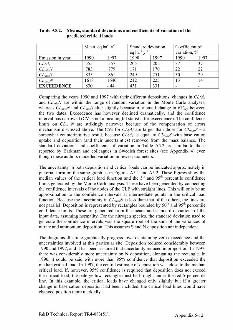
R&D Technical Report TR4-083(5)/1 Appendix 5-12
Table A5.2. Means, standard deviations and coefficients of variation of thepredicted critical loads
Mean, eq ha-1 y-1 Standard deviation,eq ha-1 y-1
Coefficient ofvariation, %
Emission in year 1990 1997 1990 1997 1990 1997CL(A) 555 557 205 205 37 37CLminN 783 779 171 170 22 22CLmaxS 835 861 249 251 30 29CLmaxN 1618 1640 212 225 13 14EXCEEDENCE 830 - 44 431 331 - -
Comparing the years 1990 and 1997 with their different depositions, changes in CL(A)and CLminN are within the range of random variation in the Monte Carlo analyses,whereas CLmaxN and CLmaxS alter slightly because of a small change in BCdep betweenthe two dates. Exceedence has however declined dramatically, and the confidenceinterval has narrowed (CV is not a meaningful statistic for exceedence). The confidencelimits on CLmaxN are strikingly narrower because of the compensation of errorsmechanism discussed above. The CVs for CL(A) are larger than those for CLmaxS – asomewhat counterintuitive result, because CL(A) is equal to CLmaxS with base cationuptake and deposition (and their uncertainties) removed from the mass balance. Thestandard deviations and coefficients of variation in Table A5.2 are similar to thosereported by Barkman and colleagues in Swedish forest sites (see Appendix 4) eventhough these authors modelled variation in fewer parameters.
The uncertainty in both deposition and critical loads can be indicated approximately inpictorial form on the same graph as in Figures A5.1 and A5.2. These figures show themedian values of the critical load function and the 5th and 95th percentile confidencelimits generated by the Monte Carlo analysis. These have been generated by connectingthe confidence intervals of the nodes of the CLF with straight lines. This will only be anapproximation to the confidence intervals at intermediate points in the critical loadfunction. Because the uncertainty in CLmaxN is less than that of the others, the lines arenot parallel. Deposition is represented by rectangles bounded by 50th and 95th percentileconfidence limits. These are generated from the means and standard deviations of theinput data, assuming normality. For the nitrogen species, the standard deviation used togenerate the confidence intervals was the square root of the sum of the variances ofnitrate and ammonium deposition. This assumes S and N deposition are independent.
The diagrams illustrate graphically progress towards attaining zero exceedence and theuncertainties involved at this particular site. Deposition reduced considerably between1990 and 1997, and it has been assumed that uncertainty reduced in proportion. In 1997,there was considerably more uncertainty on N deposition, elongating the rectangle. In1990, it could be said with more than 95% confidence that deposition exceeded themedian critical load. In 1997, the central estimate of deposition was close to the mediancritical load. If, however, 95% confidence is required that deposition does not exceedthe critical load, the pale yellow rectangle must be brought under the red 5 percentileline. In this example, the critical loads have changed only slightly but if a greaterchange in base cation deposition had been included, the critical load lines would havechanged position more markedly.
R&D Technical Report TR4-083(5)/1 Appendix 5-13
4 REFERENCES
Cronan, C.S. & Grigal, D.F. (1995) Use of calcium/aluminum ratios as indicators ofstress in forest ecosystems. Journal of Environmental Quality, 24 , 209-226.
Draaijers, G. P. J., Vanleeuwen, E. P., DeJong, P. G. H. & Erisman, J. W. (1997) Basecation deposition in Europe.1. Model description, results and uncertainties. AtmosphericEnvironment , 31, 4139-4157.
Hall, J. R., Ullyett, J., Hornung, M., Kennedy, F., Reynolds, B., Curtis, C., Langan, S.,and Fowler, D. (2001) Status of UK critical loads and exceedances Part I. Criticalloads and critical load maps, update to January 1998 report, CEH, Monks Wood,Cambs.
Hodson, M.E. & Langan, S.J. (1999) Considerations of uncertainty in setting criticalloads of acidity of soils: the role of weathering rate determination. EnvironmentalPollution, 106, 73-81.
NEGTAP (2001) Transboundary air pollution: acidification, eutrophication andground-level ozone in the UK, CEH, Edinburgh.
Posch, M. (1999) Defining an exceedance function. In Calculation and Mapping ofCritical Thresholds in Europe (Eds Posch, M., de Smet, P. A. M., Hettelingh, J.-P., andDowning, R. J.), pp. 29-32. RIVM, Bilthoven, The Netherlands.
Shaw, P. J. A. & Mcleod, A. R. (1995) The effects of SO2 and O3 on the foliar nutritionof Scots pine, Norway spruce and Sitka spruce in the Liphook Open-air FumigationExperiment. Plant Cell and Environment, 18, 237-245.
Skeffington, R.A. & Sutherland, P.M. (1995) The effects of SO2 and O3 fumigation onacid deposition and foliar leaching in the Liphook forest fumigation experiment. Plant,Cell and Environment, 18, 247-261.
Sverdrup, H. & De Vries, W. (1994) Calculating critical loads with the simple massbalance method. Water, Air and Soil Pollution, 72, 143-162.
UBA (1996) Manual on Methodologies and Criteria for Mapping Critical Levels /Loads and Geographical Areas where they are Exceeded Texte 71:96,Umweltbundesamt, Berlin.
Van Breemen, N., Mulder, J. & Driscoll, C.T. (1983) Acidification and alkalinization ofsoils. Plant and Soil, 75, 283-308.
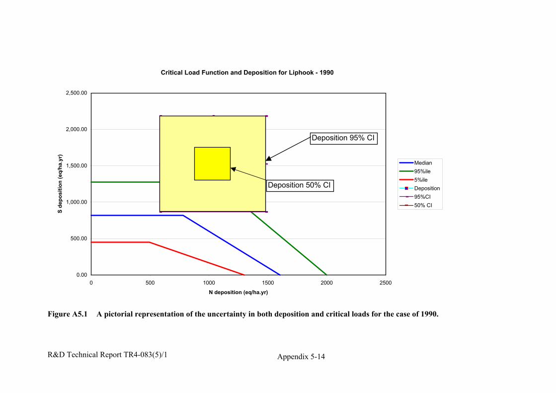
R&D Technical Report TR4-083(5)/1 Appendix 5-14
Critical Load Function and Deposition for Liphook - 1990
0.00
500.00
1,000.00
1,500.00
2,000.00
2,500.00
0 500 1000 1500 2000 2500
N deposition (eq/ha.yr)
S de
posi
tion
(eq/
ha.y
r)
Median
95%ile
5%ile
Deposition
95%CI
50% CI
Deposition 95% CI
Deposition 50% CI
Figure A5.1 A pictorial representation of the uncertainty in both deposition and critical loads for the case of 1990.
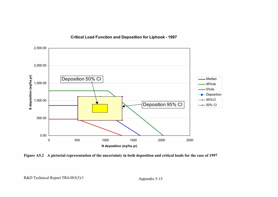
R&D Technical Report TR4-083(5)/1 Appendix 5-15
Critical Load Function and Deposition for Liphook - 1997
0.00
500.00
1,000.00
1,500.00
2,000.00
2,500.00
0 500 1000 1500 2000 2500
N deposition (eq/ha.yr)
S de
posi
tion
(eq/
ha.y
r)
Median
95%ile
5%ile
Deposition
95%CI
50% CIDeposition 95% CI
Deposition 50% CI
Figure A5.2 A pictorial representation of the uncertainty in both deposition and critical loads for the case of 1997

R&D Technical Report TR4-083(5)/1 Appendix 6-1
Appendix 6 Liphook critical loads case study outputs
CONTENTS
1 MONTE CARLO ANALYSIS OF EU AND UK CRITICAL LOADS ANDEXCEEDENCES 2

R&D Technical Report TR4-083(5)/1 Appendix 6-2
1 MONTE CARLO ANALYSIS OF EU AND UK CRITICAL LOADS AND EXCEEDENCES
In order to apply Monte Carlo (MC) analysis to the critical load equation for terrestrialecosystems it is necessary to generate sequences of random numbers for each input inthe equations. These sequences are then transformed into specified ranges with newdistributions to reflect the real character of the data. For example, some variables mayhave a rectangular distribution, some may have a log normal distribution and some mayhave a triangular distribution. These data, drawn from their respective distributions, arethen fed into the critical load equations to calculate the output critical loads. A largenumber of simulations have to be performed to generate a statistically significant outputdata set. This whole procedure has been undertaken using the Crystal Ball (2000)software package. This has been designed as an add-on to Microsoft Excel and utilizesan Excel spreadsheet to calculate the critical load values and the exceedences. Theassumptions for all of the inputs are specified, outputs selected and the number of MCsimulation trials specified. The program runs the full set of simulations to compute all ofthe output variables of interest. The software then undertakes a statistical analysis of theoutputs as well as a sensitivity analysis to determine which parameters contributesignificantly to the outputs. Before undertaking a run it is necessary to calculate thenumber of MC simulations required to produce a given level of accuracy. There are wellknown criteria based on statistical techniques for estimating the accuracy of the finaloutput set, and the Kolomogorov statistic can be used to estimate the accuracy of thedistribution. In order to achieve 95% confidence it is necessary to undertake over 750simulations. We have chosen to conduct 1000 simulations in each Monte Carlo run.
In the first two sets of analyses, the MC technique has been applied to the critical loadequation using the standard EU assumptions in which all of the base cations beingdeposited are considered. The main difference between the two runs are that in the firstrun the assumption is that most of the input distributions are uniform, as shown in Figure6.1, whereas in the second run most distributions are assumed to be triangular, as shownin Figure 6.2. Thus the two runs give us information on the effects of differing inputdistribution assumptions. Figures 6.3 and 6.4 show the Monte Carlo simulation outputsin terms of the distributions of CLmaxS, CLminN and CLmaxN for the two runs. In the caseof the first run (Figure 6.3), the distributions are assumed to be rectangular with theexception of Kgibb, the Gibbsite equilibrium parameter. In the second run thedistributions for the inputs are assumed to be triangular, reflecting the reality thatatmospheric deposition and rainfall have a wide range of behaviour but are generallyclustered around a mean annual value, and that therefore the value is likely to be in thecentre of the distribution. The output distributions for these two runs show a wide spreadof critical loads, but the spreads for the triangular distributions are smaller, indicatingthat the assumptions on the form of the inputs are important.
The Monte Carlo analyses for the UK version of the model all relate to the Liphook sitein Hampshire. The primary difference with the EU application is that magnesium andpotassium are deleted from the base cation deposition term because of the high levels ofthese in the UK and hence the bias that these give to any CL calculations for the UK.The results for Liphook simulation are summarised in Figures 6.5 to 6.8. These show thecritical load results as well as the distribution of the exceedences for the 1990 and 1997years. These 2 years were selected because there is a substantial data set for Liphook for

R&D Technical Report TR4-083(5)/1 Appendix 6-3
1990 and because by 1997 there was a large decline in S deposition and we can explorethe effects of this reduction on exceedence. As might be expected the exceedencedistributions for Liphook are relatively high in 1990 because of the high deposition of Nand S for the area. However by 1997 these exceedence levels have fallen considerably.
Finally Crystal Ball can be used to investigate sensitivity analysis of each parameter inrelation to the other parameters. For example Figures 6.9 to 6.11 show the relativesensitivity of the parameters specified in the critical load equation for the critical loadsfor sulphur and nitrogen. In each case the parameters are ranked according to theircontribution to the variance and this ranking varies depending on the critical loadfunction chosen. Thus CLmaxS has a different ranking of the parameters to the N criticalloads.
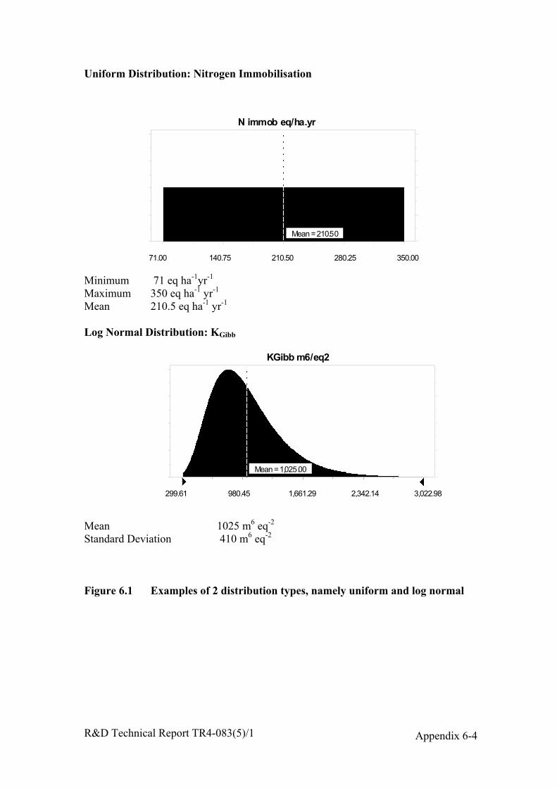
R&D Technical Report TR4-083(5)/1 Appendix 6-4
Uniform Distribution: Nitrogen Immobilisation
Minimum 71 eq ha-1yr-1
Maximum 350 eq ha-1 yr-1
Mean 210.5 eq ha-1 yr-1
Log Normal Distribution: KGibb
Mean 1025 m6 eq-2
Standard Deviation 410 m6 eq-2
Figure 6.1 Examples of 2 distribution types, namely uniform and log normal
������������������������������������������������������������������������������������������������������������������������������������������������������������������������������������������������������������������������������������������������������������������������������������������������������������������������������������������������������������������������������������������������������������������������������������������������������������������������������������������������������������������������������������������������������������������������������������������������������������������������������������������������������������������������������������������������������������������������������������������������������������������������������������������������������������������������������������������Mean = 210.50
71.00 140.75 210.50 280.25 350.00
N immob eq/ha.yr
���������������������������������������������������������������������������������������������������������������������������������������������������������������������������������������������������������������������������������������������������������������������������������������������������������������������������������������������������������������������������������������������������������������������������������������������������������������������������������������������������������������������������������������������������������������������������������������������������������������������������������������������������������������������������������������������������������������������������������������������������������������������������������������������������������������������������������������������������������������������������������������������������������������������������������������������������������������������������������������������������������������������������������������������������������������������������������������������������������������������������������������������������������������������������������������������������������������������������������������������������������������������������������������������������������������������������������������������������������������������������������������������������������������������������������������������������������������������������������������������������������������������������������������������Mean = 1,025.00��� ���
299.61 980.45 1,661.29 2,342.14 3,022.98
KGibb m6/eq2
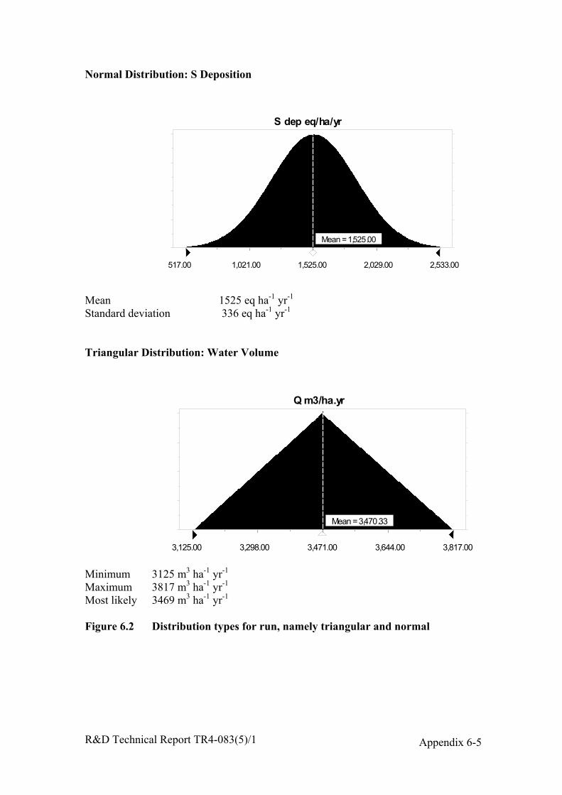
R&D Technical Report TR4-083(5)/1 Appendix 6-5
Normal Distribution: S Deposition
Mean 1525 eq ha-1 yr-1
Standard deviation 336 eq ha-1 yr-1
Triangular Distribution: Water Volume
Minimum 3125 m3 ha-1 yr-1
Maximum 3817 m3 ha-1 yr-1
Most likely 3469 m3 ha-1 yr-1
Figure 6.2 Distribution types for run, namely triangular and normal
���������������������������������������������������������������������������������������������������������������������������������������������������������������������������������������������������������������������������������������������������������������������������������������������������������������������������������������������������������������������������������������������������������������������������������������������������������������������������������������������������������������������������������������������������������������������������������������������������������������������������������������������������������������������������������������������������������������������������������������������������������������������������������������������������������������������������������������������������������������������������������������������������������������������������������������������������������������������������������������������������������������������������������������������������������������������������������������������������������������������������������������������������������������������������������������������������������������������������������������������������������������������������������������������������������������������������������������������������������������������������������������������������������������������������������������������������������������������������������������������������������������������������������������������������������������������������������������������������������������Mean = 1,525.00������
������
517.00 1,021.00 1,525.00 2,029.00 2,533.00
S dep eq/ha/yr
������������������������������������������������������������������������������������������������������������������������������������������������������������������������������������������������������������������������������������������������������������������������������������������������������������������������������������������������������������������������������������������������������������������������������������������������������������������������������������������������������������������������������������������������������������������������������������������������������������������������������������������������������������������������������������������������������������������������������������������������������������������������������������������������������������������������������������������������������������������������������������������������������������������������������������������������������������������������������������������������������������������������������������������������������������������������������������������������������������������������������������������������������������������������������������������������������������������������������������������������������������������������������������������������������������������������������������������������������������������������������������������������������������������������������������������������������������������������������������������������������������������������������������������������������������������������������������������������������������������������������������������������������������������������������������������������������������������������������������������������������������������������������������������������Mean = 3,470.33������
������
3,125.00 3,298.00 3,471.00 3,644.00 3,817.00
Q m3/ha.yr
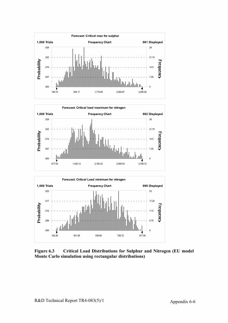
R&D Technical Report TR4-083(5)/1 Appendix 6-6
Frequency Chart����������������������������������������������������������������������������������������������������������������������������������������������������������������������������������������������������������������������������������������������������������������������������������������������������������������������������������������������������������������������������������������������������������������������������������������������������������������������������������������������������������������������������������������������������������������������������������������������������������������������������������������������������������������������������������������������������������������������������������������������������������������������������������������������������������������������������������������������������������������������������������������������������������������������������������������������������������������������������������������������������������������������������������������������������������������������������������������������������������������������������������������������������������������������������������������������������������������������������
.000
.007
.015
.022
.029
0
7.25
14.5
21.75
29
148.72 934.11 1,719.49 2,504.87 3,290.26
1,000 Trials 981 Displayed
������
������
Forecast: Critical max for sulphur
Frequency Chart����������������������������������������������������������������������������������������������������������������������������������������������������������������������������������������������������������������������������������������������������������������������������������������������������������������������������������������������������������������������������������������������������������������������������������������������������������������������������������������������������������������������������������������������������������������������������������������������������������������������������������������������������������������������������������������������������������������������������������������������������������������������������������������������������������������������������������������������������������������������������������������������������������������������������������������������������������������������������������������������������������������������������������������������������������������������������������������������������������������������������������������������������������������������������������������������������������������������������
.000
.007
.015
.022
.029
0
7.25
14.5
21.75
29
677.93 1,435.13 2,192.33 2,949.53 3,706.73
1,000 Trials 982 Displayed
������
������
Forecast: Critical load maximum for nitrogen
Frequency Chart����������������������������������������������������������������������������������������������������������������������������������������������������������������������������������������������������������������������������������������������������������������������������������������������������������������������������������������������������������������������������������������������������������������������������������������������������������������������������������������������������������������������������������������������������������������������������������������������������������������������������������������������������������������������������������������������������������������������������������������������������������������������������������������������������������������������������������������������������������������������������������������������������������������������������������������������������������������������������������������������������������������������������������������������������������������������������������������������������������������������������������������������������������������������������������������������������������������������������.000
.006
.012
.017
.023
0
5.75
11.5
17.25
23
162.26 351.08 539.90 728.72 917.54
1,000 Trials 999 Displayed
��� ���
Forecast: Critical Load minimum for nitrogen
Figure 6.3 Critical Load Distributions for Sulphur and Nitrogen (EU modelMonte Carlo simulation using rectangular distributions)

R&D Technical Report TR4-083(5)/1 Appendix 6-7
Frequency Chart����������������������������������������������������������������������������������������������������������������������������������������������������������������������������������������������������������������������������������������������������������������������������������������������������������������������������������������������������������������������������������������������������������������������������������������������������������������������������������������������������������������������������������������������������������������������������������������������������������������������������������������������������������������������������������������������������������������������������������������������������������������������������������������������������������������������������������������������������������������������������������������������������������������������������������������������������������������������������������������������������������������������������������������������������������������������������������������������������������������������������������������������������������������������������������������������������������������������������
.000
.008
.017
.025
.033
0
8.25
16.5
24.75
33
867.17 1,502.98 2,138.79 2,774.59 3,410.40
1,000 Trials 983 Displayed
������
������
Forecast: Critical load maximum for nitrogen
Frequency Chart����������������������������������������������������������������������������������������������������������������������������������������������������������������������������������������������������������������������������������������������������������������������������������������������������������������������������������������������������������������������������������������������������������������������������������������������������������������������������������������������������������������������������������������������������������������������������������������������������������������������������������������������������������������������������������������������������������������������������������������������������������������������������������������������������������������������������������������������������������������������������������������������������������������������������������������������������������������������������������������������������������������������������������������������������������������������������������������������������������������������������������������������������������������������������������������������������������������������������
.000
.006
.012
.018
.024
0
6
12
18
24
206.62 387.20 567.79 748.38 928.96
1,000 Trials 999 Displayed
������
������
Forecast: Critical Load minimum for nitrogen
Frequency Chart����������������������������������������������������������������������������������������������������������������������������������������������������������������������������������������������������������������������������������������������������������������������������������������������������������������������������������������������������������������������������������������������������������������������������������������������������������������������������������������������������������������������������������������������������������������������������������������������������������������������������������������������������������������������������������������������������������������������������������������������������������������������������������������������������������������������������������������������������������������������������������������������������������������������������������������������������������������������������������������������������������������������������������������������������������������������������������������������������������������������������������������������������������������������������������������������������������������������������.000
.007
.014
.021
.028
0
7
14
21
28
114.69 796.10 1,477.52 2,158.93 2,840.34
1,000 Trials 980 Displayed
��� ���
Forecast: Critical max for sulphur
Figure 6.4 Critical Loads for Sulphur and Nitrogen for EU Monte CarloAnalysis with Triangular Distributions
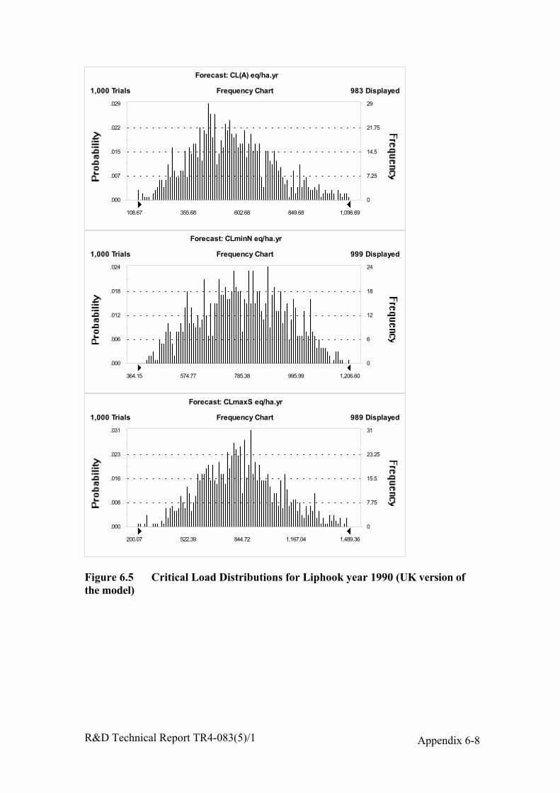
R&D Technical Report TR4-083(5)/1 Appendix 6-8
Frequency Chart����������������������������������������������������������������������������������������������������������������������������������������������������������������������������������������������������������������������������������������������������������������������������������������������������������������������������������������������������������������������������������������������������������������������������������������������������������������������������������������������������������������������������������������������������������������������������������������������������������������������������������������������������������������������������������������������������������������������������������������������������������������������������������������������������������������������������������������������������������������������������������������������������������������������������������������������������������������������������������������������������������������������������������������������������������������������������������������������������������������������������������������������������������������������������������������������������������������������������
.000
.007
.015
.022
.029
0
7.25
14.5
21.75
29
108.67 355.68 602.68 849.68 1,096.69
1,000 Trials 983 Displayed
������
������
Forecast: CL(A) eq/ha.yr
Frequency Chart����������������������������������������������������������������������������������������������������������������������������������������������������������������������������������������������������������������������������������������������������������������������������������������������������������������������������������������������������������������������������������������������������������������������������������������������������������������������������������������������������������������������������������������������������������������������������������������������������������������������������������������������������������������������������������������������������������������������������������������������������������������������������������������������������������������������������������������������������������������������������������������������������������������������������������������������������������������������������������������������������������������������������������������������������������������������������������������������������������������������������������������������������������������������������������������������������������������������������
.000
.006
.012
.018
.024
0
6
12
18
24
364.15 574.77 785.38 995.99 1,206.60
1,000 Trials 999 Displayed
������
������
Forecast: CLminN eq/ha.yr
Frequency Chart����������������������������������������������������������������������������������������������������������������������������������������������������������������������������������������������������������������������������������������������������������������������������������������������������������������������������������������������������������������������������������������������������������������������������������������������������������������������������������������������������������������������������������������������������������������������������������������������������������������������������������������������������������������������������������������������������������������������������������������������������������������������������������������������������������������������������������������������������������������������������������������������������������������������������������������������������������������������������������������������������������������������������������������������������������������������������������������������������������������������������������������������������������������������������������������������������������������������������
.000
.008
.016
.023
.031
0
7.75
15.5
23.25
31
200.07 522.39 844.72 1,167.04 1,489.36
1,000 Trials 989 Displayed
������
������
Forecast: CLmaxS eq/ha.yr
Figure 6.5 Critical Load Distributions for Liphook year 1990 (UK version ofthe model)
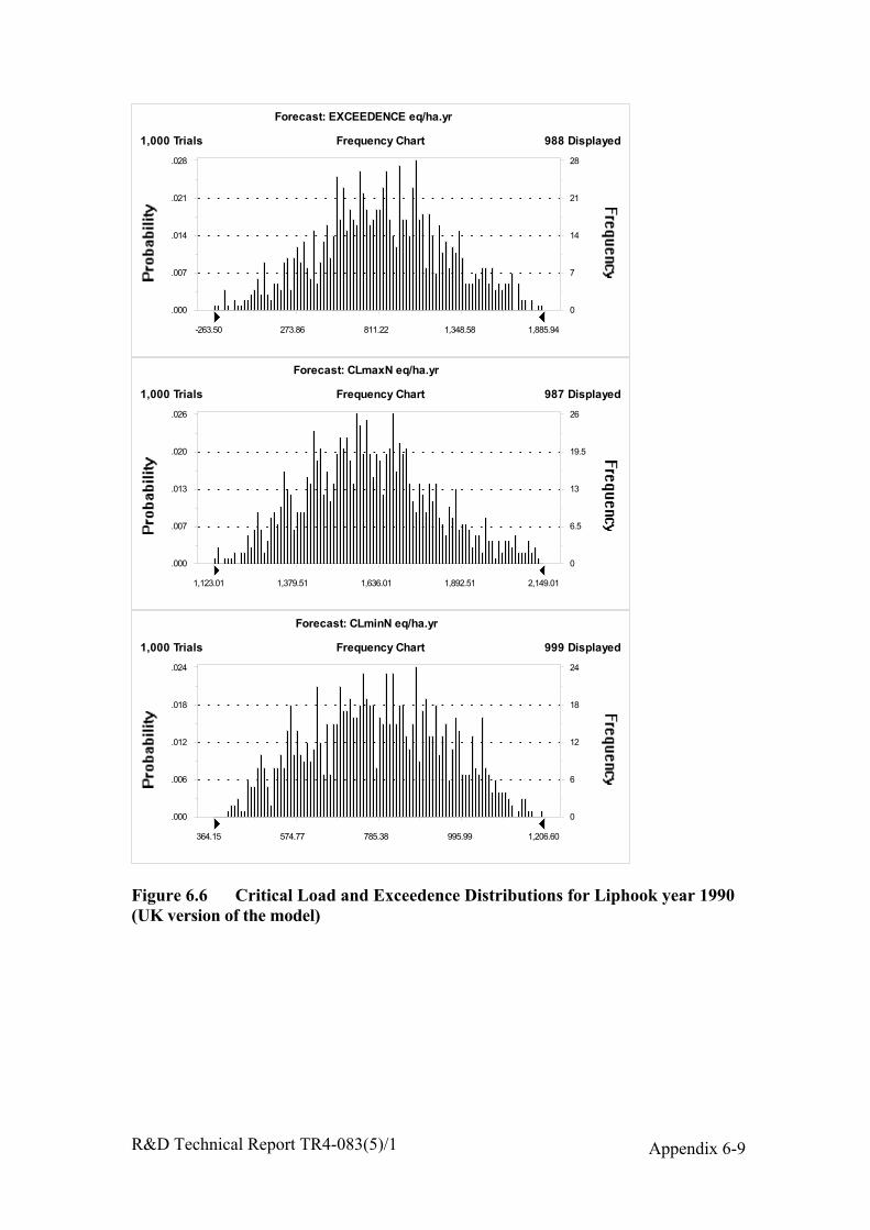
R&D Technical Report TR4-083(5)/1 Appendix 6-9
Frequency Chart����������������������������������������������������������������������������������������������������������������������������������������������������������������������������������������������������������������������������������������������������������������������������������������������������������������������������������������������������������������������������������������������������������������������������������������������������������������������������������������������������������������������������������������������������������������������������������������������������������������������������������������������������������������������������������������������������������������������������������������������������������������������������������������������������������������������������������������������������������������������������������������������������������������������������������������������������������������������������������������������������������������������������������������������������������������������������������������������������������������������������������������������������������������������������������������������������������������������������
.000
.007
.014
.021
.028
0
7
14
21
28
-263.50 273.86 811.22 1,348.58 1,885.94
1,000 Trials 988 Displayed
������
������
Forecast: EXCEEDENCE eq/ha.yr
Frequency Chart����������������������������������������������������������������������������������������������������������������������������������������������������������������������������������������������������������������������������������������������������������������������������������������������������������������������������������������������������������������������������������������������������������������������������������������������������������������������������������������������������������������������������������������������������������������������������������������������������������������������������������������������������������������������������������������������������������������������������������������������������������������������������������������������������������������������������������������������������������������������������������������������������������������������������������������������������������������������������������������������������������������������������������������������������������������������������������������������������������������������������������������������������������������������������������������������������������������������������
.000
.007
.013
.020
.026
0
6.5
13
19.5
26
1,123.01 1,379.51 1,636.01 1,892.51 2,149.01
1,000 Trials 987 Displayed
������
������
Forecast: CLmaxN eq/ha.yr
Frequency Chart����������������������������������������������������������������������������������������������������������������������������������������������������������������������������������������������������������������������������������������������������������������������������������������������������������������������������������������������������������������������������������������������������������������������������������������������������������������������������������������������������������������������������������������������������������������������������������������������������������������������������������������������������������������������������������������������������������������������������������������������������������������������������������������������������������������������������������������������������������������������������������������������������������������������������������������������������������������������������������������������������������������������������������������������������������������������������������������������������������������������������������������������������������������������������������������������������������������������������
.000
.006
.012
.018
.024
0
6
12
18
24
364.15 574.77 785.38 995.99 1,206.60
1,000 Trials 999 Displayed
������
������
Forecast: CLminN eq/ha.yr
Figure 6.6 Critical Load and Exceedence Distributions for Liphook year 1990(UK version of the model)

R&D Technical Report TR4-083(5)/1 Appendix 6-10
Frequency Chart����������������������������������������������������������������������������������������������������������������������������������������������������������������������������������������������������������������������������������������������������������������������������������������������������������������������������������������������������������������������������������������������������������������������������������������������������������������������������������������������������������������������������������������������������������������������������������������������������������������������������������������������������������������������������������������������������������������������������������������������������������������������������������������������������������������������������������������������������������������������������������������������������������������������������������������������������������������������������������������������������������������������������������������������������������������������������������������������������������������������������������������������������������������������������������������������������������������������������
.000
.007
.014
.021
.028
0
7
14
21
28
220.44 542.16 863.87 1,185.58 1,507.30
1,000 Trials 992 Displayed
������
������
Forecast: CLmaxS eq/ha.yr
Frequency Chart����������������������������������������������������������������������������������������������������������������������������������������������������������������������������������������������������������������������������������������������������������������������������������������������������������������������������������������������������������������������������������������������������������������������������������������������������������������������������������������������������������������������������������������������������������������������������������������������������������������������������������������������������������������������������������������������������������������������������������������������������������������������������������������������������������������������������������������������������������������������������������������������������������������������������������������������������������������������������������������������������������������������������������������������������������������������������������������������������������������������������������������������������������������������������������������������������������������������������
.000
.006
.013
.019
.025
0
6.25
12.5
18.75
25
368.26 571.39 774.52 977.64 1,180.77
1,000 Trials 997 Displayed
������
������
Forecast: CLminN eq/ha.yr
Frequency Chart����������������������������������������������������������������������������������������������������������������������������������������������������������������������������������������������������������������������������������������������������������������������������������������������������������������������������������������������������������������������������������������������������������������������������������������������������������������������������������������������������������������������������������������������������������������������������������������������������������������������������������������������������������������������������������������������������������������������������������������������������������������������������������������������������������������������������������������������������������������������������������������������������������������������������������������������������������������������������������������������������������������������������������������������������������������������������������������������������������������������������������������������������������������������������������������������������������������������������
.000
.006
.012
.017
.023
0
5.75
11.5
17.25
23
104.28 351.14 598.00 844.86 1,091.72
1,000 Trials 990 Displayed
������
������
Forecast: CL(A) eq/ha.yr
Figure 6.7 Critical Load Distributions for Liphook year 1997 (UK version ofthe model)
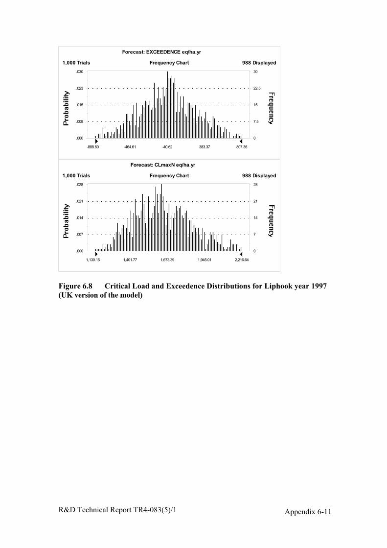
R&D Technical Report TR4-083(5)/1 Appendix 6-11
Frequency Chart����������������������������������������������������������������������������������������������������������������������������������������������������������������������������������������������������������������������������������������������������������������������������������������������������������������������������������������������������������������������������������������������������������������������������������������������������������������������������������������������������������������������������������������������������������������������������������������������������������������������������������������������������������������������������������������������������������������������������������������������������������������������������������������������������������������������������������������������������������������������������������������������������������������������������������������������������������������������������������������������������������������������������������������������������������������������������������������������������������������������������������������������������������������������������������������������������������������������������
.000
.008
.015
.023
.030
0
7.5
15
22.5
30
-888.60 -464.61 -40.62 383.37 807.36
1,000 Trials 988 Displayed
������
������
Forecast: EXCEEDENCE eq/ha.yr
Frequency Chart����������������������������������������������������������������������������������������������������������������������������������������������������������������������������������������������������������������������������������������������������������������������������������������������������������������������������������������������������������������������������������������������������������������������������������������������������������������������������������������������������������������������������������������������������������������������������������������������������������������������������������������������������������������������������������������������������������������������������������������������������������������������������������������������������������������������������������������������������������������������������������������������������������������������������������������������������������������������������������������������������������������������������������������������������������������������������������������������������������������������������������������������������������������������������������������������������������������������������
.000
.007
.014
.021
.028
0
7
14
21
28
1,130.15 1,401.77 1,673.39 1,945.01 2,216.64
1,000 Trials 988 Displayed
������
������
Forecast: CLmaxN eq/ha.yr
Figure 6.8 Critical Load and Exceedence Distributions for Liphook year 1997(UK version of the model)
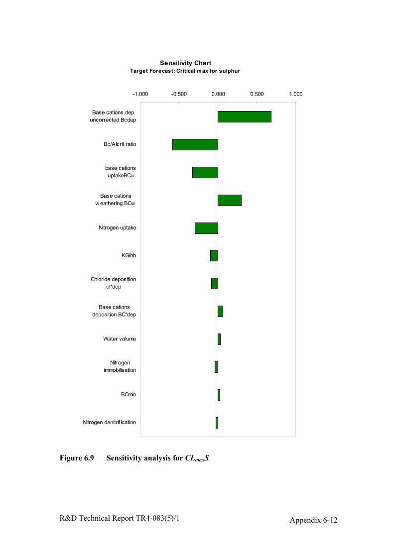
R&D Technical Report TR4-083(5)/1 Appendix 6-12
Sensitivity ChartTarget Forecast: Critical max for sulphur
-1.000 -0.500 0.000 0.500 1.000
Base cations depuncorrected Bcdep
Bc/Alcrit ratio
base cationsuptakeBCu
Base cationsw eathering BCw
Nitrogen uptake
KGibb
Chloride depositioncl*dep
Base cationsdeposition BC*dep
Water volume
Nitrogenimmobilisation
BCmin
Nitrogen denitrif ication
Figure 6.9 Sensitivity analysis for CLmaxS
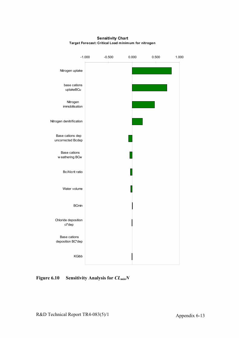
R&D Technical Report TR4-083(5)/1 Appendix 6-13
Sensitivity ChartTarget Forecast: Critical Load minimum for nitrogen
-1.000 -0.500 0.000 0.500 1.000
Nitrogen uptake
base cationsuptakeBCu
Nitrogenimmobilisation
Nitrogen denitrif ication
Base cations depuncorrected Bcdep
Base cationsw eathering BCw
Bc/Alcrit ratio
Water volume
BCmin
Chloride depositioncl*dep
Base cationsdeposition BC*dep
KGibb
Figure 6.10 Sensitivity Analysis for CLminN
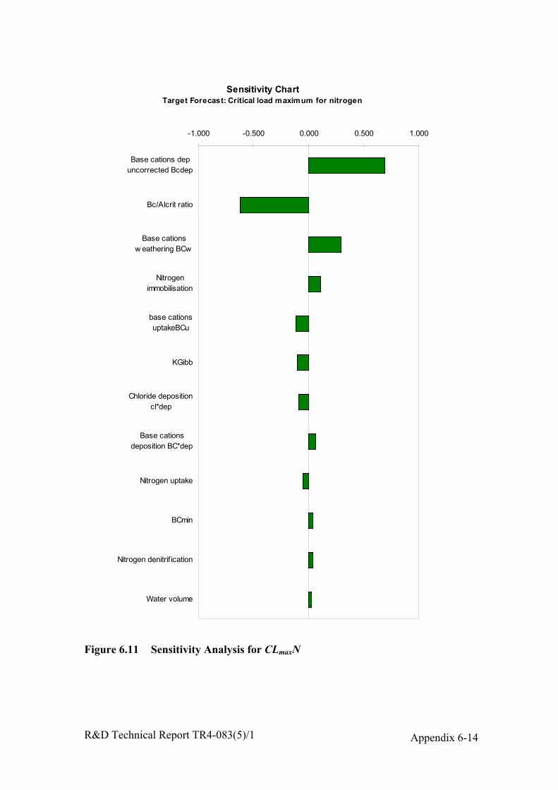
R&D Technical Report TR4-083(5)/1 Appendix 6-14
Sensitivity ChartTarget Forecast: Critical load maximum for nitrogen
-1.000 -0.500 0.000 0.500 1.000
Base cations depuncorrected Bcdep
Bc/Alcrit ratio
Base cationsw eathering BCw
Nitrogenimmobilisation
base cationsuptakeBCu
KGibb
Chloride depositioncl*dep
Base cationsdeposition BC*dep
Nitrogen uptake
BCmin
Nitrogen denitrif ication
Water volume
Figure 6.11 Sensitivity Analysis for CLmaxN

R&D Tehnical Report TR4-083(5)/1 Appendix 7-1
Appendix 7 Implications of parameter variations fornitrogen deposition modelled using the HARM model
CONTENTS
1 INTRODUCTION 2
2 EFFECTS OF VARYING INDIVIDUAL PARAMETERS 2
3 EFFECTS OF VARYING MULTIPLE PARAMETERS 4
FIGURES
Figure 1 Changes in the deposition of oxidised N caused by varying the oxidationrates of NO2 by OH (b,e) and by O3 (c,f) 7
Figure 2 Changes in oxidised N deposition with scaling the deposition velocity ofHNO3 8
Figure 3 Changes in reduced N deposition with scaling of NH3 emissions 9Figure 4 Maximum and minimum values of N deposition at selected Secondary
Network sites varying all 12 parameter values, compared with the value fromthe appropriate base case scenario 10
Figure 5 Increased deposition under multiple parameter variations compared withbase case 11
Figure 6 Decreased deposition under multiple parameter variations compared withbase case 12
Figure 7 Total N deposition (oxidised + reduced) for the base case compared withminimum (b,e) and maximum (c,f) values from model runs with all parametersvaried 13
R&D Tehnical Report TR4-083(5)/1 Appendix 7-2
1 Introduction
As set out in Chapter 4 of the main report, deposition model uncertainties have beenassessed by (a) selecting the parameters believed to be most influential in affectingmodel output, (b) selecting a range of values for these input parameters and (c) runningthe models (TRACK, HARM and FRAME) using these values. The range of parametervalues is set out in Table 4.4 in the main report. In the case of HARM and FRAME theupper parameter values were implemented one at a time (12 runs) against i) a base caseof 1997 emissions, ii) 1997 emissions, plus an additional source of 75 kt NOx, and iii)1997 emissions, plus an additional source of 150 kt NOx. A further batch of 12 modelruns generated deposition with all parameters being varied and with the additional 75 ktNOx. The outcomes of both varying individual parameters and the full set of parametersdisplay differential effects between dry and wet deposition, and hence different spatialimpacts reflecting transport distance.
2 Effects of varying individual parameters
These have been explored by looking at changes in the national deposition budgets forwet and dry deposited S and N (oxidised and reduced) and by mapping some of theresulting patterns of deposition. The effects on the budget are summarised in Table 1,numbers of the model runs are shown in parentheses. Increasing the deposition velocityof NO2 (1) has the expected effect of increasing overall dry deposition of oxidised N,although the magnitude of the effect is relatively small reflecting the greater importanceof the deposition of nitric acid to the overall budget. The increase in dry depositionresults in a small decrease in wet deposition. Changing the ratio of the rate of oxidationof NO to NO2 to the reverse photolysis rate (2), affects both the oxidised and reduced Nbudgets to a limited extent. Larger changes are caused by varying the oxidation rates ofNO2 by OH (3) to HNO3, and by O3 (4) to NO3. An increase in OH oxidation results inabout a 20% increase in dry oxidised N deposition and a smaller increase in wetdeposition. The resulting increase in ammonium aerosol production, via HNO3 (3), isalso reflected in more wet deposition of reduced N. The spatial implications of thesechanges to oxidised nitrogen deposition are illustrated in Figure 1. This shows that theincrease in dry deposition under (3) occurs in a swathe from south east to north eastEngland, close to the major source regions. The effects of increasing wet deposition, (3)and (4), occur in the upland areas of western and northern Britain. Modelled wetdeposition also increases around the North and South Downs, where increasing NO3production feeds into more orographically enhanced wet deposition. The impact ofincreasing the ammonia reaction rate, with nitric acid (5), is largely confined to areduction in dry reduced N deposition. Given the major contribution of HNO3 to dryoxidised N deposition, the effect of increasing aerosol production (6) is unsurprising,with a decrease in dry oxidised N deposition and a smaller increase in wet deposition.
Scaling up the aerosol washout rate (7) has a substantial impact on wet deposition of allthe pollutants considered (+ 20 – 26%). This effect would be amplified by the scaling ofwashout in HARM, as part of the representation of orographic enhancement, and would,therefore, be particularly significant in high rainfall areas of upland and western Britain.

R&D Tehnical Report TR4-083(5)/1 Appendix 7-3
Table 1 Percentage difference from base case scenario for 12 parametervariations with 0, 75 and 150 kt NOx emitted from additional source
Scenario Addedsource
Dry S Wet S DryNOy-N
WetNOy-N
DryNH-N
WetNH-N
0 0 0 +9 -0.3 0 -0.0575 0 0 +9 -0.3 +0.01 -0.05
(1) vd NO2
150 0 0 +9 -0.3 0 -0.030 0 0 -4.6 -2.8 +0.02 -1.075 0 0 -4.8 -2.8 +0.02 -1.0
(2) k1/J1
150 0 0 -4.9 -2.8 +0.02 -1.00 0 0 +19.6 +4 -0.2 +8.575 0 0 +19.9 +4.2 -0.2 +8.5
(3) k[NO2][OH]
150 0 0 +20.1 +4.3 -0.2 +8.50 0 0 -8.7 +12.5 0 -3.875 0 0 -8.5 +12.2 0 -3.8
(4) k[O3][NO2]
150 0 0 -8.4 +12.2 0 -3.80 0 0 -0.4 +0.2 -4.9 -0.575 0 0 -0.4 +0.2 -4.9 -0.5
(5) k[NH3][HNO3]
150 0 0 -0.4 +0.2 -4.9 -0.50 0 0 -8.9 +2.7 +0.1 -1.775 0 0 -8.92 +2.7 +0.1 -1.7
(6) k[NH3]
150 0 0 -8.92 +2.7 +0.1 -1.70 -1.9 +25.9 -9.7 +20.4 +1.7 +22.475 -1.9 +25.9 -9.7 +20.6 +1.7 +22.5
(7) washoutA
150 -1.9 +25.9 -9.7 +20.6 +1.7 +22.50 0 0 +17.3 -3 +0.09 -1.475 0 0 +17.4 -3.1 +0.09 -1.4
(8) vdHNO3
150 0 0 +17.4 -3.1 +0.09 -1.40 +50 +49.9 +4.4 -1.6 -1.5 +1475 +50 +49.9 +4.3 -1.6 -1.5 +13.9
(9) ES02
150 +50 +49.9 +5.8 -1.6 -1.5 +13.90 0 0 -6.8 +2.3 +45.9 +16.275 0 0 -6.8 +2.3 +45.9 +16.2
(10) ENH3
150 0 0 -6.8 +2.3 +45.9 +16.30 0 0 +20.7 +16 -0.1 +5.475 0 0 +20.5 +15.9 -0.1 +5.4
(11) ENOx
150 0 0 +20 +15.8 -0.1 +5.30 -9.5 +2.5 -8.6 +2.7 -9.5 +1.975 -9.5 +2.5 -8.6 +2.7 -9.5 +1.9
(12) H
150 -9.5 +2.5 -8.6 +2.8 -9.5 +1.9
Given the significance of HNO3 to the national oxidised N budget described above, it isunsurprising that scaling up the deposition velocity of HNO3 (8) has quite a largeimpact. The spatial effect of this is illustrated in Figure 2. The pattern of increase in dryoxidised N deposition is very similar to that under (3) (see Figure 1), which is notsurprising as these two parameter changes are doing very similar things. In the case of
R&D Tehnical Report TR4-083(5)/1 Appendix 7-4
(8), however, the actual deposition of more HNO3 has the effect of reducing wetoxidised N deposition. There is a knock-on effect of this change on the reduced Nbudget through the reaction of NH3 with HNO3, leaving slightly more NH3 to be drydeposited and reducing wet ammonium deposition.
As might be expected, varying the emission rates (up by 50% under (9), (10) and (11))has a significant effect on deposition. The change in S deposition is linear with thechange in emission, but it should be noted that the chemical coupling with ammoniaresults in an increase in wet deposition of reduced N. Hence the combined effect ofincreasing S emissions is greater in wet deposition dominated areas than in dry. Thechange in NH3 emission results in a large increase in dry reduced nitrogen deposition,but a smaller increase in wet deposition. The spatial expression of this is illustrated inFigure 3. The change in dry reduced N deposition is roughly proportional to the changein emission close to source reflecting the short transport distance of this pollutant. Thechange in ammonia emission also has some impact on the oxidised N budget as morenitric acid is ‘mopped up’ by the ammonia as under (5). This reduces dry oxidised Ndeposition through eastern England. Changing NOx emissions results in an increase indry deposition of 20 – 21%, and an increase in wet deposition of about 16%. Theincrease in dry deposition is linear with the change in emission, while the difference inwet deposition reflects some non-linearity in the oxidised N (see EA Technical ReportP276).
Increasing the boundary layer height (12) in a model, which assumes instantaneousmixing, has the expected effect of reducing dry deposition and increasing wetdeposition for all pollutants. This would be reflected by less deposition in sourceregions and more in remote areas.
3 Effects of varying multiple parameters
As described above, HARM has also been run varying all 12 parameter valuessimultaneously. In this case, parameter values were set both higher and lower than thedefault value. The effects of this have been explored by looking at changes in wet anddry deposition of oxidised and reduced nitrogen at the UK’s 32 Secondary Networksites, plus the former network site of Liphook (see Chapter 6). The magnitude of changeat some of these sites, compared with the base case (i.e. parameters set to their usualvalues) is shown in Figure 4. As suggested by Figures 4.27 and 4.28 in the main report,the magnitude of variability is greater at the more polluted sites (most of England,excluding the south west, and much of Wales). The cleaner sites, such as StrathvaichDam and Alt a Mharcaidh, show less variability. Within this general pattern, however,there are some interesting spatial variations between wet and dry deposition and indeedin overall behaviour compared with the base case run. The four most north westerlysites (Achanarras, Strathvaich Dam, Alt A Mharcaidh and Polloch) stand out from therest because the mean deposition from all 12 sets of parameter variations in less than thedeposition under the base (control) case. Across the rest of the UK, the mean of thevariants is higher than the base case. This may suggest that for these clean sites themodels are more likely to overestimate deposition than underestimate, whereas for therest of the country the reverse is true. We must, however, bear in mind that some keyparameters for these upland sites (e.g. wind speed, precipitation amount) were notincluded in this analysis. Overall, the increases in deposition with different parametersets were substantially larger than the decreases. Only two sites were the exception to

R&D Tehnical Report TR4-083(5)/1 Appendix 7-5
this: Strathvaich Dam and Polloch, where reductions in wet deposition of reduced andoxidised N were the largest changes recorded.
The dominant pollutant showing an increase in deposition under the various parametersets is illustrated in Figure 5. This indicates some different regional behaviour, withchanges in reduced N deposition dominating in most areas apart from eastern England.In eastern England, the largest increases were in wet oxidised and reduced N deposition.Outputs for all the sites in this area showed very similar behaviour and are illustrated bythe charts for Thorganby and Barcombe Mills on Figure 4. There was then a group ofsites across north west England, Wales and western Scotland, where the largest changeswere in wet and dry reduced N deposition. The results from Llyn Brianne (Figure 4) arean example of this. In other areas, including south west England, Northern Ireland,north east England and much of Scotland, the largest changes were in dry reduced Ndeposition (e.g. Goonhilly, Hillsborough Forest and Achanarras on Figure 4). A patterncommon across the whole of the UK was that increases in dry deposition of oxidised Nwere small.
With the exception of Polloch and Strathvaich Dam (see above), decreases in depositionunder multiple parameter variations were of minor importance. This is clearly illustratedby Figure 4. The pollutants showing the most negative change are shown in Figure 6.Changes in oxidised N deposition (both wet and dry) are the largest element of anydecrease across most of England and southern Wales. This area affected by changes inoxidised N is more extensive than the area which showed an increase in wet oxidised Ndeposition. Under these parameter sets the magnitude of the decrease in dry oxidised Ndeposition was greater than the magnitude of any increase. Only the results fromAchanarras, in the far north east of Scotland, were the exception to this. The site atStrathvaich Dam also shows its largest change in wet oxidised N deposition (followedby wet reduced N), although the magnitude of any change here is small. The rest of theUK shows the largest decreases in deposition of wet and/or dry reduced N.
Based on the results of varying 12 model parameters simultaneously, it appears that formost of the UK HARM may be underestimating N deposition (oxidised and reduced)due to uncertainties in the values assigned to these parameters. This may also be true forthe other models used in this exercise (TRACK and FRAME), but their results have notbe explored in an equivalent manner. Only at the cleanest sites are uncertainties likely tomean that the standard model overestimates. Except in central and eastern England,where oxidised N deposition is most variable under the different parameter sets, most ofthe uncertainties in deposition are related to the representation of reduced N. Thispattern needs to be considered in the light of whether reduced or oxidised N dominatesthe N budget in different areas. Changes in S deposition have not been considered.
If oxidised and reduced N deposition (total N) are taken together and considered at thenational scale, then the full impact of the parameter variations can be seen. Figure 7shows total N deposition for the base case, and then for the parameter sets producingminimum and maximum N deposition. The UK budgets are compared in Table 2.

R&D Tehnical Report TR4-083(5)/1 Appendix 7-6
Table 2 Total N deposition (oxidised and reduced) (in kt N) under the basecase and minimum and maximum values from 12 parameters variedsimultaneously
Base Minimum MaximumTotal wet N 179.2 137.9 321.1Total dry N 104.5 119.3 174.3Total N 283.7 257.2 495.3
The lowest modelled deposition yields a total, which is 90.7% of the base case, whilethe maximum modelled total is 174.6% of the base case. As indicated above, the chosenparameter variations generally lead to more deposition than the base case (11/12 runs).Assuming that the uncertainties reflected in these parameter sets are reasonable, thenthere are major implications for the calculation of critical loads exceedence.
There are clearly two sets of issues which this exercise has not addressed: thesignificance of other parameters, not included in the overall analysis, and how far theHARM model (or the other models) is actually able to reproduce the patterns ofdeposition mapped, using data from the UK measurement networks. As a result of thelatter, any inherent under or overestimation of deposition by the model cannot be takeninto account in this analysis.

R&D Tehnical Report TR4-083(5)/1 Appendix 7-7
Figure 1 Changes in the deposition of oxidised N caused by varying theoxidation rates of NO2 by OH (b,e) and by O3 (c,f)
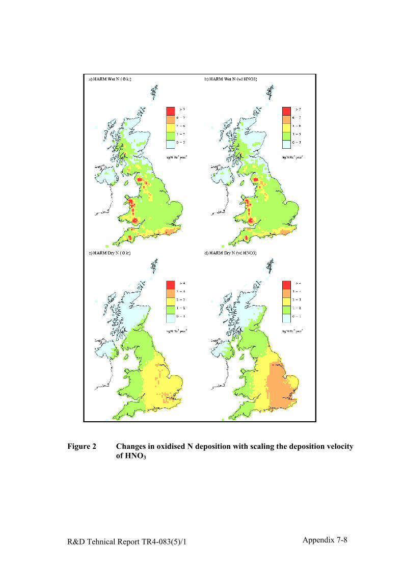
R&D Tehnical Report TR4-083(5)/1 Appendix 7-8
Figure 2 Changes in oxidised N deposition with scaling the deposition velocityof HNO3
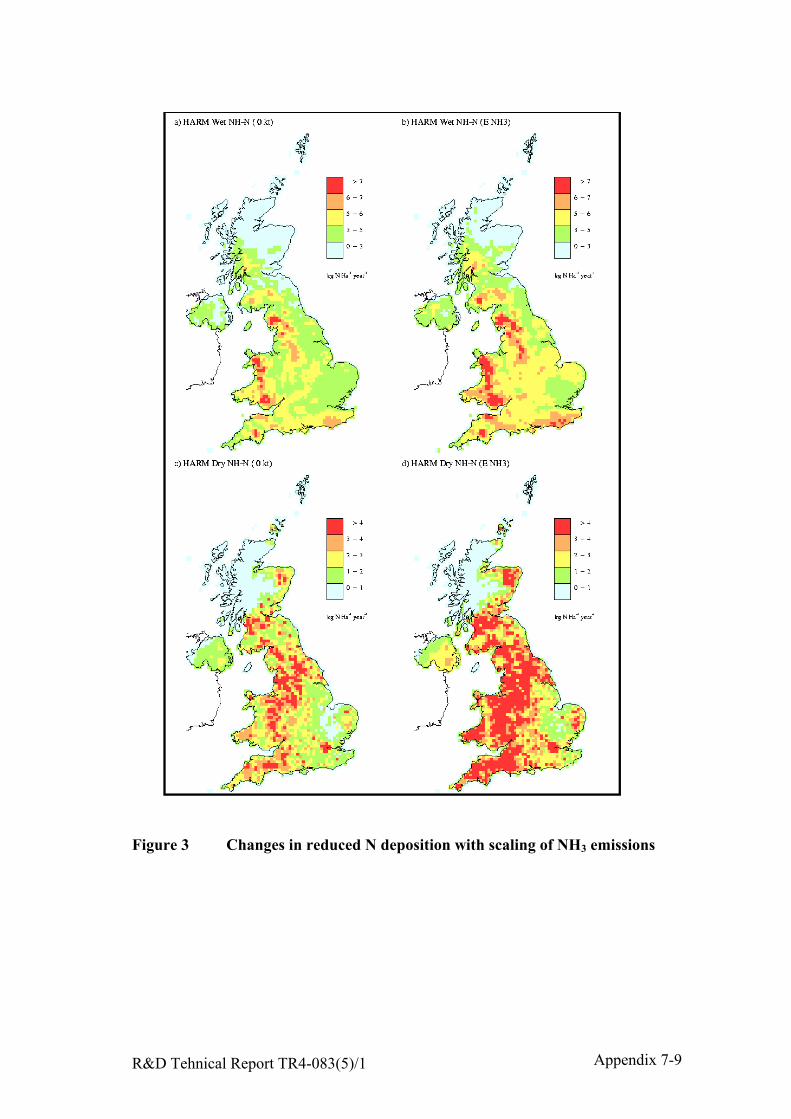
R&D Tehnical Report TR4-083(5)/1 Appendix 7-9
Figure 3 Changes in reduced N deposition with scaling of NH3 emissions
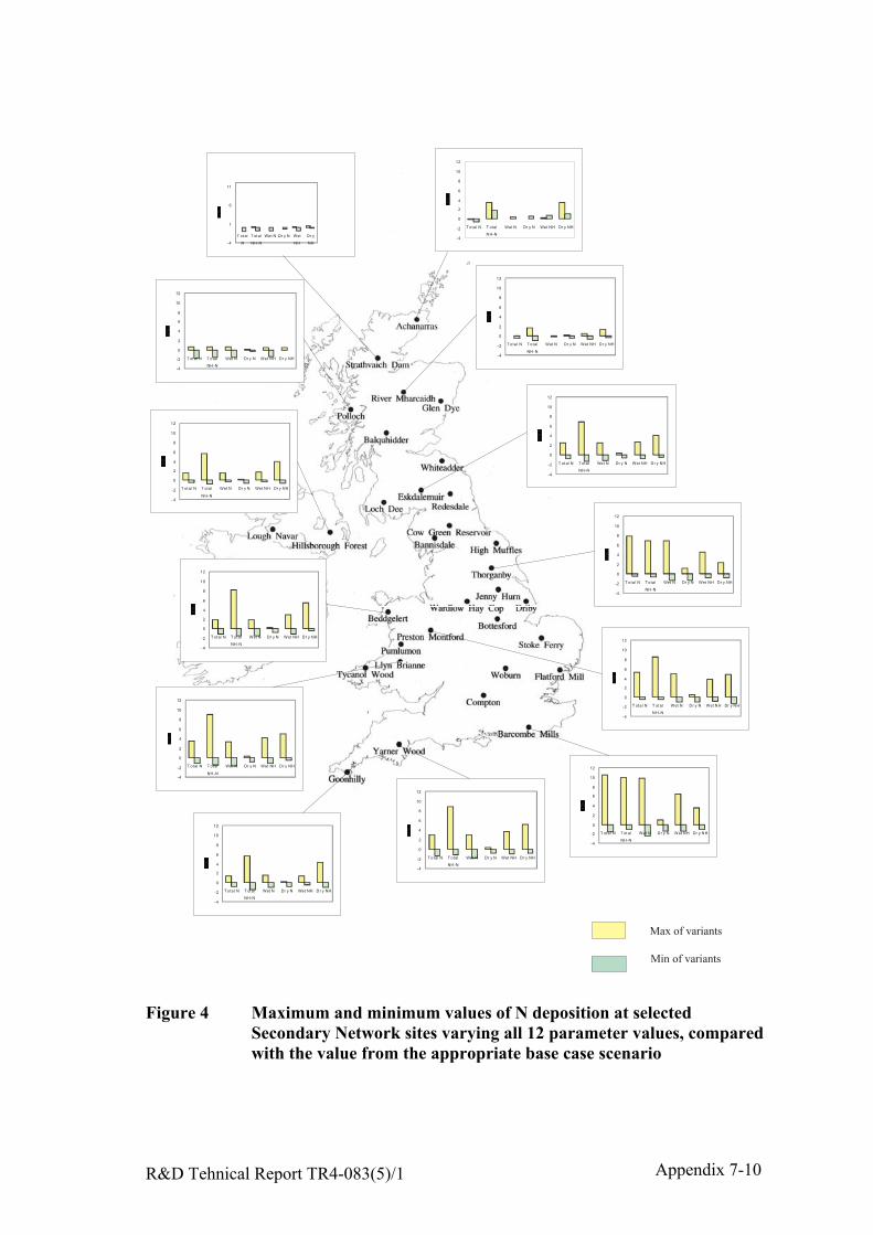
R&D Tehnical Report TR4-083(5)/1 Appendix 7-10
-4
-2
0
2
4
6
8
10
12
T otal N T otal
NH-N
Wet N Dr y N Wet NH Dr y NH
-4
-2
0
2
4
6
8
10
12
T otal N T otal
NH-N
Wet N Dr y N Wet NH Dr y NH
-4
-2
0
2
4
6
8
10
12
T ot al N T otal
NH-N
Wet N Dr y N Wet NH Dr y NH
-4
-2
0
2
4
6
8
10
12
T otal N T otal
NH-N
Wet N Dr y N Wet NH Dr y NH
-4
-2
0
2
4
6
8
10
12
T otal N T ot al
NH-N
Wet N Dr y N Wet NH Dr y NH
-4
-2
0
2
4
6
8
10
12
T otal N T ot al
NH-N
Wet N Dr y N Wet NH Dr y NH
-4
-2
0
2
4
6
8
10
12
T otal N T otal
NH-N
Wet N Dr y N Wet NH Dr y NH
-4
-2
0
2
4
6
8
10
12
T otal N T otal
NH-N
Wet N Dr y N Wet NH Dr y NH
-4
-2
0
2
4
6
8
10
12
T otal N T otal
NH-N
Wet N Dr y N Wet NH Dr y NH
-4
-2
0
2
4
6
8
10
12
T otal N T otal
NH-N
Wet N Dr y N Wet NH Dr y NH
-4
-2
0
2
4
6
8
10
12
T otal N T otal
NH-N
Wet N Dr y N Wet NH Dr y NH
-4
-2
0
2
4
6
8
10
12
T ot al N T otal
NH-N
Wet N Dr y N Wet NH Dr y NH
-4
1
6
11
T ot al
N
T ot al
NH-N
Wet N Dr y N Wet
NH
Dr y
NH
Max of variants
Min of variants
Figure 4 Maximum and minimum values of N deposition at selectedSecondary Network sites varying all 12 parameter values, comparedwith the value from the appropriate base case scenario
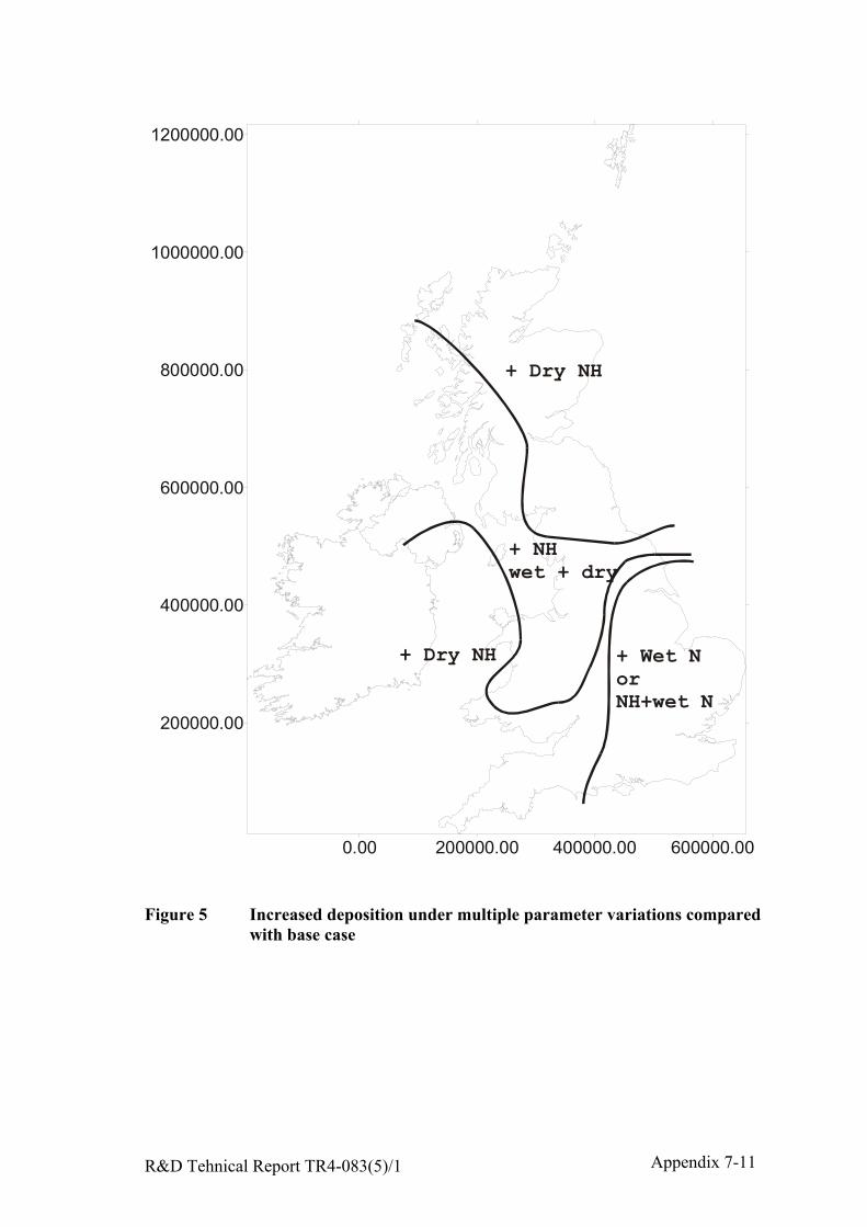
R&D Tehnical Report TR4-083(5)/1 Appendix 7-11
0.00 200000.00 400000.00 600000.00
200000.00
400000.00
600000.00
800000.00
1000000.00
1200000.00
+ Dry NH
+ Wet Nor NH+wet N
+ Dry NH
+ NH wet + dry
Figure 5 Increased deposition under multiple parameter variations comparedwith base case

R&D Tehnical Report TR4-083(5)/1 Appendix 7-12
0.00 200000.00 400000.00 600000.00
200000.00
400000.00
600000.00
800000.00
1000000.00
1200000.00
- Wet or dry NH
- Wet N
- Wet ordry N
Figure 6 Decreased deposition under multiple parameter variationscompared with base case
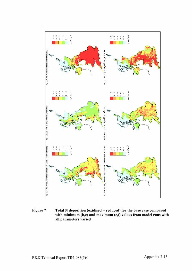
R&D Tehnical Report TR4-083(5)/1 Appendix 7-13
Figure 7 Total N deposition (oxidised + reduced) for the base case comparedwith minimum (b,e) and maximum (c,f) values from model runs withall parameters varied