Facultad

de

Ciencias

Un acercamiento numerico alproblema de los tres cuerpos

A numerical approach to the Three Body Problem

Trabajo de Fin de Gradopara acceder al

GRADO EN FISICA

Autor: Diego Martın Lopez

Director: Francisco Matorras Weinig

Julio - 2015

Abstract

The three-body problem is a nonlinear, non analytically solved without approximations prob-lem which is key in the understanding on the motion of three free bodies bounded by gravitationalattraction, such us the Sun-Earth-Moon system. The following work presents the developmentand results of a numerical program that solves the three-body problem as if none of the workaround it were done before. We’ve started from the Newton’s gravitational law and continuedwith the learnings got from the Physics degree. We’ve solved the ODE2 for the acceleration ofeach of the bodies, so we got it’s positions as a function of time, considering the bodies movedalways in a Cartesian plane. The program was developed to numerically integrate these equationsand to permit the analysis of different quantities related to the observed motion under differentconditions. We’ve extensively tested the code for different examples, such us the Sun-Earth-Moonsystem and the Satellite-Earth-Moon system. We got that, while the integration step is h < 10 sand the bodies aren’t closer than R? = 9 × 106 m, the program returns reasonable solutions forthe Sun-Earth-Moon system and the Satellite-Earth-Moon system. We’ve done a fine-tuning toget the simulated system to behave in a similar way the real system does, but getting the orbitsmore circular in order to simplify the interpretations of the results. The initial conditions wehad to set when the three bodies were free were so fine that, for example, changing the Earth’sspeed δv⊕ = 1 m/s, made its period change δT⊕ = 1 hour. When we set the initial conditions sothe bodies had to move in circular motion, we got that Earth and Moon disturbed each other.The Earth got an eccentricity of ε⊕ = 0.05 and the Moon εM = 0.28. We’ve study the Moon’sstability when making little perturbations in its orbit, while the other conditions remained thesame. We got that it needs to change its path δθ = 1.2o in order to disengage from the Earth’sorbit. We’ve make an attempt to study the stability of the system, and, during two hundredyears, it hasn’t seem to have any trend to change. Comparing the geostationary satellite withand without Moon, we got that, because of the Moon influence, it had a delay of around twohours every day. We made a study of the orbits for different distances to the Earth. We gotthat while the satellite remains near the Earth (not further than R?? ≈ 2 × 108 m), there areperiodical perturbations in the orbit with respect to the circular case, but they don’t seem topresent any trend to change its orbit. Once the satellite surpasses this critical orbit the Moontraps it and its orbit gets chaotic. In this stage the satellite usually gets so close to the Moonthat the error stack starts to be a problem. However, taking a small enough integration step, thiserror shouldn’t mean any problem. When getting too close to the Moon, the satellite gets a boostin its speed due to momentum transfer. If the energy transferred results enough, the satelliteescape from the system. Apart from the cases where the satellite and the Moon get too close toeach other, where we may need an adaptive integration step, the program works well and allowsus to make a detailed study of any case of the problem. Taking a look to the whole project,we have developed a reliable tool, within the approximations we have taken. The program hasresulted useful for the study of these type of problems and, with some improvements to coversome identified weak issues, can be used for a more detailed studies of the three body problemitself or other similar problems.

Keywords: Numerical Calculus, Three Body Problem, Runge-Kutta, artificial satellites, clas-sical gravitation.

1

Resumen

El problema de los tres cuerpos es un problema no lineal, no resoluble analıticamente sinaproximaciones, clave en la comprension del movimiento de tres cuerpos que se atraen gravita-cionalmente entre sı, como pasa en el sistema Sol-Tierra-Luna. El siguiente trabajo presenta eldesarrollo y los resultados de un programa de calculo numerico que resuelve el problema de lostres cuerpos como si ningun otro trabajo se hubiese desarrollado antes sobre el. Hemos partidode la ley de la gravitacion universal de Newton y seguido con los conocimientos adquiridos enel grado en fısica. Haciendo uso de Matlab y a traves de la implementacion del metodo RungeKutta de cuarto orden, hemos resuelto la EDO2 para la aceleracion de cada uno de estos cuer-pos, de manera que obtuvimos sus posiciones como funciones del tiempo. Consideramos que loscuerpos siempre se movıan en el plano cartesiano. El programa fue desarrollado para integrarnumericamente estas ecuaciones, y permitirnos analizar diferentes magnitudes relacionadas conel movimiento observado bajo diferentes condiciones. Realizamos un analisis exaustivo del codigocon diferentes ejemplos, como el sistema Sol-Tierra-Luna y el sistema Satelite-Tierra-Luna. Ob-tuvimos que, mientras el paso de integracion fuera h < 10 s y la distancia entre los cuerpos nofuese menor de R? = 9 × 106 m, el programa nos daba soluciones razonables para los sistemasSol-Tierra-Luna y Satelite-Tierra-Luna. Hemos hecho un ajuste fino para que las simulaciones secomportasen de manera parecida a los sistemas reales, pero con las orbitas mas circulares parapoder simplificar las interpretaciones de los resultados. Las condiciones iniciales que tuvimos queintroducir para los tres cuerpos libres eran tan sensibles que, por ejemplo, cambiando la velocidadde la Tierra δv⊕ = 1 m/s cambiaba su perıodo δT = 1 hora. Cuando inrodujimos las condicionesiniciales para que la Luna y la Tierra se movieran de manera circular d emanera separada, nosdimos cuenta que al simular el sistema completo estas dejaban de moverse circularmente pues seperturbaban la una a la otra. La excentricidad de la Tierra era de ε⊕ = 0.05 y la de la Luna deεM = 0.28. Hemos estudiado la estabilidad de la Luna tras hacer pequenas perturbaciones en suorbita, mientras el resto de las condiciones las dejabamos igual. Encontramos que esta necesitabacambiar su trayectoria 1.2o para desacoplarse de la orbita terrestre. Hemos tratado de estudiarla estabilidad del sistema, y durante doscientos anos no hemos encontrado ninguna tendencia delsistema que indique algun cambio en su trayectoria. Comparando el satelite geostacionario cony sin Luna, hemos visto que, debido a la influencia de esta, el satelite sufrıa un retraso de doshoras cada dıa. Hicimos un estudio de las orbitas del satelite a distintas distancias de la Tierra,y mientras este permaneciese no mas lejos de R?? = 2 × 108 m, encontramos perturbacionesperiodicas que no aparecen en el caso completamente circular, pero no parecen mostrar ningunatendencia a cambiar su orbita. Cuando el satelite sobrepasa la distancia lımite, la Luna lo atrapay empieza a comportarse de manera caotica. En este caso el satelite suele acercarse tanto a laLuna que el error acumulado empieza a ser problematico. Sin embargo, tomando un paso deintegracion suficientemente pequeno, este error no deberıa suponer un problema suficientementegrande como para cambiar la trayectoria del satelite. Cuando el satelite se acerca tanto a laLuna, este recibe un incremento de velocidad debido a transferencia de momento. Si esta energıaes suficientemente grande, el satelite puede incluso escapar del sistema. Aparte de los casos enlos que el satelite se acerca demasiado a la Luna, donde debieramos tomar un paso adaptativo,el programa funciona bien y nos permite hacer un estudio detallado de cualquier caso de esteproblema. Teniendo en cuenta el proyecto entero, hemos desarrollado una herramienta en la queconfiar, dentro del lımite de nuestras aproximaciones, y que ha resultado util para el estudio deeste tipo de problemas y, con algunas mejoras para suplir las deficiencias ya identificadas, puedeser empleado para estudios mas detallados del problema de los tres cuerpos u otros problemassimilares.

Palabras clave: Calculo numerico, Problema de los tres cuerpos, Runge-Kutta, satelites arti-ficiales, gravitacion clasica.

2

Contents

1 Introduction 41.1 Approaches and sense of the project . . . . . . . . . . . . . . . . . . . . . . . . . . . . 4

2 Development and tests of the code 62.1 4th order Runge Kutta . . . . . . . . . . . . . . . . . . . . . . . . . . . . . . . . . . . . 62.2 First and Second Order Differential Equations . . . . . . . . . . . . . . . . . . . . . . . 72.3 The Two Body Problem . . . . . . . . . . . . . . . . . . . . . . . . . . . . . . . . . . . 8

2.3.1 Circular orbits . . . . . . . . . . . . . . . . . . . . . . . . . . . . . . . . . . . . 92.3.2 Elliptical orbits . . . . . . . . . . . . . . . . . . . . . . . . . . . . . . . . . . . . 112.3.3 The Rocket Problem . . . . . . . . . . . . . . . . . . . . . . . . . . . . . . . . . 12

3 The Three Body Problem and the Sun-Earth-Moon system 15

4 The three body problem and the Earth-Satellite-Moon system 23

5 Conclusions 28

6 References 30

3

1 Introduction

The Three-body problem consists in solving the positions of three free bodies that move due togravitatory attraction. The equation we are interested in solving for each body is then:

d2 ~xidt2

= G(mj ~rijd3ij

+mk ~rikd3ik

)

where xi is the position of the body we are studying, mj and mk are the other two bodies masses,dij and dik are the distances between the first body and the other two and ~rij and ~rik the vectorsthat join the first body with the other two.Due to the fact that these equations can’t be solved by analytic methods without approximations,this problem has always been a very interesting topic in physics. It might appear as a subject withnot very useful applications, but when it comes to study the celestial bodies, it is the first order toolin order to solve our questions on the matter.

The present work has been outlined as if none of the previous work around the Three-body prob-lem had been made and focuses in a very practical line of work, so it starts from the Newton’s lawof universal gravitation and makes use of the 4th order Runge Kutta algorithm to make numericalsimulations of the trajectories of three different bodies from some initial conditions. Our goal is to getto simulate the three body problem and get interesting results after simulating the Sun-Earth-Moonsystem and the path of an artificial satellite between the Earth and the Moon.The inner motive of this work is learning how to plan and solve any numerical problem, and how todeal with a big project, from the planning to the conclusions.

We’ll start showing the implementation of the 4th order Runge Kutta algorithm with a first anda second order differential equations and the tests we made to make sure our program worked so far.Then we increased the complexity of the code implementing the Two-body problem with which wesimulated the Earth-Moon system. Once we had enough proves our program worked as well as weneeded we implemented the Three-body problem. After some exercises with the Sun-Earth-Moonsystem we decided to remove some complexity to the code in order to make it faster and be able toget easier conclusions from the results, so we fixed the most massive body and continued studyingthe Sun-Earth-Moon system a bit more. The last exercise was to simulate an artificial satellite fordifferent orbits between the Earth and the Moon. We’ll finally finish the report with the conclusionswe’ve got from this project.

1.1 Approaches and sense of the project

Before we start writing about the project, we must make sure the reader doesn’t get the wrong ideaabout the meaning of this work. We don’t claim we have done something new, neither somethinguseful to research or implement in a serious working environment. We’ve just developed a tool inorder to take some examples of numerically solved three body problem with some approximationsand without using the most optimized resources, but the ones we considered appropriate and thatgranted us the success of the project on a reasonable time lapse.

We focused on the project from an academic perspective. We didn’t really want to get a specificresult but to learn as much as possible from the problems we were finding along the way. At the endwe actually found some interesting results and we got to simulate the three body problem, alwayswithin the limits of our approximations.

In the first place we considered our bodies as points in a Cartesian Coordinate System plane.This means there are nor rotation or collisions. The orbits we’ve considered for the Sun-Earth-Moonsystem are set in a plane, while there’s actually a small degree of inclination between the Moon-Earthorbit plane and the Sun-Earth orbit plane.

We also tried the motion of the bodies to be as circular as possible, so the results derived fromthe simulations were easier to understand. When we wanted the results to be even simpler, we fixed

4

the most massive body, as we’ll explain later.

The physics of the problem aren’t as important, along the project, as the computational attackwe’ve made to solve it. We’ve use the three body problem as an example to solve numerically, but,making the proper changes, we could use the program to solve any other.

5

2 Development and tests of the code

I chose to work with Matlab because it’s a really friendly user tool, with lots of libraries and helpfulresources along the net, which derives from the fact that it’s widely used along the world. We alsogot to know, with the first trials we did, that Matlab was going to let us develop the tool we werelooking for in a flexible way.

In the early stages of the project, we knew it wasn’t possible, nor practical, for us to start withthe three-body problem at the very beginning. We had to take little safe steps in order to develop areliable tool.That’s the main reason why we started solving analytically easy to solve differential equations andthe well known two-body problem. We’ll start by showing the 4th order Runge Kutta method weused for the whole project and then introduce the two approaches we came with before we got intothe three-body problem.

2.1 4th order Runge Kutta

The Runge Kutta methods are an important set of useful numerical algorithms in the resolution ofordinary differential equations. These methods were developed at the beginning of the 20th centuryby the German mathematicians C. Runge and M. W. Kutta.

We chose the 4th order Runge Kutta to solve our problem because it’s conceptually simple inorder to understand how to use it and powerful enough to let us get to a reasonable result at the endof the project.

Given f ′(t, x) = f(t, x), the algorithm divides the integral we usually would do analytically intofour discrete steps, where the slope is approximated by four coefficients we’ve called x1, x2, x3 andx4. At the end of each iteration, we get the weighted average of the four portions. Between thesolution of an iteration and the next one, there’s an interval of time given by h, which is called theintegration step.The mathematical shape of the algorithm is written as follows:

x1 = f(ti, xi) (1)

x2 = f(ti +h

2, xi +

h

2x1)

x3 = f(ti +h

2, xi +

h

2x2)

x4 = f(ti + h, xi + hx3)

xi+1 = xi +h

6(x1 + 2x2 + 2x3 + x4)

where i+ 1 is the next step we are calculating, and i is the step we’ve already got.This iterative process begins from a known initial condition f(0, x).

If we want to solve a second order differential equation, f ′′(t, x) = f(t, x), then the algorithm getsa bit more complicated. In this case we have to divide the ODE2 into two ODE1 so we can proceedin a similar way as we did with the previous case. The order in which we write the line codes isimportant, because of the interdependence of coefficients on each step.

v1 = f(ti, xi) (2)

x1 = vi

v2 = f(ti +h

2, xi +

h

2x1)

x2 = vi +h

2v1

6

v3 = f(ti +h

2, xi +

h

2x2)

x3 = vi +h

2v2

v4 = f(ti + h, xi + hx3)

x4 = vi + hv3

xi+1 = xi +h

6(x1 + 2x2 + 2x3 + x4)

vi+1 = vi +h

6(v1 + 2v2 + 2v3 + v4)

where x1, x2, x3, x4, v1, v2, v3 and v4 are the coefficients we have to calculate in order to get thenext step of the integral.

Because the time inside the simulation doesn’t usually correspond to the time the simulation isrunning, we have to make a distinction between these two concepts. For example, a twenty minutesrunning time simulation, may correspond to a simulated time of one year. This means that while wehave been waiting for twenty minutes until the simulation finished, the bodies we have simulated hasbeen looping around each other for one virtual year.

Along the project we’ll see how important it is to choose the right h. The idea for the method isto choose the smallest positive h possible, but the smaller h is, the slower is the method. Because ofour limited time, we had to find a h which would give us a good precision-time relation.

2.2 First and Second Order Differential Equations

The first step we took was to solve a first order Ordinary Differential Equation (ODE):

x = −kxx = e−kt

where k is a constant, and x is a function of time t.The first prove of the success of the implemented Runge-Kutta to Matlab was the comparison betweenthe program numerical approach and the analytical solution. When plotting both solutions togetherwe found out that both overlapped, as we could expect. Then we plotted the difference δz in absolutevalue for different h.

As we see in Fig.(1)) the error function shape describes the one of an exponential function: at thebeginning the exponential function decays very fast, so the error function has a much bigger peak theless steps in time you get (less steps in time means bigger h). An interesting result here is that for aten times smaller step, the code needs ten times more time to finish the simulation, but the result isseveral orders of magnitude more precise (four in this case, as we see in Fig.(1)).

The second test for the code was a second order ODE,

x = −kxx = sin(kt) + cos(kt)

with which we proceeded the same way as with the ODE1 shown above. Once we got the numericalsolution to overlap the analytical we got the error plots for different h.

In this other example, the analytical function is periodical, so the mean error should be indepen-dent of time. However, we see in Fig.(2) that it increases with time. This comes from the fact thatin numerical analysis the error is cumulative, so for long simulated time examples we’ll see not veryprecise results for the last points if we don’t set a h small enough.

7

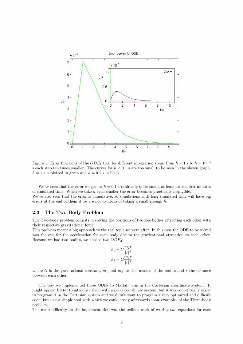
Figure 1: Error functions of the ODE1 trial for different integration steps, from h = 1 s to h = 10−4

s each step ten times smaller. The curves for h < 0.1 s are too small to be seen in the shown graph.h = 1 s is plotted in green and h = 0.1 s in black.

We’ve seen that the error we get for h = 0.1 s is already quite small, at least for the first minutesof simulated time. When we take h even smaller the error becomes practically negligible.We’ve also seen that the error is cumulative, so simulations with long simulated time will have bigerrors at the end of them if we are not cautious of taking a small enough h.

2.3 The Two Body Problem

The Two-body problem consists in solving the positions of two free bodies attracting each other withtheir respective gravitational force.This problem meant a big approach to the real topic we were after. In this case the ODE to be solvedwas the one for the acceleration for each body due to the gravitational attraction to each other.Because we had two bodies, we needed two ODE2:

x1 = Gm2r

|r|3

x2 = Gm1r

|r|3

where G is the gravitational constant, m1 and m2 are the masses of the bodies and r the distancebetween each other.

The way we implemented these ODEs to Matlab, was in the Cartesian coordinate system. Itmight appear better to introduce them with a polar coordinate system, but it was conceptually easierto program it in the Cartesian system and we didn’t want to program a very optimized and difficultcode, but just a simple tool with which we could study afterwards some examples of the Three-bodyproblem.The main difficulty on the implementation was the tedious work of writing two equations for each

8

Figure 2: Error functions of the ODE2 trial for different h, from h = 1 s to h = 10−4 s. The curvesfor h < 0.1 are too small to be seen in the shown graph. h = 1 s is plotted in green and h = 0.1 s inblack.

body (because it’s an ODE2) and coordinate four times (one for each integral part). This resultedinto thirty two different equations on the program code.Because we didn’t need every step value for any of these magnitudes, we only saved one over a hun-dred or a thousand steps in order to plot later the orbit paths or the distances between the bodies.This way, a lot of simulation time was saved, because Matlab doesn’t like to work with too largevectors.

In order to have a point of reference with a daily known case, we used the masses and distancesof the Earth-Moon system. In this case we compared our results with the expected movement of theMoon, approximating the Moon orbit around the Earth as a circular planar orbit, and letting bothbodies free. With this new code we made two tests focused in the problems we might had when weexpanded it to the three-body case. In the first place we checked which h was needed so that theMoon circular orbits closed without much error. Afterwards we put the Moon in elliptical orbits andchecked for the error of the closed orbit depending on the initial velocity angle.

2.3.1 Circular orbits

While going through the mathematical problem we may got that the orbit the body goes over isclosed, but when studying the problem from a numerical perspective it’s fair to find some error.Depending on the ratio time-quality we’ll allow more or less error in the simulation.Making the Moon go around the Earth in circular orbits was quite easy using the uniform circularmotion. We just had to give the Moon the following velocity:

v =

√GM⊕d

9

where G is the Gravitational constant, M⊕ is the mass of the Earth and d is the distance betweenthe two bodies.

In order to study the error on the circular orbit, we had to pay attention on the position of theMoon on the moment before it crossed the horizontal position after the first loop (x1, y1) and themoment when it had already crossed it (x2, y2). We can approximate the error on the loop δx asthe distance to the origin from the point of the line that links (x1, y1) and (x2, y2) that crosses thehorizontal. This is better explained with the scheme of Fig.(3). It’s easy, once we’ve got (x1, y1) and(x2, y2), to derive that,

n =y1x2 − y2x1x2 − x1

m =y1 − nx1

and

δx =−nm

where m and n are the coefficients of the linear function that includes the points (x1, y1) and (x2, y2).

Figure 3: Scheme of the error δx taken in the two bodies circular orbits example. (x0, y0) is the initialpoint of the orbit, (x1, y1) is the point before the body crosses the y = 0 line, and (x2, y2) is the pointone step after (x1, y1).

h = 10−2days h = 10−3days h = 10−4days h = 10−5days h = 10−6daysδx / m -250.78 -1.014 -0.0122 −3.31× 10−4 −1.226× 10−4

Table 1: Errors for the closed orbits in the two bodies circular orbits example.

As we see in the values from Table (1), and as we may expect from the results shown in the previ-ous sections, we get a more precise answer for a smaller integration step. Once more we see that a tentimes smaller step sometimes result in a more than ten times more precise result. It’s important notto forget that a ten times smaller step simulation is ten times slower, so we couldn’t take the smallesth to get the most precise answer, but a reasonable h so we get a reasonable relation of precision andrunning time. For the two body problem we used h = 10−4 days, which costs around four seconds ofwaiting for thirty days of simulated time. It’s important to remark that δx = 10−2 m isn’t really a bigerror if we take into account the fact that the orbits we were working with were around 6×106 m wide.

The integration step from now on has been taken in day units just because it’s more convenientto write down in the code that the Moon body is going to be orbiting for thirty times the integration

10

step in order to make one loop than multiplying it every time by sixty squared times twenty four.At the end, when taking h ≈ 10−4 days we are taking around ten seconds each step. It’s not thatimportant to take one unit or other, but to know with which unit you are working with and howmuch error are you taking at the end of the simulation.

As a conclusion from this exercise, we got that h = 10−4 days is a good enough integration stepfor our precision-running time ratio, and it’s the one we took for the following simulations.

2.3.2 Elliptical orbits

Once we finished studying the solutions of the code for the circular case, we wanted to make anautomatic sweep code, so we could avoid as much manual analysis as possible in future simulations.For this, we prepared the moon with the same initial conditions as for the circular case, and thenchanged the initial velocity angle, from 90o to different angles. We wanted it to stop after one loop,so we imposed the following condition:

if y2(i) < 0 && y2(i+ 1) > 0 : stop

so the second body (the Moon) stopped once it had crossed the horizontal line upwards.

The result of the simulation for different initial angles is presented in Fig.(4), with the path of eachof the orbits. As we expected, the bigger the angle with respect to the vertical, the more ellipticalthe orbit is.

Figure 4: Orbits of the Moon around the Earth for different initial angles.

We’ve avoid to shoot the Moon at 0o and 180o, just because at those angles the Moon crasheswith the Earth and no orbit is described.

Next thing we did was to check for the error on the closed orbits for the different angles. For thatwe draw the difference δx between the end of each loop and the initial position of the body for thefirst three loops.

As we see in Fig.(5), and as we saw with the ODE2 in the previous section, the error is cumulative.We get another learning, for close enough orbits (we see it for 15o) the error is bigger. This givesus a clue about how well works the program when two of the bodies are too close. When searchingfor the minimum distance reached between the Moon and the Earth when the initial angle is 15o, wegot Rmin = 8.705× 106 m, so in further analysis will have into account the fact that for around this

11

Figure 5: δx for the first three loops of the Moon around the Earth for different initial angles, from15o to 165o, in 15o steps. Black points are from the first loop, blue ones for the second and the redsfor the third. It’s been used h = 10−4 for this simulation.

distance or less, the program starts to be quite less precise.

The reason the program doesn’t work so well when the bodies are too close comes from the factthat the integrals are proportional to 1

d2 , so when d is small the integral in each step gets too big. Thiscould be solved with an adaptive step program that we haven’t implemented, so we could decrease hwhen the bodies came too close to each other.

We should point out that this distance between the bodies we’ve got as problematic, while seemingquite big when thinking that the bodies are just points, it’s actually quite near the Earth radius value(R⊕ ≈ 6×106 m). So the Moon represented in our program starts to move not as perfect as it shouldwhen it’s almost touching the surface of the Earth. It’s quite difficult to make ourselves a good ideaof the magnitudes we are dealing with, but this far, the results we’ve presented for the code, whilenot being really optimized, are good enough for our purpose.

We can say that the program works right for the Two-body problem, which is quite nearer oncomplexity to the Three-body problem.

2.3.3 The Rocket Problem

In order to make another automatic program, we searched for the initial speed a rocket would needto reach the Moon from the surface of the Earth. The two bodies represented were the Earth, set inthe centre of the system, and the rocket, which started in the Earth surface distance to the centre,as we see in the scheme from Fig.(6). The break condition for the program this time was reachingthe Earth-Moon distance with the second body, and the program changed the rocket initial velocityand started over once the rocket started to fall down the Earth.

We made a sweep on the velocities of the rocket until it could get to the desired height. In orderto get to RM = 3.85 × 108 m we knew the rocket needed a smaller speed than its escape velocity,with which it would never fall into the Earth again.It’s trivial to derive that the escape velocity for the rocket is:

ve =

√2GMT

RT= 3.056× 109 m/day (3)

so the velocity we were searching for was smaller than this result.

12

Figure 6: Scheme of the rocket problem. RE is the Earth radius, RM is the distance between theEarth and the Moon, and v0 is the initial speed of the rocket.

The theoretical distance we use to compare with the simulation comes from the conservation ofthe energy, so the energy when the rocket is in the Earth’s surface must be the same as the energywhen the rocket is somewhere along the way to the Moon height and just starts falling down.

E1 =−Gmimii

y0+miiv

20

2

=−Gmimii

y

= E2

where G is the gravitational constant, mi is the Earth’s mass, mii is the rocket mass, v0 is theinitial velocity of the rocket, y0 is the Earth radius (where the rocket starts from) and y is the positionof the rocket when it is starting to fall. Solving this for y we get:

y =Gmi

Gmi

y0− v20

2

(4)

so the error δh we plot in Fig.(7) is just y minus the integrated height in the simulation.

As we see in Fig.(7), the error pattern we get is quite fluctuating and decreases until it suddenlygrows up at the end. The simulation finishes with the initial velocity with which the rocket reachesthe Moon. The velocity we got is vf = 9.7× 108 m/day, which is smaller than the escape velocity, aswe expected.The figure starts with a big error probably because the rocket starts around the conflict area wherewe may say the two bodies are too close, so the program isn’t as precise as we may like.As the rocket gets away from the Earth the error decreases, because the cumulative error is lessimportant than the one that appears when the bodies are too close to each other. At the end of thegraph the error suddenly grows up probably because the initial velocity of the rocket is each loopcloser to the escape velocity, and, taking a look to Eq.(3), when that happens Eq.(4) gets closer toinfinity. This is similar to the case when the two bodies are nearby, when the program start to getnumbers too big it starts getting bigger errors.The last important point from Fig.(7) are the fluctuations. They probably come from the truncationMatlab does. For some speed the value it gets after the truncation is very similar to the theoreticalvalue, but for the very next speed the truncation makes the final result to have quite a discrepancywith respect to the theoretical one.

13

Figure 7: Difference between theory and simulation δh for the height of a rocket shot from the Earth’ssurface with certain velocity v. For this simulation it’s been used h = 10−4.

We also simulated the rocket problem with h = 10−5 days and we got that the fluctuations got ahundred times smaller, so apparently the integration step has a stronger influence over the programthan the truncations, and because we couldn’t control these last ones in an easy way, we continuedusing h as an indicator of the precision on the simulations.

With the rocket problem we got a code which was quite independent (it made long sweeps changingthe initial conditions of the system on its own) and with apparently good results.

14

3 The Three Body Problem and the Sun-Earth-Moon system

Once we got to this point we already knew we had a program that was able to simulate a two-bodysystem with quite enough precision - when the bodies weren’t too close - during around one yearof simulated time. We were finally ready to take the step of extending the code to the third body.However, before we got to the Satellite-Earth-Moon system, we got into a much better known system,the Sun-Earth-Moon system, which allowed us to interpret better the results of the simulations.

Before we get into the code checks, it’s important to specify the way the three bodies started tomove from in the program. Taking into account that we were going to simulate planar orbits, we setthe Sun in the centre of coordinates, located the Earth at the Sun-Earth distance horizontally fromthe Sun ( (xEarth, yEarth) = (dS−E ,0) ) and the Moon at the Earth-Moon distance from the Earth ((xMoon, yMoon) = (dS−E + dE−M ,0) ). From there, the three bodies were ”shot” vertically (at 90o)with their initial velocity, where the initial velocity of the Sun was such that the centre of mass was

at rest, v� = m2v⊕+m3(v⊕+vL)m1

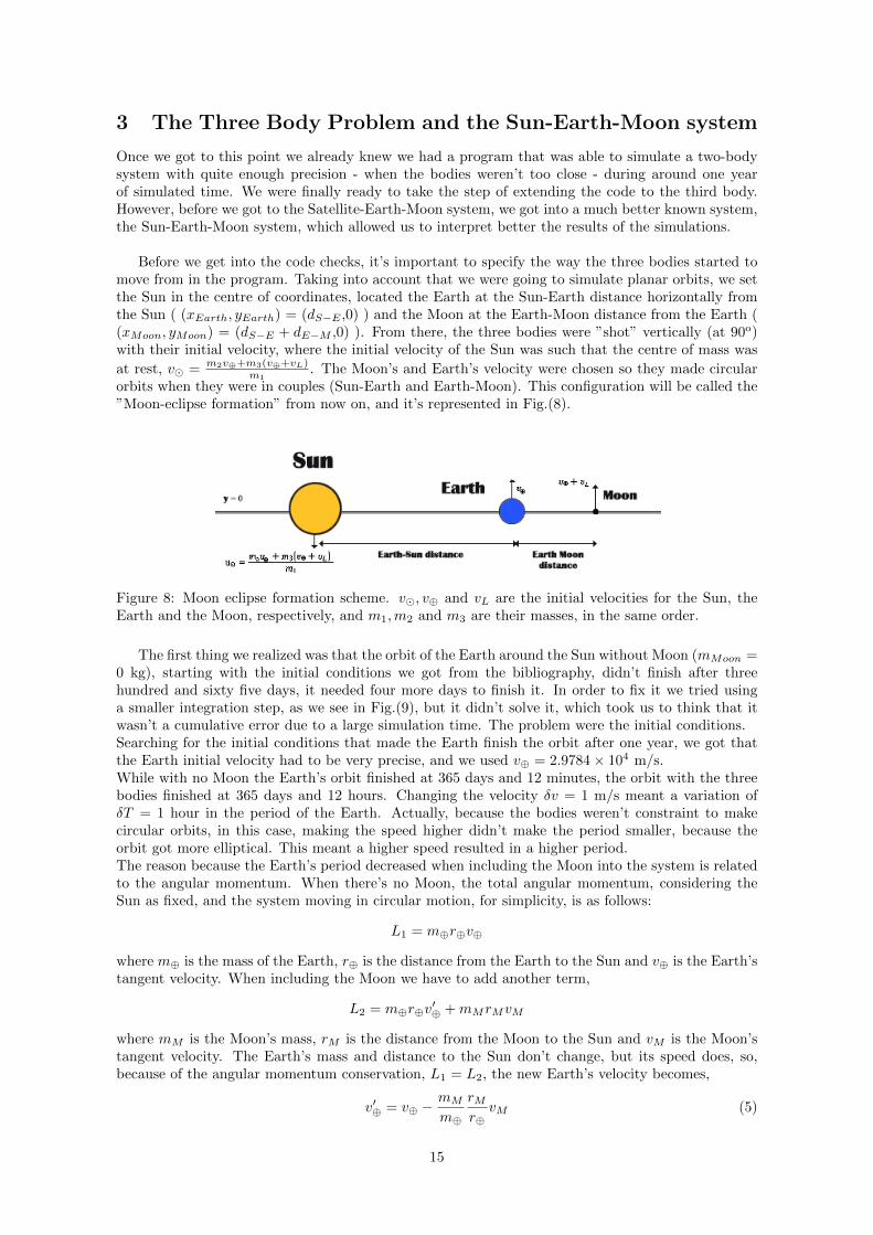
. The Moon’s and Earth’s velocity were chosen so they made circularorbits when they were in couples (Sun-Earth and Earth-Moon). This configuration will be called the”Moon-eclipse formation” from now on, and it’s represented in Fig.(8).

Figure 8: Moon eclipse formation scheme. v�, v⊕ and vL are the initial velocities for the Sun, theEarth and the Moon, respectively, and m1,m2 and m3 are their masses, in the same order.

The first thing we realized was that the orbit of the Earth around the Sun without Moon (mMoon =0 kg), starting with the initial conditions we got from the bibliography, didn’t finish after threehundred and sixty five days, it needed four more days to finish it. In order to fix it we tried usinga smaller integration step, as we see in Fig.(9), but it didn’t solve it, which took us to think that itwasn’t a cumulative error due to a large simulation time. The problem were the initial conditions.Searching for the initial conditions that made the Earth finish the orbit after one year, we got thatthe Earth initial velocity had to be very precise, and we used v⊕ = 2.9784× 104 m/s.While with no Moon the Earth’s orbit finished at 365 days and 12 minutes, the orbit with the threebodies finished at 365 days and 12 hours. Changing the velocity δv = 1 m/s meant a variation ofδT = 1 hour in the period of the Earth. Actually, because the bodies weren’t constraint to makecircular orbits, in this case, making the speed higher didn’t make the period smaller, because theorbit got more elliptical. This meant a higher speed resulted in a higher period.The reason because the Earth’s period decreased when including the Moon into the system is relatedto the angular momentum. When there’s no Moon, the total angular momentum, considering theSun as fixed, and the system moving in circular motion, for simplicity, is as follows:

L1 = m⊕r⊕v⊕

where m⊕ is the mass of the Earth, r⊕ is the distance from the Earth to the Sun and v⊕ is the Earth’stangent velocity. When including the Moon we have to add another term,

L2 = m⊕r⊕v′⊕ +mMrMvM

where mM is the Moon’s mass, rM is the distance from the Moon to the Sun and vM is the Moon’stangent velocity. The Earth’s mass and distance to the Sun don’t change, but its speed does, so,because of the angular momentum conservation, L1 = L2, the new Earth’s velocity becomes,

v′⊕ = v⊕ −mM

m⊕

rMr⊕

vM (5)

15

so the new Earth’s velocity is always smaller than the previous one, which means a delay in theEarth’s period when considering a circular motion.So, a small variation in these initial conditions meant a big difference in the Earth’s period, andwithout a very careful look, we could even get an a priori surprising result. This first conclusionmade us be much more careful with the initial conditions we set before starting any simulations.

Figure 9: Orbit of the Earth around the Sun. In the left figure the step used is h = 10−4 days andin the right figure, h = 10−5 days. However, in both orbits the Earth finishes in the very same spot.

Looking into the eccentricity of the orbits of the Earth orbit around the Sun and the Moon orbitaround the Earth, we got that the orbits described in our program were more circular than theones of the real system. The data from the bibliography are Rmax⊕ = 1.52 × 1012 m for the Earthapogee and Rmin⊕ = 1.47 × 1012 m for its perigee. In the Moon case, RmaxM

= 4.06 × 108 m andRmaxM

= 3.56× 108 m. Using the following definition for eccentricity,

ε =

√1−

(RminRmax

)2we got the theoretical values, ε⊕ = 0.2543 and εM = 0.4808. With our simulations, however, usingthe velocity we talked about before, we get ε⊕ = 0.0360 when there’s no Moon, and ε⊕ = 0.0478 andεM = 0.2776 with the Sun-Earth-Moon system complete.This more circular system we’ve got might be caused because we have search for the initial conditions,and we’ve set them in the Moon eclipse formation, as if the bodies were going to move circularly.The higher eccentricity when including the Moon in the system comes from the perturbation thatthe Moon causes in the Earth’s orbit.

Although we got really circular orbits, the Moon made twelve and a half loops around the Earth inone year - remember that the Moon period is almost a month - which is very close to the real systembehaviour, where it does almost thirteen and a half loops. As we see in Fig.(10), the Earth withoutMoon has a smooth path around the Sun, but when the Moon is included we see some perturbationson its path. Those perturbations and the path of the Moon reflects the loops of the Moon aroundthe Earth.

As we see in Fig.(11), we simulated the three body motion for over two hundred years of simu-lated time, and we didn’t find any variation trend in their paths. Nor the Earth or the Moon changeddrastically their distance from one another and the Sun, as we expected, because the real systemappears to have been working for at least that amount of time.In the figure, while the Moon-Earth distance is much smaller than the Moon-Sun or the Earth-Sun

16

Figure 10: Earth distance to Sun without Moon (blue), with Moon (red) and Moon distance to Sun(green) along one year time.

distances, it appears bigger because of the normalization and the fact that the eccentricity of theMoon orbit around the Earth is much bigger than the eccentricity of its path (or the Earth path,which is very similar) around the Sun, as we saw before.The peaks we see for the Earth-Moon distance that repeats every eleven years is a period we haven’tpay attention to, due to the fact that there doesn’t seem to be any similar correspondence with thereal Sun-Earth-Moon system, but it’s just a result of the approximations we have made. It may berelated to some sort of resonance effect with the Sun-Earth or Sun-Moon orbits.

Figure 11: Moon-Sun (black), Earth-Sun (red) and Moon-Earth (yellow) normalized distances totheir own mean value. After two hundred years of inside simulation time, no perturbation on thedistance trend of the bodies is found.

In order to have a deeper look on Moon’s stability, we tried, with the same velocity and distance

17

to the Earth and the Sun, to make it start from a different point than the one presented in theMoon eclipse formation, as we see in Fig.(12). As expected, the Moon orbit changed its path, evendisengaging from the Earth’s orbit. In this case, it seems the resultant orbit is stable, but usually,taking initial conditions a bit distorted, result in a Moon that even gets away from an orbit aroundthe Sun.It’s important to remark that, in the three body problem, although we might have got a simulationwhich represents quite good the conditions of the real Sun-Earth-Moon system, within the limits ofour approximations, we shouldn’t forget that a little change in the initial conditions we took for it,makes the whole system to finish in a very difficult to predict result.

Figure 12: Moon (red) and Earth (blue) orbits around the Sun. The Moon didn’t start from theMoon-eclipse formation, but from the same distance as the Earth from the Sun.

So far, the program worked well simulating the three body problem with the Sun-Earth-Moonsystem, always within the range of our approximations. However, in order to make the problem a bitsimpler and get results a bit easier to interpret, we decided to fix the most massive body, the Sun inthis case. This way, the code got simpler, because we removed an equation, and it got faster.The mass of the Sun is so big compared with those of the Earth and the Moon that the effect over itfrom them is almost negligible. This is the reason because this approximation is quite fair, althoughthe results of the program change a bit, getting simpler to understand because there’s one less bodymoving around.

We started by studying the perturbations that the Moon caused to the Earth again (now withthe Sun fixed) in order to get a comparison with the case when the Sun is free. Then we made acomparison between the Earth and Sun forces over the Moon and finally we looked for the angle ofdisengagement for the Moon orbit around the Earth in the Moon-eclipse formation.

As we’ve seen in Fig.(10) the Moon described twelve and a half loops around the Earth and theEarth orbit got a bit distorted due to the Moon effect. In Fig.(13) we see the same effect, withthe difference that when there’s no Moon, because the Sun doesn’t move, the Earth describes a per-fect circle around it when we use the initial conditions for the uniform circular motion, as we expected.

Another thing we were curious about was the influence of the most massive bodies on the third

18

Figure 13: Comparison of the effect of the Moon on the distance between Earth and Sun. The blueline is the distance between Earth and Sun without Moon (Moon mass equals zero), and the redcurve is the distance when there’s Moon. The green curve is the distance between Moon and Sun,that explains the perturbations on the Earth orbit and reflects the twelve months of the year with itspeaks (the Moon period around the Earth is almost a month).

one. As we could see in the orbit trace of the Moon when drawing the three bodies, it didn’t seem tomake orbits around the Earth, but around the Sun, as we see in Fig.(14).

Figure 14: Moon orbit (green) with the same orbit exaggerated (in black) so we can see the ’zig-zag’that the Moon makes around the Earth (blue path under the green path of the Moon). In the centrethere’s the fixed Sun (in red).

This isn’t a revolutionary concept, but comes a bit against the most daily intuition. It’s true thatif we observe the Moon from the Earth perspective, it moves around it. But when we come to analysewhich body the Moon motion was more influenced by, we got that both the Sun and the Earth had asimilar contribution, but the one of the Sun was stronger (twice as big actually), as we see in Fig. (15).

19

Figure 15: Ratio of forces of the Earth and Sun against the Moon. The Sun attracts the Moon twiceas much as the Earth does.

That’s because from the Sun perspective, the Moon doesn’t seem to orbit the Earth, but movesaround it with some perturbations due to the proximity of the Earth. This is of course a frame ofreference problem, because as we’ve seen in Fig.(9) from the Earth’s perspective the Moon makescircles around it. Because the Moon is almost in a constant gravitatory field (its relative differencein distance to the Sun and Earth is quite small) from its own point of view the Earth and the Sunmake almost perfect circles around itself, as we see in Fig.(16).

In order to explain the peaks on Fig.(15) we have to take a look on the distance graph comparisonon Fig.(17), just because,

FSunF⊕

∝d2⊕d2Sun

(6)

Comparing Fig.(15) and Fig.(17), we see the pronounced lower peaks correspond when the Moonget a minimum in both the distances to the Earth and the Sun. The other not so pronounced mini-mums in Fig.(15) come to be when a maximum in the Moon-Earth distance coincides with a minimumfrom the Moon-Sun distance.

When we studied the Moon stability before, when the Sun was free, we saw it was quite easy tochange its path when changing its initial conditions. Once we fixed the Sun in the centre, knowingwe could get a not so chaotic result, we tried to figured out how much do we have to change thisconditions so the Moon didn’t orbit the Earth any more.

As we see in Fig.(18), the more we get the Moon away from the vertical at the beginning of itspath, the less it orbits regularly around the Earth. It starts changing its period, as we see in green.Then it makes wider orbits, represented in magenta, until we get to 1.2o, the red curve, when it getslost around the Sun and gets away from the Earth’s path.

As an example of a case where the Moon could actually change its course 1.2o, we’ve proposed ameteorite collision, as schemed in Fig.(19).When making an easy analysis of the momentum in a perfect inelastic collision, we get that the massand velocity of a meteorite that may crash into the Moon to make it change its path 1.2o has to bemmoon

mmeteorite= 1.5 × 103 and vmeteorite

vmoon= 31.8 (the angle of the meteorite with respect to the vertical

20

Figure 16: Earth (blue) and Sun (red) orbits from the Moon’s frame of reference. Sun orbit has beenplotted fifty times smaller so it can be properly compared with the Earth’s orbit.

Figure 17: Comparison of the distance between Earth and Moon (blue) and Sun and Moon (red).Both distance curves have been normalized to their own mean, so they can be compared. The redand blue peaks phase describes quite well the peaks progression on Fig.(15).

was taken as θ = (90− 1.2)o). So this result means that a quite fast rock a thousand times ”smaller”than the Moon, would be enough to take the Moon out of its path around the Earth.

We shouldn’t forget that this is just a calculation over a rough approximation, but that gives us

21

Figure 18: Distance between the Sun and the Earth (on blue) and the Sun and the Moon (on differentcolours) for different initial angles for the Moon velocity. The green curves are for angles between90o and 89.4o, the magenta for angles between 89.4o and 88.9o, and the red curve is for an angle of88.8o.

Figure 19: Scheme for the exercise of searching velocity and mass of a meteorite that would changethe Moon path for 1.2o.

a very well idea of the complexity on the motion of the three-body problem.

22

4 The three body problem and the Earth-Satellite-Moon sys-tem

After all the tests on the program since we started by implementing the Runge-Kutta algorithm, wewere quite sure that it worked properly for the approximation we chose and while the bodies didn’t gettoo close to each other. The last thing we wanted to pay attention to was the Satellite-Earth-Moonsystem.While when studying the Sun-Earth-Moon system there wasn’t much realism in changing the initialconditions for each body from the real case perspective, when working with a body that representsan artificial satellite it has much more sense to change its conditions, depending on which orbit wewant it to loop around. We focused on the influence of the Moon on the satellite, and how its pathchanges when it gets too close to our natural satellite.We kept the most massive body fixed approximation. In this case, it’s not such a good approxima-tion, keeping the Earth motionless, as it was with the Sun. However, because the satellite mass wasnegligible in this case, our system was equivalent to the Earth-Moon centre of mass system, workingwith the reduced masses.

Before we started sweeping the space between the Earth and the Moon with the satellite, wewanted to take a look to the geostationary case, so we made sure we had enough control over thesystem, and we could claim we were able to predict what happened in the easiest case.

Figure 20: Distance between the satellite and the Earth along three months. The red line is thedistance from the Satellite to the Earth when there’s no Moon, while the blue line is the distancebetween satellite and Earth when there’s Moon.

The configuration chosen for the bodies to start from for the examples on the Earth-Satellite-Moon system was the Moon eclipse formation, presented in Fig.(8), where the previous Sun, Earthand Moon, were now represented by the Earth, the satellite and the Moon, respectively. As we seein Fig.(20), the satellite, while orbiting the Earth in the geostationary orbit, was perturbed by theMoon, so it didn’t make perfect circles around the Earth, and had a twenty eight days perturbationperiod (coinciding with the Moon period around the Earth) that made it have a delay of two daysevery thirty days.This delay in the period of the satellite comes from the same reason we saw before for the Earth. Aswe saw in Eq.(5), when introducing the third body in the system, the one looping around the massiveone gets delayed because of the conservation of the angular momentum.

23

In this case, the satellite needs an average of one hour and forty three minutes more than a day tofinish a loop. As we see in Fig.(20), this daily period changes depending on the Moon’s period. Whenthe Moon is in the middle of the period, the satellite needs some more time to finish its loop (itsdistance to the Earth increases), while when the Moon finishes its period the satellite has a one dayperiod.Taking a look into stability, we’ve simulated over ten years of inside simulation time. The satelliteremained in a stable orbit, but as we’ll see in later examples, we can’t guarantee the stability of thesatellite for a long period of time. However, because the Moon is far enough from it in this example,it’s likely to remain stable in the geostationary orbit.

The next exercise was to search for the farthest point from the Earth were the Satellite was stillstable for around a month before the Moon perturbed enough its motion.

Figure 21: Distance between the satellite and the Earth for different orbits (blue) and the referenceorbit (red) if they were perfectly circular because there was no Moon. The first orbit plotted (andmarked with its (X,Y) values at the end) is the geostationary.

As we see in Fig.(21), the farthest from the Earth we shoot the satellite, the more inhomogeneousthe orbit is, until around R ≈ 2 × 108 meters, when the orbit gets chaotic. In Table (2) we can seequantitatively the discrepancies on the orbit paths.

R0 × 107/m 4.22 7 10 13 16 19 22 25δRmax

R0× 105 5.38 12.23 23.11 37.12 60.19 90.95 243.82 341.72

Table 2: Normalized discrepancies of the orbits presented on Fig.(21). δRmax is the biggest discrep-ancy between the blue and the red lines for each orbit.

As we’ve already mentioned, we can’t ensure the stability of any of these orbits, not even thenearest to the Earth. We can just say they are stable for at least thirty days when the orbit is lessthan R ≈ 2× 108 meters from the Earth.

The orbits starting from a distance over two hundred million meters away from the Earth, illus-trate perfectly the main problem on the three-body problem, the unpredictability of the motion ofthe bodies along time. We’ve chosen the example of the orbit starting at R0 = 3.25× 108 meters asan example.

24

(a) In red, the moon path, while in blue, thesatellite path is presented.

(b) Distance to the Earth on time. In redthe Moon distance, while in blue, the satel-lite distance.

Figure 22: Distance from the satellite and Moon to Earth starting the satellite from a distance ofR0 = 3.25× 108 meters.

As we see in Fig.(22), it seems the satellite has entered a bounded orbit somewhere around theMoon. But, when exploring the orbit for some more time, as we can see in Fig.(23), the satellite sud-denly drops into another orbit and starts looping around, between the Earth and the Moon withouta trivial order.

(a) In red, the moon path, while in blue, thesatellite path is presented.

(b) Distance to the Earth on time. In redthe Moon distance, while in blue, the satel-lite distance.

Figure 23: Distance from the satellite and Moon to Earth starting the satellite from a distance ofR0 = 3.25× 108 meters.

Because it seemed that during the first seventy days the satellite orbited the Moon in some strangeway we plotted the distance from the satellite to the Moon, in order to see what would be like watch-ing the satellite from the Moon.As we see in Fig.(24b), the orbits around the Moon weren’t circular at all and the satellite actuallygot really close to the Moon position. This may make us think that the orbit shape is highly influ-enced by the program error, as we see in previous sections. However, for this simulation we’ve useda h = 10−5 days (which is equivalent to h = 0.864 s), and making use of Table (1), although thesevalues were for the two body problem case, we can make ourselves an idea that the error gatheredstep by step isn’t that important, in principle, as to change the whole orbit path.

Every time the satellite gets really close around the Moon in Fig.(24), we see in Fig.(22) that itspath suddenly changes, represented by a peak. During these peaks we suspected that something likea transference in momentum between the Moon and the satellite shall happen. As we see in Fig.(25),

25

(a) Satellite path around the Moon. (b) Zoom from (a).

Figure 24: Distance from the satellite to the Moon starting the satellite from a distance of R0 =3.25× 108 meters to the Earth.

corresponding with each peak from the seventy three first days, the satellite gets a boost in its speed.This boost comes from the Moon, which, being much more massive than the satellite, transfers partof its momentum to the satellite, when this one gets close enough to it.Later in the simulation, the satellite disengages from the weird orbits around the Moon we see inFig.(24b) and starts to go around somewhere around the centre of masses of the whole system. Thepeaks in the speed we see in this part of the simulation aren’t as pronounced as the ones from before,and just come from the gravitational pull the satellite suffers from the centre of masses.

Figure 25: Distance between the satellite and the Earth for an initial orbit of R = 3.25 × 108 m(green) and its corresponding speed in absolute value (blue) along time.

The example for the R = 3.25 × 108 m orbit, at least for the time we have plotted, described abounded orbit. However, most of the times we looked randomly for an orbit, we found that, after atransference of momentum because the satellite got really close to the Moon, it just escaped awayfrom the system. Sometimes, the satellite just got enough energy from the Moon as to escape the firstime it passed near it, as in Fig.(26), and other times it orbited some time around the system andsuddenly got away, as in Fig.(27).From these other two examples we see that, apart from the unpredictability of the motion of thesatellite once it gets close enough to the Moon, we can also say its bound to the system is usuallyuncertain in these cases.

26

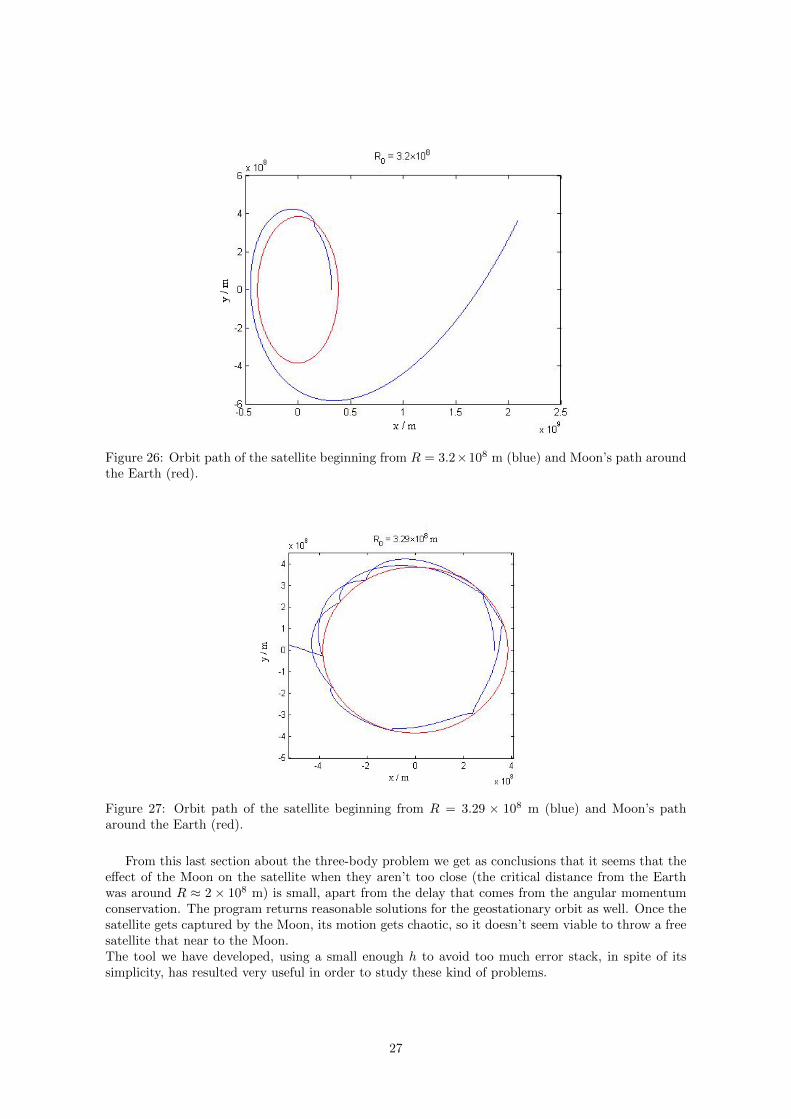
Figure 26: Orbit path of the satellite beginning from R = 3.2×108 m (blue) and Moon’s path aroundthe Earth (red).

Figure 27: Orbit path of the satellite beginning from R = 3.29 × 108 m (blue) and Moon’s patharound the Earth (red).

From this last section about the three-body problem we get as conclusions that it seems that theeffect of the Moon on the satellite when they aren’t too close (the critical distance from the Earthwas around R ≈ 2 × 108 m) is small, apart from the delay that comes from the angular momentumconservation. The program returns reasonable solutions for the geostationary orbit as well. Once thesatellite gets captured by the Moon, its motion gets chaotic, so it doesn’t seem viable to throw a freesatellite that near to the Moon.The tool we have developed, using a small enough h to avoid too much error stack, in spite of itssimplicity, has resulted very useful in order to study these kind of problems.

27

5 Conclusions

It’s important to remark that we’ve develop a program to solve the three-body problem as an example.The physics of the problem aren’t as important as the numerical approach we’ve used for its resolution.We’ve got several conclusions, achievements and learnings through the development of the project,which have already been commented in the previous sections and that will be gathered in this one.

1. We have implemented several codes in Matlab to solve ODE systems, using the fourth orderRunge Kutta algorithm, so we could study the three-body problem. We took daily knownexamples to check the results we got. The codes were made in increasing complexity, startingwith the two-body problem of the Sun-Earth system. We continued working with the three-body problem taking the Sun-Earth-Moon system and the Earth-Moon system with an artificialsatellite. We got reasonable results within the limits of our approximations. We can say theimplementation was successful, considering our results agreed with our expectations.

2. We have used two different approaches for the Sun-Earth-Moon system, letting the three bodiesfree and fixing the Sun, achieving the following results:

2.1. We’ve done a fine-tuning to get the simulated system to behave in a similar way the realsystem does, but getting the orbits more circular in order to simplify the interpretationsof the results.

2.2. The initial conditions we had to set when the three bodies were free were so fine that, forexample, changing the Earth’s speed δv⊕ = 1 m/s, made its period change δT⊕ = 1 hour.When we set the initial conditions so the bodies had to move in circular motion, we gotthat Earth and Moon disturbed each other. The Earth got an eccentricity of ε⊕ = 0.05and the Moon εM = 0.28.

2.3. We’ve make an attempt to study the stability of the system, and, during two hundredyears, it hasn’t seem to have any trend to change.

2.4. We’ve study the Moon’s stability when making little perturbations in its orbit, while theother conditions remained the same. We got that the Moon needs to change its pathδθ = 1.2o in order to disengage from the Earth’s orbit.

3. We have simulated an artificial satellite orbit around the Earth and the Moon, with the followingresults:

3.1. Comparing the geostationary satellite with and without Moon, we got that, because of theMoon influence, it had a delay of around two hours every day.

3.2. We made a study of the orbits for different distances to the Earth. We got that while thesatellite remains near the Earth (not further than R?? ≈ 2× 108 m), there are periodicalperturbations in the orbit with respect to the circular case, but they don’t seem to presentany trend to change its orbit.

3.3. When the satellite gets trapped by the Moon its motion gets chaotic. In this stage thesatellite usually gets so close to the Moon that the error stack starts to be a problem.However, taking a small enough integration step, this error shouldn’t mean any problem.When getting to close to the Moon, the satellite gets a boost in its speed due to momentumtransfer. If the energy transferred results enough, the satellite escape from the system.

3.4. Apart from the cases where the satellite and the Moon get too close to each other, wherewe may need an adaptive integration step, the program works well and allows us to makea detailed study of any case of the problem.

4. Taking everything into account, we’ve proved that we’ve developed a useful tool with reasonableresults to solve the problems we have dealt with. In order to use it in a scientific environment,however, there are several things that must be improved:

4.1. When two bodies come too close together (R? ≈ 9 × 106), because of the nature of thegravitational force (∝ 1

r2 ), the code stacks more error than usual for the rest of the simula-tion. This effect can be minimized implementing an adaptive algorithm, so the integrationstep decreases when the two bodies get too close.

28

4.2. The code would run faster if the number of equations got decreased by treating the problemtheoretically.

4.3. In order to make the code even faster, another computing program would be useful. Itcould also be prepared to be sent to more powerful computers and minimize the simulationtime.

5. The study of this problem has been a very interesting topic. It also has been useful to refreshsome computing concepts and learn a whole new. I have had to refresh how to solve the secondorder ordinary differential equations and some concepts from mechanics too. In addition, it hasbeen the first big program I have developed, and the step by step process has been a reallyenriching experience.

29

6 References

Because of the simplicity with which we have wanted to develop this work, we haven’t needed morebibliography than that for the implementation of the 4th order Runge Kutta and the initial conditionsof the bodies for the Sun-Earth-Moon system.

The information presented in Section (2.1) was taken from:https://en.wikipedia.org/wiki/Runge%E2%80%93Kutta methods#The Runge.E2.80.93Kutta method(30/06/2015)

The initial conditions for distance, mass and initial speed for the Sun, Earth and Moon withrespect to the Sun were taken from:

https://en.wikipedia.org/wiki/Sun (30/06/2015)https://en.wikipedia.org/wiki/Earth (30/06/2015)https://en.wikipedia.org/wiki/Moon (30/06/2015)

Matlab questions and problems were solved in:http://es.mathworks.com/help/matlab/ (30/06/2015)

For further reference contact the author: diegomartnlpez@gmail.com

30