UML dependency diagrams are too vague, because there are ...
76
Event-Based Programming – Chapter 1 Ted Faison Page 1 Coupling Thirty years ago Stevens, Myers and Constantine [Stevens et al., 1974] first defined coupling in a software system as “the measure of the strength of association established by a connection from one module to another”. Coupling is frequently cited with another parameter called cohesion. In their paper, Stevens et al. defined cohesion as “the degree of connectivity among the elements of a single module”. Together, coupling and cohesion are important indicators of the quality of a software system. While coupling looks at the external dependencies between modules, cohesion looks at the internal ones of a single module. In the context of EBSs, the word module should be understood as component. In the broadest terms, coupling indicates the presence of interdependencies between classes or components. High quality software should have a low degree of coupling between its components, because coupling introduces complexity and complexity makes a system more difficult to understand, test and maintain. In some sense, coupling can be viewed as a form of chaos, and attempts have been made [Shereshevsky et al., 2001] to treat coupling like entropy. Most software systems have a significant amount of coupling between their constituent components, because the designers didn’t anticipate coupling as a significant problem, and therefore didn’t invest time in preventing it or dealing with it. Given the problems that coupling causes, it is surprising that today there is no standard way to measure coupling between the various parts of a software system. Coupling has simply become one of those evils that software developers have learned to live with, even though it is clear that coupling introduces a whole set of issues into a system. The larger the system, the bigger the issues. To understand how coupling creeps in, consider how a typical software system is designed and implemented. We start by creating classes and relationships, to satisfy the system requirements. By the time the design is finished, we have a network of classes, linked in various ways by relationships. Many classes are directly or indirectly linked to practically every other class in the system. When developing small systems consisting of a single component, coupling between the classes may not be a major problem, because everything is built and deployed together, but in larger systems that use multiple components, the picture changes, and coupling-related issues often dominate others. If one component is coupled to others, which in turn are coupled to others, we quickly wind up with what is called a stovepipe system. The expression came about several years ago to denote large, monolithic systems, in which none of the system could be used unless all of the code was present. Stovepipe systems are the epitome of unreusability. To enhance reusability, components should be designed with an eye towards the minimization of dependencies on other components. While objects are routinely deployed in frameworks with lots of objects spread over multiple coupled packages, components should be deployable by themselves, in a single
-
Upload
khangminh22 -
Category
Documents
-
view
3 -
download
0
Transcript of UML dependency diagrams are too vague, because there are ...
Event-Based Programming – Chapter 1 Ted Faison Page 1
Coupling
Thirty years ago Stevens, Myers and Constantine [Stevens et al., 1974] first defined
coupling in a software system as “the measure of the strength of association established
by a connection from one module to another”. Coupling is frequently cited with another
parameter called cohesion. In their paper, Stevens et al. defined cohesion as “the degree
of connectivity among the elements of a single module”. Together, coupling and cohesion
are important indicators of the quality of a software system. While coupling looks at the
external dependencies between modules, cohesion looks at the internal ones of a single
module. In the context of EBSs, the word module should be understood as component.
In the broadest terms, coupling indicates the presence of interdependencies between
classes or components. High quality software should have a low degree of coupling
between its components, because coupling introduces complexity and complexity makes
a system more difficult to understand, test and maintain. In some sense, coupling can be
viewed as a form of chaos, and attempts have been made [Shereshevsky et al., 2001] to
treat coupling like entropy.
Most software systems have a significant amount of coupling between their constituent
components, because the designers didn’t anticipate coupling as a significant problem,
and therefore didn’t invest time in preventing it or dealing with it. Given the problems
that coupling causes, it is surprising that today there is no standard way to measure
coupling between the various parts of a software system. Coupling has simply become
one of those evils that software developers have learned to live with, even though it is
clear that coupling introduces a whole set of issues into a system. The larger the system,
the bigger the issues.
To understand how coupling creeps in, consider how a typical software system is
designed and implemented. We start by creating classes and relationships, to satisfy the
system requirements. By the time the design is finished, we have a network of classes,
linked in various ways by relationships. Many classes are directly or indirectly linked to
practically every other class in the system. When developing small systems consisting of
a single component, coupling between the classes may not be a major problem, because
everything is built and deployed together, but in larger systems that use multiple
components, the picture changes, and coupling-related issues often dominate others. If
one component is coupled to others, which in turn are coupled to others, we quickly wind
up with what is called a stovepipe system. The expression came about several years ago
to denote large, monolithic systems, in which none of the system could be used unless all
of the code was present. Stovepipe systems are the epitome of unreusability. To enhance
reusability, components should be designed with an eye towards the minimization of
dependencies on other components.
While objects are routinely deployed in frameworks with lots of objects spread over
multiple coupled packages, components should be deployable by themselves, in a single

Event-Based Programming – Chapter 1 Ted Faison Page 2
package. Independently deployable components are not just easier to deploy and use, but
are also easier to develop, test and maintain. The following axiom applies:
Axiom 1
The more complex a component is, the more decoupled it should be.
The statement might appear to be both a paradox and an oxymoron. The point is that
coupling introduces complexity, so if a component is complex to start with, due to its
internal business logic, then we want to avoid further increasing this complexity with
coupling. An immediate consequence of the first axiom is this:
Axiom 2
Coupling should be introduced into simpler components first.
The idea here is that we don’t want to introduce coupling into components that are
inherently complex, unless you have no other choice. Together, theses two axioms should
be considered the guiding principles of component-based development. A significant
amount of work should be done in the design phase to control how much coupling occurs
between components, and which components are affected most.
Coupling is inevitable
As will be shown in this chapter, there are ways to design components to minimize or
even eliminate coupling to other components. If we systematically attack the coupling
problem when designing each component in a system, we can usually find ways to shift
coupling from complex components to simpler ones. But at some point we reach a point
at which no more simplifications are possible, leaving a residual amount of coupling in
the system. In the ideal situation, the most complex components are completely
decoupled. Only the simplest components are coupled to other components. No amount
of refactoring can ever eliminate all the inter-component coupling, unless the entire
system is put into a single component, which takes us back to a stovepipe system. The
following theorem describes the inevitability of inter-component coupling in a multi-
component system.
Theorem 1
It is impossible to build a software system in which all components are completely
decoupled from each other.
Proof. To function, the classes in each component must be instantiated somehow. In most
OO languages, instantiation entails invoking a class constructor. For example, in
languages like C#, Java and C++, one must use the new operator like this:
T2 t2 = new T2();

Event-Based Programming – Chapter 1 Ted Faison Page 3
The component in which this instantiation code is located will incur coupling to the
component containing the class being instantiated. If component C1 contains class T1,
which has code to instantiate T2, contained in component C2, then C1 will be coupled to
C2, as shown in the next diagram.
T1
coupling
C1
T2
C2
<<instantiates>>
Figure 1 - Inter-component coupling due to instantiation.
We might try to use reflection to instantiate T2, but we would still need to reference a
class name (e.g. “C2.T2”) in T1’s code. The use of class names in T1 would still be a
form of coupling between C1 and C2, as we’ll see more in detail later in the chapter.
Even if we could completely eliminate coupling due to class instantiation, there would
still be another problem: Once instances are created, they will probably contain calls to
other objects. These outgoing calls must be bound to methods of other objects, some of
whom will have originated from classes in different components. If we hard code in each
class the responsibility of binding its own outgoing calls to callees, then each class incurs
compile-time coupling to all the callees, because the source code embeds method names.
To avoid compile-time coupling, we might defer binding to runtime, using a Binder class
to connect outgoing calls to methods. The problem is that now the Binder could easily
wind up being coupled to every class in the system, so we have merely shifted coupling
around in the system. This predicament is somehow reminiscent of the famous words of
Abraham Lincoln:
“You can fool all the people some of the time, and you can fool some of the people all the
time, but you can’t fool all the people all the time”.
We might adapt Lincoln’s words to describe the component-coupling problem by saying,
“You can remove all the coupling from some of the components, and you can remove
some of the coupling from all the components, but you can’t remove all the coupling from
all the components.”
We can restate this in more mathematical terms. Given a software system containing M
components:
Event-Based Programming – Chapter 1 Ted Faison Page 4
n
i 1
couplingi > 0
The word coupling represents a measurement of some kind between the i-th component
and all the other n-1 components in the system. In the next section we’ll introduce a
mathematical symbol to represent coupling. A bit later we’ll show how to measure
coupling.
An important job during the design phase is to reduce the overall inter-component
coupling in a system to the lowest level possible. But a problem arises: How do we know
when we’re finished? In other words, how do we know when coupling is at the lowest
level possible? The goal is to ensure that all complex components are entirely decoupled
from other components. To accomplish this, and because we know that coupling can’t be
completely eliminated from a system, we must find ways to shift coupling around in the
system, until it only occurs in desirable places. The rest of the chapter will show ways to
accomplish this non-trivial goal.
The Coupling Symbol
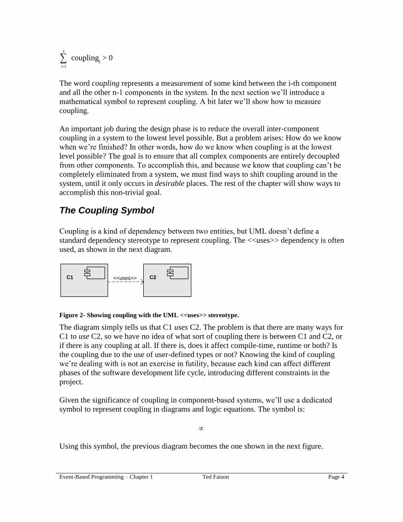
Coupling is a kind of dependency between two entities, but UML doesn’t define a
standard dependency stereotype to represent coupling. The <<uses>> dependency is often
used, as shown in the next diagram.
<<uses>>C1 C2
Figure 2- Showing coupling with the UML <<uses>> stereotype.
The diagram simply tells us that C1 uses C2. The problem is that there are many ways for
C1 to use C2, so we have no idea of what sort of coupling there is between C1 and C2, or
if there is any coupling at all. If there is, does it affect compile-time, runtime or both? Is
the coupling due to the use of user-defined types or not? Knowing the kind of coupling
we’re dealing with is not an exercise in futility, because each kind can affect different
phases of the software development life cycle, introducing different constraints in the
project.
Given the significance of coupling in component-based systems, we’ll use a dedicated
symbol to represent coupling in diagrams and logic equations. The symbol is:
Using this symbol, the previous diagram becomes the one shown in the next figure.

Event-Based Programming – Chapter 1 Ted Faison Page 5
C1 C2
Figure 3- Showing coupling with a special symbol.
In some math and physics textbooks, the symbol is used to indicate a proportionality
relationship. The decision to use this symbol for coupling was not entirely arbitrary,
because proportionality is a form of dependency. For readers wishing to reproduce the
symbol in their own documents, the coupling symbol is available in the Symbol font
under Microsoft Word. The symbol is not a Greek letter, and should be read as coupling
or is coupled to. There are several ways in which classes, objects and components can
become coupled, so we’ll use subscripts to denote the specific kind of coupling in effect
at a given time.
Is Coupling Bad?
Yes, coupling is bad, but not all forms of coupling are equal. In general, we can say that
duplicated logic, which is a form of coupling, is extremely bad. Forms of coupling that
impact compile-time, which we call static, are probably the next worse. The most benign
form of coupling is what we call dynamic, which occurs only at runtime.
The fact is that coupling, in any form, introduces complexity into a system. Different
kinds of coupling add different amounts of complexity, but it is undeniable that coupling
makes it harder to develop, test, deploy and maintain software. But concluding that
coupling is the root of all evils in software development would not be correct. For one
thing, there are many evils that aren’t dependent on coupling. Moreover, coupling isn’t
really the root of anything. It is the consequence of problems introduced at analysis,
design or implementation time. Let’s consider the main phases in the development
lifecycle in which coupling introduces complexity. For the purposes of the following
discussion, let’s assume a project uses two components A and B.
Coupling between A and B that affects compile-time will prevent A from being compiled
unless B is present. Certain changes to B will break the compilation of A, requiring A to
be changed together with B.
Coupling between A and B that affects run-time will prevent A from being run unless B
is present. Run-time coupling will make it harder to test A, because to run A we need to
also run B. B’s presence may complicate the testing scenario considerably, injecting a
whole series of issues into the test phase.
Both compile-time and run-time coupling may introduce problems at deployment time,
because coupled components may need to be deployed together. If A is from one vendor
and B from another, it may be difficult or impractical to package or deploy A and B
together. Coupling also complicates work during the maintenance phase. The more
coupled A is to B and the more difficult it will be to change B without affecting A. The

Event-Based Programming – Chapter 1 Ted Faison Page 6
magnitude of the coupling problem grows with the number of components used in a
system.
Coupling can also affect the way programmers work [Cain et al., 2002]. If A and B are
statically coupled, but under the responsibility of different team members, then the
members are going to have to work together somehow, so that changes to A and B are
made at the same time. Once B is checked out of the version control system and changed,
it can’t be checked in until A has been suitably changed. A and B will have to be checked
in essentially at the same time. The result is this: Coupled software results in coupled
developers and possibly coupled teams.
The Nature of Coupling
It is clear that coupling complicates software one way or another. Just how bad the effects
of coupling are depends on where it was introduced in the system, and which
development phases are impacted by it. The two key phases we’ll discuss are build-time
and runtime. Build-time includes compilation, linkage and any other activities required to
produce executable code from source code. For interpreted languages, these activities
occur at runtime, so there is no real distinction between build-time and runtime.
Static Coupling
If the coupling between two items affects build-time, we say that the coupling is static. If
A is statically coupled to B, then B will need to be present in order to build A. To
produce A’s executable code from source code, some part of B will need to be present.
Exactly which part is required depends on the language being used.
Modern OO languages, like C# and Java, merge the declaration and implementation of a
class together. During compilation, metadata is added to the executable code. The
metadata describes all the types defined in the class, for the benefit of compilers and
other software tools. The metadata also makes runtime type identification possible. If
classes A and B are written in a language like C# or Java, and A is statically coupled to
B, then we’ll need B’s executable code to be present when compiling A. B’s source code
is of no interest to A at build time or runtime.
Older OO languages, like C++ and ObjectPascal, separate the declaration of a class from
the implementation. If classes A and B are written in C++ or ObjectPascal, and A is
statically coupled to B, then we’ll need B’s declaration to be present when compiling A.
In C++, the class declaration is typically contained in a header file, while in ObjectPascal
the declaration is in the same file as the implementation, but in a reserved section.
To denote static coupling in diagrams and equations, we’ll use a UML dependency
arrow. The arrow will be labeled with the symbol subscripted with the word static. The
next figure shows an example.
A Bstatic

Event-Based Programming – Chapter 1 Ted Faison Page 7
Figure 4 - A diagram showing the A is statically coupled to B.
Static coupling occurs between classes A and B when A contains references to symbols
defined in B. A symbol is a name that can indicate anything from a constant to an
enumeration to a method to a type declared inside B (such as a field or inner class). The
embedding of references to externally defined types is a kind of coupling called type
coupling. We’ll look at type coupling in detail later in this chapter.
Just as static coupling can occur between classes, it can also occur between components.
Statically coupled components must always be kept in-sync with each other during the
development process. Changing one component might break the compilation of other
components that are statically coupled to it, requiring those components to be changed as
well. As a result, changes in one component can produce a ripple of changes through the
system and involve several members of the development team.
Mathematical Properties
All kinds of coupling can be treated mathematically and throughout this chapter we’ll be
exploring significant mathematical properties that apply to coupling. We’ll start our math
discussion by focusing on static coupling.
Theorem:
A static B B static A Static coupling is not commutative.
Proof: Let class A contain a reference to class B. Class A is statically coupled to class B,
because B must be present to compile A. As discussed earlier, the form of B that must be
present depends on the language. With languages like C++, B’s header file will be
needed. With languages like C# or Java, B’s executable code will be needed. Regardless
of the language, class B will not be statically coupled to class A, because class B does not
contain references to A, and can be compiled by itself.
Whether static coupling is transitive or not depends on the type of programming language
being used. With languages like C++, that use separate declaration and implementation
files for a class, static coupling may be transitive. For languages like C# and Java, that
use a single file for the declaration and implementation of a class, static coupling is not
transitive.
Theorem:
With languages that separate the class declaration from the implementation, static
coupling is transitive, if coupling is due to items in the declaration.
Proof: Assume we have three C++ classes, A, B and C. Each class has a header file and
an implementation file. We’ll call the header files A.h, B.h and C.h. We’ll call the
implementation files A.cpp, B.cpp and C.cpp. Assume A.h includes the file B.h and that
B.h includes the file C.h. With this arrangement, A is statically coupled to B and B is
statically coupled to C. When compiling A, the compiler will need to load the header file
A.h, which includes B.h. When the compiler tries to load B.h, it discovers that it also has
Event-Based Programming – Chapter 1 Ted Faison Page 8
to load C.h. As a result, to build A we’ll need (the header files of) both B and C to be
present.
Things change if the coupled items are not in header files but in implementation files.
Assume A.cpp (and not A.h) contains a reference to B. It follows that A.cpp will need to
include the file B.h. Assume also that B.cpp (and not B.h) contains a reference to C, so
B.cpp will need to include the file C.h. To compile B, we’ll need to have access to C.
When we compile A, will B need to be present? Yes, because A.cpp contains a reference
to B.h. Will C need to be present? No, because when we compile A, the only file the
compiler needs is B.h. There are no references to C in A’s code or in B.h.
Theorem:
With languages that merge the class declaration and implementation together, static
coupling is not transitive.
Proof: Let class A be statically coupled to class B, by embedding a reference to class B.
Let class B be statically coupled to class C, by embedding a reference to class C. To
compile B, we’ll need to have C. To compile A, we’ll need to have B, but not C, because
A doesn’t reference anything defined in class C. Everything the compiler needs to
compile A is contained in the compiled code for B, so C is not necessary.
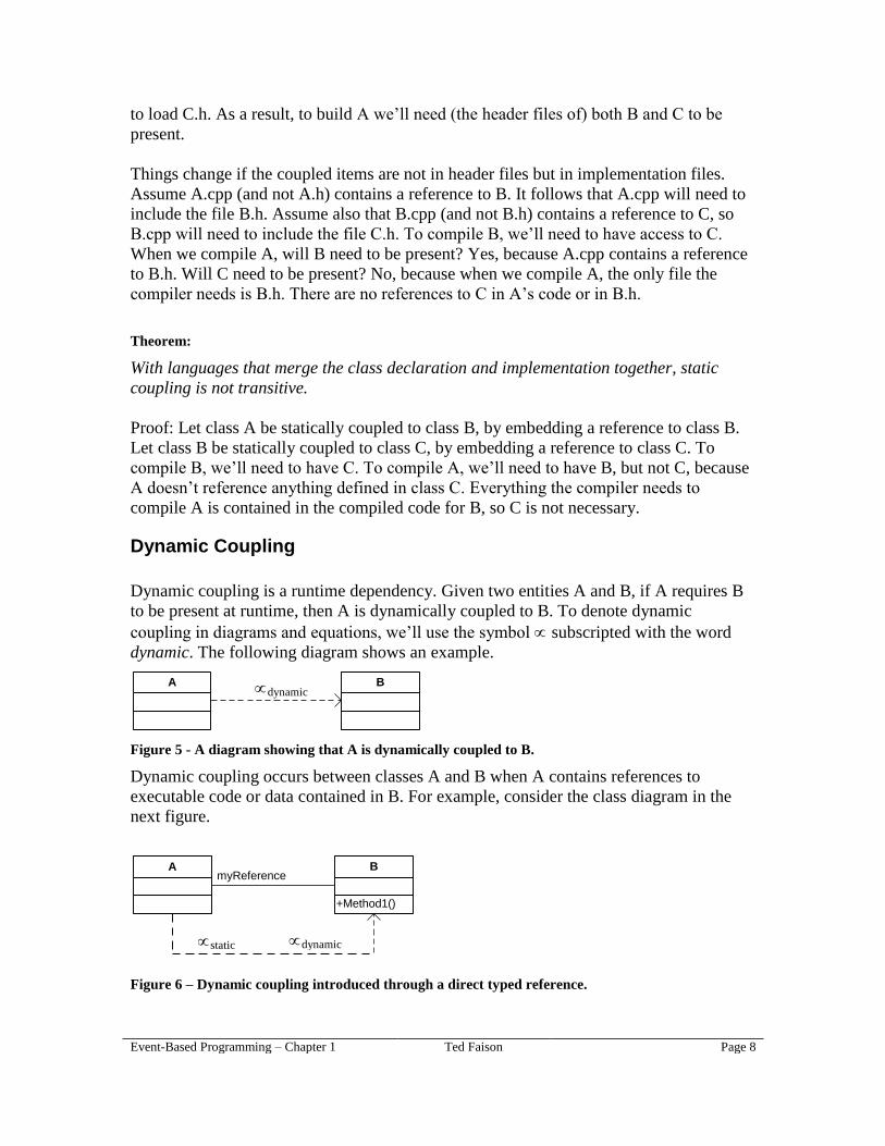
Dynamic Coupling
Dynamic coupling is a runtime dependency. Given two entities A and B, if A requires B
to be present at runtime, then A is dynamically coupled to B. To denote dynamic
coupling in diagrams and equations, we’ll use the symbol subscripted with the word
dynamic. The following diagram shows an example.
A Bdynamic
Figure 5 - A diagram showing that A is dynamically coupled to B.
Dynamic coupling occurs between classes A and B when A contains references to
executable code or data contained in B. For example, consider the class diagram in the
next figure.
A
+Method1()
BmyReference
static dynamic
Figure 6 – Dynamic coupling introduced through a direct typed reference.

Event-Based Programming – Chapter 1 Ted Faison Page 9
In this example, assume class A uses the typed reference named myReference to call
B.Method1. Class A is dynamically coupled to B because the executable code for
B.Method1 must be present at runtime. Note that class A is also statically coupled to B,
because A references the type B (through the typed reference myReference. It is possible
to eliminate the static coupling by separating the interface of B from the implementation
of B, as shown in the following diagram.
+Method1()
«interface»
B
+Method1()
C
A myReference
dynamic
static
Figure 7 – Dynamic coupling introduced through a direct reference.
Now class A holds a reference to type B, but the executable code for Method1 is in class
C, derived from B. If we assume that A.myReference is initialized using a reference
received from another object, A will have dynamic, but not static, coupling to C. A will
think myReference points to a B object, while it actually points to a C object. Class A
doesn’t know about the existence of C, and calls C.Method1 through B’s interface. Class
A is statically coupled to B because the compiler needs to know the layout of type B in
order for A to call B.Method1. At runtime, C will need to be present, because A will call
the C’s implementation of B.Method1.
Mathematical Properties of Dynamic Coupling
Let’s explore the most significant mathematical properties that pertain to dynamic
coupling.
Theorem:
A dynamic B B dynamic A Dynamic coupling is not commutative.
Proof: Let class A contain a reference to class B. Class A uses the reference to call
methods of B. Class A requires class B to be present at runtime, otherwise the executable
code for the methods that A calls won’t be present and the calls will fail. Class B doesn’t
require class A at runtime, because B doesn’t even know that A exists. Therefore class B
is not dynamically coupled to class A.
Theorem:
(A dynamic B) and (B dynamic C) (A dynamic C)
Dynamic coupling is transitive.

Event-Based Programming – Chapter 1 Ted Faison Page 10
Proof: Let class A be dynamically coupled to class B and let class B be dynamically
coupled to class C. Assume A uses a typed reference to call a method of B. When called,
B reacts by using a typed reference to call a method of C. Class A requires class B to be
present at runtime, and class B requires class C to be present at runtime. If we remove C
at runtime, then B will be unable to invoke methods of C and will fail. If B fails, A will
also fail, ergo class A is dynamically coupled to class C.
Static versus Dynamic Coupling
Which type of coupling is worse: static or dynamic? The short answer is static coupling,
because it manifests itself at compile-time. If class A were statically coupled to class B,
then changes to B could break the compilation of A. Class A would then need to be
changed to make it compilable again. In a large project, changes to one class could break
any number of classes that were statically coupled to it, and require widespread changes
throughout the system.
Dynamic coupling is much less a problem during the development phase. If class A were
dynamically coupled to class B, then A would only require B in order to run. Since B
wouldn’t have to be present at compile-time, we could change B in any way we want,
without ever breaking the compilation of A. Any catastrophes caused by changes to B
would only show up when running A.
On the other hand, static coupling is a safer form of coupling that dynamic, from a certain
perspective, and here’s why: If two classes A and B are statically coupled, the compiler
will need B to be available in order to compile A. The compiler will be able to type-check
any references A makes to items belonging to B, and this type-checking can be
immensely valuable in finding errors in source code. Dynamic coupling impacts the
system at runtime, when the compiler is long gone from the scene (at least with compiled
languages like C# and Java). Errors related to dynamic coupling only show up at runtime.
It is important to remember that the presence of dynamic coupling does not preclude
static coupling. There is no deterministic relationship between static and dynamic
coupling, so two classes may be statically, but not dynamically, coupled. Or they might
be dynamically, but not statically, coupled. Or they might be both statically and
dynamically coupled.
Coupling Flavors
Coupling can be characterized in any number of ways. The truth is that coupling is a
somewhat abstract concept, and depending on what system parameters are important to
us at a given moment, we can slice a system in different ways to expose different kinds
and levels of coupling. The word coupling is often used generically, to indicate a
dependency between objects, classes or components. One of the first classifications of
coupling in an OO setting [Eder et al., 1993] described three dimensions of coupling:
interaction coupling, component coupling and inheritance coupling. Eder introduced
predicates to compute degrees of coupling between arbitrary classes in a system. Later,
Hitz and Montazeri [Hitz et al., 1995] looked at coupling from the perspective of the

Event-Based Programming – Chapter 1 Ted Faison Page 11
level it occurs at (object-level and class-level). Attempts have been made to integrate the
various coupling classification approaches together into a framework [Briand et al.,
1999], with support for formal methods for determining degrees of coupling between
parts of a system.
In this book, we’ll look at the coupling kaleidoscope in a yet different way, identifying
three orthogonal flavors of coupling that can be treated as dimensions in a mathematical
coupling space.
Logic coupling. This flavor is the least desirable of the three, and is also the most
abstract and insidious. Logic coupling doesn’t impede the software development
process, but can result in runtime errors that are hard to find. Logic coupling often
causes headaches during the maintenance phase.
Type coupling. This flavor is probably the most recognizable form of coupling. It
arises when one component or class uses a type defined in a different component
or class.
Signature coupling. This flavor occurs only at runtime, and has the potential to
completely decouple classes from each other.
In the following sections, we’ll look at each flavor in detail, looking not only at some of
the mathematical properties that apply to them, but also at programming patterns that
allow us to convert one flavor into another.
Logic Coupling
If two classes share information or make assumptions about each other, then they are
coupled at the logic level. What happens in one class can have an effect on what happens
in another – even if the classes share no data or types. Logic coupling is often the result
of poor design, poor implementation, or both.
Definition 1
Logic coupling occurs when information is shared.
To show logic coupling on diagrams, we’ll draw a dependency line between them, using
a double-headed arrow. The following figure indicates that classes T1 and T2 are
logically coupled.
T1 T2L
Figure 8 – Types that are logically coupled.

Event-Based Programming – Chapter 1 Ted Faison Page 12
As can be seen in the figure, we denote logic coupling with a dependency line labeled
with the symbol , subscripted with the letter “L”. The arrow is double-headed to
symbolize the fact that logic coupling involves mutual coupling. T1 is logically coupled
to T2 and vice versa. In the next sections we’ll see why.
What causes logic coupling? We know that logic coupling results from the sharing of
information, but one can envision different ways for objects to share information. A
sharing relationship is somewhat vague, so we’ll need to be much more specific about
what we mean.
Let T1 and T2 be two classes. We won’t worry whether T1 and T2 are part of the same
component or not. There are basically two different ways in which T1 can share
something with T2, in terms of logic coupling:
1. T1 contains an algorithm that is related to an algorithm contained in T2. This type
of sharing is a subflavor of logic coupling we’ll call algorithmic logic coupling.
2. T1 contains a literal value that is also contained in T2 and used for the same
conceptual purpose. This type of sharing is a subflavor of logic coupling we’ll call
literal logic coupling.
In the following sections we’ll look at each subflavor in more detail. Both have a
dynamic nature: they don’t induce compilation or other errors at build time. Their effects
are felt only at runtime.
Algorithmic Logic Coupling
The easiest way to describe algorithmic logic coupling (ALC) is with an example. Let T1
and T2 be two classes. T1 uses an algorithm F to encrypt data, which is then sent to T2. If
T2 needs to decrypt the data, we’ll call the decryption algorithm G. It is obvious that the
algorithm G is dependent on the algorithm F. If T1 changes the way it encrypts the data,
then T2 will also need to change the way it decrypts the data. Class T2 is said to have
algorithmic logic coupling (ALC), or simply algorithmic coupling, to T1, as shown in the
next figure.
T1 T2La
Figure 9- Algorithmic logic coupling between T1 and T2.
As can be seen in the diagram, we use the symbol subscripted with the letters “La” to
denote ALC. The coupling arrow in the figure is double-headed to indicate that T1 and
T2 are mutually coupled. One class doesn’t depend on the other: both classes depend on
each other. If we change the coupled algorithms in either class, we’ll have to change the
algorithm in the other class as well (if we want to system to work correctly).
Event-Based Programming – Chapter 1 Ted Faison Page 13
Encryption and decryption algorithms are special cases of a broader set of algorithms
called complementary algorithms. We need to make a small digression at this point, to
describe the properties of complementary algorithms and other types of algorithms
involved in algorithmic logic coupling.
Complementary Algorithms
It is quite common way for classes to be designed in a way that one class produces
something that another consumes. Software systems often have many types of producer
and consumer classes. Sometimes a class can act as a producer of some type of
information, and a consumer or another type. In the context of coupling, the producer-
consumer pattern is important because the producer and consumer algorithms are
logically coupled: Before the consumer can consume something, it must know a number
of things about the producer, including:
1. What will be produced?
2. When will it be produced?
3. How will the information be packaged and formatted?
4. How will the information be accessible?
All this meta-information induces algorithmic logic coupling between the consumer and
producer algorithms. If the producer changes something in the way it produces
information, there is a good chance the consumer will have to be changed as well. Two
algorithms are complementary if they work together to accomplish a task or operation.
For example, one class might use an algorithm to store data in a buffer, while another
class might use a complementary algorithm to read the data from the buffer. The
operation that the writer and reader accomplish together might be anything, such as
getting data from one place to another, making information persistent, making
information secure, increasing the performance of the system, etc.
Definition:
An algorithm G is the complement of an algorithm F if G completes an operation begun
by F.
Complementary algorithms can be found for any operation that is characterized by two
facets or phases. There are many examples, but here are a few:
- Compression/decompression
- Encryption/decryption
- Writer/reader algorithms
- Producer/consumer algorithms
- Start/stop commands
- Open/close commands
Complementary algorithms are logically conjoined like Siamese twins. They are separate
parts of a single logical task. If we change one, we are probably going to have to change
the other. Complementary algorithms are designed in terms of each other, so they are
Event-Based Programming – Chapter 1 Ted Faison Page 14
intimately coupled, in a logic sense. One is generally useless without the other. The
following listing shows two C# classes, T1 and T2 that contain complementary
algorithms.
public class T1
{
public void WriteMessages(StreamWriter theWriter, ArrayList theMessages)
{
// write all the messages
foreach (string s in theMessages)
theWriter.WriteLine(s);
}
}
public class T2
{
public void ReadMessages(StreamReader theReader, ArrayList theMessages)
{
// read all the messages
while (true)
{
string s = theReader.ReadLine();
if (s == null)
break; // end of file
theMessages.Add(s);
}
}
}
Listing 1 – An example of complementary writer and reader algorithms.
The method T2.ReadMessages contains an algorithm that is designed to read not any
stream, but streams containing a list of string messages written using the algorithm in
T1.WriteMessages, so we can say that the algorithm in T2.ReadMessages is the
complement of the one in T1.WriteMessages.
Note that the relationship “is the complement of” is not commutative. If T2 is the
complement of T1, we can’t conclude that T1 is the complement of T2. For example, the
reader algorithm of our example logically completes the writer algorithm, so the reader is
the complement of the writer. The writer is not the complement of the reader, because the
writer does not logically complete any operation begun by the reader.
Inverse Algorithms
Complementary algorithms are a broad class of algorithms, of which Inverse algorithms
are a subset. An algorithm can be considered a mathematical function that transforms a
system from a certain initial state to a certain final state. Given an algorithm F that
transforms a system from the initial state S0 to the final state S1, let there be a
complementary algorithm G that transforms the system from the initial state S1 to the
final state S0. Mathematically, we could describe algorithms F and G like this:
F(S0) = S1
G(S1) = S0
Event-Based Programming – Chapter 1 Ted Faison Page 15
We can deduce two things, if G exists: that F is an invertible algorithm, and that G is the
inverse of F, if F is applied to the system when the initial state is S0. The following
equation shows explicitly that G is the inverse of F:
G(F(S0) = S0
The equation tells us that the effect of applying first F and then G to a system in the
initial state S0 will cause to system to end up in the state S0. We need a simpler way to
denote the is inverse of relationship. In math textbooks, the inverse of a function F is
usually called F-1. The problem with this convention, as pointed out by many people,
including Feynman [Feynman et al., 1997], is that it uses the same notation to describe
the inverse of F and the reciprocal of F, which is 1/F. To avoid any confusion in this
book, we’ll use the word Inverse to indicate the inverse of an algorithm. To show that G
is the inverse of F, we’ll simply use the equation:
G = Inverse(F).
Definition:
Given two algorithms F and G, we can state that G = Inverse(F), for a given initial
system state S0, if G(F(S0) = S0.
We might say that G is the undo function of F, because it cancels all effects of applying F
to a system in the state S0. It is important to note that if G is the inverse of F for a
particular initial system state (S0), it doesn’t necessarily follow that G is the inverse of F
for all possible initial system states. When G can invert F only for a certain subset of the
possible initial system states, we’ll say G is the bounded inverse of F, where the bound
denotes the set of system states for which G is able to invert F. For example, if G is able
to invert F only for the initial states {S0, S2}, then we’ll say that G is the bounded
inverse of F for the set of initial states {S0, S2}. Using mathematical symbols, we’ll state
this using the formula:
G = InverseT(F) where T = {S0, S2}
The subscript T is the set of all initial system states for which G is the inverse of F. When
G can invert F for any arbitrary initial state, we’ll say that G is the unbounded inverse of
G, or simply the inverse of F. An unbounded inverse of F, G can be described using the
equation:
G(F(Sx)) = Sx
Where Sx is an arbitrary initial system state. Using our new Inverse function, we can also
write:
G = Inverse(F)
Event-Based Programming – Chapter 1 Ted Faison Page 16
There is no subscript to the Inverse function, indicating that G is the inverse of F for all
possible initial system states. In the rest of our discussion, we’ll assume that G is the
unbounded inverse of F. Note that the “is inverse of” relationship, being a special case of
the “is complement of” relationship, is not commutative. The fact that G can invert the
results of F doesn’t entail that F can invert the results of G. G is a completely different
algorithm from F. For all we know, G may not even have an inverse function.
Symmetric Algorithms
Although the relationship “is the inverse of” is not generally commutative, there is a
subset of inverse algorithms in which the relationship is commutative. We’ll call these
algorithms symmetric algorithms, not to be confused with symmetric key algorithms used
in cryptography, which use the same key to encrypt and decrypt data.
If F has an inverse algorithm G, then G will also be the symmetric of F if F is the inverse
of G. The following definition might be easier to digest:
Definition:
Two algorithms F and G are symmetric of each other if F is the inverse of G and vice
versa.
If F and G are symmetric, the following two equations apply:
G = Inverse(F)
F = Inverse(G)
Instead of using two equations, we can make use of a new Symmetric function like this:
G = Symmetric(F)
As with Inverse algorithms, we need to specify the initial system conditions for which F
and G are symmetric. If they were symmetric only for certain initial states, then we
would say that F and G are bounded symmetric algorithms. If the set of initial states
included two states S0 and S1, then we would express this fact with the following
expression.
G = Symmetric T
(F) where T = {S0, S1}
We could express exactly the same symmetry using the expression:
F = Symmetric T
(G) where T = {S0, S1}
If we don’t specify the set T, then we imply that F and G are unbounded symmetric
algorithms, and are symmetric for all possible initial system states. Symmetry is
necessarily a mutual relationship. If F is the symmetric of G, then G must also be the
symmetric of F. The property “is symmetric to” is generally not reflexive, because it

Event-Based Programming – Chapter 1 Ted Faison Page 17
would imply that F is the inverse of itself. The sole case in which F would be the inverse
of itself is with a trivial algorithm, which doesn’t change the system state.
Given two generic complementary algorithms F and G, it is possible for G to be the
inverse of F for a certain set T of initial states, and for G to be the symmetric for a
different set U of initial states. Since symmetric algorithms are a special case of inverse
algorithms, we can deduce that one of the sets (e.g. U) must be a subset of the other (e.g.
T).
Symmetric algorithms are common in information systems. For example, consider the
algorithms for converting a decimal digit into ASCII and from ASCII to a decimal digit.
The algorithms might be coded like this:
char DigitToAscii(int theDigit)
{
// theDigit must be in the range (0..9)
return (char) (0x30 + theDigit);
}
int AsciiToDigit(char theChar)
{
return (int) theChar - 0x30;
}
Listing 2 – An example of symmetric algorithms.
To prove that the DigitToAscii and AsciiToDigit are symmetric, all we have to do is
verify that they are inverses of each other, for at least one pair of values. We can use the
following code to check value pairs programmatically:
bool AreFunctionsSymmetric(char theChar, int theDigit)
{
if (theChar != DigitToAscii(AsciiToDigit(theChar)))
return false;
if (theDigit != AsciiToDigit(DigitToAscii(theDigit)))
return false;
return true;
}
Listing 3 – Checking to see if two algorithms are mutually symmetric.
If we find even a single pair of values for which the functions are valid, we can conclude
that the functions are at least bounded symmetric functions of each other. In our example,
the functions are symmetric over the set of characters in the range {‘0’..’9’} and integers
in the range {0..9}.
Equipotent Algorithms
As we have seen, complementary algorithms work together as different facets of an
overall operation. ALC can also be introduced by a completely different class of
Event-Based Programming – Chapter 1 Ted Faison Page 18
algorithms, which we’ll call equipotent. Given two algorithms F and G, and an initial
system state S0, F and G are equipotent if they both produce the final state S1.
Definition:
Two algorithms are equipotent if they achieve the same goalj.
We use the symbol to express equipotency. To show that F and G are equipotent, we
use the equation:
G F
Two algorithms F and G might only be equipotent for a certain subset of initial
conditions. If so, we’ll say that G is the bounded equipotent of F, and we’ll need to
specify the set of initial system states using the following type of expression:
F T(G) where T = {S0, S1}
If G produces the same final system state as F for any arbitrary initial system state, we’ll
say that G is the unbounded equipotent, or simply the equipotent of F.
While complementary algorithms are designed to work in conjunction with each other,
equipotent algorithms are designed to actually produce the same results, and therefore
represent a duplication of logic. There are a couple of properties that are particularly
important. Equipotency is commutative, so if G is the equipotent of F, then F is also the
equipotent of G. Equipotency is also reflexive: An algorithm F is always equipotent to
itself, so if we duplicate an algorithm verbatim, the two copies are equipotent.
Let’s look at an example of equipotent algorithms. Assume a class T1 uses an algorithm
F to compute the hash on a message. If this message is passed to a class T2, and T2 needs
to verify the correctness of the message hash, then T2 will need to use an algorithm G
that is equipotent to F. In most cases, F and G will be exactly the same algorithm, but this
may not always be the case. T1 and T2 will incur ALC, because changing the algorithm F
in T1 will require us to also change the algorithm G in T2, and vice versa.
We need to point out that there is not necessarily a one-to-one relationship between
algorithms and functions written in a programming language. We might consider a
function to be a single algorithm, but we could also consider each line or a group of
contiguous lines to be an algorithm. For example, consider the two functions in the
following listing.
char commandCode;
char parameters;
void GetSimpleCommand(string theCommand)
{
commandCode = theCommand[0];
}

Event-Based Programming – Chapter 1 Ted Faison Page 19
void GetLongCommand(string theCommand)
{
commandCode = theCommand[0];
parameters = theCommand[1];
}
Listing 4 – Two methods that contain equipotent algorithms.
Although GetSimpleCommand and GetLongCommand contain different code, their first
lines, shown in bold text, are designed to do the same thing. We can consider each bold
line as an algorithm, so the two methods contain an equipotent algorithm, whose purpose
is to extract the command code from a command. GetLongCommand contains an
additional algorithm, to extract the parameters from a command. If the command code
position were changed in the command, both GetSimpleCommand and
GetLongCommand would need to be changed.
Literal Logic Coupling
In the previous listing, the two methods contained equipotent algorithms for extracting
the command code from a message. To get the command code, the algorithms used a
hard-coded literal value to denote the position of the command code in the message. The
presence of literals embedded in the code is a special case of logic coupling, called literal
logic coupling, or simply literal coupling (LLC).
In the example, LLC was present in two algorithms that were equipotent, but LLC can
also occur in complementary algorithms. As an example, assume a system uses a hash
table to store values. Each value is associated with a key, which might be a string. A class
T1 stores values into the hash table, while a class T2 needs to retrieve them. Clearly, T2
will need to use the same keys as T1, if it wants to obtain the values stored by T1 in the
hash table. If T1 stored a value using the code
hashtable["MyKey"] = "MyValue";
then T2 would retrieve the value with the code:
object myValue = hashtable["MyKey"];
Both T1 and T2 embed the literal value “MyKey” to access a particular value in the hash
table. If T1 is subsequently changed to use another string for the key of “MyValue”, class
T2 will break, in terms of its logic. T2 will compile without any problems, but probably
won’t work correctly. The next diagram shows the coupling graphically.
T1 T2Ll
Figure 10 – Literal logic coupling between T1 and T2.
As shown in the diagram, to denote LLC we use the symbol subscripted with the letters
“Ll”, where the second letter is a lowercase L.
Event-Based Programming – Chapter 1 Ted Faison Page 20
Another example will show how LLC might affect a system in which one class T1 sends
messages to another class T2. Let’s assume the system is used in a book library. When a
book is checked out, T1 sends a message to T2, describing the book that was checked
out. Let’s assume the message is sent as a string array A, which T1 populates using the
following C# code:
A[0] = "Frankenstein";
A[1] = "Mary Shelley";
A[2] = "1-593-08005-0";
The implication is that the message contains strings. The first element of the message
contains the book title, the second contains the author and the third contains the book’s
ISBN. In order for T2 to extract meaningful information, T2 will need to know several
things about the message, such as:
1. The message describes checked-out books.
2. The message contains strings.
3. The strings describe a book title, author and ISBN, in that specific order.
All this information represents ALC between T1 and T2, but the presence of the literal
values for the array indices also injects LLC between T1 and T2. T2 might extract data
from the message using the following C# code.
string title = Message[0];
string author = Message[1];
string isbn = Message[2];
A special case of LLC can occur even when no literal values are embedded explicitly in
the code, but are implied: This type of LLC occurs when using streams to exchange
information. If the writer adds items to the stream, those items will have an implicit order
in the stream. Although the writer doesn’t use literals to indicate where items go in the
stream, every item has its place. A class that reads the stream will have to know the
ordering of items in the stream. Streams are a subset of a broader class of shared
resources called an implicitly ordered resources. Any time an implicitly ordered resource
is used to send information between two parties, those parties will incur literal logic
coupling.
It is not uncommon to see literal values embedded in code, but projects that have the
same literal value embedded in multiple places contain duplications. We must view
duplications as software malignancies, because they generally represent sloppy design or
implementation, and add unnecessary complexity to the development and maintenance
phases.
Mathematical Properties of Logic Coupling
Now that we have seen how logic coupling can occur, let’s explore the most significant
mathematical properties that apply to it.
Theorem:
Event-Based Programming – Chapter 1 Ted Faison Page 21
A L B B L A Logic coupling is commutative.
Case 1: Literal logic coupling.
Proof: Assume two classes A and B communicate via a shared data structure. Class A
uses a literal value x to write data to the structure. The literal x might affect the value
written, its format or its position in the data structure. Let class B use a literal value y to
read the value stored by class A in the data structure. If the value of x is changed, A will
write the values associated with x in a different way. In order for class B to read the new
value correctly, its y value will need to be changed to make it compatible with x.
Conversely, changing y in class B will require us to change x in class A.
Case 2: Algorithmic logic coupling.
Proof: Let Class1 communicate with Class2 via a shared data structure. Class1 writes
data in the data structure using an algorithm F, while Class 2 reads data from the data
structure using an algorithm G. If F is changed to write data in a new way, then G will
also need to be changed, to read data in the new way. Conversely, if G is changed to read
data in a new way, then F will also need to be changed to write the data in the new way.
Theorem:
(A L B) and (B L C) (A L C) Logic coupling is transitive.
Proof: Let class A contain logic La that is coupled to logic Lb contained in class B. Let the
logic Lb be coupled to logic Lc contained in class C. If we change the logic Lc, we will
have to change the logic Lb to match the changes. If we change the logic Lb, we will have
to change La to match the changes to Lb. As a result, changes to Lc in C will require
changes to La in A, so logic coupling is transitive.
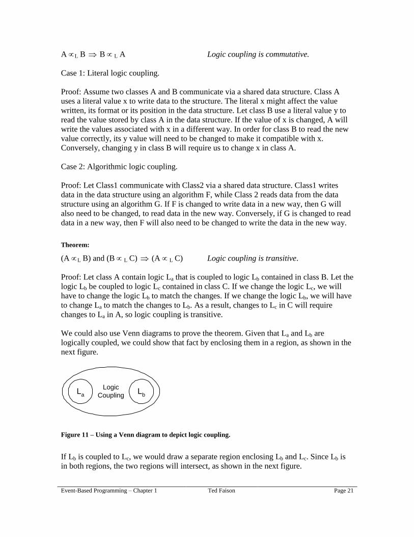
We could also use Venn diagrams to prove the theorem. Given that La and Lb are
logically coupled, we could show that fact by enclosing them in a region, as shown in the
next figure.
Logic
CouplingL
aL
b
Figure 11 – Using a Venn diagram to depict logic coupling.
If Lb is coupled to Lc, we would draw a separate region enclosing Lb and Lc. Since Lb is
in both regions, the two regions will intersect, as shown in the next figure.

Event-Based Programming – Chapter 1 Ted Faison Page 22
La
Lb
Lc
Figure 12 – Showing that Lb is coupled to both La and Lc.
A region encloses logic that is coupled. If Lb is in two regions, those two regions are
coupled, so we can coalesce the two regions into a single region enclosing La, Lb and Lc,
as shown in the next figure.
La
Lb
Lc
Figure 13 – Replacing two intersecting regions with a single one.
An interesting, but different, scenario arises if class B has two separate pieces of logic Lb1
and Lb2. If La in class A is logically coupled to Lb1 and Lb2 is logically coupled to Lc in
class C, is La dependent on changes to Lc? It depends on the relationship between Lb1 and
Lb2.
If there is no logic coupling between Lb1 and Lb2, then there is no coupling between La
and Lc, so there is no logic coupling between A and C. The Venn diagram of the system
shows the lack of coupling between Lb1 and Lb2, as the next diagram shows.
La
Lb1
Lb2
Lc
Figure 14 – A diagram showing the independence of La and Lc.
Changes to Lc will require matching changes to Lb2. Since there is no coupling between
Lb1and Lb2, there is no change requirement propagated back to Lb1, hence we won’t have
to change La. The logic Lain A will therefore be immune to changes to Lc in C. If Lb1 and
were Lb2 logically coupled, then they would be enclosed in a region, as shown in the next
diagram.

Event-Based Programming – Chapter 1 Ted Faison Page 23
La
Lb1
Lb2
Lc
Figure 15 – Depicting the case in which Lb1 and Lb2 are logically coupled.
As stated earlier, intersecting regions can be fused into a single region, as shown in the
next diagram.
La
Lb1
Lc
Lb2
Figure 16 – Fusing the previous three regions into a single one.
This last diagram tells us that changes to any of the logic in the region will have
repercussions on the other three logic entities in the region.
Type Coupling
Type coupling is the most common coupling flavor found in software systems. When
developing non-trivial object-oriented software systems, we split the design into a series
of classes. The classes collaborate through associations, relationships and links to
implement the system requirements. A typical form of collaboration is through method
calls, as shown in the next diagram.
Class1
+Method1()
Class2
myReference
T
Figure 17 – Classes that have type coupling.
The link myReference is a reference to an object of type Class2. The reference to Class2
introduces a flavor of coupling that we’ll call type coupling. Type coupling is designated
using the symbol subscripted with an uppercase T, as shown in the previous diagram.
The expression T is equivalent to the phrase type coupling. When using myReference to
call methods in Class2, Class1 will use a statement of the form:
myReference.Method1();
Class methods (also called static methods in some languages) might have a class name in
place of an instance name. In order to compile Class1, the compiler must have access to

Event-Based Programming – Chapter 1 Ted Faison Page 24
Class2, to get a description of the structure of Class2. Class1 is thus type-coupled to
Class2, and won’t be compilable if Class2 is missing.
Definition 2
Type coupling occurs when an external type is referenced.
Given a type T1, a type T2 is external to T1 if defined outside of T1. Type coupling can
be static and/or dynamic. To understand when it’s static and when dynamic, we have to
be more specific about what T1 references in T2 and how T1 uses the reference. Type
coupling is introduced in two basic situations:
If T1 creates instances of T2.
If T1 contains references to T2.
Each scenario introduces its own subflavor of type coupling, as described in the next
sections.
Unambiguous Type Coupling
Assume a type T1 has a reference to a type T2. If T1 uses the reference to create
instances of T2, then T1 must have access to T2 at runtime, in order to invoke the
constructor for T2. This form of type coupling, that involves type instantiation, is called
unambiguous type coupling (UTC), because T1 uses T2 directly. No type substitutions
for T2 (such as types derived from T2) are allowed. Unambiguous type coupling is
designated by the symbol , subscripted with the letters “Tu”. The symbol Tu
is
equivalent to the phrase unambiguous type coupling.
There are two common situations in which UTC occurs: between unrelated classes and
between related classes. We consider two classes to be related if one derives directly or
indirectly from the other. The next figure shows an example of UTC between unrelated
classes.
T1 T2creates instances of
Tu
Figure 18 –Unambiguous type coupling between unrelated classes T1 and T2.
In this example, T1 is not related to T2, meaning T1 is not derived in any way from T2. If
T1 creates instances of T2 using a constructor call, UTC is introduced. In OO languages
like C# and Java, constructors are called using the new operator like this:
T2 t2 = new T2();
Event-Based Programming – Chapter 1 Ted Faison Page 25
The new operator implicitly invokes the constructor for T2. At runtime, the executable
code for T2 will have to be available, because it contains, among other things, the
constructor code. We can avoid UTC by having T1 use reflection to instantiate T2, but in
this case T1 will need to identify the T2 class name “T2”. If the name is embedded as a
literal in T1’s code, then T1 will incur logic coupling to T2.
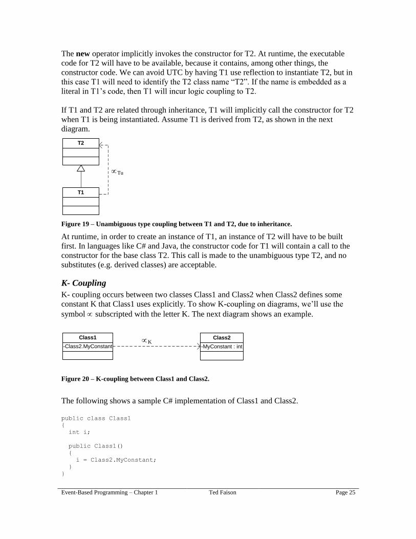
If T1 and T2 are related through inheritance, T1 will implicitly call the constructor for T2
when T1 is being instantiated. Assume T1 is derived from T2, as shown in the next
diagram.
T2
T1
Tu
Figure 19 – Unambiguous type coupling between T1 and T2, due to inheritance.
At runtime, in order to create an instance of T1, an instance of T2 will have to be built
first. In languages like C# and Java, the constructor code for T1 will contain a call to the
constructor for the base class T2. This call is made to the unambiguous type T2, and no
substitutes (e.g. derived classes) are acceptable.
K- Coupling
K- coupling occurs between two classes Class1 and Class2 when Class2 defines some
constant K that Class1 uses explicitly. To show K-coupling on diagrams, we’ll use the
symbol subscripted with the letter K. The next diagram shows an example.
-Class2.MyConstant
Class1
-MyConstant : int
Class2K
Figure 20 – K-coupling between Class1 and Class2.
The following shows a sample C# implementation of Class1 and Class2.
public class Class1
{
int i;
public Class1()
{
i = Class2.MyConstant;
}
}
Event-Based Programming – Chapter 1 Ted Faison Page 26
public class Class2
{
public const int MyConstant = 5;
}
Listing 5 - An example of classes that are K-coupled.
K-coupling is similar to UTC, in that an explicit class name is called out with the name of
the constant. K-coupling is more benign than unambiguous type coupling, because the
compiler can often remove the former. To see how, consider what a compiler might do
when compiling Class1. When the symbol Class2.MyConstant is found, the compiler will
need to have access to Class2 to determine the constant’s value. The compiler might then
embed the value of MyConstant in the executable code of Class1. At runtime, Class1 will
no longer need access to Class2, since Class1 already knows the value of
Class2.MyConstant.
There are a few caveats with K-coupling. First, the constant appearing in Class1 must be
used by value, as shown in the previous listing. In some languages, it is possible to access
constants also by reference (i.e. using a pointer), in which case Class1 won’t know the
constant’s value until the pointer is initialized at runtime. If Class1 uses a pointer to get
the constant’s value, then the coupling between Class1 and Class2 is not considered K-
coupling. What type of coupling would it be? The answer depends on the constant’s type.
If the type is built-in, such as integer or Boolean, then Class1 will have no compile-time
coupling to Class2. If the constant is of a user-defined type, then Class1 will be type-
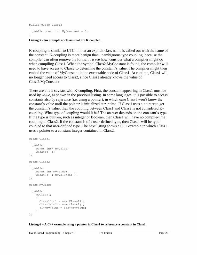
coupled to that user-defined type. The next listing shows a C++ example in which Class1
uses a pointer to a constant integer contained in Class2.
class Class1
{
public:
const int* myValue;
Class1() {}
};
class Class2
{
public:
const int myValue;
Class2() : myValue(5) {}
};
class MyClass
{
public:
MyClass()
{
Class1* c1 = new Class1();
Class2* c2 = new Class2();
c1->myValue = &c2->myValue;
}
};
Listing 6 – A C++ example using a pointer in Class1 to reference a constant in Class2.

Event-Based Programming – Chapter 1 Ted Faison Page 27
Class1 doesn’t know anything about Class2, so it can be compiled and run without the
presence of Class2. We’ll need to have Class2 present to compile MyClass. As long as
Class1.myValue is initialized to point to an integer value somewhere in the system,
Class1 will work. Of course, in order for Class1 to work correctly, the pointer will need
to point to not just any integer value, but to the right value, which is dependent on the
system requirements.
Just because T1 references a typed constant defined in T2 doesn’t necessarily entail the
presence of K-coupling between T1 and T2. The coupling is considered K-coupling only
when certain types are involved. Exactly which types qualify for K-coupling depends on
the programming language and the compiler. Common built-in types like Boolean,
integer, float and char are typically valid. In C#, all value types, which include structures,
are also valid, so if T1 references a constant structure defined in T2, K-coupling is
involved. Whether strings qualify for K-coupling depends on how the compiler treats
constant strings. Assume Class2 defined a constant string like this:
public class Class2
{
public const string MyString = "whatever";
}
Assume also that Class1 were defined like this:
public class Class1
{
string whatever;
public Class1()
{
string whatever = Class2.MyString;
}
}
The compiler can see that the string value in Class2 is constant. When compiling Class1,
the compiler might be able to embed the characters of the string “whatever” somewhere
in the executable code of the Class1. If so, then Class1 would be K-coupled to Class2. If
the compiler didn’t embed the characters in the Class1 code, it might generate code to use
a pointer to Class2.MyString, which would then induce unambiguous type coupling
between Class1 and Class2.
Ambiguous Type Coupling
If type coupling can be unambiguous, it might not be too surprising to learn that it can
also be ambiguous. If a class T1 contains a reference to a class T2, and T1 doesn’t create
any instances of T2, then T1 has ambiguous type coupling (ATC) to T2, as shown in the
next diagram.

Event-Based Programming – Chapter 1 Ted Faison Page 28
T1 T2references
Ta
Figure 21 – Ambiguous type coupling between T1 and T2.
As can been seen in the diagram, we use the symbol subscripted with the letters “Ta”
to denote ATC. The coupling is called ambiguous, because the reference in T1 can be set
to point to an instance of T2 or of a class derived from T2. The symbol Ta
is equivalent
to the phrase ambiguous type coupling. The next diagram shows T1 using a derived class
T3.
T3
T1 T2references
Ta
Figure 22 – An example of ambiguous type coupling between T1 and T2.
In order for T1 to use instances of T2 without creating them, T1 must receive the
instances from other objects. T1 might be given a T3 instance as a parameter in a method
call. Although T1 has no control over what type of object it gets, it knows one thing: the
instance must be of type T2 or a type derived from T2. With ambiguous coupling, T1 will
need T2 to be available at compile time. T1 might not require T2 at runtime, if the
compiler is able to bake a copy of T2 into T3, meaning that T2’s code is embedded
somehow inside T3’s code.
Platform Coupling
Component software is designed and implemented on top of a component platform, such
as the .Net Common Type System or the Java JDK. The platform includes built-in
components that provide commonly used services, such as memory management, file
operations and graphics primitives. The platform also defines a whole series of built-in
types. No meaningful software system can be developed without using at least some of
the built-in components and types. Consider the following trivial C# class.
class Class1
{
static void Main(System.String[] args)
{
System.Console.WriteLine("Ciao, Mondo");

Event-Based Programming – Chapter 1 Ted Faison Page 29
}
}
Class1 uses the class System.Console, contained in the built-in .Net Framework
component called System. Class1 also makes use of the built-in type System.String.
Class1 is therefore type-coupled to the classes System.Console and System.String, as
shown in the next diagram.
Class1platform type coupling
-WriteLine
System.Console
-
System.Stringplatform type coupling
Figure 23 – Type coupling between a user-defined class and a platform class.
There is no way to completely eliminate the coupling between Class1 and the built-in
classes and types, because the only way to perform standard console I/O in C# is via the
System component. We could replace System.String with a user-defined string class, but
this wouldn’t eliminate any coupling because the effect would only be to change what
Class1 is coupled to. We must accept the fact that the coupling between Class1 and the
built-in classes is not dependent on bad design, and generally can’t be avoided.
The coupling that exists between a component and a built-in type is a special case of type
coupling called platform type coupling, or simply platform coupling. All component
software incurs platform coupling, but this doesn’t typically reduce the quality of a
component or a component system. The assumption here is that the built-in components
and types are stable and well tested, but this may not always be the case. Java software
used to be particularly susceptible to problems caused by platform coupling. In the early
Java days, roughly between 1995 and 1998, new versions of the Java runtime
environment were released frequently, to add features like printing, online help, two-
dimensional graphics and others. With each new release, Sun Microsystems deprecated
certain methods and introduced others. Software written for a newer version of the
runtime would sometimes fail with an older version, if it called built-in services that the
older version didn’t support or that had been changed. The problem was due to the
platform coupling between the Java components and the Java runtime components. If the
software was developed on one version of the runtime and deployed on a different
version, there was always the potential for problems. The typical solution was to have
users upgrade to the version of the Java runtime that the system was written for.
Newer component platforms, such as the .Net Framework, reduce deployment headaches
related to runtime version dependencies by embedding information in each component
that identifies which version of the component platform it requires. If the required
platform is not available, the runtime will notify the user and prevent the affected
software from running.

Event-Based Programming – Chapter 1 Ted Faison Page 30
Mathematical Properties of Type Coupling
Let’s explore the most significant mathematical properties that apply to type coupling.
Theorem:
A T B B T A Type coupling is not commutative.
Proof: Let class A contain a reference to class B, while B contains no references to A.
Class A is therefore type-coupled to B. Class A can’t be compiled without B, but B can
be compiled without A.
Whether type coupling is transitive or not depends on the type of programming language
being used. We saw a similar situation when discussing transitivity of static coupling,
which shouldn’t be surprising, since type coupling generally has a static nature. With
languages like C++, that use separate declaration and implementation files for a class,
type coupling may be transitive. For languages like C# and Java, that use a single file for
the declaration and implementation of a class, static coupling is not transitive.
Theorem:
With languages that separate the class declaration from the implementation, static
coupling is transitive, if coupling is due to type references in the declaration.
Proof: The proof is analogous to the one given for static coupling. Assume we have three
C++ classes, A, B and C. Each class has a header file and an implementation file. We’ll
call the header files A.h, B.h and C.h. We’ll call the implementation files A.cpp, B.cpp
and C.cpp. Assume A.h contains a reference to class B, and that B.h contains a reference
to class C. With this arrangement, A is type-coupled to B and B is type-coupled to C.
When compiling A, the compiler will need to load the header file A.h, which references
B. When the compiler tries to load the declaration for B in B.h, it discovers the reference
to C, and must load C.h. As a result, to build A the compiler will need to access the
declarations for B and C. The implication is that, in this scenario, type coupling is
transitive.
Things change if the referenced types are not in header files but in implementation files.
Assume A.cpp contains a reference to B. It follows that A.cpp will need to include the
file B.h. Assume also that B.cpp contains a reference to C, so B.cpp will need to include
the file C.h. To compile B, the compiler will need C.h. To compile A, the compiler will
need B.h. This time, since B.h contains no references to C, so the compiler won’t need C.
The implication is that, in this scenario, type coupling is not transitive.
Theorem:
With languages that merge the class declaration and implementation together, type
coupling is not transitive.
Proof: Let class A contain a reference to class B, so A is type-coupled to B. Let class B
contain a reference to class C, so B is type-coupled to C. To compile B, we’ll need to
Event-Based Programming – Chapter 1 Ted Faison Page 31
have C. To compile A, we’ll need to have B, but not C, because A doesn’t reference
anything defined in class C. Everything the compiler needs to compile A is contained in
the compiled code for B.
Signature Coupling
As we have seen, type coupling is related to classes and interfaces, but there is a finer
level at which coupling can occur. If we look at the contents of a class, we find fields and
methods. It is reasonable to expect that coupling might occur not only at the class level,
but also at the field and method level. Fields are really just classes (or scalars) used inside
a class, so we can treat coupling to a field exactly like ordinary type coupling.
Methods are a completely different kind of entity from classes. They are not described by
a formal type, but by their signature. The signature specifies the number and types of
parameters passed to and from a method by a caller. When we write a method, we
implicitly define its signature. Just as an interface represents the type of an object, so a
signature represents the type of a method. As an example, consider the following C#
class:
public class A
{
public int GetAge(string theName)
{
// ...
}
}
The signature for the GetAge method is
int f(string theName)
There are three things missing from the signature:
The type to which the method belongs. Since signatures describe methods outside
the context of classes and interfaces, they don’t specify a class or interface.
The method’s access qualifier. The signature doesn’t have an access qualifier,
(e.g. public or private), because qualifiers don’t describe the method, but the
method’s accessibility, which a class-level property.
The method name. The signature doesn’t have any particular method name,
because signatures are abstract: they don’t identify a concrete method. A given
signature can apply to any number of methods. The letter ‘f’ was used in the
signature above to act as a placeholder for the method name.
In the signature, any word can be used as the method name, including the name of
particular method, so we could also write the signature of GetAge like this:
int GetAge(string theName)

Event-Based Programming – Chapter 1 Ted Faison Page 32
Any method that takes a single string argument as input and returns an integer will have
the same signature as A.GetAge.
Now that we know what a signature is, let’s see what signature coupling is. This flavor of
coupling occurs when one object makes an indirect call to a method in another object.
The caller must have a method reference that is initialized at runtime to point directly to a
method, bypassing any class interfaces of the callee. The following diagram shows two
classes that might be involved in signature coupling.
-methodReference
A
+Method1()
B
Figure 24 – Two classes with no relationships between them.
Class A has a field called methodReference that is used to make indirect calls to a
method. Although the class diagram doesn’t show the signature used by
A.methodReference, we’ll assume the signature is the same as that of B.Method1. The
class diagram reveals no information about coupling or other relationships between A and
B. A and B are completely decoupled from each other. It is perfectly possible that the
classes were implemented by different people, who didn’t or couldn’t predict that the
classes would ever be used together. Assume that at runtime there are instances of A and
B, called respectively object1 and object2, and that object1.methodReference is
initialized to point to object2.Method1, as shown in the next diagram.
methodReferenceobject1: A
object2: B
Method1()
S
Figure 25 – Objects coupled through a method signature.
At runtime, object1 becomes signature-coupled to object2, due to the method reference
pointing at object2.Method1. The only thing that object1 and object2 must agree on is
that the signature used by object1.methodReference match the signature of
object2.Method1.
Definition 3
Signature coupling occurs when one object has a reference pointing to a method in
another object.
Signature coupling is designated using the symbol subscripted with an uppercase S, as
shown in the previous diagram. The symbol S is equivalent to the phrase signature
coupling (SC). When one object is signature-coupled to another, the former requires the
latter to be present at runtime. The system shown in the figure might be implemented
using the following C# code:
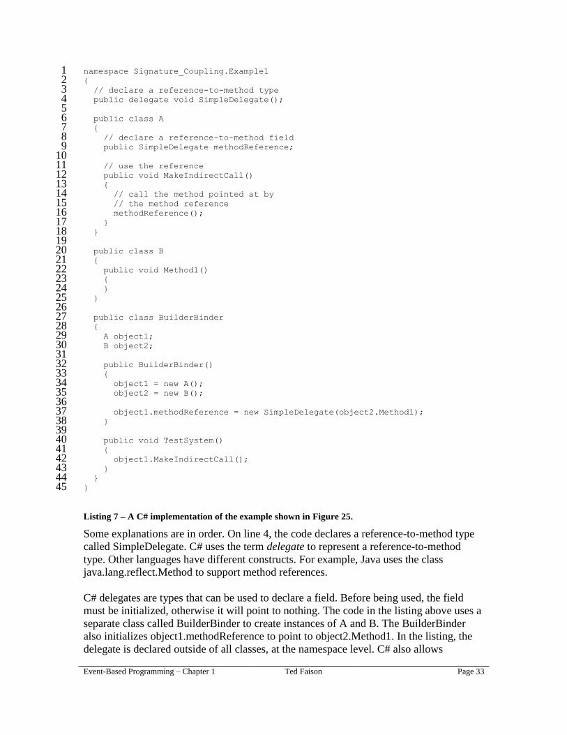
Event-Based Programming – Chapter 1 Ted Faison Page 33
namespace Signature_Coupling.Example1 1 { 2 // declare a reference-to-method type 3 public delegate void SimpleDelegate(); 4 5 public class A 6 { 7 // declare a reference-to-method field 8 public SimpleDelegate methodReference; 9 10 // use the reference 11 public void MakeIndirectCall() 12 { 13 // call the method pointed at by 14 // the method reference 15 methodReference(); 16 } 17 } 18 19 public class B 20 { 21 public void Method1() 22 { 23 } 24 } 25 26 public class BuilderBinder 27 { 28 A object1; 29 B object2; 30 31 public BuilderBinder() 32 { 33 object1 = new A(); 34 object2 = new B(); 35 36 object1.methodReference = new SimpleDelegate(object2.Method1); 37 } 38 39 public void TestSystem() 40 { 41 object1.MakeIndirectCall(); 42 } 43 } 44 } 45
Listing 7 – A C# implementation of the example shown in Figure 25.
Some explanations are in order. On line 4, the code declares a reference-to-method type
called SimpleDelegate. C# uses the term delegate to represent a reference-to-method
type. Other languages have different constructs. For example, Java uses the class
java.lang.reflect.Method to support method references.
C# delegates are types that can be used to declare a field. Before being used, the field
must be initialized, otherwise it will point to nothing. The code in the listing above uses a
separate class called BuilderBinder to create instances of A and B. The BuilderBinder
also initializes object1.methodReference to point to object2.Method1. In the listing, the
delegate is declared outside of all classes, at the namespace level. C# also allows
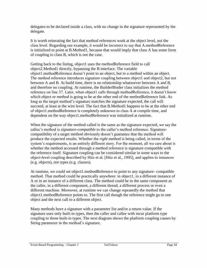
Event-Based Programming – Chapter 1 Ted Faison Page 34
delegates to be declared inside a class, with no change in the signature represented by the
delegate.
It is worth reiterating the fact that method references work at the object level, not the
class level. Regarding our example, it would be incorrect to say that A.methodReference
is initialized to point at B.Method1, because that would imply that class A has some form
of coupling to class B, which is not the case.
Getting back to the listing, object1 uses the methodReference field to call
object2.Method1 directly, bypassing the B interface. The variable
object1.methodReference doesn’t point to an object, but to a method within an object.
The method reference introduces signature coupling between object1 and object2, but not
between A and B. At build time, there is no relationship whatsoever between A and B,
and therefore no coupling. At runtime, the BuilderBinder class initializes the method
reference on line 37. Later, when object1 calls through methodReference, it doesn’t know
which object or method is going to be at the other end of the methodReference link. As
long as the target method’s signature matches the signature expected, the call will
succeed, at least at the wire level. The fact that B.Method1 happens to be at the other end
of object1.methodReference is completely unknown to class A at compile time, and
dependent on the way object1.methodReference was initialized at runtime.
When the signature of the method called is the same as the signature expected, we say the
callee’s method is signature-compatible to the caller’s method reference. Signature-
compatibility of a target method obviously doesn’t guarantee that the method will
produce the expected results. Whether the right method is being called, in terms of the
system’s requirements, is an entirely different story. For the moment, all we care about is
whether the method accessed through a method reference is signature-compatible with
the reference itself. Signature coupling can be considered similar in some ways to the
object-level coupling described by Hitz et al. [Hitz et al., 1995], and applies to instances
(e.g. objects), not types (e.g. classes).
At runtime, we could set object1.methodReference to point to any signature- compatible
method. That method could be practically anywhere: in object1, in a different instance of
A or in an instance of a different class. The method could be in the same component as
the caller, in a different component, a different thread, a different process or even a
different machine. Moreover, at runtime we can change repeatedly the method that
object1.methodReference points to. The first call though the reference might go to one
object and the next call to a different object.
Many methods have a signature with a parameter list and/or a return value. If the
signature uses only built-in types, then the caller and callee with incur platform type
coupling to those built-in types. The next diagram shows the platform coupling causes by
String parameter in the method’s signature.

Event-Based Programming – Chapter 1 Ted Faison Page 35
object2: B
object1: A Method1(System.String)methodReference
-
System.Stringplatform
type coupling
platform
type coupling
Figure 26 – Platform coupling introduced by method parameters.
If the types used in the method signature are user-defined types, then the caller and callee
will both be type coupled to the components containing the user-defined types, as shown
in the next diagram.
object2: B
object1: A Method1(MyType)methodReference
-
MyType
T T C1
Figure 27 – Type coupling introduced user-defined parameters in the target method signature.
The presence of user-defined types introduces compile-time coupling issues. If MyType
is changed, then A and B may be affected, requiring them to be changed and recompiled.
We’ll look at more details later in this chapter, in the section titled “Coupling with User-
Defined Types”.
Signatures as Types
We stated earlier that signatures are to methods as interfaces are to objects: both
signatures and interfaces are types. Let’s look at this parallelism a bit more. Consider a
class A that is ambiguously type-coupled to an interface B, as shown in the next diagram.
ATa
«interface»
B
Figure 28 – Type coupling between a class and an interface.
A is coupled ambiguously to B, meaning that A can accept an instance of any class that
implements B or implements an interface derived from B. Let C be one of these classes.
Let’s assume that A doesn’t create instances of C, but rather receives a reference to it
from another object we’ll call a Builder (not shown in the diagram). The next figure
shows the coupling diagram.

Event-Based Programming – Chapter 1 Ted Faison Page 36
ATa
«interface»
B
C
Figure 29 – Adding a derived class to the system.
All A knows about the object it receives from the Builder is that the object implements
the interface B. Class A will treat this object exactly as if it were an instance of B. What
is interesting about the diagram is the fact that there is absolutely no coupling between
classes A and C. Although A requires B to be present at compile time, it doesn’t require
C. In fact, A knows nothing about the existence of C.
Let’s now compare the coupling between a class and interface with the coupling between
a method reference and a method signature. Assume a class C1 has a method reference
that defines a certain signature S1. If we considered the signature a type, we could
describe the system using the following diagram.
«signature»
S1-methodReference : S1
C1T
Figure 30 – Signature coupling as a form of type coupling.
The method reference in C1 is coupled to S1, causing C1 to be coupled to S1. In the
context of coupling, we can treat signatures like types, albeit special types. For starters,
signatures don’t support inheritance: We can’t derive one signature from another, so
signatures can’t be arranged in a hierarchy. If inheritance doesn’t apply to signatures,
then signature coupling is always unambiguous. Why? Because if a method reference
defines a given signature, it can be pointed only at methods with that exact signature,
since derived signatures are not possible.
To reinforce the notion of signatures as types, consider they way objects use references to
typed objects at runtime, as shown in the next diagram.
MyType
Object or
Method
myReference:MyType
implements
T

Event-Based Programming – Chapter 1 Ted Faison Page 37
Figure 31 – The relationship between a typed object, the type and the type’s implementation.
The item myReference is assumed to be a field of a class. If MyType is a class or
interface, then at runtime we can point myReference at any object that implements the
class or interface. If MyType is a signature, then at runtime we can point the reference at
any method that implements the signature. In both cases, we can use myReference to call
a method. In the first case, we can call any method defined by the interface. In the second
case, we can only call one method. From this perspective, a signature looks a lot like an
interface that only defines one method.
Mathematical Properties of Signature Coupling
Let’s explore the most significant mathematical properties that apply to signature
coupling. Given the fact that signatures are special types, we can expect the properties of
signature-coupling to have similarities with those of type-coupling, while keeping in
mind that signature coupling only applies to objects – never to classes.
Theorem:
instA S instB instB S instA Signature coupling is not commutative.
Proof: Let A and B be two classes, while instA and instB are instances of the classes.
Assume class B has a single method and that at runtime a method-reference in instA is
initialized to point to the method in instB. After initialization, instA is signature-coupled
to instB, because instA contains a pointer referencing a method of instB. Since there is no
reference from instB to any method of instA, there is no signature coupling between
instB and instA.
Theorem:
(instA S instB) and (instB S instC) (instA S instC)
Signature coupling is not transitive.
Proof: Let A, B and C be three classes, while instA, instB and instC are instances of the
classes. At runtime, a method-reference in instA is initialized to point to a method in
instB, and a method-reference in instB is initialized to point to a method in instC. After
initialization, instA is signature-coupled to instB, because instA has a reference to a
method in instB. Similarly, instB is signature-coupled to instC, because instB has a
reference to a method in instC. We can then deduce that instA is not signature-coupled to
instC, because instA has no references to methods in instC.
Coupling Space
Throughout this chapter we have seen various flavors of coupling. If there were only one
flavor, then we might be able to measure coupling using a simple number, e.g. 49. The
value would tell us how coupled one entity is to another entity. Since there are multiple
flavors of coupling, we need to measure the amount of coupling for each flavor
separately. We have seen that there are three basic coupling flavors: logic-, type- and
signature-coupling. Logic coupling also has two main subflavors: literal and algorithmic.

Event-Based Programming – Chapter 1 Ted Faison Page 38
Type coupling has two main subflavors: ambiguous and unambiguous. Signature
coupling has no subflavors.
To measure the coupling of a class, we need to measure the value of the five coupling
values: Ll, La, Ta, Tu, and s. We can consider these five entities as dimensions in a
5-dimensional coupling space, and mathematically treat the space like a vector space.
Because we’re dealing with five dimensions, we can’t easily represent coupling space on
a single graph. We can use two Cartesian planes to show the bi-dimensional logic- and
type-coupling spaces, as shown in the next figure.
A) The T plane.
Tu
Ta
Ll
La
B) The L plane.
Figure 32 - The logic- and type-coupling planes of coupling space.
The fifth dimension in coupling space – signature coupling – would require a single axis
to be graphed, or just a single scalar value. Ll, La, Ta, Tu, and s can be used as unit
vectors in our coupling space because, in linear algebra terms, they are linearly
independent. Given two entities P and Q of a vector space, they are said to be linearly
independent if one can’t be written as a linear combination of the other. In other words,
there are no values that added to or multiplied by P can give Q.
How do we measure coupling for each dimension? The previous material in this chapter
has provided us with qualitative information about coupling, but not quantitative. The
approach we’ll use to measure coupling for a given dimension is by counting every single
occurrence of coupling in that dimension. For example, in the ATC dimension we would
count every ambiguous reference to all external types. If a class T1 had two ambiguous
references to class T2 and three to class T3, we would to say that T1’s ATC value is 5,
assuming T1 had no other ambiguous references to other classes. If we found three
algorithms in T1 that were logically coupled to three algorithms in T2, we would say the
T1’s ALC value is three, again assuming T1 had no other logic coupling to other classes.
We’ll use the same approach for the other three coupling dimensions.
Since we get the value of coupling for each dimension by counting coupling occurrences,
the domain for each dimension is the set of all non-negative integers. The value must be
zero or greater than zero. For example, the value for Tu might be 0, or 4, but it can’t be
1.2 or -5. Let’s summarize what we now know about coupling space.
1. It is a discrete space.
2. It is defined only in one quadrant.

Event-Based Programming – Chapter 1 Ted Faison Page 39
A discrete space is not continuous – it includes only specific points. In coupling space,
the value of each dimension is restricted to whole numbers. Moreover, those numbers
must be non-negative, so the domain for the space is the 5-dimensional quadrant in which
all values are zero or positive.
The five components of coupling define a vector, pointing from the origin of coupling
space to a specific point. We can compute the magnitude of coupling in the logic - and
type-coupling planes using standard vector algebra, as shown in the following two
equations.
(Equation 1) 22
LaLlL
(Equation 2) 22
TaTuT
Sometimes we may not be interested in dealing with the individual components of logic
and type coupling. All we care about is the magnitude of L and T. In such cases, we
can depict coupling space using a simplified three-dimensional graph, with L, T and
S as the dimensions, as shown in the next figure.
S
L
T
Figure 33 – Coupling space, reduced to a three-dimensional space.
The three dimensions are still linearly independent, so we also can consider this
simplified space a vector space, like the full five-dimensional space. The overall coupling
magnitude is defined as follows:
(Equation 3) 222
STL
Although the coupling magnitude only gives us a basic feel for a class’ level of coupling,
what really count are the magnitudes of the three coupling flavors L, T or S. In most
cases, logical coupling is more undesirable than type coupling, and type coupling is
sometimes more undesirable than signature coupling. Later in the chapter, we’ll look at
coupling transforms, which define ways to convert one coupling flavor into another.
Using coupling transforms, we can reduce the amount of coupling in one dimension at
the expense of other dimensions, allowing us to custom tailor the kind and amount of
coupling a class incurs in each dimension.

Event-Based Programming – Chapter 1 Ted Faison Page 40
Coupling Charts
We started the previous section by saying that coupling is not measured as a simple scalar
value, however we could use the magnitude to indicate the overall coupling value. The
value itself doesn’t tell us how a class is coupled, nevertheless it does give us an overall
sense of how coupled something is to other parts of the system. If we had to refactor the
most coupled classes in a system, we might compute the coupling magnitude for each of
the classes and put them in a table, sorted by magnitude. A class that has a much higher
magnitude than average may be trying to accomplish too much, and might need to be
split into a series of simpler classes.
To analyze the coupling in a system, a sorted table of magnitudes doesn’t give us a good
picture of the overall coupling of a system. A better approach is to use a bar chart, in
which the vertical axis measures the coupling magnitude, and each vertical bar shows the
magnitude of a class. The next figure shows what the coupling chart might look like for a
system containing five classes.
0
2
4
6
8
10
12
14
16
A B C D E
Class
Co
up
lin
g M
ag
nit
ud
e
Figure 34 - A coupling chart for a system having five classes.
The chart gives us an immediate bird’s eye view of the distribution of coupling in a
system. Given that coupling can be distributed in any way among the classes (and
therefore the components) of a system, is there a type of distribution that is better than
others? Is there a pattern we should be looking for in a coupling chart? Consider the
systems represented by the two coupling charts in the next figures.

Event-Based Programming – Chapter 1 Ted Faison Page 41
Figure 35 - A system with evenly distributed coupling.
Figure 36 - A system with unevenly distributed coupling.
Which distribution is more desirable? While it might appear than an even distribution is a
good thing, this is not the case. Remember axiom 2, stated at the beginning of the
chapter: Coupling should be introduced into simpler components first. If we distributed
complexity unevenly across the components of a system, we could concentrate
complexity in some components and keep other components simple. We would then want
to offload coupling from the more complex components by transferring it to the simpler
ones. As we’ll see in later chapters, class factories (which we call Builders in this book)
are extremely simple components, whose only task is to create instances of other classes.
A Builder incurs unambiguous type coupling to each class or type it instantiates, so
Builders tend to be heavily coupled. Using one or more Builders to create all the classes
of a system, we could offload a great deal of coupling from the classes that do the heavy
lifting work in a system. As a result, the coupling chart would show a small number of
classes (the Builders) with a very large coupling magnitude. The other classes would
have a small amount of residual coupling.

Event-Based Programming – Chapter 1 Ted Faison Page 42
Coupling Diagrams
A coupling diagram shows what is coupled to what, and how. Coupling is shown as a
dependency, using the coupling symbols introduced in earlier sections. The following
figure shows the coupling diagram for a simple component system.
C3C2C1
C4
Ta
Ta
Tu
Tu
La
Tu
Figure 37- A simple coupling diagram.
Logical coupling is always commutative, so it uses a double-headed arrow. Knowing the
exact flavor and subflavor of coupling we’re dealing with allows us to spot trouble, such
as the occurrence of circular coupling or complicated coupling relationships. By studying
a coupling diagram, we can decide where to intervene to alleviate coupling, by applying
the coupling transforms described in the next section. When there are multiple couplings
of the same flavor between two classes or components, we can show the exact count on
coupling diagrams by prefixing the coupling symbol with a count, in parenthesis, so we
might have a coupling arrow with the legend (10) Ta
, meaning there are ten separate
ambiguous references between one class and another. The next diagram shows a simple
example.
C2C1
(10) Ta
Figure 38- A coupling diagram showing ten ambiguous type references between C1 and C2.
Coupling diagrams are useful because they show how coupling propagates through a
system. Some coupling flavors are transitive and some aren’t. Each flavor has its own
impact on a system, so sometimes it is a good idea to draw multiple diagrams for a
system, showing only one flavor on each diagram.
A particularly interesting coupling diagram is the one that shows static coupling. We
know that static coupling affects build-time, so classes that are statically coupled may

Event-Based Programming – Chapter 1 Ted Faison Page 43
need to be changed simultaneously. If statically coupled classes are assigned to different
teams and team members, those teams and team member might have to work in a
coordinated fashion, otherwise changing one class might break the compilation of
another. Forcing team members to work this way can be a source of problems, both
logistical and inter-personal. The larger the project, the greater the problems. By looking
at the static coupling diagram of a system, we can spot couplings that cross team or
component boundaries. We might then be able to find ways to refactor the design, to
either eliminate the coupling entirely, or convert it into a more benign coupling flavor.
Coupling Transforms
While the dimensions of coupling space are all linearly independent, it is possible to
convert one coupling flavor into another, using a coupling transform. Mathematically, a
coupling transform is a function that maps a point P0 in coupling space to a new point P1.
Coupling transforms allow us to convert undesirable flavors of coupling into more
tolerable flavors. Since coupling can never be eliminated completely from an entire
system, a coupling transform typically reduces coupling in one dimension at the expense
of coupling in one or more other dimensions.
Using transforms, it becomes possible to alter the design of a system and reduce the
coupling between its components, assuming we have access to the source code. The
coupling transforms described in this chapter could be built into a tool that applies the
transforms in an automated way. The resulting system would have the same overall
functionality as the old one, with less coupling between the parts.
How malignant a certain flavor of coupling is depends often on the characteristics of the
software system being built, but in general the following two statements are true:
1. Logic coupling is less desirable than type coupling.
2. Static coupling is less desirable than dynamic coupling.
The first statement is usually true because compilers can’t detect logic coupling, at least
with current technology. Assume a system has coupled logic in two places, A and B. If
we change A, but not B, the compiler will not help us detect the fact that B is out of sync
with A. We’ll find the problem later, when we test the system.
The second statement is usually true because static coupling affects build time. If a class
A is statically coupled to a class B, then changing B can break the compilation of A.
Static coupling forces the teams working on A and B to work in coordination, so changes
to A and B are made at the same time.
From the standpoint of flexibility and impact on build-time, often the most desirable form
of coupling is signature coupling. Although it is possible to convert all forms of coupling
into signature coupling, it may not always be advisable to do so, because conversions
generally come at the expense of performance, complexity and loss of compiler type-
checking.

Event-Based Programming – Chapter 1 Ted Faison Page 44
Logic Coupling Transforms
As stated on numerous occasions, logic coupling is usually more detrimental to a system
than type coupling for two reasons. Logic coupling is often caused by duplications of
some sort in the source code, and is invisible to the compiler.
Duplications are bad, because they complicate the system and make it more difficult to
maintain. If a bad piece of code is duplicated in two places, A and B, we’ll need to fix
both. Since a system doesn’t usually keep track explicitly of where duplications occur, it
is easy for a programmer to change one of the occurrences, but not all. Since logic
coupling is invisible to the compiler, the burden is on the programmers to make sure that
a piece of code that is changed isn’t associated with a duplicate elsewhere in the system.
Converting LLC to UTC
Literal logic coupling occurs between two classes A and B if those classes both embed
their own private copy of a value that is used for the same purpose. We’ll look at a simple
transform to convert LLC to unambiguous type coupling, using an example. Assume A
creates a message that B subsequently reads. If A can create different types of messages,
there might be a reserved spot in the message to designate the message type. Assume A
and B are implemented in C# like this:
public class A
{
public void SendVehicleSoldMessage(byte[] theMessage)
{
const int MessageTypeIndex = 0;
const byte VehicleSoldMessage = 15;
theMessage[MessageTypeIndex] = VehicleSoldMessage;
// ... write the rest of the message
}
}
public class B
{
public void ProcessMessage(byte[] theMessage)
{
const int CommandCodeIndex = 0;
const int CarSoldMessage = 15;
byte commandCode = theMessage[CommandCodeIndex];
if (commandCode == CarSoldMessage)
// ... handle the message
}
}
Listing 8- Two classes that have literal logic coupling.
The coupling diagram for A and B is shown in the next figure.
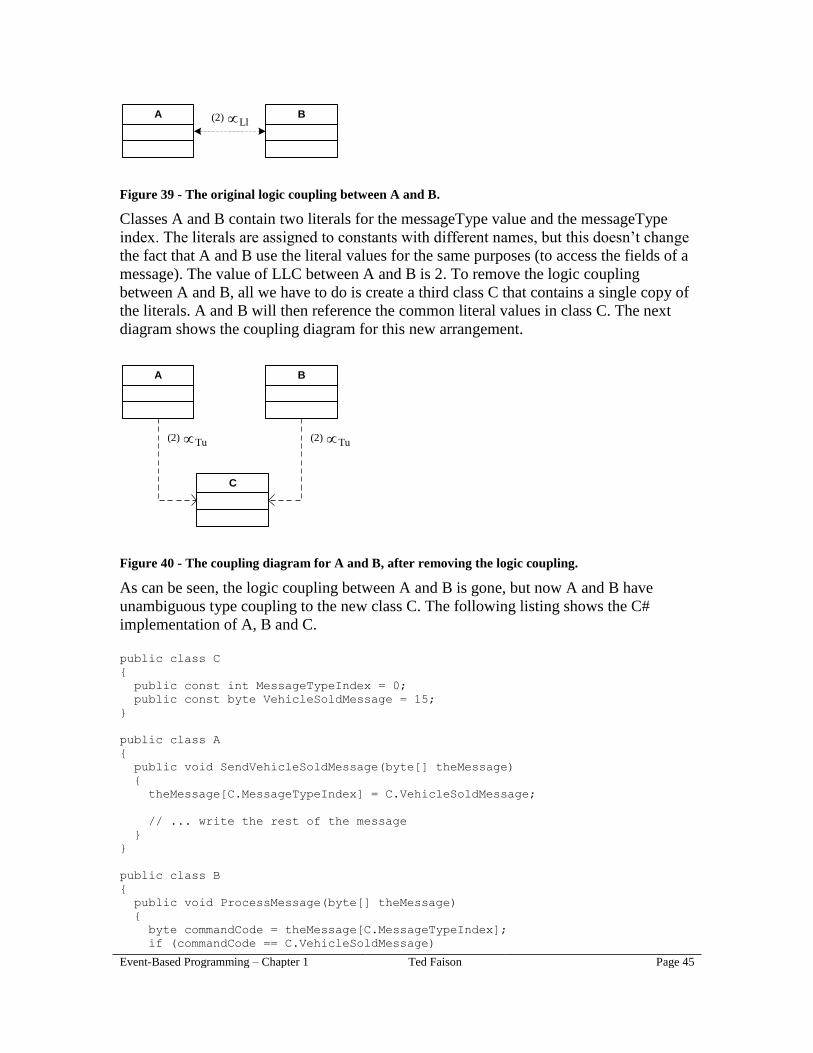
Event-Based Programming – Chapter 1 Ted Faison Page 45
A B(2) Ll
Figure 39 - The original logic coupling between A and B.
Classes A and B contain two literals for the messageType value and the messageType
index. The literals are assigned to constants with different names, but this doesn’t change
the fact that A and B use the literal values for the same purposes (to access the fields of a
message). The value of LLC between A and B is 2. To remove the logic coupling
between A and B, all we have to do is create a third class C that contains a single copy of
the literals. A and B will then reference the common literal values in class C. The next
diagram shows the coupling diagram for this new arrangement.
A B
C
(2) Tu (2) Tu
Figure 40 - The coupling diagram for A and B, after removing the logic coupling.
As can be seen, the logic coupling between A and B is gone, but now A and B have
unambiguous type coupling to the new class C. The following listing shows the C#
implementation of A, B and C.
public class C
{
public const int MessageTypeIndex = 0;
public const byte VehicleSoldMessage = 15;
}
public class A
{
public void SendVehicleSoldMessage(byte[] theMessage)
{
theMessage[C.MessageTypeIndex] = C.VehicleSoldMessage;
// ... write the rest of the message
}
}
public class B
{
public void ProcessMessage(byte[] theMessage)
{
byte commandCode = theMessage[C.MessageTypeIndex];
if (commandCode == C.VehicleSoldMessage)
Event-Based Programming – Chapter 1 Ted Faison Page 46
// ... handle the message
}
}
Listing 9- The refactored system, after eliminating logic coupling between A and B.
With the conversion, we actually increased the magnitude of coupling in the system. Now
A has no LLC to B, but there are no 4 units of UTC in the system (2 between A and C
and 2 between B and C). Is the new implementation better than the original one? It
depends on what metrics we use to define better. The original implementation had only
two classes, so it had fewer parts, but the parts contained duplicated logic. On the other
hand, the new implementation has three classes, but those classes contain no duplicated
logic.
The new implementation will probably be easier to maintain, if changes are made to the
literal values stored in C, because there is only one set of literals in the system, instead of
two. Classes A and B wind up being unambiguously type coupled to C, because A and B
use constants defined in C. By looking at the example, we can derive the pattern used in
this LLC-to-UTC transform.
Pattern for converting LLC into UTC
If two classes, A and B, contain duplicate literals, do the following:
1. Remove the duplicated values from A and B.
2. Migrate the values to a third class C.
3. Change A and B to use the common values stored in C.
Note that other transforms exist to convert LLC into UTC. For example, we could have
left the literal definitions in class A and referenced them from class B. Doing so would
have saved us the trouble of creating a third class, but might introduce other problems.
For example, if B had had LLC with another class D, where would we put the literals
shared by B and D? Either B or D. By introducing a third class C, we have a common
place to store all the literals that might be shared by many other classes. The moral of the
story is that there is no single transform that is universally best.
Converting LLC to ATC
The previous pattern produced unambiguous type coupling to a third class. A less
constraining flavor of type coupling is ambiguous type coupling, so let’s see how we
might convert LLC to ATC. Let’s assume we start with the same two classes A and B
shown in Listing 8. We’ll continue to use the class approach described in the previous
section, using a third class named C. Rather that exposing two constants, C will expose
two fields or properties that are initialized using private embedded literals. Class C might
look like this:
public class C
{
public int MessageTypeIndex = 0;
public byte VehicleSoldMessage = 15;
Event-Based Programming – Chapter 1 Ted Faison Page 47
}
Listing 10- A new class to store the literal values that were duplicated in A and B.
The class is almost identical to class C in the previous section, but the new
implementation stores the literal values in fields instead of constants. As a result, classes
A and B need an instance reference (instead of a class reference) for class C, as shown in
the next listing.
public class A
{
public C c; // must be initialized at runtime
public void SendVehicleSoldMessage(byte[] theMessage)
{
theMessage[c.MessageTypeIndex] = c.VehicleSoldMessage;
// ... write the rest of the message
}
}
public class B
{
public C c; // must be initialized at runtime
public void ProcessMessage(byte[] theMessage)
{
byte commandCode = theMessage[c.MessageTypeIndex];
if (commandCode == c.VehicleSoldMessage)
{
// ... handle the message
}
}
}
Listing 11- The new implementation for class A and B,.
The new A and B classes now contain a field of type C. This field must be initialized at
runtime, but can point to an object of type C or derived from C. Since any class derived
from C can be used, the type coupling between from A and B to C is ambiguous. A
separate class Z might initialize the fields in A and B like this:
public class D : C
{
// ...
}
public class Z
{
void InitializeAandB()
{
A a = new A();
B b = new B();
D d = new D();
a.c = d;
b.c = d;
}
}

Event-Based Programming – Chapter 1 Ted Faison Page 48
Listing 12- Using a separate class to initialize A and B.
The new code binds A and B to an instance of a class D, derived from C. The next figure
shows the coupling diagram between all the classes, after transforming LLC into ATC.
A B
C
(2) Ta
D
(2) Ta
Figure 41 - The coupling diagram for A and B, after removing the logic coupling.
As can be seen, it’s a bit more complicated to transform LLC into ATC, compared to
UTC, because A and B need to reference C by instance instead of by type. As in the
previous transform, we swapped 2 units of LLC for 4 units of type coupling, but this time
the type coupling is ambiguous. By looking over the example, we can derive the pattern
used in this LLC-to-ATC transform.
Pattern for converting LLC into ATC
If two classes, A and B, contain duplicate literals, do the following:
1. Remove the duplicated values from A and B.
2. Migrate the values as initialized fields into a third class C,
3. Change A and B to access the fields using a reference to C.
4. Initialize the reference to point to an object of type C or derived from C.
There are other ways to transform LLC into UTC. One interesting alternative is to use
virtual methods in C to return the value of the literals. By doing so, derived classes would
have the opportunity to change the literal values by overriding the base class virtual
methods.
Converting ALC to UTC
Just as LLC can be converted into type coupling, so can ALC. The ALC transforms have
many similarities with the LLC counterparts discussed in the previous two sections.

Event-Based Programming – Chapter 1 Ted Faison Page 49
As a practical example of a transform, let A and B be classes that contain complementary
algorithms to read and write data in a file. Class A contains the write algorithm, while B
contains the read algorithm. The next figure shows the coupling diagram for A and B.
+WriteFile()
A
+ReadFile()
BLa
Figure 42 - The coupling diagram for A and B, due to complementary algorithms.
Regardless of whether the coupled algorithms are complementary or equipotent, the
solution is the same: To package the coupled algorithms in the same class, as shown in
the next diagram.
A B
+WriteFile()
+ReadFile()
C
Ta Ta
Figure 43 - The system after removing the logic coupling between A and B.
The new implementation will probably be easier to maintain, because anyone changing
the WriteFile algorithm will be able to immediately change the ReadFile algorithm as
needed. The drawback of the transform is that the new system is slightly more complex
than the original one, because it has an additional class. By looking at the example, we
can derive the pattern used in this ALC-to-UTC transform.
Pattern for converting ALC into UTC
If two classes, A and B, contain logically coupled algorithms, do the following:
1. Remove the coupled algorithms from A and B.
2. Migrate the algorithms to a third class C.
3. Change A and B to reference the algorithms in C.
While it is always theoretically possible to eliminate ALC using the transform described,
in some cases it may not be practical or advisable. For example, consider a distributed
system in which components C1 and C2 are on different computers, connected over the
Internet. C1 is on a secure server, while C2 is on client machines that aren’t secure. C1
uses a proprietary encryption algorithm to send messages to C2, while C2 never sends
data back to C2, as shown in the next figure.

Event-Based Programming – Chapter 1 Ted Faison Page 50
C1
+Encrypt()
A
C2
+Decrypt()
Bencrypted messages
Internet
Figure 44 - The system after removing the logic coupling between A and B.
To use the ALC-to-UTC transform described, we would need to create a third class C and
put both the encryption and decryption algorithm in it. Our first problem is to decide
where class C should live. We have three options:
In C1.
In C2.
In a separate component C3.
The first and second arrangements are out of the question, for security reasons, because it
would entail that data would be sent over the Internet in clear text. To see how, let’s
assume C were placed on the secure computer, in component C1. Class A would call
C.Encrypt to encode messages before sending them. When B got the encrypted message,
it would have to make a remote procedure call to C.Decrypt, which would return the
decrypted message over the Internet. A similar result would occur if we put C in
component C2.
Putting class C in a separate component C3 is also problematic, because this third
component would need to be accessible to A and B. The connection to C would need to
be secure, as shown in the next figure, because it would carry both encrypted an
unencrypted messages.
C1
A
C2
Bencrypted messages
C3
+Encrypt()
+Decrypt()
C
Internet
secure connection
Event-Based Programming – Chapter 1 Ted Faison Page 51
Figure 45 – Using a third component C3 to house class C, with the encryption algorithms.
In many cases, the necessity of a secure connection between C1/C2 and C3 will render
the design impractical, because of its cost or the complexity of the resulting system.
Assuming we did opt to create a secure connection, we would no longer need the
encryption algorithms in the first place! We might realize that the system had originally
been designed to use encryption so it could rely on an inexpensive and easily available
Internet connection to send messages from A to B. Attempting to package the encryption
and decryption algorithms in a common class C is simply not a viable economic
alternative.
In this section, we showed how to convert ALC into UTC. We won’t show how to
convert ALC into ATC using a single transform, because we can achieve the same goal
by first converting ALC into UTC, and then converting UTC into ATC. We’ll show how
to perform the latter conversion in the next sections.
Type Coupling Transforms
Type coupling is usually easier than logic coupling to deal with in a system, because the
compiler can check types to prevent us from making type-related mistakes. For example,
if a class A supported the methods M1 and M2, the compiler would issue an error if we
tried to compile code containing a call to A.M3. Also, the compiler will tell us if we pass
the wrong number or type of parameters in a call to A.M1 or A.M2.
In a type-coupled system, the compiler will also protect us from partial changes. For
example, if we modified class A by removing M1 or changing the method’s signature, we
might forget to change all the code that invokes the method. The compiler will refuse to
compile some of the code, showing us where the discrepancies are.
Of the two subflavors of type coupling - unambiguous and ambiguous - the latter is often
more desirable than the former, because it provides more flexibility, so knowing how to
convert UTC into ATC is very important. All forms of type coupling are static in nature.
In later sections, we’ll show how to eliminate static coupling by converting it into
signature coupling, which is dynamic and in some cases eliminates type coupling
entirely.
Converting UTC to ATC
If a class A references another class B, UTC occurs when A can only work if B itself is
present. Classes derived from B are not acceptable to A. As we saw in the section
Unambiguous Type Coupling, the two most common ways T1 will have UTC to T2 are
the following:
1. A is derived from B.
2. A creates instances of B.
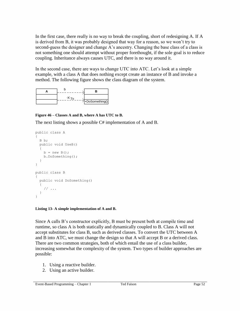
Event-Based Programming – Chapter 1 Ted Faison Page 52
In the first case, there really is no way to break the coupling, short of redesigning A. If A
is derived from B, it was probably designed that way for a reason, so we won’t try to
second-guess the designer and change A’s ancestry. Changing the base class of a class is
not something one should attempt without proper forethought, if the sole goal is to reduce
coupling. Inheritance always causes UTC, and there is no way around it.
In the second case, there are ways to change UTC into ATC. Let’s look at a simple
example, with a class A that does nothing except create an instance of B and invoke a
method. The following figure shows the class diagram of the system.
A
+DoSomething()
B
Tu
b
Figure 46 – Classes A and B, where A has UTC to B.
The next listing shows a possible C# implementation of A and B.
public class A
{
B b;
public void UseB()
{
b = new B();
b.DoSomething();
}
}
public class B
{
public void DoSomething()
{
// ...
}
}
Listing 13- A simple implementation of A and B.
Since A calls B’s constructor explicitly, B must be present both at compile time and
runtime, so class A is both statically and dynamically coupled to B. Class A will not
accept substitutes for class B, such as derived classes. To convert the UTC between A
and B into ATC, we must change the design so that A will accept B or a derived class.
There are two common strategies, both of which entail the use of a class builder,
increasing somewhat the complexity of the system. Two types of builder approaches are
possible:
1. Using a reactive builder.
2. Using an active builder.

Event-Based Programming – Chapter 1 Ted Faison Page 53
Let’s look at each approach separately.
Using a Reactive Builder
A builder works in reactive mode if it creates objects on demand and returns them to
client objects. The builder is not responsible for deciding when to create objects. Reactive
builders are similar to the Builder OO design pattern (Gamma et al, 1995). The following
diagram shows how we might use a reactive builder to solve the UTC-to-ATC transform
problem.
A
Builder B
T
Tu
Ta
Figure 47 – Using a reactive builder to eliminate Tu between A and B.
Class A delegates to Builder the task of B objects, so A calls Builder when it needs an
instance of B. Is this new design better than the original one? Let’s look at the pros and
cons. On the pro side, A is less strongly coupled to B than before, because now it has
ambiguous coupling instead of unambiguous. Also, the Builder makes the system more
flexible, because the Builder might provide A with objects of classes derived from B, that
provide features that B didn’t provide. On the con side, A is now coupled to two classes:
B and Builder. The subflavor of type coupling that occurs between A and Builder will
depend on whether A instantiates the Builder (causing Tu) or receives a reference to
Builder from another object (causing Ta).
We’re now in a position to state the first Builder pattern for converting UTC into ATC.
Pattern 1 for converting UTC into ATC
If class A needs to create an instance of class B, we can transform the coupling between
A and B from UTC into ATC by using a reactive builder as follows:
1. Introduce a Builder class, responsible for instantiating B.
2. Make A call the Builder when it needs an instance of B. The Builder might return an
instance of B or a derived class.
Using an Active Builder
We can use a builder in a slightly different manner, without adding to the coupling woes
of class A. Looking at the coupling diagram in the previous section, what we need to do
is reverse the direction of the coupling relationship between A and Builder, resulting in
the coupling diagram shown in the next figure.
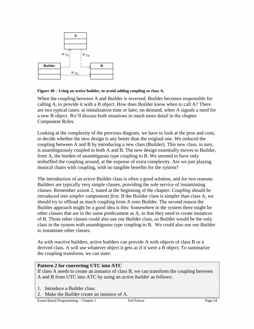
Event-Based Programming – Chapter 1 Ted Faison Page 54
A
Builder B
Tu
Tu
Ta
Figure 48 – Using an active builder, to avoid adding coupling to class A.
When the coupling between A and Builder is reversed, Builder becomes responsible for
calling A, to provide it with a B object. How does Builder know when to call A? There
are two typical cases: at initialization time or later, on demand, when A signals a need for
a new B object. We’ll discuss both situations in much more detail in the chapter
Component Roles.
Looking at the complexity of the previous diagram, we have to look at the pros and cons,
to decide whether the new design is any better than the original one. We reduced the
coupling between A and B by introducing a new class (Builder). This new class, in turn,
is unambiguously coupled to both A and B. The new design essentially moves to Builder,
from A, the burden of unambiguous type coupling to B. We seemed to have only
reshuffled the coupling around, at the expense of extra complexity. Are we just playing
musical chairs with coupling, with no tangible benefits for the system?
The introduction of an active Builder class is often a good solution, and for two reasons:
Builders are typically very simple classes, providing the sole service of instantiating
classes. Remember axiom 2, stated at the beginning of the chapter: Coupling should be
introduced into simpler components first. If the Builder class is simpler than class A, we
should try to offload as much coupling from A onto Builder. The second reason the
Builder approach might be a good idea is this: Somewhere in the system there might be
other classes that are in the same predicament as A, in that they need to create instances
of B. Those other classes could also use our Builder class, so Builder would be the only
class in the system with unambiguous type coupling to B. We could also use our Builder
to instantiate other classes.
As with reactive builders, active builders can provide A with objects of class B or a
derived class. A will use whatever object it gets as if it were a B object. To summarize
the coupling transform, we can state:
Pattern 2 for converting UTC into ATC
If class A needs to create an instance of class B, we can transform the coupling between
A and B from UTC into ATC by using an active builder as follows:
1. Introduce a Builder class.
2. Make the Builder create an instance of A.

Event-Based Programming – Chapter 1 Ted Faison Page 55
3. Make the Builder create an instance of B, or a derived class.
4. Have the builder pass a reference to B (or derived class) to the created instance of A.
Converting ATC into Signature Coupling
Signature coupling is a coupling flavor that has a dynamic nature. Given that coupling
can never completely eliminated from a system, signature coupling is sometimes the most
desirable flavor of coupling. Given two classes, A and B, assume A has ATC to B due to
the fact that A uses a typed reference to invoke a method in B. The next figure shows the
coupling diagram:
A
+M1()
B
Ta
Figure 49 – Two classes coupled by ambiguous type coupling.
The next listing shows a simple C# implementation.
public class A
{
public void UseB(B theB)
{
theB.M1(); // call method of B
}
}
public class B
{
public void M1()
{
// ...
}
}
Listing 14- A simple implementation, causing ATC between A and B.
Class A doesn’t instantiate class B, but instead receives a reference to B from another
object. To eliminate the ATC between A and B, we need to remove from A the reference
to the type B. Instead of class A calling a method through the interface B, we’ll make A
call B.M1 using a method reference. We’ll use an active Builder to initialize A’s method
reference, resulting in the coupling diagram shown in the next figure.
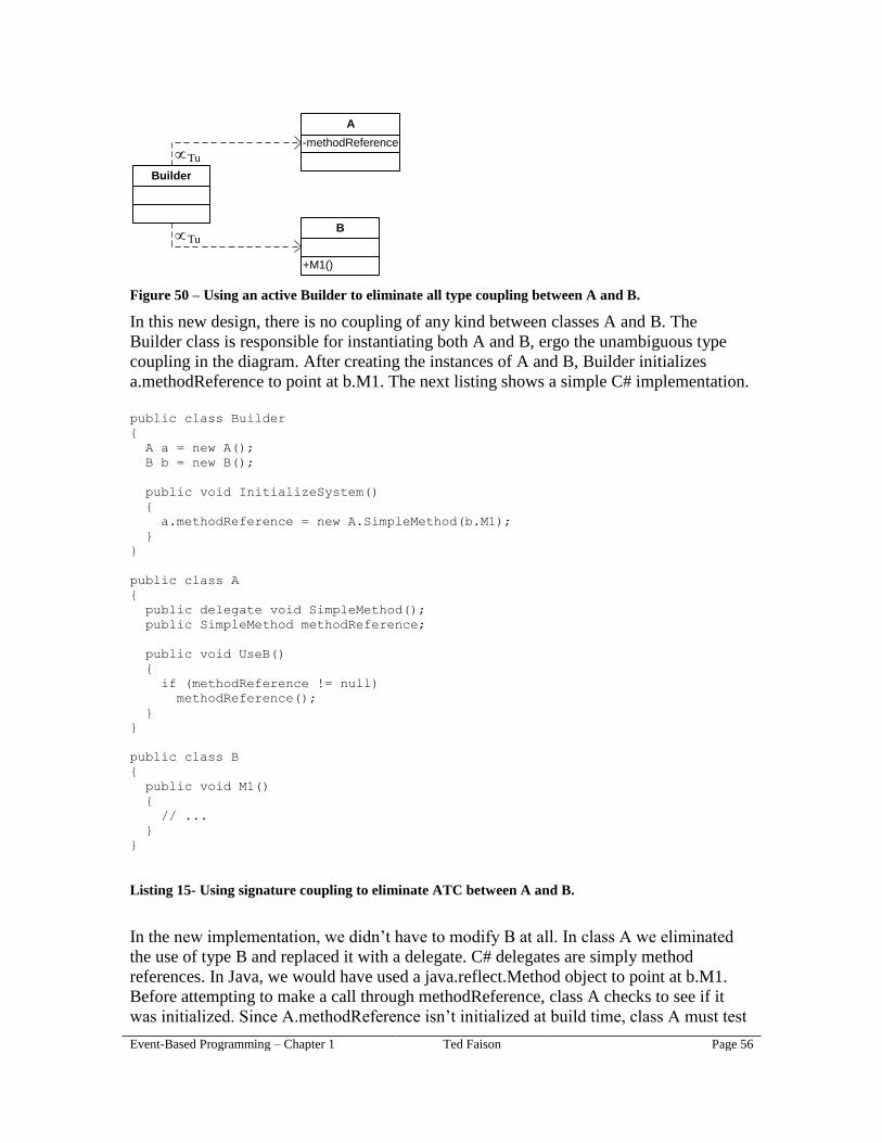
Event-Based Programming – Chapter 1 Ted Faison Page 56
-methodReference
A
Builder
+M1()
B
Tu
Tu
Figure 50 – Using an active Builder to eliminate all type coupling between A and B.
In this new design, there is no coupling of any kind between classes A and B. The
Builder class is responsible for instantiating both A and B, ergo the unambiguous type
coupling in the diagram. After creating the instances of A and B, Builder initializes
a.methodReference to point at b.M1. The next listing shows a simple C# implementation.
public class Builder
{
A a = new A();
B b = new B();
public void InitializeSystem()
{
a.methodReference = new A.SimpleMethod(b.M1);
}
}
public class A
{
public delegate void SimpleMethod();
public SimpleMethod methodReference;
public void UseB()
{
if (methodReference != null)
methodReference();
}
}
public class B
{
public void M1()
{
// ...
}
}
Listing 15- Using signature coupling to eliminate ATC between A and B.
In the new implementation, we didn’t have to modify B at all. In class A we eliminated
the use of type B and replaced it with a delegate. C# delegates are simply method
references. In Java, we would have used a java.reflect.Method object to point at b.M1.
Before attempting to make a call through methodReference, class A checks to see if it
was initialized. Since A.methodReference isn’t initialized at build time, class A must test

Event-Based Programming – Chapter 1 Ted Faison Page 57
the field at runtime before using it, because class A relies on another class (e.g. Builder)
to initialize the field.
By looking over the example, we can derive the pattern used in this ATC-to-SC
transform.
Pattern for converting ATC into SC
If a class A uses a typed reference to call a method M1 in a class B, eliminate the ATC
between A and B by doing the following:
1. Remove the typed reference from A.
2. Create a public method reference in A, using the signature of B.M1.
3. Create a Builder class to instantiate A and B as objects objA and objB.
4. Make the Builder initialize the method reference in objA to point at objB.M1.
Common Coupling Scenarios
There are numerous system architectures and design patterns in use today. A system
architecture that is used over and over again is really just a design pattern, albeit a high-
level one. Some patterns have been around since the early days of computing, before the
advent of object-oriented programming, but all patterns evolved to solve common
problems, with an eye on flexibility and simplicity. Perhaps because many of the patterns
were developed in the heyday of object oriented programming, before packaging and
inter-component coupling issues gained recognition, virtually all patterns introduce
coupling in one form or another. Most design patterns can be revisited and tweaked to
minimize or eliminate coupling. In the following sections, we’ll look at some popular
designs from a coupling perspective.
Client-Server Coupling
Client-server architectures became popular in the early 1990s as a distributed computing
solution. Conceptually, there is nothing about the client-server design pattern that
prevents it from being used in a non-distributed system. Although the expression client-
server is falling out of favor, the architecture is common. Call it what you want, but the
pattern is simple, involving a component, called the server, that makes its operations
available to other components, called clients. The next figure shows the basic
arrangement.
requests
responsesClient Server
Figure 51 – A simple client-server system
In client-server systems, the server is reactive to requests from clients. Servers don’t
contact clients, and do nothing on behalf of clients until they receive a request of some

Event-Based Programming – Chapter 1 Ted Faison Page 58
kind. Clients begin interactions with the server by calling server methods or sending
messages to the server. The kind of coupling that exists between the client and server
depends on how the two interact. Common modes are:
A. The client has a reference to an object exposed by the server.
B. The client knows the address of the server.
We’ll look at each case separately.
Client Calls Server using a Typed Reference
In this case, the client calls methods exposed by a server object. In a distributed system,
this object will generally be a local server proxy object that encapsulates the
communication with the remote server object. The client will either have unambiguous or
ambiguous type coupling to the server proxy, depending on whether the client creates the
proxy or simply gets a reference to it from another component. The following diagram
shows the coupling if the client creates the proxy object and assigns it to a reference
called myReference.
Tu
Client
Class1
Server
Proxy
Class2myReference
static
dynamic
Figure 52 – The coupling that occurs if Class1 creates an instance of a Class2 object.
It isn’t unusual for the client component to contain several classes that interact with
multiple server proxy objects. Each client class might wind up being type-coupled to
many server proxy objects. The next figure shows how the coupling chart might look for
a system in which the client component has 5 classes, named C1_1 thru C1_5.

Event-Based Programming – Chapter 1 Ted Faison Page 59
Figure 53 – The coupling chart for the classes in the client component.
If we assume that the client classes have a non-trivial amount of logic, we would like the
classes to have minimal coupling. One solution is to convert the type coupling between
client and proxy classes into signature coupling. To do so, we need to introduce a Builder
component on the client side. The Builder will be responsible for instantiating the server
proxy objects. The client classes C1_1 thru C1_5 would use method references to invoke
server methods. The delegates would be initialized by the Builder to point to methods of
the server proxy objects. The client classes would then have zero type coupling to the
server proxy classes. The coupling chart for the system might then look something like
the one in the next figure.
Figure 54 – The coupling chart after the introduction of an active Builder.
Since the Builder is the only class that has coupling to the server proxies, the other client
classes incur much less coupling, making their development and testing much simpler.
Client Sends Messages to the Server
In many distributed systems, the client talks to the server over a network connection by
sending messages. The server runs a listener daemon to process incoming client requests.
For this type of system to work, the client must obviously know the address of the server.
If the client embeds the server address as a hard-value in its code, there will be logic
coupling between the client and the server, as shown in the next diagram.
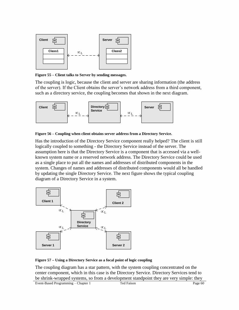
Event-Based Programming – Chapter 1 Ted Faison Page 60
L
Client
Class1
Server
Class2
Figure 55 – Client talks to Server by sending messages.
The coupling is logic, because the client and server are sharing information (the address
of the server). If the Client obtains the server’s network address from a third component,
such as a directory service, the coupling becomes that shown in the next diagram.
Client ServerDirectory
ServiceL L
Figure 56 – Coupling when client obtains server address from a Directory Service.
Has the introduction of the Directory Service component really helped? The client is still
logically coupled to something - the Directory Service instead of the server. The
assumption here is that the Directory Service is a component that is accessed via a well-
known system name or a reserved network address. The Directory Service could be used
as a single place to put all the names and addresses of distributed components in the
system. Changes of names and addresses of distributed components would all be handled
by updating the single Directory Service. The next figure shows the typical coupling
diagram of a Directory Service in a system.
Directory
Service
Client 1
Server 1
Client 2
Server 2
L
L
L
L
Figure 57 – Using a Directory Service as a focal point of logic coupling
The coupling diagram has a star pattern, with the system coupling concentrated on the
center component, which in this case is the Directory Service. Directory Services tend to
be shrink-wrapped systems, so from a development standpoint they are very simple: they
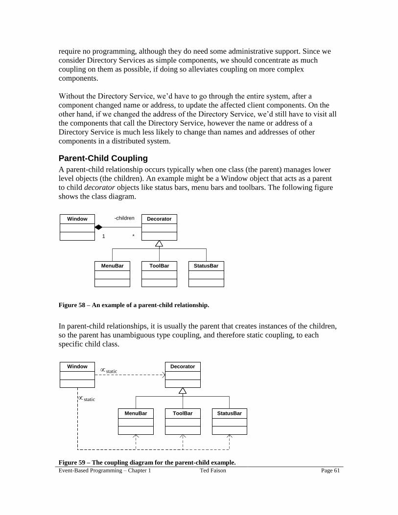
Event-Based Programming – Chapter 1 Ted Faison Page 61
require no programming, although they do need some administrative support. Since we
consider Directory Services as simple components, we should concentrate as much
coupling on them as possible, if doing so alleviates coupling on more complex
components.
Without the Directory Service, we’d have to go through the entire system, after a
component changed name or address, to update the affected client components. On the
other hand, if we changed the address of the Directory Service, we’d still have to visit all
the components that call the Directory Service, however the name or address of a
Directory Service is much less likely to change than names and addresses of other
components in a distributed system.
Parent-Child Coupling
A parent-child relationship occurs typically when one class (the parent) manages lower
level objects (the children). An example might be a Window object that acts as a parent
to child decorator objects like status bars, menu bars and toolbars. The following figure
shows the class diagram.
Window Decorator
1
-children
*
MenuBar ToolBar StatusBar
Figure 58 – An example of a parent-child relationship.
In parent-child relationships, it is usually the parent that creates instances of the children,
so the parent has unambiguous type coupling, and therefore static coupling, to each
specific child class.
Window Decorator
MenuBar ToolBar StatusBar
static
static
Figure 59 – The coupling diagram for the parent-child example.

Event-Based Programming – Chapter 1 Ted Faison Page 62
In this example, the child Decorator class and its derivatives have no coupling to the
parent Window class. The parent class is statically coupled to all the child classes, so the
parent requires all the child classes to be present at compile time. When there are many
types of children, this coupling can become a problem, because a change in any of the
children could break the compilation of the parent. To reduce coupling, a separate active
Builder object can be introduced, to handle the instantiation of the child classes. Once a
child object is created, the Builder could hand it over to the parent Window object. With
the Builder, the coupling between parent and child classes is substantially reduced, as
shown in the next diagram.
Window Decorator
MenuBar ToolBar StatusBar
Builder
static
static
static
Figure 60 – Using a Builder to reduce the coupling between parent and child classes.
With the presence of the Builder, there is no longer any static coupling between parent
and child classes, and class Window only requires the single class Decorator to be present
at build-time. It is the Builder class that now assumes static coupling to the parent and
child classes, resulting in a coupling chart that might look like the one in the next figure.
Figure 61 – The coupling chart after the introduction of a Builder.

Event-Based Programming – Chapter 1 Ted Faison Page 63
The chart shows that the Window and Decorator classes have a small amount of
coupling, while the Builder has a large amount. The graph doesn’t show coupling for the
derived decorator classes, because in this example we’re interested only at coupling on
the parent class, which is the Window class.
This presence of a Builder is often a good way to reduce parent-child coupling, because a
Builder is usually an extremely simple class, containing little or no business logic, while
the parent class is probably much more complex. In many cases, the Builder might
interact with the child classes simply by calling their constructors, and no other methods.
According to Axiom 1, introduced at the beginning of the chapter, it is better for a simple
class to be coupled than a complicated class.
In some parent-child relationships, the parent and child can be of the same type. For
example a TreeNode class, used to represent the nodes of an UI Tree control, can act
recursively as a parent to child nodes that are also TreeNode objects, as shown in the next
figure.
TreeNode
1
-children *
Figure 62 – A parent that has children of the same type.
Coupling is obviously not a problem in this case, since there is only one class involved.
Circular Coupling
In the previous section, the child classes had no reference back to the parent. There are
cases in which children need access to the parent, and the common way to achieve this is
by equipping each child with a reference to the parent, as shown in the next diagram.
Parent Child-parent
1
-children
*
Figure 63 – A parent-child relationship with children having references to the parent.
A potentially problematic consequence of adding a reference from the children to the
parent appears if we look at the design’s coupling diagram, shown in the next figure.
Parent Child
static dynamic
static dynamic
Figure 64 – Bidirectional static coupling between parent and children.

Event-Based Programming – Chapter 1 Ted Faison Page 64
The problem is that Parent requires Child to be present at build-time, but Child also
requires Parent to be present at build-time. The Parent and Child classes have circular
coupling. If both classes are part of the same component, it may be possible to compile
the component, but some languages and compilers don’t allow circular coupling under
any conditions. For example, if we implemented the system using C++, we might have
two header files called Parent.h and Child.h that contain the class declarations. But
Parent.h would need to include Child.h and vice versa, resulting in a circular file
reference. The compiler will refuse to compile either class.
The problem gets worse if Parent and Child are packaged in separate components, as
shown in the next diagram.
C1
Parent
C2
Child
static dynamic
static dynamic
Figure 65 – Circular coupling between components.
C1 is circularly coupled to C2, so neither component is independently deployable. If the
components are developed using a language that merges class declaration and
implementation together, such as C# and Java, we have an even bigger problem. C1 will
require C2’s executable code to be present at build-time and C2 will the same
requirement on C1, so neither component will even be buildable. We must either refactor
the system’s packaging, putting the Parent and Child classes in the same component
(assuming our compiler can deal with circular coupling), or we need to refactor the
design of the Parent and Child classes themselves.
Keeping the Parent and Child classes in separate components, there are two common
ways to break the circular coupling between them: using interfaces and using signature
coupling.
Breaking the Circle using Interfaces
If the child needs to very tightly coupled to the parent, in the sense that it needs to call
several parent methods, an interface approach may be appropriate. The idea is to refactor
the Parent as the implementation of an interface, and to package the interface in a third
component, as shown in the next figure.

Event-Based Programming – Chapter 1 Ted Faison Page 65
C1
Parent
C3
«interface»
InterfaceParent
C2
Child
static static
static
Figure 66 – Using a third component to break circular coupling.
The diagram shows that C1 is coupled to C2, but not vice versa. Both C1 and C2 are
coupled to C3, but C3 is not coupled to anything. Due to the structure of the coupling,
this new design imposes a strict build order: first C3, then C2 and then C1. To avoid
unambiguous type coupling between Child and Parent, which would result in static
coupling between Child and Parent, the Parent class must pass a reference to itself, typed
as an InterfaceParent, to the Child class. The next listing shows a simple implementation.
// In C3
public interface ParentInterface
{
//...
}
// In C2
public class Child
{
ParentInterface parent;
public Child(ParentInterface theParent)
{
parent = theParent;
}
}
// In C1
public class Parent : ParentInterface
{
Child child;
public Parent()
{
child = new Child(this);
}
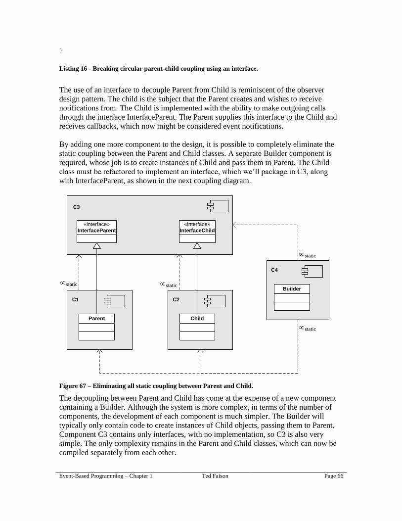
Event-Based Programming – Chapter 1 Ted Faison Page 66
}
Listing 16 - Breaking circular parent-child coupling using an interface.
The use of an interface to decouple Parent from Child is reminiscent of the observer
design pattern. The child is the subject that the Parent creates and wishes to receive
notifications from. The Child is implemented with the ability to make outgoing calls
through the interface InterfaceParent. The Parent supplies this interface to the Child and
receives callbacks, which now might be considered event notifications.
By adding one more component to the design, it is possible to completely eliminate the
static coupling between the Parent and Child classes. A separate Builder component is
required, whose job is to create instances of Child and pass them to Parent. The Child
class must be refactored to implement an interface, which we’ll package in C3, along
with InterfaceParent, as shown in the next coupling diagram.
C1
Parent
C3
«interface»
InterfaceParent
C2
Child
static
«interface»
InterfaceChild
C4
Builderstatic
static
static
Figure 67 – Eliminating all static coupling between Parent and Child.
The decoupling between Parent and Child has come at the expense of a new component
containing a Builder. Although the system is more complex, in terms of the number of
components, the development of each component is much simpler. The Builder will
typically only contain code to create instances of Child objects, passing them to Parent.
Component C3 contains only interfaces, with no implementation, so C3 is also very
simple. The only complexity remains in the Parent and Child classes, which can now be
compiled separately from each other.
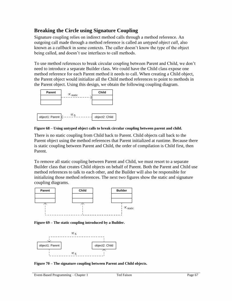
Event-Based Programming – Chapter 1 Ted Faison Page 67
Breaking the Circle using Signature Coupling
Signature coupling relies on indirect method calls through a method reference. An
outgoing call made through a method reference is called an untyped object call, also
known as a callback in some contexts. The caller doesn’t know the type of the object
being called, and doesn’t use interfaces to call methods.
To use method references to break circular coupling between Parent and Child, we don’t
need to introduce a separate Builder class. We could have the Child class expose one
method reference for each Parent method it needs to call. When creating a Child object,
the Parent object would initialize all the Child method references to point to methods in
the Parent object. Using this design, we obtain the following coupling diagram.
Parent Child
object2: Childobject1: ParentS
static
Figure 68 – Using untyped object calls to break circular coupling between parent and child.
There is no static coupling from Child back to Parent. Child objects call back to the
Parent object using the method references that Parent initialized at runtime. Because there
is static coupling between Parent and Child, the order of compilation is Child first, then
Parent.
To remove all static coupling between Parent and Child, we must resort to a separate
Builder class that creates Child objects on behalf of Parent. Both the Parent and Child use
method references to talk to each other, and the Builder will also be responsible for
initializing those method references. The next two figures show the static and signature
coupling diagrams.
Parent Child Builder
static
Figure 69 – The static coupling introduced by a Builder.
object2: Childobject1: Parent
S
S
Figure 70 – The signature coupling between Parent and Child objects.

Event-Based Programming – Chapter 1 Ted Faison Page 68
The following listing shows how the Parent, Child and Builder classes might be
implemented in C#.
public class Builder
{
public Parent parent;
public Child child;
public Builder()
{
// build the parent and child objects
parent = new Parent();
child = new Child();
// bind parent and child together
parent.OnSetVisible += new Parent.EventVisible(child.Show);
child.OnModified += new Child.EventModified(parent.UpdateScreen);
}
}
public class Parent
{
public delegate void EventVisible();
public event EventVisible OnSetVisible;
public void ShowChild()
{
if (OnSetVisible != null)
OnSetVisible();
}
public void UpdateScreen()
{
// redraw the screen and show the child
ShowChild();
}
}
public class Child
{
public delegate void EventModified();
public event EventModified OnModified;
public void DoSomething()
{
// notify the parent that we were modified
if (OnModified != null)
OnModified();
}
public void Show()
{
// show the child on the screen...
}
}
Listing 17 - Using a Builder to remove all static coupling between Parent and Child.
The Parent and Child classes use C# event properties to expose delegates. Delegates are
method references. The Builder initializes the method references of Child to point to

Event-Based Programming – Chapter 1 Ted Faison Page 69
Parent methods and vice versa. In Java, instead of using event properties, one could use
reflection, with class java.lang.reflect.Method to encapsulate method references.
Coupling With User-Defined Types
UDTs are extremely important in OO systems, because they contain the bulk of the
business logic of the system. The problem is that UDTs often increase the type coupling
in a system. Consider the interaction shown in the next figure, in which T1 and T2 are
arbitrary UDTs.
T1 T2interaction
Figure 71 – An interaction between arbitrary types.
From the perspective of coupling, it doesn’t matter whether the interaction transfers data
or control from T1 to T2. The interaction is generally implemented in one of the
following three ways.
1. T1 sends a message to T2. If the message contains a UDT, then both T1 and T2
will have to know the UDT, because T1 must serialize the UDT and T2 must
deserialize it. Both T1 and T2 will therefore be type-coupled to the UDT.
2. T1 calls a T2 method through T2’s interface, using the notation object.method.
Regardless of the signature of the T2 method being called, T1 will be type
coupled to T2 (which is a UDT), because T1 uses T2 at build time.
3. T1 calls a T2 method indirectly, using a method reference. If the method signature
references a UDT, then both T1 and T2 will need to know that UDT, because T1
must identify the UDT in the outgoing call to T2, while T2 must know what the
incoming UDT is. Hence both T1 and T2 will be type coupled to the UDT.
The first case is straightforward, but the other two need additional discussion.
Coupling Due to Interfaces
Object-oriented programming is hinged on the notions of class and interface. Objects are
entities that expose their behaviors through an interface. Clients wishing to invoke a class
method typically do so by using a typed pointer or reference, using the object.method
notation. In many OO languages, given a class T2 with a method M1, a client can invoke
M1 using notation of the form:
myT2Object.M1();
The symbol myT2Object is a reference to an object of type T2, and must be initialized at
runtime. If a class T1 uses the above notation to invoke methods of T2, then T1 will
necessarily be type-coupled to T2. If T1 and T2 are contained in different components C1
and C2, those components will be statically coupled, as shown in the next diagram.

Event-Based Programming – Chapter 1 Ted Faison Page 70
C1
T1
C2
+M1()
T2T
static
Figure 72 –The coupling caused by the use of interfaces in outbound calls from T1 to T2.
Using the object.method notation to call a method forces the caller to have a certain
familiarity with the callee, because the caller specifies at build time which T2 method to
call. Although interface-based calls entail type coupling, interfaces form the basis for
contract-based programming, a powerful OO programming technique. Classes that
expose an interface can define formal contracts, stating the pre-conditions, the post-
conditions and the side effects of each method. Tools can then verify contract
compliance, signaling and violations.
The issue of interfaces used in inter-component interactions brings us to a critical
juncture, which some people might consider controversial. As stated ad nauseam in this
book, an extremely important characteristic of components is independent deployability.
End users should be able to use a component without needing additional ones. If a
component is type coupled to other components, it will not be independently deployable.
Most interfaces in non-trivial software systems are user-defined. Making outbound calls
through a user-defined interface T invariably type-couples the caller and the callee to the
component defining T. Assume a simple system contains a component C1 with a class T1
that uses the object.method notation to call a class T2 contained in a component C2.
Also assume that T2 implements the interface T, and that T defines only a single method
M1 that takes no parameters and returns none. The coupling in this system is due entirely
to the use of the interface T in the method call. From a packaging standpoint, there are
only three places T can be defined:
In C1, requiring C2 to be statically coupled to C1.
In C2, requiring C1 to be statically coupled to C2.
In a separate component C3, requiring both C1 and C2 to be statically coupled to
C3.
The next figure shows the system coupling if the interface T is defined in C1.

Event-Based Programming – Chapter 1 Ted Faison Page 71
C2
+M1()
T2
C1
T1
«interface»
T
static
Figure 73 – Static coupling when T is packaged with T1.
The next figure shows the system coupling if T is packaged in C2.
C1
C2
T1
«interface»
T
+M1()
T2
static
Figure 74 – Static coupling when T is packaged with T2.
When the interface T is packaged with T2, the presence of the interface doesn’t help
reduce coupling between C1 and C2. T1 could call T2 directly through T2’s interface
without introducing further coupling.
The next figure shows the system coupling if T is packaged in a separate component C3.
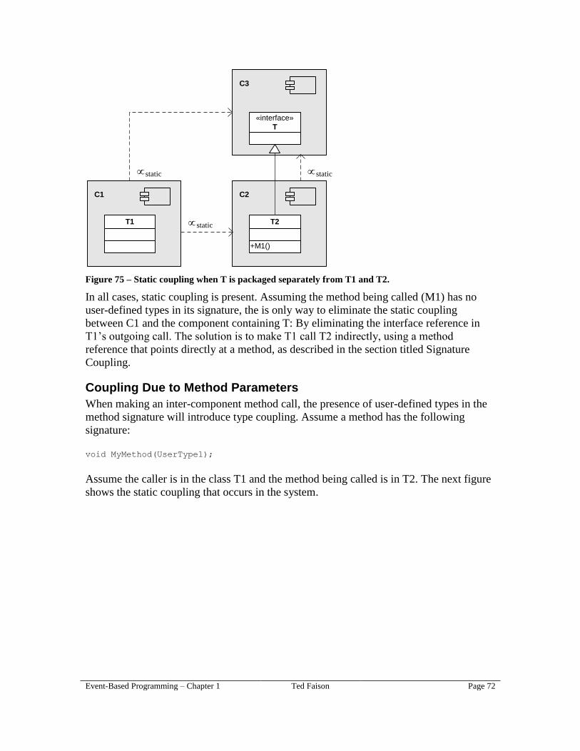
Event-Based Programming – Chapter 1 Ted Faison Page 72
C1
T1
C2
+M1()
T2
C3
«interface»
T
static
static
static
Figure 75 – Static coupling when T is packaged separately from T1 and T2.
In all cases, static coupling is present. Assuming the method being called (M1) has no
user-defined types in its signature, the is only way to eliminate the static coupling
between C1 and the component containing T: By eliminating the interface reference in
T1’s outgoing call. The solution is to make T1 call T2 indirectly, using a method
reference that points directly at a method, as described in the section titled Signature
Coupling.
Coupling Due to Method Parameters
When making an inter-component method call, the presence of user-defined types in the
method signature will introduce type coupling. Assume a method has the following
signature:
void MyMethod(UserType1);
Assume the caller is in the class T1 and the method being called is in T2. The next figure
shows the static coupling that occurs in the system.
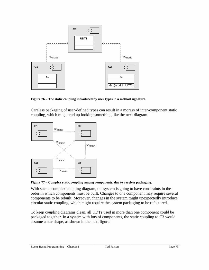
Event-Based Programming – Chapter 1 Ted Faison Page 73
C1
T1
C3
UDT1
static static
C2
+M1(in udt1 : UDT1)
T2
Figure 76 – The static coupling introduced by user types in a method signature.
Careless packaging of user-defined types can result in a morass of inter-component static
coupling, which might end up looking something like the next diagram.
C1 C2
C3 C4
static
static
static
static
static
Figure 77 – Complex static coupling among components, due to careless packaging.
With such a complex coupling diagram, the system is going to have constraints in the
order in which components must be built. Changes to one component may require several
components to be rebuilt. Moreover, changes in the system might unexpectedly introduce
circular static coupling, which might require the system packaging to be refactored.
To keep coupling diagrams clean, all UDTs used in more than one component could be
packaged together. In a system with lots of components, the static coupling to C3 would
assume a star shape, as shown in the next figure.

Event-Based Programming – Chapter 1 Ted Faison Page 74
C1
C3
UDTs
C2
C4 C5
static static
static static
Figure 78 – Packaging common user-defined types together.
The diagram tells us that changes to C3 would require the other components to be rebuilt,
but changes to C1, C2, C3 and C4 would not impact any other components. A properly
designed system should have a star-shaped static coupling diagram, with the user-type
component at the center. The system would require C3 to be built first, and then the other
components, in no particular order.

Event-Based Programming – Chapter 1 Ted Faison Page 75
References
[Briand et al., 1999]
L. C. Briand, J. W. Daly, J. K. Wüst, A Unified Framework for Coupling
Measurement in Object-Oriented Systems, IEEE Transactions on Software Engineering,
Vol. 25, No. 1 (Jan/Feb 1999).
[Cain et al., 2002]
J.W. Cain, R.J. McCrindle, An Investigation into the Effects of Code Coupling on Team
Dynamics and Productivity, 26th Annual International Computer Software and
Applications Conference (COMPSAC 2002), Oxford, England, Aug 2002.
[Hitz et al., 1995]
M. Hitz and B. Montazeri, Measuring Coupling and Cohesion in Object-Oriented
Systems, Proceedings of the International Symposium on Applied Corporate Computing
(ISACC’95), Monterrey, Mexico, Oct. 1995.
[Shereshevsky et al., 2001]
M. Shereshevsky, H. Ammari, N. Gradetsky, A. Mili, and H. H. Ammar. Information
Theoretic Metrics for Software Architectures, Proceedings of the 25th Annual IEEE
International Computer Software and Applications Conference (COMPSAC’01).
[Stevens et al., 1974]
Stevens, W., Myers, G., Constantine, L. Structure Design, IBM Systems Journal, Vol. 13,
No. 2, pp. 115-139. 1974.
[Feynman et al., 1997]
Feynman, R. P., Hutchings, E., Leighton, R. He Fixes Radios by Thinking! In “Surely
You're Joking, Mr. Feynman!: Adventures of a Curious Character”. New York: W. W.
Norton, 1997. ISBN 0-393-31604-1.
[Gamma et al., 1995]
Gamma, E., Helm, R., Johnson, R., Vlissides, J. Design Patterns. Elements of Resuable
Object-Oriented Software. Addison Wesley, 1995.

Event-Based Programming – Chapter 1 Ted Faison Page 76
Glossary
CLI Common Language Infrastructure, the runtime environment of Microsoft .Net
Framework systems.
CBD Component-Based Development
UTC Unambiguous type coupling
ATC Ambiguous type coupling
UDT User-defined type.
LC Logic coupling
TC Type coupling
LLC Literal logic coupling
ALC Algorithmic logic coupling
SC Signature coupling.