A system of types and operators for handling vague spatial objects

This article was downloaded by:[Tu Delft- Fac Citg]On: 14 August 2007Access Details: [subscription number 731711409]Publisher: Taylor & FrancisInforma Ltd Registered in England and Wales Registered Number: 1072954Registered office: Mortimer House, 37-41 Mortimer Street, London W1T 3JH, UK

International Journal of GeographicalInformation SciencePublication details, including instructions for authors and subscription information:http://www.informaworld.com/smpp/title~content=t713599799

A system of types and operators for handling vaguespatial objects

Online Publication Date: 01 January 2007To cite this Article: Dilo, Arta, de By, Rolf A. and Stein, Alfred (2007) 'A system oftypes and operators for handling vague spatial objects', International Journal ofGeographical Information Science, 21:4, 397 - 426To link to this article: DOI: 10.1080/13658810601037096URL: http://dx.doi.org/10.1080/13658810601037096

PLEASE SCROLL DOWN FOR ARTICLE

Full terms and conditions of use: http://www.informaworld.com/terms-and-conditions-of-access.pdf

This article maybe used for research, teaching and private study purposes. Any substantial or systematic reproduction,re-distribution, re-selling, loan or sub-licensing, systematic supply or distribution in any form to anyone is expresslyforbidden.

The publisher does not give any warranty express or implied or make any representation that the contents will becomplete or accurate or up to date. The accuracy of any instructions, formulae and drug doses should beindependently verified with primary sources. The publisher shall not be liable for any loss, actions, claims, proceedings,demand or costs or damages whatsoever or howsoever caused arising directly or indirectly in connection with orarising out of the use of this material.

© Taylor and Francis 2007

http://www.informaworld.com/smpp/title~content=t713599799

http://dx.doi.org/10.1080/13658810601037096

http://www.informaworld.com/terms-and-conditions-of-access.pdf

Dow

nloa

ded

By:

[Tu

Del

ft- F

ac C

itg] A

t: 16

:42

14 A

ugus

t 200

7

A system of types and operators for handling vague spatial objects

ARTA DILO*{, ROLF A. DE BY{ and ALFRED STEIN§

{GIS-Technology section, Delft University of Technology, P.O. Box 5030, 2600 GA

Delft, The Netherlands

{Department Geo-information Processing, International Institute for Geo-Information

Science and Earth Observation, P.O. Box 6, 7500 AA Enschede, The Netherlands

§Department of Earth Observation Science, International Institute for Geo-Information

Science and Earth Observation, P.O. Box 6, 7500 AA Enschede, The Netherlands

(Received 07 February 2005; in final form 04 September 2006 )

Vagueness is often present in spatial phenomena. Representing and analysing

vague spatial phenomena requires vague objects and operators, whereas current

GIS and spatial databases can only handle crisp objects. This paper provides

mathematical definitions for vague object types and operators.

The object types that we propose are a set of simple types, a set of general

types, and vague partitions. The simple types represent identifiable objects of a

simple structure, i.e. not divisible into components. They are vague points, vague

lines, and vague regions. The general types represent classes of simple type

objects. They are vague multipoint, vague multiline, and vague multiregion.

General types assure closure under set operators. Simple and general types are

defined as fuzzy sets in 2 satisfying specific properties that are expressed in

terms of topological notions. These properties assure that set membership values

change mostly gradually, allowing stepwise jumps. The type vague partition is a

collection of vague multiregions that might intersect each other only at their

transition boundaries. It allows for a soft classification of space. All types allow

for both a finite and an infinite number of transition levels. They include crisp

objects as special cases.

We consider a standard set of operators on crisp objects and define them for

vague objects. We provide definitions for operators returning spatial types. They

are regularized fuzzy set operators: union, intersection, and difference; two

operators from topology: boundary and frontier; and two operators on vague

partitions: overlay and fusion. Other spatial operators, topological predicates

and metric operators, are introduced giving their intuition and example

definitions. All these operators include crisp operators as special cases. Types

and operators provided in this paper form a model for a spatial data system that

can handle vague information. The paper is illustrated with an application of

vague objects in coastal erosion.

Keywords: Spatial data modelling; Vagueness; Fuzzy sets; Fuzzy topology

*Corresponding author. Email: [email protected]

International Journal of Geographical Information Science

Vol. 21, No. 4, April 2007, 397–426

International Journal of Geographical Information ScienceISSN 1365-8816 print/ISSN 1362-3087 online # 2007 Taylor & Francis

http://www.tandf.co.uk/journalsDOI: 10.1080/13658810601037096

Dow

nloa

ded

By:

[Tu

Del

ft- F

ac C

itg] A

t: 16

:42

14 A

ugus

t 200

7

1. Introduction

Vagueness is a type of imperfection arising in the presence of borderline cases

(Sorensen 2003). A concept is vague if locations exist that cannot be classified either

to the concept or to its complement. When mapping vegetation for example, it may

be difficult to decide whether a certain location belongs to one vegetation class or to

another. The transition from one class to another may be gradual (Fisher 2000), as

between forest and grassland in African rangelands. Also, geomorphological units

(Burrough et al. 2000, Lucieer et al. 2004), soil types (de Gruijter et al. 1997, Odeh

et al. 1992), landscape objects (Cheng and Molenaar 1999, Cheng et al. 2001, Fisher

et al. 2006), and forest types (Brown 1998), generally exhibit transition zones instead

of sharp boundaries. Other examples include soil pollution classes in environmental

applications (Hendricks Franssen et al. 1997), or hydrological studies (Bogardi et al.

1990) where spatial objects have to be delineated that cannot be sharply defined.

Several theories have been proposed to handle vagueness, of which fuzzy theory

(Zadeh 1965, 1975) is the most often used. This is also true in the spatial domain.

Attention has been given to vagueness, on the one hand by considering spatial

objects to be crisp, and reasoning being vague (Vert et al. 2002, Wang 2000). On the

other hand, models have been proposed for objects that are vague (Burrough and

Frank 1996, Cohn and Gotts 1996b, Erwig and Schneider 1997, Zhan 1997,

Schneider 1999, Roy and Stell 2001, Tang 2004) and reasoning with these objects

(see section 4).

Some image processing software allows the extraction of fuzzy objects from

imagery, or offers tools to do fuzzy reasoning over a continuous space (Robinson

2003). There is also work done for the visualization of fuzzy objects (Hengl et al.

2004). No functionality exists, however, for handling vague objects in current

geographical information systems (GISs), or in spatial database systems. These

systems focus on crisp spatial objects. Current GISs or spatial databases would

therefore benefit from an extension with data types for vague spatial objects, and

operators for their manipulation.

Before constructing an information system, a precise notion must exist of what is to be

built and how the system is expected to function. Mathematical specifications are useful

in this respect. They describe precisely the properties the system must have, without

unduly constraining how these properties are achieved in its implementation. These

specifications, called abstract specifications, are not oriented towards computer

representation, but obey a rich collection of mathematical laws. As such one can reason

effectively about the way the system will behave. The abstract specifications are later

translated into computer specifications, which are related to a specific computer

representation. The work presented here deals only with abstract specifications.

The objective of this paper is to provide a model for a spatial data system that can

handle vague objects. This model takes gradual transitions into consideration and is

based on fuzzy theory. It consists of mathematical definitions for vague spatial types

and operators. Vague spatial types are grouped into simple types, general types, and

vague partitions. A simple type represents an identifiable object of a simple

structure, i.e. not divisible into components. A general type represents a class of

simple type objects. A vague partition allows for a soft classification of space. Vague

operators defined here are operators returning spatial types. Intuition and example

definitions are provided for other spatial operators.

The paper is organized as follows. Section 2 presents examples of vague spatial

phenomena that can be described with our vague types. Section 3 gives a short

398 A. Dilo et al.

Dow

nloa

ded

By:

[Tu

Del

ft- F

ac C

itg] A

t: 16

:42

14 A

ugus

t 200

7

introduction to concepts from fuzzy topology that are needed for our definitions of

vague types and operators, also from some of the existing models for vague data.

Section 4 describes existing models proposed to handle spatial vagueness. Section 5

contains the core material of the paper. It provides intuition and definitions of vague

object types and operators returning spatial types. Section 6 discusses what is a

complete spatial system, and elaborates on the other spatial operators, spatial

predicates and metric operators. An application from coastal erosion is presented in

section 7 to illustrate the object types and operators provided in this paper. Section 8

closes the paper with discussions and conclusions.

2. Examples of spatial vagueness

In ordinary natural language adjectives are commonly attributed to phenomena.

This is certainly the case in the cognition of geography, where characteristics of

spatial phenomena are expressed in ordinary language terms, which are generally

vague.

(i) When considering densely populated residential centres, we have to identify

known locations that have different degrees of being densely populated. We

know the location precisely, but the density level itself is vague.

(ii) Considering polluted rivers, we know precisely where the river is. Close to the

source of pollution the river is certainly polluted, but further away riverine

tracks may exist with less severe pollution. Therefore, at different locations

along the river, different degrees of pollution exist that change gradually.

(iii) Traffic congestion on a road network relates the level of congestion to roads.

Part of the road network is completely blocked, and hence certainly belongs

to the traffic congestion, whereas away from the congestion, the car build-up

becomes less severe. Dissolving congestion at the end of a rush hour no

longer has a certain part. This vague characteristic, however, is still spread on

the roads.

(iv) It may be arbitrary to consider a particular location as part of a vegetated

area, or of a non-vegetated area. Some locations are certainly vegetated,

whereas other locations can be considered vegetated or non-vegetated to

some degree. There are transition zones where vegetation becomes sparse. In

some places the transition is gradual, whereas in other places the change may

be abrupt.

(v) Agricultural land suitability in Sicat et al. (2005) is based on farmers’

knowledge on soils, like soil texture, colour, depth and slope. These

parameters are linguistic variables taking values, e.g. ‘fine’, ‘moderately

fine’, and ‘coarse’ for soil texture. The suitability map is built from a

combination of values of these variables according to specific rules.

Suitability derived in this way is also a linguistic variable with values ‘least

suitable’, ‘moderately suitable’, ‘suitable’, and ‘most suitable.’ This attribute,

suitability, spread over the space, determines objects whose locations have

membership values from a finite set (of four values). Two adjacent land

parcels could have different suitability values, therefore there is a jump in

values along their common boundary.

The above examples illustrate thematic vagueness, but not always locational

vagueness. Objects describing such spatial phenomena may have a crisp location,

but their essential properties can only be expressed in vague terms. Regions resulting

A system of types and operators for handling vague spatial objects 399

Dow

nloa

ded

By:

[Tu

Del

ft- F

ac C

itg] A

t: 16

:42

14 A

ugus

t 200

7

from a classification of space have a vague extent due to the vagueness of concepts

defining the classes. For such regions, locational vagueness derives from thematic

vagueness. There are situations, however, where locational vagueness is independent

of thematic vagueness, as for example a forest region from which one way or

another we know the shape, but not the precise location. The object types proposed

in this paper can handle a thematic kind of vagueness.

3. Preliminaries

Definitions of vague spatial types and operators use concepts from general and

fuzzy topologies. We assume that concepts from fuzzy set theory and general

topology are known (see Klir and Yuan (1995) for a complete treatment of fuzzy

sets, and Willard (1970) and Kelley (1975) for general topology). The general

topologies that we use are the usual topologies T1 for , and T2 for 2. The fuzzy

topologies used for our definitions are T 1 induced by T1, and T 2 induced by T2.

Induced fuzzy topologies need the concept of semi-continuous functions. This is

explained in the next few paragraphs, together with the relation to continuous

functions. Section 3.1 introduces shortly concepts from fuzzy topology. Definitions

are given for real spaces n.

A function f: nR is lower semi-continuous at p iff for all c,f(p) there exists a

neighbourhood Up of p such that for all q g Up, c,f(q). The function f is lower semi-

continuous on Rn iff it is lower semi-continuous at every p g n (Jost 1998).

Figure 1(b) shows the graph of a lower semi-continuous function g: R . The

function is almost everywhere continuous, except for three points x0, 0 and x1 where

it is lower semi-continuous. For a value c,g(0), a neighbourhood U0 is drawn, such

that any point q g U0 has a value g(q) greater than c.

Correspondingly, a function f: nR is upper semi-continuous at p iff for all

c.f(p) there exists Up such that for all q g Up, c.f(q) (Jost 1998). The function x[a, b]

in figure 1(c) is upper semi-continuous. It is the characteristic function of the closed

interval [a, b]. The property is general: the characteristic function of a closed set in

( n, Tn) is an upper semi-continuous function, whereas the characteristic function

of an open set is a lower semi-continuous function.

A function f: nR is continuous at a point p iff it is both upper and lower semi-

continuous at p. The function f is continuous on n iff it is both upper and lower

semi-continuous on n. Figure 1(a) shows the graph of a continuous function

f: R .

Figure 1. Graphs of continuous and semi-continuous functions for the usual topology in 2:(a) a continuous function, (b) a lower semi-continuous function and (c) an upper semi-continuous function. Empty and filled circles are used to show the value of a function atdiscontinuity points; the full circle denotes the value of the function.

400 A. Dilo et al.

Dow

nloa

ded

By:

[Tu

Del

ft- F

ac C

itg] A

t: 16

:42

14 A

ugus

t 200

7

A fuzzy set m in n is a (total) function m: nR[0, 1]. This function is also called

the membership function of the fuzzy set. A classical set A can be represented by its

characteristic function xA: nR{0, 1}, which is called a crisp set. We denote the set

of all fuzzy sets in n by F nð Þ.Let X and Y be subsets of n and m, respectively. A function f:XRY induces a

function eff : F Xð Þ?F Yð Þ that produces an image of a fuzzy set in X as a fuzzy set in

Y. This is known as the extension principle (Klir and Yuan 1995). The image of a

fuzzy set m[F Xð Þ is n~eff mð Þ[F Yð Þ such that

Vp[Y , n pð Þ~sup m qð Þ q[X , f qð Þ~pjf g, Aq[X , f qð Þ~p,

0, otherwise:

�

The fuzzy set n is such that its membership value at a location p g Y is the highest

membership value of m at locations q g X that are mapped to p by the function f.

3.1 Fuzzy topology

We now turn to definitions from fuzzy topology that are needed for our vague types:

interior and closure, boundary, connected and bounded fuzzy sets. Most of these

fuzzy topology notions are described by one of the equivalent definitions of the

corresponding notion in general topology, put in a fuzzy setting. We give two

examples of fuzzy topologies for real spaces, a crisp topology and an induced fuzzy

topology. The topology notions are explained for the induced fuzzy topologies T n

for n, and some of them are illustrated for the induced topology T 1 for .

A fuzzy topology is defined similarly to a general topology as a collection

T(F nð Þ that contains the empty set 0n

and the whole set 1n

, the intersection of

any two elements of T , and any union of elements of T . The elements of T are the

open fuzzy sets in ( n, T ). Their complements are the closed fuzzy sets in ( n, T ).

The collection Cn of crisp sets from n which (corresponding classical sets) are

open in the usual topology, forms a fuzzy topology for n. Closed fuzzy sets for

this topology are the closed crisp sets in the usual topology for n. The fuzzy

topology Cn is a crisp topology for n. A general topology can be used differently

to build a fuzzy topology. The collection T n of lower semi-continuous functions in

( n, Tn) forms a fuzzy topology, which is called the induced fuzzy topology from

the usual topology for n (Weiss 1975). The fuzzy sets with lower semi-continuous

membership function are the open sets in T n, and those with upper semi-

continuous membership function are the closed sets. Open and closed fuzzy sets

for T n can be expressed in terms of open and closed a-cuts: a fuzzy set m in ( n,

T n) is open if all its strict a-cuts are open for Tn; it is closed for ( n, T n) if all its a-

cuts are closed for Tn (Weiss 1975). A fuzzy set that has a continuous function is an

open and closed (clopen) fuzzy set, e.g. the fuzzy set in whose graph is shown in

figure 1(a).

A fuzzy point in ( n, T n) is a fuzzy set that has a positive value l.0 in just one

point, say p g n (Pu and Liu 1980):

Vq[ n, m qð Þ~l if q~p,

0 if q=p:

�

A fuzzy point is denoted by pl, where p is the unique location with a positive

membership, and l is the membership value at p.


Dow

nloa

ded

By:

[Tu

Del

ft- F

ac C

itg] A

t: 16

:42

14 A

ugus

t 200

7

The interior of a fuzzy set m is the union of all open sets contained in m:

m0~z n[T n v mjf g. The closure of a fuzzy set m is the intersection of all closed sets

containing m: m~y 1{n[T m v njf g. The interior puts the value of the function at the

discontinuity points to the lower value. The closure sets the value of the function at

discontinuity points to the highest value. A fuzzy set m is regular closed iff it is equal

to the closure of its interior: m~m0.

The fuzzy boundary mb of a fuzzy set m is the intersection of all closed sets n in

F nð Þ such that n(x)>m(x) at all x g n for whichmy1{m xð Þw0 (Warren 1977).

The fuzzy boundary of a set m in ( n, T n) is equal to m at the uncertain part

{p g n|0,m(p),1}, has value 1 at the (crisp) boundary of the core, and value 0

everywhere else. The fuzzy frontier mf of m is the intersection of all closed sets n in

F Rnð Þ such that n(x)>m(x) at all x g X for which m(x).mu(x) (Cuchillo-Ibanez and

Tarres 1997). The frontier mf of a fuzzy set m in ( n, T n) has a positive value only at

the discontinuity points of m. It is an empty fuzzy set if m is continuous.

Let m be a fuzzy set in ( n, T n), and X, n. The fuzzy set m|X on n that has the

same membership value as m for all x g X and value 0 for all x=[X is a fuzzy set on X.

We call the set m|X on n the restriction of m on X. The family T Xn ~ m Xj m[T nj

n o

is a

fuzzy topology in X and is called the relative fuzzy topology for X (Pu and Liu

1980).

A fuzzy set m is disconnected if there are closed sets c and d in the subspace

supp(m) associated with the relative fuzzy topology, such that

myc=0n

, myd=0n

, cyd~0n

, and m v czd (Pu and Liu 1980). A fuzzy set mis connected if it is not disconnected. The maximal connected fuzzy set contained in mis called a component of m. A fuzzy set m is connected for ( n, T n) if it has a

connected support set. A fuzzy set m is bounded if every a-cut ma is bounded (Pu and

Liu 1980). The set m is bounded in ( n, T n) if its support set is bounded.

4. Existing models of vague spatial data

Several theoretical models have been proposed, mainly dedicated to vague regions

and their topological relations. These models can be grouped into two approaches.

One approach (Burrough and Frank 1996, Cohn and Gotts 1996b, Erwig and

Schneider 1997, Bittner and Stell 2000, Clementini and di Felice 2001, Roy and Stell

2001) considers vague regions to have a homogeneous two-dimensional boundary

instead of a one-dimensional boundary. Locations in the broad boundary all have

the same degree of membership to the region. Models of this approach do not

provide means to handle gradual transition. The other approach (Zhan 1997, 1998,

Schneider 1999, 2003, Tang 2004, Liu and Shi 2006) employs fuzzy set theory for

modelling gradual changes. In particular, the work of Schneider (1999, 2000, 2001a)

provides a complete set of object types and most of the standard operators of a

spatial data system (Guting 1994). The next two sections summarize the works from

each approach.

4.1 Broad boundary regions

The Egg-Yolk model (Cohn and Gotts 1996a,b) describes a vague region as a pair of

crisp regions, one enclosing the other. The inner region, the ‘yolk’, gives the certain

part of the vague region. The outer region, the ‘white’, is the broad boundary which

delineates limits on the range of vagueness. The white and yolk together form the

egg that is the full extent of the vague region. All these regions are Region

402 A. Dilo et al.

Dow

nloa

ded

By:

[Tu

Del

ft- F

ac C

itg] A

t: 16

:42

14 A

ugus

t 200

7

Connection Calculus (RCC) regions (Randell and Cohn 1989, Randell et al. 1992,

Cohn et al. 1997).

The proposal of Clementini and di Felice (1996, 2001) is similar to the egg-yolk

model, with definitions based on general topology. A vague region A consists of two

sets A1, A2 of 2 such that A1#A2. The broad boundary DA is the closure of their

difference: DA~A2\A1. Each set, A1 and A2, is a crisp region, i.e. a bounded, regular

closed set in 2 with connected interior (Clementini and di Felice 2001). The inner

region A1 gives the certain part of a vague region, and the broad boundary DA

delineates limits of vagueness.

A vague region is defined in Erwig and Schneider (1997) as a pair of disjoint sets:

the kernel that is the certain part of the region, and the boundary that is its uncertain

part. The kernel is a crisp region, whereas the boundary can be a region or a line, the

latter allowing a crisp region to be a special case of a vague region. This feature is

not supported by the Egg-Yolk and Clementini and di Felice models.

Finally, rough sets are used to model vague regions in Bittner and Stell (2000) and

Roy and Stell (2001). A rough set is represented by a pair of classical sets, called the

lower and upper approximation. The lower approximation consists of all the

elements that certainly belong to the set, whereas the upper approximation consists

of all elements that possibly belong to the set (Pawlak 1994). A vague region is

modelled in Roy and Stell (2001) by a pair of RCC regions representing the lower

and upper approximation. When the lower and upper approximation are equal, the

region is crisp. This model is a generalization of the Egg-Yolk model. Three-valued

Łukasiewicz algebras are used as a formal context for vague regions and operators.

4.2 Fuzzy spatial objects

Mathematical definitions of fuzzy regions and topological relations between them

are provided in Zhan (1997, 1998). Fuzzy regions are represented as fuzzy sets in

Zhan (1997). This allows the existence of irregularities, e.g. isolated points or lines

that are not desirable for regions. Fuzzy regions are redefined in Zhan (1998) in

terms of fuzzy convexity. This excludes irregularities, but it is unnecessarily

restrictive.

Schneider’s fundamental work provides formal definitions of fuzzy types

(Schneider 1999, 2003), and definitions of topological and metric operators on

fuzzy objects (Schneider 2000, 2001a,b). Fuzzy points, fuzzy lines and fuzzy regions

are defined as fuzzy sets from 2 in Schneider (1999). The definitions of fuzzy

regions and their operators are built from a regularization function expressed as a

combination of interior and closure operators, but without specifically indicating

the employed topology. The regularization function applied to a fuzzy set gives

different fuzzy sets for different fuzzy topologies. The function is thus ambiguous,

which in turn leads to ambiguity in the definitions of region types and operators. In

the next paragraph we show this ambiguity by an example.

Let y g 2 be a fuzzy set defined by

Vp[ 2, y pð Þ~1 for d2 p, Oð Þƒ1,

2{d2 p, Oð Þ for 1vd2 p, Oð Þƒ2,

0 for d2 p, Oð Þw2,

8

>

<

>

:

where d2 is the Euclidean distance in 2, and O is the origin (0, 0). Figure 2(a)

illustrates the fuzzy set y using saturation to show membership values; the boundary


Dow

nloa

ded

By:

[Tu

Del

ft- F

ac C

itg] A

t: 16

:42

14 A

ugus

t 200

7

of the core is drawn in white. Let us consider two fuzzy topologies, the induced fuzzy

topology from the usual topology T 2, and the crisp topology C2 built from T2. A

frontier notion is used in Schneider (1999) to build the regularization function. The

frontier of a fuzzy set is its restriction to the difference of its support set with the

support set of its interior: frontier(y)5y|supp(y)\supp(yu). The regularization function is

then defined as reg yð Þ~y0z frontier yð Þyfrontier y0� ��

. Application of the regular-

ization function on y for the topology T 2 gives the set itself: regT 2yð Þ~y. Such

regularization for the crisp topology gives the crisp closed unit disk:

regC2yð Þ~x

U O, 1ð Þ. Regularization yields different results when performed for

different topologies. Therefore, introducing it without specifying a topology makes

the definitions ambiguous.

Fuzzy objects are defined in Schneider (2003) based on a finite collection of

elements from a regular grid, forming a partition of a bounded subspace of 2.

Membership values are assigned to the elements of the grid: points, edges, and cells.

Each fuzzy object is built from the grid elements. The model eliminates anomalies of

calculations on real numbers performed with a finite set of numbers available in

computers. On the other side, it is an abstract model that is built upon current

possibilities of computer representations for spatial data.

Two definitions of fuzzy regions are provided in Tang (2004) using the crisp

topology C2 and a fuzzy topology. The fuzzy regions are defined as fuzzy sets

satisfying a list of properties in these topological spaces. The crisp topology

produces a coarse representation: gradual transitions cannot be expressed by these

definitions. The fuzzy topology is not specified, which makes the definitions prone

to ambiguity, in the same way ambiguity arises in Schneider (1999).

5. Vague spatial types and operators returning spatial types

This section provides formal definitions of vague spatial types and of operators

returning these types. We distinguish between simple types and general types. A

simple type represents an identifiable object with the simplest structure, i.e. non-

divisible into components. The simple types are VPoint, VLine and VRegion,

representing a vague point, a vague line, and a vague region, respectively. A general

Figure 2. Regularization of a fuzzy set for two different fuzzy topologies: (a) a fuzzy set in2 with the core boundary drawn in white, (b) its regularization for T 2 and (c) its

regularization for C2. Stronger tone indicates higher membership value, lighter tone indicateslower membership.

404 A. Dilo et al.

Dow

nloa

ded

By:

[Tu

Del

ft- F

ac C

itg] A

t: 16

:42

14 A

ugus

t 200

7

type represents a class of simple objects. The general types are VMPoint, VMLine

and VMRegion, representing a vague multipoint, a vague multiline, and a vague

multiregion, respectively. The operators are regularized set operators: union,

intersection and difference, together with two operators from topology: frontier and

boundary. The general types assure closure for the set operators, and the frontier

operator. The return type of a boundary operator is none of the above types. To

cover for this, we propose two other types, VExt and VLDim. A VExt object is a

collection of vague lines and vague regions, a VLDim object is a collection of vague

points and vague lines. To represent a soft classification of space we propose a type

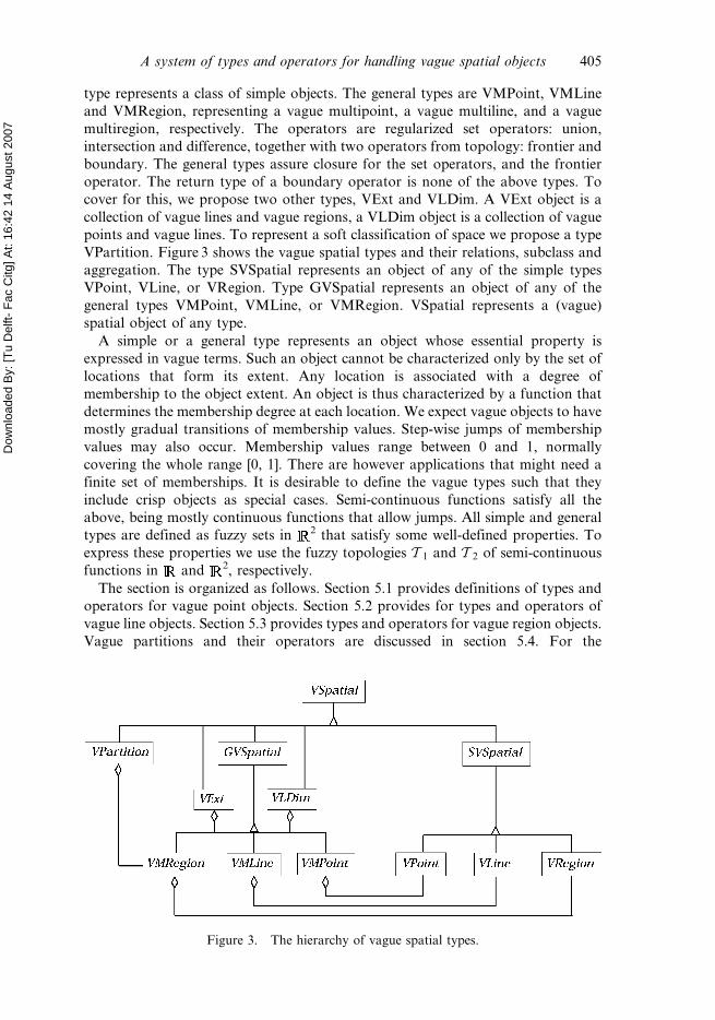
VPartition. Figure 3 shows the vague spatial types and their relations, subclass and

aggregation. The type SVSpatial represents an object of any of the simple types

VPoint, VLine, or VRegion. Type GVSpatial represents an object of any of the

general types VMPoint, VMLine, or VMRegion. VSpatial represents a (vague)

spatial object of any type.

A simple or a general type represents an object whose essential property is

expressed in vague terms. Such an object cannot be characterized only by the set of

locations that form its extent. Any location is associated with a degree of

membership to the object extent. An object is thus characterized by a function that

determines the membership degree at each location. We expect vague objects to have

mostly gradual transitions of membership values. Step-wise jumps of membership

values may also occur. Membership values range between 0 and 1, normally

covering the whole range [0, 1]. There are however applications that might need a

finite set of memberships. It is desirable to define the vague types such that they

include crisp objects as special cases. Semi-continuous functions satisfy all the

above, being mostly continuous functions that allow jumps. All simple and general

types are defined as fuzzy sets in 2 that satisfy some well-defined properties. To

express these properties we use the fuzzy topologies T 1 and T 2 of semi-continuous

functions in and 2, respectively.

The section is organized as follows. Section 5.1 provides definitions of types and

operators for vague point objects. Section 5.2 provides for types and operators of

vague line objects. Section 5.3 provides types and operators for vague region objects.

Vague partitions and their operators are discussed in section 5.4. For the

Figure 3. The hierarchy of vague spatial types.


Dow

nloa

ded

By:

[Tu

Del

ft- F

ac C

itg] A

t: 16

:42

14 A

ugus

t 200

7

illustrations of vague objects we use grey levels to show membership values. Darktones indicate high membership values, light tones indicate low memberships.

5.1 Vague point types and operators

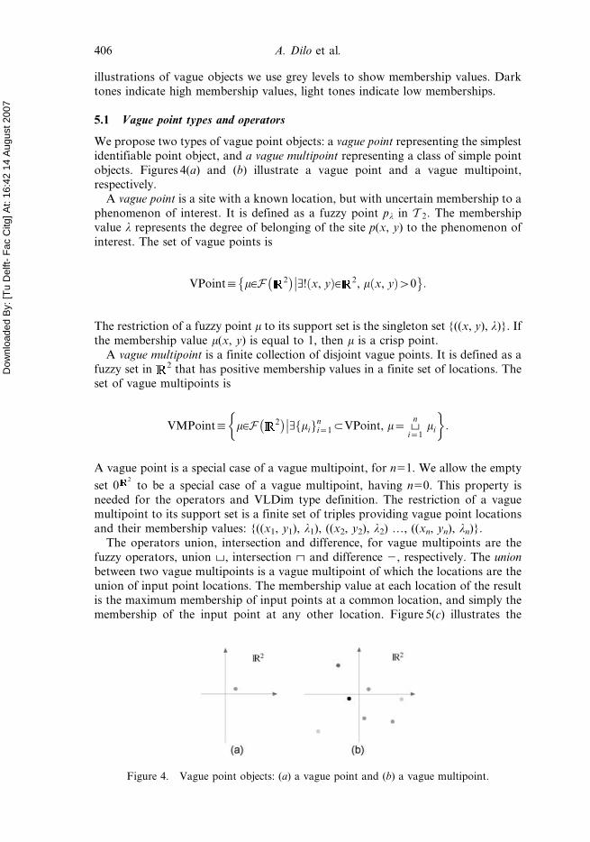
We propose two types of vague point objects: a vague point representing the simplest

identifiable point object, and a vague multipoint representing a class of simple point

objects. Figures 4(a) and (b) illustrate a vague point and a vague multipoint,respectively.

A vague point is a site with a known location, but with uncertain membership to a

phenomenon of interest. It is defined as a fuzzy point pl in T 2. The membership

value l represents the degree of belonging of the site p(x, y) to the phenomenon of

interest. The set of vague points is

VPoint: m[F 2� �

A! x, yð Þ[ 2, m x, yð Þw0�

�

� �

:

The restriction of a fuzzy point m to its support set is the singleton set {((x, y), l)}. If

the membership value m(x, y) is equal to 1, then m is a crisp point.

A vague multipoint is a finite collection of disjoint vague points. It is defined as a

fuzzy set in 2 that has positive membership values in a finite set of locations. Theset of vague multipoints is

VMPoint: m[F 2� �

A mif gni~15VPoint, m~

�

� zn

i~1mi

� �

:

A vague point is a special case of a vague multipoint, for n51. We allow the empty

set 02

to be a special case of a vague multipoint, having n50. This property is

needed for the operators and VLDim type definition. The restriction of a vague

multipoint to its support set is a finite set of triples providing vague point locations

and their membership values: {((x1, y1), l1), ((x2, y2), l2) …, ((xn, yn), ln)}.

The operators union, intersection and difference, for vague multipoints are the

fuzzy operators, union z, intersection y and difference 2, respectively. The union

between two vague multipoints is a vague multipoint of which the locations are the

union of input point locations. The membership value at each location of the resultis the maximum membership of input points at a common location, and simply the

membership of the input point at any other location. Figure 5(c) illustrates the

Figure 4. Vague point objects: (a) a vague point and (b) a vague multipoint.

406 A. Dilo et al.

Dow

nloa

ded

By:

[Tu

Del

ft- F

ac C

itg] A

t: 16

:42

14 A

ugus

t 200

7

union of two vague multipoints of figures 5(a) and (b). The operator PUnion is

defined as

PUnion : VMPoint|VMPoint?VMPoint

Vm, n[VMPoint, PUnion m, nð Þ~mzn:

The intersection between two vague multipoints is a vague multipoint of which the

locations are the common locations of input points. The membership value at each

location of the result is the minimum of memberships of input points at that

location. Figure 5(d) illustrates the intersection of the vague multipoints of

figures 5(a) and (b). The operator PIntersection is defined as

PIntersection : VMPoint|VMPoint?VMPoint

Vm, n[VMPoint, PIntersection m, nð Þ~myn:

The difference of two vague multipoints is a vague multipoint of which the locations

are those of the first input object. The membership value at a common location is

the minimum of the membership of the first object and the complemented

membership of the second object. At all other locations it is the membership of the

first object. Figure 5(e) illustrates the difference of the vague multipoint of

figure 5(a) with the vague multipoint of figure 5(b). The operator PDifference is

defined as

PDifference : VMPoint|VMPoint?VMPoint

Vm, n[VMPoint, PDifference m, nð Þ~m{n:

The set of vague multipoints is closed under these operators, i.e. the union,

intersection, and difference of two VMPoint objects is a VMPoint object. It can be

seen that PUnion, PIntersection and PDifference applied to crisp multipoints

are equivalent to the point set union, intersection and difference, respectively.

Hence, they give the corresponding crisp operator when applied to crisp

multipoints.

Figure 5. Results of vague multipoint operators: (a) and (b) two vague multipoints, (c)–(e)results of their union, intersection, and difference, respectively. Vague points with member-ship value equal to 1 are labelled with the value 1.


Dow

nloa

ded

By:

[Tu

Del

ft- F

ac C

itg] A

t: 16

:42

14 A

ugus

t 200

7

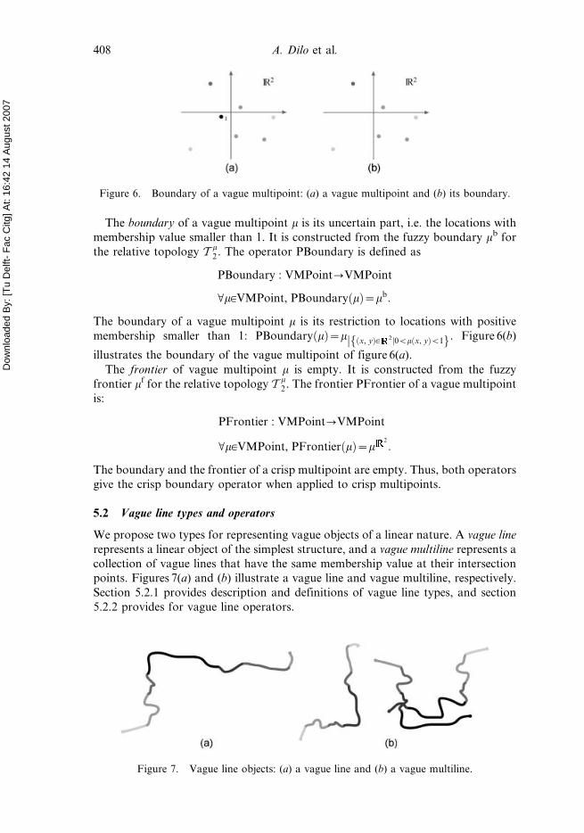
The boundary of a vague multipoint m is its uncertain part, i.e. the locations with

membership value smaller than 1. It is constructed from the fuzzy boundary mb for

the relative topology T m2. The operator PBoundary is defined as

PBoundary : VMPoint?VMPoint

Vm[VMPoint, PBoundary mð Þ~mb:

The boundary of a vague multipoint m is its restriction to locations with positive

membership smaller than 1: PBoundary mð Þ~m x, yð Þ[ 2 0vm x, yð Þv1jf gj . Figure 6(b)

illustrates the boundary of the vague multipoint of figure 6(a).

The frontier of vague multipoint m is empty. It is constructed from the fuzzy

frontier mf for the relative topology T m2. The frontier PFrontier of a vague multipoint

is:

PFrontier : VMPoint?VMPoint

Vm[VMPoint, PFrontier mð Þ~m2

:

The boundary and the frontier of a crisp multipoint are empty. Thus, both operators

give the crisp boundary operator when applied to crisp multipoints.

5.2 Vague line types and operators

We propose two types for representing vague objects of a linear nature. A vague line

represents a linear object of the simplest structure, and a vague multiline represents a

collection of vague lines that have the same membership value at their intersection

points. Figures 7(a) and (b) illustrate a vague line and vague multiline, respectively.

Section 5.2.1 provides description and definitions of vague line types, and section

5.2.2 provides for vague line operators.

Figure 6. Boundary of a vague multipoint: (a) a vague multipoint and (b) its boundary.

Figure 7. Vague line objects: (a) a vague line and (b) a vague multiline.

408 A. Dilo et al.

Dow

nloa

ded

By:

[Tu

Del

ft- F

ac C

itg] A

t: 16

:42

14 A

ugus

t 200

7

5.2.1 Vague line types. A vague line is a linear feature with known position, but

with an uncertain extent, i.e. any point of the line has some certainty degree of

belonging to the line. A vague line is a simple curve with mostly gradual transitions

of membership values between neighbour points on the line. Membership values are

positive at every location on the line, except, perhaps, at the end nodes. Stepwise

changes of membership values may occur along the line, but isolated discontinuities

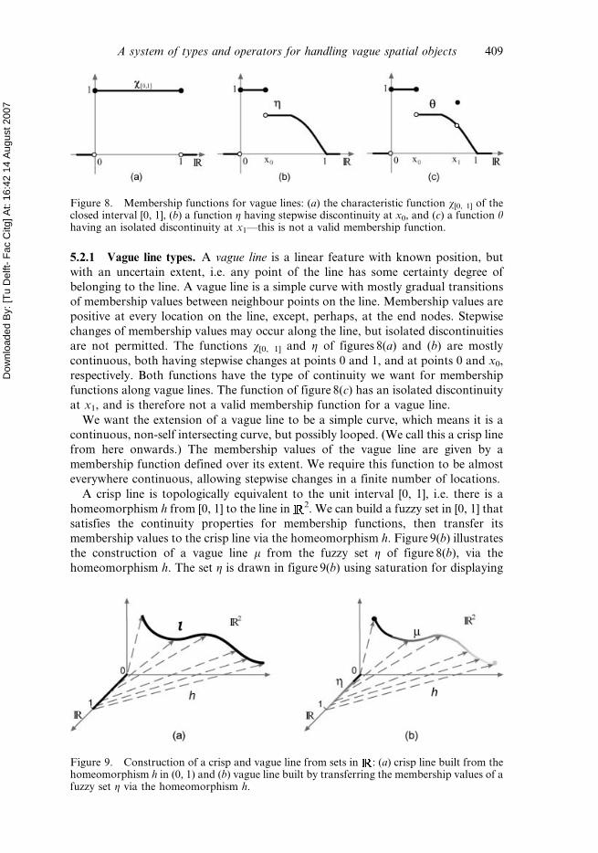
are not permitted. The functions x[0, 1] and g of figures 8(a) and (b) are mostly

continuous, both having stepwise changes at points 0 and 1, and at points 0 and x0,

respectively. Both functions have the type of continuity we want for membership

functions along vague lines. The function of figure 8(c) has an isolated discontinuity

at x1, and is therefore not a valid membership function for a vague line.

We want the extension of a vague line to be a simple curve, which means it is a

continuous, non-self intersecting curve, but possibly looped. (We call this a crisp line

from here onwards.) The membership values of the vague line are given by a

membership function defined over its extent. We require this function to be almost

everywhere continuous, allowing stepwise changes in a finite number of locations.

A crisp line is topologically equivalent to the unit interval [0, 1], i.e. there is a

homeomorphism h from [0, 1] to the line in 2. We can build a fuzzy set in [0, 1] that

satisfies the continuity properties for membership functions, then transfer its

membership values to the crisp line via the homeomorphism h. Figure 9(b) illustrates

the construction of a vague line m from the fuzzy set g of figure 8(b), via the

homeomorphism h. The set g is drawn in figure 9(b) using saturation for displaying

Figure 8. Membership functions for vague lines: (a) the characteristic function x[0, 1] of theclosed interval [0, 1], (b) a function g having stepwise discontinuity at x0, and (c) a function hhaving an isolated discontinuity at x1—this is not a valid membership function.

Figure 9. Construction of a crisp and vague line from sets in : (a) crisp line built from thehomeomorphism h in (0, 1) and (b) vague line built by transferring the membership values of afuzzy set g via the homeomorphism h.


Dow

nloa

ded

By:

[Tu

Del

ft- F

ac C

itg] A

t: 16

:42

14 A

ugus

t 200

7

membership values. The vague line m is built from the extension principle as the

image ehh gð Þ of the fuzzy set g g .

A crisp line is the image of the [0, 1] interval by the homeomorphism h:{h(t)5(x(t), y(t))|t g [0, 1]}. To allow looped lines, the homeomorphism is restricted

to (0, 1), requiring continuity at the end points 0 and 1 (Dilo 2000). An upper semi-

continuous function satisfies most of the properties we want for the membership

function of a vague line, but allows isolated discontinuities, e.g. the function of

figure 8(c). The regular closure removes such isolated discontinuities. A vague line

can now be built from a regular closed fuzzy set g in [0, 1] and the homeomorphism

h. To assure that the vague line has a continuous extent, we require the fuzzy set g to

have positive membership in [0, 1], that is g is connected for ( , T 1). A vague line isthus built as the image by a homeomorphism of a regular closed and connected

fuzzy set in [0, 1]. When the vague line is looped, the membership values at both end

nodes are equal. The set of vague lines is defined as

VLine: m[F 2� �

Ag[j F 0, 1½ �ð Þ, g~g0, and connected,�

Ah : 0, 1½ �? 2 homeomorphism in 0, 1ð Þ, continuous in 0, 1f g,

m~ehh gð Þ and h 0ð Þ~h 1ð Þ[g 0ð Þ~g 1ð Þð Þo

:

The homeomorphism h builds the extension of a vague line m as topologically

equivalent with the interval (0, 1) that is a 1-dimensional set. The extension of a

vague line cannot be a finite set of points. Hence, the type vague line is different

from the vague point and vague multipoint types. If the fuzzy set g in [0, 1] is a crisp

set, then the vague line is a crisp line.

A vague multiline is a finite collection of vague lines, of which the extensions

intersect only at their end nodes, and the lines have the same membership value at

the common end nodes (see figure 7(b)). It is constructed from the union of vague

lines from the finite collection. The set of vague multilines is

VMLine: m[F 2� �

A mif gn15VLine

�

� , m~zni~1 mi

� �

:

A vague line is a special case of a vague multiline, having n51. If n50 the vague

multiline is the empty set, a property required for the definitions of VLDim and

VExt types.

A union type VLDim has values that are collections of vague lines and vague

points. The type is defined as

m[F R2� �

Aj n[VMLine, Ac[VMPoint, m~vzc� �

:

A VLDim object m can be a vague multiline if the point component c is empty, and itcan be a vague multipoint if its line component n is empty.

5.2.2 Vague line operators. The union, intersection and difference operators for

vague lines are built from the corresponding fuzzy set operators. The union of two

vague multilines is a vague multiline produced by the fuzzy set union of the input

line objects. The union operator LUnion is defined as

LUnion : VMLine|VMLine?VMLine

Vm, n[VMLine, LUnion m, nð Þ~mzn:

The set of vague multilines is closed under union.

410 A. Dilo et al.

Dow

nloa

ded

By:

[Tu

Del

ft- F

ac C

itg] A

t: 16

:42

14 A

ugus

t 200

7

The intersection of two vague multilines produces the intersection points of the

two line extensions, associated by the membership values at these points calculated

from the fuzzy intersection operator. The (point) intersection of the extensions of

two vague multilines is produced by the intersection operator for crisp lines. Let m

and n be two vague multilines. We denote by EI the (crisp) intersection of their

extensions: EI(m, n)5Intersection(supp(m), supp(n)). The intersection operator

between vague multilines is defined from the fuzzy restriction to the intersection

of their extensions:

LIntersection : VMLine|VMLine?VMPoint

Vm, n[VMLine, LIntersection m, nð Þ~ mynð Þ EI m, nð Þj :

The difference operator between two vague multilines produces a multiline taken

from the fuzzy difference of the fuzzy sets. The extension of the result is the (classical

set) difference of the extensions of the input vague multilines. Membership values

along the extension are calculated from the fuzzy difference. If two vague multilines

m and n intersect at points, there might be isolated discontinuity at the result of

the fuzzy difference. To correct for this, we take the regular closure of fuzzy

difference m{nð Þ0 (in the relative topology T m{n2 ). The difference operator is then

defined as

LDifference : VMLine|VMLine?VMLine

Vm, n[VMLine, LDifference m, nð Þ~ m{nð Þ0:

These three operators give the corresponding crisp operators when applied to crisp

multilines.

The boundary of a vague multiline is its uncertain part. It is constructed from the

union of boundaries of its vague line components. For a vague line m expressed by a

fuzzy set g and a homeomorphism h, the boundary is constructed as the image by h

of the fuzzy boundary of g, ehh gb� �

. When the vague line m is crisp, its boundary

consists of vague points that are the end nodes of the line. When the membership

function along the line is continuous, which means that g is continuous, the

boundary of m consists of vague line components. In general, the boundary of a

vague line consists of vague points and vague lines. The boundary of a vague

multiline m~zni~1mi is the union of the boundaries of its components mi. The

boundary operator for vague multilines is defined as

LBoundary : VMLine?VLDim

Vm[VMLine, m~z mi mi~ehhi gið Þ[VLine, i[ 1 . . . nf g

�

�

�

n o

,

LBoundary mð Þ~zni~1ehhi gb

i

� �

:

Figure 10(a) illustrates a vague multiline. The end nodes of its core are shown by

empty circles. Figure 10(b) shows its boundary, which consists of vague lines and

vague points. The boundary of a vague multiline m is the restriction to the set of

locations with positive membership smaller than 1, extended by the boundary of the

core.


Dow

nloa

ded

By:

[Tu

Del

ft- F

ac C

itg] A

t: 16

:42

14 A

ugus

t 200

7

The frontier of a vague multiline is constructed in a similar way from the frontiers

of its vague line components. The frontier of a vague line m~ehh gð Þ is the image of

the fuzzy frontier of g, ehh gf� �

. The frontier of a vague multiline is the union of

frontiers of its vague line components, and is a vague multipoint. The operator is

defined as

LFrontier : VMLine?VMPoint

Vm[VMLine, m~z mi mi~ehhi gið Þ[VLine, i[ 1 . . . nf g

�

�

�

n o

,

LFrontier mð Þ~zni~1ehhi gf

i

� �

:

Figure 10(c) shows the frontier of the vague multiline of figure 10(a). The frontier of

a vague multiline is its restriction to the set of discontinuity locations of the

membership function.

The boundary LBoundary and the frontier LFrontier applied on a crisp multiline

produce the set of end nodes of its line components. Thus, both operators give the

crisp boundary operator when applied to crisp multilines.

5.3 Vague region types and operators

We distinguish two types of vague region objects, vague region representing the

simplest identifiable object, and vague multiregion representing a class of vague

regions. A vague region is a single-component fuzzy set that does not have

irregularities: isolated vague points and vague lines, or punctures and cuts, i.e.

removed vague points and vague lines, respectively. A vague multiregion is a

collection of disjoint vague regions. The fuzzy set of figure 11(a) has a puncture and

a cut, both irregularities that are not allowed for a vague region object. Figure 11(b)

illustrates a vague region, and figure 11(c) illustrates a vague multiregion.

Section 5.3.1 provides definitions for vague regions, vague multiregions and the

type vague extent. Section 5.3.2 provides definitions for vague region operators.

Illustrations for both sections are produced from data on heavy metal concentration

in the sediments of the Maas river.

5.3.1 Vague region types. A vague region is a broad boundary region, such that

points in the broad boundary typically have different membership values, which

change mostly gradually between neighbour points. The membership values can

change abruptly along a line, making a stepwise jump. Abrupt changes only at one

location, or membership values along a line changing abruptly from both sides, are

Figure 10. Boundary and frontier of a vague multiline: (a) a vague multiline with its coreboundary shown in empty circles, (b) its boundary (the core is drawn in light grey) and (c) itsfrontier (the line extension is drawn in light grey).

412 A. Dilo et al.

Dow

nloa

ded

By:

[Tu

Del

ft- F

ac C

itg] A

t: 16

:42

14 A

ugus

t 200

7

not allowed. Figure 12 illustrates different vague regions. The vague region of

figure 12(a) has a single-component core and does not have holes. Its membership

function decreases gradually from the boundary of the core to the boundary of the

support set. Every a-cut of the region is connected. The vague region of figure 12(b)

has two cores. The vague region of figure 12(c) has a single-component core, and it

contains holes. All its a-cuts are connected. The vague region of figure 12(d) has

several cores and several holes.

We want the support set of a vague region to be a crisp region, and the

membership function to be almost everywhere continuous in the support set,

allowing stepwise jumps along linear features. We require a vague region to be

bounded, regular closed, and with connected interior in ( 2, T 2). When a fuzzy set

satisfies these three properties for T 2, its support set satisfies the same properties for

T2, which means it is a crisp region. The regular closure assures stronger properties

than the upper semi-continuity: the discontinuities are stepwise jumps along lines;

no isolated discontinuities are allowed, and no discontinuity from both sides of a

line occur. It satisfies the membership function requirement. The set of vague

regions is then defined as

VRegion: m[F 2� �

m is bounded, m~m0, m0 is connectedj� �

:

Figure 12. Vague region objects.

Figure 11. Fuzzy sets in 2: (a) a fuzzy set that is not a vague region, (b) a vague region and(c) a vague multiregion.


Dow

nloa

ded

By:

[Tu

Del

ft- F

ac C

itg] A

t: 16

:42

14 A

ugus

t 200

7

The highest membership value may be less than 1. The regular closure property for

T 2 excludes the possibility for a vague line or vague multiline to be a vague region.

A crisp region is a specific case of a vague region, when the set m is a crisp set.

A vague multiregion represents a class of vague region objects. It is a multi-

component fuzzy set that is bounded and regular closed. Figure 11(b) illustrates a

vague multiregion with only one component, and figure 11(c) illustrates a multi-component region. The set of vague multiregions is defined as

VMRegion: m[F 2� �

m is bounded, m~m0j� �

:

A vague region is a special case of a vague multiregion, being a region with a single

component. A vague multiregion can also be empty.

A vague extension is a collection of vague multiregions and vague multilines. The

set of vague extensions is defined as

VExt: m[F 2� �

An[VMRegion, Ac[VMLine, m~nzcj� �

:

A VExt object m can be a vague multiregion if the line component c is empty, and it

can be a vague multiline if its region component n is empty.

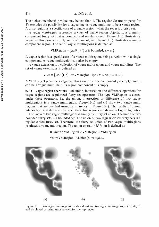
5.3.2 Vague region operators. The union, intersection and difference operators for

vague regions are regularized fuzzy set operators. The type VMRegion is closedunder these operators, i.e. the union, intersection or difference of two vague

multiregions is a vague multiregion. Figure 13(a) and (b) show two vague multi

regions that are overlaid using transparency in Figure 13(c). The results of union,

intersection, and difference between these two regions are shown in Figure 14(a)–(c).

The union of two vague multiregions is simply the fuzzy set union. The union of two

bounded fuzzy sets is a bounded set. The union of two regular closed fuzzy sets is aregular closed fuzzy set. Therefore, the fuzzy set union of two vague multiregions

produces a vague multiregion. The union operator RUnion is defined as

RUnion : VMRegion|VMRegion?VMRegion

Vm, n[VMRegion, RUnion m, nð Þ~mzn:

Figure 13. Two vague multiregions overlayed: (a) and (b) vague multiregions, (c) overlayedand displayed by using transparency for the top region.

414 A. Dilo et al.

Dow

nloa

ded

By:

[Tu

Del

ft- F

ac C

itg] A

t: 16

:42

14 A

ugus

t 200

7

The intersection of two vague multiregions is the regular closure of their fuzzy set

intersection. Fuzzy intersection of two bounded fuzzy sets is a bounded fuzzy set.

Fuzzy intersection of two regular closed fuzzy sets is not always regular closed. We

obtain a vague multiregion by applying the regular closure on the result of the fuzzy

intersection of two vague multiregions. The interior of a fuzzy intersection is equal

to the fuzzy intersection of the interiors. Therefore, we can define the intersection

operator between regions as

RInterection : VMRegion|VMRegion?VMRegion

Vm, n[VMRegion, RInterection m, nð Þ~m0yn0:

The difference operator between two vague multiregions m and n is built from the

fuzzy difference, which in turn is defined in terms of a fuzzy intersection:

my 12

{n�

. The fuzzy difference between two vague multiregions produces a

bounded fuzzy set, but not always a regular closed fuzzy set. Again, we apply the

regular closure on the result of the fuzzy operator, in order to get a vague

multiregion. The interior of the fuzzy intersection is equal to the intersection of the

interiors, and the complement of n is an open set. We can, therefore, define the

difference between vague multiregions as

RDifference : VMRegion|VMRegion?VMRegion

Vm, n[VMRegion, RDifference m, nð Þ~m0y 12{n

� �

:

The boundary of a vague multiregion m is its uncertain part, and it is constructed

from the fuzzy boundary mb. The boundary of a vague multiregion may consist of

vague regions, vague lines, or both. It is a vague extension VExt. The boundary of a

crisp region consists only of lines, whereas the boundary of a vague multiregion with

continuous membership function is a vague multiregion. Figure 15(a) illustrates a

vague multiregion with its core boundary drawn in grey, and figure 15(b) shows its

Figure 14. Results of operators on vague multiregions of figure 13: (a)–(c) union,intersection and difference, respectively.


Dow

nloa

ded

By:

[Tu

Del

ft- F

ac C

itg] A

t: 16

:42

14 A

ugus

t 200

7

boundary, which is a vague extension. The boundary operator is defined as:

RBoundary : VMRegion?VExt

Vm[VMRegion, RBoundary mð Þ~mb:

The boundary of a vague multiregion m is the restriction of m to locations with

membership values smaller than 1, extended by the boundary of the core:

RBoundary mð Þ~m p[ 2 0vm pð Þv1jf g|Lm1j :

The frontier of a vague multiregion m is calculated as the fuzzy frontier mf. The

frontier operator on vague multiregions returns a vague multiline. If m has

discontinuities, the frontier returns all lines of discontinuity. When m is continuous,

its frontier is empty. Figure 15(c) illustrates the frontier of the vague multiregion of

figure 15(a). The operator RFrontier is defined as:

RFrontier : VMRegion?VMLine

Vm[VMRegion, RFrontier mð Þ~mf :

Both operators, the boundary and the frontier, produce the crisp boundary when

applied to crisp multiregions.

5.4 Vague partitions and their operators

In practical applications, vague multiregions often originate from a soft classifica-

tion of space, for example based on remote sensing imagery. Vague multiregions

representing different classes may not be disjoint, as we expect transition zones to

intersect with each other. A soft classification cannot give a crisp partition of space,

but some characteristics of such a partition should be kept to make a meaningful

classification. A vague partition serves this purpose. It is a collection of vague

multiregions that may intersect only at their uncertain parts. The core of one region

Figure 15. Boundary and frontier of a vague multiregion: (a) a vague region with the coreboundary in grey, (b) its boundary and (c) its frontier.

416 A. Dilo et al.

Dow

nloa

ded

By:

[Tu

Del

ft- F

ac C

itg] A

t: 16

:42

14 A

ugus

t 200

7

can intersect with the support set of the other region only at their boundaries. The

set of vague partitions is defined as

VPartition: mif gni~15VMRegion Vp, Ai[ 1 . . . nf gj , mi pð Þw0;

�

Vi, j, i=j[miymj v RBoundary mið ÞyRBoundary mj

� ��

:

The first condition assures that every location has a positive membership to at least

one vague class, and the second condition assures that any two classes may intersect

only at their uncertain part.

The operators we define for vague partitions are the overlay and the fusion

operator. The overlay operator VPOverlay superimposes two vague partitions, and

creates a new vague partition with vague multiregions obtained from the

intersections of a vague multiregion of the first partition with a vague multiregion

of the second partition. It is defined as

VOverlay : VPartition|VPartition?VPartition

VP1~ mif gni~1, P2~ nj

� �m

j~1[VPartition,

VOverlay P1, P2ð Þ~ fi,j i[ 1 . . . nf g, j[ 1 . . . mf g, fi,j~RInterection mi, nj

� ��

�

� �

:

It can be shown that the set {fi,j|i g {1…n}, j g {1…m}} forms a vague partition.

The overlay operator combines two vague classifications of space, and creates a new

classification that is more refined.

The fusion operator dissolves a vague partition by merging vague multiregions

based on grouping or equality of some attribute value of regions. The operator

assumes an attribute to be associated to vague multiregions of a vague partition. Let

us call such a partition an attribute extended vague partition, and let us denote by

ADomain the domain of attribute values. The set of such partitions is

AVPartition: mi, við Þf gni~15VMRegion|ADomain mif gn

i~1[VPartition�

�

� �

:

For simplicity we consider one attribute attached to the vague multiregions of a

partition. The set ADomain can generally be a Cartesian product of domains of

several attributes. A grouping of attribute values is a function g:ADomain

RADomain. This function is defined on the assumption that the group values are

in the same domain ADomain. Such a function g is an element of the power set

(ADomain6ADomain), the collection of subsets of the Cartesian product of

ADomain with itself. The fusion operator is then defined as

VFusion : AVPartition| ADomain|ADomainð Þ?AVPartition

VA~ mi, við Þf gni~1[AVPartition, Vg[ ADomain|ADomainð Þ,

VFusion Að Þ~ fj , wj

� �� m

j~1wj

� �m

j~1~ran gð Þ

�

�

�

n

,

Vj[ 1 . . . mf g, fj~z mi g við Þ~wj

�

�

� ��

:

The generalized fuzzy union of vague multiregions has a vague multiregion as its

output, therefore fj’s are VMRegion objects. It can be shown that the set fj

� �m

1

forms a vague partition. The fusion operator allows one to generalize a vague

partition.


Dow

nloa

ded

By:

[Tu

Del

ft- F

ac C

itg] A

t: 16

:42

14 A

ugus

t 200

7

6. Other spatial operators

Abstract models for spatial data propose a list of types and fundamental operators

that are needed in spatial data systems. The ROSE algebra (Guting 1994, Guting

and Schneider 1995) and OpenGIS abstract specification (Open GIS Consortium

1999) both provide a similar list of spatial operators. (A comparison between the

two models can be found in Dilo (2006).) To present the list of operators, we follow

here the grouping provided in Guting (1994).

(i) Operators returning spatial data type values, e.g. intersection of regions—

returning regions, union of lines—returning lines, boundary of regions—

returning lines.

(ii) Spatial predicates expressing spatial relations, e.g. point within region, region

overlaps region.

(iii) Spatial operators returning numbers. These are mainly metric operators e.g.

length of a line, area of a region, distance between two regions.

(iv) Operators on collection of objects, e.g. overlay of partitions, fusion of regions

based on the equality of values of a certain attribute.

Vague spatial types introduced in section 5 form a complete set of types

describing spatial objects. Some numerical types are needed for the other

operators, spatial predicates and metric operators. The type TruthDegree;[0, 1]

is the return type of all spatial predicates. Two other types, Measure; + , and

VMeasure;{f:(0, s]R + |s g (0, 1] and f is semi-continuous} are needed for

metric operators.

The vague operators introduced in section 5 cover the first and fourth group of

spatial operators: operators returning spatial data types and operators on

collections1. Other operators returning spatial types can be expressed as a

combination of union, intersection and complement, e.g. difference and symmetric

difference. In this section we give intuition and example definitions for operators of

the two other groups, spatial predicates and metric operators.

Spatial predicates express relations between vague multipoints, vague multi-

lines and vague multiregions. We provide relations Disjoint, Touches, Crosses,

Overlaps, Within, and Equal, which is the set of relations proposed by SQL/MM

spatial (ISO 1999). The relations extend the true/false set of truth values of the

SQL/MM relations to the [0, 1] interval. That means that the truth of a relation is

a matter of degree, thus a value of type TruthDegree. A value v between 0 and 1

for a relation R(m, n) means that objects m and n are in relation R to the degree v.

A value 0 for R(m, n) means that m and n are certainly not in relation R, whereas

a value 1 means the two are certainly in R. Spatial relations are defined

from membership values of the objects involved, considering extreme values

that support a relation or disapprove it. The complete treatment of spatial

relations, intuition, definition and illustrations can be found in Dilo et al. (2005)

and Dilo (2006). Here we give the properties of the relations, and some example

definitions.

The relations Disjoint, Touches, Crosses and Overlaps between vague

objects are defined such that a relation is certain if the corresponding crisp

relation is true for their cores; a relation is certainly false if the corresponding

1 More operators are proposed in the ROSE algebra from this last group.

418 A. Dilo et al.

Dow

nloa

ded

By:

[Tu

Del

ft- F

ac C

itg] A

t: 16

:42

14 A

ugus

t 200

7

crisp relation is false for their support sets. For example, the relation Disjoint is

defined as:

Disjoint : GVSpatial|GVSpatial?TruthDegree

Vm, n[GVSpatial, Disjoint m, nð Þ~1{supp[ 2 mynð Þ pð Þf g:

The total certainty of the other two relations, Within and Equal, is modelled by

the subset and equality relation for fuzzy sets, respectively. A Within(m, n) relation is

certainly false if the corresponding crisp relation between the core of m and the

support set of n is false. Similarly, an Equal relation is certainly false if the

corresponding crisp relation between the core of one object and the support set ofthe other is false. The relation Within is defined from the bounded difference

between two fuzzy sets m and n: ;p, m,n(p)5max{0, m(p)2n(p)}. The Within relation

is defined as:

Within : GVSpatial|GVSpatial?TruthDegree

Vm, n[GVSpatial, Within m, nð Þ~0 if myn~0

2

,

1{supp m+nð Þ pð Þf g otherwise:

(

The relations have the property that only one relation can be certain at a time, i.e.

if one relation is certain, all the others have a degree smaller than 1. For some of the

relations this property is stronger: if a relation is certain, all the others are false.

Each relation gives the corresponding crisp relation when applied to crisp objects.

Metric operators that we provide are distance between two vague objects of anytype, length of a vague multiline, area, diameter and perimeter of a vague

multiregion. An operator on vague objects is such that for every a in (0, 1] it returns

the value of the analogous crisp operator applied to the a-cuts of the vague objects.

For example, the area operator returns for every a in (0, 1] the area of the a-cut of

the vague multiregion. We call these alpha operators. An alpha operator takes as

argument one or two vague objects, and returns a function from an interval in (0, 1]

to the non-negative real numbers + . The returned function by an alpha operator is

a value of type VMeasure. Again, we give here only example definitions. The

complete treatment of metric operators can be found in Dilo (2006).

The alpha area of a vague multiregion m is calculated from the areas of its a-cuts:

AREA mað Þ~Ð Ð

madx dy. If the maximum of m is lower than 1, we consider the area

Area(m) to be 0 for all a values higher than the maximum. The Area operator is

defined as:

Area : VMRegion?VMeasure

Vm[VMRegion, Area m½ � að Þ~Area mað Þ 0vaƒmaxp m pð Þf g,

0 maxp m pð Þf gvaƒ1:

(

For each alpha operator we provide a corresponding operator that produces anaverage over all values of the return function of the alpha operator. We call the

operators of this second group average operators. As the integration performs an

averaging process on functions, we define an average operator as the integral over


Dow

nloa

ded

By:

[Tu

Del

ft- F

ac C

itg] A

t: 16

:42

14 A

ugus

t 200

7

[0, 1] of the return function of the corresponding alpha operator. An average

operator returns a non-negative real number that is a value of type Measure. As an

example operator from this group see the average area operator.

The alpha area of a vague multiregion is a non-increasing and upper semi-

continuous function, thus the function Area(m) is integrable. The average area of a

region m is calculated from the integral of Area(m) over [0, 1]. The operator AvArea

is defined as:

AvArea : VMRegion?Measure

Vm[VMRegion, AvArea mð Þ~ð1

0

Area m½ � að Þda:

The average area calculated from the integral Area[m](a)da provides the volume

under the m function. Therefore, the average area is equal to

AvArea mð Þ~ð ð

m x, yð Þdx dy:

This provides a way to calculate the average area operator independently from the

alpha area operator.

An alpha operator can be used to provide a measure for a given level of

membership, whereas an average operator provides an overall measure for vague

object(s), performing an averaging over all membership levels. An average operator

gives its crisp analogue when applied to crisp objects.

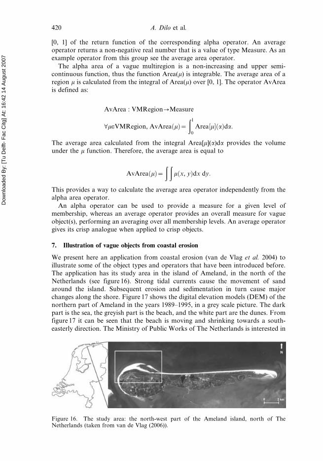
7. Illustration of vague objects from coastal erosion

We present here an application from coastal erosion (van de Vlag et al. 2004) to

illustrate some of the object types and operators that have been introduced before.

The application has its study area in the island of Ameland, in the north of the

Netherlands (see figure 16). Strong tidal currents cause the movement of sand

around the island. Subsequent erosion and sedimentation in turn cause major

changes along the shore. Figure 17 shows the digital elevation models (DEM) of the

northern part of Ameland in the years 1989–1995, in a grey scale picture. The dark

part is the sea, the greyish part is the beach, and the white part are the dunes. From

figure 17 it can be seen that the beach is moving and shrinking towards a south-

easterly direction. The Ministry of Public Works of The Netherlands is interested in

Figure 16. The study area: the north-west part of the Ameland island, north of TheNetherlands (taken from van de Vlag (2006)).

420 A. Dilo et al.

Dow

nloa

ded

By:

[Tu

Del

ft- F

ac C

itg] A

t: 16

:42

14 A

ugus

t 200

7

stabilizing the process of change in the Ameland shore. To neutralize the erosion

they carry out beach nourishment by depositing sand. They are interested to know

where the nourishment should be performed. Beach areas without vegetation have

the highest erosion risk, hence they are the areas where sand has to be deposited.

Survey data from the JARKUS database (van de Vlag et al. 2004) and

LandsatTM5 images are used for this application. The digital terrain model (DTM)

is built from survey data, and the vegetation index (NDVI) is calculated from

Landsat images. Beach areas are derived from the DTM, and the non-vegetated

areas are derived from the NDVI index. In the methodology of the Dutch National

Institute for Coastal and Marine Management (RIKZ) for the preservation of the

coast, beach areas are considered those having elevations between 21 and 2 m (a

short description is provided in van de Vlag et al. (2004)). The light grey bars in

figure 18 show the crisp classification of the zone performed by RIKZ. However, the

separation between the three classes, foreshore, beach and foredune, is not crisp.

Transition zones occur between these three classes, hence justifying an approach by

vague objects. The concepts ‘vegetated’ and ‘non-vegetated’ are also vague. There

are transition zones with scarce vegetation. An NDVI value around 0 separates

vegetated from non-vegetated areas.

Emerging objects in this application are vague partitions and vague region

objects. The vague regions are a typical example of regions resulting from a

classification over space. The three vague classes, foreshore, beach and foredune, are

vague multiregions. They are calculated from the elevation values applying the

membership functions shown in figure 18. Results of the crisp and fuzzy

classifications for the year 1995 are shown in figure 19. Part (a) is a map of

elevations in the study area, part (b) shows the result of the crisp classification of

elevations, and parts (c)–(e) are the vague classes created from the membership

functions of figure 18. The three vague classes form a vague partition of the zone,

assured from the choice of their membership functions.

Figure 17. DEM of the northern part of Ameland for years 1990–1995. Low elevationvalues are shown in black colour, high elevation values in white. The dark part is the sea, thegrey part is the beach and the white part are the dunes.

Figure 18. Membership functions for shore, beach and dune. The light grey bars show theboundaries for a crisp classification of elevations.


Dow

nloa

ded

By:

[Tu

Del

ft- F

ac C

itg] A

t: 16

:42

14 A

ugus

t 200

7

Figure 20(a) shows the NDVI index for year 1995. Figure 20(b) shows the

membership functions applied on NDVI values to derive vegetated and non-

vegetated classes. A transition zone exists when passing from vegetated to non-

vegetated objects: NDVI values in [20.05, 0.05] are taken to have a positive degree

of being both vegetated and non-vegetated at the same time (figures 20(c) and (d)).

The lower part of the area is covered by dune vegetation, tall grass and occasional

bush. This corresponds to high membership values of vegetated objects shown in

figure 20(d). Further north starts the flat area with only some sparse vegetation. This

causes an abrupt change of membership values inside the lower-most vegetated

object. Both classes, vegetated and non-vegetated are vague multiregions, and

together form a vague partition of the area.

Sand is to be deposited at non-vegetated beach areas that have a certain extent,

i.e. the area of such an object is over a certain limit. Non-vegetated beach objects are

derived from the intersection of beach and non-vegetated vague classes (figures 21(a)

and (b)). Their intersection shown in figure 21(c) is again a vague multiregion object.

It is composed of two vague regions. The average area AvArea operator is applied

on vague regions to decide whether to perform nourishment or not. Vague regions

with average area higher than a certain limit are selected for the nourishment. The

lower region has a very small (average) area. Only the upper region will be selected

for nourishment.

Illustrations and calculations for this section are done in ArcGIS, using raster

data to present a vague class, and VisualBasic programming to perform the area

calculation for a class. The average area can be easily calculated for the whole class

(raster layer), whereas its calculation for a vague region object cannot be done.

Selection of a region object, a component in the beach class, is not possible in

ArcGIS raster data. In Dilo et al. (2006) we show a possible implementation for the

vague spatial types. A vague region, stored in a TIN-like structure, can be selected in

Figure 20. Vegetation index and fuzzy classification: (a) NDVI index of Ameland for theyear 1995, low values in dark tone, high values in light tone, (b) membership functions appliedto define non-vegetated and vegetated classes, (c) and (d) non-vegetated and vegetated vagueobjects.

Figure 19. Elevation and results of crisp and fuzzy classification: (a) DEM of Ameland forthe year 1995, (b) crisp classification of elevations, (c) vague shore, (d) vague beach, (e) vaguedune. Saturated colour shows high membership for vague objects.

422 A. Dilo et al.

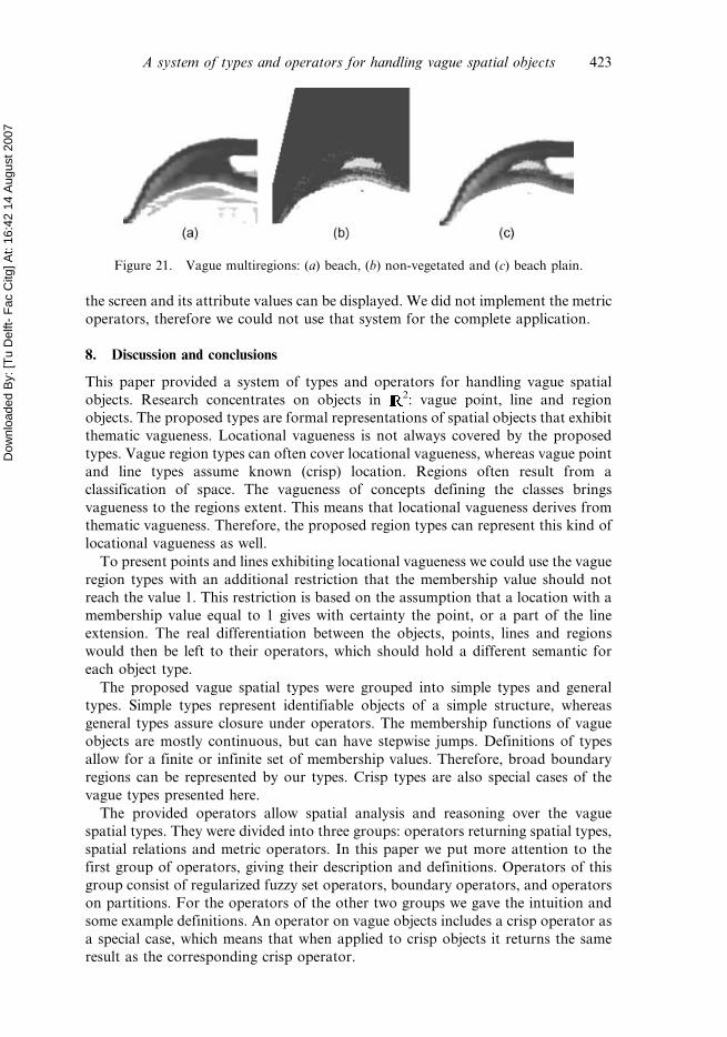
Dow

nloa

ded

By:

[Tu

Del

ft- F

ac C

itg] A

t: 16

:42

14 A

ugus

t 200

7

the screen and its attribute values can be displayed. We did not implement the metric

operators, therefore we could not use that system for the complete application.

8. Discussion and conclusions

This paper provided a system of types and operators for handling vague spatial

objects. Research concentrates on objects in 2: vague point, line and region

objects. The proposed types are formal representations of spatial objects that exhibit

thematic vagueness. Locational vagueness is not always covered by the proposed

types. Vague region types can often cover locational vagueness, whereas vague point

and line types assume known (crisp) location. Regions often result from a

classification of space. The vagueness of concepts defining the classes brings

vagueness to the regions extent. This means that locational vagueness derives from

thematic vagueness. Therefore, the proposed region types can represent this kind of

locational vagueness as well.

To present points and lines exhibiting locational vagueness we could use the vague

region types with an additional restriction that the membership value should not

reach the value 1. This restriction is based on the assumption that a location with a

membership value equal to 1 gives with certainty the point, or a part of the line

extension. The real differentiation between the objects, points, lines and regions

would then be left to their operators, which should hold a different semantic for

each object type.

The proposed vague spatial types were grouped into simple types and general

types. Simple types represent identifiable objects of a simple structure, whereas

general types assure closure under operators. The membership functions of vague

objects are mostly continuous, but can have stepwise jumps. Definitions of types

allow for a finite or infinite set of membership values. Therefore, broad boundary

regions can be represented by our types. Crisp types are also special cases of the

vague types presented here.

The provided operators allow spatial analysis and reasoning over the vague

spatial types. They were divided into three groups: operators returning spatial types,

spatial relations and metric operators. In this paper we put more attention to the

first group of operators, giving their description and definitions. Operators of this

group consist of regularized fuzzy set operators, boundary operators, and operators

on partitions. For the operators of the other two groups we gave the intuition and

some example definitions. An operator on vague objects includes a crisp operator as

a special case, which means that when applied to crisp objects it returns the same

result as the corresponding crisp operator.

Figure 21. Vague multiregions: (a) beach, (b) non-vegetated and (c) beach plain.


Dow

nloa

ded

By:

[Tu

Del

ft- F

ac C

itg] A

t: 16

:42

14 A

ugus

t 200

7

Acknowledgements

The work was funded by the European Community, under IST-1999-14189 project

REV!GIS. The datasets were made available by Rijkswaterstaat and RIKZ.

ReferencesBITTNER, T. and STELL, J.G., 2000, Rough sets in approximate spatial reasoning. In Second

International Conference on Rough Sets and Current Trends in Computing, Vol. 2005,

in the series Lecture Notes in Computer Science (LNCS), pp. 445–453 (Berlin:

Springer-Verlag).

BOGARDI, I., BARDOSSY, A. and DUCKSTEIN, L., 1990, Risk management for groundwater

contamination: fuzzy set approach. In Optimizing the Resources for Water

Management, R. Khanpilvardi and T. Gooch (Eds), pp. 442–448 (New York: ASCE).

BROWN, D.G., 1998, Mapping historical forest types in Baraga County Michigan, USA as

fuzzy sets. Plant Ecology, 134, pp. 97–111.

BURROUGH, P.A. and FRANK, A.U., 1996, Geographic Objects with Indeterminate Boundaries,

No. 2, in the series GISDATA (London: Taylor & Francis).

BURROUGH, P.A., VAN GAANS, P.F.M. and MACMILLAN, R.A., 2000, High-resolution

landform classification using fuzzy k-means. Fuzzy Sets and Systems, 113, pp. 37–52.

CHENG, T. and MOLENAAR, M., 1999, Diachronic analysis of fuzzy objects. GeoInformatica,

3, pp. 337–355.

CHENG, T., MOLENAAR, M. and LIN, H., 2001, Formalizing fuzzy objects from uncertain

classification results. International Journal of Geographical Information Science, 15,

pp. 27–42.

CLEMENTINI, E. and DI FELICE P., 1996, An algebraic model for spatial objects with

indeterminate boundaries. In Geographic Objects With Indeterminate Boundaries,

No. 2, in the series GISDATA, pp. 171–187 (London: Taylor & Francis) See Burrough

and Frank (1996).

CLEMENTINI, E. and DI FELICE P., 2001, A spatial model for complex objects with a broad

boundary supporting queries on uncertain data. Data & Knowledge Engineering, 37,

pp. 285–305.

COHN, A.G., BENNETT, B., GOODAY, J. and GOTTS, N.M., 1997, Qualitative spatial

representation and reasoning with the region connection calculus. GeoInformatica, 1,

pp. 275–316.

COHN, A.G. and GOTTS, N.M., 1996a, The ‘egg-yolk’ representation of regions with

indeterminate boundaries. In Geographic objects with indeterminate boundaries, No. 2,

in the series GISDATA, pp. 171–187 (London: Taylor & Francis) See Burrough and

Frank (1996).

COHN, A.G. and GOTTS, N.M., 1996b, Representing spatial vagueness: a mereological

approach. In Principles of Knowledge Representation and Reasoning (KR’96), L.

Carlucci Aiello, J. Doyle and S. Shapiro (Eds), pp. 230–241 (San Mateo, CA: Morgan

Kaufmann).

CUCHILLO-IBANEZ, E. and TARRES, J., 1997, On the boundary of fuzzy sets. Fuzzy Sets and

Systems, 89, pp. 113–119.

DE GRUIJTER J., WALVOORT, D. and VAN GAANS, P., 1997, Continuous soil maps—a fuzzy set

approach to bridge the gap between aggregation levels of process and distribution

models. Geoderma, 77, pp. 169–195.

DILO, A., 2000, Master’s thesis, International Institute for Geo-Information Science and

Earth Observation (ITC).

DILO, A., 2006, Representation of and reasoning with vagueness in spatial information: a

system for handling vague objects. PhD thesis, iTC Dissertation No. 135, Wageningen

University, Enschede, The Netherlands.

DILO, A., BOS, P., KRAIPEERAPUN, P. and DE BY R.A., 2006, Storage and manipulation of

vague spatial objects using existing GIS functionality. In Flexible Databases

424 A. Dilo et al.

Dow

nloa

ded

By:

[Tu

Del

ft- F

ac C

itg] A

t: 16

:42

14 A

ugus

t 200

7

Supporting Imprecision and Uncertainty, Vol. 203, in the series Studies in Fuzziness and

Soft Computing, G. Bordogna, and G. Psaila (Eds) (Berlin: Springer).

DILO, A., DE BY R.A. and STEIN, A., 2005, A proposal for spatial relations between vague

objects. In Proceedings of the International Symposium on Spatial Data Quality

ISSDQ’05, Beijing, China, L. Wu, W. Shi, Y. Fang and Q. Tong (Eds), pp. 50–59

(Beijing: The Hong Kong Polytechnic University).

ERWIG, M. and SCHNEIDER, M., 1997, Vague regions. In 5th International Symposium on

Advances in Spatial Databases (SSD’97), Vol. 1262, in the series Lecture Notes in

Computer Science, pp. 298–320 (Berlin: Springer-Verlag).

FISHER, P., 2000, Sorites paradox and vague geographies. Fuzzy Sets and Systems, 113, pp.

7–18.

FISHER, P., ARNOT, C., WADSWORTH, R. and WELLENS, J., 2006, Detecting change in vague

interpretations of landscapes. Ecological Informatics, pp. 163–178.

GUTING, R.H., 1994, An introduction to spatial database systems. VLDB Journal, 3, pp.

357–399.

GUTING, R.H. and SCHNEIDER, M., 1995, Realm-based spatial data types: the ROSE algebra.

VLDB Journal, 4, pp. 243–286.

HENDRICKS FRANSSEN, H., VAN EIJNSBERGEN, A. and STEIN, A., 1997, Use of spatial

prediction techniques and fuzzy classification for mapping soil pollutants. Geoderma,

77, pp. 243–262.

HENGL, T., WALVOORT, D.J.J., BROWN, A. and ROSSITER, D.G., 2004, A double continuous

approach to visualization and analysis of categorical maps. International Journal of

Geographical Information Science, 18, pp. 183–202.

ISO, 1999, Information technology – Database languages – SQL Multimedia and Application

Packages – Part 3: Spatial. Working Draft Text ISO/IEC 13249-3:1999(E) (London:

International Organization for Standardization) (unpublished).

JOST, J., 1998, Postmodern Analysis, in the series Universitext (Berlin: Springer).

KELLEY, J.L., 1975, General Topology, in the series Graduate Texts in Mathematics (New

York: Springer).

KLIR, G.J. and YUAN, B., 1995, Fuzzy Sets and Fuzzy logic: Theory and Application (New

Jersey: Prentice-Hall).

LIU, K. and SHI, W., 2006, Computing the fuzzy topological relations of spatial objects based

on induced fuzzy topology. International Journal of Geographical Information Science,

20, pp. 857–883.

LUCIEER, A., FISHER, P. and STEIN, A., 2004, Texture-based segmentation of remotely sensed

imagery to identify fuzzy coastal objects. In GeoDynamics (New York: CRC Press).

ODEH, I., MCBRATNEY, A. and CHITTLEBOROUGH, D.J., 1992, Soil pattern recognition with

fuzzy c-means: application to classification and soil-landform interrelationships. Soil

Science Society of America Journal, 65, pp. 505–516.

OPEN GIS CONSORTIUM, 1999, OpenGIS Simple Features Specification for SQL, Revision 1.1

(USA: Open GIS Consortium, Inc.) (unpublished).

PAWLAK, Z., 1994, Rough sets: present state and further prospects. In Third International

Workshop on Rough Set and Soft Computing (RSSC ’94), The Society of Computer

Simulation, San Diego, California, November 10–12, San Jose, California, USA, pp.

72–76.

PU, P.-M. and LIU, Y.-M., 1980, Fuzzy topology. I. Neighbourhood structure of a fuzzy point

and Moore-Smith convergence. Journal of Mathematical Analysis and Applications,

76, pp. 571–599.

RANDELL, D.A. and COHN, A.G., 1989, Modelling topological and metrical properties of

physical processes. In Proceedings of the 1st International Conference on Principles of

Knowledge Representation and Reasoning (KR’89), R.J. Brachman, H.J. Levesque

and R. Reiter (Eds), pp. 357–368 (San Mateo, CA: Morgan Kaufmann).

RANDELL, D.A., CUI, Z. and COHN, A.G., 1992, A spatial logic based on regions and

connection. In Proceedings of the Third International Conference on Principles of


Dow

nloa

ded

By:

[Tu

Del

ft- F

ac C

itg] A

t: 16

:42

14 A

ugus

t 200

7

Knowledge Representation and Reasoning (KR’92), B. Nebel, C. Rich and W.

Swartout (Eds), pp. 165–176 (San Mateo, CA: Morgan Kaufmann).

ROBINSON, V.B., 2003, A perspective on the fundamentals of fuzzy sets and their use in

geographic information systems. Transactions in GIS, 7, pp. 3–30.

ROY, A.J. and STELL, J.G., 2001, Spatial relations between indeterminate regions.

International Journal of Approximate Reasoning, 27, pp. 205–234.

SCHNEIDER, M., 1999, Uncertainty management for spatial data in databases: fuzzy spatial

data types. In SSD ’99: Proceedings of the 6th International Symposium on Advances in

Spatial Databases, Vol. 1651, Lecture Notes in Computer Science, pp. 330–351 (Berlin:

Springer-Verlag).

SCHNEIDER, M., 2000, Metric operations on fuzzy spatial objects in databases. In 8th ACM

Symposium on Geographic Information Systems (ACM GIS) (New York: ACM

Press), pp. 21–26.

SCHNEIDER, M., 2001a, A design of topological predicates for complex crisp and fuzzy

regions. In ER ’01: Proceedings of the 20th International Conference on Conceptual

Modeling, pp. 103–116 (Berlin: Springer-Verlag).

SCHNEIDER, M., 2001b, Fuzzy topological predicates, their properties, and their integration

into query languages. In 9th ACM Symposium on Geographic Information Systems

(ACM GIS) (New York: ACM Press).

SCHNEIDER, M., 2003, Design and implementation of finite resolution crisp and fuzzy spatial

objects. Data & Knowledge Engineering, 44, pp. 81–108.

SICAT, R.S., CARRANZA, E.J.M. and NIDUMOLU, U.B., 2005, Fuzzy modelling of farmers’

knowledge for land suitability classification. Agricultural Systems, 83, pp. 49–75.

SORENSEN, R., 2003, in The Stanford Encyclopedia of Philosophy, fall 2003 ed., E.N. Zalta

(Eds) (USA: The Metaphysics Research Lab CSLI).

TANG, X., 2004, Spatial object modelling in fuzzy topological spaces: with application to land

cover change. PhD thesis, International Institute for Geo-Information Science and

Earth Observation (ITC), Hengelosestraat 99, 7500 AA Enschede, The Netherlands.

VAN DE VLAG D., 2006, Modeling and visualizing dynamic landscape objects and their

qualities. PhD thesis, iTC Dissertation No. 132, Wageningen University, Enschede,

The Netherlands.

VAN DE VLAG D., STEIN, A. and VASSEUR, B., 2004, Concepts and representation of beach

nourishment by spatio-temporal ontology. In Proceedings of the International

Symposium on Spatial Data Quality (ISSDQ04), Vol. 2, GeoInfo, A. Frank, and E.

Grum (Eds). Department for Geoinformation and Cartography, Vienna University of

Technology, pp. 353–369.

VERT, G., STOCK, M. and MORRIS, A., 2002, Extending ERD modeling notation to fuzzy

management of GIS data files. Data & Knowledge Engineering, 40, pp. 163–179.

WANG, F., 2000, A fuzzy grammar and possibility theory-based natural language user

interface for spatial queries. Fuzzy Sets and Systems, 113, pp. 147–159.

WARREN, R.H., 1977, Boundary of a fuzzy set. Indiana University Mathematical Journal, 26,

pp. 191–197.

WEISS, M.D., 1975, Fixed points, separation, and induced topologies for fuzzy sets. Journal of

Mathematical Analysis and Applications, 50, pp. 142–150.

WILLARD, S., 1970, General Topology (Alberta: Addison-Wesley).

ZADEH, L.A., 1965, Fuzzy sets. Information and Control, 8, pp. 338–353.

ZADEH, L.A., 1975, Fuzzy logic and approximate reasoning. Synthese, 30, pp. 407–428.

ZHAN, B.F., 1997, Topological relations between fuzzy regions. In Proceedings of the 1997

ACM Symposium on Applied Computing (New York: ACM Press), pp. 192–196.

ZHAN, B.F., 1998, Approximate analysis of topological relations between geographic regions

with indeterminate boundaries. Soft Computing, 2, pp. 28–34.

426 A system of types and operators for handling vague spatial objects

A system of types and operators for handling vague spatial objects

Documents

Transcript of A system of types and operators for handling vague spatial objects