INFORMATION TO USERS

This manuscript has been reproduced from the microfilm master. TJMI

films the text dvectly from the ori^al or copy submitted. Thus, some

thesis and dissertation copies are in typewriter fiice, while others may be

from any type of computer printer.

The quality of this reproduction is dependent upon the quality of the

copy submitted. Broken or indistinct print, colored or poor quality

illustrations and photographs, print bleedthrough, substandard margins,

and improper alignment can adversely affect reproduction.

In the unlikely event that the author did not send UMI a complete

manuscript and there are missing pages, these will be noted. Also, if

unauthorized copyright material had to be removed, a note will indicate

the deletion.

Oversize materials (e.g., maps, drawings, charts) are reproduced by

sectioning the original, beginning at the upper left-hand comer and

continuing from left to right in equal sections with smaU overlaps. Each

original is also photographed in one exposure and is included in reduced

form at the back of the book.

Photographs included in the original manuscript have been reproduced

xerographically in this copy. I£gher quality 6" x 9" black and white

photographic prints are available for any photographs or illustrations

appearing m this copy for an additional charge. Contact UMI directly to

order.

UMI A Bell & Ebwell Infonnadon CompaiQ

300 North Zed) Road, Ann Aibor MI 4S106-1346 USA 313/761-4700 800/521-0600

Flexible composite propeller design using constrained optimization techniques

by

Abdul Monuem Khan

A dissertation submitted to the graduate faculty

in partial fulfillment of the requirements for the degree of

DOCTOR OF PHILOSOPHY

Major: Aerospace Engineering

Major Professors; Daniel O. Adams and Vinay Dayal

Iowa State University

Ames, Iowa

1997

UMX Nixmber: 9725423

UMI Microform 9725423 Copyright 1997, by UMI Company. All rights reserved.

This microform edition is protected against unauthorized copying under Title 17, United States Code.

UMI 300 North Zeeb Road Ann Arbor, MI 48103

ii

Graduate College Iowa State University

This is to certify that the Doctoral dissertation of

Abdul Monuem Khan

has met the dissertation requirement of Iowa State University

Co-major Professor

ajof^'fogram

—

For t CtfacWate College

Signature was redacted for privacy.

Signature was redacted for privacy.

Signature was redacted for privacy.

Signature was redacted for privacy.

iii

To my parents and grandparents

iv

TABLE OF CONTENTS

ACBCNOWLEDGEMENTS v

ABSTRACT vi

CHAPTER 1. INTRODUCTION 1

CHAPTER 2. THEORETICAL ASPECTS 12

CHAPTER 3. FINITE ELEMENT METHODS FOR COMPOSITE LAMINATES 47

CHAPTER 4. INITIAL RESULTS 60

CHAPTER 5. ANALYSIS AND DESIGN OF A COMPOSITE PROPELLER 83

CHAPTER 6. CONCLUSIONS 116

APPENDIX. FININTE ELEMENT FORMULATION 119

BIBLIOGRAPHY 129

ACKNOWLEDGEMENTS

An enormous amount of gratitude is owed to my advisor Dr. Daniel Adams for his

phenomenal guidance, support, patience, and invaluable advice throughout the course of my

Ph.D. program. I am also obliged to Dr. Jerald Vogel and Dr. Vinay Dayal for providing all

possible help for my research work. I am also thankful to Dr. Max Porter and Dr. Shayam

Bahadur for being part of my Ph.D. committee. I would also like to thank the people and the

government of Pakistan for the financial assistance provided to me through the scholarship

program of the Ministry of Science and Technology. My acquiring the graduate studies

would have been impossible without this scholarship program.

Fond appreciation and special thank must go to my parents and grandmother; to my

father Dr. Fasahat Ali Khan, for his encouragement, support, and advice in my life and in my

quest for knowledge and education; to my mother Mrs. Mudira Khanam, and my

grandmother Mrs. Munira Khanam Iqbal, for their love, support, and prayers, particularly

during the time of my graduate studies. I also wish to express my gratitude to my wife

Tamkeen Sultana Khanam, my son Ahmed Kamal Khan, and my daughter Arifa Khan for their

sacrifice, forbearance, and understanding throughout the course of my program and especially

while I was writing this dissertation.

I also wish to thank my uncles Wajahat Ali Khan and Azfar Ali Khan; my sisters Asifa

Khanam and Amna Khanam; and my brothers Dr. Abdus Salam Khan, Abdul Ban Khan,

Abdur Rab Khan, Abdul Malik Khan, Abdul Mateen Khan, and Abdul Aziz Khan for their

motivation and encouragement. I am also thankful to my friends Jehanzeb Masud, Irfan Aziz,

Zahid Baig and Noor Tirmizi for their help and support.

vi

ABSTRACT

An investigation of a conventional propeller, made from composite materials, was

conducted in which its characteristics were studied under quasi-static aerodynamic loading.

Also, optimized designing of a composite propeller was performed for various constrained and

unconstrained design objectives. Only symmetric ply stacking sequences were considered to

eliminate the effect of centrifugal force on the propeller. Results show that the ply stacking

sequence has an effect on the propeller characteristics of a conventional propeller. Proper

stacking sequence of the composite propeller improves its performance as compared to its

metallic counterpart. An improvement of about 47% in the propeller thrust coefficient was

observed for one of the cases. Similarly, improvement was observed in other propeller

characteristics as well. The classical blade element theory of propellers is used to calculate

propeller characteristics and the aerodynamic force distribution on the propeller blades. The

finite element method is used to calculate the resulting deformation of the propeller blades. In

the present smdy, the propeller is modeled as a variable thickness plate, discretized into a

number of quadrilateral shear-deformable finite elements. Propeller characteristics are

calculated for ply orientation angles ranging from -90 degrees to +90 degrees to study these

parameters as a function of orientation angle. These analyses were performed for six different

values of advance ratios and at two different initial blade setting angles. Improvement in

propeller design, by only changing the stacking sequence, was also considered using

techniques of numerical optimisation. It is shown that different design objectives can be

achieved by changing the stacking sequence. For carrying out design optimization of

propeller, Fortran subroutine "CONMIN" was used.

1

CHAPTER 1 INTRODUCTION

Background

Composite materials have been fully established as workable engineering materials

and are now commonly used around the world. Their applications are in the fields of

aerospace engineering, marine engineering, sporting goods, electronics, and in a number of

other fields. The success of composite materials results firom their very high strength,

stiffness and low specific gravity. Any structure itself or any of its components made firom

composite material can be termed as a composite structure.

Generally speaking, composite materials consist of one or more discontinuous phases

of material, embedded in another continuous phase material. The discontinuous phases can

be called reinforcements because they provide strength. In fiber composites, the fibers are

the reinforcing material. They are generally very strong and provide strength to the

composite structtire. The continuous phase is called the matrix and generally is weak

compared to the fibers. Thus, in describing the composite material as a system, one must

specify its constituent materials and their properties. Two systems with the same geometry

may be different fi-om each other because of their constituents. The concentration of

reinforcements, concentration distribution, and the orientation of reinforcements are some of

the parameters which may make one system different fi-om another. The orientation of

reinforcements affects the properties of the system. In fiber composites, the material has

different engineering properties in the direction parallel to the fibers than transverse to the

fibers. Such anisotropy can be controlled and used to advantage in engineering design.

As stated above, composite materials are being used in a number of engineering

fields, but these materials are most suitable in applications requiring high strength-to-weight

and stifihess-to-weight ratios. With the increased use of fiber-reinforced composites in

structural components, studies involving the behavior of such structures and their members

2

are receiving considerable attention. This study is directed towards one such engineering

application.

Recently, there has been some interest in composite propellers, because of their high

fuel efficiency and low noise. It has been reported [1] that tip velocity is a major factor in

producing noise. At high tip velocities, there is an increase in noise and a decrease in

propeller efficiency. This problem can be overcome by increasing propeller diameter and

decreasing propeller angular velocity. However, a large diameter propeller has the

shortcoming of being relatively heavy when traditional materials like aluminum are used.

The availability of light-weight and high-strength composite materials can be used to solve

this problem.

Literature Review

In this section, a literature review is presented, covering first-order and higher-order

shear deformable laminated plate theories, plate finite element literature based on classical

and shear deformable plate theories, current laminate failure criteria, blade element theory of

propellers, and any other relevant information found during the course of this work.

The initial analysis of laminated plates were performed using the classical plate

theory (CPT) leading to the development of the classical laminate theory (CLT). The CLT

uses Kirchoff-Love assumptions; (a) Normals to the mid-plane remain straight and normal

after deformation, and (b) Normals to mid-the plane do not stretch. The first assumption

means that transverse shear strains in CPT are neglected and the second assumption implies

that the strain normal to the plate's mid-plane is assumed to be zero. CPT gives good results

for thin plates, whereas in the case of thick plates, transverse shear is no longer negligible.

Similarly in the case of thick laminated plates, the assumptions of (CLT) are not valid.

Shear deformation theories of composite materials accommodate transverse shear

effects. Generally these theories are derived from shear deformation theories of isotropic

materials. The Reisser-Mindlin theory [2, 3], also known as the first order shear deformation

plate theory (FSDPT), relaxes the first Kirchoff-Love assumption, whereas the second

assumption is kept. It assumes the in-plane displacement to vary linearly through the

3

thickness of the plate and the transverse deflection to be constant through the thickness.

Reissner [2] assumed this linear distribution to be consistent with the assumption of linear

bending stress distribution through the thickness of the plate. Transverse shear stresses were

then obtained using the equilibrium conditions. Mindlin [3] introduced a shear correction

factor which modifies the transverse shear modulus of the plate so that the solution obtained

is identical to the exact elasticity solution. Mindlin foimd this factor to be n-A2 for isotropic

plates. Introduction of the shear correction factor scales the shear strain energy appropriately

to that based on exact elasticity.

The Reisser-Mindlin theory was first extended to laminated plates by Yang, Norris

and Stavsky [4]. They obtained the governing differential equation without considering the

shear correction factor, and introduced the correction factor later. The shear deformation

laminated plate theories model the plate as an equivalent anisotropic plate with uniform

"smeared" anisotropic material properties.

Techniques have been developed to overcome the deficiency of the shear-deformable

plate theory in predicting in-plane behavior. Murakami [5], and Toledano and Murakami [6]

developed a laminated plate theory to improve the accuracy of the in-plane response for shear

deformable laminated composite plates. A zigzag-shaped piece-wise linear C° fiinction was

included to model the variation of the in-plane displacement through the thickness. It was

shown to improve the accuracy of in-plane response sufficiently.

Whitney [7] assimied a parabolic transverse shear distribution through the thickness

for strains based on the distribution field. The strain energy corresponding to the transverse

shear stresses is thus acciurately represented in the formulation, eliminating the requirement

for the shear correction factor. Whitney [8], and Whitney and Pagano [9] studied the effect

of shear deformation on bending and free vibration of simply supported rectangular plates

using the first order shear deformation theory.

Pagano [10, 11] constructed a three-dimensional elasticity solution for rectangular

composite laminates with simply-supported boundary conditions. Ply orientation was either

0 or 90 degrees; No other stacking sequence was considered. Comparing with the classical

lamination theory, Pagano found that the classical lamination theory has limitations which

4

depend upon materiEiI properties, lamination geometry and span-to-depth ratio. Although

classical lamination theory gives very poor results for low span-to-depth ratios, it converges

to the exact solution as the ratio is increased.

Researchers have also looked into higher order shear deformation theories. Reddy

[12] introduced the third order theory based on a cubic displacement field. The displacement

field accommodates the vanishing of transverse shear strains and stresses on the top and the

bottom of a laminate. The theory was extended by Reddy [13] to include von Karman

strains. This theory yields the quadratic variation of transverse shear strains within each

layer and represents the true distribution of the strains through the thickness. Thus, it does

not require a shear correction factor.

With the introduction of the finite element method for shear deformable plate

theories, the problem of "shear locking" was encountered. It was found that once a thin plate

is modeled with shear deformable finite elements, the elements become too stiff and do not

give accurate results. One technique to solve this problem is reduced integration which

relaxes certain constraints by the introduction of matrix singularity. Pugh, Hinton, and

Zienkiewicz [14], conducted a series of numerical experiments using five different

quadrilateral thick plate elements for static and dynamic behavior of a rectangular plate.

They demonstrated that the reduced integration technique improved the accuracy of results

tremendously. They also found that the performance of the nine node element was near

optimal.

Averill and Reddy [15] smdied the behavior of shear deformable plate finite elements

to determine the conditions under which these elements become extremely stiff. They also

analyzed five different plate elements to model thin plate behavior. They developed an

analytical technique to derive the exact form of shear constraints. Full and selective/reduced

integration techniques were used to calculate displacement and stresses, and were compared

with analytical findings. They found that an eight-noded serendipity element performs very

poorly. They also found reduced integration to be an effective technique to avoid the shear

locking phenomenon.

5

Reddy, Khdeir and Librescu [16] developed Levy type solutions using state space

concepts. Their analysis seeks the solution of first-order shear deformation theory of

rectangular symmetric laminates with two edges subjected to simply-supported boundary

conditions and the remaining two edges subjected to firee, simply-supported, or clamped

boundary conditions. Khdeir and Reddy [17] further advanced this investigation to compare

the solution of classical, first-order, and third-order shear deformation theories with finite

element solution. They found the finite element solution to be in reasonable agreement with

the exact solution. They also found that classical laminate theory miderestimates the center

deflection when compared with first-order and third-order shear deformation theory.

Reddy and Chao [18] investigated the effect of mesh, element type, numerical

integration and boundary conditions on the accuracy of deflection, stresses and natiural

frequencies of cross-ply and anti-symmetric angle-ply plates. They used four-node linear,

eight-node quadratic and nine-node quadratic, quadrilateral elements. They found the finite

element solution in close agreement with the closed form solution. They concluded that

reduced integration is essential for the analysis of a thin plate.

Some of the initial theories studying failures in anisotropic materials were based on

the maximum stress and maximum strain models. In the maximum stress theory, the material

is assumed to fail if any of its tensile or compressive normal stresses in the principal material

direction, or the magnitude of the shear stress exceed the corresponding strength. The modes

of failure in different directions are independent of each other. In the maximum strain theory,

the failure criteria depend upon the strains transformed to principal material directions. The

material fails once the strain in any principal direction exceeds the limit. Unlike the

maximum stress theory, in this case, there is some interaction in stress space between

different failure modes.

The maximum stress and maximum strain theories yield similar failure predictions,

the difference is due to Poisson's ratio effect. The difference can be greater if the material

response becomes nonlinear. Both theories are simple to apply, which is a primary factor in

their popularity.

6

Nahas [19] reviewed the existing theories of failure for laminated fiber composites.

He stated that there exist at least 30 failure theories for composite materials. Nahas also

reviewed the theories of the post-failure behavior of composite laminates. All the theories

are categorized as either approaching the problem on a ply-by-ply basis or taking the total

laminate as a whole. He found that the maximum strain theory is the best fit for experimental

results.

Hill [20] introduced one of the first quadratic failure criteria. It was introduced to

obtain predictions closer to experimental data. This criterion allows the interaction between

strengths in different directions. Hill generalized the Von-Mises criteria for isotropic

materials to orthotropic materials. The criteria does not have any linear terms in its

formulation.

Tsai and Wu [21] proposed a quadratic failure criteria which included the linear

terms. The Tsai-Wu criteria can be applied in any material direction and not necessarily in

the principal direction. The constants of the criteria can be obtained in terms of the

unidirectional tensile and compressive strength in the material principal directions. One of

the constants needs to be evaluated from biaxial testing and may vary depending upon how

the biaxial test is performed. For a biaxial tensile stress state, it is found that this criteria

depends on compressive failure strength, which is physically not possible.

Hashin [22] proposed a criteria as a fimction of stress invariants. The modes of

failure are assumed to be independent and axe categorized as fiber mode and matrix mode.

The fiber mode failure due to tension is described by a quadratic criteria depending upon the

normal stress and shearing stress along planes parallel to fibers. For fiber compression, a

simple maximum stress theory is used. In the matrix mode failure, the failure plane is

parallel to the fiber direction. Since the stresses on this plane are independent of the normal

stress in the fiber direction, the criteria is expressed in terms of the normal stresses in matrix

direction and the in-plane shearing stresses. Hashin's criteria to predict failure has been used

in this work.

In recent years, very minimal research has been directed towards conventional

propellers. The reason can be attributed to the shift towards jet propulsion. In this case one

7

has to rely on the experimental work performed by earlier researchers. Weick [23,24]

presented the results of wind tunnel tests carried out on various metallic propellers. Propeller

characteristics of propeller no. 4102,4412,4413, and 4414 were experimentally evaluated as

a function of advance ratio. A comparison of performance characteristics among all the

propellers which were tested, was also made in these reports. These results have been used in

this study to compare the results obtained from blade element theory.

Blade element theory was used by Dwyer and Rogers [25] to investigate the possible

improvement in aircraft propeller performance by using composite material blades. The fiber

orientation was chosen to induce a coupling between centrifugal force and shearing strain.

They found that the centrifugal force due to mass of the laminate was inadequate to twist the

blade through the desired range of blade angles. This problem was overcome by introducing

concentrated masses at various locations. The resulting shearing strain, caused by

centrifugal forces at the operating RPM, changes the blade pitch angle. Their results showed

that performance can be increased by more than 5% over metallic blades.

When the finite element method was used initially for structural modeling, the

propeller or rotor was modeled as a beam consisting of many beam-type finite elements.

Chattopadhyay, McCarthy, and Seeley [26] used the classical blade element theory in

presenting an optimization procedure for improving the performance of a high speed rotor.

For the purpose of structural analysis, they used the finite element method, and treated the

rotor as a box beam. Nonlinear and integer programming was used for the purpose of

optimization. Results showed improvements in aerodynamic and structtaral performance.

Hong and Chopra [27] used quasi-steady strip theory to obtain aerodynamic forces in

investigating the effect of fiber orientation on the aeroelastic stability of a composite rotor

blade. Finite element theory was used for the purpose of structural analysis. The blade was

treated as a single-cell laminated shell beam composed of an arbitrary ply lay up. Their work

focused on the stability analysis of a rotor blade. The root locus plots of various modes were

shown and discussed.

Kosmatka and Friedmarm, [28,29] presented the firee vibration and structural

dynamic characteristics of a turbo-propeller using beam-type finite elements. A number of

8

such elements were used to model the propeller. Natural frequencies and mode shapes were

calculated for a conventional propeller and for an advanced propeller. Results were in

agreement with experimental data for lower modes.

Yamane and Friedmann, [30,31] predicted the flutter characteristics of an advanced

turbo-propeller with composite blades. Beam-type finite elements were used to calculate the

structural properties. For steady aerodynamic loads, Glauert's momentum theory was used.

Smith's unsteady cascade theory was used for unsteady aerod3mamic loads. A correction was

applied for sweep and finite span. Results showed that the natural frequency changes

occurred with fiber orientation. The authors provided a detailed analysis of flutter for one

particular value of advance ratio. They showed that flutter can be eliminated by placing

fibers in some particular orientation.

Bhumbla, Kosmatka, and Reddy [32] investigated the free vibration behavior of shear

deformable composite spinning plates, using the finite element method. They felt that in

order to study the chord-wise dynamic behavior of propeller blades, beam type finite element

would not work and one had to use the plate or shell type finite elements. Natural

frequencies and mode shapes were presented as a fimction of angular velocity, pitch angle,

and sweep angle. Natural frequencies were found to increase with the increase in angular

velocity. For a plate with sweep, natural frequencies decreased for higher modes. The

percent reduction in natural frequencies was less for a laminated plate than for an isotropic

plate.

Seshu, Ramamurti, and Babu [33] fabricated and then carried out the experimental

investigation for evaluating the performance of glass/epoxy composite blade. The

experimental results for natural frequencies and steady state strains of composite blades were

compared with finite element results. A three-noded triangular plate and shell element was

used to model the blade. The comparison between analytical and experimental results was

found to be reasonably good.

Chazly [34] did the static and dynamic analyses of a wind turbine blade. A bending

triangular plate finite element was used to compute deflection, stresses and eigen-values of a

metallic blade. Aerodynamic lift and drag at certain angles of attack were the forces acting

9

on the blade. These aerodynamic loads were extracted from the coefficient of pressure vs.

chord curves for known airfoils. The effects of tapering, pitch angle, wind speed, and twist

angle were studied.

Yamamoto and August [35] carried out the structural and aerodynamic analyses of an

advanced propeller blade. The NASTRAN finite element code was used to compute the

deflection due to centrifugal and aerodynamic loads. These deflections were passed to the

NASPROP finite difference 3-D Euler code to compute new aerodynamic loads. These loads

were fed back to the NASTRAN code to get new deflections. This entire process was

repeated until geometric equilibrium was achieved. The local pressure profiles for deflected

and undeflected blades were calculated and compared with the test data

Shirk, Hertz, and Weisshaar [36] reviewed the technology of aeroelastic in one of

their review articles. They provided the historical background of aeroelastic tailoring and the

theory of the technology. Trend studies that have been carried out were summarized, and a

discussion on some of the applications was presented.

The above literature survey shows that a reasonable amount of research has been

conducted on the conventional and advanced propeller made from composite material, but it

has been directed mostly towards dynamic analysis. The primary goal of this work is the

analysis of a conventional propellers made of composite materials under quasi-static

aerodynamic loads. The finite element method is used as an analysis tool, but efforts were

directed towards making use of present quadrilateral elements and not developing a new one.

Objectives of This Work

The objective of this research is to study the behavior of a conventional propeller,

made from composite material under quasi-static aerodynamic loading. The work is

restricted to numerical analyses. Also, optimized designing of a composite propeller will be

attempted for various constrained and unconstrained design objectives. It will be

demonstrated that those objectives can be achieved by using composite material.

Although the effect of centrifugal force is not pronounced on the conventional

composite propellers, as mentioned in reference [25], but only symmetric ply stacking

10

sequences will be considered to completely eliminate the effect of centrifugal forces on the

propeller. It is shown, in this work, that the ply stacking sequence has its effect on the

propeller characteristics of a conventional propeller; by selecting proper stacking sequence

of the composite propeller, it can give much better performance than its metallic counterpart.

The use of composite material specially helps, if a new propeller has to be designed, or any

existing design has to be improved.

To obtain a better understanding of the composite propeller behavior, the propeller

characteristics will be calculated for ply orientation angles ranging from -90 to 90 degrees,

modeling propeller as a uniform flat plate and also as a variable thickness plate. This

exercise will be done for selected values of advance ratios and initial blade setting angles. It

will help to study the behavior of propeller characteristics as a function of ply orientation

angle. From these results, some peirticular orientation angles will be selected and propeller

characteristics are calculated for the entire range of advance ratios for two initial blade setting

angles.

Since the stacking sequence has a significant effect on the propeller performance

characteristics, it will be demonstrated that various design objectives can be achieved just by

changing the ply stacking sequence without having to change geometry or some other design

parameter. Some of these design objectives may be maximizing coefficient of thrust,

maximizing propeller efficiency etc. This part is one of the most important aspect of using

composite materials to make propellers, because it gives the flexibility to achieve various

design objectives, which may not be possible with isotropic material.

In order to achieve the above stated objectives, the classical blade element theory of

propellers is used not only to calculate propeller characteristics, but also to calculate the

aerodynamic force distribution acting on the propeller. Finite element method will be used to

calculate the resulting deformation of the propeller blades.

In the present study, the propeller is modeled as a variable thickness plate made from

fibrous composite material, discretized into a number of quadrilateral fmite elements, under

pressure loading. At some places, the propeller has also been modeled as a flat plate. The

effect of centrifugal forces on transverse displacement can be completely avoided by

11

selecting symmetric stacking of composite material. The only remaining force causing any

transverse deformation is now the aerod)aiamic loads. The resulting displacement is related

to change in blade angle of attack, to calculate resulting propeller characteristics. Also, the

resulting stresses and strains are calculated which may be used by a suitable failure criteria,

so that an appropriate margin of safety can be maintjiined.

12

CHAPTER 2 THEORETICAL ASPECTS

Introduction

In this chapter, theoretical details of different topics are discussed. Initially the theory

of anisotropic material is presented briefly. The classical laminated plate theory, and shear

deformation theory are also discussed. For detailed discussion on these topics, references

[37, 38,39,40] can be consulted. After this, the theory of blade element method of

propellers is discussed. For details of this theory, one is referred to [41,42,43,44,45].

Next, the failure criteria given by Hashin [22] is discussed. In the end, the theory of

optimization is discussed very briefly. For details about this, references [46,47,48] can be

consulted.

A Brief Account of Anisotropic Elasticity

Definitions

A material is said to be homogeneous if the material properties remain unchanged

throughout, and are not a function of position. In a heterogeneous medium, material

properties are dependent on position. A material is isotropic if all its mechanical properties at

a point are independent of direction. In anisotropic material, the properties are direction

dependent, and thus can have different values in different directions.

Constitutive Relations

In a three-dimensional cartesian coordinate system, the state of deformation can be

described by six components of strain and stress. A linear relationship between the six stress

13

components of stress and six components of strain is known as the generalized Hooke's law,

which can be expressed as.

where are known as the elastic coefficients. If is constant throughout the material, the

material is homogeneous. Here cy„ o,, and ctj are normal stresses and <14, and are shear

stresses. The same terminology is used for strains. It is to be noted that equation 1 is an

abbreviated form of the tensor equation,

= Ciju % (2)

where c^j^, is a rank four tensor, known as the elasticity tensor. The elasticity tensor relates

stress tensor to strain tensor . Figure 1 describes all nine components of the stress

tensor. Since the stress and strain tensors are symmetric, equation 1 can be written as a

matrix equation, and stress and strain can be considered as a 6 x 1 vectors. Here it is also to

be noted that Cy in equation 1 is not a second order tensor, but rather a 6 x 6 matrix. Also

note that the single subscript notation of stresses and strains is based on the following

convention,

= <T]|, Oj = ^22' ^3 ~ ^33' ^4 ~ 23' ^5 ~ ^13' ^6 ~ ^12

^1 ~ ^11' ^2 ~ ^22' ^3 ~ ^3' ^4 ~ ^^23' ~ ~^I3' ^6 ~ ^^12

It is to be noted that the shearing strains are twice the magnitude of tensorial strains.

(T^=Cy£j (/,/= 1,2,...,6) (1)

Figure 1: Components of stress tensor

14

All components of Cy are not independent of each other. If all the stresses can be

dU„ derived from same strain energy density fimction, i.e. , then Cy = Cj;. Because of

0£i

this relation, there are only 21 independent elastic constants for anisotropic material. Now,

equation 2 can be written as.

'o-i Ql Q2 C,3 C,4 Qs

Cn C23 Q4 C25 C26 ^2

C33 C34 ^35 C36 4

0-4 C44 Qs C46 ^4

0-5 sym. Qs Csa £5

.0"6. ^66.

(4)

Some anisotropic materials may have material symmetries and thus may have less

than 21 constants. Materials with one plane of symmetry are called monoclinic materials and

the number of elastic coefficients for such material is 13. If a material has three mutually

perpendicular planes of elastic symmetry, then the number of independent constants will be

reduced to nine. Such materials are called orthotropic materials. If an orthotropic material is

isotropic in one of the planes of elastic symmetry, the material is called transversely

isotropic. For an isotropic material, there are unlimited planes of symmetry, and only two

independent constants exist. Making use of all these symmetries, equation 4 becomes.

r > 'C„ C,, C,, 0 0 0'

'

C„ C,, 0 0 0 ^2 0

0

0

• ~ A '

0"4 c o o 4 sym. C 0

.^6. C .^6.

(5)

where C = (C,, — C,,)/2 . These two coefficients, C,, and C,, are related to Young's

modulus, E, and Poisson's ratio,v, by

E{1 -o) „ uE Cu' (l + y)(l-2L>)

(6)

15

A single layer of composite material is generally referred to as a ply or lamina.

Typically, a single lamina is too thin (about .005 inches) to be used in any engineering

application. A number of laminae are bonded together to form a laminate. A fiber reinforced

composite material is an anisotropic material, but if it is assumed that all fibers in a lamina

are almost parallel, it can be characterized as a homogeneous orthotropic material.

Qn Q^2 0

O-r • = Qn Q22 0 * Ej

^LT. 0 0 1 \

Constitutive Relation for a Composite Lamina

The in-plane stress strain relationship of a lamina made firom composite material can

be written as.

(7)

where this relation is true for the material coordinate system (L,T,N)- For formulating the

governing equation for the structural problem, the global coordinate system (1,2,3) will be

used. At some places, the global axis system may be referred as x, y, and z axis. Figure 2 is

referred to for a better understanding of the two coordinate systems. Here, it is to be noted

that the material direction L is parallel to the direction of the fibers. When the material

coordinate system is not aligned with the global coordinate system, coordinate transformation

will be required to have the governing equations in the global coordinate system. The Oy

terms in equation 7 are obtained by using the plane stress approximation of the theory of

elasticity. These are related to engineering constants through the following relations

Qu =

Qi2 =

Qn =

Er

1 —

Qii ~ ^LT (8)

16

For obtaining the stresses in material coordinate system in terms of stresses in the

global coordinate system, equation 9 is used.

COS" 0 sin' 0 2cos0sin0

(7t > = sin" 0 cos" 0 -2cos^sin0 (9)

P'LT. -cos^sin^ cos0sin0 COS" 0-sin^ 0 .^12.

where 0 is the angle between the positive 1-axis and the positive L-axis, measured in the

counter clockwise direction (Figure 2).

3,N

Figure 2: Global and local coordinates of a lamina

The Classical Laminated Plate Theory

Assumptions of the Theory

The following basic assumptions are made in classical laminated plate theory:

1. The plate is made up of arbitrary number of layers of orthotropic composite

lamina bonded together. The material axis may not coincide with global axis.

2. The plate is thin. Thickness is much smaller than the other two dimensions.

3. Displacements are small.

4. In-plane strains are small compared to unity.

17

5. Transverse shear strains are small.

6. Tangential displacements u and v are linear functions of the z coordinate.

7. Transverse normal strain Sj is negligible.

8. Hooke's law is obeyed.

9. Rotary inertia is neglected.

Strain-Displacement Relationship

The assumptions made above allow displacements to be written as

u = + z<p^ (x,y,t)

v = v°(x,y, t) + z<P2ix,y, t) (10)

w=wix,y,t)

where u° and v" are the in-plane displacements of the mid-plane, cp, is the rotation of a

transverse normal about the global axis 2, and (p, is the rotation of a transverse normal about

the global axis 1. The rotations are related to transverse displacement w by the following

relations,

^ av « ' i=—<P2=—T- (11)

ox oy

In equations 10 and 11 and throughout this section, x, y and z refer to global axis 1. 2, and 3,

and t refers to time.

Once the displacement field of a continuous body is known, the strains can be

calculated using the following strain-displacement relation:

(/,/ = 1,2,3) (12) 1

^ij - 2 du

• +

So, finally the strain-displacement relationship is of the form.

£•, = £•," + Z/C,

e-, = + ZAC,

18

£^=el + zK (13)

where

~ ^ dy' dy dx

d^w ~ -, 7 5 ^1 ~ ~Z, ~) ^6

(14)

are the mid-plane strains and curvatures.

Equations of Motion

The equations of motion for a composite plate can be derived using either energy

methods or Newton's laws of motion (i.e. using vector mechanics approach). Using energy

methods, expressions for the energy of the plate are written. The energy principles require

minimization of the total potential energy. Energy methods not only provide equations of

motion, but also the form of boundary conditions consistent with that equation. Use of vector

mechanics requires drawing the free body diagram, identifying all forces, and finally writing

the equations of motion by summing all forces and moments. This approach is close to

physical intuition.

Using the principle of virtual displacement, an energy principle described in many

applied mechanics books, (e.g. [49]) the following equations of motions can be obtained,

^N, dN, . dw

d-M, d-M. ox oxdy dy \dx' dy

f si •• J32 o w o w + /.

dii dv\

where q is the distributed load and and A/,, are the forces and moment resultants as shown

in Figures 3 and 4.

19

ns

n

Figure 3: Forces on a laminate

^ns

n

Figure 4: Moments on a laminate

Nj and M, are given by

**4 r 1

M, '

0-.

N. <^2 ' d z , • H <^2

.^6. 56, . K . ->< .°"6.

Ij are the mass inertia, and are given by similar expressions as

20

/o 'I

II z

A. -'A 2 Z'

'pdz

Vector mechanics gives the same equations of motions.

Boundary Conditions

The essential and natural boundary conditions of the theory are

(19)

dn {^essential)

where

Qn^ {mtUrol)

= M«, + V«2 , = -M«, + V«,

dw dw dw on ox oy

+^2"2" +2A^5n,/7,

^ns = (^2 - -^1 M'^2 + ^6(«l' - «2' )

M„ = A/,/?,* + M,/?,'

M^)n^n^ + M^{n; ~n^;)

a=e," ,+an , -^ OS

(20)

where n, and n, are the directions cosine of the unit normal on the boimdary of the plate.

Constitutive Equations

The constitutive equations give a relationship between Nj, Mj and mid-plane strains

and curvatures. Consider a laminate consisting of n orthotropic laminae as shown in Figure

5. The force and moment relationship (equation 18) can be modified by replacing continuous

integral with summation of integrals representing the contribution fi:om each lamina as

follows.

21

% o-i

V II 1 A ' N , ^2 V II 1 A <^2

.^6. *=' A.-i

.^6.

dz (21)

M,

= 1 -Yi

lO--) n

I *=' A.-I

"I CT, (22)

where h is the total thickness of the laminate, and h^'s are the thickness of the individual

lamina.

Lamina

Middle Plane

Figure 5: Geometry of a multi-layered laminate

The stresses in equations 21 and 22 can be written in terms of mid-plane strains and

curvatures, and thus the resultant forces and moments can be written in terms of strains and

curvatures.

n ht 'Qn Qn Q^e' ff"! I't 'Qu Qn Q^e'

^2 II M

i Qu Q22 Q26 • >cb:+ f Qn Q22 Q2. * ^2 'zdz ' (23)

.^6. *=i I'i-i .06 Q26 k

'h-i Q\6 Q2e 066. k

22

K n

'

h. 'Qu Qn QI6 4 A. 'Qn 0.2 0.6' •

M, II

J Qv. Qn 026 * 'Zct+ j Qv. 022 026 • •z-dz' *=i A»-i Q\6 Q76 Qes. k

h-, .016 026 ^6 k S.

The material stiffiiess matrix [q^j can be expressed in terms of the by the

following transformation equations

0,1 =0,, cos'' ^+2(0,2 +2g,6)sin'^cos-0+^„sin'' 0

Qn =(011 +022 -4066• cos '0 + ,2(s in^0 + cos^&)

Qn = 011 sin^ ^ + 2(0,2 + 20,6 )sin-^cos" ^ + 022 cos^ 0

Q\f , - (Qi\ ~Qi2 -2066)sin^cos^0 +(0,2 "022 +20g6)sin^^cos0

0,6 =(01, -0,2 -2066)sin^^cos0 +(0,2 -022 + 2066)sin0cos^ 0

066 =(011 +022 -20,2 - 2066)sin* ^ cos'066 (sin^0 + cos^ 9)

Since mid-plane strains and curvatures are constant, these can be taken out of the

summation. Also, the matrix Q remains constant within a lamina and hence can be taken out

of the integral. Doing these two operations and some simplifications, equations 23 and 24

yields.

and.

•^V ' A n A2

r-«o ^1°

= An A22 ^6 ^2° • +

.^6. Ae ^26 Aee.

Ml 'BU ^12 B,s' K M, . = Bn B22 ^26 " £-° ' +

Ae ^26 1 .^6

^11 ^12 ^6 B,-, B-

B, 16

26

^26 ^66

AI A2 A A, A-, D.

IC-,

'16

'12

A 6 As

26

D, 66,

IC,

(25)

(26)

23

where.

4,= tie,

J *=i (27)

Note that if the number of plies, their orientation, and material is symmetric about the

mid-plane, elements of matrix B will be identically zero. Such laminates are termed as

symmetric laminates. Equations 25 and 26 can be written as

^1 Ml

A B

B D £

(28)

The equations of motion can now also be expressed in terms of the displacements u.

V, and w. Making use of equations 10,11,12,15, 16, 17, and 28, a system of three partial

differential equations in three displacements, may be written.

d du dv ^ du dv\ f d-yv\ voy ax) \ dx )

/' js2 \

+ B, 16 - 2 Y du

dy ' ATy*

+ 5, 16 dx-. _ { + B, 66 - 2

Sv

dxdyj

^ du dv^ dx)

d'u c^w ° dt' ' dxdr

(29)

24

d du dv ^ du ^ d y d x j •^^"1 ax"

o -w dy

+ 5, 66 - 2 dxdyj

+ 5p t^w]

Sy

du dv {du dv

(

/J 2 I ^26 dy ) - 2

dxdy. ^v c^w

~ ' d y d r

(30)

_£^ dx-

CT^W' „ <?« ^5V ^ f ^

dx dy \dy dx) \ ax ) +£>,

f s2 \ a w n d y - J

+ D J - 2 dxdy.

+ 2 d"

dxdy du dv ^ (du dv^

5, J -;— + Btf. —r~ + I -I h -7— dx -'26 dy '66 dy dx.

+ D, 16 + D. '' si ^

26

dv + ^22 ~ + 5,5

-i?;/

dy',

^ dv du

•"''"l ^ d x d y dy-B ^ ^''-dx

dx ^ dy) + Z),2 n

. 3x'r' - dy-.

(31)

+ £>. 26 - 2 dxdy.

r n d^u ^dxdr ^ dydr^

Equations 29, 30 and 31 are coupled partial differential equations in u, v, and w. The

first two equations may be uncoupled from the third equation if the laminate is symmetric i.e.

matrix B is identically zero. In that case, equation 29 and 30 can be solved for u and v, and

equation 30 can be solved for w separately. In the absence of in-plane forces and moments u

and V will be identically zero. That is to say, in case of symmetric stacking sequence, out-of-

plane forces cause out-of-plane deformation, and in-plane forces cause in-plane deformation

only.

25

The Shear Deformation Theory of Composite Laminates

In the shear deformation theory, one of the assumptions of classical theory is dropped.

A straight line normal to the mid-plane does not have to remain normal after deformation.

This means that cp, and (p, are no longer equal to ^ and .

Strain Displacement Relation

The displacement field of the shear deformation theory is given as follows;

' d y ' ^ " ' e y * a x ' ^ ~ e y * ' ' ' - ' ^ ' ' g x * ' ' ' '

d x ' d y ' a y g x - ' ' ' ' ' '

Equations of Motion

The equations of motion for shear deformation theory are similar to equations 15-17.

These are

dN, dN. (33)

dN, (34)

do,

^ + -2,=/."+/,#, (36)

aM^ aM, „

The transverse shear forces can be expressed in terms of displacements as

26

^55 ^45

•^45 -^44. (o-j =cr,3,0*4 =C723) (38)

where.

= ^>j '.y = 4,5

(39)

~ S[^v]*(^'c+i ) k^\

n

and Kjj are the shear correction factors. As far as the shear correction factor is concerned,

different values have been used by various researchers. Here the value f is used, because

this has been found to give good results.

Boundary Conditions

The essential and natural boundary conditions of the theory are,

<Pn^ (Pm^ {essential)

Qn^ {notural)

Equations of Motion in Terms of Displacements

The equations of motion can be expressed in terms of displacements (u, v, (p„ and

(Pt), the same way equations 29,30 and 31 are written.

(40)

27

d_ dx

du dv \ du dv + 5,

d(p, + B.

d(p

" dx dy

+ B, 66

d<p ^ d(p^ \ d x d y ) dy

du dv

. f i ^ + R d<p d(pj

< d x ^ d y j de ^r

(41)

dx MS

^A 45

dw ^y

dw

+ (pA +A. 55

dw dx + <z>,

^ dx •^<Px + = d^w "iP"

d r ( d w

(42)

dx ^ du ^ dv

16 du dv^

\dy^ dx, + A

d(p, d(p^_ " dx gy

+ A 16 ^ d^ y, dy dx

dx dy

dy

+ A

dv B t f ^ + 5-)g ~~ h B f ^ " dy ^

Z' ja. -> ^ du ov ~ + —

+ A. 55 +(P\

V dy dx

^(p^ d'u

MS dw .^y

= 10-^+1. ° dr ' dr-

(43)

dx r ^ ^ n d v du dv\ d(p, d(p-,

+ D, 66

dq>i d d y ^ d x , dy

du dv

dx dy

+ A •45

dw ^ dx

+ <Pi

d(p d(p^_

d y ^ d x ,

d^v

^44

du dv \ d y d x j

dw \

= / + / •'• et^ '•si'

(44)

28

For the case of symmetric laminates Bjj=0, the first two equations can be uncoupled

firom the last three. In that case, one can solve for w, (p„ and cp, independent of u and v. The

governing equations become much simplified for that case.

Blade Element Theory of Propellers

Propellers

A propeller blade can be considered as a twisted wing. The cross section is the same

as of a wing, having a well rounded leading edge and a sharp trailing edge. The orientation

of the profiles of a propeller changes considerably as one proceeds from the hub toward the

blade tip. The angle p that the chord of the blade sections forms with a plane perpendicular to

the axis of the propeller is much greater for the sections near the hub than for those near the

blade tip (Figiare 6). The large twist of the blade is necessary to ensure that each blade

section operates at a favorable angle of attack.

A propeller undergoes two general motions; it moves forward with the vehicle it is

propelling and rotates about its axis of rotation. Generally, the direction of axis of rotation

can be considered as coinciding with the direction of forward motion. The forward velocity

component V is common to all the sections of propeller blade. The rotational velocity

component u, which is parallel to the plane of the cross section and perpendicular to the

propeller axis, is different for different blade sections. In fact, u is proportional to the

distance r from the propeller axis (Figure 6).

The rotational speed of the propeller can be written in terms of either the number n of

revolution per second or angular velocity o), where co = 2m. Thus,

u = rQ} = 2nrn (45)

Angle y is defined as the angle between the plane of the rotation and the resultant velocity.

Thus.

Figure 6: A typical propeller blade and its cross sections

The angle y decreases with increasing r. The angle of attack a for any blade section is given

by

a = p - r (47)

The angle for all the blade sections, or the P distribution, is assumed to be known for a

conventional propeller. If angle y at any one blade section is known, then the y distribution

of the entire propeller can be found. At the tip of the propeller,

IV V tanx, = —= —- (48)

cod Tend

where, d is the diameter of the propeller. Now equation 46 can be rewritten as,

V d.V d tany = - = - - = —tan;', (49)

iTirn LTvr.nd 2r

Equation 47 becomes,

or=A-r=A-tan-{£:^)=^-tan-{£;j) (50)

30

V . . . . where J = — is defined as the advance ratio of the propeller and is a non-dimensional term.

nd

The propeller thrust T is the force in the direction of the propeller axis and is given

by,

T=-pn'd^Cy (51)

where Q is the thrust coefficient, which depends on the shape of the propeller, the advance

ratio, and the Reynolds number R^, p is the density of the medium in which propeller is

operating.

The propeller torque Q is the resulting moment, with respect to the propeller axis, of

the forces that are exerted on the propeller and is given by,

0 = pn-d'CQ (52)

where the torque coefficient Cq depends on the advance ratio J, the Reynolds number Re.

and the shape of the propeller.

The propeller power /*, is the rate at which work is done by torque O,

P = 27mQ = pri^d^ 27iCq= pn^d^Cp (53)

P is the power that must be transmitted to the propeller to obtain the desired angular

velocity. Cp is the coefficient of power of the propeller. On the other hand, the product of

thrust T and velocity V defines the power that is available for propulsion. Thus, propeller

efficiency 7 can be defined as the ratio of the power output to the power input.

TV TV

P ~ ImO

From equation 51 and 52,

pn-d'CrV Q V

^ pn^d^Cp Cp nd r (55)

31

Propeller Characteristics

It has already been stated above that the coefficients of thrust and power of a given

propeller design depend on the advance ratio J and the Reynolds number R,. However, the

effect of Re on Q and Cp is not very significant. The curves showing Q and C^asa

function of J are called propeller characteristics. A typical plot of characteristics curves is

shown in Figure 7. Since the angle of attack of all the blade sections decreases with

increasing J (equation 50), a decrease in Cj and Cp with increasing J is expected.

Simple Blade Element Theory

In blade element theory, each blade of a propeller is considered to be consisting of

small span-wise two-dimensional airfoil elements. The width of each element is dr. The

aerodynamic forces on each element are calculated considering it to be a two-dimensional

airfoil. All the aerodynamic forces, contributed from each blade element, are then summed to

get total aerodynamic forces acting on the blade or the propeller itself.

Assumptions of the Theory

The following assumptions are made in blade element theory:

1. Although each propeller blade is twisted, an element itself is not twisted or

warped.

2. The radial flow of air, or slip stream, is not contracted or expanded while passing

through the propeller.

3. There is no interference in the flow of the air.

4. Airflow around each element is two-dimensional, so it is unaffected by adjacent

elements.

32

0.8 0.08

0.6 0.06

o" 0.4 0.04

02 0.02

O.S 02 0.4 0 0.6

J

Figure 7: A typical propeller characteristics plot

Aerodynamic Forces on a Blade Element

Figure 8 shows a cross section of a blade element. The forces which the air exerts on

the blade element of span dr is the resultant of two component forces, lift dL and drag dD,

perpendicular and parallel, respectively, to the velocity with which the blade element is

moving in the air.

The resultant velocity Vr has two components, the horizontal component rco = 2;zr«

and the vertical component V. The angle y between V and the horizontal (tangential)

velocity component is given by,

, V , J y = tan — = tan 7 (56)

ro) 27r/j

The resultant velocity can be written in terms of its two components as.

rco

Figure 8: Aerodynamic forces on a blade element

V^' = V- +r'w' = V' +{2pnry = n'd' J' + ( iprV

(57)

The forces exerted on the blade element under consideration can be computed if the

aerodynamic characteristics of the blade profile (i.e. the coefficient CL and Co as function of

a) are known.

The angle (3 is known, because the shape of the propeller is known, and the angle y

can be calculated from equation 56. Therefore the angle of attack a~ fi-y can be

determined for any blade section. Thus the lift dL and drag dD may be calculated on any

blade element.

Resolving these forces into components, dT and dU, (parallel and perpendicular to the

propeller axis respectively), gives.

(58)

(59)

34

dT = dL cos;' - dDsvay

dU = dLsviy + dDcosy (60)

The total thrust T is obtained by summing the contribution from all elements of m blades of

the propeller. Substituting equations 58 and 59 into equation 60 and integrating gives.

jn T = m-n~d- J (Cj cos/ -C„ syxiY)cdr (61)

Using the fact T = pn'd Cj, the expression for coefficient of thrust can be written as

dn C =-^ f ' 2d- J •(f)' J- + (Q cos^-Cq imy)cdr (62)

The other component of the force acting on the blade element dU produces the

moment rdU with respect to the propeller axis. It contributes to the propeller torque Q and

the power P, which can be written as,

0 = mjrdU and P = coQ = 2mm^rdU (63)

Making use of equations 58, 59 and 60, the power P can be expressed as.

dn P = 27mm—n'd' J

^ d (C, sin / + Cp cos/)cdr (64)

Using the fact that P = pn^d^C^

dn c =— f ' d' i

J- + 2m-

^ d (Cj sin / + Co cosy)cdr (65)

Making use of the relation tan/ = J

-•*(¥)'

2;zrw 2;rr / d

r-

, enables to write

= y- [ i+cotVl = - r^ •• •* sm'/

(66)

35

Equation 65 helps to write equation 61 and equation 64 once again as

(68)

(67)

Once Cj. and Cp are known, equation 54 can be used to calculate the efficiency r\.

Advanced Blade Element Theory

Before discussing advanced blade element theory, it is considered necessary to give

some results from momentum theory of propellers. The momentum theory combined with

the simple blade element theory leads to the advanced blade element theory. For details of

this theory, references [41,44,45] can be consulted.

Momentum Theory

In momentum theory the propeller is replaced by an actuator disk. Thus, in

momentum theory the shape of the propeller, number of blades, and their profile etc. do not

have any effect as such.

Figure 9 shows a longitudinal section of the streams of air in front and rear of the

propeller or actuator disk. The regions upstream and downstream of the propeller are

separated by an infinitesimal region in which sudden changes of pressure and velocity occurs.

The pressure has different values on the two sides of the disk; p on the upstream side and

p + p' on the downstream side. The integral |p'dS extended over the disk area represent

the thrust acting towards the right. Similarly, the velocity has different values at different

positions. The velocity is V ahead of the propeller, V + vas seen by the propeller, and

36

V + v\ downstream. Application of Bernoulli's theorem and the momentum theorem in the

propeller axis direction gives

This means that one half of the total velocity increase in the axial velocity produced by

propeller occurs upstream of propeller and the other half occurs downstream.

Applying the moment of momentum theorem in the direction of the propeller axis

provides; (a) The tangential velocity component u is zero everywhere upstream of the

actuator disk, (b) Downstream of the actuator disk the moment of velocity vector with

respect to propeller axis has a constant value for each particle. Thus one can write,

=r,w, =rM (70)

The tangential velocity component u immediately downstream of the actuator disk is

assumed proportional to the distance r from the propeller axis.

the relative velocity of the air with respect to the propeller axis in the two cross sections a^-a^

and a,-a, (Figure 9) has the axial component F and V + vi, and the tangential component

and r{(jt) -co'), respectively. So, the effective velocity is the average of the relative velocity

upstream and downstream of the propeller. From this discussion, it is clear that v, and

<y' are two important parameters. The differential thrust and power on an annular element of

acmator disk of width dr are given by,

(69)

u = ra)' (71)

The force that the air exerts on the blade element has the component V + vi/2 and

r - (o'/l), parallel and perpendicular, respectively, to the propeller axis. In actual flow

(72)

37

the values of v, and co' are not known specifically and are still the unknowns. Thus, for

calculating dT and dP, these two parameters need to be determined.

Combined Theory or Advanced Blade Element Theory

Advanced blade element theory is a combination of both the simple blade element

theory and the momentum theory. It has been assumed in the simple blade element theory

that each blade element between the two radii r and r->rdr experiences a lift and drag force,

dL and dD, against the element. The velocity is assumed to consist of the axial component

V and the rotational component ro) and making the angle y with the plane of rotation. In the

momentum theory, the velocity vector is composed of an axial velocity component T + vi/2

and a rotational velocity component r (to - (i)'/2), forming an angle y' with the plane of

rotation. The quantities v, and co' are connected to dT and dP through equation 72.

In the combined theory or the advanced blade element theory, it is assumed that dT

and dP can be computed from dL and dD using equation 60. Whereas dL and dD are

produced from a velocity which has components V + vi/2 and r[(o — co'ji). It is also

assumed that equation 72 still holds. Defining two parameters a and b as,

(73)

b

V+v

Pi

b

Figure 9: Flow through the actuator disk

38

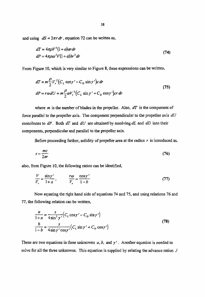
and using dS = Ifcrdr, equation 72 can be written as,

dT = AjcpV^{\ + a)ardr (/4)

dP = Ajvp<D'V{\ + a)br dr

From Figure 10, which is very similar to Figure 8, these expressions can be written,

dT = cosy'-C[) siay')cdr ^ (75)

dP = roydU = msin/' + cos/')cr dr

where m is the number of blades in the propeller. Also, dT is the component of

force parallel to the propeller axis. The component perpendicular to the propeller axis dU

contributes to dP. Both dT and dU are obtained by resolving and dD into their

components, perpendicular and parallel to the propeller axis.

Before proceeding further, solidity of propeller area at the radius r is introduced as,

also, from Figure 10, the following ratios can be identified,

V sxny' roj cosy'

F 1 + a ' F 1-6 (77)

r

Now equating the right hand side of equations 74 and 75, and using relations 76 and

77, the following relation can be written,

= • . cos;'' - Co sm/'l 1 + a 4sm*y^ " ' /

b s - — — ; 7 ( c , s i n ; ' ' + C o c o s ; ' ' ) 1-6 4sm/ cosy^

These are two equations in three unknowns a, b, and /'. Another equation is needed to

solve for all the three unknowns. This equation is supplied by relating the advance ration J

39

V(I+a)

roj(l-b)

Figure 10: Forces on a blade element in advance blade element theory

to y' .

V{l + a) , d l + a

J-^—^anr' (79) d l + a

Although equations 78 and 79 can be solved for the three unknowns, a slightly

different route is taken to calculate dT and dP. For some initial values of , the effective

angle of attack, inflow factors a and b, and the right hand side of equation 79 is calculated.

Next, J is plotted against /'. For the given value of y, the value of is picked from that

plot. Once /'is known, a, b, dT and dP are calculated. Elemental thrust and power

coefficient dC-p and dCp are computed using,

A7tJ'{\-\-a)ardr = ^2

/ X , (80) \67tJ{\-¥a)br dr

Once dC-p and dCp have been calculated for all the blade elements, they can be summed up

to get dT and dP for the propeller.

40

The case of J = 0 (i.e. no forward velocity of the propeller) is a special case of this

theory. The entire procedure for deriving expression for dCy and dCp can be repeated for

J = 0 ov V = 0. Once that is done, the same procedure can be repeated to calculated a.

b, dCj^ and dCp. The theory is really stretched for this case, but it gives good

approximated results for dT and dP. For negative values of J, (i.e. the propeller is moving

in the backward direction, instead of forward direction) one needs to be careful with the sign

of different expressions used to calculate Q and Cp. In the present situation, it is expected

that the case of J < 0 will not be encoimtered.

Force Distribution on a Propeller Blade

It is the force distribution which is needed for the finite element analysis of a

propeller blade. Therefore, the elemental thrust coefficient C-r and the power coefficient Cp

need to be converted into a force distribution on the blades, which will ultimately be used in

the finite element analysis.

The coefficient of normal force on a blade element dC^. can be found

i/Cy =dCT cos p-dC^ sin P (81)

but, dCf, ^dCp.djljtr, therefore,

d dC^. =dCj. cos p dCp sin P (82)

nr

the normal force acting on one blade element of width Ar is given by,

dN = dC^,.pn-d*

Next, two assumption are made. First, all blades in the propeller have the same force

distribution, second, the shape of the force distribution is triangular. The shape of this

triangle (altimde, area) is governed by the normal force on that blade element and the

pitching moment about the quarter chord (Figure 11).

41

The altitude of the triangle is given by,

cAr

Since the moment coefficient about the quarter chord, , for a particular airfoil is known.

(84)

JL

< c/4

-< c >-

Figure 11: Force distribution on one blade element

But firom Figure 11, the moment on a blade element can also be written as.

f c 2c ^ dM,/ = ttP Arc — —\P Arfc —c )

Yi 2 max*-" J 2max"* ^xj 3 ^ 4 (85)

With the help of equations 82 and 83, equation 84 can be solved for c,,

3i/M,

4 dN (86)

42

Once and c, are known, the pressure distribution on a blade element can be expressed

as,

P{x) = ^x 0<a:<C,

( C - X) = -^ i C-C,

The above procedure can be repeated to determine the force distribution for all blade

elements of the propeller. This process can also be automated on a computer and the results

can be plotted using some plotting software.

Failure Criteria

A failure criteria based on the theory given by Hashin [22] is used in this work. The

theory identifies four distinct failure modes for the composite material referred to as the

tensile fiber mode, compressive fiber mode, tensile matrix mode, and compressive matrix

mode of failure. The theory gives specific criteria for each.

The main assumption of the theory is that unidirectional fiber composite laminae are

transversely isotropic with respect to the fiber direction, because the fibers are randomly

placed. This means that the failure criteria needs to be invariant under any rotation in the

plane perpendicular to the fiber direction. Thus, the failure criteria has to be a function of

stress invariants under such rotation. These invariants are

/, =a-„

A ~ 0*22 CTjj

/j — 0*23 ~ ^22^33 7(^22 ^33)" ^23

= (T,, + £7,3

/s = ~^12^23^I3 ~ ^22^13 ~ ^33^22 (8^)

43

It is convenient to use the first form of the third invariant in equationSS. Also, since the

theory uses a quadratic approximation for failure, the last invariant in equation 88 cannot

appear in the criteria. Thus the most general transversely isotropic quadratic approximation

will have the form.

The one dimensional failure stresses of the material are denoted as,

= tensile failure stress in fiber direction

<Ta" = compressive failure stress in fiber direction

C7x' = tensile failure stress in transverse to fiber direction

a-r' = compressive failure stress in transverse to fiber direction

T-r = transverse failure shearing stress

The failure criterion can be summarized as

Tensile Fiber Mode: I, > 0

i4,/, + B^I^ + A2I2 + ^2^2 -^3^3 ^4-^4 ~ ^ (89)

or (90)

Compressive Fiber Mode: I, < 0

(91)

Tensile Matrix Mode: I, > 0

\ a r ) T r (92)

44

Tensile Matrix Mode: I, >

\

(93)

Optimization

A typical optimization problem can be written as

minimize F(X)

subject to:

objective function

gj(X)<0 j=l,...,m

hk(X) = 0 k=l,...,l

X,'<X,<X," i=l,...,n

inequality constraints

equality constraints

side constraints

where X are the design variables.

In structural optimization, a physical problem is converted into a mathematical

problem in the above form and then optimization techniques are applied to find the optimal

values of the design variables. For solving the optimization problem, gradients of the

objective function and of the constraints are required.

Generally the optimization procedure is performed iteratively by starting from an

initial set of design variables X°. This set is updated using the relation,

where p is the iteration number, X is the vector of design variables, S" is the search direction

and a*p is a scalar factor which scales the amount of change in X for the p"" iteration. Thus

the optimization procedure consists of two steps; the determination of search direction S*"

and the interpolation of the parameter a'p which minimizes F(X) in the direction of S''. This

transforms a multi-variable minimization problem into a single-variable minimization

problem, for the variable a. Since the objective flmction F(X) is in general a non-linear

function, the gradients need to be reevaluated at X*" and a new set of design variables

obtained. This process is repeated until a converged solution is obtained.

XP=X^' + a'p S"

45

Unconstrained Optimization

An optimization problem having only side constraints on the design variables is

known as an unconstrained optimization problem. An efficient technique to minimize the

objective fimction, is to utilize the information about the gradient of the objective fimction

VF(X). Note that the negative of VF(X°) is the direction of the steepest descent of F(X) at

X°. Generally, this direction is chosen to be the direction of search. One drawback of this

technique is that it can be very slow in convergence.

The Fletcher-Reeves conjugate-direction method is a modification of the steepest

descent method, and is favored because of its better convergence rate. In this method, the

search direction at each iteration is constructed to be Q-conjugate to the previous search

direction, where Q is the matrix of second derivatives.

Constrained Optimization

An optimization problem having constraints other than the side constraints on the

design variables is known as an constrained optimization problem. In this type of

optimization problem, the optimized solution must be within the bounds of the imposed

constraints.

For these kind of problems, the search direction is chosen such that none of the side

constraints are violated. This requires that the scalar product of the objective fimction

gradient VF(X) and the search direction S should be negative. This is known as the usability

requirement and may be written as

VF(X) • S < 0.

In addition to usability, a search direction has to be feasible such that a finite move

along the direction does not violate any active constraint. An active constraint is the one at

whose boundary the current design exists. Thus for any active constraint g,(X),

Vg , (X) .S<0.

The direction of steepest descent in the objective function can be found along a direction

where the values of Vg,(X) • S are strictly unity. This direction is tangent to the constraint

46

boundary. In order to make sure that the search direction remains feasible, the search

direction can be moved away from the constraint boundary by changing the requirement to

Vg,(X)*S + e<0

where 0 is a non negative constant.

To keep the search direction as far away as possible from the constraint boundary

while reducing the objective function as far as possible, a problem is defined,

maximize P

subject to:

Vg, (X)«S + 0 jP<O, 0 j>O, j e l^

VF(X) • S p< 0,

where 1^ is the set of active constraints (gj(X)=0), and the search direction vector S is

bounded. The quantities 0j are known as push-off factors. These quantities determine how-

far the design variable X moved from the constraint boundary. This particular method is

know as the method of feasible direction.

In this work, several design problem were investigated using the optimization

methods. It is demonstrated that by using composite materials some of the design objectives

can be achieved just by changing the stacking sequence. For this purpose the computer code

"CONMIN" [50] was used.

47

CHAPTER 3 FINITE ELEMENT METHOD FOR

COMPOSITE LAMINATES

Introduction

In order to determine the displacements and stresses in a composite laminate of

arbitrary geometry and boundary conditions, the partial differential equations given in

Chapter 2 need to be solved. Analytical solutions are available for rectangular plates with

simple support boundary conditions at all edges or with two opposite edges having simple

support boundaries and the remaining two edges with same arbitrary boundary conditions.

Energy methods such as the Rayleigh-Ritz or the Galerkin method can be used to

determine approximate solutions, but these are limited to simple geometries. In this

situation, the finite element method is one of the most effective methods to seek approximate

solutions to the governing equations.

There are three major types of finite element methods: (i) The displacement-based

finite element method, (ii) mixed and hybrid finite element methods, and (iii) finite element

methods based on equilibrium of forces. The displacement-based finite element method for

plates is based on the principle of virtual displacement. All the governing partial differential

equations are expressed in terms of displacements. This is the most common type of finite

element method used in engineering analysis. This method solves very accurately for the

unknown displacements of the problem which are physical quantities. Although, this type of

finite element method can solve for stresses, but these quantities may not be of primary

interest. For details of the finite element method and its applications, references [51, 52, 53.

54,55] can be consulted.

48

The Finite Element Method

Introduction

The finite element method is the most powerful numerical technique for solving

structural mechanics problems with complicated geometries. Analysis using the finite

element method follows a sequence of logical steps, which can be automated on a computer

using any programming language. Thus, various problems in the same class may be solved

by changing the input data defining the geometry, the initial or boundary conditions, the

material properties, or the loading conditions.

In the finite element method, the domain of interest is subdivided into a collection of

simple non-intersecting sub-domains called finite elements. This process is called finite

element discretization. Each element is defined by a number of nodes. The number of nodes

within any particular element is chosen based upon the required accuracy of the solution.

The collection of elements is called a finite element mesh. The finite element method

requires that the governing differential equations be written in the weak sense of the

weighted-integral, or variational form, over each element The solution at each node is

determined such that the governing differential equation is satisfied in the weighted-integral

sense.

The solution of the governing differential equation over each element is approximated

by a linear combination of undetermined parameters and pre-selected interpolating or

approximate functions. The undetermined parameter is the value of the dependent variable

(unknown) at the nodes of the element. The solution u(x) of the governing differential

equation in terms of its values at the nodes of the element can be written as.

>1

where is the finite element interpolation of u on a typical element Q^, Uj' is the value of

at the j-th node, and vi/j'Cx) are the interpolating or approximate polynomials.

n

(94)

49

The expression for u(x) in equation 94 is substituted back into the weak form of the

governing differential equation. This gives a set of algebraic equations in terms of the nodal

values of the dependent variable, which is still unknown and needs to be determined. The

number of these equations are the same as the number of nodes in that particular element.

Since in the beginning the domain was divided into elements, the elements must be

assembled back together into their original position utilizing the continuity of Ue(x) at

element interfaces. This is called the assembly of elements. The process of assembly gives a

very large number of algebraic equations in terms of nodal values of the dependent variable.

The number of unknowns and the number of equations are equal to the total number of nodes

in the entire domain. In general, the number of equations is very large. The solution of such

a large number of equations is carried out on a digital computer.

Weak Formulation of a DifTerential Equation

The finite element method requires construction of interpolating or approximate

functions for the governing differential equation in weak sense of the integral formulation.

Writing the governing differential equation in the weak form also gives the natural and

essential boundary conditions as the by-product of the procedure itself. In this section, the

procedure to express the governing differential equations in weak form is briefly discussed.

There are three steps in the formulation of the weak form of any particular differential

equation. In the first step, all terms in that differential equation are put on one side of the

equality, then the entire equation is multiplied by a weighting function and integrated over

the domain with respect to the independent variables. The resulting expression is called the

weighted-integral form of the differential equation. In the second step, the weighted-integral

form of the equation is integrated by parts to distribute the differentiation evenly between the

dependent variable and the weight function. This form of the equation is called the weak

form, because the dependent variable does not need that strict continuity requirement as it

required before doing this particular step. In the third step, the weight function is restricted to

satisfy the homogeneous form of the specified essential boundary conditions.

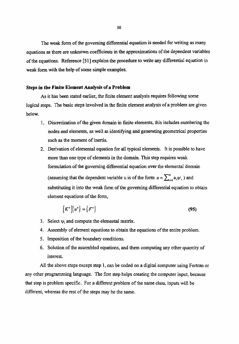
50

The weak form of the governing differential equation is needed for writing as many

equations as there are unknown coefiScients in the approximations of the dependent variables

of the equations. Reference [51] explains the procedure to write any differential equation in

weak form with the help of some simple examples.

Steps in the Finite Element Analysis of a Problem

As it has been stated earlier, the finite element analysis requires following some

logical steps. The basic steps involved in the finite element analysis of a problem are given

below.

1. Discretization of the given domain in finite elements, this includes numbering the

nodes and elements, as well as identifying and generating geometrical properties

such as the moment of inertia.

2. Derivation of elemental equation for all typical elements. It is possible to have

more than one type of elements in the domain. This step requires weak

formulation of the governing differential equation over the elemental domain

3. Select v}/; and compute the elemental matrix.

4. Assembly of element equations to obtain the equations of the entire problem.

5. Imposition of the boundary conditions.

6. Solution of the assembled equations, and them computing any other quantity of

All the above steps except step 1, can be coded on a digital computer using Fortran or

any other programming language. The first step helps creating the computer input, because

that step is problem specific. For a different problem of the same class, inputs will be

different, whereas the rest of the steps may be the same.

(assuming that the dependent variable u is of the form u = u^y/^) and

substituting it into the weak form of the governing differential equation to obtain

element equations of the form,

(95)

interest.

51

Finite Element Model of First Order Shear Deformation Theory

Formulation of the Governing Equations in Weak Form

The shear deformation theory of composite laminates has been discussed earlier.

Here the finite element model of first order shear deformation theory is presented. The

governing differential equations for static equilibrium in the case of shear deformation theory

are

dx dy J (96)

dx dy = 0 (97)

'dQ, dO, ^ — + — + dx dy

= 0 /

(98)

dx dy ~ = 0 (99)

^dM, dM, ^

dx dy - Q z = 0 (100)

where Nf and M, are the forces and moment resultants, and Q; are the transverse shear forces.

Forces and moment resultants are given by.

h] ' M ; o-|

• ^ 4 = 1 - ^2 'dz ,

^6 J .<^6. .K\

The transverse shear forces can be expressed in terms of displacements as

-I 1^2 J J/ [ ^4 >dz

52

As it has been mentioned earlier, the governing differential equations are to be written

in weak form for finite element formulation over the element. Here, each of the five

equations will be taken one by one and will be written in their weak form.

Multiplying equation 96 with weight function 5u and integrating it over the element

domain

jSu dxdy = Q n. dx dy

here it is to be noted that N, and Ng are the function of the derivatives of displacements.

Integrating the above equation by parts gives

where (n,, ny) are the direction cosines of the unit normal on the boundary Fj of the element

domain Q^. Also it is noted that (in-plane normal force). This makes the

final weak form of equation 96

I d5u

. dx

d5u dy

N. dxdy - IduN„ ds = 0 (101) r.

The same procedure is repeated for equation 97, yielding

dSv ~d

•N.+ d5v ~d

N, dxdy - |jvA^^<iy = 0 (102) r.

Multiplying equation 98 with weight flmction 6w, and integrating over the element domain

Q,

jSw, a dx dy

-<l dxdy = 0

Integrating the above equation by parts gives

^dSw A dx

ri (ydw, dSw, 1 p/ \ ][—^Q\ +-^Q6 +Sw^q\dxdy- fife = 0

a r.

Final weak form of equation 98 is

53

I dxdy-\Sw^Q„ds = 0 dx dy .

Multiplying equation 99 with weight function Sw, and integrating over the domain Q,

' dM, dM,

(103)

<?;c =

Integrating by parts and making use of the relation between M„, and M, and Mg on the

boundary.

M, + +^,0,1 dxdy-\dw^M„ds = 0 A dx dy - ) I -

(104)

Repeating the procedure for writing the weak form of equation 99, for equation 100 gives.

+^^M, +<5^3021 dxdy-\dw^M^ds = Q (105)

Finite Element Formulation

For finite element modeling, the displacements and rotations (u, v, w, (j),, (j),}. and

weight functions (5u, 5v, 6W|, Sw,, Swj) are approximated as.

II

^ = 5u=itr,

n

7=1

n

>1

7=1

fl

«'2=Z%Vy. Sw:, = y/. 7=1

(106)

54

Where i|/j are the Lagrange family of interpolation fimctions. These interpolation fimctions

are fimctions of x and y. These expressions for nodal values are substituted in the weak form

of the differential equations, and after performing some algebra (which is detailed in

Appendix), one can come up with the final finite element form of the governing equation as

= 0 / = 1,2,...,/7, k = 1,2,...,5 fel 7=1

(107)

where dj are the nodal values of displacements (Uj, Vj, w,-') and rotations (Wj-, and Wj^). The

terms and Fj'' are given by the following expressions

= K 21

n. dx dy ^ ^ V dy )\ dy + B, 66

^X J \dxdy

j>

^26 -3 + -^66 ^y dx + \dy J dy

+ .4, 66 dx \dxdv

55

= Kf

" 'ill^Jr""^ f f x j A ^ y l ^ - a y &Jr'^ - K J

'.••il(f)(^s*^t)-(f)H'"-5')H

rr43 — Kj^

Kl'-

' K f

'••il(t^S"'.t)-(t)('<-S*»-S)-«h

'='-iM'^f-"-3*(fI'<'®"'-f)*«''K

'•••iff)(«'t">.a-(t)('^t*°.a*'-".h

r,

= l^nsV^ids r,

dxdy + JN,^^if^. ds a, r,

F,' =

r.

56

F' = \^ns¥ids r.

The Appendix to this dissertation gives the algebraic details of obtaining equation 107.

The Choice of Element

In order to evaluate the expressions for on computer, a Gauss quadrature will be

used for the purpose of integration. The reason for use of quadrature instead of, say, exact

integration is its ease to program using any programming language. Secondly, the

interpolation function can be defined and all the integration can be done on one master

element. The actual elements can be mapped to the master elements again and again, to get

the contribution from each element for the global stif&ess matrix. Next to be decided is, the

form of interpolation function v[/„ and the number of nodes in an element, n. The integration

method and the interpolation function depend upon the type of element chosen. For example,

triangular elements will have a totally different interpolation fimction and a different way to

evaluate the integrals than rectangular elements. The size of the elemental stiffiiess matrix

also depends upon the type of element. For example, if a four-noded rectangular element is

chosen, the interpolation function will be linear and the elemental stiffiiess matrix will of the

size 20x20. This type of element is referred to as a linear element. If a nine-noded element

is chosen, the interpolation fimction will be quadratic, and the size of the elemental stiffiiess

matrix will be 45x45. This element is called a quadratic element, and in general performs

better than the linear element because the interpolation fimction can give a better estimate of

the exact solution of the original governing differential equations. If the in-plane degrees of

freedom (u, v) are omitted (for the uncoupled equations), the size of the matrices will be

12x12 and 27x27 for the linear and quadratic rectangular elements, respectively.

For this study mainly two types of rectangular element were chosen, four-noded

linear and nine-noded quadratic. Figure 12 shows these elements.

The interpolation function associated with both type of elements are given below.

57

Four noded element;-

Nine noded elements:-

f, =if4(l + #S)W/(l+77,)

for node /, (/ = 1,2,3,4) (108)

for comer node

for side node, = 0

for side node, Tij = 0

for the center node (109)

(a) Four noded element (b) Nine noded element

Figure 12: The elements used

Once the finite element equations for all the nodes are available, they are assembled

using continuity of nodal displacements and balance of nodal forces. Next, boundary

conditions are applied on the assembled system of equations. That system of equations is

solved for the nodal values of displacements.

Calculations of Stresses and Strains

Once the nodal values of displacements have been obtained by solving the assembled

equations of a problem, the strains are evaluated in each element by differentiating the

displacements (equation 106). In the displacement-based finite element model, the

58

displacements are continuous at the boundaries of the elements, but the strains are not.

Strains are continuous within one element. The strains, and hence stresses take different

value on the two sides of an element interface. This is one shortcoming of the displacement-

based finite element method, resulting in a less accurate solution of the problem for stresses.

In linear element the strains are constant within each element, whereas, in quadratic

elements the strains are linear and hence give a better strain (or stress) field than the linear

elements.

Strains and stresses can be computed anywhere in the element including nodes.

According to Barlow [55, 56], these quantities are most accurate if computed at (P-l)x(P-l)

Gauss points, where P is Gauss quadrature rule used to evaluate the elements of stiffiiess

matrix.

The strains and stresses obtained need to be transformed to the material coordinate

system associated with each composite layer. For domg this , first the strains calculated at

the Gauss points need to be transformed to lamina strains 8l, St' ^ln' ^tn using the

relation

COS" 9 sin" 0 cos 0 sin 0 '

> = sin" 0 COS" 0 -cos^sin^

.^LT. -IcosdsinO 2 COS 0 sin ^ 2(cos" ^-sin" 0)

COS0 - sin^ H .frv J sin0 cosO Uj

The stresses can be calculated for each ply in the material coordinate system, at the Gauss

point, using the following relation for each ply.

Qn Qn ^6 CTj.

. = Qn Qv. 026 €7

P^LT. e.6 066. .^l.T.

k/-v l_ "^4 as" kvl

Vrv-r Q*s ^5. \^LT.

59

Although the stress can be computed in the global (x, y, z) coordinate system, the

failure criteria requires that the stresses be obtained in the material (L, T, N) coordinate

system. A transformation matrix is used to switch between the two coordinate systems.

Conclusion

Based on the discussion presented above, two separate Fortran subroutines were

written which were able to calculate deformations and stresses on a plate type of structure

made from composite material. The first subroutine used four-noded linear elements and

second subroutine used nine-noded quadratic elements. In the next chapter, the results from

these subroutines are presented.

60

CHAPTER 4 INITIAL RESULTS

Introduction

In Chapter 2 the theory of composite material, propeller, blade element method, etc.

has been presented. In Chapter 3 the finite element formulation for a composite material is

presented. Fortran subroutines were written based on the theory discussed in Chapters 2 and

3 and their results are presented in this chapter. The blade element method was used to

numerically calculate the propeller performance characteristics of a propeller, and finite

element method was used to calculate deformations and stresses on a composite plate under

load. In order to gain confidence in these subroutines, they were tested against known

results. First, the restilts firom finite element analyses are given for rectangular plates under

different loading and boundary conditions, made of either isotropic or composite material.

Then the results firom blade element analyses are presented for different propellers operating

at different advance ratios.

Results of Finite Element Analysis

For all the results involving isotropic material, aluminum was used. As far as the

results involving composite materials are concerned different materials were used, depending

upon the solutions available in the literature. The specific material properties will be

presented as that particular case is discussed. References [11], [16], [40], and [51], were used

for the purpose of comparison. For verifying the behavior of finite element scheme, two

different elements were used. Those were,

1. four-noded quadrilateral element using linear shape functions,

2. nine-noded quadrilateral element using quadratic shape fiinctions.

61

In most of the cases, a uniformly-loaded plate of 12 inchesxl2 inches plate was modeled with

various finite elements mesh, under various boundary conditions. In one case a sine loading

was also applied. The parameters of interest for comparison were; the out-of-plane

displacement w, and stresses and at the center of the plate. For some studies only

was compared with known solutions. Seven different mesh size were used to model the plate

having 4, 9,16, 25,36,49 and 64 elements. The plate and four of the meshes are shown in

Figure 13.

Effect of Mesh Refinement

The effect of mesh refinement was investigated by comparing the solution obtained

firom each mesh against known series solutions of shear deformable plate theories. The

parameters compared were out-of-plane displacement and stresses at the center of plate. The

loading was uniform pressure loading. Three different boundary conditions were checked for

each mesh. These were

1. All edges of the plate are simply-supported. This will be referred to as SSSS.

2. Two opposite edges are simply-supported and the remaining two are free. This

will be referred to as SSFF.

3. Two opposite edges are simply-supported and the remaining two are clamped.

This will be referred to as SSCC.

SSSS Boundary Conditions

The material used in this case is E-glass/epoxy, with material properties as E,, = 60.7

GPa, Ei2 = 24.8 GPa, G,2 = G,3 = 11.9 GPa, and u,, = 0.23. The plate consisted of eight plies,

with the stacking sequence [(0/90)2]s. As it has been mentioned earlier, two different

elements were used, one with four nodes and the other with nine nodes. Figure 14 shows the

behavior of the out-of-plane displacement w as the mesh is refined. Figures 15 and 16 show

the behavior of stresses and CTy. It can be seen that with reasonable mesh refinement the

nine-noded element gives almost the exact solution, the difference in some cases is in the

fifth place after the decimal point.

62

y

L f- 4

(a) 12" square plate

(b) 2x2 mesh (c) 3x3 mesh

(d) 6x6 mesh (e) 8x8 mesh

Figure 13: The plate and some of its finite element mesh

63

1.10 Legend Boundary Ccmditiofir SSSS

5cackSeq[(V9aa^l5 F«or

Nine

105 s V

1 00

0.95 5 7 8 3 6 4

Mesh Refinement Level

Figure 14: Effect of mesh refinement on out-of-plane displacement w under uniform pressure loading (Material: E-glass/epoxy).

I 010

1 005

I 000

Boundary Conditionsr SSSS

Stacking Seq [0/90/0/90],

Legeod

• • Mne

—^— Four

•' - ' • Series -

Legeod

• • Mne

—^— Four

•' - ' • Series

-

0990 i-

0985 ;

0980 5 6

Mesh Refinement Level

Figure 15: Effect of mesh refinement on <j^ stress under uniform pressure loading (Material: E-glass/epoxy).

64

I 02 Boundary Conditions- SSSS

Stacking Seq:[0/9(y0/90I I

100

£

Legend 096

Nine

Foar 094

7 S 3 4 6

Mesh Reflnenient Level

Figure 16: Effect of mesh refinement on stress under uniform pressure loading (Material: E-glass/epoxy).

Another careful look at these figures shows that nine-noded elements perform much

better than its four-noded counterpart. This is expected, because nine-noded elements use

quadratic shape flmctions, as opposed to linear shape fimctions used by four-noded elements.

But the fact that four-noded elements give quite good results should not be ignored. If

computational time is considered as important as the accuracy of solution, then four-noded

elements can be used instead of nine-noded elements to produce very good solutions.

The very same exercise was repeated after changing the material of the plate. This

time it was made from aluminum, having E = 68.9 GPa and u = 0.3. The results for this

study are presented in Figure 17 and 18. The behavior of the results are as expected similar

to those for E-glass/epoxy. A reasonably refined mesh gives a solution which is less than 1%

off from the series solution.

65

lOSO Legend boundary Conditions: SSSS

Matenal Aluminufn

102S four

jT iooo

0 975

0950 8 7 5 6 3 4

Mesh Refinement Level

Figure 17: Effect of mesh refinement on out-of-plane displacement w under uniform pressure loading (Material: aluminum).

Boundary Conditions: SSSS

Material Aluminum

I 00

C "w V

b 099

Legend

Sena

Nine

Four 0 98

3 5 7 4

Mesh Refinement Level

Figure 18: Effect of mesh refinement on a, stress under uniform pressure loading (Material: aluminum).

66

For gaining more confidence in the finite element scheme, the material was changed

for the third time and the same study was repeated with graphite/epoxy having the properties

as, E„ = 153 GPa, = 10.9 GPa, G,, = = 5.6 GPa, and u,, = 0.3. The number of plies,

stacking sequence, and the loading conditions are the same as for the E-glass/epoxy discussed

earlier. The results are shown in Figures 19-21. Once again, good agreement with series

solution for refined mesh can be seen.

SSFF Boundary Condition

Next the boundary conditions were changed from SSSS to SSFF. The edges y = 0.0 •

and y=12.0 were free, and rest of the two were simply-supported. The material was

graphite/epoxy, with the properties E,, = 143.7 GPa, E22 = 7.55 GPa, G,2 = G^j = 4.27 GPa,

and u,, = 0.3 . The stacking sequence was 0/90/0 and the loading was a uniform pressure.

Parameters compared were out-of-plane displacement w and stresses cr^. Results for this case

can be seen in Figures 22 and 23. As evident from the plots, nine-noded elements performs

better than four-noded elements. With a very refined mesh, the four-noded elements do give

a very good solution. Stresses also behave in the same manner.

SSCC Boundary Condition

In this case, all conditions are same as the SSFF boundary conditions case, except the

two free boundaries are clamped. The results can be seen in Figures 24 and 25. The

performance of both the element types is good for displacements, with nine-noded element

giving almost the exact series solution. For stresses, the solution is off by less than 3% for

both element types.

Beam Modeled with Plate Elements

Finally, a cantilevered beam was modeled using nine noded plate elements. The

finite element analysis was done using 2, 4 and 8 elements of the beam. Tip deflection of the

free end and maximum stresses at the clamped end, were the quantities compared. The

67

1 04 Legend Boundary Conditions: SSSS

Material T300yS208

Stacking Seq : [Q/90AV901, Nine I 03

Fear

u M

1 00

099 S 6 7 8 3 4

Mesh Refinement Level

Figure 19: Effect of mesh refinement on out of plane displacement w under uniform pressure loading.

I 02 Boundary Conditions SSSS

Material T300/S208

Stadng Seq (0/90/tV9o],

1 00

I M

b 098

b

Legend 096

Nine

Four 094

3 S 4 6 7

Mesh Refinement Level

Figure 20: Effect of mesh refinement on stresses under uniform pressure loading.

68

1.02 Boundary Conditions SSSS

Mncrial T30Q/S208

Stacking Scq : [0/90/Q/90| ,

t 00

I

>% b 0.98

Legend

Nine

Fear 096

7 S 3 6 4

Mesh Reflnement Level

Figure 21: Effect of mesh refinement on stresses under uniform pressure loading.

I OS Boundary Conditions SSFF

Material Cp^p

Slacking Scq [0/90A})

I 00

t u u M 09S

Legend 090

Scries

Four

OSS •> 3 5 7 4 6 8

Mesh Refinement Level

Figure 22: Effect of mesh refinement on out of plane displacement w under uniform pressure loading.

69

lOS Boundary Conditions - SSFP ;

Material Gp / Ep

Stacking Scq [Of'90/0]

!00

I S M 095

K D

Legend 090

Nine

Four

085 5 6 7 3 4

Mesh Refinement Level

Figure23: Effect of mesh refinement on stresses under uniform pressure loading

I 02 Boundary Conditions SSCC i

Material Cp/Ep !

Stacking Seq [0/90/0] {

S im

n

0 98 Legend

Four

Nine

096 3 5 7 4 8 6

Mesh Refinement Level

Figure24: Effect of mesh refinement on out of plane displacement w under uniform pressure loading

70

I OS Boundary Conditions SSCC

Materia] Gp^Hp

Stacking S«t [0/90;0I

Legead

Series

Mesh Refinement Level

Figure25: Effect of mesh refinement on stresses under uniform pressure loading.

results can be seen in Figures 26 and 27. With four elements displacements are less than 1%

off. In general results are in good agreement.

Effect of Plate Thickness

This study is directed towards the possible use of finite element method in analyzing

propeller blades made up of composite materials. Since these blades have variable thickness,

it is necessary to examine the finite element results for plate of a varying thickness. Once

again results obtained are compared to results from the literature. Efforts were made to

perform this study for more than one type of material, and for several type of loading and

boundary conditions. The same three types of boundary conditions were used as mentioned

in earlier sections.

71

1.020 f

I !

1010 ^

0»

t \ ^ I 000 <

? 1 t i !

0990 f I

r

i 0 980 -

Mesh Size

Figure 26: Effect of mesh size on tip deflection for cantilevered beam modeled with plate elements.

I 04 Cantilevered Bean under Uniform Distributed Load I

Stacking Seq: Eight Piies at Zero Degrees

1 02

M 00

D I

0 98 Legend

Exact

F.EIm. 096 096 ^ 1 '

2 4 6 8

Mesh Size

Figure 27: Effect of mesh size on stress for cantilevered beam modeled with plate elements

Candievcred Beam Under Uniform Dtst Load

Stadung Seq: Eight Plies ai Zero Degrees

Legend

rEim.

72

SSSS Boundary Conditions

The effect of thickness on the linear static behavior of a simply supported rectangular

plate is presented in Figures 28 and 29. One of the dimensions of the plate is three times that

of the other dimension. The material used is graphite/epoxy, the stacking sequence is 0/90/0.

and sinusoidal loading is applied.

For this study, two meshes were used; one with 16 elements and a second with 24

elements. As expected the performance of the nine-noded elements mesh is better than that

of the four-noded mesh. Comparing Figures 28 and 29, the solution for thin plate is more

accurate than for thick plates, but the difference is less for the finer mesh. This result

indicates that a thick plate requires a finer finite element mesh to give accurate results.

SSFF and SSCC Boundary Conditions

For this study, a square plate was used, which was divided into 64 elements. The

material was graphite/epoxy, and the stacking sequence was 0/90/0. Both out-of-plane

displacement w and stress CT, were compared with known results. The results for these two

cases can be seen in Figures 30-33. In general the performance of the finite element analyses

is good, except for very thick plate. Even for a extremely thick plate the solution is within

5% of the theoretical solution.

Results of Blade Element Analysis

The blade element method for numerically calculating propeller characteristics, was

checked against the propellers experimentally tested in reference [23]. In reference [23],

experimentally-determined propeller characteristics of four different propellers are given at a

blade angle of 15.5 degrees at 75% of the radius. All propellers are metal propellers, with

diameters ranging from 9 feet to 10.5 feet. Propellers are identified by their drawing

numbers, which were 4102,4412,4413, and 4414. The same numbers will be used in this

study for identification purpose. Propeller characteristics of all four propellers are given in

the above mentioned report.

73

I 02

roo

Botmdary Conditions SSSS

Material Cp^'Ep

So of Dements 16 i

Side to Thickness Ratio

Figure 28: Thickness effect on rectangular plane, under sine loading.

102 Boundanr Conditons SSSS

Material. Gp/Ep

No of Elements 24

1.00

91 SJ

o M i

098

Legend 096

Serid

Nine

Four 094

20 0 40 60 80 100

Side to Thickness Ratio

Figure 29: Thickness effect on rectangular plane, under sine loading.

74

100 i-

Boundary Conditions SSFF

Maiehal GpiBp

Sock S€q 10/W)1

099

Legend

Side to Thickness Ratio

Figure 30: Thickness effect on out-of-plane displacement under uniform pressure loading (Material: graphite/epoxy).

102 I : I Boundary Conditions SSFF |

Material Gp/'Ep

Stack Scq (0/90/0)

I 00

M o

096 H Legend

094 50 00 too 150 200

Side to Thickness Ratio

Figure 31: Thickness effect on the stress under uniform pressure loading (Material: graphite/epoxy).

75

I 02

) 00

098

0.96

Boundary Conditions SSCC

Maiehal. Gp/'Ep

Stack Seq (O/SQ/O]

Legend

Sencs

Side to Thickness Ratio

Figure 32: Thickness effect on out-of-plane displacement under uniform pressure loading (Material: graphite epoxy).

Boundary Conditions. SSCC

Matenal. Gp/Ep Stack Seq: [0/90A)]

Side to Thickness Ratio

Figure 33: Thickness effect on the stress under uniform pressure loading (Material: graphite epoxy)

76

For the purpose of comparison of experimental and computational results,

characteristics of all four propellers were computed for values of advance ratio from 0.2 to

0.8. All the propellers were discretized into nine blade elements. Propeller 4102 was used to

carry out a small mesh sensitivity study. Thus, the characteristics for propeller 4102 were

calculated again with 19 blade elements.

Comparison of Computational and Experimental Data

The main parameters of interest were the coefficient of thrust and the coefficient

of power Cp for the entire range of advance ratios/. Although the propeller efficiency r]

was also calculated and compared, but it was not as important, since it is dependent on

a n d C p . F i g u r e s 3 4 , 3 5 a n d 3 6 s h o w t h e b e h a v i o r o f Q , C p . a n d 7 7 a s t h e a d v a n c e r a t i o J

is changed from 0.2 to 0.8, for propeller 4412. It is clear from the plots that the

computational scheme does a very good job of duplicating the vs. J behavior. As far as

the Cp is concerned, the solution from the blade element scheme is less accurate. After

looking at the Figures 37 to 45, the same observations may be made for propellers 4413,

4414 and 4102.

Propeller 4102 was then divided into 19 blade elements and the same data was

obtained. Results showing the comparison of nine blade elements and 19 blade elements to

the rigid propeller can be seen in Figures 46,47, and 48. It is observed that, there is a

definite improvement in , Cp. and 7 behavior with a refined blade element mesh.

Conclusion

As it has been discussed earlier, the blade element theory is an approximate scheme to

calculate propeller characteristics. The theory has its limitations, but over all is a satisfactory

approach. One of the main sources of error could be the airfoil data given to the computer

77

010 Prapdkr-Ui2

No ofbladedaDentt;9 QOt

002

an 00 Q20 040 060 000

Advance Ratio J

Figure 34: Behavior of versus J. (Propeller 4412)

005 r Prapdkr44l2

No ef bUde Baaems; 9 Q04

003

002

020 080 100 000 040 060

Advance Ratio J

Figure 35: Behavior of Cp versus J. (Propeller 4412)

Propdler-U12 So of Blade Ekmems: 9

060 -

020

020

Advance Ratio J

Figure 36: Behavior of versus J. (Propeller 4412)

78

0.10 PnpeUerMI3 NoofBbdeEicflKaCk:9

OOS

006 fa» o

0 02

OS 1 0 00 02 04 0 6

Advance Ratio J

Figure 37: Behavior of Ct versus J. (Propeller 4413)

COS Prepdler^n

NoofBtodeEletnenu. 9

OCW

0 02

01

00

OS 0.2

Advance Ratio J

Figure 38: Behavior of Cp versus J. (Propeller 4413)

PiQpeUer44n

So of Blade Bcreqts: 9

C

02

0 0 02 OS 0 6 in Advance Ratio J

Figure 39: Behavior of T] versus J. (Propeller 4413)

79

0.10

oot

006

U

002

10 01 04 06 0.2 OO

Advance Ratio J

Figure 40; Behavior of Ct versus J. (Propeller 4414)

003

004

0 03

0 02

0 6 1 0 0 2 04 OS 0 0

Advance Ratio J

Figure 41: Behavior of Cp versus J. (Propeller 4414)

10

08

0 6

04

02

00 U2 o u 04 06

Advance Ratio J

OS

Figure 42: Behavior of TI versus J. (Propeller 4414)

80

J"

002 i-

10 0( 04 06 0 0

Advance Ratio J

Figure 43: Behavior of Cj versus J. (Propeller 4102)

No of Blade

003 1-

u 0 02

OOi

10 OS 0 0 02 04 0 6

Advance Ratio J

Figure 44: Behavior of Cp versus J. (Propeller 4102)

10

OS

06

04

02

0 0

0(1 I (I 0 4 0 6 0 8

Advance Ratio J

Figure 45: Behavior of T| versus J. (Propeller 4102)

81

Piopdkr 4102 Esp 19 da

9c ta

001

W I

002

0 2 0 6 OS I 0 0.4 0 0

Advance Ratio J

Figure 46: Behavior of Ct versus J. (Propeller 4102)

0 05 Propeikr 4102

£xp 19 rim 9 dm

003 A> u 002

02 0 0 04 06 OS I 0 Advance lUtio J

Figure 47: Behavior of Cp versus J. (Propeller 4102)

I 0 Legend Prapdicr 4103

Exp

9 elm

19 elm

Of

06

04

02

00

00 0 6 Of 0 10 Advance Ratio J

Figure 48: Behavior of t] versus J. (Propeller 4102)

82

code, because the calculations for propeller characteristics provided by the blade element

method depend upon this data.. Another limitation of the theory is that it does not consider

tip effects. One advantage of this theory is that it is fairly easy to code on the computer.

Considering the limitations of the blade element theory, the above results are

satisfactory. The error in majority of the data does not exceed 10 percent. In limited cases

the errors was as high as 20 percent. Although an improved scheme can be used to come up

with a better force distribution on a propeller blade, blade element theory was used in this

work because of its simplicity and ease in use.

83

CHAPTER 5 ANALYSIS AND DESIGN OF A COMPOSITE

PROPELLER

Introduction

It has been shown in Chapter 4 that the blade element theory can be applied to any

propeller for determining propeller characteristics and the force distribution. It has also been

shown that the finite element method is very effective in calculating the deformation and

resuhing stresses in composite structures under load. Since this study is aimed towards

finding the composite propeller characteristics under the influence of aerodynamic loading,

the finite element method and blade element method will be applied concurrently. In this

chapter, the procedure to apply both the methods to determine composite propeller

characteristics is detailed. Various results, and some discussion on the results are presented.

Procedure

For a rigid propeller, the blade element theory is adequate to calculate its performance

characteristics. But since most engineering materials are deformable under the application of

loads, blade element theory is not sufficient for calculating the characteristics of a propeller.

The deformation of the blade affects the aerodynamic loading, and the loading in turn affects

the deformation. There is thus a need to account for the deformation of the propeller under

the aerodynamic forces and moments. The finite element method can be used to calculate the

deformation of the propeller under aerodynamic forces and moments and has been selected

here because of its ability to accommodate complex geometry.

The aerodynamic forces and moments acting on a propeller blade are a function of

altitude, forward velocity, rotation speed (revolution per minute or RPM), and initial blade

setting angle. In the begirming of the analysis, some initial blade setting angle, forward

84

velocity and RPM are chosen. Blade element theory is applied to determine the

corresponding aerodynamic loads. These aerodynamic loads are then applied to the propeller

blade and by using the finite element method, the resulting deformation of the propeller blade

is calculated. This deformation is used to determine the new blade setting angles of each

blade element of the propeller. The new blade setting angle is used to recalculate

aerodynamic loads, which are then reapplied on the propeller blade to find out the next blade

setting angle of the propeller blade. This iterative procedure is repeated until the difference

between two subsequent blade setting angles is insignificant. Once equilibrium between the

load and deformation is achieved, the blade element method is used to calculate the propeller

characteristics. The above procedure is outlined in the form of a block diagram shown in

Figure 49.

In order to ascertain that the above method works, the characteristics of propeller

4102 were calculated. For this purpose one blade of the propeller was taken and divided into

19 blade elements. For ease of programming on the computer, each blade element was

further divided into four finite elements. This made a total of 76 finite elements. The blade

element and finite element mesh for propeller 4102 can be seen in Figure 50. Nine-noded

elements were used because of their superiority over the four-noded element. The procedure

outlined in Figure 49 was adopted to calculate the propeller performance characteristics for

the same propellers made fi-om three different materials. For the first case, the material was

made extremely rigid. Results showed that the calculated propeller characteristics are

essentially the same as given by the blade element method. This makes perfect sense, as the

propeller does not deform to some new blade setting angle. After this procedure check,

material properties were changed to that of steel and aluminum, and then propeller

characteristics were recalculated.

Figures 51-53 show the behavior of Cj, Cp, and propeller efficiency r\ versus advance

ratio J, for propeller 4102 made from the rigid material, steel, and aluminum at an initial

blade setting angle of 15 degrees, at 0.75% radius, and at 1200 RPM.

85

Is diffemce less than

Yes No

End

Calculate propeller characteristics

Calculate change in blade angles

Inputs and initial values

Calculate loads using Blade Element

Theory

Calculate the change in two subsequent

blade angles

Calculate deformation using

Finite Element Method

Figure 49: Algorithm used to calculate propeller characteristics

86

Y Not to scale a

\ (a) Blade element mesh (propeller 4102)

Y

(b) Finite element mesh (propeller 4102)

Figure SO: Blade element and finite element mesh for propeller 4102

87

008 Legend

Propeller; 4102

Variable Thickness Plate Model

Seed

006 Mfid

002

000 I 0 0.0 0.2 04 0.6 0 8

J

Figure 51: Plot of vs. advance ratio for propeller 4102

004 Legend Propellen 4102

Variable Thickness Plate Model

Steel 003

001

000 00 0 2 04 0 8 t 0 06

J

Figure 52: Plot of Cp vs. advance ratio for propeller 4102

8S

Legend Propeller; 4102 Variable Tbickoess Plate Model

SiRl 08 Rigid

06

C 04

0 2

00 0 2 0 8 10 00 04 0 6

J

Figure 53: Plot of TI VS. advance ratio for propeller 4102

These three plots reveal that there is no significant difference in the behavior of these

three propellers. The reason for this behavior is that in all three cases, no blade twisting was

observed. The deformable propellers experienced bending (which was greater for the

aluminum blade than the steel blade) without significant twisting of the blade. This clearly

indicates that the procedure outlined above for calculating the propeller performance

characteristics of deformable material works and can be applied to composite propellers.

Analysis of a Composite Propeller

For analyzing composite propellers, two additional points must be considered.

1. The composite material is fimdamentally different firom an isotropic material.

Composite materials are stronger in the direction of fibers, unlike isotropic

material, whose strength is independent of direction.

89

2. The aerodynamic force distribution on a propeller blade is very complex. The

distribution varies not only in the span-wise direction, but in the chord-wise

direction, too.

For the purpose of calculating composite propeller characteristics, the composite

propeller blade was modeled as a plate of variable thickness, consisting of 20 plies of

T300/5208 graphite/epoxy composite material. The material properties used were, E,,=153

GPa, E22=IG.9GPa, G,2=G,3=5.9 GPa, u,,=0.3. The thickness of the plies were constant

within each element, but may differ from element to element. The propeller blade was

divided into 19 blade elements, and 76 finite elements. The mesh shown in Figure 50 was

used. It was decided to chose five different stacking sequences, and the performance

characteristics calculated for each stacking sequence were compared with those of the rigid

propeller. While choosing the stacking sequences, the points considered were, (a) the

stacking sequence should provide adequate strength in all directions, (b) the stacking

sequences should be similar to each other, such that some comparison among them can be

made, and (c) possible ease of fabrication. Based on the above considerations the following

five stacking sequences were considered.

1. [0/±22.5/90/±45/0/±67.5/90]s

2. [90/±22.5/0/±45/90/±67.5/0]s

3. [0/±67.5/90/±45/0/±22.5/90]s

4. [90/±22.5/0/±45/90/±67.5/0]s

5. [02/±22.5/±45/90/±67.5/90Js

The ply orientation angle is measured with respect to the x-axis, and angles are measured

with a counter-clockwise direction as positive. In this section the propellers made with these

stacking sequences will be referred to as Propeller 1, Propeller 2, Propeller 3, Propeller 4, and

Propeller 5. For each of these stacking sequences, the propeller characteristics (Cj, Cp, and

r|) were calculated and compared with those of a rigid propeller. The calculations were

performed for two different initial blade setting angles at 75% of blade radius (i.e. for Po.TSr

=15° and for P0 75, =25°).

90

For a better understanding of these composite propellers, the ratios Dig/D,,, Dig/D,,,

Difi/Dj, and are tabulated for each propeller in Table 1. A higher value of these ratios

means that the propeller is more likely to twist about the x or y axis. In addition the ratio

D„/D,,* is also tabulated, where D,,' is the highest of the five D„ value from propeller 5.

This ratio will give a measure of the relative bending stif&esses of the propellers.

The plots of Cr, Cp, and r| versus advance ratio J are presented in Figure 54-59, for all

five stacking sequences and a rigid propeller. Unlike isotropic materials, five distinct curves

can be seen in all six plots. Propellers 1 and 4 are found to be generating higher thrust than

Propellers 2,3, and the rigid propeller. Characteristics plots for Propeller 5 are closest to that

of the rigid propeller. Propellers 1 and 4 are drawing more power to produce extra thrust.

Propeller efficiencies TI seem to be closer to each other and to that of the rigid propeller. A

careful look at Figtures 58 and 59, reveals that Propeller I and 4 are more efficient for higher

values of advance ratio J. Propellers 2 and 3 are better for lower values of J.

Table 1: Strength ratios for each composite propeller.

Die/Dii ^26^11 D15/D22 026^22 D,|/D,,

Propeller 1 0.0320 0.0195 0.0816 0.0504 0.8607

Propeller 2 0.0420 0.0260 0.0492 0.0304 0.6588

Propeller 3 0.0304 0.0492 0.0260 0.0420 0.5526

Propeller 4 0.0504 0.0816 0.0195 0.0320 0.3331

Propeller 5 0.0545 0.0185 0.1206 0.0878 l.O

Table 1 shows that D,j/D,, and D^g/D,, is highest for Propeller 4, and Dig/D,, and

are highest for Propeller 1 (not considering Propeller 5). The value of D,, for

Propeller 5 is very low, thus giving it high values of Dig/D,, and Propellers 1 and 4

have the two stacking sequences which provide a higher Cj and Cp than the rigid propeller.

Propeller 4 provides the highest value of Cj and Cp. This propeller is flexible in the span-

wise direction and thus can attain a blade setting angle more than that of Propeller 1 to give

higher C-r and Cp.

91

008

Propeller: 4102

Initial Ang: IS deg

006 Rigid

. Stack. Seq. No S

Stack. Seq. No 2 Stack. Seq. No 1

004

Stack. Seq. No 4 Stack. Seq. No 3

002

ooo 0.8 oo 02 04 06

J

Figure 54: plotted against advance ratio for the five propellers

0 12

Propcllen 4102 Blade Setting Angle: 25 deg

O.IO

Rigid

008 Stack. Seq. No I

Stack. Seq. No 4 Stack. Seq. No 5 006

Stack. Seq. No 2

004

Stack. Seq. No 3

0 02

000 00 0 2 04 0 6 0 8 I 0 4

Figure 55: plotted against advance ratio for the five propellers

92

o.os Propeller; 4102

Initial Ang: 15 deg

004 Rigid

Stack. Scq. No. 1

0 03 Stack. Seq. No. 4

Stack. Seq. No 5 '

Stack. Seq. No. 2 002

Stack. Seq. No. 3

001

000 0 6 0 8 0.2 04 00

J

Figure 56: Cp plotted against advance ratio for the five propellers

010 Propeller: 4102

Blade Setting Angle: 25 deg 008

Rigid Stack. Seq. No. 4

Stack. Seq. No. I 006

Stack. Seq. No S

Stack. Scq. No. 3

Stack. Scq. No. 2 004

002

000 0 2 04 00 06 0 8 I 0

J

Figure 57: Cp plotted against advance ratio for the five propellers

93

Propeller; 4102 Initial Ang: 15 dcg

0.8

Rigid

Stack. Seq. No. 1 0 6

Stack. Seq. No. 2 c 04

Stack. Seq. No 5

Stacic Seq. No. 4 Stack. Seq. No. 3 0 2

00 I 0 04 0 8 02 0 6 00

J

Figure 58: Propeller efficiency against advance ratio for the five propellers

Propeller: 4102 Blade Setting Angle: 25 deg

Stack. Seq. No 4 Stack. Seq. No I

Stack. Seq. No 3

Rigid

0 6

Stack. Seq. No 5 c .3iackwScq._NQ.2 04

00 02 00 04 06 0 8 I 0 1 2 4

J

Figure 59: Propeller efficiency against advance ratio for the five propellers

94

As far as Propeller 2 and 3 are concerned, it is observed that Dij/D,, and are

higher for propeller 2 and that this propeller is marginally strong in the span-wise direction.

Thus the loss in Ct and Cp is minimal for propeller 2 as compared to the rigid propeller. One

interesting observation which can be made from Figures 54-59 is that the Cj and Cp curves

for Propeller 1 and 2 are closer to the Cx and Cp curve of the rigid propeller. The stacking

sequences of propeller 1 and 2 are very similar to each other, except that 0° plies and 90°

plies are interchanged. A similar observation can be made about Propeller 3 and 4; C-r and

Cp curves are far from the and Cp curve of the rigid propeller. For those propellers where

within the stacking sequence, ply-to-ply transition is smooth (i.e. Propeller 1 and 4), the C^

and Cp are higher than for the rigid propeller, and for the other two propellers these are lower.

After making all these observations, it was felt that there was a need to further

investigate the effect of ply stacking sequence on the performance characteristics of

propellers. In order to achieve this, a series of numerical tests were run to calculate the

performance of propellers having a six ply lay-up, from which one ply was changed from -

90° to 90° with the interval of 7.5°.

Effect of Ply Angle on Propeller Characteristics

As it has been mentioned above, there is a need to study the effect of ply orientation

angle or stacking sequence on the characteristics of the propeller. Propeller 4102 was chosen

to be the candidate. The propeller was modeled as a uniform flat plate consisting of six plies

of equal thickness. The material chosen was T300/5208 graphite/epoxy. The same mesh of

19 blade elements and 76 finite elements was used for this study also. The chosen stacking

sequence of the plies was [O/9O/0]s. The angle 0 was changed from -90° to +90° in a step of

7.5°. Two different blade setting angles and three different advance ratios were considered.

The blade setting angles were, Pgjsr -15 degrees and Po.7sr "25 degrees. For Po.TSr =15

degrees, the advance ratios chosen were 0.45, 0.5, and 0.55. For Pojsr "25 degrees, these

were 0.7,0.8, and 0.9. The reason for choosing these particular values was that the rigid

propeller 4102 is more efficient at these advance ratio values.

95

For better understanding of composite propellers, the elements of matrix D for each

different value of 0 were calculated. Figure 60 shows the behavior of D,„ D,6, and Dig

as 0 is changed from -90° to 90°. The values of Djj/D,,, D,6/D,„ and Dig/D,, were also

plotted against 0, and can be seen in Figure 61. D,4 and Djs peak at 30° and 60°, respectively,

their values are equal at 45°. D,, has its maximum value at 0°, and its minimum at 90°. But

the difference between the highest and lowest value of D,, is not significant, and as such it

appears almost as a straight line on the plot. As far as Djt/Dh is concerned, it goes from 0.41

at 0° to 0.48 at ±90°. Before proceeding further it is important to have a careful look at

Figure 61 again. Once 0 is varied from 0° to 90°, both Dig/D,, and Die/D,, start rising from

zero. The rate is faster for Dig/D,,, until it reaches its peak value at 30°. From there, Dij/D,,

slowly goes back to zero at 0=90°. Dis/D,, attains its peak at 60°, the maximum value is

slightly higher than the maximum value of D,6/D,,. After the peak, it sharply goes to zero.

Once 0 is varied from 0° to -90°, the behavior of both the parameters is the same, but in the

negative direction. As far as D„/D,, is concerned, it has its minimum value at 0 =0°, and

maximum value at 0=90°. The rise for D^/D,, is very sharp from 0 =22.5° to 0 =82.5°. This

plot is symmetric about 0=0°.

Propeller 4102 was modeled in two different ways for this study. Initially it was

modeled as a flat plate of uniform thickness, consisting of six plies of equal thickness. Then

it was modeled as a variable thickness plate consisting of six plies. The blade element and

finite element mesh, material properties, and aerodynamic data, were the same for both

models. Figures 62 and 63 show the behavior of versus 0 for the flat plate model.

Similarly, the plots of Cp versus 0 and propeller efficiency r\ versus 0, are presented in

Figures 64-67. Following are a few observations made about these plots.

1. The flat plate model is very stiff, the variation in the values of Ct, Cp and r\ are

not significant as compared to the rigid propeller.

2. The behavior in these plots were consistent. The trend in each plot of Cj, Cp and

t] for each case is very similar. The actual numerical values, of course, differ.

96

Z0E7

I 5E7

I.0E7

S0E6

00

Dii

-

Diy

-

- \ N. DM —

, 1 , 1 , 1 , 1 , 1 , 1 , 1 , 1 , 1 , 1 , 1 , -

-90 .75 .60 -45 -30 -15 0 15 30 45 60 75 90

0 (dcg)

40E5

3 0E5

10E5

I 0E5

00

-I0E5

-20E5

-30E5

-«0E5

Figure 60: Behavior of Dy against 0 (flat plate)

0 025 050

OOlS 0 48

046

O 044

0 42

0 40 -75 •15 -90 -45 15 30 45 60 75 90 -60 0

0 (deg)

Figure 61: Behavior of ratios Djj/D„against 6 (flat plate)

97

-Propeller 4102 (Flat Plate Model) |

Blade Setting Angle: IS deg i 1 1

-J-0.45 1

1

1

-

1 i

J=O.S 1

1

i 1

1

J=0.55 j 1

, 1 , 1 , 1 , 1 , 1 , 1 , 1 . 1 , 1 , 1 , 1 , 1

-90 -75 •«) -45 -30 -15 0 15 30 45 60 75 90

0 (deg)

Figure 62: Plot of versus 6 (flat plate model)

Propeller 4102 (Flat Plate Model) Blade Setting Angle: 25 deg

J=0.7

S=O.S

-90 -75 •« -45 -30 -15 0 15 30 45 60 75 90

0 (deg)

Figure 63: Plot of Cj versus 0 (flat plate model)

98

- PtDpeiler 4102 (Flat Plaie Model) '

-Blade Setting Angle: IS degrees ;

-

~ J=0.4S {

_

j=o.s 1

1 1 i

' " ' J=0.55 1 - , 1 , 1 , 1 , 1 , 1 , 1 , 1 , 1 , 1 . 1 , 1 , 1

-90 -75 -«0 -45 -30 -15 0 15 30 45 60 75 90

0 (deg)

Figure 64: Plot of Cp versus 0 (flat plate model)

Propeller 4102 (Flat Plate Model)

Blade Setting Angle: 25 deg

J=0.7

!

J=0.8

- i J-0.9 i

, 1 , 1 , 1 , 1 , 1 , 1 r 1 I 1 1 1 . 1 > 1 1 1 -90 -75 -60 -15 -30 -15 0 15 30 45 60 75

0(deg)

Figure 65: Plot of Cp versus 6 (flat plate model)

99

0 770 Propeller 4102 (Flat Plate Model) j

B lade Setting Angle: 15 deg

0 765

0 760

C 0 755

J«0.55 0750

0 745 45 60 75 90 -75 •45 15 30 •60 -30 0 •90

0 (deg)

Figure 66: Plot of propeller efficiency (flat plate model)

0 85

0 80

Propeller 4102 (Flat Plate Model)

Blade Setting Angle: 25 deg

J=0.9

J=0.8 I

0 75

>0.7

0 70 I • I I I I I I I • _1 I l_

-90 -75 •«) -»5 -30 -15 0 15 30 45 60 75 90

0 (deg)

Figure 67: Plot of propeller efficiency (flat plate model)

100

For the variable thickness model, the thickness values were taken from reference [23].

Figures 68 and 69 show the behavior of Cj versus 0. Plots of Cp versus 0 and propeller

efficiency r| versus 0, are presented in Figures 70-73. Some observations made from these

plots are as follows.

1. The effect of bend-twist coupling (D,6 and Djg) is very significant for this model.

For most of the cases, the values of Cj and Cp are much greater than for the rigid

propeller. Also the negative value of 0,6 and (negative 0 values) produce

higher values of Cf and Cp compared to positive values of D,6 and Djs.

2. The behavior of curves were consistent. The trend in each plot of C-r, Cp and r| for

each case is very similar. The acttial numerical values, of course, differ.

3. The plot of t] versus 0 (Figures 72 and 73), show that the stacking sequences

which produce higher Qj are in fact less efficient as compared to a rigid propeller,

because they produce high thrust by drawing a lot of power. Some of the cases,

which have higher efficiency than the rigid propeller case, are in fact producing

less thrust than the rigid propeller because the power taken is less, too.

4. The plot of 11 against 0, for blade setting angle of 15 degrees (Figure 72), appears

to be a bit confusing. However, the blade setting angle of 15 degrees does not

give a lot of spread for advance ratio J. Additionally depends on both C-r and

Cp, so even if one of the two does not have a well behaved curve, its effect will

appear on the plot of t] versus 0. For this reason, attention will be focused on the

behavior of C^ and Cp.

Figures 68-73 clearly show that once the bend-twist coupling (D,6 and D^g) become

significant, the propeller responds. The response includes the increased values of the

coefficients C-r and Cp. This increase in C-r and Cp is very high for some of the stacking

sequences, for example 0=-22.5°. Although the effect of bend-twist is present for the entire

range of 0, it is most significant from 0=-6O° to 0=0°. In the positive 0 range, the minimum

value of C-r and Cp is observed at about 0=30°. In general, 0=0° to 0=60° is the range for

lower values of C-r and Cp and higher values of tj.

101

OOS5 Propeller 4102 (Variable Thickness Plate Mode!) I

Blade Sening Angle: 15 degrees |

0050

0.045 J-0.45.

040

0035

0030

0025 -30 60 •75 -45 -15 .90 .60

0 (deg)

Figure 68: Plot of versus 6 (variable thickness plate model)

0 085 Propeller 4102 (Variable Thickness Plate Model)

Blade Setting Angle: 25 degrees

0 075

J=0.7

0 065

u J«0.8

0 055

J=0.9 0 045

0 035 -75 -45 .30 0 -15 30 15 75 90 45 60

0 (deg)

Figure 69: Plot of versus 0 (variable thickness plate model)

102

0 035 Propc!Icr 4102 (Variable Thickness Plate Model) i

Blade Setting Angle: 15 degrees

0 030

J«0.45^

J=K).5,

0 025

J^.5:

0 020 90 45 60 -30 -15 •90 -75 •60 -45

0 (deg)

Figure 70: Plot of Cp versus 6 (variable thickness plate model)

0 080 'ropeller 4102 (Variable Thickness Plate Model) V Blade Setting Angle: 25 degrees

0075

0 070

J=0.7 0 065

^ 0060

0055

0 050 J»0.«

0045

0 040 -90 -75 15 •60 -45 •30 15 45 60 75 0 30

0 (deg)

Figure 71: Plot of Cp versus 0 (variable thickness plate model)

103

0850 Propeller 4102 (Variable Thickness Plate Model)

Blade Setting Angle: 15 degrees

0800

J-0.5

e- C 750 J-0J5

0 700

0650 •75 .30 'IS 0 IS 30 45 75 90 60

e (deg)

Figure 72: Plot of propeller efficiency (variable thickness plate model)

0 850 Propeller 4102 (Variable Thickncss Plate Model)

Blade Setting Angle; 25 degrees

J-0.9 0800

J-0.1

C- 0750

J-0.7 0 700

.75 >15 0 IS 30 45 60 75 90

0 (deg)

Figure 73: Plot of propeller efficiency (variable thickness plate model)

104

The effect of Djg and Dig is opposite in the sense that their negative values give higher

values of Cx and Cp whereas their positive values give lower values of C-r and Cp.

After having examined the effect of stacking sequence on propeller 4102, the next

step was to choose some stacking sequences and see the effect on an entire range of advance

ratios J. This was done for the variable thickness plate only. The stacking sequence was

[O/9O/0]5 where only a few specific 0 values were selected. The selected values of 0 were, 0°,

±22.5°, ±45°, ±67.5° and 90°. For each of these cases, Cj, Cp, and ti were calculated for

Po 75r=15 degrees and Po.7Sr=25 degrees. Since propeller efficiency depends upon advance

ratio J also, the parameter C-r/Cp was also calculated. The results are presented in Figures 74-

81. The following observation can be made.

1. For C-r versus J and Cp versus J, (Figure 74-77), all the staking sequences give

higher values of Cj and Cp over almost the entire range of advance ratios. Certain

stacking sequences give very high values of values of Cj and Cp as compared to

the rigid propeller (e.g. 0=-22.5 degrees). In other cases the values of Ct and Cp

obtained are close to rigid propeller values.

2. The behavior is consistent, all the curves are quite smooth, and no kinks or

unusual behavior is observed.

3. For the case of C/Cp versus J and ti versus J, all the nine curves are very close to

each other. It is difficult to distinguish between each curve and show the

superiority of one case over the others based on Cj/Cp and r|.

Designing of a Composite Propeller

In the earlier sections of this chapter, the analysis of a composite propeller has been

presented and restdts have been discussed in detail. Propeller 4102 was used as an example,

to show different aspects of composite propellers analysis. The very same analysis procedure

can be used with slight changes for designing a new propeller, or to modify the existing

design of a propeller.

The task of designing can be attacked by one of the two approaches. In the first

approach, a preliminary design is considered as a starting point. The preliminary design is

105

0 10

Legend

•— 00

-22 5

•— 45 0

Propellen 4102

IniQ'al Blade Setdng Angle: 15 deg

008

900

0.06

'mm

o 225

004 675

-15 0

002

000 0.7 OS 06 04 0.5 03 0 2

J

Figure 74: Plot of versus advance ratio (variable thickness plate model)

0 10 Propellen 4102

Blade Setting Angle; 25 deg

0 08 Legend

OOdei

22-5 006

004

•Mdes i Rigid I

0 02

000 04 02 0 6 0 8 I 0 1 2

J

Figure 75: Plot of C^- versus advance ratio (variable thickness plate model)

106

oos Propeller 4102

Blade Setting Angle: 15 deg

004

003

a. U

2iS 002

OOi

000 07 08 OS 0 2 0.3 04 0 6

J

Figure 76: Plot of Cp versus advance ratio (variable thickness plate model)

0 10

Propeller 4102 Blade Setting Angle; 25 deg

006

a. U

004

002

000 0 2 0 6 0 8 I 0 04 1 2

J

Figure 77: Plot of Cp versus advance ratio (variable thickness plate model)

107

150 Legend !

I— 00 j

•— 225 i

Propller4I02 Blade Sening Angle: 15 deg

100

45 0

1 50 •45 0 O. U

hm u •47 5 '

I 00

Rigid

OSO

000 07 OS 04 05 03 06

J

Figure 78: Plot C^/Cp versus advance ratio (variable thickness plate model)

1 SO Propeller 4102

Blade Sening Angle: 25 deg I 25

I 00 Legend

u

u oso

Wiky 025

000 04 0 6 0 8 I 0 12

J

Figure 79: Plot C^/Cp versus advance ratio (variable thickness plate model)

108

Propeller 4102 Blade Setting Angle; IS deg

Legend

—A— OJ

• «SI)

Legend

—A— OJ

• «SI)

Legend

—A— OJ

• «SI)

-

1 7.3 I' no

' " ' Rtfui \\

1 7.3 I' no

' " ' Rtfui

\l '

1 1 1 1 r 1 1 i 1 1 1 1 1 r 1 1 1 1 • 1 W 1 1 1 0 2 0.3 0 4 OS 0 6 0 7 0 8

J

Figure 80: Plot of efficiency (variable thickness plate model)

Legend Propencr 4102 Blade Setting Angle: 25 deg

0 6

04 i

02

00 0 2 04 06 0 8 I 0 12 I 4

J

Figure 81: Plot of efficiency (variable thickness plate model)

109

improved by a trial and error method. This approach can be very time consuming, and still

the final design may not be the best one.

In the second approach, the entire process of designing is set up as an optimization

problem. The objective function and design variables are defined, constraints on various

parameters are identified, and a complete optimization problem is solved to come up with a

final design. References [46,47,48] can be consulted for details of optimization methods

used in engineering design.

Results of Design Optimization

The Fortran subroutines written for analyzing the conventional propeller were merged

with optimization subroutine "CONMIN" to solve the propeller optimization problems. Both

constrained and unconstrained optimization cases were attempted. For more details about

"CONMIN', reference [50] can be consulted.

Unconstrained Optimization Results

Propeller 4102 was the candidate for carrying out the unconstrained design

optimization. It was decided to design/optimize the said propeller for, (a) maximum Cj, (b)

minimum Cp, and (c) maximum ti. None of the geometric or aerodynamic parameters were

changed. One two-ply layer of the six ply symmetric stacking sequence [O/9O/0]s was

changed initially. That is to say that number of design variables was one initially. In

subsequent design optimization problems, more than one ply orientation angle was changed.

The design variable 0 was bounded between -90° to +90°. This one variable optimization

problem can be written as

maximize C-r(0) or minimize -0^(0)

subject to:

-90°< 0 < 90°

where Ct is an implicit function of 0. No constraints were imposed on this one-design

variable problem. The problems of minimizing Cp and maximizing t] can be posed in the

110

same manner. Results for these three problems are presented in Table 2, for composite

propeller 4102 made with the stacking sequence [O/9O/0]s. The goal was to identify the

particular value of 0 which optimizes the objective of the design. This optimization was

performed for the advance ratio of 0.8, and blade setting angle of 25 degrees.

Table 2: Results of one variable optimization

Objective Optimum 0 (deg.) C/Cp/ri Rigid Cr/Cp/ti % improvement

Maximize Cy -22.9 0.06434 0.05233 22.95

Minimize Cp 27.0 0.05315 0.054 1.57

Maximize r| 26.8 0.782 0.774 1.034

The results presented in Table 2 show that the value of 0 for maximizing is -22.9°,

for minimizing Cp, the value of 0 is 27°, and for maximizing propeller efficiency t] the value

of 0 should be 26.8°. The plots of C^, Cp and t] against 0 for J = 0.8, and blade setting angle

of 25 degrees has earlier been presented in Figures 69, 71, and 73. Since the stacking

sequence is the same, the above results can be compared and checked with these plots. After

solving these very simple optimization problems, two or more variable constrained or

unconstrained optimization problems can be attempted.

The next design optimization problem attempted was essentially the same except the

stacking sequence was changed to [0/90/0,/0Js. This is a two design variable optimization

problem. This problem can be formulated as,

maximize Cx(0i, O^) or minimize -Cj(0„ 0,)

subject to:

-90°< 0, < 90°

-90°< 0, < 90°

where C-^ is an implicit function of 0, and O,. Here also, the problem is of unconstrained

optimization. This particular problem was solved for J=0.5 with Pojj =15 degrees, and

I l l

J = 0.8 with Po 75r=25 degrees. The results for this problem are presented in Table 3 (J = 0.5)

and Table 4 (J = 0.8).

The results presented in Tables 3 and 4 show that by choosing some specific stacking

sequence, efSciency of the propeller can be improved by 3% for J=0.5 and 7% for J = 0.8

compared to the rigid propeller. Also, improvement of about 47 % for J = 0.5 and 32% for

J = 0.8 is possible for coefficient of thrust Cj. Similarly for the case of minimizing Cp, the

improvement was 14% for J = 0.5 and more than 23% for J = 0.8.

Table 3: Results of two variable optimization (J=0.5)

Objective Optimimi 0, Optimum 0, Cr/Cp/T] Rigid %

(deg) (deg) Cr/Cp/Ti improvement

Maximize Ct -31.1 -7.59 0.05136 0.035 46.75

Minimize Cp 30.0 22.96 0.01976 0.023 14.0

Maximize t) 29.06 65.03 0.77 0.75 2.67

Table 4:Results of two variable optimization (J=0.8)

Objective Optimum 0, Optimum 0, Cr/Cp/Ti Rigid %

(deg) (deg) Ct/CP/T] improvement

Maximize C^ -57.54 -16.6 0.067136 0.05233 32.12

Minimize Cp 24.06 38.66 0.041224 0.054 23.66

Maximize r| 25.064 41.58 0.827 0.774 6.84

Constrained Optimization Results

The previous results were for unconstrained optimized design. It has been shown that

by changing only the stacking sequence and keeping the other parameters constant,

improvement in performance parameters can be achieved.

112

In this section the results of constrained design optimization are presented. Three

different objective functions were considered. The first case was to maximize propeller

efficiency in such a manner that the coefficient of thrust is more than that of the rigid

propeller. This problem can be formulated as,

maximize 11(01,02) or minimize -r|(0„02)

subject to:

g(l)=Cr*-Cr^O

-9O°<0, <90°

-90°< 0, < 90°

where C-r* is value of C-r for rigid propeller. This problem was solved for both J = 0.5 and for

J = 0.8. The results of this design optimization can be seen in Table 5.

Table 5: Maximize propeller efficiency with constraint on C-r

J Opt. 0,

(deg.)

Opt. 0,

(deg.)

Ct Cp T1 Rigid tj % change

for r|

0.5 32.52 85.94 0.04326 0.0419 0.8243 0.76 8.46

0.8 5.1 4.78 0.0523 0.053 0.7788 0.774 0.65

Improvement in propeller efficiency was there for both values of J (0.5 and 0.8), but

was significant for the case of J = 0.5. The constraint was active for the case of J = 0.8, i.e.

the propeller was imable to produce more thrust than the rigid propeller. In the case of

J = 0.5, the constraint was not active neither it was violated, so the composite propeller

produced more thrust than the rigid propeller in this case.

The next problem considered was maximizing the coefficient of thrust with a

maximum limit on the amount of bending of the propeller blade. This particular problem can

be formulated as.

113

maximize Cr(0„ 62) or minimize -Ct(0i, Oi)

subject to:

g(l)=w„„ - w„„*< 0

-9O°<0,<9O°

-9O°<0,<9O°

where is the maximum amount of bending allowed for the propeller blade. In this

particular case the maximum bending was arbitrarily chosen as six inches. It was expected

that any other value of Wn,„' would give a different solution. This optimization problem was

solved for both J = 0.5 and for J = 0.8. The result can be seen in Table 6. For both cases, the

constraint was active.

Table 6: Maximize with Constraint on Blade Bending

J Opt. 0, (deg) Opt. 0, (deg) Ct Cp Rigid Ct

0.5 -4.2 0.7 0.04269 0.0287 0.774 0.035

0.8 10.84 -2.83 0.04922 0.04964 0.793 0.05233

A careful look at the optimal values of 0, and 0, in Table 6 tells that all the four

values are very close to zero degrees. Thus, a very high value of D,, and small values of D,6

and 0,6 were present. These type stacking sequences will try to keep the bending of the

propeller less than the constraint value and still improve the coefficient of thrust C-r- For the

case of J = 0.8, the maximum Cx was still less than that of the rigid propeller.

The last design optimization problem was to maximize the coefficient of thrust of the

propeller with a maximum limit on the amount of twist of the propeller blade. This particular

problem can be formulated as,

maximize Ct(0|, 0,) or minimize -Cj(0,, 0,)

subject to:

114

g(l)=<Pnm - <Pn,ax*^ 0

-90''<e2<90°

where cp^j^' is the maximum amount of twisting allowed for the propeller blade. In this

particular case the maximum twist was arbitrarily chosen as four degrees. If any other value

of is chosen, then the optimized solution may be different from that of four degrees.

This problem was solved for both J=0.5 and for J=0.8. The result can be seen in Table 7.

For both problems the constraint was active.

Table 7: Maximize with constraint on blade twist

J Opt. 0, (deg) Opt. 02 (deg) Ct Cp r] Rigid Cj

0.5 -35.26 -1.44 0.0477 0.03536 0.703 0.035

0.8 -46.18 -2.6 0.06553 0.07648 0.706 0.05233

In this case the objective was to limit the amount of maximum twist of the blade to

four degrees and still maximize the propeller coefficient of thrust Ct. In both case (J = 0.5

and J = 0.8) improvement in Cf is observed. For the case of J = 0.5 a 36% improvement was

obtained, and for the case of J = 0.8 the improvement was 25%. The results from Table 7

should be compared with results from Tables 3 and 4 for the unconstrained optimization

problem. There, the improvement in Cj was 47% for J = 0.5 and 32% for J = 0.8. This

comparison shows the effect of having a constraint on the design objective.

It is interesting to know the way this constraint is applied. The optimal value of G, is

more close to zero degrees in Table 7 than in Tables 3 and 4 (-7.6 degrees and -16.6 degrees),

thus giving higher value of D,, and lower values of D,, and 0,5. This optimal stacking

sequence resulted in lower twist of the propeller blade.

One can think of many more design problems and design variables. However, the

objective of this study was to demonstrate that composite materials can be used to optimally

115

design such that performance can be improved without having to change geometric and

aerodynamic properties. This objective has been successfully achieved.

Conclusion

In this chapter, the results from analysis and design optimization of a composite

propeller were presented. It was shown that a different stacking sequence can cause the

propeller to behave differently. It was observed that the presence of bend-twist coupling has

a significant effect on propeller performance characteristics. Improvement in propeller

design was also investigated by changing the ply stacking sequence for various design

objectives. It was shown that different design objectives resulted in different optimum ply

stacking sequences.

116

CHAPTER 6 CONCLUSIONS AND RECOMMENDATIONS

Propeller performance characteristics of a conventional propeller made of composite

material under quasi-static aerodynamic loads, were numerically studied. Also, optimized

designing of a composite propeller was attempted for various constrained and imconstrained

design objectives. It has been demonstrated that those objectives can be achieved by using

composite material, the same was not possible using the traditional isotropic materials.

Blade element theory and the finite element method were used to carry out this study.

Propeller blade was modeled as variable thickness plate, which was divided into a number of

blade elements and further divided into a number of finite elements. For calculating the

propeller characteristics, a simple algorithm was used in which, propeller blade deformation

and resulting changes in loading conditions were repeatedly calculated till equilibrium

between deformation and loading was achieved.

Composite materials are fundamentally different from an isotropic materials, they are

much stronger in the direction of fibers than in the direction transverse to the fibers. This

property of composite materials can be used in designing a new and improved structure. In

this work an attempt was made to design a new improved propeller by changing the ply

orientation angles of composite material. But before doing that the propeller characteristics

of composite propeller were studied in detail.

Characteristics of a candidate propeller (propeller 4102 of reference [23]) were

calculated for five different ply stacking sequences and were compared with the same

propeller made from rigid material. It was shown that the ply stacking sequence does has its

effect on the propeller characteristics. The effect of ply stacking sequence was further

investigated by changing the ply orientation from -90 degrees to 90 degrees with the

increment of 7.5 degrees, and its effect on the propeller characteristics were studied.

117

Since the composite propeller gives different propeller performance characteristics of

different stacking sequence which has been shown in Chapter 5, ply stacking sequences can

be used as design variables to come up with better propellers achieving various design

objectives. In this work numerical optimization techniques were utilized to find out such ply

stacking sequences which satisfies various design objectives. It was shown that just by

changing the ply stacking sequence, the coefficient of thrust Cj could be improved by almost

47%, the coefficient of power Cp can reduced by about 24%, and overall efficiency of the

propeller can enhanced by about 7%. In addition it was also shown that just by changing the

ply stacking sequence, few constraints like bending of the propeller caimot exceed certain

value or twisting of the propeller carmot exceed certain amount, can also be achieved. This is

one of the biggest advantage of using propeller made from composite material.

For the purpose of checking the finite element and the blade element subroutines,

solutions of various problems involving plates under different boundary conditions were

found using the finite element code and were cross-checked with known results available in

the literature. The same was done with blade element method. These results can be seen in

Chapter 4.

Based on the results presented, the following research directions are proposed for

future studies.

1. Propellers made from non-symmetric stacking sequences can also be studied.

2. The effect of centrifugal forces may be important at very high RPM. Also, even

at low RPM but with non-symmetric ply stacking sequence, it may have its effect

on the propeller characteristics.

3. In the present work, dynamic analysis was not done, the focus was more towards

quasi-static analysis. Dynamic analysis and dynamic analysis under the influence

of unsteady aerodynamic loads would be a good topic of future research.

4. The optimization problems in this work were limited to using the stacking

sequences as design variables. Some other design variables (geometry, airfoils,

etc.) can also be identified and used in designing a propeller for similar objectives.

118

Also the optimization can be undertaken for a full range of advance ratio values, so

that improvements in the fiill operating range of the propeller can be achieved.

119

APPENDIX: FINITE ELEMENT FORMULATION

Writing tiie Equations in Weak Form

The governing differential equations for static equilibrium in the case of shear

deformation theory are.

+ dx dy

= 0 (110)

dl^. dN, \ —5- + -^ =0 dx dy

(111)

dx dy + q = 0 (112)

f d M , d M ^ • +

^ £7X = 0 (113)

d M , d M , ^ + —r-^ - O,

dx dy = 0 (114)

These five equation will be mentioned as equation no 1, equation no 2, etc, for further

discussions. As it has been mentioned in chapter 3, the governing differential equations are

to be written in weak form for finite element formulation over each finite element.

In this appendix, first each of the five equation will be written in weak form. Next,

the finite element approximate functions will be written for all the unknowns, and those

functions will be substituted back in the weak form of governing equations to get the finite

element model for the element. After that, the necessary computer coding can be done to

solve for the resulting system of equations.

120

Equation No 1

Multiplying the equation with weight fiinction 6u and integrating it over the element

domain Here it is to be noted that N, and Ng are the flmction of the derivatives of

displacements.

jSu ^N, SN,

a. dx dy I dxdy = 0

Now integrating the above equation by parts gives,

/ -^N\+-^^ydxdy- \(Nyn^+N^n^Yuds = Q n > ^y J •'

where (n,, Uy) are the direction cosine of the unit normal on the boimdary of the element

domain Also it is to be noted that, (in-plane normal force). This

makes the final weak form of equation 1 as.

dSu d5u •N, +-T—iV.

t^y dxdy - jSuN„ ds = 0 (115)

r.

Equation No 2

The same procedure is repeated for this equation with weight function 5v gives.

^ (^Sv ^Sv ^

n. —iV <7y

dxdy - JSvN,^ ds = 0 (116) r.

Equation No 3

Multiplying the third equation with weight function 5w, and integrating over the

element domain Qj

dQi

dx dy + q dxdy = 0

121

Integrating the above equation by parts gives.

Q, dxcfy- f(0,n^ + Q,n,)Sw, ds = 0 / SSWy _ ^Sw,

JI dx

so finally the weak form of equation is.

jf Qx + ^06 - 5dxdy - \5w^Q„ds-^Q (117)

Equation No 4

Multiplying the equation with weight function Sw, and integrating over the domain

a,

\-Sw, ~^ + — QAdxdy = 0

Integrating by parts and making use of the relation between Mn, and Mj&Mg on the

boundary.

f M, + —7^ A/g + Sw^Q^ I dxdy - \Sw^ M ds = 0 nA ^ ^ I '

(118)

Equation No 5

Following the same procedure again for this equation

f( dSw-. ddw^ \ r I M g + A f , + < 5 ^ 3 0 2 d x d y - ^ d w ^ M , ^ d s = Q (119)

r.

Finite Element Modeling

For finite element modeling, the displacements and rotations (u,v,w,(j),,(j)2), and weight

functions are approximated as.

122

u = Y^Ujli/j, Su=\f/^ 7=1

= 5v = ii/, 7=1

W n

= Z^)^^7' Sw^=l(r, 7=1

n

S i = Wi 7=1

7=1 (120)

where n/,- are the Lagrange family of interpolation function. These interpolation functions are

a function of x and y.

Now again each equation will be taken one by one, the expressions for u, v, w, ((),, and

(j), given in equation 11 will be substituted in the weak form of the governing equations. The

resulting equations will be simplified and written in terms of nodal values, Uj, Vj, Wj'. Wj-, and

w/.

Equation No 1

The weak form of the differential equation in terms of displacements is.

J r dSu

I dx y

\ . du dv t II a. Ae dx

du dv • +

d y ^ \ d y d x ) " d x d y

fi, 16 ^ d(p, ^ d(p,^

dy dx J • +

d5v

\ d y J

f

. , d u , d v ( d u d v

' K e y * d x . +

d(p, ^16 ^ + ^26 ^66

dq) d(p^_

dy dy dx dxdy - N„5uds = 0

r.

Substituting the approximations for displacements and weight flmction,

123

. .

A ^ A ^ fv ^

" ^ d y f j " d x f f . ( ^ ^ d y / j ^ +SiiZ»';-57+Si!l»'j—+fii6 S'';-^+S"'.—

M M dy \j=i dy ^ dx

i f ) A <r A sr A fv V <?x "'Mir''' "J;- ax)

" ^ d y / . " ^ d y / ; ^ d x f / ^ " .dy/^ dxdy

-\N„y/,ds =0 f.

Rearranging terms to write the above equation in terms of Uj, Vj, Wj', Wj", and Wj^

n

-s [ifti /I

-s >1 [lltt'K n

- E 7=1 [iil

- = 0

'" ax •' ay)\ayK'' ax " ay. \dxdy

'' dy dx J V Sy > ay

d y / j d y / j \ f d y / \ { d y / . d y r \ 5..—+ 5,6— +— +

dx dy J dx dy

5. 12 dy + B, 16 dx

fdxdy

\dxdy

\dxdy

W'

w,

The above equation can be written as,

t K' "j+t '^" + S /c" "• '+t JC" " j + Z K'J M-; - f- ' = 0 ;=1.2. . . . .5 7=1 7=1 7=1 7=1 7=1

where K;/^ = 0 .

124

Equation No 2

Repeating the same procedure for this equation

fff— ^ dv

+ 5,

d y ^ d x . r_ | . R R

66 ^ d y d x ) \ ' • ~ i ? ; / d x )

ax oy (Px , d<Pi

K d y d x J dxdy- ^N„Svds = 0

r.

^¥i . d x .

. sr A ^ A \ir ^7 V >1

+

J=\

^¥i ^ d y .

j=\ J=I dy ^¥j ^

\M dy ^ dx dxdy

-\^n.¥ids =0 r.

I j=i n. I

. ^J^.(^{A ^an^A ?IL ^ d y k ' - d x d y dx dx *' dy

\dxdy u,

-I >1

7=1

n. dx J

/

^6 V

d\f/^

dy

dy/;\

dx J [«,6

d y / j

dx

+ 66 ^ x ; \ d y • • ^ yf dy "

+ 5, 66 <?>' y V (^y J \ dx dy

\dxdy

\dxdy w'

125

n

-I y=i ill— iU - = 0

dy 26 ^.. 66 +1 -^1 522-^ + 5,6 ox J

\dxdy w.

Finally,

tKfu,*±Kfvj i -±Kf>^,+±Kfw' ,*±Kfw'^-Fr=0 / = 1 ,2 , . . . .5 J=1

where Kjj^ = 0 .

Equation No 3

Repeating the same procedure for this equation,

1 [ y r 1 J (^ ^

SSw, ^ dw ^

d y ) r '

~ [Qn^^xdS

dx + <p, + A

44 T + <P2 • ~ 5 w ^ q dxdy

Substituting the approximations for displacements and weight function in the equation.

+

K d x ,

'^1 . d y )

^55 V I i 2

V7=l +A

•45 y=i /

" du/^ JL s^;-^+z^Vv V >i ' y j=i

.7=1 3X

dxdy

~ IWi^dxdy- \Q„y/, ds = 0 n, r.

Rearranging terms gives.

j=\ n. {a ? + A

. d x J l " d x " d y ) I d y dx ^44 dy w.

126

y=i

>1

dxdy w,

-j

- \ y / , q d x d y - \ Q „ y / , d s = Q n, r.

Finally,

y=I y=I M y=I y=I

where Kij^' = Yi,^- = 0 .

/ = 1,2,....5

Equation No 4

Repeating the same procedure for this equation, first writing the equation in weak

form.

+

dSw

d5w

du dv B,, + B,-, + B,

dx dy 16 dv^

^dy dxj OX

dy

du ^ dv „ dv^ + A.-^+Z).

dy

Sep-,

dy dx

+ (<Jw3)-j A,\^ + (p, + A •45

dw

" A

dxcfy - J M,,Sw, ds

dy

^1 0<p^_

\ d y d x

Substituting the approximate values of displacements and weight function, and rearranging

terms.

Z 7=1 nj dx jv dx dy

\

J V d y J dx dy \dxdy w.

II

-I M

[ { { ^ { b ^+S +felfs ^+s !!ilUrfv

127

7=1

7=1

Wi As -^ + 45 I dx dy

•I'l . n dx

D, I —~ + Z)|, " " dy

£!!i+o £! 1 dxdy w"

n

-s 7=1 ffe n.

^y Afi - + 66 - J + -3

- jM„^/,.ife = 0

Finally,

+z^.r»'; »•] --fT=o y=l y=I 7=1 7=1 7=1

/=1.2,...,5

Equation No 5

Repeating the same procedure for this equation, first writing the equation in weak

form.

\ "r ddw

I dx

, ^ du ^ dv

d y ^

du dv^

<dy dxj 2 rv f 1 2

dSw. \ \ ^ du ^ dv

ttJI » du dv^

dy^ dx.

dx

+ A,-^ + Z). * dx

26 • + A 66

d^

dy + D. 26

d y ' ^ d x

d(p d(p^_

d y ^ d x .

r dw + {Swj + <P\j +A •44

dw

dy + (Pi dxdy - M,„ Swj ds

After substituting the approximate values of displacements and weight function, and

rearranging terms.

128

S y=i n, l I I " ^x

^s j=i

n

+s 7=1

-s >1

n. '

L".

'£&¥„ £!!1. B £!!i M'-^"-fh* >dx(fy vv,

(Sif/Y ^^i\ 1 W'

y=i A Aa-^ + A '

y\ '66 ^X >

- \ „sV ids = 0

w.

r.

Finally,

Z i:*' f, + z + 2 »; + £ «; + S 'f" = o ;=U, . . .^ 7=1 >=I 7=1 7=1 7=1

So, the final finite element form of all the five equations can be summarized as,

5 n

SZ^" 7 - /• * = 0 / = 1,2, . . . ,«, k = 1,2, . . . ,5 /=i >=i

where A j are the nodal values.

129

BIBLIOGRAPHY

1. Harlamert, W. B., "Composite prop blades are quieter, lighter," Automotive Engineering, Vol. 87, No 4,1979, pp. 67-70.

2. Reissner, E., "The efifect of transverse shear deformation on the bending of elastic plate," Journal of Applied Mechanics, Vol. 12,1945, pp. 69-77.

3. Mindlin, R. D., "Influence of rotary inertia and shear deformation on the bending of elastic plate," Journal of Applied Mechanics, Vol. 18,1951, pp. 31-38.

4. Yang, P. C., Norris, C. H., and Stavsky, Y., "Elastic wave propagation in heterogeneous plates," International Journal of Solids and Structures, Vol. 2, 1966, pp. 665-684.

5. Murakami, H., "Laminate composite plate theories with improved in-plane response," Journal of Applied Mechanics, Vol. 53, 1986, pp. 661-666.

6. Toledano, A., and Murakami, H.,"A higher order laminated plate theory with improved in-plane response," International Journal of Solids and Structures, Vol. 23, No 1, 1987, pp. 111-131.

7. Whitney, J. M., "Shear correction factors for orthotropic laminates under static loading," Journal of Applied Mechanics, Vol. 40,1973, pp. 302-304.

8. Whitney, J. M., "The effect of transverse shear deformation in the bending of laminated plates," Journal of Composite Material, Vol. 3,1969, pp. 534-547.

9. Whitney, J. M., and Pagano, N. J., "Shear deformation in heterogeneous anisotropic plates," Joumal of Applied Mechanics, Vol. 37, No 4,1969, pp. 1031-1036.

10. Pagano, N. J., "Exact solution for composite laminates in cylindrical bending," Joumal of Composite Material, Vol. 3, 1967, pp. 398-411.

11. Pagano, N. J., "Exact solution for rectangular bi-directional composites and sandwich plates ," Joumal of Composite Material, Vol. 4,1967, pp. 20-34.

130

12. Reddy J. N., "A simple higher order theory for laminated composite plates," Journal of Applied Mechanics, Vol. 51, 1984, pp. 745-752.

13. Reddy J. N., "A refined non-linear theory for laminated composite plates with transverse shear deformation," International Journal of Solids and Structures, Vol. 20, No 9A.Q, 1984, pp. 881-896.

14. Pugh, E. D. L., Hinton, E., and Zienkiewicz, O. C., "A study of quadrilateral plate bending elements with 'reduced' integration," International Journal of Numerical Methods in Engineering, Vol. 12,1978, pp. 1059-1079.

15. Averill, R. C., and Reddy, J. N., "Behaviour of plate elements based on the first order shear deformation theory," Engineering Computations, Vol. 7,1990, pp. 57-74.

16. Reddy, J. N., Khdier A. A., and Librescu, L., "Levy-type solution for symmetrically laminated rectangular plate using first order shear deformation theory," Journal of Applied Mechanics, Vol. 54, 1987, pp. 640-642.

17. Khdier A. A., Reddy, J. N., "Analytical solution of refined plate theories of cross -ply composite laminates," Journal of Pressure Vessel technology. Vol. 113, 1991, pp. 570-578.

18. Reddy, J. N., and Chao, W. C., "A comparison of closed form and finite element solution of thick laminated anisotropic rectangular plates," Nuclear Engineering and Design, Vol. 64,1981, pp. 155-167.

19. Nahas, M. N., "Survey of failure and post failure theories of laminated fiber-reinforced composites," Journal of Composite Technology and Research, Vol. 8, No. 4, 1986, pp. 138-153.

20. Hill, R. "A Theory Of The Yielding And Plastic Flow Of Anisotropic Materials", Proceedings of the Royal Society of London. No A193, pp281-297, 1948.

21. Tsai, S. W. and Wu, E. M., "A general theory of strength for anisotropic materials". Journal of Composite Materials. Vol. 5, 1971, pp. 58-80

22. Hashin, Z., "Failure Criteria for unidirectional fiber composites". Journal of Applied Mechanics, Vol. 47, 1980, pp.329-334.

23. Weick, F. E., "Full Scale Wind Tunnel Tests With A Series Of Propellers Of Different Diameters On A Single Fuselage," NASA Report No. 339, 1930.

131

24. Weick, F. E., "Full Scale Wind Tunnel Tests On Several Metal Propellers Having Different Blade Forms," NASA Report No. 340,1930.

25. Dwyer, W. J. and Rogers, J. B., "Aeroelastically Tailored Propellers," Society of Automotive Engineers Paper 770455, March 1977.

26. Chattopadhyay, A., McCarthy, T. R., and Seeley, C. E., "Decomposition Based Optimization Procedure for High Speed Prop-Rotors Using Composite Tailoring," Journal of Aircraft, Vol. 32, No. 5, 1995, pp. 1026-1033.

27. Hong, C. and Chopra, I., "Aeroelastic Tailoring Analysis of a Composite Rotor Blade," Journal of the American Helicopter Society, April 1985, pp. 57-67.

28. Kosmatka, J. B., and Friedmann, P. P., "Vibration Analysis of Composite Turbo-propeller Using a Nonlinear Beam-Type Finite Element Approach," AIAA Journal, Vol. 27, No. 11,1989, pp. 1606-1614.

29. Kosmatka, J. B. and Friedmann, P. P., "Structural Dynamic Modeling of advanced Composite Propellers by the Finite Element Method," Proceedings of the 28"' AIAA/ASME/ASCE/AHS Structures, Structural Dynamics, and Materials Conference, Monterey, CA, Vol. II, 1987, pp. 111-124.

30. Yamane, T. and Friedmann, P. P., "Aeroelastic Tailoring Analysis for Preliminary Design of Advanced Propellers with Composite Blades," Journal of Aircraft, Vol. 30, No. 1, 1993,pp.119-126.

31. Yamane, T., "Aeroelastic Tailoring Analysis for advanced Turbo Propellers With Composite Blades," Computers and Fluids, Vol. 21, No. 2, 1992, pp.235-245.

32. Bhumbla, R., Kosmatka, J. B., and Reddy, J. N., "Free Vibration Behavior of Spinning Shear-Deformable Plates Composed of Composite Materials," AIAA Journal, Vol. 28, No. 11. 1990, pp. 1962-1970.

33. Seshu, P., Ramamurti, V., and Babu, B. J. C.," Theoretical and Experimental Investigation on Composite Blades," Composite Structures, Vol. 20, 1992, pp. 63-71.

34. Chazly, N. M., "Static and Dynamic Analysis of Wind Turbine Blades Using The Finite Element Method," Computers and Structures, Vol. 48, No. 2,1993, pp. 273-290.

35. Yamamoto, O. and August, R., "Structural and Aerodynamic Analysis of a Large Scale Advanced Propeller Blade," Journal of Propulsion and Power, Vol. 8, No. 2, pp. 367-373.

132

36. Shirk, M. H., Hertz, T. J., and Weisshaar, T. A., "Aeroelastic Tailoring - Theory, Practice, and Promise," Journal of Aircraft, Vol. 23, No. 1, January 1986, pp. 6-18.

37. Jones, R. M., Mechanics of Composite Materials, Scripta Book Company, Washington D. C., 1975.

38. Whitney, J. M., Structural Analysis of Laminated Anisotropic Plates, Technomic Publishing Company, Inc., 1987.

39. Agarwal, B. D., and Broutman, L. J., Analysis and Performance of Fiber Composites, John Wiley & Sons, Inc., New York, 1990.

40. Vinson, J. R., and Sierakowski, R. L, The Behavior Of Structures Composed Of Composite Materials, Martinus Nijhoff Publishers, Dordrecht, the Netherlands, 1986.

41. Von Mises, R., Theory Of Flight, Dover Publications, Inc., New York, 1945.

42. Nelson, W. C., Airplane Propellers Principles, John Wiley & Sons, Inc., New York, 1944.

43. Glauert, H., The Elements Of Airfoil And Airscrew Theory, The University Press, Cambridge, UK, 1947.

44. Weick, F. E., Aircraft Propeller Design, McGraw-Hill Book Company, Inc., New York. 1930.

45. Prouty, R. W., Helicopter Performance, Stability, and Control, Robert E. Krieger Publishing Company, Malabar, Florida, 1990.

46. Vanderplaats, G. N., Numerical Optimization techniques For Engineering Design With Applications, McGraw Hill Book Company, New York, New York, 1984.

47. Fox, R. L., Optimization Methods For Engineering Design, Addison Wesley Publishing Company, Reading, Massachusetts, 1971.

48. Haftka, R. L., and Gurdal, Z., Elements of Structural Optimization, Kluwer Academic Publishers, Boston, Massachusetts, 1992.

49. Vanderplaats, G. N., "CONMIN - A FORTRAN Program for Constrained Function Minimization," TM X-62, 282, NASA Ames Research Center, Moffett Field, California, 1973.

50. Reddy, J. N., An Introduction To The Finite Element Method, McGraw-Hill Book Company, Inc., New York, 1993.

133

51. Zienkiewicz, 0. C., The Finite Element Method, McGraw-Hill Book Company, Inc., New York, 1977.

52. Hughes, T. J. R., The Finite Element Method, Prentice-Hall, Inc., New Jersey, 1987.

53. Gallaghar, R. H., Finite Element Analysis, Prentice-Hall, Inc., New Jersey, 1975.

54. Ochoa, O. O., and Reddy, J.N., Finite Element Analysis of Composite Laminates, KJuwer Academic Publishers, Boston, 1992.

55. Barlow, J., "Optimal Stress Location in Finite Element Model", International Journal of Numerical Methods in Engineering, Vol. 10, 1976, pp. 243-251.

56. Barlow, J., "More on Optimal Stress Points — Reduced Integration, Element Distortion, and Error Estimation," International Journal of Numerical Methods in Engineering, Vol. 28, 1989, pp.1486-1504.

57. Nyhoff, L., and Leestma, S., FORTRAN 77 for Engineers and Scientists, McMillan Publishing Company, New York, 1985.