Benders.pdf - Iowa State University
78
1 Decomposition Methods Preliminary comments This set of notes is structured as follows. 1.0 Introduction 2.0 Connection with optimization: problem structure 3.0 Motivation for decomposition: solution speed 4.0 Benders decomposition 5.0 Benders simplifications 6.0 Application of Benders to other problem types 7.0 Generalized Benders for EGEAS 8.0 Application of Benders to stochastic programming 9.0 Two related problem structures 10.0 A GEP formulation resulting in a DW structure 11.0 The Dantzig-Wolfe decomposition structure 12.0 Other ways of addressing uncertainty in planning We will not have time to cover all sections, and so we make the following introductory remarks to help you consider whether you want to review the sections we will not cover. • You need optimization background to understand decomposition. • Decomposition is highly applicable in power system planning problems. • Sections 1-3 gives a good intuitive introduction to the topic that is intended to be fairly easy to follow, independent of background. • Section 4 illustrates one decomposition method, Benders, via a very simple problem, with intention to show decomposition basics from an analytic perspective. • Sections 1-4 takes about half of this document. The second half, sections 5-12, addresses various issues, some deeply and others lightly; those of you considering a research topic in this area will do well to carefully read these sections and the references provided in them. Updated: 3/25/2021
-
Upload
khangminh22 -
Category
Documents
-
view
0 -
download
0
Transcript of Benders.pdf - Iowa State University

1
Decomposition Methods Preliminary comments
This set of notes is structured as follows.
1.0 Introduction
2.0 Connection with optimization: problem structure
3.0 Motivation for decomposition: solution speed
4.0 Benders decomposition
5.0 Benders simplifications
6.0 Application of Benders to other problem types
7.0 Generalized Benders for EGEAS
8.0 Application of Benders to stochastic programming
9.0 Two related problem structures
10.0 A GEP formulation resulting in a DW structure
11.0 The Dantzig-Wolfe decomposition structure
12.0 Other ways of addressing uncertainty in planning
We will not have time to cover all sections, and so we make the
following introductory remarks to help you consider whether you
want to review the sections we will not cover.
• You need optimization background to understand decomposition.
• Decomposition is highly applicable in power system planning
problems.
• Sections 1-3 gives a good intuitive introduction to the topic that is
intended to be fairly easy to follow, independent of background.
• Section 4 illustrates one decomposition method, Benders, via a
very simple problem, with intention to show decomposition
basics from an analytic perspective.
• Sections 1-4 takes about half of this document. The second half,
sections 5-12, addresses various issues, some deeply and others
lightly; those of you considering a research topic in this area will
do well to carefully read these sections and the references
provided in them.
Updated: 3/25/2021

2
1.0 Introduction
Consider the XYZ corporation that has 3 departments, each of
which have a certain function necessary to the overall productivity
of the corporation. The corporation has capability to make 50
different products (e.g., power transformers of different voltage
ratios and different capacities), but at any particular month, it makes
some of them and does not make others. The CEO decides which
products to make. The CEO’s decision is an integer decision on each
of the 50 products. Of course, the CEO’s decision depends, in part,
on the productivity of the departments and their capability to make a
profit given the decision of which products to make.
Each department knows its own particular business very well, and
each has developed sophisticated mathematical programs
(optimization problems) which provide the best (most profitable)
way to use their resources given identification of which products to
make.
The organization works like this. The CEO makes a tentative
decision on which of the 100 products to make, and when s/he needs
them, based on his/her own mathematical program which assumes
certain profits from each department based on that decision. S/he
then passes that decision to the 3 departments. Each of the
departments use that information to determine how it is going to
operate in order to maximize profitability. For example, departments
learn that the CEO desires:
• Two 100MVA 69/161 kV units,
• Four 50MVA 13.8/69 kV units,
• One 325MVA 230/500 kV unit
• …etc
Then, the departments that make windings, cores, bushings, cooling
systems, etc., make their decisions on how to allocate their resources
(time and materials) to satisfy at minimum cost what the CEO
requires.

3
Then each department passes their information (cost of satisfying
the CEO’s request) back to the CEO. Once the CEO gets all the
information back from the departments, s/he will observe that some
departments have very large costs and some have very small costs,
and that a refined selection of products might be wise. So s/he
modifies constraints of the CEO-level optimization and re-runs it to
select the products, likely resulting in a modified choice of products.
This process of CEO-departmental interactions will repeat. At some
point, the optimization problem solved by the CEO will not change
from one iteration to the next. At this point, the CEO will believe
the current selection of products is best.
This is an example of a multidivisional problem [1, pg. 219]. Such
problems involve coordinating the decisions of separate divisions, or
departments, of a large organization, when the divisions operate
autonomously (but all of which make decisions that depend on the
CEO’s decisions). Solution of such problems often may be
facilitated by separating them into a single master problem and
subproblems where the master corresponds to the problem addressed
by the CEO and the subproblems correspond to the problems
addressed by the various departments.
However, the master-subproblem relationship may be otherwise. It
may also involve decisions on the part of the CEO to control (by
directly modifying) each department’s resources. By “resources,”
we mean amount of time and materials, represented by the right-
hand-side of the constraints. Such a scheme is referred to as a
resource-directed approach.
Alternatively, the master-subproblem relationship may involve
decisions on the part of the CEO to indirectly modify resources by
charging each department a price for the amount of resources that
are used. The CEO then modifies prices, and departments adjust
accordingly. Such a scheme is called a price-directed approach.
ASIDE: There are many such problems
where the master
problem involves choice of integer
variables and
subproblems involve choice of
continuous
variables. Such problems conform
to the form of a
mixed-integer-programming (MIP)
problem, which is a
kind of problem we often have interest.
4
Optimization approaches which reflect these types of structures are
referred to as decomposition methods.
2.0 Connection with optimization: problem structure [2]
Linear programming optimization problems are like this:
Minimize f(x)=c1x1+c2x2+…+cnxn
Subject to a1x≤b1
a2x≤b2 (1)
…
amx≤bm
We may place all elements ci into a column-vector c, all of the row-
vectors ai into a matrix A, and all elements bi into a column vector b,
so that our optimization problem is now:
Minimize cT x
Subject to A x ≤ b (2)
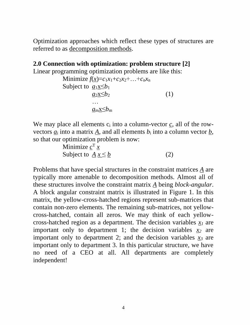
Problems that have special structures in the constraint matrices A are
typically more amenable to decomposition methods. Almost all of
these structures involve the constraint matrix A being block-angular.
A block angular constraint matrix is illustrated in Figure 1. In this
matrix, the yellow-cross-hatched regions represent sub-matrices that
contain non-zero elements. The remaining sub-matrices, not yellow-
cross-hatched, contain all zeros. We may think of each yellow-
cross-hatched region as a department. The decision variables x1 are
important only to department 1; the decision variables x2 are
important only to department 2; and the decision variables x3 are
important only to department 3. In this particular structure, we have
no need of a CEO at all. All departments are completely
independent!

5
x1
x2
x3
≤
b1
b2
b3
Figure 1: Block-angular structure
In the original description, the CEO choses values for certain
variables that affect each department (two 100MVA 69/161 kV
units, four 50MVA 13.8/69 kV units, one 325MVA 230/500 kV
unit, … etc.). This situation would have different departments linked
by these variables. For example, one department would know that
the different transformers have different cooling needs that can be
satisfied with different numbers and types of fans. Depending on the
numbers and types selected, the necessary materials and the
necessary labor hours are different. This department has 20 workers
whose time can be allocated in various ways among the different
tasks necessary to build all of the fans; the department may also hire
more workers if necessary.
The structure of the constraint matrix for this situation is shown in
Figure 2. The CEO’s decisions are integer decisions on the variables
contained in x4. Variables in x1 through x3 are decisions that each of
departments 1-3, respectively, would need to make.

6
x1
x2
x3
≤
b1
b2
b3
x4
Figure 2: Block-angular structure with linking variables
Alternatively, Figure 3 represents a structure where the decisions
linked at the CEO level are such that the CEO must watch out for
the entire organization’s consumption of resources (e.g., money and
labor hours, constrained by c0). In this case, the departments are still
independent, i.e., they are concerned only with decisions on
variables for which no other department is concerned, BUT… the
CEO is concerned with constraints that span across the variables for
all departments to consume total resources. And so we refer to this
structure as block-angular with linking constraints.
λ1
λ2
λ3
≤
c1
c2
c3
c0
Figure 3: Block-angular structure with linking constraints
7
3.0 Motivation for decomposition methods: solution speed
To motivate decomposition methods, we consider introducing
security constraints to what should be, for power engineers, a
familiar problem: the optimal power flow (OPF).
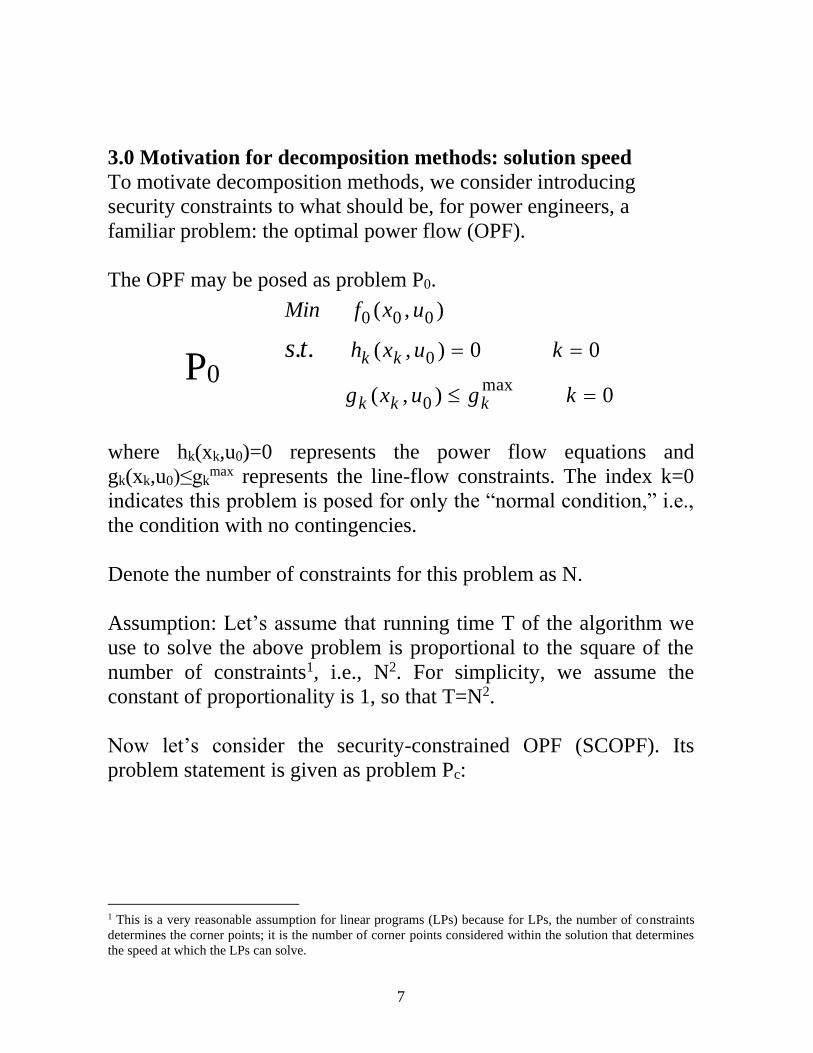
The OPF may be posed as problem P0.
P0
0),(
00),(
),(
max0
0
000
..
=
==
kguxg
kuxh
uxfMin
kkk
kkts
where hk(xk,u0)=0 represents the power flow equations and
gk(xk,u0)≤gkmax represents the line-flow constraints. The index k=0
indicates this problem is posed for only the “normal condition,” i.e.,
the condition with no contingencies.
Denote the number of constraints for this problem as N.
Assumption: Let’s assume that running time T of the algorithm we
use to solve the above problem is proportional to the square of the
number of constraints1, i.e., N2. For simplicity, we assume the
constant of proportionality is 1, so that T=N2.
Now let’s consider the security-constrained OPF (SCOPF). Its
problem statement is given as problem Pc:
1 This is a very reasonable assumption for linear programs (LPs) because for LPs, the number of constraints
determines the corner points; it is the number of corner points considered within the solution that determines
the speed at which the LPs can solve.
8
Pc
ckguxg
ckuxh
uxfMin
kkk
kkts
,...,2,1,0),(
,...,2,1,00),(
),(
max0
0
000
..
=
==
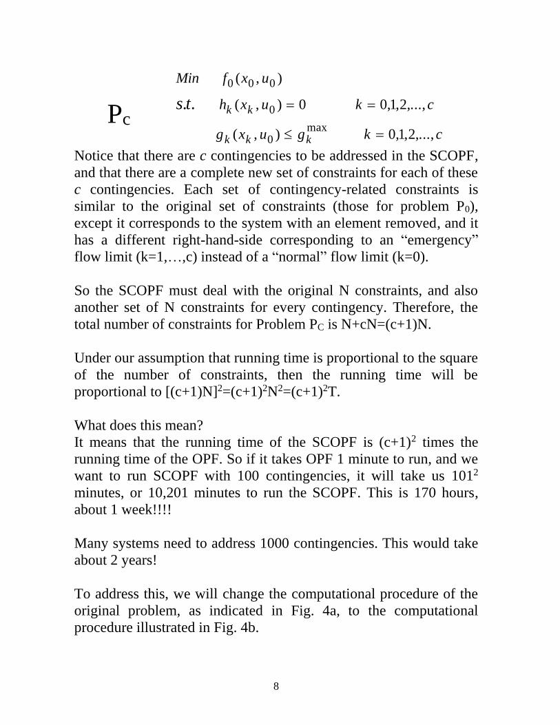
Notice that there are c contingencies to be addressed in the SCOPF,
and that there are a complete new set of constraints for each of these
c contingencies. Each set of contingency-related constraints is
similar to the original set of constraints (those for problem P0),
except it corresponds to the system with an element removed, and it
has a different right-hand-side corresponding to an “emergency”
flow limit (k=1,…,c) instead of a “normal” flow limit (k=0).
So the SCOPF must deal with the original N constraints, and also
another set of N constraints for every contingency. Therefore, the
total number of constraints for Problem PC is N+cN=(c+1)N.
Under our assumption that running time is proportional to the square
of the number of constraints, then the running time will be
proportional to [(c+1)N]2=(c+1)2N2=(c+1)2T.
What does this mean?
It means that the running time of the SCOPF is (c+1)2 times the
running time of the OPF. So if it takes OPF 1 minute to run, and we
want to run SCOPF with 100 contingencies, it will take us 1012
minutes, or 10,201 minutes to run the SCOPF. This is 170 hours,
about 1 week!!!!
Many systems need to address 1000 contingencies. This would take
about 2 years!
To address this, we will change the computational procedure of the
original problem, as indicated in Fig. 4a, to the computational
procedure illustrated in Fig. 4b.
9
Solve SCOPF
k=0, 1, 2, …, c
(normal and all contingency conditions)
0 0 0
0
max
0
( , )
( , ) 0 0,1, 2, ...,
( , ) 0,1, 2, ...,
. . k k
k k k
Min f x u
h x u k c
g x u g k c
s t = =
=
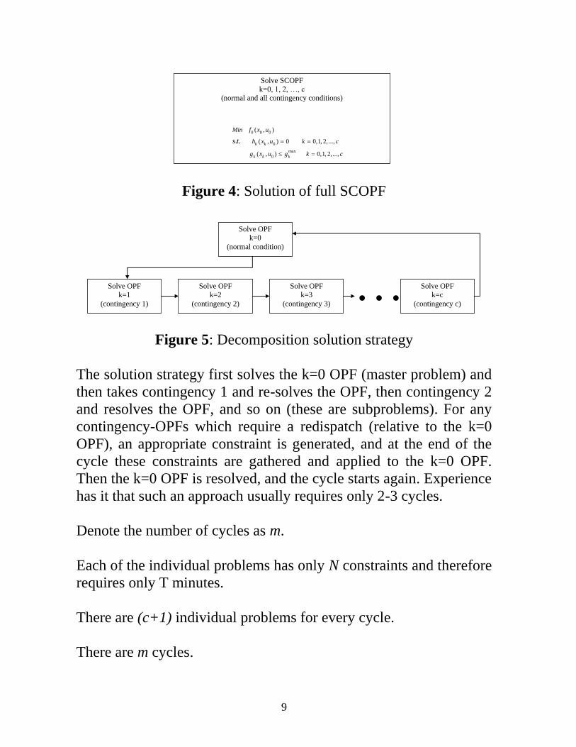
Figure 4: Solution of full SCOPF
Solve OPF
k=0
(normal condition)
Solve OPF
k=1
(contingency 1)
Solve OPF
k=2
(contingency 2)
Solve OPF
k=3
(contingency 3) … Solve OPF
k=c
(contingency c)
Figure 5: Decomposition solution strategy
The solution strategy first solves the k=0 OPF (master problem) and
then takes contingency 1 and re-solves the OPF, then contingency 2
and resolves the OPF, and so on (these are subproblems). For any
contingency-OPFs which require a redispatch (relative to the k=0
OPF), an appropriate constraint is generated, and at the end of the
cycle these constraints are gathered and applied to the k=0 OPF.
Then the k=0 OPF is resolved, and the cycle starts again. Experience
has it that such an approach usually requires only 2-3 cycles.
Denote the number of cycles as m.
Each of the individual problems has only N constraints and therefore
requires only T minutes.
There are (c+1) individual problems for every cycle.
There are m cycles.

10
So the amount of running time is m(c+1)T.
If c=100 and m=3, T=1 minute, this approach requires 303 minutes.
That would be about 5 hours (instead of 1 week).
If c=1000 and m=3, T=1 minute, this approach requires about 50
hours (instead of 2 years).
What if it takes 10 cycles instead of 3?
➔If c=1000 and m=10, T=1 minute, this approach requires 167
hours (1 week, instead of 2 years).
What if it takes 100 cycles instead of 3?
➔If c=1000 and m=100, T=1 minute, this approach requires 1668
hours (10 weeks, instead of 2 years).
In addition, this approach is easily parallelizable, i.e., each
individual OPF problem can be sent to its own CPU. This will save
even more time. Figure 6 compares computing time for a “toy”
system. The comparison is between a full SCOPF, a decomposed
SCOPF (DSCOPF), and a decomposed SCOPF where the individual
OPF problems have been sent to separate CPUs.
Figure 6
4.0 Benders decomposition
J. F. Benders [3] proposed solving a mixed-integer programming
problem by partitioning the problem into two parts – an integer part
11
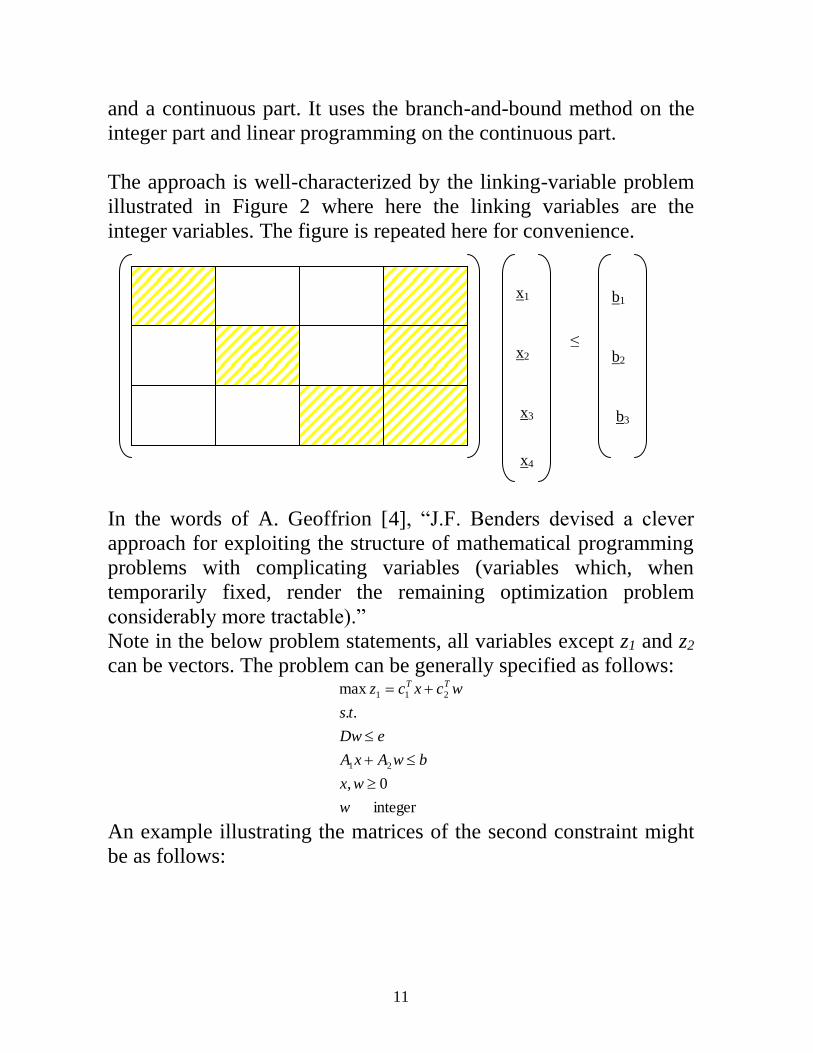
and a continuous part. It uses the branch-and-bound method on the
integer part and linear programming on the continuous part.
The approach is well-characterized by the linking-variable problem
illustrated in Figure 2 where here the linking variables are the
integer variables. The figure is repeated here for convenience.
x1
x2
x3
≤
b1
b2
b3
x4
In the words of A. Geoffrion [4], “J.F. Benders devised a clever
approach for exploiting the structure of mathematical programming
problems with complicating variables (variables which, when
temporarily fixed, render the remaining optimization problem
considerably more tractable).”
Note in the below problem statements, all variables except z1 and z2
can be vectors. The problem can be generally specified as follows:
integer
0,
..
max
21
211
w
wx
bwAxA
eDw
ts
wcxcz TT
+
+=
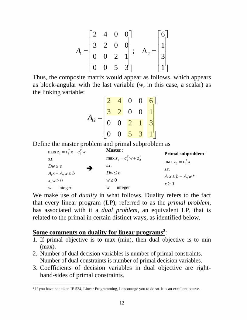
An example illustrating the matrices of the second constraint might
be as follows:
12
1 2
2 4 0 0 6
3 2 0 0 1; A
0 0 2 1 3
0 0 5 3 1
A
= =
Thus, the composite matrix would appear as follows, which appears
as block-angular with the last variable (w, in this case, a scalar) as
the linking variable:
12
2 4 0 0 6
3 2 0 0 1
0 0 2 1 3
0 0 5 3 1
A
=
Define the master problem and primal subproblem as
integer
0,
..
max
21
211
w
wx
bwAxA
eDw
ts
wcxcz TT
+
+=
➔
integer
0
..
max
:
*
221
w
w
eDw
ts
zwcz T
+=
Master
0
*
..
max
:
21
12
−
=
x
wAbxA
ts
xcz T
subproblem Primal
We make use of duality in what follows. Duality refers to the fact
that every linear program (LP), referred to as the primal problem,
has associated with it a dual problem, an equivalent LP, that is
related to the primal in certain distinct ways, as identified below.
Some comments on duality for linear programs2: 1. If primal objective is to max (min), then dual objective is to min
(max).
2. Number of dual decision variables is number of primal constraints.
Number of dual constraints is number of primal decision variables.
3. Coefficients of decision variables in dual objective are right-
hand-sides of primal constraints.
2 If you have not taken IE 534, Linear Programming, I encourage you to do so. It is an excellent course.

13
Problem Primal
21
21
2
1
21
0,0
1823
12 2
4 s.t.
53max
P Problem
+
+=
xx
xx
x
x
xxF
➔
Problem Dual
321
32
31
321
0,0,0
522
33
subject to
18124min
D Problem
+
+
++=
G
4. Coefficients of decision variables in primal objective are right-
hand-sides of dual constraints.
Problem Primal
21
21
2
1
21
0,0
1823
12 2
4 s.t.
53max
P Problem
+
+=
xx
xx
x
x
xxF
➔
Problem Dual
321
32
31
321
0,0,0
522
33
subject to
18124min
D Problem
+
+
++=
G
5. Coefficients of one variable across multiple primal constraints are
coefficients of multiple variables in one dual constraint.
Problem Primal
21
21
2
1
21
0,0
1823
12 2
4 s.t.
53max
P Problem
+
+=
xx
xx
x
x
xxF
➔
1 2 3
1 2 3
1 2 3
1 2 3
Dual Problem
Problem D
min 4 12 18
subject to
0 3 3
0 2 2 5
0, 0, 0
G
= + +
+ +
+ +
6. If primal constraints are ≤ (≥), dual constraints are ≥ (≤).
Let’s think about what the above comments 1-5 mean for our LP
“general form” problem statements (1) and (2) on pg. 4, repeated
here for convenience:
Likewise, coefficients of
one variable across multiple
dual constraints are
coefficients of multiple
variables in one primal
constraint.
All of this means that if the
primal constraint matrix is
A, the dual constraint
matrix is AT.
14
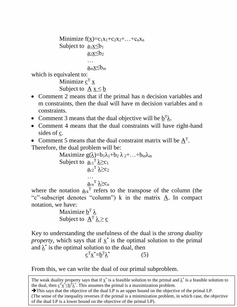
Minimize f(x)=c1x1+c2x2+…+cnxn
Subject to a1x≤b1
a2x≤b2
…
amx≤bm
which is equivalent to:
Minimize cT x
Subject to A x ≤ b
• Comment 2 means that if the primal has n decision variables and
m constraints, then the dual will have m decision variables and n
constraints.
• Comment 3 means that the dual objective will be bTλ.
• Comment 4 means that the dual constraints will have right-hand
sides of c.
• Comment 5 means that the dual constraint matrix will be AT.
Therefore, the dual problem will be:
Maximize g(λ)=b1λ1+b2 λ 2+…+bmλm
Subject to ac1T
λ≥c1
ac2T λ≥c2
…
acnT λ≥cn
where the notation ackT refers to the transpose of the column (the
“c”-subscript denotes “column”) k in the matrix A. In compact
notation, we have:
Maximize bT λ
Subject to AT λ ≥ c
Key to understanding the usefulness of the dual is the strong duality
property, which says that if x* is the optimal solution to the primal
and λ* is the optimal solution to the dual, then
cTx*=bTλ* (5)
From this, we can write the dual of our primal subproblem.
The weak duality property says that if x* is a feasible solution to the primal and λ* is a feasible solution to
the dual, then cTx*≤bTλ*. This assumes the primal is a maximization problem.
➔This says that the objective of the dual LP is an upper bound on the objective of the primal LP.
(The sense of the inequality reverses if the primal is a minimization problem, in which case, the objective
of the dual LP is a lower bound on the objective of the primal LP).
15
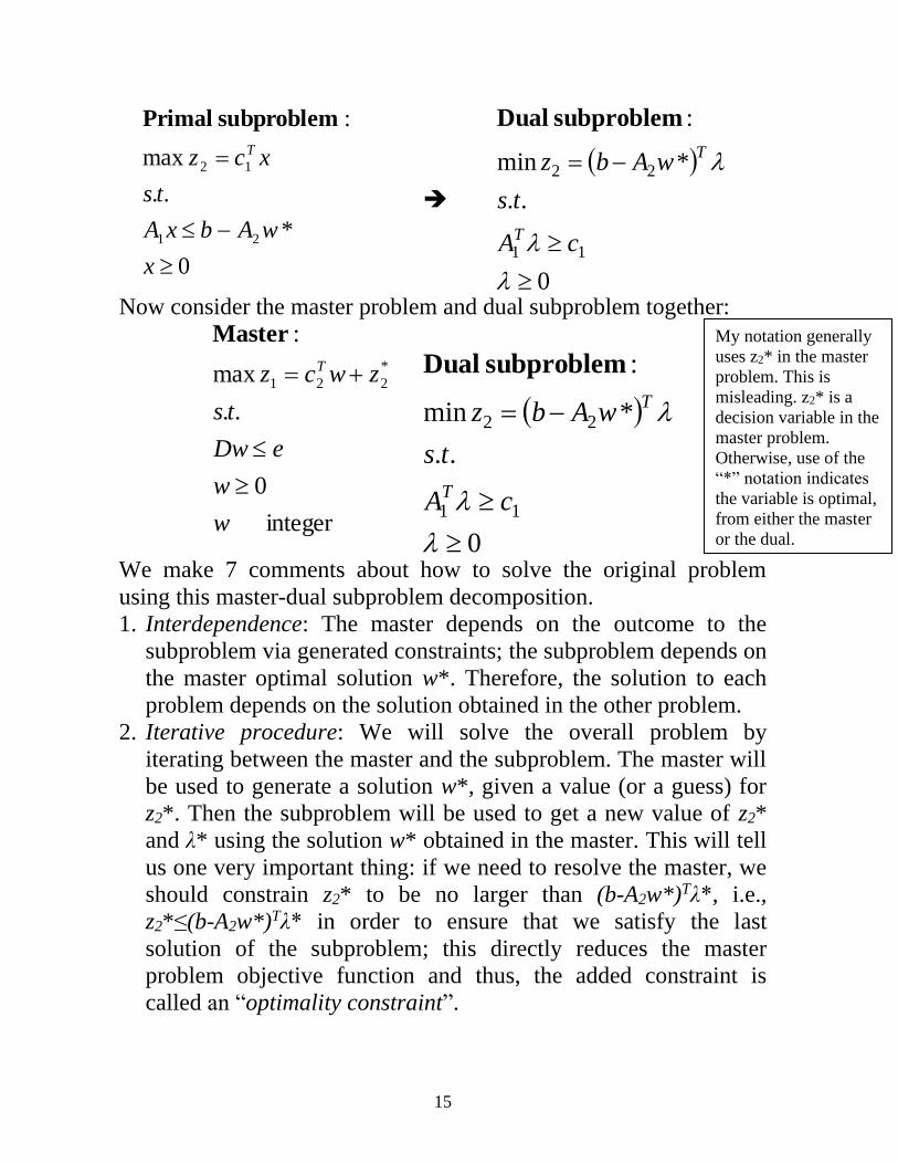
0
*
..
max
:
21
12
−
=
x
wAbxA
ts
xcz T
subproblem Primal
➔
( )
0
..
*min
:
11
22
−=
cA
ts
wAbz
T
T
subproblem Dual
Now consider the master problem and dual subproblem together:
integer
0
..
max
:
*
221
w
w
eDw
ts
zwcz T
+=
Master
( )
0
..
*min
:
11
22
−=
cA
ts
wAbz
T
T
subproblem Dual
We make 7 comments about how to solve the original problem
using this master-dual subproblem decomposition.
1. Interdependence: The master depends on the outcome to the
subproblem via generated constraints; the subproblem depends on
the master optimal solution w*. Therefore, the solution to each
problem depends on the solution obtained in the other problem.
2. Iterative procedure: We will solve the overall problem by
iterating between the master and the subproblem. The master will
be used to generate a solution w*, given a value (or a guess) for
z2*. Then the subproblem will be used to get a new value of z2*
and λ* using the solution w* obtained in the master. This will tell
us one very important thing: if we need to resolve the master, we
should constrain z2* to be no larger than (b-A2w*)Tλ*, i.e.,
z2*≤(b-A2w*)Tλ* in order to ensure that we satisfy the last
solution of the subproblem; this directly reduces the master
problem objective function and thus, the added constraint is
called an “optimality constraint”.
My notation generally
uses z2* in the master
problem. This is
misleading. z2* is a
decision variable in the
master problem.
Otherwise, use of the
“*” notation indicates
the variable is optimal,
from either the master
or the dual.

16
3. Upper bound:
a. Initial solution: Start the solution procedure by solving the
master problem with a guess for an upper bound on z2*. Since
the dual subproblem is going to minimize (lower) z2, let’s be
safe and guess a large value of the upper bound on z2* for this
initial master problem solution. Since this value of z2* is
chosen large, we can be sure that the first solution to the
master, z1*, will be above the actual (overall problem optimal)
solution, and so we will consider this solution z1* to be an
upper bound on the actual solution.
b. Successive solutions: As the iterations proceed, we will add
constraints to the master problem (adding constraints never
improves, or in this case, increases, the optimum), generated
by the subproblem, so that the master problem solution z1*,
will continuously decrease towards the actual (overall problem
optimal) solution.
Thus, the value of z1*, obtained from the master problem, serves
as an upper bound on the actual (overall problem optimal)
solution.
4. Lower bound: The dual problem results in a new value of z2*, and
it can then be added to c2Tw* (where w* was obtained from the
last master problem solution) to provide another estimate of z1*.
Since the dual problem minimizes z2, without the master problem
constraints, the term c2Tw* (from master) +z2* (from dual) will
be a lower bound on z1*.
5. Feasibility: An LP primal may result in its solution being
optimal, infeasible, or unbounded. These occurrences have
implications on what can happen in the dual. And the converse is
true: occurrences in the dual have implications regarding what
can happen in the primal. Table 1 below summarizes the
relationships.

17
Table 1: Possible combinations of dual and primal solutions
From Table 1, we observe that if the dual problem results in an
unbounded solution, then it means the primal problem must be
infeasible (note: an infeasible primal implies an unbounded or
infeasible dual). In Benders, when we solve the dual and obtain
unboundedness, it means the primal (which is contained in the
master problem) is infeasible (and so the master is infeasible),
and we must resolve the master problem with more restrictive
constraints on w to force the primal to be feasible. The associated
constraints on w are called feasibility cuts.
6. Algorithm: In what follows, we specify Q as the set of constraints
for the master program. It will change via the addition of
feasibility and optimality cuts as the algorithm proceeds. Initially,
Q={wk ≤ large number, for all k, z2*≤M, M large}.

18
Master problem:
kw
MMz
kQw
ts
zwcz
k
k
T
+=
integer
large is ,
in as dconstraine
..
max
*
2
*
221
Sub-problem (dual):
k
cA
ts
wAbz
k
T
T
−=
,0
..
*)(min
11
22
There are 3 steps to Benders decomposition.
1. Solve the master problem using Branch and Bound (or any other
integer programming method). Designate the solution as w*.
2. Using the value of w* found in step 1, solve the sub-problem (the
dual) which gives z2* and λ*. There are two possibilities:
a. If the solution is unbounded (implying the primal is
infeasible), adjoin the most constraining feasibility
constraint from (b-A2w)Tλ≥0 to Q, and go to step 1. The
constraint (b-A2w)Tλ≥0 imposes feasibility on the primal
because it prevents unboundedness in the dual by imposing
non-negativity on the coefficients of each λk. We illustrate
this challenging concept in an example below.
b. Otherwise, designate the solution as λ* and go to step 3.
3. Compare z1 found in step 1 to * *
2 2
Tc w z+ where w* is found in step
1; **)(* 22 TwAbz −= is found in step 2.There are two possibilities:
a. If they are equal (or within ε of each other), then the
solution (w*, λ*) corresponding to the subproblem dual
solution, is optimal and the primal variables x* are found as
the dual variables3 within the subproblem.
3 Dual variables are the coefficients of the objective function in the final iteration of the simplex
method and are provided with the LP solution by a solver like CPLEX. Here, our use of the word

19
b. If they are not equal, adjoin an optimality constraint to Q
given by **)(* 22 TwAbz − and go to step 1.
Step 3 is a check on Benders optimal rule, stated below.
Figure 7 illustrates the algorithm in block diagram form.
It is useful to study Figure 7 while referring to the statement of
Benders optimal rule just above it.
Figure 7: Illustration of Benders Decomposition
“dual” refers to what we previously referred to as the primal. The dual variables x must have values
that result in the two objective functions being equal at the optimum: cTx=(b-A2w*)Tλ*.
Step 1,
Master Problem
(gives upper bound):
max z1=c2Tw+z2
st Dw≤e
w≥0, w integer
constraints Q
Step 2, Subproblem:
(gives lower bound)
min z2=(b-A2w*)λ
st A1Tλ≥c1
λ≥0
w*
Step 3,
Benders opt rule
c2Tw*+z2*=z1*
Full problem
solved Adjoin to Q an optimality
constraint:
2 2* ( ) *Tz b A w −
Solved,
passes z2*
Infeasible
Unbounded
Full problem
is unbounded
or infeasible
Adjoin to Q the most
constraining feasibility
constraint:
(b-A2w)Tλ≥0
Passes
w*,z1*
?
YES NO
Benders optimal rule: If (z1*, w*) is the optimal solution to the master
problem, and (z2*, λ*) is the optimal solution to dual subproblem, and if
2
Upper boundLower bound
*
2 2 1
from master from masterz * from subproblemproblem problem
* ( *) *T Tc w b A w z+ − =,
then (z1*, w*, λ*) is the optimal solution for the complete problem.

20
We will work an example using the formalized nomenclature of the
previous summarized steps. But before we do, we introduce the
optimization solver CPLEX.
Brief tutorial for using CPLEX.
CPLEX version 12.10.0.0 resides on ISU servers. To access it, you
need to logon to an appropriate server (see
http://it.engineering.iastate.edu/remote/ for a list of servers with CPLEX). To
do that, you need a telnet and ftp facility. You can find instructions
on our course website for getting/using the appropriate telnet & ftp
facilities (see sec 2 of http://home.eng.iastate.edu/~jdm/ee552/Intro_CPLEX.pdf).
After getting the telnet and ftp facilities set up on your machine, the
next thing to do is to construct a file containing the problem. To
construct this file, you can use the program called “notepad” under
the “accessories” selection of the start button in Windows. Once you
open notepad, you can immediately save to your local directory
under the filename “filename.lp.” You can choose “filename” to be
whatever you want, but you will need the extension “lp.” To obtain
the extension “lp” when you save, do “save as” and then choose “all
files.” Otherwise, it will assign the suffix “.txt” to your file. Here is
what I typed into the file I called “example.lp”…
maximize
12 x1 + 12 x2
subject to
2 x1 + 2 x2 >= 4
3 x1 + x2 >= 3
x1 >= 0
x2 >= 0
end
Once you get the above file onto a server having access to CPLEX,
you may simply type
21
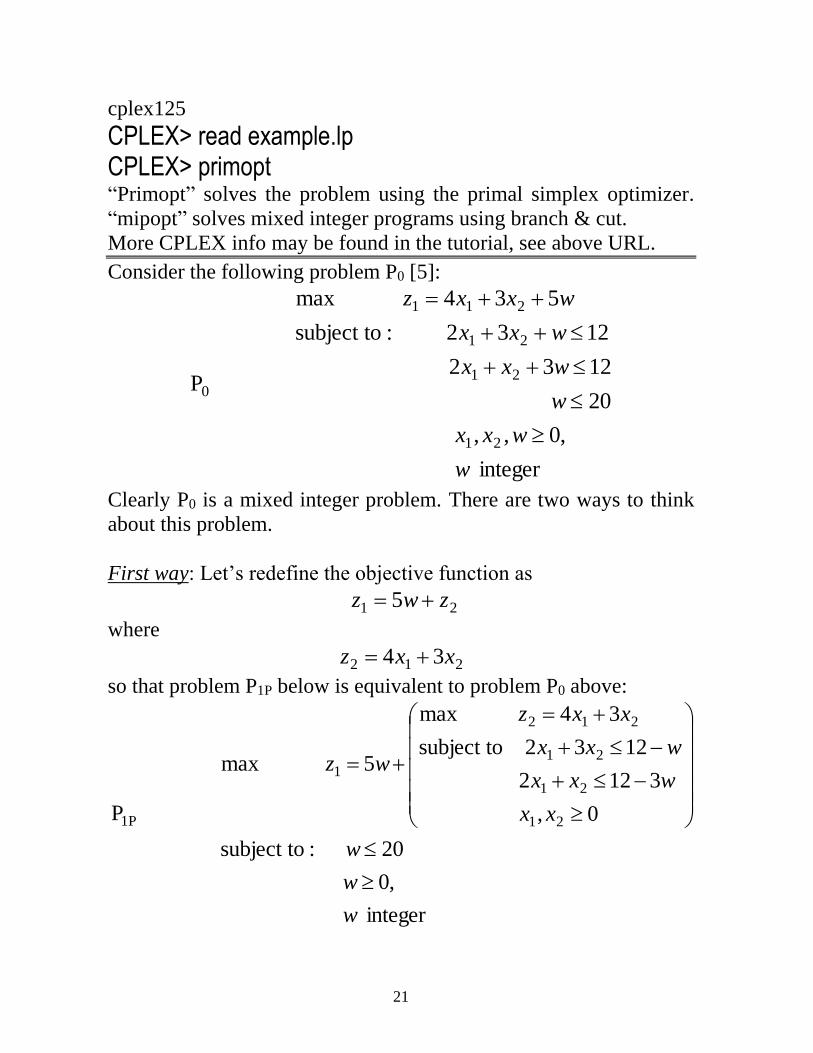
cplex125
CPLEX> read example.lp CPLEX> primopt “Primopt” solves the problem using the primal simplex optimizer.
“mipopt” solves mixed integer programs using branch & cut. More CPLEX info may be found in the tutorial, see above URL.
Consider the following problem P0 [5]:
integer
,0,,
20
1232
1232 :subject to
534 max
P
21
21
21
211
0
w
wxx
w
wxx
wxx
wxxz
++
++
++=
Clearly P0 is a mixed integer problem. There are two ways to think
about this problem.
First way: Let’s redefine the objective function as
21 5 zwz +=
where
212 34 xxz +=
so that problem P1P below is equivalent to problem P0 above:
integer
,0
20 :subject to
0,
3122
1232 subject to
34 max
5 max
P 21
21
21
212
1
1P
w
w
w
xx
wxx
wxx
xxz
wz
−+
−+
+=
+=

22
This way is similar to the way J. Bloom described his two-stage
generation planning problem in [6], which we summarize at the end
of these notes.
Second way: Here, we will simply cast the problem into the general
form outlined in our three-step procedure.
Comparing this problem (right) to our general formulation (left),
General Formulation This problem
integer
0,
..
max
21
211
w
wx
bwAxA
ts
wcxcz TT
+
+=
1 1 2
1 2
1 2
0
1 2
max 4 3 5
subject to: 2 3 12
2 3 12P
20
, , 0,
z x x w
x x w
x x w
w
x x w
= + +
+ +
+ +
integerw
we observe that
=
=
=
=
=
12
12 ,
3
1 ,
12
32
5 ,3
4
21
21
bAA
cc
In the next pages, we will go through the first iteration, which is
colored green and results in a feasibility cut, and the second
iteration, which is colored grey and results in an optimality cut.

23
Step 1: The master problem is
kw
MMzkwQ
ts
zwcz
k
k
T
+=
integerand 0
large is , , dconstraine :
..
max
*
2
*
221
or
integerand 0
, 20:
..
max
*
2
*
221
+=
w
MzwQ
ts
zwcz T
➔
integerand 0
,20:
..
5max
*
2
*
21
+=
w
MzwQ
ts
zwz
The solution to this problem is trivial: since the objective function is
being maximized, we make w and z2* as large as possible, resulting
in w*=20, z2*=M, and z1=5*20+M=100+M.
Step 2: Using the value of w found in the master, get the dual:
0
..
*)(min
11
22
−=
cA
ts
wAbz
T
T
➔
0,
3
4
13
22
..
*3
1
12
12min
21
2
1
2
1
2
−
=
ts
wz
T
Substituting, from step 1, w*=20, the subproblem becomes:
0,
3
4
13
22
..
488203
1
12
12min
21
2
1
21
2
1
2
−−=
−
=
ts
z
T
24
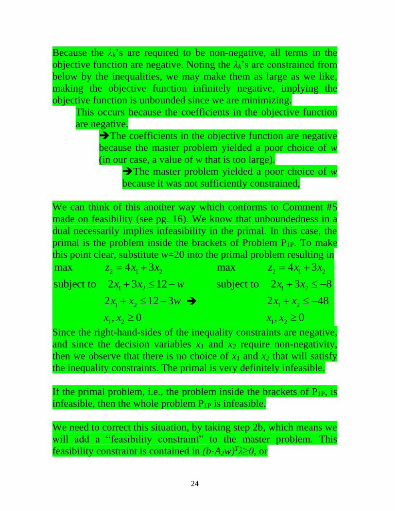
Because the λk’s are required to be non-negative, all terms in the
objective function are negative. Noting the λk’s are constrained from
below by the inequalities, we may make them as large as we like,
making the objective function infinitely negative, implying the
objective function is unbounded since we are minimizing.
This occurs because the coefficients in the objective function
are negative.
➔The coefficients in the objective function are negative
because the master problem yielded a poor choice of w
(in our case, a value of w that is too large).
➔The master problem yielded a poor choice of w
because it was not sufficiently constrained,
We can think of this another way which conforms to Comment #5
made on feasibility (see pg. 16). We know that unboundedness in a
dual necessarily implies infeasibility in the primal. In this case, the
primal is the problem inside the brackets of Problem P1P. To make
this point clear, substitute w=20 into the primal problem resulting in
2 1 2
1 2
1 2
1 2
max 4 3
subject to 2 3 12
2 12 3
, 0
z x x
x x w
x x w
x x
= +
+ −
+ −
➔
2 1 2
1 2
1 2
1 2
max 4 3
subject to 2 3 8
2 48
, 0
z x x
x x
x x
x x
= +
+ −
+ −
Since the right-hand-sides of the inequality constraints are negative,
and since the decision variables x1 and x2 require non-negativity,
then we observe that there is no choice of x1 and x2 that will satisfy
the inequality constraints. The primal is very definitely infeasible.
If the primal problem, i.e., the problem inside the brackets of P1P, is
infeasible, then the whole problem P1P is infeasible.
We need to correct this situation, by taking step 2b, which means we
will add a “feasibility constraint” to the master problem. This
feasibility constraint is contained in (b-A2w)Tλ≥0, or
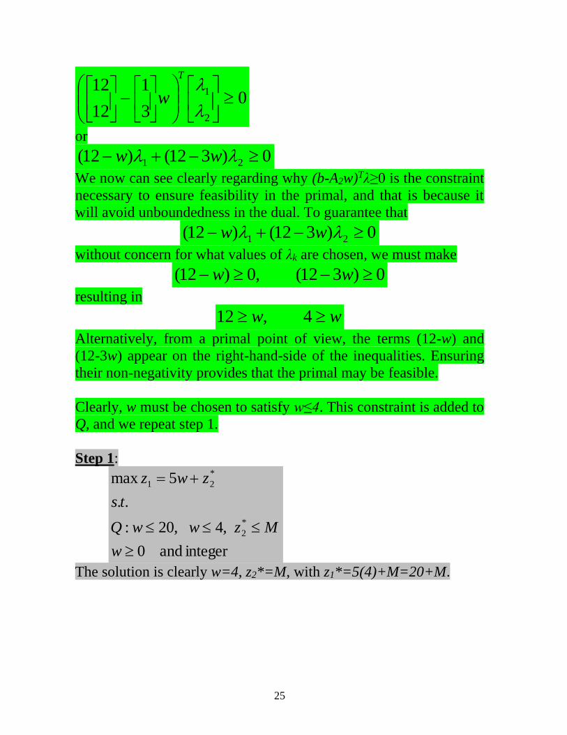
25
03
1
12
12
2
1
−
T
w
or
0)312()12( 21 −+− ww
We now can see clearly regarding why (b-A2w)Tλ≥0 is the constraint
necessary to ensure feasibility in the primal, and that is because it
will avoid unboundedness in the dual. To guarantee that
0)312()12( 21 −+− ww
without concern for what values of λk are chosen, we must make
0)312(,0)12( −− ww
resulting in
ww 4,12
Alternatively, from a primal point of view, the terms (12-w) and
(12-3w) appear on the right-hand-side of the inequalities. Ensuring
their non-negativity provides that the primal may be feasible.
Clearly, w must be chosen to satisfy w≤4. This constraint is added to
Q, and we repeat step 1.
Step 1:
integer and0
,4 ,20:
..
5max
*
2
*
21
+=
w
MzwwQ
ts
zwz
The solution is clearly w=4, z2*=M, with z1*=5(4)+M=20+M.

26
Step 2: Using the value of w=4 found in the master, get the dual.
0
..
*)(min
11
22
−=
cA
ts
wAbz
T
T
➔
0,
3
4
13
22
..
*3
1
12
12min
21
2
1
2
1
2
−
=
ts
wz
T
Substituting, from step 1, w*=4, the subproblem becomes:
0,
3
4
13
22
..
843
1
12
12min
21
2
1
1
2
1
2
=
−
=
ts
z
T
We can use CPLEX LP solver (or any other LP solver) to solve the
above, obtaining the solution λ1*=0, λ2*=3, with objective function
value z2*=0. Intuitively, one observes that minimization of the
objective subject to nonnegativity constraint on λ1 requires λ1=0;
then λ2 can be anything as long as it satisfies
3
242
2
22
Therefore an optimal solution is λ1*=0, λ2*=3. (Although this is a
solution, it is a special kind of solution referred to as degenerate
because there are many values of λ2 that are equally good solutions.)
Since we have a bounded dual solution (and therefore optimal), our
primal is feasible, and we may proceed to step 3 to test for
optimality using Benders optimal rule.
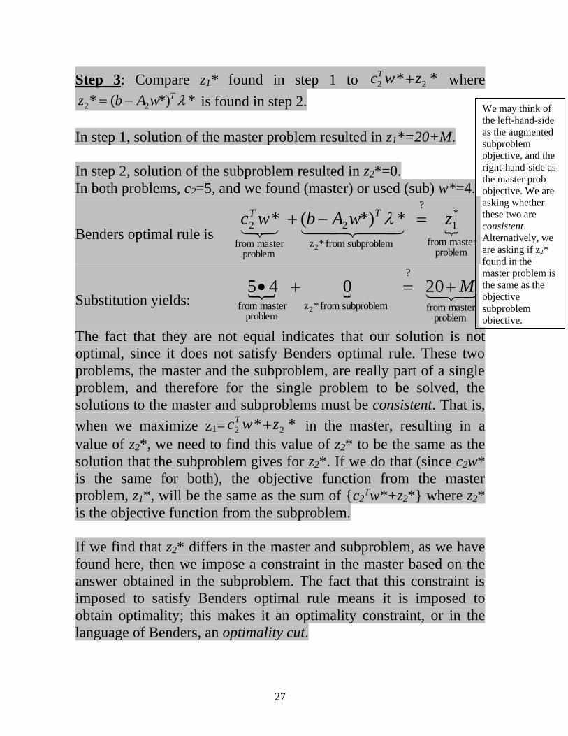
27
Step 3: Compare z1* found in step 1 to ** 22 zwcT + where
**)(* 22 TwAbz −= is found in step 2.
In step 1, solution of the master problem resulted in z1*=20+M.
In step 2, solution of the subproblem resulted in z2*=0.
In both problems, c2=5, and we found (master) or used (sub) w*=4.
Benders optimal rule is problem
master from
*
1
?
subproblem from *z
2
problemmaster from
2 **)(*
2
zwAbwc TT =−+
Substitution yields:
problemmaster from
?
subproblem from *zproblem
master from
20 0452
M+=+•
The fact that they are not equal indicates that our solution is not
optimal, since it does not satisfy Benders optimal rule. These two
problems, the master and the subproblem, are really part of a single
problem, and therefore for the single problem to be solved, the
solutions to the master and subproblems must be consistent. That is,
when we maximize z1= ** 22 zwcT + in the master, resulting in a
value of z2*, we need to find this value of z2* to be the same as the
solution that the subproblem gives for z2*. If we do that (since c2w*
is the same for both), the objective function from the master
problem, z1*, will be the same as the sum of {c2Tw*+z2*} where z2*
is the objective function from the subproblem.
If we find that z2* differs in the master and subproblem, as we have
found here, then we impose a constraint in the master based on the
answer obtained in the subproblem. The fact that this constraint is
imposed to satisfy Benders optimal rule means it is imposed to
obtain optimality; this makes it an optimality constraint, or in the
language of Benders, an optimality cut.
We may think of
the left-hand-side
as the augmented
subproblem
objective, and the
right-hand-side as
the master prob
objective. We are
asking whether
these two are
consistent.
Alternatively, we
are asking if z2*
found in the
master problem is
the same as the
objective
subproblem
objective.

28
We obtain the optimality cut from 2 2* ( ) *Tz b A w − . With
=
12
12b ,
=
3
12A ,
=
3
0
2
1
wwwwz
T
9363
0 31212
3
0
3
1
12
12*
2 −=
−−=
−
Now we return to step 1, but before we do, we distinguish between a
feasibility cut and an optimality cut:
• Feasibility cut: Takes place as a result of finding an unbounded
dual subproblem, which, by Table 1, implies an infeasible primal
subproblem. It means that for the value of w found in the
master problem, there is no possible solution in the primal
subproblem. We address this by adding a feasibility cut (a
constraint on w) to the master problem, where that cut is obtained
from dual subproblem to avoid its unboundedness, or,
alternatively, to avoid the primal subproblem infeasibility.
(b-A2w)Tλ≥0.
• Optimality cut: Takes place as a result of finding that Benders
optimal rule is not satisfied, i.e., that
of instead **)(*
problemmaster from
*1
subproblem from *z
2
problemmaster from
2
2
zwAbwc TT −+
problemmaster from
*1
subproblem from *z
2
problemmaster from
2
2
**)(* zwAbwc TT =−+
It means that the value of z2* computed in the master problem
(and contained in z1*) is larger than the value of z2* computed in
the subproblem. This must be the case (when Benders optimal
rule is not satisfied) since z1* is always an upper bound for the
solution (see comment 3 regarding “Upper bounds” on pg. 16).
We address this by adding an optimality cut (a constraint on z2*
in terms of w) to the master problem, to force z2* in the master
problem to be smaller, where that cut is obtained from Benders
optimal rule reflecting the maximum which the subproblem
allows for z2*. The optimality cut is:
*)(* 22 TwAbz −
29
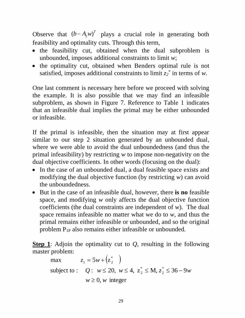
Observe that 2( )Tb A w− plays a crucial role in generating both
feasibility and optimality cuts. Through this term,
• the feasibility cut, obtained when the dual subproblem is
unbounded, imposes additional constraints to limit w;
• the optimality cut, obtained when Benders optimal rule is not
satisfied, imposes additional constraints to limit z2* in terms of w.
One last comment is necessary here before we proceed with solving
the example. It is also possible that we may find an infeasible
subproblem, as shown in Figure 7. Reference to Table 1 indicates
that an infeasible dual implies the primal may be either unbounded
or infeasible.
If the primal is infeasible, then the situation may at first appear
similar to our step 2 situation generated by an unbounded dual,
where we were able to avoid the dual unboundedness (and thus the
primal infeasibility) by restricting w to impose non-negativity on the
dual objective coefficients. In other words (focusing on the dual):
• In the case of an unbounded dual, a dual feasible space exists and
modifying the dual objective function (by restricting w) can avoid
the unboundedness.
• But in the case of an infeasible dual, however, there is no feasible
space, and modifying w only affects the dual objective function
coefficients (the dual constraints are independent of w). The dual
space remains infeasible no matter what we do to w, and thus the
primal remains either infeasible or unbounded, and so the original
problem P1P also remains either infeasible or unbounded.
Step 1: Adjoin the optimality cut to Q, resulting in the following
master problem:
( )
integer ,0
936 M,z ,4 ,20 : :subject to
z5 max
*
2
*
2
*
21
ww
wzww Q
wz
−
+=

30
This all-integer program can be solved using a branch and bound
algorithm (both CPLEX and Matlab have one), but the solution can
be identified using enumeration, since w can only be 0, 1, 2, 3, or 4.
For example, letting w=0, we have
( ) 36 M,z : :subject to
z max
*
2
*
2
*
21
=
zQ
z
The solution is recognized immediately, as z2*=36, z1*=36.
Likewise, letting w=1, we have
( )27 M,z : :subject to
z5 max
*
2
*
2
*
21
+=
zQ
z
The solution is recognized immediately, as z2*=27, z1*=32.
Continuing on, we find the complete set of solutions are
w=0, z2*=36, z1=36
w=2, z2*=27, z1=32
w=2, z2*=18, z1=28
w=3, z2*=9, z1=24
w=4, z2*=0, z1=20
Since the first one results in maximizing z1, our solution is
w*=0, z2*=36, z1*=36.
Step 2: Using the value of w found in the master, get the dual:
0
..
*)(min
11
22
−=
cA
ts
wAbz
T
T
➔
0,
3
4
13
22
..
*3
1
12
12min
21
2
1
2
1
2
−
=
ts
wz
T
Substituting, from step 1, w*=0, the subproblem becomes:

31
0,
3
4
13
22
..
121203
1
12
12min
21
2
1
21
2
1
2
+=
−
=
ts
z
T
We can use CPLEX LP solver (or any other LP solver) to solve the
above, obtaining the solution λ1*=2, λ2*=0, with objective function
value z2*=24. Since we have a bounded dual solution, our primal is
feasible, and we may proceed to step 3.
Step 3: Compare z1 found in step 1 to ** 22 zwcT + where
**)(* 22 TwAbz −= is found in step 2.
In step 1, solution of the master problem resulted in z1*=36
In step 2, solution of the subproblem resulted in z2*=24.
In both problems, c2=5, and we found (master) or used (sub) w*=0.
Benders optimal rule is problem
master from
*
1
?
subproblem from *z
2
problemmaster from
2 **)(*
2
zwAbwc TT =−+
Substitution yields:
problemmaster from
?
subproblem from *zproblem
master from
36 24052
=+•
Benders optimal rule is not satisfied, we need to obtain the
optimality cut from *)(* 22 TwAbz − . With
=
12
12b ,
=
3
12A ,
=
0
2
2
1
32
wwwwz
T
2240
2 31212
0
2
3
1
12
12*
2 −=
−−=
−
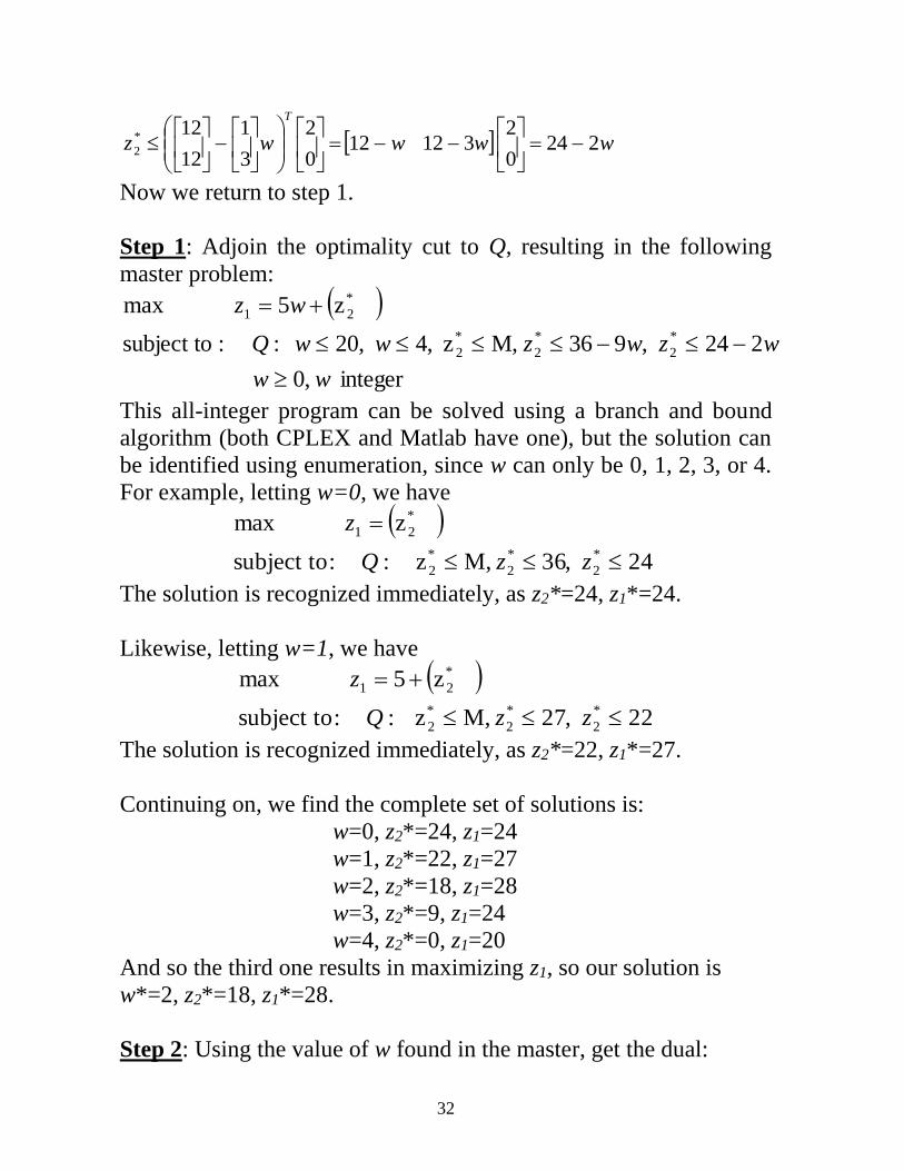
Now we return to step 1.
Step 1: Adjoin the optimality cut to Q, resulting in the following
master problem:
( )
integer ,0
224 ,936 M,z ,4 ,20 : :subject to
z5 max
*
2
*
2
*
2
*
21
ww
wzwzww Q
wz
−−
+=
This all-integer program can be solved using a branch and bound
algorithm (both CPLEX and Matlab have one), but the solution can
be identified using enumeration, since w can only be 0, 1, 2, 3, or 4.
For example, letting w=0, we have
( ) 24 ,36 M,z : :subject to
z max
*
2
*
2
*
2
*
21
=
zzQ
z
The solution is recognized immediately, as z2*=24, z1*=24.
Likewise, letting w=1, we have
( )22 ,27 M,z : :subject to
z5 max
*
2
*
2
*
2
*
21
+=
zzQ
z
The solution is recognized immediately, as z2*=22, z1*=27.
Continuing on, we find the complete set of solutions is:
w=0, z2*=24, z1=24
w=1, z2*=22, z1=27
w=2, z2*=18, z1=28
w=3, z2*=9, z1=24
w=4, z2*=0, z1=20
And so the third one results in maximizing z1, so our solution is
w*=2, z2*=18, z1*=28.
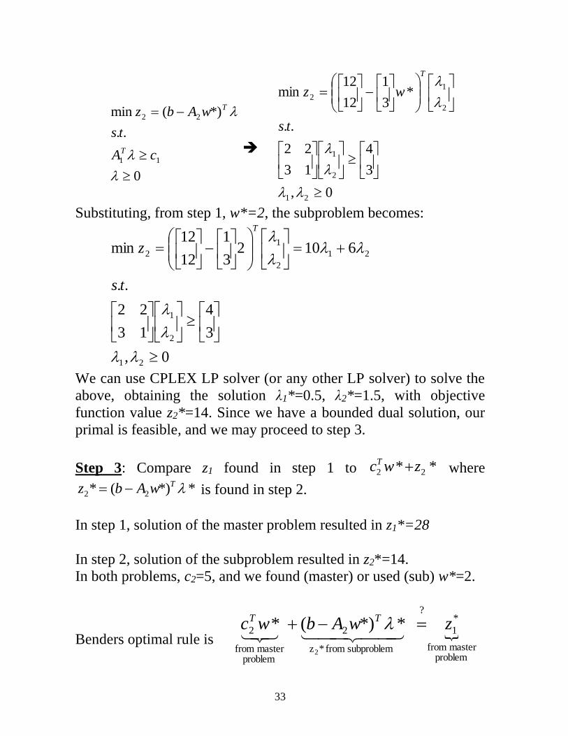
Step 2: Using the value of w found in the master, get the dual:
33
0
..
*)(min
11
22
−=
cA
ts
wAbz
T
T
➔
0,
3
4
13
22
..
*3
1
12
12min
21
2
1
2
1
2
−
=
ts
wz
T
Substituting, from step 1, w*=2, the subproblem becomes:
0,
3
4
13
22
..
61023
1
12
12min
21
2
1
21
2
1
2
+=
−
=
ts
z
T
We can use CPLEX LP solver (or any other LP solver) to solve the
above, obtaining the solution λ1*=0.5, λ2*=1.5, with objective
function value z2*=14. Since we have a bounded dual solution, our
primal is feasible, and we may proceed to step 3.
Step 3: Compare z1 found in step 1 to ** 22 zwcT + where
**)(* 22 TwAbz −= is found in step 2.
In step 1, solution of the master problem resulted in z1*=28
In step 2, solution of the subproblem resulted in z2*=14.
In both problems, c2=5, and we found (master) or used (sub) w*=2.
Benders optimal rule is problem
master from
*
1
?
subproblem from *z
2
problemmaster from
2 **)(*
2
zwAbwc TT =−+
34
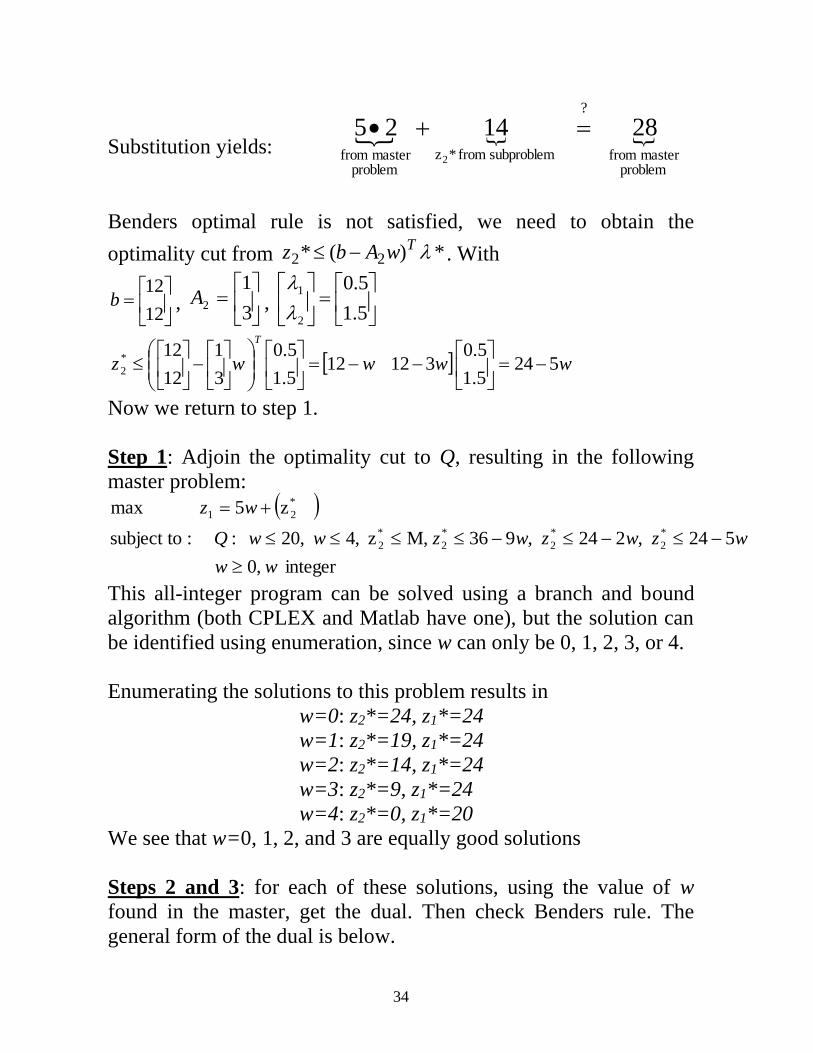
Substitution yields:
problemmaster from
?
subproblem from *zproblem
master from
28 14252
=+•
Benders optimal rule is not satisfied, we need to obtain the
optimality cut from *)(* 22 TwAbz − . With
=
12
12b ,
=
3
12A ,
=
5.1
5.0
2
1
wwwwz
T
5245.1
5.0 31212
5.1
5.0
3
1
12
12*
2 −=
−−=
−
Now we return to step 1.
Step 1: Adjoin the optimality cut to Q, resulting in the following
master problem:
( )
integer ,0
524 ,224 ,936 M,z ,4 ,20 : :subject to
z5 max
*
2
*
2
*
2
*
2
*
21
ww
wzwzwzww Q
wz
−−−
+=
This all-integer program can be solved using a branch and bound
algorithm (both CPLEX and Matlab have one), but the solution can
be identified using enumeration, since w can only be 0, 1, 2, 3, or 4.
Enumerating the solutions to this problem results in
w=0: z2*=24, z1*=24
w=1: z2*=19, z1*=24
w=2: z2*=14, z1*=24
w=3: z2*=9, z1*=24
w=4: z2*=0, z1*=20
We see that w=0, 1, 2, and 3 are equally good solutions
Steps 2 and 3: for each of these solutions, using the value of w
found in the master, get the dual. Then check Benders rule. The
general form of the dual is below.
35
0
..
*)(min
11
22
−=
cA
ts
wAbz
T
T
➔
0,
3
4
13
22
..
*3
1
12
12min
21
2
1
2
1
2
−
=
ts
wz
T
Benders optimal rule is problem
master from
*
1
?
subproblem from *z
2
problemmaster from
2 **)(*
2
zwAbwc TT =−+
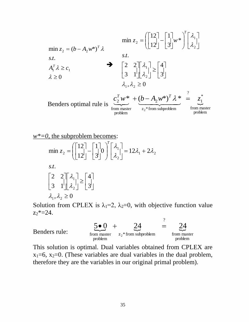
w*=0, the subproblem becomes:
0,
3
4
13
22
..
21203
1
12
12min
21
2
1
21
2
1
2
+=
−
=
ts
z
T
Solution from CPLEX is λ1=2, λ2=0, with objective function value
z2*=24.
Benders rule:
problemmaster from
?
subproblem from *zproblem
master from
24 24052
=+•
This solution is optimal. Dual variables obtained from CPLEX are
x1=6, x2=0. (These variables are dual variables in the dual problem,
therefore they are the variables in our original primal problem).
36
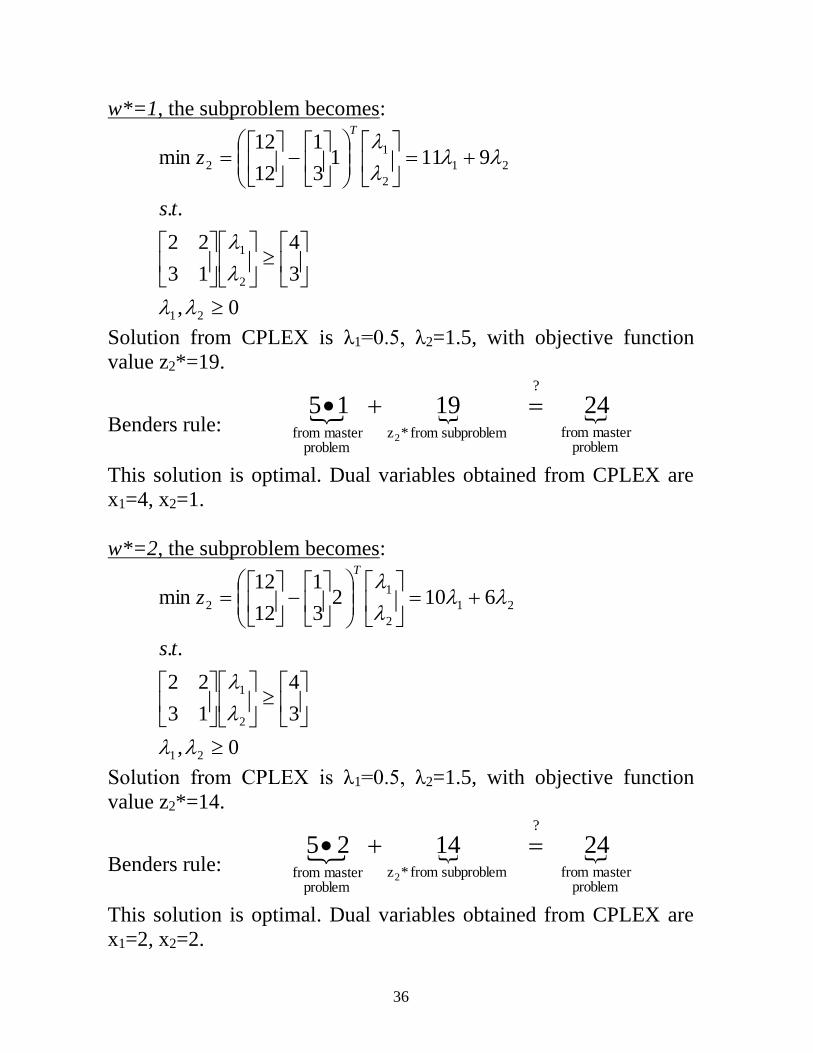
w*=1, the subproblem becomes:
0,
3
4
13
22
..
91113
1
12
12min
21
2
1
21
2
1
2
+=
−
=
ts
z
T
Solution from CPLEX is λ1=0.5, λ2=1.5, with objective function
value z2*=19.
Benders rule:
problemmaster from
?
subproblem from *zproblem
master from
24 19152
=+•
This solution is optimal. Dual variables obtained from CPLEX are
x1=4, x2=1.
w*=2, the subproblem becomes:
0,
3
4
13
22
..
61023
1
12
12min
21
2
1
21
2
1
2
+=
−
=
ts
z
T
Solution from CPLEX is λ1=0.5, λ2=1.5, with objective function
value z2*=14.
Benders rule:
problemmaster from
?
subproblem from *zproblem
master from
24 14252
=+•
This solution is optimal. Dual variables obtained from CPLEX are
x1=2, x2=2.
37
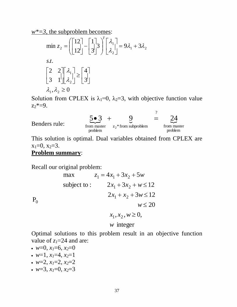
w*=3, the subproblem becomes:
0,
3
4
13
22
..
3933
1
12
12min
21
2
1
21
2
1
2
+=
−
=
ts
z
T
Solution from CPLEX is λ1=0, λ2=3, with objective function value
z2*=9.
Benders rule:
problemmaster from
?
subproblem from *zproblem
master from
24 9352
=+•
This solution is optimal. Dual variables obtained from CPLEX are
x1=0, x2=3.
Problem summary:
Recall our original problem:
integer
,0,,
20
1232
1232 :subject to
534 max
P
21
21
21
211
0
w
wxx
w
wxx
wxx
wxxz
++
++
++=
Optimal solutions to this problem result in an objective function
value of z1=24 and are:
• w=0, x1=6, x2=0
• w=1, x1=4, x2=1
• w=2, x1=2, x2=2
• w=3, x1=0, x2=3

38
Some comments about this problem:
1. It is coincidence that the values of x1 and x2 for the optimal
solution also turn out to be integers.
2. The fact that there are multiple solutions is typical of MIP
problems. MIP problems are non-convex.
5.0 Benders simplifications
In the previous section, we studied problems having the following
structure:
integer
0,
..
max
21
211
w
wx
bwAxA
eDw
ts
wcxcz TT
+
+=
and we defined the master problem and primal subproblem as
integer
0
..
max
:
*
221
w
w
eDw
ts
zwcz T
+=
Master
0
*
..
max
:
21
12
−
=
x
wAbxA
ts
xcz T
subproblem Primal
However, what if our original problem appears as below, which is
the same as the original problem except that it does not contain an
“x” in the objective function, although the “x” still remains in one of
the constraints.
39
integer
0,
..
max
21
21
w
wx
bwAxA
eDw
ts
wcz T
+
=
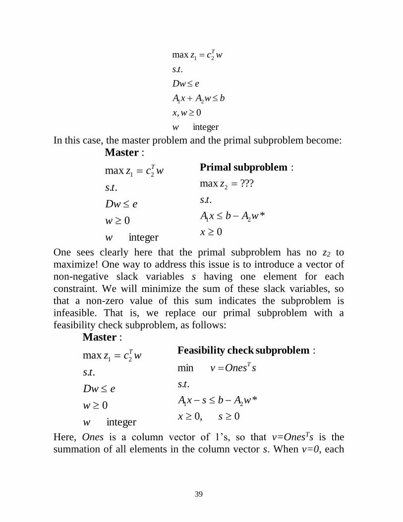
In this case, the master problem and the primal subproblem become:
integer
0
..
max
:
21
w
w
eDw
ts
wcz T
=
Master
0
*
..
???max
:
21
2
−
=
x
wAbxA
ts
z
subproblem Primal
One sees clearly here that the primal subproblem has no z2 to
maximize! One way to address this issue is to introduce a vector of
non-negative slack variables s having one element for each
constraint. We will minimize the sum of these slack variables, so
that a non-zero value of this sum indicates the subproblem is
infeasible. That is, we replace our primal subproblem with a
feasibility check subproblem, as follows:
integer
0
..
max
:
21
w
w
eDw
ts
wcz T
=
Master
0,0
*
..
min
:
21
−−
=
sx
wAbsxA
ts
sOnesv T
subproblem check yFeasibilit
Here, Ones is a column vector of 1’s, so that v=OnesTs is the
summation of all elements in the column vector s. When v=0, each

40
constraint in A1x-s≤b-A2w* is satisfied so that A1x≤b-A2w*, which
means the constraints to the original problem are in fact satisfied.
In this case, one observes that if v=0, then the problem is solved
since Benders optimality rule will always be satisfied.
problem
master from
*
1
subproblem from *z
2
problemmaster from
2
2
**)(* zwAbwc TT =−+
Here, z2 is always zero, and the other two terms come from the
master problem, therefore if the problem is feasible, it is optimal,
and no step 3 is necessary.
One question does arise, however, and that is what should be the
feasibility cuts returned to the master problem if the feasibility
check subproblem results in v>0? The answer to this is stated in [7]
and shown in [8] to be
v + λ A2(w* − w) < 0
This kind of problem is actually very common. Figure 5, using a
SCOPF to motivate decomposition methods for enhancing
computational efficiency, is of this type. This is very similar to the
so-called simultaneous feasibility test (SFT) of industry.
The SFT (Simultaneous Feasibility Test) is widely used in SCED
and SCUC [9, 10, 11]. SFT is a contingency analysis process. The
objective of SFT is to determine violations in all post-contingency
states and to produce generic constraints to feed into economic
dispatch or unit commitment, where a generic constraint is a
transmission constraint formulated using linear sensitivity
coefficients/factors.
The ED or UC is first solved without considering network
constraints and security constraints. The results are sent to perform
the security assessment in a typical power flow. If there is an
41
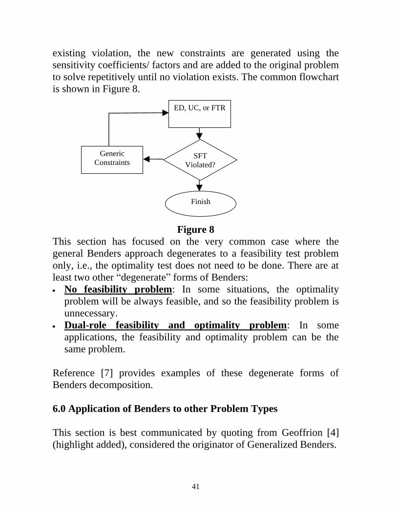
existing violation, the new constraints are generated using the
sensitivity coefficients/ factors and are added to the original problem
to solve repetitively until no violation exists. The common flowchart
is shown in Figure 8.
Figure 8
This section has focused on the very common case where the
general Benders approach degenerates to a feasibility test problem
only, i.e., the optimality test does not need to be done. There are at
least two other “degenerate” forms of Benders:
• No feasibility problem: In some situations, the optimality
problem will be always feasible, and so the feasibility problem is
unnecessary.
• Dual-role feasibility and optimality problem: In some
applications, the feasibility and optimality problem can be the
same problem.
Reference [7] provides examples of these degenerate forms of
Benders decomposition.
6.0 Application of Benders to other Problem Types
This section is best communicated by quoting from Geoffrion [4]
(highlight added), considered the originator of Generalized Benders.
ED, UC, or FTR
SFT
Violated?
Finish
Generic
Constraints

42
“J.F. Benders devised a clever approach for exploiting the structure
of mathematical programming problems with complicating variables
(variables which, when temporarily fixed, render the remaining
optimization problem considerably more tractable). For the class of
problems specifically considered by Benders, fixing the values of
the complicating variables reduces the given problem to an ordinary
linear program, parameterized, of course, by the value of the
complicating variables vector. The algorithm he proposed for
finding the optimal value of this vector employs a cutting-plane
approach for building up adequate representations of (i) the extremal
value of the linear program as a function of the parameterizing
vector and (ii) the set of values of the parameterizing vector for
which the linear program is feasible. Linear programming duality
theory was employed to derive the natural families of cuts
characterizing these representations, and the parameterized linear
program itself is used to generate what are usually deepest cuts for
building up the representations.
In this paper, Benders' approach is generalized to a broader class of
programs in which the parametrized subproblem need no longer be a
linear program. Nonlinear convex duality theory is employed to
derive the natural families of cuts corresponding to those in Benders'
case. The conditions under which such a generalization is possible
and appropriate are examined in detail.”
The spirit of the above quotations is captured by the below modified
formulation of our problem.
The problem can be generally specified as follows:
integer
0,
)(
..
)(max
2
21
w
wx
bwAxF
eDw
ts
wcxfz T
+
+=
Define the master problem and primal subproblem as
43
integer
0
..
max
:
*
221
w
w
eDw
ts
zwcz T
+=
Master
0
*)(
..
)(max
:
2
2
−
=
x
wAbxF
ts
xfz
subproblem Primal
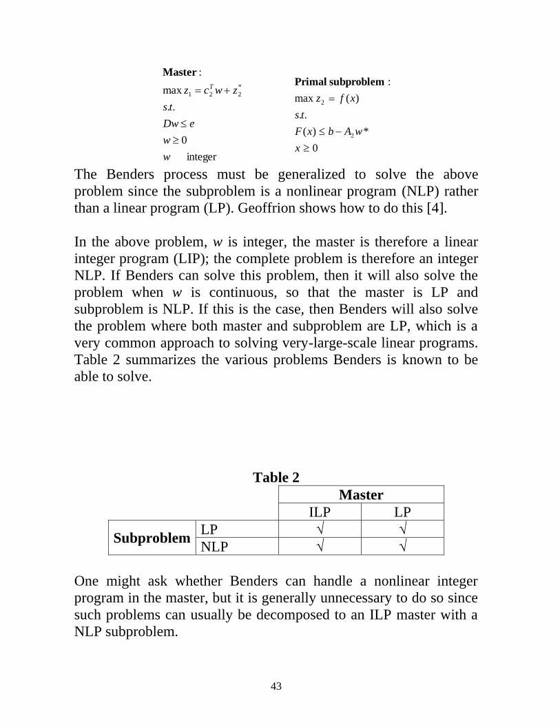
The Benders process must be generalized to solve the above
problem since the subproblem is a nonlinear program (NLP) rather
than a linear program (LP). Geoffrion shows how to do this [4].
In the above problem, w is integer, the master is therefore a linear
integer program (LIP); the complete problem is therefore an integer
NLP. If Benders can solve this problem, then it will also solve the
problem when w is continuous, so that the master is LP and
subproblem is NLP. If this is the case, then Benders will also solve
the problem where both master and subproblem are LP, which is a
very common approach to solving very-large-scale linear programs.
Table 2 summarizes the various problems Benders is known to be
able to solve.
Table 2
Master
ILP LP
Subproblem LP √ √
NLP √ √
One might ask whether Benders can handle a nonlinear integer
program in the master, but it is generally unnecessary to do so since
such problems can usually be decomposed to an ILP master with a
NLP subproblem.

44
7.0 Generalized Benders for EGEAS
The description of EGEAS provided here is adapted from [12].
The EGEAS computer model was developed by researchers at MIT
under funding from the Electric Power Research Institute (EPRI).
EGEAS can be run in both the expansion optimization and the
production simulation modes. Uncertainty analysis, based on
automatic sensitivity analysis and data collapsing via description of
function estimation, is also available. A complete description of the
model can be found in [13].
The production simulation option consists of production
cost/reliability evaluation for a specified generating system
configuration during one or more years. Probabilistic production
cost/reliability simulation is performed using a load duration curve
based model. Customer load and generating unit availability are
modeled as random variables to reflect demand fluctuations and
generation forced outages. Two algorithmic implementations are
available: an analytic representation of the load duration curve
(cumulants) and a piecewise linear numerical representation.
EGEAS has three main solution options: Screening curves, dynamic
programming, and generalized Benders (GB) decomposition. We
discuss here the latter.
GB is a non-linear optimization technique incorporating detailed
probabilistic production costing.
• It is based on an iterative interaction of a simplex algorithm
master problem with a probabilistic production costing
simulation subproblem.
• After a sufficient number of iterations, non-linear production
costs and reliability relationship are approximated with as
small an error bound as desired by the user.
45
• It is computationally more efficient than the dynamic
programming EGEAS option but produces optimal expansion
plans consisting of fractional unit capacity additions.
• It resolves correctly among planning alternative unit sizes, and
it models multiple units correctly in terms of expected energy
generated and reliability impacts.
• System reliability constraints are modeled according to the
probabilistic criterion of expected unserved energy.
• It is suitable for analyses involving thermal, limited energy and
storage units, non-dispatchable technology generation, and
certain load management activities.
• A unique capability of the GB option is the estimation of
incremental costs to the utility associated with meeting
allowed unserved energy reliability targets. This capability
replaces reliability constraints by an incremental cost of
unserved energy to consumers.
• Finally, the GB option has not been developed in its present
form to model interconnections or subyearly period production
costing/reliability considerations.
• End effects are handled by an extension period model.
The formulation of the GB generating capacity expansion planning
problem in EGEAS follows, adapted from [14].

46
• X = vector of plant capacities, Xj Megawatts (MW) (decision
variable);
• j = unique index for each plant;
• C = vector of plant present-value capacity costs, Cj $/MW;
• Yt = vector of plant utilization levels in period t, Yit MW
(decision variable);
• i= merit order position of plant in period t;
• EFt(Yt) = present-value expected operating cost function in
period t;
• EGt(Yt) = expected unserved energy function in period t;
• εt = desired reliability level in period t, measured in expected
MWhr of demand not served;
• δt = matrix which selects and sorts plants, indexed by j, into merit
order, indexed by i, in period t;
• T = number of periods (years) in planning horizon.
In this formulation it is assumed that the capacities of all plants are
decision variables in order to simplify the notation; however,
existing plants of given capacity can be incorporated.
The objective function (1) consists of two components, the capacity
costs of the plants and the expected operating costs of the system
over the planning horizon.
The constraint (2) represents the reliability standard of the system.
The constraint (3) requires that no plant be operated over its
capacity.
47
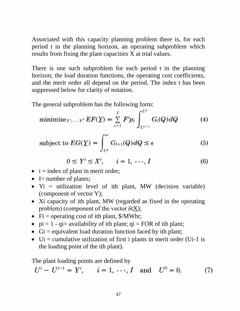
Associated with this capacity planning problem there is, for each
period t in the planning horizon, an operating subproblem which
results from fixing the plant capacities X at trial values.
There is one such subproblem for each period t in the planning
horizon; the load duration functions, the operating cost coefficients,
and the merit order all depend on the period. The index t has been
suppressed below for clarity of notation.
The general subproblem has the following form:
• i = index of plant in merit order;
• I= number of plants;
• Yi = utilization level of ith plant, MW (decision variable)
(component of vector Y);
• Xi capacity of ith plant, MW (regarded as fixed in the operating
problem) (component of the vector δtX);
• Fi = operating cost of ith plant, $/MWhr;
• pi = 1 - qi= availability of ith plant; qi = FOR of ith plant;
• Gi = equivalent load duration function faced by ith plant;
• Ui = cumulative utilization of first i plants in merit order (Ui-1 is
the loading point of the ith plant).
The plant loading points are defined by
48
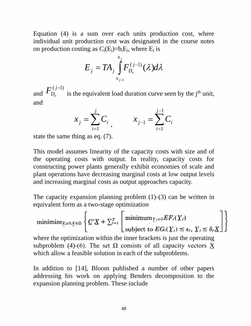
Equation (4) is a sum over each units production cost, where
individual unit production cost was designated in the course notes
on production costing as Cj(Ej)=bjEj, where Ej is
dFTAE
j
j
e
x
x
j
Djj −
−=
1
)()1(
and )1( −j
DeF is the equivalent load duration curve seen by the jth unit,
and
=
=j
i
ij Cx1
, −
=
− =1
1
1
j
i
ij Cx
state the same thing as eq. (7).
This model assumes linearity of the capacity costs with size and of
the operating costs with output. In reality, capacity costs for
constructing power plants generally exhibit economies of scale and
plant operations have decreasing marginal costs at low output levels
and increasing marginal costs as output approaches capacity.
The capacity expansion planning problem (1)-(3) can be written in
equivalent form as a two-stage optimization
where the optimization within the inner brackets is just the operating
subproblem (4)-(6). The set Ω consists of all capacity vectors X
which allow a feasible solution in each of the subproblems.
In addition to [14], Bloom published a number of other papers
addressing his work on applying Benders decomposition to the
expansion planning problem. These include

49
• Reference [15]: This paper describes methods of including power
plants with limited energy (e.g., hydro) and storage plants in the
production costing convolution algorithm we have studied, for
use in a Benders decomposition formulation of the expansion
planning problem where the production costing problem is the
subproblem, and there is one for each period of the planning
horizon.
• Reference [16]:
• Reference [17]:
In addition to the work reported on using Benders in EGEAS, there
are many other works related to application of Benders
decomposition to electric power planning problems. A representative
sample of them include [18, 19, 20, 21, 22, 23,… ].
8.0 Application of Benders to Stochastic Programming
For good, but brief overviews of Stochastic Programming, see [24]
and [25].
In our example problem, we considered only a single subproblem, as
shown below.
integer
0,
..
max
21
211
w
wx
bwAxA
eDw
ts
wcxcz TT
+
+=
To prepare for our generalization, we rewrite the above in a slightly
different form, using slightly different notation:

50
integer
0,
..
max
1
1111
111
w
wx
bxAwB
eDw
ts
xdwcZ TT
+
+=
Now we are in position to extend our problem statement so that it
includes more than a single subproblem, as indicated in the structure
provided below.
0,
..
....max
2222
1111
22111
+
+
+
++++=
wx
bxAwB
bxAwB
bxAwB
eDw
ts
xdxdxdwcZ
k
nnnm
nTn
TTT
In this case, the master problem is
0
..
)(max1
1
+= =
w
eDw
ts
xzwcZn
i
iiT
where zi provide values of the maximization subproblems given by:

51
0
..
max
−
=
i
iiii
i
T
ii
x
wBbxA
ts
xdz
Note that the constraint matrix for the complete problem appears as:
nnnn b
b
b
e
x
x
x
w
AB
AB
AB
D
2
1
2
1
22
11
The constraint matrix shown above, if one only considers D, B1, and
A1, has an L-shape, as indicated below.
nnnn b
b
b
e
x
x
x
w
AB
AB
AB
D
2
1
2
1
22
11
Consequently, methods to solve these kinds of problems, when they
are formulated as stochastic programs, are called L-shaped methods.
But what is, exactly, a stochastic program [24]?
• A stochastic program is an optimization approach to solving
decision problems under uncertainty where we make some
choices for “now” (the current period) represented by w, in order
to minimize our present costs.
• After making these choices, event i happens, so that we take
recourse4, represented by xi, in order to minimize our costs under
each event i that could occur in the next period.
4 Recourse is the act of turning or applying to a person or thing for aid.
52
• Our decision must be made a-priori, however, and so we do not
know which event will take place, but we do know that each
event i will have probability pi.
• Our goal, then, is to minimize the cost of the decision for “now”
(the current period) plus the expected cost of the later recourse
decisions (made in the next period).
An application of this problem for power systems is the security-
constrained optimal power flow (SCOPF) with corrective action.
• In this problem, we dispatch generation to minimize costs for the
network topology that exists in this 15 minute period. Each unit
generation level is a choice, and the complete decision is captured
by the vector w. The dispatch costs are represented by cTw.
• These “normal” conditions are constrained by the power flow
equations and by the branch flow and unit constraints, all of
which are captured by Dw≤e.
• Any one of i=1,…,n contingencies may occur in the next 15
minute period. Given that we are operating at w during this
period, each contingency i requires that we take corrective action
(modify the dispatch, drop load, or reconfigure the network)
specified by xi.
• The cost of the corrective action for contingency i is diTxi, so that
the expected costs over all possible contingencies is ΣpidiTxi.
• Each contingency scenario is constrained by the post-contingency
power flow equations, and by the branch flow and unit
constraints, represented by Biw+Aixi≤bi. The dependency on w
(the pre-contingency dispatch) occurs as a result of unit ramp rate
limitations, to constrain each unit’s redispatch to an amount that
can be achieved within a given time frame, i.e., for each unit, the
vector w would contain P0 (pre-contingency dispatch), the vector
x would contain ∆P+ (increases) and ∆P- (decreases), so that the
equations
P0 + ∆P+ ≤ b+, -P0 + ∆P- ≤ b-
would be represented in Biw+Aixi≤bi.

53
A 2-stage recourse problem is formulated below:
0,
..
min
2222
1111
1
1
+
+
+
+= =
wx
bxAwB
bxAwB
bxAwB
eDw
ts
xdpwcz
nnnm
i
n
i
T
ii
T
where pi is the (scalar) probability of event i, and di is the vector of
costs associated with taking recourse action xi. Each constraint
equation Biw+Aixi≤bi limits the recourse actions that can be taken in
response to event i, and depends on the decisions w made for the
current period.
Formulation of this problem for solution by Benders (the L-shaped
method) results in the master problem as
0
..
min1
1
+= =
w
eDw
ts
zwczn
i
i
T
where zi is minimized in the subproblem given by:
0
..
min
−
=
i
iiii
i
T
iii
x
wBbxA
ts
xdpz
Note that the first-period decision, w, does not depend on which
second-period scenario actually occurs (but does depend on a

54
probabilistic weighting of the various possible futures). This is
called the non-anticipativity property. The future is uncertain and so
today's decision cannot take advantage of knowledge of the future.
Recourse models can be extended to handle multistage problems,
• where a decision is made “now” (in the current period),
• we wait for some uncertainty to be resolved,
• and then we make another decision based on what happened.
The objective is to minimize the expected costs of all decisions
taken. This problem can be appropriately thought of as the coverage
of a decision tree, as shown in Fig. 7, where each “level” of the tree
corresponds to another stochastic program.
Fig. 7

55
Multistage stochastic programs have been applied to handle
uncertainty in planning problems before. This is a reasonable
approach; however, one should be aware that computational
requirements increase with number of time periods and number of
scenarios (contingencies in our example) per time period. Reference
[26] by J. Beasley provides a good but brief overview of multistage
stochastic programming. Reference [27], notes for an entire course,
provides a comprehensive treatment of stochastic programming
including material on multistage stochastic programming. Dr. Sarah
Ryan of ISU’s IMSE department teaches a course on this topic,
described below. I E 633X. Stochastic Programming. (3-0) Cr. 3. S. Prereq: I E 513 or STAT 447, I E 534 or equivalent. Mathematical programming with uncertain parameters; modeling risk within optimization; multi-stage recourse and probabilistically constrained modes; solution and approximation algorithms including dual decomposition and progressive hedging; and applications to planning, allocation and design problems.
9.0 Two related problem structures
We found the general form of the stochastic program to be
0,
..
....max
2222
1111
22111
+
+
+
++++=
wx
bxAwB
bxAwB
bxAwB
eDw
ts
xdxdxdwcz
k
nnnm
n
T
n
TTT
so that the constraint matrix appears as
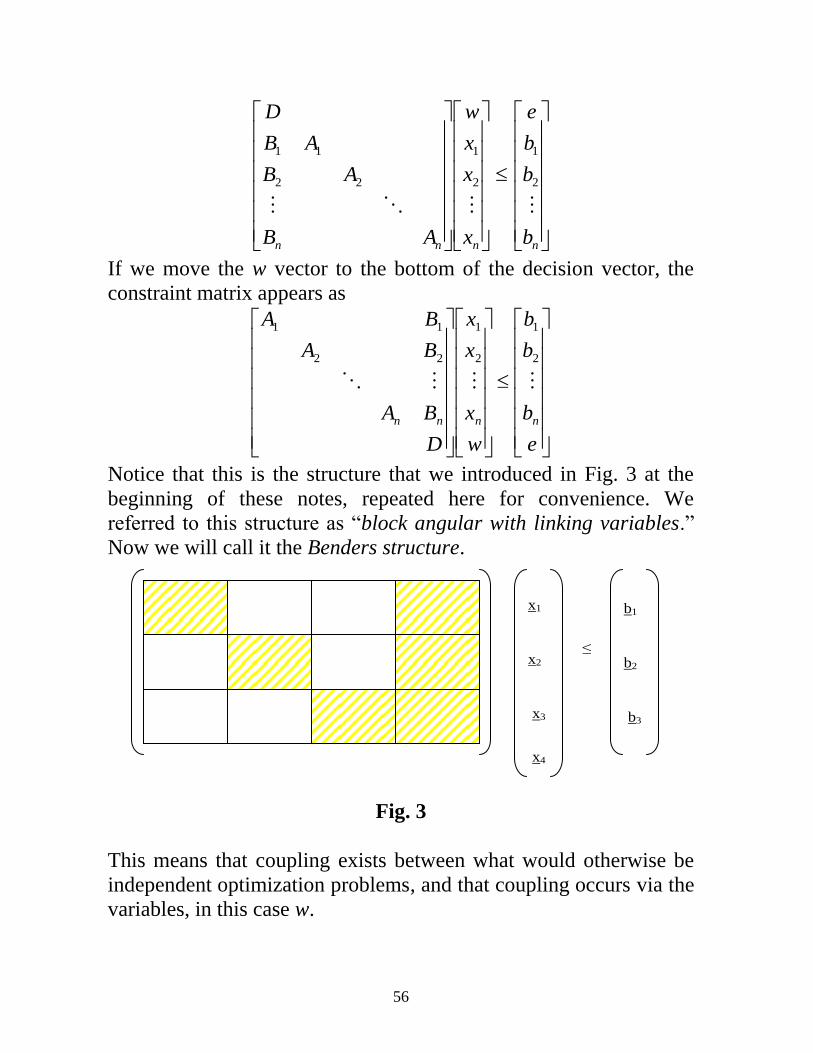
56
nnnn b
b
b
e
x
x
x
w
AB
AB
AB
D
2
1
2
1
22
11
If we move the w vector to the bottom of the decision vector, the
constraint matrix appears as
e
b
b
b
w
x
x
x
D
BA
BA
BA
nnnn
2
1
2
1
22
11
Notice that this is the structure that we introduced in Fig. 3 at the
beginning of these notes, repeated here for convenience. We
referred to this structure as “block angular with linking variables.”
Now we will call it the Benders structure.
x1
x2
x3
≤
b1
b2
b3
x4
Fig. 3
This means that coupling exists between what would otherwise be
independent optimization problems, and that coupling occurs via the
variables, in this case w.
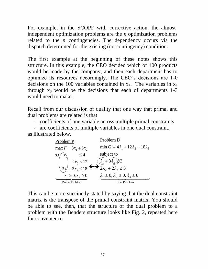
57
For example, in the SCOPF with corrective action, the almost-
independent optimization problems are the n optimization problems
related to the n contingencies. The dependency occurs via the
dispatch determined for the existing (no-contingency) condition.
The first example at the beginning of these notes shows this
structure. In this example, the CEO decided which of 100 products
would be made by the company, and then each department has to
optimize its resources accordingly. The CEO’s decisions are 1-0
decisions on the 100 variables contained in x4. The variables in x1
through x3 would be the decisions that each of departments 1-3
would need to make.
Recall from our discussion of duality that one way that primal and
dual problems are related is that
- coefficients of one variable across multiple primal constraints
- are coefficients of multiple variables in one dual constraint,
as illustrated below.
Problem Primal
21
21
2
1
21
0,0
1823
12 2
4 s.t.
53max
P Problem
+
+=
xx
xx
x
x
xxF
➔
Problem Dual
321
32
31
321
0,0,0
522
33
subject to
18124min
D Problem
+
+
++=
G
This can be more succinctly stated by saying that the dual constraint
matrix is the transpose of the primal constraint matrix. You should
be able to see, then, that the structure of the dual problem to a
problem with the Benders structure looks like Fig. 2, repeated here
for convenience.
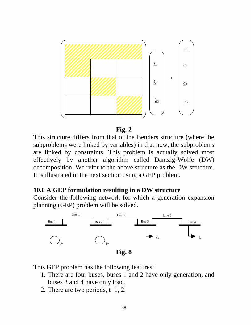
58
λ1
λ2
λ3
≤
c1
c2
c3
c0
Fig. 2
This structure differs from that of the Benders structure (where the
subproblems were linked by variables) in that now, the subproblems
are linked by constraints. This problem is actually solved most
effectively by another algorithm called Dantzig-Wolfe (DW)
decomposition. We refer to the above structure as the DW structure.
It is illustrated in the next section using a GEP problem.
10.0 A GEP formulation resulting in a DW structure
Consider the following network for which a generation expansion
planning (GEP) problem will be solved.
Fig. 8
This GEP problem has the following features:
1. There are four buses, buses 1 and 2 have only generation, and
buses 3 and 4 have only load.
2. There are two periods, t=1, 2.
Bus 1 Bus 2 Bus 3 Bus 4
Line 1 Line 2 Line 3
p2 p1
d3 d4
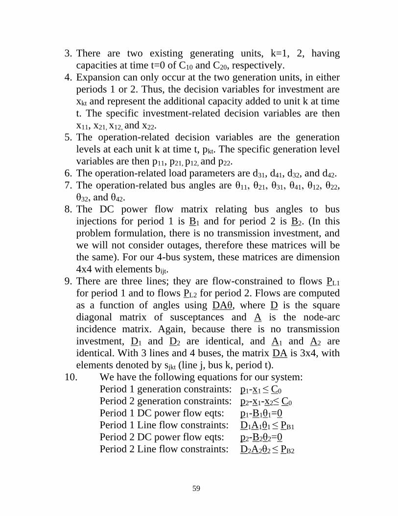
59
3. There are two existing generating units, k=1, 2, having
capacities at time t=0 of C10 and C20, respectively.
4. Expansion can only occur at the two generation units, in either
periods 1 or 2. Thus, the decision variables for investment are
xkt and represent the additional capacity added to unit k at time
t. The specific investment-related decision variables are then
x11, x21, x12, and x22.
5. The operation-related decision variables are the generation
levels at each unit k at time t, pkt. The specific generation level
variables are then p11, p21, p12, and p22.
6. The operation-related load parameters are d31, d41, d32, and d42.
7. The operation-related bus angles are θ11, θ21, θ31, θ41, θ12, θ22,
θ32, and θ42.
8. The DC power flow matrix relating bus angles to bus
injections for period 1 is B1 and for period 2 is B2. (In this
problem formulation, there is no transmission investment, and
we will not consider outages, therefore these matrices will be
the same). For our 4-bus system, these matrices are dimension
4x4 with elements bijt.
9. There are three lines; they are flow-constrained to flows PL1
for period 1 and to flows PL2 for period 2. Flows are computed
as a function of angles using DAθ, where D is the square
diagonal matrix of susceptances and A is the node-arc
incidence matrix. Again, because there is no transmission
investment, D1 and D2 are identical, and A1 and A2 are
identical. With 3 lines and 4 buses, the matrix DA is 3x4, with
elements denoted by sjkt (line j, bus k, period t).
10. We have the following equations for our system:
Period 1 generation constraints: p1-x1 ≤ C0
Period 2 generation constraints: p2-x1-x2≤ C0
Period 1 DC power flow eqts: p1-B1θ1=0
Period 1 Line flow constraints: D1A1θ1 ≤ PB1
Period 2 DC power flow eqts: p2-B2θ2=0
Period 2 Line flow constraints: D2A2θ2 ≤ PB2
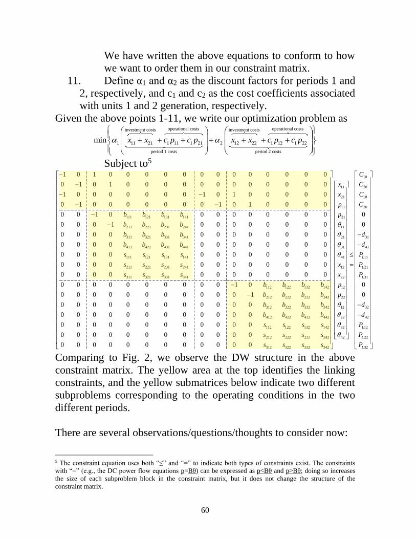
60
We have written the above equations to conform to how
we want to order them in our constraint matrix.
11. Define α1 and α2 as the discount factors for periods 1 and
2, respectively, and c1 and c2 as the cost coefficients associated
with units 1 and 2 generation, respectively.
Given the above points 1-11, we write our optimization problem as operational costs operational costsinvestment costs investment costs
1 11 21 1 11 1 21 2 12 22 1 12 1 22
period 1 costs period 2 costs
min x x c p c p x x c p c p
+ + + + + + +
Subject to5
111 121 131 141
211 221 231 241
311 321 331 341
411 421 431 441
111 121 131
1 0 1 0 0 0 0 0 0 0 0 0 0 0 0 0
0 1 0 1 0 0 0 0 0 0 0 0 0 0 0 0
1 0 0 0 0 0 0 0 1 0 1 0 0 0 0 0
0 1 0 0 0 0 0 0 0 1 0 1 0 0 0 0
0 0 1 0 0 0 0 0 0 0 0 0
0 0 0 1 0 0 0 0 0 0 0 0
0 0 0 0 0 0 0 0 0 0 0 0
0 0 0 0 0 0 0 0 0 0 0 0
0 0 0 0
b b b b
b b b b
b b b b
b b b b
s s s
−
−
− −
− −
−
−
141
211 221 231 241
311 321 331 341
112 122 132 142
212 222 232 242
312 322 332 342
412 422 432 442
112 1
0 0 0 0 0 0 0 0
0 0 0 0 0 0 0 0 0 0 0 0
0 0 0 0 0 0 0 0 0 0 0 0
0 0 0 0 0 0 0 0 0 0 1 0
0 0 0 0 0 0 0 0 0 0 0 1
0 0 0 0 0 0 0 0 0 0 0 0
0 0 0 0 0 0 0 0 0 0 0 0
0 0 0 0 0 0 0 0 0 0 0 0
s
s s s s
s s s s
b b b b
b b b b
b b b b
b b b b
s s
−
−
11
21
11
21
11
21
31
41
12
22
12
22
12
22
22 132 142 32
212 222 232 242 42
312 322 332 342
0 0 0 0 0 0 0 0 0 0 0 0
0 0 0 0 0 0 0 0 0 0 0 0
x
x
p
p
x
x
p
p
s s
s s s s
s s s s
10
20
10
20
31
41
11
21
31
32
42
12
22
32
0
0
0
0
L
L
L
L
L
L
C
C
C
C
d
d
P
P
P
d
d
P
P
P
− − = − −
Comparing to Fig. 2, we observe the DW structure in the above
constraint matrix. The yellow area at the top identifies the linking
constraints, and the yellow submatrices below indicate two different
subproblems corresponding to the operating conditions in the two
different periods.
There are several observations/questions/thoughts to consider now:
5 The constraint equation uses both “≤” and “=” to indicate both types of constraints exist. The constraints
with “=” (e.g., the DC power flow equations p=Bθ) can be expressed as p≤Bθ and p≥Bθ; doing so increases
the size of each subproblem block in the constraint matrix, but it does not change the structure of the
constraint matrix.

61
1. Observation: The subproblems in the above DW structure are
associated with the network equations in different periods.
2. Observation: The fact that the above problem decomposes by
period is encouraging with respect to increasing the fidelity of
the production cost representation.
3. Question: Bloom used Benders to solve his problem, and so
we assume he obtained a Benders structure. Is it important,
relative to obtaining a Benders structure, that Bloom did not
account for the network? That is, if we include the network,
does that influence our ability to obtain a Benders structure?
4. Question: Is the DW decomposition method efficient?
Consider the following comment from [28]:
“Thus, although (DW) has a smaller number of
constraints, its number of variables can be huge since the
number of extreme points and extreme rays of a
polyhedron can be very large. To use this idea to
effectively solve large scale LP problems, we need to
avoid considering all extreme points and extreme rays of
Cx ≥ d. This is when the idea of column generation comes
into play, i.e., we start by including only a few number of
extreme points and extreme rays in the problem and we
add more on the fly in a as needed basis.”
There is another reference, [29], that raises questions about
using either DW or Benders for decomposed, parallelized
solutions of large linear programs (in contrast to large MIPs).
For example, he writes, “At present Dantzig-Wolfe and
Benders methods in the original versions are rarely used for
solving large scale continuous linear programming problems.
The reason is their too slow convergence.”
5. Observation: The DW decomposition procedure is described in
Section 11.0. It is good to review Section 11.0 to begin to get
familiar with DW, trying to think of reasons it might not work
very well. Following review of Section 11.0, if it still looks
promising, we should identify it as a promising method and list
it among other possibly promising methods. At this point, it
62
might be good to start to review individual references about
DW, e.g., [2, 5, 46] and others.
6. Thought: Consider the following additional approaches:
a. Nested decomposition: Use a nested decomposition
algorithm [30] and solving it iteratively in a forward and
backward manner using forward and backward passes. In
essence, the forward pass iteratively solves over each
time period to yield an upper bound for each period over
the full problem, and the backward pass provides a lower
bound by generating cuts from relaxed sub-problems.
The convergence criteria is determined by a pre-defined
tolerance in terms of the difference between the upper
and lower bounds.
b. CPLEX’s barrier algorithm: One statement from [31] is
interesting: “The CPLEX barrier optimizer is
appropriate and often advantageous for large problems,
for example, those with more than 100,000 rows or
columns. It is not always the best choice, though, for
sparse models with more than 100,000 rows. It is
effective on problems with staircase structures or banded
structures in the constraint matrix. It is also effective on
problems with a small number of nonzeros per column
(perhaps no more than a dozen nonzero values per
column). In short, denseness or sparsity are not the
deciding issues when you are deciding whether to use the
barrier optimizer. In fact, its performance is most
dependent on these characteristics:
• the number of floating-point operations required to
compute the Cholesky factor;
• the presence of dense columns, that is, columns
with a relatively high number of nonzero entries.”
But what about parallelization? CPLEX offers the
parallel barrier optimizer. A good treatment of CPLEX
algorithms is in [32]. Some insights on using CPLEX for
large LPs can be found in [33]. Some related questions:

63
• Does use of GAMS offer the full capabilities of the
parallel barrier algorithm?
• Is AIMMS better at using the CPLEX parallel
barrier algorithm than GAMS?
• Does GORUBI have a better parallel barrier
algorithm than CPLEX?
• Does Pyomo have a better parallel barrier algorithm
than CPLEX?
c. Problem structure: There may be a natural decomposition
based on our particular adaptive expansion planning
problem. For example, can we parallelize the operating
problems for each future (i.e., scenario)?
d. Lagrangian relaxation (LR): LR is also an effective
approach for problems that have the DR structure (i.e.,
problems that have block structure with complicating
constraints). References [34, 35] provide good tutorial
treatment of LR. Paraphrasing from [34]:
➔In LR, the complicating constraints are removed from
the constraint equations and then dualized, i.e., added to
the objective function, with a penalty term (the Lagrange
multiplier) proportional to the amount of violation of the
dualized constraints. It is a relaxation of the original
problem because (a) the removal of some constraints
relaxes the original feasible space; (b) the solution to the
LR problem will bound the original problem (from above
if maximizing and from below if minimizing) because the
addition of the complicating constraints will always
cause the objective function to increase (if maximizing)
or decrease (if minimizing).
e. Progressive hedging: Reference [36] indicates that “PH,
sometimes referred to as a horizontal decomposition
method because it decomposes stochastic programs by
scenarios rather than by time stages, possesses
theoretical convergence properties when all decision
64
variables are continuous.” Reference [37] indicates,
“The progressive hedging algorithm (PHA) has emerged
as an effective method for solving multi-stage stochastic
programs, particularly those with discrete decision
variables in every stage. The PHA mitigates the
computational difficulty associated with large problem
instances by decomposing the extensive form according
to scenario, and iteratively solving penalized versions of
the sub-problems to gradually enforce implementability.”
f. Hybrid decomposition methods (HDM): HDM use a
combination of Benders, DW, LR, and/or some other
decomposition methods. For example, so-called cross-
decomposition uses Benders and LR [38, 39, 40].
7. Question: How would our decision change if we implemented
the production costing approach with a higher degree of
fidelity? Relatedly, what level of fidelity is required in the
expansion planning production cost model to adequately
represent storage? These are important questions because of
the need to include flexibility services6 within expansion
planning. A very good basic review of UC is contained in [41],
and a high-fidelity model for storage for production cost is
given in [42]. There have been several good papers written
recently on this topic, e.g., [43, 44, 45]. In gaining
understanding of how to include production cost modeling
fidelity within expansion planning, it is useful to review these
papers, paying attention to the papers they reference for
possible additional resources to study.
6 We define flexibility services as (1) transient frequency response (0-20 seconds following loss of
generation); (2) frequency regulation (continuous steady-state frequency control at ~4 second intervals); (3)
contingency reserve provision (capacity reserves having the ability to compensate for loss of generation
within 10-30 minutes); (4) load following or ramping reserve provision (capacity reserves having the ability
to compensate for 30-min to 4 hour daily changes in new load); and (5) planning reserve provision (capacity
reserves to satisfy the annual peak).
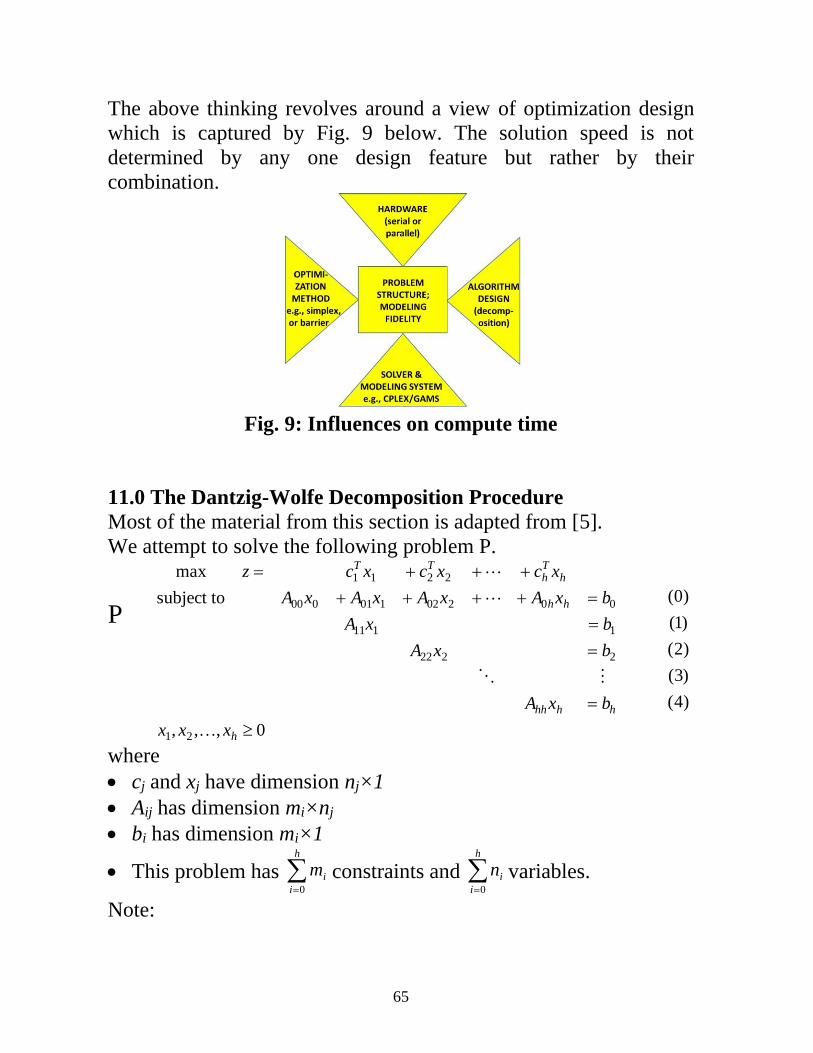
65
The above thinking revolves around a view of optimization design
which is captured by Fig. 9 below. The solution speed is not
determined by any one design feature but rather by their
combination.
Fig. 9: Influences on compute time
11.0 The Dantzig-Wolfe Decomposition Procedure
Most of the material from this section is adapted from [5].
We attempt to solve the following problem P.
P
0,,,
)4(
)3(
)2(
)1(
)0(subject to
max
21
2222
1111
00202101000
2211
=
=
=
=++++
+++=
h
hhhh
hh
hTh
TT
xxx
bxA
bxA
bxA
bxAxAxAxA
xcxcxcz
where
• cj and xj have dimension nj×1
• Aij has dimension mi×nj
• bi has dimension mi×1
• This problem has =
h
i
im0
constraints and =
h
i
in0
variables.
Note:

66
• Constraints 1, 2, 3, …,h can be thought of as constraints on
individual departments.
• Constraint 0 can be thought of as a constraint on total corporate
(organizational) resources (sum across all departments).
Definition 1: For a linear program (LP), an extreme point is a
“corner point” and represents a possible solution to the LP. The
solution to any feasible linear program is always an extreme point.
Figure 10 below illustrates 10 extreme points for some linear
program.
1
2
3
2
4
2
5
2 6
2
7
2
8
2
9
10
20
30
40
50
60
70
80
90
100
5 10
2
Fig. 10
Observation 1: Each individual subproblem represented by
iiii
i
T
i
bxA
xcz
=
=
subject to
max
has its own set of extreme points. We refer to these extreme points
as the subproblem i extreme points, denoted by
i
k
i pkx ,,1, = where pi is the number of extreme points for
subproblem i.
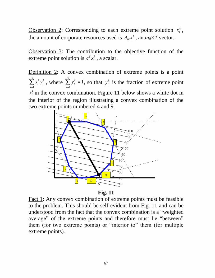
67
Observation 2: Corresponding to each extreme point solution k
ix , the amount of corporate resources used is k
ii xA0 , an m0×1 vector.
Observation 3: The contribution to the objective function of the
extreme point solution is k
i
T
i xc , a scalar.
Definition 2: A convex combination of extreme points is a point
=
ip
k
k
i
k
i yx1
, where 11
==
ip
k
k
iy , so that k
iy is the fraction of extreme point
k
ix in the convex combination. Figure 11 below shows a white dot in
the interior of the region illustrating a convex combination of the
two extreme points numbered 4 and 9.
1
2
32
42
52
62
7
2
82
9
10
20
30
40
50
60
70
80
90
100
5 102
Fig. 11
Fact 1: Any convex combination of extreme points must be feasible
to the problem. This should be self-evident from Fig. 11 and can be
understood from the fact that the convex combination is a “weighted
average” of the extreme points and therefore must lie “between”
them (for two extreme points) or “interior to” them (for multiple
extreme points).

68
Fact 2: Any point in the feasible region may be identified by
appropriately choosing the k
iy .
Observation 4a: Since the convex combination of extreme points is a
weighted average of those extreme points, then the total resource
usage by that convex combination will also be a weighted average
of the resource usage of the extreme points, i.e., ( )=
ip
k
k
i
k
ii yxA1
0 . The
total resources for the complete problem is the summation over all
of the subproblems, ( )= =
h
i
p
k
k
i
k
ii
i
yxA1 1
0 .
Observation 4b: Since the convex combination of extreme points is
a weighted average of those extreme points, then the contribution to
the objective function contribution by that convex combination will
also be a weighted average of the objective function contribution of
the extreme points, i.e., ( )=
ip
k
k
i
k
i
T
i yxc1
. The total objective function can
be expressed as the summation over all subproblems, ( )= =
h
i
p
k
k
i
k
i
T
i
i
yxc1 1
.
Based on Observations 4a and 4b, we may now transform our
optimization problem P as a search over all possible combinations of
points within the feasible regions of the subproblems to maximize
the total objective function, subject to the constraint that the k
iy must
sum to 1.0 and must be nonnegative, i.e.,
P-T
( )
( )
i
k
i
p
k
k
i
h
i
p
k
k
i
k
ii
h
i
p
k
k
i
k
i
T
i
pkhiy
hhiy
mbyxAxA
yxcz
i
i
i
,,1,,,1,0
sconstraint ,,1,1
sconstraint subject to
max
1
00
1 1
0000
1 1
==
==
=+
=
=
= =
= =
69
Note that this new problem P-T (P-transformed) has m0+h
constraints, in contrast to problem P which has =
h
i
im0
constraints.
Therefore it has far fewer constraints. However, whereas problem P
has only =
h
i
in0
variables, this new problem has as many variables as it
has total number of extreme points across the h subproblems, =
h
i
ip0
,
and so it has a much larger number of variables.
The DW decomposition method solves the new problem without
explicitly considering all of the variables.
Understanding the DW method requires having a background in
linear programming so that one is familiar with the revised simplex
algorithm. We do not have time to cover this algorithm in this class,
but it is standard in any linear programming class to do so.
Instead, we provide an economic interpretation to the DW method.
In the first constraint of problem P-T, b0 can be thought of as
representing shared resources among the various subproblems
i=1,…,h.
Let the first m0 dual variables of problem P-T be contained in the
m0×1 vector . Each of these dual variables provide the change in
the objective as the corresponding right-hand-side (a resource) is
changed.
➔ That is, if b0k is changed by b0k+∆, then the optimal value of the
objective is modified by adding k .
➔ Likewise, if the ith subproblem (department) increases its use of
resource b0k by ∆ (instead of increasing the amount of the resource
by ∆), then we can consider that that subproblem (department) has
incurred a “charge” of k . This “charge” worsens its contribution

70
to the complete problem P-T objective, and accounting for all shared
resources b0k, k=1, m0, the contribution to the objective is
ii
T
i
T
i xAxc 0− where ii xA0 is the amount of shared resources consumed
by the ith subproblem (department).
One may think of these dual variables contained in as the “prices”
that each subproblem (department) must pay for use of the
corresponding shared resources.
Assuming each subproblem i=1,…,h represents a different
department in the CEO’s organization, the DW-method may be
interpreted in the following way, paraphrased from [2]:
- If each department i worked independently of the others,
then each would simply minimize its part of the objective
function, i.e., i
T
i xc .
- However, the departments are not independent but are
linked by the constraints of using resources shared on a
global level.
- The right-hand sides b0k, k=1,…,m0, are the total amounts of
resources to be distributed among the various departments.
- The DW method consists of having the CEO make each
department pay a unit price, πk, for use of each resource k.
- Thus, the departments react by including the prices of the
resources in its own objective function. In other words,
o Each department will look for new activity levels xi
which minimize ii
T
i
T
i xAxc 0− .
o Each department performs this search by solving the
following problem:
kx
bxA
xAxc
ik
iii
ii
T
i
T
i
=
−
0
subject to
max
i
0
- The departments make proposals of activity levels xi back to
the CEO, and the CEO then determines the optimal weights k
iy for the proposals by solving problem P-T, getting a new

71
set of prices , and the process repeats until all proposals
remain the same.
Reference [2], p. 346, and [46], pp. 349-350, provide good
articulations of the above DW economic interpretation.
12.0 Other ways of addressing uncertainty in planning
Stochastic programming is an elegant mathematical tool for
addressing uncertainty in planning, but it is computationally
burdensome. Other ways include Monte Carlo simulation and robust
optimization.
A few slides presented by engineers from the Midwest ISO are
interesting.

72

73

74

75
REFERENCES
[1] F. Hillier and G. Lieberman, “Introduction to Operations Research,” 4th
edition, Holden-Day, Oakland California, 1986.
[2] M. Minoux, “Mathematical Programming: Theory and Algorithms,”
Wiley, 1986.
[3] J. Benders, “Partitioning procedures for solving mixed variables
programming problems,” Numerische Mathematics, 4, 238-252, 1962.
[4] A. M. Geoffrion, “Generalized benders decomposition”, Journal of
Optimization Theory and Applications, vol. 10, no. 4, pp. 237–260, Oct. 1972.
[5] S. Zionts, “Linear and Integer Programming,” Prentice-Hall, 1974.
[6] J. Bloom, “Solving an Electricity Generating Capacity Expansion Planning
Problem by Generalized Benders' Decomposition,” Operations Research, Vol.
31, No. 1, January-February 1983.
[7] Y. Li, “Decision making under uncertainty in power system using Benders
decomposition,” PhD Dissertation, Iowa State University, December 2008.
[8] S. Granville, M. V. F. Pereira, G. B. Dantzig, B. Avi-Itzhak, M. Avriel, A.
Monticelli, and L. M. V. G. Pinto, “Mathematical decomposition techniques
for power system”, Tech. Rep. 2473-6, EPRI, 1988.
[9] D. Streiffert, R. Philbrick, and A. Ott, “A mixed integer programming
solution for market clearing and reliability analysis”, Power Engineering
Society General Meeting, 2005. IEEE, pp. 2724–2731 Vol. 3, June 2005.
[10] PJM Interconnection, “On line training materials”,
www.pjm.com/services/training/training.html.
[11] ISO New England, “On line training materials”,
www.isone.com/support/training/courses/index.html.
[12] International Atomic Energy Agency, “EXPANSION PLANNING FOR
ELECTRICAL GENERATING SYSTEMS: A Guidebook,” 1984.
[13] ELECTRIC POWER RESEARCH INSTITUTE, Electric Generation
Expansion Analysis Systems — Vol. 1: Solution Techniques, Computing
Methods, and Results, Rep. EPRI EL-256K1982).
[14] J. Bloom, “Solving an Electricity Generating Capacity Expansion
Planning Problem by Generalized Benders' Decomposition,” Operations
Research, Vol. 31, No. 1, January-February 1983.
[15] J. Bloom and L. Charny, “Long Range Generation Planning With
Limited Energy And Storage Plants, Part I: Production Costing,” IEEE
Transactions on Power Apparatus and Systems, Vol. -PAS-102, No. 9,
September 1983, pp 2861-2870.
76
[16] J. Bloom and M. Caramanis, “Long-Range Generation Planning Using
Generalized Benders' Decomposition: Implementation and Experience,”
Operations Research, Vol. 32, No. 2, March-April, 1984.
[17] J. Bloom, “Long-Range Generation Planning Using Decomposition and
Probabilistic Simulation,” IEEE Transactions on Power Apparatus and
Systems, Vol. PAS-101, No. 4 April 1982.
[18] M. Caramanis, J. Stremel, and L. Charny, “Modeling Generating Unit
Size and Economies of Scale in Capacity Expansion with an Efficient, Real,
Number Representation of Capacity Additions,” IEEE Transactions on Power
Apparatus and Systems, Volume: PAS-103, Issue: 3, 1984, pp. 506 – 515.
[19] S. Siddiqi and M. Baughman,”Value-based transmission planning and the
effects of network models,” IEEE Transactions on Power Systems, Vol. 10,
Issue 4, 1995, pp. 1835 – 1842.
[20] S. McCusker, B. Hobbs,and J. Yuandong, “Distributed utility planning
using probabilistic production costing and generalized benders
decomposition,” IEEE Transactions on Power Systems, Volume: 17 , Issue: 2,
2002 , pp. 497 – 505.
[21] O. Tor, A. Guven, and M. Shahidehpour, “Congestion-Driven
Transmission Planning Considering the Impact of Generator Expansion,”
IEEE Transactions on Power Systems, Volume: 23 , Issue: 2, 2008 , pp. 781 –
789.
[ 22] S. Binato, M. Pereira, and S. Granville, “A New Benders Decomposition
Approach to Solve Power Transmission Network Design Problems,” IEEE
Transactions on Power Systems, Vol. 16 , Issue 2, 2001, pp. 235 – 240.
[23] R. Romero and A. Monticelli, “A hierarchical decomposition approach
for transmission network expansion planning,” IEEE Transactions on Power
Systems, Volume: 9 , Issue: 1, 1994 , pp. 373 – 380.
[24] www-fp.mcs.anl.gov/otc/Guide/OptWeb/continuous/constrained/stochastic/.
[25] http://users.iems.northwestern.edu/~jrbirge/html/dholmes/StoProIntro.html.
[26] http://people.brunel.ac.uk/~mastjjb/jeb/or/sp.html
[27] http://homepages.cae.wisc.edu/~linderot/classes/ie495/
[28] R. Rocha, “Decomposition algorithms,” chapter 4 in “Petroleum supply
planning: models, reformulations and algorithms,” Ph. D. dissertation,
Pontificia Universidade Catolica do Rio de Janeiro, May, 2010, available at
https://www.maxwell.vrac.puc-rio.br/29077/29077_5.PDF (any of the other
seven chapters available by replacing “5.pdf” with “k.pdf” where k is the
chapter number).
[29] A. Karbowski, “Decomposition and parallelization of linear
programming algorithms,” In: Szewczyk R., Zieliński C., Kaliczyńska M.
77
(eds) Progress in Automation, Robotics and Measuring Techniques. ICA
2015. Advances in Intelligent Systems and Computing, vol 350. Springer,
Cham. Available at https://link.springer.com/content/pdf/10.1007%2F978-3-
319-15796-2_12.pdf.
[30] Lara C.L., Mallapragada, D., Papageorgiou, D., Venkatesh, A., &
Grossmann I.E., Deterministic Electric Power Infrastructure Planning:
Mixed‐integer Linear Programming Model and Nested Decomposition,
European Journal of Operational Research, Vol. 271, Issue 3, 2018.
[31] “Introducing the barrier optimizer,” Notes on CPLEX Optimizer for z/OS
12.7.0, available at
www.ibm.com/support/knowledgecenter/en/SS9UKU_12.7.0/com.ibm.cplex.
zos.help/CPLEX/UsrMan/topics/cont_optim/barrier/02_barrier_intro.html.
[32] R. Lima, “IBM ILOG CPLEX: What is inside of the box?” presentation
slides, at http://egon.cheme.cmu.edu/ewo/docs/rlima_cplex_ewo_dec2010.pdf
[33] E. Klotz and A. Newman, “Practical guidelines for solving difficult linear
programs,” 2012, available at
https://pdfs.semanticscholar.org/b01f/ad44c20c372fdda95cbfb980c0d37302de
07.pdf.
[34] I. Grossman and B. Tarhan, “Tutorial on Lagrangean Decomposition:
Theory and Applications,” presentation slides, available at
http://egon.cheme.cmu.edu/ewo/docs/EWOLagrangeanGrossmann.pdf.
[35] M. Guignard, “Lagrangean Relaxation,” Sociedad de Estadistica e
Investigacion Operativa, Top (2003) Vol. 11, No. 2, pp. 151-228, available at
https://link.springer.com/article/10.1007/BF02579036.
[36 ] J. Watson and D. Woodruff, “Progressive hedging innovations for a
class of stochastic mixed-integer resource allocation problems,” Comput
Manag Sci (2011) 8:355-370.
[37] D. Gade, G. Hackebeil, S. Ryan, J. Watson, R. Wets, and D. Woodruff,
“Obtaining lower bounds from the progressive hedging algorithm for
stochastic mixed-integer programs,” available at
www.math.ucdavis.edu/~rjbw/mypage/Stochastic_Optimization_files/GHRW
WW13_lwr_1.pdf.
[38] K. Holmberg, “On the use of valid inequalities in Benders and cross
decomposition,” working paper, revised May 1991 and Jan 1995, available
from JDM.
[39] Tony J. van Roy, “A Cross Decomposition Algorithm for Capacitated
Facility Location,” Operations Research, Vol. 34, No. 1 (Jan. - Feb., 1986),
pp. 145-163, Published by: INFORMS URL: www.jstor.org/stable/170679.

78
[40] N. Deeb and S. Shahidehpour, “Cross decomposition for multi-area
optimal reactive power planning,” IEEE Transactions on Power Systems, Vol.
8, No. 4, Nov., 1993.
[41] “Unit commitment,” A summary report by CIGRE Task Force 38.01.01,
August, 1998.
[42] T. Das, V. Krishnan, and J. McCalley, “High-Fidelity Dispatch Model of
Storage Technologies for Production Costing Studies,” IEEE Transactions on
Sustainable Energy, Vol. 5, Is 4, 2014, pp. 1242-1252.
[43] C. Nweke, F. Leanez, G. Drayton, and M. Kolhe, “Benefits of
chronological optimization in capacity planning for electricity markets,” IEEE
International Conference on Power System Technology, 2012.
[44] B. Hua, R. Baldick, and J. Wang, “Representing operational flexibility in
generation expansion planning through convex relaxation of unit
commitment,” IEEE Trans. on Power Systems, Vol. 33, No. 2, March, 2018.
[45] Q, Xu, S. Li, and B. Hobbs, “Generation and storage expansion co-
optimization with consideration of unit commitment,” International
Conference on Probabilistic Methods Applied to Power Systems (PMAPS),
2018.
[46] M. Bazaraa, J. Jarvis, and H. Sherali, “Linear Programming and Network
Flows,” second edition, Wiley, 1990.