Ultra-low field magnetic resonance using optically pumped ...

LBNL·48994

ERNEST ORLANDO LAWRENCEBERKELEY NATIONAL LABORATORY

Ultra-Low Field Magnetic ResonanceUsing Optically Pumped NobleGases and SQUID Detection

Annjoe G. Wong-Foy

Materials Sciences Division

May 2001

Ph.D. Thesis

DISCLAIMER

This document was prepared as an account of work sponsored by the United StatesGovernment. While this document is believed to contain correct information, neither theUnited States Government nor any agency thereof, nor The Regents of the University ofCalifornia, nor any of their employees, makes any warranty, express or implied, orassumes any legal responsibiliiy for the accuracy, completeness, or usefulness of anyinformation, apparatus, product, or process disclosed, or represents that its u,se would notinfringe privately owned rights. Reference herein to any specific commercial product,process, or service by its trade name, trademark, manufacturer, or otherwise, does notnecessarily constitute or imply its endorsement, recommendation, or favoring by theUnited States Government or any agency thereof, or The Regents of the University ofCalifornia. The views and opinions of authors expressed herein do not necessarily state orreflect those of the United States Government or any agency thereof, or The Regents of theUniversity of California.

Ernest Orlando Lawrence Berkeley National Laboratoryis an equal opportunity employer.

nnfJnoo

o

f )

lJ

u

r'ft c

i .

I .

1- t -~

l _

- [-

l

LBNL-48994

Ultra-Low Field Magnetic Resonance Using OpticallyPumped Noble Gases and SQUID Detection

Annjoe Golangco Wong-FoyPh.D. Thesis

Department of ChemistryUniversity of California, Berkeley

and

Materials Sciences DivisionErnest Orlando Lawrence Berkeley National Laboratory

University of CaliforniaBerkeley, CA 94720

May 2001

This work was supported by the Director, Office of Science, Office of Basic Energy Sciences, MaterialsSciences Division, ofthe U.S. Department of Energy under Contract No. DE-AC03-76SF00098.

*rocyclecl paper

r\

- !-

Ultra-Low Field Magnetic Resonance using Optically Pumped NobleGases and SQUID Detection

by

Annjoe Golangco Wong-Foy

A.B. (Harvard University) 1996

A dissertation submitted in partial satisfaction of the

requirements for the degree of

Doctor of Philosophy

III

Chemistry

in the

GRADUATE DIVISION

of the

UNIVERSITY OF CALIFORNIA, BERKELEY

Committee in charge:

Professor Alexander Pines, ChairProfessor Paul A. AlivisatosProfessor Jeffrey A. Reimer

Spring 2001

f

r~

IL'-

r'L.::

- !-

f 'j

- ! ~l -"

- [-

Ultra-Low Field Magnetic Resonance Using OpticallyPumped Noble Gases and SQmD Detection

Copyright © 2001

by


The U.S. Department of Energy has the right to use this documentfor any purpose whatsoever including the right to reproduce

all or any part thereof.

r "L...:c

. - I-

, -

1

Abstract

Ultra-Low Field Magnetic Resonance using Optically Pumped Noble Ga~es and

SQUID Detection

by


Doctor of Philosophy in Chemi~try

University of California, Berkeley

Professor Alexander Pines, Chair

The focus of the research reported in this dissertation has been the development

of instrumentation and techniques for low field, low frequency magnetic resonance.

The nuclei in these experiments were subjected to magnetic fields no greater than

25 Gauss (2.5 mT). Superconducting magnet technology continually improves,

and nuclear magnetic resonance (NMR) moves inexorably from a radiofrequency

(rnegaHertz) spectroscopy to a microwave (gigaHertz) spectroscopy, but in this

body of work, NMR is an audiofrequency (kiloHertz) technique.

The main difficulty with low field NMR is the lack of sensitivity, in other words,

lack of signal. To combat this situation we have built equipment utilizing femto

Tesla-sensitive superconducting quantum interference device (SQUID) magnetic

flux detectors, both the higher sensitivity low transition temperature (liquid he

limn) devices as well as the new cutting edge high transition temperature (liquid

nitrogen) SQUIDs. We have exploited the large, non-equilibrium polarizations of

optically pumped noble gases, using helium and especially xenon as contrast agents

for magnetic resonance imaging (MRI). Our new circular flow optical pumping sys- ,

tem provides an effectively unlimited source of laser polarized xenon which we have

utilized for both MRI and NMR spectroscopy at ultra-low fields. We have achieved

rnrn resolution in the xenon JVIRI of materials and the first observation at 2.5 rnT

of the chemical shifts of xenon in different chemical environments.

2

An appropriate question to ask is why bother with weak magnet NlVIR? There

are strong and very practical reasons why low field NMR, especially low field MRI,

is useful and important, and I discuss them in Section 4.2. I will not repeat them

here. What I would like to say, since this may be the only chance I will ever have

to say it due to the constant pressure on researchers to prove utility of their work

in order to gain funding, "'rVe are scientists; we do it because we can."

r\

· ["-~ h···.- .-

Ren

-

·rlo ~·

- I- I

- ~

I

I 1I i

II

IIIIIJ

I'

~

rin

-~ L

L

For my Parents.

iii

r--

IL~-

r

, -

l- I-

l .

Contents

List of Figures

1 Basic NMR Theory1.1 Introduction...1.2 The NMR Experiment .

1.2.1 The Static Field.1.2.2 The Pulse Field .1.2.3 The NMR Signal

1.3 Non-Applied Fields and Interactions1.3.1 Chemical Shift .1.3.2 Dipolar Coupling . . .1.3.3 J-Coupling.......1.3.4 Quadrupolar Coupling

1.4 Applied Gradient Fields: Imaging Basics

2 Optical Pumping2.1 Introduction .2.2 Spin-Exchange Optical Pumping of Noble Gases

2.2.1 Rubidium Optical Pumping .2.2.2 Spin Exchange .2.2.3 Commentary: The Three-Body Problem

3 SQUID Theory and Operation3.1 Introduction.......3.2 Superconductivity.......3.3 The Josephson Junction ...3.4 Parallel Josephson Junctions.3.5 Actual SQUIDs . . . . .

3.5.1 Low-Tc Devices ....3.5.2 High-Tc Devices .. ' ..

3.6 Operation: The direct current SQUID

IV

VI

1122457889

1011

171719192123

242424262931313237

v

3.7 Operation: The Flux-Locked Loop 413.8 Flux Transformer and Gradiometer 43

4 The Low Critical Temperature SQUID Days 474.1 Introduction.......................... 474.2 Ultra Low Field Imaging . . . . . . . . . . . . . . . . . . . 47

4.2.1 MRI with Optical Pumping and MRI with SQUIDs 494.2.2 Imaging Theory: Projection Reconstruction 504.2.3 The SQUID Imaging Probe . 534.2.4 The Spectrometer. . . . . . . 564.2.5 The Optical Pumping Setups 604.2.6 The Images . . . . . . . . . . 65

4.3 Pure Nuclear Quadrupole Resonance (NQR) 704.3.1 Pure NQR 2-D Correlation Spectroscopy of Alurninurn-27 in

Ruby. . . . . . . . . . . . . . . . . 714.3.2 The NQR Probe and Spectrometer 744.3.3 Results: 2-D Ruby Spectrum . 76

5 High Transition Temperature SQUIDs 795.1 Introduction............... 795.2 The SQUID Dewar . . . . . . . . . . . 805.3 The SQUID, the Coils, and the Spectrometer. 865.4 Proton NMR Signals . . . . . . . . . . . . . . 905.5 Proton Imaging . . . . . . . . . . . . . . . . . 93

5.5.1 Projection Reconstruction: Linear Backprojection 935.5.2 Mineral Oil Images 95

5.6 Pulsed Gradients . . . . . . . . . . . . . . . 1025.7 Hyperpolarized Xenon . . . . . . . . . . . . 107

5.7.1 Recirculated Flow Optical Pumping. 1075.8 Flowing Xenon with SQUID Detection 113

5.8.1 Spin Warp Imaging. 1155.8.2 Xenon Pictures . . . . 118

5.9 The Unfulfilled Promise ... 1235.10 High-Tc SQUID Spectroscopy 124

5.10.1 Thermally Polarized Nuclei 1255.10.2 Dynamic Nuclear Polarization 1255.10.3 Ultra Low Field Chemical Shift 130

Bibliography 133

r

A Ancillary Figures 151

, iI--= ~-

f .,

t

List of Figures

1.1 Zeeman Splitting . . . . . . . . . . .1.2 1-D MRI Projections .1.3 Frequency Encoding Pulse Sequence.1.4 Phase Encoding Pulse Sequences

2.1 Equilibrium vs. Optical Pumping2.2 Rb Valence Energy Levels ..

3.1 Josephson Junction .3.2 Parallel Josephson Junctions .3.3 Tri-Layer Sandwich .3.4 Strontium Titanate Bicrystal3.5 Directly Coupled Magnetometer3.6 Carthwheel Magnetometer3.7 SQUID I-V Curve. . . . . . . .3.8 SQUID V-<P Curve .3.9 Schematic of Flux-Locked Loop3.10 Flux Transformers .

4.1 2D Imaging: Projection Reconstruction.4.2 Polar to Cartesian Raster .....4.3 Low-Tc SQUID Full-length Probe. . ..4.4 Low-Tc SQUID Dewar .4.5 Low-Tc SQUID MRI Probehead (View 1) .4.6 Low-Tc SQUID MRIProbehead (View 2) .4.7 Low-Tc SQUID Holder .4.8 Xenon Batch Optical Pumping Setup4.9 Helium High Field OP Setup. . . . .4.10 Energy Levels of Rb in 7 Tesla ...4.11 Spin Echo from Hyperpolarized Helium .4.12 MRI: Hyperpolarized He 1-D Images4.13 MRI: Frozen Hyperpolarized Xenon . . .

Vi

3131516

1820

27303335363840424446

51525455575859626364666769

4.14 NQR Spectrum of 27Al in Ruby "4.15 Low T c SQUID NQR Probehead .4.16 Pulse Sequence for 2-D NQR of Ruby .4.17 2-D Pure NQR of 27 in Ruby .

5.1 Schematic of Dewar for High-T c SQUID5.2 Photograph of Dewar for High-Tc SQUID5.3 Photo of the Dewar Headpiece . . . . . . .5.4 Photograph of Dewar Internals .5.5 Schematic of High-T c SQUID Dewar with Coils5.6 Photograph of High-Tc SQUID Dewar with Coils5.7 Proton Spectrum at 20 G .5.8 Earth's Field Proton Spectrum .5.9 In vivo Low-Field NMR Proton Spectrum from a Finger5.10 Linear Backprojection Steps 1 and 25.11 Linear Backprojection Step 35.12 MRI: "The Proton Fi;tce" .5.13 MRI: "The Proton Smile"5.14 MRI: "Chili Pepper" ...5.15 Photograph of Golay Coils5.16 Schematic of Golay Coils mounted on SQUID Dewar5.17 Photograph of Golay Coils mounted on SQUID Dewar5.18 Single Scan of Hyperpolarized Xenon .5.19 Schematic of the Circular Flow Optical Pumping System5.20 Photograph of Flowing Xenon Pumping Cell .5.21 Photograph of Optical Pumping Setup ....5.22 Proton versus Hyperpolarized Flowing Xenon5.23 Spin Warp Pulse Sequence . . . . .5.24 MRI: Xenon in Vacuum Grease . . . . . . . .5.25 MRI: Xenon in Triangle of Aerogel .5.26 MRI: Visualization of Xenon Flow through Aerogel5.27 Phosphorous-31 NMR in Phosphoric Acid5.28 Simultaneous Proton and Fluorine NMR . . . . . .5.29 Dynamic Nuclear Polarization Enhancement ....5.30 Ultra Low Field Xenon NMR Showing Chemical Shift .

A.1 Gradient Amplifier Blanking Circuit.A.2 Unity Gain Adding Amplifiers ....

VII

73757778

818284858889919294969799

100101103104105108110111112114116119120122126127128131

152153

r

rbr'1

I ,

f "ii

- ~---,- viii

Acknowledgements

I would first like to thank my advisor Professor Alexander Pines for taking me

into his group and trusting me with all of his expensive equipment. Alex is not

only one of the most brilliant persons I know, he is also one of the most inspiring.

I will be lucky if I can take with me from my time in the Pines Group (besides a

supercon magnet if it will fit in my car) even a glimmer of Alex's ability to look

at a piece of science, distinguish what makes it exciting, and convince others why

it is so.

I need to thank our research collaborator Professor John Clarke whose up

to-date technical knowledge regarding SQUIDs has always impressed me; he is

one of the only tenured professors I would still trust in a lab. I further want to

acknowledge my coworkers from the past five years, starting with the host of post

docs who challenged, motivated, and instructed me when I first started graduate

school: Roberto Seydoux, Matt Augustine, Jeff Yarger, and Marco Tomaselli; as

well as the graduate students who were the first to "show me the ropes:" Dinh

TonThat and Beth Chen; the researchers who I worked with to get the high-T c

SQUID operational: Ricardo de Souza, Klaus Schlenga, and Robert McDermott;

and finally the scientists who have helped me with the last leg of the race and get

to the finish line: Hans-Marcus Bitter, Adam Moule, Julie Seeley, and especially

the post-doc Sunil Saxena whose friendship and greater wisdom made it easier to

get through some of the more trying times. I need to thank all Pinenuts, past and

present, whose previous hard work has directly and indirectly made my research

successful and my time in Berkeley memorable. I wish to single out Boyd Goodson,

David Laws, Fred Salsbury, and Seth Bush who actively recruited meinto the group

and helped me adjust to my new home two levels below ground. IVly memories

of the group will also always include: Lana Kaiser, Yi-Qiao Song, Eike Brunner,

Tom De Swiet, Thomas Meersman, Yung-Ya Lin, David de Graw, Jamie Walls,

Maggie Marjanska, Bob Havlin, Bo Blanton, Megan Spence, and John Logan. For

the successfulness of the SQUID projects, I am grateful to Tom Lawhead in the

glass shop and to Eric Granlund in the machine shop.

IX

I owe a tremendous debt to Dione Carmichael, our group's administrative as

sistant. Without her facilitation and support, I certainly would not be graduating

this May 2001.

The road to graduate school started long before I arrived in Berkeley, and I

am indebted to my previous professors and teachers, especially my undergraduate

advisor Professor Cynthia Friend who motivated me to pursue a doctoral degree

and a career in science. In the Friend group my appreciation goes to James Batteas

and Katie Queeney who took a wide-eyed undergrad under their wings. I would be

remiss not to mention my secondary school teachers, science as well as nOlH;cience,

who ignited my enjoyment of learning: Mrs. Peinemann, lvII'S. \Visehart, Mr.

Teachworth, Mr. Shelburne, and Mr. Vigilante. I blame them for my protracted

stay in school.

I owe much gratitude to all of my friends-I would be a hermit without them.

\Vannest "Thank You's" go to my fellow grad students who encouraged and com

miserated with me these past five years: Edward Byrd (who also proofread this

dissertation), Brandon Weldon, Liz .luang-Laws, Amy Prieto, Juanita 'Wickham,

Phil Geissler, and .10 Chen. I cannot forget the five who survived Littlejohn's class

with me: Joe "Crusher" Walrath, Aaron Burstein, Louis Gascoigne, Jon Sorenson,

and again Edward Byrd. Regards are also due to my college chum Greg Ku who,

being in an M.D./Ph.D. program, always made me feel better with the knmvledge

that he would be a student longer than I would. And special thanks go to Kenia

Whitehead, my best friend from high school. She is in no small part responsible

for my being a research scientist today.

I want to thank my brother for looking out for me all of my life and for all of

the advice he has given to me. When I was younger I didn't like that he always

"got to do things first," but I appreciate now that his pioneering experienees have

made my life better. Finally, my deepest thanks and affection go to my parents

for their love, encouragement, and tolerance throughout the years. Any suecesses

that I might claim can be traced back to the care and guidance that they have

given to me and to the examples that they have set.

- f~

ow

I I

II

( I

II

I-lJ

t-....~.jl ]

r.~l,~

LU

x

This work was supported by the Director, Office of Science, Office of Basic

Energy Sciences, Materials Sciences Division, of the u.s. Department of Energy

under Contract No. DE-AC03-76SF00098.

1

Chapter 1

Basic NMR Theory

1.1 Introduction

This thesis is a record of most of the scientific or engineering accomplishments

that I was involved with while in the Pines Group at UC Berkeley. The uni

fying thread throughout this work was the implementation of Superconducting

QUantum Interference Devices (SQUIDs) for low field nuclear magnetic resonance

(NMR) and magnetic resonance imaging (MRI). A majority of the work also in

volved the application of optically pumped xenon to new techniques of low field

magnetic resonance.

This first chapter is a short primer on NMR theory for the modern day pulsed

nuclear magnetic resonance experiment. Information on continuous wave (CW)

procedures will not be found here. My favorite NMR reference is Fukushima's

"Nuts and Bolts" [1], but other theoretical and in depth texts are also suggested

[2, 3, 4, 5, 6, 7, 8]. The second chapter is an introduction to the ideas behind

spin-exchange optical pumping. Chapter 3 covers some of the theory that governs

SQUID sensors. Finally Chapters 4 and 5 give experimental details and results

from the work including the first experiments with low transition temperature

SQUIDs up to the most recent work with high transition temperature SQUIDs.

CHAPTER 1. BASIC NMR THEORY

1.2 The NMR Experiment

2

fL!-

The idea behind NMR spectroscopy is to "tickle" the nuclear spins of a sample

and gain information on parameters such as electronic or molecular structure and

dynamics by watching the spin reactions. In the NMR experiment, the sample

is placed into a very powerful magnetic field and is allowed to equilibrate. The

system is then perturbed by pulsing a second magnetic field oriented perpendicular

to the equilibration field. The signal that one detects is the magnetic motion of the

nuclear spins as they relax back to equilibrium. Pulsed Electron Spin Resonance

(ESR), also called Electron Paramagnetic Resonance (EPR), is studied in exactly

the same fashion as pulsed NMR, the difference being the detection of electron

spins as opposed to nuclear spins.

1.2.1 The Static Field

A magnetic field will break the isotropy of space and introduce a preferred ori

entation. NMR active (non-zero spin) nuclei will align in that magnetic field. For

the simplest case of spin-1j2 nuclei, the spins can orient parallel to or antiparallel

to the magnetic field, and are said to be "spin up" or "spin down." The difference

in energy between these two states is known as the Zeeman energy, see Figure 1.1.

(1.1 )

where Eo is the static magnetic field, f..L is the magnetic moment particular to the

nucleus. Note the absolute value due to the fact that f..L may be negative. The

nuclear magnetic moment is also defined by:

(1.2)

'"Y is the nuclear gyromagnetic ratio and L is the azimuthal spin angular momentum

operator. '"Y is sometimes defined as:

gnf..LN'"Y =--

Ii(1.3)

r .I,f -


E= +J.lB

3

B field strength

Figure 1.1. Zeeman splitting of the spin energy levels due to the

static magnetic field.

where gn is the g-factor for the particular nucleus and /-IN is the nuclear rnagneton

defined as 2efl = 5.05 X 10-27 Am2 where m n is the rest mass of the neutron. Thismn

is analogous to the definition of the electron gyromagnetic ratio from its g-factor

and the Bohr magneton P,B = 2en = 9.27 x 1O-:-24 Am2 where me is the rest mass

. nne

of the electron:g/-lB

"Ye = --Ii

(1.4)

The g-factor for electrons may be calculated from the Dirac Equation, but gn or

"Y for all nuclei must be measured experimentally. The two most important nuclei

for the work reported here are protons 1H and xenon 129Xe with gyromagnetic

ratios "YH = 26.7520 X 107~~ = 4.267 kgz and "YXe = -7.441 X 107;~~ = -1.187 kgz

respectively. The Larmor frequency is defined as the frequency corresponding to

the Zeeman energyEzeeman

WL =

which for spin-1/2 nuclei is simply

(1.5)

(1.6)

Since one spin state is higher in energy than the other (for spin-1/2 nuclei), one

would expect an unequal distribution of spins in the two states. Simple Boltzmann

statistics determine the relative populations of the two energy levels. Assuming

CHA.PTER 1. BASIC NMR THEORY

that the spin parallel to the field is the lower energy state:

N - N -2f1'so/kBTanti - para' e

4

(1.7)r',\

Polarization is then defined as the normalized differece in the spin populations:

P = Npara- Nanti = tanh (~Bo ) (1.8)

N para + N anti kBT

Due to the (albeit small) difference in populations, there is a net magnetic

moment due to the nuclear spins. It is the sum of all the nuclear moments:

lvI = fLPNTot (1.9)

where fL is again the nuclear moment, P is defined above and NTot is the total

number of nuclei. Polarizations and therefore magnetic moments are very small.

The protons in water at room temperature in a magnetic field of 1 Tesla (T) have

a polarization of only 10-5 , so the induced magnetic moment is very tiny. One of

the reasons why NMR spectroscopists continually try to get stronger and stronger

magnets is to increase the polarization and therefore increase the NMR signal.

1.2.2 The Pulse Field

In the two level picture described above, it is easy to imagine performing spec

troscopy by causing transitions between the two energy levels, and it is indeed

this energy difference that NMR probes. Similar to most light absorption spec

troscopies, continuous wave NMR measures the decrease in applied radiation due

to absorption by the sample. Modern Fourier Transform (pulsed) NMR measures,

instead, the nuclear spin relaxation subsequent to excitation by radiation. In terms

of the two-level picture, the quantity that is detected in an experiment is the ra

diation of the excited spins as they relax from the higher energy level back to the

lower energy level until equilibrium. Clearly the strength of the signal is dependent

on the size of the magnetic moment induced by the static field.

In order to excite the nuclei in the first place, an oscillating magnetic field

with a frequency corresponding to the energy splitting, in other words the Lar

mol' frequency, must be applied to the sample. This is done with coils that create

CHAPTER 1. BASIC NMR THEORY 5

~ - a field perpendicular to the static field. For NMR experiments done in static

fields upwards of 10 mT, which is the majority of NMR experiments, the Larmor

frequencies are in the megahertz, so NMR is sometimes referred to as radiofre

quency spectroscopy. Since I worked with static fields smaller than 10 TnT, all of

the experiments that I conducted employed much lower frequency audiofrequency

(kilohertz) pulses. The excitation coil is usually part of a circuit that is tuned to

the appropriate Larmm frequency. Using such a tuned resistor-inductor-capacitor

(RLC) "tank" circuit improves the power deposition to the sample. It also in

creases the detection sensitivity since the excitation coil serves as the detection

coil in most high field experiments.

1.2.3 The NMR Signal

The form of the NMR signal is a free induction decay (FID) typically shaped like

a sine wave oscillating at the Lannm frequency and damped with an exponential

decay envelope. It is easiest to explain the output in terms of a classical picture.

This picture starts with the net nuclear magnetic moment induced by the static

field; at equilibrium it is aligned parallel or antiparallel to the static field. Then

the system is perturbed by an second magnetic field. In the quantum mechanical

picture it is clear that the excitation field must oscillate, but to see why in the

classical picture the field B] must oscillate at the Lannor frequency, first consider

an excitation field E] that is static. Switching on the field E] aligned perpendicular

to the static field Eo will cause a torque J-lnet x B] and the moment will "tip" away

from equilibrium. Immediately it will precess due to the torque JLnet X (Bo + Bd.However unless the strength of B] is of the same order as the strength of the static

field, the tipping angle of I-inet away from the Bo axis will be small. To creatr

large perturbations the field B1 must be on resonance with the precession of the

moment; in other words, the field B] should rotate at the same frequency as the

precession frequency of the magnetic moment. From the perspective of the moment

J-lnet precessing at the Lannor frequency, the magnetic field B] rotating at the same

frequency looks static. So it efficiently tips the magnetization. The tipping angle

CHAPTER 1. BASIC Nl\!IR THEORY 6

rLt-

of the moment relative to B o is dependent on the amplitude of B 1 and the length

of the time that B 1 is turned on. A 900 or 1f/2 pulse will tip the magnetization

from equilibrium (say the z direction) completely to the transverse (x-y) plane.

This can be done with a hard pulse: high magnetic field amplitude and short

duration or with a soft pulse: smaller field magnitude and longer duration. After

the pulse, the net nuclear moment continues to precess (at the Lannor frequency)

as it relaxes back to equilibrium. The damped, rotating magnetization induces a

current in the detection coil by Faraday's law of induction.

The set of classical equations that describe the behavior of the magnetization

in an NMR experiment during the pulse are the Bloch equations:

/'

I

r'!

, .i

d1\lxdt

dAly

dtd1\'{z

dt

. Alx"(Aly Bo + "(AlzB 1szn(wt) - T

2

1\1-'VAl B + 'VAl B,cos(wt) - -y

IXO IZ T2

(1.10)

(1.11)

(1.12)

1\lx ,y,z are the components of magnetization in each of the Cartesian directions,

Ala is the initial magnetization, "( is the nuclear gyromagnetic ratio, and B o and

B 1 are the magnitudes of the static field and pulse field respectively. T1 and T2

are important time constants that describe the relaxation of the magnetization

to equilibrium. T1 is the longitudinal or spin-lattice relaxation time and is the

characteristic time at which the z-component of the magnetization will return to

its full (equilibrium) value. T2 is the transverse or spin-spin relaxation time. It

measures the time for the transverse (x-y) components of the magnetization to re

turn to their equilibrium values of zero. In the free induction decay, T2 determines

the shape (time constant) of the exponential decay envelope. More aecurately, the

time constant of the exponential decay envelope gives T;, which is the transverse

relaxation time but also includes apparent shortening of the transverse magnetiza

tion due to dephasing of all the little nuclear moments caused by effects like field

inhomogeneities. After the pulse is turned off the components of magnetization

will follow these simpler equations:

r···'- t- CHA.PTER 1. BA.SIC NMR THEORY

dNIxdt

dMy

dtdNlzdt

NIxT2

!V!- -y

T2

M z - Ala

T1

7

(1.13)

(1.14)

(1.15)

As was mentioned earlier, the signal detected in the coil takes the form of a damped

sinusoid. The mathematical form of the FID is given by:

. -I

!V! (t) = M ezwoteT2x,y a (1.16)

Note the decay constant T2 . The Fourier Transform of the free induction decay in

the time domain will give the frequency domain NMR spectrum:

F(w) = JNI(t)eiwtdt (1.17)

To reconcile the two-level "spin up" versus "spin down" picture with the fact

that the coils detect an actual macroscopic transverse magnetization, it is impor

tant to remember that "spin up" and "spin down" do not mean that the individual

nuclear spin moments point straight up or straight down. It means that the pro

jection of the spin angular momentum on the z-axis (up-down) is either n/2 or

-17)2. We have no certain information about the x or y (transverse) directions.

A density matrix calculation would be necessary to treat the system completely

quantum mechanically and predict the FID.

1.3 Non-Applied Fields and Interactions

There are a number of interactions and local magnetic fields that nuclei may

experience in addition to the fields that are externally applied. These interac

tions are in fact what make NMR such a powerful tool, and I will briefly desribe

these interactions. The basic interactions that everyone should understand are the

chemical shift, the dipolar coupling, the j-coupling, and the quadrupolar coupling.


1.3.1 Chemical Shift

8

rL

The chemical shift is a small shift in the resonance frequency of nuclei due to

the local magnetic fields generated by the interaction of the surrounding electrons

with the applied magnetic field. By Lenz's law, applying a magnetic field to

the electrons will cause them to move (circulate if possible) in such a way as

to counteract the applied field. Since the electrons try to generate local fields

opposite to the applied field, nuclei are typically shielded--they feel slightly less

of the static field. Nuclei in the vicinity of high electron density are shielded

more. However, it is possible that in certain molecular configurations, nuclei find

themselves in regions where the electron movement has served to increase the

magnetic field. In this case the nuclei are said to be deshielded. Chemical shifts

are typically small, measured in parts per million (ppm) with respect to the Larmor

frequency. They are generally non-isotropic, although in liquids the rapid motion

of molecules averages the interactions, so that it appears isotropic. The most

general mathematical form of the chemical shift Hamiltonian is:

f-

(1.18)

(1.19)

where f is the nuclear spin operator, CJ is the second-rank chemical shielding tensor,

and i30 is the static magnetic field.

1.3.2 Dipolar Coupling

Dipolar coupling is the nucleus-nucleus interaction based on the magnetostatic

case of one magnetic dipole directly interacting through-space with another dipole.

The full Hamiltonian for dipolar coupling is:

'1J' _ 1'11'2h2 (fA fA 3(i1 .f')(i2 'f'))

Tl-D - 3 l' 2 - 2r12 r12

where the subscripts refer to the nuclei, j are the spin operators, and r is the'

spatial vector joining the two nuclei. The Hamiltonian can also be expanded to

give the famous dipolar alphabet:

II.

;t •

I TI! --;

U

PL'.'J

- ~- CHAPTER 1. BASIC NMR THEORY 9

r' liz[ llD 'Yl1'; (A + B + C + D + E + F) (1.20)

rlZA I1z Izz (1 - 3cosZO) (1.21)

B1 A A A A 2

(1.22)--(ItI:; + [; Ii)(1 - 3cos 0)4

C3 '+ '+ . ' _¢

(1.23)-2(Ilz I2 + II I2z)smOcosOe l

3 " , ,(1.24)D -2 (/rzI:; + [; Izz)sinOcosOe"q>

3" z z'¢ (1.25)E --1+J+sin Oe- l4 1 Z '

3 A A Z Z'¢(1.26)F --I-J-sin Oe l

4 1 Z

Notice the dependence on the angle 0 which corresponds to the angle between the

internuclear vector and the static magnetic field vector. In liquids and gaHes the

rapid tumbling of the atoms or molecules averages 0 over all orientations and the

dipolar coupling vanishes. In solids, however, this is usually not the case, but the

averaging can be mimicked by a technique known as Magic Angle Spinning (MAS).

I will not discuss MAS, but information on the theory and practice can be found

in the references cited at the beginning of this chapter as well as any number of

theses from the Pines Group.

1.3.3 J-Coupling

J-coupling is also a nucleus-nucleus interaction that is an electron-mediated

through-bond coupling. The .i-coupling is responsible for the well-known Illultiplets

in liquid state NMR, e.g. proton lines split by other chemically distinct protons

bonded nearby in the molecule. A simple physical picture of how one nucleus

can "feel" another through the electrons in a bond is to consider a nucleus with

a spin in the state ms = ~. There are two electrons in each chemical bond, and

the electron with the parallel spin moment is likely to spend more time at that

nucleus since that is a lower energy configuration than for the antiparallel moment

to stay nearby. This means that the other electron of the chemical bond will


spend more time at the second nucleus. If that nucleus is also in the rn s = ~

spin state like the first nucleus, its energy will be raised (relative to non j-coupled

frequency) due to the interaction with the antiparallel electron. Accordingly, if the

second nucleus was in the m s = -~ spin state, its energy would be lowered by the

electron interaction.

1.3.4 Quadrupolar Coupling

Quadrupole coupling is the interaction of a quadrupolar nucleus with an elec

tric field gradient (EFG). It can be shown from quantum mechanics that parity

considerations require that quadrupoles are necessarily electric rather than mag

netic in nature. Therefore their interactions are also electric. A nucleus with a spin

~ 1 can have a quadrupole moment and will have one if its shape is non-spherical.

The first example of a quadrupolar nucleus from the periodic table is deuterium.

It has a nuclear spin 1=1, and with one proton and one neutron is obviously non

spherical. An electric field gradient (non-uniform electric field) will interact with

the non-spherically symmetric quadrupolar nucleus. The gradient can arise from

electronic distributions within a molecule or crystal, and the resulting interaction

can be very large--up to a couple hundred megaHertz. The best review on Nu

clear Quadrupole Resonance (NQR) theory remains the Das and Hahn Solid State

Physics Supplement from 1958 [3]. Using their notation below, the most general

form of the quadrupole interaction Hamiltonian is:

r

(1.27)

This is derived from the electrostatic Hamiltonian:

(1.28)

where x = position vector, p(:f) = distribution of positive charge in the nucleus,

and V(x) = electrostatic potential. After a power series expansion:

CHA.PTER 1. BA.SIC NMR THEORY 11

1i = / (d3:f!)p(x) ·to+ Lj [/ (d3x)p(x):rj] . (g;Jo +'------v----'" ' V' "

Z e:charge Pj :dipole moment

~ Lj,k [/ (d3x)p(X)Xj.'r k ] • (a;~j2;~J 0

\- 'V'

Qj k :quadrupole moment

(1.30)

The terms are arranged in Equation 1.30 to highlight the different electrostatic

quantities: charge, dipole moment, and quadrupole moment. Remembering that

E = - VF it is easy to see that the quadrupole moment interacts with an electric

field gradient.

1.4 Applied Gradient Fields: Imaging Basics

In 1972 Lauterbur demonstrated the first use of NMR as an imaging tool [9].

In the same vein Mansfield and Grannell independently showed the relationship

between NMR signal and nuclear density of samples in a field gradient [10]. The

best reference on the theory and use of magnetic resonance imaging is probably

Callaghan's book Principles of Nuclear Magnetic Resonance Microscopy

[11]. Other good references, especially regarding the use of MRI in medicine, can

be found in [12, 13, 14, 15, 16, 17, 18, 19, 20, 21, 22, 23] to name a handful.

The principle idea behind NMR imaging, dubbed magnetic resonance imaging

(MRI), is that information on the spatial distribution of NMR active nuclei in a

subject can be gained by applying different magnetic fields to different areas of the

sample. The most obvious pattern of magnetic field is a simple linear gradient in

one of the Cartesian directions. A gradient G = d~z means that the z-component

of the magnetic field (usually the static field B o ) varies in magnitude along the

x direction. Armed with two pieces of knowledge: first, the resonance frequency

CHAPTER 1. BASIC NMR THEORY 12Li-

of a given type of nucleus depends on the static field that it feels (neglecting

chemical shift and other interactions) and second, the amplitude of the NMR

signal is directly proportional to the number of nuclei, it is easy to see that a

linear magnetic field gradient will disperse the NMR spectrum (in frequency space)

according to the nuclei concentrations distributed in that gradient. Figure 1.2

shows a number of examples of this 1-D imaging. On the left are the cross sections

of various NMR tubes or samples. The right shows the corresponding lVIRI spectra

for a linear gradient. The spectra are shaped like projections onto one dimension

(or histograms) of the sample shapes.

The mathematical formulation of this effect begins with the now spatially de

pendent resonance frequency [11]:

r',;

f·l

(1.31)

(1.32)

where, is the gyromagnetic ratio, B o is the magnitude of the static field (assumed

in the z directon), r is the spatial vector, and G is the generalized gradient of the

static field:

c.... M(B) dBz A dBz A dBz A

= V 0 = -x +-y +-zdx dy dz

Next we need to consider the now spatially dependent signal from a sample. Ne

glecting the relaxation, the normalized signal from a tiny volume element dV is

(1.33)

where p(f) is the spatially dependent number density of nuclear spins. Integrating

over all space and choosing ,Bo as the reference frequency (in other ''\Tonis mixing

down the signal at the Larmor frequency) we obtain:

(1.34)

This expression is reminiscent of a Fourier Transform, and we can in fact define a

reciprocal vector k:

L- ~- CHAPTER 1. BASIC NMR THEORY

Sample Shape NMR spectrum

_I~-

13

No Gradient

IncreasingB-Field

_tf\_

Frequency

Figure 1.2. Shapes on the left are cross sections of sample tubes.

Spectra on the right are the corresponding I-D projec

tions.


... 'Yatk=

27f

Our signal now becomes

14

(1.35)

(1.36)

vVhich very conveniently means that we can recover the spatial spin density by a

simple Fourier Transform of the signal

(1.37)

In order to recover the spatial information of the spin density, it is necessary

to traverse the k space. Consider only a single gradient, say a= d~z. Referring to

Equation 1.35, either the gradient amplitude or time can be incremented in order

to step through the k space, which is one dimensional since there is only a single

gradient. Keeping the gradient fixed and incrementing time amounts to collecting

the NMR signal (FID) while the gradient is turned OIl. This modality is known

as frequency encoding. Figure 1.3 shows the simplest frequency encoding pulse

sequence where the gradient is constantly on and a simple one pulse NMR scan

is run. "RF" stands for radiofrequency and signifies the excitation pulse; "Gx " is

the gradient; and "ACQ" is acquisition.

Incrementing the gradient while keeping time fixed is known as phase encoding.

The pulse sequences for a phase encoding image experiment are shown in Figure

1.4. In this mode a series of experiments are required. The gradient is turned on

for a fixed amount of time and the signal is collected once the gradient is shut off.

Then the gradient is increased and pulsed for the same amount of time followed by

signal collection. Due to the construction of most spectrometers, the full FID is

collected; however, the only necessary piece of information from each data collec

tion is the initial point of the FID. The Fourier transform of the set of these initial

points generates the 1-D image. One method of two-dimensional imaging (Fourier

imaging) employs both frequency and phase encoding while another known as pro

jection reconstruction uses only frequency. Both of these methods will be discussed

- L- CHAPTER 1. BASIC NMR THEORY 15

RF[l

...,..... :.:.:'--' .. ", ',"'.-'

',.,,',"', ..': ..... ::.. ;-:;.:.....,,'.... :: .... :...•...;:.:: ..'

- :-'.' .:: - - - - - - -

ACO - - - 1111111111\..- _ _ _ •

Figure 1.3. Frequency encoding pulse sequence

in later experimental sections, as appropriate.


r

RF

ACQ

RF

ACQ

RF

ACQ

-~-

Cd- "- .- - - - - - - -~;;;>. "'."11

_ ~::~-:':::i--~~~ _

---~

E1_C-i _

-----~---

Figure 1.4. Phase encoding pulse sequences

L- ~ -' 17

Chapter·2

Optical Pumping

2.1 Introduction

The strength of NMR spectroscopy lies in the incredible amount of chemical and

physical information that one can obtain about a system by studying the various

interactions mentioned previously in Section 1.3. NMR is a powerful tool for the

study of structure and dynamics, especially for liquid systems and non-crystalline

solid systems. However, the biggest problem with NMR is the low sensitivit.y (small

signals). The size of the net nuclear moment is t.he inherent sensitivity or cross

section for NMR spectroscopy. Recalling the size of the induced moment given in

Equations 1.9 and 1.8, there are a number of t.hings that. can be done in order to

increase the moment: increase the number of nuclei (more sample), decrease the

temperature, or increase the magnetic field. However, there are problems with each

of these methods: more sample isn't always possible (such as cases ofrare proteins);

most NMR spectroscopists work with liquid samples, which if froz;en to the solid

state would disallow many of the high resolution liquid state NMR approaches and

force them to use solid state NMR techniques. Use of a stronger magnet is perhaps

the most obvious and most generally applicable st.rategy; unfortunately, the bigger

the magnet, the higher the cost.

An important fact to note, however, is that the magnetic moment as calculated

earlier is the thermal equilibrium induced moment. One could imagine preparing

CHAPTER 2. OPTICAL PUMPING

Equilibrium Optically Pumped

18

fI

Figure 2.1. Cartoon of spin polarization at thermal equilibrium in a

magnetic field versus polarization after optical pumping.

a non-equilibrium state so long as it would last long enough to take NMR spectra.

Noble gases can have long spin relaxation times on the order of minutes or hours

[24], which could be exploited for creating long lasting, highly non-equilibrium

situations. The non-equilibrium states can be created by optical pumping. Figure

2.1 shows a cartoon of the optically pumped versus thermal equilibrium spin states.

Optical pumping (OP) is the general technique of using circularly polarized

light to create a non-equilibrium distribution of spins up versus spins down. The

effect was first described in 1950 by Kastler [25] who subsequently demonstrated

the method of "pompage optique" to generate large electron and nuclear polariza

tions [26, 27, 28, 29]. He eventually won the 1966 Nobel Prize in Physics for this

development. A good deal of research during the 1960's focused on understand

ing and lengthening the electronic polarization relaxation rates (to equilibrium) of

various optically polarized alkali metals, especially rubidium [30, 31, 32, 33, 34].

Various buffer gases were used, including nitrogen and the noble gases. In 1960

Bouchiat, Carver, and Varnum discovered that their helium-3 buffer gas gained a

nuclear polarization from the rubidium [35]. Eighteen years later Grover was suc

cessful in using optically pumped rubidium to enhance the nuclear polarizations of

3He, 21 Ne, 83Kr, 129Xe, and 131 Xe [36]. This process known as spin-exchange opti-

j

r .,fL

- ~- CHAPTER 2. OPTICAL PUMPING 19

cal pumping has gained popularity in recent years for preparing samples of helium

and xenon with large nuclear polarizations. Reviews of some of the applications

for optically pumped nobled gases can be found in references [37, 38, 39, 40].

2.2 Spin-Exchange Optical Pumping of Noble Gases

The lighter noble gases :3He and 21 Ne can be optically polarized by a method

known as metastability exchange [41, 42, 43, 44], but no such method yet exists

for the heavier noble gases like xenon. Spin exchange with optically pumped

rubidium, however, is possible and fairly efficient [36]. As a side note, other nuclear

spin systems can be optically pumped directly such as composite semiconductors

[45, 46, 47, 48, 49]. The hyperpolarization of the noble gases via spin-exchange

optical pumping is a two step process: first is the optical pumping of rubidium to

create a large electronic polarization and second is the spin flip-flop between the

rubidium electron and the noble gas nuclear spin. One pathway of relaxation for

the rubidium is spin transfer to the noble gas nuclei, which retain their polarization

much longer than the electronic state of the rubidium.

2.2.1 Rubidium Optical Pumping

Figure 2.2 shows two simplified energy level diagrams of the valence electron of

rubidium in a weak magnetic field. Naturally abundant rubidium is a mixture of

72.12% 85Rb with a nuclear spin 1=5/2 and 27.85% 87Rb which has a spin 1=3/2.

Nevertheless, neither the hyperfine splittings nor the difference between 85Rb and

87Rb are explicitly shown in 2.2 because the energy range due to the splittings is

only 28 /-kelT = 0.23 crn- 1 and for pressures above 100 torr (which is always true

for our work), pressure broadening smears and mixes the levels [50, 51] into small

energy bands which are represented by the block energy levels in the diagram.

The selection rules for the absorption of light (allowed electric dipole transition)

require that the orbital angular momentum change by one quantum, ilrne = ±1.

The change in quantum number of the spin angular momentum is dependent on

CHAPTER 2. OPTICALPUMflNG

(a)

20

reoi,

5PI/2

r .

ms=-1/2

(b)

In:

Wsp=1I4 II

581/2 tms=-1/2

ms=+1/2

collision mixing..At- .... .... .-r

~

~~ cr+

~ Wsp=1I4, , ,Figure 2.2. (a) Optical Pumping of Rb valence electron in a small

magnetic field with no collisional mixing. (b) Optical

pumping of Rb with collisional mixing. .>J

- ~- CHAPTER 2. OPTICAL PUMPING 21

['

~f - the polarization of incoming light. Linearly polarized light, 1r, does not change the

spin quantum state of the electron, but right circularly polarized light, a+, has the

selection rule I1ms = +1, while left circularly polarized light, a-, lowers angular

momentum, I1ms = -1. 8ince electrons are spin-1/2 particles, only those with

ms = - ~ can interact with a+ light.

The branching ratio (Wsp) for spontaneous emission from the 2P1/2, m s =

+1/2 level is 2/3 back to the 281/2, m s = -1/2, and 1/3 straight down to the

281/ 2 , Tn s = + 1/2 state. The lifetime of the 8 state can be as long as many

seconds [51], so a large population difference in magnetic substates can develop.

For higher gas pressures, collisions can mix the magnetic substates, Figure 2.2 (b).

Note that the ground state sublevels are not shown to mix because the symmetric

8 orbitals are much more stable than the P states. The branching ratios are 1/4

from each P state to both 8 states. The wavelength of light needed to excite the

shown electronic transition is 794.7 nm in the near infrared, just below the visible

portion of the electromagnetic spectrum. This wavelength is easily available from

Ti-8apphire lasers as well as the new solid state diode lasers. The P3/2 state is 15

nm = 667 x 103 cm- 1 higher in energy than the P 1/2 , so transitions to it are not

made with the lasers we use.

2.2.2 Spin Exchange

The optical pumping described in the preceding section creates a large elec

tronic spin polarization of the valence electron of the rubidium. To make this

useful for NMR this polarization must be transferred to the nuclei of noble gases

during collisions. Herman (1965) was the first to present the theory of spin ex

change to explain the transfer of polarization [32]. The Hamiltonian he used to

describe the hyperfine interactions is:

H - 2 ~(f'Si 3(f'fi)(Si'fi) 81r. £(-+)1-+ S-+]- - gnf.-lnf.-l/3 L -3- - 5 - -3u Ti . i

i=l Ti Ti , ,

, polar in;eraction ' scalar ir:tel'action

(2.1 )

CHAPTER 2. OPTICAL PUMPING 22

where gn is the nuclear gyromagnetic ratio, J.Ln is the nuclear magneton, and J.L{3 is

the Bohr magneton. 1 is the noble gas nuclear spin, 5i is the ith electronic spin

where 51 is the spin of the rubidium valence electron and 52...n are the spins of the

noble gas electrons, fi is the radius vector from the noble gas nucleus to electronic

spin i. J(fi) is a Dirac delta function of the position vector. Herman calculated that

the polar interaction (dipole-dipole vector interaction) was unimportant compared

to the scalar (Fermi contact) interaction. So the important term can be written

as:

('~

!

(2.2)

expanded in a basis assuming Iz and Sz give good quantum numbers. In this form,

the spin flip-flop terms are explicitly shown with the ladder operators 1+, L, S+,

and S_.

In a refined version of the theory from Happer and coworkers [52], the polar in

teraction is again disregarded, but new terms are added. Using Happer's notation,

the appropriate Hamiltonian is:

H = aI<· 5+ AI· 5+ ryN. 5+ gsJ.LB13. 5+ grJ.LB13.l+ gglLB13. I< (2.3)

where 1 is the nuclear spin of the alkali metal, 5 is the electronic spin of the

valence electron of the alkali metal, I< is the noble gas nuclear spin, N is angular

momentum of the two interacting atoms, 13 is an externally applied magnetic

field, and the g's are g-factors. A, ry, and a are coupling coefficients which are

system specific. The last three terms describe the interaction of the spins with

the external field. The first term describes the spin transfer between electron and

nucleus. The second term is the alkali metal self hyperfine coupling. Finally, the

third term includes the coupling of the electron spin to the angular momentum of

the "molecule."

One of the main advances of Happer's theory is that he considers the nuclear

spin interacting with the electron spin coupled with the bulk rotation, realizing that

CHA.PTER 2. OPTICA.L PUMPING 23

a spin flip-flop between the rubidium electron and, for example, xenon nucleus does

not conserve angular momentum. The excess angular momentum gets coupled into

the "molecular" rotation. For both Herman and Happer, the exchange correlation

between the alkali valence electron and the noble gas core electrons increases the

efficiency of the spin exchange [32, 52]. According to Happer another reason for

the large exchange cross section is the formation of van der VVaals molecules of

alkali metal-noble gas atoms formed in three body collisions. The third body is

necessary to absorb and carry away the excess momentum from the alkali metal

and noble gas atom inelastic collision.

2.2.3 Commentary: The Three-Body Problem

Happer's 1984 Physical Review A paper (same cited above) contains state

ments such as: "Spin exchange with heavy noble gases is dominated by interactions

in long-lived van der Waals molecules." and

. .. spin-exchange rates between alkali-metal electron spins and thenuclei of heavy noble gases are completely dominated by interactionsin van der Waals molecules. A Rb atom and a Xe atom collide inthe presence of a third body, , and form a weakly bound van derWaals molecule.

Because of these statements, it has become popular in recent years for members of

the Pines Group to describe the mechanism of spin transfer between the rubidium

and xenon as being due to a three body collision that creates a van der Waals

complex. However, this is only true for low pressure situations. A previous Happer

paper [53] as well as Section X in the 1984 paper state that two-body collisions

dominate at higher pressures. And a more recent paper from 1997 [54] states

that for the conditions of most NMR applications, the spin-exchange process is

effectively binary. For practically all of the work done in the group, the spin

exchange process is best described by binary collisions and not the trinary collisions

leading to van der Waals molecules. Two other papers that discuss spin-exchange in

high pressure gases can be found in references [55, 56], and cross section parameters

can be found in reference [57].

24

Chapter 3

SQUID Theory and Operation

3.1 Introduction

Superconducting QUantum Interference Devices (SQUIDs) were first created

in 1964 [58]. They offer unsurpassed sensitivity in the detection of magnetic flux,

and their first use in NMR experiments was during the 1970s [59, 60]. The body of

work utilizing SQUIDs for magnetic resonance is still small but growing. Currently,

the most likely place that a chemist might encounter a SQUID is in a magnetic

susceptometer. Perhaps the success of some of our SQUID NMR and MRI will

make the use of SQUIDs in magnetic resonance more widespread. Before I describe

those experiments in the next two chapters, I want to explain exactly what SQUIDs

are and how they work. There are a number of good general references and reviews

on SQUIDs and their uses [61, 62, 63, 64, 65, 66].

3.2 Superconductivity

Superconductivity was first discovered in 1911, and most people today know

something of the macroscopic properties of superconductors: they have zero elec

trical'resistance, they can levitate magnets, and they must be kept really cold.

Pure metals such as niobium, lead, and aluminum typically require liquid helium

boiling at 4.2 J{ to cool them to the superconducting state. Newer ceramics,

r,

! 'i

f ',

- l- CHAPTER 3. SQUID THEORY AND OPERATION 25

r •!,!; - such as various mixtures of yttrium-barium-copper-oxide (YBCO) become super

conducting just above the boiling point of liquid nitrogen (77 K) and are called

high transition temperature superconductors. One of the ongoing "Holy Grails"

of materials science is the development of a room temperature superconductor.

For more than forty years after the first discovery of superconductivity physicists

struggled to understand how superconductivity worked. Finally in 1957 Bardeen,

Cooper, and Schrieffer published their quantitative and predictive description, now

known as BCS Theory [67, 68]. It is an elegant piece of work, and I personally

believe that all physical scientists should work through the theory at least once

in their lives. However, reproducing the mathematics is beyond the scope of this

thesis. Instead, I will outline the general ideas here in order to give a qualitative

but physical picture. For references on superconductivity, including BCS theory

as well as important superconducting effects that are not touched upon here such

as the Meissner effect, the reader is directed to references [69, 70, 71, 62, 72].

Two important effects occur in a material as the temperature is lowered towards

the superconducting phase transition: pairing of electrons and Bose condensation.

Under normal circumstances (non-superconducting temperatures) one can expect

in a metal, for example lead, that there are many electrons above the Fermi level

in the conduction band simply due to thermal energy excitation. As temperature

is lowered, there are fewer electrons in the conduction band. At the same time, re

sistance decreases since there are fewer mobile electrons for collisions on top of the

fact that they have slower speeds and less momentum to deflect other electrons.

At the phase transition the electrons form pairs with oppositely directed angu

lar momentum. Due to phonon scattering, there is an attractive potential that

is stronger than the electron-electron electrostatic repulsion. To understand this

attractive potential, remember that the electrons are not alone---there are many

positively charged nuclei around them. When one electron is excited (thermally,

for example), it leaves a positively charged hole in the lattice which attracts an

other electron. One commonly used analogy is of a ball rolling on a rubber sheet

[62]. As the ball rolls, it depresses the sheet and other balls in the vicinity roll

into the depression, seemingly following the first ball. The interaction is "phonon

CHAPTER 3. SQUID THEORY AND OPERATION 26

mediated" because the movement or excitation of one electron creates an oscillat

ing disturbance in the lattice which creates the positive potential, just as the ball

disturbs the rubber sheet.

These electron pairs, called Cooper pairs, are actually single particles. It is not

correct to envision the electrons as bonded the same way that atoms are bonded

together to make molecules, but neither are the Cooper pairs point charges with

twice the charge of electrons. A Cooper pair can be described by a wavepacket

with a diameter of about 1 ji,m, a wavelength of 1 nm, and frequency of oscillation

on the order of 1015Hz [62]. The tiny point electrons distribute themselves over

a relatively great distance in the weakly coupled pair. A further distinct property

of Cooper pairs is that they are integer-spin bosons whereas electrons are fermion

(half-integer spin particles). This allows for the superconducting phase transition's

second effect of Bose Condensation of the Cooper pairs. The Bose condensation

to a single quantum state whereby all the particles in a superconductor can be

described by a single wavefunction will be important in describing the behavior of

the Josephson junction.

3.3 The Josephson Junction

The next step in understanding the SQUID is the Josephson tunnel junction,

named after the physicist who first predicted their properties in the 1960s [73, 74,

75]. A Josephson tunnel junction is the arrangement of two superconductors in

close proximity but separated by a thin insulator. As can be guessed from the

name "tunnel junction," Cooper pairs can tunnel across the insulator between the

superconductors (as long as the insulator is thin), see Figure 3.1. It is easy to

derive the Josephson relations using a simple picture of plane wave wavefunctions

in each superconductor on either side of the barrier [70, 75, 62]. The form of the

wavefunctions in the superconductors are:

(3.1)

,- ~

\L

- ~- CHAPTER 3. SQUID THEORY AND OPERATION

Insulator

/27

,/Superconductors

Figure 3.1. Schematic of a Josephson Tunnel Junction.

where PI (x) and P2(:r:) are the Cooper pair densities in the respective wavefunctions

and ()I and ()2 are the wavefunction phases. Time evolution of these wavefunctions

is then given simply by the Schrodinger Equation:

in a~l = U1'I/Jl + K'l/J2

in a~2 = U2'I/J2 + K'l/JI

(3.2)

(3.3)

where K is the coupling constant between the wavefunctions, and UI and U2 are

the energies of '1/)1 and 'l/J2 respectively. Assuming an applied voltage difference

between the sides U2 - UI = e*(V2 - Vd = e*V, we can choose the zero point of

energy midway between the energies of the wavefunctions where e* is the charge

of the particles, equal to 2e for Cooper pairs. The time evolution is now:

(3.4)

(3.5)

We can now substitute the actual wavefunctions, Equation 3.1, into the above

equations. Separating real and imaginary parts and defining ¢ = ()2 - ()1

rf-

I~

i

r1

I

28

(3.6)

(3.8)

(3.7)

CHAPTER 3. SQUID THEORY AND OPERATION

api 2 .- = -J(v'PIP2 . szn¢at n

ap2 2 .- = --J(v'PIP2 . szn¢at naOI J( rti e* 1/at = --';:V PI . cos¢ + 217,

a02 J( ff;I e*V- = -- - ·cos¢- - (3.9)at n P2 2nSince current is the amount of charge passing through a point per unit time (re

member Amp = Coulomb/second), Equation 3.6, is basically an expression for

current density from superconductor 2 to superconductor 1:

(3.10)

.Ie is the critical current density derived by Ambegaokar and Baratoff [76, 77]:

(3.11)J = Gn ('Tr.6.(T)) 1(.6.(T))e A tan ~ k T2e 2 B

where Gn is the tunneling conductance, A is the junction area, and !1(T) is the

superconducting gap parameter, which is basically the binding energy of the elec

trons of a Cooper pair. The second Josephson relation comes from subtracting

I -

IEquation 3.8 from Equation 3.9:

and describes the time evolution of the phase difference between the superconduc

tors. The key points to note about Josephson junctions from the relations 3.10

and 3.12 is that current can flow even with no voltage. The current flow is deter

mined by the phase difference between the two superconductors and can take any

value from 0 up to a critical current that is determined by the particulars of the

junction. In fact, applying a voltage will generally stop current flow because the

current oscillates so quickly back and forth through the junction that no current

is observed [70]. Furthermore, the junction does not follow the standard Ohm's

a¢ = 2e Vat n (3.12)

u

l IiJ

f.•'.-.-./

--:/J

I 'i

k= CHAPTER 3. SQUID THEORY AND OPERATION 29

"\

- [

Law. Current is not proportional to the voltage; instead, applying a voltage to a

Josephson junction only serves to modulate the current.

3.4 Parallel Josephson Junctions

The first type of SQUID was made of two Josephson junctions in parallel [58].

Referring to Figure 3.2 we can identify four important sections: superconductor

P, superconductor Q, barrier a and barrier b. There are two Josephson junctions:

P - a - Q and P - b- Q. However the phase difference between the wavefunctions

that describe superconductors P and Q must be the same across either junction

since the plane waves that we have defined cannot have two phases in different

regions. So the integrated Josephson relation describing the phase difference across

the left junction is:

and across the right:

2e 1 -> ->!::..PQ = 6a + ~ A . ds

0, left

2e 1 ->->!:::.PQ = 6b + ~ A . ds

It right

(3.13)

(3.14)

The phase difference !::..PQ is made of two parts, an intrinsic phase difference 6a

and 6b (which can be thought of the constant of integration when the Josephson

relation 3.12 is integrated) and the phase difference due to a potential, written as

the generalized vector potential A. Setting these two equations equal and doing

the appropriate Algebra we can derive a new relation befween the intrinsic phase

differences and notice that by Stoke's Theorem the loop integral of the vector

potential is equal to the flux threading the loop:

(3.15)

where <1>0= ~ is the flux quantum. This relation basically means that magnetic

flux entering the SQUID loop causes a current flow by changing the intrinsic phase


(a)

p

Q

(b)

30

f,1

~

ri

Figure 3.2. (a) Two Josephson junctions in parallel make a SQUID.

(b) Circuit diagram representation of a SQUID.

[ ,

- L CHAPTER 3. SQUID THEORY AND OPER.ATION 31

differences, Oa,b, across the junctions. The total current from superconductor P to

Q is the sum of the current across the two junctions.

(3.16)

However, unlike the Faraday Law which says that a change in flux induces a

voltage and current in a loop, static flux will cause a current flow in a SQUID.

Another important attribute is that while the difference in intrinsic phases may be

an increasing function of flux, the actual current is still sinusoidally dependent on

magnetic flux.

3.5 Actual SQUIDs

Actual SQUIDs are basically microchips made of superconducting material

deposited onto a substrate. There are a number of procedures that have been

developed for fabricating SQUIDs. I will describe the general procedures that the

Clarke group used since they provided us with SQUIDs [78, 79].

3.5.1 Low-Tc Devices

The low transition temperature SQUIDs were fabricated based on the design of

Ketchen and Jaycox [80, 81]. They were made by photolithographical patterning

and etching of thin films deposited on silion wafers. The SQUID loop was a square

washer made of niobium with dimensions of 25 11m for the inner length and 900

fLrn for the outer. The junction barriers were composed of niobium oxide, and the

second superconductor was made of lead with 5% indium. These SQUIDs did not

look like the parallel Josephson junction diagram in the previous section. These

low temperature SQUIDs were actually tri-Iayer sandwiches with superconducting

niobium on the bottom making almost an entire loop, two tiny patches of insulator


I .

b

made of niobium oxide on top of the two ends of the "broken" loop, and finally a

lead-indium bridge on top of the insulators as shown in Figure 3.3.

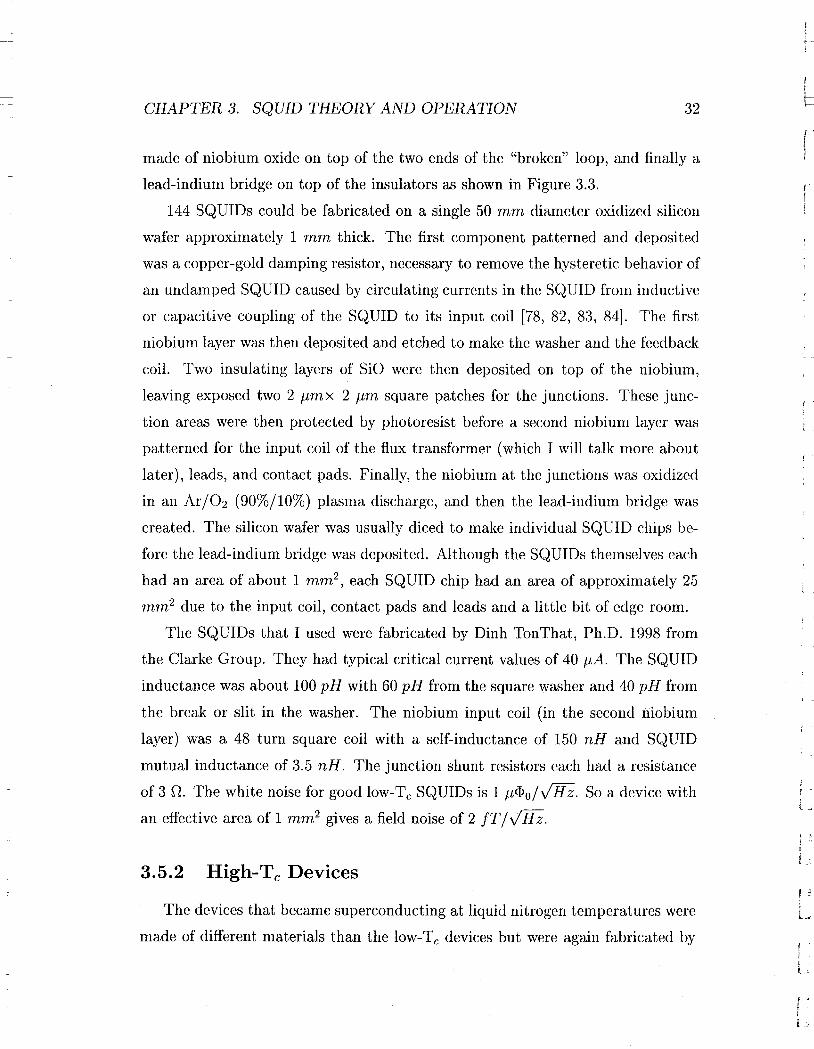
144 SQUIDs could be fabricated on a single 50 mm diameter oxidized silicon

wafer approximately 1 mm thick. The first component patterned and deposited

was a copper-gold damping resistor, necessary to remove the hysteretic behavior of

an undamped SQUID caused by circulating currents in the SQUID from inductive

or capacitive coupling of the SQUID to its input coil [78, 82, 83, 84]. The first

niobium layer was then deposited and etched to make the washer and the feedback

coil. Two insulating layers of SiO were then deposited on top of the niobium,

leaving exposed two 2 j.Lmx 2 j.Lrn square patches for the junctions. These junc

tion areas were then protected by photoresist before a second niobium layer was

patterned for the input coil of the flux transformer (which I will talk more about

later), leads, and contact pads. Finally, the niobium at the junctions was oxidized

in an Ar/02 (90%/10%) plasma discharge, and then the lead-indium bridge was

created. The silicon wafer was usually diced to make individual SQUID chips be

fore the lead-indium bridge was deposited. Although the SQUIDs themselves each

had an area of about 1 mm2 , each SQUID chip had an area of approximately 25

mm2 due to the input coil, contact pads and leads and a little bit of edge room.

The SQUIDs that I used were fabricated by Dinh TonThat, Ph.D. 1998 from

the Clarke Group. They had typical critical current values of 40 j.LA. The SQUID

inductance was about 100 pH with 60 pH from the square washer and 40 pH from

the break or slit in the washer. The niobium input coil (in the second niobium

layer) was a 48 turn square coil with a self-inductance of 150 nH and SQUID

mutual inductance of 3.5 nH. The junction shunt resistors each had a resistance

of 3 fl. The white noise for good low-Tc SQUIDs is 1 j.Lif>oIJHz. So a device with

an effective area of 1 mm2 gives a field noise of 2 fT1VHZ.

3.5.2 High-Tc Devices

The devices that became superconducting at liquid nitrogen temperatures were

made of different materials than the low-T c devices but were again fabricated by

! .

f '

\_ L

_ 1 _

i -


Figure 3.3. Schematic of the low temperature SQUID "tri-Iayer

sandwich" (shown sideways). The bottom layer is the

broken niobium square washer. The middle layer is com

posed of the two square patches of niobium oxide insu

lator. Finally the last layer is the bridge made of lead

indium spanning the two insulators and the slit in the

washer.

reactive ion etching of thin layers of superconductor deposited on a substrate.

Yttrium-barium-copper-oxide (YBCO) with an empirical formula of YBa2Cu307-x

deposited on strontium titanate (SrTi03 or STO to the physicists) were the ma

terials of choice for the Clarke group. The Josephson junctions of the high-T c de

vices are actually not superconductor-insulator-superconductor tunnel junctions.

Instead, they are known as weak link grain boundary junctions fonned at the in

terface of two superconductors that have different crystal orientations. This can

be done controllably and reproducibly by growing the SQUID onto a bicrystal

substrate made by slicing a single crystal of strontium titanate in half and cut

ting a wedge from one of the halves then fusing the crystal back together (sans

wedge), see Figure 3.4. The YBCG that is deposited on the bicrystal will follow

the two orientations of the substrate, and microbridges across the grain boundary

will produce Josephson junctions [78].

YBCO thin films were grown on the substrate by laser deposition (blasting a

chunk of YBCO with an excimer laser and allowing the crystal to reform on the

substrate). Patterning was done photolithographically and etched using a reactive

argon ion beam. The simplest high transition temperature SQUIDs formed on

grain boundaries are not trilayer sandwiches and more closely resemble the parallel

junction schematic. Some of those produced by the Clarke group were composed

of a square SQUID washer with dimensions of 32 JLrn x 32 JLrn and junction widths

of 1-3 Jlrn. White flux noise for these SQUIDs can be comparable to the noise

of low temperature devices 1.5 JLiPo/ J Hz, but the effective areas are extremely

small, meaning the magnetic field noise is high, on the order of 1 pT/ JHz, 1000

times higher than low-T c devices.

In order to increase the effective area, different magnetometer configurations

have been developed. The three types of high-T c SQUID magnetometers that I

used were: the directly coupled magnetometer, the fractional turn (multiloop),

and the multiturn flip-chip magnetometer. In the directly coupled magnetometer

there is a large 7 rnrn x 8 rnrn pickup loop which directly couples current to the 32

JLrnx 32 JLrn SQUID loop, Figure 3.5. Note that current can only circulate in the

large loop by passing through the SQUID. The field noise of the directly coupled


rL

l._


f 'i

(b)

(d)

(a)

(c)

Figure 3.4. The Strontium Titanate Bicrystal. (a) The full crystal;

lines indicate crystal orientation. (b) Split crystal. (c)

Wedge cut from crystal. (d) Crystal Halves fused back

together with lattice mismatch.


Weak-linkJosephsonJunctions

---------,..... --SQUIDwasher

r

fL

36l-

f!

Figure 3.5. Schematic of the high transition temperature SQUID di

rectly coupled magnetometer. Figure not to scale. The

large rectangular loop is the pickup loop. The SQUID

washer is shown in the right part of the pickup loop. The

dashed line represents the grain boundary. The junctions

are 1-3 Ilrn wide. They are the only narrow lines of su

perconductor material crossing the grain boundary.

f-~

L- I--- CHAPTER 3. SQUID THEORY AND OPERATION 37

f '

\

f- 1:- -

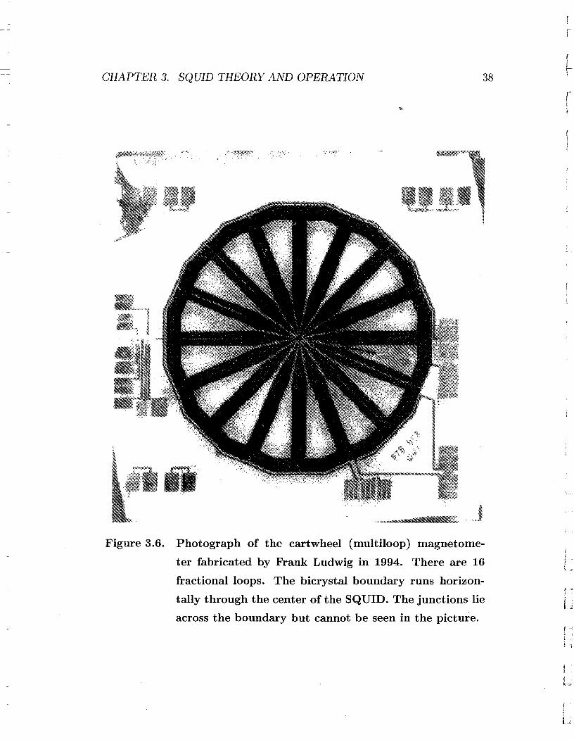
SQUID that I used was 70 fT / JHz. The fractional turn, also called multiloop

or cartwheel, magnetometer increases its effective area by cleverly joining many

small loops in parallel [85, 86, 87, 78]. Figure 3.6 shows a photograph of the

SQUID fabricated by Frank Ludwig in 1994. There are 16 fractional loops, and

the bicrystal boundary runs horizontally through the middle of the SQUID. This

device had an outside diameter of 7 rnrn, and an effective area of 1.84 m,m2 . It had

a flux noise of 25 ttiJ>o/ J Hz, giving a field noise of 30 fT / J Hz. A third design is

the flip-chip magnetometer in which a large coil and a small coil connected together

(in a flux transformer configuration) are patterned from YBCa on a separate piece

of strontium titanate and then flipped over on top of the SQUID [88, 78]. The flux

transformer and SQUID are inductively coupled since flux that enters the large

loop causes a supercurrent flow in the small loop producing a flux directly at the

SQUID. The last SQUID magnetometer that I used was such a SQUID. Its pickup

area was approximately 1 crn2 , while its effective area (number for calculating field

noise) was approximately 1 rnrn2. This particular SQUID had a rather high white

noise of 160 fT/JHz.

3.6 Operation: The direct current SQUID

There are two basic configurations or methods of SQUID operation as a mag

netometer. There is the direct current (dc) SQUID [58] and the radiofrequency

(rf) SQUID [89] . The rf SQUID was discovered later than the dc SQUID but

has been more widely commercially available since the 1970s. It is generally less

sensitive than the dc SQUID; therefore, all of the SQUIDs currently used in the

Pines Group are dc SQUIDs. For more information on the rf SQUID, good places

to start looking are in references [89, 78]. I showed in Section 3.4 that flux entering

the SQUID loop causes a current in the SQUID. SO measuring this current should

give a direct measure of magnetic fields. Unfortunately, there is not a good method

to measure this current. Instead, the SQUID is driven to a voltage mode by the

application of an external dc current, causing it to act as a ftux-to-voltage con

verter. To understand how this works, first consider a complete superconducting


rIt

Figure 3.6. Photograph of the cartwheel (multiloop) magnetome

ter fabricated by Frank Ludwig in 1994. There are 16

fractional loops. The bicrystal boundary runs horizon

tally through the center of the SQUID. The junctions lie

across the boundary but cannot be seen in the picture.J

f 'I

.. - I- CHAPTER 3. SQUID THEORY AND OPERATION 39f •

t .

i,l _

loop. As flux passes through this loop, a supercurrent (current with no resistance)

circulates in the loop in an effort to quantize the flux in the loop. For integer

number of flux quanta in the loop, no current will flow. Both of these phenomena

are also true for a superconducting loop with two flaws in it (i.e. a SQUID). But

one difference is that this flawed loop can not support the same amount of super

current as the perfect loop. There is a maximum current or "critical current" that

the Josephson junctions can support, as was implied from the Josephson Equation

3.10. A potential (voltage) will be necessary to force more current through the

junctions. The converse is also true, when more current than the critial current

passes through the junctions, a voltage is developed. By applying a bias current

to the SQUID of an amount just over the SQUID critical current, the sum of the

individual junction critical currents, any flux that enters the SQUID loop will in

duce a circulating current in the loop which will produce a voltage that can be

measured.

The SQUID current vs. voltage (I-V) curve is shown in Figure 3.7. The first

thing to note is that no voltage is developed until the critical current is surpassed.

The next important feature of the I-V curve is that the critical current changes

depending on the amount of flux in the loop. It has a maximum value for integer

numbers of flux quanta (epa), and a minimum value for half-integer numbers of flux

quanta. The asymptotic limit of the curves is the resistance R equal to the junction

shunt resistance. A simple picture from Clarke [78] considers a SQUID with two

Josephson junctions a and b, each with a critical current of la, so the maximum

current that the SQUID can support before going to the voltage state (developing

a voltage) is equal to 210 , If a small flux, less than epo/2, is applied to the SQUID,

a current J will circulate in order to cancel the flux and force the number of

flux quanta in the loop to an integer (zero in this case). The current through

junction a is now equal to +J and equal to -J through junction b (circulating

current, remember). Now imagine applying a direct current, 1, to the SQUID.

It will split evenly to both junctions. The current now flowing through junction

a is ~ + J, and likewise junction b now has a current ~ - J. If we continue to

increase the applied current to the SQUID, junction a will hit its critical current


n<l>o IL ~

r a--~-~,-_.,.,~._., ',.....",-"_.",,., IbiasI~ ~ I~ "-+ (n+O.5)<I>o

I1V II

Voltage

40

rl(

• i1

Figure 3.7. Current versus Voltage characteristic of SQUIDs. Volt

age is developed only after the SQUID critical current

is surpassed. The critical current· is dependent on the

magnetic flux in the SQUID loop.


( ~

I~ -

at ~ + .1 = 10 or rearranged I = 210 - 2.1. This means that the current flowing

through junction b is (210 - 2.1) /2 - .1 = 10 - 2.1. Any more applied current would"----vo--'"

Icreate a voltage~-the SQUID has reached its effective critical current. The sum

of the currents flowing through the junctions is 10 +10 - 2.1 = 210 - 2.7, which'-v-" "-v-"

a b

is smaller than the maximum critical current. This effective critical current will

continue to decrease to a minimum as the applied flux reaches <1>0/2. For more

flux than <1>0/2, the SQUID decides that instead of cancelling the flux, it would be

better to add to the flux and bring the flux to a full flux quantum. So the current .1

reverses direction, and as flux increases to a full flux quantum, the SQUID critical

current also increases up to its maximum value.

The SQUID critical current is a periodic function of magnetic flux. So operated

in the de mode by applying an external current slightly higher than the SQUID

critical current, voltage is also a periodic function of magnetic flux, Figure 3.8.

This means that a SQUID actually cannot detect anything greater than a flux

quantum, <1>0. It detects flux modulo flux quantum.

3.7 Operation: The Flux-Locked Loop

The way to get around this limitation is with additional electronics. We use a

design by Drung [90, 91] that has a very high bandwidth, from DC up to 5A1H z

with the correct components. The electronics that we use have a bandwidth of

about 1 A1H z. The idea behind the electronics is to read the voltage from the

SQUID (indicating external flux threading the SQUID loop) and then return flux

to the SQUID in order to cancel the flux that it is sensing. The order of events is

as follows: the SQUID (operated with a bias current) feels a little bit of flux, the

electronics detect a voltage and send current to a small coil beneath the SQUID

in order to cancel the flux so that no voltage is generated across the SQUID. If

the external flux increases, the current that the electronics sent to the coil will not

be enough to cancel the flux, the SQUID feels a net flux, develops a voltage, and

the electronics again try to compensate by increasing the current to the coil. This


e>~~Q.,)e

II~ ----.::;;;;;.........-.;:So

>

42

{

I

Figure 3.8. dc SQUID voltage versus flux. Voltage is a sine function

of flux in the SQUID loop when the SQUID is operated in

the direct current mode. For small oscillating magnetic

fluxes, precessing magnetization for example, the voltage

is given by the flux multiplied by the slope of the V-<P

curve at that point, V <p.

f~

iI -

- k CHAPTER 3. SQUID THEORY AND OPERATION 43

f '\f - positive feedback flux-locked loop effectively locks the SQUID to one position on

its voltage versus flux (V-1» curve. And the steeper the slope ~~ at the position

that the SQUID is locked, the more sensitive the magnetometer. The modulation

depth is the value .6.V' in Figure 3.8. Since the period of the V-1> curve is always the

flux quantum, 1>0' the modulation depth basically determines the slope ~~ = Vel>'

Therefore it is important to have a large modulation depth in order to operate;

a shallow .6.1" will mean less sensitivity as well as more difficulty in locking the

SQUID.

Figure 3.9 shows a schematic of the SQUID operated with a flux-locked loop. A

bias current I B is passed to the SQUID. When flux enters the SQUID, it develops

a voltage. The voltage is amplified by two stages of amplification (pre-amp and

amplifier) before it is passed to the integrator. The now phase corrected voltage

is split to a buffer and to the feedback coil which is inductively coupled to the

SQUID with a mutual inductance Alf . The feedback resistor R f converts the

voltage into a current for the feedback coil. The buffer holds the SQUID signal

and creates the proper 50 n output impedance so that external electronics can

properly interface with the SQUID feedback electronics. Finally the "Reset" is

a an externally controlled photocoupled analog switch (Siliconix DG308) which

shorts out the integrator when the NMR excitation pulse is applied. Without the

switch, the integrator invariably saturates (to the electronic rail) disabling it and

the rest of the circuit. The recovery time of the integrator without the reset and

therefore the NMR dead time (time between the application of the pulse and the

start of signal acquisition) is on the order of milliseconds~toolong for many Nl\!IR

experiments.

3.8 Flux Transformer and Gradiometer

The superconducting flux transformer is another important device or concept

necessary to use the SQUID as a magnetometer. The length of the square loop

for practical SQUIDs is on the order of 100 IJ:m. Like any tiny coil, the effective

sensing area is very small. This means that a bare SQUID can sense only tiny


r-

fL

44 !-

r,i

...- .....1·

...- ..1· ,

....- ..1·

......--..1·

Figure 3.9. Schematic showing the Flux-Locked Loop.


f 0

I

L

r '!

- ~ -

samples or tiny fractions of larger samples. Since the NMR signal scales with the

number of nuclei in a sample (or number that the detector can "see"), having a tiny

SQUID means getting a miniscule signal. Therefore SQUIDs, especially the low

T c SQUIDs, often employ superconducting flux transformers in order to increase

their sensing area. Figure 3.10 shows schematically two types of flux transformers.

The first type in (a) is a simple design with a single turn pickup coil and a 4-turn

input coil. A magnetic flux <P at the pickup coil induces a current J that flows

through the input coil. Since the input coil is located close to the SQUID, and often

patterned on the same chip, flux is coupled directly and efficiently into the SQUID

washer. The pickup coil and input coil are generally not identical loops, but do

have matched inductances [78]. Using a flux transformer for an NMR experiment is

convenient since the SQUID does not have to be located close to either the static or

pulse magnetic fields. It can be far removed and well shielded from ambient noise.

Figure 3.10 (b) is a variation on the flux transformer. Instead of a single pickup

loop, there are two, counterwound loops. This is a first-order (axial) gradiometer.

Magnetic fields that are constant in both loops create currents that cancel each

other, and nothing is sent to the SQUID. Magnetic field gradients, on the other

hand, are detected by this configuration. In an NMR experiment the gradiometer

is centered in the static and pulsed fields while the sample is placed in only one of

the loops. The static and excitation fields are transparent to the SQUID, but the

signal from the sample is detected since no signal is generated in the empty loop.

CH.APTER 3. SQUID THEORY AND OPERATION 46

~-

!

(a)

-"(

"J.....

(b)

-I~J

-~

J

Figure 3.10. Superconducting flux transformers. (a) Simple flux

transformer. (b) Gradiometric flux transformer.

r .~

!L

- l-

I "Il -c

r .I

47

Chapter 4

The Low Critical Temperature

SQUID Days

4.1 Introduction

The first SQUIDs in the Pines Group were low transition temperature SQUIDs.

By the time I joined the group, the commercial SQUID made,by Biomagnetic Tech

nologies, Inc. (BTl) was long gone. Instead, we used SQUIDs manufactured by

our collaborators in the Clarke group. They were made of niobium, niobium oxide,

and lead-indium and required liquid helium to operate. The experiments that were

accomplished using the low-T c SQUID were I-D imaging of hyperpolarized helium

gas in a static field of 5 Gauss (17.6 KHz), 2-D imaging of hyperpolarized solid

xenon at 10 Gauss (11.8kHz). These Magnetic Resonance Imaging (MRI) pictures

remain the lowest field images of milliliter sized samples with millimeter resolution

ever taken. We also acquired the first directly detected 2-D pure NQR spectrum

taken of 27Al in ruby.

4.2 Ultra Low Field Imaging

In 1972 Lauterbur, Mansfield and Grannell took the first nuclear magnetic

resonance images [9, 10]. MRI has since proven to be a powerful imaging technique

CHAPTER 4. THE LOW CRITICAL TEMPERATURE SQUID DAYS 48

f-

for medical diagnostics and materials characterization. At the same time that MRI

was being born, X-ray computed tomography (CT) was also being developed [92].

And after thirty years, there are more CT scanners in existence than MRI machines.

CT scans use harmful x-rays compared to MRI's harmless radio waves. l'vIRI is

capable of a higher resolution due to limitations in the beam collimation process

in X-ray CT [11]. It is also possible for slice selection at any angle using MRI. So

why do hospitals prefer X-ray CT over MRI? One reason may be familiarity since

X-ray imaging has been around for so much longer than MRI (in non-CT mode),

and some people may know and still be scared that MRI is truly nuclear- magnetic

resonance imaging. But the biggest reason for paucity of MRI machines is that they

are expensive, and the cost of MRI scans is high. A regular chest x-ray will cost

a patient $20 compared to a body MRI scan billed around $1500. The main cost

comes from the construction and operation of the huge superconducting magnets.

Field strengths around 1.5 Tesla are typically required to achieve the sensitivity and

resolution necessary for medical diagnostics. A further requirement that the static

magnetic field be homogeneous in the region to be imaged necessitates making the

magnets bigger and bigger and more and more expensive. "Open lVIRI" machines

further complicate the engineering.

The ability to take MRI pictures without the superconducting magnet, per

haps using only Earth's magnetic field, would be an incredible advancement. It

would mean cheaper, more widely available, and more versatile MRI. Furthermore

it would obviate the problem of susceptibility artifacts that arise from magnetic

susceptibility differences in neighboring tissues, like ghosting or overlap of struc

tures in the image. To understand this effect, keep in mind that nuclei will precess

at the Larmor frequency corresponding to the magnetic field that they feel, which

is not necessarily the field that is applied to them. Since the magnetic susceptibility

of a certain tissue affects the magnitude of the magnetic field in that tissue, image

overlap, for example, can occur when nuclei in different tissues feel the same mag

netic field although the applied magnetic fields are different. Because the nuclei

would then precess at the same frequency, they would appear in the MRI in the

same location. Susceptibility effects scale linearly with field strength; therefore,

r 'I

r~

LI--- CHAPTER 4. THE LOW CRITICAL TEMPERATURE SQUID DA.YS 49

f "

\i, -

the weaker the applied field, the smaller the effect.

The difficulty with simply imaging without the powerful magnet is twofold: first

of all the smaller the magnetic fields, the smaller the magnetization and therefore

signal from the sample (recall Equations 1.8 and 1.9). Secondly the sensitivity

of the detection equipment decreases as the Larmor frequency decreases. The

standard tuned circuit detects changing magnetization according to the Faraday

Law. Signal in terms of voltage, V, is proportional to the change in magnetic flux,

~~. For a magnetic moment precessing at the frequency w, the voltage is then

proportional to the frequency w.

r - . dip1/(t) ex - ex w

dt(4.1)

f, -

i!

Both of these factors lead to the same observable: smaller signal. Besides the

obvious reason that smaller signal is harder to detect, signal-to-noise is also an

important determinant of resolution in MR!. Mathematically, fvIRI resolution de

termined by gradient strength; however, strong gradients spread out the signal

and decrease the peak signal-to-noise. With too small a signal, it does not matter

what the theoretical resolution due to the strength of the gradients may be. So in

practice, the most important determinant of resolution in MRI is signal-to-noise

per voxel (3-D pixel). Vanishingly small NMR signal would suggest that Earth's

field MRI is prohibitive, at least using conventional approaches (refer to Section

5.9 for quantitative estimates). Therefore we use an unconventional method: ultra

low field MRI by combining the techniques of optical pumping of noble gases with

the detection of MRI signal using superconducting quantum interference devices

(SQUIDs).

4.2.1 MRI with Optical Pumping and MRI with SQUIDs

The first use of optically polarized noble gases for magnetic resonance imaging

was reported in 1994 by Albert and coworkers [93]. Since then, hyperpolarized

noble gas MRI has been rapidly becoming a standard technique [94, 95, 96, 97, 98,

38, 39]. Around the same time, the first use of a SQUID for MRI (which was in


fact low-field MRI) was reported by Seton and coworkers in 1995 [99]. Other early

work was also from those researchers [100, 101]. Before the work described here

[102] there was one prior published work using hyperpolarized helium in low-field

MRI [103]. As of the writing of this thesis, the interest in low-field MRI using

OP gases has increased [104, 105]. But since these experiments used conventional

tuned circuit detectors, they were performed at higher magnetic fields than our

work.

4.2.2 Imaging Theory: Projection Reconstruction

Recall from Section 1.4 that having a gradient in the applied magnetic field

will spread out the NMR spectrum in frequency space, which can be related to

distance space by knowing the gradient strength and the gyromagnetic ratio of the

nuclei one is looking at. A gradient in one direction, the x direction for example,

projects into the frequency domain the spatial distribution of nuclei in the x direc

tion. A gradient in the y direction would be necessary to get information on the

density of nuclei in the y direction. The principle behind the method of Projection

Reconstruction is that by collecting a series of these 1-D projections each with

different orientations of the gradient with respect to the sample a 2-dimensional

(or even 3-D) map of the nuclear distributions can be obtained. Figure 4.1 shows

a cartoon of the frequency domain MRI spectra that would be obtained for the

two circular objects in different orientations in a magnetic field with gradient. The

low transition temperature SQUID imaging probe contained only a single pair of

gradient coils, so it was necessary to rotate the sample inside the probe in order

to collect different spectral projections and obtain 2-D images.

The raw data from our sample rotations was a polar raster of time space with

each FID having its native time dimension and further having an angle dimension.

We decided that it was best to convert the data tQ a regular timex time Cartesian

space. Figure 4.2 shows the relation between the experimental polar raster and the

Cartesian raster. In order to fill out the Cartesian plane, we interpolated points

based on a linear average of the four polar points (true data) that surround any

rtr

r,!

r '1L

- I- CHAPTER 4. THE LOvV CRITICAL TEMPERATURE SQUID DAYS 51

!l _

u[ -

::l .

Objects

••

•

••

----I~

Directionof Gradient

Spectra

------~Frequency

(or Distance)

Figure 4.1. 2D Imaging: Projection Reconstruction. 2 dimensional

imaging is done by changing the orientation of the gradi

ent relative to the sample. The I-D projections can then

be reconstructed to give the full 2-D image.

CHAPTER 4. THE LOl-V CRITICAL TEMPERATURE SQUID DAYS

•

52

r

rb

F'ii

•

n~ ~~fW

• •fW

~ t 4.~~ ... -... ~ I- .. -• • • •-. -- ~t ~, -• •-. -I- .- -, -

... b. b.

1"",-Ill. •• --- - --• ~ ~ 4t •- -- ~

• • • •• ..- """~ ~~

• •, U

•

•Figure 4.2. Polar to Cartesian Raster. The solid circles represent the

polar raster of time space sitting in the regular Cartesian

(square) raster. The four circles around the star are the

four pieces of real data used to interpolate that point.

r~

i - I-- CHAPTER 4. THE LOW CRITICAL TEMPERATURE SQUID DAYS 53

l 0

I- f

l

- f-

I

Cartesian point not on axis of a polar ray. Once the Cartesian time space was

filled out, a two dimensional Fourier Transform produced the 2-D maps of nuclear

density.

4.2.3 The SQUID Imaging Probe

Figure 4.3 is a photograph of the 1.5 rn long low transition temperature SQUID

probe. The important parts to take note of are the feedback electronics mounted

to the brass flange at the top of the probe and the cylindrical lead shield at the

bottom where the SQUID and the MRI probehead were housed. The long length

of the probe was necessary since it was mounted to double nitrogen and helium

glass dewars (Figure 4.4). Everything but the electronics were submerged in liquid

helium. The dewar housing was a simple wooden cabinet. In order to further shield

noise, there was a cylindrical mu-metal shield around the outside of the dewar in

the region of the probehead, and the entire setup was locked into a copper mesh

Faraday cage (screen room).

Figures 4.5 and 4.6 show two schematics of the same imaging probehcad. Sam

ples were required to have an outer diameter no larger than 8 mrn and were tied

to strings or sticks in order to put them in place in the probe and then pull them

out again. The static field was supplied by a pair of rectangular coils 65 x 24

rnrn in a pseudo-Helmholtz configuration-pseudo because Helmholtz is a spe

cific coil geometry with round coils whose separation is equal to the radius of the

coils. Each coil was made of 30 turns of copper clad niobium-titanium (Nb-Ti)

26 gauge (A IFG) wire. The gradient coils were a quasi Maxwell pair (a pair of

counterwound coils), also rectangular 60 x 20 rnrn each made of 5 turns of cop

per clad Nb-Ti. wire. The gradient coils were on axis with the static coils, so

they produced a gradient dBz/dz. The gradient and static coils were run with

persistent current charged by a Hewlett-Packard 6253A Dual DC Power Supply.

Simple superconducting switches were built from insulated niobium wire, resistors,

and epoxy. Superconducting connections were made by spot-welding the niobium

wires to pieces of niobium foil and then covering them with epoxy to insulate and

CHAPTER 4. THE L()~V CRITICAL TEMPERATURE SQUID DAYS

SQUID FeedbackElectronics

Long aluminumtube

Lead shieldcovering SQUIDand probehead

Figure 4.3. Low-Tc SQUID full-length probe

54

flL~

,l

f----


SQUIDfeedback

electronics

Copper MeshScreen Room

Nitrogen andhelium glass

dewars

Mu-metalshield

Woodendewar

housing

Figure 4.4. The low-Tc SQUID dewar. The SQUID probe is inside

the double nitrogen and helium dewars. The photo was

taken through the open door of the copper mesh Faraday

cage.

CHAPTER 4. THE LOvV CRITICAL TEMPERATURE SQUID DAYS 56

rprotect the connections.

The audiofrequency (af) excitation coils were a pair of Helmholtz coils with

a diameter and a separation of 15.6 mm. These coils were made of 20 turns of

26 AlVG, insulated copper wire. The pickup coil was a 2 turn solenoid 9 mm

in diameter and made of insulated niobium wire. It formed the flux transformer

with the input coil patterned on the SQUID. The pickup coil was connected to

the niobium foils on the G-lO fiberglass SQUID holder, see Figure 4.7, by pressure

contacts made by sandwiching each wire between the niobium foil on the SQUID

holder and a block of niobium (not shown in schematic) that was screwed to the

fiberglass in order to squeeze the wire. The niobium foil pads were connected to

the patterned input coil on the SQUID chip by ultrasonic wire bonds. Voltage and

current connections were made by ultrasonically bonding aluminum wires from the

on-chip contact pads to the copper contact strips on the fiberglass. The SQUID

was epoxied to the holder and hermetically sealed by epoxying a fiberglass case

on top. When sealed, the only parts exposed were the large niobium and copper

contacts. A 10 turn copper coil for feedback was stuck· to the outside of the

fiberglass enclosure beneath the SQUID by Blue-Tack, a putty-like material similar

in appearance to poster gum. Blue-Tack hardens at cryogenic temperatures but

doesn't shrink much, doesn't crack and continues to adhere to the substrate. The

SQUID holder with feedback coil is mounted inside a niobium cylinder to further

shield the SQUID from noise, see Figure 4.5.

4.2.4 The Spectrometer

To run the imaging experiments we used a TecMag Aries interfaced to an Apple

Macintosh IIci. The TecMag control software was MacNMR version 4.5.9. One

TTL line from the Aries was used for the SQUID trigger to blank the integrator

in the SQUID electronics (to prevent saturation as mentioned in Chapter 3). One

TTL line was used to gate a Hewlett-Packard 3314A Function Generator. The

output of this synthesizer was connected to a 10:1 voltage divider and then to the

input of an ENI 1040L power amplifier (55 dB gain from 10 kHz to 500 kHz). The

f'i!-

- - I-- CHAPTER 4. THE LOlV CRITICAL TEIVIPERATURE SQUID DAYS 57

f \

Figure 4.5. Low-Tc SQUID MRI Probehead (View 1). The flux

transformer is not seen in the photograph since it is in

side the probehead.

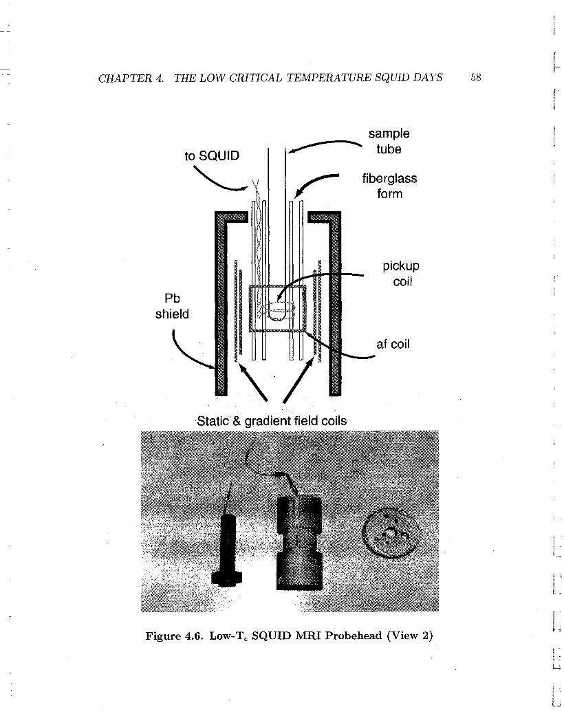
CHAPTER 4. THE LOW CRITICAL TEMPERATURE SQUID DAYS 58L!-

sample~·tube

to SQUID

~.1

Pbshield

\7

fiberglassform

pickupcoil

af coil

Static &gradient field coils

Figure 4.6. Low-Tc SQUID MRI Probehead (View 2)

r·~

I- L CH.APTER 4. THE LOV\l CRITICAL TEMPERATURE SQUID DAYS

(a)

SQUID

59

Niobium padsfor pickup coil

connects

(b)

Niobiumcontact pads

Copper padsfor I,V connects

Figure 4.7. Low-Tc SQUID Holder. (a) Schematic (not to scale)

showing various connections from the SQUID chip to the

niobium contact pads for the pickup coil connection and

to the copper contact pads for the current and voltage

connections. (b) Photograph of a fiberglass holder with

no SQUID or connections.

CHAPTER 4. THE LO~V CRITICAL TEMPERATURE SQUID DAYS 60

output of the amplifier was sent through two pairs of crossed diodes, through a 50

ohm resistor to match the output impedance of the amplifier, and then fed through

the copper Faraday cage into the af excitation coil. The signal from the SQUID

electronics was sent to a Princeton Amplifier Research (PAR) battery powered

amplifier where it was low-pass filtered at 50 kHz and amplified by 20 dB. It was

passed out of the SQUID cage to a Rockland Wavetek Model 442 filter where it

"vas high-pass filtered and again amplified by 20 dB before going into the digitizer

in the TecMag.

4.2.5 The Optical Pumping Setups

Our xenon sample was approximately 2 atm of naturally abundant xenon, 20

rnbar of nitrogen gas, and a few milligrams of rubidium sealed in a cylindrical

Pyrex cell with an inner diameter of 0.48 em and length of 1.5 ern, giving a volume

of 0.27 mL. One end was flattened while the other was pointed (from the sealing of

the glass). The laser used to pump this sample was a 1 watt (TV) titanium sapphire

(Ti:Sapph) laser, model SEO Titan-Cw made by Schwartz Electron Optics, Inc.,

tuned to 794.7 nm pumped by a 10 VV argon ion laser, model Innova 300 man

ufactured by Coherent. The beam from the Ti:sapph laser was passed through a

quarter-waye plate to circularly polarize the light before entering the sample. The

sample was heated to 400 K with a simple resistive heater made of nichrome wire

mounted in a glass beaker. We pumped the sample for 5 minutes per run. One

end of the cell was not optically clear (since it was not flat), so it was not possible

to place the power meter behind the cell and tune the laser frequency by checking

for light absorption as was typical procedure for flat-end pumping cells. Therefore

we tuned by looking for the purple-white glow of the rudibium dimer fluoresellce

which one can see when the rudibium partial pressure is too high and nitrogen

partial pressure (which quenches the fluoresence) is too low. Typical polarizations

that we achieved were 3% as calibrated in a high field magnet against thermally

polarized xenon. The coils that the sample sat in produced a magnetic field of 30

Gauss with a current of 15 amps. Figure 4.8 shows a schematic of the setup used

r!

r-

L- ~- CHAPTER 4. THE LOv\! CRITICAL TElVIPERATURE SQUID DAYS 61

for the optical pumping of xenon. No mirrors are drawn in the diagram for the

purpose of clarity, but they are in place wherever the light beams appear to bend.

The helium samples were cylindrical Pyrex cells containing 1 atm of 90% iso

topically enriched 3He, 11 torr of nitrogen gas, and a few milligrams of rubidium.

The helium pumping cells each had an inner diameter of 0.68 rmn and lengths of

about 15 em. Due to the length of the cell and the necessity for higher pump

ing temperatures (typically 473 K), we diverted the laser beam to the large blue

Helmholtz coils with a diameter of 80 em which produced a field of 30 G with a

current of 15 amps. For heating, we tried using a resistive heater: nichrome wire

wound around the sample, same as for the xenon. However, it proved to be incon

venient and time-consuming (as the polarization was relaxing) to quickly remove

and insert the sample in the coil. Another method we tried was to use a heat gun

to heat the sample. This turned out to be more convenient. However, we never

observed large signals with the SQUID using either of these methods. \lVe decided

to use a high field magnet to check the polarization, and then further decided

to modify the probe in order to optically pump the helium inside of the Pines

Group "Delta" magnet (300 MHz ~ 7 Testa). We used the Spectra Diode Labs

8DL-8630 0.5 watt solid state diode laser and pumped the sample for half an hour

inside the magnet. The beam was directed through the top of the magnet into the

sample and was aligned by eye. In this case we heated only the bottom portion of

the sample rather than the whole tube. The probe was a simple home-built "stick

probe" with a small solenoidal heating coil and a saddle-shaped transmitter coil.

Figure 4.9 shows a schematic of the optical pumping setup for the helium.

Mechanisms of optical pumping in high field are different than in the low fields

(30 G) that are typically used. Spin exchange optical pumping in high magnetic

fields was first investigated by Augustine and Zilm in 1996 [106, 107, 108]. Figure

4.10 shows the valence electron energy level diagram of rubidium in a field of 7 T.

Note that this figure still ignores the difference between the two rubidium isotopes.

The large splittings of the magnetic sublevels allows optical pumping selectivity

based on light frequency as well as light polarization. It is not necessary to use

CHAPTER 4. THE LOltV CRJTICAL TKMPERATURE SQUID DAYS 62L~-

("!

~..c ~c.(])C.ooco ct:l(J)-

J=

~

(]) CJ.)

ECiio (]).c..c° (]).- ~Z .

:=

(])O)..c Xc_-- -- "'0c.:=cE = ct:l::J(])..ca..° CC

"'0(])-- 00u..-° -0-"t:j0co-(J)

co ~c (])o 000) co~«

~0\(]) .N (])-- -~ coco- c.d:~~ co~ :=::J~0--= ~0-

Figure 4.8. Xenon Batch Optical Pumping Setup. Not to scale.

f ~"

L- i----

['I,I .

I "

I

CH.APTER 4. THE LOvV CRITICAL TEMPERATURE SQUID DAYS 63

Q)~ -.§ "0

()Q)e>E c0:;::;~ co

.r::. Q)

.2 .r::.Z

~

Q)(J)

-J ctS0....1enQ)

"'0oo

/

Figure 4.9. Helium High Field OP Setup. Not to scale.

CHAPTER 4. THE LOW CRITICAL TEMPERiiTURE SQUID DAYS 64

iLI

rI

5P1/2 -...,----<.

ms=+1/2

65.6 GHz

ms=-1/2

794.7 nm = 377 THz

581/2 _...:..--<

ms=+1/2

196.8 GHz

ms=-1/2

Figure 4.10. Valence electron energy levels of rubidium in a field of

7 Tesla.


[ ~

!,, c

circularly polarized light to optically pump the rubidium in high field [107]. Once

the rubidium is spin polarized, the mechanism of spin transfer to the noble gas

is similar to the mechanism at low field, as suggested by the measurements on

spin-exchange cross sections between xenon and rubidium at high field [108].

4.2.6 The Images

Due to the long dead time of the SQUID electronics after the audiofrequency

pulse, we used a simple 90-90 spin echo pulse sequence for all of the collections.

Figure 4.11 is an example of the typical spin echo response. Each excitation pulse

consisted of a single cycle with a magnitude o,f 0.09 mT at a frequency 1./ = 17.6

kHz and were separated by 0.66 ms, leading to arefocusing of the magnetization

at 1.32 ms. The helium 1-D time domain echoes were apodized by multiplication

by hyperbolic secant functions centered at 1.32 ms and widths of 1.5 111,8 and

then Fourier transformed. Three spectra are shown in Figure 4.12. All spectra

were acquired in a static field of B o = 0.54 mT, giving a resonance frequency of

17.6 kHz. The bottom spectrum (c) was produced with no gradient and shows a

rather large 1 kHz full width half max(Jwhm) linewidth, most likely due to the

inhomogeneity of B o • The middle spectrum is a 1-D helium image with a gradient

of G = 0.33 mT/ em and spatial resolution of 700 JLm. The top spectrum was

taken with a gradient of G = 0.46 mT/ em and a corresponding spatial resolution

of 500 JLm. The solid lines are the acquired data. The dashed lines in Figure

4.12(a) and (b) are the circular distribution functions that represent the expected

density of a uniform material in a cylinder projected onto one axis. In other

words, the spectral shape that you would expect from a applying a linear gradient

to a cylindrical sample perpendicular to the axis of the cylinder. The dotted

lines in 4.12(a) and (b) are the simulated 1-D images obtained by convolution of

the circular distribution functions with a Lorentzian function describing the NMR

lineshape.

The xenon data were acquired by sequentially rotating the sample tube in a

static field of B o = 1 mT, corresponding to a Larmor frequency of 11.8 kHz, and

CHAPTER 4. THE LOW CRITICAL TEMPERATURE SQUID DAYS

f

Lt

(-

66 brL

f'r-

AFpulse

AFpulse

rI

! .

I ,

I0.0

I0.5

I1.0

Time (ms)

I1.5

Figure 4.11. Spin Echo from Hyperpolarized Helium. I ~

u! 3I -:

L~

I"I

U

f 'I

_ L-

- I-

r 'l

CHAPTER 4. THE L01V CRITICAL TEMPERATURE SQUID DAYS 67

f '

!l _

f- 1-

(a)80 =5.6 GaussG = 0.54 G/mm

1

6I.o

d [mm]

1-6

(b)80 =5.6 GaussG =0.35 G/mm

(c)80 =5.6 GaussNo Gradient

1 1 1 112 6 0 -6

d [mm]

1 1 130 20 10

roO/21t [kHz]

Figure 4.12. Hyperpolarized He 1-D Images

!LI

CHA.PTER 4. THE LOW' CRITICAL TElvIPERATURE SQUID DAYS 68L1--

a fixed linear gradient G = dBz/dz = 0.46 mT/em. A () - () spin echo sequence

was used with each af pulse giving a () = 100 tipping angle. This 2-D data set

required more signal processing than the helium single projections. \Ve 2 times

oversamples and collected 12 spectra each separated by 300• We only needed 6

spectra separated by 300 to take the complete image because a gradient in the +x

direction contained the same information as a gnidient in the -;1: direction---except

that the two projections were mirror images of each other. Therefore we could not

simply add spectra as one would for signal averaging. 'vVe cut each time domain

signal at the top of the echo and threw away the beginning points to make 12

non-echo FIDs. We then arranged the 12 FIDs in a 2 dimensional polar time space

where the origin corresponded to the start of each of the FIDs. Throwing away half

of the echoes and reassembling the 12 spectra did not help us gain signal-to-noise,

but it did allow for inhomogeneities in the gradient and static field to be averaged

out that would otherwise distort the image. \V"e normalized the intensities based

on the maximum of each FID since each spectrum was progressively less intense

as each pulse "destroyed" the nonequilibrium magnetizaton during acquisition.

From the FIDs arranged in a radial pattern we interpolated the Cartesian space

as described earlier in 4.2.2 and performed a 2-D Fourier transform to obtain the

data in frequency space. And knowing the strength of the static gradient, G, and

nuclear gyromagnetic ratio, ,,/, it is simple to convert the frequency, v, axes to

distance, D, axes.

(4.2)v(Hz)

D(em) = "/ (~z) G C~)

Figure 4.13 shows the xenon "embryo" frozen to the side of the sample tube. Figure

4.13(a) is the actual data showing the pixel resolution. The picture is 30 points

by 30 points giving approximately 1.2 em on a side. Each pixel is approximately

0.4 mm wide, but because of the 520 Hz linewidth of solid xenon [109], the pixel

resolution is better than the actual resolution of 950 f--lm. In this case the picture

was resolution limited by the xenon linewidth. Figure 4.13(b) is the digitally

smoothed version of the top image. Smoothing was done in Matlab by a method

known as Gouraud shading which subdivides each pixel into many smaller pixels

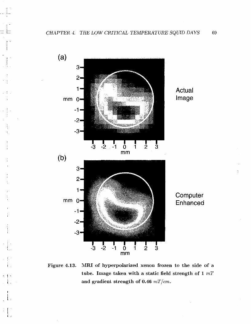
CHAPTER 4. THE LO''''' CRITICAL TEMPERATURE SQUID DAYS

-

L70

I-

r-!

and linearly assigns a color to each subpixel based on the predefined colormap.

Note that this was the "jet" colormap in Matlab. The white circle in both pictures

represents the 4.8 mm diameter of the sample tube. The xenon density that

extends beyond the white tube is caused by resolution limitations.

4.3 Pure Nuclear Quadrupole Resonance (NQR)

The history of nuclear quadrupole resonance dates to the 1940's with the molec

ular beam magnetic resonance experiment of Nierenberg, Ramsey, and Brody [110]

based on the experiments by Rabi and coworkers in the late 1930's [111]. NQR was

initially a method to simply measure quadrupole moments and to verify various

aspects of the fledgling quantum mechanics theory. But it is a powerful analytical

technique to gain physical and chemical information about molecules. IVlore than

~ of all elements have mainly quadrupolar isotopes, and the quadrupolar inter

action is highly sensitive to the local electronic environment. High-field NMR of

quadrupolar nuclei provides quadrupolar interaction information, but spectra can

often be difficult to interpret due to the sheer number of lines and the NMR solid

state powder pattern that could mask information. An alternative is zero field

NQR, otherwise known as pure NQR.

The first pure NQR pulsed experiments were published starting in 1954 [112,

113, 114]. Although performed in CW mode, the next big evolution in NQR

occurred in 1959 when Anderson applied the method offield cycling to quadrupolar

metals [115]. The notion of field cycling had been introduced in 1951 by Ramsey

and Pound [116] just after Pound had published his. definitive work on NQR in

crystals using a continuous wave technique [117]. The general idea behind field

cycling is that the sample is first subjected to a strong magnetic field to polarize

the nuclei. The field is then turned off allowing the nuclear interactions (such as

the quadrupolar interaction) to evolve without the Zeeman interaction. The field

is then switched back on to detect the magnetization.

Various field cycling methods have been developed such as "Double Resonance

Lab Frame" [118, 119] and "Double Resonance Level Crossing" [120, 121, 122] with

r~

L- ~-

CHAPTER 4. THE LOvV CRITICAL TEMPERATURE SQUID DAYS 71[ ... "1

lr '

r

l

perhaps some of the most elegant work done in the Pines group [123, 124, 125]

with a method known as "Time Domain Field Cycling." But the problem with

most field cycling experiments is that they are inherently 2-D experiments since the

magnetization's slow precession cannot be detected directly: one dimension for the

evolution in zero field of the quadrupole magnetization and the other dimension

for the detection of the magnetization at high field. A SQUID, on the other hand,

can detect the low frequency pure NQR magnetic resonances directly with high

sensitivity, meaning simpler 1-D experiments. It should be mentioned that Tycko

developed a clever technique in 1988 to perform zero field NQR in a high field

magnet by spinning the sample and applying RF pulses [126, 127]. The advantage

of using a SQUID for NQR compared to Tycko's method is that there is a fractional

scaling factor for the magnetic interactions using his technique. There is already

a growing body of work involving SQUID detected NQR [128, 129, 130, 131, 132,

133, 134, 135, 136, 137, 138, 139]. I present below the first pure NQR correlation

spectrum using a SQUID taken with one directly detected dimension [139]. Note:

yes I realize that I don't share authorship 011 the paper; these results were added

to a review that was almost complete before the data was collected.

4.3.1 Pure NQR 2-D Correlation Spectroscopy of Aluminum

27 in Ruby

27Al is a spin-5/2 nucleus, so in general there are six spin energy levels. Ruby

is sapphire (Ab03) doped with Cr3+. In the crystal structure of A120 3, each

aluminum is octahedrally coordinated to six oxygen atoms. This high symmetry

causes the six levels to become only three energy levels each doubly degenerate. It

is easy to see this from the quadrupolar Hamiltonian:

11. = -(eQ)(eq) . (3]2 - ]2 + TJ(j2 - ]2)) (4.3)Q 41(2I - 1) z x y

This form of the Hamiltonian is different than that given earlier in Section 1.3.4

Equation 1.30. Though equivalent, this is perhaps more useful for magnetic reso

nance spectroscopy. eQ is the quadrupole moment magnitude of the nucleus, and

eq is the quadrupole moment magnitude of the interacting electric field gradient.

In practice, the quadrupole coupling constant e2Qq cannot be decomposed. The

spin of the nucleus is given by land the respective spin operators f and fz, fa:,

and f y . r} is the asymmetry parameter of the electric field gradient, ranging from

zero to one. A value of 1 corresponds to planar symmetry whereas a value of 0

corresponds to axial symmetry. For octahedral coordination, TJ = O. This simplifies

the Hamiltonian.

CHAPTER 4. THE LOW CRITICAL TEMPERATURE SQUID DAYS

1i = -(eQ)(eq) . (3]2 _ ]2)Q 41(21 - 1) z

f z and f commute, so each matrix element of the Hamiltonian is given by:

72

(4.4)

r

rl

) _ -(eQ)(eq) (2) r:((m)I1iQ I(n) - 41(21 _ 1)' 3m - 1(1 + 1) . 6mn (4.0)

where 6mn is the Kronecker Delta function. States I(m)) and I(-m)) have the

same energy, so integer spin nuclei have a nondegenerate ground state 1(0)) and all

other states doubly degenerate. Half-integer spin quadrupolar nuclei have (21 +1) /2 doubly degenerate energy levels. For spin-5/2 nuclei like aluminum, this

corresponds to two allowable transitions: between the 1(±1/2)) and 1(±3/2)) levels

and the 1(±3/2)) and 1(±5/2)) levels. For sapphire, those transitions have energies

corresponding to the frequencies 359 kHz and 714 kHz respectively. Figure 4.14

shows a spectrum of the ruby sample with both transitions irradiated. The sample

was composed of 500 mm3 of ruby in the form of little ruby spheres with 0.5 mm

diameters. The chromium dopant level was 7%. Doping sapphire with CrH not

only makes the balls a pretty red color, the paramagnetic impurity also significantly

shortens the T 1 (longitudinal relaxation) of the aluminum. The T j of pure sapphire

at 4.2 K is 1 minute. In contrast, the 7% chromium dopant level cut the T 1 to

approximately 10 ms.

I.

I ::

f '\!

- 1---

[~

i\-

CHAPTER 4. THE LO~V CRITICAL TEMPERATURE SQUID DAYS 73

-

c..E«

360

Frequency (kHz)

720

Figure 4.14. NQR Spectrum of 27Al in Ruby. Both transitions were

irradiated.

CHAPTER 4. THE LOHI CRITICAL TEMPERATURE SQUID DAYS

4.3.2 The NQR Probe and Spectrometer

;-I

I

~r-

74

rt

Figure 4.15 shows a schematic of the NQR probe. The pickup coil was a four

turn axial gradiometer. The pulse coil was a two-layer solenoid 15 mrn in diameter

and 30 rnm long. It was wound with 28 AH/G copper magnet wire (formvar

insulation) on a Rulon form. Rulon is a material composed of paper compressed

with plastic. There was a superconducting lead shield around the whole probehead

to shield all external fields. It was important to balance well the gradiometer in the

AF coil-in other words, position the gradiometer for maximum signal rejection

from the AF coil. This could be achieved by sending a signal (100 kHz from a

function generator) into the AF coil and connecting the ends of the gradiometer

to a good scope, such as the Hewlett-Packard 3561A Dynamic Signal Analyzer.

The Signal Analyzer was useful since it carried out a real-time Fourier Transform

to easily track the amplitude of the signal that was being sent to the AF coil. By

moving the gradiometer on its Rulon form relative to the AF coil (see exploded

view of the probehead in Figure 4.15), it was possible to balance the gradiometer

to better than 0.1% (10 mv' pickup from 10 V input at 100 kHz).

These NQR experiments did not use the TecMag Aries. We had been using

an old version of MacNMR (v.4.5.9) since newer versions did not run on the old

Macintosh lIei. It did not perform the collection and file-save options that we

wanted. We felt that we could easily put together a spectrometer that would do

exactly what we wanted. The pulse timer that we used was a Stanford Research

Systems Model DG535 Four Channel Digital DelayjPulse' Generator. One TTL

line from the gated output (i.e. A-B or C-D rather than A, B, C, or D) was used

to trigger the SQUID. The other gated TTL line was split to the external trigger

inputs of two Hewlett-Packard 3314A Function Generators, one tuned to 360 kHz

and the other tuned to 720 kHz. The function generator outputs were mixed with

a simple 10:1 voltage divider and connected to the input of an ENI 1040L Power

Amplifier. The output of the amplifier was passed through two pairs of crossed

diodes and a 50 n high power resistor before it was fed through the Faraday cage to

the pulse coil. Output from the SQUID electronics went to a Princeton Amplifier

t '\L

CHAPTER 4. THE L01>\/ CRITICAL TEMPERATURE SQUID DAYS

Sampletube

to SQUID

Pickupcoil

Pbshield

75

Figure 4.15. Schematic and photograph of the low T c SQUID NQR

probehead. Photograph shows disassembled view. This

probehead replaces the MRI probehead on the long

SQUID probe.

CHAPTER 4. THE LOliV' CRITICAL TEJvIPERATURE SQUID DAYS 76

r

k

Research filter where it was amplified by 20 dB. The signal was then passed out of

the Faraday cage and put through one channel of a Rockland Wavetek Model 442

Filter. The signal was then digitized by a Tektronix DSA 602 Digitizing Signal

Analyzer with llA72 Two Channel Amplifier (the input module). An Intel 486

DX25 (25 /1.1H z processor) based PC was outfitted with a National Instruments

IEEE-488 communications card to interface the computer to the pulse generator

and digitizing scope. The IEEE-488 (also called HPIB) interface allows the daisy

chaining of devices, so only one interface card in the computer was required to

control multiple instruments. I wrote a simple Instrument BASIC (I-BASIC) pro

gram to fully automate data collection. It controlled and synchronized both the

Stanford pulse programmer and the Tektronix digitizing scope. After each NQR

scan, it automatically downloaded the data from the Tektronix digitizing scope

and saved it in a simple text file to be read into Matlab.

4.3.3 Results: 2-D Ruby Spectrum

The pulse sequence used for the 2-D collection is shown in Figure 4.16. The

second pair of pulses mixes the spin populations after the time Tl' By taking NQR

spectra with different values of Tl we can resolve the resonance correlation that

is caused by the mixing. The step size of the time Tl (coherence mixing time)

between acqusitions was 0.5 p,s. The 2-D data set was composed of 64 FIDs each

averaged 512 times. The data in Figure 4.17 clearly shows two diagonal peaks

corresponding to the 359 kHz and 714 kHz transitions. But there are also cross

peaks indicative of the coherence transfer between the magnetic resonances. The

weakest signal in the map is the on-diagonal low energy transition (1(±1/2)) to

1(±3/2))), and the strongest signal is from the on-diagonal high energy transition

(1(±3/2)) to 1(±5/2))).

r!

1

r 'iI ~

- i-

l _

CHAPTER 4. THE LOvV CRITICAL TEMPERATURE SQUID DAYS 77

AFPulse-

360 kHz

,AFPulse-

720 kHz

Ac uisition

"['1

AFPulse~

AFPulse~

Ir, -,i ,

Figure 4.16. Pulse Sequence for 2-D NQR of Ruby. The sequence

shows the two frequencies irradiated simultaneously.

The time Tl was incremented by 0.5 f.LS between scans.


1000

0

- 800N

I Do 0~'-"

~() 600c 0Q):::s0-Q)

U'-u.. 400

0

200 ....... ...... -0oןס ___

200 400 600 800 1000

Frequency (kHz)

Figure 4.17. 2-D Pure NQR of 27 in Ruby. The off-diagonal peaks

. indicate magnetization transfer between the two reso-

nances.

[

b

r

f--""

L- I---

\ -

79

Chapter 5

High Transition Temperature

SQUIDs

5.1 Introduction

There were two main reasons for the move from using a liquid helium low-T c

SQUID to using a high-T c device that would operate at liquid nitrogen temper

ature. The first was that our low transition temperature SQUID setup suffered

from a serious handicap. It operated cold and required that samples also be cold.

One problem with this limitation was that there were no good "standard samples"

for 4 Kelvin operation in order to tune or trouble-shoot the probe. Gooel NMR

standards like water have intolerably long relaxation times in the solid state sitting

in liquid helium. The second reason was that while we were taking pictures with

the highest resolution at the lowest fields, imaging objects in an 8 mm hole at 4.2

K elvin was not the most widely applicable technique. So we wanted room temper

ature samples, and while it would have been possible to build a probe to insulate

the 4.2 K SQUID from a room temperature sample [140, 141, 142]' using the new

high-Tc SQUIDs would greatly simplify the cryogenics [143]. After the high-Tc

setup was completed, however, it was clear that it did not have the sensitivity

to take the hyperpolarized xenon images that we wanted. We were able to take

proton MRI pictures at fields of 2 mT, corresponding to a Larmor frequency of

CHAPTER 5. HIGH TRANSITION TEI\IIPERATURE SQUIDS 80

f-

r

87 kHz. But for gas imaging, we needed another upgrade: a continuously flowing

optical pumping system.

In this chapter I describe first the high-Tc SQUID MRI system and the pro

ton spectra and proton images that were acquired. I then detail the subsequent

spectrometer improvements that gave us pulsed gradient capability. With pulsed

gradients we were finally able to use modern imaging pulse sequences and more

importantly, we could image without having to rotate the subject. This chapter

also contains a description of the new flowing optical pumping system and the

hyperpolarized xenon images that we were able to acquire. The last part of the

chapter is devoted to the low field spectroscopy using the high-Tc SQUID detector.

The work in this chapter was mostly published [144, 145, 146, 147, 148].

5.2 The SQUID Dewar

Just before we had completed the first hyperpolarized xenon, SQUID detected

MRI, Lee and coworkers in the Clarke group had designed a dewar for high critical

temperature SQUIDs that seemed like the perfect design for our purposes [149].

This so-called "SQUID Microscope" would allow one to bring a warm (room tem

perature) sample in very close proximity (less than 1.5 mm in our case) to the cold

SQUID. Figure 5.1 shows a schematic of the design, and Figure 5.2 is a picture of

the dewar.

The outer enclosure was made of G-lO fiberglass approximately 1 em thick and

coated with epoxy (clear Stycast 1266A & B) to prevent gas diffusion through the

porous fiberglass. There was a 1 liter brass can inside which held the liquid nitro

gen. Mounted just beneath the can was an aluminum plate onto which charcoal

was glued as a dessicant. Also on the plate was a nichrome wire resistive heater

to bake out the charcoal. There was also a nichrome heater around the brass can.

The brass can was held in place by three rods screwed to the top of the fiberglass

dewar. Also mounted to the top of the can was a copper rod 1 em in diameter. It

projected into the dewar so that it was always partially submerged in the liquid

nitrogen. The part of the rod extending out of the can was clamped to a 10 em

fl

,..-J

f'<\

\.L

CHAPTER 5. HIGH TRANSITION TEMPERATURE SQUIDS 81

f 't

l _

r i

Window~__~

piece

Dewar top

C-;Sapphirecold finger

Fiberglass~enclosure

SQUID

,-- Headpiece

Coppercold finger

Brass cancontainingliquid nitrogen

Figure 5.1. Schematic of dewar for high-Tc SQUID. The SQUID is

shown "floating" for clarity. In reality, it is stuck to the

sapphire rod.

CHAPTER 5. HIGH TRANSITION TEMPERATURE SQUIDS 82ri

Figure 5.2. Photograph of dewar for high-Tc SQUID. The fill tubes

are prominently displayed jutting from the top of the

dewar..

I C

L- ~- CHAPTER 5. HIGH TRANSITION TEMPERATURE SQUIDS 83

_ l_

long sapphire rod (Ab03 single crystal) also 1 em in diameter. The SQUID was

mounted on top of this rod. We found that the best compound to stick it in place

and have good thermal contact was Apiezon N high vacuum grease. vVrapped

around the sapphire rod just beneath the SQUID were a one-turn feedback coil

and a two-turn feedback coil used for the flux-locked loop. The externals of the

dewar were all fiberglass except for the window directly above the SQUID. It was

a 3 mil (0.003 in = 762 J-lm) thick sapphire plate, 2.5 em in diameter. The fiber

glass top was sealed to the dewar bottom with either a large Viton or Buna o-ring

and held in place by nylon screws. Likewise the headpiece (the fiberglass that

covered the sapphire rod) was sealed to the top by an o-ring and held by nylon

screws. The window was epoxied to a window-piece which was made of fiberglass

and inserted into the headpiece and sealed with an o-ring. There were also three or

four layers of aluminized mylar (superinsulation like that inside the vacuum space

of superconducting magnets) covering the brass can and cold finger for radiation

shielding. Figure 5.3 is a photograph of the headpiece showing the clear sapphire

window and the SQUID (square object inside the cylinder). The gray and black

objects on the very right of the photo are the liquid nitrogen fill tubes. Figure 5.4

is a photograph showing the internals of the dewar. Mostly visible are the mylar

superinsulation, the dewar's fiberglass top, and the mylar covered sapphire cold

finger.

Electrical connectors were epoxied to the fiberglass top as well as two nitrogen

fill and vent tubes (not shown in the diagram). There were four connectors: the

first comprised the voltage and current connections to the SQUID as well as leads

to the feedback coil; the second provided connections to the second feedback coil

(originally planned for use as the Additional Positive Feedback (APF) coil, see

references [150, 151] on APF) and to the "PTlOO" platinum resistor mounted at

the top of the sapphire rod close to the SQUID for monitoring temperature. The

third connector contained contacts for the two platinum resistors mounted on the

brass can and on the charcoal plate; and finally the fourth connector for the three

heating coils. The heating coils were driven by a simple Variac.

The first dewar connector was routed through a simple switch box before con-

CHAPTER 5. HIGH TRANSITION TEMPERATURE SQUIDS

,r

r

84r-

rI

C en(J) (J)0).0o :Jlo.... ~.......Z .......

- Io 3:E 0 (J)ctl 'U ()(J)"c (J)

Cf) 3: "0.

(J)()(J)

0.'Uctl(J)

I

r, -

f .:I -

Figure 5.3. Photo of the Dewar Headpiece. The SQUID is visible

through the clear sapphire window. 1_"

L- ~-

r~,,I


Figure 5.4. Photograph of Dewar Internals. Note: picture is rotated.


rIi

~

nection to the SQUID feedback electronics box. The purpose of the switch box was

to short the voltage and current connections so that any little spikes corning from

flipping switches on the SQUID feedback box (such as the bias current switch)

would not directly spike the SQUID. The last three dewar connectors were sent

to another small electronics box whose purpose was to interface to the Variac and

the ohmmeter and provide a simple switch to choose between the different heaters

and temperature sensors (platinum resistors).

This was a completely different design philosophy compared to the low tem

perature SQUID probe. One difference was of course that the high-T c SQUID

was not submerged in the cryogen as was true for the low-Tc SQUID, the con

sequence being that special care was needed to make sure that the SQUID had

good contact to the cold finger and was cold enough to be superconducting. An

other important difference was that the SQUID magnetometer detected directly

the NMR signal rather than remotely through a flux transformer as was the case in

the low temperature probe, see Chapter 4. The low temperature SQUID could be

meticulously shielded from all types of magnetic fields including the fields necE',s

sary for NMR. This was not the case for the SQUID microscope,asituation which

often required us to have extra patience in tracking down and eliminating noise.

A design for a liquid nitrogen NMR/MRI probe or dewar that utilized a large flux

transformer that encircled the sample was unfortunately not possible because no

one had yet developed high-T c superconducting wire. As of the writing of this

thesis, researchers had successfully made a flexible ribbon made of plastic with

YBCO. Perhaps composite materials like this will enable the design of a better

high transition temperature SQUID NMR/MRI probe.

5.3 The SQUID, the Coils, and the Spectrometer

For proton spectroscopy and imaging we used the SQUID "Cartwheel Magne

tometer" described in Section 3.5.2 and shown in Figure 3.6. Out of the sixteen

loops, three were verified visually as being dead due to obvious erosion in the

YBCO pattern. Others may have been dead, but we could not tell; nevertheless,

('

l!

r ',

I '

! "

- L~ CHAPTER 5. HIGH TRANSITION TEMPERATURE SQUIDS 87F~

Ii -

r -

I -

\

the four year old device still functioned. The l/f noise elbow was situated aropnd 5

kHz, and the high frequency noise figure for the system was almost 30 fT/Hz 1/

2.

This corresponded to a system flux noise of 25 f.J,ipo/H Zl/2 for the 1.8 rnrn2 effective

area of the SQUID.

The static field Bo was produced by a pair of Helmholtz coils each with a

diameter of 12 ern and a separation of 6 ern. Each coil was wrapped with 1,300

turns of 30 A~VG copper magnet wire. The excitation field B] coils were also

a Helmholtz pair oriented perpendicular to the Bo coils. These AF coils had a

diameter of 8.6 ern and 20 turns of 26 Al'VG copper wire. They were tuned by

simply soldering a capacitor in series with the coils. The gradient field G = d:!zo

was produced by a Maxwell pair situated on axis and just outside of the static field

coils. These coils also had a diameter of 12 ern and 50 turns of 30 AlVG copper

wire. The coil frame was made of G-10 fiberglass and plexiglass and was screwed

down to the top of the SQUID dewar. Figures 5.5 and 5.6 are a schematic and a

photo, respectively, showing the dewar with coils. The maximum coil size was

limited by the length of the headpiece. If we had made coils larger than 12 em,

their sweet spot would have been much higher than the effective sensing depth of

the SQUID. On the other hand, it was not possible to build coils to enclose the

entire SQUID dewar because they would not have fit inside the triple layer t-t,-metal

shield that enclosed the whole system. The f.J,-metal can was necessary to shield the

low frequency magnetics which the Faraday cage did not properly shield. External

DC fields were attenuated by a factor of 1,430 by the extra shielding.

The pulse programmer and digitizer we used was a TecMag ARIES controlled

by MacNMR V.4.5.9 running on a Macintosh IIci. One TTL signal line was dedi

cated to the SQUID trigger. Another TTL line was used to gate a Hewlett-Packard

3314A Function Generator to produce the excitation pulses. The output of the

function generator was fed to an old Krohn-Hite Model 3322 Filter which we em

ployed as a 20 dE power amplifier. The output was then sent through the Faraday

cage into the pulse coils. The output of the SQUID electronics (the signal) was

fed out of the Faraday cage where it was split: one signal line was connected to

the input of a Hewlett-Packard 3561A Dynamic Signal Analyzer while the other


f-!

88 kr~

!r!

static field af coils

coils Bz ""

vacuum

!gradient coils dBz/dz

sample

t-1.5mm

1SQUID

Figure 5.5. Schematic of High-Tc SQUID Dewar with Coils·

i .,


Figure 5.6. Photograph of High-Tc SQUID Dewar with Coils

89

CHAPTER 5. HIGH TRANSITION TElVlPERATURE SQUIDS 90

~-

rb

was routed to a Rockland Wavetek Model 44~ filter where it was amplified by 40

dB and band-pass filtered before sent to the digitizer of the ARIES. The signal

analyzer was necessary to track in real-time whether or not the SQUID was locked

during the acquisition. While it was possible to track real-time signal on the Tec

Mag, it displayed the running average of acquisitions rather than the last single

scan, which is what we were interested in. We spent many, many hours simply

watching the screen of the signal analyer, waiting for a discontinuous jump in the

time trace signifying that the SQUID had "jumped" flux quantum states and the

feedback electronics were not properly tuned. Flux jumps inevitably happened; in

best case, it meant that the feedback electronics needed to be adjusted in order to

"keep up" and cancel the incident flux. In worst case, the SQUID had absorbedJ

too much flux which was trapped in flux vortices and pinning sites changing the

critical current and making the SQUID unstable. ·When a jump occurred, the

SQUID cage had to be opened (sometimes acquisition stopped, sometimes not),

and the electronics tuned to feed back more (or less) current to the feedback coil.

If the SQUID could not be re-Iocked, then it needed to be thermal cycled. Thermal

cycling the SQUID simply meant heating the SQUID a few degrees above the su

perconducting transition to allow the trapped flux to dissipate. After cooling the

SQUID· back to a superconducting temperature, experiments could be resumed.

The signal analyzer also required a TTL trigger line from the TecMag ARIES so

that it would collect at the proper time.

5.4 Proton NMR Signals

Figure 5.7 is a proton spectrum of 1 rnL of mineral oil in a field of 20 Gauss.

The NMR peak had a small 2:1 signal-to-noise, but it was acquired with only a

single scan. The ~ pulse was 200 f.J,S long with a field amplitude of 60 {LT. The

resonance frequency was v = 86.7 kHz, and the thermal polarization was 7 x 10-9 .

A particularly impressive spectrum is shown in Figure 5.8. It displays a proton

NMR spectrum of 1 rnL of mineral oil at Earth's magnetic field. Notice that I

say "at" rather than "in." Because of the triple layer mu-metal shield that the

f"- L

- 1-- CHAPTER 5. HIGH TRANSITION TEMPERATURE SQUIDS 91

! '

!, -

1.0 -

r ! -:::J

ctS_.~ 0.5 ~:::J

:t::::::

~~.

~~i u ~.

~rJ1

~1

V

0.0 . I I

85 86 87 88

Frequency (kHz)

0-E«

Figure 5.7. Proton Spectrum at 20 G. Only a single scan on 1 mL of

mineral oil


-

1.0 I I I I I .

rl-I

[92 l-

er-'r.-

L

a.E«

v

2 3

Frequency (kHz)

0.01

I I I I

4

I

5

Figure 5.8. Earth's Field Proton Spectrum. 10,000 scans of 1 mL of

mineral oil in a static field of 59 J1T.


f .

!, .

SQUID dewar sat in, Earth's field was shielded out. So we charged our static field

coils to 0.59 G and were able to see the proton peak at 2.57 kHz with a signal-to

noise ratio of 2:1 in only 10,000 scans. While the first Earth's field proton NMR

was taken in 1954 by Packard and Varian [152], they had prepolarized the sample

above Earth's field thermal equilibrium. The final spectrum, Figure 5.9 is again

of protons in 20 G but not from mineral oil. This is a spectrum of in vivo water

in a finger. The finger belonged to Dr. Ricardo de Souza; he only had to place his

finger on the sapphire plate over the SQUID for about a minute while 100 scans

were collected.

Because of the high nuclei density, high gyromagnetic ratio of protons, and

short relaxation times, the room temperature mineral oil proved to be a conve

nient sample for reliably taking spectra and testing the new SQUID instrument.

Mineral oil is an unquantified mixture of long chain hydrocarbons and has a proton

density similar to water's 100 rnola-r. It had short relaxation times for faster signal

averaging. Small signals made it difficult to accurately measure relaxation rates

with our equipment, but we ballparked the T[ to be about 50 rns and T 2 to be

about 15 rns at 20 Gauss. Mineral oil was the easiest sample to work with, and

we used this standard for almost all of the proton MRI experiments.

5.5 Proton Imaging

5.5.1 Projection Reconstruction: Linear Backprojection

For the 2-D imaging done with the low critical temperature SQUID, we em

ployed a projection reconstruction method of rotating the sample in a static gra

dient and then remapping the polar raster of data to a Cartesian space where we

could perform a 2-D Fourier transform (see Section 4.2.2). For all of the proton

imaging with the new SQUID, it was still necessary to rotate the sample in a static

gradient, but the data reconstruction was different; we decided to use a method

known as linear backprojection [153] simply because we had not used it before.

The main difference between the two methods is that the first method combines


r"iIr

r94

1=

[

I I

L

-::Jct:S ! .--a>

"C::J+-'

c..E«

, .

I

80I

85I

90

IN

95

! ..II u

Frequency (kHz)

Figure 5.9. In vivo Low-Field NMR Proton Spectrum from a Finger.

Lu

f -",-- L~ CHAPTER 5. HIGH TRANSITION TEMPERATURE SQUIDS 95

r ~

I

l

rI

the data in time space and uses the 2-D Fourier transform to convolute the data

and produce the image. The second method combines the data in frequency space

(requiring first the individual Fourier transforms of each of the spectra) and then

adds the projections together.

The linear backprojection procedure involved first Fourier transforming all of

the FIDs and finding the centers of each of the 1-D images-which should all have

been at the same central NMR resonance frequency unless there was drift in the

static or gradient fields during the acquisition. Refer to Figure 1.2 in Chapter 1 for

a reminder of what 1-D projections look like. Most points of each spectrum were

thrown away leaving just the peak (the image) and some of the points directly

surrounding it. Each spectrum was transcribed to its appropriate position in a

square matrix. Figure 5.10(a) shows two spectra transcribed in matrices, one from

a 0° projection and one from a 45° projection. For clarity, two arrays of numbers

are used in the figure rather than pictures of the 1-D projections. The next step

was to fill the matrix with the particular projection in the directions orthogonal

to how each spectrum was placed in the matrix (see Figure 5.10(b)). The bottom

matrix of the 45° projection is partially empty to make it easier to see how the

matrix was filled. The empty boxes were not automatically filled by backprojecting

the diagonal array, so they needed to be filled by averaging the four (or three) boxes

around each empty box. That is where the numbers "5" and "4" come from. The

same procedure is done for each spectrum and the matrices are added together to

give the final picture, Figure 5.11.

5.5.2 Mineral Oil Images

In the high-Tc system, we used the SQUID as an NMR surface coil, so it

was most sensitive to samples with the same area as the coil and with a depth

approximately half of the diameter. Since the SQUID "Cartwheel Magnetometer"

had a diameter of 7 mm we prepared samples that also had diameters of 7 mm.

The first presentable image we acquired is shown in Figure 5.12. The sample

was mineral oil contained in a tube made of 7 mm ID Pyrex glass epoxied to


rl

(a)

(b)

0° projection

1 1 2 3 5 3 2 1 1

1 1 2 3 5 3 2 1 11 1 2 3 5 3 2 1 11 1 2 3 5 3 2 1 11 1 2 3 5 3 2 1 11 1 2 3 5 3 2 1 11 1 2 3 5 3 2 1 11 1 2 3 5 3 2 1 11 1 2 3 5 3 2 1 11 1 2 3 5 3 2 1 1

45° projection

11

17

77

11

1

7 7 7 5 1 1 1 1 17 7 7 7 4 1 1 17 7 7 7 7 4 1 15 7 7 7 7 7 11 4 7 7 7 7 11 1 4 7 7 71 1 1 7 7 71 1 1 7 71 1 1 7 7

Figure 5.10. Linear Backprojection Steps 1 and 2

- ~-

I• f

I 0

!,

CHA.PTER 5. HIGH TRANSITION TEMPERA.TURE SQUIDS 97

1 1 2 3 5 3 2 1 11 1 2 3 5 3 2 1 11 1 2 3 5 3 2 1 11 1 2 3 5 3 2 1 11 1 2 3 5 3 2 1 11 1 2 3 5 3 2 1 11 1 2 3 5 3 2 1 11 1 2 3 5 3 2 1 11 1 2 3 5 3 2 1 1

+

7 7 7 5 1 1 1 1 17 7 7 7 4 1 1 1 17 7 7 7 7 4 1 1 15 7 7 7 7 7 4 1 11 4 7 7 7 7 7 4 11 1 4 7 7 7 7 7 51 1 1 4 7 7 7 7 71 1 1 1 4 7 7 7 71 1 1 1 1 5 7 7 7

8 8 9 8 6 4 3 2 28 8 9 10 9 4 3 2 28 8 8 10 12 7 3 2 26 8 9 10 12 10 6 2 22 5 9 10 12 10 9 5 22 2 6 10 12 10 9 8 62 2 3 7 12 10 8 8 82 2 3 4 9 10 9 8 82 2 3 4 6 8 9 8 8

Figure 5.11. Linear Backprojection Step 3


r,!----

a 1 mil quartz slide cover (for optical microscope slides). The thin slide cover

helped tremendously in getting the sample as close to the SQUID as possible. The

two "eyes" of the round face correspond to two glass rods each with diameters of

about 1.5 mm glued to the bottom of the cell with a separation of about 2 mrn.

Since they displaced the mineral oil, they show up in the image as missing proton

density. Figure 5.12(a) shows the true data pixelated image with an inset depicting

the cross section of the sample tube while (b) is the digitally smoothed version.

Also imaged was a "smile," Figure 5.13 which was again mineral oil in one of our

custom sample cells but with a "C" cut from a tube of plexiglass (Lucite) epoxied

to the bottom slide cover.

Confident that we could image glass and plastic phantoms, we decided to try

something fancier. The final proton image shows the cross section of a Serrano

green chili pepper, Figure 5.14. The pepper slice had an outside diameter of 7

mm (to fit in the cells) and a height of 5 mm. Due to the poor image quality, the

pepper pictures (of which I already show the best) were never published. And color

interpolation made them look even worse. Nevertheless, the broad features like the

pepper pockets are visible in the image, proving that non-mineral oil samples could

be imaged as well. Figure 5.14(a) is a picture of the actual pepper cross section;

(b) is the proton MRI.

Each of these images was taken in a static magnetic field Bo = 2.037 rnT, cor

responding to a proton Larmor frequency v = 86.72 kHz. We pulsed on resonance

at 86.7 kHz with a pulse width of 120 J-lS and magnetic field magnitude of 58.6

J-lT. This corresponded to a 54° tipping angle, which allowed us to pulse at a rate

of 25 Hz (pulse delay of 40 ms) rather than wait the rule-of-thumb 5 times T l

after a 90° pulse. We used· a single pulse sequence (rather than a two pulse spin

echo) and had a dead time of 200 J-lS after the pulse before we could acquire signal.

All of these images were also taken using a single gradient and rotation of the\

sample. The gradient was in the z direction (on axis with the static field) and had

a strength dJ:zz = 0.02 mT/em. Each image was composed of 24 1-D projections

obtained by sequential rotation of the sample in 15° increments. Each projection

was a composite of 30,000 averages. We oversampled by two times just as we had

- t-- ~- CHAPTER 5. HIGH TRANSITION TEMPERATURE SQUIDS 99

r '

I (a)8

4

-4

-8

(b)

-8

8

4

-4

-8-8

-4

-4

o(mm)

o(mm)

4

4

8

8

Figure 5.12. "The Proton Face." MRI of mineral oil in sample tube

with two glass rods displacing the mineral oil.

CH.APTER 5. HIGH TRANSITION TEMPERATURE SQUIDS 100

f

Li

ri

(a)8

4

-EOE-

-4

-8

(b)

-8

8

4

-~O-

-4

-8-8

-4

-4

o(mm)

o(mm)

4

4

8

8

- i -

Figure 5.13. "The Proton Smile." MRI of mineral oil in sample tube

with a plastic "C" displacing the mineral oil.

-L- ~- CHAPTER 5. HIGH TRANSITION TEMPERATURE SQUIDS 101

f 'j

~ -

(a)

(b)

5

-~ 0--

-5

-5 o(mm)

5

Figure 5.14. "Chili Pepper." (a) Actual pepper cross section. (b)

MRI image of the pepper.

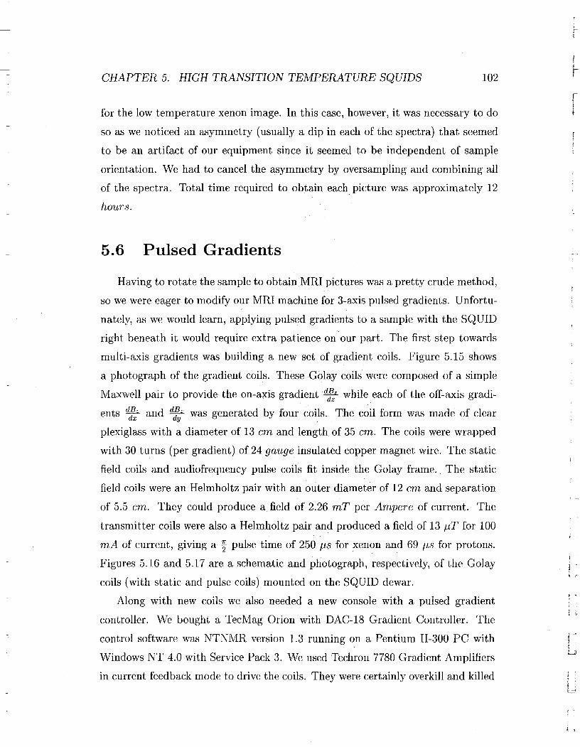
CHAPTER 5. HIGH TRANSITION TEA1PERATURE SQUIDS 102L~-

for the low temperature xenon image. In this case, however, it was necessary to do

so as we noticed an asymmetry (usually a dip in each of the spectra) that seemed

to be an artifact of our equipment since it seemed to be independent of sample

orientation. We had to cancel the asymmetry by oversampling and combining all

of the spectra. Total time required to obtain each picture was approximately 12

hours.

5.6 Pulsed Gradients

Having to rotate the sample to obtainMRI pictures was a pretty crude method,

so we were eager to modify our MRI machine for 3-axis pulsed gradients. Unfortu

nately, as we would learn, applying pulsed gradients to a sample with the SQUID

right beneath it would require extra patience on our part. The first step towards

multi-axis gradients was building a new set of gradient coils. Figure 5.15 shows

a photograph of the gradient coils. These Golay coils were composed of a simple

Maxwell pair to provide the on-axis gradient d:!zz while each of the off-axis gradi

ents d~- and dZz was generated by four coils. The coil form was made of clear

plexiglass with a diameter of 13 em and length of 35 em. The coils were wrapped

with 30 turns (per gradient) of 24 gauge insulated copper magnet wire. The static

field coils and audiofrequency pulse coils fit inside the Golay frame. The static

field coils were an Helmholtz pair with an outer diameter of 12 em and separation

of 5.5 em. They could produce a. field of 2.26 mT per Ampere of current. The

transmitter coils were also a Helmholtz pair and produced a field of 13 flT for 100

mA of current, giving a ~ pulse time of 250 flS for xenon and 69 p,s for protons.

Figures 5.16 and 5.17 are a schematic and photograph, respectively, of the Golay

coils (with static and pulse coils) mounted on the SQUID dewar.

Along with new coils we also needed a new console with a pulsed gradient

controller. We bought a TecMag Orion with DAC-18 Gradient Controller. The

control software was NTNMR version 1.3 running on a Pentium II-300 PC with

\iVindows NT 4.0 with Service Pack 3. We used Techron 7780 Gradient Amplifiers

in current feedback mode to drive the coils. They were certainly overkill and killed

rI

- ~----:- CHAPTER 5. HIGH TRANSITION TEMPERATURE SQUIDS

Figure 5.15. Photograph of Golay Coils

103


3-axis gradient coilsat coils I

static field c~z I .A-",-_-..,

\ \i'"

I '

isample

f-1.5mm

!SQUID

104

L!

L~-

(

I

_..... -----~- -

Figure 5.16. Schematic of Golay coils mounted on SQUID dewar

r "!

- ~- CHAPTER 5. HIGH TRANSITION TEMPERATURE SQUIDS 105

tIi\ ,

- ,"

Figure 5.17. Photograph of Golay coils mounted on SQUID dewar


rL~-

our coils on more than one occasion. However, they were the best bipolar power

amplifiers (to drive current both positive and negative) on the market and were

purchased with the notion that we would eventually need them for microimaging

or imaging big things, like people.

Vve made two improvements that helped cut the noise from the gradient circuits.

The first was a triggered blanking circuit connected at the output of the amplifiers

before the coils. The circuit diagram is sketched in Figure A.1 in Appendix A. A

TTL signal from the pulse programmer turned on the two transistors in the circuit

which then dumped the current from the amplifiers at the input of the circuit

to ground before the current could get to the gradient coils. The crossed diodes

insured that the low voltages due to the amplifier noise got grounded out rather

than sent to the coils.

The second modification was the set of baseline correction circuits placed at

the output of the DAC-18 gradient controller and before the inputs to the gradient

amplifier. We found that small offsets in voltage from the gradient controller on

the order of 1 mV resulted in a sizable current from the amplifiers on the order

of 10 mA passing through the gradient coils. There was an offset potentiometer

inside the gradient controller box for each of the channels x, y, and z. However

the resolutions of these variable resistors were not fine enough to cancel the offset

satisfactorily. Also there was always drift of the baseline voltage during the course

of any long acquisition, due possibly to changes in temperature. So itwas necessary

to build external circuits to cancel the drift. The circuits were simple unity gain

adding amplifiers which added a manually controlled, variable voltage from an

internal battery to the output of the gradient controller, see Figure A.2 also in

the Appendix. These baseline correction circuits also proved to be necessary to

accurately set the current amplitude of the phase encoding gradient pulse. The

TecMag system did not provide fine enough control of the small currents that we

were using.

ri

- ~ ~ CHAPTER 5. HIGH TRANSITION TEMPERATURE SQUIDS 107

f"I,I . 5.7 Hyperpolarized Xenonr •! Figure 5.18 is a spectrum of hyperpolarized xenon in a static magnetic field

of 1.27 mT, giving a resonance frequency of 14.9 kHz. The sample of naturally

abundant xenon with a pressure of 2 atm was contained in a sample tube 1.4 em

long and 0.5 em in diameter. It was optically pumped using the setup described

in Section 4.2.5 to a polarization of approximately 2%. With a single ~ pulse we

obtained a large signal-to-noise ratio (SNR) of almost 100. Unfortunately, we could

never reproduce this result. Out of the dozens of attempts, we were able to observe

only a few spectra. There are still many unanswered questions as to why we were

so unsuccessful: was the optical pumping not successful or was the polarization

lost and where was it lost? There were too many variables involved in pumping

sample in Hildebrand D-60 (the old Gamma room), freezing the sample from the

pumping cell into a suitable sample cell, running the xenon down to Hildebrand

D-45 (the old SQUID room), defrosting the sample, transferring it through the

mu-metal shield through the SQUID coils, and finally taking an NMR scan. VVe

needed a method to consistently polarize and deliver the xenon to the SQUID. SO

we built a flowing xenon, continuous optical pumping system.

5.7.1 Recirculated Flow Optical Pumping

One of the limitations that most hyperpolarized noble gas NMR. and MRI sys

tems suffer from (including our previous SQUID imager) is the non-recoverable

nature of optically pumped nuclei. Since the gas is prepared in a non-equilibrium

state, the completion of one NMR. or MR.I scan using a ~ pulse destroys the en

hanced polarization. In this so-called "batch" pumping mode, a volume (typieally

on the order of 100 mL at 100 mTorr) of optically pumped gas is prepared in

about 20 minutes. Since it is ineonvenient to wait one third of an hour between

scans while more gas is being polarized, it is possible to eolled and store a large

volume of hyperpolarized gas for later use, since it retains a high polarization for

about a day if kept in a strong magnetic field. However, unless you have hired


-::lctl--Q)

I-"0::l

:t=a.E«

108r,,!

10•

12•

14

II.

•16

I

18 20

Frequency (kHz)

Figure 5.18. Single scan of hyperpolarized xenon in a field of 1.27 rnT.

f "f-r:: CHAPTER 5. HIGH TRANSITION TEMPERATURE SQUIDS 109

f'I

_ L~

[ -

someone just to polarize gas for you, you are still spending a great deal of time

preparing the gas. Alternatively, if the sample is large and detection equipment is

very sensitive, a number of scans can be collected using small tip angle pulses. The

latter is possible in certain cases at higher frequencies or with our low transition

temperature SQUID system, but this batch mode becomes a serious restriction

for high resolution MR.I or microscopy, especially at low fields where maximum

possible signal strength is critical.

On the other hand a circular flow [154, 155, 156, 157, 158] optical pumping

system provides a continuous, stable, and infinite source of hyperpolarized xenon---

making possible the use of large tip angle pulses and signal averaging. In fact,

this ability to signal average using a circular flow hyperpolarized xenon setup was

critical in enabling Kaiser et at. [159] to obtain MR.I images with 100 J.Lrn resolution

with a 4.2 Testa imaging system.

In Figure 5.19 we schematically show our optical pumping apparatus. The cen

terpiece was the Pyrex glass pumping cell composed of parts (B), (C), and (D).

A photo of the pumping cell is shown in Figure 5.20. The rubidium reservoir (B)

supplied rubidium atoms to the irradiation bulb (C) where they absorbed circu

larly polarized light and collided with xenon, transferring the laser light angular

momentum. The water jacket (D) then cooled the gases and condensed out the ru

bidium. Parts (B) and (C) were mounted inside of an air-heated oven (not shown)

made of aluminum with a 3.2 mm, thick quartz window. The oven was built into

the center of a pair of 23 em diameter, air-cooled Helmholtz coils (A) (only one of

the pairs shown for clarity) that produced a field of 8 mT with an applied current

of 10 A. A photograph of the coils, oven, and pumping cell is shown in Figure

5.21. The xenon was circulated between the pumping cell and the sample using

a completely sealed, maintenance free, high pressure circulation pump manufac

tured by Brey, Inc (G). It was capable of a range of gas flow rates depending on

the input voltage. The sample cell (E) was a flat-bottomed, stoppered Pyrex glass

cylinder with an inner diameter of 1 em and capacity of almost 1 mL. It had 1/4

in Pyrex glass delivery tubes on opposite sides of the cell. The stopper could be

easily unscrewed to gain access to the sample. (F) was the SQUID detector. All

CHAPTER 5. HIGH TRANSITION TEMPERATURE SQUIDS 110L~ .

r!L

u.

I

«

Figure 5.19. Schematic of the Circular Flow Optical Pumping System

i- l---


Rubidiumreservoir

Illuminationbulb

Cold waterjacket

t - Figure 5.20. Photograph of Flowing Xenon Pumping Cell


Figure 5.21. Photograph of Optical Pumping Setup

112

L~-

r!


; ,itl -

I -

connections between components of the gas lines were made using standard 1/8 in

or 1/4 in teflon tubing and 1/8 in or 1/4 in brass Swagelok fittings. Permanent

brass ferrules were used for all brass/teflon tubing connections, and teflon ferrules

were used for the brass/glass connections at the ends of the optical pumping cell

and the ends of the sample cell. Finally the laser (J) was a 120 H/aft diode laser

made by Opto Power operating at the near-infrared wavelength of 795 n:m. At

first we used the Opto Power Corp. Model OPC-A100-FC/RB water-cooled diode

laser but switched to the more reliable OPC-A150-795-RPPS. The light from the

diode array was piped through fiber-optic cable, through a quarter-wave circular

polarizer (part of the laser head) and into the pumping cell (C). At full power, we

found that the beam was intense enough to melt the Pyrex glass cell, so we regu

larly operated with only half of the laser power simply by turning off four of the

eight diodes. (H) and (I) were the gas inlet valve and pressure gauge respectively.

We typically used 1 atm of natural abundance xenon, 1 atm of nitrogen gas,

and 5 atm of helium. For all of our experiments we circulated the gases at a

constant flow rate of about 0.3 cfh = 2.4 mL/s. The oven was heated to 143

°C, giving us a rubidium vapor pressure of 0.41 Po,. The sample cell was kept at

room temperature. The xenon polarization stayed constant over a 14 ho'nr period

and averaged 1-2 % on any given day. We found that this high pressure, high flow

continuous pumping method generally yielded lower xenon polarization than batch

methods; however, its advantages of "instant" and unlimited gases outweighed the

few percent loss in polarization.

5.8 Flowing Xenon with SQUID Detection

Figure 5.22 displays two spectra comparing the signal from mineral oil to hy

perpolarized xenon produced in our circular flow system. The static field applied

to the protons was 0.62 mT and 2.3 mT for xenon, meaning the Larmor frequency

was 27 kHz in both cases. Using our SQUID-based spectrometer 1 rnL of mineral

oil provides a proton NMR signal-to-noise of 2-3 after 80,000 scans. In contrast, the

same volume of hyperpolarized xenon gas at a pressure of 1 atm (roughly 10,000

CH.APTER 5. HIGH TRANSITION TElvIPERATURE SQUIDS

Proton

HyperpolarizedXenon

Iii iii iii Iii iii iii I Iii iii iii iii iii iii iii

29 27 25(kHz)

114

t _

Figure 5.22. Proton versus Hyperpolarized Flowing Xenon. The res

onance frequency was tuned to 27 kHz in both cases.

The proton spectrum required 80,000 scans and only

100 scans with a much better SNR for the xenon.

L- ~- CHAPTER 5. HIGH TRANSITION TEMPERATURE SQUIDS 115

r "I! -

r -!

times fewer nuclei), yields an SNR of 25-30 after only 100 scans. This corresponds

to a xenon polarization of approximately 1%, 7 orders of magnitude higher than

the thermal polarization. With the new circular flow optical pumping system, we

were able to acquire xenon signal with full ~ pulses, and the time required for

collection was only a few seconds. In contrast, the small mineral oil NMR signal

required approximately 2 hours.

5.8.1 Spin Warp Imaging

Two dimensional images were obtained using the standard 2D "spin warp"

pulse sequence [11]. Recall from Section 1.4 that there are two ways to traverse

the one dimensional (for 1-D projections) k space:

.... "(Gtk=

27r(5.1 )

by stepping the gradient (phase encoding) or by stepping the time (frequency en

coding). Spin-warp takes advantage of this in order to step through a 2-dimensional

k space for 2-dimensional imaging. In one gradient direction, say z, the information

is phase encoded while information from the second direction, i.e. x, is frequency

encoded. The pulse sequence is shown in Figure 5.23. The z-gradient pulse (G z )

looks like a "ladder" because it represents the fact that this gradient is incremented

(starting from a large negative amplitude) each time the sequence is run. The AF

pulse and the x gradient (Gx ) are the same for each acquisition. The switched neg

ative to positive amplitude of the x gradient gives the "gradient echo" signal shape

in the acquisition (ACQ). A walkthrough of what happens to the nuclear magneti

zation due to this pulse sequence is as follows (neglecting local effects like chemical

shift or static field inhomogeneity): first the AF pulse tips the net magnetic. mo

ment from equilibrium along z to the x-y plane where the moment precesses at the

Larmor frequency. The z-gradient is then turned on causing the individual nuclear

spins to precess at different frequencies depending on their location in space along

the z-axis. The distribution of resonance frequencies causes the spins to dephase

relative to each other, and the stronger the gradient, the greater the dephasing


rL

L~-

AFn_~si _

--------

ACO - - - - - -;.-

Figure 5.23. Spin warp pulse sequence

r-'t


r '\i-

,

!

for a given amount of time. But also during the phase encoding gradient, the x

gradient is turned on. It has the same effect as the z gradient except it modifies

the resonance frequency of spins according to position in the x direction. ·When

the z gradient is switched off, the nuclei will stop dephasing due to their distribu

tion along z. Since the x gradient is now reversed from negative to positive, the

nuclei will re-phase because the slow nuclei (lower precession frequency) will now

be the fast nuclei and vice-versa, allowing the previously "lagging" nuclei to "catch

up" to the other spins. This causes the refocusing of the magnetization and the

formation of the gradient spin echo. The signal is collected over time with the ;;:

gradient at a constant amplitude, giving the frequency encoded information. Each

time the sequence is run, the amplitude of the z gradient is set to a different value,

causing a different amount of dephasing. The information of z nuclei distribution

is encoded in the phase of the magnetization.

A full spin warp MRI collection generates a 2-D data set with time on one

axis (the directly detected dimension) and z gradient strength on the other (the

indirectly detected dimension). A straightforward 2-D Fourier transform will pro

duce the image, but care must be taken to properly convert the dimensions to end

up with distance x distance. After the Fourier transform, the units of the direct

dimension will be frequency (Hz) and of the indirect dimension will be inverse gra

dient strength (i.e. c:;). The conversion from frequency to distance was already

discussed previously. Inverse gradient strength can be converted to distance by

multiplication by the nuclear gyromagnetic ratio and the length of time that the

gradient was turned OIl.

1(em) (HZ) (1)D(em) = G T x'Y Txt Hz (5.2)

It is also necessary to calculate the bandwidth or total spread of the indirect

dimension (in units of c;:'). This is done simply by calculating the reciprocal of

the gradient step size, in other words, the reciprocal of the incremental amplitude

of the magnetic gradient. This is completely analogous to time-frequency, where

the bandwidth of the frequency domain is calculated by taking the reciprocal of

the dwell time (the time step of digitization).


5.8.2 Xenon Pictures

118

, .;,

r .,~

Throughout this thesis, as well as my graduate school career, I had always

advertised our "Hyperpolarized Xenon, SQUID-detected MRI technique" as being

important for medicine. Unfortunately, we were never licensed to work with human

or vertebrate subjects, not to mention the fact that our technology never advanced

to the point where we could take human or animal MRIs. So the closest that our

work ever came to biological subjects was the "finger spectrum" and the poorly

resolved chili pepper MRI. All of our work has been for "proof-of-principle." These

final MRI pictures are no exception; however, I personally like to think that they

have a slight biological aspect to them. Four MRI's are shown in Figures 5.24, 5.25,

5.26(a) and (b). The first two images are of hyperpolarized xenon in, what I like

to refer to as, the industrial equivalents of fat and lungs. Figure 5.24 shows xenon

in an approximately 1.5 rnm thick layer of Dow Corning High Vacuum Grease--·

a high viscosity, lipophilic lubricant not unlike body fat-coating the bottom of

our sample cell. The second image is of xenon in a triangular prism of aerogel.

Aerogel is a silicon based, low density, very high surface area, solid foam that was

selected as the industrial analog of lungs. Figures 5.26(a) and (b) are visualizations

of xenon flowing through a sample cell packed with more synthetic lung material

(aerogel).

The heart-shaped blob of vacuum grease is clearly shown in Figure 5.24. The

image has a resolution in the :1: (frequency encoded) dimension of 0.097 ern and

0.072 em in the z direction. The artery at the bottom of the image is actually the

gas delivery tube.

The rough outline of a triangle is demonstrated in Figure 5.25. The rounded

corners are due to limits of the resolution which were 0.14 em and 0.072 em in

the x and z directions, respectively. The distortions in the body of the triangle

were due partially to the difficulty in cutting a perfect prism from the very brittle

aerogel. Finally, some distortions may also have been due to flow effects of the

gas trying to get around the object. Our estimated Reynolds number given the

density of the gas and the flow rate was about 100, suggesting that the gas was in

f ~,i -

----=!---

I '

\t -

CH.A.PTER 5. HIGH TRANSITION TEMPERATURE SQUIDS 119

oLO

-E 0E-

LOC\I

I

oLO

I

-5.0 -2.5 o(mm)

2.5 5.0

Figure 5.24. Xenon MRI of Vacuum Grease


r'r

[120 I-

f=I~-

["'L

oLO

LOC\I

LOC\I

I

oLO

I -5.0 -2.5 o(mm)

2.5 5.0

I'

! '

i

1

Figure 5.25. Xenon MRI of Triangle of Aerogel

t~·~iU

f 'L


laminar flow. However, the estimate did not take into account the object (aerogel)

in the flow path. One interesting point of note is that except for possible flow

artifacts, there was no xenon signal from the gas outside of the aerogel. This was

due to the xenon adsorbing to the extensive surfaces ofthe aerogel and effectively

increasing the xenon concentration inside the aerogel compared to the surrounding

free space. We expect this to happen in real lungs, allowing the differentiation of

tissue from large empty pockets without any extra work.

Figures 5.26(a) and (b) are MRIs of xenon flowing through a sample cell packed

with aerogel, taken with two different exposure times. This quasi-stroboscopic pho

tography was takes advantage of the non-equilibrium nature of optical pumping.

In our spin warp imaging pulse sequence we apply a 1r12 pulse which transfers the

xenon magnetization to the transverse plane. After the pulse the enhanced po

larization has been used up. Therefore the next 1r12 pulse will only read the new

xenon that has entered the sample since the last excitation pulse. Visualization

pictures of the xenon flow can be obtained by varying the time between scans (i.e.

the recycle delay). Figure 5.26(a) shows the xenon penetration into the aerogel

after 0.5 seconds. Figure 5.26(b) shows the increased travel of the xenon after 2

seconds. The only difference in imaging procedure between the two pictures is the

wait time between scans.

The SQUID used for these experiments was the high noise (160 Jfiz) "flip chip"

magnetometer described in Section 3.5.2. All images were collected in a static field

strength of 2.5 rnT, corresponding to a xenon Larmor frequency of 29.6 kHz. This

resonance frequency was chosen because it was the lowest frequency outside of

the SQUID's low frequency intrinsic noise (1/f noise) that was also in a region

less inundated with electrical noise from the laboratory surroundings than slightly

lower frequencies. The phase encoded gradient was the dBzldz gradient, and the

frequency encoded dimension was in the x direction. For the first image that we

show, Figure 5.24, the magnitude of the x gradient was 8 p,Tlcrn. The maximum

z gradient amplitude was 3 ,J,T1crn with a step size of 0.2 ,J,T1crn. The gradient

pulse length was 42 ms. We collected 32 slices of 8192 points with a dwell time of

12.5 p,s. Each slice was signal-averaged 400 times with a 2 second delay between

CHAPTER 5. HIGH TRANSITION TElVIPERATURE SQUIDS 122

rI~

r

(a)

5.02.5o(mm)

-2.5-5.0

LOC\J

LOC\J

I

oLri

I

...-..EoE..........

LOC\i

...-..EoE..........

L!':!C\J

I

0Lri

I

-5.0 -2.5 0 2.5 5.0(b) (mm)

0LO

Figure 5.26. Visualization of Xenon Flow through Aerogel

[I

- ~- CHAPTER 5. HIGH TRANSITION TEJvlPERATURE SQUIDS 123

scans. The second image, Figure 5.25, had slightly different collection conditions.

The z gradient was the same as the first image, but the x gradient was stronger

with a magnitude of .011 mT/cm. We collected 32 slices of 4096 points with a

dwell time of 12.5 f..J,S. We averaged 400 scans per slice also with a 2 second delay

between scans. Finally the last two images were collected with the same settings

as the first image except for the scan delay which was 0.5 s for Figure 5.26(a) and

2 S for (b) as previously described.

5.9 The Unfulfilled Promise

Each of the last four xenon images required 8 to 12 hours to collect. The long

acquisition times were due to the very high noise of the SQUID magnetometer,

the long recycle delay, and the high number of averages. Although the bulk gas

flow rate would refresh the volume of an empty sample cell in about 500 rns, the

presence of the sample effectively slowed the passage of the xenon, and we were

forced to use the 2 s delay. Furthermore, we were limited in the magnitude of the

z gradient that we could apply. Gradients stronger than 0.003 mT/ em would force

a significant amount of magnetic flux through the SQUID, making it difficult to

operate. In order to obtain the millimeter resolutions, we increased the gradient

pulse length. The consequence of this was a decreased signal amplitude from spin

relaxation by the time we were actually collecting signal. Fortunately we had a

circular flow system that enabled us to average for as long as we needed to complete

the images. The large collection times (as well as the 2 mT static field) do not

reflect the true potential of combining circular flow optical pumping with SQUID

detection.

Following Greenberg's formalism [160], we can estimate the signal-to-noise ratio

of various NMR experiments using standard inductive detection. If one were to

use a spectrometer that gives an SNR of 100 in one pulse for 1 mL of water at 1 T,

the SNR of the same water sample in 0.05 mT (Earth's field) would be 7 x 10-5 ,

requiring 200 million signal averages just to get an SNR of 1. Now, if one were

to take a single NMR scan of 1 mL of 1 atm of gaseous xenon at Earth's field,

CHAPTER 5. HIGH TRANSITION TEA-IPERATURE SQUIDS 124

f

i!

one would find that the lower gyromagnetic ratio of xenon coupled with the fewer

number of nuclei (gas compared to liquid) would drop the SNR down to around

1.2 x 10-10 , requiring a whopping 64 x 1018 averages to get an SNR of 1. But, if

one were to optically pump the xenon to a polarization of a modest 1% the signal

for just a single scan would be 2 billion times larger than the non-hyperpolarized

xenon. Unfortunately, that SNR is still only 1/4. That is where better detection

equipment could improve the picture.

It is easy to calculate the signal-to-noise ratios for the same cases as above

but using a low-Tc SQUID or a good high-Tc' SQUID, where a white noise of 1

fT / H Zl/2 is achievable, instead of a standard coil. Assuming identical experimen

tal conditions of temperature, sample size, and filling factor, one finds that water

at 1 T gives an SNR of about 400. A single pulse on water at Earth's field would

give an SNR of 0.04, only 625 scans away from unity SNR.. Gaseous xenon ther

mally polarized at 0.05 rnT gives a still miniscule SNR of 1.5 x 10-7, corresponding

to 44 x 1012 averages to get to an SNR of 1. Using xenon hyperpolarized to 1%

again increases the signal by a factor of 2 billion, meaning a SQUID would see

an SNR of 300 in only one scan. That is better at Earth's field than the 1 Tesla

proton imagers in hospitals today.

rj

5.10 High-Tc SQUID Spectroscopy

This final section describes some of the successful spectroscopy accomplished

with the high-TcSQUID instrument. These include NMR signal from phosphorous

31 in phosphoric acid as well as proton and fluorine signal detected simultaneously

from a sample of trifluoroacetic acid. We were also able to observe a dynamic

nuclear polarization (DNP) enhanced proton signal, and finally I present the first

ultra low field observation of chemical shift. In a static field of only 2.54 rnT

we were able to resolve (hyperpolarized) gaseous xenon from xenon adsorbed to

polypropylene. The chemical shift of about 200 pprn is only 4.6 Hz compared to

the free gas xenon Larmor frequency of 30.07 kHz.

! .\ .


5.10.1 Thermally Polarized Nuclei

125

f ., One of the distinct advantages of our low field NMR system with SQUID de

tection was that we could change the strength of the static magnetic field by a.

quick turn of the knob on the power supply that charged the coils. Furthermore,

the SQUID magnetometer was a broadband, untuned detector that allowed us to

work with different nuclei without modifying our setup. Previously shown spectra

included thermally polarized proton signal and optically polarized xenon signal.

Figure 5.27 is a spectrum of thermally polarized .31 P in 1 mL of phosphoric acid.

The static field of 2.35 mT corresponded to a Larmor frequency of 40 kHz. The

peak had a low SNR of about 2:1 and already required 400,000 signal averages.

Figure 5.28 is an NMR spectrum of 1 mL of 2,67 1\11 deuterated trifluoroacetic

acid in water. We were able to excite both the 1Hand 19F nuclei with a pulse

whose frequency was centered between the resonance frequencies of the two nuclei.

We were also able to then simultaneously detect both nuclei. The static field of

1.98 mT gave resonance frequencies for the protons and the fluorines of 84.3 kHz

(left) and 79.3 kHz (right) respectively. 40,000 scans were acquired to produce

the spectrum.

5.10.2 Dynamic Nuclear Polarization

Figure 5.29 shows two proton spectra. Although they are of the same sample,

in the same static magnetic field and with the same number of averages, the spec

tra have different peak amplitudes. Figure 5.29(a) shows the NMR signal from

thermally polarized protons in mineral oil, whereas (b) demonstrates the signal

enhancement from a technique known as dynamic nuclear polarization (DNP).

DNP takes advantage of the fact that the electron gyromagnetic ratio is roughly

three orders of magnitude larger than nuclear gyromagnetic ratios; therefore, the

thermal equilibrium electron polarization is larger than nuclear spin polarizations

by the same amount. This larger polarization can be partially transferred to nu

clear spins simply by exciting the electronic spins. As the excited free electrons

in the sample relax to equilibrium, they cause spin flips in the "nuclear lattice"


r!

f

-.

a.E«

39 40Frequency (kHz)

41

Figure 5.27. Phosphorous-31 NMR in Phosphoric Acid

I '----,L- t-

f "

t" L


-

a.E<t:

127

89I

82Frequency (kHz)

75

Figure 5.28. Simultaneous Proton and Fluorine NMR

rL

CHAPTER 5. HIGH TRANSITION TElV/PERATURE SQUIDS 128L~ .

f

Lf!!

-~ N0 I~ .::£ i

---

-~ No I~ .::£---

-.0---

-CCI---------------_............. ~

Figure 5.29. Dynamic Nuclear Polarization Enhancement. (a) show

non-enhanced proton signal. (b) DNP enhanced proton

signal.

r "L


r~,f - that they are coupled to. This transfer of electronic spin polarization to nuclear

spin polarization via the relaxation of the excited electronic spins is known as the

Overhauser effect [161, 162, 8].

DNP is actually similar in some respects to spin exchange opt.ical pumping

in that polarization is transferred from excited electronic spins to nuclear spins.

The big differences are first in the method of electronic excitation and secondly in

the coupling between the electrons and the nuclei. Spin exchange optical pump

ing excites the valence electrons in an alkali metal electrically and magnetically

by light absorption; whereas, DNP excites unpaired electrons only magnetically

by manipulating the electron spin resonance (ESR) by radiofrequency pulses (or

higher frequency microwave pulses) the same way that nuclear spins are excited

in NMR. The other difference between OP and DNP is that DNP's spin cross re

laxation Overhauser effect relies on electron-nuclear spin flip-flops by dipole-dipole

coupling, scalar (j) coupling or a combination of the two. OP relies on the Fermi

contact hyperfine coupling during the collision between the alkali metal a.nd the

noble gas; since the polarization transfer is still due to relaxation of the electrons,

this is still the Overhauser effect, but with a more specific mechanism. Optical

pumping can produce much higher polarizations than DNP, but DNP is useful

since only a few systems can be optically pumped efficiently.

The sample we used was a 10 rnM solution of 4-amino 2,2,6,6-tetramethyl-1

piperdinyloxyl (TEMPO, a stable free radical commonly used in ESR) in mineral

oil. In a static magnetic field of 2.37 rnT, the proton resonance frequency was

101.5 kHz and the 7r16 ESR transition [163] was at 116.4 illH z. We excited the

electron resonance with a transmitter coil built expressly for this purpose. It was a

Helmholtz pair 9.5 ern in diameter and separation of 4.75 em placed adjacent to the

nuclear excitation coils. It was tuned to 116 NIHz by addition of a 30 pF Polyflon

tuning capacitor soldered in series. The input circuit to the coils contained a PTS

500 frequency synthesizer gated to form pulses by mixing the continuous wave with

a TTL pulse from the TecMag Orion using a simple MiniCircuits ZAD-IH mixer.

The RF pulses were fed to an ENI 5100L RF Power Amplifier and then to the

excitation coil. To obtain the DNP enhanced signal, the electrons of the TEMPO


Li,

Lf-

were excited just before the NMR signal was collected. For the factor of 2 gain

in signal, only 1 watt of power was applied to the electrons. More power will in

general provide larger signal enhancements. However, any more than 1 watt of.

power pulsed to the RF coils caused the SQUID detector to become unstable and

unusable.

5.10.3 Ultra Low Field Chemical Shift

Finally Figure 5.30 presents the first observed chemical shift in the weak static

field of 2.54 mT. Chemical shift is one of the most important pieces of analytical

chemical information for NMR spectroscopists. However, no one has previously

detected an NMR chemical shift in the weak fields that we operate in. One of the

reasons is that the naturallinewidth (due to transverse relaxation, in other words

T 2) of the most commonly studied NMR nuclei, protons and carbon, is larger than

the chemical shift range of these nuclides in the majority of molecules (not to rule

out extraordinary samples) at such low fields. What allowed us to see ultra low

field chemical shift was the use of xenon, and in particular, flowing hyperpolar

ized xenon. First of all, xenon has a wide chemical shift range due to its large

and polarizable electron cloud, see for example reference [37]. Being a noble gas,

xenon generally has a long relaxation time since it interacts only weakly with most

materials. The narrow naturallinewidth (from the slow relaxation) in conjunction

with the large chemical shift range make xenon uniquely suited for low field NMR

spectroscopy. However, the low fields also mean small polarizations and signals,

but the long relaxation times make signal averaging impractical. This was another

situation where the circular flow optical pumping apparatus really proved its use

fulness. Not only was signal enhanced by the optical pumping, but signal averaging

was possible since the hyperpolarized gas was constantly replenished. Figure 5.30

features a respectable signal-to-noise in only 2000 scans on a small sample volume

of 0.03 mL. The Larmor frequency of the free xenon was 30.070 kHz while the

resonance frequency of the xenon adsorbed to the powdered polypropylene was

about 30.075 kHz. This corresponds to a 200 ppm chemical shift.

riI

fI

r '

- l-

f'

Ir "!,


30.100 30.069Frequency (kHz)

30.038

i _

f_ l _

_ I.

Figure 5.30. Ultra low field xenon NMR showing chemical shift. The

lower frequency peak is from free xenon while the higher

frequency peak is from xenon adsorbed to polypropy

lene.


~I

One might ask the question, "Besides zero field NQR, why bother with NMR

spectroscopy in low fields?" Stronger fields provide larger magnetizations, better

spectrometer sensitivity, and higher spectral resolution. Magnetic resonance imag

ing in low fields might be useful but not magnetic resonance spectroscopy. Perhaps

ultra low field NMR cannot compete with high field NMR spectroscopy. But low

field JVIRI can only become a more beneficial technique if analytical information

can be gained with the same equipment and at the same time. The ability to

distinguish between different nuclides (like the proton and fluorine) or between

xenon in different physiochemical environments during an MRI scan would be in

credibly powerful. The possibilities include not only nuclide selective or chemical

shift selective imaging but perhaps in vivo diagnostics and immunoassays as well.

r!

['

L- ~-

f'

Ir .!

- ~

133

Bibliography

[1] E. Fukushima and B.W. Roeder. Experimental Pulse NMR: A Nuts and Bolts

Approach. Addison-Wesley Pub. Co., Advanced Book Program, Reading,

MA,1981.

[2] E.L. Hahn. Spin echoes. Physical Review, 80(4):580--594, 1950.

[3] T.P. Das and E.L. Hahn. Nuclear Quadrupole Resonance SpectT'OscoPY, vol

ume 1 of Solid State Physics. Supplement. Academic Press, New York, 1958.

[4] A. Abragam. Principles of Nuclear Magnetism. Oxford University Press,

1961.

[5] M. Mehring. High Resolution NMR Spectroscopy in Solids. Springer, Berlin,

2nd edition, 1983.

[6] RR Ernst, G. Bodenhausen, and A. Wokaun. Principles of Nuclear Mag

netic Resonance in One and Two Dimensions. Oxford, 1994.

[7] L. Emsley, D.D. Laws, and A. Pines. Lectures on pulsed NMR In B. JVlar

aviglia, editor, Proceedings of the International School of Physics "Enrico

Fermi", Magnetic Resonance and Brain Function: Approaches from Physics,

pages 45-210. Societa Italiana di Fisica, 3rd edition, 1999.

[8] C.P. Slichter. Principles of Magnetic Resonance. Springer-Verlag, Berlin,

·3rd edition, 1996.

[9] P.C. Lauterbur. Image formation by induced local interactions-examples

employing nuclear magnetic resonance. Nature, 242(5394):190-191, 1973.

BIBLIOGRAPHY 134

fL~-

[10] P. Mansfield and P.K. Grannell. NMR diffraction in solids. Journal of Physics

C-Solid State Physics, 6(22):L422-L426, 1973.

[11] P.T. Callaghan. Principles of Nuclear Magnetic Resonance MicTOscopy. Ox

ford, 1991.

[12] P.C. Lauterbur. Magnetic resonance zeugmatography. Pure and Applied

Chemistry, 40(1-2):149--157, 1974.

[13] A.N. Garroway, P.K. Grannell, and P. Mansfield. Image formation in NMR.

by a selective irradiative process. Journal of Physics C-Solid State Physic8,

7(24):L457-L462, 1974.

[14] G.L. Brownell, T.F. Budinger, P.C. Lauterbur, and P.L. McGeer.

Positron tomography and nuclear magnetic resonance nnagmg. Science,

215(4533):619-626, 1982.

[15] D.G. Gadian. Nuclear Magnetic Re80nance and its Application to Living

Systems. Oxford University Press, Oxford, 1982.

[16] P. Mansfield and P.G. Morris. NMR Imaging in Biomedicine. Academic

Press, New York, 1982.

[17] T.F. Budinger and P.C. Lauterbur. Nuclear magnetic resonance technology

for medical studies. Science, 226(4672):288-298, 1984.

[18] P.C. Lauterbur. NMR images of microscopic flow. Nature, 336(6197):310,

Nov 1988.

[19] F.W. Wehrli. From NMR diffraction and zeumatography to modern imaging

and beyond. Prog. NMR Spectrosc., 28:87-135,1995.

[20] T.M. de Swiet. Diffusive edge enhancement in imaging. Journal of Magnetic

Resonance, 109(1):12-18, Oct 1995.

[21] YXia. Contrast in NMR imaging and microscopy. Concepts in Magnetic

Resonance, 8:205-225, 1996.

ri

['L

- ~- BIBLIOGRAPHY 135

r "Ir ~

!t -

,r -

I .

- r-~

[22] W.S. Price. NMR imaging. Annual Reports on NMR Spectroscopy, 35:140

191, 1998.

[23] A. Mohoric, J. Stepisnik, M. Kos, and G. Planinsic. Self-diffusion imaging

by spin echo in Earth's magnetic field. Journal of Magnetic Resonance,

136(1):22-26, Jan 1999.

[24] M. Gatzke, G.D. Cates, B. Driehuys, D. Fox, VV. Happer, and B. Saam.

Extraordinarily slow nuclear-spin relaxation in frozen laser-polarized Xe-129.

Physical Review Letters, 70(5):690-693, Feb 1993.

[25] A. Kastler. Quelques suggestions concernant la production optique et la

detection optique dune inegalite de population des niveaux de quantification

spatiale des atomes--application a lexperience de stern et gerlach et a la

resonance magnetique. Journal de Physique et Ie Radium, 11(6):255--265,

1950.

[26] J. Brossel, A. Kastler, and J. Winter. Creation optique dune inegalite de

population entre les sous-niveaux zeeman de letat fondamental des atomes.

Journal de Physique et Ie Radium, 13(12):668, 1952.

[27] J. Brossel, B. Cagnac, and A. Kastler. Resonance magnetique sur des atomes

orientes optiquement. Journal de Physique et Ie Radium, 15(1):6-8, 1954.

[28] A. Kastler. Optical methods of atomic orientation and of magnetic resonance.

Journal of the Optical Society of America, 47(6):460-465, 1957.

[29] A. Kastler. Methodes optiques de production et de detection des moments

magnetiques longitudinaux Mz et transversaux Mt dune collection datomes.

Physica, 33(1):73, 1967.

[30] R.J. McNeal. Disorientation cross sections in optical pumping. The Journal

of Chemical Physics, 37, 1962.

[31] R.M. Herman. Noble-gas-induced rubidium spin disorientation. Physical

Review, 136(6A):A1576-A1582, 1964.

BIBLIOGRAPHY 136

[32] R.M. Herman. Theory of spin exchange between optically pumped rubidium

and foreign gas nuclei. Physical Review, 137(4A):A1062-A1065, 1965.

[33] C.C. Bouchiat, M.A. Bouchiat, and L.C. Pottier. Evidence for R.b-rare-gas

molecules from the relaxation of polarized Rb atoms in a rare gas. Theory.

Physical Review, 181(1):144-165, May 1969.

[34] M.A. Bouchiat, J. Brossel, and L.C. Pottier. Evidence for Rb-rare-gas

molecules from the relaxation of polarized Rb atoms in a rare gas. Exper

imental results. The Journal of Chemical Physics, 56(7):3703---3714, Apr

1972.

[35] M.A. Bouchiat, T.R. Carver, and C.M. Varnum. Nuclear polarization in

He-3 gas induced by optical pumping and dipolar exchange. Physical Review

Letters, 5(8):373-375, 1960.

[36] B.C. Grover. Noble-gas NMR detection through noble-gas-rubidium hyper

fine contact interaction. Physical Review Letter-s, 40(6):391---392, Feb 1978.

[37] T. Pietrass and H.C. Gaede. Optically polarized 129Xe in NMR spectroscopy.

Advanced Materials, 7(10):826-838, 1995.

[38] Y.Q. Song, B.M. Goodson, and A. Pines. NMR and MRI usmg laser

polarized xenon. Spectroscopy, 14(7):26-33, Jul 1999.

[39] B.M. Goodson. Using injectable carriers of laser-polarized noble gases for

enhancing NMR and MR.!. Concepts in Magnetic Resonance, 11(4):203--223,

1999.

[40] B.M. Goodson. Nuclear Magnetic Resonance of Laser--Polar-ized Noble Gases

in Molecules, Mater-ials, and Or-ganisms. PhD thesis, University of California,

Berkeley, 1999.

[41] F.D. Colegrove, L.D. Schearer, and G.K. Walters. Polarization of He-3 gas

by optical pumping. Physical Review, 132(6):2561-2572, 1963.

r-,

!L


r~

Ir 'i

[42] RL. Gamblin and T.R. Carver. Polarization and relaxation processes in

He-3 gas. Physical Review, 138(4A):A946, 1965.

[43] M. Leduc, F. Laloe, and J. Brossel. Optical pumping of Ne-21. Comptes

Rendus Hebdomadaires des Seances de L 'Academie des Sciences Serie B,

271(5):342, 1970.

[44] A. Noel, M. Leduc, and F. Laloe. Orientation of excited levels of Ne-21 by

optical pumping in a discharge. Comptes Rendus Hebdomadaires des Seances

de L 'Academie des Sciences Serie B, 274(1):77, 1972.

[45] S.E. Barrett, R Tycko, L.N. Pfeiffer, and K.W. "Vest. Directly detected nu

clear magnetic resonance of optically pumped GaAs quantum wells. Physical

Review Letters, 72:1368-1372, 1994.

[46] R Tycko and J.A. Reimer. Optical pumping in solid state nuclear magnetic

resonance. Journal of Physical Chemistry, 100:13240-13250, 1996.

[47] T. Pietrass, A. Bifone, T. Room, and E.L. Hahn. Optically enhanced high

field NMR of GaAs. Physical Review B, 53:4428-4433, 1996.

[48] R Tycko. Optical pumping in indium phosphide: P-31 NMR measurements

and potential for signal enhancement in biological state NMR Solid State

Nuclear Magnetic Resonance, 11:1-9, 1998.

[49] T. Pietrass and M. Tomaselli. Optically pumped NMR in CdS single crystals.

Physical Review B, 59:1986-1989, 1999.

[50] J.C. Campara, RP. Frueholz, and C.H. Volk. Inhomogeneous light shift in

alkali-metal atoms. Physical Review A, 27(4):1914-1924, 1983.

[51] H.W. Long. Applications of Highly Spin-Polarized Xenon in NMR. PhD

thesis, University of California, Berkeley, 1993.

BIBLIOGRAPHY 138

[52] W. Happel', E. Miron, S. Schaefer, D. Schreiber, W.A. van vVijngaarden,

and X. Zeng. Polarization of the nuclear spins of noble-gas atoms by spin

exchange with optically pumped alkali-metal aroms. Physical Review A,

29(6):3092-3110, 1984.

[53] N.D. Bhaskar, W. Happel', and T. McClelland. Efficiency of spin exchange

between rubidium spins and Xe-129 nuclei in a gas. Physical Review Letters,

49(1):25--28, 1982.

[54] T.G. Walker and W. Happel'. Spin-exchange optical pumping of noble-gas

nuclei. Reviews of Modern Physics, 69(2):629--642, April 1997.

[55] B. Larson, O. Hausser, P.P.J. Delheiji, D.M. Whittal, and D. Thiessen. Opti

cal pumping of Rb in the presence of high-pressure He-3 buffer gas. Physical

Review A, 44(5), Sep 1991.

[56] G.D. Cates, RJ. Fitzgerald, A.S. Barton, P. Bogorad, M.Gatzke, N.R New

bury, and B. Saam. Rb- 129Xe spin-exchange rates due to binary and three

body collisions at high Xe pressures. Physical Review A, 45(7):4631-4639,

Apr 1992.

[57] T.G. Walker. Estimates of spin-exchange parameters for alkali-metal noble

gas pairs. Physical Review A, 40(9):4959-4963, Nov 1989.

[58] RC. Jaklevic, J. Lambe, A.H. silver, and J.E. Mercereau. Quantum inter

ference effects in Josephson tunneling. Physical Review Letters, 12:159--160,

1964.

[59] E.P. Day. Detection of NMR using a Josephson-junction magnetometer.

Physical Review Letters, 29:540, 1972.

[60] RV. Chamberlin, L.A. Moberly, and O.G. Symko. High-sensitivity mag

netic resonance by SQUID detection. Journal of Low Ternperatur-e Physics,

35(3/4):337-347, 1979.

L

1 -

BIBLIOGRAPHY 139

r -!r _

[61] J. Clarke. Superconducting quantum interference devices for low frequency

measurements. In B. Schwartz and S. Foner, editors, Superconductor Ap

plications: SQUIDs and Machines, chapter 3, pages 67--124. Plenum Press,

New York, 1977.

[62] T. Van Duzer and C.W. Turner. Principles of Superconductive Devices and

Circuits. Elsevier North Holland, New York, 1981.

[63] T. Ryhansen, H. Seppa, R Ilmoniemi, and J. Knuutila. SQUID magnetome

ters for low-frequency applications. Journal of Low Tempemture Physics,

76:287-386, 1989.

[64] A. Barone, editor. Principles and Applications of Superconducting Quantum

Interference Devices. World Scientific Publishing Company, Singapore, 1992.

[65] H. Weinstock and RW. Ralston, editors. The New Superconducting Elec

tronics. Kluwer Academic Publishers, Dordrecht, 1993.

[66] H. Weinstock, editor. SQUID Sensors: Fundamentals, Fabrication and Ap

plications. Kluwer Academic Publishers, Netherlands, 1996.

[67] J. Bardeen, L.N. Cooper, and J.R Schrieffer. Microscopic theory of super

conductivity. Physical. Review, 106(1):162-164, 1957.

[68] J. Bardeen, L.N. Cooper, and .l.R Schrieffer. Theory of superconductivity.

Physical Review, 108(5):1175-1204, 1957.

[69] E.A. Lynton. Superconductivity. John Wiley and Sons Inc., New York, 1962.

[70] RP. Feynman, RB. Leighton, and M. Sands. The Feynrnan Lect'ltres on

Physics, volume III. Addison-Wesley, Reading, MA, 1963.

[71] M. Tinkham. Introduction to Superconductivity. McGraw-Hill, New York,

·1975.

[72] F. London. Superjluids, volume I. John Wiley and Sons, Inc., New York,

1950.

BIBLIOGRAPHY 140

rr

[73] B.D. Josephson. Possible new effects in superconductive tunneling. Physics

Letters, 1:251-253, 1962.

[74] B.D. Josephson. Supercurrents through barriers. Advances zn Physics,

14:419-451, 1965.

[75] B.D. Josephson. Weakly coupled superconductors. In R.D. Parkes, editor,

Superconductivity, volume I. Marcel Dekker, New York, 1969.

[76] V. Ambegaokar and A. Baratoff. Tunneling between superconductors. Phys

ical Review Letters, 10:486-491, Jun 1963.

[77] V. Ambegaokar and A. Baratoff. Tunneling between superconductors. Phys

ical Review Letters, 11, .luI 1963.

[78] J. Clarke. SQUID Fundamentals. In H. Weinstock, editor, SQUID Sensors:

Fundamentals, Fabrication and Applications, pages 1-62. Kluwer Academic

Publishers, Netherlands, 1996.

[79] D.M. TonThat. DC SQUID Spectrometers for Nuclear Quadrupole and Low

Field Nuclear Magnetic Resonance Spectroscopy. PhD thesis, University of

California, Berkeley, 1998.

[80] M.B. Ketchen and J.M. Jaycox. Ultra-low noise tunnel junction dc SQUID

with a tightly coupled planar input coil. Applied Physics Letters, 40:736--738,

1982.

[81] J.M. Jaycox and M.B. Ketchen. Planar coupling scheme for ultra low noise

dc SQUIDs. IEEE Transactions on Magnetism, MAG-17:400--403, 1981.

[82] H.H. Zappe and B.S. Landman. Experimental investigation of resonances

in low-Q Josephson interferometer devices. Journal of Applied Physics,

49(7):4149-4154, 1978.

rL

r'-

! -

-r-= BIBLIOGRAPH}" 141

f '

i

[83] K. Enpuku, S. Kohjiro, and K. Yoshida. Noise characteristics of a de

SQUID with a resistively shunted inductance. Journal of Applied Physics,

60(12):4218-4223, 1986.

[84] S. Kohjiro, K. Enpuku, K. Yoshida, and K. Yamafuji. Experimental study of

noise characteristics oflarge-jJ dc SQUID with resistively shunted inductance.

Japanese Joumal of Applied Physics, 27(10):1871, 1988.

[85] .J.E. Zimmerman. Sensitivity enhancement of superconducting quantum in

terference devices through the use offractional-turn loops. Joumal of Applied

Physics, 42:4483-4487, 1971.

[86] F. Ludwig, E. Dantsker, R Kleiner, D. Koelle, .J. Clarke, S. Knappe,

D. Drung, H. Koch, N.M. Alford, and T.W. Button. Integrated high T c

multiloop magnetometer. Applied Physics Letters, 66(11):1418-1420, Mar

1995.

[87] F. Ludwig, E. Dantsker, D. Koelle, R Kleiner, A.H. Miklich, D.T. Nemeth,

.J. Clarke, D. Drung, S. Knappe, and H. Koch. High-Tc multilayer magne

tometers with improved l/f noise. IEEE Transactions on Applied Supercon

ductivity, 5(2):2919-2922, .Jun 1995.

[88] F. Ludwig, D. Koelle, E. Dantsker, D.T. Nemeth, A.H. Miklich, .J. Clarke,

and RE. Thomson. Low noise YBa2Cu307-x / SrTi03 / YBa2Cu307-x

multilayers for improved superconducting magnetometers. Applied Physics

Letter's, 66(3):373-375, 1995.

[89] .J.E. Zimmerman, P. Thiene, and .J.T. Harding. Design and operation of sta

ble rf-based superconducting point-contact quantum devices, and a note on

the properties of perfectly clean metal contacts. Journal of Applied Physics,

41:1572-1580, 1970.

[90] D. Drung, R Cantor, M. Peters, H..J. Scheer, and H. Koch. Low-noise high

speed dc superconducting quantum interference device magnetometer with

BIBLIOGRAPHY 142l~ .

simplified feedback electronics. Applied Physics Letters, 57(4):406-408, Jul

1990.

[91] D. Drung, H. Matz, and H. Koch. A 5-MHz bandwidth SQUID magne

tometer with additional positive feedback. Review of Scient~fic Instruments,

66(4), Apr 1995.

[92] G.N. Hounsfield. Computerized transverse axial scanning (tomography). 1.

description of system. British Journal of Radiology, 46(552):1016-1022, 1973.

[93] M.S. Albert, G.D. Cates, B. Driehuys, W. Happer, B. Saam, C.S. Springer,

and A. Wishnia. Biological Magnetic-Resonance-Imaging using laser polar

ized Xe-129. Nature, 370(6486):199-·201, July 1994.

[94] Y.Q. Song, H.C. Gaede, T. Pietrass, G.A. Barrall, G.C. Chingas, M.R Ayers,

and A. Pines. Spin-polarized Xe-129 gas imaging of materials. Journal of

Magnetic Resonance, 115(1):127130, Jul 1995.

[95] H. Middleton, RD. Black, B. Saam, G.D. Cates, G.P. Cofer, R Guenther,

W. Happer, L.W. Hedlund, G.A. Johnson, K. Juvan, and J. Swartz. MR

imaging with hyperpolarized He-3 gas. Magnetic Resonance in Medicine,

33(2):271-275, Feb 1995.

[96] P. Bachert, L.R Schad, M. Bock, M.V. Knopp, M. Ebert, T. Grossman,

W. Heil, D. Hoffmann, R Surkau, and E.W. Otten. Nuclear magnetic reso

nance imaging of airways in humans with use of hyperpolarized He-3. Mag

netic Resonance in Medicine, 36(2):192-196, Aug 1996.

[97] G. Navon, Y.Q. Song, T. Room, S. Appelt, RE. Taylor, and A. Pines. En

hancement of solution NMR and MRI with laser-polarized xenon. Science,

271(5257):1848-1851, Mar 1996.

[98] M.S. Albert and D. Balamore. Development of hyperpolarized noble gas

MRI. Nuclear Instrments and Methods in Physics Research Section A,

402:441-453, 1998.

ft

rL


r-';,l - [99] H.C. Seton, D.M. Bussell, J .M.S. Hutchison, and D.J. Lurie. Use of a dc

SQUID receiver preamplifier in a low-field MRI system. IEEE Transactions

on Applied Superconductivity, 5(2):3218--3221, Jun 1995.

[100] H.C. Seton, J.M.S. Hutchison, and D.M. Bussell. A 4.2 K receiver coil and

SQUID amplifier used to improve the SNR of low-field magnetic resonance

images of the human arm. Measur'ement Science (1 Technology, 8(2): 198-207,

Feb 1997.

[101] H.C. Seton, J.M.S. Hutchison, and D.M. Bussell. A tuned SQUID amplifier

for MRI based on a DOlT flux locked loop. IEEE Transactions on Applied

Superconductivity, 7(2):3213-3216, Jun 1997.

[102] M. P. Augustine, A. Wong-Foy, J. L. Yarger, M. Tomaselli, D. M. TonThat,

J. Clarke, and A, Pines. Low field magnetic resonance images of polarized

noble gases obtained with a dc superconducting quantum interference device.

Applied Physics Letters, 72(15):1908--1910, 1998.

[103] B. Saam, N. Drukker, and W. Happer. Edge enhancement observed with

hyperpolarized He-3. Chemical Physics Letters, 263(3-4):481--487, Dec 1996.

[104] C.H. Tseng, G.P. Wong, V.R Pomeroy, RW. Mail', D.P. Hinton, D. Hoff

mann, RE. Stoner, F.W. Hersman, D.G. Cory, and RL. vValsworth. Low

field MRI of laser polarized noble gas. Physical Review Letters, 81(17):3785

3788, Oct 1998.

[105] M. Albert, A. Venkatesh, A. Zhang, C.H. Oh, F. Jolesz, L. Kubatina, and

D. Balamore. Vey low-field hyperpolarized noble gas MRJ in vivo. In 41st E.7;

perimental Nuclear Magnetic Resonance Conference, Asilomar, CA, number

Poster 205 in Biomedical, Apr 2000.

[106] M.P. Augustine and KW. Zilm. Optical pumping magnetic resonance in high

magnetic fields: Characterization of nuclear relaxation during pumping. The

Journal of Chemical Physics, 105(8):2998-3011, 1996.

BIBLIOGRAPHY 144

rIL~-

[107] M.P. Augustine and K.W. Zilm. Optical pumping magnetic resonance in

high magnetic fields: Characterization of the optical properties of Rb-Xe

mixtures. Molecular Physics, 89(3):737-752, 1996.

[108] M.P. Augustine and K.W. Zilm. Optical pumping magnetic resonance in

high magnetic fields: Measurement of high field spin exchange cross sections.

Chemical Physics Letters, 280(1-2):24-30, 1997.

[109] D.M. TonThat, M. Ziegeweid, Y.Q. Song, E.J. Munson, S. Appelt, A. Pines,

and J. Clarke. SQUID detected NMR of laser-polarized xenon at 4.2 K and

at frequencies down to 200 Hz. Chemical Physics Letters, 272(3-4):245-249,

Jun 1997.

[110] W.A. Nierenberg, N.F. Ramsey, and S.B. Brody. Measurements of nuclear

quadrupole moment interactions. Physical Review, 70:773, 1946.

[111] 1.1. Rabi, S. Millman, P. Kusch, and J.R. Zacharias. The molecular beam res

onance method for measuring nuclear magnetic moments. PhY8ical Review,

55:526, 1939.

[112] M. Bloom and R.E. Norberg. Transient nuclear induction signals associated

with pure quadrupole interactions. Physical Review, 93:638-639, 1954.

[113] E.L. Hahn and B. Herzog. Anisotropic relaxation of quadrupole spin echoes.

Physical Review, 93:639-640, 1954.

[114] M. Bloom, E.L. Hahn, and B. Herzog. Free magnetic induction in nuclear

quadrupole resonance. Physical Review, 97(6):1699--1709, 19,54.

[115] A.G. Anderson. Nonresonant nuclear spin absorption in lithium" sodium,

and aluminum. Physical Review, 11,5(4):863-868, 19,59.

[116] N.F. Ramsey and R.V. Pound. Nuclear audiofrequency spectros'copy by

resonant heating of the nuclear spin system. Physical Review, 81:278-280,

1951.

Ir-

f '

-L BIBLIOGRAPHY 145

[117] RV. Pound. Nuclear electric quadrupole interactions in crystals. Physical

Review, 79(4):685-702, 1950.

[118] A.G. Redfield. Pure nuclear electric quadrupole resonance in impure copper.

Physical Review, 130(2):589-595, 1963.

[119] RE. Slusher and E.L. Hahn. Sensitive detection of nuclear quadrupole in

teractions in solids. Physical Review, 166(2):332-347, 1968.

[120] J.C. Koo. PhD thesis, University of California, Berkeley, 1969.

[121] J. Koo and Y-N. Hsieh. 14N nuclear quadrupole coupling constants in imi

dazole. Chemical Physics Letters, 9(3):238-241, 1971.

[122] D.T. Edmonds. Nuclear quadrupole double resonance. Physics Report8,

29(4):234-290, 1977.

[123] D.P. Weitekamp, A. Bielecki, D. Zax, K. Zilm, and A. Pines. Zero-field nu

clear magnetic resonance. PhY8ical Review Letters, 50(22):1807~1810, 1983.

[124] D.B. Zax. Fourier Transform Zero Field NMR and NQR. PhD thesis, Uni

versity of California, Berkeley, 1984.

[125] D.B. Zax, A. Bielecki, K. Zilm, A. Pines, and D.P. \iVeitekamp. Zero field

NMR and NQR. The Journal of Chemical Physics, 83:4877--4905, 1985.

[126] R Tycko. Zero field nuclear magnetic resonance in high field--the untrun

cation of dipole-dipole couplings by coherent averaging. Physical Review

Letters, 60:2734, 1988.

[127] R Tycko. Zero field nuclear magnetic resonance in high field. The Journal

of Chemical Physics, 92(10):5776-5793, 1990.

[128] C. Hilbert, J. Clarke, T. Sleator, and E.L. Hahn. Nuclear quadrupole reso

nance detected at 30 MHz with a dc superconducting quantum interference

device. Applied Physics Letter's, 47(6):637-639, 1985.

BIBLIOGRAPHY 146

f,r

[129] J. Chang, C. Connor, E.L. Hahn, H. Huber, and A. Pines. Direct detec

tion of Al-27 resonance with a SQUID spectrometer. Journal of Magnetic

Resonance, 82(2):387--391, Apr 1989.

[130] C. Connor, J. Chang, and A. Pines. Aluminum and boron nudear quadrupole

resonance with a direct current superconducting quantum interference de

vice. The Journal of Chemical Physics, 93(11):7679-7646, Dec 1990.

[131] C. Connor, J. Chang, and A. Pines. Magnetic resonance spectrometer with

a dc SQUID detector. Review of Scientific Instruments, 61(3):1059--1063,

1990.

[132] N.Q. Fan and J. Clarke. Low-frequency nuclear magnetic resonance and

nuclear quadrupole resonance spectrometer based on a dc superconducting

quantum interference device. Review of Scient~fic Instruments, 62(6):1453

1459, Jun 1991.

[133] M.D. Hurlimann, C.H. Pennington, N.Q. Fan, J. Clarke, A. Pines, and E.L.

Hahn. Pulse fourier-transform NQR of 14N with a dc SQUID. Physical

Review Letters, 69(4), Jul 1992.

[134] B. Black. Methyl Quantum Tunneling and Nitrogen-14 NQR NMR Studies

Using a SQUID Magnetic Resonance Spectrometer. PhD thesis, University

of California, Berkeley, 1993.

[135] U. Werner, B. Black, M. Ziegeweid, and A. Pines. SQUID-NQR of nitrogen

14 in amino acids and small peptides. Chemical Physics Letters, 209(1-2):17

21, 1993.

[136] U. Werner-Zwanziger, M. Ziegeweid, B. Black, and A. Pines. Nitrogen-14

SQUID NQR of l-ala-l-his and of serine. Zeitschrift fur Naturfol'schung Sec

tion A -A Journal of Physical Sciences, 49(12):1188-1192, 1994.

[137] J.P. Yesinowski, M.L. Buess, A.N. Garroway, M. Ziegeweid, and A. Pines.

BIBLIOGRAPHY 147

Detection of N-14 and Cl-35 in cocaine base and hydrochloride using NQR

Analytical Chemistry, 67(13):2256-2263, 1995.

[138] D.M. TonThat and J. Clarke. Direct current superconducting quantum in

terference device spectrometer for pulsed nuclear magnetic resonance and

nuclear quadrupole resonance at frequencies up to 5 MHz. Review of Scien

tific Instruments, 67(8):2890-2893, Aug 1996.

[139] M.P. Augustine, D.lVI. TonThat, and J. Clarke. SQUID detected NMR and

NQR Solid State Nuclear Magnetic Resonance, 11:139-156, 1998.

[140] H.C. Seton, D.M. Bussell, J.M.S. Hutchison, I. Nicholson, and D.J. Lurie.

DC SQUID-based NMR detection from room-temperature samples. Physics

in Medicine and Biology, 37(11):2133-2138, Nov 1992.

[141] S. Kumar, B.D. Thorson, and vV.F. Avrin. Broad-band SQUID NMR with

room-temperature samples. Journal of Magnetic Resonance, 107(3):252-259,

Jun 1995.

[142] S. Kumar, W.F. Avrin, and B.R Whitecotton. NMR of room temperature

samples with a flux-locked dc SQUID. IEEE Transactions on Magnetics,

32(6):5261-5264, Nov 1996.

[143] S. Kumar, R Matthews, S.G. Haupt, D.K. Lathrop, M. Takigawa, J.R

Rozen, S.L. Brown, and RH. Koch. Nuclear magnetic resonance using a high

temperature superconducting quantum interference device. Applied Physics

Letters, 70(8):1037-1039, Feb 1997.

[144] K. Schlenga, RF. McDermott, J. Clarke, RE. de Souza, A. vVong-Fay, and

A. Pines. High Tc squids for low-field NMR and MRI of room temperature

samples. In IEEE Transactions on Applied Superconductivity, volume 9 of

Part 3, pages 4424-4427, Jun 1999.

[145] RE. de Souza, K. Schlenga, A. Wong-Foy, R McDermott, A. Pines, and

J. Clarke. NMR and MRI obtained with high transition temperature dc

SQUIDs. Journal of the Brazilian Chemical Society, 10(4):307-312, Jul-Aug

1999.

BIBLIOGRAPHY 148L~.

rL

[146] K. Schlenga, RF. McDermott, J. Clarke, RE. de Souza, A. \Nong-Foy, and

A. Pines. Low-field magnetic resonance imaging with a high-Tc de supercon

ducting quantum interference device. Applied Physics Letters, 75(23):3695

3697, Dec 1999.

[147] A. Wong-Foy, S. Saxena, A.J. Moule, H.L. Bitter, J.A. Seeley, J. Clarke, and

A. Pines. Hyperpolarized 129Xe NMR and MRI at ultra low fields. to be

submitted, 2001.

[148] S. Saxena, A. Wong-Foy, A.J. Moule, J.A. Seeley, R.F. McDermott, J. Clarke,

and A. Pines. Resolution of xenon-129 chemical shifts at ultralow magnetic

fields. to be submitted, 2001.

[149] T.S. Lee, E. Dantsker, and J. Clarke. High-transition temperature snper

conducting quantum interference device microscope. Review of Scient~fic

Instruments, 67(12):4208-4215, Dec 1996.

[150] D. Drung and H. Koch. An integrated dc SQUID magnetometer with variable

additional positive feedback. Supercondueting Science Technology, 7:242-245,

1994.

[151] D. Drung, E. Dantsker, F. Ludwig, H. Koch, R Kleiner, J. Clarke, S. Krey,

D. Reimer, B. David, and O. Doessel. Low noise YBa2Cu307-x SQUID

magnetometers operated with additional feedback. Applied Physics Letters,

68(13):1856-1858, Mar 1996.

[152] M. Packard and R Varian. Free nuclear induction in the Earth's magnetic

field. Physical Review, 93(4):941, 1954.

[153] A.K. Jain. Fundamentals of Digital Image Processing. Prentice Hall in

formation and systems sciences series. Prentice Hall, Englewood Cliffs, NJ,

1989.

BIBLIOGRAPHY 149

[-, -

[154] B. Driehuys, G.D. Cates, E. Miron, K. Sauer, D.K. Walter, and ""V. Happer.

High-volume production of laser-polarized Xe-129. Applied Physics Letter's,

69(12):1668-1670, Sep 1996.

[155] M. Haake, A. Pines, J.A. Reimer, and R. Seydoux. Surface-enhanced NMR

using continuous-flow laser-polarized xenon. Journal of the American Chem

ical Society, 119(48):11711-11712, Dec 1997.

[156] E. Brunner, R. Seydoux, M. Haake, A. Pines, and J.A. Reimer. Surface NMR

using laser-polarized Xe-129 under magic angle spinning condition. Journal

of Magnetic Resonance, 130:145-148, 1998.

[157] R. Seydoux, A. Pines, M. Haake, and J.A. Reimer. NMR with a continuously

circulating flow of laser-polarized Xe-129. Journal of Physical Chemistry B,

103(22):4629-4637, 1999.

[158] E. Brunner, M. Haake, L. Kaiser, A. Pines, and J.A. Reimer. Gas flow MRI

using circulating laser-polarized xenon-129. Journal of Magnetic Resonaii,ce,

138:155-159, 1999.

[159] L.G. Kaiser, T. Meersmann, J.W. Logan, and A. Pines. Visualization of gas

flow and diffusion in porous media. Proceedings of the National Academy of

Sciences of the United States of America, 97(6):2414-2418, 2000.

[160] YS. Greenberg. Application of superconducting quantum interference de

vices to nuclear magnetic resonance. Reviews of Modern Physics, 70(1):175

222, Jan 1998.

[161] A.W. Overhauser. Paramagnetic relaxation in metals. Physical Review,

89(4):689-700, 1953.

[162] A. Abragam. Overhauser effect in nonmetals. Pysical Review, 98(6):1729-

1735, 1955.

BIBLIOGRAPHY 150lt-

[163] G. Planinsic, T. Guiberteau, and D. Grucker. Dynamic nuclear polarization

imaging in very low magnetic fields. Journal of Magnetic Resonance, Series

B, 110(2):205-209, 1996.

rLr!

r '·L

---= ~-:

r'!I. l

- !il

Appendix A

Ancillary Figures

151

APPENDIX A. ANCILLARY FIGURES

Techron 7780GradientAmplifiers

__ "" TTL

--•

152

[r

l

,, -

Il co

Gradient Coils --•Figure A.I. Gradient Amplifier Blanking Circuit

I 0

Il "

f'!

- f -

APPENDIX A. ANCILLARY FIGURES

DAC-18GradientController

10kQ

Techron 7780GradientAmplifiers

153

Figure A.2. Unity gain adding amplifiers for gradient controller offset.

Lt

rL

Ultra-low field magnetic resonance using optically pumped ...

Documents

Transcript of Ultra-low field magnetic resonance using optically pumped ...