arX

iv:0

912.

2860

v1 [

phys

ics.

optic

s] 1

5 D

ec 2

009

On type I cascaded quadratic soliton compression in lithium niobate: Compressing

femtosecond pulses from high-power fiber lasers

Morten Bache1, ∗ and Frank W. Wise2

1DTU Fotonik, Department of Photonics Engineering,

Technical University of Denmark, DK-2800 Kgs. Lyngby, Denmark2Department of Applied and Engineering Physics, Cornell University, Ithaca, New York 14853

(Dated: December 15, 2009)

The output pulses of a commercial high-power femtosecond fiber laser or amplifier are typicallyaround 300-500 fs with a wavelength around 1030 nm and 10s of µJ pulse energy. Here we presenta numerical study of cascaded quadratic soliton compression of such pulses in LiNbO3 using a typeI phase matching configuration. We find that because of competing cubic material nonlinearitiescompression can only occur in the nonstationary regime, where group-velocity mismatch inducedRaman-like nonlocal effects prevent compression to below 100 fs. However, the strong group velocitydispersion implies that the pulses can achieve moderate compression to sub-130 fs duration inavailable crystal lengths. Most of the pulse energy is conserved because the compression is moderate.The effects of diffraction and spatial walk-off is addressed, and in particular the latter could becomean issue when compressing in such long crystals (around 10 cm long). We finally show that the secondharmonic contains a short pulse locked to the pump and a long multi-ps red-shifted detrimentalcomponent. The latter is caused by the nonlocal effects in the nonstationary regime, but because itis strongly red-shifted to a position that can be predicted, we show that it can be removed using abandpass filter, leaving a sub-100 fs visible component at λ = 515 nm with excellent pulse quality.

PACS numbers: 42.65.Re, 42.65.Ky, 05.45.Yv, 42.70.Mp, 42.65.Hw, 42.65.Jx, 42.65.Jx

I. INTRODUCTION

Pulsed fiber laser systems are currently undergoing arapid development, and by employing the chirped pulseamplification (CPA) technique high-energy femtosecondpulses can be generated with µJ–sub-mJ pulse energies[1]. Combined with the fact that the fiber laser technologyoffers a rugged, cheap and compact platform, ultrafastfiber CPA (fCPA) systems could compete with solid-stateamplifier systems. However, the gain bandwidth of theYb-doped fibers typically used for lasing in the 1.0 µmregion is considerably lower than competing solid-statematerials (such as Ti:Sapphire crystals). Thus, due tothe build up of an excessive nonlinear phase shift Yb-based fCPA lasers are often limited to a pulse durationthat typically is sub-ps at best (around 500− 700 fs) for∼ 100 µJ pulses [2] while shorter pulses can be reached(∼ 250 fs) for ∼ 30 µJ pulses [3].

Efficient external compression methods are thereforeneeded. A prototypical compressor consists of a piece ofnonlinear material, where a broadening of the pulse band-width occurs by self-phase modulation (SPM), followedby a dispersive element (gratings or chirped mirrors) thatprovides temporal compression. With this method (usinga short piece of fiber as nonlinear material) 27 fs sub-µJpulses were generated from 270 fs 0.8 µJ pulses from anfCPA system [4]. Alternative methods consist of usinglong (0.5 m or more) gas cells or filaments [5] as non-linear material, and this works with pulse energies from

∗moba@fotonik.dtu.dk

50 µJ to around 1 mJ (limited in part by self-focusingeffects) or possibly even higher energies [6].

Using soliton compression both the SPM-induced pulsebroadening and dispersion-induced compression occur inthe same material [7]. However, as self-focusing solitonsrequire anomalous dispersion this can only be achievedin the near-IR through strong waveguide dispersion. Thismeans using specially designed fibers, such as micro-structured fibers. Fibers have a very limited maximumpulse energy of a few nJ, albeit large mode-area micro-structured solid-core and hollow-core fiber compressorscan support up to 1 µJ [8].

Unfortunately the pulse energy from fCPA systemslies exactly in the gap between these methods. We willhere study a compression method that can compensatefor this. It is a soliton compressor based on cascadedquadratic nonlinearities [9–11], see Fig. 1. This has sev-eral advantages: As it relies on a self-defocusing nonlin-earity, there are no problems with self-focusing effects,and multi-mJ pulse-energies can be compressed. More-over, solitons require normal instead of anomalous dis-persion, implying that solitons can be generated in the

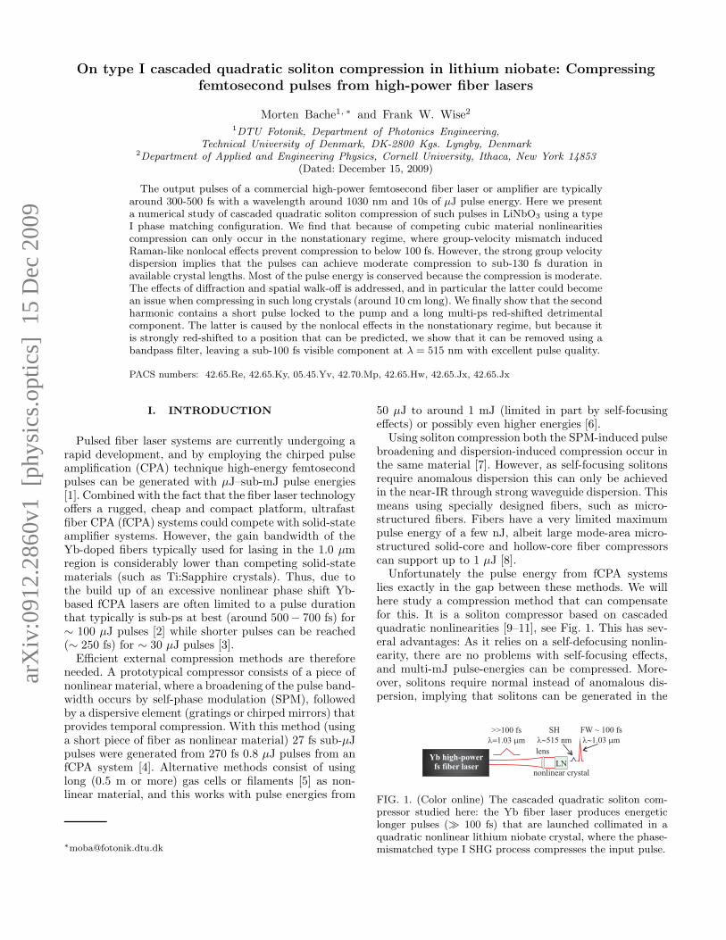
FIG. 1. (Color online) The cascaded quadratic soliton com-pressor studied here: the Yb fiber laser produces energeticlonger pulses (≫ 100 fs) that are launched collimated in aquadratic nonlinear lithium niobate crystal, where the phase-mismatched type I SHG process compresses the input pulse.

2

visible and near-IR. Finally, it is extremely simple as itrelies on just a small piece of quadratic nonlinear crystal,preceded only by a lens or a beam expander [12].

The basis for the cascaded quadratic soliton com-pressor (CQSC) is phase-mismatched second-harmonicgeneration (SHG). The cascaded energy transfer fromthe pump (fundamental wave, FW) to the second har-monic (SH) and back imposes a strong SPM-like non-linear phase shift on the FW, whose sign can be madeself-defocusing [13, 14]. Thereby the FW pulse can becompressed with normal dispersion [9], and soliton com-pression becomes possible in the visible and near-IR [10].

In this paper we investigate the CQSC in a type Ilithium niobate (LiNbO3, LN) crystal, where the goalis to perform moderate compression of longer fs pulsesfrom fCPA systems at the Yb gain wavelength of 1030nm. We show that in order to overcome the detrimen-tal cubic nonlinearities the phase mismatch has to bechosen so low so that the compression occurs in the so-called nonstationary regime. This regime is dominatedby group-velocity mismatch (GVM) effects, and exactlythe large GVM is a well-known drawback of using LNin the near-IR for SHG. However, when only moderatecompression is desired, the soliton order can be kept low,and we show through numerical simulations that reason-able pulse quality can be achieved and that up to 80%of the pulse energy is retained in the central spike. Thecompression limit is found to be around 120 fs FWHM,which is a limit set by the GVM effects. The compressionoccurs in a crystal of reasonable length, 10 cm. This ispossible only because LN has a very large 2. order dis-persion. Finally, we show that bandpass filtering of theSH actually can lead to a very clean sub-100 fs visiblepulse with around 0.1% conversion efficiency.

In this paper we first discuss the general compressionproperties of LN in a cascaded type I SHG interactionsetup in Sec. II, and then show some numerical simu-lations in Sec. III of pulses coming from two differentcommercially available fCPA systems. We conclude inSec. IV. The properties of LN are discussed in App. A,and App. B discusses the anisotropic Kerr nonlinear re-sponse of LN. Appendix C and D discuss the conversionrelations between Gaussian and SI units for cubic non-linear coefficients and Miller’s rule, respectively.

II. TYPE I COMPRESSION PROPERTIES OFLITHIUM NIOBATE CRYSTALS

With the CQSC high-energy few-cycle compressedpulses can be generated, as was experimentally observedat 1250 nm [15]. However, the first studies performed at800 nm were plagued by GVM effects, that preventedreaching the few-cycle regime [9, 10, 15]. These studiesused a β-barium–borate (BBO) crystal in a type I SHGoo → e configuration, where the FW (ordinary polar-ization) is orthogonal to the SH (extraordinary polariza-tion) and where birefringent phase matching is possible

by angle-tuning the crystal. BBO is in many respects anideal nonlinear crystal: it has low dispersion, a very largetransparency window, and a reasonably strong quadraticnonlinearity relative to the detrimental cubic one. As wehave shown in previous theoretical and numerical studies,BBO provides an excellent compression of longer pulsesto ultra-short duration at the Yb gain wavelengths [16–18]. The problem with BBO is that good quality waveg-uides are not supported and that it is very difficult togrow long crystals. Especially the latter is important ifonly moderate compression of longer pulses is desired. Inmoderate soliton compression most of the pulse energy isconserved in the compressed pulse, and the pulse has areduced pedestal. The problem is that compression willonly occur after a long propagation length.

We therefore turn here to LN, which is a widely usedquadratic nonlinear crystal for IR frequency conversion.LN is attractive due to extremely large effective quadraticnonlinearities (up to 10 times larger than BBO), that canbe accessed through a quasi-phase matched (QPM) type0 SHG phase matching configuration where FW and SHhave identical polarization. However, here we study LNin a type I configuration as BBO. The effective quadraticnonlinearity is more than twice as large as in BBO.

LN is usually not considered very suitable for SHGof short pulses in the near-IR because the SH becomesvery dispersive; thus, the FW and SH group velocitiesare very different resulting in large GVM. This is alsowhy LN has not been used in the near-IR as nonlin-ear medium for the CQSC, for which GVM is a verydetrimental effect. Another disadvantage for the CQSCis that the Kerr nonlinear response is several times largerthan BBO, which counteracts the advantage of the largequadratic nonlinearity of LN. Therefore the CQSC exper-iments done so far using LN were done in the telecommu-nication band and exploited QPM in a type 0 configura-tion [19], where effective quadratic nonlinearity is aroundthree times larger than what can be achieved in a typeI configuration. However, we now show that type I LNoffers a quite decent compression performance withouthaving to custom design a QPM grating.

A. Solitons with cascaded quadratic nonlinearities

In cascaded quadratic interaction the FW effectivelyexperiences a Kerr-like nonlinear refractive index. Thisis in addition to the cubic (Kerr) nonlinearities that arealways present in all media. We can write the total re-fractive index of the FW [see Eq. (C2)]

n = n1 + 12 |E1|2ncubic = n1 + I1n

Icubic (1)

where n1 is the FW linear refractive index, E1 is theFW electric field, and I1 the FW intensity. It is typi-cal to report the nonlinear refractive index relative tothe electric field, ncubic, or to the intensity, nI

cubic. Wehave here for simplicity neglected cross-phase modula-tion (XPM) contributions since they are small in cas-

3

caded SHG. As mentioned we have contributions fromboth cascaded quadratic and cubic Kerr nonlinearities

nIcubic = nI

SHG + nIKerr,11 (2)

where nIKerr,11 is the SPM Kerr nonlinear refractive index

of the FW (see App. B for details on the notation etc.).The contribution from the cascaded quadratic nonlinear-ities can in the large phase mismatch limit (∆kL ≫ 1,where L is the crystal length) be approximated as [13]

nISHG ≃ − 4πd2

eff

cε0λ1n21n2∆k

(3)

where deff is the effective χ(2) nonlinearity. For ∆k =k2 − 2k1 > 0 the cascaded contribution is negative, i.e.self-defocusing. Here kj = 2π/λj is the wavenumber.

The effective quadratic nonlinearity of the type I oo→e interaction for the 3m crystal class (LN, BBO) is

deff = d31 sin θ − d22 cos θ sin 3φ (4)

where the angles are defined in Fig. 9 in App. B. Choosingφ = −π/2 gives maximum nonlinearity (see App. A).

In cascaded quadratic soliton compression the aim is toget nI

SHG < 0 and |nISHG| > nI

Kerr,11 as to achieve a totalself-defocusing cubic nonlinearity. The soliton interactioncan then be described by an effective soliton order [17]

N2eff = N2

SHG −N2Kerr (5)

= LD,1k1Iin(|nISHG| − nI

Kerr,11)

where NSHG = LD,1k1Iin|nISHG| is the soliton order of

the self-defocusing cascaded quadratic nonlinearity, andNKerr = LD,1k1Iinn

IKerr,11 is the soliton order of the

material Kerr self-focusing cubic nonlinearity. The FW

dispersion length is LD,1 = T 2in/|k

(2)1 |, where k

(2)1 is

the FW group-velocity dispersion (GVD). We generallyuse the following notation for the dispersion parameters

k(m)j = ∂mkj/∂ω

m|ω=ωj.

B. Linear and nonlinear response of LN at 1.03 µm

Selecting λ1 = 1.03 µm, the operating wavelength ofmost Yb-based fiber laser amplifiers, the properties ofLN are summarized in Fig. 2: the phase mismatch (a)becomes small at θ ≃ 1.3 radians (70 − 75). As shownin (e) in this range deff ≃ 5.2 pm/V, and the total non-linear refractive index (f), as expressed by Eq. (2), canbecome negative, implying that the cascaded nonlinear-ity is stronger than the Kerr nonlinearity. This happensfor ∆k < 62 mm−1 (or θ > 70.4). At θ = 75.8 phasematching is achieved, after which nI

SHG > 0 and thusself-focusing.

GVM is very large, see Fig. 2(b), which as we will seelater sets a strong limitation to the compression perfor-mance. The GVD is shown in Fig. 2(c), and importantlyFW GVD (red) is large and normal (i.e. positive). It willstay normal until λ1 > 1.9 µm, after which it becomes

HaL

0.0 0.5 1.0 1.50

100

200

300

Θ @radD

Dk@Πm

mD

HbL

0.0 0.5 1.0 1.5-1000

-900

-800

-700

-600

Θ @radD

d 12@f

sm

mD

HcL

0.0 0.5 1.0 1.50

200

400

600

800

Θ @radD

ΒjH2L@f

s2 m

mD

HdL

0.0 0.5 1.0 1.50.0

0.5

1.0

1.5

2.0

Θ @DegD

Ρ@D

egD

HeL

0.0 0.5 1.0 1.5

2.53.03.54.04.55.0

Θ @radD

d eff@p

mVD

Hf L

0.0 0.5 1.0 1.5

-30-20-10

0102030

Θ @radD

n cub

icI@1

0-20

m2

WD

FIG. 2. (Color online) Properties at λ1 = 1.03 µm when angle-tuning the LN crystal: (a) Phase mismatch, (b) GVM param-eter, (c) GVD of FW (red) and SH (blue), and (d) the spatialwalk-off angle ρ. The effective quadratic nonlinearity neglect-ing (black) and including (dashed red) spatial walk-off areshown in (e) and (f) is the total cubic Kerr nonlinearity (2)from cascaded quadratic nonlinearities and Kerr SPM (usingnI

Kerr = 18 × 10−20 m2/W, see App. B).

anomalous and self-defocusing solitons are no longer sup-ported. The SH GVD (blue) is about 3 times larger thanthe FW GVD.

Since the type I critical phase matching is employed,the walk-off angle ρ = arctan[tan(θ)n2

o/n2e]− θ (valid for

a negative uniaxial crystal) is nonzero, see Fig. 2(d). InFig. 2(e) it is apparent that deff is largely unaffected bywalk-off. However, walk-off does set a limit to the effectiveinteraction length between the pump and the SH as wewill discuss later.

C. Compression diagram for type I LN

We now generalize to other wavelengths and summa-rize the type I compression performance of LN in Fig. 3 1.This compression diagram shows the different compres-sion regimes for the CQSC as the wavelength and thephase mismatch is varied.

Above the red curve the total nonlinear refractive indexis focusing nI

cubic > 0, so solitons are not supported since

1 The specific crystal chosen in this work is 1% MgO doped stoi-chiometric LN, as the MgO doping gives a much higher materialdamage threshold. Also 5% MgO doped congruent LN wouldwork well. See App. A for more details about the crystal.

4

1.0 1.2 1.4 1.6 1.80

50

100

Nonstationary regim

e

GV

M effects dom

inateStationary regim

e

Cascaded effects dominate

Er fiber lasers

SHG effects dominate:solitons possible

k [m

m-1

]

[ m]

compressionwindow

Kerr effects dominate: no solitons

ksr

kc,max

Yb fiber lasers

FIG. 3. (Color online) Compression diagram for 1% MgO:sLNat room temperature and aligned for type I SHG. For vari-ous pump wavelengths λ1 the choice of phase-mismatch pa-rameter ∆k affects the compression. In order to excite soli-tons the phase-mismatch must be kept below the red line(∆k < ∆kc,max), because otherwise the material cubic nonlin-earities are too strong (nI

Kerr,11 > |nISHG|). Optimal compres-

sion occurs when the cascaded nonlinearities dominate overGVM effects (∆k > ∆ksr, above the black line). We have alsoindicated the operation wavelengths of Yb and Er doped fiberlasers. The red line uses Miller’s rule to estimate the nonlin-ear quadratic and cubic susceptibilities at other wavelengths,cf. Eqs. (D1)-(D2), and uses nI

Kerr,11 = 20 × 10−20 m2/W forλ = 0.78 µm (see App. B for an extended discussion).

the FW GVD is normal. The curve is found by setting|nI

SHG| = nIKerr,11 giving [17]

∆kc,max = k12d2

eff

cε0n21n2nI

Kerr,11

(6)

Below the black curve the compression performance isdominated by GVM effects (nonstationary regime) whileabove it is dominated by cascaded effects (stationaryregime). The curve is to second order 2 given by [16]

∆ksr =d212

2k(2)2

(7)

where d12 = k(1)1 −k(1)

2 is the GVM parameter and k(2)2 is

the SH GVD. The lower this curve is the better becausethis implies that the chance of observing solitons in thestationary regime increases. Thus, the very large GVMparameter d12 is detrimental because it pushes the curveupwards. Instead the huge SH GVD values, see Fig. 2(c), are actually helping to push the curve downwards.Therefore a large SH GVD can actually be beneficial forclean soliton compression.

2 A more accurate transition can easily be calculated numericallyusing the full SH dispersion operator [18], which we have donein what follows.

The optimal compression occurs in the so-called “com-pression window” [16], where the soliton compressorworks most efficiently because solitons are supported inthe stationary regime. The diagram shows a compressionwindow for type I LN in the regime λ1 = 1.6 − 1.9 µm.Unfortunately in this range there are no fCPA systems.

Fortunately, as we will show also in the nonstationaryregime compression is possible, as long as the effectivesoliton order is low enough. This is what we will try toexploit in the regime around λ1 ∼ 1.03 − 1.06 µm.

Coming back to λ1 = 1.03 µm we observe that solitonsare supported for when 0 ≪ ∆k < ∆kc,max = 62 mm−1.However, when getting too close to ∆kc,max the inten-sities required to observe solitons become very large im-plying excessive Kerr XPM effects and increased Raman-like GVM effects [18]. On the other hand for ∆k toosmall the cascading limit ceases to hold, and also thecompressor performance decreases due to excessive GVMeffects [18]. In fact, as a rule of thumb the compres-sion limit in the nonstationary regime (in which thesystem will always be for ∆k ∼ 0) the compressionlimit is roughly given by the pulse duration for whichLcoh = LGVM, where Lcoh = π/|∆k| is the coherencelength and LGVM = ∆tsoliton/|d12| is the dynamic GVMlength of a sech-shaped soliton. With “dynamic” we meanthat the GVM length changes as the soliton compresses.Thus, in the nonstationary regime the limit is 3

∆tFWHMlimit ∼ 2 ln(1 +

√2)π|d12||∆k| (8)

where the factor in front of the fraction is the conversionfactor to FWHM for a sech-shaped pulse. Obviously as∆k approaches the phase matching point the soliton can-not compress to short durations. We numerically foundthe optimal compression point in the ∆k = 35−50 mm−1

regime, and with the best results for ∆k = 45 mm−1, forwhich nI

SHG = 25 × 10−20 m2/W.

D. Predicting the compression performance

The next step is to estimate what the compression per-formance could look like. Here the scaling laws 4 comeinto the picture, which can be used to predict the prop-agation distance for optimal compression zopt, the com-pression factor fc and the pulse quality Qc [17].

As we have pointed recently [16], it is the phase mis-match and the GVM (zero and first order dispersion)that really control the compression properties. The onlyrequirement to the second order dispersion is that FW

3 Note that this expression differs with a factor of π/2 from thelimit TR,SHG = 2|d12/∆k| that we suggested in [18]; this ispurely an empirical choice.

4 Note that the scaling laws presented here are only ball-park fig-ures when used in the nonstationary regime as they were foundin the stationary regime.

5

GVD is normal k(2)1 > 0 as to support solitons. Other-

wise as we discuss below the FW GVD is basically justdetermining the optimum compression length. The SHGVD instead plays a minor role in the compression prop-erties, cf. Eq. (7). Our initial idea was to exploit that LNis quite dispersive when pumped at λ1 ∼ 1.0 µm, so thevery large FW GVD makes it possible to compress thepulse in a short crystal.

So why and when is it interesting to increase GVD asto compress in a short crystal? Obviously, the crystalshave length limits, which for LN is around 100 mm. Theoptimal compression point scales as [17]

zopt

z0=

0.44

Neff+

2.56

N3eff

− 0.002. (9)

where z0 = π2LD,1 is the soliton length [20]. So the point

where the pulse compression is optimal depends on theeffective soliton order, the input pulse duration and theFW GVD. Therefore since quality LN crystals are maxi-mum 100 mm long, the CQSC works best when the soli-ton order is large and the GVD length is short. But whenthe soliton order is large, the detrimental effects due toGVM are strongly increased [15, 18], in particular in thenonstationary regime. Therefore, in the case we studyhere clean compression can only be done with low soli-ton order, and therefore the FW GVD must be large asto ensure compression in realistic crystal lengths.

A downside to the large GVD is the following: giventhat some effective soliton order is required then since

Neff ∝√

IinLD,1 ∝ Tin

√

Iin/|k(2)1 | we have that a large

GVD gives a short GVD length, and thus larger inten-sities are needed to excite a soliton. The same problemis found for short input pulses, say from a Ti:Sapphireamplifier. However, this is only an issue if operatingwith intensities close to the damage threshold, which isnot the case here: the intensities are moderate (Iin ≪100 GW/cm2), and instead our issue is to get the soli-tons to compress in a crystal that is not too long.

The compression factor fc = Tin/∆topt, where ∆topt

is the pulse compressed pulse duration at zopt, is alsoaffected by the effective soliton order [17]

fc = 4.7(Neff − 0.86) (10)

The pulse quality can also be predicted, and is definedas the ratio between the compressed pulse fluence withthat of the input pulse. It scales as [17]

Qc = [0.24(Neff − 1)1.11 + 1]−1. (11)

We can use this to calculate the compressed pulse peakintensity Iopt = QcfcIin and energy Eopt = QcEin. Anadvantage of using low soliton orders is that Qc remainshigh, and thus the compressed pulse retains most of theinitial pulse energy.

E. Compression performance of fCPA systems

Let us use these scaling laws to predict the compressionperformance of fCPA systems. High-energy femtosecondpulses from fCPA systems use both Yb doped and Erdoped gain fibers. Since fCPA systems are diode pumpedwith a wavelength just below 1.0 µm the quantum effi-ciency of Yb doped systems is higher, and therefore themajority of commercial and scientific systems prefer touse Yb over Er. Most systems operate at the λ = 1.03 µmYb emission line and can for low pulse energies (< 15 µJ)generate pulses as short as 250 fs, while higher pulse ener-gies result in longer pulses (currently 50 µJ 450 fs pulsesis the state-of-the-art for commercial systems). In Er am-plifier systems much lower pulse energies are available,typically 1−3 µJ and 500−700 fs pulses at λ = 1.55 µm;such low pulse energies and long pulse duration meanthat only very low soliton orders can be excited, and thusthe CQSC can only achieve very moderate compressionoccurring in very long crystals.

The basis for the following case studies and numericalsimulations is therefore a couple of commercially avail-able Yb-based fCPA systems, both operating at 1030 nm.Case (1) is a Clark MXR Impulse 5 giving 15 µJ 250 fsFWHM pulses, which represents a system giving quiteshort, yet still reasonably energetic pulses as a startingpoint. Case (2) is an Amplitude Systemes Tangerine 6

giving 50 µJ 450 fs FWHM pulses, which represents asystem with more energetic but also longer pulses.

The two cases are studied together taking ∆k =45 mm−1. Figure 4(a) shows that in case (1) we needto focus the pulses to w0 < 600 µm to observe solitons:in this regime Fig. 4(d) shows that the Rayleigh lengthzR = πw2

0/λ is only 5-6 times larger than the optimalcompression point zopt of around 100 mm. This is border-line at the risk of experiencing diffraction problems. Evenincreasing or decreasing the waist does not improve thisratio much. In case (2) instead, the increased pulse energymakes solitons appear already at w0 ≃ 1.6 mm, despitethe longer pulse duration. This means that diffractionshould be less of an issue: in Fig. 4(d) the pulse compres-sion point relative to the Rayleigh length of the focusedbeam is significantly smaller in case (2).

Fig. 4(c) indicates that the spatial walk-off in the crys-tal can become an issue: the crystal should be shorterthan the spatial walk-off length Lwo = w0/ tanρ ≃ w0/ρto ensure proper interaction between the FW and the SH,but evidently the pulse compression lengths in both casesare at least a factor of 2-3 longer than the spatial walk-off length. It might therefore be necessary to compensatefor this by using two crystals, one inverted relative to theother so the walk-off direction in the 2. crystal is invertedwith respect to the 1. crystal [21].

5 http://www.clark-mxr.com6 http://www.amplitude-systemes.com

6

(a) (b)

(c) (d)

(e) (f)

(1)

(1)

(1)

(1)

(1)

(1)

(1)

(2)

(2)

(2)

(2)

(2)

(2) (2)

single cycle limit

soliton limit

DtlimitFWHM

Lwo

FIG. 4. (Color online) Practical operation range of the LNtype I compression system at λ1 = 1.03 µm for ∆k =45 mm−1. The plots show the predicted behaviour when theFW waist w0 is varied. The two cases are (1) pump pulseswith TFWHM

in = 250 fs and 15 µJ pulse energy, and (2) pumppulses with TFWHM

in = 450 fs and 50 µJ pulse energy. Thecurves in (b)-(f) are calculated based on Neff shown in (a) byusing the scaling laws [17] that hold for Neff > 1.

An alternative solution to the walk-off problem is toturn to a noncritical phase matching scheme, where ρ =0. This happens for θ = 0 or π/2, see Fig. 2(d). Of coursethis removes the possibility of tuning the phase matchingvia θ, and one has to turn to temperature tuning of ∆k.The temperature needed to get to the desired operationpoint (∆k ≃ 40 − 50 mm−1) can be estimated using thetemperature dependent Sellmeier equations [22], and ourcalculations indicate that it should happen already at atemperature of around 45 C. This would make an easysolution to the walk-off problem.

The strong GVM implies that compression of Yb-basedsystems can only occur in the nonstationary regime, seeFig. 3. Thus, unless Neff is close to unity the GVM in-duced Raman-like effects dominate, and the FW pulse be-comes extremely distorted and very poorly compressed.Actually, as a rule of thumb it never makes sense to useNeff larger than what is sufficient to reach the limit ex-pressed by Eq. (8), and typically even an Neff smallerthan that. The limit is drawn as a dotted line in Fig. 4(e),and it is reached around w0 = 400 µm in case (1) andw0 = 800 µm in case 2.

Finally, Fig. 4(b) shows that quite moderate input in-tensities must be used to achieve solitons in both cases.This is related to the quite long input pulse durations.Furthermore, Fig. 4(f) shows that the low soliton ordersconserve most of the pulse energy in both cases.

FIG. 5. (Color online) Numerical simulation of soliton com-pression in LN with λ1 = 1.03 µm, TFWHM

in = 250 fs,∆k = 45 mm−1 and Neff = 1.4 (implying Iin = 6.9 GW/cm2).The FW pulse shown in (a) compresses to ∆topt = 126 fs(FWHM) after propagating 91 mm. The SH time plot (c) andFW (b) and SH (d) spectra are also shown on a logarithmicscale, and Uj are normalized to the peak input FW electricfield. In (e) and (f) cuts are shown at the optimal compressionpoint z = 91 mm (corresponding to the white line in the 2Dplots). Note that the SH in (e) is magnified 100 times.

III. NUMERICAL SIMULATIONS

We here present numerical simulations of the two casesusing a plane-wave temporal model based on the slowlyevolving wave equation (see more details in [17] and refer-ences therein), which includes self-steepening effects andhigher-order dispersion. This model is justified as longas diffraction is minimal, which we assume is the casewhen the crystal length is much shorter than the Rayleighlength, and when spatial walk-off is minimal. This re-quirement will be discussed further below.

A. Case (1): 250 fs 15 µJ pulses

For the 250 fs 15 µJ pulses from a Clark laser systemwe found that the best compression was obtained withNeff ∼ 1.3− 1.5. This soliton order can be achieved with15 µJ pulse energy when the pump is focused to aroundw0 = 400 µm, see Fig. 4(a).

The theoretical compression factor for such soliton or-ders is fc = 2−3, i.e., a ∆topt ∼ 80−125 fs FWHM com-pressed pulse is predicted. In Fig. 5 we show the resultsof a simulation with Neff = 1.4. This soliton order gavethe best compression: a slightly asymmetric ∆topt = 126fs (FWHM) pulse is observed after 91 mm of propaga-tion, see (a) and cut in (e). The compression is not quiteas strong as predicted by the scaling law (10), but this is

7

-500 0 5000.0

0.5

1.0

1.5

input pulse|U1|2 =

I 1/I i

n

t [fs]

Neff

=1.4, zopt

=91 mm N

eff=2.0, z

opt=43 mm

Neff

=2.5, zopt

=28 mm

(a)

topt

=126 fs (FWHM)

-1000 0 1000 2000 3000 40000.000

0.002

0.004

0.006

0.008

0.010 (b)

|U2|2 =I

2/I in

t [fs]

FIG. 6. (Color online) Simulations as in Fig. 5 but with in-creasing Neff . The red curve corresponds to the optimal com-pression point from Fig. 5(e), while the black curves showwhat happens as the effective soliton order increases (makingthe optimal compression point occurring sooner).

because the scaling laws are based on pulse compressionin the stationary regime. On the other hand the pulsequality is large, Qc = 0.82, so most of the pulse energyis retained in the central compressed part, and the pulsepedestal is also very small. These are the main advan-tages of soliton compression with low soliton orders.

The FW spectrum (b) experiences upon propagationSPM-like broadening, where the blue-shifted shoulderclearly dominates; this is a sign of the cascaded quadraticnonlinearities dominating, and the fact that it is blueshifted is related to the negative sign of d12.

In the SH time-plot (c) we observe the strong GVMfirst inducing a weak component quickly escaping fromthe central part of the pulse, and later the GVM inducesthe characteristic DC-like trailing temporal pulse in theSH (this often occurs close to or at phase matching inpresence of GVM, see also [23]). This behaviour is alsoreflected in the SH spectrum, see (d) and cut in (f), whichshows a very strong and extremely narrow red-shiftedcomponent building up, which eventually becomes thedominating contribution. As we discuss below its spec-tral position can accurately be predicted by the nonlocaltheory that was recently developed by us [16, 18]. Webelieve that this strong and long SH trailing componentactually causes the trailing part of the FW to be stronglydepleted, and that this is the main reason for the asym-metrical FW shape.

The question is now: can we increase the effective soli-ton order and achieve further compression below 100 fsas to approach the limit predicted by Eq. (8)? This turnsout to be impossible: when Neff is increased the GVMeffects become stronger, making the compressed pulsemore distorted. This is clearly observed in Fig. 6, wherewe increase Neff and compare with the compression ofFig. 5: For Neff = 2.0 the compressed FW pulse in (a) isstill quite short, but clearly is less clean. For Neff = 2.5the compressed pulse instead becomes quite distorted.It is also evident in the SH time plots that the trailingDC-like component increases with Neff , while the centralpart in all cases is a sub-100 fs FWHM pulse. It is quiteweak because most of the converted SH energy is fed intothe DC-like part of the pulse, which is connected to thestrong spectral peak in the SH spectrum. This spectral

peak becomes stronger with increased Neff (not shown),but does not change position as it does not dependent onNeff .

In order to understand the spectral content of thedifferent temporal components, the cross-correlationfrequency-resolved optical gating (XFROG) method isuseful. The spectral strength is given by [24]

Sj(z, T,Ω) =

∣

∣

∣

∣

∫ ∞

−∞

dteiΩtEj(z, t)Egate(t− T )

∣

∣

∣

∣

2

(12)

where Egate(t) is a properly chosen gating pulse. Thespectrograms of the compressed pulses in Fig. 6 forNeff = 1.4 are shown in Fig. 7. The FW compressedpulse is slightly blue-shifted (around 2 THz), and thecompressed part (located at T ∼ 200 fs) shows a signifi-cantly broader spectrum.

The SH spectrum is very particular: the part of thepulse that propagates with the FW group velocity (the“locked” part) shows a quite clean short pulse. This groupvelocity locking of the SH has been observed before [19,23] and can be understood from the nonlocal theory [16,18]: the SH has a component that is basically slaved tothe FW due to the cascading nonlinearities. In frequencydomain it can be compactly expressed as [18]

U2(z,Ω) ∝ R−(Ω)F [U21 (z, t)] (13)

where F [.] denotes the forward Fourier transform, and Uj

are properly normalized fields. Thus, the spectral contentof the SH is slaved to the spectral content of the spectrumof U2

1 . The weight is provided by the nonlocal Raman-likeresponse function in the nonstationary regime [18]

R−(Ω) = (2π)−1/2 Ω+Ω−

(Ω − Ω−)(Ω − Ω+)(14)

where Ω± = Ωa±Ωb. These frequencies can be calculated(to 2. order) from the dispersion of the system as Ωa =

d12/k(2)2 = −1.044 PHz and Ωb = |2∆k/k

(2)2 − Ω2

a|1/2 =0.963 PHz. In the center around Ω = 0, where F [U2

1 (z, t)]is residing in this case, the response is quite flat: thus weget a SH component locked to the FW and when the FWcompresses so does this SH component.

Another striking feature of the SH spectrogram is theDC-like component: it is very evident as a long pulse cen-tered around Ω ∼ −80 THz. Also this peak can be under-stood from Eq. (13), because according to Eq. (14) thenonlocal response function in the nonstationary regimehas sharp resonance peaks in the response at Ω = Ω±.Inserting the dispersion values of the simulation we getΩ+ = −81.6 THz in excellent correspondence with theobserved peak position as the red dashed line indicates.Instead Ω− is located too far into the red side of thespectrum to affect the behaviour.

Considering this spectral composition, it might even bepossible to filter away the disturbing SH component atΩ = Ω+, which in time-domain would give a quite decentSH pulse. In (c) we show that this is feasible: we pass theSH pulse through a super-Gaussian (n = 3) bandpass

8

FIG. 7. (Color online) XFROG-like spectrograms of the simulation in Fig. 5 at the optimal compression point zopt = 91 mm.The sech-shaped gating pulse had TFWHM

0 = 70 fs, and the spectrograms are normalized to the peak value of S1. The top andside plots show the purely temporal and spectral traces, respectively, and are thus identical to Fig. 5(e) and (f). The red dashedline in (b) indicates the value Ω+ as calculated by the nonlocal theory. The spectrogram in (c) shows the SH passed through a3. order super-Gaussian bandpass filter centered at the SH carrier frequency λ2 = 0.515 µm and with a FWHM of 100 THz.

filter centered at ω2 and with a bandwidth of 100 THzFWHM (corresponding to 15 nm): this filters away thedisturbing sharp peak, and a 80 fs FWHM pulse remainsat λ = 0.515 nm. The peak intensity in this short pulseis around 0.006Iin = 0.0414 GW/cm2. If we assume thatit is created with 15 µJ pulse energy focused to w0 = 0.5mm to achieve Neff = 1.4, and that the generated SH hasroughly the same spot size, then the pulse energy of thefiltered 80 fs pulse would be around 50 nJ.

B. Case (2): 450 fs 50 µJ pulses

In case (2) the pulse duration is longer, 450 fs. Whenthe pulse duration is longer the soliton will for a fixedsoliton order compress after a longer distance. This isbecause according to Eq. (9) zopt ∝ LD,1 ∝ T 2

in. How-ever, we may compensate for this by increasing the effec-tive soliton order enough to reach the limit governed byEq. (8). For a 450 fs 50 µJ pulse it is achieved aroundw0 = 0.8 mm, see Fig. 4(e), resulting in Neff ∼ 2.0− 2.5.This higher soliton order should make it possible to com-

-500 0 5000.0

0.5

1.0

1.5

2.0

2.5

input pulse|U1|2 =

I 1/I i

n

t [fs]

Neff

=2.0, zopt

=153 mm N

eff=2.6, z

opt=95 mm

Neff

=3.0, zopt

=78 mm

(a)

topt

=121 fs (FWHM)

-1000 0 1000 2000 3000 40000.000

0.002

0.004

0.006

0.008

0.010

0.012 (b)

|U2|2 =I

2/I in

t [fs]

FIG. 8. (Color online) Numerical simulations using 450 fs 50µJ input pulses and taking ∆k = 45 mm−1. The best pulsewas observed for Neff = 2.0 (red curve) where pulse compres-sion occurs after 15 cm. The black curves show what happensas the effective soliton order increases (in which case the op-timal compression point occurs sooner).

press in crystal lengths of around 10-15 cm, see Fig. 4(c).In Fig. 8 we show some numerical simulations using

these longer more energetic pulses. The best pulse ob-served shows a three-fold compression to ∆topt = 121 fs(FWHM) at Neff = 2.0. The compression occurred afteraround 15 cm propagation, so spatial walk-off would bean issue here. Increasing the soliton order to Neff = 2.6the pulse becomes more distorted, but still compresses toaround 150 fs FWHM after 9.5 cm, a more realistic in-teraction length. Finally, at Neff = 3.0 the pulse becomestoo distorted as the GVM effects become stronger.

In the two cases the pulses therefore eventually com-press to the same duration, which is the limit imposedby the nonlocal GVM effects. The more energetic pulsesin case (2) allow for a more defocused pump beam so thecompression should be less affected by diffraction. On theother hand, as the pulses are longer they compress later,so spatial walk-off is a more severe issue. A more optimalsituation in both cases would therefore be more energeticpulses so the pump can be defocused with a factor 2-3.This would diminish spatial walk-off effects.

IV. CONCLUSION

Here we have shown that lithium niobate (LN) crystalsin a type I cascaded SHG interaction can provide moder-ate compression of fs pulses from Yb-based fiber amplifiersystems (1.03 µm wavelength). The phase mismatch wascontrolled through angle tuning (critical phase matchinginteraction). Using numerical simulations we found thatthe best compression was to around 120 fs FWHM afteraround 10 cm propagation.

Better compression was prevented in part by strongGVM effects, caused by strong dispersion in the LNcrystal, and competing material Kerr nonlinear effects.These are focusing of nature and counteract the defocus-ing Kerr-like nonlinearities from the cascaded SHG. Inorder to make the total nonlinear phase shift negative

9

the phase mismatch had to be taken quite low, and inthis regime GVM effects dominate (the “nonstationary”regime). GVM imposes a strongly nonlocal temporal re-sponse in the cascaded nonlinearity that feeds most ofthe converted energy into a narrow red-shifted peak. Inthe temporal trace this gave a SH with a multi-ps longtrailing component. The FW therefore experienced a dis-torted compression less the soliton order was kept verylow. For such low soliton orders the compression distanceincreases substantially, but here the strong dispersion ofthe LN crystal actually becomes an advantage: due to alarge GVD the soliton dynamics occur in much shortercrystals than usual, and the numerics indicated compres-sion in realistic crystal lengths (10 cm).

It was noted that using low soliton orders gave a com-pressed pulse retaining most of the input pulse energy (inthe cases we showed around 80%), and that the unavoid-able soliton pedistal was less pronounced.

We also discussed the implications of using long crys-tals. Spatial walk-off will be an issue since it is a criti-cal phase matching scheme is used that exploits birefrin-gence, and also diffraction can be a problem. In orderto counteract these detrimental effects the pump pulsesneed to be as energetic and short as possible. Two caseswere highlighted taken from commercially available sys-tems, and we argued that diffraction should not preventobserving the predicted compression, but that some sortof walk-off compensation might be needed. Future sys-tems with more energetic pulses and reasonably shortpulse durations (< 500 fs) would be able to beat the walk-off problem. Walk-off could also be prevented by using anoncritical type I phase matching scheme (θ = π/2) andincreasing the temperature slightly to around 45 C.

We finally noted that the peculiar SH shape in the non-stationary regime gave a very characteristic spectrogram:as mentioned above nonlocal GVM effects resulted in asharp spectral red-shifted peak with a long multi-ps trail-ing temporal component. Another pulse component wasinstead locked to the group velocity of the compressedFW soliton. This locked visible pulse was located at theSH wavelength (515 nm), quite far from the red-shiftedpeak. We showed that a simple bandpass filter could ac-tually remove the detrimental red-shifted peak leavinga very clean 80 fs visible pulse (λ = 515 nm). This isthe opposite approach compared to other studies, see e.g.[23, 25], where focus was on exploiting “spectral compres-sion” of fs pulses to obtain longer ps pulses. Despite thatthe cascaded SHG by nature has a low conversion effi-ciency, the pulse energy of this short visible pulse caneasily be 50-100 nJ. Such pulses could be used for two-color ultra-fast energetic pump-probe spectroscopy.

This study showed that cascaded quadratic pulse com-pression is possible even in a very dispersive nonlinearcrystal. However, if compression occurs in a medium withstronger quadratic nonlinearities then it would be possi-ble to increase the phase mismatch, and thereby enterthe stationary regime where the nonlocal GVM effectsare much weaker. The benefit would be triple: cleaner

compressed pulses could be generated, higher soliton or-ders could be used to achieve stronger compression, andit would occur in a shorter crystal. This conclusion is inline with what was noted previously in a fiber context[26], where one of us found that the very dispersive na-ture of wave-guided cascaded SHG could be overcome ifa strong enough quadratic nonlinearity is present. We arecurrently investigating other possible nonlinear crystalsand phase matching conditions to achieve this.

V. ACKNOWLEDGMENTS

Support is acknowledged from the Danish Council forIndependent Research (Technology and Production Sci-ences, grant no. 274-08-0479 Femto-VINIR, and NaturalSciences, grant no. 21-04-0506). Jeff Moses and BinbinZhou are acknowledged for useful discussions.

Appendix A: LN crystal parameters

LN is a negative uniaxial crystal of symmetry class 3m.Its low damage threshold due to photorefractive effectsand problems with green induced IR absorption can beimproved dramatically by doping the crystal, in partic-ular with MgO doping [27, 28]. 1% MgO doping in sto-ichiometric LN (1% MgO:sLN) is enough to practicallyremove photorefractive effects and increase dramaticallythe damage threshold, while 5% is needed in congruentLN (5% MgO:cLN) to do the same [28]. 1% MgO:sLNalso has a shorter UV absorption edge (λ = 0.31 µm).

We here use 1% MgO:sLN, and the Sellmeier equa-tions from [22]: note that for 1% MgO:sLN they onlymeasured ne, but we checked that the 5% MgO:cLN no

Sellmeier equation matches well (at room temperature)the 1% sLN no equation from [29]. The quadratic nonlin-ear coefficients have been measured at λ = 1.06 µm andare d31 = −4.7 pm/V and d33 = 23.8 pm/V [30], whiled22 = 2.1 pm/V [31] was measured for undoped LN. Thefact that d31d22 < 0 has been established in, e.g., [32].The effective quadratic nonlinearity of the type I oo→ einteraction is given by Eq. (4). Because d31d22 < 0 [32]the maximum nonlinearity is realized with φ = −π/2.

Appendix B: Anisotropic Kerr nonlinear refraction

We previously studied type I cascaded SHG in a BBOcrystal [16–18], assuming an isotropic Kerr nonlinearity

χ(3)eff,11 = χ

(3)eff,22 = 3χ

(3)eff,12 (B1)

where χ(3)eff,jj are the FW and SH SPM coefficients, and

χ(3)eff,12 is the XPM coefficient. However, all quadratic non-

linear crystals are anisotropic, and below we address this.Note first that the error made in assuming an isotropic

response for the CQSC is probably small as the crucial

10

FIG. 9. Definition (in accordance with the IRE/IEEE stan-dard [33]) of the crystal coordinate system xyz relative to thebeam propagation direction indicated by k.

parameter is the FW SPM coefficient. As we will see nowfor type I this is identical in the isotropic and in theanisotropic cases. However, it should be emphasized thatthe various experimental attempts to measure the Kerrnonlinear refractive index of nonlinear crystals do not al-ways measure the tensor component relevant to our pur-pose, namely the c11 component, see Table I later. Theanalysis presented here should help understanding whatexactly has been measured, and put the results into thecontext of cascaded quadratic soliton compression.

For a nonlinear crystal in the symmetry group 3m (LNand BBO) there are 37 nonzero elements for the χ(3)

tensor, and of these only 14 are independent [34]

xxxx = yyyy = xxyy + xyxy + xyyx

xxzz = xzxz = xzzx = yyzz = yzyz = yzzy

= zyyz = zyzy = zzyy = zxxz = zxzx = zzxx

xxyy = xyxy = xyyx = yxxy = yxyx = yyxx

xxyz = xxzy = xyxz = xyzx = xzxy = xzyx

= −yyyz = −yyzy = −yzyy = yxxz = yxzx

= yzxx = −zyyy = zxxy = zxyx = zyxx

zzzz (B2)

where Kleinman symmetry has been invoked, and the po-larization relative to the crystal coordinate system is de-fined in Fig. 9. Under Kleinman symmetry the nonlinearcoefficients are assumed dispersionless and the criterionfor this assumption is that the system is far from any

resonances. Using the notation χ(3)ijkl = cµm where

for µ : x→ 1 y → 2 z → 3

for m : xxx→ 1 yyy → 2 zzz → 3 yzz → 4

yyz → 5 xzz → 6 xxz → 7 xyy → 8

xxy → 9 xyz → 0 (B3)

these tensor components are equivalent to

c11 = c22 = 3c18

c16 = c24 = c35 = c37

c18 = c29

c10 = −c25 = c27 = −c32 = c39

c33 (B4)

On the reduced form the cubic tensor becomes

c = (B5)

c11 0 0 0 0 c16 0 c11

3 0 c100 c11 0 c16 −c10 0 c10 0 c11

3 00 −c10 c33 0 c16 0 c16 0 c10 0

These results conform with the IRE/IEEE standard [35].We now want to evaluate the cubic nonlinear response

for a type I interaction. Using the notation from [17] thecubic nonlinear polarization response is

P(3)NL = ε0χ

(3)...EEE (B6)

We have here only considered an instantaneous (elec-tronic) cubic nonlinear response [36]. Let us consider thetype I SHG interaction where two ordinarily polarizedFW photons are converted to an extraordinarily polar-ized SH photon (oo → e). In the coordinate system ac-cording to the IRE/IEEE standard [33], see Fig. 9, theunit vectors for o-polarized and e-polarized light are

eo =

− sinφcosφ

0

ee =

− cos θ cosφ− cos θ sinφ

sin θ

(B7)

where walk-off has been neglected.We then introduce slowly varying envelopes polarized

along arbitrary directions

E(t) = Re[u1E1(t)e−iω1t + u2E2(t)e

−iω2t] (B8)

where uj is the unit polarization vector. For type I SHGwe have u1 = e

o and u2 = ee. The nonlinear slowly

varying polarization response

P(3)NL(t) = Re[u1P

(3)NL,1(t)e

−iω1t + u2P(3)NL,2(t)e

−iω2t]

then becomes

P(3)NL,i =

3

4ε0

[

χ(3)eff,ii|Ei|2 + 2χ

(3)eff,ij |Ej |2

]

Ei, (B9)

where i, j = 1, 2 and j 6= i. We have here only includedphase-matched components and frequency-mixing termswhere 2ω1 − ω2 = 0. The numerical prefactor 3

4 is theK-factor [37] for a third order nonlinear effect creatingan intensity dependent refractive index with degenerate

frequencies, and the factor 2 on the XPM terms χ(3)eff,ij

stems from the fact that the K-factor for cross-phasemodulation with non-degenerate frequencies is 3

2 .For calculating the cubic nonlinear coefficients, it is

convenient to use an effective cubic nonlinearity [38]

χ(3)eff = ud · χ(3)

...uaubuc = ud · c · u(3), (B10)

a, b, c, d = 1, 2. Here ud is the unit vector of the field un-der consideration; thus, if we are interested in calculatingthe cubic nonlinear polarization for the FW [taking i = 1in Eq. (B9)], then ud = u1. The other three unit vec-tors ua,b,c are the unit vectors of each field appearing in

11

Eq. (B6), and can in the case we are considering here beeither u1 or u2 according to the identity (B8). Most com-binations are not phase matched or have 2ω1 − ω2 6= 0,and are therefore not included in Eq. (B9). The rank 4tensor on reduced form, as given by Eq. (B5) for LN,

can be used to find the tensor product χ(3)...uaubuc as a

simple matrix-vector product c · u(3) where

u(3) =

Lxxx

Lyyy

Lzzz

Lyzz + Lzyz + Lzzy

Lyyz + Lyzy + Lzyy

Lxzz + Lzxz + Lzzx

Lxxz + Lxzx + Lzxx

Lxyy + Lyxy + Lyyx

Lxxy + Lxyx + Lyxx

Lxyz + Lxzy + Lzxy + Lyxz + Lyzx + Lzyx

(B11)

Here Ljkl ≡ ua,jub,kuc,l where the jkl indices refer to thex, y or z components of the unit vectors.

It is convenient at this stage to simplify the notationbased on the type I SHG interaction we are interestedin. The effective cubic nonlinearity (B10) then reducesto the nonlinear coefficients appearing in Eq. (B9)

χ(3)eff,ij = ui · χ(3)

...uiujuj (B12)

The SPM terms can now be calculated as follows. TheFW SPM interaction has i = j = 1 in Eq. (B12), and isan ooo → o process: u1 = e

o. The SH SPM interactionhas i = j = 2 and is an eee → e process, so u2 = e

e.

We then need to calculate χ(3)...uiuiui using the reduced

notation. Since for the SPM terms all the unit vectors inu

(3) are degenerate in frequency, all Ljkl components in agiven vector entry are identical, e.g. Lyzz = Lzyz = Lzzy.We then get for the FW

χ(3)...u1u1u1 =

−c11 sinφc11 cosφ

−c10 cos3 φ

(B13)

A similar expression can be calculated for the SH SPMcomponent, although it is substantially more complex.In the final step we carry out the vector dot product ofthese vectors with ui, as dictated by Eq. (B12), and getfor the FW (i = 1) and the SH (i = 2) [35]

χ(3)eff,11 = c11 (B14)

χ(3)eff,22 = −4c10 sin θ cos3 θ sin 3φ+ c11 cos4 θ

+ 32c16 sin2 2θ + c33 sin4 θ (B15)

For the XPM terms note that the three unit vec-tors used to calculate Eq. (B11) are non-degenerate in

frequency. As an example, for χ(3)...u2u1u1 terms like

-3 -2 -1 0 1 2 3

-25

-20

-15

-10

-5

0

5

Ψ @radD

n SH

GI@1

0-20

m2WD

FIG. 10. The calculated effective Kerr nonlinear contributionsfrom cascaded SHG to the measured Kerr nonlinear refractiveindex by Kulagin et al. [39]. The beam propagates with θ =π/2 into a LN crystal, and ψ denotes the polarization angle(ψ = 0 gives o-polarized light, while ψ = π/2 gives e-polarizedlight). The angle φ was not reported, but we checked it haslittle influence on the nI

SHG value shown here.

Lxyy + Lyxy + Lyyx must be evaluated, whose compo-nents are Lxyy = − cos θ cos3 φ and Lyxy = Lyyx =

cos θ sin2 φ cosφ. This gives χ(3)eff,12 = χ

(3)eff,21 and [35, 39]

χ(3)eff,12 = 1

3c11 cos2 θ + c16 sin2 θ + c10 sin 2θ sin 3φ(B16)

The next step is to obtain the the values for LN ofeach component in Eqs. (B14)-(B16). The value of thecubic nonlinear refractive index has been measured bymany authors and for many different pulse durations andcrystal cuts. In Tab. I the χ(3) tensor components and thenI

Kerr are reported in electrostatic units values, and thelatter is also given in SI units (see App. C for details).

In one of the earliest studies the tensorial nature of LNwas studied [44]. Another early study found that c11 =3c10 [48]. Later studies used Z-scan methods and often anonlinear refractive index value was found without anymentioning of the tensorial nature of the cubic nonlinearsusceptibility. The cascaded quadratic contributions werealso often forgotten or neglected.

A recent study by Kulagin et al. went into a detailedexperimental determination of the various cubic tensorcomponents of LN, and found c11 = 2.4 × 10−13 esuat λ = 1.06 µm, and that c18 = 1.2c16 = 1.4c33 [39].Through the relation c11 = 3c18, see Eq. (B4), the othercoefficients are c16 = c11/3.6, c33 = c11/4.2. A problemwith this study is that the cascaded quadratic nonlin-ear contributions to the observed Z-scan results were ne-glected. Instead, based on an analysis of the anisotropicKerr tensor components the Z-scan transmission functionwas calculated, and the various tensor components werefound by fitting to experimental data. In the experimentthe pump propagated with θ = π/2, i.e. with the k-vectorperpendicular to the OA. The angle of the polarizationvector was then varied; this gives either pure o-polarizedlight, pure e-polarized light, or a linear mixture.

We have done an analysis of the various cascaded SHGprocesses that come into play (oo → o, oo → e, oe → e,oe → o, ee → e, and ee → o), evaluated their respective

12

λ χ(3)eff nI

Kerr nIKerr tFWHM Rep. θ pol n cij Ref. Note

[nm] [10−13 esu] [10−13 esu] [10−20 m2/W] [ps] [deg]1064 1.1 4.8 9.1 30 single 90 e 2.2 c33 [40] x-cut1064 0.73 3.2 6.0 55 2 Hz 90 o 2.2337a c11 [41] paraxial fit1064 0.66 2.9 5.4 55 2 Hz 90 o 2.2337a c11 [41] Gaussian fit1064 2.4 10 19 55 2 Hz 90 o 2.2337 c11 [39] Fit to transmission curve1064 0.80 3.4 6.3 55 2 Hz 90 e+o 2.2337 c12, c18 [39] ”, c12 = c11/31064 0.57 2.8 4.9 55 2 Hz 90 e 2.1495 c33 [39] ”, c33 = c12/1.41064 0.67 2.9 5.5 55 2 Hz 90 e+o 2.1912 c23, c16 [39] ”, c23 = c12/1.2800 1.8 7.8 15 0.42 1 kHz ? ? 2.1677a ? [42] x-cut, z-cut780 2.6 11.0 20 0.15 76 MHz 0 o 2.2552a c11 [43] 6% MgO:LN, z-cut577 1.6 6.6 12 5,000 40 Hz 0 o 2.301a c18 [44] c18 = c11/3532 10 44 83 22 single 90 e 2.23 c33 [40] x-cut532 6.6 28 53 25 10 Hz 0 o 2.2244a c11 [45] z-cut520 5.0 21 39 0.2 1 kHz 90 e 2.24 c33 [46] 5% MgO 0.06% Fe cLN

a Linear refractive index not provided; this value was calculated by us for conversion purposes.

TABLE I. Nonlinear Kerr refractive index of LN measured mainly by the Z-scan method [47]. The underlined results are thevalues reported. The other entries have been calculated using Eqs. (C8)-(C11).

deff -values and phase mismatch values as the input po-larization angle changes. In total we arrived at a stronglyvarying cascaded contribution shown in Fig. 10. At ψ = 0the contribution from nI

SHG is focusing, implying that thec11 component in Kulagin et al. might be too high with afactor of 7.0×10−20 m2/W. There are also strongly defo-cusing contributions at other polarization angles, whichshould give rise to an underestimated value of the othertensor components. Moreover, the overall shape remindsstrongly of the shape found in Fig. 5 in [39]: the focus-ing peaks from cascaded SHG could explain the valleysfound there, and the defocusing valleys from cascadedSHG could instead explain the peaks. In summary webelieve the c11 value to be too high, and the relation tothe other tensor components to be dubious.

There are other issues with the Z-scan method: If therepetition rate is too high, there will also be contributionsto the measured nI

Kerr from thermal effects as well as two-photon excited free carriers [49], and hence nI

Kerr does notcontain just the instantaneous electronic response, as it issupposed to. Similarly conclusions can be made for pulseslonger than 1 ps. For more on these issues, see e.g. [50].

For the CQSC system the by far most important com-ponent is the FW SPM coefficient nI

Kerr,11. The SH SPMand the XPM coefficients only play minor roles in ex-treme cases close to transitions (e.g., close to the solitonexistence line in Fig. 3). We checked in the cases we stud-ied in this paper that even increasing the SH SPM andXPM Kerr coefficient several times the isotropic valuesdid not significantly change the compression results.

Therefore until detailed reliable measurements of thecubic tensorial components of LN become available, wedecided to use an isotropic Kerr response, and focus onusing a realistic value of the FW SPM coefficient. Thebest choice seems to be nI

Kerr = 20 × 10−20 m2/W atλ = 0.78 µm found in Ref. [43]. In this experiment they

have θ = 0 and thus what they measure is χ(3)eff = c11.

For orthogonal input polarization (corresponding to φ =

0, π/2, both cases o-polarized) they find the same value

as they should since this χ(3)eff does not depend on φ, cf.

Eq. (B14). Since they used fs pulses problems with longpulses are avoided. The high repetition rate could causeconcern, but they checked that lowering it to below 1MHz did not change the results. Finally, the contribu-tion from the cascaded nonlinearities should be low: weestimate |nI

SHG| < 10−21 m2/W.As discussed later in App. D we use Miller’s rule to con-

vert the nonlinear coefficients to the λ1 = 1.03 µm thatwe use in the simulations in Sec. III. This implies thatin the numerics we use nI

Kerr,11 = 18.0 × 10−20 m2/W,

nIKerr,12 = 6.0 × 10−20 m2/W, and nI

Kerr,22 = 18.3 ×10−20 m2/W.

Appendix C: Conversion relations

Often the nonlinear susceptibility is reported in Gaus-sian cgs units (esu) instead of the SI mks units. The con-version between esu and SI is

χ(3)SI = 4πχ(3)

esu(104/c)2 (C1)

where c is the speed of light in SI units. The 4π comesfrom the Gaussian unit definition of the electric displace-ment D = E+4πP, and the 104/c comes from convertingstatvolt/cm to V/m.

In most cases the nonlinear Kerr refractive index isused. It is usually defined as the intensity-dependentchange ∆n in the refractive index observed by the light

n = n0 + 12∆n = n0 + nKerr

12 |E0|2 = n0 + nI

KerrI0(C2)

Here n0 represents the linear refractive index, E0 and I0the input electric field and intensity, respectively. In ourcase the total polarization (linear and cubic, in absence of

quadratic nonlinearities) can be written as Pi = P(1)i +

P(3)NL,i = ε0(εi + εNL,i)Ei. Now writing the sum of the

13

linear and nonlinear relative permittivities as εi+εNL,i =(ni + 1

2∆ni)2 ≃ n2

i + ni∆ni (here we take ∆ni ≪ ni)then we can write the change in refractive index due tothe Kerr nonlinearity on the form

∆ni ≃ nKerr,ii|Ei|2 + 2nKerr,ij |Ej |2 (C3)

When comparing with Eq. (B9) we get in SI units [51]

nKerr,ij(SI) =3

4niχ

(3)eff,ij(SI), i, j = 1, 2 (C4)

Note that the numerical prefactor 3/4 is the K-factor dis-cussed above. Adopting the intensity notation the changein refractive index is ∆ni ≃ 2(nI

Kerr,iiIi+2nIKerr,ijIj), and

since in SI units Ii = 12ε0nic|Ei|2, we get

nIKerr,ij(SI) =

1

njε0cnKerr,ij(SI) (C5)

=3

4ninjε0cχ

(3)eff,ij(SI) (C6)

With Gaussian cgs units we would instead get [51]

nKerr,ij(esu) =3π

niχ

(3)eff,ij(esu) (C7)

nIKerr,ij(esu) =

4π

njcnKerr,ij(esu) (C8)

=12π2

ninjcχ

(3)eff,ij(esu) (C9)

We have here used that in Gaussian units the intensity isIi(esu) = (8π)−1nic|Ei(esu)|2. The K-factor appears alsoin Eq. (C7) as 3

44π = 3π. Note that c is still in SI unitsin these expressions.

The connection between the Gaussian and SI systemscan best be done via Eq. (C1) and (C6) to give [37, 51]

χ(3)eff,ij(esu) =

ninjc

120π2nI

Kerr,ij(SI) (C10)

nKerr,ij(esu) =njc

40πnI

Kerr,ij(SI) (C11)

where we have used that the SI system defines ε0c2 =

1/µ0 = 107/4π using c = 299 792 458 m/s exactly.Note that often the definition of the Kerr nonlinear

refractive index is n = n0 + ∆n = n0 + nKerr|E|2 =n0 + nI

KerrI (in Ref. [17] we used this notation), whichintroduces an additional factor of 2 between nKerr andnI

Kerr, while the relation between nIKerr and χ(3) is unaf-

fected. Thus, working with χ(3) and nIKerr is the safest

because one never has to worry about this factor of 2;as an example Eq. (C10) is still valid, while with thealternative definition Eq. (C11) becomes nKerr(esu) =(n0c/80π)nI

Kerr(SI) [37].

Appendix D: Wavelength scaling of the nonlinearsusceptibility: Miller’s delta

In the results presented here we account for the wave-length dependence of the nonlinear coefficients by usingMiller’s rule, which states that the following coefficients(the Miller’s delta) are frequency independent [52]

δ(2) =χ

(2)ijk

χ(1)ii χ

(1)jj χ

(1)kk

, i, j, k = x, y, z (D1)

and we remind that the linear susceptibility is 1+χ(1)ii =

n2i . A similar relation holds for the cubic nonlinearity

δ(3) =χ

(3)ijkl

χ(1)ii χ

(1)jj χ

(1)kk χ

(1)ll

, i, j, k, l = x, y, z (D2)

We remark that Miller’s delta is based on an anharmonicoscillator with a single resonant frequency and only givesa ballpark estimate of the value, and thus is not to beexpected to have a large accuracy (see, e.g., [53, 54]).However, it has been shown to work decently for mostnonlinear crystals [55].

[1] M. Fermann and I. Hartl, IEEE J. Sel. Top. QuantumElectron. 15, 191 (2009).

[2] J. Limpert, F. Roser, T. Schreiber, and A. Tunnermann,IEEE J. Sel. Top. Quantum Electron. 12, 233 (2006).

[3] L. Kuznetsova and F. W. Wise, Opt. Lett. 32, 2671(2007).

[4] T. Eidam, F. Roser, O. Schmidt, J. Limpert, andA. Tunnermann, Appl. Phys. B 92, 9 (2008).

[5] M. Nisoli, S. D. Silvestri, and O. Svelto, Appl. Phys.Lett. 68, 2793 (1996); C. Hauri, W. Kornelis, F. Helbing,A. Heinrich, A. Couairon, A. Mysyrowicz, J. Biegert, andU. Keller, Appl. Phys. B 79, 673 (2004).

[6] J. Chen, A. Suda, E. J. Takahashi, M. Nurhuda, andK. Midorikawa, Opt. Lett. 33, 2992 (2008).

[7] L. F. Mollenauer, R. H. Stolen, and J. P. Gordon, Phys.Rev. Lett. 45, 1095 (Sep 1980).

[8] D. Ouzounov, C. Hensley, A. Gaeta, N. Venkateraman,M. Gallagher, and K. Koch, Opt. Express 13, 6153(2005); J. Lægsgaard and P. J. Roberts, J. Opt. Soc.Am. B 26, 783 (2009).

[9] X. Liu, L. Qian, and F. W. Wise, Opt. Lett. 24, 1777(1999).

[10] S. Ashihara, J. Nishina, T. Shimura, and K. Kuroda, J.Opt. Soc. Am. B 19, 2505 (2002).

[11] F. W. Wise and J. Moses, “Self-focusing and self-defocusing of femtosecond pulses with cascaded quadraticnonlinearities,” in Self-focusing: Past and Present, Top-ics in Applied Physics, Vol. 114, edited by R. W. Boyd,S. G. Lukishova, and Y. R. Shen (Springer, Berlin, 2009)pp. 481–506.

[12] J. Moses, E. Alhammali, J. M. Eichenholz, and F. W.Wise, Opt. Lett. 32, 2469 (2007).

14

[13] R. DeSalvo, D. Hagan, M. Sheik-Bahae, G. Stegeman,E. W. Van Stryland, and H. Vanherzeele, Opt. Lett. 17,28 (1992).

[14] G. I. Stegeman, D. J. Hagan, and L. Torner, Opt. Quan-tum Electron. 28, 1691 (1996).

[15] J. Moses and F. W. Wise, Opt. Lett. 31, 1881 (2006).[16] M. Bache, O. Bang, J. Moses, and F. W. Wise, Opt. Lett.

32, 2490 (2007).[17] M. Bache, J. Moses, and F. W. Wise, J. Opt. Soc. Am.

B 24, 2752 (2007).[18] M. Bache, O. Bang, W. Krolikowski, J. Moses, and F. W.

Wise, Opt. Express 16, 3273 (2008).[19] S. Ashihara, T. Shimura, K. Kuroda, N. E. Yu,

S. Kurimura, K. Kitamura, M. Cha, and T. Taira, Appl.Phys. Lett. 84, 1055 (2004); X. Zeng, S. Ashihara, N. Fu-jioka, T. Shimura, and K. Kuroda, Opt. Express 14, 9358(2006).

[20] G. P. Agrawal, Nonlinear fiber optics, 3rd ed. (AcademicPress, London, 2001).

[21] J.-J. Zondy, M. Abed, and S. Khodja, J. Opt. Soc. Am.B 11, 2368 (1994).

[22] O. Gayer, Z. Sacks, E. Galun, and A. Arie, Appl. Phys.B 91, 343 (2008).

[23] L. D. Noordam, H. J. Bakker, M. P. de Boer, and H. B.van Linden van den Heuvell, Opt. Lett. 15, 1464 (1990);H. J. Bakker, W. Joosen, and L. D. Noordam, Phys. Rev.A 45, 5126 (1992); W. Su, L. Qian, H. Luo, X. Fu,H. Zhu, T. Wang, K. Beckwitt, Y. Chen, and F. Wise, J.Opt. Soc. Am. B 23, 51 (2006).

[24] S. Linden, H. Giessen, and J. Kuhl, Phys. Stat. Sol. B206, 119 (1998).

[25] M. A. Marangoni, D. Brida, M. Quintavalle, G. Cirmi,F. M. Pigozzo, C. Manzoni, F. Baronio, A. D. Capo-bianco, and G. Cerullo, Opt. Express 15, 8884 (2007).

[26] M. Bache, J. Opt. Soc. Am. B 26, 460 (2009).[27] D. A. Bryan, R. Gerson, and H. E. Tomaschke, Appl.

Phys. Lett. 44, 847 (1984); Y. Furukawa, K. Kitamura,S. Takekawa, A. Miyamoto, M. Terao, and N. Suda,ibid. 77, 2494 (2000); Y. Furukawa, K. Kitamura,S. Takekawa, K. Niwa, and H. Hatano, Opt. Lett. 23,1892 (1998).

[28] Y. Furukawa, K. Kitamura, A. Alexandrovski, R. K.Route, M. M. Fejer, and G. Foulon, Appl. Phys. Lett.78, 1970 (2001).

[29] M. Nakamura, S. Higuchi, S. Takekawa, K. Terabe, Y. Fu-rukawa, and K. Kitamura, Jap. J. Appl. Phys. 41, L49(2002).

[30] I. Shoji, T. Ue, K. Hayase, A. Arai, M. Takeda,S. Nakajima, A. Neduka, R. Ito, and Y. Furukawa, inNonlinear Optics: Materials, Fundamentals and Applications(Optical Society of America, 2007) p. WE30.

[31] R. C. Miller, W. A. Nordland, and P. M.Bridenbaugh, J. Appl. Phys. 42, 4145 (1971);V. Dmitriev, G. Gurzadyan, and D. Nikogosyan,Handbook of Nonlinear Optical Crystals, Springer Se-

ries in Optical Sciences, Vol. 64 (Springer, Berlin,1999).

[32] R. S. Klein, G. E. Kugel, A. Maillard, and K. Polgar,Ferroelectrics 296, 57 (2003).

[33] D. Roberts, IEEE J. Quantum Electron. 28, 2057 (1992).[34] B. Boulanger and J. Zyss, “International tables for crys-

tallography,” (Springer, 2006) Chap. 1.7 Nonlinear op-tical properties, pp. 178–219.

[35] P. S. Banks, M. D. Feit, and M. D. Perry, J. Opt. Soc.Am. B 19, 102 (2002).

[36] The Raman response of LN has been studied in the past,see, e.g., A. S. Barker and R. Loudon, Phys. Rev. 158,433 (1967), but since we deal with quite long pulses > 50fs it is safe to neglect such effects in our simulations

[37] P. N. Butcher and D. Cotter,The elements of nonlinear optics (Cambridge UniversityPress, Cambridge, 1990).

[38] X. L. Yang and S. W. Xie, Appl. Opt. 34, 6130 (1995).[39] I. A. Kulagin, R. A. Ganeev, R. I. Tugushev, A. I. Ryas-

nyansky, and T. Usmanov, J. Opt. Soc. Am. B 23, 75(2006).

[40] R. DeSalvo, A. A. Said, D. Hagan, E. W. Van Stryland,and M. Sheik-Bahae, IEEE J. Quantum Electron. 32,1324 (1996).

[41] R. Ganeev, I. Kulagin, A. Ryasnyansky, R. Tugushev,and T. Usmanov, Opt. Commun. 229, 403 (2004).

[42] J. Burghoff, H. Hartung, S. Nolte, and A. Tunnermann,Appl. Phys. A 86, 165 (2007).

[43] H. P. Li, C. H. Kam, Y. L. Lam, and W. Ji, OpticalMaterials 15, 237 (2001).

[44] J. J. Wynne, Phys. Rev. Lett. 29, 650 (1972).[45] H. Li, F. Zhou, X. Zhang, and W. Ji, Opt. Commun. 144,

75 (1997).[46] Z. H. Wang, X. Z. Zhang, J. J. Xu, Q. A. Wu, H. J.

Qiao, B. Q. Tang, R. Rupp, Y. F. Kong, S. L. Chen,Z. H. Huang, B. Li, S. G. Liu, and L. Zhang, Chin. Phys.Lett. 22, 2831 (2005).

[47] M. Sheik-Bahae, A. Said, T.-H. Wei, D. Hagan, andE. Van Stryland, IEEE J. Quantum Electron. 26, 760(Apr 1990).

[48] H. J. Eichler, H. Fery, J. Knof, and J. Eichler, Z. PhysikB 28, 297 (1977).

[49] T. D. Krauss and F. W. Wise, Appl. Phys. Lett. 65, 1739(1994).

[50] A. Gnoli, L. Razzari, and M. Righini, Opt. Express 13,7976 (2005).

[51] D. C. Hutchings, M. Sheik-Bahae, D. J. Hagan, andE. W. V. Stryland, Opt. Quantum Electron. 24, 1 (1992).

[52] R. C. Miller, Appl. Phys. Lett. 5, 17 (1964).[53] M. I. Bell, Phys. Rev. B 6, 516 (1972).[54] I. Shoji, T. Kondo, A. Kitamoto, M. Shirane, and R. Ito,

J. Opt. Soc. Am. B 14, 2268 (1997).[55] W. J. Alford and A. V. Smith, J. Opt. Soc. Am. B 18,

524 (2001).