Two- and Three-dimensional Modelling of Half-Space and Train Track Embankment under Dynamic Loading
15
UNCORRECTED PROOF Two- and three-dimensional modelling of half-space and train-track embankment under dynamic loading M. Adam a, * , G. Pflanz b , G. Schmid c a Department of Civil Engineering, Faculty of Engineering (Shoubra), Zagazig University, El-Hosamy Street, Kaha, El-Kalubia, Egypt b Computational Structural Dynamics, Ruhr University, Bochum, Germany c Department of Civil Engineering, Ruhr University, Bochum, Germany Abstract Two modelling approaches for the analyses of half-space and train-track embankment on half-space subjected to dynamic loads are presented and compared. A three-dimensional (3D) modelling approach is performed by a coupled Boundary Element–Boundary Element method (BE–BE) and a two-dimensional (2D) one by a coupled Boundary Element–Finite Element method (BE–FE). Both approaches employ time domain algorithms. The comparison between the results of the presented approaches points out whether a problem can be treated as a 2D or as a 3D case. As an application, a parametric study of the wave propagation problem in a train-track embankment with an underlying half-space is presented. q 2000 Elsevier Science Ltd. All rights reserved. Keywords: Two- and three-dimensional responses; Half-space; Train-track embankment; Wave propagation; BE–BE coupling; BE–FE coupling 1. Introduction Ground vibrations caused by railway traffic have increased considerably during the last three decades leading to several environmental consequences. Heavy-axle trains that are running at low speeds on ground surface lines give rise to surface wave propagation to nearby buildings. The main component of such vibrations lies in the frequency range of about 4–50 Hz [1,2]. The waves propagating at the low end of this frequency range may excite the natural vertical modes of vibration of the nearby buildings. Vibra- tions in the frequency range from about 50 to 200 Hz, which are mainly associated with trains running in tunnels, excite the bending resonance of walls and floors in buildings which then radiate sound directly into their interior. Although the high levels of vibration are associated with heavy-axle freight traffic, passenger traffic and light rail systems can also cause such type of vibrations and unacceptable levels of rumbling noise. Recently, with the expansion of high-speed train networks, concern has been expressed about the effects of moving loads on the track, the embankment and the nearby structures. In some locations with soft ground conditions, very high levels of displacement have been observed [3]. In addition, some theoretical work has pointed out a substantial increase of the vibration level at the line side due to trains passing with speed, which exceeds the Rayleigh wave speed of the ground [4]. It is thus important to study these phenom- ena in order to present engineering solutions for reducing their impact on the built environment. Since there are a number of effects of vibration covering surface propagation in different frequency ranges, it is not surprising that a range of different modelling approaches are used. In order to predict the response at a line-side location or at the foundation of a building, a model for the wave propaga- tion through the ground must be implemented. Due to inher- ent limitations, standard numerical techniques for dynamic analysis are not well suited to consider essential response controlling factors adequately. For instance, the FE methods are ideal for problems with a complex geometry and inho- mogeneous and/or nonlinear materials in finite domains. But when applied to infinite domains, artificial boundaries have to be used that cause wave reflection leading to loss of accuracy. Many researchers [5–9] suggested some formula- tions and special types of infinite elements to handle such problems. Boundary Element methods are superior in deal- ing with infinite domains [10] but they are most efficient for linear problems, without significant enlargement in the computational effort using sub-domain techniques [11]. To use the advantages and avoid the limitations of the two methods, Zienkiewicz et al. [12] proposed a hybrid Soil Dynamics and Earthquake Engineering 00 (2000) 000–000 SDEE2487 0267-7261/00/$ - see front matter q 2000 Elsevier Science Ltd. All rights reserved. PII: S0267-7261(00)00068-3 www.elsevier.com/locate/soildyn * Corresponding author. Fax: 120-13-601-510. E-mail addresses: [email protected] (M. Adam), pfl[email protected] bi.ruhr-uni-bochum.de (G. Pflanz), [email protected] (G. Schmid). Soil Dynamics and Earthquake Engineering – Model 5 – Ref style 3 – AUTOPAGINATION 2 01-09-2000 16:45 SD0761 ks A lden
Transcript of Two- and Three-dimensional Modelling of Half-Space and Train Track Embankment under Dynamic Loading
UNCORRECTED PROOF
Two- and three-dimensional modelling of half-space and train-trackembankment under dynamic loading
M. Adama,*, G. P¯anzb, G. Schmidc
aDepartment of Civil Engineering, Faculty of Engineering (Shoubra), Zagazig University, El-Hosamy Street, Kaha, El-Kalubia, EgyptbComputational Structural Dynamics, Ruhr University, Bochum, Germany
cDepartment of Civil Engineering, Ruhr University, Bochum, Germany
Abstract
Two modelling approaches for the analyses of half-space and train-track embankment on half-space subjected to dynamic loads are
presented and compared. A three-dimensional (3D) modelling approach is performed by a coupled Boundary Element±Boundary Element
method (BE±BE) and a two-dimensional (2D) one by a coupled Boundary Element±Finite Element method (BE±FE). Both approaches
employ time domain algorithms. The comparison between the results of the presented approaches points out whether a problem can be
treated as a 2D or as a 3D case. As an application, a parametric study of the wave propagation problem in a train-track embankment with an
underlying half-space is presented. q 2000 Elsevier Science Ltd. All rights reserved.
Keywords: Two- and three-dimensional responses; Half-space; Train-track embankment; Wave propagation; BE±BE coupling; BE±FE coupling
1. Introduction
Ground vibrations caused by railway traf®c have
increased considerably during the last three decades leading
to several environmental consequences. Heavy-axle trains
that are running at low speeds on ground surface lines give
rise to surface wave propagation to nearby buildings. The
main component of such vibrations lies in the frequency
range of about 4±50 Hz [1,2]. The waves propagating at
the low end of this frequency range may excite the natural
vertical modes of vibration of the nearby buildings. Vibra-
tions in the frequency range from about 50 to 200 Hz, which
are mainly associated with trains running in tunnels, excite
the bending resonance of walls and ¯oors in buildings which
then radiate sound directly into their interior. Although the
high levels of vibration are associated with heavy-axle
freight traf®c, passenger traf®c and light rail systems can
also cause such type of vibrations and unacceptable levels of
rumbling noise.
Recently, with the expansion of high-speed train
networks, concern has been expressed about the effects of
moving loads on the track, the embankment and the nearby
structures. In some locations with soft ground conditions,
very high levels of displacement have been observed [3]. In
addition, some theoretical work has pointed out a substantial
increase of the vibration level at the line side due to trains
passing with speed, which exceeds the Rayleigh wave speed
of the ground [4]. It is thus important to study these phenom-
ena in order to present engineering solutions for reducing
their impact on the built environment. Since there are a
number of effects of vibration covering surface propagation
in different frequency ranges, it is not surprising that a range
of different modelling approaches are used.
In order to predict the response at a line-side location or at
the foundation of a building, a model for the wave propaga-
tion through the ground must be implemented. Due to inher-
ent limitations, standard numerical techniques for dynamic
analysis are not well suited to consider essential response
controlling factors adequately. For instance, the FE methods
are ideal for problems with a complex geometry and inho-
mogeneous and/or nonlinear materials in ®nite domains. But
when applied to in®nite domains, arti®cial boundaries have
to be used that cause wave re¯ection leading to loss of
accuracy. Many researchers [5±9] suggested some formula-
tions and special types of in®nite elements to handle such
problems. Boundary Element methods are superior in deal-
ing with in®nite domains [10] but they are most ef®cient for
linear problems, without signi®cant enlargement in the
computational effort using sub-domain techniques [11]. To
use the advantages and avoid the limitations of the
two methods, Zienkiewicz et al. [12] proposed a hybrid
Soil Dynamics and Earthquake Engineering 00 (2000) 000±000
SDEE2487
0267-7261/00/$ - see front matter q 2000 Elsevier Science Ltd. All rights reserved.
PII: S0267-7261(00)00068-3
www.elsevier.com/locate/soildyn
* Corresponding author. Fax: 120-13-601-510.
E-mail addresses: [email protected] (M. Adam), p¯[email protected]
bi.ruhr-uni-bochum.de (G. P¯anz), [email protected]
(G. Schmid).
Soil Dynamics and Earthquake Engineering ± Model 5 ± Ref style 3 ± AUTOPAGINATION 2 01-09-2000 16:45 SD0761 ks
Alden
UNCORRECTED PROOF
BE±FE method for complex geometry, heterogeneous and
nonlinear problems. Then, the coupled BE±FE method was
used for transient response investigation of ¯exible two-
dimensional (2D) strip foundations, layered half-space and
2D trenches under external dynamic loads and seismic wave
excitations [13±15]. Different 2D models are used to study
the propagation in layered soil and vibration due to train
passage in tunnels [16±18]. The dynamic responses of
three-dimensional (3D) surface foundations and the 3D
soil railway-track interaction problem are investigated by
a coupled BE±FE approach [19,20]. The ®rst application
of the coupled technique to inelastic problems was
performed by Pavlatos and Beskos [21] and recently, Abou-
seeda and Dakoulas [22] applied it to the nonlinear dynamic
earth dam±foundation interaction.
To investigate the wave propagation phenomena due to a
high speed moving load, 3D models have to be used.
Yoshioka et al. [23]present the in¯uence of masses and
axle arrangement on vibration amplitudes for different
train velocities. The peak displacement amplitudes of a
half-space surface arising from a passing rectangular load
are given in Ref. [24]as a function of load velocity. Jones et
al. [25]and Lefeuve-Mesgouez [26] present extensive
studies of moving oscillating loads on layered ground and
Hanazato et al. [27]investigate the effect of pavement
structures on the reduction of ground vibration. Chang et
al. [28]made a summary of former models for analysis
of the soil±train-track embankment system, called
ªGEOTRACKº and a recent wider survey on the modelling
of ground-borne vibration from railways is presented by
Petyt and Jones[2].
In this paper, two time domain modelling approaches to
investigate the dynamic response and the wave propagation
in the train-track embankment and the underlying half-space
are demonstrated and compared. A 3D model by means of a
coupled Boundary Element±Boundary Element (BE±BE)
method and a 2D one that employs the coupled Boundary
Element±Finite Element (BE±FE) method are presented.
The radiation conditions are ful®lled in both approaches
and no absorbing boundary conditions have to be used.
First, the validity of each algorithm is demonstrated by
comparison with results from literature. Second, in order
to determine the applicability and the limitation of 2D solu-
tions, the responses of a half-space due to vertical and hori-
zontal impulse loads are obtained by both methods and
compared. Last, as a main application, a parametric study
of the wave propagation through a train-track embankment
and along the surface of the underlying half-space is
performed using both approaches.
2. 2 Analytical and numerical approaches
2.1. Boundary integral formulation
The differential equation of LameÂ-Navier describes the
displacement ®eld of a linear-elastic continuum that is
subjected to dynamic loads. Under the assumption of homo-
geneous initial conditions and vanishing body forces this
differential equation can be transformed to the following
boundary integral equation [29]
cikuk�j; t� �ZGx
Zt
0up
ik�x; t; j; t� ti�x; t�dt dGx
2ZGx
Zt
0tpik�x; t; j; t� ui�x; t�dt dGx; �1�
where tpik and up
ik are the fundamental solutions (see Ref.
[30]) for traction and displacement at the ®eld point x at
time t, caused by a Dirac-load acting at the boundary point jat time t . The fundamental solutions depend on the material
parameters of the continuum, i.e. the velocities of the long-
itudinal and the transverse waves, cp and cs, respectively and
the mass density r .
The ui and the ti represent the boundary values for the
displacements and the traction, respectively. The integration
is carried out over the boundary G with respect to x as
indicated using Gx. The matrix cik includes the integral-
free terms, which depend on the geometry in the vicinity
of the source point j.
Generally, for each point on the boundary G either the
displacements or the traction are known, and Eq. (1) is used
to evaluate the unknown boundary values.
2.2. 3D BEM
For numerical solution the boundary integral equation Eq.
(1) is discretized in time and space and solved. The time
domain is subdivided into equal intervals where a constant,
linear or quadratic time interpolation function is used to
represent the continuous time history of traction and displa-
cements. Then, the time integration of Eq. (1) for the bound-
ary values can be carried out analytically (see Ref. [31])
leading to functions that depend on space variables only.
These functions can not be integrated analytically for an
arbitrary boundary geometry. Therefore, the boundary G is
divided into constant or quadratic isoparametric quadrilat-
eral boundary elements with one or eight nodes per element,
respectively. After discretization, Eq. (1) can be written in
the following form:
cikui�j; tN�1XLl�1
XNm�1
ZG l
T �N2m11�ik �x; j�dG lx
�l�u�m�i
�XLl�1
XNm�1
ZG l
U�N2m11�ik �x; j�dGlx
�l�t�m�i ; �2�
where Tik and Uik are the traction and displacement kernels,
respectively, resulting from the fundamental solution's
temporal integration. The outer summation in Eq. (2) is
carried out over the total number of elements L, and the
inner one is carried out over the number of time steps N.
Gaussian quadrature is used to evaluate the integrals over
M. Adam et al. / Soil Dynamics and Earthquake Engineering 00 (2000) 000±0002
Soil Dynamics and Earthquake Engineering ± Model 5 ± Ref style 3 ± AUTOPAGINATION 2 01-09-2000 16:45 SD0761 ks
Alden

UNCORRECTED PROOFthe boundary Gl The quadrature scheme has to be modi®ed
for N� mto account for the singularities of T 1ik and U1
ik when
the distance r between the source point j and the ®eld point
x approaches zero [32]. In this case, the traction kernel has a
strong singularity �O�1=r 2�� and the corresponding integral
exists in a principal value sense only. The displacement
kernel has a weak singularity �O�1=r��; therefore its integral
is regular. However, particular techniques are required in
both cases to obtain a higher accuracy with a lower number
of Gaussian points. In this work, a transformation to trian-
gular polar coordinates approach is used [33]. The quadratic
elements are divided into triangles and subsequently each
triangle is mapped onto a quadratic reference element in
such a way that the singular point of the triangle becomes
one side of the reference element, thus reducing the order of
the singularity by one, which is suf®cient for the displace-
ment kernels. The strongly singular traction kernels are trea-
ted with an additional Taylor-series expansion in
combination with a subtraction of the singular terms [34±
37]. This expansion and subtraction allows for the analytical
integration of the strong singularity, while the regular and
weakly singular parts are integrated numerically.
After integration, Eq. (2) can be written in matrix notation
as:
U1tN � T1uN 1 EN; EN �
XNm�2
TmuN2m11 2 UmtN2m11
�3�where Um and Tm are the coef®cient matrices of the system
at time mDt. For the current time step N, all traction vectors
tm, m� 1 to N, and previous displacement vectors um, m� 1
to N 2 1, are known.
2.2.1. BEM±BEM coupling in time domain
In order to consider problems containing several domains
with different material properties, a substructure method is
applied. The interfaces of two adjacent regions are coupled
under the condition that equilibrium and compatibility are
maintained. In general, two possibilities exist to perform the
BEM±BEM coupling in time domain, the ®rst approach
using elements of the same size with different time steps
for both domains. The second approach uses identical time
step for both domains but different element sizes [38]. In
this work the second possibility is employed. To perform the
coupling, traction conditions were formulated in an integral
sense, i.e. the sum of the integral of the surface traction over
the two common surfaces of each element pair to be coupled
has to vanish. For the displacements linear interpolation was
used to formulate the coupling conditions, which allows to
couple domains where nodes of both regions do not have to
coincide at the interface. This also allows to couple domains
with different shape interpolation functions.
2.2.2. Numerical improvements
An algorithm to save computational time and memory for
3D BE calculations was developed and implemented. It is
based on the translation property of the fundamental solu-
tions and can be used for all 3D problems whose geometry
has an axis such that all cross-sections perpendicular to this
axis are identical (see Fig. 1 for an example). A geometry
like this can be assumed for the analysis of many problems
related to traf®c loads, like vibration caused by trains, planes
on the runway or trucks on a road. The algorithm can be
applied for both moving and stationary loads. A uniform
element mesh is required for the algorithm.
The algorithm represents an extension of the algorithm
developed by Neidhart [38] for a plane geometry. As the
in¯uence of a given source point on a given ®eld element
depends on their relative position and their orientation with
respect to the global coordinate system only, the entry in the
in¯uence matrices for source point c1 and ®eld element F1
will be identical to the entry for source point c2 and element
F2 (see Fig. 1). Therefore, only the source points located
within the two rows on either end of the geometry (see
grey-shaded rows in Fig. 1) have to be considered to obtain
all matrix entries. For all other combinations of source
points and ®eld elements the result of the integration are
identical to the result of the source point and the ®eld
element obtained by a translation of the source point parallel
to the axis of the geometry to one of the two reference rows
M. Adam et al. / Soil Dynamics and Earthquake Engineering 00 (2000) 000±000 3
Fig. 1. Reduction of computational time and memory in 3D-BEM based on
the translation property of the fundamental solution.
Fig. 2. 2D BE±FE domains.
Soil Dynamics and Earthquake Engineering ± Model 5 ± Ref style 3 ± AUTOPAGINATION 2 01-09-2000 16:45 SD0761 ks
Alden
UNCORRECTED PROOF
at the end of the geometry and a translation of the ®eld
element with the same translation vector.
Using this scheme has the following advantages: The
in¯uence matrices can be stored as rectangular matrices
where the number of rows corresponds to the number of
source points in the two reference rows multiplied by the
degrees of freedom of each node. The number of
columns corresponds to the total number of degrees of
freedom of the discretized domain. Therefore, the
computational effort increases only linearly with the
length of the cylinder. Furthermore, for a constant
number of source points in the reference rows the larger
the problem the higher the advantage of the proposed
algorithm compared to the standard one, which calcu-
lates and stores all entries. The algorithm works for
constant space interpolation as well as for elements
with order space interpolation functions.
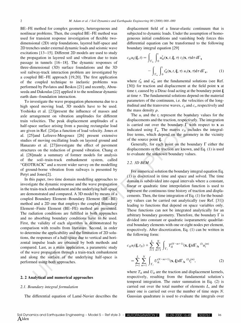
Considering the example of a train-track embankment
discretized with 50 (space constant) elements in the direc-
tion of the axis of the geometry and ®ve elements in each
row perpendicular to the axis of the geometry, using the
standard scheme each in¯uence matrix consists of 5 £ 10 £3 rows and columns, i.e. each matrix has 22 500 entries.
Using the proposed scheme, only 5 £ 2 £ 3 rows of the
matrix have to be calculated and saved, whereas the number
of columns is equal to the number of columns in the stan-
dard scheme. This results in 450 entries per matrix, only 2%
of the number of entries for the standard scheme. As a result
the computational time to assemble the matrices for each
time step and the memory required to save each matrix is
reduced by a factor of 50 for this example. If a sparse matrix
scheme is employed together with the standard scheme, the
number of 22 500 can be reduced, since the zero entries are
not stored. However, the memory savings using a sparse
matrix scheme in time domain BEM are small compared
to the proposed method. For the time required to assemble
the in¯uence matrices no savings can be obtained compared
to the standard scheme.
Together with the substructure method the proposed algo-
rithm can reduce the computational cost considerably. If the
M. Adam et al. / Soil Dynamics and Earthquake Engineering 00 (2000) 000±0004
Fig. 3. Surface discretization for 3D BEM model.
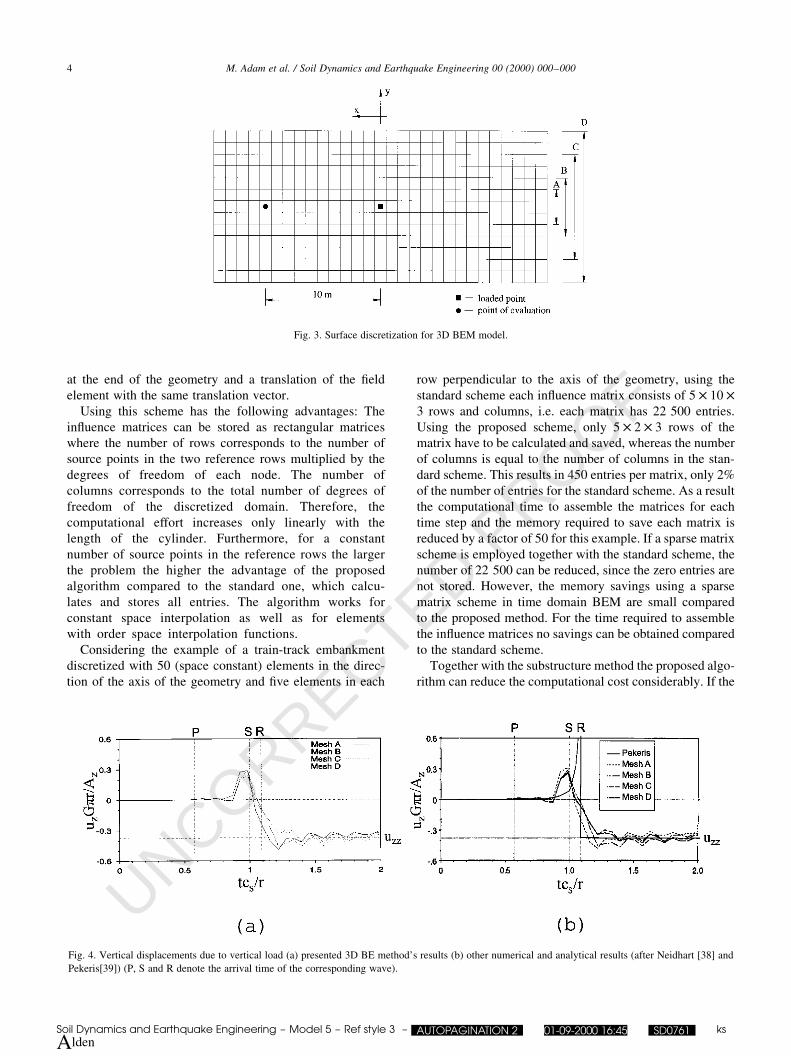
Fig. 4. Vertical displacements due to vertical load (a) presented 3D BE method's results (b) other numerical and analytical results (after Neidhart [38] and
Pekeris[39]) (P, S and R denote the arrival time of the corresponding wave).
Soil Dynamics and Earthquake Engineering ± Model 5 ± Ref style 3 ± AUTOPAGINATION 2 01-09-2000 16:45 SD0761 ks
Alden
UNCORRECTED PROOF
geometry of the problem consists of several domains (e.g.
train-track embankment, half-space and foundation), the
proposed algorithm can be used for those domains where
the geometry requirements Ð as stated above Ð hold (e.g.
train-track embankment and half-space), while the other
domains (e.g. foundation) have to be treated with the stan-
dard scheme.
2.3. 2D coupled BE±FE method
In the following, a general 2D BE±FE coupling formula-
tion is presented where the problem in hand is divided into
two parts as shown in Fig. 2. The uniform half-space domain
C reduces to a plane region and is modelled by boundary
elements. The non-homogeneous part V, that can be an
embankment, a dam or a structure will be modelled by ®nite
elements. The compatibility and equilibrium conditions
have to be satis®ed along the common interface line
between the two parts Gi. It should be noted that the integral
representation in Eq. (1) holds on the same form for both 3D
and 2D problems but reduces to a line integral and the
subscripts i, k take the values one and two only, for the
2D case.
The governing equation of motion of the ®nite element
domain due to a time dependent applied load P(t) can be
expressed and partitioned for the current time step N as:
Moo Moi
Mio Mii
" #�uo
�ui
( )N
1Coo Coi
Cio Cii
" #_uo
_ui
( )N
1Koo Koi
Kio Kii
" #
�uo
ui
( )N
�Po
Pi
( )N
(4)
where M, C and K are the mass, damping and stiffness
matrices, respectively. The vectors contain the nodal accel-
erations, velocities and displacements, respectively. The
variables on the interface Gi are denoted by the subscript i
and the other variables are denoted by the subscript o. Simi-
larly, using the subscript i for the interface nodes and s for
the surface nodes of the boundary element domain, Eq. (3)
can be written as:
U 1ss U1
si
U1is U1
ii
" #ts
ti
( )N
� T1ss T1
si
T1is T1
ii
" #us
ui
( )N
1Es
Ei
( )N
: �5�
Employing the traction-free condition on the surface, and
solving for the interface node variables, the nodal traction
along the interface can be expressed as:
{ti}N � �Kb�{ui}
N 2 {Ebu}N; �6�
where [Kb] and {Ebu} are the results from the necessary
M. Adam et al. / Soil Dynamics and Earthquake Engineering 00 (2000) 000±000 5
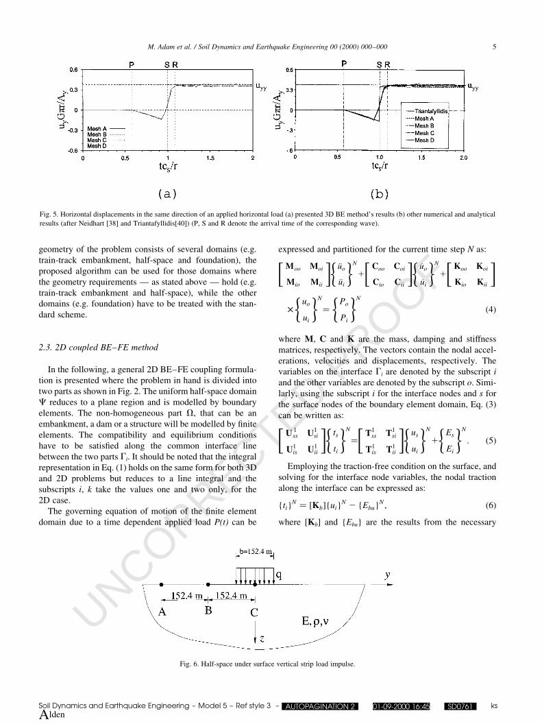
Fig. 5. Horizontal displacements in the same direction of an applied horizontal load (a) presented 3D BE method's results (b) other numerical and analytical
results (after Neidhart [38] and Triantafyllidis[40]) (P, S and R denote the arrival time of the corresponding wave).
Fig. 6. Half-space under surface vertical strip load impulse.
Soil Dynamics and Earthquake Engineering ± Model 5 ± Ref style 3 ± AUTOPAGINATION 2 01-09-2000 16:45 SD0761 ks
Alden

UNCORRECTED PROOF
M. Adam et al. / Soil Dynamics and Earthquake Engineering 00 (2000) 000±0006
Fig. 7. Vertical responses calculated at points A, B, and C (a) presented methods' results (3D BE and 2D BE±FE) (b) others' results (after Abouseeda et al.
[47]).
Fig. 8. Surface discretizations of half-space for comparison with 2D (a) Discretizations for different ratios of L/B (b) Section A±A.
Soil Dynamics and Earthquake Engineering ± Model 5 ± Ref style 3 ± AUTOPAGINATION 2 01-09-2000 16:45 SD0761 ks
Alden
UNCORRECTED PROOF
matrix and vector operations. The principle of virtual work
is used employing interpolation functions over each bound-
ary element to transform the traction in Eq. (6) into the
nodal force vector {Pbb}:
{Pbb}N � �Kbb�{ui}N 2 {Fb}N
; �7�
where [Kbb] and {Fb} represent [Kb] and {Ebu} after trans-
formation, respectively. Then, the principle of weighted
residual is applied along the interface to obtain the coupled
equation of motion as:
Koo Koi
Kio Kii 1 Kbb
" #p uo
ui
( )N
�Po
Pbb
( )Np
�8�
where the superscript p denotes the resulting coupled terms
including the contributions of the boundary element domain
as well as the mass and damping matrices of the ®nite
element domain.
3. Numerical examples and discussions
3.1. Validations
The 3D response of an elastic half-space to a Heaviside
type point load is obtained by a 3D Boundary Element
Method and compared with other numerical and analytical
solutions. Coupling is not required here, since the half-space
is treated as one domain. The discretized model is shown in
Fig. 3 where the black square indicates the location where
the load is applied at t� 0 and the black circle indicates the
location where the displacements are evaluated. The results
of the present method are shown in Figs. 4(a) and 5(a) while
Figs. 4(b) and 5(b) display the numerical results of Neidhart
[38] as well as the analytical solutions of Pekeris [39] and
Triantafyllidis [40]. The horizontal axis displays dimension-
less time, where r is the distance between the loaded point
and the observation point. P, S and R indicate the arrival of
the longitudinal, the transverse and the Rayleigh
waves, respectively. The vertical axis displays dimension-
less displacements where Ai is the force applied in the
M. Adam et al. / Soil Dynamics and Earthquake Engineering 00 (2000) 000±000 7
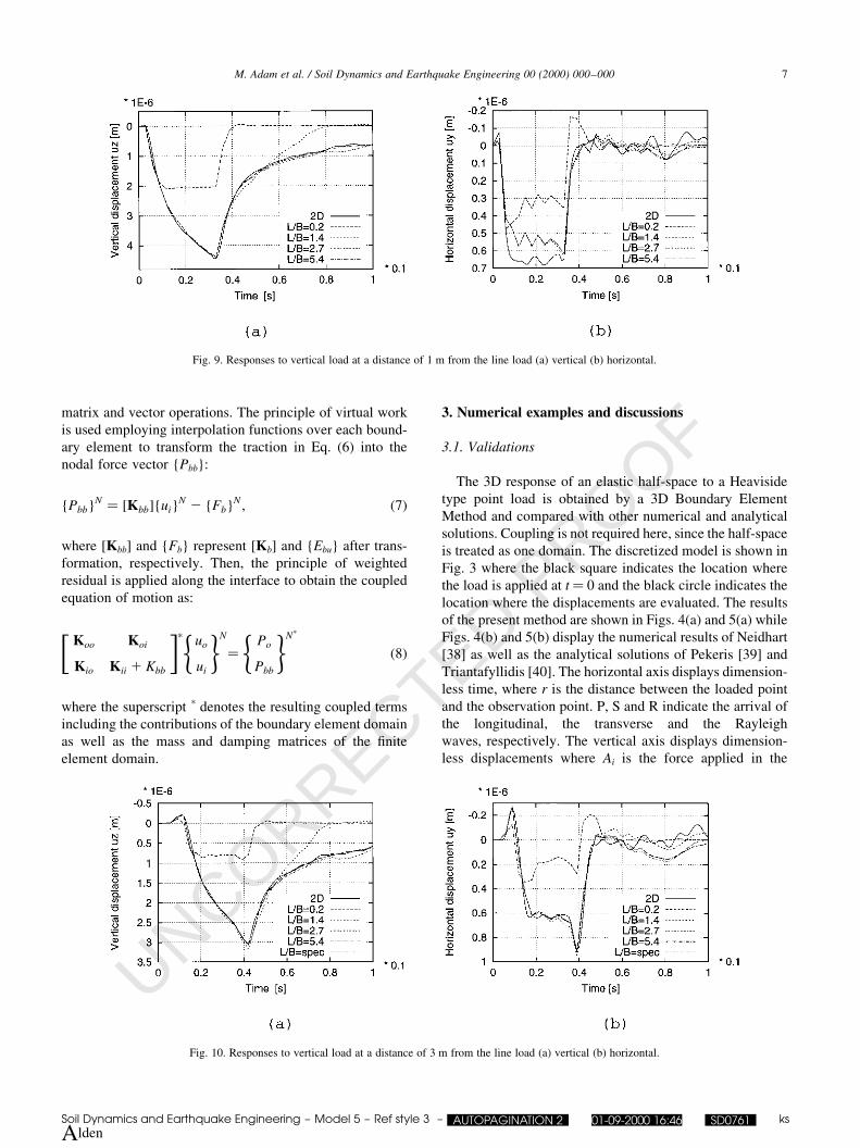
Fig. 9. Responses to vertical load at a distance of 1 m from the line load (a) vertical (b) horizontal.
Fig. 10. Responses to vertical load at a distance of 3 m from the line load (a) vertical (b) horizontal.
Soil Dynamics and Earthquake Engineering ± Model 5 ± Ref style 3 ± AUTOPAGINATION 2 01-09-2000 16:46 SD0761 ks
Alden
UNCORRECTED PROOF
i-direction. The parameters uzz and uyy denote the value of
the static solution of the corresponding Boussinesq-
problem, which is given by
uzz � uzGpr
Az
� v 2 1
2� 20:375 �9�
for the vertical response to a vertical loading and by
uyy �uyGpr
Ay
� 1 2 v
2� 0:375 �10�
for the horizontal response to a horizontal loading.
Different meshes A, B, C and D are used to investigate the
in¯uence of discretization, where mesh D represents the
largest mesh and mesh A is the smallest one as shown in
Fig. 3. The overall behavior of the presented results is in
very good agreement with the other solutions as shown in
Fig. 4 for vertical response due to vertical load and Fig. 5 for
horizontal response due to horizontal load. As a result of the
®nite size of the boundary elements and the approximation
of a point load to a surface area load, the numerical solution
can only approximate the abrupt change at the singularity at
the arrival of the Rayleigh-wave front. After the Rayleigh
wave has passed, the numerical and the analytical solutions
converge to the corresponding static solution given in Eqs.
(9) and (10), respectively. To achieve a better agreement
with the analytical solution a ®ner mesh with more elements
and smaller time steps would be required. However, since
this section is only for validation no convergence studies are
conducted at this point.
The two presented methods (3D BEM and 2D BE±FE
coupling) are now applied to obtain the response of an elas-
tic half-space under discontinuous boundary stress distribu-
tion as shown in Fig. 6. This test example was used for
comparison by many authors using different methods
[22,41±43]. A vertical impulse traction q � 68:95MPa is
applied on a strip of width b � 152:4 m: The elastic half-
space has a Young's modulus E � 17240 MPa; mass
density r � 3150 kg=m3 and a Poisson's ratio n � 0.25.
For the analysis using the 3D Boundary Element approach,
a length of about 3000 m is discretized in the x-direction and
a width of about 1000 m in the y-direction.
M. Adam et al. / Soil Dynamics and Earthquake Engineering 00 (2000) 000±0008
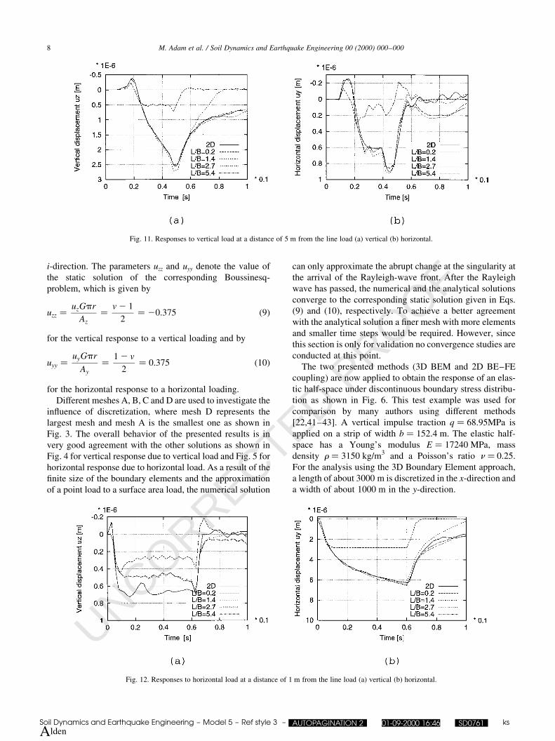
Fig. 11. Responses to vertical load at a distance of 5 m from the line load (a) vertical (b) horizontal.
Fig. 12. Responses to horizontal load at a distance of 1 m from the line load (a) vertical (b) horizontal.
Soil Dynamics and Earthquake Engineering ± Model 5 ± Ref style 3 ± AUTOPAGINATION 2 01-09-2000 16:46 SD0761 ks
Alden
UNCORRECTED PROOF
The vertical response is calculated at points A, B, and C
as shown in Fig. 6. The results of the present methods are
given in Fig. 7(a), while the results of the other authors are
scanned from Ref. [22]and displayed in Fig. 7(b). We
assumed the positive direction downward opposite to
other results, which makes no difference on the results. It
can be seen from Fig. 7(a) that for the 3D computation
results are obtained that are almost identical to those of
the 2D computation. The results demonstrate clearly the
good agreement of the presented methods with the
published solutions at all three points.
3.2. 2D and 3D responses of half-space
Plane-strain conditions and 2D solutions are assumed for
problems that have in®nite length in the third direction. In
order to ®nd whether 2D analysis of problems with ®nite
length in the third direction yields a good approximation to
the 3D solution, a problem of half-space under a line load
(see Fig. 8) is investigated using both presented approaches.
The amplitude of the line load is 1 kN/m for the time t
between 0 and 0.03 s and zero otherwise.
In the 3D model, a certain width B is discretized in
the y-direction and different stretches of length L are
discretized in the x-direction as shown in Fig. 8(a).
Unless stated otherwise, the length of the line load is
assumed to be equal to the discretized length. In the 2D
modelling, the same width B is discretized in the y-
direction. The line load is applied in the x-direction in
the middle of the discretized width B.
The case of vertical load is analyzed and the response at
three points of evaluation (see Fig. 8(a)) with different
distances from the line load along the width B are obtained.
The vertical and horizontal displacements at distances of 1,
3 and 5 m are shown in Figs. 9±11, respectively. The solid
lines display the 2D results, the dashed and the dotted lines
give the 3D ones. The comparison is performed in terms of
the L/B ratio. It can be seen that as the ratio L/B increases,
the 3D solutions approach the 2D ones. A very good match-
ing is obtained for L=B � 2:7 and higher for the vertical
response and a good matching for the maximum value is
achieved when L=B � 1:4: Concerning the horizontal
response, the best matching is obtained when L=B � 2:7
and no better matching can be obtained even for a very
M. Adam et al. / Soil Dynamics and Earthquake Engineering 00 (2000) 000±000 9
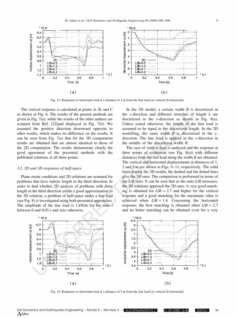
Fig. 13. Responses to horizontal load at a distance of 3 m from the line load (a) vertical (b) horizontal.
Fig. 14. Responses to horizontal load at a distance of 5 m from the line load (a) vertical (b) horizontal.
Soil Dynamics and Earthquake Engineering ± Model 5 ± Ref style 3 ± AUTOPAGINATION 2 01-09-2000 16:46 SD0761 ks
Alden

UNCORRECTED PROOF
high ratio of L/B. The same behavior is concluded at other
distances, which are not shown here.
For applied horizontal load, the responses at distances of
1, 3 and 5 m are shown in Figs. 12±14 respectively. In these
cases the matching between results of the two methods is
obtained for a higher L/B ratio than in the previous case,
especially for the vertical responses. This may be due to the
wave scattering by the truncated surface edges, which is
stronger in the case of horizontal load.
In addition another 3D calculation is performed, where
the discretized length in the x-direction is larger than the line
load length, which is denoted by L � 5:4B�p� in Fig. 8(a).
The results of this case are compared with the results of the
3D calculation of the similar case with shorter discretization
in the x-direction and shown in Fig. 15. The obtained iden-
tical results re¯ect that further increasing the discretized
area in the third direction has no effect on the result and it
is enough to discretize the loaded area only.
Based on these results, we can state that a problem can be
treated as a 2D case if the length to width ratio is about three
or more. It can be well approximated by a 2D solution when
this ratio is not less than 1.5. For smaller ratios, the 2D
model is not appropriate and the problem must be treated
as a 3D case.
3.3. Transient response of a train-track embankment on
half-space
As an application, the responses of half-space to station-
ary train-track loading are investigated. Fig. 16 shows the
dimensions and the con®guration of the considered train-
track embankment. The 0.8 m thick embankment layer is
assumed to be resting on a uniform half-space. The train-
track load is represented by two concentrated line loads in
the form of an impulse with unit amplitude (1 kN/m) that
lasts for 0.02 s. The time history and the frequency content
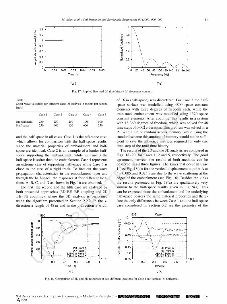
of such a load are given in Fig. 17(a) and (b), respectively.
The duration of the unit amplitude of 0.02 s is chosen in
such a way that the frequency content of the load covers the
typical range of frequencies of vibration as they are caused
by heavy-axle trains. Different values for the shear wave
velocity vs are assumed for ®ve cases as given in Table 1.
The mass density r � 2000 kg/m3 and Poisson's ratio
n � 1/3 are assumed to be identical for the embankment
M. Adam et al. / Soil Dynamics and Earthquake Engineering 00 (2000) 000±00010
Fig. 15. Responses to vertical load at a distance of 1 and 5 m (3D approach) (a) vertical (b) horizontal.
Fig. 16. Train-track embankment on half-space.
Soil Dynamics and Earthquake Engineering ± Model 5 ± Ref style 3 ± AUTOPAGINATION 2 01-09-2000 16:46 SD0761 ks
Alden
UNCORRECTED PROOF
and the half-space in all cases. Case 1 is the reference case,
which allows for comparison with the half-space results,
since the material properties of embankment and half-
space are identical. Case 2 is an example of a harder half-
space supporting the embankment, while in Case 3 the
half-space is softer than the embankment. Case 4 represents
an extreme case of supporting half-space while Case 5 is
close to the case of a rigid track. To ®nd out the wave
propagation characteristics in the embankment layer and
through the half-space, the responses at four different loca-
tions, A, B, C, and D as shown in Fig. 16 are obtained.
The ®rst, the second and the ®fth case are analyzed by
both presented approaches (3D BE±BE coupling and 2D
BE±FE coupling), where the 3D analysis is performed
using the algorithm presented in Section 2.2.2. In the x-
direction a length of 48 m and in the y-direction a width
of 16 m (half-space) was discretized. For Case 5 the half-
space surface was modelled using 4800 space constant
elements with three degrees of freedom each, while the
train-track embankment was modelled using 1320 space
constant elements. After coupling, this results in a system
with 18 360 degrees of freedom, which was solved for 48
time steps of 0:00 �2 s duration. This problem was solved on a
PC with 1 Gb of random access memory; while using the
standard scheme this amount of memory would not be suf®-
cient to save the in¯uence matrices required for only one
time step of the total time history.
The results of the 2D and the 3D analysis are compared in
Figs. 18±20, for Cases 1, 2 and 5, respectively. The good
agreement between the results of both methods can be
observed in all three ®gures. The kinks that occur in Case
1 (see Fig. 18(a)) for the vertical displacement at point A at
t� 0.005 and 0.025 s are due to the wave scattering at the
edges of the embankment (see Fig. 16). Besides the kinks
the results presented in Fig. 18(a) are qualitatively very
similar to the half-space results given in Fig. 9(a). This
can be expected since the embankment and the underlying
half-space possess the same material properties and there-
fore the only differences between Case 1 and the half-space
case considered in Section 3.2 are the geometry of the
M. Adam et al. / Soil Dynamics and Earthquake Engineering 00 (2000) 000±000 11
Fig. 17. Applied line load (a) time history (b) frequency content.
Fig. 18. Comparison of 2D and 3D responses at two different locations for Case 1 (a) vertical (b) horizontal.
Table 1
Shear-wave velocities for different cases of analysis in meters per second
[m/s]
Case 1 Case 2 Case 3 Case 4 Case 5
Embankment 250 250 250 100 500
Half-space 250 400 150 600 250
Soil Dynamics and Earthquake Engineering ± Model 5 ± Ref style 3 ± AUTOPAGINATION 2 01-09-2000 16:46 SD0761 ks
Alden
UNCORRECTED PROOF
embankment and the fact that the embankment is subjected
to two line loads while the half-space in Section 3.2 is
subjected to one line load only.
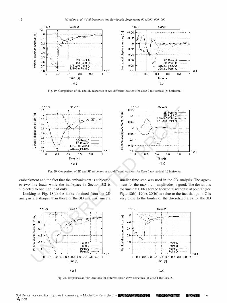
Looking at Fig. 18(a) the kinks obtained from the 2D
analysis are sharper than those of the 3D analysis, since a
smaller time step was used in the 2D analysis. The agree-
ment for the maximum amplitudes is good. The deviations
for time t . 0.06 s for the horizontal response at point C (see
Figs. 18(b), 19(b), 20(b)) are due to the fact that point C is
very close to the border of the discretized area for the 3D
M. Adam et al. / Soil Dynamics and Earthquake Engineering 00 (2000) 000±00012
Fig. 19. Comparison of 2D and 3D responses at two different locations for Case 2 (a) vertical (b) horizontal.
Fig. 20. Comparison of 2D and 3D responses at two different locations for Case 5 (a) vertical (b) horizontal.
Fig. 21. Responses at four locations for different shear-wave velocities (a) Case 1 (b) Case 2.
Soil Dynamics and Earthquake Engineering ± Model 5 ± Ref style 3 ± AUTOPAGINATION 2 01-09-2000 16:46 SD0761 ks
Alden
UNCORRECTED PROOF
analysis. The comparison con®rms our ®nding from the
previous analysis Ð 2D and 3D results match well for a
ratio of L/B of about three Ð now also for the case of
substructures with different material properties. As the 2D
and the 3D results are the same the following discussion is
based on the results of the 2D approach.
The time histories of vertical responses at the selected
four locations are shown in Fig. 21(a) and (b), for Case 1
and Case 2, respectively. The time delay and the amplitude
decrease for the maximum response at each location are
clearly depicted for both cases. The slight effect of wave
scattering by the inclined edges of the embankment for Case
1 is shown. In Case 2 a larger effect can be observed due to
the wave scattering by the subsurface between the embank-
ment and the half-space. As the half-space has more rigidity
and higher wave speed in Case 2, the maximum peaks arrive
earlier at locations B, C and D. In addition, the maximum
responses at all locations are reduced to about 50 to 60% of
the responses in Case 1.
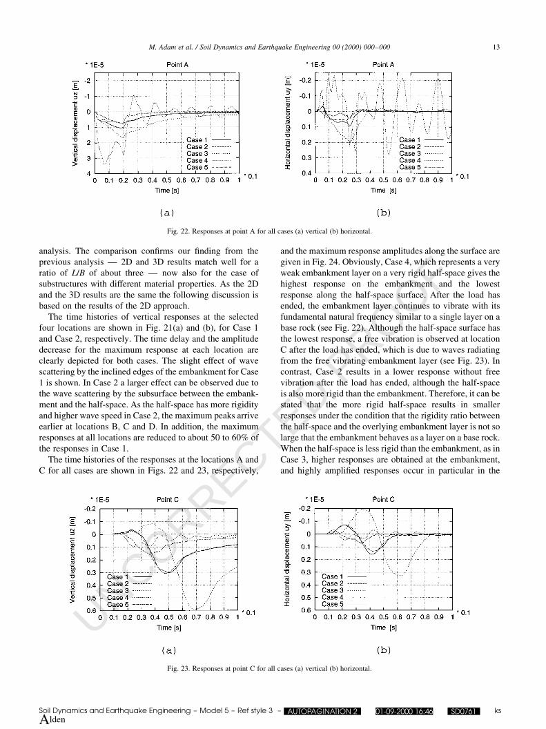
The time histories of the responses at the locations A and
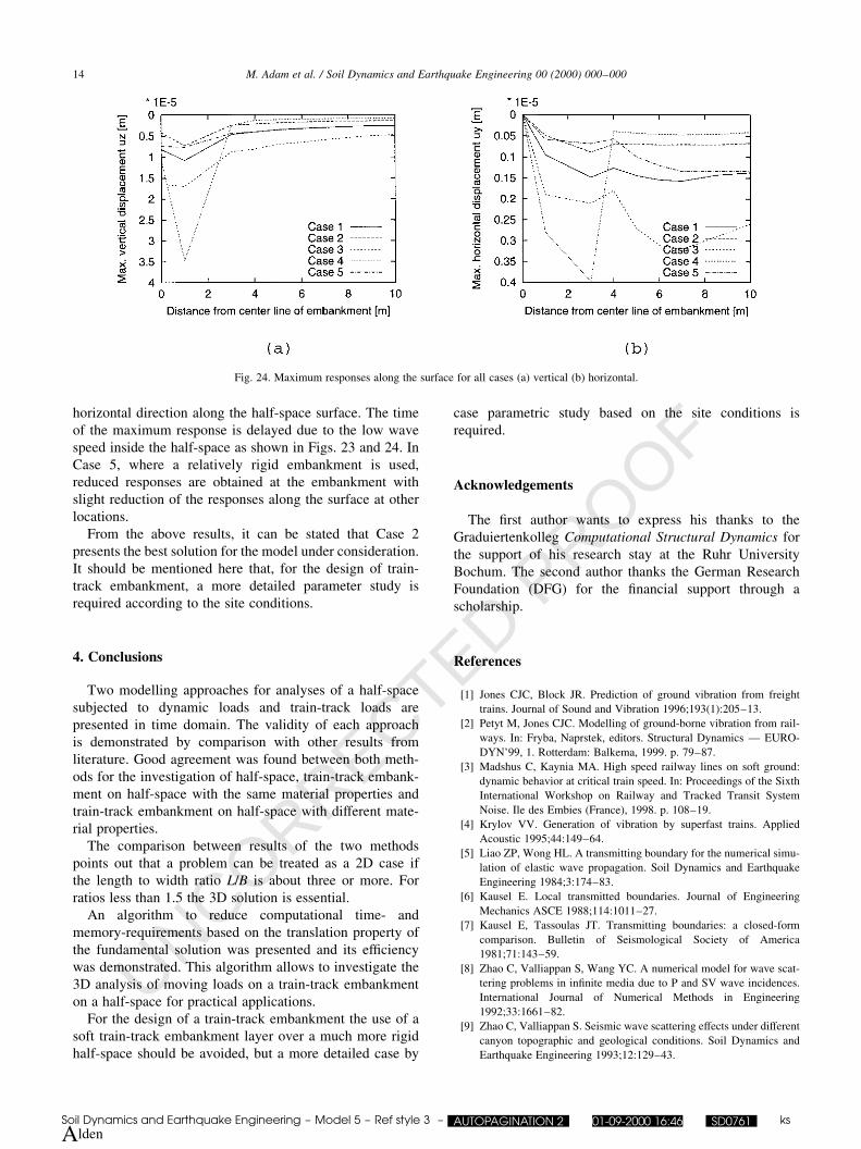
C for all cases are shown in Figs. 22 and 23, respectively,
and the maximum response amplitudes along the surface are
given in Fig. 24. Obviously, Case 4, which represents a very
weak embankment layer on a very rigid half-space gives the
highest response on the embankment and the lowest
response along the half-space surface. After the load has
ended, the embankment layer continues to vibrate with its
fundamental natural frequency similar to a single layer on a
base rock (see Fig. 22). Although the half-space surface has
the lowest response, a free vibration is observed at location
C after the load has ended, which is due to waves radiating
from the free vibrating embankment layer (see Fig. 23). In
contrast, Case 2 results in a lower response without free
vibration after the load has ended, although the half-space
is also more rigid than the embankment. Therefore, it can be
stated that the more rigid half-space results in smaller
responses under the condition that the rigidity ratio between
the half-space and the overlying embankment layer is not so
large that the embankment behaves as a layer on a base rock.
When the half-space is less rigid than the embankment, as in
Case 3, higher responses are obtained at the embankment,
and highly ampli®ed responses occur in particular in the
M. Adam et al. / Soil Dynamics and Earthquake Engineering 00 (2000) 000±000 13
Fig. 22. Responses at point A for all cases (a) vertical (b) horizontal.
Fig. 23. Responses at point C for all cases (a) vertical (b) horizontal.
Soil Dynamics and Earthquake Engineering ± Model 5 ± Ref style 3 ± AUTOPAGINATION 2 01-09-2000 16:46 SD0761 ks
Alden
UNCORRECTED PROOF
horizontal direction along the half-space surface. The time
of the maximum response is delayed due to the low wave
speed inside the half-space as shown in Figs. 23 and 24. In
Case 5, where a relatively rigid embankment is used,
reduced responses are obtained at the embankment with
slight reduction of the responses along the surface at other
locations.
From the above results, it can be stated that Case 2
presents the best solution for the model under consideration.
It should be mentioned here that, for the design of train-
track embankment, a more detailed parameter study is
required according to the site conditions.
4. Conclusions
Two modelling approaches for analyses of a half-space
subjected to dynamic loads and train-track loads are
presented in time domain. The validity of each approach
is demonstrated by comparison with other results from
literature. Good agreement was found between both meth-
ods for the investigation of half-space, train-track embank-
ment on half-space with the same material properties and
train-track embankment on half-space with different mate-
rial properties.
The comparison between results of the two methods
points out that a problem can be treated as a 2D case if
the length to width ratio L/B is about three or more. For
ratios less than 1.5 the 3D solution is essential.
An algorithm to reduce computational time- and
memory-requirements based on the translation property of
the fundamental solution was presented and its ef®ciency
was demonstrated. This algorithm allows to investigate the
3D analysis of moving loads on a train-track embankment
on a half-space for practical applications.
For the design of a train-track embankment the use of a
soft train-track embankment layer over a much more rigid
half-space should be avoided, but a more detailed case by
case parametric study based on the site conditions is
required.
Acknowledgements
The ®rst author wants to express his thanks to the
Graduiertenkolleg Computational Structural Dynamics for
the support of his research stay at the Ruhr University
Bochum. The second author thanks the German Research
Foundation (DFG) for the ®nancial support through a
scholarship.
References
[1] Jones CJC, Block JR. Prediction of ground vibration from freight
trains. Journal of Sound and Vibration 1996;193(1):205±13.
[2] Petyt M, Jones CJC. Modelling of ground-borne vibration from rail-
ways. In: Fryba, Naprstek, editors. Structural Dynamics Ð EURO-
DYN'99, 1. Rotterdam: Balkema, 1999. p. 79±87.
[3] Madshus C, Kaynia MA. High speed railway lines on soft ground:
dynamic behavior at critical train speed. In: Proceedings of the Sixth
International Workshop on Railway and Tracked Transit System
Noise. Ile des Embies (France), 1998. p. 108±19.
[4] Krylov VV. Generation of vibration by superfast trains. Applied
Acoustic 1995;44:149±64.
[5] Liao ZP, Wong HL. A transmitting boundary for the numerical simu-
lation of elastic wave propagation. Soil Dynamics and Earthquake
Engineering 1984;3:174±83.
[6] Kausel E. Local transmitted boundaries. Journal of Engineering
Mechanics ASCE 1988;114:1011±27.
[7] Kausel E, Tassoulas JT. Transmitting boundaries: a closed-form
comparison. Bulletin of Seismological Society of America
1981;71:143±59.
[8] Zhao C, Valliappan S, Wang YC. A numerical model for wave scat-
tering problems in in®nite media due to P and SV wave incidences.
International Journal of Numerical Methods in Engineering
1992;33:1661±82.
[9] Zhao C, Valliappan S. Seismic wave scattering effects under different
canyon topographic and geological conditions. Soil Dynamics and
Earthquake Engineering 1993;12:129±43.
M. Adam et al. / Soil Dynamics and Earthquake Engineering 00 (2000) 000±00014
Fig. 24. Maximum responses along the surface for all cases (a) vertical (b) horizontal.
Soil Dynamics and Earthquake Engineering ± Model 5 ± Ref style 3 ± AUTOPAGINATION 2 01-09-2000 16:46 SD0761 ks
Alden
UNCORRECTED PROOF
[10] Beskos DE. Boundary element methods in dynamic analysis. Applied
Mechanics Reviews 1987;40:1±23.
[11] Ahmad S, Banerjee PK. Multi-domain BEM for two-dimensional
problems of elastodynamics. International Journal of Numerical
Methods in Engineering 1988;26:891±911.
[12] Zienkiewicz OC, Kelly DM, Bettes P. The coupling of the ®nite
element method and the boundary solution procedures. International
Journal of Numerical Methods in Engineering 1977;11:355±76.
[13] Spyrakos CC, Beskos DE. Dynamic response of ¯exible strip-founda-
tion by boundary and ®nite elements. Soil Dynamics and Earthquake
Engineering 1986;5:84±96.
[14] Von Estorff O, Kausel E. Coupling of boundary element and ®nite
elements for soil±structure interaction problems. Earthquake Engi-
neering and Structural Dynamics 1989;18:1065±75.
[15] Von Estorff O, Prabucki MJ. Dynamic response in time domain by
coupled boundary and ®nite elements. Computational Mechanics
1990;9:35±46.
[16] Chua KH, Balendra T, Lo KW. Groundborne vibrations due to trains
in tunnels. Earthquake Engineering and Structural Dynamics
1992;21:445±60.
[17] Jones CJC. Use of numerical models to determine the effectiveness of
anti-vibration systems for railways. Proceedings of the Institution of
Civil Engineers and Transportation 1994;105(2):43±51.
[18] Jones CJC, Wang A, Down TM. Modelling the propagation of vibra-
tion from railway tunnels. In: Computational acoustic and its envir-
onmental applications. Southampton: Computational Mechanics
Publications, 1995. p. 285±92.
[19] Karabalis DL, Beskos DE. Dynamic response of 3-D ¯exible surface
foundations by time domain ®nite and boundary element methods.
International Journal of Soil Dynamics and Earthquake Engineering
1985;4:91±101.
[20] Mohammadi M, Karabalis DL. Dynamic 3-D soil-railway track inter-
action by BEM±FEM. Earthquake Engineering and Structural
Dynamics 1995;24:1177±93.
[21] Pavlatos GD, Beskos DE. Dynamic elastoplastic analysis by BEM/
FEM. Engineering Analysis with Boundary Elements 1994;14:51±63.
[22] Abouseeda H, Dakoulas P. Non-linear dynamic earth dam±founda-
tion interaction using BE±FE method. Earthquake Engineering and
Structural Dynamics 1998;27:917±36.
[23] Yoshioka O, Ashiya K. Effects of masses and axle arrangements of
rolling stock on train induced ground vibrations. Quarterly Review of
RTRI 1990;31(3):145±52.
[24] P¯anz G. Wellenausbreitung in elastischen Kontinua infolge sich
bewegender Lasten. In: Schmid G, editor. Graduiertenkolleg Compu-
tational Structural Dynamics an der Ruhr-UniversitaÈt Bochum.
Tagungsband zum Abschlubkolloquium. Fortschrittsberichte VDI,
Reihe 18, DuÈsseldorf, Germany, 1999. p. 244±253.
[25] Jones CJC, Sheng X, Petyt M. Simulation of ground vibration from a
moving harmonic load on a railway track. Journal of Sound and
Vibration 2000;231(3):739±51.
[26] Lefeuve-Mesgouez G. Propagation d'ondes dans un massif soumis a
des charges se deplacËant a vitesse constante. PhD-Thesis, Ecole
Centrale de Nantes, No. ED:82-399, 1999.
[27] Hanazato T, Ugai K, Mori M, Sakaguchi R. Three dimensional analy-
sis of traf®c induced ground vibrations. Journal of Geotechnical Engi-
neering Division ASCE 1991;117(8):1133±51.
[28] Chang CS, Selig ET, Adegoke CW. GEOTRACK model for railroad
track performance. Journal of Geotechnical Engineering Division
ASCE 1980;106(11):1201±18.
[29] Dominguez J. Boundary elements in dynamics. Southampton\Boston
and London: Computational Mechanics Publications and Elsevier
Applied Science, 1993.
[30] Stokes GG. On the dynamical theory of diffraction. Transactions of
Cambridge Philosophical Society 1849;9:793±7.
[31] Hubert W. Implementierung von Ansatzfunktionen hoÈherer Ordnung
in Ort und Zeit in ein 3-D-Rechenprogramm zur Simulation von
ErschuÈtterungsausbreitung durch Schienenverkehr mittels der Rande-
lementmethode im Zeitbereich. Germany: Ruhr-UniversitaÈt Bochum,
Theorie der Tragwerke und Simulationstechnik, 1999.
[32] Gaul L, Fiedler C. Methode der Randelemente in Statik und Dynamik
Fundamentals and Advances in the Engineering Sciences. Germany:
Wiesbaden Vieweg, 1997.
[33] Li HB, Guo-Ming H. A new method for evaluating singular integrals
in stress analysis of solids by the direct boundary element method.
International Journal of Numerical Methods in Engineering
1985;21:2071±98.
[34] Aliabadi MH, Hall WS. Taylor expansions for singular kernels in the
Boundary Element Method. International Journal for Numerical
Methods in Engineering 1985;21:2221±36.
[35] Guiggiani M, Gigante A. A general algorithm for multidimensional
Cauchy principal value integrals in the Boundary Element Method.
Journal of Applied Mechanics ASME 1990;57:906±15.
[36] Guiggiani M. Computing principal value integrals in 3-D BEM for
time-harmonic elastodynamics Ð a direct approach. Communica-
tions in Applied Numerical Methods 1992;8:141±9.
[37] Lanzerath H. Zur Modalanalyse unter Verwendung der Randelement-
methode. Germany: Ruhr-UniversitaÈt Bochum, IFM. 1996. p. 103.
[38] Neidhart, T. LoÈsung dreidimensionaler linearer Probleme der Boden-
dynamik mit der Randelementmethode. Germany: University of
Karlsruhe, VeroÈffentlichungen des Institutes fuÈr Bodenmechanik
und Felsmechanik, Heft. 1994. p. 131.
[39] Pekeris CL. The seismic surface pulse. Proceedings of the National
Academy of Sciences 1955;41:469±80.
[40] Triantafyllidis T. HalbraumloÈsungen zur Behandlung bodenmecha-
nischer Probleme mit der Randelementmethode. Germany: University
of Karlsruhe, VeroÈffentlichungen des Institutes fuÈr Bodenmechanik
und Felsmechanik, Heft, 1989. p. 116.
[41] Mansur WJ, Brebbia CA. Formulation of the boundary element
method for transient problems governed by the scalar wave equation.
Applied Mathematical Modelling 1982;6:307±11.
[42] Antes H. A boundary element procedure for transient wave propaga-
tion in two-dimensional isotropic elastic media. Finite Elements in
Analysis and Design 1985;1:313±23.
[43] Cruse TA, Rizzo FJ. A direct formulation and numerical solution of
the general transient elastodynamic problem 1. International Journal
of Mathematical Analysis Applications 1968;22:244±59.
M. Adam et al. / Soil Dynamics and Earthquake Engineering 00 (2000) 000±000 15
Soil Dynamics and Earthquake Engineering ± Model 5 ± Ref style 3 ± AUTOPAGINATION 2 01-09-2000 16:46 SD0761 ks
Alden