Twenty Questions and Answers About the Ozone Layer

Scientific Assessment of Ozone Depletion: 2018

World Meteorological OrganizationUnited Nations Environment Programme

National Oceanic and Atmospheric AdministrationNational Aeronautics and Space Administration

European Commission

Twenty Questions and Answers About the Ozone Layer:

2018 Update

Lead AuthorRoss J. Salawitch

CoauthorsDavid W. Fahey

Michaela I. Hegglin Laura A. McBrideWalter R. TribettSarah J. Doherty

32

Why has an “ozone hole” appeared over Antarctica when ozone-depleting substances are present throughout the stratosphere? Q9

The severe depletion of stratospheric ozone in late winter and early spring in the Antarctic is known as the “ozone hole” (see Q10). The ozone hole appears over Antarctica because meteo-rological and chemical conditions unique to this region increase the effectiveness of ozone destruction by reactive halogen

gases (see Q7 and Q8). In addition to a large abundance of these reactive gases, the formation of the Antarctic ozone hole requires temperatures low enough to form polar stratospheric clouds (PSCs), isolation from air in other stratospheric regions, and sunlight (see Q8).

Ozone-depleting substances are present throughout the stratospheric ozone layer because they are transported great distances by atmospheric air motions. The severe depletion of the Antarctic ozone layer known as the “ozone hole” occurs because of the special meteorological and chemical conditions that exist there and nowhere else on the globe. The very low winter temperatures in the Antarctic stratosphere cause polar stratospheric clouds (PSCs) to form. Special reactions that occur on PSCs, combined with the isolation of polar stratospheric air in the polar vortex, allow chlorine and bromine reactions to produce the ozone hole in Antarctic springtime.

Figure Q9-1. Arctic and Antarctic tem-peratures. Air temperatures in both polar regions reach minimum values in the lower stratosphere in the winter season. Average daily minimum values over Antarctica are as low as −92°C in July and August in a typical year. Over the Arctic, average mini-mum values are near −80°C in late Decem-ber and January. Polar stratospheric clouds (PSCs) are formed in the ozone layer when winter minimum temperatures fall below their formation threshold of about −78°C. This occurs on average for 1 to 2 months over the Arctic and about 5 months over Antarctica each year (see heavy red and blue lines). Reactions on liquid and solid PSC particles cause the highly reactive chlorine gas ClO to be formed, which catalytically destroys ozone (see Q8). The range of winter minimum temperatures found in the Arctic is much greater than that in the Antarctic. In some years, PSC formation temperatures are not reached in the Arctic, and significant ozone depletion does not occur. In contrast, PSC formation temperatures are always present for many months somewhere in the Antarctic, and severe ozone depletion occurs each winter season (see Q10).

Section II: The ozone depletion process

Antarctic winter

May June July August Sept Oct

Arctic winter

Minimum Air Temperatures in the Polar Stratosphere

Nov Dec Jan Feb March April–50

–55

– 60

– 65

–70

–75

– 80

–85

–90

–95

Tem

pera

ture

(deg

rees

Cel

sius

)

Antarctic 1979 to 2018Arctic 1979/80 to 2017/18

Average daily values

PSC formation temperature

Ranges of daily values

Arctic

Antarctic

50º to 90º Latitude – 60

–70

– 80

– 90

–100

–110

–120

–130

–140

Tem

pera

ture

(deg

rees

Fah

renh

eit)

33Section II: The ozone depletion process

2018 Update | Twenty Questions | Q9

Distribution of halogen gases. Halogen source gases that are emitted at Earth’s surface and have lifetimes longer than about 1 year (see Table Q6-1) are present in comparable abundances throughout the stratosphere in both hemispheres, even though most of the emissions occur in the Northern Hemisphere. The abundances are comparable because most long-lived source gases have no significant natural removal processes in the lower atmosphere, and because winds and convection redistribute and mix air efficiently throughout the troposphere on the times-cale of weeks to months. Halogen gases (in the form of source gases and some reactive products) enter the stratosphere pri-marily from the tropical upper troposphere. Stratospheric air motions then transport these gases upward and toward the pole in both hemispheres.

Low polar temperatures. The severe ozone destruction that leads to the ozone hole requires low temperatures to be present over a range of stratospheric altitudes, over large geographical regions, and for extended time periods. Low temperatures are important because they allow liquid and solid PSCs to form. Reactions on the surfaces of these PSCs initiate a remarkable increase in the most reactive chlorine gas, chlorine monoxide (ClO) (see below as well as Q7 and Q8). Stratospheric tempera-tures are lowest in the polar regions in winter. In the Antarctic winter, minimum daily temperatures are generally much lower and less variable than those in the Arctic winter (see Figure Q9-1). Antarctic temperatures also remain below PSC formation temperatures for much longer periods during winter. These and other meteorological differences occur because of variations be-tween the hemispheres in the distributions of land, ocean, and mountains at middle and high latitudes. As a consequence, win-ter temperatures are low enough for PSCs to form somewhere in the Antarctic for nearly the entire winter (about 5 months), and only for limited periods (10–60 days) in the Arctic for most winters.

Isolated conditions. Stratospheric air in the polar regions is rel-atively isolated for long periods in the winter months. The isola-tion is provided by strong winds that encircle the poles during winter, forming a polar vortex, which prevents substantial trans-port and mixing of air into or out of the polar stratosphere. This circulation strengthens in winter as stratospheric temperatures decrease. The Southern Hemisphere polar vortex circulation tends to be stronger than that in the Northern Hemisphere be-cause northern polar latitudes have more land and mountain-ous regions than southern polar latitudes. This situation leads to more meteorological disturbances in the Northern Hemisphere, which increase the mixing in of air from lower latitudes that warms the Arctic stratosphere. Since winter temperatures are lower in the Southern than in the Northern Hemisphere polar stratosphere, the isolation of air in the polar vortex is much more effective in the Antarctic than in the Arctic. Once temperatures drop low enough, PSCs form within the polar vortex and induce chemical changes such as an increase in the abundance of ClO (see Q8) that are preserved for many weeks to months due to the isolation of polar air.

Polar stratospheric clouds (PSCs). Reactions on the surfaces of liquid and solid PSCs can substantially increase the relative abundances of the most reactive chlorine gases. These reactions convert the reservoir forms of reactive chlorine gases, chlorine nitrate (ClONO2) and hydrogen chloride (HCl), to the most reac-tive form, ClO (see Figure Q7-3). The abundance of ClO increases from a small fraction of available reactive chlorine to comprise nearly all chlorine that is available. With increased ClO, the cata-lytic cycles involving ClO and BrO become active in the chemical destruction of ozone whenever sunlight is available (see Q8).

Different types of liquid and solid PSC particles form when stratospheric temperatures fall below about −78°C (−108°F) in polar regions (see Figure Q9-1). As a result, PSCs are often found over large areas of the winter polar regions and over significant

Figure Q9-2. Polar stratospheric clouds. This photograph of an Arctic polar stratospheric cloud (PSC) was taken in Kiruna, Sweden (67°N), on 27 January 2000. PSCs form in the ozone layer during winters in the Arctic and Antarctic, wherever low temperatures occur (see Figure Q9-1). The particles grow from the condensation of water, nitric acid (HNO3), and sulfuric acid (H2SO4). The clouds often can be seen with the human eye when the Sun is near the horizon. Reactions on PSCs cause the formation of the highly reac-tive gas chlorine monoxide (ClO), which is very effective in the chemical destruction of ozone (see Q7 and Q8).

Arctic Polar Stratospheric Clouds (PSCs)

34

Q9 | Twenty Questions | 2018 Update

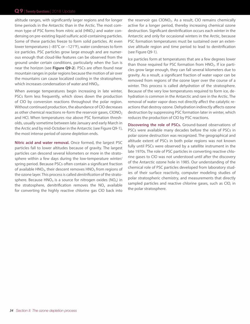
altitude ranges, with significantly larger regions and for longer time periods in the Antarctic than in the Arctic. The most com-mon type of PSC forms from nitric acid (HNO3) and water con-densing on pre-existing liquid sulfuric acid-containing particles. Some of these particles freeze to form solid particles. At even lower temperatures (−85°C or −121°F), water condenses to form ice particles. PSC particles grow large enough and are numer-ous enough that cloud-like features can be observed from the ground under certain conditions, particularly when the Sun is near the horizon (see Figure Q9-2). PSCs are often found near mountain ranges in polar regions because the motion of air over the mountains can cause localized cooling in the stratosphere, which increases condensation of water and HNO3.

When average temperatures begin increasing in late winter, PSCs form less frequently, which slows down the production of ClO by conversion reactions throughout the polar region. Without continued production, the abundance of ClO decreases as other chemical reactions re-form the reservoir gases, ClONO2 and HCl. When temperatures rise above PSC formation thresh-olds, usually sometime between late January and early March in the Arctic and by mid-October in the Antarctic (see Figure Q9-1), the most intense period of ozone depletion ends.

Nitric acid and water removal. Once formed, the largest PSC particles fall to lower altitudes because of gravity. The largest particles can descend several kilometers or more in the strato-sphere within a few days during the low-temperature winter/spring period. Because PSCs often contain a significant fraction of available HNO3, their descent removes HNO3 from regions of the ozone layer. This process is called denitrification of the strato-sphere. Because HNO3 is a source for nitrogen oxides (NOx) in the stratosphere, denitrification removes the NOx available for converting the highly reactive chlorine gas ClO back into

the reservoir gas ClONO2. As a result, ClO remains chemically active for a longer period, thereby increasing chemical ozone destruction. Significant denitrification occurs each winter in the Antarctic and only for occasional winters in the Arctic, because PSC formation temperatures must be sustained over an exten-sive altitude region and time period to lead to denitrification (see Figure Q9-1).

Ice particles form at temperatures that are a few degrees lower than those required for PSC formation from HNO3. If ice parti-cles grow large enough, they can fall several kilometers due to gravity. As a result, a significant fraction of water vapor can be removed from regions of the ozone layer over the course of a winter. This process is called dehydration of the stratosphere. Because of the very low temperatures required to form ice, de-hydration is common in the Antarctic and rare in the Arctic. The removal of water vapor does not directly affect the catalytic re-actions that destroy ozone. Dehydration indirectly affects ozone destruction by suppressing PSC formation later in winter, which reduces the production of ClO by PSC reactions.

Discovering the role of PSCs. Ground-based observations of PSCs were available many decades before the role of PSCs in polar ozone destruction was recognized. The geographical and altitude extent of PSCs in both polar regions was not known fully until PSCs were observed by a satellite instrument in the late 1970s. The role of PSC particles in converting reactive chlo-rine gases to ClO was not understood until after the discovery of the Antarctic ozone hole in 1985. Our understanding of the chemical role of PSC particles developed from laboratory stud-ies of their surface reactivity, computer modeling studies of polar stratospheric chemistry, and measurements that directly sampled particles and reactive chlorine gases, such as ClO, in the polar stratosphere.


35



The Discovery of the Antarctic Ozone HoleThe first decreases in Antarctic total ozone were observed in the early 1980s over research stations located on the Antarctic continent. The measurements were made with ground-based Dobson spectrophotometers (see box in Q4) installed as part of the effort to increase observations of Earth’s atmosphere during the International Geophysical Year that began in 1957 (see Figure Q0-1).The observations showed unusually low total ozone during the late winter/early spring months of September, October, and November. Total ozone was lower in these months compared with previous observations made as early as 1957. The early published reports came from the Japan Meteorological Agency and the British Antarctic Sur-vey. The results became widely known to the world after three scientists from the British Antarctic Survey published their observations in the prestigious scientific journal Nature in 1985. They suggested that rising abundances of atmospheric CFCs were the cause of the steady decline in total ozone over the Halley Bay research station (76°S) observed during suc-cessive Octobers starting in the early 1970s. Soon after, satellite measurements confirmed the spring ozone depletion and further showed that for each late winter/early spring season starting in the early 1980s, the depletion of ozone extended over a large region centered near the South Pole. The term “ozone hole” came about as a description of the very low values of total ozone, apparent in satellite images, that encircle the Antarctic continent for many weeks each October (spring in the Southern Hemisphere) (see Q10). Currently, the formation and severity of the Antarctic ozone hole are documented each year by a combination of satellite, ground-based, and balloon observations of ozone.

Very early Antarctic ozone measurements. The first total ozone measurements made in Antarctica with Dobson spec-trophotometers occurred in the 1950s following extensive measurements in the Northern Hemisphere and Arctic region. Total ozone values observed in the Antarctic spring were found to be around 300 Dobson units (DU), lower than those in the Arctic spring. The Antarctic values were surprising because the assumption at the time was that the two polar regions would have similar values. We now know that these 1950s Antarctic values were not anomalous; in fact, similar values were observed near the South Pole in the 1970s, before the ozone hole appeared (see Figure Q10-3). Antarctic total ozone values in early spring are systematically lower than those in the Arctic early spring because the Southern Hemisphere polar vortex is much stronger and colder and, therefore, much more effective in reducing the transport of ozone-rich air from midlati-tudes to the pole (compare Figures Q10-3 and Q11-2).

36 Section III: Stratospheric ozone depletion

How severe is the depletion of the Antarctic ozone layer? Q10

The severe depletion of Antarctic ozone, known as the “ozone hole”, was first reported in the mid-1980s (see box in Q9). The depletion is attributable to chemical destruction by reactive halogen gases (see Q7 and Q8), which increased everywhere in the stratosphere in the latter half of the 20th century (see Q15). Conditions in the Antarctic winter and early spring stratosphere enhance ozone depletion because of (1) the long periods of

extremely low temperatures, which cause polar stratospheric clouds (PSCs) to form; (2) the large abundance of reactive hal-ogen gases produced in reactions on PSCs; and (3) the isolation of stratospheric air, which allows time for chemical destruction processes to occur. The severity of Antarctic ozone depletion as well as long-term changes can be seen using satellite observa-tions of total ozone and ozone altitude profiles.

Severe depletion of the Antarctic ozone layer was first reported in the mid-1980s. Antarctic ozone depletion is seasonal, occurring primarily in late winter and early spring (August–November). Peak depletion occurs in early October when ozone is often completely destroyed over a range of stratospheric altitudes, thereby reducing total ozone by as much as two-thirds at some locations. This severe depletion creates the “ozone hole” apparent in images of Antarctic total ozone acquired using satellite instruments. In most years the maximum area of the ozone hole far exceeds the size of the Antarctic continent.

Figure Q10-1. Antarctic ozone hole. Total ozone values are shown for high southern latitudes between 21 and 30 Sep-tember 2017 as measured by a satellite instrument. The dark blue and purple regions over the Antarctic continent show the severe ozone depletion or “ozone hole” now found every austral spring. Minimum values of total ozone inside the ozone hole are close to 150 Dobson units (DU) compared with Antarctic springtime values of about 350 DU observed in the early 1970s (see Figure Q10-3). The area of the ozone hole is usually defined as the geographical region within the 220-DU contour (see white line) on total ozone maps. The maximum values of total ozone in the Southern Hemisphere in late win-ter/early spring are generally located in a crescent-shaped region that surrounds and is isolated from the ozone hole, due to stratospheric winds at the boundary of the polar vor-tex. In late spring or early summer (November–December), these atmospheric winds weaken and the ozone hole dis-appears due to the transport of ozone-enriched air masses towards the pole.

21−30 September 2017

100 200 300 400 500 600Total Ozone (Dobson units)

Antarctic Ozone Hole

37Section III: Stratospheric ozone depletion


Antarctic ozone hole. The most widely used images of Antarctic ozone depletion are derived from measurements of total ozone made with satellite instruments. A map of Antarctic early spring measurements shows a large region centered near the South Pole in which total ozone is highly depleted (see Figure Q10-1). This region has come to be called the “ozone hole” because of the near-circular contours of low ozone values in the maps. The area of the ozone hole is defined here as the geographical re-gion within the 220-Dobson unit (DU) contour in total ozone maps (see white line in Figure Q10-1) averaged between 21–30 September for a given year. The area reached a maximum of 28 million square km (about 11 million square miles) in 2006, which is more than twice the area of the Antarctic continent (see Figure Q10-2). Minimum values of total ozone inside the ozone hole averaged in late September to mid-October are near 120 DU, which is nearly two-thirds below springtime values of about 350 DU observed in the early 1970s (see Figures Q10-3 and Q11-1). Low total ozone inside the ozone hole contrasts strongly with the distribution of much larger values outside the ozone hole. This common feature can be seen in Figure Q10-1, where a crescent-shaped region with values around 400 DU surrounds a significant portion of the ozone hole in September 2017, and reveals the edge of the polar vortex that acts as a barrier to the transport of ozone-rich midlatitude air into the polar region (see Q9).

Altitude profiles of Antarctic ozone. The low total ozone values within the ozone hole are caused by nearly complete removal

of ozone in the lower stratosphere. Balloon-borne instruments (see Q4) demonstrate that this depletion occurs within the ozone layer, the altitude region that normally contains the high-est abundances of ozone. At geographic locations with the lowest total ozone values, balloon measurements show that the chemical destruction of ozone has often been complete over an altitude region of up to several kilometers. For example, in the ozone profile over South Pole, Antarctica on 9 October 2006 (see red line in left panel of Figure Q11-3), ozone abundances are essentially zero over the altitude region of 14 to 21 km. The lowest winter temperatures and highest reactive chlorine (ClO) abundances occur in this altitude region (see Figure Q7-3). The differences in the average South Pole ozone profiles between the decade 1962–1971 and the years 1990–2018 in Figure Q11-3 show how reactive halogen gases have dramatically altered the ozone layer. In the 1960s, a normal ozone layer is clearly evident in the October average profile, with a peak near 16 km altitude. In the 1990–2018 average profile, a broad minimum centered near 16 km now occurs, with ozone values reduced by up to 90% relative to normal values.

Long-term total ozone changes. Prior to 1960, the amount of reactive halogen gases in the stratosphere was insufficient to cause significant chemical loss of Antarctic ozone. Ground-based observations show that the steady decline in total ozone over the Halley Bay, Antarctic research station (76°S) (see box in Q9) during each October first became apparent in the early 1970s.

Figure Q10-2. Antarctic ozone hole fea-tures. Long-term changes are shown for key aspects of the Antarctic ozone hole: the area enclosed by the 220-DU contour on maps of total ozone (upper panel) and the minimum total ozone amount measured over Antarc-tica (lower panel). The values are based upon satellite observations and averaged for each year at a time near the peak of ozone deple-tion, as defined by the dates shown in each panel. The areas of continents are included for reference in the upper panel. The mag-nitude of Antarctic ozone depletion grad-ually increased beginning in 1980. In the past two and a half decades the depletion reached steady year-to-year values, except for the unusually small amount of deple-tion in 2002 (see Figure Q10-4 and follow-ing box). The magnitude of Antarctic ozone depletion will steadily decline as ODSs are removed from the atmosphere (see Figure Q15-1). The return of Antarctic total ozone to 1980 values is expected to occur around 2060 (see Q20).

1980

200

30

10

0

20

150

100

1990 2000 2010Year

Min

imum

tota

l ozo

ne(D

obso

n un

its)

Are

a (m

illio

n sq

uare

kilo

met

ers)

Antarctic Ozone Depletion

Average daily minimum(21 September–16 October)

Average daily area(21–30 September, 220 DU)

AfricaNorthAmerica

SouthAmerica

Antarctica

Europe

Australia

2020



Figure Q10-3. Antarctic total ozone. Long-term changes in Antarctic total ozone are demonstrated with this series of total ozone maps derived from satellite observations. Each map is an average during October, the month of maximum ozone deple-tion over Antarctica. In the 1970s, no ozone hole was observed, as defined by a significant region with total ozone values less than 220 DU (dark blue and purple colors). The ozone hole initially appeared in the early 1980s and increased in size until the early 1990s. A large ozone hole has occurred each year since the early 1990s as shown in Figure Q10-2. Maps from the mid-2010s show the large extent (about 25 million square km) of recent ozone holes. The largest values of total ozone in the South-ern Hemisphere during October are still found in a crescent-shaped region outside of the ozone hole. The satellite data show that these maximum values and their geographic extent have significantly diminished since the 1970s.

2015 2016 2017

1971 1972 1979

1997

1998

1996

1984

19861985

Antarctic Total Ozone(October monthly averages)

100 200 300 400 500 600

Total ozone (Dobson units)



The 2002 Antarctic Ozone Hole The 2002 Antarctic ozone hole showed features that looked surprising at the time (see Figure Q10-4). That year exhibited much less ozone depletion as measured by the area of the ozone hole or minimum total ozone amounts in comparison with ozone holes in 2001 and 2003. The 2002 values now stand out clearly in the year-to-year changes in these quantities displayed in Figure Q10-2. There were no forecasts of an ozone hole with unusual features in 2002 because the meteo-rological and chemical conditions required to deplete ozone, namely low temperatures and available reactive halogen gases, were present that year and did not differ substantially from those in previous years. The ozone hole initially formed as expected in August and early September 2002. Later, during the last week of September, a rare meteorological event occurred that dramatically reshaped the ozone hole into two separate depleted regions (see Figure Q10-4). As a result of this disturbance, the combined area of these two regions in late September and early October was significantly less than that observed for the previous or subsequent ozone holes.

The unexpected meteorological influence in 2002 resulted from specific atmospheric air motions that sometimes occur in polar regions. Meteorological analyses of the Antarctic stratosphere show that it was warmed by very strong, large-scale weather systems that originated in the lower atmosphere (troposphere) at midlatitudes in late September. At that time, Antarctic temperatures are generally very low (see Q9) and ozone destruction rates are near their peak values. The influ-ence of these tropospheric systems extended poleward and upward into the stratosphere, disturbing the normal circum-polar wind (polar vortex) and warming the lower stratosphere where ozone depletion was ongoing. Higher temperatures in late September reduced the rate of ozone depletion and led to the higher minimum value for total ozone shown in Figure Q10-2. The greater-than-normal impact of these weather disturbances during late winter/early spring when ozone loss processes are normally most effective resulted in less Antarctic ozone depletion in 2002.

The 2002 stratospheric warming event is the strongest in the many decades of Antarctic meteorological observations. Another warming event in 1988 caused somewhat smaller changes in the ozone hole features than in 2002. Large warming events are difficult to predict because of the complex conditions leading to their formation.

The size and maximum ozone depletion (depth) of the ozone hole from 2003 through 2017 returned to values similar to those observed from the mid-1990s to 2001 (see Figure Q10-2). The high ozone depletion found since the mid-1990s, with the exception of 2002, is expected to be typical of coming years. A significant, sustained reduction of Antarctic ozone deple-tion, leading to full recovery of total ozone, requires comparable, sustained reductions of ozone-depleting substances in the stratosphere. Even with the halogen source gas reductions already underway (see Q15), the return of Antarctic total ozone to 1980 values is not expected to occur until around 2060 (see Q20).

Satellite observations reveal that in 1979, total ozone during October near the South Pole was slightly lower than found at other high southerly latitudes (see Figure 10-3). Computer model simulations indicate Antarctic ozone depletion actual-ly began in the early 1960s. Until the early 1980s, total ozone depletion was not large enough to result in minimum values falling below the 220 DU threshold that is now commonly used to denote the boundary of the ozone hole (see Figure Q10-1). Starting in the mid-1980s, a region of total ozone well below 220 DU centered over the South Pole became apparent in satellite maps of October total ozone (see Figure Q10-3). Observations of total ozone from satellite instruments can be used in multi-ple ways to examine how ozone depletion has changed in the Antarctic region over the past 50 years, including:

• First, ozone hole areas displayed in Figure Q10-2 show that depletion increased after 1980, then became fairly stable in the 1990s, 2000s, and into the mid-2010s, often reach-ing an area of 24 million square km (about the size of North America). An exception is the unexpectedly low depletion

in 2002, which is explained in the box at the end of this Question. The ozone hole area was larger in 2015, compared to 2014 and 2016, due to the presence of an unusually cold and stable polar vortex in 2015 as well as an increase in stratospheric particles due to the Calbuco volcanic eruption in southern Chile during April 2015.

• Second, minimum Antarctic ozone amounts displayed in Figure Q10-2 show that the severity of the depletion in-creased beginning around 1980 along with the rise in the ozone hole area. Fairly constant minimum values of total ozone, near 110 DU, were observed in the 1990s and 2000s, with the exception of 2002. There is some indication of an increase in the minimum value of total ozone since the early 2010s.

• Third, total ozone maps over the Antarctic and surrounding regions show how the ozone hole has developed over time in Figure Q10-3. October averages show the absence of an ozone hole in the 1970s, the extent of the ozone hole



around the time of its discovery in 1985 (see box in Q9), and the annual occurrence throughout the 1990s and 2010s.

• Fourth, values of total ozone averaged poleward of 63°S for each October show how total ozone has changed in the Antarctic region in Figure Q11-1. After decreasing steeply in the early years of the ozone hole, polar-cap averages of total ozone are now approximately 30% smaller than those in pre-ozone hole years (1970–1982). These Antarctic-region ozone values exhibit larger year-to-year variability than the other ozone measures noted above because this average includes areas outside the ozone hole. Increased year-to-year variability in Antarctic-region ozone is evident over the past decade. As noted above, the exceptionally low value of total ozone in 2015 is attributed in part to the effects of the Calbuco volcanic eruption, whereas the 2017 ozone hole was less extensive than prior years due to unusual meteo-rological conditions in the Southern Hemisphere. The maps in Figure Q10-3 show how the maximum in total ozone surrounding the ozone hole each year has also diminished

over the last four decades, adding to the decreases noted in Figure Q11-1.

Disappearance of the Antarctic ozone hole in spring. The se-vere depletion of Antarctic ozone occurs in the late winter/early spring season. In austral spring (mid-October), temperatures in the polar lower stratosphere increase (see Figure Q9-1), stop-ping the formation of PSCs and production of ClO and, conse-quently, the most effective chemical cycles that destroy ozone (see Q8). The polar vortex breaks down, ending the wintertime isolation of high-latitude air and increasing the exchange of air between the Antarctic stratosphere and lower latitudes. This allows substantial amounts of ozone-rich air to be transported poleward, where it displaces or mixes with air depleted in ozone. The midlatitude air also contains higher abundances of nitrogen oxide gases (NOx), which help convert the most reactive chlorine gases (ClO) back into the chlorine reservoir gas ClONO2 (see Q7 and Q9). As a result of these large-scale transport and mixing pro-cesses, the ozone hole typically disappears by mid-December.

Figure Q10-4. Unusual 2002 ozone hole. Views from space of the Antarctic ozone hole are shown for 24 September in the years 2001, 2002, and 2003. The ozone holes in 2001 and 2003 are considered typical of those observed since the early 1990s. An initially circular hole in 2002 was transformed into two smaller, depleted regions in the days preceding 24 September. This unusual event is attribut-able to an early warming of the polar stratosphere caused by meteorological disturbances that originated in the troposphere at midlatitudes. Higher tempera-tures reduced the rate of ozone depletion in 2002. As a consequence, total ozone depletion was unusually low that year in comparison with 2001 and 2003 and all other years since the early 1990s (see Figure Q10-2).

24 September 2001 24 September 2002 24 September 2003

100 200 300 400 500 600Total ozone (Dobson units)

Unusual 2002 Antarctic Ozone Hole

41

Is there depletion of the Arctic ozone layer? Q11

Section III: Stratospheric ozone depletion

Significant depletion of ozone has been observed in the Arctic stratosphere in recent decades. The depletion is attributable to chemical destruction by reactive halogen gases (see Q8), which increased in the stratosphere in the latter half of the 20th cen-tury (see Q15). Arctic depletion also occurs in the late winter/early spring period (January–March), however over a somewhat shorter period than in the Antarctic (July–October). Similar to the Antarctic (see Q10), Arctic ozone depletion occurs because of (1) periods of very low temperatures, which lead to the for-mation of polar stratospheric clouds (PSCs); (2) the large abun-dance of reactive halogen gases produced in reactions on PSCs; and (3) the isolation of polar stratospheric air, which allows time for chemical destruction processes to occur.

Arctic ozone depletion is much less than that observed each Antarctic winter/spring season. Extensive and recurrent ozone holes as found in the Antarctic stratosphere do not occur in the Arctic. Stratospheric ozone abundances during early winter, before the onset of ozone depletion, are naturally higher in the Arctic than in the Antarctic because transport of ozone from its source region in the tropics to higher latitudes is more vig-orous in the Northern Hemisphere. Furthermore, ozone deple-tion is limited because, in comparison to Antarctic conditions, average temperatures in the Arctic stratosphere are always significantly higher (see Figure Q9-1) and the isolation of polar stratospheric air is less effective (see Q9). These differences occur because northern polar latitudes have more land and mountainous regions than southern polar latitudes (compare Figures Q10-3 and Q11-2 at 60° latitude), which creates more meteorological disturbances that warm the Arctic stratosphere (see box in Q10). Consequently, the extent and timing of Arctic ozone depletion varies considerably from year to year. In a few of the Arctic winters for the years shown in Figure Q11-1, PSCs did not form because temperatures were never sufficiently low. Ozone depletion in some winter/spring seasons occurs over

many weeks, in others only for brief early or late periods, and in some not at all.

Long-term total ozone changes. Two important ways in which satellite observations can be used are to examine the average total ozone abundances in the Arctic region for the last half cen-tury and to contrast these values with Antarctic abundances:

• First, total ozone averaged poleward of 63°N for each March shows how total ozone has changed in the Arctic (see Figure Q11-1). The seasonal poleward and downward transport of ozone-rich air is naturally stronger in the Northern Hemisphere. As a result, total ozone values at the beginning of each winter season in the Arctic are con-siderably higher than those in the Antarctic. Before ozone depletion begins, normal Arctic values are close to 450 DU while Antarctic values are close to 330 DU. Decreases from pre-ozone-hole average values (1970–1982) were observed in the Arctic by the mid-1980s, when larger changes were already occurring in the Antarctic. The decreases in total ozone in the Arctic are generally much smaller than those found in the Antarctic and lead to total ozone values that are typically about 10 to 20% below normal. Maximum de-creases in total ozone of about 30% observed in March 1997 and 2011 for considerable regions of the Arctic (see Figure Q11-2) are the most comparable to Antarctic depletion. In both of these Arctic winters, meteorological conditions in-hibited transport of ozone-rich air to high latitudes, and in 2011 persistently low temperatures facilitated severe chem-ical depletion of ozone by reactive halogens (see Q8).

Overall, Arctic total ozone values exhibit larger year-to-year variability than those in the Antarctic. Ozone differences from the 1970–1982 average value are due to a combina-tion of chemical destruction by halogens and meteorologi-cal (natural) variations. In the last quarter century, these two

Yes, significant depletion of the Arctic ozone layer now occurs in most years in the late winter and early spring period (January–March). However, Arctic ozone depletion is less severe than that observed in the Antarctic and exhibits larger year-to-year differences as a consequence of the highly variable meteorological conditions found in the Arctic polar stratosphere. Even the most severe Arctic ozone depletion does not lead to total ozone amounts as low as those seen in the Antarctic, because Arctic ozone abundances during early winter before the onset of ozone depletion are much larger than those in the Antarctic. Consequently, an extensive and recurrent “ozone hole”, as found in the Antarctic stratosphere, does not occur in the Arctic.



aspects have contributed about equally to observed ozone changes. The amount of chemical destruction depends in large part on stratospheric temperatures. Meteorological conditions determine how well Arctic stratospheric air is isolated from ozone-rich air at lower latitudes and also in-fluence the extent and persistence of low temperatures.

• Second, total ozone maps over the Arctic and surrounding regions (see Figure Q11-2) show year-to-year changes in total ozone during March. In the 1970s, total ozone values were near 450 DU when averaged over the Arctic region in March. Beginning in the 1990s and continuing into the mid-2010s, values above 450 DU were increasingly absent from the March average maps. A comparison of the maps in the 1970s and early to mid-2010s, for example, shows a striking reduction of total ozone throughout the Arctic region. The large geographical extent of low total ozone in the maps of March 1997 and March 2011 represent exceptional events in the Arctic observational record of the last four decades as noted above in the discussion of Figure Q11-1. The high val-ues of total ozone observed throughout the Arctic during March 2018 followed a meteorological warming event in late February that disrupted the polar vortex circulation

and transported large amounts of ozone to high northerly latitudes. The large-scale differences between Arctic ozone distributions observed in March 2011, 2014, and 2018 are a prime example of the influence of meteorology in driving year-to-year variations in Arctic ozone depletion.

Altitude profiles of Arctic ozone. Arctic ozone is measured using a variety of instruments (see Q4), as in the Antarctic, to document daily to seasonal changes within the ozone layer. Spring Arctic and Antarctic balloon-borne measurements are shown in Figure Q11-3. Arctic profiles were obtained from the Ny-Ålesund research station at 79°N. For 1990–2018, the March average reveals a substantial ozone layer, contrasting sharply with the severely depleted Antarctic ozone layer in the October average over a similar time period. This contrast further demon-strates how higher stratospheric temperatures and more vari-able meteorology have protected the Arctic ozone layer from the greater ozone losses that occur in the Antarctic, despite sim-ilar abundances of reactive halogen gases (see Q7) in the two regions.

The Arctic profiles shown in Figure Q11-3 for 29 March 1996 and 1 April 2011 are two of the most severely depleted in the 30-year

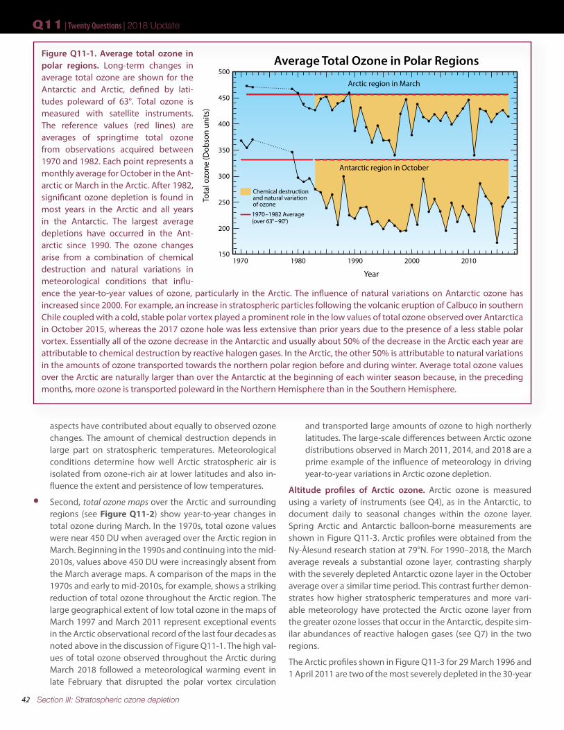
Figure Q11-1. Average total ozone in polar regions. Long-term changes in average total ozone are shown for the Antarctic and Arctic, defined by lati-tudes poleward of 63°. Total ozone is measured with satellite instruments. The reference values (red lines) are averages of springtime total ozone from observations acquired between 1970 and 1982. Each point represents a monthly average for October in the Ant-arctic or March in the Arctic. After 1982, significant ozone depletion is found in most years in the Arctic and all years in the Antarctic. The largest average depletions have occurred in the Ant-arctic since 1990. The ozone changes arise from a combination of chemical destruction and natural variations in meteorological conditions that influ-ence the year-to-year values of ozone, particularly in the Arctic. The influence of natural variations on Antarctic ozone has increased since 2000. For example, an increase in stratospheric particles following the volcanic eruption of Calbuco in southern Chile coupled with a cold, stable polar vortex played a prominent role in the low values of total ozone observed over Antarctica in October 2015, whereas the 2017 ozone hole was less extensive than prior years due to the presence of a less stable polar vortex. Essentially all of the ozone decrease in the Antarctic and usually about 50% of the decrease in the Arctic each year are attributable to chemical destruction by reactive halogen gases. In the Arctic, the other 50% is attributable to natural variations in the amounts of ozone transported towards the northern polar region before and during winter. Average total ozone values over the Arctic are naturally larger than over the Antarctic at the beginning of each winter season because, in the preceding months, more ozone is transported poleward in the Northern Hemisphere than in the Southern Hemisphere.

Chemical destructionand natural variationof ozone

1970 –1982 Average(over 63° – 90° )

Arctic region in March

Antarctic region in October

Average Total Ozone in Polar Regions500

450

400

350

300

250

200

Tota

l ozo

ne (D

obso

n un

its)

20102000199019801970

Year

150



Figure Q11-2. Arctic total ozone. Long-term changes in Arctic total ozone are evident in this series of total ozone maps derived from satellite observations. Each map is an average during March, the month when some ozone depletion is usually observed in the Arctic. In the 1970s and 1980s, the Arctic region had normal ozone values in March, with values of 450 DU and above (red colors). Ozone depletion on the scale of the Antarctic ozone hole does not occur in the Arctic. Instead, late winter/early spring ozone depletion has eroded the normal high values of total ozone. For most years starting in the 1990s, the extent of ozone values of 450 DU and above is greatly reduced in comparison with the 1970s. The large regions of low total ozone in 1997 and 2011 (blue colors) are unusual in the Arctic record, although not unexpected. Meteorological conditions led to below-average stratospheric temperatures and a strong polar vortex in these winters, conditions favorable to strong ozone depletion.

1971 1972 1979

19971996 1998

2011 201820142001

1984

2000

Arctic Total Ozone(March monthly averages)

100 200 300 400 500 600

Total ozone (Dobson units)



record from Ny-Ålesund. Although significant, the depletion during both events is smaller in comparison to that routinely observed in the Antarctic, such as in the profile from 9 October 2006. In the Antarctic stratosphere, near-complete depletion of ozone over many kilometers in altitude and over areas almost as large as North America is a common occurrence. Ozone de-pletion of this magnitude has never been observed in the Arctic stratosphere.

Restoring ozone in spring. As in the Antarctic, ozone depletion in the Arctic is largest in the late winter/early spring season. In

spring, temperatures in the polar lower stratosphere increase (see Figure Q9-1), halting the formation of PSCs, the produc-tion of ClO, and the chemical cycles that destroy ozone. The breakdown of the polar vortex ends the isolation of air in the high-latitude region, allowing more ozone-rich air to be trans-ported poleward where it displaces or mixes with air in which ozone may have been depleted. As a result of these large-scale transport and mixing processes, any ozone depletion at high northern latitudes typically disappears by April or earlier.

Figure Q11-3. Vertical distribution of Antarctic and Arctic ozone. At high latitudes during winter and spring, most stratospheric ozone resides between about 10 and 30 km (6 to 19 miles) above Earth’s surface. Long-term observations of the ozone layer with balloon-borne instruments also allow vertical profiles of ozone during winter to be compared between the Antarctic and Arctic regions. In the Antarctic at the South Pole (left panel), a normal ozone layer was observed to be present between 1962 and 1971. As shown here, ozone was almost completely destroyed between 14 and 21 km (9 to 13 miles) over the South Pole on 9 October 2006. Average October values of ozone in the last three decades (1990–2018) are 90% lower than pre-1980 values at the peak altitude of the ozone layer (16 km). The Arctic ozone layer is shown by the average March profile for 1990–2018 obtained over the Ny-Ålesund research station (right panel). No data from Ny-Ålesund are available for the 1962–1971 period. Some profiles reveal significant depletion, as shown here for 29 March 1996 and 1 April 2011. In such years, winter minimum temperatures are generally lower than normal, allowing for formation of PSCs and increases in ClO over longer periods of time. The number in parentheses for each profile is the total ozone value in Dobson units (DU) (see box in Q4). On 9 October 2006 at the South Pole, the total ozone value of 93 DU was less than one-third of the October average ozone measured at the South Pole between 1962 and 1971. Depletion of ozone of this magnitude has never been observed in the Arctic. Ozone abundances are shown here as the pressure of ozone at each altitude using the unit “milli-Pascals” (mPa) (100 million mPa = atmospheric sea-level pressure).

29 March 1996 (258 DU)1 April 2011 (260 DU)

Polar Ozone Depletion

5 10 150 5 10 150

5

10

15

20

25

30

Alti

tude

(km

)

Ozone abundance (mPa)

Antarctic ozoneSouth Pole (90°S)

Arctic ozoneNy-Ålesund (79°N)

October averages

1962 – 1971 (298 DU)1990 – 2018 (146 DU)

9 October 2006 (93 DU)

March averages

1990 – 2018 (381 DU)

Altit

ude

(mile

s)

0

5

10

15

1962 – 1971 (no data available)

80 Section VII: Appendix

Terminology

CCM chemistry-climate modelCFC chlorofluorocarbon, a group of industrial compounds that contains at least one chlorine, fluorine, and carbon atomCFC-11-equivalent a unit for the measure of the mass of emission of an ODS, equal to the product of the actual mass emission of the ODS times its ODPCO2-equivalent a unit for the measure of the mass of emission of a GHG, equal to the product of the actual mass emission of the GHG times its GWP DU Dobson unit, a measure of total column ozone; 1 DU = 2.687 ×1016 molecules/cm2

EESC equivalent effective stratospheric chlorine, a measure of the total amount of reactive chlorine and bromine gases in the stratosphere that is available to deplete stratospheric ozoneGHG greenhouse gasgigatonne 1 billion (109) metric tons = 1 trillion (1012) kilogramsGWP global warming potential, a measure of the effectiveness of the emission of a gas to cause an increase in the radiative forcing of climate, relative to the radiative forcing caused by the emission of the same mass of CO2; all GWPs used here are for a 100-year time intervalhalon a group of industrial compounds that contain at least one bromine and carbon atom; may or may not contain a chlorine atomHCFC hydrochlorofluorocarbon, a group of industrial compounds that contain at least one hydrogen, chlorine, fluorine, and carbon atomHFC hydrofluorocarbon, a group of industrial compounds that contain at least one hydrogen, fluorine, and carbon atom and no chlorine or bromine atomsHFO hydrofluoroolefin, a group of industrial compounds that contain at least one hydrogen, fluorine, and carbon atom and no chlorine or bromine atoms, and also include a double carbon bond that causes these gases to be more reactive in the troposphere than other HFCsIPCC Intergovernmental Panel on Climate Changekilotonne 1000 metric tons = 1 million (106) kilogramsmegatonne 1 million (106) metric tons = 1 billion (109) kilogramsmPa millipascal; 100 million mPa = atmospheric sea-level pressurenm nanometer, one billionth of a meter (10-9 m)ODP ozone-depletion potential, a measure of the effectiveness of the emission of a gas to deplete the ozone

layer, relative to the ozone depletion caused by the emission of the same mass of CFC-11ODS ozone-depleting substanceozone layer the region in the stratosphere with the highest concentration of ozone, between about 15 and 35 km altitudeppb parts per billion; 1 part per billion equals the presence of one molecule of a gas per billion (109) total air moleculesppm parts per million; 1 part per million equals the presence of one molecule of a gas per million (106) total air moleculesppt parts per trillion; 1 part per trillion equals the presence of one molecule of a gas per trillion (1012) total air moleculesPFC perfluorocarbon, a group of industrial compounds that contain only carbon and fluorine atomsPSC polar stratospheric cloudRCP Representative Concentration PathwayRF radiative forcing of climateSAOD stratospheric aerosol optical depthstratosphere layer of the atmosphere above the troposphere that extends up to around 50 km altitude, and that includes the ozone layerTEAP Technology and Economic Assessment Panel of the Montreal Protocoltroposphere lower layer of the atmosphere that extends from the surface to about 10-15 km (6-9 miles) altitudeUNEP United Nations Environment ProgrammeUNFCCC United Nations Framework Convention on Climate Change

Terminology | Twenty Questions | 2018 Update

81Section VII: Appendix

2018 Update | Twenty Questions | Terminology

UV ultraviolet radiationUV-A ultraviolet radiation between wavelengths of 315 and 400 nmUV-B ultraviolet radiation between wavelengths of 280 and 315 nmUV-C ultraviolet radiation between wavelengths of 100 and 280 nmWMO World Meteorological Organization

Chemical FormulaeBromine Compounds: Other Halogens: CBrClF2 halon-1211 CHF3 HFC-23 CBrF3 halon-1301 CH2F2 HFC-32 CBrF2CBrF2 halon-2402 CHF2CF3 HFC-125 CH2Br2 dibromomethane CH2FCF3 HFC-134a CHBr3 bromoform CH3CF3 HFC-143a CH3Br methyl bromide CH3CHF2 HFC-152a Br atomic bromine CF₃CF=CH₂ HFO-1234yf BrO bromine monoxide CF4 carbon tetrafluoride BrCl bromine monochloride C2F6 perfluoroethane IO iodine monoxideChlorine Compounds: SF6 sulfur hexafluoride CCl3F CFC-11 CCl2F2 CFC-12 Other gases: CCl2FCClF2 CFC-113 CH4 methane CCl4 carbon tetrachloride CO carbon monoxide CH2Cl2 dichloromethane CO2 carbon dioxide CH3CCl3 methyl chloroform H atomic hydrogen CH3Cl methyl chloride H2O water vapor CHF2Cl HCFC-22 HNO3 nitric acid CH3CCl2F HCFC-141b H2SO4 sulfuric acid CH3CClF2 HCFC-142b N2 molecular nitrogen Cl atomic chlorine N2O nitrous oxide ClO chlorine monoxide NOx nitrogen oxides (ClO)2 chlorine monoxide dimer, O atomic oxygen chemical structure ClOOCl O2 molecular oxygen ClONO2 chlorine nitrate O3 ozone HCl hydrogen chloride

Twenty Questions and Answers About the Ozone Layer

Documents

Transcript of Twenty Questions and Answers About the Ozone Layer