Twenty-First-Century Climate Impacts from a Declining Arctic Sea Ice Cover

Twenty-First-Century Climate Impacts from a Declining Arctic Sea Ice Cover

JOY S. SINGARAYER, JONATHAN L. BAMBER, AND PAUL J. VALDES

School of Geographical Sciences, Bristol University, Bristol, United Kingdom

(Manuscript received 14 October 2004, in final form 20 April 2005)

ABSTRACT

A steady decline in Arctic sea ice has been observed over recent decades. General circulation modelspredict further decreases under increasing greenhouse gas scenarios. Sea ice plays an important role in theclimate system in that it influences ocean-to-atmosphere fluxes, surface albedo, and ocean buoyancy. Theaim of this study is to isolate the climate impacts of a declining Arctic sea ice cover during the currentcentury. The Hadley Centre Atmospheric Model (HadAM3) is forced with observed sea ice from 1980 to2000 (obtained from satellite passive microwave radiometer data derived with the Bootstrap algorithm) andpredicted sea ice reductions until 2100 under one moderate scenario and one severe scenario of ice decline,with a climatological SST field and increasing SSTs. Significant warming of the Arctic occurs during thetwenty-first century (mean increase of between 1.6° and 3.9°C), with positive anomalies of up to 22°Clocally. The majority of this is over ocean and limited to high latitudes, in contrast to recent observationsof Northern Hemisphere warming. When a climatological SST field is used, statistically significant impactson climate are only seen in winter, despite prescribing sea ice reductions in all months. When correspond-ingly increasing SSTs are incorporated, changes in climate are seen in both winter and summer, although theimpacts in summer are much smaller. Alterations in atmospheric circulation and precipitation patterns aremore widespread than temperature, extending down to midlatitude storm tracks. Results suggest that areasof Arctic land ice may even undergo net accumulation due to increased precipitation that results from lossof sea ice. Intensification of storm tracks implies that parts of Europe may experience higher precipitationrates.

1. Introduction

Studies from a variety of sources have documentedevidence for recent change in the environment of highnorthern latitudes (Serreze et al. 2000; Johannessen etal. 2004). Observations of Arctic sea ice from satellitepassive microwave radiometer data have demonstrateda downward trend in both annual mean ice extent (areawithin the ice–ocean margin) and ice area (extent mi-nus open water area within the ice pack) of �2% and�3%, respectively, during the last 25 yr (Parkinson etal. 1999; Johannessen et al. 2004; Comiso 2002a). Seaice thickness has also decreased in recent decades(Rothrock 1999; Laxon et al. 2003; Johannessen et al.2004), although estimates vary considerably and thevariability is less well known than that of ice extent.

Over the same time period global temperatures haveincreased, with largest increases over land between 40°and 70° latitude in winter/spring. Global circulationmodels (GCMs) predict that anthropogenic greenhousegas warming will be amplified at northern high latitudes(Räisänen 2001), due in part to ice–albedo feedbackmechanisms arising from continuing decline in Arcticsea ice.

Dowdeswell et al. (1997) examined 40 Arctic ice capsand glaciers and found that most have had negativemass balances over the past few decades, while a few, inparts of Scandinavia and Iceland, have been positivebecause of increased winter precipitation. Bamber et al.(2004) attribute an anomalous positive elevationchange between 1996 and 2002 on the largest ice cap inthe Eurasian Arctic (Austfonna, eastern Svalbard) toan increase in accumulation rate due to loss of localperennial sea ice and resultant local increase in precipi-tation. Kattsov and Walsh (2000) also tentatively asso-ciated observational and modeled trends in precipita-tion with changes in the sea ice boundary. The possi-

Corresponding author address: Dr. Joy S. Singarayer, School ofGeographical Sciences, Bristol University, Bristol Road, BristolBS8 1SS, United Kingdom.E-mail: [email protected]

1 APRIL 2006 S I N G A R A Y E R E T A L . 1109

© 2006 American Meteorological Society

JCLI3649

bility of further decreases in sea ice over the nextcentury, given current trends, suggests that there maybe significant impacts for the mass balance of otherArctic land ice.

Projections of continuing decline in the Arctic sea icecover for the coming decades are supported by GCMsimulations under global warming scenarios (Vinnikovet al. 1999; Walsh and Timlin 2003; Gregory et al. 2002).The predicted trends vary considerably across variousmodels (Walsh and Timlin 2003). However, simulateddecreases are consistently larger in summer, with muchof the Arctic Ocean being ice free during the summerminimum by the end of the twenty-first century. Assuch, sea ice is often used as an indicator of climatechange. However, it also plays an active role in theclimate system through its influence on ocean-to-atmosphere fluxes, surface albedo, and ocean buoy-ancy.

It is difficult from data analysis alone to establishwhat impact sea ice anomalies have on climate. It canalso be relatively difficult using fully coupled GCMs toelucidate information concerning the active influenceof sea ice from total greenhouse-gas-induced climatechange. Modeling and observational studies have foundthat atmospheric influence on sea ice by thermody-namic and wind stress forcing generally dominates (e.g.,Maslanik et al. 2000; Deser et al. 2000; Partington et al.2003), hampering detection of sea ice forcing on theatmosphere. An exception to this is the sea ice covereast of Greenland, which has been shown, using obser-vational datasets, to affect the position of the localstorm track through surface heat flux anomalies (Deseret al. 2000); it has also been shown that reductions insea ice have been associated with decreased sea levelpressure in this area (Slonosky et al. 1997). Rind et al.(1995) have estimated that sea ice composes 37% of thetemperature sensitivity to CO2, in 2 � CO2 experimentswhere sea ice changes were artificially prevented, whichimportantly diminished cloud cover and water vaporfeedbacks.

Several recent AGCM simulations have examined at-mospheric circulation changes associated with surfaceboundary conditions (sea ice and sea surface tempera-ture). For example, Parkinson et al. (2001) ran anAGCM with uniformly larger and smaller ice concen-trations to quantify how inaccuracies in sea ice datamight affect atmospheric simulations. They found thatsurface air temperatures (SATs) increased linearly asice concentration decreased, with the greatest changesin winter in regions directly above changes in ice. Al-exander et al. (2004) used actual ice extents for recentwinters with particularly large positive or negative

anomalies to force the National Center for Atmo-spheric Research (NCAR) Community Climate Model(CCM3). They found local warming, enhanced precipi-tation, and reduced sea level pressure directly over ar-eas of sea ice reductions and the reverse for regions ofincreased sea ice, also found by Singarayer et al. (2005).Ice anomalies in the Atlantic sector produced a large-scale response resembling the Arctic Oscillation/NorthAtlantic Oscillation (AO/NAO). Studies by Magnus-dottir et al. (2004) and Deser et al. (2004) examined theatmospheric response to both sea ice extent and seasurface temperature (SST) anomalies confined to theNorth Atlantic region, with both studies also usingCCM3. Trends in the boundary conditions were de-rived from the last 40 yr, although the anomalies wereamplified, and the anomalies were calculated to corre-spond to the pattern of the trend, varying seasonally butnot changing from year to year. Sea ice anomalies weremore efficient at producing an atmospheric responsethan SST anomalies. The response to sea ice anomalieswas opposite to the observed atmospheric trend, sug-gesting a negative ice–atmosphere feedback.

In this study we investigate the direct climate impactsof decreasing Arctic sea ice using an atmosphericGCM. We perform atmospheric simulations on the Ha-dley Centre Atmospheric Model (HadAM3) whilevarying prescribed Arctic sea ice alone to represent thecontinuing decline predicted for the twenty-first cen-tury. In contrast to the studies described above, we varyArctic sea ice concentrations from year to year usingtrends for this century derived from observed data. Thelocal and large-scale atmospheric response to sea icedecline is examined. A further simulation investigatesthe response to combined sea ice decline and corre-spondingly increasing SSTs, also using HadAM3. Bythe use of an atmospheric-only model these simulationsfocus on the influence of sea ice on the albedo andocean–atmosphere fluxes only. A subsequent study willinvestigate ocean buoyancy effects.

2. Methods

a. Observations of recent changes in Arctic sea ice

Passive microwave radiometer (PMR) satellite datahave provided the most comprehensive record of seaice concentrations for the entire Arctic since 1978.Various algorithms have been formulated to derive seaice concentrations from PMR, such as the NationalAeronautics and Space Administration (NASA) team(Cavalieri et al. 1991) and bootstrap (Comiso et al.1997) algorithms. There are discrepancies in the con-centrations from different datasets that can be up to20% in summer (Partington et al. 2003; Singarayer and

1110 J O U R N A L O F C L I M A T E — S P E C I A L S E C T I O N VOLUME 19

Bamber 2003), which are the result of the various meth-ods used to handle ice temperature fluctuations or sea-sonal variations in ice/water signatures, for example.Previous comparisons have found that the Bootstraprecord may be more reliable than others (Comiso et al.1997; Singarayer and Bamber 2003). Therefore, Boot-strap-derived sea ice concentrations were used in thisstudy; they are publicly available from the NationalSnow and Ice Data Center (Comiso 2002c; 25 km reso-lution on a polar stereographic projection).

The decline in annual mean Arctic sea-ice-coveredarea calculated from the Bootstrap record is 3% perdecade from 1980 to 2000. Examination of monthlymean trends shows that this decrease is stronglyweighted to the summer months (Fig. 1), although therehas been a reduction in all months over this time pe-riod. The perennial sea ice cover, as described by thesummer minimum, is reducing at a rate of 9% per de-cade (Comiso 2002b). Comiso (2002a) observed a muchmore variable summer ice cover in the 1990s than the1980s, suggesting a thinning in perennial ice in the lasttwo decades.

The spatial distribution of change in Arctic sea ice isnot uniform. The largest decreases in concentrationhave occurred around the ice margin (Parkinson et al.1999; Comiso 2002b), in the Bering, Okhotsk, andGreenland–Iceland–Norway (GIN) Seas in winter, andalong the Siberian/north Eurasian coast and CanadianArchipelago in summer. Anomalies in ice concentra-tions in these regions are strongly correlated with sur-face ice temperature anomalies (Comiso 2002a). Par-tington et al. (2003), using empirical orthogonal func-tion analysis, show that the major modes of NorthernHemisphere sea ice variability, distributed chiefly inthese marginal regions, exhibit a 1-yr lagged response

to the North Atlantic Oscillation. These modes accountfor 18% of the total monthly variance.

b. Projected sea ice trends

Observations over the last few decades show an over-all monotonic, approximately linear decline in Arcticsea ice area and extent. Coupled climate model predic-tions under increasing CO2 scenarios result in continu-ing decreases for the next century (Walsh and Timlin2003). The magnitude varies considerably betweenmodels. However, several models predict that the Arc-tic Ocean will be almost ice free in summer by the endof the twenty-first century.

To examine the effects on climate of a continuingdecline in Arctic sea ice the trends obtained from theBootstrap record of sea ice concentration for 1980–2000were projected up to 2100. A monthly mean dataset offuture sea ice concentrations was achieved by first cal-culating a trend for each month from a time series ateach grid point. The calculated linear trends were ex-trapolated for a further hundred years. The resultingpredicted sea ice area time series for the March andSeptember monthly means are displayed in Figs. 2a and2b, respectively (“ICE1” lines). Over the period 1980–2100, March ice-covered area decreases by �8%, andSeptember area decreases by �39%. In summer espe-cially, this trend is conservative when compared toHadCM3 coupled model predictions (Walsh and Timlin2003). The slower decline is because the main ice packhas a slower rate of decline than the ice edge, and whenthe current ice edge disappears, the ice that is left toform the new ice edge reduces more slowly than itwould in reality.

Consequently, a second sea ice time series was con-structed that used the same observed Bootstrap trendswhilst including an additional time-dependent factor(different for each month) to allow the total mean ice-covered area to continue decreasing roughly linearlywith the same gradient, as calculated for the observedperiod (1980–2000). March and September time seriesare shown in Figs. 2a and 2b (“ICE2”). In this case, thedecreases from 1980 to 2100 are 26% and 82%, respec-tively. Such large decreases in total ice-covered areaand continuing quasi-linear trends are comparable inmagnitude to those simulated by some of the more se-vere Intergovernmental Panel on Climate Change(IPCC) scenarios (Gregory et al. 2002).

There is reasonable consistency between the ob-served and predicted portions of Fig. 2. No additionalnoise/variability was introduced to the predicted sea icefields. Figure 3 depicts the predicted spatial distributionof sea ice in March (Fig. 3a) and September (Fig. 3b) in

FIG. 1. Average trend in Arctic sea ice covered area for eachmonth (% per decade). Monthly mean sea ice concentrations(1980–2000) from passive microwave radiometer data derived us-ing the Bootstrap algorithm were used.


the years 2000, 2025, 2050, 2075, and 2099 for both theICE1 and ICE2 data. In March, the ice fractions in thecentral Arctic show little decrease in ICE1. ICE2 showlarger decreases than ICE1 in marginal ice areas such asthe Bering, Okhotsk, and Barents Seas, as well as smallcentral Arctic decreases. Summer minimum ice extent(Fig. 3b) is reduced to the high Arctic, and there is alsoa significant increase in the amount of open waterwithin the ice pack, that is, the ice concentrations arelower, resulting in greater decrease in ice-covered areathan ice extent, similar to observed (Comiso 2002a; Par-kinson et al. 1999). ICE1 displays some areas with highice fractions even in 2099, as well as ice in the FramStrait. September ice fractions in ICE2 are mostly �0.5by 2099, and the extent is smaller than ICE1, which is

more consistent with coupled model predictions (Jo-hannessen et al. 2004).

The ICE1 dataset provides a moderate scenario ofsea ice decline, whereas the ICE2 dataset provides amore severe scenario. The techniques used here to es-timate future sea ice and the assumption of lineartrends may be simplistic. However, the sea ice datasetsthat have been constructed allow the simulation resultsto bracket a range of possible estimates of Arctic sea icedecline to the end of this century that can test the sen-sitivity of climate-to-sea ice reductions.

c. Experimental setup

Two datasets of 120 yr of monthly mean sea ice frac-tions were compiled from Bootstrap observations from

FIG. 2. Time series of (a) March mean and (b) September average Arctic sea ice areas.Observed data are used from 1980 to 2000, and observed linear trends are extrapolated to givepredicted ice areas up to 2100 (filled symbols; ICE1). Open symbols (ICE2) provide a datasetwith a faster rate of sea ice decline. See text for details.


1980 to 2000 and projected trends for 2001 to 2100(ICE1 and ICE2). These were used to drive HadAM3.Sea ice depth was calculated within the model as a func-tion of ice fraction. Snow depth over sea ice was mod-eled. To ensure that any changes in climate are solely aresult of changes in Arctic sea ice, a climatological Ant-

arctic sea ice cover was used that was derived from theU.K. Met Office (UKMO) sea ice climatology. Tenyears of climatological sea ice was prescribed for 1970–80 to allow for model spinup. Following the spinup pe-riod, three experiments were performed, as listed be-low:

FIG. 3. Spatial maps of sea ice for the two datasets ICE1 and ICE2 for years 2000, 2025, 2050, 2075, and 2099in (a) March and (b) September.


1) EXPT1: HadAM3 with prescribed sea ice from theICE1 time series and climatological SST field.

2) EXPT2: HadAM3 with prescribed sea ice from theICE2 time series and climatological SST field (runas an ensemble consisting of six simulations withinitial-condition perturbations).

3) EXPT3: HadAM3 with prescribed sea ice from theICE2 time series and increasing SST field.

In all experiments, the sea ice prescription for 1980–2000 is the same.

SSTs were based on the Global Sea Ice and Sea Sur-face Temperature (GISST) climatology (Parker et al.1995). The climatological SST field was modifiedslightly for use in EXPT1 and EXPT2 so that gridpoints that were ice covered at any time for a particularmonth were given an SST of 271.35 K in the climatology(freezing point of saline water). For EXPT3 a repre-sentation was introduced of the increase in SSTs as seaice decreases, as would occur because of increased ab-sorption of radiation by the ocean. The rate of increasewas based on previous coupled simulation results withthe Third Hadley Centre Coupled Ocean–AtmosphereGCM (HadCM3). A simple function was fitted to de-scribe the change in SST with sea ice concentration,only used for grid boxes that initially had nonzero iceconcentrations. Different constants were used for eachmonth, so that any SST increases due to lower sea iceconcentrations were larger in the summer months thanin winter.

The atmospheric model used, HadAM3, is a compo-nent of the coupled HadCM3 model, a version of theUKMO unified forecast and climate model. HadAM3is run at a horizontal resolution of 2.5° latitude � 3.75°longitude using 19 vertical hybrid coordinate levels anda time step of 30 min. The atmospheric boundary layercan occupy up to the bottom five model layers (Johns etal. 1997), and the parameterization uses Monin–Obukhov similarity theory. A first-order turbulent mix-ing scheme is used to mix the conserved thermody-namic variables and momentum in the vertical (Smith1990). A land surface scheme, the Met Office SurfaceExchange Scheme (MOSES; Cox et al. 1999), whichincludes a representation of soil moisture freezing andmelting and should lead to better simulations of surfacetemperatures, is included. A zero heat flux condition isimposed at the base of the soil model to conserve heatwithin the system. Over land, surface roughness char-acteristics are prescribed according to climatologicalsurface type. At sea points, however, the roughnesslength over open water is computed from local windspeeds. Where there is partial sea ice cover, separatefluxes are computed for sea ice and leads within a grid

box. A full description of the model and revisions madefrom the previous versions can be found in Pope et al.(2000). Trace gas concentrations were set to preindus-trial concentrations and held constant throughout therun, thus emphasizing the role of sea ice only.

Because of the prescription of SSTs, the model doesnot fully conserve energy since energy absorbed in theocean is not permitted to warm it. It should be notedalso that because of the specification of SSTs, the fulleffect of sea ice changes on climate cannot be assessedfrom these simulations because of limits of oceanicfeedbacks. However, the three experiments enable theisolation of sea-ice-induced climate changes, which aredifficult to disentangle in coupled experiments, particu-larly because atmosphere-to-sea ice forcing normallydominates.

3. Results

a. Atmospheric changes due to observed Arctic seaice decline (1980–2000)

The results presented in this section are taken pri-marily from the EXPT2 ensemble run. SAT is a usefulfield to examine, as it integrates changes in surface en-ergy budget. There are significant increases in simu-lated surface air temperature as a result of the decreasein sea ice cover during the 20 yr of observational data.Modeled Arctic annual average SATs (60°–90°N lati-tude) show a positive trend of 0.11°–0.23°C per decadefor the six simulations (Fig. 4a), compared with theobserved 0.33°C per decade (data from Lugina et al.2003). Comiso (2003) also calculated an observed SATtrend of 0.33° � 0.16°C per decade from 1981 to 2000over sea ice, using satellite thermal infrared data (and0.5°C per decade over Eurasia, 1.06°C per decade overNorth America). The average simulated SAT increase(0.16° � 0.6°C per decade) is roughly half that observedover the Arctic.

The use of a constant SST field may contribute toproducing a smaller trend and smaller interannual vari-ability in the modeled data than observed. The EXPT3simulation, which included an increasing SST field, pro-duced a larger trend for the period 1980–2000 of 0.38°Cper decade, although the simulated interannual vari-ability was still less than observed.

The difference between modeled and observed glob-al annual change in SAT is greater than for the Arcticalone. Between 1980 and 2000 the simulated global an-nual temperature increases by less than 0.05°C com-pared with an observed increased of �0.3°C. Evenglobal annual temperatures in EXPT3 increase by only0.051°C during the same period. This suggests that sea


ice changes are only a small component of globalchange.

Both the observed and mean ensemble annual ArcticSAT time series from 1980 to 2000 demonstrate signifi-cant anticorrelations with annual sea ice area, with cor-

relation coefficients of �0.71 and �0.88, respectively.The simulated and observed data correlate moststrongly in years 1993–96, noted as being years with thelargest interannual variation in ice area (e.g., 1995 hadthe lowest annual sea ice area of the observed period

FIG. 4. Time series from 1980 to 1999 of (a) simulated Arctic (60°–90°N) annual mean SATanomalies from each ensemble member (m1, m2, m3, m4, m5, and m6), and observed datafrom Lugina (2003). (b) Simulated Arctic annual mean total precipitation anomalies fromeach ensemble member, and NCEP reanalysis. (c) Observed normalized NAO index com-pared with modeled. NAO index data provided by the Climate Analysis Section, NCAR,Boulder, CO; Hurrell (1995). Inset shows the simulated ensemble average NAO index. Seetext for details.


compared with relatively high areas in the precedingand following years). The warmest year in the majorityof the simulation members and observed SAT is 1995(Fig. 4a). It is suggested that the instantaneous feed-back from sea ice changes into the atmosphere domi-nates the surface energy balance more strongly in thisyear because the negative sea ice anomaly was main-tained from late winter in this year through to the be-ginning of the next year, before recovering.

Time series of annual average Arctic precipitation(60°–90°N) for each simulation are shown in Fig. 4b.The simulated annual mean Arctic precipitation rate is0.75 mm day�1 (70°–90°N), which is comparable to ob-served values. Kattsov and Walsh (2000) suggest that alarge portion of the twentieth-century increase in Arc-tic precipitation is attributable to sea ice boundary andsea surface temperature conditions based on model/observation comparisons. Observational data over theArctic are hindered by sparse station networks and un-dercatch of solid precipitation (Kattsov and Walsh2000), so consequently the simulated data have beencompared to National Centers for Environmental Pre-diction (NCEP) reanalysis. Modeled results show amagnitude of interannual variation similar to reanaly-sis. The modeled time series of precipitation was sig-nificantly anticorrelated with annual mean sea ice area,whereas the NCEP reanalysis was not (although thiscould be an artifact of the reanalysis processing). Thehighest correlation in the model was achieved withsummer sea ice area, which is the season with maximumArctic precipitation.

The NAO (Hurrell 1995) is the leading mode of win-tertime variability (climate variability is defined here as

fluctuation in climate, which could last for a specifiedperiod of time, usually of the order of years to decades)in the Northern Hemisphere, defined as an index ofnormalized sea level pressure differences between Ice-landic low and Azores high. In section 2a evidence ofthe impact of the NAO on sea ice variability (Parting-ton et al. 2003) was mentioned. Here, a simulated NAOindex has been calculated to investigate the potentialfor sea ice to directly influence North Atlantic variabil-ity. The index was based on the normalized differencein December–February (DJF) mean sea level pressure(MSLP) anomalies between 42.5°N, 15°W and 67.5°N,7.5°W. Over the period 1980–2000 the observed NAOindex (Hurrell 1995) has had a tendency to be positive(Fig. 4c). Similar to SAT and precipitation time series,comparison of modeled and observed NAO indices re-veals a smaller interannual variability in the modeleddata. The ensemble mean shows some tendency to bepositive in the late 1980s and early 1990s, similar toobservations. However, there is no correlation betweenthe time series for prescribed sea ice and simulatedNAO.

Serreze et al. (1997) describe large reductions inMSLP over the Arctic Ocean, which locally exceed 4mb, while increases were observed over central Europeand the Northeastern Pacific between 1979 and 1994.Figure 5a shows a similar pattern in the modeled results(mapped difference of the 1990–99 average minus the1980–89 average). The regional reductions over theArctic reach 2 mb. The MSLP reduction over the ArcticOcean extends over Greenland and Iceland in bothmodeled and observed fields (NCEP reanalysis MSLPanomalies are displayed in Fig. 5b for comparison). De-

FIG. 5. (a) Mean winter (DJF) differences in sea level pressure between decadal means,1990–1999 minus 1980–1989, where the values used are the averages of the ensemble mem-bers. Dotted lines/light shadings are negative and solid lines/dark shadings are positive dif-ferences (0.3-hPa contour interval). (b) NCEP reanalysis anomalies over the same periods at1-hPa contour intervals.


creases in sea ice concentrations have directly contrib-uted to changes in atmospheric circulation in a mannerstrongly resembling observational patterns.

b. Twenty-first-century climate under decreasingArctic sea ice cover

1) TEMPERATURE

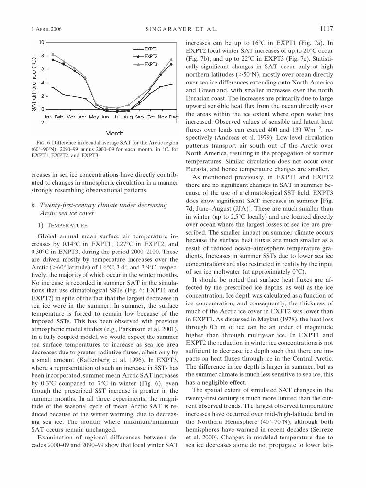
Global annual mean surface air temperature in-creases by 0.14°C in EXPT1, 0.27°C in EXPT2, and0.30°C in EXPT3, during the period 2000–2100. Theseare driven mostly by temperature increases over theArctic (�60° latitude) of 1.6°C, 3.4°, and 3.9°C, respec-tively, the majority of which occur in the winter months.No increase is recorded in summer SAT in the simula-tions that use climatological SSTs (Fig. 6: EXPT1 andEXPT2) in spite of the fact that the largest decreases insea ice were in the summer. In summer, the surfacetemperature is forced to remain low because of theimposed SSTs. This has been observed with previousatmospheric model studies (e.g., Parkinson et al. 2001).In a fully coupled model, we would expect the summersea surface temperatures to increase as sea ice areadecreases due to greater radiative fluxes, albeit only bya small amount (Kattenberg et al. 1996). In EXPT3,where a representation of such an increase in SSTs hasbeen incorporated, summer mean Arctic SAT increasesby 0.3°C compared to 7°C in winter (Fig. 6), eventhough the prescribed SST increase is greater in thesummer months. In all three experiments, the magni-tude of the seasonal cycle of mean Arctic SAT is re-duced because of the winter warming, due to decreas-ing sea ice. The months where maximum/minimumSAT occurs remain unchanged.

Examination of regional differences between de-cades 2000–09 and 2090–99 show that local winter SAT

increases can be up to 16°C in EXPT1 (Fig. 7a). InEXPT2 local winter SAT increases of up to 20°C occur(Fig. 7b), and up to 22°C in EXPT3 (Fig. 7c). Statisti-cally significant changes in SAT occur only at highnorthern latitudes (�50°N), mostly over ocean directlyover sea ice differences extending onto North Americaand Greenland, with smaller increases over the northEurasian coast. The increases are primarily due to largeupward sensible heat flux from the ocean directly overthe areas within the ice extent where open water hasincreased. Observed values of sensible and latent heatfluxes over leads can exceed 400 and 130 Wm�2, re-spectively (Andreas et al. 1979). Low-level circulationpatterns transport air south out of the Arctic overNorth America, resulting in the propagation of warmertemperatures. Similar circulation does not occur overEurasia, and hence temperature changes are smaller.

As mentioned previously, in EXPT1 and EXPT2there are no significant changes in SAT in summer be-cause of the use of a climatological SST field. EXPT3does show significant SAT increases in summer [Fig.7d; June–August (JJA)]. These are much smaller thanin winter (up to 2.5°C locally) and are located directlyover ocean where the largest losses of sea ice are pre-scribed. The smaller impact on summer climate occursbecause the surface heat fluxes are much smaller as aresult of reduced ocean–atmosphere temperature gra-dients. Increases in summer SSTs due to lower sea iceconcentrations are also restricted in reality by the inputof sea ice meltwater (at approximately 0°C).

It should be noted that surface heat fluxes are af-fected by the prescribed ice depths, as well as the iceconcentration. Ice depth was calculated as a function ofice concentration, and consequently, the thickness ofmuch of the Arctic ice cover in EXPT2 was lower thanin EXPT1. As discussed in Maykut (1978), the heat lossthrough 0.5 m of ice can be an order of magnitudehigher than through multiyear ice. In EXPT1 andEXPT2 the reduction in winter ice concentrations is notsufficient to decrease ice depth such that there are im-pacts on heat fluxes through ice in the Central Arctic.The difference in ice depth is larger in summer, but asthe summer climate is much less sensitive to sea ice, thishas a negligible effect.

The spatial extent of simulated SAT changes in thetwenty-first century is much more limited than the cur-rent observed trends. The largest observed temperatureincreases have occurred over mid-/high-latitude land inthe Northern Hemisphere (40°–70°N), although bothhemispheres have warmed in recent decades (Serrezeet al. 2000). Changes in modeled temperature due tosea ice decreases alone do not propagate to lower lati-

FIG. 6. Difference in decadal average SAT for the Arctic region(60°–90°N), 2090–99 minus 2000–09 for each month, in °C, forEXPT1, EXPT2, and EXPT3.


tudes or vertically in the troposphere above �700 hPa(Fig. 8; data from EXPT2), as was also found by Mag-nusdottir et al. (2004) and Alexander et al. (2004). Thedifferences between modeled and observed spatial pat-terns in SAT suggest that sea ice impacts in the atmo-sphere affect local temperatures, but that other non-sea-ice influences are important for explaining the ob-served spatial features at lower latitudes, and/orfeedback mechanisms involving ocean circulation arepotentially required to enable propagation of tempera-ture anomalies outside higher latitudes.

2) PRECIPITATION AND P � E

Coupled model simulations under global warmingscenarios predict increases in precipitation related tohigher water vapor content and convergence of pole-ward vapor transport (Kattenberg et al. 1996). In the

FIG. 8. Zonally averaged temperature change in EXPT2 as afunction of geopotential height, Z for the 2090–99 winter (DJF)average minus the 2000–09 average (1°C contour intervals).

FIG. 7. Mean differences in SAT between decadal means (2090–2099 minus 2000–2009) for (a) EXPT2DJF, (b) EXPT1 DJF, and EXPT3 (c) DJF and (d) JJA. Shading indicates regions where the Student’st-test statistic exceeds the 95% confidence level.


current simulations sea ice variations alone producedan increase in Arctic (60°–90°C) annual precipitation of0.15 mm day�1 (�14%) in EXPT2, whereas in the moreconservative simulation, EXPT1, the increase was only0.05 mm day�1 (�5%). This increase occurs mainly inwinter and spring, with no significant changes in sum-mer, when precipitation is highest over the Arctic, noteven in EXPT3.

Maps of winter precipitation differences between the2000–09 average and 2090–99 average are displayed inFig. 9a. Directly over regions of decrease in Arctic seaice extent, an increase in winter evaporation (notshown) is simulated where the sea ice fraction is lower.In the model, this leads to an increase in convective andlow cloud cover in these regions in winter (and autumn/spring) and an increase in precipitation, mainly over theCentral Arctic basin. The largest Arctic precipitationincreases occur over the marginal ice zone, as foundalso by Kattsov and Walsh (2000) in atmospheric simu-lations driven by changing sea ice, SSTs, and CO2.There are also precipitation increases over regions ofwestern Europe and off the east coast of NorthAmerica (along the North Atlantic storm track), mostprevalent in the EXPT2 ensemble mean. Decreases inwinter precipitation occur over the initial (1980s)marginal ice area (Bering, Okhotsk, and GIN seas). Inthese regions, where ice cover is already much re-duced in the 2000–09 winter average, the ocean-to-atmosphere latent heat flux is reduced (due to increas-ing atmospheric humidity). As a result, there is reducedprecipitation over areas around southern Greenlandand the Labrador Sea, as well as Iceland and Svalbardin EXPT2, whilst higher precipitation is seen overnorthern Greenland and the Canadian Archipelago andcentral Arctic areas.

The three experiments show similar general spatialanomalies, especially the significant increase in precipi-tation over the Arctic Ocean. The positive anomaliesare larger and more widespread in EXTP2 and EXPT3than EXPT1, as would be expected given the largerdecrease in sea ice. The experiments all display de-creased precipitation over the West Coast of the UnitedStates, most clearly seen in EXPT3, but also apparentin EXPT2 and EXPT1. Similar reductions in precipita-tion over western North America were obtained bySewall and Sloan (2004) using an atmospheric modeldriven with decreasing sea ice and increasing SSTs,which they related to changes in storm track position.

Changes in precipitation minus evaporation (P � E)may be more relevant to examine than precipitationalone. Variations in P � E over the Arctic Ocean mayimpact freshwater transports into the North Atlantic

(Serreze et al. 2000) and may be an important controlupon changes in ocean circulation (Stocker et al. 1992).Two observational studies of P � E over the Arcticfound no significant trends in the last few decades(Walsh et al. 1994; Serreze et al. 1995). Atmosphericsimulations by Alexander et al. (2004) forced with ob-served sea ice anomalies also found that most changesin evaporation were compensated for by changes inprecipitation.

Here, the modeled patterns of winter P � E changefrom the 2000–09 average to the 2090–99 average areshown in Fig. 9b. Large changes in P � E (�0.2 mmday�1) are not as widespread over the Arctic as changesin precipitation. In the central Arctic Basin and EastSiberian Sea there is an increase in both precipitationand evaporation but slightly negative change in P � Ein all the simulations. This results from a warmer loweratmosphere, which can hold more moisture, so that theincrease in evaporation is larger than the increase inprecipitation. Negative P � E anomalies in the CentralArctic are largest in EXPT3, as a result of warmingSSTs. In areas where the decrease in winter sea ice hasbeen greatest (Bering Straits, GIN, and Barents Seas)and also North Pacific and western North Atlantic(along storm tracks), there are significant positivechanges in P � E simulated in EXPT2, which wouldlead to freshening of waters in these regions. This ismore clearly seen in the EXPT2 ensemble mean thanthe other simulations. The spatial pattern of P � Etrends in EXPT2 suggests an increase in P � E oversome areas where there is land ice, such as Svalbard andnorthern parts of Greenland. An increase in precipita-tion is accompanied by an increase in SAT. However,since temperatures do not exceed the melting point inwinter and do not change in summer, it may be likelythat changes in the hydrological cycle result in accumu-lation of land ice and changes in snow cover in someregions.

3) ATMOSPHERIC CIRCULATION

In section 3a, the changes in MSLP from 1980 to 2000were discussed. Spatial patterns of modeled changesresembled those observed during recent decades (Fig.5), although the magnitude of the changes was half ofthose observed. During the modeled twenty-first cen-tury, there is a continued decrease in the winter MSLPArctic high with a more extensive spatial pattern reach-ing into the Canadian Arctic Archipelago and BeringSea (Fig. 10). There are also smaller increases near theAzores high in EXPT1 and EXPT2, although mostlynot statistically significant anomalies. Unlike in Fig. 5,there is an average decrease in MSLP over the Bering


Sea/North Pacific and North Atlantic. Decreases inMSLP over the Arctic locally exceed 4 mb in EXPT1, 5mb in EXPT2, and 6 mb in EXPT3. Significant anoma-lies are less extensive in simulation EXPT1. The wide-spread MSLP decrease is the result of the trend towarda warmer, less stable atmosphere. A direct atmosphericresponse to warm SAT anomalies is a drop in MSLPand anomalous cyclonic surface winds.

In accordance with a less stable atmosphere, changesin Northern Hemisphere storm tracks occur. Stormtracks are responsible for a large proportion of midlati-tude precipitation, and therefore these changes giverise to much of the change in midlatitude precipitation(Fig. 9a). Storm track activity has been calculated usingthe high-pass transient poleward temperature flux at850 hPa, showing areas of maximum high-frequency

FIG. 9. (a) Total precipitation rate changes 2090–99 DJF average minus 2000–09 DJFaverage for EXPT1, EXPT2, and EXPT3. Contour interval is 0.1 mm day�1, except EXPT3,at 0.3 mm day�1. (b) Precipitation minus evaporation (P � E ) difference. Contour interval is0.2 mm day�1. Shading denotes regions where the t statistic exceeds the 95% level; dark (light)shading indicates significant positive (negative) changes.


variability (Fig. 11a, shaded). Changes in storm trackstrength (Figs. 11a or 11b, contours; only EXPT2 re-sults are shown) display a meridional dipole structure.This corresponds to a sharpening of the storm track,with an enhancement at the start of the North Atlantictrack off the east coast of North America and to a lesserdegree over Europe. The North Pacific storm trackshifts slightly south. In addition, there is a widespreadweakening of the storm track from the end of the Pa-cific Ocean, and across North America. This weakeningof the storm track is consistent with the weakening ofthe meridional temperature gradient (due to a warmerArctic, accompanied by negligible temperature changeat lower latitudes). However, the increase in the stormtrack over the west Atlantic is inconsistent with thechanges in temperature gradient. In this more southerlyregion, diabatic processes, specifically latent heating,may also be important. Release of latent heat throughcondensation may positively feed back on the growth ofthe storm track. In addition, there is a strengthening ofthe trough over east North America (and also over theNorth Pacific), which results in a stronger jet over theeastern seaboard on North America, and hence poten-tially influencing the North Atlantic storm track. Thischange in the planetary waves may be associated withthe changes in the storm tracks upstream of the NorthAtlantic (Hoskins and Valdes 1990). The suppressionof storm tracks by a strong jet (e.g., Nakamura 1992;Nakamura et al. 2002) may explain some aspects of theweakening of the storm track over the North Pacific butis of less relevance to the North Atlantic, where theoverall jet strength is weaker than in the North Pacific.

While there is a change in the mean winter atmo-spheric circulation in terms of MSLP and storm trackactivity due to decreases in sea ice, there is no signifi-cant trend in wintertime NAO variability, based on thenormalized difference in DJF mean sea level pressureanomalies between 42.5°N, 15°W and 67.5°N, 7.5°W.Figure 12 represents the NAO index from 1980 to 2100from one of the ensemble members of EXPT2. TheNAO indices display no trend or periodicity in interan-nual variation. No trend was observed in EXPT1 orEXPT3. The isolated decline in sea ice enforced in thisexperiment does not appear to have an impact on thismajor mode of wintertime climate variability.

←

FIG. 10. Mean winter (DJF) differences in sea level pressurebetween decadal means (2090–2099 minus 2000–2009) for eachexperiment, in mb. Light (dark) shading indicates regions of nega-tive (positive) anomalies where the t statistic exceeds the 95%confidence level.


4) RADIATIVE CHARACTERISTICS

Because of the prescription of SSTs, the model doesnot fully conserve energy, since energy absorbed in theocean is not permitted to warm it. Consequently, thenet radiation at the top of the atmosphere (TOA) inthese simulations is nonzero. Time series of annualmean TOA net radiation show a negative balance in allsimulations (more incoming radiation than outgoing).In EXPT1 and EXPT2 the net radiation balance be-comes increasingly negative throughout the simulation,decreasing by 0.12 and 0.30 W m�2 from 1980 to 2100.This results from a combination of an increase in out-going longwave (LW) radiation, due partly to greaterarea of relatively warm open-ocean being exposed, butalso because larger decrease in upward shortwave (SW)radiation, due to greater absorption of SW at the sur-

face given a lower overall surface albedo. The overallchange is small compared to the expected changes inradiative forcing during this century. In EXPT3, theincorporation of increasing SSTs also results in a nega-tive TOA net radiation, but no significant trend (netradiation decreases by only �0.03 W m�2), for the rea-son that the decrease in upward SW radiation ismatched by the increase in outgoing LW radiation.

4. Discussion

The impact on climate of the twenty-first-century de-cline in the Arctic sea ice cover has been investigated.Observations of sea ice in recent decades show an ap-proximately linear decrease in extent, while there havebeen coherent changes in other environmental fields,such as Arctic temperatures and precipitation. The pur-pose of this study was to examine the spatial and tem-poral patterns of change in the climate that might resultgiven a continuing decrease in sea ice, using prescribedsea ice fields from years 1980 to 2100 to force HadAM3.The sea ice fields were based on satellite passive mi-crowave radiometer data derived with the Bootstrapalgorithm and contained the observed data from 1980to 2000. Two scenarios of ice decline were used to in-vestigate the climate sensitivity to sea ice; one predicteda moderate decrease (EXPT1) and the other predicteda more severe reduction (used in EXPT2 and EXPT3).

During simulations driven with observed sea ice,from 1980 to 2000, annual Arctic average SAT in-creases at a rate of 0.16° � 0.06°C per decade, which is

FIG. 12. Time series of NAO index from ensemble member m1in EXPT2 from 1980 to 2099.

FIG. 11. (a) Simulated storm track activity in the Northern Hemisphere, EXPT2 average,calculated from the high-pass transient poleward temperature flux (m2 s�2) at 850 hPa in DJFaveraged over years 2000–09. Shaded contour interval is 1 m2 s�2. Storm track anomalies(2090–99 average minus 2000–09 average) are plotted over in line contours. (b) Same as in (a),but contour interval is 0.5 m2 s�2, with dark (light) shading representing areas of significantpositive (negative) change.


half the observed rate over the same period. Increasesin annual Arctic average SAT from 2000–99 were 1.6°Cin EXPT1, 3.4°C in EXPT2, and 3.9°C in EXPT3. Witha moderate rate of sea ice decline (EXPT1), the simu-lated SAT increases at roughly the same rate in 2000–99as 1980–2000. If a severe twenty-first-century sea icedecline is prescribed (EXPT2 and EXPT3) then therate of SAT increase is around twice that value. Thecomparisons are subject to errors due to internally gen-erated interannual variations in the simulations (whichare reduced by performing ensemble runs for EXPT2)and interannual variation in the observed sea ice rec-ord.

Modeled trends suggest that although decreases inice extent were prescribed in each month, these onlyhave a significant impact on wintertime SATs, as longas SSTs are not allowed to increase. Winter warming insimulated years 1980–2000 occurs mainly over FramStrait and the GIN and Barents Seas. By the end of thetwenty-first century, significant increases occur in allsimulations over the entire Arctic basin, regardless ofwhether there is much open water prescribed in thisregion (as in EXPT2) or not (EXPT1). Winter reduc-tion of total Arctic sea ice area of 21% (from 2000 to2099) produced local maximum increases of 20°C in thecase of a larger sea ice decline (EXPT2). Even in theconservative scenario (EXPT1), winter decreases in icearea of 7% result in local increases of up to 16°C.

It is well known that satellite PMR data suffer frominaccuracies regarding interpretation of areas of sum-mer surface melt ponds. Areas with surface melt maybe incorrectly interpreted as open water. Because ofrecent increases in surface temperature, it is probablethat the amount of surface melting has increased also.The calculated monthly trends used to form the pre-dicted ice decreases used here may be slightly overes-timated as a result. Fortuitously, the summer climate ismuch less sensitive to sea ice than in winter. There areno significant changes to summer SATs in EXPT1 orEXPT2, both of which used a climatological SST field.When an increasing SST field was prescribed in EXPT3there were small increases in temperature of 0.3°C inthe Arctic average and up to 2.5°C locally, but far lessthan winter increases of up to 22°C.

Changes in SAT are largest over ocean and are lim-ited to northern high latitudes, unlike current observa-tions of climate warming, where increases have beenlargest over land. Reductions in sea ice do induce morewidespread changes in atmospheric circulation. As aresult of increased temperatures, a reduction in MSLPoccurs that extends to the North Pacific and North At-lantic. This appears to have a significant effect for mid-

latitude storm tracks, which increase in intensitythroughout the simulations. All these changes have animportant role in altering precipitation patterns, espe-cially over western and southern Europe in winter,which in EXPT2 experience significant increases. Withregards to global warming, impacts for the hydrologicalcycle are potentially more important than increasingtemperatures. There may be implications for terrestrialice mass balance, which ultimately influences the salin-ity of Arctic waters also. Increases in modeled precipi-tation occurred over areas of ocean where sea ice areadecreased. In addition, increases in P � E were ob-served over some parts of the Arctic covered by landice (EXPT2). A short-term net accumulation over theseglaciers and ice caps may occur if there is a furtherdecrease in sea ice in those regions. Other regions mayexperience decreases in precipitation, such as Iceland,and also parts of the west coast of North America thatalready suffer from limited water resources (Sewall andSloan 2004).

In EXPT2, a greater loss of sea ice area was pre-scribed than in EXPT1, as well as small reductions inice concentrations in the Central Arctic not included inEXPT1. The magnitude of the climate changes induceddepends on the scenario of sea ice decline used. How-ever, the spatial extents of SAT anomalies producedare similar in EXPT1 and EXPT2. The spatial extent ofMSLP changes is also similar. The prescription of openwater within the ice pack does influence more stronglythe extent of changes in precipitation over the Arctic.

A caveat to this study is that, while in one simulationincreasing SSTs were prescribed, no coupled oceanmodel was used. This allowed us to isolate the effects ofsea-ice-induced changes in the albedo and surface heatflux but consequently underestimates the overall effectof sea ice on climate change. The incorporation of in-creasing SSTs corresponding to sea ice decreases resultsin year-round higher temperatures, but by �1°C com-pared to climatological SST. Feedbacks between thehydrological cycle and the ocean and effects such asbrine rejection were not included in this study. Changesin the Arctic freshwater budget may have effects in theAtlantic, and possibly the global ocean, through deepconvection. This will be the subject of additional simu-lations. The results of the present study suggest thatsea-ice-induced albedo and heat flux changes have asmall effect on Northern Hemisphere landmasses, but amore substantial impact on the hydrological cycle.

Acknowledgments. This study was funded underNERC Grant NER/T/S/2001/01279 under the NERCCOAPEC theme. Computer time was provided by theNERC Centres for Atmospheric Sciences (NCAS).


REFERENCES

Alexander, M. A., U. M. Bhatt, J. E. Walsh, M. S. Timlin, J. S.Miller, and J. D. Scott, 2004: The atmospheric response torealistic Arctic sea ice anomalies in an AGCM during winter.J. Climate, 17, 890–905.

Andreas, E. L, C. A. Paulson, R. M. Williams, R. W. Lindsay, andJ. A. Businger, 1979: Turbulent heat-flux from Arctic leads.Bound.-Layer Meteor., 17, 57–91.

Bamber, J. L., W. Krabill, V. Raper, and J. Dowdeswell, 2004:Anomalous recent growth of part of a large Arctic ice cap:Austfonna, Svalvard. Geophys. Res. Lett., 31, L12402,doi:10.1029/2004GL019667.

Cavalieri, D. J., J. P. Crawford, M. R. Drinkwater, D. T. Eppler,L. D. Farmer, R. R. Jentz, and C. C. Wackerman, 1991: Air-craft active and passive microwave validations of sea-ice con-centrations from the DMSP SSM/I. J. Geophys. Res., 96,21 989–22 008.

Comiso, J. C., 2002a: Correlation and trend studies of the sea-icecover and surface temperatures in the Arctic. Ann. Glaciol.,34, 420–428.

——, 2002b: A rapidly declining perennial sea ice cover in theArctic. Geophys. Res. Lett., 29, 1956, doi:10.1029/2002GL015650.

——, cited 2002c: Bootstrap sea ice concentrations from Nimbus-7SMMR and DMSP SSM/I. National Snow and Ice Data Cen-ter, Boulder, CO. [Available online at http://nsidc.org/data/nsidc-0079.html.]

——, 2003: Warming trends in the Arctic from clear sky satelliteobservations. J. Climate, 16, 3498–3510.

——, D. Cavalieri, C. Parkinson, and P. Gloersen, 1997: Passivemicrowave algorithms for sea ice concentration: A compari-son of two techniques. Remote Sens. Environ., 60, 357–384.

Cox, P. M., R. A. Betts, C. B. Bunton, R. L. H. Essery, P. R.Rowntree, and J. Smith, 1999: The impact of new land surfacephysics on the GCM simulation of climate and climate sen-sitivity. Climate Dyn., 15, 183–203.

Deser, C., J. E. Walsh, and M. S. Timlin, 2000: Arctic sea-ice vari-ability in the context of recent atmospheric circulation trends.J. Climate, 13, 617–633.

——, G. Magnusdottir, R. Saravanan, and A. Phillips, 2004: Theeffects of North Atlantic SST and sea ice anomalies on thewinter circulation in CCM3. Part II: Direct and indirect com-ponents of the response. J. Climate, 17, 877–889.

Dowdeswell, J. A., and Coauthors, 1997: The mass balance ofcircum-Arctic glaciers and recent climate change. Quat. Res.,48, 1–14.

Gregory, J. M., P. A. Stott, D. J. Cresswell, N. A. Rayner, C. Gor-don, and D. M. H. Sexton, 2002: Recent and future changesin Arctic sea ice simulated by the HadCM3 AOGCM. Geo-phys. Res. Lett., 29, 2175, doi:10.1029/2001GL014575.

Hoskins, B. J., and P. J. Valdes, 1990: On the existence of stormtracks. J. Atmos. Sci., 47, 1854–1864.

Hurrell, J. W., 1995: Decadal trends in the North Atlantic Oscil-lation regional temperatures and precipitation. Science, 269,676–679.

Johannessen, O. M., and Coauthors, 2004: Arctic climate change:Observed and modelled temperature and sea-ice variability.Tellus, 56A, 328–341.

Johns, T. C., R. E. Carnell, J. F. Crossley, J. M. Gregory, J. F. B.Mitchell, C. A. Senior, S. F. B. Tett, and R. A. Wood, 1997:

The second Hadley Centre coupled ocean-atmosphere GCM:Model description, spinup and validation. Climate Dyn., 13,103–134.

Kattenberg, A., and Coauthors, 1996. Climate models—Projections of future climate. Climate Change 1995: The Sci-ence of Climate Change, J. T. Houghton et al., Eds., Cam-bridge University Press, 289–357.

Kattsov, M. K., and J. E. Walsh, 2000: Twentieth-century trends ofArctic precipitation from observational data and a climatemodel simulation. J. Climate, 13, 1362–1370.

Laxon, S., N. Peacock, and D. Smith, 2003: High interannual vari-ability of sea ice thickness in the Arctic region. Nature, 425,947–949.

Lugina, K. M., P. Ya. Groisman, K. Ya. Vinnikov, V. V. Kok-naeva, and N. A. Speranskaya, 2003: Monthly surface airtemperature time series area-averaged over the 30-degreelatitudinal belts of the globe, 1881–2002. Trends Online: ACompendium of Data on Global Change, Carbon DioxideInformation Analysis Center, Oak Ridge National Labora-tory, U.S. Department of Energy, Oak Ridge, TN. [Availableonline at http://cdiac.esd.ornl.gov/trends/temp/lugina/lugina.html.]

Magnusdottir, G., C. Deser, and R. Saravanan, 2004: The effectsof North Atlantic SST and sea ice anomalies on the wintercirculation in CCM3. Part I: Main features and storm trackcharacteristics of the response. J. Climate, 17, 857–876.

Maslanik, L. A., A. H. Lynch, M. C. Serreze, and W. Wu, 2000: Acase study of regional climate anomalies in the Arctic: Per-formance requirements for a coupled model. J. Climate, 13,383–401.

Maykut, G. A., 1978: Energy exchange over young sea ice in theCentral Arctic. J. Geophys. Res., 83, 3646–3658.

Nakamura, H., 1992: Midwinter suppression of baroclinic waveactivity in the Pacific. J. Atmos. Sci., 49, 1629–1641.

——, T. Izumi, and T. Sampe, 2002: Interannual and decadalmodulations recently observed in the Pacific storm track ac-tivity and east Asian winter monsoon. J. Climate, 15, 1855–1874.

Parker, D. E., C. K. Folland, and M. Jackson, 1995: Marine sur-face temperature: Observed variations and data require-ments. Climate Change, 31 (2–4), 559–600.

Parkinson, C. L., D. J. Cavalieri, P. Gloersen, H. J. Zwally, andJ. C. Comiso, 1999: Sea ice extents, areas, and trends, 1978–1996. J. Geophys. Res., 104 (C9), 20 837–20 856.

——, D. Rind, R. J. Healy, and D. G. Martinson, 2001: The impactof sea ice concentration accuracies on climate model simula-tions with a GISS GCM. J. Climate, 14, 2606–2623.

Partington, K., T. Flynn, D. Lamb, C. Bertoia, and K. Dedrick,2003: The late twentieth century Northern Hemisphere seaice record from U.S. National Ice Center ice charts. J. Geo-phys. Res., 108, 3343, doi:10.1029/2002JC001623.

Pope, V. D., M. L. Gallani, P. R. Rowntree, and R. A. Stratton,2000: The impact of new physical parameterisations in theHadley Centre climate model: HadAM3. Climate Dyn., 16,123–146.

Räisänen, J., 2001: CO2-induced climate change in CMIP2 experi-ments: Quantification of agreement and role of internal vari-ability. J. Climate, 14, 2088–2104.

Rind, D., R. Healy, C. Parkinson, and D. Martinson, 1995: Therole of sea ice in 2 � CO2 climate model sensitivity. Part I:The total influence of sea ice thickness and extent. J. Climate,8, 449–463.


Rothrock, D. A., Y. Yu, and G. A. Maykut, 1999: Thinning of theArctic sea-ice cover. Geophys. Res. Lett., 26, 3469–3472.

Serreze, M. C., R. G. Barry, and J. E. Walsh, 1995: Atmosphericwater vapor characteristics at 70°N. J. Climate, 8, 719–731.

——, F. Carse, R. G. Barry, and J. C. Rogers, 1997: Icelandic lowcyclone activity: Climatological features, linkages with theNAO, and relationships with recent changes in the NorthernHemisphere circulation. J. Climate, 10, 453–464.

——, and Coauthors, 2000: Observational evidence of recentchange in the northern high-latitude environment. ClimateChange, 46, 159–207.

Sewall J. O., and L. C. Sloan, 2004: Disappearing Arctic sea icereduces available water in the American west. Geophys. Res.Lett., 31, L06209, doi:10.1029/2003GL019133.

Singarayer, J. S., and J. L. Bamber, 2003: EOF analysis of threerecords of sea-ice concentration spanning the last 30 years.Geophys. Res. Lett., 30, 1251–1254.

——, P. J. Valdes, and J. L. Bamber, 2005: The atmospheric im-

pact of uncertainties in recent Arctic sea ice reconstructions.J. Climate, 18, 3996–4012.

Slonosky, V. C., L. A. Mysak, and J. Derome, 1997: Linking Arc-tic sea ice and atmospheric circulation anomalies on interan-nual and decadal timescales. Atmos.–Ocean, 35, 333–366.

Smith, R. N. B., 1990: A scheme for predicting layer clouds andtheir water-content in a general circulation model. Quart. J.Roy. Meteor. Soc., 116, 435–460.

Stocker, T. F., D. G. Wright, and L. A. Mysak, 1992: A zonallyaveraged, coupled ocean–atmosphere model for paleoclimatestudies. J. Climate, 5, 773–797.

Vinnikov, K. Y., and Coauthors, 1999: Global warming andNorthern Hemisphere sea ice extent. Science, 286, 1934–1937.

Walsh, J. E., and M. S. Timlin, 2003: Northern hemisphere sea icesimulations by global climate models. Polar Res., 22, 75–82.

——, X. Zhou, D. Portis, and M. C. Serreze, 1994: Atmosphericcontribution to hydrologic variations in the Arctic. Atmos.–Ocean, 34, 733–755.


Twenty-First-Century Climate Impacts from a Declining Arctic Sea Ice Cover

Documents

Transcript of Twenty-First-Century Climate Impacts from a Declining Arctic Sea Ice Cover